Embed Size (px)
Citation preview

Technische Universitat Ilmenau
Fakultat fur Mathematik und Naturwissen-
schaften
Arbeitsgruppe Analysis und Systemtheorie
On Differential-Algebraic Control Systems
Dissertation zur Erlangung des akademischen Grades Dr. rer. nat.
Thomas Berger
betreut vonProf. Dr. Achim Ilchmann
Tag der Einreichung: 5. Juli 20131. Gutachter: Prof. Dr. Achim Ilchmann
(Technische Universitat Ilmenau)2. Gutachter: Jun.-Prof. Dr. Thomas Hotz
(Technische Universitat Ilmenau)3. Gutachter: Prof. Dr. Volker Mehrmann
(Technische Universitat Berlin)Tag der Verteidigung: 14. Oktober 2013
Ilmenau, 28. Oktober 2013

5
Zusammenfassung
In der vorliegenden Dissertation werden differential-algebraischeGleichungen (differential-algebraic equations, DAEs) der Form d
dtEx =
Ax + f betrachtet, wobei E und A beliebige Matrizen sind. FallsE nichtverschwindende Eintrage hat, dann kommen in der GleichungAbleitungen der entsprechenden Komponenten von x vor. Falls E eineNullzeile hat, dann kommen in der entsprechenden Gleichung keineAbleitungen vor und sie ist rein algebraisch. Daher werden Gleichung-en vom Typ d
dtEx = Ax + f differential-algebraische Gleichungengenannt.
Ein Ziel dieser Dissertation ist es, eine strukturelle Zerlegung einerDAE in vier Teile herzuleiten: einen ODE-Anteil, einen nilpotentenAnteil, einen unterbestimmten Anteil und einen uberbestimmten An-teil. Jeder Anteil beschreibt ein anderes Losungsverhalten in Hinblickauf Existenz und Eindeutigkeit von Losungen fur eine vorgegebene In-homogenitat f und Konsistenzbedingungen an f . Die Zerlegung, na-mentlich die quasi-Kronecker Form (QKF), verallgemeinert die wohl-bekannte Kronecker-Normalform und behebt einige ihrer Nachteile.
Die QKF wird ausgenutzt, um verschiedene Konzepte der Kontrol-lierbarkeit und Stabilisierbarkeit fur DAEs mit f = Bu zu studieren.Hier bezeichnet u den Eingang des differential-algebraischen Systems.Es werden Zerlegungen unter System- und Feedback-Aquivalenz, sowiedie Folgen einer Behavioral-Steuerung Kxx + Kuu = 0 fur die Stabil-isierung des Systems untersucht.
Falls fur das DAE-System zusatzlich eine Ausgangs-Gleichung y =Cx gegeben ist, dann lasst sich das Konzept der Nulldynamik wie folgtdefinieren: die Nulldynamik ist, grob gesagt, die Dynamik, die amAusgang nicht sichtbar ist, d.h. die Menge aller Losungs-Trajektorien(x, u, y) mit y = 0. Fur rechts-invertierbare Systeme mit autonomerNulldynamik wird eine Zerlegung hergeleitet, welche die Nulldynamikentkoppelt. Diese versetzt uns in die Lage, eine Behavior-Steuerung zuentwickeln, die das System stabilisiert, vorausgesetzt die Nulldynamikselbst ist stabil.
Wir betrachten auch zwei Regelungs-Strategien, die von den Eigen-schaften der oben genannten System-Klasse profitieren: Hochver-starkungs- und Funnel-Regelung. Ein System d
dtEx = Ax + Bu, y =Cx, hat die Hochverstarkungseigenschaft, wenn es durch die Anwen-

6
dung der proportionalen Ausgangsruckfuhrung u = −ky, mit k > 0hinreichend groß, stabilisiert werden kann. Wir beweisen, dass rechts-invertierbare Systeme mit asymptotisch stabiler Nulldynamik, die einebestimmte Relativgrad-Annahme erfullen, die Hochverstarkungseigen-schaft haben. Wahrend der Hochverstarkungs-Regler recht einfach ist,ist es jedoch a priori nicht bekannt, wie groß die Verstarkungskon-stante k gewahlt werden muss. Dieses Problem wird durch den Funnel-Regler gelost: durch die adaptive Justierung der Verstarkung ubereine zeitabhangige Funktion k(·) und die Ausnutzung der Hochver-starkungseigenschaft wird erreicht, dass große Werte k(t) nur dannangenommen werden, wenn sie notig sind. Eine weitere wesentlicheEigenschaft ist, dass der Funnel-Regler das transiente Verhalten desFehlers e = y − yref der Bahnverfolgung, wobei yref die Referenztra-jektorie ist, beachtet. Fur einen vordefinierten Performanz-Trichter(funnel) ψ wird erreicht, dass ‖e(t)‖ < ψ(t).Schließlich wird der Funnel-Regler auf die Klasse von MNA-Modellen
von passiven elektrischen Schaltkreisen mit asymptotisch stabilen in-varianten Nullstellen angewendet. Dies erfordert die Einschrankung derMenge der zulassigen Referenztrajektorien auf solche die, in gewisserWeise, die Kirchhoffschen Gesetze punktweise erfullen.

7
Abstract
In the present thesis we consider differential-algebraic equations(DAEs) of the form d
dtEx = Ax + f , where E and A are arbitrary
matrices. If E has nonzero entries, then derivatives of the respectivecomponents of x are involved in the equation. If E has a zero row, thenthe respective equation involves no derivatives and is purely algebraic.This justifies to call d
dtEx = Ax+ f a differential-algebraic equation.
One aim of the thesis is to derive a structural decomposition of theDAE into four parts: the ODE part, nilpotent part, underdeterminedpart and overdetermined part. Each part describes a different solutionbehavior regarding existence and uniqueness of solutions for given in-homogeneities f and consistency conditions on f . The decomposition,namely the quasi-Kronecker form (QKF), generalizes the well-knownKronecker canonical form and resolves some of its disadvantages.
The QKF is exploited to study the different controllability and sta-bilizability concepts for DAEs with f = Bu. Here u denotes the in-put of the differential-algebraic system. Decompositions under systemand feedback equivalence and the consequence of behavioral controlKxx+Kuu = 0 for the stabilization of the system is investigated.
If the DAE system is accompanied by an output equation y = Cx,we may define the concept of zero dynamics: roughly speaking, thezero dynamics are those dynamics which are not visible at the output,i.e., the set of all solution trajectories (x, u, y) with y = 0. For right-invertible systems with autonomous zero dynamics a decomposition isderived, which decouples the zero dynamics of the system and enablesus to derive a behavioral control which stabilizes the system, providedthat the zero dynamics are stable as well.
We will also consider two control strategies which benefit from theproperties of the above mentioned system class: high-gain and funnelcontrol. We say that a system d
dtEx = Ax+Bu, y = Cx, has the high-gain property if it is stabilizable by the application of the feedbacku = −ky for sufficiently large k > 0. It is proved that right-invertiblesystems with asymptotically stable zero dynamics which satisfy a cer-tain relative degree assumption possess the high-gain property. Whilethe high-gain controller is quite simple, it is, however, not known apriori how large the gain constant k must be chosen. This problem isresolved by the funnel controller: by adaptively adjusting the gain via

8
a time-varying function k(·) and exploiting the high-gain property, itis achieved that high values of k(t) are used only when required. More-over, and most important, the funnel controller takes the transientbehavior of the tracking error e = y − yref , where yref is a referencesignal, into account. For a prespecified performance funnel ψ it can beguaranteed that ‖e(t)‖ < ψ(t).Finally, the funnel controller is applied to the class of MNA models
of passive electrical circuits with asymptotically stable invariant zeros.This requires to restrict the set of allowable reference trajectories suchthat any trajectory, in a sense, satisfies Kirchhoff’s laws pointwise.

9
Danksagung
Zuallererst gilt mein Dank Achim Ilchmann fur die Schaffung einerangenehmen und konstruktiven Arbeitsatmosphare. Mit hilfreichenRatschlagen und angebrachter Kritik hat er auch bei kleinsten Un-sicherheiten ausgeholfen. Ich danke ihm vor allem auch fur die Anre-gung zum Schreiben meiner Bachelorarbeit uber DAEs, die ich Ende2007 begann, welche in meiner Masterarbeit fortgesetzt wurde undschließlich in der vorliegenden Dissertation (wenn auch thematisch an-ders gelagert) gipfelte. In diesen sechs Jahren war er mir ein hervorra-gender Mentor und, nicht zuletzt, ein guter Freund.
Ich danke meiner Freundin Lisa Hoffmann fur ihre ununterbrocheneUnterstutzung. Auch in hektischen und stressigen Situationen war undist sie an meiner Seite, und ich weiß, dass es nicht immer einfach fursie war, da ich doch oft einiges unbewusst von ihr vorausgesetzt habe.
Stephan Trenn und Timo Reis danke ich fur die gute und angenehmeZusammenarbeit, aus der verschiedene gemeinsame Publikationen, dieauch einen Beitrag zu der vorliegenden Arbeit leisten, hervorgegangensind.
Nicos Karcanias und George Halikias (beide City University Lon-don) gilt mein Dank fur die Gastfreundlichkeit, die mir bei meinemForschungsaufenthalt in London entgegenbracht wurde. Die resultier-ende angenehme Atmosphare war die Grundlage fur eine effektive Zu-sammenarbeit. Ich danke auch dem Deutschen Akademischen Aus-tauschdienst fur die Mitfinanzierung dieses Forschungsaufenthalts.
Ich bedanke mich bei den Gutachtern Volker Mehrmann (TU Berlin),Thomas Hotz (TU Ilmenau) und naturlich Achim dafur, dass sie sichdie Zeit genommen haben meine Arbeit grundlich zu lesen und zu be-werten.
Weiterhin danke ich all denen, die sich in den letzten Jahren gern aneiner wissenschaftlichen Diskussion mit mir beteiligten, sei es auf einerTagung oder bei einer angenehmen Kaffeerunde gewesen. Besonderserwahnen mochte ich dabei Volker Mehrmann, Fabian Wirth, CarstenTrunk, Henrik Winkler, Markus Muller, Karl Worthmann und StefanBrechtken.
Außerdem gilt mein Dank der Deutschen Forschungsgemeinschaft furdie Ermoglichung dieser Arbeit durch die Finanzierung meiner Stelleuber das Projekt Il25/9.

10
Meinen Eltern mochte ich schließlich fur ihre kontinuierliche Un-terstutzung danken und dafur, dass sie mir diesen Lebensweg ermoglichthaben.
Contents 11
Contents
1 Introduction 15
1.1 The Weierstraß and Kronecker canonical form . . . . . 161.2 Controllability . . . . . . . . . . . . . . . . . . . . . . . 181.3 Zero dynamics . . . . . . . . . . . . . . . . . . . . . . . 191.4 High-gain and funnel control . . . . . . . . . . . . . . . 201.5 Electrical circuits . . . . . . . . . . . . . . . . . . . . . 211.6 Previously published results and joint work . . . . . . . 22
2 Decomposition of matrix pencils 25
2.1 Definitions . . . . . . . . . . . . . . . . . . . . . . . . . 272.2 Quasi-Weierstraß form . . . . . . . . . . . . . . . . . . 31
2.2.1 Wong sequences and QWF . . . . . . . . . . . . 312.2.2 Eigenvector chains and WCF . . . . . . . . . . 40
2.3 Quasi-Kronecker form . . . . . . . . . . . . . . . . . . 472.3.1 Main results . . . . . . . . . . . . . . . . . . . . 482.3.2 Preliminaries and interim QKF . . . . . . . . . 512.3.3 Proofs of the main results . . . . . . . . . . . . 702.3.4 KCF, elementary divisors and minimal indices . 73
2.4 Solution theory . . . . . . . . . . . . . . . . . . . . . . 812.4.1 Solutions in terms of QKF . . . . . . . . . . . . 812.4.2 Solutions in terms of KCF . . . . . . . . . . . . 89
2.5 Notes and References . . . . . . . . . . . . . . . . . . . 93
3 Controllability 95
3.1 Controllability concepts . . . . . . . . . . . . . . . . . 973.2 Solutions, relations and decompositions . . . . . . . . . 106
3.2.1 System and feedback equivalence . . . . . . . . 1073.2.2 A decomposition under system equivalence . . . 1113.2.3 A decomposition under feedback equivalence . . 112

12 Contents
3.3 Criteria of Hautus type . . . . . . . . . . . . . . . . . . 1223.4 Feedback, stability and autonomous systems . . . . . . 127
3.4.1 Stabilizability, autonomy and stability . . . . . 1283.4.2 Stabilization by feedback . . . . . . . . . . . . . 1323.4.3 Control in the behavioral sense . . . . . . . . . 136
3.5 Invariant subspaces . . . . . . . . . . . . . . . . . . . . 1403.6 Kalman decomposition . . . . . . . . . . . . . . . . . . 1453.7 Notes and References . . . . . . . . . . . . . . . . . . . 151
4 Zero dynamics 159
4.1 Autonomous zero dynamics . . . . . . . . . . . . . . . 1614.2 System inversion . . . . . . . . . . . . . . . . . . . . . 1774.3 Asymptotically stable zero dynamics . . . . . . . . . . 185
4.3.1 Transmission zeros . . . . . . . . . . . . . . . . 1864.3.2 Detectability . . . . . . . . . . . . . . . . . . . 1894.3.3 Characterization of stable zero dynamics . . . . 190
4.4 Stabilization . . . . . . . . . . . . . . . . . . . . . . . . 1974.5 Notes and References . . . . . . . . . . . . . . . . . . . 208
5 High-gain and funnel control 211
5.1 High-gain control . . . . . . . . . . . . . . . . . . . . . 2125.2 Funnel control . . . . . . . . . . . . . . . . . . . . . . . 219
5.2.1 Main result . . . . . . . . . . . . . . . . . . . . 2195.2.2 Simulations . . . . . . . . . . . . . . . . . . . . 234
5.3 Regular systems and relative degree . . . . . . . . . . . 2395.3.1 Vector relative degree . . . . . . . . . . . . . . . 2425.3.2 Strict relative degree . . . . . . . . . . . . . . . 2455.3.3 Simulations . . . . . . . . . . . . . . . . . . . . 260
5.4 Notes and References . . . . . . . . . . . . . . . . . . . 262
6 Electrical circuits 265
6.1 Positive real rational functions . . . . . . . . . . . . . . 2666.2 Graph theoretical preliminaries . . . . . . . . . . . . . 2696.3 Circuit equations . . . . . . . . . . . . . . . . . . . . . 2726.4 Zero dynamics and invariant zeros . . . . . . . . . . . . 2786.5 High-gain stabilization . . . . . . . . . . . . . . . . . . 2816.6 Funnel control . . . . . . . . . . . . . . . . . . . . . . . 2836.7 Simulation . . . . . . . . . . . . . . . . . . . . . . . . . 2956.8 Notes and References . . . . . . . . . . . . . . . . . . . 298

Contents 13
References 301
List of Symbols 319
Abbreviations 324
Index 325

15
1 Introduction
About fifty years ago, Gantmacher published his famous book [100]and therewith laid the foundations for the rediscovery of differential-algebraic equations (DAEs), the first main theories of which were de-veloped by Weierstraß [243] and Kronecker [149] in terms ofmatrix pencils. DAEs have then been discovered to be an appropri-ate tool for modeling many problems in economics [173], demogra-phy [62], mechanical systems [8, 46, 99, 111, 197], multibody dynam-ics [90,111,216,221], electrical networks [8,30,61,89,168,183,207], fluidmechanics [8, 106, 168] and chemical engineering [79, 84, 85, 194], whichoften cannot be modeled by standard ordinary differential equations(ODEs). These problems indeed have in common that the dynamicsare algebraically constrained, for instance by tracks, Kirchhoff laws, orconservation laws. As a result of the power in application, DAEs arenowadays an established field in applied mathematics and subject ofvarious monographs [46, 62, 63, 80, 107] and textbooks [152, 154].
In general, DAEs are implicit differential equations, and in the sim-plest case just a combination of differential equations along with al-gebraic constraints (from which the name DAE comes from). Thesealgebraic constraints however may cause that the solutions of initialvalue problems are no longer unique, or that there do not exist solu-tions at all. Furthermore, when considering inhomogeneous problems,the inhomogeneity has to be ‘consistent’ with the DAE in order for so-lutions to exist. Dealing with these problems, a broad solution theoryfor DAEs has been developed, starting with the pioneer contributionby Wilkinson [244]. Nowadays, the whole theory can be looked upin the aforementioned textbooks and monographs; for a comprehensiverepresentation see the survey [229]. A good overview of DAE theoryand a historical background can also be found in [158].
A lot of the aforementioned contributions deal with regular DAEs,

16 1 Introduction
i.e., equations of the form
ddtEx(t) = Ax(t) + f(t), x(0) = x0,
where for any continuous inhomogeneity f there exist initial values x0
for which the corresponding initial value problem has a solution (i.e.,a differentiable function x satisfying the equation for all t ∈ R) andthis solution is unique. This has been proved to be equivalent to thecondition that E,A are square matrices and det(sE −A) ∈ R[s] \ {0}.The aim of the present thesis is to present a control theory for
differential-algebraic systems. Most results are on nonregular systems,in particular E and A may be rectangular. Applications with theneed for nonregular DAEs appear in the modeling of electrical cir-cuits [89, 207] for instance. Furthermore, systems arising from modernautomatic modeling tools are usually nonregular DAEs. We also like tostress that general, possibly nonregular, DAE systems are a sub-classof the class of so-called differential behaviors, introduced by Willems
in [245], see also [198, 246] and the survey [248]. In the present thesiswe will pay a special attention to the behavioral setting, formulatingmost of the results and the concepts by using the underlying set oftrajectories (behavior) of the system.The guiding research idea is funnel control. In Chapters 2–4 we
develop a theory which is also the basis for the application of the funnelcontroller to nonregular DAE systems in Chapter 5 and to passiveelectrical circuits in Chapter 6. For the application of funnel control itis necessary that the inputs and outputs of the DAE system (see (1.3.1))are fixed a priori by the designer in order to establish the control law.This is different from other approaches based on the behavioral setting,see [65], where only the free variables in the system are viewed as inputs;this may require a reinterpretation of states as inputs and of inputs asstates. In the present thesis we will assume that such a reinterpretationof variables has already been done or is not feasible, and the given DAEsystem is fix.
1.1 The Weierstraß and Kronecker canonical
form
Weierstraß [243] and Kronecker [149] have independently devel-

1.1 The Weierstraß and Kronecker canonical form 17
oped the fundamental decompositions of regular and nonregular ma-trix pencils, resp., which are nowadays the basis for nearly any the-ory on time-invariant DAEs. Let us consider regular matrix pencilssE − A ∈ R[s]n×n first, i.e., det(sE − A) ∈ R[s] \ {0}. We may thenobserve that via a suitable choice of new variables and appropriate ma-nipulations of the equations we may equivalently express the system
ddtEx(t) = Ax(t) as
ddtx1(t) = Jx1(t)
ddtNx2(t) = x2(t),
where N is a nilpotent matrix. Here, x1 are called the differentialvariables and x2 the algebraic variables; the latter notion arising fromthe fact that the equation d
dtNx2(t) = x2(t) has only the trivial so-lution (this equation gets interesting when inhomogeneities are in-volved). Weierstraß observed that this transformation can be ob-tained by only applying an equivalence transformation to the matrixpencil sE −A, that is there exist S, T ∈ Gln(R) such that
S(sE − A)T =
[sI − J 0
0 sN − I
],
and J,N are in Jordan canonical form and N is nilpotent. This formis called the Weierstraß canonical form (WCF).If sE − A ∈ R[s]m×n is an arbitrary matrix pencil, then, compared
to the ODE and nilpotent part in the WCF, two additional parts arisein its Kronecker canonical form (KCF): an underdetermined part andan overdetermined part. They consist of blocks of the type
sKi − Li or sK⊤i − L⊤
i , resp.,
where
Ki =[1 0
1 0
], Li =
[0 1
0 1
]∈ R(i−1)×i, i ∈ N.
Clearly, in equations of the type(ddtKi−Li)x(t) = f(t) the component
xi can be chosen freely and solutions exist for any x(0) ∈ Ri and for anyf ∈ C(R;Ri), but it is far from being unique; in equations of the type(ddtK
⊤i −L⊤
i )x(t) = f(t) a solution x does only exist if the initial valuex(0) and the inhomogeneity f satisfy a certain consistency condition,but then the solution is unique - we omit the details here.
18 1 Introduction
A major drawback of the WCF and the KCF is that, due to possiblecomplex eigenvalues of the matrix J , the Jordan form and accompa-nying transformation matrices may be complex-valued. Hence, evenin the case of a real-valued matrix pencil sE − A, its WCF or KCFare in general complex-valued. Furthermore, it is often not necessarythat J and N are in Jordan form, but the knowledge that the pen-cil sE − A can be decomposed into 2 (4, resp.) parts of the follow-ing types suffices: ODE part, nilpotent part, (underdetermined part,overdetermined part). These blocks can be described via simple rankconditions. This leads to the quasi-Weierstraß form (QWF) and thequasi-Kronecker form (QKF) discussed in Chapter 2.
1.2 Controllability
Controllability is, roughly speaking, the property of a system that anytwo trajectories can be concatenated by another admissible trajectory.The precise concept however depends on the specific framework, asquite a number of different concepts of controllability are present today.
Since the famous work by Kalman [137–139], who introduced thenotion of controllability about fifty years ago, the field of mathemat-ical control theory has been revived and rapidly growing ever since,emerging into an important area in applied mathematics, mainly dueto its contributions to fields such as mechanical, electrical and chemi-cal engineering (see e.g. [2, 78, 232]). For a good overview of standardmathematical control theory, i.e., involving ODEs, and its history seee.g. [115, 131, 132, 136, 213, 223].
DAEs found its way into control theory ever since the famous bookby Rosenbrock [210], in which he developed his ideas of the descrip-tion of linear systems by polynomial system matrices. Then a rapiddevelopment followed with important contributions of Rosenbrock
himself [211] and Luenberger [169–172], not to forget the work byPugh et al. [201], Verghese et al. [237, 239–241], Pandolfi [192, 193],Cobb [73, 74, 76, 77], Yip et al. [254] and Bernard [42]. Pioneercontributions for the development of the concepts of controllability arecertainly [77,241,254]. Further developments were made by Lewis andOzcaldiran [161, 162] and by Bender and Laub [21, 22]. The firstmonograph which summarizes the development of control theory for

1.3 Zero dynamics 19
DAEs so far was the one by Dai [80].
All of the above mentioned contributions deal with regular systems.However, a major drawback in the consideration of regular systemsarises when it comes to feedback: the class of regular DAE systemsis not closed under the action of a feedback group [12]. This alsojustifies the investigation of nonregular DAE systems. In Chapter 3,we introduce and investigate the different controllability concepts forDAEs (which are not consistently treated in the literature; we clarifythis) as well as feedback and important system decompositions.
1.3 Zero dynamics
Consider a differential-algebraic input-output system of the form
ddtEx(t) = Ax(t) +Bu(t), y(t) = Cx(t) , (1.3.1)
where E,A ∈ Rl×n, B ∈ Rl×m, C ∈ Rp×n and the functions u : R → Rm
and y : R → Rp are called input and output of the system, resp. Thezero dynamics of the system is the set of those trajectories (x, u, y) :R → Rn ×Rm ×Rp which solve (1.3.1) and satisfy y = 0, i.e., the zerodynamics are, loosely speaking, the vector space of those dynamics ofthe system which are not visible at the output. The concept of zerodynamics has been introduced by Byrnes and Isidori [54]. For ODEs,exploiting the zero dynamics proved fruitful in a lot of control theoretictopics such as output regulation [56, 58], stabilization [131, Sec. 7.1],adaptive control [215] and distributed parameter systems [59]. ForDAEs, the zero dynamics have been used in [28, 34, 35] to prove high-gain stabilizability and feasibility of funnel control.
The concepts of autonomous and asymptotically stable zero dynam-ics are introduced and investigated in Chapter 4. Particular emphasisis placed on algebraic and geometric characterizations (via invariantsubspaces) and system decomposition such as the zero dynamics form.The transmission zeros of the system are related to asymptotic stabil-ity of the zero dynamics. Furthermore, system inversion is studied forsystems with autonomous zero dynamics.

20 1 Introduction
1.4 High-gain and funnel control
Consider a system (1.3.1) with the same number of inputs and outputs.A classical control strategy in order to achieve stabilization is constanthigh-gain output feedback, that is the application of the controller
u(t) = −k y(t) (1.4.1)
to the system (1.3.1). Stabilization is achieved if any solution x of theclosed-loop system
ddtEx(t) = (A− kBC)x(t)
satisfies limt→∞ x(t) = 0. We show in Chapter 5 that stabilization canbe achieved for right-invertible systems with asymptotically stable zerodynamics which satisfy a certain relative degree assumption (the matrixΓ in (5.1.2) exists and satisfies Γ = Γ⊤ ≥ 0). Regular systems witharbitrary known positive strict relative degree are also treated, but aderivative output feedback has to be used in this case. A drawback ofhigh-gain control is that it is not known a priori how large the high-gainconstant must be.Another strategy is the ‘classical’ adaptive high-gain controller
u(t) = −k(t) y(t), k(t) = ‖y(t)‖2, k(0) = k0, (1.4.2)
which resolves the above mentioned problem by adaptively increasingthe high gain. The drawback of the control strategy (1.4.2) is that,albeit k is bounded, it is monotonically increasing and potentially solarge that the input is very sensitive to noise corrupting the outputmeasurement. Further drawbacks are that (1.4.2) does not toleratemild output perturbations, tracking would require an internal modeland, most importantly, transient behaviour is not taken into account.These issues are discussed for ODE systems (with strictly proper trans-fer function of strict relative degree one and asymptotically stable zerodynamics) in the survey [123].
To overcome these drawbacks, we introduce, for k > 0, the funnelcontroller (introduced by Ilchmann, Ryan and Sangwin [125] forODEs; see also [123] and the references therein)
u(t) = −k(t) y(t), k(t) =k
1− ϕ(t)2‖y(t)‖2 , (1.4.3)
1.5 Electrical circuits 21
where ϕ : R≥0 → R≥0 is a suitable function. The control objectiveis that the application of the funnel controller (1.4.3), which is a pro-portional nonlinear time-varying high-gain output feedback, to (1.3.1)yields a closed-loop system where the output evolves within the funnel,i.e., ‖y(t)‖ < ϕ(t)−1 for all t > 0. In particular, this prescribes the tran-sient behavior of the output. The intuition of the control law (1.4.3)is as follows: if ‖y(t)‖ gets close to the funnel boundary ϕ(t)−1, thenk increases and the high-gain property of the system is exploited andforces ‖y(t)‖ away from the funnel boundary; k decreases if a high gainis not necessary. The control design (1.4.3) has two advantages: k isnonmonotone and (1.4.3) is a static time-varying proportional outputfeedback of striking simplicity.
In Chapter 5 we consider the output regulation problem by funnelcontrol: given any reference signal yref , the funnel controller achievestracking of a reference signal by the output signal within a prespeci-fied performance funnel. We show that funnel control is feasible for allsystems which have the high-gain property: right-invertible DAE sys-tems with asymptotically stable zero dynamics for which the matrix Γin (5.1.2) exists and satisfies Γ = Γ⊤ ≥ 0 (this class includes regularsystems with strict relative degree one or proper inverse transfer func-tion). Regular systems with arbitrary known positive strict relativedegree are also treated, where the funnel controller is combined with afilter; this filter ‘adjusts’ the higher relative degree.
1.5 Electrical circuits
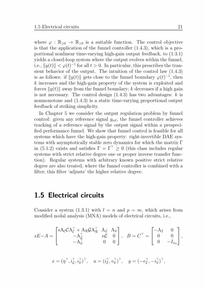
Consider a system (1.3.1) with l = n and p = m, which arises frommodified nodal analysis (MNA) models of electrical circuits, i.e.,
sE−A =
sACCA⊤
C + ARGA⊤R AL AV
−A⊤L sL 0
−A⊤V 0 0
, B = C⊤ =
−AI 00 00 −InV
,
x = (η⊤, i⊤L , i⊤V )
⊤, u = (i⊤I , v⊤V )
⊤, y = (−v⊤I ,−i⊤V )⊤,
22 1 Introduction
where
C ∈ RnC×nC ,G ∈ RnG×nG ,L ∈ RnL×nL,
AC ∈ Rne×nC ,AR ∈ Rne×nG ,AL ∈ Rne×nL,AV ∈ Rne×nV ,AI ∈ Rne×nI ,
n = ne + nL + nV , m = nI + nV .
Here AC, AR, AL, AV and AI denote the element-related incidence ma-trices, C, G and L are the matrices expressing the consecutive relationsof capacitances, resistances and inductances, η(t) is the vector of nodepotentials, iL(t), iV(t), iI(t) are the vectors of currents through induc-tances, voltage and current sources, and vV(t), vI(t) are the voltages ofvoltage and current sources, resp.In Chapter 6 we generalize a characterization of asymptotic stability
of the circuit and give sufficient topological criteria for its invariant ze-ros being located in the open left half-plane. We show that asymptoticstability of the zero dynamics can be characterized by means of theinterconnectivity of the circuit and that it implies that the circuit ishigh-gain stabilizable with any positive high-gain factor. Thereafter weconsider the output regulation problem for electrical circuits by funnelcontrol. We show that for circuits with asymptotically stable zero dy-namics, the funnel controller achieves tracking of a class of referencesignals within a prespecified funnel; this means in particular that thetransient behaviour of the output error can be prescribed and the funnelcontroller does neither incorporate any internal model for the referencesignals nor any identification mechanism, it is simple in its design. Theresults are illustrated by a simulation of a discretized transmission line.
1.6 Previously published results and joint
work
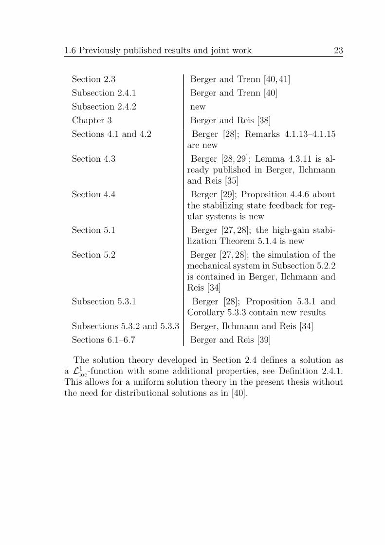
Parts of the present thesis have already been published or submittedfor publication as indicated in the following table.
Section contained in
Section 2.1 new
Section 2.2 Berger, Ilchmann and Trenn [36]
1.6 Previously published results and joint work 23
Section 2.3 Berger and Trenn [40, 41]
Subsection 2.4.1 Berger and Trenn [40]
Subsection 2.4.2 new
Chapter 3 Berger and Reis [38]
Sections 4.1 and 4.2 Berger [28]; Remarks 4.1.13–4.1.15are new
Section 4.3 Berger [28, 29]; Lemma 4.3.11 is al-ready published in Berger, Ilchmannand Reis [35]
Section 4.4 Berger [29]; Proposition 4.4.6 aboutthe stabilizing state feedback for reg-ular systems is new
Section 5.1 Berger [27, 28]; the high-gain stabi-lization Theorem 5.1.4 is new
Section 5.2 Berger [27, 28]; the simulation of themechanical system in Subsection 5.2.2is contained in Berger, Ilchmann andReis [34]
Subsection 5.3.1 Berger [28]; Proposition 5.3.1 andCorollary 5.3.3 contain new results
Subsections 5.3.2 and 5.3.3 Berger, Ilchmann and Reis [34]
Sections 6.1–6.7 Berger and Reis [39]
The solution theory developed in Section 2.4 defines a solution asa L1
loc-function with some additional properties, see Definition 2.4.1.This allows for a uniform solution theory in the present thesis withoutthe need for distributional solutions as in [40].

25
2 Decomposition of matrix pencils
In this chapter we study (singular) linear matrix pencils
sE −A ∈ K[s]m×n, where K is Q, R or C.
Two matrix pencils sE1−A1 and sE2−A2 are called equivalent if, andonly if, there exist invertible matrices S and T such that
(SE1T, SA1T
)=(E2, A2
);
we write (E1, A1) ∼= (E2, A2). Indeed, this is an equivalence relation onKm×n × Km×n. In the literature this is also sometimes called strict orstrong equivalence, see e.g. [100, Ch. XII, § 1] and [152, Def. 2.1]. Basedon this notion of equivalence it is of interest to find the ‘simplest’ matrixpencil within an equivalence class. As discussed in Section 1.1, forregular matrix pencils this problem was solved by Weierstraß [243]and for general matrix pencils later by Kronecker [149] (see also[100,152]). Nevertheless, the analysis of matrix pencils is still an activeresearch area, mainly because of numerical issues or to find ways toobtain the WCF and KCF efficiently (see e.g. [17, 81, 82, 234–236]).A main goal in this chapter is to highlight the importance of the
Wong sequences [250] for the analysis of matrix pencils. The Wongsequences for the matrix pencil sE − A are given by the followingsequences of subspaces (see the List of Symbols for the definition of thepreimage)
V0 := Kn, Vi+1 := A−1(EVi) ⊆ Kn,
W0 := {0}, Wi+1 := E−1(AWi) ⊆ Kn.
As a motivation for the Wong sequences we may consider a classical(i.e., continuously differentiable) solution x : R → Kn ofEx(t) = Ax(t).Using that the linear spaces Vi are closed and thus invariant under

26 2 Decomposition of matrix pencils
differentiation, the following implications hold true:
∀ t ∈ R : x(t) ∈ Kn = V0
=⇒ ∀ t ∈ R : x(t) ∈ V0Ex=Ax=⇒ ∀ t ∈ R : x(t) ∈ A−1(EV0) = V1
=⇒ ∀ t ∈ R : x(t) ∈ V1Ex=Ax=⇒ ∀ t ∈ R : x(t) ∈ A−1(EV1) = V2
=⇒ etc.
Therefore, after finitely many iterations it is established that the so-lution x must evolve in V∗ :=
⋂i∈N0
Vi, i.e., x(t) ∈ V∗ for all t ∈ R.In fact, it is shown in Section 2.3 that V∗ consists of the ODE partand the underdetermined part of the DAE and thus contains all so-lutions. W∗ :=
⋃i∈N0
Wi in turn constitutes the nilpotent part andthe overdetermined part of the DAE - which lead to trivial solutionsof the homogeneous DAE d
dtEx(t) = Ax(t). All four parts together
constitute the quasi-Kronecker form of the matrix pencil sE − A, seeTheorem 2.3.3.In Section 2.2 we first consider regular matrix pencils sE − A and
show that V∗ ∩ W∗ = {0}, which means that the underdeterminedpart is not present, and that V∗ + W∗ = Kn, which means that theoverdetermined part is not present. Therefore, the Wong sequencesdirectly lead to a decomposition of the pencil into an ODE part and anilpotent part - the quasi-Weierstraß form, see Theorem 2.2.5.The QKF is derived step by step via several interim decompositions,
which are interesting in their own right. The WCF and the KCF canbe obtained as a corollary from the QWF and the QKF, resp. Anoverview of all decompositions used in this chapter and their relationsis provided in Section 2.1.The consequences of the quasi-Kronecker form for the characteriza-
tion of solutions of the DAE ddtEx(t) = Ax(t) + f(t) are discussed in
Section 2.4. The solutions to each part are determined separately inTheorem 2.4.8 which allow to characterize consistency of the inhomo-geneity and initial values. In particular, it is shown that the Wongsequences completely characterize the solution behavior of the DAE.An important feature of the Wong sequences is that they (and some
modifications of them) fully determine the KCF of the underlying ma-trix pencil (without the corresponding transformation matrices). Moreprecisely, the row and column minimal indices, the degrees of the fi-nite and infinite elementary divisors and the finite eigenvalues can becalculated using only the Wong sequences, see Subsection 2.3.4.

2.1 Definitions 27
An advantage of the Wong sequence approach is that we respect thedomain of the entries in the matrix pencil, e.g. if our matrices are real-valued, then all transformations remain real-valued. We formulatedour results in such a way that they are valid for K = Q, K = R
and K = C. Especially for K = Q it was also necessary to re-checkknown results, whether their proofs are also valid in Q. We believethat the case K = Q is of special importance because this allows forthe implementation of our approach in exact arithmetic which might befeasible if the matrices are sparse and not too big. In fact, we believethat the construction of the QWF and QKF is also possible if thematrix pencil sE−A contains symbolic entries as it is common for theanalysis of electrical circuits, where one might just add the symbol Rinto the matrix instead of a specific value of the corresponding resistor;however, we have not formalized this. This is a major difference of ourapproach to the ones available in literature which often aim for unitarytransformation matrices (due to numerical stability) and are thereforenot suitable for symbolic calculations.We like to stress that indeed most of the results in Section 2.2 can
be derived using more general results from Section 2.3. However, welike to point out the peculiarities of the regular case considered in Sec-tion 2.2. In particular, the Wong sequences constitute a direct sumV∗ ⊕ W∗ = Kn and the transformation matrices for the QWF can becalculated easily in the regular case compared to the more general set-ting. Furthermore, the transformation to WCF is calculated explicitly.
2.1 Definitions
In this section we define different decompositions of matrix pencilswhich will be derived in Sections 2.2 and 2.3. First we consider decom-positions for the class of regular matrix pencils: sE − A ∈ K[s]m×n iscalled regular if, and only if, m = n and det(sE − A) ∈ K[s] \ {0}.
Definition 2.1.1 (Quasi-Weierstraß form).A regular matrix pencil sE − A ∈ K[s]n×n is said to be in quasi-Weierstraß form (QWF) if, and only if,
sE −A = s
[In1
00 N
]−[J 00 In2
](2.1.1)
28 2 Decomposition of matrix pencils
for some n1, n2 ∈ N0, J ∈ Kn1×n1, N ∈ Kn2×n2 such that N is nilpotent.
It is shown in Theorem 2.2.5 that any regular matrix pencil can betransformed into QWF and the transformation matrices can be calcu-lated via the Wong sequences.If the entries J and N in (2.1.1) are in Jordan canonical form,
then (2.1.1) is called the Weierstraß canonical form. This form is de-rived in Corollary 2.2.19, again using the Wong sequences.
Definition 2.1.2 (Weierstraß canonical form).A regular matrix pencil sE − A ∈ K[s]n×n is said to be in Weierstraßcanonical form (WCF) if, and only if, sE−A satisfies (2.1.1) such thatJ and N are in Jordan canonical form and N is nilpotent.
If regularity of sE − A is not required, then additional blocks mayappear in the decomposition of the pencil. As a first step towardsthe quasi-Kronecker form, which is derived in Section 2.3, we derivethe interim quasi-Kronecker triangular form in Theorem 2.3.19, whichdecouples the regular part, the underdetermined part and the overde-termined part of the pencil. This form is defined as follows.
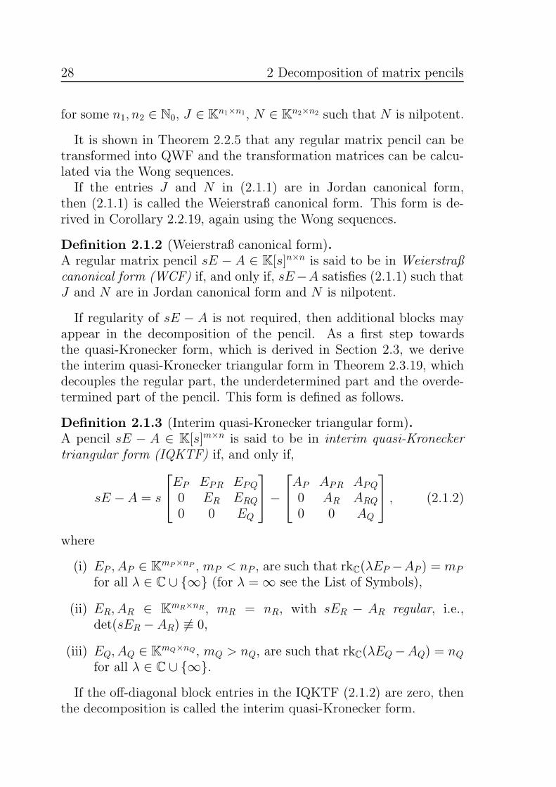
Definition 2.1.3 (Interim quasi-Kronecker triangular form).A pencil sE − A ∈ K[s]m×n is said to be in interim quasi-Kroneckertriangular form (IQKTF) if, and only if,
sE −A = s
EP EPR EPQ
0 ER ERQ
0 0 EQ
−
AP APR APQ
0 AR ARQ
0 0 AQ
, (2.1.2)
where
(i) EP , AP ∈ KmP×nP , mP < nP , are such that rkC(λEP −AP ) = mP
for all λ ∈ C ∪ {∞} (for λ = ∞ see the List of Symbols),
(ii) ER, AR ∈ KmR×nR, mR = nR, with sER − AR regular, i.e.,det(sER − AR) 6≡ 0,
(iii) EQ, AQ ∈ KmQ×nQ, mQ > nQ, are such that rkC(λEQ−AQ) = nQfor all λ ∈ C ∪ {∞}.
If the off-diagonal block entries in the IQKTF (2.1.2) are zero, thenthe decomposition is called the interim quasi-Kronecker form.
2.1 Definitions 29
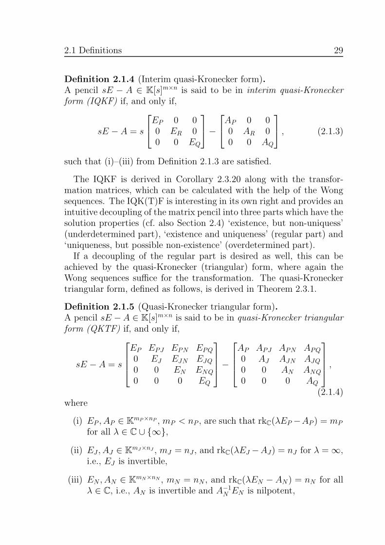
Definition 2.1.4 (Interim quasi-Kronecker form).A pencil sE − A ∈ K[s]m×n is said to be in interim quasi-Kroneckerform (IQKF) if, and only if,
sE − A = s
EP 0 00 ER 00 0 EQ
−
AP 0 00 AR 00 0 AQ
, (2.1.3)
such that (i)–(iii) from Definition 2.1.3 are satisfied.
The IQKF is derived in Corollary 2.3.20 along with the transfor-mation matrices, which can be calculated with the help of the Wongsequences. The IQK(T)F is interesting in its own right and provides anintuitive decoupling of the matrix pencil into three parts which have thesolution properties (cf. also Section 2.4) ‘existence, but non-uniquess’(underdetermined part), ‘existence and uniqueness’ (regular part) and‘uniqueness, but possible non-existence’ (overdetermined part).If a decoupling of the regular part is desired as well, this can be
achieved by the quasi-Kronecker (triangular) form, where again theWong sequences suffice for the transformation. The quasi-Kroneckertriangular form, defined as follows, is derived in Theorem 2.3.1.
Definition 2.1.5 (Quasi-Kronecker triangular form).A pencil sE −A ∈ K[s]m×n is said to be in quasi-Kronecker triangularform (QKTF) if, and only if,
sE − A = s
EP EPJ EPN EPQ
0 EJ EJN EJQ
0 0 EN ENQ
0 0 0 EQ
−
AP APJ APN APQ
0 AJ AJN AJQ
0 0 AN ANQ
0 0 0 AQ
,
(2.1.4)where
(i) EP , AP ∈ KmP×nP , mP < nP , are such that rkC(λEP −AP ) = mP
for all λ ∈ C ∪ {∞},
(ii) EJ , AJ ∈ KmJ×nJ , mJ = nJ , and rkC(λEJ −AJ) = nJ for λ = ∞,i.e., EJ is invertible,
(iii) EN , AN ∈ KmN×nN , mN = nN , and rkC(λEN − AN) = nN for allλ ∈ C, i.e., AN is invertible and A−1
N EN is nilpotent,

30 2 Decomposition of matrix pencils
(iv) EQ, AQ ∈ KmQ×nQ, mQ > nQ, are such that rkC(λEQ−AQ) = nQfor all λ ∈ C ∪ {∞}.
If the off-diagonal block entries in the QKTF (2.1.4) are zero, thenthe decomposition is called the quasi-Kronecker form.
Definition 2.1.6 (Quasi-Kronecker form).A pencil sE−A ∈ K[s]m×n is said to be in quasi-Kronecker form (QKF)if, and only if,
sE − A = s
EP 0 0 00 EJ 0 00 0 EN 00 0 0 EQ
−
AP 0 0 00 AJ 0 00 0 AN 00 0 0 AQ
, (2.1.5)
such that (i)–(iv) from Definition 2.1.5 are satisfied.
The QKF is derived in Theorem 2.3.3. If more structure of the blockentries is desired, it is possible to refine the QKF to the well-knownKronecker canonical form, which is derived in Corollary 2.3.21. Weuse the notation Nk, Lk, Kk for k ∈ N which is defined in the List ofSymbols.
Definition 2.1.7 (Kronecker canonical form).A pencil sE − A ∈ K[s]m×n is said to be in Kronecker canonical form(KCF) if, and only if, there exist a, b, c, d ∈ N0 and ε1, . . . , εa, ρ1, . . . , ρb,σ1, . . . , σc, η1, . . . , ηd ∈ N0, λ1, . . . , λb ∈ K, such that
sE −A = diag(Pε1(s), . . . ,Pεa(s),J λ1
ρ1 (s), . . . ,J λbρb (s),
Nσ1(s), . . . ,Nσc
(s),Qη1(s), . . . ,Qηd(s)), (2.1.6)
where
Pε(s) = s[0 1
0 1
]−[1 0
1 0
]= sLε+1 −Kε+1 ∈ K[s]ε×(ε+1),
J λρ (s) = (s− λ)Iρ −
[01
1 0
]= (s− λ)Iρ −Nρ ∈ K[s]ρ×ρ,
Nσ(s) = s
[01
1 0
]− Iσ = sNσ − Iσ ∈ K[s]σ×σ,
Qη(s) = s
[01
01
]−[1
0
10
]= sL⊤
η+1 −K⊤η+1 ∈ K[s](η+1)×η,
and ε ∈ N0, ρ ∈ N, λ ∈ K, σ ∈ N, η ∈ N0.
2.2 Quasi-Weierstraß form 31
2.2 Quasi-Weierstraß form
In this section we derive the quasi-Weierstraß form for regular matrixpencils sE − A ∈ K[s]n×n. In Subsection 2.2.1 we derive some prop-erties of the Wong sequences and exploit them to derive the QWF.In Subsection 2.2.2 we consider chains of generalized eigenvectors andshow how to exploit them to re-derive the Weierstraß canonical form.The results of this section have already been published in a joint
work with Achim Ilchmann and Stephan Trenn [36].
2.2.1 Wong sequences and QWF
As pointed out earlier, our approach is based on the Wong sequences.They can be calculated via a recursive subspace iteration. Since theyare used in later sections as well, we define the Wong sequences forgeneral matrix pencils sE − A ∈ K[s]m×n.
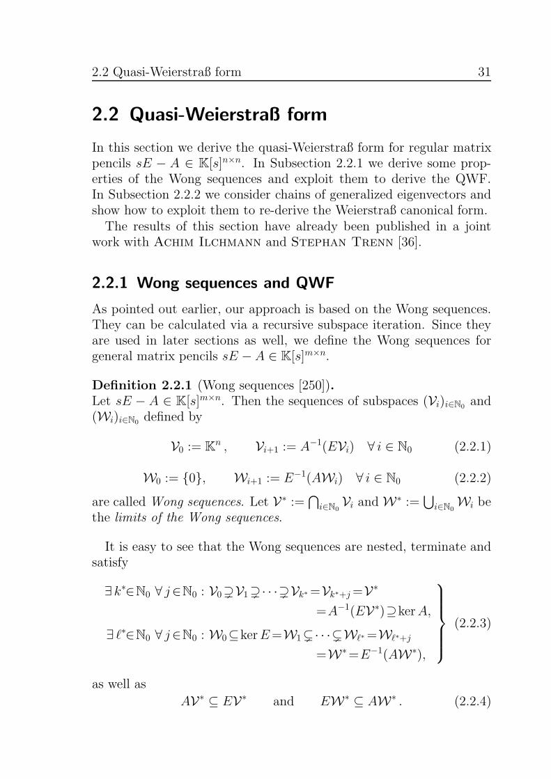
Definition 2.2.1 (Wong sequences [250]).Let sE − A ∈ K[s]m×n. Then the sequences of subspaces (Vi)i∈N0
and(Wi)i∈N0
defined by
V0 := Kn , Vi+1 := A−1(EVi) ∀ i ∈ N0 (2.2.1)
W0 := {0}, Wi+1 := E−1(AWi) ∀ i ∈ N0 (2.2.2)
are called Wong sequences. Let V∗ :=⋂
i∈N0Vi and W∗ :=
⋃i∈N0
Wi bethe limits of the Wong sequences.
It is easy to see that the Wong sequences are nested, terminate andsatisfy
∃ k∗∈N0 ∀ j∈N0 : V0)V1) · · ·)Vk∗=Vk∗+j=V∗
=A−1(EV∗)⊇kerA,
∃ ℓ∗∈N0 ∀ j∈N0 : W0⊆kerE=W1( · · ·(Wℓ∗=Wℓ∗+j
=W∗=E−1(AW∗),
(2.2.3)
as well as
AV∗ ⊆ EV∗ and EW∗ ⊆ AW∗ . (2.2.4)
32 2 Decomposition of matrix pencils
In the following Lemma 2.2.2 some elementary properties of theWong sequences are derived, they are essential for proving basic prop-erties of the subspaces V∗ and W∗ in Proposition 2.2.3. These re-sults are inspired by the observation of Campbell [62, p. 37] whoproves, for K = C, that the space of consistent initial values is givenby im
((A − λE)−1E
)νfor any λ ∈ C\ spec(sE − A) and ν ∈ N0 the
index of the matrix (A− λE)−1E, [62, p. 7]. However, Campbell didnot consider the Wong sequences explicitly.
Lemma 2.2.2 (Spectrum and properties of Vi and Wi).If sE − A ∈ K[s]n×n is regular, then the Wong sequences (2.2.1)and (2.2.2) satisfy
∀λ ∈ K\ spec(sE − A) ∀ i ∈ N0 : Vi = im((A− λE)−1E
)i
and Wi = ker((A− λE)−1E
)i.
In particular,
∀ i ∈ N0 : dimVi + dimWi = n. (2.2.5)
Proof: Since sE − A ∈ K[s]n×n is regular, let
E := (A− λE)−1E, for arbitrary but fixed λ ∈ K\ spec(sE −A).(2.2.6)
Step 1: We prove by induction: Vi = im Ei for all i ∈ N0. Clearly,V0 = Kn = im E0. Suppose that im Ei = Vi holds for some i ∈ N0.Step 1a: We show: Vi+1 ⊇ im Ei+1. Let x ∈ im Ei+1 ⊆ im Ei.
Then there exists y ∈ im Ei such that x = (A− λE)−1
Ey. Therefore,
(A−λE)x = Ey = E(y+λx−λx) and so, for y := y+λx ∈ im Ei = Vi,we have Ax = Ey. This implies x ∈ V i+1.Step 1b: We show: Vi+1 ⊆ im Ei+1. Let x ∈ Vi+1 and choose y ∈ Vi
such that Ax = Ey. Then (A − λE)x = E(y − λx) or, equivalently,x = (A−λE)−1E(y−λx). From x ∈ Vi+1 ⊆ Vi it follows that y−λx ∈Vi = im Ei and therefore x ∈ im Ei+1.Step 2: We prove by induction: Wi = ker Ei for all i ∈ N0. Clearly,
W0 = {0} = ker E0. Suppose that ker Ei = Wi for some i ∈ N0.
First observe that (I + λE) restricted to ker Ei is an operator (I +
λE) : ker Ei → ker Ei with inverse∑i−1
j=0(−λ)jEj. Thus the following

2.2 Quasi-Weierstraß form 33
equivalences hold
x ∈ Wi+1 ⇐⇒ ∃ y ∈ Wi : Ex = Ay = (A− λE)y + λEy
⇐⇒ ∃ y ∈ Wi = ker Ei : Ex = (I + λE)y =: y
⇐⇒ ∃ y ∈ ker Ei : Ex = y
⇐⇒ x ∈ ker Ei+1.
Next we prove important properties of the subspaces V∗ and W∗,some of which can be found in [250], but the present presentation ismore straightforward.
Proposition 2.2.3 (Properties of V∗ and W∗).If sE −A ∈ K[s]n×n is regular, then V∗ and W∗ as in (2.2.3) satisfy:
(i) k∗ = l∗, where k∗, l∗ are given in (2.2.3),
(ii) V∗ ⊕W∗ = Kn,
(iii) kerE ∩ V∗ = {0} , kerA ∩W∗ = {0} , kerE ∩ kerA = {0} .
Proof: (i): This is a consequence of (2.2.5).(ii): In view of (2.2.5), it suffices to show that V∗ ∩ W∗ = {0}.
Using the notation as in (2.2.6), we may conclude: If x ∈ V∗ ∩W∗ =im Ek∗ ∩ ker Ek∗, then there exists y ∈ Kn such that x = Ek∗y and
so 0 = Ek∗x =(Ek∗)2y = E2k∗y , whence, in view of y ∈ ker E2k∗ =
ker Ek∗, 0 = Ek∗y = x.(iii): This is a direct consequence from (2.2.3) and (ii).
Example 2.2.4 (Regular pencil).Consider the linear pencil sE −A ∈ K[s]4×4 given by
A :=
3 0 1 00 2 2 −11 2 3 00 −1 0 2
, E :=
1 −1 −3 00 2 0 −1−3 −1 1 2−2 −2 0 2
.
Since det(sE−A) = 36s(s−1), the pencil is regular and not equivalentto a pencil sI4− J , J ∈ K4×4, i.e., it is not an ODE. A straightforward

34 2 Decomposition of matrix pencils
calculation gives
V1 = im
1 0 00 1 00 0 11 1 1
, W1 = kerE = im
1102
and
V2 = imV, where V :=
1 00 2−1 −10 1
,
W2 = imW, where W :=
1 00 11 −10 2
.
Both sequences terminate after these two iterations and therefore V∗ =V2, W∗ = W2 and k∗ = ℓ∗ = 2. The statements of Proposition 2.2.3and (2.2.4) are readily verified. Finally, we stress, in view of (2.2.5),that for this example
V1 ∩W1 = W1 ) {0}.
We are now in a position to state the main result of this section: TheWong sequences (Vi)i∈N0
and (Wi)i∈N0, converge in finitely many steps
to the subspaces V∗ and W∗, and the latter constitute a transformationof the original pencil sE −A into two decoupled pencils.
Theorem 2.2.5 (The quasi-Weierstraß form).Consider a regular matrix pencil sE − A ∈ K[s]n×n and correspondingspaces V∗ and W∗ as in (2.2.3). Let
n1 := dimV∗, V ∈ Kn×n1 : imV = V∗
and n2 := n− n1 = dimW∗, W ∈ Kn×n2 : imW = W∗.
Then [V,W ] and [EV,AW ] are invertible and[EV,AW ]−1 (sE − A) [V,W ] is in QWF (2.1.1) such that Nk∗ = 0for k∗ as given in (2.2.3).
Before we prove Theorem 2.2.5, some comments may be warranted.

2.2 Quasi-Weierstraß form 35
Remark 2.2.6 (The quasi-Weierstraß form).Let sE −A ∈ K[s]n×n be a regular matrix pencil and use the notationfrom Theorem 2.2.5.
(i) It is immediate, and will be used in later analysis, that[EV,AW ]−1 (sE −A) [V,W ] is in QWF (2.1.1) if, and only if,
AV = EV J and EW = AWN (2.2.7)
or, equivalently, if
E = [EV,AW ]
[I 00 N
][V,W ]−1
and A = [EV,AW ]
[J 00 I
][V,W ]−1 . (2.2.8)
(ii) If (2.2.7) is solvable and if [EV,AW ] is invertible, then it isstraightforward to see that J and N in (2.2.7) are uniquely givenby
J := (EV )+AV and N := (AW )+EW, resp., (2.2.9)
where M+ := (M∗M)−1M∗ for M ∈ Kp×q with rkKM = q.
(iii) The spaces V∗ and W∗ determine uniquely – up to similarity –the solutions J and N of (2.2.7), resp. More precisely, let
V ∈ Kn×n1: im V = V∗ and W ∈ Kn×n2: im W = W∗.
Then
∃S ∈ Gln1(K): V S = V and ∃T ∈ Gln2
(K): WT = W ,
and a simple calculation yields that J and N are similar to
(EV )+AV = S−1JS and (AW )+EW = T−1NT , resp.
(iv) If detE 6= 0, then V∗ = Vi = Kn and W∗ = Wi = {0} for alli ∈ N0. Therefore
E−1 (sE − A) = sI − E−1A
is in QWF.

36 2 Decomposition of matrix pencils
(v) Let K = C. In view of (iii), the matrices V andW may always bechosen so that J and N in (2.1.1) are in Jordan canonical form,in this case (2.1.1) is in WCF.
(vi) For K = C, there are various numerical methods available to cal-culate the WCF, see e.g. [17, 81, 82]. However, since the QWFdoes not invoke any eigenvalues and eigenvectors (here only thedecoupling (2.1.1) and J and N without any special structure isimportant), it is possible that the above mentioned algorithmscan be improved by using the Wong sequences. To calculate thesubspaces (2.2.1) and (2.2.2) of the Wong sequences, one may usemethods to obtain orthogonal bases for deflating subspaces; seefor example [24] and [135].Furthermore, the QWF – in contrast to the WCF – allows toconsider matrix pencils over rational or even symbolic rings andthe algorithm is still applicable. In fact, we will show in Proposi-tion 2.2.9 that the number of subspace iterations equals the indexof the matrix pencil (cf. Definition 2.2.8); hence in many practicalsituations only one or two iterations must be carried out.
(vii) A time-varying pendant to the QWF is the standard canonicalform developed in [64, 68] and studied in [32, 33]. This form hasthe same block structure as the QWF, but with time-varying Jand N , where N is pointwise strictly lower triangular.
Proof of Theorem 2.2.5: Invertibility of [V,W ] follows from Propo-sition 2.2.3 (ii). The implication
∀α ∈ Kn1 :
(EV α = 0
Prop. 2.2.3 (iii)=⇒ V α = 0
rkV=n1=⇒ α = 0
)
shows rkEV = n1, and a similar argument yields rkAW = n2. Now,invertibility of [EV,AW ] is equivalent to imEV ∩ imAW = {0}, andthe latter is a consequence of
∀α ∈ Kn1 ∀β ∈ Kn2 : EV α = AWβ =⇒ V α ∈ E−1(AW∗)(2.2.3)= W∗
Prop. 2.2.3 (ii)=⇒ V α = 0 =⇒ α = 0 ∧ β = 0.
Now the subset inequalities (2.2.4) imply that (2.2.7) is solvable and[EV,AW ]−1 (sE −A) [V,W ] is in the form (2.1.1). It remains to prove
2.2 Quasi-Weierstraß form 37
that N is nilpotent. To this end, we show
∀ i ∈ {0, . . . , k∗} : imWN i ⊆ Wk∗−i . (2.2.10)
The statement is clear for i = 0. Suppose, for some i ∈ {0, . . . , k∗− 1},we have
imWN i ⊆ Wk∗−i . (2.2.11)
Then
imAWN i+1 (2.2.7)= imEWN i
(2.2.11)
⊆ EWk∗−i
(2.2.2)
⊆ AWk∗−i−1
and, by invoking Proposition 2.2.3 (iii),
imWN i+1 ⊆ Wk∗−i−1.
This proves (2.2.10). Finally, (2.2.10) for i = k∗ together with the factthat W has full column rank and W0 = {0}, implies that Nk∗ = 0.
Example 2.2.7 (Example 2.2.4 revisited).For V and W as defined in Example 2.2.4 we have
[V,W ] =
1 0 1 00 2 0 1−1 −1 1 −10 1 0 2
and [EV,AW ] =
4 1 4 −10 3 2 −2−4 −1 4 −1−2 −2 0 3
and the corresponding transformation [EV,AW ]−1 (sE − A) [V,W ]shows that a QWF of this example is given by
s
[I2 00 N
]−[J 00 I2
]where J :=
1
3
[2 1−2 1
], N :=
2
3
[−1 1−1 1
].
It follows from Remark 2.2.6 (iii) that the following definition of theindex of a regular pencil is well defined since it does not depend on thespecial choice of N in the QWF.
Definition 2.2.8 (Index of sE − A).Let sE − A ∈ K[s]n×n be a regular matrix pencil and consider theQWF (2.1.1). Then
ν∗ :=
{min { ν ∈ N | Nν = 0 } , if N exists0, otherwise
is called the index of sE −A.

38 2 Decomposition of matrix pencils
The classical definition of the index of a regular matrix pencil (seee.g. [152, Def. 2.9]) is via theWCF. However, invoking Remark 2.2.6 (v),we see that ν∗ in Definition 2.2.8 is the same number.
Proposition 2.2.9 (Index of sE −A).If sE −A ∈ K[s]n×n is regular, then the Wong sequence in (2.2.2) andW and N as in Theorem 2.2.5 satisfy
∀ i ∈ N0 : Wi =W kerN i . (2.2.12)
This implies that ν∗ = k∗; i.e., the index ν∗ coincides with k∗ deter-mined by the Wong sequences in (2.2.3).
Proof: We use the notation as in Theorem 2.2.5 and the form (2.1.1),and also the following simple formula
∀ i ∈ N0 :
[I 00 N
]−1 [J 00 I
]({0n1
}kerN i
)=
({0n1
}kerN i+1
). (2.2.13)
Next, we conclude, for W0 := {0} and all i ∈ N,
Wi := [V,W ]−1Wi(2.2.3)= [V,W ]−1E−1AWi−1
(2.2.8)=
[I 00 N
]−1
[EV,AW ]−1A[V,W ]Wi−1
=
([I 00 N
]−1 [J 00 I
])· · ·([
I 00 N
]−1 [J 00 I
])
︸ ︷︷ ︸i-times
W0
(2.2.13)=
([I 00 N
]−1 [J 00 I
])· · ·([
I 00 N
]−1 [J 00 I
])
︸ ︷︷ ︸(i−1)-times
({0n1}kerN
)
(2.2.13)=
({0n1
}kerN i
)
and hence (2.2.12).
Example 2.2.10 (Example 2.2.4, 2.2.7 revisited).For W and N as defined in Example 2.2.4 and 2.2.7, resp., we see that
2.2 Quasi-Weierstraß form 39
N2 = 0 and confirm the statement of Proposition 2.2.9:
W kerN =W im
[11
]= im
1102
= W1.
An immediate consequence of Theorem 2.2.5 is
det(sE − A) =
det([EV,AW ]) det(sIn1− J) det(sN − In2
) det([V,W ]−1) ,
and since any nilpotent matrix N satisfies det(sN − In2) = (−1)n2, we
arrive at the following corollary.
Corollary 2.2.11 (Properties of the determinant).Suppose sE − A ∈ K[s]n×n is a regular matrix pencil. Then, using thenotation of Theorem 2.2.5 and the form (2.1.1), we have:
(i) det(sE −A) = c det(sIn1− J),
for c := (−1)n2 det([EV,AW ]) det([V,W ]−1) 6= 0,
(ii) spec(sE −A) = spec(sIn1− J),
(iii) dimV∗ = deg(det(sE − A)
).
In the remainder of this subsection we characterize V∗ in geometricterms as a largest subspace. [42] already stated that V∗ is the largestsubspace such that AV∗ ⊆ EV∗.
Proposition 2.2.12 (V∗ largest subspaces).Let sE − A ∈ K[s]n×n be a regular matrix pencil. Then V∗ determinedby the Wong sequences (2.2.3) is the largest subspace of Kn such thatAV∗ ⊆ EV∗.
Proof: We have to show that any subspace U ⊆ Kn so that AU ⊆ EUsatisfies U ⊆ V∗. Let u0 ∈ U . Then
∃u1, . . . , uk∗ ∈ U ∀ i = 1, . . . , k∗ : Aui−1 = Eui .

40 2 Decomposition of matrix pencils
By Theorem 2.2.5,
∃α0, . . . , αk∗ ∈ Kn1 ∃β0, . . . , βk∗ ∈ Kn2 ∀ i = 0, . . . , k∗ :
ui = [V,W ]
(αi
βi
)
and hence
∀ i = 1, . . . , k∗ : A[V,W ]
(αi−1
βi−1
)= E[V,W ]
(αi
βi
)
or, equivalently,
∀ i = 1, . . . , k∗ : [EV,AW ]
(−αi
βi−1
)= [AV,EW ]
(−αi−1
βi
)
(2.2.7)= [EV,AW ]
[J 00 N
](−αi−1
βi
);
since [EV,AW ] is invertible, we arrive at
∀ i = 1, . . . , k∗ : βi−1 = Nβi
and thereforeβ0 = Nβ1 = . . . = Nk∗βk∗ = 0.
This yields u0 = V α0 ∈ imV = V∗ and proves U ⊆ V∗.
2.2.2 Eigenvector chains and WCF
In this subsection we show that the generalized eigenvectors of a regularpencil sE − A ∈ C[s]n×n constitute a basis which transforms sE − Ainto WCF. From this point of view, the WCF is a generalized Jordancanonical form. The chains of eigenvectors and eigenspaces are derivedin terms of the matrices E and A; the QWF is only used in the proofs.This again shows the unifying power of the Wong-sequences and allowsfor a ‘natural’ proof of the WCF.Note that eigenvalues and eigenvectors of real or rational matrix
pencils are in general complex valued, thus in the following we restrictthe analysis to the case K = C. We recall the well known conceptof chains of generalized eigenvectors; for infinite eigenvectors see [23,Def. 2] and also [158, 159].

2.2 Quasi-Weierstraß form 41
Definition 2.2.13 (Chains of generalized eigenvectors).Let sE−A ∈ C[s]n×n be a matrix pencil. Then (v1, . . . , vk) ∈ (Cn\{0})kis called a chain (of sE −A at eigenvalue λ) if, and only if,
λ ∈ spec(sE −A) : (A− λE)v1 = 0, (A− λE)v2 = Ev1,
. . . , (A− λE)vk = Evk−1;
λ = ∞ : Ev1 = 0, Ev2 = Av1,
. . . , Evk = Avk−1;
(2.2.14)the ith vector vi of the chain is called generalized eigenvector of order iat λ.
Note that (v1, . . . , vk) is a chain at λ ∈ spec(sE −A) if, and only if,for all i ∈ {1, . . . , k},
AVi = EVi
λ 1
1λ
where Vi := [v1, . . . , vi] . (2.2.15)
Remark 2.2.14 (Linear relations).It may be helpful to consider the concept of generalized eigenvectors, inparticular for eigenvalues at ∞, from the viewpoint of linear relations,see e.g. [5]:
R ⊆ Cn × Cn is called a linear relation if, and only if, R is a linearspace; its inverse relation is R−1 := {(y, x) ∈ Cn × Cn| (x, y) ∈ R},and the multiplication with a relation S ⊆ Cn ×Cn is RS := {(x, y) ∈Cn × Cn| ∃ z ∈ Cn : (x, z) ∈ S ∧ (z, y) ∈ R}. λ ∈ C is called aneigenvalue of a relation R with eigenvector x ∈ Cn \ {0} if, and only if,(x, λx) ∈ R; see [214]. Clearly, λ 6= 0 is an eigenvalue of R if, and onlyif, 1/λ is an eigenvalue of R−1; this justifies to call ∞ an eigenvalue ofR if, and only if, 0 is an eigenvalue of R−1.
In the context of a matrix pencil sE − A ∈ C[s]n×n, the matrices Aand E induce the linear relations
A := {(x, Ax)|x ∈ Cn} and E := {(x, Ex)|x ∈ Cn} , resp.

42 2 Decomposition of matrix pencils
and therefore,
E−1 = { (Ex, x) | x ∈ Cn } ,E−1A = { (x, y) ∈ Cn × Cn | Ax = Ey } ,A−1 = { (Ax, x) | x ∈ Cn } ,A−1E = { (x, y) ∈ Cn × Cn | Ex = Ay } .
It now follows that
λ ∈ C is an eigenvalue of E−1A ⇐⇒ det(λE −A) = 0∞ is an eigenvalue of E−1A ⇐⇒ 0 is an eigenvalue of A−1E0 is an eigenvalue of A−1E ⇐⇒ E is not invertible.
In [214] also chains for relations are considered. In the context of theabove example this reads: v1, . . . , vk ∈ Cn \ {0} form a (Jordan) chainat eigenvalue λ ∈ C ∪ {∞} if, and only if,
λ ∈ spec(sE −A) : (v1, λv1), (v2, v1 + λv2),
. . . , (vk, vk−1 + λvk) ∈ E−1A;
λ = ∞ : (0, v1), (v1, v2),
. . . , (vk−1, vk) ∈ E−1A.
(2.2.16)
Obviously, (2.2.16) is equivalent to (2.2.14), but the former may be amore ‘natural’ definition. Linear relations have also been analyzed andexploited for matrix pencils in [25].
In order to decompose V∗, we have to be more specific with the spacesspanned by generalized eigenvectors at eigenvalues.
Definition 2.2.15 (Generalized eigenspaces).Let sE − A ∈ C[s]n×n be a matrix pencil. Then the sequences ofeigenspaces (of sE − A at eigenvalue λ) are defined by G0
λ := {0} and
∀ i ∈ N0 : Gi+1λ :=
{(A− λE)−1(EGi
λ), if λ ∈ spec(sE − A)
E−1(AGiλ), if λ = ∞.
The generalized eigenspace (of sE − A at eigenvalue λ ∈ spec(sE −A) ∪ {∞}) is defined by
Gλ :=⋃
i∈N0
Giλ.
2.2 Quasi-Weierstraß form 43
For the multiplicities we use the following notion
gm(λ) := dimG1λ is called the geometric multiplicity of
λ ∈ spec(sE −A) ∪ {∞},am(λ) := multiplicity of λ ∈ spec(sE −A) ∪ {∞} as a zero of
det(sE −A) is called the algebraic multiplicity of λ,
am(∞) := n− ∑λ∈spec(sE−A)
am(λ) = n− deg(det(sE − A)
)is
called the algebraic multiplicity at ∞.
Readily verified properties of the eigenspaces are the following.
Remark 2.2.16 (Eigenspaces).For any regular sE − A ∈ C[s]n×n and λ ∈ spec(sE − A) ∪ {∞} wehave:
(i) For each i ∈ N0, Giλ is the vector space spanned by the eigenvec-
tors up to order i at λ.
(ii) ∃ p∗ ∈ N0 ∀ j ∈ N0 : G0λ ( · · · ( Gp−1
λ ( Gp∗
λ = Gp∗+jλ .
The following result is formulated in terms of the pencil sE −A, itsproof invokes the QWF.
Proposition 2.2.17 (Eigenvectors and eigenspaces).Let sE − A ∈ C[s]n×n be regular.
(i) Every chain (v1, . . . , vk) at any λ ∈ spec(sE−A)∪{∞} satisfies,for all i ∈ {1, . . . , k}, vi ∈ Gi
λ\Gi−1λ .
(ii) Let λ ∈ spec(sE − A) ∪ {∞} and k ∈ N. Then for any v ∈Gkλ\Gk−1
λ , there exists a unique chain (v1, . . . , vk) such that vk = v.
(iii) The vectors of any chain (v1, . . . , vk) at λ ∈ spec(sE −A)∪ {∞}are linearly independent.
(iv)
Gλ ⊆{
V∗, if λ ∈ spec(sE −A)
W∗, if λ = ∞.

44 2 Decomposition of matrix pencils
(v)∀λ ∈ spec(sE − A) ∪ {∞} : dimGλ = am(λ).
Proof: Step 1 : Invoking the notation of Theorem 2.2.5 and of theform (2.1.1), we first show that
∀ i ∈ N0 : Giλ =
{V ker(J − λI)i, if λ ∈ spec(sE −A)
Wi =W kerN i, if λ = ∞.(2.2.17)
Suppose λ ∈ spec(sE − A).Step 1a: We prove by induction that
∀ i ∈ N0 : Giλ ⊆ V ker(J − λI)i. (2.2.18)
The claim is clear for i = 0. Suppose (2.2.18) holds for i = k − 1. Letvk ∈ Gk
λ \ {0} and vk−1 ∈ Gk−1λ such that (A − λE)vk = Evk−1. By
Proposition 2.2.3 (ii) we may set
vk = V α +Wβ for unique α ∈ Cn1, β ∈ Cn2 .
By (2.2.7), (A− λE)vk = Evk−1 is equivalent to
AW (I − λN)β = Evk−1 + EV (λI − J)α ,
and so, since by induction hypothesis
vk−1 ∈ Gk−1λ ⊆ V ker(J − λI)k−1 ⊆ V∗,
we conclude
W (I − λN)β ∈ A−1(EV∗)(2.2.1)= V∗.
Now Proposition 2.2.3 (ii) yields, since W has full column rank, (I −λN)β = 0 and hence, sinceN is nilpotent, β = 0. It follows from vk−1 ∈V ker(J − λI)k−1 that there exists u ∈ Cn1 such that vk−1 = V u and(J−λI)k−1u = 0. Then EV (J−λI)α = EV u and Proposition 2.2.3 (iii)gives, since V has full column rank, (J−λI)α = u. Therefore, vk = V αand (J − λI)kα = 0, hence vk ∈ V ker(J − λI)k and this completes theproof of (2.2.18).Step 1b: We prove by induction that
∀ i ∈ N0 : Giλ ⊇ V ker(J − λI)i. (2.2.19)

2.2 Quasi-Weierstraß form 45
The claim is clear for i = 0. Suppose (2.2.19) holds for i = k − 1. Letvk ∈ ker(J − λI)k and vk−1 ∈ ker(J − λI)k−1 such that (J − λI)vk =vk−1. Since EV has full column rank, this is equivalent to EV (J −λI)vk = EV vk−1 which is, by invoking (2.2.7), equivalent to (A −λE)V vk = EV vk−1 and then the induction hypothesis yields V vk−1 ∈Gk−1λ , thus having V vk ∈ Gk
λ. This proves (2.2.19) and completes theproof of (2.2.17) for finite eigenvalues.Step 1c: The statement ‘Wi = W kerN i for all i ∈ N0’ follows by
Proposition 2.2.9, and ‘Gi∞ = Wi for all i ∈ N0’ is clear from the
definition.Step 2 : The Assertions (i)–(iv) follow immediately from (2.2.17)
and the respective results of the classical eigenvalue theory, see forexample [155, Sec. 12.5, 12.7] and [95, Sec. 4.6]. Assertion (v) is aconsequence of Corollary 2.2.11 (i) and am(∞) = n − deg
(det(sE −
A))= n2. This completes the proof of the proposition.
An immediate consequence of Proposition 2.2.17 and (2.2.17) is thefollowing Theorem 2.2.18. We stress that our proof relies essentially onthe relationship between the eigenspaces of sE−A and the eigenspacesof sI−J and sI−N where J and N are as in (2.1.1). Alternatively, wecould prove Theorem 2.2.18 by using chains and cyclic subspaces only,however the present proof via the Quasi-Weierstraß form is shorter.
Theorem 2.2.18 (Decomposition and basis of V∗).Let sE − A ∈ C[s]n×n be regular, λ1, . . . , λk be the pairwise distinctzeros of det(sE − A) and use the notation of Theorem 2.2.5. Then
∀λ ∈ {λ1, . . . , λk} ∀ j ∈ {1, . . . , gm(λ)} ∃nλ,j ∈ N
∃ chain(v1λ,j, v
2λ,j, . . . , v
nλ,j
λ,j
)at λ :
Gλ =
gm(λ)⊕
j=1
im[v1λ,j, . . . , v
nλ,j
λ,j
]
︸ ︷︷ ︸=:Vλ,j∈Cn×nλ,j
. (2.2.20)
andV∗ = Gλ1
⊕ Gλ2⊕ . . .⊕ Gλk
and W∗ = G∞ .
In Corollary 2.2.19 we show that the generalized eigenvectors of aregular matrix pencil sE−A at the finite eigenvalues and at the infinite

46 2 Decomposition of matrix pencils
eigenvalue constitute a basis which transforms sE − A into the wellknown Weierstraß canonical form. So the WCF can be viewed as ageneralized Jordan canonical form.
Corollary 2.2.19 (Weierstraß canonical form).Let sE − A ∈ C[s]n×n be regular, n1 := dimV∗, n2 := n − n1 andλ1, . . . , λk be the pairwise distinct zeros of det(sE −A). Then we maychoose
Vf :=[Vλ1,1, . . . , Vλ1,gm(λ1), Vλ2,1, . . . , Vλ2,gm(λ2),
. . . , Vλk,1, . . . , Vλk,gm(λk)
],
V∞ :=[V∞,1, . . . , V∞,gm(∞)
],
where Vλi,j consists of a chain at λi as in (2.2.20), j = 1, . . . , gm(λi),i = 1, . . . , k, resp. For any such Vf , V∞, the matrices [Vf , V∞],[EVf , AV∞] ∈ Cn×n are invertible and [EVf , AV∞]−1(sE−A)[Vf , V∞] isin WCF.
Proof: The existence of Vf and V∞ satisfying the eigenvector condi-tions formulated in the corollary follows from Theorem 2.2.18. In viewof (2.2.15), it follows from the definition of chains that[EVf , AV∞]−1(sE − A)[Vf , V∞] is in the form (2.1.1) for some matri-ces J ∈ Cn1×n1 and N ∈ Cn2×n2 in Jordan canonical form and nilpotentN .
Definition 2.2.20 (Canonical form).Given a group G, a set S, and a group action α : G × S → S whichdefines an equivalence relation s
α∼ s′, that is ∃U ∈ G : α(U, s) = s′.Then a map γ : S → S is called a canonical form for α [43] if, and onlyif,
∀ s, s′ ∈ S : γ(s)α∼ s ∧
[s
α∼ s′ ⇔ γ(s) = γ(s′)].
Therefore, the set S is divided into disjoint orbits (i.e., equivalenceclasses) and the mapping γ picks a unique representative in each equiv-alence class.
Remark 2.2.21 (QWF is not canonical).In the setup of equivalence of regular matrix pencils, using the nota-tion from Definition 2.2.20, the group is G = Gln(K) × Gln(K), theconsidered set is
S ={[E,A] ∈
(Kn×n
)2 ∣∣∣ det(sE −A) ∈ K[s] \ {0}}

2.3 Quasi-Kronecker form 47
and the group action α((S, T ), [E,A]
)= [SET, SAT ] corresponds to
∼=. The QWF from Theorem 2.2.5 does not provide a mapping γ. Thatmeans that the form (2.1.1) is not a unique representative within theequivalence class and hence the QWF is not a canonical form. TheWCF however is a canonical form, if we prescribe the order of theeigenvalues and assume that the Jordan blocks corresponding to eacheigenvalue (in C sup{∞}) are arranged according to increasing size.This justifies the name Weierstraß canonical form.
2.3 Quasi-Kronecker form
In this section we derive the quasi-Kronecker form for general ma-trix pencils sE − A ∈ K[s]m×n. In Subsection 2.3.1 we redefine theWong sequences for this general setting and state the main resultsof this section: the quasi-Kronecker triangular form (QKTF) and thequasi-Kronecker form. Before we prove these results, some preliminarylemmas and an interim QK(T)F are derived in Subsection 2.3.2. Theproofs of the main results are carried out in Subsection 2.3.3. In Sub-section 2.3.4 we show that it is easy to obtain the KCF from the QKFand that moreover the complete KCF (except for the transformationmatrices) can be obtained from the Wong sequences.
We have to admit that our proof of the KCF does not reach theelegance of the proof of Gantmacher [100], however Gantmacher
does not provide any geometrical insight. On the other end of thespectrum, Armentano [7] uses the Wong sequences to obtain a resultsimilar to the QKTF, however his approach is purely geometrical sothat it is not directly possible to deduce the transformation matriceswhich are necessary to obtain the QKTF or QKF. Our result overcomesthis drawback because it presents geometrical insights and, at the sametime, is constructive.
We like to stress that the representation in this section is self-con-tained; results from Section 2.2 are not needed, only some standardresults from linear algebra are required. The results of this sectionstem from two joint works with Stephan Trenn [40, 41].
48 2 Decomposition of matrix pencils
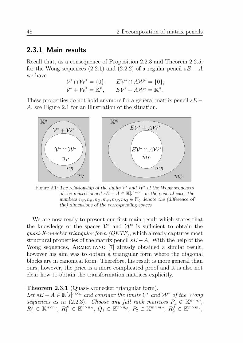
2.3.1 Main results
Recall that, as a consequence of Proposition 2.2.3 and Theorem 2.2.5,for the Wong sequences (2.2.1) and (2.2.2) of a regular pencil sE − Awe have
V∗ ∩W∗ = {0}, EV∗ ∩ AW∗ = {0},V∗ +W∗ = Kn, EV∗ +AW∗ = Kn.
These properties do not hold anymore for a general matrix pencil sE−A, see Figure 2.1 for an illustration of the situation.
Kn
nQ
V∗ +W∗
nR
V∗ ∩W∗
nP
Km
mQ
EV∗ + AW∗
mR
EV∗ ∩ AW∗
mP
Figure 2.1: The relationship of the limits V∗ and W∗ of the Wong sequencesof the matrix pencil sE − A ∈ K[s]m×n in the general case; thenumbers nP , nR, nQ, mP , mR, mQ ∈ N0 denote the (difference ofthe) dimensions of the corresponding spaces.
We are now ready to present our first main result which states thatthe knowledge of the spaces V∗ and W∗ is sufficient to obtain thequasi-Kronecker triangular form (QKTF), which already captures moststructural properties of the matrix pencil sE−A. With the help of theWong sequences, Armentano [7] already obtained a similar result,however his aim was to obtain a triangular form where the diagonalblocks are in canonical form. Therefore, his result is more general thanours, however, the price is a more complicated proof and it is also notclear how to obtain the transformation matrices explicitly.
Theorem 2.3.1 (Quasi-Kronecker triangular form).Let sE −A ∈ K[s]m×n and consider the limits V∗ and W∗ of the Wongsequences as in (2.2.3). Choose any full rank matrices P1 ∈ Kn×nP ,RJ
1 ∈ Kn×nJ , RN1 ∈ Kn×nN , Q1 ∈ Kn×nQ, P2 ∈ Km×mP , RJ
2 ∈ Km×mJ ,
2.3 Quasi-Kronecker form 49
RN2 ∈ Km×mN , Q2 ∈ Km×mQ such that
imP1 = V∗ ∩W∗, (V∗ ∩W∗)⊕ imRJ1 = V∗,
V∗ ⊕ imRN1 = V∗ +W∗, (V∗ +W∗)⊕ imQ1 = Kn,
imP2 = EV∗ ∩ AW∗, (EV∗ ∩ AW∗)⊕ imRJ2 = EV∗,
EV∗ ⊕ imRN2 = EV∗ +AW∗, (EV∗ + AW∗)⊕ imQ2 = Km.
Then it holds that Ttrian = [P1, RJ1 , R
N1 , Q1] and Strian =
[P2, RJ2 , R
N2 , Q2]
−1 are invertible and Strian(sE − A)Ttrian is inQKTF (2.1.4).
Remark 2.3.2.
(i) The sizes of the blocks in (2.1.4) are uniquely determined by thematrix pencil sE−A because they only depend on the subspacesconstructed by the Wong sequences and not on the choice of basesthereof. It is also possible that mP = 0 (or nQ = 0) which meansthat there are matrices with no rows (or no columns). On theother hand, if nP = 0, nJ = 0, nN = 0 or mQ = 0 then theP -blocks, J-blocks, N -block or Q-blocks are not present at all.Furthermore, it is easily seen that if sE−A fulfills (i), (ii), (iii) or(iv) itself, then sE −A is already in QKTF with Ttrian = P1 = I,Ttrian = RJ
1 = I, Ttrian = RN1 = I or Ttrian = Q1 = I, and
Strian = P−12 = I, Strian = (RJ
2 )−1 = I, Strian = (RN
2 )−1 = I or
Strian = Q−12 = I.
(ii) In Theorem 2.3.1 the special choice of RJ2 = ERJ
1 and RN2 =
ARN1 , which is feasible due to Steps 2 and 3 of the proof of The-
orem 2.3.1 (see Subsection 2.3.3), yields that (2.1.4) simplifiesto
s
EP 0 EPN EPQ
0 InJEJN EJQ
0 0 N ENQ
0 0 0 EQ
−
AP APJ 0 APQ
0 AJ 0 AJQ
0 0 InNANQ
0 0 0 AQ
,
where N is nilpotent.
(iii) From Lemma 2.3.7 (see Subsection 2.3.2) we know that E(V∗ ∩W∗) = EV∗ ∩ AW∗ = A(V∗ ∩W∗), hence
EV∗ ∩ AW∗ = E(V∗ ∩W∗) +A(V∗ ∩W∗).
50 2 Decomposition of matrix pencils
Furthermore, due to (2.2.4),
EV∗ +AW∗ = E(V∗ +W∗) +A(V∗ +W∗).
Hence the subspace pairs (V∗ ∩ W∗, EV∗ ∩ AW∗) and (V∗ +W∗, EV∗ + AW∗) are reducing subspaces of the matrix pencilsE − A in the sense of [235] and are in fact the minimal andmaximal reducing subspaces.
The QKTF is already useful for the analysis of the matrix pencilsE −A and the associated DAE d
dtEx = Ax+ f . However, a completedecoupling of the different parts, i.e., a block diagonal form, is moresatisfying from a theoretical viewpoint and is also a necessary step toobtain the KCF as a corollary. In the next result we show that we cantransform any matrix pencil sE −A into a block diagonal form, whichwe call quasi-Kronecker form (QKF) because all the important featuresof the KCF are captured. In fact, it turns out that the diagonal blocksof the QKTF (2.1.4) already are the diagonal blocks of the QKF.
Theorem 2.3.3 (Quasi-Kronecker form).Using the notation from Theorem 2.3.1 the following equations are solv-able for matrices F1, F2, G1, G2, H1, H2, K1, K2, L1, L2,M1,M2 of appro-priate size:
0 =[
EJQ
ENQ
]+[EJ EJN
0 EN
] [G1F1
]+[G2F2
]EQ
0 =[
AJQ
ANQ
]+[AJ AJN
0 AN
] [G1
F1
]+[G2
F2
]AQ
(2.3.1a)
0 = (EPQ + EPNF1 + EPJG1) + EPK1 +K2EQ
0 = (APQ +APNF1 + APJG1) + APK1 +K2AQ(2.3.1b)
0 = EJN + EJH1 +H2EN
0 = AJN +AJH1 +H2AN(2.3.1c)
0 = [EPJ , EPN ][I H10 I
]+ EP [M1, L1] + [M2, L2]
[EJ 00 EN
]
0 = [APJ , APN ][I H1
0 I
]+AP [M1, L1] + [M2, L2]
[AJ 00 AN
] (2.3.1d)
and for any such matrices let
S :=
[ I −M2 −L2 −K2
0 I −H2 −G20 0 I −F2
0 0 0 I
]−1
Strian, T := Ttrian
[ I M1 L1 K1
0 I H1 G10 0 I F1
0 0 0 I
].

2.3 Quasi-Kronecker form 51
Then S and T are invertible and S(sE−A)T is in QKF (2.1.5), wherethe block diagonal entries are the same as for the QKTF (2.1.4). Inparticular, the QKF (without the transformation matrices S and T ) canbe obtained with only the Wong sequences (i.e., without solving (2.3.1)).Furthermore, the QKF (2.1.5) is unique in the following sense
(E,A) ∼= (E ′, A′) ⇔ (EP , AP ) ∼= (E ′P , A
′P ), (EJ , AJ) ∼= (E ′
J , A′J),
(EN , AN) ∼= (E ′N , A
′N), (EQ, AQ) ∼= (E ′
Q, A′Q), (2.3.2)
where E ′P , A
′P , E
′J , A
′J , E
′N , A
′N , E
′P , A
′P are the corresponding blocks of
the QKF of the matrix pencil sE ′ −A′.
2.3.2 Preliminaries and interim QKF
In this subsection we provide the preliminary results for the proofs ofTheorems 2.3.1 and 2.3.3. To this end, we prove important resultsconcerning the Wong sequences, singular chains, the KCF for full rankpencils and the solvability of Sylvester equations. As a main step to-wards the QKF we derive the interim quasi-Kronecker (triangular) form(IQK(T)F). In the latter form we do not decouple the regular part ofthe matrix pencil. This is already a useful and interesting result inits own right, because the decoupling into three parts which have thesolution properties (cf. also Section 2.4) ‘existence, but non-uniquess’(underdetermined part), ‘existence and uniqueness’ (regular part) and‘uniqueness, but possible non-existence’ (overdetermined part) seemsvery intuitive.
Standard results from linear algebra
Lemma 2.3.4 (Orthogonal complements and (pre-)images).For any matrix M ∈ Kp×q we have:
(i) for all subspaces S ⊆ Kp it holds that (M−1S)⊥ =M∗(S⊥).
(ii) for all subspaces S ⊆ Kq it holds that (MS)⊥ =M−∗(S⊥).
Proof: Property (i) is shown e.g. in [16, Property 3.1.3]. Property (ii)follows from (i) forM∗,S⊥ instead ofM,S and then taking orthogonalcomplements.

52 2 Decomposition of matrix pencils
Lemma 2.3.5 (Rank of matrices).Let A,B ∈ Km×n with imB ⊆ imA. Then for almost all c ∈ K:
rkA = rk(A+ cB),
or, equivalently,imA = im(A+ cB).
In fact, rkA > rk(A + cB) can only hold for at most r = rkA manyvalues of c.
Proof: Consider the Smith form [222] of A:
UAV =
[Σr 00 0
]
with invertible matrices U ∈ Km×m and V ∈ Kn×n and Σr =diag (σ1, σ2, . . . , σr), σi ∈ K \ {0}, r = rkA. Write
UBV =
[B11 B12
B21 B22
],
where B11 ∈ Kr×r. Since imB ⊆ imA it follows that B21 = 0 andB22 = 0. Hence we obtain the following implications:
rk(A+ cB) < rkA ⇒ rk[Σr + cB11, cB12] < rk[Σr, 0] = r
⇒ rk(Σr + cB11) < r ⇒ det(Σr + cB11) = 0.
Since det(Σr + cB11) is a polynomial in c of degree at most r but notthe zero polynomial (since det(Σr) 6= 0) it can have at most r zeros.This proves the claim.
Without proof we record the following well-known result.
Lemma 2.3.6 (Dimension formulae).Let S ⊆ Kn be any linear subspace and M ∈ Km×n. Then
dimMS = dimS − dim(kerM ∩ S).
Furthermore, for any two linear subspaces S, T of Kn we have
dim(S + T ) = dimS + dim T − dim(S ∩ T ).
2.3 Quasi-Kronecker form 53
The Wong sequences
The next lemma highlights an important property of the intersectionof the limits of the Wong sequences.
Lemma 2.3.7 (Property of V∗ ∩W∗).Let sE−A ∈ K[s]m×n and V∗, W∗ be the limits of the Wong sequencesas in (2.2.3). Then
E(V∗ ∩W∗) = EV∗ ∩ AW∗ = A(V∗ ∩W∗).
Proof: Clearly, invoking (2.2.4),
E(V∗ ∩W∗) ⊆ EV∗ ∩ EW∗ ⊆ EV∗ ∩ AW∗
and A(V∗ ∩W∗) ⊆ AV∗ ∩ AW∗ ⊆ EV∗ ∩ AW∗,
hence it remains to show the converse subspace relationship. To thisend choose x ∈ EV∗ ∩ AW∗, which implies existence of v ∈ V∗ andw ∈ W∗ such that
Ev = x = Aw,
hence
v ∈ E−1{Aw} ⊆ E−1(AW∗) = W∗, w ∈ A−1{Ev} ⊆ A−1(EV∗) = V∗.
Therefore v, w ∈ V∗ ∩ W∗ and x = Ev ∈ E(V∗ ∩ W∗) as well asx = Aw ∈ A(V∗ ∩W∗) which concludes the proof.
For the proof of the main result we briefly consider the Wong se-quences of the (conjugate) transposed matrix pencil sE∗ − A∗; theseare connected to the original Wong sequences as follows.
Lemma 2.3.8 (Wong-sequences of the transposed matrix pencil).Consider a matrix pencil sE − A ∈ K[s]m×n with limits of the Wong
sequences V∗ and W∗ as in (2.2.3). Denote by V∗ and W∗ the limits ofthe Wong sequences of the (conjugate) transposed matrix pencil sE∗ −A∗. Then the following holds
W∗ = (EV∗)⊥ and V∗ = (AW∗)⊥.

54 2 Decomposition of matrix pencils
Proof: We show that for all i ∈ N0
(EVi)⊥ = Wi+1 and (AWi)
⊥ = Vi, (2.3.3)
from which the claim follows. For i = 0 this follows from
(EV0)⊥ = (imE)⊥ = kerE∗ = E−∗(A∗{0}) = W1
and(AW0)
⊥ = {0}⊥ = Rm = V0.
Now suppose that (2.3.3) holds for some i ∈ N0. Then
(EVi+1)⊥ =
(EA−1(EVi)
)⊥Lem. 2.3.4 (ii)
= E−∗(A−1(EVi))⊥
Lem. 2.3.4 (i)= E−∗ (A⊤(EVi)
⊥)
= E−∗(A⊤Wi+1
)= Wi+2.
Analogously it follows (AWi+1)⊥ = Vi+1, hence we have inductively
shown (2.3.3).
Singular chains
In this paragraph we introduce the notion of singular chains for ma-trix pencils. This notion is inspired by the theory of linear relations,see [214], where they are a vital tool for analyzing the structure oflinear relations. They also play an important role in former works onthe KCF, see e.g. [100, Ch. XII] and [7]; however in these works onlysingular chains of minimal length are considered. We use them here todetermine the structure of the intersection V∗∩W∗ of the limits of theWong sequences.
Definition 2.3.9 (Singular chain).Let sE − A ∈ K[s]m×n. For k ∈ N0 the tuple (x0, . . . , xk) ∈ (Kn)k+1 iscalled a singular chain of the matrix pencil sE − A if, and only if,
0 = Ax0, Ex0 = Ax1, . . . , Exk−1 = Axk, Exk = 0
or, equivalently, if the polynomial vector x(s) = x0+x1s+ . . .+xksk ∈
K[s]n satisfies (sE −A)x(s) = 0.
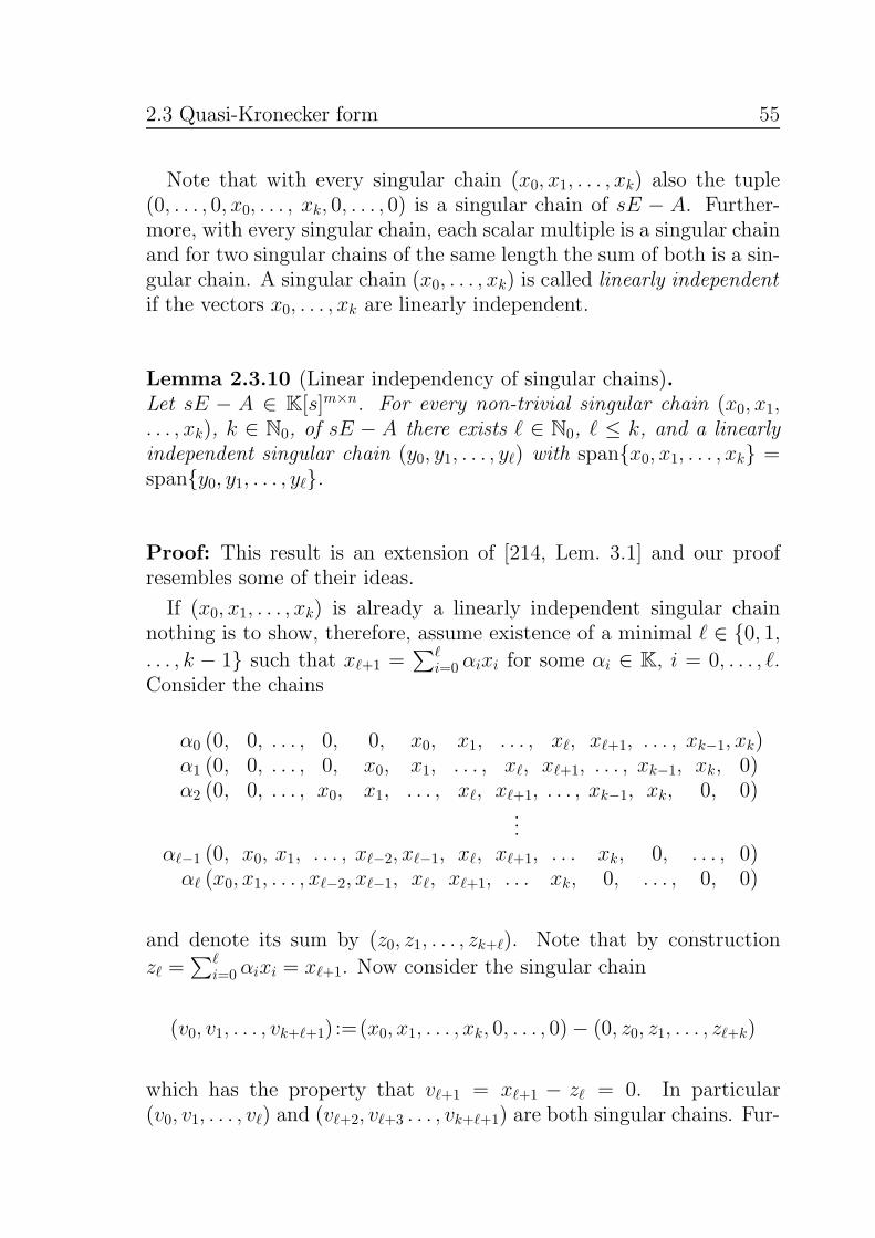
2.3 Quasi-Kronecker form 55
Note that with every singular chain (x0, x1, . . . , xk) also the tuple(0, . . . , 0, x0, . . . , xk, 0, . . . , 0) is a singular chain of sE − A. Further-more, with every singular chain, each scalar multiple is a singular chainand for two singular chains of the same length the sum of both is a sin-gular chain. A singular chain (x0, . . . , xk) is called linearly independentif the vectors x0, . . . , xk are linearly independent.
Lemma 2.3.10 (Linear independency of singular chains).Let sE − A ∈ K[s]m×n. For every non-trivial singular chain (x0, x1,. . . , xk), k ∈ N0, of sE − A there exists ℓ ∈ N0, ℓ ≤ k, and a linearlyindependent singular chain (y0, y1, . . . , yℓ) with span{x0, x1, . . . , xk} =span{y0, y1, . . . , yℓ}.
Proof: This result is an extension of [214, Lem. 3.1] and our proofresembles some of their ideas.
If (x0, x1, . . . , xk) is already a linearly independent singular chainnothing is to show, therefore, assume existence of a minimal ℓ ∈ {0, 1,. . . , k − 1} such that xℓ+1 =
∑ℓi=0 αixi for some αi ∈ K, i = 0, . . . , ℓ.
Consider the chains
α0 (0, 0, . . . , 0, 0, x0, x1, . . . , xℓ, xℓ+1, . . . , xk−1, xk)α1 (0, 0, . . . , 0, x0, x1, . . . , xℓ, xℓ+1, . . . , xk−1, xk, 0)α2 (0, 0, . . . , x0, x1, . . . , xℓ, xℓ+1, . . . , xk−1, xk, 0, 0)
...αℓ−1 (0, x0, x1, . . . , xℓ−2, xℓ−1, xℓ, xℓ+1, . . . xk, 0, . . . , 0)αℓ (x0, x1, . . . , xℓ−2, xℓ−1, xℓ, xℓ+1, . . . xk, 0, . . . , 0, 0)
and denote its sum by (z0, z1, . . . , zk+ℓ). Note that by construction
zℓ =∑ℓ
i=0 αixi = xℓ+1. Now consider the singular chain
(v0, v1, . . . , vk+ℓ+1) :=(x0, x1, . . . , xk, 0, . . . , 0)− (0, z0, z1, . . . , zℓ+k)
which has the property that vℓ+1 = xℓ+1 − zℓ = 0. In particular(v0, v1, . . . , vℓ) and (vℓ+2, vℓ+3 . . . , vk+ℓ+1) are both singular chains. Fur-
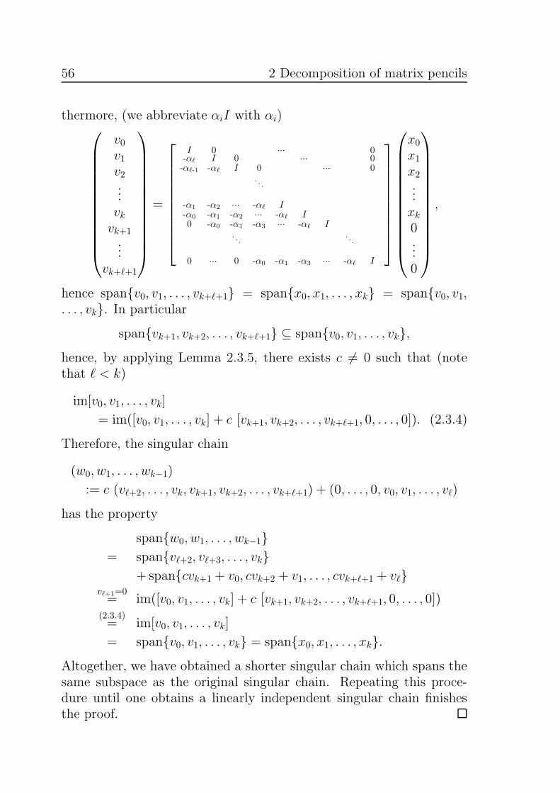
56 2 Decomposition of matrix pencils
thermore, (we abbreviate αiI with αi)
v0v1v2...vkvk+1
...vk+ℓ+1
=
I 0 ··· 0-αℓ I 0 ··· 0-αℓ-1 -αℓ I 0 ··· 0
. . .
-α1 -α2 ··· -αℓ I-α0 -α1 -α2 ··· -αℓ I0 -α0 -α1 -α3 ··· -αℓ I
. . .. . .
0 ··· 0 -α0 -α1 -α3 ··· -αℓ I
x0x1x2...xk0...0
,
hence span{v0, v1, . . . , vk+ℓ+1} = span{x0, x1, . . . , xk} = span{v0, v1,. . . , vk}. In particular
span{vk+1, vk+2, . . . , vk+ℓ+1} ⊆ span{v0, v1, . . . , vk},hence, by applying Lemma 2.3.5, there exists c 6= 0 such that (notethat ℓ < k)
im[v0, v1, . . . , vk]
= im([v0, v1, . . . , vk] + c [vk+1, vk+2, . . . , vk+ℓ+1, 0, . . . , 0]). (2.3.4)
Therefore, the singular chain
(w0, w1, . . . , wk−1)
:= c (vℓ+2, . . . , vk, vk+1, vk+2, . . . , vk+ℓ+1) + (0, . . . , 0, v0, v1, . . . , vℓ)
has the property
span{w0, w1, . . . , wk−1}= span{vℓ+2, vℓ+3, . . . , vk}
+span{cvk+1 + v0, cvk+2 + v1, . . . , cvk+ℓ+1 + vℓ}vℓ+1=0= im([v0, v1, . . . , vk] + c [vk+1, vk+2, . . . , vk+ℓ+1, 0, . . . , 0])
(2.3.4)= im[v0, v1, . . . , vk]
= span{v0, v1, . . . , vk} = span{x0, x1, . . . , xk}.Altogether, we have obtained a shorter singular chain which spans thesame subspace as the original singular chain. Repeating this proce-dure until one obtains a linearly independent singular chain finishesthe proof.

2.3 Quasi-Kronecker form 57
Corollary 2.3.11 (Basis of the singular chain subspace).Consider a matrix pencil sE −A ∈ K[s]m×n and let the singular chainsubspace be given by
K :=
{x∈Rn
∣∣∣∣∃ k, i∈N0 ∃ sing. chain (x0, . . . , xi−1, x = xi, xi+1,
. . . , xk) ∈ (Kn)k+1
},
i.e., K is the set of all vectors x appearing somewhere in some singularchain of sE − A. Then there exists a linearly independent singularchain (x0, x1, . . . , xk) of sE −A such that
K = span{x0, . . . , xk}.
Proof: First note that K is indeed a linear subspace of Kn, since thescalar multiple of every chain is also a chain and the sum of two chains(extending the chains appropriately with zero vectors) is again a chain.Let y0, y1, . . . , yℓ be any basis of K. By the definition of K, for eachi = 0, 1, . . . , ℓ there exist chains (yi0, y
i1, . . . , y
iki) which contain yi. Let
(v0, v1, . . . , vk) with k = k0+ k1+ . . .+ kℓ be the chain which results byconcatenating the chains (yi0, y
i1, . . . , y
iki). Clearly, span{v0, . . . , vk} =
K, hence Lemma 2.3.10 yields the claim.
The following result can, in substance, be found in [7]. However,the proof therein is difficult to follow, involving quotient spaces andadditional sequences of subspaces. We aim for a presentation which ismore straightforward and simpler.
Lemma 2.3.12 (Singular chain subspace and the Wong sequences).Consider a matrix pencil sE−A ∈ K[s]m×n with the limits V∗ and W∗
of the Wong sequences as in (2.2.3). Let the singular chain subspace Kbe given as in Corollary 2.3.11, then
V∗ ∩W∗ = K.
Proof: Step 1: We show K ⊆ V∗ ∩ W∗. Let (x0, . . . , xk) be a sin-gular chain. Clearly we have x0 ∈ A−1(E{0}) = kerA ⊆ V∗ andxk ∈ E−1(A{0}) = kerE ⊆ W∗ , hence inductively we have, fori = 0, 1, . . . , k − 1 and j = k, k − 1, . . . , 1
xi+1 ∈ A−1(E{xi}) ⊆ A−1(EV∗) = V∗
and xj−1 ∈ E−1(A{xj}) ⊆ E−1(AW∗) = W∗.
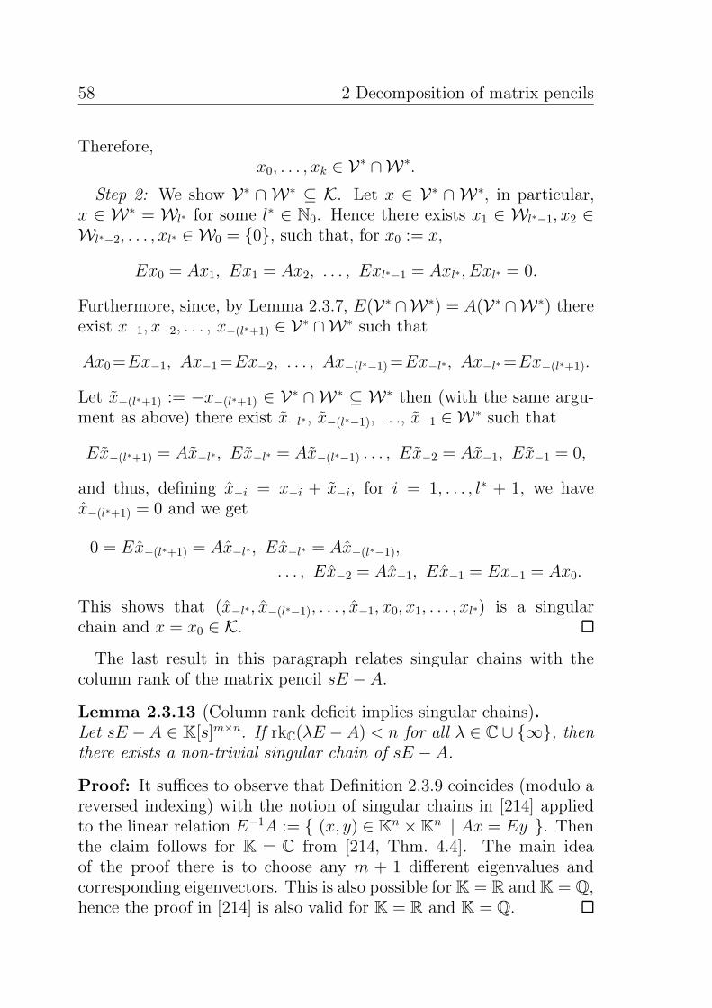
58 2 Decomposition of matrix pencils
Therefore,x0, . . . , xk ∈ V∗ ∩W∗.
Step 2: We show V∗ ∩ W∗ ⊆ K. Let x ∈ V∗ ∩ W∗, in particular,x ∈ W∗ = Wl∗ for some l∗ ∈ N0. Hence there exists x1 ∈ Wl∗−1, x2 ∈Wl∗−2, . . . , xl∗ ∈ W0 = {0}, such that, for x0 := x,
Ex0 = Ax1, Ex1 = Ax2, . . . , Exl∗−1 = Axl∗, Exl∗ = 0.
Furthermore, since, by Lemma 2.3.7, E(V∗ ∩W∗) = A(V∗ ∩W∗) thereexist x−1, x−2, . . . , x−(l∗+1) ∈ V∗ ∩W∗ such that
Ax0=Ex−1, Ax−1=Ex−2, . . . , Ax−(l∗−1)=Ex−l∗, Ax−l∗=Ex−(l∗+1).
Let x−(l∗+1) := −x−(l∗+1) ∈ V∗ ∩W∗ ⊆ W∗ then (with the same argu-ment as above) there exist x−l∗, x−(l∗−1), . . ., x−1 ∈ W∗ such that
Ex−(l∗+1) = Ax−l∗, Ex−l∗ = Ax−(l∗−1) . . . , Ex−2 = Ax−1, Ex−1 = 0,
and thus, defining x−i = x−i + x−i, for i = 1, . . . , l∗ + 1, we havex−(l∗+1) = 0 and we get
0 = Ex−(l∗+1) = Ax−l∗, Ex−l∗ = Ax−(l∗−1),
. . . , Ex−2 = Ax−1, Ex−1 = Ex−1 = Ax0.
This shows that (x−l∗, x−(l∗−1), . . . , x−1, x0, x1, . . . , xl∗) is a singularchain and x = x0 ∈ K.
The last result in this paragraph relates singular chains with thecolumn rank of the matrix pencil sE − A.
Lemma 2.3.13 (Column rank deficit implies singular chains).Let sE −A ∈ K[s]m×n. If rkC(λE −A) < n for all λ ∈ C ∪ {∞}, thenthere exists a non-trivial singular chain of sE − A.
Proof: It suffices to observe that Definition 2.3.9 coincides (modulo areversed indexing) with the notion of singular chains in [214] appliedto the linear relation E−1A := { (x, y) ∈ Kn ×Kn | Ax = Ey }. Thenthe claim follows for K = C from [214, Thm. 4.4]. The main ideaof the proof there is to choose any m + 1 different eigenvalues andcorresponding eigenvectors. This is also possible for K = R and K = Q,hence the proof in [214] is also valid for K = R and K = Q.
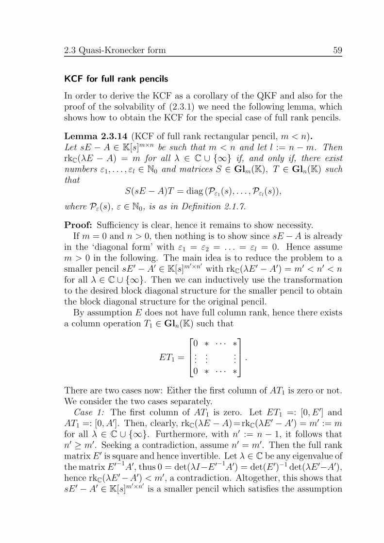
2.3 Quasi-Kronecker form 59
KCF for full rank pencils
In order to derive the KCF as a corollary of the QKF and also for theproof of the solvability of (2.3.1) we need the following lemma, whichshows how to obtain the KCF for the special case of full rank pencils.
Lemma 2.3.14 (KCF of full rank rectangular pencil, m < n).Let sE − A ∈ K[s]m×n be such that m < n and let l := n −m. ThenrkC(λE − A) = m for all λ ∈ C ∪ {∞} if, and only if, there existnumbers ε1, . . . , εl ∈ N0 and matrices S ∈ Glm(K), T ∈ Gln(K) suchthat
S(sE −A)T = diag (Pε1(s), . . . ,Pεl(s)),
where Pε(s), ε ∈ N0, is as in Definition 2.1.7.
Proof: Sufficiency is clear, hence it remains to show necessity.If m = 0 and n > 0, then nothing is to show since sE −A is already
in the ‘diagonal form’ with ε1 = ε2 = . . . = εl = 0. Hence assumem > 0 in the following. The main idea is to reduce the problem to asmaller pencil sE ′ − A′ ∈ K[s]m
′×n′
with rkC(λE′ − A′) = m′ < n′ < n
for all λ ∈ C ∪ {∞}. Then we can inductively use the transformationto the desired block diagonal structure for the smaller pencil to obtainthe block diagonal structure for the original pencil.By assumption E does not have full column rank, hence there exists
a column operation T1 ∈ Gln(K) such that
ET1 =
0 ∗ · · · ∗......
...0 ∗ · · · ∗
.
There are two cases now: Either the first column of AT1 is zero or not.We consider the two cases separately.Case 1: The first column of AT1 is zero. Let ET1 =: [0, E ′] and
AT1 =: [0, A′]. Then, clearly, rkC(λE − A)=rkC(λE′ − A′) = m′ := m
for all λ ∈ C ∪ {∞}. Furthermore, with n′ := n − 1, it follows thatn′ ≥ m′. Seeking a contradiction, assume n′ = m′. Then the full rankmatrixE ′ is square and hence invertible. Let λ ∈ C be any eigenvalue ofthe matrixE ′−1A′, thus 0 = det(λI−E ′−1A′) = det(E ′)−1 det(λE ′−A′),hence rkC(λE
′−A′) < m′, a contradiction. Altogether, this shows thatsE ′ − A′ ∈ K[s]m
′×n′
is a smaller pencil which satisfies the assumption
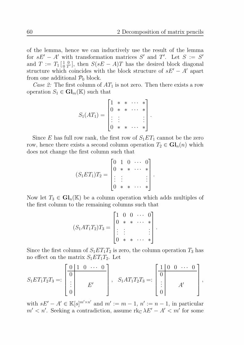
60 2 Decomposition of matrix pencils
of the lemma, hence we can inductively use the result of the lemmafor sE ′ − A′ with transformation matrices S ′ and T ′. Let S := S ′
and T := T1 [1 00 T ′ ], then S(sE − A)T has the desired block diagonal
structure which coincides with the block structure of sE ′ − A′ apartfrom one additional P0 block.Case 2: The first column of AT1 is not zero. Then there exists a row
operation S1 ∈ Glm(K) such that
S1(AT1) =
1 ∗ ∗ · · · ∗0 ∗ ∗ · · · ∗......
...0 ∗ ∗ · · · ∗
.
Since E has full row rank, the first row of S1ET1 cannot be the zerorow, hence there exists a second column operation T2 ∈ Gln(n) whichdoes not change the first column such that
(S1ET1)T2 =
0 1 0 · · · 00 ∗ ∗ · · · ∗......
...0 ∗ ∗ · · · ∗
.
Now let T3 ∈ Gln(K) be a column operation which adds multiples ofthe first column to the remaining columns such that
(S1AT1T2)T3 =
1 0 0 · · · 00 ∗ ∗ · · · ∗......
...0 ∗ ∗ · · · ∗
.
Since the first column of S1ET1T2 is zero, the column operation T3 hasno effect on the matrix S1ET1T2. Let
S1ET1T2T3 =:
0 1 0 · · · 00... E ′
0
, S1AT1T2T3 =:
1 0 0 · · · 00... A′
0
,
with sE ′ − A′ ∈ K[s]m′×n′
and m′ := m− 1, n′ := n − 1, in particularm′ < n′. Seeking a contradiction, assume rkC λE
′ − A′ < m′ for some

2.3 Quasi-Kronecker form 61
λ ∈ C ∪ {∞}. If λ = ∞ then this implies that E ′ does not have fullrow rank which would also imply that E does not have full row rank,which is not the case. Hence we may choose a vector v′ ∈ Cm′
such thatv′(λE ′ − A′) = 0. Let v := [0, v′]S1. Then a simple calculation revealsv(λE − A) = [0, v′(λE ′ − A′)](T1T2T3)−1 = 0, which contradicts fullcomplex rank of λE − A. As in the first case we can now inductivelyuse the result of the lemma for the smaller matrix pencil sE ′ − A′ toobtain transformations S ′ and T ′ which put sE ′ − A′ in the desiredblock diagonal form. With S := [ 1 0
0 S′ ]S1 and T := T1T2T3 [1 00 T ′ ] we
obtain the same block diagonal structure for sE − A as for sE ′ − A′
apart from the first block which is Pε1+1 instead of Pε1.
The following corollary follows directly from Lemma 2.3.14 by trans-posing the respective matrices.
Corollary 2.3.15 (KCF of full rank rectangular pencils, m > n).Let sE − A ∈ K[s]m×n be such that m > n and let l := m − n. ThenrkC(λE−A) = n for all λ ∈ C∪{∞} if, and only if, there exist numbersη1, . . . , ηl ∈ N0 and matrices S ∈ Glm(K), T ∈ Gln(K) such that
S(sE −A)T = diag (Qη1(s), . . . ,Qηl(s)),
where Qη(s), η ∈ N0, is as in Definition 2.1.7.
Solvability of linear matrix equations
In generalization of the method presented in [71, Sec. 6] we reduce theproblem of solvability of (2.3.1) to the problem of solving a generalizedSylvester equation
AXB − CXD = E. (2.3.5)
To this end the following lemma is crucial.
Lemma 2.3.16 (Solutions of Sylvester equation).Let A,C ∈ Km×n, B,D ∈ Kp×q, E, F ∈ Km×q and consider the systemof matrix equations with ‘unknowns’ Y ∈ Kn×q and Z ∈ Km×p
0 = E +AY + ZD,
0 = F + CY + ZB.(2.3.6)
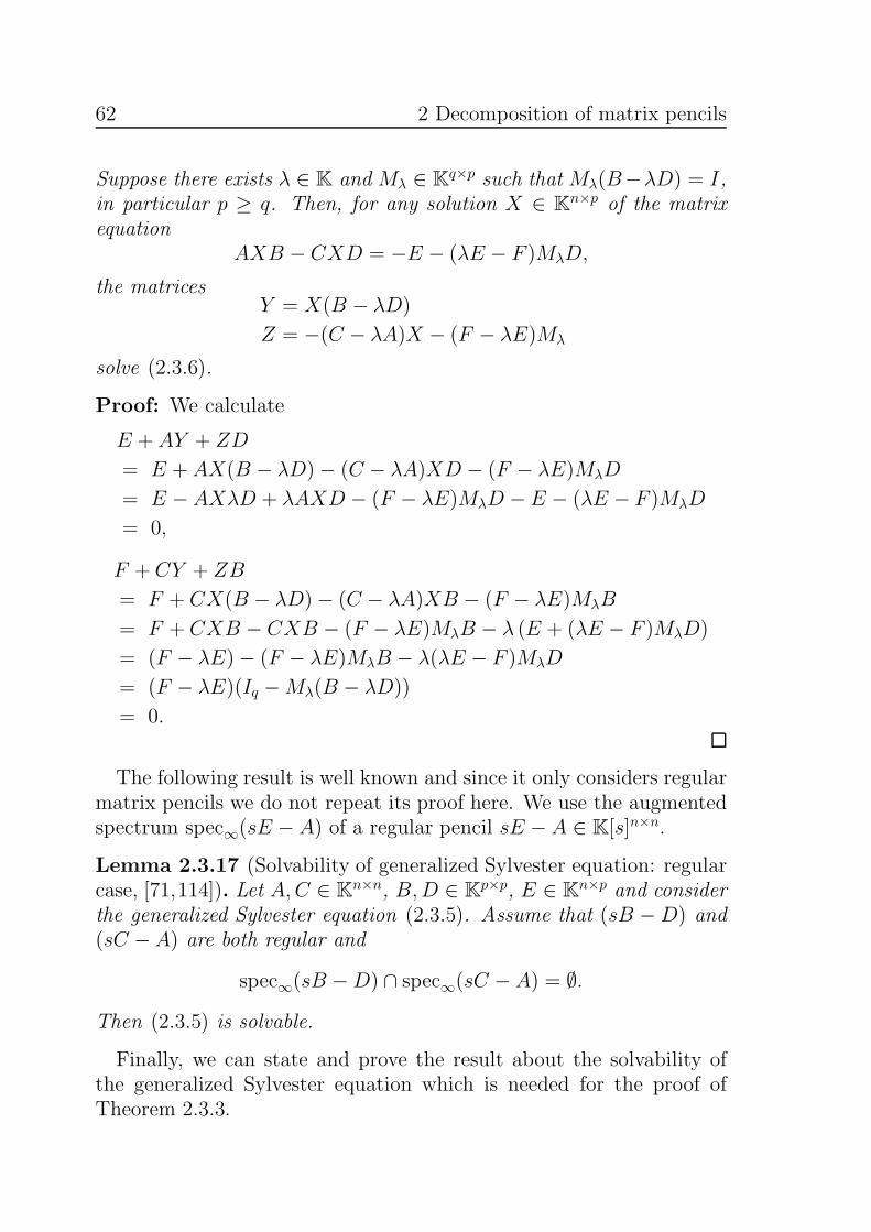
62 2 Decomposition of matrix pencils
Suppose there exists λ ∈ K and Mλ ∈ Kq×p such that Mλ(B−λD) = I,in particular p ≥ q. Then, for any solution X ∈ Kn×p of the matrixequation
AXB − CXD = −E − (λE − F )MλD,
the matricesY = X(B − λD)
Z = −(C − λA)X − (F − λE)Mλ
solve (2.3.6).
Proof: We calculate
E + AY + ZD
= E +AX(B − λD)− (C − λA)XD − (F − λE)MλD
= E −AXλD + λAXD − (F − λE)MλD − E − (λE − F )MλD
= 0,
F + CY + ZB
= F + CX(B − λD)− (C − λA)XB − (F − λE)MλB
= F + CXB − CXB − (F − λE)MλB − λ (E + (λE − F )MλD)
= (F − λE)− (F − λE)MλB − λ(λE − F )MλD
= (F − λE)(Iq −Mλ(B − λD))
= 0.
The following result is well known and since it only considers regularmatrix pencils we do not repeat its proof here. We use the augmentedspectrum spec∞(sE − A) of a regular pencil sE − A ∈ K[s]n×n.
Lemma 2.3.17 (Solvability of generalized Sylvester equation: regularcase, [71,114]). Let A,C ∈ Kn×n, B,D ∈ Kp×p, E ∈ Kn×p and considerthe generalized Sylvester equation (2.3.5). Assume that (sB −D) and(sC −A) are both regular and
spec∞(sB −D) ∩ spec∞(sC − A) = ∅.
Then (2.3.5) is solvable.
Finally, we can state and prove the result about the solvability ofthe generalized Sylvester equation which is needed for the proof ofTheorem 2.3.3.
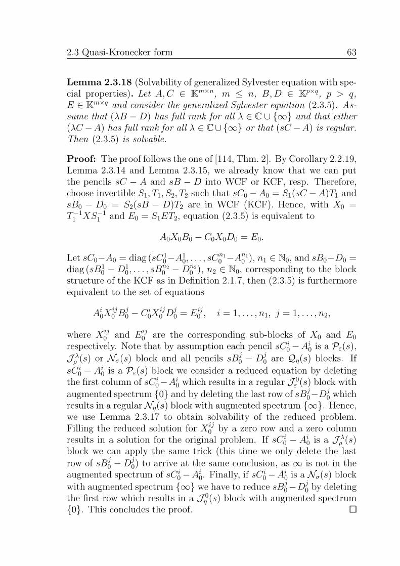
2.3 Quasi-Kronecker form 63
Lemma 2.3.18 (Solvability of generalized Sylvester equation with spe-cial properties). Let A,C ∈ Km×n, m ≤ n, B,D ∈ Kp×q, p > q,E ∈ Km×q and consider the generalized Sylvester equation (2.3.5). As-sume that (λB −D) has full rank for all λ ∈ C ∪ {∞} and that either(λC−A) has full rank for all λ ∈ C∪{∞} or that (sC−A) is regular.Then (2.3.5) is solvable.
Proof: The proof follows the one of [114, Thm. 2]. By Corollary 2.2.19,Lemma 2.3.14 and Lemma 2.3.15, we already know that we can putthe pencils sC − A and sB − D into WCF or KCF, resp. Therefore,choose invertible S1, T1, S2, T2 such that sC0 −A0 = S1(sC −A)T1 andsB0 − D0 = S2(sB − D)T2 are in WCF (KCF). Hence, with X0 =T−11 XS−1
1 and E0 = S1ET2, equation (2.3.5) is equivalent to
A0X0B0 − C0X0D0 = E0.
Let sC0−A0 = diag (sC10−A1
0, . . . , sCn1
0 −An1
0 ), n1 ∈ N0, and sB0−D0 =diag (sB1
0 −D10, . . . , sB
n2
0 −Dn2
0 ), n2 ∈ N0, corresponding to the blockstructure of the KCF as in Definition 2.1.7, then (2.3.5) is furthermoreequivalent to the set of equations
Ai0X
ij0 B
j0 − C i
0Xij0 D
j0 = Eij
0 , i = 1, . . . , n1, j = 1, . . . , n2,
where X ij0 and Eij
0 are the corresponding sub-blocks of X0 and E0
respectively. Note that by assumption each pencil sC i0 −Ai
0 is a Pε(s),
J λρ (s) or Nσ(s) block and all pencils sBj
0 − Dj0 are Qη(s) blocks. If
sC i0 − Ai
0 is a Pε(s) block we consider a reduced equation by deletingthe first column of sC i
0−Ai0 which results in a regular J 0
ε (s) block with
augmented spectrum {0} and by deleting the last row of sBj0−Dj
0 whichresults in a regularNη(s) block with augmented spectrum {∞}. Hence,we use Lemma 2.3.17 to obtain solvability of the reduced problem.Filling the reduced solution for X ij
0 by a zero row and a zero columnresults in a solution for the original problem. If sC i
0 − Ai0 is a J λ
ρ (s)block we can apply the same trick (this time we only delete the last
row of sBj0 −Dj
0) to arrive at the same conclusion, as ∞ is not in theaugmented spectrum of sC i
0−Ai0. Finally, if sC
i0−Ai
0 is a Nσ(s) block
with augmented spectrum {∞} we have to reduce sBj0−Dj
0 by deletingthe first row which results in a J 0
η (s) block with augmented spectrum{0}. This concludes the proof.

64 2 Decomposition of matrix pencils
Interim quasi-Kronecker form
As a first step towards the QKF we derive the interim quasi-Kroneckertriangular form (IQKTF). In this form we decouple the underdeter-mined part, the regular part and the overdetermined part of the matrixpencil.
Theorem 2.3.19 (Interim quasi-Kronecker triangular form).Let sE −A ∈ K[s]m×n and consider the limits V∗ and W∗ of the Wongsequences as in Definition 2.2.1. Choose any full rank matrices P1 ∈Kn×nP , P2 ∈ Km×mP , R1 ∈ Kn×nR, R2 ∈ Km×mR, Q1 ∈ Kn×nQ, Q2 ∈Km×mQ such that
imP1 = V∗ ∩W∗, V∗ ∩W∗ ⊕ imR1 = V∗ +W∗,
(V∗ +W∗)⊕ imQ1 = Kn,
imP2 = EV∗ ∩ AW∗, EV∗ ∩ AW∗ ⊕ imR2 = EV∗ +AW∗,
(EV∗ + AW∗)⊕ imQ2 = Km.
Then Ttrian = [P1, R1, Q1] ∈ Gln(K), Strian = [P2, R2, Q2]−1 ∈ Glm(K)
and Strian(sE − A)Ttrian is in IQKTF (2.1.2).
Proof: We proceed in several steps.Step 1: We show the block-triangular form (2.1.2). By the choice
of P1, R1, Q1 and P2, R2, Q2 it follows immediately that Ttrian and Strian
are invertible. Note that Strian(sE − A)Ttrian is in IQKTF (2.1.2) if,and only if, the following equations are solvable for given E,A andP1, R1, Q1, P2, R2, Q2:
EP1 = P2EP , AP1 = P2AP ,
ER1 = P2EPR + R2ER, AR1 = P2APR + R2AR,
EQ1 = P2EPQ + R2ERQ +Q2EQ, AQ1 = P2APQ + R2ARQ +Q2AQ.
The solvability of the latter is a consequence of the following subspaceinclusions
E(V∗ ∩W∗) ⊆ EV∗ ∩ AW∗, A(V∗ ∩W∗) ⊆ EV∗ ∩ AW∗,
E(V∗ +W∗) ⊆ EV∗ +AW∗, A(V∗ +W∗) ⊆ EV∗ +AW∗,
EKn ⊆ Km, AKn ⊆ Km,
which clearly hold due to (2.2.4).
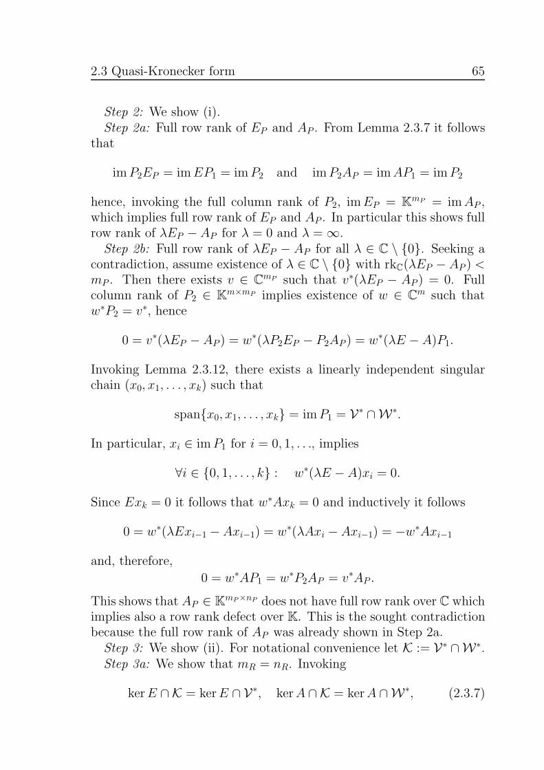
2.3 Quasi-Kronecker form 65
Step 2: We show (i).Step 2a: Full row rank of EP and AP . From Lemma 2.3.7 it follows
that
imP2EP = imEP1 = imP2 and imP2AP = imAP1 = imP2
hence, invoking the full column rank of P2, imEP = KmP = imAP ,which implies full row rank of EP and AP . In particular this shows fullrow rank of λEP −AP for λ = 0 and λ = ∞.Step 2b: Full row rank of λEP − AP for all λ ∈ C \ {0}. Seeking a
contradiction, assume existence of λ ∈ C \ {0} with rkC(λEP − AP ) <mP . Then there exists v ∈ CmP such that v∗(λEP − AP ) = 0. Fullcolumn rank of P2 ∈ Km×mP implies existence of w ∈ Cm such thatw∗P2 = v∗, hence
0 = v∗(λEP − AP ) = w∗(λP2EP − P2AP ) = w∗(λE − A)P1.
Invoking Lemma 2.3.12, there exists a linearly independent singularchain (x0, x1, . . . , xk) such that
span{x0, x1, . . . , xk} = imP1 = V∗ ∩W∗.
In particular, xi ∈ imP1 for i = 0, 1, . . ., implies
∀i ∈ {0, 1, . . . , k} : w∗(λE − A)xi = 0.
Since Exk = 0 it follows that w∗Axk = 0 and inductively it follows
0 = w∗(λExi−1 − Axi−1) = w∗(λAxi −Axi−1) = −w∗Axi−1
and, therefore,
0 = w∗AP1 = w∗P2AP = v∗AP .
This shows that AP ∈ KmP×nP does not have full row rank over C whichimplies also a row rank defect over K. This is the sought contradictionbecause the full row rank of AP was already shown in Step 2a.Step 3: We show (ii). For notational convenience let K := V∗ ∩W∗.Step 3a: We show that mR = nR. Invoking
kerE ∩ K = kerE ∩ V∗, kerA ∩ K = kerA ∩W∗, (2.3.7)

66 2 Decomposition of matrix pencils
and Lemmas 2.3.6, 2.3.7, the claim follows from
mR = rkR2
= dim(EV∗ +AW∗)− dim(EV∗ ∩ AW∗)
= dimEV∗ + dimAW∗ − 2 dim(EV∗ ∩ AW∗)
= dimV∗ − dim(kerE ∩ V∗) + dimW∗ − dim(kerA ∩W∗)
− dimEK − dimAK= dimV∗ − dim(kerE ∩ V∗) + dimW∗ − dim(kerA ∩W∗)
− dimK + dim(kerE ∩ K)− dimK + dim(kerA ∩ K)
(2.3.7)= dimV∗ + dimW∗ − 2 dimK= dim(V∗ +W∗)− dim(V∗ ∩W∗)
= rkR1 = nR.
Step 3b: We show that det(sER−AR) 6≡ 0. Seeking a contradiction,assume det(sER − AR) is the zero polynomial. Then λER − AR has acolumn rank defect for all λ ∈ C ∪ {∞}, hence
∀λ ∈ C ∪ {∞} : rkC(λER − AR) < nR.
Now, Lemma 2.3.13 ensures existence of a nontrivial singular chain(y0, y1, . . . , yk) of the matrix pencil sER −AR.We show that there exists a singular chain (x0, x1, . . . , xk, xk+1, . . . , xk)of sE − A such that xi = [P1, R1] (
ziyi ) for i = 0, . . . , k. To this end
denote some right inverse of AP (invoking full row rank of AP as shownin Step 2a) with A+
P and let
z0 = −A+PAPRy0, zi+1 = A+
P (EPzi + EPRyi − APRyi+1), i = 0, . . . , k,
where yk+1 = 0. Then it follows that
Axi = A[P1, R1]
(ziyi
)= ATtrian
ziyi0
= S−1
trian
AP APR APQ
0 AR ARQ
0 0 AQ
ziyi0
= S−1trian
APzi + APRyi
ARyi0

2.3 Quasi-Kronecker form 67
and, analogously,
Exi = S−1trian
EPzi + EPRyi
ERyi0
,
hence Ax0 = 0 and Exi = Axi+1 for i = 0, . . . , k. Note that, if weset xk+1 = P1zk+1, then xk+1 ∈ V∗ ∩ W∗ ⊆ W∗ and identically asshown in the first part of Step 2 of the proof of Lemma 2.3.12 thereexist xk+2, . . . , xk, k > k, such that Exk+1 = Axk+2, . . . , Exk−1 =Axk, Exk = 0 and, therefore, (x0, x1, . . . , xk) is a singular chain ofsE − A. Lemma 2.3.12 implies that {x0, x1, . . . , xk} ⊆ imP1, hencexi = [P1, R1] (
ziyi ) implies yi = 0 for all i ∈ {0, . . . , k}, which contradicts
non-triviality of (y0, . . . , yk).Step 4: We show (iii). We will consider the (conjugate) transposed
matrix pencil sE∗ − A∗ with corresponding Wong sequences and willshow that the block (E∗
Q, A∗Q) will play the role of the block (EP , AP ).
Therefore, denote the limits of the Wong-sequences of sE∗ −A∗ by V∗
and W∗. Let
Q1 := ([0, 0, InQ][P1, R1, Q1]
−1)∗, Q2 := ([0, 0, ImQ][P2, R2, Q2]
−1)∗,
then
Q∗iQi = I and im Qi = (im[Pi, Ri])
⊥, for i = 1, 2.
In fact, the latter follows from n− nQ = nP + nR and
Q∗1[P1, R1] = [0, 0, InQ
]
InP
00 InR
0 0
= 0
for i = 1 and analogously for i = 2. We will show in the following that
E∗Q2 = Q1E∗Q, A∗Q2 = Q1A
∗Q,
im Q2 = V∗ ∩ W∗, im Q1 = E∗V∗ ∩ A∗V∗,
then the arguments from Step 2 can be applied to sE∗Q − A∗
Q and theclaim is shown.
68 2 Decomposition of matrix pencils
Step 4a: We show E∗Q2 = Q1E∗Q and A∗Q2 = Q1A
∗Q. Using that
Strian(sE −A)Ttrian is in the form (2.1.2) we obtain
Q∗2E = Q∗
2[P2, R2, Q2]︸ ︷︷ ︸=[0 0 I]
[EP EPR EPQ
0 ER ERQ
0 0 EQ
][P1, R1, Q1]
−1
= [0 0 EQ][P1, R1, Q1]−1 = EQQ
∗1,
hence E∗Q2 = Q1E∗Q. Analog arguments show that A∗Q2 = Q1A
∗Q.
Step 4b: We show im Q2 = V∗ ∩ W∗. By construction and Lem-ma 2.3.8
im Q2=(im[P2, R2])⊥=(EV∗ +AW∗)⊥=(EV∗)⊥ ∩ (AW∗)⊥= V∗ ∩ W∗.
Step 4c: We show im Q1 = E∗V∗ ∩ A∗V∗. Lemma 2.3.8 applied to(E∗, A∗) gives
(E∗V∗)⊥ = W∗ and (A∗W∗)⊥ = V∗
or, equivalently,
E∗V∗ = W∗⊥ and A∗W∗ = V∗⊥.
Hence
im Q1 = (im[P1, R1])⊥ = (V∗ +W∗)⊥ = V∗⊥ ∩W∗⊥ = A∗W∗ ∩ E∗V∗.
This concludes the proof of the theorem.
As a corollary of Theorem 2.3.19 we show that it is possible to get ridof the off-diagonal blocks in the IQKTF by solving a set of generalizedSylvester equations using Lemma 2.3.18
Corollary 2.3.20 (Interim quasi-Kronecker form).Using the notation from Theorem 2.3.19 the following equations aresolvable for matrices F1, F2, G1, G2, H1, H2 of appropriate size:
0 = ERQ + ERF1 + F2EQ
0 = ARQ +ARF1 + F2AQ(2.3.8a)
0 = EPR + EPG1 +G2ER
0 = APR +APG1 +G2AR(2.3.8b)
0 = (EPQ + EPRF1) + EPH1 +H2EQ
0 = (APQ + APRF1) +APH1 +H2AQ(2.3.8c)

2.3 Quasi-Kronecker form 69
and for any such matrices let
S :=
I −G2 −H2
0 I −F2
0 0 I
−1
Strian
= [P2, R2 − P2G2, Q2 − P2H2 −R2F2]−1 and
T := Ttrian
I G1 H1
0 I F1
0 0 I
= [P1, R1 + P1G1, Q1 + P1H1 + R1F1].
Then S ∈ Glm(K), T ∈ Gln(K) and S(sE − A)T is in IQKF (2.1.3),where the block diagonal entries are the same as for the IQKTF (2.1.2).In particular, the IQKF (without the transformation matrices S andT ) can be obtained with only the Wong sequences (i.e., without solv-ing (2.3.8)). Furthermore, the IQKF (2.1.3) is unique in the followingsense
(E,A) ∼= (E ′, A′) ⇔(EP , AP ) ∼= (E ′
P , A′P ), (ER, AR) ∼= (E ′
R, A′R), (EQ, AQ) ∼= (E ′
Q, A′Q),
(2.3.9)
where E ′P , A
′P , E
′R, A
′R, E
′P , A
′P are the corresponding blocks of the IQKF
of the matrix pencil sE ′ −A′.
Proof: By the properties of the pencils sEP−AP , sER−AR and sEQ−AQ there exist λ ∈ K and full rank matrices NP
λ , NRλ , M
Rλ and MQ
λ
such that (λEP −AP )NPλ = I, (λER−AR)N
Rλ = I,MR
λ (λER−AR) = I
and MQλ (λEQ − AQ) = I. Hence Lemma 2.3.16 shows that it suffices
to consider solvability of the following generalized Sylvester equations
ERX1AQ −ARX1EQ = −ERQ − (λERQ − ARQ)MQλ EQ (2.3.10a)
EPX2AR − APX2ER = −EPR − (λEPR − APR)MRλ ER (2.3.10b)
EPX3AQ − APX3EQ = −(EPQ + EPRF1)− (λ(EPQ + EPRF1)
− (APQ + APRF1))MQλ EQ, (2.3.10c)
where F1 is any solution of (2.3.8a), whose existence will follow fromsolvability of (2.3.10a). Furthermore, the properties of sEP − AP ,sEQ − AQ and sER − AR imply that Lemma 2.3.18 is applicable to

70 2 Decomposition of matrix pencils
the equations (2.3.10) (where (2.3.10b) must be considered in the (con-jugate) transposed form) and ensures existence of solutions. Now, asimple calculation shows that for any solution of (2.3.8) the secondpart of the statement of Corollary 2.3.20 holds.Finally, to show uniqueness in the sense of (2.3.9) assume first that
(E,A) ∼= (E ′, A′). Then there exist invertible matrices S ′ and T ′ suchthat (E ′, A′) = (S ′ET ′, S ′AT ′). It is easily seen, that the Wong se-quences V ′
i, W ′i, i ∈ N0, of the pencil sE ′ −A′ fulfill
V ′i = T ′−1Vi, W ′
i = T ′−1Wi, E ′V ′i = S ′EVi, A′W ′
i = S ′AWi.(2.3.11)
Hence, using the notation of Theorem 2.3.19, there exist invertiblematrices MP , MR, MQ, NP , NR, NQ such that
[P ′1, R
′1, Q
′1] = T ′−1
[P1MP , R1MR, Q1MQ],
[P ′2, R
′2, Q
′2] = S ′[P2NP , R2NR, Q2NQ],
in particular the block sizes of the corresponding IQKFs coincide.Therefore,
s
[EP ∗ ∗0 ER ∗0 0 EQ
]−[AP ∗ ∗0 AR ∗0 0 AQ
]= [P2, R2, Q2]
−1(sE −A)[P1, R1, Q1]
=
[NP 0 00 NR 00 0 NQ
][P ′
2, R′2, Q
′2]S
′(sE − A)T ′[P ′1, R
′2, Q
′2]
[MP 0 00 MR 00 0 MQ
]−1
=
[NP 0 00 NR 00 0 NQ
][P ′
2, R′2, Q
′2](sE
′ − A′)[P ′1, R
′2, Q
′2]
[M−1
P 0 0
0 M−1R 0
0 0 M−1Q
]
= s
[NPE
′PM
−1P ∗ ∗
0 NRE′RM
−1R ∗
0 0 NQE′QM
−1Q
]−[
NPA′PM
−1P ∗ ∗
0 NRARM−1R ∗
0 0 NQAQM−1Q
].
Hence the necessity part of (2.3.9) is shown. Sufficiency follows fromthe simple observation that equivalence of the IQKFs implies equiva-lence of the original matrix pencils.
2.3.3 Proofs of the main results
In this subsection we prove the main results about the QKTF and theQKF, where, compared to the IQKTF and IQKF, the regular part is

2.3 Quasi-Kronecker form 71
decoupled into an ODE part and a nilpotent part. In the IQKTF andIQKF we directly completed a basis of V∗ ∩W∗ to a basis of V∗ +W∗,and a basis of EV∗ ∩ AW∗ to a basis of EV∗ + AW∗, resp. For theQKTF and the QKF we consider V∗ and EV∗ as intermediate steps.
Proof of Theorem 2.3.1
Step 1 : We show that Strian(sE − A)Ttrian is in the form (2.1.4) andprove (i) and (iv). It follows from (2.2.4) that
E(V∗ ∩W∗) ⊆ EV∗ ∩ AW∗, A(V∗ ∩W∗) ⊆ EV∗ ∩ AW∗,
EV∗ = EV∗, AV∗ ⊆ EV∗,
E(V∗ +W∗) ⊆ EV∗ + AW∗, A(V∗ +W∗) ⊆ EV∗ + AW∗,
EKn ⊆ Km, AKn ⊆ Km.
These inclusions imply solvability of
EP1=P2EP , AP1=P2AP ,
ERJ1=P2EPJ +RJ
2EJ , ARJ1=P2APJ + RJ
2AJ ,
ERN1 =P2EPN + RJ
2EJN + RN2 EN , ARN
1 =P2APN + RJ2AJN + RN
2 AN ,
EQ1=P2EPQ+RJ2EJQ+R
N2 ENQ+Q2EQ, AQ1=P2APQ+R
J2AJQ+R
N2 ANQ+Q2AQ.
(2.3.12)which is equivalent to Strian(sE − A)Ttrian being in the form (2.1.4).The properties (i) and (iv) immediately follow from Theorem 2.3.19 asthe choice of bases here is more special.Step 2 : We show (EV∗ ∩AW∗)⊕ imERJ
1 = EV∗. As imRJ1 ⊆ V∗ it
follows that (EV∗ ∩ AW∗) + imERJ1 ⊆ EV∗. Invoking EW∗ ⊆ AW∗,
the opposite inclusion is immediate from
EV∗ = E((V∗ ∩W∗)⊕ imRJ1 ) ⊆ E(V∗ ∩W∗) + imERJ
1
⊆ (EV∗ + AW∗) + imERJ1 .
It remains to show that the intersection is trivial. To this end letx ∈ (EV∗ ∩ AW∗) ∩ imERJ
1 , i.e., x = Ey with y ∈ imRJ1 . Further,
x ∈ EV∗ ∩ AW∗ = E(V∗ ∩ W∗) (where the subspace equality followsfrom Lemma 2.3.7) and this yields that x = Ez with z ∈ V∗∩W∗, thusz−y ∈ kerE ⊆ W∗. Hence, since z ∈ W∗, it follows y ∈ W∗∩ imRJ
1 ={0}.
72 2 Decomposition of matrix pencils
Step 3 : We show EV∗ ⊕ imARN1 = EV∗ + AW∗. We immediately
see that, since AV∗ ⊆ EV∗,
EV∗ + AW∗ = EV∗ +AV∗ + AW∗ = EV∗ +A(V∗ +W∗) =
EV∗ +A(V∗ + imRN1 ) = EV∗ +AV∗ + A imRN
1 = EV∗ + imARN1 .
In order to show that the intersection is trivial, let x ∈ EV∗∩ imARN1 ,
i.e., x = Ay = Ez with y ∈ imRN1 and z ∈ V∗. Therefore, y ∈
A−1(EV∗) = V∗ and y ∈ imRN1 , thus y = 0.
Step 4 : We show mJ = nJ and mN = nN . By Step 2 and Step 3 wehave that mJ = rkERJ
1 ≤ nJ and mN = rkARN1 ≤ nN . In order to see
that we have equality in both cases observe that: ERJ1v = 0 for some
v ∈ KnJ implies RJ1 v ∈ imRJ
1 ∩ kerE = {0}, since kerE ⊆ W∗, andhence v = 0 as RJ
1 has full column rank; ARN1 v = 0 for some v ∈ KnN
implies RN1 v ∈ imRN
1 ∩kerA = {0}, since kerA ⊆ V∗, and hence v = 0as RN
1 has full column rank.Step 5 : We show that EJ and AN are invertible. For the first,
assume that there exists v ∈ KnJ \ {0} such that EJv = 0. Then
ERJ1 v
(2.3.12)= P2EPJv and hence ERJ
1 v ∈ imERJ1 ∩ imP2
Step 2= {0}, a
contradiction with the fact that ERJ1 has full column rank (as shown
in Step 4). In order to show that AN is invertible, let v ∈ KnN \ {0} be
such that ANv = 0. Then ARN1 v
(2.3.12)= P2APNv + RJ
2AJNv and hence
ARN1 v ∈ imARN
1 ∩ im[P2, RJ2 ]
Step 3= {0}, a contradiction with the fact
that ARN1 has full column rank (as shown in Step 4).
Step 6 : It only remains to show that A−1N EN is nilpotent. In order
to prove this we will show that, for ℓ∗ as in (2.2.3),
∀ i ∈ {0, . . . , ℓ∗} : V∗ ⊕ imRN1 (A
−1N EN)
i ⊆ V∗ +Wℓ∗−i. (2.3.13)
We show this by induction. For i = 0 the assertion is clear from thechoice of RN
1 . Suppose (2.3.13) holds for some i ∈ {0, . . . , ℓ∗−1}. Then
A(V∗ + imRN1 (A
−1N EN)
i+1) ⊆ AV∗ + imARN1 (A
−1N EN)
i+1
(2.3.12)
⊆ EV∗ + im(P2APN +RJ2AJN +RN
2 AN)(A−1N EN)
i+1
⊆ EV∗ + imP2APN(A−1N EN)
i+1
︸ ︷︷ ︸⊆EV∗
+ imRJ2AJN(A
−1N EN)
i+1
︸ ︷︷ ︸⊆EV∗
+ imRN2 EN(A
−1N EN)
i

2.3 Quasi-Kronecker form 73
(2.3.12)
⊆ EV∗ + im(ERN1 − P2EPN −RJ
2EJN)(A−1N EN)
i
⊆ EV∗ + imERN1 (A
−1N EN)
i + imP2EPN(A−1N EN)
i
︸ ︷︷ ︸⊆EV∗
+imRJ2EJN(A
−1N EN)
i
︸ ︷︷ ︸⊆EV∗
⊆ E(V∗ + imRN1 (A
−1N EN)
i)(2.3.13)
⊆ EV∗ + EWℓ∗−i ⊆ EV∗ + AWℓ∗−i−1
and hence
V∗ + imRN1 (A
−1N EN)
i+1 ⊆ A−1(EV∗ + AWℓ∗−i−1)
⊆ A−1(EV∗) +Wℓ∗−i−1 ⊆ V∗ +Wℓ∗−i−1.
Furthermore, we have
V∗ ∩ imRN1 (A
−1N EN)
i+1 ⊆ V∗ ∩ imRN1 = {0}
and hence we have proved (2.3.13). Now (2.3.13) for i = ℓ∗ yieldsRN
1 (A−1N EN)
ℓ∗ = 0, and since RN1 has full column rank we may conclude
that (A−1N EN)
ℓ∗ = 0. �
Proof of Theorem 2.3.3
We may choose λ ∈ C and Mλ of appropriate size such that Mλ(AN −λEN) = I and, due to Lemma 2.3.16, for the solvability of (2.3.1c) itthen suffices to consider solvability of
EJXAN −AJXEN = −EJN − (λEJN − AJN)MλEN ,
which however is immediate from Lemma 2.3.17. Solvability of theother equations (2.3.1a), (2.3.1b), (2.3.1d) then follows as in the proofof Corollary 2.3.20.Uniqueness in the sense of (2.3.2) can be established along lines sim-
ilar to the proof of Corollary 2.3.20. �
2.3.4 KCF, elementary divisors and minimal indices
An analysis of the matrix pencils sEP − AP and sEQ − AQ in (2.1.5),invoking Lemma 2.3.14 and Corollary 2.3.15, together with Corolla-ry 2.2.19 allows now to obtain the KCF as a corollary.

74 2 Decomposition of matrix pencils
Corollary 2.3.21 (Kronecker canonical form).For every matrix pencil sE − A ∈ K[s]m×n there exist transformationmatrices S ∈ Glm(C) and T ∈ Gln(C) such that S(sE−A)T ∈ C[s]m×n
is in KCF (2.1.6).
The numbers ρi, σi, εi and ηi in Definition 2.1.7 are usually called(degrees of) elementary divisors and minimal indices and play an im-portant role in the analysis of matrix pencils, see e.g. [100,166,167,175].More precisely, ρ1, . . . , ρb are the degrees of the finite elementary di-visors, σ1, . . . , σc are the degrees of the infinite elementary divisors,ε1, . . . , εa are the columns minimal indices and η1, . . . , ηd are the rowminimal indices. The minimal indices completely determine (under thestanding assumption that 0 ≤ ε1 ≤ . . . ≤ εa and 0 ≤ η1 ≤ . . . ≤ ηd) thesingular part of the KCF. The following result shows that the minimalindices can be determined via the Wong sequences. Another methodfor determining the minimal indices via the control theoretic versionof the Wong sequences can be found in [167, Prop. 2.2], however theminimal indices there correspond to a feedback canonical form.
Theorem 2.3.22 (Minimal indices).Let sE − A ∈ K[s]m×n, consider the Wong sequences (2.2.3) and thenotation from Corollary 2.3.21 so that S(sE −A)T is in KCF (2.1.6).
Let K = V∗ ∩ W∗, Wi := (EVi−1)⊥, i = 1, 2, . . ., and K = (AW∗)⊥ ∩
(EV∗)⊥. Then
a = dim(W1 ∩ K), d = dim(W1 ∩ K)
and with, for i = 0, 1, 2, . . . ,
∆i := dim(Wi+2 ∩ K)− dim(Wi+1 ∩ K),
∆i := dim(Wi+2 ∩ K)− dim(Wi+1 ∩ K),
it holds that
ε1 = . . . = εa−∆0= 0, εa−∆i−1+1 = . . . = εa−∆i
= i, i = 1, 2, . . . ,
and
η1 = . . . = ηd−∆0= 0, ηd−∆i−1+1 = . . . = ηd−∆i
= i, i = 1, 2, . . . .
Furthermore, the minimal indices are invariant under matrix pencilequivalence. In particular, the KCF is unique.

2.3 Quasi-Kronecker form 75
Proof: First consider two equivalent matrix pencils sE−A and sE ′−A′
and the relationship of the corresponding Wong sequences (2.3.11).From this it follows that the subspace dimension used for the calcula-tions of a, d, ∆i and ∆i, i = 0, 1, 2, . . . , are invariant under equivalencetransformations. Hence it suffices to show the claim when the matrixpair is already in KCF (2.1.6). In particular, uniqueness of the KCFthen also follows from this invariance.Note that the Wong sequences of a matrix pencil in IQKF (2.1.3)
fulfill
Vi=
I00
VP
i ⊕
0I0
VR
i ⊕
00I
VQ
i , Wi=
I00
WP
i ⊕
0I0
WR
i ⊕
00I
WQ
i ,
where VPi , WP
i , VRi , WR
i , VQi , WQ
i , i ∈ N0, are the Wong sequencescorresponding to the matrix pencils sEP−AP , sER−AR and sEQ−AQ.Furthermore, due to Corollary 2.3.20 and the uniqueness result therein,it follows that
V∗ ∩W∗ = im
I 0 00 0 00 0 0
.
Altogether it is therefore sufficient to show the claim for the singularblock sEP − AP with its Wong sequences VP
i and WPi ; the result for
the singular block sEQ − AQ follows by considering the (conjugate)transpose and invoking Lemma 2.3.8. Since KP := VP ∗ ∩WP ∗
= Rnp
we have WPi ∩ KP = WP
i and the claim simplifies again.The remaining proof is quite simple but the notation is rather cum-
bersome, therefore we accompany the proof with an illustrative exam-ple:
sEP −AP = s
[0 0 0 1 0 0 0 0 0 00 0 0 0 0 1 0 0 0 00 0 0 0 0 0 0 1 0 00 0 0 0 0 0 0 0 1 00 0 0 0 0 0 0 0 0 1
]−[
0 0 1 0 0 0 0 0 0 00 0 0 0 1 0 0 0 0 00 0 0 0 0 0 1 0 0 00 0 0 0 0 0 0 1 0 00 0 0 0 0 0 0 0 1 0
]. (2.3.14)
In this example a = 5, ε1 = ε2 = 0 (indicated by the bars in (2.3.14)),ε3 = ε4 = 1 and ε5 = 3. Denote by κ1, κ2, . . . , κa the position where anew Pε(s) block begins in sEP − AP , for the example this is κ1 = 1,κ2 = 2, κ3 = 3, κ4 = 5, κ5 = 7. By definition
WP1 = kerEP = im[eκ1
, eκ2, . . . , eκa
] =: imW P1 ,
76 2 Decomposition of matrix pencils
where eℓ denotes the ℓ-th unit vector. This shows a = dimWP1 =
dim (W1 ∩ K).Let νi, i = 0, 1, 2, . . . , mP be the number of Pε(s)-blocks of size i in
sEP − AP , for our example (2.3.14) this means ν0 = 2, ν1 = 2, ν2 = 0,ν3 = 1, ν4 = 0, ν5 = 0. Then
APWP1 = [0, . . . , 0︸ ︷︷ ︸
ν0
, e1, . . . , eν1︸ ︷︷ ︸ν1
, eν1+1, eν1+3, . . . , eν1+2(ν2−1)︸ ︷︷ ︸ν2
, . . . ,
eν1+2ν2+...+(mP−1)νmP−1+1, . . . , eν1+2ν2+...+(mP−1)νmP−1+mP (νmP−1)︸ ︷︷ ︸
νmP
].
For (2.3.14) this reads as
APWP1 =
[0 0 1 0 00 0 0 1 00 0 0 0 10 0 0 0 00 0 0 0 0
].
Denote by β1 the smallest index such that εβ1≥ 1, if it exists, β1 = a+1
otherwise (for our example, β1 = 3). It then follows that
WP2 = EP
−1(APWP1 )
= WP1 ⊕ im[eκβ1+1, eκβ1+1+1, . . . , eκa+1]
= im[eκ1, . . . , eκβ1−1
, eκβ1, eκβ1
+1, eκβ1+1, eκβ1+1+1, . . . , eκa
, eκa+1]
=: imW P2 .
For the example (2.3.14) this is
WP2 = WP
1 ⊕ im[e4, e6, e8] = im[e1, e2, e3, e4, e5, e6, e7, e8].
Since ∆0 = dimWP2 − dimWP
1 = a− (β1− 1) and ε1 = . . . = εβ1−1 = 0we have shown that ε1 = . . . = εa−∆0
= 0.With βi being the smallest index such that εβi
≥ i (or βi = a+1 if itdoes not exist) and with an analogue argument as above we inductivelyconclude that
WPi+1 = WP
i ⊕ im[eκβi+i, eκβi+1+i, . . . , eκa+i], i = 2, 3, . . .
In the example we obtain β2 = β3 = 5 and β4 = β5 = . . . = 6 and
WP3 = WP
2 ⊕ im[e9],
WP4 = WP
3 ⊕ im[e10],
WP5 = WP
4 , WP6 = WP
5 , . . . .
2.3 Quasi-Kronecker form 77
Hence ∆i−1 = dimWi+1 − dimWi = a − (βi − 1) and by induction∆i = a− (βi+1− 1). By definition, εβi−1
= . . . = εβi−1 = i and thereforeεa−∆i−1
= . . . = εa−(∆i−1) = i.
Note that ∆i−1 = ∆i or ∆i−1 = ∆i is possible for some i. In thatcase there are no minimal indices of value i because the correspondingindex range is empty. Furthermore, once ∆i = 0 or ∆i = 0 for some
index i or i then ∆i+j = 0 and ∆i+j = 0 for all j ≥ 0 and j ≥ 0. Inparticular, there are no minimal indices with values larger than i andi, respectively.The proof of Theorem 2.3.22 uses the KCF and therefore, in particu-
lar it uses Lemma 2.3.14 and Corollary 2.3.15 which provide an explicitmethod to obtain the KCF for the full rank matrix pencils sEP − AP
and sEQ − AQ in the QKF (2.1.5). However, if one is only interestedin the singular part of the KCF (without the necessary transforma-tion), Theorem 2.3.22 shows that knowledge of the Wong sequences isalready sufficient; there is no need to carry out the tedious calculationsof Lemma 2.3.14 and Corollary 2.3.15.In the following we show that the index (of the nilpotent part) of the
matrix pencil and the degrees of the infinite elementary divisors maybe obtained from the Wong sequences as well.
Proposition 2.3.23 (Index and infinite elementary divisors).Consider the Wong sequences Vi and Wi and the notation from Theo-rem 2.3.1 and the form (2.1.4). Let
ν := min { i ∈ N0 | V∗ +Wi = V∗ +Wi+1 } .If ν ≥ 1, then ν is the index of nilpotency of A−1
N EN , i.e., (A−1N EN)
ν = 0and (A−1
N EN)ν−1 6= 0. If ν = 0, then nN = 0, i.e., the pencil sEN −AN
is absent in the form (2.1.5).Furthermore, if ν ≥ 1, let
∆i := dim(V∗ +Wi+1)− dim(V∗ +Wi) ≥ 0, i = 0, 1, 2, . . . ν.
Then ∆i−1 ≥ ∆i, i = 1, 2, . . . , ν and, for c = ∆0, let the numbersσ1, σ2, . . . , σc ∈ N0 be given by (where in case of ∆i−1 = ∆i the respec-tive index range is empty)
σc−∆i−1+1 = . . . = σc−∆i= i, i = 1, 2, . . . , ν.
Then (EN , AN) ∼= (N, I) where N = diag (Nσ1, Nσ2
, . . . , Nσc).

78 2 Decomposition of matrix pencils
Proof: As in the proof of Theorem 2.3.22 we may assume, without lossof generality, that sE − A is in KCF (2.1.6). Decomposing the Wongsequences into the four parts corresponding to each type of blocks inthe QKF (2.1.5), that is
Vi = VPi × VJ
i × VNi × VQ
i , Wi = WPi ×WJ
i ×WNi ×WQ
i ,
and supposing that sEP −AP , sEJ −AJ = sI−J , sEN −AN = sN −Iand sEQ − AQ are in KCF, we find that:
(i) VP1 = A−1
P (imEP ) = A−1P KnP = KnP =⇒ ∀ i ≥ 0 : VP
i = KnP .
(ii) VJ1 = J−1KnJ = KnJ =⇒ ∀ i ≥ 0 : VJ
i = KnJ .
(iii) VN1 = imN and VN
i+1 = NVNi =⇒ ∀ i ≥ 0 : VN
i = imN i.
(iv) For the derivation of VQi , we assume for a moment that sEQ−AQ
consists only of one block, that is sEQ − AQ = Qη(s) for someη ∈ N0. Then
VQ1 = A−1
Q (imEQ) =
{x ∈ KnQ
∣∣∣∣ ∃ y ∈ KnQ :
(x0
)=
(0y
) }
= { x ∈ KnQ | x1 = 0 } ,
and, iteratively, VQi = { x ∈ KnQ | x1 = . . . = xi = 0 }. For a
higher number of blocks the calculation is analogous, but whatmatters is that there exists some j ∈ N0 such that VQ
j = {0}.
The above yields that
V∗ = KnP ×KnJ × {0}nN × {0}nQ.
Now observe that:
(i) WN1 = kerN and WN
i+1 = N−1WNi =⇒ ∀ i ≥ 0 : WN
i = kerN i.
(ii) WQ1 = kerEQ = {0} =⇒ ∀ i ≥ 0 : WQ
i = {0}nQ.
The assertion of the proposition is then immediate from
V∗ +Wi = KnP ×KnJ × kerN i × {0}nQ, i ≥ 0.
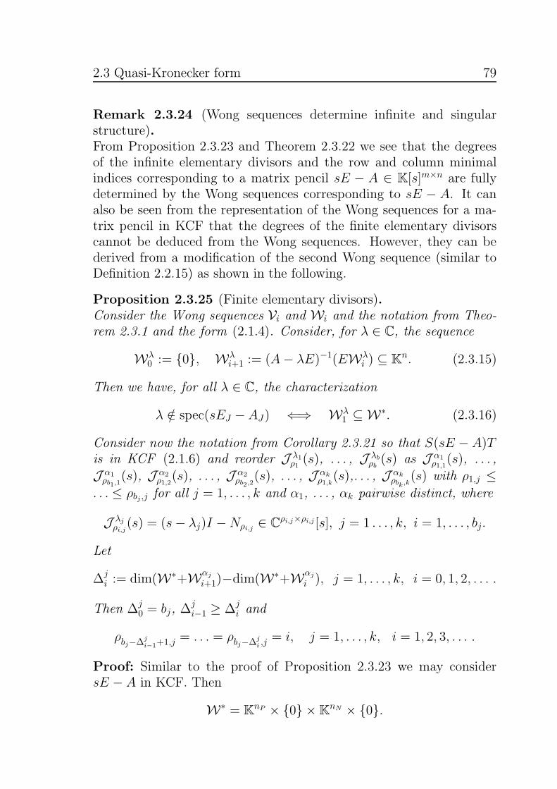
2.3 Quasi-Kronecker form 79
Remark 2.3.24 (Wong sequences determine infinite and singularstructure).From Proposition 2.3.23 and Theorem 2.3.22 we see that the degreesof the infinite elementary divisors and the row and column minimalindices corresponding to a matrix pencil sE − A ∈ K[s]m×n are fullydetermined by the Wong sequences corresponding to sE − A. It canalso be seen from the representation of the Wong sequences for a ma-trix pencil in KCF that the degrees of the finite elementary divisorscannot be deduced from the Wong sequences. However, they can bederived from a modification of the second Wong sequence (similar toDefinition 2.2.15) as shown in the following.
Proposition 2.3.25 (Finite elementary divisors).Consider the Wong sequences Vi and Wi and the notation from Theo-rem 2.3.1 and the form (2.1.4). Consider, for λ ∈ C, the sequence
Wλ0 := {0}, Wλ
i+1 := (A− λE)−1(EWλi ) ⊆ Kn. (2.3.15)
Then we have, for all λ ∈ C, the characterization
λ /∈ spec(sEJ −AJ) ⇐⇒ Wλ1 ⊆ W∗. (2.3.16)
Consider now the notation from Corollary 2.3.21 so that S(sE − A)Tis in KCF (2.1.6) and reorder J λ1
ρ1(s), . . . , J λb
ρb(s) as J α1
ρ1,1(s), . . . ,
J α1ρb1,1
(s), J α2ρ1,2
(s), . . . , J α2ρb2,2
(s), . . . , J αkρ1,k
(s),. . . , J αkρbk,k
(s) with ρ1,j ≤. . . ≤ ρbj ,j for all j = 1, . . . , k and α1, . . . , αk pairwise distinct, where
J λjρi,j
(s) = (s− λj)I −Nρi,j ∈ Cρi,j×ρi,j [s], j = 1 . . . , k, i = 1, . . . , bj.
Let
∆ji := dim(W∗+Wαj
i+1)−dim(W∗+Wαj
i ), j = 1, . . . , k, i = 0, 1, 2, . . . .
Then ∆j0 = bj, ∆
ji−1 ≥ ∆j
i and
ρbj−∆ji−1+1,j = . . . = ρbj−∆j
i ,j= i, j = 1, . . . , k, i = 1, 2, 3, . . . .
Proof: Similar to the proof of Proposition 2.3.23 we may considersE − A in KCF. Then
W∗ = KnP × {0} ×KnN × {0}.

80 2 Decomposition of matrix pencils
The proof now follows from the observation that, for all λ ∈ C andi ∈ N0,
W∗ +Wλi = KnP ×
×
j=1,...,k
l=1,...,bk
(kerJ αj
ρl,j(λ))i
×KnN × {0}nQ
and kerJ αjρl,j(λ) = {0} for λ 6= αj.
Remark 2.3.26 (Jordan canonical form).In case of a pencil sI − A, the following simplifications can be madein Proposition 2.3.25: W∗ = {0}, and hence Wλ
i = ker(A − λI)i.Then (2.3.16) becomes the classical eigenvalue definition
λ ∈ σ(A) ⇐⇒ ker(A− λI) 6= {0},
Furthermore,
∆ji = dimker(A− λjI)
i+1 − dim ker(A− λjI)i,
and hence we obviously obtain the Jordan canonical form of A, that isthe sizes and numbers of Jordan blocks, from Proposition 2.3.25.
Remark 2.3.27 (Determination of the KCF).The results presented in this subsection show that the KCF of a pencilsE − A (without the corresponding transformation matrices) is com-pletely determined by the Wong sequences:
(i) The row and column minimal indices ηi and εi are given by The-orem 2.3.22, which directly give the KCF of the singular part ofthe matrix pencil.
(ii) The degrees σi of the infinite elementary divisors are given byProposition 2.3.23 yielding the KCF of the matrix pencil sEN −AN .
(iii) Finally, the finite eigenvalues can be determined by deriving theroots of det(λEJ − AJ) or using (2.3.16), and the degrees ρi ofthe finite elementary divisors (corresponding to the above eigen-values) are given by Proposition 2.3.25. This yields the Jordancanonical form of E−1
J AJ completing the KCF.

2.4 Solution theory 81
2.4 Solution theory
In this section we study the DAE
ddtEx(t) = Ax(t) + f(t) (2.4.1)
corresponding to the matrix pencil sE − A ∈ R[s]m×n. Note that werestrict ourselves here to the field K = R, because 1) the vast majorityof DAEs arising from modeling physical phenomena are not complex-valued, 2) all the results for K = R carry over to K = C withoutmodification (the converse is not true in general), 3) the case K = Q israther artificial when considering solutions of the DAE (2.4.1), becausethen we had to consider functions f : R → Q or even f : Q → Q.In Subsection 2.4.1 we show that a complete characterization of the
solutions of the DAE (2.4.1) can be given in terms of the QKF, henceonly using the Wong sequences. This result is based on using a unimod-ular extension of the underdetermined (overdetermined) part of sE−Aand the inverse of it. While this is a simple and general characteriza-tion, the drawback of this approach is that, due to non-uniqueness ofthe extension and hence the unknown degree of the inverse, we have torequire that all functions involved are infinitely times (weakly) differ-entiable. To resolve this problem we use the KCF in Subsection 2.4.2and derive a characterization with minimal smoothness requirements.The results of Subsection 2.4.1 are partly contained in a joint work
with Stephan Trenn [40].
2.4.1 Solutions in terms of QKF
In this subsection we will show (see Theorem 2.4.8 and Remark 2.4.9)that the Wong sequences are sufficient to completely characterize thesolution behavior of the DAE (2.4.1) including the characterization ofconsistent initial values as well as constraints on the inhomogeneity f .Although (versions of) the Wong sequences appear frequently in theliterature (see Section 2.5 (i)), it seems that their relevance for a com-plete solution theory of DAEs associated to a singular matrix pencilhas been overlooked and the present characterization is novel.We first have to decide in which (function) space we consider the
DAE (2.4.1). We consider the space L1loc, because we like to allow for
step functions as inhomogeneities and, in the later chapters, as inputs of

82 2 Decomposition of matrix pencils
DAE control systems. However, we require the solution x ∈ L1loc(R;R
n)
to be smooth in the sense that Ex ∈ W1,1loc (R;R
m). This leads to cer-tain smoothness requirements on the inhomogeneity and excludes thepossibility of derivatives of step functions to appear in the solution,which would require distributional solutions. A distributional solu-tion setup (from a control theoretic point of view) has been consideredin [101,188,200] for instance, see also [77]. A typical argumentation inthese works is that inconsistent initial values cause distributional so-lutions in a way that the state trajectory is composed of a continuousfunction and a linear combination of Dirac’s delta impulse and some ofits derivatives. However, some frequency domain considerations in [182]refute this approach (see [229] for an overview on inconsistent initializa-tion). This justifies that we do only consider integrable solutions. Fora mathematically rigorous approach to distributional solution theory oflinear DAEs we refer to [227, 228] by Trenn, see also Section 2.5 (iii).We have motivated the following definition.
Definition 2.4.1 (Solutions of DAEs).Let sE − A ∈ R[s]m×n, t0 ∈ R, x0 ∈ Rn and f ∈ L1
loc(R;Rm). Then
x ∈ L1loc(R;R
n) is called a solution of the initial value problem (2.4.1),
x(t0) = x0, if, and only if, Ex ∈ W1,1loc (R;R
m), x(0) = x0, and (2.4.1) issatisfied for almost all t ∈ R.x is called a solution of the DAE (2.4.1) if, and only if, there exist t0 ∈
R, x0 ∈ Rn such that x is a solution of the initial value problem (2.4.1),x(t0) = x0.If f ∈ C∞(R;Rm), then the initial value x0 is called consistent at t0
for (2.4.1) if, and only if, the initial value problem (2.4.1), x(t0) = x0,has at least one solution x ∈ C∞(R;Rn).
Note that the existence of a solution of (2.4.1) may automaticallyrequire a higher (weak) differentiability of (components of) the inho-mogeneity f . This is also reflected in the definition of consistent initialvalues: since solutions are in general only unique almost everywhere,more smoothness of f and the solution x is required here.Before stating our main results concerning the solution theory of the
DAE (2.4.1), we need a preliminary result about polynomial matrices.A (square) polynomial matrix U(s) ∈ K[s]n×n is called unimodular if,and only if, it is invertible over the ringK[s]n×n, i.e., there exists V (s) ∈K[s]n×n such that U(s)V (s) = I. We will say that P (s) ∈ K[s]m×n can
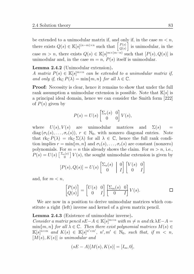
2.4 Solution theory 83
be extended to a unimodular matrix if, and only if, in the case m < n,
there exists Q(s) ∈ K[s](n−m)×n such that[P (s)Q(s)
]is unimodular, in the
case m > n, there exists Q(s) ∈ K[s]m×(m−n) such that [P (s), Q(s)] isunimodular and, in the case m = n, P (s) itself is unimodular.
Lemma 2.4.2 (Unimodular extension).A matrix P (s) ∈ K[s]m×n can be extended to a unimodular matrix if,and only if, rkC P (λ) = min{m, n} for all λ ∈ C.
Proof: Necessity is clear, hence it remains to show that under the fullrank assumption a unimodular extension is possible. Note that K[s] isa principal ideal domain, hence we can consider the Smith form [222]of P (s) given by
P (s) = U(s)
[Σr(s) 00 0
]V (s),
where U(s), V (s) are unimodular matrices and Σ(s) =diag (σ1(s), . . . , σr(s)), r ∈ N0, with nonzero diagonal entries. Notethat rkC P (λ) = rkCΣ(λ) for all λ ∈ C, hence the full rank condi-tion implies r = min{m, n} and σ1(s), . . . , σr(s) are constant (nonzero)polynomials. For m = n this already shows the claim. For m > n, i.e.,P (s) = U(s)
[Σn(s)
0
]V (s), the sought unimodular extension is given by
[P (s), Q(s)] = U(s)
[Σn(s) 00 I
] [V (s) 00 I
]
and, for m < n,[P (s)Q(s)
]=
[U(s) 00 I
] [Σm(s) 0
0 I
]V (s).
We are now in a position to derive unimodular matrices which con-stitute a right (left) inverse and kernel of a given matrix pencil.
Lemma 2.4.3 (Existence of unimodular inverse).Consider a matrix pencil sE−A ∈ K[s]m×n withm 6= n and rkλE−A =min{m, n} for all λ ∈ C. Then there exist polynomial matrices M(s) ∈K[s]n×m and K(s) ∈ K[s]n
′×m′
, n′, m′ ∈ N0, such that, if m < n,[M(s), K(s)] is unimodular and
(sE −A)[M(s), K(s)] = [Im, 0],
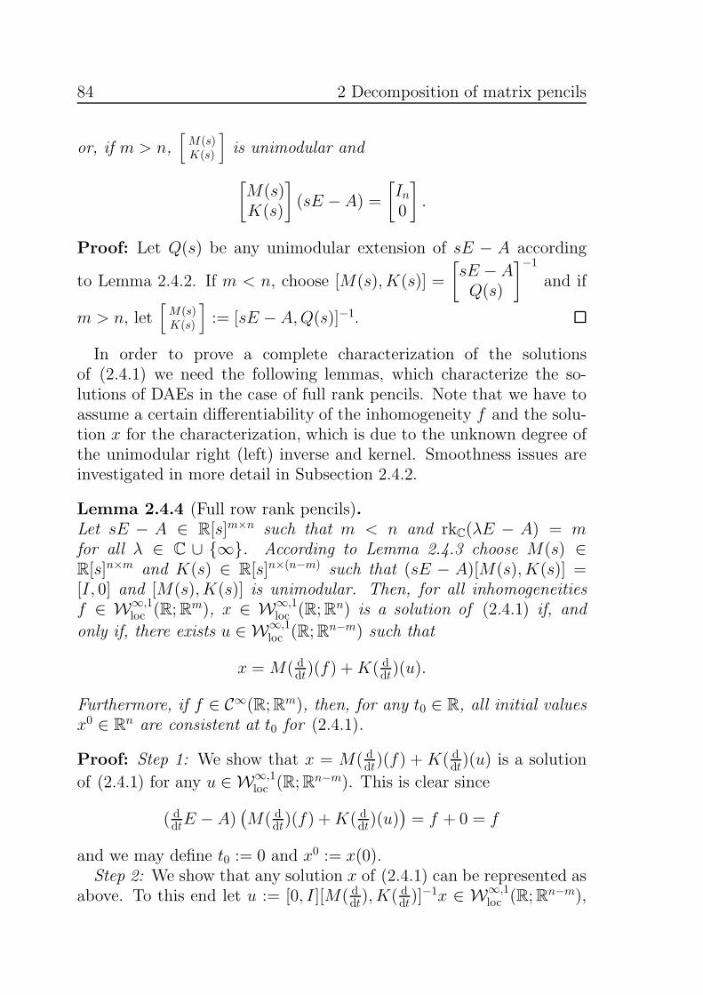
84 2 Decomposition of matrix pencils
or, if m > n,[M(s)K(s)
]is unimodular and
[M(s)K(s)
](sE −A) =
[In0
].
Proof: Let Q(s) be any unimodular extension of sE − A according
to Lemma 2.4.2. If m < n, choose [M(s), K(s)] =
[sE − AQ(s)
]−1
and if
m > n, let[M(s)K(s)
]:= [sE − A,Q(s)]−1.
In order to prove a complete characterization of the solutionsof (2.4.1) we need the following lemmas, which characterize the so-lutions of DAEs in the case of full rank pencils. Note that we have toassume a certain differentiability of the inhomogeneity f and the solu-tion x for the characterization, which is due to the unknown degree ofthe unimodular right (left) inverse and kernel. Smoothness issues areinvestigated in more detail in Subsection 2.4.2.
Lemma 2.4.4 (Full row rank pencils).Let sE − A ∈ R[s]m×n such that m < n and rkC(λE − A) = mfor all λ ∈ C ∪ {∞}. According to Lemma 2.4.3 choose M(s) ∈R[s]n×m and K(s) ∈ R[s]n×(n−m) such that (sE − A)[M(s), K(s)] =[I, 0] and [M(s), K(s)] is unimodular. Then, for all inhomogeneitiesf ∈ W∞,1
loc (R;Rm), x ∈ W∞,1loc (R;Rn) is a solution of (2.4.1) if, and
only if, there exists u ∈ W∞,1loc (R;Rn−m) such that
x = M( ddt)(f) +K( d
dt)(u).
Furthermore, if f ∈ C∞(R;Rm), then, for any t0 ∈ R, all initial valuesx0 ∈ Rn are consistent at t0 for (2.4.1).
Proof: Step 1: We show that x = M( ddt)(f) + K( d
dt)(u) is a solution
of (2.4.1) for any u ∈ W∞,1loc (R;Rn−m). This is clear since
( ddtE − A)
(M( d
dt)(f) +K( ddt)(u)
)= f + 0 = f
and we may define t0 := 0 and x0 := x(0).Step 2: We show that any solution x of (2.4.1) can be represented as
above. To this end let u := [0, I][M( ddt), K( d
dt)]−1x ∈ W∞,1
loc (R;Rn−m),
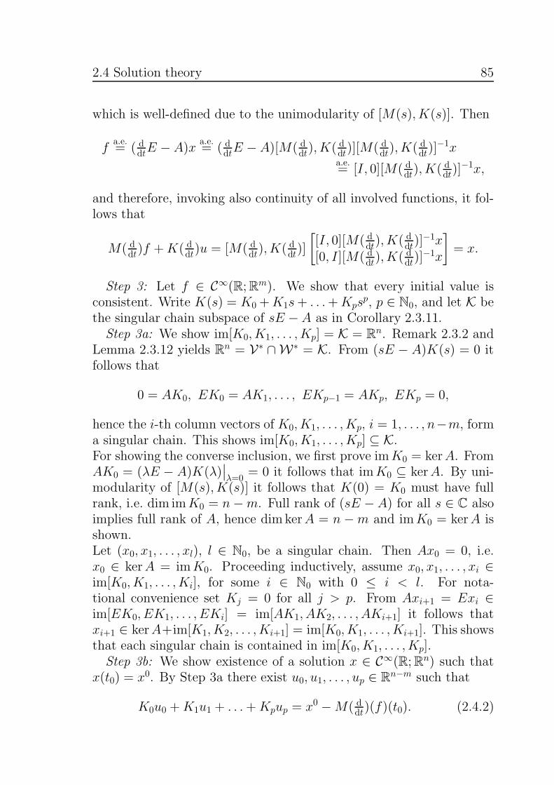
2.4 Solution theory 85
which is well-defined due to the unimodularity of [M(s), K(s)]. Then
fa.e.= ( d
dtE − A)xa.e.= ( d
dtE − A)[M( ddt), K( d
dt)][M( ddt), K( d
dt)]−1x
a.e.= [I, 0][M( d
dt), K( ddt)]
−1x,
and therefore, invoking also continuity of all involved functions, it fol-lows that
M( ddt)f +K( d
dt)u = [M( ddt), K( d
dt)]
[[I, 0][M( d
dt), K( d
dt)]−1x
[0, I][M( ddt), K( d
dt)]−1x
]= x.
Step 3: Let f ∈ C∞(R;Rm). We show that every initial value isconsistent. Write K(s) = K0 +K1s+ . . .+Kps
p, p ∈ N0, and let K bethe singular chain subspace of sE −A as in Corollary 2.3.11.Step 3a: We show im[K0, K1, . . . , Kp] = K = Rn. Remark 2.3.2 and
Lemma 2.3.12 yields Rn = V∗ ∩W∗ = K. From (sE − A)K(s) = 0 itfollows that
0 = AK0, EK0 = AK1, . . . , EKp−1 = AKp, EKp = 0,
hence the i-th column vectors of K0, K1, . . . , Kp, i = 1, . . . , n−m, forma singular chain. This shows im[K0, K1, . . . , Kp] ⊆ K.For showing the converse inclusion, we first prove imK0 = kerA. FromAK0 = (λE − A)K(λ)
∣∣λ=0
= 0 it follows that imK0 ⊆ kerA. By uni-modularity of [M(s), K(s)] it follows that K(0) = K0 must have fullrank, i.e. dim imK0 = n−m. Full rank of (sE − A) for all s ∈ C alsoimplies full rank of A, hence dimkerA = n −m and imK0 = kerA isshown.Let (x0, x1, . . . , xl), l ∈ N0, be a singular chain. Then Ax0 = 0, i.e.x0 ∈ kerA = imK0. Proceeding inductively, assume x0, x1, . . . , xi ∈im[K0, K1, . . . , Ki], for some i ∈ N0 with 0 ≤ i < l. For nota-tional convenience set Kj = 0 for all j > p. From Axi+1 = Exi ∈im[EK0, EK1, . . . , EKi] = im[AK1, AK2, . . . , AKi+1] it follows thatxi+1 ∈ kerA+im[K1, K2, . . . , Ki+1] = im[K0, K1, . . . , Ki+1]. This showsthat each singular chain is contained in im[K0, K1, . . . , Kp].Step 3b: We show existence of a solution x ∈ C∞(R;Rn) such that
x(t0) = x0. By Step 3a there exist u0, u1, . . . , up ∈ Rn−m such that
K0u0 +K1u1 + . . .+Kpup = x0 −M( ddt)(f)(t0). (2.4.2)
86 2 Decomposition of matrix pencils
Let
u(t) := u0 + (t− t0)u1 +(t− t0)
2
2u2 + . . .+
(t− t0)p
p!up, t ∈ R.
Then we have that u ∈ C∞(R;Rn−m) and
K( ddt)(u)(t0) = K0u0 +K1u1 + . . .+Kpup
(2.4.2)= x0 −M( d
dt)(f)(t0),
(2.4.3)which implies that the solution x =M( d
dt)(f) +K( ddt)(u) ∈ C∞(R;Rn)
satisfies
x(t0) =M( ddt)(f)(t0) +K( d
dt)(u)(t0)(2.4.3)= x0.
Remark 2.4.5 (Full row rank and eigenvalue ∞).A careful analysis of the proof of Lemma 2.4.4 reveals that for thesolution formula the full row rank of λE−A for λ = ∞ is not necessary.The latter is only necessary to show that all initial value problems havea solution.
Lemma 2.4.6 (Full column rank pencils).Let sE − A ∈ R[s]m×n such that m > n and rkC(λE − A) = n forall λ ∈ C ∪ {∞}. According to Lemma 2.4.3 choose M(s) ∈ R[s]n×m
and K(s) ∈ R[s](m−n)×m such that[M(s)K(s)
](sE − A) = [ I0 ] and
[M(s)K(s)
]
is unimodular. Then, for all f ∈ W∞,1loc (R;Rm), x ∈ W∞,1
loc (R;Rn) is asolution of (2.4.1) if, and only if,
x = M( ddt)(f) and K( d
dt)(f) = 0.
Furthermore, every component or linear combination of f is restrictedin some way, more precisely K(s)F has no zero column for any invert-ible F ∈ Rm×m.
Proof: The characterization of the solution follows from the equiva-lence
( ddtE − A)x
a.e.= f ⇐⇒
[M( d
dt)K( d
dt)
]( ddtE − A)
︸ ︷︷ ︸=[ I0 ]
xa.e.=
[M( d
dt)fK( d
dt)f
]
and continuity of the involved functions. To show that K(s)F doesnot have any zero column, write K(s) = K0 + K1s + . . . + Kps
p.
2.4 Solution theory 87
Since (sE⊤ − A⊤)K(s)⊤ = 0 it follows with the same arguments asin Step 3a of Lemma 2.4.4 that im[K⊤
0 , K⊤1 , . . . , K
⊤p ] = Rm. Hence,
ker[K⊤0 , K
⊤1 , . . . , K
⊤p ]
⊤ = {0} which shows that the only v ∈ Rm withKiv = 0 for all i = 1, . . . , p is v = 0. This shows that K(s)F does nothave a zero column for any invertible F ∈ Rm×m.
Remark 2.4.7 (Full column rank and eigenvalue ∞).Analogously, as pointed out in Remark 2.4.5, the condition that λE−Amust have full column rank for λ = ∞ is not needed to characterizethe solution. It is only needed to show that the inhomogeneity is ‘com-pletely’ restricted.
The following theorem gives a complete characterization of the solu-tion behavior of the DAE (2.4.1) just based on the QKF (2.1.5) withouta knowledge of a more detailed structure (e.g., some staircase form orthe KCF of some of the blocks).
Theorem 2.4.8 (Complete characterization of solutions in terms ofQKF).Let sE−A ∈ R[s]m×n and use the notation from Theorem 2.3.3 so thatS(sE − A)T is in QKF (2.1.5). Let f ∈ W∞,1
loc (R;Rm) and(f⊤
P , f⊤J , f
⊤N , f
⊤Q )
⊤ := Sf , where the splitting corresponds to the blocksizes in (2.1.5). According to Lemma 2.4.3 choose unimodular matrices
[MP (s), KP (s)] ∈ R[s]nP×(mP+(nP−mP )),[MQ(s)KQ(s)
]∈ R[s](nQ+(mQ−nQ))×mQ
such that
(sEP−AP )[MP (s), KP (s)] = [I, 0] and
[MQ(s)KQ(s)
](sEQ−AQ) =
[I0
].
Then there exists a solution x ∈ W∞,1loc (R;Rn) of the DAE (2.4.1) if,
and only if,
KQ(ddt)(fQ) = 0. (2.4.4)
If f ∈ C∞(R;Rm) and (2.4.4) holds, then an initial value
x0 = T(x0P
⊤, x0J
⊤, x0N
⊤, x0Q
⊤)⊤
is consistent at t0 ∈ R for (2.4.1) if,
and only if,
x0Q =(MQ(
ddt)(fQ)
)(t0) and
x0N = −(
nN−1∑
k=0
(A−1
N EN
)k( ddt)k(fN)
)(t0).
(2.4.5)

88 2 Decomposition of matrix pencils
If (2.4.4) and (2.4.5) hold, then x = T(xP
⊤, xJ⊤, xN⊤, xQ⊤)⊤
∈ W∞,1loc (R;Rn) is a solution of the initial value problem (2.4.1), x(t0) =
x0, if, and only if, we have
xP = MP (ddt)(fP ) +KP (
ddt)(ux0
P),
xJ = eE−1J AJ(·−t0)x0J +
∫ ·t0eE
−1J AJ (·−s)fJ(s) ds ,
xN = −∑nN−1k=0
(A−1
N EN
)k( ddt)
k(fN),
xQ = MQ(ddt)(fQ).
(2.4.6)
where ux0P∈ W∞,1
loc (R;RnP−mP ) is such that
(KP (
ddt)(ux0
P))(t0) = x0P −
(MP (
ddt)(fP )
)(t0). (2.4.7)
Proof: The first statement of the theorem about existence of solutionsof (2.4.1) follows from Lemma 2.4.6. In order to prove the secondstatement about consistent initial values let f ∈ C∞(R;Rm) and observethat:Step 1 : Assume that x0 is consistent at t0 for (2.4.1). Then there
exists a solution x ∈ C∞(R;Rn) of (2.4.1), x(t0) = x0. Clearly, byLemma 2.4.6, x0Q = xQ(t0) =
(MQ(
ddt)(fQ)
)(t0). For the second condi-
tion we calculate
x0N = xN(t0) = ddt
(A−1
N EN
)xN(t0)− fN(t0)
= ddt
(A−1
N EN
) (ddt
(A−1
N EN
)xN(t0)− fN(t0)
)− fN(t0)
= . . .
= −(
nN−1∑
k=0
(A−1
N EN
)k( ddt)
k(fN)
)(t0).
Step 2 : Assume that (2.4.5) holds true. We show that there existsa solution x ∈ C∞(R;Rn) of (2.4.1), x(t0) = x0. Clearly x as in (2.4.6)is a solution of (2.4.1), where existence of ux0
P∈ C∞(R;Rnp−mp) is
guaranteed by Lemma 2.4.4, and the initial value conditions in (2.4.5)are satisfied.The last statement of the theorem about the representation of so-
lutions of initial value problems follows from the above considerationsand the fact that due to Lemma 2.4.4 it is always possible to chooseux0
P∈ W∞,1
loc (R;RnP−mP ) such that (2.4.7) is satisfied.

2.4 Solution theory 89
Remark 2.4.9 (Characterization in terms of QKTF).A similar statement as in Theorem 2.4.8 is also possible if we only con-sider the QKTF (2.1.4). The corresponding conditions for the Q-partremain the same, in the condition for the N -part the inhomogeneityfN is replaced by fN − ( d
dtENQ −ANQ)(xQ), in the J-part the inhomo-
geneity fJ is replaced by fJ − ( ddtEJN −AJN)(xN)− ( d
dtEJQ−AJQ)(xQ)
and in the P -part the inhomogeneity fP is replaced by fP − ( ddtEPJ −
APJ)(xJ)− (EPNddt − APN)(xN)− (EPQ
ddt − APQ)(xQ).
Remark 2.4.10 (Solutions on (finite) time intervals).The solution of a DAE (2.4.1) on some time interval I ( R can bedefined in a straightforward manner (compare Definition 2.4.1). FromTheorem (2.4.8) we can infer that any solution x on some finite timeinterval I ( R can be extended to a solution on the whole real axisprovided the inhomogeneity f is defined on R.
2.4.2 Solutions in terms of KCF
In this subsection we aim to derive a characterization of solutionsof (2.4.1) without any further smoothness requirements on the solu-tion using the KCF. However, we cannot use the KCF of the wholepencil; we use the QKF and transform all parts except for the ODEpart into KCF. This can be achieved by combining Theorem 2.3.3,Lemma 2.3.14, Corollary 2.3.15 and the Jordan canonical form of anilpotent matrix and leads to the following result.
Corollary 2.4.11.For any sE − A ∈ R[s]m×n there exist S ∈ Glm(R) and T ∈ Gln(R)such that, using the notation from Definition 2.1.7,
S(sE −A)T = diag(sIk − J,Pε1(s), . . . ,Pεa(s),Nσ1
(s),
. . . ,Nσc(s),Qη1(s), . . . ,Qηd(s)
), (2.4.8)
where k ∈ N0 and J ∈ Rk×k.
This leads to the separate consideration of the DAEs correspondingto each type of blocks:

90 2 Decomposition of matrix pencils
(i) The ODE block sI−J corresponds to the ODE ddtx(t) = Jx(t)+
f(t) whose solution satisfies
x(t) = eJ(t−t0)x(t0) +
∫ t
t0
eJ(t−τ)f(τ)dτ, t ∈ R.
In particular, solvability is guaranteed by f ∈ L1loc(R;R
m). Theinitial value x(t0) ∈ Rn can be chosen arbitrarily; the prescriptionof f ∈ L1
loc(R;Rm) and x(t0) ∈ Rn guarantees uniqueness of the
solution.
(ii) Solutions of the DAE corresponding to a block Nσ(s) = sNσ − I,namely d
dtNσx(t) = x(t) + f(t), can be calculated as done in theproof of Theorem 2.4.8:
xa.e.= d
dtNσx− fa.e.= d
dtNσ
(ddtNσx− f
)− f
a.e.= ( d
dtNσ)
2(ddtNσx− f
)− d
dtNσf − f
a.e.= . . .
a.e.= −
σ−1∑
k=0
( ddtNσ)
kf.
(2.4.9)
Here, only the property of x being a solution of (2.4.1) (and henceNσx ∈ W1,1
loc (R;Rσ)) and no further smoothness is used. However,
the solution requires a certain smoothness of the inhomogeneity,expressed by
σ−2∑
k=0
Nσ(ddtNσ)
kf ∈ W1,1loc (R;R
σ). (2.4.10)
In fact, we can prove that for f ∈ L1loc(R;R
σ) there exists a so-lution x ∈ L1
loc(R;Rσ) of d
dtNσx(t) = x(t) + f(t) if, and only if,
condition (2.4.10) holds: The ‘⇒’-part follows from pre-multiply-ing (2.4.9) with Nσ and the fact that Nσx ∈ W1,1
loc (R;Rσ). The
‘⇐’-part follows by defining x := −∑σ−1k=0(
ddtNσ)
kf and observ-ing that by (2.4.10) x is indeed well-defined and satisfies x ∈L1loc(R;R
σ) and Nσx ∈ W1,1loc (R;R
σ), thus x is a solution ofddtNσx(t) = x(t) + f(t).
Note that, similar to Theorem 2.4.8, for f ∈ C∞(R;Rσ) an initialvalue x0 ∈ Rσ is consistent at t0 ∈ R for d
dtNσx(t) = x(t) + f(t)

2.4 Solution theory 91
if, and only if,
x0 = −(
σ−1∑
k=0
( ddtNσ)
k(f)
)(t0).
However, solutions to initial value problems may even exist forinconsistent initial values, see Example 2.4.12.
(iii) An underdetermined block Pε(s) = sLε+1 −Kε+1 corresponds toa DAE d
dtLε+1x = Kε+1x + f . Using the structure of Lε+1 andKε+1 and
x− :=
x2...
xε+1
,
we may rewrite this equation as
ddtx−(t) = Nεx−(t) + e1x1(t) + f(t)
and e1 is the first unit vector. Hence, a solution exists for all f ∈L1loc(R;R
ε) and all x1 ∈ L1loc(R;R) as well as x2(t0), . . . , xε+1(t0).
This system is therefore underdetermined in the sense that onecomponent as well as all initial values can be freely chosen. Henceany existing solution for fixed inhomogeneity f and fixed initialvalue x(t0) is far from being unique.
(iv) An overdetermined block Qη(s) = sL⊤η+1 − K⊤
η+1 corresponds to
a DAE ddtL⊤η+1x = K⊤
η+1x + f . Using the structure of L⊤η+1 and
K⊤η+1 and denoting
x+ :=
(x0
),
we obtain the equivalent equation
ddtNη+1x+(t) = x+(t) + f(t).
Hence we obtain x+a.e.= −∑η
k=0(ddtNη+1)
kf , which gives
xa.e.= −[Iη, 0]
η∑
k=0
( ddtNη+1)
kf

92 2 Decomposition of matrix pencils
together with the consistency condition on the inhomogeneity(which is a special case of (2.4.4)):
e⊤η+1
η∑
k=0
( ddtNη+1)
kfa.e.= 0. (2.4.11)
The smoothness condition
η−1∑
k=0
Nη+1(ddtNη+1)
kf ∈ W1,1loc (R;R
η+1)
is therefore not enough to guarantee existence of a solution; theadditional constraint formed by (2.4.11) has to be satisfied, too.Furthermore, as in (ii), consistency of the initial value x0 at t0 isrestricted by the inhomogeneity f .
Example 2.4.12 (Inconsistent initial values).Consider the simple DAE
0 = x(t) + f(t) (2.4.12)
for f ∈ C∞(R;R). Clearly, x0 ∈ R is consistent at t0 ∈ R for (2.4.12)if, and only if, x0 = −f(t0). However, the solution of (2.4.12) isonly unique almost everywhere since any y ∈ L1
loc(R;R) which satisfiesy(t) = −f(t) for almost all t ∈ R is a solution of (2.4.12). Therefore,any initial value problem (2.4.12), x(t0) = x0, with arbitrary x0 ∈ R
has a solution, but only x0 = −f(t0) is consistent.Summarizing the above considerations we obtain the following the-
orem which characterizes existence of solutions of a DAE (2.4.1) bysmoothness and consistency conditions on the inhomogeneity. Thesmoothness conditions reflect the limits of the solution setup usingintegrable functions only: if any component of the inhomogeneity doesnot obey these conditions this directly leads to Dirac impulses in thesolution and hence the requirement for a distributional solution setup,see also Section 2.5 (iii). We omit the characterization of consistentinitial values; this can be concluded from (i)–(iv) above.
Theorem 2.4.13 (Characterization of solutions of the DAE in termsof KCF).
2.5 Notes and References 93
Let sE − A ∈ R[s]m×n and use the notation from Corollary 2.4.11 sothat (2.4.8) holds. Let f ∈ L1
loc(R;Rm) and, according to the block
structure of (2.4.8),
(f⊤J , f
⊤P,1, . . . , f
⊤P,a, f
⊤N,1, . . . , f
⊤N,c, f
⊤Q,1, . . . , f
⊤Q,d
)⊤:= Sf.
Then there exists a solution x ∈ L1loc(R;R
n) of (2.4.1) if, and only if,the smoothness conditions
∀ i = 1, . . . , c :σi−2∑k=0
Nσi( ddtNσi
)kfN,i ∈ W1,1loc (R;R
σi) and
∀ i = 1, . . . , d :ηi−1∑k=0
Nηi+1(ddtNηi+1)
kfQ,i ∈ W1,1loc (R;R
ηi+1)
(2.4.13)and the consistency condition
∀ i = 1, . . . , d : e⊤ηi+1
ηi∑
k=0
( ddtNηi+1)
kfQ,ia.e.
= 0
are satisfied.
Note that the smoothness conditions (2.4.13) in Theorem 2.4.13 im-plicitly require a higher (weak) differentiability of certain componentsof f so that (2.4.13) is satisfied.
2.5 Notes and References
(i) The Wong sequences can be traced back to Dieudonne [87],however his focus is only on the first of the two Wong sequences.Bernhard [42] and Armentano [7] used the Wong sequencesto carry out a geometric analysis of matrix pencils. In [185] thefirst Wong sequence is introduced as a ‘fundamental geometrictool in the characterization of the subspace of consistent initialconditions’ of a regular DAE. Both Wong sequences are intro-duced in [184] where the authors obtain a quasi-Kronecker stair-case form; however, they did not consider both Wong sequencesin combination so that the important role of the spaces V∗ ∩W∗,V∗ + W∗, EV∗ ∩ AW∗, EV∗ + AW∗ (see Definition 2.2.1, Fig-ure 2.1 and Theorem 2.3.1) is not highlighted. They also appear

94 2 Decomposition of matrix pencils
in [3,4,151,233]. In control theory, modified versions of the Wongsequences (where imB is added to EVi and AWi resp.) havebeen studied extensively for not necessarily regular DAEs, seee.g. [3, 11, 13, 14, 92, 159, 167, 188, 200] and they have been foundto be an appropriate tool to construct invariant subspaces, thereachable space and provide a Kalman decomposition, to namebut a few features.
(ii) The notion of consistent initial values as in Definition 2.4.1 is mostimportant for DAEs and therefore as old as the theory of DAEsitself, see e.g. [100]. The space of consistent initial values is oftenused and sometimes called viability kernel [45], see also [9, 10].
(iii) Since solutions of a DAE (2.4.1) might involve derivatives of theinhomogeneities, jumps in the inhomogeneity might lead to non-existence of solutions due to a lack of differentiability. This ischaracterized by the smoothness conditions in Theorem 2.4.13.However, this is not a ‘structural non-existence’ since everysmooth approximation of the jump could lead to well definedsolutions. Therefore, one might extend the solution space byconsidering distributions (or generalized functions) as formallyintroduced by Schwartz [218]. The advantage of this larger so-lution space is that each distribution is ‘smooth’, in particularthe unit step function (Heaviside function) has a derivative: theDirac impulse. Unfortunately, the whole space of distributionsis too large, for example it is in general not possible to speak ofan initial value, because evaluation of a distribution at a specifictime is not defined. To overcome this obstacle one might con-sider the smaller space of piecewise-smooth distributions DpwC∞
as introduced in [227, 228]. For piecewise-smooth distributions aleft- and right-sided evaluation is possible, i.e., for D ∈ DpwC∞ thevalues D(t−) ∈ R and D(t+) ∈ R are well defined for all t ∈ R.
(iv) Distributional solutions for time-invariant DAEs have alreadybeen considered by Cobb [75] and Geerts [101, 102] and fortime-varying DAEs by Rabier and Rheinboldt [202] andKunkel and Mehrmann [152].

95
3 Controllability
In this chapter we consider linear differential-algebraic control systemsof the form
ddtEx(t) = Ax(t) + Bu(t),
with E,A ∈ Rl×n, B ∈ Rl×m; the set of these systems is denoted byΣl,n,m, and we write [E,A,B] ∈ Σl,n,m. We do not assume that thepencil sE −A ∈ R[s]l×n is regular.
The function u : R → Rm is called input ; x : R → Rn is called(generalized) state. Note that, strictly speaking, x(t) is in general nota state in the sense that the free system (i.e., u ≡ 0) satisfies a semi-group property [145, Sec. 2.2]. We will, however, speak of the state x(t)for sake of brevity, especially since x(t) contains the full informationabout the system at time t. Furthermore, one might argue that (espe-cially in the behavioral setting) it is not correct to call u an ‘input’,because due to the implicit nature of (3.1.1) it may be that actuallysome components of u are uniquely determined and some componentsof x are free, and only the free variables should be called inputs inthe behavioral setting. However, the controllability concepts given inDefinition 3.1.5 explicitly distinguish between x and u and not betweenfree and determined variables. We feel that, in some cases, it mightstill be the choice of the designer to assign the input variables, that isu, and if some of these are determined, then the input space has to berestricted in an appropriate way.
By virtue of Definition 2.4.1, a trajectory (x, u) : R → Rn × Rm
is said to be a solution of [E,A,B] if, and only if, it belongs to the

96 3 Controllability
behavior of [E,A,B]:B[E,A,B] :={(x, u) ∈ L1
loc(R;Rn × Rm) | Ex ∈ W1,1
loc (R;Rl)
and (x, u) satisfies ddtEx(t) = Ax(t) + Bu(t)
for almost all t ∈ R}.
Note that, by linearity of the system [E,A,B], B[E,A,B] is a vectorspace. This chapter is organized as follows.In Section 3.1 the concepts of impulse controllability, controllabil-
ity at infinity, R-controllability, controllability in the behavioral sense,strong and complete controllability, as well as strong and completereachability and stabilizability in the behavioral sense, strong and com-plete stabilizability will be defined and described in time-domain. Inthe DAE literature these notions are not consistently treated; for aclarification see Section 3.7. Some relations between the concepts arealso included in Section 3.1.In Section 3.2 we concentrate on decompositions under state space
transformation and, further, under state space, input and feedbacktransformations. We introduce the concepts of system and feedbackequivalence and state decompositions under these equivalences, whichfor instance generalize the Brunovsky form. It is also discussed whenthese forms are canonical and what properties (regarding controllabilityand stabilizability) the appearing subsystems have.The generalized Brunovsky form enables us to give short proofs of
equivalent criteria, in particular generalizations of the Hautus test, forthe controllability concepts in Section 3.3, the most of which are ofcourse well-known - we discuss the relevant literature.In Section 3.4 we revisit the concept of feedback for DAE systems
and prove new results concerning the equivalence of stabilizability ofDAE control systems and the existence of a feedback which stabilizesthe closed-loop system. Stabilization via control in the behavioral senseis investigated as well.In Section 3.5 we give a brief summary of some selected results of the
geometric theory using invariant subspaces which lead to a represen-tation of the reachable space and criteria for controllability at infinity,impulse controllability, controllability in the behavioral sense, completeand strong controllability.Finally, in Section 3.6 the results regarding the Kalman decomposi-
tion for DAE systems are stated and it is shown how the controllability
3.1 Controllability concepts 97
concepts can be related to certain properties of the Kalman decompo-sition.The results of this chapter have been published in a joint work with
Timo Reis [38].
3.1 Controllability concepts
In this section we introduce and investigate controllability concepts forcontrol systems
ddtEx(t) = Ax(t) + Bu(t), (3.1.1)
where [E,A,B] ∈ Σl,n,m. The following spaces play a fundamental rolein this chapter:
(a) The space of consistent initial states
V[E,A,B] =
{x0 ∈ Rn
∣∣∣∣∃ (x, u) ∈ B[E,A,B] :
x ∈ W1,1loc (R;R
n) ∧ x(0) = x0
}.
(b) The space of consistent initial differential variables
Vdiff[E,A,B] =
{x0 ∈ Rn
∣∣∣∣∃ (x, u) ∈ B[E,A,B] :
x ∈ W1,1loc (R;R
n) ∧ Ex(0) = Ex0
}.
(c) The reachable space at time t ≥ 0
Rt[E,A,B] =
{x0 ∈ Rn
∣∣∣∣∃ (x, u) ∈ B[E,A,B] : x ∈ W1,1
loc (R;Rn)
∧ x(0) = 0 ∧ x(t) = x0
}
and the reachable space
R[E,A,B] =⋃
t≥0
Rt[E,A,B].
(d) The controllable space at time t ≥ 0
Ct[E,A,B] =
{x0 ∈ Rn
∣∣∣∣∃ (x, u) ∈ B[E,A,B] : x ∈ W1,1
loc (R;Rn)
∧ x(0) = x0 ∧ x(t) = 0
}
and the controllable space
C[E,A,B] =⋃
t≥0
Ct[E,A,B].

98 3 Controllability
Remark 3.1.1 (Fundamental spaces).
(i) Note that by linearity of the system, V[E,A,B], Vdiff[E,A,B],Rt
[E,A,B] and
Ct[E,A,B] are linear subspaces of Rn. We will show that Rt1
[E,A,B] =
Rt2[E,A,B] = Ct1
[E,A,B] = Ct2[E,A,B] for all t1, t2 > 0, see Lemma 3.1.4.
This implies R[E,A,B] = Rt[E,A,B] = Ct
[E,A,B] = C[E,A,B] for all t > 0.
(ii) In the definition of the above spaces we require thatx ∈ W1,1
loc (R;Rn). If we had assumed that for (x, u) ∈ B[E,A,B] the
state x belongs to L1loc(R;R
n), and not necessarily toW1,1loc (R;R
n),then any initial state x(0) = x0 ∈ Rn would be consistent for theequation 0 = x. However, it is desirable that the only consis-tent initial value of 0 = x is x0 = 0, which is guaranteed byx ∈ W1,1
loc (R;Rn).
Likewise, the reachable and controllable spaces for the equation0 = x should be {0} as well, which again is reflected by therequirement x ∈ W1,1
loc (R;Rn).
(iii) We have that V[E,A,B] ⊆ Vdiff[E,A,B] and the inclusion is in general
strict (cf. Lemma 3.1.4). Consider for example
ddt
[0 01 0
](x1(t)x2(t)
)=
[1 00 1
](x1(t)x2(t)
)+
[00
]u(t),
where
V[E,A,B] = {0} and Vdiff[E,A,B] = im
[01
].
Note that the sets of solutions in the definitions of V[E,A,B] and
Vdiff[E,A,B] coincide, but in Vdiff
[E,A,B] we may take x0 ‘larger’, so that
it is not an initial value.
Since the matrices in (3.1.1) are time-invariant, the behavior is shift-invariant, that is (στx, στu) ∈ B[E,A,B] for all τ ∈ R and (x, u) ∈B[E,A,B]. Therefore, we have for all t ∈ R that
V[E,A,B] =
{x0 ∈ Rn
∣∣∣∣∃ (x, u) ∈ B[E,A,B] :
x ∈ W1,1loc (R;R
n) ∧ x(t) = x0
}, (3.1.2)
Vdiff[E,A,B] =
{x0 ∈ Rn
∣∣∣∣∃ (x, u) ∈ B[E,A,B] :
x ∈ W1,1loc (R;R
n) ∧ Ex(t) = Ex0
}.
3.1 Controllability concepts 99
In the following three lemmas we clarify some of the relations betweenthe fundamental spaces, before we state the controllability concepts.
Lemma 3.1.2 (Inclusions for reachable spaces).For [E,A,B] ∈ Σl,n,m and t1, t2 > 0 with t1 < t2, the following holdstrue:
(a) Rt1[E,A,B] ⊆ Rt2
[E,A,B].
(b) If Rt1[E,A,B] = Rt2
[E,A,B], then Rt1[E,A,B] = Rt
[E,A,B] for all t ∈ R witht > t1.
Proof:
(a) Let x ∈ Rt1[E,A,B]. By definition, there exists some (x, u) ∈ B[E,A,B]
with x ∈ W1,1loc (R;R
n), x(0) = 0 and x(t1) = x. Define (x1, u1) :R → Rn × Rm such that
(x1(t), u1(t)) =
{(x(t− t2 + t1), u(t− t2 + t1)), if t > t2 − t1
(0, 0), if t ≤ t2 − t1
Then x(0) = 0 implies that x1 is continuous at t2 − t1. Since,furthermore,
x1|(−∞,t2−t1]∈ W1,1
loc ((−∞, t2 − t1];Rn)
and x1|[t2−t1,∞) ∈ W1,1loc ([t2 − t1,∞);Rn),
we have (x1, u1) ∈ W1,1loc (R;R
n)× L1loc(R;R
m). By shift-invariance,ddtEx1(t) = Ax1(t) + Bu1(t) holds true for almost all t ∈ R, i.e.,
(x1, u1) ∈ B[E,A,B]. Then, due to x1(0) = 0 and x = x(t1) = x1(t2),
we obtain x ∈ Rt2[E,A,B].
(b) Step 1: We show that Rt1[E,A,B] = Rt2
[E,A,B] implies Rt1[E,A,B]
= Rt1+2(t2−t1)[E,A,B] : By (a), it suffices to show the inclusion “⊇”. As-
sume that x ∈ Rt1+2(t2−t1)[E,A,B] , i.e., there exists some (x1, u1) ∈ B[E,A,B]
with x1 ∈ W1,1loc (R;R
n), x1(0) = 0 and x1(t1+2(t2− t1)) = x. Sincex1(t2) ∈ Rt2
[E,A,B] = Rt1[E,A,B], there exists some (x2, u2) ∈ B[E,A,B]

100 3 Controllability
with x2 ∈ W1,1loc (R;R
n), x2(0) = 0 and x2(t1) = x1(t2). Now con-sider the trajectory
(x(t), u(t)) =
{(x2(t), u2(t)), if t < t1,
(x1(t+ (t2 − t1)), u1(t+ (t2 − t1))), if t ≥ t1.
Since x is continuous at t1, we can apply the same arguments as inthe proof of (a) to infer that x ∈ W1,1
loc (R;Rn) and (x, u) ∈ B[E,A,B].
The result to be shown in the present step is now a consequence ofx(0) = x2(0) = 0 and
x = x1(t1 + 2(t2 − t1)) = x(t2) ∈ Rt2[E,A,B] = Rt1
[E,A,B].
Step 2: We show (b): From the result shown in the first step, wemay inductively conclude that Rt1
[E,A,B] = Rt2[E,A,B] implies
Rt1[E,A,B] = Rt1+i(t2−t1)
[E,A,B] for all i ∈ N. Let t ∈ R with t > t1. Then
there exists some i ∈ N with t ≤ t1 + i(t2 − t1). Then statement(a) implies
Rt1[E,A,B] ⊆ Rt
[E,A,B] ⊆ Rt1+i(t2−t1)[E,A,B] ,
and, by Rt1[E,A,B] = Rt1+i(t2−t1)
[E,A,B] , we obtain the desired result.
Now we present some relations between controllable and reachablespaces of [E,A,B] ∈ Σl,n,m and its backward system [−E,A,B] ∈ Σl,n,m.It can easily be verified thatB[−E,A,B] =
{(x, u)
∣∣ (x, u) ∈ B[E,A,B]
}. (3.1.3)
Lemma 3.1.3 (Reachable and controllable spaces of the backwardsystem).For [E,A,B] ∈ Σl,n,m and t > 0, we have
Rt[E,A,B] = Ct
[−E,A,B], and Ct[E,A,B] = Rt
[−E,A,B].
Proof: Both assertions follow immediately from the fact that (x, u) ∈B[E,A,B], if, and only if, (σt(x), σt(u)) ∈ B[−E,A,B].
The previous lemma enables us to show that the controllable andreachable spaces of [E,A,B] ∈ Σl,n,m are even equal. We further provethat both spaces do not depend on time t > 0.

3.1 Controllability concepts 101
Lemma 3.1.4 (Initial conditions and controllable spaces).For [E,A,B] ∈ Σl,n,m, the following holds true:
(a) Rt1[E,A,B] = Rt2
[E,A,B] for all t1, t2 > 0.
(b) Rt[E,A,B] = Ct
[E,A,B] for all t > 0.
(c) Vdiff[E,A,B] = V[E,A,B] + kerRE.
Proof:
(a) By Lemma 3.1.2 (a), we have
Rt1
n+1
[E,A,B] ⊆ R2t1n+1
[E,A,B] ⊆ · · · ⊆ Rnt1n+1
[E,A,B] ⊆ Rt1[E,A,B] ⊆ Rn,
and thus
0 ≤ dimRt1
n+1
[E,A,B] ≤ dimR2t1n+1
[E,A,B] ≤
· · · ≤ dimRnt1n+1
[E,A,B] ≤ dimRt1[E,A,B] ≤ n.
As a consequence, there has to exist some j ∈ {1, . . . , n+ 1} with
dimRjt1n+1
[E,A,B] = dimR(j+1)t1n+1
[E,A,B].
Together with the subset inclusion, this yields
Rjt1n+1
[E,A,B] = R(j+1)t1n+1
[E,A,B].
Lemma 3.1.2 (b) then implies the desired statement.
(b) Let x ∈ Rt[E,A,B]. Then there exists some (x1, u1) ∈ B[E,A,B] with
x1 ∈ W1,1loc (R;R
n), x1(0) = 0 and x1(t) = x. Since, by (a), we havex1(2t) ∈ Rt
[E,A,B], there also exists some (x2, u2) ∈ B[E,A,B] with
x2 ∈ W1,1loc (R;R
n), x2(0) = 0 and x2(t) = x1(2t). By linearity andshift-invariance, we have
(x, u) := (σtx1 − x2, σtu1 − u2) ∈ B[E,A,B] ∧ x ∈ W1,1loc (R;R
n).

102 3 Controllability
The inclusion Rt[E,A,B] ⊆ Ct
[E,A,B] then follows from
x(0) = x1(t)− x2(0) = x, x(t) = x1(2t)− x2(t) = 0.
To prove the opposite inclusion, we make use of the previouslyshown subset relation and Lemma 3.1.3 to infer that
Ct[E,A,B] = Rt
[−E,A,B] ⊆ Ct[−E,A,B] = Rt
[E,A,B].
(c) We first show that Vdiff[E,A,B] ⊆ V[E,A,B] + kerRE: Assume that x0 ∈
Vdiff[E,A,B], i.e., Ex0 = Ex(0) for some (x, u) ∈ B[E,A,B] with x ∈
W1,1loc (R;R
n). By x(0) ∈ V[E,A,B], x(0)− x0 ∈ kerRE, we obtain
x0 = x(0) + (x0 − x(0)) ∈ V[E,A,B] + kerRE.
To prove V[E,A,B]+kerRE ⊆ Vdiff[E,A,B], assume that x0 = x(0)+ x for
some (x, u) ∈ B[E,A,B] with x ∈ W1,1loc (R;R
n) and x ∈ kerRE. Then
x0 ∈ Vdiff[E,A,B] is a consequence of Ex0 = E(x(0) + x) = Ex(0).
By Lemma 3.1.4 it is sufficient to consider only the spaces V[E,A,B]
and R[E,A,B] in the following. We are now in the position to definethe central notions of controllability, reachability and stabilizabilityconsidered in this thesis.
Definition 3.1.5.The system [E,A,B] ∈ Σl,n,m is called
(a) controllable at infinity
:⇐⇒ ∀x0 ∈ Rn ∃ (x, u) ∈ B[E,A,B] :
x ∈ W1,1loc (R;R
n) ∧ x(0) = x0
(or, equivalently, V[E,A,B] = Rn).
(b) impulse controllable
:⇐⇒ ∀x0 ∈ Rn ∃ (x, u) ∈ B[E,A,B] :
x ∈ W1,1loc (R;R
n) ∧ Ex0 = Ex(0)
(or, equivalently, Vdiff[E,A,B] = Rn).
3.1 Controllability concepts 103
(c) controllable within the set of reachable states (R-controllable)
:⇐⇒ ∀x0, xf ∈ V[E,A,B] ∃ t > 0 ∃ (x, u) ∈ B[E,A,B] :
x ∈ W1,1loc (R;R
n) ∧ x(0) = x0 ∧ x(t) = xf .
(d) controllable in the behavioral sense
:⇐⇒ ∀ (x1, u1), (x2, u2) ∈ B[E,A,B] ∃T > 0 ∃ (x, u) ∈ B[E,A,B] :
(x(t), u(t)) =
{(x1(t), u1(t)), if t < 0,
(x2(t), u2(t)), if t > T.
(e) stabilizable in the behavioral sense
:⇐⇒ ∀ (x, u) ∈ B[E,A,B] ∃ (x, u) ∈ B[E,A,B] :
(x, u)|(−∞,0)a.e.= (x, u)|(−∞,0)
∧ limt→∞
ess-sup[t,∞) ‖(x, u)‖ = 0.
(f) completely reachable
:⇐⇒ ∃ t > 0 ∀xf ∈ Rn ∃ (x, u) ∈ B[E,A,B] :
x ∈ W1,1loc (R;R
n) ∧ x(0) = 0 ∧ x(t) = xf
(or, equivalently, Rt[E,A,B] = Rn for some t > 0).
(g) completely controllable
:⇐⇒ ∃ t > 0 ∀x0, xf ∈ Rn ∃ (x, u) ∈ B[E,A,B] :
x ∈ W1,1loc (R;R
n) ∧ x(0) = x0 ∧ x(t) = xf .
(h) completely stabilizable
:⇐⇒ ∀x0 ∈ Rn ∃ (x, u) ∈ B[E,A,B] :
x ∈ W1,1loc (R;R
n) ∧ x(0) = x0 ∧ limt→∞
x(t) = 0.
(i) strongly reachable
:⇐⇒ ∃ t > 0 ∀xf ∈ Rn ∃ (x, u) ∈ B[E,A,B] :
Ex(0) = 0 ∧ Ex(t) = Exf .

104 3 Controllability
(j) strongly controllable
:⇐⇒ ∃ t > 0 ∀x0, xf ∈ Rn ∃ (x, u) ∈ B[E,A,B] :
Ex(0) = Ex0 ∧ Ex(t) = Exf .
(k) strongly stabilizable (or merely stabilizable)
:⇐⇒ ∀x0 ∈ Rn ∃ (x, u) ∈ B[E,A,B] :
Ex(0) = Ex0 ∧ limt→∞
Ex(t) = 0.
For the development of the controllability and stabilizability conceptsof Definition 3.1.5 see Section 3.7. In particular, for an explanation ofthe origin of the names ‘controllability at infinity’ and ‘impulse con-trollability’ see Section 3.7 (v).
Remark 3.1.6 (Controllability concepts).In the definition of behavioral controllability and stabilizability andstrong reachability, controllability and stabilizability, different fromthe other concepts we do not require that x ∈ W1,1
loc (R;Rn). In the
behavioral setting this is indeed not needed and for the strong con-trollability concepts we have that the considered function Ex satisfiesEx ∈ W1,1
loc (R;Rl). The resulting continuity of Ex also justifies the
limit in the definition of strong stabilizability.
The following dependencies hold true between the concepts from Def-inition 3.1.5. Some further relations will be derived in Section 3.3.
Proposition 3.1.7.For any [E,A,B] ∈ Σl,n,m the following implications hold true:

3.1 Controllability concepts 105
controllableat infinity
completelycontrol-lable
completelyreachable
completelystabiliz-able
impulsecontrollable
stronglycontrol-lable
stronglyreachable
stronglystabiliz-able
If “⇒” holds, then “⇐” does, in general, not hold.
Proof: Since it is easy to construct counterexamples for any directionwhere in the diagram only “⇒” holds, we skip their presentation. Thefollowing implications are immediate consequences of Definition 3.1.5:
completely controllable ⇒ controllable at infinity ⇒ impulse con-trollable,
completely controllable ⇒ strongly controllable ⇒ impulse control-lable,
completely controllable ⇒ completely reachable ⇒ strongly reach-able,
strongly controllable ⇒ strongly reachable,
completely stabilizable ⇒ controllable at infinity,
strongly stabilizable ⇒ impulse controllable,
completely stabilizable ⇒ strongly stabilizable.
It remains to prove the following assertions:
(a) completely reachable ⇒ completely controllable,

106 3 Controllability
(b) strongly reachable ⇒ strongly controllable,
(c) completely reachable ⇒ completely stabilizable,
(d) strongly reachable ⇒ strongly stabilizable.
(a) Let x0, xf ∈ Rn. Then, by complete reachability of [E,A,B], thereexist t > 0 and some (x1, u1) ∈ B[E,A,B] with x1(0) = 0 and x1(t) =x0. Further, there exists (x2, u2) ∈ B[E,A,B] with x2(0) = 0 andx2(t) = xf − x1(2t). By linearity and shift-invariance, we have
(x, u) := (σtx1 + x2, σtu1 + u2) ∈ B[E,A,B].
On the other hand, this trajectory fulfills x(0) = x1(t)+x2(0) = x0and x(t) = x1(2t) + x2(t) = xf .
(b) The proof of this statement is analogous to (a).
(c) By (a) it follows that the system is completely controllable. Com-plete controllability implies that there exists some t > 0, such thatfor all x0 ∈ Rn there exists (x1, u1) ∈ B[E,A,B] with x1(0) = x0 andx1(t) = 0. Then, since (x, u) with
(x(τ), u(τ)) =
{(x1(τ), u1(τ)), if τ ≤ t
(0, 0), if τ ≥ t
satisfies (x, u) ∈ B[E,A,B] (cf. the proof of Lemma 3.1.2(a)) , thesystem [E,A,B] is completely stabilizable.
(d) The proof of this statement is analogous to (c).
3.2 Solutions, relations and decompositions
In this section we give the definitions for system and feedback equiva-lence of DAE control systems (see [103, 211, 241]) and state a decom-position under system and feedback equivalence (see [167]).

3.2 Solutions, relations and decompositions 107
3.2.1 System and feedback equivalence
We define the essential concepts of system and feedback equivalence.System equivalence was first studied by Rosenbrock [211] (called re-stricted system equivalence in his work, see also [241]) and later becamea crucial concept in the control theory of DAEs [34, 35, 103, 104, 113].Feedback equivalence for DAEs seems to have been first consideredin [103] to derive a feedback canonical form for regular systems, littlelater also in [167] (for general DAEs) where additionally also derivativefeedback was investigated and respective canonical forms derived, seealso Subsection 3.2.3.
Definition 3.2.1 (System and feedback equivalence).Two systems [Ei, Ai, Bi] ∈ Σl,n,m, i = 1, 2, are called
• system equivalent if, and only if,
∃W ∈ Gll(R), T ∈ Gln(R) :
[sE1 − A1 B1
]=W
[sE2 −A2 B2
] [T 00 Im
];
we write
[E1 , A1 , B1 ]W,T∼se [E2 , A2 , B2 ] .
• feedback equivalent if, and only if,
∃W ∈ Gll(R), T ∈ Gln(R), V ∈ Glm(R), F ∈ Rm×n :
[sE1 − A1 B1
]=W
[sE2 − A2 B2
] [ T 0−F V
];
(3.2.1)
we write
[E1 , A1 , B1 ]W,T,V,F∼fe [E2 , A2 , B2 ] .
It is easy to observe that both system and feedback equivalenceare equivalence relations on Σl,n,m. To see the latter, note that if
[E1 , A1 , B1 ]W,T,V,F∼fe [E2 , A2 , B2 ], then
[E2 , A2 , B2 ]W−1,T−1,V −1,−V −1FT−1
∼fe [E1 , A1 , B1 ].
108 3 Controllability
The behaviors of system and feedback equivalent systems are connectedvia
If [E1 , A1 , B1 ]W,T∼se [E2 , A2 , B2 ] , then
(x, u) ∈ B[E1,A1,B1] ⇔ (Tx, u) ∈ B[E2,A2,B2]
If [E1 , A1 , B1 ]W,T,V,F∼fe [E2 , A2 , B2 ] , then
(x, u) ∈ B[E1,A1,B1] ⇔ (Tx, Fx+ V u) ∈ B[E2,A2,B2].
(3.2.2)
In particular, if [E1 , A1 , B1 ]W,T∼se [E2 , A2 , B2 ], then
V[E1,A1,B1] = T−1 · V[E2,A2,B2], Rt[E1,A1,B1]
= T−1 · Rt[E2,A2,B2]
.
Further, if [E1 , A1 , B1 ]W,T,V,F∼fe [E2 , A2 , B2 ], then
V[E1,A1,B1] = T−1 · V[E2,A2,B2], Rt[E1,A1,B1]
= T−1 · Rt[E2,A2,B2]
,
and properties of controllability at infinity, impulse controllability, R-controllability, behavioral controllability, behavioral stabilizability,complete controllability, complete stabilizability, strong controllabil-ity and strong stabilizability are invariant under system and feedbackequivalence.
Remark 3.2.2 (Equivalence and minimality in the behavioral sense).
(i) Another equivalence concept has been introduced by Willems
in [246] (see also [198, Def. 2.5.2]): Two systems are called equiv-alent in the behavioral sense, if their behaviors coincide. Thisdefinition however, would be a bit too restrictive in the frame-work of this thesis, since the two systems
[[0], [1], [0]],
[[01
],
[10
],
[00
]]
would not be equivalent in the behavioral sense as in the firstsystem any function which vanishes almost everywhere belongsto the behavior, while the behavior of the second system consistsonly of the zero function. This is due to the requirement that

3.2 Solutions, relations and decompositions 109
Ex ∈ W1,1loc (R;R
l) in the definition of the behavior. To resolve thisproblem, we say that [Ei, Ai, Bi] ∈ Σli,n,m, i = 1, 2, are equivalentin the behavioral sense if, and only if,B[E1,A1,B1] ∩ C∞(R;Rn × Rm) = B[E2,A2,B2] ∩ C∞(R;Rn × Rm).
(ii) It is shown in [198, Thm. 2.5.4] that for a unimodular matrixU(s) ∈ R[s]l×l and [E,A,B] ∈ Σl,n,m it holds that (x, u) ∈B[E,A,B] ∩ C∞(R;Rn × Rm) if, and only if,
U( ddt)
ddtEx = U( d
dt)Ax+ U( ddt)Bu.
The unimodular matrix U(s) can be chosen such that
U(s)[sE −A, −B
]=
[Rx(s) Ru(s)0 0
],
where[Rx(s) Ru(s)
]∈ R[s]k×(n+m) has full row rank over
R(s) [198, Thm. 3.6.2]. It is shown that Rx(ddt)x + Ru(
ddt)u = 0
is minimal in the behavioral sense, i.e., it describes the behaviorby a minimal number of k differential equations among all behav-ioral descriptions of B[E,A,B]. By using a special decomposition,we will later remark that for any [E,A,B] ∈ Σl,n,m there existsa unimodular transformation from the left such that the resultingdifferential-algebraic system is minimal in the behavioral sense.
(iii) Conversely, if two systems [Ei, Ai, Bi] ∈ Σli,n,m, i = 1, 2 are equiv-alent in the behavioral sense, and, moreover, l1 = l2, then thereexists some unimodular U(s) ∈ R[s]l1×l1, such that
U(s)[sE1 − A1, −B1
]=[sE2 − A2, −B2
].
If [Ei, Ai, Bi] i = 1, 2, contain different numbers of equations (suchas, e.g. l1 > l2), then one can first add l1−l2 equations of type ‘0 =0’ to the second system and, thereafter, perform a unimodulartransformation leading from one system to the other.
(iv) Provided that a unimodular transformation of ddtEx(t) = Ax(t)+
Bu(t) again leads to a differential-algebraic system (that is, nei-ther a derivative of the input nor a higher derivative of the state

110 3 Controllability
occurs), the properties of controllability at infinity, R-controllabi-lity, behavioral controllability, behavioral stabilizability, completecontrollability, complete stabilizability are invariant under thistransformation. However, since the differential variables may bechanged under a transformation of this kind, the properties ofimpulse controllability, strong controllability and strong stabiliz-ability are not invariant. We will see in Remark 3.2.12 that any[E,A,B] ∈ Σl,n,m is, in the behavioral sense, equivalent to a sys-tem that is controllable at infinity.
For the purpose of this chapter we need a version of the quasi-Kronecker form from Theorem 2.3.3 where the nilpotent, the under-determined and the overdetermined part are in Kronecker canonicalform and the transformation matrices are real-valued. Due to this re-quirement we cannot use the KCF of the whole pencil; we use the QKFand transform all parts except for the ODE part into KCF as carriedout in Corollary 2.4.11; we state this result again here. For the notationused in the following proposition see the List of Symbols.
Proposition 3.2.3 (Quasi-Kronecker form).For any matrix pencil sE − A ∈ R[s]l×n there exist W ∈ Gll(R), T ∈Gln(R) such that
W (sE − A)T =
sIns−As 0 0 00 sNα − I|α| 0 00 0 sKβ − Lβ 00 0 0 sK⊤
γ − L⊤γ
(3.2.3)for some As ∈ Rns×ns and multi-indices α ∈ Nnα, β ∈ Nnβ , γ ∈ Nnγ .The multi-indices α, β, γ are uniquely determined by sE −A. Further,the matrix As is unique up to similarity.
The components of α are the orders of the infinite elementary divi-sors, the components of β are the column minimal indices and the com-ponents of γ are the row minimal indices of the matrix pencil sE−A, seeSubsection 2.3.4. The number of column (row) minimal indices equal toone corresponds to the dimension of kerRE∩kerRA (kerRE
⊤∩kerRA⊤)or, equivalently, the number of zero columns (rows) in a QKF of sE−A.Further, note that sIns
− As may be further transformed into Jordancanonical form to obtain the finite elementary divisors.

3.2 Solutions, relations and decompositions 111
Since the multi-indices α ∈ Nnα, β ∈ Nnγ , γ ∈ Nnγ are well-definedby means of the pencil sE − A and, furthermore, the matrix As isunique up to similarity, this justifies the introduction of the followingquantities.
Definition 3.2.4 (Index of sE − A).Let the matrix pencil sE − A ∈ R[s]l×n be given with QKF (3.2.3).Then the index ν ∈ N0 of sE − A is defined as
ν = max{α1, . . . , αℓ(α), γ1, . . . , γℓ(γ), 0}.
The index is larger or equal to the index of nilpotency ζ of Nα, i.e.,ζ ≤ ν, N ζ
α = 0 and N ζ−1α 6= 0. By means of the QKF (3.2.3) it can be
seen that the index of sE − A does not exceed one if, and only if,
imRA ⊆ imRE +A · kerRE. (3.2.4)
This is moreover equivalent to the fact that for some (and hence any)real matrix Z with imR Z = kerRE, we have
imR[E,AZ] = imR[E,A]. (3.2.5)
Since each block in sKβ − Lβ (sK⊤γ − L⊤
γ ) causes a single drop of thecolumn (row) rank of sE − A, we have
ℓ(β) = n− rkR(s)(sE − A), ℓ(γ) = l − rkR(s)(sE −A). (3.2.6)
Further, λ ∈ C is an eigenvalue of sE − A if, and only if,
rkC(λE − A) < rkR(s)(sE − A).
3.2.2 A decomposition under system equivalence
Using Proposition 3.2.3 it is easy to determine a decomposition undersystem equivalence. For regular systems this decomposition was firstdiscovered by Rosenbrock [211].
Corollary 3.2.5 (Decoupled DAE).Let [E,A,B] ∈ Σl,n,m. Then there exist W ∈ Gll(R), T ∈ Gln(R) such

112 3 Controllability
that
[E,A,B]W,T∼se
Ins0 0 0
0 Nα 0 00 0 Kβ 00 0 0 K⊤
γ
,
As 0 0 00 I|α| 0 00 0 Lβ 00 0 0 L⊤
γ
,
Bs
Bf
Bu
Bo
,
(3.2.7)for some Bs ∈ Rns×m, Bf ∈ R|α|×m, Bo ∈ R(|β|−ℓ(β))×m, Bu ∈ R|γ|×m,As ∈ Rns×ns and multi-indices α ∈ Nnα, β ∈ Nnβ , γ ∈ Nnγ . This isinterpreted, in terms of the DAE (3.1.1), as follows: (x, u) ∈ B[E,A,B]
if, and only if, (x⊤s , x
⊤f , x
⊤u , x
⊤o
)⊤:= Tx
with
xf =
xf [1]...
xf [ℓ(α)]
, xu =
xu[1]...
xu[ℓ(β)]
, xo =
xo[1]...
xo[ℓ(γ)]
solves the decoupled DAEs
ddtxs(t) = As xs(t) +Bs u(t),
ddtNαi
xf [i](t) = xf [i](t) + Bf [i] u(t) for i = 1, . . . , ℓ(α),
ddtKβi
xu[i](t) = Lβixu[i](t) +Bu[i] u(t) for i = 1, . . . , ℓ(β),
ddtK
⊤γixo[i](t) = L⊤
γixo[i](t) +Bo[i] u(t) for i = 1, . . . , ℓ(γ)
with suitably labeled partitions of Bf , Bu and Bo.
Note that the form (3.2.7) is not a canonical form in the sense ofDefinition 2.2.20 since it is not a unique representative within its equiv-alence class. Compared to the above derived decomposition under sys-tem equivalence, more information can be gathered from the decompo-sition under feedback equivalence obtained in the next subsection.
3.2.3 A decomposition under feedback equivalence
A decomposition under feedback transformation (3.2.1) was first stud-ied for systems governed by ordinary differential equations by

3.2 Solutions, relations and decompositions 113
Brunovsky [48]. In this subsection we present a generalization of theBrunovsky form for general DAE systems [E,A,B] ∈ Σl,n,m from [167].For more details on the feedback form and a more geometric point ofview on feedback invariants and feedback canonical forms see [143,167].
Theorem 3.2.6 (Decomposition under feedback equivalence [167]).Let [E,A,B] ∈ Σl,n,m. Then there exist W ∈ Gll(R), T ∈ Gln(R), V ∈Glm(R), F ∈ Rm×n such that
[E,A,B]W,T,V,F∼fe
I|α| 0 0 0 0 00 Kβ 0 0 0 0
0 0 L⊤γ 0 0 0
0 0 0 K⊤δ 0 0
0 0 0 0 Nκ 00 0 0 0 0 Inc
,
N⊤α 0 0 0 0 00 Lβ 0 0 0 0
0 0 K⊤γ 0 0 0
0 0 0 L⊤δ 0 0
0 0 0 0 I|κ| 00 0 0 0 0 Ac
,
Eα 0 00 0 00 Eγ 00 0 00 0 00 0 0
,
(3.2.9)
for some multi-indices α ∈ Nnα, β ∈ Nnβ , γ ∈ Nnγ , δ ∈ Nnδ , κ ∈ Nnκ anda matrix Ac ∈ Rnc×nc. This is interpreted, in terms of the DAE (3.1.1),as follows: (x, u) ∈ B[E,A,B] if, and only if,
(x⊤c , x
⊤u , x
⊤ob, x
⊤o , x
⊤f , x
⊤c
)⊤:= Tx,
(u⊤c , u
⊤ob, u
⊤s
)⊤:= V (u− Fx),
with
xc =
xc[1]...
xc[ℓ(α)]
, uc =
uc[1]...
uc[ℓ(α)]
, xu =
xu[1]...
xu[ℓ(β)]
,
xob =
xob[1]...
xob[ℓ(γ)]
, uob =
uob[1]...
uob[ℓ(γ)]
, xo =
xo[1]...
xo[ℓ(δ)]
,
xf =
xf [1]...
xf [ℓ(κ)]
114 3 Controllability
solves the decoupled DAEs
ddtxc[i](t) = N⊤
αixc(t) + e[αi]
αiuc[i](t) for i = 1, . . . , ℓ(α) (3.2.10a)
ddtKβi
xu[i](t) = Lβixu[i](t) for i = 1, . . . , ℓ(β), (3.2.10b)
ddtL
⊤γixob[i](t) = K⊤
γixob[i](t) + e[γi]γi
uob[i] for i = 1, . . . , ℓ(γ), (3.2.10c)
ddtK
⊤δixo[i](t) = L⊤
δixo[i](t) for i = 1, . . . , ℓ(δ), (3.2.10d)
ddtNκi
xf [i](t) = xc(t) for i = 1, . . . , ℓ(κ) (3.2.10e)
ddtxc(t) = Ac xc(t). (3.2.10f)
Note that the decomposition (3.2.9) is not a canonical form in thesense of Definition 2.2.20. However, if we apply an additional statespace transformation to the block [Inc
, Ac, 0] which puts Ac into Jordancanonical form, and then prescribe the order of the blocks of each type,e.g. from largest dimension to lowest (what would mean α1 ≥ α2 ≥. . . ≥ αℓ(α) for α for instance), then (3.2.9) becomes a canonical form.
Remark 3.2.7 (DAEs corresponding to the blocks in the feedbackform).The form in Theorem 3.2.6 again leads to the separate considerationof the differential-algebraic equations (3.2.10a)-(3.2.10f):
(i) (3.2.10a) is given by [Iαi, N⊤
αi, e
[αi]αi ], and is completely control-
lable by the classical results for ODE systems (see e.g. [230,Sec. 3.2]). This system has furthermore the properties of be-ing R-controllable, and both controllable and stabilizable in thebehavioral sense.
(ii) (3.2.10b) corresponds to an under-determined system with zerodimensional input space. From Subsection 2.4.2 we know thatwith
zu[i] :=
xu[i],1...
xu[i],βi−1
,
we may rewrite this equation as
ddtzu[i](t) = N⊤
βi−1zu[i](t) + e[βi]βixu[i],βi
(t),
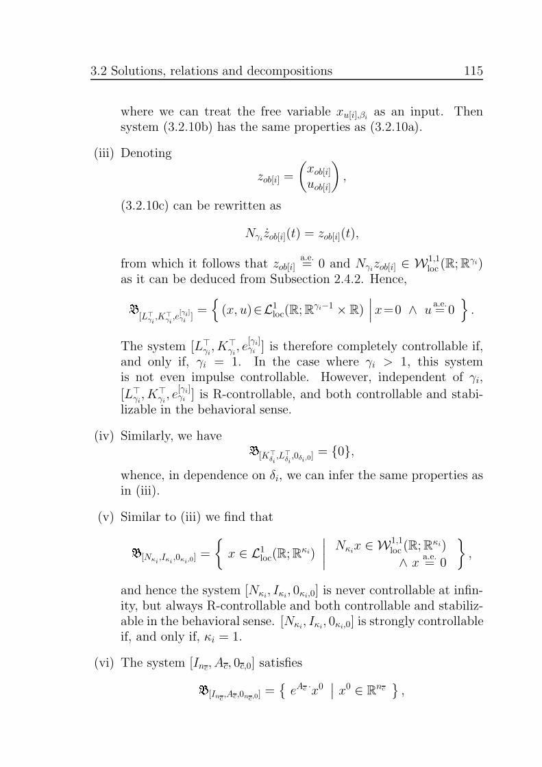
3.2 Solutions, relations and decompositions 115
where we can treat the free variable xu[i],βias an input. Then
system (3.2.10b) has the same properties as (3.2.10a).
(iii) Denoting
zob[i] =
(xob[i]uob[i]
),
(3.2.10c) can be rewritten as
Nγizob[i](t) = zob[i](t),
from which it follows that zob[i]a.e.= 0 and Nγizob[i] ∈ W1,1
loc (R;Rγi)
as it can be deduced from Subsection 2.4.2. Hence,B[L⊤
γi,K⊤
γi,e
[γi]γi
]={(x, u)∈L1
loc(R;Rγi−1 × R)
∣∣∣x=0 ∧ ua.e.= 0
}.
The system [L⊤γi, K
⊤γi, e
[γi]γi ] is therefore completely controllable if,
and only if, γi = 1. In the case where γi > 1, this systemis not even impulse controllable. However, independent of γi,
[L⊤γi, K
⊤γi, e
[γi]γi ] is R-controllable, and both controllable and stabi-
lizable in the behavioral sense.
(iv) Similarly, we have B[K⊤δi,L⊤
δi,0δi,0]
= {0},whence, in dependence on δi, we can infer the same properties asin (iii).
(v) Similar to (iii) we find thatB[Nκi,Iκi ,0κi,0]
=
{x ∈ L1
loc(R;Rκi)
∣∣∣∣Nκi
x ∈ W1,1loc (R;R
κi)
∧ xa.e.= 0
},
and hence the system [Nκi, Iκi
, 0κi,0] is never controllable at infin-ity, but always R-controllable and both controllable and stabiliz-able in the behavioral sense. [Nκi
, Iκi, 0κi,0] is strongly controllable
if, and only if, κi = 1.
(vi) The system [Inc, Ac, 0c,0] satisfiesB[Inc ,Ac,0nc,0]
={eAc ·x0
∣∣ x0 ∈ Rnc},

116 3 Controllability
whence it is controllable at infinity, but neither strongly control-lable nor controllable in the behavioral sense nor R-controllable.The properties of complete and strong stabilizability and sta-bilizability in the behavioral sense are attained if, and only if,σ(Ac) ⊆ C−.
By using the implications shown in Proposition 3.1.7, we can deduce theproperties of the systems arising in the feedback form, see Figure 3.1.
Corollary 3.2.8.A system [E,A,B] ∈ Σl,n,m with feedback form (3.2.9) is
(a) controllable at infinity if, and only if, γ = (1, . . . , 1), δ = (1, . . . , 1)and ℓ(κ) = 0;
(b) impulse controllable if, and only if, γ = (1, . . . , 1), δ = (1, . . . , 1)and κ = (1, . . . , 1);
(c) strongly controllable (and thus also strongly reachable) if, and onlyif, γ = (1, . . . , 1), δ = (1, . . . , 1), κ = (1, . . . , 1) and nc = 0;
(d) completely controllable (and thus also completely reachable) if, andonly if, γ = (1, . . . , 1), δ = (1, . . . , 1) and ℓ(κ) = nc = 0;
(e) R-controllable if, and only if, nc = 0;
(f) controllable in the behavioral sense if, and only if, nc = 0;
(g) strongly stabilizable if, and only if, γ = (1, . . . , 1), δ = (1, . . . , 1),ℓ(κ) = 0, and σ(Ac) ⊆ C−;
(h) completely stabilizable if and only if, γ = (1, . . . , 1), δ = (1, . . . , 1),κ = (1, . . . , 1), and σ(Ac) ⊆ C−;
(i) stabilizable in the behavioral sense if, and only if, σ(Ac) ⊆ C−.
Remark 3.2.9 (Parametrization of the behavior of systems in feedbackform).With the findings in Remark 3.2.7, we may explicitly characterize thebehavior of systems in feedback form. Define
Vq(s) = [1, s, . . . , sq]⊤ ∈ R[s]q×1, q ∈ N,
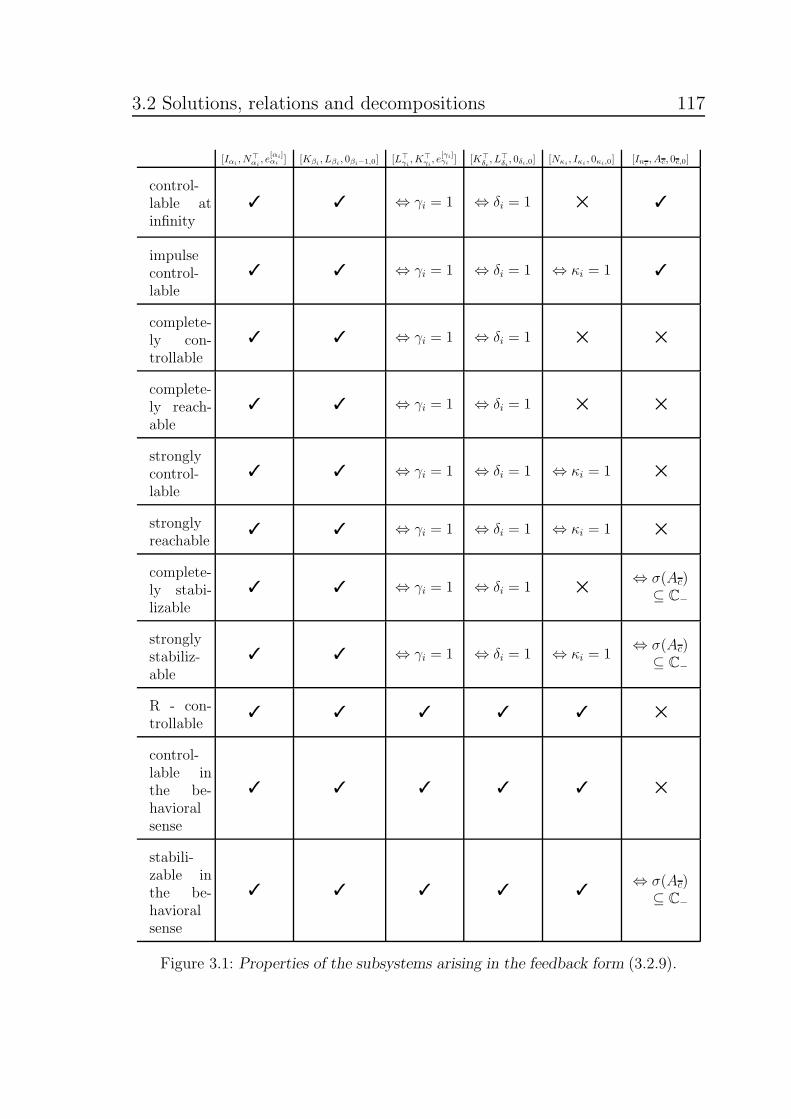
3.2 Solutions, relations and decompositions 117
[Iαi, N⊤
αi, e
[αi]αi
] [Kβi, Lβi
, 0βi−1,0] [L⊤γi,K⊤
γi, e
[γi]γi
] [K⊤δi, L⊤
δi, 0δi,0] [Nκi
, Iκi, 0κi,0] [Inc
, Ac, 0c,0]
control-lable atinfinity
✓ ✓ ⇔ γi = 1 ⇔ δi = 1 ✕ ✓
impulsecontrol-lable
✓ ✓ ⇔ γi = 1 ⇔ δi = 1 ⇔ κi = 1 ✓
complete-ly con-trollable
✓ ✓ ⇔ γi = 1 ⇔ δi = 1 ✕ ✕
complete-ly reach-able
✓ ✓ ⇔ γi = 1 ⇔ δi = 1 ✕ ✕
stronglycontrol-lable
✓ ✓ ⇔ γi = 1 ⇔ δi = 1 ⇔ κi = 1 ✕
stronglyreachable
✓ ✓ ⇔ γi = 1 ⇔ δi = 1 ⇔ κi = 1 ✕
complete-ly stabi-lizable
✓ ✓ ⇔ γi = 1 ⇔ δi = 1 ✕⇔ σ(Ac)
⊆ C−
stronglystabiliz-able
✓ ✓ ⇔ γi = 1 ⇔ δi = 1 ⇔ κi = 1⇔ σ(Ac)
⊆ C−
R - con-trollable
✓ ✓ ✓ ✓ ✓ ✕
control-lable inthe be-havioralsense
✓ ✓ ✓ ✓ ✓ ✕
stabili-zable inthe be-havioralsense
✓ ✓ ✓ ✓ ✓⇔ σ(Ac)
⊆ C−
Figure 3.1: Properties of the subsystems arising in the feedback form (3.2.9).

118 3 Controllability
and, for some multi-index µ = (µ1, . . . , µq) ∈ Nq,
Vµ(s) = diag (Vµ1(s), . . . , Vµq
(s)) ∈ R[s]|µ|×ℓ(µ),
Wµ(s) = diag (sµ1, . . . , sµq) ∈ R[s]ℓ(µ)×ℓ(µ).
Further let µ+ k := (µ1 + k, . . . , µq + k) for k ∈ Z, and
Wµ,1loc (R;R
ℓ(µ)) := Wµ1,1loc (R;R)× · · · ×Wµℓ(µ),1
loc (R;R)
and define
Z(R;Rq) :={f ∈ L1
loc(R;Rq)∣∣∣ f a.e.
= 0}.
Then the behavior of a system in feedback form can, formally, be writ-ten asB[E,A,B] =
Vα−1(ddt) 0 0 0 0 0
0 Vβ−1(ddt) 0 0 0 0
0 0 0 0 0 00 0 0 0 0 00 0 Eκ 0 0 00 0 0 eAc· 0 0
Wα(ddt) 0 0 0 0 0
0 0 0 0 Iℓ(γ) 00 0 0 0 0 Iξ
·
Wα,1loc (R;R
ℓ(α))
Wβ−1,1loc (R;Rℓ(β))
Z(R;Rℓ(κ))
Rnc
Z(R;Rℓ(γ))
L1loc(R;R
ξ)
,
where the sizes of the blocks are according to the block structure in thefeedback form (3.2.9), ξ = m − ℓ(α) − ℓ(γ), and the horizontal line isthe dividing line between x- and u-variables. If the system [E,A,B] ∈Σl,n,m is not in feedback form, then a parametrization of the behaviorcan be found by using the above representation and relation (3.2.2)expressing the connection between behaviors of feedback equivalentsystems.For general differential behaviors, a parametrization of the above
kind is called image representation [198, Sec. 6.6].
Remark 3.2.10 (Derivative feedback).A canonical form under proportional and derivative feedback (PD feed-back) was derived in [167] as well (note that PD feedback defines an

3.2 Solutions, relations and decompositions 119
equivalence relation on Σl,n,m). The main tool for doing this is therestriction pencil (see Section 3.7 (xi)): Clearly, the system
ddtNEx = NAx,
u = B†( ddtEx− Ax)
is equivalent under PD feedback to the system
ddtNEx = NAx,
u = 0.
Then putting sNE−NA into KCF yields a PD canonical form for theDAE system with a 5× 4-block structure.We may, however, directly derive this PD canonical form from thedecomposition (3.2.9). To this end we may observe that the system
[Iαi, N⊤
αi, e
[αi]αi ] can be written as
ddtKαi
xc[i](t) = Lαixc[i](t),
ddtxc[i],αi
(t) = uc[i](t),
and hence is, via PD feedback, equivalent to the system[[Kαi
0
],
[Lαi
0
],
[01
]].
On the other hand, the system [L⊤γi, K
⊤γi, e
[γi]γi ] can be written as
ddtNγi−1xob[i](t) = xob[i](t),
ddtxob[i],γi−1
(t) = uob[i](t),
and hence is, via PD feedback, equivalent to the system[[Nγi−1
0
],
[Iγi−1
0
],
[01
]].
A canonical form for [E,A,B] ∈ Σl,n,m under PD feedback (for theproof see [167]) is therefore given by
[E,A,B] ∼PD
Kβ 0 0 00 K⊤
δ 0 00 0 Nκ 00 0 0 Inc
0 0 0 0
,
Lβ 0 0 00 L⊤
δ 0 00 0 I|κ| 00 0 0 Ac
0 0 0 0
,
0 00 00 00 0Iζ 0
,

120 3 Controllability
where Ac is in Jordan canonical form, and the blocks of each type areordered from largest dimension to lowest.Note that the properties of complete controllability, controllability at
infinity and controllability in the behavioral sense are invariant underPD feedback. However, since derivative feedback changes the set ofdifferential variables, the properties of strong controllability as well asimpulse controllability may be lost/gained after PD feedback.
Remark 3.2.11 (Connection to Kronecker form).We may observe from (3.2.1) that feedback transformation may bealternatively considered as a transformation of the extended pencil
sE − A =[sE −A, −B
], (3.2.11)
that is based on a multiplication from the left by W = W ∈ Gll(R),and from the right by
T =
[T 0−F V
]∈ Gln+m(R).
This equivalence is therefore a subclass of the class which is induced bythe pre- and post-multiplication of sE − A by arbitrary invertible ma-trices. Loosely speaking, one can hence expect a decomposition underfeedback equivalence which specializes the QKF of sE −A. Indeed, thelatter form may be obtained from the feedback form of [E,A,B] by sev-eral simple row transformations of sE−A which are not interpretable asfeedback group actions anymore. More precisely, simple permutationsof columns lead to the separate consideration of the extended pencilscorresponding to the systems (3.2.10a)-(3.2.10f): The extended pen-
cils corresponding to [Iαi, N⊤
αi, e
[αi]αi ] and [Kβi
, Lβi, 0αi,0] are sKαi
− Lαi
and sKβi− Lβi
, resp. The extended matrix pencil corresponding to
the system [L⊤γi, K
⊤γi , e
[γi]γi ] is given by sNγi − Iγi. The extended matrix
pencils corresponding to the systems [K⊤δi, L⊤
δi, 0δi,0], [Nκi
, Iκi, 0κi,0] and
[Inc, Ac, 0c,0] are obviously given by sK⊤
δi−L⊤
δi, sNκi
− Iκiand sInc
−Ac,respectively. In particular, λ ∈ C is an eigenvalue of sE − A, if, andonly if, λ ∈ σ(Ac).
Remark 3.2.12 (Minimality in the behavioral sense).
(i) According to Remark 3.2.2, a differential-algebraic system[E,A,B] ∈ Σl,n,m is minimal in the behavioral sense if, and only

3.2 Solutions, relations and decompositions 121
if, the extended pencil sE − A as in (3.2.11) has full row rankover R(s). On the other hand, a system [E,A,B] ∈ Σl,n,m withfeedback form (3.2.9) satisfies
rkR(s)(sE − A) = l − ℓ(δ).
Using that rkR(s)(sE − A) is invariant under feedback transfor-mation (3.2.1), we can conclude that minimality of [E,A,B] ∈Σl,n,m in the behavioral sense corresponds to the absence of blocksof type (3.2.10d) in its feedback form.
(ii) The findings in Remark 3.2.7 imply that a system in feedbackform is, in the behavioral sense, equivalent to
I|α| 0 0 0 0 00 Kβ 0 0 0 00 0 0 0 0 00 0 0 0 0 00 0 0 0 0 00 0 0 0 0 Inc
,
N⊤α 0 0 0 0 00 Lβ 0 0 0 0
0 0 K⊤γ 0 0 0
0 0 0 I|δ|−ℓ(δ) 0 00 0 0 0 I|κ| 00 0 0 0 0 Ac
,
Eα 0 00 0 00 Eγ 00 0 00 0 00 0 0
.
This system can alternatively be achieved by multiplying the ex-tended pencil (3.2.11) in feedback form (3.2.9) from the left withthe polynomial matrix
Z(s)=diag
(I|α|, I|β|−ℓ(β), −
νγ−1∑
k=0
skNkγ , Pδ(s), −
νκ−1∑
k=0
skNkκ , Inc
),
where νγ = max{γ1, . . . , γℓ(γ)}, νκ = max{κ1, . . . , κℓ(κ)}, and
Pδ(s) = diag
([0δi−1,1, −
δi−2∑
k=0
sk(N⊤
δi−1
)k])
j=1,...,ℓ(δ)
.
(iii) Let a differential-algebraic system [E,A,B] ∈ Σl,n,m be given.Using the notation from (3.2.9) and the previous item, a behav-iorally equivalent and minimal system [EM , AM , BM ] ∈ Σl−ℓ(δ),n,m
can be constructed by[sEM −AM , −BM
]= Z(s)W
[sE −A, −B
].
It can be seen that this representation is furthermore control-lable at infinity. Moreover, it minimizes, among all differential-algebraic equations representing the same behavior, the index and

122 3 Controllability
the rank of the matrix in front of the state derivative (that is,loosely speaking, the number of differential variables). This pro-cedure is very much related to index reduction [152, Sec. 6.1].
3.3 Criteria of Hautus type
In this section we derive equivalent criteria on the matricesE,A ∈ Rl×n,B ∈ Rl×m for the controllability and stabilizability concepts of Defini-tion 3.1.5. The criteria are generalizations of the Hautus test (alsocalled Popov-Belevitch-Hautus test, since independently developed byPopov [199], Belevitch [18] and Hautus [112]) in terms of rankcriteria on the involved matrices. Note that these conditions are notnew – we refer to the relevant literature. However, we provide proofsusing only the feedback form (3.2.9).First we show that certain rank criteria on the matrices involved in
control systems are invariant under feedback equivalence. After that,we relate these rank criteria to the feedback form (3.2.9).
Lemma 3.3.1.Let [E1, A1, B1], [E2, A2, B2] ∈ Σl,n,m be given such that forW ∈ Gll(R),T ∈ Gln(R), V ∈ Glm(R) and F ∈ Rm×n we have
[E1 , A1 , B1 ]W,T,V,F∼fe [E2 , A2 , B2 ] .
Then, for all λ ∈ C,
imRE1 + imRA1 + imRB1 =W (imRE2 + imRA2 + imRB2) ,
imRE1 + A1 kerRE1 + imRB1 =W (imRE2 +A2 kerRE2 + imRB2) ,
imRE1 + imRB1 =W (imRE2 + imRB2) ,
imC(λE1 − A1) + imCB1 =W (imC(λE2 −A2) + imCB2) ,
imR(s)(sE1 −A1) + imR(s)B1 =W(imR(s)(sE2 − A2) + imR(s)B2
).
Proof: Immediate from (3.2.1).
Lemma 3.3.2 (Algebraic criteria via feedback form).For a system [E,A,B] ∈ Σl,n,m with feedback form (3.2.9) the followingstatements hold true:
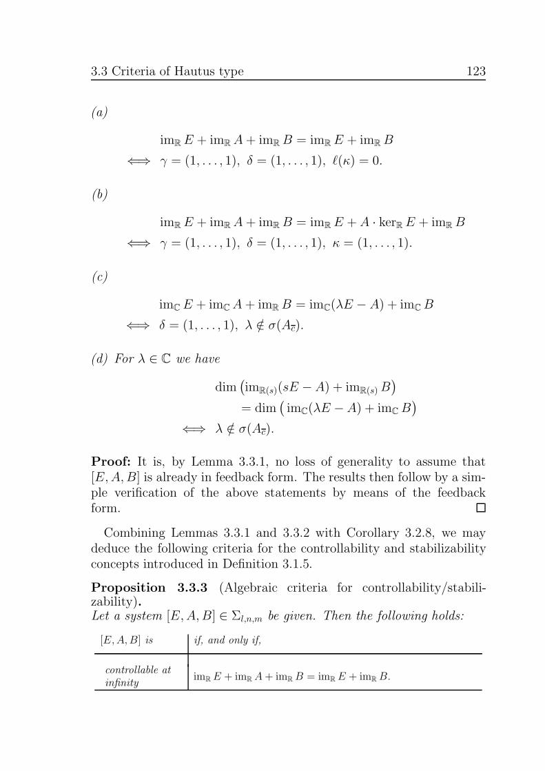
3.3 Criteria of Hautus type 123
(a)
imRE + imRA+ imRB = imRE + imRB
⇐⇒ γ = (1, . . . , 1), δ = (1, . . . , 1), ℓ(κ) = 0.
(b)
imRE + imRA+ imRB = imRE + A · kerRE + imRB
⇐⇒ γ = (1, . . . , 1), δ = (1, . . . , 1), κ = (1, . . . , 1).
(c)
imCE + imCA+ imRB = imC(λE − A) + imCB
⇐⇒ δ = (1, . . . , 1), λ /∈ σ(Ac).
(d) For λ ∈ C we have
dim(imR(s)(sE −A) + imR(s)B
)
= dim(imC(λE −A) + imCB
)
⇐⇒ λ /∈ σ(Ac).
Proof: It is, by Lemma 3.3.1, no loss of generality to assume that[E,A,B] is already in feedback form. The results then follow by a sim-ple verification of the above statements by means of the feedbackform.
Combining Lemmas 3.3.1 and 3.3.2 with Corollary 3.2.8, we maydeduce the following criteria for the controllability and stabilizabilityconcepts introduced in Definition 3.1.5.
Proposition 3.3.3 (Algebraic criteria for controllability/stabili-zability).Let a system [E,A,B] ∈ Σl,n,m be given. Then the following holds:
[E,A,B] is if, and only if,
controllable atinfinity
imRE + imRA+ imRB = imRE + imRB.

124 3 Controllability
impulse control-lable
imRE + imRA + imRB = imRE + A · kerRE + imRB.
completely con-trollable
imRE+imRA+imRB=imRE+imRB
∧ imCE+imCA+imCB=imC(λE − A)+imCB ∀λ ∈ C.
strongly control-lable
imRE+imRA+imRB=A · kerRE+imRB
∧ imCE+imCA+imCB=imC(λE − A)+imCB ∀λ ∈ C.
completely stabi-lizable
imRE+imRA+imRB=imRE+imRB
∧ imCE+imCA+imCB=imC(λE − A)+imCB ∀λ ∈ C+.
strongly stabiliz-able
imRE+imRA+imRB=imRE+A · kerRE+imRB
∧ imCE+imCA+imCB=imC(λE − A)+imCB ∀λ ∈ C+.
controllable inthe behavioralsense
rkR(s)[sE − A,B] = rkC[λE − A,B] ∀λ ∈ C.
stabilizable inthe behavioralsense
rkR(s)[sE − A,B] = rkC[λE − A,B] ∀λ ∈ C+.
The above result leads to the an extension of the diagram in Propo-sition 3.1.7, which is shown in Figure 3.2. Note that the equivalence ofR-controllability and controllability in the behavioral sense was alreadyshown in Corollary 3.2.8.In the following we consider further criteria for the concepts intro-
duced in Definition 3.1.5.
Remark 3.3.4 (Controllability at infinity).Proposition 3.3.3 immediately implies that controllability at infinity isequivalent to
imRA ⊆ imRE + imRB.
In terms of a rank criterion, this is the same as
rkR[E,A,B] = rkR[E,B]. (3.3.1)
Criterion (3.3.1) has first been derived by Geerts [101, Thm. 4.5] forthe case rk[E,A,B] = l, although he does not use the name ‘controlla-

3.3 Criteria of Hautus type 125
controll-able atinfinity
completelycontrol-lable
completelyreachable
completelystabiliz-able
impulsecontrollable
stronglycontrol-lable
stronglyreachable
stronglystabiliz-able
controllablein the be-havioralsense
R-control-lable
stabilizablein the be-havioralsense
Figure 3.2: Relations between the controllability concepts.
bility at infinity’.In the case of regular sE −A ∈ R[s]n×n, condition (3.3.1) reduces to
rkR[E,B] = n.
Remark 3.3.5 (Impulse controllability).By Proposition 3.3.3, impulse controllability of [E,A,B] ∈ Σl,n,m isequivalent to
imRA ⊆ imRE + A · kerRE + imRB.
Another equivalent characterization is that, for one (and hence any)matrix Z with imR Z = kerRE, we have
rkR[E,A,B] = rkR[E,AZ,B]. (3.3.2)
This has first been derived by Geerts [101, Rem. 4.9], again for thecase rk[E,A,B] = l. In [130, Thm. 3] and [117] it has been obtained
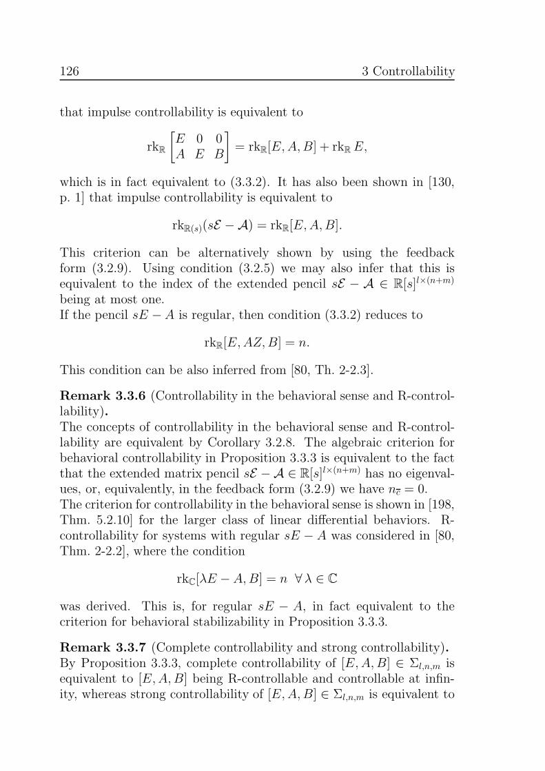
126 3 Controllability
that impulse controllability is equivalent to
rkR
[E 0 0A E B
]= rkR[E,A,B] + rkRE,
which is in fact equivalent to (3.3.2). It has also been shown in [130,p. 1] that impulse controllability is equivalent to
rkR(s)(sE − A) = rkR[E,A,B].
This criterion can be alternatively shown by using the feedbackform (3.2.9). Using condition (3.2.5) we may also infer that this isequivalent to the index of the extended pencil sE − A ∈ R[s]l×(n+m)
being at most one.If the pencil sE −A is regular, then condition (3.3.2) reduces to
rkR[E,AZ,B] = n.
This condition can be also inferred from [80, Th. 2-2.3].
Remark 3.3.6 (Controllability in the behavioral sense and R-control-lability).The concepts of controllability in the behavioral sense and R-control-lability are equivalent by Corollary 3.2.8. The algebraic criterion forbehavioral controllability in Proposition 3.3.3 is equivalent to the factthat the extended matrix pencil sE − A ∈ R[s]l×(n+m) has no eigenval-ues, or, equivalently, in the feedback form (3.2.9) we have nc = 0.The criterion for controllability in the behavioral sense is shown in [198,Thm. 5.2.10] for the larger class of linear differential behaviors. R-controllability for systems with regular sE − A was considered in [80,Thm. 2-2.2], where the condition
rkC[λE −A,B] = n ∀λ ∈ C
was derived. This is, for regular sE − A, in fact equivalent to thecriterion for behavioral stabilizability in Proposition 3.3.3.
Remark 3.3.7 (Complete controllability and strong controllability).By Proposition 3.3.3, complete controllability of [E,A,B] ∈ Σl,n,m isequivalent to [E,A,B] being R-controllable and controllable at infin-ity, whereas strong controllability of [E,A,B] ∈ Σl,n,m is equivalent to

3.4 Feedback, stability and autonomous systems 127
[E,A,B] being R-controllable and impulse controllable.Banaszuk et al. [12] already obtained the condition in Proposi-tion 3.3.3 for complete controllability considering discrete systems.Complete controllability is called H-controllability in [12]. Recently,Zubova [260] considered full controllability, which is just completecontrollability with the additional assumption that solutions have tobe unique, and obtained three equivalent criteria [260, Sec. 7], wherethe first one characterizes the uniqueness and the other two are equiv-alent to the condition for complete controllability in Proposition 3.3.3.For regular systems, the conditions in Proposition 3.3.3 for completeand strong controllability are also derived in [80, Thm. 2-2.1 & Thm. 2-2.3].
Remark 3.3.8 (Stabilizability).By Proposition 3.3.3, complete stabilizability of [E,A,B] ∈ Σl,n,m isequivalent to [E,A,B] being stabilizable in the behavioral sense andcontrollable at infinity, whereas strong stabilizability of [E,A,B] ∈Σl,n,m is equivalent to [E,A,B] being stabilizable in the behavioralsense and impulse controllable.The criterion for stabilizability in the behavioral sense is shown in [198,Thm. 5.2.30] for the class of linear differential behaviors.
3.4 Feedback, stability and autonomous
systems
State feedback is, roughly speaking, the special choice of the inputas a function of the state. Due to the mutual dependence of stateand input in a feedback system, this is often referred to as closed-loopcontrol. In the linear case, feedback is the imposition of the additionalrelation u(t) = Fx(t) for some F ∈ Rm×n. This results in the system
ddtEx(t) = (A+ BF )x(t).
Feedback for linear ODE systems was studied by Wonham [251], whereit is shown that controllability of [I, A,B] ∈ Σn,n,m is equivalent to anyset Λ ⊆ C which has at most n elements and is symmetric with respectto the imaginary axis (that is, λ ∈ Λ ⇔ λ ∈ Λ) being achievable bya suitable feedback, i.e., there exists some F ∈ Rm×n with the property

128 3 Controllability
that σ(A+BF ) = Λ. In particular, the input may be chosen in a waythat the closed-loop system is stable, i.e., any state trajectory tends tozero. Using the Kalman decomposition [138] (see also Section 3.6), itcan be shown for ODE systems that stabilizability is equivalent to theexistence of a feedback such that the resulting system is stable.These results have been generalized to regular DAE systems by Cobb
[74], see also [80, 96, 162, 163, 189, 191]. Note that, for DAE systems,not only the problem of assignment of eigenvalues occurs, but also theindex may be changed by imposing feedback.The crucial ingredient for the treatment of DAE systems with non-
regular pencil sE−A will be the feedback form by Loiseau et al. [167](see Thm. 3.2.6).
3.4.1 Stabilizability, autonomy and stability
The feedback law u(t) = Fx(t) applied to (3.1.1) results in a DAE inwhich the input is completely eliminated. We now focus on DAEs with-out input, and we introduce several properties and concepts. Consider,for matrices E,A ∈ Rl×n, the DAE
ddtEx(t) = Ax(t); (3.4.1)
the set of these systems is denoted by Σl,n. Its behavior is given byB[E,A] :=
{x ∈ L1
loc(R;Rn)
∣∣∣∣Ex∈W1,1
loc (R;Rl) and x satisfies (3.4.1)
for almost all t ∈ R
}.
Definition 3.4.1 (Stability/Stabilizability concepts for DAEs). A lin-ear time-invariant DAE [E,A] ∈ Σl,n is called
(a) completely stabilizable
:⇔ ∀x0 ∈ Rn ∃x ∈ B[E,A] :
x ∈ W1,1loc (R;R
) ∧ x(0) = x0 ∧ limt→∞
x(t) = 0.
(b) strongly stabilizable
:⇔ ∀x0 ∈ Rn ∃x ∈ B[E,A] : Ex(0) = Ex0 ∧ limt→∞
Ex(t) = 0.
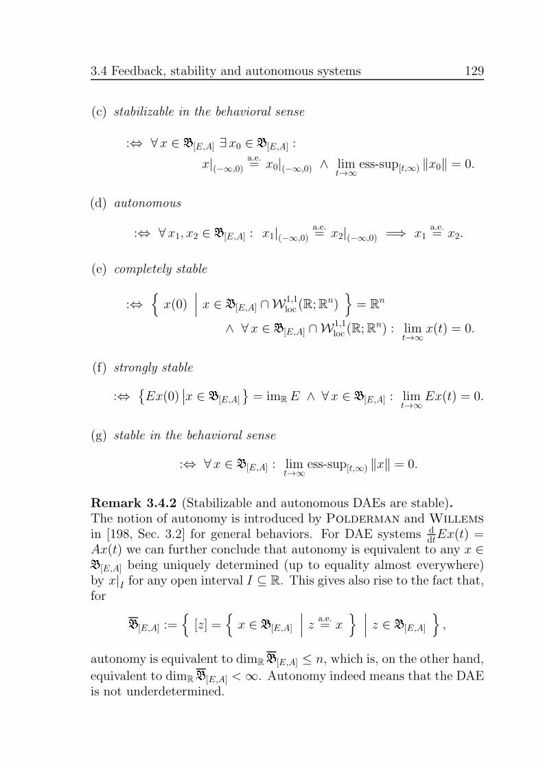
3.4 Feedback, stability and autonomous systems 129
(c) stabilizable in the behavioral sense
:⇔ ∀x ∈ B[E,A] ∃x0 ∈ B[E,A] :
x|(−∞,0)a.e.= x0|(−∞,0) ∧ lim
t→∞ess-sup[t,∞) ‖x0‖ = 0.
(d) autonomous
:⇔ ∀x1, x2 ∈ B[E,A] : x1|(−∞,0)a.e.= x2|(−∞,0) =⇒ x1
a.e.= x2.
(e) completely stable
:⇔{x(0)
∣∣∣ x ∈ B[E,A] ∩W1,1loc (R;R
n)}= Rn
∧ ∀x ∈ B[E,A] ∩W1,1loc (R;R
n) : limt→∞
x(t) = 0.
(f) strongly stable
:⇔{Ex(0)
∣∣x ∈ B[E,A]
}= imRE ∧ ∀x ∈ B[E,A] : lim
t→∞Ex(t) = 0.
(g) stable in the behavioral sense
:⇔ ∀x ∈ B[E,A] : limt→∞
ess-sup[t,∞) ‖x‖ = 0.
Remark 3.4.2 (Stabilizable and autonomous DAEs are stable).The notion of autonomy is introduced by Polderman and Willems
in [198, Sec. 3.2] for general behaviors. For DAE systems ddtEx(t) =
Ax(t) we can further conclude that autonomy is equivalent to any x ∈B[E,A] being uniquely determined (up to equality almost everywhere)by x|I for any open interval I ⊆ R. This gives also rise to the fact that,for B[E,A] :=
{[z] =
{x ∈ B[E,A]
∣∣∣ z a.e.= x
} ∣∣∣ z ∈ B[E,A]
},
autonomy is equivalent to dimRB[E,A] ≤ n, which is, on the other hand,
equivalent to dimRB[E,A] < ∞. Autonomy indeed means that the DAEis not underdetermined.
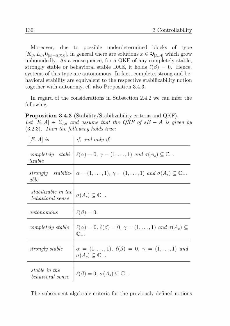
130 3 Controllability
Moreover, due to possible underdetermined blocks of type[Kβ, Lβ, 0|β|−ℓ(β),0], in general there are solutions x ∈ B[E,A] which growunboundedly. As a consequence, for a QKF of any completely stable,strongly stable or behavioral stable DAE, it holds ℓ(β) = 0. Hence,systems of this type are autonomous. In fact, complete, strong and be-havioral stability are equivalent to the respective stabilizability notiontogether with autonomy, cf. also Proposition 3.4.3.
In regard of the considerations in Subsection 2.4.2 we can infer thefollowing.
Proposition 3.4.3 (Stability/Stabilizability criteria and QKF).Let [E,A] ∈ Σl,n and assume that the QKF of sE − A is given by(3.2.3). Then the following holds true:
[E,A] is if, and only if,
completely stabi-lizable
ℓ(α) = 0, γ = (1, . . . , 1) and σ(As) ⊆ C−.
strongly stabiliz-able
α = (1, . . . , 1), γ = (1, . . . , 1) and σ(As) ⊆ C−.
stabilizable in thebehavioral sense
σ(As) ⊆ C−.
autonomous ℓ(β) = 0.
completely stable ℓ(α) = 0, ℓ(β) = 0, γ = (1, . . . , 1) and σ(As) ⊆C−.
strongly stable α = (1, . . . , 1), ℓ(β) = 0, γ = (1, . . . , 1) andσ(As) ⊆ C−.
stable in thebehavioral sense
ℓ(β) = 0, σ(As) ⊆ C−.
The subsequent algebraic criteria for the previously defined notions

3.4 Feedback, stability and autonomous systems 131
of stabilizability and autonomy follow from Proposition 3.4.3 by us-ing the invariance under transformation and the direct verification ofthe criteria by means of the QKF – similar to the argumentation inSection 3.3.
Corollary 3.4.4 (Algebraic criteria for stabilizability).Let [E,A] ∈ Σl,n. Then the following holds true:
[E,A] is if, and only if,
completely stabi-lizable
imRA ⊆ imRE andrkR(s)(sE −A) = rkC(λE − A) for all λ ∈ C+.
strongly stabiliz-able
imRA ⊆ imRE + A · kerRE andrkR(s)(sE −A) = rkC(λE − A) for all λ ∈ C+.
stabilizable in thebehavioral sense
rkR(s)(sE − A) = rkC(λE −A) for all λ ∈ C+.
autonomous kerR(s)(sE −A) = {0}.
Corollary 3.4.4 leads to the following implications:
completelystable
stronglystable
stablein thebehavioralsense
completelystabiliz-able
stronglystabiliz-able
stabilizablein the be-havioralsense
autonomousindex atmost one
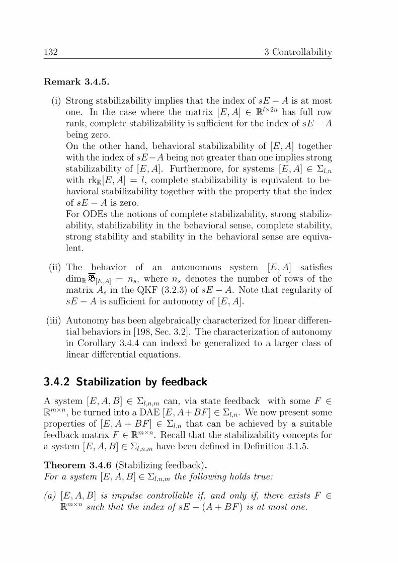
132 3 Controllability
Remark 3.4.5.
(i) Strong stabilizability implies that the index of sE −A is at mostone. In the case where the matrix [E,A] ∈ Rl×2n has full rowrank, complete stabilizability is sufficient for the index of sE −Abeing zero.On the other hand, behavioral stabilizability of [E,A] togetherwith the index of sE−A being not greater than one implies strongstabilizability of [E,A]. Furthermore, for systems [E,A] ∈ Σl,n
with rkR[E,A] = l, complete stabilizability is equivalent to be-havioral stabilizability together with the property that the indexof sE − A is zero.For ODEs the notions of complete stabilizability, strong stabiliz-ability, stabilizability in the behavioral sense, complete stability,strong stability and stability in the behavioral sense are equiva-lent.
(ii) The behavior of an autonomous system [E,A] satisfiesdimRB[E,A] = ns, where ns denotes the number of rows of thematrix As in the QKF (3.2.3) of sE −A. Note that regularity ofsE − A is sufficient for autonomy of [E,A].
(iii) Autonomy has been algebraically characterized for linear differen-tial behaviors in [198, Sec. 3.2]. The characterization of autonomyin Corollary 3.4.4 can indeed be generalized to a larger class oflinear differential equations.
3.4.2 Stabilization by feedback
A system [E,A,B] ∈ Σl,n,m can, via state feedback with some F ∈Rm×n, be turned into a DAE [E,A+BF ] ∈ Σl,n. We now present someproperties of [E,A + BF ] ∈ Σl,n that can be achieved by a suitablefeedback matrix F ∈ Rm×n. Recall that the stabilizability concepts fora system [E,A,B] ∈ Σl,n,m have been defined in Definition 3.1.5.
Theorem 3.4.6 (Stabilizing feedback).For a system [E,A,B] ∈ Σl,n,m the following holds true:
(a) [E,A,B] is impulse controllable if, and only if, there exists F ∈Rm×n such that the index of sE − (A+ BF ) is at most one.
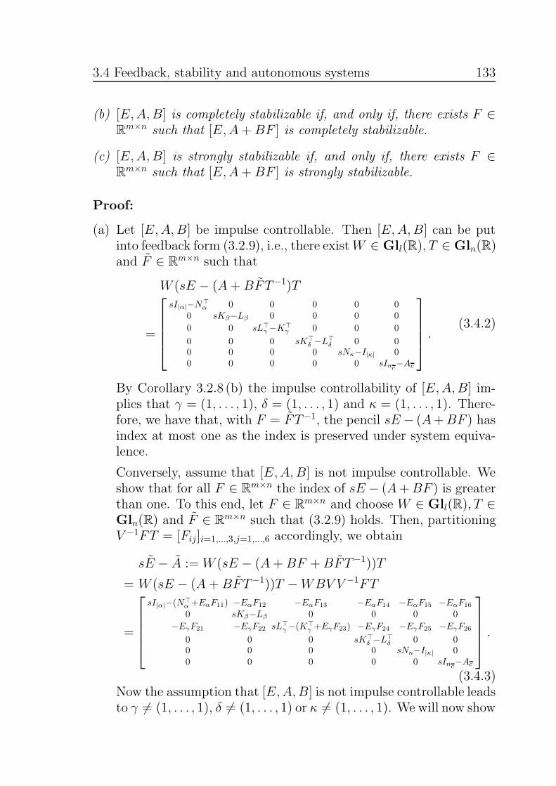
3.4 Feedback, stability and autonomous systems 133
(b) [E,A,B] is completely stabilizable if, and only if, there exists F ∈Rm×n such that [E,A+ BF ] is completely stabilizable.
(c) [E,A,B] is strongly stabilizable if, and only if, there exists F ∈Rm×n such that [E,A+ BF ] is strongly stabilizable.
Proof:
(a) Let [E,A,B] be impulse controllable. Then [E,A,B] can be putinto feedback form (3.2.9), i.e., there existW ∈ Gll(R), T ∈ Gln(R)and F ∈ Rm×n such that
W (sE − (A+ BFT−1)T
=
sI|α|−N⊤α 0 0 0 0 0
0 sKβ−Lβ 0 0 0 0
0 0 sL⊤γ −K⊤
γ 0 0 0
0 0 0 sK⊤δ −L⊤
δ 0 00 0 0 0 sNκ−I|κ| 00 0 0 0 0 sInc−Ac
.
(3.4.2)
By Corollary 3.2.8 (b) the impulse controllability of [E,A,B] im-plies that γ = (1, . . . , 1), δ = (1, . . . , 1) and κ = (1, . . . , 1). There-fore, we have that, with F = F T−1, the pencil sE − (A+BF ) hasindex at most one as the index is preserved under system equiva-lence.
Conversely, assume that [E,A,B] is not impulse controllable. Weshow that for all F ∈ Rm×n the index of sE − (A+BF ) is greaterthan one. To this end, let F ∈ Rm×n and choose W ∈ Gll(R), T ∈Gln(R) and F ∈ Rm×n such that (3.2.9) holds. Then, partitioningV −1FT = [Fij]i=1,...,3,j=1,...,6 accordingly, we obtain
sE − A :=W (sE − (A+BF +BFT−1))T
= W (sE − (A+ BFT−1))T −WBV V −1FT
=
sI|α|−(N⊤α +EαF11) −EαF12 −EαF13 −EαF14 −EαF15 −EαF16
0 sKβ−Lβ 0 0 0 0
−EγF21 −EγF22 sL⊤γ −(K⊤
γ +EγF23) −EγF24 −EγF25 −EγF26
0 0 0 sK⊤δ −L⊤
δ 0 00 0 0 0 sNκ−I|κ| 00 0 0 0 0 sInc−Ac
.
(3.4.3)Now the assumption that [E,A,B] is not impulse controllable leadsto γ 6= (1, . . . , 1), δ 6= (1, . . . , 1) or κ 6= (1, . . . , 1). We will now show

134 3 Controllability
that the index of sE − (A+BF +BFT−1) is greater than one byshowing this for the equivalent pencil in (3.4.3) via applying thecondition in (3.2.5): Let Z be a real matrix with imR Z = kerR E.Then
Z =
[0 Z⊤
1 0 0 0 00 0 0 0 Z⊤
2 0
]⊤,
where imZ1 = kerKβ = imEβ and imZ2 = kerNκ = imEκ. Tak-ing into account that imREγ ⊆ imR L
⊤γ , we obtain that
imR
[0|α|−ℓ(α)+|β|−ℓ(β),l I|γ|+|δ|+|κ| 0l,nc
] [E AZ
]
= imR
L⊤γ 0 0 EγF25Z2
0 K⊤δ 0 0
0 0 Nκ Z2
.
On the other hand, we have
imR
[0|α|−ℓ(α)+|β|−ℓ(β),l I|γ|+|δ|+|κ| 0l,nc
] [E A
]
= imR
L⊤γ 0 0 K⊤
γ + EγF23 EγF24 EγF25
0 K⊤δ 0 0 L⊤
δ 00 0 Nκ 0 0 I|κ|
.
Since the assumption that at least one of the multi-indices satisfiesγ 6= (1, . . . , 1), δ 6= (1, . . . , 1), or κ 6= (1, . . . , 1) and the fact thatimZ2 = imEκ lead to
imR
[L⊤γ 0 0 EγF25Z2
0 K⊤δ 0 0
0 0 Nκ Z2
]( imR
[L⊤γ 0 0 K⊤
γ +EγF23 EγF24 EγF25
0 K⊤δ 0 0 L⊤
δ 00 0 Nκ 0 0 I|κ|
],
and thusimR
[E AZ
]( imR
[E A
],
we find that, by condition (3.2.5), the index of sE − (A + BF +BFT−1) has to be greater than one. Since F was chosen arbitrarilywe may conclude that sE − (A+ BF ) has index greater than onefor all F ∈ Rm×n, which completes the proof of (a).
(b) If [E,A,B] is completely stabilizable, then we may transform thesystem into feedback form (3.4.2). Corollary 3.2.8 (h) implies γ =(1, . . . , 1), δ = (1, . . . , 1), ℓ(κ) = 0, and σ(Ac) ⊆ C−. Further,

3.4 Feedback, stability and autonomous systems 135
by [230, Thm. 4.20], there exists some F11 ∈ R|α|×ℓ(α) such that
σ(Nα + EαF11) ⊆ C−. Setting F := [Fij]i=1,...,3,j=1,...,6 with Fij = 0
for i 6= 1 or j 6= 1, we obtain that with F = F T−1 + V FT−1 thesystem [E,A+BF ] is completely stabilizable by Proposition 3.4.3as complete stabilizability is preserved under system equivalence.
On the other hand, assume that [E,A,B] is not completely stabi-lizable. We show that for all F ∈ Rm×n the system [E,A + BF ]is not completely stabilizable. To this end, let F ∈ Rm×n andobserve that we may apply a transformation as in (3.4.3). Thenthe assumption that [E,A,B] is not completely stabilizable yieldsγ 6= (1, . . . , 1), δ 6= (1, . . . , 1), ℓ(κ) > 0, or σ(Ac) 6⊆ C−. Ifγ 6= (1, . . . , 1), δ 6= (1, . . . , 1) or ℓ(κ) > 0, then imR A 6⊆ imR E, andby Corollary 3.4.4 the system [E, A] is not completely stabilizable.On the other hand, if γ = (1, . . . , 1), δ = (1, . . . , 1), ℓ(κ) = 0, andλ ∈ σ(Ac) ∩ C+, we find imC
(λE − A
)( imC E, which implies
rkC(λE−A)<rkCE=n−ℓ(β)−ℓ(κ)=n−ℓ(β) (3.2.6)= rkR(s)(sE−A).
Hence, applying Corollary 3.4.4 again, the system [E, A] is notcompletely stabilizable. As complete stabilizability is invariant un-der system equivalence it follows that [E,A+BF +BFT−1] is notcompletely stabilizable. Since F was chosen arbitrarily we mayconclude that [E,A + BF ] is not completely stabilizable for allF ∈ Rm×n, which completes the proof of (b).
(c) The proof is analogous to (b).
Remark 3.4.7 (State feedback).
(i) If the pencil sE−A is regular and [E,A,B] is impulse controllable,then a feedback F ∈ Rm×n can be constructed such that thepencil sE − (A + BF ) is regular and its index does not exceedone: First we choose W,T, F such that we can put the systeminto the form (3.4.2). Now, impulse controllability implies thatγ = (1, . . . , 1), δ = (1, . . . , 1) and κ = (1, . . . , 1). Assuming
ℓ(δ) > 0 implies that for all F ∈ Rm×n any QKF of the pencil
sE − (A+BFT−1 +BF ) satisfies ℓ(γ) > 0 (in the form (3.2.3)),
as the feedback F cannot act on this block, which contradicts
136 3 Controllability
regularity of sE − A. Hence it holds ℓ(δ) = 0 and from l = n wefurther obtain that ℓ(γ) = ℓ(β). Now applying another feedbackas in (3.4.3), where we choose F22 = E⊤
β ∈ Rℓ(β)×|β| and Fij = 0otherwise, we obtain, taking into account that Eγ = Iℓ(γ) and that
the pencil
[sKβ − Lβ
−E⊤β
]is regular, that sE − (A+ BF ) is indeed
regular with index at most one.
(ii) The matrix F11 in the proof of Theorem 3.4.6 (b) can be con-structed as follows: For j = 1, . . . , ℓ(α), consider vectors
aj = −[ajαj−1, . . . , aj0] ∈ R1×αj .
Then, forF11 = diag (a1, . . . , aℓ(α)) ∈ Rℓ(α)×|α|
the matrix Nα+EαF11 is diagonally composed of companion ma-trices, whence, for
pj(s) = sαj + ajαj−1sαj−1 + . . .+ aj0 ∈ R[s]
the characteristic polynomial of Nα + EαF11 is given by
det(sI|α| − (Nα + EαF11)) =
ℓ(α)∏
j=1
pj(s).
Hence, choosing the coefficients aji, j = 1, . . . , ℓ(α), i = 0, . . . , αj
such that the polynomials p1(s), . . . , pℓ(α)(s) ∈ R[s] are all Hur-witz, i.e., all roots of p1(s), . . . , pℓ(α)(s) are in C−, we obtain sta-bility.
3.4.3 Control in the behavioral sense
The hitherto presented feedback concept consists of the additionalapplication of the relation u(t) = Fx(t) to the system d
dtEx(t) =Ax(t) + Bu(t). Feedback can therefore be seen as an additional al-gebraic constraint that can be resolved for the input. Control in thebehavioral sense or, also called, control via interconnection [248] gener-alizes this approach by also allowing further algebraic relations in whichthe state does not necessarily uniquely determine the input. That is, for
3.4 Feedback, stability and autonomous systems 137
given (or to be determined)K = [Kx, Ku] withKx ∈ Rq×n, Ku ∈ Rq×m,we consider the interconnected behaviorBK
[E,A,B] :=
{(x, u) ∈ B[E,A,B]
∣∣∣∣(x(t)⊤, u(t)⊤)⊤ ∈ kerRKfor almost all t ∈ R
}
= B[E,A,B] ∩ B[0q,n,Kx,Ku].
We can alternatively writeBK[E,A,B] = B[EK ,AK ],
where
[EK, AK] =
[[E 00 0
],
[A BKx Ku
]].
The concept of control in the behavioral sense has its origin in the worksby Willems, Polderman and Trentelman [19, 198, 231, 247, 248],where differential behaviors and their stabilization via control by in-terconnection is considered. The latter means a systematic additionof some further (differential) equations such that a desired behavior isachieved. In contrast to these works we only add equations which arepurely algebraic. This justifies to speak of control by interconnectionusing static control laws. We will give equivalent conditions for thistype of generalized feedback stabilizing the system. Note that, in prin-ciple, one could make the extreme choice K = In+m to end up witha behaviorBK
[E,A,B] ⊆{(x, u) ∈ L1
loc(R;Rn × Rm)
∣∣∣ (x, u) a.e.= 0
},
which is obviously autonomous and stable in the behavioral sense. This,however, is not suitable from a practical point of view, since in this in-terconnection, the space of consistent initial differential variables isa proper subset of the initial differential variables which are consistentwith the original system [E,A,B]. Consequently, the interconnectedsystem does not have the causality property - that is, the implementa-tion of the controller at a certain time t ∈ R is not possible, since thiscauses jumps in the differential variables. To avoid this, we introducethe concept of compatibility.
Definition 3.4.8 (Compatible and stabilizing control).Let [E,A,B] ∈ Σl,n,m. The control matrixK = [Kx, Ku] ∈ Rq×n×Rq×m
is called
138 3 Controllability
(a) compatible for [E,A,B] if, and only if, for any x0 ∈ Vdiff[E,A,B], there
exists some (x, u) ∈ BK[E,A,B] with Ex(0) = Ex0.
(b) stabilizing for [E,A,B] if, and only if, [EK, AK] ∈ Σl+q,n+m is sta-bilizable in the behavioral sense.
Remark 3.4.9 (Compatible control).Our definition of compatible control is a slight modification of theconcept introduced by Julius and van der Schaft in [134] wherean interconnection is called compatible, if any trajectory of the systemwithout control law can be concatenated with a trajectory of the in-terconnected system. This certainly implies that the space of initialdifferential variables of the interconnected system cannot be smallerthan the corresponding set for the nominal system.
Theorem 3.4.10 (Stabilizing control in the behavioral sense).Let [E,A,B] ∈ Σl,n,m. Then there exists a compatible and stabilizingcontrol K = [Kx, Ku] ∈ Rq×n × Rq×m for [E,A,B], if, and only if,[E,A,B] is stabilizable in the behavioral sense. If [E,A,B] is stabiliz-able in the behavioral sense, then the compatible and stabilizing controlK can moreover be chosen such that [EK, AK] is autonomous, i.e., theinterconnected system [EK, AK] is stable in the behavioral sense.
Proof: Since, by definition, [E,A,B] ∈ Σl,n,m is stabilizable in thebehavioral sense if, and only if, for sE − A = [sE − A,−B], the DAE[E ,A] ∈ Σl,n+m is stabilizable in the behavioral sense, necessity followsfrom setting q = 0.In order to show sufficiency, let K = [Kx, Ku] ∈ Rq×n × Rq×m be a
compatible and stabilizing control for [E,A,B]. Now the system canbe put into feedback form, i.e., there exist W ∈ Gll(R), T ∈ Gln(R),V ∈ Glm(R) and F ∈ Rm×n such that
[sE − A B
−Kx Ku
]=
[W 00 I
] [sE −A B−Kx Ku
] [T 0−F V
],
where [E, A, B] is in the form (3.2.9). Now the behavioral stabilizabil-
ity of [EK, AK] implies that the system [EK, AK] :=[[
E 00 0
],[
A BKx Ku
]]
is stabilizable in the behavioral sense as well. Assume that [E,A,B] isnot stabilizable in the behavioral sense, that is, by Corollary 3.2.8 (i),

3.4 Feedback, stability and autonomous systems 139
there exists λ ∈ σ(Ac) ∩ C+. Hence we find x06 ∈ Rnc \ {0} such that
Acx06 = λx06. Then, with x(·) :=
(0, . . . , 0, (eλ·x06)
⊤)⊤, we have that
(x, 0) ∈ B[E,A,B]. As x(0) ∈ Vdiff[E,A,B]
= T−1 · Vdiff[E,A,B], the compatibil-
ity of the control K implies that there exists (x, u) ∈ BK[E,A,B] with
Ex(0) = ETx(0). This gives (WET )T−1x(0) = WETx(0) and writ-ing T−1x(t) = (x1(t)
⊤, . . . , x6(t)⊤)⊤ with vectors of appropriate size,we obtain x6(0) = x06. Since the solution of the initial value problemy = Acy, y(0) = x06, is unique, we find x6(t) = eλtx06 for all t ∈ R. Now(T−1x,−V −1FT−1x+ V −1u) ∈ B[EK ,AK ] and as for all (x, u) ∈ B[EK ,AK ]
with (x(t), u(t)) = (T−1x(t),−V −1FT−1x + V −1u(t)) for almost allt < 0 we have x6(t) = x6(t) for all t ∈ R, and x6(t) 6→ 0 as t→ ∞ sinceλ ∈ C+, this contradicts that [E
K, AK] is stabilizable in the behavioralsense.It remains to show the second assertion, that is, for a system
[E,A,B] ∈ Σl,n,m that is stabilizable in the behavioral sense, thereexists some compatible and stabilizing control K such that [EK, AK] isautonomous: Since, for [E1, A1, B1], [E2, A2, B2] ∈ Σl,n,m with
[E1 , A1 , B1 ]W,T,V,F∼fe [E2 , A2 , B2 ] ,
K2 ∈ Rq×(n+m) and K1 = K2
[T 0F V
],
the behaviors of the interconnected systems are related by
[T 0F V
]BK1
[E1,A1,B1]= BK2
[E2,A2,B2],
it is no loss of generality to assume that [E,A,B] is in feedbackform (3.2.9), i.e.,
sE − A =
sI|α|−Nα 0 0 0 0 00 sKβ−Lβ 0 0 0 0
0 0 sK⊤γ −L⊤
γ 0 0 0
0 0 0 sK⊤δ −L⊤
δ 0 00 0 0 0 sNκ−I|κ| 00 0 0 0 0 sInc−Ac
,
B =
Eα 0 00 0 00 Eγ 00 0 00 0 00 0 0
.
140 3 Controllability
Let F11 ∈ Rℓ(α)×|α| be such that det(sI|α| − (Nα + EαF11)) is Hurwitz.Then the DAE
[I|α| 00 0
]z(t) =
[Nα Eα
F11 −Iℓ(α)
]z(t)
is stable in the behavioral sense. Furthermore, by reasoning as in Re-mark 3.4.7 (ii), for
aj = [ajβj−2, . . . , aj0, 1] ∈ R1×βj
with the property that the polynomials
pj(s) = sβj + ajβj−1sβj−1 + . . .+ aj0 ∈ R[s]
are Hurwitz for j = 1, . . . , ℓ(α), the choice
Kx = diag (a1, . . . , aℓ(β)) ∈ Rℓ(β)×|β|
leads to an autonomous system
[Kβ
0
]z(t) =
[Lβ
Kx
]z(t),
which is also stable in the behavioral sense. Since, moreover, by Corol-lary 3.2.8 (i), we have σ(Ac) ⊆ C−, the choice
K =
F11 0 0 0 0 0 −Iℓ(α) 0 00 Kx 0 0 0 0 0 0 00 0 0 0 0 0 0 0 Im−ℓ(α)−ℓ(γ)
leads to a behavioral stable (in particular autonomous) system. Sincethe differential variables can be arbitrarily initialized in any of thepreviously discussed subsystems, the constructed control is also com-patible.
3.5 Invariant subspaces
This section is dedicated to some selected results of the geometric the-ory of differential-algebraic control systems. Geometric theory plays

3.5 Invariant subspaces 141
a fundamental role in standard ODE system theory and has been in-troduced independently by Wonham and Morse and Basile andMarro, see the famous books [16, 252] and also [230], which are thethree standard textbooks on geometric control theory. In [159] Lewis
gave an overview of the to date geometric theory of DAEs. As wewill do here he put special emphasis on the two fundamental sequences(Vi)i∈N0
and (Wi)i∈N0of subspaces defined as follows:
V0 := Rn, Vi+1 := A−1(EVi + imRB) ⊆ Rn, V∗ :=⋂
i∈N0
Vi,
W0 := {0}, Wi+1 := E−1(AWi + imRB) ⊆ Rn, W∗ :=⋃
i∈N0
Wi.
Compared to the Wong sequences for matrix pencils in Definition 2.2.1,in the definition of the sequences (Vi)i∈N0
and (Wi)i∈N0the image of B
is added before taking the pre-image. If B = 0, then we end up withthe Wong sequences. However, if B 6= 0, then (Vi)i∈N0
and (Wi)i∈N0
are in general not Wong sequences corresponding to any matrix pencil.This justifies to call (Vi)i∈N0
and (Wi)i∈N0augmented Wong sequences
with respect to the control system (3.1.1).The reachable space of a system [E,A,B] can be represented by the
intersection of the limits of the augmented Wong sequences.
Proposition 3.5.1 (Reachable space [200, Sec. 4]).For [E,A,B] ∈ Σl,n,m and limits V∗ and W∗ of the augmented Wongsequences we have
R[E,A,B] = V∗ ∩W∗.
It has been shown in [13] (for discrete systems), see also [11, 14, 45,188], that the limit V∗ of the first augmented Wong sequence is thespace of consistent initial states. For regular systems this was provedin [158].
Proposition 3.5.2 (Consistent initial states [13]).For [E,A,B] ∈ Σl,n,m and limit V∗ of the first augmented Wong se-quence we have
V[E,A,B] = V∗.
Various other properties of V∗ and W∗ have been derived in [13] inthe context of discrete systems.
142 3 Controllability
For regular systems Ozcaldiran [187] showed that V∗ is the supre-mal (A,E,B)-invariant subspace of Rn and W∗ is the infimal restricted(E,A,B)-invariant subspace of Rn. These concepts, which have alsobeen used in [3, 13, 158, 175] are defined as follows.
Definition 3.5.3 ((A,E,B)- and (E,A,B)-invariance [187]).Let [E,A,B] ∈ Σl,n,m. A subspace V ⊆ Rn is called (A,E,B)-invariantif, and only if,
AV ⊆ EV + imRB.
A subspace W ⊆ Rn is called restricted (E,A,B)-invariant if, and onlyif,
W = E−1(AW + imRB).
It is easy to verify that the proofs given in [187, Lems. 2.1 & 2.2]remain the same for general E,A ∈ Rl×n and B ∈ Rl×m - this wasshown in [13] as well. For V∗ this can be found in [3], see also [175]. Sowe have the following proposition.
Proposition 3.5.4 (Augmented Wong sequences as invariant sub-spaces).Consider [E,A,B] ∈ Σl,n,m and the limits V∗ and W∗ of the augmentedWong sequences. Then the following statements hold true.
(a) V∗ is (A,E,B)-invariant and for any V ⊆ Rn which is (A,E,B)-invariant it holds V ⊆ V∗;
(b) W∗ is restricted (E,A,B)-invariant and for any W ⊆ Rn which isrestricted (E,A,B)-invariant it holds W∗ ⊆ W.
It is now clear how the controllability concepts can be characterizedin terms of the invariant subspaces V∗ and W∗. However, the state-ment about R-controllability (behavioral controllability) seems to benew. The only other appearance of a subspace inclusion as a charac-terization of R-controllability that the author is aware of occurs in [70]for regular systems: if A = I, then the system is R-controllable if, andonly if, imRE
D ⊆ 〈ED|B〉, where ED is the Drazin inverse of E, cf.Section 3.7 (iv).
Theorem 3.5.5 (Geometric criteria for controllability).Consider [E,A,B] ∈ Σl,n,m and the limits V∗ and W∗ of the augmentedWong sequences. Then [E,A,B] is

3.5 Invariant subspaces 143
(a) controllable at infinity if, and only if, V∗ = Rn;
(b) impulse controllable if, and only if, V∗ + kerRE = Rn or, equiva-lently, EV∗ = imRE;
(c) controllable in the behavioral sense if, and only if, V∗ ⊆ W∗;
(d) completely controllable if, and only if, V∗ ∩W∗ = Rn;
(e) strongly controllable if, and only if, (V∗ ∩W∗) + kerRE = Rn or,equivalently, E(V∗ ∩W∗) = imRE.
Proof: By Propositions 3.5.1 and 3.5.2 it is clear that it only remainsto prove (c). We proceed in several steps.Step 1 : Let [E1, A1, B1], [E2, A2, B2] ∈ Σl,n,m such that for someW ∈
Gll(R), T ∈ Gln(R), V ∈ Glm(R) and F ∈ Rm×n it holds
[E1 , A1 , B1 ]W,T,V,F∼fe [E2 , A2 , B2 ] .
We show that the augmented Wong sequences V1i , W1
i of [E1, A1, B1]and the augmented Wong sequences V2
i , W2i of [E2, A2, B2] are related
by∀ i ∈ N0 : V1
i = T−1V2i ∧ W1
i = T−1W2i .
We prove the statement by induction. It is clear that V10 = T−1V2
0 .Assuming that V1
i = T−1V2i for some i ≥ 0 we find that, by (3.2.1),
V1i+1 = A−1
1 (E1V1i + imRB1)
=
{x ∈ Rn
∣∣∣∣∃ y ∈ V1
i ∃u ∈ Rm :
W (A2T + B2T )x =WE2Ty +WB2V u
}
={x ∈ Rn
∣∣ ∃ z ∈ V2i ∃ v ∈ Rm : A2Tx = E2z + B2v
}
= T−1(A−1
2 (E2V1i + imRB2)
)= T−1V2
i+1.
The statement about W1i and W2
i can be proved analogous.Step 2 : By Step 1 we may without loss of generality assume that
[E,A,B] is given in feedback form (3.2.9). We make the conventionthat if α ∈ Nk is some multi-index, then α− 1 := (α1 − 1, . . . , αk − 1).It not follows that
∀ i ∈ N0 : Vi = R|α| × R|β| × imRNiγ−1 × imR(N
⊤δ−1)
i × imRNiκ × Rnc,(3.5.1)
144 3 Controllability
which is immediate from observing that K⊤γ x = L⊤
γ y + Eγu for some
x, y, u of appropriate dimension yields x = Nγ−1y and L⊤δ x = K⊤
δ y forsome x, y yields x = N⊤
δ−1y. Note that in the case γi = 1 or δi = 1,i.e., we have a 1× 0 block, we find that Nγi−1 and Nδi−1 are absent, sothese relations are consistent.On the other hand we find that
∀ i ∈ N0 :
Wi = kerRNiα × kerRN
iβ × kerRN
iγ−1 × {0}|δ|−ℓ(δ) × kerRN
iκ × {0}nc,
(3.5.2)
which indeed needs some more rigorous proof. First observe thatimREα = kerRNα, kerRKβ = kerRNβ and (L⊤
γ )−1(imREγ) = imREγ−1
= kerRNγ−1. Therefore we have
W1 = E−1(imRB)
= kerRNα × kerRNβ × kerRNγ−1 × {0}|δ|−ℓ(δ) × kerRNκ × {0}nc.
Further observe that N iαN
⊤α = NαN
⊤αN
i−1α for all i ∈ N and, hence, if
x = N⊤α y+Eαu for some x, u and y ∈ kerRN
i−1α it follows x ∈ kerRN
iα.
Likewise, if L⊤γ x = K⊤
γ y+Eγu for some x, u and y ∈ kerRNi−1γ−1 we find
x = N⊤γ−1y + E⊤
γ−1u and hence x ∈ kerRNiγ−1. Finally, if Kβx = Lβy
for some x and some y ∈ kerRNi−1β it follows that by adding some zero
rows we obtain Nβx = NβN⊤β y and hence, as above, x ∈ kerRN
iβ. This
proves (3.5.2).Step 3 : From (3.5.1) and (3.5.2) it follows that
V∗ = R|α| × R|β| × imR{0}|γ|−ℓ(γ) × {0}|δ|−ℓ(δ) × {0}|κ| × Rnc,
W∗ = R|α| × R|β| × imRR|γ|−ℓ(γ) × {0}|δ|−ℓ(δ) × R|κ| × {0}nc.
As by Corollary 3.2.8 (f) the system [E,A,B] is controllable in thebehavioral sense if, and only if, nc = 0 we may immediately deduce thatthis is the case if, and only if, V∗ ⊆ W∗. This proves the theorem.
Remark 3.5.6 (Representation of the reachable space).From Proposition 3.5.1 and the proof of Theorem 3.5.5 we may imme-diately observe that, using the notation from Theorem 3.2.6, we have
R[E,A,B]
= T−1(R|α| × R|β| × imR{0}|γ|−ℓ(γ) × {0}|δ|−ℓ(δ) × {0}|κ| × {0}nc
).

3.6 Kalman decomposition 145
3.6 Kalman decomposition
Nearly fifty years ago Kalman [138] derived his famous decompositionof linear ODE control systems. This decomposition has later beengeneralized to regular DAEs by Verghese at al. [241], see also [80]. AKalman decomposition of general discrete-time DAE systems has beenprovided by Banaszuk et al. [14] (later generalized to systems withoutput equation in [11]) in a very nice way using the augmented Wongsequences (cf. Section 3.5). They derive a system
[[E11 E12
0 E22
],
[A11 A12
0 A22
],
[B1
0
]], (3.6.1)
which is system equivalent to given [E,A,B] ∈ Σl,n,m with the prop-erties that the system [E11, A11, B1] is completely controllable and thematrix [E11, A11, B1] has full row rank (strongly H-controllable in thenotation of [14]) and, furthermore, R[E22,A22,0] = {0}.This last condition is reasonable, as one should wonder what prop-
erties a Kalman decomposition of a DAE system should have. In thecase of ODEs the decomposition simply is
[[A11 A12
0 A22
],
[B1
0
]], where [A11, B1] is controllable.
Therefore, an ODE system is decomposed into a controllable and anuncontrollable part, since clearly [A22, 0] is not controllable at all. ForDAEs however, the situation is more subtle, since in a decomposi-tion (3.6.1) with [E11, A11, B1] completely controllable (and[E11, A11, B1] full row rank) the conjectural ‘uncontrollable’ part[E22, A22, 0] may still have a controllable subsystem, since systems ofthe type [Kβ, Lβ, 0] are always controllable. To exclude this and ensurethat all controllable parts are included in [E11, A11, B1] we may statethe additional condition (as in [14]) that
R[E22,A22,0] = {0}.
This then also guarantees certain uniqueness properties of the Kalmandecomposition. Hence, any system (3.6.1) with the above propertieswe may call a Kalman decomposition.

146 3 Controllability
Definition 3.6.1 (Kalman decomposition).A system [E,A,B] ∈ Σl,n,m is said to be a Kalman decomposition if,and only if,
[E,A,B] =
[[E11 E12
0 E22
],
[A11 A12
0 A22
],
[B1
0
]], (3.6.2)
where E11, A11 ∈ Rl1×n1, E12, A12 ∈ Rl1×n2, E22, A22 ∈ Rl2×n2 and B1 ∈Rl1×m, such that [E11, A11, B1] ∈ Σl1,n1,m is completely controllable,rkR[E11, A11, B1] = l1 and R[E22,A22,0l2,m] = {0}.
We cite the result of [14] and sketch the proof.
Theorem 3.6.2 (Kalman decomposition).For [E,A,B] ∈ Σl,n,m, there exist W ∈ Gll(R), T ∈ Gln(R) such that[WET,WAT,WB] is a Kalman decomposition 3.6.2.
Proof: The Kalman decomposition (3.6.2) can be derived using thelimits V∗ and W∗ of the augmented Wong sequences presented in Sec-tion 3.5. It is clear that these spaces satisfy the following subspacerelations:
E(V∗ ∩W∗) ⊆ (EV∗ + imRB) ∩ (AW∗ + imRB),
A(V∗ ∩W∗) ⊆ (EV∗ + imRB) ∩ (AW∗ + imRB).
Therefore, if we choose any full rank matrices R1 ∈ Rn×n1, P1 ∈ Rn×n2,R2 ∈ Rl×l1, P2 ∈ Rl×l2 such that
imRR1 = V∗ ∩W∗, imRR1 ⊕ imR P1 = Rn, imRR2 ⊕ imR P2 = Rl,
imRR2 = (EV∗ + imRB) ∩ (AW∗ + imRB),
then [R1, P1] ∈ Gln(R) and [R2, P2] ∈ Gll(R), and, furthermore, thereexist matrices E11, A11 ∈ Rl1×n1, E12, A12 ∈ Rl1×n2, E22, A22 ∈ Rl2×n2
such that
ER1 = R2E11, AR1 = R2A11,EP1 = R2E12 + P2E22, AP1 = R2A12 + P2A22.
Since imRB ⊆ (EV∗+ imRB)∩ (AW∗+ imRB) = imRR2, there existsB1 ∈ Rl1×m such that B = R2B1. All these relations together yieldthe decomposition (3.6.2) with W = [R2, P2] and T = [R1, P1]
−1. The
3.6 Kalman decomposition 147
properties of the entries in (3.6.2) essentially rely on the observationthat by Proposition 3.5.1
R[E,A,B] = V∗ ∩W∗ = imRR1 = T−1(Rn1 × {0}n2).
We omit the proof of this and refer to [14].
Remark 3.6.3 (Kalman decomposition).It is important to note that a trivial reachable space does not necessarilyimply that B = 0. An intriguing example which illustrates this is thesystem
[E,A,B] =
[[10
],
[01
],
[10
]]. (3.6.3)
Another important fact we like to stress by means of this example isthat B 6= 0 does no necessarily imply n1 6= 0 in the Kalman decompo-sition (3.6.2). In fact, the above system [E,A,B] is already in Kalmandecomposition with l1 = l2 = 1, n1 = 0, n2 = 1, m = 1 and E12 = 1,A12 = 0, B1 = 1 as well as E22 = 0, A22 = 1. Then all the requiredproperties are satisfied, in particular rkR[E11, A11, B1] = rkR[1] = 1 andthe system [E11, A11, B1] is completely controllable as it is in feedbackform (3.2.9) with γ = 1; complete controllability then follows fromCorollary 3.2.8. However, [E11, A11, B1] is hard to view as a controlsystem as no equation can be written down. Nevertheless, the spaceR[E11,A11,B1] has dimension zero and obviously every state can be steeredto every other state.
We now analyze how two forms of type (3.6.2) of one system [E,A,B]∈ Σl,n,m differ.
Proposition 3.6.4 (Uniqueness of the Kalman decomposition).Let [E,A,B] ∈ Σl,n,m be given and assume that, for all i ∈ {1, 2}, thesystems [Ei, Ai, Bi]
Wi,Ti∼se [E,A,B] with
sEi − Ai =
[sE11,i − A11,i sE12,i − A12,i
0 sE22,i − A22,i
], Bi =
[B1,i
0
]
where E11,i, A11,i ∈ Rl1,i×n1,i, E12,i, A12,i ∈ Rl1,i×n2,i, E22,i, A22,i ∈ Rl2,i×n2,i,B1,i ∈ Rl1,i×m are Kalman decompositions.

148 3 Controllability
Then l1,1 = l1,2, l2,1 = l2,2, n1,1 = n1,2, n2,1 = n2,2. Moreover, forsomeW11 ∈ Gll1,1(R),W12 ∈ Rl1,1×l2,1,W22 ∈ Gll2,1(R), T11 ∈ Gln1,1
(R),T12 ∈ Rn1,1×n2,1, T22 ∈ Gln2,1
(R), we have
W2W−11 =
[W11 W12
0 W22
], T−1
1 T2 =
[T11 T120 T22
].
In particular, the systems [E11,1, A11,1, B1,1], [E11,2, A11,2, B1,2] and, re-spectively,[E22,1, A22,1, 0], [E22,2, A22,2, 0] are system equivalent.
Proof: It is no loss of generality to assume that W1 = Il, T1 = In.Then we obtain
Rn1,1 × {0} = R[E1,A1,B1] = T2R[E2,A2,B2] = T2(Rn1,2 × {0}
).
This implies n1,1 = n1,2 and
T2 =
[T11 T120 T22
]for some T11 ∈ Gln1,1
, T12 ∈ Rn1,1××n2,1, T22 ∈ Gln2,1.
Now partitioning
W2 =
[W11 W12
W21 W22
],
W11 ∈ Rl1,1×l1,2, W12 ∈ Rl1,1×l2,2,
W21 ∈ Rl2,1×l1,2, W22 ∈ Rl2,1×l2,2,
the block (2, 1) of the equations W1E1T1 = E2, W1A1T1 = A2 andW1B1 = B2 give rise to
0 =W21
[E11,2 A11,2 B1,2
].
Since the latter matrix is supposed to have full row rank, we obtainW21 = 0. The assumption ofW2 being invertible then leads to l1,1 ≤ l1,2.Reversing the roles of [E1, A1, B1] and [E2, A2, B2], we further obtainl1,2 ≤ l1,1, whence l1,2 = l1,1. Using again the invertibility of W , weobtain that both W11 and W22 are invertible.
It is immediate from the form (3.6.2) that [E,A,B] is completelycontrollable if, and only if, n1 = n. The following result character-izes the further controllability and stabilizability notions in terms ofproperties of the submatrices in (3.6.2).
3.6 Kalman decomposition 149
Corollary 3.6.5 (Properties induced from the Kalman decomposi-tion).Consider [E,A,B] ∈ Σl,n,m with
[E,A,B]W,T∼se [E, A, B] =
[[E11 E12
0 E22
],
[A11 A12
0 A22
],
[B1
0
]]
such that [E, A, B] is a Kalman decomposition. Then the followingstatements hold true:
(a) rkR(s)(sE22 −A22) = n2.
(b) If sE − A is regular, then both pencils sE11 − A11 and sE22 − A22
are regular. In particular, it holds l1 = n1 and l2 = n2.
(c) If [E,A,B] is impulse controllable, then the index of the pencilsE22 − A22 is at most one.
(d) [E,A,B] is controllable at infinity if, and only if, imRA22⊆ imRE22.
(e) [E,A,B] is controllable in the behavioral sense if, and only if,rkR(s)(sE22 −A22) = rkC(λE22 −A22) for all λ ∈ C.
(f) [E,A,B] is stabilizable in the behavioral sense if, and only if,rkR(s)(sE22 −A22) = rkC(λE22 −A22) for all λ ∈ C+.
Proof:
(a) Assuming that rkR(s)(sE22 − A22) < n2, then, in a QKF (3.2.3)of sE22 − A22, it holds ℓ(β) > 0 by (3.2.6). By the findings ofRemark 3.2.7 (ii), we can conclude R[E22,A22,0l2,m] 6= {0}, a contra-diction.
(b) We can infer from (a) that n2 ≤ l2. We can further deduce from theregularity of sE−A that n2 ≥ l2. The regularity of sE11−A11 andsE22 − A22 then follows immediately from det(sE − A) = det(W ·T ) · det(sE11 − A11) · det(sE22 − A22).
(c) Assume that [E,A,B] is impulse controllable. By Proposition 3.3.3and the invariance of impulse controllability under system equiva-lence this implies that
imR
[A11 A12
0 A22
]⊆ imR
[E11 E12 B1 A11Z1 + A12Z2
0 E22 0 A22Z2
],

150 3 Controllability
where Z = [Z⊤1 , Z
⊤2 ]
⊤ is a real matrix such that imR Z= kerR
[E11 E120 E22
]. The last condition in particular implies that
imR Z2 ⊆ kerRE22 and therefore we obtain
imRA22 ⊆ imRE22 + A22 kerRE22,
which is, by (3.2.4), equivalent to the index of sE22 −A22 being atmost one.
(d) Since rkR[E11, A11, B1] = l1 and the system [E11, A11, B1] is con-trollable at infinity, Proposition 3.3.3 leads to rkR[E11, B1] = l1.Therefore, we have
imR
[E11 E12 B1
0 E22 0
]= Rl1 × imRE22.
Analogously, we obtain
imR
[E11 E12 A11 A12 B1
0 E22 0 A22 0
]= Rl1 × (imRE22 + imRA22) .
Again using Proposition 3.3.3 and the invariance of controllabil-ity at infinity under system equivalence, we see that [E,A,B] iscontrollable at infinity if, and only if,
Rl1 × (imRE22 + imRA22) = Rl1 × imRE22,
which is equivalent to imRA22 ⊆ imRE22.
(e) Since rkR[E11, A11, B1] = l1 and [E11, A11, B1] ∈ Σl1,n1,m is com-pletely controllable it holds
rkC[λE11 − A11, B1] = l1 for all λ ∈ C.
Therefore, we have
rkC[λE −A,B] = rkC
[λE11 −A11 λE12 −A12 B1
0 λE22 −A22 0
]
= l1 + rkC(λE22 − A22),
and, analogously, rkR(s)[sE −A,B] = l1 + rkR(s)(sE22 −A22). Nowapplying Proposition 3.3.3 we find that [E,A,B] is controllable inthe behavioral sense if, and only if, rkR(s)(sE22−A22) = rkC(λE22−A22) for all λ ∈ C.

3.7 Notes and References 151
(f) The proof of this statement is analogous to (e).
Remark 3.6.6 (Kalman decomposition and controllability).Note that the condition of the index of sE22 − A22 being at most onein Corollary 3.6.5(c) is equivalent to the system [E22, A22, 0l2,m] beingimpulse controllable. Likewise, the condition imRA22 ⊆ imRE22 in (d)is equivalent to [E22, A22, 0l2,m] being controllable at infinity. Obviously,the conditions in (e) and (f) are equivalent to behavioral controllabilityand stabilizability of [E22, A22, 0l2,m], resp.Furthermore, the converse implication in (b) does not hold true. Thatis, the index of sE22−A22 being at most one is in general not sufficientfor [E,A,B] being impulse controllable. For instance, reconsider sys-tem (3.6.3) which is not impulse controllable, but sE22 − A22 = −1 isof index one. Even in the case where sE−A is regular, the property ofthe index of sE22−A22 being zero or one is not enough to infer impulsecontrollability of sE −A. As a counterexample, consider
[E,A,B] =
[[0 10 0
],
[1 00 1
],
[10
]].
3.7 Notes and References
(i) The controllability concepts are not consistently treated in theliterature. For instance, one has to pay attention if it is (tacitly)claimed that [E,B] ∈ Rl×(n+m) or [E,A,B] ∈ Rl×(2n+m) have fullrank.For regular systems we have the following:
concept coincides with no-tion in
called [...] in
controllability at infinity see item (v) reachability at ∞in [158]
impulse controllability [77] and [121,Rem. 2]
controllability at∞ in [158]; con-trollability at in-finity in [6, 7, 241]
R-controllability [70, 80, 254] and[121, Rem. 2]
–

152 3 Controllability
complete controllability [70, 80, 254] controllabilityin [77]
strong controllability [241] and [121,Rem. 2]
impulse controlla-bility in [103]
Some of these aforementioned articles introduce the controlla-bility by means of certain rank criteria for the matrix triple[E,A,B]. The connection of the concepts introduced in Def-inition 3.1.5 to linear algebraic properties of E, A and B arehighlighted in Section 3.3.
For general DAE systems we have:
concept coincides with no-tion in
called [...] in
controllability at infinity – –
impulse controllability [101, 117, 130] controllability atinfinity in [52]
R-controllability – –
complete controllability [188] controllabilityin [98]
strong controllability – controllabilityin [188]
Our behavioral controllability coincides with the framework whichis introduced in [198, Definition 5.2.2] for so-called differential be-haviors, which are general (possibly higher order) DAE systemswith constant coefficients. Note that the concept of behavioralcontrollability does not require a distinction between input andstate. The concepts of reachability and controllability in [12–15]coincide with our behavioral and complete controllability, resp.(see Sec. 3.3). Full controllability of [260] is our complete con-trollability together with the additional assumption that solutionshave to be unique.
(ii) Stabilizability in the behavioral sense is introduced in [198, Def-inition 5.2.2]. For regular systems, stabilizability is usually de-fined either via linear algebraic properties of E, A and B, or

3.7 Notes and References 153
by the existence of a stabilizing state feedback, see [50, 51, 96]and [80, Definition 3-1.2.]. Our concepts of behavioral stabi-lizability and stabilizability coincide with the notions of inter-nal stability and complete stabilizability, resp., defined in [177]for the system E z(t) = Az(t) with E = [E , 0 ], A = [A , B ],z(t) = [ x⊤(t) , u⊤(t) ]⊤.
(iii) Other concepts, not related to the ones considered in this chapter,are e.g. the instantaneous controllability (reachability) of order kin [188] or the impulsive mode controllability in [117]. Further-more, the concept of strong controllability introduced in [230, Ex-ercise 8.5] for ODE systems differs from the concepts consideredin this thesis.
(iv) The reachable and controllable spaces are some of the most im-portant notions for (DAE) control systems and have been con-sidered in [158] for regular systems. They are the fundamentalsubspaces considered in the geometric theory, see Section 3.5.Further usage of these concepts can be found in the following:in [190] generalized reachable and controllable subspaces of regu-lar systems are considered; Eliopoulou and Karcanias [92]consider reachable and almost reachable subspaces of generalDAE systems; Frankowska [98] considers the reachable sub-space in terms of differential inclusions.A nice formula for the reachable space of a regular system hasbeen derived by Yip et al. [254] (and later been adopted byCobb [77], however called controllable subspace): Consider aregular system [E,A,B] ∈ Σn,n,m with (E,A) in QWF (2.1.1) (infact, the WCF is considered in [254], but the calculation is thesame) and B partitioned accordingly, that is
E =
[In1
00 N
], A =
[J 00 In2
], B =
[B1
B2
],
where N is nilpotent. Then [254, Thm. 2]
R[E,A,B] = 〈J |B1〉 × 〈N |B2〉,where 〈K|L〉 := imR[L,KL, . . . , K
n−1L] for some matrices K ∈Rn×n, L ∈ Rn×m. Furthermore, we have [254, Thm. 3]
V[E,A,B] = Rn1 × 〈N |B2〉.
154 3 Controllability
This result has been improved later in [70] so that the QWF isno longer needed. Denoting by ED the Drazin inverse of a givenmatrix E ∈ Rn×n (see [66]), it is shown [70, Thm. 3.1] that, forA = I,
R[E,A,B] = ED〈ED|B〉 ⊕ (I − EED)〈E|B〉,
where the consideration of A = I is justified by a certain (time-varying) transformation of the system [192]. We further have [70,Thm. 3.2]
V[E,A,B] = imRED ⊕ (I − EED)〈E|B〉.
Yet another approach was followed by Cobb [73] who obtainsthat
R[E,A,B] = 〈(αE − A)−1E|(αE − A)−1B〉for some α ∈ R with det(αE − A) 6= 0. A simple proof of thisresult can also be found in [259].
(v) Impulse controllability and controllability at infinity are usu-ally defined by considering distributional solutions of (3.1.1), seee.g. [77,101,130], sometimes called impulsive modes, see [20,117,241]. For regular systems, impulse controllability has been intro-duced by Verghese et al. [241] (called controllability at infinityin this work) as controllability of the impulsive modes of thesystem, and later made more precise by Cobb [77], see also Ar-
mentano [6,7] (who also calls it controllability at infinity) for amore geometric point of view. In [241] the authors do also de-velop the notion of strong controllability as impulse controllabilitywith, additionally, controllability in the regular sense. Cobb [74]showed that under the condition of impulse controllability, theinfinite eigenvalues of regular sE −A can be assigned via a statefeedback u = Fx to arbitrary finite positions. Armentano [6]later showed how to calculate F . This topic has been furtherpursued in [150] in the form of invariant polynomial assignment.The name ‘controllability at infinity’ comes from the claim thatthe system has no infinite uncontrollable modes: Speaking interms of rank criteria (see also Section 3.3) the system [E,A,B] ∈Σl,n,m is said to have an uncontrollable mode at α
β if, and only if,
3.7 Notes and References 155
rk[αE + βA,B] < rk[E,A,B] for some α, β ∈ C. If β = 0, thenthe uncontrollable mode is infinite. Controllability at infinity hasbeen introduced by Rosenbrock [211] - although he does notuse this phrase - as controllability of the infinite frequency zeros.Later Cobb [77] compared the concepts of impulse controllabil-ity and controllability at infinity, see [77, Thm. 5]; the notions weuse in the present thesis go back to the distinction in this work.The concepts have later been generalized by Geerts [101](see [101, Thm. 4.5 & Rem. 4.9], however he does not use thename ‘controllability at infinity’). Controllability at infinityof (3.1.1) is equivalent to the strictness of the corresponding dif-ferential inclusion [98, Prop. 2.6]. The concept of impulsive modecontrollability in [117] is even weaker than impulse controllability.
(vi) For a discussion of distributional solutions for DAEs see Sec-tion 2.5. We briefly refer to [227, 228], where the notions ofimpulse controllability and jump controllability are introduced,which coincide with our impulse controllability and behavioralcontrollability, resp.
(vii) R-controllability has been first defined in [254] for regular DAEs.Roughly speaking, R-controllability is the property that any con-sistent initial state x0 can be steered to any reachable state xf ,where here xf is reachable if, and only if, there exist t > 0
and (x, u) ∈ B[E,A,B] such that x ∈ W1,1loc (R;R
n), x(0) = 0 andx(t) = xf ; by (3.1.2) the latter is equivalent to xf ∈ V[E,A,B], asstated in Definition 3.1.5.
(viii) The concept of behavioral controllability has been introduced byWillems [245], see also [198]. This concept is suitable for gener-alizations in various directions, see e.g. [53, 67, 120, 153, 203, 248,253]. Having found the behavior of the considered control sys-tem one can take over the definition of behavioral controllabilitywithout the need for any further changes. From this point of viewthis appears to be the most natural of the controllability concepts.However, this concept also seems to be the least regarded in theDAE literature.
(ix) The controllability theory of DAE systems can also be treated
156 3 Controllability
with the theory of differential inclusions [9, 10] as showed byFrankowska [98].
(x) Karcanias and Hayton [141] pursued a special ansatz to sim-plify the system (3.1.1): provided that B has full column rank,take a left annihilator N and the left inverse B† = (B⊤B)−1B⊤
of B (i.e., NB = 0 and B†B = I) such that W =[NB†
]is in-
vertible and then pre-multiply (3.1.1) by W , thus obtaining theequivalent system
ddtNEx = NAx,
u = B†( ddtEx−Ax).
The reachability (controllability) properties of (3.1.1) may nowbe studied in terms of the pencil sNE − NA, which is calledthe restriction pencil [133], first introduced as zero pencil for theinvestigation of system zeros of ODEs in [147,148], see also [144].For a comprehensive study of the properties of the pencil sNE−NA see e.g. [140–143].
(xi) Banaszuk and Przy luski [15] have considered perturbationsof DAE control systems and obtained conditions under which thesets of all completely controllable systems (systems controllable inthe behavioral sense) within the set of all systems Σl,n,m containan open and dense subset, or its complement contains an openand dense subset.
(xii) For regular systems which are completely controllable, two canon-ical forms of [E,A,B] ∈ Σn,n,m under system equivalence havebeen obtained: the Jordan control canonical form in [104] and,later, the simpler canonical form in [113] based on the Hermitecanonical form for controllable ODEs [I, A,B].
(xiii) It is known [12,103] that the class of regular DAE systems is notclosed under the action of state feedback. Therefore, in [219] theclass of regular systems is divided into the families
Σθ := { (E,A,B) ∈ Σn,n,m | det(cos θ E − sin θ A) 6= 0 } ,
for θ ∈ [0, π), and it is shown that any of these families is dense inthe set of regular systems and the union of these families is exactly

3.7 Notes and References 157
the set of regular systems. The authors of [219] then introducethe ‘constant-ratio proportional and derivative’ feedback on Σθ,i.e.
u = F (cos θ x− sin θ x) + v.
This feedback leads to a group action and enables them to obtaina generalization of Brunovsky’s theorem [48] on each of the sub-sets of completely controllable systems in Σθ, see [219, Thm. 6].
(xiv) Glusing-Luerßen [103] derived a canonical form under theunchanged feedback equivalence (3.2.1) on the set of stronglycontrollable (called impulse controllability in [103]) regular sys-tems, see [103, Thm. 4.7]. In particular it is shown that this setis closed under the action of a feedback group.
(xv) For regular systems [E,A,B] ∈ Σn,n,m with det(sE −A) ∈ R[s] \{0} the usual Hautus and Kalman criteria can be found in asummarized form e.g. in [80]. Other approaches to derive con-trollability criteria rely on the expansion of (sE − A)−1 as apower series in s at s0 = 0, which is only feasible in the regu-lar case. For instance, in [178] the numerator matrices of thisexpansion, i.e., the coefficients of the polynomial adj (sE − A),are used to derive a rank criterion for complete controllability.Then again, in [146] Kalman rank criteria for complete control-lability, R-controllability and controllability at infinity are de-rived in terms of the coefficients of the power series expansionof (sE − A)−1. The advantage of these criteria, especially thelast one, is that no transformation of the system needs to be per-formed as it is usually necessary in order to derive Kalman rankcriteria for DAEs, see e.g. [80].However, simple criteria can be obtained using only a left trans-formation of little impact: if α ∈ R is chosen such that det(αE−A) 6= 0, then the system is complete controllable if, and onlyif, [259, Cor. 1]
rkR[(αE − A)−1B,
((αE −A)−1E
)(αE − A)−1B, . . .
. . . ,((αE − A)−1E
)n−1(αE − A)−1B
]= n,

158 3 Controllability
and it is impulse controllable if, and only if, [259, Thm. 2]
imR(αE − A)−1E + ker(αE − A)−1E + imR(αE − A)−1B = Rn.
The result concerning complete controllability has also been ob-tained in [70, Thm. 4.1] for the case A = I and α = 0.Yet another approach was followed by Kucera andZagalak [150] who introduced controllability indices and char-acterized strong controllability in terms of an equation for theseindices.
(xvi) The augmented Wong sequences (for B 6= 0) have been exten-sively studied by several authors, see e.g. [158, 174, 175, 186, 187,189, 190, 238] for regular systems and [3, 11, 13, 14, 44, 45, 92, 159,167,188,200] for general DAE systems. Frankowska [98] did anice investigation of systems (3.1.1) in terms of differential inclu-sions [9,10], however requiring controllability at infinity (see [98,Prop. 2.6]). Nevertheless, she is the first to derive a formula forthe reachable space [98, Thm. 3.1], which was later generalizedby Przy luski and Sosnowski [200, Sec. 4] (in fact, the samegeneralization has been announced in [167, p. 296], [159, Sec. 5]and [11, p. 1510], however without proof); it also occurred in [92,Thm. 2.5].
(xvii) A characterization of the limits V∗ and W∗ of the augmentedWong sequences in terms of distributions is given in [200]: V∗ +kerRE is the set of all initial values such that the distributionalinitial value problem [200, (3)] has a smooth solution (x, u); W∗
is the set of all initial values such that [200, (3)] has an impul-sive solution (x, u); V∗ + W∗ is the set of all initial values suchthat [200, (3)] has an impulsive-smooth solution (x, u).
159
4 Zero dynamics
In this chapter we study linear differential-algebraic control systems ofthe form
ddtEx(t) = Ax(t) + Bu(t)
y(t) = Cx(t) ,
where E,A ∈ Rl×n, B ∈ Rl×m, C ∈ Rp×n. The set of these systems isdenoted by Σl,n,m,p and we write [E,A,B, C] ∈ Σl,n,m,p. We put specialemphasis on the non-regular case, i.e., we do not assume that sE − Ais regular.Compared to the class of systems studied in Chapter 3, here we allow
for an additional output equation y(t) = Cx(t). The functions u : R →Rm and y : R → Rp are called input and output of the system, resp.By virtue of Definition 2.4.1, a trajectory (x, u, y) : R → Rn×Rm×Rp
is said to be a solution of [E,A,B, C] if, and only if, it belongs to thebehavior of [E,A,B, C]:B[E,A,B,C] :=
{(x, u, y) ∈ L1
loc(R;Rn × Rm × Rp) | Ex ∈ W1,1
loc (R;Rl)
and (x, u) satisfies ddtEx(t) = Ax(t) +Bu(t),
y(t) = Cx(t) for almost all t ∈ R}.
Particular emphasis is placed on the zero dynamics of [E,A,B, C].These are, for [E,A,B, C] ∈ Σl,n,m,p, defined by
ZD[E,A,B,C] :={(x, u, y) ∈ B[E,A,B,C]
∣∣∣ y a.e.= 0
}.
By linearity of [E,A,B, C], ZD[E,A,B,C] is a real vector space.The zero dynamics of [E,A,B, C] are called autonomous if, and only
if,
∀w1, w2 ∈ ZD[E,A,B,C] ∀ I ⊆ R open nonempty interval :
w1|Ia.e.= w2|I =⇒ w1
a.e.= w2 ;

160 4 Zero dynamics
and asymptotically stable if, and only if,
∀ (x, u, y) ∈ ZD[E,A,B,C] : limt→∞
ess-sup[t,∞) ‖(x, u)‖ = 0.
Note that the above definitions are within the spirit of the behavioralapproach [198] and take into account that the zero dynamicsZD[E,A,B,C]
are a linear behavior. In this framework the definition for autonomyof a general behavior is given in [198, Sec. 3.2] and the definition ofasymptotic stability in [198, Def. 7.2.1].(Asymptotically stable) zero dynamics are the vector space of those
trajectories of the system which are, loosely speaking, not visible atthe output (and tend to zero).For convenience we call the extended matrix pencil
[sE−A −B−C 0
]the
system pencil of [E,A,B, C] ∈ Σl,n,m,p. In Section 4.1 we will derivea so called ‘zero dynamics form’ of [E,A,B, C] within the equivalenceclass defined by system equivalence (in generalization of the conceptintroduced in Definition 3.2.1): two systems [Ei, Ai, Bi, Ci] ∈ Σl,n,m,p,i = 1, 2, are called system equivalent if, and only if,
∃S ∈ Gll(R), T ∈ Gln(R) :[S 00 Ip
] [sE1 −A1 B1
C1 0
] [T 00 Im
]=
[sE2 −A2 B2
C2 0
];
we write
[E1 , A1 , B1 , C1 ]S,T∼ [E2 , A2 , B2 , C2 ] .
It is easy to see that system equivalence is an equivalence relationon Σl,n,m,p × Σl,n,m,p. The notion of system equivalence goes back toRosenbrock [211], cf. also Section 3.2.This chapter is organized as follows: In Section 4.1 we study au-
tonomous zero dynamics and derive several important characterizationsfor it as well as one of the main results of this chapter, the zero dy-namics form (ZDF) in Theorem 4.1.7; this form is obtained by usingthe largest (A,E,B)-invariant subspace included in kerC. The ZDF isthen refined in Theorem 4.2.7 in Section 4.2, where concepts of systeminvertibility are introduced and studied in relation to the zero dynam-ics. We also show how the inverse system can be calculated and underwhich condition a system with autonomous zero dynamics is right-invertible. This class of systems is then considered in Section 4.3 and

4.1 Autonomous zero dynamics 161
it is shown in Theorem 4.3.12 that its elements have asymptoticallystable zero dynamics if, and only if, the conditions stabilizability in thebehavioral sense, detectability in the behavioral sense and the absenceof transmission zero in the closed right complex half-plane are satisfied;these concepts are rigorously introduced and characterized. The resultof Theorem 4.3.12 is then exploited for stabilization via compatiblecontrol in the behavioral sense in Theorem 4.4.3 in Section 4.4. It isshown that the Lyapunov exponent of the interconnected system canbe assigned to the Lyapunov exponent of the zero dynamics.The results of Sections 4.1, 4.2 and 4.3 are partly contained in the
submitted manuscript [28]. The submitted work [29] contains (partsof) Sections 4.3 and 4.4. Lemma 4.3.11 has already been published ina joint work with Achim Ilchmann and Timo Reis [35].
4.1 Autonomous zero dynamics
In this section we investigate autonomy of the zero dynamics of controlsystems
ddtEx(t) = Ax(t) + Bu(t)
y(t) = Cx(t) ,(4.1.1)
where [E,A,B, C] ∈ Σl,n,m,p. We derive several important character-izations of autonomous zero dynamics and, as the main result of thissection, the so called zero dynamics form in Theorem 4.1.7. The follow-ing observation is immediate from the definition of autonomous zerodynamics.
Remark 4.1.1 (Autonomous zero dynamics).Since ZD[E,A,B,C] is a real vector space, the zero dynamics ZD[E,A,B,C]
are autonomous if, and only if, for any w ∈ ZD[E,A,B,C] which satisfies
w|Ia.e.= 0 on some open interval I ⊆ R, it follows that w
a.e.= 0.
In order to characterize (autonomous) zero dynamics we use theconcept of (A,E,B)-invariance from Definition 3.5.3. For a system[E,A,B, C] ∈ Σl,n,m,p, we define the set of all (A,E,B)-invariant sub-spaces included in kerC by
L(E,A,B; kerC) :=
{V ⊆ Rn
∣∣∣∣V is (A,E,B)-invariant subspace
of Rn and V ⊆ kerC
}.

162 4 Zero dynamics
It can easily be verified that L(E,A,B; kerC) is closed under subspaceaddition and thus L(E,A,B; kerC) is an upper semi-lattice relative tosubspace inclusion and addition. Hence, by [252, Lem. 4.4], there existsa supremal element of L(E,A,B; kerC), namely
max(E,A,B; kerC) := supL(E,A,B; kerC) = maxL(E,A,B; kerC).
We show that max(E,A,B; kerC) can be derived from a sequence ofsubspaces which terminates after finitely many steps. These sequencescan be viewed as a modification of the (augmented) Wong sequencesfrom Definition 2.2.1 (see also Section 3.5).
Lemma 4.1.2 (Subspace sequences leading to max(E,A,B; kerC)).Let [E,A,B, C] ∈ Σl,n,m,p and define V0 := kerC and
∀ i ∈ N : Vi := A−1(EVi−1 + imB) ∩ kerC.
Then the sequence (Vi)i∈N0satisfies
∃ k∗ ∈ N ∀ j ∈ N :
V0 ) V1 ) · · · ) Vk∗ = Vk∗+j = A−1(EVk∗ + imB) ∩ kerC. (4.1.2)
Furthermore,Vk∗ = max(E,A,B; kerC) (4.1.3)
and, if (x, u, y) ∈ ZD[E,A,B,C], then
for almost all t ∈ R : x(t) ∈ Vk∗.
Proof: It is easy to see that (4.1.2) holds true and (4.1.3) followsfrom [187, Lem. 2.1]. For the last statement let (x, u, y) ∈ ZD[E,A,B,C].Then we have
Ax(t) = ddtEx(t)− Bu(t) and x(t) ∈ kerC
for almost all t ∈ R. Since, for any subspace S ⊆ Rn, if x(t) ∈ S foralmost all t ∈ R, then d
dtEx(t) ∈ ES for almost all t ∈ R, we conclude
x(t) ∈ A−1({ ddtEx(t)}+ imB) ∩ kerC ⊆ V1 for almost all t ∈ R.
Inductively, we obtain x(t) ∈ Vk∗ for almost all t ∈ R.
4.1 Autonomous zero dynamics 163
For later use we collect the following lemma about the quasi-Kron-ecker form from Proposition 3.2.3.
Lemma 4.1.3 (Full column rank and quasi-Kronecker form).
Let sE − A ∈ R[s]l×n and consider any QKF (3.2.3) of sE − A. Then
ℓ(β) = 0 if, and only if, rkR[s] sE − A = n.
Proof: The assertion is immediate from (3.2.6) and rkR[s] sE − A =
rkR(s) sE − A.
As an immediate consequence of Lemma 4.1.2 we infer that thestate x of any trajectory (x, u, y) ∈ ZD[E,A,B,C] evolves inmax(E,A,B; ker C).
Proposition 4.1.4 (Characterization of zero dynamics).Let [E,A,B, C] ∈ Σl,n,m,p. If (x, u, y) ∈ B[E,A,B,C], then
(x, u, y) ∈ ZD[E,A,B,C]
⇐⇒ x(t) ∈ max(E,A,B; ker C) for almost all t ∈ R .
Next, we state some important characterizations of autonomous zerodynamics in terms of a pencil rank condition (exploiting the QKF)and some conditions involving the largest (A,E,B)-invariant subspaceincluded in kerC.
Proposition 4.1.5 (Characterization of autonomous zero dynamics).
Let [E,A,B, C] ∈ Σl,n,m,p. Then the following three statements areequivalent:
(i) ZD[E,A,B,C] is autonomous.
(ii) rkR[s]
[sE − A −B−C 0
]= n+m.
(iii) (A1) rkB = m,
(A2) kerE ∩max(E,A,B; ker C) = {0},(A3) imB ∩ Emax(E,A,B; ker C) = {0} .

164 4 Zero dynamics
Proof: In view of Proposition 3.2.3, there exist S ∈ Gll+p(R), T ∈Gln+m(R) such that
S
[sE −A −B−C 0
]T =
sIns−As 0 0 00 sNα − I|α| 0 00 0 sKβ − Lβ 00 0 0 sK⊤
γ − L⊤γ
(4.1.4)(i)⇒(ii): Suppose that (ii) does not hold. Then Lemma 4.1.3 yields
ℓ(β) > 0. Therefore, we find z ∈ C∞(R,R|β|) \ {0} and I ⊆ R openinterval such that z|I = 0 and ( d
dtKβ − Lβ)z = 0. This implies that
[ddtE − A −B−C 0
]T (0, z⊤, 0, 0)⊤ = 0,
which contradicts autonomous zero dynamics.(ii)⇒(i): By (ii) and Lemma 4.1.3 it follows that ℓ(β) = 0 in (4.1.4).
Let w ∈ ZD[E,A,B,C] and I ⊆ R be an open interval such that w|Ia.e.= 0.
Then, with(v⊤1 , v
⊤2 , v
⊤3 )
⊤ := T−1w, we have
S−1
ddtIns
−As 0 00 d
dtNα − I|α| 0
0 0 ddtK
⊤γ − L⊤
γ
v1v2v3
a.e.=
[ddtE −A −B−C 0
]w
a.e.= 0,
and thus ( ddtIns
−As)v1a.e.= 0, ( d
dtNα−I|α|)v2 a.e.= 0, and ( d
dtK⊤γ −L⊤
γ )v3a.e.=
0. Then, successively solving each block in ( ddtNα − I|α|)v2
a.e.= 0 and
( ddtK
⊤γ −L⊤
γ )v3a.e.= 0 (cf. also Subsection 2.4.2) gives v2
a.e.= 0 and v3
a.e.= 0.
Since v1|Ia.e.= 0 it follows that v1 = 0. So we may conclude that w
a.e.= 0,
by which the zero dynamics are autonomous.(i)⇒(iii): Step 1 : (A1) follows from (ii).Step 2 : We show (A2). Let V ∈ Rn×k with full column rank such
that imV = max(E,A,B; ker C). By definition of max(E,A,B; ker C)there exist N ∈ Rk×k,M ∈ Rm×k such that AV = EV N + BM andCV = 0. Therefore, we have
(s
[E 00 0
]−[A BC 0
])[V
−M
]=
[EV0
](sIk −N)

4.1 Autonomous zero dynamics 165
By (ii) we find s0 ∈ C such that[s0E−A −B−C 0
]has full column rank and
s0Ik−N is invertible. Let y ∈ kerE∩max(E,A,B; ker C). Then thereexists x ∈ Rk such that y = V x and EV x = 0. Therefore,
[s0E − A −B
−C 0
] [V
−M
](s0Ik −N)−1x =
[EV0
]x = 0.
This implies that[
V−M
](s0Ik −N)−1x = 0 and since V has full column
rank we find x = 0.Step 3 : We show (A3). Choose W ∈ Rn×(n−k) such that [V,W ] ∈
Gln(R). Then
[sE −A −B−C 0
] [[V,W ] 0
0 Im
]=
[s[EV,EW ]− [AV,AW ] −B
[0, C2] 0
]
and since EV has full column rank by Step 2, there exists S ∈ Gll(R)such that SEV = [ I0 ], thus
[S 00 Ip
][sE − A −B−C 0
][[V,W ] 0
0 Im
]=
s[I E2
0 E4
]−[A1 A2
A3 A4
] [B1
B2
]
[0, C2] 0
.
(4.1.5)Since AV = EV N +BM , we obtain SAV = SEV N + SBM , whence
[A1
A3
]=
[N0
]+
[B1MB2M
].
Therefore,
[S 00 Ip
] [sE −A −B−C 0
] [[V,W ] 0
0 Im
] [In 0
[M, 0] Im
]
=
s[I E2
0 E4
]−[N A2
0 A4
] [B1
B2
]
[0, C2] 0
,
Now, let v ∈ Rk and w ∈ Rm be such that EV v = Bw ∈ imB ∩Emax(E,A,B; ker C), hence
(v0
)= SEV v = SBw =
(B1wB2w
).

166 4 Zero dynamics
For s0 as in Step 2 we finds0I −N s0E2 − A2 B1
0 s0E4 − A4 B2
0 C2 0
−(s0I −N)−1v
0w
= 0,
and so v = 0 and w = 0.(iii)⇒(i): By (A2) we obtain that (4.1.5) holds. Incorporating (A3)
gives
{0} = imB ∩ Emax(E,A,B; ker C)
= imSB ∩ imSEV = im
[B1
B2
]∩ im
[Ik0
],
by which B1 = 0. From (A1) it follows that B2 has full column rank.Now, let (x, u, y) ∈ ZD[E,A,B,C] and I ⊆ R an open interval such that
(x, u)|Ia.e.= 0. Applying the coordinate transformation (z⊤1 , z
⊤2 )
⊤ =[V,W ]−1x and observing that, by Proposition 4.1.4, x(t) ∈ imV foralmost all t ∈ R, it follows Wz2(t) = x(t) − V z1(t) ∈ imW ∩ imV =
{0} for almost all t ∈ R. Therefore, z2a.e.= 0 and w := z1 + E2z2 ∈
W1,1loc (R;R
k) satisfies wa.e.= z1. Furthermore, A1z1
a.e.= A1w, A3z1
a.e.= A3w
and since E4z2 ∈ W1,1loc (R;R
n−k) we find ddtE4z2
a.e.= 0. Then (4.1.5)
implies thatddtw
a.e.= A1w,
0a.e.= A3w + B2u,
hencew|I
a.e.= z1|I
a.e.= V x|I
a.e.= 0
gives w = 0 and therefore ua.e.= 0.
The characterization in Proposition 4.1.5 was observed for ODE sys-tems(I, A,B, C) ∈ Σn,n,m,m by Ilchmann and Wirth (personal communi-cation, 2012). The following zero dynamics form in Definition 4.1.6 wasderived for ODE systems (I, A,B, C) by Isidori [131, Rem. 6.1.3]. InTheorem 4.1.7 we derive the zero dynamics form for DAE systems withautonomous zero dynamics; in [131] it is not clear that the assumptions(A1), (A3) are equivalent to autonomous zero dynamics (note that (A2)is superfluous for ODEs).

4.1 Autonomous zero dynamics 167
Definition 4.1.6 (Zero dynamics form).A system [E,A,B, C] ∈ Σl,n,m,p is said to be in zero dynamics form if,and only if,
E =
Ik E2
0 E4
0 E6
, A =
A1 A2
A3 A4
0 A6
, B =
0Im0
, C = [0, C2] (4.1.6)
such that k = dimmax(E,A,B; ker C),
max
([E4
E6
],
[A4
A6
],
[Im0
], C2
)= {0}, (4.1.7)
and A1 ∈ Rk×k, E2 ∈ Rk×(n−k), A2 ∈ Rk×(n−k), A3 ∈ Rm×k E4 ∈Rm×(n−k), A4 ∈ Rm×(n−k), E6 ∈ R(l−k−m)×(n−k), A6 ∈ R(l−k−m)×(n−k),C2 ∈ Rp×(n−k).
Theorem 4.1.7 (Zero dynamics form).Consider [E,A,B, C] ∈ Σl,n,m,p and suppose that the zero dynamicsZD[E,A,B,C] are autonomous. Let V ∈ Rn×k be such that imV =
max(E,A,B; ker C) and rkV = k. Then there exist W ∈ Rn×(n−k)
and S ∈ Gll(R) such that [V,W ] ∈ Gln(R) and
[E,A,B, C]S, [V,W ]∼ [E, A, B, C], (4.1.8)
where [E, A, B, C] is in zero dynamics form.
For uniqueness we have: If [E,A,B, C], [E, A, B, C] ∈ Σl,n,m,p arein zero dynamics form and
[E,A,B, C]S, T∼ [E, A, B, C] for some S ∈ Gll(R), T ∈ Gln(R),
(4.1.9)then
S =
S1 0 S3
0 Im S6
0 0 S9
, T =
[S−11 T20 T4
],
where S1 ∈ Glk(R), S9 ∈ Gll−k−m(R), T4 ∈ Gln−k(R) and S3, S6, T2are of appropriate sizes. In particular the dimensions of the matricesin (4.1.6) are unique and A1 is unique up to similarity, hence σ(A1) isunique.

168 4 Zero dynamics
Proof: Step 1 : We prove (4.1.8) and (4.1.6). By Proposition 4.1.5,autonomous zero dynamics are equivalent to the conditions (A1)–(A3).These conditions imply that k + m ≤ l. Then we may find W ∈Rn×(n−k) such that [V,W ] ∈ Gln(R). Considering the transformedsystem
(E[V,W ], A[V,W ], B, C[V,W ]
), we find that CV = 0, since
imV ⊆ kerC. Further observe that EV has full column rank by (A2)and, since B has full column rank by (A1) and imEV ∩ imB = {0}by (A3), we obtain that [EV,B] has full column rank. Hence, we findS ∈ Gll(R) such that
S [EV,B] =
Ik 00 Im0 0
.
Therefore,
[E,A,B, C]S, [V,W ]∼
(SE[V,W ], SA[V,W ], SB,C[V,W ]
)
=
Ik E2
0 E4
0 E6
,
A1 A2
A3 A4
A5 A6
,
0Im0
, [0, C2]
.
By (A,E,B)-invariance of imV , there exist N ∈ Rk×k,M ∈ Rm×k suchthat AV = EV N + BM , thus
S−1
A1
A3
A5
= AV = EV N +BM = S−1
Ik00
N + S−1
0Im0
M,
which gives A5 = 0.
Step 2 : We show (4.1.7). Let (E,A,B, C) :=([
E4
E6
],[A4
A6
],[Im0
], C2
)
and q ∈ N0, Z ∈ R(n−k)×q, X ∈ Rq×q, Y ∈ Rm×q be such that
AZ = EZX +BY ∧ CZ = 0.
We show that V := im[V,WZ] is (A,E,B)-invariant and included inkerC.Step 2a: We show (A,E,B)-invariance of V . Since AV = EV A1+BA3,
4.1 Autonomous zero dynamics 169
this follows from
A[V,WZ]
=
EV A1 +BA3, S
−1
A2
A4
A6
Z
=
EV A1 +BA3, S
−1
A2ZE4ZX + YE6ZX
=
EV A1 +BA3, S
−1
E2
E4
E6
ZX +
A2Z − E2ZX
00
+ BY
= [EV A1 + BA3, EWZX + EV (A2Z − E2ZX) + BY ]
= E[V,WZ]
[A1 A2Z − E2ZX0 X
]+ B[A3, Y ].
Step 2b: We show that V is included in kerC. This is immediate from
C[V,WZ] = [0, C2Z] = 0.
Now, since imV is the largest (A,E,B)-invariant subspace included inkerC, if follows that im[V,WZ] ⊆ imV and hence, since imV ∩imW ={0} and W has full column rank, Z = 0. This implies (4.1.7).Step 3 : We show the uniqueness property. To this end we first show
that
max(SET, SAT, SB; kerCT ) = T−1max(E,A,B; kerC).
Let V ∈ Rn×k with full column rank such that imV =max(E,A,B; ker C). By definition of max(E,A,B; ker C) there ex-ist N ∈ Rk×k,M ∈ Rm×k such that AV = EV N + BM and CV = 0.Then
(SAT )(T−1V ) = SEV N + SBM = (SET )(T−1V )N + (SB)M
and (CT )(T−1V ) = CV = 0, which proves the assertion. This showsin particular that
dimmax(SET, SAT, SB; kerCT ) = dimmax(E,A,B; kerC)

170 4 Zero dynamics
and hence the block structures of [E,A,B, C] and [E, A, B, C] coincide.We now show that
max(E,A,B; kerC) = max(SET, SAT, SB; kerCT ) = im
[Ik0
].
(4.1.10)First, we consider max(E,A,B; kerC). Since
A
[Ik0
]=
A1
A3
0
= E
[Ik0
]A1 + BA3 ∧ C
[Ik0
]= 0,
we find that im[Ik0
]is (A,E,B)-invariant and included in kerC. In
order to show maximality, let V =[V1
V2
]∈ Rn×q, N ∈ Rq×q, M ∈ Rm×q
be such thatAV = EV N + BM ∧ CV = 0.
In particular, this implies that[A4
A6
]V2 =
[E4
E6
]V2N +
[Im0
][M,A3V1] ∧ C2V2 = 0,
and hence (4.1.7) implies that V2 = 0, thus imV ⊆ im[Ik0
]. Since
[SET, SAT, SB,CT ] has the same block structure as [E,A,B, C], wehave proved (4.1.10).From (4.1.10) we obtain
im
[Ik0
]= max(SET, SAT, SB; kerCT ) =
T−1max(E,A,B; kerC) = imT−1
[Ik0
],
by which T takes the form T =[T1 T20 T4
], T1 ∈ Glk(R), T4 ∈ Gln−k(R).
Moreover,0Im0
= B = SB = S
0Im0
, and hence S =
S1 0 S3
S4 Im S6
S7 0 S9
.
Now, Ik00
= E
[Ik0
]= SET
[Ik0
]=
S1T1S4T1S7T1
,
4.1 Autonomous zero dynamics 171
by which T1 = S−11 , S4 = 0 and S7 = 0. This completes the proof of
the theorem.
Remark 4.1.8 (Zero dynamics form).The name ‘zero dynamics form’ for the form (4.1.6) may be justifiedsince the zero dynamics are decoupled in this form. If (x, u, y) ∈ZD[E,A,B,C], then, applying the coordinate transformation (z⊤1 , z
⊤2 )
⊤ =[V,W ]−1x from Theorem 4.1.7, gives x = V z1 +Wz2 and from Propo-sition 4.1.4 we obtain x(t) ∈ imV for almost all t ∈ R. Then imV ∩imW = {0} gives z2
a.e.= 0 and w := z1 + E2z2 ∈ W1,1
loc (R;Rk) (which
satisfies wa.e.= z1) and u solve
ddtw
a.e.= A1w,
0a.e.= A3w + u.
Therefore, w as the solution of an ODE characterizes the ‘dynamics’within the zero dynamics (almost everywhere) and z2 and u are givenby algebraic equations depending on w.
Remark 4.1.9 (How close is the ZDF to a canonical form?).Recall the definition of a canonical form from Definition 2.2.20. Inthe present setup, the group is G = Gll(R) × Gln(R), the consid-ered set is S = Σl,n,m,p and the group action α
((S, T ), [E,A,B, C]
)=
[SET, SAT, SB,CT ] corresponds toS,T∼ . However, Theorem 4.1.7 does
not provide a mapping γ. That means the ZDF is not a unique repre-sentative within the equivalence class and hence it is not a canonicalform. The entries E2, A2, E4, A4 are not even unique up to matrixequivalence (recall that two matrices M,N ∈ Rl×n are equivalent if,and only if, there exist S ∈ Gll(R), T ∈ Gln(R) such that SMT = N):it is easy to construct an example such that (4.1.9) is satisfied and in
the respective forms we have, e.g., A2 = 0 and A2 6= 0. However, thelast statement in Theorem 4.1.7 provides that A1, A3, E6, A6 and C2
are unique up to similarity or equivalence, resp.
Next we characterize the condition (4.1.7) in Definition 4.1.6 by triv-ial zero dynamics and by left invertibility of the system pencil; thisbecomes important for a further refinement of the ZDF (4.1.6) in The-orem 4.2.7.

172 4 Zero dynamics
Proposition 4.1.10 (Invariant subspace, trivial zero dynamics andsystem pencil).Let [E,A,B, C] ∈ Σl,n,m,p. Then the following statements are equiva-lent:
(i) rkB = m and max(E,A,B; kerC) = {0},
(ii) ZD[E,A,B,C] ⊆{w ∈ L1
loc(R;Rn × Rm × Rm)
∣∣∣ w a.e.
= 0},
(iii)
[sE − A −B−C 0
]is left invertible over R[s].
Proof: (i)⇒(ii): Let (x, u, y) ∈ ZD[E,A,B,C] and observe that by
max(E,A,B; kerC) = {0} and Proposition 4.1.4 we have xa.e.= 0. Then
rkB = m implies ua.e.= 0 and (ii) is shown.
(ii)⇒(iii): Since the zero dynamics are trivial (almost everywhere),they are autonomous, and by Proposition 4.1.5 the system pencil hasfull column rank. Hence, invoking Lemma 4.1.3, in a QKF (4.1.4) ofthe system pencil it holds ℓ(β) = 0. Furthermore, we obtain ns = 0,since otherwise we could find nontrivial solutions of the ODE z = Aszwhich would lead to nontrivial trajectories within the zero dynamics.Now,
(sNα − I|α|)−1 = −I|α| − sNα − . . .− sν−1Nν−1
α ,
where ν is the index of[sE−A −B−C 0
]. Furthermore, by a permutation of
the rows of sK⊤γ − L⊤
γ we may achieve that there exists S ∈ Gl|γ|(R)such that
S(sK⊤γ − L⊤
γ ) =
[sN − I|γ|−ℓ(γ)
sK − L
],
where N ∈ R(|γ|−ℓ(γ))×(|γ|−ℓ(γ)) is nilpotent and K, L are matrices ofappropriate sizes. Then sK⊤
γ −L⊤γ has left inverse [(sN−I|γ|−ℓ(γ))
−1, 0]Sover R[s].(iii)⇒(i): Clearly, (iii) implies rkB = m. In order to show
max(E,A,B; kerC) = {0} we prove that for all k ∈ N, V ∈ Rn×k,N ∈ Rk×k and M ∈ Rm×k the implication
(AV = EV N + BM ∧ CV = 0
)=⇒ V = 0

4.1 Autonomous zero dynamics 173
holds. If the left hand side holds true, then we have[sE −A −B−C 0
] [V
−M
]=
[EV0
](sIk −N) ∈ R[s](l+p)×k.
By existence of a left inverse L(s) ∈ R[s](n+m)×(l+p) of[sE−A −B−C 0
]we
find that[V
−M
]= L(s)
[EV0
](sIk −N) =
[L1(s)EV (sIk −N)L2(s)EV (sIk −N)
]
with L1(s) =∑q
i=0 siLi
1 ∈ R[s]n×l and L2(s) ∈ R[s]m×l. Comparison ofcoefficients of the first equation gives
V = −L01EV N, L
01EV = L1
1EV N, L11EV = L2
1EV N,
. . . , Lq−11 EV = Lq
1EV N, Lq1EV = 0,
and backward solution yields V = 0, which concludes the proof of theproposition.
Remark 4.1.11 (Zero dynamics and system pencil/Kronecker form).We stress the difference in the characterization of autonomous andtrivial zero dynamics in terms of the system pencil as they arise fromPropositions 4.1.5 and 4.1.10: The zero dynamics are autonomous if,and only if, the system pencil has full column rank over R[s]; they aretrivial if, and only if, the system pencil is left invertible over R[s].Using the quasi-Kronecker form, it follows that the zero dynamics
ZD[E,A,B,C] are
(i) autonomous if, and only if, in a QKF (4.1.4) of the system pencilno underdetermined blocks are present, i.e., ℓ(β) = 0. The dy-namics within the zero dynamics are then characterized by theODE z = Asz.
(ii) trivial if, and only if, in a QKF (4.1.4) of the system pencil nounderdetermined blocks and no ODE blocks are present, i.e.,ℓ(β) = 0 and ns = 0. The remaining nilpotent and overdeter-mined blocks then have trivial solutions only.
The ZDF also allows to derive a vector space isomorphism betweenthe largest (A,E,B)-invariant subspace included in kerC and the zerodynamics provided that the lower right corner in the ZDF has uniquesolutions.
174 4 Zero dynamics
Corollary 4.1.12 (Vector space isomorphism).Suppose that [E,A,B, C] ∈ Σl,n,m,p satisfies the following:
(i) The zero dynamics ZD[E,A,B,C] are autonomous.
(ii) Using the notation from Theorem 4.1.7 and the form (4.1.6) itholds that
rkR[s]
(s
[E4
E6
]−[A4
A6
])= n− k.
Then the linear mapping, described in terms of Theorem 4.1.7,
ϕ : max(E,A,B; ker C)
→ ZD[E,A,B,C] ∩(C1(R;Rn)× C(R;Rm)× C(R;Rp)
),
x0 7→ (x, Fx, Cx) ,
where F := [−A3, 0] [V,W ]−1 and x solves
Ex = (A+ BF )x, x(0) = x0,
is a vector space isomorphism.
Proof: Step 1 : We show that ϕ is well-defined, that means to showthat for arbitrary x0 ∈ max(E,A,B; ker C), the (continuously differ-entiable) solution of
Ex = (A+BF ) x, x(0) = x0 (4.1.11)
is unique and global and satisfies
(x, u, y) := (x, Fx, Cx) ∈ ZD[E,A,B,C]. (4.1.12)
Applying the coordinate transformation (z⊤1 , z⊤2 )
⊤ = [V,W ]−1x fromTheorem 4.1.7 and invoking
BF = S−1
0Im0
[−A3, 0][V,W ]−1 = S−1
0 0−A3 00 0
[V,W ]−1,
we findz1 + E2z2 = A1z1 +A2z2,
E4z2 = A4z2,E6z2 = A6z2,

4.1 Autonomous zero dynamics 175
and the initial value satisfies
V z1(0) +Wz2(0) = x(0) ∈ imV.
Therefore, Wz2(0) = x(0) − V z1(0) ∈ imW ∩ imV = {0}, by whichWz2(0) = 0 and hence, invoking the full column rank of W , z2(0) = 0.Now, by (ii), Proposition 3.2.3, Lemma 4.1.3 and a straightforwardcalculation of the solution of the system in QKF, we find that
[E4
E6
]y =[
A4A6
]y satisfies uniqueness, i.e., any local solution y ∈ C1(I;Rn−k),
I ⊆ R an interval, can be extended to a unique global solution onall of R. This yields z2 = 0. Therefore, x = V z1 and z1 satisfiesz1 = A1z1, z1(0) = [Ik, 0][V,W ]−1x(0), which is a unique and globalsolution. Finally, x(t) = V z1(t) ∈ imV ⊆ kerC for all t ∈ R and hencey = Cx = 0.Step 2 : We show that ϕ is injective. Let x1, x2 ∈
max(E,A,B; ker C)(0) so that ϕ(x1)(·) = ϕ(x2)(·). Then
(x1, ∗, ∗) = ϕ(x1)(·)∣∣t=0
= ϕ(x2)(·)∣∣t=0
= (x2, ∗, ∗).
Step 3 : We show that ϕ is surjective. Let
(x, u, y) ∈ ZD[E,A,B,C] ∩(C1(R;Rn)× C(R;Rm)× C(R;Rp)
).
Then Proposition 4.1.4 yields that x(t) ∈ max(E,A,B; ker C) for allt ∈ R. Hence, applying the coordinate transformation (z⊤1 , z
⊤2 )
⊤ =[V,W ]−1x from Theorem 4.1.7 to (4.1.1) gives V z1(t)+Wz2(t) = x(t) ∈imV for all t ∈ R and, similar to Step 1, we may conclude z2 = 0.Therefore,
z1 = A1z1,0 = A3z1 + u.
(4.1.13)
The second equation in (4.1.13) now gives
u = −A3z1 = −A3[I, 0][V,W ]−1x = Fx.
Finally, a simple calculation shows that x = V z1 satisfies Ex = (A +BF )x and, clearly, x(0) = V z1(0) ∈ max(E,A,B; ker C).
In the remainder of this section we derive a representation of thezero dynamics in terms of the ZDF, show that the behavior can bedecomposed into a direct sum of the zero dynamics and some summand,and prove that the zero dynamics are a dynamical system.

176 4 Zero dynamics
Remark 4.1.13 (Representation of zero dynamics).Let [E,A,B, C] ∈ Σl,n,m,p have autonomous zero dynamics and usethe notation from Theorem 4.1.7 and the form (4.1.6). Invoking theconsiderations in Remark 4.1.8, the zero dynamics may be written as
ZD[E,A,B,C] ={(x, u, y) ∈ L1
loc(R;Rn × Rm × Rp) | x = V z1 +Wz2,
z1 ∈ L1loc(R;R
k), z2 ∈ L1loc(R;R
n−k),
z1 + E2z2 = eA1·z01, z01 ∈ Rk, z2
a.e.= 0,
ua.e.= −A3z1, y
a.e.= 0
}.
Remark 4.1.14 (Zero dynamics and behavior).It may be interesting to see that for any [E,A,B, C] ∈ Σl,n,m,p with au-tonomous zero dynamics the (continuous part of the) behaviorB[E,A,B,C]
can be decomposed, in terms of the transformation matrix [V,W ] fromTheorem 4.1.7, into a direct sum of the zero dynamics and summandas B[E,A,B,C] ∩
(C1(R;Rn)× C(R;Rm)× C(R;Rp)
)
= ZD[E,A,B,C] ∩(C1(R;Rn)× C(R;Rm)× C(R;Rp)
)
⊕{(x, u, y) ∈ C1(R;Rn)× C(R;Rm)× C(R;Rp) | (x, u, y)
solves (4.1.1) and [Ik, 0][V,W ]−1x(0) = 0}
This decomposition is immediate from Remark 4.1.13.
Remark 4.1.15 (Zero dynamics are a dynamical system).Let [E,A,B, C] ∈ Σl,n,m,p have autonomous zero dynamics and use thenotation from Theorem 4.1.7 and the form (4.1.6). Define
X :=
{ (x0
u0
)∈ Rn+m
∣∣∣∣x0 ∈ max(E,A,B; kerC)∧ u0 = A3V [Ik, 0][V,W ]−1x0
}
and
Dϕ := R× R×X × {0}.Then, let the state transition map be defined as
ϕ : Dϕ → X,
(t, t0,
(x0
u0
), u(·)
)7→(
V eA1(t−t0)[Ik, 0][V,W ]−1x0
A3V eA1(t−t0)[Ik, 0][V,W ]−1x0
),

4.2 System inversion 177
and the output map as
η : R×X × {0} → Rp,
(t,
(x0
u0
), u(·)
)7→ 0.
Invoking that x0 ∈ max(E,A,B; kerC) = imV if, and only if, x0 = V z01for some z01 ∈ Rk, it is readily verified that the structure (R,Rm, {0},Rn,Rp, ϕ, η) is an R-linear time-invariant dynamical system as definedin [115, Defs. 2.1.1, 2.1.24, 2.1.26].By Remark 4.1.13 we have that
(x, u, y) ∈ ZD[E,A,B,C] ∩(C1(R;Rn)× C(R;Rm)× C(R;Rp)
)
if, and only if,(x(t)u(t)
)= ϕ
(t, t0,
(x(t0)u(t0)
), 0
)∧ y(t) = η
(t,
(x(t0)u(t0)
), 0
),
and hence the map
Ψ: Dϕ,0 → ZD[E,A,B,C] ∩(C1(R;Rn)× C(R;Rm)× C(R;Rp)
),(
0, 0,
(x0
u0
), u(·)
)
7→([In, 0]ϕ
(·, 0,
(x0
u0
), u(·)
), [0, Im]ϕ
(·, 0,
(x0
u0
), u(·)
),
η
(·,(x0
u0
), u(·)
)),
where
Dϕ,0 :=
{(0, 0,
(x0
u0
), u(·)
)∈ Dϕ
}⊆ Dϕ,
is a vector space isomorphism. In this sense, we may say that
ZD[E,A,B,C] ∩(C1(R;Rn)× C(R;Rm)× C(R;Rp)
)
is a dynamical system.
4.2 System inversion
In this section we investigate the properties of left-invertibility, right-invertibility, and invertibility of DAE systems and relate them to the
178 4 Zero dynamics
zero dynamics. In order to treat these problems we derive a refinementof the zero dynamics form from Definition 4.1.6.In the following we give the definition of left- and right-invertibility
of a system, which are from [230, Sec. 8.2] - generalized to the DAEcase. A detailed survey of left- and right-invertibility of ODE systemscan also be found in [205].
Definition 4.2.1 (System invertibility).[E,A,B, C] ∈ Σl,n,m,p is called
(i) left-invertible if, and only if,
∀ (x1, u1, y1), (x2, u2, y2) ∈ B[E,A,B,C] :[y1
a.e.= y2 ∧ Ex1(0) = Ex2(0) = 0
]=⇒ u1
a.e.= u2.
(ii) right-invertible if, and only if,
∀ y ∈ C∞(R;Rp) ∃ (x, u) ∈ L1loc(R;R
n)× L1loc(R;R
m) :
(x, u, y) ∈ B[E,A,B,C].
(iii) invertible if, and only if, [E,A,B, C] is left-invertible and right-invertible.
Remark 4.2.2 (Left-invertibility).By linearity of the behavior B[E,A,B,C], left-invertibility of [E,A,B, C] ∈Σl,n,m,p is equivalent to
∀ (x, u, y) ∈ B[E,A,B,C] :[y
a.e.= 0 ∧ Ex(0) = 0
]=⇒ u
a.e.= 0. (4.2.1)
Remark 4.2.3 (Inverse system).For ODE systems, the problem of finding a realization of the inverseof a system [I, A,B, C] ∈ Σn,n,m,m is usually described as the prob-lem of finding a realization for the inverse of its transfer functionC(sI−A)−1B, provided it exists, see e.g. [136, p. 557]. This means thatin the corresponding behaviors inputs and outputs are interchanged.In the differential-algebraic setting we may generalize this in the fol-lowing way: a system [E, A, B, C] ∈ Σl,n,p,m is called the inverse of

4.2 System inversion 179
[E,A,B, C] ∈ Σl,n,m,p if, and only if,
∀ (u, y) ∈ L1loc(R;R
m)×L1loc(R;R
p) :[∃x ∈ L1
loc(R;Rn) : (x, u, y) ∈ B[E,A,B,C]
]
⇐⇒[∃ x ∈ L1
loc(R;Rn) : (x, y, u) ∈ B[E,A,B,C]
]. (4.2.2)
In fact, in the differential-algebraic framework condition (4.2.2) is soweak that it is possible to show that any system [E,A,B, C] ∈ Σl,n,m,p
has an inverse - thus, the existence of an inverse is in no relation to thenotion of invertibility of the system.Let [E,A,B, C] ∈ Σl,n,m,p with rkB = q ≤ m. Then there exist
S1 ∈ Rq×l, S2 ∈ R(l−q)×l and T ∈ Glm(R) such that S1BT = [Iq, 0]and S2BT = 0. Let (x, u, y) ∈ B[E,A,B,C] with u := T−1u = (u⊤1 , u
⊤2 )
⊤,where u1 ∈ L1
loc(R;Rq), u2 ∈ L1
loc(R;Rm−q). Then
ddtS1Ex
a.e.= S1Ax+ u1
ddtS2Ex
a.e.= S2Ax
ya.e.= Cx.
Now, u1 depends on the derivative of S1Ex, so we introduce the newvariable w ∈ L1
loc(R;Rq) such that w
a.e.= d
dtS1Ex; and u2 is the vectorof free inputs (which are free outputs in the inverse system), so weintroduce the new variable z := u2, which will not be restricted in theinverse system. Clearly, adding these equations to the original systemdoes not change it. Switching the roles of inputs and outputs and usingthe new augmented state (x⊤, w⊤, z⊤)⊤ ∈ L1
loc(R;Rn+q+(m−q)) we may
rewrite the system as follows:
ddtS1Ex
a.e.= w
ddtS2Ex
a.e.= S2Ax
0a.e.= −Cx+ y
u1a.e.= −S1Ax+ w
u2a.e.= z.
Therefore, an inverse of [E,A,B, C] is[[
S1E 0 0S2E 0 00 0 0
],
[0 Iq 0
S2A 0 0−C 0 0
],[
00Ip
], T[−S1A Iq 0
0 0 Im−q
]]∈ Σl+p,n+m,p,m.
180 4 Zero dynamics
Note also that for (x⊤, w⊤, z⊤)⊤ ∈ L1loc(R;R
n+q+(m−q)) we have
Ex ∈ W1,1loc (R;R
n) ⇐⇒
S1E 0 0S2E 0 00 0 0
xwz
∈ W1,1
loc (R;Rn+m).
Next, we will show that a DAE system with autonomous zero dy-namics is left-invertible. However, the converse does, in general, nothold true as the following example illustrates.
Example 4.2.4.Consider the system (4.1.1) with
E =
[1 0 00 0 1
], A =
[0 1 00 0 1
], B =
[01
], C = [0, 0, 1].
Let (x, u, y) ∈ ZD[E,A,B,C] and x = (x1, x2, x3)⊤. Then y
a.e.= 0 and
hence x3 = 0 and ua.e.= 0, but x1 ∈ W1,1
loc (R;R) is free and x2a.e.=
ddtx1. Therefore, the zero dynamics are not autonomous. However,[E,A,B, C] is left-invertible since (4.2.1) is satisfied.
Lemma 4.2.5 (Autonomous zero dynamics imply left-invertibility).If [E,A,B, C] ∈ Σl,n,m,p has autonomous zero dynamics, then it is left-invertible.
Proof: We show that (4.2.1) is satisfied. To this end let (x, u, y) ∈B[E,A,B,C] with ya.e.= 0 and Ex(0) = 0. Hence, (x, u, y) ∈ ZD[E,A,B,C]
and applying the coordinate transformation (z⊤1 , z⊤2 )
⊤ = [V,W ]−1x
from Theorem 4.1.7 yields V z1(t) +Wz2(t) = x(t)Prop. 4.1.4
∈ imV for
almost all t ∈ R. Therefore, z2a.e.= 0 and we have that w := z1+E2z2 ∈
W1,1loc (R;R
k) satisfies wa.e.= z1 and d
dtwa.e.= A1w. Since Ex(0) = 0 we
obtain from (4.1.6) that w(0) = 0, and hence it follows that w = 0 and
thus z1a.e.= 0 and u
a.e.= −A3z1
a.e.= 0.
In the following we investigate right-invertibility for systems withautonomous zero dynamics. In order for [E,A,B, C] ∈ Σl,n,m,p to beright invertible it is necessary that C has full row rank (i.e., imC =Rp). This additional assumption leads to the following system inversionform for [E,A,B, C] specializing the zero dynamics form (4.1.6); thederivation of the system inversion form is the main result of this sectionand proved in Theorem 4.2.7.

4.2 System inversion 181
Definition 4.2.6 (System inversion form).A system [E,A,B, C] ∈ Σl,n,m,p is said to be in system inversion formif, and only if,
E =
Ik 0 00 E22 E23
0 E32 N0 E42 E43
, A =
Q A12 0A21 A22 00 0 In3
0 A42 0
, B =
0Im00
, C = [0, Ip, 0],
(4.2.3)such that k = dimmax(E,A,B; kerC) and N ∈ Rn3×n3, n3 = n−k−p,is nilpotent with Nν = 0 and Nν−1 6= 0, ν ∈ N, E22, A22 ∈ Rm×p andall other matrices are of appropriate sizes.
Theorem 4.2.7 (System inversion form).Let [E,A,B, C] ∈ Σl,n,m,p have autonomous zero dynamics and rkC =p. Then there exist S ∈ Gll(R) and T ∈ Gln(R) such that
[E,A,B, C]S,T∼ [E, A, B, C], (4.2.4)
where [E, A, B, C] is in system inversion form.
Proof: By Theorem 4.1.7 system [E,A,B, C] is equivalent to[E, A, B, C] in zero dynamics form (4.1.6). Since C and therefore C2
has full row rank, there exists T ∈ Gln−k(R) such that C2T = [Ip, 0].Hence,
[E, A, B, C]
I,[I 00 T
]
∼Ik E12 E13
0 E22 E23
0 E32 E33
,
A11 A12 A13
A21 A22 A23
0 A32 A33
,
0Im0
, [0, Ip, 0]
.
Now, since
max
([E22 E23
E32 E33
],
[A22 A23
A32 A33
],
[Im0
]; ker [Ip, 0]
)= {0}
by Theorem 4.1.7 and (4.1.7), we may infer from Proposition 4.1.10
182 4 Zero dynamics
that there exists X(s) ∈ R[s](n+m−k)×(l+p−k) such that
X11(s) X12(s) X13(s)X21(s) X22(s) X23(s)X31(s) X32(s) X33(s)
sE22 − A22 sE23 − A23 ImsE32 − A32 sE33 − A33 0
Ip 0 0
=
Ip 0 00 In−k−p 00 0 Im
.
Obviously, X21(s) = 0 and hence X22(s)(sE33 − A33) = In−k−p, i.e.,
sE33−A33 is left invertible over R[s]. This implies that in a QKF (3.2.3)of sE33 − A33 it holds ns = 0 and ℓ(β) = 0. By a permutation of the
rows in the block sK⊤γ − L⊤
γ we may achieve that there exists S ∈Gll−k−m(R), T ∈ Gln−k−p(R) such that S(sE33 − A33)T =
[sN−In3sE43−A43
],
where N is nilpotent. Hence,
[E, A, B, C]
[I 0
0[I 00 S
]],
[I 0
0 T ·[I 00 T
]]
∼
Ik E12 E13
0 E22 E23
0 E32 N
0 E42 E43
,
A11 A12 A13
A21 A22 A23
0 A32 In3
0 A42 A43
,
0Im00
, [0, Ip, 0]
.
Applying additional elementary row and column operations we obtainthat
[E,A,B, C]S,T∼ [E,A,B, C]
for some S ∈ Gll(R) and T ∈ Gln(R), where
E =
Ik 0 E13
0 E22 E23
0 E32 N0 E42 E43
, A =
Q A12 0A21 A22 00 0 In3
0 A42 0
, B =
0Im00
, C = [0, Ip, 0].
It only remains to show that by an additional transformation we can

4.2 System inversion 183
obtain that E13 = 0. To this end consider
S :=
I 0 QL 00 I A21L 00 0 I 00 0 0 I
, T :=
I −QLE32 −L0 I 00 0 I
, L :=
ν−1∑
i=0
QiE13Ni,
and observe that SB = B = B, CT = C = C and SET , SAT havethe same block structure as E, A and N is nilpotent.
Remark 4.2.8 (Uniqueness).Uniqueness of the entries in the form (4.2.3) may be analyzed similarto the last statement in Theorem 4.1.7. It is easy to see that Q isunique up to similarity, and that there are entries which are not evenunique up to matrix equivalence (cf. Remark 4.1.9). In particular, theform (4.2.3) is not a canonical form.
Remark 4.2.9 (DAE of system inversion form and inverse system).Let [E,A,B, C] ∈ Σl,n,m,p have autonomous zero dynamics and rkC =p. The behavior of the DAE (4.1.1) may be interpreted, in terms ofthe system inversion form (4.2.4), (4.2.3) in Theorem 4.2.7, as follows:(x, u, y) ∈ B[E,A,B,C] ∩
(W1,1
loc (R;Rn)× L1
loc(R;Rm)×Wν+1,1
loc (R;Rp))if,
and only if, (Tx, u, y) solves
x1 = Qx1 +A12y
0 = −E22y −∑ν−1
k=0E23NkE32y
(k+2) +A21x1 +A22y + u
x3 =∑ν−1
k=0NkE32y
(k+1)
0 = −E42y −∑ν−1
k=0E43NkE32y
(k+2) +A42y,
(4.2.5)
where Tx = (x⊤1 , y⊤, x⊤3 )
⊤ ∈ W1,1loc (R;R
k+p+n3); see also Figure 4.1.From the form (4.2.3), also the inverse system can be read off immedi-
ately. Introducing the new variables x2 = y and x4 =ddt
(E22x2+E23x3
),
an inverse system, with state (x⊤1 , x⊤2 , x
⊤3 , x
⊤4 )
⊤, is given by
[ Ik 0 0 0
0 E22 E23 00 E32 N 00 E42 E43 00 0 0 0
],
Q A12 0 00 0 0 Im0 0 In3 00 A42 0 00 −Ip 0 0
,[
0000Ip
],
[−A⊤
21
−A⊤22
0Im
]⊤ ∈ Σl+p,n+m,p,m.

184 4 Zero dynamics
−A21+
∫+ A12
Q
ddtE32
ddtN
+
ddtN
++
ddtN
+
ddtE23
ddtE22 − A22
u x1 x1 y
x3
Figure 4.1: System [E,A,B, C] ∈ Σl,n,m,p in form (4.2.3)
Remark 4.2.10 (Index of nilpotency).The index of nilpotency ν of the matrix N in the system inversionform (4.2.3) from Definition 4.2.6 may be larger than the index of thepencil sE − A: Consider
sE −A =
0 0 00 −1 ss 0 −1
, B =
100
, C = [1, 0, 0].
It is easy to see, that [E,A,B, C] is in the form (4.2.3) with k = 0,
n3 = 2, E32 = [ 01 ], N = [ 0 10 0 ] and all other entries in E in (4.2.3) are
zero or not present. Hence ν = 2, but the index of sE − A is 1, sincethere exist S, T ∈ Gl3(R) such that
S(sE −A)T =
[sK⊤
1 − L⊤1 0
0 sK3 − L3
],
i.e., we have an overdetermined block of size 1× 0 and an underdeter-mined block of size 2× 3 (cf. the QKF 3.2.3).
The next corollary follows directly from Theorem 4.2.7 and theform (4.2.3).
Corollary 4.2.11 (Asymptotically stable zero dynamics).Let [E,A,B, C] ∈ Σl,n,m,p have autonomous zero dynamics and rkC =

4.3 Asymptotically stable zero dynamics 185
p. Then, using the notation from Theorem 4.2.7 and the form (4.2.3),the zero dynamics ZD[E,A,B,C] are asymptotically stable if, and only if,σ(Q) ⊆ C−.
As discussed in Remark 4.2.9, a realization of the inverse system canbe found for [E,A,B, C] ∈ Σl,n,m,p with autonomous zero dynamics andrkC = p. However, due to the last equation in (4.2.5), [E,A,B, C] isin general not right-invertible. Necessary and sufficient conditions forthe latter are derived next.
Proposition 4.2.12 (System invertibility).Let [E,A,B, C] ∈ Σl,n,m,p have autonomous zero dynamics. Then, interms of the form (4.2.3) from Theorem 4.2.7,
[E,A,B, C] is invertible ⇐⇒{
rkC = p, E42 = 0, A42 = 0 and
E43NjE32 = 0 for j = 0, . . . , ν − 1.
Proof: By Lemma 4.2.5, [E,A,B, C] is left-invertible, so it remains toshow the equivalence for right-invertibility.⇒: It is is clear that rkC = p, otherwise we might choose any
constant y ≡ y0 with y0 6∈ imC, which cannot be attained by theoutput of the system. Now, by Theorem 4.2.7 we may assume, withoutloss of generality, that the system is in the form (4.2.3). Assume thatA42 6= 0. Hence, there exists y0 ∈ Rp such that A42y
0 6= 0. Then, fory ≡ y0 and all x ∈ L1
loc(R;Rn), u ∈ L1
loc(R;Rm), it holds that (x, u, y) 6∈B[E,A,B,C] (since the last equation in (4.2.5) is not satisfied), which
contradicts right-invertibility. Therefore, we have A42 = 0. Repeatingthe argument for E42 and E43N
jE32 with y(t) = ty0 and y(t) = tj+2y0,resp., yields that E42 = 0 and E43N
jE32 = 0, j = 0, . . . , ν − 1.⇐: This is immediate from (4.2.5) since y ∈ C∞(R;Rp).
Remark 4.2.13.Let [E,A,B, C] ∈ Σl,n,m,p have autonomous zero dynamics. If l = n,p = m and rkC = m, then [E,A,B, C] is invertible. This can be seenusing the form (4.2.3) from Theorem 4.2.7.
4.3 Asymptotically stable zero dynamics
In this section we give a characterization of asymptotically stable zerodynamics and introduce the concepts of transmission zeros and de-tectability in the behavioral sense. These are exploited to prove the
186 4 Zero dynamics
main result of this section, that is that for the class of right-invertiblesystems with autonomous zero dynamics, the asymptotic stability ofthe zero dynamics is equivalent to the three conditions: stabilizabilityin the behavioral sense, detectability in the behavioral sense, and thecondition that all transmission zeros of the system are in the open leftcomplex half-plane.
4.3.1 Transmission zeros
In this subsection we introduce the concept of transmission zeros forsystems [E,A,B, C] ∈ Σl,n,m,p with autonomous zero dynamics andgive a characterization for them.In order to define transmission zeros, we need the concepts of poles
and zeros of rational matrix functions. To this end, we introduce theSmith-McMillan form.
Definition 4.3.1 (Smith-McMillan form [136, Sec. 6.5.2]).Let G(s) ∈ R(s)m×p with rkR(s)G(s) = r. Then there exist unimodularU(s) ∈ Glm(R[s]), V (s) ∈ Glp(R[s]) such that
U(s)G(s)V (s) = diag
(ε1(s)
ψ1(s), . . . ,
εr(s)
ψr(s), 0(m−r)×(p−r)
),
where εi(s), ψi(s) ∈ R[s] are monic, coprime and satisfy εi(s)|εi+1(s),ψi+1(s)|ψi(s) for i = 1, . . . , r − 1. The number s0 ∈ C is called a zeroof G(s) if, and only if, εr(s0) = 0 and a pole of G(s) if, and only if,ψ1(s0) = 0.
In the following we give the definition of transmission zeros for thesystem [E,A,B, C]. In fact, there are many different possibilities todefine transmission zeros of control systems, even in the ODE case,see [97]; and they are not equivalent. We go along with the definitiongiven by Rosenbrock [210]: For [I, A,B, C] ∈ Σn,n,m,p, the transmis-sion zeros are the zeros of the transfer function C(sI − A)−1B. Thisdefinition has been generalized to regular DAE systems with transferfunction C(sE−A)−1B in [35, Def. 5.3]. In the present framework, wedo not require regularity of sE − A and so a transfer function does ingeneral not exist. However, it is possible to give a generalization of theinverse transfer function if the zero dynamics of [E,A,B, C] ∈ Σl,n,m,p

4.3 Asymptotically stable zero dynamics 187
are autonomous: Let L(s) be a left inverse of[sE−A −B−C 0
]over R(s)
(which exists by Proposition 4.1.5) and define
H(s) := −[0, Im]L(s)
[0Ip
]∈ R(s)m×p. (4.3.1)
We show that H(s) is independent of the choice of the left inverseL(s) and if sE − A is regular and m = p, then H(s) =
(C(sE −
A)−1B)−1
, i.e., H(s) is indeed the inverse of the transfer function incase of regularity.In the following we parameterize all left inverses of the system pencil
for right-invertible systems with autonomous zero dynamics; this isimportant to read off some properties of the block matrices in theform (4.2.3). Furthermore, it is shown that the lower right block inany left inverse is well-defined and therefore H(s) in (4.3.1) is well-defined. The existence of a left inverse of the system pencil over R(s)is clear, since by Proposition 4.1.5 autonomous zero dynamics lead toa full column rank of the system pencil over R[s].
Lemma 4.3.2 (Left inverse of system pencil).Let [E,A,B, C] ∈ Σl,n,m,p be right-invertible and have autonomous zerodynamics. Then L(s) ∈ R(s)(n+m)×(l+p) is a left inverse of
[sE−A −B−C 0
]if,
and only if, using the notation from Theorem 4.2.7 and the form (4.2.3),
L(s) =
[T 00 Im
]
(sIk −Q)−1 0 0 X14(s) X15(s)0 0 0 X24(s) Ip0 0 (sN − In3
)−1 X34(s) X35(s)X41(s) Im X43(s) X44(s) X45(s)
[S 00 Ip
],
(4.3.2)
where [X14(s)⊤, X24(s)
⊤, X34(s)⊤, X44(s)
⊤]⊤ ∈ R(s)(n+m)×(l+p−n−m) and
X15(s) = (sI −Q)−1A12, X35(s) = −s(sN − I)−1E32,
X41(s) = A21(sI −Q)−1, X43(s) = −sE23(sN − I)−1,
X45(s) = −(sE22 − A22) + A21(sI −Q)−1A12 + s2E23(sN − I)−1E32,
and L(s) is partitioned according to the block structure of (4.2.3).
188 4 Zero dynamics
If L1(s), L2(s) ∈ R(s)(n+m)×(l+p) are two left inverse matrices of[sE−A −B−C 0
], then
[0, Im]L1(s)
[0Ip
]= [0, Im]L2(s)
[0Ip
].
Proof: By Proposition 4.2.12 we have rkC = p and hence the as-sumptions of Theorem 4.2.7 are satisfied. The statements can then beverified by a simple calculation.
Remark 4.3.3 (Regular systems).Let [E,A,B, C] ∈ Σn,n,m,m be such that sE −A is regular. If L(s) is aleft inverse of the system pencil, then we have
[In (sE −A)−1B0 Im
]= L(s)
[sE −A −B−C 0
] [In (sE −A)−1B0 Im
]
= L(s)
[sE −A 0−C −C(sE − A)−1B
],
and therefore C(sE − A)−1B is invertible over R(s), and H(s) as
in (4.3.1) satisfies H(s) =(C(sE − A)−1B
)−1, i.e., H(s) is exactly
the inverse transfer function of the system [E,A,B, C]. Note that, ifsE − A is not regular, then the transfer function C(sE − A)−1B doesnot exist.
Remark 4.3.3 and the fact that the zeros of H(s)−1 are the poles ofH(s) and vice versa motivate the following definition.
Definition 4.3.4 (Transmission zeros).Let [E,A,B, C] ∈ Σl,n,m,p have autonomous zero dynamics, L(s) be aleft inverse of
[sE−A −B−C 0
]over R(s) and let H(s) be given as in (4.3.1).
Then s0 ∈ C is called transmission zero of [E,A,B, C] if, and only if,s0 is a pole of H(s).
Concluding this subsection we characterize the transmission zeros interms of the form (4.2.3).
Corollary 4.3.5 (Transmission zeros in decomposition).Let [E,A,B, C] ∈ Σl,n,m,p be right-invertible and have autonomous zerodynamics. Let L(s) be a left inverse of
[sE−A −B−C 0
]over R(s) and let
4.3 Asymptotically stable zero dynamics 189
H(s) be given as in (4.3.1). Then, using the notation from Theo-rem 4.2.7 and the form (4.2.3),
H(s) = sE22 − A22 − A21(sIk −Q)−1A12 − s2E23(sN − In3)−1E32
and s0 ∈ C is a transmission zero of [E,A,B, C] if, and only if, s0 isa pole of
A21(sIk −Q)−1A12.
Proof: The representation of H(s) follows from Lemma 4.3.2 and thecharacterization of transmission zeros is then immediate since sE22 −A22 − s2E23(sN − I)−1E32 is a polynomial as N is nilpotent and hence
(sN − I)−1 = −I − sN − . . .− sν−1Nν−1. (4.3.3)
4.3.2 Detectability
In this subsection we introduce and characterize the concept of de-tectability in the behavioral sense. Detectability has been first definedand characterized for regular systems in [20]. For general DAE sys-tems, a definition and characterization can be found in [118]; see alsothe equivalent definition in [198, Sec. 5.3.2]. The latter definition isgiven within the behavioral framework, however it is yet too restrictivefor our purposes and it is not dual to the respective stabilizability con-cept from Definition 3.1.5. We use the following concept of behavioraldetectability.
Definition 4.3.6 (Detectability).[E,A,B, C] ∈ Σl,n,m,p is called detectable in the behavioral sense if, andonly if,
∀ (x, 0, 0) ∈ B[E,A,B,C] ∃ (x, 0, 0) ∈ B[E,A,B,C] :
x|(−∞,0)a.e.= x|(−∞,0) ∧ lim
t→∞ess-sup[t,∞) ‖x‖ = 0.
In order to characterize behavioral detectability we derive a dualityresult for detectability and stabilizability in the behavioral sense. Tothis end, we also use the concept of behavioral stabilizability introducedfor DAEs [E,A] in Definition 3.4.1. We call a system [E,A,B, C] ∈Σl,n,m,p stabilizable in the behavioral sense if, and only if, [E,A,B] isstabilizable in the behavioral sense as in Definition 3.1.5.

190 4 Zero dynamics
Lemma 4.3.7 (Duality).Let [E,A,B, C] ∈ Σl,n,m,p. Then the following statements are equiva-lent:
(i) [E,A,B, C] is stabilizable in the behavioral sense.
(ii) [[E, 0], [A,B]] is stabilizable in the behavioral sense.
(iii)[[
E⊤
0
],[A⊤
B⊤
]]is stabilizable in the behavioral sense.
(iv) [E⊤, A⊤, C⊤, B⊤] is detectable in the behavioral sense.
Proof: It follows from the definition that (i)⇔(ii) and (iii)⇔(iv). ByCorollary 3.4.4, (ii) is equivalent to
∀λ ∈ C+ : rkC[λE − A,−B] = rkR(s)[sE −A,−B].
Since ranks are invariant under matrix transpose, we find that (ii) isequivalent to
∀λ ∈ C+ : rkC
[λE⊤ − A⊤
−B⊤
]= rkR(s)
[sE⊤ −A⊤
−B⊤
],
which, again by Corollary 3.4.4, is equivalent to (iv). This completesthe proof.
In view of Lemma 4.3.7 and Corollary 3.4.4 we may infer the follow-ing.
Corollary 4.3.8 (Characterization of stabilizability and detectabil-ity).Let [E,A,B, C] ∈ Σl,n,m,p. Then [E,A,B, C] is detectable in the behav-ioral sense if, and only if,
∀λ ∈ C+ : rkC
[λE − A−C
]= rkR(s)
[sE −A−C
].
4.3.3 Characterization of stable zero dynamics
In this subsection we derive some characterizations of asymptoticallystable zero dynamics and, in particular, the main result of this section,that is Theorem 4.3.12.In terms of the system pencil we get the following characterization
of asymptotically stable zero dynamics.

4.3 Asymptotically stable zero dynamics 191
Lemma 4.3.9 (Characterization of asymptotically stable zero dynam-ics).Let [E,A,B, C] ∈ Σl,n,m,p. Then
ZD[E,A,B,C] are asymptotically stable
⇐⇒ ∀λ ∈ C+ : rkC
[λE −A −B−C 0
]= n+m.
Proof: ⇒: Suppose there exist λ ∈ C+ and x0 ∈ Rn, u0 ∈ Rm suchthat [
λE −A −B−C 0
](x0
u0
)= 0.
Let x : R → Rn, t 7→ eλtx0 and u : R → Rm, t 7→ eλtu0. Then
ddtEx(t) = eλt(λEx0) = eλt(Ax0 + Bu0) = Ax(t) + Bu(t), Cu(t) = 0,
hence (x, u, 0) ∈ ZD[E,A,B,C], which contradicts asymptotic stability ofZD[E,A,B,C].⇐: The rank condition implies that the system pencil must have full
column rank over R[s]. Therefore, by Lemma 4.1.3, in a QKF (4.1.4)of the system pencil it holds that ℓ(β) = 0. It is also immediate thatσ(As) ⊆ C−. The asymptotic stability of ZD[E,A,B,C] then follows froma consideration of the solutions to each block in the OKF (4.1.4).
Remark 4.3.10 (Asymptotically stable zero dynamics are auto-nomous).If follows from Lemma 4.3.9 that for any [E,A,B, C] ∈ Σl,n,m,p withasymptotically stable zero dynamics, the system pencil must have fullcolumn rank for some and hence almost all s ∈ C. This implies full col-umn rank over R[s]. Therefore, by Proposition 4.1.5, the zero dynamicsZD[E,A,B,C] are autonomous.
For the proof of the main result of this section, that is Theorem 4.3.12,we first show the following technical lemma.
Lemma 4.3.11 (Eigenvalues and poles).Consider [In, A, B, C] ∈ Σn,n,m,p and assume that µ ∈ σ(A) is not apole of C(sI − A)−1B ∈ R(s)p×m. Then
rkC [µI − A, B] < n ∨ rkC [µI − A⊤, C⊤] < n .
192 4 Zero dynamics
Proof: Without loss of generality, we assume that A is in Jordancanonical form and A,B, C are partitioned as follows
A =
λ1In1
+N1
. . .
λkInk+Nk
, B =
B1
...Bk
, C =
[C1, . . . , Ck
],
where σ(A) = {λ1, . . . , λk}, λ1, . . . , λk pairwise distinct, µ = λ1 andN1, . . . , Nk are nilpotent with indices of nilpotency ν1, . . . , νk and ap-propriate formats. Then
C(sI − A)−1B =k∑
i=1
νi−1∑
j=0
CiNjiBi
(s− λi)j+1
and the set of poles of C(sI − A)−1B is given by
{λi ∈ σ(A)
∣∣∣ i ∈ {1 . . . , k} ∧ ∃ j ∈ {0, . . . , νi − 1} : CiNjiBi 6= 0
}.
Suppose µ is not a pole of C(sI − A)−1B and rkC [µI − A⊤, C⊤] = n;then C1N
ν1−11 B1 = 0 and rk [N⊤
1 , C⊤1 ] = n1. Since
[N1
C1
](Nν1−1
1 B1) = 0 ,
we conclude Nν1−11 B1 = 0 and so
Nν1−11 · [N1 , B1 ] = 0 .
Since Nν1−11 6= 0, it follows that rk [N1, B1] < n1 and thus rkC [µI −
A, B] < n.Analogously, one may show that ‘µ is not a pole of C(sI −A)−1B andrkC [µI − A, B] = n’ yields rkC [µI − A⊤, C⊤] < n; this is omitted.This completes the proof of the lemma.
Theorem 4.3.12 (Stable zero dynamics vs. transmission zeros, de-tectability & stabilizability).Let [E,A,B, C] ∈ Σl,n,m,p be right-invertible and have autonomous zerodynamics. Then the zero dynamics ZD[E,A,B,C] are asymptotically sta-ble if, and only if, the following three conditions hold:
4.3 Asymptotically stable zero dynamics 193
(i) [E,A,B, C] is stabilizable in the behavioral sense,
(ii) [E,A,B, C] is detectable in the behavioral sense,
(iii) [E,A,B, C] has no transmission zeros in C+.
Proof: Since right-invertibility of [E,A,B, C] implies, by Proposi-tion 4.2.12, that rkC = p, the assumptions of Theorem 4.2.7 are sat-isfied and we may assume that, without loss of generality, [E,A,B, C]is in the form (4.2.3).⇒: Step 1 : We show (i). Let
T1(s) :=
Ik 0 0 00 Ip 0 00 0 In3
0−A21 sE22 −A22 sE23 −Im
∈ Gln+m(R[s])
and observe that, since E42 = A42 = 0 by Proposition 4.2.12,
[sE − A,−B]T1(s) =
sIk −Q −A12 0 00 0 0 Im0 sE32 sN − In3
00 0 sE43 0
.
Then, with
T2(s) :=
Ik (sIk −Q)−1A12 0 00 Ip 0 00 0 In3
00 0 0 −Im
∈ Gln+m(R(s)),
and
T3(s) :=
Ik 0 0 00 Ip 0 00 −s(sN − In3
)−1E32 In30
0 0 0 −Im
∈ Gln+m(R[s]),
where we note that it follows from (4.3.3) that T3(s) is a polynomial,we obtain
[sE − A,−B]T1(s)T2(s)T3(s) =
sIk −Q 0 0 00 0 0 Im0 0 sN − In3
00 X(s) sE43 0
,

194 4 Zero dynamics
where X(s) = −s2E43(sN − In3)−1E32 = 0 by Proposition 4.2.12
and (4.3.3). Finally,
S1(s) :=
Ik 0 0 00 Ip 0 00 In3 00 0 −sE43(sN − In3
)−1 −Im
∈ Gln+m(R[s])
yields
S1(s)[sE − A,−B]T1(s)T2(s)T3(s) =
sIk −Q 0 0 00 0 0 Im0 0 sN − In3
00 0 0 0
and hence rkR(s)[sE − A,−B] = k + n3 + m = n + m − p, since
n3 = n − k − p by Theorem 4.2.7. Now let λ ∈ C+ and observethat, by Corollary 4.2.11, λIk − Q is invertible. Hence, the matricesT1(λ), T2(λ), T3(λ) and S1(λ) exist and are invertible. Thus, using thesame transformations as above for fixed λ ∈ C+ now, we find thatrkC[λE −A,−B] = n+m− p. This proves (i).Step 2 : We show (ii). Similar to Step 1 it can be shown that
∀λ ∈ C+ : rkC
[λE − A−C
]= rkR(s)
[sE − A−C
]= n.
Step 3 : We show (iii). By Corollary 4.3.5, the transmission zeros of[E,A,B, C] are the poles of
F (s) := A21(sIk −Q)−1A12.
Every pole of F (s) is also an eigenvalue of Q. In view of Corol-lary 4.2.11, we have that σ(Q) ⊆ C− and so (iii) follows.⇐: By Corollary 4.2.11, we have to show that if λ ∈ σ(Q), then
λ ∈ C−. Let λ ∈ σ(Q). We distinguish two cases:Case 1 : λ is a pole of F (s). Then, by Corollary 4.3.5, λ is a trans-
mission zero of [E,A,B, C] and by (iii) we obtain λ ∈ C−.Case 2 : λ is not a pole of F (s). Then Lemma 4.3.11 applied to
[Ik, Q, A12, A21] and λ yields that
(a) rkC[λIk −Q,A12] < k or (b) rkC[λIk −Q⊤, A⊤21] < k.

4.3 Asymptotically stable zero dynamics 195
If (a) holds, then there exists v1 ∈ Ck \ {0} such that
v⊤1 [λIk −Q,A12] = 0.
Let v4 ∈ C(l−n)+(p−m) be arbitrary and define
v⊤3 := −λv⊤4 E43(λN − In3)−1.
Now observe that
(v⊤1 , 0, v⊤3 , v
⊤4 )
λIk −Q −A12 0 0−A21 λE22 − A22 λE23 Im0 λE32 λN − In3
00 0 λE43 0
= (0, w⊤, 0, 0),
where
w⊤ = −v⊤1 A12 + λv⊤3 E32 = −λ2v⊤4 E43(λN − In3)−1E32 = 0
by Proposition 4.2.12 and (4.3.3). This implies that K := ker [λE −A,−B]⊤ ⊆ Cl has dimension dimK ≥ (l−n)+ (p−m)+1. Therefore,
rkC[λE − A,−B] ≤ l − dimK ≤ n+m− p− 1
= rkR(s)[sE −A,−B]− 1 < rkR(s)[sE −A,−B], (4.3.4)
where rkR(s)[sE − A,−B] = n + m − p has been proved in Step 1 of“⇒”. Hence, (4.3.4) together with (i) implies that λ ∈ C−.If (b) holds, then there exists v1 ∈ Ck \ {0} such that v⊤1 [λIk −
Q⊤, A⊤21] = 0. Therefore,
λIk −Q −A12 0−A21 λE22 − A22 λE23
0 λE32 λN − In3
0 0 λE43
0 Ip 0
v100
= 0
and thus
rkC
[λE −A−C
]< n = rkR(s)
[sE − A−C
], (4.3.5)
where rkR(s)[sE−A−C
]= n has been proved in Step 2 of “⇒”. Hence,
(4.3.5) together with (ii) implies that λ ∈ C−. This completes theproof of the theorem.

196 4 Zero dynamics
For regular systems with invertible transfer function we may charac-terize asymptotic stability of the zero dynamics by Hautus criteria forstabilizability and detectability and the absence of zeros of the transferfunction in the closed right complex half-plane (recall Definition 4.3.1for the definition of a zero of a rational matrix function).
Corollary 4.3.13 (Regular systems).Let [E,A,B, C] ∈ Σn,n,m,m be such that sE −A is regular and G(s) :=C(sE − A)−1B is invertible over R(s). Then the zero dynamicsZD[E,A,B,C] are asymptotically stable if, and only if, the following threeconditions hold:
(i) ∀λ ∈ C+ : rkC[λE − A,−B] = n,
(ii) ∀λ ∈ C+ : rkC
[λE − A−C
]= n,
(iii) G(s) has no zeros in C+.
Proof: Since G(s) ∈ Glm(R(s)) it is a simple calculation thatrkR[s]
[sE−A −B−C 0
]= n +m and hence it follows from Proposition 4.1.5
that ZD[E,A,B,C] are autonomous. Furthermore, rkC = m and hencewe may infer from Remark 4.2.13 that [E,A,B, C] is right-invertible.Now, we may apply Theorem 4.3.12 to deduce that ZD[E,A,B,C] areasymptotically stable if, and only if,
(a) [E,A,B, C] is stabilizable in the behavioral sense,
(b) [E,A,B, C] is detectable in the behavioral sense,
(c) [E,A,B, C] has no transmission zeros in C+.
Since regularity of sE−A gives that rkR(s)[sE−A,−B] = rkR(s)[sE−A−C
]
= n, we find that (i)⇔(a) and (ii)⇔(b). (iii)⇔(c) follows from the factthat by Remark 4.3.3 we have H(s) = G(s)−1 for H(s) as in (4.3.1)and that transmission zeros of [E,A,B, C] are, by definition, exactlythe poles of H(s).

4.4 Stabilization 197
4.4 Stabilization
In this section, we introduce the Lyapunov exponent for DAEs andshow that for any right-invertible system with autonomous zero dy-namics there exists a compatible control such that the Lyapunov expo-nent of the interconnected system is equal to the Lyapunov exponentof the zero dynamics of the nominal system.In order to get a most general definition of the Lyapunov expo-
nent, we use a definition similar to the Bohl exponent for DAEs in [26,Def. 3.4], not requiring a fundamental solution matrix as in [165].
Definition 4.4.1 (Lyapunov exponent).Let E,A ∈ Rl×n. The Lyapunov exponent of [E,A] is defined as
kL(E,A) := inf
{µ ∈ R
∣∣∣∣∃Mµ > 0 ∀x ∈ B[E,A] for a.a. t ≥ s :
‖x(t)‖ ≤Mµeµ(t−s)‖x(s)‖
}.
Note that we use the convention inf ∅ = +∞.
The (infimal) exponential decay rate of the (asymptotically stable)zero dynamics of a system can be determined by the Lyapunov expo-nent of the DAE [[ E 0
0 0 ] , [A BC 0 ]].
Lemma 4.4.2 (Lyapunov exponent and stable zero dynamics).Let [E,A,B, C] ∈ Σl,n,m,p have autonomous zero dynamics and rkC =p. Then, using the notation from Theorem 4.2.7, the form (4.2.3) andk = dimmax(E,A,B; kerC), we have
kL(ZD[E,A,B,C])
:= inf
{µ ∈ R
∣∣∣∣∃Mµ > 0 ∀w ∈ ZD[E,A,B,C] for a.a. t ≥ s :
‖w(t)‖ ≤Mµeµ(t−s)‖w(s)‖
}
= kL
([E 00 0
],
[A BC 0
])
=
{max { Re λ | λ ∈ σ(Q) } , if k > 0
−∞, if k = 0.
Proof: The first equality follows from the fact that the trajectories inZD[E,A,B,C] can be identified with those in the behavior B[[E 0
0 0 ],[A BC 0 ]]
.

198 4 Zero dynamics
The second equality can be seen by using the decomposition (4.2.3):Since the Lyapunov exponent is invariant under transformation of thesystem (see e.g. [26, Prop. 3.17]) we may assume that, without lossof generality, [E,A,B, C] is in the form (4.2.3). Now observe that
(x, u, y) ∈ ZD[E,A,B,C], where x = (x1, y, x3), if, and only if, ya.e.= 0,
x3a.e.= 0 and x1 ∈ W1,1
loc (R;Rk), u ∈ L1
loc(R;Rm) satisfy
ddtx1
a.e.= Qx1, u
a.e.= −A21x1.
This equivalence of solution trajectories yields the assertion.
Note that it follows from Corollary 4.2.11 and Lemma 4.4.2 thatasymptotic stability of the zero dynamics implies exponential stabilityof the zero dynamics, i.e., any trajectory tends to zero exponentially.We are now in a position to prove the main result of this subsection,
which states that for right-invertible systems with autonomous zerodynamics there exists a compatible control such that the Lyapunov ex-ponent of the interconnected system is equal to the Lyapunov exponentof the zero dynamics of the nominal system; in particular, this showsthat asymptotic stability of the zero dynamics implies that the systemcan be asymptotically stabilized in the sense that every solution of theinterconnected system tends to zero. Recall the concepts of compatiblecontrol and interconnected system (behavior) from Subsection 3.4.3;we call a control K ∈ Rq×(n+m) compatible for [E,A,B, C] ∈ Σl,n,m,p if,and only if, K is compatible for [E,A,B] as in Definition 3.4.8.
Theorem 4.4.3 (Compatible and stabilizing control).Let [E,A,B, C] ∈ Σl,n,m,p be right-invertible with autonomous zero dy-namics. If dimmax(E,A,B; kerC) > 0, then there exists a compatiblecontrol matrix K = [Kx, Ku] ∈ Rq×n × Rq×m for [E,A,B, C] such that
kL
([E 00 0
],
[A BKx Ku
])= kL(ZD[E,A,B,C]). (4.4.1)
If dimmax(E,A,B; kerC) = 0, then for all µ ∈ R there exists a com-patible control matrix K = [Kx, Ku] ∈ Rq×n × Rq×m for [E,A,B, C]such that
kL
([E 00 0
],
[A BKx Ku
])≤ µ. (4.4.2)

4.4 Stabilization 199
Proof: Since the Lyapunov exponent is invariant under transformationof the system (see e.g. [26, Prop. 3.17]) we may, similar to the proof ofTheorem 4.3.12, assume that, without loss of generality, [E,A,B, C] isin the form (4.2.3). Then, with similar transformations as in Step 1 ofthe proof of Theorem 4.3.12, it can be shown that
∀λ ∈ C : rkC
λE22 −A22 λE23 Im
λE32 λN − In3 00 λE43 0
= rkR(s)
sE22 −A22 sE23 Im
sE32 sN − In30
0 sE43 0
,
and hence, by Proposition 3.3.3, the system
[E, A, B, C
]:=
E22 E23
E32 N0 E43
,
A22 00 In3
0 0
,
Im00
, [Ip, 0]
is controllable in the behavioral sense.We will now mimic the proof of Theorem 3.4.10 without repeating
all of its arguments: It follows from the above controllability in thebehavioral sense and Corollary 3.2.8 that in the feedback form (3.2.9)of [E, A, B] we have nc = 0. Therefore, for any given µ ∈ R and ε > 0,it is possible to choose F11 and Kx in the proof of Theorem 3.4.10 suchthat the resulting control matrix K = [K1, K2] ∈ Rq×(n−k) × Rq×m is
compatible for[E, A, B, C
]and satisfies
kL
([E 00 0
],
[A BK1 K2
])≤ µ− ε. (4.4.3)
We show that
K = [Kx Ku] := [K2A21, K1 K2] ∈ Rq×k × Rq×(n−k) × Rq×m,
is compatible for [E,A,B, C] and satisfies (4.4.1) or (4.4.2), resp.Step 1 : We show compatibility. Let
x0 ∈{x0 ∈ Rn
∣∣∣∣∃ (x, u, y) ∈ B(4.1.1) : x ∈ W1,1
loc (R;Rn)
∧ Ex(0) = Ex0
}

200 4 Zero dynamics
and partition x0 =((x01)
⊤, (x02)⊤)⊤ with x01 ∈ Rk, x02 ∈ Rn−k. Then
there exist x1 ∈ W1,1loc (R;R
k), x2 ∈ W1,1loc (R;R
n−k) and u ∈ L1loc(R;R
m)such that
ddtx1
a.e.= Qx1 + [A12, 0]x2,
ddtEx2
a.e.=
A21
00
x1 + Ax2 + Bu,
x1(0) = x01,
Ex2(0) = Ex02.
(4.4.4)
Therefore,
x02 ∈{x02 ∈ Rn
∣∣∣∣∣∃ (x2, u, Cx2) ∈ B[E,A,B,C] : x2 ∈ W1,1
loc (R;Rn−k)
∧ Ex2(0) = Ex02
},
and by compatibility of [K1, K2] for[E, A, B, C
]there exists (x2, v) ∈B[K1,K2]
[E,A,B]such that
ddtEx2
a.e.= Ax2 + Bv,
0a.e.= K1x2 +K2v,
(4.4.5)
and Ex2(0) = Ex02. Define
x1(t) := eQtx01 +
∫ t
0
eQ(t−s)[A12, 0]x2(s) ds , t ∈ R,
which is well-defined since x2 ∈ L1loc(R;R
n−k), and let u := v − A21x1.Then (x1, x2, u) solves (4.4.4) and satisfies
K2A21x1 +K1x2 +K2ua.e.= K2A21x1 +K1x2 +K2v −K2A21x1
a.e.= 0,
which proves that [K2A21, K1, K2] is compatible for [E,A,B, C].Step 2 : We show that (4.4.2) is satisfied in case that k =
dimmax(E,A,B; kerC) = 0. This follows from (4.4.3) since
kL
([E 00 0
],
[A BKx Ku
])= kL
([E 00 0
],
[A BK1 K2
])≤ µ− ε
with arbitrary µ ∈ R and ε > 0.

4.4 Stabilization 201
Step 3 : We show that (4.4.1) is satisfied in case that k > 0. Denote
µ := kL(ZD[E,A,B,C])Lem. 4.4.2
= max { Re λ | λ ∈ σ(Q) }
and let ρ > 0 be arbitrary. Then there exists Mρ > 0 such that, for allt ≥ 0, ‖eQt‖ ≤Mρe
(µ+ρ)t.Step 3a: We show “≥” in (4.4.1). Since, for any solution x1 ∈W1,1
loc (R;Rk) of d
dtx1 = Qx1 we have
((x⊤1 , 0)
⊤,−A21x1, 0)∈ BK
[E,A,B],
it follows that
kL
([E 00 0
],
[A BKx Ku
])≥ µ.
Step 3b: We show “≤” in (4.4.1). Let (x, u) ∈ BK[E,A,B] and write
x =(x⊤1 , x
⊤2
)⊤with x1 ∈ W1,1
loc (R;Rk) and x2 ∈ L1
loc(R;Rn−k). Then we
haveddtx1
a.e.= Qx1 + [A12, 0]x2,
ddtEx2
a.e.=
A21
00
x1 + Ax2 + Bu,
0a.e.= K2A21x1 +K1x2 +K2u.
Observe that (x2, w := u + A21x1) solves (4.4.5) and hence, by (4.4.3)for µ and some ε > 0, there exists M1 > 0 such that
for a.a. t ≥ s :
∥∥∥∥(x2(t)w(t)
)∥∥∥∥ ≤M1e(µ−ε)(t−s)
∥∥∥∥(x2(s)w(s)
)∥∥∥∥ .
Therefore,
‖x1(t)‖ ≤ ‖eQ(t−s)‖ · ‖x1(s)‖+∫ t
s
‖eQ(t−τ)‖ · ‖[A12, 0]‖ ·∥∥∥∥(x2(τ)w(τ)
)∥∥∥∥ dτ
≤ Mρe(µ+ρ)(t−s)‖x1(s)‖
+M1Mρe(µ+ρ)(t−s) · ‖[A12, 0]‖ ·
∥∥∥∥(x2(s)w(s)
)∥∥∥∥∫ t
s
e−(ε+ρ)(t−τ) dτ︸ ︷︷ ︸
≤1/ε

202 4 Zero dynamics
for almost all t, s ∈ R with t ≥ s. This implies that
kL
([E 00 0
],
[A BKx Ku
])≤ µ+ ρ
and since ρ > 0 is arbitrary the claim is shown.
Remark 4.4.4 (Construction of the control).The construction of the control K in the proof of Theorem 4.4.3 relieson the construction used in Theorem 3.4.10. Here we make it precise.We have split up the procedure into several steps.
(i) The first step is to transform the given system [E,A,B, C] ∈Σl,n,m,p into the form (4.2.3). The first transformation which hasto be applied in order to achieve this is the ZDF stated in The-orem 4.1.7 and uses the maximal (A,E,B)-invariant subspaceincluded in kerC. This subspace can be obtained easily via a sub-space iteration as described in Lemma 4.1.2. The second trans-formation which has to be applied is stated in Theorem 4.2.7.Denote the resulting system by
[sE − A BC 0
]=
[P 00 Ip
] [sE −A BC 0
] [Q 00 Im
].
(ii) Next we have to consider the subsystem
[E, A, B, C
]:=
E22 E23
E32 N0 E43
,
A22 00 In3
0 0
,
Im00
, [Ip, 0]
and transform it into a feedback form (3.2.9). Since [E, A, B]is controllable in the behavioral sense and rk B = m this formcan be simplified, i.e., there exist S ∈ Gll−k(R), T ∈ Gln−k(R),V ∈ Glm(R), F ∈ Rm×(n−k) such that
[sE − A, B] = S[sE − A, B]
[T 0−F V
],

4.4 Stabilization 203
where
[E, A, B]
=
I|α| 0 0 0 00 Kβ 0 0 0
0 0 L⊤γ 0 0
0 0 0 K⊤δ 0
0 0 0 0 Nκ
,
N⊤α 0 0 0 00 Lβ 0 0 0
0 0 K⊤γ 0 0
0 0 0 L⊤δ 0
0 0 0 0 I|κ|
,[
Eα 00 00 Eγ
0 00 0
] ,
for some multi-indices α, β, γ, δ, κ.
(iii) Let µ ∈ R be arbitrary. We construct a compatible control in the
behavioral sense for [E, A, B] such that the interconnected systemhas Lyapunov exponent smaller or equal to µ. Let F11 ∈ Rℓ(α)×|α|
be such that
max { Re λ | λ ∈ σ(Nα + EαF11) } ≤ µ.
This can be achieved as follows: For j = 1, . . . , ℓ(α), considervectors
aj = −[ajαj−1, . . . , aj0] ∈ R1×αj .
Then, forF11 = diag (a1, . . . , aℓ(α)) ∈ Rℓ(α)×|α|,
the matrix Nα+EαF11 is diagonally composed of companion ma-trices, whence, for
pj(s) = sαj + ajαj−1sαj−1 + . . .+ aj0 ∈ R[s]
the characteristic polynomial of Nα + EαF11 is given by
det(sI|α| − (Nα + EαF11)) =
ℓ(α)∏
j=1
pj(s).
Hence, choosing the coefficients aji, j = 1, . . . , ℓ(α), i = 0, . . . , αj
such that the roots of the polynomials p1(s), . . . , pℓ(α)(s) ∈ R[s]are all smaller or equal to µ yields the assertion.
Now we find that
kL
([I|α| 00 0
],
[Nα Eα
F11 −Iℓ(α)
])≤ µ.
204 4 Zero dynamics
Furthermore, by the same reasoning as above, for
aj = [ajβj−2, . . . , aj0, 1] ∈ R1×βj
with the property that the roots of the polynomials
pj(s) = sβj + ajβj−1sβj−1 + . . .+ aj0 ∈ R[s]
are all smaller or equal to µ for j = 1, . . . , ℓ(α), the choice
Kx = diag (a1, . . . , aℓ(β)) ∈ Rℓ(β)×|β|
leads to
kL
([Kβ
0
],
[Lβ
Kx
])≤ µ.
Therefore, the control matrix
K = [K1, K2] =
[F11 0 0 0 0 −Iℓ(α) 00 Kx 0 0 0 0 0
]∈ Rq×(n−k)×Rq×m,
where q = ℓ(α) + ℓ(β), establishes that
kL
([E 00 0
],
[A B
K1 K2
])≤ µ.
Since the differential variables can be arbitrarily initialized in anyof the previously discussed subsystems, the constructed controlK is also compatible for [E, A, B].
(iv) We show that K leads to a compatible control K for [E, A, B]such that the interconnected system has Lyapunov exponent-smaller or equal to µ. Observe that
[S−1 00 Iq
] [sE − A B
K1 K2
] [T−1 0
V −1FT−1 V −1
]
=
[sE − A B
K1 + K2V−1FT 1 K2V
−1
]
and hence, by invariance of the Lyapunov exponent under trans-formation of the system (see e.g. [26, Prop. 3.17]), we find thatfor
[K1, K2] := [K1 + K2V−1FT 1, K2V
−1] ∈ Rq×(n−k) × Rq×m,
4.4 Stabilization 205
we have
kL
([E 00 0
],
[A BK1 K2
])≤ µ.
(v) If k = dimmax(E,A,B; kerC) = 0, then we can choose µ ∈ R aswe like and obtain
kL
([E 00 0
],
[A B
Kx := K1 Ku := K2
])
= kL
([E 00 0
],
[A BK1 K2
])≤ µ.
If k > 0, then we can choose µ < kL(ZD[E,A,B,C]) and obtain,with
[Kx Ku] := [K2A21, K1 K2] ∈ Rq×k × Rq×(n−k) × Rq×m,
that
kL
([E 00 0
],
[A BKx Ku
])= kL(ZD[E,A,B,C]).
This is shown in the proof of Theorem 4.4.3.
(vi) The desired compatible control K for [E,A,B, C] is now givenby
K = [KxQ−1, Ku].
Note that the practical computation of the decompositions in (i) and (ii)is in general not numerically stable. This can be achieved by using or-thogonal transformations and condensed forms as in [49]. It seems thatwith some effort the form (4.2.3) in (i) can also be obtained with or-thogonal transformations, but this needs to be investigated in detail.Instead of the feedback form (3.2.9) in (ii) a condensed form from [49]could be used. However, in the present thesis we do not focus on thenumerical aspect.
Remark 4.4.5 (Implementation of the control). As explained in Sub-section 3.4.3, the control law
Kxx(t) +Kuu(t) = 0
cannot necessarily be solved for u(t). This rises the question for theimplementation of the controller. There are basically two perspectivesin this regard:
206 4 Zero dynamics
(i) In order to implement the controller it is necessary that all freevariables of the open-loop system d
dtEx(t) = Ax(t)+Bu(t) can bemanipulated. The free variables of the system can be identifiedvia the quasi-Kronecker form (see Proposition 3.2.3) of the pencils[E, 0] − [A,B]; each underdetermined block sKβi
− Lβiin the
quasi-Kronecker form yields one free variable, i.e., there are ℓ(β)free variables in the system. The set of free variables may consistof input variables as well as state variables and not necessarily allinput variables are free variables. For the implementation of thecontrol, the free variables are treated as controls and the controllaw can be solved for the free variables. A similar approach hasbeen discussed in [65].
(ii) For an alternative approach, where we do not wish to reinterpretvariables, we use the fact that (cf. also Remark 4.4.4 (iii)) thecontrol law can be rewritten in the form
[K1
K2
]x(t) +
[Ir 00 0
](u1(t)u2(t)
)= 0,
where a suitable input space transformation has been performed.Then we may solve the first row for u1(t) and implement thiscontrol. It only remains to implement the algebraic conditionK2x(t) = 0. In practice, this relation can be implemented byintegrating appropriate components (such as dampers or resis-tors) into the given plant. In particular, it is not necessary to(actively) manipulate specific state variables, only the implemen-tation of an algebraic relation between some of the state variablesis necessary.
Theorem 4.4.3 shows that right-invertible systems [E,A,B, C] ∈Σl,n,m,p with asymptotically stable zero dynamics can be stabilized bya compatible control so that any solution of the interconnected systemtends to zero. It is well known [131, Rem. 6.1.3] that any linear ODEsystem with asymptotically stable zero dynamics (and p = m) is sta-bilizable by state feedback , i.e., the compatible control is of the formu = Fx, cf. also Subsection 3.4.2. For time-invariant (nonlinear) ODEsystems, stabilization by state feedback is well investigated [55,57,131].For regular DAE systems this has not been investigated yet.

4.4 Stabilization 207
Proposition 4.4.6 (Regular systems and state feedback).If sE − A ∈ R[s]n×n in Theorem 4.4.3 is regular, then the compatiblecontrol K can be chosen as a state feedback in each case, i.e., K =[Kx,−Im] ∈ Rm×n × Rm×m.
Proof: We use the procedure presented in Remark 4.4.4 and modifyit at some instances.
(i) Consider the system [E, A, B, C] from Remark 4.4.4 (ii) and ob-serve that, using the same argument as in Remark 3.4.7 (i), weobtain ℓ(δ) = 0 and ℓ(β) = ℓ(γ).
(ii) For any multi-index η ∈ Nl let
Fη := diag (e[η1]1 , . . . , e
[ηl]1 ) ∈ R|η|×l.
A straightforward calculation yields that there exists a permuta-tion matrix P ∈ Rξ×ξ, ξ := |β|+ |γ| − ℓ(γ), such that
P
(s
[Kβ 00 L⊤
γ
]−[Lβ 0
EγF⊤β K⊤
γ
])= sN − Iξ,
where N ∈ Rξ×ξ is nilpotent.
(iii) Changing the control matrix K in Remark 4.4.4 (iii) to
K = [K1, K2]
=
[F11 0 0 0 0 −Iℓ(α) 00 F⊤
β 0 0 0 0 −Iℓ(γ)
]∈ Rm×(n−k) × Rm×m,
where it is worth noting that ℓ(α) + ℓ(γ) = m, and invoking theobservation in (ii), we obtain the same result for the Lyapunovexponent, and the control can be equivalently expressed as a statefeedback
u1 = F11x1, u2 = F⊤β x2.
Since K2 = −Im we can write [K1, K2] in Remark 4.4.4 (iv) as
[K1, K2] = [V K1 − FT−1,−Im]
and, furthermore, we have Ku = −Im in Remark 4.4.4 (vi).Therefore, the compatible control K is a state feedback.

208 4 Zero dynamics
4.5 Notes and References
(i) Autonomous zero dynamics seem to have their first appearancein [257], where it is mentioned that in the Byrnes-Isidori form(BIF) of a nonlinear ODE system the equation for the internaldynamics describes autonomous zero dynamics in case of zero out-put. However, it seems that this concept was not perceived verywell within the control theory community and the only real uti-lization (except for the previously published results of the presentthesis) seems to be [195], whose authors use it for the analysisof inverted pendulum systems. However, as mentioned in Sec-tion 4.1, it were Ilchmann and Wirth who recognized that theassumptions imposed by Isidori in [131, Rem. 6.1.3], in orderto derive conditions for the stabilization of linear systems, areequivalent to autonomous zero dynamics after all.
(ii) The name ‘zero dynamics form’ is also used in the literature as asynonym for the Byrnes-Isidori form for linear ODE systems, seee.g. [156,179]. The BIF was originally developed in [131, Sec. 5.1]for nonlinear systems; for time-invariant multi-input multi-outputsystems see [127], for time-varying systems see [122]. In fact, thiscan be justified because in the BIF the zero dynamics of the sys-tem are decoupled, similarly to the ZDF (4.1.6), cf. Remark 4.1.8.
(iii) System inversion for linear ODE systems was first discussedin [256] and already well investigated in the sixties [47, 88, 220].For DAEs, only few results are available: for regular systems, sys-tem inversion was first studied by Lewis [157] and investigatedfurther in [160, 226]; nonregular systems have been investigatedin [91], although several additional assumptions are made on theDAE system. Left- and right-invertibility, as introduced in Defi-nition 4.2.1, have been studied in [160] for regular DAE systems.
(iv) Zero dynamics have been the essential tool for the theory of sta-ble system inversion developed in [69, 258]. Compared to right-invertibility as in Definition 4.2.1, according to [69] we may calla system (4.1.1) stably invertible if, and only if, for any suffi-ciently smooth reference trajectory y with compact support (i.e.,y(t) = 0 for all t ∈ R \K, K ⊆ R compact) there exists an input

4.5 Notes and References 209
u and a state x, both continuous, such that (x, u, y) ∈ B[E,A,B,C]
and limt→∞ ‖u(t)‖ = limt→∞ ‖x(t)‖ = 0. It is clear that sta-ble invertibility implies right-invertibility. Furthermore, as it canbe deduced from Theorem 4.2.7 and Corollary 4.2.11, a system[E,A,B, C] ∈ Σl,n,m,p with autonomous zero dynamics is stablyinvertible if, and only if, its zero dynamics ZD[E,A,B,C] are asymp-totically stable.

211
5 High-gain and funnel control
In this chapter we study high-gain and funnel control for linear differ-ential-algebraic control systems
ddtEx(t) = Ax(t) + Bu(t)
y(t) = Cx(t) ,
where E,A ∈ Rl×n, B ∈ Rl×m, C ∈ Rm×n, i.e., we assume that thenumber of inputs and outputs coincide. As in Chapter 4 we use thenotation Σl,n,m,m for the set of these systems.Throughout this chapter we restrict ourselves to right-invertible sys-
tems[E,A,B, C] ∈ Σl,n,m,m with autonomous zero dynamics. An importantproperty which will be exploited is asymptotically stable zero dynam-ics; this property has been investigated in detail in Section 4.3 for theconsidered class of systems. We will show in Section 5.1 that constanthigh-gain output feedback (1.4.1) (cf. also Section 1.4) achieves sta-bilization of the system for sufficiently large k > 0 (we say that thesystem has the high-gain property), provided that the zero dynamicsare asymptotically stable and the matrix Γ in (5.1.2) exists and satisfiesΓ = Γ⊤ ≥ 0. This specializes the stabilization results of Section 4.4 ina certain sense: under the given assumptions, the compatible controlKxx +Kuu = 0 in Theorem 4.4.3 can be chosen as u = −kCx = −kyfor some k > 0, i.e., Kx = kC and Ku = Im.A drawback of high-gain control (1.4.1) is that it is not known a
priori how large the constant k > 0 must be chosen. This problemcan be resolved by the funnel controller (1.4.3) introduced in [125] (cf.Section 1.4). For feasibility of funnel control it is not necessary to knowspecific parts of the system or to use an identification method; onlystructural assumptions have to be made. We will show in Section 5.2that funnel control is feasible for right-invertible systems [E,A,B, C] ∈

212 5 High-gain and funnel control
Σl,n,m,m with asymptotically stable zero dynamics for which Γ in (5.1.2)exists and satisfies Γ = Γ⊤ ≥ 0. The proof of this result exploits thatsystems within this class have the high-gain property.In the context of vector relative degree, as discussed in Section 5.3
for regular systems, the above assumption of existence of Γ as in (5.1.2)turns out to be satisfied, provided that the vector relative degree is com-ponentwise smaller or equal to one. High-gain and funnel control forregular system with positive strict relative degree and positive definitehigh-frequency gain matrix is studied as well in Section 5.3.The funnel control results of this chapter are illustrated by a sim-
ulation of position and velocity control of a ‘real world’ mechanicalsystem in Subsections 5.2.2 and 5.3.3. To point out the peculiarities ofthe singular case, a simulation of an academic example is also includedin Subsection 5.2.2.Parts of Sections 5.1 and 5.2 and Subsection 5.3.1 are contained in
the manuscript [28] and the short note [27], which are submitted forpublication. The results of Subsection 5.3.2 were obtained in a jointwork with Achim Ilchmann and Timo Reis [34], which also con-tains the simulations of the mechanical system from Subsections 5.2.2and 5.3.3.
5.1 High-gain control
In this section we consider constant high-gain proportional output feed-back given by
u(t) = −k y(t) (5.1.1)
applied to DAE systems [E,A,B, C] ∈ Σl,n,m,m. It is our aim to deriveconditions which guarantee high-gain stabilizability.
Definition 5.1.1 (High-gain stabilizability).A system [E,A,B, C] ∈ Σl,n,m,m is called high-gain stabilizable if, andonly if,
∃ k∗ ≥ 0 ∀ k ≥ k∗ ∀x ∈ B[E,A−kBC] ∩ C1(R;Rn) : limt→∞
x(t) = 0.
Roughly speaking, in view of Definition 5.1.1, a system [E,A,B, C] ∈Σl,n,m,m is high-gain stabilizable if, and only if, the closed-loop sys-tem (4.1.1), (5.1.1), that is d
dtEx(t) = (A−kBC)x(t), is asymptoticallystable.

5.1 High-gain control 213
In order to prove high-gain stabilizability for a certain class of sys-tems, we derive a simplification of the form (4.2.3) under the conditionthat for a left inverse L(s) of
[sE−A −B−C 0
]the matrix
Γ = − lims→∞
s−1[0, Im]L(s)
[0Ip
]∈ Rm×p (5.1.2)
exists. This simplified form then provides an integral-differential-alge-braic equation as shown in Lemma 5.1.3. Note that by Lemma 4.3.2 wehave that if Γ in (5.1.2) exists, then it does not depend on the choiceof L(s).For single-input, single-output systems with transfer function g(s) =
p(s)q(s) ∈ R(s)\{0}, the matrix Γ in (5.1.2) exists if, and only if, deg q(s)−deg p(s) ≤ 1, i.e., g(s) has strict relative degree smaller or equal to one(cf. Section 5.3). For a connection of the existence of Γ in (5.1.2) to the(vector) relative degree of the system [E,A,B, C] see Subsection 5.3.1.Now we investigate the consequences of the assumption of existence
of Γ in (5.1.2).
Lemma 5.1.2 (Consequences of existence of Γ).Let [E,A,B, C] ∈ Σl,n,m,p be right-invertible and have autonomous zerodynamics. Suppose that, for a left inverse L(s) of
[sE−A −B−C 0
]over
R(s), the matrix Γ in (5.1.2) exists. Then, using the notation fromTheorem 4.2.7 and Definition 4.2.6, we have
∀ k = 0, . . . , ν − 1 : E23NkE32 = 0. (5.1.3)
and, furthermore, Γ = E22.
Proof: The left inverse L(s) is given in (4.3.2) and Γ is independentof the choice of L(s) by Lemma 4.3.2. By existence of Γ the matrixs−1[0, Im]L(s)[0, Ip]
⊤ is proper, which implies that
s−1X45(s) = −(E22−s−1A22)+s−1A21(sI−Q)−1A12+sE23(sN−I)−1E32
is proper. Hence, sE23(sN − I)−1E32 =∑ν−1
k=0E23NkE32s
k+1 has to beproper. This yields (5.1.3) and the last statement is then an immediateconsequence of Γ = − lims→∞ s−1X45(s) = E22.
The following simplification of the form (4.2.3) relies on partiallysolving the equations (4.2.5) using the condition (5.1.3) derived inLemma 5.1.2. This form is used in the proofs of Theorems 5.1.4and 5.2.3.
214 5 High-gain and funnel control
Lemma 5.1.3 (Behavior and underlying equations).Let [E,A,B, C] ∈ Σl,n,m,p be right-invertible and have autonomous zerodynamics. Suppose that, for a left inverse L(s) of
[sE−A −B−C 0
]over
R(s), the matrix Γ in (5.1.2) exists. Then, using the notation fromTheorem 4.2.7 and Definition 4.2.6, for any (x, u, y) ∈ B[E,A,B,C] ∩(C1(R;Rn) × C0(R;Rm) × Cν+1(R;Rp)
)and Tx = (x⊤1 , y
⊤, x⊤3 )⊤ ∈
C1(R;Rk+p+n3), (Tx, u, y) solves
x1(t) = Qx1(t) + A12 y(t)
Γ y(t) = A22 y(t) + Ψ(x1(0), y)(t) + u(t)
x3(t) =∑ν−1
k=0NkE32 y
(k+1)(t),
0 = 0,
(5.1.4)
where
Ψ : Rk × Cν(R;Rm) → Cν+1(R;Rm),
(x01, y) 7→(t 7→ A21e
Qtx01 +
∫ t
0
A21eQ(t−τ)A12 y(τ) dτ
).
Ψ is linear in each argument and, if σ(Q) ⊆ C−, then Ψ has the prop-erty
Ψ(Rk×(L∞(R;Rp)∩Cν(R;Rp))
)⊆ L∞(R;Rm)∩Cν+1(R;Rm). (5.1.5)
Proof: The assumptions of Theorem 4.2.7 are satisfied and, invok-ing Lemma 5.1.2, it is clear that the respective first and third equa-tions in (4.2.5) and (5.1.4) coincide. By Proposition 4.2.12 and right-invertibility of [E,A,B, C], the fourth equation in (4.2.5) reads 0 = 0.Therefore, it remains to show that under the additional assumptionof existence of Γ, the second equation in (5.1.4) follows from (4.2.5).To this end, observe that by Lemma 5.1.2, namely (5.1.3), the secondequation in (4.2.5) reads
E22y(t) = A22y(t) + A21x1(t) + u(t). (5.1.6)
Insertion of the solution of the first equation in (4.2.5) into (5.1.6) thenyields the assertion.
5.1 High-gain control 215
Statement (5.1.5) about Ψ is obvious from the representation of Ψand the fact that if σ(Q) ⊆ C−, then there exist µ,M > 0 such that
∀ t ≥ 0 : ‖eQt‖ ≤Me−µt.
We are now in the position to prove the main result of this section.
Theorem 5.1.4 (High-gain control).Let [E,A,B, C] ∈ Σl,n,m,m be right-invertible and have autonomous zerodynamics. Suppose that, for a left inverse L(s) of
[sE−A −B−C 0
]over R(s),
the matrix Γ in (5.1.2) exists and satisfies Γ = Γ⊤ ≥ 0. Then
ZD[E,A,B,C] is asymptotically stable
=⇒ [E,A,B, C] is high-gain stabilizable.
The converse implication is in general false even for ODE systems.
Proof: We prove “⇒”. By virtue of Lemma 5.1.3 we may withoutloss of generality consider [E,A,B, C] in the form (5.1.4) with A21x1 =Ψ(x1(0), y) and x = T−1(x⊤1 , y
⊤, x⊤3 )⊤ ∈ C1(R;Rk+p+n3). Application of
the high-gain controller (5.1.1) leads to
x1(t) = Qx1(t) +A12y(t)
Γy(t) = A21x1(t) + (A22 − kIm)y(t)
x3(t) =∑ν−1
k=0NkE32y
(k+1)(t).
(5.1.7)
Since Γ = Γ⊤ ≥ 0, there exists an orthogonal matrix V ∈ Glm(R)and a diagonal matrix D ∈ Rm1×m1 with only positive entries for some0 ≤ m1 ≤ m, such that
Γ = V ⊤[D 00 0
]V.
In order to decouple the second equation in (5.1.7) we introduce thenew variables y1(·) = [Im1
, 0]V y(·) and y2(·) = [0, Im−m1]V y(·). Rewrit-
ing (5.1.7) and using A12V = [A1, A2] ∈ Rk×m1 × Rk×(m−m1) and
V ⊤A22V =
[A11 A12
A21 A22
], A11 ∈ Rm1×m1, A22 ∈ R(m−m1)×(m−m1),

216 5 High-gain and funnel control
this leads to the system, without the third equation in (5.1.7),
x1(t) = Qx1(t) + A1y1(t) + A2y2(t)
y1(t) = [D−1, 0]V ⊤A21x1(t) +D−1(A11 − kIm1)y1(t) +D−1A12y2(t)
0 = [0, Im−m1]V ⊤A21x1(t) + A21y1(t) + (A22 − kIm−m1
)y2(t).
Assuming that k ≥ ‖A22‖ we may solve the third equation for y2, i.e.,
y2(t) = −(A22 − kIm−m1)−1([0, Im−m1
]V ⊤A21x1(t) + A21y1(t)),
(5.1.8)and insert this into the first and second equation, thus obtaining
x1(t) =(Q− A2(A22 − kIm−m1
)−1[0, Im−m1]V ⊤A21
)x1(t)
+(A1 − A2(A22 − kIm−m1
)−1A21
)y1(t)
y1(t) =([D−1, 0]V ⊤A21 −D−1A12(A22 − kIm−m1
)−1
×[0, Im−m1]V ⊤A21
)x1(t) +
(D−1(A11 − kIm1
)
−D−1A12(A22 − kIm−m1)−1A21
)y1(t).
(5.1.9)
In order to show asymptotic stability of (5.1.9) we use a Lyapunovfunction approach. By σ(Q) ⊆ C− and [212, Thm. 7.10] there exists asolution P ∈ Glk(R) with P = P⊤ and
β1Ik ≤ P ≤ β2Ik, β1, β2 > 0, (5.1.10)
of the Lyapunov equation
Q⊤P + PQ = −Ik.
Define the Lyapunov function
V : Rk × Rm1 → R, (x1, y1) 7→ x⊤1 Px1 + y⊤1 y1.
Then, for any solution (x1, y1) ∈ C1(R;Rk × Rm1) of (5.1.9) and all
5.1 High-gain control 217
t ∈ R, we have
ddtV (x1(t), y1(t))
= 2x1(t)⊤P((Q− A2(A22 − kIm−m1
)−1[0, Im−m1]V ⊤A21
)x1(t)
+(A1 − A2(A22 − kIm−m1
)−1A21
)y1(t)
)
+2y1(t)⊤(D−1
([Im1
, 0]V ⊤A21 − A12(A22 − kIm−m1)−1
×[0, Im−m1]V ⊤A21
)x1(t) +D−1
((A11 − kIm1
)
−A12(A22 − kIm−m1)−1A21
)y1(t)
).
Observe that there exist positive constants M1, . . . ,M5 such that thefollowing inequalities hold:
− 2x1(t)⊤PA2(A22 − kIm−m1
)−1[0, Im−m1]V ⊤A21x1(t)
≤M1‖(A22 − kIm−m1)−1‖‖x1(t)‖2 ≤
M1
k − ‖A22‖‖x1(t)‖2,
− 2x1(t)⊤PA2(A22 − kIm−m1
)−1A21y1(t)
≤ M2
k − ‖A22‖‖x1(t)‖ · ‖y1(t)‖ ≤ M2
k − ‖A22‖(‖x1(t)‖2 + ‖y1(t)‖2),
2x1(t)⊤PA1y1(t)+2y1(t)
⊤[D−1, 0]V ⊤A21x1(t) ≤1
2‖x1(t)‖2+M3‖y1(t)‖2,
− 2y1(t)⊤D−1A12(A22 − kIm−m1
)−1[0, Im−m1]V ⊤A21x1(t)
≤ M4
k − ‖A22‖(‖x1(t)‖2 + ‖y1(t)‖2),
−2y1(t)⊤D−1A12(A22 − kIm−m1
)−1A21y1(t) ≤M5
k − ‖A22‖‖y1(t)‖2.
Furthermore, since D−1 is positive definite, there exist α > 0 andM6 > 0 such that
2y1(t)⊤D−1(A11 − kIm1
)y1(t) ≤M6‖y1(t)‖2 − αk‖y1(t)‖2.

218 5 High-gain and funnel control
Incorporating these inequalities we find that
ddtV (x1(t), y1(t)) ≤
K1
k − ‖A22‖− 1
2︸ ︷︷ ︸
=:γ1(k)
‖x1(t)‖2
+
K2 +
K1
k − ‖A22‖− αk
︸ ︷︷ ︸
=:γ2(k)
‖y1(t)‖2.
Now let k∗ > ‖A22‖ be such that γ1 := −γ1(k∗) > 0 and γ2 :=
−γ2(k∗) > 0, and define γ := min{
γ1β2, γ2
}> 0. Then, for all k ≥ k∗,
ddtV (x1(t), y1(t))
(5.1.10)
≤ −γ(x1(t)
⊤Px1(t) + y1(t)⊤y1(t)
)
= −γV (x1(t), y1(t)).By integrating both sides of the inequality and using (5.1.10) we mayconclude that
limt→∞
x1(t) = 0 ∧ limt→∞
y1(t) = 0.
Invoking (5.1.8), this implies limt→∞ y2(t) = 0 and, since y1 and y2decay exponentially, limt→∞ x3(t) = 0. Therefore,
limt→∞
x(t) = limt→∞
T−1(x⊤1 , y⊤, x⊤3 )
⊤ = 0.
We have shown that [E,A,B, C] is high-gain stabilizable.To see that “⇐” does, in general, not hold true, consider
system (4.1.1) for
E = I, A =
[0 −11 0
], B =
[01
], C = [0, 1], (5.1.11)
which is in form (4.2.3) and in particular [E,A,B, C] is right-invertiblewith autonomous zero dynamics. We may observe that Q = 0 andtherefore the zero dynamics of (5.1.11) are not asymptotically stable.However, the closed-loop system (5.1.11), (5.1.1) takes the form
ddtx(t) = Akx(t) =
[0 −11 −k
]x(t),

5.2 Funnel control 219
which is, since σ(Ak) ={−k/2±
√k2/4 − 1
}, asymptotically stable
for all k > 0. This shows that [E,A,B, C] is high-gain stabilizable.
5.2 Funnel control
In this section we show that funnel control is feasible for the classof right-invertible systems [E,A,B, C] ∈ Σl,n,m,m with asymptoticallystable zero dynamics for which Γ in (5.1.2) exists and satisfies Γ =Γ⊤ ≥ 0. It was shown in Section 5.1 that this class has the high-gainproperty - this is exploited here. We conclude the section with someillustrative simulations.
5.2.1 Main result
We consider funnel control for systems [E,A,B, C] ∈ Σl,n,m,m. For amotivation of funnel control we consider some classical control strate-gies: One possibility is constant high-gain control (5.1.1) as consideredin Section 5.1. High-gain stabilization can be achieved under the as-sumptions of Theorem 5.1.4. However, it is not known a priori howlarge the high gain constant must be and the transient behavior is nottaken into account.An alternative strategy, that is adaptive high-gain control (1.4.2) as
discussed in Section 1.4, has the advantage that it resolves the abovementioned problem by adaptively increasing the high gain. However,the gain function is monotonically increasing and potentially so largethat the input is very sensitive to output perturbations.To overcome these drawbacks, the concept of ‘funnel control’ is in-
troduced (see [123] and the references therein): For any function ϕbelonging to
Φµ :=
ϕ ∈ Cµ(R≥0;R) ∩ B1(R≥0;R)
∣∣∣∣∣∣
ϕ(0) = 0, ϕ(s) > 0for all s > 0 andlim infs→∞ ϕ(s) > 0
for µ ∈ N, we associate the performance funnel
Fϕ :={(t, e) ∈ R≥0 × Rm
∣∣ ϕ(t)‖e‖ < 1}, (5.2.1)

220 5 High-gain and funnel control
λ0 t−λ
b(0, e(0))
ϕ(t)−1e(t)
Figure 5.1: Error evolution in a funnel Fϕ with boundary ϕ(t)−1 which hasa pole at t = 0.
see Figure 5.1. The control objective is feedback control so that thetracking error e = y − yref , where yref is the reference signal, evolveswithin Fϕ and all variables are bounded. More specific, the transientbehavior is supposed to satisfy
∀ t > 0 : ‖e(t)‖ < ϕ(t)−1,
and, moreover, if ϕ is chosen so that ϕ(t) ≥ 1/λ for all t sufficientlylarge, then the tracking error remains smaller than λ.By choosing ϕ(0) = 0 we ensure that the width of the funnel is
infinity at t = 0, see Figure 5.1. In the following we only treat ‘infinite’funnels for technical reasons, since if the funnel is finite, that is ϕ(0) >0, then we need to assume that the initial error is within the funnelboundaries at t = 0, i.e., ϕ(0)‖Cx0− yref(0)‖ < 1, and this assumptionsuffices.As indicated in Figure 5.1, we do not assume that the funnel bound-
ary decreases monotonically. Certainly, in most situations it is conve-nient to choose a monotone funnel, however there are situations wherewidening the funnel at some later time might be beneficial, e.g., whenit is known that the reference signal varies strongly.To ensure error evolution within the funnel, we introduce, for k > 0,
the funnel controller :
u(t) = −k(t) e(t), where e(t) = y(t)− yref(t)
k(t) =k
1− ϕ(t)2‖e(t)‖2 .(5.2.2)

5.2 Funnel control 221
If we assume asymptotically stable zero dynamics, we see intuitivelythat, in order to maintain the error evolution within the funnel, highgain values may only be required if the norm ‖e(t)‖ of the error isclose to the funnel boundary ϕ(t)−1: k increases if necessary to ex-ploit the high-gain property of the system and decreases if a high gainis not necessary. This intuition underpins the choice of the gain k(t)
in (5.2.2), where the constant k > 0 is only of technical importance,see Remark 5.2.1. The control design (5.2.2) has two advantages: k isnon-monotone and (5.2.2) is a static time-varying proportional outputfeedback of striking simplicity.
We will show that funnel control for systems (4.1.1) is feasible underthe following structural assumptions:
• [E,A,B, C] has asymptotically stable zero dynamics,
• [E,A,B, C] is right-invertible,
• the matrix
Γ = − lims→∞
s−1[0, Im]L(s)
[0Im
]∈ Rm×m (5.2.3)
exists and satisfies Γ = Γ⊤ ≥ 0, where L(s) denotes a left inverseof[sE−A −B−C 0
]over R(s),
• k in (5.2.2) satisfies
k >
∥∥∥∥ lims→∞
([0, Im]L(s)
[0Im
]+ sΓ
)∥∥∥∥ . (5.2.4)
Note that by Lemma 4.3.2, Γ is independent of the choice of L(s).
The condition (5.2.4) on k seems undesirable, since at first glance it
is not known how large k must be chosen; this is just the drawback ofhigh-gain control that we seek to avoid by the introduction of funnelcontrol. However, condition (5.2.4) turns out to be structural, since−[0, Im]L(s)[0, Im]
⊤ is a generalization of the inverse transfer function(cf. Remark 4.3.3) and we only need a bound for the norm of theconstant coefficient in its Laurent series. In several important cases itis indeed possible to calculate the bound explicitly, see Remark 5.2.1.

222 5 High-gain and funnel control
Remark 5.2.1 (Initial gain).The condition (5.2.4) is specific for DAEs and already appears in [34,35], but not in the ODE case, see [125]. A careful inspection of theproof of Theorem 5.2.3 shows that we have to ensure that the matrixA22−k(t)Im is invertible for all t ≥ 0, and in order to avoid singularities
we choose, as a simple condition, the ‘minimal value’ k of k to be largerthan ‖A22‖ ≥ ‖A22‖. We perform the calculation of the lower bound
for k in (5.2.4) for some classes of ODEs: Consider the system
x(t) = Ax(t) +Bu(t),
y(t) = Cx(t) +Du(t) ,(5.2.5)
where A ∈ Rn×n, B, C⊤ ∈ Rn×m, D ∈ Rm×m. System (5.2.5) can berewritten in the form (4.1.1) as
ddt
[In 00 0
](x(t)w(t)
)=
[A 00 −Im
](x(t)w(t)
)+
[BD
]u(t)
y(t) = [C, I]
(x(t)w(t)
).
Observe that s[In 00 0
]−[A 00 −Im
]is regular, and hence applying Re-
mark 4.3.3 gives
Γ = lims→∞
s−1
([C, I]
[sI −A 0
0 I
]−1 [BD
])−1
= lims→∞
s−1(C(sI −A)−1B +D
)−1.
Assume now that D ∈ Glm(R), i.e., the system has strict relativedegree 0 (cf. Section 5.3). Then
Γ = lims→∞
s−1D−1∞∑
k=0
(−D−1C(sI − A)−1B
)k= 0,
and
lims→∞
([0, Im]L(s)
[0Im
]+ sΓ
)
= − lims→∞
D−1∞∑
k=0
(−D−1C(sI − A)−1B
)k= −D−1.
5.2 Funnel control 223
Therefore, (5.2.4) reads k > ‖D−1‖. If D = 0 and CB ∈ Glm(R), i.e.,the system has strict relative degree 1 (cf. Section 5.3), then similar
calculations lead to Γ =(CB)−1
and (5.2.4) simply reads k > 0; the
latter is a general condition compared to the choice k = 1 in [125].For single-input, single-output systems the above conditions can also
be motivated by just looking at the output equation y = cx + du,c⊤ ∈ Rn, d ∈ R. If a feedback u = −ky, k > 0 is applied, then(1 + dk)y = cx and in order to solve this equation for y it is sufficientthat either k > 0 (no further condition) if d = 0, or k > |d−1| if d 6= 0.
Before we state our main result, we need to define consistency ofthe initial value of the closed-loop system and solutions of the latter.Compared to Chapters 2-4, here we require more smoothness of thetrajectories.
Definition 5.2.2 (Consistent initial value).Let [E,A,B, C] ∈ Σl,n,m,m, ϕ ∈ Φ1 and yref ∈ B1(R≥0;R
m). An initialvalue x0 ∈ Rn is called consistent for the closed-loop system (4.1.1),(5.2.2) if, and only if, there exists a solution of the initial value prob-lem (4.1.1), (5.2.2), x(0) = x0, i.e., a function x ∈ C1([0, ω);Rn) forsome ω ∈ (0,∞], such that x(0) = x0 and x satisfies (4.1.1), (5.2.2) forall t ∈ [0, ω).
Note that, in practice, consistency of the initial state of the ‘un-known’ system should be satisfied as far as the DAE [E,A,B, C] is thecorrect model.We are now in a position to state the main result of this section.
Theorem 5.2.3 (Funnel control).Let [E,A,B, C] ∈ Σl,n,m,m be right-invertible and have asymptoticallystable zero dynamics. Suppose that, for a left inverse L(s) of
[sE−A −B−C 0
]
over R(s), the matrix Γ in (5.2.3) exists and satisfies Γ = Γ⊤ ≥ 0.
Let k > 0 be such that (5.2.4) is satisfied. Using the notation fromTheorem 4.2.7 and Definition 4.2.6, let ϕ ∈ Φν+1 define a performancefunnel Fϕ.Then, for any reference signal yref ∈ Bν+2(R≥0;R
m) and any consis-tent initial value x0 ∈ Rn, the application of the funnel controller (5.2.2)to (4.1.1) yields a closed-loop initial-value problem that has a solutionand every solution can be extended to a global solution. Furthermore,for every global solution x,

224 5 High-gain and funnel control
(i) x is bounded and the corresponding tracking error e = Cx − yrefevolves uniformly within the performance funnel Fϕ; more pre-cisely,
∃ ε > 0 ∀ t > 0 : ‖e(t)‖ ≤ ϕ(t)−1 − ε . (5.2.6)
(ii) the corresponding gain function k given by (5.2.2) is bounded:
∀ t > 0 : k(t) ≤ k
1− (1− ϕ(t)ε)2.
Proof: Note that Γ is well-defined by Lemma 4.3.2. We proceed inseveral steps.Step 1 : By Lemma 5.1.3, the closed-loop system (4.1.1), (5.2.2) is,
without loss of generality, in the form
x1(t) = Qx1(t) +A12 e(t) + A12 yref(t)
Γ e(t) = (A22 − k(t)Im) e(t) + A22 yref(t)− Γ yref(t) + Ψ(x01, e)(t)
x3(t) =∑ν−1
k=0NkE32 e
(k+1)(t) +∑ν−1
k=0NkE32 y
(k+1)ref (t)
k(t) = k1−ϕ(t)2‖e(t)‖2 ,
(5.2.7)where x01 = [Ik, 0, 0]T
−1x0 and
Ψ(x01, e)(t) = Ψ(x01, e)(t) + Ψ(x01, yref)(t)−A21eQtx01, t ≥ 0.
Note that, as [0, Im]L(s)[0, Im]⊤ = X45(s) for the representation
in (4.3.2),
k >∥∥∥ lims→∞
([0, Im]L(s)[0, Im]
⊤ + sΓ)∥∥∥ = ‖A22‖.
By consistency of the initial value x0 there exists a local solution(x1, e, x3, k) ∈ C1([0, ρ);Rn+1) of (5.2.7) for some ρ > 0 and initialdata
(x1, e, x3, k)(0) =
T−1x0 −
0yref(0)
0
k
,
5.2 Funnel control 225
where the differentiability follows since yref ∈ Bν+2(R≥0;Rm) and ϕ ∈
Cν+1(R≥0;R). It is clear that (t, e(t)) belongs to the set Fϕ for allt ∈ [0, ρ). Even more so, we have that
∀ t ∈ [0, ρ) : (t, x1(t), e(t), x3(t), k(t))
∈ D :={(t, x1, e, x3, k) ∈ R≥0 × Rn+1
∣∣ ϕ(t)‖e‖ < 1}.
We will now, for the time being, ignore the first and third equationin (5.2.7) and construct an integral-differential equation from the sec-ond and fourth equation, which is solved by (e, k). To this end, observethat by Γ = Γ⊤ ≥ 0, there exists an orthogonal matrix V ∈ Glm(R)and a diagonal matrix D ∈ Rm1×m1 with only positive entries for some0 ≤ m1 ≤ m, such that
Γ = V ⊤[D 00 0
]V.
In order to decouple the second equation in (5.2.7) into an ODE and analgebraic equation, we introduce the new variables e1(·) = [Im1
, 0]V e(·)and e2(·) = [0, Im−m1
]V e(·). Rewriting (5.2.7) and invoking ‖e(t)‖2 =‖V e(t)‖2 = ‖e1(t)‖2 + ‖e2(t)‖2, this leads to the system
e1(t) = [D−1, 0](V A22V⊤ − k(t)Im)
(e1(t)e2(t)
)
+[D−1, 0]V Θ1(e1, e2)(t)
0 = [0, Im−m1]V A22V
⊤(e1(t)e2(t)
)− k(t)e2(t)
+[0, Im−m1]V Θ1(e1, e2)(t)
k(t) = k1−ϕ(t)2(‖e1(t)‖2+‖e2(t)‖2) ,
(5.2.8)
on R≥0 where
Θ1 : Cν(R≥0;Rm1)× Cν(R≥0;R
m−m1) → Cν+1(R≥0;Rm),
(e1, e2) 7→(t 7→ A22 yref(t)− Γ yref(t) + Ψ(x01, V
⊤(e⊤1 , e⊤2 )
⊤)(t)).
Introduce the set
D :=
{(t, k, e1, e2) ∈R≥0 × [k,∞)× Rm1 × Rm−m1
∣∣∣∣ ϕ(t)2(‖e1‖2 + ‖e2‖2) < 1
}

226 5 High-gain and funnel control
and define
f1 : D × Rm → Rm1, (t, k, e1, e2, ξ) 7→ [D−1, 0](V A22V⊤ − kIm)
(e1e2
)
+ [D−1, 0]V ξ.
By differentiation of the second equation in (5.2.8), and using
A22 = [0, Im−m1]V A22V
⊤[
0Im−m1
], A21 = [0, Im−m1
]V A22V⊤[Im1
0
],
we get
0=A21e1(t)+A22e2(t)−k(t)e2(t)−k(t)e2(t)+[0, Im−m1]V d
dtΘ1(e1, e2)(t).(5.2.9)
Observe that the derivative of k is given by
k(t) = 2k(1− ϕ(t)2(‖e1(t)‖2 + ‖e2(t)‖2)
)−2
×(ϕ(t)ϕ(t)(‖e1(t)‖2 + ‖e2(t)‖2) + ϕ(t)2(e1(t)
⊤e1(t) + e2(t)⊤e2(t))
).
(5.2.10)
Now let
M : D → Glm−m1(R), (t, k, e1, e2) 7→(
A22 − k(Im−m1
+ 2ϕ(t)2(1− ϕ(t)2(‖e1‖2 + ‖e2‖2)
)−1e2e
⊤2
)),
Θ2 : Cν(R≥0;Rm1)× Cν(R≥0;R
m−m1) → Cν(R≥0;Rm),
(e1, e2) 7→(t 7→ A22 yref(t)− Γ yref(t) +
ddtΨ(x01, yref)(t)
+
∫ t
0
A21QeQ(t−τ)A12 V
⊤(e1(τ)e2(τ)
)dτ
)
and
f2 : D × Rm1 × Rm → R(m−m1), (t, k, e1, e2, e1, ξ) 7→2k(1− ϕ(t)2(‖e1‖2 + ‖e2‖2)
)−2 (ϕ(t)ϕ(t)(‖e1‖2 + ‖e2‖2)
+ ϕ(t)2(e⊤1 e1))e2 − A21e1 − [0, Im−m1]V
(A21A12V
⊤(e⊤1 , e⊤2 )
⊤ + ξ).

5.2 Funnel control 227
We show that M is well-defined. To this end let
G : D → R(m−m1)×(m−m1),
(t, k, e1, e2) 7→ 2ϕ(t)2(1− ϕ(t)2(‖e1‖2 + ‖e2‖2)
)−2e2e
⊤2
and observe that G is symmetric and positive semi-definite every-where, hence there exist V : D → R(m−m1)×(m−m1), V orthogonal ev-erywhere, and D : D → R(m−m1)×(m−m1), D a diagonal matrix withnonnegative entries everywhere, such that G = V −1DV . Therefore,(I +G)−1 = V −1(I + D)−1V and (I + D)−1 is diagonal with entries in(0, 1] everywhere, which implies that ‖(I + G)−1‖ ≤ 1. Then, for all(t, k, e1, e2) ∈ D, we obtain
‖k−1(I +G(t, k, e1, e2))−1A22‖ ≤ k−1‖A22‖ ≤ k−1‖A22‖ < 1.
and hence k−1(I + G(t, e1, e2))−1A22 − I is invertible, which gives in-
vertibility of
M(t, k, e1, e2) = A22 − k(I +G(t, k, e1, e2)).
Now, inserting k from (5.2.10) into (5.2.9) and rearranging accordingto e2 gives
M(t, k(t), e1(t), e2(t)
)e2(t) = f2
(t, k(t), e1(t), e2(t), e1(t),Θ2(e1, e2)(t)
).
With
f2 : D × Rm × Rm → R(m−m1), (t, k, e1, e2, ξ1, ξ2) 7→M(t, k, e1, e2)
−1f2(t, k, e1, e2, f1(t, k, e1, e2, ξ1), ξ2),
and
f3 : D × Rm × Rm → R, (t, k, e1, e2, ξ1, ξ2) 7→2k(1− ϕ(t)2(‖e1‖2 + ‖e2‖2)
)−2 (ϕ(t)ϕ(t)(‖e1‖2 + ‖e2‖2)
+ ϕ(t)2(e⊤1 f1(t, k, e1, e2, ξ1) + e⊤2 f2(t, k, e1, e2, ξ1, ξ2)))
we get the system
e1(t) = f1(t, k(t), e1(t), e2(t),Θ1(e1, e2)(t))
e2(t) = f2(t, k(t), e1(t), e2(t),Θ1(e1, e2)(t),Θ2(e1, e2)(t))
k(t) = f3(t, k(t), e1(t), e2(t),Θ1(e1, e2)(t),Θ2(e1, e2)(t)).
(5.2.11)
228 5 High-gain and funnel control
(k, e1, e2) ∈ C1([0, ρ);Rm+1) obtained from (e, k) is a local solutionof (5.2.11) with
(k, e1, e2)(0) =(k, V ([0, Im, 0]T
−1x0 − yref(0)))=: η (5.2.12)
and∀ t ∈ [0, ρ) : (t, k(t), e1(t), e2(t)) ∈ D.
Step 2 : We show that the local solution (x1, e, x3, k) can be extendedto a maximal solution, the graph of which leaves every compact subsetof D.With z = (k, e⊤1 , e
⊤2 )
⊤ and appropriate F : D × R2m → Rm+1, we maywrite (5.2.11), (5.2.12) in the form
z(t) = F (t, z(t), (Tz)(t)), z(0) = η, (5.2.13)
where Tz = (Θ1(e1, e2)⊤,Θ2(e1, e2)
⊤)⊤ and T : C(R≥0;Rm+1) →
C(R≥0;R2m) is an operator with the properties as in [124, Def. 2.1]
(note that in [124] only operators with domain C(R≥0;R) are consid-ered, but the generalization to domain C(R≥0;R
q) is straightforward).It is immediate that T satisfies properties (i)–(iii) in [124, Def. 2.1];(iv) follows from the fact that σ(Q) ⊆ C− by the asymptotically stablezero dynamics (cf. also (5.1.5)) and yref ∈ Bν+2(R≥0;R
m).Furthermore, for µ := max{1, ν} and the functions defined in Step 1,
we find that f1 and f2 are µ-times continuously differentiable (since ϕ ∈Cν+1(R≥0;R)). Furthermore, M is µ-times continuously differentiableand invertible on D, hence M−1 is µ-times continuously differentiableas well. Finally, this gives that f2 and f3 are µ-times continuouslydifferentiable and hence we have F ∈ Cµ(D × R2m;Rm+1).Let z = (k, e⊤1 , e
⊤2 )
⊤ ∈ C1([0, ρ);Rm+1) be the local solutionof (5.2.11) obtained at the end of Step 1. Then z solves (5.2.13).Observe that, since F is µ-times continuously differentiable and T isessentially an integral-operator, i.e., it increments the degree of differ-entiability, we have z ∈ Cµ+1([0, ρ);Rm+1). Then [124, Thm. B.1]1 isapplicable to the system (5.2.13) and we may conclude that
(a) there exists a solution of (5.2.13), i.e., a function z ∈ C([0, ρ);Rm+1)for some ρ ∈ (0,∞] such that z is locally absolutely continuous,
1In [124] a domain D ⊆ R≥0 × R is considered, but the generalization to the higher dimensionalcase is only a technicality.
5.2 Funnel control 229
z(0) = η, (t, z(t)) ∈ D for all t ∈ [0, ρ) and (5.2.13) holds for almostall t ∈ [0, ρ),
(b) every solution can be extended to a maximal solution z ∈C([0, ω);Rm+1), i.e., z has no proper right extension that is alsoa solution,
(c) if z ∈ C([0, ρ);Rm+1) is a maximal solution, then the closure ofgraph z is not a compact subset of D.
Property (c) follows since F is locally essentially bounded, as it is atleast continuously differentiable. Clearly z is a solution (in the contextof (a)) of (5.2.13), hence by (b) it can be extended to a maximal solu-tion z ∈ C([0, ω);Rm+1). Similar to z, z is (µ + 1)-times continuouslydifferentiable.We show that the extended solution z leads to an extended solution
of (5.2.7). Clearly, z is a solution of (5.2.11). Integrating the equationsfor k and e2 in (5.2.11) and invoking consistency of the initial valuesgives that (k, e1, e2) also solve the problem (5.2.8) and this leads to amaximal solution (x1, e, x3, k) ∈ C1([0, ω);Rn+1), ω ∈ (0,∞], of (5.2.7)(extension of the original local solution (x1, e, x3, k) - for brevity we usethe same notation) with graph (x1, e, x3, k) ⊆ D. Furthermore, by (c)we have
the closure of graph (x1, e, x3, k) is not a compact subset of D.(5.2.14)
Step 3 : We show that k is bounded. Seeking a contradiction, assumethat k(t) → ∞ for t → ω. Using e1(·) = [Im1
, 0]V e(·) and e2(·) =[0, Im−m1
]V e(·), we obtain from (5.2.8) that
‖e2(t)‖ ≤‖(A22 − k(t)Im−m1
)−1‖(‖A21e1(t)‖+ ‖[0, Im−m1
]VΘ1(e1, e2)(t)‖).
Observing that, since ‖A22‖ ≤ ‖A22‖ < k,
‖(A22 − k(t)Im−m1
)−1‖ = k(t)−1‖(Im−m1 − k(t)−1A22
)−1‖
≤ k(t)−1 1
1− k(t)−1‖A22‖≤ k(t)−1 k
k − ‖A22‖,
230 5 High-gain and funnel control
and invoking boundedness of e1 (since e evolves within the funnel) andboundedness of Θ1(e1, e2) (since yref ∈ Bν+2(R≥0;R
m) and (5.1.5) holds)we obtain
‖e2(t)‖ ≤
k(t)−1 k
k − ‖A22‖
(‖A21e1‖∞ + ‖[0, Im−m1
]VΘ1(e1, e2)‖∞)−→t→ω
0.
(5.2.15)
Now, if m1 = 0 then e = e2 and we have limt→ω ‖e(t)‖ = 0, which im-plies, by boundedness of ϕ, limt→ω ϕ(t)
2‖e(t)‖2 = 0, hence limt→ω k(t) =
k, a contradiction. Hence, in the following we assume that m1 > 0.Let δ ∈ (0, ω) be arbitrary but fix and λ := inft∈(0,ω) ϕ(t)−1 > 0.
Since ϕ is bounded and lim inft→∞ ϕ(t) > 0 we find that ddt ϕ|[δ,∞) (·)−1
is bounded and hence there exists a Lipschitz bound L > 0of ϕ|[δ,∞) (·)−1. Furthermore, let A11 := [Im1
, 0]V A22V⊤[Im1
, 0]⊤, A12 :=
[Im1, 0]V A22V⊤[0, Im−m1]
⊤ and
α := ‖D−1A11‖‖e1‖∞ + ‖[D−1, 0]VΘ1(e1, e2)‖∞,β := 2
λk‖D−1A12‖,
γ := k
k−‖A22‖
(‖A21e1‖∞ + ‖[0, Im−m1
]VΘ1(e1, e2)‖∞),
κ := λ2k4 σmax(Γ)
> 0,
where σmax(Γ) denotes the largest eigenvalue of the positive semi-definite matrix Γ and σmax(Γ) > 0 since m1 > 0.Choose ε > 0 small enough so that
ε ≤ min
{λ
2, mint∈[0,δ]
(ϕ(t)−1 − ‖e1(t)‖)}
and
L ≤ −α− βγε+κ
ε. (5.2.16)
We show that
∀ t ∈ (0, ω) : ϕ(t)−1 − ‖e1(t)‖ ≥ ε. (5.2.17)

5.2 Funnel control 231
By definition of ε this holds on (0, δ]. Seeking a contradiction supposethat
∃ t1 ∈ [δ, ω) : ϕ(t1)−1 − ‖e1(t1)‖ < ε.
Then for
t0 := max{t ∈ [δ, t1)
∣∣ ϕ(t)−1 − ‖e1(t)‖ = ε}
we have for all t ∈ [t0, t1] that
ϕ(t)−1 − ‖e1(t)‖ ≤ ε and ‖e1(t)‖ ≥ ϕ(t)−1 − ε ≥ λ− ε ≥ λ
2
and
k(t) =k
1− ϕ(t)2‖e(t)‖2 ≥ k
1− ϕ(t)2‖e1(t)‖2
=k
(1− ϕ(t)‖e1(t)‖)(1 + ϕ(t)‖e1(t)‖≥ k
2εϕ(t)≥ λk
2ε.
Now we have, for all t ∈ [t0, t1],
1
2ddt‖e1(t)‖2 = e1(t)
⊤e1(t)
= e1(t)⊤(D−1(A11 − k(t)Im1
)e1(t) +D−1A12e2(t)
+[D−1, 0]V Θ1(e1, e2)(t))
≤ α‖e1(t)‖+ ‖D−1A12‖‖e2(t)‖‖e1(t)‖ −λk
2εe1(t)
⊤D−1e1(t)⊤
≤ α‖e1(t)‖+ ‖D−1A12‖‖e2(t)‖‖e1(t)‖ −λk
2ε σmax(Γ)‖e1(t)‖2.
Moreover, from the inequality in (5.2.15) we obtain that, for all t ∈[t0, t1],
‖e2(t)‖ ≤ k(t)−1γ ≤ 2
λkγε.
This yields that
1
2ddt‖e1(t)‖2 ≤
(α+ βγε− κ
ε
)‖e1(t)‖
(5.2.16)
≤ −L‖e1(t)‖.
232 5 High-gain and funnel control
Therefore, using
1
2ddt‖e1(t)‖2 = ‖e1(t)‖ d
dt‖e1(t)‖,
we find that
‖e1(t1)‖ − ‖e1(t0)‖ =
∫ t1
t0
1
2‖e1(t)‖−1 d
dt‖e1(t)‖2 dt
≤ −L(t1 − t0) ≤ −|ϕ(t1)−1 − ϕ(t0)−1| ≤ ϕ(t1)
−1 − ϕ(t0)−1,
and hence
ε = ϕ(t0)−1 − ‖e1(t0)‖ ≤ ϕ(t1)
−1 − ‖e1(t1)‖ < ε,
a contradiction.Therefore, (5.2.17) holds and by (5.2.15) there exists t ∈ [0, ω) such
that ‖e2(t)‖ ≤ ε for all t ∈ [t, ω). Then, invoking ε ≤ λ2 , we obtain for
all t ∈ [t, ω)
‖e(t)‖2 = ‖e1(t)‖2 + ‖e2(t)‖2 ≤ (ϕ(t)−1 − ε)2 + ε2
≤ ϕ(t)−2 − 2ελ+ 2ε2 ≤ ϕ(t)−2 − 2ε2.
This implies boundedness of k, a contradiction.Step 4 : We show that x1 and x3 are bounded. To this end, ob-
serve that z = (k, e⊤1 , e⊤2 )
⊤ solves (5.2.13) and, by Step 3, z is bounded.Using (5.1.5) and yref ∈ Bν+2(R≥0;R
m) we find that Tz is boundedas well. This implies, since F is continuously differentiable, that z isbounded. Then again, we obtain that d
dt(Tz) is bounded and differen-
tiating (5.2.13) gives boundedness of z. Iteratively, we have that
∀ j = 0, . . . , ν + 1 :(∃ c0, . . . , cj > 0 ∀ t ∈ [0, ω) : ‖z(t)‖ ≤ c0, . . . , ‖z(j)(t)‖ ≤ cj
)
=⇒(∃C > 0 ∀ t ∈ [0, ω) : ‖(Tz)(j)(t)‖ ≤ C
)
and successive differentiation of (5.2.13) finally yields that z, z, . . . ,z(ν+1) are bounded. This gives boundedness of e, e, . . . , e(ν+1). Then,from the first and third equation in (5.2.7) and the fact that σ(Q) ⊆ C−and yref ∈ Bν+2(R≥0;R
m), it is immediate that x1 and x3 are bounded.
5.2 Funnel control 233
Step 5 : We show that ω = ∞. First note that by Step 3 and Step 4we have that (x1, e, x3, k) : [0, ω) → Rn+1 is bounded. Further notingthat boundedness of k is equivalent to (5.3.21) (for t ∈ [0, ω)), theassumption ω < ∞ implies existence of a compact subset K ⊆ D suchthat graph (x1, e, x3, k) ⊆ K. This contradicts (5.2.14).Step 6 : It remains to show (ii). This follows from
∀ t > 0 : k(t) = k + k(t)ϕ(t)2‖e(t)‖2(5.3.21)
≤k + k(t)ϕ(t)2(ϕ(t)−1 − ε)2 = k + k(t)(1− ϕ(t)ε)2.
Remark 5.2.4.
(i) The problem of finding a solution of (5.2.13) with the properties(a)–(c) as in the proof of Theorem 5.2.3 is not solved just by theconsistency of the initial value, i.e., existence of a local solution,since it is not clear that this solution can be extended to a maxi-mal solution which leaves every compact subset of D. Solvabilityfor any other initial value (for (5.2.13)) is required for this.
(ii) Note that ν in Theorem 5.2.3 is in general not known explicitly.However, we have, by Theorem 4.2.7, the estimate ν ≤ n3 =n− k −m, where k = dimmax(E,A,B; kerC). Hence, choosingϕ and yref to be (n−m+2)-times continuously differentiable willalways suffice.
(iii) The differentiability assumption yref ∈ Bν+2(R≥0;Rm) in Theo-
rem 5.2.3 can in general not be relaxed in order to avoid Diracimpulses in the state variables. For an example consider the sys-tem
x1 + u = 0, x1 = x2, x2 = x3, y = x1.
Application of the funnel controller (5.2.2) leads to the equation
y(t) =k(t)
k(t)− 1yref(t),
where k(t) ≥ k > 1. If yref is continuous, but not continuouslydifferentiable (ν = 2 here), then x2 = y has jumps and in x3 = x2we will have Dirac impulses. By adding equations of the formxi+1 = xi we may construct systems with Dirac impulses in its
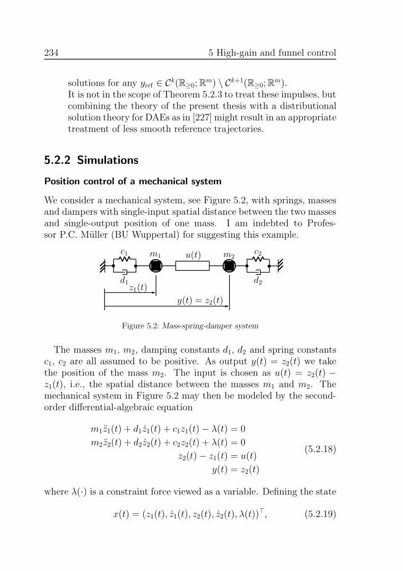
234 5 High-gain and funnel control
solutions for any yref ∈ Ck(R≥0;Rm) \ Ck+1(R≥0;R
m).It is not in the scope of Theorem 5.2.3 to treat these impulses, butcombining the theory of the present thesis with a distributionalsolution theory for DAEs as in [227] might result in an appropriatetreatment of less smooth reference trajectories.
5.2.2 Simulations
Position control of a mechanical system
We consider a mechanical system, see Figure 5.2, with springs, massesand dampers with single-input spatial distance between the two massesand single-output position of one mass. I am indebted to Profes-sor P.C. Muller (BU Wuppertal) for suggesting this example.
s
u(t)m1 m2s ss
c1
d1
c2
d2-
-
z1(t)
y(t) = z2(t)
Figure 5.2: Mass-spring-damper system
The masses m1, m2, damping constants d1, d2 and spring constantsc1, c2 are all assumed to be positive. As output y(t) = z2(t) we takethe position of the mass m2. The input is chosen as u(t) = z2(t) −z1(t), i.e., the spatial distance between the masses m1 and m2. Themechanical system in Figure 5.2 may then be modeled by the second-order differential-algebraic equation
m1z1(t) + d1z1(t) + c1z1(t)− λ(t) = 0
m2z2(t) + d2z2(t) + c2z2(t) + λ(t) = 0
z2(t)− z1(t) = u(t)
y(t) = z2(t)
(5.2.18)
where λ(·) is a constraint force viewed as a variable. Defining the state
x(t) = (z1(t), z1(t), z2(t), z2(t), λ(t))⊤, (5.2.19)

5.2 Funnel control 235
model (5.2.18) may be rewritten as the linear differential-algebraicinput-output system (4.1.1) for
sE −A =
s −1 0 0 0c1 sm1 + d1 0 0 −10 0 s −1 00 0 c2 sm2 + d2 1−1 0 1 0 0
, B =
00001
, C =
00100
⊤
.
(5.2.20)We may immediately see that the pencil sE − A is regular and hasindex ν = 3. The zero dynamics of (5.2.20) are asymptotically stable:setting y = 0 in (5.2.18) yields z2 = 0, λ = 0, z1 = −u and m1 z1(t) +d1z1(t) + c1z1(t) = 0 for all t ≥ 0; positivity of m1, d1 and c1 then giveslimt→∞ z1(t) = limt→∞ z1(t) = 0. Right-invertibility of (5.2.20) can beeasily read off (5.2.18). The transfer function
G(s) = C(sE − A)−1B =m1s
2 + d1s+ c1(m1 +m2)s2 + (d1 + d2)s+ (c1 + c2)
has proper inverse: lims→∞G−1(s) = (m1 +m2)/m1. Therefore, invok-ing Remark 4.3.3,
Γ = lims→∞
s−1G(s)−1 = 0.
Summarizing, system (5.2.20) satisfies the assumptions ofTheorem 5.2.3.As reference signal yref : R≥0 → R, we take the first component of the
solution of the following initial-value problem for the Lorenz system
ξ1(t) = 10 (ξ2(t)− ξ1(t)), ξ1(0) = 5
ξ2(t) = 28 ξ1(t)− ξ1(t) ξ3(t)− ξ2(t), ξ2(0) = 5
ξ3(t) = ξ1(t) ξ2(t)− 83 t ξ3(t), ξ3(0) = 5 .
(5.2.21)
This may be viewed as a rather academic choice, however it is wellknown (see for example [224, App. C]) that the Lorenz system is chaotic(and thus the reference signal is rather ‘wild’), the unique global so-lution of (5.2.21) is bounded with bounded derivative on the positivereal axis (and thus our assumptions on the class of reference signals aresatisfied). The solution of (5.2.21) is depicted in Figure 5.3.The funnel Fϕ is determined by the function
ϕ : R≥0 → R≥0, t 7→ 0.5 te−t + 2 arctan t . (5.2.22)

236 5 High-gain and funnel control
0 1 2 3 4 5 6 7 8 9 10-30
-20
-10
0
10
20
30
40
50
�
��
��
��
Figure 5.3: Components ξi of the Lorenz system (5.2.21)
Note that this prescribes an exponentially (exponent 1) decaying funnelin the transient phase [0, T ], where T ≈ 3, and a tracking accuracyquantified by λ = 1/π thereafter, see e.g. Figure 5.4d.Spring and damping constants, masses and their initial positions are
chosen, for the simulations, as
m1 = 1, m2 = 3, c1 = 2, c2 = 1, d1 = 3, d2 = 5,
z1(0) = 101, z2(0) = 21 and k = 5.(5.2.23)
Straightforward calculations show that the closed-loop system (5.2.2),(5.2.18) has uniquely determined initial velocities z1(0), z2(0) as wellas initial constraint force λ(0) and that the initialization is consistent.Since
k = 5 > 4 = lims→∞
G−1(s) =∥∥∥ lims→∞
(G(s)−1 + sΓ
)∥∥∥ ,all assumptions of Theorem 5.2.3 are satisfied and we may apply thefunnel controller (5.2.2) with funnel boundary specified in (5.2.22) andreference signal yref = ξ1 given in (5.2.21).All numerical simulations are performed in MATLAB (solver: ode15s,
relative tolerance: 10−14, absolute tolerance: 10−5). The simulationsover the time interval [0, 10] are depicted in Figure 5.4: Figure 5.4ashows the output y tracking the rather ‘vivid’ reference signal yrefwithin the funnel shown in Figure 5.4d. Note that the input u inFigure 5.4c as well as the gain function k in Figure 5.4b have spikes atthose times t when the norm of the error ‖e(t)‖ is ‘close’ to the funnel

5.2 Funnel control 237
0 2 4 6 8 1 0
- 2 0
- 1 0
0
1 0
2 0
3 0
t
�
Figure a: Solution y
0 2 4 6 8 1 0
0
5 0
1 0 0
1 5 0
2 0 0
t
�
Figure b: Gain k
0 2 4 6 8 1 0
- 1 0 0
- 5 0
0
5 0
1 0 0
t
�
Figure c: Input u
0 1 2 3 4 5 6 7
0
1
2
3
4
5
6
7
t
���
���
Figure d: Norm of error |e| and fun-nel boundary ϕ−1
Figure 5.4: Simulation of the funnel controller (5.2.2) with funnel boundaryspecified in (5.2.22) and reference signal yref = ξ1 given in (5.2.21)applied to the mechanical model (5.2.18) with data (5.2.23).
boundary ϕ(t)−1; this is due to rapid change of the reference signal.We stress that the gain function k is nonmonotone.
Singular academic example
For purposes of illustration we consider an example of a singular differ-ential-algebraic system (4.1.1), where Γ is neither zero nor invertible.Consider system (4.1.1) with
[E,A,B, C] :=
1 0 00 1 −10 −1 1
,
−1 1 −23 1 10 0 1
,
0 01 00 1
,[0 1 00 0 1
] .
(5.2.24)
238 5 High-gain and funnel control
It is immediate that [E,A,B, C] is right-invertible and in theform (4.2.3), has asymptotically stable zero dynamics, and the matrix
Γ =
[1 −1−1 1
]
satisfies (5.2.3) and Γ = Γ⊤ ≥ 0. We set
k := 2 >√2 =
∥∥∥∥[1 10 1
]∥∥∥∥ = ‖A22‖ =∥∥∥ lims→∞
([0, Im]L(s)[0, Im]⊤ + sΓ)
∥∥∥ ,(5.2.25)
where L(s) is an inverse of the system pencil, see also Step 1 in theproof of Theorem 5.2.3 for the latter equalities. The (consistent) initialvalue for the closed-loop system (5.2.24), (5.2.2) is chosen as
x0 = (−4, 3,−2)⊤. (5.2.26)
As reference signal yref : R≥0 → R2, we take the first and secondcomponent of the solution of the Lorenz system (5.2.21). The funnelFϕ is determined by (5.2.22).
The simulation has been performed in MATLAB (solver: ode15s,relative tolerance: 10−14, absolute tolerance: 10−5). In Figure 5.5 thesimulation, over the time interval [0, 10], of the funnel controller (5.2.2)with funnel boundary specified in (5.2.22) and reference signal yref =(ξ1, ξ2)
⊤ given in (5.2.21), applied to system (5.2.24) with initialdata (5.2.25), (5.2.26) is depicted. Figure 5.5a shows the output com-ponents y1 and y2 tracking the reference signal yref within the funnelshown in Figure 5.5d. Note that an action of the input components u1and u2 in Figure 5.5c and the gain function k in Figure 5.5b is requiredonly if the error ‖e(t)‖ is close to the funnel boundary ϕ(t)−1. It canbe seen that initially the error is very close to the funnel boundary andhence the gain rises sharply. Then, at approximately t = 0.2, the dis-tance between error and funnel boundary gets larger and the gain dropsaccordingly. After t = 2, the error gets close to the funnel boundaryagain which causes the gain to rise again. This in particular shows thatthe gain function k is nonmonotone.

5.3 Regular systems and relative degree 239
0 2 4 6 8 1 0
- 3 0
- 2 0
- 1 0
0
1 0
2 0
3 0
�
��
��
Figure a: Solution components y1and y2
0 2 4 6 8 1 0
0
5
1 0
1 5
2 0
�
�
Figure b: Gain k
0 2 4 6 8 1 0
- 3 0
- 2 0
- 1 0
0
1 0
2 0
3 0
�
��
��
Figure c: Input components u1
and u2
0 2 4 6 8 1 0
0
1
2
3
4
5
�
������ � �����
���
Figure d: Norm of error ‖e‖ andfunnel boundary ϕ−1
Figure 5.5: Simulation of the funnel controller (5.2.2) with funnel bound-ary specified in (5.2.22) and reference signal yref = (ξ1, ξ2)
⊤
given in (5.2.21) applied to system (5.2.24) with initialdata (5.2.25), (5.2.26).
5.3 Regular systems and relative degree
In this section we consider systems [E,A,B, C] ∈ Σn,n,m,p for whichsE − A is regular and hence the transfer function
G(s) = C(sE −A)−1B ∈ R(s)p×m (5.3.1)
is well defined. We will introduce the notions of vector and strict rela-tive degree and show that systems with a vector relative degree whichis componentwise smaller or equal to one can be treated within theframeworks of Theorems 5.1.4 and 5.2.3. Furthermore, we show thatfor systems with positive strict relative degree, high-gain and funnelcontrol is feasible provided the controllers are modified in order to ac-
240 5 High-gain and funnel control
count for output derivatives.As a preliminary result we derive some characterizations of autono-
mous zero dynamics and right-invertibility for regular systems.
Proposition 5.3.1 (Autonomous zero dynamics and right-invertibil-ity).Let [E,A,B, C] ∈ Σn,n,m,p be such that sE − A is regular and let G(s)be as in (5.3.1). Then the following statements hold true:
(i) ZD[E,A,B,C] is autonomous ⇐⇒ rkR[s]G(s) = m.
(ii) [E,A,B, C] is right-invertible ⇐⇒ rkR[s]G(s) = p.
(iii) If p = m, then the following conditions are equivalent:
(a) ZD[E,A,B,C] is autonomous,
(b) [E,A,B, C] is right-invertible,
(c) G(s) ∈ Glm(R(s)).
Proof: (i): We show “⇒”: If the zero dynamics are autonomous, thenthe system pencil has a left inverse over R(s) and it can be concluded,using the same calculation as in Remark 4.3.3, that G(s) has a leftinverse over R(s). Equivalently, rkR[s]G(s) = m.We show “⇐”: By assumption there exists GL(s) ∈ R(s)m×p such thatGL(s)G(s) = Im. Calculating
[(sE−A)−1 −(sE−A)−1BGL(s)
0 −GL(s)
] [In 0
C(sE−A)−1 Im
] [sE−A −B−C 0
]
=[(sE−A)−1 −(sE−A)−1BGL(s)
0 −GL(s)
] [sE−A −B
0 −G(s)
]= In+m,
yields that the system pencil[sE−A −B−C 0
]is left invertible over R(s).
Hence, by Proposition 4.1.5, the zero dynamics are autonomous.(ii): We show “⇒”: Seeking a contradiction assume that rkR[s]G(s)<
p. Hence, there exists q(s) ∈ R(s)p \ {0} such that q(s)⊤G(s) = 0. Letp(s) ∈ R[s] \ {0} be such that q(s) := p(s)q(s) satisfies
(q(s)⊤C(sE − A)−1, q(s)⊤)⊤ ∈ R[s]n+p.
Now there exists y ∈ C∞(R;Rp) such that q( ddt)
⊤y 6= 0. By right-invertibility of [E,A,B, C] we find (x, u) ∈ L1
loc(R;Rn×Rm) such that
5.3 Regular systems and relative degree 241
(x, u, y) ∈ B[E,A,B,C]. Therefore, heeding that all poles in the rationalfunctions are canceled out,
q( ddt)
⊤y = (q( ddt)
⊤C(E ddt − A)−1, q( d
dt)⊤)
(0y
)
a.e.= (q( d
dt)⊤C(E d
dt− A)−1, q( d
dt)⊤)
[E d
dt − A −B−C 0
](xu
)a.e.= 0,
a contradiction.We show “⇐”: By assumption there exists GR(s) ∈ R(s)m×p suchthat G(s)GR(s) = Ip. Similar to (i) we may calculate that that thesystem pencil
[sE−A −B−C 0
]is right invertible over R(s). Then applying
Lemma 4.1.3 to its transpose yields that ℓ(γ) = 0 in a QKF (4.1.4) ofthe system pencil. Let y ∈ C∞(R;Rp) and S(0, y⊤)⊤ =: (y⊤1 , y
⊤2 , y
⊤3 )
⊤
according to the block structure of (4.1.4). Then, by Theorem 2.4.13,there exist solutions z1 ∈ L1
loc(R;Rns), z2 ∈ L1
loc(R;R|α|), z3 ∈
L1loc(R;R
|β|) of ddtz1
a.e.= Asz1 + y1,
ddtNαz2
a.e.= z2 + y2 and d
dtKβz3a.e.=
Lβz3 + y3. Therefore,
(0y
)a.e.= S−1
ddtIns
− As 0 00 d
dtNα − I|α| 00 0 d
dtKβ − Lβ
z1z2z3
and hence (x⊤, u⊤)⊤ := T (z⊤1 , z⊤2 , z
⊤3 )
⊤ satisfies (x, u, y) ∈ B[E,A,B,C].(iii): The assertion is immediate from (i) and (ii).
A consequence of Proposition 5.3.1 is that the class of regular sys-tems with proper inverse transfer function can be treated within theframeworks of Theorems 5.1.4 and 5.2.3.
Definition 5.3.2 (Proper rational matrix function).A rational matrix G(s) ∈ R(s)p×m is called proper if, and only if,lims→∞G(s) = D for some D ∈ Rp×m. It is called strictly proper if,and only if, lims→∞G(s) = 0.
Corollary 5.3.3 (Proper inverse transfer function).Let [E,A,B, C] ∈ Σn,n,m,m be such that sE − A is regular and thatG(s) as in (5.3.1) is invertible over R(s) and G(s)−1 is proper. Then[E,A,B, C] is right-invertible, has autonomous zero dynamics and Γas in (5.2.3) exists and satisfies Γ = 0.
242 5 High-gain and funnel control
Proof: Right-invertibility and autonomy of the zero dynamics followfrom Proposition 5.3.1. The last assertion is a consequence of Re-mark 4.3.3 by which
Γ = lims→∞
s−1G(s)−1 = 0.
5.3.1 Vector relative degree
In this subsection we give the definition of vector relative degree fortransfer functions of regular systems [E,A,B, C] ∈ Σn,n,m,p and relatethis property to the frameworks of Theorems 5.1.4 and 5.2.3.
Definition 5.3.4 (Vector relative degree).We say that G(s) ∈ R(s)p×m has vector relative degree (ρ1, . . . , ρp) ∈Z1×p if, and only if, the limit
D := lims→∞
diag (sρ1, . . . , sρp)G(s) ∈ Rp×m
exists and satisfies rkD = p.
Remark 5.3.5 (Vector relative degree).
(i) It is an easy calculation that if G(s) ∈ R(s)p×m has a vector rel-ative degree, then the vector relative degree is unique. However,a vector relative degree does not necessarily exist, even if G(s) is(strictly) proper; see Example 5.3.7.
(ii) Isidori [131, Sec. 5.1] introduced a local version of vector rela-tive degree for nonlinear systems. Definition 5.3.4 coincides withIsidori’s definition if strictly proper transfer functions are con-sidered. In this sense, Definition 5.3.4 is a generalization to arbi-trary rational transfer functions. For linear ODE systems a globalversion of the vector relative degree has been stated in [180]. Itis straightforward to show that [In, A, B, C] ∈ Σn,n,m,m has vectorrelative degree (ρ1, . . . , ρp) in the sense of [180, Def. 2.1] if, andonly if, C(sI − A)−1B has vector relative degree (ρ1, . . . , ρp).
In the following we show that a regular system with transfer functionwhich has componentwise vector relative degree smaller or equal toone, is right-invertible, has autonomous zero dynamics and Γ in (5.2.3)exists.

5.3 Regular systems and relative degree 243
Proposition 5.3.6 (Vector relative degree ≤ 1 implies existence of Γ).
Let [E,A,B, C] ∈ Σn,n,m,m be such that sE − A is regular and G(s)in (5.3.1) has vector relative degree (ρ1, . . . , ρm) with ρi ≤ 1 for alli = 1, . . . , m. Then
(i) ZD(4.1.1) are autonomous,
(ii) [E,A,B, C] is right-invertible,
(iii)
[sE −A −B−C 0
]has inverse L(s) over R(s) and the matrix Γ
in (5.2.3) exists and satisfies
∀ j = 1, . . . , m :
Γej =
(lims→∞
diag (sρ1, . . . , sρp)G(s))−1
ej , if ρj = 1,
0, if ρj < 1.(5.3.2)
Proof: Step 1 : We show that G(s) is invertible over R(s). To this end,let F (s) := diag (sρ1, . . . , sρp)G(s). Since
D := lims→∞
F (s) = lims→∞
diag (sρ1, . . . , sρp)G(s) ∈ Glm(R)
exists, Gsp(s) := F (s) − D ∈ R(s)m×m is strictly proper, i.e.,lims→∞Gsp(s) = 0. Since D is invertible, F (s) is invertible as well,as by the Sherman-Morrison-Woodbury formula (see [105, p. 50])
F (s)−1 = D−1−D−1Gsp(s)(I +D−1Gsp(s))−1D−1 ∈ R(s)m×m. (5.3.3)
It is then immediate that G(s) has inverse G(s)−1 =F (s)−1 diag (sρ1, . . . , sρp) over R(s).Step 2 : In view of Step 1, (i) and (ii) follow from Proposition 5.3.1.Step 3 : We show (iii). As in Remark 4.3.3 we may conclude that
[0, Im]L(s)[0, Im]⊤ = −G(s)−1 and
s−1G(s)−1 =(diag (sρ1, . . . , sρp)G(s)
)−1diag (sρ1−1, . . . , sρp−1)
(5.3.3)=
(D−1−D−1Gsp(s)(I+D
−1Gsp(s))−1D−1
)diag (sρ1−1, . . . , sρp−1).
244 5 High-gain and funnel control
Hence, using ρi ≤ 1 for i = 1, . . . , m, we obtain existence of
Γ = lims→∞
s−1G(s)−1 ∈ Rm×m,
where Γej = D−1ej if ρj = 1 and Γej = 0 if ρj < 1, for all j =1, . . . , m.
We illustrate the vector relative degree and Proposition 5.3.6 bymeans of an example.
Example 5.3.7.Consider system (4.1.1) with
E =
[1 00 0
], A =
[1 20 3
], B = C = I2.
It can be seen that sE − A is regular and
G(s) = C(sE − A)−1B =
[s− 1 −20 −3
]−1
=
[ 1s−1
− 23(s−1)
0 −13
].
We calculate
D := lims→∞
diag (s, 1)G(s) =
[1 −2
30 −1
3
]∈ Gl2(R),
and hence G(s) has vector relative degree (1, 0). Proposition 5.3.6 thenimplies that ZD(4.1.1) are autonomous, [E,A,B, C] is right-invertible,and Γ in (5.2.3) exists. In fact, it is easy to see that the zero dynamicsare asymptotically stable and
Γ = lims→∞
s−1G(s)−1 =
[1 00 0
]
satisfies (5.3.2): Γe1 = D−1e1 =[1 −20 −3
]e1 and Γe2 = 0. Since Γ = Γ⊤ ≥
0, the assumptions of Theorems 5.1.4 and 5.2.3 are satisfied.We like to stress that, compared to the above, the regular sys-
tem (5.2.24) from Subsection 5.2.2 does not have a vector relative de-gree: while its transfer function G(s) is proper, the limit
lims→∞
G(s) = −1
3
[1 11 1
]
does not have full row rank. Nevertheless, as shown in Section 5.2.2,funnel control is feasible.
5.3 Regular systems and relative degree 245
5.3.2 Strict relative degree
In this subsection we introduce the concept of strict relative degree,which is a special vector relative degree, and develop high-gain andfunnel controllers for systems with positive strict relative degree.
Definition 5.3.8 (Strict relative degree).We say that a square matrix functionG(s) ∈ R(s)m×m has strict relativedegree sr degG(s) = ρ ∈ Z if, and only if,
D := lims→∞
sρG(s) ∈ Glm(R).
The matrix D is called high-frequency gain matrix .
Remark 5.3.9 (Strict relative degree and high-frequency gain).
(i) If G(s) ∈ R(s)m×m has vector relative degree (ρ1, . . . , ρm) ∈ Z1×m,then ρ = ρ1 = . . . = ρm if, and only if, G(s) has strict relativedegree ρ.
(ii) If g(s) = p(s)/q(s), for p(s) ∈ R[s] and q(s) ∈ R[s]\{0}, is a scalarrational function, then the strict relative degree always exists andcoincides with the well-known definition of relative degree:
sr deg g(s) = deg q(s)− deg p(s).
(iii) An ODE system [E,A,B, C] = [In, A, B, C] ∈ Σn,n,m,m has trans-fer function
G(s) = C(sI −A)−1B = CB s−1 + CAB s−2 + CA2B s−3 + . . .
and therefore strict relative degree ρ ∈ N, if, and only if,
det(CAρ−1B) 6= 0 and, if ρ > 1, ∀ k = 0, . . . , ρ−2 : CAkB = 0 .
(iv) For systems [E,A,B, C] ∈ Σn,n,m,m with regular sE − A, trans-fer function G(s) as in (5.3.1) and strict relative degree ρ ∈N we have: If ρ = 1, then by Proposition 5.3.6, Γ in (5.2.3)exists and we have, from the proof of Proposition 5.3.6, Γ =(lims→∞ sG(s)
)−1, i.e., Γ is exactly the inverse of the high-fre-
quency gain matrix. Since, furthermore, Γ is also defined when no
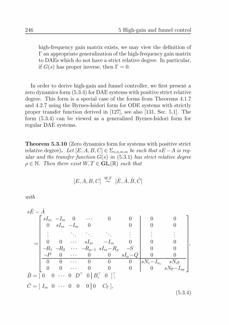
246 5 High-gain and funnel control
high-frequency gain matrix exists, we may view the definition ofΓ an appropriate generalization of the high-frequency gain matrixto DAEs which do not have a strict relative degree. In particular,if G(s) has proper inverse, then Γ = 0.
In order to derive high-gain and funnel controller, we first present azero dynamics form (5.3.4) for DAE systems with positive strict relativedegree. This form is a special case of the forms from Theorems 4.1.7and 4.2.7 using the Byrnes-Isidori form for ODE systems with strictlyproper transfer function derived in [127], see also [131, Sec. 5.1]. Theform (5.3.4) can be viewed as a generalized Byrnes-Isidori form forregular DAE systems.
Theorem 5.3.10 (Zero dynamics form for systems with positive strictrelative degree). Let [E,A,B, C] ∈ Σn,n,m,m be such that sE−A is reg-ular and the transfer function G(s) in (5.3.1) has strict relative degreeρ ∈ N. Then there exist W,T ∈ Gln(R) such that
[E,A,B, C]W,T∼ [E, A, B, C]
with
sE − A
=
sIm −Im 0 · · · 0 0 0 00 sIm −Im 0 0 0 0...
. . .. . .
. . ....
......
0 0 · · · sIm −Im 0 0 0−R1 −R2 · · · −Rρ−1 sIm−Rρ −S 0 0−P 0 · · · 0 0 sIµ−Q 0 00 0 · · · 0 0 0 sNc−Inc
sNcc
0 0 · · · 0 0 0 0 sNc−Inc
,
B = [ 0 0 · · · 0 D⊤ 0 B⊤c 0 ]⊤,
C = [ Im 0 · · · 0 0 0 0 Cc ],(5.3.4)

5.3 Regular systems and relative degree 247
where, for some nc, nc ∈ N0, and µ = n− nc − nc − ρm,
D = lims→∞
sρG(s) ∈ Glm(R) is the high-frequency gain matrix,
S ∈ Rm×µ , P ∈ Rµ×m , Q ∈ Rµ×µ ,[R1, . . . , Rρ
]∈ Rm×ρm,
Bc ∈ Rnc×m , Cc ∈ Rm×nc , Ncc ∈ Rnc×nc
Nc ∈ Rnc×nc , Nc ∈ Rnc×nc are nilpotent, and rk[Nc , Bc] = nc.(5.3.5)
The entries R1, . . . , Rρ are unique, system [I, Q, P, S] is unique up
to system equivalenceT−1,T∼ , and the matrices Nc and Nc are unique up
to similarity.If E is invertible, then nc = nc = 0, this means only the upper left
block in E is present.The form (5.3.4) is called zero dynamics form of (4.1.1). The trans-
fer function satisfies, where Rρ+1 := −I,
G(s) = −[ρ+1∑
i=1
Risi−1 + S(sIµ −Q)−1P
]−1
D. (5.3.6)
For the proof of Theorem 5.3.10 we need the following preliminarylemma.
Lemma 5.3.11 (Decomposition for systems with strictly proper trans-fer function).Let [E,A,B, C] ∈ Σn,n,m,m be such that sE − A is regular and thetransfer function G(s) in (5.3.1) is strictly proper. Then there existsW,T ∈ Gln(R) such that
[E,A,B, C]
W,T∼
Ins
0 00 Nc Ncc
0 0 Nc
,
As 0 00 Infc
00 0 Infc
,
Bs
Bfc
0
,[Cs 0 Cfc
]
(5.3.7)
for some As ∈ Rns×ns, Bs ∈ Rns×m, Cs ∈ Rm×ns, Nc ∈ Rnfc×nfc, Ncc ∈Rnfc×nfc, Nc ∈ Rnfc×nfc, Bfc ∈ Rnfc×m and Cfc ∈ Rm×nfc, where Nc, Nc
are nilpotent and rk[Nc , Bfc] = nfc. The dimensions ns, nfc, nfc ∈ N0
are unique, the matrices As, Nc and Nc are unique up to similarity.
248 5 High-gain and funnel control
Furthermore, system [E,A,B, C] has strict relative degree ρ ∈ N if,and only if,
det(CsAρ−1s Bs) 6= 0 and, if ρ > 1, ∀ k = 0, . . . , ρ−2 : CsA
ksBs = 0 .(5.3.8)
Proof: Step 1 : We show that there exist W,T ∈ Gln(R) suchthat (5.3.7) holds true. It follows from Theorem 2.2.5 that there existW1, T1 ∈ Gln(R) such that
[E,A,B, C]W,T∼
[[Ins
00 N
],
[As 00 Inf
],
[Bs
Bf
],[Cs Cf
]],
for some Bs ∈ Rnf×m, Bf ∈ Rnf×m, Cs ∈ Rm×ns, Cf ∈ Rm×ns, As ∈Rns×ns and nilpotent N ∈ Rnf×nf . Then [80, Sec. 2-1.] yields thatsystem [N, Inf
, Bf , Cf ] may be decomposed into controllability form sothat, for some T2 ∈ Glnf
(R),
[N, Inf, Bf , Cf ]
T−12 ,T2∼
[[Nc Ncc
0 Nc
],
[Infc
00 Infc
],
[Bfc
0
],[Cfc, Cfc
]],
where Nc ∈ Rnfc×nfc, Nc ∈ Rnfc×nfc, N12 ∈ Rnfc×nfc, Bfc ∈ Rnfc×m,Cfc ∈ Rm×nfc, and Cfc ∈ Rm×nfc, such that Nc, Nc are nilpotent andrk[Nc , Bfc ] = nfc.We show that Cfc = 0: Since the transfer function is invariant under
system equivalence we have, using (sNc−Inf)−1 = −Inf
−sN −s2N2−. . .− sν−1Nν−1,
G(s) = C(sE −A)−1B = Cs(sIns− As)
−1Bs −ν−1∑
k=0
skCfcNkcBfc,
and since G(s) is strictly proper, it follows that CfcNicBfc = 0 for
i = 1, . . . , ν − 1. The nilpotency of Nc gives CfcNν−1c [Nc , Bfc ] = 0,
whence CfcNν−1c = 0. Repeating this argumentation ν − 1 times, we
obtain Cfc = 0.
Setting W :=W1
[I 00 T−1
2
]and T :=
[I 00 T2
]T1, we obtain (5.3.7).
Step 2 : We show that the dimensions ns, nfc, nfc ∈ N0 are unique andthat the matrices As, Nc and Nc are unique up to similarity: Assume
5.3 Regular systems and relative degree 249
that
Ins1
0 00 Nc1 Ncc1
0 0 Nc1
,
As1 0 00 Infc1
00 0 Infc1
,
Bs1
Bfc1
0
,[Cs1 0 Cfc1
]
W,T∼
Ins2 0 00 Nc2 Ncc2
0 0 Nc2
,
As2 0 00 Infc2
00 0 Infc2
,
Bs2
Bfc2
0
,[Cs2 0 Cfc2
] .
Remark 2.2.6 gives that ns1 = ns2 as well as the similarity of As1
and As2. Remark 2.2.6 also yields the existence of T11 ∈ Rnfc1×nfc2,T12 ∈ Rnfc1×nfc2, T21 ∈ Rnfc1×nfc2, and T22 ∈ Rnfc1×nfc2 such that
T =
[T11 T12T21 T22
]∈ Glnf
(R), and
[Nc1 Ncc1
0 Nc1
] [T11 T12T21 T22
]
=
[T11 T12T21 T22
] [Nc2 Ncc2
0 Nc2
],
[Bfc1
0
]=
[T11 T12T21 T22
] [Bfc2
0
].
Therefore, 0 = T21Bfc2 and T21Nc2 = Nc1T21. Hence, for k = 1, . . . , ν−1, we have T21N
kc2Bfc2 = Nk
c1T21Bfc2 = 0, and so T21Nν−1c2 [Nc2 Bfc2 ] =
0, whence T21Nν−1c2 = 0. Repeating this argumentation ν − 1 times, we
obtain T21 = 0. Then T ∈ Glnf(R) yields nfc2 ≤ nfc1. By reversing
the roles of the above matrices, we analogously obtain nfc1 ≤ nfc2 andthus nfc1 = nfc2, nfc1 = nfc2. This shows that T11 and T22 are square.Together with T ∈ Glnf , we obtain T11 ∈ Glnfc
(R) and T22 ∈ Glnfc(R).
Hence Nc1, Nc2 and Nc1, Nc2 are similar, respectively.Step 3 : We show that [E,A,B, C] has strict relative degree ρ > 0
if, and only if, (5.3.8) holds. This is an immediate consequence of thefact that, due to Step 1, the transfer function has the representationG(s) = C(sE−A)−1B = Cs(sIns
−As)−1Bs. This completes the proof
of the lemma.
Proof of Theorem 5.3.10: We proceed in several steps.Step 1 : We show that there exist W,T ∈ Gln(R) such that
[E,A,B, C]W,T∼ [E, A, B, C] for [E, A, B, C] as in (5.3.4). Since a
positive strict relative degree implies that G(s) is strictly proper, wemay apply Lemma 5.3.11 to obtain (5.3.7) for some W1, T1 ∈ Gln(R).Furthermore, (5.3.8) holds and hence we may transform [I, As, Bs, Cs]

250 5 High-gain and funnel control
into Byrnes-Isidori form (see [127, Lemma 3.5]), i.e., there exists T2 ∈Glns
(R) such that
[I, As, Bs, Cs]
T−12 ,T2∼
I,
0 Im 0 · · · 0 00 0 Im 0 0...
. . .. . .
. . ....
0 0 · · · 0 Im 0R1 R2 · · · Rρ−1 Rρ SP 0 · · · 0 0 Q
,
00...0D0
,
Im0
...
0
⊤
.
(5.3.9)
Set W := W1
[I 00 T−1
2
]and T :=
[I 00 T2
]T1. Since Nc, Nc are nilpotent
and rk[Nc , Bfc] = nfc, the claim follows.
Step 2 : For the proof of the uniqueness statements see [31, Thm. 2.5]or [37, Thm. B.7] in combination with Lemma 5.3.11. In particular, Dis uniquely determined.
Step 3 : It remains to prove (5.3.6) and that D = lims→∞ sρC(sE −A)−1B.We prove (5.3.6): Determine the solution X(s) of the linear equation
sIm −Im. . .
. . .
sIm −Im−R1 . . . −Rρ−1 sIm −Rρ −S−P 0 . . . 0 sIµ −Q
X1(s)X2(s)...
Xρ(s)Xρ+1(s)
=
0...0D0
.
(5.3.10)A simple iterative calculation yields
for i = 1, . . . ρ− 1 : sXi(s) = Xi+1(s),
−ρ−1∑i=1
RiXi(s) + (sIm − Rρ)Xρ(s)− SXρ+1(s) = D,
−PX1(s) + (sIµ −Q)Xρ+1(s) = 0,

5.3 Regular systems and relative degree 251
and this is equivalent to
X(s) =(X1(s)
⊤, sX1(s)⊤, . . . , sρ−1X1(s)
⊤, Xρ+1(s)⊤)⊤ ,
D = −ρ−1∑i=1
Risi−1X1(s) + (sIm −Rρ)s
ρ−1X1(s)− SXρ+1(s),
Xρ+1(s) = (sIµ −Q)−1PX1(s).(5.3.11)
Since the transfer function is invariant under system equivalence wehave
C(sE − A)−1B = C(sE − A)−1B
=[Im 0 · · · 0
]sIn−nfc−nfc
−
0 Im 0 ··· 0 00 0 Im 0 0...
. . .. . .
. . ....
0 0 ··· 0 Im 0R1 R2 ··· Rρ−1 Rρ SP 0 ··· 0 0 Q
−1
0...0D0
+[0 Cfc
] [sNc − InfcsNcc
0 sNc − Infc
]−1 [Bfc
0
].
=[Im 0 · · · 0
]sIn−nfc−nfc
−
0 Im 0 ··· 0 00 0 Im 0 0...
. . .. . .
. . ....
0 0 ··· 0 Im 0R1 R2 ··· Rρ−1 Rρ SP 0 ··· 0 0 Q
−1
0...0D0
(5.3.10)= X1(s)
(5.3.11),Rρ+1=−I= −
[ρ+1∑
i=1
Risi−1 + S(sIµ −Q)−1P
]−1
D.
This proves (5.3.6). Finally,
D = lims→∞
−[ρ+1∑
i=1
Risi−1 + S(sIµ −Q)−1P
]G(s)
= −ρ∑
i=1
Ri lims→∞
si−1G(s) + lims→∞
sρG(s)− lims→∞
S(sIµ −Q)−1P G(s)
= lims→∞
sρG(s)

252 5 High-gain and funnel control
and the proof of the theorem is complete.
Remark 5.3.12 (Zero dynamics form for DAEs).An immediate consequence of Theorem 5.3.10 is the simplified repre-sentation of system [E,A,B, C] ∈ Σn,n,m,m: If ν denotes the index ofsE −A, then a trajectory satisfies
(x, u, y) ∈ B[E,A,B,C] ∩(C1(R;Rn)× Cν−1(R;Rm)× Cρ(R;Rm)
)
if, and only if, Tx =(y⊤, y⊤, . . . , y(ρ−1)⊤, η⊤, x⊤c , x
⊤c
)⊤∈ C1(R;Rn)
fulfills
y(ρ)(t) =ρ∑
i=1
Riy(i−1)(t) + Sη(t) + Γu(t)
η(t) = P y(t) + Qη(t)
xc(t) = −ν−1∑i=0
N icBcu
(i)(t)
xc(t) = 0.
(5.3.12)
See Figure 5.6.
High-gain control
In this subsection we consider high-gain control for DAE systems withpositive strict relative degree. From the form (5.3.4) we deduce thatthe input u only influences the ρth derivative of the output y. Hencewe need derivative output feedback in order to achieve stabilization.We consider the high-gain controller
u(t) = −k p( ddt) y(t), (5.3.13)
where k > 0 and p(s) ∈ R[s] is Hurwitz, i.e., all roots of p(s) are in C−.We show that asymptotically stable zero dynamics are sufficient, but
not necessary, for the closed-loop system (4.1.1), (5.3.13) to be asymp-totically stable. For [E,A,B, C] ∈ Σn,n,m,m, the system (4.1.1), (5.3.13)is called asymptotically stable if, and only if, for all x ∈ C∞(R;Rn) thefollowing implication holds:
ddtEx = Ax− k p( d
dt)BCx =⇒ limt→∞
x(t) = 0.

5.3 Regular systems and relative degree 253
ξρ =
ρ∑
i=1
Riξi + y
+ CAρ−1Bu
ddt
ddt
η = Qη + Py
y = Sη
ξ1 = y
y
y
u
ξ1ξ2 = y
ξ2· · ·ξρ = y(ρ−1)
ξρ
y
Bc
ddtNc
+
ddtNc
+ +
ddtNc
+
0
xc
xc
Figure 5.6: Zero dynamics form for systems with positive strict relative de-gree
Theorem 5.3.13 (High-gain control).Let [E,A,B, C] ∈ Σn,n,m,m be such that sE − A is regular, the trans-fer function G(s) in (5.3.1) has strict relative degree ρ ∈ N and thehigh-frequency gain matrix (cf. (5.3.5)) is positive definite. Let p(s) =∑ρ−1
i=0 pisi ∈ R[s] be Hurwitz and pρ−1 > 0. Then
ZD[E,A,B,C] is asympt. stable
=⇒{ ∃ k∗ ≥ 0 ∀ k ≥ k∗ :
‘ (4.1.1) & (5.3.13)’ is asympt. stable.
The converse implication is in general false even for ODE systems.
For the proof of Theorem 5.3.13 a lemma is required.
Lemma 5.3.14 (High-gain lemma).Consider, for D ∈ Glm(C), R ∈ Cm×m, S⊤, P ∈ C(n−m)×m, Q ∈C(n−m)×(n−m), the parameterized matrix
Aκ :=
[R − κD S
P Q
], κ ≥ 0 .

254 5 High-gain and funnel control
Denote the spectra of D and Q by
σ(D) = {γ1, . . . , γm} ⊆ C\{0} and σ(Q) = {qm+1, . . . , qn} ⊆ C , resp.
Then there exist z1, . . . , zm ∈ C and θ > 0 with the following property:For all ε > 0 and all θ ∈ (0, θ) there exist r ≥ 0 and κ∗ ≥ 1 suchthat, with a suitable enumeration of the eigenvalues λ1(Aκ), . . . , λn(Aκ)of Aκ, we have, for all κ ≥ κ∗,
(i) B(zi − κγi, r + κ θ
)∩B(0, 1/ε) = ∅ for i = 1, . . . , m,
(ii) λi(Aκ) ∈⋃m
j=1B(zj − κγj, r + κ θ
)for i = 1, . . . , m,
(iii) λi(Aκ) ∈⋃n
j=m+1B(qj, ε
)for i = m+ 1, . . . , n,
where B(z, ε) = { w ∈ C | |z − w| < ε } denotes the ball of radius εaround z in C.
Proof:2 Let
θ := 14 min
{|γ1|, . . . , |γm|
}> 0 (5.3.14)
and choose arbitrary θ ∈ (0, θ). Let U1 ∈ Glm(C), U2 ∈ Gln−m(C) suchthat, for appropriately chosen δ1, . . . , δn−1 ∈ {0, 1}, we have Jordanforms
U1DU−11 =
γ1 δ1. . .
. . .
γm−1 δm−1
γm
, U2QU
−12 =
qm+1 δm+1
. . .. . .
qn−1 δn−1
qn
.
Set
Tθ := diag (θ, θ2, . . . , θm) and Tα := diag (α, α2, . . . , αn−m) for α > 0
2Many thanks to Achim Ilchmann (Ilmenau University of Technology) and Fabian Wirth (Univer-sity of Wurzburg) for the proof.

5.3 Regular systems and relative degree 255
and transform Aκ to the similar matrix
M(κ, θ, α) :=
[T−1θ U−1
1 00 TαU
−12
] [R− κD S
P Q
] [U1Tθ 00 U2T
−1α
]
=
T−1θ U−1
1 RU1Tθ − κ
[γ1 θδ1
. . .. . .
γm−1 θδm−1γm
]T−1θ U−1
1 SU2T−1α
TαU−12 PU1Tθ
[qm+1 δm+1/α
. . .. . .qn−1 δn−1/α
qn
]
,
and the off-diagonal column sums
ρj(κ, θ, α) :=
n∑
i=1
i 6=j
|M(κ, θ, α)ij| , j = 1, . . . , n.
Fix ε > 0. We may now choose α > 0 sufficiently large so that theeffect of the scaling matrix T−1
α in the last n−m columns ofM(κ, θ, α)is
∀ i = m+ 1, . . . , n : ρj(κ, θ, α) = ρj(α) ∈ [0, ε) .
Consider next the first m columns of M(κ, θ, α). Noting that everysummand in ρi(κ, θ, α) which involves κ must be a product of κ and θ,we find that there exists r = r(α, θ) ≥ 0 such that
∀ i = 1, . . . , m ∀κ ≥ 0 : ρi(κ, θ, α) ≤ r + κ θ . (5.3.15)
Define the diagonal entries
zi := (U−11 RU1)ii = (T−1
θ U−11 RU1Tθ)ii, i = 1, . . . , m.
We now show that the center of the balls B (zi − κγi, r + κ θ), i =1, . . . , m, tends, as κ → ∞, to infinity at a faster pace than its radius.To this end note that using (5.3.14) gives
|zi − κγi| ≥∣∣|zi| − 4κθ
∣∣
and for κ > (r + |zi|)/θ we have |zi| < κθ and hence
|zi − κγi| > 3κθ − |zi| > 2κθ + r > κθ + (r + κθ) .

256 5 High-gain and funnel control
Therefore,|zi − κγi| − (κθ + r) > κθ ,
which implies that B (zi − κγi, r + κ θ) ∩ B(0, κθ) = ∅. Choosing
κ∗ > max{1/(εθ), (r + |z1|)/θ, . . . , (r + |zm|)/θ
}
we obtain assertion (i). Since γi 6= 0 for all i = 1, . . . , m, we may nowchoose κ∗ ≥ 1 sufficiently large so that
∀κ ≥ κ∗ :m⋃
i=1
B (zi − κγi, r + κ θ) ∩n⋃
j=m+1
B(qj, ε) = ∅ .
We are now in a position to apply Gershgorin’s disks, see [115,Thm 4.2.19], to deduce (ii) and (iii). This completes the proof of thelemma.
Proof of Theorem 5.3.13: We prove “⇒”. By Theorem 5.3.10,[E,A,B, C] is equivalent to a system in the form (5.3.12). We in-troduce the ‘new states’
ξ := 1pρ−1
· p ( ddt)y, χ :=
(y⊤, y⊤, . . . ,
(y(ρ−2)
)⊤, η⊤)⊤
,
and observe that
ξ(t) = R ξ(t) + S χ(t) +Du(t)
χ(t) = P ξ(t) + Q χ(t),(5.3.16)
where R, S are matrices of appropriate size and
P = [0, . . . , 0, Im, 0]⊤, Q =
[A 0
P Q
],
with A =
0 I. . .
. . .
0 I− p0
pρ−1I . . . −pρ−3
pρ−1I −pρ−2
pρ−1I
, P = [P, 0, . . . , 0].
Note that σ(A) ⊆ C− since p(s) is Hurwitz. The feedback (5.3.13)reads in the new coordinates
u(t) = −k p ( ddt) y(t) = −k pρ−1 ξ(t), (5.3.17)
5.3 Regular systems and relative degree 257
and therefore the application of (5.3.13) to [E,A,B, C] results, in termsof the new system (5.3.16), in the closed-loop system
ddt
(ξ(t)χ(t)
)=
[R − kpρ−1D S
P Q
]
︸ ︷︷ ︸=:Ak
(ξ(t)χ(t)
). (5.3.18)
Note that the closed-loop system (4.1.1), (5.3.13) is asymptotically sta-ble if (5.3.18) is asymptotically stable. This is due to the fact thatp(s) is Hurwitz and if y decays exponentially so do all derivatives ofy and, by (5.3.12), also u and all derivatives of u, which finally givesthat xc decays exponentially. The variable transformation is feasiblein this case as x ∈ C∞(R;Rn) and hence y = Cx ∈ C∞(R;Rm) andu = −k p( d
dt)y ∈ C∞(R;Rm).
We show that (5.3.18) is asymptotically stable. Note that Q is Hurwitzsince Q is Hurwitz. Therefore, by pρ−1 > 0, D positive definite and
σ(Q) ⊆ C−, we may apply Lemma 5.3.14 to conclude that
∃ k∗ ≥ 0 ∀ k ≥ k∗ : σ(Ak) ⊆ C−.
This proves the claim.To see that “⇐” does, in general not hold true, consider the coun-
terexample (5.1.11) from the proof of Theorem 5.1.4. It is easy to seethat (5.1.11) is in zero dynamics form (5.3.4) and has strict relativedegree 1, hence the same arguments apply here.
Remark 5.3.15 (High-gain stabilizability).In case of strict relative degree one, the feedback law (5.3.13) reducesto the proportional output feedback u(t) = −k y(t), i.e. (5.1.1). If thesystem has higher relative degree, (5.3.13) incorporates a compensatorp(s) (and thus derivative feedback) to achieve a relative degree onesystem.For ODE systems, the result is proved in [60] for relative degree one.By using the form (5.3.4), this result can be generalized to differential-algebraic systems with positive strict relative degree by using the sametechniques.
Funnel control
In this subsection we consider funnel control for DAE systems withpositive strict relative degree. The form (5.3.4) shows that the input u
258 5 High-gain and funnel control
only influences the ρth derivative of the output y. Hence, it is notpossible to use the standard funnel controller (5.2.2) in order to achieveoutput feedback regulation, but a filter has to be incorporated into thecontroller.Use the notation from Section 5.2.1. The control objective is out-
put feedback regulation in the sense that the funnel controller, ap-plied to any system [E,A,B, C] ∈ Σn,n,m,m with positive strict rel-ative degree achieves tracking of the output of any reference signalyref ∈ Bν+1(R≥0;R
m), where ν is the index of the sE − A, with pre-specified transient behaviour, cf. also Section 5.2.1.For DAE systems [E,A,B, C] ∈ Σn,n,m,m with positive strict rela-
tive degree the higher degree is an obstacle; in (5.3.13) we have usedderivative feedback while now we will incorporate a filter. This ideagoes back to ODEs, it is shown in [126] that funnel control is feasibleif a filter is incorporated in the feedback. This filter is constructed asfollows
z(t) =
−Im Im 0 · · · 0 00 −Im Im · · · 0 00 0 −Im · · · 0 0...
......
. . ....
...0 0 0 · · · −Im Im0 0 0 · · · 0 −Im
︸ ︷︷ ︸=:Fρ
z(t)+
000...0Im
︸ ︷︷ ︸=:Gρ
u(t), z(0) = z0
(5.3.19)with initial data z0 ∈ R(ρ−1)m. The feedback law is defined recursivelyby the C∞-functions
γ1 : R× Rm → Rm,(k, e) 7→ k e ,
γ2 : R× Rm × Rm → Rm,(k, e, z1) 7→ γ1(k, e) + ‖Dγ1(k, e)‖2 k4 (1 + ‖z1‖2)
×(z1 + γ1(k, e))
and, for i = 3, . . . , ρ,
γi : R× Rm × R(i−1)m → Rm, (k, e, (z1, . . . , zi−1)) 7→γi−1(k, e, (z1, . . . , zi−2)) + ‖Dγi−1(k, e, (z1, . . . , zi−2))‖2
k4 (1 + ‖(k, e, (z1, . . . , zi−1))‖2)(zi−1 + γi−1(k, e, (z1, . . . , zi−2))
),

5.3 Regular systems and relative degree 259
where D denotes the derivative (Jacobian matrix). For a lengthy dis-cussion of the intuition for the filter see [126]. Now the funnel controller(with filter (5.3.19)) for systems [E,A,B, C] ∈ Σn,m with positive strictrelative degree ρ ∈ N takes the form
u(t) = −γρ(k(t), e(t), z(t)
), e(t) = y(t)− yref(t) ,
z(t) = Fρz(t) +Gρu(t), k(t) = 11−ϕ(t)2‖e(t)‖2 .
(5.3.20)
We will show that the assumption of asymptotically stable zero dy-namics of a system (4.1.1) which has positive strict relative degree andpositive definite high-frequency gain matrix implies feasibility of funnelcontrol. In view of the fact that such systems are high-gain stabilizable(see Theorem 5.3.13), intuitively we may believe that if ‖e(t)‖ is closeto the funnel boundary ϕ(t)−1, then the high-gain k(t) forces ‖e(t)‖away from the funnel boundary. This is the essential property to allowfor funnel control of these systems: k(t) is designed in such a way thatit is large if the the error ‖e(t)‖ is close to the funnel boundary ϕ(t)−1,hence avoiding contact.Before stating the main result about funnel control we define consis-
tency of initial values.
Definition 5.3.16 (Consistent initial value).Let [E,A,B, C] ∈ Σn,n,m,m, ϕ ∈ Φ1 and yref ∈ B1(R≥0;R
m). An initialvalue x0 ∈ Rn is called consistent for the closed-loop system (4.1.1),(5.3.20) if, and only if, there exists a solution of the initial value prob-lem (4.1.1), (5.3.20), x(0) = x0, i.e., a function x ∈ C1([0, ω);Rn) forsome ω ∈ (0,∞], such that x(0) = x0 and x satisfies (4.1.1), (5.3.20)for all t ∈ [0, ω).
Theorem 5.3.17 (Funnel control).Let [E,A,B, C] ∈ Σn,n,m,m be such that sE − A is regular, the trans-fer function G(s) in (5.3.1) has strict relative degree ρ ∈ N and thehigh-frequency gain matrix (cf. (5.3.5)) is positive definite. Supposefurthermore that [E,A,B, C] has asymptotically stable zero dynamics,and let ν be the index of sE − A. Let ϕ ∈ Φν+1 define a performancefunnel Fϕ.Then, for any reference signal yref ∈ Bν+1(R≥0;R
m) and any consistentinitial value x0 ∈ Rn, the application of the funnel controller (5.3.20)to (4.1.1) yields a closed-loop initial value problem with precisely one

260 5 High-gain and funnel control
maximal continuously differentiable solution x : [0, ω) → Rn and thissolution is global (i.e. ω = ∞), and all functions x, z, k, u are bounded.Most importantly, the tracking error e = Cx− yref satisfies
∃ ε > 0 ∀ t > 0 : ‖e(t)‖ ≤ ϕ(t)−1 − ε , (5.3.21)
(that means e evolves within the performance funnel Fϕ and is uni-formly bounded away from the boundary) and for the same ε the gainis bounded by
∀ t > 0 : k(t) ≤ 1
1− (1− ϕ(t)ε)2. (5.3.22)
Proof: Without restriction of generality, one may consider [E,A,B, C]in theform (5.3.12). Ignoring the bottom two algebraic equations in (5.3.12),existence and uniqueness of a global solution x and the bound on efollow from [126, Theorem 2]. Since γρ is a C∞-function, it is easy tosee that u is (ν − 1)-times continuously differentiable and all of thesederivatives are bounded functions. Therefore, xc and xc in (5.3.12) arebounded functions. It remains to show the bound on k in (5.3.22):This follows from the following, which hold for all t > 0:
k(t) = k + k(t)ϕ(t)2‖e(t)‖2(5.3.21)
≤ k + k(t)ϕ(t)2(ϕ(t)−1 − ε)2
= k + k(t)(1− ϕ(t)ε)2.
5.3.3 Simulations
In this subsection we consider velocity control for the mechanical sys-tem depicted in Figure 5.2. The input is the relative velocity betweenthe masses m1 and m2, i.e., u(t) = z2(t)− z1(t). Then the mechanicalsystem in Figure 5.2 may, analogous to position control as carried out inSubsection 5.2.2, be modeled by the second-order differential-algebraicequation
m1z1(t) + d1z1(t) + c1z1(t)− λ(t) = 0
m2z2(t) + d2z2(t) + c2z2(t) + λ(t) = 0
z2(t)− z1(t) = u(t)
y(t) = z2(t).
(5.3.23)

5.3 Regular systems and relative degree 261
Defining the state as in (5.2.19), the model (5.3.23) may be rewrittenas the linear differential-algebraic input-output system (4.1.1) for
A =
0 1 0 0 0−c1 −d1 0 0 10 0 0 1 00 0 −c2 −d2 −10 1 0 −1 0
and E, B, C as in (5.2.20).
(5.3.24)We may immediately see that the pencil sE − A is regular and hasindex ν = 2; The transfer function
G(s) = C(sE −A)−1B =m1s
2 + d1s+ c1(m1 +m2)s3 + (d1 + d2)s2 + (c1 + c2)s
,
has strict relative degree 1: lims→∞ s · G(s) = m1/(m1 +m2). Asin Subsection 5.2.2, we may see that the zero dynamics of (5.3.24)are asymptotically stable, whence we are in the situation of Theo-rem 5.3.17. We choose the initial velocities
z1(0) = −11, z2(0) = −3 (5.3.25)
and clearly there is a unique initial constraint force λ(0) and the ini-tialization of (5.3.20), (5.3.24) is consistent.Since the system has relative degree one with positive high-frequency
gain D = m1/(m1 +m2) = 1/4, all assumptions of Theorem 5.3.17 aresatisfied and we may apply the funnel controller (5.3.20) with fun-nel boundary specified in (5.2.22) and reference signal yref = ξ1 givenin (5.2.21).The simulations over the time interval [0, 10], which have been per-
formed in MATLAB (solver: ode15s, relative tolerance: 10−14, absolutetolerance: 10−5), are depicted in Figure 5.7: Figure 5.7a shows the out-put y tracking the reference signal yref; the error within the funnel isdepicted in Figure 5.7d. Note that, due to the rather ‘academic choice’of the example, the input u (in Figure 5.7c) and the gain function k(in Figure 5.7b) both take considerable larger values than for positioncontrol as in Subsection 5.2.2. Another reason for this behaviour isthat we have kept the funnel as tight as for position control simulatedin Figure 5.4, and the velocity exhibits a very ‘vivid’ behaviour whichcauses the error to approach the funnel boundary faster, resulting inthe high values of the gain function.
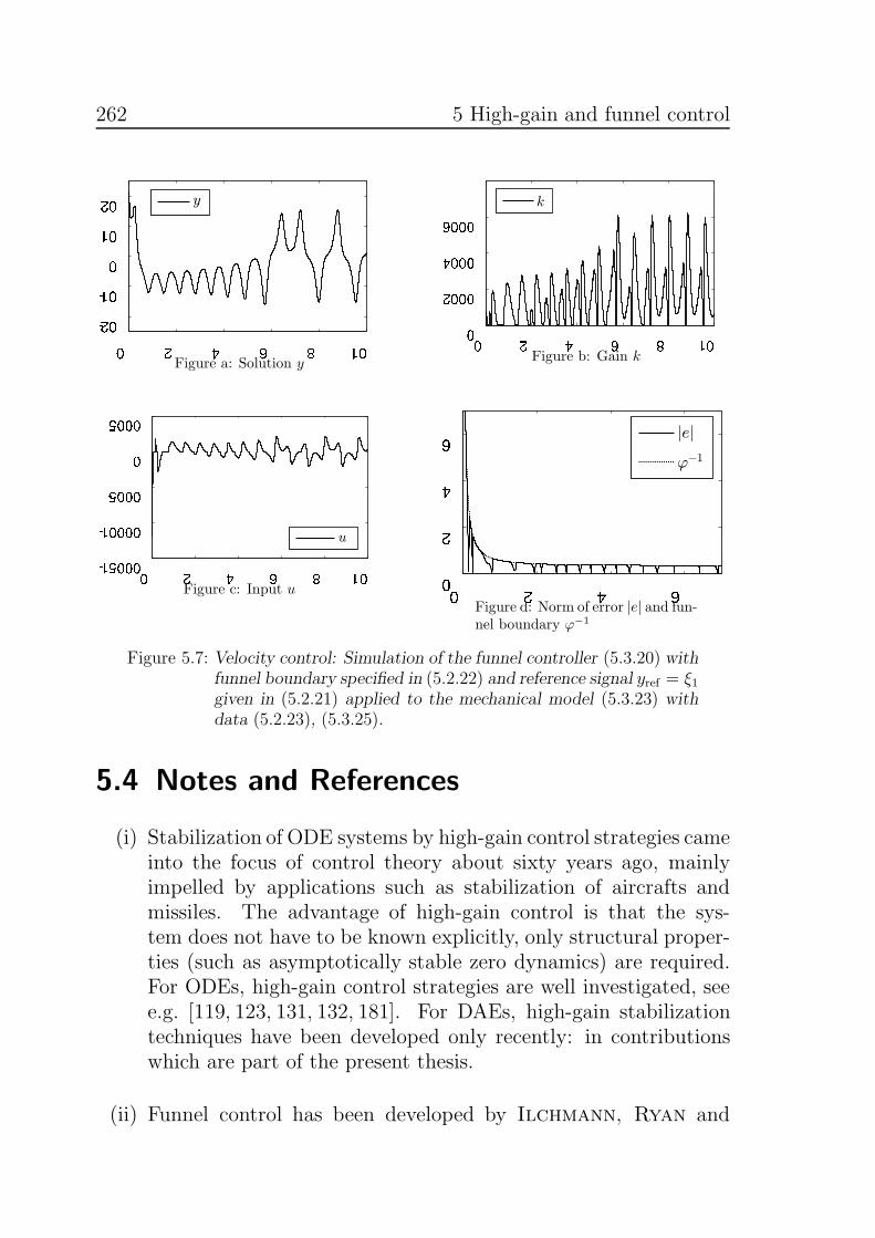
262 5 High-gain and funnel control
0 2 4 6 8 1 0
- 2 0
- 1 0
0
1 0
2 0 �
Figure a: Solution y
0 2 4 6 8 1 0
0
2 0 0 0
4 0 0 0
6 0 0 0
�
Figure b: Gain k
0 2 4 6 8 1 0
- 1 5 0 0 0
- 1 0 0 0 0
- 5 0 0 0
0
5 0 0 0
�
Figure c: Input u 0 2 4 6
0
2
4
6 ���
���
Figure d: Norm of error |e| and fun-nel boundary ϕ−1
Figure 5.7: Velocity control: Simulation of the funnel controller (5.3.20) withfunnel boundary specified in (5.2.22) and reference signal yref = ξ1given in (5.2.21) applied to the mechanical model (5.3.23) withdata (5.2.23), (5.3.25).
5.4 Notes and References
(i) Stabilization of ODE systems by high-gain control strategies cameinto the focus of control theory about sixty years ago, mainlyimpelled by applications such as stabilization of aircrafts andmissiles. The advantage of high-gain control is that the sys-tem does not have to be known explicitly, only structural proper-ties (such as asymptotically stable zero dynamics) are required.For ODEs, high-gain control strategies are well investigated, seee.g. [119, 123, 131, 132, 181]. For DAEs, high-gain stabilizationtechniques have been developed only recently: in contributionswhich are part of the present thesis.
(ii) Funnel control has been developed by Ilchmann, Ryan and

5.4 Notes and References 263
Sangwin [125] to overcome the disadvantages of high-gain con-trol with the intuition to incorporate a time-varying gain func-tion k(·) and use high values k(t) only when required such thattracking with prescribed transient behavior is guaranteed (cf. Sec-tion 5.2). Nowadays, funnel controllers have been applied ina lot of technical areas, such as chemical reactor models [129],control of two-mass systems [108, 128], electrical drives [217],robotics [109] and mechatronics [110]. The simple design andmoderate structural requirements make funnel controllers an em-inent alternative to standard PI/PID controllers, which are oftenused in the engineering sciences.
(iii) The definition of vector relative degree given by Isidori [131,Sec. 5.1] is local, i.e., stated for a neighborhood of a nominalpoint x0; for single-input single-output systems a global version(the uniform relative degree) is given in [131, Sec. 9.1]. An exten-sion of the uniform relative degree concept to time-invariant non-linear systems is given by Liberzon, Morse and Sontag [164].For linear ODE systems, a global version of the vector relativedegree has been stated by Mueller [180, 181]. The concept ofstrict relative degree for multi-input multi-output systems hasbeen extended to time-varying linear and nonlinear systems byIlchmann and Mueller [122].

265
6 Electrical circuits
In this chapter we consider linear differential-algebraic systems[E,A,B, C] ∈ Σn,n,m,m of the form
ddtEx(t) = Ax(t) + Bu(t)
y(t) = Cx(t) ,
which arise from modified nodal analysis (MNA) models of electricalcircuits, cf. Section 1.5. The considered circuits may contain linear re-sistances, capacitances and inductances. The circuits can be describedby differential-algebraic input-output systems, where the input consistsof voltages of voltage sources and currents of current sources and theoutput consists of currents of voltage sources and voltages of currentsources (cf. Section 6.8 (ii) for alternative output assignments).As a main tool for the study of electrical circuits the notion of positive
real rational functions is introduced and related to certain configura-tions of circuits in Section 6.1. In order to introduce the MNA modelingprocedure, graph theoretical preliminaries are explained in Section 6.2and the absence of K-cutsets and K-loops is characterized in terms ofincidence matrices. The latter is important to derive topological cri-teria for asymptotic stability of electrical circuits in Section 6.3; forthis result a reduction of the circuit pencil is developed. In Section 6.4we show that, for models of electrical circuits, asymptotic stability ofthe zero dynamics is a structural property. That is, this property canbe guaranteed if the circuit has certain interconnectivity properties.These criteria do not incorporate any parameter values. In this con-text, we also characterize the absence of invariant zeros in the closedright half-plane. Stabilization by high-gain output-feedback is inves-tigated in Section 6.5. For systems with asymptotically stable zerodynamics, we prove that funnel control is feasible in Section 6.6. Thisresult is illustrated by the simulation of a discretized transmission line
266 6 Electrical circuits
in Section 6.7.The results in Sections 6.1–6.7 stem from a joint work with Timo
Reis which is submitted for publication [39].
6.1 Positive real rational functions
In this section we introduce the concept of positive realness for rationalmatrix functions and state a representation for this class. We alsoderive equivalent conditions for positive realness of matrix pencils andderive some properties of these pencils. These concepts and findingswill play an important role for the analysis of MNA models.
Definition 6.1.1 (Positive real rational function).A rational matrix function G(s) ∈ R(s)m×m is called positive real if,and only if, G(s) does not have any poles in C+ and, for all λ ∈ C+,we have
G(λ) +G∗(λ) ≥ 0.
For the definition of a pole of a rational matrix function see Defini-tion 4.3.1.
Lemma 6.1.2 (Properties of positive real functions [2, Sec. 5.1]).Let G(s) ∈ R(s)m×m be positive real. Then there exist ω1, . . . , ωk ∈ R,Hermitian and positive semi-definite matrices M1, . . . ,Mk ∈ Cm×m,M0,M∞ ∈ Rm×m and some proper and positive real function Gs(s) ∈R(s)m×m which does not have any poles on iR, such that
G(s) = Gs(s) + sM∞ +M0
s+
k∑
j=1
Mj
s− iωj+
M j
s+ iωj.
In particular, we may characterize the positive realness of matrixpencils sE−A ∈ R[s]n×n by means of certain definiteness properties ofthe matrices E,A ∈ Rn×n.
Lemma 6.1.3 (Positive real matrix pencils).A matrix pencil sE − A ∈ R[s]n×n is positive real if, and only if, E =E⊤ ≥ 0 and A+ A⊤ ≤ 0.
6.1 Positive real rational functions 267
Proof: “⇒”: Since sE −A is positive real, Lemma 6.1.2 implies exis-tence of some additive decomposition
sE − A = sM∞ +Gs(s),
where Gs(s) ∈ R(s)n×n is proper and positive real, and M∞ ∈ Rn×n
is symmetric and positive semi-definite. Therefore, we obtain E =E⊤ = M∞ ≥ 0, and the constant rational function Gp(s) = −A ispositive real. The latter implies, by definition of positive realness, thatA+ A⊤ ≤ 0.“⇐”: Since E = E⊤ ≥ 0 and A + A⊤ ≤ 0 we have that, for all
λ ∈ C+,
(λE−A)+(λE−A)∗ = λE+λE⊤−A−A⊤ = 2Re(λ)E−(A+A⊤) ≥ 0.(6.1.1)
Therefore, sE −A is positive real.
In the following we collect some further properties of positive realmatrix pencils sE−A with the additional assumption that the kernelsof E and A intersect trivially. This in particular encompasses regu-lar MNA models of passive electrical networks. Recall that λ ∈ C isan eigenvalue of sE − A if, and only if,
rkC(λE − A) < rkR(s)(sE − A).
Lemma 6.1.4 (Properties of positive real pencil).Let a positive real pencil sE−A ∈ R[s]n×n be such that kerE ∩kerA ={0}. Then the following holds true:
(i) sE −A is regular.
(ii) (sE − A)−1 ∈ R(s)n×n is positive real.
(iii) All eigenvalues of sE −A have non-positive real part.
(iv) All eigenvalues of sE−A on the imaginary axis are semi-simple.
(v) The index of sE − A is at most two.
Proof: Step 1 : To prove that (i) and (iii) hold true, we show thatker(λE − A) = {0} for all λ ∈ C+. Seeking a contradiction, assume

268 6 Electrical circuits
that λ ∈ C+ and x ∈ Cn \ {0} are such that (λE − A)x = 0. Then weobtain
0 = x∗((λE − A) + (λE − A)∗
)x
(6.1.1)= 2Re(λ)x∗Ex− x∗(A+ A⊤)x.
Since, by Lemma 6.1.3, we have E ≥ 0, A + A⊤ ≤ 0 and Re(λ) > 0,it follows x∗Ex = x∗(A + A⊤)x = 0, whence, in particular, Ex = 0.Therefore, the equation (λE − A)x = 0 gives also rise to Ax = 0 andconsequently, x ∈ kerE ∩ kerA = {0}, a contradiction.Step 2 : We show (ii). This is a consequence of
(λE − A)−1 + (λE −A)−∗
= (λE −A)−1((λE − A)∗ + (λE − A))(λE − A)−∗
(6.1.1)= (λE −A)−1(2Re(λ)E − (A+ A⊤))(λE − A)−∗,
E ≥ 0, A+A⊤ ≤ 0 and Re(λ) > 0.Step 3 : It remains to show that (iv) and (v) are valid: Since (sE −
A)−1 is positive real by (ii), Lemma 6.1.2 gives rise to the fact thatall poles on the imaginary axis are of order one and, moreover, (sE −A)−1 = sM + Gp(s), where Gp(s) ∈ R[s]n×n is proper and M ∈ Rn×n.This in particular means that s−1(sE − A)−1 is proper. Let W,T ∈Gln(C) be such that W (sE − A)T is in KCF as in Corollary 2.3.21.Regularity of sE −A then gives rise to
(sE − A)−1
= T−1diag (J λ1ρ1(s)−1, . . . ,J λb
ρb(s)−1,Nσ1
(s)−1, . . . ,Nσc(s)−1)W−1.
(6.1.2)
Assuming that (iv) does not hold, i.e., there exists some ω ∈ R suchthat iω is an eigenvalue of sE−A which is not semi-simple. Then thereexists some j ∈ {1, . . . , b} such that λj = iω and ρj > 1. Hence, due to
J iωρj (s)
−1 =
ρj−1∑
l=0
1
(s− iω)l+1N l
ρj ,
the formula (6.1.2) implies that (sE −A)−1 has a pole of order greaterthan one on the imaginary axis, a contradiction.
6.2 Graph theoretical preliminaries 269
Assume that (v) does not hold, i.e., the index of sE − A exceeds two.Then there exists some j ∈ {1, . . . , c} such that σj > 2 and
Nσj(s)−1 = −
σj−1∑
l=0
slN lσj.
This contradicts properness of s−1(sE − A)−1.
6.2 Graph theoretical preliminaries
In this section we introduce the graph theoretical concepts (cf. for in-stance [86]) which are crucial for the modified nodal analysis of electri-cal circuits. We derive some characterizations for the absence of cutsetsand loops in a given subgraph. These characterizations will be givenin terms of algebraic properties of the incidence matrices.
Definition 6.2.1 (Graph theoretical concepts).A graph is a triple G = (V, E, ϕ) consisting of a node set V and a branchset E together with an incidence map
ϕ : E → V × V, e 7→ ϕ(e) = (ϕ1(e), ϕ2(e)) ,
where ϕ1(e) 6= ϕ2(e) for all e ∈ E, i.e., the graph does not containself-loops. If ϕ(e) = (v1, v2), we call e to be directed from v1 to v2. v1is called the initial node and v2 the terminal node of e. Two graphsGa = (Va, Ea, ϕa), Gb = (Vb, Eb, ϕb) are called isomorphic, if there existbijective mappings ιE : Ea → Eb, ιV : Va → Vb, such that ϕa,1 =ι−1V ◦ ϕb,1 ◦ ιE and ϕa,2 = ι−1
V ◦ ϕb,2 ◦ ιE.Let V ′ ⊆ V and let E ′ be a set of branches satisfying
E ′ ⊆ E|V ′ := { e ∈ E | ϕ1(e) ∈ V ′ and ϕ2(e) ∈ V ′ } .
Further let ϕ|E′ be the restriction of ϕ to E ′. Then the triple K :=(V ′, E ′, ϕ|E′) is called a subgraph of G. In the case where E ′ = E|V ′,we call K the induced subgraph on V ′. If V ′ = V , then K is calleda spanning subgraph. A proper subgraph is one with E 6= E ′.G is called finite, if both the node and the branch set are finite.For each branch e, define an additional branch −e being directed
from the terminal to the initial node of e, that is ϕ(−e) = (ϕ2(e), ϕ1(e))
270 6 Electrical circuits
for e ∈ E. Now define the set E = { e | e ∈ E or − e ∈ E }. A tuplew = (w1, . . . , wr) ∈ Er, where for i = 1, . . . , r − 1,
v0 := ϕ1(v1), vi := ϕ2(wi) = ϕ1(wi+1)
is called path from v0 to vr; w is called elementary path, if v1, . . . , vr aredistinct. A loop is an elementary path with v0 = vr. Two nodes v, v′
are called connected, if there exists a path from v to v′. The graph itselfis called connected, if any two nodes are connected. A subgraph K =(V ′, E ′, ϕ|E′) is called a component of connectivity, if it is connectedand Kc := (V \ V ′, E \ E ′, ϕ|E\E′) is a subgraph.
A spanning subgraph K = (V, E ′, ϕ|E′) is called a cutset of G =(V, E, ϕ), if its branch set is non-empty, G −K := (V, E \E ′, ϕ|E\E′) is
a disconnected subgraph and G − K′ is a connected subgraph for anyproper spanning subgraph K′ of K.
For finite graphs we can set up special matrices which will be usefulto describe Kirchhoff’s laws.
Definition 6.2.2 (Incidence matrix).Let a finite graph G = (V, E, ϕ) with l branches E = {e1, . . . , el} andk nodes V = {v1, . . . , vk} be given. Then the all-node incidence matrixof G is given by A0 = (aij) ∈ Rk×l, where
aij =
1, if ϕ1(ej) = vi,
−1, if ϕ2(ej) = vi,
0, otherwise.
Since the rows of A0 sum up to the zero row vector, one might deletean arbitrary row of A0 to obtain a matrix A having the same rank asA0. We call A an incidence matrix of G.
This section continues with some results on the relation betweenproperties of subgraphs and linear algebraic properties of correspondingsubmatrices of incidence matrices. First we declare some manners ofspeaking.
Definition 6.2.3.Let G be a graph, K be a spanning subgraph of G, L be a subgraph ofG, and ℓ be a path of G.

6.2 Graph theoretical preliminaries 271
(i) L is called a K-cutset, if L is a cutset of K.
(ii) ℓ is called a K-loop, if ℓ is a loop of K.
A spanning subgraph K of the finite graph G has an incidence matrixAK which is constructed by deleting columns of the incidence matrixA of G corresponding to the branches of the complementary spanningsubgraph G−K. By a suitable reordering of the branches, the incidencematrix reads
A =[AK AG−K
]. (6.2.1)
The following lemma can be inferred form [209, Lem. 2.1 & Lem. 2.3].
Lemma 6.2.4 (Subgraphs and incidence matrices).Let G be a connected graph with incidence matrix A ∈ R(k−1)×l. Further,let K be a spanning subgraph. Assume that the branches of G are sortedin a way that (6.2.1) is satisfied. Then the following holds true:
(i) The following two assertions are equivalent:
a) G does not contain K-cutsets.
b) kerA⊤G−K = {0}.
(ii) The following two assertions are equivalent:
a) G does not contain K-loops.
b) kerAK = {0}.
The following two auxiliary results are concerned with properties ofsubgraphs of subgraphs, and give some equivalent characterizations interms of properties of their incidence matrices.
Lemma 6.2.5 (Loops in subgraphs [209, Prop. 4.5]).Let G be a connected graph with incidence matrix A ∈ R(k−1)×l. Further,let K be a spanning subgraph of G, and let L be a spanning subgraph ofK. Assume that the branches of G are sorted in a way that
A =[AL AK−L AG−K
]and AK =
[AL AK−L
].
Then the following two assertions are equivalent:
a) G does not contain K-loops except for L-loops.

272 6 Electrical circuits
b) kerAK = kerAL × {0}.
Lemma 6.2.6 (Cutsets in subgraphs [209, Prop. 4.4]).Let G be a connected graph with incidence matrix A ∈ R(k−1)×l. Further,let K be a spanning subgraph of G, and let L be a spanning subgraph ofK. Assume that the branches of G are sorted in a way that
A =[AL AK−L AG−K
]and AG−L =
[AK−L AG−K
].
Then the following two assertions are equivalent:
a) G does not contain K-cutsets except for L-cutsets.
b) kerA⊤G−K = kerA⊤
G−L.
6.3 Circuit equations
It is well-known [83,116] that the graph underlying an electrical circuitcan be described by an incidence matrix A ∈ R(k−1)×l, which can bedecomposed into submatrices
A =[AC AR AL AV AI
]
where AC ∈ Rne×nC ,AR ∈ Rne×nG ,AL ∈ Rne×nL,AV ∈ Rne×nV ,AI ∈Rne×nI , ne = k− 1 and l = nC + nG + nL + nV + nI . Each submatrix isthe incidence matrix of a specific subgraph of the circuit graph. AC isthe incidence matrix of the subgraph consisting of all circuit nodes andall branches corresponding to capacitors. Similarly, AR,AL,AV ,AI arethe incidence matrices corresponding to the resistor, inductor, voltagesource and current source subgraphs, resp. Then using the standardMNA modeling procedure [116], which is just a clever arrangementof Kirchhoff’s laws together with the characteristic equations of thedevices, results in a differential-algebraic system (4.1.1) with
sE−A =
sACCA⊤
C +ARGA⊤R AL AV
−A⊤L sL 0
−A⊤V 0 0
, B = C⊤ =
−AI 00 00 −InV
,
(6.3.1)x = (η⊤, i⊤L , i
⊤V )
⊤, u = (i⊤I , v⊤V )
⊤, y = (−v⊤I ,−i⊤V )⊤, (6.3.2)
6.3 Circuit equations 273
where
C ∈ RnC×nC ,G ∈ RnG×nG ,L ∈ RnL×nL,
AC ∈ Rne×nC ,AR ∈ Rne×nG ,AL ∈ Rne×nL,AV ∈ Rne×nV ,AI ∈ Rne×nI ,
n = ne + nL + nV , m = nI + nV .
(6.3.3)C, G and L are the matrices expressing the consecutive relations ofcapacitances, resistances and inductances, η(t) is the vector of nodepotentials, iL(t), iV(t), iI(t) are the vectors of currents through induc-tances, voltage and current sources, and vV(t), vI(t) are the voltages ofvoltage and current sources.
Definition 6.3.1 (MNA model).For a given linear electrical circuit, any differential-algebraicsystem (4.1.1) satisfying (6.3.1)–(6.3.3), which arises from the MNAmodeling procedure [116], is said to be an MNA model of the circuit.
It is a reasonable assumption that an electrical circuit is connected;otherwise, since the components of connectivity do not physically inter-act, one might consider them separately. Furthermore, in the presentchapter we consider circuits with passive devices. These assumptionslead to the following assumptions on the MNA model (6.3.1)–(6.3.3) ofthe circuit (compare Lemma 6.2.4).
(C1) rk[AC AR AL AV AI
]= ne,
(C2) C = C⊤ > 0,L = L⊤ > 0,G + G⊤ > 0.
It is possible that in the circuit equations (4.1.1) there are still re-dundant equations and superfluous variables, i.e., in general the pencilsE − A arising from (6.3.1), (6.3.3) is not regular. In the followingwe show how this can be overcome by a simple transformation; thereduced circuit model is regular and positive real. This transformationis also important to show feasibility of funnel control in Section 6.6.
Theorem 6.3.2 (Reduction of circuit pencil).Let sE − A ∈ R[s]n×n with E,A as in (6.3.1), (6.3.3) be given andsuppose that (C1) and (C2) hold. Let ZCRLV , Z ′
CRLV , ZV , Z ′V be real
matrices with full column rank such that
imZCRLV = ker[AC AR AL AV
]⊤, im ZV = kerAV ,
imZ ′CRLV = im
[AC AR AL AV
], im Z ′
V = imA⊤V .
274 6 Electrical circuits
Then we have
T =
Z ′CRLV 0 0 ZCRLV 00 InL
0 0 00 0 Z ′
V 0 ZV
∈ Gln(R), (6.3.4)
and
T⊤(sE −A)T =
[sE − A 0
0 0
],
where the pencil
sE − A =
[(Z ′
CRLV)⊤(sACCA⊤
C +ARGA⊤R
)Z ′CRLV (Z ′
CRLV)⊤AL (Z ′
CRLV)⊤AV Z
′V
−A⊤LZ
′CRLV sL 0
−Z ′VA
⊤VZ
′CRLV 0 0
]
(6.3.5)
is regular and satisfies ker E∩ker A = {0}, E = E⊤ ≥ 0 and A+ A⊤ ≤0.
Proof: The invertibility of T is a consequence of imZCRLV ⊕ imZ ′CRLV
= Rne and im ZV ⊕ im Z ′V = RnV . The properties E = E⊤ ≥ 0 and
A+ A⊤ ≤ 0 follow immediately from the construction of E and A. Toprove that sE − A is regular, it suffices by Lemma 6.1.4 to show thatker E ∩ ker A = {0}: Let x ∈ ker E ∩ ker A. Partitioning according
to the block structure of E and A, i.e., x = (x⊤1 , x⊤2 , x
⊤3 )
⊤, and using
that, by (C2), C > 0, L > 0 and G + G⊤ > 0, we obtain from x⊤Ex =
x⊤(A+ A⊤)x = 0 that x2 = 0 and
[A⊤
CA⊤
R
]Z ′CRLVx1 = 0. (6.3.6)
Furthermore, Ax = 0 gives rise to
(a) (Z ′V)
⊤A⊤VZ
′CRLVx1 = 0,
(b) A⊤LZ
′CRLVx1 = 0, and
(c) (Z ′CRLV)
⊤AVZ ′Vx3 = 0.
(a) implies
A⊤VZ
′CRLVx1 ∈ ker(Z ′
V)⊤ = (im Z ′
V)⊥ = (imA⊤
V )⊥,

6.3 Circuit equations 275
whence A⊤VZ
′CRLVx1 = 0. Together with (6.3.6) and (b) this yields
Z ′CRLVx1 ∈ ker
[AC AR AL AV
]⊤= imZCRLV = (imZ ′
CRLV)⊥,
and therefore x1 = 0. By (c) we find
AVZ′Vx3 ∈ ker(Z ′
CRLV)⊤ = (imZ ′
CRLV)⊥
= ker[AC AR AL AV
]⊤ ⊆ kerA⊤V = (imAV)
⊥,
and thus AVZ ′Vx3 = 0. From this, we obtain
Z ′Vx3 ∈ kerAV = (imA⊤
V )⊥ = (im Z ′
V)⊥,
whence x3 = 0.
We may infer the following characterization of the presence of eigen-values from Theorem 6.3.2.
Corollary 6.3.3 (Kernel and eigenvalues).Let sE − A ∈ R[s]n×n with E,A as in (6.3.1), (6.3.3) be given andsuppose that (C1) and (C2) hold. Then
kerR(s) sE −A = kerR(s)[AC AR AL AV
]⊤ × {0} × kerR(s)AV .
Furthermore, λ ∈ C is not an eigenvalue of sE −A if, and only if,
kerC λE − A = kerC[AC AR AL AV
]⊤ × {0} × kerCAV .
Proof: Using the transformation matrix T in (6.3.4) and accompany-ing notation from Theorem 6.3.2, we obtain (denoting the number ofcolumns of ZCRLV by k1 and the number of columns of ZV by k2) that
kerR(s) sE −A = T(kerR(s)(sE − A)︸ ︷︷ ︸
={0}
× R(s)k1+k2)
= imR(s)ZCRLV × {0} × imR(s) ZV
= kerR(s)[AC AR AL AV
]⊤ × {0} × kerR(s)AV .
Now let λ ∈ C and observe that
kerC λE −A = T(kerC λE − A× Ck1+k2
).

276 6 Electrical circuits
Recall that λ is not an eigenvalue of sE−A if, and only if, rkC λE−A =rkR(s) sE − A or, equivalently, dimkerC λE − A = dimkerR(s) sE − A.
Therefore, λ is not an eigenvalue of sE−A if, and only if, kerC λE−A ={0} and this implies the last statement of the corollary.
In the following we will use expressions like VL-loop for a loop in thecircuit graph whose branch set consists only of branches correspond-ing to voltage sources and/or inductors. Likewise, a IC-cutset is acutset in the circuit graph whose branch set consist only of branchescorresponding to current sources and/or capacitors.
Corollary 6.3.4 (Regularity of circuit pencil).Let sE−A ∈ R[s]n×n with E,A as in (6.3.1), (6.3.3) be an MNA modelof an electrical circuit and suppose that (C1) and (C2) hold. Then thefollowing statements are equivalent:
(i) sE − A is regular.
(ii) ker[AC AR AL AV
]⊤= {0} and kerAV = {0}.
(iii) The circuit neither contains V-loops nor I-cutsets.Proof: The result follows immediately from Corollary 6.3.3 andLemma 6.2.4.
Next we give sufficient criteria for the absence of purely imaginaryeigenvalues of the pencil sE−A as in (6.3.1), (6.3.3). This result can beseen as a generalization of the results in [209] to circuits which mightcontain I-cutsets and/or V-loops, i.e., where sE −A is not necessarilyregular.
Theorem 6.3.5 (Absence of imaginary eigenvalues).Let sE − A ∈ R[s]n×n with E,A as in (6.3.1), (6.3.3) be an MNAmodel of an electrical circuit and suppose that (C1) and (C2) hold.Furthermore, suppose that at least one of the following two assertionsholds:
(i) The circuit neither contains VL-loops except for V-loops, norICL-cutsets except for IL-cutsets; equivalently
ker[AV AL
]= kerAV × {0}
and ker[AR AV
]⊤= ker
[AC AR AV
]⊤.
(6.3.7)

6.3 Circuit equations 277
(ii) The circuit neither contains IC-cutsets except for I-cutsets, norVCL-loops except for VC-loops; equivalently
ker[AR AL AV
]⊤= ker
[AC AR AL AV
]⊤
and ker[AV AC AL
]= ker
[AV AC
]× {0}.
(6.3.8)
Then all eigenvalues of sE −A are contained in C−.
Proof: The equivalent characterizations of the absence of certain loopsor cutsets in the circuit graph, resp., and kernel conditions on theelement-related incidence matrices follow from Lemmas 6.2.5 and 6.2.6.By Theorem 6.3.2 and Lemma 6.1.4 all eigenvalues of sE − A are
contained in C−. Then, using Corollary 6.3.3, we have to show that
∀ω ∈ R : kerC(iωE −A) = kerC[AC AR AL AV
]⊤ × {0} × kerCAV .(6.3.9)
Since “⊇” does always hold true, we show “⊆”. Let ω ∈ R and x1 ∈Cne, x2 ∈ CnL and x3 ∈ CnV be such that
x := (x⊤1 , x⊤2 , x
⊤3 )
⊤ ∈ kerC(iωE − A). (6.3.10)
By the structure of sE−A as in (6.3.1), relation (6.3.10) implies A⊤Vx1 =
0 and
0 = x∗((iωE −A) + (iωE −A)∗
)x = −x∗(A+A⊤)x
= −x∗1AR(G + G⊤)A⊤Rx1,
hence A⊤Rx1 = 0 since G + G⊤ > 0 by (C2).
We show that (i) implies (6.3.9): Since x1 ∈ kerC[AR AV
]⊤we
obtain from (6.3.7) that x1 ∈ kerCA⊤C . Then (6.3.10) implies ALx2 +
AVx3 = 0 and by (6.3.7) we find AVx3 = 0 and x2 = 0. The latterimplies that x1 ∈ kerCA
⊤L . Altogether, we have that (6.3.9) is valid.
We show that (ii) implies (6.3.9): From (6.3.10) we have
AC(iωCA⊤C x1) + ALx2 +AVx3 = 0, (6.3.11)
and by (6.3.8) we obtain x2 = 0. This implies A⊤Lx1 = 0, hence
x1 ∈ kerC[AR AL AV
]⊤which by (6.3.8) yields
[AC AR AL AV
]⊤x1 = 0.
Now, from (6.3.11) we have AVx3 = 0 and (6.3.9) is shown.

278 6 Electrical circuits
6.4 Zero dynamics and invariant zeros
In this section we derive topological characterizations of autonomousand asymptotically stable zero dynamics of the circuit system. Thelatter is done by an investigation of the invariant zeros of the system.
Using a simple transformation of the system, properties of the zerodynamics can be led back to properties of a circuit pencil where voltagesources are replaced with current sources, and vice versa. To this end,consider [E,A,B, C] ∈ Σn,n,m,m with (6.3.1), (6.3.3) and define thematrices W,T ∈ Gln+m(R) by
W =
Ine0 0 0 −AV
0 InL0 0 0
0 0 0 −InI0
0 0 0 0 InV
0 0 InV 0 0
, T =
Ine0 0 0 0
0 InL0 0 0
0 0 0 InV0
0 0 InI0 0
−A⊤V 0 0 0 InV
.
Then we obtain
W
[sE − A −B−C 0
]T =
sACCA⊤C + ARGA⊤
R AL AI 0 0−A⊤
L sL 0 0 0−A⊤
I 0 0 0 00 0 0 InV
00 0 0 0 InV
.
(6.4.1)As desired, the upper left part is a matrix pencil which is an MNAmodel of a circuit in which voltage sources are replaced with currentsources, and vice versa. We may now derive the following importantproperties, which are immediate from Corollary 6.3.3 and (6.4.1).
Corollary 6.4.1 (Kernel and eigenvalues of system pencil).Let [E,A,B, C] ∈ Σn,n,m,m with (6.3.1), (6.3.3) be an MNA model of

6.4 Zero dynamics and invariant zeros 279
an electrical circuit and suppose that (C1) and (C2) hold. Then
kerR(s)
[sE −A −B−C 0
]
=
x1(s)00
x3(s)−A⊤
Vx1(s)
∣∣∣∣∣∣∣∣∣∣
x1(s) ∈ kerR(s)[AC AR AL AI
]⊤,
x3(s) ∈ kerR(s)AI
.
Furthermore, λ ∈ C is not an eigenvalue of[sE−A −B−C 0
]if, and only if,
kerC
[λE − A −B−C 0
]
=
x100x3
−A⊤Vx1
∣∣∣∣∣∣∣∣∣∣
x1 ∈ kerC[AC AR AL AI
]⊤,
x3 ∈ kerCAI
.
We now aim to characterize autonomous zero dynamics.
Proposition 6.4.2 (Autonomous zero dynamics).Let [E,A,B, C] ∈ Σn,n,m,m with (6.3.1), (6.3.3) be an MNA model ofan electrical circuit and suppose that (C1) and (C2) hold. Then thefollowing statements are equivalent:
(i) The zero dynamics ZD[E,A,B,C] are autonomous.
(ii) rkR(s)[sE−A −B−C 0
]= n+m.
(iii) kerR(s)[sE−A −B−C 0
]= {0}.
(iv) ker[AC AR AL AI
]⊤= {0} and kerAI = {0}.
(v) The circuit neither contains I-loops nor V-cutsets.Proof: The equivalence of (i) and (ii) follows from Proposition 4.1.5since the rank over R[s] and over R(s) coincide. (ii)⇔(iii) is clear and(iii)⇔(iv) follows from Corollary 6.4.1. The equivalence of (iv) and (v)is then a consequence of Lemma 6.2.4.

280 6 Electrical circuits
In order to characterize asymptotic stability of the zero dynamics weneed the concept of invariant zeros. An invariant zero of [E,A,B, C] ∈Σn,n,m,m is defined as an eigenvalue of
[sE−A −B−C 0
], see e.g. [176].
Definition 6.4.3 (Invariant zeros).Let [E,A,B, C] ∈ Σn,n,m,m. Then λ ∈ C is called an invariant zero of[E,A,B, C] if, and only if,
rkC
[λE − A −B−C 0
]< rkR(s)
[sE − A −B−C 0
].
From Theorem 6.3.5 and (6.4.1) we get the following result on thelocation of invariant zeros.
Corollary 6.4.4 (Location of invariant zeros).Let [E,A,B, C] ∈ Σn,n,m,m with (6.3.1), (6.3.3) be an MNA model of anelectrical circuit and suppose that (C1) and (C2) hold. Furthermore,suppose that at least one of the following two assertions holds:
(i) The circuit neither contains IL-loops except for I-loops, norVCL-cutsets except for VL-cutsets.
(ii) The circuit neither contains VC-cutsets except for V-cutsets, norICL-loops except for IC-loops.
Then all invariant zeros of [E,A,B, C] are contained in C−.
We are now in the position to characterize asymptotically stable zerodynamics.
Theorem 6.4.5 (Asymptotically stable zero dynamics).Let [E,A,B, C] ∈ Σn,n,m,m with (6.3.1), (6.3.3) be an MNA model of anelectrical circuit and suppose that (C1) and (C2) hold. Then the zerodynamics ZD[E,A,B,C] are asymptotically stable if, and only if,
a) ZD[E,A,B,C] are autonomous and
b) all invariant zeros of [E,A,B, C] are contained in C−.
Furthermore, suppose that at least one of the following two assertionsholds:

6.5 High-gain stabilization 281
(i) The circuit neither contains IL-loops, nor VCL-cutsets except forVL-cutsets with at least one inductor.
(ii) The circuit neither contains VC-cutsets, nor ICL-loops except forIC-loops with at least one capacitor.
Then the zero dynamics ZD[E,A,B,C] are asymptotically stable.
Proof: Step 1 : We show that asymptotically stable zero dynamicsimply a) and b). a) follows from the fact that asymptotically stablezero dynamics are autonomous and b) follows from Lemma 4.3.9.Step 2 : We show that a) and b) imply asymptotically stable zero
dynamics. By a) and Proposition 6.4.2 we find that rkR(s)[sE−A −B−C 0
]=
n+m. Then b) implies that
∀λ ∈ C+ : rkC
[λE − A −B−C 0
]= rkR(s)
[sE −A −B−C 0
]= n+m,
and therefore Lemma 4.3.9 gives asymptotic stability of the zero dy-namics.Step 3 : We show that (i) or (ii) implies asymptotically stable zero
dynamics. In particular, we have “The circuit neither contains I-loopsnor V-cutsets” and hence Proposition 6.4.2 implies a). Furthermore, (i)or (ii) from Corollary 6.4.4 holds true and therefore b) is valid. Thisyields the assertion of the theorem.
6.5 High-gain stabilization
In this section we consider high-gain output feedback for a system[E,A,B, C] ∈ Σn,n,m,m which arises from MNA modeling of an electri-cal circuit. Recall that by Definition 5.1.1, roughly speaking, a systemis called high-gain stabilizable if the closed-loop system
ddtEx(t) = (A− kBC)x(t). (6.5.1)
is asymptotically stable for k > 0 large enough. In other words, thereexists κ > 0 such that for all k ≥ κ the pencil sE − (A − kBC) isregular and all of its eigenvalues are contained in C−.

282 6 Electrical circuits
We will show that for electrical circuits, i.e., [E,A,B, C]with (6.3.1), (6.3.3), the high-gain need not be high; any positive kis sufficient. In order to achieve this, note that we have
sE − (A− kBC) =
sACCA⊤
C +ARGA⊤R + kAIA⊤
I AL AV−A⊤
L sL 0−A⊤
V 0 kInV
.
(6.5.2)Then, for
W =
Ine
0 −k−1AV0 InL
00 0 k−1InV
, T =
Ine0 0
0 InL0
k−1A⊤V 0 InV
,
we find that
W (sE − (A− kBC))T
=
sACCA⊤
C +ARGA⊤R + kAIA⊤
I + k−1AVA⊤V AL 0
−A⊤L sL 0
0 0 InV
. (6.5.3)
The upper left part is a matrix pencil which is an MNA model ofa circuit in which all current and voltage sources are replaced withresistances of values k−1 and k, resp. We may therefore conclude thefollowing from Corollary 6.3.4.
Corollary 6.5.1 (Closed-loop pencil is regular).Let [E,A,B, C] ∈ Σn,n,m,m with (6.3.1), (6.3.3) be given and supposethat (C1) and (C2) hold true. Then, for all k > 0, the pencil sE −(A− kBC) is regular.
As a consequence of Theorem 6.3.5, we can furthermore analyze theasymptotic stability of the closed-loop system.
Theorem 6.5.2 (Asymptotic stability of closed-loop pencil).Let [E,A,B, C] ∈ Σn,n,m,m with (6.3.1), (6.3.3) be an MNA model of anelectrical circuit and suppose that (C1) and (C2) hold. Furthermore,suppose that at least one of the following two assertions holds true:
(i) The circuit neither contains L-loops, nor CL-cutsets except forL-cutsets.

6.6 Funnel control 283
(ii) The circuit neither contains C-cutsets, nor CL-loops except forC-loops.
Then, for any k > 0, all eigenvalues of sE − (A− kBC) are containedin C−.
Remark 6.5.3 (Asymptotically stable zero dynamics and high-gain).Let [E,A,B, C] ∈ Σn,n,m,m with (6.3.1), (6.3.3) be an MNA model ofan electrical circuit and suppose that (C1) and (C2) hold. Then, underone of the assumptions (i) or (ii) from Theorem 6.4.5, the respectiveassumption from Theorem 6.5.2 holds true, but not vice versa. There-fore, the (topological condition for) asymptotic stability of the zerodynamics implies high-gain stabilizability, but in general not the otherway round, cf. Theorems 5.1.4 and 5.3.13.
6.6 Funnel control
In this section we consider funnel control for systems [E,A,B, C] ∈Σn,n,m,m
with (6.3.1), (6.3.3). The aim is to achieve tracking of a reference tra-jectory by the output signal with prescribed transient behavior. We usethe theory developed in Chapter 5 and the notation from Section 5.2.1.The control objective is output feedback regulation so that the track-
ing error e = y − yref, where yref is the reference signal, evolves withina given funnel Fϕ and all variables are bounded; here ϕ belongs to theclass
Φ :=
ϕ ∈ C∞(R≥0;R) ∩ B1(R≥0;R)
∣∣∣∣∣∣
ϕ(0) = 0, ϕ(s) > 0for all s > 0 andlim infs→∞ ϕ(s) > 0
,
that is, compared to Section 5.2.1, we require that the funnel boundaryϕ−1 is infinitely times continuously differentiable.To ensure error evolution within the funnel, we use the funnel con-
troller (5.2.2) with k = 1:
u(t) = −k(t) e(t), where e(t) = y(t)− yref(t)
k(t) =1
1− ϕ(t)2‖e(t)‖2 .(6.6.1)

284 6 Electrical circuits
Before we state and prove feasibility of funnel control for electricalcircuits, we need to define consistency of the initial value of the closed-loop system and solutions of the latter. We also define what ‘feasibilityof funnel control’ will mean.
Definition 6.6.1 (Consistent initial value).Let [E,A,B, C] ∈ Σn,n,m,m, ϕ ∈ Φ and yref ∈ B∞(R≥0;R
m). An initialvalue x0 ∈ Rn is called consistent for the closed-loopsystem (4.1.1), (6.6.1) if, and only if, there exists a solution of theinitial value problem (4.1.1), (6.6.1), x(0) = x0, i.e., a function x ∈C1([0, ω);Rn) for some ω ∈ (0,∞], such that x(0) = x0 and x satis-fies (4.1.1), (6.6.1) for all t ∈ [0, ω).
Note that, in practice, consistency of the initial state of the ‘un-known’ system should be satisfied as far as the DAE [E,A,B, C] is thecorrect model.In the following we define feasibility of funnel control for a system on
a set of reference trajectories. For reference trajectories we allow signalsin B∞(R≥0;R
m), whereas in Section 5.2.1 signals in Bν+2(R≥0;Rm) are
allowed and ν ∈ N0 is a number which can be calculated out of thesystem inversion form from Definition 4.2.6. For electrical circuits thiscalculation is involved and we omit it here; we restrict ourselves to thecase of B∞(R≥0;R
m).
Definition 6.6.2 (Feasibility of funnel control).Let [E,A,B, C] ∈ Σn,n,m,m and S ⊆ B∞(R≥0;R
m) be a set of refer-ence trajectories. We say that funnel control is feasible for [E,A,B, C]on S if, and only if, for all ϕ ∈ Φ, any reference signal yref ∈ S andany consistent initial value x0 ∈ Rn the application of the funnel con-troller (6.6.1) to (4.1.1) yields a closed-loop initial-value problem thathas a solution and every solution can be extended to a global solution.Furthermore, for every global solution x,
(i) x is bounded and the corresponding tracking error e = Cx −yref evolves uniformly within the performance funnel Fϕ; moreprecisely,
∃ ε > 0 ∀ t > 0 : ‖e(t)‖ ≤ ϕ(t)−1 − ε . (6.6.2)
(ii) the corresponding gain function k given by (6.6.1) is bounded.

6.6 Funnel control 285
Remark 6.6.3 (Bound for the gain).If funnel control is feasible as stated in Definition 6.6.2, then the gainfunction k is bounded in the following way:
∀ t > 0 : k(t) ≤ 1
1− (1− ϕ(t)ε)2,
where ε is given in (6.6.2). For a proof see Step 6 of the proof ofTheorem 5.2.3.
In the following we show that funnel control for systems [E,A,B, C]∈ Σn,n,m,m with (6.3.1), (6.3.3) is feasible provided that the invari-ant zeros have negative real part and the reference signal is suffi-ciently smooth and evolves in a certain subspace. The former meansthat the autonomous part of the zero dynamics has to be asymp-totically stable, but autonomy of the whole zero dynamics is not re-quired. As a preliminary result we derive that, for positive real systems[E,A,B, C] ∈ Σn,n,m,m with asymptotically stable zero dynamics, fun-nel control will be feasible for any sufficiently smooth reference signal.
Proposition 6.6.4 (Funnel control for systems with stable zero dy-namics).Let [E,A,B, C] ∈ Σn,n,m,m be such that E = E⊤ ≥ 0, A+A⊤ ≤ 0, andB = C⊤. Further, assume that the zero dynamics of [E,A,B, C] areasymptotically stable. Then funnel control is feasible for [E,A,B, C]on B∞(R≥0;R
m).
Proof: We aim to apply Theorem 5.2.3 for k = 1 and to this end verifyits assumptions.Step 1 : The zero dynamics of [E,A,B, C] are asymptotically stable
by assumption.Step 2 : We show that for the (left) inverse L(s) of
[sE−A −B−C 0
]over
R(s) the matrix Γ in (5.2.3) exists and satisfies Γ = Γ⊤ ≥ 0. ByLemma 6.1.3, the pencil
[sE −A −BC 0
]=
[In 00 −Im
] [sE − A −B−C 0
]
is positive real. Then L(s) := L(s)[In 00 −Im
]is the inverse of
[sE−A −BC 0
],
and we have
L(λ) + L(λ)∗ = L(λ)([
λE−A −BC 0
]∗+[λE−A −B
C 0
])L(λ)∗ ≥ 0
286 6 Electrical circuits
for all λ ∈ C+. Furthermore, since[sE−A −B−C 0
]does not have any in-
variant zeros in C+, L(s) has no poles in C+. This shows that L(s)is positive real. Hence, H(s) := [0, Im]L(s)[0, Im]
⊤ is positive real andsatisfies H(s) = −[0, Im]L(s)[0, Im]
⊤. Now Lemma 6.1.2 yields that
Γ = lims→∞
s−1H(s) ∈ Rm×m,
exists and satisfies Γ = Γ⊤ ≥ 0.Step 3 : We show that [E,A,B, C] is right-invertible. Since the zero
dynamics of [E,A,B, C] are in particular autonomous it follows fromProposition 6.4.2 (ii) that rkC = m and hence right-invertibility canbe concluded from Remark 4.2.13.Step 4 : It remains to show that k in Theorem 5.2.3 can be chosen
as k = 1 and funnel control is still feasible. A careful inspection of theproof of Theorem 5.2.3 reveals that ‘k large enough’ is needed
a) in Step 1 of the proof of Theorem 5.2.3 to show that the mapM(·) =A22−k
(I+G(·)
), where G(·) = G(·)⊤ ≥ 0 pointwise, is well-defined
(i.e., pointwise invertible) for k ≥ k,
b) in Step 3 of the proof of Theorem 5.2.3 to show that A22− k ·k(t)Imis invertible for all t ≥ 0.
It can be deduced that both a) and b) are satisfied with k = 1 if
A22 − kIm is negative definite for all k > 0, where
A22 = [0, Im−m1]V A22V
⊤[
0Im−m1
],
m1 and the orthogonal matrix V have been defined in Step 1 of theproof of Theorem 5.2.3, and
A22 = lims→∞
([0, Im]L(s)
[0Im
]+ sΓ
)
stems from the form (5.1.4). We may calculate that
A22 = lims→∞
(sΓ−H(s)) = −H0 − lims→∞
Hsp(s)
6.6 Funnel control 287
where, since H(s) is positive real, by Lemma 6.1.2 the rational functionH0 + Hsp(s) is positive real and lims→∞Hsp(s) = 0. Hence, it is easyto derive that H0 ≥ 0 (H0 not necessarily symmetric) and hence
A22 − kIm = −H0 − kIm < 0
for all k > 0 (again A22−kIm not necessarily symmetric). This implies
that A22 − kIm is negative definite for all k > 0.
Before we prove our main result we need to know how feasibility offunnel control behaves under transformation of the system.
Lemma 6.6.5 (Funnel control under system transformation).Let E,A ∈ Rn×n, B,C⊤ ∈ Rn×m and S ⊆ B∞(R≥0;R
m). Further, letW,T ∈ Gln(R), U ∈ Om(R), and define
[E, A, B, C] := [WET,WAT,WBU, U⊤CT ].
Then funnel control is feasible for [E,A,B, C] on S if, and only if,
funnel control is feasible for [E, A, B, C] on U⊤S.
Proof: Observe that (x, u, y) ∈ B[E,A,B,C] and yref ∈ S if, and only if,
(x, u, y) = (T−1x, U⊤u, U⊤y) ∈ B[E,A,B,C] ∧ U⊤yref ∈ U⊤S.
Then the assertion follows from the observation that, for any ϕ ∈ Φ,and tracking errors e = y − yref , e = y − yref we have, for all t ≥ 0,
1
1− ϕ(t)2‖e(t)‖2 =1
1− ϕ(t)2‖e(t)‖2 .
In the following, in order to show that funnel control is feasible forcircuits where all invariant zeros are located in C−, but the zero dynam-ics are not necessarily autonomous, we derive a transformation of thecircuit which decouples the ‘nonautonomous part’ of the zero dynam-ics. This part, in particular, does not affect the input-output behaviorof the system.
Proposition 6.6.6 (Decoupling of circuit pencil).Let [E,A,B, C] ∈ Σn,n,m,m with (6.3.1), (6.3.3) be an MNA model of
288 6 Electrical circuits
an electrical circuit and suppose that (C1) and (C2) hold. Let Z ′CRLI ∈
Rne×k1, ZCRLI ∈ Rne×k2 with full column rank such that
imZCRLI = ker[AC AR AL AI
]⊤,
and imZ ′CRLI = im
[AC AR AL AI
].
Further, let ZV−CRLI ∈ RnV×k3, Z ′V−CRLV ∈ RnV×k4, ZI ∈ RnI×k5, Z ′
I ∈RnI×k6 with orthonormal columns such that
imZV−CRLI = kerZ⊤CRLIAV , im ZI = kerAI ,
imZ ′V−CRLI = imA⊤
VZCRLI , im Z ′I = imA⊤
I .
Then we have
W⊤ := T :=
ZCRLI Z ′
CRLI 0 0 00 0 InL 0 00 0 0 ZV−RCLI Z ′
V−RCLI
∈ Gln(R)
(6.6.3a)and
U :=
[0 ZI Z ′
I 0Z ′V−RCLI 0 0 ZV−RCLI
]∈ Om(R), (6.6.3b)
and
W (sE − A)T =
0 0 Z⊤CRLIAVZ
′V−CRLI
0 sEr − Ar
[(Z ′
CRLI)⊤AVZ
′V−CRLI
00
]
−(Z ′V−CRLI)
⊤A⊤VZCRLI [−(Z ′
V−CRLI)⊤A⊤
VZ′CRLI , 0, 0 ] 0
(6.6.4)
and
WBU =(U⊤CT
)⊤=
0 0
0 Br
[−Ik4, 0] 0
, (6.6.5)
where
sEr − Ar =
[(Z ′
CRLI)⊤(sACCA⊤
C +ARGA⊤R)Z ′
CRLI (Z ′CRLI)
⊤AL Z⊤CRLIAVZV−CRLI
−A⊤LZ
′CRLI sL 0
−Z⊤V−CRLIA
⊤VZ
′CRLI 0 0
],
Br = C⊤r =
[−(Z ′
CRLI)⊤AIZ
′I 0
0 00 −Ik3
]
(6.6.6)Furthermore, the following holds true:

6.6 Funnel control 289
(a) k2 = k4 and Z⊤CRLIAVZ ′
V−CRLI ∈ Glk2(R).
(b) The zero dynamics of the system [Er, Ar, Br, Cr] are autonomous.
(c) λ ∈ C is an invariant zero of [E,A,B, C] if, and only if, λ is an
invariant zero of [Er, Ar, Br, Cr].
Proof: The invertibility of W,T and U is a consequence of
imZ ′CRLI ⊕ imZCRLI
= im[AC AR AL AI
]⊕ ker
[AC AR AL AI
]⊤= Rne,
imZ ′V−RCLI ⊕ imZV−RCLI = imA⊤
VZCRLI ⊕ kerZ⊤CRLIAV = RnV ,
im Z ′I ⊕ im ZI = imA⊤
I ⊕ kerAI = RnI .
Furthermore, by choice of ZV−CRLI , Z ′V−CRLV , ZI and Z ′
I the ma-trix U is orthogonal. The representation of the transformed systemin (6.6.4), (6.6.5) and (6.6.6) is then a simple calculation.We prove assertions (a)–(c).
(a) The assertion will be inferred from the fact that both matricesZ⊤CRLIAVZ ′
V−CRLI and (Z⊤CRLIAVZ ′
V−CRLI)⊤ have trivial kernels. To
prove the first assertion, let z ∈ kerZ⊤CRLIAVZ ′
V−CRLI . Then
Z ′V−CRLIz ∈ kerZ⊤
CRLIAV = (imA⊤VZCRLI)
⊥ = (imZ ′V−CRLI)
⊥.
Therefore, Z ′V−CRLIz = 0, and the full column rank of Z ′
V−CRLIimplies z = 0. Now let z ∈ ker(Z ′
V−CRLI)⊤A⊤
VZCRLI . Then
A⊤VZCRLIz ∈ ker(Z ′
V−CRLI)⊤ = (imZ ′
V−CRLI)⊥ = (imA⊤
VZCRLI)⊥.
Thus, ZCRLIz ∈ kerA⊤V and by choice of ZCRLI we have
ZCRLIz ∈ ker[AC AR AL AI
]⊤ ∩ kerA⊤V
(C1)= {0},
Hence, we obtain z = 0 from the full column rank of ZCRLI .
(b) By Proposition 6.4.2 it is sufficient to show that the pencil
sE − A :=
[sEr − Ar Br
−Cr 0
]=
[sEr − Ar −Br
−Cr 0
] [I 00 −I
]

290 6 Electrical circuits
is regular. Observing that E = E⊤ ≥ 0 and A + A⊤ ≤ 0, we canuse Lemma 6.1.4 to further reduce the problem to showing thatker E ∩ kerA = {0}:Let z = (z1, z2, z3, z4, z5) ∈ ker E ∩ kerA be suitably partitioned
according to the block structure of Er, Ar, Br and Cr as in (6.6.6).Then, by (C2), the equation z⊤Ez = z⊤(A + A⊤)z = 0 gives riseto z2 = 0 and
z1 ∈ ker[AC AR
]⊤Z ′CRLI .
The equation Az = 0 further implies z3 = 0 and
z1 ∈ kerA⊤LZ
′CRLI ∧ z1 ∈ ker(Z ′
I)⊤A⊤
IZ′CRLI .
The latter implies
A⊤IZ
′CRLIz1 ∈ ker(Z ′
I)⊤ = (im Z ′
I)⊥ = (imA⊤
I )⊥,
whencez1 ∈ kerA⊤
IZ′CRLI .
Altogether, we have
Z ′CRLIz1 ∈ ker
[AC AR AL AI
]⊤
=(im[AC AR AL AI
])⊥= (imZ ′
CRLI)⊥.
The full column rank of Z ′CRLI now implies that z1 = 0. Now using
that z1 = 0, z2 = 0 and z3 = 0, we can infer from Az = 0 thatz5 = 0 and
(Z ′CRLI)
⊤AIZ′Iz4 = 0.
Thus,
AIZ′Iz4 ∈ ker(Z ′
CRLI)⊤ = (imZ ′
CRLI)⊥
=(im[AC AR AL AI
])⊥ ⊆ (imAI)⊥.
Therefore, AIZ ′Iz4 = 0 or, equivalently,
Z ′Iz4 ∈ kerAI = (imA⊤
I )⊥ = (im Z ′
I)⊥.
This implies Z ′Iz4 = 0, and since Z ′
I has full column rank, we havethat z4 = 0.

6.6 Funnel control 291
(c) It can be obtained from simple row and column operations that forall λ ∈ C we have
rkC
[λE −A −B−C 0
]= rkC
[λWET −WAT −WBU
−U⊤CT 0
]=
rkC
[λEr − Ar −Br
−Cr 0
]+ 2k4
and, similarly,
rkR(s)
[sE −A −B−C 0
]= rkR(s)
[sEr − Ar −Br
−Cr 0
]+ 2k4.
This implies that the eigenvalues of[sE−A −B−C 0
]coincide with those
of[sE−Ar −Br
−Cr 0
]and hence the assertion is proved.
This concludes the proof of the proposition.
We are now in the position to prove the main result of this section.
Theorem 6.6.7 (Funnel control for circuits).Let [E,A,B, C] ∈ Σn,n,m,m with (6.3.1), (6.3.3) be an MNA model of anelectrical circuit and suppose that (C1) and (C2) hold. Assume that thesystem [E,A,B, C] does not have any invariant zeros on the imaginaryaxis. Let ZCRLI be a matrix with full column rank such that
imZCRLI = ker[AC AR AL AI
]⊤.
Then funnel control is feasible for [E,A,B, C] on
B∞ (R≥0; imA⊤I × kerZ⊤
CRLIAV).
Proof: Step 1 : Use the notation from Proposition 6.6.6 and define
[E, A, B, C] := [WET,WAT,WBU, U⊤CT ].
Then, by Lemma 6.6.5, it suffices to prove that funnel control is feasiblefor [E, A, B, C] on
S := U⊤B∞ (R≥0; imA⊤I × kerZ⊤
CRLIAV).

292 6 Electrical circuits
Step 2 : We show that [Er, Ar, Br, Cr] has asymptotically stable zero
dynamics. By Proposition 6.6.6 (c), the zero dynamics of [Er, Ar, Br, Cr]are autonomous. Furthermore, by Proposition 6.6.6 (d) and the factthat the invariant zeros of [E,A,B, C] all have negative real part, we
obtain from Theorem 6.4.5 that the zero dynamics of [Er, Ar, Br, Cr]are asymptotically stable.Step 3 : We reduce the feasibility problem of funnel control to that of
thesystem [Er, Ar, Br, Cr]. Let
(x, u, y) ∈ B[E,A,B,C] and yref = U⊤(yref,1yref,2
)∈ S.
Since
yref,1 ∈ imA⊤I = im Z ′
I =(im ZI
)⊥= ker Z⊤
I
and
yref,2 ∈ kerZ⊤CRLIAV = imZV−CRLI
= (imZ ′V−CRLI)
⊥= ker
(Z ′V−CRLI
)⊤
we obtain that
yref =(0, 0, yref,1, yref,2
)⊤,
where yref,1 =(Z ′I)⊤yref,1 and yref,2 = Z⊤
V−CRLIyref,2. By suitably parti-tioning
x(t) =
x1(t)x2(t)x3(t)x4(t)x5(t)
, u(t) =
u1(t)u2(t)u3(t)u4(t)
, y(t) =
y1(t)y2(t)y3(t)y4(t)
according to the block structure of sE − A as in (6.6.4), and B, Cas in (6.6.5), we obtain Z⊤
CRLIAVZ ′V−CRLIx5 = 0, whence, by Proposi-
tion 6.6.6 (b), we have x5 = 0, and thus also y1 = 0. Moreover, y2 = 0and
x1 = −(Z⊤CRLIAVZ
′V−CRLI)
−1(Z ′V−CRLI)
⊤A⊤VZ
′CRLIx2 − u1,

6.6 Funnel control 293
and, further
xr(t) =
x2(t)x3(t)x4(t)
, ur(t) =
(u3(t)u4(t)
), yr(t) =
(y3(t)y4(t)
)
satisfy(xr, ur, yr) ∈ B[Er ,Ar,Br,Cr ]
.
Application of the funnel controller (6.6.1) then yields u = −k(y− yref)and hence u1 = 0 and u2 = 0. Therefore, funnel control is feasi-ble for [E, A, B, C] on S if, and only if, funnel control is feasible for
[Er, Ar, Br, Cr] on B∞(R≥0;Rk3+k6). The latter however follows from
Step 2 and Proposition 6.6.4. This concludes the proof of the theo-rem.
Remark 6.6.8 (Topological criteria for funnel control).We analyze the constraints on the reference trajectories inTheorem 6.6.7.
(a) The subspace restriction
∀ t ≥ 0 : yref(t) ∈ imA⊤I × kerZ⊤
CRLIAV (6.6.7)
on the reference signal can be interpreted as follows: If the circuitcontains a V-cutset, then, by Kirchhoff’s current law, the currentsof the voltage sources in the V-cutset sum up to zero. Likewise,if the circuit contains an I-loop, then Kirchhoff’s voltage law im-plies that the voltages of the current sources in the I-loop sum upto zero. Condition (6.6.7) therefore means that, in a sense, thereference signal has to satisfy Kirchhoff’s laws pointwise, see alsoFigure 6.1.
(b) Invoking that
kerZ⊤CRLI = (imZCRLI)
⊥ =(ker[AC AR AL AI
]⊤)⊥
= im[AC AR AL AI
],
we find
kerZ⊤CRLIAV =
{x ∈ RnV
∣∣ AVx ∈ im[AC AR AL AI
] }.

294 6 Electrical circuits
iV1(t) iV2(t) ⇒ iV1(t) = iV2(t)
uI1(t) uI2(t) ⇒ uI1(t) = uI2(t)
Figure 6.1: Interpretation of condition (6.6.7) in terms of Kirchhoff’s laws
In particular, this space is independent of the choice of the matrix
ZCRLI with imZCRLI = ker[AC AR AL AI
]⊤.
(c) We have that kerZ⊤CRLIAV = RnV if, and only if,
imAV ⊆ kerZ⊤CRLI = (imZCRLI)
⊥ =(ker[AC AR AL AI
]⊤)⊥
= im[AC AR AL AI
].
Hence, by (C1), kerZ⊤CRLIAV = RnV is equivalent to
im[AC AR AL AI
]= Rne.
The latter is, by Lemma 6.2.4, equivalent to the absence of V-cutsets in the given electrical circuit.
Furthermore, imA⊤I = RnI if, and only if, {0} =
(imA⊤
I)⊥
=kerAI . By Lemma 6.2.4 the latter is equivalent to the absence ofI-loops in the given electrical circuit.
(d) By virtue of Theorem 6.6.7 and Corollary 6.4.4, we see that funnelcontrol is feasible for passive and connected electrical circuits (ona suitable set of reference trajectories) provided that at least oneof the following two properties is satisfied:
(i) The circuit neither contains IL-loops except for I-loops, norVCL-cutsets except for VL-cutsets.
(ii) The circuit neither contains VC-cutsets except for V-cutsets,nor ICL-loops except for IC-loops.
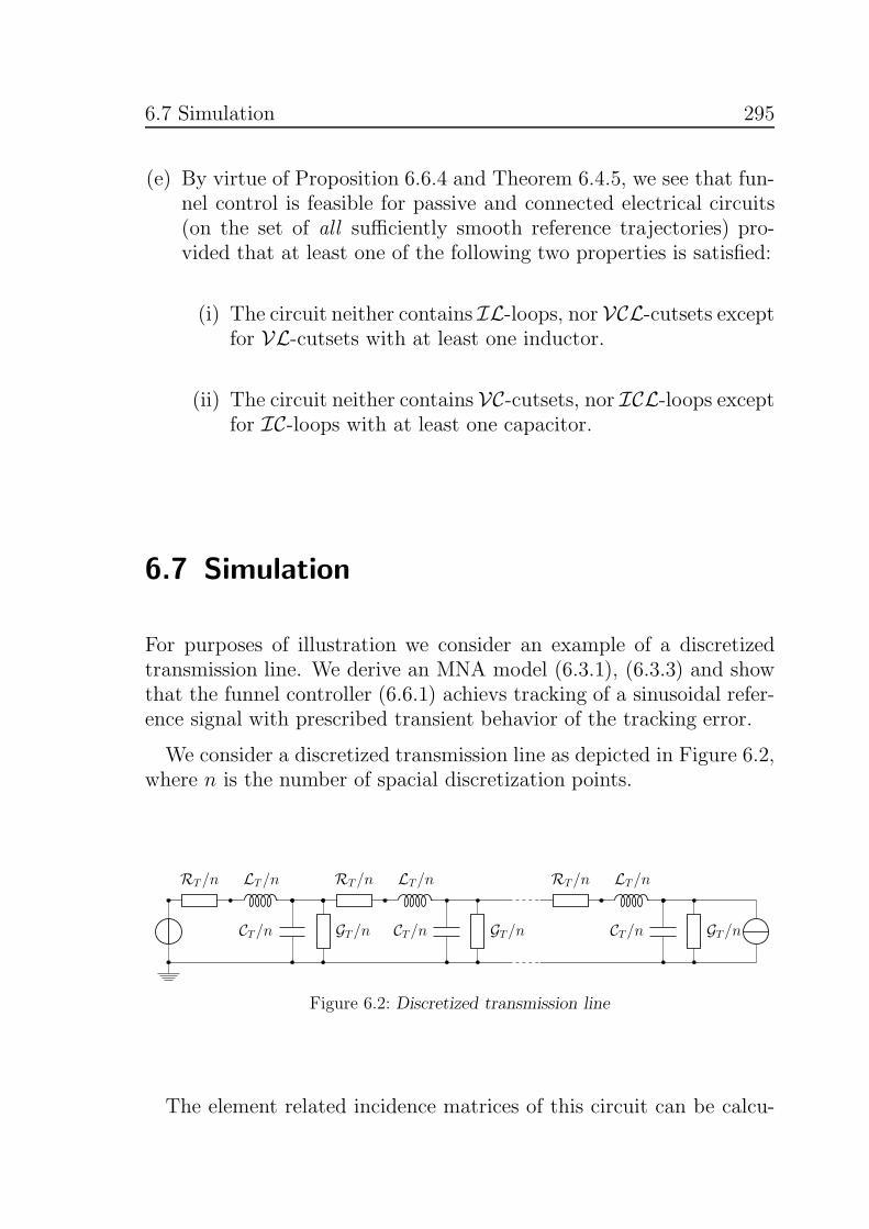
6.7 Simulation 295
(e) By virtue of Proposition 6.6.4 and Theorem 6.4.5, we see that fun-nel control is feasible for passive and connected electrical circuits(on the set of all sufficiently smooth reference trajectories) pro-vided that at least one of the following two properties is satisfied:
(i) The circuit neither contains IL-loops, nor VCL-cutsets exceptfor VL-cutsets with at least one inductor.
(ii) The circuit neither contains VC-cutsets, nor ICL-loops exceptfor IC-loops with at least one capacitor.
6.7 Simulation
For purposes of illustration we consider an example of a discretizedtransmission line. We derive an MNA model (6.3.1), (6.3.3) and showthat the funnel controller (6.6.1) achievs tracking of a sinusoidal refer-ence signal with prescribed transient behavior of the tracking error.
We consider a discretized transmission line as depicted in Figure 6.2,where n is the number of spacial discretization points.
RT/n LT/n RT/n LT/n RT/n LT/n
GT/nCT/nGT/nCT/nGT/nCT/n
Figure 6.2: Discretized transmission line
The element related incidence matrices of this circuit can be calcu-
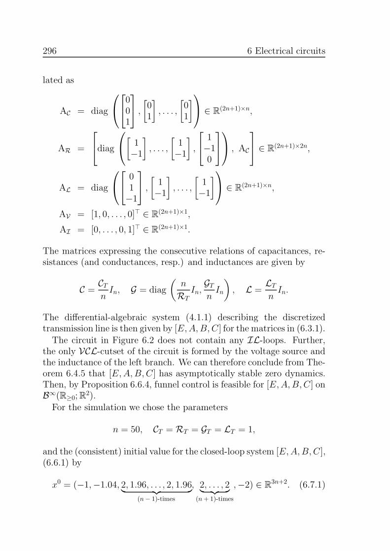
296 6 Electrical circuits
lated as
AC = diag
001
,[01
], . . . ,
[01
] ∈ R(2n+1)×n,
AR =
diag
[1−1
], . . . ,
[1−1
],
1−10
, AC
∈ R(2n+1)×2n,
AL = diag
01−1
,[1−1
], . . . ,
[1−1
] ∈ R(2n+1)×n,
AV = [1, 0, . . . , 0]⊤ ∈ R(2n+1)×1,
AI = [0, . . . , 0, 1]⊤ ∈ R(2n+1)×1.
The matrices expressing the consecutive relations of capacitances, re-sistances (and conductances, resp.) and inductances are given by
C =CTnIn, G = diag
(n
RTIn,
GT
nIn
), L =
LT
nIn.
The differential-algebraic system (4.1.1) describing the discretizedtransmission line is then given by [E,A,B, C] for the matrices in (6.3.1).
The circuit in Figure 6.2 does not contain any IL-loops. Further,the only VCL-cutset of the circuit is formed by the voltage source andthe inductance of the left branch. We can therefore conclude from The-orem 6.4.5 that [E,A,B, C] has asymptotically stable zero dynamics.Then, by Proposition 6.6.4, funnel control is feasible for [E,A,B, C] onB∞(R≥0;R
2).For the simulation we chose the parameters
n = 50, CT = RT = GT = LT = 1,
and the (consistent) initial value for the closed-loop system [E,A,B, C],(6.6.1) by
x0 = (−1,−1.04, 2, 1.96, . . . , 2, 1.96︸ ︷︷ ︸(n− 1)-times
, 2, . . . , 2︸ ︷︷ ︸(n+ 1)-times
,−2) ∈ R3n+2. (6.7.1)
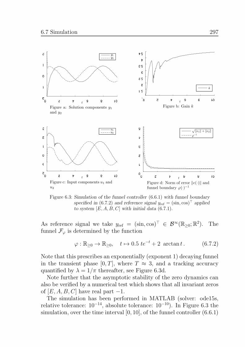
6.7 Simulation 297
0 2 4 6 8 1 0
- 2
- 1
0
1
2
�
��
��
Figure a: Solution components y1and y2
0 2 4 6 8 1 0
1
1 . 5
2
2 . 5
3
3 . 5
4
4 . 5
�
�
Figure b: Gain k
0 2 4 6 8 1 0
- 2
- 1
0
1
2
3
�
��
��
Figure c: Input components u1 andu2
0 2 4 6 8 1 0
0
1
2
3
4
5
�
����� � ����
���
Figure d: Norm of error ‖e(·)‖ andfunnel boundary ϕ(·)−1
Figure 6.3: Simulation of the funnel controller (6.6.1) with funnel boundaryspecified in (6.7.2) and reference signal yref = (sin, cos)⊤ appliedto system [E,A,B, C] with initial data (6.7.1).
As reference signal we take yref = (sin, cos)⊤ ∈ B∞(R≥0;R2). The
funnel Fϕ is determined by the function
ϕ : R≥0 → R≥0, t 7→ 0.5 te−t + 2 arctan t . (6.7.2)
Note that this prescribes an exponentially (exponent 1) decaying funnelin the transient phase [0, T ], where T ≈ 3, and a tracking accuracyquantified by λ = 1/π thereafter, see Figure 6.3d.Note further that the asymptotic stability of the zero dynamics can
also be verified by a numerical test which shows that all invariant zerosof [E,A,B, C] have real part −1.The simulation has been performed in MATLAB (solver: ode15s,
relative tolerance: 10−14, absolute tolerance: 10−10). In Figure 6.3 thesimulation, over the time interval [0, 10], of the funnel controller (6.6.1)

298 6 Electrical circuits
with funnel boundary specified in (6.7.2) and reference signal yref =(sin, cos)⊤, applied to system [E,A,B, C] with initial data (6.7.1) isdepicted. Figure 6.3a shows the output components y1 and y2 trackingthe reference signal yref within the funnel shown in Figure 6.3d. Notethat an action of the input components u1 and u2 in Figure 6.3c and thegain function k in Figure 6.3b is required only if the error ‖e(t)‖ is closeto the funnel boundary ϕ(t)−1. It can be seen that initially the erroris very close to the funnel boundary and hence the gain rises sharply.Then, at approximately t = 1, the distance between error and funnelboundary gets larger and the gain drops accordingly. In particular wesee that the gain function k is non-monotone.
6.8 Notes and References
(i) The modified nodal analysis procedure has been developed by Hoet al. [116] at IBM, see also [93, 204, 206–208, 242]. As describedin Sections 6.2 and 6.3, MNA is based on a graph theoreticalconsideration of the electrical circuit; the circuit topology can bedirectly read off from the equations arising from 6.3.1. It is avery general modeling method which can handle all basic circuitelements and, moreover and not discussed in Sections 6.1 - 6.7,other elements such as the operational amplifier, two-port ele-ments including the gyrator, and the ideal transformer. At thesame time, the MNA model takes a very compact form (cf. 6.3.1)and is hence widely used and an appropriate tool for the compu-tational solution of circuit equations. In particular, the modelingcan be done automatically and MNA is hence used in several cir-cuit simulation programs, such as SPICE R©.For a historical overview of the development of MNA and ac-companying simulation software see [196]. A very good survey of“DAEs in circuit modelling” including MNA can also be foundin [208].
(ii) In the MNA model (6.3.1)–(6.3.3) of a given electrical circuit wechose the input vector to consist of the currents of current sourcesand voltages of voltage sources, which is a canonical choice. How-ever, choosing the output vector to consist of the voltages of cur-rent sources and currents of voltage sources is restrictive, since

6.8 Notes and References 299
one may want to measure the current through any element of thecircuit or the voltage between any two points of the circuit. Thiscan be achieved within the framework of the model (6.3.1)–(6.3.3)by adding ‘virtual’ sources to the circuit in the following way1:
1) If the current through an element X needs to be measured,then establish a series connection of X with a voltage sources(which is added to the circuit) of voltage v = 0. The current ithrough the voltage source is the same as the current throughX and can hence be measured at the source. Since v = 0,the addition of the source does not influence the remainingcircuit.
2) If the voltage between two points of the circuit needs to bemeasured, say two nodes with potentials η1 and η2, then estab-lish a parallel connection of the circuit between these pointsand a current source (which is added to the circuit connectingthe two nodes) of current i = 0. It follows that the voltagev across the voltage source satisfies v = η1 − η2, i.e., it is thesame as the voltage between the two points of the circuit andcan hence be measured at the source. Since i = 0, the additionof the source does not influence the remaining circuit.
With this procedure it can be achieved that any current or volt-age in the circuit can be assigned as output, while the circuitcan still be described by a model of the form (6.3.1)–(6.3.3),where some input constraints (currents and voltages of the addedsources must be zero) have to be added. This can be realized byadding respective rows to B and zero rows to the pencil sE −A.Of course, the analysis presented in the previous sections cannotsimply be carried over, but a thorough investigation with respectto the additional input constraints must be performed; this is anopen problem.
(iii) It is interesting to note that the MNA procedure can also han-dle so called memristive devices . One such device, the memris-tor (memory-resistor), has been postulated by Chua [72] as thefourth basic circuit element besides resistors, capacitors and in-ductors, on the basis of symmetry considerations. The memristor
1Many thanks to Thomas Hotz (Ilmenau University of Technology) for pointing this out to me.

300 6 Electrical circuits
provides a functional relation between electric charge and mag-netic flux. The actual discovery of the memristor by Strukov etal. [225] from HP labs in 2008 (see also [249]) had a great impactin the electrical engineering community and a lot of potential ap-plications have been reported since, see [208] and the referencestherein. Recent research [94, 255] reveals that the MNA methodcan be extended to treat memristors by introducing the magneticflux as a new state variable. As a consequence, SPICE-like circuitsimulators can be used for electrical circuits with memristors.An interesting topic for further research is the investigation ofhigh-gain and funnel control for nonlinear electrical circuits con-taining memristors.

References 301
References
[1] Adams, R. A. Sobolev Spaces. No. 65 in Pure and Applied Mathematics.Academic Press, New York, London, 1975.
[2] Anderson, B. D. O., and Vongpanitlerd, S. Network Analysis andSynthesis – A Modern Systems Theory Approach. Prentice-Hall, EnglewoodCliffs, NJ, 1973.
[3] Aplevich, J. D. Minimal representations of implicit linear systems. Auto-matica 21, 3 (1985), 259–269.
[4] Aplevich, J. D. Implicit Linear Systems. No. 152 in Lecture Notes in Controland Information Sciences. Springer-Verlag, Berlin, 1991.
[5] Arens, R. Operational calculus of linear relations. Pacific J. Math. 9 (1961),9–23.
[6] Armentano, V. A. Eigenvalue placement for generalized linear systems. Syst.Control Lett. 4 (1984), 199–202.
[7] Armentano, V. A. The pencil (sE−A) and controllability-observability forgeneralized linear systems: a geometric approach. SIAM J. Control Optim. 24(1986), 616–638.
[8] Ascher, U. M., and Petzold, L. R. Computer methods for ordinarydifferential equations and differential-algebraic equations. SIAM Publications,Philadelphia, 1998.
[9] Aubin, J.-P., and Cellina, A. Differential Inclusions: Set-Valued Maps andViability Theory. No. 264 in Grundlehren der mathematischen Wissenschaften.Springer-Verlag, Berlin-Heidelberg-New York-Tokyo, 1984.
[10] Aubin, J.-P., and Frankowska, H. Set Valued Analysis. Birkhauser,Boston, 1990.
[11] Banaszuk, A., Kociecki, M., and Lewis, F. L. Kalman Decompositionfor Implicit Linear Systems. IEEE Trans. Autom. Control 37, 10 (1992), 1509–1514.
302 References
[12] Banaszuk, A., Kociecki, M., and Przy luski, K. M. On Hautus-typeconditions for controllability of implicit linear discrete-time systems. CircuitsSystems Signal Process. 8, 3 (1989), 289–298.
[13] Banaszuk, A., Kociecki, M., and Przy luski, K. M. Implicit lineardiscrete-time systems. Math. Control Signals Syst. 3, 3 (1990), 271–297.
[14] Banaszuk, A., Kociecki, M., and Przy luski, K. M. Kalman-type de-compostion for implicit linear discrete-time systems, and its applications. Int.J. Control 52, 5 (1990), 1263–1271.
[15] Banaszuk, A., and Przy luski, K. M. On perturbations of controllableimplicit linear systems. IMA J. Math. Control & Information 16 (1999), 91–102.
[16] Basile, G., and Marro, G. Controlled and Conditioned Invariants in Lin-ear System Theory. Prentice-Hall, Englewood Cliffs, NJ, 1992.
[17] Beelen, T. G. J., and Van Dooren, P. M. An improved algorithm forthe computation of Kronecker’s canonical form of a singular pencil. Lin. Alg.Appl. 105 (1988), 9–65.
[18] Belevitch, V. Classical Network Theory. Holden-Day, San Francisco, 1968.
[19] Belur, M. N., and Trentelman, H. L. Stabilization, pole placement andregular implementability. IEEE Trans. Autom. Control 47, 5 (2002), 735–744.
[20] Bender, D., and Laub, A. The linear quadratic optimal regulator problemfor descriptor systems. IEEE Trans. Autom. Control 32 (1987), 672–688.
[21] Bender, D. J., and Laub, A. J. Controllability and observability at infinityof multivariable linear second-order models. IEEE Trans. Autom. Control AC-30 (1985), 1234–1237.
[22] Bender, D. J., and Laub, A. J. The linear-quadratic optimal regulator fordescriptor systems. In Proc. 24th IEEE Conf. Decis. Control, Ft. Lauderdale,FL (1985), pp. 957–962.
[23] Bender, D. J., and Laub, A. J. The linear-quadratic optimal regulator fordescriptor systems: Discrete-time case. Automatica 23 (1987), 71–85.
[24] Benner, P. Advances in balancing-related model reduction for circuit simu-lation. In Scientific Computing in Electrical Engineering, SCEE 2008, J. Rossand L. Costa, Eds., vol. 14. Springer-Verlag, 2009.
[25] Benner, P., and Byers, R. An arithmetic for matrix pencils: theory andnew algorithms. Numer. Math. 103 (2006), 539–573.
[26] Berger, T. Bohl exponent for time-varying linear differential-algebraic equa-tions. Int. J. Control 85, 10 (2012), 1433–1451.

References 303
[27] Berger, T. Funnel control for linear DAEs. PAMM (Proc. Appl. Math.Mech.) 13 (2013). Submitted for publication.
[28] Berger, T. Zero dynamics and funnel control of general linear differential-algebraic systems. Submitted to Math. Control Signals Syst., preprint availablefrom the website of the author, 2013.
[29] Berger, T. Zero dynamics and stabilization for linear DAEs. Submitted toDifferential-Algebraic Equations Forum, preprint available from the website ofthe author, 2013.
[30] Berger, T., Halikias, G., and Karcanias, N. Effects of dynamic andnon-dynamic element changes in RC and RL networks. Int. J. Circ. Theor.Appl. (2013). Early View, doi: 10.1002/cta.1923.
[31] Berger, T., and Ilchmann, A. Zero dynamics of time-varying linear sys-tems. Preprint 10-05 available online, Institute for Mathematics, Ilmenau Uni-versity of Technology, 2010.
[32] Berger, T., and Ilchmann, A. On stability of time-varying lineardifferential-algebraic equations. Int. J. Control 86, 6 (2013), 1060–1076.
[33] Berger, T., and Ilchmann, A. On the standard canonical form of time-varying linear DAEs. Quart. Appl. Math. 71, 1 (2013), 69–87.
[34] Berger, T., Ilchmann, A., and Reis, T. Normal forms, high-gain, andfunnel control for linear differential-algebraic systems. In Control and Opti-mization with Differential-Algebraic Constraints, L. T. Biegler, S. L. Campbell,and V. Mehrmann, Eds., vol. 23 of Advances in Design and Control. SIAM,Philadelphia, 2012, pp. 127–164.
[35] Berger, T., Ilchmann, A., and Reis, T. Zero dynamics and funnel controlof linear differential-algebraic systems. Math. Control Signals Syst. 24, 3 (2012),219–263.
[36] Berger, T., Ilchmann, A., and Trenn, S. The quasi-Weierstraß form forregular matrix pencils. Lin. Alg. Appl. 436, 10 (2012), 4052–4069.
[37] Berger, T., Ilchmann, A., and Wirth, F. Zero dynamics and stabiliza-tion for analytic linear systems. Submitted to Acta Applicandae Mathematicae,preprint available from the website of the authors, 2013.
[38] Berger, T., and Reis, T. Controllability of linear differential-algebraic sys-tems - a survey. In Surveys in Differential-Algebraic Equations I, A. Ilchmannand T. Reis, Eds., Differential-Algebraic Equations Forum. Springer-Verlag,Berlin-Heidelberg, 2013, pp. 1–61.
[39] Berger, T., and Reis, T. Zero dynamics and funnel control for linearelectrical circuits. Submitted to SIAM J. Control Optim., preprint availablefrom the website of the authors, 2013.

304 References
[40] Berger, T., and Trenn, S. The quasi-Kronecker form for matrix pencils.SIAM J. Matrix Anal. & Appl. 33, 2 (2012), 336–368.
[41] Berger, T., and Trenn, S. Addition to “The quasi-Kronecker form formatrix pencils”. SIAM J. Matrix Anal. & Appl. 34, 1 (2013), 94–101.
[42] Bernhard, P. On singular implicit linear dynamical systems. SIAM J. Con-trol Optim. 20, 5 (1982), 612–633.
[43] Birkhoff, G., and MacLane, S. A Survey of Modern Algebra, 4th ed.Macmillan Publishing Co., New York, 1977.
[44] Bonilla E., M., and Malabre, M. On the control of linear systems havinginternal variations. Automatica 39 (2003), 1989–1996.
[45] Bonilla E., M., Malabre, M., and Loiseau, J.-J. Implicit systemsreachability: A geometric point of view. In Joint 48th IEEE Conference onDecision and Control and 28th Chinese Control Conference (Shanghai, P.R.China, 2009), pp. 4270–4275.
[46] Brenan, K. E., Campbell, S. L., and Petzold, L. R. Numerical Solutionof Initial-Value Problems in Differential-Algebraic Equations. North-Holland,Amsterdam, 1989.
[47] Brockett, R. W. Poles, zeros, and feedback: State space interpretation.IEEE Trans. Autom. Control 10, 2 (1965), 129–135.
[48] Brunovsky, P. A classification of linear controllable systems. Kybernetika 3(1970), 137–187.
[49] Bunse-Gerstner, A., Byers, R., Mehrmann, V., and Nichols, N. K.
Feedback design for regularizing descriptor systems. Lin. Alg. Appl. 299 (1999),119–151.
[50] Bunse-Gerstner, A., Mehrmann, V., and Nichols, N. K. On derivativeand proportional feedback design for descriptor systems. In Proceedings of theInternational Symposium on the Mathematical Theory of Networks and Systems(Amsterdam, Netherlands, 1989), M. A. Kaashoek et al., Eds.
[51] Bunse-Gerstner, A., Mehrmann, V., and Nichols, N. K. Regular-ization of descriptor systems by derivative and proportional state feedback.Report, University of Reading, Dept. of Math., Numerical Analysis Group,Reading, UK, March 1991.
[52] Byers, R., Geerts, A. H. W. T., and Mehrmann, V. Descriptor systemswithout controllability at infinity. SIAM J. Control Optim. 35 (1997), 462–479.
[53] Byers, R., Kunkel, P., and Mehrmann, V. Regularization of linear de-scriptor systems with variable coefficients. SIAM J. Control Optim. 35 (1997),117–133.

References 305
[54] Byrnes, C. I., and Isidori, A. A frequency domain philosophy for nonlinearsystems, with application to stabilization and to adaptive control. In Proc.23rd IEEE Conf. Decis. Control (1984), vol. 1, pp. 1569–1573.
[55] Byrnes, C. I., and Isidori, A. New results and examples in nonlinearfeedback stabilization. Syst. Control Lett. 12, 5 (1989), 437–442.
[56] Byrnes, C. I., and Isidori, A. Output regulation of nonlinear systems.IEEE Trans. Autom. Control 35, 2 (1990), 131–140.
[57] Byrnes, C. I., and Isidori, A. Asymptotic stabilization of minimum phasenonlinear systems. IEEE Trans. Autom. Control 36, 10 (1991), 1122–1137.
[58] Byrnes, C. I., and Isidori, A. Limit sets, zero dynamics, and internalmodels in the problem of nonlinear output regulation. IEEE Trans. Autom.Control 48, 10 (2003), 1712–1723.
[59] Byrnes, C. I., Lauko, I. G., Gilliam, D. S., and Shubov, V. I. Zerodynamics for relative degree one SISO distributed parameter systems. In Proc.37th IEEE Conf. Decis. Control (1998), pp. 2390–2391.
[60] Byrnes, C. I., and Willems, J. C. Adaptive stabilization of multivariablelinear systems. In Proc. 23rd IEEE Conf. Decis. Control (1984), pp. 1574–1577.
[61] Calahan, D. A. Computer-Aided Network Design, rev. ed. McGraw-Hill,New York, 1972.
[62] Campbell, S. L. Singular Systems of Differential Equations I. Pitman, NewYork, 1980.
[63] Campbell, S. L. Singular Systems of Differential Equations II. Pitman, NewYork, 1982.
[64] Campbell, S. L. One canonical form for higher-index linear time-varyingsingular systems. Circuits Systems Signal Process. 2, 3 (1983), 311–326.
[65] Campbell, S. L., Kunkel, P., and Mehrmann, V. Regularizationof linear and nonlinear descriptor systems. In Control and Optimizationwith Differential-Algebraic Constraints, L. T. Biegler, S. L. Campbell, andV. Mehrmann, Eds., vol. 23 of Advances in Design and Control. SIAM,Philadelphia, 2012, pp. 17–36.
[66] Campbell, S. L., Meyer, Jr., C. D., and Rose, N. J. Applicationsof the Drazin inverse to linear systems of differential equations with singularconstant coefficients. SIAM J. Appl. Math. 31, 3 (1976), 411–425.
[67] Campbell, S. L., Nichols, N. K., and Terrell, W. J. Duality, observ-ability, and controllability for linear time-varying descriptor systems. CircuitsSystems Signal Process. 10, 4 (1991), 455–470.
306 References
[68] Campbell, S. L., and Petzold, L. R. Canonical forms and solvable sin-gular systems of differential equations. SIAM J. Alg. & Disc. Meth. 4 (1983),517–521.
[69] Chen, D., and Paden, B. Stable inversion of nonlinear non-minimum phasesystems. Int. J. Control 64, 1 (1996), 81–97.
[70] Christodoulou, M. A., and Paraskevopoulos, P. N. Solvability, con-trollability, and observability of singular systems. J. Optim. Th. & Appl. 45(1985), 53–72.
[71] Chu, K.-w. E. The solution of the matrix equations AXB − CXD = E and(Y A−DZ, Y C −BZ) = (E, F ). Lin. Alg. Appl. 93 (1987), 93–105.
[72] Chua, L. O. Memristor - the missing circuit element. IEEE Trans. Circ.Theory CT-18, 5 (1971), 507–519.
[73] Cobb, J. D. Descriptor Variable and Generalized Singularly Perturbed Sys-tems: A Geometric Approach. Univ. of Illinois, Dept. of Electrical Engineering,Urbana-Champaign, 1980.
[74] Cobb, J. D. Feedback and pole placement in descriptor variable systems. Int.J. Control 33, 6 (1981), 1135–1146.
[75] Cobb, J. D. On the solution of linear differential equations with singularcoefficients. J. Diff. Eqns. 46 (1982), 310–323.
[76] Cobb, J. D. Descriptor variable systems and optimal state regulation. IEEETrans. Autom. Control AC-28 (1983), 601–611.
[77] Cobb, J. D. Controllability, observability and duality in singular systems.IEEE Trans. Autom. Control AC-29 (1984), 1076–1082.
[78] Crouch, P. E., and van der Schaft, A. J. Variational and HamiltonianControl Systems. No. 101 in Lecture Notes in Control and Information Sciences.Springer-Verlag, Berlin, 1986.
[79] Cuthrell, J. E., and Biegler, L. T. On the optimization of differential-algebraic process systems. AIChE Journal 33, 8 (1987), 1257–1270.
[80] Dai, L. Singular Control Systems. No. 118 in Lecture Notes in Control andInformation Sciences. Springer-Verlag, Berlin, 1989.
[81] Demmel, J. W., and Kagstrom, B. The generalized Schur decompositionof an arbitrary pencil A − λB: Robust software with error bounds and appli-cations. Part I: Theory and Algorithms. ACM Trans. Math. Soft 19 (1993),160–174.
[82] Demmel, J. W., and Kagstrom, B. The generalized Schur decompositionof an arbitrary pencil A−λB: Robust software with error bounds and applica-tions. Part II: Software and Applications. ACM Trans. Math. Soft 19 (1993),175–201.

References 307
[83] Desoer, C. A., and Kuh, E. S. Basic Circuit Theory. McGraw-Hill, NewYork, 1969.
[84] Diehl, M., Bock, H. G., Schloder, J. P., Findeisen, R., Nagy, Z.,
and Allgower, F. Real-time optimization and nonlinear model predictivecontrol of processes governed by differential-algebraic equations. Journal ofProcess Control 12 (2002), 577–585.
[85] Diehl, M., Uslu, I., Findeisen, R., Schwarzkopf, S., Allgower, F.,
Bock, H. G., Burner, T., Gilles, E. D., Kienle, A., Schloder, J. P.,
and Stein, E. Real-time optimization for large scale processes: Nonlinearmodel predictive control of a high purity distillation column. In Online Opti-mization of Large Scale Systems: State of the Art, M. Grotschel, S. O. Krumke,and J. Rambau, Eds. Springer-Verlag, 2001, pp. 363–384.
[86] Diestel, R. Graph theory, vol. 173 of Graduate Texts in Mathematics.Springer-Verlag, Berlin, 2005.
[87] Dieudonne, J. Sur la reduction canonique des couples des matrices. Bull. dela Societe Mathematique de France 74 (1946), 130–146.
[88] Dorato, P. On the inverse of linear dynamical systems. IEEE Trans. SystemsScience and Cybernetics 5, 1 (1969), 43–48.
[89] Dziurla, B., and Newcomb, R. W. Nonregular semistate systems: exam-ples and input-output pairing. IEEE Press, New York, 1987.
[90] Eich-Soellner, E., and Fuhrer, C. Numerical Methods in MultibodyDynamics. Teubner, Stuttgart, 1998.
[91] El-Tohami, M., Lovass-Nagy, V., and Powers, D. L. On minimal-order inverses of discrete-time descriptor systems. Int. J. Control 41, 4 (1985),991–1004.
[92] Eliopoulou, H., and Karcanias, N. Properties of reachability and almostreachability subspaces of implicit systems: The extension problem. Kybernetika31, 6 (1995), 530–540.
[93] Estevez Schwarz, D., and Tischendorf, C. Structural analysis for elec-tric circuits and consequences for MNA. Int. J. Circuit Theory Appl. 28, 2(2000), 131–162.
[94] Fei, W., Yu, H., Zhang, W., and Yeo, K. S. Design Exploration ofHybrid CMOS and Memristor Circuit by New Modified Nodal Analysis. IEEETransactions on Very Large Scale Integration (VLSI) Systems 20, 6 (2012),1012–1025.
[95] Fischer, G. Lineare Algebra, 15. ed. Vieweg, Wiesbaden, 2005.
[96] Fletcher, L. R., Kautsky, J., and Nichols, N. K. Eigenstructureassignment in descriptor systems. IEEE Trans. Autom. Control AC-31 (1986),1138–1141.

308 References
[97] Francis, B. A., and Wonham, W. M. The role of transmission zeros inlinear multivariable regulators. Int. J. Control 22, 5 (1975), 657–681.
[98] Frankowska, H. On controllability and observability of implicit systems.Syst. Control Lett. 14 (1990), 219–225.
[99] Fuhrer, C., and Leimkuhler, B. J. Numerical solution of differential-algebraic equations for constrained mechanical motion. Numer. Math. 59(1991), 55–69.
[100] Gantmacher, F. R. The Theory of Matrices (Vol. I & II). Chelsea, NewYork, 1959.
[101] Geerts, A. H. W. T. Solvability conditions, consistency and weak consis-tency for linear differential-algebraic equations and time-invariant linear sys-tems: The general case. Lin. Alg. Appl. 181 (1993), 111–130.
[102] Geerts, A. H. W. T., and Mehrmann, V. Linear differential equationswith constant coefficients: A distributional approach. Tech. Rep. SFB 34390-073, Bielefeld University, Germany, Germany, 1990.
[103] Glusing-Luerßen, H. Feedback canonical form for singular systems. Int.J. Control 52, 2 (1990), 347–376.
[104] Glusing-Luerßen, H., and Hinrichsen, D. A Jordan control canonicalform for singular systems. Int. J. Control 48, 5 (1988), 1769–1785.
[105] Golub, G. H., and van Loan, C. F. Matrix Computations, 3rd ed. No. 3 inJohns Hopkins series in the mathematical sciences. Johns Hopkins UniversityPress, Baltimore, MD, 1996.
[106] Gresho, P. M. Incompressible fluid dynamics: Some fundamental formula-tion issues. Annu. Rev. Fluid Mech. 23 (1991), 413–453.
[107] Griepentrog, E., and Marz, R. Differential-algebraic equations and theirnumerical treatment. No. 88 in Teubner-Texte zur Mathematik. Teubner,Leipzig, 1986.
[108] Hackl, C. M., Endisch, C., and Schroder, D. Error reference control ofnonlinear two-mass flexible servo systems. In Proceedings of the 16th Mediter-ranean Conference on Control and Automation, MED 2008 - Ajaccio, France,June 25-27 (2008), pp. 1047–1053.
[109] Hackl, C. M., Endisch, C., and Schroder, D. Funnel-Control inrobotics: An introduction. In Proceedings of the 16th Mediterranean Con-ference on Control and Automation, MED 2008 - Ajaccio, France, June 25-27(2008), pp. 913–919.
[110] Hackl, C. M., Hofmann, A. G., and Kennel, R. M. Funnel controlin mechatronics: An overview. In Proc. 50th IEEE Conf. Decis. Control andEuropean Control Conference ECC 2011, Orlando, USA (2011), pp. 8000–8007.
References 309
[111] Haug, E. J. Computer-Aided Kinematics and Dynamics of Mechanical Sys-tems. Allyn and Bacon, Boston, 1989.
[112] Hautus, M. L. J. Controllability and observability condition for linear au-tonomous systems. Ned. Akademie. Wetenschappen, Proc. Ser. A 72 (1969),443–448.
[113] Helmke, U., and Shayman, M. A. A canonical form for controllable sin-gular systems. Syst. Control Lett. 12, 2 (1989), 111–122.
[114] Hernandez, V., and Gasso, M. Explicit solution of the matrix equationAXB − CXD = E. Lin. Alg. Appl. 121 (1989), 333–344.
[115] Hinrichsen, D., and Pritchard, A. J. Mathematical Systems Theory I.Modelling, State Space Analysis, Stability and Robustness, vol. 48 of Texts inApplied Mathematics. Springer-Verlag, Berlin, 2005.
[116] Ho, C.-W., Ruehli, A. E., and Brennan, P. A. The modified nodalapproach to network analysis. IEEE Trans. Circuits Syst. CAS-22, 6 (1975),504–509.
[117] Hou, M. Controllability and elimination of impulsive modes in descriptorsystems. IEEE Trans. Autom. Control 49, 10 (2004), 1723–1727.
[118] Hou, M., and Muller, P. C. Observer design for descriptor systems. IEEETrans. Autom. Control 44, 1 (1999), 164–168.
[119] Ilchmann, A. Non-Identifier-Based High-Gain Adaptive Control, vol. 189 ofLecture Notes in Control and Information Sciences. Springer-Verlag, London,1993.
[120] Ilchmann, A., and Mehrmann, V. A behavioural approach to time-varyinglinear systems, Part 1: General theory. SIAM J. Control Optim. 44, 5 (2005),1725–1747.
[121] Ilchmann, A., and Mehrmann, V. A behavioural approach to time-varyinglinear systems, Part 2: Descriptor systems. SIAM J. Control Optim. 44, 5(2005), 1748–1765.
[122] Ilchmann, A., and Mueller, M. Time-varying linear systems: Relativedegree and normal form. IEEE Trans. Autom. Control 52, 5 (2007), 840–851.
[123] Ilchmann, A., and Ryan, E. P. High-gain control without identification: asurvey. GAMM Mitt. 31, 1 (2008), 115–125.
[124] Ilchmann, A., and Ryan, E. P. Performance funnels and tracking control.Int. J. Control 82, 10 (2009), 1828–1840.
[125] Ilchmann, A., Ryan, E. P., and Sangwin, C. J. Tracking with prescribedtransient behaviour. ESAIM: Control, Optimisation and Calculus of Variations7 (2002), 471–493.

310 References
[126] Ilchmann, A., Ryan, E. P., and Townsend, P. Tracking control withprescribed transient behaviour for systems of known relative degree. Syst.Control Lett. 55, 5 (2006), 396–406.
[127] Ilchmann, A., Ryan, E. P., and Townsend, P. Tracking with prescribedtransient behavior for nonlinear systems of known relative degree. SIAM J.Control Optim. 46, 1 (2007), 210–230.
[128] Ilchmann, A., and Schuster, H. PI-funnel control for two mass systems.IEEE Trans. Autom. Control 54, 4 (2009), 918–923.
[129] Ilchmann, A., and Trenn, S. Input constrained funnel control with appli-cations to chemical reactor models. Syst. Control Lett. 53, 5 (2004), 361–375.
[130] Ishihara, J. Y., and Terra, M. H. Impulse controllability and observ-ability of rectangular descriptor systems. IEEE Trans. Autom. Control 46, 6(2001), 991–994.
[131] Isidori, A. Nonlinear Control Systems, 3rd ed. Communications and ControlEngineering Series. Springer-Verlag, Berlin, 1995.
[132] Isidori, A. Nonlinear Control Systems II. Communications and ControlEngineering Series. Springer-Verlag, London, 1999.
[133] Jaffe, S., and Karcanias, N. Matrix pencil characterization of almost(A,B)-invariant subspaces: A classification of geometric concepts. Int. J. Con-trol 33, 1 (1981), 51–93.
[134] Julius, A. A., and van der Schaft, A. J. Compatibility of behaviorinterconnections. In Proc. 7th European Control Conf. 2003, Cambridge, UK(2003).
[135] Kagstrom, B., and Van Dooren, P. M. A generalized state-space ap-proach for the additive decomposition of a transfer matrix. J. Numer. LinearAlgebra Appl. 1, 2 (1992), 165–181.
[136] Kailath, T. Linear Systems. Prentice-Hall, Englewood Cliffs, NJ, 1980.
[137] Kalman, R. E. On the general theory of control systems. In Proceedings ofthe First International Congress on Automatic Control, Moscow 1960 (London,1961), Butterworth’s, pp. 481–493.
[138] Kalman, R. E. Canonical structure of linear dynamical systems. Proc. Nat.Acad. Sci. (USA) 48, 4 (April 1962), 596–600.
[139] Kalman, R. E. Mathematical description of linear dynamical systems. SIAMJ. Control Optim. 1 (1963), 152–192.
[140] Karcanias, N. Regular state-space realizations of singular system controlproblems. In Proc. 26th IEEE Conf. Decis. Control (Los Angeles, CA, 1987),pp. 1144–1146.
References 311
[141] Karcanias, N., and Hayton, G. E. Generalised autonomous dynamicalsystems, algebraic duality and geometric theory. In Proc. 8th IFAC WorldCongress (Kyoto, 1981), pt. III (1981), pp. 13–18.
[142] Karcanias, N., and Kalogeropoulos, G. A matrix pencil approach tothe study of singular systems: algebraic and geometric aspects. In Proc. Int.Symp. on Singular Systems (Atlanta, GA, 1987), pp. 29–33.
[143] Karcanias, N., and Kalogeropoulos, G. Geometric theory and feedbackinvariants of generalized linear systems: a matrix pencil approach. CircuitsSystems Signal Process. 8, 3 (1989), 375–397.
[144] Karcanias, N., and Kouvaritakis, B. The output zeroing problem andits relationship to the invariant zero structure: a matrix pencil approach. Int.J. Control 30, 3 (1979), 395–415.
[145] Knobloch, H. W., and Kwakernaak, H. Lineare Kontrolltheorie.Springer-Verlag, Berlin, 1985.
[146] Koumboulis, F. N., and Mertzios, B. G. On Kalman’s controllability andobservability criteria for singular systems. Circuits Systems Signal Process. 18,3 (1999), 269–290.
[147] Kouvaritakis, B., and MacFarlane, A. G. J. Geometric approach toanalysis and synthesis of system zeros Part 1. Square systems. Int. J. Control23, 2 (1976), 149–166.
[148] Kouvaritakis, B., and MacFarlane, A. G. J. Geometric approach toanalysis and synthesis of system zeros Part 2. Non-square systems. Int. J.Control 23, 2 (1976), 167–181.
[149] Kronecker, L. Algebraische Reduction der Schaaren bilinearer Formen.Sitzungsberichte der Koniglich Preußischen Akademie der Wissenschaften zuBerlin (1890), 1225–1237.
[150] Kucera, V., and Zagalak, P. Fundamental theorem of state feedback forsingular systems. Automatica 24, 5 (1988), 653–658.
[151] Kuijper, M. First-Order Representations of Linear Systems. Birkhauser,Boston, 1994.
[152] Kunkel, P., and Mehrmann, V. Differential-Algebraic Equations. Analysisand Numerical Solution. EMS Publishing House, Zurich, Switzerland, 2006.
[153] Kunkel, P., Mehrmann, V., and Rath, W. Analysis and numericalsolution of control problems in descriptor form. Math. Control Signals Syst. 14(2001), 29–61.
[154] Lamour, R., Marz, R., and Tischendorf, C. Differential Algebraic Equa-tions: A Projector Based Analysis, vol. 1 of Differential-Algebraic EquationsForum. Springer-Verlag, Heidelberg-Berlin, 2013.
312 References
[155] Lang, S. Linear Algebra, 2nd ed. Addison-Wesley, Reading, Massachusetts,1970. fourth printing 1973.
[156] Lau, K., Middleton, R. H., and Braslavsky, J. H. Undershoot andsettling time tradeoffs for nonminimum phase systems. IEEE Trans. Autom.Control 48, 8 (1990), 1389–1393.
[157] Lewis, F. L. Inversion of descriptor systems. In Proc. American ControlConf. 1983 (San Francisco, CA, 1983), pp. 1153–1158.
[158] Lewis, F. L. A survey of linear singular systems. IEEE Proc. Circuits, Systemsand Signal Processing 5, 1 (1986), 3–36.
[159] Lewis, F. L. A tutorial on the geometric analysis of linear time-invariantimplicit systems. Automatica 28, 1 (1992), 119–137.
[160] Lewis, F. L., Christodoulou, M. A., and Mertzios, B. G. Systeminversion using orthogonal functions. Circuits Systems Signal Process. 6, 3(1987), 347–362.
[161] Lewis, F. L., and Ozcaldiran, K. Reachability and controllability fordescriptor systems. In Proc. 27, Midwest Symp. on Circ Syst. (Morgantown,WV, 1984).
[162] Lewis, F. L., and Ozcaldiran, K. On the eigenstructure assignment ofsingular systems. IEEE Press, New York, 1985.
[163] Lewis, F. L., and Ozcaldiran, K. Geometric structure and feedback insingular systems. IEEE Trans. Autom. Control AC-34, 4 (1989), 450–455.
[164] Liberzon, D., Morse, A. S., and Sontag, E. D. Output-input stabilityand minimum-phase nonlinear systems. IEEE Trans. Autom. Control 47, 3(2002), 422–436.
[165] Linh, V. H., and Mehrmann, V. Lyapunov, Bohl and Sacker-Sell spectralintervals for differential-algebraic equations. J. of Dynamics and DifferentialEquations 21 (2009), 153–194.
[166] Loiseau, J.-J. Some geometric considerations about the Kronecker normalform. Int. J. Control 42, 6 (1985), 1411–1431.
[167] Loiseau, J.-J., Ozcaldiran, K., Malabre, M., and Karcanias, N.
Feedback canonical forms of singular systems. Kybernetika 27, 4 (1991), 289–305.
[168] Lotstedt, P., and Petzold, L. R. Numerical solution of nonlinear differ-ential equations with algebraic constraints I: Convergence results for backwarddifferentiation formulas. Math. Comp. 46, 174 (1986), 491–516.
[169] Luenberger, D. G. Dynamic equations in descriptor form. IEEE Trans.Autom. Control AC-22 (1977), 312–321.
References 313
[170] Luenberger, D. G. Time-invariant descriptor systems. Automatica 14(1978), 473–480.
[171] Luenberger, D. G. Introduction to Dynamic Systems: Theory, Models andApplications. John Wiley and Sons Inc., New York, 1979.
[172] Luenberger, D. G. Nonlinear descriptor systems. J. Econ. Dyn. Contr. 1(1979), 219–242.
[173] Luenberger, D. G., and Arbel, A. Singular dynamic Leontief systems.Econometrica 45 (1977), 991–995.
[174] Malabre, M. More geometry about singular systems. IEEE Press, New York,1987.
[175] Malabre, M. Generalized linear systems: geometric and structural ap-proaches. Lin. Alg. Appl. 122,123,124 (1989), 591–621.
[176] Martins, N., Pellanda, P. C., and Rommes, J. Computation of transferfunction dominant zeros with applications to oscillation damping control oflarge power systems. IEEE Trans. Power Syst. 22, 4 (2007), 1657–1664.
[177] Masubuchi, I. Stability and stabilization of implicit systems. In Proc.39th IEEE Conf. Decis. Control, Sydney, Australia (2000), vol. 12, pp. 3636–3641.
[178] Mertzios, B. G., Christodoulou, M. A., Syrmos, B. L., and Lewis,
F. L. Direct controllability and observability time domain conditions of sin-gular systems. IEEE Trans. Autom. Control 33, 8 (1988), 788–791.
[179] Middleton, R. H., and Braslavsky, J. H. On the relationship betweenlogarithmic sensitivity integrals and limiting optimal control problems. Tech.Rep. EE0009, Department of Electrical and Computer Engineering, Universityof Newcastle, 2000.
[180] Mueller, M. Normal form for linear systems with respect to its vector relativedegree. Lin. Alg. Appl. 430, 4 (2009), 1292–1312.
[181] Mueller, M. Output feedback control and robustness in the gap metric. PhDthesis, Institut fur Mathematik, Technische Universitat Ilmenau, Univ.-Verl.Ilmenau, Ilmenau, 2009.
[182] Muller, P. C. Remark on the solution of linear time-invariant descriptorsystems. PAMM (Proc. Appl. Math. Mech.) 5 (2005), 175–176.
[183] Newcomb, R. W. The semistate description of nonlinear time-variable cir-cuits. IEEE Trans. Circuits Syst. CAS-28 (1981), 62–71.
[184] Oara, C., and Van Dooren, P. M. An improved algorithm for the compu-tation of structural invariants of a system pencil and related geometric aspects.Syst. Control Lett. 30, 1 (March 1997), 39–48.
314 References
[185] Owens, D. H., and Debeljkovic, D. L. Consistency and Liapunov stabilityof linear descriptor systems: A geometric analysis. IMA J. Math. Control &Information 2 (1985), 139–151.
[186] Ozcaldiran, K. Control of descriptor systems. PhD thesis, Georgia Instituteof Technology, 1985.
[187] Ozcaldiran, K. A geometric characterization of the reachable and control-lable subspaces of descriptor systems. IEEE Proc. Circuits, Systems and SignalProcessing 5 (1986), 37–48.
[188] Ozcaldiran, K., and Haliloclu, L. Structural properties of singular sys-tems. Kybernetika 29, 6 (1993), 518–546.
[189] Ozcaldiran, K., and Lewis, F. L. A geometric approach to eigenstructureassignment for singular systems. IEEE Trans. Autom. Control AC-32, 7 (1987),629–632.
[190] Ozcaldiran, K., and Lewis, F. L. Generalized reachability subspaces forsingular systems. SIAM J. Control Optim. 27 (1989), 495–510.
[191] Ozcaldiran, K., and Lewis, F. L. On the regularizability of singularsystems. IEEE Trans. Autom. Control 35, 10 (1990), 1156.
[192] Pandolfi, L. Controllability and stabilization for linear systems of algebraicand differential equations. J. Optim. Th. & Appl. 30 (1980), 601–620.
[193] Pandolfi, L. On the regulator problem for linear degenerate control systems.J. Optim. Th. & Appl. 33 (1981), 241–254.
[194] Pantelides, C. C. The consistent initialization of differential-algebraic sys-tems. SIAM J. Sci. Stat. Comput. 9 (1988), 213–231.
[195] Park, M.-S., and Chwa, D. Orbital stabilization of inverted-pendulumsystems via coupled sliding-mode control. IEEE Trans. Ind. Electron. 56, 9(2009), 3556–3570.
[196] Pederson, D. O. A Historical Review of Circuit Simulation. IEEE Trans.Circuits Syst. CAS-31, 1 (1984), 103–111.
[197] Petzold, L. R. Numerical solution of differential-algebraic equations in me-chanical systems simulation. Physica D 60 (1992), 269–279.
[198] Polderman, J. W., and Willems, J. C. Introduction to MathematicalSystems Theory. A Behavioral Approach. Springer-Verlag, New York, 1998.
[199] Popov, V. M. Hyperstability of Control Systems. Springer-Verlag, Berlin-Heidelberg-New York, 1973. Translation based on a revised text preparedshortly after the publication of the Romanian ed., 1966.
[200] Przy luski, K. M., and Sosnowski, A. M. Remarks on the theory ofimplicit linear continuous-time systems. Kybernetika 30, 5 (1994), 507–515.
References 315
[201] Pugh, A. C., and Ratcliffe, P. A. On the Zeros and Poles of a RationalMatrix. Int. J. Control 30 (1979), 213–226.
[202] Rabier, P. J., and Rheinboldt, W. C. Classical and generalized solutionsof time-dependent linear differential-algebraic equations. Lin. Alg. Appl. 245(1996), 259–293.
[203] Rath, W. Feedback Design and Regularization for Linear Descriptor Systemswith Variable Coefficients. Dissertation, TU Chemnitz, Chemnitz, Germany,1997.
[204] Reis, T. Circuit synthesis of passive descriptor systems - a modified nodalapproach. Int. J. Circ. Theor. Appl. 38 (2010), 44–68.
[205] Respondek, W. Right and left invertibility of nonlinear control systems.In Nonlinear controllability and optimal control, H. J. Sussmann, Ed. MarcelDekker, New York, 1990, pp. 133–177.
[206] Riaza, R. Time-domain properties of reactive dual circuits. Int. J. Circ.Theor. Appl. 34, 3 (2006), 317–340.
[207] Riaza, R. Differential-Algebraic Systems. Analytical Aspects and Circuit Ap-plications. World Scientific Publishing, Basel, 2008.
[208] Riaza, R. DAEs in Circuit Modelling: A Survey. In Surveys in Differential-Algebraic Equations I, A. Ilchmann and T. Reis, Eds., Differential-AlgebraicEquations Forum. Springer-Verlag, Berlin-Heidelberg, 2013, pp. 97–136.
[209] Riaza, R., and Tischendorf, C. Qualitative features of matrix pencils andDAEs arising in circuit dynamics. Dynamical Systems 22, 2 (2007), 107–131.
[210] Rosenbrock, H. H. State Space and Multivariable Theory. John Wiley andSons Inc., New York, NY, 1970.
[211] Rosenbrock, H. H. Structural properties of linear dynamical systems. Int.J. Control 20 (1974), 191–202.
[212] Rugh, W. J. Linear System Theory. Information and System Sciences Series.Prentice-Hall, NJ, 1993.
[213] Rugh, W. J. Linear System Theory, 2nd ed. Information and System SciencesSeries. Prentice-Hall, NJ, 1996.
[214] Sandovici, A., De Snoo, H., and Winkler, H. The structure of linearrelations in Euclidean spaces. Lin. Alg. Appl. 397 (2005), 141–169.
[215] Sastry, S. S., and Isidori, A. Adaptive Control of Linearizable Systems.IEEE Trans. Autom. Control 34, 11 (1989), 1123–1131.
[216] Schiehlen, W. Multibody system dynamics: Roots and perspectives. Multi-body System Dynamics 1 (1997), 149–188.

316 References
[217] Schuster, H., Hackl, C. M., Westermaier, C., and Schroder, D.
Funnel-control for electrical drives with uncertain parameters. In Proc. 7th Int.Power Engineering Conf. IPEC (2005), pp. 517–522.
[218] Schwartz, L. Theorie des Distributions. Hermann, Paris, 1957, 1959.
[219] Shayman, M. A., and Zhou, Z. Feedback control and classification ofgeneralized linear systems. IEEE Trans. Autom. Control 32, 6 (1987), 483–490.
[220] Silverman, L. M. Inversion of multivariable linear systems. IEEE Trans.Autom. Control AC-14 (1969), 270–276.
[221] Simeon, B., Fuhrer, C., and Rentrop, P. Differential-algebraic equationsin vehicle system dynamics. Surv. Math. Ind. 1 (1991), 1–37.
[222] Smith, H. J. S. On systems of linear indeterminate equations and con-gruences. Philos. Trans. Roy. Soc. London 151 (1861–1862), 293–326. =Coll. Math. Papers, pp. 367–406.
[223] Sontag, E. D. Mathematical Control Theory: Deterministic Finite Dimen-sional Systems, 2nd ed. Springer-Verlag, New York, 1998.
[224] Sparrow, C. The Lorenz Equations: Bifurcations, Chaos, and Strange At-tractors. No. 41 in Applied Mathematical Sciences. Springer-Verlag, 1982.
[225] Strukov, D. B., Snider, G. S., Stewart, D. R., and Williams, R. S.
The missing memristor found. Nature 453 (2008), 80–83.
[226] Tan, S. H., and Vandewalle, J. Inversion of singular systems. IEEETrans. Circuits Syst. CAS-35 (1988), 583–587.
[227] Trenn, S. Distributional differential algebraic equations. PhD thesis, Institutfur Mathematik, Technische Universitat Ilmenau, Universitatsverlag Ilmenau,Ilmenau, Germany, 2009.
[228] Trenn, S. Regularity of distributional differential algebraic equations. Math.Control Signals Syst. 21, 3 (2009), 229–264.
[229] Trenn, S. Solution concepts for linear DAEs: a survey. In Surveys inDifferential-Algebraic Equations I, A. Ilchmann and T. Reis, Eds., Differential-Algebraic Equations Forum. Springer-Verlag, Berlin-Heidelberg, 2013, pp. 137–172.
[230] Trentelman, H. L., Stoorvogel, A. A., and Hautus, M. L. J. Con-trol Theory for Linear Systems. Communications and Control Engineering.Springer-Verlag, London, 2001.
[231] Trentelman, H. L., and Willems, J. C. The behavioral approach as aparadigm for modelling interconnected systems. European J. Control 9, 2-3(2003), 296–306.
References 317
[232] van der Schaft, A. J. System Theoretic Descriptions of Physical Systems.No. 3 in CWI Tract. CWI, Amsterdam, 1984.
[233] van der Schaft, A. J., and Schumacher, J. M. H. The complementary-slackness class of hybrid systems. Math. Control Signals Syst. 9 (1996), 266–301.
[234] Van Dooren, P. M. The computation of Kronecker’s canonical form of asingular pencil. Lin. Alg. Appl. 27 (1979), 103–140.
[235] Van Dooren, P. M. Reducing subspaces: Definitions, properties, and al-gorithms. In Matrix Pencils, Lecture Notes in Mathematics, B. Kagstrom andA. Ruhe, Eds., vol. 973. Springer-Verlag, Berlin, 1983, pp. 58–73.
[236] Varga, A. Computation of Kronecker-like forms of a system pencil: appli-cations, algorithms and software. In Proceedings of the IEEE InternationalSymposium on Computer-Aided Control System Design (Dearborn, MI, USA,September 1996), pp. 77–82.
[237] Verghese, G. C. Infinite-frequency Behavior in Generalized Dynamical Sys-tems. PhD thesis, Stanford University, 1978.
[238] Verghese, G. C. Further notes on singular systems. In Proc. Joint AmericanContr. Conf. (1981). Paper TA-4B.
[239] Verghese, G. C., and Kailath, T. Eigenvector chains for finite and in-finite zeros of rational matrices. In Proc. 18th Conf. Dec. and Control (Ft.Lauderdale, FL, 1979), pp. 31–32.
[240] Verghese, G. C., and Kailath, T. Impulsive behavior in dynamical sys-tems: structure and significance. In Proc. 4th MTNS (1979), P. Dewilde, Ed.,pp. 162–168.
[241] Verghese, G. C., Levy, B. C., and Kailath, T. A generalized state-space for singular systems. IEEE Trans. Autom. Control AC-26, 4 (August1981), 811–831.
[242] Wedepohl, L. M., and Jackson, L. Modified nodal analysis: an essentialaddition to electrical circuit theory and analysis. Engineering Science andEducation Journal 11, 3 (2002), 84–92.
[243] Weierstraß, K. Zur Theorie der bilinearen und quadratischen Formen.Berl. Monatsb. (1868), 310–338.
[244] Wilkinson, J. H. Linear differential equations and Kronecker’s canonicalform. In Recent Advances in Numerical Analysis, C. de Boor and G. H. Golub,Eds. Academic Press, 1978, pp. 231–265.
[245] Willems, J. C. System theoretic models for the analysis of physical systems.Ricerche di Automatica 10 (1979), 71–106.
318 References
[246] Willems, J. C. Paradigms and puzzles in the theory of dynamical systems.IEEE Trans. Autom. Control AC-36, 3 (1991), 259–294.
[247] Willems, J. C. On interconnections, control, and feedback. IEEE Trans.Autom. Control 42 (1997), 326–339.
[248] Willems, J. C. The behavioral approach to open and interconnected systems.IEEE Control Systems Magazine 27, 6 (2007), 46–99.
[249] Williams, R. S. How We Found The Missing Memristor. IEEE Spectrum45, 12 (1976), 28–35.
[250] Wong, K.-T. The eigenvalue problem λTx + Sx. J. Diff. Eqns. 16 (1974),270–280.
[251] Wonham, W. M. On pole assignment in multi–input controllable linear sys-tems. IEEE Trans. Autom. Control AC-12 (1967), 660–665.
[252] Wonham, W. M. Linear Multivariable Control: A Geometric Approach,3rd ed. Springer-Verlag, New York, 1985.
[253] Wood, J., and Zerz, E. Notes on the definition of behavioural controllabil-ity. Syst. Control Lett. 37 (1999), 31–37.
[254] Yip, E. L., and Sincovec, R. F. Solvability, controllability and observabilityof continuous descriptor systems. IEEE Trans. Autom. Control AC-26 (1981),702–707.
[255] Yu, H., and Fei, W. A new modified nodal analysis for nano-scale memristorcircuit simulation. In Proc. IEEE Int. Symp. Circuits Syst., Paris, France(2010), pp. 3148–3151.
[256] Zadeh, L. A., and Desoer, C. A. Linear System Theory — The StateSpace Approach. McGraw-Hill, New York, 1963.
[257] Zhao, H., and Chen, D. Stable inversion for exact and stable trackingcontrollers: A flight control example. In Proc. 4th IEEE Conference on ControlApplications (1995), pp. 482–487.
[258] Zhao, H., and Chen, D. A finite energy property of stable inversion tononminimum phase nonlinear systems. IEEE Trans. Autom. Control 43, 8(1998), 1170–1174.
[259] Zhou, Z., Shayman, M. A., and Tarn, T.-J. Singular systems: A newapproach in the time domain. IEEE Trans. Autom. Control 32, 1 (1987), 42–50.
[260] Zubova, S. P. On full controllability criteria of a descriptor system. The poly-nomial solution of a control problem with checkpoints. Autom. Rem. Control72, 1 (2011), 23–37.
List of Symbols 319
List of Symbols
N, N0, Z set of natural numbers, N0 = N ∪ {0}, set of all integers,resp.
ℓ(α), |α| length ℓ(α) = l and absolute value |α| = ∑li=1 αi of a
multi-index α = (α1, . . . , αl) ∈ Nl
K rational numbers Q, real numbers R or complex numbersC
R≥0 (R>0, R≤0, R<0)= [0,∞) ((0,∞), (−∞, 0], (−∞, 0)), resp.
C+, C− the open set of complex numbers with positive, negativereal part, resp.
R[s] the ring of polynomials with coefficients in a ring R andindeterminate s
R(s) the quotient field of R[s]
deg p(s) the degree of the polynomial p(s) ∈ R[s]
e[n]i ith canonical unit vector in Rn, or ei if the dimension is
clear from the context
Rn×m the set of n×m matrices with entries in a ring R
In = diag (1, . . . , 1) ∈ Rn×n, or I if the dimension is clearfrom the context
0n,m a zero matrix of size n×m
320 List of Symbols
Nk =
[01
1 0
]∈ Rk×k, k ∈ N
Kk =[1 0
1 0
]∈ R(k−1)×k, k ∈ N
Lk =[0 1
0 1
]∈ R(k−1)×k, k ∈ N
Nα = diag (Nα1, . . . , Nαk
) ∈ R|α|×|α| for some multi-indexα = (α1, . . . , αk) ∈ Nk
Kα = diag (Kα1, . . . , Kαk
) ∈ R(|α|−k)×|α| for some multi-indexα = (α1, . . . , αk) ∈ Nk
Lα = diag (Lα1, . . . , Lαk
) ∈ R(|α|−k)×|α| for some multi-indexα = (α1, . . . , αk) ∈ Nk
Eα = diag (e[α1]α1 , . . . , e
[αk]αk ) ∈ R|α|×k for some multi-index
α = (α1, . . . , αk) ∈ Nk
Gln(R) the set of invertible n× n matrices with entries in a ringR
On(R) the group of orthogonal matrices in Rn×n
σ(A) the spectrum of a matrix A ∈ Rn×n with entries in a ringR
det(A) the determinant of a matrix A ∈ Rn×n with entries in aring R
rkP A, imP A, kerP A;the rank, image and kernel of A ∈ Rn×m over a subringP of a ring R resp., or rkA, imA, kerA if P = R
rkC(∞E − A)= rkCE for E,A ∈ Cn×m
spec(sE −A)= { λ ∈ C | det(λE −A) = 0 }, the spectrum of a ma-trix pencil sE −A ∈ C[s]n×n

List of Symbols 321
spec∞(sE − A)= { λ ∈ C ∪ {∞} | rkC(λE −A) < n }, the augmentedspectrum of a matrix pencil sE − A ∈ C[s]n×n
A∗ = A⊤, the conjugate transpose of A ∈ Cn×m
‖x‖ =√x⊤x, the Euclidean norm of x ∈ Rn
‖A‖ = max { ‖Ax‖ | x ∈ Rm, ‖x‖ = 1 }, the induced matrixnorm of A ∈ Rn×m
AS = { Ax | x ∈ S }, the image of a set S ⊆ Km underA ∈ Kn×m
A−1S = { x ∈ Km | Ax ∈ S }, the preimage of the set S ⊆ Kn
under A ∈ Kn×m
S⊥ = { x ∈ Kn | ∀s ∈ S : x∗s = 0 }, the orthogonal com-plement of S ⊆ Kn
L1loc(I;R
n) the set of locally Lebesgue integrable functions f : I →Rn, where
∫K‖f(t)‖ dt < ∞ for all compact K ⊆ I and
I ⊆ R is an interval
f (f (i)) the (ith) weak derivative of f ∈ L1loc(I;R
n), i ∈ N0, I ⊆ R
an interval, see [1, Chap. 1]
Wk,1loc (I;R
n) ={f ∈ L1
loc(I;Rn)∣∣ f (i) ∈ L1
loc(I;Rn) for i = 0, . . . , k
},
k ∈ N0 ∪ {∞}, I ⊆ R an interval
L∞(I;Rn) the set of essentially bounded functions f : I → Rn,I ⊆ R an interval, see [1, Chap. 2]
Ck(I;Rn) the set of k-times continuously differentiable functionsf : I → Rn, k ∈ N0 ∪ {∞}, I ⊆ R an interval
Bk(I;Rn) ={f ∈ Ck(I;Rn)
∣∣ f (i) ∈ L∞(I;Rn) for i = 0, . . . , k},
k ∈ N0 ∪ {∞}, I ⊆ R an interval
fa.e.= g means that f, g ∈ L1
loc(I;Rn) are equal ‘almost every-
where’, i.e., f(t) = g(t) for almost all (a.a.) t ∈ I, I ⊆ R
an interval
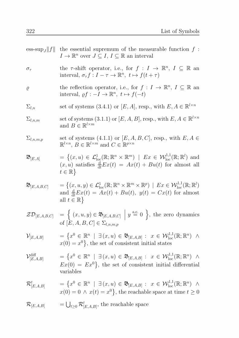
322 List of Symbols
ess-supJ‖f‖ the essential supremum of the measurable function f :I → Rn over J ⊆ I, I ⊆ R an interval
στ the τ -shift operator, i.e., for f : I → Rn, I ⊆ R aninterval, στf : I − τ → Rn, t 7→ f(t+ τ)
the reflection operator, i.e., for f : I → Rn, I ⊆ R aninterval, f : −I → Rn, t 7→ f(−t)
Σl,n set of systems (3.4.1) or [E,A], resp., with E,A ∈ Rl×n
Σl,n,m set of systems (3.1.1) or [E,A,B], resp., with E,A ∈ Rl×n
and B ∈ Rl×m
Σl,n,m,p set of systems (4.1.1) or [E,A,B, C], resp., with E,A ∈Rl×n, B ∈ Rl×m and C ∈ Rp×nB[E,A] ={(x, u) ∈ L1
loc(R;Rn × Rm) | Ex ∈ W1,1
loc (R;Rl) and
(x, u) satisfies ddtEx(t) = Ax(t) + Bu(t) for almost all
t ∈ R}B[E,A,B,C] =
{(x, u, y) ∈ L1
loc(R;Rn ×Rm ×Rp) | Ex ∈ W1,1
loc (R;Rl)
and ddtEx(t) = Ax(t) + Bu(t), y(t) = Cx(t) for almost
all t ∈ R}
ZD[E,A,B,C] ={(x, u, y) ∈ B[E,A,B,C]
∣∣∣ y a.e.= 0
}, the zero dynamics
of [E,A,B, C] ∈ Σl,n,m,p
V[E,A,B] ={x0 ∈ Rn | ∃ (x, u) ∈ B[E,A,B] : x ∈ W1,1
loc (R;Rn) ∧
x(0) = x0}, the set of consistent initial states
Vdiff[E,A,B] =
{x0 ∈ Rn | ∃ (x, u) ∈ B[E,A,B] : x ∈ W1,1
loc (R;Rn) ∧
Ex(0) = Ex0}, the set of consistent initial differential
variables
Rt[E,A,B] =
{x0 ∈ Rn | ∃ (x, u) ∈ B[E,A,B] : x ∈ W1,1
loc (R;Rn) ∧
x(0) = 0 ∧ x(t) = x0}, the reachable space at time t ≥ 0
R[E,A,B] =⋃
t≥0Rt[E,A,B], the reachable space
List of Symbols 323
Ct[E,A,B] =
{x0 ∈ Rn | ∃ (x, u) ∈ B[E,A,B] : x ∈ W1,1
loc (R;Rn) ∧
x(0) = x0 ∧ x(t) = 0}, the controllable space at time
t ≥ 0
C[E,A,B] =⋃
t≥0 Ct[E,A,B], the controllable space
∼= denotes the equivalence of matrix pencils in Chapter 2
W,T∼se denotes the system equivalence of systems in Σl,n,m byinvertible matrices W and T in Chapter 3
W,T,V,F∼fe denotes the feedback equivalence of systems in Σl,n,m byinvertible matrices W , T and V and some feedback ma-trix F in Chapter 3
S,T∼ denotes the system equivalence of systems in Σl,n,m,p byinvertible matrices S and T in Chapter 4
kL(E,A) = inf{µ ∈ R | ∃Mµ > 0 ∀x ∈ B[E,A] for a.a. t ≥
s : ‖x(t)‖ ≤ Mµeµ(t−s)‖x(s)‖
}, the Lyapunov exponent
of [E,A] ∈ Σl,n

324 List of Symbols
Abbreviations
BIF Byrnes-Isidori form
DAE differential-algebraic equation
IQKF interim quasi-Kronecker form
IQKTF interim quasi-Kronecker triangular form
KCF Kronecker canonical form
MNA modified nodal analysis
ODE ordinary differential equation
QKF quasi-Kronecker form
QKTF quasi-Kronecker triangular form
QWF quasi-Weierstraß form
WCF Weierstraß canonical form
ZDF zero dynamics form

Index 325
Index
asymptotically stable, 212
backward system, 100behavior, 96, 128, 159, 176
image representation, 118interconnected, 137, 198shift invariant, 98
behavioral approach, 160branch
directed, 269set, 269
Byrnes-Isidori form, 208, 246
canonical form, 46, 171Brunovsky, 113Hermite, 156Jordan, 28, 80Jordan control, 156Kronecker, 17, 30, 74, 80, 120of full rank pencil, 59
Weierstraß, 17, 28, 46capacitance, 265, 272closed-loop system, 212, 223,
281, 284control
compatible, 137, 198in the behavioral sense, 136stabilizing, 137, 198via interconnection, 136
control system, 95, 159, 211
controllability, 18controllable
at infinity, 102, 114, 116, 123,143, 149
completely, 103, 114, 116,123, 143
impulse, 102, 114, 116, 123,133, 143, 149
in the behavioral sense, 103,114, 116, 123, 143, 149
R-, 103, 116, 123, 142strongly, 104, 114, 116, 123,
143within the set of reachable
states, see R-controllablecontrollable space, 97current, 265, 273
source, 265, 272cutset, 270, 272
K-, 271IC-, 276
decompositionfeedback, 113system equivalence, 111
derivative feedback, see feedbackdetectable
in the behavioral sense, 189,192
differential-algebraic equation,

326 Index
15, 81autonomous, 129completely stabilizable, 128completely stable, 129decoupled, 111stabilizable in the behavioral
sense, 129stable in the behavioral
sense, 129strongly stabilizable, 128strongly stable, 129underdetermined, 129
dimension formula, 52duality, 190dynamical system, 176
eigenspacedecomposition, 45generalized, 42
eigenvalue, 41, 111, 267, 275eigenvector
chains, 41generalized, 41
electrical circuit, 21, 265, 273passive, 273
elementary divisor, 74finite, 74, 79infinite, 74, 77
equivalence class, 46equivalent
feedback, 107in the behavioral sense, 108,
120matrix pencils, 25system, 107, 160
extended pencil, 120
feedback
constant-ratio proportionaland derivative, 157
derivative, 118form, 113group, 157PD, 118stabilization by, 132state, 132, 206
funnel control, 20, 220, 259, 283,291
feasibility, 284topological criteria, 293
gainfunction, 224initial, 222
graph, 269circuit, 272connected, 270finite, 269isomorphic, 269sub-, see subgraph
Hautus test, 122high-frequency gain matrix, 245high-gain
adaptive controller, 20control, 20, 211, 215, 252lemma, 253property, 211stabilizability, 212, 281
incidencemap, 269matrix, 270, 272
indexof a matrix pencil, 111of a regular pencil, 37of matrix pencils, 133of nilpotent part, 77

Index 327
reduction, 122inductance, 265, 272inhomogeneity
consistent, 17initial differential variable, 97initial state, 97
consistent, 97, 141initial value
consistent, 17, 82, 94, 223,259, 284
inconsistent, 82, 92problem, 82
input, 95, 159interim quasi-Kronecker form,
29, 68interim quasi-Kronecker triangu-
lar form, 28, 64invariance
(A,E,B), 142, 161restricted (E,A,B), 142
invariant subspace, 140maximal, 162, 172
invariant zero, 280inverse system, 178, 183invertbility
right-, 178invertibility
left-, 178of a control system, 178right-, 192
Jordan canonical form, 28
Kalman criterion, 157Kalman decomposition, 146
left inverseof system pencil, 187
linear relation, 41loop, 270, 271
K-, 271VL-, 276
Lyapunovequation, 216exponent, 197function, 216
matrixnilpotent, 153
matrix pencil, 25equivalence, 25regular, 27, 149
mechanical system, 234memristive device, 299memristor, 299minimal
in the behavioral sense, 108,120
minimal indices, 74column, 74row, 74
modified nodal analysis, 265model, 273
multiplicityalgebraic, 43geometric, 43
nodeinitial, 269set, 269terminal, 269
ordinary differential equation, 15orthogonal complement, 51output, 159output feedback
high-gain, 20, 211, 215output map, 177
path, 270

328 Index
elementary, 270PD feedback, see feedbackperformance funnel, 219pole
of a rational matrix function,186
polynomialHurwitz, 136, 252
quasi-Kronecker form, 18, 30,50, 110, 120, 130, 173
quasi-Kronecker triangular form,29, 48
quasi-Weierstraß form, 18, 27,34, 153
rational matrixpole, 186positive real, 266proper, 241strictly proper, 241zero, 186
reachablecompletely, 103strongly, 103
reachable space, 97, 141, 144regular
matrix pencil, 27, 149relative degree, 239
strict, 213, 245vector, 242
resistance, 265, 272
shift invariant behavior, 98singular chain, 54
linearly independent, 55subspace, 57
Smith form, 52, 83Smith-McMillan form, 186solution
distributional, 82of a control system, 95, 159of a DAE, 82, 87of an initial value problem, 82on finite time intervals, 89
spectrum, 32, 41augmented, 62
stabilizablecompletely, 103, 114, 116,
123, 133in the behavioral sense, 103,
114, 116, 123, 149, 192strongly, 104, 114, 116, 123,
133stabilization, 20, 132, 197standard canonical form, 36state, 95
feedback, see feedback, statestate transition map, 176subgraph, 269, 271, 272
induced, 269proper, 269spanning, 269
Sylvester equationgeneralized, 61
system inversion, 177stable, 208
system inversion form, 181system pencil, 160, 172, 278
transfer function, 213, 239proper inverse, 241
transmission zero, 188, 192
unimodularextension, 83inverse, 83polynomial matrix, 82
vector space isomorphism, 174

Index 329
voltage, 265, 273source, 265, 272
Weierstraß canonical form, 28Wong sequences, 25, 31, 53, 162
augmented, 141, 146, 162limits, 31, 48
zeroinvariant, see invariant zero
of a rational matrix function,186
zero dynamics, 19, 159
asymptotically stable, 19,160, 185, 190, 192
autonomous, 19, 159, 279
trivial, 172
zero dynamics form, 19, 167, 246


![Tensor Triangulated Categories in Algebraic Geometry · The focus of this study are tensor triangulated categories in algebraic geometry. The starting point was Balmer’s paper [3]](https://img.pdfslide.org/doc/110x75/5f0287107e708231d404b53a/tensor-triangulated-categories-in-algebraic-geometry-the-focus-of-this-study-are.jpg)