Embed Size (px)
Citation preview
BACHELORARBEIT
Parallelization Strategies for
Particle Monte Carlo Simulations
ausgeführt am Institut für Mikroelektronik
der Technischen Universität Wien
unter der Anleitung von
Ao.Univ.Prof. Dipl.-Ing. Dr.techn. Erasmus Langer
Dipl.-Ing. Dr.techn. Josef Weinbub, BSc
Dr.techn. Paul Ellinghaus, MSc, B.Eng.
durch
Matthias Franz Glanz
MatNr. 1325620
November 21, 2016
Zusammenfassung
In den letzten Jahren sind Mehrzweck-Gra�kberechnungs Beschleuniger (auf En-glisch "General Purpose Graphics Processing Units" - GPGPU) und Coprozes-soren auf Basis von vielen integrierten Prozessor Kernen (auf Englisch "Many In-tegrated Cores" - MIC) rapide entwickelt und verbreitet worden. Diese modernenVielkern-Plattformen bringen ein enormes Potenzial an Parallelisierung mit sich,welches wiederum die Möglichkeit bietet, numerische Simulation um ein Vielfacheszu beschleunigen. Diese Arbeit gibt einen Überblick, wie diese neuen Ressourcenfür Partikel basierte Monte Carlo Simulationen, wie den Open-Source EnsembleWigner Monte Carlo Simulator in ViennaWD, verwendet werden können. Eingroÿer Teil der wissenschaftlichen Simulatoren verwenden heute das sogenannteMessage Passing Interface (MPI) um die Rechenaufgaben auf eine groÿe Anzahlvon Berechnungs-Knoten zu verteilen. Aufgrund dessen soll in dieser Arbeit einÜberblick gegeben werden, wie Gra�kkarten und Coprozessoren in den einzelnenBerechnungs-Knoten verwendet werden können, insbesondere auch innerhalb einerMPI Umgebung, welches das Potenzial für weitere Simulations-Beschleunigungerhöht. Die Parallelisierungssprachen OpenMP und CUDA werden verglichen,konkret im Aufwand, der benötigt wird um existierenden Code zu parallelisierenund in der Flexibilität verschiedene Plattformen zu unterstützten. Am Beispieleiner vereinfachten, aber doch aussagekräftigen, Monte Carlo Simulation auf MPIBasis wird der Vergleich präsentiert und es wird untersucht wie die Implemen-tierung auf den unterschiedlichen parallelen Plattformen unterstützt wird. DieErgebnisse zeigen klar, dass die Verwendung von hybrider Parallelisierung einwichtiger und mit angemessenem Aufwand erreichbarer Schritt ist, um die moder-nen Plattformen von morgen zu unterstützen.
Abstract
In recent years General Purpose Graphics Processing Units (GPGPUs) and Co-processors based on Many Integrated Cores (MIC) were rapidly developed andwidely distributed. These modern many-core computing platforms hold enormouspotential for parallelism, which o�ers the opportunity to speed-up numerical simu-lations signi�cantly. This thesis gives an overview how particle based Monte Carlosimulations can utilize these new resources for their typical large computationalworkloads, such as the free open-source ensemble Wigner Monte Carlo simulatorshipped with ViennaWD. Usually, scienti�c simulators in general use the so-calledMessage Passing Interface (MPI) to distribute computational tasks to a number ofdistributed compute nodes. Therefore, this thesis additionally compares di�erentapproaches to utilize many-core processors on single compute nodes in combina-tion with using the MPI for hybrid parallelization, to further increase the potentialsimulation speed-up. The parallel programming languages OpenMP and CUDAare compared with respect to programming e�ort to parallelize existing code and�exibility to support di�erent platforms. To that end, a simpli�ed yet representa-tive example problem of a Monte Carlo simulation, which is distributed over MPI,is presented and di�erent hybrid parallelization approaches are discussed. The re-sults clearly show that utilizing hybrid parallelization techniques is an importantand reasonably achievable e�ort for particle Monte Carlo simulators to e�cientlyutilize today's and tomorrow's computing platforms.
Acronyms
ALU: Arithmetic Logic Unit
API: Application Programming Interface
AVX: Advanced Vector Extensions
CPU: Central Processing Unit
CUDA: Compute Uni�ed Device Architecture
FLOPS: Floating Point Operations Per Second
GDDR: Graphics Double Data Rate
GPC: Graphics Processing Cluster
GPGPU: General Purpose Graphics Processing Units
GPU: Graphics Processing Unit
HBM: High Bandwidth Memory
HPC: High Performance Computing
MIC: Many Integrated Cores
MPI: Message Passing Interface
NUMA: Non-Uni�ed Memory Access
OpenMP: Open Multi-Processing
PC: Personal Computer
PCIe: Peripheral Component Interconnect Express
RAM: Random-Access Memory
SIMD: Single Instruction Multiple Data
Contents
1 Introduction 1
2 Overview of Computing Platforms 3
2.1 Multi-Core Processors . . . . . . . . . . . . . . . . . . . . . . . . . 52.2 Xeon Phi Many-Core Coprocessors . . . . . . . . . . . . . . . . . . 72.3 Nvidia CUDA Accelerator Cards . . . . . . . . . . . . . . . . . . . 9
3 Parallel Programming Approaches 11
3.1 MPI . . . . . . . . . . . . . . . . . . . . . . . . . . . . . . . . . . . 123.1.1 Structure of MPI Programs . . . . . . . . . . . . . . . . . . 133.1.2 MPI Implementations . . . . . . . . . . . . . . . . . . . . . 15
3.2 OpenMP . . . . . . . . . . . . . . . . . . . . . . . . . . . . . . . . . 163.2.1 Structure of OpenMP Programs . . . . . . . . . . . . . . . . 173.2.2 OpenMP on Coprocessors . . . . . . . . . . . . . . . . . . . 19
3.3 CUDA C . . . . . . . . . . . . . . . . . . . . . . . . . . . . . . . . . 213.3.1 CUDA Execution Model . . . . . . . . . . . . . . . . . . . . 223.3.2 Structure of CUDA Programs . . . . . . . . . . . . . . . . . 23
4 Example Problem 25
4.1 MPI . . . . . . . . . . . . . . . . . . . . . . . . . . . . . . . . . . . 274.2 OpenMP . . . . . . . . . . . . . . . . . . . . . . . . . . . . . . . . . 314.3 OpenMP on Xeon Phi . . . . . . . . . . . . . . . . . . . . . . . . . 324.4 CUDA C . . . . . . . . . . . . . . . . . . . . . . . . . . . . . . . . . 33
5 Conclusion and Outlook 36
5.1 Comparison of Programming E�ort . . . . . . . . . . . . . . . . . . 365.2 Future Developments and Outlook . . . . . . . . . . . . . . . . . . 38
Bibliography i
1 Introduction
Since the 1970s the increasing use of computer simulations in physics has starteda disruption of the classical division of physics into theoretical and experimentalphysics. Computer simulations can be seen as a third branch next to the two clas-sical ones [1]. Analytical problems with many degrees of freedom can often not besolved without a number of approximations. Information gathered by experimentssometimes does not lead to conclusive answers because some conditions of the ex-perimental sample are not exactly known or unknown impurity e�ects occur [2].The fundamental advantage of computer simulations is that it is easy to re-runa new simulation-based experiment with adapted parameters. Repeating regularlaboratory experiments, often requires a de�ned surrounding controlled via, for in-stance, clean rooms - which are extremely expensive to operate and investigationsmight take a long time and man-power.
One of the major computer simulation techniques are so-called Monte Carlo sim-ulations, which are widely used in statistical physics [1]. Monte Carlo methodsare used in a variety of scienti�c �elds from �nancial modelling, population biol-ogy, computer vision to interacting particle approximations. Particle based MonteCarlo simulations are used to, for instance, calculate electron, neutron and photontransport often within a certain geometrical con�guration of cells [3]. These cellsare used to have a discrete location grid on which the particles can move. Interact-ing mechanisms between particles and between particle and cell, e.g., scattering,absorption, local emission, and annihilation must be simulated on the cells.
Deterministic methods solve problems for the average particle behaviour. How-ever, the Monte Carlo method simulates millions of particles and their individualhistory through the material [3]. By summation of particles at a given point andnormalization the probability density of particles is calculated. The probabilitydistribution resulting from a stimulation step is statistically sampled to describethe total phenomenon [4]. Probability distributions are randomly sampled usingtransport data to determine the quantities of interest for each simulation step.
1
This thesis gives an introduction into programming techniques necessary to per-form Monte Carlo Simulations on today's available hardware and analyses thee�ort involved. The range of available computing resources reaches from stand-alone Personal Computers (PCs) to cluster systems with thousands of processors[5]. In recent years, GPGPUs and MIC coprocessor cards extended the variety ofavailable computing platforms [6].
In Chapter 2, the available hardware is introduced and compared. Chapter 3focuses on the di�erent programming approaches to parallelize Monte Carlo algo-rithms. An example simulation problem, based on ViennaWD's ensemble WignerMonte Carlo simulator [7], is presented in Chapter 4. The required changes torun this example on various hardware platforms and with di�erent parallelizationstrategies are discussed. The conclusion presented in Chapter 5 compares the nec-essary changes which acts as a basis for estimating the required e�ort to utilizethe analysed computing platforms.
2
2 Overview of Computing
Platforms
Today, the number of transistors per chip still keeps doubling every 18 months asMoore's Law predicted [8]. In 2004 multi-core scaling began to change the proces-sor landscape. As single-core processors reached their physical limits of chip levelpower and thermal implications the chip clock rate nearly saturated and couldonly be marginally increased [9]. The race for clock rate increases came to an endand other ways to improve processing power had to be found. Multi-core archi-tectures enabled chip manufacturers to further increase the number of transistorson their processors. New technologies as dynamic voltage and frequency scalingwere introduced to reduce the chip temperature. While the improvement of microarchitectures has led to minor increases in processing power, the increasing numberof cores was the reason for major performance increases [10]. The number of coresper die started rising with every new processor generation. Traditional parametersas per transistor speed or microcode e�ciency rose far slower than the number ofcores. Modern Central Processing Units (CPUs) with 18 cores are on the marketnow and the number of cores will keep increasing.
Graphics Processing Units (GPUs) have been originally designed to accelerategraphics related to professional graphics-focused applications as well as computergames [11]. With increasing realism the number of polygons per second processedon the cards kept rising continuously. Graphics calculations are computationallyvery extensive and in the early 2000s research software engineers started to uti-lize the massive computing potential of GPUs for their simulation problems. Theterm GPGPU was shaped. The raw throughput of primarily �oating point-heavyoperations exceeded the throughput of CPUs drastically. Extensions to high levelprogramming languages founded the basis of Nvidia's Compute Uni�ed Device Ar-chitecture (CUDA) platform (Chapter 2.3) which is widely used in scienti�c sim-ulations today. Aside from Nvidia's CUDA platform, OpenCL is an open sourcealternative to allow uni�ed and high level access to multi- and many-core comput-ing platforms, such as CPUs and GPUs, but is not further considered in this work.However, e�ort of developing in OpenCL and CUDA are comparable and thus theCUDA �ndings presented in this work apply to a large extent to OpenCL as well.
3
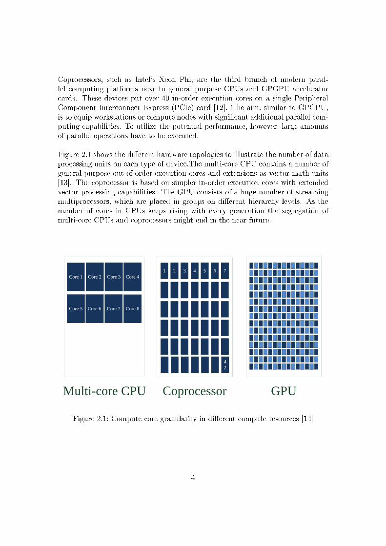
Coprocessors, such as Intel's Xeon Phi, are the third branch of modern paral-lel computing platforms next to general purpose CPUs and GPGPU acceleratorcards. These devices put over 40 in-order execution cores on a single PeripheralComponent Interconnect Express (PCIe) card [12]. The aim, similar to GPGPU,is to equip workstations or compute nodes with signi�cant additional parallel com-puting capabilities. To utilize the potential performance, however, large amountsof parallel operations have to be executed.
Figure 2.1 shows the di�erent hardware topologies to illustrate the number of dataprocessing units on each type of device.The multi-core CPU contains a number ofgeneral purpose out-of-order execution cores and extensions as vector math units[13]. The coprocessor is based on simpler in-order execution cores with extendedvector processing capabilities. The GPU consists of a huge number of streamingmultiprocessors, which are placed in groups on di�erent hierarchy levels. As thenumber of cores in CPUs keeps rising with every generation the segregation ofmulti-core CPUs and coprocessors might end in the near future.
Core 1
1
Core 2 Core 3 Core 4
Core 5 Core 6 Core 7 Core 8
4
2
2 3 4 5 6 7
Multi-core CPU Coprocessor GPU
Figure 2.1: Compute core granularity in di�erent compute resources [14]
4
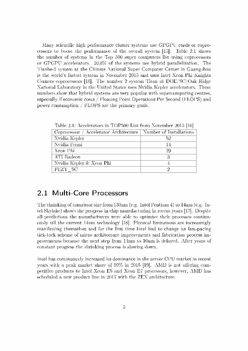
Many scienti�c high performance cluster systems use GPGPU cards or copro-cessors to boost the performance of the overall system [15]. Table 2.1 showsthe number of systems in the Top 500 super computers list using coprocessorsor GPGPU accelerators. 20,8% of the systems use hybrid parallelization. TheTianhe-2 system at the Chinese National Super Computer Center in Guangzhouis the world's fastest system in November 2015 and uses Intel Xeon Phi KnightsCorners coprocessors [16]. The number 2 system Titan at DOE/SC/Oak RidgeNational Laboratory in the United States uses Nvidia Kepler accelerators. Thesenumbers show that hybrid systems are very popular with supercomputing centres,especially if economic costs / Floating Point Operations Per Second (FLOPS) andpower consumption / FLOPS are the primary goals.
Table 2.1: Accelerators in TOP500 List from November 2015 [16]Coprocessor / Accelerator Architecture Number of InstallationsNvidia Kepler 52Nvidia Fermi 14Xeon Phi 29ATI Radeon 3Nvidia Kepler & Xeon Phi 4PEZY_SC 2
2.1 Multi-Core Processors
The shrinking of transistor size from 130nm (e.g. Intel Pentium 4) to 14nm (e.g. In-tel Skylake) shows the progress in chip manufacturing in recent years [17]. Despiteall predictions the manufacturers were able to optimize their processes continu-ously till the current 14nm technology [18]. Physical limitations are increasinglymanifesting themselves and for the �rst time Intel had to change its fast-pacingtick-tock scheme of micro architecture improvements and fabrication process im-provements because the next step from 14nm to 10nm is delayed. After years ofconstant progress the shrinking process is slowing down.
Intel has continuously increased its dominance in the server CPU market in recentyears with a peak market share of 99% in 2015 [19]. AMD is not o�ering com-petitive products to Intel Xeon E5 and Xeon E7 processors, however, AMD hasscheduled a new product line in 2017 with the ZEN architecture.
5
Contrary to Intel's x86 CPU architecture, IBM's Power architecture is used in23 clusters in the TOP500 supercomputing list (November 2015) [16]. The Power8architecture was �rst presented in 2013 and allows up to 96 threads per socket [20].IBM has launched the OpenPOWER initiative in 2013 with partners like Nvidiaand Google to promote the use of Power processors in combination with NvidiaTesla accelerators in High Performance Computing (HPC) environments to createan alternative to Intel based systems.
In recent years, clusters using ARM processors have been built to demonstratethe potential of modern mobile computing cores [21]. Power consumption is be-coming a limiting resource in HPC. Mobile computing cores used in smart phonesand tablet computers have drastically increased their computational power in re-cent years while being optimized for low power demand. These cores can be usedfor higher packaging density and lower cost per processor core chips. ARM addedfully pipelined double precision �oating point units in the Cortex A15 family toenable fast computation of complex problems. Furthermore, the NEON SingleInstruction Multiple Data (SIMD) extension was designed to process multiple nu-merical operations in parallel to make ARM systems appealing to customers outof the mobile chip sector. While there might be potential for ARM based HPCclusters, they are mostly being used in storage appliances and database systemswhich are very I/O depending and do not require very high peak computing per-formance [22]. However, starting from this niche ARM based severs could gainmarket share in HPC in the next years.
Characteristics all these multi-core architectures have in common:
� Out-of-order execution of processor instructions to optimize the usage ofavailable hardware resources on the chip
� Branch prediction to process branches while e�ciently using pipelines
� Multiple Arithmetic Logical Units (ALUs) for �oating point and integerarithmetic
� Di�erent pipelines for di�erent instructions
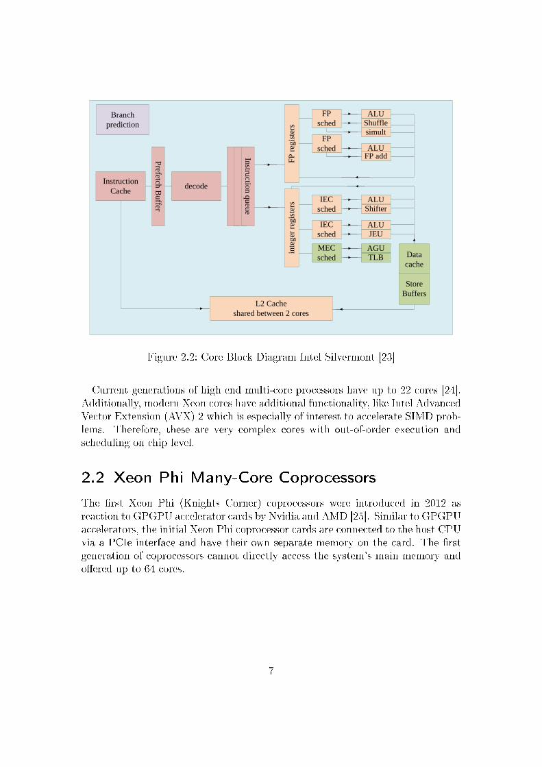
Figure 2.2 shows Intel's Silvermont Core architecture. This out-of-order execu-tion core represents the lower end of Intel's current product range [23]. It has allthe characteristics mentioned above and is used in tablet computers and low endlaptops.
6
Instruction
Cache
Branch
prediction
L2 Cache
shared between 2 cores
Prefetch
Buffer
decode
Instru
ction q
ueu
eF
P r
egis
ters
FP
sched
inte
ger
reg
iste
rs
FP
sched
ALUShufflesimult
ALUFP add
IEC
sched
IEC
sched
ALUShifter
ALUJEU
MEC
sched
AGUTLB Data
cache
Store
Buffers
Figure 2.2: Core Block Diagram Intel Silvermont [23]
Current generations of high end multi-core processors have up to 22 cores [24].Additionally, modern Xeon cores have additional functionality, like Intel AdvancedVector Extension (AVX) 2 which is especially of interest to accelerate SIMD prob-lems. Therefore, these are very complex cores with out-of-order execution andscheduling on chip level.
2.2 Xeon Phi Many-Core Coprocessors
The �rst Xeon Phi (Knights Corner) coprocessors were introduced in 2012 asreaction to GPGPU accelerator cards by Nvidia and AMD [25]. Similar to GPGPUaccelerators, the initial Xeon Phi coprocessor cards are connected to the host CPUvia a PCIe interface and have their own separate memory on the card. The �rstgeneration of coprocessors cannot directly access the system's main memory ando�ered up to 64 cores.
7
Instruction Decode
Scalar Unit Vector Unit
Scalar
Registers
Vector
Registers
32K L1 I-Cache
32K L1 D-Cache
512K L2 Cache
Ring
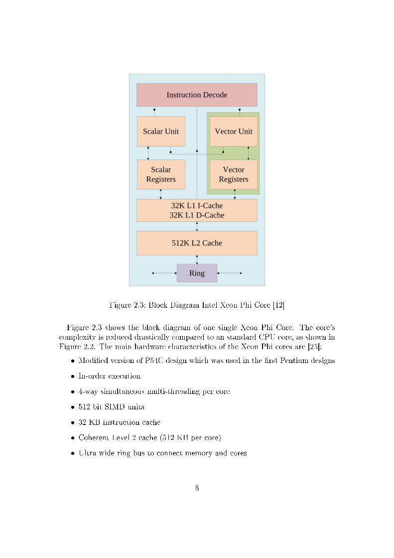
Figure 2.3: Block Diagram Intel Xeon Phi Core [12]
Figure 2.3 shows the block diagram of one single Xeon Phi Core. The core'scomplexity is reduced drastically compared to an standard CPU core, as shown inFigure 2.2. The main hardware characteristics of the Xeon Phi cores are [25]:
� Modi�ed version of P54C design which was used in the �rst Pentium designs
� In-order execution
� 4-way simultaneous multi-threading per core
� 512 bit SIMD units
� 32 KB instruction cache
� Coherent Level 2 cache (512 KB per core)
� Ultra wide ring bus to connect memory and cores
8
2.3 Nvidia CUDA Accelerator Cards
Nvidia's Tesla architecture started changing the processing possibilities of GPUsdrastically when it was introduced in November 2006 [26] [27]. The architectureuni�ed vertex and pixel processors and extended the programmability. PreviousGPUs consisted of graphics pipelines with separate stages. Vertex processors exe-cuted vertex shader programs and pixel fragment processors executed pixel shaderprograms. By unifying these elements into one functional unit non-graphics re-lated parallel tasks are easier processed by the cards. Nvidia introduced the CUDAprogramming model and thus enabled utilizing the cards via an extended C pro-gramming language.
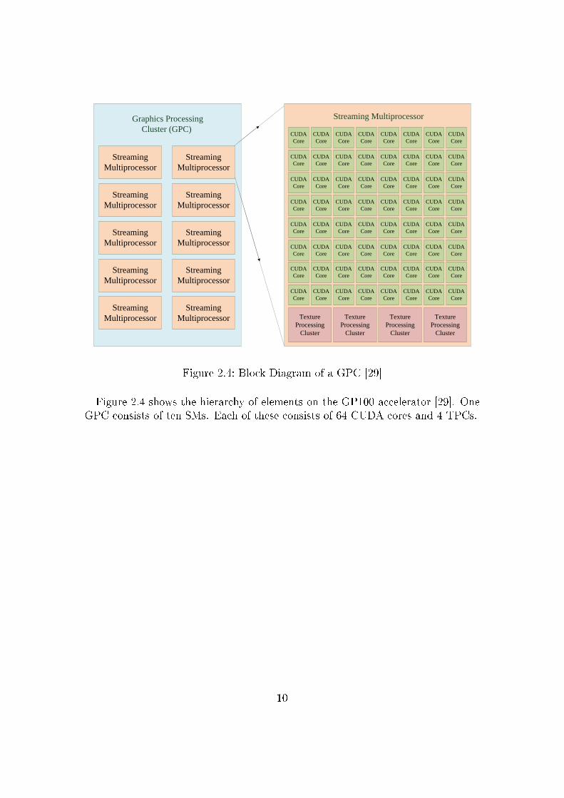
Nvidia's latest Tesla generation is the P100 GPU accelerator series with Nvidia'sPascal architecture [28]. These accelerators are optimized for HPC and deep learn-ing applications. The Graphics Double Data Rate (GDDR) memory was replacedwith second generation High Bandwidth Memory (HBM2). This memory is con-nected via Chip-on-Waver-on-Substrate to minimize the length of data paths. Fur-thermore, the accelerators are not only available with a PCIe interface but alsowith a NVLink interface which is promised to speed up the data link between twoaccelerators for up to �ve times. Calculations with half precision (16 bit �oatingpoint numbers) are now possible. This is expected to further boost applicationslike deep learning applications where throughput is more important than precision.A GP100 accelerator consists of an array of Graphics Processing Clusters (GPCs),Texture Processing Clusters (TPCs), and Streaming Multiprocessors (SMs) [29].
The hardware characteristics of one GP100 accelerator are:
� 6 GPCs per accelerator
� 10 SMs per GPC
� 64 single precision CUDA cores and 4 TPCs per SM
� Total 3850 single precision CUDA cores per accelerator
� Total 240 texture units per accelerator
� 4096 KB Level 2 Cache per accelerator
9
Texture
Processing
Cluster
CUDA
Core
Streaming
Multiprocessor
Streaming
Multiprocessor
Streaming
Multiprocessor
Streaming
Multiprocessor
Streaming
Multiprocessor
Streaming
Multiprocessor
Streaming
Multiprocessor
Streaming
Multiprocessor
Streaming
Multiprocessor
Streaming
Multiprocessor
Graphics Processing
Cluster (GPC)CUDA
Core
CUDA
Core
CUDA
Core
CUDA
Core
CUDA
Core
CUDA
Core
CUDA
Core
CUDA
Core
CUDA
Core
CUDA
Core
CUDA
Core
CUDA
Core
CUDA
Core
CUDA
Core
CUDA
Core
CUDA
Core
CUDA
Core
CUDA
Core
CUDA
Core
CUDA
Core
CUDA
Core
CUDA
Core
CUDA
Core
CUDA
Core
CUDA
Core
CUDA
Core
CUDA
Core
CUDA
Core
CUDA
Core
CUDA
Core
CUDA
Core
CUDA
Core
CUDA
Core
CUDA
Core
CUDA
Core
CUDA
Core
CUDA
Core
CUDA
Core
CUDA
Core
CUDA
Core
CUDA
Core
CUDA
Core
CUDA
Core
CUDA
Core
CUDA
Core
CUDA
Core
CUDA
Core
CUDA
Core
CUDA
Core
CUDA
Core
CUDA
Core
CUDA
Core
CUDA
Core
CUDA
Core
CUDA
Core
CUDA
Core
CUDA
Core
CUDA
Core
CUDA
Core
CUDA
Core
CUDA
Core
CUDA
Core
CUDA
Core
Texture
Processing
Cluster
Texture
Processing
Cluster
Texture
Processing
Cluster
Streaming Multiprocessor
Figure 2.4: Block Diagram of a GPC [29]
Figure 2.4 shows the hierarchy of elements on the GP100 accelerator [29]. OneGPC consists of ten SMs. Each of these consists of 64 CUDA cores and 4 TPCs.
10
3 Parallel Programming
Approaches
Soon after scientists started using computer simulations to verify theories the sim-ulation problems started to exceed the memory and/or computing capabilities of asingle workstation. The next step was to use multiple workstations to distribute theworkload. ARCNET was the �rst commercially available cluster solution launchedin 1977 [30]. Approaches to run software on di�erent computing nodes had to befound. Distribution of software, synchronisation between nodes, and collection ofresults had to be de�ned. Di�erent approaches were in use when the standardiza-tion of MPI started in 1992 [31]. The MPI enables to conveniently exchange databetween compute nodes which work together to solve a computational problem.Due to the distributed-memory nature of the MPI, the developer is forced to care-fully consider the structuring, decomposition, movement, and placement of datain the development phase to achieve e�cient parallel implementations.
Multi-threading led to new concepts of parallelism on a single computer usinga shared-memory approach, where all the threads of the thread-group can accessthe same memory address space (in contrast to MPI, where the MPI processesdo not have access to each others memories). Utilizing multiple physical coresto work on a single task required new approaches designed for multi-core com-puters: POSIX threads (Pthreads) became a standard in 1995 whereas in 1997the OpenMP standard was introduced [32]. OpenMP allows programmers to useparallel sections in software at a high level of abstraction, making it easier to de-velop parallel programs. OpenMP reduces the complexity of developing parallelprograms drastically and is therefore widely used in modern simulations.
Hybrid parallelization typically uses MPI to realise communication between di�er-ent compute nodes but on individual nodes the tasks are assigned to the availablecores using, for instance, a shared-memory OpenMP approach or o�oaded to acoprocessors or GPGPU accelerator (e.g. Nvidia Tesla accelerator) [33]. OpenMPo�ers a range of scheduling mechanisms with the aim to keep the utilization of thesingle cores as high as possible.
11
If a local compute node has a coprocessor or an accelerator card the computationtasks have to be realised using, for example, o�oad-OpenMP or CUDA program-ming [34]. Furthermore, coprocessors and accelerators have their own memoryspaces. Therefore, data locality, reducing communication, and synchronisation iscritical for achieving e�ciently parallelized applications.
In Chapter 3.1, the basic concepts, topologies, and usage of MPI are presented.Chapter 3.2 gives on overview over shared memory multi-thread programmingusing OpenMP. In Chapter 3.2.2, the traditional multi-core OpenMP model is ex-tended and approaches to utilize coprocessors using o�oad and hybrid OpenMPare presented. Finally, Chapter 3.3 focuses on the usage of GPGPU acceleratorcards using the CUDA programming language.
3.1 MPI
The MPI was designed with the goal to unify syntax and precise semantics ofmessage passing libraries [31]. The standardization began in 1992 and the initialversion 1.0 of the standard was released in 1994. MPI is a message-passing Ap-plication Programming Interface (API). There are many implementations of theMPI standard of which several are free open-source projects and several commer-cial software packages.
The main reasons for using the MPI are [35]:
� Standardization: The MPI is the only message passing library that can beconsidered a standard that is supported on virtually all HPC platforms.
� Portability: When using a di�erent platform that supports the MPI standardthere is little to no need to modify source code.
� Performance Opportunities: Vendor implementations can use native hard-ware features to increase the MPI transmission speed.
� Functionality: There are over 430 MPI routines in MPI3 which cover nearlyevery use case. Most simple MPI programs can be written with about 10MPI routines.
12
3.1.1 Structure of MPI Programs
The MPI uses objects called communicators and groups to de�ne which collectionsof processes can communicate with each other. For larger and more complex prob-lems it can be very useful to group and name processes to increase the readabilityof source code. Furthermore, every MPI process has a unique integer identi�ercalled rank. The rank is an integer value within a communicator and can be usedto assign certain tasks to speci�c MPI processes (e.g. if(rank==0),{...}). Thisis useful when, for instance, rank 0 is used as master process which reads dataand sends computing tasks to the remaining processes following a master/slaveapproach. Then every process does a number of calculations processing a subsetof the initial problem and ultimately sends the sub-results back to rank 0 for post-processing.
Figure 3.1 shows the structure of an MPI program. The essential MPI calls usingthe C programming language are discussed in the following [36].
MPI Program Structure
MPI include file
Declarations, prototypes, etc.
Program begins
Do work & make message
passing calls
Terminate MPI environment
Initialize MPI environment Parallel code begins
Parallel code ends
Program ends
...
...
Figure 3.1: Structure of a MPI program [35]
13
Initializing the MPI environment:
� MPI_Init( int *argc, char ***argv ): Initializes the MPI environment.Must be called before any other MPI function.
� MPI_Comm_size( MPI_Comm comm, int *size ): Returns the number ofprocesses in the speci�ed communicator (e.g. MPI_COMM_WORLD)
� MPI_Comm_rank( MPI_Comm comm, int *rank ): Returns the rank (integervalue) of the process within the speci�ed communicator
After initializing the MPI environment the communication between di�erent pro-cesses can be started. There are two types of communication in MPI: point-to-point message passing (e.g. MPI_Send) and collective (global) operations (e.g.MPI_Bcast). Point-to-point messages can be blocking or non-blocking. Whenusing blocking calls the program waits until the data transfer is �nished and pro-ceeds afterwards. Non-blocking operations are sending and receiving data in thebackground while the process still executes other operations which introduces thepotential for overlapping communication with computation, albeit in reality thisis not always achieved [37]. Common point-to-point and collective operations:
� MPI_Send(const void *buf, int count, MPI_Datatype datatype, int
dest, int tag, MPI_Comm comm): Blocking send only returns after thedata is stored in the send bu�er and it is safe to write more data there.
� MPI_Recv(void *buf, int count, MPI_Datatype datatype, int source,
int tag, MPI_Comm comm, MPI_Status *status): Blocking receive returnsafter the data arrived and is ready-to-use by the process
� MPI_Isend(const void *buf, int count, MPI_Datatype datatype, int
dest, int tag, MPI_Comm comm, MPI_Request *request): Non-blockingsend returns almost immediately, i.e., the MPI does not wait for any callsor messages that con�rm the data transmission. To ensure a correct datatransfer status and wait mechanisms have to be used.
� MPI_Irecv(void *buf, int count, MPI_Datatype datatype, int source,
int tag, MPI_Comm comm, MPI_Request *request): Non-blocking receivereturns almost immediately and starts receiving data in the background.
� MPI_Wait(MPI_Request *request, MPI_Status *status): Waits for allnon-blocking communications to be �nished
� MPI_Bcast( void *buffer, int count, MPI_Datatype datatype, int root,
MPI_Comm comm ): Sends a broadcast message from the process with ranknumber root to all other processes in the communicator.
14
� MPI_Barrier( MPI_Comm comm): Synchronizes processes in the communica-tor. All processes are blocked until every process reaches the barrier.
After the MPI program �nished the MPI environments needs to be appropriatelyshut down:
� MPI_Finalize( void ): Finalizes the MPI environment. No more MPIcalls must be made after this command.
If errors or unde�ned conditions occur during the process execution the whole MPIprogram needs to be aborted.
� MPI_Abort(MPI_Comm comm, int errorcode): Terminates all MPI processesin the speci�ed communicator. A simple exit() call would only end one pro-cess while the rest of the processes keep running. To avoid this unde�nedstate MPI_Abort is used.
The presented set of commands constitutes a subset of the provided API features,however, already with this small set it is possible to set up many MPI programsfor various purposes. In general, communication between processes should beas limited as possible because it causes overhead and slows down the programexecution. Often communication is responsible for limiting the parallel scalabilityand ultimately the execution performance.
3.1.2 MPI Implementations
The MPI standard describes the protocol and the semantics which have to becovered by a MPI implementation [38]. The behaviour of di�erent MPI imple-mentations should be as similar as possible to allow for portability. There are twowidely used and free open-source MPI implementations at the moment: MPICH[39] and OpenMPI [40].
MPICH is a high quality open-source implementation of the latest MPI stan-dard [41]. MPICH is used as base for a number of derivative implementations,e.g., Intel MPI, MVAPICH, Cray MPI, and IBM MPI. These implementationsprovide some specializations, for instance, the Intel MPI implementation providesoptimized support for Xeon Phi coprocessors used within MPI environments. [42].
OpenMPI is an open-source MPI implementation based on the code of LAM/MPI,LA-MPI and FT-MPI [43]. It is widely used by the Top 500 supercomputers. Onedesign goal was to support all widely used interconnects as TCP/IP, shared mem-ory systems, Myrinet, Quadrics and In�niBand. OpenMPI's process managerORTE o�ers some advantages over the MPICH's Hydra process manager [44].
15
3.2 OpenMP
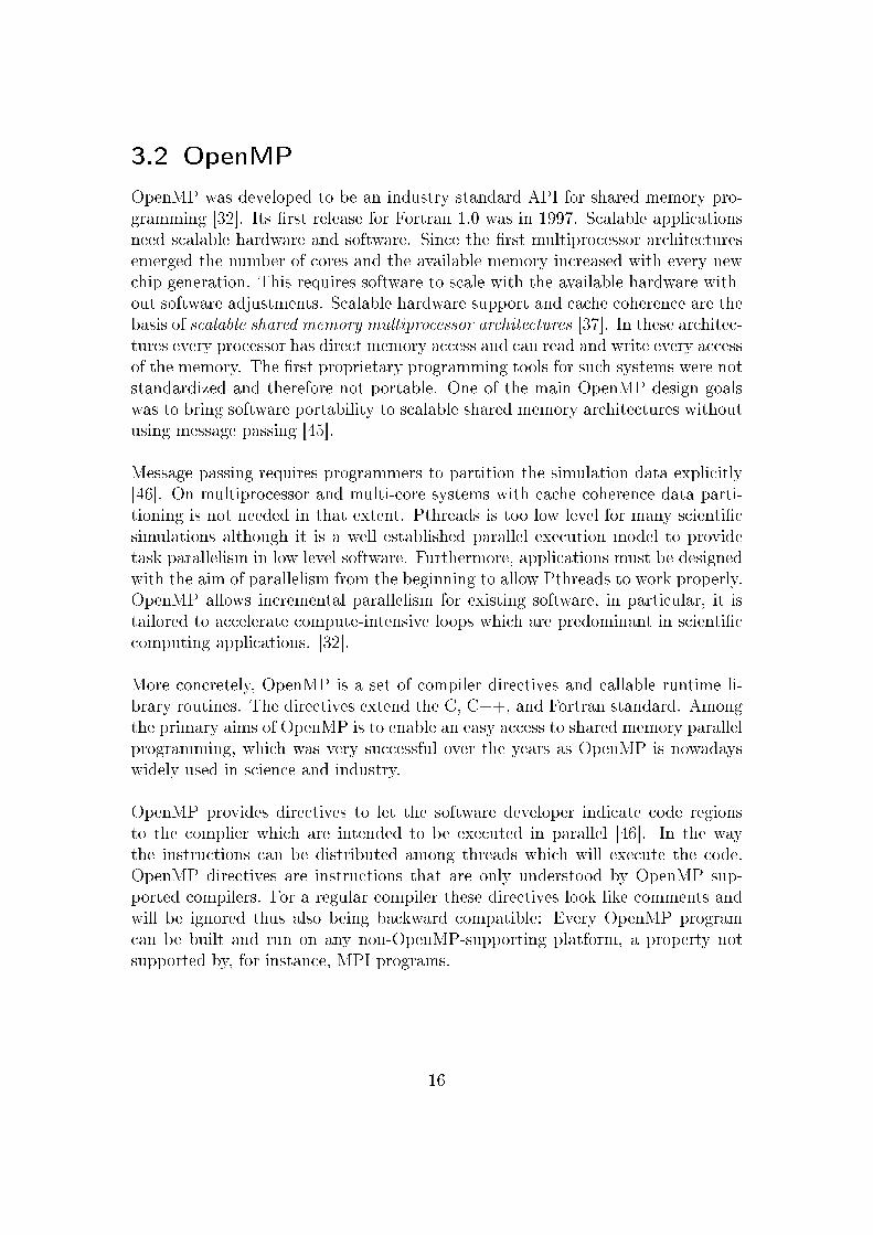
OpenMP was developed to be an industry standard API for shared memory pro-gramming [32]. Its �rst release for Fortran 1.0 was in 1997. Scalable applicationsneed scalable hardware and software. Since the �rst multiprocessor architecturesemerged the number of cores and the available memory increased with every newchip generation. This requires software to scale with the available hardware with-out software adjustments. Scalable hardware support and cache coherence are thebasis of scalable shared memory multiprocessor architectures [37]. In these architec-tures every processor has direct memory access and can read and write every accessof the memory. The �rst proprietary programming tools for such systems were notstandardized and therefore not portable. One of the main OpenMP design goalswas to bring software portability to scalable shared memory architectures withoutusing message passing [45].
Message passing requires programmers to partition the simulation data explicitly[46]. On multiprocessor and multi-core systems with cache coherence data parti-tioning is not needed in that extent. Pthreads is too low level for many scienti�csimulations although it is a well established parallel execution model to providetask parallelism in low level software. Furthermore, applications must be designedwith the aim of parallelism from the beginning to allow Pthreads to work properly.OpenMP allows incremental parallelism for existing software, in particular, it istailored to accelerate compute-intensive loops which are predominant in scienti�ccomputing applications. [32].
More concretely, OpenMP is a set of compiler directives and callable runtime li-brary routines. The directives extend the C, C++, and Fortran standard. Amongthe primary aims of OpenMP is to enable an easy access to shared memory parallelprogramming, which was very successful over the years as OpenMP is nowadayswidely used in science and industry.
OpenMP provides directives to let the software developer indicate code regionsto the complier which are intended to be executed in parallel [46]. In the waythe instructions can be distributed among threads which will execute the code.OpenMP directives are instructions that are only understood by OpenMP sup-ported compilers. For a regular compiler these directives look like comments andwill be ignored thus also being backward compatible: Every OpenMP programcan be built and run on any non-OpenMP-supporting platform, a property notsupported by, for instance, MPI programs.
16
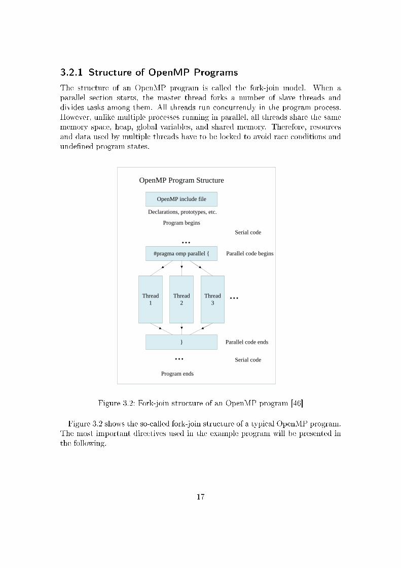
3.2.1 Structure of OpenMP Programs
The structure of an OpenMP program is called the fork-join model. When aparallel section starts, the master thread forks a number of slave threads anddivides tasks among them. All threads run concurrently in the program process.However, unlike multiple processes running in parallel, all threads share the samememory space, heap, global variables, and shared memory. Therefore, resourcesand data used by multiple threads have to be locked to avoid race conditions andunde�ned program states.
OpenMP Program Structure
OpenMP include file
Declarations, prototypes, etc.
Program begins
Thread
2
}
#pragma omp parallel {
Serial code
Parallel code begins
Parallel code ends
Program ends
Serial code
...
...
Thread
3
Thread
1
...
Figure 3.2: Fork-join structure of an OpenMP program [46]
Figure 3.2 shows the so-called fork-join structure of a typical OpenMP program.The most important directives used in the example program will be presented inthe following.
17
All OpenMP directives used in a C program need to start with #pragma omp.A valid OpenMP instruction needs to appear after the pragma and before anyclauses. For example:
� #pragma omp parallel default(shared) private(beta,pi)
The parallel region is the fundamental OpenMP construct. It is a block of in-structions executed by multiple threads. When a parallel block starts one threadbecomes the master thread with thread id 0. After the end of the parallel regiononly the master thread will be executed.
� #pragma omp parallel { }: Directive to start and end a parallel region.
� omp_set_num_threads(int num_threads): Sets the number of threads tobe started within the parallel region. The number can alternatively be de-�ned using the OMP_NUM_THREADS environment variable.
� int omp_get_num_threads(void): Returns the number of threads in a par-allel region.
� int omp_get_thread_num(void): Returns the thread id of the calling thread.Threads are numbered from 0 (master) to omp_get_num_threads()-1.
For loops are ideal blocks to be run in parallel. The big restriction of parallelfor loops is that the program must not depend on the chronological order of theexecuted iterations.
� #pragma omp for { }: Directive to execute iterations of a for loop parallel
� #pragma omp for schedule (static,dynamic) {}: Allows to set the schedul-ing to di�erent policies, such as, dynamic or static. Static scheduling di-vides the iteration space into (near)equal parts while dynamic schedulingdistributes the iteration space into smaller chunks, gradually feeding thoseto threads once a thread is �nished with processing the previous one. Staticscheduling has less overhead but is only suitable to problems where the com-putational e�ort for each iteration remains nearly constant. On the contrary,dynamic scheduling allows to handle varying computational e�ort per itera-tion better and is thus typically used for load-unbalanced situations.
18
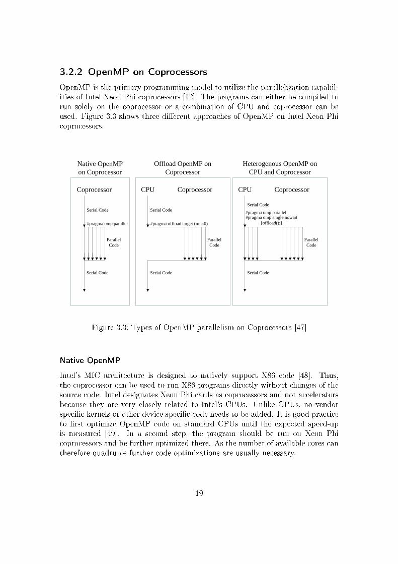
3.2.2 OpenMP on Coprocessors
OpenMP is the primary programming model to utilize the parallelization capabil-ities of Intel Xeon Phi coprocessors [12]. The programs can either be compiled torun solely on the coprocessor or a combination of CPU and coprocessor can beused. Figure 3.3 shows three di�erent approaches of OpenMP on Intel Xeon Phicoprocessors.
Coprocessor
Serial Code
Serial Code
#pragma omp parallel
Parallel
Code
CPU Coprocessor
Serial Code
Serial Code
#pragma offload target (mic:0)
Parallel
Code
CPU Coprocessor
Serial Code
Serial Code
#pragma omp single nowait
{offload();}
Parallel
Code
#pragma omp parallel
Native OpenMP
on Coprocessor
Offload OpenMP on
Coprocessor
Heterogenous OpenMP on
CPU and Coprocessor
Figure 3.3: Types of OpenMP parallelism on Coprocessors [47]
Native OpenMP
Intel's MIC architecture is designed to natively support X86 code [48]. Thus,the coprocessor can be used to run X86 programs directly without changes of thesource code. Intel designates Xeon Phi cards as coprocessors and not acceleratorsbecause they are very closely related to Intel's CPUs. Unlike GPUs, no vendorspeci�c kernels or other device speci�c code needs to be added. It is good practiceto �rst optimize OpenMP code on standard CPUs until the expected speed-upis measured [49]. In a second step, the program should be run on Xeon Phicoprocessors and be further optimized there. As the number of available cores cantherefore quadruple further code optimizations are usually necessary.
19
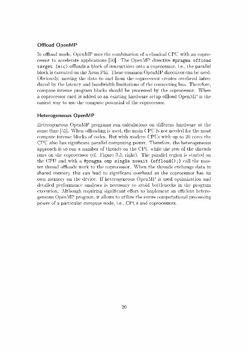
O�oad OpenMP
In o�oad mode, OpenMP uses the combination of a classical CPU with an copro-cessor to accelerate applications [50]. The OpenMP directive #pragma offload
target (mic) o�oads a block of instructions onto a coprocessor, i.e., the parallelblock is executed on the Xeon Phi. There common OpenMP directives can be used.Obviously, moving the data to and from the coprocessor creates overhead intro-duced by the latency and bandwidth limitations of the connecting bus. Therefore,compute intense program blocks should be processed by the coprocessor. Whena coprocessor card is added to an existing hardware setup o�oad OpenMP is theeasiest way to use the compute potential of the coprocessor.
Heterogeneous OpenMP
Heterogeneous OpenMP programs run calculations on di�erent hardware at thesame time [51]. When o�oading is used, the main CPU is not needed for the mostcompute intense blocks of codes. But with modern CPUs with up to 20 cores theCPU also has signi�cant parallel computing power. Therefore, the heterogeneousapproach is to run a number of threads on the CPU while the rest of the threadsruns on the coprocessor (cf. Figure 3.3, right). The parallel region is started onthe CPU and with a #pragma omp single nowait {offload();} call the mas-ter thread o�oads work to the coprocessor. When the threads exchange data inshared memory this can lead to signi�cant overhead as the coprocessor has itsown memory on the device. If heterogeneous OpenMP is used optimization anddetailed performance analyses is necessary to avoid bottlenecks in the programexecution. Although requiring signi�cant e�ort to implement an e�cient hetero-geneous OpenMP program, it allows to utilize the entire computational processingpower of a particular compute node, i.e., CPUs and coprocessors.
20
3.3 CUDA C
GPUs are massively parallel processors which support thousands of active threads(up to 20480 on GP100) [52]. This highly parallel computing platform requiresa specialized programming model to e�ciently express that kind of parallelism(most important data parallelism). Nvidia's CUDA represents such a tailoredmodel. CUDA is a co-evolved hardware and software architecture which allowsHPC developers to utilize the resources in a familiar programming environment[53]. The CUDA programming language extends the classical C language by sev-eral new instructions.
When scientists started to use GPUs for GPGPU computing they �rst used graph-ics programming APIs, such as OpenGL [53]. This approach limited the �exibilityof the developed software and was an obstacle to HPC software developers whowere often not familiar with graphics-focused programming. Nvidia's CUDA ar-chitecture enabled programming in C-like syntax and semantics, which was one ofthe primary reason for its success due to the broad C user base. Today, all currentNvidia GPUs can be accessed via CUDA. The Tesla product line is speci�callydeveloped for the HPC �eld and gained signi�cant market share as accelerator forscienti�c simulations [54].
In real world applications where CUDA on accelerator cards is used speed-upsfrom 10x to 100x compared to conventional approaches are achieved [53]. Medicalimaging was one of the �rst topics where performance increase of this magnitudechanges the way diagnostics are used [55]. Today, GPGPU is of interest to all ar-eas of compute-intensive science and engineering applications, such as mechanical-,chemical-, and electrical engineering as well as �uid dynamics, meteorology etc.
To clarify if program parts are executed on the compute node's CPU or the accel-erator Nvidia introduced following de�nitions in its CUDA documentation [56]:
� Host: CPU of the compute node on which the accelerator is installed
� Device: accelerator
� Kernel: parallel parts of an application executed on the accelerator. Onlyone kernel is executed at a time. Many threads execute each kernel.
21
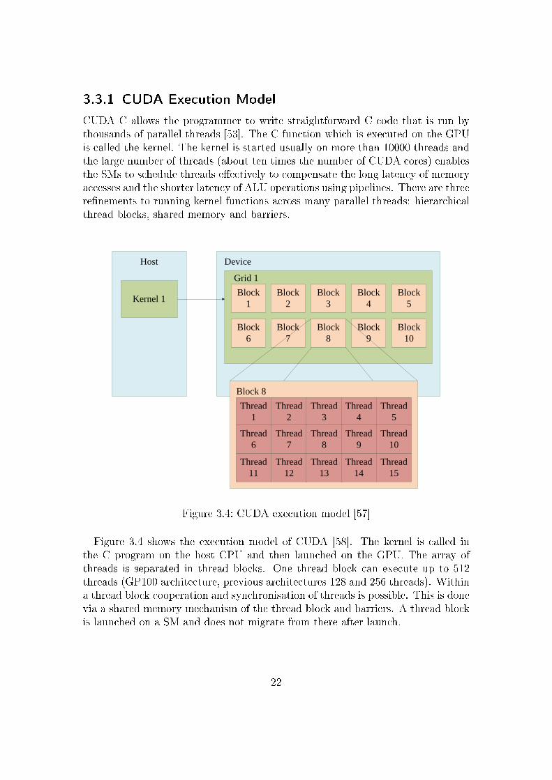
3.3.1 CUDA Execution Model
CUDA C allows the programmer to write straightforward C code that is run bythousands of parallel threads [53]. The C function which is executed on the GPUis called the kernel. The kernel is started usually on more than 10000 threads andthe large number of threads (about ten times the number of CUDA cores) enablesthe SMs to schedule threads e�ectively to compensate the long latency of memoryaccesses and the shorter latency of ALU operations using pipelines. There are threere�nements to running kernel functions across many parallel threads: hierarchicalthread blocks, shared memory and barriers.
Kernel 1Block
1
Block
2
Block
3
Block
4
Block
5
Block
6
Block
7
Block
8
Block
9
Block
10
Thread
1
Thread
2
Thread
3
Thread
4
Thread
5
Thread
6
Thread
7
Thread
8
Thread
9
Thread
10
Thread
11
Thread
12
Thread
13
Thread
14
Thread
15
Block 8
Grid 1
Host Device
Figure 3.4: CUDA execution model [57]
Figure 3.4 shows the execution model of CUDA [58]. The kernel is called inthe C program on the host CPU and then launched on the GPU. The array ofthreads is separated in thread blocks. One thread block can execute up to 512threads (GP100 architecture, previous architectures 128 and 256 threads). Withina thread block cooperation and synchronisation of threads is possible. This is donevia a shared memory mechanism of the thread block and barriers. A thread blockis launched on a SM and does not migrate from there after launch.
22
The thread blocks are organized in a grid. A kernel is executed by a grid ofthread blocks. The organisation of threads in thread blocks and grids allows theprogrammer to �ne tune the parallelism to a speci�c problem. On low cost, lowpower GPUs one thread block with all synchronisation and shared memory canbe run while on high end Tesla cards dozens of thread blocks are executed at thesame time.
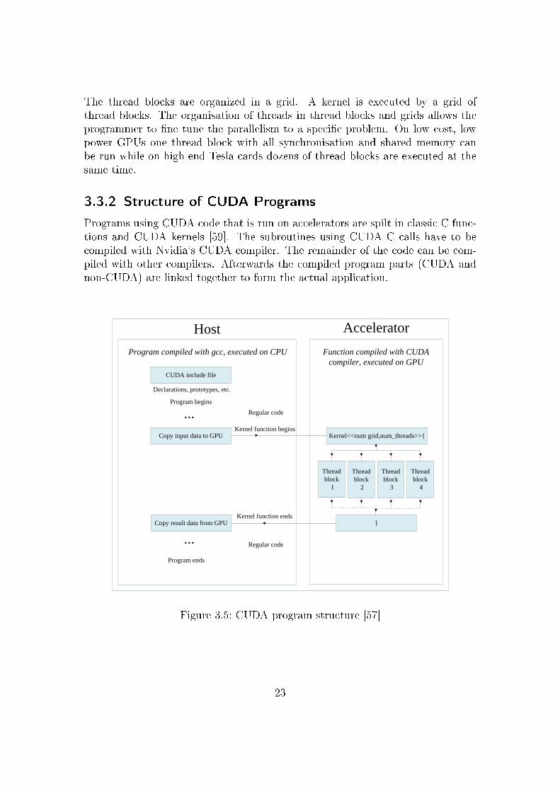
3.3.2 Structure of CUDA Programs
Programs using CUDA code that is run on accelerators are spilt in classic C func-tions and CUDA kernels [59]. The subroutines using CUDA C calls have to becompiled with Nvidia's CUDA compiler. The remainder of the code can be com-piled with other compilers. Afterwards the compiled program parts (CUDA andnon-CUDA) are linked together to form the actual application.
CUDA include file
Declarations, prototypes, etc.
Program begins
}
Kernel<<num grid,num_threads>>{
Regular code
Kernel function begins
Kernel function ends
Program ends
Regular code
Thread
block
1
Thread
block
2
Thread
block
3
Thread
block
4
Program compiled with gcc, executed on CPU Function compiled with CUDA
compiler, executed on GPU
...
...
Copy input data to GPU
Copy result data from GPU
Host Accelerator
Figure 3.5: CUDA program structure [57]
23
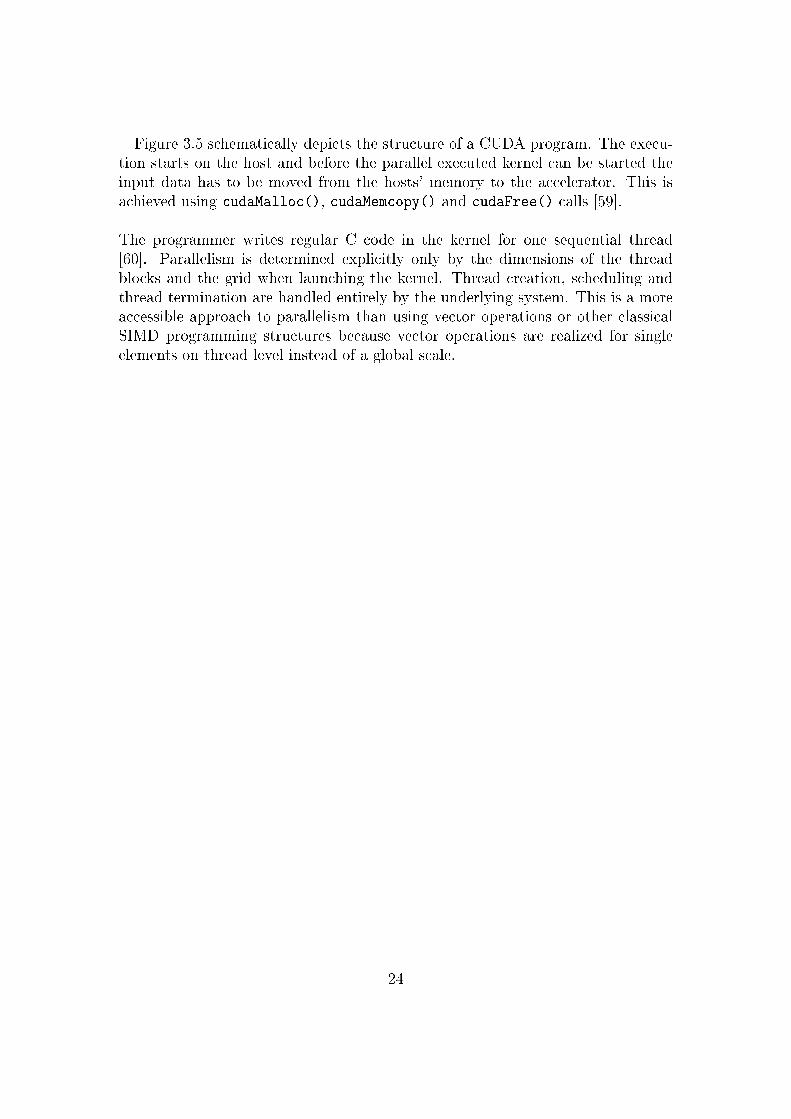
Figure 3.5 schematically depicts the structure of a CUDA program. The execu-tion starts on the host and before the parallel executed kernel can be started theinput data has to be moved from the hosts' memory to the accelerator. This isachieved using cudaMalloc(), cudaMemcopy() and cudaFree() calls [59].
The programmer writes regular C code in the kernel for one sequential thread[60]. Parallelism is determined explicitly only by the dimensions of the threadblocks and the grid when launching the kernel. Thread creation, scheduling andthread termination are handled entirely by the underlying system. This is a moreaccessible approach to parallelism than using vector operations or other classicalSIMD programming structures because vector operations are realized for singleelements on thread level instead of a global scale.
24
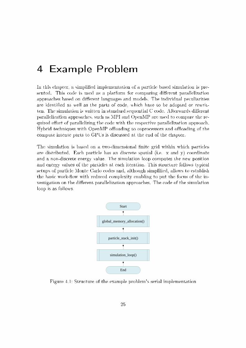
4 Example Problem
In this chapter, a simpli�ed implementation of a particle based simulation is pre-sented. This code is used as a platform for comparing di�erent parallelizationapproaches based on di�erent languages and models. The individual peculiaritiesare identi�ed as well as the parts of code, which have to be adopted or rewrit-ten. The simulation is written in standard sequential C code. Afterwards di�erentparallelization approaches, such as MPI and OpenMP are used to compare the re-quired e�ort of parallelizing the code with the respective parallelization approach.Hybrid techniques with OpenMP o�oading to coprocessors and o�oading of thecompute intense parts to GPUs is discussed at the end of the chapter.
The simulation is based on a two-dimensional �nite grid within which particlesare distributed. Each particle has an discrete spatial (i.e. x and y) coordinateand a non-discrete energy value. The simulation loop computes the new positionand energy values of the particles at each iteration. This structure follows typicalsetups of particle Monte Carlo codes and, although simpli�ed, allows to establishthe basic work-�ow with reduced complexity enabling to put the focus of the in-vestigation on the di�erent parallelization approaches. The code of the simulationloop is as follows.
Start
global_memory_allocation()
particle_stack_init()
simulation_loop()
End
Figure 4.1: Structure of the example problem's serial implementation
25
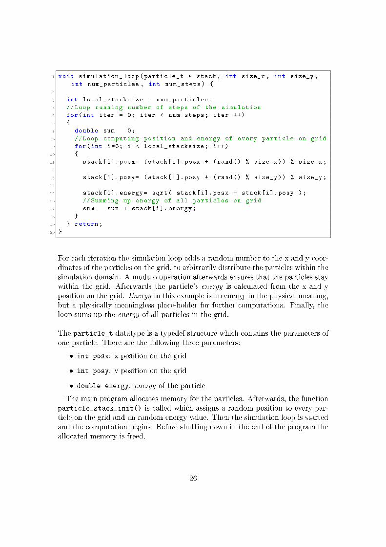
1 void simulation_loop(particle_t * stack , int size_x , int size_y ,
int num_particles , int num_steps) {
2
3 int local_stacksize = num_particles;
4 //Loop running number of steps of the simulation
5 for(int iter = 0; iter < num_steps; iter ++)
6 {
7 double sum = 0;
8 //Loop computing position and energy of every particle on grid
9 for(int i=0; i < local_stacksize; i++)
10 {
11 stack[i].posx= (stack[i].posx + (rand() % size_x)) % size_x;
12
13 stack[i].posy= (stack[i].posy + (rand() % size_y)) % size_y;
14
15 stack[i]. energy= sqrt( stack[i].posx + stack[i].posy );
16 // Summing up energy of all particles on grid
17 sum = sum + stack[i]. energy;
18 }
19 } return;
20 }
For each iteration the simulation loop adds a random number to the x and y coor-dinates of the particles on the grid, to arbitrarily distribute the particles within thesimulation domain. A modulo operation afterwards ensures that the particles staywithin the grid. Afterwards the particle's energy is calculated from the x and yposition on the grid. Energy in this example is no energy in the physical meaning,but a physically meaningless place-holder for further computations. Finally, theloop sums up the energy of all particles in the grid.
The particle_t datatype is a typedef structure which contains the parameters ofone particle. There are the following three parameters:
� int posx: x position on the grid
� int posy: y position on the grid
� double energy: energy of the particle
The main program allocates memory for the particles. Afterwards, the functionparticle_stack_init() is called which assigns a random position to every par-ticle on the grid and an random energy value. Then the simulation loop is startedand the computation begins. Before shutting down in the end of the program theallocated memory is freed.
26
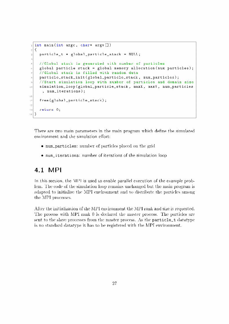
1 int main(int argc , char* argv [])
2 {
3 particle_t * global_particle_stack = NULL;
4
5 // Global stack is generated with number of particles
6 global_particle_stack = global_memory_allocation(num_particles);
7 // Global stack is filled with random data
8 particle_stack_init(global_particle_stack , num_particles);
9 // Start simulation loop with number of particles and domain size
10 simulation_loop(global_particle_stack , maxX , maxY , num_particles
, num_iterations);
11
12 free(global_particle_stack);
13
14 return 0;
15 }
There are two main parameters in the main program which de�ne the simulatedenvironment and the simulation e�ort:
� num_particles: number of particles placed on the grid
� num_iterations: number of iterations of the simulation loop
4.1 MPI
In this section, the MPI is used to enable parallel execution of the example prob-lem. The code of the simulation loop remains unchanged but the main program isadapted to initialize the MPI environment and to distribute the particles amongthe MPI processes.
After the initialization of the MPI environment the MPI rank and size is requested.The process with MPI rank 0 is declared the master process. The particles aresent to the slave processes from the master process. As the particle_t datatypeis no standard datatype it has to be registered with the MPI environment.
27
1 int mpi_size , mpi_rank;
2 const int mpi_master = 0;
3
4 // initialize the MPI environment
5 MPI_Init (&argc , &argv);
6
7 // retrieve the number of MPI processes in the execution
8 // as well as the MPI rank (i.e. id) of the current process
9 MPI_Comm_size(MPI_COMM_WORLD , &mpi_size);
10 MPI_Comm_rank(MPI_COMM_WORLD , &mpi_rank);
11
12 // Register the particle struct with the MPI Backend
13 MPI_Datatype MPI_PARTICLE;
14 particle_t particle;
15 mpi_register_particle (&particle , &MPI_PARTICLE);
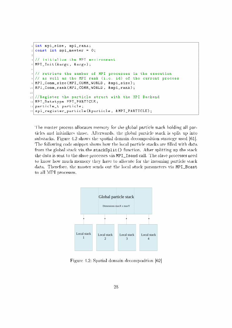
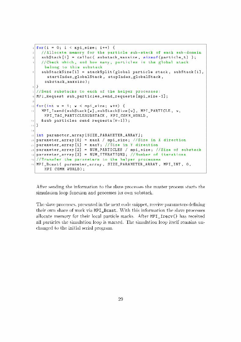
The master process allocates memory for the global particle stack holding all par-ticles and initializes those. Afterwards, the global particle stack is split up intosubstacks. Figure 4.2 shows the spatial domain decomposition strategy used [61].The following code snippet shows how the local particle stacks are �lled with datafrom the global stack via the stackSplit() function. After splitting up the stackthe data is sent to the slave processes via MPI_Isend call. The slave processes needto know how much memory they have to allocate for the incoming particle stackdata. Therefore, the master sends out the local stack parameters via MPI_Bcast
to all MPI processes.
Global particle stack
Dimensions maxX x maxY
Local stack
1Local stack
2
Local stack
3
Local stack
4
Figure 4.2: Spatial domain decomposition [62]
28
1 for(i = 0; i < mpi_size; i++) {
2 // Allocate memory for the particle sub -stack of each sub -domain
3 subStack[i] = calloc( substack_maxsize , sizeof(particle_t) );
4 // Check which , and how many , particles in the global stack
belong to this substack
5 subStackSize[i] = stackSplit(global_particle_stack , subStack[i],
startIndex_globalStack , stopIndex_globalStack ,
substack_maxsize);
6 }
7 //Send substacks to each of the helper processes:
8 MPI_Request sub_particles_send_requests[mpi_size -1];
9
10 for(int w = 1; w < mpi_size; w++) {
11 MPI_Isend(subStack[w],subStackSize[w], MPI_PARTICLE , w,
MPI_TAG_PARTICLESUBSTACK , MPI_COMM_WORLD ,
12 &sub_particles_send_requests[w-1]);
13 }
14
15 int parameter_array[SIZE_PARAMETER_ARRAY ];
16 parameter_array [0] = maxX / mpi_size; //Size in X direction
17 parameter_array [1] = maxY; //Size in Y direction
18 parameter_array [2] = NUM_PARTICLES / mpi_size; //Size of substack
19 parameter_array [3] = NUM_ITERATIONS; // Number of iterations
20 // Transfer the parameters to the helper processes
21 MPI_Bcast( parameter_array , SIZE_PARAMETER_ARRAY , MPI_INT , 0,
MPI_COMM_WORLD);
After sending the information to the slave processes the master process starts thesimulation loop function and processes its own substack.
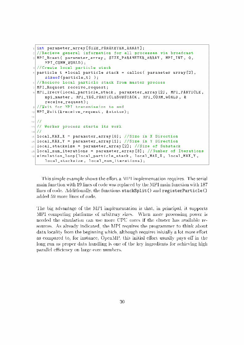
The slave processes, presented in the next code snippet, receive parameters de�ningtheir own share of work via MPI_Bcast. With this information the slave processesallocate memory for their local particle stacks. After MPI_Irecv() has receivedall particles the simulation loop is started. The simulation loop itself remains un-changed to the initial serial program.
29
1 int parameter_array[SIZE_PARAMETER_ARRAY ];
2 // Recieve general information for all processes via broadcast
3 MPI_Bcast( parameter_array , SIZE_PARAMETER_ARRAY , MPI_INT , 0,
MPI_COMM_WORLD);
4 // Create local particle stack
5 particle_t *local_particle_stack = calloc( parameter_array [2],
sizeof(particle_t) );
6 // Recieve local particle stack from master process
7 MPI_Request receive_request;
8 MPI_Irecv(local_particle_stack , parameter_array [2], MPI_PARTICLE ,
mpi_master , MPI_TAG_PARTICLESUBSTACK , MPI_COMM_WORLD , &
receive_request);
9 //Wait for MPI transmission to end
10 MPI_Wait (& receive_request , &status);
11
12 //
13 // Worker process starts its work
14 //
15 local_MAX_X = parameter_array [0]; //Size in X Direction
16 local_MAX_Y = parameter_array [1]; //Size in Y Direction
17 local_stacksize = parameter_array [2]; //Size of Substack
18 local_num_iterations = parameter_array [3]; // Number of Iterations
19 simulation_loop(local_particle_stack , local_MAX_X , local_MAX_Y ,
local_stacksize , local_num_iterations);
This simple example shows the e�ort a MPI implementation requires. The serialmain function with 19 lines of code was replaced by the MPI main function with 187lines of code. Additionally, the functions stackSplit() and registerParticle()
added 59 more lines of code.
The big advantage of the MPI implementation is that, in principal, it supportsMPI computing platforms of arbitrary sizes. When more processing power isneeded the simulation can use more CPU cores if the cluster has available re-sources. As already indicated, the MPI requires the programmer to think aboutdata locality from the beginning which, although requires initially a lot more e�ortas compared to, for instance, OpenMP, this initial e�ort usually pays o� in thelong run as proper data handling is one of the key ingredients for achieving highparallel e�ciency on large core numbers.
30
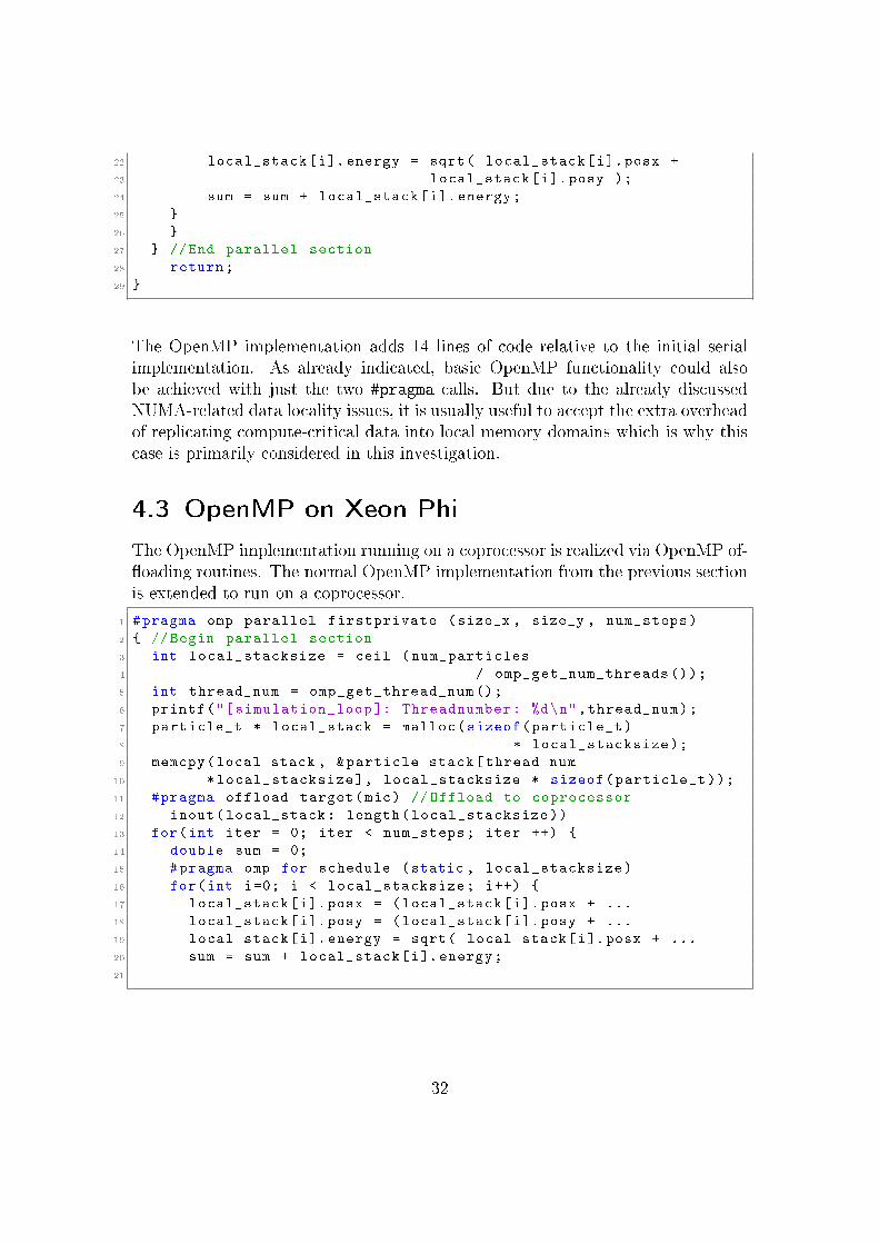
4.2 OpenMP
The implementation of the OpenMP parallelization is only done in the simulationloop subroutine, as it hosts the central compute-intensive loop over the particlestack. The initial serial main program remains unchanged. On a side note, theMPI main program can also be used to use MPI for the distribution over multiplecomputing nodes and OpenMP for parallelism on the local shared memory node,paving the way for a hybrid MPI-OpenMP approach.
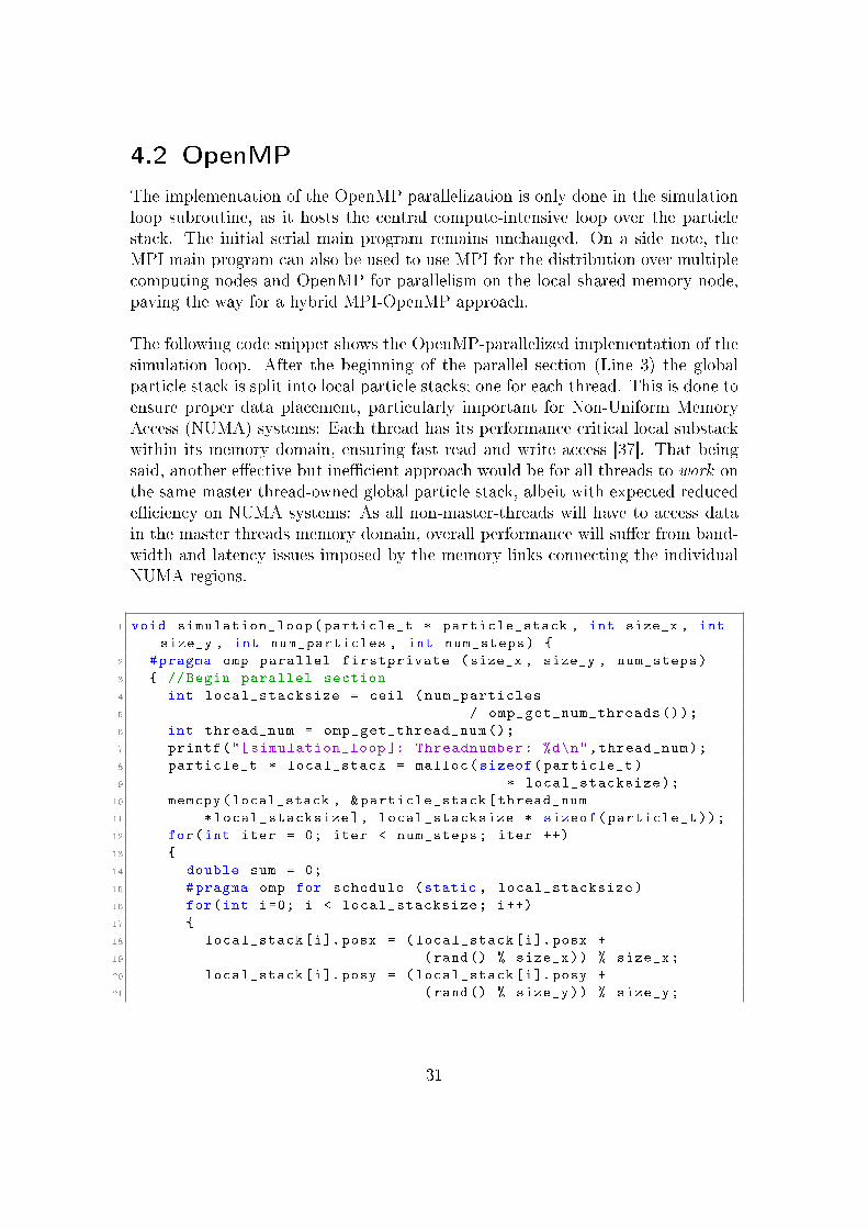
The following code snippet shows the OpenMP-parallelized implementation of thesimulation loop. After the beginning of the parallel section (Line 3) the globalparticle stack is split into local particle stacks; one for each thread. This is done toensure proper data placement, particularly important for Non-Uniform MemoryAccess (NUMA) systems: Each thread has its performance critical local substackwithin its memory domain, ensuring fast read and write access [37]. That beingsaid, another e�ective but ine�cient approach would be for all threads to work onthe same master thread-owned global particle stack, albeit with expected reducede�ciency on NUMA systems: As all non-master-threads will have to access datain the master threads memory domain, overall performance will su�er from band-width and latency issues imposed by the memory links connecting the individualNUMA regions.
1 void simulation_loop(particle_t * particle_stack , int size_x , int
size_y , int num_particles , int num_steps) {
2 #pragma omp parallel firstprivate (size_x , size_y , num_steps)
3 { // Begin parallel section
4 int local_stacksize = ceil (num_particles
5 / omp_get_num_threads ());
6 int thread_num = omp_get_thread_num ();
7 printf("[simulation_loop ]: Threadnumber: %d\n",thread_num);
8 particle_t * local_stack = malloc(sizeof(particle_t)
9 * local_stacksize);
10 memcpy(local_stack , &particle_stack[thread_num
11 *local_stacksize], local_stacksize * sizeof(particle_t));
12 for(int iter = 0; iter < num_steps; iter ++)
13 {
14 double sum = 0;
15 #pragma omp for schedule (static , local_stacksize)
16 for(int i=0; i < local_stacksize; i++)
17 {
18 local_stack[i].posx = (local_stack[i].posx +
19 (rand() % size_x)) % size_x;
20 local_stack[i].posy = (local_stack[i].posy +
21 (rand() % size_y)) % size_y;
31
22 local_stack[i]. energy = sqrt( local_stack[i].posx +
23 local_stack[i].posy );
24 sum = sum + local_stack[i]. energy;
25 }
26 }
27 } //End parallel section
28 return;
29 }
The OpenMP implementation adds 14 lines of code relative to the initial serialimplementation. As already indicated, basic OpenMP functionality could alsobe achieved with just the two #pragma calls. But due to the already discussedNUMA-related data locality issues, it is usually useful to accept the extra overheadof replicating compute-critical data into local memory domains which is why thiscase is primarily considered in this investigation.
4.3 OpenMP on Xeon Phi
The OpenMP implementation running on a coprocessor is realized via OpenMP of-�oading routines. The normal OpenMP implementation from the previous sectionis extended to run on a coprocessor.
1 #pragma omp parallel firstprivate (size_x , size_y , num_steps)
2 { // Begin parallel section
3 int local_stacksize = ceil (num_particles
4 / omp_get_num_threads ());
5 int thread_num = omp_get_thread_num ();
6 printf("[simulation_loop ]: Threadnumber: %d\n",thread_num);
7 particle_t * local_stack = malloc(sizeof(particle_t)
8 * local_stacksize);
9 memcpy(local_stack , &particle_stack[thread_num
10 *local_stacksize], local_stacksize * sizeof(particle_t));
11 #pragma offload target(mic) // Offload to coprocessor
12 inout(local_stack: length(local_stacksize))
13 for(int iter = 0; iter < num_steps; iter ++) {
14 double sum = 0;
15 #pragma omp for schedule (static , local_stacksize)
16 for(int i=0; i < local_stacksize; i++) {
17 local_stack[i].posx = (local_stack[i].posx + ...
18 local_stack[i].posy = (local_stack[i].posy + ...
19 local_stack[i]. energy = sqrt( local_stack[i].posx + ...
20 sum = sum + local_stack[i]. energy;
21
32
The di�erence to the standard OpenMP implementation is the offload clause(Line 11-12). This call o�oads the contained code to the coprocessor. The inout()part speci�es which data is copied to and from the coprocessor. The offload callis placed there and not in the beginning of the parallel section for performancereasons. Splitting up the global particle stack and copying the data is typicallyfaster on the CPU than on the coprocessor. The local particle stacks and theircomputation is then o�oaded to the coprocessor.
This implementation can be called from the serial main routine or the MPI coun-terpart, again underlining the potential for an extension towards hybrid paral-lelization.
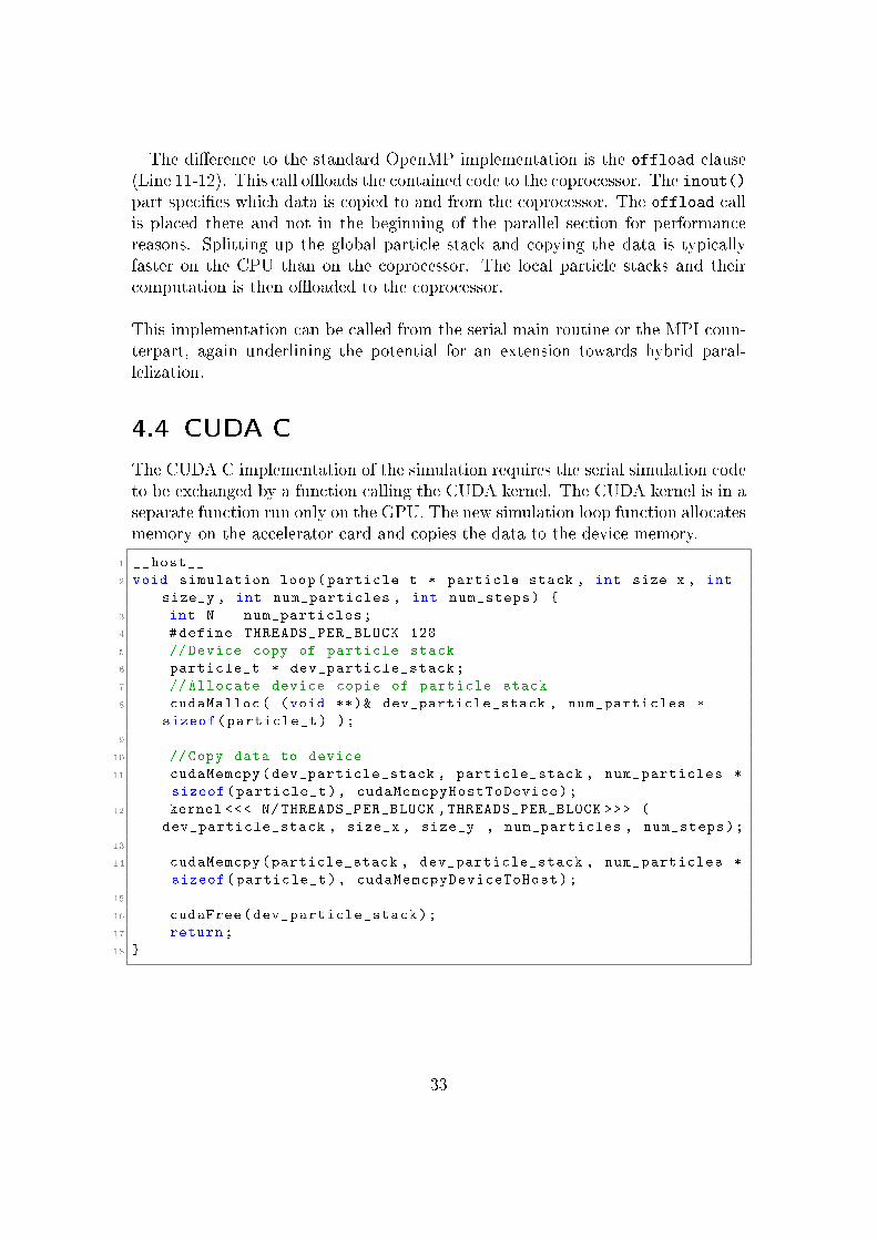
4.4 CUDA C
The CUDA C implementation of the simulation requires the serial simulation codeto be exchanged by a function calling the CUDA kernel. The CUDA kernel is in aseparate function run only on the GPU. The new simulation loop function allocatesmemory on the accelerator card and copies the data to the device memory.
1 __host__
2 void simulation_loop(particle_t * particle_stack , int size_x , int
size_y , int num_particles , int num_steps) {
3 int N = num_particles;
4 #define THREADS_PER_BLOCK 128
5 // Device copy of particle stack
6 particle_t * dev_particle_stack;
7 // Allocate device copie of particle stack
8 cudaMalloc( (void **)& dev_particle_stack , num_particles *
sizeof(particle_t) );
9
10 //Copy data to device
11 cudaMemcpy(dev_particle_stack , particle_stack , num_particles *
sizeof(particle_t), cudaMemcpyHostToDevice);
12 kernel <<< N/THREADS_PER_BLOCK ,THREADS_PER_BLOCK >>> (
dev_particle_stack , size_x , size_y , num_particles , num_steps);
13
14 cudaMemcpy(particle_stack , dev_particle_stack , num_particles *
sizeof(particle_t), cudaMemcpyDeviceToHost);
15
16 cudaFree(dev_particle_stack);
17 return;
18 }
33
The __host__ statement de�nes that this function is only run on the host. Thisfunction and the kernel have to be compiled using the Nvidia CUDA compiler. Thekernel call with �Gridsize, Blocksize� launches the kernel on the accelerator.The blocksize is �xed with 128 threads to allow the program to be executed onolder CUDA accelerators, which had a maximum number of 128 threads. Modernaccelerators increased this number to 256 or 512 threads per block. The gridsizeis calculated from the number of particles in the simulation. The kernel is a newfunction and the __global__ statement de�nes that it can be called from the hostor the device.
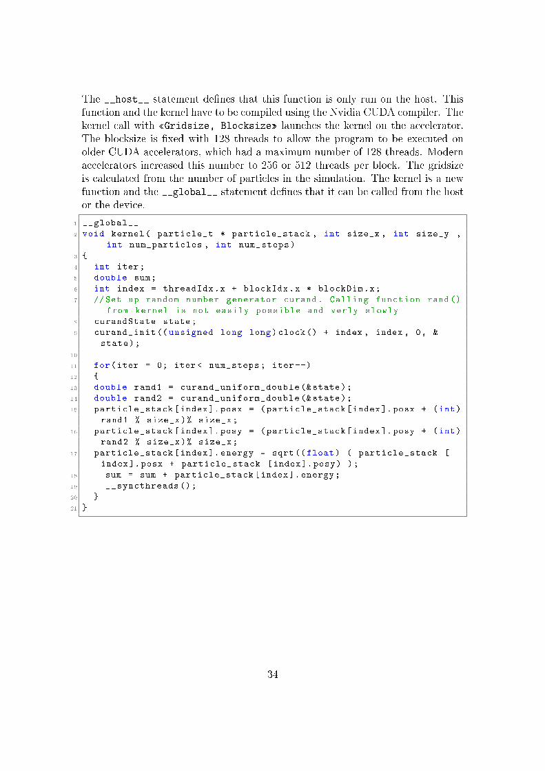
1 __global__
2 void kernel( particle_t * particle_stack , int size_x , int size_y ,
int num_particles , int num_steps)
3 {
4 int iter;
5 double sum;
6 int index = threadIdx.x + blockIdx.x * blockDim.x;
7 //Set up random number generator curand. Calling function rand()
from kernel is not easily possible and verly slowly
8 curandState state;
9 curand_init (( unsigned long long)clock () + index , index , 0, &
state);
10
11 for(iter = 0; iter < num_steps; iter ++)
12 {
13 double rand1 = curand_uniform_double (&state);
14 double rand2 = curand_uniform_double (&state);
15 particle_stack[index ].posx = (particle_stack[index].posx + (int)
rand1 % size_x)% size_x;
16 particle_stack[index ].posy = (particle_stack[index].posy + (int)
rand2 % size_x)% size_x;
17 particle_stack[index ]. energy = sqrt((float) ( particle_stack [
index ].posx + particle_stack [index].posy) );
18 sum = sum + particle_stack[index]. energy;
19 __syncthreads ();
20 }
21 }
34
The standard rand() function is not available on the GPU, therefore, the cu-Rand random number generator is used to create random numbers.
The serial simulation loop implementation has 15 lines of code whereas the CUDAimplementation requires 39 lines of code. To enable data processing on the accel-erator data has to be copied to and from the GPU via CUDA memcpy calls.
The CUDA C implementation of the simulation loop can be called from the serialmain or the MPI main. MPI can be used to distribute data to the computingnodes and the single nodes use GPU accelerators to compute the simulation re-sults, again showing the support for hybrid parallelization. Exchanging data ismore di�cult because the simulation data is being processed on the GPU. Nvidiapresented CUDA-aware MPI to address this problem and make synchronisationand data exchange easier on HPC clusters using GPU accelerators, however, forthe sake of portability and clarity this is not further investigated in this work.
35
5 Conclusion and Outlook
This �nal chapter summarizes and analyses the results of the previous chapters andgives an outlook to the future of parallelization. In Chapter 5.1 the programminge�ort and portability of the di�erent example problem implementations are dis-cussed. Finally, Chapter 5.2 gives an overview over expected future developmentsin many-core programming.
5.1 Comparison of Programming E�ort
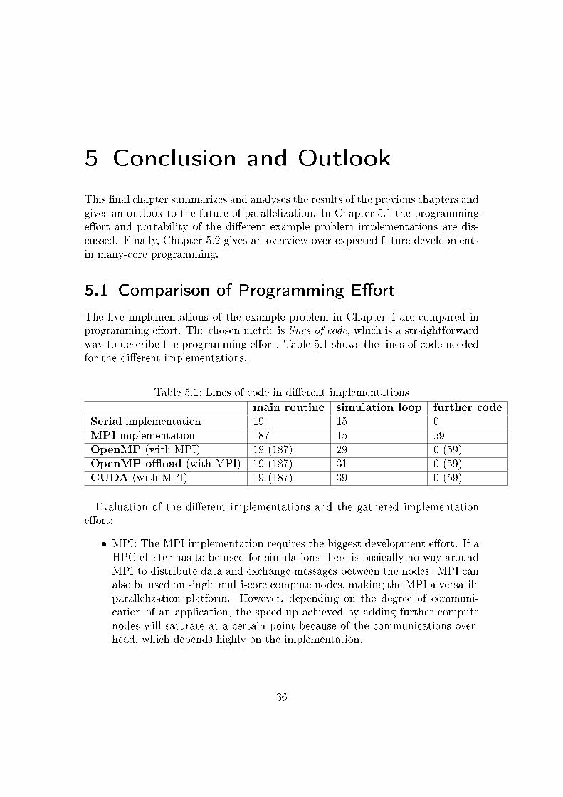
The �ve implementations of the example problem in Chapter 4 are compared inprogramming e�ort. The chosen metric is lines of code, which is a straightforwardway to describe the programming e�ort. Table 5.1 shows the lines of code neededfor the di�erent implementations.
Table 5.1: Lines of code in di�erent implementationsmain routine simulation loop further code
Serial implementation 19 15 0MPI implementation 187 15 59OpenMP (with MPI) 19 (187) 29 0 (59)OpenMP o�oad (with MPI) 19 (187) 31 0 (59)CUDA (with MPI) 19 (187) 39 0 (59)
Evaluation of the di�erent implementations and the gathered implementatione�ort:
� MPI: The MPI implementation requires the biggest development e�ort. If aHPC cluster has to be used for simulations there is basically no way aroundMPI to distribute data and exchange messages between the nodes. MPI canalso be used on single multi-core compute nodes, making the MPI a versatileparallelization platform. However, depending on the degree of communi-cation of an application, the speed-up achieved by adding further computenodes will saturate at a certain point because of the communications over-head, which depends highly on the implementation.
36
� OpenMP: Parallelization of existing code with OpenMP requires compara-tively less e�ort, however, signi�cant optimization e�ort has to be consideredto reach high parallel e�ciency. OpenMP can be used to e�ectively and ef-�ciently extend serial code step by step by parallel counterparts.
� O�oad OpenMP: When OpenMP code is supposed to be o�oaded to a co-processor the OpenMP code should be �rst optimized on a regular CPU host,before moving tuning to a coprocessor system. The signi�cant increase inthe core numbers of a coprocessor will make further optimizations necessaryto signi�cantly outperform a HPC CPU-only host.
� CUDA C: Utilizing GPU accelerators requires the computations to be rewrit-ten in CUDA C. GPUs have di�erent functionalities than CPUs and thereforemany routines cannot be used directly. The separate device memory requiresthe programmer to think about data locality and communication overheads.
� Hybrid implementations: As clusters with coprocessors and accelerators havealready a large market share in the HPC market programmers have to be-come familiar with hybrid parallelization. Using MPI on a high level tocommunicate between compute nodes and OpenMP or CUDA C on the lo-cal node to utilize available coprocessors or accelerators is a viable option toutilize heterogeneous compute platforms..
MPI and OpenMP o�er vendor-independent implementations. Both are availablefor all HPC clusters and stand-alone workstations. O�oad OpenMP on coproces-sors and CUDA C for Nvidia GPUs support only speci�c hardware. Therefore,implementations using those approaches are in a so-called vendor lock, meaningthat the implementations cannot be used on other platforms outside the vendorshardware ecosystem. This fact might become problematic to research softwaredevelopers as they might become dependent on the availability of a speci�c typeof compute environment, especially as a lack of manpower and funding in researchsoftware projects renders repeated code porting to new platforms highly challeng-ing and often simply not possible.
37
5.2 Future Developments and Outlook
In the near future, many-core applications will be more and more used to fol-low the hardware trend towards increasing core numbers. Medical imaging andother computationally challenging scienti�c simulations will rely more and moreon these highly parallel platforms. However, to increase the usability new, moreaccessible language approaches, like OpenACC are being developed [63]. Usingdirectives similar to OpenMP should make it easier for programmers new to the�eld of many-core programming to utilize accelerators and co-processors . On thecontrary, OpenMP was extended to support o�oading to coprocessors in speci�-cation 4.0 [64]. Researchers are working on approaches to run C code with o�oadOpenMP code on GPUs, to further the reach of OpenMP beyond CPUs and co-processors.
Hybrid parallelization has a big chance of becoming a standard for future im-plementations of scienti�c simulators. Today's high end multi core CPUs havemore than 20 cores on a single chip (e.g. Intel Broadwell-EX). The gap to copro-cessors is closing and there is no way around parallelization techniques to utilizethis potential. This trend is expected to continue: The processor roadmaps predictrising core numbers and a transition from the multi core architecture to many corearchitectures [65]. For research software developers hybrid parallelization will haveto become a standard method for utilizing all available, heterogeneous computingresources on single workstations or on clusters to support the ongoing quest formore accurate and faster computer simulations.
38
Bibliography
[1] K. Binder, D. Heermann, Monte Carlo Simulation in Statistical Physics: AnIntroduction (Springer Science & Business Media, 2010)
[2] A.B. Bortz, M.H. Kalos, J.L. Lebowitz, A New Algorithm for Monte CarloSimulation of Ising Spin Systems, Journal of Computational Physics 17(1),10 (1975)
[3] J.F. Briesmeister, et al., MCNPTM - A General Monte Carlo N-ParticleTransport Code, Version 4C, LA-13709-M, Los Alamos National Laboratory(2000)
[4] A. Smith, A. Doucet, N. de Freitas, N. Gordon, Sequential Monte CarloMethods in Practice (Springer Science & Business Media, 2013)
[5] H. Gould, J. Tobochnik, W. Christian, An Introduction to ComputerSimulation Methods, vol. 1 (Addison-Wesley New York, 1988)
[6] A. Heinecke, M. Klemm, H.J. Bungartz, From GPGPU to Many-Core:Nvidia Fermi and Intel Many Integrated Core Architecture, Computing inScience & Engineering 14(2), 78 (2012)
[7] ViennaWD. "http://viennawd.sourceforge.net" (2016). [Online;accessed 5-October-2016]
[8] H. Esmaeilzadeh, E. Blem, R.S. Amant, K. Sankaralingam, D. Burger,Power Challenges May End the Multi-Core Era, Communications of theACM 56(2), 93 (2013)
[9] C. Isci, A. Buyuktosunoglu, C.Y. Cher, P. Bose, M. Martonosi, An Analysisof E�cient Multi-Core Global Power Management Policies: MaximizingPerformance for a Given Power Budget, in Proceedings of the 39th annualIEEE/ACM International Symposium on Microarchitecture (IEEEComputer Society, 2006), pp. 347�358
i
[10] L. Chai, Q. Gao, D.K. Panda, Understanding the Impact of Multi-CoreArchitecture in Cluster Computing: A Case Study with Intel Dual-CoreSystem, in Seventh IEEE International Symposium on Cluster Computingand the Grid (CCGrid '07) (2007), pp. 471�478. DOI10.1109/CCGRID.2007.119
[11] R. Vuduc, J. Choi, A Brief History and Introduction to GPGPU, in ModernAccelerator Technologies for Geographic Information Science (Springer,2013), pp. 9�23
[12] J. Je�ers, J. Reinders, Intel Xeon Phi Coprocessor High PerformanceProgramming (Newnes, 2013)
[13] B. Leback, D. Miles, M. Wolfe, Tesla vs. Xeon Phi vs. Radeon A CompilerWriter's Perspective, Technical News from The Portland Group (2013)
[14] J. Ghorpade, J. Parande, M. Kulkarni, A. Bawaskar, GPGPU Processing inCUDA Architecture, arXiv preprint arXiv:1202.4347 (2012)
[15] T. Rauber, G. Rünger, Parallel Programming: For Multi-Core and ClusterSystems (Springer Science & Business Media, 2013)
[16] Top500.org. Top 500 Super Computer List. "https://www.top500.org/"(2016). [Online; accessed 12-May-2016]
[17] J. Schutz, C. Webb, A Scalable X86 CPU Design for 90 nm Process, inSolid-State Circuits Conference, 2004. Digest of Technical Papers. ISSCC.2004 IEEE International (IEEE, 2004), pp. 62�513
[18] A. Nalamalpu, N. Kurd, A. Deval, C. Mozak, J. Douglas, A. Khanna,F. Paillet, G. Schrom, B. Phelps, Broadwell: A Family of IA 14nmProcessors, in 2015 Symposium on VLSI Circuits (VLSI Circuits) (IEEE,2015), pp. C314�C315
[19] Bloomberg. Intel Server Sales."http://www.bloomberg.com/news/articles/2015-07-15/intel-forecast-shows-server-demands-makes-up-for-pc-market-woes"(2015). [Online; accessed 5-July-2016]
[20] B. Sinharoy, J. Van Norstrand, R.J. Eickemeyer, H.Q. Le, J. Leenstra, D.Q.Nguyen, B. Konigsburg, K. Ward, M. Brown, J.E. Moreira, et al., IBMPOWER8 Processor Core Microarchitecture, IBM Journal of Research andDevelopment 59(1), 2 (2015)
ii
[21] N. Rajovic, A. Rico, N. Puzovic, C. Adeniyi-Jones, A. Ramirez, Tibidabo:Making the Case for an ARM-based HPC System, Future GenerationComputer Systems (2013). DOI 10.1016/j.future.2013.07.013
[22] M.A. Laurenzano, A. Tiwari, A. Jundt, J. Peraza, W.A. Ward Jr,R. Campbell, L. Carrington, Characterizing the Performance-EnergyTradeo� of Small ARM Cores in HPC Computation, in Euro-Par 2014Parallel Processing (Springer, 2014), pp. 124�137
[23] Intel. Intel Silvermont Architecture."https://software.intel.com/sites/default/files/managed/bb/2c/02_Intel_Silvermont_Microarchitecture.pdf" (2015). [Online; accessed27-April-2016]
[24] Intel. Intel Xeon E7 Servers. "http://www.intel.com/content/www/us/en/processors/xeon/xeon-processor-e7-family.html" (2016). [Online;accessed 16-July-2016]
[25] G. Chrysos, Intel Xeon Phi Coprocessor-The Architecture, Intel Whitepaper(2014)
[26] E. Lindholm, J. Nickolls, S. Oberman, J. Montrym, NVIDIA Tesla: AUni�ed Graphics and Computing Architecture, IEEE micro 28(2), 39 (2008)
[27] K. Rupp, J. Weinbub, F. Rudolf, Highly Productive ApplicationDevelopment with ViennaCL for Accelerators, in AGU Fall MeetingAbstracts, vol. 1 (2012), vol. 1, p. 1528
[28] Nvidia. Nvidia P100 Architecture."http://www.nvidia.com/object/tesla-p100.html" (2016). [Online;accessed 22-July-2016]
[29] Nvidia. Nvidia GP100 Whitepaper."https://images.nvidia.com/content/pdf/tesla/whitepaper/pascal-architecture-whitepaper.pdf" (2016). [Online; accessed24-August-2016]
[30] P. Sharma, B. Kumar, P. Gupta, An Introduction to Cluster Computingusing Mobile Nodes, in 2009 Second International Conference on EmergingTrends in Engineering & Technology (IEEE, 2009), pp. 670�673
[31] W. Gropp, E. Lusk, N. Doss, A. Skjellum, A High-Performance, PortableImplementation of the MPI Message Passing Interface Standard, ParallelComputing 22(6), 789 (1996). DOI 10.1016/0167-8191(96)00024-5
iii
[32] L. Dagum, R. Menon, OpenMP: An Industry Standard API forShared-Memory Programming, IEEE Computational Science andEngineering 5(1), 46 (1998). DOI 10.1109/99.660313
[33] P. Raki¢, D. Mila²inovi¢, �. �ivanov, Z. Suvajdºin, M. Nikoli¢,M. Hajdukovi¢, MPI CUDA Parallelization of a Finite-Strip Program forGeometric Nonlinear Analysis: A Hybrid Approach, Advances inEngineering Software 42(5), 273 (2011)
[34] V. Heuveline, M.J. Krause, J. Latt, Towards a Hybrid Parallelization ofLattice Boltzmann Methods, Computers & Mathematics with Applications58(5), 1071 (2009)
[35] R.L. Graham, The MPI 2.2 Standard and the Emerging MPI 3 Standard(Springer Berlin Heidelberg, Berlin, Heidelberg, 2009), pp. 2�2. DOI10.1007/978-3-642-03770-2_2
[36] W. Gropp, E. Lusk, R. Thakur, Using MPI-2: Advanced Features of theMessage-Passing Interface (MIT Press, Cambridge, MA, USA, 1999)
[37] G. Hager, G. Wellein, Introduction to High Performance Computing forScientists and Engineers, 1st edn. (CRC Press, Inc., Boca Raton, FL, USA,2010)
[38] J.J. Dongarra, S.W. Otto, M. Snir, D. Walker, An Introduction to the MPIStandard. Tech. rep., Knoxville, TN, USA (1995)
[39] High-Performance Portable MPI Implementation MPICH."http://www.mpich.org/" (2016). [Online; accessed 12-September-2016]
[40] The OpenMP API Speci�cation for Parallel Programming."http://openmp.org/wp/" (2016). [Online; accessed 12-September-2016]
[41] P. Bridges, N. Doss, W. Gropp, E. Karrels, E. Lusk, A. Skjellum, User'sGuide to MPICH, a Portable Implementation of MPI, Argonne NationalLaboratory 9700, 60439 (1995)
[42] M. Si, Y. Ishikawa, M. Tatagi, Direct MPI Library for Intel Xeon PhiCo-Processors, in Parallel and Distributed Processing Symposium WorkshopsPhD Forum (IPDPSW), 2013 IEEE 27th International (2013), pp. 816�824.DOI 10.1109/IPDPSW.2013.179
iv
[43] E. Gabriel, G.E. Fagg, G. Bosilca, T. Angskun, J.J. Dongarra, J.M. Squyres,V. Sahay, P. Kambadur, B. Barrett, A. Lumsdaine, R.H. Castain, D.J.Daniel, R.L. Graham, T.S. Woodall, Open MPI: Goals, Concept, and Designof a Next Generation MPI Implementation (Springer Berlin Heidelberg,Berlin, Heidelberg, 2004), pp. 97�104. DOI 10.1007/978-3-540-30218-6_19
[44] J. Hursey, J.M. Squyres, T.I. Mattox, A. Lumsdaine, The Design andImplementation of Checkpoint/Restart Process Fault Tolerance for OpenMPI, in 2007 IEEE International Parallel and Distributed ProcessingSymposium (2007), pp. 1�8. DOI 10.1109/IPDPS.2007.370605
[45] D. Molka, R. Schöne, D. Hackenberg, M.S. Müller, Memory Performanceand SPEC OpenMP Scalability on Quad-Socket x86_64 Systems (SpringerBerlin Heidelberg, Berlin, Heidelberg, 2011), pp. 170�181. DOI10.1007/978-3-642-24650-0_15
[46] B. Chapman, G. Jost, R.v.d. Pas, Using OpenMP: Portable Shared MemoryParallel Programming (Scienti�c and Engineering Computation) (The MITPress, 2007)
[47] R. Chandra, L. Dagum, D. Kohr, D. Maydan, J. McDonald, R. Menon,Parallel Programming in OpenMP (Morgan Kaufmann Publishers Inc., SanFrancisco, CA, USA, 2001)
[48] D. Schmidl, T. Cramer, S. Wienke, C. Terboven, M.S. Müller, Assessing thePerformance of OpenMP Programs on the Intel Xeon Phi (Springer BerlinHeidelberg, Berlin, Heidelberg, 2013), pp. 547�558. DOI10.1007/978-3-642-40047-6_56
[49] E. Saule, K. Kaya, Ü.V. Çatalyürek, Performance Evaluation of SparseMatrix Multiplication Kernels on Intel Xeon Phi (Springer BerlinHeidelberg, Berlin, Heidelberg, 2014), pp. 559�570. DOI10.1007/978-3-642-55224-3_52
[50] A. Duran, M. Klemm, The Intel Many Integrated Core Architecture, inInternational Conference on High Performance Computing and Simulation(HPCS) (2012), pp. 365�366. DOI 10.1109/HPCSim.2012.6266938
[51] E. Ayguadé, Badia, Extending OpenMP to Survive the HeterogeneousMulti-Core Era, International Journal of Parallel Programming 38(5), 440(2010). DOI 10.1007/s10766-010-0135-4
v
[52] D. Kirk, NVIDIA CUDA Software and GPU Parallel ComputingArchitecture, in Proceedings of the 6th International Symposium on MemoryManagement (ACM, New York, NY, USA, 2007), ISMM '07, pp. 103�104.DOI 10.1145/1296907.1296909
[53] D. Luebke, CUDA: Scalable Parallel Programming for High-PerformanceScienti�c Computing, in 2008 5th IEEE International Symposium onBiomedical Imaging: From Nano to Macro (2008), pp. 836�838. DOI10.1109/ISBI.2008.4541126
[54] M. Wang, H. Klie, M. Parashar, H. Sudan, Solving Sparse Linear Systemson NVIDIA Tesla GPUs (Springer Berlin Heidelberg, Berlin, Heidelberg,2009), pp. 864�873. DOI 10.1007/978-3-642-01970-8_87
[55] L. Pan, L. Gu, J. Xu, Implementation of Medical Image Segmentation inCUDA, in 2008 International Conference on Information Technology andApplications in Biomedicine (2008), pp. 82�85. DOI10.1109/ITAB.2008.4570542
[56] C. Nvidia. Programming Guide (2008)
[57] S. Cook, CUDA Programming: A Developer's Guide to Parallel Computingwith GPUs, 1st edn. (Morgan Kaufmann Publishers Inc., San Francisco, CA,USA, 2013)
[58] J. Sanders, E. Kandrot, CUDA by Example: An Introduction toGeneral-Purpose GPU Programming, 1st edn. (Addison-Wesley Professional,2010)
[59] J. Nickolls, I. Buck, M. Garland, K. Skadron, Scalable Parallel Programmingwith CUDA, Queue 6(2), 40 (2008). DOI 10.1145/1365490.1365500
[60] S. Che, M. Boyer, J. Meng, D. Tarjan, J.W. Shea�er, K. Skadron, APerformance Study of General-Purpose Applications on Graphics Processorsusing CUDA , Journal of Parallel and Distributed Computing 68(10), 1370(2008). DOI 10.1016/j.jpdc.2008.05.014
[61] P. Ellinghaus, J. Weinbub, M. Nedjalkov, S. Selberherr, I. Dimov,Distributed-Memory Parallelization of the Wigner Monte Carlo Methodusing Spatial Domain Decomposition, Journal of Computational Electronics14(1), 151 (2015). DOI 10.1007/s10825-014-0635-3
vi
[62] J. Weinbub, P. Ellinghaus, M. Nedjalkov, Domain Decomposition Strategiesfor the Two-Dimensional Wigner Monte Carlo Method, Journal ofComputational Electronics 14(4), 922 (2015). DOI10.1007/s10825-015-0730-0
[63] S. Wienke, P. Springer, C. Terboven, D. an Mey, OpenACC � FirstExperiences with Real-World Applications (Springer Berlin Heidelberg,Berlin, Heidelberg, 2012), pp. 859�870. DOI 10.1007/978-3-642-32820-6_85
[64] C. Bertolli, S.F. Antao, A.E. Eichenberger, K. O'Brien, Z. Sura, A.C. Jacob,T. Chen, O. Sallenave, Coordinating GPU Threads for OpenMP 4.0 inLLVM, in Proceedings of the 2014 LLVM Compiler Infrastructure in HPC(IEEE Press, Piscataway, NJ, USA, 2014), LLVM-HPC '14, pp. 12�21. DOI10.1109/LLVM-HPC.2014.10
[65] L. Seiler, D. Carmean, E. Sprangle, T. Forsyth, M. Abrash, P. Dubey,S. Junkins, A. Lake, J. Sugerman, R. Cavin, R. Espasa, E. Grochowski,T. Juan, P. Hanrahan, Larrabee: A Many-Core x86 Architecture for VisualComputing, ACM Trans. Graph. 27(3), 18:1 (2008). DOI10.1145/1360612.1360617
vii
Hiermit erkläre ich, dass die vorliegende Arbeit ohne unzulässige Hilfe Dritter und ohne Benutzung anderer als der angegebenen Hilfsmittel angefertigt wurde.
Die aus anderen Quellen oder indirekt übernommenen Daten und Konzepte sind unter Angabe der Quelle gekennzeichnet.
Die Arbeit wurde bisher weder im In– noch im Ausland in gleicher oder in
ähnlicher Form in anderen Prufungsverfahren vorgelegt.
Wien, 21.11.2016
__________________________________
Matthias Franz Glanz


![Tobias Langdon: Strategies of Competition in Western PoliticsLaufendes-2015 X Strategies of Competition X C C] /strategies-of-competition-in-western-politics/#comments](https://img.pdfslide.org/doc/110x75/5e6b8db531a52856ba2f977c/tobias-langdon-strategies-of-competition-in-western-laufendes-2015-x-strategies.jpg)