Saarland UniversityFaculty of Natural Sciences and Technology I

Department of Computer Science

Master’s Thesis

Robust Principal Component Analysis as aNonlinear Eigenproblem

submitted by

Anastasia Podosinnikova

submitted

July 3, 2013

Reviewers:

Prof. Dr. Matthias HeinDr. Rainer Gemulla

Eidesstattliche ErklarungIch erklare hiermit an Eides Statt, dass ich die vorliegende Arbeit selbststandig verfasst undkeine anderen als die angegebenen Quellen und Hilfsmittel verwendet habe.

Statement in Lieu of an OathI hereby confirm under oath that I have written this thesis on my own and that I have notused any other media or materials than the ones referred to in this thesis.

Eidesstattliche ErklarungIch erklare hiermit an Eides Statt, dass die vorliegende Arbeit mit der elektronischen Ver-sion ubereinstimmt.

Statement in Lieu of an OathI hereby confirm the congruence of the contents of the printed data and the electronic ver-sion of the thesis.

EinverstandniserklarungIch bin damit einverstanden, dass meine (bestandene) Arbeit in beiden Versionen in dieBibliothek der Informatik aufgenommen und damit veroffentlicht wird.

Declaration of ConsentI agree to make both versions of my thesis (with a passing grade) accessible to the publicby having them added to the library of the Computer Science Department.

Saarbrucken, ............................... ..........................................(Datum / Date) (Unterschrift / Signature)

Acknowledgements

First of all, I would like to thank Matthias Hein for the opportunity to write my Master thesisunder his supervision and for his support and encouragement during the work on this thesis.Moreover, I would like to thank all the members of the Machine Learning Group – SahelyBhadra, Thomas Buhler, Leonardo Jost, Shyam Sundar Rangapuram, Martin Slawski andPramod Kaushik Mudrakarta – for the friendly environment, motivation and the positiveinfluence to my knowledge in the fields of machine learning and statistics. Last but notleast, I would like to thank the International Max Planck Research School for ComputerScience for the opportunity to study at Saarland University and their constant support andfriendly atmosphere during all the time of my studies.

5

Abstract

Principal Component Analysis (PCA) is a widely used tool for, e.g., exploratory data analy-sis, dimensionality reduction and clustering. However, it is well known that PCA is stronglyaffected by the presence of outliers and, thus, is vulnerable to both gross measurement errorand adversarial manipulation of the data. This phenomenon motivates the development ofrobust PCA as the problem of recovering the principal components of the uncontaminateddata.

In this thesis, we propose two new algorithms, QRPCA and MDRPCA, for robust PCAcomponents based on the projection-pursuit approach of Huber. While the resulting op-timization problems are non-convex and non-smooth, we show that they can be efficientlyminimized via the RatioDCA using bundle methods/accelerated proximal methods for theinterior problem. The key ingredient for the most promising algorithm (QRPCA) is a ro-bust, location invariant scale measure with breakdown point 0.5. Extensive experimentsshow that our QRPCA is competitive with current state-of-the-art methods and outper-forms other methods in particular for a large number of outliers.

7

Contents

1 PCA, Robust Statistics and Projection-Pursuit 131.1 Principal Component Analysis . . . . . . . . . . . . . . . . . . . . . . . . . . 131.2 Robust Principal Component Analysis . . . . . . . . . . . . . . . . . . . . . . 141.3 Basics of Robust Statistics and Projection-Pursuit . . . . . . . . . . . . . . . 151.4 On the Way to the New Algorithms . . . . . . . . . . . . . . . . . . . . . . . 17

2 Previous Algorithms 212.1 The Grid Search Algorithm (GRID) . . . . . . . . . . . . . . . . . . . . . . . 212.2 The High Dimensional Robust PCA Algorithm (HR-PCA) . . . . . . . . . . . 222.3 The Maximum Mean Absolute Deviation Rounding Algorithm (MDR) . . . . 232.4 Robust PCA as a Matrix Decomposition Problem . . . . . . . . . . . . . . . . 24

2.4.1 Principal Component Pursuit (PCP) . . . . . . . . . . . . . . . . . . . 242.4.2 Low-Leverage Decomposition (LLD) and Outlier-Pursuit (OP-RPCA) 24

2.5 Robust PCA through Robust Covariance Matrix Estimation (ROBPCA) . . . 25

3 Robust PCA as a Nonlinear Eigenproblem 273.1 The Nonlinear Eigenproblem and RatioDCA . . . . . . . . . . . . . . . . . . 273.2 Projection-Pursuit Robust PCA with the Quartile Difference Measure (QR-

PCA) . . . . . . . . . . . . . . . . . . . . . . . . . . . . . . . . . . . . . . . . 283.3 The Dual Approach to the Solution of the Inner Problem of QRPCA . . . . . 283.4 The Primal Approach to the Solution of the Inner Problem of QRPCA . . . . 29

3.4.1 Bundle Method for the Solution of the Constrained Inner Problem . . 303.4.2 Bundle Method for the Solution of the Unconstrained Inner Problem . 34

3.5 Projection-Pursuit Robust PCA with the Median Absolute Deviation ScaleMeasure (MDRPCA) . . . . . . . . . . . . . . . . . . . . . . . . . . . . . . . . 36

4 Experiments 394.1 The Experiments with Toy Data Sets . . . . . . . . . . . . . . . . . . . . . . . 404.2 The Experiments with Real World Data Sets . . . . . . . . . . . . . . . . . . 424.3 Runtime and Conclusion . . . . . . . . . . . . . . . . . . . . . . . . . . . . . . 43

5 Critical Discussion and Conclusion 45

6 Appendix 476.1 The Algorithm for the Projection onto the Intersection of L1-Ball and L∞-

Ball in O(n) Time . . . . . . . . . . . . . . . . . . . . . . . . . . . . . . . . . 476.2 Derivation of the Lipschitz Constant for FISTA . . . . . . . . . . . . . . . . . 506.3 Matrix Norms . . . . . . . . . . . . . . . . . . . . . . . . . . . . . . . . . . . . 51

9

Introduction

Principal Component Analysis (PCA) was invented by Pearson in 1901 [42] and is a widelyused tool in statistics, machine learning, image processing and other fields of science andengineering (e.g. [33]). It can either be seen as finding the best low-dimensional subspaceapproximating the data or as finding the subspace of highest variance. However, due to thefact that the variance is not robust, PCA can be badly affected by outliers. Indeed, even oneoutlier can change the principal components (PCs) drastically. This phenomenon motivatesthe development of robust PCA as the problem of recovering the principal components ofthe uncontaminated data. Note that potential sources of contamination are not only grossmeasurement errors but also adversarial manipulation of the data. We treat the robust PCAproblem in the framework of robust statistics. A key characteristic of a robust estimator isthe breakdown point which, intuitively, is the maximal fraction of arbitrary outliers in thedataset which does not break down the estimate completely. The variance used in normalPCA has a breakdown point of zero, that is even a single outlier can lead to arbitraryvalues.

Several approaches to robust PCA have been proposed. The most direct one is based on therobust estimation of the covariance matrix (e.g. [27, 17]). Indeed, having found a robustcovariance matrix one can determine the PCs by performing the eigenvalue decomposi-tion of this matrix. However, it has been shown that robust covariance matrix estimatorswith desirable properties, such as positive semi-definiteness and affine equivariance, have abreakdown point upper bounded by the inverse of the dimensionality [17, p.298].

Another approach is based on a matrix decomposition of the data matrix into a low-rankpart and a sparse part [4, 52, 40] capturing the outliers. Two models of the “sparse” parthave been considered. In [4] the sparse part is assumed to be “elementwise”-sparse whichdoes not correspond to the usual model of a data set with outliers. In the other two papersthe second component is assumed to be row sparse (observations are in the rows) whichcorresponds to the typical model where an observation is corrupted. However, these matrixdecomposition methods required a regularization parameter which is non-trivial to chooseas we are in an unsupervised setting.

Moreover, several heuristic algorithms that try first to detect/remove outliers were proposed(e.g. [29, 31, 51]). These algorithms, mostly, randomized and use some greedy techniquesfor outlier detection/removal. We will see, however, that removing true data points at thepre-processing step may lead to poor results.

Finally, one can do robust PCA via projection-pursuit ([36, 26]), where one maximizes overall possible directions a robust scale measure (instead of the standard deviation) appliedto the projection of the data onto this direction. Projection-pursuit methods have thebest possible breakdown point of 0.5. However, opposed to standard PCA, they lead to anon-convex, typically non-smooth problem and the current state-of-the-art are approximategreedy search algorithms [8]. In this thesis, we propose two computationally tractable algo-rithms for projection-pursuit robust PCA: QRPCA and MDRPCA. The QRPCA algorithmis based on a more stable variant of the Q-scale measure introduced by [45] while the MDR-PCA algorithm is based on the modification of the median absolution deviation about themedian. To the best of our knowledge, the proposed algorithms are the first computationallytractable solutions of projection-pursuit robust PCA. Moreover, our optimization approachis better in terms of the found objective than search based methods of [8]. Our extensiveexperiments show that we outperform by far the greedy search algorithms for projection-pursuit robust PCA and are competitive compared to the state-of-the-art algorithms withimprovements for a large fraction of outliers.

In this thesis we introduce two new algorithms for robust PCA that are based on theprojection-pursuit approach. We present all basics required for understanding of this ap-

11

proach in chapter 1. The projection-pursuit problem is NP hard and, to our best knowledge,there is no efficient solution available. We provide a description of the most promising robustPCA algorithms in chapter 2. The derivation of the proposed algorithms is presented inchapter 3. The thesis is completed with the experimental Section 4, where we do extensiveexperiments and compare to all current state-of-the-art methods for robust PCA, as well ascritical discussion Section 5.

Notation

We will assume that all vectors are column vectors. Moreover, if different is not specified,we use the following notations and abbreviations throughout the thesis.

X ∈ Rn×p the data matrix containing the observations in rowsx1, . . . , xn observations, i.e. rows of XXt ∈ Rnt×p the true dataXo ∈ Rno×p the outliers such that X = Xt ∪Xo

n = nt + no the number of observationsλ ∈ (0, 0.5) the fraction of outliersno = λn the number of the outliers in Xnt = (1− λ)n the number of the true points in Xu1, . . . , ud the first d true PCs, i.e. the PCs of the true data Xt

u1, . . . , ud the first d robust PCs of the data X obtained by a robust PCA method

X the data matrix X centered with respect to some vector xm (to be specified)x1, . . . , xn the elements of the centered matrix, i.e. xi = xi − xmp the dimension of each observationd the number of principal componentsm = (n2 − n)/2 the number of pairwise differences of the observationsk approx., the quartile of m; k = h(h− 1)/2 with h = bn/2c+ 1(·)i the ith element of a vectory(ξ) the ξth smallest element in the univariate set yini=1 (each yi ∈ R)〈x, u〉(ξ) the ξth smallest element in the univariate set 〈xi, u〉ni=1, where u ∈ Rpej for j = 1, . . . , p the vector of all zeros except for 1 in the jth position1 the vector of all onesI the identity matrix of required sizei.i.d. independently and identically distributedsign(x) the signum function, i.e. is −1 if x < 0, 1 if x > 0 and 0 otherwise

12

1 PCA, Robust Statistics and Projection-Pursuit

In this thesis we present a new algorithm for robust PCA which is based on the projection-pursuit approach which maximizes a robust scale measure of a data set projected on adirection over all possible directions. In order to proceed, we briefly recall the formulationsof standard PCA, some notions of robust statistics such as robust estimators of scale andthe breakdown point, the projection-pursuit approach to robust PCA.

1.1 Principal Component Analysis

We briefly recall four equivalent formulations of standard PCA. For more detailed discussionwe refer to [2, 19]. We consider a data set X = xini=1 where each observation xi ∈ Rp.We refer to xm ∈ Rp as the coordinatewise (columnwise) mean of the dataset X and toX as the centered data set X with respect to the mean xm, where each observation of thecentered data set is xi = xi − xm.

Formulation 1. As introduced by Pearson [42], for a given data set xini=1 ⊂ Rp PCA findsa low dimensional representation zini=1 ⊂ Rd of the original data set that minimizes theresiduals

∑ni=1 ‖xi−zi‖22 where d < p. This is equivalent to finding a subspace U ⊂ Rd that

minimizes the residuals of the observations and their projections onto this subspace

U = arg minV⊂Rp, dim(V )=d

n∑i=1

‖PV xi − xi‖22 , (1)

where PV denotes the projection onto V . When the subspace is found the prototypes zi ofthe points are the projections onto U , i.e. zi = PU xi. The vectors that span the optimalsubspace U are called principal components (PCs). This formulation is referred to as theerror minimization formation.

Formulation 2. It is well known that PCA is closely related to the eigendecomposition ofthe empirical covariance matrix C = 1

n

∑ni=1 xix

Ti . Indeed (e.g. [2]), after some transfor-

mations of the problem (1) and in accordance with the Courant-Fisher Min-Max principleone gets that the first d PCs are the d largest eigenvalues of the covariance matrix:

u1, . . . , ud = arg maxu1,...,ud∈Rp

uk⊥ul,∀k,l

d∑j=1

uTj

(n∑i=1

xixTi

)uj . (2)

Formulation 3. Moreover, the PCs are known as the directions that explain most of thevariance. Indeed, the objective of (2) is 〈u,Cu〉 = 〈u, 1

nXT Xu〉 = 1

n‖Xu‖22 and the previous

formulation is, equivalently,

u1 = arg max‖u‖2=1

‖Xu‖22, ur = arg maxu⊥u1,...,u⊥ur−1,‖u‖2=1

‖Xu‖22, r = 2, . . . , d, (3)

where u1 ∈ Rp is the 1st PC and is a direction that maximizes the variance of the obser-vations projected onto it (i.e. the variance of Xu1) and u2, . . . , ud are all subsequent PCs.Note, that the objectives of (3) up to a constant factor is the squared standard deviationof the projected data set. This is one of the measures of the data spread along a direction.The standard deviation is not robust to outliers which is the reason of non-robustness ofPCA. In the projection-pursuit approach one replaces the standard deviation in (3) withother robust scale measures.

Formulation 4. Finally, standard PCA can be formulated as a matrix factorization prob-lem.

13

Lemma 1.1. Standard PCA is the solution of the following optimization problem

(V ∗, U∗) = arg minU∈Rn×p,V ∈Rp×p; V TV=I

‖X − UV T ‖2F . (4)

Proof. Let us show that the minimizer V ∗ is nothing else as a matrix with eigenvec-tors of the empirical covariance matrix in its columns. The singular value decomposi-tion (SVD) of the centered data matrix is X = UDV T and then the eigenvalue de-composition of the empirical covariance matrix is XT X = V D2V T , where the matri-ces U and V are orthogonal. Introducing a substitution U∗ = UD and (V ∗)T = V T ,we get ‖X − U∗(V ∗)T ‖2F = tr

(XTX − V ∗(U∗)TX −XTU∗(V ∗)T + V ∗(U∗)TU∗(V ∗)T

)=

tr(

2V D2V T − 2V D2V T)

= 0, where we used UT U = V T V = I . Hence, V ∗ and U∗ are the

minimizers of the problem (4) and reconstruct the data matrix through X = U∗(V ∗)T .

Interestingly, the problem (4) is bi-convex and not convex, however, the minimization ispossible due to the SVD.

1.2 Robust Principal Component Analysis

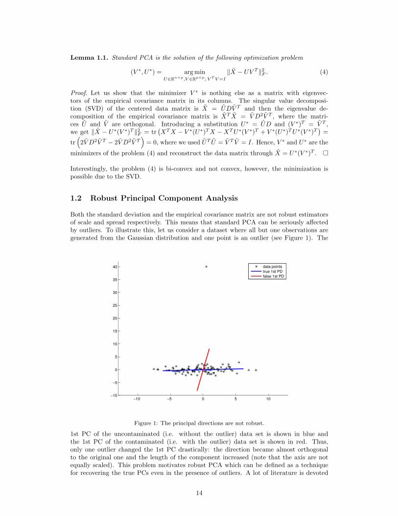
Both the standard deviation and the empirical covariance matrix are not robust estimatorsof scale and spread respectively. This means that standard PCA can be seriously affectedby outliers. To illustrate this, let us consider a dataset where all but one observations aregenerated from the Gaussian distribution and one point is an outlier (see Figure 1). The

−10 −5 0 5 10−10

−5

0

5

10

15

20

25

30

35

40

data points

true 1st PD

false 1st PD

Figure 1: The principal directions are not robust.

1st PC of the uncontaminated (i.e. without the outlier) data set is shown in blue andthe 1st PC of the contaminated (i.e. with the outlier) data set is shown in red. Thus,only one outlier changed the 1st PC drastically: the direction became almost orthogonalto the original one and the length of the component increased (note that the axis are notequally scaled). This problem motivates robust PCA which can be defined as a techniquefor recovering the true PCs even in the presence of outliers. A lot of literature is devoted

14

to this topic, e.g., [36, 26, 29, 10, 8, 40, 51, 35, 6, 13] and many others. We will have anoverview of the literature in Section 2.

Formally, the robust PCA problem can be formulated as follows. Let a data set X ∈ Rn×pconsists of the nt < n true points Xt and, probably unknown number, no = n−nt of outliersXo and we denote it as X = Xt∪Xo. The idealized goal of robust PCA is to find the PCs ofthe true data set Xt given the contaminated dataset X. We assume throughout this thesisthat we have no knowledge about the fraction of outliers and, thus, work in the worst-casescenario, where the fraction of outliers can be as large as 50%.

1.3 Basics of Robust Statistics and Projection-Pursuit

In this section we discuss robust estimators of location and scale and their robustness prop-erties as well as projection-pursuit robust PCA. The latter forms the basis for the newalgorithms proposed in this thesis while the former is the key ingredient in analysis of therobustness properties of the new algorithms.

Scale Measure: Let us first consider a univariate data set Y = yini=1 with the i.i.d.points generated from some good probability measure (e.g., without heavy tails) with anunknown mean µ. In this case, the empirical mean ym = 1/n

∑ni=1 yi is a location estimator

of the latent mean µ. Similarly, the standard deviation S(Y ) =√

1/(n− 1)∑ni=1(yi − ym)2

is an estimator of the latent scale σ. Both estimators are the functions of the data setY = yini=1 and give good estimates under the given condition, i.e. ym ≈ µ and S(Y ) ≈ σwith high probability. In presence of outliers, however, the estimators ym and S(Y ) candiffer significantly from the latent mean µ and the latent scale σ. So, one is interested inrobust estimators of location and scale.

Let us first consider robust estimators of univariate data sets. We will discuss the extensionto the multivariate setting later. We first notice, that every scale measure should at leastfulfill two properties: translation invariance, S(Y + c) = S(Y ) for c ∈ R, and equivarianceunder rescaling (also called scale equivariance), S(αY ) = |α|S(Y ), for α ∈ R. The secondrequirement implies that S is 1-homogeneous1. This is an important property of the scaleestimators which will be used during the derivation of the new algorithms.

One example of robust location or scale measure is the class of L-estimators which is definedas linear combinations of order statistics [17]. In general, given Y = yini=1 ⊂ R the L-estimator of these points is

S(Y ) =

n∑i=1

aiy(i),

where ai ∈ R are some coefficients and the order statistics are y(1) ≤ · · · ≤ y(n). Forexample, the sample median y(bn/2c) is a robust location L-estimator. An example of theL-estimator of scale is the median absolute deviation about the median (MAD) estimatoris given by

MAD(Y ) = c ·medi

∣∣yi −medjyj∣∣, (5)

where c > 0 is a consistency constant [16].

In the literature (e.g. [40, 6, 13, 35]) another L-estimator of scale is considered, which canbe refer to as L1-scale measure and is defined as

SL1(Y ) =

n∑i=1

|yi − ym|, (6)

1A function f(x) is 1-homogeneous if for any α ∈ R it holds f(αx) = |α|f(x).

15

where ym is a location measure of the data Y , e.g., the non-robust mean or the robustmedian. We will discuss the robustness properties of this estimator below.

Breakdown Point: One of the robustness measures of an estimator is the breakdownpoint. Intuitively, it is the minimal fraction of outliers that has to be added to a data setto make the estimate arbitrarily bad. We use the notion of the finite sample replacementbreakdown point for scale estimators as stated in [45]. For more details, see [27, 17].Definition 1.1. The breakdown point ε∗n(S, Y ) of a scale estimator S at a finite data setY = yini=1 is the smallest amount of outliers in Y that can have arbitrary large effect onS:

ε∗n(S, Y ) = minε+n (S, Y ), ε−n (S, Y ),

where

ε+n (S, Y ) = min

m

n; supY

S(Y ) =∞

and ε−n (S, Y ) = min

m

n; infYS(Y ) = 0

,

where Y is obtained by replacing any m observations of Y by arbitrary values.

The quantities ε−n and ε+n are called the explosion breakdown point and the implosion

breakdown point [45]. It was shown ([45], theorem 1) that the breakdown point of any scaleequivariant scale estimator at any univariate sample in which no two points coincide has thehighest possible value of 0.5. Observe that MAD (5) has the highest possible breakdownpoint of 0.5 while the L1-scale estimator has 0 breakdown point, i.e. not robust in thissense.

Efficiency: Another measure of an estimator’s performance is its efficiency, which, roughlyspeaking, measures the variance of an estimator. We give here the definition of efficiencyin accordance with [46]. Let θ(Y) be an estimator of parameters θ = (θ1, . . . , θm) based onY. Assume the distribution P (Y|θ) has a density p(y|θ) such that ln p(y|θ) is differentiablewith respect to θ. The Fisher information matrix I is given by

Iij = Eθ[∂θi ln p(Y|θ) · ∂θj ln ln p(Y|θ)

]and the covariance matrix of the estimator θ(Y) is defined by

Bij = Eθ

[(θi − Eθ

[θi

])(θj − Eθ

[θj

])],

where for some random variable ξ(y) the expectation Eθ [ξ(y)] = EP (y|θ) [ξ(y)]. The covari-

ance matrix B can be used to bound the probability that θ(Y) deviates from θ by more

than a certain amount. The statistical efficiency e of an estimator θ(Y) is defined as

e =1

det IB

and is upper bounded by 1 for unbiased estimators (see [46] for more details).

The maximum likelihood estimators have asymptotically the largest efficiency of 1 amongall unbiased estimators. However, on finite samples the efficiency of the maximum likelihoodestimators is not necessary optimal. As for the estimators of scale, the MAD estimator hasrelatively low efficiency of 37%.

Robust PCA Based on Projection-Pursuit: Projection-pursuit (PP) has been pro-posed in [36, 26]. The idea is to analyze the data only via projections onto a one-dimensionalsubspace, that is, given a direction u ∈ Rp and a set of multivariate points X = xini=1 withxi ∈ Rp, one considers Xu = 〈u, xi〉ni=1. This idea is motivated by the third formulationof robust PCA from Section 1.1, where the first PCs are the directions that maximize thevariance projected onto it (3). Replacing the standard deviation with a robust scale measure

16

S having non-zero breakdown point, one can then define a general family of robust PCAmethods for finding the first robust PCA component u1 [36, 26] as finding the maximumnonlinear eigenvector of a nonlinear eigenproblem [20],

u1 = arg maxu∈Rp

S(Xu)

‖u‖2. (7)

In PP notation, the robust scale measure used as the objective of the problem (7) is calledthe projection index.

The problem (7) is a nonlinear eigenproblem as the square of S, in general, can not bewritten as a quadratic form as it is the case in standard PCA and, thus, cannot be reducedto the standard eigenproblem. This also implies that, generally, the computation of the PProbust PCA components is a non-smooth and non-convex optimization problem. It is anopen problem how to compute and even define higher-order nonlinear eigenvectors [20]. Inpractice, the greedy procedure of deflation (e.g. [38]) is used, that is given the first r − 1robust PCs u1, . . . , ur−1, the next robust PC ur is found as

ur = arg maxu∈Rp

S(Xru)

‖u‖2, where Xr = Xr−1

(I − ur−1u

Tr−1

), (8)

i.e. the new data set Xr is obtained by projecting the original data set X to the sub-space orthogonal to the one spanned by u1, . . . , ur−1 and, thus, the problem of finding thesubsequent robust PC is reduced to the same problem as computing the first robust PCAcomponent.

Note that the PP approach to robust PCA preserves the properties of the projection index[36], that is the PP-PCA is robust if and only if the scale measure is robust. Thus PP-PCAbased on the L1-scale (6), see [40, 35, 6, 13], is not robust as the breakdown point of SL1

is0.

Scale Measure for Multivariate Data: Let us now focus our attention on the case ofmultivariate data sets. Examples of the multivariate location measure are coordinatewisemean and coordinatewise median or L1-median (also known as geometric median) [37].When discussing PP-PCA we have seen the extension of the univariate scale measure to themultivariate setting. Indeed, given a direction u ∈ Rp one defines a univariate observation asthe scalar product of the multivariate observation xi ∈ Rp and the direction, i.e. yi = 〈xi, u〉for all i = 1, . . . , n. Hence, one defines the scale estimator along a direction S(Xu) as theunivariate scale estimator of the univariate data Xu = 〈xi, u〉ni=1 ⊂ R. For simplicity,we will in the following just write S(u) instead of S(Xu) or S(Xru) as it is clear from thecontext which data matrix is used. Moreover, as we are only interested in a direction thatmaximizes a robust scale measure (see (7) and (8)), we will always omit the consistencyconstant c for all estimators.

1.4 On the Way to the New Algorithms

The goal of this section is to introduce two new robust scale measures with breakdownpoints 0.5, thus, maximally robust, and which are more accessible for optimization than theMAD estimator.

The Q Estimator: Another L-estimator of scale with 0.5 breakdown point and with higherefficiency than MAD is the estimator Q [45] which for a univariate data set Y = yini=1 isdefined2 as

Q(Y ) = |yi − yj |; i < j, i, j = 1, . . . , n(k), k =

(bn/2c+ 1

2

), (9)

2Note, that the consistency constant was omitted.

17

It was shown [45], that the Q estimator of scale has breakdown point 0.5 and its efficiencyat the normal distribution is equal to 82%. Note, that at the Cauchy distribution theasymptotic efficiency of MAD is 81% while for the Q-estimator it is 98%. As described inSection 1.3, the univariate Q-estimator (9) has the following extension to the multivariatecase

Q(u) = | 〈xi, u〉 − 〈xj , u〉 |; i < j, i, j = 1, . . . , n(k).

Intuitively, the Q estimator is (approximately) the quartile of the distances between any twopoints from the dataset. As we have maximal 50% outliers, the quartile is the largest numberwhich can still correspond to the pairwise distances of the uncontaminated data. Anotherimportant property distinguishing this estimator from other estimators is that it is locationfree, that is it does not depend on the way the data is centered initially. Even though thereare several robust centering techniques available, we will show in the experimental Section4 that the choice of the robust centering technique can have quite some influence on robustPCA methods which are not location free.

The Q Estimator: While the Q estimator has very nice properties already, it basicallyjust depends on the two observations which realize the quartile and thus can be consideredas slightly unstable. We therefore propose to use instead the Q estimator, which sums upall distances up to quartile. We call Q the quartile difference estimator, which we define tobe

Q(u) =1

k

k∑ξ=1

|〈xi, u〉 − 〈xj , u〉|; i < j(ξ), (10)

where i, j = 1, . . . , n and k is defined as for (9). The next theorem shows that Q has thesame properties as the original Q measure.Theorem 1. The quartile difference measure Q has a breakdown point of 0.5 and is locationfree.

Proof. It is clear that |〈xi, u〉 − 〈xj , u〉|; i < j(ξ) ≤ |〈xi, u〉 − 〈xj , u〉|; i < j(k) for all ξ ≤k. Thus, directly form the definitions of Q and Q, it follows that

ε+n (Q,Xu) = ε+

n (Q,Xu) and ε+n (Q,Xu) = ε−n (Q,Xu),

that is the breakdown points of both Q and Q are equal to each other. Thus, the breakdownpoint of the quartile difference measure is 0.5. As Q just depends on the differences of thedata points, it is location free.

While this extension can be considered as minor, our main contribution is to show that theQ estimator can be efficiently optimized in the projection-pursuit framework. The key forthis efficient implementation is that we can write Q as a difference of convex (d.c.) functions(e.g. [18]).Theorem 2. The quartile difference measure Q admits a d.c. representation, i.e. Q(u) =Q1(u)− Q2(u), where Q1(u) and Q2(u) are positively 1-homogeneous and convex in u:

Q1(u) =1

k

m∑ξ=1

|〈xi, u〉 − 〈xj , u〉|; i < j(ξ), Q2(u) =1

k

m∑ξ=k+1

|〈xi, u〉 − 〈xj , u〉|; i < j(ξ).

Proof. As any of the elements |〈xi, u〉 − 〈xj , u〉| is positively 1-homogeneous in u then sumof some of them is also positively 1-homogeneous. Let us show show that the functionsQ1(u) and Q2(u) are convex in u. The function gij(u) = |〈xi, u〉 − 〈xj , u〉| is convex in uas the absolute value | · | is convex and the affine transformation does not affect convexity.Thus, Q1(u), which is the sum of gij(u) for all i < j, is convex. Q2(u) is the sum of the

18

k-largest convex functions gij(u), i < j, which can be rewritten as the pointwise maximumof a set of convex functions,

Q2(u) = maxgr1s1 + . . .+ grksk | 1 ≤ r1 < . . . < rk ≤ m and ri < si, i = 1, . . . , k,

which is known to be convex (e.g. [3]).

The MD Estimator: Finally, by analogy with the MAD estimator we introduce a medianabsolute deviation3 of a centered data set X as follows

MD(u) =

bn/2c∑i=1

|Xu|(i). (11)

This estimator, as opposed to the MAD estimator, admits the following d.c. decomposition(the proof is similar to the proof of Theorem 2), which is the key to the optimizationtechnique we are going to use.Theorem 3. The median absolut deviation MD estimator of scale can be represented as adifference of convex functions as follows MD(u) = S1(u)− S2(u), where

MD1(u) =

n∑i=1

|Xu|(i), MD2(u) =

n∑i=bn/2c+1

|Xu|(i).

3Note the difference with the estimator defined in [40], where the sum is taken up to n.

19

2 Previous Algorithms

As we already mentioned a lot of literature (e.g. [36, 26, 29, 10, 8, 40, 51, 35, 6, 13]) isdevoted to robust PCA algorithms. We give an overview of some of these algorithms inthis section. In particular, we are focusing on the state-of-the-art algorithms and recentlyproposed algorithms. In addition, we try to connect each algorithm with formulationsof standard PCA (described in Section 1.1), which can be seen as a motivation for thealgorithm.

The error minimization formulation 1 and the Pearson’s definition of PCA as a low dimen-sional subspace can be seen as a motivation to a branch of robust PCA research related tothe decomposition of the data matrix into a low-rank matrix and another matrix containingoutliers (e.g. [4, 5, 52, 40]). We discuss some of the algorithms for this approach in section2.4.

The second formulation of PCs as the eigenvalues of the covariance matrix motivates theresearch focused on the construction of a robust covariance matrix (e.g., M-estimators [39]).In this case, robust PCA is obtained through the eigenvalue decomposition of a robust co-variance matrix (e.g. [28] and references therein). These methods for robust PCA, however,are not computationally efficient. Moreover, they often do not have high breakdown point,e.g., any affine equivariant M-estimator has a breakdown point bounded by the inverse ofthe dimensionality (e.g. [17], p. 298).

Moreover, as we have already seen, the third formulation of standard PCA is the basis forthe PP robust PCA [26, 36]. As already mentioned, the PP estimators of PCs preserve thebreakdown point and other properties of the projection index. Moreover, PP robust PCAleads to an NP hard problem and the only known computationally tractable algorithm,which gives estimates with 0.5 breakdown point, is an approximate grid search of [8].

Finally, the R1-PCA algorithms of [13], which tries to find the PCs as a matrix factoriza-tion problem (4) where the L2-norm is replaced with the L1-norm, suffers from the samedrawback as PP-PCA methods [40, 35, 6, 13] – 0 breakdown point. This method can alsobe seen as an approach motivated by the 4th formulation of standard PCA as a matrixdecomposition problem.

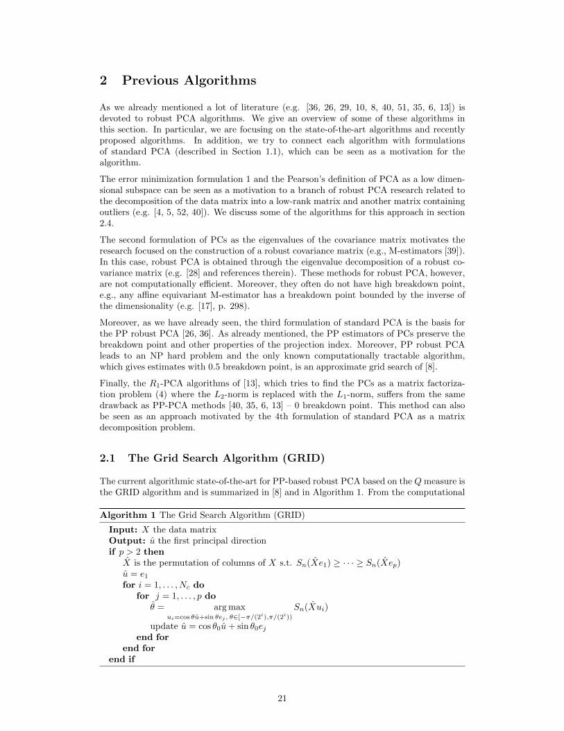
2.1 The Grid Search Algorithm (GRID)

The current algorithmic state-of-the-art for PP-based robust PCA based on the Q measure isthe GRID algorithm and is summarized in [8] and in Algorithm 1. From the computational

Algorithm 1 The Grid Search Algorithm (GRID)

Input: X the data matrixOutput: u the first principal directionif p > 2 then

X is the permutation of columns of X s.t. Sn(Xe1) ≥ · · · ≥ Sn(Xep)u = e1

for i = 1, . . . , Nc dofor j = 1, . . . , p do

θ = arg maxui=cos θu+sin θej , θ∈[−π/(2i),π/(2i))

Sn(Xui)

update u = cos θ0u+ sin θ0ejend for

end forend if

21

point of view, it only requires fast computation of an estimator of scale (Q(u)). The ideaof the algorithm is based on the fact that it is easy to maximize S in 2D over all vectorswith unit norm: partition the unit two dimensional sphere with some grid size and greedysearch it. On every iteration of the algorithm a 2-dimensional plane is considered and a scaleestimator is maximized over all unit vectors onto the plane. There are no guarantees on theresult provided. Moreover, the algorithm does not search all the possible directions and itsperformance in high dimensions becomes quite poor, which is confirmed by the experiments.Furthermore, decreasing the grid size does not necessarily increase the solution because itleads to a different plane on the next iteration.

2.2 The High Dimensional Robust PCA Algorithm (HR-PCA)

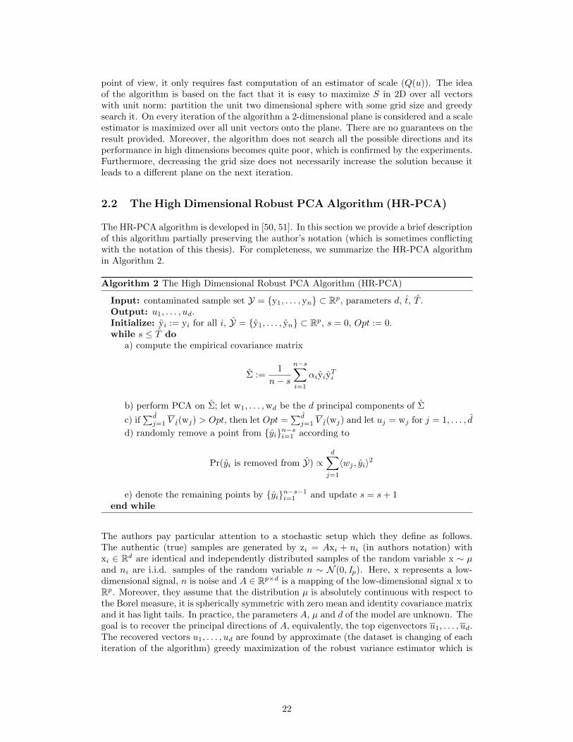
The HR-PCA algorithm is developed in [50, 51]. In this section we provide a brief descriptionof this algorithm partially preserving the author’s notation (which is sometimes conflictingwith the notation of this thesis). For completeness, we summarize the HR-PCA algorithmin Algorithm 2.

Algorithm 2 The High Dimensional Robust PCA Algorithm (HR-PCA)

Input: contaminated sample set Y = y1, . . . , yn ⊂ Rp, parameters d, t, T .Output: u1, . . . , ud.Initialize: yi := yi for all i, Y = y1, . . . , yn ⊂ Rp, s = 0, Opt := 0.while s ≤ T do

a) compute the empirical covariance matrix

Σ :=1

n− s

n−s∑i=1

αiyiyTi

b) perform PCA on Σ; let w1, . . . ,wd be the d principal components of Σ

c) if∑dj=1 V t(wj) > Opt, then let Opt =

∑dj=1 V t(wj) and let uj = wj for j = 1, . . . , d

d) randomly remove a point from yin−si=1 according to

Pr(yi is removed from Y) ∝d∑j=1

〈wj , yi〉2

e) denote the remaining points by yin−s−1i=1 and update s = s+ 1

end while

The authors pay particular attention to a stochastic setup which they define as follows.The authentic (true) samples are generated by zi = Axi + ni (in authors notation) withxi ∈ Rd are identical and independently distributed samples of the random variable x ∼ µand ni are i.i.d. samples of the random variable n ∼ N (0, Ip). Here, x represents a low-dimensional signal, n is noise and A ∈ Rp×d is a mapping of the low-dimensional signal x toRp. Moreover, they assume that the distribution µ is absolutely continuous with respect tothe Borel measure, it is spherically symmetric with zero mean and identity covariance matrixand it has light tails. In practice, the parameters A, µ and d of the model are unknown. Thegoal is to recover the principal directions of A, equivalently, the top eigenvectors u1, . . . , ud.The recovered vectors u1, . . . , ud are found by approximate (the dataset is changing of eachiteration of the algorithm) greedy maximization of the robust variance estimator which is

22

defined as

V t(u) =1

n

t∑i=1

|〈u, y〉|2(i), (12)

where |〈u, y〉|2(1) ≤ · · · ≤ |〈u, y〉|2(n).

The idea on how the HR-PCA algorithm works is as follows. Given an upper bound on thenumber of the outliers t one computes standard PCA of the whole data set and the robustvariance estimator based on the obtained PCs. If the value of the estimator is small, thanone deletes randomly one of the “furthest” points is the given direction. On the contrary,if the value of the estimator is big, one hopes that the obtained PCs are close to the trueones. Note, that in the paper provided the lower bounds on the explained (expressed, inauthors notation) variance, which is defined as follows

E.V. =

∑dj=1 u

Tj AA

Tuj∑dj=1 u

Tj AA

Tuj=

∑dj=1 u

Tj AA

Tuj

trace(AAT ), (13)

where, clearly, 0 ≤ E.V. ≤ 1.

The HR-RPCA is not location invariant and, thus, requires preliminary centering of thedata. Even though there are 0.5 breakdown point estimators of multivariate location areavailable in the literature (e.g., [37]), the mentioned phenomenon may lead to problems inhigh dimensions, as we will see in the experimental Section 4.

Finally, the deterministic version of the HR-PCA algorithm (DHR-PCA) was proposed in[31]. This algorithm is similar to the HR-PCA algorithm, however, does not show betterresults in practice.

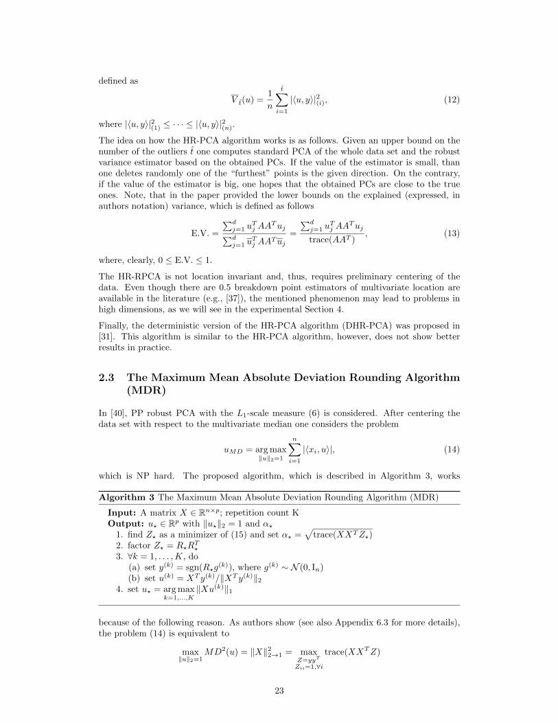
2.3 The Maximum Mean Absolute Deviation Rounding Algorithm(MDR)

In [40], PP robust PCA with the L1-scale measure (6) is considered. After centering thedata set with respect to the multivariate median one considers the problem

uMD = arg max‖u‖2=1

n∑i=1

|〈xi, u〉|, (14)

which is NP hard. The proposed algorithm, which is described in Algorithm 3, works

Algorithm 3 The Maximum Mean Absolute Deviation Rounding Algorithm (MDR)

Input: A matrix X ∈ Rn×p; repetition count KOutput: u? ∈ Rp with ‖u?‖2 = 1 and α?

1. find Z? as a minimizer of (15) and set α? =√

trace(XXTZ?)2. factor Z? = R?R

T?

3. ∀k = 1, . . . ,K, do(a) set y(k) = sgn(R?g

(k)), where g(k) ∼ N (0, In)(b) set u(k) = XT y(k)/‖XT y(k)‖2

4. set u? = arg maxk=1,...,K

‖Xu(k)‖1

because of the following reason. As authors show (see also Appendix 6.3 for more details),the problem (14) is equivalent to

max‖u‖2=1

MD2(u) = ‖X‖22→1 = maxZ=yyT

Zii=1,∀i

trace(XXTZ)

23

and the following semidefinite relaxation is applied

α2? = max

Z<0Zii=1,∀i

trace(XXTZ). (15)

As discussed above, the MDR algorithm, together with the algorithms of [6, 13, 35], leadsto the estimates of PCs with 0 breakdown point and is not robust in this sense.

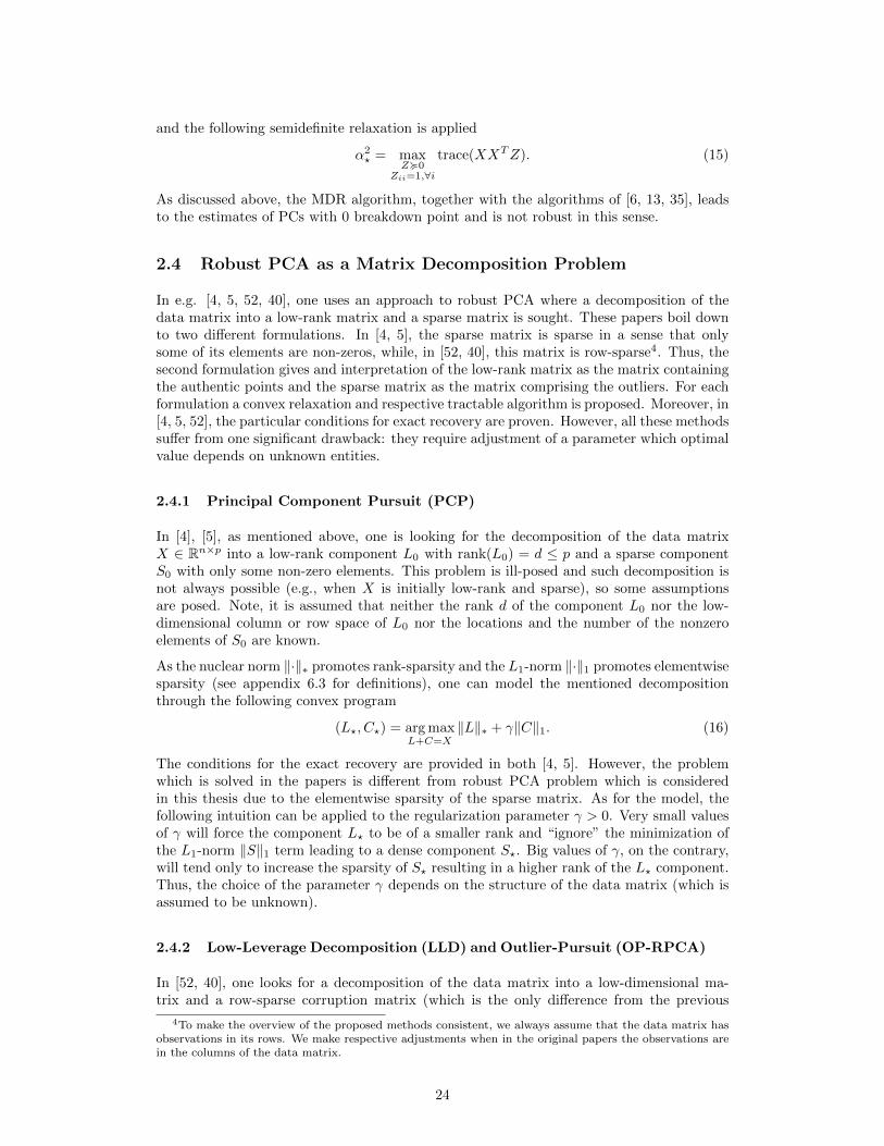
2.4 Robust PCA as a Matrix Decomposition Problem

In e.g. [4, 5, 52, 40], one uses an approach to robust PCA where a decomposition of thedata matrix into a low-rank matrix and a sparse matrix is sought. These papers boil downto two different formulations. In [4, 5], the sparse matrix is sparse in a sense that onlysome of its elements are non-zeros, while, in [52, 40], this matrix is row-sparse4. Thus, thesecond formulation gives and interpretation of the low-rank matrix as the matrix containingthe authentic points and the sparse matrix as the matrix comprising the outliers. For eachformulation a convex relaxation and respective tractable algorithm is proposed. Moreover, in[4, 5, 52], the particular conditions for exact recovery are proven. However, all these methodssuffer from one significant drawback: they require adjustment of a parameter which optimalvalue depends on unknown entities.

2.4.1 Principal Component Pursuit (PCP)

In [4], [5], as mentioned above, one is looking for the decomposition of the data matrixX ∈ Rn×p into a low-rank component L0 with rank(L0) = d ≤ p and a sparse componentS0 with only some non-zero elements. This problem is ill-posed and such decomposition isnot always possible (e.g., when X is initially low-rank and sparse), so some assumptionsare posed. Note, it is assumed that neither the rank d of the component L0 nor the low-dimensional column or row space of L0 nor the locations and the number of the nonzeroelements of S0 are known.

As the nuclear norm ‖·‖∗ promotes rank-sparsity and the L1-norm ‖·‖1 promotes elementwisesparsity (see appendix 6.3 for definitions), one can model the mentioned decompositionthrough the following convex program

(L?, C?) = arg maxL+C=X

‖L‖∗ + γ‖C‖1. (16)

The conditions for the exact recovery are provided in both [4, 5]. However, the problemwhich is solved in the papers is different from robust PCA problem which is consideredin this thesis due to the elementwise sparsity of the sparse matrix. As for the model, thefollowing intuition can be applied to the regularization parameter γ > 0. Very small valuesof γ will force the component L? to be of a smaller rank and “ignore” the minimization ofthe L1-norm ‖S‖1 term leading to a dense component S?. Big values of γ, on the contrary,will tend only to increase the sparsity of S? resulting in a higher rank of the L? component.Thus, the choice of the parameter γ depends on the structure of the data matrix (which isassumed to be unknown).

2.4.2 Low-Leverage Decomposition (LLD) and Outlier-Pursuit (OP-RPCA)

In [52, 40], one looks for a decomposition of the data matrix into a low-dimensional ma-trix and a row-sparse corruption matrix (which is the only difference from the previous

4To make the overview of the proposed methods consistent, we always assume that the data matrix hasobservations in its rows. We make respective adjustments when in the original papers the observations arein the columns of the data matrix.

24

approach). The robust PCs are then obtained as the standard PCs of the low-dimensionalmatrix.

In order to show the equivalence of the problems considered in [52] and [40] we rewritethem in a unique notation. The data matrix X ∈ Rn×p is as always5 and there is thefraction λ of the outliers in it (the value of λ is unknown). One looks for the decompositionX = L0 +C0, where C0 is the row-sparse matrix with (1−λ)n rows are zero vectors and L0

has low rank(L) = d ≤ p (d is unknown) and the rows of L0 corresponding to the non-zerorows of C0 are vectors of all zeros. Natural formulation of the decomposition is

(L?, C?) = minX=L+C

rank(L) + γ‖C‖0,c,

where ‖ · ‖0,c is the number of non-zero columns of a matrix. This problem is, however,non-convex and NP hard and one applies a convex relaxation

(L?, C?) = arg minL+C=X

‖L‖∗2,2 + γ‖C‖∗2,∞ = arg minL+C=X

‖L‖∗ + γ‖C‖1,2, (17)

where γ > 0 and the nuclear norm ‖·‖∗ = ‖·‖∗2→2 promotes low-rank solutions (rank sparsity)and the norm ‖·‖1,2 = ‖·‖∗2→∞ promotes group sparsity of the rows (see Appendix 6.3 for theproof of equivalence). Thus, through solving the problem (17) one gets the robust principaldirections as the subset of d largest right singular values of the matrix L?. This leads to theLLD algorithm of [40] and the OP-RPCA algorithms of [52]. As both algorithms boil downto the semidefinite program we will use the unique name Semidefinite Programming (SDP)to refer to them. The respective algorithm is summarized in Algorithm 4.

Algorithm 4 Semidefinite Programming (SDP)

Input: X ∈ Rn×p the data matrixOutput: V? the basis of low dimensional subspace; I? the indices of outliers

1. find (L?, C?) = arg minX=L+C

‖L‖∗ + γ‖C‖1,2

2. compute SVD L? = UΣV T and output V? = V3. output the set of non-zero columns of C?, i.e. I? = i

∣∣(c?)ij 6= 0 for some j

It worth mentioning the difference of the approach used by [52]. They do not strive for theexact recovery of the components rather than just interested in identifying the indices I ofthe non-zero rows of the corruption matrix C (i.e. the outliers in case of exact recovery).The rows of X with indices I are then the outliers.

The choice of the parameter γ is again a problem as we are in the unsupervised setting.In accordance to [40], when γ ≥ 1 the solution C? = 0 and when γ ≤ 1/

√n the solution

L? = 0. The authors suggest a heuristic to choose γ a bit less than√p/n, e.g., γ = 0.8

√p/n,

commenting that this choice is good for finding principal directions but weak for findingoutliers.

2.5 Robust PCA through Robust Covariance Matrix Estimation(ROBPCA)

For this approach to the robust PCA problem, we restrict our attention only to the ROBPCAalgorithm [29] because it is the only highly robust and computationally efficient algorithm

5Note, that X has observations in rows, not in columns as defined in [52]. The outlier-pursuit algorithmis adjusted respectively. The adjustment is straightforward as the nuclear norm is invariant under thetranspose of the matrix, i.e. ‖A‖∗ = ‖AT ‖∗ (the singular values of both matrices are the same) and as inthe outlier-pursuit algorithm one is only interested in the positions of the non-zero columns (here, rows) forC.

25

of this type. The ROBPCA algorithm tries to combine the ideas of the PP approach, todetect the outliers, and the robust covariance matrix estimation, for the final estimation ofthe robust PCs. Such pre-processing step is required as robust covariance matrix estimatorshave the breakdown point bounded by the inverse of the dimensionality.

The algorithm works as follows. First, it tries to find the “least outlying” h points where n−his an upper bound for the number of outliers and h is an input parameter for the algorithm.They use the outlyingness measure as it is defined for the Stahel-Donoho estimator [14] and[47], i.e. the outlyingness of xi is

t(xi) = max‖u‖=1

|〈xi, u〉 − µ(Xu)|σ(Xu)

, (18)

where µ(Xu) is a robust location estimator and σ(Xu) is a robust scale estimator. As theseestimators the algorithm uses the ones obtained by the minimum covariance determinant(MCD) estimator [44] of the covariance matrix. The resulting problem (18) is non-convexand non-smooth. To compute the outlyingness measure for each of the observations xi ∈ Rp,the ROBPCA algorithm uses a very simple greedy technique by taking the maximum over250 randomly chosen directions, which are formed by the randomly chosen pairs of theobservations in the data set. Finally, when the points are found one estimates the robustcovariance matrix with the MCD estimator and finds the robust PCs as the eigenvectors ofthis matrix.

26

3 Robust PCA as a Nonlinear Eigenproblem

3.1 The Nonlinear Eigenproblem and RatioDCA

Let us, for a moment, leave the general form of the scale measure S(u). We already discussedin section 1.3 that PP robust PCA leads to the nonlinear eigenproblem (7), which is NPhard. The key idea to solve this problem is finding the d.c. representation of the scalemeasure, i.e.

S(u) = S1(u)− S2(u), (19)

where S1(u) and S2(u) are convex functions, and applying RatioDCA [21]. As the numeratorand denominator are positively 1-homogeneous and non-negative functions we can flip thenumerator and the denominator and rewrite the problem (7) equivalently as

u1 = arg minu∈Rp

‖u‖2S(u)

= arg minu∈Rp

‖u‖2S1(u)− S2(u)

, (20)

where we used a d.c. decomposition (19). We denote the objective of the problem (20),which is the ratio of positively 1-homogeneous non-negative d.c. functions, as

λ(u) =‖u‖2

S1(u)− S2(u).

At every iteration of RatioDCA, one solves the following convex problem

uk+1 = arg min‖u‖≤1

‖u‖2 + λ(uk)

(S2(u)− 〈u, s1(uk)〉

)= arg min‖u‖≤1

Θ(u), (21)

where the subgradient6 s1(uk) ∈ ∂S1(uk) and any norm ‖ · ‖ can be chosen for the con-straint. As the objective of this problem is positively 1-homogeneous, then the solutionof the optimization problem above is either achieved at the boundary or 0. Moreover, asdiscussed in [21], the objective of the inner problem (21) is zero when the vector from theprevious iteration (for which λ(uk) is calculated) is used, i.e. Θ(uk) = 0. If there is adescent then Θ(u) < 0 and the minimum of the 1-homogeneous objective is achieved onthe boundary. Hence, as ‖uk‖2 = 1 by construction, and the solution of the problem (21)has unit norm, i.e. ‖uk+1‖2 = 1. This implies that the problem (21) is equivalent to thefollowing problem

uk+1 = arg min‖u‖2≤1

S2(u)− 〈u, s1(uk)〉

. (22)

We summarize the complete method in Algorithm 5.

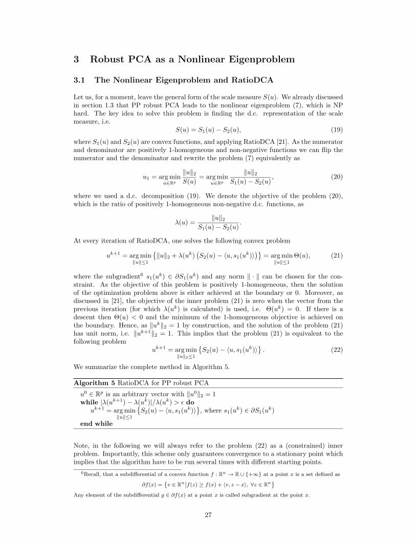
Algorithm 5 RatioDCA for PP robust PCA

u0 ∈ Rp is an arbitrary vector with ‖u0‖2 = 1while |λ(uk+1)− λ(uk)|/λ(uk) > ε do

uk+1 = arg min‖u‖≤1

S2(u)− 〈u, s1(uk)〉

, where s1(uk) ∈ ∂S1(uk)

end while

Note, in the following we will always refer to the problem (22) as a (constrained) innerproblem. Importantly, this scheme only guarantees convergence to a stationary point whichimplies that the algorithm have to be run several times with different starting points.

6Recall, that a subdifferential of a convex function f : Rn → R ∪ +∞ at a point x is a set defined as

∂f(x) =v ∈ Rn

∣∣f(z) ≥ f(x) + 〈v, z − x〉, ∀z ∈ Rn

Any element of the subdifferential g ∈ ∂f(x) at a point x is called subgradient at the point x.

27

3.2 Projection-Pursuit Robust PCA with the Quartile DifferenceMeasure (QRPCA)

The projection-pursuit robust PCA with the quartile difference measure algorithm (QR-PCA) is the main contribution of this thesis. This algorithm solves the projection-pursuitrobust PCA problem (7), where the quartile difference measure (10) is used as the projectionindex, with RatioDCA and the main ingredient to the solution is the d.c. representationof the quartile difference measure Q(u) = Q1(u)− Q2(u) (see Theorem 2). However, Algo-rithm 5 requires to solve the convex inner problem (22) and, as it has to be done on everyiteration, the solution should be efficient. In the following sections we present several pos-sible solutions for the inner problem. We start with a more straightforward dual approach,where we use accelerated proximal methods [1]. This approach is, however, computationallyexpensive. This motivates us to consider different approach, a primal approach, where weuse the bundle methods [23] to solve the inner problem.

3.3 The Dual Approach to the Solution of the Inner Problem ofQRPCA

In this section we consider the inner problem (22) and solve it by constructing a dualproblem. The dual problem is mainly obtained due to the following property of convex,1-homogeneous functions.Theorem 4. Every convex, positively 1-homogeneous function, S : Rn → R, has the form

S(u) = supy∈U〈u, y〉,

where U is a convex set (e.g. [22]).

We recall, that the even, convex and positively 1-homogeneous function Q2(u) is

Q2(u) =1

k

m∑ξ=k+1

|〈xi, u〉 − 〈xj , u〉|; i < j(ξ).

Let us introduce a new mapping Ω : Rp → Rm such that Ωu = 〈xi, u〉 − 〈xj , u〉; i < j andm is the number of all pairwise differences of the elements from the set 〈xi, u〉ni=1 then

the function Q2(u) takes the form

Q2(u) =1

k

m∑ξ=k+1

|Ωu|(ξ),

which can be seen as a sum of κ = m − k largest components of |Ωu|. In accordance toTheorem 4, the function Q2(u) admits the following representation

Q2(u) = supα∈C〈Ωu, α〉, (23)

where the convex set C is defined as C =α ∈ Rm

∣∣‖α‖1 ≤ κ,−1 ≤ αi ≤ 1, i = 1, 2, . . . ,m

.This formulation uses the property of the linear program (note that the problem (23) is aninstance) that its extremum is achieved at an extreme point of the constraint set, i.e. thevalues of the elements of the optimal vector α are either −1, 1 or 0. Hence, it sums up κelements of Ωu with either positive or negative sign and the pointwise supremum forces tochoose the largest in absolute value elements.

The new form (23) of the function Q2(u) allows us to rewrite the constrained inner problem(22) of RatioDCA for the quartile difference measure as

J∗ = min‖u‖2≤1

maxα∈C〈u,ΩTα− q1(uk)〉,

28

where q1(uk) ∈ ∂Q1(uk). This is a saddle-point problem over the compact domain ‖u‖2 ≤1 × C and by Corollary 37.3.2. in [43] we can exchange min and max and get

J∗ = maxα∈C

min‖u‖2≤1

〈u,ΩTα− q1(uk)〉. (24)

For the minimization problem we get u = −(ΩTα−q1(uk))/‖ΩTα−q1(uk)‖2 and substitutingthis into (24) we obtain

J∗ = −minα∈C

∥∥ΩTα− q1(uk)∥∥

2, (25)

where uk+1 = −(ΩTαk+1 − q1(uk)

)/∥∥ΩTαk+1 − q1(uk)

∥∥2.

The solution for the dual problem (25) of the inner problem of RatioDCA can be found,e.g., with FISTA [1]. This approach is, however, intractable in practice due to the fact thatthe dual variable α has dimension m = O(n2) and the algorithm becomes prohibitively slowwhen the sample size is, e.g., n = 1000. In Section 3.5, we will apply the same approach toPP robust PCA with the median absolute deviation measure MDRPCA.

3.4 The Primal Approach to the Solution of the Inner Problem ofQRPCA

The key to an efficient method is to have a fast algorithm to solve the convex inner problem(22). We have just seen that accelerated proximal methods [1] are not applicable for (22) asone gets O(n2) dual variables due to the structure of Q2 and thus the method would not scalewell with the number of data points. However, as we will show, it turns out that althoughQ2 seems to require O(p n2) operations to compute a function value, it can be evaluated inO(n(log n+p)) and delivers on the fly a subgradient q2 ∈ ∂Q2 at that point. This motivatesus to consider bundle methods (e.g. [23]), which are efficient when the objective and itssubgradient can be computed fast at any point. In particular, we propose to use the primalbundle method with penalty ([23], pp. 301–317).

The solution of the constrained inner problem of the RatioDCA (22) can also be equivalentlyfound by solving an unconstrained problem. We first formulate the unconstrained problemitself ant then develop the algorithms for the minimization of the problems.Lemma 3.1. The solution of the constrained inner problem (22) is equal to the normalizedsolution of the following unconstrained problem

uk+1 = arg minu∈Rp

Q2(u) +

1

2‖u− q1(uk)‖22

, (26)

that is uk+1 = uk+1/∥∥uk+1

∥∥2.

Proof. The necessary and sufficient condition (e.g. [22]) for the minimizer of the constrainedproblem (22) is

0 ∈ ∂Q2(uk+1)− q1(uk) +N‖·‖2≤1(uk+1),

where N‖·‖2≤1(u) stands for the normal cone of L2-norm unit ball. When deriving equa-

tion (22) we have shown that∥∥uk+1

∥∥2

= 1 and the respective normal cone has the form

N‖·‖2≤1(u) =αu∣∣ α ∈ R≥0

. This implies that the minimizer is

uk+1 ∈ − 1

α

(∂Q2(uk+1)− q1(uk)

)(27)

and α is chosen to satisfy∥∥uk+1

∥∥2

= 1, i.e. α =∥∥∥∂Q2(uk+1)− q1(uk)

∥∥∥2.

29

At the same time, the necessary and sufficient condition for the minimizer of the uncon-strained problem (26) is

0 ∈ ∂Q2(uk+1) + uk+1 − q1(uk).

and the respective optimizer is

uk+1 ∈ −(Q2(uk+1)− q1(uk)

). (28)

Comparing (27) and (28) we see that uk+1 = uk+1/∥∥uk+1

∥∥2.

3.4.1 Bundle Method for the Solution of the Constrained Inner Problem

In this section we present the algorithm – the bundle method with penalty – for the so-lution of the convex constrained minimization problem (22). Before we proceed with thedescription of the bundle method, let us first show that the objective of problem (22)f(u) = Q2(u) − 〈u, q1(uk)〉 as well as its subgradient g(u) ∈ ∂f(u) can be efficiently eval-uated at a point. In particular, we explicitly describe an algorithm for the evaluation off(u) and g(u) which is an extension of the algorithm for finding kth element of pairwisedifferences [9] and/or [32].Lemma 3.2. The objective f(u) and the subgradient g(u) ∈ ∂f(u) can be computed at anyu ∈ Rp in O

(n(log n+ p)

)time.

Proof. As a proof, we present the algorithm to evaluate the value of the objective f(u) =Q2(u)−〈q1(uk), u〉 of the inner problem (22) and its subgradient g ∈ ∂f(u) at a given pointu in O(n(log n+ p)) time. We first show that the value of the function Q2(u) and the valueof its subgradient q2(u) ∈ ∂Q2(u) can be obtained in O(n(log n+ p)) time.

Recall, that the function Q2(u) is defined in Thm. 2 and has the form

Q2(u) =1

k

m∑ξ=k+1

|〈xi, u〉 − 〈xj , u〉|; i < j(ξ),

where m = (n2 − n)/2 and k =(bn/2c+1

2

). We introduce κ = m − k + 1. To compute the

function value of Q2(u) we extend the algorithm described in [9]which is based on [32]. Forcompleteness, we provide the full description of the algorithm.

First of all, we compute the κth largest element of the pairwise distances of the projectedpoints. We consider the 1-dimensional array y = Xu ∈ R (which takes O(np) to compute)and sort it, which takes O(n log n) time, i.e. the vector y is defined as yi = 〈xj , u〉, where jbelongs to a permutation of 1, . . . , n such that y0 ≤ y1 ≤ y2 ≤ · · · ≤ yn−1. The algorithmworks on the following matrix B ∈ Rn×n (which is clearly never generated)

0 0 ... ... ... ... ... 0y1 − y0 0 0 ... ... ... ... ...y2 − y0 y2 − y1 0 ... ... ... ... ...y3 − y0 y3 − y1 y3 − y2 0 ... ... ... ...... ... ... ... ... 0 ... ...

yn−2 − y0 yn−2 − y1 yn−2 − y2 yn−2 − y3 ... yn−1 − yn−2 0 ...yn−1 − y0 yn−1 − y1 yn−1 − y2 yn−1 − y3 ... yn−1 − yn−3 yn−1 − yn−2 0

All elements of the matrix B are nonnegative and no more than m of them are positive.These m elements correspond to the absolute values of the differences |〈xi, u〉 − 〈xj , u〉| andwe are interested in finding the κth largest element in the matrix B. The algorithm forcomputing this value in O(n log n) time is described below and is based on the algorithm of[32].

Findind κth largest element in B:

30

1. For each row i of B, search is restricted by Lb and Bb indices, where, e.x., Lbi points tothe element yi−yLbi . Initially, Lbi = 0 and Rbi = i−1 for all i (note that Rb0 = −1).Let also

R = card (yi − yj |yi − yj ≥ yi − yRbi) ,

L = card (yi − yj |yi − yj > yi − yLbi) .

Initially, R = m and L = 0.

2. while R− L > n do

Let for all i = 0, 1, ..., n − 1 such that Lbi ≤ Rbi, a = ai|ai = yi − yji and w =wi|wi = Rbi − Lbi + 1, where ji = b(Lbi +Rbi)/2c

Let am ∈ a be the weighted median of a with weights w.

Let for all i = 0, 1, ..., n− 1

Pi =

−1, if yi − y0 ≤ am,maxj|yi − yj > am, o.w.

Qi =

i, if yi − yi−1 ≥ am,minj|yi − yj < am, o.w.

Let sumP =∑n−1i=0 (Pi + 1) and sumQ =

∑n−1i=0 Qi.

if sumP ≥ κ then Rbi = Pi and R = sumP

else if sumQ < κ then Lbi = Qi and L = sumQ

else return am

3. Let t = tl|tl = yi − yj , for all Lbi ≤ j ≤ Rbi and all i = 0, 1, ..., n − 1. Then sort tin increasing (nondecreasing) order and return tR−κ.

The value of the κth largest element B(κ) of the matrix B (consequently, of the pairwisedistances) is found in O(n log n) time. Now, by bisection on the columns of the matrix B (asthe elements in the columns are nondecreasing), we can find all the elements of B that aregreater than B(κ) in O(n log n) time. Sum of these elements gives the value of the function

Q2(u) at the given point u. Moreover, having track of the indices of the element B(κ) andall the elements that are larger than B(κ), one can easily compute the subgradient q2(u)at the given point u. Indeed, if the element Bi,j = 〈xi, u〉 − 〈xj , u〉 (with 〈xi, u〉 ≥ 〈xj , u〉by construction) contributes to the function value Q2(u) then it also contributes to thesubgradient q2(u) with xi − xj (i.e. q2(u) is the sum of all such differences).

After the function value Q2(u) and the subgradient q2(u) are computed at the point u, thevalue of the function f(u) and its subgradient g are obtained by adding −〈q1(uk), u〉 andq1(uk), respectively. Note, that the representation of the pairwise distances of the projectedpoints Xu with the matrix B allows also to compute the subgradient q1(uk) ∈ ∂Q1(uk) onthe fly. Indeed, the sorting of Xu is already done and the subgradient is equal to the sumof all xi− xj with i, j such that 〈xi, uk〉 ≥ 〈xj , uk〉 (i.e., as they are contained in the matrixB).

The Bundle Method for the Constrained Inner Problem: To define the model,which is minimized with some penalization at each iteration of the bundle method, let usfirst introduce some notation. The linear underestimator of the function f(u) at a givenpoint ui is

`i(u) = f(ui) + 〈g(ui), u− ui〉 = 〈g(ui), u〉,

where the last equation holds due to the fact that the function f(u) is 1-homogeneous and,hence, f(ui) = 〈g(ui), ui〉. Next, given the linear underestimators at the points u1, . . . , uB

31

and introducing a matrix G ∈ RB×p where a row Gi = g(ui)T is a subgradient for all

i = 1, . . . , B, we define the model of the function f(u) as

φB(u) = maxi=1,...,B

〈g(ui), u〉 = maxi=1,...,B

(Gu)i.

Another perspective on this is that every 1-homogeneous function ψ can be written as ψ(u) =supw∈∂ψ(0) 〈w, u〉 and ∂ψ(u) = w ∈ ∂ψ(0) | 〈w, u〉 = ψ(u). Thus, it holds that

f(u) = supw∈∂f(0)

〈w, u〉 ≥ maxi=1,...,B

〈g(ui), u〉 = φB(u).

The elements in G together with the points ui form the bundle. As the number of elementsB increases the model becomes a better approximation of f .

The bundle method with penalty is based on the following idea: given a stability centervj ∈ Rp, at each iteration j of the bundle method the penalized model has to be minimized,i.e.

uj+1 = arg min‖u‖2≤1

max

i=1,2,...,B(Gu)i +

1

2t‖u− vj‖22

, (29)

where the model is constructed from B linear underestimators obtained at some of theprevious iterations of the bundle method and t is a step size. For the new point uj+1 thedescent can be measured with7

δj = f(vj)− φB(uj+1)− 1

2t‖vj − uj+1‖22

and the stability center is defined as one of the previous points obtained with the bun-dle method at which the function had “sufficient” descent, that is defined as f(uj+1) ≤f(vj) −mδj for some m ∈ (0, 1). If at the next iteration there is no “sufficient” descent, anull step happens, which means, that the stability center is not changed and only the modelis updated. Importantly, for the model only some limited number Bmax of linear underesti-mators is stored. We observe in practice that Bmax ≈ 15 is already sufficient which makesthe method very fast. However, the subgradient which corresponds to the stability centeralway have to be in the bundle.

The main computational problem at each iteration of the bundle method is, apart from theevaluation of the objective and its subgradient, the solution of (29).Lemma 3.3. The solution of the optimization problem (29) is

uj+1 =

vj − tGTα‖vj − tGTα‖2

if∥∥vj − tGTα∥∥2

≥ 1,

vj − tGTα else.

, (30)

where

αj+1 = arg minα∈∆B

1

2t

∥∥vj − tGTα∥∥2

2, (31)

and ∆B =α ∈ RB

∣∣ ∑Bi=1 αi = 1, αi ≥ 0, ∀i = 1, . . . , B

is the simplex.

Proof. We notice first that maxi=1,2,...,B(Gu)i = maxα∈∆B〈α,Gu〉. Thus we get a saddle-

point problem over the compact domain ‖u‖2 ≤ 1 × ∆B with a finite convex-concavefunction. By Corollary 37.3.2. in [43] we can exchange min and max and get

min‖u‖2≤1

maxi=1,2,...,B

(Gu)i +

1

2t‖u− vj‖22

= maxα∈∆B

min‖u‖22≤1

〈GTα, u〉+

1

2t‖u− vj‖22

. (32)

7Note, it is always holds that δj ≥ 0. Indeed, the optimality condition of (29) is 0 ∈ 1t(uj+1 − vj) +

∂φB(uj+1), hence, 1t(vj−uj+1) ∈ ∂φB(uj+1) and it holds that f(vj) = φB(vj) ≥ φB(uj+1)+〈sj , vj−uj+1〉

for any subgradient sj ∈ ∂φB(uj+1) of the linear model.

32

We note that the objective can be rewritten as⟨GTα, u

⟩+

1

2t‖u− vj‖22 =

1

2t

∥∥u− vj + tGTα∥∥2

2− 1

2t

∥∥tGTα− vj∥∥2

2+

1

2t‖vj‖22 .

Thus the minimization over u with, ‖u‖2 ≤ 1, has the solution

u∗ =

vj − tGTα‖vj − tGTα‖2

if∥∥vj − tGTα∥∥2

≥ 1,

vj − tGTα else.

The remaining optimization problem over α is for both cases equivalent to

minα∈∆B

∥∥vj − tGTα∥∥2

2.

Algorithm 6 The Bundle Method for the Constrained Inner Problem of RatioDCA (22)

Input: v1 = uk, ε > 0, the descent-coefficient m ∈ (0, 1), the max bundle size Bmax, tFind αj+1 from (31) and evaluate u+ j + 1 from (30)Compute the stopping criterion δj = f(vj)− φB(uj+1)− 1

2t‖vj − uj+1‖22if δj ≤ ε, terminate, end ifif f(uj+1) ≤ f(vj)−mδj , update the stability center, else null step end ifManage the bundle size B such that B ≤ Bmax

The minimization problem (31) can be efficiently solved with FISTA [1] and, hence, we cansummarize the bundle method in Algorithm 6.

The Solution of the Subproblem with FISTA: As a part of the bundle method theoptimization problem with respect to α (31) have to be solved. This problem can be solvedwith the fast iterative shrinkage–thresholding algorithm (FISTA) [1]. This algorithm dealswith the convex optimization problems that can be represented in a form

min

Φ(x) ≡ φ1(x) + φ2(x)∣∣x ∈ Rn

,

where the following assumptions on the functions φ1(x) and φ2(x) are made

1. φ1(x) : Rn → R is a smooth convex function of the type C1,1, i.e. continuouslydifferentiable with Lipschitz continuous gradient L(φ1)

‖∇φ1(x)−∇φ1(y)‖2 ≤ L(φ1)‖x− y‖2 for every x, y ∈ Rn,

where L(φ1) > 0 is the Lipschitz constant of ∇φ1;

2. φ2(x) : Rn → R is a convex function which is possibly non-smooth.

In case of the problem (31) the functions φ1(α) = 12t

∥∥vj − tGTα∥∥2

2and φ2(α) = ι∆B

(α),where the indicator function of the simplex ∆B is defined as

ι∆B(α) =

0, α ∈ ∆B ,∞, α 6∈ ∆B .

The functions φ1 and φ2 fulfill the stated above requirements of FISTA. Moreover, thegradient of φ1(α) is ∇φ1(α) = tGGTα−Gvj and its Lipschitz constant is L = tλmax(GGT ),where λmax(·) stands for the largest eigenvalue of a matrix (see derivation in Section 6.2). Asthe algorithm only requires an upper bound for this Lipschitz constant, we use the Frobeniusnorm (due to the fact that the size of the problem B ≤ Bmax ≈ 15, this upper bound does

33

not decrease the speed of convergence a lot). The proximal map, which is considered atevery iteration of FISTA, has the form

pL(β) = arg minα∈RB

L

2

∥∥∥∥α− (β − 1

L∇φ1(β)

)∥∥∥∥2

2

+ ι∆B(α)

= arg minα∈∆B

∥∥∥∥α− (β − 1

L(tGGTβ −Gvj)

)∥∥∥∥2

2

.

This proximal map is just a projection onto the simplex and can be done in linear time [34].The algorithm is summarized in Algorithm 7.

Algorithm 7 The Solution of the Subproblem (31) with FISTA

Input: ε, t1 = 1, some vector α0 ∈ RB , β1 = α0

calculate L = t‖GGT ‖F ≥ tλmax(GGT )while (duality gap ≥ ε) do

Compute αk as a projection of βk − (1/L)∇φ1(βk) onto ∆B

sk+1 =

(1 +

√1 + 4s2

k

)/2

βk+1 = αk + ((sk − 1)/(sk+1)) (αk − αk−1)end while

As a stopping criterion we use the duality gap, i.e. the difference of the primal (29) andthe dual (31) objectives at the current dual point. It is not complicated to show that theduality gap is

GAPk(αk+1) = maxi=1,...,B

(Guk+1)i − 〈uk+1, GTαk+1〉,

where uk+1 = (vj − tGTαk+1)/‖vj − tGTαk+1‖2 if ‖vj − tGTαk+1‖2 ≥ 1 and uk+1 =vj − tGTαk+1 otherwise.

3.4.2 Bundle Method for the Solution of the Unconstrained Inner Problem

In this section we provide the algorithm for the optimization of the unconstrained innerproblem (26) which is also based on the bundle method with penalty. We use the notionsdefined in Section 3.4.1 and only describe the differences from the previous algorithm.

We denote the objective of the unconstrained inner problem (26) as f(u) = Q2(u)− 12‖u−

q1(uk)‖22 and its subgradient through g(u) ∈ ∂f(u). Again, they can be evaluated efficientlyat a point.Lemma 3.4. The objective f(u) and the subgradient g(u) ∈ ∂f(u) of the unconstrainedinner problem (26) can be computed at any u ∈ Rp in O(n(log n+ p)) time.

Proof. We have already proven in Lemma 3.3 that the function value Q2(u) and its sub-gradient q2(u) can be computed at any u ∈ Rp in O(n(log n + p)) time. The rest of thecomputations takes O(n) time and, hence, the statement of the lemma follows.

The Bundle Method for the Unconstrained Inner Problem: The linear under esti-mator at ui ∈ Rp has the form

`i(u) = f(ui) + 〈g(ui), u− ui〉

and does not admit simplification as above as the function f(u) is not 1-homogeneous thistime. Introducing a matrix G ∈ RB×p with a row Gi = g(ui)

T and a vector b ∈ RB with

34

an element bi = f(ui) − 〈g(ui), ui〉 for all i = 1, . . . , B, we write the model of the functionf(u) as

φB(u) = maxi=1,...,B

(Gu+ b)i

and by analogy with (29) one minimizes the penalized linear model which, in this case, hasthe form

uj+1 = arg minu∈Rp

max

i=1,2,...,B(Gu+ b)i +

1

2t‖u− vj‖22

, (33)

Lemma 3.5. Using again the notation ∆B for the simplex, we get the following solution ofthe optimization problem (33)

uj+1 = vj − tGTαj+1 (34)

and

αj+1 = arg minα∈∆B

1

2t‖GTα‖22 − 〈Gvj + b, α〉

. (35)

Proof. The proof is similar to the proof of Lemma 3.3. We rewrite the model as a maximumover the simplex as φB(u) = maxi=1,2,...,B (Gu+ b)i. This transforms the problem (33)into a saddle point problem over the compact domain Rp×∆B and, hence, we can exchangemin and max. The solution of the unconstrained convex quadratic minimization problemwith respect to u is u = vj− tGTα. After plugging this expression into the objective of (33)we get the expression for αj+1 after some simplifications.

The bundle method for the solution of the problem (26) is summarized in Algorithm 8.

Algorithm 8 The Bundle Method for the Unconstrained Inner Problem of RatioDCA (26)

Input: v1 = uk, ε > 0, the descent-coefficient m ∈ (0, 1), the max bundle size Bmax, tFind αj+1 from (35) and compute uj+1 from (34)Compute the stopping criterion δj = f(vj)− φB(uj+1)− 1

2 t‖GTαj+1‖22

if δj ≤ ε, terminate, end ifif f(uj+1) ≤ f(vj)−mδj , update the stability center, else null step end ifManage the bundle size B such that B ≤ Bmax

The Solution of the Subproblem (35) with FISTA: For completeness, let us describethe FISTA algorithm for the solution of the problem (35). By analogy with the previoussection, the functions φ1(α) = 1

2 t‖GTα‖22 − 〈Gvj + b, α〉 and φ2(α) = ι∆B

(α). Next, therespective gradient is ∇φ1(α) = tGGTα + (Gvj + b) and its Lipschitz constant is L =tλmax(GGT ). The proximal map, which is considered at every iteration of FISTA, has theform

pL(β) = arg minα∈RB

L

2

∥∥∥∥α− (β − 1

L∇φ1(β)

)∥∥∥∥2

2

+ ι∆B(α)

= arg minα∈∆B

∥∥∥∥α− (β − 1

L

(tGGTβ + (Gvj + b)

))∥∥∥∥2

2

.

This proximal map is again nothing else as the projection onto the simplex ∆B , which canbe done in linear time. The following expression holds for the duality gap

GAPk(αk+1) = maxi=1,2,...,B

(Guk+1 + b)i+1

2t‖uk+1 − vj‖22 +

1

2t‖GTαk+1‖22 − 〈Gvj + b, αk+1〉

= maxi=1,2,...,B

(Gvj + b− tGGTαk+1)i

+ t‖GTαk+1‖22 − 〈Gvj + b, α〉

35

We refer to Algorithm 7 for the description of the algorithm.

Convergence of the Bundle Method: In accordance to ([23], theorem XV.3.2.4), thefollowing guarantees hold for the bundle method with penalty.Theorem 5. Consider algorithm 6 with the stopping tolerance δ = 0. Assume that K isfinite: for some k0, each iteration k ≥ k0 produces a null-step. If

tk ≤ tk−1 for all k > k0∑k>k0

t2ktk−1

= +∞

then xk0 minimizes f .

This means that the constant choice of tk also guarantees the convergence. In practice,we normally use the value t = 0.1 as the parameter for the bundle method for the con-strained inner problem and the value t = 0.01 as the parameter for the unconstrained innerproblem.

3.5 Projection-Pursuit Robust PCA with the Median Absolute De-viation Scale Measure (MDRPCA)

In this section we provide an algorithm for PP robust PCA with the median absolutedeviation (11) as the scale measure. For the algorithm we use RatioDCA as it is describedin Section 3.1 as well as a d.c. decomposition of MD from Theorem 3. To solve the innerproblem of RatioDCA we follow the dual approach described in Section 3.3.

As we have shown in Theorem 3 a d.c. representation of the median absolute deviation isMD(u) = MD1(u)−MD2(u), where the both functions MD1(u) and MD2(u) are convexand positively 1-homogeneous. Thus, the PP robust PCA problem (7) with median absolutedeviation as the scale measure has the form

u1 = arg minu∈Rp

‖u‖2MD(u)

= arg minu∈Rp

‖u‖2MD1(u)−MD2(u)

,

where MD1(u) and MD2(u) are defined in Theorem 3 and the inner problem of RatioDCA(22) takes the form

uk+1 = arg min‖u‖≤1

MD2(u)− 〈u,md1(uk)〉

(36)

= arg min‖u‖≤1

n∑

i=bn/2c+1

|Xu|(i) − 〈u,md1(uk)〉

, (37)

where |Xu|(1) ≤ · · · ≤ |Xu|(n) and we compute a subgradient md1(uk) ∈ ∂MD1(uk) inaccordance with the expression

(md1(u))j =

n∑i=1

sign((Xu)i

)Xij for all j = 1, . . . , p,

where sign is the signum function8.

To solve the convex inner problem (36) we construct the dual problem by analogy withSection 3.3. Indeed, the function MD2(u) is positively 1-homogeneous and, hence, admitsthe following prepresentation

MD2(u) = maxα∈C〈α, Xu〉

8That is, sign(x) = −1 if x < 0, sign(x) = 0 if x = 0 and sign(x) = 1 if x > 0.

36

where again the set C =α ∈ Rn

∣∣‖α‖1 ≤ bn/2c , ‖α‖∞ ≤ 1

is the intersection of the L1-ball and L∞-ball (equivalently, box constraints). Substituting this expression for MD2(u)into the the formulation of the inner problem (36) we get the saddle point problem over thecompact set ‖u‖2 ≤ 1 × C. This allows us to exchange min and max and we get

J∗ = maxα∈C

min‖u‖≤1

〈u, XTα−md1(uk)〉

=−minα∈C

∥∥∥XTα−md1(uk)∥∥∥

2, (38)

where the second equality holds due to the fact that minimum of the linear function isattained on the boundary of the constraint region, in particular, the primal and the dualvariables at the optimum are connected via uk+1 = −(XTαk+1 − md1(uk))/‖XTαk+1 −md1(uk)‖2.

The subproblem (38) can be efficiently solved with FISTA. Again, the functions φ1(α) =12‖X

Tα −md1(uk)‖22 and φ2(α) = ιC(α), where ιC(α) stands for the indicator function of

the set C. The gradient for the function φ1(α) is ∇φ1(α) = XXTα − Xmd1(uk) and the

Lipschitz constant of this gradient is L = λmax

(XXT

)(see Section 6.2 for the derivation).

This leads to the proximal map which is equivalent to the projection onto the set C and,thus, we summarize the algorithm in Algorithm 9.

Algorithm 9 The Solution of the Subproblem (38) with FISTA

Initialize: ε, s1 = 1, some vector α0 ∈ Rn, β1 = α0

calculate L = λmax(XXT ) ≤ ‖XXT ‖Fwhile (GAPk(αk) ≤ ε) do

Compute αk as a projection of βk − (1/L)∇φ1(βk) onto C

sk+1 =

(1 +

√1 + 4s2

k

)/2

βk+1 = αk + ((sk − 1)/(sk+1)) (αk − αk−1)end while

We show that the projection onto C can be performed in linear time by explicitly describingthe algorithm. This algorithm is a systematic description with a slight modification of[12].Lemma 3.6. The projection onto the intersection of L1-ball and L∞-ball (equivalently, ballconstraints) can be computed in O(n) time.

Proof. The explicit description of the algorithm is provided in Section 6.1.

The expression for the duality gap is the following

GAPk(αk) =

n∑j=bn/2c+1

|Xuk|(j) − 〈uk,md1(uk)〉+ ‖XTαk −md1(uk)‖2

with uk = −(XTαk −md1(uk))/‖XTαk −md1(uk)‖2 for each iteration k of FISTA.

In practice we observed that this algorithm does not scale well with the number of obser-vations n in terms of runtime. In fact, n is the dimension of the dual space and FISTA,which have to be solved on each iteration of RatioDCA, might take a lot of time. However,we presented this algorithm for the completeness of the description of the work done andto illustrate that the approach to PP robust PCA, which we used in this thesis, can beextended to different formulation of PP robust PCA.

37

4 Experiments

In this section we compare the performance of the algorithm QRPCA with the state-of-the-art for PP robust PCA – the grid search algorithm GRID – as well as the state-of-the-artalgorithms for robust PCA: ROBPCA, (D)HRPCA and SDP. For all experiments we use theauthor’s implementation of the code. In particular, we use the following “software”:

• the HRPCA algorithm which is available at the personal web page of H. Xu [49]

• the DHRPCA algorithm which was kindly provided to us by the authors

• the implementation of the ROBPCA algorithm from LIBRA [48]

• the GRID algorithm which is available at [11] and the estimator Q from LIBRA

• the LLD algorithm which is available at the personal web page of M. McCoy [41]

• the algorithm for the L1-median available at [25]

The Parameter Setting: To make the comparison fair, we use identical parameter settingfor all the methods. In particular, we assume that the fraction of outliers λ is unknown and,thus, we set this parameter to 0.5, which corresponds to the worst case scenario. Thisassumption is absolutely realistic, because in practice the information about the amountof contamination in the dataset is often unavailable. Moreover, we assume that the truedataset is not centered at 0, but, on the contrary, has some arbitrary shift. This is a naturaltransformation of the data, which is also often encountered in practice. For the experiments,if not stated otherwise, the data has been centered with the geometric median

m = arg minc∈Rp

n∑i=1

‖c− xi‖2

which is known to have breakdown point 0.5 and has nice properties such as translationand rotation invariance. Note that QRPCA is independent of any prior centering, as Q islocation free. Furthermore, we assume everywhere that all the principal components haveunit L2-norm, which can be easily achieved by normalization.

The Choice of the Regularization Parameter for SDP: As we already mentioned, itis not straightforward to choose the regularization parameter γ for the matrix factorizationformulation of robust PCA (17) in the unsupervised setting. As we work in the worstcase setting, where the outliers can be up to 50% of the data, we tune γ such that 50%components of C have non-zero row norm. This leads to much better performance thanγ = 0.8

√p/n as proposed in [40], however, increases computational time substantially, as

the problem has to be solved many times.

The Performance Measure: As a performance measure we use the explained variance ofthe first d robust PCA components (e.g. [38]),

ev(u1, . . . , ud) =

∑di=1〈ui, Ctui〉∑di=1〈ui, Ctui〉

(39)

with respect to the true data, where Ct = 1ntXTt Xt is the covariance matrix and u1, . . . , ud

the PCs of Xt. Clearly, one has 0 ≤ ev ≤ 1. Please note, that to improve clarity ofthe plots the explained variance is plotted either in the range [0.5, 1] or [0, 1]. Moreover,we show always also the performance of “false PCA”, that is the PCA components of thecontaminated data.

39

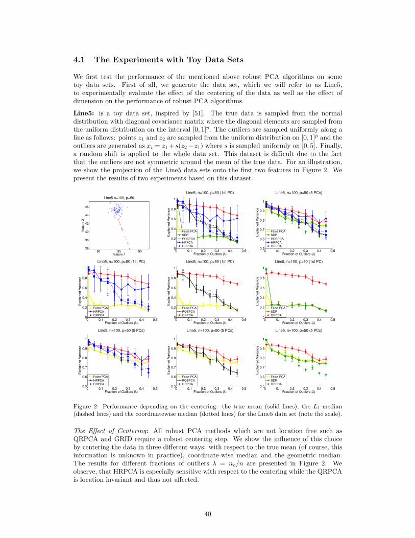
4.1 The Experiments with Toy Data Sets

We first test the performance of the mentioned above robust PCA algorithms on sometoy data sets. First of all, we generate the data set, which we will refer to as Line5,to experimentally evaluate the effect of the centering of the data as well as the effect ofdimension on the performance of robust PCA algorithms.

Line5: is a toy data set, inspired by [51]. The true data is sampled from the normaldistribution with diagonal covariance matrix where the diagonal elements are sampled fromthe uniform distribution on the interval [0, 1]p. The outliers are sampled uniformly along aline as follows: points z1 and z2 are sampled from the uniform distribution on [0, 1]p and theoutliers are generated as xi = z1 +s(z2−z1) where s is sampled uniformly on [0, 5]. Finally,a random shift is applied to the whole data set. This dataset is difficult due to the factthat the outliers are not symmetric around the mean of the true data. For an illustration,we show the projection of the Line5 data sets onto the first two features in Figure 2. Wepresent the results of two experiments based on this dataset.

80 85 9036

38

40

42

44

46

feature 1

featu

re 2

Line5 n=100, p=50

0 0.1 0.2 0.3 0.4 0.50

0.2

0.4

0.6

0.8

1

Fraction of Outliers (λ)

Expla

ined V

ariance

Line5, n=100, p=50 (1st PC)

False PCA

SDP

ROBPCA

HRPCA

QRPCA

0 0.1 0.2 0.3 0.4 0.50.5

0.6

0.7

0.8

0.9

1

Fraction of Outliers (λ)E

xpla

ined V

ariance

Line5, n=100, p=50 (5 PCs)

False PCA

SDP

ROBPCA

HRPCA

QRPCA

0 0.1 0.2 0.3 0.4 0.50

0.2

0.4

0.6

0.8

1

Fraction of Outliers (λ)

Expla

ined V

ariance

Line5, n=100, p=50 (1st PC)

False PCA

HRPCA

QRPCA

0 0.1 0.2 0.3 0.4 0.50

0.2

0.4

0.6

0.8

1

Fraction of Outliers (λ)

Expla

ined V

ariance

Line5, n=100, p=50 (1st PC)

False PCA

ROBPCA

QRPCA

0 0.1 0.2 0.3 0.4 0.50

0.2

0.4

0.6

0.8

1

Fraction of Outliers (λ)

Expla

ined V

ariance

Line5, n=100, p=50 (1st PC)

False PCA

SDP

QRPCA

0 0.1 0.2 0.3 0.4 0.50.5

0.6

0.7

0.8

0.9

1

Fraction of Outliers (λ)

Expla

ined V

ariance

Line5, n=100, p=50 (5 PCs)

False PCA

HRPCA

QRPCA

0 0.1 0.2 0.3 0.4 0.50.5

0.6

0.7

0.8

0.9

1

Fraction of Outliers (λ)

Expla

ined V

ariance

Line5, n=100, p=50 (5 PCs)

False PCA

ROBPCA

QRPCA

0 0.1 0.2 0.3 0.4 0.50.5

0.6

0.7

0.8

0.9

1

Fraction of Outliers (λ)

Expla

ined V

ariance

Line5, n=100, p=50 (5 PCs)

False PCA

SDP

QRPCA

Figure 2: Performance depending on the centering: the true mean (solid lines), the L1-median(dashed lines) and the coordinatewise median (dotted lines) for the Line5 data set (note the scale).

The Effect of Centering: All robust PCA methods which are not location free such asQRPCA and GRID require a robust centering step. We show the influence of this choiceby centering the data in three different ways: with respect to the true mean (of course, thisinformation is unknown in practice), coordinate-wise median and the geometric median.The results for different fractions of outliers λ = no/n are presented in Figure 2. Weobserve, that HRPCA is especially sensitive with respect to the centering while the QRPCAis location invariant and thus not affected.

40

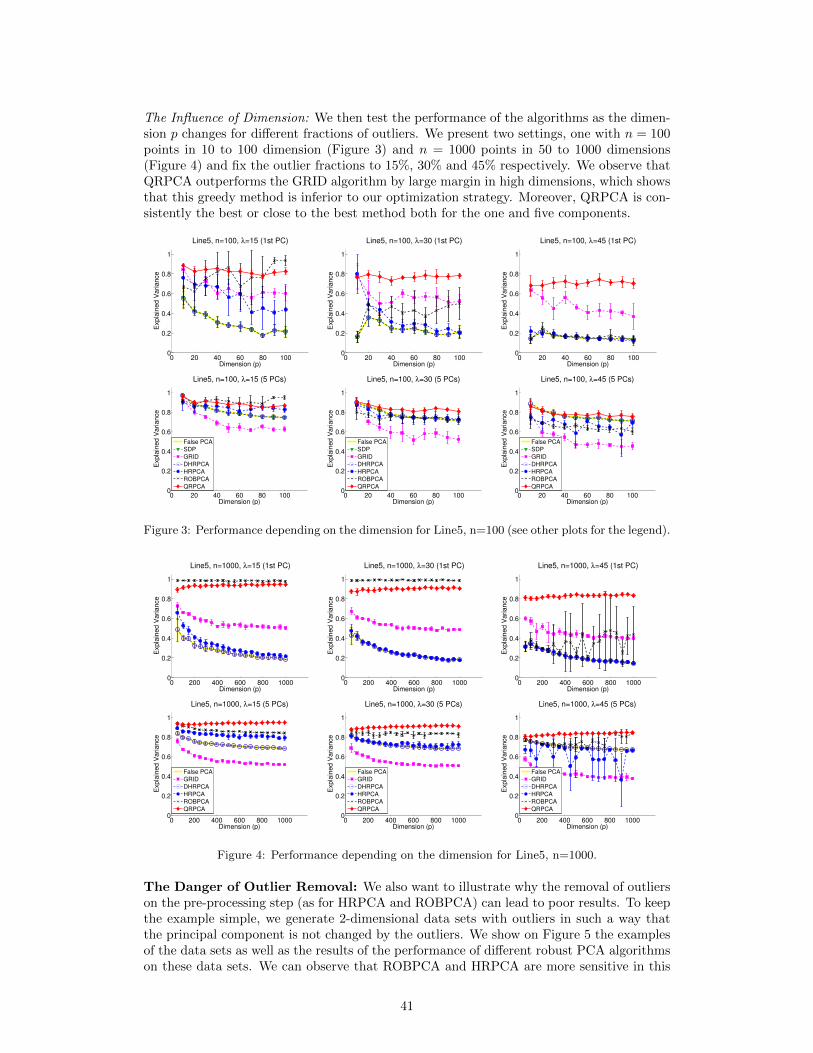
The Influence of Dimension: We then test the performance of the algorithms as the dimen-sion p changes for different fractions of outliers. We present two settings, one with n = 100points in 10 to 100 dimension (Figure 3) and n = 1000 points in 50 to 1000 dimensions(Figure 4) and fix the outlier fractions to 15%, 30% and 45% respectively. We observe thatQRPCA outperforms the GRID algorithm by large margin in high dimensions, which showsthat this greedy method is inferior to our optimization strategy. Moreover, QRPCA is con-sistently the best or close to the best method both for the one and five components.

0 20 40 60 80 1000

0.2

0.4

0.6

0.8

1

Dimension (p)

Exp

lain

ed

Va

ria

nce

Line5, n=100, λ=15 (1st PC)

0 20 40 60 80 1000

0.2

0.4

0.6

0.8

1

Dimension (p)

Exp

lain

ed

Va

ria

nce

Line5, n=100, λ=30 (1st PC)

0 20 40 60 80 1000

0.2

0.4

0.6

0.8

1

Dimension (p)

Exp

lain

ed

Va

ria

nce

Line5, n=100, λ=45 (1st PC)

0 20 40 60 80 1000

0.2

0.4

0.6

0.8

1

Dimension (p)

Exp

lain

ed

Va

ria

nce

Line5, n=100, λ=15 (5 PCs)

False PCA

SDP

GRID

DHRPCA

HRPCA

ROBPCA

QRPCA

0 20 40 60 80 1000

0.2

0.4

0.6

0.8

1

Dimension (p)

Exp

lain

ed

Va

ria

nce

Line5, n=100, λ=30 (5 PCs)

False PCA

SDP

GRID

DHRPCA

HRPCA

ROBPCA

QRPCA

0 20 40 60 80 1000

0.2

0.4

0.6

0.8

1

Dimension (p)E

xp

lain

ed

Va

ria

nce

Line5, n=100, λ=45 (5 PCs)

False PCA

SDP

GRID

DHRPCA

HRPCA

ROBPCA

QRPCA

Figure 3: Performance depending on the dimension for Line5, n=100 (see other plots for the legend).

0 200 400 600 800 10000

0.2

0.4

0.6

0.8

1

Dimension (p)

Exp

lain

ed

Va

ria

nce

Line5, n=1000, λ=15 (1st PC)

0 200 400 600 800 10000

0.2

0.4

0.6

0.8

1

Dimension (p)

Exp

lain

ed

Va

ria

nce

Line5, n=1000, λ=30 (1st PC)

0 200 400 600 800 10000

0.2

0.4

0.6

0.8

1

Dimension (p)

Exp

lain

ed

Va

ria

nce

Line5, n=1000, λ=45 (1st PC)

0 200 400 600 800 10000

0.2

0.4

0.6

0.8

1

Dimension (p)

Exp

lain

ed

Va

ria

nce

Line5, n=1000, λ=15 (5 PCs)

False PCA

GRID

DHRPCA

HRPCA

ROBPCA

QRPCA

0 200 400 600 800 10000

0.2

0.4

0.6

0.8

1

Dimension (p)

Exp

lain

ed

Va

ria

nce

Line5, n=1000, λ=30 (5 PCs)

False PCA

GRID

DHRPCA

HRPCA

ROBPCA

QRPCA

0 200 400 600 800 10000

0.2

0.4

0.6

0.8

1

Dimension (p)

Exp

lain

ed

Va

ria

nce

Line5, n=1000, λ=45 (5 PCs)

False PCA

GRID

DHRPCA

HRPCA

ROBPCA

QRPCA

Figure 4: Performance depending on the dimension for Line5, n=1000.

The Danger of Outlier Removal: We also want to illustrate why the removal of outlierson the pre-processing step (as for HRPCA and ROBPCA) can lead to poor results. To keepthe example simple, we generate 2-dimensional data sets with outliers in such a way thatthe principal component is not changed by the outliers. We show on Figure 5 the examplesof the data sets as well as the results of the performance of different robust PCA algorithmson these data sets. We can observe that ROBPCA and HRPCA are more sensitive in this

41

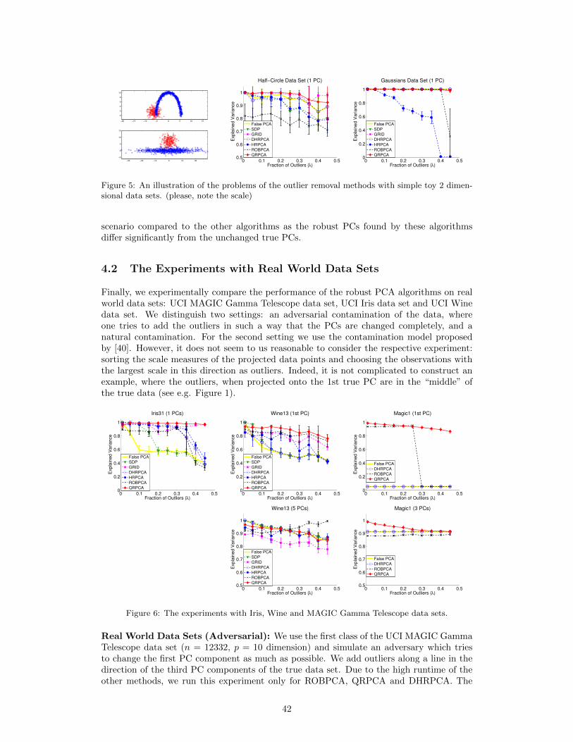
−20 −15 −10 −5 0 5 10 15

0

2

4

6

8

10

−30 −20 −10 0 10 20

−5

0

5

10

15

0 0.1 0.2 0.3 0.4 0.50.5

0.6

0.7

0.8

0.9

1

Fraction of Outliers (λ)

Expla

ined V

ariance

Half−Circle Data Set (1 PC)

False PCA

SDP

GRID

DHRPCA

HRPCA

ROBPCA

QRPCA

0 0.1 0.2 0.3 0.4 0.50

0.2

0.4

0.6

0.8

1

Fraction of Outliers (λ)

Expla

ined V

ariance

Gaussians Data Set (1 PC)

False PCA

SDP

GRID

DHRPCA

HRPCA

ROBPCA

QRPCA

Figure 5: An illustration of the problems of the outlier removal methods with simple toy 2 dimen-sional data sets. (please, note the scale)

scenario compared to the other algorithms as the robust PCs found by these algorithmsdiffer significantly from the unchanged true PCs.

4.2 The Experiments with Real World Data Sets

Finally, we experimentally compare the performance of the robust PCA algorithms on realworld data sets: UCI MAGIC Gamma Telescope data set, UCI Iris data set and UCI Winedata set. We distinguish two settings: an adversarial contamination of the data, whereone tries to add the outliers in such a way that the PCs are changed completely, and anatural contamination. For the second setting we use the contamination model proposedby [40]. However, it does not seem to us reasonable to consider the respective experiment:sorting the scale measures of the projected data points and choosing the observations withthe largest scale in this direction as outliers. Indeed, it is not complicated to construct anexample, where the outliers, when projected onto the 1st true PC are in the “middle” ofthe true data (see e.g. Figure 1).

0 0.1 0.2 0.3 0.4 0.50

0.2

0.4

0.6

0.8

1

Fraction of Outliers (λ)

Expla

ined V

ariance

Iris31 (1 PCs)

False PCA

SDP

GRID

DHRPCA

HRPCA

ROBPCA

QRPCA

0 0.1 0.2 0.3 0.4 0.50

0.2

0.4

0.6

0.8

1

Fraction of Outliers (λ)

Expla

ined V

ariance

Wine13 (1st PC)

False PCA

SDP

GRID

DHRPCA

HRPCA

ROBPCA

QRPCA

0 0.1 0.2 0.3 0.4 0.50

0.2

0.4

0.6

0.8

1

Fraction of Outliers (λ)

Expla

ined V

ariance

Magic1 (1st PC)

False PCA

DHRPCA

ROBPCA

QRPCA

0 0.1 0.2 0.3 0.4 0.50.5

0.6

0.7

0.8

0.9

1

Fraction of Outliers (λ)

Expla

ined V

ariance

Wine13 (5 PCs)

False PCA

SDP

GRID

DHRPCA

HRPCA

ROBPCA

QRPCA

0 0.1 0.2 0.3 0.4 0.50.5

0.6

0.7

0.8

0.9

1

Fraction of Outliers (λ)

Expla

ined V

ariance

Magic1 (3 PCs)

False PCA

DHRPCA

ROBPCA

QRPCA

Figure 6: The experiments with Iris, Wine and MAGIC Gamma Telescope data sets.

Real World Data Sets (Adversarial): We use the first class of the UCI MAGIC GammaTelescope data set (n = 12332, p = 10 dimension) and simulate an adversary which triesto change the first PC component as much as possible. We add outliers along a line in thedirection of the third PC components of the true data set. Due to the high runtime of theother methods, we run this experiment only for ROBPCA, QRPCA and DHRPCA. The

42

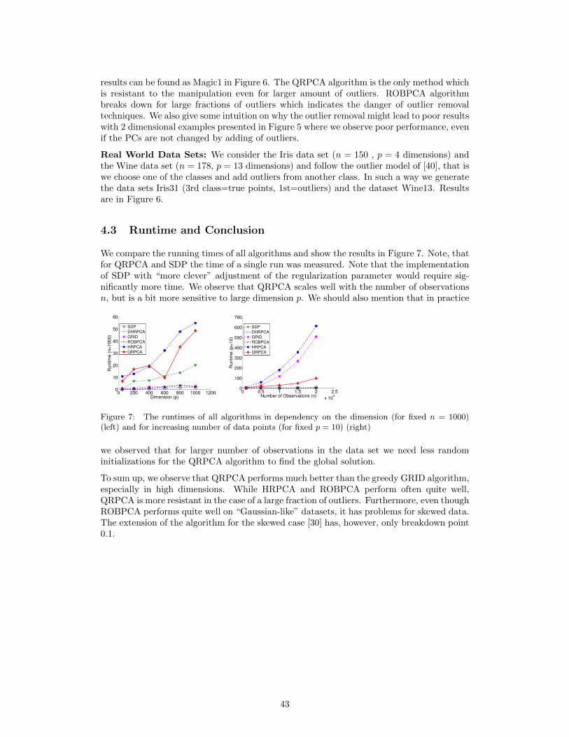
results can be found as Magic1 in Figure 6. The QRPCA algorithm is the only method whichis resistant to the manipulation even for larger amount of outliers. ROBPCA algorithmbreaks down for large fractions of outliers which indicates the danger of outlier removaltechniques. We also give some intuition on why the outlier removal might lead to poor resultswith 2 dimensional examples presented in Figure 5 where we observe poor performance, evenif the PCs are not changed by adding of outliers.

Real World Data Sets: We consider the Iris data set (n = 150 , p = 4 dimensions) andthe Wine data set (n = 178, p = 13 dimensions) and follow the outlier model of [40], that iswe choose one of the classes and add outliers from another class. In such a way we generatethe data sets Iris31 (3rd class=true points, 1st=outliers) and the dataset Wine13. Resultsare in Figure 6.

4.3 Runtime and Conclusion

We compare the running times of all algorithms and show the results in Figure 7. Note, thatfor QRPCA and SDP the time of a single run was measured. Note that the implementationof SDP with “more clever” adjustment of the regularization parameter would require sig-nificantly more time. We observe that QRPCA scales well with the number of observationsn, but is a bit more sensitive to large dimension p. We should also mention that in practice

0 200 400 600 800 1000 12000

10

20

30

40

50

60

Dimension (p)

Ru

ntim

e (

n=

10

00

)

SDP

DHRPCA

GRID

ROBPCA

HRPCA

QRPCA

0 0.5 1 1.5 2 2.5

x 104

0

100

200

300

400

500

600

700

Number of Observations (n)

Runtim

e (

p=

10)

SDP

DHRPCA

GRID

ROBPCA

HRPCA

QRPCA

Figure 7: The runtimes of all algorithms in dependency on the dimension (for fixed n = 1000)(left) and for increasing number of data points (for fixed p = 10) (right)

we observed that for larger number of observations in the data set we need less randominitializations for the QRPCA algorithm to find the global solution.

To sum up, we observe that QRPCA performs much better than the greedy GRID algorithm,especially in high dimensions. While HRPCA and ROBPCA perform often quite well,QRPCA is more resistant in the case of a large fraction of outliers. Furthermore, even thoughROBPCA performs quite well on “Gaussian-like” datasets, it has problems for skewed data.The extension of the algorithm for the skewed case [30] has, however, only breakdown point0.1.

43

5 Critical Discussion and Conclusion

In this thesis we presented the new computationally tractable algorithm – QRPCA – forprojection-pursuit robust PCA with the quartile difference measure. Our optimization ap-proach is better in terms of obtained objective than the current state-of-the-art algorithmfor projection-pursuit robust PCA – the GRID algorithm of [8]. The QRPCA algorithmenjoys such good properties as location invariance and the highest possible 0.5 breakdownpoint. We have seen in the experimental section 4 the promising results of the performanceof the new algorithm.

We have also tried to extend the optimization approach used in QRPCA to different estima-tors of scale, in particular, to the median absolute deviation MD estimator. Moreover, onecan also use this optimization approach to maximize the trimmed variance estimator9, thatis V (u) = 1

t

∑t<ni=1 〈xri , u〉

2(i), where 〈xr1 , u〉

2(1) ≤ . . . ≤ 〈xrn , u〉

2(n) and t ≥ bn/2c is a lower

bound on the number of true points in a sample. Note, that the trimmed variance estimatoris basically the same as the robust variance estimator defined in [51]. This implies that forthe future work one can think of extending the optimization technique used in the QRPCAalgorithm to other estimators of scale. This would extend the modeling freedom and onecould think about analyzing the performance of projection-pursuit robust PCA algorithmsbased on different scale estimators.

We have seen that robust PCA based on both outlier detection/removal techniques and thematrix factorization approach have some problems in practice. However, projection-pursuitrobust PCA is also not a perfect approach. Let us have a look at a particular example of thetrimmed variance as the robust scale estimator which gives us the following problem

w1 = arg max‖u‖2=1

t<n∑i=1

⟨x(ri), u

⟩2(i), (40)

where t ≥ bn/2c is again a lower bound on the number of true points in a sample. Now, letus recall the first formulation of PCA from Section 1.1 as the minimization of reconstructionerror which is equivalent to the maximization of the variance. When we trim the largestcomponents from the variance it seems to be natural to also trim the largest components fromthe reconstruction error. This gives us an equivalent of the minimization of reconstructionerror in this robust case which reads as follows

u1 = arg min‖u‖2=1

t<n∑i=1

∥∥⟨x(ri), u⟩u− x(ri)

∥∥2

(i). (41)

In general, the problems (40) and (41) are not equivalent. In this sense, the equivalence ofthe minimization of the reconstruction error and the maximization of a scale estimator, asopposed to standard PCA, does not hold in general in the robust setting. This, in particular,can be seen as a motivation for the construction of the new models for robust PCA.

To sum up, in this thesis we presented a new algorithm QRPCA for projection-pursuitrobust PCA based on a new scale estimator – the quartile difference measure. The newalgorithm QRPCA have shown improvement in terms of objective compared to the currentstate-of-the-art projection-pursuit robust PCA algorithm – the GRID algorithm [8]. TheQRPCA algorithm showed also good results when compared with other state-of-the-artalgorithms for robust PCA, in particular, the QRPCA algorithm often outperforms otheralgorithms when the fraction of outliers in data is large. However, we have seen that thereis no universally good robust PCA algorithm and one might be interested in constructingfurther models (as well as performance measures) for robust PCA.

9The respective algorithm is beyond consideration of this thesis.

45

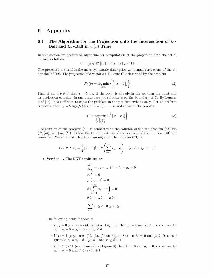
6 Appendix

6.1 The Algorithm for the Projection onto the Intersection of L1-Ball and L∞-Ball in O(n) Time

In this section we present an algorithm for computation of the projection onto the set Cdefined as follows

C =x ∈ Rn

∣∣‖x‖1 ≤ α, ‖x‖∞ ≤ 1

The presented material is the more systematic description with small corrections of the al-gorithm of [12]. The projection of a vector b ∈ Rn onto C is described by the problem

PC(b) = arg minx∈C

1

2‖x− b‖22

(42)

First of all, if b ∈ C then x = b, i.e. if the point is already in the set then the point andits projection coinside. In any other case the solution is on the boundary of C. By Lemma3 of [15], it is sufficient to solve the problem in the positive orthant only. Let us performtransformation vi = bisign(bi) for all i = 1, 2, . . . , n and consider the problem

x∗ = arg min‖x‖1≤α0≤xi≤1

1

2‖x− v‖22

(43)

The solution of the problem (42) is connected to the solution of the the problem (43) via(PC(b))i = x∗i sign(bi). Below the two derivations of the solution of the problem (43) arepresented. We note first, that the Lagrangian of the problem (43) is

L(x, θ, λ, µ) =1

2‖x− v‖22 + θ

(n∑i=1

xi − α

)− 〈λ, x〉+ 〈µ, x− 1〉

• Version 1. The KKT conditions are

∂L

∂xi= xi − vi + θ − λi + µi = 0

xiλi = 0

µi(xi − 1) = 0

θ

(n∑i=1

xi − α

)= 0

θ ≥ 0, λ ≥ 0, µ ≥ 0n∑i=1

xi ≤ α, 0 ≤ xi ≤ 1

The following holds for each i:

– if xi = 0 (e.g., cases (4) or (5) on Figure 8) then µi = 0 and λi ≥ 0, consequently,xi = vi − θ + λi = 0 and vi ≤ θ

– if xi = 1 (e.g., cases (1), (3), (5) on Figure 8) then λi = 0 and µi ≥ 0, conse-quently, xi = vi − θ − µi = 1 and vi ≥ θ + 1

– if 0 < xi < 1 (e.g., case (2) on Figure 8) then λi = 0 and µi = 0, consequently,xi = vi − θ and θ < vi < θ + 1

47

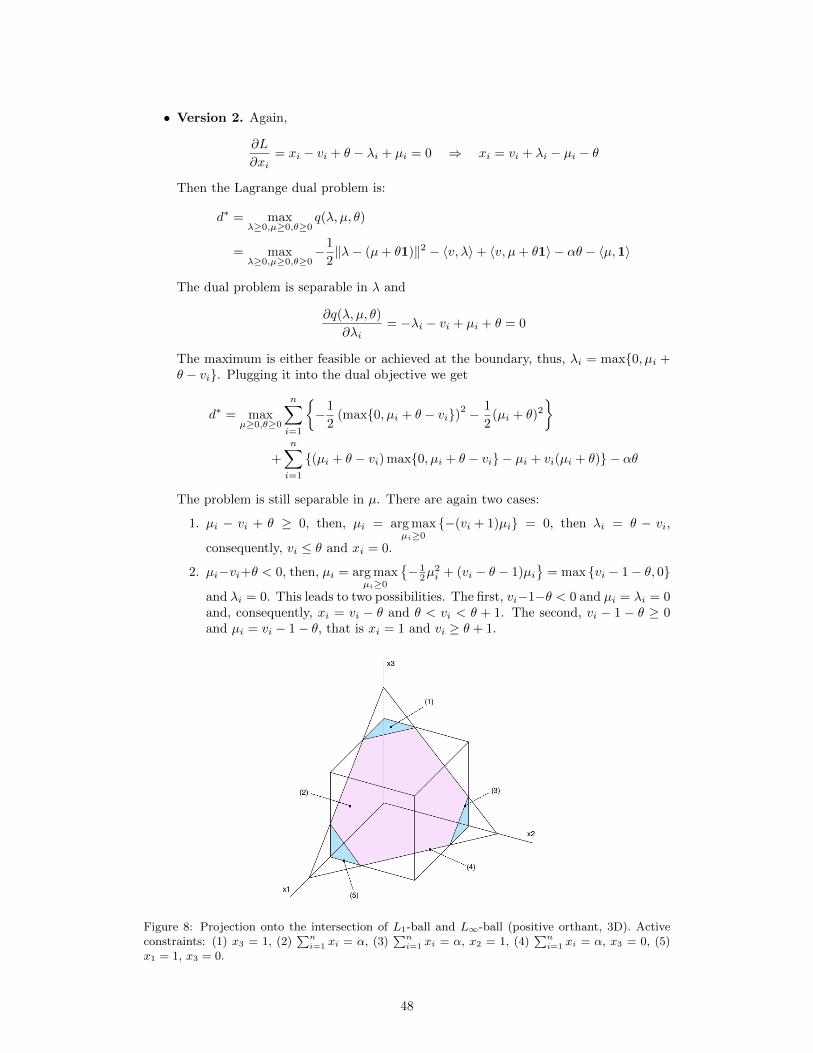
• Version 2. Again,

∂L

∂xi= xi − vi + θ − λi + µi = 0 ⇒ xi = vi + λi − µi − θ

Then the Lagrange dual problem is:

d∗ = maxλ≥0,µ≥0,θ≥0

q(λ, µ, θ)

= maxλ≥0,µ≥0,θ≥0

−1

2‖λ− (µ+ θ1)‖2 − 〈v, λ〉+ 〈v, µ+ θ1〉 − αθ − 〈µ,1〉

The dual problem is separable in λ and

∂q(λ, µ, θ)

∂λi= −λi − vi + µi + θ = 0

The maximum is either feasible or achieved at the boundary, thus, λi = max0, µi +θ − vi. Plugging it into the dual objective we get

d∗ = maxµ≥0,θ≥0

n∑i=1

−1

2(max0, µi + θ − vi)2 − 1

2(µi + θ)2

+

n∑i=1

(µi + θ − vi) max0, µi + θ − vi − µi + vi(µi + θ) − αθ

The problem is still separable in µ. There are again two cases:

1. µi − vi + θ ≥ 0, then, µi = arg maxµi≥0

−(vi + 1)µi = 0, then λi = θ − vi,

consequently, vi ≤ θ and xi = 0.

2. µi−vi+θ < 0, then, µi = arg maxµi≥0

− 1

2µ2i + (vi − θ − 1)µi

= max vi − 1− θ, 0

and λi = 0. This leads to two possibilities. The first, vi−1−θ < 0 and µi = λi = 0and, consequently, xi = vi − θ and θ < vi < θ + 1. The second, vi − 1 − θ ≥ 0and µi = vi − 1− θ, that is xi = 1 and vi ≥ θ + 1.

Figure 8: Projection onto the intersection of L1-ball and L∞-ball (positive orthant, 3D). Activeconstraints: (1) x3 = 1, (2)

∑ni=1 xi = α, (3)

∑ni=1 xi = α, x2 = 1, (4)

∑ni=1 xi = α, x3 = 0, (5)

x1 = 1, x3 = 0.

48

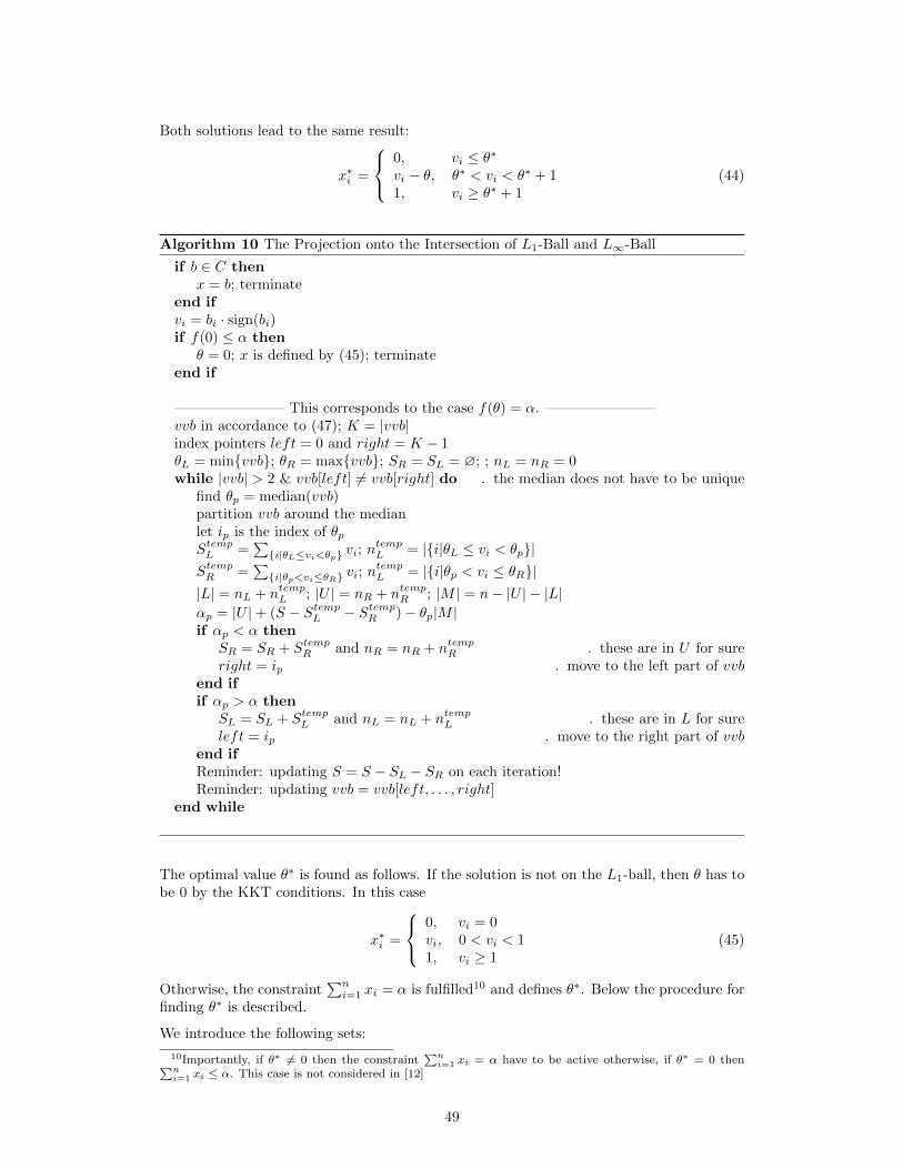
Both solutions lead to the same result:

x∗i =

0, vi ≤ θ∗vi − θ, θ∗ < vi < θ∗ + 11, vi ≥ θ∗ + 1

(44)

Algorithm 10 The Projection onto the Intersection of L1-Ball and L∞-Ball

if b ∈ C thenx = b; terminate

end ifvi = bi · sign(bi)if f(0) ≤ α then

θ = 0; x is defined by (45); terminateend if

———————– This corresponds to the case f(θ) = α. ———————–vvb in accordance to (47); K = |vvb|index pointers left = 0 and right = K − 1θL = minvvb; θR = maxvvb; SR = SL = ∅; ; nL = nR = 0while |vvb| > 2 & vvb[left] 6= vvb[right] do . the median does not have to be unique

find θp = median(vvb)partition vvb around the medianlet ip is the index of θpStempL =

∑i|θL≤vi<θp vi; n

tempL = |i|θL ≤ vi < θp|

StempR =∑i|θp<vi≤θR vi; n

tempL = |i|θp < vi ≤ θR|

|L| = nL + ntempL ; |U | = nR + ntempR ; |M | = n− |U | − |L|αp = |U |+ (S − StempL − StempR )− θp|M |if αp < α then

SR = SR + StempR and nR = nR + ntempR . these are in U for sureright = ip . move to the left part of vvb

end ifif αp > α then

SL = SL + StempL and nL = nL + ntempL . these are in L for sureleft = ip . move to the right part of vvb

end ifReminder: updating S = S − SL − SR on each iteration!Reminder: updating vvb = vvb[left, . . . , right]

end while

The optimal value θ∗ is found as follows. If the solution is not on the L1-ball, then θ has tobe 0 by the KKT conditions. In this case

x∗i =

0, vi = 0vi, 0 < vi < 11, vi ≥ 1

(45)

Otherwise, the constraint∑ni=1 xi = α is fulfilled10 and defines θ∗. Below the procedure for

finding θ∗ is described.

We introduce the following sets:

10Importantly, if θ∗ 6= 0 then the constraint∑n

i=1 xi = α have to be active otherwise, if θ∗ = 0 then∑ni=1 xi ≤ α. This case is not considered in [12]

49

• L =i ∈ 1, 2, . . . , n

∣∣ vi ≤ θ, which corresponds to the indices of the elements ofthe optimal vector x∗i such that x∗i = 0;

• M =i ∈ 1, 2, . . . , n

∣∣ θ < vi < θ + 1

, which corresponds to such indices that 0 <x∗i < 1;

• U =i ∈ 1, 2, . . . , n

∣∣ vi ≥ θ + 1

, which corresponds to such indices that x∗i = 1.

Thus, using the notation | · | for the cardinality of a set, we introduce a function

f(θ) =

n∑i=1

xi = |U | − θ|M |+∑i∈M

vi = α

where for the last equality we used that the constraint∑ni=1 xi = α is active. This leads to

the equation for the calculation of θ in case the sets L, M and U are known

θ =

(|U |+

∑i∈M

vi − α

)/|M | (46)

The function f(θ) has discontinuity points vi, vi − 1 for all i = 1, 2, . . . , n. We notice thatf(θ) is monotonically decreasing in θ as every increase of θ either does not change xi ordecrease it (recall, that f(θ) =

∑ni=1 xi). Thus, one easily gets O(n log n) algorithm for the

projection: (1) sort all of the discontinuity points θi for all i = 1, 2, . . . ,m with m ≤ 2n ofthe function f(θ) in nondecreasing order; (2) go over each of this points in the given orderand calculate f(θi) until the sets L, M and U are found; (3) calculate θ∗ with the formula(46).

The linear time algorithm for the projection requires the linear time algorithm for findinga (lower-)median xm of the points x1, . . . , xn and partitioning the points into the followingthree sets xi | xi < xm, xi | xi = xm and xi | xi > xm (e.g. [7]). Such procedure,in particular, is summarized in algorithm 10, where the following notation is used. Theset

vvb = vj | vj ∈ vini=1 ∪ vi − 1ni=1 and vj > 0 (47)

denotes all the positive11 discontinuity points of the function f . Moreover, θL, θR definesuch interval that θ∗ ∈ [θL, θR] for sure; SL is the sum and nL is the number of elementsthat are in L for sure; SR and nR – the same for U .

In figure 8, an example of the set C for the 3 dimensional case is presented. For more intuitionon the problem, in the comments the examples of the points with the corresponding activeconstraints are shown.

6.2 Derivation of the Lipschitz Constant for FISTA

In this section we derive the Lipschitz constant L for the function ∇f(x) = AT (Ax + b),where L is defined through ‖∇f(x1)−∇f(x2)‖2 ≤ L ‖x1 − x2‖2. Substituting the definitionof the function ∇f(x) into the inequality, we get

L ≥∥∥ATA(x1 − x2)

∥∥2

‖x1 − x2‖2=

(〈x1 − x2, A

TAATA(x1 − x2)〉‖x1 − x2‖22

)1/2

On the other hand, by the Courant-Fisher Min-Max principle,

〈x1 − x2, ATAATA(x1 − x2)〉‖x1 − x2‖22

≤ λmax(ATAATA

)11Note, that the case θ = 0 is considered separately and by dual feasibility θ ≥ 0, i.e. we are not interested

in the non-positive discontinuity points.

50

with the equality achieved in the case when the vector x1 − x2 is equal to the maximaleigenvector of the matrix ATAATA. This immediately leads to the expression for L

L ≥(λmax

(ATAATA

))1/2= λmax

(ATA

)where we used that λmax

(B2)

= λ2max (B) for any square symmetric matrix B.

6.3 Matrix Norms

For matrices A,B ∈ Rn×m the operator norm ‖A‖p,q and its dual ‖B‖∗p,q are

‖A‖p,q = sup‖u‖p=1‖Au‖q and ‖B‖∗p,q = sup‖A‖p,q=1〈B,A〉

where the scalar product 〈B,A〉 =∑ni=1

∑mj=1 aijbij = trace(ATB) = trace(AB)trace(BA) =

trace(BTA). We consider the following matrix/operator norms:

• ‖A‖2,2 = σmax(A), where σmax(A) is the maximum singular value of A

Proof: A = UΣV T and ‖Au‖22 = 〈UΣV Tu, UΣV Tu〉 = 〈V Tu,ΣTUTUΣV Tu〉 =〈z,ΣTΣz〉, where z = V Tu. Clearly, ‖z‖22 = 〈V Tu, V Tu〉 = 〈u, V V Tu〉 = ‖u‖22 = 1.Moreover, 〈z,ΣTΣz〉 =

∑mi=1

∑mj=1(ΣTΣ)ijzizj =

∑mi=1 Σ2

iiz2i =

∑mi=1 σi(A)2z2

i ≤σ2max(A)‖z‖22 = σ2

max(A). Consequently, ‖Au‖2 ≤ σmax(A) if ‖u‖ = 1. This upperbound is achieved by choosing such vector u that the vector z has zi∗ = 1 and zi = 0,∀i 6= i∗, where i∗ = arg max

i=1,...,mσi(A).

• ‖B‖∗2,2 =∑mi=1 σi(B) = ‖B‖∗ is the sum of the singular values and also known as the

nuclear norm

Proof: can be found, e.g., in [24], p. 440.

• ‖A‖2,∞ = maxi=1,...,n

‖ai‖2, where ai is the ith row of A

Proof: by the Cauch-Schwarz inequality |〈ai, u〉|2 ≤ ‖ai‖22‖u‖22 = ‖ai‖22 if ‖u‖2 = 1.Thus, ‖Au‖21 = max

i=1,...,n〈ai, u〉2 ≤ max

i=1,...,n‖ai‖22. The equality is achieved by choosing

the vector u = ai∗/‖ai∗‖2, where i∗ = arg maxi=1,...,n

‖ai‖2.

• ‖B‖∗2,∞ =∑ni=1 ‖bi‖2 = ‖B‖1,2 is the sum of L2-norms of the rows of B

Proof: 〈B,A〉 = trace(BAT ) =∑ni=1〈bi, ai〉 ≤

∑ni=1 ‖bi‖2‖ai‖2 ≤ ‖ai∗‖2

∑ni=1 ‖bi‖2 =∑n

i=1 ‖bi‖2 as ‖A‖2,∞ = ‖ai∗‖2 = 1, where again i∗ = arg maxi=1,...,n

‖ai‖2. The equality is

achieved by choosing A with all rows ai equal to each other and with ‖ai‖2 = 1.

• ‖X‖22→1 = ‖XXT ‖∞→1 = max‖y‖∞=1

yTXXT y = maxZ=yyT

Zii=1,∀i

trace(XXTZ) see [40]

• ‖A‖F =√∑m

i=1 σ2i (A) is the Frobenius norm

• ‖A‖1 =∑i,j |aij |

51

References

[1] A. Beck and M. Teboulle. Fast gradient-based algorithms for constrained total variationimage denoising and deblurring problems. IEEE Trans. Image Processing, 18(11):2419–2434, 2009.

[2] C. M. Bishop. Pattern Recognition and Machine Learning. Springer, 2006.

[3] S. Boyd and L. Vandenberghe. Convex Optimization. Cambridge University Press,2004.

[4] E.J. Candes, X. Li, Y. Ma, and J. Wright. Robust principal component analysis?JACM, 58(3), 2011.

[5] V. Chandrasekaran, S. Sanghavi, P.A. Parrilo, and A.S. Willsky. Rank-sparsity inco-herence for matrix decomposition. SIAM J. Opt., 21(2):572–596, 2011.

[6] V. Choulakian. `1-norm projection pursuit principal component analysis. Comput.Stat. Data Anal., 50(6):1441–1451, 2006.

[7] T.H. Cormen, C.E. Leiserson, R.L. Rivest, and Stein C. Introduction to Algorithms.The MIT Press, 3rd edition, 2009.

[8] C. Croux, P. Pilzmoser, and M. R. Oliveira. Algorithms for projection–pursuit robustprincipal component analysis. Chemometr. Intell. Lab., 87:218–225, 2007.

[9] C. Croux and J. Rousseeuw. Time–efficient algorithms for two highly robust estimatorsof scale. Compu. Stat., 1:411–428, 1992.

[10] C. Croux and A. Ruiz-Gazen. High breakdown estimators for principal components:the projection–pursuit approach revisited. J. Multivar. Anal., 95:206–226, 2005.

[11] C. Croux and A. Ruiz-Gazen. High breakdown estimators for principal components:the projection–pursuit approach revisited. http://www.econ.kuleuven.be/public/

NDBAE06/programs/#pca, 2005.

[12] M. Das Gupta, S. Kumar, and J. Xiao. `1 projections with box constraints. CoRR,abs:1010.0141v1, 2010.

[13] C. Ding, D. Zhou, X. He, and H. Zha. R1-PCA: Rotational invariant `1-norm principalcomponent analysis for robust subspace factorization. In ICML, 2006.

[14] D. L. Donoho. Breakdown properties of multivariate location estimators. Qualifyingpaper, Department of Statistics, Harvard University, 1982.

[15] J. Duchi, S. Shalev-Shwartz, Y. Singer, and T. Chandra. Efficient projections onto the`1-ball for learning in high dimensions. In ICML, 2008.

[16] F. R. Hampel. The influence curve and its role in robust estimation. JASA, 69(346):383–393, 1974.

[17] F. R. Hampel, E. M. Ronchetti, P. J. Rousseeuw, and W. A. Stahel. Robust Statistics.The Approach Based on Influence Functions. John Wiley and Sons, 1986.

[18] P. Hartman. On functions representable as a difference of convex functions. Pacific J.Math., 9(3):707–713, 1959.

[19] T. Hastie, R. Tibshirani, and J. Friedman. The Elements of Statistical Learning.Springer, 2nd edition, 2009.

[20] M. Hein and T. Buhler. Eigenproblems with applications in 1-spectral clustering andsparse PCA. In NIPS, pages 847–855, 2010.

53

[21] M. Hein and S. Setzer. Beyond spectral clustering – tight relaxations of balanced graphcuts. In NIPS, pages 2366–2374, 2011.

[22] J.-B. Hiriart-Urruty and Lemarechal. Fundamentals of Convex Analysis. Springer,2001.

[23] J.-B. Hiriart-Urruty and C. Lemarechal. Convex Analysis and Minimization AlgorithmsII. Advanced Theory and Bundle Methods. Springer, 2nd edition, 1996.

[24] R.A. Horn and C.R. Johnson. Matrix Analysis. Cambridge University Press, 1990.

[25] O. Hossjer and C. Croux. Generalizing univariate signed rank statistics for testingand estimating a multivariate location parameter. http://www.econ.kuleuven.be/

public/NDBAE06/programs/pca/L1median.txt, 1995.

[26] P. J. Huber. Projection pursuit. Ann. Stat., 13(2):435–475, 1985.

[27] P.J. Huber and E.M. Ronchetti. Robust Statistics. John Wiley and Sons, 2nd edition,2009.

[28] M. Hubert, P. J. Rousseeuw, and S. Van Aelst. High-breakdown robust multivariatemethods. Statistical Science, 23(1):92–119, 2008.

[29] M. Hubert, P. J. Rousseeuw, and K. Vanden Branden. ROBPCA: a new approach torobust principal component analysis. Technometrics, 47(1):64–79, 2005.

[30] M. Hubert, P. J. Rousseeuw, and T. Verdonck. Robust PCA for skewed data and itsoutlier map. Comput. Stat. Data Anal., 53:2264–2274, 2009.

[31] Feng J., Xu H., and Yan S. Robust PCA in high-dimension: a deterministic approach.In ICML, 2012.

[32] D.B. Johnson and T. Mizoguchi. Selecting the Kth element in X + Y and X1 +X2 +· · ·+Xm. SIAM J. Comput., 7(2), 1978.

[33] I.T. Jolliffe. Principal Component Analysis. Springer, 2nd edition, 2002.

[34] K. Kiwiel. On Linear-Time algorithms for the continuous quadratic knapsack problem.J. Opt. Theory Appl., 134(3):549–554, 2007.

[35] N. Kwak. Principal component analysis based on `1-norm maximization. IEEE Trans.Pattern Anal. Mach. Intell., pages 1672–1680, 2008.

[36] G. Li and Z. Chen. Projection–pursuit approach to robust dispersion matrices andprincipal components: Primary theory and Monte Carlo. JASA, 80(391):759–766, 1985.

[37] H. P. Lopuhaa and P. J. Rousseeuw. Breakdown points of affine equivariant estimatorsof multivariate location and covariance matrices. Ann. Stat., 19(1):229–248, 1991.

[38] L. Mackey. Deflation methods for sparse PCA. In NIPS, pages 1017–1024, 2009.

[39] R. A. Maronna, R. D. Martin, and V. J. Yohai. Robust Statistics: Theory and Methods.John Wiley and Sons, 2006.

[40] M. McCoy and J. A. Tropp. Two proposals for robust PCA using semidefinite pro-gramming. Elec. J. Stat., 5:1123–1160, 2011.

[41] M. McCoy and J.A. Tropp. The lld algorithm. http://users.cms.caltech.edu/

~mccoy/code/.

[42] K. Pearson. On lines and planes of closest fit to systems of points in space. Philos.Mag., 2(6):559–572, 1901.

[43] R.T. Rockafellar. Convex Analysis. Princeton University Press, 1970.

54

[44] P. J. Rousseeuw. Least median of squares regression. JASA, 79(388):871–880, 1984.

[45] P. J. Rousseeuw and C. Croux. Alternatives to the median absolute deviation. JASA,88(424):1273–1283, 1993.

[46] B. Scholkopf and A. J. Smola. Learning with Kernels. Support Vector Machines, Reg-ularization, Optimization, and Beyond. The MIT Press, 2001.

[47] W. A. Stahel. Robust estimation: Infinitesimal optimality and covariance matrix esti-mators. PhD thesis, ETH, Zurich, 1981. In German.

[48] S. Verboven and M. Hubert. LIBRA: a MATLAB library for robust analysis. http:

//wis.kuleuven.be/stat/robust/LIBRA, 2005.

[49] H. Xu, C. Caramanis, and S. Mannor. The hrpca algorithm. http://guppy.mpe.nus.edu.sg/~mpexuh/code/HRPCA.zip.

[50] H. Xu, C. Caramanis, and S. Mannor. Principal component analysis with contaminateddata: The high dimensional case. In COLT, 2010.

[51] H. Xu, C. Caramanis, and S. Mannor. Outlier-robust PCA: the high dimensional case.IEEE Trans. Inf. Theory, 59(1):546–572, 2013.

[52] H. Xu, C. Caramanis, and S. Sanghavi. Robust PCA via outlier pursuit. IEEE Trans.Inf. Theory, 58(5):3047–3064, 2012.

55