econstor www.econstor.eu

Der Open-Access-Publikationsserver der ZBW – Leibniz-Informationszentrum WirtschaftThe Open Access Publication Server of the ZBW – Leibniz Information Centre for Economics

Standard-Nutzungsbedingungen:

Die Dokumente auf EconStor dürfen zu eigenen wissenschaftlichenZwecken und zum Privatgebrauch gespeichert und kopiert werden.

Sie dürfen die Dokumente nicht für öffentliche oder kommerzielleZwecke vervielfältigen, öffentlich ausstellen, öffentlich zugänglichmachen, vertreiben oder anderweitig nutzen.

Sofern die Verfasser die Dokumente unter Open-Content-Lizenzen(insbesondere CC-Lizenzen) zur Verfügung gestellt haben sollten,gelten abweichend von diesen Nutzungsbedingungen die in der dortgenannten Lizenz gewährten Nutzungsrechte.

Terms of use:

Documents in EconStor may be saved and copied for yourpersonal and scholarly purposes.

You are not to copy documents for public or commercialpurposes, to exhibit the documents publicly, to make thempublicly available on the internet, or to distribute or otherwiseuse the documents in public.

If the documents have been made available under an OpenContent Licence (especially Creative Commons Licences), youmay exercise further usage rights as specified in the indicatedlicence.

zbw Leibniz-Informationszentrum WirtschaftLeibniz Information Centre for Economics

Aichele, Rahel; Felbermayr, Gabriel J.; Heiland, Inga

Working Paper

Going Deep: The Trade and Welfare Effects of TTIP

CESifo Working Paper, No. 5150

Provided in Cooperation with:Ifo Institute – Leibniz Institute for Economic Research at the University ofMunich

Suggested Citation: Aichele, Rahel; Felbermayr, Gabriel J.; Heiland, Inga (2014) : Going Deep:The Trade and Welfare Effects of TTIP, CESifo Working Paper, No. 5150

This Version is available at:http://hdl.handle.net/10419/107325

Going Deep: The Trade and Welfare Effects of TTIP

Rahel Aichele Gabriel Felbermayr

Inga Heiland

CESIFO WORKING PAPER NO. 5150 CATEGORY 8: TRADE POLICY

DECEMBER 2014

An electronic version of the paper may be downloaded • from the SSRN website: www.SSRN.com • from the RePEc website: www.RePEc.org

• from the CESifo website: Twww.CESifo-group.org/wp T

CESifo Working Paper No. 5150

Going Deep: The Trade and Welfare Effects of TTIP

Abstract Since July 2013, the EU and the US have been negotiating a preferential trade agreement (PTA), the Transatlantic Trade and Investment Partnership (TTIP). We use a multi-country, multi-industry Ricardian trade model with national and international input-output linkages to quantify its potential economic consequences. We structurally estimate the sectoral trade flow elasticities of trade costs and of existing PTAs. We simulate the trade, value added, and welfare effects of the TTIP, assuming that the agreement would eliminate all transatlantic tariffs and reduce non-tariff barriers as other deep PTAs have. The long-run level of real per capita income would change by 2.12% in the EU, by 2.68% in the US, and by -0.03% in the rest of the world relative to the status quo. However, there is substantial heterogeneity across the 134 geographical entities that we investigate. Gross value of EU-US trade could triple, but its value added would grow by substantially less. Moreover, trade diversion effects are more pronounced in value added trade than in gross trade. This signals a deepening of the transatlantic value chain.

JEL-Code: F130, F140, F170.

Keywords: structural gravity, preferential trade agreements, TTIP.

Rahel Aichele Ifo Institute – Leibniz Institute for

Economic Research at the University of Munich

Poschingerstrasse 5 Germany – 81679 Munich

aichele@ifo.de Gabriel Felbermayr

Ifo Institute – Leibniz Institute for Economic Research

at the University of Munich Poschingerstrasse 5

Germany – 81679 Munich felbermayr@ifo.de

Inga Heiland Ifo Institute – Leibniz Institute for

Economic Research at the University of Munich

Poschingerstrasse 5 Germany – 81679 Munich

heiland@ifo.de We thank Lorenzo Caliendo, Peter Egger, Marc-Andreas Muendler, Mario Larch, and seminar participants in Lisbon, Munich, Rome, Venice, and Vienna for comments and suggestions. This paper provides the technical details for a report that the authors have prepared for the Bertelsmann foundation.

1 Motivation

In July 2013, the EU and the US have begun negotiations on a Transatlantic Trade and

Investment Partnership (TTIP). According to the High-Level Working Group (HLWG)

on Jobs and Growth, set up by the so called Transatlantic Economic Council (TEC),

the ambition is to eliminate all tariffs and to create “. . . a comprehensive, ambitious

agreement that addresses a broad range of bilateral trade and investment issues, including

regulatory issues, and contributes to the development of global rules” that “goes beyond

what the United States and the EU have achieved in previous trade agreements.” In this

paper, we attempt a quantification of the potential effects of this endeavor.

TTIP is the first big trade agreement that tries to fill the “gap between 21st century

trade and the 20th century trade rules” (Baldwin, 2011) that the relative stasis of the

World Trade Organization (WTO) has left developed countries in. Our analysis captures

the reality of international production networks and trade in intermediate inputs. It

focuses on non-tariff barriers besides tariffs, and it explores scenarios in which the systemic

importance of the TTIP also leads to trade cost reductions elsewhere, either through what

Francois et al. (2013) have called spillovers, or through the completion of the Doha Round.

And it does so by extending the recent quantitative trade models by Eaton and Kortum

(2002) and Caliendo and Parro (2014) to PTAs. Our framework covers 32 industries

from the services, manufacturing and agriculture sectors for 134 countries or regions.

It incorporates tariffs as well as non-tariff measures (NTMs). By allowing intra- and

international trade of intermediate inputs into this stochastic Ricardian model, it allows

to model international production networks and allows to differentiate the value added

content from the gross value of bilateral trade flows. In contrast to the conventional CGE

trade models, the key parameters – the Frechet parameter governing the distribution of

productivities within sectors, or the coefficients of the trade cost function – are estimated

using structural relationships strictly implied by the theoretical setup.

1

Using data on sectoral trade flows and input-output linkages from the Global Trade

Analysis Project (GTAP) and applying instrumental variables (IV) techniques to obtain

unbiased parameter estimates, the central assumption of the analysis is that the TTIP

between the EU and the USA will reduce trade costs by as much as other already existing

deep trade agreements have. The key results are that the TTIP will yield a long-run

increase in the level of real per capita income of 2.12% and 2.68% in the EU and the

US, respectively. It would only marginally lower average real income in the rest of the

world, leaving the world as a whole better off by about 1.32%. If it were combined with

the full elimination of tariffs within the group of WTO countries, almost all countries in

the world would win. Similarly, if trade cost reductions between the EU and the US also

improve the access of third countries to the TTIP partners or to each other, all could be

made better off.

We find that the TTIP would result in a significant amount of trade creation between

the insiders. For example, trade between Germany and the US, as measured at the

customs, could go up by more than 200%. At the same time, trade with the other

EU countries would fall by between 5 and 10%, reflecting trade diversion by preference

erosion. Similarly, trade with most third countries or regions would go down. However,

imports from suppliers of raw materials or intermediates can go up, reflecting the effect

of higher income and of increased industrial production in TTIP partners. Also, trade

diversion can be attenuated by imported competitiveness: when TTIP partners supply

intermediates at lower prices to third countries, changes in relative prices of final goods

are dampened. This latter effect, plus the restructuring of production chains explains

the interesting finding that the value added content of trade flows goes up, sometimes

substantially, in many trade relationships.

The introduction of a TTIP would alter the composition of aggregate value added. It

would lead to a slight reindustrialization in the TTIP partners, reflecting the fact that

the reduction in trade barriers is larger in manufacturing than in services. Moreover, the

2

model does not predict that the sectoral impact simply follows the structure of compar-

ative advantage as measured by the Balassa-Samuelson index. Again, this follows from

the fact that changes in the competitiveness of sectors is very much driven by changes in

the prices of intermediate goods, both domestic and imported.

The paper is related to three important strands of literature. First, it builds on re-

cent work on quantitative trade models. Costinot and Rodrıguez-Clare (2014) provide an

excellent survey. The central element in these models is the gravity equation, a parsimo-

nious relationship which allows to estimate parameters with the help of relatively simple

econometrics but which requires strong functional assumptions. In our case, the Frechet

distribution and CES demand systems. The great advantage of the gravity equation is

its excellent empirical fit. However, this does not imply that out-of-sample its fit will

be perfect as well. Nonetheless, the new “quantitative trade theory” offers important

advantages over the more conventional large-scale CGE approach. First, the parsimony

allows going relatively far with analytical descriptions. This feature reduces (but does not

undo) the black box nature of large general equilibrium models. Second, the approach

allows a tight link between theoretical structure and parameter estimation which allows

a neater calibration. Finally, by exploiting what we know from existing deep agreements,

one does not require bottom-up estimates of NTMs and one can let the data define the

TTIP scenario.

Second, our work builds on earlier quantitative evaluations of the TTIP. In a study for

the European Commission, Francois et al. (2013) employ a large scale CGE framework

based on the well-known GTAP model (Hertel, ed, 1997) and extended to include features

from the Francois et al. (2005) model. While their work is at the frontier of classical CGE

modeling, it does not utilize the breakthroughs described in Costinot and Rodrıguez-Clare

(2014). It requires bottom-up estimates of NTMs which are, however, only available for

a small set of bilateral trade links, and it defines the scenario on the basis of expert input

rather than data. Egger et al. (2014) use the same model, but they rely on a top-down,

3

gravity-based approach to NTMs. However, they do not derive the gravity equation from

the model and they seem to use ad hoc calibration to parameterize other model parameters

(such as trade elasticities). Moreover, these studies work with regional aggregates.

Felbermayr et al. (2013) and Felbermayr et al. (2014) apply the model and econometric

approach of Egger et al. (2011) to simulate the effects of a possible TTIP. The model

is a single-sector framework based on the Krugman (1980) model augmented with an

extensive margin to capture the prevalence of zero-trade flows. The approach features a

tight link between gravity estimation and model structure. However, it does not feature

sectoral detail nor does it allow addressing production networks. The work by Anderson

et al. (2014) sticks to the single-sector setup but endogenizes the capital stock in a fully

structural quantitative trade model. These models have the advantage of great tractability

and they can be understood as reduced-form approaches to more complicated setups.

Finally, the present paper relates to a large empirical literature on the determinants

and effects of PTAs. Much of the earlier work, as surveyed by Cipollina and Salvatici

(2010), is based on reduced form equations and does not properly deal with the poten-

tial endogeneity of trade agreements. More recent empirical studies provide a tight link

between theoretical model and estimation (see Head and Mayer, 2014), and devote much

attention to obtain the causal effects of PTAs on trade flows (see Egger et al., 2011, and

the discussion of literature therein). The critical step is to find exogenous drivers of PTA

formation. Controlling for tariffs, the estimated treatment effect of PTAs can be used to

quantify how PTAs have reduced the costs of non-tariff barriers to trade. Interestingly,

the literature suggests that OLS estimates tend to underestimate the true effects of PTAs

and that their effect on NTMs must be quite substantial. In our work we provide instru-

mental variables estimates for 32 sectors (including services) and we distinguish between

two types of PTA depth, borrowing a classification provided by Dur et al. (2014).

The remainder of this paper is structured as follows. Section 2 provides a quick

overview of the theoretical model. Section 3 discusses the data and the identification of

4

parameters. Section 4 provides the results of the simulation of counterfactual scenarios

pertaining to the TTIP. Finally, Section 5 summarizes and concludes.

2 Methodology

We briefly summarize the Eaton and Kortum (2002)-type multi-sector, input-output grav-

ity model developed by Caliendo and Parro (2014) used in our simulations. Their counter-

factual analysis deals with the elimination of tariffs between the NAFTA countries. The

TTIP will reduce NTMs along with tariffs. It will also provide a deep trade liberalization

and go beyond the trade liberalizing effect of many existing PTAs. So to better capture

these tariff and NTM trade cost reductions, we introduce PTAs of different depth into

the Caliendo and Parro (2014) framework. We characterize the equilibrium changes after

a trade policy shock to pave the path for our counterfactual analysis.

Compared to one sector models or models without input-output linkages, the model

chosen here features additional welfare channels—an intermediates goods and sector link-

ages channel (see the discussion in Caliendo and Parro, 2014). Global value chains are

increasingly important. The model helps to capture the additional effects.

2.1 The Gravity Model

In n = 1, . . . , N countries, the utility function of the representative household is described

by a Cobb-Douglas function over j = 1, . . . , J sectoral composite goods. αjn denotes a

sector’s expenditure share. The household receives labor income In and lump-sum tariff

rebates.

Each sector j comprises a continuum of varieties. Labor and the composite goods of

each sector k = 1, . . . , J are the inputs in j’s production process. Let βjn ∈ [0, 1] denote

the cost share of labor and γk,jn ∈ [0, 1] the share of sector k in sector j’s intermediate

5

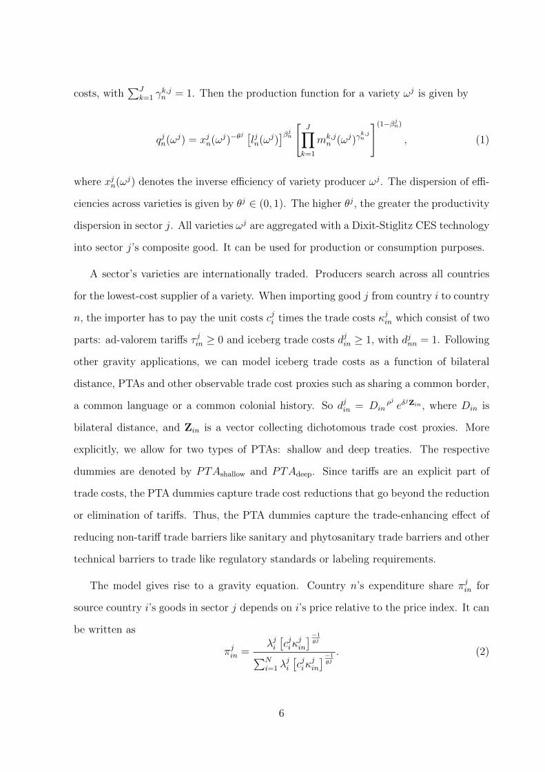
costs, with∑J

k=1 γk,jn = 1. Then the production function for a variety ωj is given by

qjn(ωj) = xjn(ωj)−θj [ljn(ωj)

]βjn [ J∏k=1

mk,jn (ωj)γ

k,jn

](1−βjn), (1)

where xjn(ωj) denotes the inverse efficiency of variety producer ωj. The dispersion of effi-

ciencies across varieties is given by θj ∈ (0, 1). The higher θj, the greater the productivity

dispersion in sector j. All varieties ωj are aggregated with a Dixit-Stiglitz CES technology

into sector j’s composite good. It can be used for production or consumption purposes.

A sector’s varieties are internationally traded. Producers search across all countries

for the lowest-cost supplier of a variety. When importing good j from country i to country

n, the importer has to pay the unit costs cji times the trade costs κjin which consist of two

parts: ad-valorem tariffs τ jin ≥ 0 and iceberg trade costs djin ≥ 1, with djnn = 1. Following

other gravity applications, we can model iceberg trade costs as a function of bilateral

distance, PTAs and other observable trade cost proxies such as sharing a common border,

a common language or a common colonial history. So djin = Dinρj eδ

jZin , where Din is

bilateral distance, and Zin is a vector collecting dichotomous trade cost proxies. More

explicitly, we allow for two types of PTAs: shallow and deep treaties. The respective

dummies are denoted by PTAshallow and PTAdeep. Since tariffs are an explicit part of

trade costs, the PTA dummies capture trade cost reductions that go beyond the reduction

or elimination of tariffs. Thus, the PTA dummies capture the trade-enhancing effect of

reducing non-tariff trade barriers like sanitary and phytosanitary trade barriers and other

technical barriers to trade like regulatory standards or labeling requirements.

The model gives rise to a gravity equation. Country n’s expenditure share πjin for

source country i’s goods in sector j depends on i’s price relative to the price index. It can

be written as

πjin =λji[cjiκ

jin

]−1

θj∑Ni=1 λ

ji

[cjiκ

jin

]−1

θj

. (2)

6

This trade share can be interpreted as the probability that, for country n, the lowest cost

supplier of a variety in sector j is trade partner i. The model is closed with goods market

clearing and an income-equals-expenditure condition for each country n.

Due to intermediates goods trade, there is double-counting of value added in trade

statistics. Koopman et al. (2014) show how to decompose countries’ trade flows into

various value added and double-counted parts.5 Aichele and Heiland (2014) propose to

study production networks by looking at the value added flows that are processed into

final goods by one region and then absorbed in another one. Following Johnson and

Noguera (2012), they derive counterfactual value added trade flows after a trade policy

shock in the Caliendo and Parro (2014) model setup. We apply the same methodology and

contrast the effects of the TTIP on trade flows, value added trade flows and production

networks.

2.2 Comparative Statics in General Equilibrium

We are interested in the trade and welfare effects of the TTIP. In this section, we describe

how the model reacts to a trade policy shock. Let x ≡ x′/x be the relative change

in a variable from its initial level x to the counterfactual level x′. The formation of

a PTA implies changes in the tariff schedule and the reduction of NTMs. So the trade

cost changes are given by κjin = τ jineδjshallow(PTA

′shallow,in−PTAshallow,in)+δ

jdeep(PTA

′deep,in−PTAdeep,in).

Since all trade flows between liberalizing countries benefit from the tariff and NTM cost

reductions, the approach implicitly assumes that either rules of origin do not matter or

the local content is sufficiently high.

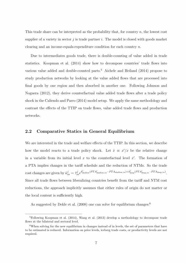
As suggested by Dekle et al. (2008) one can solve for equilibrium changes:6

5Following Koopman et al. (2014), Wang et al. (2013) develop a methodology to decompose tradeflows at the bilateral and sectoral level.

6When solving for the new equilibrium in changes instead of in levels, the set of parameters that haveto be estimated is reduced. Information on price levels, iceberg trade costs, or productivity levels are notrequired.

7

cjn = wβjnn

(J∏k=1

[pkn]γk,jn )1−βjn

, (3)

pjn =

(N∑i=1

πjin[κjinc

ji

]−1/θj)−θj, (4)

πjin =

(cjipjnκjin

)−1/θj, (5)

Xj′

n =J∑k=1

γj,kn (1− βkn)

(N∑i=1

πk′ni

1 + τ k′

ni

Xk′

i

)+ αjnI

′n, (6)

J∑j=1

F j′

n Xj′

n + Sn =J∑j=1

N∑i=1

πj′

ni

1 + τ j′

ni

Xj′

i , (7)

where wn denotes the wage change, Xjn denotes the sectoral expenditure level, F j

n ≡∑Ni=1

πjin(1+τ jin)

, I ′n = wnwnLn +∑J

j=1Xj′n (1− F j′

n )− Sn, Ln is country n’s labor force7, and

Sn is the trade surplus. Equation (3) shows how unit costs react to input price changes,

i.e. to wage and intermediate price changes. Trade cost changes affect the sectoral price

index pjn directly, and also indirectly by affecting unit costs (see Equation (4)). Changes

in trade shares result from these trade cost, unit cost and price changes. The strength

of the reaction is governed by the productivity dispersion θj. A high θj implies bigger

trade changes. Equation (6) ensures goods market clearing in the new equilibrium and

Equation (7) corresponds to the counterfactual income-equals-expenditure or balanced

trade condition. The change in real income which is given by

Wn =In

ΠJj=1(p

jn)α

jn

(8)

serves as a statistic to assess welfare changes.

Caliendo and Parro (2014) extend the single-sector solution algorithm proposed by

7Labor can move freely between sectors. However, it cannot cross international borders.

8

Alvarez and Lucas (2007) to solve the system of equations given by (3)-(7). The algorithm

starts with an initial guess about a vector of wage changes. With (3) and (4), it then

computes price and trade share changes and the new expenditure levels based on those

wage changes, evaluates the trade balance condition (7), and then updates the wage

change based on the error in the trade balance.

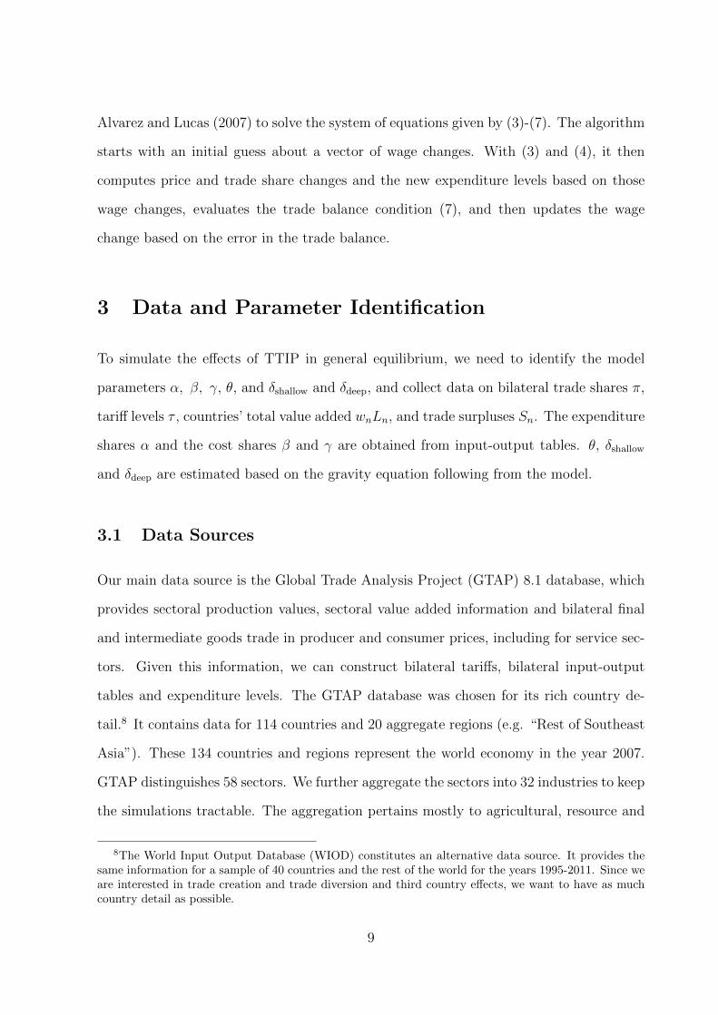
3 Data and Parameter Identification

To simulate the effects of TTIP in general equilibrium, we need to identify the model

parameters α, β, γ, θ, and δshallow and δdeep, and collect data on bilateral trade shares π,

tariff levels τ , countries’ total value added wnLn, and trade surpluses Sn. The expenditure

shares α and the cost shares β and γ are obtained from input-output tables. θ, δshallow

and δdeep are estimated based on the gravity equation following from the model.

3.1 Data Sources

Our main data source is the Global Trade Analysis Project (GTAP) 8.1 database, which

provides sectoral production values, sectoral value added information and bilateral final

and intermediate goods trade in producer and consumer prices, including for service sec-

tors. Given this information, we can construct bilateral tariffs, bilateral input-output

tables and expenditure levels. The GTAP database was chosen for its rich country de-

tail.8 It contains data for 114 countries and 20 aggregate regions (e.g. “Rest of Southeast

Asia”). These 134 countries and regions represent the world economy in the year 2007.

GTAP distinguishes 58 sectors. We further aggregate the sectors into 32 industries to keep

the simulations tractable. The aggregation pertains mostly to agricultural, resource and

8The World Input Output Database (WIOD) constitutes an alternative data source. It provides thesame information for a sample of 40 countries and the rest of the world for the years 1995-2011. Since weare interested in trade creation and trade diversion and third country effects, we want to have as muchcountry detail as possible.

9

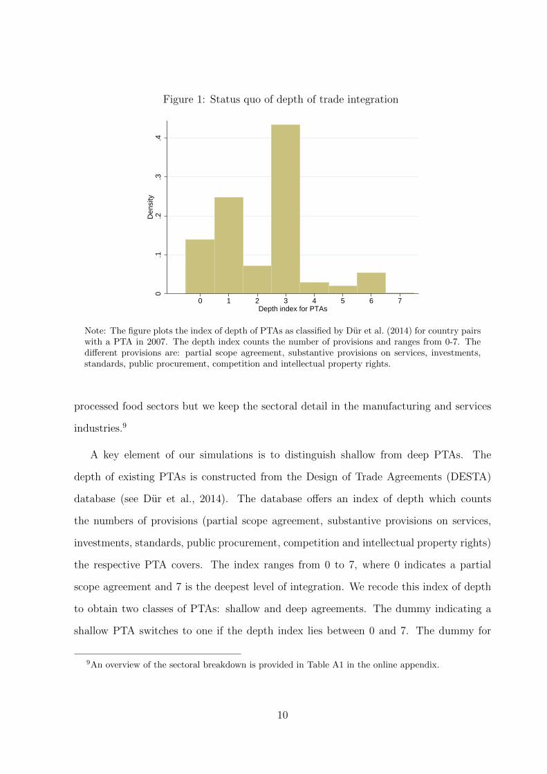
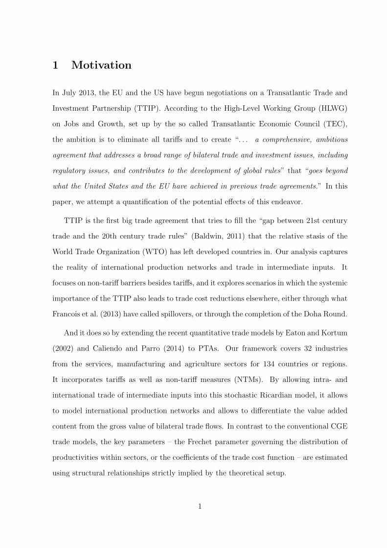
Figure 1: Status quo of depth of trade integration

0.1

.2.3

.4D

ensi

ty

0 1 2 3 4 5 6 7Depth index for PTAs

Note: The figure plots the index of depth of PTAs as classified by Dur et al. (2014) for country pairswith a PTA in 2007. The depth index counts the number of provisions and ranges from 0-7. Thedifferent provisions are: partial scope agreement, substantive provisions on services, investments,standards, public procurement, competition and intellectual property rights.

processed food sectors but we keep the sectoral detail in the manufacturing and services

industries.9

A key element of our simulations is to distinguish shallow from deep PTAs. The

depth of existing PTAs is constructed from the Design of Trade Agreements (DESTA)

database (see Dur et al., 2014). The database offers an index of depth which counts

the numbers of provisions (partial scope agreement, substantive provisions on services,

investments, standards, public procurement, competition and intellectual property rights)

the respective PTA covers. The index ranges from 0 to 7, where 0 indicates a partial

scope agreement and 7 is the deepest level of integration. We recode this index of depth

to obtain two classes of PTAs: shallow and deep agreements. The dummy indicating a

shallow PTA switches to one if the depth index lies between 0 and 7. The dummy for

9An overview of the sectoral breakdown is provided in Table A1 in the online appendix.

10

a deep PTA takes the value of one if it index is between 4 and 7.10 Figure 1 shows the

distribution of the depth of existing PTAs for the year 2007. About 10% of the PTAs (i.e.,

836 bilateral relations out of the 7997 with a PTA) are classified as deep according to our

definition; examples include NAFTA, the EU or USA-Korea. The Andean Community,

MERCOSUR or ASEAN are examples for shallow agreements.

3.2 Identification of Trade Cost Parameters

The trade cost parameters θ and δ can be identified from the gravity equation. Take the

trade share equation (2), plug in the functional form for trade costs and multiply by the

total expenditure Xjn, to obtain the following log-linearized estimable gravity equation for

each sector j:

ln(πjinXjn) = − 1

θjln τ jin −

ρj

θjlnDin −

δdj

θjPTAd,in −

ζj

θjZin + νji + µjn + εjin, (9)

where δdj = {shallow, deep}, νji ≡ ln(λjic

ji ) and µjn ≡ ln(Xj

n/∑N

i=1 λji

[cjiκ

jin

]−1

θj ) are

importer and exporter fixed effects, respectively, and εjin is an i.i.d. error term.

The coefficient on tariffs directly identifies the productivity dispersion, 1/θj. The

higher 1/θj, the stronger the response of trade flows to a cost shifter (here bilateral tariffs).

The coefficients on PTAs, −δdjθj

, are expected to be positive. Forming a PTA reduces non-

tariff trade barriers, and thus, bilateral trade increases. The coefficient is allowed to vary

by sector since non-tariff measures are sector-specific. PTAshallow captures the effect of

having a PTA. PTAdeep captures the additional effects of having a deep agreement. If

− δdeepj

θjis not statistically different from zero, in our data, deep trade liberalization does

not provide stronger trade cost reductions than a shallow PTA. In our counterfactual

analysis, we assume that the TTIP will reduce the costs of non-tariff measures by the

10In the regressions, the average effect of a PTA is given by the coefficient on the shallow PTA; theeffect of the deep PTA is added to this average.

11

same amount that other PTAs have reduced trade barriers. Thus, we do no not need

direct estimates of the levels of NTMs for the 18,000 trade pairs in our analysis,11 nor do

we need to speculate about changes in the costs of NTMs that may result from signing

the TTIP.

The importer and exporter fixed effects take into account that bilateral trade volumes

are influenced by country characteristics. However, the estimates of the PTA dummies

could still suffer from an endogeneity bias when, e.g., countries that trade more with

each other are also more likely to sign a PTA. In this case, the PTA dummy would

overestimate the trade enhancing effect of a PTA. To reduce the endogeneity bias, we use

an instrumental variables approach. The instruments should influence the probability to

sign a PTA, but other than through the PTA should not affect current trade levels. One

such instrument is the contagion index developed by Baldwin and Jaimovich (2012) and,

e.g., also used in Martin et al. (2012). It measures the threat of trade diversion country

i faces in a trade partner j’s market, by counting j’s PTAs with third countries weighted

with how important the third country’s market is for i (i.e. with the third country’s

share in i’s exports). Additionally, we use historical and recent war frequency and lagged

average variables for political similarity (average of 2000-2005) as instruments (see Egger

et al., 2008, for a brief discussion). The rationale for these variables is that past conflicts

will make it harder to negotiate PTAs, while political similarity might make it easier.

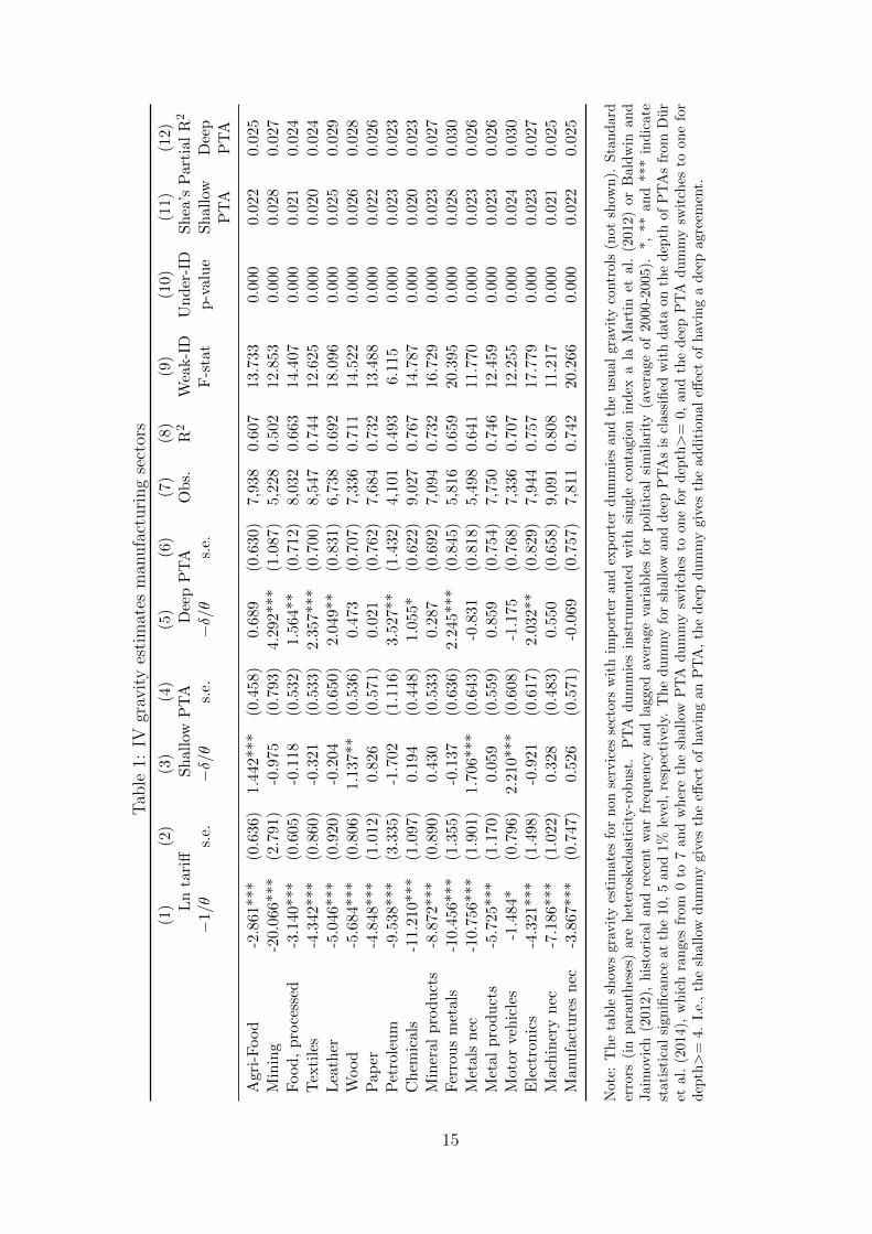
Table 1 displays the IV gravity results for the productivity dispersion and the PTA

effects for the 17 manufacturing sectors.12 We drop the 0.5% of outlier observations with

the highest tariffs from the sample. In general, our estimations can explain between 60

11We model 134× 133 = 17, 822 country pairs.12The estimation is based on trade data from UN COMTRADE. The sample is restricted to the

GTAP countries. Data on bilateral tariffs for manufacturing sectors are taken from UNCTAD’s TRAINSdatabase. The database can be accessed via the World Bank’s World Integrated Trade Solution (WITS)project, https://wits.worldbank.org. The full regression output is relegated to Tables A2 and A3in the online appendix. We use effectively applied tariffs which are aggregated to the GTAP sectorclassification with import weights. Other trade cost proxies, i.e., bilateral distance and a dummy forcontiguity, are obtained from the CEPII distance database.

12

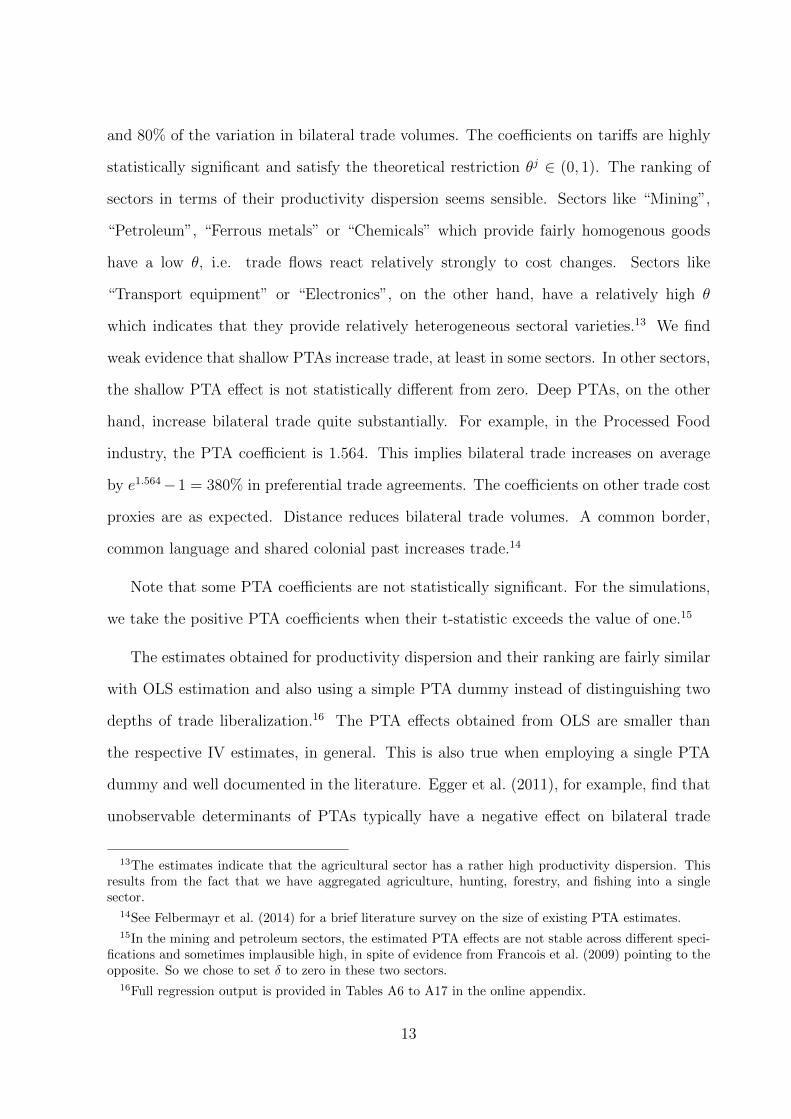
and 80% of the variation in bilateral trade volumes. The coefficients on tariffs are highly

statistically significant and satisfy the theoretical restriction θj ∈ (0, 1). The ranking of

sectors in terms of their productivity dispersion seems sensible. Sectors like “Mining”,

“Petroleum”, “Ferrous metals” or “Chemicals” which provide fairly homogenous goods

have a low θ, i.e. trade flows react relatively strongly to cost changes. Sectors like

“Transport equipment” or “Electronics”, on the other hand, have a relatively high θ

which indicates that they provide relatively heterogeneous sectoral varieties.13 We find

weak evidence that shallow PTAs increase trade, at least in some sectors. In other sectors,

the shallow PTA effect is not statistically different from zero. Deep PTAs, on the other

hand, increase bilateral trade quite substantially. For example, in the Processed Food

industry, the PTA coefficient is 1.564. This implies bilateral trade increases on average

by e1.564−1 = 380% in preferential trade agreements. The coefficients on other trade cost

proxies are as expected. Distance reduces bilateral trade volumes. A common border,

common language and shared colonial past increases trade.14

Note that some PTA coefficients are not statistically significant. For the simulations,

we take the positive PTA coefficients when their t-statistic exceeds the value of one.15

The estimates obtained for productivity dispersion and their ranking are fairly similar

with OLS estimation and also using a simple PTA dummy instead of distinguishing two

depths of trade liberalization.16 The PTA effects obtained from OLS are smaller than

the respective IV estimates, in general. This is also true when employing a single PTA

dummy and well documented in the literature. Egger et al. (2011), for example, find that

unobservable determinants of PTAs typically have a negative effect on bilateral trade

13The estimates indicate that the agricultural sector has a rather high productivity dispersion. Thisresults from the fact that we have aggregated agriculture, hunting, forestry, and fishing into a singlesector.

14See Felbermayr et al. (2014) for a brief literature survey on the size of existing PTA estimates.15In the mining and petroleum sectors, the estimated PTA effects are not stable across different speci-

fications and sometimes implausible high, in spite of evidence from Francois et al. (2009) pointing to theopposite. So we chose to set δ to zero in these two sectors.

16Full regression output is provided in Tables A6 to A17 in the online appendix.

13

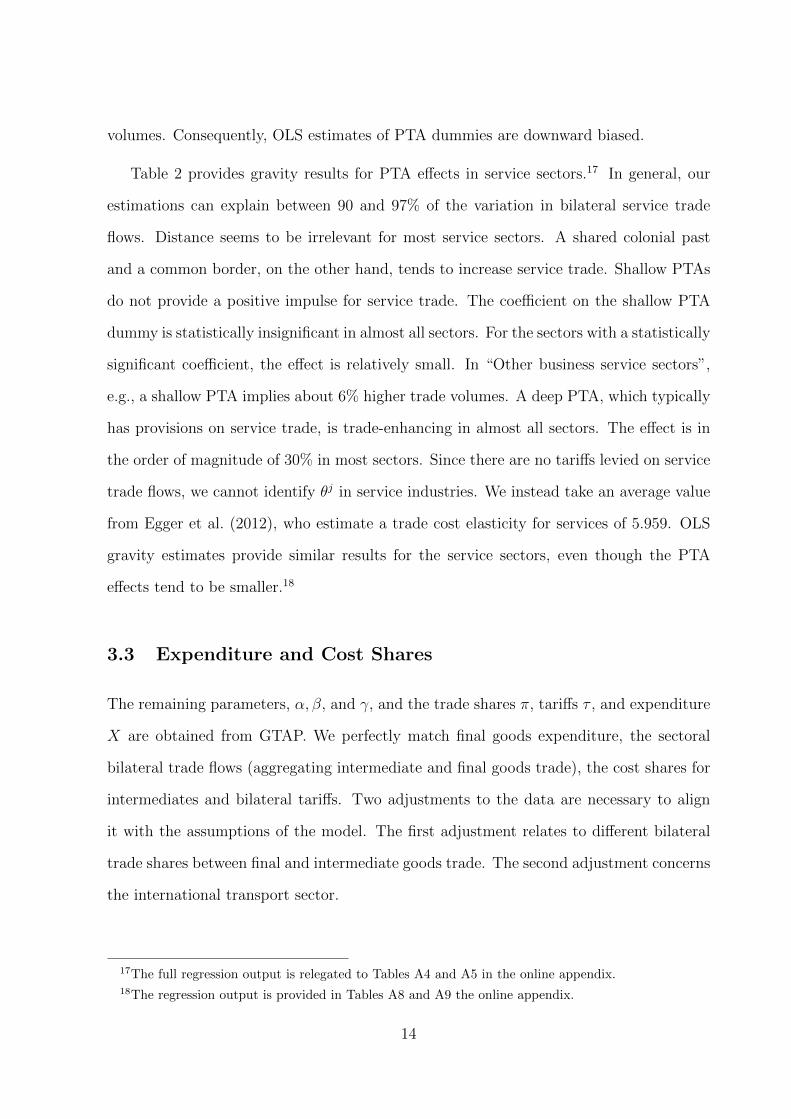
volumes. Consequently, OLS estimates of PTA dummies are downward biased.

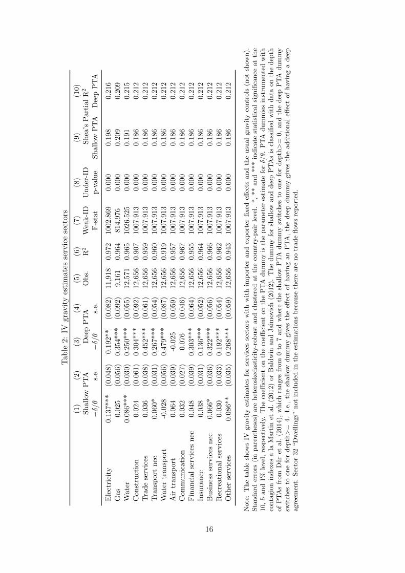
Table 2 provides gravity results for PTA effects in service sectors.17 In general, our

estimations can explain between 90 and 97% of the variation in bilateral service trade

flows. Distance seems to be irrelevant for most service sectors. A shared colonial past

and a common border, on the other hand, tends to increase service trade. Shallow PTAs

do not provide a positive impulse for service trade. The coefficient on the shallow PTA

dummy is statistically insignificant in almost all sectors. For the sectors with a statistically

significant coefficient, the effect is relatively small. In “Other business service sectors”,

e.g., a shallow PTA implies about 6% higher trade volumes. A deep PTA, which typically

has provisions on service trade, is trade-enhancing in almost all sectors. The effect is in

the order of magnitude of 30% in most sectors. Since there are no tariffs levied on service

trade flows, we cannot identify θj in service industries. We instead take an average value

from Egger et al. (2012), who estimate a trade cost elasticity for services of 5.959. OLS

gravity estimates provide similar results for the service sectors, even though the PTA

effects tend to be smaller.18

3.3 Expenditure and Cost Shares

The remaining parameters, α, β, and γ, and the trade shares π, tariffs τ , and expenditure

X are obtained from GTAP. We perfectly match final goods expenditure, the sectoral

bilateral trade flows (aggregating intermediate and final goods trade), the cost shares for

intermediates and bilateral tariffs. Two adjustments to the data are necessary to align

it with the assumptions of the model. The first adjustment relates to different bilateral

trade shares between final and intermediate goods trade. The second adjustment concerns

the international transport sector.

17The full regression output is relegated to Tables A4 and A5 in the online appendix.18The regression output is provided in Tables A8 and A9 the online appendix.

14

Tab

le1:

IVgr

avit

yes

tim

ates

man

ufa

cturi

ng

sect

ors

(1)

(2)

(3)

(4)

(5)

(6)

(7)

(8)

(9)

(10)

(11)

(12)

Ln

tari

ffS

hall

owP

TA

Dee

pP

TA

Ob

s.R

2W

eak-I

DU

nd

er-I

DS

hea

’sP

art

ial

R2

−1/θ

s.e.

−δ/θ

s.e.

−δ/θ

s.e.

F-s

tat

p-v

alu

eS

hall

owD

eep

PT

AP

TA

Agr

i-F

ood

-2.8

61*

**(0

.636)

1.442

***

(0.4

58)

0.68

9(0

.630

)7,

938

0.607

13.7

33

0.0

00

0.0

22

0.0

25

Min

ing

-20.

066

***

(2.7

91)

-0.9

75(0

.793

)4.

292*

**(1

.087

)5,

228

0.5

02

12.8

53

0.0

00

0.0

28

0.0

27

Food

,p

roce

ssed

-3.1

40**

*(0

.605)

-0.1

18

(0.5

32)

1.56

4**

(0.7

12)

8,03

20.

663

14.4

07

0.0

00

0.0

21

0.0

24

Tex

tile

s-4

.342*

**(0

.860)

-0.3

21

(0.5

33)

2.35

7***

(0.7

00)

8,54

70.

744

12.6

25

0.0

00

0.0

20

0.0

24

Lea

ther

-5.0

46*

**(0

.920)

-0.2

04

(0.6

50)

2.04

9**

(0.8

31)

6,73

80.

692

18.0

96

0.0

00

0.0

25

0.0

29

Wood

-5.6

84**

*(0

.806

)1.1

37*

*(0

.536

)0.

473

(0.7

07)

7,33

60.7

11

14.5

22

0.0

00

0.0

26

0.0

28

Pap

er-4

.848

***

(1.0

12)

0.826

(0.5

71)

0.02

1(0

.762

)7,

684

0.7

32

13.4

88

0.0

00

0.0

22

0.0

26

Pet

role

um

-9.5

38*

**(3

.335)

-1.7

02

(1.1

16)

3.52

7**

(1.4

32)

4,10

10.4

93

6.1

15

0.0

00

0.0

23

0.0

23

Ch

emic

als

-11.

210

***

(1.0

97)

0.194

(0.4

48)

1.05

5*(0

.622

)9,

027

0.767

14.7

87

0.0

00

0.0

20

0.0

23

Min

eral

pro

du

cts

-8.8

72*

**(0

.890)

0.4

30

(0.5

33)

0.28

7(0

.692

)7,

094

0.7

32

16.7

29

0.0

00

0.0

23

0.0

27

Fer

rou

sm

etal

s-1

0.4

56*

**(1

.355)

-0.1

37

(0.6

36)

2.24

5***

(0.8

45)

5,81

60.6

59

20.3

95

0.0

00

0.0

28

0.0

30

Met

als

nec

-10.

756

***

(1.9

01)

1.7

06*

**(0

.643

)-0

.831

(0.8

18)

5,49

80.6

41

11.7

70

0.0

00

0.0

23

0.0

26

Met

al

pro

du

cts

-5.7

25*

**(1

.170)

0.0

59

(0.5

59)

0.85

9(0

.754

)7,

750

0.7

46

12.4

59

0.0

00

0.0

23

0.0

26

Moto

rve

hic

les

-1.4

84*

(0.7

96)

2.210

***

(0.6

08)

-1.1

75(0

.768

)7,

336

0.7

07

12.2

55

0.0

00

0.0

24

0.0

30

Ele

ctro

nic

s-4

.321*

**(1

.498)

-0.9

21

(0.6

17)

2.03

2**

(0.8

29)

7,94

40.

757

17.7

79

0.0

00

0.0

23

0.0

27

Mach

iner

yn

ec-7

.186

***

(1.0

22)

0.328

(0.4

83)

0.55

0(0

.658

)9,

091

0.8

08

11.2

17

0.0

00

0.0

21

0.0

25

Manu

fact

ure

sn

ec-3

.867

***

(0.7

47)

0.526

(0.5

71)

-0.0

69(0

.757

)7,

811

0.742

20.2

66

0.0

00

0.0

22

0.0

25

Not

e:T

he

tab

lesh

ows

grav

ity

esti

mat

esfo

rn

onse

rvic

esse

ctors

wit

him

port

eran

dex

port

erd

um

mie

san

dth

eu

sual

gra

vit

yco

ntr

ols

(not

show

n).

Sta

nd

ard

erro

rs(i

np

aran

thes

es)

are

het

eros

ked

asti

city

-rob

ust

.P

TA

du

mm

ies

inst

rum

ente

dw

ith

sin

gle

conta

gio

nin

dex

ala

Mart

inet

al.

(2012)

or

Bald

win

an

dJai

mov

ich

(201

2),

his

tori

cal

and

rece

nt

war

freq

uen

cyan

dla

gged

aver

age

vari

ab

les

for

poli

tica

lsi

mil

ari

ty(a

vera

ge

of

2000-2

005).

*,

**

an

d***

ind

icate

stat

isti

cal

sign

ifica

nce

atth

e10

,5

and

1%le

vel,

resp

ecti

vely

.T

he

du

mm

yfo

rsh

all

owan

dd

eep

PT

As

iscl

ass

ified

wit

hd

ata

on

the

dep

thof

PT

As

from

Du

ret

al.

(201

4),

wh

ich

ran

ges

from

0to

7an

dw

her

eth

esh

allow

PT

Ad

um

my

swit

ches

toone

for

dep

th>

=0,

an

dth

ed

eep

PT

Ad

um

my

swit

ches

toon

efo

rd

epth>

=4.

I.e.

,th

esh

allo

wd

um

my

give

sth

eeff

ect

ofh

avin

gan

PT

A,

the

dee

pd

um

my

giv

esth

ead

dit

ion

al

effec

tof

hav

ing

ad

eep

agre

emen

t.

15

Tab

le2:

IVgr

avit

yes

tim

ates

serv

ice

sect

ors

(1)

(2)

(3)

(4)

(5)

(6)

(7)

(8)

(9)

(10)

Sh

allo

wP

TA

Dee

pP

TA

Ob

s.R

2W

eak-I

DU

nder

-ID

Sh

ea’s

Part

ial

R2

−δ/θ

s.e.

−δ/θ

s.e.

F-s

tat

p-v

alu

eS

hall

owP

TA

Dee

pP

TA

Ele

ctri

city

0.137

***

(0.0

48)

0.19

2**

(0.0

82)

11,9

180.

972

1002

.869

0.000

0.1

98

0.2

16

Gas

0.0

25

(0.0

56)

0.35

4***

(0.0

92)

9,16

10.

964

814.

976

0.000

0.2

09

0.2

09

Wate

r0.0

86*

**(0

.030)

0.25

0***

(0.0

55)

12,5

710.

965

1026

.525

0.0

000.1

91

0.2

15

Con

stru

ctio

n0.

024

(0.0

61)

0.3

04**

*(0

.092

)12

,656

0.90

710

07.9

13

0.0

00

0.1

86

0.2

12

Tra

de

serv

ices

0.0

36

(0.0

38)

0.45

2***

(0.0

61)

12,6

560.

959

1007

.913

0.000

0.1

86

0.2

12

Tra

nsp

ort

nec

0.060

*(0

.031)

0.26

7***

(0.0

54)

12,6

560.

960

1007

.913

0.0

00

0.1

86

0.2

12

Wate

rtr

an

spor

t-0

.028

(0.0

56)

0.47

9***

(0.0

87)

12,6

560.

919

1007

.913

0.000

0.1

86

0.2

12

Air

tran

sport

0.0

64

(0.0

39)

-0.0

25(0

.059

)12

,656

0.95

710

07.9

13

0.000

0.1

86

0.2

12

Com

mu

nic

atio

n0.0

32

(0.0

27)

0.07

6(0

.046

)12

,656

0.96

710

07.9

130.0

00

0.1

86

0.2

12

Fin

an

cial

serv

ices

nec

0.0

48

(0.0

39)

0.3

03**

*(0

.064

)12

,656

0.95

510

07.9

13

0.000

0.1

86

0.2

12

Insu

ran

ce0.0

38

(0.0

31)

0.13

6***

(0.0

52)

12,6

560.

964

1007

.913

0.0

000.1

86

0.2

12

Bu

sin

ess

serv

ices

nec

0.066

*(0

.036)

0.32

2***

(0.0

56)

12,6

560.

966

1007

.913

0.0

00

0.1

86

0.2

12

Rec

reati

onal

serv

ices

0.030

(0.0

33)

0.19

2***

(0.0

54)

12,6

560.

962

1007

.913

0.0

00

0.1

86

0.2

12

Oth

erse

rvic

es0.0

86*

*(0

.035

)0.2

68**

*(0

.059

)12

,656

0.94

310

07.9

13

0.000

0.1

86

0.2

12

Not

e:T

he

tab

lesh

ows

IVgr

avit

yes

tim

ates

for

serv

ices

sect

ors

wit

hw

ith

imp

ort

eran

dex

port

erfi

xed

effec

tsan

dth

eu

sual

gra

vit

yco

ntr

ols

(not

show

n).

Sta

nd

ard

erro

rs(i

np

aren

thes

es)

are

het

eros

ked

asti

city

-rob

ust

an

dcl

ust

ered

at

the

cou

ntr

y-p

air

leve

l.*,

**

an

d***

ind

icate

stati

stic

al

sign

ifica

nce

at

the

10,

5an

d1%

level

,re

spec

tivel

y.T

he

coeffi

cien

ton

the

coeffi

cien

ton

the

PT

Ad

um

my

isth

ep

ara

met

eres

tim

ate

forδ/θ.

PT

Ad

um

mie

sin

stru

men

ted

wit

hco

nta

gion

ind

exes

ala

Mar

tin

etal

.(2

012)

orB

ald

win

an

dJaim

ovic

h(2

012).

Th

ed

um

my

for

shall

owan

ddee

pP

TA

sis

class

ified

wit

hd

ata

on

the

dep

thof

PT

As

from

Du

ret

al.

(201

4),

wh

ich

ran

ges

from

0to

7an

dw

her

eth

esh

all

owP

TA

dum

my

swit

ches

toon

efo

rd

epth>

=0,

an

dth

ed

eep

PT

Ad

um

my

swit

ches

toon

efo

rd

epth>

=4.

I.e.

,th

esh

allo

wd

um

my

giv

esth

eeff

ect

of

hav

ing

an

PT

A,

the

dee

pd

um

my

give

sth

eadd

itio

nal

effec

tof

hav

ing

ad

eep

agre

emen

t.S

ecto

r32

“Dw

elli

ngs

”n

otin

clu

ded

inth

ees

tim

ati

on

sb

ecau

seth

ere

are

no

trad

efl

ows

rep

ort

ed.

16

In the model, the bilateral trade shares are assumed to be identical across use. In the

GTAP data, however, bilateral trade shares differ across final and intermediate usage. We

match sectoral bilateral trade flows, final goods expenditure shares, and cost shares for

intermediates to their empirical counterpart and bilateralize final and intermediate goods

trade with the common bilateral trade share. And GTAP has a separate international

transportation sector. To match the iceberg trade cost assumption, we assign the inter-

national transport margin and its respective share of intermediate demand to the sector

demanding the international transportation service. This increases the respective sector’s

production value. The sectoral value added is calculated as the difference between the so

obtained production value and intermediate costs.19

4 Simulation results: Trade and Welfare Effects of

TTIP

We now have paved the way to simulate the effect of PTAs in general equilibrium. The

setup allows to explore different scenarios: from a tariffs-only liberalization in selected

sectors (e.g., excluding services and agriculture), to a deep PTA encompassing all 32

industries. We apply the framework to the case of the TTIP. We first review some

important facts; then we analyze trade creation and diversion. Does TTIP strengthen

the transatlantic production network? Then we describe the predicted sectoral value

added changes and discuss whether comparative advantage plays a role in shaping sectoral

responses to our trade policy shock. Last, we investigate the welfare changes under TTIP.

The base scenario is a deep TTIP. However, we also characterize the welfare changes in

different scenarios such as deep vs. shallow TTIP, no spillovers vs. spillovers, and we also

investigate the interactions of TTIP with a round of multilateral trade liberalization. In

19This implies that production taxes are part of value added.

17

the online appendix, we also provide some sensitivity checks pertaining to the parameter

estimates, i.e. OLS vs. IV estimation and a single PTA dummy vs. two levels of PTA

depth.

4.1 Cross-industry facts for the EU and the US

Tables 3 and 4 provide information on the status quo of trade between the EU and the

US for 32 industries. All values are in US dollars and relate to the base year of 2007.20

Column (1) of Table 3 reports for the EU the value added generated in each sector. 73%

of total value added (GDP) is generated in the services sectors, 25% in manufacturing,

and 2% in agriculture. Columns (2) and (3) shows that total EU exports to the US

amount to 465 bn. US dollars; this amounts to about 8% of total exports to non-EU

countries. However, in value added terms, the exports of 428 bn. US dollars amount to

almost 11% of the total.21 This signals that EU exports to the US incorporate relatively

little reexports of foreign (including of the US) value added. Column (4) provides trade-

weighted sector-level tariff rates that EU exports encounter in the US. Tariffs are low;

the average rate (excluding services trade) is just 1.35%. Exports to the world encounter

very similar tariff rates; thus, earlier rounds of (multilateral) trade liberalization have not

particularly favored EU exports to the US. Columns (5) and (6) report EU exports to

the world. This shows that the US is a particularly important market for EU services

exporters: in this area the share of exports going to the US usually exceeds the 11%

overall average (in VA terms) by a wide margin. The opposite is true in agri-food. The

manufacturing industries mostly are below the 11% average, with a few exceptions, most

notably Chemicals.

Table 4 provides information for the US side. It shows that the weight of the services

20This is the most recent year for which input-output data for 134 countries/regions is available. Wedo not predict baseline values for some future year, as Fontagne et al. (2013) or Francois et al. (2013),since this would introduce additional margins of error.

21European value added embodied in US absorption.

18

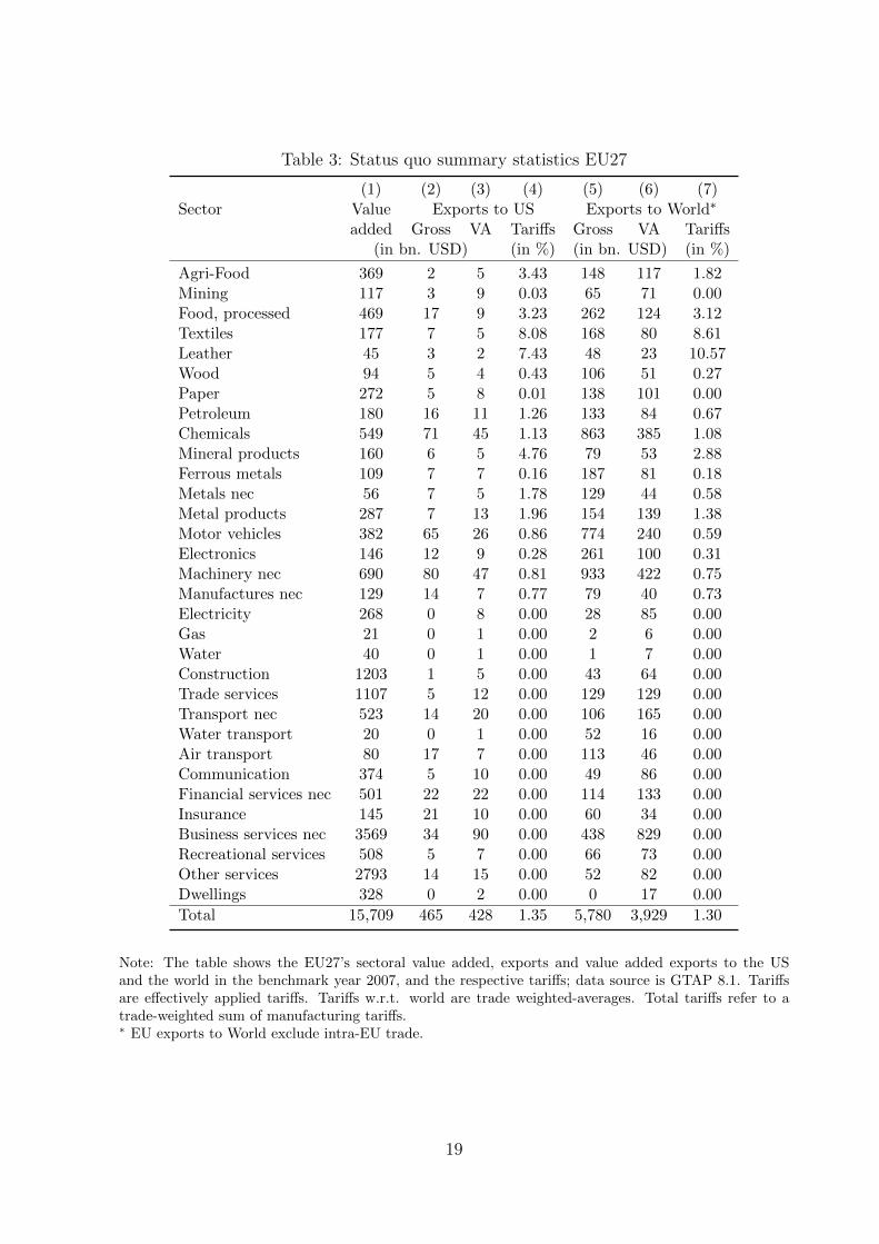
Table 3: Status quo summary statistics EU27

(1) (2) (3) (4) (5) (6) (7)Sector Value Exports to US Exports to World∗

added Gross VA Tariffs Gross VA Tariffs(in bn. USD) (in %) (in bn. USD) (in %)

Agri-Food 369 2 5 3.43 148 117 1.82Mining 117 3 9 0.03 65 71 0.00Food, processed 469 17 9 3.23 262 124 3.12Textiles 177 7 5 8.08 168 80 8.61Leather 45 3 2 7.43 48 23 10.57Wood 94 5 4 0.43 106 51 0.27Paper 272 5 8 0.01 138 101 0.00Petroleum 180 16 11 1.26 133 84 0.67Chemicals 549 71 45 1.13 863 385 1.08Mineral products 160 6 5 4.76 79 53 2.88Ferrous metals 109 7 7 0.16 187 81 0.18Metals nec 56 7 5 1.78 129 44 0.58Metal products 287 7 13 1.96 154 139 1.38Motor vehicles 382 65 26 0.86 774 240 0.59Electronics 146 12 9 0.28 261 100 0.31Machinery nec 690 80 47 0.81 933 422 0.75Manufactures nec 129 14 7 0.77 79 40 0.73Electricity 268 0 8 0.00 28 85 0.00Gas 21 0 1 0.00 2 6 0.00Water 40 0 1 0.00 1 7 0.00Construction 1203 1 5 0.00 43 64 0.00Trade services 1107 5 12 0.00 129 129 0.00Transport nec 523 14 20 0.00 106 165 0.00Water transport 20 0 1 0.00 52 16 0.00Air transport 80 17 7 0.00 113 46 0.00Communication 374 5 10 0.00 49 86 0.00Financial services nec 501 22 22 0.00 114 133 0.00Insurance 145 21 10 0.00 60 34 0.00Business services nec 3569 34 90 0.00 438 829 0.00Recreational services 508 5 7 0.00 66 73 0.00Other services 2793 14 15 0.00 52 82 0.00Dwellings 328 0 2 0.00 0 17 0.00

Total 15,709 465 428 1.35 5,780 3,929 1.30

Note: The table shows the EU27’s sectoral value added, exports and value added exports to the USand the world in the benchmark year 2007, and the respective tariffs; data source is GTAP 8.1. Tariffsare effectively applied tariffs. Tariffs w.r.t. world are trade weighted-averages. Total tariffs refer to atrade-weighted sum of manufacturing tariffs.∗ EU exports to World exclude intra-EU trade.

19

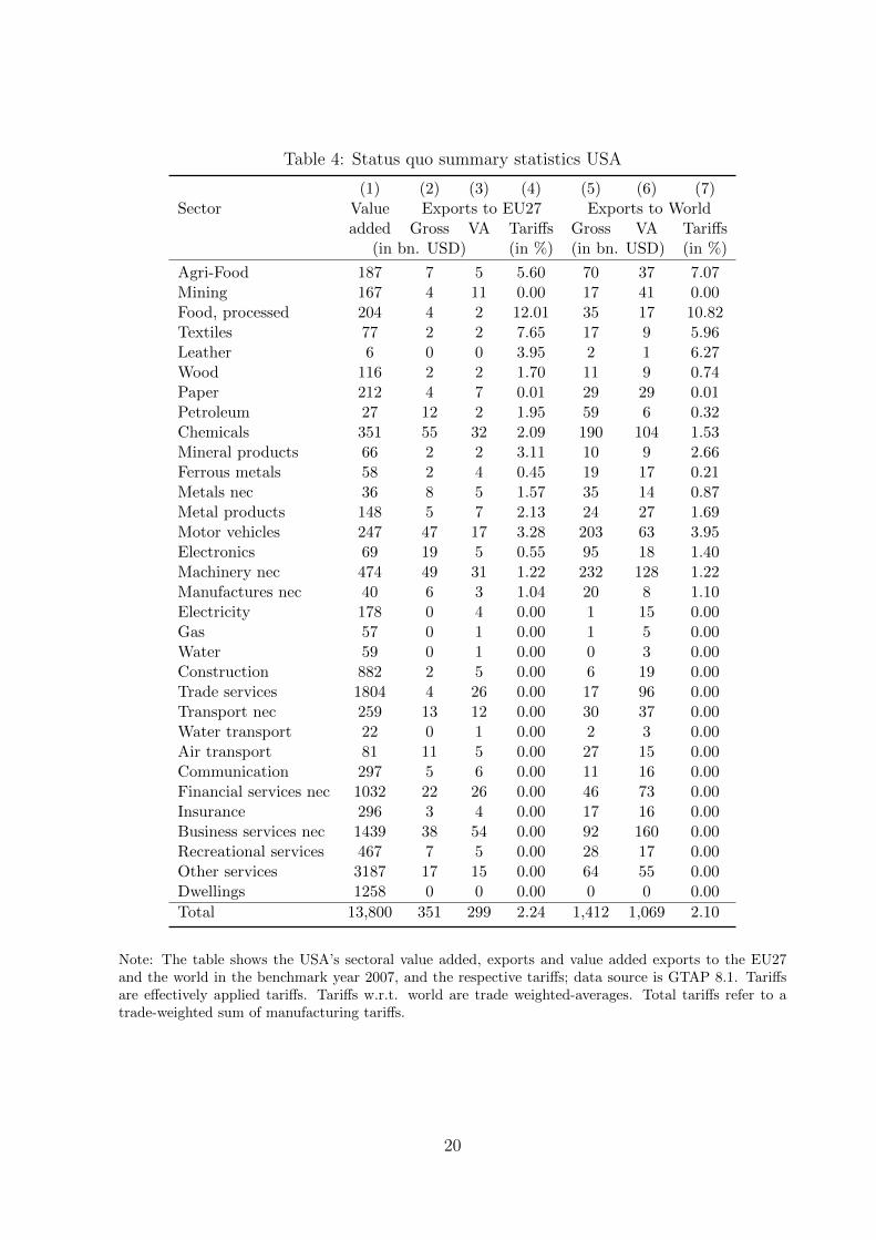
Table 4: Status quo summary statistics USA

(1) (2) (3) (4) (5) (6) (7)Sector Value Exports to EU27 Exports to World

added Gross VA Tariffs Gross VA Tariffs(in bn. USD) (in %) (in bn. USD) (in %)

Agri-Food 187 7 5 5.60 70 37 7.07Mining 167 4 11 0.00 17 41 0.00Food, processed 204 4 2 12.01 35 17 10.82Textiles 77 2 2 7.65 17 9 5.96Leather 6 0 0 3.95 2 1 6.27Wood 116 2 2 1.70 11 9 0.74Paper 212 4 7 0.01 29 29 0.01Petroleum 27 12 2 1.95 59 6 0.32Chemicals 351 55 32 2.09 190 104 1.53Mineral products 66 2 2 3.11 10 9 2.66Ferrous metals 58 2 4 0.45 19 17 0.21Metals nec 36 8 5 1.57 35 14 0.87Metal products 148 5 7 2.13 24 27 1.69Motor vehicles 247 47 17 3.28 203 63 3.95Electronics 69 19 5 0.55 95 18 1.40Machinery nec 474 49 31 1.22 232 128 1.22Manufactures nec 40 6 3 1.04 20 8 1.10Electricity 178 0 4 0.00 1 15 0.00Gas 57 0 1 0.00 1 5 0.00Water 59 0 1 0.00 0 3 0.00Construction 882 2 5 0.00 6 19 0.00Trade services 1804 4 26 0.00 17 96 0.00Transport nec 259 13 12 0.00 30 37 0.00Water transport 22 0 1 0.00 2 3 0.00Air transport 81 11 5 0.00 27 15 0.00Communication 297 5 6 0.00 11 16 0.00Financial services nec 1032 22 26 0.00 46 73 0.00Insurance 296 3 4 0.00 17 16 0.00Business services nec 1439 38 54 0.00 92 160 0.00Recreational services 467 7 5 0.00 28 17 0.00Other services 3187 17 15 0.00 64 55 0.00Dwellings 1258 0 0 0.00 0 0 0.00

Total 13,800 351 299 2.24 1,412 1,069 2.10

Note: The table shows the USA’s sectoral value added, exports and value added exports to the EU27and the world in the benchmark year 2007, and the respective tariffs; data source is GTAP 8.1. Tariffsare effectively applied tariffs. Tariffs w.r.t. world are trade weighted-averages. Total tariffs refer to atrade-weighted sum of manufacturing tariffs.

20

industries in GDP is even more important for the US than for the EU (82%), but that the

agri-food area contributes even less (1%). Moreover, the levels of GDP are similar, with

the EU having a slight advantage. The US is more closed; domestic value added embodied

in foreign absorption relative to GDP amounts to 8%; in the EU the number stands at

about 25%. The EU has a bilateral surplus with the US of 114 bn. USD in gross terms

and of 129 bn. USD in value added terms. This signals that EU value added is exported

to the US via third countries, e.g., Canada or China. Exports to the EU are relatively

more important for the US than exports to the US for the EU. US tariffs appear slightly

higher than EU tariffs, but the correlation between the two tariff schedules is relatively

high (about 61%).

4.2 Global trade effects of a deep TTIP

Reflecting the official ambitions for the TTIP, our scenario assumes that all transatlantic

tariffs are eliminated and costs of NTMs fall to the level observed in other deep PTAs.22

Moreover, we do not allow the agreement to affect trade costs in non-TTIP country pairs,

i.e., we abstract from regulatory spillovers. In this case, the volume of international trade

increases from 15.3 to 16.4 tn. US dollars23, i.e. aggregate trade grows by about 7.3%,

see also Table 5. Manufacturing trade (about 80% of the initially observed trade volume)

increases by 7.8%, trade in agricultural goods even by 12.9%, whereas the growth rate

in services trade is only 3.5%. So with TTIP, the share of manufacturing trade increases

further (by about 0.46 percentage points) at the expense of the trade in services share

which falls by 0.62 percentage points. This seems plausible, since the trade cost reductions

are largest in manufacturing.

The impressive trade growth our model predicts might however overstate the value

added generated under the TTIP. Trade in intermediates—that are used to produce other

22We provide sensitivity analysis below.23Note that intra-regional trade in GTAP’s “Rest of ...” regions is not included in this figure.

21

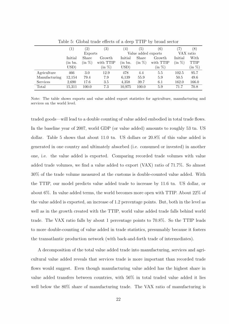
Table 5: Global trade effects of a deep TTIP by broad sector

(1) (2) (3) (4) (5) (6) (7) (8)Exports Value added exports VAX ratio

Initial Share Growth Initial Share Growth Initial With(in bn. (in %) with TTIP (in bn. (in %) with TTIP (in %) TTIPUSD) (in %) USD) (in %) (in %)

Agriculture 466 3.0 12.9 478 4.4 5.5 102.5 95.7Manufacturing 12,154 79.4 7.9 6,139 55.9 5.9 50.5 49.6Services 2,690 17.6 3.5 4,358 39.7 6.1 162.0 166.0Total 15,311 100.0 7.3 10,975 100.0 5.9 71.7 70.8

Note: The table shows exports and value added export statistics for agriculture, manufacturing andservices on the world level.

traded goods—will lead to a double counting of value added embodied in total trade flows.

In the baseline year of 2007, world GDP (or value added) amounts to roughly 53 tn. US

dollar. Table 5 shows that about 11.0 tn. US dollars or 20.8% of this value added is

generated in one country and ultimately absorbed (i.e. consumed or invested) in another

one, i.e. the value added is exported. Comparing recorded trade volumes with value

added trade volumes, we find a value added to export (VAX) ratio of 71.7%. So almost

30% of the trade volume measured at the customs is double-counted value added. With

the TTIP, our model predicts value added trade to increase by 11.6 tn. US dollar, or

about 6%. In value added terms, the world becomes more open with TTIP. About 22% of

the value added is exported, an increase of 1.2 percentage points. But, both in the level as

well as in the growth created with the TTIP, world value added trade falls behind world

trade. The VAX ratio falls by about 1 percentage points to 70.8%. So the TTIP leads

to more double-counting of value added in trade statistics, presumably because it fosters

the transatlantic production network (with back-and-forth trade of intermediates).

A decomposition of the total value added trade into manufacturing, services and agri-

cultural value added reveals that services trade is more important than recorded trade

flows would suggest. Even though manufacturing value added has the highest share in

value added transfers between countries, with 56% in total traded value added it lies

well below the 80% share of manufacturing trade. The VAX ratio of manufacturing is

22

only 50.5%. This indicates that (1) manufacturing trade partly takes place in the form

of intermediates trade and that (2) traded manufacturing goods embody value added of

the services industries. Indeed, while the recorded services trade is about 2.7 bn. USD,

the trade in embodied services value added is 4.4 bn. USD. So in terms of value added,

services account for 40% of value added trade, against 17% in recorded trade volumes.

The VAX ratio for services is 162%, implying that service value added trade is by 62%

higher than recorded trade. A large fraction of services value added is traded indirectly

via the domestic value chain. An example would be domestic accounting or IT services

that are embodied in exported cars.

Under the TTIP, agricultural, manufacturing and services value added trade all grow.

But whereas recorded manufacturing trade increases by 7.8%, manufacturing value added

associated with trade flows only increases by 5.9% (and starting from a lower level). The

reverse happens in services sectors, which grow with 6.1% in terms of value added trade,

compared to only 3.5% in recorded trade. So, our simulations now suggest that the TTIP

will lead to a slight increase in the share of services value added trade of 0.05 percentage

points, at the costs of manufacturing (-0.03 percentage points) and agricultural (-0.02 per-

centage points) value added trade. While the TTIP predominantly fosters manufacturing

trade, indirectly, i.e. via domestic supply chains, a lot of the associated value added is

generated in the service sectors and not in manufacturing. Given that both liberalizing

regions, the US and the EU, are mature economies with a large share of value added in

services, this may not come as a surprise. The VAX ratio in agriculture is roughly 103% in

the initial situation; with the TTIP it falls to 96%. The US has a comparative advantage

in agriculture and increases its agricultural exports. In the US, agriculture uses more

services inputs than the average country. This explains why the agricultural VAX ratio

goes down with TTIP.

23

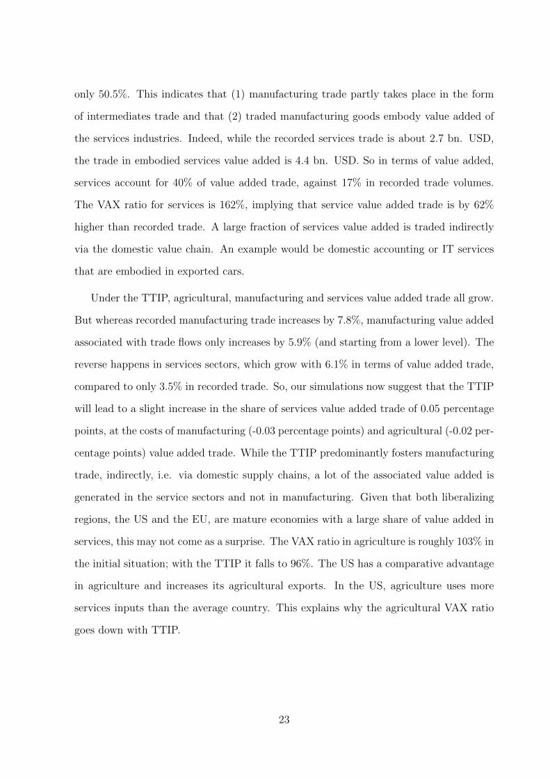
Table 6: Aggregate trade effects of deep TTIP

(1) (2) (3) (4) (5) (6) (7) (8) (9) (10)Region ASEANb Brazil Canada China EU27∗ Germany Mexico SACUa Turkey USA

Export growth (in %) from ... toASEANb -1 -0 -2 -3 -1 -3 -3 -0 -0 -7Brazil -2 -1 -8 -3 0 0 -7 -2 1 -7Canada -1 1 -1 -1 -2 6 -4 1 2 -8China -2 1 -2 -1 -1 -5 -3 1 1 -7EU27∗ -6 -5 -9 -6 -1 -5 -7 -4 -5 171Germany -7 -6 -9 -6 -8 -1 -7 -3 -4 216Mexico 0 1 -5 -1 4 -11 -1 2 1 -6SACUa -3 -1 -4 -4 2 1 -4 -1 -0 -11Turkey -1 -1 -3 -1 -4 -3 -3 -0 -1 -5USA -4 -3 -6 -4 212 259 -5 -2 21 -2

Growth of value added transfers (in %) from ... toASEANb -1 0 -3 -1 1 0 -4 -0 -0 -6Brazil -2 -1 -6 -3 0 0 -6 -1 -0 -5Canada -0 1 -1 -1 25 42 -4 3 9 -9China -1 1 -3 -1 2 1 -3 1 1 -7EU27∗ -6 -5 7 -6 -2 -7 7 -6 -7 120Germany -7 -6 12 -7 -10 -2 4 -6 -8 136Mexico 0 2 -6 0 44 33 -1 5 13 -9SACUa -3 -2 -5 -4 -0 -0 -6 -1 -0 -0Turkey -2 -2 -1 -3 -6 -4 -2 -2 -1 21USA -2 -2 -9 -3 149 169 -8 10 34 -2

Note: The table shows bilateral changes in trade flows and value added transfers (in %) from deep TTIP.The diagonal describes changes in intra-national trade and/or in the trade volume within a region.∗ EU27 without Germany. a Southern African Customs Union, b Association of Southeast Asian Nations.

4.3 Bilateral trade effects of a deep TTIP

While Table 5 offers insights into the evolution of total trade flows under the TTIP,

Table 6 looks into its effects on regional trade links. Again, we discuss trade and value

added trade changes. Our model predicts a substantial amount of trade creation between

the EU and the US in the long run. German and EU exports to the US are expected to

roughly triple. And also the US exports to the EU and Germany are expected to go up

by 212 and 259%, respectively. However, trade statistics exaggerate the transfer of value

added between the two transatlantic economies. German value added exports to the US,

e.g., are predicted to increase by 136% instead of 216%. And also the US export growth

with Germany is only 169% under the TTIP. One explanation for this observed pattern

24

is the deepening of transatlantic production chains. Then, the US would process more

EU value added in the form of intermediate inputs under the TTIP and vice versa. As

a consequence, changes in recorded trade flows would overstate how much value added is

generated. We will look into this possibility in more detail in the next section.

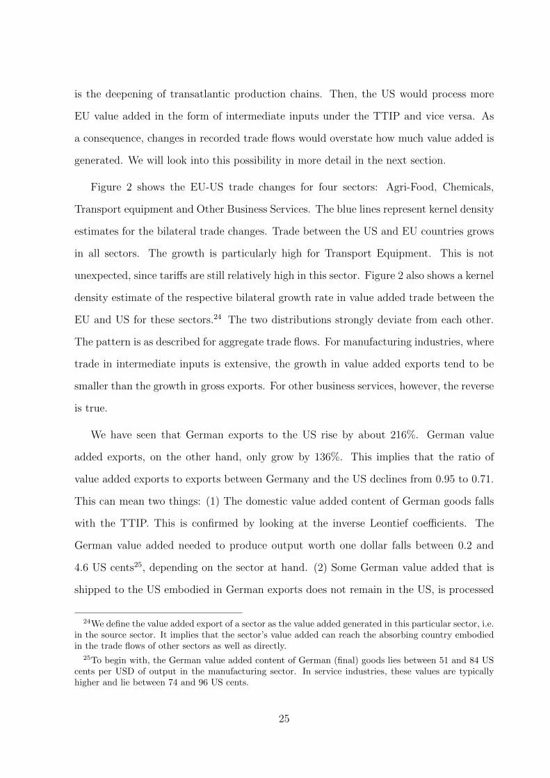
Figure 2 shows the EU-US trade changes for four sectors: Agri-Food, Chemicals,

Transport equipment and Other Business Services. The blue lines represent kernel density

estimates for the bilateral trade changes. Trade between the US and EU countries grows

in all sectors. The growth is particularly high for Transport Equipment. This is not

unexpected, since tariffs are still relatively high in this sector. Figure 2 also shows a kernel

density estimate of the respective bilateral growth rate in value added trade between the

EU and US for these sectors.24 The two distributions strongly deviate from each other.

The pattern is as described for aggregate trade flows. For manufacturing industries, where

trade in intermediate inputs is extensive, the growth in value added exports tend to be

smaller than the growth in gross exports. For other business services, however, the reverse

is true.

We have seen that German exports to the US rise by about 216%. German value

added exports, on the other hand, only grow by 136%. This implies that the ratio of

value added exports to exports between Germany and the US declines from 0.95 to 0.71.

This can mean two things: (1) The domestic value added content of German goods falls

with the TTIP. This is confirmed by looking at the inverse Leontief coefficients. The

German value added needed to produce output worth one dollar falls between 0.2 and

4.6 US cents25, depending on the sector at hand. (2) Some German value added that is

shipped to the US embodied in German exports does not remain in the US, is processed

24We define the value added export of a sector as the value added generated in this particular sector, i.e.in the source sector. It implies that the sector’s value added can reach the absorbing country embodiedin the trade flows of other sectors as well as directly.

25To begin with, the German value added content of German (final) goods lies between 51 and 84 UScents per USD of output in the manufacturing sector. In service industries, these values are typicallyhigher and lie between 74 and 96 US cents.

25

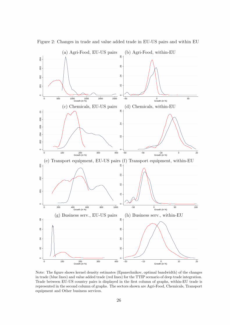
Figure 2: Changes in trade and value added trade in EU-US pairs and within EU

(a) Agri-Food, EU-US pairs (b) Agri-Food, within-EU

0.0

01.0

02.0

03.0

04

0 500 1000 1500 2000 2500Growth (in %)

Gross exports VA exports

Kernel density estimate

0.0

2.0

4.0

6.0

8

−50 0 50Growth (in %)

Gross exports VA exports

Kernel density estimate

(c) Chemicals, EU-US pairs (d) Chemicals, within-EU

0.0

02.0

04.0

06.0

08.0

1

0 100 200 300 400Growth (in %)

Gross exports VA exports

Kernel density estimate

0.0

2.0

4.0

6

−60 −40 −20 0 20Growth (in %)

Gross exports VA exports

Kernel density estimate

(e) Transport equipment, EU-US pairs (f) Transport equipment, within-EU

0.0

01.0

02.0

03

0 200 400 600 800 1000Growth (in %)

Gross exports VA exports

Kernel density estimate

0.0

1.0

2.0

3.0

4

−50 0 50 100Growth (in %)

Gross exports VA exports

Kernel density estimate

(g) Business serv., EU-US pairs (h) Business serv., within-EU

0.0

2.0

4.0

6.0

8

0 100 200 300 400Growth (in %)

Gross exports VA exports

Kernel density estimate

0.0

2.0

4.0

6.0

8

−20 −10 0 10 20Growth (in %)

Gross exports VA exports

Kernel density estimate

Note: The figure shows kernel density estimates (Epanechnikov, optimal bandwidth) of the changesin trade (blue lines) and value added trade (red lines) for the TTIP scenario of deep trade integration.Trade between EU-US country pairs is displayed in the first column of graphs, within-EU trade isrepresented in the second column of graphs. The sectors shown are Agri-Food, Chemicals, Transportequipment and Other business services.

26

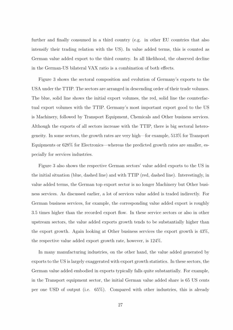
further and finally consumed in a third country (e.g. in other EU countries that also

intensify their trading relation with the US). In value added terms, this is counted as

German value added export to the third country. In all likelihood, the observed decline

in the German-US bilateral VAX ratio is a combination of both effects.

Figure 3 shows the sectoral composition and evolution of Germany’s exports to the

USA under the TTIP. The sectors are arranged in descending order of their trade volumes.

The blue, solid line shows the initial export volumes, the red, solid line the counterfac-

tual export volumes with the TTIP. Germany’s most important export good to the US

is Machinery, followed by Transport Equipment, Chemicals and Other business services.

Although the exports of all sectors increase with the TTIP, there is big sectoral hetero-

geneity. In some sectors, the growth rates are very high—for example, 513% for Transport

Equipments or 628% for Electronics—whereas the predicted growth rates are smaller, es-

pecially for services industries.

Figure 3 also shows the respective German sectors’ value added exports to the US in

the initial situation (blue, dashed line) and with TTIP (red, dashed line). Interestingly, in

value added terms, the German top export sector is no longer Machinery but Other busi-

ness services. As discussed earlier, a lot of services value added is traded indirectly. For

German business services, for example, the corresponding value added export is roughly

3.5 times higher than the recorded export flow. In these service sectors or also in other

upstream sectors, the value added exports growth tends to be substantially higher than

the export growth. Again looking at Other business services the export growth is 43%,

the respective value added export growth rate, however, is 124%.

In many manufacturing industries, on the other hand, the value added generated by

exports to the US is largely exaggerated with export growth statistics. In these sectors, the

German value added embodied in exports typically falls quite substantially. For example,

in the Transport equipment sector, the initial German value added share is 65 US cents

per one USD of output (i.e. 65%). Compared with other industries, this is already

27

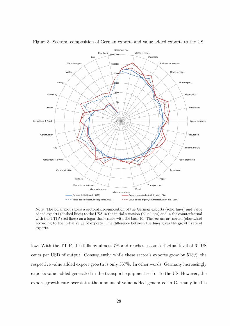
Figure 3: Sectoral composition of German exports and value added exports to the US

0.1

1

10

100

1000

10000

100000

1000000

Machinery necMotor vehicles

Chemicals

Business services nec

Other services

Air transport

Electronics

Metals nec

Metal products

Insurance

Ferrous metals

Food, processed

Petroleum

Paper

Transport nec

WoodMineral products

Manufactures nec

Financial services nec

Textiles

Communication

Recreational services

Trade

Construction

Agriculture & Food

Leather

Electricity

Mining

Water

Water transport

Gas

Dwellings

Exports, initial (in mio. USD) Exports, counterfactual (in mio. USD)

Value added export, initial (in mio. USD) Value added export, counterfactual (in mio. USD)

Note: The polar plot shows a sectoral decomposition of the German exports (solid lines) and valueadded exports (dashed lines) to the USA in the initial situation (blue lines) and in the counterfactualwith the TTIP (red lines) on a logarithmic scale with the base 10. The sectors are sorted (clockwise)according to the initial value of exports. The difference between the lines gives the growth rate ofexports.

low. With the TTIP, this falls by almost 7% and reaches a counterfactual level of 61 US

cents per USD of output. Consequently, while these sector’s exports grow by 513%, the

respective value added export growth is only 367%. In other words, Germany increasingly

exports value added generated in the transport equipment sector to the US. However, the

export growth rate overstates the amount of value added generated in Germany in this

28

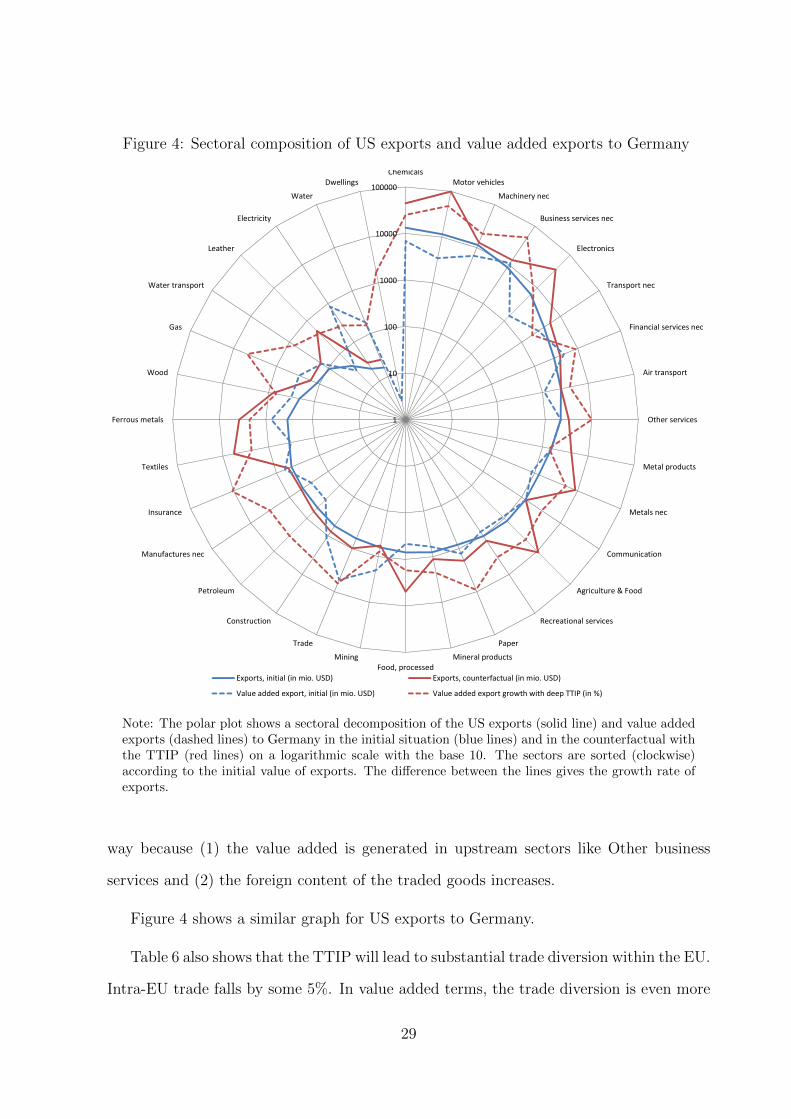
Figure 4: Sectoral composition of US exports and value added exports to Germany

1

10

100

1000

10000

100000

ChemicalsMotor vehicles

Machinery nec

Business services nec

Electronics

Transport nec

Financial services nec

Air transport

Other services

Metal products

Metals nec

Communication

Agriculture & Food

Recreational services

Paper

Mineral productsFood, processed

Mining

Trade

Construction

Petroleum

Manufactures nec

Insurance

Textiles

Ferrous metals

Wood

Gas

Water transport

Leather

Electricity

Water

Dwellings

Exports, initial (in mio. USD) Exports, counterfactual (in mio. USD)

Value added export, initial (in mio. USD) Value added export growth with deep TTIP (in %)

Note: The polar plot shows a sectoral decomposition of the US exports (solid line) and value addedexports (dashed lines) to Germany in the initial situation (blue lines) and in the counterfactual withthe TTIP (red lines) on a logarithmic scale with the base 10. The sectors are sorted (clockwise)according to the initial value of exports. The difference between the lines gives the growth rate ofexports.

way because (1) the value added is generated in upstream sectors like Other business

services and (2) the foreign content of the traded goods increases.

Figure 4 shows a similar graph for US exports to Germany.

Table 6 also shows that the TTIP will lead to substantial trade diversion within the EU.

Intra-EU trade falls by some 5%. In value added terms, the trade diversion is even more

29

pronounced. Value added exports fall by 7%. Figure 2 provides a more disaggregated view

for selected sectors. It shows the kernel density estimates of the trade and value added

trade changes within the EU. The distribution of value added changes lies to the left of

the distribution of recorded trade changes in all shown sectors. This pattern is stronger

for more upstream sectors like Chemicals or Other Business Services. Value added trade

also captures indirect effects via sectors that use the sector’s output as input. So the

pattern of bigger reductions in value added terms can be explained either by the fact that

other sectors (in Germany or abroad) reduce the usage of the sector’s intermediates or

that sectors which heavily rely on the sector’s inputs have adverse trade effects or that

more of the sector’s value added does not stay in the EU trade partner but is processed

and shipped on (e.g. to the US), or all of the above.

The TTIP will not only lead to trade diversion within the EU. Both the EU and

the US are predicted to export less to non-TTIP countries and mostly also import less

from non-TTIP countries. In value added terms, however, the picture is more nuanced. In

particular, the predicted patterns show how the growing transatlantic production network

interacts with the NorthAmerican production network. Even though the EU exports less

to Canada (-9%), Canadian absorption of European value added increases (by +7% for

EU27 exclusive Germany, and by even +12% for Germany). A similar pattern emerges

for EU trade with Mexico. So, more EU value added is embodied in US goods, and thus

absorbed in Canada and Mexico which trade intensively with the US. Vice versa, the

EU increases its absorption of Canadian and Mexican value added. It reaches the EU

embodied in US exports. Canadian value added exports to the EU27 exclusive Germany,

e.g., increases by 25%, and to Germany by 42%; compared to changes of Canadian exports

of -2 and +6%, respectively.

The EU, on the other hand, has production networks e.g. with Turkey and South

Africa. Even though the SACU exports to the US fall by 11%, the SACU value added

exports to the US remain constant (i.e. +0%). EU imports from SACU countries increase,

30

and so are (partly) indirectly transferred to the US. Another interesting case is the US’s

trade relationship with Turkey. Turkey is in a currency union with the EU, and so the

Turkish import tariffs on US products would fall away with the TTIP. Thus, US exports

to Turkey are stimulated and increase by 21%. The asymmetric nature of the Turkish

currency union with the EU becomes evident when looking at the Turkish exports to the

US. The US does not eliminate its import tariffs on Turkish products with the TTIP, and

hence, Turkish exporters suffer from trade diversion on the US market. Turkish exports

to the US fall by 5%. But indirectly (presumably via the EU because the input-output

linkages between Turkey and the EU are strong), Turkish value added exports to the US

grow by 21%.

Last, the TTIP tends to reduce trade flows between third countries. But in some cases,

it will lead to trade creation between third countries, such as, e.g., between China and

Brazil. This general ambiguity is due to the joint effects of two opposing facts: first, as

incomes in third countries fall, demand for imports generally decline; second, trade may

rise as exports that went to the EU or the US in the baseline situation are redirected.

Summarizing, trade and value added trade changes mostly follow similar patterns.

However, there are some important exceptions where recorded and value added trade

flows change nonproportionally or even go in different directions. This is the result of

newly forming or existing international production chains.

The described trade changes have important implications for the openness of countries.

Our data set allows us to describe changes in countries’ openness in value added terms.

How does the TTIP affect the amount of foreign value added contained in domestic

absorption? In the US, the initial foreign value added share in domestic absorption is

12.8%. With the TTIP, the absorption of foreign value added increases by almost a

quarter to 15.8%. So the US becomes more open with the TTIP. In the EU, the foreign

31

value added share in absorption is higher to start with. The EU average is 26%.26 It

is lowest in France (21%), and highest in Malta (70%). With a foreign value added

share of 26%, Germany lies well within the EU average. With the TTIP, the EU on

average increases the foreign value added share by 6.5%. Germany and the UK (both

9%) experience the largest increases of foreign value added absorption. On the other

end of the within-EU distribution are Slovenia, Estonia and the Czech Republic with an

increase of below 0.5%.

While the foreign value added in absorption increases in the TTIP countries, it falls by

1.3%, on average, in non-TTIP countries. The reductions are largest for Canada (-3.1%),

Mexico (-2.6%), and Japan (-2.4%); while in some African, non-EU European and Central

Asian countries the foreign value added in domestic absorption increases slightly. So, in

general, non-TTIP countries tend to become less open.

4.4 Bilateral trade balances

Missing an intertemporal savings-investment tradeoff, the model fixes multilateral trade

imbalances to the initial situation. However, in the counterfactual situation, the structure

of trade imbalances will change. With the TTIP, the US increases its trade deficit with

the EU from 118.4 bn. USD (of which 43.5 with Germany) to 179.0 bn. USD.27 This is a

long-term increase of more than 40 bn. USD. The US deficit with the SACU region and

the oil exporting countries also increases. On the other hand, the US deficit with most

other regions is reduced. For example, the deficit with Canada is reduced by 9.4 bn. USD,

the one with the Pacific Alliance countries by 6.3 bn. USD. Furthermore, the deficit with

Asian countries, in particular China (+22 bn. USD), East Asia (+18 bn. USD), ASEAN

(+7 bn. USD) and South Asia (+4 bn. USD) is cut substantially. The same pattern

emerges for the US bilateral deficit in value added transfers.

26This is a weighted average, where the country’s total absorption is used as weight.27To construct the trade balances, imports are valued inclusive of tariffs.

32

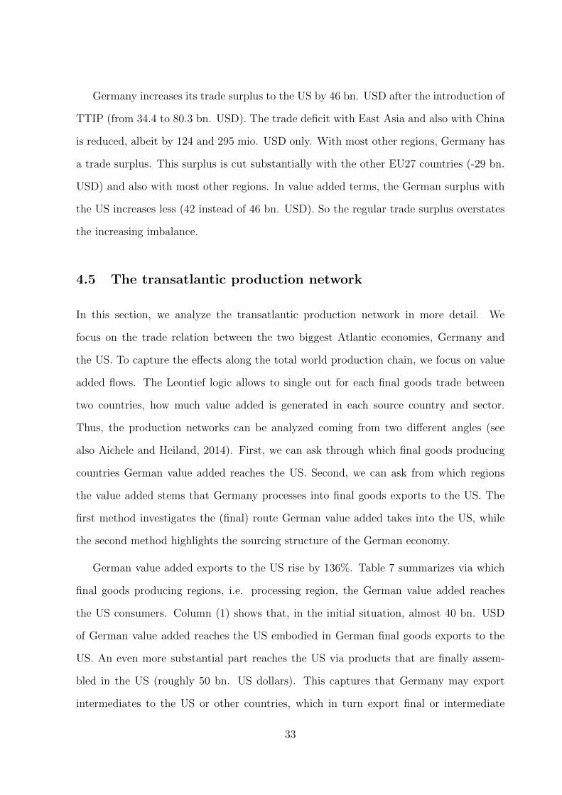
Germany increases its trade surplus to the US by 46 bn. USD after the introduction of

TTIP (from 34.4 to 80.3 bn. USD). The trade deficit with East Asia and also with China

is reduced, albeit by 124 and 295 mio. USD only. With most other regions, Germany has

a trade surplus. This surplus is cut substantially with the other EU27 countries (-29 bn.

USD) and also with most other regions. In value added terms, the German surplus with

the US increases less (42 instead of 46 bn. USD). So the regular trade surplus overstates

the increasing imbalance.

4.5 The transatlantic production network

In this section, we analyze the transatlantic production network in more detail. We

focus on the trade relation between the two biggest Atlantic economies, Germany and

the US. To capture the effects along the total world production chain, we focus on value

added flows. The Leontief logic allows to single out for each final goods trade between

two countries, how much value added is generated in each source country and sector.

Thus, the production networks can be analyzed coming from two different angles (see

also Aichele and Heiland, 2014). First, we can ask through which final goods producing

countries German value added reaches the US. Second, we can ask from which regions

the value added stems that Germany processes into final goods exports to the US. The

first method investigates the (final) route German value added takes into the US, while

the second method highlights the sourcing structure of the German economy.

German value added exports to the US rise by 136%. Table 7 summarizes via which

final goods producing regions, i.e. processing region, the German value added reaches

the US consumers. Column (1) shows that, in the initial situation, almost 40 bn. USD

of German value added reaches the US embodied in German final goods exports to the

US. An even more substantial part reaches the US via products that are finally assem-

bled in the US (roughly 50 bn. US dollars). This captures that Germany may export

intermediates to the US or other countries, which in turn export final or intermediate

33

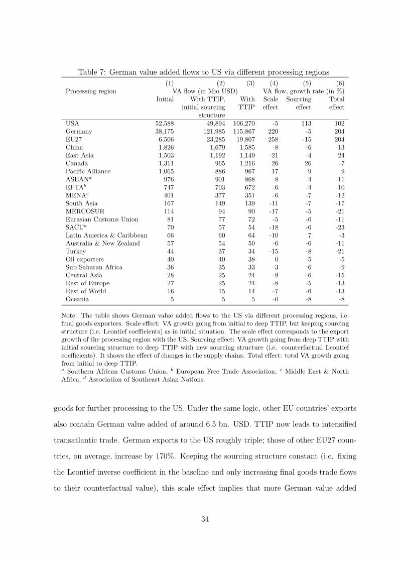
Table 7: German value added flows to US via different processing regions

(1) (2) (3) (4) (5) (6)Processing region VA flow (in Mio USD) VA flow, growth rate (in %)

Initial With TTIP, With Scale Sourcing Totalinitial sourcing TTIP effect effect effect

structureUSA 52,588 49,894 106,270 -5 113 102Germany 38,175 121,985 115,867 220 -5 204EU27 6,506 23,285 19,807 258 -15 204China 1,826 1,679 1,585 -8 -6 -13East Asia 1,503 1,192 1,149 -21 -4 -24Canada 1,311 965 1,216 -26 26 -7Pacific Alliance 1,065 886 967 -17 9 -9ASEANd 976 901 868 -8 -4 -11EFTAb 747 703 672 -6 -4 -10MENAc 401 377 351 -6 -7 -12South Asia 167 149 139 -11 -7 -17MERCOSUR 114 94 90 -17 -5 -21Eurasian Customs Union 81 77 72 -5 -6 -11SACUa 70 57 54 -18 -6 -23Latin America & Caribbean 66 60 64 -10 7 -3Australia & New Zealand 57 54 50 -6 -6 -11Turkey 44 37 34 -15 -8 -21Oil exporters 40 40 38 0 -5 -5Sub-Saharan Africa 36 35 33 -3 -6 -9Central Asia 28 25 24 -9 -6 -15Rest of Europe 27 25 24 -8 -5 -13Rest of World 16 15 14 -7 -6 -13Oceania 5 5 5 -0 -8 -8

Note: The table shows German value added flows to the US via different processing regions, i.e.final goods exporters. Scale effect: VA growth going from initial to deep TTIP, but keeping sourcingstructure (i.e. Leontief coefficients) as in initial situation. The scale effect corresponds to the exportgrowth of the processing region with the US. Sourcing effect: VA growth going from deep TTIP withinitial sourcing structure to deep TTIP with new sourcing structure (i.e. counterfactual Leontiefcoefficients). It shows the effect of changes in the supply chains. Total effect: total VA growth goingfrom initial to deep TTIP.a Southern African Customs Union, b European Free Trade Association, c Middle East & NorthAfrica, d Association of Southeast Asian Nations.

goods for further processing to the US. Under the same logic, other EU countries’ exports

also contain German value added of around 6.5 bn. USD. TTIP now leads to intensified

transatlantic trade. German exports to the US roughly triple; those of other EU27 coun-

tries, on average, increase by 170%. Keeping the sourcing structure constant (i.e. fixing

the Leontief inverse coefficient in the baseline and only increasing final goods trade flows

to their counterfactual value), this scale effect implies that more German value added

34

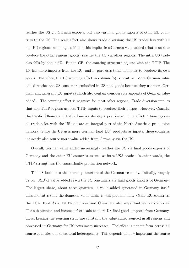
reaches the US via German exports, but also via final goods exports of other EU coun-

tries to the US. The scale effect also shows trade diversion; the US trades less with all

non-EU regions including itself, and this implies less German value added (that is used to

produce the other regions’ goods) reaches the US via other regions. The intra US trade

also falls by about 6%. But in GE, the sourcing structure adjusts with the TTIP. The

US has more imports from the EU, and in part uses them as inputs to produce its own

goods. Therefore, the US sourcing effect in column (5) is positive. More German value

added reaches the US consumers embodied in US final goods because they use more Ger-

man, and generally EU inputs (which also contain considerable amounts of German value

added). The sourcing effect is negative for most other regions. Trade diversion implies

that non-TTIP regions use less TTIP inputs to produce their output. However, Canada,

the Pacific Alliance and Latin America display a positive sourcing effect. These regions

all trade a lot with the US and are an integral part of the North American production

network. Since the US uses more German (and EU) products as inputs, these countries

indirectly also source more value added from Germany via the US.

Overall, German value added increasingly reaches the US via final goods exports of

Germany and the other EU countries as well as intra-USA trade. In other words, the

TTIP strengthens the transatlantic production network.

Table 8 looks into the sourcing structure of the German economy. Initially, roughly

52 bn. USD of value added reach the US consumers via final goods exports of Germany.

The largest share, about three quarters, is value added generated in Germany itself.

This indicates that the domestic value chain is still predominant. Other EU countries,

the USA, East Asia, EFTA countries and China are also important source countries.

The substitution and income effect leads to more US final goods imports from Germany.

Thus, keeping the sourcing structure constant, the value added sourced in all regions and

processed in Germany for US consumers increases. The effect is not uniform across all

source countries due to sectoral heterogeneity. This depends on how important the source

35

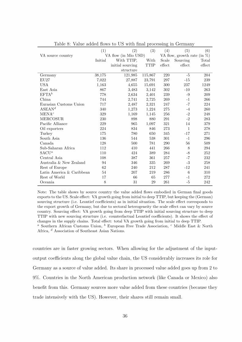
Table 8: Value added flows to US with final processing in Germany

(1) (2) (3) (4) (5) (6)VA source country VA flow (in Mio USD) VA flow, growth rate (in %)

Initial With TTIP, With Scale Sourcing Totalinitial sourcing TTIP effect effect effect

structureGermany 38,175 121,985 115,867 220 -5 204EU27 7,022 27,887 23,791 297 -15 239USA 1,163 4,655 15,691 300 237 1249East Asia 867 3,483 3,142 302 -10 263EFTAb 778 2,634 2,401 239 -9 209China 744 2,741 2,725 269 -1 266Eurasian Customs Union 717 2,487 2,321 247 -7 224ASEANd 340 1,273 1,224 275 -4 260MENAc 329 1,169 1,145 256 -2 248MERCOSUR 230 898 880 291 -2 283Pacific Alliance 229 965 1,097 321 14 379Oil exporters 224 834 846 273 1 278Turkey 175 780 650 345 -17 271South Asia 136 544 538 301 -1 296Canada 128 500 781 290 56 509Sub-Saharan Africa 112 410 441 266 8 294SACUa 110 424 389 284 -8 252Central Asia 108 387 361 257 -7 232Australia & New Zealand 94 346 335 269 -3 258Rest of Europe 62 240 212 287 -12 241Latin America & Caribbean 54 207 219 286 6 310Rest of World 17 66 65 277 -1 272Oceania 8 31 29 261 -5 242

Note: The table shows by source country the value added flows embodied in German final goodsexports to the US. Scale effect: VA growth going from initial to deep TTIP, but keeping the (German)sourcing structure (i.e. Leontief coefficients) as in initial situation. The scale effect corresponds tothe export growth of Germany, but due to sectoral heterogeneity the scale effect can vary by sourcecountry. Sourcing effect: VA growth going from deep TTIP with initial sourcing structure to deepTTIP with new sourcing structure (i.e. counterfactual Leontief coefficients). It shows the effect ofchanges in the supply chains. Total effect: total VA growth going from initial to deep TTIP.a Southern African Customs Union, b European Free Trade Association, c Middle East & NorthAfrica, d Association of Southeast Asian Nations.

countries are in faster growing sectors. When allowing for the adjustment of the input-

output coefficients along the global value chain, the US considerably increases its role for

Germany as a source of value added. Its share in processed value added goes up from 2 to

9%. Countries in the North American production network (like Canada or Mexico) also

benefit from this. Germany sources more value added from these countries (because they

trade intensively with the US). However, their shares still remain small.

36

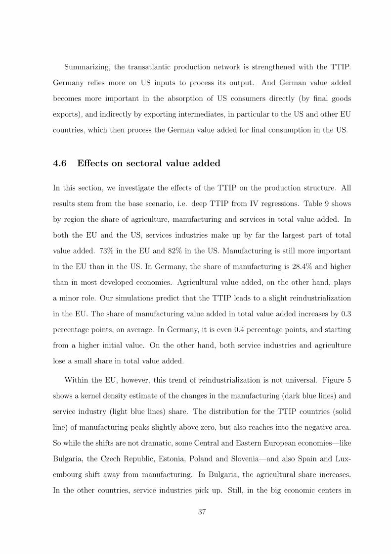
Summarizing, the transatlantic production network is strengthened with the TTIP.

Germany relies more on US inputs to process its output. And German value added

becomes more important in the absorption of US consumers directly (by final goods

exports), and indirectly by exporting intermediates, in particular to the US and other EU

countries, which then process the German value added for final consumption in the US.

4.6 Effects on sectoral value added

In this section, we investigate the effects of the TTIP on the production structure. All

results stem from the base scenario, i.e. deep TTIP from IV regressions. Table 9 shows

by region the share of agriculture, manufacturing and services in total value added. In

both the EU and the US, services industries make up by far the largest part of total

value added. 73% in the EU and 82% in the US. Manufacturing is still more important

in the EU than in the US. In Germany, the share of manufacturing is 28.4% and higher

than in most developed economies. Agricultural value added, on the other hand, plays

a minor role. Our simulations predict that the TTIP leads to a slight reindustrialization

in the EU. The share of manufacturing value added in total value added increases by 0.3

percentage points, on average. In Germany, it is even 0.4 percentage points, and starting

from a higher initial value. On the other hand, both service industries and agriculture

lose a small share in total value added.

Within the EU, however, this trend of reindustrialization is not universal. Figure 5

shows a kernel density estimate of the changes in the manufacturing (dark blue lines) and

service industry (light blue lines) share. The distribution for the TTIP countries (solid

line) of manufacturing peaks slightly above zero, but also reaches into the negative area.

So while the shifts are not dramatic, some Central and Eastern European economies—like

Bulgaria, the Czech Republic, Estonia, Poland and Slovenia—and also Spain and Lux-

embourg shift away from manufacturing. In Bulgaria, the agricultural share increases.

In the other countries, service industries pick up. Still, in the big economic centers in

37

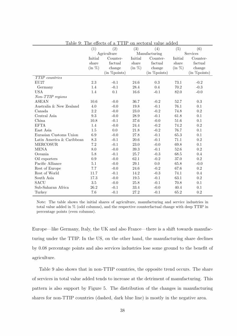
Table 9: The effects of a TTIP on sectoral value added(1) (2) (3) (4) (5) (6)

Agriculture Manufacturing ServicesInitial Counter- Initial Counter- Initial Counter-share factual share factual share factual(in %) change (in %) change (in %) change

(in %points) (in %points) (in %points)TTIP countriesEU27 2.3 -0.1 24.6 0.3 73.1 -0.2

Germany 1.4 -0.1 28.4 0.4 70.2 -0.3USA 1.4 0.1 16.6 -0.1 82.0 -0.0Non-TTIP regionsASEAN 10.6 -0.0 36.7 -0.2 52.7 0.3Australia & New Zealand 4.0 -0.0 19.8 -0.1 76.1 0.1Canada 2.2 -0.0 23.0 -0.2 74.8 0.2Central Asia 9.3 -0.0 28.9 -0.1 61.8 0.1China 10.8 -0.1 37.6 -0.0 51.6 0.1EFTA 1.4 -0.0 24.4 -0.2 74.2 0.2East Asia 1.5 0.0 21.8 -0.2 76.7 0.1Eurasian Customs Union 6.9 -0.0 27.8 -0.1 65.3 0.1Latin America & Caribbean 8.3 -0.1 20.6 -0.1 71.1 0.2MERCOSUR 7.2 -0.1 23.0 -0.0 69.8 0.1MENA 8.0 -0.0 39.3 -0.1 52.6 0.2Oceania 5.8 -0.1 25.7 -0.3 68.5 0.4Oil exporters 0.9 -0.0 62.1 -0.2 37.0 0.2Pacific Alliance 5.1 -0.0 29.1 0.0 65.8 -0.0Rest of Europe 7.7 -0.0 24.6 -0.2 67.6 0.2Rest of World 11.7 -0.1 14.2 -0.3 74.1 0.4South Asia 17.3 -0.0 19.5 -0.1 63.1 0.2SACU 3.5 -0.0 25.8 -0.1 70.8 0.1Sub-Saharan Africa 26.2 -0.1 33.4 -0.0 40.4 0.1Turkey 7.6 -0.1 27.2 -0.1 65.2 0.2

Note: The table shows the initial shares of agriculture, manufacturing and service industries intotal value added in % (odd columns), and the respective counterfactual change with deep TTIP inpercentage points (even columns).

Europe—like Germany, Italy, the UK and also France—there is a shift towards manufac-

turing under the TTIP. In the US, on the other hand, the manufacturing share declines

by 0.08 percentage points and also services industries lose some ground to the benefit of

agriculture.

Table 9 also shows that in non-TTIP countries, the opposite trend occurs. The share

of services in total value added tends to increase at the detriment of manufacturing. This

pattern is also support by Figure 5. The distribution of the changes in manufacturing

shares for non-TTIP countries (dashed, dark blue line) is mostly in the negative area.

38

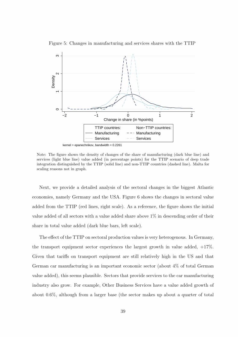
Figure 5: Changes in manufacturing and services shares with the TTIP

01

23

Den

sity

−2 −1 0 1 2Change in share (in %points)

TTIP countries: Non−TTIP countries:Manufacturing ManufacturingServices Services

kernel = epanechnikov, bandwidth = 0.2261

Kernel density estimate

Note: The figure shows the density of changes of the share of manufacturing (dark blue line) andservices (light blue line) value added (in percentage points) for the TTIP scenario of deep tradeintegration distinguished by the TTIP (solid line) and non-TTIP countries (dashed line). Malta forscaling reasons not in graph.

Next, we provide a detailed analysis of the sectoral changes in the biggest Atlantic

economies, namely Germany and the USA. Figure 6 shows the changes in sectoral value

added from the TTIP (red lines, right scale). As a reference, the figure shows the initial

value added of all sectors with a value added share above 1% in descending order of their

share in total value added (dark blue bars, left scale).

The effect of the TTIP on sectoral production values is very heterogenous. In Germany,

the transport equipment sector experiences the largest growth in value added, +17%.

Given that tariffs on transport equipment are still relatively high in the US and that

German car manufacturing is an important economic sector (about 4% of total German

value added), this seems plausible. Sectors that provide services to the car manufacturing

industry also grow. For example, Other Business Services have a value added growth of

about 0.6%, although from a larger base (the sector makes up about a quarter of total

39

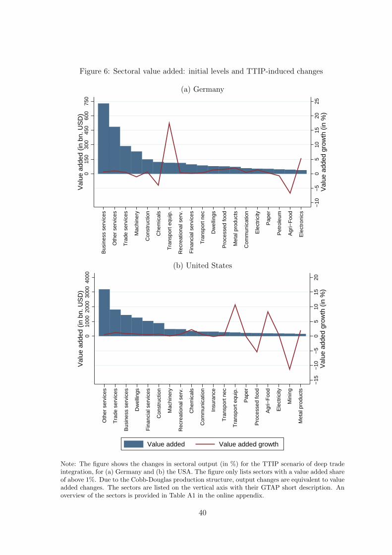
Figure 6: Sectoral value added: initial levels and TTIP-induced changes

(a) Germany

−10

−5

05

1015

2025

Val

ue a

dded

gro

wth

(in

%)

015

030

045

060

075

0−

150

−30

0

Val

ue a

dded

(in

bn.

US

D)

Bus

ines

s se

rvic

es

Oth

er s

ervi

ces

Tra

de s

ervi

ces

Mac

hine

ry

Con

stru

ctio

n

Che

mic

als

Tra

nspo

rt e

quip

.

Rec

reat

iona

l ser

v.

Fin

anci

al s

ervi

ces

Tra

nspo

rt n

ec

Dw

ellin

gs

Pro

cess

ed fo

od

Met

al p

rodu

cts

Com

mun

icat

ion

Ele

ctric

ity

Pap

er

Pet

role

um

Agr

i−F

ood

Ele

ctro

nics

Value added (in bn. USD) Value added growth (in %)(b) United States

−15

−10

−5

05

1015

20V

alue

add

ed g

row

th (

in %

)

010

0020

0030

0040

00−

1000

−20

00−

3000

Val

ue a

dded

(in

bn.

US

D)

Oth

er s

ervi

ces

Tra

de s

ervi

ces

Bus

ines

s se

rvic

es

Dw

ellin

gs

Fin

anci

al s

ervi

ces

Con

stru

ctio

n

Mac

hine

ry

Rec

reat

iona

l ser

v.

Che

mic

als

Com

mun

icat

ion

Insu

ranc

e

Tra

nspo

rt n

ec

Tra

nspo

rt e

quip

.

Pap

er

Pro

cess

ed fo

od

Agr

i−F

ood

Ele

ctric

ity

Min

ing

Met

al p

rodu

cts

Value added Value added growth

Note: The figure shows the changes in sectoral output (in %) for the TTIP scenario of deep tradeintegration, for (a) Germany and (b) the USA. The figure only lists sectors with a value added shareof above 1%. Due to the Cobb-Douglas production structure, output changes are equivalent to valueadded changes. The sectors are listed on the vertical axis with their GTAP short description. Anoverview of the sectors is provided in Table A1 in the online appendix.

40

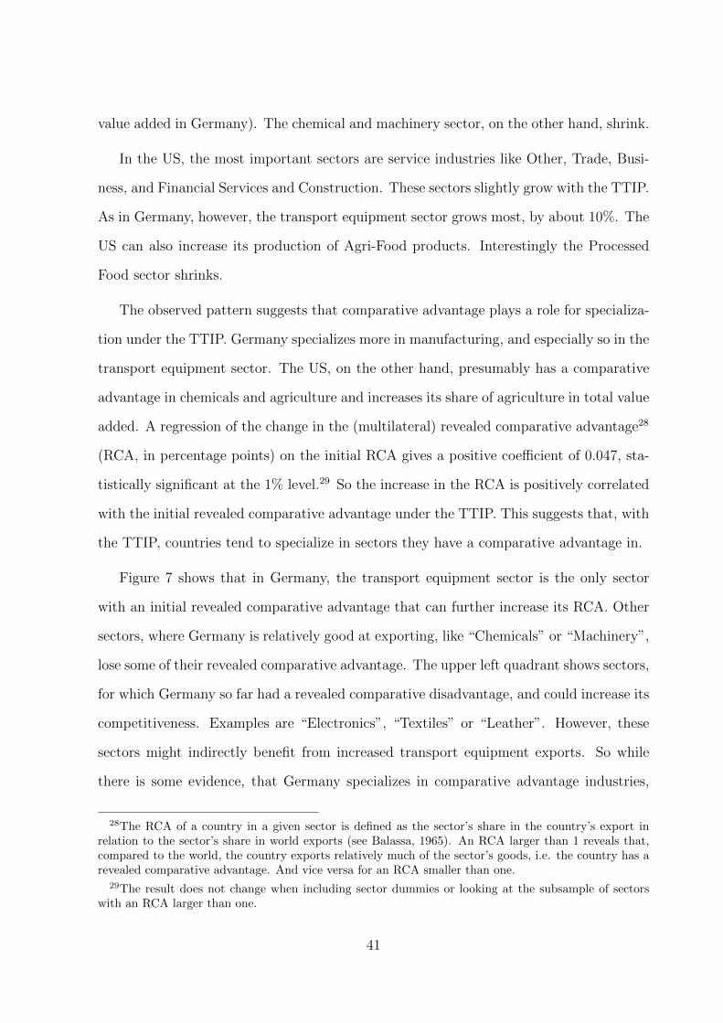
value added in Germany). The chemical and machinery sector, on the other hand, shrink.

In the US, the most important sectors are service industries like Other, Trade, Busi-

ness, and Financial Services and Construction. These sectors slightly grow with the TTIP.

As in Germany, however, the transport equipment sector grows most, by about 10%. The

US can also increase its production of Agri-Food products. Interestingly the Processed

Food sector shrinks.

The observed pattern suggests that comparative advantage plays a role for specializa-

tion under the TTIP. Germany specializes more in manufacturing, and especially so in the

transport equipment sector. The US, on the other hand, presumably has a comparative

advantage in chemicals and agriculture and increases its share of agriculture in total value

added. A regression of the change in the (multilateral) revealed comparative advantage28

(RCA, in percentage points) on the initial RCA gives a positive coefficient of 0.047, sta-

tistically significant at the 1% level.29 So the increase in the RCA is positively correlated

with the initial revealed comparative advantage under the TTIP. This suggests that, with

the TTIP, countries tend to specialize in sectors they have a comparative advantage in.

Figure 7 shows that in Germany, the transport equipment sector is the only sector

with an initial revealed comparative advantage that can further increase its RCA. Other

sectors, where Germany is relatively good at exporting, like “Chemicals” or “Machinery”,

lose some of their revealed comparative advantage. The upper left quadrant shows sectors,

for which Germany so far had a revealed comparative disadvantage, and could increase its

competitiveness. Examples are “Electronics”, “Textiles” or “Leather”. However, these

sectors might indirectly benefit from increased transport equipment exports. So while

there is some evidence, that Germany specializes in comparative advantage industries,

28The RCA of a country in a given sector is defined as the sector’s share in the country’s export inrelation to the sector’s share in world exports (see Balassa, 1965). An RCA larger than 1 reveals that,compared to the world, the country exports relatively much of the sector’s goods, i.e. the country has arevealed comparative advantage. And vice versa for an RCA smaller than one.

29The result does not change when including sector dummies or looking at the subsample of sectorswith an RCA larger than one.

41

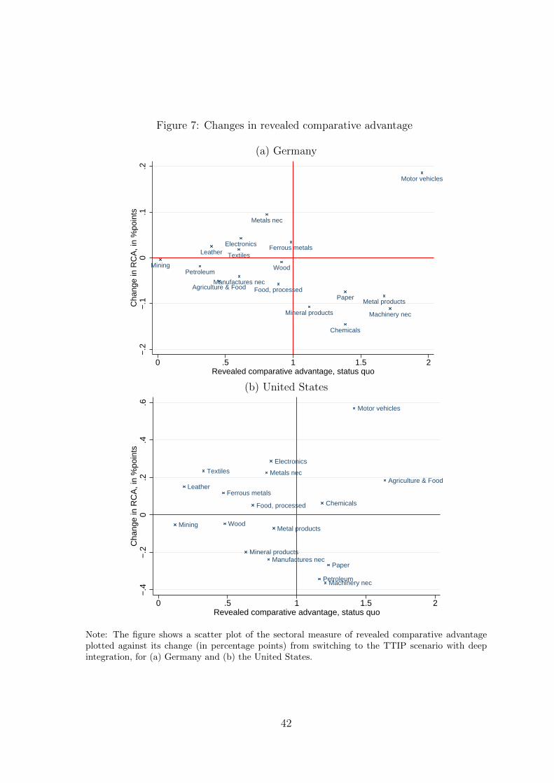
Figure 7: Changes in revealed comparative advantage

(a) Germany

Agriculture & Food

Mining

Food, processed

TextilesLeather

Wood

Paper

Petroleum

Chemicals

Mineral products

Ferrous metals

Metals nec

Metal products

Motor vehicles

Electronics

Machinery nec

Manufactures nec

−.2

−.1

0.1

.2C

hang

e in

RC

A, i

n %

poin

ts

0 .5 1 1.5 2Revealed comparative advantage, status quo

(b) United States

Agriculture & Food

Mining

Food, processed

Textiles

Leather

Wood

Paper

Petroleum

Chemicals

Mineral products

Ferrous metals

Metals nec

Metal products

Motor vehicles

Electronics

Machinery nec

Manufactures nec

−.4

−.2

0.2

.4.6

Cha

nge

in R

CA

, in

%po

ints

0 .5 1 1.5 2Revealed comparative advantage, status quo

Note: The figure shows a scatter plot of the sectoral measure of revealed comparative advantageplotted against its change (in percentage points) from switching to the TTIP scenario with deepintegration, for (a) Germany and (b) the United States.

42

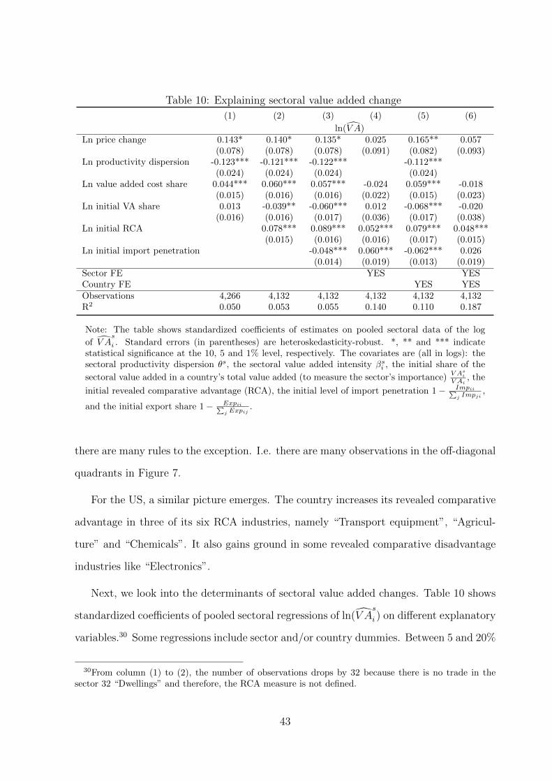
Table 10: Explaining sectoral value added change

(1) (2) (3) (4) (5) (6)

ln(V A)Ln price change 0.143* 0.140* 0.135* 0.025 0.165** 0.057

(0.078) (0.078) (0.078) (0.091) (0.082) (0.093)Ln productivity dispersion -0.123*** -0.121*** -0.122*** -0.112***

(0.024) (0.024) (0.024) (0.024)Ln value added cost share 0.044*** 0.060*** 0.057*** -0.024 0.059*** -0.018

(0.015) (0.016) (0.016) (0.022) (0.015) (0.023)Ln initial VA share 0.013 -0.039** -0.060*** 0.012 -0.068*** -0.020

(0.016) (0.016) (0.017) (0.036) (0.017) (0.038)Ln initial RCA 0.078*** 0.089*** 0.052*** 0.079*** 0.048***

(0.015) (0.016) (0.016) (0.017) (0.015)Ln initial import penetration -0.048*** 0.060*** -0.062*** 0.026

(0.014) (0.019) (0.013) (0.019)Sector FE YES YESCountry FE YES YESObservations 4,266 4,132 4,132 4,132 4,132 4,132R2 0.050 0.053 0.055 0.140 0.110 0.187

Note: The table shows standardized coefficients of estimates on pooled sectoral data of the log

of V As

i . Standard errors (in parentheses) are heteroskedasticity-robust. *, ** and *** indicatestatistical significance at the 10, 5 and 1% level, respectively. The covariates are (all in logs): thesectoral productivity dispersion θs, the sectoral value added intensity βs

i , the initial share of the

sectoral value added in a country’s total value added (to measure the sector’s importance)V As

i

V Ai, the

initial revealed comparative advantage (RCA), the initial level of import penetration 1− Impii∑j Impji

,

and the initial export share 1− Expii∑j Expij

.

there are many rules to the exception. I.e. there are many observations in the off-diagonal

quadrants in Figure 7.

For the US, a similar picture emerges. The country increases its revealed comparative

advantage in three of its six RCA industries, namely “Transport equipment”, “Agricul-

ture” and “Chemicals”. It also gains ground in some revealed comparative disadvantage

industries like “Electronics”.

Next, we look into the determinants of sectoral value added changes. Table 10 shows

standardized coefficients of pooled sectoral regressions of ln(V As

i ) on different explanatory

variables.30 Some regressions include sector and/or country dummies. Between 5 and 20%

30From column (1) to (2), the number of observations drops by 32 because there is no trade in thesector 32 “Dwellings” and therefore, the RCA measure is not defined.

43

of the variation in sectoral changes of value added can be explained with our regressions.

Aside from country or sector dummies, a sector’s productivity dispersion has the highest

explanatory power for sectoral changes in value added. A one standard deviation increase

of ln θ leads to a reduction of lnV A of about 0.12 of a standard deviation. In highly

dispersed sectors, i.e. sectors with a high θ, output reacts less to our trade policy shock.31

In more dispersed sectors sectoral varieties are less substitutable. Consequently, trade

cost changes have a smaller impact on sectoral trade and sectoral output. The second

most important explanatory variable is revealed comparative advantage. Sectors with a

higher initial revealed comparative advantage experience stronger growth in sectoral value

added. So with the TTIP, countries tend to specialize in sectors in which they have a

comparative advantage. Higher import penetration, on the other hand, deters sectoral

growth. Labor-intensive sectors have higher value added growth. A sector’s initial share

in total value added is negatively related to sectoral growth. However, the coefficient is

not statistically different from zero in most cases. So there is some weak evidence, that

countries do not necessarily grow in important sectors. An alternative explanation for

this finding is that growth rates are smaller in large sectors because they start from a

higher initial output level.

4.7 Welfare effects of the TTIP

In our baseline scenario, we assume that the TTIP will be a deep PTA. Given that most

new PTAs between developed countries are PTAs of the new generation and go way be-

yond a mere reduction or elimination of bilateral tariffs, this choice seems reasonable.

Moreover, the negotiating mandate that EU member states have given to the EU Com-

mission makes the high level of ambition for the agreement very clear. Nonetheless, we

contrast the so obtained results with alternative TTIP scenarios in the next section. In a

31Note that, since productivity is sector-specific but does not vary across countries, we cannot identifythe coefficient on sectoral productivity dispersion once we include sector fixed effects.

44

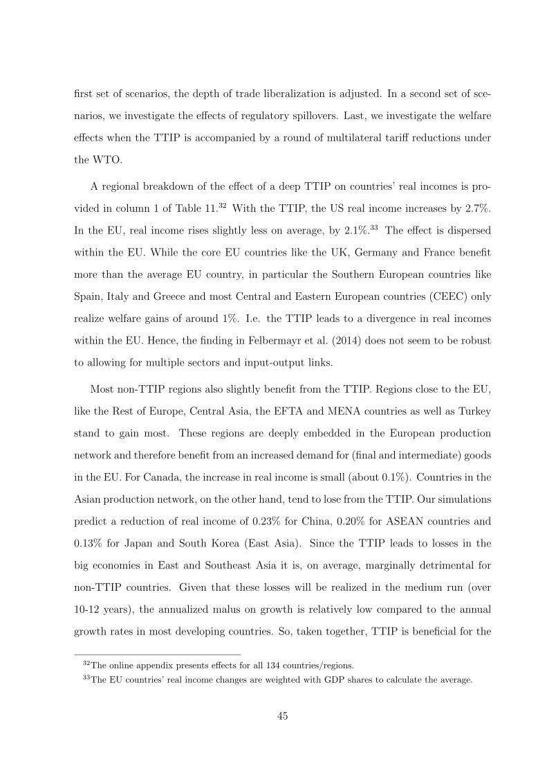
first set of scenarios, the depth of trade liberalization is adjusted. In a second set of sce-

narios, we investigate the effects of regulatory spillovers. Last, we investigate the welfare

effects when the TTIP is accompanied by a round of multilateral tariff reductions under

the WTO.

A regional breakdown of the effect of a deep TTIP on countries’ real incomes is pro-

vided in column 1 of Table 11.32 With the TTIP, the US real income increases by 2.7%.

In the EU, real income rises slightly less on average, by 2.1%.33 The effect is dispersed

within the EU. While the core EU countries like the UK, Germany and France benefit

more than the average EU country, in particular the Southern European countries like

Spain, Italy and Greece and most Central and Eastern European countries (CEEC) only

realize welfare gains of around 1%. I.e. the TTIP leads to a divergence in real incomes

within the EU. Hence, the finding in Felbermayr et al. (2014) does not seem to be robust

to allowing for multiple sectors and input-output links.

Most non-TTIP regions also slightly benefit from the TTIP. Regions close to the EU,

like the Rest of Europe, Central Asia, the EFTA and MENA countries as well as Turkey

stand to gain most. These regions are deeply embedded in the European production

network and therefore benefit from an increased demand for (final and intermediate) goods

in the EU. For Canada, the increase in real income is small (about 0.1%). Countries in the

Asian production network, on the other hand, tend to lose from the TTIP. Our simulations

predict a reduction of real income of 0.23% for China, 0.20% for ASEAN countries and

0.13% for Japan and South Korea (East Asia). Since the TTIP leads to losses in the

big economies in East and Southeast Asia it is, on average, marginally detrimental for

non-TTIP countries. Given that these losses will be realized in the medium run (over

10-12 years), the annualized malus on growth is relatively low compared to the annual

growth rates in most developing countries. So, taken together, TTIP is beneficial for the

32The online appendix presents effects for all 134 countries/regions.33The EU countries’ real income changes are weighted with GDP shares to calculate the average.

45

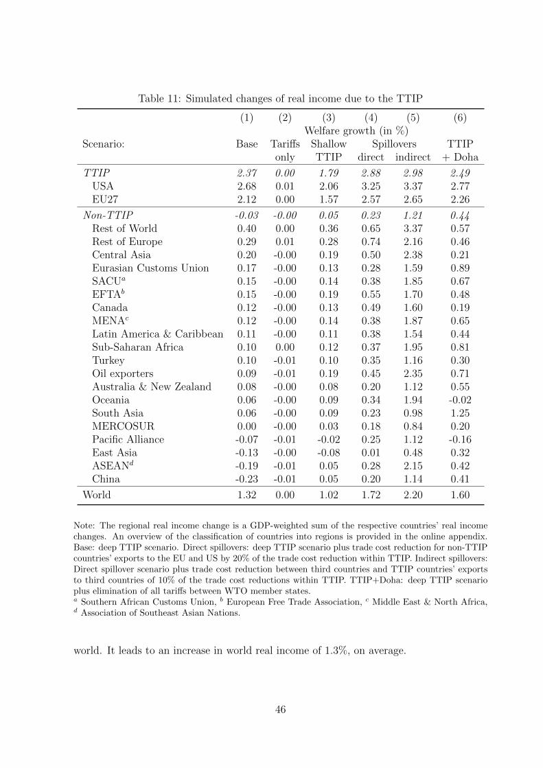
Table 11: Simulated changes of real income due to the TTIP

(1) (2) (3) (4) (5) (6)Welfare growth (in %)

Scenario: Base Tariffs Shallow Spillovers TTIPonly TTIP direct indirect + Doha

TTIP 2.37 0.00 1.79 2.88 2.98 2.49USA 2.68 0.01 2.06 3.25 3.37 2.77EU27 2.12 0.00 1.57 2.57 2.65 2.26

Non-TTIP -0.03 -0.00 0.05 0.23 1.21 0.44Rest of World 0.40 0.00 0.36 0.65 3.37 0.57Rest of Europe 0.29 0.01 0.28 0.74 2.16 0.46Central Asia 0.20 -0.00 0.19 0.50 2.38 0.21Eurasian Customs Union 0.17 -0.00 0.13 0.28 1.59 0.89SACUa 0.15 -0.00 0.14 0.38 1.85 0.67EFTAb 0.15 -0.00 0.19 0.55 1.70 0.48Canada 0.12 -0.00 0.13 0.49 1.60 0.19MENAc 0.12 -0.00 0.14 0.38 1.87 0.65Latin America & Caribbean 0.11 -0.00 0.11 0.38 1.54 0.44Sub-Saharan Africa 0.10 0.00 0.12 0.37 1.95 0.81Turkey 0.10 -0.01 0.10 0.35 1.16 0.30Oil exporters 0.09 -0.01 0.19 0.45 2.35 0.71Australia & New Zealand 0.08 -0.00 0.08 0.20 1.12 0.55Oceania 0.06 -0.00 0.09 0.34 1.94 -0.02South Asia 0.06 -0.00 0.09 0.23 0.98 1.25MERCOSUR 0.00 -0.00 0.03 0.18 0.84 0.20Pacific Alliance -0.07 -0.01 -0.02 0.25 1.12 -0.16East Asia -0.13 -0.00 -0.08 0.01 0.48 0.32ASEANd -0.19 -0.01 0.05 0.28 2.15 0.42China -0.23 -0.01 0.05 0.20 1.14 0.41

World 1.32 0.00 1.02 1.72 2.20 1.60

Note: The regional real income change is a GDP-weighted sum of the respective countries’ real incomechanges. An overview of the classification of countries into regions is provided in the online appendix.Base: deep TTIP scenario. Direct spillovers: deep TTIP scenario plus trade cost reduction for non-TTIPcountries’ exports to the EU and US by 20% of the trade cost reduction within TTIP. Indirect spillovers:Direct spillover scenario plus trade cost reduction between third countries and TTIP countries’ exportsto third countries of 10% of the trade cost reductions within TTIP. TTIP+Doha: deep TTIP scenarioplus elimination of all tariffs between WTO member states.a Southern African Customs Union, b European Free Trade Association, c Middle East & North Africa,d Association of Southeast Asian Nations.

world. It leads to an increase in world real income of 1.3%, on average.

46

4.8 Welfare effects of TTIP—Alternative scenarios

To get a better sense of the magnitude of the effects, we now vary the intensity of trade

cost reductions the TTIP may provide. First, the TTIP may only lead to the elimination

of tariffs. Second, it may only achieve a shallow instead of a deep reduction of NTMs.

The results are presented in columns 2 and 3 of Table 11. The tariffs between the EU and

the US are already relatively low. An elimination of the bilateral tariffs therefore does not

lead to any measurable gains from trade. If the negotiated TTIP agreement is shallow

the gains from trade fall slightly short of the ones in the baseline scenario. However, the

expected welfare gains are still sizable, 2.1% higher real income for the US and 1.6% for

the EU, on average. The negative consequences for third countries are also less severe.

Non-TTIP countries slightly raise their real income by 0.05%, on average.

Next, we discuss two scenarios where the TTIP also leads to spillovers. The rationale

behind these scenarios is that the TTIP might lead to unified transatlantic product stan-

dards due to regulatory cooperation, or the mutual recognition of standards (see, e.g.,

the discussions in WTO, 2012). This potentially leads to trade cost reductions for firms

who export to the US and the EU (direct spillovers) because they only have to abide by

one standard for exports to both regions.34 If the TTIP shapes global product standards,

the trade cost reductions may even spill over to trade between third countries (indirect

spillovers).35 Whether spillovers are likely is not clear. So far, there is little empirical

evidence pointing toward positive third-country effects of mutual recognition agreements

or standard harmonization (see Chen and Mattoo, 2008; Baller, 2007). And if so, it seems

to be crucial that the countries can adopt the (high) standards. So especially developing

countries are hurt by standard harmonization.36 Therefore, we use rather ad-hoc assump-

34For the simulation, we work with a trade cost reduction of 20% of the full PTA effect that arisesbetween the TTIP countries.

35We assume that the indirect spillovers amount to 10% of the trade cost reduction between the TTIPcountries.

36Cadot et al. (2012) show that regulatory cooperation in North-South PTAs deters South-South trade.

47

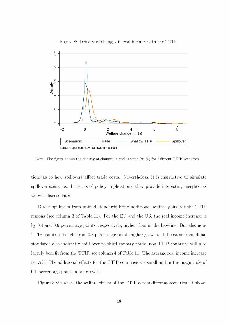
Figure 8: Density of changes in real income with the TTIP

0.5

11.

52

2.5

Den

sity

−2 0 2 4 6 8Welfare change (in %)

Scenarios: Base Shallow TTIP Spillover

kernel = epanechnikov, bandwidth = 0.1091

Note: The figure shows the density of changes in real income (in %) for different TTIP scenarios.

tions as to how spillovers affect trade costs. Nevertheless, it is instructive to simulate

spillover scenarios. In terms of policy implications, they provide interesting insights, as

we will discuss later.

Direct spillovers from unified standards bring additional welfare gains for the TTIP

regions (see column 3 of Table 11). For the EU and the US, the real income increase is

by 0.4 and 0.6 percentage points, respectively, higher than in the baseline. But also non-

TTIP countries benefit from 0.3 percentage points higher growth. If the gains from global

standards also indirectly spill over to third country trade, non-TTIP countries will also

largely benefit from the TTIP, see column 4 of Table 11. The average real income increase

is 1.2%. The additional effects for the TTIP countries are small and in the magnitude of

0.1 percentage points more growth.

Figure 8 visualizes the welfare effects of the TTIP across different scenarios. It shows

48

the density of the distribution of real income changes. The dark blue line represents

the baseline scenario. It has two peaks, one around zero which captures the real income

effects for non-TTIP countries and a second peak to the right (around 2%) which traces the

effects on TTIP countries. With a shallow TTIP (light blue line), the two peaks slightly

move together. The effects for both TTIP and non-TTIP countries are dampened. With

direct spillovers (orange line), the distribution moves to the right. All countries tend to be

better off and there are virtually no negative real income effects. What is more, the shift

of the first peak is relatively larger. So non-TTIP countries benefit more from spillovers.

Nevertheless, the TTIP countries would also benefit from unified product standards.

These findings imply that a TTIP with spillovers is a win-win situation for the TTIP

insiders as well as outsiders. Consequently, an inclusive TTIP that, e.g., interprets rules

of origins fairly generously can increase good-will in third countries. This in turn may

stimulate multilateral trade liberalization. But of course it all hinges on the (implicit)

assumption, that developing countries can meet the set standards.

Last, we simulate the effects of a TTIP in a world where a further wave of multilateral

tariff liberalizations could be achieved in the Doha round. More specifically, the simu-

lation is based on eliminating all tariffs between WTO member states. If the TTIP is

inclusive, i.e. the agreement is such that trade diversion in third countries is limited as

best as possible, it may help to stimulate another round of multilateral tariff liberaliza-

tion. Indeed, the international economics literature discusses whether PTAs constitute a

“building block” or “stumbling block” for free trade (see Bhagwati, 1991, for an introduc-

tion of the concepts). In the TTIP + Doha scenario, we find that real income rises for

all regions except Oceania and the Pacific Alliance. The additional effects for the TTIP

countries are relatively small. However, for some regions like South Asia, Sub-Saharan

Africa or the Eurasian Customs Union a sizeable positive impulse for the economy can be

expected. These regions are still characterized by considerable MFN tariffs.

Summarizing, only a deep TTIP will reap the full gains from trade for TTIP countries.

49

They are in the order of magnitude of 2 to 3% real income growth. If the TTIP is

accompanied by spillover effects, adverse effects for other regions of the world can be

prevented and instead turned into small welfare increases as well. This is also beneficial

for TTIP countries. Especially from the point of view of developing countries, it is highly

desirable to accompany the TTIP by another round of multilateral trade liberalization.

This will raise real income in all regions as well.

5 Conclusion

A number of systemically relevant preferential trade agreements (PTAs) are under ne-

gotiation. The largest of these mega-regionals is the proposed Transatlantic Trade and

Investment Partnership (TTIP). In this paper, we have extended the recent multi-country,

multi-industry Ricardian trade model by Caliendo and Parro (2014) so that it features

PTAs, the costs of non-tariff measures (NTMs), and also covers services trade. We use the

gravity equation generated by the model to estimate the Frechet parameters governing

the world-wide dispersion of productivities within sectors and the trade cost reductions

achieved by existing shallow and deep PTAs. We simulate the model to quantify the

trade and welfare effects that a deep TTIP could have. However, the model could also be

applied to PTAs, or to trade policy initiatives at the multilateral level.

The main assumption of our quantitative experiment is that the TTIP eliminates

tariffs between EU countries and the US and lowers the costs of NTMs by the amount

empirically identified for existing bilateral agreements. We find that the potential effects

of the TTIP are quite substantial: per capita income could go up by between 2% and 3% in

the EU and US, respectively. Average per capita income in the world would also increase,

but some non-TTIP countries, mostly in East and Southeast Asia would lose. These

effects are driven by a strong amount of trade creation within the TTIP. The framework

is ideally suited to study the effects of the agreement on the structure of regional and

50

global production networks. Our results suggest that the TTIP would strengthen trade

in parts and components across the Atlantic, thereby creating a transatlantic production

network.

Our framework is close to recent work surveyed by Costinot and Rodrıguez-Clare

(2014). New quantitative trade theory uses parsimonious trade models and shows how

they can be brought to the data by structurally estimating the key parameters. For the

time being, these frameworks are only starting to be applied to the analysis of real trade

policy initiatives; most existing work still uses more traditional large-scale computable

general equilibrium (CGE) models. While the availability of industry-level trade and out-

put data, the information on existing PTAs, and the state-of-the-art of econometric tools

has much improved over the last years, there is particular need for further work in at least

four areas: First, the unbiased econometric estimation of structural parameters requires

quasi-experimental variation and appropriate methods. This remains an important area

for future work. Second, top-down approaches to NTMs, as used in this paper, differ from

bottom-up assessments based on Francois et al. (2009). Understanding this discrepancy

is key if one wants to narrow the interval of welfare predictions found in studies with

different approaches to NTMs. Third, both traditional CGE models as well as the frame-

works surveyed by Costinot and Rodrıguez-Clare (2014) neglect foreign direct investment.

This is particularly important in the transatlantic context. Fourth, estimates presented

in this paper may underestimate the true effects as they do not account for effects of

trade liberalization on the incentives to develop new products or engineer new processes.

A tractable dynamic framework would be highly welcome.

51

References

Aichele, Rahel and Inga Heiland, “Where is the Value Added? Trade Liberalization and

Production Networks,” Technical Report, mimeo 2014.

Alvarez, Fernando and Robert Jr. Lucas, “General equilibrium analysis of the Eaton-

Kortum model of international trade,” Journal of Monetary Economics, September

2007, 54 (6), 1726–1768.

Anderson, James E., Mario Larch, and Yoto V. Yotov, “On the Effects of the Transatlantic

Trade and Investment Partnership on Trade and Capital Accumulation,” Technical

Report, Boston University 2014.

Balassa, Bela, “Trade Liberalization and Revealed Comparative Advantage,” The Manch-

ester School, 1965, 33 (2), 99–123.

Baldwin, Richard, “21st Century Regionalism: Filling the gap between 21st century trade

and 20th century trade rules,” CEPR Policy Insight No. 56, Center for Economic Policy

Research May 2011.

and Dany Jaimovich, “Are Free Trade Agreements contagious?,” Journal of Interna-

tional Economics, 2012, 88 (1), 1 – 16.

Baller, Silja, Trade Effects Of Regional Standards Liberalization : A Heterogeneous Firms

Approach, The World Bank, 2007.

Bhagwati, Jagdish N., The World Trading System at Risk, Princeton University Press,

1991.

Cadot, Olivier, Anne-Celia Disdier, and Lionel Fontagne, “North-South Standards Har-

monization and International Trade,” CEPR Discussion Papers 8767, Centre for Eco-

nomic Policy Research January 2012.

52

Caliendo, Lorenzo and Fernando Parro, “Estimates of the Trade and Welfare Effects of

NAFTA,” Review of Economic Studies, 2014, forthcoming.

Chen, Maggie Xiaoyang and Aaditya Mattoo, “Regionalism in standards: good or bad

for trade?,” Canadian Journal of Economics, August 2008, 41 (3), 838–863.

Cipollina, Maria and Luca Salvatici, “Reciprocal Trade Agreements in Gravity Models:

A Meta-Analysis,” Review of International Economics, February 2010, 18 (1), 63–80.

Costinot, Arnaud and Andres Rodrıguez-Clare, “Trade Theory with Numbers: Quanti-

fying the Consequences of Globalization,” in Gita Gopinath, Elhanan Helpman, and

Kenneth Rogoff, eds., Handbook of International Economics, Vol. 4 2014, chapter 4,

pp. 197–261.

Dekle, Robert, Jonathan Eaton, and Samuel Kortum, “Global Rebalancing with Gravity:

Measuring the Burden of Adjustment,” IMF Staff Papers, July 2008, 55 (3), 511–540.

Dur, Andreas, Leonardo Baccini, and Manfred Elsig, “The Design of International Trade

Agreements: Introducing a New Database,” Review of International Organizations,

2014, 9 (3), 353–375.

Eaton, Jonathan and Samuel Kortum, “Technology, Geography, and Trade,” Economet-

rica, September 2002, 70 (5), 1741–1779.

Egger, Hartmut, Peter Egger, and David Greenaway, “The trade structure effects of

endogenous regional trade agreements,” Journal of International Economics, 2008, 74

(2), 278 – 298.

Egger, Peter, Joseph Francois, Miriam Manchin, and Douglas Nelson, “Non- Tariff Barri-

ers, Integration, and the Trans-Atlantic Economy,” Technical Report, paper prepared

for the 60th Panel Meeting of Economic Policy, October 2014, Rom 2014.

53

, Mario Larch, and Kevin E Staub, “Trade Preferences and Bilateral Trade in Goods and

Services: A Structural Approach,” CEPR Discussion Papers 9051, C.E.P.R. Discussion

Papers July 2012.

, , Kevin E. Staub, and Rainer Winkelmann, “The Trade Effects of Endogenous Pref-

erential Trade Agreements,” American Economic Journal: Economic Policy, August

2011, 3 (3), 113–43.

Felbermayr, Gabriel, Benedikt Heid, and Sybille Lehwald, “Transatlantic Free Trade:

Winners, Losers, and Necessary Accompanying Measures,” Law and Business Review

of the Americas, 2013, 19 (4), 445–484.

, , Mario Larch, and Erdal Yalcin, “Macroeconomic potentials of transatlantic free

trade: A high resolution perspective for Europe and the world,” Technical Report,

paper prepared for the 60th Panel Meeting of Economic Policy, October 2014 2014.

Fontagne, Lionel, Julien Gourdon, and Sebastian Jean, “Transatlantic Trade: Whither

Partnership, Which Economic Consequences?,” CEPII Policy Brief No. 2013-01, CEPII

September 2013.

Francois, Joseph, Hans van Meijl, and Frank van Tongeren, “Trade liberalization in the

Doha Development Round,” Economic Policy, April 2005, 20 (42), 349–391.

, Koen Berden, Saara Tamminen, Martin Thelle, and Paul Wymenga, “NonTariff Mea-

sures in EU-US Trade and Investment – An Economic Analysis,” Technical Report 2009.

Study commissioned by the European Commission, DG Trade, ECORYS Netherland

BV.

, Miriam Manchin, Hanna Norberg, Olga Pindyuk, and Patrick Tomberger, “Reducing

Transatlantic Barriers to Trade and Investment. An Economic Assessment,” Technical

Report, Centre for Economic Policy Research 2013.

54

Head, Keith and Thierry Mayer, “Gravity Equations: Workhorse,Toolkit, and Cook-

book,” in G. Gopinath, E. Helpman, and K. Rogoff, eds., Handbook of International

Economics, Vol. 4 2014, chapter 3, pp. 131–195.

Hertel, T.W., ed., Global Trade Analysis: Modeling and Applications, Cambridge Univer-

sity Press, 1997.

Johnson, Robert C. and Guillermo Noguera, “Accounting for intermediates: Production

sharing and trade in value added,” Journal of International Economics, March 2012,

86 (2), 224–236.

Koopman, Robert, Zhi Wang, and Shang-Jin Wei, “Tracing Value-added and Double

Counting in Gross Exports,” American Economic Review, 2014, 104 (2), 459–494.

Krugman, Paul, “Scale Economies, Product Differentiation, and the Pattern of Trade,”

The American Economic Review, 1980, 70 (5), 950–959.

Martin, Philippe, Thierry Mayer, and Mathias Thoenig, “The Geography of Conflicts and

Regional Trade Agreements,” American Economic Journal: Macroeconomics, October

2012, 4 (4), 1–35.

Wang, Zhi, Shang-Jin Wei, and Kunfu Zhu, “Quantifying International Production Shar-

ing at the Bilateral and Sector Levels,” NBER Working Paper No. 19677, National

Bureau of Economic Research November 2013.

WTO, World Trade Report 2012—Trade and public policies: A closer look at non-tariff

measures in the 21st century, World Trade Organization, 2012.

55

Online Appendix to

Going Deep: The Trade and Welfare Effects of TTIP

CESifo Working Paper No. 5150, 2014

Rahel Aichele∗, Gabriel Felbermayr† and Inga Heiland‡

∗ifo Institute–Leibniz Institute for Economic Research at the University of Munich, Poschingerstr. 5,81679 Munich, Germany and CESifo.†ifo Institute–Leibniz Institute for Economic Research at the University of Munich, Ludwig-

Maximilians-University Munich, CESifo, and GEP.‡ifo Institute–Leibniz Institute for Economic Research at the University of Munich.

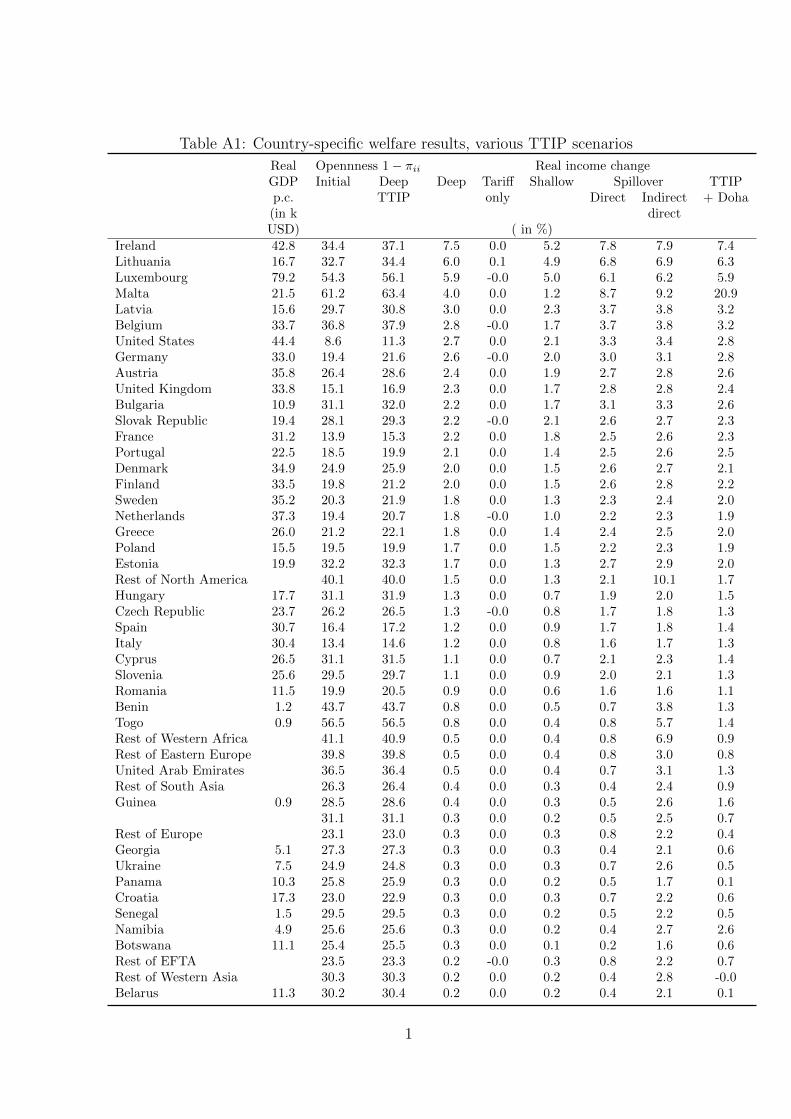
Table A1: Country-specific welfare results, various TTIP scenarios

Real Opennness 1− πii Real income changeGDP Initial Deep Deep Tariff Shallow Spillover TTIPp.c. TTIP only Direct Indirect + Doha(in k directUSD) ( in %)

Ireland 42.8 34.4 37.1 7.5 0.0 5.2 7.8 7.9 7.4Lithuania 16.7 32.7 34.4 6.0 0.1 4.9 6.8 6.9 6.3Luxembourg 79.2 54.3 56.1 5.9 -0.0 5.0 6.1 6.2 5.9Malta 21.5 61.2 63.4 4.0 0.0 1.2 8.7 9.2 20.9Latvia 15.6 29.7 30.8 3.0 0.0 2.3 3.7 3.8 3.2Belgium 33.7 36.8 37.9 2.8 -0.0 1.7 3.7 3.8 3.2United States 44.4 8.6 11.3 2.7 0.0 2.1 3.3 3.4 2.8Germany 33.0 19.4 21.6 2.6 -0.0 2.0 3.0 3.1 2.8Austria 35.8 26.4 28.6 2.4 0.0 1.9 2.7 2.8 2.6United Kingdom 33.8 15.1 16.9 2.3 0.0 1.7 2.8 2.8 2.4Bulgaria 10.9 31.1 32.0 2.2 0.0 1.7 3.1 3.3 2.6Slovak Republic 19.4 28.1 29.3 2.2 -0.0 2.1 2.6 2.7 2.3France 31.2 13.9 15.3 2.2 0.0 1.8 2.5 2.6 2.3Portugal 22.5 18.5 19.9 2.1 0.0 1.4 2.5 2.6 2.5Denmark 34.9 24.9 25.9 2.0 0.0 1.5 2.6 2.7 2.1Finland 33.5 19.8 21.2 2.0 0.0 1.5 2.6 2.8 2.2Sweden 35.2 20.3 21.9 1.8 0.0 1.3 2.3 2.4 2.0Netherlands 37.3 19.4 20.7 1.8 -0.0 1.0 2.2 2.3 1.9Greece 26.0 21.2 22.1 1.8 0.0 1.4 2.4 2.5 2.0Poland 15.5 19.5 19.9 1.7 0.0 1.5 2.2 2.3 1.9Estonia 19.9 32.2 32.3 1.7 0.0 1.3 2.7 2.9 2.0Rest of North America 40.1 40.0 1.5 0.0 1.3 2.1 10.1 1.7Hungary 17.7 31.1 31.9 1.3 0.0 0.7 1.9 2.0 1.5Czech Republic 23.7 26.2 26.5 1.3 -0.0 0.8 1.7 1.8 1.3Spain 30.7 16.4 17.2 1.2 0.0 0.9 1.7 1.8 1.4Italy 30.4 13.4 14.6 1.2 0.0 0.8 1.6 1.7 1.3Cyprus 26.5 31.1 31.5 1.1 0.0 0.7 2.1 2.3 1.4Slovenia 25.6 29.5 29.7 1.1 0.0 0.9 2.0 2.1 1.3Romania 11.5 19.9 20.5 0.9 0.0 0.6 1.6 1.6 1.1Benin 1.2 43.7 43.7 0.8 0.0 0.5 0.7 3.8 1.3Togo 0.9 56.5 56.5 0.8 0.0 0.4 0.8 5.7 1.4Rest of Western Africa 41.1 40.9 0.5 0.0 0.4 0.8 6.9 0.9Rest of Eastern Europe 39.8 39.8 0.5 0.0 0.4 0.8 3.0 0.8United Arab Emirates 36.5 36.4 0.5 0.0 0.4 0.7 3.1 1.3Rest of South Asia 26.3 26.4 0.4 0.0 0.3 0.4 2.4 0.9Guinea 0.9 28.5 28.6 0.4 0.0 0.3 0.5 2.6 1.6

31.1 31.1 0.3 0.0 0.2 0.5 2.5 0.7Rest of Europe 23.1 23.0 0.3 0.0 0.3 0.8 2.2 0.4Georgia 5.1 27.3 27.3 0.3 0.0 0.3 0.4 2.1 0.6Ukraine 7.5 24.9 24.8 0.3 0.0 0.3 0.7 2.6 0.5Panama 10.3 25.8 25.9 0.3 0.0 0.2 0.5 1.7 0.1Croatia 17.3 23.0 22.9 0.3 0.0 0.3 0.7 2.2 0.6Senegal 1.5 29.5 29.5 0.3 0.0 0.2 0.5 2.2 0.5Namibia 4.9 25.6 25.6 0.3 0.0 0.2 0.4 2.7 2.6Botswana 11.1 25.4 25.5 0.3 0.0 0.1 0.2 1.6 0.6Rest of EFTA 23.5 23.3 0.2 -0.0 0.3 0.8 2.2 0.7Rest of Western Asia 30.3 30.3 0.2 0.0 0.2 0.4 2.8 -0.0Belarus 11.3 30.2 30.4 0.2 0.0 0.2 0.4 2.1 0.1

1

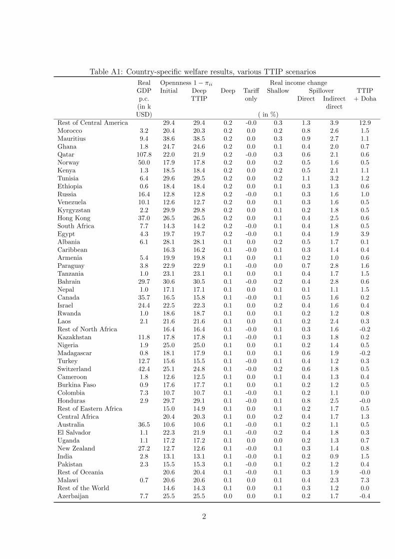
Table A1: Country-specific welfare results, various TTIP scenarios

Real Opennness 1− πii Real income changeGDP Initial Deep Deep Tariff Shallow Spillover TTIPp.c. TTIP only Direct Indirect + Doha(in k directUSD) ( in %)

Rest of Central America 29.4 29.4 0.2 -0.0 0.3 1.3 3.9 12.9Morocco 3.2 20.4 20.3 0.2 0.0 0.2 0.8 2.6 1.5Mauritius 9.4 38.6 38.5 0.2 0.0 0.3 0.9 2.7 1.1Ghana 1.8 24.7 24.6 0.2 0.0 0.1 0.4 2.0 0.7Qatar 107.8 22.0 21.9 0.2 -0.0 0.3 0.6 2.1 0.6Norway 50.0 17.9 17.8 0.2 0.0 0.2 0.5 1.6 0.5Kenya 1.3 18.5 18.4 0.2 0.0 0.2 0.5 2.1 1.1Tunisia 6.4 29.6 29.5 0.2 0.0 0.2 1.1 3.2 1.2Ethiopia 0.6 18.4 18.4 0.2 0.0 0.1 0.3 1.3 0.6Russia 16.4 12.8 12.8 0.2 -0.0 0.1 0.3 1.6 1.0Venezuela 10.1 12.6 12.7 0.2 0.0 0.1 0.3 1.6 0.5Kyrgyzstan 2.2 29.9 29.8 0.2 0.0 0.1 0.2 1.8 0.5Hong Kong 37.0 26.5 26.5 0.2 0.0 0.1 0.4 2.5 0.6South Africa 7.7 14.3 14.2 0.2 -0.0 0.1 0.4 1.8 0.5Egypt 4.3 19.7 19.7 0.2 -0.0 0.1 0.4 1.9 3.9Albania 6.1 28.1 28.1 0.1 0.0 0.2 0.5 1.7 0.1Caribbean 16.3 16.2 0.1 -0.0 0.1 0.3 1.4 0.4Armenia 5.4 19.9 19.8 0.1 0.0 0.1 0.2 1.0 0.6Paraguay 3.8 22.9 22.9 0.1 -0.0 0.0 0.7 2.8 1.6Tanzania 1.0 23.1 23.1 0.1 0.0 0.1 0.4 1.7 1.5Bahrain 29.7 30.6 30.5 0.1 -0.0 0.2 0.4 2.8 0.6Nepal 1.0 17.1 17.1 0.1 0.0 0.1 0.1 1.1 1.5Canada 35.7 16.5 15.8 0.1 -0.0 0.1 0.5 1.6 0.2Israel 24.4 22.5 22.3 0.1 0.0 0.2 0.4 1.6 0.4Rwanda 1.0 18.6 18.7 0.1 0.0 0.1 0.2 1.2 0.8Laos 2.1 21.6 21.6 0.1 0.0 0.1 0.2 2.4 0.3Rest of North Africa 16.4 16.4 0.1 -0.0 0.1 0.3 1.6 -0.2Kazakhstan 11.8 17.8 17.8 0.1 -0.0 0.1 0.3 1.8 0.2Nigeria 1.9 25.0 25.0 0.1 0.0 0.1 0.2 1.4 0.5Madagascar 0.8 18.1 17.9 0.1 0.0 0.1 0.6 1.9 -0.2Turkey 12.7 15.6 15.5 0.1 -0.0 0.1 0.4 1.2 0.3Switzerland 42.4 25.1 24.8 0.1 -0.0 0.2 0.6 1.8 0.5Cameroon 1.8 12.6 12.5 0.1 0.0 0.1 0.4 1.3 0.4Burkina Faso 0.9 17.6 17.7 0.1 0.0 0.1 0.2 1.2 0.5Colombia 7.3 10.7 10.7 0.1 -0.0 0.1 0.2 1.1 0.0Honduras 2.9 29.7 29.1 0.1 -0.0 0.1 0.8 2.5 -0.0Rest of Eastern Africa 15.0 14.9 0.1 0.0 0.1 0.2 1.7 0.5Central Africa 20.4 20.3 0.1 0.0 0.2 0.4 1.7 1.3Australia 36.5 10.6 10.6 0.1 -0.0 0.1 0.2 1.1 0.5El Salvador 1.1 22.3 21.9 0.1 -0.0 0.2 0.4 1.8 0.3Uganda 1.1 17.2 17.2 0.1 0.0 0.0 0.2 1.3 0.7New Zealand 27.2 12.7 12.6 0.1 -0.0 0.1 0.3 1.4 0.8India 2.8 13.1 13.1 0.1 -0.0 0.1 0.2 0.9 1.5Pakistan 2.3 15.5 15.3 0.1 -0.0 0.1 0.2 1.2 0.4Rest of Oceania 20.6 20.4 0.1 -0.0 0.1 0.3 1.9 -0.0Malawi 0.7 20.6 20.6 0.1 0.0 0.1 0.4 2.3 7.3Rest of the World 14.6 14.3 0.1 0.0 0.1 0.3 1.2 0.0Azerbaijan 7.7 25.5 25.5 0.0 0.0 0.1 0.2 1.7 -0.4

2

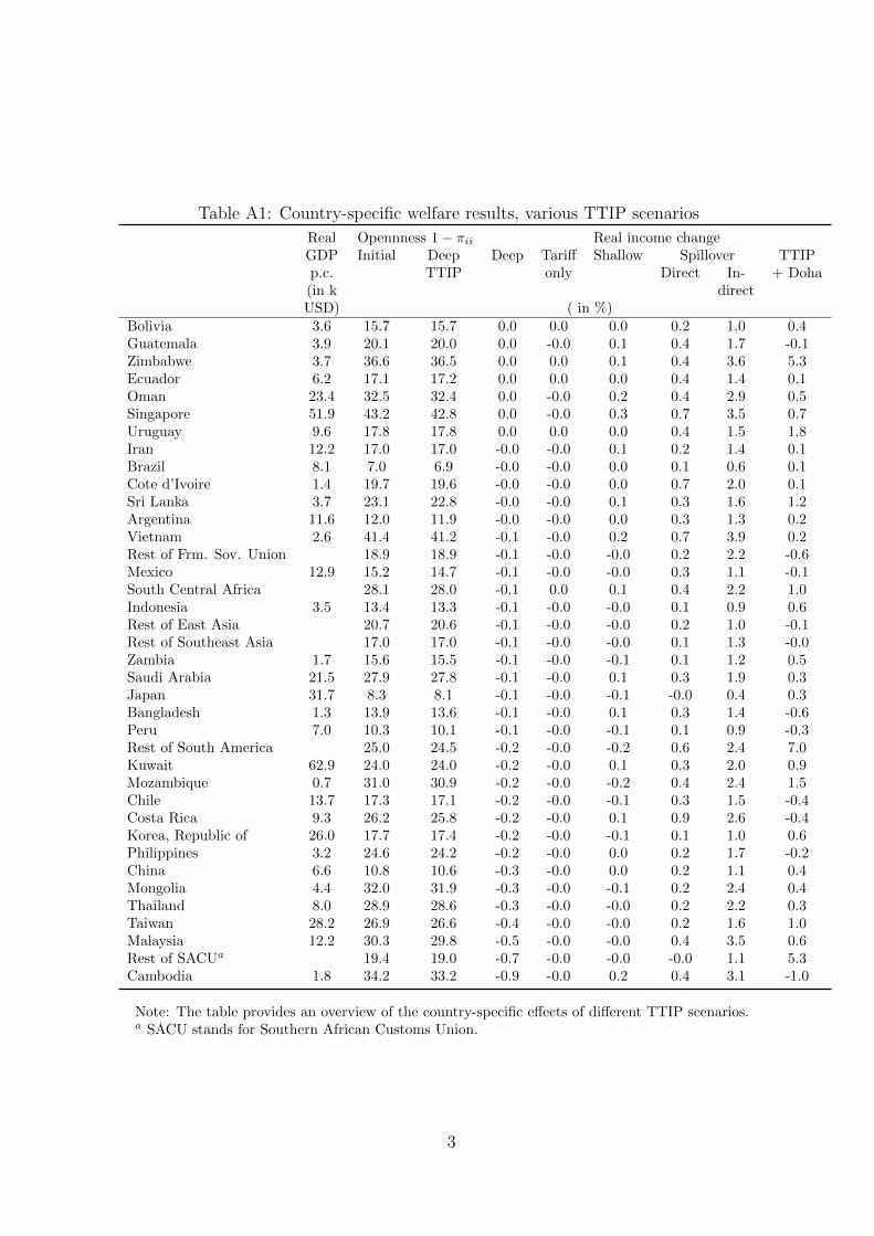
Table A1: Country-specific welfare results, various TTIP scenarios

Real Opennness 1− πii Real income changeGDP Initial Deep Deep Tariff Shallow Spillover TTIPp.c. TTIP only Direct In- + Doha(in k directUSD) ( in %)

Bolivia 3.6 15.7 15.7 0.0 0.0 0.0 0.2 1.0 0.4Guatemala 3.9 20.1 20.0 0.0 -0.0 0.1 0.4 1.7 -0.1Zimbabwe 3.7 36.6 36.5 0.0 0.0 0.1 0.4 3.6 5.3Ecuador 6.2 17.1 17.2 0.0 0.0 0.0 0.4 1.4 0.1Oman 23.4 32.5 32.4 0.0 -0.0 0.2 0.4 2.9 0.5Singapore 51.9 43.2 42.8 0.0 -0.0 0.3 0.7 3.5 0.7Uruguay 9.6 17.8 17.8 0.0 0.0 0.0 0.4 1.5 1.8Iran 12.2 17.0 17.0 -0.0 -0.0 0.1 0.2 1.4 0.1Brazil 8.1 7.0 6.9 -0.0 -0.0 0.0 0.1 0.6 0.1Cote d’Ivoire 1.4 19.7 19.6 -0.0 -0.0 0.0 0.7 2.0 0.1Sri Lanka 3.7 23.1 22.8 -0.0 -0.0 0.1 0.3 1.6 1.2Argentina 11.6 12.0 11.9 -0.0 -0.0 0.0 0.3 1.3 0.2Vietnam 2.6 41.4 41.2 -0.1 -0.0 0.2 0.7 3.9 0.2Rest of Frm. Sov. Union 18.9 18.9 -0.1 -0.0 -0.0 0.2 2.2 -0.6Mexico 12.9 15.2 14.7 -0.1 -0.0 -0.0 0.3 1.1 -0.1South Central Africa 28.1 28.0 -0.1 0.0 0.1 0.4 2.2 1.0Indonesia 3.5 13.4 13.3 -0.1 -0.0 -0.0 0.1 0.9 0.6Rest of East Asia 20.7 20.6 -0.1 -0.0 -0.0 0.2 1.0 -0.1Rest of Southeast Asia 17.0 17.0 -0.1 -0.0 -0.0 0.1 1.3 -0.0Zambia 1.7 15.6 15.5 -0.1 -0.0 -0.1 0.1 1.2 0.5Saudi Arabia 21.5 27.9 27.8 -0.1 -0.0 0.1 0.3 1.9 0.3Japan 31.7 8.3 8.1 -0.1 -0.0 -0.1 -0.0 0.4 0.3Bangladesh 1.3 13.9 13.6 -0.1 -0.0 0.1 0.3 1.4 -0.6Peru 7.0 10.3 10.1 -0.1 -0.0 -0.1 0.1 0.9 -0.3Rest of South America 25.0 24.5 -0.2 -0.0 -0.2 0.6 2.4 7.0Kuwait 62.9 24.0 24.0 -0.2 -0.0 0.1 0.3 2.0 0.9Mozambique 0.7 31.0 30.9 -0.2 -0.0 -0.2 0.4 2.4 1.5Chile 13.7 17.3 17.1 -0.2 -0.0 -0.1 0.3 1.5 -0.4Costa Rica 9.3 26.2 25.8 -0.2 -0.0 0.1 0.9 2.6 -0.4Korea, Republic of 26.0 17.7 17.4 -0.2 -0.0 -0.1 0.1 1.0 0.6Philippines 3.2 24.6 24.2 -0.2 -0.0 0.0 0.2 1.7 -0.2China 6.6 10.8 10.6 -0.3 -0.0 0.0 0.2 1.1 0.4Mongolia 4.4 32.0 31.9 -0.3 -0.0 -0.1 0.2 2.4 0.4Thailand 8.0 28.9 28.6 -0.3 -0.0 -0.0 0.2 2.2 0.3Taiwan 28.2 26.9 26.6 -0.4 -0.0 -0.0 0.2 1.6 1.0Malaysia 12.2 30.3 29.8 -0.5 -0.0 -0.0 0.4 3.5 0.6Rest of SACUa 19.4 19.0 -0.7 -0.0 -0.0 -0.0 1.1 5.3Cambodia 1.8 34.2 33.2 -0.9 -0.0 0.2 0.4 3.1 -1.0

Note: The table provides an overview of the country-specific effects of different TTIP scenarios.a SACU stands for Southern African Customs Union.

3

A Regional and sectoral breakdown

Countries and regions in GTAP The 114 countries in GTAP are: Albania, Ar-

gentina, Armenia, Australia, Austria, Azerbaijan, Bangladesh, Belarus, Belgium, Benin,

Bolivia, Botswana, Brazil, Bulgaria, Burkina Faso, Cambodia, Cameroon, Canada, Chile,

China, Colombia, Costa Rica, Cote d Ivoire, Croatia, Cyprus, Czech Republic, Denmark,

Ecuador, Egypt, El Salvador, Estonia, Ethiopia, Finland, France, Georgia, Germany,

Ghana, Greece, Guatemala, Guinea, Honduras, Hong Kong, Hungary, India, Indonesia,

Iran, Ireland, Israel, Italy, Japan, Kazakhstan, Kenya, Kuwait, Kyrgyzstan, Laos, Latvia,

Lithuania, Luxembourg, Madagascar, Malawi, Malaysia, Malta, Mauritius, Mexico, Mon-

golia, Morocco, Mozambique, Namibia, Nepal, Netherlands, New Zealand, Nicaragua,

Nigeria, Norway, Oman, Pakistan, Panama, Paraguay, Peru, Philippines, Poland, Por-

tugal, Qatar, Russian Federation, Rwanda, Saudi Arabia, Senegal, Singapore, Slovakia,

Slovenia, South Africa, South Korea, Spain, Sri Lanka, Sweden, Switzerland, Taiwan,

Tanzania, Thailand, Togo, Tunisia, Turkey, Uganda, Ukraine, United Arab Emirates,

United Kingdom, United States of America, Uruguay, Venezuela, Vietnam, Zambia and

Zimbabwe.

Other countries are aggregated into 20 regional composites such as, e.g., Rest of South-

east Asia comprising Brunei Darussalam, Myanmar, and Timor Leste.

Region listing The following list provides an overview of the regional breakdown we

use to present the results. Note that the simulations are performed with the 134 original

GTAP countries and regions, though.

• ASEAN: Indonesia, Cambodia, Laos, Malaysia, Philippines, Singapore, Thailand,

Vietnam, Rest of Southeast Asia (Brunei Darussalam, Myanmar, Timor Leste1)

1Timor Leste is not part of ASEAN. However, in GTAP’s regional breakdown it is included in theregion “Rest of Southeast Asia” together with Brunei Darussalam and Myanmar, both ASEAN memberstates. Therefore, we assigned the region “Rest of Southeast Asia” to ASEAN.

4

• Central Asia: Azerbaijan, Georgia, Kyrgyzstan, Ukraine, Mongolia, Rest of East-

ern Europe (Moldova), Rest of Former Soviet Union (Tajikistan, Turkmenistan,

Uzbekistan)

• China: China, Hong Kong

• East Asia: Japan, South Korea, Taiwan

• EFTA: Norway, Switzerland, Rest of EFTA (Iceland, Liechtenstein)

• Eurasian Customs Union: Armenia, Belarus, Kazakhstan, Russian Federation

• Latin America & Caribbean: Bolivia, Ecuador, Guatemala, Honduras, Nicaragua,

Panama, El Salvador, Rest of Central America (Belize), Rest of South America

(Falkland Islands, French Guiana, Guyana, South Georgia and the South Sandwich

Islands, Suriname), Caribbean (Anguilla, Antigua & Barbuda, Aruba, Bahamas,

Barbados, Cayman Islands, Cuba, Dominica, Dominican Republic, Grenada, Haiti,

Jamaica, Montserrat, Netherlands Antilles, Puerto Rico, Saint Kitts and Nevis,

Saint Lucia, Saint Vincent and the Grenadines, Trinidad and Tobago, Turks and

Caicos Islands, Virgin Islands British, Virgin Islands U.S.)

• MERCOSUR: Argentina, Brazil, Paraguay, Uruguay, Venezuela

• Middle East & North Africa: Israel, Egypt, Iran, Morocco, Tunisia, Rest of North

Africa (Algeria, Libyan Arab Jamahiriya, Western Sahara), Rest of Western Asia

(Iraq, Jordan, Lebanon, Palestinian Territory Occupied, Syrian Arab Republic,

Yemen)

• Oil exporters: United Arab Emirates, Bahrain, Kuwait, Oman, Qatar, Saudi Arabia

• Pacific Alliance: Chile, Colombia, Costa Rica, Mexico, Peru

5

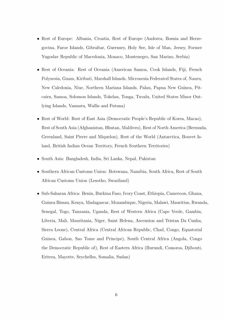
• Rest of Europe: Albania, Croatia, Rest of Europe (Andorra, Bosnia and Herze-

govina, Faroe Islands, Gibraltar, Guernsey, Holy See, Isle of Man, Jersey, Former

Yugoslav Republic of Macedonia, Monaco, Montenegro, San Marino, Serbia)

• Rest of Oceania: Rest of Oceania (American Samoa, Cook Islands, Fiji, French

Polynesia, Guam, Kiribati, Marshall Islands, Micronesia Federated States of, Nauru,

New Caledonia, Niue, Northern Mariana Islands, Palau, Papua New Guinea, Pit-

cairn, Samoa, Solomon Islands, Tokelau, Tonga, Tuvalu, United States Minor Out-

lying Islands, Vanuatu, Wallis and Futuna)

• Rest of World: Rest of East Asia (Democratic People’s Republic of Korea, Macao),

Rest of South Asia (Afghanistan, Bhutan, Maldives), Rest of North America (Bermuda,

Greenland, Saint Pierre and Miquelon), Rest of the World (Antarctica, Bouvet Is-

land, British Indian Ocean Territory, French Southern Territories)

• South Asia: Bangladesh, India, Sri Lanka, Nepal, Pakistan

• Southern African Customs Union: Botswana, Namibia, South Africa, Rest of South

African Customs Union (Lesotho, Swaziland)

• Sub-Saharan Africa: Benin, Burkina Faso, Ivory Coast, Ethiopia, Cameroon, Ghana,

Guinea Bissau, Kenya, Madagascar, Mozambique, Nigeria, Malawi, Mauritius, Rwanda,

Senegal, Togo, Tanzania, Uganda, Rest of Western Africa (Cape Verde, Gambia,

Liberia, Mali, Mauritania, Niger, Saint Helena, Ascension and Tristan Da Cunha,

Sierra Leone), Central Africa (Central African Republic, Chad, Congo, Equatorial

Guinea, Gabon, Sao Tome and Principe), South Central Africa (Angola, Congo

the Democratic Republic of), Rest of Eastern Africa (Burundi, Comoros, Djibouti,

Eritrea, Mayotte, Seychelles, Somalia, Sudan)

6

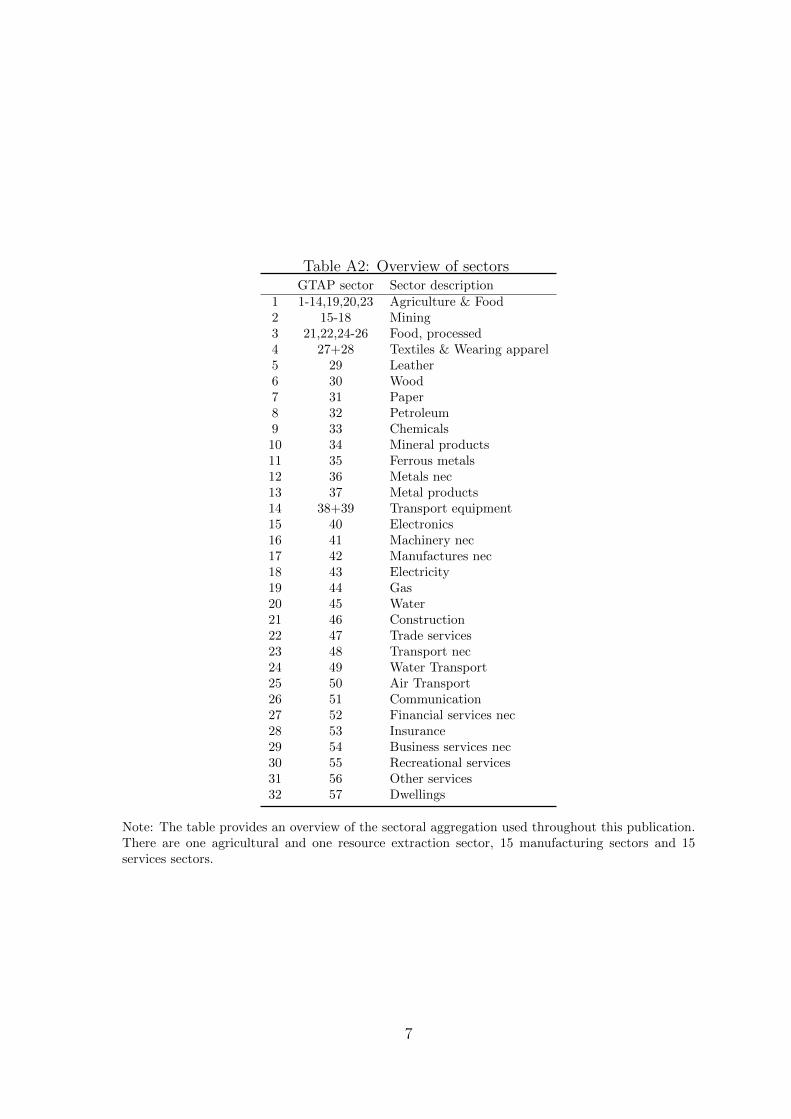
Table A2: Overview of sectorsGTAP sector Sector description

1 1-14,19,20,23 Agriculture & Food2 15-18 Mining3 21,22,24-26 Food, processed4 27+28 Textiles & Wearing apparel5 29 Leather6 30 Wood7 31 Paper8 32 Petroleum9 33 Chemicals10 34 Mineral products11 35 Ferrous metals12 36 Metals nec13 37 Metal products14 38+39 Transport equipment15 40 Electronics16 41 Machinery nec17 42 Manufactures nec18 43 Electricity19 44 Gas20 45 Water21 46 Construction22 47 Trade services23 48 Transport nec24 49 Water Transport25 50 Air Transport26 51 Communication27 52 Financial services nec28 53 Insurance29 54 Business services nec30 55 Recreational services31 56 Other services32 57 Dwellings

Note: The table provides an overview of the sectoral aggregation used throughout this publication.There are one agricultural and one resource extraction sector, 15 manufacturing sectors and 15services sectors.

7

B Detailed estimation results

8

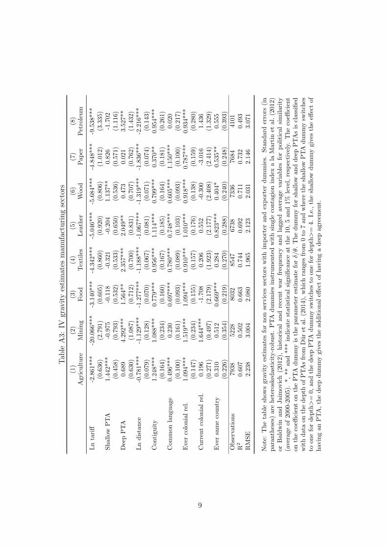
Tab

leA

3:IV

grav

ity

esti

mat

esm

anufa

cturi

ng

sect

ors

(1)

(2)

(3)

(4)

(5)

(6)

(7)

(8)

Agr

icu

ltu

reM

inin

gF

ood

Tex

tile

sL

eath

erW

ood

Pap

erP

etro

leu

m

Ln

tari

ff-2

.861

***

-20.

066***

-3.1

40***

-4.3

42***

-5.0

46***

-5.6

84***

-4.8

48***

-9.5

38***

(0.6

36)

(2.7

91)

(0.6

05)

(0.8

60)

(0.9

20)

(0.8

06)

(1.0

12)

(3.3

35)

Sh

allo

wP

TA

1.44

2***

-0.9

75

-0.1

18

-0.3

21

-0.2

04

1.1

37**

0.8

26

-1.7

02

(0.4

58)

(0.7

93)

(0.5

32)

(0.5

33)

(0.6

50)

(0.5

36)

(0.5

71)

(1.1

16)

Dee

pP

TA

0.68

94.

292***

1.5

64**

2.3

57***

2.0

49**

0.4

73

0.0

21

3.5

27**

(0.6

30)

(1.0

87)

(0.7

12)

(0.7

00)

(0.8

31)

(0.7

07)

(0.7

62)

(1.4

32)

Ln

dis

tan

ce-0

.781

***

-1.1

29***

-1.2

77***

-1.1

88***

-1.0

67***

-1.3

19***

-1.8

36***

-2.2

16***

(0.0

79)

(0.1

28)

(0.0

70)

(0.0

67)

(0.0

81)

(0.0

71)

(0.0

74)

(0.1

43)

Con

tigu

ity

1.24

8***

1.08

8***

0.7

79***

0.9

56***

1.1

14***

0.7

99***

0.3

70**

0.9

54***

(0.1

64)

(0.2

34)

(0.1

60)

(0.1

67)

(0.1

85)

(0.1

64)

(0.1

81)

(0.2

61)

Com

mon

lan

guag

e0.

496*

**0.

230

0.6

97***

0.7

80***

0.7

48***

0.6

05***

1.1

50***

0.0

20

(0.1

00)

(0.1

61)

(0.0

93)

(0.0

89)

(0.1

03)

(0.0

93)

(0.1

00)

(0.2

17)

Eve

rco

lonia

lre

l.1.

094*

**1.

519***

1.0

94***

0.9

10***

1.0

10***

0.9

18***

0.7

87***

0.9

34***

(0.1

47)

(0.2

34)

(0.1

55)

(0.1

57)

(0.1

76)

(0.1

38)

(0.1

59)

(0.2

80)

Cu

rren

tco

lon

ial

rel.

0.19

61.

644***

-1.7

08

0.2

06

0.5

52

-0.3

00

-3.0

16

1.4

36

(0.2

71)

(0.4

97)

(2.1

79)

(1.9

23)

(2.1

77)

(2.4

08)

(2.4

14)

(1.3

29)

Eve

rsa

me

cou

ntr

y0.

310

0.51

20.6

69***

0.2

84

0.8

23***

0.4

04*

0.5

35**

0.5

55

(0.2

26)

(0.3

54)

(0.2

19)

(0.2

70)

(0.2

88)

(0.2

40)

(0.2

48)

(0.3

93)

Ob

serv

atio

ns

7938

5228

8032

8547

6738

7336

7684

4101

R2

0.60

70.

502

0.6

63

0.7

44

0.6

92

0.7

11

0.7

32

0.4

93

RM

SE

2.23

83.

004

2.0

80

1.9

65

2.1

23

2.0

31

2.1

46

3.0

71

Not

e:T

he

tab

lesh

ows

grav

ity

esti

mat

esfo

rn

on

serv

ices

sect

ors

wit

him

port

eran

dex

port

erd

um

mie

s.S

tan

dard

erro

rs(i

np

aran

thes

es)

are

het

eros

ked

asti

city

-rob

ust

.P

TA

du

mm

ies

inst

rum

ente

dw

ith

sin

gle

conta

gio

nin

dex

ala

Mart

inet

al.

(2012)

orB

ald

win

and

Jai

mov

ich

(201

2),

his

tori

cal

an

dre

cent

war

freq

uen

cyan

dla

gged

aver

age

vari

ab

les

for

poli

tica

lsi

mil

ari

ty(a

vera

geof

2000

-200

5).

*,**

and

***

indic

ate

stati

stic

al

sign

ifica

nce

at

the

10,

5an

d1%

level

,re

spec

tive

ly.

Th

eco

effici

ent

onth

eco

effici

ent

onth

eP

TA

du

mm

yis

the

para

met

eres

tim

ate

forδ/θ.

Th

ed

um

my

for

shall

owan

dd

eep

PT

As

iscl

ass

ified

wit

hd

ata

onth

ed

epth

ofP

TA

sfr

omD

ur

etal.

(2014),

wh

ich

ran

ges

from

0to

7an

dw

her

eth

esh

all

owP

TA

du

mm

ysw

itch

esto

one

for

dep

th>

=0,

and

the

dee

pP

TA

du

mm

ysw

itch

esto

on

efo

rd

epth>

=4.

I.e.

,th

esh

all

owd

um

my

giv

esth

eeff

ect

of

hav

ing

anP

TA

,th

ed

eep

du

mm

ygi

ves

the

ad

dit

ion

al

effec

tof

hav

ing

ad

eep

agre

emen

t.

9

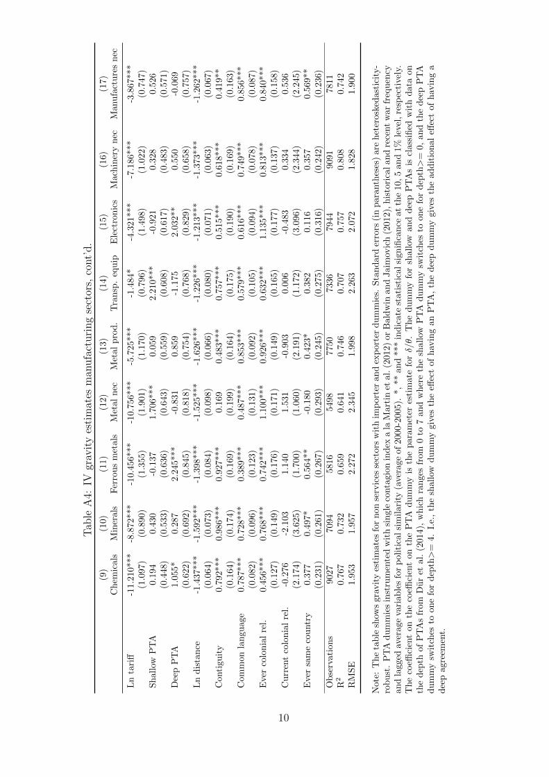
Tab

leA

4:IV

grav

ity

esti

mat

esm

anufa

cturi

ng

sect

ors,

cont’

d.

(9)

(10)

(11)

(12)

(13)

(14)

(15)

(16)

(17)

Ch

emic

als

Min

eral

sF

erro

us

met

als

Met

al

nec

Met

al

pro

d.

Tra

nsp

.eq

uip

Ele

ctro

nic

sM

ach

iner

yn

ecM

anu

fact

ure

sn

ec

Ln

tari

ff-1

1.21

0***

-8.8

72**

*-1

0.456***

-10.7

56***

-5.7

25***

-1.4

84*

-4.3

21***

-7.1

86***

-3.8

67***

(1.0

97)

(0.8

90)

(1.3

55)

(1.9

01)

(1.1

70)

(0.7

96)

(1.4

98)

(1.0

22)

(0.7

47)

Sh

allo

wP

TA

0.19

40.

430

-0.1

37

1.7

06***

0.0

59

2.2

10***

-0.9

21

0.3

28

0.5

26

(0.4

48)

(0.5

33)

(0.6

36)

(0.6

43)

(0.5

59)

(0.6

08)

(0.6

17)

(0.4

83)

(0.5

71)

Dee

pP

TA

1.05

5*0.

287

2.24

5***

-0.8

31

0.8

59

-1.1

75

2.0

32**

0.5

50

-0.0

69

(0.6

22)

(0.6

92)

(0.8

45)

(0.8

18)

(0.7

54)

(0.7

68)

(0.8

29)

(0.6

58)

(0.7

57)

Ln

dis

tan

ce-1

.437

***

-1.5

92**

*-1

.398***

-1.5

25***

-1.6

26***

-1.2

26***

-1.2

13***

-1.3

73***

-1.2

62***

(0.0

64)

(0.0

73)

(0.0

84)

(0.0

98)

(0.0

66)

(0.0

80)

(0.0

71)

(0.0

63)

(0.0

67)

Con

tigu

ity

0.79

2***

0.98

6***

0.927***

0.1

69

0.4

83***

0.7

57***

0.5

15***

0.6

18***

0.4

19**

(0.1

64)

(0.1

74)

(0.1

69)

(0.1

99)

(0.1

64)

(0.1

75)

(0.1

90)

(0.1

69)

(0.1

63)

Com

mon

lan

guag

e0.

787*

**0.

728*

**0.

389***

0.4

87***

0.8

53***

0.5

79***

0.6

16***

0.7

49***

0.8

56***

(0.0

82)

(0.0

96)

(0.1

23)

(0.1

31)

(0.0

92)

(0.1

05)

(0.0

94)

(0.0

78)

(0.0

87)

Eve

rco

lon

ial

rel.

0.45

6***

0.76

8***

0.74

2***

1.1

00***

0.9

26***

0.6

32***

1.1

35***

0.8

13***

0.8

40***

(0.1

27)

(0.1

49)

(0.1

76)

(0.1

71)

(0.1

49)

(0.1

65)

(0.1

77)

(0.1

37)

(0.1

58)

Cu

rren

tco

lonia

lre

l.-0

.276

-2.1

031.1

40

1.5

31

-0.9

03

0.0

06

-0.4

83

0.3

34

0.5

36

(2.1

74)

(3.6

25)

(1.7

00)

(1.0

60)

(2.1

91)

(1.1

72)

(3.0

96)

(2.3

44)

(2.2

45)

Eve

rsa

me

cou

ntr

y0.

377

0.49

7*0.

564**

-0.1

80

0.4

23*

0.3

82

0.1

16

0.3

57

0.5

69**

(0.2

31)

(0.2

61)

(0.2

67)

(0.2

93)

(0.2

45)

(0.2

75)

(0.3

16)

(0.2

42)

(0.2

36)

Ob

serv

atio

ns

9027

7094

5816

5498

7750

7336

7944

9091

7811

R2

0.76

70.

732

0.6

59

0.6

41

0.7

46

0.7

07

0.7

57

0.8

08

0.7

42

RM

SE

1.95

31.

957

2.2

72

2.3

45

1.9

98

2.2

63

2.0

72

1.8

28

1.9

00

Not

e:T

he

tab

lesh

ows

grav

ity

esti

mat

esfo

rn

onse

rvic

esse

ctors

wit

him

port

eran

dex

port

erd

um

mie

s.S

tan

dard

erro

rs(i

np

ara

nth

eses

)are

het

erosk

edast

icit

y-

rob

ust

.P

TA

du

mm

ies

inst

rum

ente

dw

ith

single

conta

gion

ind

exa

laM

art

inet

al.

(2012)

or

Bald

win

an

dJaim

ovic

h(2

012),

his

tori

calan

dre

cent

war

freq

uen

cyan

dla

gged

aver

age

vari

able

sfo

rp

olit

ical

sim

ilar

ity

(ave

rage

of

2000-2

005).

*,**

an

d***

ind

icate

stati

stic

alsi

gn

ifica

nce

at

the

10,5

an

d1%

level

,re

spec

tive

ly.

Th

eco

effici

ent

onth

eco

effici

ent

onth

eP

TA

du

mm

yis

the

para

met

eres

tim

ate

forδ/θ.

Th

ed

um

my

for

shall

owan

dd

eep

PT

As

iscl

ass

ified

wit

hd

ata

on

the

dep

thof

PT

As

from

Du

ret

al.

(201

4),

wh

ich

ran

ges

from

0to

7an

dw

her

eth

esh

all

owP

TA

du

mm

ysw

itch

esto

on

efo

rd

epth>

=0,

an

dth

edee

pP

TA

du

mm

ysw

itch

esto

one

for

dep

th>

=4.

I.e.

,th

esh

allo

wd

um

my

giv

esth

eeff

ect

of

hav

ing

an

PT

A,

the

dee

pd

um

my

giv

esth

ead

dit

ion

al

effec

tof

hav

ing

ad

eep

agre

emen

t.

10

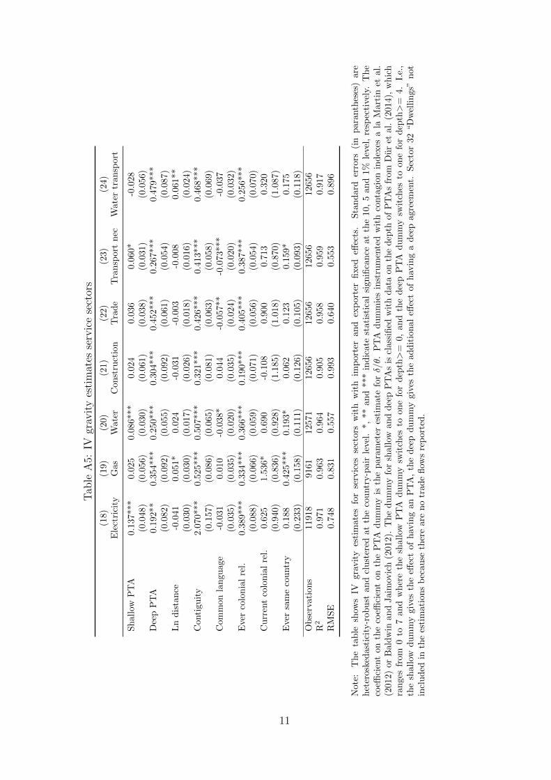
Tab

leA

5:IV

grav

ity

esti

mat

esse

rvic

ese

ctor

s

(18)

(19)

(20)

(21)

(22)

(23)

(24)

Ele

ctri

city

Gas

Wate

rC

on

stru

ctio

nT

rad

eT

ran

sport

nec

Wate

rtr

an

sport

Sh

allo

wP

TA

0.13

7***

0.025

0.0

86***

0.0

24

0.0

36

0.0

60*

-0.0

28

(0.0

48)

(0.0

56)

(0.0

30)

(0.0

61)

(0.0

38)

(0.0

31)

(0.0

56)

Dee

pP

TA

0.19

2**

0.35

4***

0.2

50***

0.3

04***

0.4

52***

0.2

67***

0.4

79***

(0.0

82)

(0.0

92)

(0.0

55)

(0.0

92)

(0.0

61)

(0.0

54)

(0.0

87)

Ln

dis

tan

ce-0

.041

0.05

1*

0.0

24

-0.0

31

-0.0

03

-0.0

08

0.0

61**

(0.0

30)

(0.0

30)

(0.0

17)

(0.0

26)

(0.0

18)

(0.0

16)

(0.0

24)

Con

tigu

ity

2.07

0***

0.52

5***

0.5

07***

0.3

21***

0.4

26***

0.4

13***

0.4

68***

(0.1

57)

(0.0

86)

(0.0

65)

(0.0

81)

(0.0

63)

(0.0

58)

(0.0

69)

Com

mon

lan

guag

e-0

.031

0.010

-0.0

38*

0.0

44

-0.0

57**

-0.0

73***

-0.0

37

(0.0

35)

(0.0

35)

(0.0

20)

(0.0

35)

(0.0

24)

(0.0

20)

(0.0

32)

Eve

rco

lonia

lre

l.0.

389*

**0.

334***

0.3

66***

0.1

90***

0.4

05***

0.3

87***

0.2

56***

(0.0

88)

(0.0

66)

(0.0

59)

(0.0

71)

(0.0

56)

(0.0

54)

(0.0

70)

Cu

rren

tco

lon

ial

rel.

0.62

51.

536*

0.6

90

-0.1

08

0.9

00

0.7

13

0.3

20

(0.9

40)

(0.8

36)

(0.9

28)

(1.1

85)

(1.0

18)

(0.8

70)

(1.0

87)

Eve

rsa

me

cou

ntr

y0.

188

0.42

5***

0.1

93*

0.0

62

0.1

23

0.1

59*

0.1

75

(0.2

33)

(0.1

58)

(0.1

11)

(0.1

26)

(0.1

05)

(0.0

93)

(0.1

18)

Ob

serv

atio

ns

1191

89161

12571

12656

12656

12656

12656

R2

0.97

10.

963

0.9

64

0.9

05

0.9

58

0.9

59

0.9

17

RM

SE

0.74

80.

831

0.5

57

0.9

93

0.6

40

0.5

53

0.8

96

Not

e:T

he

tab

lesh

ows

IVgr

avit

yes

tim

ates

for

serv

ices

sect

ors

wit

hw

ith

imp

ort

eran

dex

port

erfi

xed

effec

ts.

Sta

nd

ard

erro

rs(i

np

ara

nth

eses

)are

het

eros

ked

asti

city

-rob

ust

and

clu

ster

edat

the

cou

ntr

y-p

air

leve

l.*,

**

an

d***

ind

icate

stati

stic

al

sign

ifica

nce

at

the

10,

5an

d1%

leve

l,re

spec

tive

ly.

Th

eco

effici

ent

onth

eco

effici

ent

onth

eP

TA

du

mm

yis

the

para

met

eres

tim

ate

forδ/θ.

PT

Ad

um

mie

sin

stru

men

ted

wit

hco

nta

gio

nin

dex

esa

laM

art

inet

al.

(201

2)or

Bal

dw

inan

dJai

mov

ich

(201

2).

Th

ed

um

my

for

shall

owan

dd

eep

PT

As

iscl

ass

ified

wit

hd

ata

on

the

dep

thof

PT

As

from

Du

ret

al.

(2014),

wh

ich

ran

ges

from

0to

7an

dw

her

eth

esh

allo

wP

TA

du

mm

ysw

itch

esto

on

efo

rd

epth>

=0,

an

dth

ed

eep

PT

Ad

um

my

swit

ches

toon

efo

rd

epth>

=4.

I.e.

,th

esh

allo

wd

um

my

give

sth

eeff

ect

ofh

avin

gan

PT

A,

the

dee

pd

um

my

giv

esth

ead

dit

ion

al

effec

tof

hav

ing

ad

eep

agre

emen

t.S

ecto

r32

“D

wel

lin

gs”

not

incl

ud

edin

the

esti

mat

ion

sb

ecau

seth

ere

are

no

trad

efl

ows

rep

ort

ed.

11

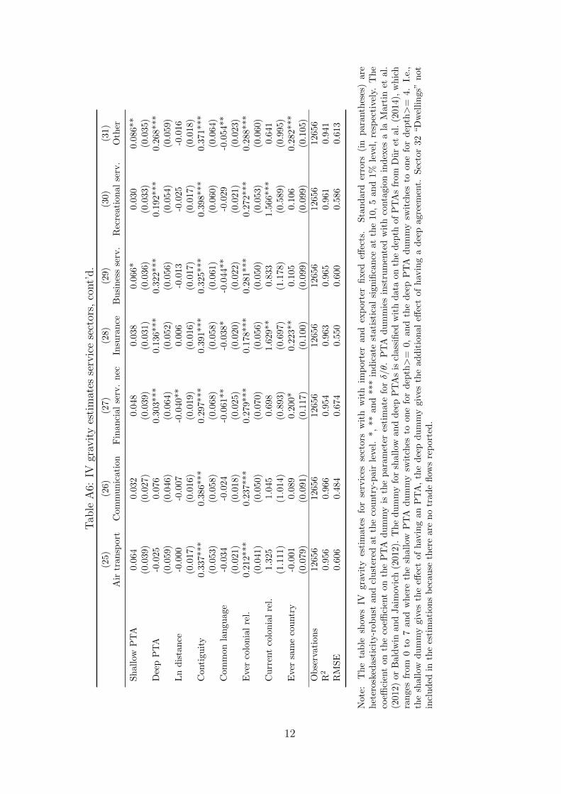
Tab

leA

6:IV

grav

ity

esti

mat

esse

rvic

ese

ctor

s,co

nt’

d.

(25)

(26)

(27)

(28)

(29)

(30)

(31)

Air

tran

spor

tC

omm

un

icati

on

Fin

an

cial

serv

.n

ecIn

sura

nce

Bu

sin

ess

serv

.R

ecre

ati

onal

serv

.O

ther

Sh

allo

wP

TA

0.06

40.

032

0.0

48

0.0

38

0.0

66*

0.0

30

0.0

86**

(0.0

39)

(0.0

27)

(0.0

39)

(0.0

31)

(0.0

36)

(0.0

33)

(0.0

35)

Dee

pP

TA

-0.0

250.

076

0.3

03***

0.1

36***

0.3

22***

0.1

92***

0.2

68***

(0.0

59)

(0.0

46)

(0.0

64)

(0.0

52)

(0.0

56)

(0.0

54)

(0.0

59)

Ln

dis

tan

ce-0

.000

-0.0

07

-0.0

40**

0.0

06

-0.0

13

-0.0

25

-0.0

16

(0.0

17)

(0.0

16)

(0.0

19)

(0.0

16)

(0.0

17)

(0.0

17)

(0.0

18)

Con

tigu

ity

0.33

7***

0.38

6***

0.2

97***

0.3

91***

0.3

25***

0.3

98***

0.3

71***

(0.0

53)

(0.0

58)

(0.0

68)

(0.0

58)

(0.0

61)

(0.0

60)

(0.0

64)

Com

mon

lan

guag

e-0

.034

-0.0

24

-0.0

61**

-0.0

38*

-0.0

44**

-0.0

29

-0.0

54**

(0.0

21)

(0.0

18)

(0.0

25)

(0.0

20)

(0.0

22)

(0.0

21)

(0.0

23)

Eve

rco

lon

ial

rel.

0.21

2***

0.23

7***

0.2

79***

0.1

78***

0.2

81***

0.2

72***

0.2

88***

(0.0

41)

(0.0

50)

(0.0

70)

(0.0

56)

(0.0

50)

(0.0

53)

(0.0

60)

Cu

rren

tco

lonia

lre

l.1.

325

1.04

50.6

98

1.6

29**

0.8

33

1.5

66***

0.6

41

(1.1

11)

(1.0

14)

(0.8

93)

(0.6

97)

(1.1

78)

(0.5

89)

(0.9

95)

Eve

rsa

me

cou

ntr

y-0

.001

0.08

90.2

00*

0.2

23**

0.1

05

0.1

06

0.2

82***

(0.0

79)

(0.0

91)

(0.1

17)

(0.1

00)

(0.0

99)

(0.0

99)

(0.1

05)

Ob

serv

atio

ns

1265

612

656

12656

12656

12656

12656

12656

R2

0.95

60.

966

0.9

54

0.9

63

0.9

65

0.9

61

0.9

41

RM

SE

0.60

60.

484

0.6

74

0.5

50

0.6

00

0.5

86

0.6

13

Not

e:T

he

tab

lesh

ows

IVgr

avit

yes

tim

ates

for

serv

ices

sect

ors

wit

hw

ith

imp

ort

eran

dex

port

erfi

xed

effec

ts.

Sta

nd

ard

erro

rs(i

np

ara

nth

eses

)are

het

eros

ked

asti

city

-rob

ust

and

clu

ster

edat

the

cou

ntr

y-p

air

leve

l.*,

**

an

d***

ind

icate

stati

stic

al

sign

ifica

nce

at

the

10,

5an

d1%

leve

l,re

spec

tive

ly.

Th

eco

effici

ent

onth

eco

effici

ent

onth

eP

TA

du

mm

yis

the

para

met

eres

tim

ate

forδ/θ.

PT

Ad

um

mie

sin

stru

men

ted

wit

hco

nta

gio

nin

dex

esa

laM

art

inet

al.

(201

2)or

Bal

dw

inan

dJai

mov

ich

(201

2).

Th

ed

um

my

for

shall

owan

dd

eep

PT

As

iscl

ass

ified

wit

hd

ata

on

the

dep

thof

PT

As

from

Du

ret

al.

(2014),

wh

ich

ran

ges

from

0to

7an

dw

her

eth

esh

allo

wP

TA

du

mm

ysw

itch

esto

on

efo

rd

epth>

=0,

an

dth

ed

eep

PT

Ad

um

my

swit

ches

toon

efo

rd

epth>

=4.

I.e.

,th

esh

allo

wd

um

my

give

sth

eeff

ect

ofh

avin

gan

PT

A,

the

dee

pd

um

my

giv

esth

ead

dit

ion

al

effec

tof

hav

ing

ad

eep

agre

emen

t.S

ecto

r32

“D

wel

lin

gs”

not

incl

ud

edin

the

esti

mat

ion

sb

ecau

seth

ere

are

no

trad

efl

ows

rep

ort

ed.

12

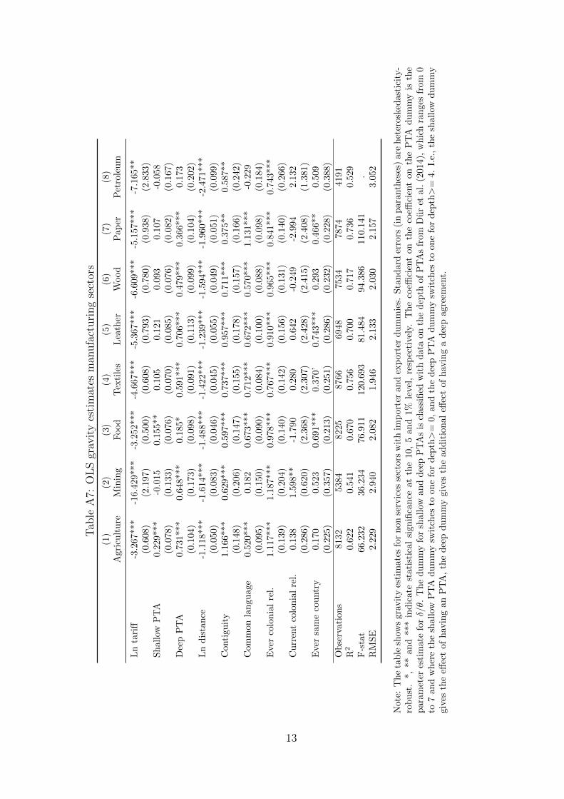
Tab

leA

7:O

LS

grav

ity

esti

mat

esm

anufa

cturi

ng

sect

ors

(1)

(2)

(3)

(4)

(5)

(6)

(7)

(8)

Agr

icu

ltu

reM

inin

gF

ood

Tex

tile

sL

eath

erW

ood

Pap

erP

etro

leu

m

Ln

tari

ff-3

.267

***

-16.

429***

-3.2

52***

-4.6

67***

-5.3

67***

-6.6

09***

-5.1

57***

-7.1

65**

(0.6

08)

(2.1

97)

(0.5

00)

(0.6

08)

(0.7

93)

(0.7

80)

(0.9

38)

(2.8

33)

Sh

allo

wP

TA

0.22

9***

-0.0

15

0.1

55**

0.1

05

0.1

21

0.0

93

0.1

07

-0.0

58

(0.0

78)

(0.1

33)

(0.0

76)

(0.0

70)

(0.0

85)

(0.0

76)

(0.0

82)

(0.1

67)

Dee

pP

TA

0.73

1***

0.64

8***

0.1

85*

0.5

91***

0.7

06***

0.4

79***

0.3

66***

0.1

73

(0.1

04)

(0.1

73)

(0.0

98)

(0.0

91)

(0.1

13)

(0.0

99)

(0.1

04)

(0.2

02)

Ln

dis

tan

ce-1

.118

***

-1.6

14***

-1.4

88***

-1.4

22***

-1.2

39***

-1.5

94***

-1.9

60***

-2.4

71***

(0.0

50)

(0.0

83)

(0.0

46)

(0.0

45)

(0.0

55)

(0.0

49)

(0.0

51)

(0.0

99)

Con

tigu

ity

1.16

6***

0.62

9***

0.5

97***

0.7

37***

0.9

57***

0.7

11***

0.3

75**

0.5

87**

(0.1

48)

(0.2

06)

(0.1

47)

(0.1

55)

(0.1

78)

(0.1

57)

(0.1

66)

(0.2

42)

Com

mon

lan

guag

e0.

520*

**0.

182

0.6

73***

0.7

12***

0.6

72***

0.5

70***

1.1

31***

-0.2

29

(0.0

95)

(0.1

50)

(0.0

90)

(0.0

84)

(0.1

00)

(0.0

88)

(0.0

98)

(0.1

84)

Eve

rco

lonia

lre

l.1.

117*

**1.

187***

0.9

78***

0.7

67***

0.9

10***

0.9

65***

0.8

41***

0.7

43***

(0.1

39)

(0.2

04)

(0.1

40)

(0.1

42)

(0.1

56)

(0.1

31)

(0.1

40)

(0.2

66)

Cu

rren

tco

lon

ial

rel.

0.13

81.

598**

-1.7

90

0.2

80

0.6

42

-0.2

49

-2.9

94

2.1

32

(0.2

86)

(0.6

20)

(2.3

68)

(2.3

07)

(2.4

28)

(2.4

15)

(2.4

08)

(1.3

81)

Eve

rsa

me

cou

ntr

y0.

170

0.52

30.6

91***

0.3

70’

0.7

43***

0.2

93

0.4

66**

0.5

09

(0.2

25)

(0.3

57)

(0.2

13)

(0.2

51)

(0.2

86)

(0.2

32)

(0.2

28)

(0.3

88)

Ob

serv

atio

ns

8132

5384

8225

8766

6948

7534

7874

4191

R2

0.62

20.

541

0.6

70

0.7

56

0.7

00

0.7

17

0.7

36

0.5

29

F-s

tat

66.2

3236

.234

76.9

11

120.6

93

81.4

84

94.3

86

110.1

41

.R

MS

E2.

229

2.94

02.0

82

1.9

46

2.1

33

2.0

30

2.1

57

3.0

52

Not

e:T

he

tab

lesh

ows

grav

ity

esti

mat

esfo

rn

onse

rvic

esse

ctors

wit

him

port

eran

dex

port

erd

um

mie

s.S

tan

dard

erro

rs(i

np

ara

nth

eses

)are

het

erosk

edast

icit

y-

rob

ust

.*,

**an

d**

*in

dic

ate

stat

isti

cal

sign

ifica

nce

atth

e10,

5an

d1%

level

,re

spec

tive

ly.

Th

eco

effici

ent

on

the

coeffi

cien

ton

the

PT

Ad

um

my

isth

ep

aram

eter

esti

mat

efo

rδ/θ.

Th

ed

um

my

for

shal

low

and

dee

pP

TA

sis

class

ified

wit

hdata

on

the

dep

thof

PT

As

from

Du

ret

al.

(2014),

wh

ich

ran

ges

from

0to

7an

dw

her

eth

esh

allo

wP

TA

du

mm

ysw

itch

esto

one

for

dep

th>

=0,

and

the

dee

pP

TA

du

mm

ysw

itch

esto

on

efo

rd

epth>

=4.

I.e.

,th

esh

all

owd

um

my

give

sth

eeff

ect

ofh

avin

gan

PT

A,

the

dee

pd

um

my

give

sth

ead

dit

ion

al

effec

tof

hav

ing

ad

eep

agre

emen

t.

13

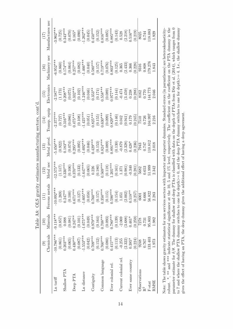
Tab

leA

8:O

LS

grav

ity

esti

mat

esm

anufa

cturi

ng

sect

ors,

cont’

d.

(9)

(10)

(11)

(12)

(13)

(14)

(15)

(16)

(17)

Ch

emic

als

Min

eral

sF

erro

us

met

als

Met

al

nec

Met

al

pro

d.

Tra

nsp

.eq

uip

Ele

ctro

nic

sM

ach

iner

yn

ecM

anu

fact

ure

sn

ec

Ln

tari

ff-1

0.78

6***

-9.1

18**

*-1

0.092***

-12.5

75***

-5.4

50***

-2.3

77***

-2.5

87**

-6.9

52***

-3.9

62***

(0.8

61)

(0.8

57)

(1.2

69)

(1.5

17)

(0.9

22)

(0.7

27)

(1.1

73)

(0.8

60)

(0.7

25)

Sh

allo

wP

TA

0.20

3***

0.08

80.

247**

0.3

30***

0.1

83**

0.3

16***

0.2

08***

0.1

74***

0.3

43***

(0.0

65)

(0.0

81)

(0.1

00)

(0.1

06)

(0.0

74)

(0.0

86)

(0.0

75)

(0.0

64)

(0.0

70)

Dee

pP

TA

0.43

0***

0.24

7**

0.671***

0.3

70***

0.2

95***

0.4

75***

0.3

32***

0.2

57***

0.1

65*

(0.0

87)

(0.1

01)

(0.1

27)

(0.1

33)

(0.0

95)

(0.1

08)

(0.1

02)

(0.0

82)

(0.0

90)

Ln

dis

tan

ce-1

.553

***

-1.6

75**

*-1

.605***

-1.6

47***

-1.6

92***

-1.4

25***

-1.2

46***

-1.4

66***

-1.2

62***

(0.0

42)

(0.0

49)

(0.0

58)

(0.0

65)

(0.0

46)

(0.0

51)

(0.0

46)

(0.0

40)

(0.0

45)

Con

tigu

ity

0.70

9***

0.97

9***

0.760***

0.2

26

0.4

29***

0.8

25***

0.3

53**

0.5

80***

0.4

50***

(0.1

52)

(0.1

64)

(0.1

57)

(0.1

80)

(0.1

53)

(0.1

55)

(0.1

74)

(0.1

57)

(0.1

52)

Com

mon

lan

guag

e0.

760*

**0.

708*

**0.

350***

0.5

69***

0.8

24***

0.6

30***

0.5

58***

0.7

19***

0.8

16***

(0.0

80)

(0.0

93)

(0.1

15)

(0.1

18)

(0.0

89)

(0.0

99)

(0.0

89)

(0.0

76)

(0.0

85)

Eve

rco

lon

ial

rel.

0.41

5***

0.78

0***

0.59

0***

1.2

05***

0.8

91***

0.8

29***

0.9

77***

0.8

03***

0.8

85***

(0.1

13)

(0.1

39)

(0.1

54)

(0.1

61)

(0.1

30)

(0.1

46)

(0.1

44)

(0.1

25)

(0.1

43)

Cu

rren

tco

lonia

lre

l.-0

.255

-2.0

691.0

51

1.3

71

-0.8

79

0.0

42

-0.4

74

0.3

65

0.5

28

(2.3

22)

(3.6

88)

(2.0

02)

(0.9

81)

(2.3

28)

(0.9

41)

(3.4

59)

(2.4

33)

(2.2

18)

Eve

rsa

me

cou

ntr

y0.

385*

0.46

1*0.

518**

-0.3

40

0.4

28*

0.1

79

0.2

38

0.3

66

0.5

16**

(0.2

24)

(0.2

59)

(0.2

57)

(0.2

81)

(0.2

36)

(0.2

45)

(0.2

88)

(0.2

28)

(0.2

19)

Ob

serv

atio

ns

9248

7278

6001

5682

7943

7510

8162

9316

8025

R2

0.76

70.

731

0.6

66

0.6

53

0.7

47

0.7

26

0.7

70

0.8

08

0.7

44

F-s

tat

133.

403

95.8

0356

.822

51.9

99

110.8

12

104.9

97

144.7

73

179.2

76

118.0

83

RM

SE

1.97

31.

982

2.2

83

2.3

42

2.0

18

2.2

16

2.0

46

1.8

43

1.9

29

Not

e:T

he

tab

lesh

ows

grav

ity

esti

mat

esfo

rn

onse

rvic

esse

ctors

wit

him

port

eran

dex

port

erd

um

mie

s.S

tan

dard

erro

rs(i

np

ara

nth

eses

)are

het

erosk

edast

icit

y-

rob

ust

.*,

**an

d**

*in

dic

ate

stat

isti

cal

sign

ifica

nce

atth

e10,

5an

d1%

level

,re

spec

tive

ly.

Th

eco

effici

ent

on

the

coeffi

cien

ton

the

PT

Ad

um

my

isth

ep

aram

eter

esti

mat

efo

rδ/θ.

Th

ed

um

my

for

shal

low

and

dee

pP

TA

sis

class

ified

wit

hdata

on

the

dep

thof

PT

As

from

Du

ret

al.

(2014),

wh

ich

ran

ges

from

0to

7an

dw

her

eth

esh

allo

wP

TA

du

mm

ysw

itch

esto

one

for

dep

th>

=0,

and

the

dee

pP

TA

du

mm

ysw

itch

esto

on

efo

rd

epth>

=4.

I.e.

,th

esh

all

owd

um

my

give

sth

eeff

ect

ofh

avin

gan

PT

A,

the

dee

pd

um

my

give

sth

ead

dit

ion

al

effec

tof

hav

ing

ad

eep

agre

emen

t.

14

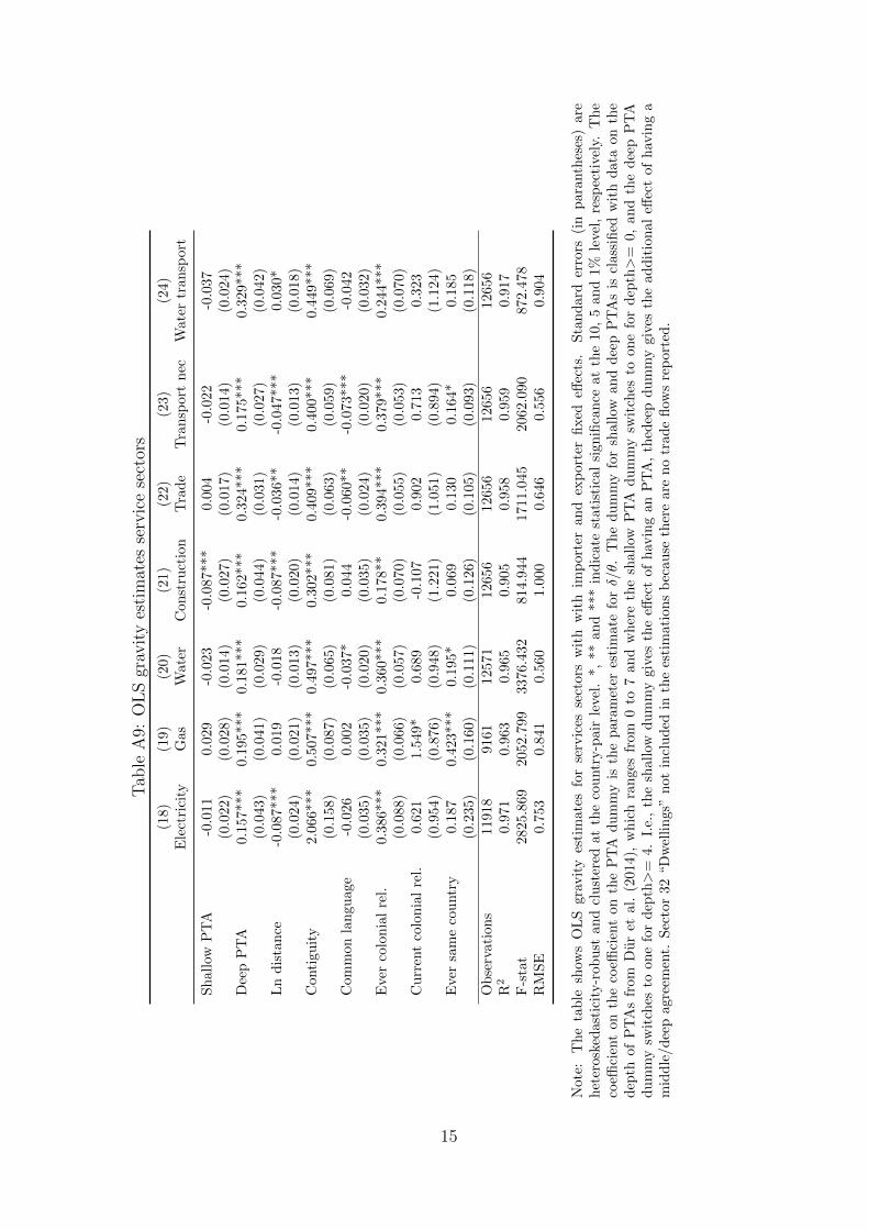
Tab

leA

9:O

LS

grav

ity

esti

mat

esse

rvic

ese

ctor

s

(18)

(19)

(20)

(21)

(22)

(23)

(24)

Ele

ctri

city

Gas

Wate

rC

on

stru

ctio

nT

rad

eT

ran

sport

nec

Wate

rtr

an

sport

Sh

allo

wP

TA

-0.0

110.

029

-0.0

23

-0.0

87***

0.0

04

-0.0

22

-0.0

37

(0.0

22)

(0.0

28)

(0.0

14)

(0.0

27)

(0.0

17)

(0.0

14)

(0.0

24)

Dee

pP

TA

0.15

7***

0.19

5***

0.1

81***

0.1

62***

0.3

24***

0.1

75***

0.3

29***

(0.0

43)

(0.0

41)

(0.0

29)

(0.0

44)

(0.0

31)

(0.0

27)

(0.0

42)

Ln

dis

tan

ce-0

.087

***

0.019

-0.0

18

-0.0

87***

-0.0

36**

-0.0

47***

0.0

30*

(0.0

24)

(0.0

21)

(0.0

13)

(0.0

20)

(0.0

14)

(0.0

13)

(0.0

18)

Con

tigu

ity

2.06

6***

0.50

7***

0.4

97***

0.3

02***

0.4

09***

0.4

00***

0.4

49***

(0.1

58)

(0.0

87)

(0.0

65)

(0.0

81)

(0.0

63)

(0.0

59)

(0.0

69)

Com

mon

lan

guag

e-0

.026

0.002

-0.0

37*

0.0

44

-0.0

60**

-0.0

73***

-0.0

42

(0.0

35)

(0.0

35)

(0.0

20)

(0.0

35)

(0.0

24)

(0.0

20)

(0.0

32)

Eve

rco

lonia

lre

l.0.

386*

**0.

321***

0.3

60***

0.1

78**

0.3

94***

0.3

79***

0.2

44***

(0.0

88)

(0.0

66)

(0.0

57)

(0.0

70)

(0.0

55)

(0.0

53)

(0.0

70)

Cu

rren

tco

lon

ial

rel.

0.62

11.

549*

0.6

89

-0.1

07

0.9

02

0.7

13

0.3

23

(0.9

54)

(0.8

76)

(0.9

48)

(1.2

21)

(1.0

51)

(0.8

94)

(1.1

24)

Eve

rsa

me

cou

ntr

y0.

187

0.42

3***

0.1

95*

0.0

69

0.1

30

0.1

64*

0.1

85

(0.2

35)

(0.1

60)

(0.1

11)

(0.1

26)

(0.1

05)

(0.0

93)

(0.1

18)

Ob

serv

atio

ns

1191

89161

12571

12656

12656

12656

12656

R2

0.97

10.

963

0.9

65

0.9

05

0.9

58

0.9

59

0.9

17

F-s

tat

2825

.869

2052.7

99

3376.4

32

814.9

44

1711.0

45

2062.0

90

872.4

78

RM

SE

0.75

30.

841

0.5

60

1.0

00

0.6

46

0.5

56

0.9

04

Not

e:T

he

tab

lesh

ows

OL

Sgr

avit

yes

tim

ates

for

serv

ices

sect

ors

wit

hw

ith

imp

ort

eran

dex

port

erfi

xed

effec

ts.

Sta

nd

ard

erro

rs(i

np

ara

nth

eses

)are

het

eros

ked

asti

city

-rob

ust

and

clu

ster

edat

the

cou

ntr

y-p

air

leve

l.*,

**

an

d***

ind

icate

stati

stic

al

sign

ifica

nce

at

the

10,

5an

d1%

leve

l,re

spec

tive

ly.

Th

eco

effici

ent

onth

eco

effici

ent

onth

eP

TA

du

mm

yis

the

para

met

eres

tim

ate

forδ/θ.

Th

edu

mm

yfo

rsh

all

owan

dd

eep

PT

As

iscl

ass

ified

wit

hd

ata

on

the

dep

thof

PT

As

from

Du

ret

al.

(201

4),

wh

ich

ran

ges

from

0to

7and

wh

ere

the

shall

owP

TA

du

mm

ysw

itch

esto

on

efo

rd

epth>

=0,

an

dth

ed

eep

PT

Ad

um

my

swit

ches

toon

efo

rd

epth>

=4.

I.e.

,th

esh

allo

wd

um

my

giv

esth

eeff

ect

of

hav

ing

an

PT

A,

thed

eep

du

mm

ygiv

esth

ead

dit

ion

al

effec

tof

hav

ing

am

idd

le/d

eep

agre

emen

t.S

ecto

r32

“Dw

elli

ngs

”n

otin

clu

ded

inth

ees

tim

ati

ons

bec

au

seth

ere

are

no

trad

efl

ows

rep

ort

ed.

15

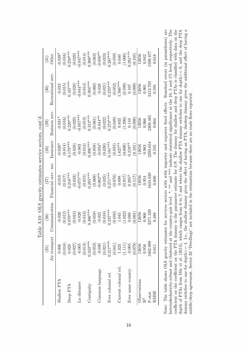
Tab

leA

10:

OL

Sgr

avit

yes

tim

ates

serv

ice

sect

ors,

cont’

d.

(25)

(26)

(27)

(28)

(29)

(30)

(31)

Air

tran

spor

tC

omm

un

icati

on

Fin

an

cial

serv

.n

ecIn

sura

nce

Bu

sin

ess

serv

.R

ecre

ati

on

al

serv

.O

ther

Sh

allo

wP

TA

0.00

6-0

.020

-0.0

18

-0.0

26*

-0.0

31*

-0.0

23

-0.0

28*

(0.0

16)

(0.0

12)

(0.0

17)

(0.0

14)

(0.0

16)

(0.0

15)

(0.0

16)

Dee

pP

TA

0.02

80.

079*

**

0.2

16***

0.1

79***

0.2

29***

0.1

67***

0.2

59***

(0.0

27)

(0.0

24)

(0.0

33)

(0.0

28)

(0.0

29)

(0.0

28)

(0.0

29)

Ln

dis

tan

ce-0

.005

-0.0

20-0

.075***

-0.0

03

-0.0

57***

-0.0

44***

-0.0

47***

(0.0

13)

(0.0

13)

(0.0

15)

(0.0

13)

(0.0

13)

(0.0

14)

(0.0

14)

Con

tigu

ity

0.34

3***

0.38

6***

0.2

85***

0.3

96***

0.3

12***

0.3

94***

0.3

69***

(0.0

53)

(0.0

58)

(0.0

69)

(0.0

58)

(0.0

61)

(0.0

60)

(0.0

63)

Com

mon

lan

guag

e-0

.030

-0.0

21-0

.062**

-0.0

34*

-0.0

44**

-0.0

28

-0.0

50**

(0.0

21)

(0.0

18)

(0.0

25)

(0.0

20)

(0.0

22)

(0.0

21)

(0.0

23)

Eve

rco

lonia

lre

l.0.

217*

**0.

237*

**

0.2

71***

0.1

81***

0.2

73***

0.2

70***

0.2

87***

(0.0

41)

(0.0

50)

(0.0

70)

(0.0

55)

(0.0

49)

(0.0

52)

(0.0

59)

Cu

rren

tco

lon

ial

rel.

1.32

31.

045

0.6

98

1.6

27**

0.8

33

1.5

66***

0.6

40

(1.1

11)

(1.0

22)

(0.9

17)

(0.6

96)

(1.2

06)

(0.5

99)

(1.0

06)

Eve

rsa

me

cou

ntr

y-0

.005

0.08

80.2

05*

0.2

19**

0.1

10

0.1

07

0.2

81***

(0.0

79)

(0.0

91)

(0.1

17)

(0.1

01)

(0.0

98)

(0.0

99)

(0.1

05)

Ob

serv

atio

ns

1265

612

656

12656

12656

12656

12656

12656

R2

0.95

60.

966

0.9

54

0.9

63

0.9

66

0.9

61

0.9

42

F-s

tat

1802

.999

3271

.339

1634.0

20

2293.6

54

2309.4

65

2412.7

02

1599.4

77

RM

SE

0.61

10.

488

0.6

80

0.5

55

0.6

04

0.5

91

0.6

18

Not

e:T

he

tab

lesh

ows

OL

Sgr

avit

yes

tim

ates

for

serv

ices

sect

ors

wit

hw

ith

imp

ort

eran

dex

port

erfi

xed

effec

ts.

Sta

nd

ard

erro

rs(i

np

ara

nth

eses

)are

het

eros

ked

asti

city

-rob

ust

and

clu

ster

edat

the

cou

ntr

y-p

air

leve

l.*,

**

an

d***

ind

icate

stati

stic

al

sign

ifica

nce

at

the

10,

5an

d1%

leve

l,re

spec

tive

ly.

Th

eco

effici

ent

onth

eco

effici

ent

onth

eP

TA

du

mm

yis

the

para

met

eres

tim

ate

forδ/θ.

Th

edu

mm

yfo

rsh

all

owan

dd

eep

PT

As

iscl

ass

ified

wit

hd

ata

on

the

dep

thof

PT

As

from

Du

ret

al.

(201

4),

wh

ich

ran

ges

from

0to

7and

wh

ere

the

shall

owP

TA

du

mm

ysw

itch

esto

on

efo

rd

epth>

=0,

an

dth

ed

eep

PT

Ad

um

my

swit

ches

toon

efo

rd

epth>

=4.

I.e.

,th

esh

allo

wd

um

my

giv

esth

eeff

ect

of

hav

ing

an

PT

A,

thed

eep

du

mm

ygiv

esth

ead

dit

ion

al

effec

tof

hav

ing

am

idd

le/d

eep

agre

emen

t.S

ecto

r32

“Dw

elli

ngs

”n

otin

clu

ded

inth

ees

tim

ati

ons

bec

au

seth

ere

are

no

trad

efl

ows

rep

ort

ed.

16

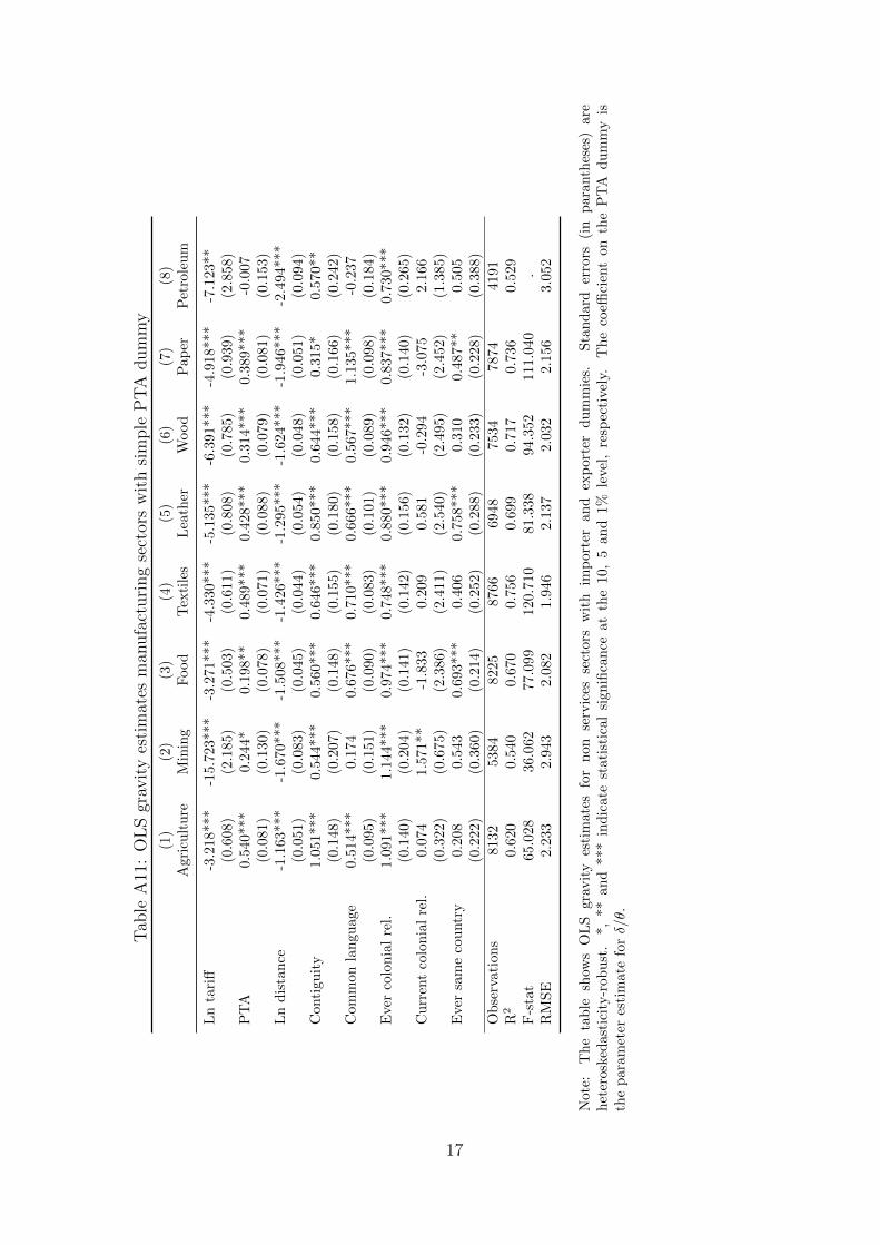
Tab

leA

11:

OL

Sgr

avit

yes

tim

ates

man

ufa

cturi

ng

sect

ors

wit

hsi

mple

PT

Adum

my

(1)

(2)

(3)

(4)

(5)

(6)

(7)

(8)

Agr

icu

ltu

reM

inin

gF

ood

Tex

tile

sL

eath

erW

ood

Pap

erP

etro

leu

m

Ln

tari

ff-3

.218

***

-15.

723***

-3.2

71***

-4.3

30***

-5.1

35***

-6.3

91***

-4.9

18***

-7.1

23**

(0.6

08)

(2.1

85)

(0.5

03)

(0.6

11)

(0.8

08)

(0.7

85)

(0.9

39)

(2.8

58)

PT

A0.

540*

**0.

244*

0.1

98**

0.4

89***

0.4

28***

0.3

14***

0.3

89***

-0.0

07

(0.0

81)

(0.1

30)

(0.0

78)

(0.0

71)

(0.0

88)

(0.0

79)

(0.0

81)

(0.1

53)

Ln

dis

tan

ce-1

.163

***

-1.6

70***

-1.5

08***

-1.4

26***

-1.2

95***

-1.6

24***

-1.9

46***

-2.4

94***

(0.0

51)

(0.0

83)

(0.0

45)

(0.0

44)

(0.0

54)

(0.0

48)

(0.0

51)

(0.0

94)

Con

tigu

ity

1.05

1***

0.54

4***

0.5

60***

0.6

46***

0.8

50***

0.6

44***

0.3

15*

0.5

70**

(0.1

48)

(0.2

07)

(0.1

48)

(0.1

55)

(0.1

80)

(0.1

58)

(0.1

66)

(0.2

42)

Com

mon

lan

guag

e0.

514*

**0.

174

0.6

76***

0.7

10***

0.6

66***

0.5

67***

1.1

35***

-0.2

37

(0.0

95)

(0.1

51)

(0.0

90)

(0.0

83)

(0.1

01)

(0.0

89)

(0.0

98)

(0.1

84)

Eve

rco

lonia

lre

l.1.

091*

**1.

144***

0.9

74***

0.7

48***

0.8

80***

0.9

46***

0.8

37***

0.7

30***

(0.1

40)

(0.2

04)

(0.1

41)

(0.1

42)

(0.1

56)

(0.1

32)

(0.1

40)

(0.2

65)

Cu

rren

tco

lon

ial

rel.

0.07

41.

571**

-1.8

33

0.2

09

0.5

81

-0.2

94

-3.0

75

2.1

66

(0.3

22)

(0.6

75)

(2.3

86)

(2.4

11)

(2.5

40)

(2.4

95)

(2.4

52)

(1.3

85)

Eve

rsa

me

cou

ntr

y0.

208

0.54

30.6

93***

0.4

06

0.7

58***

0.3

10

0.4

87**

0.5

05

(0.2

22)

(0.3

60)

(0.2

14)

(0.2

52)

(0.2

88)

(0.2

33)

(0.2

28)

(0.3

88)

Ob

serv

atio

ns

8132

5384

8225

8766

6948

7534

7874

4191

R2

0.62

00.

540

0.6

70

0.7

56

0.6

99

0.7

17

0.7

36

0.5

29

F-s

tat

65.0

2836

.062

77.0

99

120.7

10

81.3

38

94.3

52

111.0

40

.R

MS

E2.

233

2.94

32.0

82

1.9

46

2.1

37

2.0

32

2.1

56

3.0

52

Not

e:T

he

tab

lesh

ows

OL

Sgr

avit

yes

tim

ates

for

non

serv

ices

sect

ors

wit

him

port

eran

dex

port

erd

um

mie

s.S

tan

dard

erro

rs(i

np

ara

nth

eses

)are

het

eros

ked

asti

city

-rob

ust

.*,

**an

d**

*in

dic

ate

stat

isti

cal

sign

ifica

nce

at

the

10,

5an

d1%

leve

l,re

spec

tivel

y.T

he

coeffi

cien

ton

the

PT

Ad

um

my

isth

ep

aram

eter

esti

mat

efo

rδ/θ.

17

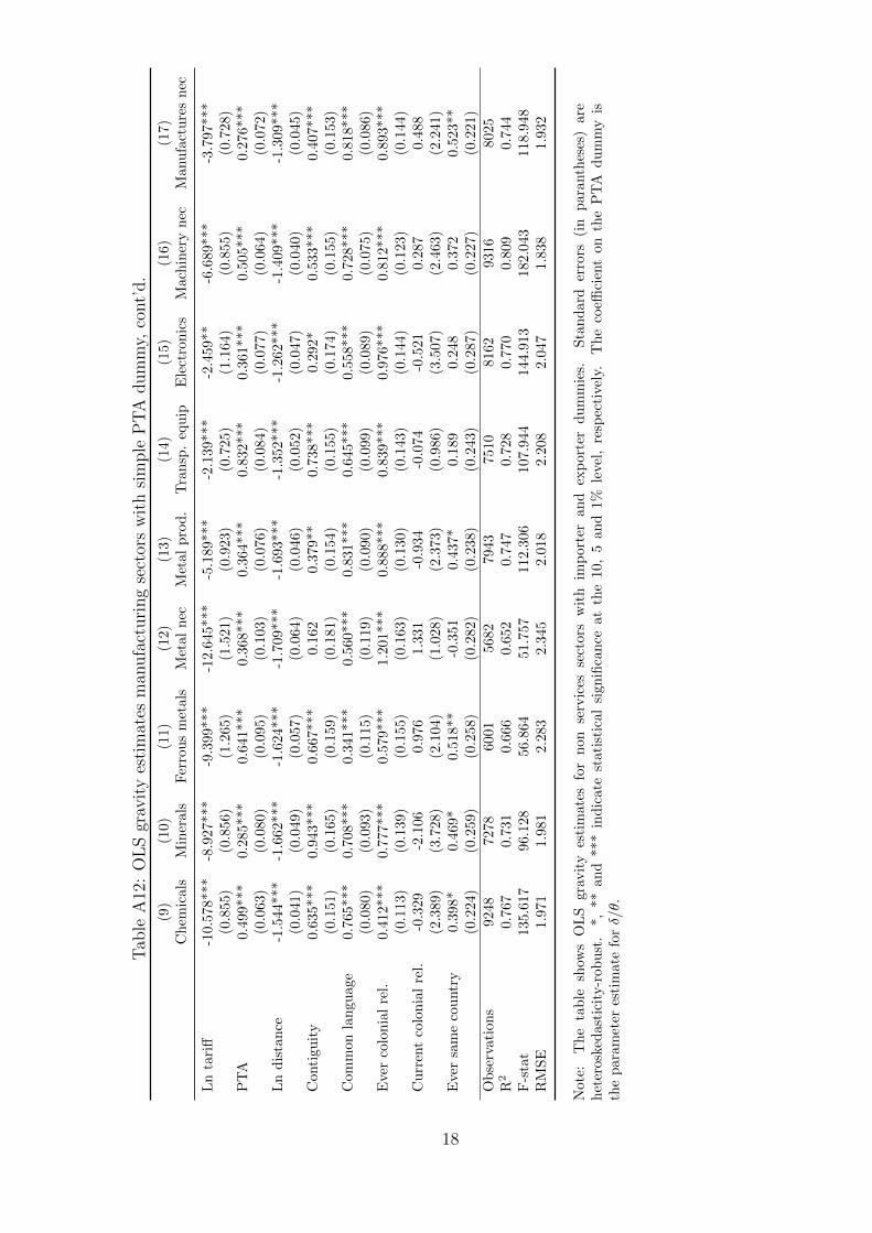
Tab

leA

12:

OL

Sgr

avit

yes

tim

ates

man

ufa

cturi

ng

sect

ors

wit

hsi

mple

PT

Adum

my,

cont’

d.

(9)

(10)

(11)

(12)

(13)

(14)

(15)

(16)

(17)

Ch

emic

als

Min

eral

sF

erro

us

met

als

Met

al

nec

Met

al

pro

d.

Tra

nsp

.eq

uip

Ele

ctro

nic

sM

ach

iner

yn

ecM

anu

fact

ure

sn

ec

Ln

tari

ff-1

0.57

8***

-8.9

27**

*-9

.399***

-12.6

45***

-5.1

89***

-2.1

39***

-2.4

59**

-6.6

89***

-3.7

97***

(0.8

55)

(0.8

56)

(1.2

65)

(1.5

21)

(0.9

23)

(0.7

25)

(1.1

64)

(0.8

55)

(0.7

28)

PT

A0.

499*

**0.

285*

**0.

641***

0.3

68***

0.3

64***

0.8

32***

0.3

61***

0.5

05***

0.2

76***

(0.0

63)

(0.0

80)

(0.0

95)

(0.1

03)

(0.0

76)

(0.0

84)

(0.0

77)

(0.0

64)

(0.0

72)

Ln

dis

tan

ce-1

.544

***

-1.6

62**

*-1

.624***

-1.7

09***

-1.6

93***

-1.3

52***

-1.2

62***

-1.4

09***

-1.3

09***

(0.0

41)

(0.0

49)

(0.0

57)

(0.0

64)

(0.0

46)

(0.0

52)

(0.0

47)

(0.0

40)

(0.0

45)

Con

tigu

ity

0.63

5***

0.94

3***

0.667***

0.1

62

0.3

79**

0.7

38***

0.2

92*

0.5

33***

0.4

07***

(0.1

51)

(0.1

65)

(0.1

59)

(0.1

81)

(0.1

54)

(0.1

55)

(0.1

74)

(0.1

55)

(0.1

53)

Com

mon

lan

guag

e0.

765*

**0.

708*

**0.

341***

0.5

60***

0.8

31***

0.6

45***

0.5

58***

0.7

28***

0.8

18***

(0.0

80)

(0.0

93)

(0.1

15)

(0.1

19)

(0.0

90)

(0.0

99)

(0.0

89)

(0.0

75)

(0.0

86)

Eve

rco

lon

ial

rel.

0.41

2***

0.77

7***

0.57

9***

1.2

01***

0.8

88***

0.8

39***

0.9

76***

0.8

12***

0.8

93***

(0.1

13)

(0.1

39)

(0.1

55)

(0.1

63)

(0.1

30)

(0.1

43)

(0.1

44)

(0.1

23)

(0.1

44)

Cu

rren

tco

lonia

lre

l.-0

.329

-2.1

060.9

76

1.3

31

-0.9

34

-0.0

74

-0.5

21

0.2

87

0.4

88

(2.3

89)

(3.7

28)

(2.1

04)

(1.0

28)

(2.3

73)

(0.9

86)

(3.5

07)

(2.4

63)

(2.2

41)

Eve

rsa

me

cou

ntr

y0.

398*

0.46

9*0.

518**

-0.3

51

0.4

37*

0.1

89

0.2

48

0.3

72

0.5

23**

(0.2

24)

(0.2

59)

(0.2

58)

(0.2

82)

(0.2

38)

(0.2

43)

(0.2

87)

(0.2

27)

(0.2

21)

Ob

serv

atio

ns

9248

7278

6001

5682

7943

7510

8162

9316

8025

R2

0.76

70.

731

0.6

66

0.6

52

0.7

47

0.7

28

0.7

70

0.8

09

0.7

44

F-s

tat

135.

617

96.1

2856

.864

51.7

57

112.3

06

107.9

44

144.9

13

182.0

43

118.9

48

RM

SE

1.97

11.

981

2.2

83

2.3

45

2.0

18

2.2

08

2.0

47

1.8

38

1.9

32

Not

e:T

he

tab

lesh

ows

OL

Sgr

avit

yes

tim

ates

for

non

serv

ices

sect

ors

wit

him

port

eran

dex

port

erd

um

mie

s.S

tan

dard

erro

rs(i

np

ara

nth

eses

)are

het

eros

ked

asti

city

-rob

ust

.*,

**an

d**

*in

dic

ate

stat

isti

cal

sign

ifica

nce

at

the

10,

5an

d1%

leve

l,re

spec

tivel

y.T

he

coeffi

cien

ton

the

PT

Ad

um

my

isth

ep

aram

eter

esti

mat

efo

rδ/θ.

18

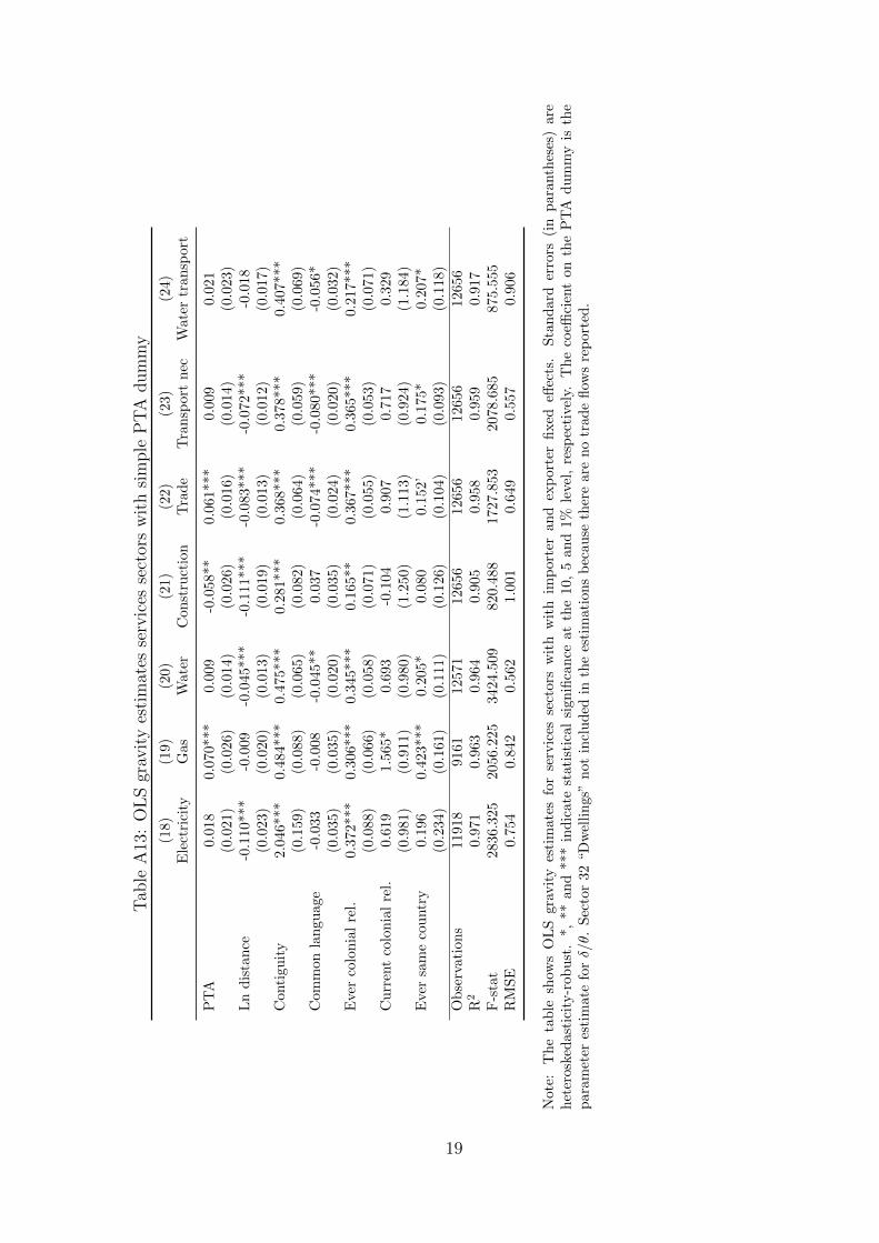
Tab

leA

13:

OL

Sgr

avit

yes

tim

ates

serv

ices

sect

ors

wit

hsi

mple

PT

Adum

my

(18)

(19)

(20)

(21)

(22)

(23)

(24)

Ele

ctri

city

Gas

Wate

rC

on

stru

ctio

nT

rad

eT

ran

sport

nec

Wate

rtr

an

sport

PT

A0.

018

0.07

0***

0.0

09

-0.0

58**

0.0

61***

0.0

09

0.0

21

(0.0

21)

(0.0

26)

(0.0

14)

(0.0

26)

(0.0

16)

(0.0

14)

(0.0

23)

Ln

dis

tan

ce-0

.110

***

-0.0

09

-0.0

45***

-0.1

11***

-0.0

83***

-0.0

72***

-0.0

18

(0.0

23)

(0.0

20)

(0.0

13)

(0.0

19)

(0.0

13)

(0.0

12)

(0.0

17)

Con

tigu

ity

2.04

6***

0.48

4***

0.4

75***

0.2

81***

0.3

68***

0.3

78***

0.4

07***

(0.1

59)

(0.0

88)

(0.0

65)

(0.0

82)

(0.0

64)

(0.0

59)

(0.0

69)

Com

mon

lan

guag

e-0

.033

-0.0

08

-0.0

45**

0.0

37

-0.0

74**

*-0

.080***

-0.0

56*

(0.0

35)

(0.0

35)

(0.0

20)

(0.0

35)

(0.0

24)

(0.0

20)

(0.0

32)

Eve

rco

lonia

lre

l.0.

372*

**0.

306***

0.3

45***

0.1

65**

0.3

67**

*0.3

65***

0.2

17***

(0.0

88)

(0.0

66)

(0.0

58)

(0.0

71)

(0.0

55)

(0.0

53)

(0.0

71)

Cu

rren

tco

lon

ial

rel.

0.61

91.

565*

0.6

93

-0.1

04

0.9

07

0.7

17

0.3

29

(0.9

81)

(0.9

11)

(0.9

80)

(1.2

50)

(1.1

13)

(0.9

24)

(1.1

84)

Eve

rsa

me

cou

ntr

y0.

196

0.42

3***

0.2

05*

0.0

80

0.1

52’

0.1

75*

0.2

07*

(0.2

34)

(0.1

61)

(0.1

11)

(0.1

26)

(0.1

04)

(0.0

93)

(0.1

18)

Ob

serv

atio

ns

1191

891

61

12571

12656

12656

12656

12656

R2

0.97

10.

963

0.9

64

0.9

05

0.9

58

0.9

59

0.9

17

F-s

tat

2836

.325

2056

.225

3424.5

09

820.4

88

1727.8

53

2078.6

85

875.5

55

RM

SE

0.75

40.

842

0.5

62

1.0

01

0.6

49

0.5

57

0.9

06

Not

e:T

he

tab

lesh

ows

OL

Sgr

avit

yes

tim

ates

for

serv

ices

sect

ors

wit

hw

ith

imp

ort

eran

dex

port

erfi

xed

effec

ts.

Sta

nd

ard

erro

rs(i

np

ara

nth

eses

)are

het

eros

ked

asti

city

-rob

ust

.*,

**an

d**

*in

dic

ate

stat

isti

cal

sign

ifica

nce

at

the

10,

5an

d1%

leve

l,re

spec

tive

ly.

Th

eco

effici

ent

on

the

PT

Ad

um

my

isth

ep

aram

eter

esti

mat

efo

rδ/θ.

Sec

tor

32“D

wel

lin

gs”

not

incl

ud

edin

the

esti

mati

on

sb

ecau

seth

ere

are

no

trad

efl

ows

rep

ort

ed.

19

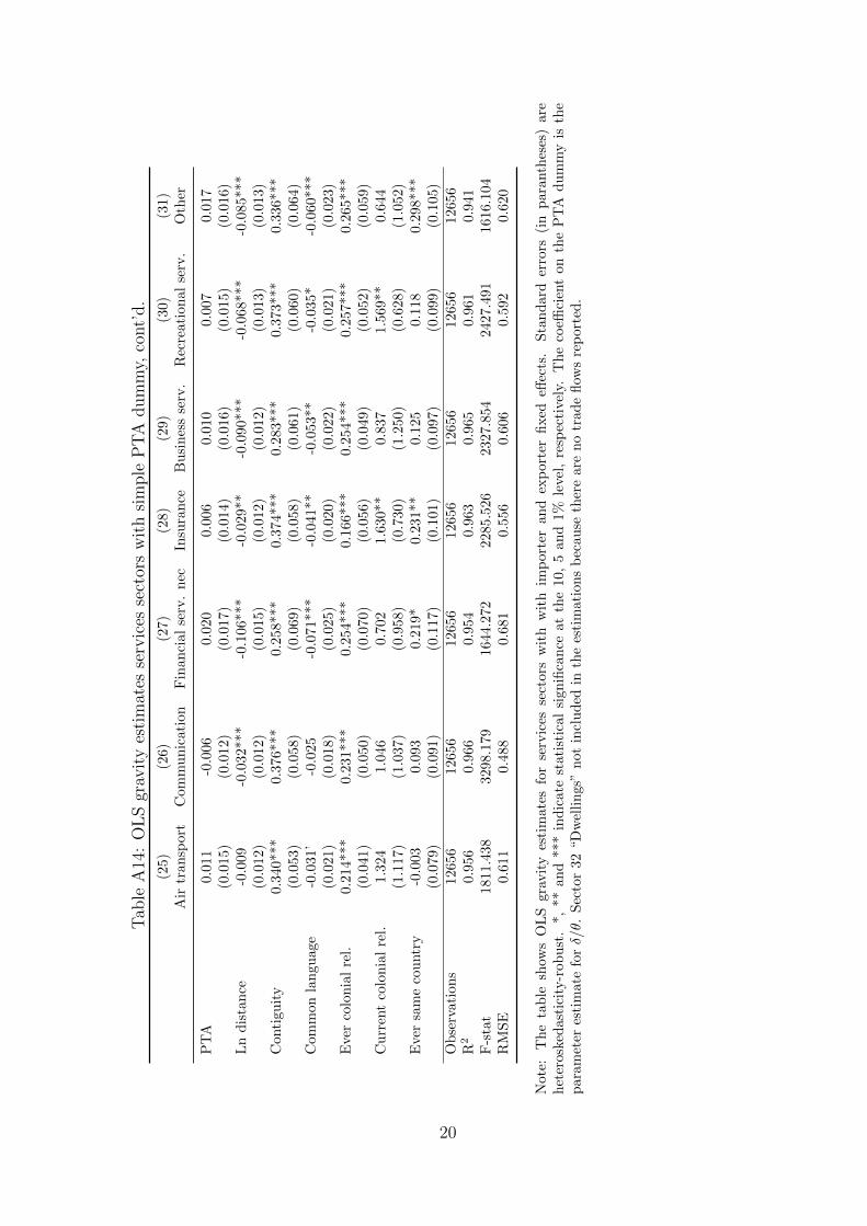
Tab

leA

14:

OL

Sgr

avit

yes

tim

ates

serv

ices

sect

ors

wit

hsi

mple

PT

Adum

my,

cont’

d.

(25)

(26)

(27)

(28)

(29)

(30)

(31)

Air

tran

spor

tC

omm

un

icati

on

Fin

an

cial

serv

.n

ecIn

sura

nce

Bu

sin

ess

serv

.R

ecre

ati

on

al

serv

.O

ther

PT

A0.

011

-0.0

060.0

20

0.0

06

0.0

10

0.0

07

0.0

17

(0.0

15)

(0.0

12)

(0.0

17)

(0.0

14)

(0.0

16)

(0.0

15)

(0.0

16)

Ln

dis

tan

ce-0

.009

-0.0

32***

-0.1

06***

-0.0

29**

-0.0

90***

-0.0

68***

-0.0

85***

(0.0

12)

(0.0

12)

(0.0

15)

(0.0

12)

(0.0

12)

(0.0

13)

(0.0

13)

Con

tigu

ity

0.34

0***

0.37

6***

0.2

58***

0.3

74***

0.2

83***

0.3

73***

0.3

36***

(0.0

53)

(0.0

58)

(0.0

69)

(0.0

58)

(0.0

61)

(0.0

60)

(0.0

64)

Com

mon

lan

guag

e-0

.031

’-0

.025

-0.0

71***

-0.0

41**

-0.0

53**

-0.0

35*

-0.0

60***

(0.0

21)

(0.0

18)

(0.0

25)

(0.0

20)

(0.0

22)

(0.0

21)

(0.0

23)

Eve

rco

lonia

lre

l.0.

214*

**0.

231*

**

0.2

54***

0.1

66***

0.2

54***

0.2

57***

0.2

65***

(0.0

41)

(0.0

50)

(0.0

70)

(0.0

56)

(0.0

49)

(0.0

52)

(0.0

59)

Cu

rren

tco

lon

ial

rel.

1.32

41.

046

0.7

02

1.6

30**

0.8

37

1.5

69**

0.6

44

(1.1

17)

(1.0

37)

(0.9

58)

(0.7

30)

(1.2

50)

(0.6

28)

(1.0

52)

Eve

rsa

me

cou

ntr

y-0

.003

0.09

30.2

19*

0.2

31**

0.1

25

0.1

18

0.2

98***

(0.0

79)

(0.0

91)

(0.1

17)

(0.1

01)

(0.0

97)

(0.0

99)

(0.1

05)

Ob

serv

atio

ns

1265

612

656

12656

12656

12656

12656

12656

R2

0.95

60.

966

0.9

54

0.9

63

0.9

65

0.9

61

0.9

41

F-s

tat

1811

.438

3298

.179

1644.2

72

2285.5

26

2327.8

54

2427.4

91

1616.1

04

RM

SE

0.61

10.

488

0.6

81

0.5

56

0.6

06

0.5

92

0.6

20

Not

e:T

he

tab

lesh

ows

OL

Sgr

avit

yes

tim

ates

for

serv

ices

sect

ors

wit

hw

ith

imp

ort

eran

dex

port

erfi

xed

effec

ts.

Sta

nd

ard

erro

rs(i

np

ara

nth

eses

)are

het

eros

ked

asti

city

-rob

ust

.*,

**an

d**

*in

dic

ate

stat

isti

cal

sign

ifica

nce

at

the

10,

5an

d1%

leve

l,re

spec

tive

ly.

Th

eco

effici

ent

on

the

PT

Ad

um

my

isth

ep

aram

eter

esti

mat

efo

rδ/θ.

Sec

tor

32“D

wel

lin

gs”

not

incl

ud

edin

the

esti

mati

on

sb

ecau

seth

ere

are

no

trad

efl

ows

rep

ort

ed.

20

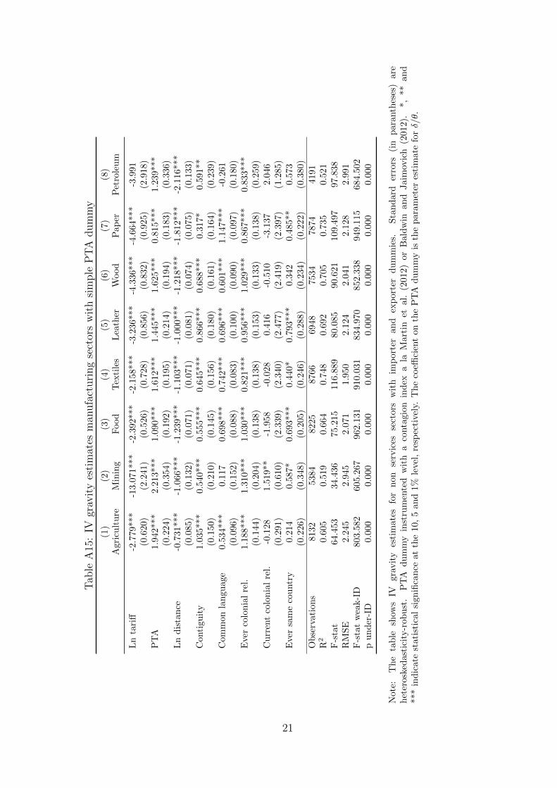
Tab

leA

15:

IVgr

avit

yes

tim

ates

man

ufa

cturi

ng

sect

ors

wit

hsi

mple

PT

Adum

my

(1)

(2)

(3)

(4)

(5)

(6)

(7)

(8)

Agr

icu

ltu

reM

inin

gF

ood

Tex

tile

sL

eath

erW

ood

Pap

erP

etro

leu

m

Ln

tari

ff-2

.779

***

-13.

071***

-2.3

92***

-2.1

58***

-3.2

36***

-4.3

36***

-4.6

64***

-3.9

91

(0.6

20)

(2.2

41)

(0.5

26)

(0.7

28)

(0.8

56)

(0.8

32)

(0.9

25)

(2.9

18)

PT

A1.

942*

**2.

213***

1.0

90***

1.6

12***

1.4

45***

1.6

25***

0.8

15***

1.2

39***

(0.2

24)

(0.3

54)

(0.1

92)

(0.1

95)

(0.2

14)

(0.1

94)

(0.1

83)

(0.3

36)

Ln

dis

tan

ce-0

.731

***

-1.0

66***

-1.2

39***

-1.1

03***

-1.0

00***

-1.2

18***

-1.8

12***

-2.1

16***

(0.0

85)

(0.1

32)

(0.0

71)

(0.0

71)

(0.0

81)

(0.0

74)

(0.0

75)

(0.1

33)

Con

tigu

ity

1.03

5***

0.54

0***

0.5

55***

0.6

45***

0.8

66***

0.6

88***

0.3

17*

0.5

91**

(0.1

50)

(0.2

10)

(0.1

45)

(0.1

56)

(0.1

80)

(0.1

61)

(0.1

64)

(0.2

39)

Com

mon

lan

guag

e0.

534*

**0.

117

0.6

98***

0.7

42***

0.6

96***

0.6

01***

1.1

47***

-0.2

61

(0.0

96)

(0.1

52)

(0.0

88)

(0.0

83)

(0.1

00)

(0.0

90)

(0.0

97)

(0.1

80)

Eve

rco

lonia

lre

l.1.

188*

**1.

310***

1.0

30***

0.8

21***

0.9

56***

1.0

29***

0.8

67***

0.8

33***

(0.1

44)

(0.2

04)

(0.1

38)

(0.1

38)

(0.1

53)

(0.1

33)

(0.1

38)

(0.2

59)

Cu

rren

tco

lon

ial

rel.

-0.1

281.

519**

-1.9

58

-0.0

28

0.4

16

-0.5

10

-3.1

37

2.0

46

(0.2

91)

(0.6

10)

(2.3

39)

(2.3

40)

(2.4

77)

(2.4

19)

(2.3

97)

(1.2

85)

Eve

rsa

me

cou

ntr

y0.

214

0.587*

0.6

93***

0.4

40*

0.7

93***

0.3

42

0.4

85**

0.5

73

(0.2

26)

(0.3

48)

(0.2

05)

(0.2

46)

(0.2

88)

(0.2

34)

(0.2

22)

(0.3

80)

Ob

serv

atio

ns

8132

5384

8225

8766

6948

7534

7874

4191

R2

0.60

50.

519

0.6

64

0.7

48

0.6

92

0.7

05

0.7

35

0.5

21

F-s

tat

64.4

5334

.436

75.2

15

116.8

89

80.0

85

90.6

21

109.4

97

97.8

38

RM

SE

2.24

52.

945

2.0

71

1.9

50

2.1

24

2.0

41

2.1

28

2.9

91

F-s

tat

wea

k-I

D80

3.58

260

5.2

67

962.1

31

910.0

31

834.9

70

852.3

38

949.1

15

684.5

02

pu

nd

er-I

D0.

000

0.000

0.0

00

0.0

00

0.0

00

0.0

00

0.0

00

0.0

00

Not

e:T

he

tab

lesh

ows

IVgr

avit

yes

tim

ates

for

non

serv

ices

sect

ors

wit

him

port

eran

dex

port

erdu

mm

ies.

Sta

nd

ard

erro

rs(i

np

ara

nth

eses

)are

het

eros

ked

asti

city

-rob

ust

.P

TA

du

mm

yin

stru

men

ted

wit

ha

conta

gio

nin

dex

ala

Mart

inet

al.

(2012)

or

Bald

win

an

dJaim

ovic

h(2

012).

*,

**

an

d**

*in

dic

ate

stat

isti

cal

sign

ifica

nce

atth

e10

,5

and

1%le

vel

,re

spec

tive

ly.

Th

eco

effici

ent

on

the

PT

Ad

um

my

isth

ep

ara

met

eres

tim

ate

forδ/θ.

21

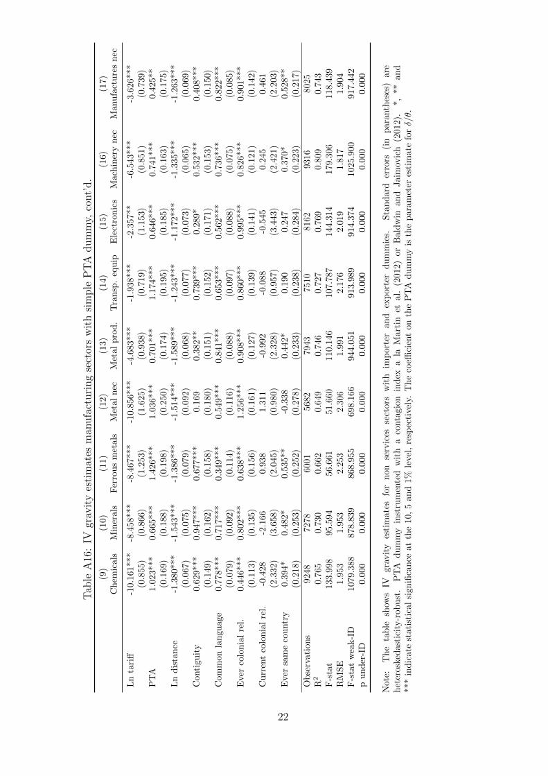
Tab

leA

16:

IVgr

avit

yes

tim

ates

man

ufa

cturi

ng

sect

ors

wit

hsi

mple

PT

Adum

my,

cont’

d.

(9)

(10)

(11)

(12)

(13)

(14)

(15)

(16)

(17)

Ch

emic

als

Min

eral

sF

erro

us

met

als

Met

al

nec

Met

al

pro

d.

Tra

nsp

.eq

uip

Ele

ctro

nic

sM

ach

iner

yn

ecM

anu

fact

ure

sn

ec

Ln

tari

ff-1

0.16

1***

-8.4

58**

*-8

.467***

-10.8

56***

-4.6

83***

-1.9

38***

-2.3

57**

-6.5

43***

-3.6

26***

(0.8

55)

(0.8

66)

(1.2

53)

(1.6

25)

(0.9

38)

(0.7

19)

(1.1

53)

(0.8

51)

(0.7

39)

PT

A1.

023*

**0.

665*

**1.

426***

1.0

36***

0.7

01***

1.1

74***

0.6

46***

0.7

41***

0.4

25**

(0.1

69)

(0.1

88)

(0.1

98)

(0.2

50)

(0.1

74)

(0.1

95)

(0.1

85)

(0.1

63)

(0.1

75)

Ln

dis

tan

ce-1

.380

***

-1.5

43**

*-1

.386***

-1.5

14***

-1.5

89***

-1.2

43***

-1.1

72***

-1.3

35***

-1.2

63***

(0.0

67)

(0.0

75)

(0.0

79)

(0.0

92)

(0.0

68)

(0.0

77)

(0.0

73)

(0.0

65)

(0.0

69)

Con

tigu

ity

0.62

9***

0.94

7***

0.677***

0.1

69

0.3

82**

0.7

39***

0.2

89*

0.5

32***

0.4

08***

(0.1

49)

(0.1

62)

(0.1

58)

(0.1

80)

(0.1

51)

(0.1

52)

(0.1

71)

(0.1

53)

(0.1

50)

Com

mon

lan

guag

e0.

778*

**0.

717*

**0.

349***

0.5

49***

0.8

41***

0.6

53***

0.5

62***

0.7

36***

0.8

22***

(0.0

79)

(0.0

92)

(0.1

14)

(0.1

16)

(0.0

88)

(0.0

97)

(0.0

88)

(0.0

75)

(0.0

85)

Eve

rco

lon

ial

rel.

0.44

6***

0.80

2***

0.63

8***

1.2

56***

0.9

08***

0.8

60***

0.9

95***

0.8

26***

0.9

01***

(0.1

13)

(0.1

35)

(0.1

56)

(0.1

61)

(0.1

27)

(0.1

39)

(0.1

41)

(0.1

21)

(0.1

42)

Cu

rren

tco

lonia

lre

l.-0

.428

-2.1

660.9

38

1.3

11

-0.9

92

-0.0

88

-0.5

45

0.2

45

0.4

61

(2.3

32)

(3.6

58)

(2.0

45)

(0.9

80)

(2.3

28)

(0.9

57)

(3.4

43)

(2.4

21)

(2.2

03)

Eve

rsa

me

cou

ntr

y0.

394*

0.48

2*0.

535**

-0.3

38

0.4

42*

0.1

90

0.2

47

0.3

70*

0.5

28**

(0.2

18)

(0.2

53)

(0.2

52)

(0.2

78)

(0.2

33)

(0.2

38)

(0.2

84)

(0.2

23)

(0.2

17)

Ob

serv

atio

ns

9248

7278

6001

5682

7943

7510

8162

9316

8025

R2

0.76

50.

730

0.6

62

0.6

49

0.7

46

0.7

27

0.7

69

0.8

09

0.7

43

F-s

tat

133.

998

95.5

9456

.661

51.6

60

110.1

46

107.7

87

144.3

14

179.3

06

118.4

39

RM

SE

1.95

31.

953

2.2

53

2.3

06

1.9

91

2.1

76

2.0

19

1.8

17

1.9

04

F-s

tat

wea

k-I

D10

79.3

8887

8.83

986

8.9

55

698.1

66

944.0

51

913.9

89

914.3

74

1025.9

00

917.4

42

pu

nd

er-I

D0.

000

0.00

00.0

00

0.0

00

0.0

00

0.0

00

0.0

00

0.0

00

0.0

00

Not

e:T

he

tab

lesh

ows

IVgr

avit

yes

tim

ates

for

non

serv

ices

sect

ors

wit

him

port

eran

dex

port

erdu

mm

ies.

Sta

nd

ard

erro

rs(i

np

ara

nth

eses

)are

het

eros

ked

asti

city

-rob

ust

.P

TA

du

mm

yin

stru

men

ted

wit

ha

conta

gio

nin

dex

ala

Mart

inet

al.

(2012)

or

Bald

win

an

dJaim

ovic

h(2

012).

*,

**

an

d**

*in

dic

ate

stat

isti

cal

sign

ifica

nce

atth

e10

,5

and

1%le

vel

,re

spec

tive

ly.

Th

eco

effici

ent

on

the

PT

Ad

um

my

isth

ep

ara

met

eres

tim

ate

forδ/θ.

22

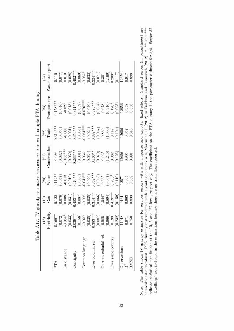
Tab

leA

17:

IVgr

avit

yes

tim

ates

serv

ices

sect

ors

wit

hsi

mple

PT

Adum

my

(18)

(19)

(20)

(21)

(22)

(23)

(24)

Ele

ctri

city

Gas

Wate

rC

on

stru

ctio

nT

rad

eT

ran

sport

nec

Wate

rtr

an

sport

PT

A0.

169*

*0.

122

0.1

12**

-0.0

36

0.3

14***

0.1

58***

0.1

10

(0.0

72)

(0.0

76)

(0.0

47)

(0.0

82)

(0.0

56)

(0.0

46)

(0.0

77)

Ln

dis

tan

ce-0

.064

*0.

008

-0.0

13

-0.1

06***

-0.0

05

-0.0

27

0.0

10

(0.0

33)

(0.0

31)

(0.0

19)

(0.0

30)

(0.0

21)

(0.0

18)

(0.0

28)

Con

tigu

ity

2.03

9***

0.48

3***

0.4

70***

0.2

83***

0.3

54***

0.3

71***

0.4

02***

(0.1

58)

(0.0

87)

(0.0

65)

(0.0

81)

(0.0

64)

(0.0

59)

(0.0

69)

Com

mon

lan

guag

e-0

.029

-0.0

06

-0.0

41**

0.0

34

-0.0

64**

*-0

.076***

-0.0

52*

(0.0

35)

(0.0

35)

(0.0

20)

(0.0

34)

(0.0

24)

(0.0

20)

(0.0

32)

Eve

rco

lon

ial

rel.

0.38

3***

0.31

4***

0.3

52***

0.1

63**

0.3

87***

0.3

75***

0.2

24***

(0.0

87)

(0.0

66)

(0.0

58)

(0.0

70)

(0.0

57)

(0.0

54)

(0.0

71)

Cu

rren

tco

lonia

lre

l.0.

585

1.544*

0.6

65

-0.0

95

0.8

30

0.6

78

0.3

01

(0.9

66)

(0.8

94)

(0.9

67)

(1.2

40)

(1.0

90)

(0.9

10)

(1.1

69)

Eve

rsa

me

cou

ntr

y0.

193

0.41

9***

0.2

03*

0.0

82

0.1

42

0.1

70*

0.2

03*

(0.2

32)

(0.1

59)

(0.1

10)

(0.1

25)

(0.1

04)

(0.0

93)

(0.1

17)

Ob

serv

atio

ns

1191

891

61

12571

12656

12656

12656

12656

R2

0.97

10.

963

0.9

64

0.9

05

0.9

57

0.9

58

0.9

17

RM

SE

0.75

00.

833

0.5

59

0.9

91

0.6

48

0.5

56

0.8

98

Not

e:T

he

tab

lesh

ows

IVgr

avit

yes

tim

ates

for

serv

ices

sect

ors

wit

hw

ith

imp

ort

eran

dex

port

erfi

xed

effec

ts.

Sta

nd

ard

erro

rs(i

np

ara

nth

eses

)are

het

eros

ked

asti

city

-rob

ust

.P

TA

du

mm

yin

stru

men

ted

wit

ha

conta

gio

nin

dex

ala

Mart

inet

al.

(2012)

or

Bald

win

an

dJaim

ovic

h(2

012).

*,

**

an

d***

ind

icat

est

atis

tica

lsi

gnifi

can

ceat

the

10,

5an

d1%

leve

l,re

spec

tivel

y.T

he

coeffi

cien

ton

the

PT

Ad

um

my

isth

ep

ara

met

eres

tim

ate

forδ/θ.

Sec

tor

32

“Dw

elli

ngs

”n

otin

clu

ded

inth

ees

tim

atio

ns

bec

ause

ther

eare

no

trad

efl

ows

rep

ort

ed.

23

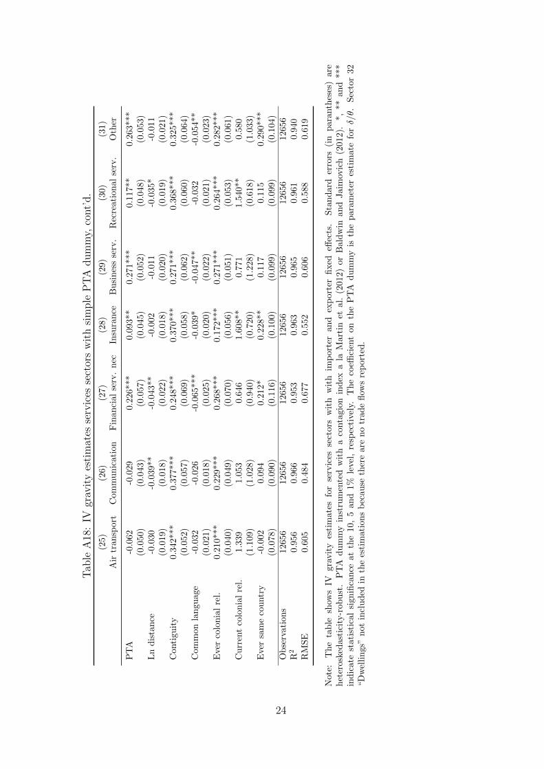
Tab

leA

18:

IVgr

avit

yes

tim

ates

serv

ices

sect

ors

wit

hsi

mple

PT

Adum

my,

cont’

d.

(25)

(26)

(27)

(28)

(29)

(30)

(31)

Air

tran

spor

tC

omm

un

icati

on

Fin

an

cial

serv

.n

ecIn

sura

nce

Bu

sin

ess

serv

.R

ecre

ati

onal

serv

.O

ther

PT

A-0

.062

-0.0

290.2

26***

0.0

93**

0.2

71***

0.1

17**

0.2

63***

(0.0

50)

(0.0

43)

(0.0

57)

(0.0

45)

(0.0

52)

(0.0

48)

(0.0

53)

Ln

dis

tan

ce-0

.030

-0.0

39**

-0.0

43**

-0.0

02

-0.0

11

-0.0

35*

-0.0

11

(0.0

19)

(0.0

18)

(0.0

22)

(0.0

18)

(0.0

20)

(0.0

19)

(0.0

21)

Con

tigu

ity

0.34

2***

0.37

7***

0.2

48***

0.3

70***

0.2

71***

0.3

68***

0.3

25***

(0.0

52)

(0.0

57)

(0.0

69)

(0.0

58)

(0.0

62)

(0.0

60)

(0.0

64)

Com

mon

lan

guag

e-0

.032

-0.0

26

-0.0

65***

-0.0

39*

-0.0

47**

-0.0

32

-0.0

54**

(0.0

21)

(0.0

18)

(0.0

25)

(0.0

20)

(0.0

22)

(0.0

21)

(0.0

23)

Eve

rco

lon

ial

rel.

0.21

0***

0.22

9***

0.2

68***

0.1

72***

0.2

71***

0.2

64***

0.2

82***

(0.0

40)

(0.0

49)

(0.0

70)

(0.0

56)

(0.0

51)

(0.0

53)

(0.0

61)

Cu

rren

tco

lonia

lre

l.1.

339

1.05

30.6

46

1.6

08**

0.7

71

1.5

40**

0.5

80

(1.1

09)

(1.0

28)

(0.9

40)

(0.7

20)

(1.2

28)

(0.6

18)

(1.0

33)

Eve

rsa

me

cou

ntr

y-0

.002

0.09

40.2

12*

0.2

28**

0.1

17

0.1

15

0.2

90***

(0.0

78)

(0.0

90)

(0.1

16)

(0.1

00)

(0.0

99)

(0.0

99)

(0.1

04)

Ob

serv

atio

ns

1265

612

656

12656

12656

12656

12656

12656

R2

0.95

60.

966

0.9

53

0.9

63

0.9

65

0.9

61

0.9

40

RM

SE

0.60

50.

484

0.6

77

0.5

52

0.6

06

0.5

88

0.6

19

Not

e:T

he

tab

lesh

ows

IVgr

avit

yes

tim

ates

for

serv

ices

sect

ors

wit

hw

ith

imp

ort

eran

dex

port

erfi

xed

effec

ts.

Sta

nd

ard

erro

rs(i

np

ara

nth

eses

)are

het

eros

ked

asti

city

-rob

ust

.P

TA

du

mm

yin

stru

men

ted

wit

ha

conta

gio

nin

dex

ala

Mart

inet

al.

(2012)

or

Bald

win

an

dJaim

ovic

h(2

012).

*,

**

an

d***

ind

icat

est

atis

tica

lsi

gnifi

can

ceat

the

10,

5an

d1%

leve

l,re

spec

tivel

y.T

he

coeffi

cien

ton

the

PT

Ad

um

my

isth

ep

ara

met

eres

tim

ate

forδ/θ.

Sec

tor

32

“Dw

elli

ngs

”n

otin

clu

ded

inth

ees

tim

atio

ns

bec

ause

ther

eare

no

trad

efl

ows

rep

ort

ed.

24

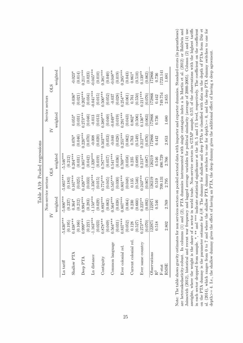
Tab

leA

19:

Pool

edre

gres

sion

s

Non

-ser

vic

ese

ctors

Ser

vic

ese

ctors

IVO

LS

IVO

LS

wei

ghte

dw

eighte

dw

eighte

dw

eighte

d

Ln

tari

ff-5

.630

***

-5.6

06***

-5.6

65***

-5.5

46***

(0.1

95)

(0.2

37)

(0.1

83)

(0.2

12)

Sh

allo

wP

TA

0.43

8***

0.3

64*

0.1

67***

0.2

04***

0.0

76*

0.0

53*

-0.0

36*

-0.0

23*

(0.1

66)

(0.2

12)

(0.0

25)

(0.0

31)

(0.0

46)

(0.0

31)

(0.0

21)

(0.0

14)

Dee

pP

TA

0.99

9***

0.99

4***

0.4

26***

0.3

85***

0.2

20***

0.2

73***

0.202***

0.2

11***

(0.2

21)

(0.2

83)

(0.0

33)

(0.0

42)

(0.0

70)

(0.0

46)

(0.0

34)

(0.0

23)

Ln

dis

tan

ce-1

.163

***

-1.1

50***

-1.3

56***

-1.3

20***

-0.0

08

-0.0

13

-0.0

41***

-0.0

45***

(0.0

23)

(0.0

29)

(0.0

15)

(0.0

19)

(0.0

20)

(0.0

13)

(0.0

15)

(0.0

10)

Con

tigu

ity

0.87

8***

0.893***

0.7

74***

0.7

87***

0.5

03***

0.3

89***

0.5

00***

0.3

81***

(0.0

49)

(0.0

63)

(0.0

45)

(0.0

57)

(0.0

53)

(0.0

40)

(0.0

52)

(0.0

40)

Com

mon

lan

guag

e0.

564*

**0.

564***

0.5

45***

0.5

41***

-0.0

40

-0.0

49**

-0.0

37

-0.0

48**

(0.0

31)

(0.0

38)

(0.0

30)

(0.0

36)

(0.0

28)

(0.0

19)

(0.0

28)

(0.0

19)

Eve

rco

lon

ial

rel.

0.83

7***

0.80

7***

0.8

01***

0.7

69***

0.2

55***

0.2

91***

0.254***

0.2

85***

(0.0

52)

(0.0

64)

(0.0

48)

(0.0

58)

(0.0

62)

(0.0

43)

(0.0

61)

(0.0

43)

Cu

rren

tco

lonia

lre

l.0.

128

0.2

30

0.1

35

0.2

35

0.7

63

0.8

62*

0.7

61

0.8

61*

(0.5

27)

(0.6

60)

(0.5

46)

(0.6

89)

(0.5

49)

(0.5

06)

(0.5

50)

(0.5

10)

Eve

rsa

me

cou

ntr

y0.

273*

**0.

225**

0.2

43***

0.2

13**

0.2

12***

0.1

36**

0.2

11***

0.1

39**

(0.0

70)

(0.0

92)

(0.0

67)

(0.0

87)

(0.0

76)

(0.0

63)

(0.0

76)

(0.0

62)

Ob

serv

atio

ns

1229

7112

2971

126219

126219

172866

172866

172866

172866

R2

0.51

80.5

46

0.5

19

0.5

46

0.4

42

0.7

36

0.4

42

0.7

36

F-s

tat

709.1

31

490.7

29

749.7

54

1723.1

41

RM

SE

2.80

22.

769

2.7

95

2.7

66

2.8

53

1.6

80

2.8

55

1.6

81

Not

e:T

he

tab

lesh

ows

grav

ity

esti

mat

esfo

rn

onse

rvic

esse

ctors

on

poole

dse

ctora

ld

ata

wit

him

port

erand

exp

ort

erd

um

mie

s.S

tand

ard

erro

rs(i

np

ara

nth

eses

)ar

eh

eter

osked

asti

city

-rob

ust

.In

colu

mn

s(1

)an

d(2

),P

TA

du

mm

ies

inst

rum

ente

dw

ith

sin

gle

conta

gio

nin

dex

ala

Mart

inet

al.

(2012)

or

Bald

win

an

dJai

mov

ich

(201

2),

his

tori

cal

and

rece

nt

war

freq

uen

cyan

dla

gged

aver

age

vari

ab

les

for

politi

cal

sim

ilari

ty(a

vera

ge

of

2000-2

005).

Colu

mn

(2)

an

d(4

)u

seaw

eigh

ts,

wh

ere

the

wei

ght

isth

esh

are

ofa

sect

orin

worl

dtr

ad

e.N

on

-ser

vic

ese

ctors

inG

TA

Psa

mp

le,

0.5

%of

the

ob

serv

ati

on

sw

ith

the

hig

hes

tta

riff

sin

each

sect

ord

rop

ped

from

sam

ple

.*,

**an

d**

*in

dic

ate

stati

stic

al

sign

ifica

nce

at

the

10,

5an

d1%

level

,re

spec

tive

ly.

Th

eco

effici

ent

on

the

coeffi

cien

ton

the

PT

Ad

um

my

isth

ep

aram

eter

esti

mat

efo

rδ/θ.

Th

ed

um

my

for

shall

owan

dd

eep

PT

As

iscl

ass

ified

wit

hd

ata

on

the

dep

thof

PT

As

from

Du

ret

al.

(201

4),

wh

ich

ran

ges

from

0to

7an

dw

her

eth

esh

all

owP

TA

du

mm

ysw

itch

esto

on

efo

rd

epth>

=0,

an

dth

ed

eep

PT

Ad

um

my

swit

ches

toon

efo

rd

epth>

=4.

I.e.

,th

esh

allo

wd

um

my

give

sth

eeff

ect

ofh

avin

gan

PT

A,

the

dee

pd

um

my

giv

esth

ead

dit

ion

al

effec

tof

hav

ing

ad

eep

agre

emen

t.

25

C Sensitivity checks: welfare effects from alternative

empirical specifications

The results presented so far rely on the PTA coefficients and θs estimated with an IV ap-

proach and using two different depths of PTAs. Next, we investigate the sensitivity of the

results pertaining to this choice. Table A20 presents results for three different empirical

specifications. In column (1) and (2), the simulations are based on a single PTA dummy.

In Column (1), the PTA dummy is instrumented with the contagion index. Column (2)

is based on OLS regression. By and large, the predicted region-specific growth rates of

real income are stable. The correlation of the country-specific results in the baseline with

the instrumented and uninstrumented results are very high, with a correlation coefficient

of 0.97 in both cases, statistically significant at the 1% level. With a single PTA dummy,

the expected effects are slightly larger. But the overall tendencies are similar, except for

ASEAN and China. For these two regions, the baseline predicts negative results of around

0.2%, while the effects are positive and in the order of magnitude of 0.1% with a single

PTA dummy.

The real income changes in column (4) are based on trade elasticity estimates including

a shallow and deep PTA dummy, but the PTA dummies are not instrumented. The

correlation coefficient of the country-specific results in the baseline with this specification

is again very high, 0.98 and statistically highly significant. The sorting of the regions is

very similar, with the largest negative effects in China and the ASEAN region. But the

predicted effects are substantially smaller. TTIP is still predicted to be positive for TTIP

countries, on average, but it only raises real income by 0.4%.

Last, column (5) presents results when sectoral heterogeneity in the treatment inten-

sity is supressed. We run two estimations on pooled sectoral data, one for the manu-

26

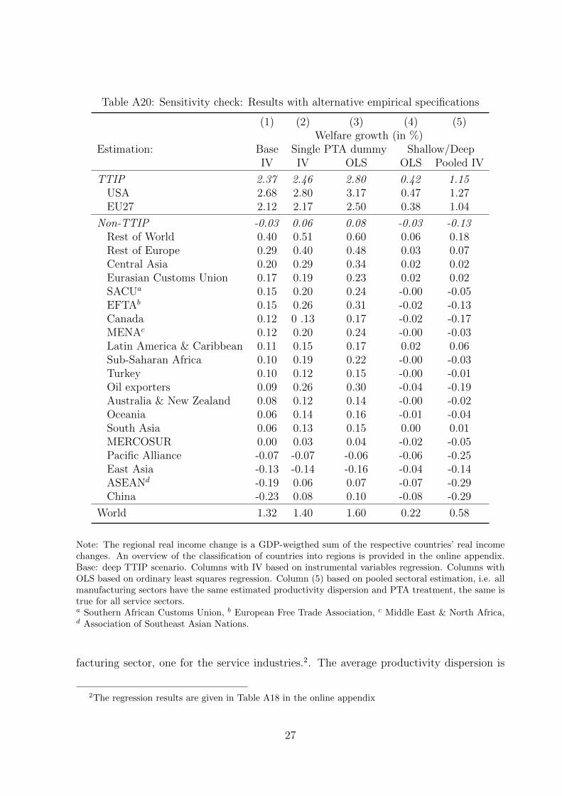
Table A20: Sensitivity check: Results with alternative empirical specifications

(1) (2) (3) (4) (5)Welfare growth (in %)

Estimation: Base Single PTA dummy Shallow/DeepIV IV OLS OLS Pooled IV

TTIP 2.37 2.46 2.80 0.42 1.15USA 2.68 2.80 3.17 0.47 1.27EU27 2.12 2.17 2.50 0.38 1.04

Non-TTIP -0.03 0.06 0.08 -0.03 -0.13Rest of World 0.40 0.51 0.60 0.06 0.18Rest of Europe 0.29 0.40 0.48 0.03 0.07Central Asia 0.20 0.29 0.34 0.02 0.02Eurasian Customs Union 0.17 0.19 0.23 0.02 0.02SACUa 0.15 0.20 0.24 -0.00 -0.05EFTAb 0.15 0.26 0.31 -0.02 -0.13Canada 0.12 0 .13 0.17 -0.02 -0.17MENAc 0.12 0.20 0.24 -0.00 -0.03Latin America & Caribbean 0.11 0.15 0.17 0.02 0.06Sub-Saharan Africa 0.10 0.19 0.22 -0.00 -0.03Turkey 0.10 0.12 0.15 -0.00 -0.01Oil exporters 0.09 0.26 0.30 -0.04 -0.19Australia & New Zealand 0.08 0.12 0.14 -0.00 -0.02Oceania 0.06 0.14 0.16 -0.01 -0.04South Asia 0.06 0.13 0.15 0.00 0.01MERCOSUR 0.00 0.03 0.04 -0.02 -0.05Pacific Alliance -0.07 -0.07 -0.06 -0.06 -0.25East Asia -0.13 -0.14 -0.16 -0.04 -0.14ASEANd -0.19 0.06 0.07 -0.07 -0.29China -0.23 0.08 0.10 -0.08 -0.29

World 1.32 1.40 1.60 0.22 0.58

Note: The regional real income change is a GDP-weigthed sum of the respective countries’ real incomechanges. An overview of the classification of countries into regions is provided in the online appendix.Base: deep TTIP scenario. Columns with IV based on instrumental variables regression. Columns withOLS based on ordinary least squares regression. Column (5) based on pooled sectoral estimation, i.e. allmanufacturing sectors have the same estimated productivity dispersion and PTA treatment, the same istrue for all service sectors.a Southern African Customs Union, b European Free Trade Association, c Middle East & North Africa,d Association of Southeast Asian Nations.

facturing sector, one for the service industries.2. The average productivity dispersion is

2The regression results are given in Table A18 in the online appendix

27

approximately 1/5.6. This finding is in line with the literature, which typically finds esti-

mates of the elasticity of substitution of between 5-7, (see e.g. Broda and Weinstein, 2006;

Bergstrand et al., 2012). Shallow treaties have positive effects on bilateral trade, but the

empirical evidence is less strong for service industries. Deep agreements, on the other

hand, have a strong positive and statistically significant effect in both manufacturing and

services. The estimates suggest, that a deep PTA increases bilateral manufacturing trade

by 1.7 or 170% (≡ e0.999 − 1) and service trade by around 25%. On the country level,

the correlation of real income changes with the base scenario is again very high, 0.92, and

statistically significant. For TTIP countries, the effects are in the order of magnitude of

1% real income increase. So they are smaller than in the baseline. The negative effect on

non-TTIP countries is more pronounced, with -0.13% on average. China and the ASEAN

region are again the biggest losers.

28

References

Baldwin, Richard and Dany Jaimovich, “Are Free Trade Agreements contagious?,” Jour-

nal of International Economics, 2012, 88 (1), 1 – 16.

Bergstrand, Jeffrey H., Peter Egger, and Mario Larch, “Gravity Redux: Estimation of

gravity-equation coefficients, elasticities of substitution, and general equilibrium com-

parative statics under asymmetric bilateral trade costs,” Journal of International Eco-

nomics, 2012.

Broda, C. and D. Weinstein, “Globalization and the Gains from Variety,” Quarterly Jour-

nal of Economics, May 2006, 121 (2), 541–585.

Dur, Andreas, Leonardo Baccini, and Manfred Elsig, “The Design of International Trade

Agreements: Introducing a New Database,” Review of International Organizations,

2014, 9 (3), 353–375.

Martin, Philippe, Thierry Mayer, and Mathias Thoenig, “The Geography of Conflicts and

Regional Trade Agreements,” American Economic Journal: Macroeconomics, October

2012, 4 (4), 1–35.

29