econstor www.econstor.eu

Der Open-Access-Publikationsserver der ZBW – Leibniz-Informationszentrum WirtschaftThe Open Access Publication Server of the ZBW – Leibniz Information Centre for Economics

Standard-Nutzungsbedingungen:

Die Dokumente auf EconStor dürfen zu eigenen wissenschaftlichenZwecken und zum Privatgebrauch gespeichert und kopiert werden.

Sie dürfen die Dokumente nicht für öffentliche oder kommerzielleZwecke vervielfältigen, öffentlich ausstellen, öffentlich zugänglichmachen, vertreiben oder anderweitig nutzen.

Sofern die Verfasser die Dokumente unter Open-Content-Lizenzen(insbesondere CC-Lizenzen) zur Verfügung gestellt haben sollten,gelten abweichend von diesen Nutzungsbedingungen die in der dortgenannten Lizenz gewährten Nutzungsrechte.

Terms of use:

Documents in EconStor may be saved and copied for yourpersonal and scholarly purposes.

You are not to copy documents for public or commercialpurposes, to exhibit the documents publicly, to make thempublicly available on the internet, or to distribute or otherwiseuse the documents in public.

If the documents have been made available under an OpenContent Licence (especially Creative Commons Licences), youmay exercise further usage rights as specified in the indicatedlicence.

zbw Leibniz-Informationszentrum WirtschaftLeibniz Information Centre for Economics

Barseghyan, Levon; Molinari, Francesca; O'Donoghue, Ted; Teitelbaum,Joshua C.

Working Paper

The nature of risk preferences: Evidence frominsurance choices

CESifo Working Paper: Behavioural Economics, No. 3933

Provided in Cooperation with:Ifo Institute – Leibniz Institute for Economic Research at the University ofMunich

Suggested Citation: Barseghyan, Levon; Molinari, Francesca; O'Donoghue, Ted; Teitelbaum,Joshua C. (2012) : The nature of risk preferences: Evidence from insurance choices, CESifoWorking Paper: Behavioural Economics, No. 3933

This Version is available at:http://hdl.handle.net/10419/64845

The Nature of Risk Preferences: Evidence from Insurance Choices

Levon Barseghyan Francesca Molinari Ted O’Donoghue

Joshua C. Teitelbaum

CESIFO WORKING PAPER NO. 3933 CATEGORY 13: BEHAVIOURAL ECONOMICS

SEPTEMBER 2012

An electronic version of the paper may be downloaded • from the SSRN website: www.SSRN.com • from the RePEc website: www.RePEc.org

• from the CESifo website: Twww.CESifo-group.org/wp T

CESifo Working Paper No. 3933

The Nature of Risk Preferences: Evidence from Insurance Choices

Abstract We use data on insurance deductible choices to estimate a structural model of risky choice that incorporates "standard" risk aversion (diminishing marginal utility for wealth) and probability distortions. We find that probability distortions - characterized by substantial overweighting of small probabilities and only mild insensitivity to probability changes - play an important role in explaining the aversion to risk manifested in deductible choices. This finding is robust to allowing for observed and unobserved heterogeneity in preferences. We demonstrate that neither Kőszegi-Rabin loss aversion alone nor Gul disappointment aversion alone can explain our estimated probability distortions, signifying a key role for probability weighting.

JEL-Code: D010, D030, D120, D810, G220.

Levon Barseghyan Department of Economics

Cornell University Ithaca, NY 14853 / USA

lb247@cornell.edu

Francesca Molinari Department of Economics

Cornell University Ithaca, NY 14853 / USA

fm72@cornell.edu

Ted O’Donoghue Department of Economics

Cornell University Ithaca, NY 14853 / USA

edo1@cornell.edu

Joshua C. Teitelbaum Law Center

Georgetown University Washington, DC 20001 / USA jct48@law.georgetown.edu

This version: July 26, 2012 / prior versions: June 30, 2011, July 21, 2010 For helpful comments, we thank seminar and conference participants at Berkeley, Collegio Carlo Alberto, Georgetown University, Harvard University, Heidelberg University, Michigan State University, Princeton Uni- versity, University of Arizona, UCLA, University of Pennsylvania, University of Western Ontario, the 2010 Behavioral Economics Annual Meeting, the Workshops on Behavioral and Institutional Research and Financial Regulation, FUR XIV, the 85th Annual Conference of the Western Economic Association International, the 2011 American Economic Association Annual Meeting, the 21st Annual Meeting of the American Law and Economics Association, CORIPE, and the 2011 CESifo Area Conference on Behavioural Economics. We also thank Darcy Steeg Morris for excellent research assistance. We acknowledge financial support from National Science Foundation grant SES-1031136. In addition, Barseghyan acknowledges financial support from the Institute for Social Sciences at Cornell University, O’Donoghue acknowledges financial support from CESifo, and Molinari acknowledges financial support from NSF grants SES-0617482 and SES-0922330.

1 Introduction

Households are averse to risk– they require a premium to invest in equity and they purchase

insurance at actuarially unfair rates. The standard expected utility model attributes risk

aversion to a concave utility function defined over final wealth states (diminishing marginal

utility for wealth). Indeed, many empirical studies of risk preferences assume expected utility

and estimate such "standard" risk aversion (e.g., Cohen and Einav 2007).

A considerable body of research, however, suggests that in addition to (or perhaps instead

of) standard risk aversion, households’aversion to risk may be attributable to other, "non-

standard" features of risk preferences. A large strand of the literature focuses on probability

weighting and loss aversion, two features that originate with prospect theory (Kahneman and

Tversky 1979; Tversky and Kahneman 1992). Alternatively, Gul (1991) and others propose

models that feature various forms of disappointment aversion. More recently, Koszegi and

Rabin (2006, 2007) develop a model of reference-dependent preferences that features a form

of "rational expectations" loss aversion (which we label KR loss aversion).

In this paper, we use data on households’deductible choices in auto and home insurance

to estimate a structural model of risky choice that incorporates standard risk aversion and

these non-standard features, and we investigate which combinations of features best explain

our data. We show that, in our domain, probability weighting, KR loss aversion, and Gul

disappointment aversion all imply an effective distortion of probabilities relative to the ex-

pected utility model. Hence, we focus on estimating a model that features standard risk

aversion and "generic" probability distortions. We then investigate what we can learn from

our estimates about the possible sources of probability distortions. We find that probability

distortions– in the form of substantial overweighting of claim probabilities– play a key role

in explaining households’deductible choices. We then demonstrate that neither KR loss

aversion alone nor Gul disappointment aversion alone can explain our estimated probability

distortions, signifying a crucial role for probability weighting.1

In Section 2, we provide an overview of our data. The source of the data is a large U.S.

property and casualty insurance company that offers multiple lines of insurance, including

auto and home coverage. The full dataset comprises yearly information on more than 400,000

households who held auto or home policies between 1998 and 2006. For reasons we explain,

we restrict attention in our main analysis to a core sample of 4170 households who hold

both auto and home policies and who first purchased their auto and home policies from

the company in the same year, in either 2005 or 2006. For each household, we observe the

1In our data, literal probability weighting is indistinguishable from systematic risk misperceptions. Hence,we use "probability weighting" as shorthand for either literal probability weighting or systematic risk mis-perceptions. We discuss the relevance of the distinction in our concluding remarks in Section 7.

1

household’s deductible choices in three lines of coverage– auto collision, auto comprehensive,

and home all perils. We also observe the coverage-specific menus of premium-deductible

combinations from which each household’s choices were made. In addition, we observe each

household’s claims history for each coverage, as well as a rich set of demographic information.

We utilize the data on claim realizations and demographics to assign each household a

predicted claim probability for each coverage.

In Section 3, we develop our theoretical framework. We begin with an expected utility

model of deductible choice, which incorporates standard risk aversion. We then general-

ize the model to allow for probability distortions– specifically, we permit a household with

claim probability µ to act as if its claim probability were Ω(µ). In our baseline analysis, we

take a semi-nonparametric approach, and do not impose a parametric form on the proba-

bility distortion function Ω(µ). For the utility for wealth function, we use a second-order

Taylor expansion, which allows us to measure standard risk aversion by the coeffi cient of ab-

solute risk aversion r. Finally, to account for observationally equivalent households choosing

different deductibles, and for individual households making "inconsistent" choices across cov-

erages (Barseghyan et al. 2011; Einav et al. 2012), we assume random utility with additively

separable choice noise (McFadden 1974, 1981).

In Section 3.3, we demonstrate that a key feature of our data– namely, that the choice

set for each coverage includes more than two deductible options– enables us to separately

identify standard risk aversion r and the probability distortion Ω(µ). To illustrate the

basic intuition, consider a household with claim probability µ, and suppose we observe the

household’s maximum willingness to pay (WTP ) to reduce its deductible from $1000 to

$500. If that were all we observed, we could not separately identify r and Ω(µ), because

multiple combinations can explain this WTP . However, because standard risk aversion and

probability distortions generate aversion to risk in different ways, each of these combinations

implies a different WTP to further reduce the deductible from $500 to $250. Therefore, if

we also observe this WTP , we can pin down r and Ω(µ).

In Section 4, we report the results of our baseline analysis in which we assume homogenous

preferences– i.e., we assume each household has the same standard risk aversion r and the

same probability distortion function Ω(µ). We take three approaches based on the method

of sieves (Chen 2007) to estimating Ω(µ), each of which yields the same main message:

large probability distortions, characterized by substantial overweighting of claim probabilities

and only mild insensitivity to probability changes, in the range of our data. Under our

primary approach, for example, our estimates imply Ω(0.02) = 0.08, Ω(0.05) = 0.11, and

Ω(0.10) = 0.16. In Section 4.2, we demonstrate the statistical and economic significance of

our estimated Ω(µ).

2

In Section 4.3, we discuss what we learn from our baseline estimates about the possi-

ble sources of probability distortions. We briefly describe models of probability weighting,

KR loss aversion, and Gul disappointment aversion, and derive the probability distortion

function implied by each model.2 We demonstrate that models of KR loss aversion and of

Gul disappointment aversion imply probability distortions that are inconsistent with our

estimated Ω(µ). We therefore conclude that we can "reject" the hypothesis that KR loss

aversion alone or Gul disappointment aversion alone is the source of our estimated proba-

bility distortions, and that instead our results point to probability weighting. In addition,

we highlight that our estimated Ω(µ) bears a close resemblance to the probability weighting

function originally posited by Kahneman and Tversky (1979).

In Section 5, we expand the model to permit heterogeneous preferences– i.e., we allow

each household to have a different combination of standard risk aversion and probability

distortions. We take three approaches, permitting first only observed heterogeneity, then

only unobserved heterogeneity, and then both observed and unobserved heterogeneity.3 We

find that our main message is robust to allowing for heterogeneity in preferences. While our

estimates indicate substantial heterogeneity, under each approach the average probability

distortion function is remarkably similar to our baseline estimated Ω(µ).

In Section 6, we investigate the sensitivity of our estimates to other modeling assump-

tions. Most notably, we extend the model to account for unobserved heterogeneity in claim

probabilities, we consider the case of constant relative risk aversion (CRRA) utility, and we

address the issue of moral hazard. All in all, we find that our main message is quite robust.

We conclude in Section 7 by discussing certain implications and limitations of our study.

Numerous previous studies estimate risk preferences from observed choices, relying in

most cases on survey and experimental data and in some cases on economic field data.

Most studies that rely on field data– including two that use data on insurance deductible

choices (Cohen and Einav 2007; Sydnor 2010)– estimate expected utility models, which

permit only standard risk aversion. Only a handful of studies use field data to estimate

models that feature probability weighting. Cicchetti and Dubin (1994), who use data on

telephone wire insurance choices, and Jullien and Salanié (2000), who use data on bets on

U.K. horse races, find little evidence of probability weighting. Kliger and Levy (2009) use

data on call options on the S&P 500 index to estimate a prospect theory model, and find

that probability weighting is manifested by their data. Snowberg and Wolfers (2010) use

data on bets on U.S. horse races to test the fit of two models– a model with standard risk2Detailed descriptions of these models appear in the Appendix.3A number of recent papers have studied the role of unobserved heterogeneity in risk preferences (e.g.,

Cohen and Einav 2007; Chiappori et al. 2009; Andrikogiannopoulou 2010).

3

aversion alone and a model with probability weighting alone– and find that the latter model

better fits their data. Lastly, Andrikogiannopoulou (2010) uses data on bets in an online

sportsbook to estimate a prospect theory model, and finds that the average bettor exhibits

moderate probability weighting.4 Each of the foregoing studies, however, either (i) uses

market-level data, which necessitates taking a representative agent approach (Jullien and

Salanié 2000; Kliger and Levy 2009; Snowberg and Wolfers 2010), (ii) estimates a model that

does not simultaneously feature standard risk aversion and probability weighting (Kliger

and Levy 2009; Snowberg and Wolfers 2010; Andrikogiannopoulou 2010),5 or (iii) takes

a parametric approach to probability weighting, specifying one of the common inverse-S-

shaped functions (Cicchetti and Dubin 1994; Jullien and Salanié 2000; Kliger and Levy

2009; Andrikogiannopoulou 2010). An important contribution of our study is that we use

household-level field data on insurance choices to jointly estimate standard risk aversion and

non-standard probability distortions without imposing a parametric form on the latter.6 Our

approach in this regard yields two important results. First, by imposing no parametric form

on Ω(µ), we estimate a function that is inconsistent with the inverse-S-shaped probability

weighting functions that are commonly used in the literature (e.g., Tversky and Kahneman

1992; Lattimore et al. 1992; Prelec 1998). Second, by jointly estimating r and Ω(µ), we can

empirically assess their relative impact on choices, and we find that probability distortions

generally have a larger economic impact than standard risk aversion.

2 Data Description

2.1 Overview and Core Sample

We acquired the data from a large U.S. property and casualty insurance company. The

company offers multiple lines of insurance, including auto, home, and umbrella policies. The

full dataset comprises yearly information on more than 400,000 households who held auto

4Bruhin et al. (2010) is another recent study that echoes our conlcusion that probability weighting isimportant. They use experimental data on subjects’ choices over binary money lotteries to estimate amixture model of cumulative prospect theory. They find that approximately 20 percent of subjects canessentially be characterized as expected value maximizers, while approximately 80 percent exhibit significantprobability weighting.

5As noted above, Snowberg and Wolfers (2010) estimate two separate models– one with standard riskaversion alone and one with probability weighting alone. Kliger and Levy (2009) and Andrikogiannopoulou(2010) estimate cumulative prospect theory models, which feature a value function defined over gains andlosses in lieu of the standard utility function defined over final wealth states. Both studies, incidentally, findevidence of "status quo" loss aversion.

6This is the case for our baseline analysis in Section 4. In our analysis in Sections 5 and 6, we take aparametric approach that is guided by the results of our baseline analysis.

4

or home policies between 1998 and 2006.7 For each household, the data contain all the

information in the company’s records regarding the households and their policies (except for

identifying information). The data also record the number of claims that each household

filed with the company under each of its policies during the period of observation.

We restrict attention to households’deductible choices in three lines of coverage: (i) auto

collision coverage; (ii) auto comprehensive coverage; and (iii) home all perils coverage.8 In

addition, we consider only the initial deductible choices of each household. This is meant

to increase confidence that we are working with active choices; one might be concerned that

some households renew their policies without actively reassessing their deductible choices.

Finally, we restrict attention to households who hold both auto and home policies and who

first purchased their auto and home policies from the company in the same year, in either

2005 or 2006. The latter restriction is meant to avoid temporal issues, such as changes in

household characteristics and in the economic environment. In the end, we are left with

a core sample of 4170 households. Table 1 provides descriptive statistics for a subset of

variables, specifically those we use later to estimate the households’utility parameters.

TABLE 1

2.2 Deductibles and Premiums

For each household in the core sample, we observe the household’s deductible choices for auto

collision, auto comprehensive, and home, as well as the premiums paid by the household for

each type of coverage. In addition, the data contain the exact menus of premium-deductible

combinations that were available to each household at the time it made its deductible choices.

Tables 2 and 3 summarize the deductible choices and the premium menus, respectively, of

the households in the core sample.9

TABLES 2 & 3

Because it is important to understand the sources of variation in premiums, we briefly

describe the plan the company uses to rate a policy in each line of coverage. We emphasize

that the company’s rating plan is subject to state regulation and oversight. In particular,

7The dataset used in this paper is not the same dataset used in Barseghyan et al. (2011). This datasetincludes households that purchase insurance from a single insurance company (through multiple insuranceagents), whereas that dataset includes households that purchase insurance through a single insurance agent(from multiple insurance companies).

8A brief description of each type of coverage appears in the Appendix. For simplicity, we often refer tohome all perils merely as home.

9Tables A.1 through A.3 in the Appendix summarize the premium menus conditional on households’actual deductible choices.

5

the regulations require that the company receive prior approval of its rating plan by the

state insurance commissioner, and they prohibit the company and its agents from charging

rates that depart from the plan. Under the plan, the company determines a base price p

for each household according to a coverage-specific rating function, which takes into account

the household’s coverage-relevant characteristics and any applicable discounts. Using the

base price, the company then generates a household-specific menu (pd, d) : d ∈ D, whichassociates a premium pd with each deductible d in the coverage-specific set of deductible

options D, according to a coverage-specific multiplication rule, pd = (g(d) · p) + c, where

g (·) > 0 and c > 0. The multiplicative factors g(d) : d ∈ D are known in the industry asthe deductible factors and c is a small markup known as the expense fee. The deductible

factors and the expense fee are coverage specific but household invariant.

2.3 Claim Probabilities

For purposes of our analysis, we need to estimate for each household the likelihood of ex-

periencing a claim for each coverage. We begin by estimating how claim rates depend on

observables. In an effort to obtain the most precise estimates, we use the full dataset:

1,348,020 household-year records for auto and 1,265,229 household-year records for home.

For each household-year record, the data record the number of claims filed by the household

in that year. We assume that household i’s claims under coverage j in year t follow a Pois-

son distribution with arrival rate λijt. In addition, we assume that deductible choices do not

influence claim rates, i.e., households do not suffer from moral hazard.10 We treat the claim

rates as latent random variables and assume that

lnλijt = X ′ijtβj + εij,

where Xijt is a vector of observables,11 εij is an unobserved iid error term, and exp(εij)

follows a gamma distribution with unit mean and variance φj. We perform standard Poisson

panel regressions with random effects to obtain maximum likelihood estimates of βj and φjfor each coverage j. By allowing for unobserved heterogeneity, the Poisson random effects

model accounts for overdispersion, including due to excess zeros, in a similar way as the

(pooled) negative binomial model (see, e.g., Wooldridge 2002, ch. 19).12 The results of the

10We revisit this assumption in Section 6.4.11In addition to the variables in Table 1 (which we use later to estimate the households’utility parameters),

Xijt includes numerous other variables (see Tables A.4 and A.5 in the Appendix).12An alternative approach would be a zero-inflated model. However, Vuong (1989) and likelihood ratio

tests select the negative binomial model over the zero-inflated model, suggesting that adjustment for excesszeros is not necessary once we allow for unobserved heterogeneity.

6

claim rate regressions are reported in Tables A.4 and A.5 in the Appendix.

Next, we use the results of the claim rate regressions to generate predicted claim prob-

abilities. Specifically, for each household i, we use the regression estimates to generate a

predicted claim rate λij for each coverage j, conditional on the household’s ex ante char-

acteristics Xij and ex post claims experience.13 In principle, during the policy period, a

household may experience zero claims, one claim, two claims, and so forth. In the model, we

assume that households disregard the possibility of more than one claim (see Section 3.1).14

Given this assumption, we transform λij into a predicted claim probability µij using15

µij = 1− exp(−λij).

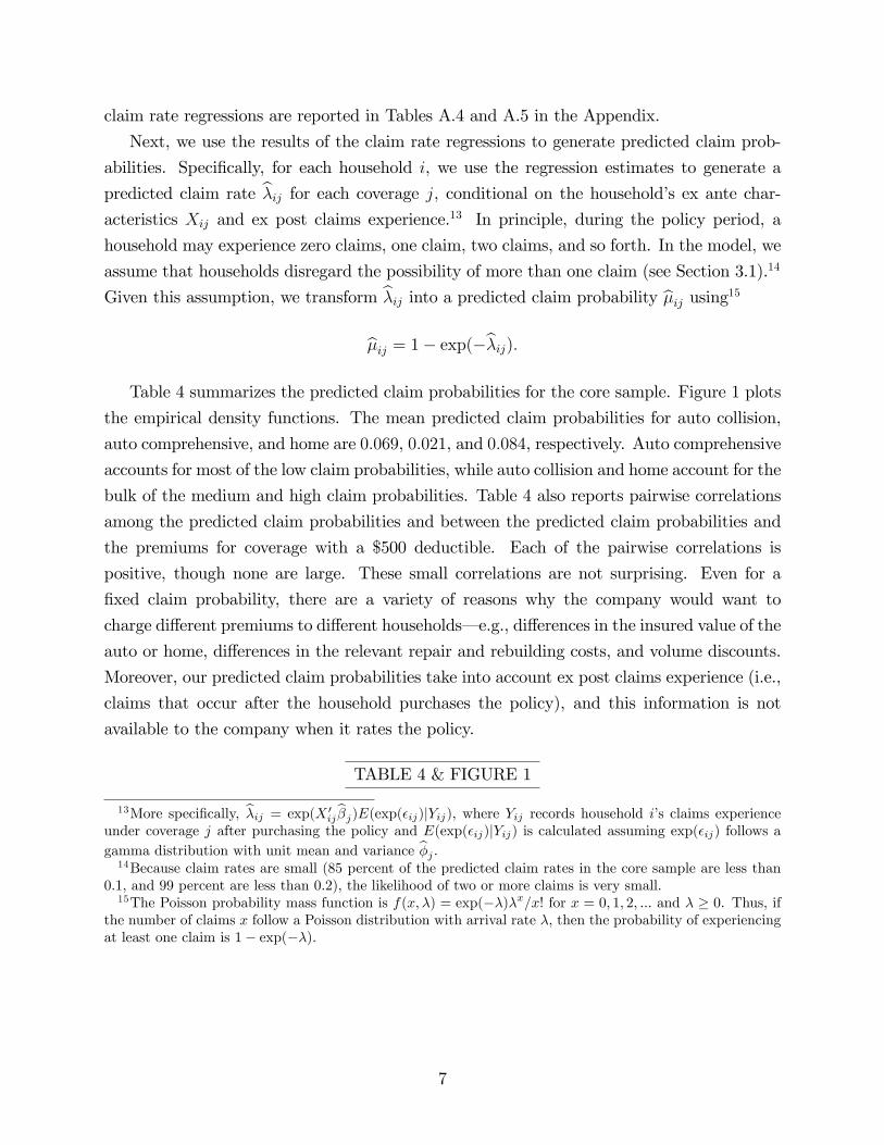
Table 4 summarizes the predicted claim probabilities for the core sample. Figure 1 plots

the empirical density functions. The mean predicted claim probabilities for auto collision,

auto comprehensive, and home are 0.069, 0.021, and 0.084, respectively. Auto comprehensive

accounts for most of the low claim probabilities, while auto collision and home account for the

bulk of the medium and high claim probabilities. Table 4 also reports pairwise correlations

among the predicted claim probabilities and between the predicted claim probabilities and

the premiums for coverage with a $500 deductible. Each of the pairwise correlations is

positive, though none are large. These small correlations are not surprising. Even for a

fixed claim probability, there are a variety of reasons why the company would want to

charge different premiums to different households– e.g., differences in the insured value of the

auto or home, differences in the relevant repair and rebuilding costs, and volume discounts.

Moreover, our predicted claim probabilities take into account ex post claims experience (i.e.,

claims that occur after the household purchases the policy), and this information is not

available to the company when it rates the policy.

TABLE 4 & FIGURE 1

13More specifically, λij = exp(X ′ij βj)E(exp(εij)|Yij), where Yij records household i’s claims experienceunder coverage j after purchasing the policy and E(exp(εij)|Yij) is calculated assuming exp(εij) follows agamma distribution with unit mean and variance φj .14Because claim rates are small (85 percent of the predicted claim rates in the core sample are less than

0.1, and 99 percent are less than 0.2), the likelihood of two or more claims is very small.15The Poisson probability mass function is f(x, λ) = exp(−λ)λx/x! for x = 0, 1, 2, ... and λ ≥ 0. Thus, if

the number of claims x follow a Poisson distribution with arrival rate λ, then the probability of experiencingat least one claim is 1− exp(−λ).

7

3 Model, Estimation, and Identification

3.1 Model

We assume that a household treats its three deductible choices as independent decisions.

This assumption is motivated in part by computational considerations,16 but also by the

literature on "narrow bracketing" (e.g., Read et al. 1999), which suggests that when people

make multiple choices, they frequently do not assess the consequences in an integrated way,

but rather tend to make each choice in isolation. Thus, we develop a model for how a house-

hold chooses the deductible for a single type of insurance coverage. To simplify notation,

we suppress the subscripts for household and coverage (though we remind the reader that

premiums and claim probabilities are household and coverage specific).

The household faces a menu of premium-deductible pairs (pd, d) : d ∈ D, where pdis the premium associated with deductible d, and D is the set of deductible options. We

assume that the household disregards the possibility of experiencing more than one claim

during the policy period, and that the household believes the probability of experiencing one

claim is µ. In addition, we assume that the household believes that its choice of deductible

does not influence its claim probability, and that every claim exceeds the highest available

deductible.17 Under the foregoing assumptions, the choice of deductible involves a choice

among deductible lotteries of the form

Ld ≡ (−pd, 1− µ;−pd − d, µ) .

Under expected utility theory, a household’s preferences over deductible lotteries are

influenced only by standard risk aversion. Given initial wealth w, the expected utility of

deductible lottery Ld is given by

EU(Ld) = (1− µ)u (w − pd) + µu (w − pd − d) ,

where u(w) represents standard utility defined over final wealth states. Standard risk aversion

is captured by the concavity of u(w).

Over the years, economists and other social scientists have proposed alternative models

16If instead we were to assume that a household treats its deductible choices as a joint decision, then thehousehold would face 120 options and the utility function would have several hundred terms.17We make the latter assumption more plausible by excluding the $2500 and $5000 deductible options

from the home menu. Only 1.6 percent of households in the core sample chose a home deductible of $2500or $5000. We assign these households a home deductible of $1000. In this respect, we follow Cohen andEinav (2007), who also exclude the two highest deductible options (chosen by 1 percent of the policyholdersin their sample) and assign the third highest deductible to policyholders who chose the two highest options.

8

that feature additional sources of aversion to risk. Kahneman and Tversky (1979, 1992)

offer prospect theory, which features probability weighting and loss aversion. Gul (1991)

proposes a model of disappointment aversion. More recently, Koszegi and Rabin (2006, 2007)

develop a model of reference-dependent utility that features loss aversion with an endogenous

reference point, which we label KR loss aversion. In the Appendix, we show that, in our

setting, probability weighting, KR loss aversion, and Gul disappointment aversion all imply

an effective distortion of probabilities relative to the expected utility model. Specifically,

each implies that there exists a probability distortion function Ω (µ) such that the utility of

deductible lottery Ld may be written as

U(Ld) = (1− Ω (µ))u (w − pd) + Ω (µ)u (w − pd − d) . (1)

In the estimation, we do not take a stand on the underlying source of probability distortions.

Their separate identification would require parametric assumptions which we are unwilling

to make. Rather, we focus on estimating "generic" probability distortions– i.e., we estimate

the function Ω (µ). We then discuss what we learn from our estimated Ω (µ) about the

possible sources of probability distortions (see Section 4.3).

In our analysis, we estimate both the utility function u(w) and the probability distortion

function Ω (µ). For u(w), we generally follow Cohen and Einav (2007) and Barseghyan et al.

(2011) and consider a second-order Taylor expansion. Also, because u(w) is unique only up

to an affi ne transformation, we normalize the scale of utility by dividing u′(w). This yields

u(w + ∆)

u′(w)− u(w)

u′(w)= ∆− r

2∆2,

where r ≡ −u′′(w)/u′(w) is the coeffi cient of absolute risk aversion. Because the term

u(w)/u′(w) enters as an additive constant, it does not affect utility comparisons; hence, we

drop it. With this specification, equation (1) becomes

U(Ld) = − [pd + Ω(µ)d]− r

2

[(1− Ω(µ)) (pd)

2 + Ω(µ) (pd + d)2] . (2)

The first term reflects the expected value of deductible lottery Ld with respect to the distorted

claim probability Ω(µ). The second term reflects disutility from bearing risk– it is the

expected value of the squared losses, scaled by standard risk aversion r.18

Our goal is to estimate both standard risk aversion r and and the probability distortion

18Note that this specification differs slightly from Cohen and Einav (2007) and Barseghyan et al. (2011),who use U(Ld) = − [pd + λd]− r

2

[λd2](where λ is the Poisson arrival rate). The difference derives from the

fact that those papers additionally take the limit as the policy period becomes arbitrarily small.

9

Ω (µ). In our baseline analysis in Section 4, we take a semi-nonparametric approach and

estimate Ω (µ) via sieve methods (Chen 2007). In Sections 5 and 6, we take a parametric

approach that is guided by the results of our baseline analysis.

3.2 Estimation

In the estimation, we must account for observationally equivalent households choosing differ-

ent deductibles, and for individual households making "inconsistent" choices across coverages

(Barseghyan et al. 2011; Einav et al. 2012). We follow McFadden (1974, 1981) and assume

random utility with additively separable choice noise. Specifically, we assume that the utility

from deductible d ∈ D is given by

U(d) ≡ U(Ld) + εd, (3)

where εd is an iid random variable that represents error in evaluating utility. We assume that

εd follows a type 1 extreme value distribution with scale parameter σ.19 A household chooses

deductible d when U(d) > U(d′) for all d′ 6= d, and thus the probability that a household

chooses deductible d is

Pr (d) ≡ Pr (εd′ − εd < U(Ld)− U(Ld′) ∀ d′ 6= d) =exp (U(Ld)/σ)∑

d′∈D exp (U(Ld′)/σ).

We use these choice probabilities to construct the likelihood function in the estimation.

In our main analysis, we estimate equation (3) assuming that utility is specified by

equation (2) and that µij = µij (i.e., household i’s predicted claim probability µij corresponds

to it subjective claim probability µij). We use combined data for all three coverages. Each

observation comprises, for a household i and a coverage j, a deductible choice d∗ij, a vector

of household characteristics Zi, a predicted claim probability µij, and a menu of premium-

deductible combinations (pdij , dij) : dij ∈ Dj. To be estimated are:

ri — coeffi cient of absolute risk aversion (ri = 0 means no standard risk aversion);

Ωi(µ) — probability distortion function (Ωi(µ) = µ means no probability distortions); and

σj — scale of choice noise for coverage j (σj = 0 means no choice noise).

Note that because the scale of utility is pinned down in equation (2), we can identify σL,

σM , and σH separately for auto collision, auto comprehensive, and home, respectively.

19The scale parameter σ is a monotone transformation of the variance of εd, and thus a larger σ meanslarger variance. Our estimation procedure permits σ to vary across coverages.

10

3.3 Identification

3.3.1 Identifying r and Ω(µ)

The random utility model in equation (3) comprises the sum of a utility function U(Ld)

and an error term εd. Using the results of Matzkin (1991), normalizations that fix scale

and location, plus regularity conditions that are satisfied in our model, allow us to identify

nonparametrically the utility function U(Ld) within the class of monotone and concave utility

functions. As we explain below, identification of U(Ld) allows us to identify r and Ω(µ).

Take any three deductible options a, b, c ∈ D, with a > b > c, and consider a household

with premium pa for deductible a and claim probability µ. The household’s r and Ω(µ)

determine the premium pb that makes the household indifferent between deductibles a and

b, as well as the premium pc that makes the household indifferent between deductibles a and

c. Notice that pb−pa reflects the household’s maximum willingness to pay (WTP ) to reduce

its deductible from a to b, and pc − pb reflects the household’s additional WTP to reduce

its deductible from b to c. In the Appendix, we prove the following properties of pb and pcwhen U(Ld) is specified by equation (2).

Property 1. Both pb and pc are strictly increasing in r and Ω(µ).

Property 2. For any fixed Ω(µ), r = 0 implies pb−papc−pb = a−b

b−c , and the ratiopb−papc−pb is strictly

increasing in r.

Property 3. If pb − pa is the same for (r,Ω(µ)) and (r′,Ω(µ)′) with r < r′ (and thus

Ω(µ) > Ω(µ)′), then pc − pb is greater for (r,Ω(µ)) than for (r′,Ω(µ)′).

Property 1 is straightforward: A household’sWTP to reduce its deductible (and thereby

reduce its exposure to risk) will be greater if either its standard risk aversion is larger or its

(distorted) claim probability is larger.

Property 2 is an implication of standard risk aversion. For any fixed Ω(µ), a risk neutral

household is willing to pay, for instance, exactly twice as much to reduce its deductible from

$1000 to $500 as it is willing to pay to reduce its deductible from $500 to $250. In contrast,

a risk averse household is willing to pay more than twice as much, and the larger is the

household’s standard risk aversion the greater is this ratio.

Property 3 is the key property for identification. To illustrate the underlying intuition,

consider a household with claim probability µ = 0.05 who faces a premium pa = $200 for

deductible a = $1000. Suppose that pb − pa = $50– i.e., the household’s WTP to reduce

its deductible from a = $1000 to b = $500 is fifty dollars. Property 1 implies that multiple

combinations of r and Ω(0.05) are consistent with this WTP , and that in each combination

11

a larger r implies a smaller Ω(0.05). For example, both (i) r = 0 and Ω(0.05) = 0.10 and (ii)

r′ = 0.00222 and Ω(0.05)′ = 0.05 are consistent with pb − pa = $50. Property 3, however,

states that these different combinations of r and Ω(0.05) have different implications for the

household’s WTP to reduce its deductible from b = $500 to c = $250. For instance, r = 0

and Ω(0.05) = 0.10 would imply pc − pb = $25, whereas r′ = 0.00222 and Ω(0.05)′ = 0.05

would imply pc − pb = $18.61. More generally– given the household’s WTP to reduce its

deductible from $1000 to $500– the smaller is the household’s WTP to reduce it deductible

from $500 to $250, the larger must be its r and the smaller must be its Ω(0.05).

Property 3 reveals that our identification strategy relies on a key feature of our data–

namely, that there are more than two deductible options. Given this feature, we can sepa-

rately identify r and Ω(µ) by observing how deductible choices react to exogenous changes in

premiums for a fixed claim probability.20 We then can identify the shape of Ω(µ) by observ-

ing how deductible choices react to exogenous changes in claim probabilities. In other words,

given three or more deductible options, it is exogenous variation in premiums for a fixed µ

that allows us to pin down r and Ω(µ), and it is exogenous variation in claim probabilities

that allows us to map out Ω(µ) for all µ in the range of our data.

3.3.2 Exogenous Variation in Premiums and Claim Probabilities

Within each coverage, there is substantial variation in premiums and claim probabilities.

A key identifying assumption is that there is variation in premiums and claim probabilities

that is exogenous to the households’risk preferences. In our estimation, we assume that a

household’s utility parameters– r and Ω(µ)– depend on a vector of observables Z that is

a strict subset of the variables that determine premiums and claim probabilities. Many of

the variables outside Z that determine premiums and claim probabilities, such as protection

class and territory code,21 are undoubtedly exogenous to the households’risk preferences.

In addition, there are other variables outside Z that determine premiums but not claim

probabilities, including numerous discount programs, which also are undoubtedly exogenous

to the households’risk preferences.

Given our choice of Z, there is substantial variation in premiums and claim probabilities

that is not explained by Z. In particular, regressions of premiums and predicted claim

probabilities on Z yield low coeffi cients of determination (R2). In the case of auto collision

coverage, for example, regressions of premiums (for coverage with a $500 deductible) on Z

20Note that if the data included only two deductible options, as in Cohen and Einav (2007), we could notseparately identify r and Ω(µ) without making strong functional form assumptions about Ω(µ).21Protection class gauges the effectiveness of local fire protection and building codes. Territory codes

are based on actuarial risk factors, such as traffi c and weather patterns, population demographics, wildlifedensity, and the cost of goods and services.

12

and predicted claim probabilities on Z yield R2 of 0.16 and 0.34, respectively.22

In addition to the substantial variation in premiums and claim probabilities within a

coverage, there also is substantial variation in premiums and claim probabilities across cov-

erages. A key feature of the data is that for each household we observe deductible choices

for three coverages, and (even for a fixed Z) there is substantial variation in premiums and

claim probabilities across the three coverages. Thus, even if the within-coverage variation

in premiums and claim probabilities were insuffi cient in practice, we still might be able to

estimate the model using across-coverage variation.

4 Analysis with Homogenous Preferences

We begin our analysis by assuming homogeneous preferences– i.e., r and Ω(µ) are the same

for all households. This permits us to take a semi-nonparametric approach to estimating

the model without facing a curse of dimensionality. As a point of reference, we note that if

we do not allow for probability distortions– i.e., we restrict Ω(µ) = µ– the estimate for r is

0.0129 (standard error: 0.0004).

4.1 Estimates

We take three sieve approaches to estimating Ω(µ). In Model 1a, we estimate a Cheby-

shev polynomial expansion of ln Ω(µ), which naturally constrains Ω(µ) > 0. We consider

expansions up to the 20th degree, and select a quadratic on the basis of the Bayesian in-

formation criterion (BIC). In Model 1b, we estimate a Chebyshev polynomial expansion of

Ω(µ), which nests the case Ω(µ) = µ.23 As before, we consider expansions up to the 20th

degree. Here, the BIC selects a cubic. However, because the BIC for the quadratic and cubic

are essentially the same, we report results for the quadratic to facilitate direct comparisons

with Model 1a. In Model 1c, we estimate Ω(µ) using an 11-point cubic spline on the interval

(0, 0.20), wherein lie 99.4 percent of the predicted claim probabilities in the core sample.

Table 5 reports our results. The estimates for Ω(µ) indicate large probability dis-

tortions. To illustrate, Figure 2 depicts the estimated Ω(µ) for Models 1a, 1b, and 1c,

along with the 95 percent pointwise bootstrap confidence bands for Model 1c.24 In each

model, there is substantial overweighting of claim probabilities. In Model 1a, for example,

22They are even lower for auto comprehensive and home. In the case of auto comprehensive the coeffi cientsof determination are 0.07 and 0.31, and in the case of home they are 0.04 and 0.15.23Here we impose the restriction that Ω(µ) > 0.24Figure 2 shows the estimated Ω(µ) on the interval (0, 0.16), wherein lie 98.2 percent of the predicted

claim probabilities in the core sample.

13

Ω(0.020) = 0.083, Ω(0.050) = 0.111, Ω(0.075) = 0.135, and Ω(0.100) = 0.156. In addi-

tion, there is only mild insensitivity to probability changes. For instance, in Model 1a,

[Ω(0.050)− Ω(0.020)]/[0.050− 0.020] = 0.933, [Ω(0.075)− Ω(0.050)]/[0.075− 0.050] = 0.960,

and [Ω(0.100)− Ω(0.075)]/[0.100− 0.075] = 0.840. Moreover, all three models imply nearly

identical distortions of claim probabilities between zero and 14 percent (wherein lie 96.7 per-

cent of the predicted claim probabilities in the core sample), and even for claim probabilities

greater than 14 percent the three models are statistically indistinguishable (Models 1a and

1b lie within the 95 percent confidence bands for Model 1c). Given this overweighting, the

estimates for r are smaller than without probability distortions. Specifically, r is 0.00064,

0.00063, and 0.00049 in Models 1a, 1b, and 1c, respectively. Lastly, we note the estimates

for the scale of choice noise: σL = 26.3, σM = 17.5, and σH = 68.5.

TABLE 5 & FIGURE 2

4.2 Statistical and Economic Significance

To assess the relative statistical importance of probability distortions and standard risk

aversion, we estimate restricted models and perform Vuong (1989) model selection tests.25

We find that a model with probability distortions alone is "better" at the 1 percent level

than a model with standard risk aversion alone. However, a likelihood ratio test rejects

at the 1 percent level both (i) the null hypothesis of standard risk neutrality (r = 0) for

Models 1a and 1b and (ii) the null hypothesis of no probability distortions (Ω(µ) = µ) for

Model 1b.26 This suggests that probability distortions and standard risk aversion both play

a statistically significant role.

To give a sense of the economic significance of our estimates for r and Ω(µ), we consider

the implications for a household’s maximum willingness to pay (WTP ) for lower deductibles.

Specifically, consider the household’sWTP to reduce its deductible from $1000 to $500 when

the premium for coverage with a $1000 deductible is $200. Table 6 displaysWTP for selected

claim probabilities µ and several preference combinations, using the estimates for r and

Ω(µ) from Model 1a. It illustrates that our estimated probability distortions have a larger

economic impact than our estimated standard risk aversion, except at claim probabilities at

the high end of our data, where the impacts are comparably large.

25Vuong’s (1989) test allows one to select between two nonnested models on the basis of which best fitsthe data. Neither model is assumed to be correctly specified. Vuong (1989) shows that testing whether onemodel is significantly closer to the truth (its loglikelihood value is significantly greater) than another modelamounts to testing the null hypothesis that the loglikelihoods have the same expected value.26We do not perform a likelihood ratio test of the null hypothesis of no probability distortions for Model

1a because it does not nest the case Ω(µ) = µ.

14

TABLE 6

Lastly, to give a sense of the economic significance of our estimates for the scale of

choice noise (σL, σM , and σH), we consider the potential for such noise to affect households’

deductible choices. In particular, we use Model 1a to simulate– both with and without choice

noise– the deductible choices of the households in the core sample. Over 1000 iterations,

we find that the households’"noisy" choices match their "noiseless" choices about half the

time: 56 percent in auto collision, 43 percent in auto comprehensive, and 50 percent in home.

Moreover, we find that households’"noisy" choices are within one rank (i.e., one step up or

down on the menu of deductible options) of their "noiseless" choices more than four-fifths of

the time: 94 percent in collision, 82 percent in auto comprehensive, and 95 percent in home.

This suggests that choice noise, at the scale we estimate, is important but not dominant.27

4.3 Sources of Probability Distortions

There are a number of possible sources of the estimated probability distortions depicted in

Figure 2. In this section, we discuss what we learn from our estimated Ω(µ) about several

potential sources.

One potential source of probability distortions is probability weighting, whereby proba-

bilities are transformed into decision weights.28 Under a probability weighting model, and

adopting the rank-dependent approach of Quiggin (1982), the utility of deductible lottery

Ld is given by

U(Ld) = (1− π (µ))u (w − pd) + π (µ)u (w − pd − d) , (4)

where π(µ) is the probability weighting function. Clearly, equation (4) is equivalent to equa-

tion (1) with Ω(µ) = π(µ). Insofar as Ω(µ) reflects probability weighting, our estimated

Ω(µ) is striking in its resemblance to the probability weighting function originally posited

by Kahneman and Tversky (1979). In particular, it is consistent with a probability weight-

ing function that exhibits overweighting of small probabilities, exhibits mild insensitivity

to changes in probabilities, and trends toward a positive intercept as µ approaches zero

(though we have relatively little data for µ < 0.01). By contrast, the probability weighting

functions later suggested by Tversky and Kahneman (1992), Lattimore et al. (1992), and

Prelec (1998)– which are commonly used in the literature (e.g., Jullien and Salanié 2000;

Kliger and Levy 2009; Bruhin et al. 2010; Andrikogiannopoulou 2010)– will not fit our data

27After all, with extreme noise, we would find match rates that are two to three times smaller, becausethe probability that a household’s "noisy" choice would equal any given deductible would be 20 percent inauto collision, 17 percent in auto comprehensive, and 25 percent in home.28As we discuss in Section 7, in our data literal probability weighting is indistinguishable from systematic

risk misperceptions (i.e., incorrect subjective beliefs about claim probabilities).

15

well, because they trend toward a zero intercept and typically exhibit oversensitivity for

probabilities less than five to ten percent.29

Another possible source of probability distortions is loss aversion. The original, "status

quo" loss aversion proposed by Kahneman and Tversky (1979)– wherein gains and losses are

defined relative to initial wealth– cannot explain aversion to risk in the context of insurance

deductible choices because all outcomes are losses relative to initial wealth. More recently,

however, Koszegi and Rabin (2007) and Sydnor (2010) have suggested that a form of "ratio-

nal expectations" loss aversion proposed by Koszegi and Rabin (2006)– wherein gains and

losses are defined relative to expectations about outcomes– can explain the aversion to risk

manifested in insurance deductible choices. In the Appendix, we describe the Koszegi-Rabin

(KR) model of loss aversion and derive its implications for deductible lotteries.30 Under the

KR model, the utility of deductible lottery Ld is given by

U(Ld) = [(1− µ)u(w − pd) + µu(w − pd − d)] (5)

−Λ (1− µ)µ [u(w − pd)− u(w − pd − d)] .

The first bracketed term is merely the standard expected utility of Ld. The second bracketed

term reflects the expected disutility due to loss aversion, where Λ ≥ 0 captures the degree

of loss aversion (Λ = 0 means no loss aversion). When Λ > 0, the outcome of experiencing

a claim "looms larger" than the outcome of not experiencing a claim because the former is

perceived as a loss relative to the latter. Equation (5) is equivalent to equation (1) with

Ω(µ) = µ + Λ (1− µ)µ. If Λ > 0 then Ω(µ) 6= µ. Thus, KR loss aversion can generate

probability distortions. The probability distortions implied by KR loss aversion, however,

are qualitatively different from the probability distortions we estimate– see panel (a) of

Figure 3. In particular, the probability distortion function implied by KR loss aversion is

too steep in the range of our data and trends toward a zero intercept. Hence, KR loss

aversion alone cannot explain our data.

Probability distortions also can arise from disappointment aversion. In the Appendix, we

describe the model of disappointment aversion proposed by Gul (1991), in which disutility

29For instance, if we impose on Ω(µ) the one-parameter functional form proposed by Prelec (1998), weestimate Prelec’s α = 0.7. This estimate implies that Ω′(µ) > 1.0 for µ < 0.075 and Ω′(µ) > 1.5 forµ < 0.027.30Specifically, we apply the concept of "choice-acclimating personal equilibrium" (CPE), which KR suggest

is appropriate for insurance choices because the insured commits to its policy choices well in advance of theresolution of uncertainty. In addition, we explain that although the KR model contains two parameters, one(λ) that captures the degree of loss aversion and one (η) that captures the importance of gain-loss utilityrelative to standard utility, under CPE these parameters always appear as the product η(λ − 1), which welabel Λ.

16

arises when the outcome of a lottery is less than the certainty equivalent of the lottery.31

Under Gul’s model, the utility of deductible lottery Ld is given by

U(Ld) =

(1− µ(1 + β)

1 + βµ

)u(w − pd) +

(µ(1 + β)

1 + βµ

)u(w − pd − d), (6)

where β ≥ 0 captures the degree of disappointment aversion (β = 0means no disappointment

aversion). When β > 0, the outcome of experiencing a claim is overweighted (relative to µ)

because of the disappointment associated therewith. Equation (6) is equivalent to equation

(1) with Ω(µ) = µ(1 + β)/(1 + βµ). If β > 0 then Ω(µ) 6= µ. Thus, Gul disappointment

aversion can generate probability distortions. Again, however, the probability distortions

implied by Gul disappointment aversion are qualitatively different from the probability dis-

tortions we estimate– see panel (b) of Figure 3. As before, the implied probability distortion

function is too steep and trends toward a zero intercept. Hence, Gul disappointment aversion

alone cannot explain our data.

Because we can "reject" the hypotheses that KR loss aversion alone or Gul disappoint-

ment aversion alone can explain our estimated probability distortions, our analysis provides

evidence that probability weighting (perhaps partly reflecting risk misperceptions) is playing

a key role in the households’deductible choices.

Finally, we consider a combination of sources. In the Appendix, we derive that, if house-

holds have probability weighting π(µ) and KR loss aversion Λ, then the utility of deductible

lottery Ld is given by

U(Ld) = [(1− π(µ))u(w − pd) + π(µ)u(w − pd − d)]

−Λ (1− π(µ))π(µ) [u(w − pd)− u(w − pd − d)] ,

which is equivalent to equation (1) with Ω(µ) = π(µ)[1 + Λ(1− π(µ))]. From this equation,

it is clear that, unless we impose strong functional form assumptions on π(µ), we cannot

separately identify Λ and π(µ). Rather, the best we can do is to derive, for various values of

Λ, an implied probability weighting function π(µ). Panel (c) of Figure 3 performs this exer-

cise. It reinforces our conclusion that KR loss aversion alone cannot explain our estimated

probability distortions, because it is clear from the figure that no value of Λ will generate an

implied π(µ) that lies on the 45-degree line.32

FIGURE 3

31In the Appendix, we explain that versions of the somewhat different approaches of Bell (1985) andLoomes and Sugden (1986) imply probability distortions identical to those implied by KR loss aversion.32While we focus on a combination of probability weighting and KR loss aversion, a similar analysis of a

combination of probability weighting and Gul disappointment aversion yields analogous conclusiuons.

17

5 Analysis with Heterogenous Preferences

In this section, we expand the model to permit heterogenous preferences. With heterogeneous

preferences, it is no longer feasible to take a semi-nonparametric approach to estimating the

model, due to the curse of dimensionality and to the computational burden of our estimation

procedure. Hence, we now take a parametric approach to Ω(µ). Because Models 1a, 1b, and

1c yield nearly identical results, and because it naturally constrains Ω(µ) > 0, throughout

this section we estimate a quadratic Chebyshev polynomial expansion of ln Ω(µ) (which is the

best fit in Model 1a). As before, we estimate equation (3) assuming that utility is specified

by equation (2) and that µij = µij, and we use combined data for all three coverages. We

assume that choice noise is independent of any observed or unobserved heterogeneity in

preferences, and as before we permit the scale of choice noise to vary across coverages.

We take three approaches to modeling heterogeneity in preferences. In Model 2, we allow

for observed heterogeneity in ri and Ωi(µ) by assuming

ln ri = βrZi and ln Ωi(µ) = βΩ,1Zi +(βΩ,2Zi

)µ+

(βΩ,3Zi

)µ2,

where Zi comprises a constant plus the variables in Table 1. We estimate Model 2 via maxi-

mum likelihood, and the parameter vector to be estimated is θ ≡ (βr, βΩ,1, βΩ,2, βΩ,3, σL, σM , σH).

In Models 3 and 4, we allow for unobserved heterogeneity in ri and Ωi(µ). In particular,

we assume

ln ri = βrZi + ξr,i and ln Ωi(µ) = βΩ,1Zi +(βΩ,2Zi

)µ+

(βΩ,3Zi

)µ2 + ξΩ,i,

where (ξr,i

ξΩ,i

)iid∼ Normal

([0

0

],Φ

), with Φ ≡

[Φr Φr,Ω

Φr,Ω ΦΩ

].

In Model 3, we allow for only unobserved heterogeneity, and thus Zi is a constant. In Model

4, we allow for both unobserved and observed heterogeneity, and Zi comprises a constant

plus the variables in Table 1. We estimate Models 3 and 4 via Markov Chain Monte Carlo

(MCMC), and the parameters to be estimated are θ and Φ.33 Details regarding the MCMC

estimation procedure are set forth in the Appendix.34 After each estimation, we use the

estimates to assign fitted values of ri and Ωi(µ) to each household i.35

33The resulting econometric model is a mixed multinomial logit (McFadden and Train 2000). Within theliterature on estimating risk preferences, a similar specification is employed by Andrikogiannopoulou (2010).34The procedure closely follows Train (2009, ch. 12). The estimation was performed in MATLAB using a

modified version of Train’s software, "Mixed logit estimation by Bayesian methods." Convergence diagnostictests were run using the CODA package adapted for MATLAB by James P. LeSage.35In the case of Models 3 and 4, the fitted values are calculated taking into account the estimates for Φ.

18

Table 7 summarizes the estimates for Models 2, 3, and 4.36 For comparison, it also

restates the estimates from Model 1a. Figure 4 depicts the mean fitted value of Ω(µ) for

each model. For comparison, it also depicts the estimated Ω(µ) in Models 1a and 1c, along

with the 95 percent confidence bands for Model 1c.

TABLE 7 & FIGURE 4

The mean estimated probability distortions in Models 2, 3, and 4 are nearly identical

to each other and to the estimated probability distortions in Model 1. Hence, whether

we assume preferences are homogeneous or allow for observed or unobserved heterogeneity,

the main message is the same: large probability distortions characterized by substantial

overweighting of claim probabilities and only mild insensitivity to probability changes.

By contrast, the estimated degree of standard risk aversion is somewhat sensitive to the

modeling approach. In Model 2, the mean fitted value of r is 0.00073, slightly higher than

in Model 1a. In Models 3 and 4, the estimates for r are higher still– the mean fitted values

are 0.00156 and 0.00147, respectively.

The estimates for the scale of choice noise are similarly sensitive. Whereas the estimates

for Model 2 differ only slightly from those in Model 1a, the estimates for Models 3 and 4

(though similar to each other) differ sizably from those in Model 1a– roughly speaking, σLand σM are forty percent lower and σH is forty percent higher. That said, the estimates for

each model display the same qualitative pattern: σM < σL << σH .

Lastly, we make two observations about the estimated variance-covariance matrix of

unobserved heterogeneity. First, the variance estimates imply that there indeed is unobserved

heterogeneity in preferences. Consider, for instance, Model 3 (the message is the same for

Model 4, although the calculations are more involved because of the presence of observed

heterogeneity). For standard risk aversion, the estimate of Φr = 0.55 implies that the 2.5th,

25th, 75th, and 97.5th percentiles are 0.00028, 0.00072, 0.00195, and 0.00507, respectively.

For probability distortions, the estimate of ΦΩ = 0.37 implies that the 2.5th, 25th, 75th, and

97.5th pointwise percentiles are 0.25Ω(µ), 0.55Ω(µ), 1.25Ω(µ), and 2.73Ω(µ), where Ω(µ)

is the mean fitted probability distortion depicted in Figure 4. This substantial unobserved

heterogeneity is consistent with similar findings on standard risk aversion by Cohen and Einav

(2007) and on cumulative prospect theory parameters by Andrikogiannopoulou (2010). We

note, however, that we find less unobserved heterogeneity in standard risk aversion than

do Cohen and Einav (2007).37 Despite this unobserved heterogeneity, our main message

Specifically, ri = exp(βrZi + (Φr/2)) and Ωi(µ) = exp(βΩ,1Zi + (βΩ,2Zi)µ+ (βΩ,3Zi)µ2 + (ΦΩ/2)).

36The complete estimates are reported in Tables A.6, A.7, and A.8 in the Appendix.37This is perhaps not surprising given that we have a second dimension of unobserved heterogeneity in

19

persists: the data is best explained by large probability distortions among the majority of

households. Furthermore, our conclusions regarding the sources of probability distortions–

and in particular that neither KR loss aversion alone nor Gul disappointment aversion alone

can explain our estimated probability distortions– also persist.

Our second observation is that the covariance estimate implies a negative correlation

between unobserved heterogeneity in r and Ω(µ): −0.49 in both Models 3 and 4.38 This

suggests that the unexplained variation in the households’deductible choices (after control-

ling for premiums, claim probabilities, and observed heterogeneity) is best explained not by

heterogeneity in their "overall" aversion to risk but rather by heterogeneity in their combi-

nations of standard risk aversion and probability distortions. After all, if such unexplained

variation in deductible choices were best explained by heterogeneity in overall aversion to

risk, we would expect a positive correlation because moving r and Ω(µ) in the same direction

is the most "effi cient" way of varying overall aversion to risk. However, if there were little

heterogeneity in overall aversion to risk, moving r and Ω(µ) in opposite directions would be

necessary to explain such variation in deductible choices.

6 Sensitivity Analysis

Our main analysis yields a clear main message: large probability distortions characterized by

substantial overweighting and mild insensitivity. Moreover, our main analysis suggests that

this message is robust to different approaches to modeling heterogeneity in preferences. In

this section, we further investigate the sensitivity of this message, and we find that it is robust

to various other modeling assumptions. By contrast, we generally find that the estimates for

standard risk aversion are more sensitive. To conserve space, we only summarize the results

of the sensitivity analysis below. The complete results are available in the Appendix (Tables

A.9 through A.22). In most of the sensitivity analysis, we restrict attention to Models 2 and

3. (Recall that Model 2 allows for observed heterogeneity in preferences and Model 3 allows

for unobserved heterogeneity in preferences.) We do not re-estimate Model 4 because of the

extreme computational burden of estimating the model with both observed and unobserved

preferences. Because Andrikogiannopoulou (2010) estimates a very different model– which in particularassumes no standard risk aversion and imposes a functional form for probability weighting that reflects avery different shape from ours– it is diffi cult to compare the magnitude of our estimates of unobservedheterogeneity with those in her paper.38To be clear, Table 7 reports that the implied correlation between ξr,i and ξΩ,i is −0.72. Given the

log-linear specifications for ri and Ωi(µ), this implies that the correlation between ri and Ωi(µ) due tounobserved heterogeneity is −0.49.

20

heterogeneity,39 and also because Models 2, 3 and 4 (not to mention Model 1) all yield the

same main message.

6.1 Unobserved Heterogeneity in Risk

In our main analysis, we assume that the households’subjective claim probabilities corre-

spond to our predicted claim probabilities, which reflect only observed heterogeneity. The

results of our claim rate regressions, however, imply that there is unobserved heterogeneity.

In this section, we take two approaches to accounting for this unobserved heterogeneity.

In our first approach, we assume that unobserved heterogeneity in risk is not correlated

with unobserved heterogeneity in preferences. With this assumption, we use the results of

the claim rate regressions to assign to each household a predicted distribution of claim prob-

abilities, F (µ), and then integrate over F (µ) to construct the likelihood function. Column

(a) of Table 8 summarizes the estimates for Models 2 and 3 when we allow for unobserved

heterogeneity in risk in this way. For comparison, the table also restates the benchmark

estimates. Our main message remains unchanged. The estimates for Ω(µ) indicate similarly

large probability distortions– see Figure A.1 in the Appendix. The estimates for r indicate

levels of standard risk aversion that are somewhat higher than the benchmark estimates.

Lastly, we note that the estimates for the scale of choice noise, as well as the estimates for

Φ, are similar to the benchmark estimates.

TABLE 8

In our second approach, we allow for correlation between unobserved heterogeneity in

risk and unobserved heterogeneity in preferences. In principle, we could estimate Model 3

with the addition of unobserved heterogeneity in claim probabilities and permit a flexible

correlation structure among the various sources of unobserved heterogeneity. Doing so,

however, would impose an undue computational burden and put a strain on identification.

Instead, we estimate the following model:

ln ri = r + ξr,i and Ωij(µ) = a+ bµij exp(ξb,ij),

where (ξr,i, ξb,iL, ξb,iM , ξb,iH)iid∼ Normal(0,Ψ) and the parameters to be estimated are r, a,

b, and Ψ. Relative to Model 3, this model imposes a more restrictive functional form on

Ω(µ) and also alters the way in which unobserved heterogeneity enters into Ω(µ). However,

39Estimating Model 4 takes approximately one week (on a Dell Precision 7500 with dual XEON 5680processors with 24GB of memory). In comparison, estimating Model 3 takes approximately one day, andestimating Model 2 takes less than an hour.

21

it has several compensating virtues. Perhaps most important, given the way ξb enters the

model, it can be interpreted as unobserved heterogeneity in probability distortions (as in

our first approach), but it also can be interpreted as unobserved heterogeneity in subjective

risk perceptions (i.e., subjective claim probabilities). Thus, the model nests– when a = 0

and b = 1– a standard expected utility model with no probability distortions but with

unobserved heterogeneity in both risk and standard risk aversion (and a flexible correlation

structure).40 In addition, it allows for coverage-specific unobserved heterogeneity, and it is

simple and computationally tractable.

Table A.11 in the Appendix reports our MCMC estimates for this model. For Ω(µ), we

obtain an intercept of a = 0.041 (standard error: 0.002) and a slope of b = 0.864 (standard

error: 0.029). These estimates clearly reject a standard expected utility model and yield

probability distortions that are quite similar to Model 3.41 Hence, our main message remains

unchanged. The estimates for standard risk aversion and for the scale of choice noise are

also similar to Model 3. The estimates for the variance-covariance matrix Ψ imply much

higher variances of unobserved heterogeneity in risk than do the estimates for φ from the

claim rate regressions, suggesting either that there is substantial unobserved heterogeneity

in probability distortions or that there indeed is unobserved heterogeneity in subjective

risk perceptions beyond the unobserved heterogeneity in objective risk. Interestingly, the

variance estimates are quite similar for auto collision and home, but substantially higher for

auto comprehensive, perhaps suggesting that households have more accurate beliefs about

risk in domains in which adverse events occur more frequently. Lastly, the cross-coverage

correlations of unobserved heterogeneity in risk are all high, supporting our benchmark

modeling assumption that there is a household-specific component in probability distortions

that is common across coverages.

Finally, we note that unobserved heterogeneity in risk creates an adverse selection prob-

lem for the insurance company. However, adverse selection from the company’s perspective

is irrelevant to our analysis. What matters here is to account for selection based on unob-

servable risk, which is precisely what we do.

40Technically, this nesting is complete only if we further impose that (ξr,i, ξb,iL, ξb,iM , ξb,iH)iid∼

Normal(Υ,Ψ), where Υj = −Ψjj/2. If we impose this restriction, the results are very similar to thosewe report (which assume Υ = 0).41The somewhat lower intercept is compensated by the higher variance of the unobserved heterogeneity

terms, Ψb, which imply a higher E(exp(ξb)).

22

6.2 Restricted Choice Noise

In the model, we use choice noise to account for observationally equivalent households choos-

ing different deductibles, and for individual households making "inconsistent" choices across

coverages. In this section, we investigate the sensitivity of our main message to this mod-

eling choice by restricting the scale of choice noise. Column (b) of Table 8 summarizes the

estimates for Models 2 and 3 when we restrict the scale of choice noise to half its estimated

magnitude (i.e., we fix σj ≡ 12σj). Our main message is unchanged. Indeed, the estimated

probability distortions become even more pronounced– see Figure A.2 in the Appendix. At

the same time, the estimate for standard risk aversion becomes extremely small.

6.3 CRRA Utility

In our analysis, we use a second-order Taylor expansion of the utility function. As a check of

this approach, we consider CRRA utility, u(w) = w1−ρ/(1−ρ), where ρ > 0 is the coeffi cient

of relative risk aversion. The CRRA family is "the most widely used parametric family for

fitting utility functions to data" (Wakker 2008). With CRRA utility, equation (1) becomes

U(Ld) = (1− Ω(µ))(w − pd)1−ρ

(1− ρ)+ Ω(µ)

(w − pd − d)1−ρ

(1− ρ).

A disadvantage of CRRA utility is that it requires wealth as an input, and moreover

there surely is heterogeneity in wealth across the households in our core sample. To account

for these issues, we assume that (i) wealth is proportional to home value and (ii) average

wealth is $33,000 (approximately equal to 2010 U.S. per capita disposable personal income).

The average home value in the core sample is approximately $191,000. Thus, we assume

w = (33/191)× (home value).42

We re-estimate Models 2 and 3.43 For Model 2, we assume ln ρ = βρZi, where Zicomprises a constant plus the variables in Table 1. For Model 3, we assume ln ρ = βρ + ξρ,i.

We otherwise proceed exactly as described in Section 5. Panel (c) of Table 8 summarizes the

estimates, and Figure A.3 in the Appendix depicts the mean estimated Ω(µ) for each model.

The main message is much the same: we find large probability distortions characterized by

substantial overweighting and mild insensitivity. In fact, the probability distortions become

somewhat more pronounced. At the same time, the estimates for standard risk aversion

42We also restrict households to have positive wealth. The results presented here restrict w ≥ $12, 000(i.e., if a household’s implied w is less than $12,000, we assign it a wealth of $12,000). We investigatedsensitivity to this cutoff, and it matters very little (because very few households are affected).43To enable a global search over ρ, we scale the model by (33, 000)ρ. Locally, the results are indistinguish-

able from those obtained without re-scaling.

23

become very small. The mean fitted values of ρ are 0.37 and 0.21 in Models 2 and 3,

respectively. Evaluated at average wealth of $33,000, these estimates imply a coeffi cient of

absolute risk aversion on the order of r = 0.00001.

6.4 Moral Hazard

Throughout our analysis, we assume that deductible choice does not influence claim risk.

That is, we assume there is no deductible-related moral hazard. In this section, we assess

this assumption.

There are two types of moral hazard that might operate in our setting. First, a house-

hold’s deductible choice might influence its incentives to take care (ex ante moral hazard).

Second, a household’s deductible choice might influence its incentives to file a claim after

experiencing a loss (ex post moral hazard), especially if its premium is experience rated or

if the loss results in a "nil" claim (i.e., a claim that does not exceed its deductible). For

either type of moral hazard, the incentive to alter behavior– i.e., take more care or file fewer

claims– is stronger for households with larger deductibles. Hence, we investigate whether

moral hazard is a significant issue in our data by examining whether our predicted claim

probabilities change if we exclude households with high deductibles.

Specifically, we re-run our claim rate regressions using a restricted sample of the full

data set in which we drop all household-coverage-year records with deductibles of $1000 or

larger.44 We then use the new estimates to generate revised predicted claim probabilities for

all households in the core sample (including those with deductibles of $1000 or larger). Com-

paring the revised predicted claim rates with the benchmark predicted claim rates, we find

that they are essentially indistinguishable– in each coverage, pairwise correlations exceed

0.995 and linear regressions yield intercepts less than 0.001 and coeffi cients of determination

(R2) greater than 0.99. Moreover, the estimates of the variance of unobserved heterogeneity

in claim rates are nearly identical.45 Not surprisingly, if we re-estimate our baseline model

using the revised predicted claim probabilities, the results are virtually identical.

The foregoing analysis suggests that moral hazard is not a significant issue in our data.

This is perhaps not surprising, for two reasons. First, the empirical evidence on moral hazard

in auto insurance markets is mixed. (We are not aware of any empirical evidence on moral

hazard in home insurance markets.). Most studies that use "positive correlation" tests of

asymmetric information in auto insurance do not find evidence of a correlation between

44We draw the line at the $1000 deductible and not the $500 deductible because realistically it is diffi cultto imagine claimable events that result in losses smaller than $500.45The revised estimates are 0.22, 0.56, and 0.44 in auto collision, auto comprehensive, and home, respec-

tively, whereas the corresponding benchmark estimates are 0.22, 0.57, and 0.45.

24

coverage and risk (e.g., Chiappori and Salanié 2000; for a recent review of the literature, see

Cohen and Siegelman 2010).46 Second, there are theoretical reasons to discount the force

of moral hazard in our setting. In particular, because deductibles are small relative to the

overall level of coverage, ex ante moral hazard strikes us as implausible in our setting.47

As for ex post moral hazard, households have countervailing incentives to file claims no

matter the size of the loss– under the terms of the company’s policies, if a household fails to

report a claimable event (especially an event that is a matter of public record– e.g., collision

events typically entail police reports), it risks denial of all forms of coverage (notably liability

coverage) for such event and also cancellation (or nonrenewal) of its policy.

Finally, we note that, even if our predicted claim rates are roughly correct, the possibility

of nil claims could bias our results, as they violate our assumption that every claim exceeds

the highest available deductible (which underlies how we define the deductible lotteries). To

investigate this potential, we re-estimate Model 1a under the extreme counterfactual assump-

tion that claimable events invariably result in losses between $500 and $1000, specifically

$750. With this assumption, our model is unchanged except that the lottery associated with

a $1000 deductible becomes L1000 ≡ (−p1000, 1− µ;−p1000 − 750, µ). Because this change

makes the $1000 deductible more attractive, we will need more overall aversion to risk to ex-

plain households choosing smaller deductibles– i.e., r or Ω(µ) will need to increase. It turns

out that the estimates for Ω(µ) indicate very similar probability distortions– see Figure A.4

in the Appendix. What changes is the estimate for standard risk aversion: r increases to

0.002. This suggests that our main message is robust to the possibility of nil claims.

6.5 Additional Sensitivity Checks

In the Appendix, we report the results of several additional sensitivity checks, in which we

consider: constant absolute risk aversion (CARA) utility; alternative samples of the data;

restricted menus of deductible options; and alternative assumptions about the structure of

choice noise. In each case, the estimates indicate probability distortions that are similar to

the benchmark, further reinforcing our main message.

46Beginning with Abbring et al. (2003a,b), a second strand of literature tests for moral hazard in longi-tudinal auto insurance data using various dynamic approaches. Abbring et al. (2003b) find no evidence ofmoral hazard in French data. A handful of subsequent studies present some evidence of moral hazard usingdata from Canada and Europe. The only study of which we are aware that uses U.S. data is Israel (2004),which reports a small moral hazard effect for drivers in Illinois. Each of these studies, however, identifies amoral hazard effect with respect to either liability coverage or a composite coverage that confounds liabilitycoverage with other coverages. None of them identifies a separate moral hazard attributable to the choice ofdeductible in the auto coverages we study.47We note that Cohen and Einav (2007) reach the same conclusion. Furthermore, we note that the principal

justification for deductibles is the insurer’s administrative costs (Arrow 1963).

25

7 Discussion

We develop a structural model of risky choice that permits standard risk aversion and non-

standard probability distortions, and we estimate the model using data on households’de-

ductible choices in auto and home insurance. We find that large probability distortions–

characterized by substantial overweighting of small probabilities and only mild insensitiv-

ity to probability changes– play a statistically and economically significant role in explain-

ing households’deductible choices. Our results yield important insights about the possible

sources of these probability distortions. In particular, our analysis offers evidence of prob-

ability weighting, and suggests a probability weighting function that closely resembles the

form originally suggested by Kahneman and Tversky (1979). In addition, we can "reject"

the hypothesis that KR loss aversion alone or Gul disappointment aversion alone can explain

our estimated probability distortions, though we cannot say whether they might be playing

a role in conjunction with probability weighting.

Perhaps the main takeaway of the paper is that economists should pay greater attention

to the question of how people evaluate risk. Prospect theory incorporates two key features:

a value function that describes how people evaluate outcomes and a probability weighting

function that describes how people evaluate risk. The behavioral literature, however, has

focused primarily on the value function, and there has been relatively little focus on prob-

ability weighting.48 In light of our work, as well as other recent work that reaches similar

conclusions using different data and methods, it seems clear that future research on decision

making under uncertainty should focus more attention on probability weighting.49

Another takeaway relates to Rabin’s (2000) critique of expected utility theory. Rabin

demonstrates that reliance on the expected utility model to explain aversion to moderate-

stakes risk is problematic, because the "estimated" model would imply an implausible de-

gree of risk aversion over large-stakes risk.50 Indeed, when we estimate an expected utility

model– which does not permit probability distortions– our estimate of standard risk aver-

sion is "too large" in the Rabin sense. However, when we estimate our model– which permits

probability distortions– there is far less standard risk aversion. This suggests that it may be

possible– contrary to what some have argued– to resolve Rabin’s anomaly without moving

48Two prominent review papers– an early paper that helped set the agenda for behavioral economics(Rabin 1998) and a recent paper that surveys the current state of empirical behavioral economics (DellaVigna2009)– contain almost no discussion of probability weighting. The behavioral finance literature has paid moreattention to probability weighting (see, e.g., Barberis and Huang 2008; Barberis 2012)49Indeed, Prelec (2000) conjectured that "probability nonlinearity will eventually be recognized as a more

important determinant of risk attitudes than money nonlinearity."50More narrowly, Drèze (1981) and Sydnor (2010) describe how real-world insurance deductibles seem to

imply "too much" risk aversion.

26

to models that impose zero standard risk aversion and use a non-standard value function to

explain aversion to risk.

That said, it is worth highlighting certain limitations of our analysis. An important

limitation is that, while our analysis clearly indicates that a lot of "action" lies in how people

evaluate risk, it does not enable us to say whether households are engaging in probability

weighting per se or whether their subjective beliefs about risk simply do not correspond

to the objective probabilities.51 In some ways, this distinction is not important, because

it is irrelevant for predicting simple risky choices like those we study in this paper. But

in other ways, this distinction is quite relevant. Notably, the arguments in favor of policy

interventions to educate households about the risks they face have more purchase if our

estimated probability distortions reflect risk misperceptions. They have less purchase, and

perhaps none, if our estimated probability distortions reflect probability weighting.

Another important limitation is that our analysis relies exclusively on insurance de-

ductible choices, and hence we urge caution when generalizing our conclusions to other do-

mains. In particular, the vast majority of the claim probabilities we observe lie between zero

and sixteen percent, and thus our analysis implies little about what probability distortions

might look like outside that range. While we suspect that our main message would resonate

in many domains beyond insurance deductible choices that involve similar probabilities, we

hesitate to make any conjectures about settings where larger probabilities are involved.

Finally, we highlight a natural question that arises from our analysis: Are firms aware

of the nature of households’risk preferences and do they react optimally to these risk pref-

erences? Investigating this question would require significant further thought. Even if we

thought that the insurance company were a risk neutral expected profit maximizer, it would

be too simplistic to assume that it merely maximizes the (negative) expected value of the

deductible lottery chosen by households in our setting. Optimal insurance contracts also

depend on the legal restrictions imposed by regulators, the nature of competition with other

insurance companies, and the nature of an insurance company’s costs (for underwriting poli-

cies, servicing claims, etc.). Moreover, insurance companies care also about dynamic demand,

which is something we have not considered in this paper. Hence, we view this question as

beyond the scope of the present paper, but an important question for future research.

51Relatedly, although probability weighting is a natural candidate for explaining the probability distortionsthat we find, other mechanisms, such as ambiguity aversion, also could give rise to similar probabilitydistortions. In fact, Fellner (1961) suggests using "distorted probabilities" to model the aversion to ambiguityin the Ellsberg (1961) paradox.

27

References

Abbring, J. H., P.-A. Chiappori, J. Heckman, and J. Pinquet (2003a): “Adverse Se-

lection and Moral Hazard in Insurance: Can Dynamic Data Help to Distinguish?” Journal

of the European Economic Association, 1, 512—521.

Abbring, J. H., P.-A. Chiappori, and J. Pinquet (2003b): “Moral Hazard and Dy-

namic Insurance Data,”Journal of the European Economic Association, 1, 767—820.

Andrikogiannopoulou, A. (2010): “Estimating Real Preferences from a Large Panel of

Real-World Betting Choices,”Working Paper, Princeton University.

Arrow, K. J. (1963): “Uncertainty and the Welfare Economics of Medical Care,”American

Economic Review, 53, 941—969.

Barberis, N. (2012): “A Model of Casino Gambling,”Management Science, 58, 35—51.

Barberis, N. and M. Huang (2008): “Stocks as Lotteries: The Implications of Probability

Weighting for Security Prices,”American Economic Review, 98, 2066—2100.

Barseghyan, L., J. Prince, and J. C. Teitelbaum (2011): “Are Risk Preferences

Stable Across Contexts? Evidence from Insurance Data,”American Economic Review,

101, 591—631.

Bell, D. E. (1985): “Disappointment in Decision Making under Uncertainty,”Operations

Research, 33, 1—27.

Bruhin, A., H. Fehr-Duda, and T. Epper (2010): “Risk and Rationality: Uncovering

Heterogeneity in Probability Distortion,”Econometrica, 78, 1375—1412.

Chen, X. (2007): “Large Sample Sieve Estimation of Semi-Nonparametric Models,” in

Handbook of Econometrics, ed. by J. J. Heckman and E. E. Leamer, Elsevier, vol. 6, part

B, chap. 76, 5549—5632.

Chiappori, P.-A., A. Gandhi, B. Salanié, and F. Salanié (2009): “Identifying Pref-

erences under Risk from Discrete Choices,”American Economic Review: Papers & Pro-

ceedings, 99, 356—362.

Chiappori, P.-A. and B. Salanié (2000): “Testing for Asymmetric Information in In-

surance Markets,”Journal of Political Economy, 108, 56—78.

28

Cicchetti, C. J. and J. A. Dubin (1994): “AMicroeconometric Analysis of Risk Aversion

and the Decision to Self-Insure,”Journal of Political Economy, 102, 169—186.

Cohen, A. and L. Einav (2007): “Estimating Risk Preferences from Deductible Choice,”

American Economic Review, 97, 745—788.

Cohen, A. and P. Siegelman (2010): “Testing for Adverse Selection in Insurance Mar-

kets,”Journal of Risk and Insurance, 77, 39—84.

DellaVigna, S. (2009): “Psychology and Economics: Evidence from the Field,”Journal

of Economic Literature, 47, 315—372.

Drèze, J. H. (1981): “Inferring Risk Tolerance from Deductibles in Insurance Contracts,”

Geneva Papers on Risk and Insurance, 20, 48—52.

Einav, L., A. Finkelstein, I. Pascu, and M. R. Cullen (2012): “How General are

Risk Preferences? Choice under Uncertainty in Different Domains,”American Economic

Review, 102, forthcoming.

Ellsberg, D. (1961): “Risk, Ambiguity, and the Savage Axioms,”Quarterly Journal of

Economics, 75, 643—669.

Fellner, W. (1961): “Distortion of Subjective Probabilities as a Reaction to Uncertainty,”

Quarterly Journal of Economics, 75, 670—689.

Gul, F. (1991): “A Theory of Disappointment Aversion,”Econometrica, 59, 667—686.

Israel, M. (2004): “DoWe Drive More Safely When Accidents are More Expensive? Identi-

fying Moral Hazard from Experience Rating Schemes,”CSIO Working Paper 0043, North-

western University.

Jullien, B. and B. Salanié (2000): “Estimating Preferences under Risk: The Case of

Racetrack Bettors,”Journal of Political Economy, 108, 503—530.

Kahneman, D. and A. Tversky (1979): “Prospect Theory: An Analysis of Decision

under Risk,”Econometrica, 47, 263—291.

KOszegi, B. and M. Rabin (2006): “AModel of Reference-Dependent Preferences,”Quar-

terly Journal of Economics, 121, 1133—1166.

– – – (2007): “Reference-Dependent Risk Attitudes,” American Economic Review, 97,

1047—1073.

29

Kliger, D. and O. Levy (2009): “Theories of Choice under Risk: Insights from Financial

Martkets,”Journal of Economic Behavior and Organization, 71, 330—346.

Lattimore, P. K., J. R. Baker, and A. D. Witte (1992): “The Influence of Proba-

bility on Risky Choice: A Parametric Examination,”Journal of Economic Behavior and

Organization, 17, 377—400.

Loomes, G. and R. Sugden (1986): “Disappointment and Dynamic Consistency in Choice

under Uncertainty,”Review of Economic Studies, 53, 271—282.

Matzkin, R. L. (1991): “Semiparametric Estimation of Monotone and Concave Utility

Functions for Polychotomous Choice Models,”Econometrica, 59, 1315—1327.

McFadden, D. (1974): “Conditional Logit Analysis of Qualitative Choice Behavior,” in

Frontiers in Econometrics, ed. by P. Zarembka, New York: Academic Press.

– – – (1981): “Econometric Models of Probabilistic Choice,” in Structural Analysis of

Discrete Data with Econometric Applications, ed. by C. F. Manski, Cambridge, MA: MIT

Press.

McFadden, D. and K. Train (2000): “Mixed MNL Models for Discrete Response,”

Journal of Applied Econometrics, 15, 447—470.

Prelec, D. (1998): “The Probability Weighting Function,”Econometrica, 66, 497—527.

– – – (2000): “Compound Invariant Weighting Functions in Prospect Theory,”in Choices,

Values, and Frames, ed. by D. Kahneman and A. Tversky, Cambridge: Cambridge Uni-

versity Press.

Quiggin, J. (1982): “A Theory of Anticipated Utility,”Journal of Economic Behavior and

Organization, 3, 323—343.

Rabin, M. (1998): “Psychology and Economics,”Journal of Economic Literature, 36, 11—46.

– – – (2000): “Risk Aversion and Expected-Utility Theory: A Calibration Theorem,”

Econometrica, 68, 1281—1292.

Read, D., G. Loewenstein, and M. Rabin (1999): “Choice Bracketing,” Journal of

Risk and Uncertainty, 19, 171—197.

Snowberg, E. and J. Wolfers (2010): “Explaining the Favorite-Longshot Bias: Is It

Risk-Love or Misperceptions?” Journal of Political Economy, 118, 723—746.

30

Sydnor, J. (2010): “(Over)Insuring Modest Risks,”American Economic Journal: Applied

Economics, 2, 177—199.

Train, K. E. (2009): Discrete Choice Methods with Simulation, Cambridge: Cambridge

University Press, 2nd ed.

Tversky, A. and D. Kahneman (1992): “Advances in Prospect Theory: Cumulative

Representation of Uncertainty,”Journal of Risk and Uncertainty, 5, 297—323.

Vuong, Q. H. (1989): “Likelihood Ratio Tests for Model Selection and Non-Nested Hy-

potheses,”Econometrica, 57, 307—333.

Wakker, P. P. (2008): “Explaining the Characteristics of the Power (CRRA) Utility

Family,”Health Economics, 17, 1329—1344.

Wooldridge, J. M. (2002): Econometric Analysis of Cross Section and Panel Data, Cam-

bridge, MA: MIT Press.

31

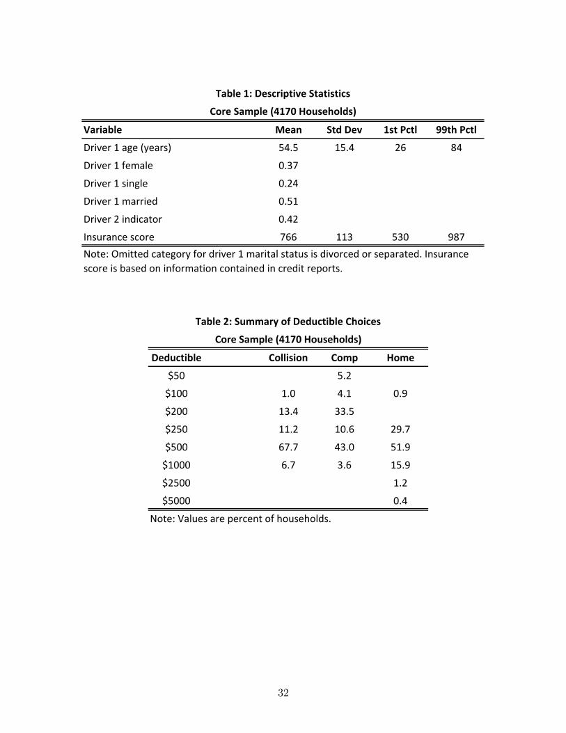
Variable Mean Std Dev 1st Pctl 99th Pctl

Driver 1 age (years) 54.5 15.4 26 84

Driver 1 female 0.37

Driver 1 single 0.24

Driver 1 married 0.51

Driver 2 indicator 0.42

Insurance score 766 113 530 987

Deductible Collision Comp Home

$50 5.2

$100 1.0 4.1 0.9

$200 13.4 33.5

$250 11.2 10.6 29.7

$500 67.7 43.0 51.9

$1000 6.7 3.6 15.9

$2500 1.2

$5000 0.4

Note: Values are percent of households.

Table 1: Descriptive Statistics

Core Sample (4170 Households)

Note: Omitted category for driver 1 marital status is divorced or separated. Insurance

score is based on information contained in credit reports.

Table 2: Summary of Deductible Choices

Core Sample (4170 Households)

32

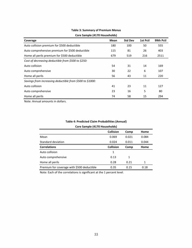
Coverage Mean Std Dev 1st Pctl 99th Pctl

Auto collision premium for $500 deductible 180 100 50 555

Auto comprehensive premium for $500 deductible 115 81 26 403

Home all perils premium for $500 deductible 679 519 216 2511

Cost of decreasing deductible from $500 to $250:

Auto collision 54 31 14 169

Auto comprehensive 30 22 6 107

Home all perils 56 43 11 220

Savings from increasing deductible from $500 to $1000:

Auto collision 41 23 11 127

Auto comprehensive 23 16 5 80

Home all perils 74 58 15 294

Note: Annual amounts in dollars.

Collision Comp Home

Mean 0.069 0.021 0.084

Standard deviation 0.024 0.011 0.044

Correlations Collision Comp Home

Auto collision 1

Auto comprehensive 0.13 1

Home all perils 0.28 0.21 1

Premium for coverage with $500 deductible 0.35 0.15 0.18

Note: Each of the correlations is significant at the 1 percent level.

Table 3: Summary of Premium Menus

Core Sample (4170 Households)

Table 4: Predicted Claim Probabilities (Annual)

Core Sample (4170 Households)

33

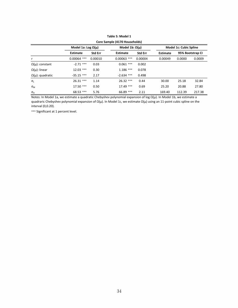
Std Err Std Err Estimate

r 0.00064 *** 0.00010 0.00063 *** 0.00004 0.00049 0.0000 0.0009

Ω(μ): constant ‐2.71 *** 0.03 0.061 *** 0.002

Ω(μ): linear 12.03 *** 0.30 1.186 *** 0.078

Ω(μ): quadratic ‐35.15 *** 2.17 ‐2.634 *** 0.498

σL 26.31 *** 1.14 26.32 *** 0.44 30.00 25.18 32.84

σM 17.50 *** 0.50 17.49 *** 0.69 25.20 20.88 27.80

σH 68.53 *** 5.76 66.89 *** 2.11 169.40 112.39 217.38

*** Significant at 1 percent level.

Notes: In Model 1a, we estimate a quadratic Chebyshev polynomial expansion of log Ω(μ). In Model 1b, we estimate a

quadraric Chebyshev polynomial expansion of Ω(μ). In Model 1c, we estimate Ω(μ) using an 11‐point cubic spline on the

interval (0,0.20).

Table 5: Model 1

Core Sample (4170 Households)

Model 1a: Log Ω(μ) Model 1b: Ω(μ) Model 1c: Cubic Spline

Estimate Estimate 95% Bootstrap CI

34

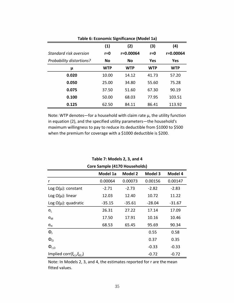
(1) (2) (3) (4)

Standard risk aversion r=0 r=0.00064 r=0 r=0.00064

Probability distortions? No No Yes Yes

μ WTP WTP WTP WTP

0.020 10.00 14.12 41.73 57.20

0.050 25.00 34.80 55.60 75.28

0.075 37.50 51.60 67.30 90.19

0.100 50.00 68.03 77.95 103.51

0.125 62.50 84.11 86.41 113.92

Model 1a Model 2 Model 3 Model 4

r 0.00064 0.00073 0.00156 0.00147

Log Ω(μ): constant ‐2.71 ‐2.73 ‐2.82 ‐2.83

Log Ω(μ): linear 12.03 12.40 10.72 11.22

Log Ω(μ): quadratic ‐35.15 ‐35.61 ‐28.04 ‐31.67

σL 26.31 27.22 17.14 17.09

σM 17.50 17.91 10.16 10.46

σH 68.53 65.45 95.69 90.34

Φr 0.55 0.58

ΦΩ 0.37 0.35

Φr,Ω ‐0.33 ‐0.33

Implied corr(ξr,i,ξΩ,i) ‐0.72 ‐0.72

Table 6: Economic Significance (Model 1a)

Note: WTP denotes—for a household with claim rate μ, the utility function

in equation (2), and the specified utility parameters—the household's

maximum willingness to pay to reduce its deductible from $1000 to $500

when the premium for coverage with a $1000 deductible is $200.

Table 7: Models 2, 3, and 4

Core Sample (4170 Households)

Note: In Models 2, 3, and 4, the estimates reported for r are the mean

fitted values.

35

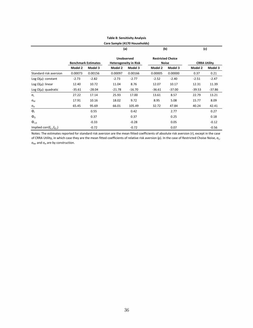
Model 2 Model 3 Model 2 Model 3 Model 2 Model 3 Model 2 Model 3

Standard risk aversion 0.00073 0.00156 0.00097 0.00166 0.00005 0.00000 0.37 0.21

Log Ω(μ): constant ‐2.73 ‐2.82 ‐2.73 ‐2.77 ‐2.52 ‐2.40 ‐2.51 ‐2.47

Log Ω(μ): linear 12.40 10.72 11.04 8.76 12.07 10.17 12.31 11.39

Log Ω(μ): quadratic ‐35.61 ‐28.04 ‐21.78 ‐16.70 ‐36.61 ‐37.00 ‐39.53 ‐37.86

σL 27.22 17.14 25.93 17.00 13.61 8.57 22.79 13.21

σM 17.91 10.16 18.02 9.72 8.95 5.08 15.77 8.09

σH 65.45 95.69 66.01 105.49 32.72 47.84 40.24 42.41

Φr 0.55 0.42 2.77 0.27

ΦΩ 0.37 0.37 0.25 0.18

Φr,Ω ‐0.33 ‐0.28 0.05 ‐0.12

Implied corr(ξr,i,ξΩ,i) ‐0.72 ‐0.72 0.07 ‐0.56

CRRA Utility

Table 8: Sensitivity Analysis

Core Sample (4170 Households)

Notes: The estimates reported for standard risk aversion are the mean fitted coefficients of absolute risk aversion (r), except in the case

of CRRA Utility, in which case they are the mean fitted coefficients of relative risk aversion (ρ). In the case of Restricted Choise Noise, σL,

σM, and σH are by construction.

Benchmark Estimates

Unobserved

Heterogeneity in Risk

Restricted Choice

Noise

(a) (b) (c)

36

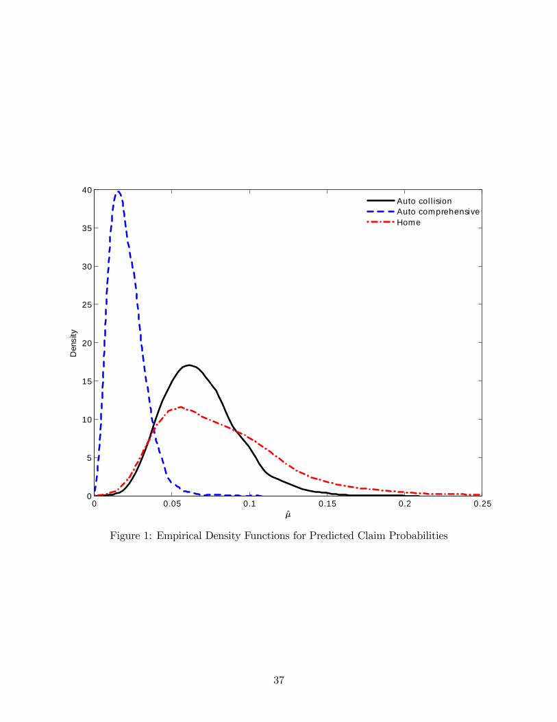
0 0.05 0.1 0.15 0.2 0.250

5

10

15

20

25

30

35

40

Den

sity

Auto col l isionAuto comprehensiveHome

Figure 1: Empirical Density Functions for Predicted Claim Probabilities

37

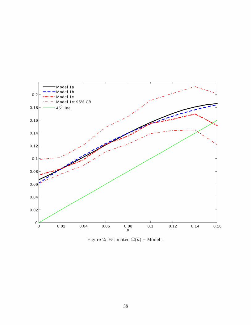
0 0.02 0.04 0.06 0.08 0.1 0.12 0.14 0.160

0.02

0.04

0.06

0.08

0.1

0.12

0.14

0.16

0.18

0.2

Model 1aModel 1bModel 1cModel 1c: 95% CB45o line

Figure 2: Estimated Ω(µ) —Model 1

38

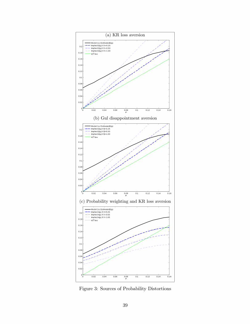
(a) KR loss aversion

0 0.02 0.04 0.06 0.08 0.1 0.12 0.14 0.160

0.02

0.04

0.06

0.08

0.1

0.12

0.14

0.16

0.18

0.2

Model 1a: Es timatedΩ(µ)Implied Ω(µ) if Λ=0.25Implied Ω(µ) if Λ=0.50Implied Ω(µ) if Λ=1.00

45o line

(b) Gul disappointment aversion

0 0.02 0.04 0.06 0.08 0.1 0.12 0.14 0.160

0.02

0.04

0.06

0.08

0.1

0.12

0.14

0.16

0.18

0.2

Model 1a: Es timatedΩ(µ)Implied Ω(µ) if β=0.25Implied Ω(µ) if β=0.50Implied Ω(µ) if β=1.00

45o line

(c) Probability weighting and KR loss aversion

0 0.02 0.04 0.06 0.08 0.1 0.12 0.14 0.160

0.02

0.04

0.06

0.08

0.1

0.12

0.14

0.16

0.18

0.2

Model 1a: Es timatedΩ(µ)Implied π(µ) if Λ=0.25Implied π(µ) if Λ=0.50Implied π(µ) if Λ=1.00

45o line

Figure 3: Sources of Probability Distortions

39

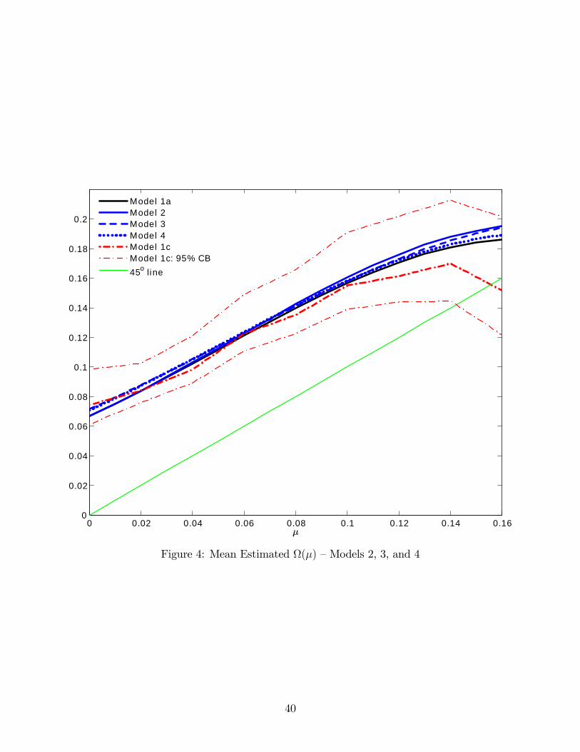
0 0.02 0.04 0.06 0.08 0.1 0.12 0.14 0.160

0.02

0.04

0.06

0.08

0.1

0.12

0.14

0.16

0.18

0.2

Model 1aModel 2Model 3Model 4Model 1cModel 1c: 95% CB45o line

Figure 4: Mean Estimated Ω(µ) —Models 2, 3, and 4

40