Embed Size (px)
Citation preview
Single optical
microfibre-based
modal interferometer
Dissertationzur
Erlangung des Doktorgrades (Dr. rer. nat.)der
Mathematisch-Naturwissenschaftlichen Fakultätder
Rheinischen Friedrich-Wilhelms-Universität Bonn
vorgelegt von
Konstantin Karapetyanaus
Moskau
Bonn 2012


Angefertigt mit Genehmigungder Mathematisch-Naturwissenschaftlichen Fakultätder Rheinischen Friedrich-Wilhelms-Universität Bonn
1. Gutachter: Prof. Dr. Dieter Meschede2. Gutachter: Prof. Dr. Stephan Schlemmer
Tag der Promotion: 18. Oktober 2012
Erscheinungsjahr: 2012

Abstract
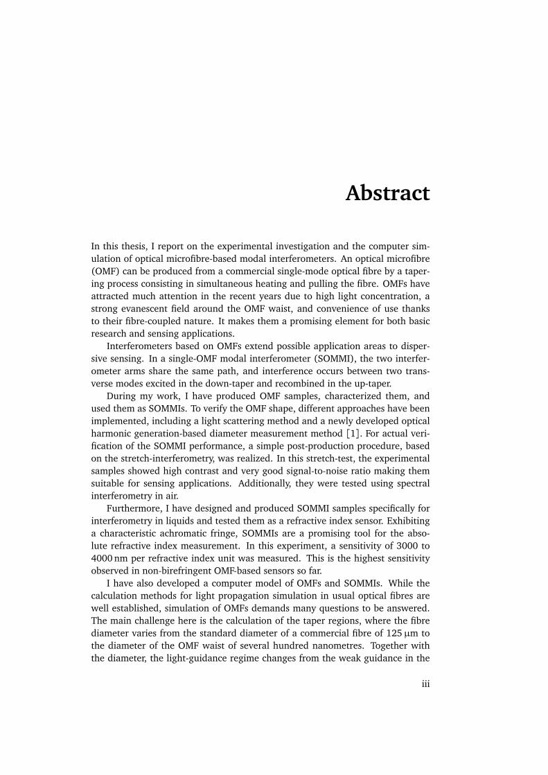
In this thesis, I report on the experimental investigation and the computer sim-ulation of optical microfibre-based modal interferometers. An optical microfibre(OMF) can be produced from a commercial single-mode optical fibre by a taper-ing process consisting in simultaneous heating and pulling the fibre. OMFs haveattracted much attention in the recent years due to high light concentration, astrong evanescent field around the OMF waist, and convenience of use thanksto their fibre-coupled nature. It makes them a promising element for both basicresearch and sensing applications.
Interferometers based on OMFs extend possible application areas to disper-sive sensing. In a single-OMF modal interferometer (SOMMI), the two interfer-ometer arms share the same path, and interference occurs between two trans-verse modes excited in the down-taper and recombined in the up-taper.
During my work, I have produced OMF samples, characterized them, andused them as SOMMIs. To verify the OMF shape, different approaches have beenimplemented, including a light scattering method and a newly developed opticalharmonic generation-based diameter measurement method [1]. For actual veri-fication of the SOMMI performance, a simple post-production procedure, basedon the stretch-interferometry, was realized. In this stretch-test, the experimentalsamples showed high contrast and very good signal-to-noise ratio making themsuitable for sensing applications. Additionally, they were tested using spectralinterferometry in air.
Furthermore, I have designed and produced SOMMI samples specifically forinterferometry in liquids and tested them as a refractive index sensor. Exhibitinga characteristic achromatic fringe, SOMMIs are a promising tool for the abso-lute refractive index measurement. In this experiment, a sensitivity of 3000 to4000 nm per refractive index unit was measured. This is the highest sensitivityobserved in non-birefringent OMF-based sensors so far.
I have also developed a computer model of OMFs and SOMMIs. While thecalculation methods for light propagation simulation in usual optical fibres arewell established, simulation of OMFs demands many questions to be answered.The main challenge here is the calculation of the taper regions, where the fibrediameter varies from the standard diameter of a commercial fibre of 125µm tothe diameter of the OMF waist of several hundred nanometres. Together withthe diameter, the light-guidance regime changes from the weak guidance in the
iii
iv
untapered fibre to the strong guidance in the waist, requiring different modelsto be combined. To the best of my knowledge, I have created the first reliablyworking software code for automatic calculation of all guided modes supportedby tapered fibres [2]. I have then used this code to create computer models forstretch- and spectral-interference in SOMMIs. The experimental results confirmthe validity of these models.
Some results reported in this thesis have been published as:
1. Wiedemann, U., Karapetyan, K., Dan, C., Pritzkau, D., Alt, W., Irsen, S. &Meschede, D. Measurement of submicrometre diameters of tapered opticalfibres using harmonic generation. Optics Express 18, 7693 (2010).
2. Karapetyan, K., Alt, W. & Meschede, D. Optical fibre toolbox for Matlab,version 2.1 [www.mathworks.com/matlabcentral/fileexchange/27819] (2011).
3. Garcia-Fernandez, R., Alt, W, Bruse, F, Dan, C, Karapetyan, K., Rehband,O., Stiebeiner, A., Wiedemann, U., Meschede, D. & Rauschenbeutel, A.Optical nanofibers and spectroscopy. Appl. Phys. B 105, 3–15 (2011).

To my family.Dla mojej Kasi

Acknowledgements
I would like to express my sincere gratitude to people who have helped me duringthis project.
All our samples were fabricated using the fibre pulling machine in the groupof Arno Rauschenbeutel. “Production” trips to Mainz and Vienna were not onlynecessary for the work, but also really enjoyable thanks to the wonderful peopleand atmosphere in this group.
I am grateful to Gilberto Brambilla for inviting me to visit his group andperform some experiments in ORC, Southampton. Discussions with Gilberto andhis colleagues Tim Lee, Yongmin Jung, and Peter Horak during and after this triphave especially helped in building the theoretical model of microfibres.
John Wooler from Fibrecore Ltd., Southampton, generously provided us withmany fine details of fibre manufacturing.
High-quality SEM measurements could be performed thanks to Stephan Irsenfrom Research Center CAESAR, Bonn. During sample preparation and measure-ments, Angelika Sehrbrock has helped us a lot.
Ganz herzlich bedanke ich mich bei allen Mitarbeitern der mechanischenWerkstatt, as well as the whole “support team” of our institute: Annelise von Rudloff-Miglo, Fien Latumahina, Ilona Jaschke, Dietmar Haubrich, and Friedrich Ernst.
The results reported in this thesis could not have been achieved without thejoint work with my wonderful team-mates Fabian Bruse, Cristian Dan, DimaPritzkau, and Uli Wiedemann. Uli was not only my colleague, but also a con-tinuous supporter from my very first hour in Bonn.
Throughout my time in Bonn, but especially in the last two years, when Iswitched to investigation of interferometers, Wolfgang Alt was my helpful advisorin all aspects of experimental, theoretical, and even programming work.
Successful work is impossible without the creative and joyful atmosphere inthe research group. And I am fortunate to have not only spent the last five yearsin the group of Prof. Meschede, but also to have made many good friends here,including Andreas Steffen, Tobias Kampschulte, René Reimann, Wolfgang, Uli,Dima, and hopefully many others.
Of course, nothing of this would have been possible at all if Prof. Meschededid not invite me to come to Bonn and take part in this exciting project.
vii

viii
I thank my friends Dagmar Broemme, Boris Banchevsky, and Sergei Zhukovskyand my whole family, especially my beloved Kasia and my brother Daniel, fortheir support during my time in Germany, in particular in the not so easy periods.
Contents
Introduction xiii
Abbreviations xv
1 Single optical microfibre modal interferometer 11.1 Optical microfibres (OMFs) . . . . . . . . . . . . . . . . . . . . . . . . . 1
1.1.1 How to make an OMF . . . . . . . . . . . . . . . . . . . . . . . 21.1.2 Light guidance in optical fibres and microfibres . . . . . . . . 31.1.3 Fibre modes . . . . . . . . . . . . . . . . . . . . . . . . . . . . . 41.1.4 Fundamental mode evolution in OMF . . . . . . . . . . . . . 7
1.2 Single OMF modal interferometer (SOMMI) . . . . . . . . . . . . . . 101.2.1 Mode coupling . . . . . . . . . . . . . . . . . . . . . . . . . . . . 101.2.2 Mode interference . . . . . . . . . . . . . . . . . . . . . . . . . . 131.2.3 Evanescent field and phase velocity of the two modes in
the waist . . . . . . . . . . . . . . . . . . . . . . . . . . . . . . . 13
2 Computer simulation 152.1 What needs to be calculated . . . . . . . . . . . . . . . . . . . . . . . . 152.2 Problems of available software . . . . . . . . . . . . . . . . . . . . . . . 172.3 Mathematical model of light propagation in OMF . . . . . . . . . . . 18
2.3.1 Dielectric cylindrical waveguide—two-layer model . . . . . 192.3.2 Taper regions—three-layer model . . . . . . . . . . . . . . . . 242.3.3 Choosing right model for each OMF region . . . . . . . . . . 302.3.4 Mode coupling . . . . . . . . . . . . . . . . . . . . . . . . . . . . 312.3.5 Critical angle theory . . . . . . . . . . . . . . . . . . . . . . . . 33
2.4 Optical Fibre Toolbox (OFT) . . . . . . . . . . . . . . . . . . . . . . . . 352.4.1 What OFT can do . . . . . . . . . . . . . . . . . . . . . . . . . . 352.4.2 Example: Application to diameter measurement based on
harmonic generation . . . . . . . . . . . . . . . . . . . . . . . . 352.5 SOMMI simulation . . . . . . . . . . . . . . . . . . . . . . . . . . . . . . 38
2.5.1 Cylinder interferometer . . . . . . . . . . . . . . . . . . . . . . 382.5.2 Spectral interferometry . . . . . . . . . . . . . . . . . . . . . . 392.5.3 Stretch-interferometry . . . . . . . . . . . . . . . . . . . . . . . 412.5.4 Actual SOMMI shape . . . . . . . . . . . . . . . . . . . . . . . . 44
ix
x CONTENTS
2.6 Summary . . . . . . . . . . . . . . . . . . . . . . . . . . . . . . . . . . . . 49
3 Samples 513.1 Production . . . . . . . . . . . . . . . . . . . . . . . . . . . . . . . . . . . 51
3.1.1 Optical fibre tapering . . . . . . . . . . . . . . . . . . . . . . . . 513.1.2 Pulling machine . . . . . . . . . . . . . . . . . . . . . . . . . . . 523.1.3 Optical fibre type selection . . . . . . . . . . . . . . . . . . . . 533.1.4 Target sample shape . . . . . . . . . . . . . . . . . . . . . . . . 543.1.5 Sample shape verification . . . . . . . . . . . . . . . . . . . . . 60
3.2 Stretch-interferometry . . . . . . . . . . . . . . . . . . . . . . . . . . . . 693.2.1 Setup . . . . . . . . . . . . . . . . . . . . . . . . . . . . . . . . . 693.2.2 Experiment . . . . . . . . . . . . . . . . . . . . . . . . . . . . . . 693.2.3 Results and analysis . . . . . . . . . . . . . . . . . . . . . . . . . 70
3.3 Handling . . . . . . . . . . . . . . . . . . . . . . . . . . . . . . . . . . . . 733.3.1 Fibre holder design . . . . . . . . . . . . . . . . . . . . . . . . . 743.3.2 Using samples in experiments . . . . . . . . . . . . . . . . . . 76
3.4 Conclusions . . . . . . . . . . . . . . . . . . . . . . . . . . . . . . . . . . 78
4 Spectral interferometry 814.1 Optical setup . . . . . . . . . . . . . . . . . . . . . . . . . . . . . . . . . . 814.2 Automated spectrum acquisition . . . . . . . . . . . . . . . . . . . . . . 824.3 Spectrum analysis . . . . . . . . . . . . . . . . . . . . . . . . . . . . . . 82
4.3.1 Characteristic shape: simulation . . . . . . . . . . . . . . . . . 824.3.2 Characteristic shape: experiment . . . . . . . . . . . . . . . . 834.3.3 Data processing . . . . . . . . . . . . . . . . . . . . . . . . . . . 854.3.4 Use of zero-dispersion point for diameter determination . . 86
4.4 Spectral interferometry in air . . . . . . . . . . . . . . . . . . . . . . . . 874.5 Interferometry in liquids . . . . . . . . . . . . . . . . . . . . . . . . . . 89
4.5.1 Setup . . . . . . . . . . . . . . . . . . . . . . . . . . . . . . . . . 904.5.2 Test liquids . . . . . . . . . . . . . . . . . . . . . . . . . . . . . . 924.5.3 Temperature variation . . . . . . . . . . . . . . . . . . . . . . . 934.5.4 Sample design . . . . . . . . . . . . . . . . . . . . . . . . . . . . 934.5.5 Results and analysis . . . . . . . . . . . . . . . . . . . . . . . . . 95
4.6 Conclusions . . . . . . . . . . . . . . . . . . . . . . . . . . . . . . . . . . 97
5 Summary and outlook 995.1 Pulling machine . . . . . . . . . . . . . . . . . . . . . . . . . . . . . . . . 1005.2 Sample shape . . . . . . . . . . . . . . . . . . . . . . . . . . . . . . . . . 1015.3 Dispersion measurement of atoms and molecules . . . . . . . . . . . 1025.4 Simulation . . . . . . . . . . . . . . . . . . . . . . . . . . . . . . . . . . . 102
Appendix A Guided mode solutions 103A.1 Two-layer waveguide . . . . . . . . . . . . . . . . . . . . . . . . . . . . 103
A.1.1 Scalar approximation (LP modes) . . . . . . . . . . . . . . . . 103
CONTENTS xi
A.1.2 Vector solution . . . . . . . . . . . . . . . . . . . . . . . . . . . . 104A.2 Three-layer fibre . . . . . . . . . . . . . . . . . . . . . . . . . . . . . . . 104
A.2.1 Scalar approximation (LP modes) . . . . . . . . . . . . . . . . 104A.2.2 Vector solution . . . . . . . . . . . . . . . . . . . . . . . . . . . . 104
A.3 Anisotropic fibre . . . . . . . . . . . . . . . . . . . . . . . . . . . . . . . 105A.4 Model applicability . . . . . . . . . . . . . . . . . . . . . . . . . . . . . . 105
Appendix B Algorithm description 107B.1 Search for guided modes . . . . . . . . . . . . . . . . . . . . . . . . . . 107B.2 Tracing the dispersion curve . . . . . . . . . . . . . . . . . . . . . . . . 108
Appendix C OMF samples 109
Appendix D Fibre holder 111D.1 Fixing a sample in the holder . . . . . . . . . . . . . . . . . . . . . . . . 111D.2 Transportation and storage . . . . . . . . . . . . . . . . . . . . . . . . . 113
Appendix E Sample 204 in Cargille liquids 115
Bibliography 117

Introduction
People have been progressing in their attempts to manipulate propagation oflight for more than 2500 years,∗ and have achieved significant success on theway. Today we can transfer single photons over dozens of kilometres using op-tical fibres [4] and perform almost magic by producing invisibility cloaks usingphotonic crystals [5].
Light usually propagates either inside an optical material—as in fibres, prisms,and photonic crystals—or in the space between optical elements such as lensesand mirrors. From this point of view, optical microfibres fill the gap: Light fol-lows a microfibre, which can be bent or curled, as with usual fibres. At the sametime, it remains open for interaction with the surrounding medium, almost like afree-space beam.
* * *
Until the 1960s, optical fibres were only used for illumination and technicaland medical imaging, because high absorption losses were making any glass ele-ment thicker (longer) than a few dozens of centimetres useless [6]. In 1966, intheir Nobel prize-winning paper [7], Kao and Hokcham predicted that glass fi-bres can have very small absorption losses. The modern era of fibre optics beganin 1970, when Corning researchers made Kao’s theoretical prediction a reality.
In the early days of fibre optics, light was guided in glass threads surroundedby air or a low refractive index liquid—i. e. by total internal reflection at theouter surface of the fibre. Already in the 1950s, it became obvious that the light-guiding core of the fibre should be surrounded by a transparent low-refractive-index cladding, to minimize the influence of the outer medium on light prop-agation. The core was made almost as large as the cladding, to maximize theimaging resolution and the power efficiency of devices [6]. In their paper, Kaoand Hokcham have not only considered losses in the fibre material, but alsothought of the optimal conditions to guide light. They suggested that it was ac-tually beneficial to reduce the diameter of the core relative to the cladding: in avery thin—just a few wavelengths in diameter—core surrounded by a claddingof almost the same refractive index, light can only propagate in the fundamental
∗The first lenses were probably produced by the Assyrians, such as the famous Nimrud lens.
xiii
xiv INTRODUCTION
transverse mode. This ensures a high data transmission rate (used in telecom-munication) and an excellent output beam quality, due to which these fibres arecommonly used in research labs.
Usually, propagating light should be “protected” from any disturbances, there-fore it is transported deep inside the fibre. The standard cladding diameter is125µm, about 20 . . . 40 times larger than the core. However, for many applica-tions such as signal routing and energy splitting, as well as for basic researchit is of obvious interest to gain physical access to propagating light and make itinteract with surroundings. Ideally, this zone of interaction should be restricted,leaving a “normal” fibre optimized for guidance at both ends of the interactionregion. This idea leads to fibre tapering, which is a local reduction of the fibrediameter [8].
Tapering is performed by simultaneously heating and carefully stretching ofa fibre. The fibre gets thinner but continues to guide light. Even when taperingis as drastic as from 125µm down to ∼ 0.5µm, tapered fibres can have almost100 % transmission [9].
Such microfibres have a number of interesting properties. Due to the verysmall diameter and a high refractive index step at the surface (between glass andair), they concentrate guided light into a small transverse area, thereby increasingintensity and providing for such effects as harmonic and supercontinuum genera-tion at low peak power [10–12]. Also, depending on the diameter, more than halfof the light can propagate in the evanescent field around the fibre. This makessuch microfibres useful for a number of applications, ranging from light couplingbetween fibres [13] to sensing [14] to probing atomic fluorescence [15] to atomtrapping [16]. In sensing, the strong light concentration around the microfibreprovides for a very high sensitivity [17].
Dispersive sensing is one more application area for optical microfibres. It canbe used for off-resonant and therefore non-absorbing sensing, refractive indexmeasurement, and non-destructive monitoring of light-sensitive objects such asorganic molecules. Microfibre-based interferometers can be significantly smallerthan their fibre-less counterparts. They also combine the convenience of fibre-coupled devices with the high sensitivity of microfibres. Interferometers can con-tain a microfibre in one arm [18], in both arms [19], or can actually be builtwith just a single microfibre, the two interferometer arms being represented bytwo different transverse guided modes [20]. Interferometers of the latter typepromise the most compact devices [21] and can be easily manufactured at thecurrent level of technology. They are the subject of the present thesis.
Abbreviations
EVE eigenvalue equationHE/EH hybrid fibre modesLP linearly polarized (mode)OFT Optical Fibre Toolbox [2]OMF optical microfibreOSA optical spectrum analyserSEM scanning electron microscope/microscopySHG second harmonic generationSOMMI single OMF-based modal interferometerTE transverse electric (mode)THG third harmonic generationTM transverse magnetic (mode)UV ultravioletZDW zero-dispersion wavelength
xv


CHAPTER 1Single optical microfibre modal
interferometer
In this chapter, I introduce OMFs and the subject of this project—single-microfibremodal interferometer—without mathematics. The rigorous theoretical treatmentis given in Chapter 2, where I describe the computer simulation of our interfer-ometers.
1.1 Optical microfibres
Microfibre and nanofibre, ultrathin optical fibre, tapered optical fibre, photonicnanowire—these and many other names met in the literature are all used for thesame optical element—a dielectric light waveguide with one part (called waist)having transverse dimensions on the scale of the wavelength of guided light anda much larger length. Usually, microfibres have a circular symmetry, though somegroups have tried to use polarization-maintaining fibres of different geometries[22, 23]. In this project, only circularly symmetric fibres are considered.
The large variety of names is explained partly by the fact that these elementshave attracted wide interest only recently, and no name has been commonly ac-cepted yet. On the other hand, depending on the exact design and application,there is a desire to emphasize different aspects of physics and engineering ofthese elements.
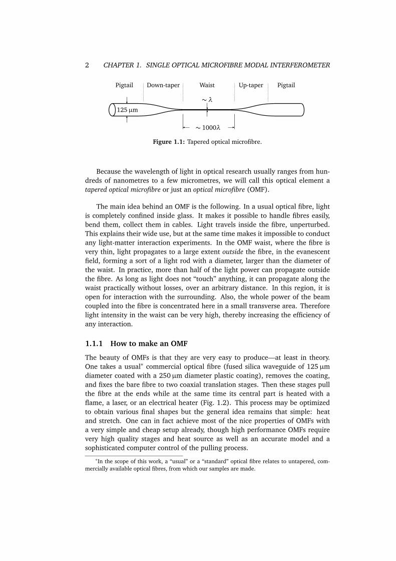
At both ends the waist is connected to a usual optical fibre (typical diameter125µm) with the so called tapers—relatively long conical regions with a slowlychanging diameter (Fig. 1.1). The ends of the OMF, where it can be spliced toanother optical fibre or where a free-space beam can be coupled in or out of theOMF, are called pigtails.
1
2 CHAPTER 1. SINGLE OPTICAL MICROFIBRE MODAL INTERFEROMETER
125µm
∼ λ
∼ 1000λ
Waist Up-taperDown-taperPigtail Pigtail
Figure 1.1: Tapered optical microfibre.
Because the wavelength of light in optical research usually ranges from hun-dreds of nanometres to a few micrometres, we will call this optical element atapered optical microfibre or just an optical microfibre (OMF).
The main idea behind an OMF is the following. In a usual optical fibre, lightis completely confined inside glass. It makes it possible to handle fibres easily,bend them, collect them in cables. Light travels inside the fibre, unperturbed.This explains their wide use, but at the same time makes it impossible to conductany light-matter interaction experiments. In the OMF waist, where the fibre isvery thin, light propagates to a large extent outside the fibre, in the evanescentfield, forming a sort of a light rod with a diameter, larger than the diameter ofthe waist. In practice, more than half of the light power can propagate outsidethe fibre. As long as light does not “touch” anything, it can propagate along thewaist practically without losses, over an arbitrary distance. In this region, it isopen for interaction with the surrounding. Also, the whole power of the beamcoupled into the fibre is concentrated here in a small transverse area. Thereforelight intensity in the waist can be very high, thereby increasing the efficiency ofany interaction.
1.1.1 How to make an OMF
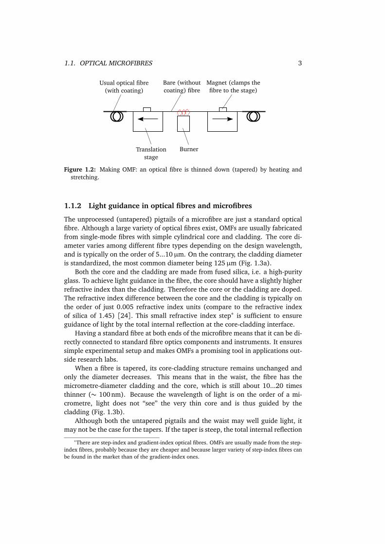
The beauty of OMFs is that they are very easy to produce—at least in theory.One takes a usual∗ commercial optical fibre (fused silica waveguide of 125µmdiameter coated with a 250µm diameter plastic coating), removes the coating,and fixes the bare fibre to two coaxial translation stages. Then these stages pullthe fibre at the ends while at the same time its central part is heated with aflame, a laser, or an electrical heater (Fig. 1.2). This process may be optimizedto obtain various final shapes but the general idea remains that simple: heatand stretch. One can in fact achieve most of the nice properties of OMFs witha very simple and cheap setup already, though high performance OMFs requirevery high quality stages and heat source as well as an accurate model and asophisticated computer control of the pulling process.
∗In the scope of this work, a “usual” or a “standard” optical fibre relates to untapered, com-mercially available optical fibres, from which our samples are made.
1.1. OPTICAL MICROFIBRES 3
Usual optical fibre(with coating)
Bare (withoutcoating) fibre
BurnerTranslationstage
Magnet (clamps thefibre to the stage)
Figure 1.2: Making OMF: an optical fibre is thinned down (tapered) by heating andstretching.
1.1.2 Light guidance in optical fibres and microfibres
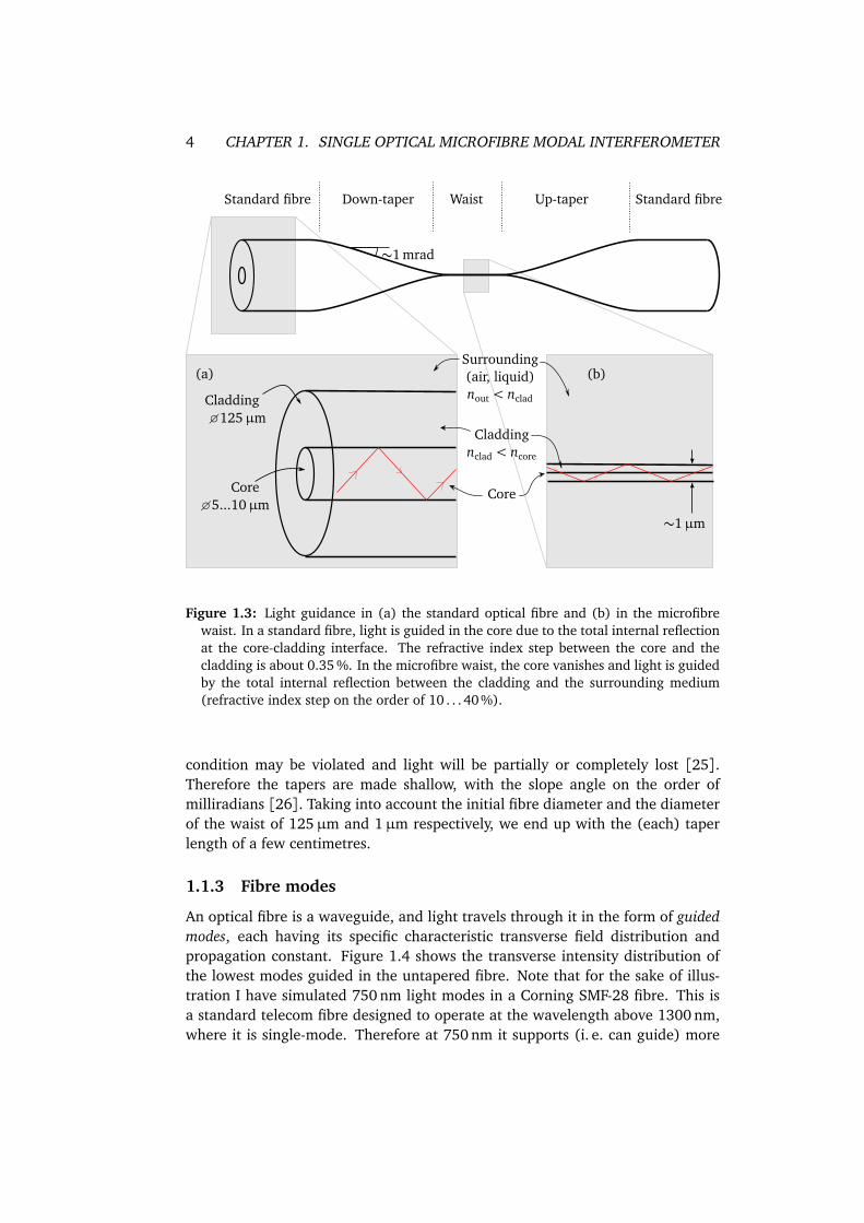
The unprocessed (untapered) pigtails of a microfibre are just a standard opticalfibre. Although a large variety of optical fibres exist, OMFs are usually fabricatedfrom single-mode fibres with simple cylindrical core and cladding. The core di-ameter varies among different fibre types depending on the design wavelength,and is typically on the order of 5...10µm. On the contrary, the cladding diameteris standardized, the most common diameter being 125µm (Fig. 1.3a).
Both the core and the cladding are made from fused silica, i.e. a high-purityglass. To achieve light guidance in the fibre, the core should have a slightly higherrefractive index than the cladding. Therefore the core or the cladding are doped.The refractive index difference between the core and the cladding is typically onthe order of just 0.005 refractive index units (compare to the refractive indexof silica of 1.45) [24]. This small refractive index step∗ is sufficient to ensureguidance of light by the total internal reflection at the core-cladding interface.
Having a standard fibre at both ends of the microfibre means that it can be di-rectly connected to standard fibre optics components and instruments. It ensuressimple experimental setup and makes OMFs a promising tool in applications out-side research labs.
When a fibre is tapered, its core-cladding structure remains unchanged andonly the diameter decreases. This means that in the waist, the fibre has themicrometre-diameter cladding and the core, which is still about 10...20 timesthinner (∼ 100nm). Because the wavelength of light is on the order of a mi-crometre, light does not “see” the very thin core and is thus guided by thecladding (Fig. 1.3b).
Although both the untapered pigtails and the waist may well guide light, itmay not be the case for the tapers. If the taper is steep, the total internal reflection
∗There are step-index and gradient-index optical fibres. OMFs are usually made from the step-index fibres, probably because they are cheaper and because larger variety of step-index fibres canbe found in the market than of the gradient-index ones.
4 CHAPTER 1. SINGLE OPTICAL MICROFIBRE MODAL INTERFEROMETER
(a) (b)
∼1 mrad
Core
∼1µm
Standard fibre Down-taper Waist Up-taper Standard fibre
5...10µm
Surrounding(air, liquid)nout < nclad
Claddingnclad < ncore
Core
Cladding125µm
Figure 1.3: Light guidance in (a) the standard optical fibre and (b) in the microfibrewaist. In a standard fibre, light is guided in the core due to the total internal reflectionat the core-cladding interface. The refractive index step between the core and thecladding is about 0.35 %. In the microfibre waist, the core vanishes and light is guidedby the total internal reflection between the cladding and the surrounding medium(refractive index step on the order of 10 . . . 40%).
condition may be violated and light will be partially or completely lost [25].Therefore the tapers are made shallow, with the slope angle on the order ofmilliradians [26]. Taking into account the initial fibre diameter and the diameterof the waist of 125µm and 1µm respectively, we end up with the (each) taperlength of a few centimetres.
1.1.3 Fibre modes
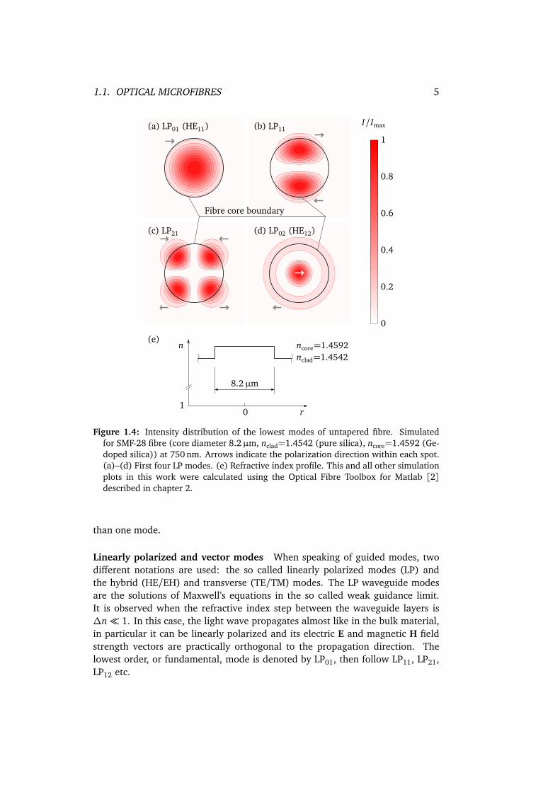
An optical fibre is a waveguide, and light travels through it in the form of guidedmodes, each having its specific characteristic transverse field distribution andpropagation constant. Figure 1.4 shows the transverse intensity distribution ofthe lowest modes guided in the untapered fibre. Note that for the sake of illus-tration I have simulated 750 nm light modes in a Corning SMF-28 fibre. This isa standard telecom fibre designed to operate at the wavelength above 1300 nm,where it is single-mode. Therefore at 750 nm it supports (i. e. can guide) more
1.1. OPTICAL MICROFIBRES 5
Fibre core boundary
(a) LP01 (HE11) (b) LP11
(d) LP02 (HE12)(c) LP21
0
0.2
0.4
0.6
0.8
1
I/Imax
ncore=1.4592nclad=1.4542
(e)
8.2µm
n
r01
Figure 1.4: Intensity distribution of the lowest modes of untapered fibre. Simulatedfor SMF-28 fibre (core diameter 8.2µm, nclad=1.4542 (pure silica), ncore=1.4592 (Ge-doped silica)) at 750 nm. Arrows indicate the polarization direction within each spot.(a)–(d) First four LP modes. (e) Refractive index profile. This and all other simulationplots in this work were calculated using the Optical Fibre Toolbox for Matlab [2]described in chapter 2.
than one mode.
Linearly polarized and vector modes When speaking of guided modes, twodifferent notations are used: the so called linearly polarized modes (LP) andthe hybrid (HE/EH) and transverse (TE/TM) modes. The LP waveguide modesare the solutions of Maxwell’s equations in the so called weak guidance limit.It is observed when the refractive index step between the waveguide layers is∆n 1. In this case, the light wave propagates almost like in the bulk material,in particular it can be linearly polarized and its electric E and magnetic H fieldstrength vectors are practically orthogonal to the propagation direction. Thelowest order, or fundamental, mode is denoted by LP01, then follow LP11, LP21,LP12 etc.
6 CHAPTER 1. SINGLE OPTICAL MICROFIBRE MODAL INTERFEROMETER
A completely different situation occurs when the refractive index step of theguiding surface is large. By solving Maxwell’s equations, it turns out that, ingeneral, all six field components Ex ,y,z and Hx ,y,z are non-zero. Depending onthe exact relation between different components, the modes are then denoted asHE, EH, TE, and TM.
Thus, the LP modes are the approximation of the exact HE/EH/TE/TM solu-tions. In the LP approximation, Maxwell’s equations can be solved using scalarmathematics, and therefore these modes are sometimes called scalar modes.The rigorous solution requires vector calculations, therefore the HE/EH/TE/TMmodes are called vector modes.
The two modes we mainly care about in the scope of this work are the HE11and HE12 modes, to which, in the scalar approximation, correspond the LP01and LP02 modes. The LP11 and LP21 modes correspond to a bunch of vectormodes each, meaning that in the scalar approximation some of the vector modesbecome degenerate in the propagation constant (Tab. 1.1; see also also Fig. 2.5on page 24).
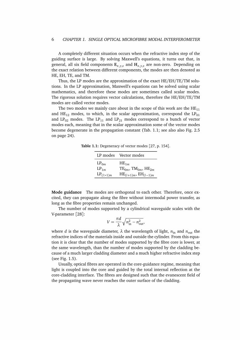
Table 1.1: Degeneracy of vector modes [27, p. 154].
LP modes Vector modes
LP0m HE1mLP1m TE0m, TM0m, HE2mLP(l>1)m HE(l+1)m, EH(l−1)m
Mode guidance The modes are orthogonal to each other. Therefore, once ex-cited, they can propagate along the fibre without intermodal power transfer, aslong as the fibre properties remain unchanged.
The number of modes supported by a cylindrical waveguide scales with theV-parameter [28]:
V =πd
λ
Æ
n2in− n2
out,
where d is the waveguide diameter, λ the wavelength of light, nin and nout therefractive indices of the materials inside and outside the cylinder. From this equa-tion it is clear that the number of modes supported by the fibre core is lower, atthe same wavelength, than the number of modes supported by the cladding be-cause of a much larger cladding diameter and a much higher refractive index step(see Fig. 1.5).
Usually, optical fibres are operated in the core-guidance regime, meaning thatlight is coupled into the core and guided by the total internal reflection at thecore-cladding interface. The fibres are designed such that the evanescent field ofthe propagating wave never reaches the outer surface of the cladding.
1.1. OPTICAL MICROFIBRES 7
Cladding
Core, ncore ∼ 1.5
5...10µm
125µm
∆n∼ 0.005
∆n∼ 0.1...0.5
Surrounding(liquids, air)
Figure 1.5: Refractive index steps in a typical optical fibre.
1.1.4 Fundamental mode evolution in OMF
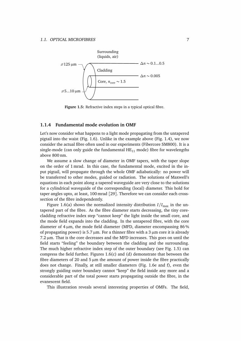
Let’s now consider what happens to a light mode propagating from the untaperedpigtail into the waist (Fig. 1.6). Unlike in the example above (Fig. 1.4), we nowconsider the actual fibre often used in our experiments (Fibercore SM800). It is asingle-mode (can only guide the fundamental HE11 mode) fibre for wavelengthsabove 800 nm.
We assume a slow change of diameter in OMF tapers, with the taper slopeon the order of 1 mrad. In this case, the fundamental mode, excited in the in-put pigtail, will propagate through the whole OMF adiabatically: no power willbe transferred to other modes, guided or radiation. The solutions of Maxwell’sequations in each point along a tapered waveguide are very close to the solutionsfor a cylindrical waveguide of the corresponding (local) diameter. This hold fortaper angles upto, at least, 100 mrad [29]. Therefore we can consider each cross-section of the fibre independently.
Figure 1.6(a) shows the normalized intensity distribution I/Imax in the un-tapered part of the fibre. As the fibre diameter starts decreasing, the tiny core-cladding refractive index step “cannot keep” the light inside the small core, andthe mode field expands into the cladding. In the untapered fibre, with the corediameter of 4µm, the mode field diameter (MFD, diameter encompassing 86 %of propagating power) is 5.7µm. For a thinner fibre with a 3µm core it is already7.2µm. That is the core decreases and the MFD increases. This goes on until thefield starts “feeling” the boundary between the cladding and the surrounding.The much higher refractive index step of the outer boundary (see Fig. 1.5) cancompress the field further. Figures 1.6(c) and (d) demonstrate that between thefibre diameters of 20 and 5µm the amount of power inside the fibre practicallydoes not change. Finally, at still smaller diameters (Fig. 1.6e and f), even thestrongly guiding outer boundary cannot “keep” the field inside any more and aconsiderable part of the total power starts propagating outside the fibre, in theevanescent field.
This illustration reveals several interesting properties of OMFs. The field,
8 CHAPTER 1. SINGLE OPTICAL MICROFIBRE MODAL INTERFEROMETER
MFD: 13µm MFD: 3.4µm MFD: 0.81µm MFD: 0.66µm
MFD: 7.2µmMFD: 5.7µm
ncore=1.4574nclad=1.4525
(g) n
r0nout = 1
dclad
4µm
0
0.2
0.4
0.6
0.8
1
I/Imax
(a) HE11 mode in untapered fibre, core 4µm
3µm
(b) Core 3µm
(c) Cladding: 20µm (d) 5µm (e) 1µm (f) 0.5µm
Cladding surfaceCore
Core
Figure 1.6: (a)–(f) Variation of the normalized intensity of the HE11 mode with fibrediameter. (g) Refractive index profile. Note: plots (a) and (b) are not to scale toplots (c)–(f). In plots (c)–(f) the cladding diameter is shown constant to better showthe mode expansion relative to the fibre. The actual mode field is compressed (noteMFD). Fibre: Fibercore SM800 (core 4µm, cladding 125µm, NA=0.12). Wavelength:850 nm.
1.1. OPTICAL MICROFIBRES 9
coupled into the input pigtail, is transversely compressed, leading to the increaseof intensity. The effective area of the HE11 mode in Fig. 1.6(f) is 74 times smallerthan in Fig. 1.6(a). The actual losses in our OMF samples are below 5 %, whichmeans that the intensity of the field increases by about a factor of 70.
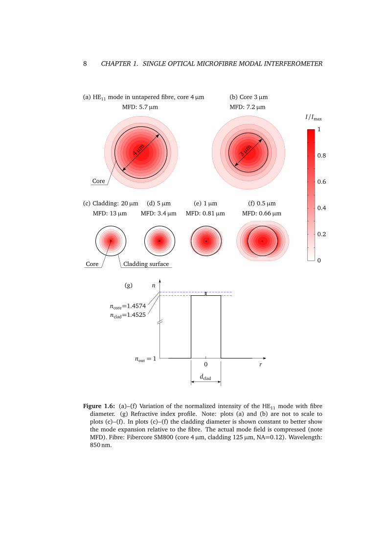
Another, not so obvious effect, is the increase of intensity outside the fibre,in the surrounding medium. Figure 1.7 shows the dependence of the intensity(azimuthally averaged) at the surface of the fibre. For very small diameters,even the strongly guiding cladding-surrounding surface does not confine lightany more, the mode field expands and eventually becomes infinitely large ford = 0, leading to zero intensity everywhere.
0 0.5 1 1.5 20
Diameter, µm
Inte
nsit
yat
the
surf
ace,
a.u.
Figure 1.7: Intensity just outside the fibre (HE11 mode at 750 nm, silica fibre in air).
At the maximum intensity point in Fig. 1.7, the light intensity around theOMF is similar to that in the focal point of a tightly focussed free-space beam.However, unlike the free-space beam after the focal point, the fibre mode doesnot rapidly expand but remains confined and guided by the OMF waist. The waistcan theoretically be infinitely long, and practically it is much longer (millimetres)than the depth of focus in case of tight free-space focusing (on the order of awavelength, i. e. microns). This creates a unique situation of “infinite focus”providing
• high light intensity
• over large length
• in free space around the fibre
and setting excellent conditions for light-matter interaction experiments. Themost straightforward way of using microfibres is putting some absorbing material
10 CHAPTER 1. SINGLE OPTICAL MICROFIBRE MODAL INTERFEROMETER
on or around the waist, shine white light into the input end and observe the spec-trum at the output end. Due to the high intensity and the long interaction length,this approach is very suitable for high-sensitivity absorption spectroscopy [17].
1.2 Single OMF modal interferometer (SOMMI)
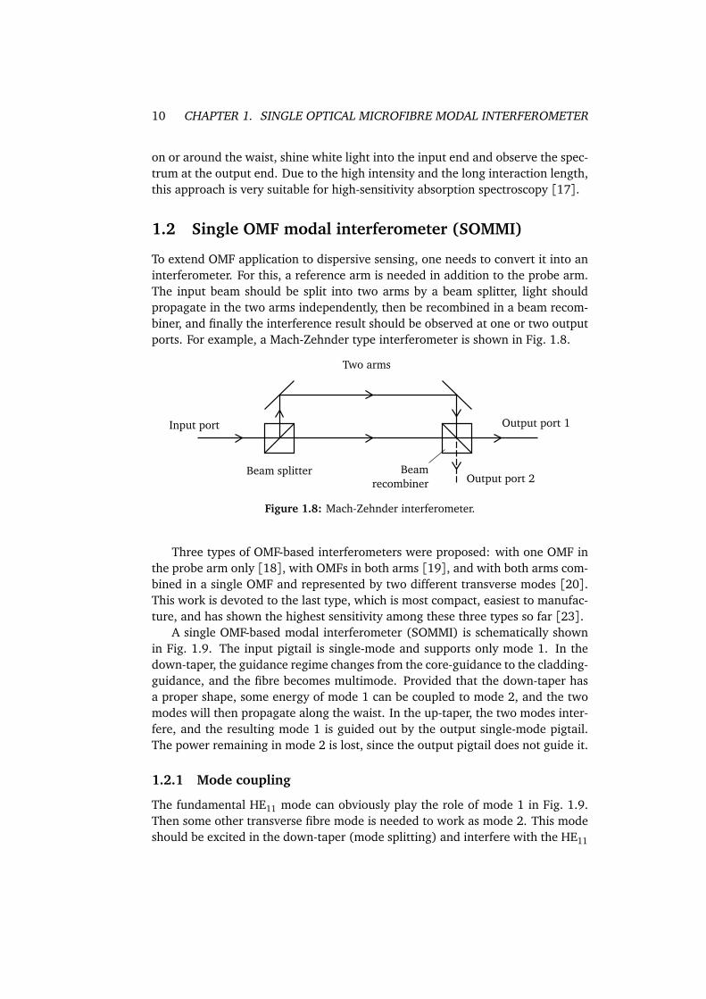
To extend OMF application to dispersive sensing, one needs to convert it into aninterferometer. For this, a reference arm is needed in addition to the probe arm.The input beam should be split into two arms by a beam splitter, light shouldpropagate in the two arms independently, then be recombined in a beam recom-biner, and finally the interference result should be observed at one or two outputports. For example, a Mach-Zehnder type interferometer is shown in Fig. 1.8.
Beam splitter
Two arms
Input port Output port 1
Beamrecombiner Output port 2
Figure 1.8: Mach-Zehnder interferometer.
Three types of OMF-based interferometers were proposed: with one OMF inthe probe arm only [18], with OMFs in both arms [19], and with both arms com-bined in a single OMF and represented by two different transverse modes [20].This work is devoted to the last type, which is most compact, easiest to manufac-ture, and has shown the highest sensitivity among these three types so far [23].
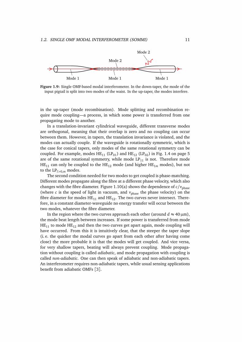
A single OMF-based modal interferometer (SOMMI) is schematically shownin Fig. 1.9. The input pigtail is single-mode and supports only mode 1. In thedown-taper, the guidance regime changes from the core-guidance to the cladding-guidance, and the fibre becomes multimode. Provided that the down-taper hasa proper shape, some energy of mode 1 can be coupled to mode 2, and the twomodes will then propagate along the waist. In the up-taper, the two modes inter-fere, and the resulting mode 1 is guided out by the output single-mode pigtail.The power remaining in mode 2 is lost, since the output pigtail does not guide it.
1.2.1 Mode coupling
The fundamental HE11 mode can obviously play the role of mode 1 in Fig. 1.9.Then some other transverse fibre mode is needed to work as mode 2. This modeshould be excited in the down-taper (mode splitting) and interfere with the HE11
1.2. SINGLE OMF MODAL INTERFEROMETER (SOMMI) 11
Mode 1 Mode 1Mode 1
Mode 2
Mode 2
Figure 1.9: Single OMF-based modal interferometer. In the down-taper, the mode of theinput pigtail is split into two modes of the waist. In the up-taper, the modes interfere.
in the up-taper (mode recombination). Mode splitting and recombination re-quire mode coupling—a process, in which some power is transferred from onepropagating mode to another.
In a translation-invariant cylindrical waveguide, different transverse modesare orthogonal, meaning that their overlap is zero and no coupling can occurbetween them. However, in tapers, the translation invariance is violated, and themodes can actually couple. If the waveguide is rotationally symmetric, which isthe case for conical tapers, only modes of the same rotational symmetry can becoupled. For example, modes HE11 (LP01) and HE12 (LP02) in Fig. 1.4 on page 5are of the same rotational symmetry, while mode LP11 is not. Therefore modeHE11 can only be coupled to the HE12 mode (and higher HE1m modes), but notto the LPl>0,m modes.
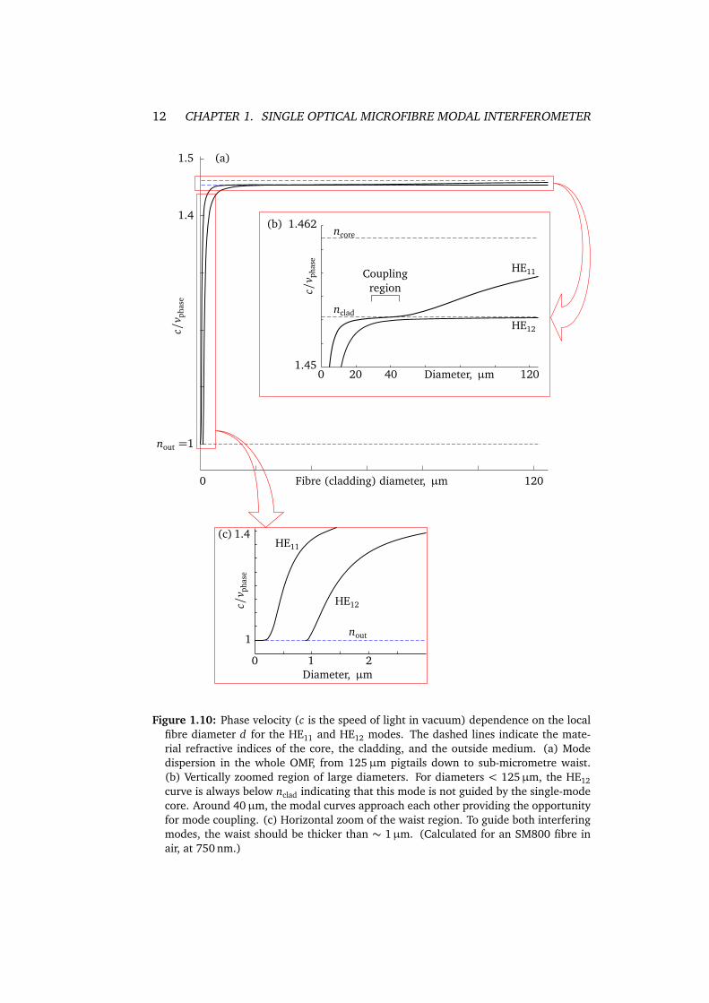
The second condition needed for two modes to get coupled is phase-matching.Different modes propagate along the fibre at a different phase velocity, which alsochanges with the fibre diameter. Figure 1.10(a) shows the dependence of c/vphase(where c is the speed of light in vacuum, and vphase the phase velocity) on thefibre diameter for modes HE11 and HE12. The two curves never intersect. There-fore, in a constant diameter-waveguide no energy transfer will occur between thetwo modes, whatever the fibre diameter.
In the region where the two curves approach each other (around d ≈ 40µm),the mode beat length between increases. If some power is transferred from modeHE11 to mode HE12 and then the two curves get apart again, mode coupling willhave occurred. From this it is intuitively clear, that the steeper the taper slope(i. e. the quicker the modal curves go apart from each other after having comeclose) the more probable it is that the modes will get coupled. And vice versa,for very shallow tapers, beating will always prevent coupling. Mode propaga-tion without coupling is called adiabatic, and mode propagation with coupling iscalled non-adiabatic. One can then speak of adiabatic and non-adiabatic tapers.An interferometer requires non-adiabatic tapers, while usual sensing applicationsbenefit from adiabatic OMFs [3].
12 CHAPTER 1. SINGLE OPTICAL MICROFIBRE MODAL INTERFEROMETER
c/v p
hase
Fibre (cladding) diameter, µm 120
nout =1
1.4
1.5
0
nout
c/v p
hase
Diameter, µm0 1201.45
1.462
HE11
HE12
ncore
nclad
HE11
HE12
20 40
(a)
(b)
(c)
Couplingregion
c/v p
hase
Diameter, µm0 1 2
1
1.4
Figure 1.10: Phase velocity (c is the speed of light in vacuum) dependence on the localfibre diameter d for the HE11 and HE12 modes. The dashed lines indicate the mate-rial refractive indices of the core, the cladding, and the outside medium. (a) Modedispersion in the whole OMF, from 125µm pigtails down to sub-micrometre waist.(b) Vertically zoomed region of large diameters. For diameters < 125µm, the HE12curve is always below nclad indicating that this mode is not guided by the single-modecore. Around 40µm, the modal curves approach each other providing the opportunityfor mode coupling. (c) Horizontal zoom of the waist region. To guide both interferingmodes, the waist should be thicker than ∼ 1µm. (Calculated for an SM800 fibre inair, at 750 nm.)
1.2. SINGLE OMF MODAL INTERFEROMETER (SOMMI) 13
1.2.2 Mode interference
Once the fundamental mode HE11 of the input pigtail is split into the HE11 andHE12 modes in the down-taper, these two modes can propagate further alongthe fibre adiabatically, because of the large phase mismatch everywhere outsidethe coupling region (see Fig. 1.10c). If the tapers are adiabatic beyond the modesplitting region and the waist is thick enough to guide the HE12 mode (mode HE11is always guided), the two modes will propagate until they reach the couplingregion in the up-taper. (The up-taper is usually symmetric to the down-taper.)There the modes again couple to each other.
Depending on the phase relation between the modes, this second couplingcan result in constructive or destructive interference for the HE11 mode. Theoutput pigtail of the OMF can only guide the HE11 mode out, the HE12 modebeing lost in the up-taper. Thus, the power of the output signal depends on thephase relation between the two modes, and the OMF becomes an interferometer.
1.2.3 Evanescent field and phase velocity of the two modes in thewaist
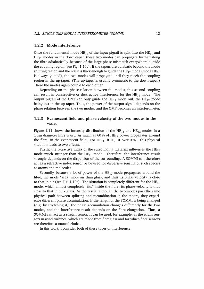
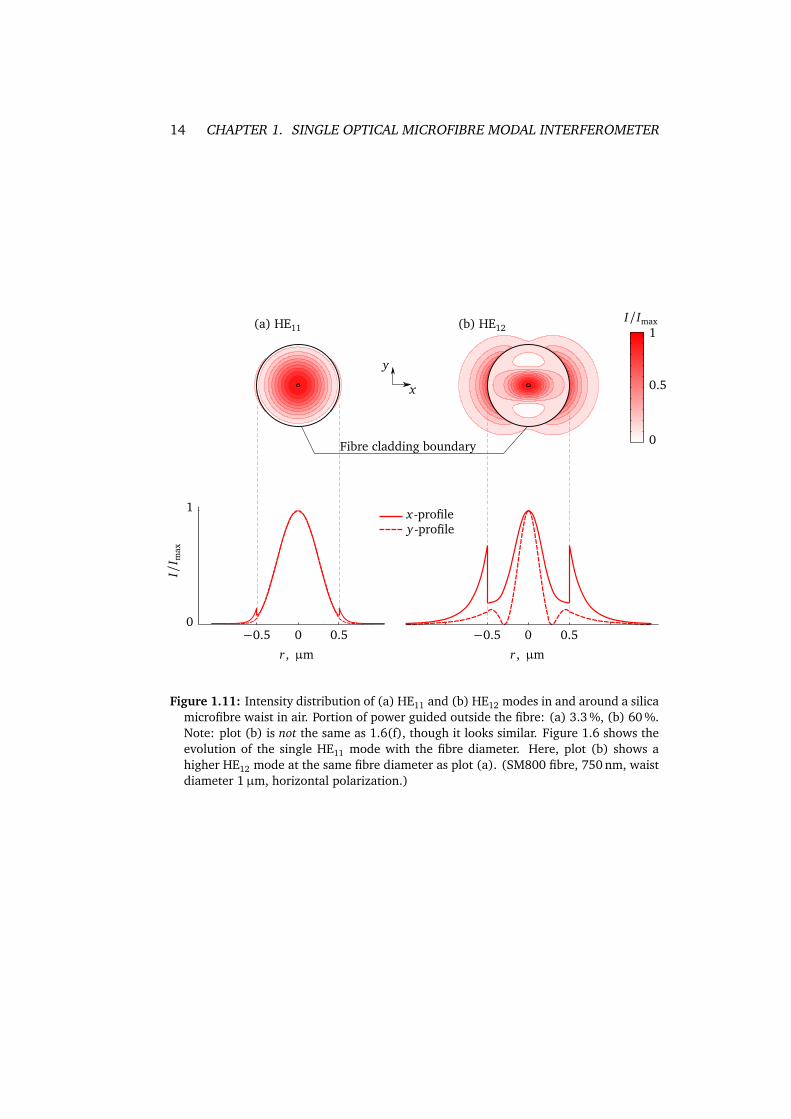
Figure 1.11 shows the intensity distribution of the HE11 and HE12 modes in a1µm diameter fibre waist. As much as 60 % of HE12 power propagates aroundthe fibre, in the evanescent field. For HE11, it is just over 3 %. This physicalsituation leads to two effects.
Firstly, the refractive index of the surrounding material influences the HE12mode much stronger than the HE11 mode. Therefore, the interference resultstrongly depends on the dispersion of the surrounding. A SOMMI can thereforeact as a refractive index sensor or be used for dispersive sensing of such speciesas atoms and molecules.
Secondly, because a lot of power of the HE12 mode propagates around thefibre, the mode “sees” more air than glass, and thus its phase velocity is closeto that in air (see Fig. 1.10c). The situation is completely different for the HE11mode, which almost completely “fits” inside the fibre; its phase velocity is thusclose to that in bulk glass. As the result, although the two modes pass the samephysical path between splitting and recombination in the tapers, they experi-ence different phase accumulation. If the length of the SOMMI is being changed(e. g. by stretching it), the phase accumulation changes differently for the twomodes, and the interference result depends on the fibre elongation. Thus, aSOMMI can act as a stretch sensor. It can be used, for example, as the strain sen-sors in wind turbines, which are made from fibreglass and for which fibre sensorsare therefore a natural choice.
In this work, I consider both of these types of interference.
14 CHAPTER 1. SINGLE OPTICAL MICROFIBRE MODAL INTERFEROMETER
x
y
0−0.5 0.50
x-profiley-profile
r, µm
I/I m
ax
0−0.5 0.5
1
r, µm
0
0.5
1I/Imax
Fibre cladding boundary
(a) HE11 (b) HE12
Figure 1.11: Intensity distribution of (a) HE11 and (b) HE12 modes in and around a silicamicrofibre waist in air. Portion of power guided outside the fibre: (a) 3.3 %, (b) 60 %.Note: plot (b) is not the same as 1.6(f), though it looks similar. Figure 1.6 shows theevolution of the single HE11 mode with the fibre diameter. Here, plot (b) shows ahigher HE12 mode at the same fibre diameter as plot (a). (SM800 fibre, 750 nm, waistdiameter 1µm, horizontal polarization.)
CHAPTER 2Computer simulation
The goal of computer simulation is to theoretically understand in detail howOMFs work to be able to design samples and to analyse measurement results.One of our first experimental achievements was the development of a method tomeasure the diameter of the OMF waist using optical harmonic generation [1].This method also required the simulation of guided modes in OMFs. Finally,taking into account the complexity of the calculations and the total number ofsamples we have produced for all our experiments (more than 200), it proved tobe inefficient to each time perform calculations in a semi-manual mode employedby many other groups. We have therefore created a software toolbox capable ofperforming all the needed calculations in the automatic mode [2].
2.1 What needs to be calculated
The modal interferometer response depends on the phase relation between thetwo propagating modes at the recombination point. Therefore we need to knowthe full phase evolution of each of the excited modes along the whole interfer-ometer, starting at the down-taper, along the waist, and ending in the up-taper.
For our harmonic generation-based method of OMF diameter measurement,we need to calculate the so called phase-matching condition—a set of OMF pa-rameters providing a constant phase relation between the fundamental and har-monic waves at given wavelengths. For efficient harmonic generation, it is alsoimportant to maximize the overlap between the field distributions of the funda-mental and harmonic modes.
Thus, we need the full information about the phase and the amplitude of themodes propagating in the OMFs.
15
16 CHAPTER 2. COMPUTER SIMULATION
A light wave, propagating in an optical fibre, can be described mathematicallyby defining its electric E(r, t) and magnetic H(r, t) field distributions, where r andt are the position in space and the time. E and H are treated similarly, thereforein this text I speak of E only, while still taking H into account in all calculations.
If the optical axis of the fibre coincides with the coordinate axis z, we candefine the electric field of a propagating mode as
E(r, t) = Etr(r)exp(iωt − iβz). (2.1)
Here Etr(x , y, z) is the transverse field distribution, β the propagation constant(waveguide analogue of the free-space wavenumber k), and ω the angular fre-quency of light. If the characteristic length of the z-dependent change of thefibre diameter is large compared to the wavelength of light (e. g. for our sam-ples it’s millimetres compared to hundreds of nanometres), then in Eq. (2.1) wehave split the fast oscillating z- and t-dependent terms from the slowly varyingtransverse field distribution Etr.
Etr and β are found by solving the wave equation derived from Maxwell’sequations for the case of a cylindrical dielectric waveguide [30, 31]. As the re-sult, one obtains an eigenvalue equation (EVE)∗ for β , which has to be solvednumerically. When β has been found, the field distribution Etr is calculated ana-lytically.
If β is imaginary, Eq. (2.1) describes a so called lossy, or radiation mode—amode, which is a correct solution of Maxwell’s equations but which cannot beguided by the waveguide. Physically, the power of this mode is quickly lost fromthe waveguide due to radiation as the wave propagates along the waveguide.We are not interested in such modes and will therefore only consider the realsolutions of EVEs.
The propagation constant β is connected to the phase velocity vphase of thepropagating wave:
β =2π
λneff, vphase =
c
neff, (2.2)
where neff is the effective refractive index of the mode, c the speed of light invacuum. Note that neff plays the same role for a waveguide mode, as the materialrefractive index is playing for a wave propagating in a bulk medium: it slowsdown the wave-front (and decreases the wavelength).
Thus, to fully describe a propagating wave in a fibre, one needs to calculatethe field distribution Etr and the propagation constant β or the effective refractiveindex neff for the corresponding guided mode. The phase evolution of the modeas it propagates along the fibre is given by its propagation constant.
If the fibre diameter is changing (this is exactly the case in the tapers of oursamples) or the measurements are performed with a broadband light source (as
∗Actually, a set of EVEs for different symmetries of the field distribution. Each equation isnumbered with index l and each solution of a specific EVE is indexed with m. The found modethen has two indices (l, m).
2.2. PROBLEMS OF AVAILABLE SOFTWARE 17n e
ff
Wavelength, nm600 850 1100
1
1.4
(a) neff(λ) (b) neff(d)
n eff
Diameter, µm0 1 2
1
1.4
nsilica nsilica
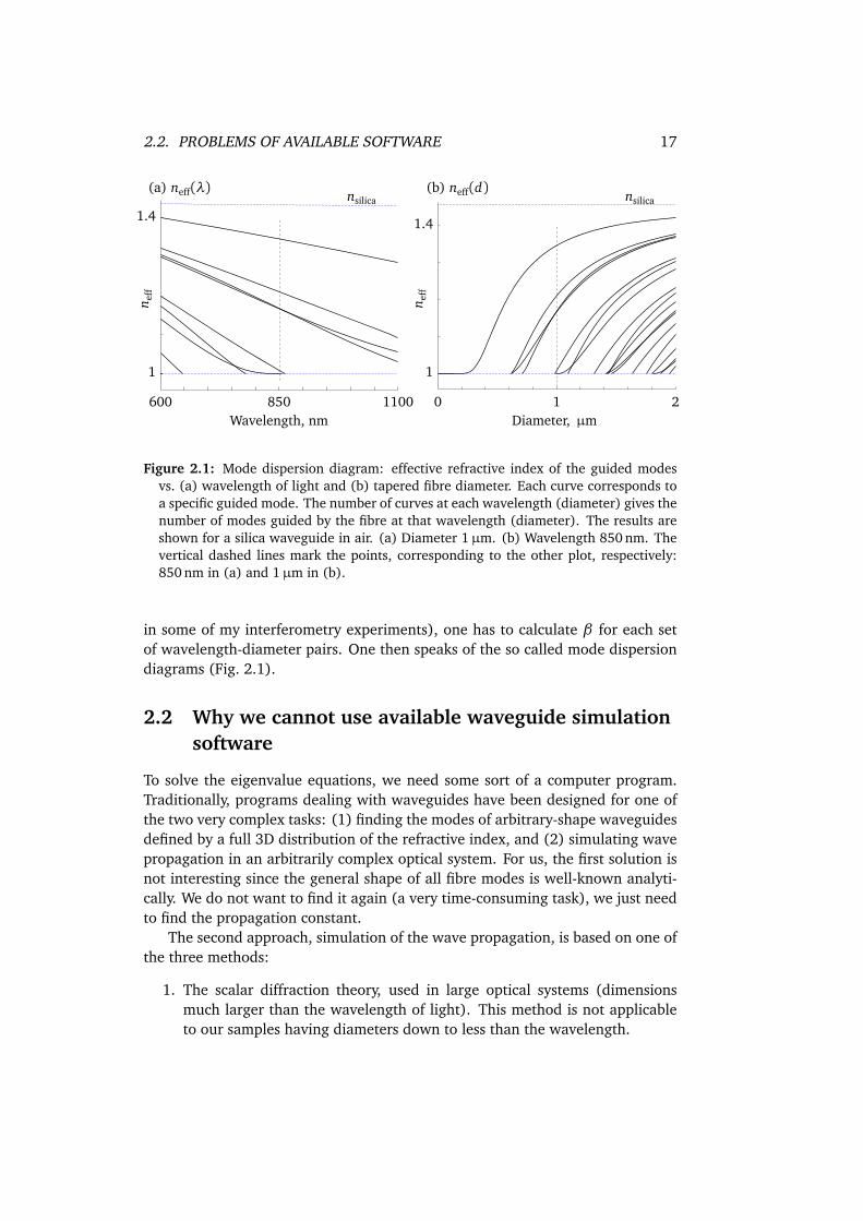
Figure 2.1: Mode dispersion diagram: effective refractive index of the guided modesvs. (a) wavelength of light and (b) tapered fibre diameter. Each curve corresponds toa specific guided mode. The number of curves at each wavelength (diameter) gives thenumber of modes guided by the fibre at that wavelength (diameter). The results areshown for a silica waveguide in air. (a) Diameter 1µm. (b) Wavelength 850 nm. Thevertical dashed lines mark the points, corresponding to the other plot, respectively:850 nm in (a) and 1µm in (b).
in some of my interferometry experiments), one has to calculate β for each setof wavelength-diameter pairs. One then speaks of the so called mode dispersiondiagrams (Fig. 2.1).
2.2 Why we cannot use available waveguide simulationsoftware
To solve the eigenvalue equations, we need some sort of a computer program.Traditionally, programs dealing with waveguides have been designed for one ofthe two very complex tasks: (1) finding the modes of arbitrary-shape waveguidesdefined by a full 3D distribution of the refractive index, and (2) simulating wavepropagation in an arbitrarily complex optical system. For us, the first solution isnot interesting since the general shape of all fibre modes is well-known analyti-cally. We do not want to find it again (a very time-consuming task), we just needto find the propagation constant.
The second approach, simulation of the wave propagation, is based on one ofthe three methods:
1. The scalar diffraction theory, used in large optical systems (dimensionsmuch larger than the wavelength of light). This method is not applicableto our samples having diameters down to less than the wavelength.
18 CHAPTER 2. COMPUTER SIMULATION
2. The full vector solution of Maxwell’s equations using the finite elementsnumerical method. This approach allows to solve any optical problemand is successfully used for small-scale optical systems. However it is pro-hibitively slow and extremely memory-expensive in case of OMFs with theircentimetre-scale length.
3. The mode expansion method based on the known analytical solutions ofthe wave equation. In an optical fibre, this method is the only applicablemethod of the three. However it requires continuous calculation of thefield distributions along the fibre and is therefore much slower than thesimple solving of the eigenvalue equation. The advantage of this methodover our approach is that it inherently calculates mode transformation incase of non-adiabatic transitions in the fibre.
As the outcome of this situation, all the groups working in the field of taperedoptical fibres, to the best of my knowledge, are writing their own codes to solvethe EVEs and find β . There is no ready-to-use software tool to accomplish thistask. That’s why we had to create our own one.
While doing so, I have been able to implement an almost completely auto-matic calculation: one “assembles” a program for each task from the providedfunctions in a LEGO-manner, and then the calculation happens automatically.This is a useful feature because we typically need to solve the EVE for many dif-ferent fibre diameters or wavelengths. We also need to repeat the calculationsfor each new type of fibre (core/cladding ratio and materials) as well as for eachnew material of the fibre surrounding. Therefore, manual tuning of the startingpoints, which is a common procedure I have seen in other groups, or verificationof the calculation results become prohibitively time-consuming operations.
2.3 Mathematical model of light propagation in OMF
Our samples consist of the unprocessed pigtails (commercial optical fibre), twotaper sections with varying diameter, and a waist. The unprocessed parts and thewaist have a constant (along the fibre axis) diameter and therefore the modes inthese parts are relatively easy to calculate. These parts are also most interestingin terms of the OMF guiding properties:
• The input unprocessed part determines, which modes can be deliveredfrom a light source to the waist.
• The waist is the part where light is open to interaction with the surroundingand also where it usually has the highest intensity; this is where light-matter interaction occurs primarily.
• The unprocessed output end determines what can be seen by the detectorat the output.
2.3. MATHEMATICAL MODEL OF LIGHT PROPAGATION IN OMF 19
The tapers should be properly designed to transfer light from the input pigtail tothe waist and from the waist to the output pigtail. Being made from the samecommercial fibre as the pigtails, the taper also has similar properties. At thesame time, modes in the tapers, where the fibre diameter and thus the guidingproperties are constantly changing, should be calculated in a different manner.I start with the calculation of the cylindrical input, output, and waist parts andconsider the taper regions afterwards.
2.3.1 Dielectric cylindrical waveguide—two-layer model
2.3.1.1 Unprocessed parts of OMF
The unprocessed pigtails consist of a cylindrical core (diameter ∼ 5µm) sur-rounded by a cylindrical cladding (125µm diameter). The protective plasticcoating of the fibre (250µm diameter) is always removed before producing thetapered samples; therefore I ignore it in the model. The cladding is thus sur-rounded by air, vacuum, or some other medium.
The core is made from a material with a slightly higher refractive index thanthe one of the cladding. This makes light guidance in the fibre core possible dueto total internal reflection.
Commercial fibres are designed in such a way that light is completely confinedin the region close to the core and does not reach the cladding surface. For exam-ple, the Fibercore SM800 fibre∗ primarily used in our experiments has the modefield diameter (diameter encompassing 86 % of guided power) of 5.6µm [32].Since the cladding diameter is 125µm, no light even “touches” the fibre surface.Be it not the case, light would be lost due to absorption or scattering in the coat-ing.
As a result, when calculating light modes in the unprocessed part of the fi-bre, we can ignore the presence of the surrounding, be it air, vacuum, liquid oranything else—light just does not “see” it. The fibre can then be considered asa glass rod (core) surrounded by an infinite glass cladding with a slightly lowerrefractive index and, hence, modelled considering only these two layers (the coreand the cladding).
The solution of Maxwell’s equations in a two-layer dielectric cylindrical sys-tem is well known [30, 33]. The eigenvalue equation for β is [31, Eq. (B-11)]†
J ′l (ha)
haJl(ha)+
K ′l (qa)
qaKl(qa)
n21J ′l (ha)
haJl(ha)+
n22K ′l (qa)
qaKl(qa)
− l2
1
qa
2
+
1
ha
22
β
k0
2
= 0, (2.3)
∗Its specifications are given in Tab. 3.1 on page 54.†There is a typo in K ′ argument the equation in the book: ha instead of qa. It can be checked
by comparison with [30, Tab. 12-4 on p. 253].
20 CHAPTER 2. COMPUTER SIMULATION
where
h2 = n21k2
0 − β2,
q2 = β2− n22k2
0,
J is the Bessel function of the first kind, K the modified Bessel function of thesecond kind, a the radius of the waveguide, n1 and n2 the material refractive in-dices of the inner and outer layers, k0 = 2π/λ0 =ω/c the vacuum wave number,l the azimuthal mode index, which is present in the field components in the term(cf. Eq. (2.1))
exp[i(ωt + lφ − βz)].
For each azimuthal mode index l > 0, Eq. (2.3) can have several roots num-bered (l, k). Each root βlk corresponds to a separate transverse mode. Thesemodes are called hybrid and have a characteristic feature that both their elec-tric and magnetic vectors have non-zero components parallel to the direction ofpropagation z. For a given index l, the modes with the magnetic z-componentlarger than the electric one (these modes are called the HE modes) alternate withthe ones with a larger electric z-component (called EH): the lowest-order modeis HEl1, then follow EHl1, HEl2 and so on (see Fig. 2.2). The second mode indexis usually marked with m. Thus the root number k corresponding to a particularmode can be calculated as k = 2m+ 1 for HE modes and k = 2m for EH modes.
If l = 0, we have a special case of transverse electric and transverse magneticmodes. They have the zero z-component of the electric or magnetic fields and arecalled TE0m and TM0m respectively. The EVEs for these modes look simpler [31,Eq. (B-17)]:
J1(ha)haJ0(ha)
+K1(qa)
qaK0(ha)= 0, (2.4)
J1(ha)haJ0(ha)
+n2
2K1(qa)
n21qaK0(ha)
= 0, (2.5)
and m is just a root number.If the refractive index step at the guiding interface (where total internal re-
flection occurs) is small, ∆n12 1, one speaks of a weakly-guiding fibre, and thelinearly polarized (LP) modes are a valid approximation. The EVE in this caseis [31, p. 131]:
haJl+1(ha)Jl(ha)
− qaKl+1(qa)Kl(qa)
= 0.
This solution is derived from the scalar wave equation. Therefore the LP modesare sometimes called scalar modes.
Using the EVEs, one can calculate the mode dispersion (versus wavelengthor core diameter) of a typical fibre. As an example, let’s consider the plot neffvs. wavelength calculated for a Corning SMF-28∗ fibre in air (Fig. 2.3). Untapered,
∗For SMF-28 specs see Sec. 3.1.3 on page 53.
2.3. MATHEMATICAL MODEL OF LIGHT PROPAGATION IN OMF 21n e
ff
Diameter, µm
0.5 1 1.5 2 2.5 3
1
1.1
1.2
1.3
1.4
1.5 HE11
EH11
HE12
EH12
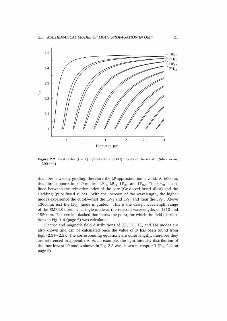
Figure 2.2: First order (l = 1) hybrid (HE and EH) modes in the waist. (Silica in air,300 nm.)
this fibre is weakly-guiding, therefore the LP-approximation is valid. At 600 nm,this fibre supports four LP modes: LP01, LP11, LP21, and LP02. Their neff is con-fined between the refractive index of the core (Ge-doped fused silica) and thecladding (pure fused silica). With the increase of the wavelength, the highermodes experience the cutoff—first the LP02 and LP21 and then the LP11. Above1300 nm, just the LP01 mode is guided. This is the design wavelength rangeof the SMF-28 fibre: it is single-mode at the telecom wavelengths of 1310 and1550 nm. The vertical dashed line marks the point, for which the field distribu-tions in Fig. 1.4 (page 5) was calculated.
Electric and magnetic field distributions of HE, EH, TE, and TM modes arealso known and can be calculated once the value of β has been found fromEqs. (2.3)–(2.5). The corresponding equations are quite lengthy, therefore theyare referenced in appendix A. As an example, the light intensity distribution ofthe four lowest LP-modes shown in Fig. 2.3 was shown in chapter 1 (Fig. 1.4 onpage 5).
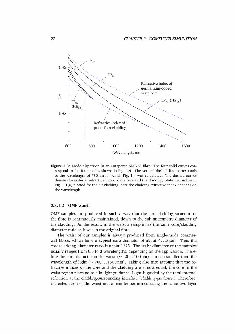
22 CHAPTER 2. COMPUTER SIMULATION
n eff
Wavelength, nm
600 800 1000 1200 1400 1600
1.45
1.46
Refractive index ofgermanium-dopedsilica core
Refractive index ofpure silica cladding
LP01 (HE11)
LP11
LP21
LP02(HE12)
Figure 2.3: Mode dispersion in an untapered SMF-28 fibre. The four solid curves cor-respond to the four modes shown in Fig. 1.4. The vertical dashed line correspondsto the wavelength of 750 nm for which Fig. 1.4 was calculated. The dashed curvesdenote the material refractive index of the core and the cladding. Note that unlike inFig. 2.1(a) plotted for the air cladding, here the cladding refractive index depends onthe wavelength.
2.3.1.2 OMF waist
OMF samples are produced in such a way that the core-cladding structure ofthe fibre is continuously maintained, down to the sub-micrometre diameter ofthe cladding. As the result, in the waist a sample has the same core/claddingdiameter ratio as it was in the original fibre.
The waist of our samples is always produced from single-mode commer-cial fibres, which have a typical core diameter of about 4 . . . 5µm. Thus thecore/cladding diameter ratio is about 1/25. The waist diameter of the samplesusually ranges from 0.5 to 3 wavelengths, depending on the application. There-fore the core diameter in the waist (∼ 20 . . . 100 nm) is much smaller than thewavelength of light (∼ 700 . . . 1500 nm). Taking also into account that the re-fractive indices of the core and the cladding are almost equal, the core in thewaist region plays no role in light guidance. Light is guided by the total internalreflection at the cladding-surrounding interface (cladding-guidance.) Therefore,the calculation of the waist modes can be performed using the same two-layer
2.3. MATHEMATICAL MODEL OF LIGHT PROPAGATION IN OMF 23
n eff
Diameter, µm
0 2
1
1.4
0.4 0.8 1.2 1.6
HE11 TE01 TM01
HE21
HE12EH11
HE31
nsilica
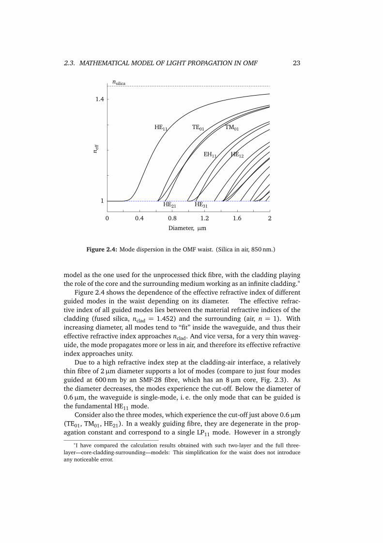
Figure 2.4: Mode dispersion in the OMF waist. (Silica in air, 850 nm.)
model as the one used for the unprocessed thick fibre, with the cladding playingthe role of the core and the surrounding medium working as an infinite cladding.∗
Figure 2.4 shows the dependence of the effective refractive index of differentguided modes in the waist depending on its diameter. The effective refrac-tive index of all guided modes lies between the material refractive indices of thecladding (fused silica, nclad = 1.452) and the surrounding (air, n = 1). Withincreasing diameter, all modes tend to “fit” inside the waveguide, and thus theireffective refractive index approaches nclad. And vice versa, for a very thin waveg-uide, the mode propagates more or less in air, and therefore its effective refractiveindex approaches unity.
Due to a high refractive index step at the cladding-air interface, a relativelythin fibre of 2µm diameter supports a lot of modes (compare to just four modesguided at 600 nm by an SMF-28 fibre, which has an 8µm core, Fig. 2.3). Asthe diameter decreases, the modes experience the cut-off. Below the diameter of0.6µm, the waveguide is single-mode, i. e. the only mode that can be guided isthe fundamental HE11 mode.
Consider also the three modes, which experience the cut-off just above 0.6µm(TE01, TM01, HE21). In a weakly guiding fibre, they are degenerate in the prop-agation constant and correspond to a single LP11 mode. However in a strongly
∗I have compared the calculation results obtained with such two-layer and the full three-layer—core-cladding-surrounding—models: This simplification for the waist does not introduceany noticeable error.
24 CHAPTER 2. COMPUTER SIMULATION
n eff
Diameter, µm0 0.4 0.8 1.2 1.6 2
1.32
1.34
1.36
1.38
1.4
1.42
1.44
1.46
LP01
LP11
LP21
LP02
nsilica
nwater
HE11
TE01
TM01
HE21HE12
EH11
HE31
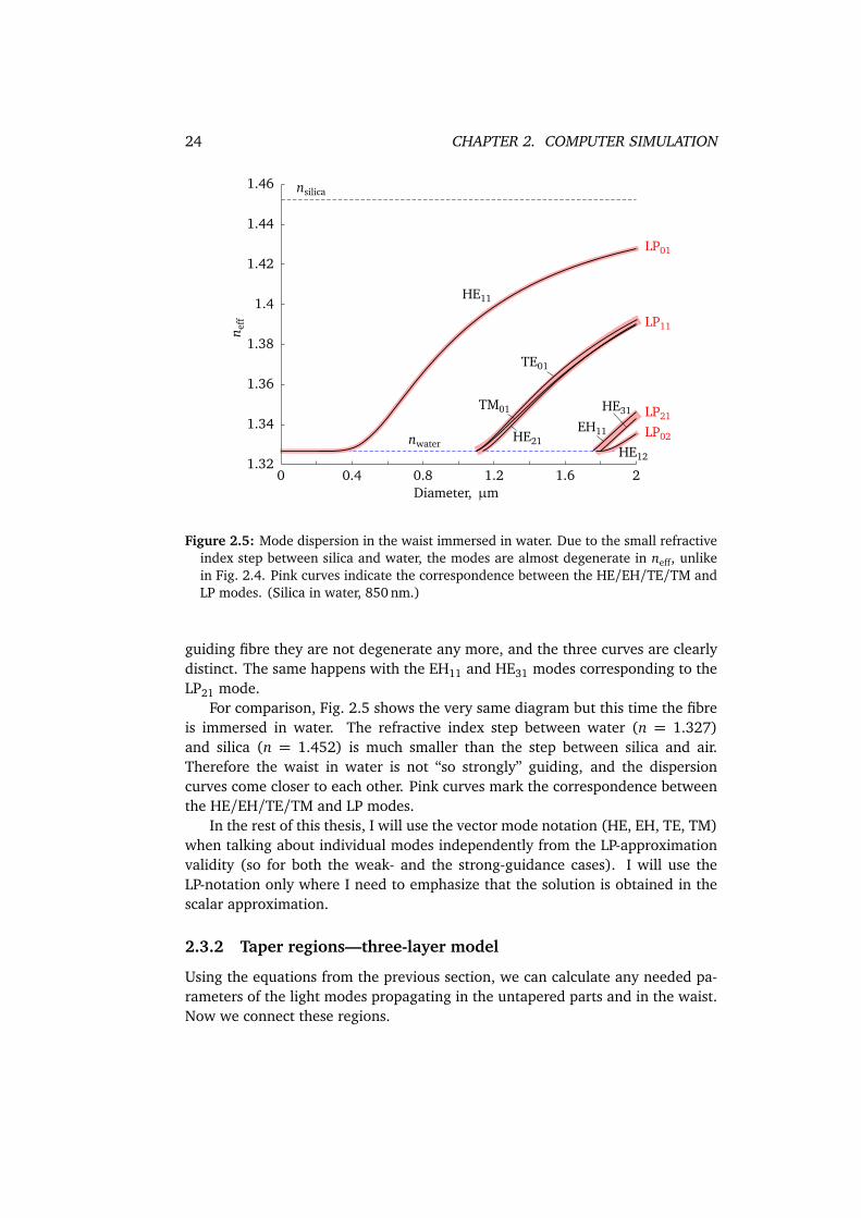
Figure 2.5: Mode dispersion in the waist immersed in water. Due to the small refractiveindex step between silica and water, the modes are almost degenerate in neff, unlikein Fig. 2.4. Pink curves indicate the correspondence between the HE/EH/TE/TM andLP modes. (Silica in water, 850 nm.)
guiding fibre they are not degenerate any more, and the three curves are clearlydistinct. The same happens with the EH11 and HE31 modes corresponding to theLP21 mode.
For comparison, Fig. 2.5 shows the very same diagram but this time the fibreis immersed in water. The refractive index step between water (n = 1.327)and silica (n = 1.452) is much smaller than the step between silica and air.Therefore the waist in water is not “so strongly” guiding, and the dispersioncurves come closer to each other. Pink curves mark the correspondence betweenthe HE/EH/TE/TM and LP modes.
In the rest of this thesis, I will use the vector mode notation (HE, EH, TE, TM)when talking about individual modes independently from the LP-approximationvalidity (so for both the weak- and the strong-guidance cases). I will use theLP-notation only where I need to emphasize that the solution is obtained in thescalar approximation.
2.3.2 Taper regions—three-layer model
Using the equations from the previous section, we can calculate any needed pa-rameters of the light modes propagating in the untapered parts and in the waist.Now we connect these regions.
2.3. MATHEMATICAL MODEL OF LIGHT PROPAGATION IN OMF 25n e
ff
Fibre diameter, µm0 40 80 120
1
1.4
n eff
Fibre diameter, µm0 40 80 120
1.45
1.46 ncore
nclad
coreguidance
claddingguidance
HEcore11
HEclad11
1.3
1.2
1.1
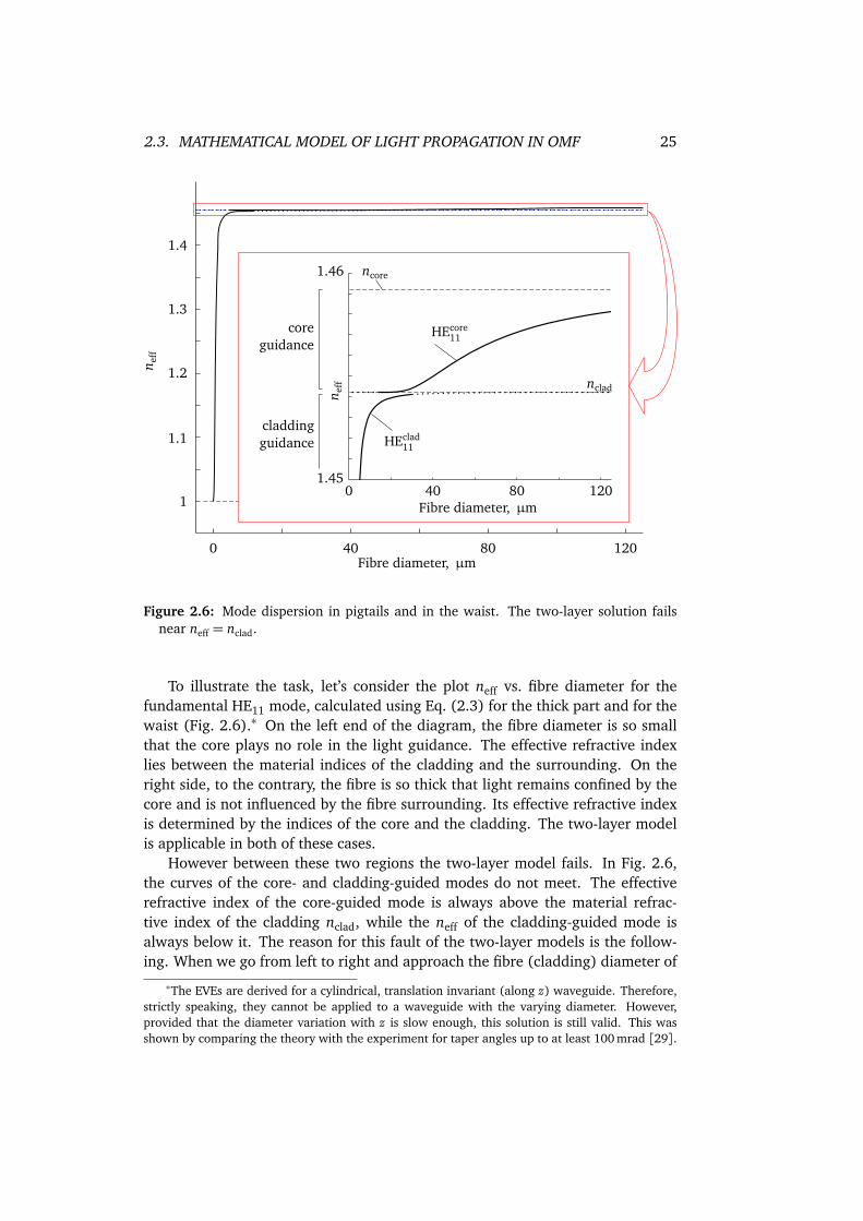
Figure 2.6: Mode dispersion in pigtails and in the waist. The two-layer solution failsnear neff = nclad.
To illustrate the task, let’s consider the plot neff vs. fibre diameter for thefundamental HE11 mode, calculated using Eq. (2.3) for the thick part and for thewaist (Fig. 2.6).∗ On the left end of the diagram, the fibre diameter is so smallthat the core plays no role in the light guidance. The effective refractive indexlies between the material indices of the cladding and the surrounding. On theright side, to the contrary, the fibre is so thick that light remains confined by thecore and is not influenced by the fibre surrounding. Its effective refractive indexis determined by the indices of the core and the cladding. The two-layer modelis applicable in both of these cases.
However between these two regions the two-layer model fails. In Fig. 2.6,the curves of the core- and cladding-guided modes do not meet. The effectiverefractive index of the core-guided mode is always above the material refrac-tive index of the cladding nclad, while the neff of the cladding-guided mode isalways below it. The reason for this fault of the two-layer models is the follow-ing. When we go from left to right and approach the fibre (cladding) diameter of
∗The EVEs are derived for a cylindrical, translation invariant (along z) waveguide. Therefore,strictly speaking, they cannot be applied to a waveguide with the varying diameter. However,provided that the diameter variation with z is slow enough, this solution is still valid. This wasshown by comparing the theory with the experiment for taper angles up to at least 100 mrad [29].
26 CHAPTER 2. COMPUTER SIMULATION
about 20. . . 30µm, the core diameter increases to a value, comparable to the lightwavelength (about 1µm). So we cannot ignore the core any more. At the sametime, the fibre diameter is still small enough for the evanescent field around thecore to reach the surface of the cladding. Therefore we should take into accountall three layers: the core, the cladding, and the surrounding of the fibre.
2.3.2.1 Mathematical model
The mathematical model for the three-layer system is not as well-known as thetwo-layer one. The derivation of the two-layer eigenvalue equation is quite longand cumbersome [30, 33], and the one for three layers is almost unreasonablyhard. That’s why, to the best of my knowledge, the groups working in the fieldof tapered optical microfibres have been either using the full numerical calcula-tion [34, 35] or significantly simplifying the task and using approximations [36].
Still, the eigenvalue equations for the three-layer system were published sev-eral times by researchers involved in fibre sensors [37–43], the first papers dat-ing back to the 1980s. Unfortunately, these papers have remained more or lessunnoticed. Even within this series of publications, the work done in 1982 byMonerie [38] is basically repeated in 1994 by Henry [40]. Just a few weeks agoyet another publication appeared, again deriving what Monerie published thirtyyears ago [44]. This can be partly explained by the fact that information, that apaper deals with the three-layer model, is not always “visible” from the abstractor the title and thus is not always found when people need it. Also, for someunfortunate coincidence, the most important of these papers, were not, until re-cently, returned by the search engines of the publishers.
There is also another severe problem: most of these publications contain ty-pos. Taking into account that a full set of equations needed to calculate vectormodes takes about five pages [41, 43], it is practically impossible to spot a mis-take, not only for the reader but also for the authors. It is also very difficult tosimply program all these equations without introducing further mistakes. There-fore it took quite some time to implement the working three-layer model, andI will shortly describe it here.
2.3.2.2 Implementation
The first publication I was able to find was the English translation of a Russianpaper back to 1976 [37]. The authors give the exact equations for the electricand magnetic fields, however they derive the eigenvalue equation only in theapproximation of a small refractive index step (weak guidance). This approxima-tion is valid for the core-cladding interface, where the refractive index step is onthe order of 0.5 %, and is therefore of interest for the so called double-claddingfibres. In 1982, the results for weakly guiding three-layer fibres, in a somewhatsimpler, easier to use form, were published by Monerie [38]; I implemented hisequations in our toolbox [2].
2.3. MATHEMATICAL MODEL OF LIGHT PROPAGATION IN OMF 27
The Monerie solution cannot be used in the tapers and in the waist, because ofthe high refractive index step at the outer OMF surface (cladding-surrounding).The first accessible publication with the exact three-layer eigenvalue equationis the one by Tsao et al. from 1989 [39]. This paper contains the eigenvalueequation for the HE and EH modes as well as for the simpler TE and TM modes.Unfortunately, the authors did not try to solve the derived equation for the hybridmodes themselves (having explained it by the complexity of the required numericcalculations) and have used the equations for the TE mode in the examples. Ihave programmed all the equations from the paper but the one for the HE/EHmode does not have any roots.∗ Probably it is due to a typo in the paper or evena mistake in the derivation [46].
In 1997, Erdogan again publishes the eigenvalue equation for the hybridmodes [41]. He follows the Tsao approach and derives an equation for the cladding-guided modes. There were several typos in the published paper, and in 2000 theerrata were published [42].
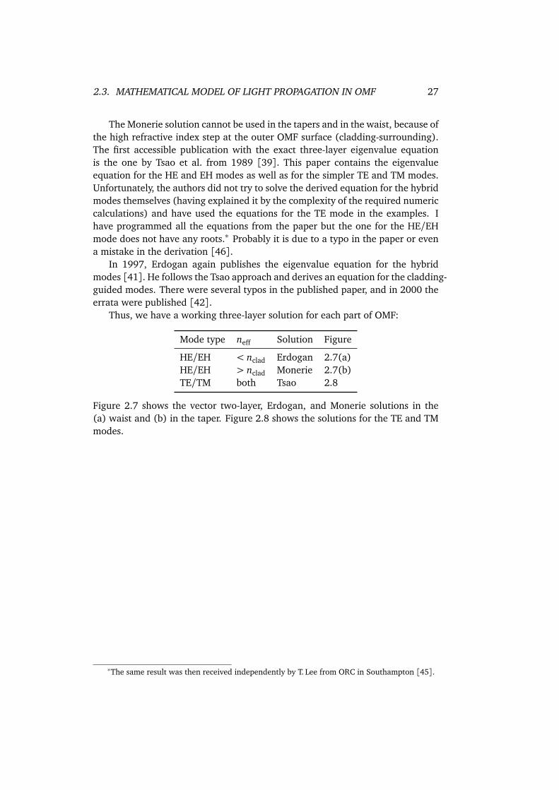
Thus, we have a working three-layer solution for each part of OMF:
Mode type neff Solution Figure
HE/EH < nclad Erdogan 2.7(a)HE/EH > nclad Monerie 2.7(b)TE/TM both Tsao 2.8
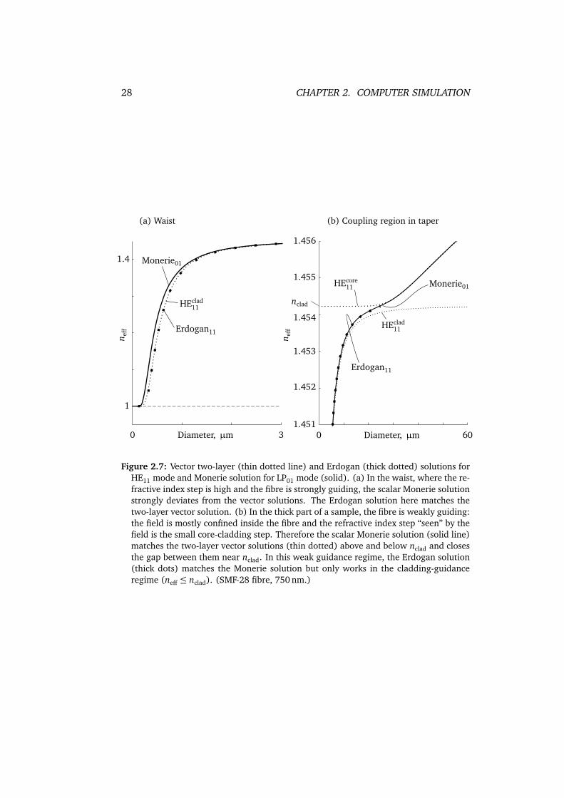
Figure 2.7 shows the vector two-layer, Erdogan, and Monerie solutions in the(a) waist and (b) in the taper. Figure 2.8 shows the solutions for the TE and TMmodes.
∗The same result was then received independently by T. Lee from ORC in Southampton [45].
28 CHAPTER 2. COMPUTER SIMULATION
n eff
Diameter, µm0 601.451
1.456
n eff
Diameter, µm0 3
1
1.4
HEclad11
Monerie01
HEclad11
Erdogan11
Erdogan11
Monerie01HEcore11
(a) Waist (b) Coupling region in taper
1.452
1.453
1.455
nclad
1.454
Figure 2.7: Vector two-layer (thin dotted line) and Erdogan (thick dotted) solutions forHE11 mode and Monerie solution for LP01 mode (solid). (a) In the waist, where the re-fractive index step is high and the fibre is strongly guiding, the scalar Monerie solutionstrongly deviates from the vector solutions. The Erdogan solution here matches thetwo-layer vector solution. (b) In the thick part of a sample, the fibre is weakly guiding:the field is mostly confined inside the fibre and the refractive index step “seen” by thefield is the small core-cladding step. Therefore the scalar Monerie solution (solid line)matches the two-layer vector solutions (thin dotted) above and below nclad and closesthe gap between them near nclad. In this weak guidance regime, the Erdogan solution(thick dots) matches the Monerie solution but only works in the cladding-guidanceregime (neff ≤ nclad). (SMF-28 fibre, 750 nm.)
2.3. MATHEMATICAL MODEL OF LIGHT PROPAGATION IN OMF 29
n eff
1.4
11.454
1.4542
1.4544
n eff
1.4
1
n eff
n eff
1.454
1.4542
1.4544
0 3Diameter, µm
1 2 40 80Diameter, µm
706050
40 80Diameter, µm
7060500 3Diameter, µm
1 2
Tsao TM01
Tsao TE01
Monerie11
TM(clad)01
TE(clad)01
TM(clad)01
TE(clad)01
TM(core)01
TE(core)01
(a) (b)
(c) (d)
Monerie11
Tsao TE01
Waist Taper
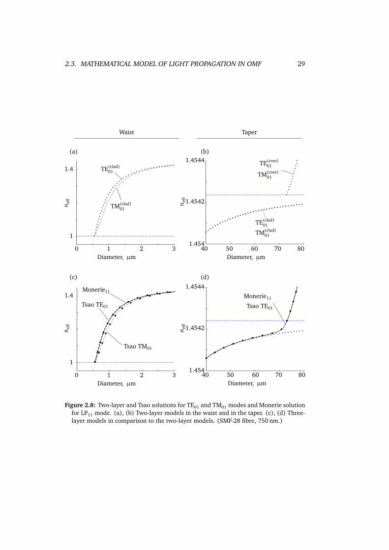
Figure 2.8: Two-layer and Tsao solutions for TE01 and TM01 modes and Monerie solutionfor LP11 mode. (a), (b) Two-layer models in the waist and in the taper. (c), (d) Three-layer models in comparison to the two-layer models. (SMF-28 fibre, 750 nm.)
30 CHAPTER 2. COMPUTER SIMULATION
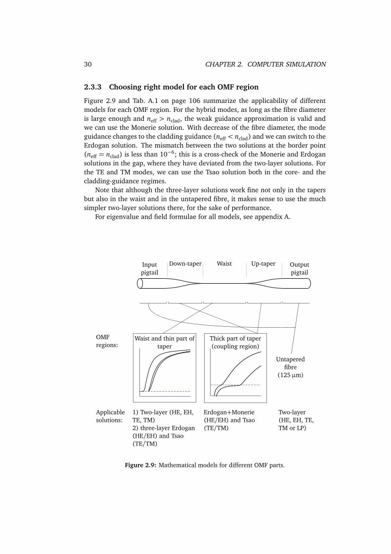
2.3.3 Choosing right model for each OMF region
Figure 2.9 and Tab. A.1 on page 106 summarize the applicability of differentmodels for each OMF region. For the hybrid modes, as long as the fibre diameteris large enough and neff > nclad, the weak guidance approximation is valid andwe can use the Monerie solution. With decrease of the fibre diameter, the modeguidance changes to the cladding guidance (neff < nclad) and we can switch to theErdogan solution. The mismatch between the two solutions at the border point(neff = nclad) is less than 10−6; this is a cross-check of the Monerie and Erdogansolutions in the gap, where they have deviated from the two-layer solutions. Forthe TE and TM modes, we can use the Tsao solution both in the core- and thecladding-guidance regimes.
Note that although the three-layer solutions work fine not only in the tapersbut also in the waist and in the untapered fibre, it makes sense to use the muchsimpler two-layer solutions there, for the sake of performance.
For eigenvalue and field formulae for all models, see appendix A.
Waist Up-taperDown-taperInputpigtail
Outputpigtail
1) Two-layer (HE, EH,TE, TM)2) three-layer Erdogan(HE/EH) and Tsao(TE/TM)
Applicablesolutions:
Erdogan+Monerie(HE/EH) and Tsao(TE/TM)
Untaperedfibre
(125µm)
Two-layer(HE, EH, TE,TM or LP)
Waist and thin part oftaper
Thick part of taper(coupling region)
OMFregions:
Figure 2.9: Mathematical models for different OMF parts.
2.3. MATHEMATICAL MODEL OF LIGHT PROPAGATION IN OMF 31
2.3.4 Mode coupling
The theory explained until now is sufficient to calculate the parameters of theguided modes in an OMF at any given diameter. If we consider the actual prop-agation of a wave along an OMF, we can face two different cases. One is theadiabatic mode propagation, when the power within a given mode is conservedalong the whole OMF. For SOMMI, we are interested in another one—the non-adiabatic propagation—when the HE11 mode of the input pigtail is split into theHE11 and HE12 modes in the down-taper. This splitting (and recombination inthe up-taper) is governed by mode coupling.
Calculation of mode coupling can be done based on the coupled local modetheory [30, Chap. 28]. The pre-requisite for applicability of this theory is that theparameters of the waveguide (e. g. the fibre diameter) do not change rapidlyalong the fibre. As shown in [25, 29], mode coupling in tapers as steep as160 mrad can be adequately modelled using this approach. In our experiments,tapers had a slope of 1 . . . 60mrad, so this model should work as well.
2.3.4.1 Coupling equations
Mode coupling means that the power and the phase of one mode depends onthose of the other modes. The exact field E(x , y, z) in the fibre can be written inthe form
E(x , y, z) =∑
j
[b j(z) + b− j(z)]e j(x , y,β j(z)),
H(x , y, z) =∑
j
[b j(z) + b− j(z)]h j(x , y,β j(z)),
where e and h are the normalized amplitudes of the individual orthogonal modes,j the mode number (among all modes considered), β j(z) the local mode propa-gation constant. Since the fibre parameters vary with z, the propagation constantβ also depends on z. The complex factors b describe the amplitude and the phaseof the forward (b+ j) and backward (b− j) propagating modes, in each point alongthe fibre axis z, i. e.
b± j(z) = a± j(z)exp
±i
∫ z
0
β j(z)dz
,
where a is the amplitude.The equations for b j(z) can be derived by substituting Eqs. (2.6) into Maxwell’s
equations [30, Chap. 31 and Eq. (28-2)]:
db j
dz− iβ j b j =
∑
l
[C jl bl + C j,−l b−l],
db− j
dz− iβ j b− j =
∑
l
[C− j,l bl + C− j,−l b−l],
32 CHAPTER 2. COMPUTER SIMULATION
where C jl are the coupling coefficients [30, Eq. (28-4)]
C jl =k
4
r
ε0
µ0
1
β j − βl
∫
A∞
e∗j · el∂ n2
∂ zdA, j 6= l, C j j = 0, (2.7)
and A∞ is the infinite cross-section.By definition, if there is no coupling to the backwards propagating modes
(no reflection in the fibre), C j,−l = 0 and C− j,l = 0 for any j and l. Furthermore,since in a SOMMI only two modes—HE11 and HE12—are excited, we end up witha system of just two differential equations:
db1
dz− iβ1 b1 = C12 b2, (2.8a)
db2
dz− iβ2 b2 = C21 b1. (2.8b)
2.3.4.2 Coupling coefficients C
In this work I consider only the step-index fibres, so the refractive index is con-stant within the core and within the cladding and changes only at the interface.Thus ∂ n2/∂ z in Eq. (2.7) equals zero everywhere except at the core-cladding andcladding-surrounding interfaces. If we ignore the cladding-surrounding interface(because the evanescent field of the low-order modes in the surrounding regionat the diameters, at which the coupling occurs, is very small∗), we can considerthe cladding to be infinitely large and describe the fibre as [30, Eq. (28-11)]:
n2(r, z) = n2co
1− 2∆H(r −ρ(z))
,
or, alternatively, as
1
n2(r, z)=
1
n2co
1+2∆
1− 2∆H(r −ρ(z))
,
where ∆ = (n2co − n2
cl)/2n2co is the so called fibre profile height parameter, 2ρ(z)
the z-dependent fibre core diameter, H the Heaviside step function (H(x) = 1 ifx > 0, H(x) = 0 otherwise). The integrand in Eq. (2.7) can be written as
e2j el∂ n2
∂ z=
e∗φ jeφl + e∗z jezl
∂ n2
∂ z−
n2e∗r j
n2er l
∂
∂ z
1
n2
.
(Note that eφ , ez and n2er are continuous across the interface, unlike er .) Finally,with
∂ n2
∂ z=−2n2
co∆δ(r −ρ)dρ
dz∗Taking into account a very good matching of the theoretical and experimental results obtained
with this theory [25, 29], this assumption does not introduce any significant error.
2.3. MATHEMATICAL MODEL OF LIGHT PROPAGATION IN OMF 33
and∂
∂ z
1
n2
=2n2
co∆
n2con2
cl
δ(r −ρ)dρ
dz,
we obtain from Eq. (2.7)
C jl =−k
2
r
ε0
µ0
n2co∆
β j − βl
ρdρ
dz
×∫ 2π
0
ec.c.φ j eφl + ec.c.
z j ezl +
n2
n2co
ec.c.r j
n2
n2cl
er l
r=ρ(z)
dφ, j 6= l. (2.9)
If ∆ is very small ( 1), we have the case of a weakly guiding fibre, thelongitudinal field components ez vanish, the transverse components er and eφare both continuous across the interface, and the last equation can be rewrittenas [30, Eq. (28-13)]
C jl =k
2
r
ε0
µ0
n2co∆
β j − βl
ρdρ
dz
∫ 2π
0
et j · etl
r=ρ(z)dφ, j 6= l, (2.10)
where the subscript t means “transverse”.
2.3.4.3 Coupling calculation
To calculate the coupling coefficients according to Eq. (2.9) or (2.10), we shoulduse the three-layer model described in Sec. 2.3.2. The two-layer model cannotcorrectly describe the mode field behaviour when the effective refractive index ofa mode gets close to the refractive index of the cladding material.
In practice, we need mode coupling calculation to design an optimal tapershape: to split power between the HE11 and HE12 modes in the 1:1 ratio to max-imize interference contrast. Equations (2.8) should be solved numerically and,to achieve appropriate accuracy, it takes many hours. Although I have createdthe first draft of the corresponding code, I have not had time to debug it yet.Therefore I do not give the simulation results for mode coupling here. On theother hand, as will be explained in chapter 3, the reproducibility of our manufac-turing procedure is not very high and leads to a different OMF shape each time asample is pulled. Therefore it does not make much sense to numerically optimizethe taper shape with a high precision. Instead, the tapers were designed usingthe approximate critical angle theory and tested interferometrically. Of course, inthe future the manufacturing reproducibility should be improved and the optimalshape found theoretically and verified experimentally.
2.3.5 Critical angle theory
To design the tapers, a nice practical solution is provided by the critical angletheory [25, 47].
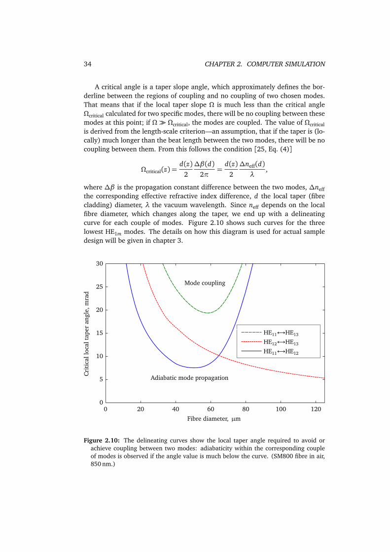
34 CHAPTER 2. COMPUTER SIMULATION
A critical angle is a taper slope angle, which approximately defines the bor-derline between the regions of coupling and no coupling of two chosen modes.That means that if the local taper slope Ω is much less than the critical angleΩcritical calculated for two specific modes, there will be no coupling between thesemodes at this point; if Ω Ωcritical, the modes are coupled. The value of Ωcriticalis derived from the length-scale criterion—an assumption, that if the taper is (lo-cally) much longer than the beat length between the two modes, there will be nocoupling between them. From this follows the condition [25, Eq. (4)]
Ωcritical(z) =d(z)
2
∆β(d)2π
=d(z)
2
∆neff(d)λ
,
where ∆β is the propagation constant difference between the two modes, ∆neffthe corresponding effective refractive index difference, d the local taper (fibrecladding) diameter, λ the vacuum wavelength. Since neff depends on the localfibre diameter, which changes along the taper, we end up with a delineatingcurve for each couple of modes. Figure 2.10 shows such curves for the threelowest HE1m modes. The details on how this diagram is used for actual sampledesign will be given in chapter 3.
Fibre diameter, µm
0 20 40 60 80 100 1200
5
10
15
20
25
30
Mode coupling
Adiabatic mode propagationCri
tica
lloc
alta
per
angl
e,m
rad
HE11↔HE12
HE11↔HE13
HE12↔HE13
Figure 2.10: The delineating curves show the local taper angle required to avoid orachieve coupling between two modes: adiabaticity within the corresponding coupleof modes is observed if the angle value is much below the curve. (SM800 fibre in air,850 nm.)
2.4. OPTICAL FIBRE TOOLBOX (OFT) 35
2.4 Computer implementation—Optical Fibre Toolbox(OFT)
The computer realization of the above models should be able to perform, basi-cally, two tasks:
• find the guided modes, i. e. find out how many roots the corresponding EVEhas in total for a given configuration and determine all these roots;
• “trace” each modal curve neff vs. d or λ within a given range of diametersor wavelengths.
Several aspects of this problem are to be taken into account. The EVEs can onlybe solved numerically, and therefore, having found a root, the program cannotdetermine, to which mode it corresponds until all guided modes have been found.At the same time, the program does not know in advance how many roots thereshould be in total, so it should somehow make sure it has not missed any. Finally,in some areas the modal curves lie very close to each other. Special care shouldbe taken to avoid numerical hops from one curve to another during tracing. Allthese issues were successfully resolved and a fast adaptive algorithm was created.The main ideas are described in appendix B. The whole procedure was realizedas the Optical Fibre Toolbox for Matlab (OFT) [2]. Our experience of more thanthree years of regular use of this code shows that it is sufficiently robust andapplicable in the real working conditions.
2.4.1 What OFT can do
OFT’s basic functionality allows finding guided modes of a given fibre within agiven range of parameters (wavelength or fibre diameter) and trace the disper-sion curves for hybrid, TE and TM modes of two-layer step-index fibres as well asthe modes of the three-layer structures according to the Monerie, Erdogan andTsao solutions.
The toolbox can also calculate field distributions (E and H) and the amountof power guided inside the fibre and in the evanescent field. It can also automat-ically find phase-matching points in multiple-harmonic dispersion diagrams.
2.4.2 Example: Application to diameter measurement based onharmonic generation
To give an example of practical use of OFT, I briefly describe here its applicationin our microfibre diameter measurement method. The physical principles andexperimental part of the method are described in detail in [1].
Light, coupled into the untapered end of a sample, is guided mainly in thecore, which has a diameter of about 5µm. The waist of some of our samplesis as small as 0.5µm in diameter, i. e. 10 times smaller. Therefore, when the
36 CHAPTER 2. COMPUTER SIMULATION
mode gets from the thick part into the waist, its gets transversely compressed bya factor of about 100. Accordingly, its intensity increases by a factor of 100. Thisleads to efficient nonlinear interaction between light and the material of the fibrein the waist—fused silica. Fused silica has a small third-order nonlinearity [48].Therefore third-harmonic light is generated as the wave propagates through thewaist.
Moreover, despite the inversion symmetry of bulk fused silica, which resultsin χ(2) = 0, second-harmonic generation was observed even in untapered fi-bres [49]. It can be explained by breaking the symmetry at the defects in thefibre [50, p. 367]. In OMFs, with their high light intensity at the surface, thesurface effect plays a significant role too [50, p. 344].
In order for the harmonic generation process to be effective, the phase-match-ing condition should be fulfilled. This means, that the phase velocities of theinitial (pump) and third-harmonic waves should be equal or, equivalently,
neff,ω = neff,3ω. (2.11)
In a bulk isotropic material, this is never the case due to material dispersion: re-fractive indices of the same material at different frequencies are different. How-ever, the modal dispersion of the fibre modes can compensate this effect.
Figure 2.11 shows the modal dispersion neff(d) diagram for the pump and thethird harmonic. Clearly, the curves of the fundamental HE11 modes of the ω and3ω waves do not intersect, so there is no chance of fulfilling condition (2.11).However, the curve of the fundamental mode of the pump wavelength does in-tersect those of the higher third-harmonic modes (points A, B etc.). Thus if thefibre diameter is equal, for example, to dC, the second harmonic can in fact begenerated.
If the pump wavelength is different, the modal diagram looks similar butthe curves are all slightly shifted (gray curves in Fig. 2.11). Therefore the phase-matching condition is also fulfilled at slightly different fibre diameter values. Thisis shown graphically in Fig. 2.12. We can thus conclude, that efficient second-harmonic generation can only occur, if the fibre diameter matches in a specialway the pump wavelength.
Our measurement technique is then very simple. We take a sample thatshould be measured, couple light from a tunable laser into it and, while con-tinuously changing the wavelength, observe the signal at the output. The peakof the third-harmonic response occurs when the phase-matching wavelength isreached. Finally, from Fig. 2.12, we determine the fibre diameter.
To plot the phase-matching diagram in Fig. 2.12, the dispersion diagramsshould first be plotted for several wavelengths. For a different fibre, these di-agrams should be calculated again. Using the OFT, we can build each disper-sion diagram and automatically find intersection points within approximately aminute, and thus the whole process becomes fast enough to be used in real work.
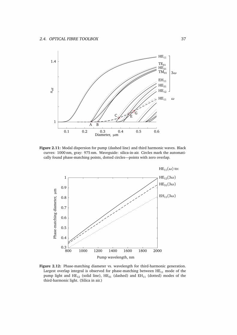
2.4. OPTICAL FIBRE TOOLBOX 37
n eff
Diameter, µm0.1 0.2 0.3 0.4 0.5 0.6
1
1.4
A B
C EG
EH11
HE31
HE12
TE01
TM01
HE21
HE11
HE11
3ω
ω
Figure 2.11: Modal dispersion for pump (dashed line) and third harmonic waves. Blackcurves: 1000 nm, gray: 975 nm. Waveguide: silica-in-air. Circles mark the automati-cally found phase-matching points, dotted circles—points with zero overlap.
Pump wavelength, nm
Phas
e-m
atch
ing
diam
eter
,µ
m
HE11(ω) to:
HE12(3ω)
HE31(3ω)
EH11(3ω)
800 1000 1200 1400 1600 1800 2000
0.4
0.5
0.6
0.7
0.8
0.9
1
0.3
Figure 2.12: Phase-matching diameter vs. wavelength for third-harmonic generation.Largest overlap integral is observed for phase-matching between HE11 mode of thepump light and HE12 (solid line), HE31 (dashed) and EH11 (dotted) modes of thethird-harmonic light. (Silica in air.)
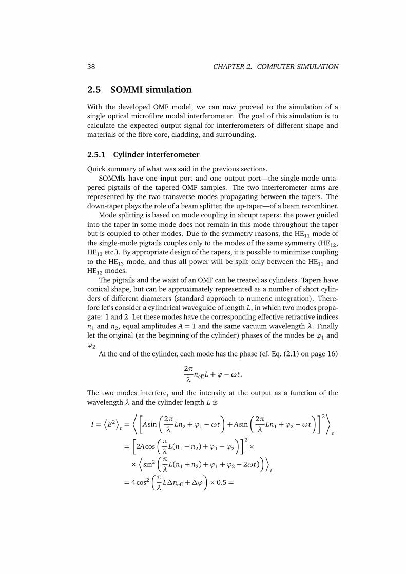
38 CHAPTER 2. COMPUTER SIMULATION
2.5 SOMMI simulation
With the developed OMF model, we can now proceed to the simulation of asingle optical microfibre modal interferometer. The goal of this simulation is tocalculate the expected output signal for interferometers of different shape andmaterials of the fibre core, cladding, and surrounding.
2.5.1 Cylinder interferometer
Quick summary of what was said in the previous sections.SOMMIs have one input port and one output port—the single-mode unta-
pered pigtails of the tapered OMF samples. The two interferometer arms arerepresented by the two transverse modes propagating between the tapers. Thedown-taper plays the role of a beam splitter, the up-taper—of a beam recombiner.
Mode splitting is based on mode coupling in abrupt tapers: the power guidedinto the taper in some mode does not remain in this mode throughout the taperbut is coupled to other modes. Due to the symmetry reasons, the HE11 mode ofthe single-mode pigtails couples only to the modes of the same symmetry (HE12,HE13 etc.). By appropriate design of the tapers, it is possible to minimize couplingto the HE13 mode, and thus all power will be split only between the HE11 andHE12 modes.
The pigtails and the waist of an OMF can be treated as cylinders. Tapers haveconical shape, but can be approximately represented as a number of short cylin-ders of different diameters (standard approach to numeric integration). There-fore let’s consider a cylindrical waveguide of length L, in which two modes propa-gate: 1 and 2. Let these modes have the corresponding effective refractive indicesn1 and n2, equal amplitudes A= 1 and the same vacuum wavelength λ. Finallylet the original (at the beginning of the cylinder) phases of the modes be ϕ1 andϕ2
At the end of the cylinder, each mode has the phase (cf. Eq. (2.1) on page 16)
2π
λneff L+ϕ−ωt.
The two modes interfere, and the intensity at the output as a function of thewavelength λ and the cylinder length L is
I =¬
E2¶
t=
®
Asin
2π
λLn2+ϕ1−ωt
+ Asin
2π
λLn1+ϕ2−ωt
2¸
t
=
2Acosπ
λL(n1− n2) +ϕ1−ϕ2
2×
×
sin2π
λL(n1+ n2) +ϕ1+ϕ2− 2ωt)
·
t
= 4 cos2π
λL∆neff+∆ϕ
× 0.5=
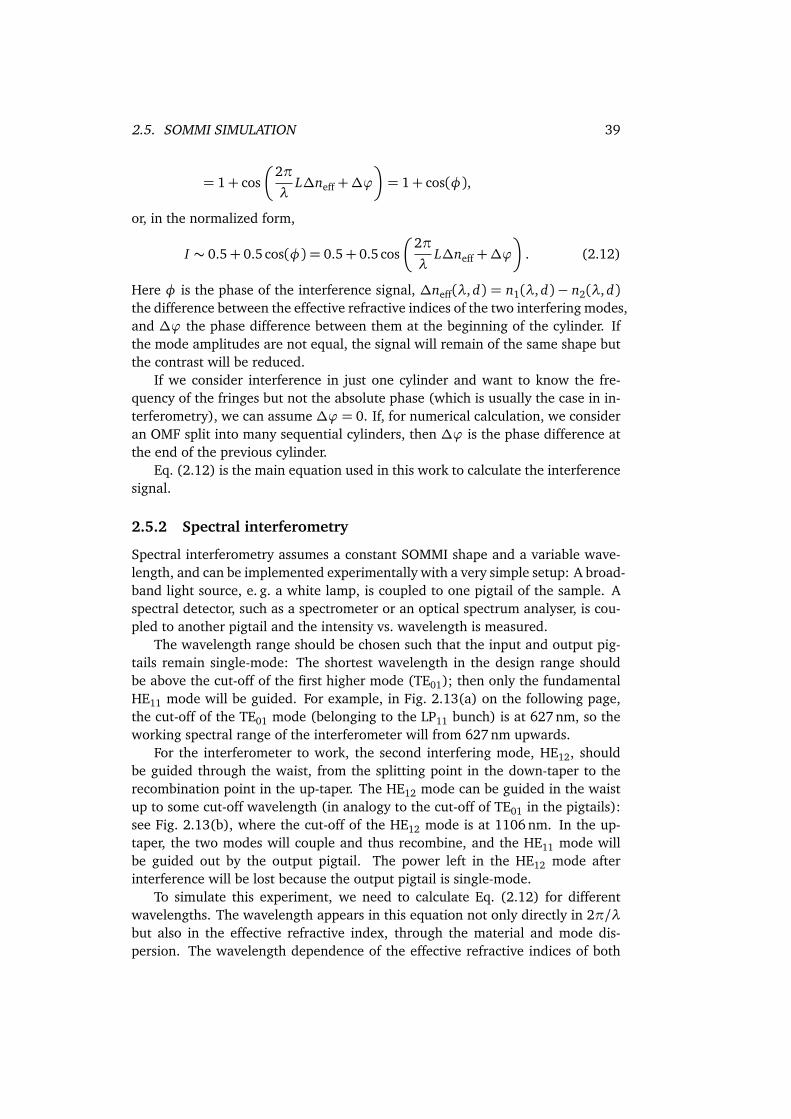
2.5. SOMMI SIMULATION 39
= 1+ cos
2π
λL∆neff+∆ϕ
= 1+ cos(φ),
or, in the normalized form,
I ∼ 0.5+ 0.5 cos(φ) = 0.5+ 0.5cos
2π
λL∆neff+∆ϕ
. (2.12)
Here φ is the phase of the interference signal, ∆neff(λ, d) = n1(λ, d)− n2(λ, d)the difference between the effective refractive indices of the two interfering modes,and ∆ϕ the phase difference between them at the beginning of the cylinder. Ifthe mode amplitudes are not equal, the signal will remain of the same shape butthe contrast will be reduced.
If we consider interference in just one cylinder and want to know the fre-quency of the fringes but not the absolute phase (which is usually the case in in-terferometry), we can assume ∆ϕ = 0. If, for numerical calculation, we consideran OMF split into many sequential cylinders, then ∆ϕ is the phase difference atthe end of the previous cylinder.
Eq. (2.12) is the main equation used in this work to calculate the interferencesignal.
2.5.2 Spectral interferometry
Spectral interferometry assumes a constant SOMMI shape and a variable wave-length, and can be implemented experimentally with a very simple setup: A broad-band light source, e. g. a white lamp, is coupled to one pigtail of the sample. Aspectral detector, such as a spectrometer or an optical spectrum analyser, is cou-pled to another pigtail and the intensity vs. wavelength is measured.
The wavelength range should be chosen such that the input and output pig-tails remain single-mode: The shortest wavelength in the design range shouldbe above the cut-off of the first higher mode (TE01); then only the fundamentalHE11 mode will be guided. For example, in Fig. 2.13(a) on the following page,the cut-off of the TE01 mode (belonging to the LP11 bunch) is at 627 nm, so theworking spectral range of the interferometer will from 627 nm upwards.
For the interferometer to work, the second interfering mode, HE12, shouldbe guided through the waist, from the splitting point in the down-taper to therecombination point in the up-taper. The HE12 mode can be guided in the waistup to some cut-off wavelength (in analogy to the cut-off of TE01 in the pigtails):see Fig. 2.13(b), where the cut-off of the HE12 mode is at 1106 nm. In the up-taper, the two modes will couple and thus recombine, and the HE11 mode willbe guided out by the output pigtail. The power left in the HE12 mode afterinterference will be lost because the output pigtail is single-mode.
To simulate this experiment, we need to calculate Eq. (2.12) for differentwavelengths. The wavelength appears in this equation not only directly in 2π/λbut also in the effective refractive index, through the material and mode dis-persion. The wavelength dependence of the effective refractive indices of both
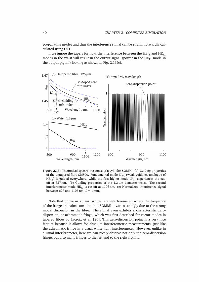
40 CHAPTER 2. COMPUTER SIMULATION
propagating modes and thus the interference signal can be straightforwardly cal-culated using OFT.
If we ignore the tapers for now, the interference between the HE11 and HE12modes in the waist will result in the output signal (power in the HE11 mode inthe output pigtail) looking as shown in Fig. 2.13(c).
Tran
smis
sion
0
1
n eff
Wavelength, nm500 1300
1.4
1
1.47
Ge-doped corerefr. index
Wavelength, nm500 1300
Silica claddingrefr. index
LP11
HE11
n eff
Wavelength, nm600 1100
627
1106
HE12
HE11
900900
(a) Untapered fibre, 125µm
(b) Waist, 1.3µm
(c) Signal vs. wavelength
1.45
Zero-dispersion point
Figure 2.13: Theoretical spectral response of a cylinder SOMMI. (a) Guiding propertiesof the untapered fibre SM800. Fundamental mode LP01 (weak-guidance analogue ofHE11) is guided everywhere, while the first higher mode LP11 experiences the cut-off at 627 nm. (b) Guiding properties of the 1.3µm diameter waist. The secondinterferometer mode HE12 is cut-off at 1106 nm. (c) Normalized interference signalbetween 627 and 1106 nm, L = 1 mm.
Note that unlike in a usual white-light interferometer, where the frequencyof the fringes remains constant, in a SOMMI it varies strongly due to the strongmodal dispersion in the fibre. The signal even exhibits a characteristic zero-dispersion, or achromatic fringe, which was first described for vector modes intapered fibres by Lacroix et al. [20]. This zero-dispersion point is a very nicefeature because it allows for absolute interferometric measurements, just likethe achromatic fringe in a usual white-light interferometer. However, unlike ina usual interferometer, here we can nicely observe not only the zero-dispersionfringe, but also many fringes to the left and to the right from it.
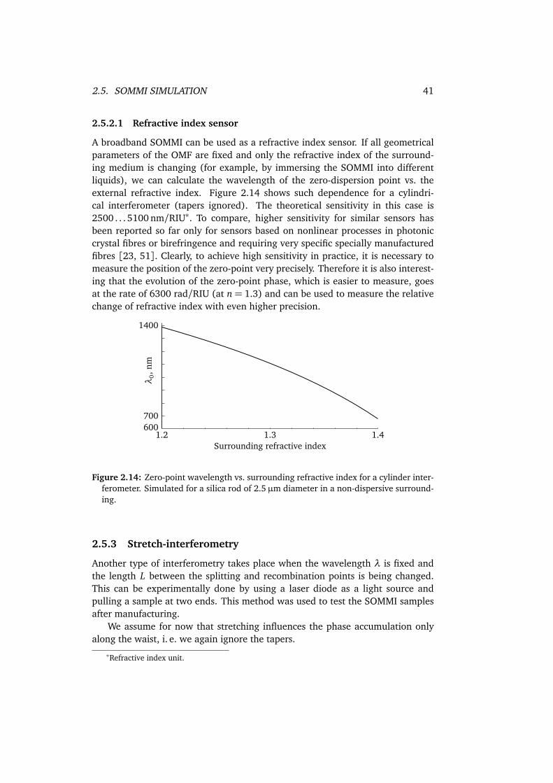
2.5. SOMMI SIMULATION 41
2.5.2.1 Refractive index sensor
A broadband SOMMI can be used as a refractive index sensor. If all geometricalparameters of the OMF are fixed and only the refractive index of the surround-ing medium is changing (for example, by immersing the SOMMI into differentliquids), we can calculate the wavelength of the zero-dispersion point vs. theexternal refractive index. Figure 2.14 shows such dependence for a cylindri-cal interferometer (tapers ignored). The theoretical sensitivity in this case is2500 . . . 5100 nm/RIU∗. To compare, higher sensitivity for similar sensors hasbeen reported so far only for sensors based on nonlinear processes in photoniccrystal fibres or birefringence and requiring very specific specially manufacturedfibres [23, 51]. Clearly, to achieve high sensitivity in practice, it is necessary tomeasure the position of the zero-point very precisely. Therefore it is also interest-ing that the evolution of the zero-point phase, which is easier to measure, goesat the rate of 6300 rad/RIU (at n= 1.3) and can be used to measure the relativechange of refractive index with even higher precision.
1.2 1.41.3Surrounding refractive index
600
1400
700
λ0,n
m
Figure 2.14: Zero-point wavelength vs. surrounding refractive index for a cylinder inter-ferometer. Simulated for a silica rod of 2.5µm diameter in a non-dispersive surround-ing.
2.5.3 Stretch-interferometry
Another type of interferometry takes place when the wavelength λ is fixed andthe length L between the splitting and recombination points is being changed.This can be experimentally done by using a laser diode as a light source andpulling a sample at two ends. This method was used to test the SOMMI samplesafter manufacturing.
We assume for now that stretching influences the phase accumulation onlyalong the waist, i. e. we again ignore the tapers.
∗Refractive index unit.
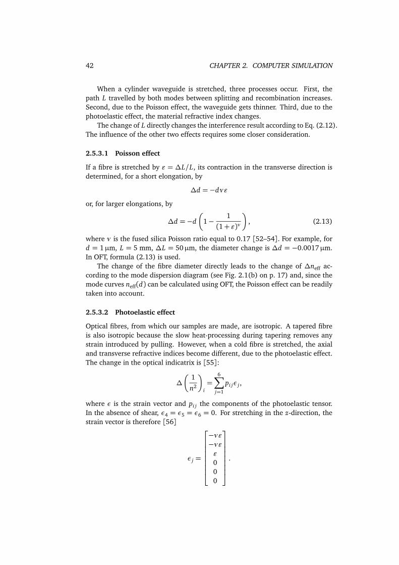
42 CHAPTER 2. COMPUTER SIMULATION
When a cylinder waveguide is stretched, three processes occur. First, thepath L travelled by both modes between splitting and recombination increases.Second, due to the Poisson effect, the waveguide gets thinner. Third, due to thephotoelastic effect, the material refractive index changes.
The change of L directly changes the interference result according to Eq. (2.12).The influence of the other two effects requires some closer consideration.
2.5.3.1 Poisson effect
If a fibre is stretched by ε = ∆L/L, its contraction in the transverse direction isdetermined, for a short elongation, by
∆d =−dνε
or, for larger elongations, by
∆d =−d
1−1
(1+ ε)ν
, (2.13)
where ν is the fused silica Poisson ratio equal to 0.17 [52–54]. For example, ford = 1µm, L = 5 mm, ∆L = 50µm, the diameter change is ∆d = −0.0017µm.In OFT, formula (2.13) is used.
The change of the fibre diameter directly leads to the change of ∆neff ac-cording to the mode dispersion diagram (see Fig. 2.1(b) on p. 17) and, since themode curves neff(d) can be calculated using OFT, the Poisson effect can be readilytaken into account.
2.5.3.2 Photoelastic effect
Optical fibres, from which our samples are made, are isotropic. A tapered fibreis also isotropic because the slow heat-processing during tapering removes anystrain introduced by pulling. However, when a cold fibre is stretched, the axialand transverse refractive indices become different, due to the photoelastic effect.The change in the optical indicatrix is [55]:
∆
1
n2
i=
6∑
j=1
pi jε j ,
where ε is the strain vector and pi j the components of the photoelastic tensor.In the absence of shear, ε4 = ε5 = ε6 = 0. For stretching in the z-direction, thestrain vector is therefore [56]
ε j =
−νε−νεε
000
.
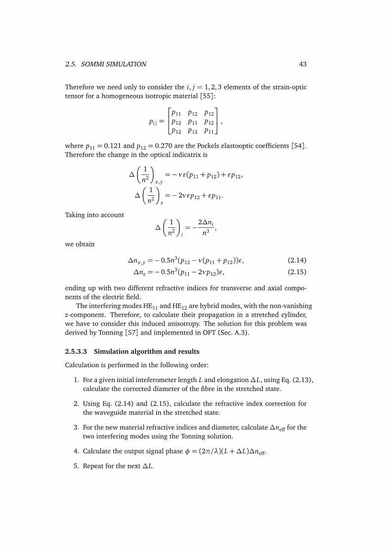
2.5. SOMMI SIMULATION 43
Therefore we need only to consider the i, j = 1,2, 3 elements of the strain-optictensor for a homogeneous isotropic material [55]:
pi j =
p11 p12 p12p12 p11 p12p12 p12 p11
,
where p11 = 0.121 and p12 = 0.270 are the Pockels elastooptic coefficients [54].Therefore the change in the optical indicatrix is
∆
1
n2
x ,y=− νε(p11+ p12) + εp12,
∆
1
n2
z=− 2νεp12+ εp11.
Taking into account
∆
1
n2
i=−
2∆ni
n3 ,
we obtain
∆nx ,y =− 0.5n3(p12− ν(p11+ p12))ε, (2.14)
∆nz =− 0.5n3(p11− 2νp12)ε, (2.15)
ending up with two different refractive indices for transverse and axial compo-nents of the electric field.
The interfering modes HE11 and HE12 are hybrid modes, with the non-vanishingz-component. Therefore, to calculate their propagation in a stretched cylinder,we have to consider this induced anisotropy. The solution for this problem wasderived by Tonning [57] and implemented in OFT (Sec. A.3).
2.5.3.3 Simulation algorithm and results
Calculation is performed in the following order:
1. For a given initial inteferometer length L and elongation∆L, using Eq. (2.13),calculate the corrected diameter of the fibre in the stretched state.
2. Using Eq. (2.14) and (2.15), calculate the refractive index correction forthe waveguide material in the stretched state.
3. For the new material refractive indices and diameter, calculate∆neff for thetwo interfering modes using the Tonning solution.
4. Calculate the output signal phase φ = (2π/λ)(L+∆L)∆neff.
5. Repeat for the next ∆L.
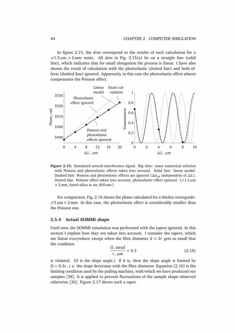
44 CHAPTER 2. COMPUTER SIMULATION
In figure 2.15, the dots correspond to the results of such calculation for a1.5µm ×2 mm waist. All dots in Fig. 2.15(a) lie on a straight line (solidline), which indicates that for small elongation the process is linear. I have alsoshown the result of calculation with the photoelastic (dotted line) and both ef-fects (dashed line) ignored. Apparently, in this case the photoelastic effect almostcompensates the Poisson effect.
0 4 8 12 16 20
3490
3500
3510
3520
3530
∆L, µm
Phas
e,ra
d
Linearmodel
Poisson andphotoelasticeffects ignored
Photoelasticeffect ignored
0 2 4 6 8 100
0.2
0.4
0.6
0.8
1
∆L, µm
Tran
smis
sion
Exact cal-culation
Figure 2.15: Simulated stretch-interference signal. Big dots: exact numerical solutionwith Poisson and photoelastic effects taken into account. Solid line: linear model.Dashed line: Poisson and photoelastic effects are ignored (∆neff independent of ∆L).Dotted line: Poisson effect taken into account, photoelastic effect ignored. (1.5µm×2 mm, fused silica in air, 850nm.)
For comparison, Fig. 2.16 shows the phase calculated for a thicker waveguide:5µm×2 mm. In this case, the photoelastic effect is considerably smaller thanthe Poisson one.
2.5.4 Actual SOMMI shape
Until now, the SOMMI simulation was performed with the tapers ignored. In thissection I explain how they are taken into account. I consider the tapers, whichare linear everywhere except when the fibre diameter d = 2r gets so small thatthe condition
Ω, mrad
r, µm< 0.3 (2.16)
is violated. (Ω is the slope angle.) If it is, then the slope angle is limited byΩ = 0.3r, i. e. the slope decreases with the fibre diameter. Equation (2.16) is thelimiting condition used by the pulling machine, with which we have produced oursamples [58]. It is applied to prevent fluctuations of the sample shape observedotherwise [26]. Figure 2.17 shows such a taper.
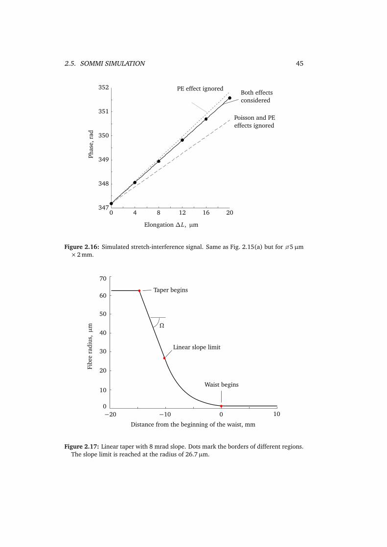
2.5. SOMMI SIMULATION 45
0 4 8 12 16 20347
348
349
350
351
352
Poisson and PEeffects ignored
PE effect ignoredBoth effectsconsidered
Elongation ∆L, µm
Phas
e,ra
d
Figure 2.16: Simulated stretch-interference signal. Same as Fig. 2.15(a) but for 5µm×2 mm.
Fibr
era
dius
,µ
m
Distance from the beginning of the waist, mm
−20 100
70
Waist begins
Linear slope limit
Taper begins
Ω
60
10
−10 0
20
30
40
50
Figure 2.17: Linear taper with 8 mrad slope. Dots mark the borders of different regions.The slope limit is reached at the radius of 26.7µm.
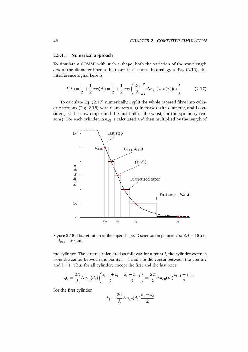
46 CHAPTER 2. COMPUTER SIMULATION
2.5.4.1 Numerical approach
To simulate a SOMMI with such a shape, both the variation of the wavelengthand of the diameter have to be taken in account. In analogy to Eq. (2.12), theinterference signal here is
I(λ) =1
2+
1
2cos(φ) =
1
2+
1
2cos
2π
λ
∫
L
∆neff(λ, d(z))dz
(2.17)
To calculate Eq. (2.17) numerically, I split the whole tapered fibre into cylin-dric sections (Fig. 2.18) with diameters di (i increases with diameter, and I con-sider just the down-taper and the first half of the waist, for the symmetry rea-sons). For each cylinder, ∆neff is calculated and then multiplied by the length of
Rad
ius,
µm
0
60
Discretized taper
Last step
First step
(zi , di)
(zi+1, di+1)dmax
z1z2zN zi
Waist
10
Figure 2.18: Discretisation of the taper shape. Discretisation parameters: ∆d = 10µm,dmax = 50µm.
the cylinder. The latter is calculated as follows: for a point i, the cylinder extendsfrom the center between the points i−1 and i to the center between the points iand i+ 1. Thus for all cylinders except the first and the last ones,
φi =2π
λ∆neff(di)
zi−1+ zi
2−
zi + zi+1
2
=2π
λ∆neff(di)
zi−1− zi+1
2.
For the first cylinder,
φ1 =2π
λ∆neff(d1)
z1− z2
2
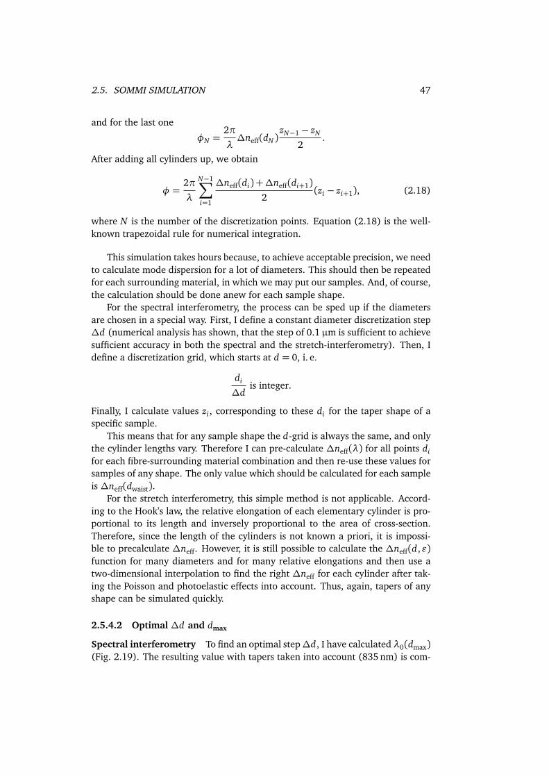
2.5. SOMMI SIMULATION 47
and for the last one
φN =2π
λ∆neff(dN )
zN−1− zN
2.
After adding all cylinders up, we obtain
φ =2π
λ
N−1∑
i=1
∆neff(di) +∆neff(di+1)2
(zi − zi+1), (2.18)
where N is the number of the discretization points. Equation (2.18) is the well-known trapezoidal rule for numerical integration.
This simulation takes hours because, to achieve acceptable precision, we needto calculate mode dispersion for a lot of diameters. This should then be repeatedfor each surrounding material, in which we may put our samples. And, of course,the calculation should be done anew for each sample shape.
For the spectral interferometry, the process can be sped up if the diametersare chosen in a special way. First, I define a constant diameter discretization step∆d (numerical analysis has shown, that the step of 0.1µm is sufficient to achievesufficient accuracy in both the spectral and the stretch-interferometry). Then, Idefine a discretization grid, which starts at d = 0, i. e.
di
∆dis integer.
Finally, I calculate values zi , corresponding to these di for the taper shape of aspecific sample.
This means that for any sample shape the d-grid is always the same, and onlythe cylinder lengths vary. Therefore I can pre-calculate ∆neff(λ) for all points difor each fibre-surrounding material combination and then re-use these values forsamples of any shape. The only value which should be calculated for each sampleis ∆neff(dwaist).
For the stretch interferometry, this simple method is not applicable. Accord-ing to the Hook’s law, the relative elongation of each elementary cylinder is pro-portional to its length and inversely proportional to the area of cross-section.Therefore, since the length of the cylinders is not known a priori, it is impossi-ble to precalculate ∆neff. However, it is still possible to calculate the ∆neff(d,ε)function for many diameters and for many relative elongations and then use atwo-dimensional interpolation to find the right ∆neff for each cylinder after tak-ing the Poisson and photoelastic effects into account. Thus, again, tapers of anyshape can be simulated quickly.
2.5.4.2 Optimal ∆d and dmax
Spectral interferometry To find an optimal step∆d, I have calculated λ0(dmax)(Fig. 2.19). The resulting value with tapers taken into account (835 nm) is com-
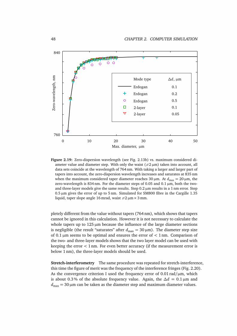
48 CHAPTER 2. COMPUTER SIMULATION
0 50Max. diameter, µm
760
840Ze
ro-w
avel
engt
h,nm
Erdogan 0.1
2-layer
2-layer 0.05
Erdogan 0.2
Erdogan
Mode type ∆d, µm
0.1
0.5
10 20 30 40
Figure 2.19: Zero-dispersion wavelength (see Fig. 2.13b) vs. maximum considered di-ameter value and diameter step. With only the waist (2µm) taken into account, alldata sets coincide at the wavelength of 764 nm. With taking a larger and larger part oftapers into account, the zero-dispersion wavelength increases and saturates at 835 nmwhen the maximum considered taper diameter reaches 30µm. At dmax = 20µm, thezero-wavelength is 834 nm. For the diameter steps of 0.05 and 0.1µm, both the two-and three-layer models give the same results. Step 0.2µm results in a 1 nm error. Step0.5µm gives the error of up to 5 nm. Simulated for SM800 fibre in the Cargille 1.35liquid, taper slope angle 16 mrad, waist 2µm× 3 mm.
pletely different from the value without tapers (764 nm), which shows that taperscannot be ignored in this calculation. However it is not necessary to calculate thewhole tapers up to 125µm because the influence of the large diameter sectionsis negligible (the result “saturates” after dmax = 30µm). The diameter step sizeof 0.1µm seems to be optimal and ensures the error of < 1 nm. Comparison ofthe two- and three-layer models shows that the two layer model can be used withkeeping the error < 1nm. For even better accuracy (if the measurement error isbelow 1 nm), the three-layer models should be used.
Stretch-interferometry The same procedure was repeated for stretch-interference,this time the figure of merit was the frequency of the interference fringes (Fig. 2.20).As the convergence criterion I used the frequency error of 0.01 rad/µm, whichis about 0.3 % of the absolute frequency value. Again, the ∆d = 0.1µm anddmax = 30µm can be taken as the diameter step and maximum diameter values.
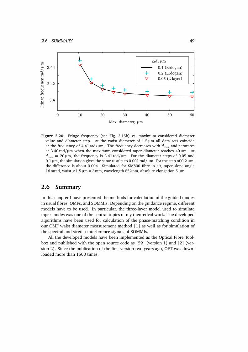
2.6. SUMMARY 49
0.1 (Erdogan)
0.05 (2-layer)0.2 (Erdogan)
∆d, µm
Max. diameter, µm
0 10 20 30 40 50 60
3.4
3.42
3.44
Frin
gefr
eque
ncy,
rad/
µm
Figure 2.20: Fringe frequency (see Fig. 2.15b) vs. maximum considered diametervalue and diameter step. At the waist diameter of 1.5µm all data sets coincideat the frequency of 4.41 rad/µm. The frequency decreases with dmax and saturatesat 3.40 rad/µm when the maximum considered taper diameter reaches 40µm. Atdmax = 20µm, the frequency is 3.41 rad/µm. For the diameter steps of 0.05 and0.1µm, the simulation gives the same results to 0.001 rad/µm. For the step of 0.2µm,the difference is about 0.004. Simulated for SM800 fibre in air, taper slope angle16 mrad, waist 1.5µm× 3mm, wavelength 852 nm, absolute elongation 5µm.
2.6 Summary
In this chapter I have presented the methods for calculation of the guided modesin usual fibres, OMFs, and SOMMIs. Depending on the guidance regime, differentmodels have to be used. In particular, the three-layer model used to simulatetaper modes was one of the central topics of my theoretical work. The developedalgorithms have been used for calculation of the phase-matching condition inour OMF waist diameter measurement method [1] as well as for simulation ofthe spectral and stretch-interference signals of SOMMIs.
All the developed models have been implemented as the Optical Fibre Tool-box and published with the open source code as [59] (version 1) and [2] (ver-sion 2). Since the publication of the first version two years ago, OFT was down-loaded more than 1500 times.

CHAPTER 3Samples
In this chapter I describe manufacturing, characterization and handling of OMFand SOMMI samples.
3.1 Production
3.1.1 Optical fibre tapering
Micrometre-scale diameter glass fibres were first produced and studied in the19th century [60, 61], however they were inappropriate for optical applicationsdue the high losses in glass itself. It was only in 1970 that, following the dis-covery of Kao and Hockham [7], Corning managed to produce the first opticalfibre with sufficiently low attenuation for telecom purposes. This also raised in-terest to research aimed on creating more fibre-based devices than just opticaltransmission elements.
Fibre tapers were used to couple light between two fibres (fibre couplers) aswell as to excite light propagation in the cladding and then couple it back to thecore. However such tapers need neither a high shape uniformity, nor a very smalldiameter.
In 1985, the first paper mentioning an optical fibre tapered down to 10µmwas published [62]. The research of small-diameter fibre tapers immediately fol-lowed [20, 39, 63]. However the shape quality of these OMFs (produced simplyby flame-heating and pulling a commercial fibre) was still not high enough, lead-ing to high losses.
For efficient light-matter interaction it is important to be able to make thefibre waist as long and as constant in diameter as possible. For fine control oflight propagation it is also critical to control the shape of the tapers. In 1992,Birks and Li have developed a theory of fibre tapering and experimentally verifiedit using the “flame-brushing” technique [64–66]. In this method, a fibre is pulled
51
52 CHAPTER 3. SAMPLES
by two translation stages while at the same time being heated by a flame movingback and forth under the fibre, thereby imitating a varying flame length. Theymanaged to achieve excellent control over the waist and taper shape, which wasimportant for such applications as the directional couplers and the fibre beamexpanders. However the diameter of the waist was on the order of dozens ofmicrometres.
In 2003, Tong et al. proposed a rather complicated method of drawing highquality subwavelength-diameter fibres [67]. Finally, in 2004, Brambilla et al. forthe first time reported a successful production of a low-loss sub-micrometre-diameter fibre using the flame-brushing technique [9]. This flame-brushing methodwith its modifications employing various types of heat sources (gas flame, electri-cal microheater, laser-heated sapphire furnace) is the one usually used nowadaysaround the world to produce high-quality (sub)micrometre-diameter tapered fi-bres.
There are also alternative methods based on fibre etching or polishing [68,69]. As such, they yield OMFs of lower optical quality than fibre pulling [70] andare therefore rarely used today. However, polishing provides additional controlover the waist shape and can be used in combination with tapering as for examplein [23].
3.1.2 Pulling machine
To manufacture our samples, we have used the fibre pulling machine developedand built in our group a few years ago [26] and currently belonging to the groupof Arno Rauschenbeutel (Fig. 3.1). Its primary parts are two computer-controlledtranslation stages, stacked on top of each other, and an oxygen-hydrogen burner.Two steel plates with precision V-grooves are fixed on top of the stages. Thegrooves are aligned coaxially to each other and parallel to the axis of motionof the stages. The fibre to be pulled is clamped in these V-grooves with strongmagnets and thus is aligned relative to the stages.
The bottom (translator) stage is moving left and right and the burner is sta-tionary. The top stage (stretcher) is continuously pulling the fibre while the bot-tom stage is moving the whole fibre left and right imitating the movement of theflame. In comparison to the original flame-brushing design of Birks [66], thisvariant offers a simpler construction (due to the fixed burner) and lower air flowinfluence on the flame (the flame is not moving).
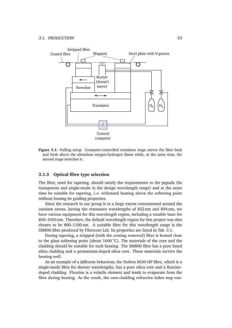
3.1. PRODUCTION 53
O2 H2
Stretcher
Translator
Burner(doesn’tmove)
MagnetsCoated fibre
Controlcomputer
Steel plate with V-grooveStripped fibre
Figure 3.1: Pulling setup. Computer-controlled translator stage moves the fibre backand forth above the ultraclean oxygen-hydrogen flame while, at the same time, thesecond stage stretches it.
3.1.3 Optical fibre type selection
The fibre, used for tapering, should satisfy the requirements to the pigtails (betransparent and single-mode in the design wavelength range) and at the sametime be suitable for tapering, i. e. withstand heating above the softening pointwithout loosing its guiding properties.
Since the research in our group is to a large extent concentrated around thecaesium atoms, having the resonance wavelengths of 852 nm and 894 nm, wehave various equipment for this wavelength region, including a tunable laser for850–1050 nm. Therefore, the default wavelength region for this project was alsochosen to be 800–1100 nm. A suitable fibre for this wavelength range is theSM800 fibre produced by Fibercore Ltd. Its properties are listed in Tab. 3.1.
During tapering, a stripped (with the coating removed) fibre is heated closeto the glass softening point (about 1600 C). The materials of the core and thecladding should be suitable for such heating. The SM800 fibre has a pure fusedsilica cladding and a germanium-doped silica core. These materials survive theheating well.
As an example of a different behaviour, the Nufern S630-HP fibre, which is asingle-mode fibre for shorter wavelengths, has a pure silica core and a fluorine-doped cladding. Fluorine is a volatile element and tends to evaporate from thefibre during heating. As the result, the core-cladding refractive index step van-
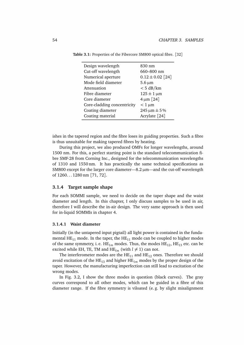
54 CHAPTER 3. SAMPLES
Table 3.1: Properties of the Fibercore SM800 optical fibre. [32]
Design wavelength 830 nmCut-off wavelength 660–800 nmNumerical aperture 0.12± 0.02 [24]Mode field diameter 5.6µmAttenuation < 5 dB/kmFibre diameter 125± 1µmCore diameter 4µm [24]Core-cladding concentricity < 1µmCoating diameter 245µm± 5 %Coating material Acrylate [24]
ishes in the tapered region and the fibre loses its guiding properties. Such a fibreis thus unsuitable for making tapered fibres by heating.
During this project, we also produced OMFs for longer wavelengths, around1500 nm. For this, a perfect starting point is the standard telecommunication fi-bre SMF-28 from Corning Inc., designed for the telecommunication wavelengthsof 1310 and 1550 nm. It has practically the same technical specifications asSM800 except for the larger core diameter—8.2µm—and the cut-off wavelengthof 1260. . . 1280 nm [71, 72].
3.1.4 Target sample shape
For each SOMMI sample, we need to decide on the taper shape and the waistdiameter and length. In this chapter, I only discuss samples to be used in air,therefore I will describe the in-air design. The very same approach is then usedfor in-liquid SOMMIs in chapter 4.
3.1.4.1 Waist diameter
Initially (in the untapered input pigtail) all light power is contained in the funda-mental HE11 mode. In the taper, the HE11 mode can be coupled to higher modesof the same symmetry, i. e. HE1m modes. Thus, the modes HE12, HE13 etc. can beexcited while EH, TE, TM and HElm (with l 6= 1) can not.
The interferometer modes are the HE11 and HE12 ones. Therefore we shouldavoid excitation of the HE13 and higher HE1m modes by the proper design of thetaper. However, the manufacturing imperfection can still lead to excitation of thewrong modes.
In Fig. 3.2, I show the three modes in question (black curves). The graycurves correspond to all other modes, which can be guided in a fibre of thisdiameter range. If the fibre symmetry is viloated (e. g. by slight misalignment
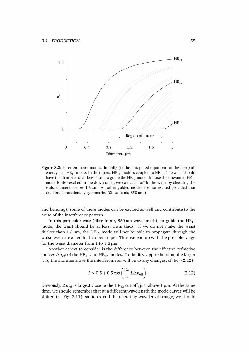
3.1. PRODUCTION 55
n eff
Diameter, µm
0 2
1
1.4
0.4 0.8 1.2 1.6
HE11
HE13
Region of interest
HE12
Figure 3.2: Interferometer modes. Initially (in the untapered input part of the fibre) allenergy is in HE11 mode. In the tapers, HE11 mode is coupled to HE12. The waist shouldhave the diameter of at least 1µm to guide the HE12 mode. In case the unwanted HE13mode is also excited in the down-taper, we can cut if off in the waist by choosing thewaist diameter below 1.8µm. All other guided modes are not excited provided thatthe fibre is rotationally symmetric. (Silica in air, 850 nm.)
and bending), some of these modes can be excited as well and contribute to thenoise of the interference pattern.
In this particular case (fibre in air, 850 nm wavelength), to guide the HE12mode, the waist should be at least 1µm thick. If we do not make the waistthicker than 1.8µm, the HE13 mode will not be able to propagate through thewaist, even if excited in the down-taper. Thus we end up with the possible rangefor the waist diameter from 1 to 1.8µm.
Another aspect to consider is the difference between the effective refractiveindices ∆neff of the HE11 and HE12 modes. To the first approximation, the largerit is, the more sensitive the interferometer will be to any changes, cf. Eq. (2.12):
I ∼ 0.5+ 0.5cos
2π
λL∆neff
, (2.12)
Obviously, ∆neff is largest close to the HE12 cut-off, just above 1µm. At the sametime, we should remember that at a different wavelength the mode curves will beshifted (cf. Fig. 2.11), so, to extend the operating wavelength range, we should
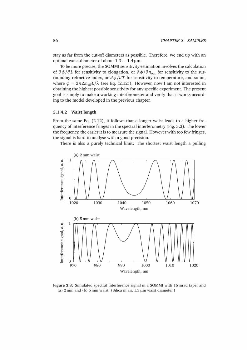
56 CHAPTER 3. SAMPLES
stay as far from the cut-off diameters as possible. Therefore, we end up with anoptimal waist diameter of about 1.3 . . . 1.4µm.
To be more precise, the SOMMI sensitivity estimation involves the calculationof ∂ φ/∂ L for sensitivity to elongation, or ∂ φ/∂ nout for sensitivity to the sur-rounding refractive index, or ∂ φ/∂ T for sensitivity to temperature, and so on,where φ = 2π∆neff L/λ (see Eq. (2.12)). However, now I am not interested inobtaining the highest possible sensitivity for any specific experiment. The presentgoal is simply to make a working interferometer and verify that it works accord-ing to the model developed in the previous chapter.
3.1.4.2 Waist length
From the same Eq. (2.12), it follows that a longer waist leads to a higher fre-quency of interference fringes in the spectral interferometry (Fig. 3.3). The lowerthe frequency, the easier it is to measure the signal. However with too few fringes,the signal is hard to analyse with a good precision.
There is also a purely technical limit: The shortest waist length a pulling
1020 1030 1040 1050 1060 10700
1
970 980 990 1000 1010 10200
1
Inte
rfer
ence
sign
al,a
.u.
Inte
rfer
ence
sign
al,a
.u.
Wavelength, nm
Wavelength, nm
(a) 2 mm waist
(b) 5 mm waist
Figure 3.3: Simulated spectral interference signal in a SOMMI with 16 mrad taper and(a) 2 mm and (b) 5 mm waist. (Silica in air, 1.3µm waist diameter.)
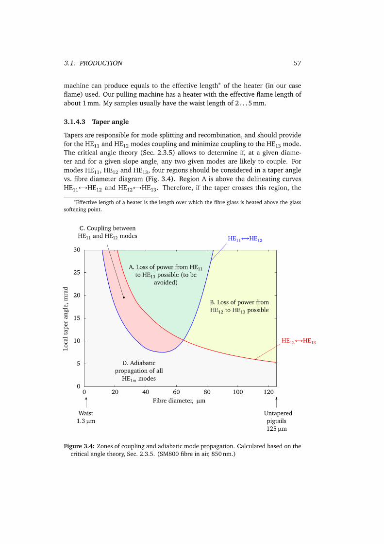
3.1. PRODUCTION 57
machine can produce equals to the effective length∗ of the heater (in our caseflame) used. Our pulling machine has a heater with the effective flame length ofabout 1 mm. My samples usually have the waist length of 2 . . . 5mm.
3.1.4.3 Taper angle
Tapers are responsible for mode splitting and recombination, and should providefor the HE11 and HE12 modes coupling and minimize coupling to the HE13 mode.The critical angle theory (Sec. 2.3.5) allows to determine if, at a given diame-ter and for a given slope angle, any two given modes are likely to couple. Formodes HE11, HE12 and HE13, four regions should be considered in a taper anglevs. fibre diameter diagram (Fig. 3.4). Region A is above the delineating curvesHE11↔HE12 and HE12↔HE13. Therefore, if the taper crosses this region, the
∗Effective length of a heater is the length over which the fibre glass is heated above the glasssoftening point.
0 20 40 60 80 100 1200
5
10
15
20
25
30
Loca
ltap
eran
gle,
mra
d
Fibre diameter, µm
B. Loss of power fromHE12 to HE13 possible
A. Loss of power from HE11to HE13 possible (to be
avoided)
C. Coupling betweenHE11 and HE12 modes
D. Adiabaticpropagation of all
HE1m modes
Waist1.3µm
Untaperedpigtails125µm
HE12↔HE13
HE11↔HE12
Figure 3.4: Zones of coupling and adiabatic mode propagation. Calculated based on thecritical angle theory, Sec. 2.3.5. (SM800 fibre in air, 850 nm.)
58 CHAPTER 3. SAMPLES
power can be lost to the HE13 mode, which is to be avoided. Region B is abovethe HE12↔HE13 delineating curve but below the HE11↔HE12 one. Thereforeonly the power in the HE12 mode can be lost to HE13. However, mode HE12 is de-coupled from HE11 in this region (it is below the HE11↔HE12 curve), thereforethis loss does not influence the interference result. Region C is the one where theHE11 and HE12 modes are coupled and no coupling occurs with mode HE13. Thisis therefore the target area for mode splitting and recombination. Finally, regionD is the area of adiabatic propagation of all modes.
The OMF pigtails have the diameter of 125µm, and thus the down-taperalways starts in areas B or D, which is fine. The slope should then be largeenough for the Ω(d) curve (we call it a taper trajectory) to cross area C but nottoo large, so that it does not get into area A. In the waist, the slope angle is zero,therefore the waist is always in area D, and the two interfering modes propagateadiabatically. The up-taper trajectory should again cross area C to achieve moderecombination. It does not matter in which area—B or D—is the output pigtail:neither mode HE12 nor mode HE13 are detected at the output (both are lostbecause the pigtail is single-mode).
The pulling machine used in this project can only produce symmetric tapers,so the trajectories for the down- and the up-taper are the same. Moreover, dur-ing building the pulling machine it was discovered that if the Ω/d ratio is toolarge, the tapers do not exhibit a well defined shape [26]. Therefore the controlsoftware of the pulling machine limits the slope to [73]∗
Ω/d = 0.15mrad/µm.
In Fig. 3.5, this limit is indicated by the dashed line. At no point can our samplesget above this line. Apparently, this line satisfies the above requirements: it startsin area B, crosses area C, gets to the waist, and then returns through C to B. Itnever crosses the “forbidden” area A. Therefore, for most of my samples I justspecified the value of 16 mrad as the desired taper angle, the pulling machinelimited it to Ωmax = 0.15d, and this trajectory (shown with the thick solid line)worked fine as can be seen from the rest of the thesis.
For comparison, the step-wise line at the bottom of Fig. 3.5 indicates the tra-jectory often used for our adiabatic samples. Figure 3.6 shows both the 16 mradand the 3-1-3 mrad taper shapes.
∗To be more precise, the limiting factor depends on the effective flame width given to thecontrol software of the machine by the user and is 0.265 for 0.7 mm flame, 0.193 for 1.0 mm, and0.118 for 1.6 mm. I have found these values by fitting an exponential curve to the design tapershape plotted by the pulling control software [17]. The flame width of course does not changebut is not known exactly. Besides, by decreasing this parameter, one can achieve steeper tapersby compromising their smoothness a little; it makes sense when designing a SOMMI: we are moreinterested in the efficient coupling leading to a higher contrast than in the no-loss propagation.Without loss of generality, I will be using the value of 0.15 mrad/µm in this text; the exact valuesare used in all taper shape-related calculations.
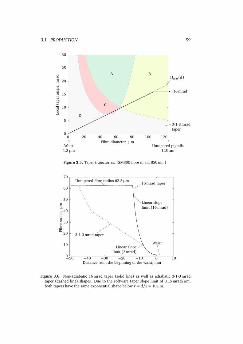
3.1. PRODUCTION 59
0 20 40 60 80 100 1200
5
10
15
20
25
30Lo
calt
aper
angl
e,m
rad
Fibre diameter, µmWaist
1.3µmUntapered pigtails
125µm
16 mrad
3-1-3 mradtaper
Ωmax(d)A B
C
D
Figure 3.5: Taper trajectories. (SM800 fibre in air, 850 nm.)
Fibr
era
dius
,µ
m
Distance from the beginning of the waist, mm−50 −40 −30 −20 −10 0 100
10
20
30
40
50
60
70
16 mrad taper
Linear slopelimit (16 mrad)
3-1-3 mrad taper
Waist
Untapered fibre radius 62.5µm
Linear slopelimit (3 mrad)
Figure 3.6: Non-adiabatic 16 mrad taper (solid line) as well as adiabatic 3-1-3 mradtaper (dashed line) shapes. Due to the software taper slope limit of 0.15 mrad/µm,both tapers have the same exponential shape below r = d/2= 10µm.
60 CHAPTER 3. SAMPLES
3.1.5 Sample shape verification
To be able to reliably interpret experimental results, it should be checked whetherthe samples we produce are actually the ones we design. The pulling machine isequipped with a microscope for a visual inspection. However since the samplesare very thin, the visual inspection does not provide much information except forsome dramatic problems (like broken waist or significant bending). Thereforeseveral other methods have been used during this project.
3.1.5.1 Scanning electron microscopy
Since the sample length is on the order of several centimetres and the diameterrange is 0.5...125µm, the instrument of obvious choice to characterize our sam-ples is a scanning electron microscope (SEM): The resolution of an SEM on theorder of 1 nm and the achievable accuracy on the order of 10 nm∗ are suitablefor our purposes. At the same time, SEM allows measuring larger samples thanaccessible with a more accurate transmission electron microscope.
Waist diameter As far as I know, our group was the first one to reliably measurethe microfibre waist diameter with high precision using an SEM. This processrequires special handling of the samples and recalibration of the microscope foreach series of measurement to obtain the maximum accuracy accessible withSEM. All details can be found in the Diplom work of Pritzkau [74] and, in ashorter form, in [1]. Figure 3.7 shows SEM images of the taper and the waist ofone of our submicrometre-diameter samples.
SEM poses some problems when considering our samples. Glass gets chargedby the electron beam and deflects electrons from their original trajectory, thusreducing the accuracy of measurement. To prevent this effect, the fibre mustbe coated with gold. The thickness of the golden layer is not perfectly well de-fined thus contributing to the overall error of measurement. Besides, a gold-coated sample is of course unusable in optical experiments. Another problem wehave faced is that lengthy exposure to the electron beam required to obtain high-quality images results in damaging (burning) the thin sample’s waist. A cleardisadvantage of the SEM measurements is also the required time—a few hoursper sample, provided that the microscope is readily available.
The main advantage over other methods is the high resolution along the fi-bre axis (below 1µm, determined by translation stages of the SEM) allowing toresolve small shape irregularities.
Our SEM results are summarized in Sec. 3.1.5.3 on page 62.
∗Usually SEMs are calibrated to ±5% corresponding to ±50 nm for a 1µm sample. A bet-ter accuracy can be achieved by recalibrating the SEM during the measurement using calibrationtargets.
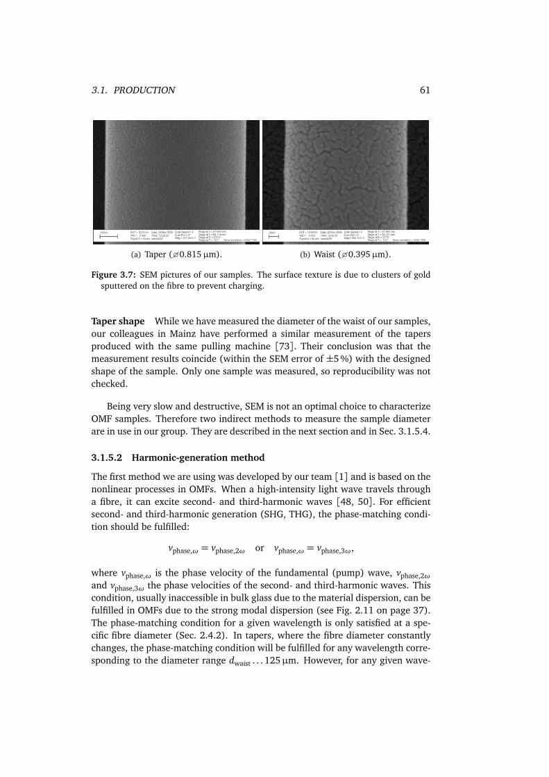
3.1. PRODUCTION 61
(a) Taper (0.815µm). (b) Waist (0.395µm).
Figure 3.7: SEM pictures of our samples. The surface texture is due to clusters of goldsputtered on the fibre to prevent charging.
Taper shape While we have measured the diameter of the waist of our samples,our colleagues in Mainz have performed a similar measurement of the tapersproduced with the same pulling machine [73]. Their conclusion was that themeasurement results coincide (within the SEM error of ±5%) with the designedshape of the sample. Only one sample was measured, so reproducibility was notchecked.
Being very slow and destructive, SEM is not an optimal choice to characterizeOMF samples. Therefore two indirect methods to measure the sample diameterare in use in our group. They are described in the next section and in Sec. 3.1.5.4.
3.1.5.2 Harmonic-generation method
The first method we are using was developed by our team [1] and is based on thenonlinear processes in OMFs. When a high-intensity light wave travels througha fibre, it can excite second- and third-harmonic waves [48, 50]. For efficientsecond- and third-harmonic generation (SHG, THG), the phase-matching condi-tion should be fulfilled:
vphase,ω = vphase,2ω or vphase,ω = vphase,3ω,
where vphase,ω is the phase velocity of the fundamental (pump) wave, vphase,2ωand vphase,3ω the phase velocities of the second- and third-harmonic waves. Thiscondition, usually inaccessible in bulk glass due to the material dispersion, can befulfilled in OMFs due to the strong modal dispersion (see Fig. 2.11 on page 37).The phase-matching condition for a given wavelength is only satisfied at a spe-cific fibre diameter (Sec. 2.4.2). In tapers, where the fibre diameter constantlychanges, the phase-matching condition will be fulfilled for any wavelength corre-sponding to the diameter range dwaist . . . 125µm. However, for any given wave-
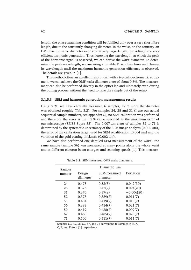
62 CHAPTER 3. SAMPLES
length, the phase-matching condition will be fulfilled only over a very short fibrelength, due to the constantly changing diameter. In the waist, on the contrary, anOMF has the same diameter over a relatively large length, providing for a veryefficient harmonic-generation. Thus, knowing the wavelength, at which the peakof the harmonic signal is observed, we can derive the waist diameter. To deter-mine the peak wavelength, we are using a tunable Ti:sapphire laser and changeits wavelength until the maximum harmonic generation efficiency is observed.The details are given in [1].
This method offers an excellent resolution: with a typical spectrometric equip-ment, we can achieve the OMF waist diameter error of about 0.5%. The measure-ment can also be performed directly in the optics lab and ultimately even duringthe pulling process without the need to take the sample out of the setup.
3.1.5.3 SEM and harmonic-generation measurement results
Using SEM, we have carefully measured 6 samples, for 3 more the diameterwas obtained roughly (Tab. 3.2). For samples 24, 28 and 31 (I use our actualsequential sample numbers, see appendix C), no SEM calibration was performedand therefore the error is the ±5% value specified as the maximum error ofour microscope (ZEISS Supra 55). The 0.007µm error of samples 52 to 71 isdetermined by the systematic uncertainty of the SEM image analysis (0.005µm),the error of the calibration target used for SEM recalibration (0.004µm) and thevariation of the gold coating thickness (0.002µm).
We have also performed one detailed SEM measurement of the waist: thesame sample (sample 56) was measured at many points along the whole waistand at different electron beam energies and scanning speeds [1]. This measure-
Table 3.2: SEM-measured OMF waist diameters.
Samplenumber
Diameter, µm
Designdiameter
SEM-measureddiameter
Deviation
24 0.478 0.52(3) 0.042(30)28 0.376 0.47(2) 0.094(20)31 0.376 0.37(2) −0.006(20)52 0.378 0.389(7) 0.011(7)55 0.404 0.419(7) 0.015(7)56 0.393 0.414(7) 0.021(7)59 0.419 0.428(7) 0.009(7)67 0.460 0.485(7) 0.025(7)71 0.500 0.511(7) 0.011(7)
Samples 52, 55, 56, 59, 67, and 71 correspond to samples D, E, A,C, B, and F from [1] respectively.
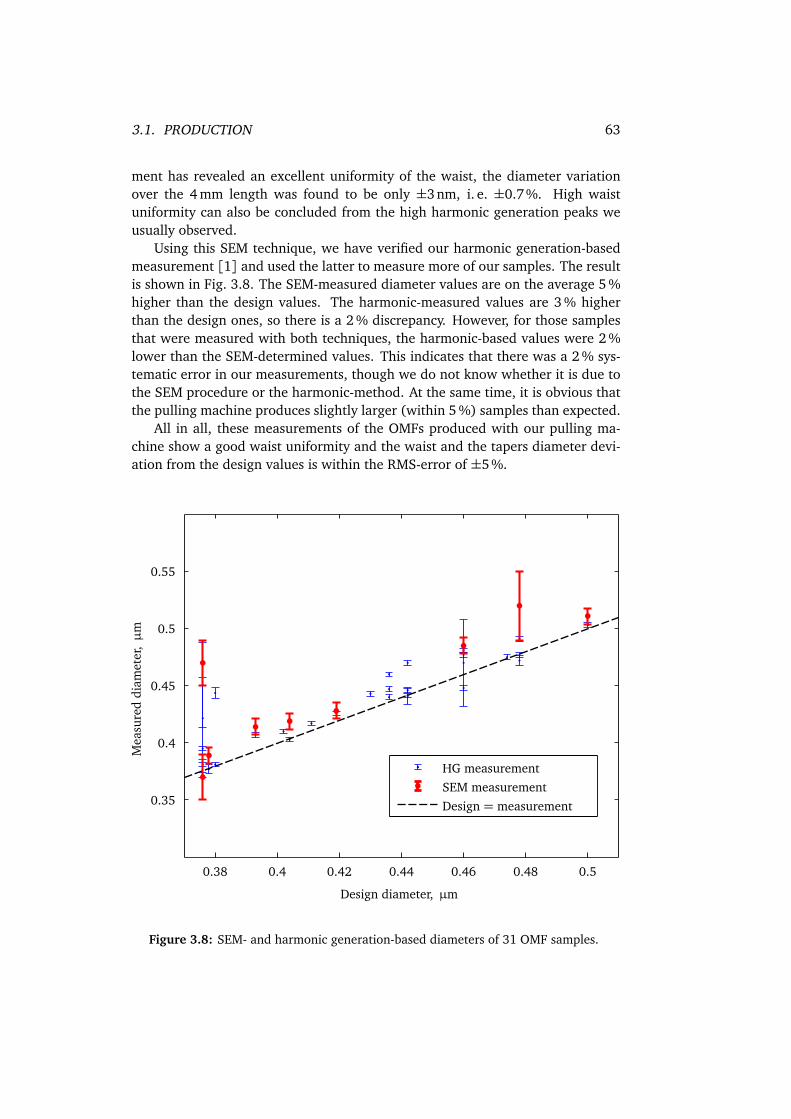
3.1. PRODUCTION 63
ment has revealed an excellent uniformity of the waist, the diameter variationover the 4 mm length was found to be only ±3nm, i. e. ±0.7%. High waistuniformity can also be concluded from the high harmonic generation peaks weusually observed.
Using this SEM technique, we have verified our harmonic generation-basedmeasurement [1] and used the latter to measure more of our samples. The resultis shown in Fig. 3.8. The SEM-measured diameter values are on the average 5 %higher than the design values. The harmonic-measured values are 3 % higherthan the design ones, so there is a 2 % discrepancy. However, for those samplesthat were measured with both techniques, the harmonic-based values were 2 %lower than the SEM-determined values. This indicates that there was a 2 % sys-tematic error in our measurements, though we do not know whether it is due tothe SEM procedure or the harmonic-method. At the same time, it is obvious thatthe pulling machine produces slightly larger (within 5 %) samples than expected.
All in all, these measurements of the OMFs produced with our pulling ma-chine show a good waist uniformity and the waist and the tapers diameter devi-ation from the design values is within the RMS-error of ±5%.
0.38 0.4 0.42 0.44 0.46 0.48 0.5
0.35
0.4
0.45
0.5
0.55
Design diameter, µm
Mea
sure
ddi
amet
er,µ
m
HG measurementSEM measurementDesign = measurement
Figure 3.8: SEM- and harmonic generation-based diameters of 31 OMF samples.
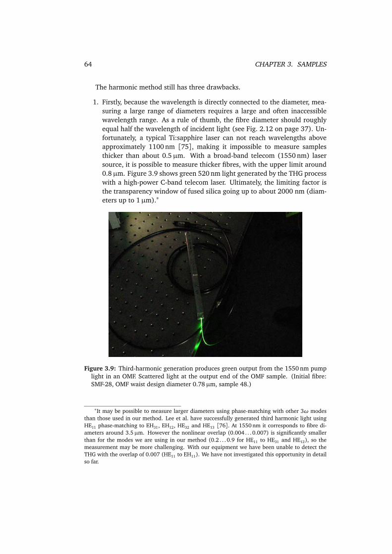
64 CHAPTER 3. SAMPLES
The harmonic method still has three drawbacks.
1. Firstly, because the wavelength is directly connected to the diameter, mea-suring a large range of diameters requires a large and often inaccessiblewavelength range. As a rule of thumb, the fibre diameter should roughlyequal half the wavelength of incident light (see Fig. 2.12 on page 37). Un-fortunately, a typical Ti:sapphire laser can not reach wavelengths aboveapproximately 1100 nm [75], making it impossible to measure samplesthicker than about 0.5µm. With a broad-band telecom (1550 nm) lasersource, it is possible to measure thicker fibres, with the upper limit around0.8µm. Figure 3.9 shows green 520 nm light generated by the THG processwith a high-power C-band telecom laser. Ultimately, the limiting factor isthe transparency window of fused silica going up to about 2000 nm (diam-eters up to 1µm).∗
Figure 3.9: Third-harmonic generation produces green output from the 1550 nm pumplight in an OMF. Scattered light at the output end of the OMF sample. (Initial fibre:SMF-28, OMF waist design diameter 0.78µm, sample 48.)
∗It may be possible to measure larger diameters using phase-matching with other 3ω modesthan those used in our method. Lee et al. have successfully generated third harmonic light usingHE11 phase-matching to EH31, EH12, HE32 and HE13 [76]. At 1550 nm it corresponds to fibre di-ameters around 3.5µm. However the nonlinear overlap (0.004 . . . 0.007) is significantly smallerthan for the modes we are using in our method (0.2 . . . 0.9 for HE11 to HE31 and HE12), so themeasurement may be more challenging. With our equipment we have been unable to detect theTHG with the overlap of 0.007 (HE11 to EH11). We have not investigated this opportunity in detailso far.
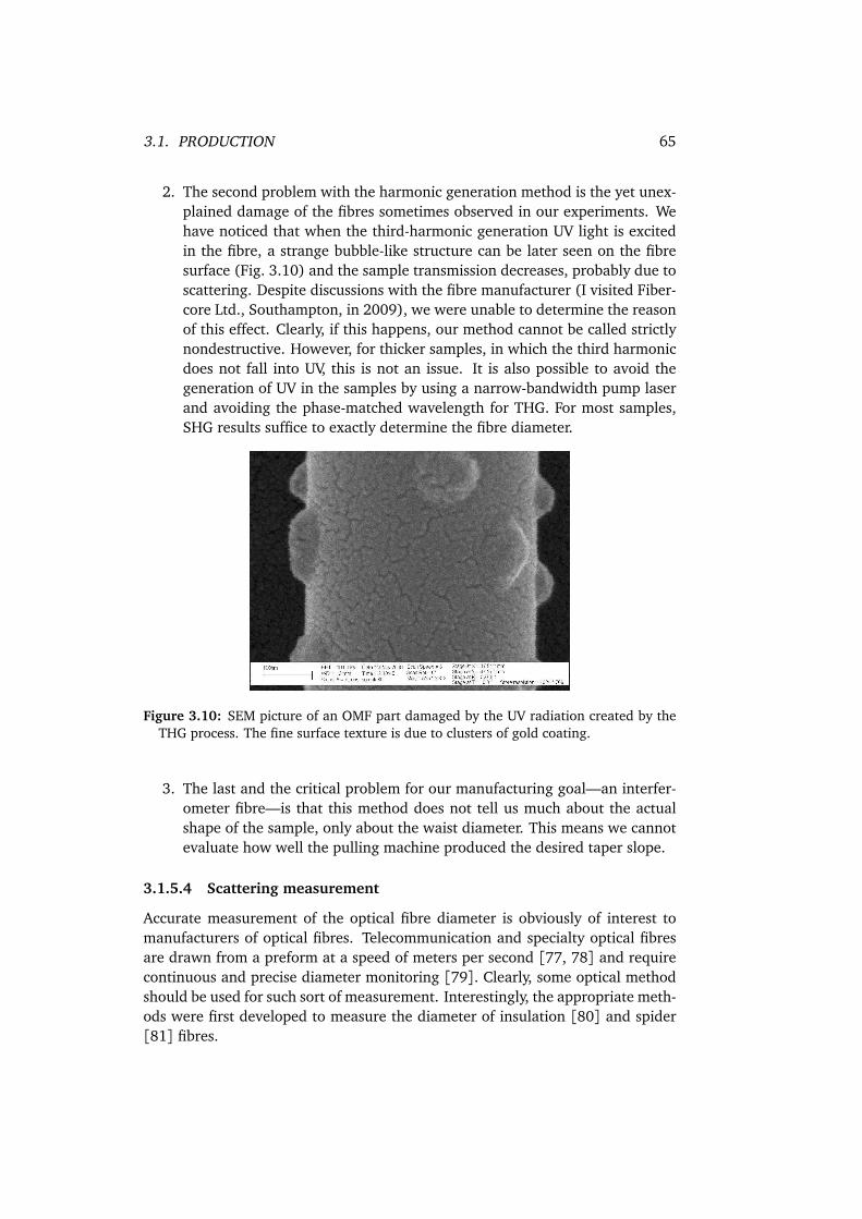
3.1. PRODUCTION 65
2. The second problem with the harmonic generation method is the yet unex-plained damage of the fibres sometimes observed in our experiments. Wehave noticed that when the third-harmonic generation UV light is excitedin the fibre, a strange bubble-like structure can be later seen on the fibresurface (Fig. 3.10) and the sample transmission decreases, probably due toscattering. Despite discussions with the fibre manufacturer (I visited Fiber-core Ltd., Southampton, in 2009), we were unable to determine the reasonof this effect. Clearly, if this happens, our method cannot be called strictlynondestructive. However, for thicker samples, in which the third harmonicdoes not fall into UV, this is not an issue. It is also possible to avoid thegeneration of UV in the samples by using a narrow-bandwidth pump laserand avoiding the phase-matched wavelength for THG. For most samples,SHG results suffice to exactly determine the fibre diameter.
Figure 3.10: SEM picture of an OMF part damaged by the UV radiation created by theTHG process. The fine surface texture is due to clusters of gold coating.
3. The last and the critical problem for our manufacturing goal—an interfer-ometer fibre—is that this method does not tell us much about the actualshape of the sample, only about the waist diameter. This means we cannotevaluate how well the pulling machine produced the desired taper slope.
3.1.5.4 Scattering measurement
Accurate measurement of the optical fibre diameter is obviously of interest tomanufacturers of optical fibres. Telecommunication and specialty optical fibresare drawn from a preform at a speed of meters per second [77, 78] and requirecontinuous and precise diameter monitoring [79]. Clearly, some optical methodshould be used for such sort of measurement. Interestingly, the appropriate meth-ods were first developed to measure the diameter of insulation [80] and spider[81] fibres.
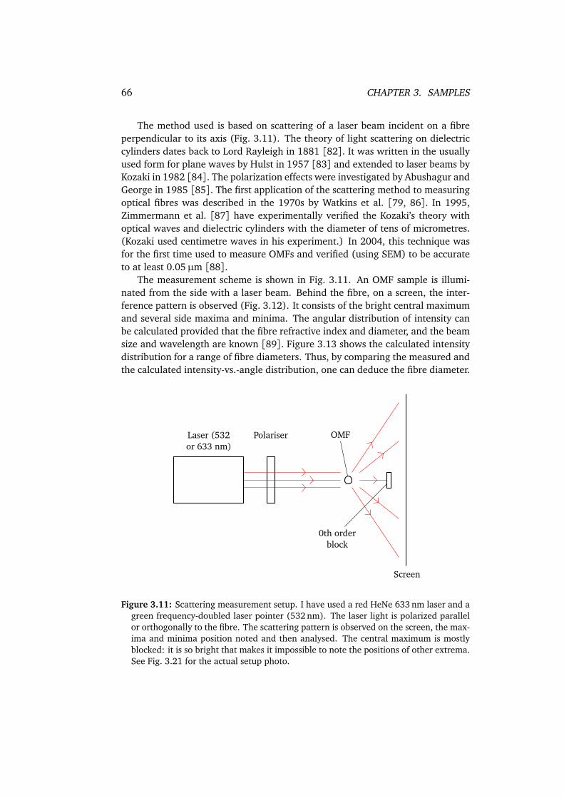
66 CHAPTER 3. SAMPLES
The method used is based on scattering of a laser beam incident on a fibreperpendicular to its axis (Fig. 3.11). The theory of light scattering on dielectriccylinders dates back to Lord Rayleigh in 1881 [82]. It was written in the usuallyused form for plane waves by Hulst in 1957 [83] and extended to laser beams byKozaki in 1982 [84]. The polarization effects were investigated by Abushagur andGeorge in 1985 [85]. The first application of the scattering method to measuringoptical fibres was described in the 1970s by Watkins et al. [79, 86]. In 1995,Zimmermann et al. [87] have experimentally verified the Kozaki’s theory withoptical waves and dielectric cylinders with the diameter of tens of micrometres.(Kozaki used centimetre waves in his experiment.) In 2004, this technique wasfor the first time used to measure OMFs and verified (using SEM) to be accurateto at least 0.05µm [88].
The measurement scheme is shown in Fig. 3.11. An OMF sample is illumi-nated from the side with a laser beam. Behind the fibre, on a screen, the inter-ference pattern is observed (Fig. 3.12). It consists of the bright central maximumand several side maxima and minima. The angular distribution of intensity canbe calculated provided that the fibre refractive index and diameter, and the beamsize and wavelength are known [89]. Figure 3.13 shows the calculated intensitydistribution for a range of fibre diameters. Thus, by comparing the measured andthe calculated intensity-vs.-angle distribution, one can deduce the fibre diameter.
Laser (532or 633 nm)
Polariser OMF
Screen
0th orderblock
Figure 3.11: Scattering measurement setup. I have used a red HeNe 633 nm laser and agreen frequency-doubled laser pointer (532 nm). The laser light is polarized parallelor orthogonally to the fibre. The scattering pattern is observed on the screen, the max-ima and minima position noted and then analysed. The central maximum is mostlyblocked: it is so bright that makes it impossible to note the positions of other extrema.See Fig. 3.21 for the actual setup photo.
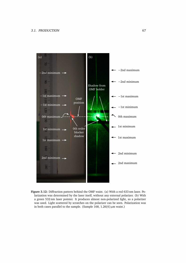
3.1. PRODUCTION 67
0th maximum
1st minimum
1st maximum
2nd minimum
−1st minimum
−1st maximum
−2nd minimum
0th maximum
1st minimum
1st maximum
2nd minimum
−1st minimum
−1st maximum
−2nd minimum
−2nd maximum
2nd maximum
(b)(a)
Shadow fromOMF holder
0th orderblockershadow
OMFposition
Figure 3.12: Diffraction pattern behind the OMF waist. (a) With a red 633 nm laser. Po-larization was determined by the laser itself, without any external polarizer. (b) Witha green 532 nm laser pointer. It produces almost non-polarized light, so a polarizerwas used. Light scattered by scratches on the polarizer can be seen. Polarization wasin both cases parallel to the sample. (Sample 168, 1.26(6)µm waist.)
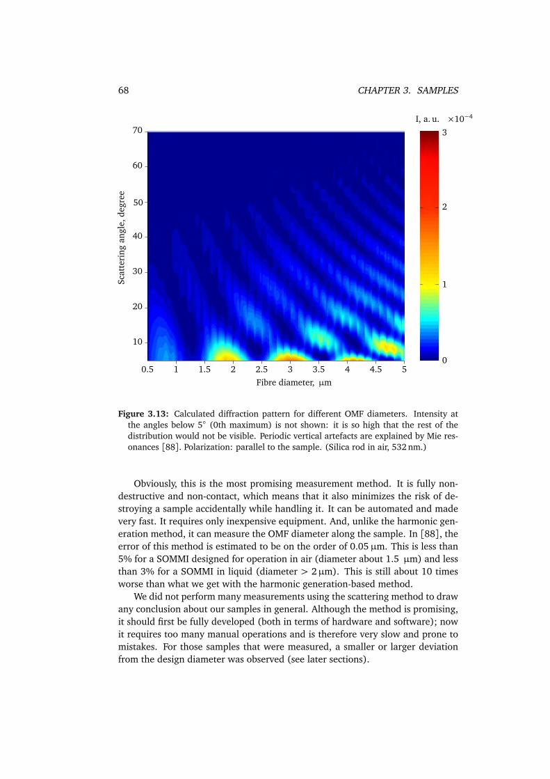
68 CHAPTER 3. SAMPLES
0.5 1 1.5 2 2.5 3 3.5 4 4.5 5
10
20
30
40
60
70
0
1
2
3
×10−4
50
Scat
teri
ngan
gle,
degr
ee
Fibre diameter, µm
I, a. u.
Figure 3.13: Calculated diffraction pattern for different OMF diameters. Intensity atthe angles below 5 (0th maximum) is not shown: it is so high that the rest of thedistribution would not be visible. Periodic vertical artefacts are explained by Mie res-onances [88]. Polarization: parallel to the sample. (Silica rod in air, 532 nm.)
Obviously, this is the most promising measurement method. It is fully non-destructive and non-contact, which means that it also minimizes the risk of de-stroying a sample accidentally while handling it. It can be automated and madevery fast. It requires only inexpensive equipment. And, unlike the harmonic gen-eration method, it can measure the OMF diameter along the sample. In [88], theerror of this method is estimated to be on the order of 0.05µm. This is less than5% for a SOMMI designed for operation in air (diameter about 1.5 µm) and lessthan 3% for a SOMMI in liquid (diameter > 2µm). This is still about 10 timesworse than what we get with the harmonic generation-based method.
We did not perform many measurements using the scattering method to drawany conclusion about our samples in general. Although the method is promising,it should first be fully developed (both in terms of hardware and software); nowit requires too many manual operations and is therefore very slow and prone tomistakes. For those samples that were measured, a smaller or larger deviationfrom the design diameter was observed (see later sections).
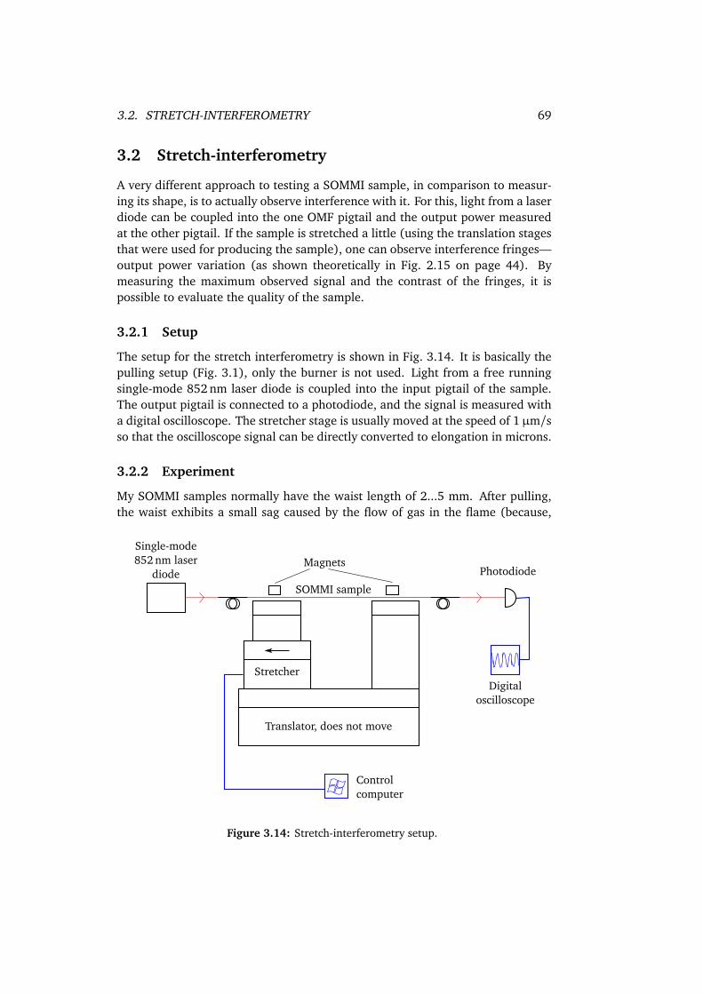
3.2. STRETCH-INTERFEROMETRY 69
3.2 Stretch-interferometry
A very different approach to testing a SOMMI sample, in comparison to measur-ing its shape, is to actually observe interference with it. For this, light from a laserdiode can be coupled into the one OMF pigtail and the output power measuredat the other pigtail. If the sample is stretched a little (using the translation stagesthat were used for producing the sample), one can observe interference fringes—output power variation (as shown theoretically in Fig. 2.15 on page 44). Bymeasuring the maximum observed signal and the contrast of the fringes, it ispossible to evaluate the quality of the sample.
3.2.1 Setup
The setup for the stretch interferometry is shown in Fig. 3.14. It is basically thepulling setup (Fig. 3.1), only the burner is not used. Light from a free runningsingle-mode 852 nm laser diode is coupled into the input pigtail of the sample.The output pigtail is connected to a photodiode, and the signal is measured witha digital oscilloscope. The stretcher stage is usually moved at the speed of 1µm/sso that the oscilloscope signal can be directly converted to elongation in microns.
3.2.2 Experiment
My SOMMI samples normally have the waist length of 2...5 mm. After pulling,the waist exhibits a small sag caused by the flow of gas in the flame (because,
Stretcher
Magnets
SOMMI sample
Controlcomputer
Single-mode852 nm laser
diode Photodiode
Digitaloscilloscope
Translator, does not move
Figure 3.14: Stretch-interferometry setup.
70 CHAPTER 3. SAMPLES
during tapering, the fibre is pulled a little more than just by the stages). The thin-ner the waist, the larger is this sag. To straighten the samples, we stretch thema little after switching the burner off. As long as the waist is sagging, the stagescan be moved apart without actual elongation of the fibre, therefore the photo-diode signal remains constant. A movement of 20 . . . 30µm is usually enoughto straighten the waist. As soon as the sag disappears, further movement of thestretcher results in the actual elongation of the sample, which can be immediatelyseen as the variation of the output power according to Eq. (2.12):
I(∆L)∼ A+ B cos
2π
λ(L+∆L)∆neff
,
where ∆L is the fibre elongation. The photodiode response recorded duringstretching is shown in Fig. 3.15.
We discovered experimentally that the samples, which have the waist lengthof 2 . . . 5 mm, can be stretched by approximately 400 . . . 500µm before they tear.The oscillation period is about 5µm. Therefore, to perform the stretch-interfe-rometry, I usually elongated the fibre by 50 . . . 100µm, which was not more than5 % of the waist length and less than 0.2 % of the total sample length. Thereforeit is safe to assume that the elongation is elastic.
To check the last assumption, I also performed multiple stretch-destretchcycles and verified that the harmonic signal fully reproduced itself in the de-stretching measurement. Of course, there may be a long-term influence on the fi-bre, which cannot be detected using this method. Therefore I always de-stretchedthe fibre to the original straight state before fixing it in the fibre holder.
3.2.3 Results and analysis
Figure 3.15 shows the stretch-signal for one of our samples. By fitting a sine waveto this curve, a fringe period of 3.95µm is obtained. This particular sample wasdesigned to have a waist of 1.3µm diameter, 2 mm waist length, and 16 mradtapers. Simulation for this shape according to Sec. 2.5.4 gives the fringe periodof 4.1µm (4 % deviation from the measured value).
Table 3.3 shows the result of analysis of 12 samples pulled with almost thesame parameters: 16 mrad tapers and 1.3µm waist diameter. In all cases but onethe simulated result is within the error-bar of the measured one.
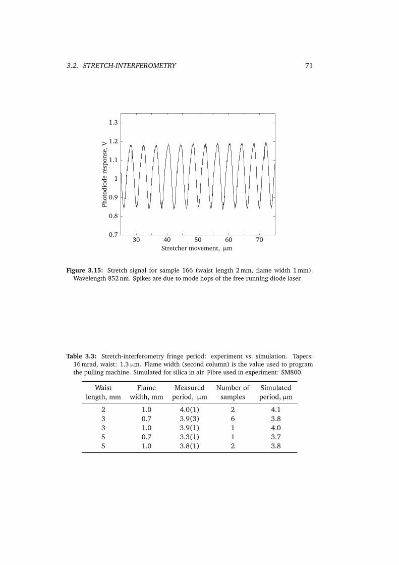
3.2. STRETCH-INTERFEROMETRY 71
Stretcher movement, µm
Phot
odio
dere
spon
se,V
30 40 50 60 700.7
0.8
0.9
1
1.1
1.2
1.3
Figure 3.15: Stretch signal for sample 166 (waist length 2 mm, flame width 1 mm).Wavelength 852 nm. Spikes are due to mode hops of the free-running diode laser.
Table 3.3: Stretch-interferometry fringe period: experiment vs. simulation. Tapers:16 mrad, waist: 1.3µm. Flame width (second column) is the value used to programthe pulling machine. Simulated for silica in air. Fibre used in experiment: SM800.
Waistlength, mm
Flamewidth, mm
Measuredperiod, µm
Number ofsamples
Simulatedperiod,µm
2 1.0 4.0(1) 2 4.13 0.7 3.9(3) 6 3.83 1.0 3.9(1) 1 4.05 0.7 3.3(1) 1 3.75 1.0 3.8(1) 2 3.8
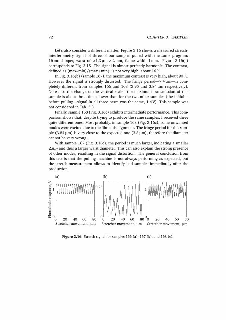
72 CHAPTER 3. SAMPLES
Let’s also consider a different matter. Figure 3.16 shows a measured stretch-interferometry signal of three of our samples pulled with the same program:16 mrad taper, waist of 1.3µm ×2 mm, flame width 1 mm. Figure 3.16(a)corresponds to Fig. 3.15. The signal is almost perfectly harmonic. The contrast,defined as (max–min)/(max+min), is not very high, about 16 %.
In Fig. 3.16(b) (sample 167), the maximum contrast is very high, about 90 %.However the signal is strongly distorted. The fringe period—7.4µm—is com-pletely different from samples 166 and 168 (3.95 and 3.84µm respectively).Note also the change of the vertical scale: the maximum transmission of thissample is about three times lower than for the two other samples (the initial—before pulling—signal in all three cases was the same, 1.4 V). This sample wasnot considered in Tab. 3.3.
Finally, sample 168 (Fig. 3.16c) exhibits intermediate performance. This com-parison shows that, despite trying to produce the same samples, I received threequite different ones. Most probably, in sample 168 (Fig. 3.16c), some unwantedmodes were excited due to the fibre misalignment. The fringe period for this sam-ple (3.84µm) is very close to the expected one (3.8µm), therefore the diametercannot be very wrong.
With sample 167 (Fig. 3.16c), the period is much larger, indicating a smaller∆neff and thus a larger waist diameter. This can also explain the strong presenceof other modes, resulting in the signal distortion. The general conclusion fromthis test is that the pulling machine is not always performing as expected, butthe stretch-measurement allows to identify bad samples immediately after theproduction.
Stretcher movement, µm Stretcher movement, µm Stretcher movement, µm
Phot
odio
dere
spon
se,V
0
1
0 8020 40 60
(a) (b) (c)
0
0.25
0
1
0 8020 40 60 0 8020 40 60
Figure 3.16: Stretch signal for samples 166 (a), 167 (b), and 168 (c).
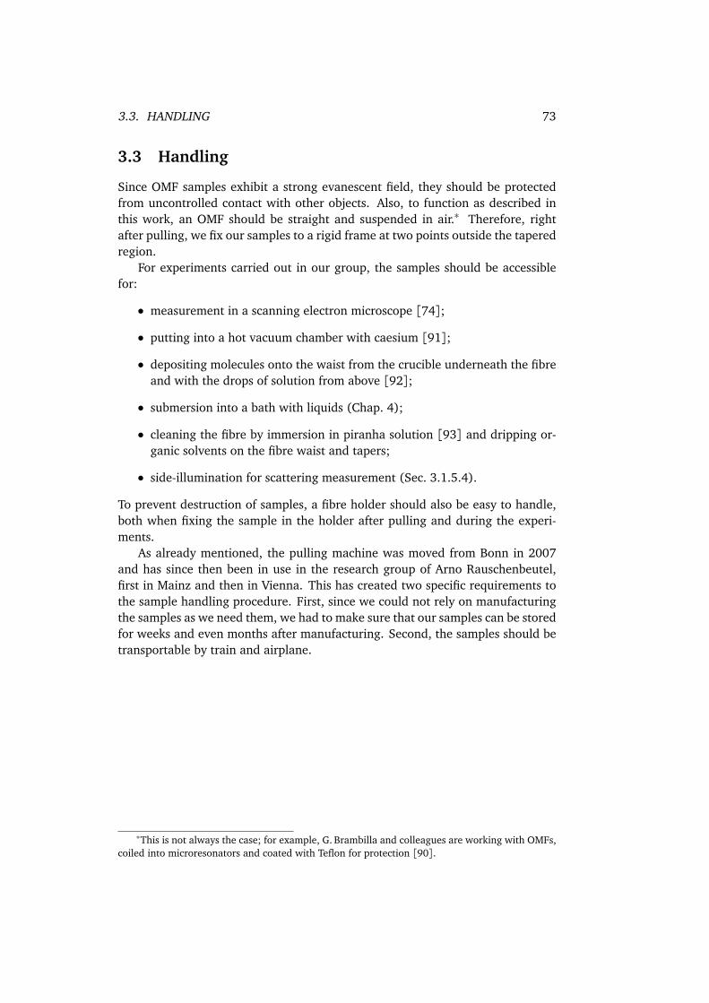
3.3. HANDLING 73
3.3 Handling
Since OMF samples exhibit a strong evanescent field, they should be protectedfrom uncontrolled contact with other objects. Also, to function as described inthis work, an OMF should be straight and suspended in air.∗ Therefore, rightafter pulling, we fix our samples to a rigid frame at two points outside the taperedregion.
For experiments carried out in our group, the samples should be accessiblefor:
• measurement in a scanning electron microscope [74];
• putting into a hot vacuum chamber with caesium [91];
• depositing molecules onto the waist from the crucible underneath the fibreand with the drops of solution from above [92];
• submersion into a bath with liquids (Chap. 4);
• cleaning the fibre by immersion in piranha solution [93] and dripping or-ganic solvents on the fibre waist and tapers;
• side-illumination for scattering measurement (Sec. 3.1.5.4).
To prevent destruction of samples, a fibre holder should also be easy to handle,both when fixing the sample in the holder after pulling and during the experi-ments.
As already mentioned, the pulling machine was moved from Bonn in 2007and has since then been in use in the research group of Arno Rauschenbeutel,first in Mainz and then in Vienna. This has created two specific requirements tothe sample handling procedure. First, since we could not rely on manufacturingthe samples as we need them, we had to make sure that our samples can be storedfor weeks and even months after manufacturing. Second, the samples should betransportable by train and airplane.
∗This is not always the case; for example, G. Brambilla and colleagues are working with OMFs,coiled into microresonators and coated with Teflon for protection [90].
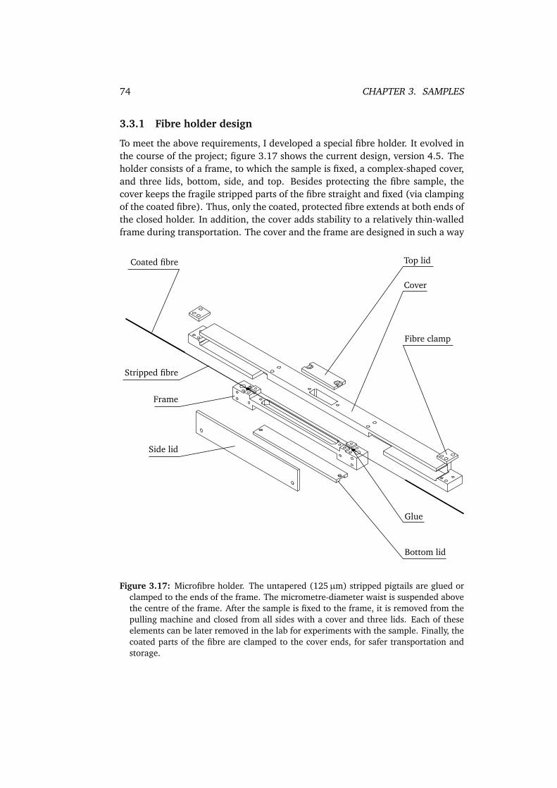
74 CHAPTER 3. SAMPLES
3.3.1 Fibre holder design
To meet the above requirements, I developed a special fibre holder. It evolved inthe course of the project; figure 3.17 shows the current design, version 4.5. Theholder consists of a frame, to which the sample is fixed, a complex-shaped cover,and three lids, bottom, side, and top. Besides protecting the fibre sample, thecover keeps the fragile stripped parts of the fibre straight and fixed (via clampingof the coated fibre). Thus, only the coated, protected fibre extends at both ends ofthe closed holder. In addition, the cover adds stability to a relatively thin-walledframe during transportation. The cover and the frame are designed in such a way
Top lid
Cover
Fibre clamp
Frame
Coated fibre
Stripped fibre
Side lid
Bottom lid
Glue
Figure 3.17: Microfibre holder. The untapered (125µm) stripped pigtails are glued orclamped to the ends of the frame. The micrometre-diameter waist is suspended abovethe centre of the frame. After the sample is fixed to the frame, it is removed from thepulling machine and closed from all sides with a cover and three lids. Each of theseelements can be later removed in the lab for experiments with the sample. Finally, thecoated parts of the fibre are clamped to the cover ends, for safer transportation andstorage.
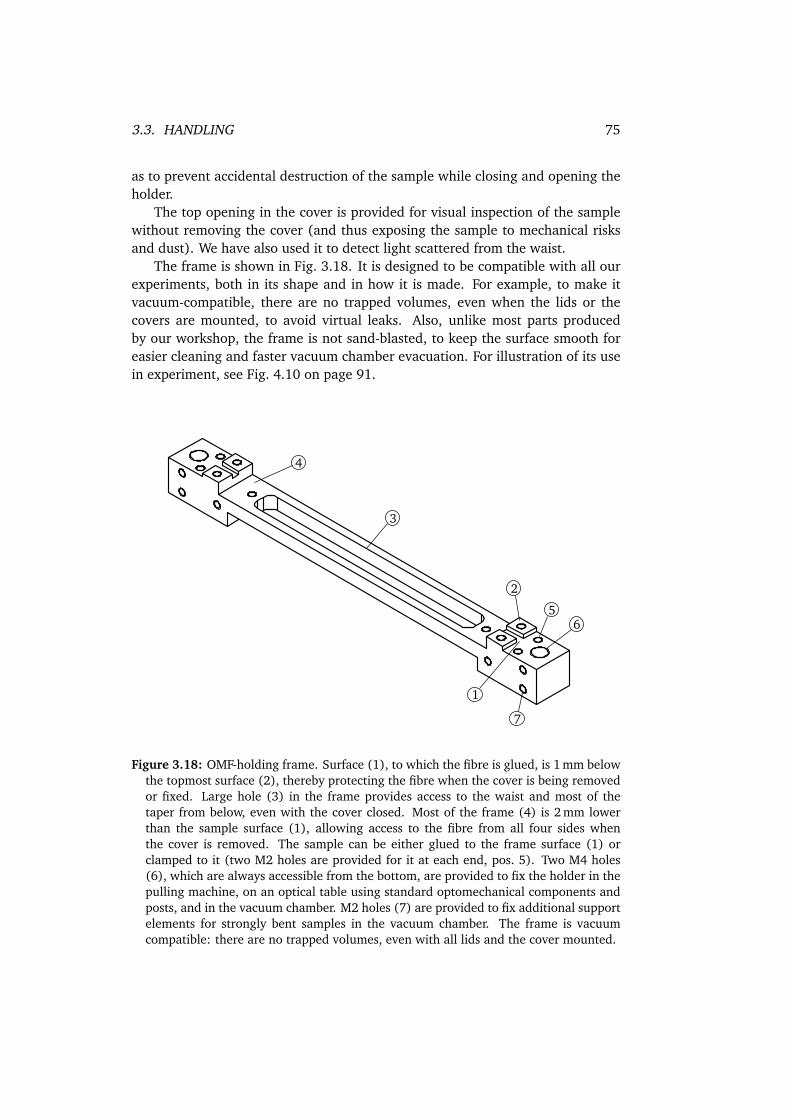
3.3. HANDLING 75
as to prevent accidental destruction of the sample while closing and opening theholder.
The top opening in the cover is provided for visual inspection of the samplewithout removing the cover (and thus exposing the sample to mechanical risksand dust). We have also used it to detect light scattered from the waist.
The frame is shown in Fig. 3.18. It is designed to be compatible with all ourexperiments, both in its shape and in how it is made. For example, to make itvacuum-compatible, there are no trapped volumes, even when the lids or thecovers are mounted, to avoid virtual leaks. Also, unlike most parts producedby our workshop, the frame is not sand-blasted, to keep the surface smooth foreasier cleaning and faster vacuum chamber evacuation. For illustration of its usein experiment, see Fig. 4.10 on page 91.
6
7
3
4
2
1
5
Figure 3.18: OMF-holding frame. Surface (1), to which the fibre is glued, is 1 mm belowthe topmost surface (2), thereby protecting the fibre when the cover is being removedor fixed. Large hole (3) in the frame provides access to the waist and most of thetaper from below, even with the cover closed. Most of the frame (4) is 2 mm lowerthan the sample surface (1), allowing access to the fibre from all four sides whenthe cover is removed. The sample can be either glued to the frame surface (1) orclamped to it (two M2 holes are provided for it at each end, pos. 5). Two M4 holes(6), which are always accessible from the bottom, are provided to fix the holder in thepulling machine, on an optical table using standard optomechanical components andposts, and in the vacuum chamber. M2 holes (7) are provided to fix additional supportelements for strongly bent samples in the vacuum chamber. The frame is vacuumcompatible: there are no trapped volumes, even with all lids and the cover mounted.
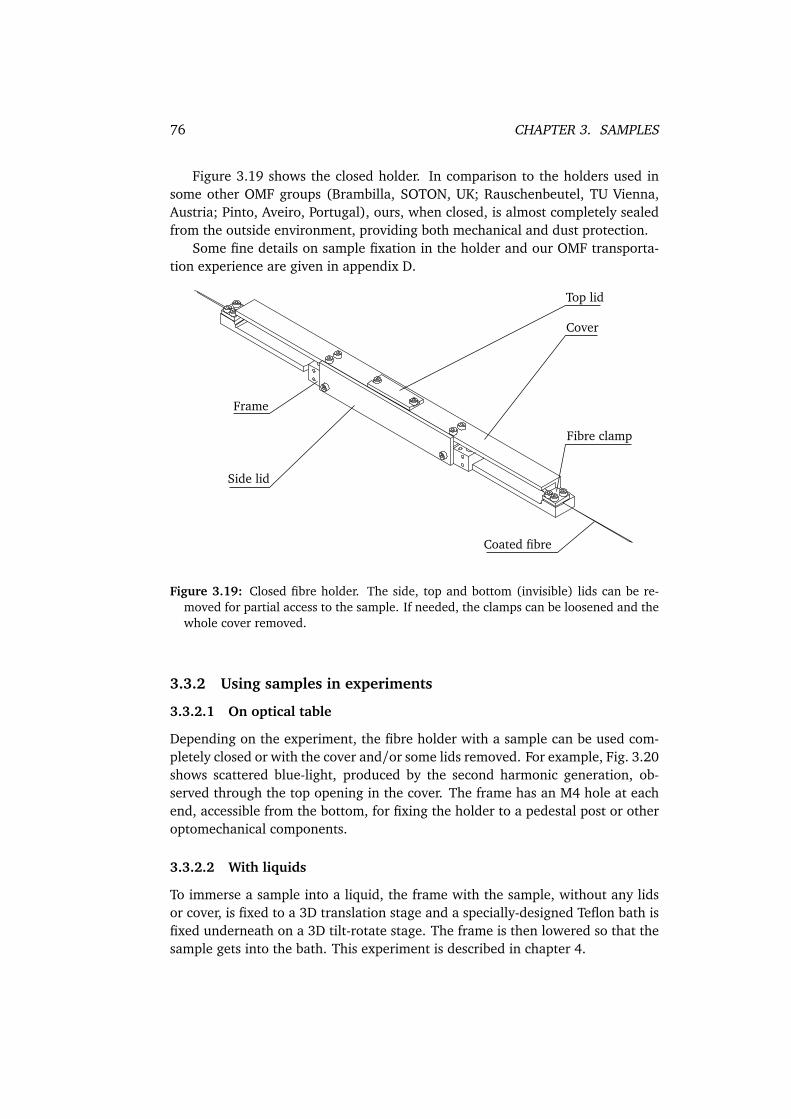
76 CHAPTER 3. SAMPLES
Figure 3.19 shows the closed holder. In comparison to the holders used insome other OMF groups (Brambilla, SOTON, UK; Rauschenbeutel, TU Vienna,Austria; Pinto, Aveiro, Portugal), ours, when closed, is almost completely sealedfrom the outside environment, providing both mechanical and dust protection.
Some fine details on sample fixation in the holder and our OMF transporta-tion experience are given in appendix D.
Frame
Cover
Top lid
Side lid
Fibre clamp
Coated fibre
Figure 3.19: Closed fibre holder. The side, top and bottom (invisible) lids can be re-moved for partial access to the sample. If needed, the clamps can be loosened and thewhole cover removed.
3.3.2 Using samples in experiments
3.3.2.1 On optical table
Depending on the experiment, the fibre holder with a sample can be used com-pletely closed or with the cover and/or some lids removed. For example, Fig. 3.20shows scattered blue-light, produced by the second harmonic generation, ob-served through the top opening in the cover. The frame has an M4 hole at eachend, accessible from the bottom, for fixing the holder to a pedestal post or otheroptomechanical components.
3.3.2.2 With liquids
To immerse a sample into a liquid, the frame with the sample, without any lidsor cover, is fixed to a 3D translation stage and a specially-designed Teflon bath isfixed underneath on a 3D tilt-rotate stage. The frame is then lowered so that thesample gets into the bath. This experiment is described in chapter 4.
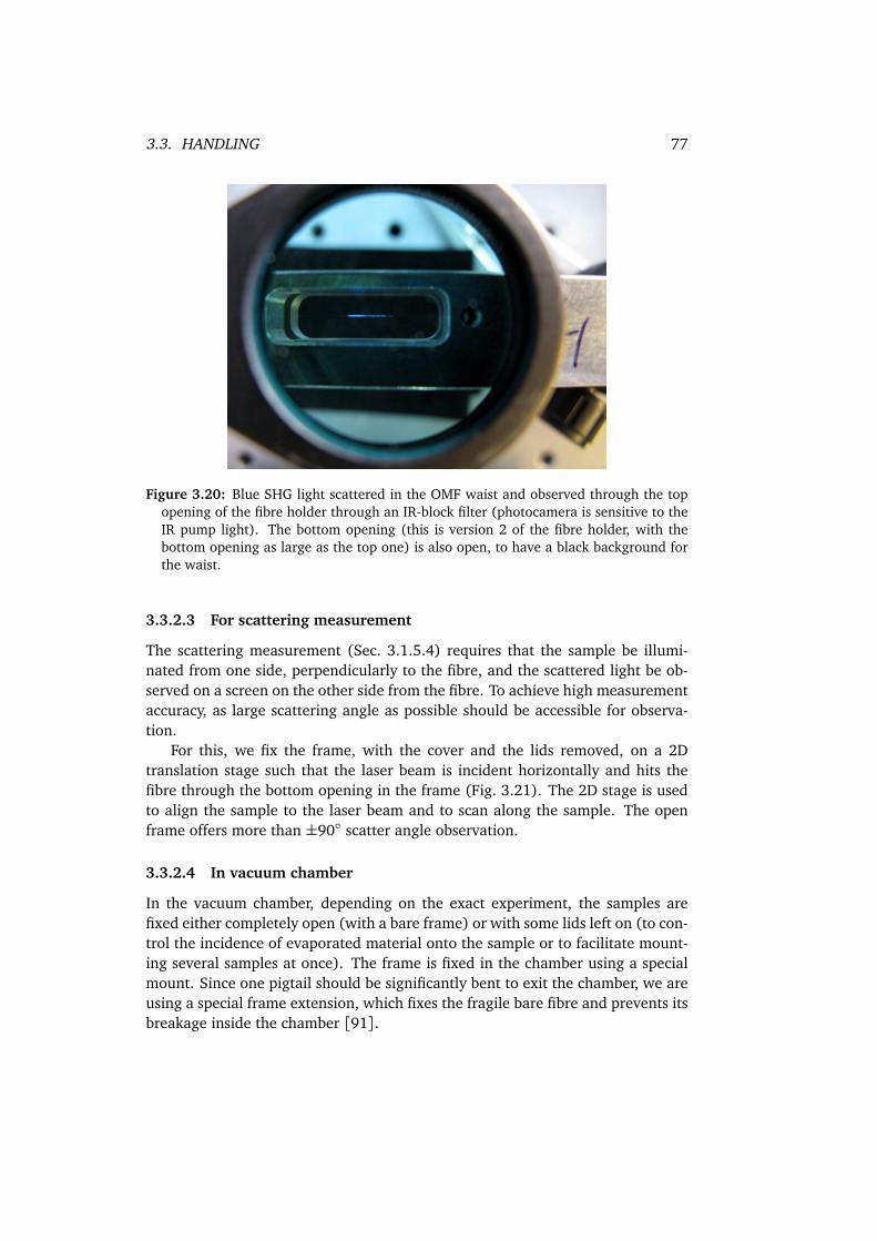
3.3. HANDLING 77
Figure 3.20: Blue SHG light scattered in the OMF waist and observed through the topopening of the fibre holder through an IR-block filter (photocamera is sensitive to theIR pump light). The bottom opening (this is version 2 of the fibre holder, with thebottom opening as large as the top one) is also open, to have a black background forthe waist.
3.3.2.3 For scattering measurement
The scattering measurement (Sec. 3.1.5.4) requires that the sample be illumi-nated from one side, perpendicularly to the fibre, and the scattered light be ob-served on a screen on the other side from the fibre. To achieve high measurementaccuracy, as large scattering angle as possible should be accessible for observa-tion.
For this, we fix the frame, with the cover and the lids removed, on a 2Dtranslation stage such that the laser beam is incident horizontally and hits thefibre through the bottom opening in the frame (Fig. 3.21). The 2D stage is usedto align the sample to the laser beam and to scan along the sample. The openframe offers more than ±90 scatter angle observation.
3.3.2.4 In vacuum chamber
In the vacuum chamber, depending on the exact experiment, the samples arefixed either completely open (with a bare frame) or with some lids left on (to con-trol the incidence of evaporated material onto the sample or to facilitate mount-ing several samples at once). The frame is fixed in the chamber using a specialmount. Since one pigtail should be significantly bent to exit the chamber, we areusing a special frame extension, which fixes the fragile bare fibre and prevents itsbreakage inside the chamber [91].
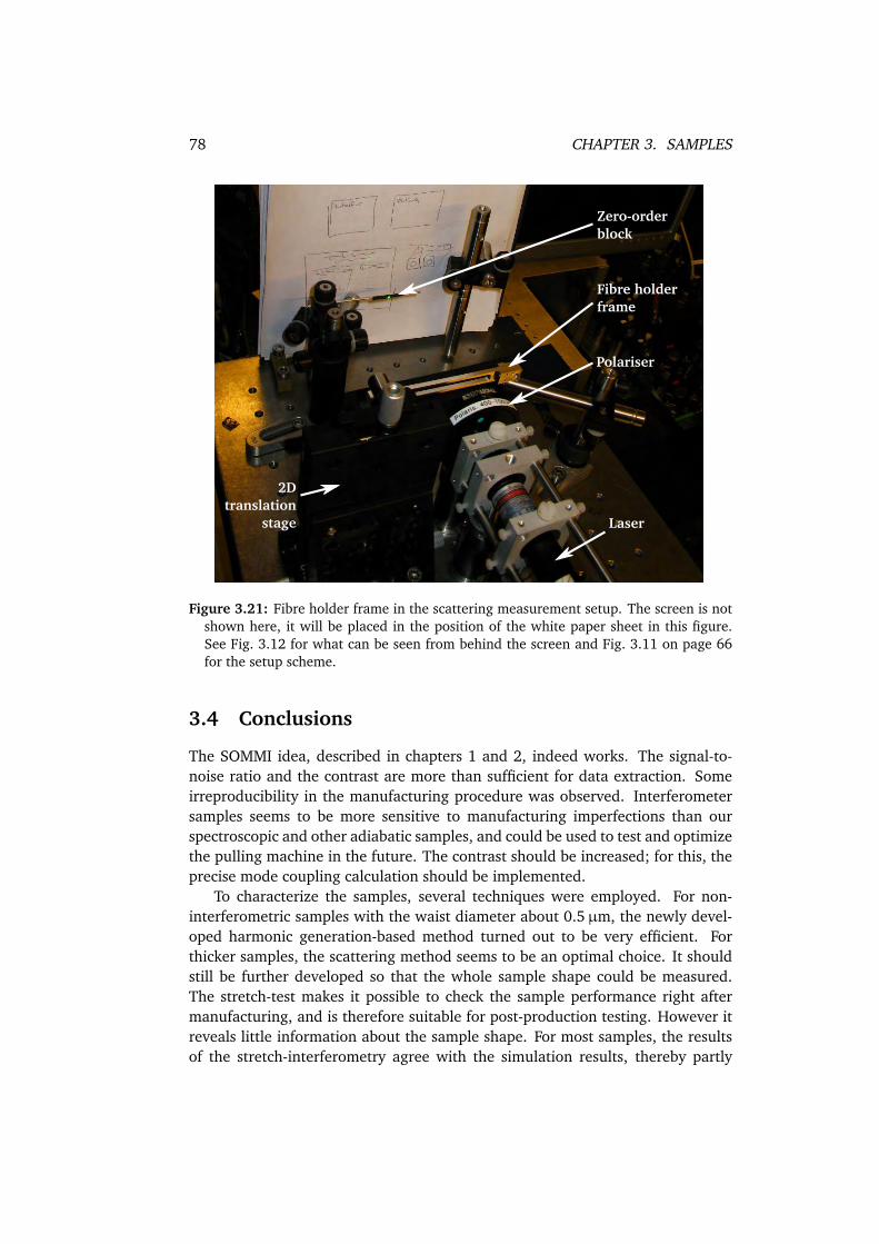
78 CHAPTER 3. SAMPLES
Laser
Polariser
Fibre holderframe
Zero-orderblock
2Dtranslation
stage
Figure 3.21: Fibre holder frame in the scattering measurement setup. The screen is notshown here, it will be placed in the position of the white paper sheet in this figure.See Fig. 3.12 for what can be seen from behind the screen and Fig. 3.11 on page 66for the setup scheme.
3.4 Conclusions
The SOMMI idea, described in chapters 1 and 2, indeed works. The signal-to-noise ratio and the contrast are more than sufficient for data extraction. Someirreproducibility in the manufacturing procedure was observed. Interferometersamples seems to be more sensitive to manufacturing imperfections than ourspectroscopic and other adiabatic samples, and could be used to test and optimizethe pulling machine in the future. The contrast should be increased; for this, theprecise mode coupling calculation should be implemented.
To characterize the samples, several techniques were employed. For non-interferometric samples with the waist diameter about 0.5µm, the newly devel-oped harmonic generation-based method turned out to be very efficient. Forthicker samples, the scattering method seems to be an optimal choice. It shouldstill be further developed so that the whole sample shape could be measured.The stretch-test makes it possible to check the sample performance right aftermanufacturing, and is therefore suitable for post-production testing. However itreveals little information about the sample shape. For most samples, the resultsof the stretch-interferometry agree with the simulation results, thereby partly

3.4. CONCLUSIONS 79
confirming the theory developed in chapter 2.Finally, a reliable sample handling procedure was developed. A special mul-
tipurpose fibre holder was designed, and proved to work well throughout thesample lifetime, from manufacturing to transporting to experiments in varioussetups and environments.

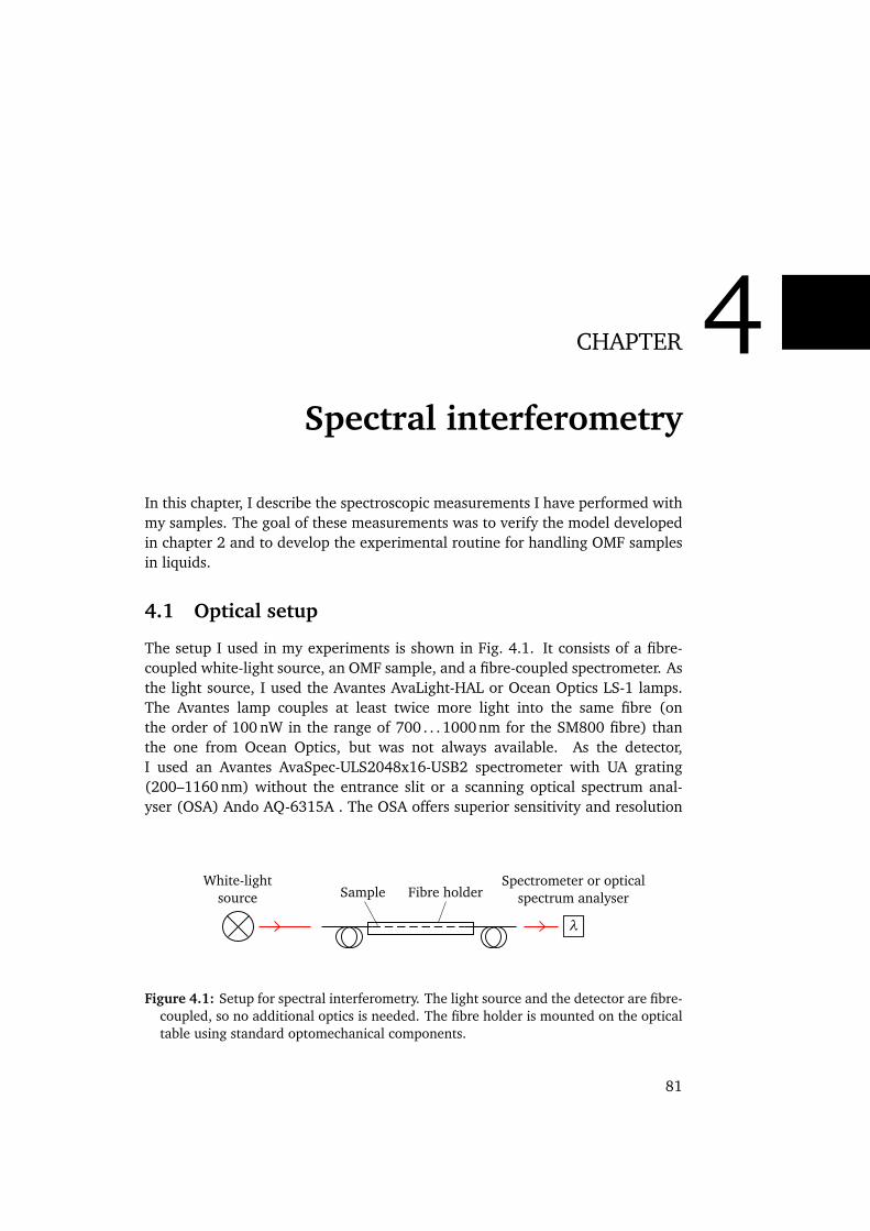
CHAPTER 4Spectral interferometry
In this chapter, I describe the spectroscopic measurements I have performed withmy samples. The goal of these measurements was to verify the model developedin chapter 2 and to develop the experimental routine for handling OMF samplesin liquids.
4.1 Optical setup
The setup I used in my experiments is shown in Fig. 4.1. It consists of a fibre-coupled white-light source, an OMF sample, and a fibre-coupled spectrometer. Asthe light source, I used the Avantes AvaLight-HAL or Ocean Optics LS-1 lamps.The Avantes lamp couples at least twice more light into the same fibre (onthe order of 100 nW in the range of 700 . . . 1000 nm for the SM800 fibre) thanthe one from Ocean Optics, but was not always available. As the detector,I used an Avantes AvaSpec-ULS2048x16-USB2 spectrometer with UA grating(200–1160 nm) without the entrance slit or a scanning optical spectrum anal-yser (OSA) Ando AQ-6315A . The OSA offers superior sensitivity and resolution
λ
SampleWhite-light
sourceSpectrometer or optical
spectrum analyserFibre holder
Figure 4.1: Setup for spectral interferometry. The light source and the detector are fibre-coupled, so no additional optics is needed. The fibre holder is mounted on the opticaltable using standard optomechanical components.
81
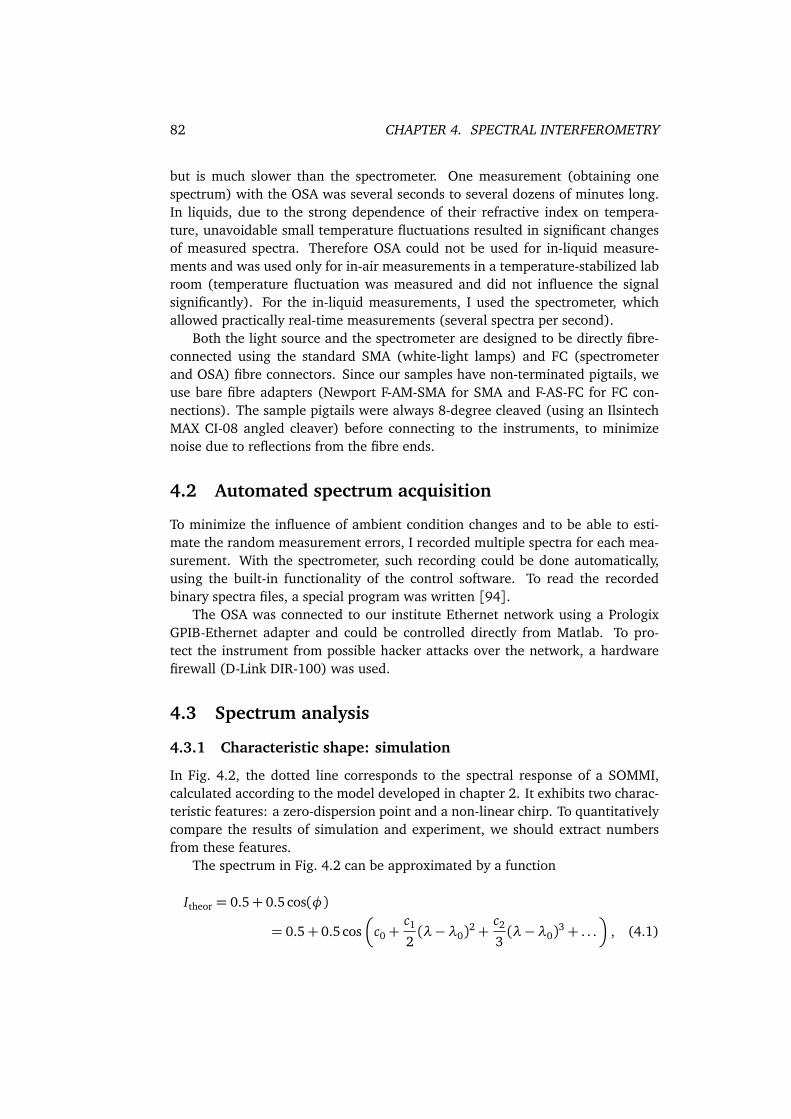
82 CHAPTER 4. SPECTRAL INTERFEROMETRY
but is much slower than the spectrometer. One measurement (obtaining onespectrum) with the OSA was several seconds to several dozens of minutes long.In liquids, due to the strong dependence of their refractive index on tempera-ture, unavoidable small temperature fluctuations resulted in significant changesof measured spectra. Therefore OSA could not be used for in-liquid measure-ments and was used only for in-air measurements in a temperature-stabilized labroom (temperature fluctuation was measured and did not influence the signalsignificantly). For the in-liquid measurements, I used the spectrometer, whichallowed practically real-time measurements (several spectra per second).
Both the light source and the spectrometer are designed to be directly fibre-connected using the standard SMA (white-light lamps) and FC (spectrometerand OSA) fibre connectors. Since our samples have non-terminated pigtails, weuse bare fibre adapters (Newport F-AM-SMA for SMA and F-AS-FC for FC con-nections). The sample pigtails were always 8-degree cleaved (using an IlsintechMAX CI-08 angled cleaver) before connecting to the instruments, to minimizenoise due to reflections from the fibre ends.
4.2 Automated spectrum acquisition
To minimize the influence of ambient condition changes and to be able to esti-mate the random measurement errors, I recorded multiple spectra for each mea-surement. With the spectrometer, such recording could be done automatically,using the built-in functionality of the control software. To read the recordedbinary spectra files, a special program was written [94].
The OSA was connected to our institute Ethernet network using a PrologixGPIB-Ethernet adapter and could be controlled directly from Matlab. To pro-tect the instrument from possible hacker attacks over the network, a hardwarefirewall (D-Link DIR-100) was used.
4.3 Spectrum analysis
4.3.1 Characteristic shape: simulation
In Fig. 4.2, the dotted line corresponds to the spectral response of a SOMMI,calculated according to the model developed in chapter 2. It exhibits two charac-teristic features: a zero-dispersion point and a non-linear chirp. To quantitativelycompare the results of simulation and experiment, we should extract numbersfrom these features.
The spectrum in Fig. 4.2 can be approximated by a function
Itheor = 0.5+ 0.5cos(φ)
= 0.5+ 0.5cos
c0+c1
2(λ−λ0)
2+c2
3(λ−λ0)
3+ . . .
, (4.1)
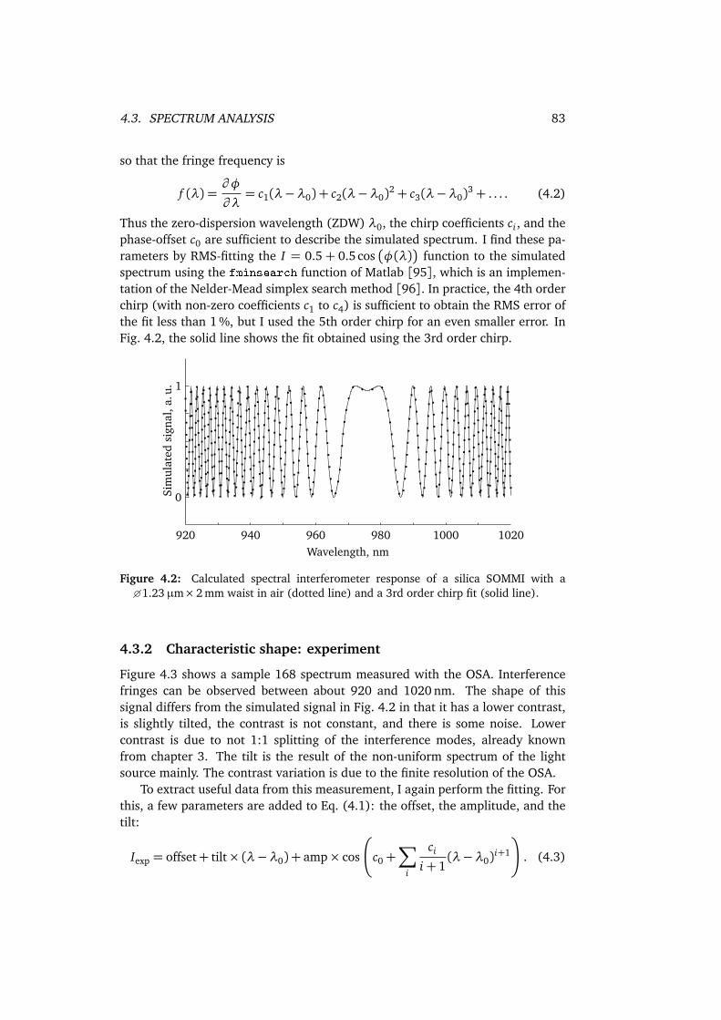
4.3. SPECTRUM ANALYSIS 83
so that the fringe frequency is
f (λ) =∂ φ
∂ λ= c1(λ−λ0) + c2(λ−λ0)
2+ c3(λ−λ0)3+ . . . . (4.2)
Thus the zero-dispersion wavelength (ZDW) λ0, the chirp coefficients ci , and thephase-offset c0 are sufficient to describe the simulated spectrum. I find these pa-rameters by RMS-fitting the I = 0.5+ 0.5cos
φ(λ)
function to the simulatedspectrum using the fminsearch function of Matlab [95], which is an implemen-tation of the Nelder-Mead simplex search method [96]. In practice, the 4th orderchirp (with non-zero coefficients c1 to c4) is sufficient to obtain the RMS error ofthe fit less than 1 %, but I used the 5th order chirp for an even smaller error. InFig. 4.2, the solid line shows the fit obtained using the 3rd order chirp.
Wavelength, nm
Sim
ulat
edsi
gnal
,a.u
.
920 940 960 980 1000 1020
0
1
Figure 4.2: Calculated spectral interferometer response of a silica SOMMI with a1.23µm× 2 mm waist in air (dotted line) and a 3rd order chirp fit (solid line).
4.3.2 Characteristic shape: experiment
Figure 4.3 shows a sample 168 spectrum measured with the OSA. Interferencefringes can be observed between about 920 and 1020 nm. The shape of thissignal differs from the simulated signal in Fig. 4.2 in that it has a lower contrast,is slightly tilted, the contrast is not constant, and there is some noise. Lowercontrast is due to not 1:1 splitting of the interference modes, already knownfrom chapter 3. The tilt is the result of the non-uniform spectrum of the lightsource mainly. The contrast variation is due to the finite resolution of the OSA.
To extract useful data from this measurement, I again perform the fitting. Forthis, a few parameters are added to Eq. (4.1): the offset, the amplitude, and thetilt:
Iexp = offset+ tilt× (λ−λ0) + amp× cos
c0+∑
i
ci
i+ 1(λ−λ0)
i+1
!
. (4.3)
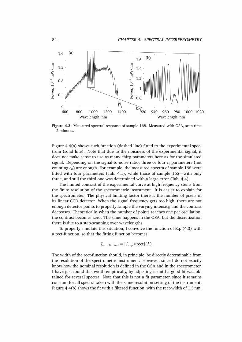
84 CHAPTER 4. SPECTRAL INTERFEROMETRY
Wavelength, nm
Pow
er,1
0−7
mW/n
m
600 800 1000 1200 1400Wavelength, nm
920 940 960 980 1000 1020
1.6
0
0.4
0.8
1.2
0.6
1.6
1.2
0.8
1
1.4
Pow
er,1
0−7
mW/n
m
(a)(b)
Figure 4.3: Measured spectral response of sample 168. Measured with OSA, scan time2 minutes.
Figure 4.4(a) shows such function (dashed line) fitted to the experimental spec-trum (solid line). Note that due to the noisiness of the experimental signal, itdoes not make sense to use as many chirp parameters here as for the simulatedsignal. Depending on the signal-to-noise ratio, three or four ci parameters (notcounting c0) are enough. For example, the measured spectra of sample 168 werefitted with four parameters (Tab. 4.1), while those of sample 165—with onlythree, and still the third one was determined with a large error (Tab. 4.4).
The limited contrast of the experimental curve at high frequency stems fromthe finite resolution of the spectrometric instrument. It is easier to explain forthe spectrometer. The physical limiting factor there is the number of pixels inits linear CCD detector. When the signal frequency gets too high, there are notenough detector points to properly sample the varying intensity, and the contrastdecreases. Theoretically, when the number of points reaches one per oscillation,the contrast becomes zero. The same happens in the OSA, but the discretizationthere is due to a step-scanning over wavelengths.
To properly simulate this situation, I convolve the function of Eq. (4.3) witha rect-function, so that the fitting function becomes
Iexp, limited = [Iexp ∗ rect](λ).
The width of the rect-function should, in principle, be directly determinable fromthe resolution of the spectrometric instrument. However, since I do not exactlyknow how the nominal resolution is defined in the OSA and in the spectrometer,I have just found this width empirically, by adjusting it until a good fit was ob-tained for several spectra. Note that this is not a fit parameter, since it remainsconstant for all spectra taken with the same resolution setting of the instrument.Figure 4.4(b) shows the fit with a filtered function, with the rect-width of 1.5 nm.
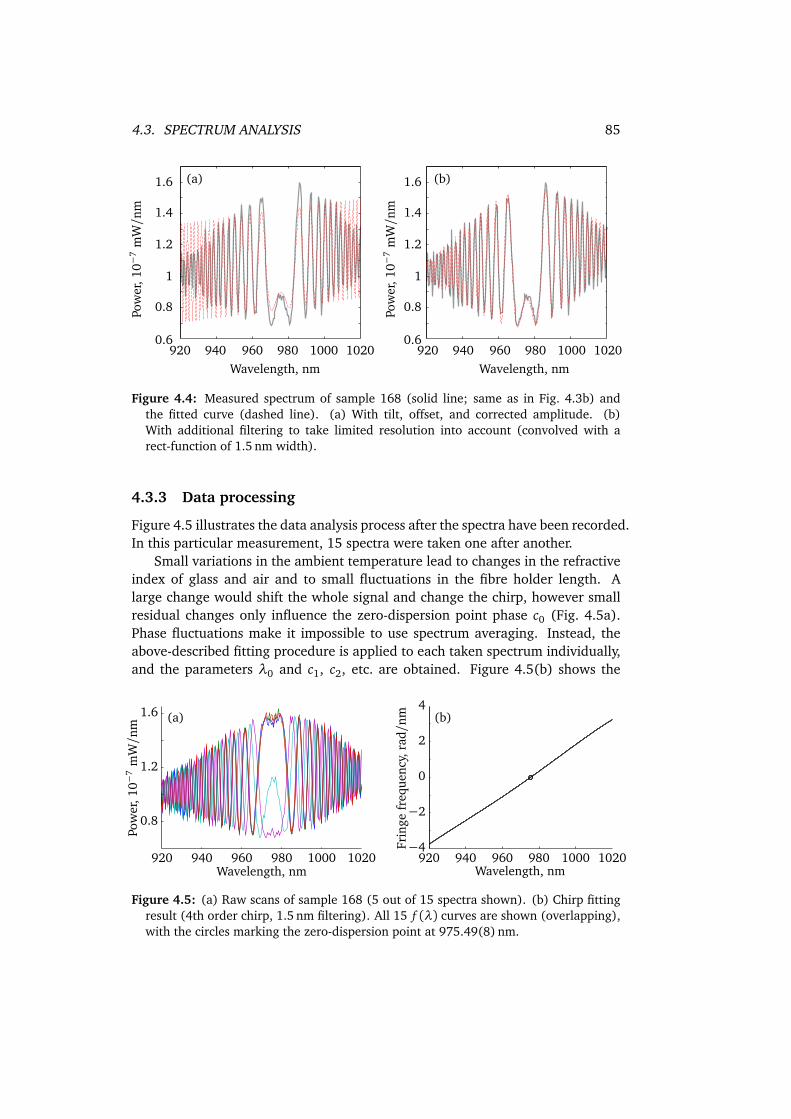
4.3. SPECTRUM ANALYSIS 85
0.6
1.6
1.2
0.8
1
1.4
0.6
1.6
1.2
0.8
1
1.4
920 940 10201000980960 920 940 10201000980960Wavelength, nm Wavelength, nm
Pow
er,1
0−7
mW/n
m
Pow
er,1
0−7
mW/n
m
(a) (b)
Figure 4.4: Measured spectrum of sample 168 (solid line; same as in Fig. 4.3b) andthe fitted curve (dashed line). (a) With tilt, offset, and corrected amplitude. (b)With additional filtering to take limited resolution into account (convolved with arect-function of 1.5 nm width).
4.3.3 Data processing
Figure 4.5 illustrates the data analysis process after the spectra have been recorded.In this particular measurement, 15 spectra were taken one after another.
Small variations in the ambient temperature lead to changes in the refractiveindex of glass and air and to small fluctuations in the fibre holder length. Alarge change would shift the whole signal and change the chirp, however smallresidual changes only influence the zero-dispersion point phase c0 (Fig. 4.5a).Phase fluctuations make it impossible to use spectrum averaging. Instead, theabove-described fitting procedure is applied to each taken spectrum individually,and the parameters λ0 and c1, c2, etc. are obtained. Figure 4.5(b) shows the
(a) (b)
Wavelength, nm
Frin
gefr
eque
ncy,
rad/
nm
920 940 960 980 1000 1020−4
−2
0
2
4
Wavelength, nm
Pow
er,1
0−7
mW/n
m
920 940 960 980 1000 1020
0.8
1.2
1.6
Figure 4.5: (a) Raw scans of sample 168 (5 out of 15 spectra shown). (b) Chirp fittingresult (4th order chirp, 1.5 nm filtering). All 15 f (λ) curves are shown (overlapping),with the circles marking the zero-dispersion point at 975.49(8) nm.
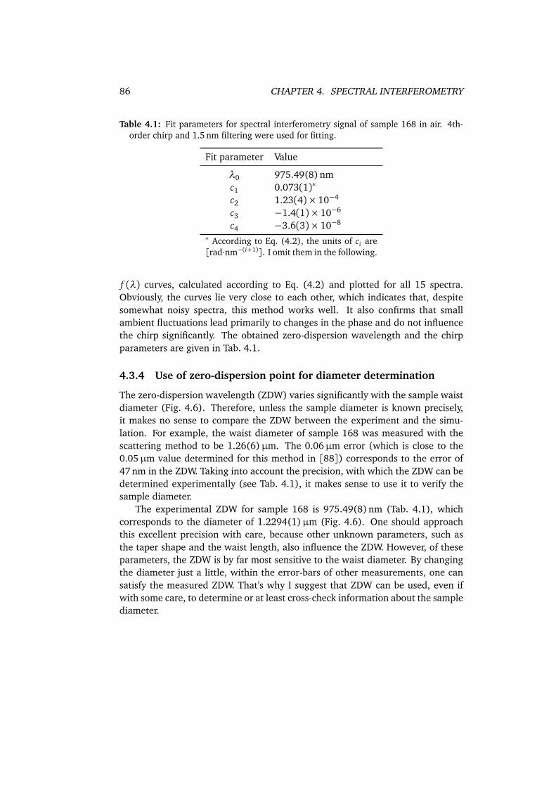
86 CHAPTER 4. SPECTRAL INTERFEROMETRY
Table 4.1: Fit parameters for spectral interferometry signal of sample 168 in air. 4th-order chirp and 1.5 nm filtering were used for fitting.
Fit parameter Value
λ0 975.49(8) nmc1 0.073(1)∗
c2 1.23(4)× 10−4
c3 −1.4(1)× 10−6
c4 −3.6(3)× 10−8
∗ According to Eq. (4.2), the units of ci are[rad·nm−(i+1)]. I omit them in the following.
f (λ) curves, calculated according to Eq. (4.2) and plotted for all 15 spectra.Obviously, the curves lie very close to each other, which indicates that, despitesomewhat noisy spectra, this method works well. It also confirms that smallambient fluctuations lead primarily to changes in the phase and do not influencethe chirp significantly. The obtained zero-dispersion wavelength and the chirpparameters are given in Tab. 4.1.
4.3.4 Use of zero-dispersion point for diameter determination
The zero-dispersion wavelength (ZDW) varies significantly with the sample waistdiameter (Fig. 4.6). Therefore, unless the sample diameter is known precisely,it makes no sense to compare the ZDW between the experiment and the simu-lation. For example, the waist diameter of sample 168 was measured with thescattering method to be 1.26(6)µm. The 0.06µm error (which is close to the0.05µm value determined for this method in [88]) corresponds to the error of47 nm in the ZDW. Taking into account the precision, with which the ZDW can bedetermined experimentally (see Tab. 4.1), it makes sense to use it to verify thesample diameter.
The experimental ZDW for sample 168 is 975.49(8) nm (Tab. 4.1), whichcorresponds to the diameter of 1.2294(1)µm (Fig. 4.6). One should approachthis excellent precision with care, because other unknown parameters, such asthe taper shape and the waist length, also influence the ZDW. However, of theseparameters, the ZDW is by far most sensitive to the waist diameter. By changingthe diameter just a little, within the error-bars of other measurements, one cansatisfy the measured ZDW. That’s why I suggest that ZDW can be used, even ifwith some care, to determine or at least cross-check information about the samplediameter.
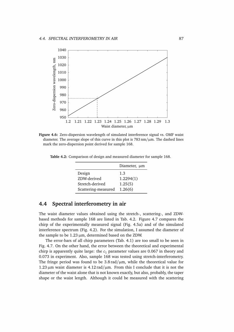
4.4. SPECTRAL INTERFEROMETRY IN AIR 87
Waist diameter,µm
Zero
-dis
pers
ion
wav
elen
gth,
nm
1.2 1.21 1.22 1.23 1.24 1.25 1.26 1.27 1.28 1.29 1.3950
960
970
980
990
1000
1010
1020
1030
1040
Figure 4.6: Zero-dispersion wavelength of simulated interference signal vs. OMF waistdiameter. The average slope of this curve in this plot is 783 nm/µm. The dashed linesmark the zero-dispersion point derived for sample 168.
Table 4.2: Comparison of design and measured diameter for sample 168.
Diameter, µm
Design 1.3ZDW-derived 1.2294(1)Stretch-derived 1.25(5)Scattering-measured 1.26(6)
4.4 Spectral interferometry in air
The waist diameter values obtained using the stretch-, scattering-, and ZDW-based methods for sample 168 are listed in Tab. 4.2. Figure 4.7 compares thechirp of the experimentally measured signal (Fig. 4.5a) and of the simulatedinterference spectrum (Fig. 4.2). For the simulation, I assumed the diameter ofthe sample to be 1.23µm, determined based on the ZDW.
The error-bars of all chirp parameters (Tab. 4.1) are too small to be seen inFig. 4.7. On the other hand, the error between the theoretical and experimentalchirp is apparently quite large: the c1 parameter values are 0.067 in theory and0.073 in experiment. Also, sample 168 was tested using stretch-interferometry.The fringe period was found to be 3.8 rad/µm, while the theoretical value for1.23µm waist diameter is 4.12 rad/µm. From this I conclude that it is not thediameter of the waist alone that is not known exactly, but also, probably, the tapershape or the waist length. Although it could be measured with the scattering
88 CHAPTER 4. SPECTRAL INTERFEROMETRY
Wavelength, nm
Frin
gefr
eque
ncy,
rad/
nm
920 940 960 980 1000 1020−4
−2
0
2
4
Experiment
Simulation
Figure 4.7: Spectral interference fringe frequency. Experimental curves (solid; all 15curves are shown, overlapping) for sample 168. Simulated curve (dashed) is obtainedfor a sample with 1.23µm×2 mm waist, 16 mrad tapers, silica in air (like sample168, but with thinner waist, see text).
method, it requires taking and processing a large amount of data and can onlybe reasonably done with an automated setup. This should still be built.
I have measured spectral interference for 15 samples in total, however onlyone more sample—165—was also measured with the scattering method andtested with stretch-interferometry. For this sample, the design diameter and thediameter values obtained with different methods lie quite close to each other(Tab. 4.3). However, the chirp curve still has significantly different slope valuesc1 in the simulation and measurements (Fig. 4.8(b), Tab. 4.4). This to some ex-tent confirms the suggestion made for sample 168, that the whole sample shapeinfluences the spectra. Note that the spectra obtained with this sample were verynoisy: compare Fig. 4.5(a) and Fig. 4.8(a). Nevertheless, the ZDW was againdetermined with a very small error of 0.07 nm.
The other 13 samples, designed for interferometry in air, show a similar be-haviour but their diameter was not measured using the scattering method. The
Table 4.3: Comparison of design and measured diameter for sample 165.
Diameter, µm
Design 1.3ZDW-derived 1.2827(1)Stretch-derived 1.25(5)Scattering-measured 1.27(1)
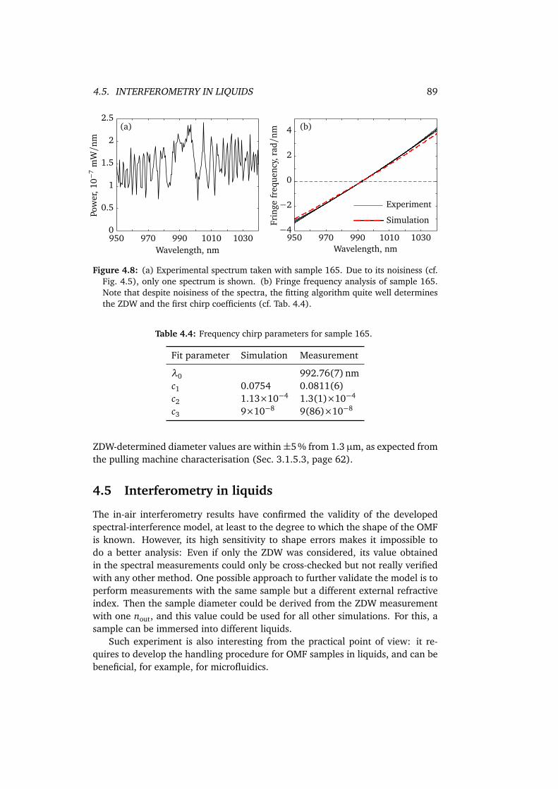
4.5. INTERFEROMETRY IN LIQUIDS 89
Wavelength, nm
Pow
er,1
0−7
mW/n
m
950 970 990 1010 10300
0.5
1
1.5
2
2.5
Wavelength, nm
Frin
gefr
eque
ncy,
rad/
nm
950 970 990 1010 1030−4
−2
0
2
4(a) (b)
Experiment
Simulation
Figure 4.8: (a) Experimental spectrum taken with sample 165. Due to its noisiness (cf.Fig. 4.5), only one spectrum is shown. (b) Fringe frequency analysis of sample 165.Note that despite noisiness of the spectra, the fitting algorithm quite well determinesthe ZDW and the first chirp coefficients (cf. Tab. 4.4).
Table 4.4: Frequency chirp parameters for sample 165.
Fit parameter Simulation Measurement
λ0 992.76(7) nmc1 0.0754 0.0811(6)c2 1.13×10⁻⁴ 1.3(1)×10−4
c3 9×10⁻⁸ 9(86)×10−8
ZDW-determined diameter values are within±5% from 1.3µm, as expected fromthe pulling machine characterisation (Sec. 3.1.5.3, page 62).
4.5 Interferometry in liquids
The in-air interferometry results have confirmed the validity of the developedspectral-interference model, at least to the degree to which the shape of the OMFis known. However, its high sensitivity to shape errors makes it impossible todo a better analysis: Even if only the ZDW was considered, its value obtainedin the spectral measurements could only be cross-checked but not really verifiedwith any other method. One possible approach to further validate the model is toperform measurements with the same sample but a different external refractiveindex. Then the sample diameter could be derived from the ZDW measurementwith one nout, and this value could be used for all other simulations. For this, asample can be immersed into different liquids.
Such experiment is also interesting from the practical point of view: it re-quires to develop the handling procedure for OMF samples in liquids, and can bebeneficial, for example, for microfluidics.
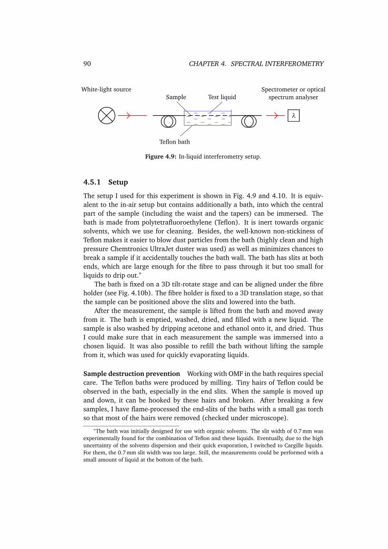
90 CHAPTER 4. SPECTRAL INTERFEROMETRY
λ
SampleWhite-light source Spectrometer or optical
spectrum analyser
Teflon bath
Test liquid
Figure 4.9: In-liquid interferometry setup.
4.5.1 Setup
The setup I used for this experiment is shown in Fig. 4.9 and 4.10. It is equiv-alent to the in-air setup but contains additionally a bath, into which the centralpart of the sample (including the waist and the tapers) can be immersed. Thebath is made from polytetrafluoroethylene (Teflon). It is inert towards organicsolvents, which we use for cleaning. Besides, the well-known non-stickiness ofTeflon makes it easier to blow dust particles from the bath (highly clean and highpressure Chemtronics UltraJet duster was used) as well as minimizes chances tobreak a sample if it accidentally touches the bath wall. The bath has slits at bothends, which are large enough for the fibre to pass through it but too small forliquids to drip out.∗
The bath is fixed on a 3D tilt-rotate stage and can be aligned under the fibreholder (see Fig. 4.10b). The fibre holder is fixed to a 3D translation stage, so thatthe sample can be positioned above the slits and lowered into the bath.
After the measurement, the sample is lifted from the bath and moved awayfrom it. The bath is emptied, washed, dried, and filled with a new liquid. Thesample is also washed by dripping acetone and ethanol onto it, and dried. ThusI could make sure that in each measurement the sample was immersed into achosen liquid. It was also possible to refill the bath without lifting the samplefrom it, which was used for quickly evaporating liquids.
Sample destruction prevention Working with OMF in the bath requires specialcare. The Teflon baths were produced by milling. Tiny hairs of Teflon could beobserved in the bath, especially in the end slits. When the sample is moved upand down, it can be hooked by these hairs and broken. After breaking a fewsamples, I have flame-processed the end-slits of the baths with a small gas torchso that most of the hairs were removed (checked under microscope).
∗The bath was initially designed for use with organic solvents. The slit width of 0.7 mm wasexperimentally found for the combination of Teflon and these liquids. Eventually, due to the highuncertainty of the solvents dispersion and their quick evaporation, I switched to Cargille liquids.For them, the 0.7 mm slit width was too large. Still, the measurements could be performed with asmall amount of liquid at the bottom of the bath.
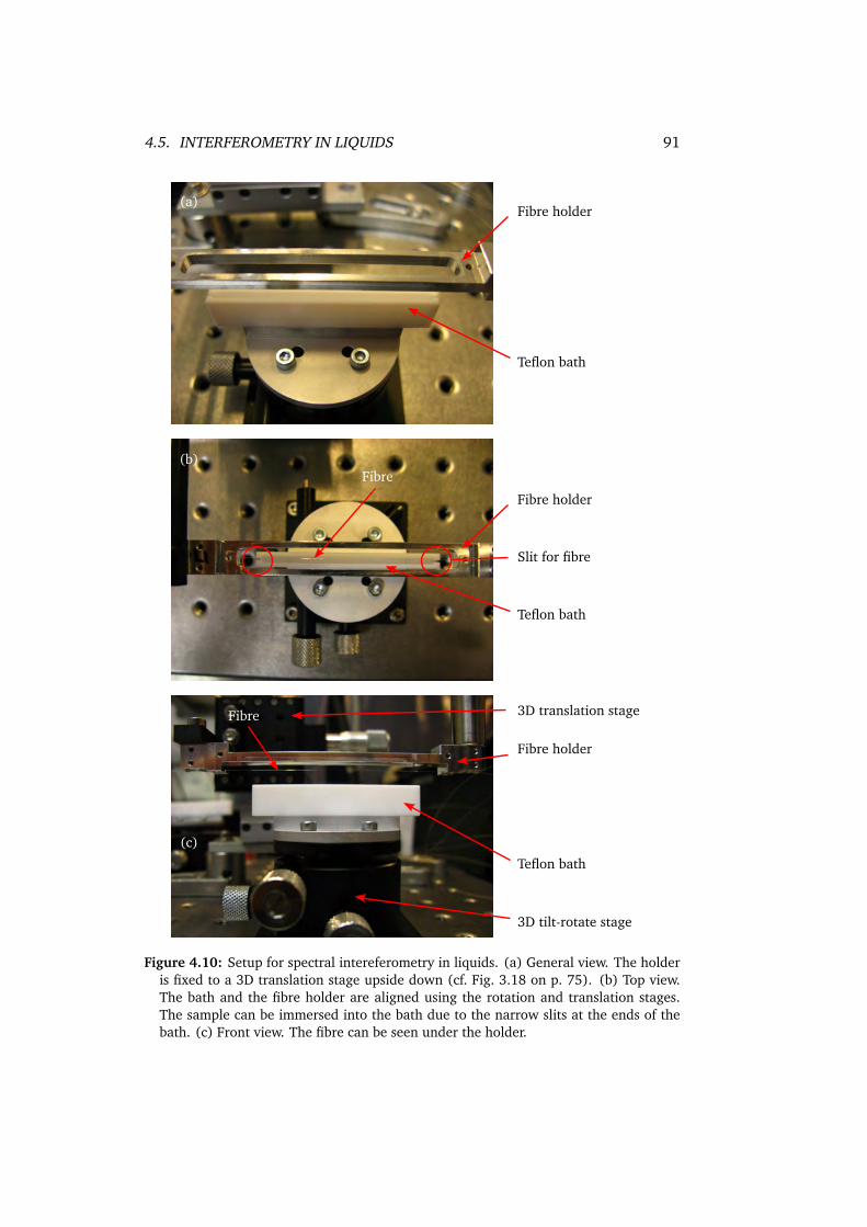
4.5. INTERFEROMETRY IN LIQUIDS 91
Fibre holder
Fibre
Teflon bath
Teflon bath
Fibre holder
Fibre holder
Teflon bath
Fibre
3D tilt-rotate stage
3D translation stage
(a)
(b)
(c)
Slit for fibre
Figure 4.10: Setup for spectral intereferometry in liquids. (a) General view. The holderis fixed to a 3D translation stage upside down (cf. Fig. 3.18 on p. 75). (b) Top view.The bath and the fibre holder are aligned using the rotation and translation stages.The sample can be immersed into the bath due to the narrow slits at the ends of thebath. (c) Front view. The fibre can be seen under the holder.
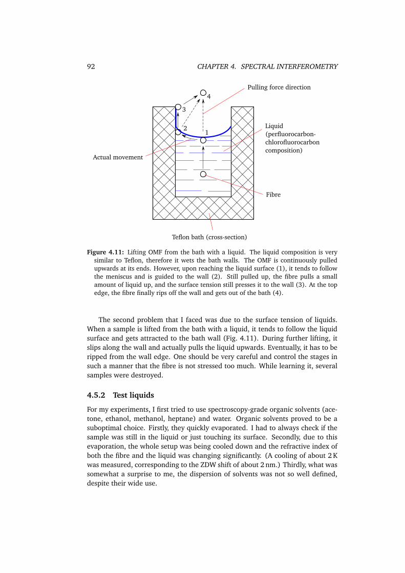
92 CHAPTER 4. SPECTRAL INTERFEROMETRY
Teflon bath (cross-section)
Fibre
Liquid(perfluorocarbon-chlorofluorocarboncomposition)
12
3
4Pulling force direction
Actual movement
Figure 4.11: Lifting OMF from the bath with a liquid. The liquid composition is verysimilar to Teflon, therefore it wets the bath walls. The OMF is continuously pulledupwards at its ends. However, upon reaching the liquid surface (1), it tends to followthe meniscus and is guided to the wall (2). Still pulled up, the fibre pulls a smallamount of liquid up, and the surface tension still presses it to the wall (3). At the topedge, the fibre finally rips off the wall and gets out of the bath (4).
The second problem that I faced was due to the surface tension of liquids.When a sample is lifted from the bath with a liquid, it tends to follow the liquidsurface and gets attracted to the bath wall (Fig. 4.11). During further lifting, itslips along the wall and actually pulls the liquid upwards. Eventually, it has to beripped from the wall edge. One should be very careful and control the stages insuch a manner that the fibre is not stressed too much. While learning it, severalsamples were destroyed.
4.5.2 Test liquids
For my experiments, I first tried to use spectroscopy-grade organic solvents (ace-tone, ethanol, methanol, heptane) and water. Organic solvents proved to be asuboptimal choice. Firstly, they quickly evaporated. I had to always check if thesample was still in the liquid or just touching its surface. Secondly, due to thisevaporation, the whole setup was being cooled down and the refractive index ofboth the fibre and the liquid was changing significantly. (A cooling of about 2 Kwas measured, corresponding to the ZDW shift of about 2 nm.) Thirdly, what wassomewhat a surprise to me, the dispersion of solvents was not so well defined,despite their wide use.
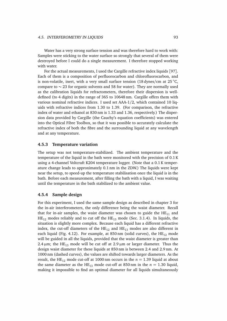
4.5. INTERFEROMETRY IN LIQUIDS 93
Water has a very strong surface tension and was therefore hard to work with:Samples were sticking to the water surface so strongly that several of them weredestroyed before I could do a single measurement. I therefore stopped workingwith water.
For the actual measurements, I used the Cargille refractive index liquids [97].Each of them is a composition of perfluorocarbon and chlorofluorocarbon, andis non-volatile, inert, with a very small surface tension (18 dynes/cm at 25 C,compare to ∼ 23 for organic solvents and 58 for water). They are normally usedas the calibration liquids for refractometers, therefore their dispersion is well-defined (to 4 digits) in the range of 365 to 10648 nm. Cargille offers them withvarious nominal refractive indices. I used set AAA-1/2, which contained 10 liq-uids with refractive indices from 1.30 to 1.39. (For comparison, the refractiveindex of water and ethanol at 830 nm is 1.33 and 1.36, respectively.) The disper-sion data provided by Cargille (the Cauchy’s equation coefficients) was enteredinto the Optical Fibre Toolbox, so that it was possible to accurately calculate therefractive index of both the fibre and the surrounding liquid at any wavelengthand at any temperature.
4.5.3 Temperature variation
The setup was not temperature-stabilized. The ambient temperature and thetemperature of the liquid in the bath were monitored with the precision of 0.1 Kusing a 4-channel Voltcraft K204 temperature logger. (Note that a 0.1 K temper-ature change leads to approximately 0.1 nm in the ZDW.) The liquids were keptnear the setup, to speed-up the temperature stabilisation once the liquid is in thebath. Before each measurement, after filling the bath with a liquid, I was waitinguntil the temperature in the bath stabilized to the ambient value.
4.5.4 Sample design
For this experiment, I used the same sample design as described in chapter 3 forthe in-air interferometers, the only difference being the waist diameter. Recallthat for in-air samples, the waist diameter was chosen to guide the HE11 andHE12 modes reliably and to cut off the HE13 mode (Sec. 3.1.4). In liquids, thesituation is slightly more complex. Because each liquid has a different refractiveindex, the cut-off diameters of the HE12 and HE13 modes are also different ineach liquid (Fig. 4.12). For example, at 850 nm (solid curves), the HE12 modewill be guided in all the liquids, provided that the waist diameter is greater than2.4µm; the HE13 mode will be cut off at 2.9µm or larger diameter. Thus thedesign waist diameter for these liquids at 850 nm is between 2.4 and 2.9 nm. At1000 nm (dashed curves), the values are shifted towards larger diameters. As theresult, the HE12 mode cut-off at 1000 nm occurs in the n = 1.39 liquid at aboutthe same diameter as the HE13 mode cut-off at 850 nm in the n = 1.30 liquid,making it impossible to find an optimal diameter for all liquids simultaneously
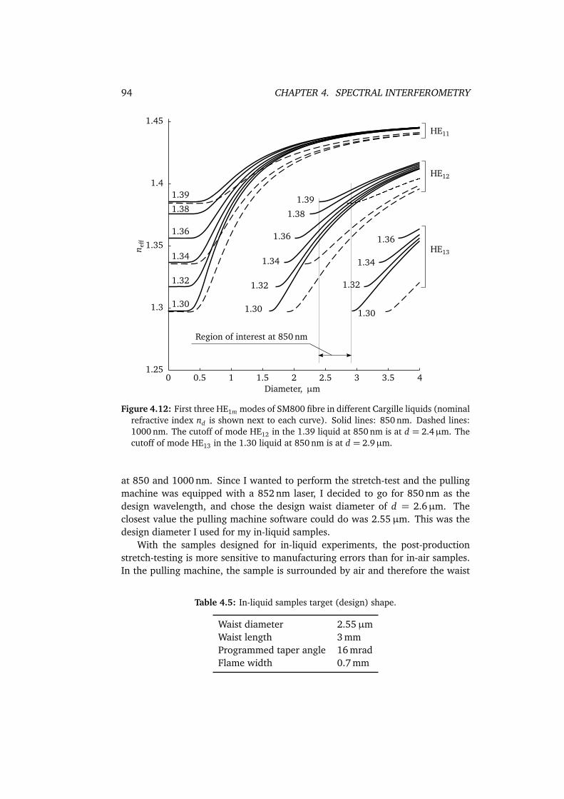
94 CHAPTER 4. SPECTRAL INTERFEROMETRY
n eff
Diameter, µm0 0.5 1 1.5 2 2.5 3 3.5 4
1.25
1.3
1.35
1.4
1.45
Region of interest at 850 nm
HE11
HE13
HE12
1.30
1.32
1.34
1.36
1.30
1.32
1.34
1.36
1.38
1.39
1.30
1.32
1.34
1.36
1.38
1.39
Figure 4.12: First three HE1m modes of SM800 fibre in different Cargille liquids (nominalrefractive index nd is shown next to each curve). Solid lines: 850 nm. Dashed lines:1000 nm. The cutoff of mode HE12 in the 1.39 liquid at 850 nm is at d = 2.4µm. Thecutoff of mode HE13 in the 1.30 liquid at 850 nm is at d = 2.9µm.
at 850 and 1000 nm. Since I wanted to perform the stretch-test and the pullingmachine was equipped with a 852 nm laser, I decided to go for 850 nm as thedesign wavelength, and chose the design waist diameter of d = 2.6µm. Theclosest value the pulling machine software could do was 2.55µm. This was thedesign diameter I used for my in-liquid samples.
With the samples designed for in-liquid experiments, the post-productionstretch-testing is more sensitive to manufacturing errors than for in-air samples.In the pulling machine, the sample is surrounded by air and therefore the waist
Table 4.5: In-liquid samples target (design) shape.
Waist diameter 2.55µmWaist length 3 mmProgrammed taper angle 16 mradFlame width 0.7 mm
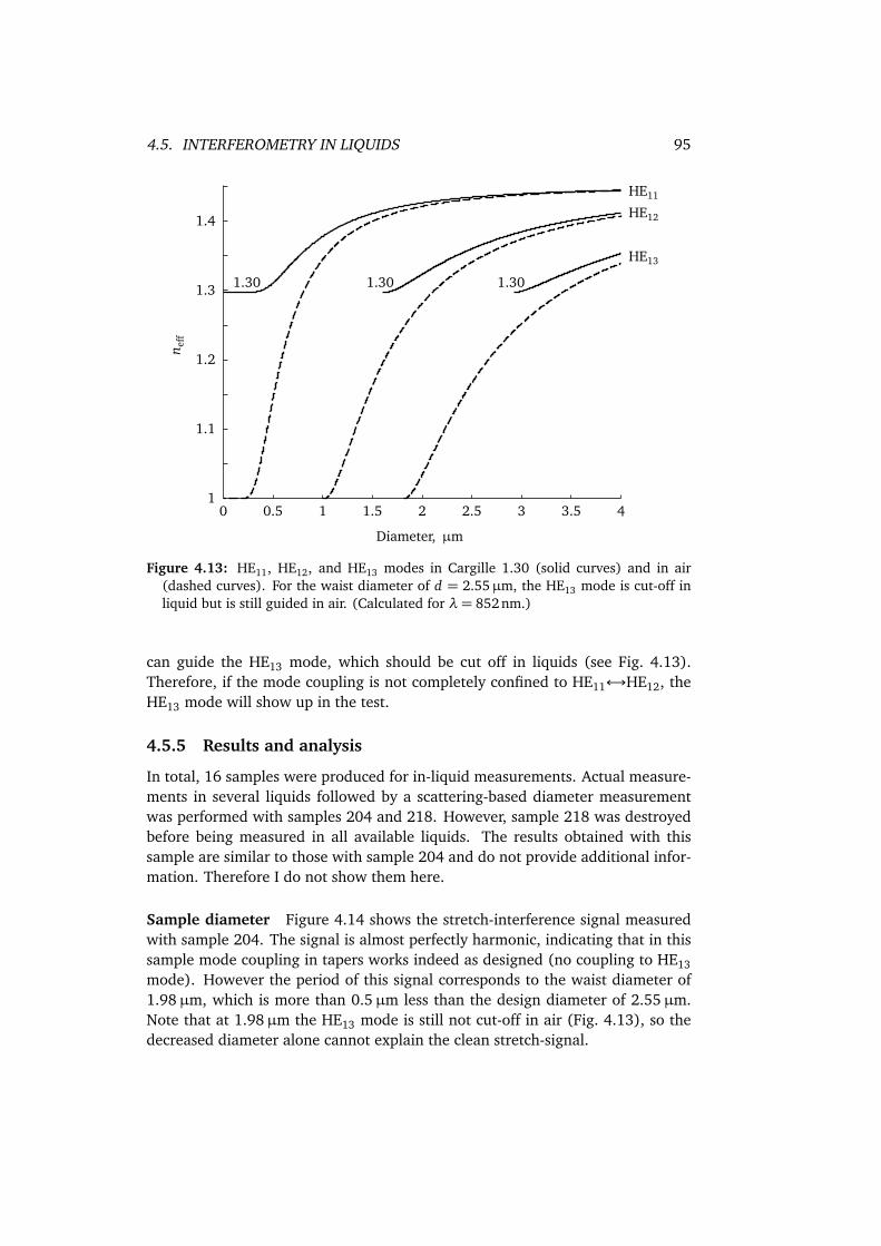
4.5. INTERFEROMETRY IN LIQUIDS 95
n eff
Diameter, µm
0 0.5 1 1.5 2 2.5 3 3.5 41
1.1
1.2
1.3
1.4
HE13
HE12
HE11
1.30 1.30 1.30
Figure 4.13: HE11, HE12, and HE13 modes in Cargille 1.30 (solid curves) and in air(dashed curves). For the waist diameter of d = 2.55µm, the HE13 mode is cut-off inliquid but is still guided in air. (Calculated for λ= 852 nm.)
can guide the HE13 mode, which should be cut off in liquids (see Fig. 4.13).Therefore, if the mode coupling is not completely confined to HE11↔HE12, theHE13 mode will show up in the test.
4.5.5 Results and analysis
In total, 16 samples were produced for in-liquid measurements. Actual measure-ments in several liquids followed by a scattering-based diameter measurementwas performed with samples 204 and 218. However, sample 218 was destroyedbefore being measured in all available liquids. The results obtained with thissample are similar to those with sample 204 and do not provide additional infor-mation. Therefore I do not show them here.
Sample diameter Figure 4.14 shows the stretch-interference signal measuredwith sample 204. The signal is almost perfectly harmonic, indicating that in thissample mode coupling in tapers works indeed as designed (no coupling to HE13mode). However the period of this signal corresponds to the waist diameter of1.98µm, which is more than 0.5µm less than the design diameter of 2.55µm.Note that at 1.98µm the HE13 mode is still not cut-off in air (Fig. 4.13), so thedecreased diameter alone cannot explain the clean stretch-signal.
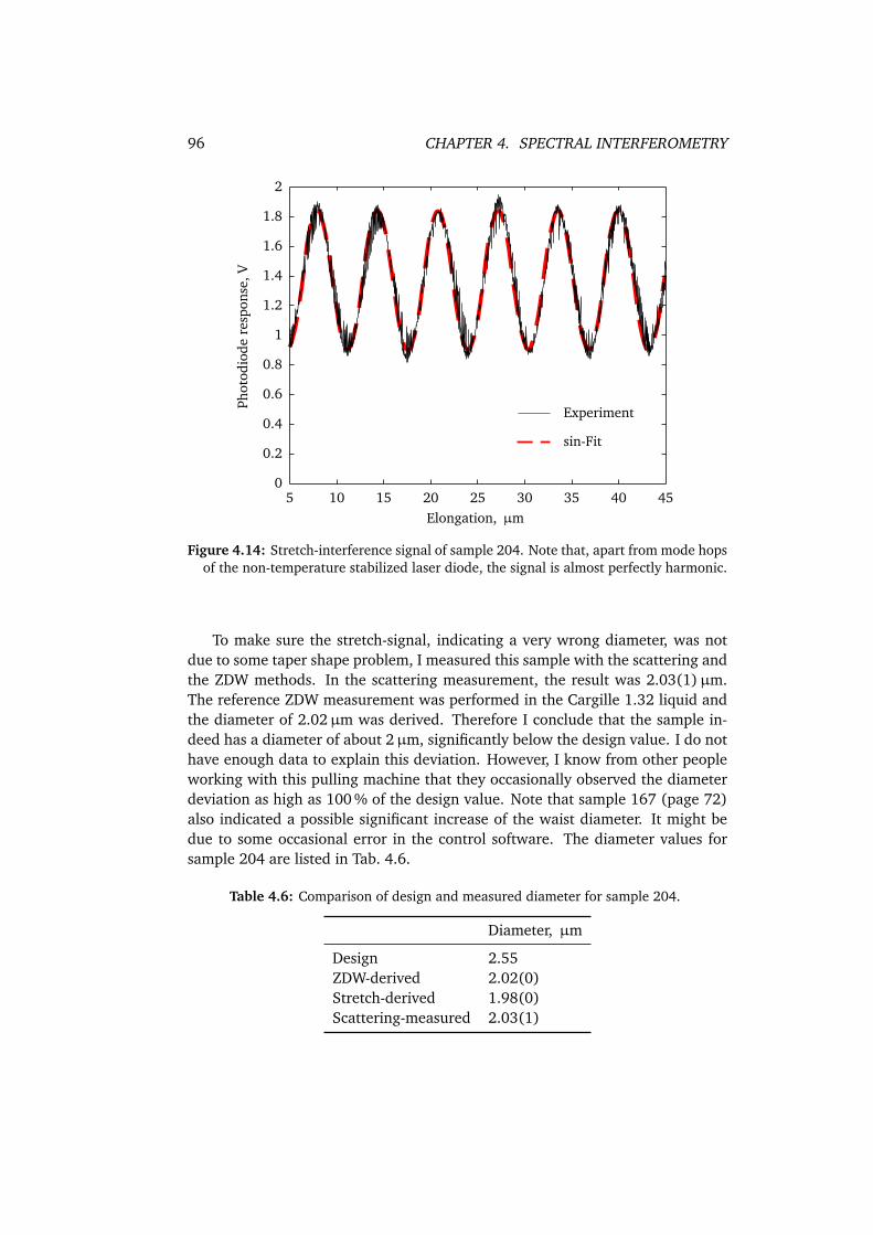
96 CHAPTER 4. SPECTRAL INTERFEROMETRY
Phot
odio
dere
spon
se,V
5 10 15 20 25 30 35 40 450
0.2
0.4
0.6
0.8
1
1.2
1.4
1.6
1.8
2
Elongation, µm
Experiment
sin-Fit
Figure 4.14: Stretch-interference signal of sample 204. Note that, apart from mode hopsof the non-temperature stabilized laser diode, the signal is almost perfectly harmonic.
To make sure the stretch-signal, indicating a very wrong diameter, was notdue to some taper shape problem, I measured this sample with the scattering andthe ZDW methods. In the scattering measurement, the result was 2.03(1)µm.The reference ZDW measurement was performed in the Cargille 1.32 liquid andthe diameter of 2.02µm was derived. Therefore I conclude that the sample in-deed has a diameter of about 2µm, significantly below the design value. I do nothave enough data to explain this deviation. However, I know from other peopleworking with this pulling machine that they occasionally observed the diameterdeviation as high as 100 % of the design value. Note that sample 167 (page 72)also indicated a possible significant increase of the waist diameter. It might bedue to some occasional error in the control software. The diameter values forsample 204 are listed in Tab. 4.6.
Table 4.6: Comparison of design and measured diameter for sample 204.
Diameter, µm
Design 2.55ZDW-derived 2.02(0)Stretch-derived 1.98(0)Scattering-measured 2.03(1)
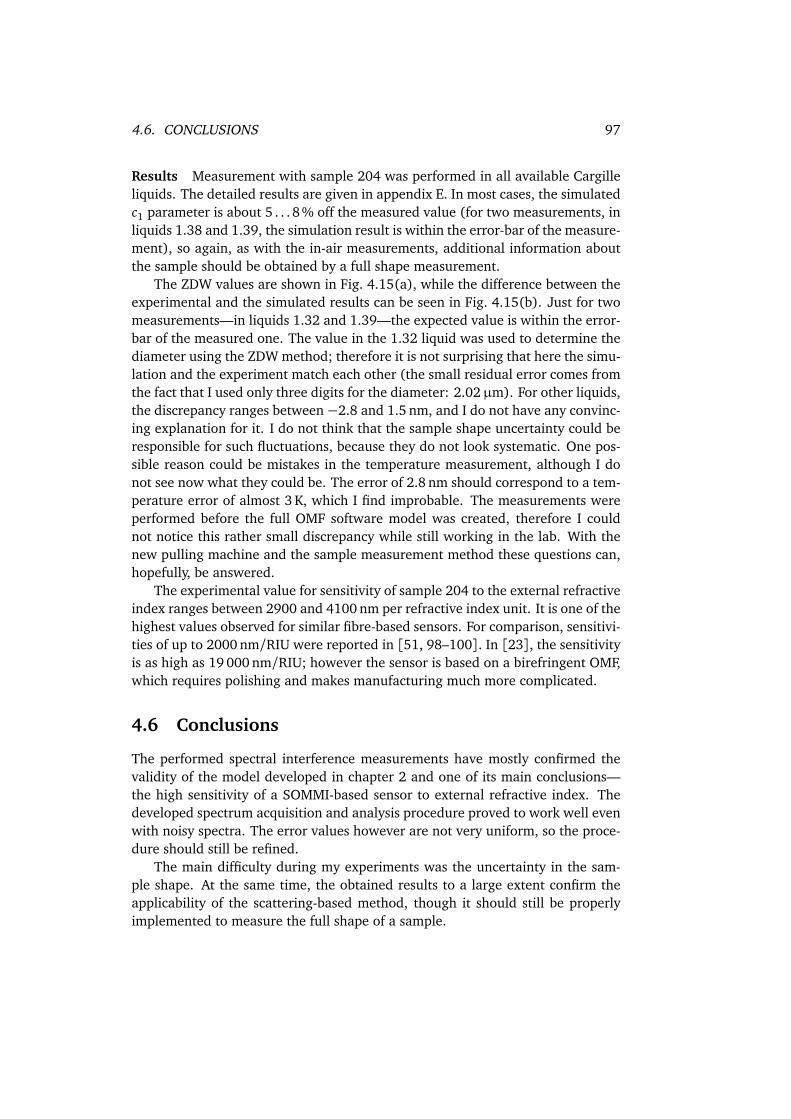
4.6. CONCLUSIONS 97
Results Measurement with sample 204 was performed in all available Cargilleliquids. The detailed results are given in appendix E. In most cases, the simulatedc1 parameter is about 5 . . . 8% off the measured value (for two measurements, inliquids 1.38 and 1.39, the simulation result is within the error-bar of the measure-ment), so again, as with the in-air measurements, additional information aboutthe sample should be obtained by a full shape measurement.
The ZDW values are shown in Fig. 4.15(a), while the difference between theexperimental and the simulated results can be seen in Fig. 4.15(b). Just for twomeasurements—in liquids 1.32 and 1.39—the expected value is within the error-bar of the measured one. The value in the 1.32 liquid was used to determine thediameter using the ZDW method; therefore it is not surprising that here the simu-lation and the experiment match each other (the small residual error comes fromthe fact that I used only three digits for the diameter: 2.02µm). For other liquids,the discrepancy ranges between −2.8 and 1.5 nm, and I do not have any convinc-ing explanation for it. I do not think that the sample shape uncertainty could beresponsible for such fluctuations, because they do not look systematic. One pos-sible reason could be mistakes in the temperature measurement, although I donot see now what they could be. The error of 2.8 nm should correspond to a tem-perature error of almost 3 K, which I find improbable. The measurements wereperformed before the full OMF software model was created, therefore I couldnot notice this rather small discrepancy while still working in the lab. With thenew pulling machine and the sample measurement method these questions can,hopefully, be answered.
The experimental value for sensitivity of sample 204 to the external refractiveindex ranges between 2900 and 4100 nm per refractive index unit. It is one of thehighest values observed for similar fibre-based sensors. For comparison, sensitivi-ties of up to 2000 nm/RIU were reported in [51, 98–100]. In [23], the sensitivityis as high as 19 000 nm/RIU; however the sensor is based on a birefringent OMF,which requires polishing and makes manufacturing much more complicated.
4.6 Conclusions
The performed spectral interference measurements have mostly confirmed thevalidity of the model developed in chapter 2 and one of its main conclusions—the high sensitivity of a SOMMI-based sensor to external refractive index. Thedeveloped spectrum acquisition and analysis procedure proved to work well evenwith noisy spectra. The error values however are not very uniform, so the proce-dure should still be refined.
The main difficulty during my experiments was the uncertainty in the sam-ple shape. At the same time, the obtained results to a large extent confirm theapplicability of the scattering-based method, though it should still be properlyimplemented to measure the full shape of a sample.
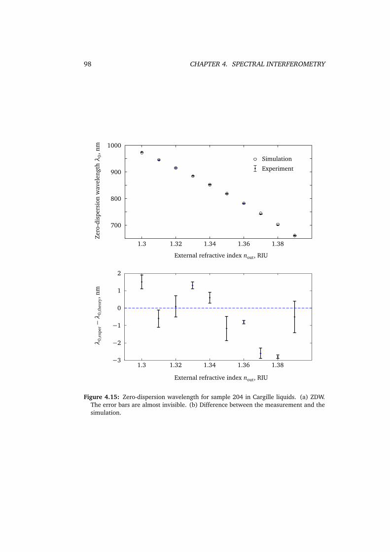
98 CHAPTER 4. SPECTRAL INTERFEROMETRY
Zero
-dis
pers
ion
wav
elen
gthλ
0,n
mλ
0,ex
per−λ
0,th
eory
,nm
External refractive index nout, RIU
External refractive index nout, RIU
1.3 1.32 1.34 1.36 1.38−3
−2
−1
0
1
2
Simulation
Experiment
1.3 1.32 1.34 1.36 1.38
700
800
900
1000
Figure 4.15: Zero-dispersion wavelength for sample 204 in Cargille liquids. (a) ZDW.The error bars are almost invisible. (b) Difference between the measurement and thesimulation.
CHAPTER 5Summary and outlook
The results presented in this thesis provide the basis for optical microfibre (OMF)-based interferometry. For the first time, experimental and theoretical investiga-tions of single OMF modal interferometers (SOMMIs) were performed at suchlevel of detail. Many practical techniques had to be developed to reliably trans-port and handle the fragile OMF samples, clean them, put them into an electronmicroscope, a vacuum chamber, and bathes with liquids, and to perform repro-ducible measurements in these different setups. The high sensitivity of SOMMIsto variation of ambient conditions made it important to take such variations intoaccount, both in experiment and in theoretical model. An almost real-time spec-tral measurement technique was implemented, and an appropriate data extrac-tion algorithm was developed for automated processing of hundreds of spectrataken within each measurement. This algorithm proved to be surprisingly stable(< 1nm) even for very noisy measured spectra. At the same time, it providedexcellent data extraction precision (down to 0.03 nm with a spectrometer reso-lution of 1.5 nm) for high-quality spectra. Various approaches were employed tomaximize the signal-to-noise ratio in all measurements.
Detailed understanding of mode propagation and phase-matching in OMFsallowed to create a novel optical harmonic generation-based method for OMFwaist-diameter measurement [1]. It is non-destructive, quite fast, and allows de-termination of the sub-micrometre OMF waist diameter with the absolute preci-sion of 0.5 %—the best value for OMFs to date. To verify this method, scanningelectron microscopy measurements were performed. Again, to achieve high pre-cision and obtain detailed information about the diameter variation along theOMF, numerous images had to be taken in automated mode. A special imageanalysis algorithm was developed to extract information about the sample shapefrom them [74].
The harmonic method was used to characterize the pulling machine, withwhich our samples were produced. However, the SOMMI samples themselves
99
100 CHAPTER 5. SUMMARY AND OUTLOOK
could not be measured with this method due to a very different diameter range.Therefore, two other methods were developed to verify the produced SOMMIsamples: a stretch-interference test and a zero-dispersion wavelength method.Being fast and non-destructive, these could be performed for each produced sam-ple.
To theoretically analyse light guidance in OMFs and obtain physically mean-ingful information from measured data, a special software tool—Optical fibretoolbox for Matlab (OFT)—was created [2]. To the best of my knowledge, thisis the only software code with such functionality today. While the existing soft-ware usually specializes on either thick telecom fibres or microoptical devices andtherefore cannot accommodate the large diameter variation in OMFs, OFT com-bines different models for calculation of mode propagation through the wholetapered OMF. Its characteristic feature is the automatic search for guided modesand their tracing for varying wavelength and diameter. Due to this feature, theharmonic generation effect in OMFs could be turned into a practical measure-ment method. It also allowed me to model in detail the behaviour of SOMMIsin various liquids in detail, with full consideration of the sample shape, the ma-terial dispersion of glass and liquids, and temperature effects. In the stretch in-terference simulation, I successfully calculated the SOMMI response, taking intoaccount the Poisson, the photoelastic and the induced birefringence effects.
For possible practical applications it is of interest that SOMMIs exhibit thehighest sensitivity among similar fibre-based sensors so far—about 3000 to 4000 nmper refractive index unit in the present measurements, which is only exceeded bydevices based on rectangular fibres.
Several directions for further work can be suggested.
5.1 Pulling machine
During this project, experimental samples were produced using the pulling ma-chine in the group of Arno Rauschenbeutel (Mainz/Vienna). For practical rea-sons, it would be beneficial to have easy access to an OMF pulling machine,because destruction of samples and the inability to experiment with the sampleshape were some of the main technical problems during this work. Therefore, anew pulling machine is currently being built in our group.
The stretch-experiment has revealed significant shape variation from sam-ple to sample with the current pulling machine. It is important to analyse andeliminate this effect. We mainly suspect problems with the fibre fixation in themachine. I have therefore designed a new clamping mechanism, which has beenbuilt and is now awaiting first tests.
In addition, it is necessary to improve the pulling control software, so thatthe target shape of the fibre is determined more precisely (for example, by notusing the rectangular flame approximation). The control software should alsobe improved in terms of interaction with the user, to notify her of any implicit
5.2. SAMPLE SHAPE 101
changes applied to the design shape of the sample as well as of any problemspossibly occurring during pulling.
5.2 Sample shape
The developed simulation software was already used to design OMF samples forharmonic generation at various wavelengths and SOMMI samples for interferom-etry in air and in liquids. Future possible applications might include the designof samples with maximized sensitivity to and increased working range of the ex-ternal refractive index and minimization of the taper length for more compactsamples.
The most important next step, however, would be an implementation of arobust and reliable sample shape measurement procedure. This can be basedon the scattering-measurement technique that was used in this work. The tech-nique was shown before to be applicable to the OMF measurement and providean error within 0.05µm [88]. The method can be further improved, as shown inthis work, by using more than just one wavelength for the same sample. I havealready used two lasers, at 633 and 532 nm; between them, the error for somesamples was within 0.02µm. At different wavelengths, the scattering patterns aresignificantly different, which minimizes statistical and systematic errors. There-fore, it seems beneficial to extend the wavelength range to near-infrared andblue.
To obtain the sample shape and not just the waist diameter (as done in thiswork), it is necessary to implement a setup with automatic scanning along thesample and simultaneous image analysis. Scanning can be easily realized if themeasurement is done in the same pulling machine where the sample is produced.Similarly to the stretch-test described in this work, such measurement could thenbe performed for each sample right after pulling, and provide the detailed infor-mation about its shape.
Verification could be performed using the same SEM-based technique as weused to verify the harmonic generation-based results [1, 74]. Another approachwould be to measure the waist diameter using the harmonic method and then de-termine the relative variation of the diameter using the whispering gallery modesmethod [101].
The ongoing development of the theoretical model during this project waslagging behind the experiment, and the full stretch- and spectral-interferencemodels, capable of taking into account the real sample shape, were realized onlyin the recent months, after the completion of the experimental work. As a re-sult, the samples were measured with lower precision than simulation is nowallowing. This explains the noticeable difference between the experimental andsimulation results for spectral and stretch interferometry. Once the full shapemeasurement procedure is implemented, verification of the models developed inthis work should be repeated.
102 CHAPTER 5. SUMMARY AND OUTLOOK
5.3 Dispersion measurement of atoms and molecules
It would be interesting to apply the SOMMI to the dispersive detection of anatomic gas (for example, caesium) around the sample. A similar interferometricmeasurement without fibres is known as the hook method [102]. Within thescope of this work, it was not possible to perform such measurements, due to theproblems with OMF samples in the vacuum chamber with caesium vapour [91,93]. However, these problems were rather technical than physical, some othergroups having succeeded in putting OMF samples into dense alkali vapour [103].
It would also be of interest to combine a SOMMI with photochromic molecules,where the molecule absorption (and hence the dispersion) can be controlled withlight. Switching of molecules on an OMF surface was successfully demonstratedin our group [92]. However, a quick attempt to measure interference responsedid not show any result (i. e. molecule switching was not detected interferomet-rically). This could be due to a sub-optimal combination of the SOMMI sampleand the molecules, the latter being absorbing in the ultraviolet and visible range,and the SOMMI having been designed for the infrared.
For the improvement and analysis of such measurements, it is also impor-tant to be able to simulate dispersion and absorption with atoms and moleculesaround the OMF. Theoretically, it is straightforward to do using a complex mate-rial refractive index of such surrounding materials [104]:
n(ω) =p
1+ 4πχ(1)(ω),
where ω = 2πν = 2πc/λ is the angular frequency of light wave and χ(1) thecomplex linear susceptibility. With the present implementation of the software,one cannot perform such calculations due to a fundamental reason: The algo-rithm is based on a very efficient routine to find the roots of the eigenvalue equa-tions. However, this routine is unable to work with complex numbers. For thisparticular task, another algorithm could be implemented in the future.
5.4 Simulation
A calculation still missing in OFT is the full mode coupling analysis. Replacingthe critical angle theory, it would allow more precise design of SOMMI samples,e. g. for maximized interference contrast. For non-interferometric OMFs, it couldbe used to design complex tapers for shorter samples.
The exciting aspect of science is that it never comes to an end.
APPENDIX AGuided mode solutions
In this appendix I provide references for the equations needed to calculate theguided modes (propagation constant and field distribution) in an OMF. Theseequations are quite complex and hence
• it is almost impossible to avoid typos in their reproduction (proven by nu-merous typos in published papers);
• they provide little insight in physics of modes.
Therefore, instead of retyping them from the original papers and textbooks, Ireference the sources themselves, indicating where necessary the found typos.Many of these equations have also been implemented in Matlab code in our Opti-cal fibre toolbox (OFT) [2]. If you want to implement them in the code yourself,I recommend to copy them directly from OFT or to use the functions of OFT asa reference to verify your own code. In appropriate places I reference the corre-sponding OFT functions. In the end, a table with all models per OMF region isprovided (Tab. A.1).
A.1 Two-layer waveguide
A.1.1 Scalar approximation (LP modes)
Can be used for input and output pigtails of OMFs or for usual telecom fibres.
A.1.1.1 Eigenvalue equation
This EVE is referenced in many sources. I have taken it from [31], Eq. (3.3-26).In OFT it is implemented in file eve2LS.m.
103
104 APPENDIX A. GUIDED MODE SOLUTIONS
A.1.1.2 Field equations
The field equations can be also taken from [31]: Eq. (3.3-24) and (3.3-25). OFTfile: modeFieldLP.m.
A.1.2 Vector solution
Can be used instead of two-layer LP modes and for OMF waist far from the core-cladding guidance transition point (neff nclad).
A.1.2.1 Eigenvalue equation
EVE is taken from [31], Eqs. (B-11), (B-17a), and (B17b) for HE/EH, TE and TMmodes respectively. Note a typo in Eq. (B-11): argument of function K and itsderivative K ′ should be (qa) instead of (ha). OFT file: eve2LS.m.
A.1.2.2 Field equations
Field equations are given in [30, p. 250]. OFT file: modeField.m.
A.2 Three-layer fibre
These models are required for simulation of modes in OMF tapers.
A.2.1 Scalar approximation (LP modes)
Three-layer LP modes is a valid approximation for large diameters, where thecladding-surrounding boundary does not play a significant role.
A.2.1.1 Eigenvalue equation
This is nicely and without typos given in [38]. The eigenvalue equations areEq. (3) for cladding-guided modes (nout neff ≤ nclad) and Eq. (4) for core-guided modes (nclad ≤ neff < ncore). OFT file: eve3LS.m.
A.2.1.2 Field equations
Field equations can be found in [25], Eqs. (29)–(31), and in [38], Eqs. (1)–(2).The field coefficients are defined in Appendix I in [38].
A.2.2 Vector solution
This is the most correct description of OMF modes, however it is also the slowestto calculate. Therefore it can be recommended to use simpler models wherepossible, see Tab. A.1 on page 106.
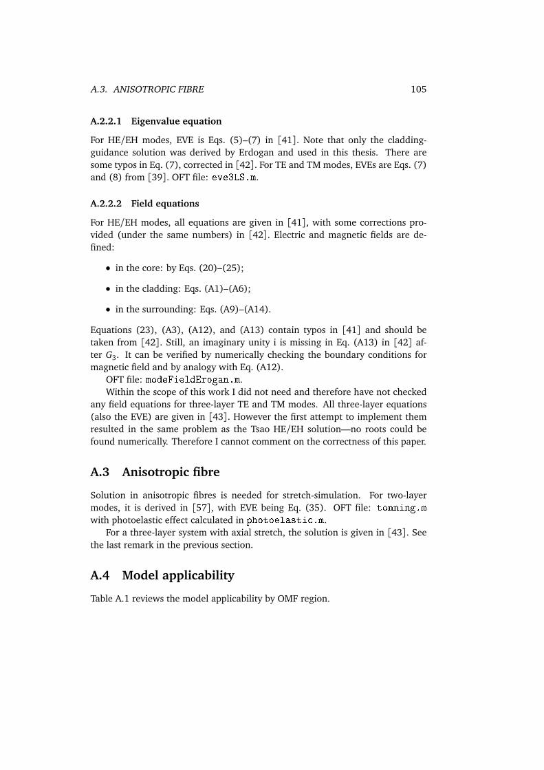
A.3. ANISOTROPIC FIBRE 105
A.2.2.1 Eigenvalue equation
For HE/EH modes, EVE is Eqs. (5)–(7) in [41]. Note that only the cladding-guidance solution was derived by Erdogan and used in this thesis. There aresome typos in Eq. (7), corrected in [42]. For TE and TM modes, EVEs are Eqs. (7)and (8) from [39]. OFT file: eve3LS.m.
A.2.2.2 Field equations
For HE/EH modes, all equations are given in [41], with some corrections pro-vided (under the same numbers) in [42]. Electric and magnetic fields are de-fined:
• in the core: by Eqs. (20)–(25);
• in the cladding: Eqs. (A1)–(A6);
• in the surrounding: Eqs. (A9)–(A14).
Equations (23), (A3), (A12), and (A13) contain typos in [41] and should betaken from [42]. Still, an imaginary unity i is missing in Eq. (A13) in [42] af-ter G3. It can be verified by numerically checking the boundary conditions formagnetic field and by analogy with Eq. (A12).
OFT file: modeFieldErogan.m.Within the scope of this work I did not need and therefore have not checked
any field equations for three-layer TE and TM modes. All three-layer equations(also the EVE) are given in [43]. However the first attempt to implement themresulted in the same problem as the Tsao HE/EH solution—no roots could befound numerically. Therefore I cannot comment on the correctness of this paper.
A.3 Anisotropic fibre
Solution in anisotropic fibres is needed for stretch-simulation. For two-layermodes, it is derived in [57], with EVE being Eq. (35). OFT file: tonning.mwith photoelastic effect calculated in photoelastic.m.
For a three-layer system with axial stretch, the solution is given in [43]. Seethe last remark in the previous section.
A.4 Model applicability
Table A.1 reviews the model applicability by OMF region.
Table A.1: Model applicability by region in an OMF
Hybrid TE TM
Region 2L LP 2L HE/EH Monerie Erdogan 2L LP 2L TE Tsao TE Monerie 2L LP 2L TM Tsao TM Monerie
d dtr — Ø — Ø Ø Ø Ø Ø — Ø Ø —
d ≈ dtr,neff ≤ nclad
— — Ø Ø — — Ø Ø — — Ø Ø
d ≈ dtr,neff ≥ nclad
— — Ø — — — Ø Ø — — Ø Ø
d = 125µm Ø Ø Ø — Ø Ø Ø Ø Ø Ø Ø Ø
Here “2L” denotes two-layer models, dtr is the transition diameter where neff = nclad and the cladding guidancechanges into the core guidance (or vice versa).
How to use this table: (1) Determine your region of interest in terms of diameter and neff. (2) Determine whichmodes you are interested in. For example, the SOMMI modes are HE11 and HE12 (hybrid). (3) Find the applicablemodel, taking into account that the 2-layer calculation is in general faster than the 3-layer one, and the scalarmodels (LP and Monerie) are faster than the vector ones.
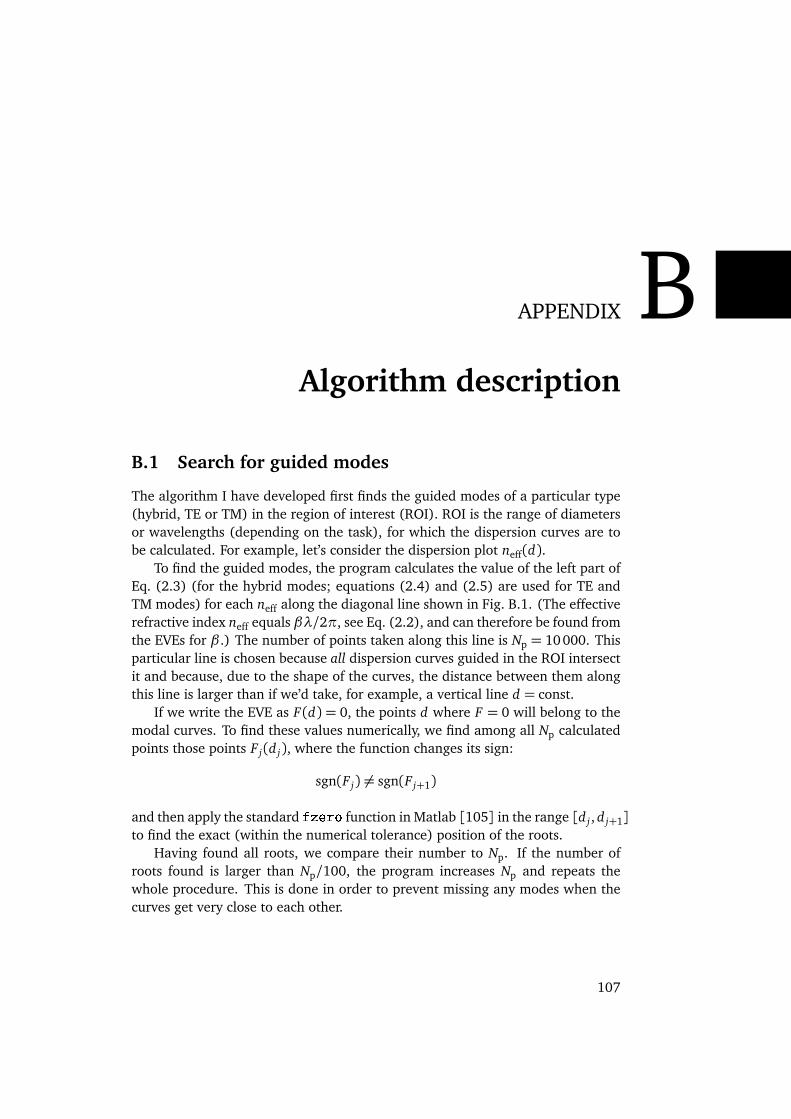
APPENDIX BAlgorithm description
B.1 Search for guided modes
The algorithm I have developed first finds the guided modes of a particular type(hybrid, TE or TM) in the region of interest (ROI). ROI is the range of diametersor wavelengths (depending on the task), for which the dispersion curves are tobe calculated. For example, let’s consider the dispersion plot neff(d).
To find the guided modes, the program calculates the value of the left part ofEq. (2.3) (for the hybrid modes; equations (2.4) and (2.5) are used for TE andTM modes) for each neff along the diagonal line shown in Fig. B.1. (The effectiverefractive index neff equals βλ/2π, see Eq. (2.2), and can therefore be found fromthe EVEs for β .) The number of points taken along this line is Np = 10000. Thisparticular line is chosen because all dispersion curves guided in the ROI intersectit and because, due to the shape of the curves, the distance between them alongthis line is larger than if we’d take, for example, a vertical line d = const.
If we write the EVE as F(d) = 0, the points d where F = 0 will belong to themodal curves. To find these values numerically, we find among all Np calculatedpoints those points F j(d j), where the function changes its sign:
sgn(F j) 6= sgn(F j+1)
and then apply the standard fzero function in Matlab [105] in the range [d j , d j+1]to find the exact (within the numerical tolerance) position of the roots.
Having found all roots, we compare their number to Np. If the number ofroots found is larger than Np/100, the program increases Np and repeats thewhole procedure. This is done in order to prevent missing any modes when thecurves get very close to each other.
107
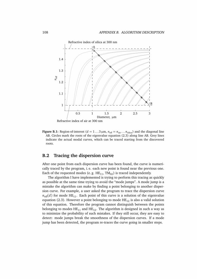
108 APPENDIX B. ALGORITHM DESCRIPTION
n eff
Diameter, µm0.5 1 1.5 2 2.5 3
1
1.1
1.2
1.3
1.4
Refractive index of silica at 300 nm
Refractive index of air at 300 nm
A
B
Figure B.1: Region-of-interest (d = 1 . . . 3µm, neff = nair . . . nsilica) and the diagonal lineAB. Circles mark the roots of the eigenvalue equation (2.3) along line AB. Grey linesindicate the actual modal curves, which can be traced starting from the discoveredroots.
B.2 Tracing the dispersion curve
After one point from each dispersion curve has been found, the curve is numeri-cally traced by the program, i. e. each new point is found near the previous one.Each of the requested modes (e. g. HE11, TM02) is traced independently.
The algorithm I have implemented is trying to perform this tracing as quicklyas possible at the same time trying to avoid the “mode jumps”. A mode jump is amistake the algorithm can make by finding a point belonging to another disper-sion curve. For example, a user asked the program to trace the dispersion curveneff(d) for mode HE11. Each point of this curve is a solution of the eigenvalueequation (2.3). However a point belonging to mode HE12 is also a valid solutionof this equation. Therefore the program cannot distinguish between the pointsbelonging to modes HE11 and HE12. The algorithm is designed in such a way asto minimize the probability of such mistakes. If they still occur, they are easy todetect: mode jumps break the smoothness of the dispersion curves. If a modejump has been detected, the program re-traces the curve going in smaller steps.
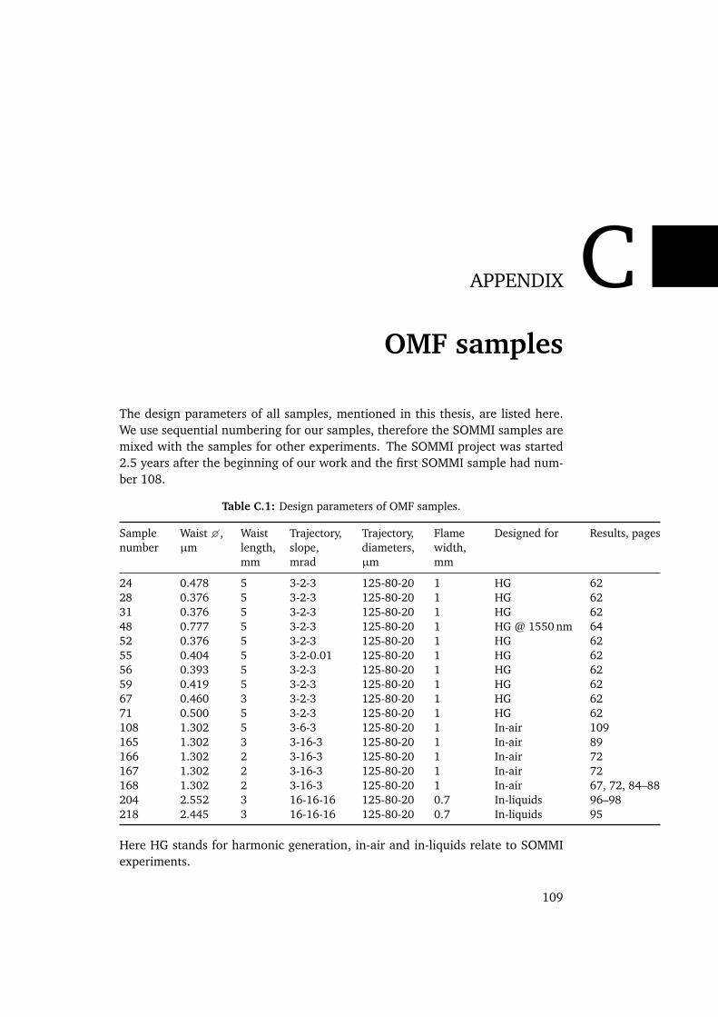
APPENDIX COMF samples
The design parameters of all samples, mentioned in this thesis, are listed here.We use sequential numbering for our samples, therefore the SOMMI samples aremixed with the samples for other experiments. The SOMMI project was started2.5 years after the beginning of our work and the first SOMMI sample had num-ber 108.
Table C.1: Design parameters of OMF samples.
Samplenumber
Waist ,µm
Waistlength,mm
Trajectory,slope,mrad
Trajectory,diameters,µm
Flamewidth,mm
Designed for Results, pages
24 0.478 5 3-2-3 125-80-20 1 HG 6228 0.376 5 3-2-3 125-80-20 1 HG 6231 0.376 5 3-2-3 125-80-20 1 HG 6248 0.777 5 3-2-3 125-80-20 1 HG @ 1550 nm 6452 0.376 5 3-2-3 125-80-20 1 HG 6255 0.404 5 3-2-0.01 125-80-20 1 HG 6256 0.393 5 3-2-3 125-80-20 1 HG 6259 0.419 5 3-2-3 125-80-20 1 HG 6267 0.460 3 3-2-3 125-80-20 1 HG 6271 0.500 5 3-2-3 125-80-20 1 HG 62108 1.302 5 3-6-3 125-80-20 1 In-air 109165 1.302 3 3-16-3 125-80-20 1 In-air 89166 1.302 2 3-16-3 125-80-20 1 In-air 72167 1.302 2 3-16-3 125-80-20 1 In-air 72168 1.302 2 3-16-3 125-80-20 1 In-air 67, 72, 84–88204 2.552 3 16-16-16 125-80-20 0.7 In-liquids 96–98218 2.445 3 16-16-16 125-80-20 0.7 In-liquids 95
Here HG stands for harmonic generation, in-air and in-liquids relate to SOMMIexperiments.
109

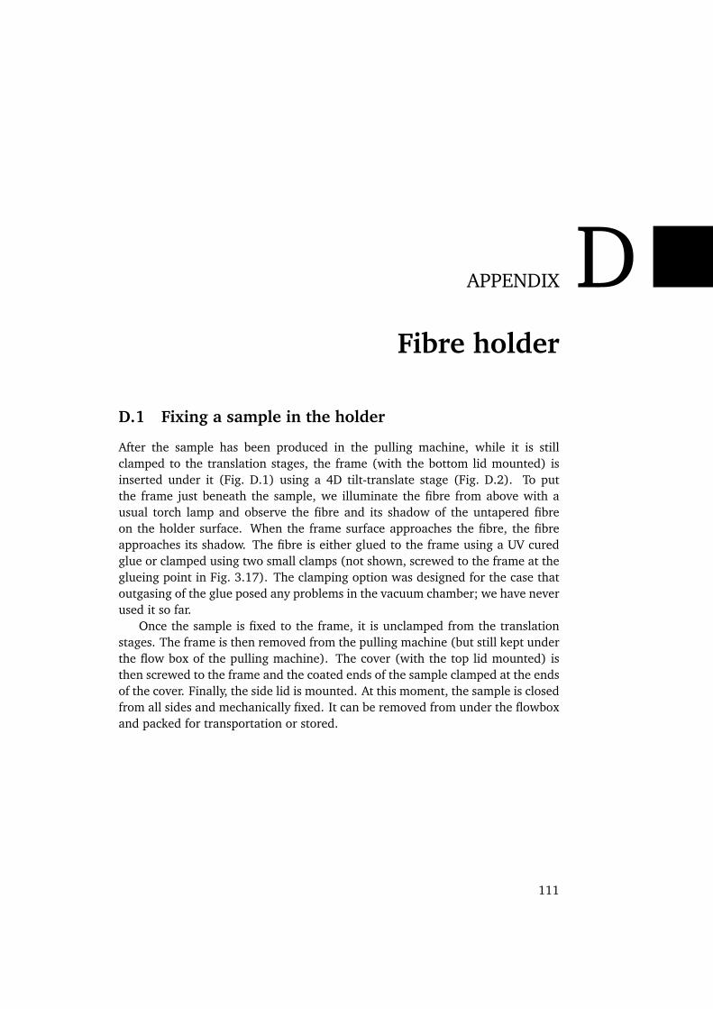
APPENDIX DFibre holder
D.1 Fixing a sample in the holder
After the sample has been produced in the pulling machine, while it is stillclamped to the translation stages, the frame (with the bottom lid mounted) isinserted under it (Fig. D.1) using a 4D tilt-translate stage (Fig. D.2). To putthe frame just beneath the sample, we illuminate the fibre from above with ausual torch lamp and observe the fibre and its shadow of the untapered fibreon the holder surface. When the frame surface approaches the fibre, the fibreapproaches its shadow. The fibre is either glued to the frame using a UV curedglue or clamped using two small clamps (not shown, screwed to the frame at theglueing point in Fig. 3.17). The clamping option was designed for the case thatoutgasing of the glue posed any problems in the vacuum chamber; we have neverused it so far.
Once the sample is fixed to the frame, it is unclamped from the translationstages. The frame is then removed from the pulling machine (but still kept underthe flow box of the pulling machine). The cover (with the top lid mounted) isthen screwed to the frame and the coated ends of the sample clamped at the endsof the cover. Finally, the side lid is mounted. At this moment, the sample is closedfrom all sides and mechanically fixed. It can be removed from under the flowboxand packed for transportation or stored.
111
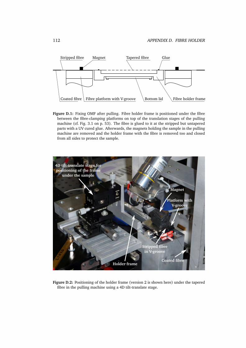
112 APPENDIX D. FIBRE HOLDER
Coated fibre
Tapered fibreMagnetStripped fibre Glue
Fibre platform with V-groove Fibre holder frameBottom lid
Figure D.1: Fixing OMF after pulling. Fibre holder frame is positioned under the fibrebetween the fibre-clamping platforms on top of the translation stages of the pullingmachine (cf. Fig. 3.1 on p. 53). The fibre is glued to it at the stripped but untaperedparts with a UV cured glue. Afterwards, the magnets holding the sample in the pullingmachine are removed and the holder frame with the fibre is removed too and closedfrom all sides to protect the sample.
Platform withV-groove
Magnet
Coated fibre
Stripped fibrein V-groove
4D tilt-translate stage forpositioning of the frame
under the sample
Holder frame
Figure D.2: Positioning of the holder frame (version 2 is shown here) under the taperedfibre in the pulling machine using a 4D tilt-translate stage.
D.2. TRANSPORTATION AND STORAGE 113
D.2 Transportation and storage
As already mentioned, the pulling machine we were using was located first inMainz and later in Vienna. We thus had to bring the samples to Bonn, by trainor by plane. Two samples were also once taken to England, to perform someexperiments in the group of G. Brambilla, University of Southampton.
We have developed a simple routine which has worked fine over four years ofour project. After the sample has been fixed in the holder, the fibre pigtails (about1 m long) are rolled and fixed to the cover using an antistatic (ESD) adhesivetape. The holder is then put into a plastic ESD (pink) zipper bag.∗ Ideally, thisshould be done under the flowbox of the pulling machine. We normally put twosamples in each bag.
So packed, the samples can be stored in a usual room for months and reusedmany times.
For transportation, all sample bags are stacked on top of each other in anotebook computer bag (which offers mechanical protection), with a bubble filmunder and above this stack. Finally, this sandwich is fixed in the notebook bagwith a strap. The remaining space in the bag can be used for a notebook or anyother stuff.
It is worth mentioning that the airport security is normally interested in thecontents of this bag: on an X-ray screen, the stack of holders with fibres looks likeseveral metal boxes with a clutter of wires around them. For this very reason, wehave never tried to check it in. The security officer should be informed that theseare fragile research samples so that she doesn’t open the bag herself or at leastdoes it very carefully; the bag can then be opened, the bubble film unwrappedand the top samples shown to the officer without being removed from the ESDbag. We have transported samples by plane three times, and everything wentsmoothly. We have not tried to fly with these holders to or from Israel so far.
Out of more than 200 samples produced and brought to Bonn over four yearsof use of these holders, not a single one was broken or damaged during trans-portation or storage.
∗We are using ESD-compatible packaging for better protection of the samples against dust. Wehave not done any tests as to whether it actually has any benefit or not. However we know thatOMFs are extremely sensitive to dust: Left open outside a flowbox, they loose transmission over2–3 days. Under a chemistry fume hood (which sucks outside air into the hood), the transmissionis lost within approximately half an hour.

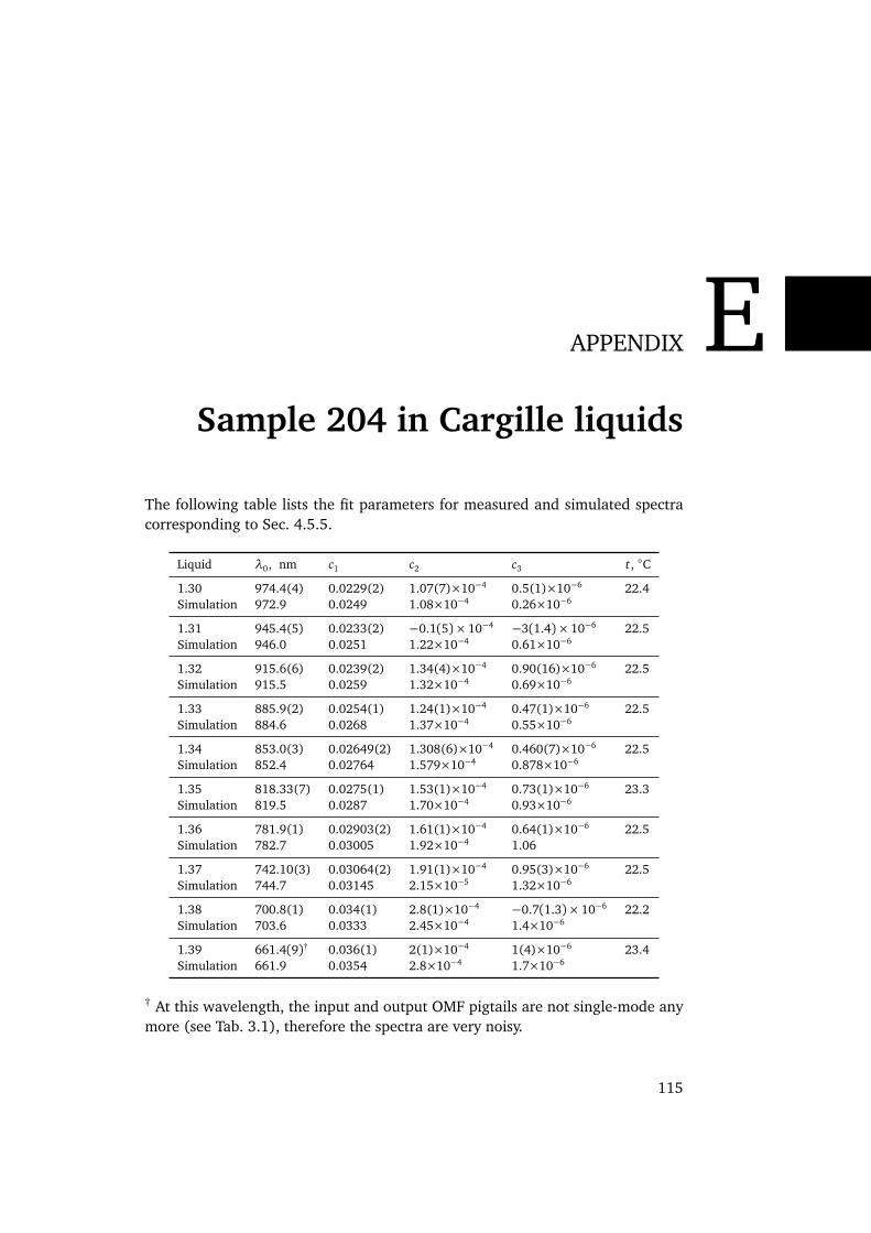
APPENDIX ESample 204 in Cargille liquids
The following table lists the fit parameters for measured and simulated spectracorresponding to Sec. 4.5.5.
Liquid λ0, nm c1 c2 c3 t, C
1.30 974.4(4) 0.0229(2) 1.07(7)×10−4 0.5(1)×10−6 22.4Simulation 972.9 0.0249 1.08×10⁻⁴ 0.26×10⁻⁶
1.31 945.4(5) 0.0233(2) −0.1(5)× 10−4 −3(1.4)× 10−6 22.5Simulation 946.0 0.0251 1.22×10⁻⁴ 0.61×10⁻⁶
1.32 915.6(6) 0.0239(2) 1.34(4)×10−4 0.90(16)×10−6 22.5Simulation 915.5 0.0259 1.32×10⁻⁴ 0.69×10⁻⁶
1.33 885.9(2) 0.0254(1) 1.24(1)×10−4 0.47(1)×10−6 22.5Simulation 884.6 0.0268 1.37×10⁻⁴ 0.55×10⁻⁶
1.34 853.0(3) 0.02649(2) 1.308(6)×10−4 0.460(7)×10−6 22.5Simulation 852.4 0.02764 1.579×10⁻⁴ 0.878×10⁻⁶
1.35 818.33(7) 0.0275(1) 1.53(1)×10−4 0.73(1)×10−6 23.3Simulation 819.5 0.0287 1.70×10⁻⁴ 0.93×10⁻⁶
1.36 781.9(1) 0.02903(2) 1.61(1)×10−4 0.64(1)×10−6 22.5Simulation 782.7 0.03005 1.92×10⁻⁴ 1.06
1.37 742.10(3) 0.03064(2) 1.91(1)×10−4 0.95(3)×10−6 22.5Simulation 744.7 0.03145 2.15×10⁻⁵ 1.32×10⁻⁶
1.38 700.8(1) 0.034(1) 2.8(1)×10−4 −0.7(1.3)× 10−6 22.2Simulation 703.6 0.0333 2.45×10⁻⁴ 1.4×10⁻⁶
1.39 661.4(9)† 0.036(1) 2(1)×10−4 1(4)×10−6 23.4Simulation 661.9 0.0354 2.8×10⁻⁴ 1.7×10⁻⁶
† At this wavelength, the input and output OMF pigtails are not single-mode anymore (see Tab. 3.1), therefore the spectra are very noisy.
115

Bibliography
1. Wiedemann, U., Karapetyan, K., Dan, C., Pritzkau, D., Alt, W., Irsen, S. &Meschede, D. Measurement of submicrometre diameters of tapered opticalfibres using harmonic generation. Optics Express 18, 7693 (2010).
2. Karapetyan, K., Alt, W. & Meschede, D. Optical fibre toolbox for Matlab,version 2.1 [www.mathworks.com/matlabcentral/fileexchange/27819] (2011).
3. Garcia-Fernandez, R., Alt, W, Bruse, F, Dan, C, Karapetyan, K., Rehband,O., Stiebeiner, A., Wiedemann, U., Meschede, D. & Rauschenbeutel, A.Optical nanofibers and spectroscopy. Appl. Phys. B 105, 3–15 (2011).
4. Kimura, T., Nambu, Y., Hatanaka, T., Tomita, A., Kosaka, H. & Nakamura,K. Single-photon Interference over 150 km Transmission Using Silica-basedIntegrated-optic Interferometers for Quantum Cryptography. Japanese Jour-nal of Applied Physics 43, L1217–L1219 (2004).
5. Fischer, J., Ergin, T. & Wegener, M. Three-dimensional polarization-independentvisible-frequency carpet invisibility cloak. Optics Letters 36, 2059 (2011).
6. Van Heel, A. C. S. A New Method of transporting Optical Images withoutAberrations. Nature 173, 39 (1954).
7. Kao, K. & Hockham, G. Dielectric-fibre surface waveguides for optical fre-quencies. Proceedings IEE 133, 1151 (1966).
8. Ozeki, T. & Kawasaki, B. S. Optical directional coupler using tapered sec-tions in multimode fibers. Applied Physics Letters 28, 528 (1976).
9. Brambilla, G., Finazzi, V. & Richardson, D. J. Ultra-low-loss optical fibernanotapers. Optics Express 12, 2258 (2004).
10. Grubsky, V. & Savchenko, A. Glass micro-fibers for efficient third harmonicgeneration. Optics Express 13, 6798 (2005).
11. Leon-Saval, S, Birks, T, Wadsworth, W, St J Russell, P & Mason, M. Super-continuum generation in submicron fibre waveguides. Optics Express 12,2864–9 (2004).
12. Gattass, R. R., Svacha, G. T., Tong, L. & Mazur, E. Supercontinuum gen-eration in submicrometer diameter silica fibers. Optics Express 14, 9408(2006).
117
118 BIBLIOGRAPHY
13. Paschotta, R. Tapered Fibers [http://www.rp-photonics.com/tapered_fibers.html] (visited on 06/25/2012).
14. Brambilla, G., Xu, F., Horak, P., Jung, Y., Koizumi, F., Sessions, N. P., Koukharenko,E., Feng, X., Murugan, G. S., Wilkinson, J. S. & Richardson, D. J. Opticalfiber nanowires and microwires: fabrication and applications. Advances inOptics and Photonics 1, 107 (2009).
15. Nayak, K. P., Melentiev, P. N., Morinaga, M, Kien, F. L., Balykin, V. I. &Hakuta, K. Optical nanofiber as an efficient tool for manipulating andprobing atomic Fluorescence. Optics Express 15, 5431 (2007).
16. Sagué, G., Vetsch, E., Alt, W., Meschede, D. & Rauschenbeutel, A. Cold-Atom Physics Using Ultrathin Optical Fibers: Light-Induced Dipole Forcesand Surface Interactions. Physical Review Letters 99, 1–4 (2007).
17. Warken, F., Vetsch, E., Meschede, D., Sokolowski, M. & Rauschenbeutel,a. Ultra-sensitive surface absorption spectroscopy using sub-wavelengthdiameter optical fibers. Optics Express 15, 11952 (2007).
18. Lou, J., Tong, L. & Ye, Z. Modeling of silica nanowires for optical sensing.Optics Express 13, 2135–2140 (2005).
19. Li, Y. & Tong, L. Mach-Zehnder interferometers assembled with opticalmicrofibers or nanofibers. Optics Letters 33, 303–305 (2008).
20. Lacroix, S., Gonthier, F., Black, R. J. & Bures, J. Tapered-fiber interfero-metric wavelength response: the achromatic fringe. Optics Letters 13, 395(1988).
21. Villatoro, J., Minkovich, V. & Monzón-Hernández, D. Compact modal inter-ferometer built with tapered microstructured optical fiber. Photonics Tech-nology Letters, IEEE 18, 1258–1260 (2006).
22. Jung, Y., Brambilla, G. & Richardson, D. J. Polarization-maintaining opticalmicrofiber. Optics Letters 35, 2034 (2010).
23. Li, J., Sun, L.-P., Gao, S., Quan, Z., Chang, Y.-L., Ran, Y., Jin, L. & Guan,B.-O. Ultrasensitive refractive-index sensors based on rectangular silica mi-crofibers. Optics Letters 36, 3593 (2011).
24. Private communication with John Wooler, Fibercore Ltd.: Refractive index ofSM800 (2009).
25. Love, J. D., Henry, W. M., Stewart, W. J., Black, R. J., Lacroix, S. & Gonthier,F. Tapered single-mode fibres and devices. I. Adiabaticity criteria. IEE Pro-ceedings J. 138, 343–354 (1991).
26. Warken, F. Ultradünne Glasfasern als Werkzeug zur Kopplung von Licht undMaterie PhD thesis (2007).
27. Bures, J. Guided Optics: Optical Fibers and All-fiber Components 368 (2008).

BIBLIOGRAPHY 119
28. Paschotta, R. V-number [http://www.rp-photonics.com/v_number.html] (visited on 06/24/2012).
29. Black, R. J., Lacroix, S., Gonthier, F. & Love, J. Tapered single-mode fi-bres and devices. Pt. 2: experimental and theoretical quantification. IEEProceedings J. 138, 355–364 (1991).
30. Snyder, A. & Love, J. Optical waveguide theory (Chapman & Hall, London,1983).
31. Yariv, A. & Yeh, P. Photonics: Optical Electronics in Modern Communications836 (2007).
32. Fibercore Ltd. Singlemode Optical Fiber [http://www.fibercore.com/Products/SMSeries/tabid/89/agentType/View/PropertyID/259/Default.aspx] (visited on 08/23/2011).
33. Yariv, A. Optical Electronics in Modern Communications 5th, 768 (OxfordUniversity Press, USA, 1997).
34. Private communication with Peter Horak (2009).
35. Private communication with Limin Tong (2011).
36. Private communication with Gilberto Brambilla (2009).
37. Belanov, A. S., Dianov, E. M., Ezhov, G. I. & Prokhorov, A. M. Propagationof normal modes in multilayer optical waveguides I. Component fields anddispersion characteristics. Soviet Journal of Quantum Electronics 6, 43–50(1976).
38. Monerie, M. Propagation in doubly clad single-mode fibers. IEEE Journalof Quantum Electronics 18, 535–542 (1982).
39. Tsao, C., Payne, D. & Gambling, W. Modal characteristics of three-layeredoptical fiber waveguides: a modified approach. Journal of the Optical Soci-ety of America A 6, 555–563 (1989).
40. Henry, W. M. An investigation of coated tapered optical fibres. Sensors andActuators B: Chemical 22, 101–107 (1994).
41. Erdogan, T. Cladding-mode resonances in short- and long-period fiber grat-ing filters. Journal of the Optical Society of America A 14, 1760 (1997).
42. Erdogan, T. Cladding-mode resonances in short- and long-period fiber grat-ing filters: errata. Journal of the Optical Society of America A 17, 2113(2000).
43. Zhang, Z.-j. & Shi, W.-k. Eigenvalue and field equations of three-layereduniaxial fibers and their applications to the characteristics of long-periodfiber gratings with applied axial strain. Journal of the Optical Society ofAmerica A 22, 2516 (2005).
120 BIBLIOGRAPHY
44. Linslal, C. L., S. Mohan, P. M., Halder, a. & Gangopadhyay, T. K. Eigenvalueequation and core-mode cutoff of weakly guiding tapered fiber as threelayer optical waveguide and used as biochemical sensor. Applied Optics51, 3445 (2012).
45. Private communication with Timothy Lee (2010).
46. Private communication with David Payne (2011).
47. Love, J. & Henry, W. Quantifying loss minimisation in single-mode fibretapers. Electronics Letters 22, 912 (1986).
48. Agrawal, G. P. Nonlinear Fiber Optics 3rd, 467 (Academic Press, 2001).
49. Terhune, R. W. & Weinberger, D. a. Second-harmonic generation in fibers.Journal of the Optical Society of America B 4, 661 (1987).
50. Simmons, J. H. & Potter, K. S. Optical materials (2000).
51. Liao, C., Wang, D., He, X. & Yang, M. in Proceedings of SPIE 23 (2011),77534I–77534I–4. doi:10.1117/12.885826.
52. Bertholds, A & Dändliker, R. High-resolution photoelastic pressure sensorusing low-birefringence fiber. Applied Optics 25, 340 (1986).
53. Bamber, M. J., Cooke, K. E., Mann, A. B. & Derby, B. Accurate determina-tion of Young’s modulus and Poisson’s ratio of thin films by a combinationof acoustic microscopy and nanoindentation. Thin Solid Films 399, 299–305 (2001).
54. Gianino, P. D. & Bendow, B. Calculations of stress-induced changes in thetransverse refractive-index profile of optical fibers. Applied Optics 20, 430(1981).
55. Hocker, G. B. Fiber-optic sensing of pressure and temperature. Applied Op-tics 18, 1445 (1979).
56. Butter, C. D. & Hocker, G. B. Fiber optics strain gauge. Applied Optics 17,2867 (1978).
57. Tonning, A. Circularly Symmetric Optical Waveguide with Strong Anisotropy.IEEE Transactions on Microwave Theory and Techniques 30, 790–794 (1982).
58. Stiebeiner, A, Garcia-Fernandez, R. & Rauschenbeutel, A. Design and opti-mization of broadband tapered optical fibers with a nanofiber waist. OpticsExpress 18, 22677–22685 (2010).
59. Karapetyan, K., Wiedemann, U., Bruse, F., Alt, W., Pritzkau, D., Dan, C. &Meschede, D. Optical fibre toolbox for Matlab and Octave [http://www.mathworks.com/matlabcentral/fileexchange/27819] (2010).
60. Boys, C. V. On the Production, Properties, and some suggested Uses ofthe Finest Threads. Proceedings of the Physical Society of London 9, 8–19(1887).
BIBLIOGRAPHY 121
61. Threlfall, R. On laboratory arts (MACMILLAN and CO., LTD., 1898).
62. Cassidy, D. T., Johnson, D. C. & Hill, K. O. Wavelength-dependent trans-mission of monomode optical fiber tapers. Applied Optics 24, 945 (1985).
63. Gonthier, F., Lapierre, J., Veilleux, C., Lacroix, S. & Bures, J. Investigationof power oscillations along tapered monomode fibers. Applied Optics 26,444 (1987).
64. Bilodeau, F., Hill, K., Faucher, S. & Johnson, D. Low-loss highly overcou-pled fused couplers: fabrication and sensitivity to external pressure. Jour-nal of Lightwave Technology 6, 1476–1482 (1988).
65. Kenny, R., Birks, T. & Oakley, K. Control of optical fibre taper shape. Elec-tronics Letters 27, 1654 (1991).
66. Birks, T. A. & Li, Y. W. The shape of fiber tapers. Journal of LightwaveTechnology 10, 432–438 (1992).
67. Tong, L., Gattass, R. R., Ashcom, J. B., He, S., Lou, J., Shen, M., Maxwell, I.& Mazur, E. Subwavelength-diameter silica wires for low-loss optical waveguiding. Nature 426, 816–819 (2003).
68. Lamont, R. G., Hill, K. O. & Johnson, D. C. Tuned-port twin biconical-taperfiber splitters: fabrication from dissimilar low-mode-number fibers. OpticsLetters 10, 46 (1985).
69. Sorin, W., Jackson, K. & Shaw, H. Evanescent amplification in a single-mode optical fibre. Electronics Letters 19, 820 (1983).
70. Henry, W. Evanescent field devices: a comparison between tapered opticalfibres and polished or D-fibres. Optical and Quantum Electronics 26, S261–S272 (1994).
71. Corning Inc. Corning SMF-28 ULL Optical Fiber 1–2 (2011).
72. Corning Inc. Corning SMF-28e+ Photonic Optical Fiber 1–4 (2010).
73. Stiebeiner, A., Garcia-Fernandez, R. & Rauschenbeutel, A. Design and opti-mization of broadband tapered optical fibers with a nanofiber waist. OpticsExpress 18, 22677–22685 (2010).
74. Pritzkau, D. Measurement of submicrometer diameters of tapered optical fi-bres using scanning electron microscopy. Diplom thesis (2010).
75. Paschotta, R. Titanium–sapphire lasers [http://www.rp-photonics.com/titanium_sapphire_lasers.html] (visited on 05/19/2012).
76. Lee, T., Jung, Y., Codemard, C. A., Ding, M., Broderick, N. G. R. & Bram-billa, G. Broadband third harmonic generation in tapered silica fibres. Op-tics Express 20, 8503 (2012).
77. Paek, U. High-speed high-strength fiber drawing. Journal of LightwaveTechnology 4, 1048–1060 (1986).
122 BIBLIOGRAPHY
78. Wei, Z., Lee, K.-M., Tchikanda, S. W., Zhou, Z. & Hong, S.-P. Free SurfaceFlow in High Speed Fiber Drawing With Large-Diameter Glass Preforms.Journal of Heat Transfer 126, 713 (2004).
79. Smithgall, D. H., Watkins, L. S. & Frazee, Jr., R. E. High-speed noncontactfiber-diameter measurement using forward light scattering. Applied Optics16, 2395 (1977).
80. Kerker, M. & Matijevic, E. Scattering of Electromagnetic Waves from Con-centric Infinite Cylinders. Journal of the Optical Society of America 51, 506(1961).
81. Matijevic, E., Ottewill, R. H. & Kerker, M. Light Scattering by InfiniteCylinders Spider Fibers. Journal of the Optical Society of America 51, 115(1961).
82. Rayleigh, L. XLI. The dispersal of light by a dielectric cylinder. Philosophi-cal Magazine Series 6 36, 365–376 (1918).
83. Van de Hulst, H. C. Light scattering by small particles 360, 470. doi:10.1002/qj.49708436025 (John Wiley & Sons, London, 1957).
84. Kozaki, S. Scattering of a Gaussian beam by a homogeneous dielectriccylinder. Journal of Applied Physics 53, 7195 (1982).
85. Abushagur, M. A. G. & George, N. Polarization and wavelength effects onthe scattering from dielectric cylinders. Applied Optics 24, 4141 (1985).
86. Watkins, L. S. Scattering from side-illuminated clad glass fibers for deter-mination of fiber parameters. Journal of the Optical Society of America 64,767 (1974).
87. Zimmermann, E., Dändliker, R., Souli, N. & Krattiger, B. Scattering of anoff-axis Gaussian beam by a dielectric cylinder compared with a rigorouselectromagnetic approach. Journal of the Optical Society of America A 12,398 (1995).
88. Warken, F. & Giessen, H. Fast profile measurement of micrometer-sizedtapered fibers with better than 50-nm accuracy. Optics Letters 29, 1727(2004).
89. Butler, D. J. & Forbes, G. W. Fiber-Diameter Measurement by Occlusion ofa Gaussian Beam. Applied Optics 37, 2598 (1998).
90. Brambilla, G., Xu, F., Horak, P., Jung, Y., Koizumi, F., Sessions, N. P., Koukharenko,E., Feng, X., Murugan, G. S., Wilkinson, J. S. & Richardson, D. J. Opticalfiber nanowires and microwires: fabrication and applications. Advances inOptics and Photonics 1, 107 (2009).
91. Bruse, F. Harmonic Generation with Optical Microfibres under ControlledAtmospheres. Diplom thesis Diplomarbeit (Bonn, 2011), 653.
92. Wiedemann, U. Nonlinear optics and molecules with microfibres PhD thesis(2011).
BIBLIOGRAPHY 123
93. Hartung, J. Optical microfibre surface protection for caesium spectroscopyMSc thesis (2012).
94. Karapetyan, K. Matlab toolbox for Avantes data files processing [http://www.mathworks.com/matlabcentral/fileexchange/37103](2011).
95. Mathworks. Matlab fminsearch function [http://www.mathworks.com/help/techdoc/ref/fminsearch.html] (2012).
96. Lagarias, J. C., Reeds, J. A., Wright, M. H. & Wright, P. E. ConvergenceProperties of the Nelder–Mead Simplex Method in Low Dimensions. SIAMJournal on Optimization 9, 112 (1998).
97. Cargille refractive index liquids [http://www.cargille.com/refractivestandards.shtml] (visited on 06/19/2012).
98. Xu, F., Brambilla, G. & Lu, Y. A microfluidic refractometric sensor based ongratings in optical fibre microwires. Optics Express 17, 20866–71 (2009).
99. Wang, P., Brambilla, G., Ding, M., Semenova, Y., Wu, Q. & Farrell, G. High-sensitivity, evanescent field refractometric sensor based on a tapered, mul-timode fiber interference. Optics Letters 36, 2233 (2011).
100. Yang, J, Jiang, L, Wang, S., Li, B, Wang, M, Xiao, H, Lu, Y & Tsai, H. Highsensitivity of taper-based Mach–Zehnder interferometer embedded in athinned optical fiber for refractive index sensing. Applied Optics 50, 5503(2011).
101. Birks, T. A., Knight, J. & Dimmick, T. High-resolution measurement of thefiber diameter variations using whispering gallery modes and no opticalalignment. IEEE Photonics Technology Letters 12, 182–183 (2000).
102. Bigio, L. Density measurements of Hg(63P0,1,2) in a discharge using sat-urated laser absorption and hook methods. Journal of Applied Physics 63,5259 (1988).
103. Hendrickson, S. M., Pittman, T. B. & Franson, J. D. Nonlinear transmissionthrough a tapered fiber in rubidium vapor. Journal of the Optical Society ofAmerica B 26, 267 (2009).
104. Boyd, R. Nonlinear optics (Academic Press, 1992).
105. Mathworks. Matlab fzero function [http://www.mathworks.de/help/techdoc/ref/fzero.html] (2011).