Embed Size (px)
Citation preview
Taming Complex Modal andDescription Logics
Zusammenfassung der wissenschaftlichen Arbeiten
vorgelegt dem Rat desFachbereichs 3 – Mathematik und Informatik
der Universitat Bremen
anstelle einer Habilitationsschrift
von Dr. rer. nat. Thomas Schneidergeboren am 15. Juni 1976 in Leipzig
11. Oktober 2015

Abstract
Modal logics and syntactic variants thereof are widely used in knowledge representation andverification. The availability of modal logics with a suitable trade-o↵ between expressive powerand computational complexity is paramount for applications. This thesis reports on our workon “taming” expressive temporal, description, and hybrid logics by identifying computationallywell-behaved fragments and studying modularity. Our work is threefold: it consists of systematiccomplexity studies of sub-Boolean fragments of expressive modal(-like) logics, theoretical andpractical studies of module extraction and decomposition of description logic ontologies, and acomplexity study of branching-time temporal description logics.
iii

Contents
1 Introduction 1
2 Complexity of Sub-Boolean Fragments 52.1 Introduction . . . . . . . . . . . . . . . . . . . . . . . . . . . . . . . . . . . . 52.2 Boolean Operators and Post’s Lattice . . . . . . . . . . . . . . . . . . . . . . . 72.3 Linear Temporal Logic . . . . . . . . . . . . . . . . . . . . . . . . . . . . . . 82.4 Description Logic . . . . . . . . . . . . . . . . . . . . . . . . . . . . . . . . . 162.5 Hybrid Logic . . . . . . . . . . . . . . . . . . . . . . . . . . . . . . . . . . . 20
3 Module Extraction and Modularization 293.1 Introduction . . . . . . . . . . . . . . . . . . . . . . . . . . . . . . . . . . . . 293.2 Logic-Based Module Extraction . . . . . . . . . . . . . . . . . . . . . . . . . 333.3 Logic-Based Modularization . . . . . . . . . . . . . . . . . . . . . . . . . . . 46
4 Branching-Time Temporal Description Logics 574.1 Introduction . . . . . . . . . . . . . . . . . . . . . . . . . . . . . . . . . . . . 574.2 Preliminaries . . . . . . . . . . . . . . . . . . . . . . . . . . . . . . . . . . . 584.3 Results . . . . . . . . . . . . . . . . . . . . . . . . . . . . . . . . . . . . . . . 604.4 Discussion . . . . . . . . . . . . . . . . . . . . . . . . . . . . . . . . . . . . . 62
Bibliography 63
A List of Submitted Papers 77
B Overview of My Contributions 79
C Illustrative Figures for Chapter 2 81
v

Chapter 1
Introduction
Modal logic (ML) has its roots in philosophy. It was devised as an extension of classicalpropositional logic that overcomes some of the paradoxes of classical implication, and it wasdesigned to study the concepts of necessity and possibility. The most influential work connectedto modern ML is C. I. Lewis’s work on symbolic logic from the 1910s [Lew18, LL32]. Lewisintroduced the diamond operator ^ and five logical systems based on axiomatizations of varyingstrength. His work led to the study of what we consider modern modal logics: extensions ofclassical propositional logic with modalities for speaking and reasoning about concepts suchas obligation, belief, knowledge, and temporal successorship. The foundations for the modernmodel theory of ML were laid by the seminal work of Jonsson and Tarski [JT52a, JT52b], Kripkeand Hintikka [Kri59, Kri63a, Kri63b, Hin62], and Lemmon and Scott [LS77].
In addition to their rich philosophical background, modal logics have been found to be veryuseful in computer science: for the past few decades, they have been playing an important role inartificial intelligence. Numerous variants of MLs are in use to represent knowledge and drawinferences; the two most successful groups are certainly the following.
• Temporal logics originate from Prior’s philosophical work on tense logic [Pri57, Pri67,Pri68]. In the past decades, tense logic was developed into formalisms for specifyingand verifying properties of interactive systems, which is a vital component in the designof reliable hardware and software, allowing to systematically check relevant systemproperties such as correctness, reachability, safety, liveness, fairness. Classical temporallogics include linear temporal logic LTL [Pnu77], computation tree logic CTL [EC82] andCTL* [EH86], and propositional dynamic logic PDL [Pra76]. More recently, real-timeand probabilistic variants such as TCTL and PCTL [ACD90, SL94] have been studied.Based on these logics, a wide range of techniques for model checking (the verificationof interactive systems) has been developed [CGP99, BK08]. Modern model-checkingsystems such as SPIN, (Nu)SMV, Uppaal, Kronos, and PRISM [Hol97, Hol04, CCGR00,BDL04, Yov97, KNP04] can deal with large-scale industrial systems of impressive sizes.
• More recently, the large family of description logics [BCM+03] has become a success-ful formalism for representing domain knowledge in logical theories (ontologies) andfor performing automated reasoning over this knowledge, with or without instance data.Description logics have been developed for this purpose and implemented in early knowl-edge representation systems [BS85, Neb90a, MDW91, Pel91, Mac91]. Nowadays, theW3C Web Ontology Language OWL1 [HPSv03], based on the powerful description logicSROIQ [HKS06a], is a widely accepted standard, and OWL ontologies are used in diverseapplication areas such as knowledge representation and management, semantic databases,
1http://www.w3.org/TR/owl2-overview
1
Chapter 1 Introduction
the semantic web, biomedical informatics, the life sciences, linguistics, the geosciences.Modern ontologies contain up to several hundreds of thousands of logical statements,and highly optimized reasoning systems such as Racer, FaCT++, CEL, Pellet, and Her-miT [HM01, TH06, BLS06, SPC+07, MSH09] are able to infer implicit knowledge withimpressive e�ciency. Initially, the development of description logic was independent ofmodal logic, but soon it was observed that description logics are notational variants ofmodal logics [Sch91, DL94, Sch94]. From now on, we will use the term modal-like logicsfor referring to modal and description logics alike.
Though incomparable in success with the above two, hybrid logics have gained attention becauseof their distinguishing ability to refer to states in structures directly. Going back to Prior’s andBull’s philosophical work [Pri58, Pri67, Pri68, Bul70], hybrid logics are extensions of modal-likelogics with the ability to name single states in structures and to describe specific substructures.These powerful logics could certainly have become established representation and specificationlanguages, were it not for their bad computational properties [ABM99, ABM00, FdS03]. Despitethis problem, reasoning with hybrid logics has been implemented in the systems HTab andSpartacus [HA09, GKS10].
Applications usually impose two rivaling requirements on logics used for representation andreasoning: on the one hand, a logic should provide high expressive power, allowing to makestatements relevant for the respective application domain in a comfortable and natural way. Onthe other hand, they should allow for e�cient reasoning – that is, the relevant decision problems(e.g., satisfiability, entailment) should admit e�cient procedures that lend themselves easilyto implementation. Unsurprisingly, there is a trade-o↵ between these two requirements: withincreasing expressivity of a formalism, the computational complexity of its associated reasoningtasks usually increases. A classical example for this trade-o↵ is propositional logic versusfirst-order logic: while the former has an NP-complete satisfiability problem, satisfiability forthe latter is undecidable.
The trade-o↵ between expressivity and computational complexity can be observed particularlywell when comparing the wide range of existing description logics: at the “bottom” of thisrange, there are lightweight DLs such as those from the EL and DL-Lite families [BBL05,BBL08, CDL+05, ACKZ09a], which do not even contain full propositional logic and admitstandard reasoning tasks in polynomial time. At the “top”, there are very expressive DLs suchas SROIQ [HKS06a], whose combination of features has been carefully tailored such thatsatisfiability is still decidable, although with a rather high complexity (N2EXPTIME-complete[Kaz08]). SROIQ as well as EL and DL-Lite are considered important modeling languages;they form the foundation of OWL and its profiles EL and QL, and many modern ontologies arewritten in OWL: prominent examples include SNOMED CT, the “Systematized Nomenclature ofMedicine, Clinical Terms”2 [Spa00], which falls within EL, and the NCI Thesaurus [GFH+03].The NCBO BioPortal ontology repository3 contains almost 400 biomedical ontologies of varyingexpressivity and size.
The work reported in this cumulative habilitation thesis approaches the described trade-o↵ fromthe direction of hard modal-like logics and studies two specific ways to alleviate reasoning: (a)by systematically studying fragments obtained by restricting the Boolean part of the logic, and(b) by advancing logic-based module extraction and modularization techniques. More precisely,
2http://www.ihtsdo.org/snomed-ct3http://bioportal.bioontology.org
2
we start from expressive modal-like logics that have computationally hard or even undecidablestandard reasoning problems (satisfiability, model checking, subsumption), and we contribute
in Chapter 2 a systematic study of the computational complexity for syntactic fragments of tem-poral, description, and hybrid logics obtained by restricting the Boolean operators, whichidentifies decidable and tractable fragments, and delineates a fine-grained decidabilityand/or tractability border;
in Chapter 3 a comprehensive study of theoretical and practical aspects of logic-based moduleextraction and modularization of description logic ontologies written in OWL, fosteringthe replacement of a large ontology with one or several logically indistinguishable subsets(not only) in order to perform reasoning more e�ciently;
in Chapter 4 a pioneering study of new lightweight variants of temporal description logics,which allow for expressing temporal knowledge in ontologies, and which notoriouslybecome undecidable when including features such as time-invariant binary relations.
General preliminaries
In Chapters 2 and 4, we will use the standard notions of complexity theory and circuit complexityas defined, e.g., in [Pap94, AB09]. In particular, we will make use of the following standardcomplexity classes and the known inclusions between them.
L ✓ NL ✓ P✓ NP ✓✓ CONP ✓ PSPACE ✓ EXPTIME ✓ NEXPTIME ✓ 2EXPTIME ✓ N2EXPTIME ⇢ CORE
Problems that are in no kEXPTIME are called inherently nonelementary. Unless stated otherwise,our hardness and completeness results will be based on logarithmic-space and polynomial-timereductions log
m and pm, and their corresponding equivalences ⌘log
m and ⌘pm.
3

Chapter 2
Complexity of Sub-Boolean Fragments
2.1 Introduction
As announced in Chapter 1, this chapter will report on a systematic study of the computationalcomplexity for syntactic fragments of temporal, description, and hybrid logics obtained byrestricting the Boolean operators, which will identify decidable and tractable fragments, anddelineate a fine-grained decidability and/or tractability border.
One obvious choice for obtaining syntactic fragments of expressive modal-like logics wouldbe to restrict the available modal-like features (modal operators; DL features such as cardinalityrestrictions, inverse roles, nominals, complex role hierarchies; hybrid binders) or their interaction.The literature contains an extensive account of the e↵ects of allowing certain subsets of modal-like features on the decidability and complexity of reasoning for temporal, description, and hybridlogic [SC85, HB91, CDLN01, Tob01, BCM+03, HKS06a, HKS06b, Kaz08, ABM99, ABM00].Consequently, there is generally a clear understanding of good and bad modal-like features orcombinations thereof – those whose presence tends to have mild e↵ects on the complexity ofreasoning, and those which notoriously lead to undecidability or intractability. Some of theseresults seem to imply that, in order to obtain computationally easy fragments, one would have tocompletely avoid certain bad operators.
However, if we want to keep the bad modal-like operators in order to benefit from theirexpressive power, we can try to restrict other features of the logic, such as the Boolean operatorspresent. This way, we can reduce the expressive power stemming from interactions betweenmodal-like and Boolean operators without completely forgoing the bad operators. In this chapter,we thus systematically study the e↵ects of allowing arbitrary sets of Boolean operators intemporal, hybrid, and description logics on the computational behavior of these logics. Thetractable lightweight description logic EL already mentioned in Chapter 1 is a prominent examplefor a computationally well-behaved sub-Boolean fragment of a reasonably expressive modal-likelogic (in this case, the description logicALC). EL allows conjunction and the constant 1 as theonly Boolean operators and the existential quantifier as the only modal-like feature; a number ofits extensions with further modal-like features remain tractable [Bra04, BBL05, BBL08]) andare thus computationally well-behaved fragments of expressive description logics in the sense ofthis chapter.
Rather than considering specific combinations of Boolean operators separately, we studyall combinations (with certain closure properties). This will result in a classification of thedecidability and complexity of the respective decision problem for an infinite family of fragmentsfor each logic. Our study will not only identify all cases in this framework where the respectivedecision problem is decidable or even tractable; it will also provide a better insight into thesources of hardness by identifying the combinations of modal-like and Boolean operators thatlead to computationally hard or even undecidable fragments.
5
Chapter 2 Complexity of Sub-Boolean Fragments
More precisely, we classify the decidability and computational complexity of the standarddecision problems for the following logics.
1. Linear Temporal Logic (LTL) and its satisfiability and model-checking problem, which arePSPACE-complete when all Boolean and temporal operators are allowed [SC85] (Section2.3);
2. The basic DL ALC and several variants of its standard consistency and concept satisfi-ability problems,1 all of which are EXPTIME-complete when all Boolean operators areallowed [Sch94, DM00] (Section 2.4);
3. Hybrid logic (HL) with the downarrow binder # and its standard satisfiability problem overa number of classes of Kripke structures, which is undecidable over all Kripke structureswhen all Boolean operators are allowed [BS95, ABM99] (Section 2.5).
In case 2, our results can be seen as a systematic underpinning of the folklore knowledge thatthe EL and DL-Lite families are the only reasonably useful ALC fragments whose standardreasoning tasks relative to unrestricted TBoxes are tractable.
Related work. The e↵ect of Boolean restrictions on the complexity of a logic was first con-sidered in this systematic way for the case of satisfiability for propositional logic by H. Lewisin [Lew79]. He established a dichotomy: depending on the set of Boolean operators, satisfiabilityis either NP-complete or decidable in polynomial time. Lewis’s classification is complete interms of restrictions on the Boolean operators. It follows the structure of Post’s lattice of allclosed sets of Boolean functions [Pos41], which captures the multitude of all sets of Booleanoperators in a strong sense, as we will explain in Section 2.2.
Since Lewis’s seminal study, Post’s lattice has been used for systematically studying the com-plexity of various decision problems for sub-Boolean fragments of classical and non-classicallogics and constraint satisfaction problems, among them the problems of counting solutions[RW00], learnability [Dal00], deciding equivalence [Rei01], finding minimal solutions [RV03],circumscription [Nor05, Tho12], the formula value problem [Sch07], and abduction [CST12] forpropositional logic. For modal logic, Bauland et al. established a trichotomy for the satisfiabilityproblem over several standard classes of Kripke structures: depending on the allowed Booleanoperators, the problem is PSPACE-complete, CONP-complete, or in P [BHSS06, HSS10]. Asystematic study of this kind has also been applied to various decision and enumeration prob-lems from default logic [CHS07, BMTV12], autoepistemic logic [CMVT12] and for constraintsatisfaction problems [BCC+04, SS07, SS08, ABI+09, BH09, BBC+10].
We analyze the same systematic Boolean restrictions for the logics and decision problemslisted above combined with restrictions to the modal-like operators. We study decidability andcomputational complexity of these infinitely many problems.
Bibliographic notes. The results on LTL in Section 2.3 are from [BSS+09] and [BMS+11];those on ALC in Section 2.4 appeared in [MS13]; Section 2.5 on hybrid logic was publishedin [MMS+10] and [GMM+12].
1Consistency and satisfiability are no longer equivalent when certain Boolean operators are omitted.
6
2.2 Boolean Operators and Post’s Lattice
2.2 Boolean Operators and Post’s Lattice
A Boolean function is a function f : {0, 1}n ! {0, 1}. We identify an n-ary Boolean operatorc with the n-ary Boolean function f as follows: f (a1, . . . , an) = 1 if and only if the formulac(x1, . . . , xn) becomes true when assigning ai to xi for all 1 i n. Given a modal-like logic Lthat contains propositional logic, we consider arbitrary sub-Boolean fragments L� of L, each ofwhich allows only a certain set of Boolean operators, which can be nested arbitrarily. The set ofoperators expressible in each such L� thus corresponds to a set B of Boolean functions with thefollowing properties.
1. B is closed under superposition, that is, if B contains an n-ary function f m-ary functionsg1, . . . , gn, then it also contains the m-ary function h defined by
h(a1, . . . , am) = f�g1(a1, . . . , am), . . . , gn(a1, . . . , am)
�.
2. B contains the projections (identities) idnk , where 1 k n, defined by
idnk(a1, . . . , an) = ak.
These two properties are necessary to represent nesting of Boolean operators correspondingto the functions in B: for example, if we allow binary disjunction ^2 as an operator, then weimplicitly allow all disjunctions ^n of arbitrary arity. The Boolean functions andn correspondingto ^n are obtained from the binary function and2 via superposition, involving projections:
and3(a1, a2, a3) = and2⇣id3
1(a1, a2, a3), and2�id3
2(a1, a2, a3), id33(a1, a2, a3)
�⌘etc.
We call a set of Boolean functions that satisfies Properties 1 and 2 a clone [Pip97]. Given a setB of Boolean functions, we denote with [B] the smallest clone containing B and call B a basefor [B]. It is clear that the set of Boolean operators expressible in a fragment L� as given abovecorresponds to a clone. For example, if we allow binary conjunction as the only explicit Booleanoperator in L�, then the corresponding clone is E2 = [{and2}]. There are infinitely many clones,and Emil Post [Pos41] established their lattice and found a finite base for each clone.
In order to present Post’s lattice, we first need to define some specific Boolean functions andproperties of Boolean functions. From now on, we deliberately use operator symbols for thecorresponding functions, for example ¬ for the unary negation function, ^,_ for the binaryconjunction and disjunction, and � for the binary exclusive-or function, i.e., a1 � a2 = 1 if andonly if a1 , a2. We denote with cn
a the n-ary constant function defined by cna(a1, . . . , an) = a. For
c11(a) and c1
0(a) we simply write 1 and 0.
Definition 1. Let f be an n-ary Boolean function; let a 2 {0, 1} and m � 2.
• f is a-reproducing if f (a, . . . , a) = a.
• f is monotone2 if a1 b1, . . . , an bn implies f (a1, . . . , an) f (b1, . . . , bn).
• f is a-separating if there is some i 2 {1, . . . , n} such that f (a1, . . . , an) = a implies ai = 1.
• f is a-separating of degree m if, for all U ✓ {0, 1}n with |U | = m, the following hold: iff (a1, . . . , an) = a for all (a1, . . . , an) 2 U, then there is some i 2 {1, . . . , n} such that ai = afor all (a1, . . . , an) 2 U.
• f is self-dual if f ⌘ dual( f ), where dual( f )(a1, . . . , an) = ¬ f (¬a1, . . . ,¬an).
7
Chapter 2 Complexity of Sub-Boolean Fragments
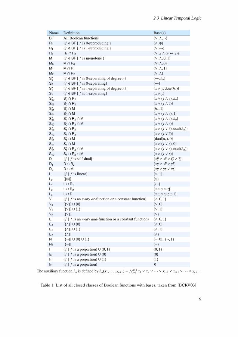
• f is linear if f ⌘ a1 � · · · � an � c for a constant c 2 {0, 1} and variables a1, . . . , an.
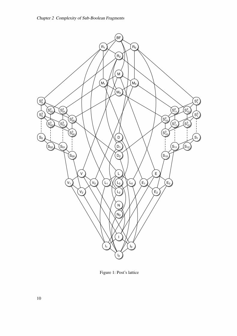
In Table 1 we define all clones and give Post’s bases [Pos41] for them. Post’s lattice is given inFigure 1. Now Lewis’s dichotomy can be described using Post’s lattice as follows, denotingwith SAT(B) the satisfiability problem of the fragment of propositional logic that allows onlyBoolean operators corresponding to a given set B of Boolean functions.
Theorem 2. [Lew79] SAT(B) is NP-complete if S1 ✓ [B] and solvable in polynomial timeotherwise.
In a similar fashion, Bauland et al.’s trichotomy for the basic modal logic K can be described asfollows. For a nonempty subset M ✓ {^,⇤} of the two standard modal operators ^ (“possibly”)and ⇤ (“necessarily”), and a set B of Boolean functions, let KM(B)-SAT be the satisfiabilityproblem for the fragment of K that allows only the modal operators in M and the Booleanoperators corresponding to B.
Theorem 3. [BHSS06, HSS10] K^,⇤(B)-SAT is
• PSPACE-complete if S11 ✓ [B],
• CONP-complete if E0 ✓ [B] ✓ E, and
• solvable in polynomial time otherwise.
K^(B)-SAT and K⇤(B)-SAT are PSPACE-complete if S1 ✓ [B] and solvable in polynomial timeotherwise.
Bauland et al.’s result is more general and captures multiple modalities, formulas given bycircuits, and di↵erent modal logics such as KD, T, S4, S5, i.e., the modal logics of serial,reflexive, transitive, and complete frames, respectively.
2.3 Linear Temporal Logic
Linear Temporal Logic (LTL) was introduced by Pnueli in [Pnu77] as a formalism for reasoningabout the properties and the behaviors of parallel programs and concurrent systems, and haswidely been used for these purposes. The standard reasoning tasks include satisfiability andmodel checking. The former asks whether, given an LTL formula ', there is a linear path atwhose starting point ' is true; the latter’s existential version additionally receives as input aKripke structureM and a state s and asks whether ' is true at some path starting at s inM.Validity and universal model checking are additional standard reasoning tasks; however, are notin the scope of our work.
Sistla and Clarke were the first to study the computational complexity of satisfiability and(existential) model checking. For full LTL with the operators F (eventually), G (invariantly),X (next-time), U (until), and S (since), they showed that both problems are PSPACE-complete;for some restrictions to the temporal operators – allowing only {X} or at most {F,G} –, theyestablished NP-completeness [SC85]. They also showed that the restriction to atomic negation
2 Monotone operators and the corresponding fragments of logics are often called positive, partly for historic reasons,partly in order to avoid false associations with the distinction between logics with monotonic and non-monotonicinference. All logics studied in this chapter have monotonic inference, and some of their fragments contain onlymonotone (positive) Boolean operators. We have decided to prefer “monotone” to “positive” because of theestablished clone name M.
8
2.3 Linear Temporal Logic
Name Definition Base(s)BF All Boolean functions {_,^,¬}R0 { f 2 BF | f is 0-reproducing } {^,�}R1 { f 2 BF | f is 1-reproducing } {_,$}R2 R1 \ R0 {_, x ^ (y$ z)}M { f 2 BF | f is monotone } {_,^, 0, 1}M0 M \ R0 {_,^, 0}M1 M \ R1 {_,^, 1}M2 M \ R2 {_,^}Sn
0 { f 2 BF | f is 0-separating of degree n} {!, hn}S0 { f 2 BF | f is 0-separating} {!}Sn
1 { f 2 BF | f is 1-separating of degree n} {x ^ y, dual(hn)}S1 { f 2 BF | f is 1-separating} {x ^ y}Sn
02 Sn0 \ R2 {x _ (y ^ z), hn}
S02 S0 \ R2 {x _ (y ^ z)}Sn
01 Sn0 \M {hn, 1}
S01 S0 \M {x _ (y ^ z), 1}Sn
00 Sn0 \ R2 \M {x _ (y ^ z), hn}
S00 S0 \ R2 \M {x _ (y ^ z)}Sn
12 Sn1 \ R2 {x ^ (y _ z), dual(hn)}
S12 S1 \ R2 {x ^ (y _ z)}Sn
11 Sn1 \M {dual(hn), 0}
S11 S1 \M {x ^ (y _ z), 0}Sn
10 Sn1 \ R2 \M {x ^ (y _ z), dual(hn)}
S10 S1 \ R2 \M {x ^ (y _ z)}D { f | f is self-dual} {xy _ xz _ (y ^ z)}D1 D \ R2 {xy _ xz _ yz}D2 D \M {xy _ yz _ xz}L { f | f is linear} {�, 1}L0 [{�}] {�}L1 L \ R1 {$}L2 L \ R2 {x � y � z}L3 L \ D {x � y � z � 1}V { f | f is an n-ary or-function or a constant function} {^, 0, 1}V0 [{_}] [ {0} {_, 0}V1 [{_}] [ {1} {_, 1}V2 [{_}] {_}E { f | f is an n-ary and-function or a constant function} {^, 0, 1}E0 [{^}] [ {0} {^, 0}E1 [{^}] [ {1} {^, 1}E2 [{^}] {^}N [{¬}] [ {0} [ {1} {¬, 0}, {¬, 1}N2 [{¬}] {¬}I { f | f is a projection} [ {0, 1} {0, 1}I0 { f | f is a projection} [ {0} {0}I1 { f | f is a projection} [ {1} {1}I2 { f | f is a projection} ;
The auxiliary function hn is defined by hn(x1, . . . , xn+1) =Vn+1
i=1 x1 _ x2 _ · · · _ xi�1 _ xi+1 _ · · · _ xn+1 .
Table 1: List of all closed classes of Boolean functions with bases, taken from [BCRV03]
9
Chapter 2 Complexity of Sub-Boolean Fragments
BF
R1 R0
R2
M
M1 M0
M2
S20
S202 S2
01S3
0S2
00S3
02 S301
S300
S0
S02 S01
S00
D
D1
D2
V
V1 V0
V2
L
L1 L3 L0
L2
N
N2
I
I1 I0
I2
S21
S212S2
11S3
1S2
10S3
12S311
S310
S1
S12S11
S10
E
E0E1
E2
Figure 1: Post’s lattice
10
2.3 Linear Temporal Logic
leads to NP-completeness in the case of {F,X}. These results imply that, under reasonablecomplexity-theoretic assumptions, reasoning with LTL is not tractable.
Subsequently, the e↵ect of restricting the set of temporal operators on the complexity of thesatisfiability and model-checking for LTL was studied more systematically in the literature,together with single restrictions of the Boolean operators: Demri and Schnoebelen [DS02]investigated satisfiability and existential model checking for restrictions on the set of temporaloperators, their nesting, and the number of atomic propositions. Markey [Mar04] studied thecomplexity of all four standard decision problems for LTL fragments with various subsets oftemporal operators (including the past versions of F and X), together with further restrictions onthe interaction between future and past operators, and between temporal operators and negation.He showed that these fragments are (CO)NP- or PSPACE-complete, respectively. Muscholland Walukiewicz [MW05] showed that satisfiability for the LTL variant that allows {F,G}together with a version of X “guarded” by atomic propositions is NP-complete – in contrastto PSPACE-completeness for the fragment {F,X} [SC85]. Since only Demri and Schnoebelenexhibit tractable fragments at all, it can be concluded that a multitude of LTL fragments have anintractable satisfiability and/or model-checking problem. In fact, not even the restriction to Hornformulas leads to a decrease in complexity of satisfiability for LTL, as shown earlier by Chenand Lin [CL93], and Dixon et al. [DFR00].
Fragments of related temporal logics have been investigated too: Emerson et al. [EES90]studied three fragments of computation tree logic (CTL) with temporal and Boolean restrictionsand showed tractability or NP-completeness. Hemaspaandra [Hem01] showed that satisfiabilityfor modal logic over linear frames drops from NP-complete to tractable if Boolean operatorsare restricted to conjunction and atomic negation. Finally, one of the first to systematicallystudy the complexity of fragments of modal-like logics was Halpern [Hal95]. He investigatedsatisfiability for multimodal logics, bounding the depth of modal operators and the number ofatomic propositions. Only the combination of both restrictions led to tractable fragments.
2.3.1 Basic Notions
Let PROP be a countable set of propositional variables, B be a finite set of Boolean functions, andT be a set of temporal operators. The set of temporal B-formulas over T is defined inductivelyby the grammar
' ::= p | � f (', . . . ,') | ⌧(', . . . ,'),
where p 2 PROP, � f is a Boolean operator (of the appropriate arity) corresponding to a functionf 2 B, and ⌧ is a temporal operator (of the appropriate arity) from T . We consider the unarytemporal operators X (next-time), F (eventually), G (invariantly) and the binary temporal operatorsU (until), R (release) and S (since). The set of all temporal B-formulas over T is denoted byLTLT (B).
LTL-formulas are interpreted over infinite paths of states, which intuitively can be seen asdi↵erent points of time, with propositional assignments. It is common to consider potentiallyinfinite sets of paths, represented by a class of finite Kripke structures, called transition systems.A transition system is a triple K = (W,R, ⌘), where W is a finite set of states, R ✓ W ⇥W is a totalbinary relation (i.e., for each a 2 W, there is some b 2 W such that aRb), and ⌘ : W ! 2PROPK
for a finite set PROPK ✓ PROP of variables. A path ⇡ in K is an infinite sequence denoted as(⇡0, ⇡1, . . . ), where, for all i � 0, ⇡i 2 W and ⇡iR⇡i+1.
For a transition system K = (W,R, ⌘), a path ⇡ in K, and a temporal B-formula over the
11
Chapter 2 Complexity of Sub-Boolean Fragments
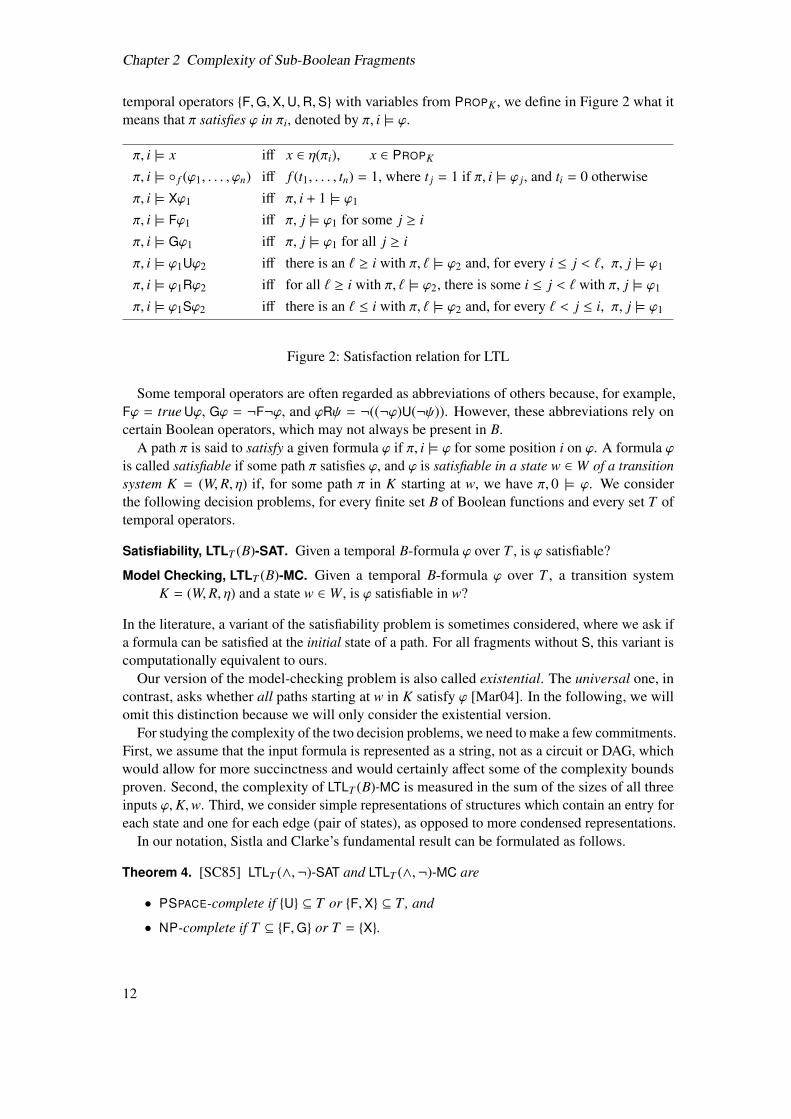
temporal operators {F,G,X,U,R,S} with variables from PROPK , we define in Figure 2 what itmeans that ⇡ satisfies ' in ⇡i, denoted by ⇡, i |= '.
⇡, i |= x i↵ x 2 ⌘(⇡i), x 2 PROPK
⇡, i |= � f ('1, . . . ,'n) i↵ f (t1, . . . , tn) = 1, where t j = 1 if ⇡, i |= ' j, and ti = 0 otherwise⇡, i |= X'1 i↵ ⇡, i + 1 |= '1
⇡, i |= F'1 i↵ ⇡, j |= '1 for some j � i⇡, i |= G'1 i↵ ⇡, j |= '1 for all j � i⇡, i |= '1U'2 i↵ there is an ` � i with ⇡, ` |= '2 and, for every i j < `, ⇡, j |= '1
⇡, i |= '1R'2 i↵ for all ` � i with ⇡, ` |= '2, there is some i j < ` with ⇡, j |= '1
⇡, i |= '1S'2 i↵ there is an ` i with ⇡, ` |= '2 and, for every ` < j i, ⇡, j |= '1
Figure 2: Satisfaction relation for LTL
Some temporal operators are often regarded as abbreviations of others because, for example,F' = true U', G' = ¬F¬', and 'R = ¬((¬')U(¬ )). However, these abbreviations rely oncertain Boolean operators, which may not always be present in B.
A path ⇡ is said to satisfy a given formula ' if ⇡, i |= ' for some position i on '. A formula 'is called satisfiable if some path ⇡ satisfies ', and ' is satisfiable in a state w 2 W of a transitionsystem K = (W,R, ⌘) if, for some path ⇡ in K starting at w, we have ⇡, 0 |= '. We considerthe following decision problems, for every finite set B of Boolean functions and every set T oftemporal operators.
Satisfiability, LTLT (B)-SAT. Given a temporal B-formula ' over T , is ' satisfiable?
Model Checking, LTLT (B)-MC. Given a temporal B-formula ' over T , a transition systemK = (W,R, ⌘) and a state w 2 W, is ' satisfiable in w?
In the literature, a variant of the satisfiability problem is sometimes considered, where we ask ifa formula can be satisfied at the initial state of a path. For all fragments without S, this variant iscomputationally equivalent to ours.
Our version of the model-checking problem is also called existential. The universal one, incontrast, asks whether all paths starting at w in K satisfy ' [Mar04]. In the following, we willomit this distinction because we will only consider the existential version.
For studying the complexity of the two decision problems, we need to make a few commitments.First, we assume that the input formula is represented as a string, not as a circuit or DAG, whichwould allow for more succinctness and would certainly a↵ect some of the complexity boundsproven. Second, the complexity of LTLT (B)-MC is measured in the sum of the sizes of all threeinputs ',K,w. Third, we consider simple representations of structures which contain an entry foreach state and one for each edge (pair of states), as opposed to more condensed representations.
In our notation, Sistla and Clarke’s fundamental result can be formulated as follows.
Theorem 4. [SC85] LTLT (^,¬)-SAT and LTLT (^,¬)-MC are
• PSPACE-complete if {U} ✓ T or {F,X} ✓ T, and
• NP-complete if T ✓ {F,G} or T = {X}.
12
2.3 Linear Temporal Logic
2.3.2 Satisfiability
Using Post’s lattice, we examine the satisfiability problem for every possible fragment of LTLdetermined by an arbitrary set of Boolean operators and any subset of the five temporal operators{F,G,X,U,S} studied by Sistla and Clarke. We determine the computational complexity ofthese problems, showing that all cases – except for two sets of Boolean operators – are eitherPSPACE-complete, NP-complete, or in P.
Among our results, we exhibit cases with nontrivial tractability as well as the smallest possiblesets of Boolean and temporal operators that already lead to NP-completeness or PSPACE-completeness, respectively. Examples for the first group are cases in which only the unary notfunction, or only monotone functions are allowed, but there is no restriction on the temporaloperators. As for the second group, if only the binary function f with f (x, y) = (x ^ y) ispermitted, then satisfiability is NP-complete already in the case of propositional logic [Lew79].Our results show that the presence of the same function f separates the tractable languages fromthe NP-complete and PSPACE-complete ones, depending on the set of temporal operators used.According to this, minimal sets of temporal operators leading to PSPACE-completeness togetherwith f are, for example, {U} and {F,X}.
Our results are formulated in Theorem 5 and depicted in Figure 10 (Appendix C).
Theorem 5. LTLT (B)-SAT is
• NP-complete if S1 ✓ [B] and T ✓ {F,G} or T = {X},• PSPACE-complete if S1 ✓ [B] and T is not covered by the previous case, and
• solvable in polynomial time in all other cases except for [B] = L0 or [B] = L .
The technically most involved proof is that of PSPACE-hardness in the case T = {S}. Thedi�culty lies in simulating the quantifier tree of a Quantified Boolean Formula (QBF) in a linearstructure. We do this in three steps: first, we partition a finite prefix of a path ⇡ into 2n subsequentintervals, each of which satisfies a distinct combination of truth values of the n universallyquantified variables occurring in the given QBF. This requires an LTL-subformula using ^, ¬,and a constant number of S-operators. Second, we construct another LTL-subformulas using^, _, ¬, and S, which sets the values for the existentially quantified variables in the previouslydelineated intervals. Finally, we rewrite all occurrences of ^, _, ¬ using polynomially-sizedformulas over the base f (x, y) = (x ^ y) of S1, using a standard technique that goes back to aresult of Lewis’s [Lew79].
The two missing cases [B] = L0 or [B] = L are based on the binary xor function and havealready defied classification in [BHSS06, HSS10] for modal logics of reflexive frames classes.Due to reflexivity, which is implicit in the semantics of LTL, a formula F' is satisfied at somestate whenever ' is. This prohibits attempts to treat the propositional part of a formula separatelyfrom the “remainder” when trying to find decision procedures. On the other hand, the restrictedexpressivity of xor makes it di�cult to prove lower bounds.
The results in Theorem 5 establish a homogeneous complexity landscape and reveal a clearborderline between tractable and intractable fragments: the intractable3 cases are characterizedby the ability to express the Boolean function f (x, y) = x^y, independently of the set of temporaloperators allowed. The further separation between NP- and PSPACE-completeness is determinedsolely by the temporal operators allowed.
3Throughout this thesis, we assume P , NP.
13
Chapter 2 Complexity of Sub-Boolean Fragments
2.3.3 Model Checking
Using Post’s lattice, we examine the existential model-checking problem for every possiblefragment of LTL determined by an arbitrary set of Boolean operators and any subset of the fivetemporal future operators {F,G,X,U,R}. We separate the model-checking problem for almost allof these fragments into tractable (here: polynomial-time solvable) and intractable (here: NP-hardor PSPACE-hard) cases. In contrast to earlier work discussed above, we exhibit many tractablefragments, and they are even in NL (nondeterministic logarithmic space). As for satisfiability, wehad to leave open the case of the binary xor-operator.
I
V E N
M L
BFFor the model-checking problem, the Boolean con-
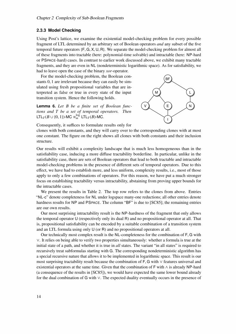
stants 0, 1 are irrelevant because they can easily be sim-ulated using fresh propositional variables that are in-terpreted as false or true in every state of the inputtransition system. Hence the following holds.
Lemma 6. Let B be a finite set of Boolean func-tions and T be a set of temporal operators. ThenLTLT (B [ {0, 1})-MC ⌘log
m LTLT (B)-MC.
Consequently, it su�ces to formulate results only forclones with both constants, and they will carry over to the corresponding clones with at mostone constant. The figure on the right shows all clones with both constants and their inclusionstructure.
Our results will exhibit a complexity landscape that is much less homogeneous than in thesatisfiability case, inducing a more di↵use tractability borderline. In particular, unlike in thesatisfiability case, there are sets of Boolean operators that lead to both tractable and intractablemodel-checking problems in the presence of di↵erent sets of temporal operators. Due to thise↵ect, we have had to establish more, and less uniform, complexity results, i.e., most of thoseapply to only a few combinations of operators. For this reason, we have put a much strongerfocus on establishing tractability versus intractability, abstaining from proving upper bounds forthe intractable cases.
We present the results in Table 2. The top row refers to the clones from above. Entries“NL-c” denote completeness for NL under logspace many-one reductions; all other entries denotehardness results for NP and PSPACE. The column “BF” is due to [SC85]; the remaining entriesare our own results.
Our most surprising intractability result is the NP-hardness of the fragment that only allowsthe temporal operator U (respectively only its dual R) and no propositional operator at all. Thatis, propositional satisfiability can be encoded by a suitable combination of a transition systemand an LTL formula using only U (or R) and no propositional operators at all.
Our technically most complex result is the NL-completeness for the combination of F,G with_. It relies on being able to verify two properties simultaneously: whether a formula is true at theinitial state of a path, and whether it is true in all states. The variant “in all states” is required torecursively treat subformulas starting with G. The corresponding nondeterministic algorithm hasa special recursive nature that allows it to be implemented in logarithmic space. This result is ourmost surprising tractability result because the combination of F,G with _ features universal andexistential operators at the same time. Given that the combination of F with ^ is already NP-hard(a consequence of the results in [SC85]), we would have expected the same lower bound alreadyfor the dual combination of G with _. The expected duality eventually occurs in the presence of
14
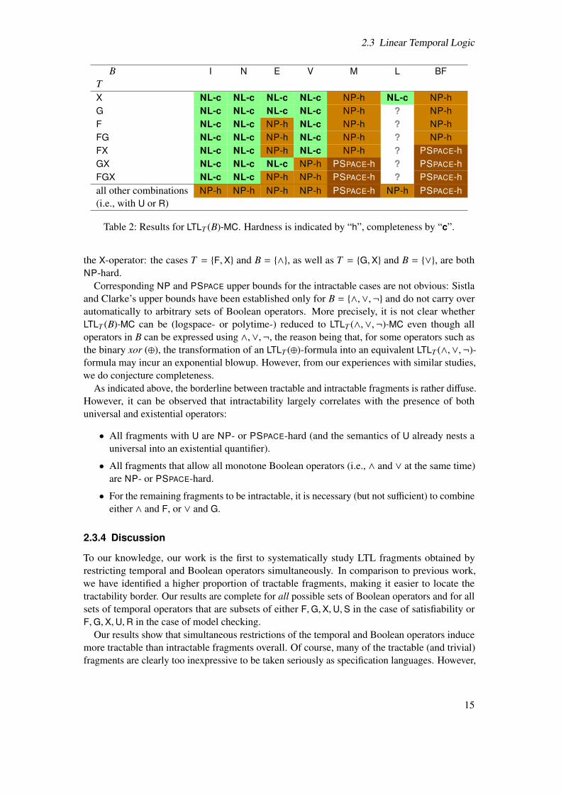
2.3 Linear Temporal Logic
B I N E V M L BFTX NL-c NL-c NL-c NL-c NP-h NL-c NP-hG NL-c NL-c NL-c NL-c NP-h ? NP-hF NL-c NL-c NP-h NL-c NP-h ? NP-hFG NL-c NL-c NP-h NL-c NP-h ? NP-hFX NL-c NL-c NP-h NL-c NP-h ? PSPACE-hGX NL-c NL-c NL-c NP-h PSPACE-h ? PSPACE-hFGX NL-c NL-c NP-h NP-h PSPACE-h ? PSPACE-hall other combinations NP-h NP-h NP-h NP-h PSPACE-h NP-h PSPACE-h(i.e., with U or R)
Table 2: Results for LTLT (B)-MC. Hardness is indicated by “h”, completeness by “c”.
the X-operator: the cases T = {F,X} and B = {^}, as well as T = {G,X} and B = {_}, are bothNP-hard.
Corresponding NP and PSPACE upper bounds for the intractable cases are not obvious: Sistlaand Clarke’s upper bounds have been established only for B = {^,_,¬} and do not carry overautomatically to arbitrary sets of Boolean operators. More precisely, it is not clear whetherLTLT (B)-MC can be (logspace- or polytime-) reduced to LTLT (^,_,¬)-MC even though alloperators in B can be expressed using ^,_,¬, the reason being that, for some operators such asthe binary xor (�), the transformation of an LTLT (�)-formula into an equivalent LTLT (^,_,¬)-formula may incur an exponential blowup. However, from our experiences with similar studies,we do conjecture completeness.
As indicated above, the borderline between tractable and intractable fragments is rather di↵use.However, it can be observed that intractability largely correlates with the presence of bothuniversal and existential operators:
• All fragments with U are NP- or PSPACE-hard (and the semantics of U already nests auniversal into an existential quantifier).
• All fragments that allow all monotone Boolean operators (i.e., ^ and _ at the same time)are NP- or PSPACE-hard.
• For the remaining fragments to be intractable, it is necessary (but not su�cient) to combineeither ^ and F, or _ and G.
2.3.4 Discussion
To our knowledge, our work is the first to systematically study LTL fragments obtained byrestricting temporal and Boolean operators simultaneously. In comparison to previous work,we have identified a higher proportion of tractable fragments, making it easier to locate thetractability border. Our results are complete for all possible sets of Boolean operators and for allsets of temporal operators that are subsets of either F,G,X,U,S in the case of satisfiability orF,G,X,U,R in the case of model checking.
Our results show that simultaneous restrictions of the temporal and Boolean operators inducemore tractable than intractable fragments overall. Of course, many of the tractable (and trivial)fragments are clearly too inexpressive to be taken seriously as specification languages. However,
15
Chapter 2 Complexity of Sub-Boolean Fragments
some tractable fragments are quite expressive, for example those with monotone Booleanoperators (in the case of satisfiability) or with only conjunction (in the case of satisfiabilityand model checking). There is clearly a parallel to lightweight description logics such as EL(see Section 2.1). It is possible that monotone fragments of LTL are su�cient to formulatespecifications in certain applications of verification. These applications could rely on the e�cientdecision procedures emanating from our results.
We chose the temporal operators in the case of satisfiability because they were considered bySistla and Clarke [SC85], and in the case of model checking because they are the standard futureoperators. We provide more justifications for this choice in our original work [BMS+11].
For future work, it would be tempting to initiate an even more systematic study that is completewith respect to all possible sets of temporal operators, including past operators (which werestudied previously [SC85, Mar04]), but also operators defined by arbitrary LTL formulas, e.g.the ternary operator O(↵, �, �) = F↵ _ (�U�), or even operators based on automata [Wol83].Unfortunately, it is not very realistic to achieve this kind of completeness, because of thecombinatorial explosion incurred:
First, even if one adds only the five past counterparts of the above F,G,X,U,R, the number offragments to consider will blow up significantly: 210 � 1 = 1023 instead of 25 � 1 = 31 sets oftemporal operators, each combined with a large number of sets of Boolean operators. Given thelarge number of NL-complete fragments in Table 2 and the fact that many of the proofs for theirupper bounds rely on the absence of past operators, we expect that a huge number of additionalsingle theorems would have to be proven. So far, we can at least say that almost all fragmentscontaining the S (since) operator are as hard as the corresponding fragments with U, for thesame reasons. However, there are exceptions which are due to the asymmetry that paths have afirst, but no last, state [BMS+09]. Still, it would of course be interesting to find out whether theconclusion “past is for free” drawn in [Mar04] extends to sub-Boolean fragments of LTL.
Second, a truly systematic account of all possible temporal operators would have to start withcataloging all definitions of temporal operators in the formalisms mentioned above, analogouslyto Post’s lattice of all Boolean functions. Since these formalisms are much more expressive thanpropositional logic, it is unclear whether such a research program would be feasible at all (if oneconsiders that Post’s lattice already took its author several years to establish).
A di↵erent, more feasible, direction for future work is to apply our systematic study tobranching-time temporal logics, such as CTL(*) (but satisfiability has already been classified[MMTV09]), to the µ-calculus, which extends both LTL and CTL(*), or even to the hybridµ-calculus [SV01].
2.4 Description Logic
We already know from Chapter 1 that description logics (DLs) [BCM+03] are a successful familyof knowledge representation languages. They are decidable fragments of first-order logic andunderlie the W3C Web Ontology Language OWL. The main feature of DLs is the ability todescribe concepts (e.g., “a patient who has a history of high blood pressure”), to define newconcepts in terms of others (e.g., “HighRiskPatient” in the context of heart diseases), and toexpress background knowledge (e.g., “a patient who has a history of high blood pressure issomeone who has an increased risk of su↵ering a stroke”). Definitions and background knowledgeare specified in terminologies, also called TBoxes, via axioms that relate concept descriptionswith each other, such as concept inclusions. The standard reasoning tasks of satisfiability and
16
2.4 Description Logic
subsumption ask whether a given concept description has a model or whether a given conceptdescription implies another (in both cases possibly with respect to a given TBox). They havebeen studied extensively for various DLs of di↵erent expressivity. Their complexity rangesbetween trivial for fragments of the basic DL ALC and N2EXPTIME for the OWL 2 standardSROIQ. Another factor that determines the complexity is the distinction whether terminologicalknowledge, general background knowledge, or no TBoxes at all are allowed.
ForALC with general TBoxes, satisfiability and subsumption are interreducible and EXPTIME-complete: the upper bound is due to the correspondence with propositional dynamic logic[Pra78, VW86, DM00], and the lower bound was proved by Schild [Sch94]. To obtain tractableDLs with tractable reasoning problems, specific fragments ofALC based on restrictions to theallowed Boolean operators and quantifiers has been studied. Notable examples include membersof the prominent EL and DL-Lite families (see Section 2.1). The following is a brief survey ofthe complexity landscape for such specific sub-BooleanALC fragments (it must be observedthat, unlike forALC, the standard reasoning problems are no longer interreducible in the absenceof certain Boolean operators).
• EL allows only conjunctions and existential restrictions [Baa03], and thus satisfiabilityfor EL is uninteresting because every EL-concept and -TBox is satisfiable. Conceptsubsumption with or without TBoxes is tractable in EL [Baa03, Bra04], and it remainstractable under a variety of extensions such as nominals, concrete domains, role chaininclusions, and domain and range restrictions [BBL05, BBL08].
• In contrast, the presence of universal quantifiers usually breaks tractability: subsumptionin FL0, which allows only conjunction and universal restrictions, is CONP-complete[Neb90b]. Relative to TBoxes, the complexity increases to PSPACE-complete for cyclicTBoxes [Baa96, Kd03] and EXPTIME-complete for general TBoxes [BBL05, Hof05]. In[DLN+92, DLNN97], concept satisfiability and subsumption for several logics belowand above ALC that extend FL0 with disjunction, negation and existential restrictionsand other features, is shown to be tractable, NP-complete, CONP-complete or PSPACE-complete.
• EXPTIME-hardness of subsumption relative to general TBoxes can be observed alreadyin fragments of ALC containing either conjunction or disjunction and both existentialand universal restrictions [GMWK02], or only conjunction, universal restrictions andunqualified existential restrictions [Don03].
• In the historically first member of the large DL-Lite family, where unqualified existentialrestrictions, atomic negation on the right-hand side of concept inclusions, as well as inverseand functional roles are allowed, satisfiability is tractable [CDL+05]. Several extensionsof DL-Lite are shown to have tractable, NP-complete, or EXPTIME-complete satisfiabilityproblems in [ACKZ07, ACKZ09a, ACKZ09b].
DLs from the above families with tractable reasoning problems are called lightweight DLs. Theyare based on specific sets of allowed Boolean operators and quantifiers (and, in some cases, relyon further limitations, such as unqualified existential restrictions). Despite the success of the ELand DL-Lite families, the principled question remains whether it is possible to design lightweightDLs based on di↵erent restrictions. By giving a systematic account of the complexity of DLswith restricted Boolean operators and quantifiers, we aim at answering this question. We pursuethe same approach as in the previous section and classify satisfiability with respect to TBoxes forALC fragments obtained by arbitrary sets of Boolean operators and quantifiers.
17
Chapter 2 Complexity of Sub-Boolean Fragments
2.4.1 Basic Notions
We use the standard syntax and semantics ofALC [BCM+03], with the Boolean operators u, t,¬,>,? replaced by arbitrary operators � f corresponding to Boolean functions f : {0, 1}n ! {0, 1}of arity n. Let NC, NR and NI be sets of atomic concepts, roles and individuals, and let B bea set of Boolean functions and Q ✓ {9,8} a set of quantifiers. Then the set of ALC-conceptdescriptions using only operators from B and Q, for short (B,Q)-concepts, is defined by
C ::= A | � f (C, . . . ,C) | q r.C,
where A 2 NC, r 2 NR, � f 2 B is a Boolean operator corresponding to a function f 2 B, andq 2 Q is a quantifier. A general (B,Q)-concept inclusion ((B,Q)-GCI) is an axiom of the formC v D where C,D are B-concepts. A (B,Q)-TBox is a finite set of (B,Q)-GCIs. A (B,Q)-ABoxis a finite set of axioms of the form C(a) or r(a, b), where C is a (B,Q)-concept, r 2 NR anda, b 2 NI. A (B,Q)-ontology is the union of a (B,Q)-TBox and (B,Q)-ABox (this simplifiedview su�ces for our purposes).
An interpretation is a pair I = (�I, ·I), where �I is a nonempty set and the interpretationfunction ·I maps every atomic concept to a subset of �I, every role to a binary relation over �I,and every individual to an element of �I. The interpretation function is extended to arbitrary(B,Q)-concepts as follows.
� f (C1, . . . ,Cn)I = {x 2 �I | f (t1, . . . , tn) = 1}, where ti = 1 if x 2CIi , and ti = 0 otherwise
9R.CI = {x 2 �I | {y 2 CI | (x, y) 2 RI} , ;}8R.CI = {x 2 �I | {y 2 CI | (x, y) < RI} = ;}
An interpretation I satisfies the GCI C v D, written I |= C v D, if CI ✓ DI. Furthermore, Isatisfies C(a) or R(a, b) if aI 2 CI or (aI, bI) 2 RI. An interpretation I satisfies a TBox (ABox,ontology) if it satisfies every axiom therein. It is then called a model of this set of axioms.
The following decision problems are of interest for this section.
Concept satisfiability CSATQ(B):Given a (B,Q)-concept C, is there an interpretation I s.t. CI , ; ?
TBox satisfiability TSATQ(B):Given a (B,Q)-TBox T , is there an interpretation I s.t. I |= T ?
TBox-concept satisfiability TCSATQ(B):Given a (B,Q)-TBox T and a (B,Q)-concept C, is there an I s.t. I |= T and CI , ; ?
Ontology satisfiability OSATQ(B):Given a (B,Q)-ontology O, is there an interpretation I s.t. I |= O ?
Ontology-concept satisfiability OCSATQ(B):Given a (B,Q)-ontology O and a (B,Q)-concept C, is there an I s.t. I |= O and CI , ; ?
We are interested in the complexity of these problems. The first, concept satisfiability withoutaxioms, is already covered by Bauland et al.’s study of the satisfiability problem for modal logic(Theorem 3) becauseALC is a notational variant of the modal logic K with the quantifiers 9,8corresponding to the modal operators ^,⇤.
18
2.4 Description Logic
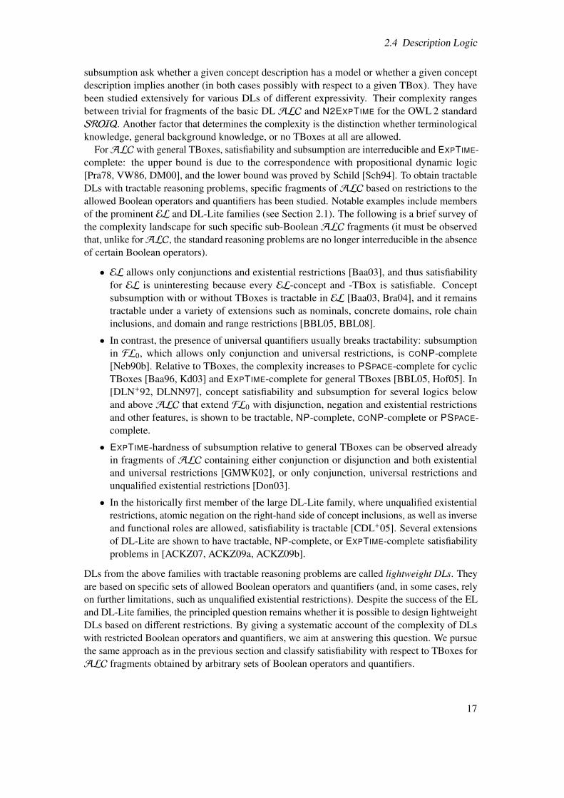
TSATQ(B) I0 I V0 V E0 E N2,N S11 to R0 M L0 L3 to BF else
Q = ; t NL t P t P NL t NP t NP tQ = {9} t P t EXP t P EXP t EXP t EXP tQ = {8} t P t P t EXP EXP t EXP t EXP tQ = {9,8} t EXP t EXP t EXP EXP t EXP t EXP t
remaining
Q = ; NL P NL NP tQ = {9} P EXPTIME P EXPTIME tQ = {8} P EXPTIME tQ = {9,8} EXPTIME t
Table 3: Results for TSAT and the remaining three problems TCSAT,OSAT,OCSAT. All entriesdenote completeness. “EXP” abbreviates “EXPTIME”, and “t” stands for “trivial”.
It can easily be seen that there are some reducibilities between the satisfiability problemsindependently of B and Q:
CSATQ(B) logm TCSATQ(B) and
TSATQ(B) logm TCSATQ(B) log
m OSATQ(B) ⌘logm OCSATQ(B)
2.4.2 Results and Discussion
Our results are given in Table 3 and Figures 11–14 (Appendix C). They are complete withrespect to arbitrary sets of Boolean operators and quantifiers. We can furthermore extract thetractability border by listing the maximal tractable sub-Boolean fragments of ALC, i.e., themaximal combinations of B and Q for which TSATQ(B) (and the other three problems) aretractable:
1. B = R1 (1-reproducing functions) and Q arbitrary
2. B = R0 (1-reproducing functions) and Q arbitrary – only TSAT
3. B = E (conjunction and both constants) and Q ✓ {9}4. B = V (disjunction and both constants) and Q ✓ {8}5. B = N (negation and both constants) and Q = ;
In other words, the maximal lightweight DLs obtained by restricting Boolean operators andquantifiers are given by this short list. We can now answer our original question by observingthat this list contains no interesting candidate for a lightweight DL other than those that arealready known:
• Item 3 is EL?, the extension of ELwith the?-operator, which is subsumed by the tractablelogic EL++ underlying the OWL EL profile.
19
Chapter 2 Complexity of Sub-Boolean Fragments
• Item 4 is a logic allowing only the duals of the operators in EL?, which can safely be ruledout as a reasonable modeling language.
• Item 5 is a very simple logic in which one can only express subsumption and disjointnessbetween concept names, i.e., this logic allows to model only taxonomies with disjointnessinformation.
• Items 1 and 2 denote the maximal fragments for which satisfiability is even trivial. Inthis case, subsumption is the relevant decision problem. Subsumption was studied byMeier [Mei11], whose results surprisingly yield that subsumption for the cases B = R1and B = R0 is intractable. The maximal fragments with tractable subsumption (and trivialsatisfiability) are determined by B = E1,Q = {9} and B = V1,Q = {8}, but these arealready subsumed by items 3 and 4.
Our study therefore provides a systematic underpinning of the folklore assumption that therestrictions to the Boolean operators and quantifiers that underlie the known families of light-weight DLs lead to the only useful sub-BooleanALC-fragments for which satisfiability in thepresence of general TBoxes is tractable. On the one hand, this conclusion is more generalthan the results in [BBL05] that extensions of EL with ¬ and t are intractable. On the otherhand, it is restricted to the case of general TBoxes and can therefore not be transferred to, e.g.,acyclic TBoxes. Another limitation of our study is that is does not allow any conclusion aboutunqualified use of quantifiers, which contributes to the good computational properties of logicsin the DL-Lite family. A study that takes these two aspects into consideration would be a naturalcontinuation; however, we consider it unlikely that it would yield significant further insights.
If we compare the results of this study with the previously discussed analyses of propositionaland modal logic [Lew79, BHSS06, HSS10] or with our studies for temporal and hybrid logic inSections 2.3 and 2.5, we can observe intractable fragments considerably closer to the bottom ofthe lattice – even down to the I-clones in the case Q = {9,8}. This di↵erence is not too surprising,given that TBoxes reintroduce a limited form of implication and conjunction, which inducesu�cient expressive power for encoding EXPTIME-hard problems.
A natural question for future work is whether the complexity landscape, including the trac-tability border, changes if the use of general concept inclusions is restricted, for example, toacyclic terminologies, i.e., TBoxes where axioms are cycle-free definitions A ⌘ C with A beingatomic. Theories so restricted are useful for establishing taxonomies, and concept satisfiabilityforALC w.r.t. acyclic terminologies is still PSPACE-complete [BH91, Cal96]. Furthermore, alarge part of SNOMED CT is an acyclic EL terminology. Another natural direction for futurework is mentioned above: the investigation of fragments with unqualified quantifiers.
2.5 Hybrid Logic
Hybrid logics extend modal logic with the ability to refer explicitly to states in Kripke structures,using nominals, the satisfaction operator @, and/or the downarrow binder #. This additionalexpressive power is sometimes paid with unsatisfactory computational properties: while the basicuni-modal language K extended with nominals and @ remains PSPACE-complete [ABM99], theaddition of only # to K leads to undecidability [ABM99].
In order to regain decidability, several syntactic and semantic restrictions of the hybridbinder language have been considered. Ten Cate and Franceschet in [tF05] have reestablisheddecidability by restricting the interactions between # and universal modal operators – such as
20
2.5 Hybrid Logic
⇤, its inverse, and its global counterpart – and, separately, by restricting attention to Kripkestructures of bounded width: depending on the severity of the single restrictions and on thequestion whether they are combined, K# is NP-, EXPTIME-, NEXPTIME- or 2EXPTIME-complete.Our previous work was concerned with di↵erent semantic restrictions for regaining decidability:K# is NEXPTIME-complete over transitive and complete Kripke structures, and while K#,@ isundecidable over transitive Kripke structures, it is still NEXPTIME-complete over complete Kripkestructures [MSSW10]. Over equivalence relations, even K extended with the more powerful“jumping” binder 9 is decidable, namely N2EXPTIME-complete [MS09]. Furthermore, overacyclic Kripke structures such as linear structures and transitive trees, # on its own does not addany expressivity; extensions such as K#,@ have been shown to be decidable but nonelementary in[FdS03, MSSW10]. Elementary fragments have been obtained by bounding the number of statevariables [SW07, Web09, BL10].
We aim for a more detailed view of the complexity landscape of hybrid binder languages thatexhibits a more fine-grained boundary between decidable and undecidable, between elementaryand nonelementary, and between tractable and intractable fragments of K#,@. We systematicallystudy fragments obtained by restrictions to the Boolean operators as in the previous sections,combined with restrictions to the modal and hybrid operators, over several classes of Kripkestructures. The unrestricted hybrid language from which we start contains ^ and ⇤, as well asnominals, @, and #. The classes of Kripke structures that we consider fall into two groups:
• Classes of structures that allow cycles: all structures, transitive structures, total structures(where every state has at least one successor), and structures with equivalence relations(ER structures for short)
• Classes of acyclic structures: general linear orders and the special case of the naturalnumbers with the “less than” relation
One benefit that we expect from this systematic study is an insight into possible extensionsof specification languages (such as LTL) and knowledge representation languages (such asDLs) with hybrid operators. Given the negative results listed above, there is no hope to gaincomputationally well-behaved logics by just adding # without any restrictions. By consideringsub-Boolean fragments, we hope to lay the foundations for the future design of “lightweight”hybrid extensions of LTL or DLs that stand a chance of being useful and well-behaved.
2.5.1 Basic Notions
We define the standard terminology of hybrid logic as in [At07]. Let PROP be a countable setof propositional variables, NOM a countable set of nominals, SVAR a countable set of statevariables, and ATOM = PROP [ NOM [ SVAR. The formulas of hybrid (modal) logic HL aredefined by
' ::= a | � f (', . . . ,') | ^' | ⇤' | #x.' | @t ',
where a 2 ATOM, � f is a Boolean operator corresponding to the Boolean function f , and wherex 2 SVAR and t 2 NOM [ SVAR.
HL formulas are interpreted on (hybrid) Kripke structures K = (W,R, ⌘), consisting of a setof states W, a transition relation R ✓ W ⇥W, and a labeling function ⌘ : PROP [ NOM ! 2W
satisfying |⌘(i)| = 1 for all i 2 NOM. In order to evaluate #-formulas, we use assignmentsg : SVAR ! W similar to assignments in first-order logic. Given an assignment g, a state variablex and a state w, the x-variant gx
w of g is the assignment satisfying gxw(x) = w and gx
w(x0) = g(x0)
21
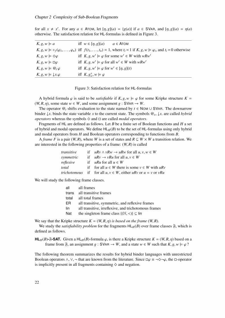
Chapter 2 Complexity of Sub-Boolean Fragments
for all x , x0. For any a 2 ATOM, let [⌘, g](a) = {g(a)} if a 2 SVAR, and [⌘, g](a) = ⌘(a)otherwise. The satisfaction relation for HL-formulas is defined in Figure 3.
K, g,w |= a i↵ w 2 [⌘, g](a) a 2 ATOM
K, g,w |= � f ('1, . . . ,'n) i↵ f (t1, . . . , tn) = 1, where ti = 1 if K, g,w |= 'i, and ti = 0 otherwiseK, g,w |= ^' i↵ K, g,w0 |= ' for some w0 2 W with wRw0
K, g,w |= ⇤' i↵ K, g,w0 |= ' for all w0 2 W with wRw0
K, g,w |= @t ' i↵ K, g,w0 |= ' for w0 2 [⌘, g](t)K, g,w |= #x.' i↵ K, gx
w,w |= '
Figure 3: Satisfaction relation for HL-formulas
A hybrid formula ' is said to be satisfiable if K, g,w |= ' for some Kripke structure K =(W,R, ⌘), some state w 2 W, and some assignment g : SVAR ! W.
The operator @t shifts evaluation to the state named by t 2 NOM [ SVAR. The downarrowbinder #x. binds the state variable x to the current state. The symbols @x, #x. are called hybridoperators whereas the symbols ^ and ⇤ are called modal operators.
Fragments of HL are defined as follows. Let B be a finite set of Boolean functions and H a setof hybrid and modal operators. We define HLH(B) to be the set of HL-formulas using only hybridand modal operators from H and Boolean operators corresponding to functions from B.
A frame F is a pair (W,R), where W is a set of states and R ✓ W ⇥W a transition relation. Weare interested in the following properties of a frame: (W,R) is called
transitive if uRv ^ vRw! uRw for all u, v,w 2 Wsymmetric if uRv! vRu for all u, v 2 Wreflexive if uRu for all u 2 Wtotal if for all u 2 W there is some v 2 W with uRvtrichotomous if for all u, v 2 W, either uRv or u = v or vRu
We will study the following frame classes.
all all framestrans all transitive framestotal all total framesER all transitive, symmetric, and reflexive frameslin all transitive, irreflexive, and trichotomous framesNat the singleton frame class {(N, <)} ✓ lin
We say that the Kripke structure K = (W,R, ⌘) is based on the frame (W,R).We study the satisfiability problem for the fragments HLH(B) over frame classes F, which is
defined as follows.
HLH(B)-F-SAT. Given a HLH(B)-formula ', is there a Kripke structure K = (W,R, ⌘) based on aframe from F, an assignment g : SVAR ! W, and a state w 2 W such that K, g,w |= ' ?
The following theorem summarizes the results for hybrid binder languages with unrestrictedBoolean operators ^,_,¬ that are known from the literature. Since ⇤' ⌘ ¬^¬', the ⇤-operatoris implicitly present in all fragments containing ^ and negation.
22
2.5 Hybrid Logic
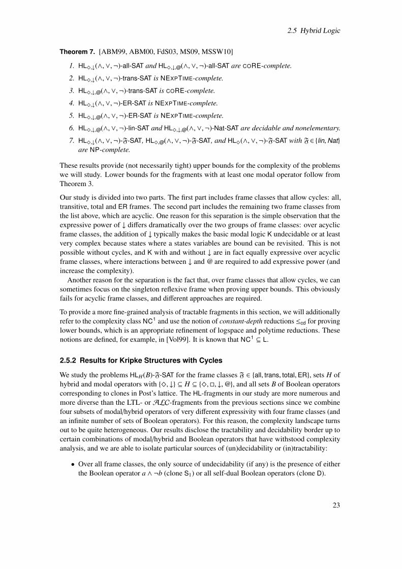
Theorem 7. [ABM99, ABM00, FdS03, MS09, MSSW10]
1. HL^,#(^,_,¬)-all-SAT and HL^,#,@(^,_,¬)-all-SAT are CORE-complete.
2. HL^,#(^,_,¬)-trans-SAT is NEXPTIME-complete.
3. HL^,#,@(^,_,¬)-trans-SAT is CORE-complete.
4. HL^,#(^,_,¬)-ER-SAT is NEXPTIME-complete.
5. HL^,#,@(^,_,¬)-ER-SAT is NEXPTIME-complete.
6. HL^,#,@(^,_,¬)-lin-SAT and HL^,#,@(^,_,¬)-Nat-SAT are decidable and nonelementary.
7. HL^,#(^,_,¬)-F-SAT, HL^,@(^,_,¬)-F-SAT, and HL^(^,_,¬)-F-SAT with F 2 {lin,Nat}are NP-complete.
These results provide (not necessarily tight) upper bounds for the complexity of the problemswe will study. Lower bounds for the fragments with at least one modal operator follow fromTheorem 3.
Our study is divided into two parts. The first part includes frame classes that allow cycles: all,transitive, total and ER frames. The second part includes the remaining two frame classes fromthe list above, which are acyclic. One reason for this separation is the simple observation that theexpressive power of # di↵ers dramatically over the two groups of frame classes: over acyclicframe classes, the addition of # typically makes the basic modal logic K undecidable or at leastvery complex because states where a states variables are bound can be revisited. This is notpossible without cycles, and K with and without # are in fact equally expressive over acyclicframe classes, where interactions between # and @ are required to add expressive power (andincrease the complexity).
Another reason for the separation is the fact that, over frame classes that allow cycles, we cansometimes focus on the singleton reflexive frame when proving upper bounds. This obviouslyfails for acyclic frame classes, and di↵erent approaches are required.
To provide a more fine-grained analysis of tractable fragments in this section, we will additionallyrefer to the complexity class NC1 and use the notion of constant-depth reductions cd for provinglower bounds, which is an appropriate refinement of logspace and polytime reductions. Thesenotions are defined, for example, in [Vol99]. It is known that NC1 ✓ L.
2.5.2 Results for Kripke Structures with Cycles
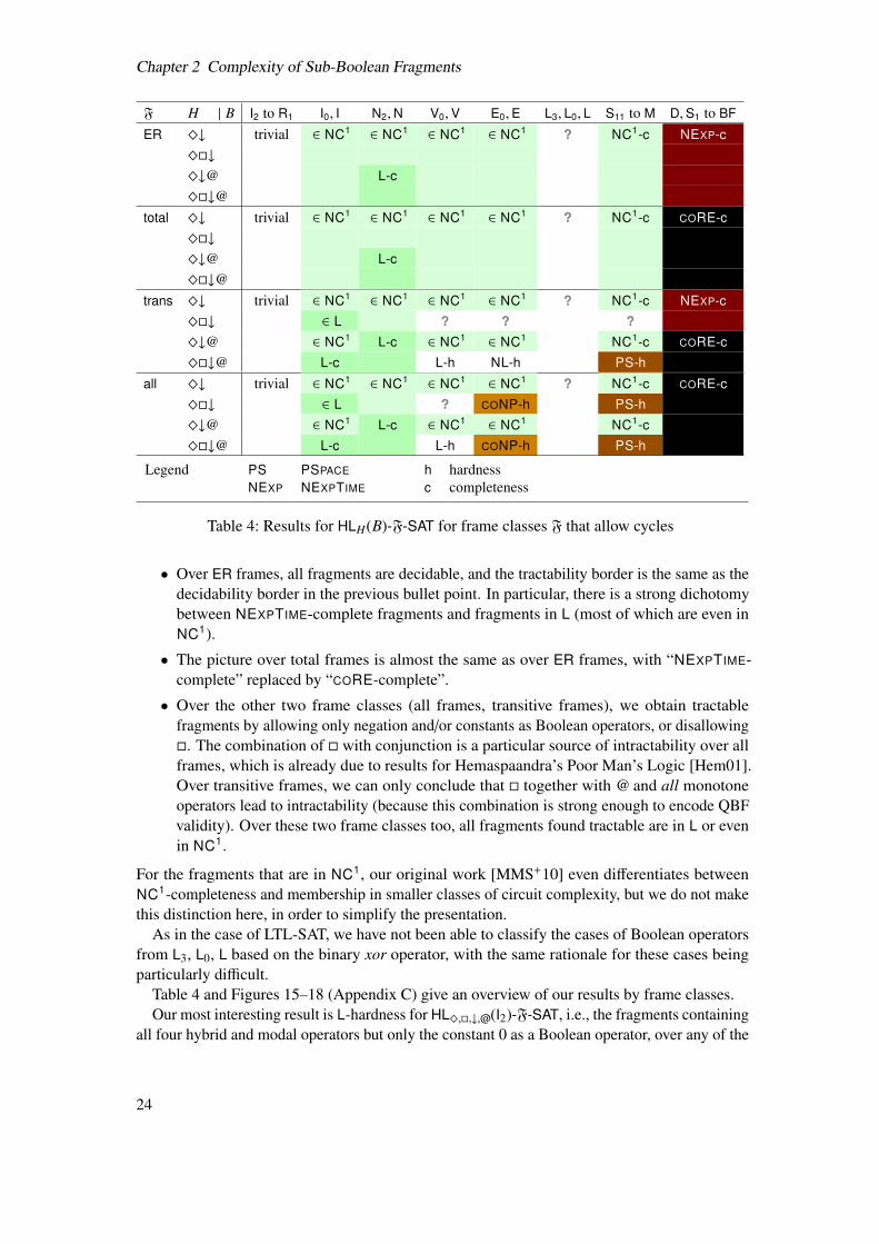
We study the problems HLH(B)-F-SAT for the frame classes F 2 {all, trans, total,ER}, sets H ofhybrid and modal operators with {^, #} ✓ H ✓ {^,⇤, #,@}, and all sets B of Boolean operatorscorresponding to clones in Post’s lattice. The HL-fragments in our study are more numerous andmore diverse than the LTL- or ALC-fragments from the previous sections since we combinefour subsets of modal/hybrid operators of very di↵erent expressivity with four frame classes (andan infinite number of sets of Boolean operators). For this reason, the complexity landscape turnsout to be quite heterogeneous. Our results disclose the tractability and decidability border up tocertain combinations of modal/hybrid and Boolean operators that have withstood complexityanalysis, and we are able to isolate particular sources of (un)decidability or (in)tractability:
• Over all frame classes, the only source of undecidability (if any) is the presence of eitherthe Boolean operator a ^ ¬b (clone S1) or all self-dual Boolean operators (clone D).
23
Chapter 2 Complexity of Sub-Boolean Fragments
F H | B I2 to R1 I0, I N2,N V0,V E0,E L3, L0, L S11 to M D,S1 to BFER ^# trivial 2 NC1 2 NC1 2 NC1 2 NC1 ? NC1-c NEXP-c
^⇤#^#@ L-c^⇤#@
total ^# trivial 2 NC1 2 NC1 2 NC1 2 NC1 ? NC1-c CORE-c^⇤#^#@ L-c^⇤#@
trans ^# trivial 2 NC1 2 NC1 2 NC1 2 NC1 ? NC1-c NEXP-c^⇤# 2 L ? ? ?^#@ 2 NC1 L-c 2 NC1 2 NC1 NC1-c CORE-c^⇤#@ L-c L-h NL-h PS-h
all ^# trivial 2 NC1 2 NC1 2 NC1 2 NC1 ? NC1-c CORE-c^⇤# 2 L ? CONP-h PS-h^#@ 2 NC1 L-c 2 NC1 2 NC1 NC1-c^⇤#@ L-c L-h CONP-h PS-h
Legend PS PSPACE h hardnessNEXP NEXPTIME c completeness
Table 4: Results for HLH(B)-F-SAT for frame classes F that allow cycles
• Over ER frames, all fragments are decidable, and the tractability border is the same as thedecidability border in the previous bullet point. In particular, there is a strong dichotomybetween NEXPTIME-complete fragments and fragments in L (most of which are even inNC1).
• The picture over total frames is almost the same as over ER frames, with “NEXPTIME-complete” replaced by “CORE-complete”.
• Over the other two frame classes (all frames, transitive frames), we obtain tractablefragments by allowing only negation and/or constants as Boolean operators, or disallowing⇤. The combination of ⇤ with conjunction is a particular source of intractability over allframes, which is already due to results for Hemaspaandra’s Poor Man’s Logic [Hem01].Over transitive frames, we can only conclude that ⇤ together with @ and all monotoneoperators lead to intractability (because this combination is strong enough to encode QBFvalidity). Over these two frame classes too, all fragments found tractable are in L or evenin NC1.
For the fragments that are in NC1, our original work [MMS+10] even di↵erentiates betweenNC1-completeness and membership in smaller classes of circuit complexity, but we do not makethis distinction here, in order to simplify the presentation.
As in the case of LTL-SAT, we have not been able to classify the cases of Boolean operatorsfrom L3, L0, L based on the binary xor operator, with the same rationale for these cases beingparticularly di�cult.
Table 4 and Figures 15–18 (Appendix C) give an overview of our results by frame classes.Our most interesting result is L-hardness for HL^,⇤,#,@(I2)-F-SAT, i.e., the fragments containing
all four hybrid and modal operators but only the constant 0 as a Boolean operator, over any of the
24
2.5 Hybrid Logic
F H ⇢ {⇤, #,@} H = {⇤, #,@} {^} ✓ H ⇢ {^,⇤, #,@} H = {^,⇤, #,@}lin NC1 NC1 NP nonelem.Nat NC1 L NP PSPACE
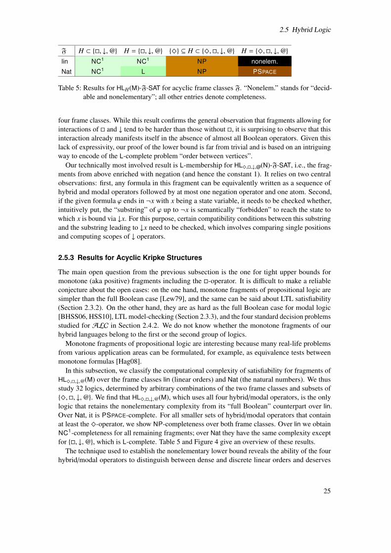
Table 5: Results for HLH(M)-F-SAT for acyclic frame classes F. “Nonelem.” stands for “decid-able and nonelementary”; all other entries denote completeness.
four frame classes. While this result confirms the general observation that fragments allowing forinteractions of ⇤ and # tend to be harder than those without ⇤, it is surprising to observe that thisinteraction already manifests itself in the absence of almost all Boolean operators. Given thislack of expressivity, our proof of the lower bound is far from trivial and is based on an intriguingway to encode of the L-complete problem “order between vertices”.
Our technically most involved result is L-membership for HL^,⇤,#,@(N)-F-SAT, i.e., the frag-ments from above enriched with negation (and hence the constant 1). It relies on two centralobservations: first, any formula in this fragment can be equivalently written as a sequence ofhybrid and modal operators followed by at most one negation operator and one atom. Second,if the given formula ' ends in ¬x with x being a state variable, it needs to be checked whether,intuitively put, the “substring” of ' up to ¬x is semantically “forbidden” to reach the state towhich x is bound via #x. For this purpose, certain compatibility conditions between this substringand the substring leading to #x need to be checked, which involves comparing single positionsand computing scopes of # operators.
2.5.3 Results for Acyclic Kripke Structures
The main open question from the previous subsection is the one for tight upper bounds formonotone (aka positive) fragments including the ⇤-operator. It is di�cult to make a reliableconjecture about the open cases: on the one hand, monotone fragments of propositional logic aresimpler than the full Boolean case [Lew79], and the same can be said about LTL satisfiability(Section 2.3.2). On the other hand, they are as hard as the full Boolean case for modal logic[BHSS06, HSS10], LTL model-checking (Section 2.3.3), and the four standard decision problemsstudied for ALC in Section 2.4.2. We do not know whether the monotone fragments of ourhybrid languages belong to the first or the second group of logics.
Monotone fragments of propositional logic are interesting because many real-life problemsfrom various application areas can be formulated, for example, as equivalence tests betweenmonotone formulas [Hag08].
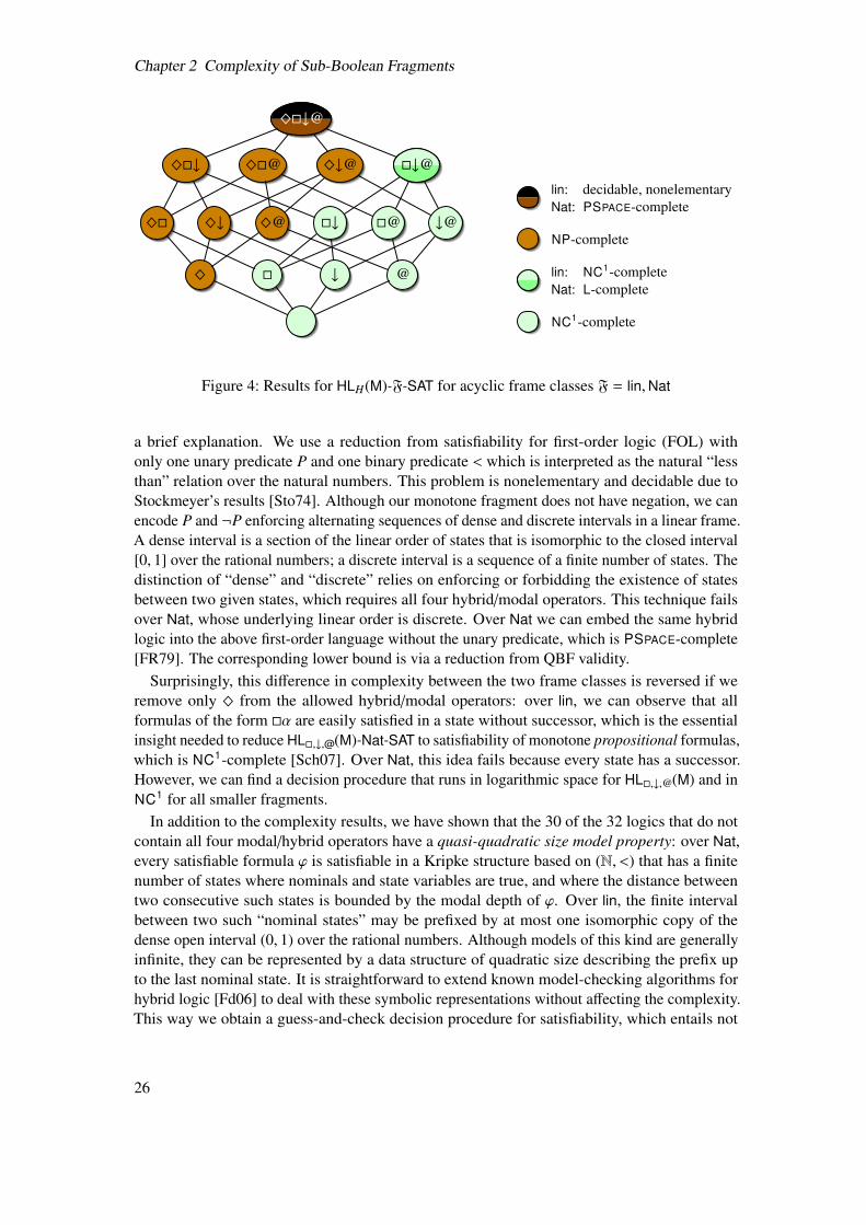
In this subsection, we classify the computational complexity of satisfiability for fragments ofHL^,⇤,#,@(M) over the frame classes lin (linear orders) and Nat (the natural numbers). We thusstudy 32 logics, determined by arbitrary combinations of the two frame classes and subsets of{^,⇤, #,@}. We find that HL^,⇤,#,@(M), which uses all four hybrid/modal operators, is the onlylogic that retains the nonelementary complexity from its “full Boolean” counterpart over lin.Over Nat, it is PSPACE-complete. For all smaller sets of hybrid/modal operators that containat least the ^-operator, we show NP-completeness over both frame classes. Over lin we obtainNC1-completeness for all remaining fragments; over Nat they have the same complexity exceptfor {⇤, #,@}, which is L-complete. Table 5 and Figure 4 give an overview of these results.
The technique used to establish the nonelementary lower bound reveals the ability of the fourhybrid/modal operators to distinguish between dense and discrete linear orders and deserves
25
Chapter 2 Complexity of Sub-Boolean Fragments
^ ⇤ # @
^⇤ ^# ^@ ⇤# ⇤@ #@
^⇤# ^⇤@ ^#@ ⇤#@
^⇤#@
lin: decidable, nonelementaryNat: PSPACE-complete
NP-complete
lin: NC1-completeNat: L-complete
NC1-complete
Figure 4: Results for HLH(M)-F-SAT for acyclic frame classes F = lin,Nat
a brief explanation. We use a reduction from satisfiability for first-order logic (FOL) withonly one unary predicate P and one binary predicate < which is interpreted as the natural “lessthan” relation over the natural numbers. This problem is nonelementary and decidable due toStockmeyer’s results [Sto74]. Although our monotone fragment does not have negation, we canencode P and ¬P enforcing alternating sequences of dense and discrete intervals in a linear frame.A dense interval is a section of the linear order of states that is isomorphic to the closed interval[0, 1] over the rational numbers; a discrete interval is a sequence of a finite number of states. Thedistinction of “dense” and “discrete” relies on enforcing or forbidding the existence of statesbetween two given states, which requires all four hybrid/modal operators. This technique failsover Nat, whose underlying linear order is discrete. Over Nat we can embed the same hybridlogic into the above first-order language without the unary predicate, which is PSPACE-complete[FR79]. The corresponding lower bound is via a reduction from QBF validity.
Surprisingly, this di↵erence in complexity between the two frame classes is reversed if weremove only ^ from the allowed hybrid/modal operators: over lin, we can observe that allformulas of the form ⇤↵ are easily satisfied in a state without successor, which is the essentialinsight needed to reduce HL⇤,#,@(M)-Nat-SAT to satisfiability of monotone propositional formulas,which is NC1-complete [Sch07]. Over Nat, this idea fails because every state has a successor.However, we can find a decision procedure that runs in logarithmic space for HL⇤,#,@(M) and inNC1 for all smaller fragments.
In addition to the complexity results, we have shown that the 30 of the 32 logics that do notcontain all four modal/hybrid operators have a quasi-quadratic size model property: over Nat,every satisfiable formula ' is satisfiable in a Kripke structure based on (N, <) that has a finitenumber of states where nominals and state variables are true, and where the distance betweentwo consecutive such states is bounded by the modal depth of '. Over lin, the finite intervalbetween two such “nominal states” may be prefixed by at most one isomorphic copy of thedense open interval (0, 1) over the rational numbers. Although models of this kind are generallyinfinite, they can be represented by a data structure of quadratic size describing the prefix upto the last nominal state. It is straightforward to extend known model-checking algorithms forhybrid logic [Fd06] to deal with these symbolic representations without a↵ecting the complexity.This way we obtain a guess-and-check decision procedure for satisfiability, which entails not
26
2.5 Hybrid Logic
only an alternative argument for NP-membership, but also a new NP-membership result for thesame fragments over the frame class {(Q, <)}.
The question remains whether the PSPACE-complete largest fragment over (N, <) admitssome quasi-polynomial size model property. Furthermore, this study can be extended in severalpossible ways: by allowing negation on atomic propositions, by considering frame classes thatconsist only of dense frames, such as (Q, <), or by considering arbitrary sets of Boolean operatorsas in Section 2.5.2. For atomic negation, it follows quite easily that the largest fragment is ofnonelementary complexity over (N, <), too, and that all fragments except H = {⇤, #,@} are NP-complete. However, our proof of the quasi-quadratic size model property does not immediatelygo through in the presence of negated atomic propositions. Over (Q, <), we conjecture that allfragments, except possibly for the largest one, have the same complexity and model properties asover (N, <).
2.5.4 Lessons learned
Our study of hybrid languages exhibits a number of fragments of tractable or intermediatecomplexity, which raises hopes that restricting the interaction of # with other operators mayindeed lead to useful extensions of knowledge representation and specification languages. Forexample, our results in Table 4 make it seem likely that extensions of lightweight descriptionlogics such as EL with the # operator have reasonable computational properties. However, thisconjecture needs to be tested carefully because, in DLs, one is usually interested in satisfiability orsubsumption with respect to a set of axioms, and it remains to investigate whether the interactionof those with # will lead to a worse computational behavior.
As a second example, our results in Table 5 show that the monotone fragment of LTLF,G
extended with both # and @ is not harder than plain LTLF,G,X. This fragment can be consideredas a “lightweight” LTL fragment that imposes less restrictions than the successful lightweightdescription logic EL because it allows disjunctions and G. It is therefore conceivable that thisfragment turns out to be a useful specification language. It still remains to be seen, however,whether this language is computationally well-behaved in terms of model checking too. Sincemodel checking with hybrid binders is not as computationally expensive as satisfiability [Fd06],there is hope for a positive answer.
As an ambitious goal, it would be interesting to put this study on an even more systematicfooting by systematizing all possible modal/hybrid operators and all possible frame classes.Similarly to the remarks at the end of Section 2.3, this is likely to be an overly ambitiousresearch program. A quite substantial step into this more systematic direction has been takenby Hemaspaandra and Schnoor, who classified the satisfiability problem of the (“full Boolean”)basic modal logic K over frame classes that can be defined by universal first-order Horn formulasinto NP-complete and PSPACE-hard in [HS08].
27

Chapter 3
Module Extraction and Modularization
3.1 Introduction
Ontologies are logical theories that specify a vocabulary for a domain of interest and describethe relationships between the terms in that vocabulary. They have manifold applications in areassuch as knowledge representation, knowledge management, semantic databases, the semanticweb, biomedical informatics, the life sciences, linguistics, the geosciences. The needs of theseapplications are served by a variety of ontology languages. Description logics (DLs) [BCM+03],which we have already introduced in the previous chapters, comprise a widely used family ofontology languages and underlie the W3C Web Ontology Language OWL.
DLs are designed to provide a good trade-o↵ between expressive power and computationalcomplexity. Expressive DLs, such as ALC and SROIQ, are designed to maximize expres-sive power while still retaining decidability of standard reasoning tasks such as satisfiabil-ity and subsumption. Their computational complexity is usually high: ALC is EXPTIME-complete [Sch94, DM00] and SROIQ is N2EXPTIME-complete [Kaz08]. Despite the highcomplexity, reasoning with these DLs can be feasible in practice thanks to highly optimizedreasoning systems [HM01, TH06, BLS06, SPC+07, MSH09].
The success of DLs as ontology languages has been significantly determined by the availabilityof reasoning services within sophisticated ontology development systems such as Protege,1
Swoop [KPS+06], and the TopBraid composer. The traditional standard reasoning services forDLs are satisfiability and subsumption (studied in Section 2.4), asking whether all terms inthe specified vocabulary are free of contradictions, or making the is-a hierarchy between theterms of the vocabulary explicit, which is useful for browsing and inspection. In recent years,however, the need for further reasoning services has arisen. Existing ontologies are more oftenconsiderably large: SNOMED CT [Spa00] has ⇡400,000 logical axioms; the National CancerInstitute’s (NCI) Thesaurus [GFH+03] has ⇡110,000 logical axioms. These large ontologies poseserious challenges not only to the best optimized reasoners, but to all constituents of the ontologydevelopment process, such as navigation, editing, comprehension, and debugging. In particular,the following application scenarios are a↵ected by the problems with handling large ontologies:
Scenario 1: Ontology Reuse. When engineers develop a new ontology, they often want toimport knowledge that is already represented in existing ontologies. If those ontologies arelarge, it is not feasible to import them on the whole, for the reasons just stated. It is moredesirable to import a subset of each external ontology that is self-contained with respect tothe respective subdomain of interest, and there are several ways to define self-containment.Reasoning services are available to check whether a subset of an ontology is self-containedin this sense, and to extract such subsets.
1http://protege.stanford.edu
29
Chapter 3 Module Extraction and Modularization
Scenario 2: Collaborative Ontology Development. When a team of developers maintains alarge ontology, each expert wants to focus on a part of the ontology that corresponds to hersubdomain of expertise (identified by a subset of its vocabulary) and make modificationsunder the assumption that they only touch this part. In particular, they want to make surethat their modifications have no impact on other, intuitively unrelated parts of the ontology.Since ontologies are complex logical theories, this is not automatically guaranteed and itis typically very di�cult to check for such undesired consequences. Reasoning servicesare available to verify that unrelated parts of the ontology (again identified by parts of itsvocabulary) have not changed, and signal a potential problem if this is not the case.
Scenario 3: Ontology comprehension. When an ontology developer wants to know whetherthe modeling in their large ontology corresponds to their understanding of the domain ofinterest, or when an ontology user wants to understand the topics of an ontology and theirlogical interrelations, then it is not useful to inspect a monolithic ontology axiom by axiom.The situation is similar to the task of understanding a large software project: instead ofinspecting each single line of code, users and developers look at the dependencies betweenself-contained parts of the code, such as classes, packages, and modules. Analogously,the ontology user and developer can benefit from a partition of the ontology into logicallyself-contained parts that identify an ontology’s main topics and represent the logicalinteractions within a topic as well as between topics.
To serve these application scenarios, additional reasoning services are needed: module extractionand modularization. Module extraction is concerned with determining a subset (module) of anontology that “says the same” about a certain vocabulary of interest as the whole ontology. Thistask can be generalized to the question whether two arbitrary ontologies that are not necessarilyin the subset relation “say the same” about a certain vocabulary, which is relevant, for example,for ontology versioning. Two ontologies with a positive answer to this question are calledindistinguishable or inseparable (with respect to the corresponding vocabulary). In all thesecases, there are several ways to define what “says the same” means, and each of them leads to adedicated notion of a module or inseparability.
Modularization is concerned with decomposing an ontology into parts that represent its maintopics – again represented by subsets of its vocabulary – and satisfy similarly strong propertiesregarding self-containment as modules. While it is straightforward to partition an ontology’svocabulary, it is not obvious how to obtain a corresponding partition of the axioms in theontology into modules in the above sense. In particular, modules for disjoint subsets of thevocabulary typically overlap. Therefore, modularization should aim at identifying a partitionwhose constituents represent modules in a well-defined way.
From the above considerations, it becomes clear that modules play an important role as proxiesof an ontology that can be used more conveniently because they are smaller and can thus beloaded, inspected, and reasoned over more e�ciently. In this sense, this chapter on modularitycontributes to the overall aim of the thesis: to identify ways to alleviate reasoning in expressivemodal-like logics. In contrast to the previous chapter, where we systematically searched forrestrictions to the logic that allow for e�cient decision procedures, this chapter is devoted tostudying ways of reducing the size of a theory in order to speed up the decision problems of theunderlying logic, which are typically highly intractable, as in the case of OWL (SROIQ). Thestrong logical guarantees required in Scenarios 1–3 and the respective module notions will be thecentral subject of study in this chapter.
30
3.1 Introduction
The general topic of ontology modules and modularity is becoming increasingly importantfor the engineering of large-scale ontologies. In contrast to software development, wheremodularity is a well-understood and widely used paradigm, modularity of ontologies has onlyrecently developed into an active field of research [CPSK06, KLWW08, CHKS08, JCS+08,Sun08, SPS09, CHKS10, ACH12, TP12], studying questions such as: How can a module of anontology be defined? When is a module self-contained with respect to a certain vocabulary?How can this be verified algorithmically? How can a module for a given vocabulary be extractedfrom a large ontology? Can ontology modules help understand, develop, and e�ciently reasonover a large ontology written in an expressive DL?
The foundation for the strong logical guarantees required in the scenarios above is provided byconservative extensions (CEs) and the closely related notion of inseparability. The requirementthat a subset O0 of an ontology O be self-contained regarding a vocabulary (set of concept androle names) ⌃ can be formalized by the requirement that O be a conservative extension (CE)of O0 with respect to the symbols in ⌃. As mentioned above, it is sometimes more convenientto replace CEs with inseparability, which does not require that the compared ontologies are inthe subset relation. Intuitively, ontologies O and O0 are ⌃-inseparable if the ⌃-part of O and O0cannot be distinguished. In Scenario 2 it is important to ensure that the original ontology O issig(O) \ ⌃-inseparable from the new ontology O0, where sig(O) is the overall vocabulary of Oand ⌃ is the vocabulary corresponding to the respective domain expert’s topic.
CEs have a long tradition in mathematical logic and are used in software specification toexpress that one specification refines another [TM87, BP90, Mai97] and to support modularspecifications [DGS93, Mos04]. It was not until 2006 that the importance of CEs and insep-arability for modularity was identified by Ghilardi et al. [GLW06]. In the years to follow, awhole host of research was dedicated to understanding and characterizing CEs of DL ontolo-gies [KLWW09, LW10, KWZ10], to analyzing the computational properties of deciding CEs[LWW07, KLWW08, KPS+09, KWZ10, KKL+11], and to defining notions of modules basedon CEs [KLWW08, CHKS08, KWZ10]. There are several variants of CEs, the most classicalbeing the deductive and model-theoretic ones, see [KLWW09] and Section 3.2.2.
Unfortunately, CEs and inseparability have poor computational properties, which largely forbidtheir use in practical applications: the computational complexity of deciding deductive CEs istypically by an exponential higher than standard satisfiability, and it is undecidable for modestextensions of the basic DL ALC [GLW06, LWW07]. Model-theoretic CEs are undecidablealready for the lightweight DL EL [LW10], with the notable exception that, when TBoxes arerestricted to being acyclic, model-CEs are decidable in polynomial time for EL and ⇧p
2-completeforALC [KLWW08]. These predominantly negative results imply that, for DLs of medium orhigh expressivity, there is no hope to define a notion of a module based on dCEs if one expectsto be able to extract minimal modules e↵ectively and e�ciently. For this reason, the notion oflocality was introduced [CHKS08], which yields a su�cient condition for being a CE and forinseparability, and whose computational complexity is not higher than standard satisfiability(for the semantic version of locality) or even in polynomial time (for the syntactic version).Locality-based modules are thus a “safe approximation” of CE-based modules in the sense thatthey always contain the minimal CE-based module but are typically a bit larger.
Nowadays, locality-based modules (LBMs) play an important role in practical applications.They have been implemented, to a large part by the author of this thesis, in the OWL API2 (apowerful Java interface for manipulating ontologies that underlies the ontology editor Protege)
2http://owlapi.sourceforge.net
31
Chapter 3 Module Extraction and Modularization
and in a web service for module extraction.3 According to the tra�c on various mailing listsrelated to OWL and Protege, ontology engineers make use of LBMs. Furthermore, someprincipled approaches to incremental and modular reasoning are based on LBMs [CHKS10,ACH12, TP12], and some of the above questions have been answered. However, before webegan the work reported in this chapter, locality-based modules had just been invented, and thefollowing questions were yet to be answered.
1. Do the theoretical properties of LBMs justify their suitability in the scenarios above?For example, are they robust under imports – that is, is the property of being a moduleuna↵ected when importing a module of an ontology into an arbitrary other ontology?
2. If so, what is a systematic way to employ LBMs in the three scenarios above?
3. How do LBMs compare with other module notions in terms of size, extraction time, andusefulness? In particular, what is the typical di↵erence in size between an LBM and thecorresponding minimal CE-based module?
4. How does a user or engineer specify the vocabulary of interest? This is a nontrivial taskbecause single topics (such as “diseases” or “anatomy” in a medical ontology) do notcorrespond to obvious sets of concept and role names.
5. How to determine the modular structure of an ontology, based on logically self-containedmodules, and thus reveal the logical interactions within the ontology?
6. How to make use of this modular structure in order to present, understand, and (collabora-tively) maintain an ontology, and to optimize reasoning?
In this chapter, we report on several theoretical and empirical studies aimed at making LBMs andother logic-based module notions usable for the reasoning services and applications discussedabove. The chapter is divided into two parts: Section 3.2 studies LBMs, and Section 3.3introduces a new modularization technique called Atomic Decomposition.
Our studies of LBMs deal with Questions 1, 2, and 3: we begin with devising a methodologythat explicates the use of LBMs in Scenario 1, proving that LBMs have the required stronglogical properties (Section 3.2.3). We then investigate and confirm robustness properties ofLBMs relevant for all three scenarios (Section 3.2.4). We finish this part with a summary ofempirical studies of LBMs, documenting the usefulness of LBMs and the applicability of ourmethodology to real-life import/reuse scenarios (Section 3.2.5).
Our work on Atomic Decomposition (AD) deals with Questions 5 and 6: we begin withproviding empirical evidence that the typical number of modules of an ontology is indeedprohibitively large, dashing hopes to compute the modular structure from all modules (Section3.3.2). We then introduce AD as a principled approach to representing all modules in a partitionof the ontology’s axioms, whose computation requires only a linear number of module extractions.This approach is universal in the sense that it is applicable to all module notions that providecertain logical guarantees (Section 3.3.3). We show how to use AD to speed up the extraction ofa single module (Section 3.3.4), and provide empirical evidence that AD behaves well in practice,applying it to a large corpus of existing ontologies and reporting on the shape of the resultingdecompositions (Section 3.3.5). Although we cannot answer Question 4 fully yet, we will arguethat AD bears the potential to help identify of a vocabulary of interest.
3http://mowl-power.cs.man.ac.uk:8080/modularity
32
3.2 Logic-Based Module Extraction
It remains to observe that our work focuses on a-posteriori modularity and modularization:applying module extraction and modularization techniques to existing ontologies. In contrast,a-priori approaches aim at imposing a modular structure on an ontology to foster its modulardevelopment. These approaches are typically based on heuristics without logical guarantees (suchas the distribution over thematic files), or on extensions of DLs designed to specify ontologymodules and syntactic links between them [BVSH09, ST09, CPS09]. However, AD seems tohave the potential to become an a-priori modularization approach as well: the modular structurerepresented in the AD of an ontology at some point of its development process may turn out tobe useful for its further modular development.
Bibliographic notes. The methodology for using LBMs discussed in Section 3.2.3 appearedin [JCS+08]. Our investigation of robustness properties (Section 3.2.4) is from [SSZ09]. Theempirical studies reported in Section 3.2.5 are published in [JCS+08, SSZ09, DKP+13]. Thefoundations of atomic decomposition (Section 3.3.3) are introduced in [DPSS11]; the preparatoryempirical study of module numbers (Section 3.3.2) is from [PS10]. Fast module extraction viaAD (Section 3.3.4) and the study of AD and fast module extraction in practice (Section 3.3.5)are described in [DGK+11].
3.2 Logic-Based Module Extraction
3.2.1 A Reuse Scenario
We sketch a particular use case for Scenario 1, ontology reuse, in a real-world application –namely the development of an ontology, called JRAO, to describe a kind of arthritis calledJRA (Juvenile Rheumatoid Arthritis) within the Health-e-Child project.4 This project aimed atcreating a repository of ontologies that can be used by clinicians in various applications.
The specific kinds of JRA to be modeled in JRAO are distinguished by several factors such asthe joints a↵ected, incurred responses (e.g., fever), and the treatment required. Well-establishedbiomedical ontologies such as NCI (mentioned in Chapter 1) and GALEN5 serve as referenceontologies: they contain information relevant to JRA, such as detailed descriptions of the humanjoints, diseases, symptoms. Figure 5 shows a fragment of NCI that defines JRA, together withour reuse scenario, where C1, . . . ,C7 refer to the kinds of JRA to be defined in JRAO.
The JRAO developers want to reuse knowledge from NCI and GALEN for three reasons: (a)they want to save time through reusing existing ontologies rather than writing their own; (b) theyvalue knowledge that is commonly accepted by the community and used in similar applications;(c) they are not experts in all areas covered by NCI and GALEN. In doing so, they need to ensurethat JRAO correctly reflects the reused knowledge but does not grow too much. An appropriatereuse methodology should therefore provide two guarantees.
(1) The use of certain concepts from NCI and GALEN in JRAO should not change theiroriginal meaning.
(2) The JRAO developers want to import only those axioms from NCI and GALEN that arerelevant for JRAO. By importing only fragments of NCI and GALEN, they should not loseimportant information.
4http://www.health-e-child.org5http://www.co-ode.org/galen
33
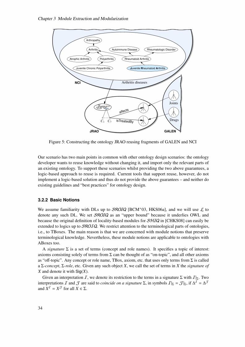
Chapter 3 Module Extraction and Modularization
NCI
JRAO GALEN
Arthropathy
Arthritis Autoimmune Disease Rheumatologic Disorder
Atrophic Arthritis Polyarthritis Rheumatoid Arthritis
Juvenile Chronic Polyarthritis Juvenile Rheumatoid Arthritis
Arthritis diseases
C1
. . .C7
Joints
Drugs
affects
isTreatedBy
Figure 5: Constructing the ontology JRAO reusing fragments of GALEN and NCI
Our scenario has two main points in common with other ontology design scenarios: the ontologydeveloper wants to reuse knowledge without changing it, and import only the relevant parts ofan existing ontology. To support these scenarios whilst providing the two above guarantees, alogic-based approach to reuse is required. Current tools that support reuse, however, do notimplement a logic-based solution and thus do not provide the above guarantees – and neither doexisting guidelines and “best practices” for ontology design.
3.2.2 Basic Notions
We assume familiarity with DLs up to SROIQ [BCM+03, HKS06a], and we will use L todenote any such DL. We set SROIQ as an “upper bound” because it underlies OWL andbecause the original definition of locality-based modules for SHIQ in [CHKS08] can easily beextended to logics up to SROIQ. We restrict attention to the terminological parts of ontologies,i.e., to TBoxes. The main reason is that we are concerned with module notions that preserveterminological knowledge. Nevertheless, these module notions are applicable to ontologies withABoxes too.
A signature ⌃ is a set of terms (concept and role names). It specifies a topic of interest:axioms consisting solely of terms from ⌃ can be thought of as “on-topic”, and all other axiomsas “o↵-topic”. Any concept or role name, TBox, axiom, etc. that uses only terms from ⌃ is calleda ⌃-concept, ⌃-role, etc. Given any such object X, we call the set of terms in X the signature ofX and denote it with Sig(X).
Given an interpretation I, we denote its restriction to the terms in a signature ⌃ with I|⌃. Twointerpretations I and J are said to coincide on a signature ⌃, in symbols I|⌃ = J|⌃, if �I = �J
and XI = XJ for all X 2 ⌃.
34
3.2 Logic-Based Module Extraction
Conservative extensions, safety, and modules. Guarantee (1) above requires a preservationof knowledge (“should not change their meaning”), which is best captured by the notion ofa conservative extension (CE) [GLW06, LWW07]. Depending on the degree of knowledgepreservation required, CEs come in several variants. We focus on the following basic ones.
Definition 8. Let L be a DL, T1 ✓ T be TBoxes, and ⌃ a signature.
1. T is a deductive ⌃-conservative extension (⌃-dCE) of T1 if, for every axiom ↵ over L withSig(↵) ✓ ⌃, we have T |= ↵ i↵ T1 |= ↵.
2. T is a deductive conservative extension (dCE) of T1 if T is a Sig(T1)-dCE of T1.
3. T is a model-theoretic ⌃-cons. extension (⌃-mCE) of T1 if {I|⌃ | I |= T1} = {I|⌃ | I |= T }.4. T is a model-theoretic conservative extension (dCE) of T1 if T is a Sig(T1)-mCE of T1.
It is clear that T being a (⌃-)mCE ofM implies that T is a (⌃-)dCE ofM.Definition 8 (1) applies to our example as follows: T1 is the ontology to be reused (NCI), T is
the union of JRAO and NCI, and ⌃ represents the terms reused from NCI. Item (2) captures thecase where we want to reuse all terms from NCI. Items (3) and (4) provide su�cient conditions.
Since the ontology to be reused (NCI) is usually under development beyond the control ofthe JRAO developers, it is convenient to make the axioms in NCI available on demand via areference such that the developers of JRAO need not commit to a particular version of NCI. Thenotion of safety [CHKS08] is a generalization of dCE that abstracts away from the ontology tobe reused and focuses on the reused terms.
Definition 9. Let T be a TBox and ⌃ a signature. T is safe for ⌃ if, for every TBox T 0 withSig(T ) \ Sig(T 0) ✓ ⌃, we have that T [ T 0 is a ⌃-dCE of T 0.
Guarantee (2) requires a preservation of knowledge (“should not lose important information”)that can be captured by the notion of a module [CHKS08].
Definition 10. Let T 01 ✓ T 0 be TBoxes and ⌃ a signature. T 01 is a ⌃-module in T 0 if, for everyTBox T with Sig(T ) \ Sig(T 0) ✓ ⌃, we have that T [ T 0 is a Sig(T )-dCE of T [ T 01.
The notions of safety and module are related as follows:
Proposition 11. [CHKS08] If T 0 \ T 01 is safe for ⌃ [ Sig(T 01), then T 01 is a ⌃-module in T 0.
Locality. The decision problems associated with dCEs, safety and modules are undecidablealready for the fragmentALCQIO of SROIQ [LWW07], and mCEs are undecidable already forthe lightweight DL EL [LW10]. Locality has been proposed as a decidable su�cient conditionfor safety: if all axioms in T satisfy the locality conditions, then T is safe, but the converse doesnot necessarily hold [CHKS08]. By means of Proposition 11, locality can be used for extractingmodules too. The main reasons for the success of locality are the facts that (a) locality is aproperty of a single axioms and does not depend on the other axioms in the ontology, and (b) thesyntactic variant can be checked in polynomial time.
The main intuition underlying locality is to check, given a signature ⌃, whether the axiom inquestion can be satisfied independently of the interpretation of the ⌃-terms, but in a restrictedway: by interpreting all non-⌃ terms either as the empty set (;-locality) or as the full domain6
6Or, in the case of roles, the set of all pairs of domain individuals.
35
Chapter 3 Module Extraction and Modularization
(�-locality). This intuition leads to two dual variants of locality, which reflect distinct ways ofreusing terms, namely generalization and refinement. The following definition introduces thesetwo variants of semantic locality [CHKS08].
Definition 12. An axiom ↵ over a logic L is called ;-local (�-local) w.r.t. signature ⌃ if, foreach interpretation I, there exists an interpretation J such that I|⌃ = J|⌃, J |= ↵, and foreach X 2 Sig(↵) \ ⌃, XJ = ; (for each C 2 Sig(↵) \ ⌃, CJ = � and for each R 2 Sig(↵) \ ⌃,RJ = � ⇥ �).
It has been shown in [CHKS08] that, if T1 ✓ T and all axioms in T \ T1 are ;-local (or allaxioms are �-local) w.r.t. ⌃ [ Sig(T1), then T is a ⌃-mCE of T1. The converse does not hold.
Both ;- and �-locality can be tested using available DL reasoners: just check whether theaxiom ↵0 obtained from ↵ by replacing all non-⌃ terms with ? (or >) is a tautology. In somecases, ↵0 is not a SROIQ axiom, but standard reasoners can be extended in a straightforward way.Deciding semantic locality is thus considerably easier than deciding dCE. However, reasoning inexpressive DLs is still complex, e.g. N2EXPTIME-complete for SROIQ.
In order to achieve tractable module extraction, a syntactic approximation of semantic localitywas introduced in [CHKS08]. (Syntactic) ?-locality is based on two grammars defining conceptdescriptions that are equivalent to ? or > if all non-⌃ symbols are interpreted as ?. An axiomC v D is then ?-local if C is ?- or D is >-equivalent. The definition of >-locality is analogous.It is straightforward to extend both definitions to cover all features of SROIQ, as we have donein the implementation of locality in the OWL API. Obviously, ?-locality (>-locality) is su�cientfor ;-locality (�-locality). Therefore, all axioms in T \ T1 being ?-local (or all axioms being>-local) w.r.t. ⌃ [ Sig(T1) is su�cient for T to be a ⌃-mCE of T1. The converse does not hold.Syntactic locality can be tested in polynomial time [CHKS08].
From now on, we use x to refer to any of the four locality variants. We say that a TBox is x-localif all of its axioms are x-local. All four variants of locality are su�cient for safety:
Proposition 13. [CHKS08] If a TBox T is x-local w.r.t. ⌃, for any x 2 {;,�,?,>}, then T issafe for ⌃.
Propositions 11 and 13 suggest the following definition of modules in terms of locality.
Definition 14. Let T1 ✓ T be TBoxes and ⌃ a signature. T1 is an x-module for ⌃ in T , for anyx 2 {;,�,?,>}, if T \ T1 is x-local w.r.t. ⌃ [ Sig(T1).
It is known that x-modules are modules as in Definition 10:
Proposition 15. [CHKS08] Let T1 be an x-module for ⌃ in T , for any x 2 {;,�,?,>}, and let⌃0 = ⌃ [ Sig(T1). Then T1 is a ⌃0-module in T .
In order to be able to extract a module based on any of the four locality notions x 2 {;,�,?,>}for some T and ⌃, it is important to observe that there is a unique minimal x-module for ⌃in T [CHKS08]. These modules are obtained by starting with an empty set of axioms andsubsequently adding axioms from O that are non-local, extending the signature against whichlocality is checked with the terms of the added axioms. To avoid confusion, the initial signature⌃ is called the seed signature for the module. The procedure is given in Algorithm 1, and theunique minimal locality-based module (from now on called LBM) is introduced in Definition16. LBMs can be made made smaller by nesting >-extraction (�-extraction) into ?-extraction
36
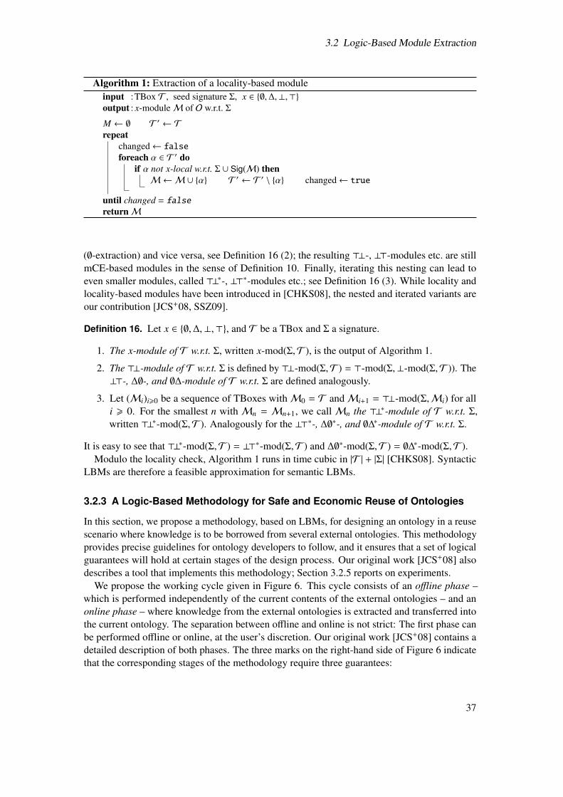
3.2 Logic-Based Module Extraction
Algorithm 1: Extraction of a locality-based moduleinput :TBox T , seed signature ⌃, x 2 {;,�,?,>}output : x-moduleM of O w.r.t. ⌃
M ; T 0 Trepeat
changed falseforeach ↵ 2 T 0 do
if ↵ not x-local w.r.t. ⌃ [ Sig(M) thenM M [ {↵} T 0 T 0 \ {↵} changed true
until changed = falsereturnM
(;-extraction) and vice versa, see Definition 16 (2); the resulting >?-, ?>-modules etc. are stillmCE-based modules in the sense of Definition 10. Finally, iterating this nesting can lead toeven smaller modules, called >?⇤-, ?>⇤-modules etc.; see Definition 16 (3). While locality andlocality-based modules have been introduced in [CHKS08], the nested and iterated variants areour contribution [JCS+08, SSZ09].
Definition 16. Let x 2 {;,�,?,>}, and T be a TBox and ⌃ a signature.
1. The x-module of T w.r.t. ⌃, written x-mod(⌃,T ), is the output of Algorithm 1.
2. The >?-module of T w.r.t. ⌃ is defined by >?-mod(⌃,T ) = >-mod(⌃,?-mod(⌃,T )). The?>-, �;-, and ;�-module of T w.r.t. ⌃ are defined analogously.
3. Let (Mi)i>0 be a sequence of TBoxes withM0 = T andMi+1 = >?-mod(⌃,Mi) for alli > 0. For the smallest n withMn = Mn+1, we callMn the >?⇤-module of T w.r.t. ⌃,written >?⇤-mod(⌃,T ). Analogously for the ?>⇤-, �;⇤-, and ;�⇤-module of T w.r.t. ⌃.
It is easy to see that >?⇤-mod(⌃,T ) = ?>⇤-mod(⌃,T ) and �;⇤-mod(⌃,T ) = ;�⇤-mod(⌃,T ).Modulo the locality check, Algorithm 1 runs in time cubic in |T | + |⌃| [CHKS08]. Syntactic
LBMs are therefore a feasible approximation for semantic LBMs.
3.2.3 A Logic-Based Methodology for Safe and Economic Reuse of Ontologies
In this section, we propose a methodology, based on LBMs, for designing an ontology in a reusescenario where knowledge is to be borrowed from several external ontologies. This methodologyprovides precise guidelines for ontology developers to follow, and it ensures that a set of logicalguarantees will hold at certain stages of the design process. Our original work [JCS+08] alsodescribes a tool that implements this methodology; Section 3.2.5 reports on experiments.
We propose the working cycle given in Figure 6. This cycle consists of an o↵line phase –which is performed independently of the current contents of the external ontologies – and anonline phase – where knowledge from the external ontologies is extracted and transferred intothe current ontology. The separation between o↵line and online is not strict: The first phase canbe performed o↵line or online, at the user’s discretion. Our original work [JCS+08] contains adetailed description of both phases. The three marks on the right-hand side of Figure 6 indicatethat the corresponding stages of the methodology require three guarantees:
37
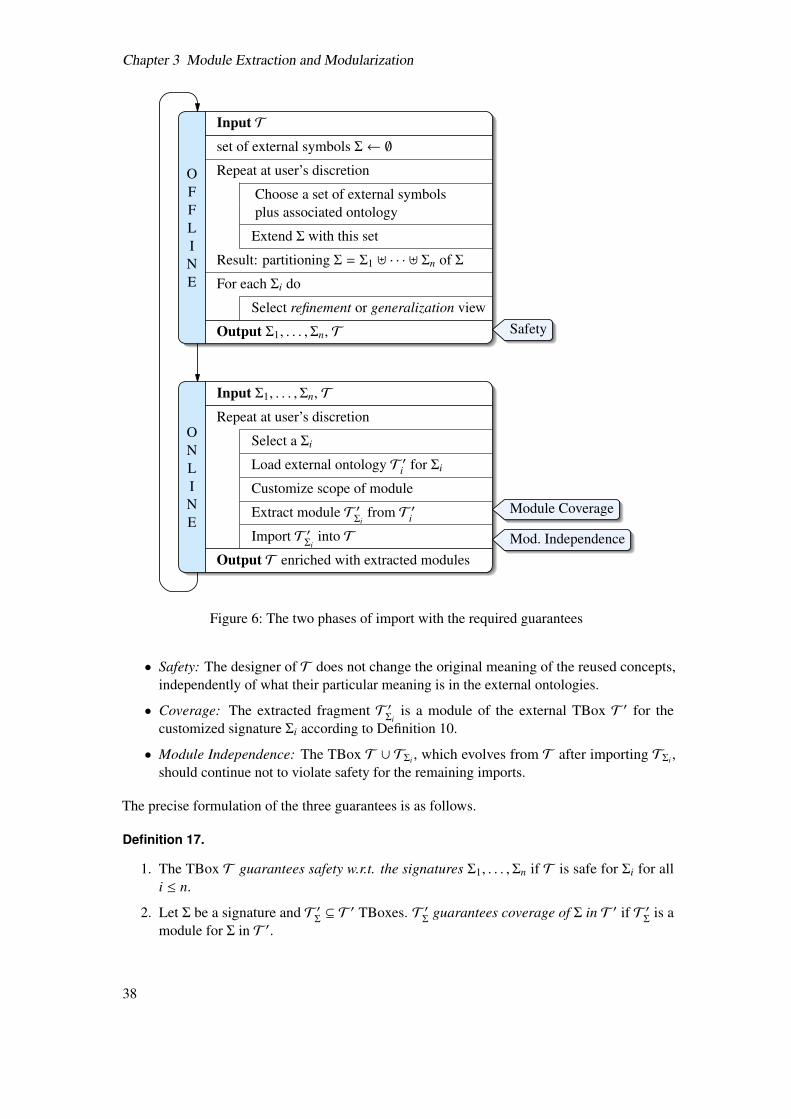
Chapter 3 Module Extraction and Modularization
OFFLINE
Input Tset of external symbols ⌃ ;Repeat at user’s discretion
Choose a set of external symbolsplus associated ontology
Extend ⌃ with this set
Result: partitioning ⌃ = ⌃1 ] · · · ] ⌃n of ⌃
For each ⌃i do
Select refinement or generalization view
Output ⌃1, . . . ,⌃n, T
ONLINE
Input ⌃1, . . . ,⌃n, TRepeat at user’s discretion
Select a ⌃i
Load external ontology T 0i for ⌃i
Customize scope of module
Extract module T 0⌃ifrom T 0i
Import T 0⌃iinto T
Output T enriched with extracted modules
Safety
Module Coverage
Mod. Independence
Figure 6: The two phases of import with the required guarantees
• Safety: The designer of T does not change the original meaning of the reused concepts,independently of what their particular meaning is in the external ontologies.
• Coverage: The extracted fragment T 0⌃iis a module of the external TBox T 0 for the
customized signature ⌃i according to Definition 10.
• Module Independence: The TBox T [ T⌃i , which evolves from T after importing T⌃i ,should continue not to violate safety for the remaining imports.
The precise formulation of the three guarantees is as follows.
Definition 17.
1. The TBox T guarantees safety w.r.t. the signatures ⌃1, . . . ,⌃n if T is safe for ⌃i for alli n.
2. Let ⌃ be a signature and T 0⌃ ✓ T 0 TBoxes. T 0⌃ guarantees coverage of ⌃ in T 0 if T 0⌃ is amodule for ⌃ in T 0.
38
3.2 Logic-Based Module Extraction
3. Let T be a TBox and ⌃1,⌃2 be signatures. T guarantees module independence if, forall T 01 with Sig(T ) \ Sig(T 01) ✓ ⌃1 and for all T 02 with Sig(T ) \ Sig(T 02) ✓ ⌃2 andSig(T 01) \ Sig(T 02) = ;, it holds that T [ T 01 [ T 02 is a conservative extension of T [ T 01.
Both safety and coverage can be achieved using ?- and >-locality:
Proposition 18.
1. Let T be a TBox and ⌃ = ⌃1 ] . . . ] ⌃n be the union of disjoint signatures. If, for each ⌃i,T is either ?-local or >-local w.r.t. ⌃i, then T guarantees safety w.r.t. ⌃1, . . . ,⌃n.
2. Any of the modules ?-mod(⌃,T 0), . . . ,>?-mod(⌃,T 0), . . . ,>?⇤-mod(⌃,T 0), . . . guaran-tees coverage of ⌃ in T 0.
Module independence can be guaranteed only in a restricted way; see the technical report7 fordetails and a discussion of the restriction.
Proposition 19. Let T be a TBox and ⌃1,⌃2 disjoint signatures. If the following conditions aresatisfied, where x denotes either ? or >, then T [ T 01 is x-local, and thus safe, w.r.t. ⌃2.
(a) T is x-local with respect to ⌃2.
(b) Sig(T 01) \ ⌃2 = ;.(c) T 01 is x-local with respect to the empty signature.
We have implemented our methodology in a preliminary tool, a prototype plugin for the Protegeontology editor. Section 3.2.5 reports on experiments that indicate that LBMs are indeed ofacceptable size. The problem that remains to be solved is the di�culty to determine a suitablesignature, in particular the seed signature for a module, see Section 3.2.6.
3.2.4 Robustness Properties of Locality-Based Modules
In this section we survey existing logic-based approaches to extracting a module in the senseof Definition 10, focusing on syntactic approximations via locality. We will compare di↵erentkinds of LBMs with each other and with CE-based modules. In particular, we will explore nestedLBMs more in-depth than the previous literature. The comparison of module kinds will be basedon examining properties relevant for ontology reuse. It will help learning which modules arebest suited for which requirements.
We have seen that a module T1 of a TBox T w.r.t. a signature ⌃ is a subset of T that isindistinguishable from T w.r.t. ⌃ for certain classes of entailments. Inseparability relations amore general: they compare arbitrary ontologies that are not necessarily in the subset relation,and provide a uniform framework for comparing arbitrary definitions of modules. We studyrobustness properties of inseparability relations that have been identified in [KLWW09], andwhich are relevant for the corresponding module notions because they ensure that an ontologydeveloper
• does not need to import a di↵erent module when she restricts the set of terms that she isinterested in (robustness under vocabulary restrictions);
7http://www.informatik.uni-bremen.de/%7Ets/publ/safe-eco-reuse-report.pdf
39
Chapter 3 Module Extraction and Modularization
• does not need to import a di↵erent module when she extends the set of terms that she isinterested in with terms that she does not use in her ontology (robustness under vocabularyextensions);
• can always import the same module in di↵erent ontologies whenever she is interested inthe same set of relevant terms (robustness under replacement);
• does not need to import two indistinguishable versions of the same ontology (robustnessunder joins).
The notions of modules defined so far were induced by CEs and di↵erent notions of locality.We will now put them into a more general context of modules generated by inseparabilityrelations. For a given logic L, an inseparability relation is a family S = {⌘S
⌃| ⌃ is a signature}
of equivalence relations on the set of L-TBoxes. The intuition behind this notion is as follows:T1 ⌘S
⌃T2 means that T1 and T2 are indistinguishable w.r.t. ⌃, i.e., they represent the same
knowledge about the topic represented by ⌃. The exact meaning of “indistinguishable” and “thesame knowledge” depends on the precise definition of the inseparability relation. T1 being amodule for ⌃ of T should be equivalent to T1 ✓ T and T1 being inseparable w.r.t. ⌃ from T .
The requirement to preserve entailments or models leads to the following inseparabilityrelations, which have been examined, among others, in [KLWW09].
• T1 and T2 are ⌃-concept name inseparable, written T1 ⌘c⌃T2, if for all ⌃-concept names
C,D, it holds that T1 |= C v D if and only if T2 |= C v D.
• T1 and T2 are ⌃-subsumption inseparable w.r.t. a logic L, written T1 ⌘s⌃T2, if for all
terms X and Y that are concept expressions over ⌃ or role names from ⌃, it holds thatT1 |= X v Y if and only if T2 |= X v Y .
• T1 and T2 are ⌃-model inseparable, written T1 ⌘sem⌃T2, if {I|⌃ | I |= T1} = {I|⌃ | I |= T2}.
We denote the respective sets of inseparability relations with Sc, Ss, and Ssem. It is easy to seethat, for each signature ⌃, it holds that ⌘sem
⌃✓ ⌘s
⌃✓ ⌘c
⌃.
Inseparability relations induce modules as follows.
Definition 20. Let S be an inseparability relation, T1 ✓ T TBoxes, and ⌃ a signature. T1 is
1. an S⌃-module of T if T1 ⌘S⌃T ;
2. a self-contained S⌃-module of T if T1 ⌘S⌃[Sig(T1) T ;
3. a depleting S⌃-module of T if ; ⌘S⌃[Sig(T1) T \ T1.
T1 is called a minimal (self-contained, depleting) ⌘⌃-module of T if T1, but no proper subset ofT1, is a (self-contained, depleting) ⌘⌃-module of T .
Due to the shift from ⌃ to ⌃ [ Sig(T1), it is not necessarily the case that every self-contained (ordepleting) S⌃-module of T is an S⌃-module of T . However, under certain robustness properties,this implication holds. While there can be exponentially many minimal S⌃-modules, minimaldepleting modules are uniquely determined – under mild conditions involving inseparabilityrelations. This last property makes depleting modules essential for at least two applications:
The first application is the above described import scenario. If T1 is a depleting S⌃-module ofT and S satisfies certain robustness properties, then, for every external TBox T 0 that shares withT only terms from ⌃[ Sig(T1), we can import T 0 into T \ T1 because they do not interfere witheach other: (T \ T1) [ T 0 ⌘S
⌃0 T 0.
40
3.2 Logic-Based Module Extraction
The second application is the computation of all justifications for an entailment ⌘ of anontology T [HPS08]. For appropriate inseparability relations S , Definition 20 (1) ensures thateach SSig(⌘)-module of T contains at least one justification for ⌘, but not necessarily all. It isrelatively easy to show that depletion, together with mild additional properties, guarantees thatevery SSig(⌘)-module of T contains all justifications for ⌘.
We define new inseparability relations for LBMs, proceeding by analogy to inseparabilityrelations for conservativity: TBoxes T1 and T2 are inseparable if they have the same modules,i.e., if the module extraction algorithm returns the same output for each of them. We havethus replaced the semantic criterion “the same entailments/models” in conservativity-basedinseparability with a syntactic criterion “the same extraction result”, given that LBMs are definedalgorithmically. While this new type of inseparability imposes much stronger requirements(“have the same modules” is syntax-dependent), it is the best available computationally cheapapproximation of the computationally hard inseparability relations ⌘s
⌃and ⌘sem
⌃, analogously to
how LBMs approximate CE-based modules.We consider the following inseparability relations for LBMs.
Relation T1 and T2 are in relation if . . .⌘;⌃
;-mod(⌃,T1) = ;-mod(⌃,T2)⌘�⌃ �-mod(⌃,T1) = �-mod(⌃,T2)⌘?⌃ ?-mod(⌃,T1) = ?-mod(⌃,T2)⌘>⌃ >-mod(⌃,T1) = >-mod(⌃,T2)
Relation T1 and T2 are in relation if . . .⌘>?⌃ >?-mod(⌃,T1) = >?-mod(⌃,T2)⌘?>⌃ ?>-mod(⌃,T1) = ?>-mod(⌃,T2)⌘>?⇤⌃ >?⇤-mod(⌃,T1) = >?⇤-mod(⌃,T2)
Evidently, they all are equivalence relations. Furthermore, they are related to the previouslydefined inseparability relations as follows.
Proposition 21. Let ⌃ be a signature. For any ⌘•⌃ of the above 7 relations, we have ⌘•⌃ ✓ ⌘sem⌃
.
We can now define the four robustness properties described above.
Definition 22. Let L be a DL. The inseparability relation S is called
1. robust under vocabulary restrictions if, for all L-TBoxes T1,T2 and all signatures ⌃,⌃0
with ⌃ ✓ ⌃0, the following holds: if T1 ⌘S⌃0 T2, then T1 ⌘S
⌃T2.
2. robust under vocabulary extensions if, for all L-TBoxes T1,T2 and all signatures ⌃,⌃0
with ⌃0 \ (Sig(T1) [ Sig(T2)) ✓ ⌃ : if T1 ⌘S⌃T2, then T1 ⌘S
⌃0 T2.
3. robust under replacement if, for all L-TBoxes T1,T2, all signatures ⌃ and every L-TBoxT with Sig(T ) \ (Sig(T1) [ Sig(T2)) ✓ ⌃, the following holds: if T1 ⌘S
⌃T2, then T1 [
T ⌘S⌃T2 [ T .
4. robust under joins if, for all L-TBoxes T1,T2 and signatures ⌃ with Sig(T1)\Sig(T2) ✓ ⌃and every i = 1, 2, the following holds: if T1 ⌘S
⌃T2, then Ti ⌘S
⌃T1 [ T2.
We have examined the properties of the inseparability relations S;, S�, S?, S>, S>?, S?>, S>?⇤ ,
and compared them with those of Ssem, Ss, Sc. The results are given in Table 6. The first fourlines give the module notion which is generalized by the respective inseparability relation, andindicate whether each such module for ⌃ is a (minimal) S⌃-module, or a (minimal) self-containedS⌃-module, or a (minimal) depleting S⌃-module. For Sc, this question is meaningless becausethere is no corresponding standard module notion, apart from redefining ⌃-dCEs to take only
41
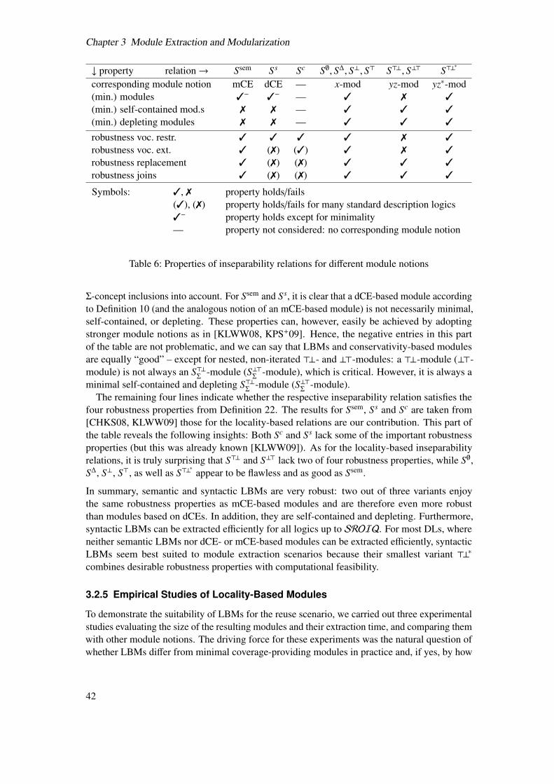
Chapter 3 Module Extraction and Modularization
# property relation! Ssem Ss Sc S;, S�, S?, S> S>?, S?> S>?⇤
corresponding module notion mCE dCE — x-mod yz-mod yz⇤-mod(min.) modules 3� 3� — 3 7 3(min.) self-contained mod.s 7 7 — 3 3 3(min.) depleting modules 7 7 — 3 3 3
robustness voc. restr. 3 3 3 3 7 3robustness voc. ext. 3 (7) (3) 3 7 3robustness replacement 3 (7) (7) 3 3 3robustness joins 3 (7) (7) 3 3 3
Symbols: 3, 7 property holds/fails(3), (7) property holds/fails for many standard description logics3� property holds except for minimality— property not considered: no corresponding module notion
Table 6: Properties of inseparability relations for di↵erent module notions
⌃-concept inclusions into account. For Ssem and Ss, it is clear that a dCE-based module accordingto Definition 10 (and the analogous notion of an mCE-based module) is not necessarily minimal,self-contained, or depleting. These properties can, however, easily be achieved by adoptingstronger module notions as in [KLWW08, KPS+09]. Hence, the negative entries in this partof the table are not problematic, and we can say that LBMs and conservativity-based modulesare equally “good” – except for nested, non-iterated >?- and ?>-modules: a >?-module (?>-module) is not always an S>?⌃ -module (S?>⌃ -module), which is critical. However, it is always aminimal self-contained and depleting S>?⌃ -module (S?>⌃ -module).
The remaining four lines indicate whether the respective inseparability relation satisfies thefour robustness properties from Definition 22. The results for Ssem, Ss and Sc are taken from[CHKS08, KLWW09] those for the locality-based relations are our contribution. This part ofthe table reveals the following insights: Both Sc and Ss lack some of the important robustnessproperties (but this was already known [KLWW09]). As for the locality-based inseparabilityrelations, it is truly surprising that S>? and S?> lack two of four robustness properties, while S;,S�, S?, S>, as well as S>?
⇤ appear to be flawless and as good as Ssem.
In summary, semantic and syntactic LBMs are very robust: two out of three variants enjoythe same robustness properties as mCE-based modules and are therefore even more robustthan modules based on dCEs. In addition, they are self-contained and depleting. Furthermore,syntactic LBMs can be extracted e�ciently for all logics up to SROIQ. For most DLs, whereneither semantic LBMs nor dCE- or mCE-based modules can be extracted e�ciently, syntacticLBMs seem best suited to module extraction scenarios because their smallest variant >?⇤combines desirable robustness properties with computational feasibility.
3.2.5 Empirical Studies of Locality-Based Modules
To demonstrate the suitability of LBMs for the reuse scenario, we carried out three experimentalstudies evaluating the size of the resulting modules and their extraction time, and comparing themwith other module notions. The driving force for these experiments was the natural question ofwhether LBMs di↵er from minimal coverage-providing modules in practice and, if yes, by how
42
3.2 Logic-Based Module Extraction
much. In other words, are LBMs a good approximation of minimal coverage-providing modules?Unfortunately, this question is impossible to answer in general because undecidability of mCEsand dCEs for DLs of higher expressivity forbids the extraction of minimal coverage-providingmodules. However, it is possible to empirically answer the following questions:
1. How large can LBMs of real-life ontologies become? Can we expect LBMs to be signifi-cantly smaller than the whole ontology, for seed signatures of reasonable size?
2. For ontologies in lightweight DLs, which permit e↵ective extraction of mCE- or dCE-based modules, do LBMs di↵er in size and extraction time from the latter and, if yes, byhow much?
3. Do syntactic and semantic LBMs di↵er in size and extraction time and, if yes, by howmuch? That is, are syntactic LBMs a good approximation of semantic LBMs?
Answers to these questions will allow for a more informed choice of which module extractiontechnique to select under a given set of circumstances.
Initial experiment evaluating ?- and >?-modules. In [JCS+08] we report on an experimenttowards Question 1. We extracted ?- and >?-modules from Galen, NCI, and SNOMED CT for(a) random seed signatures of varying size and (b) real-life seed signatures from the Health-e-Child project. The modules obtained in (a) were small on average, and their growth relative tothe signature size was smooth and always linear up to signature size 100. For (b), seed signaturesof size 40–131 from Galen (4170 axioms) led to LBMs of size 490–1151; signatures of size48–356 from NCI (⇡ 400,000 axioms) led to LBMs of size 300–1258.
In this study we also compared?- and>?-modules for Galen and NCI with ontology fragmentsobtained by Seidenberg’s segmentation approach [Sei09], which does not provide coverage or asimilar logical guarantee. The >?-modules were always smaller than the Seidenberg fragmentsfor the same seed signatures; in the case of Galen, they were orthogonal.
Comparison with other approaches. In [SSZ09] we report on experiments towards Ques-tions 1 and 2. We extracted ?- and >?⇤-modules for ontologies in lightweight DLs and comparedthem with mCE- or dCE-based modules, which can be extracted e↵ectively in these DLs.
We first took three real-life seed signatures for SNOMED CT with terms relevant for anintensive care unit, and compared the ?- and >?⇤-modules for these signatures with the depletingmCE-based modules extracted e�ciently via the MEX approach [KLWW08]. The LBMs ex-tracted from the ⇡ 400,000 axioms in SNOMED for these signatures of size 2,700–24,000 wereof size 15,000–56,000 and thus comprised 4–15% of the whole ontology. In contrast, the size ofthe MEX modules ranged between 1,7 and 10%. All modules were extracted in 1–4 seconds.
Second, we extracted LBMs and minimal conservativity-based modules from two DL-LiteNboolontologies from a commercial supply-chain management system in [KPS+09] (not part of thisthesis). We extracted >?⇤-modules as a preprocessing step to computing minimal Sc-, Sq- (basedon query-inseparability), and depleting Sq-modules using QBF solvers. We included all singletonseed signatures and randomly generated seed signatures of size 10; the two ontologies were ofsize 1247 and 1283. The di↵erence in size between LBMs and Sc- or Sq-modules was oftenconsiderable, particularly when the Sc-modules consisted only of a few axioms. However, mostof the di↵erence seems to be caused by depletion because, in 5 out of 6 cases, the average sizeof LBMs was limited to 150% of the average size of depleting Sq-modules. Each LBM wasextracted in a few seconds, while a depleting Sq-module took up to 30 minutes to compute. The
43
Chapter 3 Module Extraction and Modularization
experimental results in our follow-up work [KKL+11] (not part of this thesis) on modules basedon query inseparability for DL-LiteNcore, which underlies the OWL 2 QL profile, are similar.
In-depth comparison of syntactic LBMs with semantic LBMs and mCE-based modules.In [DKP+13] we report on a systematic experiment towards Questions 2 and 3. We chose alarge corpus consisting of most ontologies from the NCBO BioPortal ontology repository8 andselected ontologies from the TONES repository9. The 242 ontologies in this corpus cover a widerange of expressivity (fromAL to SROIQ(D)) and size (10–16,066 axioms, 10–16,068 terms).Each ontology was additionally trimmed to a subset that is acyclic and in ELI, in order to beable to apply MEX. Furthermore we extended the reasoner FaCT++ to be able to test (semantic)�-locality, which involves tautology checks for axioms using the >-role in a way that violatesthe OWL syntax.
We specified Questions 2 and 3 more precisely: we asked (i) whether, for a given seed signature⌃, it is likely that there is a di↵erence between the syntactic, the semantic, and the MEX modulesfor ⌃; if so, the size of the di↵erence;10 and (ii) how feasible the extraction of semantic LBMsis. For this purpose, we compared (a) ;-semantic with ?-syntactic locality, �-semantic with>-syntactic locality, (b) ;- with ?-modules, �- with >-modules, �;⇤- with >?⇤-modules, and (c)MEX modules with �;⇤-modules.
Due to the recursive nature of Algorithm 1, our investigation is both on a
• per-axiom-basis: given axiom ↵ and signature ⌃, is it likely that ↵ is ;-local (�-local,resp.) w.r.t. ⌃ but not ?-local (>-local, resp.) w.r.t. ⌃?
• per-module basis: given a seed signature ⌃, is it likely that
– ?-mod(⌃,O) , ;-mod(⌃,O), or
– >-mod(⌃,O) , �-mod(⌃,O), or
– >?⇤-mod(⌃,O) , �;⇤-mod(⌃,O), or
– �;⇤-mod(⌃,O) , MEX-mod(⌃,O)?
If yes, is it likely that the di↵erence is large?
We considered two kinds of signatures: genuine and random signatures. Genuine signaturesare the signatures of single axioms in the ontology, and they are interesting for two reasons:they lead to coherent modules (i.e., modules that cannot be decomposed into the union of two✓-incomparable modules), and every ontology has only linearly many genuine modules, asopposed to the exponential number of all signatures. For random signatures, we chose 400distinct signatures (or all signatures if the ontology contained < 9 terms), each of which includesevery term with probability 0.5. We have set the sample size to 400 because this ensures statisticalsignificance of the results for the overall population of all modules independently of the ontologysize. Our selection of signatures thus contains small (genuine) and large (random) signatures.
The results of our experiment show that, for the vast majority of the ontologies in our corpus, nodi↵erence between syntactic and semantic locality is observed, for all three variants ? vs. ;, >vs. �, and >?⇤ vs. �;⇤. More precisely, for 209 out of 242 ontologies and all sampled signatures,there is no di↵erence between syntactic LBMs and the corresponding semantic LBMs, and
8http://bioportal.bioontology.org9http://owl.cs.manchester.ac.uk/repository/
10Recall: the MEX module for ⌃ is a subset of the semantic ⌃-module, which is a subset of the syntactic ⌃-module.
44
3.2 Logic-Based Module Extraction
between any axiom being syntactically or semantically local. Hence, for these 209 ontologies,there is no statistically significant di↵erence between semantic and syntactic locality of any kind,and between semantic and syntactic LBMs of any kind. The 209 ontologies include Galen andPeople, which are renowned for having unusually large ?-modules [CHKS08, PS10]. In mostcases, extracting a semantic and syntactic LBM each took only a few milliseconds. For twoontologies, the semantic LBM took considerably longer to extract than the syntactic: up to 5times for nested-modules in MoleculeRole, and up to 34 times in Galen.
Di↵erences between syntactic and semantic locality have been observed in the remaining 33ontologies. In 6 of these, the di↵erences are solely due to simple tautologies that have entered thepublished version by accident. In 21 of the remaining 27 ontologies, the di↵erences a↵ect onlylocality of single axioms, and never modules. The remaining 6 ontologies with di↵erences inmodules comprise 4 from BioPortal and 2 from TONES; their sizes range from 170 to 1925, andtheir expressivity fromAL to SRIQ(D). Summarizing the detailed tables in our original work[DKP+13] and its accompanying technical report,11 it can be argued that the observed di↵erencesare negligible for all 6 ontologies: in four cases, the syntactic and corresponding semantic LBMdi↵er by at most 12 axioms. For a fifth ontology, di↵erences greater than 11 axioms (or 2% ofthe semantic LBM) occur only for very small seed signatures, and the sixth ontology exhibitslarge di↵erences only between >- and �-modules – and never between the more economic >?⇤-and �;⇤-modules. Module extraction time was always a few milliseconds.
To explain the reasons for the observed di↵erences between semantic and syntactic locality,we have identified and extensively described four types of axioms that cause these di↵erences bybeing ?-local (>-local, respectively) w.r.t. some signature ⌃ but not ;-local (�-local, respectively)w.r.t. ⌃. We call these four types culprits. Sometimes, culprit axioms “pull” additional axiomsinto the syntactic LBM, due to the signature extension during module extraction (Alg. 1). Weconjecture that one culprit type can be avoided by a straightforward extension to the definition ofsyntactic locality. For two culprit types, there is no hope for an exhaustive such extension. Thefourth type simply encompasses the above mentioned tautologies.
Di↵erences between LBMs and MEX modules have been observed for 66 of the 242 ontologies(⇡ 27%). The average di↵erence in module size is at most 13 axioms for genuine seed signaturesand 26 axioms (13% of the MEX module) for random seed signatures. The occurrence ofdi↵erences is not correlated with the size of the original ontology, but with its expressivity – andthus with the amount of trimming necessary to obtain an acyclic ELI subontology. In particular,all 66 ontologies with di↵erences had been pruned by at least 30 (and at most 12,185) axioms.Furthermore, these 66 ontologies coincide exactly with those where equivalences occur in theELI-TBox. Because of the low expressivity of ELI, we conjecture that MEX- and �;⇤-modulescan only ever di↵er due to the presence of equivalences. We cannot compare extraction timesbecause the MEX implementation combines loading and module extraction.
In summary, we obtain three main observations from our experiments. (1) In general, there is noor little di↵erence between semantic and syntactic locality. Hence, the computationally cheapersyntactic locality is a good approximation of semantic locality. (2) In most cases, there is no orlittle di↵erence between LBMs and MEX modules. (3) Though in principle hard to compute,semantic LBMs can be extracted quite fast in practice, although often not as fast as syntacticLBMs. Due to results (1) and (2), hardly any benefit can be expected from preferring potentiallysmaller modules (MEX or semantic LBMs) to cheaper syntactic LBMs. In the course of our studywe furthermore provided the first implementation of semantic LBMs.
11 https://sites.google.com/site/cheapischeerful/technical-report
45
Chapter 3 Module Extraction and Modularization
3.2.6 Discussion
The task of extracting one coverage-providing module given a seed signature is well understoodand starting to be deployed in standard ontology development environments, such as Protege 4and in standalone tools. The extraction of LBMs has already been e↵ectively used in the fieldfor ontology reuse [JJBR08] as well as a subservice for incremental reasoning [CHKS10] andmodular reasoning [ACH12, TP12].
The di�culty that still has to be overcome is the necessity for the user to know in advance theright seed signature for a suitable module; i.e., Question 4 from Section 3.1 remains open. Thereis currently no general method for constructing a seed signature from an intuitive descriptionof a topic (such as “all the knowledge about anatomy in NCI”). Even if the final signature ofthe module were known, it would not help to determine the seed signature because of the non-obvious relations between the two. As a result, users are often unsure how to generate a properrequest and confused by the results. To provide guidance for choosing the right seed signature,an appropriate methodology has yet to be developed, and there are at least two possibilities.The first is to develop a fundamental theory of topicality, connecting the cognitive notion ofa topic with the logical notion of a vocabulary. First steps in this direction were made by DelVescovo et al. in [DPS11], who identified five notions of logical coherence as being central for atheory of topicality, and showed how to base one of these five on labeled atomic decomposition,see also the discussion in Section 3.3.6. The second possibility is more heuristic: it consists inproviding tool support that allows the user to “shop” for symbols to include in the seed signatureand inspect a preview of the resulting module until she is satisfied with it.
3.3 Logic-Based Modularization
In the previous section, we have studied the task of extracting one module given a seed signature.This task, from now on called GetOne, is an important and useful service but, by itself, it tellsus nothing about the modular structure of the ontology as a whole. The modular structure isdetermined by the set of all modules and their inter-relations, or at least a suitable subset thereof.The task of a-posteriori determining the modular structure of an ontology is called GetStruct,and the task of extracting all modules is called GetAll. While GetOne is well-understoodand often computationally cheap, GetAll and GetStruct have not been examined for modulenotions with strong logical guarantees, with a few preliminary exceptions, see Sections 3.3.1and 3.3.2. If ontology engineers had access to the overall modular structure of the ontologydetermined by GetStruct, they might be able to use it to guide their extraction choices and,supported by the experience described in [CPSK06], to understand its topicality, connectedness,structure, superfluous parts, or agreement between actual and intended modeling. For example,by inspecting the modular structure and observing unconnected parts that are intended to beconnected, ontology designers could learn of weakly modeled parts of their ontology.
In the worst case, however, the number of all modules of an ontology is exponential in thenumber of terms or axioms in the ontology, as we will see in Section 3.3.2. More importantly,even for very small ontologies, the number of all modules is far too large for them to be inspectedby a user or even computed; e.g., the tutorial ontology Koala consisting of 42 axioms has 3, 660modules, and GetAll fails even on many ontologies consisting of less than one hundred axioms.
In Section 3.3.3, we report on new insights regarding the modular structure of ontologieswhich leads to a new algorithm for GetStruct that generates a linear-sized, partially ordered setof modules and atoms which succinctly represent all modules of an ontology. This algorithm can
46
3.3 Logic-Based Modularization
be used with arbitrary module notions that satisfy reasonable properties, including LBMs, and itruns in polynomial time modulo module extraction. In Section 3.3.4, we describe an algorithmfor fast module extraction based on the result of our algorithm for GetStruct. In Section 3.3.5,we report on systematic experiments carried out with an implementation of the algorithms forAD and fast module extraction.
3.3.1 Existing Approaches
One solution to GetStruct is described in [CPSK06] via partitions related to E-connections. Whenthis approach succeeds, it partitions an ontology into three kinds of subsets: (A) those whichimport vocabulary (and axioms) from others, (B) those whose vocabulary (and axiom set) isimported, and (C) isolated subsets. In various experiments, the numbers of subsets extractedwere quite low, and the graph induced by the “imports” relation between the subsets oftencorresponded usefully to user understanding. For example, the tutorial ontology Koala, consistingof 42 logical axioms, was partitioned into one A-subset about animals and three B-subsets aboutgenders, degrees and habitats, which are “imports”-related to the former. Furthermore, certaincombinations of these subsets provide coverage [CPSK06]. For Koala, the only such combinationis the whole ontology (though smaller parts of Koala have coverage as well).
This kind of ontology partitions requires rather strong conditions to ensure modular separation.They have been observed to force together axioms and terms which are logically separable. Asa consequence, some ontologies with a fairly elaborate modular structure have impoverishedE-connections based structures. Furthermore, the robustness properties of the parts (e.g., undervocabulary extension) are not as well-understood as those of locality-based modules. Partitionsensure, however, a linear upper bound on the number of subsets.
Another approach to GetStruct was described in [BFZE08] and implemented in ModOnto, atool aiming at providing support for working with ontology modules, borrowing intuitions fromsoftware modules. To the best of our knowledge, however, it is not known whether such modulesprovide coverage. Furthermore, ModOnto does not aim at obtaining a complete modularization.
A further method for partitioning an ontology is developed in [SK04]. It only takes the concepthierarchy of the ontology into account and does therefore not provide coverage.
In [KLPW10], a method for decomposing the signature of an ontology is described, with theaim of disclosing the dependencies between its terms. In contrast to previous such approaches,this one is syntax-independent. While disclosing term dependencies is one goal of the approachwe develop in Section 3.3.3, we are also interested in the modules of the ontology.
3.3.2 The Modular Structure of an Ontology
We are interested in the question whether the task GetAll can be used as a basis for GetStruct,that is, whether the modular structure of the ontology as a whole can be determined by extractingthe set of all modules, for some module notion with strong logical guarantees. In the worstcase, an ontology can have exponentially many subsets that are modules, which would makeGetAll infeasible. However, for module notions such as LBMs, which are determined by a seedsignature, it is easy to observe that one module can have several seed signatures. Hence it isconceivable that, for most real ontologies, only a small proportion of their subsets are in factmodules; ideally, those could be used directly for GetStruct.
In this section, we report on experiments testing the hypothesis that real ontologies tend tohave a small number of modules. We extracted all syntactic LBMs from real ontologies and
47
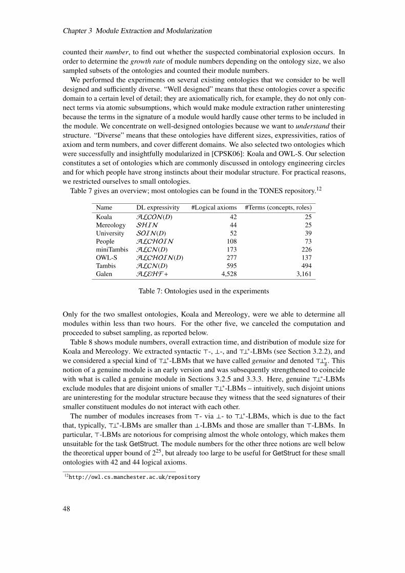
Chapter 3 Module Extraction and Modularization
counted their number, to find out whether the suspected combinatorial explosion occurs. Inorder to determine the growth rate of module numbers depending on the ontology size, we alsosampled subsets of the ontologies and counted their module numbers.
We performed the experiments on several existing ontologies that we consider to be welldesigned and su�ciently diverse. “Well designed” means that these ontologies cover a specificdomain to a certain level of detail; they are axiomatically rich, for example, they do not only con-nect terms via atomic subsumptions, which would make module extraction rather uninterestingbecause the terms in the signature of a module would hardly cause other terms to be included inthe module. We concentrate on well-designed ontologies because we want to understand theirstructure. “Diverse” means that these ontologies have di↵erent sizes, expressivities, ratios ofaxiom and term numbers, and cover di↵erent domains. We also selected two ontologies whichwere successfully and insightfully modularized in [CPSK06]: Koala and OWL-S. Our selectionconstitutes a set of ontologies which are commonly discussed in ontology engineering circlesand for which people have strong instincts about their modular structure. For practical reasons,we restricted ourselves to small ontologies.
Table 7 gives an overview; most ontologies can be found in the TONES repository.12
Name DL expressivity #Logical axioms #Terms (concepts, roles)Koala ALCON(D) 42 25Mereology SHIN 44 25University SOIN(D) 52 39People ALCHOIN 108 73miniTambis ALCN(D) 173 226OWL-S ALCHOIN(D) 277 137Tambis ALCN(D) 595 494Galen ALEHF+ 4,528 3,161
Table 7: Ontologies used in the experiments
Only for the two smallest ontologies, Koala and Mereology, were we able to determine allmodules within less than two hours. For the other five, we canceled the computation andproceeded to subset sampling, as reported below.
Table 8 shows module numbers, overall extraction time, and distribution of module size forKoala and Mereology. We extracted syntactic >-, ?-, and >?⇤-LBMs (see Section 3.2.2), andwe considered a special kind of >?⇤-LBMs that we have called genuine and denoted >?⇤g. Thisnotion of a genuine module is an early version and was subsequently strengthened to coincidewith what is called a genuine module in Sections 3.2.5 and 3.3.3. Here, genuine >?⇤-LBMsexclude modules that are disjoint unions of smaller >?⇤-LBMs – intuitively, such disjoint unionsare uninteresting for the modular structure because they witness that the seed signatures of theirsmaller constituent modules do not interact with each other.
The number of modules increases from >- via ?- to >?⇤-LBMs, which is due to the factthat, typically, >?⇤-LBMs are smaller than ?-LBMs and those are smaller than >-LBMs. Inparticular, >-LBMs are notorious for comprising almost the whole ontology, which makes themunsuitable for the task GetStruct. The module numbers for the other three notions are well belowthe theoretical upper bound of 225, but already too large to be useful for GetStruct for these smallontologies with 42 and 44 logical axioms.
12http://owl.cs.manchester.ac.uk/repository
48
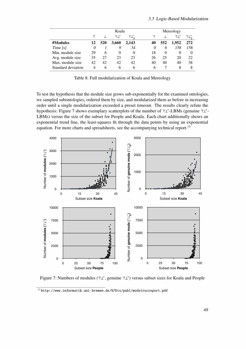
3.3 Logic-Based Modularization
Koala Mereology> ? >?⇤ >?⇤g > ? >?⇤ >?⇤g
#Modules 12 520 3,660 2,143 40 552 1,952 272Time [s] 0 1 9 34 0 6 158 158Min. module size 29 6 0 0 18 0 0 0Avg. module size 35 27 23 23 26 25 20 22Max. module size 42 42 42 42 40 40 40 38Standard deviation 4 6 6 6 6 7 8 8
Table 8: Full modularization of Koala and Mereology
To test the hypothesis that the module size grows sub-exponentially for the examined ontologies,we sampled subontologies, ordered them by size, and modularized them as before in increasingorder until a single modularization exceeded a preset timeout. The results clearly refute thehypothesis: Figure 7 shows exemplary scatterplots of the number of >?⇤-LBMs (genuine >?⇤-LBMs) versus the size of the subset for People and Koala. Each chart additionally shows anexponential trend line, the least-squares fit through the data points by using an exponentialequation. For more charts and spreadsheets, see the accompanying technical report.13
Num
bero
fmod
ules
(>?⇤
)
0
1000
2000
3000
4000
0 15 30 45
Num
bero
fgen
uine
mod
s(>?⇤ g
)
0
1000
2000
3000
0 15 30 45
Subset size Koala Subset size Koala
Num
bero
fmod
ules
(>?⇤
)
0
2500
5000
7500
10000
0 25 50 75 100
Num
bero
fgen
uine
mod
s(>?⇤ g
)
0
2500
5000
7500
10000
0 25 50 75 100
Subset size People Subset size People
Figure 7: Numbers of modules (>?⇤, genuine >?⇤) versus subset sizes for Koala and People
13 http://www.informatik.uni-bremen.de/%7Ets/publ/modstrucreport.pdf
49
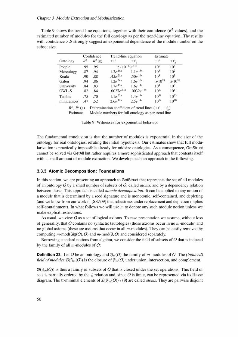
Chapter 3 Module Extraction and Modularization
Table 9 shows the trend-line equations, together with their confidence (R2 values), and theestimated number of modules for the full ontology as per the trend-line equation. The resultswith confidence >.8 strongly suggest an exponential dependence of the module number on thesubset size.
Confidence Trend-line equation EstimateOntology R2 R2 (g) >?⇤ >?⇤g >?⇤ >?⇤gPeople .95 .95 2 · 10�13e.41n 106 106
Mereology .87 .94 1.2e.16n 1.1e.13n 103 102
Koala .90 .88 .45e.21n .50e.19n 103 103
Galen .94 .86 1.2e.24n 1.6e.16n �1099 �1099
University .84 .83 1.7e.19n 1.6e.14n 104 103
OWL-S .82 .84 .0027e.17n .0032e.16n 1017 1017
Tambis .75 .70 1.1e.22n 1.4e.13n 1058 1033
miniTambis .47 .52 2.6e.18n 2.5e.14n 1014 1010
R2, R2 (g) Determination coe�cient of trend lines (>?⇤, >?⇤g)Estimate Module numbers for full ontology as per trend line
Table 9: Witnesses for exponential behavior
The fundamental conclusion is that the number of modules is exponential in the size of theontology for real ontologies, refuting the initial hypothesis. Our estimates show that full modu-larization is practically impossible already for midsize ontologies. As a consequence, GetStructcannot be solved via GetAll but rather requires a more sophisticated approach that contents itselfwith a small amount of module extraction. We develop such an approach in the following.
3.3.3 Atomic Decomposition: Foundations
In this section, we are presenting an approach to GetStruct that represents the set of all modulesof an ontology O by a small number of subsets of O, called atoms, and by a dependency relationbetween those. This approach is called atomic decomposition. It can be applied to any notion ofa module that is determined by a seed signature and is monotonic, self-contained, and depleting(and we know from our work in [SSZ09] that robustness under replacement and depletion impliesself-containment). In what follows we will use m to denote any such module notion unless wemake explicit restrictions.
As usual, we view O as a set of logical axioms. To ease presentation we assume, without lossof generality, that O contains no syntactic tautologies (those axioms occur in no m-module) andno global axioms (these are axioms that occur in all m-modules). They can be easily removed bycomputing m-mod(Sig(O),O) and m-mod(;,O) and considered separately.
Borrowing standard notions from algebra, we consider the field of subsets of O that is inducedby the family of all m-modules of O:
Definition 23. Let O be an ontology and Fm(O) the family of m-modules of O. The (induced)field of modules B(Fm(O)) is the closure of Fm(O) under union, intersection, and complement.
B(Fm(O)) is thus a family of subsets of O that is closed under the set operations. This field ofsets is partially ordered by the ✓ relation and, since O is finite, can be represented via its Hassediagram. The ✓-minimal elements of B(Fm(O)) \ {;} are called atoms. They are pairwise disjoint
50
3.3 Logic-Based Modularization
and thus form a partition of O; in particular the number of atoms is bounded by the number ofaxioms in O. Furthermore, every module is the union of some atoms. Hence the set of atoms isa succinct representation of all modules of O – provided that we equip it with information thatallows to reconstruct the modules. Even more, we will see that the set of atoms can be computedin polynomial time modulo module extraction.
Since modules provide coverage, it is natural to say that an axiom ↵ logically depends onanother axiom � if, whenever ↵ occurs in a moduleM, then � also belongs toM. This idea canbe generalized to atoms:
Definition 24. Let a and b be two distinct atoms of an ontology O. We say that
• a depends on b (written a ⌫ b) if, for every moduleM 2 Fm(O) such that a ✓M, we haveb ✓M.
• a and b are independent if there exist two disjoint modulesM1,M2 2 Fm(O) such thata ✓M1 and b ✓M2.
For a monotonic, self-contained, and depleting module notion, Definition 24 describes thepossible relations between atoms exhaustively, which relies on the following insight.
Proposition 25. For every atom a in B(Fm(O)) and every nonempty set of axioms {↵1, . . . ,↵k} ✓a, we have that m-mod({Sig(↵1) [ . . . [ Sig(↵k)},O) is the smallest m-module containing a.
LetM↵ = m-mod(Sig(↵),O) for any axiom ↵ 2 O. As a consequence of Proposition 25, we get:
Corollary 26. Given an atom a, for any axiom ↵ 2 a we have thatM↵ = m-mod(Sig(a),O).Moreover, a depends on all atoms belonging toM↵ \ a.
The binary relation ⌫ is a partial order over the set of atoms in B(Fm(O)).
We call the set of atoms with the dependency relation ⌫ the atomic decomposition of O, writtenAD(O). Definition 24 and Corollary 26 allow us to draw a Hasse diagram for AD(O), too, seeFigure 8 for that of Koala. Atoms are scaled by their size; the arrows represent the ⌫ relation.There are 23 atoms; four of them are isolated (numbers 9, 13, 15, 22), and the remaining atomsall depend on two large ones (numbers 7, 5). Those two consist of definitions of the terms centralto the ontology: Animal, Male, Female, Gender, hasGender, and hasHabitat.
As an immediate consequence of our observations so far, a module is a disjoint finite union ofatoms:
Definition 27. The principal ideal of an atom a is the set (a] = {↵ 2 b | b � a} ✓ O.
Proposition 28. For every atom a, (a] is a module.
Conversely, not every union of atoms is necessarily a module. However, we can compute themodules from AD(O) if we store the ✓-minimal seed signatures that lead to (a]: we say that anatom a is relevant for a module >?⇤-mod(⌃,O) if there is a seed signature ⌃0 for (a] with ⌃0 ✓ ⌃.
Proposition 29. >?⇤-mod(⌃,O) =S {(a] | a is relevant for ⌃}.
As a consequence, AD(O) is indeed a succinct representation of all modules: its linearly manyatoms represent all its worst-case exponentially many modules. We can even compute AD(O)e�ciently, i.e., by a polynomial-time algorithm with a linear number of oracle calls to a moduleextractor. If we use syntactic LBMs, then this algorithm has a polynomial-time overall run-time. The main ingredients are modules “generated” by single axioms, i.e., the linearly manym-mod(Sig(↵),O) for ↵ 2 O. We call these modules genuine because they can be shown to beexactly those that are not the union of two incomparable (w.r.t. set inclusion) modules.
51
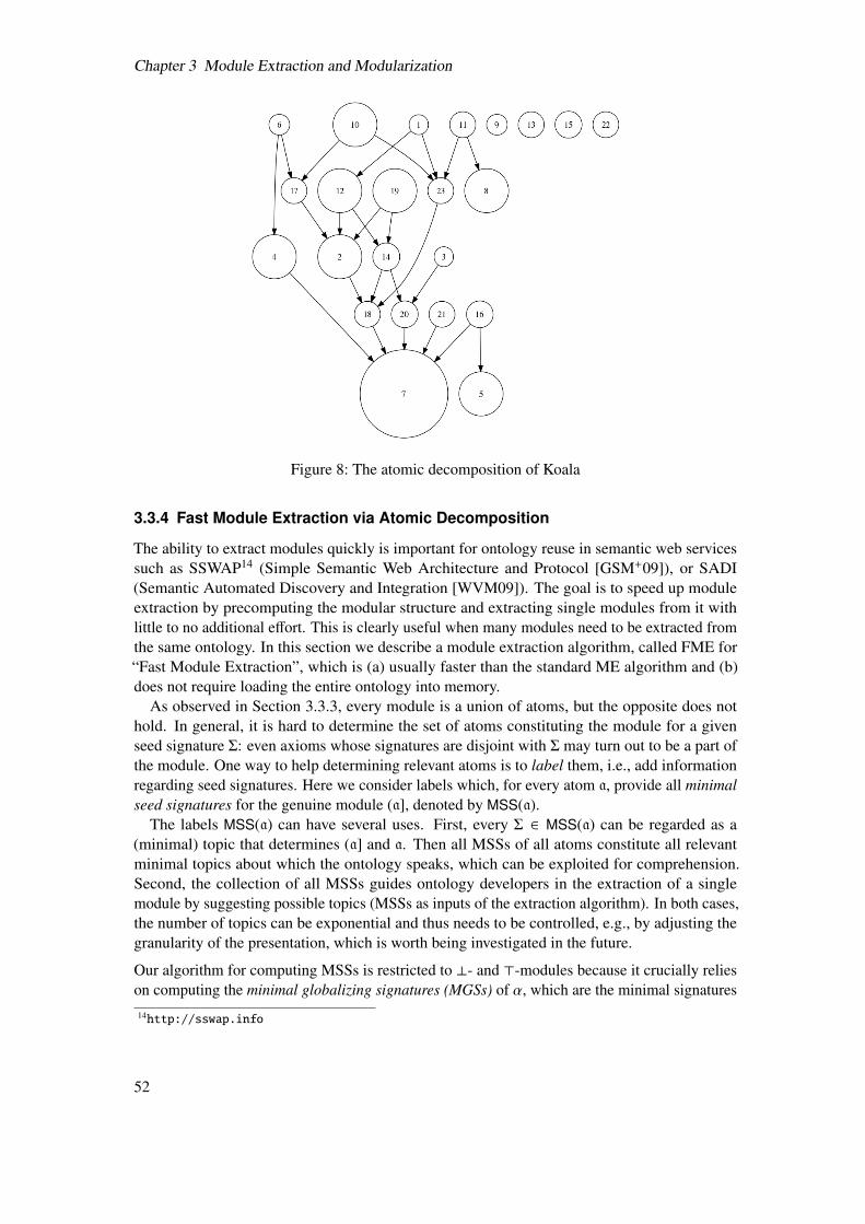
Chapter 3 Module Extraction and Modularization
Figure 8: The atomic decomposition of Koala
3.3.4 Fast Module Extraction via Atomic Decomposition
The ability to extract modules quickly is important for ontology reuse in semantic web servicessuch as SSWAP14 (Simple Semantic Web Architecture and Protocol [GSM+09]), or SADI(Semantic Automated Discovery and Integration [WVM09]). The goal is to speed up moduleextraction by precomputing the modular structure and extracting single modules from it withlittle to no additional e↵ort. This is clearly useful when many modules need to be extracted fromthe same ontology. In this section we describe a module extraction algorithm, called FME for“Fast Module Extraction”, which is (a) usually faster than the standard ME algorithm and (b)does not require loading the entire ontology into memory.
As observed in Section 3.3.3, every module is a union of atoms, but the opposite does nothold. In general, it is hard to determine the set of atoms constituting the module for a givenseed signature ⌃: even axioms whose signatures are disjoint with ⌃ may turn out to be a part ofthe module. One way to help determining relevant atoms is to label them, i.e., add informationregarding seed signatures. Here we consider labels which, for every atom a, provide all minimalseed signatures for the genuine module (a], denoted by MSS(a).
The labels MSS(a) can have several uses. First, every ⌃ 2 MSS(a) can be regarded as a(minimal) topic that determines (a] and a. Then all MSSs of all atoms constitute all relevantminimal topics about which the ontology speaks, which can be exploited for comprehension.Second, the collection of all MSSs guides ontology developers in the extraction of a singlemodule by suggesting possible topics (MSSs as inputs of the extraction algorithm). In both cases,the number of topics can be exponential and thus needs to be controlled, e.g., by adjusting thegranularity of the presentation, which is worth being investigated in the future.
Our algorithm for computing MSSs is restricted to ?- and >-modules because it crucially relieson computing the minimal globalizing signatures (MGSs) of ↵, which are the minimal signatures14http://sswap.info
52
3.3 Logic-Based Modularization
⌃ such that ↵ is local w.r.t. ⌃. The notion of MGSs is not meaningful for a nested module notionsuch as >?⇤. The desirable transfer to >?⇤-modules would thus require an entirely new approach.
The algorithm first computes the set MGS(↵) for every axiom ↵ 2 a, comprising the MGSsof ↵. For atoms a that do not depend on any other atoms, MSS(a) is the union of the MGS(↵)for all its axioms ↵. For the remaining atoms, the ⌃ 2 MGS(a) are not necessarily minimal seedsignatures for (a]: some ⌃0 ( ⌃ might be a seed signature for a module (b] with b � a if ⌃ iscontained in the extended signature ⌃0 [ Sig((b]) against which locality is checked when themodule (b] is extracted, see Algorithm 1. This constellation needs to be detected for every seedsignature ⌃ 2 MGS(a) and every atom b on which a (transitively) depends; we call this subroutineelaborating ⌃.
The algorithm requires time exponential in the size of the ontology in the worst case, but hasthe anytime property: the subroutine for elaborating a seed signature can be interrupted uponsome timeout, which will result in computing some subset of the MSS set for an atom – inthis case we call the atom dirty. Dirty atoms require special handling during module extractionbecause their relevance cannot be determined: our FME algorithm will need to include themin the module even though they may be irrelevant. Consequently, FME performance dependsdirectly on the presence of atoms left dirty by the MSS algorithm. The amount of “dirtiness” andits impact on FME is subject of the evaluation in Section 3.3.5.
The final FME algorithm is now a simple variant of the plain module extraction algorithm(Algorithm 1), where the addition of all non-local axioms is replaced by the addition of all atomsrelevant for ⌃ [ Sig(M) (and all dirty atoms).
The FME algorithm has two important advantages over the standard ME algorithm. First,it should be faster for most ontologies because it benefits from the labeled AD in two ways:(i) it exploits labels to quickly detect relevant atoms; (ii) once an atom a is established to berelevant, the corresponding module (a] is added to the module without further checks. Second, itconsumes substantially less memory since only relevant atoms (and their principal ideals) needto be loaded. This is especially significant when modules are small compared to the size of theontology, which we have observed for most of the BioPortal ontologies (the median module sizefor small seed signatures is < 1%), see Section 3.3.5.
In addition, the FME algorithm only needs access to the AD graph and labels, not to theaxioms. This is relevant for maintaining large ontologies, or even large repositories thereof.Contrary to the standard ME, the FME algorithm can extract modules by loading only the axiomsof relevant (and dirty) atoms. For example, if BioPortal ontologies were maintained in thedecomposed form, it would be possible to provide clients, such as SSWAP, with modules for arequired seed signature in a scalable (from the memory perspective) way.
3.3.5 Atomic Decomposition in Practice
This section is concerned with testing whether AD is useful in practice, providing answers to thequestions of whether all or which ontologies decompose “well”, what it means to decomposewell, and which properties of an ontology lead to “good” decomposability. We discuss andevaluate the performance of ADs w.r.t. three specific tasks:
Task 1: Ontology reuse and collaborative development (see Scenarios 1 and 2 from Section 3.1)
Task 2: Topicality for ontology comprehension (relevant for Scenario 3 from Section 3.1)
Task 3: Fast module extraction (as discussed in Section 3.3.4)
53
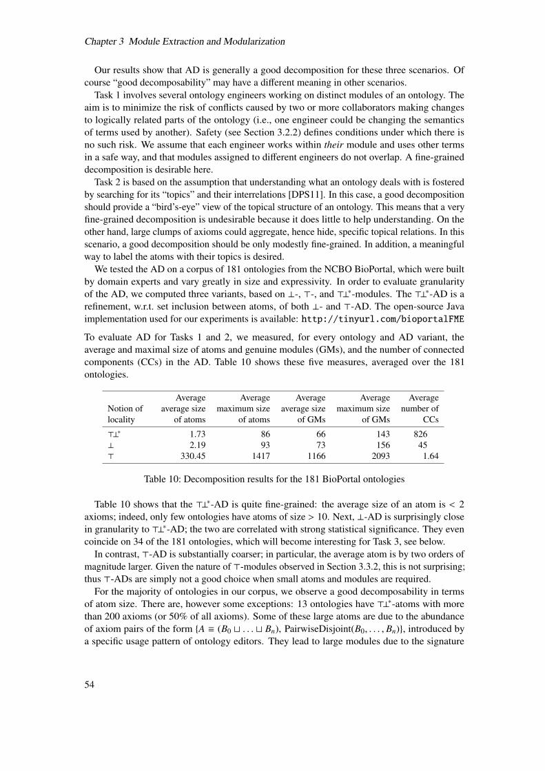
Chapter 3 Module Extraction and Modularization
Our results show that AD is generally a good decomposition for these three scenarios. Ofcourse “good decomposability” may have a di↵erent meaning in other scenarios.
Task 1 involves several ontology engineers working on distinct modules of an ontology. Theaim is to minimize the risk of conflicts caused by two or more collaborators making changesto logically related parts of the ontology (i.e., one engineer could be changing the semanticsof terms used by another). Safety (see Section 3.2.2) defines conditions under which there isno such risk. We assume that each engineer works within their module and uses other termsin a safe way, and that modules assigned to di↵erent engineers do not overlap. A fine-graineddecomposition is desirable here.
Task 2 is based on the assumption that understanding what an ontology deals with is fosteredby searching for its “topics” and their interrelations [DPS11]. In this case, a good decompositionshould provide a “bird’s-eye” view of the topical structure of an ontology. This means that a veryfine-grained decomposition is undesirable because it does little to help understanding. On theother hand, large clumps of axioms could aggregate, hence hide, specific topical relations. In thisscenario, a good decomposition should be only modestly fine-grained. In addition, a meaningfulway to label the atoms with their topics is desired.
We tested the AD on a corpus of 181 ontologies from the NCBO BioPortal, which were builtby domain experts and vary greatly in size and expressivity. In order to evaluate granularityof the AD, we computed three variants, based on ?-, >-, and >?⇤-modules. The >?⇤-AD is arefinement, w.r.t. set inclusion between atoms, of both ?- and >-AD. The open-source Javaimplementation used for our experiments is available: http://tinyurl.com/bioportalFME
To evaluate AD for Tasks 1 and 2, we measured, for every ontology and AD variant, theaverage and maximal size of atoms and genuine modules (GMs), and the number of connectedcomponents (CCs) in the AD. Table 10 shows these five measures, averaged over the 181ontologies.
Average Average Average Average AverageNotion of average size maximum size average size maximum size number oflocality of atoms of atoms of GMs of GMs CCs
>?⇤ 1.73 86 66 143 826? 2.19 93 73 156 45> 330.45 1417 1166 2093 1.64
Table 10: Decomposition results for the 181 BioPortal ontologies
Table 10 shows that the >?⇤-AD is quite fine-grained: the average size of an atom is < 2axioms; indeed, only few ontologies have atoms of size > 10. Next, ?-AD is surprisingly closein granularity to >?⇤-AD; the two are correlated with strong statistical significance. They evencoincide on 34 of the 181 ontologies, which will become interesting for Task 3, see below.
In contrast, >-AD is substantially coarser; in particular, the average atom is by two orders ofmagnitude larger. Given the nature of >-modules observed in Section 3.3.2, this is not surprising;thus >-ADs are simply not a good choice when small atoms and modules are required.
For the majority of ontologies in our corpus, we observe a good decomposability in termsof atom size. There are, however some exceptions: 13 ontologies have >?⇤-atoms with morethan 200 axioms (or 50% of all axioms). Some of these large atoms are due to the abundanceof axiom pairs of the form {A ⌘ (B0 t . . . t Bn), PairwiseDisjoint(B0, . . . , Bn)}, introduced bya specific usage pattern of ontology editors. They lead to large modules due to the signature
54
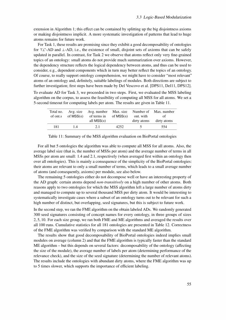
3.3 Logic-Based Modularization
extension in Algorithm 1; this e↵ect can be contained by splitting up the big disjointness axiomsor making disjointness implicit. A more systematic investigation of patterns that lead to hugeatoms remains for future work.
For Task 1, these results are promising since they exhibit a good decomposability of ontologiesfor >?⇤-AD and ?-AD, i.e., the existence of small, disjoint sets of axioms that can be safelyupdated in parallel. In contrast, for Task 2 we observe that atoms reflect only very fine-grainedtopics of an ontology: small atoms do not provide much summarization over axioms. However,the dependency structure reflects the logical dependency between atoms, and thus can be used toconsider, e.g., dependent components which in turn may better reflect the topics of an ontology.Of course, to really support ontology comprehension, we might have to consider “most relevant”atoms of an ontology and, definitely, suitable labelings of modules. Both directions are subject tofurther investigation; first steps have been made by Del Vescovo et al. [DPS11, Del11, DPS12].
To evaluate AD for Task 3, we proceeded in two steps. First, we evaluated the MSS labelingalgorithm on the corpus, to assess the feasibility of computing all MSS for all atoms. We set a5-second timeout for computing labels per atom. The results are given in Table 11.
Total no. Avg. size Avg. number Max. size Number of Max. numberof ont.s of MSS(a) of terms in of MSS(a) ont. with of
all MSS(a) dirty atoms dirty atoms
181 1.4 2.1 4252 5 554
Table 11: Summary of the MSS algorithm evaluation on BioPortal ontologies
For all but 5 ontologies the algorithm was able to compute all MSS for all atoms. Also, theaverage label size (that is, the number of MSSs per atom) and the average number of terms in allMSSs per atom are small: 1.4 and 2.1, respectively (when averaged first within an ontology thenover all ontologies). This is mainly a consequence of the simplicity of the BioPortal ontologies:their atoms are relevant to only a small number of terms, which leads to a small average numberof atoms (and consequently, axioms) per module, see also below.
The remaining 5 ontologies either do not decompose well or have an interesting property ofthe AD graph: certain atoms depend non-transitively on a high number of other atoms. Bothreasons apply to two ontologies for which the MSS algorithm left a large number of atoms dirtyand managed to compute up to several thousand MSS per dirty atom. It would be interesting tosystematically investigate cases where a subset of an ontology turns out to be relevant for such ahigh number of distinct, but overlapping, seed signatures, but this is subject to future work.
In the second step, we ran the FME algorithm on the obtain labeled ADs. We randomly generated300 seed signatures consisting of concept names for every ontology, in three groups of sizes2, 5, 10. For each size group, we ran both FME and ME algorithms and averaged the results overall 100 runs. Cumulative statistics for all 181 ontologies are presented in Table 12. Correctnessof the FME algorithm was verified by comparison with the standard ME algorithm.
The results show that good decomposability of BioPortal ontologies indeed implies smallmodules on average (column 2) and that the FME algorithm is typically faster than the standardME algorithm – but this depends on several factors: decomposability of the ontology (a↵ectingthe size of the module), the average number of labels per atom (determining performance of therelevance check), and the size of the seed signature (determining the number of relevant atoms).The results include the ontologies with abundant dirty atoms, where the FME algorithm was upto 5 times slower, which supports the importance of e�cient labeling.
55
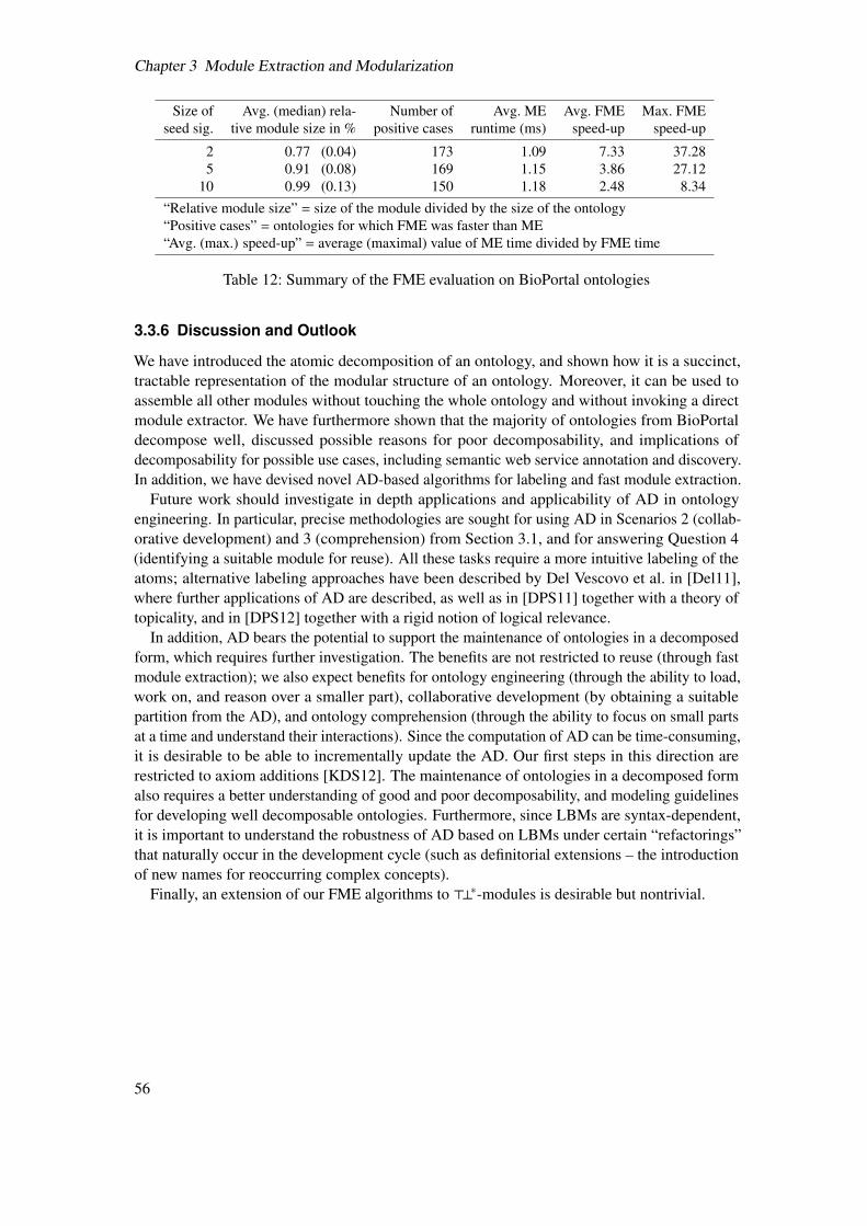
Chapter 3 Module Extraction and Modularization
Size of Avg. (median) rela- Number of Avg. ME Avg. FME Max. FMEseed sig. tive module size in % positive cases runtime (ms) speed-up speed-up
2 0.77 (0.04) 173 1.09 7.33 37.285 0.91 (0.08) 169 1.15 3.86 27.12
10 0.99 (0.13) 150 1.18 2.48 8.34“Relative module size” = size of the module divided by the size of the ontology“Positive cases” = ontologies for which FME was faster than ME“Avg. (max.) speed-up” = average (maximal) value of ME time divided by FME time
Table 12: Summary of the FME evaluation on BioPortal ontologies
3.3.6 Discussion and Outlook
We have introduced the atomic decomposition of an ontology, and shown how it is a succinct,tractable representation of the modular structure of an ontology. Moreover, it can be used toassemble all other modules without touching the whole ontology and without invoking a directmodule extractor. We have furthermore shown that the majority of ontologies from BioPortaldecompose well, discussed possible reasons for poor decomposability, and implications ofdecomposability for possible use cases, including semantic web service annotation and discovery.In addition, we have devised novel AD-based algorithms for labeling and fast module extraction.
Future work should investigate in depth applications and applicability of AD in ontologyengineering. In particular, precise methodologies are sought for using AD in Scenarios 2 (collab-orative development) and 3 (comprehension) from Section 3.1, and for answering Question 4(identifying a suitable module for reuse). All these tasks require a more intuitive labeling of theatoms; alternative labeling approaches have been described by Del Vescovo et al. in [Del11],where further applications of AD are described, as well as in [DPS11] together with a theory oftopicality, and in [DPS12] together with a rigid notion of logical relevance.
In addition, AD bears the potential to support the maintenance of ontologies in a decomposedform, which requires further investigation. The benefits are not restricted to reuse (through fastmodule extraction); we also expect benefits for ontology engineering (through the ability to load,work on, and reason over a smaller part), collaborative development (by obtaining a suitablepartition from the AD), and ontology comprehension (through the ability to focus on small partsat a time and understand their interactions). Since the computation of AD can be time-consuming,it is desirable to be able to incrementally update the AD. Our first steps in this direction arerestricted to axiom additions [KDS12]. The maintenance of ontologies in a decomposed formalso requires a better understanding of good and poor decomposability, and modeling guidelinesfor developing well decomposable ontologies. Furthermore, since LBMs are syntax-dependent,it is important to understand the robustness of AD based on LBMs under certain “refactorings”that naturally occur in the development cycle (such as definitorial extensions – the introductionof new names for reoccurring complex concepts).
Finally, an extension of our FME algorithms to >?⇤-modules is desirable but nontrivial.
56
Chapter 4
Branching-Time Temporal Description Logics
4.1 Introduction
Classical description logics (DLs) aim at the representation of, and reasoning about, static knowl-edge. The objective of enhancing DLs with means to capture temporal aspects of knowledge has,over the past 20 years, led to much e↵ort being spent on the study of temporal description logics(TDLs), as discussed in detail in the surveys [AF00, LWZ08] and the references therein. TDLsare useful for applications where knowledge involving a dynamic aspect is to be represented. Forexample, it is desirable to model in SNOMED CT concepts such as “a patient who may need ablood transfusion in the future” or “a disease whose occurrence may cause certain other diseasesin the future”.
A prominent approach to TDLs, following Schild’s original proposal [Sch93], is to combineDLs with the standard temporal logics LTL and CTL(*), based on a two-dimensional product-like semantics in the style of many-dimensional DLs [GKWZ03]. In addition to choosing thecomponent logics, the design of a TDLs requires further choices: whether temporal operators areapplied to concepts, roles and/or TBoxes, or whether we want to define some DL roles or conceptsas rigid, which would mean that they will not change their interpretation over time. For example,since every human has the same genetic disorders during their life, the relation “has geneticdisorder” between humans and diseases should be modeled by a rigid role hasGeneticDisease.Consequently, it has been argued that rigid roles are required in applications of TDLs, e.g., intemporal data modeling [AKRZ14] or in medical ontologies such as SNOMED CT.
If the temporal component is chosen to be LTL, we speak of linear-time TDLs. For theseLTDLs, the landscape of the expressivity and computational complexity is well-understood[AKL+07, BGL08, FT11, AKRZ14]. Various design choices have been explored, and bothlightweight and expressive DLs have been considered. An important insight gained is thatLTDLs based on ALC become undecidable in the presence of general TBoxes as soon astemporal operators are applied to concepts and roles, or if rigid roles are allowed.
More generally, combinations of DLs and modal logics allowing for rigid roles and generalTBoxes tend to have very high computational complexity. This can be partly explained by thewell-known correspondence of DL combinations with product modal logics (PMLs) [GKWZ03,Chapters 3, 14]: the standard reasoning problem in TDLs, concept satisfiability with respect to aTBox, is then a variant of the global consequence problem in the corresponding PML. Globalconsequence is typically undecidable in PMLs [GKWZ03].
In the context of LTDLs, recent work has aimed at regaining decidability in the presenceof rigid roles and general TBoxes, investigating LTDLs based on lightweight DLs from theEL and DL-Lite families [AKL+07, AKRZ14]. The results exhibit a stark contrast betweendecidable DL-Lite based and undecidable EL-based LTDLs. Undecidability in the EL case isexplained by an interaction of non-convexity (the ability to simulate disjunctions, here using only
57
Chapter 4 Branching-Time Temporal Description Logics
LTL-operators) with the known fact that EL with disjunctions can encode ALC; hence theseEL-based LTDLs are as hard as theirALC-counterpart.
From the viewpoint of some DL applications, it has been argued that representing the existenceof di↵erent possible futures, represented by a branching-time structure, is necessary for a moreappropriate modeling [GJL12]: in the medical domain, symptoms or diseases may evolve indi↵erent ways in the future. As an example, consider the statement: “any patient with diabeteswill possibly develop glaucoma in the future”. In an LTDL it can be modeled as
Patient u 9hasDisease.Diabetes v ^9develops.Glaucoma,
which is too strong – it says that each diabetes patient will eventually develop glaucoma. Inbranching-time TDLs we can use the existential path quantifier E together with ^ to state morecarefully that there exists a possible future where the patient develops glaucoma.
In contrast to LTDLs, the study of branching time TDLs (BTDLs) has been limited, mainlyfocusing on decidability boundaries obtained in the context of first-order branching temporallogic [HWZ02, BHWZ04]. Only recently were tight elementary bounds presented for BTDLsbased onALC and EL in the case where only (local) (i.e., non-rigid) roles are allowed [GJL12].
An aspect which, to our knowledge, has received no attention in the context of TDLs is therestriction of TBoxes to classical or acyclic TBoxes. This is surprising because this restriction isa fairly obvious design choice: given two observations: (a) it is likely to “ease” the prohibitivecomputational behavior in the presence of general TBoxes of LTDLs (and, as we will show,of BTDLs), and (b) TDLs designed this way seem well-suited as modeling languages forapplications – for example, in the biomedical domain, given that large parts of SNOMED CTand the Gene Ontology GO [Gen00] are acyclic EL-TBoxes.The work reported in this chapter thus aims at answering the following two questions.
1. Do BTDLs with rigid roles behave computationally better than LTDLs? Since the standardway to express a disjunction using LTL operators fails for CTL(*), there is justifiablehope for convex EL-based BTDLs, which can reasonably be expected to have goodcomputational properties.
2. Does the restriction to acyclic TBoxes improve the computational properties of TDLs?
To answer these questions, we will study the decidability and complexity of BTDLs obtainedfrom combining CTL withALC and lightweight DLs from the EL and DL-Lite families, withrigid roles, with temporal operators restricted to be applied to concepts only, and with generalas well as acyclic TBoxes. We will analyze the decidability and complexity of the standardreasoning problems.
Bibliographic notes. Our results for general TBoxes appeared in [GJS14]; those for restrictedTBoxes were published in [GJS15].
4.2 Preliminaries
We introduce CTLALC. Let NC and NR be countably infinite sets of concept names and rolenames. We assume that NR is partitioned into two countably infinite sets Nrig and Nloc of rigidrole names and local role names, respectively. CTLALC-concepts C are defined by the followinggrammar
C := > | A | ¬C | C u D | 9r.C | E�C | E⇤C | E(CUD)
58
4.2 Preliminaries
where A ranges over NC, r over NC. The operators ?,t,8,E^,A⇤,A^,AU can be defined interms of the above in the usual way, see also [CGP99]. We moreover consider the strict (·<)versions of the temporal operators: E⇤<C = E�E⇤C, E(CU<D) = E�E(CUD).
The semantics of CTLALC is given in terms of temporal interpretations, which are infinitetrees whose every node is associated with a classical DL interpretation. Here a tree is a directedgraph T = (W, E) where W ✓ (N \ {0})⇤ is a prefix-closed nonempty set of nodes and E ={(w,wc) | wc 2 W,w 2 N⇤, c 2 N} a set of edges; we generally assume that wc 2 W and c0 < cimplies wc0 2 W and that E is a total relation. The node " 2 W is the root of T . In the context oftemporal DLs we refer to nodes of T as time points or worlds.
A temporal interpretation is a structure I = (�,T, {Iw}w2W) where T = (W, E) is a tree and,for each w 2 W, Iw is an interpretation with domain � such that rIw = rIw0 for all r 2 Nrig andw,w0 2 W. We usually write AI,w instead of AIw , and intuitively d 2 AI,w means that, in theinterpretation I, the object d is an instance of the concept name A at time point w. Moreover,we make the constant domain assumption, that is, all time points share the same domain �. ForBoolean-complete TDLs, CDA is more general than assuming expanding, decreasing and varyingdomains because those can all be reduced to CDA [GKWZ03, Prop. 3.32]. For the sub-Booleanlogics studied here, CDA is not w.l.o.g. Indeed, we will identify a logic where reasoning withexpanding domains cannot be reduced to the constant domain case (unless P = PSPACE).
We now define the semantics of CTLALC-concepts. A path in a tree T = (W, E) startingat a node w is a minimal set ⇡ ✓ W such that w 2 ⇡ and, for each w0 2 ⇡, there is a c 2 Nwith w0c 2 ⇡. We use Paths(w) to denote the set of all paths starting at the node w. For a path⇡ = w0w1w1 · · · and i � 0, we use ⇡[i] to denote wi. The mapping ·I,w is extended from conceptnames to CTLALC-concepts as shown in Figure 9.
>I,w = �
(¬C)I,w = � \CI,w
(C u D)I,w = CI,w \ DI,w
(9r.C)I,w = {d 2 � | 9e.(d, e) 2 rI,w ^ e 2 CI,w}(E�C)I,w = {d 2 � | d 2 CI,⇡[1] for some ⇡ 2 Paths(w)}(E⇤C)I,w = {d 2 � | 8 j � 0.d 2 CI,⇡[ j] for some ⇡ 2 Paths(w)}(E(CUD))I,w = {d 2� | 9 j� 0.(d 2DI,⇡[ j] ^ (8 0 k< j. d 2CI,⇡[k])) for some ⇡ 2 Paths(w)}
Figure 9: Satisfaction relation for CTLALC-concepts
A general CTLALC-TBox T is a finite set of concept inclusions (CIs) C v D with C,DCTLALC concepts. An acyclic CTLALC-TBox T is a finite set of concept definitions (CDs)A ⌘ D with A 2 NC and D a CTLALC concept, such that (1) no two CDs have the same left-handside, and (2) there are no CDs A1 ⌘ C1, . . . , Ak ⌘ Ck in T such that Ai+1 occurs in Ci for1 i k, where Ak+1 = A1.
A temporal interpretation I satisfies a concept C if CI," , ;; it satisfies a CI C v D, writtenI |= C v D, if CI,w ✓ DI,w for all w 2 W; it is a model of a TBox T if it satisfies all CIs in T .Thus, a TBox T is interpreted globally in the sense that it has to be satisfied at every time point.
A concept C is satisfiable with respect to a CTLALC-TBox T if there is a model of T thatsatisfies C. A concept D subsumes a concept C with respect to a TBox T , written T |= C v D,if I |= C v D for all models I of T . For CTLALC and DL-LiteNbool, we consider the conceptsatisfiability problem: given a concept C and a TBox T , decide whether C is satisfiable with
59
Chapter 4 Branching-Time Temporal Description Logics
Rigid roles? no yes yes yesTBoxes general general acyclic emptyCTLALC = EXPTIME1 undecidable nonelementary and decidable
CTLE^EL , CTLE�
EL P1 nonelem./undecid. P P
CTLE�,E^EL = EXPTIME1,2 undecidable � CONP, CONEXPTIME = CONP
CTLE^,A⇤EL = PSPACE1 nonelementary = PSPACE PSPACE
1 [GJL12] 2 lower bound follows from our results � hardness membership = completeness
Table 13: Overview of previous and new complexity results
respect to T . For EL, we consider the subsumption problem: given a TBox T and two conceptsC and D, decide whether D subsumes C with respect to T .
We will denote fragments of CTLALC determined by restrictions to the temporal operatorsby putting the available temporal operators as a superscript; for example, CTLE^,A⇤
ALC denotes thefragment with the only temporal operators E^ and A⇤. Analogously, we use EL and DL-LiteNboolas subscripts for TDLs based on these lightweight DLs.
4.3 Results
Our results forALC- and EL-based TDLs are summarized – and put into the context of previouswork – in Table 13.
General TBoxes. We start with the combination of CTL and ALC, showing undecidabilityof concept satisfiability already for the fragment with only the operators E^ and A⇤. For thisresult, we combine results for products of “transitive” PMLs [GKWZ05] with a well-knownDL-technique for encoding transitivity in a TBox [Tob01]. Our result is more general: it saysthat the global satisfiability problem for all PMLs determined by frame classes C1 and C2 isundecidable if C2 contains only transitive frames and if C2 and the class of all transitive framesin C1 contain frames of arbitrarily large finite or infinite depth.
We continue by investigating the subsumption problem for BTDLs based on EL and severalfragments of CTL. These CTL fragments are subsets of the CTL operators that were previouslyshown to lead to a decrease in complexity for the standard CTL satisfiability problem [MMTV09].We first identify the following non-convex BTDLs.
CTLE^,A^EL CTLE^E�
EL CTLEUEL CTLEU<
EL CTLE^<,E⇤<EL CTLE^,E⇤
EL
We show their undecidability using the technique described above. Next we identify convexBTDLs based on EL, showing closure under direct products of FO-models:
CTLE�EL CTLE^
EL CTLE^,A⇤EL
It is reasonable to hope that these three BTDLs would behave computationally well, given that thisis typically the case for convex logics, including two-dimensional ones: e.g, the combination ofEL with the CTL operator E^ in the case where only local roles are allowed [GJL12] is tractable,and various combinations of the modal logic S5 with EL are easier than the correspondingALCvariant [LS10, GJLS11]. Surprisingly, we show that the above three logics are undecidable or at
60
4.3 Results
least nonelementary, see Table 13. The proofs of these results are challenging and technicallyinvolved because the absence of disjunction makes it di�cult to use standard techniques forestablishing lower complexity bounds, such as tilings. For the undecidability of CTLE�
EL we use areduction from the halting problem of 2-counter automata introduced by Minsky [Min67]; for thenonelementary lower bound of CTLE^
EL we show how to encode k-exponential counters, adoptingStockmeyer’s technique [Sto74], and then reduce from the word problem of k-exponentiallyspace-bounded Turing machines.
Finally, we investigate concept satisfiability for BTDLs based on DL-LiteNbool, showing that thetechnique developed in [AKRZ14] for LTDLs is robust in the sense that it can be carried over tomost BTDLs based on CTL. This technique consists in reducing CTLDL-LiteNbool
to the one-variablefragment of first-order temporal logic, and then eliminating existential quantifiers to obtain anequivalent CTL formula. We thus obtain tight complexity bounds, namely PSPACE- and EXPTIME-completeness, according to the complexity for the corresponding CTL fragments [MMTV09].Unfortunately, elimination of the quantifiers does not work for full CTLDL-LiteNbool
because theoriginal shifting technique [AKRZ14, Lemma 4.2] relies on the past being unbounded, whichis not the case for the standard CTL semantics. However, the problem can be circumvented by(1) disallowing local roles – which makes shifting superfluous – or (2) restricting the temporaloperators to those that are tolerant to a certain variant of unraveling into the temporal direction,related to stutter invariance [Lam83]. We thus obtain:
Theorem 30. Concept satisfiability relative to general TBoxes is EXPTIME-complete forCTLDL-LiteNbool
without local roles and for CTLEU,E⇤DL-LiteNbool
, and PSPACE-complete for CTLE^DL-LiteNbool
.
A more systematic investigation of CTLDL-LiteNboolis left for future work; we plan to pursue an
automata-based approach in the style of [GJL12].
Restricted TBoxes. As above, we start with CTLALC, showing that satisfiability relative toempty and acyclic TBoxes is nonelementary and decidable. To establish the upper bound,we proceed in two steps analogously to Hodkinson et al. [HWZ00, HWZ02]: we characterizesatisfiability by the existence of a quasimodel [GKWZ03] and encode the latter as a formulain monadic second-order logic, which is decidable over countably branching trees [Rab69].Thanks to unfolding [Neb90b], there is no di↵erence between the cases of acyclic TBoxes andthe empty TBox. The nonelementary lower bound holds already for CTLE^
ALC and CTLE�ALC: they
are notational variants of the PMLs S4 ⇥ K and K ⇥ K, whose satisfiability problem is inherentlynonelementary [GJL15].
We continue by replacing ALC with EL and maintaining the restriction to E^,E� andempty TBoxes. We show that the resulting TDLs are decidable in P with one of the twooperators, and CONP-complete with both. The P upper bound is obtained by extending theknown characterization of EL subsumption via homomorphisms between concept descriptiontrees [BKM99] to the two-dimensional case: given two CTLE�
EL -concepts C,D, we have C v D ifand only if D is satisfied in the root of the canonical model of C. While constructing the latter isstraightforward, showing its canonicity is technically intricate. The same technique goes throughwith minor modifications for CTLE^
EL . The CONP upper bound for CTLE�,E^EL is obtained by
combining the previous machinery with expansion vectors, which were introduced by Haase andLutz [HL08] for proving CONP membership of ELtrans, i.e., EL extended with transitive roles.The matching lower bound is due to a straightforward reduction from ELtrans.
61
Chapter 4 Branching-Time Temporal Description Logics
Our main results are the P- and PSPACE-completeness for CTLEL fragments over acyclicTBoxes: we lift the P upper bound for CTLE�
EL and CTLE^EL to the case of acyclic TBoxes and
show that the addition of A⇤ leads to PSPACE-completeness. For the P upper bound, we usea two-dimensional variant of the standard EL completion algorithm [BBL05], which relies onthe input TBox being acyclic. For the PSPACE upper bound, a suitable extension of the sameprocedure would require an exponentially-sized data structure. To avoid its full computation, ourPSPACE procedure computes only single paths, explores each such trace in a tableau-like fashion,and enumerates all traces in an appropriate order. Here, acyclicity is crucial for bounding thelength of traces polynomially. The matching PSPACE lower bound is via a reduction from QBFvalidity. By a slight variation of that reduction, we are able to show that CTLE�
EL and CTLE^EL
with rigid roles, acyclic TBoxes, and expanding domains are already PSPACE-hard.As for CTLE�,E^
EL over acyclic TBoxes, unfolding immediately yields a CONEXPTIME upperbound. This time we cannot obtain a lower bound via a reduction from EL with transitive roles(which is PSPACE-hard over acyclic TBoxes [HL08]) because Haase and Lutz’ hardness proofuses two roles, which cannot both be modeled by the temporal dimension. It remains for futurework to search for tight complexity bounds; we are currently trying to combine the general ideabehind expansion vectors with our completion procedure.
All upper bounds are una↵ected if rigid concepts are included.
4.4 Discussion
With our results, we have made progress towards understanding the landscape of the computa-tional complexity and expressivity of BTDLs allowing for rigid roles. We identified EL-basedBTDLs that are convex but nevertheless computationally badly behaved over general TBoxes.
By restricting the TBoxes, we have obtained a relatively low complexity for the same BTDLs,which is in stark contrast with the negative results for general TBoxes. The restriction to acyclicTBoxes has thus enabled us to identify the first computationally well-behaved TDLs with rigidroles based on EL and classical temporal logics.
Our positive results for CTLEL over empty TBoxes are of significance for PMLs too: theyentail that implication for the positive fragments of K ⇥ K and S4 ⇥ K is in P.
The picture of the complexity landscape of TDLs with rigid roles obtained thus far can beextended in several ways. First, over general TBoxes, decidability could be regained by certainmodifications, such as considering expanding domains (which might cause the complexity todrop over general TBoxes), or by replacing DL-Litebool with DL-Litecore (which was successfulfor LTDLs [AKRZ14]). Second, the positive results obtained over acyclic TBoxes encourageattempts to enrich the language, e.g., by adding role inclusions, by allowing temporal roles, bystudying cyclic TBoxes, or by changing the temporal component to LTL or even the µ-calculus.
62
Bibliography
[AB09] S. Arora and B. Barak. Computational Complexity – A Modern Approach. Cam-bridge University Press, 2009.
[ABI+09] E. Allender, M. Bauland, N. Immerman, H. Schnoor, and H. Vollmer. The com-plexity of satisfiability problems: Refining Schaefer’s theorem. J. of Computer andSystem Sciences, 75(4):245–254, 2009.
[ABM99] C. Areces, P. Blackburn, and M. Marx. A road-map on complexity for hybridlogics. In Proc. of CSL-99, volume 1683 of LNCS, pages 307–321. Springer-Verlag,1999.
[ABM00] C. Areces, P. Blackburn, and M. Marx. The computational complexity of hybridtemporal logics. Logic J. of the IGPL, 8(5):653–679, 2000.
[ACD90] R. Alur, C. Courcoubetis, and D. L. Dill. Model-checking for real-time systems.In Proc. of LICS-90, pages 414–425. IEEE Computer Society, 1990.
[ACH12] A. Armas Romero, B. Cuenca Grau, and I. Horrocks. MORe: Modular combinationof OWL reasoners for ontology classification. In Proc. of ISWC-12 (1), volume7649 of LNCS, pages 1–16. Springer-Verlag, 2012.
[ACKZ07] A. Artale, D. Calvanese, R. Kontchakov, and M. Zakharyaschev. DL-Lite in thelight of first-order logic. In Proc. of AAAI-07, pages 361–366, 2007.
[ACKZ09a] A. Artale, D. Calvanese, R. Kontchakov, and M. Zakharyaschev. Adding weight toDL-Lite. In Proc. of DL 2009, CEUR-WS, 2009.
[ACKZ09b] A. Artale, D. Calvanese, R. Kontchakov, and M. Zakharyaschev. The DL-Litefamily and relations. J. of Artificial Intelligence Research, 36:1–69, 2009.
[AF00] A. Artale and E. Franconi. A survey of temporal extensions of description logics.Ann. of Mathematics and Artificial Intelligence, 30(1-4):171–210, 2000.
[AKL+07] A. Artale, R. Kontchakov, C. Lutz, F. Wolter, and M. Zakharyaschev. Temporalisingtractable description logics. In Proc. of TIME-07, pages 11–22. IEEE ComputerSociety Press, 2007.
[AKRZ14] A. Artale, R. Kontchakov, V. Ryzhikov, and M. Zakharyaschev. A cookbookfor temporal conceptual data modelling with description logics. ACM Trans.Computational Logic, 15(3):25, 2014.
[At07] C. Areces and B. ten Cate. Hybrid logics. In Handbook of Modal Logic, volume 3,chapter 14, pages 821–868. Elsevier, 2007.
63
Chapter 4 Branching-Time Temporal Description Logics
[Baa96] F. Baader. Using automata theory for characterizing the semantics of terminologicalcycles. Ann. of Mathematics and Artificial Intelligence, 18(2-4):175–219, 1996.
[Baa03] F. Baader. Terminological cycles in a description logic with existential restrictions.In Proc. of IJCAI-03, pages 325–330. Morgan Kaufmann, 2003.
[BBC+10] M. Bauland, E. Bohler, N. Creignou, S. Reith, H. Schnoor, and H. Vollmer. Thecomplexity of problems for quantified constraints. Theory of Computing Systems,47(2):454–490, 2010.
[BBL05] F. Baader, S. Brandt, and C. Lutz. Pushing the EL envelope. In Proc. of IJCAI-05,pages 364–369, 2005.
[BBL08] F. Baader, S. Brandt, and C. Lutz. Pushing the EL envelope further. In Proc. ofOWLED-08DC, 2008.
[BCC+04] M. Bauland, P. Chapdelaine, N. Creignou, M. Hermann, and H. Vollmer. Analgebraic approach to the complexity of generalized conjunctive queries. In Proc.of SAT-04, 2004.
[BCM+03] F. Baader, D. Calvanese, D. McGuinness, D. Nardi, and P. F. Patel-Schneider, edi-tors. The Description Logic Handbook: Theory, Implementation, and Applications.Cambridge University Press, 2003.
[BCRV03] E. Bohler, N. Creignou, S. Reith, and H. Vollmer. Playing with Boolean blocks, partI: Post’s lattice with applications to complexity theory. SIGACT News, 34(4):38–52,2003.
[BDL04] G. Behrmann, A. David, and K. G. Larsen. A tutorial on Uppaal. In RevisedLectures of SFM-RT ’04, volume 3185 of LNCS, pages 200–236. Springer-Verlag,2004.
[BFZE08] C. Bezerra, F. Freitas, A. Zimmermann, and J. Euzenat. ModOnto: A tool formodularizing ontologies. In Proc. of WONTO-08, volume 427 of CEUR-WS.org,2008.
[BGL08] F. Baader, S. Ghilardi, and C. Lutz. LTL over description logic axioms. In Proc. ofKR-08, pages 684–694. AAAI Press, 2008.
[BH91] F. Baader and B. Hollunder. A terminological knowledge representation systemwith complete inference algorithms. In Proc. of PDK-91, volume 567 of LNCS,pages 67–86. Springer-Verlag, 1991.
[BH09] M. Bauland and E. Hemaspaandra. Isomorphic implication. Theory of ComputingSystems, 44(1):117–139, 2009.
[BHSS06] M. Bauland, E. Hemaspaandra, H. Schnoor, and I. Schnoor. Generalized modal sat-isfiability. In Proc. of STACS-06, volume 3884 of LNCS, pages 500–511. Springer-Verlag, 2006.
[BHWZ04] S. Bauer, I. Hodkinson, F. Wolter, and M. Zakharyaschev. On non-local proposi-tional and weak monodic quantified CTL. J. of Logic and Computation, 14(1):3–22,2004.
64
[BK08] C. Baier and J.-P. Katoen. Principles of Model Checking. The MIT Press, 2008.
[BKM99] F. Baader, R. Kusters, and R. Molitor. Computing least common subsumers indescription logics with existential restrictions. In Proc. of IJCAI-99. MorganKaufmann, 1999.
[BL10] L. Bozzelli and R. Lanotte. Complexity and succinctness issues for linear-timehybrid logics. Theoretical Computer Science, 411(2):454–469, 2010.
[BLS06] F. Baader, C. Lutz, and B. Suntisrivaraporn. CEL – a polynomial-time reasonerfor life science ontologies. In Proc. of IJCAR-06, volume 4130 of LNCS, pages287–291. Springer-Verlag, 2006.
[BMS+09] M. Bauland, M. Mundhenk, T. Schneider, H. Schnoor, I. Schnoor, and H. Vollmer.The tractability of model-checking for LTL: the good, the bad, and the ugly frag-ments. In Proc. of M4M-5, volume 231 of ENTCS, pages 277–292, 2009.
[BMS+11] M. Bauland, M. Mundhenk, T. Schneider, H. Schnoor, I. Schnoor, and H. Vollmer.The tractability of model checking for LTL: the good, the bad, and the uglyfragments. ACM Trans. Computational Logic, 12(2):13, 2011.
[BMTV12] O. Beyersdor↵, A. Meier, M. Thomas, and H. Vollmer. The complexity of reasoningfor fragments of default logic. J. of Logic and Computation, 22(3):587–604, 2012.
[BP90] P. Byers and D. Pitt. Conservative extensions: A cautionary note. EATCS-Bulletin,41, 1990.
[Bra04] S. Brandt. Polynomial time reasoning in a description logic with existentialrestrictions, GCI axioms, and—what else? In Proc. of ECAI-04, pages 298–302.IOS Press, 2004.
[BS85] R. J. Brachman and J. G. Schmolze. An overview of the KL-ONE knowledgerepresentation system. Cognitive Science, 9(2):171–216, 1985.
[BS95] P. Blackburn and J. Seligman. Hybrid languages. J. of Logic, Language andInformation, 4(3):251–272, 1995.
[BSS+09] M. Bauland, T. Schneider, H. Schnoor, I. Schnoor, and H. Vollmer. The complexityof generalized satisfiability for linear temporal logic. Logical Methods in ComputerScience, 5(1), 2009.
[Bul70] R. Bull. An approach to tense logic. Theoria, 36:282–300, 1970.
[BVSH09] J. Bao, G. Voutsadakis, G. Slutzki, and V. Honavar. Package-based descriptionlogics. In Stuckenschmidt et al. [SPS09], pages 349–371.
[Cal96] D. Calvanese. Reasoning with inclusion axioms in description logics: Algorithmsand complexity. In Proc. of ECAI-96, pages 303–307. John Wiley & Sons, 1996.
[CCGR00] A. Cimatti, E. M. Clarke, F. Giunchiglia, and M. Roveri. NuSMV: a new symbolicmodel checker. Int. J. on Software Tools for Technology Transfer, 2(4):410–425,2000.
65
Chapter 4 Branching-Time Temporal Description Logics
[CDL+05] D. Calvanese, G. De Giacomo, D. Lembo, M. Lenzerini, and R. Rosati. DL-Lite:Tractable description logics for ontologies. In Proc. of AAAI-05, pages 602–607.AAAI Press / The MIT Press, 2005.
[CDLN01] D. Calvanese, G. De Giacomo, M. Lenzerini, and D. Nardi. Reasoning in expressivedescription logics. In J. A. Robinson and A. Voronkov, editors, Handbook ofAutomated Reasoning, pages 1581–1634. Elsevier and MIT Press, 2001.
[CGP99] E. M. Clarke, O. Grumberg, and D. A. Peled. Model Checking. MIT Press, 1999.
[CHKS08] B. Cuenca Grau, I. Horrocks, Y. Kazakov, and U. Sattler. Modular reuse ofontologies: Theory and practice. J. of Artificial Intelligence Research, 31:273–318,2008.
[CHKS10] B. Cuenca Grau, C. Halaschek-Wiener, Y. Kazakov, and B. Suntisrivaraporn. Incre-mental classification of description logics ontologies. J. of Automated Reasoning,44(4):337–369, 2010.
[CHS07] P. Chapdelaine, M. Hermann, and I. Schnoor. Complexity of default logic ongeneralized conjunctive queries. In Proc. of LPNMR-07, volume 4483 of LNCS,pages 58–70. Springer-Verlag, 2007.
[CL93] C.-C. Chen and I-P. Lin. The computational complexity of satisfiability of temporalHorn formulas in propositional linear-time temporal logic. Information ProcessingLetters, 45(3):131–136, 1993.
[CMVT12] N. Creignou, A. Meier, H. Vollmer, and M. Thomas. The complexity of reasoningfor fragments of autoepistemic logic. ACM Trans. Computational Logic, 13(2),2012.
[CPS09] B. Cuenca Grau, B. Parsia, and E. Sirin. Ontology integration using E-connections.In Stuckenschmidt et al. [SPS09], pages 293–320.
[CPSK06] B. Cuenca Grau, B. Parsia, E. Sirin, and A. Kalyanpur. Modularity and webontologies. In Proc. of KR-06, pages 198–209, 2006.
[CST12] N. Creignou, J. Schmidt, and M. Thomas. Complexity classifications for proposi-tional abduction in Post’s framework. J. of Logic and Computation, 22(5):1145–1170, 2012.
[Dal00] V. Dalmau. Computational Complexity of Problems over Generalized Formulas.PhD thesis, Universitat Politecnica de Catalunya, 2000.
[Del11] C. Del Vescovo. The modular structure of an ontology: Atomic decompositiontowards applications. In Proc. of DL 2011, volume 745 of CEUR-WS.org, 2011.
[DFR00] C. Dixon, M. Fisher, and M. Reynolds. Execution and proof in a Horn-clausetemporal logic. In H. Barringer, M. Fisher, D. Gabbay, and G. Gough, editors,Advances in Temporal Logic, volume 16 of Applied Logic Series, pages 413–433.Kluwer, 2000.
66
[DGK+11] C. Del Vescovo, D. Gessler, P. Klinov, B. Parsia, U. Sattler, T. Schneider, andA. Winget. Decomposition and modular structure of BioPortal ontologies. In Proc.of ISWC-11, volume 7031 of LNCS, pages 130–145. Springer-Verlag, 2011.
[DGS93] R. Diaconescu, J. Goguen, and P. Stefaneas. Logical support for modularisation.In G. Huet and G. Plotkin, editors, Logical Environments. Cambridge UniversityPress, 1993.
[DKP+13] C. Del Vescovo, P. Klinov, B. Parsia, U. Sattler, T. Schneider, and D. Tsarkov.Empirical study of logic-based modules: Cheap is cheerful. In Proc. of ISWC-13(1), volume 8218 of LNCS, pages 84–100. Springer-Verlag, 2013.
[DL94] G. De Giacomo and M. Lenzerini. Boosting the correspondence between descrip-tion logics and propositional dynamic logics. In Proc. of AAAI-94, pages 205–212.AAAI Press, 1994.
[DLN+92] F. M. Donini, M. Lenzerini, D. Nardi, B. Hollunder, W. Nutt, and A. Marchetti-Spaccamela. The complexity of existential quantification in concept languages.Artificial Intelligence, 53(2-3):309–327, 1992.
[DLNN97] F. M. Donini, M. Lenzerini, D. Nardi, and W. Nutt. The complexity of conceptlanguages. Information and Computation, 134(1):1–58, 1997.
[DM00] F. M. Donini and F. Massacci. EXPTIME tableaux forALC. Artificial Intelligence,124(1):87–138, 2000.
[Don03] F. M. Donini. Complexity of reasoning. In Baader et al. [BCM+03], pages 96–136.
[DPS11] C. Del Vescovo, B. Parsia, and U. Sattler. Topicality in logic-based ontologies. InProc. of ICCS-11, volume 6828 of LNCS, pages 187–200. Springer-Verlag, 2011.
[DPS12] C. Del Vescovo, B. Parsia, and U. Sattler. Logical relevance in ontologies. In Proc.of DL 2012, volume 846 of CEUR-WS.org, 2012.
[DPSS10] C. Del Vescovo, B. Parsia, U. Sattler, and T. Schneider. The modular structure of anontology: an empirical study. In Proc. of DL 2010, volume 573 of CEUR-WS.org,2010.
[DPSS11] C. Del Vescovo, B. Parsia, U. Sattler, and T. Schneider. The modular structureof an ontology: Atomic decomposition. In Proc. of IJCAI-11, pages 2232–2237,2011.
[DS02] S. Demri and P. Schnoebelen. The complexity of propositional linear temporallogics in simple cases. Information and Computation, 174(1):84–103, 2002.
[EC82] E. A. Emerson and E. M. Clarke. Using branching time temporal logic to synthesizesynchronization skeletons. Science of Computer Programming, 2:241–266, 1982.
[EES90] E. A. Emerson, M. Evangelist, and J. Srinivasan. On the limits of e�cient temporaldecidability. In Proc. of LICS-90, pages 464–475. IEEE Computer Society Press,1990.
67
Chapter 4 Branching-Time Temporal Description Logics
[EH86] E. A. Emerson and J. Y. Halpern. “Sometimes” and “not never” revisited: onbranching versus linear time temporal logic. J. of the ACM, 33(1):151–178, 1986.
[Fd06] M. Franceschet and M. de Rijke. Model checking for hybrid logics (with anapplication to semistructured data). J. of Applied Logic, 4(3):279–304, 2006.
[FdS03] M. Franceschet, M. de Rijke, and B.-H. Schlinglo↵. Hybrid logics on linearstructures: Expressivity and complexity. In Proc. of TIME-03, pages 166–173.IEEE Computer Society Press, 2003.
[FR79] J. Ferrante and C. W. Racko↵. The Computational Complexity of Logical Theories.Springer-Verlag, 1979.
[FT11] E. Franconi and D. Toman. Fixpoints in temporal description logics. In Proc. ofIJCAI-11, pages 875–880. AAAI Press, 2011.
[Gen00] The Gene Ontology Consortium. Gene ontology: Tool for the unification of biology.Nature Genetics, 25:25–29, 2000.
[GFH+03] J. Golbeck, G. Fragoso, F. Hartel, J. Hendler, J. Oberthaler, and B. Parsia. TheNational Cancer Institute’s thesaurus and ontology. J. of Web Semantics, 1(1):75–80, 2003.
[GJL12] V. Gutierrez-Basulto, J. C. Jung, and C. Lutz. Complexity of branching temporaldescription logics. In Proc. of ECAI-12, volume 242 of Frontiers in AI and Appl.,pages 390–395. IOS Press, 2012.
[GJL15] S. Goller, J. C. Jung, and M. Lohrey. The complexity of decomposing modal andfirst-order theories. ACM Trans. Computational Logic, 16(1):9:1–9:43, 2015.
[GJLS11] V. Gutierrez-Basulto, J. C. Jung, C. Lutz, and L. Schroder. A closer look at theprobabilistic description logic Prob-EL. In Proc. of AAAI-11. AAAI Press, 2011.
[GJS14] V. Gutierrez-Basulto, J. C. Jung, and T. Schneider. Lightweight description logicsand branching time: a troublesome marriage. In Proc. of KR-14. AAAI Press,2014.
[GJS15] V. Gutierrez-Basulto, J. C. Jung, and T. Schneider. Lightweight temporal descrip-tion logics with rigid roles and restricted TBoxes. In Proc. of IJCAI-15, pages3015–3021. AAAI Press, 2015.
[GKS10] D. Gotzmann, M. Kaminski, and G. Smolka. Spartacus: A tableau prover forhybrid logic. ENTCS, 262:127–139, 2010.
[GKWZ03] D. Gabbay, A. Kurucz, F. Wolter, and M. Zakharyaschev. Many-dimensional modallogics: theory and applications, volume 148 of Studies in Logic. Elsevier, 2003.
[GKWZ05] David Gabelaia, Agi Kurucz, Frank Wolter, and Michael Zakharyaschev. Productsof ‘transitive’ modal logics. J. of Symbolic Logic, 70(3):993–1021, 2005.
[GLW06] S. Ghilardi, C. Lutz, and F. Wolter. Did I damage my ontology? A case forconservative extensions in description logics. In Proc. of KR-06, pages 187–197,2006.
68
[GMM+12] S. Goller, A. Meier, M. Mundhenk, T. Schneider, M. Thomas, and F. Weiß. Thecomplexity of monotone hybrid logics over linear frames and the natural numbers.In Proc. of AiML-9, pages 261–278. College Publications, 2012.
[GMWK02] R. Givan, D. A. McAllester, C. Witty, and D. Kozen. Tarskian set constraints.Information and Computation, 174(2):105–131, 2002.
[GSM+09] D. Gessler, G. S. Schiltz, G. D. May, S. Avraham, C. D. Town, D. M. Grant,and R. T. Nelson. SSWAP: A simple semantic web architecture and protocol forsemantic web services. BMC Bioinformatics, 10, 2009.
[HA09] G. Ho↵mann and C. Areces. HTab: a terminating tableaux system for hybrid logic.ENTCS, 231:3–19, 2009.
[Hag08] M. Hagen. Algorithmic and Computational Complexity Issues of Monet. PhDthesis, University of Jena, 2008.
[Hal95] J. Y. Halpern. The e↵ect of bounding the number of primitive propositions andthe depth of nesting on the complexity of modal logic. Artificial Intelligence,75(2):361–372, 1995.
[HB91] B. Hollunder and F. Baader. Qualifying number restrictions in concept languages.In Proc. of KR-91, pages 335–346. Morgan Kaufmann, 1991.
[Hem01] E. Hemaspaandra. The complexity of Poor Man’s Logic. J. of Logic and Computa-tion, 11(4):609–622, 2001.
[Hin62] J. Hintikka. Knowledge and Belief. Cornell University Press, 1962.
[HKS06a] I. Horrocks, O. Kutz, and U. Sattler. The even more irresistible SROIQ. In Proc.of KR-06, pages 57–67. AAAI Press, 2006.
[HKS06b] I. Horrocks, O. Kutz, and U. Sattler. The irresistible SRIQ. In Proc. of OWLED-05,volume 188 of CEUR-WS.org, 2006.
[HL08] C. Haase and C. Lutz. Complexity of subsumption in the EL family of descriptionlogics: Acyclic and cyclic TBoxes. In Proc. of ECAI-08, 2008.
[HM01] V. Haarslev and R. Moller. RACER system description. In Proc. of IJCAR-01,volume 2083 of LNAI. Springer-Verlag, 2001.
[Hof05] Martin Hofmann. Proof-theoretic approach to description-logic. In Proc. of LICS-05, pages 229–237. IEEE Computer Society, 2005.
[Hol97] G. J. Holzmann. The model checker SPIN. IEEE Trans. on Software Engineering,23(5):279–295, 1997.
[Hol04] G. J. Holzmann. The SPIN Model Checker – primer and reference manual. Addison-Wesley, 2004.
[HPS08] M. Horridge, B. Parsia, and U. Sattler. Laconic and precise justifications in OWL.In Proc. of ISWC-08, volume 5318 of LNCS, pages 323–338. Springer-Verlag,2008.
69
Chapter 4 Branching-Time Temporal Description Logics
[HPSv03] I. Horrocks, P. F. Patel-Schneider, and F. van Harmelen. From SHIQ and RDF toOWL: The making of a web ontology language. J. of Web Semantics, 1(1):7–26,2003.
[HS08] E. Hemaspaandra and H. Schnoor. On the complexity of elementary modal logics.In Proc. of STACS-08, volume 1 of LIPIcs, pages 349–360. Schloss Dagstuhl, 2008.
[HSS10] E. Hemaspaandra, H. Schnoor, and I. Schnoor. Generalized modal satisfiability. J.of Computer and System Sciences, 76(7):561–578, 2010.
[HWZ00] I. Hodkinson, F. Wolter, and M. Zakharyaschev. Decidable fragments of first-ordertemporal logics. Ann. of Pure and Applied Logic, 106:85–134, 2000.
[HWZ02] I. Hodkinson, F. Wolter, and M. Zakharyaschev. Decidable and undecidablefragments of first-order branching temporal logics. In Proc. of LICS-02, pages393–402. IEEE Computer Society Press, 2002.
[JCS+08] E. Jimenez-Ruiz, B. Cuenca Grau, U. Sattler, T. Schneider, and R. Berlanga Llavori.Safe and economic re-use of ontologies: A logic-based methodology and toolsupport. In Proc. of ESWC-08, volume 5021 of LNCS, pages 185–199. Springer-Verlag, 2008.
[JJBR08] A. Jimeno, E. Jimenez-Ruiz, R. Berlanga, and D. Rebholz-Schuhmann. Use ofshared lexical resources for e�cient ontological engineering. In Proc. of SWAT4LS-08, volume 435 of CEUR-WS.org, 2008.
[JT52a] B. Jonsson and A. Tarski. Boolean algebras with operators, Part I. American J. ofMathematics, 73:891–939, 1952.
[JT52b] B. Jonsson and A. Tarski. Boolean algebras with operators, Part II. American J. ofMathematics, 74:127–162, 1952.
[Kaz08] Y. Kazakov. RIQ and SROIQ are harder than SHOIQ. In Proc. of KR-08, pages274–284. AAAI Press, 2008.
[Kd03] Y. Kazakov and H. de Nivelle. Subsumption of concepts in FL0 for (cyclic)terminologies with respect to descriptive semantics is PSPACE-complete. In DL-2003, volume 81 of CEUR-WS.org, 2003.
[KDS12] P. Klinov, C. Del Vescovo, and T. Schneider. Incrementally updateable and persis-tent decomposition of OWL ontologies. In Proc. of OWLED-12, volume 849 ofCEUR-WS.org, 2012.
[KKL+11] B. Konev, R. Kontchakov, M. Ludwig, T. Schneider, F. Wolter, and M. Za-kharyaschev. Conjunctive query inseparability of OWL 2 QL TBoxes. In Proc. ofAAAI-11. AAAI Press, 2011.
[KLPW10] B. Konev, C. Lutz, D. Ponomaryov, and F. Wolter. Decomposing description logicontologies. In Proc. of KR-10. AAAI Press, 2010.
[KLWW08] B. Konev, C. Lutz, D. Walther, and F. Wolter. Semantic modularity and moduleextraction in description logics. In Proc. of ECAI-08, volume 178 of Frontiers inAI and Appl., pages 55–59. IOS Press, 2008.
70
[KLWW09] B. Konev, C. Lutz, D. Walther, and F. Wolter. Formal properties of modularization.In Stuckenschmidt et al. [SPS09], pages 25–66.
[KNP04] M. Z. Kwiatkowska, G. Norman, and D. Parker. Probabilistic symbolic modelchecking with PRISM: a hybrid approach. Int. J. on Software Tools for TechnologyTransfer, 6(2):128–142, 2004.
[KPS+06] A. Kalyanpur, B. Parsia, E. Sirin, B. Cuenca Grau, and J. Hendler. Swoop: A Webontology editing browser. J. of Web Semantics, 4(2):144–153, 2006.
[KPS+09] R. Kontchakov, L. Pulina, U. Sattler, T. Schneider, P. Selmer, F. Wolter, andM. Zakharyaschev. Minimal module extraction from DL-Lite ontologies usingQBF solvers. In Proc. of IJCAI-09, pages 836–841, 2009.
[Kri59] S. Kripke. A completeness theorem in modal logic. J. of Symbolic Logic, 24(1):1–14, 1959.
[Kri63a] S. Kripke. Semantical analysis of modal logic I: Normal modal propositionalcalculi. Zeitschrift fur Mathematische Logik und Grundlagen der Mathematik,6:67–96, 1963.
[Kri63b] S. Kripke. Semantical considerations on modal logic. Acta Philosophica Fennica,16:83–94, 1963.
[KWZ10] R. Kontchakov, F. Wolter, and M. Zakharyaschev. Logic-based ontology compari-son and module extraction, with an application to DL-Lite. Artificial Intelligence,174(15):1093–1141, 2010.
[Lam83] Leslie Lamport. What good is temporal logic? In Prof. of IFIP Congress, pages657–668, 1983.
[Lew18] C. I. Lewis. A survey of symbolic logic. University of California Press, 1918.Reprint, New York, 1960.
[Lew79] H. Lewis. Satisfiability problems for propositional calculi. Mathematical SystemsTheory, 13:45–53, 1979.
[LL32] C. I. Lewis and C. H. Langford. Symbolic logic. Dover, 1932. Corrected reprint,New York, 1959.
[LS77] E. Lemmon and D. Scott. An Introduction to Modal Logic. Blackwell, 1977.
[LS10] C. Lutz and L. Schroder. Probabilistic description logics for subjective uncertainty.In Proc. of KR-10. AAAI Press, 2010.
[LW10] C. Lutz and F. Wolter. Deciding inseparability and conservative extensions in thedescription logic EL. J. of Symbolic Computation, 45(2):194–228, 2010.
[LWW07] C. Lutz, D. Walther, and F. Wolter. Conservative extensions in expressive descrip-tion logics. In Proc. of IJCAI-07, pages 453–458, 2007.
[LWZ08] C. Lutz, F. Wolter, and M. Zakharyaschev. Temporal description logics: A survey.In Proc. of TIME-08, pages 3–14. IEEE Computer Society Press, 2008.
71
Chapter 4 Branching-Time Temporal Description Logics
[Mac91] R. MacGregor. The evolving technology of classification-based knowledge repre-sentation systems. In J. F. Sowa, editor, Principles of Semantic Networks, pages385–400. Morgan Kaufmann, 1991.
[Mai97] T. Maibaum. Conservative extensions, interpretations between theories and all that!In Proc. of CAAP/FASE-97, volume 1214 of LNCS, pages 40–66. Springer-Verlag,1997.
[Mar04] N. Markey. Past is for free: on the complexity of verifying linear temporalproperties with past. Acta Informatica, 40(6–7):431–458, 2004.
[MDW91] E. Mays, R. Dionne, and R. Weida. K-REP system overview. SIGART Bull.,2(3):93–97, 1991.
[Mei11] A. Meier. On the Complexity of Modal Logic Variants and their Fragments. PhDthesis, Leibniz University of Hannover, 2011.
[Min67] M. L. Minsky. Computation: Finite and Infinite Machines. Prentice-Hall, Inc., 1stedition, 1967.
[MMS+10] A. Meier, M. Mundhenk, T. Schneider, M. Thomas, V. Weber, and F. Weiß. Thecomplexity of satisfiability for fragments of hybrid logic – part I. J. of AppliedLogic, 8(4):409–421, 2010.
[MMTV09] A. Meier, M. Mundhenk, M. Thomas, and H. Vollmer. The complexity of satisfia-bility for fragments of CTL and CTL*. Int. J. Found. Comput. Sci., 20(5):901–918,2009.
[Mos04] P. Mosses, editor. CASL Reference Manual, volume 2960 of LNCS. Springer-Verlag,2004.
[MS09] M. Mundhenk and T. Schneider. The complexity of hybrid logics over equivalencerelations. J. of Logic, Language and Information, 18(4):493–514, 2009.
[MS13] A. Meier and T. Schneider. Generalized satisfiability for the description logic ALC.Theoretical Computer Science, 505:55–73, 2013.
[MSH09] B. Motik, R. Shearer, and I. Horrocks. Hypertableau reasoning for descriptionlogics. J. of Artificial Intelligence Research, 36:165–228, 2009.
[MSSW10] M. Mundhenk, T. Schneider, T. Schwentick, and V. Weber. Complexity of hybridlogics over transitive frames. J. of Applied Logic, 8(4):422–440, 2010.
[MW05] A. Muscholl and I. Walukiewicz. An NP-complete fragment of LTL. Int. J. Found.Comput. Sci., 16(4):743–753, 2005.
[Neb90a] B. Nebel. Reasoning and Revision in Hybrid Representation Systems, volume 422of LNCS. Springer-Verlag, 1990.
[Neb90b] B. Nebel. Terminological reasoning is inherently intractable. Artificial Intelligence,43(2):235–249, 1990.
72
[Nor05] G. Nordh. A trichotomy in the complexity of propositional circumscription. InProc. of LPAR 2004, volume 3452 of LNCS, pages 257–269. Springer-Verlag, 2005.
[Pap94] C. H. Papadimitriou. Computational Complexity. Addison-Wesley, 1994.
[Pel91] C. Peltason. The BACK system – an overview. SIGART Bull., 2(3):114–119, 1991.
[Pip97] N. Pippenger. Theories of Computability. Cambridge University Press, 1997.
[Pnu77] A. Pnueli. The temporal logic of programs. In Proc. of FOCS-77, pages 46–67.IEEE Computer Society Press, 1977.
[Pos41] E. Post. The two-valued iterative systems of mathematical logic. Annals ofMathematical Studies, 5:1–122, 1941.
[Pra76] V. R. Pratt. Semantical considerations on Floyd-Hoare logic. In Proc. of FOCS-76,pages 109–121. IEEE Computer Society Press, 1976.
[Pra78] V. R. Pratt. A practical decision method for propositional dynamic logic: Prelimi-nary report. In Proc. of STOC-78, pages 326–337. ACM, 1978.
[Pri57] A. N. Prior. Time and Modality. Oxford: University Press, 1957.
[Pri58] A. Prior. The syntax of time-distinctions. Franciscan Studies, 18:105–120, 1958.
[Pri67] A. N. Prior. Past, Present and Future. Oxford: Clarendon Press, 1967.
[Pri68] A. N. Prior. Papers on Time and Tense. Oxford: Clarendon Press, 1968.
[PS10] B. Parsia and T. Schneider. The modular structure of an ontology: An empiricalstudy. In Proc. of KR-10. AAAI Press, 2010.
[Rab69] M. O. Rabin. Decidability of second-order theories and automata on infinite trees.Trans. of the American Math. Society, 141:1–35, 1969.
[Rei01] S. Reith. Generalized Satisfiability Problems. PhD thesis, Universitat Wurzburg,2001.
[RV03] S. Reith and H. Vollmer. Optimal satisfiability for propositional calculi and con-straint satisfaction problems. Information and Computation, 186(1):1–19, 2003.
[RW00] S. Reith and K. W. Wagner. The complexity of problems defined by Booleancircuits. In Proc. of Int. Conf. Mathematical Foundation of Informatics ’99, pages25–28, 2000.
[SC85] A. P. Sistla and E. M. Clarke. The complexity of propositional linear temporallogics. J. of the ACM, 32(3):733–749, 1985.
[Sch91] K. Schild. A correspondence theory for terminological logics: Preliminary report.In Proc. of IJCAI-91, pages 466–471. Morgan Kaufmann, 1991.
[Sch93] K. Schild. Combining terminological logics with tense logic. In Proc. of EPIA-93,volume 727 of LNCS, pages 105–120. Springer-Verlag, 1993.
73
Chapter 4 Branching-Time Temporal Description Logics
[Sch94] K. Schild. Terminological cycles and the propositional µ-calculus. In Proc. ofKR-94, pages 509–520. Morgan Kaufmann, 1994.
[Sch07] H. Schnoor. Algebraic Techniques for Satisfiability Problems. PhD thesis, Univer-sitat Hannover, 2007.
[Sei09] J. Seidenberg. Web ontology segmentation: Extraction, transformation, evaluation.In Stuckenschmidt et al. [SPS09], pages 211–243.
[SK04] H. Stuckenschmidt and M. Klein. Structure-based partitioning of large concepthierarchies. In Proc. of ISWC-04, volume 3298 of LNCS, pages 289–303. Springer-Verlag, 2004.
[SL94] R. Segala and N. A. Lynch. Probabilistic simulations for probabilistic processes.In Proc. of CONCUR-94, volume 836 of LNCS, pages 481–496. Springer-Verlag,1994.
[Spa00] K.A. Spackman. Managing clinical terminology hierarchies using algorithmiccalculation of subsumption: Experience with SNOMED-RT. J. of the Amer. Med.Informatics Ass., 2000.
[SPC+07] E. Sirin, B. Parsia, B. Cuenca Grau, A. Kalyanpur, and Y. Katz. Pellet: A practicalOWL-DL reasoner. J. of Web Semantics, 5(2):51–53, 2007.
[SPS09] H. Stuckenschmidt, C. Parent, and S. Spaccapietra, editors. Modular Ontologies:Concepts, Theories and Techniques for Knowledge Modularization, volume 5445of LNCS. Springer-Verlag, 2009.
[SS07] H. Schnoor and I. Schnoor. Enumerating all solutions for constraint satisfactionproblems. In Proc. of STACS-07, volume 4393 of LNCS, pages 694–705. Springer-Verlag, 2007.
[SS08] H. Schnoor and I. Schnoor. Partial polymorphisms and constraint satisfactionproblems. In Complexity of Constraints, volume 5250 of LNCS, pages 229–254.Springer-Verlag, 2008.
[SSZ09] U. Sattler, T. Schneider, and M. Zakharyaschev. Which kind of module should Iextract? In Proc. of DL 2009, volume 477 of CEUR-WS.org, 2009.
[ST09] L. Serafini and A. Tamilin. Composing modular ontologies with DistributedDescription Logics. In Stuckenschmidt et al. [SPS09], pages 321–347.
[Sto74] L. J. Stockmeyer. The complexity of decision problems in automata theory andlogic. PhD thesis, Massachusetts Institute of Technology (MIT), 1974.
[Sun08] B. Suntisrivaraporn. Module extraction and incremental classification: A pragmaticapproach for EL+ ontologies. In Proc. of ESWC-08, volume 5021 of LNCS, pages230–244. Springer-Verlag, 2008.
[SV01] U. Sattler and M. Y. Vardi. The hybrid µ-calculus. In Proc. of IJCAR-01, volume2083 of LNCS, pages 76–91. Springer-Verlag, 2001.
74
[SW07] T. Schwentick and V. Weber. Bounded-variable fragments of hybrid logics. InSTACS-07, volume 4393 of LNCS, pages 561–572. Springer-Verlag, 2007.
[tF05] B. ten Cate and M. Franceschet. On the complexity of hybrid logics with binders.In CSL-05, volume 3634 of LNCS, pages 339–354. Springer-Verlag, 2005.
[TH06] D. Tsarkov and I. Horrocks. FaCT++ description logic reasoner: System descrip-tion. In Proc. of IJCAR-06, volume 4130 of LNCS, pages 292–297. Springer-Verlag,2006.
[Tho12] M. Thomas. The complexity of circumscriptive inference in Post’s lattice. Theoryof Computing Systems, 50(3):401–419, 2012.
[TM87] W. Turski and T. Maibaum. The Specification of Computer Programs. AddisonWesley, 1987.
[Tob01] S. Tobies. Complexity Results and Practical Algorithms for Logics in KnowledgeRepresentation. PhD thesis, RWTH Aachen, 2001.
[TP12] D. Tsarkov and I. Palmisano. Divide et impera: Metareasoning for large ontologies.In Proc. of OWLED-12, volume 849 of CEUR-WS.org, 2012.
[Vol99] H. Vollmer. Introduction to Circuit Complexity – a Uniform Approach. Texts inTheoretical Computer Science. Springer-Verlag, 1999.
[VW86] M. Y. Vardi and P. Wolper. Automata-theoretic techniques for modal logics ofprograms. J. of Computer and System Sciences, 32(2):183–221, 1986.
[Web09] V. Weber. Branching-time logics repeatedly referring to states. J. of Logic, Lan-guage and Information, 18(4):593–624, 2009.
[Wol83] P. Wolper. Temporal logic can be more expressive. Information and Control,56(1/2):72–99, 1983.
[WVM09] M. D. Wilkinson, B. Vandervalk, and L. McCarthy. SADI semantic web services –’cause you can’t always GET what you want! In Proc. of APSCC-09, pages 13–18,2009.
[Yov97] S. Yovine. KRONOS: A verification tool for real-time systems. Int. J. on SoftwareTools for Technology Transfer, 1(1-2):123–133, 1997.
75

Appendix A
List of Submitted Papers
Papers are listed per chapter and in the order of their appearance in this thesis.
Chapter 2: Complexity of Sub-Boolean Fragments
[BSS+09] M. Bauland, T. Schneider, H. Schnoor, I. Schnoor, and H. Vollmer. The Complex-ity of Generalized Satisfiability for Linear Temporal Logic. Logical Methods inComputer Science, 5(1), 2009.
[BMS+11] M. Bauland, M. Mundhenk, T. Schneider, H. Schnoor, I. Schnoor, and H. Vollmer.The Tractability of Model-Checking for LTL: The Good, the Bad, and the UglyFragments. ACM Transactions on Computational Logic, 12(2), 2011.
[MS13] A. Meier and T. Schneider. Generalized Satisfiability for the Description LogicALC. Theoretical Computer Science, 505:55–73, 2013.
[MMS+10] A. Meier, M. Mundhenk, T. Schneider, M. Thomas, V. Weber, and F. Weiß. TheComplexity of Satisfiability for Fragments of Hybrid Logic – Part I. Journal ofApplied Logic, 8, 409–421, 2010.
[GMM+12] S. Goller, A. Meier, M. Mundhenk, T. Schneider, M. Thomas, and F. Weiß. TheComplexity of Monotone Hybrid Logics over Linear Frames and the Natural Num-bers. In Proc. of AiML-12, College Publications, pg. 261–278, 2012.
Chapter 3: Module Extraction and Modularization
[JCS+08] E. Jimenez-Ruiz, B. Cuenca Grau, U. Sattler, T. Schneider, and R. Berlanga Llavori.Safe and Economic Re-Use of Ontologies: A Logic-Based Methodology and ToolSupport. In Proc. of ESWC-08, volume 5021 of LNCS, pg. 185–199. Springer-Verlag, 2008. Nominated for Best Paper Award.
[SSZ09] U. Sattler, T. Schneider, and M. Zakharyaschev. Which Kind of Module Should IExtract? In Proc. of DL 2009, volume 477 of CEUR-WS.org, 2009.
[DKP+13] C. Del Vescovo, P. Klinov, B. Parsia, U. Sattler, T. Schneider, and D. Tsarkov.Empirical Study of Logic-Based Modules: Cheap Is Cheerful. In Proc. of ISWC-13 (1), LNCS 8218, pg. 84–100. Springer-Verlag, 2013. Nominated for Best PaperAward.
77
Appendix A List of Submitted Papers
[PS10] B. Parsia and T. Schneider. The Modular Structure of an Ontology: an EmpiricalStudy. In Proc. of KR-10, pg. 584–586, 2010.
[DPSS11] C. Del Vescovo, B. Parsia, U. Sattler, and T. Schneider. The Modular Structure ofan Ontology: Atomic Decomposition. In Proc. of IJCAI-11, pg. 2232–2237, 2011.
[DGK+11] C. Del Vescovo, D. Gessler, P. Klinov, B. Parsia, U. Sattler, T. Schneider, and A.Winget. Decomposition and Modular Structure of BioPortal Ontologies. In Proc. ofISWC-11, LNCS 7031, pg. 130–145, 2011.
Chapter 4: Branching-Time Temporal Description Logics
[GJS14] V. Gutierrez Basulto, J. C. Jung, and T. Schneider. Lightweight Description Logicsand Branching Time: a Troublesome Marriage. In Proc. of KR-14, AAAI Press,2014.
[GJS15] V. Gutierrez Basulto, J. C. Jung, and T. Schneider. Lightweight Temporal De-scription Logics with Rigid Roles and Restricted TBoxes. In Proc. of IJCAI-15,pg. 3015–3021, AAAI Press, 2015.
78

Appendix C
Illustrative Figures for Chapter 2
The following pages contain overviews of our results in the sections 2.3.2, 2.4.2, and 2.5.2,arranged in Post’s lattice.
81
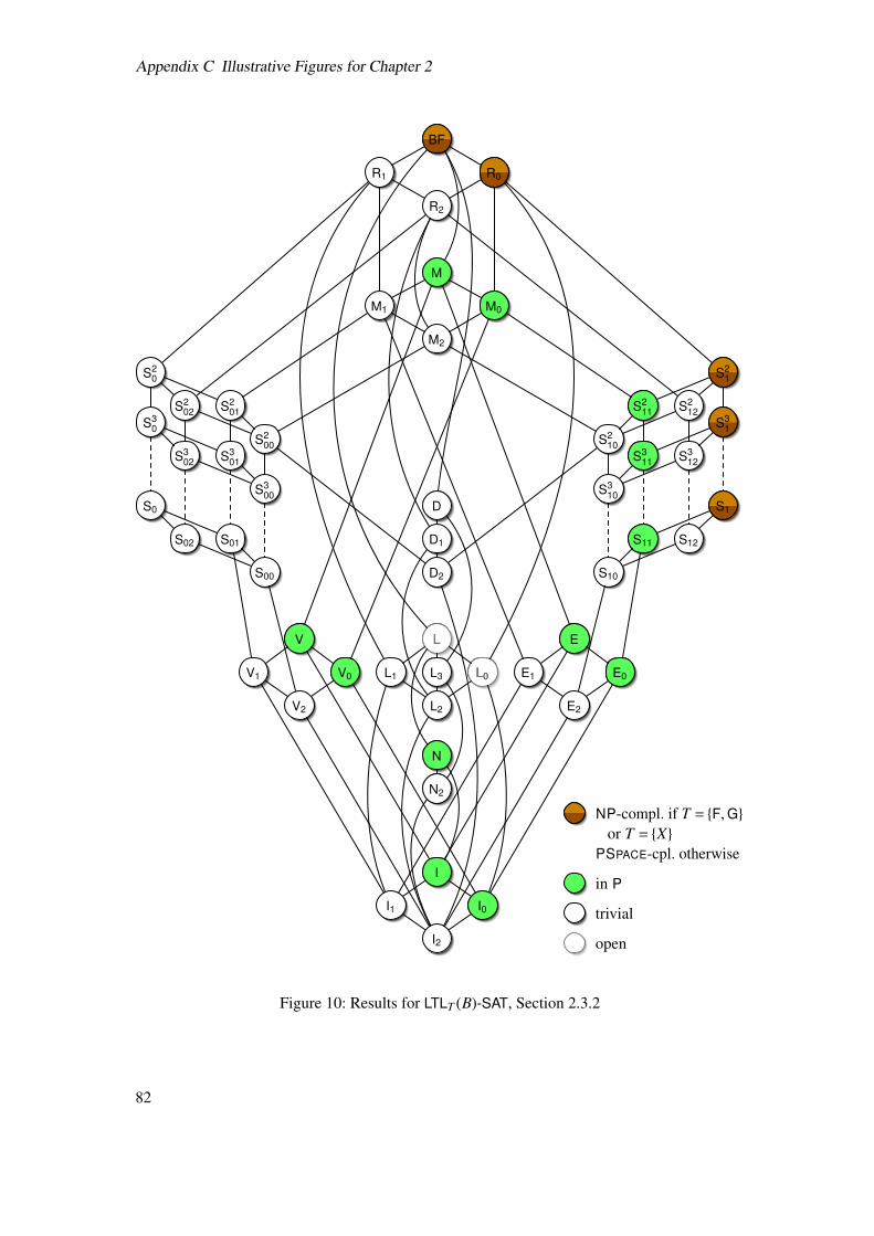
Appendix C Illustrative Figures for Chapter 2
BF
R1 R0
R2
M
M1 M0
M2
S20
S202 S2
01S3
0S2
00S3
02 S301
S300
S0
S02 S01
S00
D
D1
D2
V
V1 V0
V2
L
L1 L3 L0
L2
N
N2
I
I1 I0
I2
S21
S212S2
11S3
1S2
10S3
12S311
S310
S1
S12S11
S10
E
E0E1
E2
L
L0
NP-compl. if T = {F,G}or T = {X}
PSPACE-cpl. otherwise
in P
trivial
open
Figure 10: Results for LTLT (B)-SAT, Section 2.3.2
82
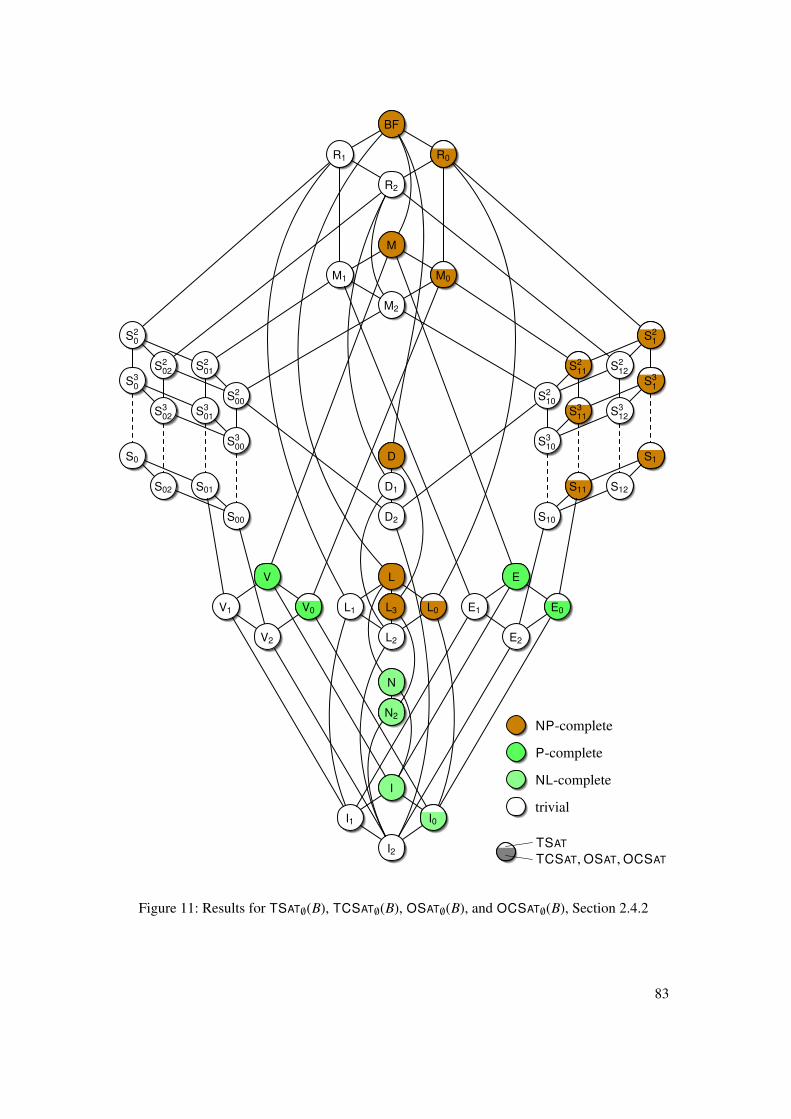
BF
R1 R0
R2
M
M1 M0
M2
S20
S202 S2
01S3
0S2
00S3
02 S301
S300
S0
S02 S01
S00
D
D1
D2
V
V1 V0
V2
L
L1 L3 L0
L2
N
N2
I
I1 I0
I2
S21
S212S2
11S3
1S2
10S3
12S311
S310
S1
S12S11
S10
E
E0E1
E2
NP-complete
P-complete
NL-complete
trivial
TSATTCSAT,OSAT,OCSAT
Figure 11: Results for TSAT;(B), TCSAT;(B), OSAT;(B), and OCSAT;(B), Section 2.4.2
83
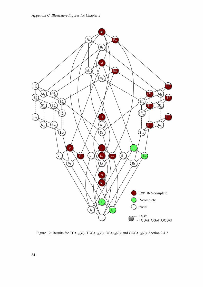
Appendix C Illustrative Figures for Chapter 2
BF
R1 R0
R2
M
M1 M0
M2
S20
S202 S2
01S3
0S2
00S3
02 S301
S300
S0
S02 S01
S00
D
D1
D2
V
V1 V0
V2
L
L1 L3 L0
L2
N
N2
I
I1 I0
I2
S21
S212S2
11S3
1S2
10S3
12S311
S310
S1
S12S11
S10
E
E0E1
E2
N2
N
L0L3
L
D
S11
S211
S311
S1
S21
S31
M0
M
R0
BF
V
V0
EXPTIME-complete
P-complete
trivial
TSATTCSAT,OSAT,OCSAT
Figure 12: Results for TSAT9(B), TCSAT9(B), OSAT9(B), and OCSAT9(B), Section 2.4.2
84
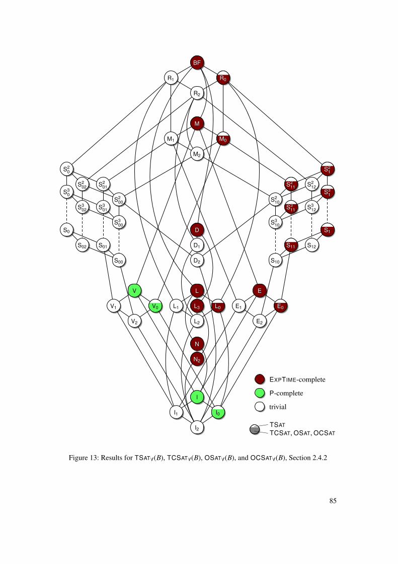
BF
R1 R0
R2
M
M1 M0
M2
S20
S202 S2
01S3
0S2
00S3
02 S301
S300
S0
S02 S01
S00
D
D1
D2
V
V1 V0
V2
L
L1 L3 L0
L2
N
N2
I
I1 I0
I2
S21
S212S2
11S3
1S2
10S3
12S311
S310
S1
S12S11
S10
E
E0E1
E2
N2
N
L0L3
L
D
S11
S211
S311
S1
S21
S31
M0
M
R0
BF
E
E0
EXPTIME-complete
P-complete
trivial
TSATTCSAT,OSAT,OCSAT
Figure 13: Results for TSAT8(B), TCSAT8(B), OSAT8(B), and OCSAT8(B), Section 2.4.2
85
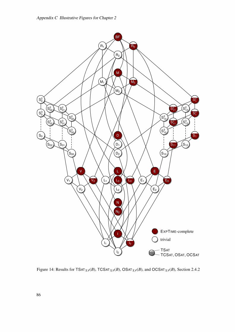
Appendix C Illustrative Figures for Chapter 2
BF
R1 R0
R2
M
M1 M0
M2
S20
S202 S2
01S3
0S2
00S3
02 S301
S300
S0
S02 S01
S00
D
D1
D2
V
V1 V0
V2
L
L1 L3 L0
L2
N
N2
I
I1 I0
I2
S21
S212S2
11S3
1S2
10S3
12S311
S310
S1
S12S11
S10
E
E0E1
E2
N2
N
L0L3
L
D
S11
S211
S311
S1
S21
S31
M0
M
R0
BF
V
V0
E
E0
I
I0
EXPTIME-complete
trivial
TSATTCSAT,OSAT,OCSAT
Figure 14: Results for TSAT9,8(B), TCSAT9,8(B), OSAT9,8(B), and OCSAT9,8(B), Section 2.4.2
86
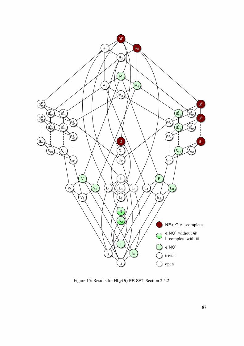
BF
R1 R0
R2
M
M1 M0
M2
S20
S202 S2
01S3
0S2
00S3
02 S301
S300
S0
S02 S01
S00
D
D1
D2
V
V1 V0
V2
L
L1 L3 L0
L2
N
N2
I
I1 I0
I2
S21
S212S2
11S3
1S2
10S3
12S311
S310
S1
S12S11
S10
E
E0E1
E2
D S1
S21
S31
R0
BF
L3 L0
L
NEXPTIME-complete
2 NC1 without @L-complete with @
2 NC1
trivial
open
Figure 15: Results for HLH(B)-ER-SAT, Section 2.5.2
87
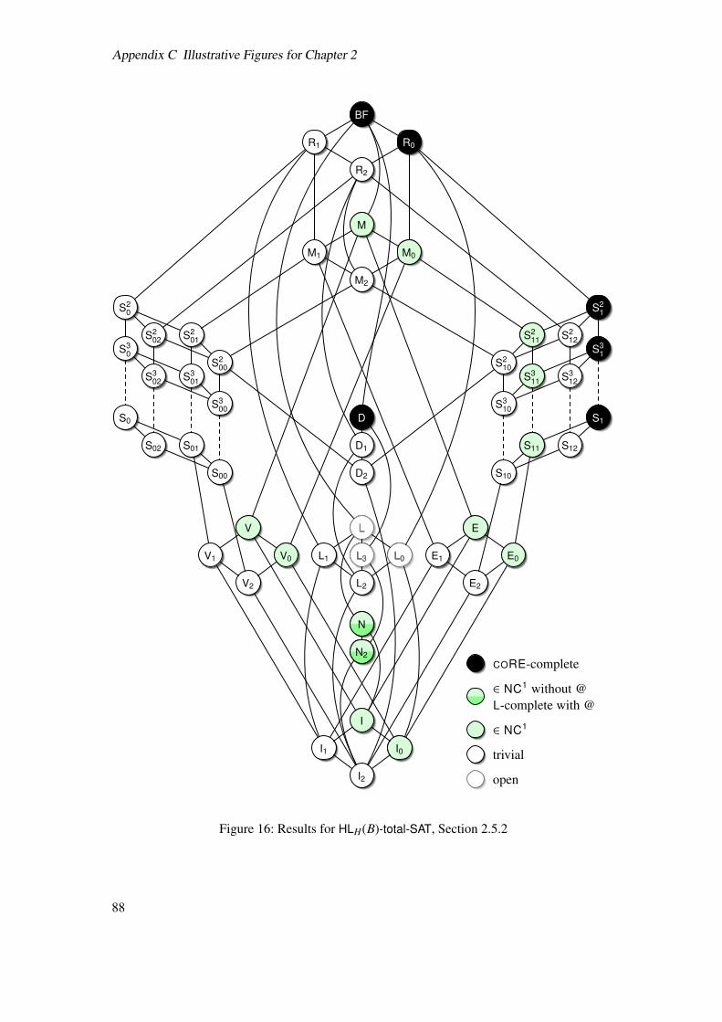
Appendix C Illustrative Figures for Chapter 2
BF
R1 R0
R2
M
M1 M0
M2
S20
S202 S2
01S3
0S2
00S3
02 S301
S300
S0
S02 S01
S00
D
D1
D2
V
V1 V0
V2
L
L1 L3 L0
L2
N
N2
I
I1 I0
I2
S21
S212S2
11S3
1S2
10S3
12S311
S310
S1
S12S11
S10
E
E0E1
E2
D S1
S21
S31
R0
BF
L3 L0
L
CORE-complete
2 NC1 without @L-complete with @
2 NC1
trivial
open
Figure 16: Results for HLH(B)-total-SAT, Section 2.5.2
88
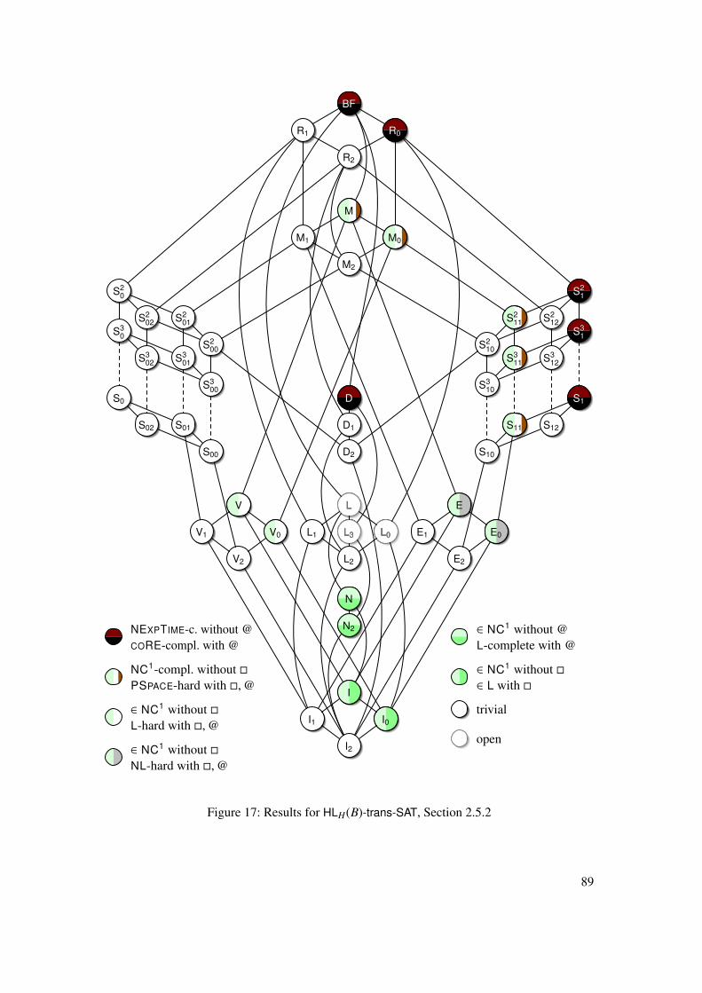
BF
R1 R0
R2
M
M1 M0
M2
S20
S202 S2
01S3
0S2
00S3
02 S301
S300
S0
S02 S01
S00
D
D1
D2
V
V1 V0
V2
L
L1 L3 L0
L2
N
N2
I
I1 I0
I2
S21
S212S2
11S3
1S2
10S3
12S311
S310
S1
S12S11
S10
E
E0E1
E2
D S1
S21
S31
R0
BF
L3 L0
L
NEXPTIME-c. without @CORE-compl. with @
NC1-compl. without ⇤PSPACE-hard with ⇤,@
2 NC1 without ⇤L-hard with ⇤,@
2 NC1 without ⇤NL-hard with ⇤,@
2 NC1 without @L-complete with @
2 NC1 without ⇤2 L with ⇤
trivial
open
Figure 17: Results for HLH(B)-trans-SAT, Section 2.5.2
89

Appendix C Illustrative Figures for Chapter 2
BF
R1 R0
R2
M
M1 M0
M2
S20
S202 S2
01S3
0S2
00S3
02 S301
S300
S0
S02 S01
S00
D
D1
D2
V
V1 V0
V2
L
L1 L3 L0
L2
N
N2
I
I1 I0
I2
S21
S212S2
11S3
1S2
10S3
12S311
S310
S1
S12S11
S10
E
E0E1
E2
D S1
S21
S31
R0
BF
L3 L0
L
CORE-complete
NC1-compl. without ⇤PSPACE-hard with ⇤
2 NC1 without ⇤L-hard with ⇤,@
2 NC1 without ⇤CONP-hard with ⇤
2 NC1 without @L-complete with @
2 NC1 without ⇤2 L with ⇤
trivial
open
Figure 18: Results for HLH(B)-all-SAT, Section 2.5.2
90