Spatial free plastic forming of slender parts-numerical

SPECIAL ISSUE PAPER

Spatial free plastic forming of slender parts—numericalapproaches for strain-hardening material

M Thalmair1 and H Lippmann2*1AGCO GmbH and Company KG, Marktoberdorf, Germany2Lehrstuhl fur Werkstoffkunde und Werkstoffmechanik, Technische Universitat Munchen, Garching, Germany

Abstract: A new metal forming process is described in which a slender part may be brought to aprescribed �nal shape by means of an appropriate, pre-calculated motion of its free ends only.Corresponding calculation schemes are presented for elastic/plastic material with strain hardening,and these are illustrated by practical examples.

Keywords: metal forming, plasticity, bending, torsion, theory, experiment, numerical methods

NOTATION

a length of the rodA point on the central trajectory: left end

(support)b generalized bending (component)B point on the central trajectory: right end

(support)C point on the central trajectory: arbitraryd…Q, z† multiplier function for plastic

deformation in the elastic/plasticconstitutive law

d generalized equivalent straind, d column matrix, component of generalized

strainD point on the central trajectory: rear of the

plastic zonee, e unit vector, componentf …Q†, f …Q† generalized yield criterion, yield potentialF, F column matrix, component of the force on

the cross-sectiong…q† complementary yield potentialK, K compliance matrix, elementm coef�cient of the yield curve functionM, M column matrix, component of the

generalized moment on the cross-section:in particular the bending moment

n coef�cient of the yield curve functionN normal force acting on the cross-section

O origin of coordinates �xed in spaceP point on the central trajectory: front of

the plastic zoneq, q column matrix, component of generalized

strainQ, Q column matrix, component of the

generalized stress on the cross-sectionr ˆ OC, r radius vector, componentR distance from the cone axiss arc lengtht timeT torque on the cross-sectionV transversal force on the cross-sectionW, W column matrix, coordinate of the virtual

angular velocityY generalized yield limit: in particular the

limit torque

a scalara, a inclination angles of the conical spiralg generalized shear (component)D denoting an increment in the subsequent

quantity, for instance DzD

e, e column matrix, coordinate of thegeneralized longitudinal or shear strain: inparticular the tension/compressionnormal to the cross-section

z material longitudinal coordinate of thecentral trajectory

y mathematical torsion of the centraltrajectory

, W column matrix, coordinate of thegeneralized bending and twist: inparticular the torsion

L rate of work per unit initial length

The M S was received on 9 June 2003 and was accepted after revision forpublication on 17 December 2003.* Corresponding author: Lehrstuhl fur W erkstoffkunde und W erkstoff-mechanik, Technische Universitat M unchen, Boltzmannstrasse 15,D-85748 Garching, Germany.

641

C08903 # IMechE 2004 Proc. Instn Mech. Engrs Vol. 218 Part C: J. Mechanical Engineering Science at Technical University of Munich University Library on November 4, 2016pic.sagepub.comDownloaded from

http://pic.sagepub.com/

r apex angle of the conej rotation angle around the inward normal

to the cone

Subscripts

i, j, k referring to material bases �xed to thecross-section, or counting components ofthe generalized stress/strain ˆ 1, 2, 3

j0, k 0, l0 counting components of the generalizedstress/strain ˆ 1, . . . , 6

L referring to the plastic limit statet referring to the tangent of the central

trajectory

k, l referring to the basis �xed in space ˆ x , y, z

Superscripts

A, B, C, D, O, Preferring to the corresponding points

e referring to elastic deformationp referring to plastic deformation0 referring to the initial time or value? referring to the terminal state of the

forming process

* referring to the terminal position of D, forexample, to the rear of a permanentplastically undeformed zone

1 INTRODUCTION

The elementary plane bending process in which a slenderpart is gripped at both its ends by hands or byappropriate tools, the motion of which leads to thegeneration of the �nal shape, has been further developedin several investigations (cf. references {1} and {2})towards a new industrial forming process. The motionsof the clamping tools are calculated in advance using anassociated PC and are then fed into the control of themachine drives. In this way a large number of prescribed�nal shapes could be produced with fairly goodaccuracy, and the reproduction accuracy is even better.The lumped-mass approach presented in reference {3}opens up an alternative way to pre-calculate the motionof the clamping tools in particular under conditions ofdynamics, although it is currently still con�ned to theprimary problem (inverse to the one to be treated below)where the motion of the end cross-sections is prescribedwhile the �nal shape is searched for.

The generalization of the new metal forming processto spatial forming has been theoretically proposed inreference {4} and practically tested in reference {5},although this process is still under investigation. Forinstance, the numerical integration scheme for the basicdifferential equations proposed in reference {4} is based

on an incremental approach unfortunately demanding anumerical time differentiation. This may become asource of numerical error, and so a �nite scheme wasused instead, although still without detailed descriptionin reference {5}. Such a �nite constitutive law may bephysically less correct than the incremental approach.However, besides reduced numerical effort, it also leadsto a reduced numerical �uctuation because there is, incontrast to the incremental procedure, no error accumu-lation at the consecutive time steps. For plane bending,the �nite scheme proved as suf�cient anyway {2}. There-fore, in the present paper the still missing description ofthe �nite integration scheme for spatial forming will bepresented. Moreover, this scheme can also be appliedsuccessively in order to simulate the time steps of anincremental approach. Based on the �nite scheme, thespatial forming process will be illustrated by two exam-ples, i.e. a similarly bent and twisted bar of rectangularcross-section and a conical spiral of circular cross-section.

The integration methods to be developed are non-standard in the following sense. Although the initial shapeand the �nal shape of the rod, i.e. the initial and the �naldistributions of displacement and of rotation of the cross-sections, are prescribed, the corresponding distribution ofthe external load is not of primary interest. On thecontrary, the side condition holds, i.e. that there must notbe any load distributed along the part. Actually, externalloads are allowed at the end supports only. However, forthese supports a complete motion history has to be found,bringing the part into the desired shape without any loadacting at other places. From previous publications{1, 2, 4, 5} it is clear that this motion history has to bebased on a plastic zone moving from one end of the part,to be called A, towards the other end, B, thus leaving theplastically �nished region of the part behind, while theplastically still undeformed region is in front of themoving zone. This zone shrinks to one single cross-sectionrepresenting a plastic hinge if the generalized yield limit,Y , is constant (ideal plasticity).

Subsequently it will be shown how this model can betransformed into an adequate numerical scheme. Unfor-tunately, a precise characterization of the possible shapesthus attainable is not known as yet. However, experienceshows that a large variety of corresponding parts can beproduced, provided the length is limited in order to avoidre-plasti�cation of the already �nished zone. A check ofthis situation has also to be included in the software, whileother forming defects such as buckling of preferably thin-walled rods, or the deformation of the cross-sections ingeneral, will not be discussed in this paper.

2 BASIC EQUATIONS

The slender part under consideration, brie�y referred toas the rod, will be represented by a central trajectory AB

M THALMAIR AND H LIPPMANN642

Proc. Instn Mech. Engrs Vol. 218 Part C: J. Mechanical Engineering Science C08903 # IMechE 2004 at Technical University of Munich University Library on November 4, 2016pic.sagepub.comDownloaded from


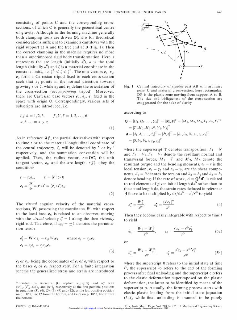
consisting of points C and the corresponding cross-sections, of which C is generally the geometrical centreof gravity. Although in the forming machine generallyboth clamping tools are driven {5}, it is for theoreticalconsiderations suf�cient to examine a cantilever with therigid support at A and the free end at B (Fig. 1). Thenthe correct clamping in the machine requires no morethan a superimposed rigid body transformation. Here, srepresents the arc length (initially s0), a is the totallength (initially a0) and z is a material coordinate in theconstant limits, i.e. zA 4 z 4 zB. The unit vectors e1, e2,e3 form a Cartesian tripod �xed to each cross-sectionsuch that e1 points in the normal direction towardsgrowing s or z, while e2 and e3 de�ne the orientation ofthe cross-section (accompanying tripod). Moreover,there are Cartesian base vectors ex, ey, ez �xed in thespace with origin O. Correspondingly, various sets ofsubscripts are introduced, i.e.

i, j, k ˆ 1, 2, 3, j0, k 0, l0 ˆ 1, 2, . . . , 6

k, l, . . . ˆ x , y, z

…1†

As in reference {4}*, the partial derivatives with respectto time t or to the material longitudinal coordinate ofthe central trajectory, z, will be denoted by ° or by 0

respectively, and the summation convention will beapplied. Then, the radius vector, r ˆ OC, the unittangent vector, et, and the arc length, s…z†, obey theconditions

r ˆ rlel, s0 ˆ jr0j > 0

et ˆ drds

ˆ r0=s0 ˆ …r0k=s0†ek

…2†

The virtual angular velocity of the material cross-sections, W, possessing the coordinates W j with respectto the local base ej, is related to an observer, movingwith the virtual velocity z0 ˆ 1 along the then virtuallyrigid rod. Therefore, if eijk ˆ +1 denotes the permuta-tion tensor

e0j ˆ W6ej ˆ eijk W iek where ej ˆ ejkek

et ˆ ejej ˆ ejejkek

…3†

ej or ejk being the coordinates of et or ej with respect tothe bases ej or ek respectively. For a �nite integrationscheme the generalized stress and strain are introduced

according to

Q ˆ ‰Q1, Q2, . . . , Q6ŠT ˆ ‰M, FŠT ˆ ‰M 1, M 2, M 3, F1, F2, F3ŠTˆ ‰T , M 2, M 3, N , V 2, V 3ŠT

d ˆ ‰d1, d2, . . . , d6ŠT ˆ ‰ , eŠT ˆ ‰W1, W2, W3, e1, e2, e3ŠT

ˆ ‰W, b2, b3, e, g2, g3ŠT

where the superscript T denotes transposition, F1 ˆ Nand F2 ˆ V 2, F3 ˆ V 3 denote the resultant normal andtransversal forces, M 1 ˆ T and M 2, M 3 denote theresultant torque and the bending moments, e1 ˆ e is thelocal tension, e2 ˆ g2 and e3 ˆ g3 are the shear compo-nents, W1 ˆ W denotes the torsion and W2 ˆ b2 and W3 ˆ b3

denote bending. If the rate of work, L ˆ QTd°, is relatedto rod elements of given initial length ds0 rather than tothe actual length ds, the strain rates deduced in reference{4}have to be multiplied by ds=ds0 ˆ s0=s00 to yield

W°k ˆ W °

k

s00 , e°k ˆ …s0ek†°

s0 0 …4†

Then they become easily integrable with respect to time tto yield

Wk ˆ W k ¡ W 0k

s0 0 , ek ˆ s0ek ¡ s0 0e0k

s00 …5a†

or

Wek ˆ W k ¡ W ?

k

s00 , eek ˆ s0ek ¡ s?0e?

k

s0 0 …5b†

where the superscript 0 refers to the initial state at timet0, the superscript ? refers to the end of the formingprocess after �nal unloading and the superscript e refersto the elastic deformation superimposed on the plasticdeformation, the latter to be identi�ed by means of thesuperscript p. Actually, the forming process starts withelastic–plastic loading from the initial state {equation(5a)}, while �nal unloading is assumed to be purely

Fig. 1 Central trajectory of slender part AB with arbitrarypoint C and material cross-section, here rectangular.DP is the plastic zone moving from support A to B.The size and obliqueness of the cross-section areexaggerated for the sake of clarity

* Erratum to reference {4}: replace w0k , v0

k , o0k and w°

k with…w0†k , …v0†k , …o0†k and …w°†k respectively at the �rst possible positionsin equations (3), (4), (5), (7), (9) and (12), at the last possible positionon p. 1855, line 12 from the bottom, and twice on p. 1855, line 7 fromthe bottom.

SPATIAL FREE PLASTIC FORMING OF SLENDER PARTS 643



elastic {equation (5b)}. Equilibrium along the rod isexpressed similarly to the equation two lines after (11) inreference {4} in terms of

M 0k ‡ eijk…W iM j ‡ s0eiFj† ‡ s0 0mk ˆ 0 …6†

F 0k ‡ eijkW iFj ‡ s00pk ˆ 0 …7†

where the force or moment distributions, pk or mk, nowper unit initial length rather than per unit actual length,may generally be disregarded under metal formingconditions. The column matrices of total strain will bedecomposed into an elastic part and a plastic partregarding (1) according to

d ˆ de ‡ dp ˆ ‰dej0 ŠT ‡ ‰dp

j0 ŠT …8†The generalized Hooke’s law will be assumed to hold forthe elastic part

de ˆ KQ, where K ˆ ‰Kj0k 0 Š ˆ ‰Kk 0 Š ˆ KT …9†where K is the usual compliance matrix of the elastic rod.Regarding the plastic part, the generalized equivalentstrain increment, d ¡ d 0 ˆ g…dp†, is introduced, where d 0

is the initial distribution of equivalent strain. Moreover,the �ow potential f ˆ f …Q† and the yield criterion f ˆf …Q† are considered. All of these functions are mathe-matically homogeneous {6}, obeying the relations

f …aQ† ˆ jaj f …Q† > 0, f …aQ† ˆ jaj f …Q† > 0

g…adp† ˆ jaj g…dp† > 0

gqf

qQj0

� ´: f

qg

qqpj0

Á !:1 if Q 6ˆ 0; dp 6ˆ 0, a 6ˆ 0

…10†in which a is a scalar and g is uniquely determined via thelast identity by f, or vice versa, provided the functionsare continuously differentiable with a non-vanishinggradient

qfqQj 0

6ˆ 0,qg

qqpj0

6ˆ 0

everywhere, and if the hypersurfaces in the Q-space or inthe q-space respectively, i.e. f …Q† ˆ constant, f …Q† ˆconstant and g…q† ˆ constant, are strictly convex; the �rstof these is the generalized yield surface. Then thegeneralized yield condition, the generalized �nite �owrule and its inverse may be expressed in terms of

f …Q† ˆ Y …d, z†, dpj0 ˆ …d ¡ d

0† qfqQj 0

Qj0 ˆ f …Q† qg

qdpj0

…11†Y 50 being the generalized yield limit, the temperaturedependence of which is not explicitly considered; Y may,for instance, be chosen as a limit bending or torsion

moment. Here, d 0 represents a possible prestrain so thatd 0 ˆ 0 at a virgin rod. Because of strain hardening, Y isstrictly monotonically growing as a function of d , so thatY may uniquely be inverted in terms of the functiond…Y , z†, from which another function d…Q, z† will beconstructed according to

d…Q, z† ˆ d…Y , z† ¡ d 0 ˆ d… f …Q†, z† ¡ d 050

if Y …d 0, z† 4 f …Q† …plastic state†d…Q, z† ˆ 0

if f …Q† < Y …d0, z† …elastic state†

…12†Then the �nite elastic/plastic constitutive law may bewritten, observing (8), (10) and (12), as

d ˆ KQ ‡ d…Q, z† qf …Q†qQ

…13†

As d has been de�ned observing equations (5) indifferent ways for the loading and the unloading state,the latter is also covered by equation (13). Conversely, ifa plastic state of strain dp 6ˆ 0 is known, the generalizedstress Q follows from equations (10) and (11) accordingto

Ql0 ˆ f …Q†f …Q† f …Q† qg…dp†

qdpl0

ˆ f …qg=qdpk 0 †

f …qg=qdpk 0 †

Y …d , z† qg…dp†qdp

l0

ˆ Y …d , z†f …qg=qdp

k 0 †qg…dp†

qdpl0

…14†

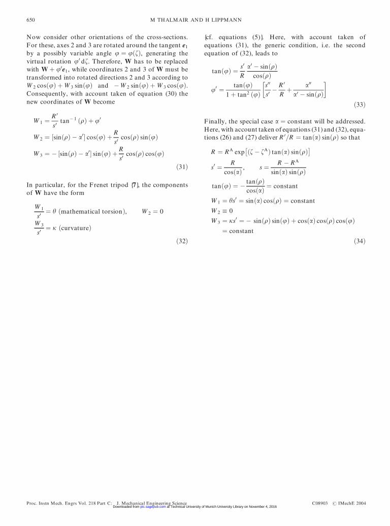
3 INTEGRATION SCHEMES

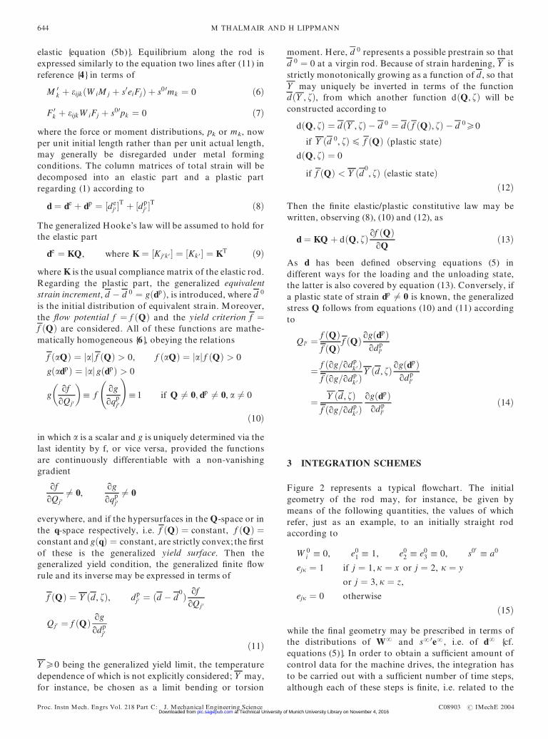
F igure 2 represents a typical �owchart. The initialgeometry of the rod may, for instance, be given bymeans of the following quantities, the values of whichrefer, just as an example, to an initially straight rodaccording to

W 0i : 0, e0

1 : 1, e02 : e0

3 : 0, s00: a0

ejk ˆ 1 if j ˆ 1, k ˆ x or j ˆ 2, k ˆ y

or j ˆ 3, k ˆ z,

ejk ˆ 0 otherwise

…15†

while the �nal geometry may be prescribed in terms ofthe distributions of W? and s?0e?, i.e. of d? {cf.equations (5)}. In order to obtain a suf�cient amount ofcontrol data for the machine drives, the integration hasto be carried out with a suf�cient number of time steps,although each of these steps is �nite, i.e. related to the




initial state or to the terminal state rather than toprevious steps. For this purpose, the meaning of thematerial coordinate zD representing the position of therear point of the plastic zone, D, will be generalized tobecome a dimensionless virtual time for the entireforming process. The integration may be carried outconsecutively with the assumed number of discretevalues of zD . To this end, the forming process will besubdivided into three phases:

1. ¡ 0:2 4 zD < 0, elastic/plastic pre-loading withD : A.

2. 0 4 zD 4 z*, D moving from A to its �nal positionD* at which zD ˆ z* 4 zB.

3. z* < zD 4 z* ‡ 0:2, �nal elastic unloading with,D : D*.

The limit + 0:2 has been chosen as arbitrary.First of all, the limit stress QD ˆ QDA ˆ ‰QDA

i0 ŠT hasto be calculated for the left-hand support A bysubstituting the corresponding prescribed plastic straind?A into equation (14). Then the integration stepsduring phase 1 refer to the generalized stress

QD ˆ …1 ‡ 5zD †QDA at D ˆ A …16a†

and QD acts as the boundary value at D for the stressdistribution to be determined below. As, in equation(16a), the proportional preloading may be replaced withany other preloading procedure, the deformationprocess is not unique during phase 1.

In phase 2 the assumed discrete values of zD refer todifferent positions of D, where

dp ˆ d?…zD † at z ˆ zD if zA < zD 4 z* …16b†

is prescribed while the corresponding stress QD , actingagain as the boundary value, follows from equation (14).

This phase 2, most important for the forming process, isunique.

To each value of zD the corresponding frontal pointP…z ˆ zP† of the plastic zone is determined, duringphases 1 and 2, regarding equation (16b), by checkingthe solution of the differential equations to be for-mulated below with respect to the condition

dp ˆ 0 at z ˆ zP provided zD 4 zP < zB and

d?…zD † 6ˆ 0

P ˆ B, i:e: zP ˆ zB if dp 6ˆ 0 for zD < z 4 zB

P ˆ D, i:e: zP ˆ zD if d?…zD † ˆ 0

…16c†

The loading process is �nished after zD has reached its�nal position, denoted by z*. This coincides in mostcases with zB. However, it may be that the last section ofthe formed rod will remain undeformed. In this event, z*

is the value of z at the rear of that undeformed section,because, for reasons of continuity, d?…z*† ˆ 0 has to beprescribed so that P ˆ D* is found from the thirdequation of (16c). In the subsequent unloading phase 3,assumed to be elastic, the stress QD*, belonging to D*,will be reduced stepwise down to zero according to

QD ˆ f1 ‡ 5…z* ¡ zD †gQD* if D : D* …16d†

As this linear approach is arbitrary, unloading is notunique.

During the loading process in phases 1 and 2, thebasic �rst-order differential equations for the general-ized stress distribution Q consist of the equilibriumconditions (6) and (7) in which W i and s0ei have beenreplaced with dj0 …Q† ˆ dj0 …F, M† via equations (5a) and(13) according to

F 0k ‡ eijk W 0

i ‡ s0 0Wi…F, M†© ªFj ‡ s0 0pk ˆ 0 …17†

Fig. 2 Flow chart of the code for the �nite strain approach without the Bernoulli hypothesis




M 0k ‡ eijk W 0

i ‡ s00Wi…F, M†© ªM j ‡ s00e0

i ‡ s00ei…F, M†© ªFj

¡ ¢‡ s00mk ˆ 0 …18†

where pk and mk may generally be disregarded. At eachtime step these equations have to be integrated(numerically) along the rod under the boundary or endconditions (16a) to (16d), i.e. mutually with thegeometric relations following from (2), (3) and (5)according to

e0jl ˆ eijk W 0

i ‡ s00Wi…F, M†¡ ¢ekl

r0l ˆ ekl s0 0ek …F, M† ‡ s00e0

k

¡ ¢if z5zD

…19†

Here, the initial conditions r ˆ 0 and ej ˆ eA0j at A have

to be observed, eA0j representing the initial values of the

accompanying tripod. The elastic version of the abovedifferential equations, de®ned in equations (12), has tobe applied partly during phase 1, but always in front ofD and during phase 3. In the latter event, i.e. duringelastic unloading, equation (5b) has to be used ratherthan equation (5a) in order to set up (17) to (19), so thatW 0

i and s0 0e0k have to be replaced with W ?

i and s?0e?k

respectively. After each integration step, the staticadmissibility of the found stress solution has to bechecked along the entire rod according to

f …Q† 4 Y …d , z† …20†where d ˆ d

0in front of P.

In any phase or at any time, the above differentialequations deliver directly the position r ˆ rB and thecorresponding orientation of the cross-section ei ˆ eB

ifor the end support B. These are the relevant controlquantities of the system shown in F ig. 1.

Basically, the �nite integration scheme describedbefore may be applied, again incrementally, using thesame equations, but now stepwise in a successivemanner. The initial distributions (15) and d 0 ˆ 0 validfor the virgin rod have to be replaced, for any step, withthe corresponding outcome of the foregoing step.Consequently, the stepwise numerical errors add up.Present practical experience shows that this is worsethan the error due to the physically less correct �niteapproach.

4 BERNOULLI HYPOTHESIS

As a special approach suf�cient for most applications,the Bernoulli hypothesis is often introduced, accordingto which f and f do not depend on F while

Kj 0l0 ˆ 0 if j0, l0 ˆ 4, 5, 6 so that ep : ee : 0

…21†

Under assumption (15), this means that et : e1 ands : s0 : s? so that the cross-sections of the nowinextensible rod are permanently orthogonal to thecentral trajectory. However, then the function g is nolonger uniquely determined by f via equations (10); inparticular, g may also depend in an arbitrary way on ep,or otherwise more or less arbitrary boundary conditionsFD become possible for the normal and the shear forcesacting on the cross-sections. Although these forces areof minor importance for the deformation of slenderrods, they may effect failure of the forming processowing to re-plasti�cation. In the examples below, noshear forces have been assumed at D, while the normalforce was used tentatively to minimize the workgenerated at the supports.

5 EXAMPLES

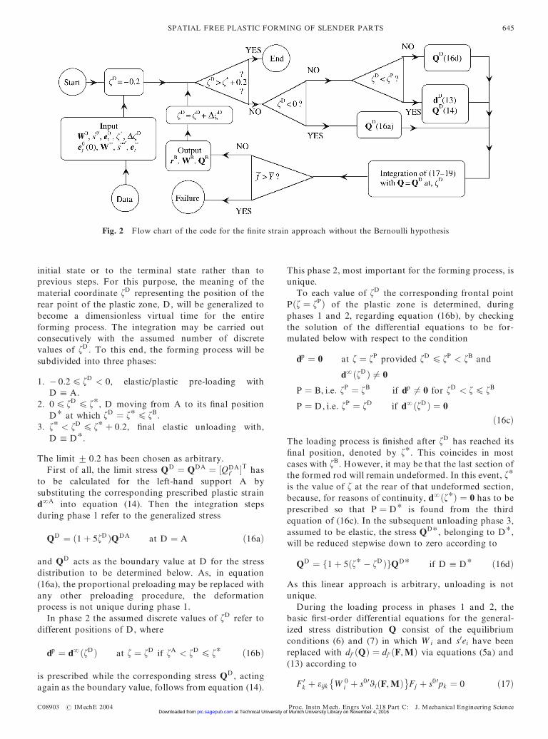
Straight, untwisted rods from aluminium alloy AlMgSi0.5 F22 (German standard designation, length a0 ˆ100 mm) with rectangular cross-sections (3 mm610 mmin directions 2 and 3 respectively) have been formedby combined bending and torsion according to theprescribed, �nal state of deformation given in F ig. 3.The elastic moduli, i.e. E ˆ 65 000 N= mm2 (Young’smodulus) and G ˆ 24 500N= mm2 (shear modulus)as well as the moments of inertia of the cross-sectionsare known, so that the compliance coef�cients, Kj0k 0 ,could be formed regarding equations (21) in the usualmanner. The torsion yield curve, Y ˆ Y …d†, was deter-mined experimentally; it can be approximated by theformula

Y =Y0 ˆ 1 ‡ m exp…nd† …22†

with Y0 ˆ 2:94 N m, m ˆ 1:626 and n ˆ 0:167 mm, while

Fig. 3 Prescribed �nal deformation for a bent and twisted rodwith bendings b2 ˆ b?

2 and b3 ˆ b?3 and torsion

W ˆ W?. Invariant arc length s and total length a




the coef�cients in the following Bernoulli-type approach

f ˆ f ˆ��

Tt

� ´2

‡ M 2

·2

� ´2

‡ M 3

·3

� ´2s

g ˆ��tWp… †2‡ ·2bp

2

¡ ¢2‡ ·3bp3

¡ ¢2q

, t ˆ 1

…23†

havebeen determined from simplebendingor torsion tests,yielding

·2 ˆ M 2L

T Lˆ 0:9, ·3 ˆ M 3L

T Lˆ 3:0 …24†

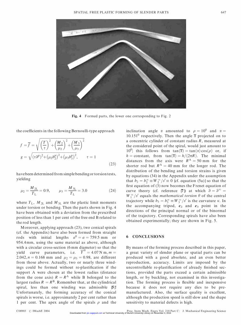
where T L, M 2L and M 3L are the plastic limit momentsunder torsion or bending. Then the parts shown in Fig. 4have been obtained with a deviation from the prescribedposition of less than 1 per cent of the free end B related tothe rod length.

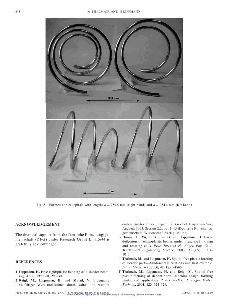
Moreover, applying approach (23), two conical spirals(cf. the Appendix) have also been formed from straightrods with initial lengths a0 ˆ a ˆ 759:5 mm or954.4mm, using the same material as above, althoughwith a circular cross-section (6 mm diameter) so that theyield curve parameters, i.e. Y

0 ˆ 4:07 N m, m ˆ2:042, n ˆ 0:168 mm and ·2 ˆ ·3 ˆ 0:98, are differentfrom those above. Actually, two or nearly three wind-ings could be formed without re-plasti�cation if thesupport A were chosen at the lowest radius (distancefrom the cone axis) R ˆ RA while B belonged to thelargest radius R ˆ R B. Remember that, at the cylindricalspiral, less than one winding was admissible {5}!Unfortunately, the forming accuracy of the conicalspirals is worse, i.e. approximately 2 per cent rather than1 per cent. The apex angle of the spirals r and the

inclination angle a amounted to r ˆ 100 and a ˆ10:1510 respectively. Then the angle a projected on toa concentric cylinder of constant radius R , measured atthe considered point of the spiral, would just amount to100; this follows from tan…a† ˆ tan…a† cos…r† or, ifh ˆ constant, from tan…a† ˆ h=…2pR†. The minimaldistances from the axis were R A ˆ 50 mm for theshorter rod but R A ˆ 40 mm for the longer rod. Thedistribution of the bending and torsion strains is givenby equations (34) in the Appendix under the assumptionthat b2 ˆ b?

2 :W ?2 =s0: 0 {cf. equation (5a)}so that the

�rst equation of (3) now becomes the F renet equation ofcurve theory (cf. reference {7}) at which W ˆ W? ˆW ?

1 =s0 equals the mathematical torsion y of the centraltrajectory while b3 ˆ b?

3 :W ?3 =s0 is the curvature k. In

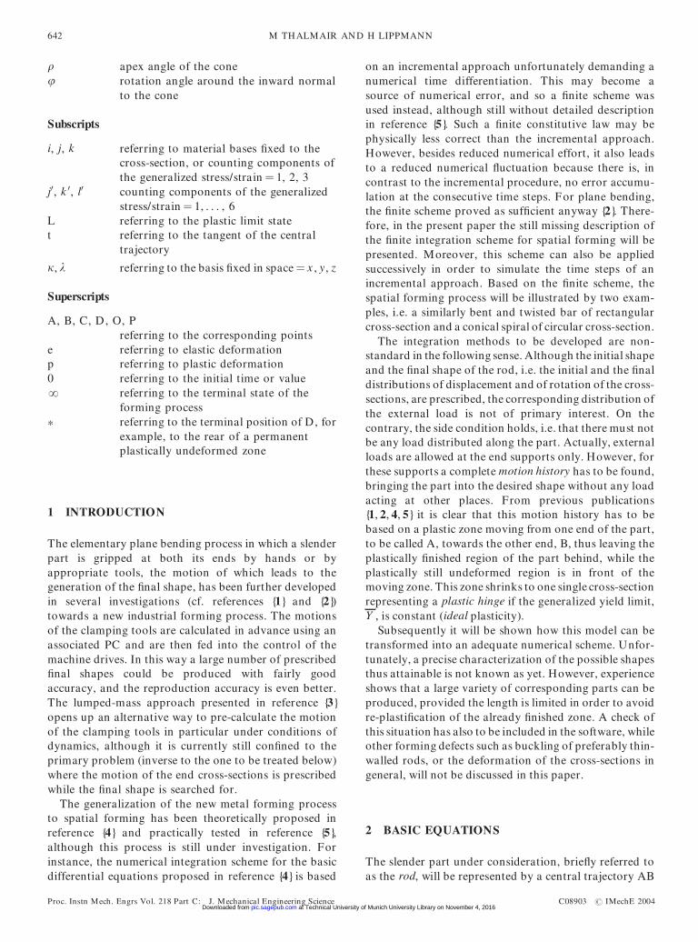
the accompanying tripod, e2 and e3 point in thedirections of the principal normal or of the binormalof the trajectory. Corresponding spirals have also beenobtained experimentally; they are shown in Fig. 5.

6 CONCLUSIONS

By means of the forming process described in this paper,a great variety of slender plane or spatial parts can beproduced with a good absolute, and an even betterreproduction, accuracy. Limits are imposed by theuncontrollable re-plasti�cation of already �nished sec-tions, provided the parts exceed a certain admissiblelength, or by buckling, not examined in this investiga-tion. The forming process is �exible and inexpensivebecause it does not require any dies to be pre-manufactured. Also, the surface quality is excellent,although the production speed is still slow and the shapesensitivity to material defects is high.

Fig. 4 Formed parts, the lower one corresponding to F ig. 2




ACKNOWLEDGEMENT

The �nancial support from the Deutsche Forschungsge-meinschaft (DFG) under Research Grant Li 115/44 isgratefully acknowledged.

REFERENCES

1 Lippmann, H. Free rigid/plastic bending of a slender beam.Ing. Arch., 1990, 60, 293–302.

2 Reigl, M., Lippmann, H. and Mannl, V. Erzeugungvielfaltiger Werkstuckformen durch kaltes und warmes

endgesteuertes freies Biegen. In Flex ibel Umformtechnik,Aachen, 1995, Section 2.2, pp. 1–15 (Deutsche Forschungs-gemeinschaft, Wissenschaftsverlag, Mainz).

3 Huang, X., Yu, T. X., Lu, G. and Lippmann, H. Largede�ection of elastoplastic beams under prescribed movingand rotating ends. Proc. Instn M ech. Engrs, Part C: J.M echanical Engineering Science, 2003, 217(C9), 1001–1013.

4 Thalmair, M. and Lippmann, H. Spatial free plastic formingof slender parts—fundamental relations and �rst example.Int. J. M ech. Sci., 2000, 42, 1851–1865.

5 Thalmair, M., Lippmann, H. and Reigl, M. Spatial freeplastic forming of slender parts—machine design, forminglimits, and application. Trans. ASM E, J. Engng M ater.Technol., 2001, 123, 524–529.

Fig. 5 Formed conical spirals with lengths a ˆ 759:5 mm (right hand) and a ˆ 954:4 mm (left hand)




6 Hill, R. Constitutive dual potentials in classical plasticity.J. M ech. Phys. Solids, 1987, 35, 23–33.

7 Blaschke, W. Introduction to Differential Geometry (inGerman), 1950 (Springer-Verlag, Berlin, Germany).

APPENDIX

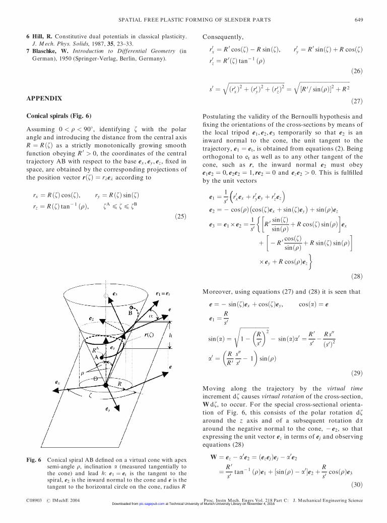
Conical spirals (Fig. 6)

Assuming 0 < r < 90¯, identifying z with the polarangle and introducing the distance from the central axisR ˆ R …z† as a strictly monotonically growing smoothfunction obeying R 0 > 0, the coordinates of the centraltrajectory AB with respect to the base ex , ey , ez , �xed inspace, are obtained by the corresponding projections ofthe position vector r…z† ˆ rlel according to

rx ˆ R …z† cos…z†, ry ˆ R …z† sin…z†rz ˆ R…z† tan¡ 1 …r†, zA 4 z 4 zB

…25†

Consequently,

r0x ˆ R 0 cos…z† ¡ R sin…z†, r0

y ˆ R 0 sin…z† ‡ R cos…z†r0z ˆ R 0…z† tan¡ 1 …r†

…26†

s0 ˆ��…r0

x †2 ‡ …r0y†2 ‡ …r0

z†2q

ˆ��‰R 0= sin…r†Š2 ‡ R 2

q…27†

Postulating the validity of the Bernoulli hypothesis and�xing the orientations of the cross-sections by means ofthe local tripod e1, e2, e3 temporarily so that e2 is aninward normal to the cone, the unit tangent to thetrajectory, e1 ˆ et , is obtained from equations (2). Beingorthogonal to et as well as to any other tangent of thecone, such as r, the inward normal e2 must obeye1e2 ˆ 0, e2e2 ˆ 1, re2 ˆ 0 and eze2 > 0. This is ful�lledby the unit vectors

e1 ˆ 1s0 r0

x ex ‡ r0yey ‡ r0

zez

²e2 ˆ ¡ cos…r† cos…z†ex ‡ sin…z†ey

¡ ¢ ‡ sin…r†ez

e3 ˆ e16e2 ˆ 1s0 R 0 sin…z†

sin…r† ‡ R cos…z† sin…r†µ ¶

ex

�

‡µ

¡ R 0 cos…z†sin…r† ‡ R sin…z† sin…r†

¶

6ey ‡ R cos…r†ez

¼…28†

Moreover, using equations (27) and (28) it is seen that

e ˆ ¡ sin…z†ex ‡ cos…z†ey , cos…a† ˆ e

e1 ˆ Rs0

sin…a† ˆ��1 ¡ R

s0

� ´2s

¡ sin…a†a0 ˆ R 0

s0 ¡ Rs00

…s0†2

a0 ˆ RR 0

s00

s0 ¡ 1

� ´sin…r†

…29†

Moving along the trajectory by the virtual timeincrement dz causes virtual rotation of the cross-section,W dz, to occur. For the special cross-sectional orienta-tion of F ig. 6, this consists of the polar rotation dzaround the z axis and of a subsequent rotation daaround the negative normal to the cone, ¡ e2, so thatexpressing the unit vector ez in terms of ej and observingequations (28)

W ˆ ez ¡ a0e2 ˆ …ezej†ej ¡ a0e2

ˆ R 0

s0 tan¡ 1 …r†e1 ‡ sin…r† ¡ a0‰ Še2 ‡ Rs0 cos…r†e3

…30†

Fig. 6 Conical spiral AB de�ned on a virtual cone with apexsemi-angle r, inclination a (measured tangentially tothe cone) and lead h: e1 ˆ et is the tangent to thespiral, e2 is the inward normal to the cone and e is thetangent to the horizontal circle on the cone, radius R




Now consider other orientations of the cross-sections.For these, axes 2 and 3 are rotated around the tangent e1

by a possibly variable angle j ˆ j…z†, generating thevirtual rotation j0 dz. Therefore, W has to be replacedwith W ‡ j0e1, while coordinates 2 and 3 of W must betransformed into rotated directions 2 and 3 according toW 2 cos…j† ‡ W 3 sin…j† and ¡ W 2 sin…j† ‡ W 3 cos…j†.Consequently, with account taken of equation (30) thenew coordinates of W become

W 1 ˆ R 0

s0 tan¡ 1 …r† ‡ j0

W 2 ˆ sin…r† ¡ a0‰ Š cos…j† ‡ Rs0 cos…r† sin…j†

W 3 ˆ ¡ sin…r† ¡ a0‰ Š sin…j† ‡ Rs0 cos…r† cos…j†

…31†

In particular, for the F renet tripod {7}, the componentsof W have the form

W 1

s0 ˆ y …mathematical torsion†, W 2 ˆ 0

W 3

s0 ˆ k …curvature†…32†

{cf. equations (5)}. Here, with account taken ofequations (31), the generic condition, i.e. the secondequation of (32), leads to

tan…j† ˆ s0

Ra0 ¡ sin…r†

cos…r†j0 ˆ tan…j†

1 ‡ tan2 …j†s00

s0 ¡ R 0

R‡ a00

a0 ¡ sin…r†µ ¶

…33†

F inally, the special case a ˆ constant will be addressed.Here, with account taken of equations (31) and (32), equa-tions (26) and (27) deliver R 0=R ˆ tan…a† sin…r† so that

R ˆ RA exp …z ¡ zA† tan…a† sin…r†£ ¤s0 ˆ R

cos…a† , s ˆ R ¡ RA

sin…a† sin…r†tan…j† ˆ ¡ tan…r†

cos…a† ˆ constant

W 1 ˆ ys0 ˆ sin…a† cos…r† ˆ constant

W 2 : 0

W 3 ˆ ks0 ˆ ¡ sin…r† sin…j† ‡ cos…a† cos…r† cos…j†ˆ constant

…34†




Documents

Spatial free plastic forming of slender parts-numerical