Embed Size (px)
Citation preview
Slender Ca II H fibrils observed bySUNRISE/SuFI
Dissertationzur Erlangung des mathematisch-naturwissenschaftlichen Doktorgrades
“Doctor rerum naturalium”
der Georg-August-Universität Göttingen
im Promotionsprogramm PROPHYS
der Georg-August University School of Science (GAUSS)
vorgelegt von
Ricardo Jorge Maranhas Gafeiraaus Melo, Portugal
Göttingen, 2017
Betreuungsausschuss
Prof. Dr. Sami K. SolankiMax-Planck-Institut für Sonnensystemforschung, Göttingen, Germany
Prof. Dr. Laurent GizonInstitut für Astrophysik, Georg-August-Universität Göttingen, Germany
Dr. Andreas LaggMax-Planck-Institut für Sonnensystemforschung, Göttingen, Germany
Mitglieder der Prüfungskommision
Referent: Prof. Dr. Sami K. SolankiMax-Planck-Institut für Sonnensystemforschung, Göttingen, Germany
Korreferent: Prof. Dr. Laurent GizonInstitut für Astrophysik, Georg-August-Universität Göttingen, Germany
Weitere Mitglieder der Prüfungskommission:
Prof. Dr. Hardi PeterMax-Planck-Institut für Sonnensystemforschung, Göttingen, Germany
Prof. Dr. Jean NiemeyerInstitut für Astrophysik, Georg-August-Universität Göttingen, Germany
Prof. Dr. Wolfram KollatschnyInstitut für Astrophysik, Georg-August-Universität Göttingen, Germany
Prof. Dr. Ariane FreyInstitut für Astrophysik, Georg-August-Universität Göttingen, Germany
Tag der mündlichen Prüfung: 31. Januar 2018
Contents
Summary 5
Zusammenfassung 7
1 Introduction 91.1 Connection between the photosphere and
chromosphere . . . . . . . . . . . . . . . . . . . . . . . . . . . . . . . . 111.2 Chromospheric jets and fibril like structures . . . . . . . . . . . . . . . . 15
1.2.1 General properties of small scale chromospheric jet and fibril-likestructures . . . . . . . . . . . . . . . . . . . . . . . . . . . . . . 16
1.2.2 MHD waves . . . . . . . . . . . . . . . . . . . . . . . . . . . . 211.3 The SUNRISE Observatory . . . . . . . . . . . . . . . . . . . . . . . . . 24
1.3.1 SUNRISE Filter Imager (SUFI) . . . . . . . . . . . . . . . . . . . 271.3.2 Data reduction . . . . . . . . . . . . . . . . . . . . . . . . . . . 28
2 Paper I- Morphological properties of Ca II H slender fibrils 312.1 Abstract . . . . . . . . . . . . . . . . . . . . . . . . . . . . . . . . . . . 312.2 Introduction . . . . . . . . . . . . . . . . . . . . . . . . . . . . . . . . . 312.3 Data . . . . . . . . . . . . . . . . . . . . . . . . . . . . . . . . . . . . . 322.4 Fibril detection and tracking . . . . . . . . . . . . . . . . . . . . . . . . 322.5 Fibril morphology . . . . . . . . . . . . . . . . . . . . . . . . . . . . . . 35
2.5.1 Lifetime . . . . . . . . . . . . . . . . . . . . . . . . . . . . . . . 352.5.2 Width . . . . . . . . . . . . . . . . . . . . . . . . . . . . . . . . 392.5.3 Length . . . . . . . . . . . . . . . . . . . . . . . . . . . . . . . 402.5.4 Curvature . . . . . . . . . . . . . . . . . . . . . . . . . . . . . . 422.5.5 Brightness variation . . . . . . . . . . . . . . . . . . . . . . . . 42
2.6 Discussion and conclusions . . . . . . . . . . . . . . . . . . . . . . . . . 47
3 Paper II- Oscillations on width and intensity of slender Ca II H fibrils 513.1 Abstract . . . . . . . . . . . . . . . . . . . . . . . . . . . . . . . . . . . 513.2 Introduction . . . . . . . . . . . . . . . . . . . . . . . . . . . . . . . . . 513.3 Observations . . . . . . . . . . . . . . . . . . . . . . . . . . . . . . . . 523.4 Analysis and results . . . . . . . . . . . . . . . . . . . . . . . . . . . . . 54
3.4.1 Wavelet analysis . . . . . . . . . . . . . . . . . . . . . . . . . . 553.4.2 Statistics . . . . . . . . . . . . . . . . . . . . . . . . . . . . . . 58
3.5 Discussion and conclusions . . . . . . . . . . . . . . . . . . . . . . . . . 60
3
Contents
4 Conclusion and Outlook 63
Bibliography 67
A Transverse Oscillations in Slender Ca II H Fibrils Observed with SUNRISE/SUFI 81A.1 Introduction . . . . . . . . . . . . . . . . . . . . . . . . . . . . . . . . . 81A.2 Observations . . . . . . . . . . . . . . . . . . . . . . . . . . . . . . . . 83A.3 Analysis and Results . . . . . . . . . . . . . . . . . . . . . . . . . . . . 84
A.3.1 Image Restoration and Fibril Identification . . . . . . . . . . . . 85A.3.2 Transverse Oscillations . . . . . . . . . . . . . . . . . . . . . . . 87A.3.3 Wave Analysis . . . . . . . . . . . . . . . . . . . . . . . . . . . 89A.3.4 Statistics . . . . . . . . . . . . . . . . . . . . . . . . . . . . . . 93A.3.5 Energy Budget . . . . . . . . . . . . . . . . . . . . . . . . . . . 96
A.4 Discussion and Conclusions . . . . . . . . . . . . . . . . . . . . . . . . 97
Publications 103
Acknowledgements 105
Curriculum vitae 107
4
Summary
This thesis is devoted to analyzing the morphological and oscillatory properties of slenderCa II H fibrils (SCFs) in the lower solar chromosphere. The aim of this study is to deepenour understanding of the physical nature of these structures and their relevance for theenergetics in the solar chromosphere and the layers above.
For this purpose, we use seeing-free high spatial and temporal resolution data in theline core of the Ca II H line, which is formed in the chromosphere. A time series ofnarrow-band images in this line of almost 1 hour was obtained during the second scienceflight of the the SUNRISE observatory by the SUNRISE Filter Imager (SUFI).
In the first part of the thesis we identify and track 598 elongated bright structures(fibrils), observed in the Ca II H intensity images, in order to estimate their morphologicalproperties. We obtain an average width of around 180 km, a length between 500 and4000 km, an average lifetime of ≈400 s, an average curvature of 0.002 arcsec−1, and amaximum lifetime of ≈2000 s. We identify two different types of brightness evolution inthe SCFs. In one type the intensity increases starting from the center and moving to theedges, and in the other type the increase in intensity first becomes visible near one or bothof the ends and expands from there toward the center of the fibril. The results from thesestudies allow us to compare some of the properties of the SCFs with other chromosphericstructures such as spicules of type I and II, or Ca II K fibrils.
The second part of this work is dedicated to the study of the oscillatory behavior ofSCFs using a wavelet analysis. One analysis focuses on the oscillations in width and in-tensity. These parameters are measured at several positions along the fibrils and their peri-ods and phase speeds are analyzed. The width and intensity oscillations show overlappingdistributions with median values for their periods of 32±17 s and 36±25 s, respectively.For the phase speeds of these perturbations we obtain values of 11+49
−11 km s−1 for widthand 15+34
−15 km s−1 for the intensity. By computing the cross-power spectrum between thetwo oscillations we observe that in most of the cases they show either an anti-phase orin-phase behavior, with the anti-phase case being much more frequent. This indicates thatboth oscillations are probably caused by the same wave mode. By comparing the oscil-latory behavior and the local sound and Alfvén speeds, we conclude that the most likelywave mode to explain all measurements is the fast sausage mode. A few cases are alsocompatible with slow sausage mode waves.
Transverse motions of the SCFs were also studied. We obtained median amplitudesand periods on the order of 2.4±0.8 km s−1 and 83±29 s, respectively. We find thatthe transverse waves usually propagate along the SCFs with a median phase speed of9±14 km s−1. In some cases waves propagating in both directions, and also standingwaves are observed. This oscillatory behavior can be then described by the so-called kink
5

Summary
waves that, for the computed wave parameters, can carry an energy flux of ≈15 kW m−2,which is sufficiently high to heat the chromosphere.
6
Zusammenfassung
Diese Arbeit widmet sich der Analyse der morphologischen Eigenschaften und der Oszil-lationen sogenannter slender Ca II H fibrils (SCFs) in den niedrigen Schichten der Chro-mosphäre der Sonne. Das Ziel dieser Studie ist es, das Verständnis über die physikalischeNatur dieser Strukturen zu vertiefen und deren Bedeutung für die Energetik der Chromo-sphäre und den darüberliegenden Schichten zu ergründen.
Zu diesem Zweck verwenden wir Daten aufgenommen im Kern der Ca II H Linie, diein der unteren Chromosphäre gebildet wird. Diese Daten sind frei von atmosphärischenStörungen und zeichnen sich durch höchste räumliche und zeitliche Auflösung aus. Einefast einstündige Zeitserie schmalbandiger Aufnahmen in dieser Linie konnte während deszweiten Fluges des SUNRISE Observatoriums mit dem SUNRISE Filter Imager (SUFI)gewonnen werden.
Im ersten Teil dieser Arbeit werden 598 langgezogene, helle Strukturen (Fibrilen) inden Ca II H Intensitätsbildern identifiziert und zeitlich verfolgt, um deren morphologis-chen Eigenschaften zu bestimmen. Dabei erhalten wir eine für die Breite dieser Struk-turen einen Mittelwert von 180 km, eine durchschnittliche Lebensdauer von ≈400 s, einedurchschnittliche Krümmung von 0.002 arcsec−1, und eine maximale Lebensdauer von≈2000 s. Zwei unterschiedliche Arten von Helligkeitsvariationen in diesen SCFs wurdengefunden. In einem Fall steigt die Intensität in den Fibrilen zuerst in deren Zentrum undbreitet sich dann entlang des Fibrils aus, im anderen Fall beginnt die Helligkeitssteigerungin einem oder beiden Fußpunkten und wandert dann zum Zentrum des Fibrils. Die Re-sultate dieser Studie erlauben eine Gegenüberstellung der Eigenschaften von SCFs mitanderen chromosphärischen Strukturen, zum Beispiel Spikulen vom Typ I oder II, oderauch den Ca II K Fibrilen.
Der zweite Teil der Arbeit widmet sich der Studie der Oszillationen der SCFs mit-tels einer Wavelet-Analyse. Die erste Analyse konzentriert sich dabei auf die Oszillationder Helligkeit und der Breite der SCFs. An mehreren Positionen entlang der Fibrilen wer-den diese Oszillationen bestimmt und daraus ihre Perioden und Phasengeschwindigkeitenabgeleitet. Die Oszillationen in beiden Parametern zeigen überlappende Perioden von32± 17 s für die Helligkeitsvariation und 36± 25 s für die Variation der Breite. DiePhasengeschwindigkeit dieser Wellen konnte auf 11+49
−11 km s−1 für die Breite und auf15+34−15 km s−1 für die Helligkeit bestimmt werden. Durch die Berechnung des sogenannten
cross-power Spektrums zwischen den beiden Oszillationen konnten wir beobachten, dasssie in den meisten Fällen in Phase oder in Gegenphase ablaufen, wobei die gegenphasigeOszillation bei weitem überwiegt. Dies deutet darauf hin, dass beide Oszillationen vomselben Wellentyp verursacht werden. Durch den Vergleich mit der lokalen Schall- undAlféngeschwindigkeit konnten wir schlussfolgern, dass es sich bei den beobachteten Os-
7
Summary
zillationen um sogenannte fast-sausage-mode Wellen handelt. Enige Fälle sind auch kom-patibel mit dem slow-sausage-mode Typ.
Es wurden auch die transversalen Bewegungen der SCFs untersucht. Dabei erhal-ten wir mittlere Amplituden im Bereich von 2.4±0.8 km s−1 und Perioden von 83±29 s.Wir konnten die mittlere Phasengeschwindigkeit dieser transversalen Bewegung entlangder SCFs auf 9±14 km s−1 bestimmen. In einigen Fällen pflanzen sich die Wellen inbeide Richtungen fort, aber auch stehende Wellen konnten beobachtet werden. Diese Os-zillationen können als sogenannte kink-Wellen bezeichnet werden. Mit den berechnetenParametern der Oszillation können diese Wellen einen Energiefluss von ≈15 kW m−2
beinhalten , eine Energiemenge, die für die Heizung der Chromosphäre ausreichend ist .
8
1 Introduction
Since the invention of the telescope in the 17th century the solar atmosphere has beensubject of observational, theoretical and computational studies that allowed for great ad-vances in understanding of the solar features, and their relation with the solar magneticfield.
Together with the increase of knowledge about the Sun, the techniques and the tech-nologies available to the scientists evolved in time. This led to the discovery of the strat-ification of the solar atmosphere in the end of the 19th century by using, for example,spectroscopic techniques.
Based on physical properties (temperature, density, spectral emission, ...) the solar at-mosphere can be divided in four layers: the photosphere, chromosphere, transition regionand the most external layer, the corona (Figure 1.1).
In Figure 1.2 we can see the different physical properties of these layers, the plasmadensity, temperature, and the electron density as a function of height. Note that this isa vastly simplified representation of the true solar atmosphere and that the values givenbelow are also horizontally averaged (e.g., temperature and density in the corona canvary by over an order of magnitude). The plasma density is characterized by a relativelysteady decrease from the photosphere to the top of the chromosphere (from around 10−4
down to 10−9 kg m−3), and then a drastic decrease in the transition region to values of10−11 kg m−3, and an average value of 10−12 kg m−3 throughout most of the corona. Atthe same time, the temperature decreases from values near 6 000 K at the visible pho-
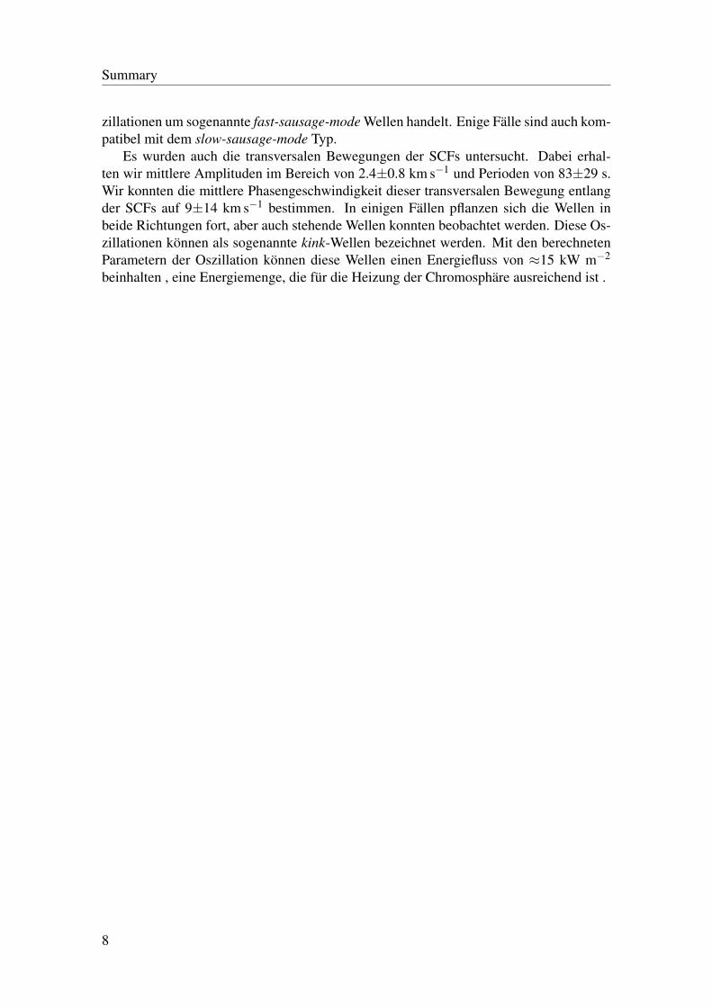
Figure 1.1: Solar atmospheric structure. The different layers are characterized by theircharacteristic temperatures. Image: ESA
9
1 Introduction
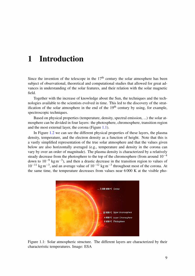
Figure 1.2: Average temperature and density profiles in the solar atmosphere (Courtesyof Eugene Avrett, Smithsonian Astrophysical Observatory).
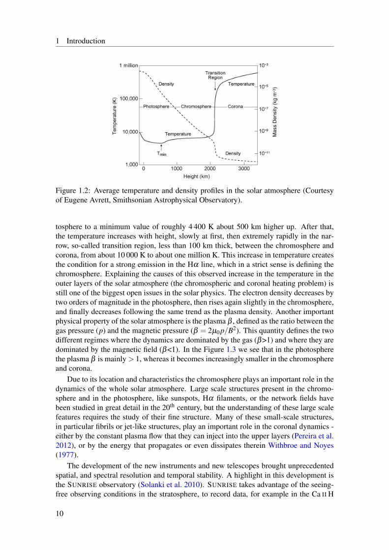
tosphere to a minimum value of roughly 4 400 K about 500 km higher up. After that,the temperature increases with height, slowly at first, then extremely rapidly in the nar-row, so-called transition region, less than 100 km thick, between the chromosphere andcorona, from about 10 000 K to about one million K. This increase in temperature createsthe condition for a strong emission in the Hα line, which in a strict sense is defining thechromosphere. Explaining the causes of this observed increase in the temperature in theouter layers of the solar atmosphere (the chromospheric and coronal heating problem) isstill one of the biggest open issues in the solar physics. The electron density decreases bytwo orders of magnitude in the photosphere, then rises again slightly in the chromosphere,and finally decreases following the same trend as the plasma density. Another importantphysical property of the solar atmosphere is the plasma β , defined as the ratio between thegas pressure (p) and the magnetic pressure (β = 2µ0 p/B2). This quantity defines the twodifferent regimes where the dynamics are dominated by the gas (β>1) and where they aredominated by the magnetic field (β<1). In the Figure 1.3 we see that in the photospherethe plasma β is mainly > 1, whereas it becomes increasingly smaller in the chromosphereand corona.
Due to its location and characteristics the chromosphere plays an important role in thedynamics of the whole solar atmosphere. Large scale structures present in the chromo-sphere and in the photosphere, like sunspots, Hα filaments, or the network fields havebeen studied in great detail in the 20th century, but the understanding of these large scalefeatures requires the study of their fine structure. Many of these small-scale structures,in particular fibrils or jet-like structures, play an important role in the coronal dynamics -either by the constant plasma flow that they can inject into the upper layers (Pereira et al.2012), or by the energy that propagates or even dissipates therein Withbroe and Noyes(1977).
The development of the new instruments and new telescopes brought unprecedentedspatial, and spectral resolution and temporal stability. A highlight in this development isthe SUNRISE observatory (Solanki et al. 2010). SUNRISE takes advantage of the seeing-free observing conditions in the stratosphere, to record data, for example in the Ca II H
10
1.1 Connection between the photosphere andchromosphere
Figure 1.3: Plasmaβ as function of height for magnetic field from 150 to 2500 G repre-sented by the grey area. Taken from Gary (2001).
line, with highest spatial and spectral resolution for a long period of time for the first time.Within the framework of this thesis, we focus on the analysis of bright elongated
structures in the chromosphere that are observed in the data set recorded during the secondscientific flight of the SUNRISE observatory. I present their morphological properties andoscillatory behaviour. The outcome of this work will help to improve the understanding ofthe physical processes in the lower chromosphere and consequently the coupling betweenthe photosphere to the atmospheric layers above.
1.1 Connection between the photosphere andchromosphere
The small-scale chromospheric fibrils are the main topic of this thesis. In this chapter weconcentrate on the layer, where these structures are rooted, the solar photosphere, and itsinfluence on the chromospheric layers.
The photosphere is the lowest part of the solar atmosphere and many of the mostprominent solar features are present there. For example, sunspots, pores or plage regions,that are characterized by the interaction between the photospheric plasma and the mag-netic field (Hale 1908) have been observed for centuries. The magnetic field that drivesthese structures is controlled by the solar dynamo (Brandenburg and Subramanian 2004;Charbonneau 2010). A review summarizing the variety of magnetic features in the solarphotosphere is given by Solanki et al. (2006).
Observing the Sun in white light outside active regions shows that the surface is domi-nated by a granular pattern of bright cells and dark lanes, created by the convective motionof the plasma (see left panel in Figure 1.4). The typical lifetime of these granular cellsis around 10 minutes and their sizes are around 1 Mm (Hirzberger 2003). The cells arecharacterised by central upflows with velocities in the range of 1 km s−1. This rising hotplasma cools down at the surface and flows back in narrow intergranular lanes markingthe boundaries of the granular cells with typical velocities of 2 km s−1.
11
1 Introduction
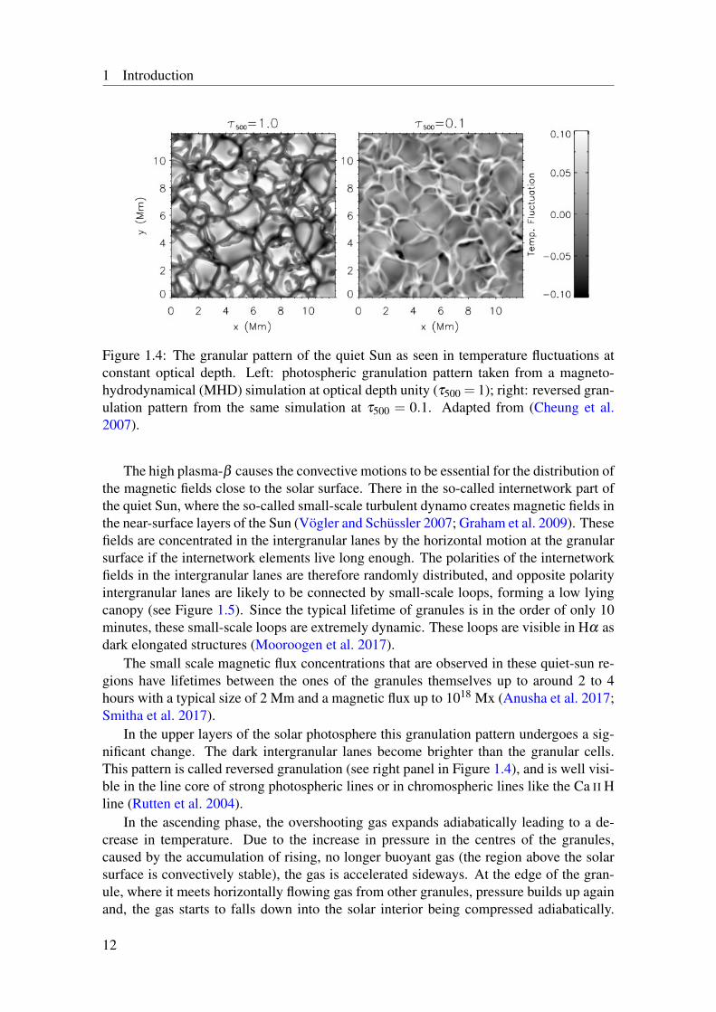
Figure 1.4: The granular pattern of the quiet Sun as seen in temperature fluctuations atconstant optical depth. Left: photospheric granulation pattern taken from a magneto-hydrodynamical (MHD) simulation at optical depth unity (τ500 = 1); right: reversed gran-ulation pattern from the same simulation at τ500 = 0.1. Adapted from (Cheung et al.2007).
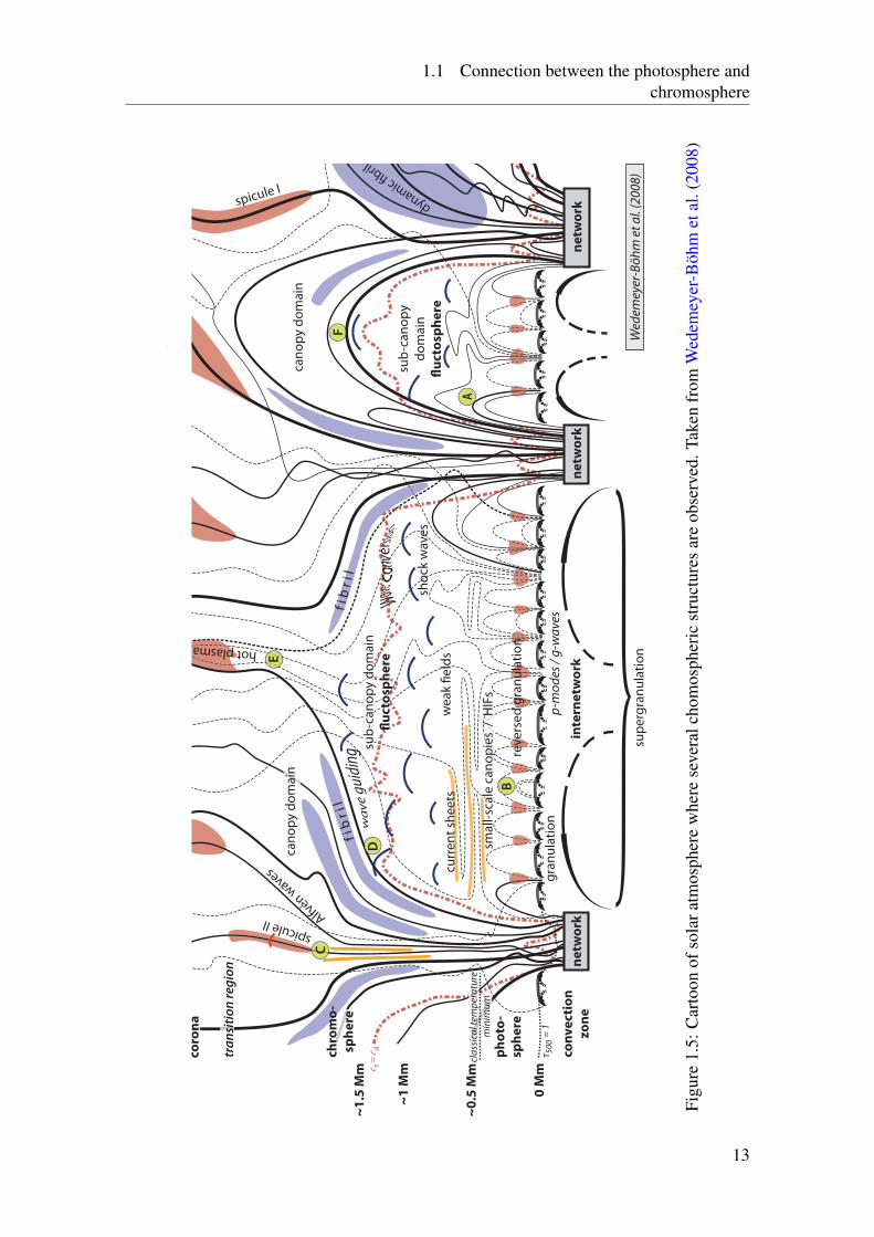
The high plasma-β causes the convective motions to be essential for the distribution ofthe magnetic fields close to the solar surface. There in the so-called internetwork part ofthe quiet Sun, where the so-called small-scale turbulent dynamo creates magnetic fields inthe near-surface layers of the Sun (Vögler and Schüssler 2007; Graham et al. 2009). Thesefields are concentrated in the intergranular lanes by the horizontal motion at the granularsurface if the internetwork elements live long enough. The polarities of the internetworkfields in the intergranular lanes are therefore randomly distributed, and opposite polarityintergranular lanes are likely to be connected by small-scale loops, forming a low lyingcanopy (see Figure 1.5). Since the typical lifetime of granules is in the order of only 10minutes, these small-scale loops are extremely dynamic. These loops are visible in Hα asdark elongated structures (Mooroogen et al. 2017).
The small scale magnetic flux concentrations that are observed in these quiet-sun re-gions have lifetimes between the ones of the granules themselves up to around 2 to 4hours with a typical size of 2 Mm and a magnetic flux up to 1018 Mx (Anusha et al. 2017;Smitha et al. 2017).
In the upper layers of the solar photosphere this granulation pattern undergoes a sig-nificant change. The dark intergranular lanes become brighter than the granular cells.This pattern is called reversed granulation (see right panel in Figure 1.4), and is well visi-ble in the line core of strong photospheric lines or in chromospheric lines like the Ca II Hline (Rutten et al. 2004).
In the ascending phase, the overshooting gas expands adiabatically leading to a de-crease in temperature. Due to the increase in pressure in the centres of the granules,caused by the accumulation of rising, no longer buoyant gas (the region above the solarsurface is convectively stable), the gas is accelerated sideways. At the edge of the gran-ule, where it meets horizontally flowing gas from other granules, pressure builds up againand, the gas starts to falls down into the solar interior being compressed adiabatically.
12
1.1 Connection between the photosphere andchromosphere
inte
rne
two
rk
ph
oto
-
sph
ere
can
op
y d
om
ain
gra
nu
lati
on
con
ve
cti
on
zo
ne
tra
nsi
tio
n r
eg
ion
curr
en
t sh
ee
ts
sho
ck w
ave
s
τ
=
15
00
we
ak
!e
lds
reve
rse
d g
ran
ula
tio
n
p-m
od
es /
g-w
ave
s
sup
erg
ran
ula
tio
n
mo
ss
0 M
m
~0
.5 M
m
~1
Mm
~1
.5 M
m
ne
two
rk
sub
-ca
no
py
do
ma
in
!u
cto
sph
ere
can
op
y d
om
ain
f i b
r i
l
coro
na
Ff
i b r
i l
D
E
hot plasma
cla
ssic
al t
emp
era
ture
min
imu
m
sub
-ca
no
py
do
ma
in
!u
cto
sph
ere
sma
ll-s
cale
ca
no
pie
s /
HIF
s
Wed
emey
er-B
öh
m e
t a
l. (2
00
8)
ne
two
rk
chro
mo
-
sph
ere
spicule II
dynamic !bril
CAlfv
én waves
c =
cs
c
= c
c =
cA
c =
c
ne
two
rk
spicule I
B
A
Figu
re1.
5:C
arto
onof
sola
ratm
osph
ere
whe
rese
vera
lcho
mos
pher
icst
ruct
ures
are
obse
rved
.Tak
enfr
omW
edem
eyer
-Böh
met
al.(
2008
)
13
1 Introduction
This process of compression increases the gas temperature, creating the reversal of thebrightness pattern in layers around 200 km above the τ = 1 level as shown in Figure 1.5or in Ca II H intensity maps.
On a larger scale of around 10 to 50 Mm, the magnetic fields in the quiet Sun areorganized in the so-called network. The network structure is caused by large convectivecells called supergranules (Leighton et al. 1962), having lifetimes in the order of daysand typical horizontal motions in the range of 0.5 km s−1. The upflow and downflowvelocities are in the order of 50 and 100 m s−1, respectively. Similarly to what happensin the granulation the horizontal motion concentrates the magnetic field at the edges ofthe cells, particularly the interception of different cells (Wang et al. 1995; Schrijver et al.1997). Liu et al. (1994) estimated that the life time of the network elements are about50 hours. Please note that this value is highly dependant on the used method.
The size range of these magnetic patches varies from 1 to 10 Mm with a typical mag-netic flux of about 1018 to 1019 Mx (Brown et al. 2001) and with magnetic fields withstrengths in the 1.5 kG range. The network fields might be connected by strong horizon-tal magnetic field (Lites et al. 2008), the so-called canopy fields (e.g. Jones and Giovanelli1982; Solanki and Steiner 1990).
To produce the even stronger magnetic field present in sunspots, pores or plage, theemergence of magnetic flux is required. At this moment two main different theories canexplain this process. The first one, that for decades was the standard theory, is based on therising of buoyant flux tubes to the surface (Schüssler et al. 1994). One key element of thismodel is amplification and conversion of the poloidal magnetic field into a toroidal field inthe tachocline by the differential rotation. The high magnetic pressure in these flux tubescauses a low plasma pressure, making the flux tubes buoyant and rising to the surface,where they form bipolar active regions. The field is then dragged by the meridional flowfirst to the poles and later again to the bottom on the convective zone as a poloidal fieldand the process repeats. This cycle is the 11 years solar cycle, that is characterised byperiods of strong activity at the solar surface alternating with quiet periods (Hathawayet al. 1994).
According to an alternative, distributed dynamo model (see review of Charbonneau2010) the magnetic field generation occurs all over the convection zone, due to turbulenteffects being important in addition to differential rotation. Such a dynamo generatesdiffuse large-scale fields everywhere in the convection zone. These magnetic fields arepostulated to become unstable near the surface and form active regions due to anotherturbulent effect (Brandenburg et al. 2016).
Active regions containing these strong magnetic fields are observed to live from daysup weeks and contain several pores and/or sunspots (see Figure 1.6). They show a widerange in diameter from 15 to 150 Mm, and a magnetic flux around 1022 Mx.
Sunspots and pores are surrounded by so-called plage regions, extending several Mmaround them. They appear as a bright ring within active regions in low-resolution ob-servations. These areas are characterized by a high density of kG features (Howard andStenflo 1972; Frazier and Stenflo 1972; Stenflo 1973) in form of small flux tubes (Solanki1993a) with diameters of around 100 km or less in the quiet-sun internetwork regions,and several hundred km in plage regions. Due to the small size of these flux tubes, theycan be modelled as a thin flux tube, i.e., where the horizontal size of the tube is smallerthan the pressure scale height (Spruit 1976; Defouw 1976). (Buehler et al. 2015) estimate
14
1.2 Chromospheric jets and fibril like structures
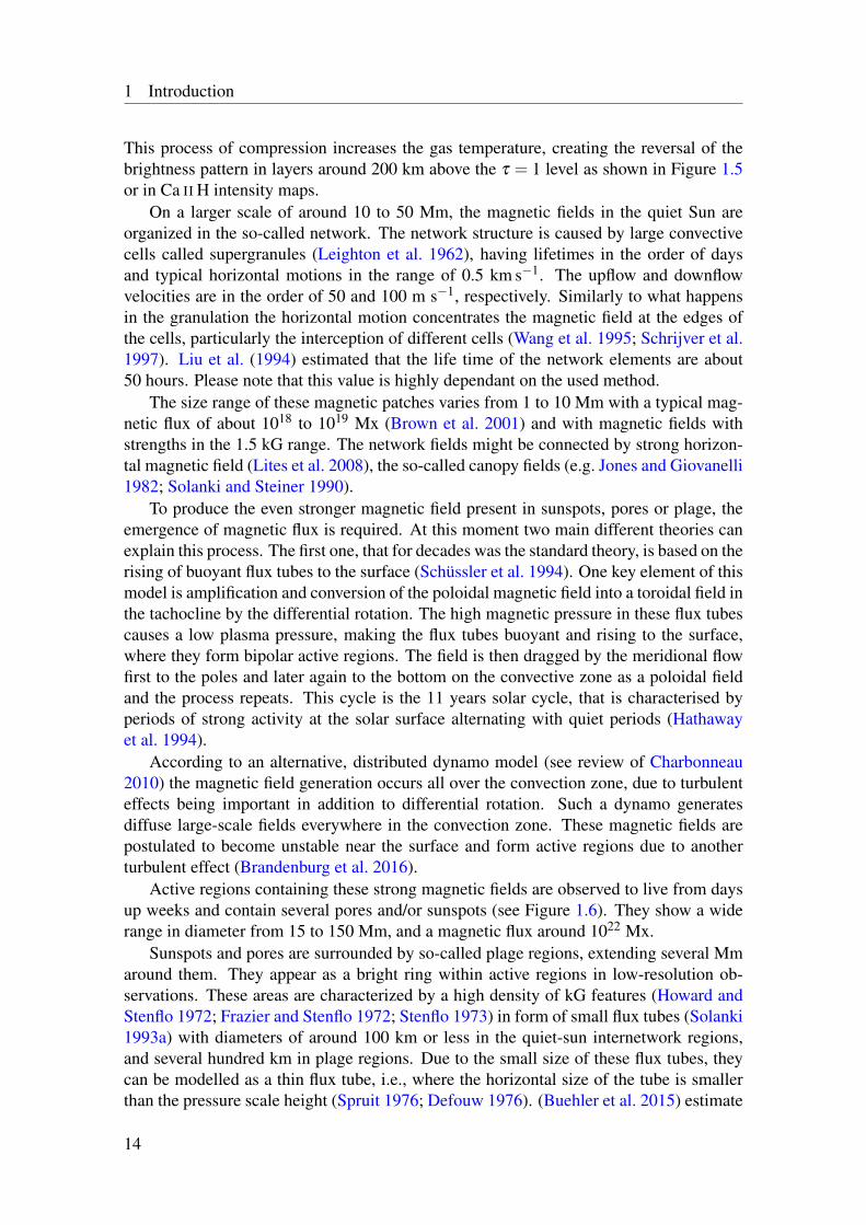
Figure 1.6: Active region constituted by big sunspots and small pores, and surrounded bythe bright plage regions. Credit: NASA’s Solar Dynamics Observatory.
that the inclinations of the flux tubes are preferentially vertical with angles between 10 to15 degrees and magnetic fields of ≈1500 G at log(τ) = -0.9. This vertical orientation is aresult of the buoyancy of the flux tubes (Schüssler 1986).
All these magnetic field concentrations finally reach up to the chromosphere (Pietarila,A. et al. 2010) where they create several different features depending on the characteristicsof the magnetic field and their location (Wedemeyer-Böhm et al. 2008). The data analyzedin this thesis are coming from such plage regions.
1.2 Chromospheric jets and fibril like structures
As mentioned in Sect. 1, the solar chromosphere is a highly warped layer on top of thesolar photosphere with an average thickness of about 1.5 Mm (Wedemeyer-Böhm et al.2008). In the upper chromosphere the structure and dynamics are dominated by the mag-netic field (plasma β<1) contrary to the lower chromosphere and photosphere (β>1).
A prominent feature of the solar chromosphere above plage and network fields aresmall-scale, elongated fibrils, well visible in chromospheric lines like the Ca II H&K orthe Hα lines. In this section we describe these highly dynamic chromospheric structures,appearing in the literature as mottles, fibrils, straws, rapid blue excursions (RBEs), andspicules (see Tsiropoula et al. 2012, and Sect. 1.2.1). These structures possibly play amajor rule in the energy and mass transport from the lower to the upper layers of the Sun(see, e.g., Pereira et al. 2012). Observations using filtergraph instruments allow to char-acterize the morphological properties and dynamics of these structures. More recently,spectroscopic and spectropolarimetric observations allow to infer the physical processesand conditions like density, temperature and plasma flows within these structures.
The SUNRISE data used in this work, reached a new level in terms of spatial resolution.This allows us to apply wave analysis techniques in order to identify the wave modes (thatwe describe in more detail in section Sect. 1.2.2) present in these elongated structures.According to some models, the energy transported by such waves is high enough to heatthe solar chromosphere (Withbroe and Noyes 1977; Vernazza et al. 1981).
Despite all the observational and computational studies, the formation and the rolein the mass and energy transport to the solar corona of chromospheric jets and fibril-like
15
1 Introduction
structures are still not well understood. To improve the understanding it is essential toinvestigate their detailed morphological properties and their dynamics.
1.2.1 General properties of small scale chromospheric jet and fibril-like structures
Figure 1.5 illustrates the complexity of the chromosphere, containing structures of allsizes, from filaments spanning over half a solar radius to the features barely resolvablewith modern solar telescopes. In this work I concentrate on the small-scale structures.Here is a short overview of some terms used in the literature:
1.2.1.1 Mottles
Mottles are usually referred as highly dynamic, hair-like jets observed on disk in the quietSun in chromospheric spectral lines like Hα or the Ca II lines. They typically appear asdark, elongated structures, and are best observed in the wings of the Hα-line (± 0.5 Åaround the line core). However, some observational studies report of the existence ofbright mottles in the same location as the dark mottles. One possible explanation sug-gested by Banos and Macris (1970) is that the bright mottles are the base of the darkstructures. Contradicting this explanation, Alissandrakis and Macris (1971) claim that thetwo types of mottles are completely different structures. With the analysis of the new highresolution observations it has been speculated that the bright mottles are likely to be thebright background under the dark mottles (Tsiropoula et al. 2012).
Mottles are the most common elements seen in Hα that constitute the highly-warpedand dynamic chromosphere. They display a complex geometric pattern, outlining theboundaries of the chromospheric network. The latter is well visible in the Ca lines (al-though the mottles themselves are not). Based on their location and number they canbe divided in two different categories. Small groups, called chains, that are created byalmost parallel structures emanating along the common boundary of two supergranularcells. Second, larger groups called rosettes, consist of usually radially expanding struc-tures around the common boundary area of three or more supergranular cells. Tanaka(1974) also found that about 30% of all the dark mottles appear in pairs or can be re-solved into double structures in Hα wing observations.
The dimension of mottles spans from 1 to 10 Mm and width around 500 km (Brayand Loughhead 1974) and they show different shapes: oval, round, filament- or arch-like, and lumpy, (Sawyer 1972). The elongated, filament- or arch-like ones are the mostcommon. Due to the highly dynamic behaviour the life time of these structures is difficultto determine. The values range from 3 to 15 min (Bratsolis et al. 1993).
1.2.1.2 Fibrils
Fibrils are small-scale, dark, elongated structures observed on the solar disc in the plagewithin active regions (see Figure 1.7 for an example). Similarly to mottles they are alsohighly dynamic. Unfortunately, the same term is also used for two other types of largerscale structures: dark structures (in Hα) on top of the sunspot penumbrae that expand ra-dially from the centre of the umbra with typical lengths in the range of ten Mm, and struc-
16
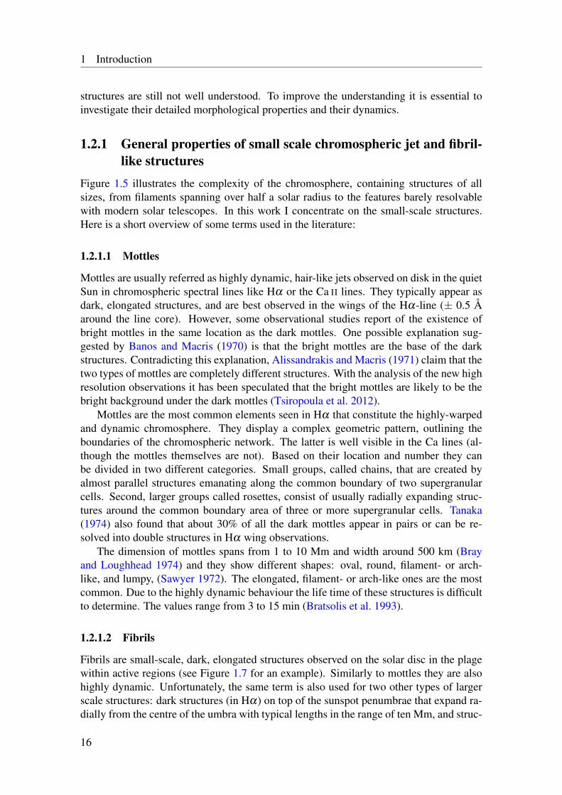
1.2 Chromospheric jets and fibril like structures
Figure 1.7: Different types of fibrils observed in Hα (right panel). The longer fibrils tendto originate in the umbra / penumbra of the sunspot (see Hα wideband image on the left),the shorter ones are more concentrated in the plage of the active region. Adapted from DePontieu et al. (2007).
tures that do not show a jet-like behavior in the vicinity of active region plage (Tsiropoulaet al. 2012). The latter two are probably part of a low-lying canopy connecting the oppo-site polarity areas within an active region. This thesis analyses in detail the short fibrils inthe plage of active regions.
The analysis of filtergrams of Hα fibrils in plage regions shows their structural simi-larity to the ones in the quiet Sun. For example, structures similar to rosettes and mottlesin the quiet Sun, rooted in network bright points (NBPs), are also existing in plage re-gions at smaller scales (Tsiropoula et al. 2012). The principal differences between thetwo regimes are on the one hand a larger number density of small-scale magnetic fieldconcentrations in plage compared to the number density of NBPs and on the other handthe bigger size of the fibrils observed in plage than in the network.
This possible relationship between the structures observed in the quiet and active chro-mosphere was analyzed by Foukal (1971b). He proposed that there is a gradual changebetween the quiet-sun mottles, oriented close to the vertical, and the more horizontallyoriented fibrils in plage regions.
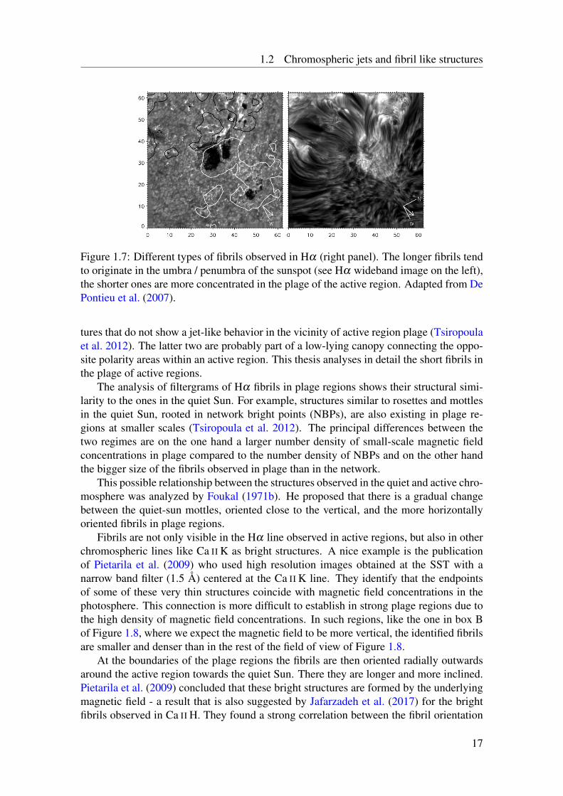
Fibrils are not only visible in the Hα line observed in active regions, but also in otherchromospheric lines like Ca II K as bright structures. A nice example is the publicationof Pietarila et al. (2009) who used high resolution images obtained at the SST with anarrow band filter (1.5 Å) centered at the Ca II K line. They identify that the endpointsof some of these very thin structures coincide with magnetic field concentrations in thephotosphere. This connection is more difficult to establish in strong plage regions due tothe high density of magnetic field concentrations. In such regions, like the one in box Bof Figure 1.8, where we expect the magnetic field to be more vertical, the identified fibrilsare smaller and denser than in the rest of the field of view of Figure 1.8.
At the boundaries of the plage regions the fibrils are then oriented radially outwardsaround the active region towards the quiet Sun. There they are longer and more inclined.Pietarila et al. (2009) concluded that these bright structures are formed by the underlyingmagnetic field - a result that is also suggested by Jafarzadeh et al. (2017) for the brightfibrils observed in Ca II H. They found a strong correlation between the fibril orientation
17
1 Introduction
Figure 1.8: Ca II K filtergram of a small active regions. The boxes identify different solarregions of interest. Box A is placed over the boundary between the plage region and thequiet Sun. Box B shows only the plage region. Box C contains a small pore. Box Drepresent a region between two magnetic polarities.
Taken from Pietarila et al. (2009).
and the magnetic field lines obtained by magnetic field extrapolation from photosphericvector magnetograms.
Foukal (1971a) for the first time compared some morphological properties of Hα
fibrils and spicules. He saw a similarity of these two structures in terms of lifetime,density, temperature, and velocity, but reported on higher lengths for spicules and strongermagnetic fields in fibrils. However, this description is still speculative.
The typical fibrils show a huge range of their morphological properties. The life-time varies from less than a minute to 20 minutes, the width between few hundreds ofkm to 2 Mm, and the length between few hundreds of km to 15 Mm. A subcategoryof these fibrils are the so-called dynamic fibrils, (DF, Grossmann-Doerth and Schmidt1992; Hansteen et al. 2006). These DFs are shorter than the typical fibrils and shorterlived. They are mainly observed in the vicinity of plage regions or strong magnetic fieldconcentrations.
DFs, when observed in Hα , have life times of 120 to 650 s with an average value of290 s, typical sizes of 400 to 5200 km and a mean length of 1250 km, and widths be-tween 120 and 380 km that remain almost constant during the fibril lifetime. De Pontieuet al. (2007) identify a variation of these properties depending on their location, conclud-
18
1.2 Chromospheric jets and fibril like structures
ing that the fibrils observed in denser plage regions are shorter in length and lifetime.Pietarila et al. (2009) estimated also some properties for the bright fibrils observed in theCa II K line. They estimate the width to lie between 75 and 150 km and a length of ap-proximately 900 km. Anan et al. (2010) used observations in Ca II H (band width of 3 Å)from the Hinode Solar Optical Telescope (SOT) / Broadband Filter Imager (BFI) (Tsunetaet al. 2008) to analyze the brightness and the morphological properties of these structures.They identify two classes of brightness variations, where 80% of them show a parabolicevolution, i.e. a slow brightening followed by a slow fading, and 10% a "fade out" behav-ior. The lengths of these fibrils were estimated to be between 0.8 Mm and 2.3 Mm, andthe lifetimes between 100 s and 400 s.
1.2.1.3 Rapid Blueshifted Excursions
Rapid Blueshifted Excursions (RBEs) are observed on disk structures that are character-ized by a blueshift or a fast, asymmetric broadening in the blue wing of chromosphericlines like Hα and Ca II IR (Langangen et al. 2008). Common properties observed in bothspectral lines are their short mean lifetime of 45±13 s and a typical width of 0.5 Mm.However, some of the properties depend on the line the RBEs are observed in: the onesobserved in Hα are on average longer than the ones observed in Ca II IR (3 Mm com-pared to 2 Mm). The blueshift is approximately 35 km s−1 in Hα (15 km s−1 Ca II), andthe Doppler width of the blueshifted component is 13 km s−1 compared to 7 km s−1 inCa II (Langangen et al. 2008; Rouppe van der Voort et al. 2009).
One possible explanation for this rapid blueshifts was suggested by Langangen et al.(2008) who used a Monte Carlo simulation to show that the observed lineshifts are likelyto be caused by a combination of different orientations of spicules and changes in opacityin the upper chromosphere.
Using data from the CRisp Imaging SpectroPolarimeter (CRISP; Scharmer et al.2008) at the Swedish 1-m Solar Telescope (SST Scharmer et al. 2003a), (Wang et al.1998) analyzed in detail very similar, but longer lived events in Hα and Ca II IR. Theyestimate that the density of these structures if observed at the limb is around 1.9 per lineararcsecond. Judge et al. (2011) estimate that the number of RBEs in the Sun is ≈ 105 atany given time. They also suggested that the RBEs could be the counterparts of type-IIspicules on disk, since they are visible in both spectral lines.
1.2.1.4 Spicules
Spicules are bright, elongated, jet-like structures that are observed off-limb (Beckers1968, 1972; Sterling 2000) in lines like Hα and Ca II H, showing the same behavior inboth lines (Pereira et al. 2016). The first to use the term spicule was Roberts (1945) whenanalyzing Hα off limb chronograph images. He observed that these jets reach heights ofaround 10 Mm and last between 2 and 11 minutes. Even earlier, in 1877, observationsof jet-like structures were already reported by Father Angelo Secchi. Lippincott (1957)classified spicules in two categories. The first one, called porcupine, contains spiculeswith a size of 18 Mm. The porcupines tend to be oriented radially outwards from a com-mon point. The second category, called wheat, has a size of 140 Mm. The wheat havea dominant inclination direction with respect to the limb direction. She also computed
19
1 Introduction
for the first time the propagation velocity of the material within these spicules that rangefrom a few km s−1 up to 60 km s−1.
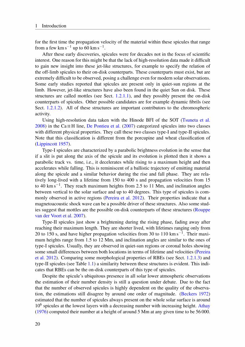
After these early discoveries, spicules were for decades not in the focus of scientificinterest. One reason for this might be that the lack of high-resolution data made it difficultto gain new insight into these jet-like structures, for example to specify the relation ofthe off-limb spicules to their on-disk counterparts. These counterparts must exist, but areextremely difficult to be observed, posing a challenge even for modern solar observations.Some early studies reported that spicules are present only in quiet-sun regions at thelimb. However, jet-like structures have also been found in the quiet Sun on disk. Thesestructures are called mottles (see Sect. 1.2.1.1), and they possibly present the on-diskcounterparts of spicules. Other possible candidates are for example dynamic fibrils (seeSect. 1.2.1.2). All of these structures are important contributors to the chromosphericactivity.
Using high-resolution data taken with the Hinode BFI of the SOT (Tsuneta et al.2008) in the Ca II H line, De Pontieu et al. (2007) categorized spicules into two classeswith different physical properties. They call these two classes type-I and type-II spicules.Note that this classification is different from the porcupine and wheat classification of(Lippincott 1957).
Type-I spicules are characterized by a parabolic brightness evolution in the sense thatif a slit is put along the axis of the spicule and its evolution is plotted then it shows aparabolic track vs. time, i.e., it decelerates while rising to a maximum height and thenaccelerates while falling. This is reminiscent of a ballistic trajectory of emitting materialalong the spicule and a similar behavior during the rise and fall phase. They are rela-tively long-lived with a lifetime from 150 to 400 s and propagation velocities from 15to 40 km s−1. They reach maximum heights from 2.5 to 11 Mm, and inclination anglesbetween vertical to the solar surface and up to 40 degrees. This type of spicules is com-monly observed in active regions (Pereira et al. 2012). Their properties indicate that amagnetoacoustic shock wave can be a possible driver of these structures. Also some stud-ies suggest that mottles are the possible on-disk counterparts of these structures (Rouppevan der Voort et al. 2007).
Type-II spicules just show a brightening during the rising phase, fading away afterreaching their maximum length. They are shorter lived, with lifetimes ranging only from20 to 150 s, and have higher propagation velocities from 30 to 110 km s−1. Their maxi-mum heights range from 1.5 to 12 Mm, and inclination angles are similar to the ones oftype-I spicules. Usually, they are observed in quiet-sun regions or coronal holes showingsome small differences between both locations in terms of lifetime and velocities (Pereiraet al. 2012). Comparing some morphological properties of RBEs (see Sect. 1.2.1.3) andtype-II spicules (see Table 1.1) a similarity between these structures is evident. This indi-cates that RBEs can be the on-disk counterparts of this type of spicules.
Despite the spicule’s ubiquitous presence in all solar lower atmospheric observationsthe estimation of their number density is still a question under debate. Due to the factthat the number of observed spicules is highly dependent on the quality of the observa-tion, the estimations still disagree by around one order of magnitude. (Beckers 1972)estimated that the number of spicules always present on the whole solar surface is around106 spicules at the lowest layers with a decreasing number with increasing height. Athay(1976) computed their number at a height of around 5 Mm at any given time to be 56 000.
20
1.2 Chromospheric jets and fibril like structures
More recent studies analyze in more detail the distribution of type I and II spicules. Judgeand Carlsson (2010) estimate that at a given moment there exist 2×10⁷ type-II spicules,distributed to 1600 spicules within each supergranule. On the other hand Moore et al.(2011) estimate that this number is much smaller (only around 50 spicules per supergran-ule). This discrepancy shows that the detection of these structures still poses a challengeeven for modern solar observations, possibly requiring improved instrumentation to settlethis issue in the future.
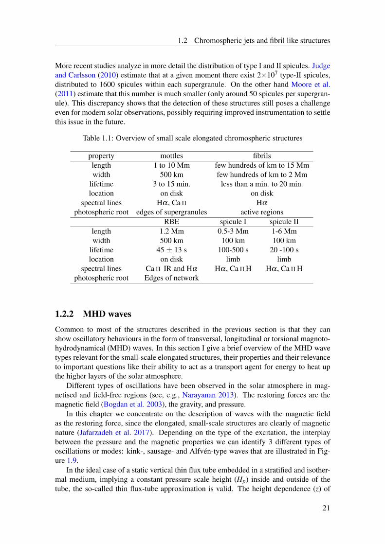
Table 1.1: Overview of small scale elongated chromospheric structures
property mottles fibrilslength 1 to 10 Mm few hundreds of km to 15 Mmwidth 500 km few hundreds of km to 2 Mm
lifetime 3 to 15 min. less than a min. to 20 min.location on disk on disk
spectral lines Hα , Ca II Hα
photospheric root edges of supergranules active regionsRBE spicule I spicule II
length 1.2 Mm 0.5-3 Mm 1-6 Mmwidth 500 km 100 km 100 km
lifetime 45 ± 13 s 100-500 s 20 -100 slocation on disk limb limb
spectral lines Ca II IR and Hα Hα , Ca II H Hα , Ca II Hphotospheric root Edges of network
1.2.2 MHD wavesCommon to most of the structures described in the previous section is that they canshow oscillatory behaviours in the form of transversal, longitudinal or torsional magnoto-hydrodynamical (MHD) waves. In this section I give a brief overview of the MHD wavetypes relevant for the small-scale elongated structures, their properties and their relevanceto important questions like their ability to act as a transport agent for energy to heat upthe higher layers of the solar atmosphere.
Different types of oscillations have been observed in the solar atmosphere in mag-netised and field-free regions (see, e.g., Narayanan 2013). The restoring forces are themagnetic field (Bogdan et al. 2003), the gravity, and pressure.
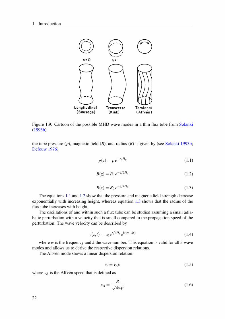
In this chapter we concentrate on the description of waves with the magnetic fieldas the restoring force, since the elongated, small-scale structures are clearly of magneticnature (Jafarzadeh et al. 2017). Depending on the type of the excitation, the interplaybetween the pressure and the magnetic properties we can identify 3 different types ofoscillations or modes: kink-, sausage- and Alfvén-type waves that are illustrated in Fig-ure 1.9.
In the ideal case of a static vertical thin flux tube embedded in a stratified and isother-mal medium, implying a constant pressure scale height (Hp) inside and outside of thetube, the so-called thin flux-tube approximation is valid. The height dependence (z) of
21
1 Introduction
Figure 1.9: Cartoon of the possible MHD wave modes in a thin flux tube from Solanki(1993b).
the tube pressure (p), magnetic field (B), and radius (R) is given by (see Solanki 1993b;Defouw 1976)
p(z) = pe−z/Hp (1.1)
B(z) = B0 e−z/2Hp (1.2)
R(z) = R0 e−z/4Hp (1.3)
The equations 1.1 and 1.2 show that the pressure and magnetic field strength decreaseexponentially with increasing height, whereas equation 1.3 shows that the radius of theflux tube increases with height.
The oscillations of and within such a flux tube can be studied assuming a small adia-batic perturbation with a velocity that is small compared to the propagation speed of theperturbation. The wave velocity can be described by
v(z, t) = v0 ez/4Hp ei(wt−kz) (1.4)
where w is the frequency and k the wave number. This equation is valid for all 3 wavemodes and allows us to derive the respective dispersion relations.
The Alfvén mode shows a linear dispersion relation:
w = vAk (1.5)
where vA is the Alfvén speed that is defined as
vA =B√4πρ
(1.6)
22
1.2 Chromospheric jets and fibril like structures
The Alfvén mode is characterized by an incompressible torsional motion and can beexcited by flux tubes twisted by rotating flows.
For the kink mode the dispersion relation is
w2 =C2Kk2 +w2
c,k (1.7)
where Ck is the kink mode propagation velocity for high frequencies with respect to thekink cutoff frequency , and w2
c,k is the kink cutoff frequency. This type of mode is char-acterised by a transversal displacement of the flux tube and is excited for example by thebuffeting of granules.
The dispersion relation for the sausage mode is given by
w2 =C2T k2 +w2
c,T (1.8)
where CT is the so-called tube speed for high frequencies compared to the cutoff fre-quency (w2
c,T ). This mode is characterized by longitudinal motions along the tube and canbe excited by tube compression from opposite sides.
Some of these modes can be observed in the structures described in Sect. 1.2.1 andare summarized in Table 1.1.
The relevance of these waves to small-scale fibrilar structures is described in threeexamples described in the following subsections. For a more complete review please seeZaqarashvili and Erdélyi (2009); Rutten (2012); Tsiropoula et al. (2012).
1.2.2.1 Kink waves in dynamic fibrils
The first observation of kink waves in the solar atmosphere was made by Pasachoff et al.(1968), who found them in Hα fibrils. Since then this type of oscillation has been ob-served in several structures. They are of high relevance for solar physics research, sincerecent studies suggest that kink waves, at least when observed in the photosphere or chro-mosphere, have enough energy to heat the quiet corona (He et al. 2009; Jafarzadeh et al.2017)
Pietarila et al. (2011) analyzed dynamic fibrils observed in the chromospheric Ca II
8542 Å line using CRISP. They were able to analyze the transverse motions of thesestructures in time, and clearly identified these motions to be kink waves. The waveshave periods between 2 and 3 minutes with a mean value of 135 s, an apparent speedof 1 km s−1, and a phase speed of around 290 km s−1. Using the approximation of avertical thin flux tube and the expression given by Nakariakov and Verwichte (2005) thatrelates the magnetic field and the wave period they were able to estimate the magneticfield strength inside the fibrils to vary from 220 to 330 G from one fibril to another. Allthese values are similar to the ones observed by He et al. (2009) for spicules at heightsbelow 2 Mm.
1.2.2.2 Alfvén waves in spicules
By analyzing off-limb Ca II H images taken by Hinode/SOT, de Pontieu et al. (2007) ob-served that spicules show an ubiquitous transverse oscillatory behavior. Comparing theobservation with the results of a self-consistent 3D radiative MHD simulation, they con-clude that this displacement is caused by Alfvén waves propagating along the spicules
23
1 Introduction
that are excited in the photosphere by the granular motion. The computed periods forthese waves were between 100 and 500 s with amplitudes that range from 10 to 25 km.In the same study they estimate that these waves can transport enough energy flux to thesolar corona and drive the solar wind and possible contribute to the quiet corona heating.
1.2.2.3 Sausage waves in Hα fibrils
Morton et al. (2012) used Hα data taken by the Rapid Oscillations in Solar Atmosphere(ROSA) imager Jess et al. (2010) to analyze intensity and width variations along theHα fibrils. They found an anti-phase periodic behaviour of these two quantities withperiods of 197±8 s, phase speeds of 67±15km s−1 and apparent velocity amplitudes of1-2 km s−1. The observed perturbation is traveling at speeds similar to the Alfvén speedthat leads to the interpretation of these waves as a fast MHD sausage mode. The anti-phase correlation between the variation in intensity and width illustrates the compressivenature of this wave mode.
The authors also conclude that the sausage wave is in the so-called leaky regime. Thatmeans that the wave can radiate energy away from the wave guide, i.e., the magnetic fluxtube, with decay times on the order of the wave period. It is the task of further studies toperform a careful analysis of the amount of energy that is carried and dissipated by thistype of wave.
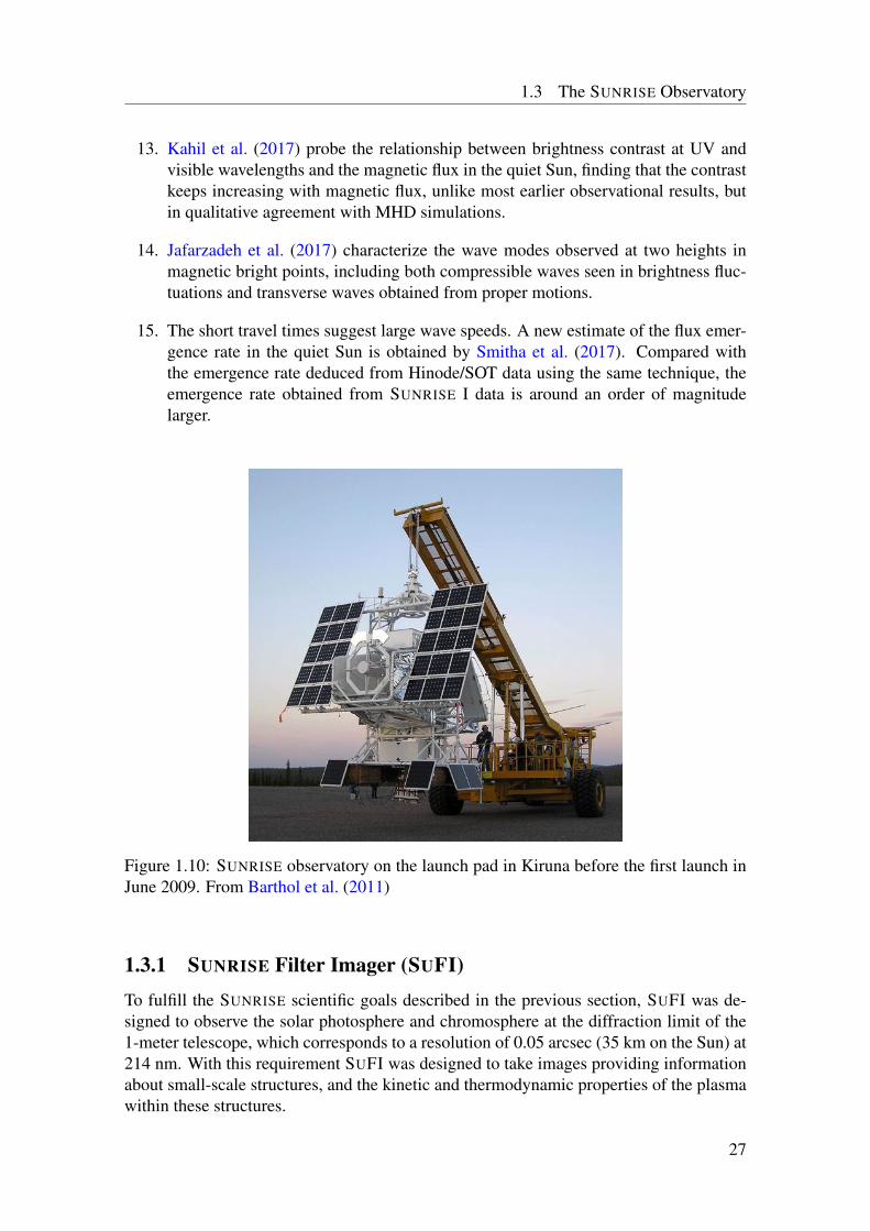
1.3 The SUNRISE ObservatoryThe SUNRISE observatory (Solanki et al. 2010; Barthol et al. 2011) is a balloon-bornescientific mission with a 1-meter Gregorian telescope (see Figure 1.10). Its scientific goalis the observation of the photosphere and the chromosphere at highest spatial resolutionand with long temporal stability. The main science goals of Sunrise as defined in Bartholet al. (2011) are:
1. What are the origin and the properties of the intermittent magnetic structure, in-cluding the kilo-Gauss concentrations?
2. How is the magnetic flux brought to and removed from the solar surface? What isthe role played by local dynamo action and reconnection processes?
3. How does the magnetic field assimilate and provide energy to heat the upper solaratmosphere?
4. How does the variable magnetic field modify the solar brightness?
Questions (1) and (3) are directly related to the topic of this thesis. The small scalestructures described in this work outline the connection between the photosphere and thechromosphere and are of high relevance for answering the questions related to the energytransport to the higher layers of the solar atmosphere. A key will be to investigate howthese structures interact and how they influence the energy balance between the magneticfield, plasma motion, heat and radiation transfer.
The location of the observatory in the stratosphere allows for observations in the ultra-violet wavelength region from 200 to 400 nm, a region not accessible from the ground. In
24
1.3 The SUNRISE Observatory
addition, the earth atmosphere at this height provides almost seeing-free conditions whichallowed for the recording of the highest quality data in this spectral range ever.
The observatory flew twice. The first flight lasted from 8-13 June 2009. SUNRISE
was launched from Kiruna, northern Sweden, and landed on Somerset island, northernCanada and with a mean altitude of 36 km (Solanki et al. 2010). The second flight tookplace from 12-17 June 2013. SUNRISE was launched from Kiruna, northern Sweden, andlanded on the peninsula of Boothia in northern Canada, with mean flight altitude of 36km (Solanki et al. 2017). The technical differences between the first and the second flightwhere small. Mainly some of the instrumentation were updated and new UV filters wereused.
The scientific payload of SUNRISE consists of two instruments: the SUNRISE Fil-ter Imager (SUFI Gandorfer et al. 2011) for observations in the range between 200 and400 nm, including the Mg II K and Ca II H lines broad with FHWM of 1.8 Å and narrowband with FHWM of 1.1 Å filter) lines.
The second instrument is the Imaging Magnetograph eXperiment (IMaX MartínezPillet et al. 2011), based on a tunable Fabry-Pérot filter sampling various wavelengths inthe highly Zeeman-sensitive Fe I line at 525.02 nm.
The work described in this thesis focuses on the analysis of SUFI filtergrams. In thissection we briefly describe the instrument SUFI (see Sect. 1.3), and the reduction of thedata gathered by this instrument (Sect. 1.3.2), with special focus on the observations inthe Ca II H line.
The two SUNRISE flights resulted in many high-impact scientific articles, and in twospecial issues of the Astrophysical Journal Supplements (ApJS). Here I repeat the sum-mary of the articles of the second special issue as given by Solanki et al. (2017). Thisliteral repetition also contains the summary of the two papers being part of this thesis (seeSect. 2 and Sect. 3):
1. Centeno et al. (2017) analyzed emerging flux regions with a detailed description ofthe interrelated dynamics of the gas and the field, including the
reports on two emerging flux events, describing in greater detail than previouslypossible the interrelated dynamics of the gas and the field, as well as the likelyoccurrence of magnetic reconnection during the emergence.
2. The properties of a likely siphon flow and of the small, initially low-lying loopconnecting magnetic elements with a pore are deduced by Requerey et al. (2017a)and the 3D structure of the magnetic field lines and hence of the flow vector aredetermined.
3. The properties and dynamics of moving magnetic features (MMFs) on one sideof the largest pore in the IMaX FOV are deduced by Kaithakkal et al. (2017) andcontrasted with the properties of MMFs around sunspots.
4. The proper motion of magnetic bright points in different parts of the quiet Sunand of an active region are analyzed by Jafarzadeh et al. (2017). They find verydifferent behaviors depending on the location, with the features moving stronglysuperdiffusively in the internetwork, diffusively in the network and in between theseextremes in the active region.
25
1 Introduction
5. Riethmüller et al. (2017) present a novel inversion technique employing magne-tohydrodynamic (MHD) simulations to provide the model atmospheres needed tocompute synthetic Stokes vectors that reproduce the observed Stokes parameters.They illustrate the quality of the inversions by applying the technique to the SUN-RISE II polarimetric data.
6. The properties of the slender fibrils dominating the SUFI Ca II H images are deter-mined by Gafeira et al. (2017b), who show that the fibrils live much longer than asimple analysis would suggest, if one takes into account that they often fade awayand reappear after some time.
7. The discovery of ubiquitous transverse waves travelling along these fibrils and car-rying copious amounts of energy is reported by Jafarzadeh et al. (2017), whileGafeira et al. (2017a) present the discovery of compressible waves travelling alongthe fibrils, which they identify as sausage waves.
8. Jafarzadeh et al. (2017) find evidence that these slender fibrils seen in Ca II H outlinea canopy of magnetic field lying below that known from Hα and Ca II 8542 Å fibrilobservations.
9. Chitta et al. (2017) observed that coronal loops are rooted in regions with mixed-polarity fields. They provide evidence for flux cancellation and presence of inverseY-shaped jets (signatures of magnetic reconnection) at the base of coronal loops thatmight supply (hot) plasma to the overlying coronal loop. They suggest a revisionof the traditional picture in which each loop footpoint is smoothly connected tounipolar regions on the solar surface.
10. Danilovic et al. (2017) compare an Ellerman bomb observed by SUNRISE II witha similar, simulated event in which magnetic reconnection occurs at the locationof emerging flux. The 3D radiation-MHD simulation reveals the complexity of theunderlying physical process and the limitations of the observational data. Thus, theSUNRISE/IMaX data cannot determine the height at which magnetic reconnectiontakes place. The authors also show, however, that the velocity and magnetic vectormeasured at the high resolution of SUNRISE/IMaX reveals how shortcomings of theMHD simulations can be overcome.
11. Wiegelmann et al. (2017) have computed general linear magneto-static equilibriaof the magnetic field and gas using the SUNRISE II/IMaX observations as a bound-ary condition. In this way they obtain the magnetic field structure in the upperatmosphere without having to assume the validity of the force-free assumption inthe solar photosphere. They computed linear magneto-static equilibria for all theIMaX frames of the active region, without the problems faced when modeling themagnetic field in different atmospheric layers of the quiet Sun.
12. Such papers include the investigation by Requerey et al. (2017b) in which the au-thors uncover the tight connection between concentrated magnetic fields and con-vectively driven sinks in the quiet Sun.
26
1.3 The SUNRISE Observatory
13. Kahil et al. (2017) probe the relationship between brightness contrast at UV andvisible wavelengths and the magnetic flux in the quiet Sun, finding that the contrastkeeps increasing with magnetic flux, unlike most earlier observational results, butin qualitative agreement with MHD simulations.
14. Jafarzadeh et al. (2017) characterize the wave modes observed at two heights inmagnetic bright points, including both compressible waves seen in brightness fluc-tuations and transverse waves obtained from proper motions.
15. The short travel times suggest large wave speeds. A new estimate of the flux emer-gence rate in the quiet Sun is obtained by Smitha et al. (2017). Compared withthe emergence rate deduced from Hinode/SOT data using the same technique, theemergence rate obtained from SUNRISE I data is around an order of magnitudelarger.
Figure 1.10: SUNRISE observatory on the launch pad in Kiruna before the first launch inJune 2009. From Barthol et al. (2011)
1.3.1 SUNRISE Filter Imager (SUFI)To fulfill the SUNRISE scientific goals described in the previous section, SUFI was de-signed to observe the solar photosphere and chromosphere at the diffraction limit of the1-meter telescope, which corresponds to a resolution of 0.05 arcsec (35 km on the Sun) at214 nm. With this requirement SUFI was designed to take images providing informationabout small-scale structures, and the kinetic and thermodynamic properties of the plasmawithin these structures.
27
1 Introduction
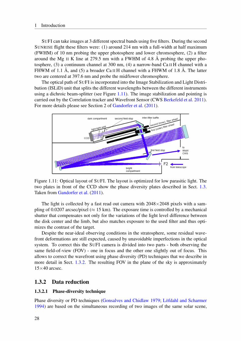
SUFI can take images at 3 different spectral bands using five filters. During the secondSUNRISE flight these filters were: (1) around 214 nm with a full-width at half maximum(FWHM) of 10 nm probing the upper photosphere and lower chromosphere, (2) a filteraround the Mg II K line at 279.5 nm with a FWHM of 4.8 Å probing the upper pho-tosphere, (3) a continuum channel at 300 nm, (4) a narrow-band Ca II H channel with aFHWM of 1.1 Å, and (5) a broader Ca II H channel with a FHWM of 1.8 Å. The lattertwo are centered at 397.6 nm and probe the mid/lower chromosphere.
The optical path of SUFI is incorporated into the Image Stabilization and Light Distri-bution (ISLiD) unit that splits the different wavelengths between the different instrumentsusing a dichroic beam-splitter (see Figure 1.11). The image stabilization and pointing iscarried out by the Correlation tracker and Wavefront Sensor (CWS Berkefeld et al. 2011).For more details please see Section 2 of Gandorfer et al. (2011).
Figure 1.11: Optical layout of SUFI. The layout is optimized for low parasitic light. Thetwo plates in front of the CCD show the phase diversity plates described in Sect. 1.3.Taken from Gandorfer et al. (2011).
The light is collected by a fast read out camera with 2048×2048 pixels with a sam-pling of 0.0207 arcsec/pixel (≈ 15 km). The exposure time is controlled by a mechanicalshutter that compensates not only for the variations of the light level difference betweenthe disk center and the limb, but also matches exposure to the used filter and thus opti-mizes the contrast of the target.
Despite the near-ideal observing conditions in the stratosphere, some residual wave-front deformations are still expected, caused by unavoidable imperfections in the opticalsystem. To correct this the SUFI camera is divided into two parts - both observing thesame field-of-view (FOV) - one in focus and the other one slightly out of focus. Thisallows to correct the wavefront using phase diversity (PD) techniques that we describe inmore detail in Sect. 1.3.2. The resulting FOV in the plane of the sky is approximately15×40 arcsec.
1.3.2 Data reduction1.3.2.1 Phase-diversity technique
Phase diversity or PD techniques (Gonsalves and Chidlaw 1979; Löfdahl and Scharmer1994) are based on the simultaneous recording of two images of the same solar scene,
28
1.3 The SUNRISE Observatory
one with an unknown wave-front deformation and a second one with the same unknownwave-front deformation plus a known aberration. This can be expressed in the set of thetwo following equations (Löfdahl and Scharmer 1994):
d0 = f ∗ t0 +n0 (1.9)
anddk = f ∗ tk +nk (1.10)
where f is the real solar scene, d0 and dk are the image with the unknown and the imagewith unknown plus known deformations respectively, t0 and tk are the correspondent pointspread functions, and n0 and nk represent the noise of the measurement. The symbol ∗indicates the convolution.
The goal of this method is to solve these equations to obtain the real solar scene fby estimating the unknown wave-front deformation. The main limitation of the methodcomes from the noise represented by n, resulting in small-scale errors in the wave-frontestimation. These errors lead to reconstruction artifacts in the restored images.
The SUFI approach to this method (for more details see Hirzberger et al. 2011) wasto record the two images on the same detector, one in focus and the other out of focus byapproximately half a wave. This is achieved by splitting the light beam by two inclinedparallel glass plates located in the secondary focus. The special coating of these platesallows half of the light to pass through them without reflections and the other half to bereflected between the plates deviating the beam and increasing the optical path lengthleading to the desired defocus of half a wave in the image.
The PD reconstruction is the last step in the SUFI data reduction process. It is appliedafter flat-fielding and dark current correction. As a result we then get 3 levels of data inaddition to the raw data:
• level-0: raw data, including both focused and defocused images,
• level-1: flat-field and dark-current corrected data,
• level-2: PD reconstructed data using an individual PSF estimation for each frame,and
• level-3: PD reconstructed data using a PSF estimation averaged in time over thewhole observing sequence.
1.3.2.2 Multi Object Multi Frame Blind Deconvolution technique
After all the standard procedures of data reduction, other post-processing numerical tech-niques can be used to further increase the quality of the dataset. These techniques areusual because they correct aberrations of higher order than the Adaptive Optics (AO) andPD system can (Berkefeld 2007; Rimmele and Marino 2011)
In solar physics two techniques are commonly used for this further image improve-ment: the speckle reconstruction technique (Speckle Imaging, SI, Keller and von der Lühe1992) and the Multi Object Multi Frame Blind Deconvolution technique (MOMFBD, Löf-dahl 2002; van Noort et al. 2005). Both methods have their strengths and weaknesses andthe choice depends on the specific application. In the case of SI the main disadvantages are
29
1 Introduction
the impossibility to estimate the degradation function, the high number of measurementsneeded (around 100), and performance problems if the AO is active. The MOMFBDmain disadvantages are related to the computational cost and non-idela performance inlow contrast images.
In this thesis we use only the second method, MOMFBD, and more precisely just themulti-frame blind deconvolution (MFBD; van Noort et al. 2005) because the reconstruc-tion was just preformed using only one filter, and therefore only one object exists.
To apply this method some requirements need to be fulfilled. The first is, the modelassumes that the wavefront degradation is linear and space-invariant. The second is thatmultiple images of the same object are required, and the solar scene during the recordingof these images must be time invariant, i.e., the temporal evolution of the solar structuresmust be much slower than the time needed to record the images. This is a result of the factthat the true solar scene and the degradation function are unknown, and therefore severalindependent measurements of the same unchanged object are required. For a typical wide-band filter at least 5 frames are required. To ensure that the space invariance is valid, theFOV needs to be smaller than the so called seeing isoplanatic patch. This implies that forlager FOVs the image needs to be divided in smaller regions which have to be restoredindependently.
The MFBD technique uses a set of many aberrated and noisy measurements to retrievethe unchanged real solar scene. It is described by (following van Noort et al. 2005):
Ii = H iatm+telI+Ni (1.11)
where the Ii represent the aberrated, independent measurements, the H iatm+tel represent
the optical transfer function (OTF), I the unabberated solar scene, and Ni is the Fouriertransform of the noise. In the case of SUNRISE, due to the almost seeing free conditions,the only significant contribution to the OTF comes from the telescope itself.
The solution to this problem is archived by minimizing the error matrix (L) using theleast square differences between the recorded Ii and the estimated ones (Paxman et al.1996):
L(k) = ∑k
(N f rames−1
∑i=0
|Ii|2−|∑N f rames−1
i=0 I∗i H iatm+tel|
2
∑N f rames−1i=0 |H i
atm+tel|2 + γ
), (1.12)
where the coefficients k = ki,m are the expansion coefficients from the seeing-aberratedwavefronts δi (see equation 1.13), H i
atm+tel are the estimated OTFs and γ is the regular-ization term of a simple Wiener deconvolution (Saha 2007).
The seeing-aberrated wavefront is described by
δi = δ0,i +Nmodes−1
∑m=0
ki,mΩi,m (1.13)
were Nmodes represents the number of modes, Ωi,m are the tilts terms (that takes intoaccount the deviations in the beam direction) and atmospheric Karhunen-Loéve modesrepresented by Zernike polynomials, and δ0,i describe possible know phase differences.
In a final step the so-retrieved seeing-aberrated wavefront is used to compute the OTFand to retrieve I, the true solar scenery.
30
2 Paper I- Morphological properties ofCa II H slender fibrils1
2.1 Abstract
We use seeing-free high spatial resolution Ca II H data obtained by the SUNRISE obser-vatory to determine properties of slender fibrils in the lower solar chromosphere. In thiswork we use intensity images taken with the SUFI instrument in the Ca II H line duringthe second scientific flight of the SUNRISE observatory to identify and track elongatedbright structures. After the identification, we analyze theses structures in order to extracttheir morphological properties. We identify 598 slender Ca II H fibrils (SCFs) with an av-erage width of around 180 km, a length between 500 and 4000 km, an average lifetime of≈400 s, and an average curvature of 0.002 arcsec−1. The maximum lifetime of the SCFswithin our time series of 57 minutes is ≈2000 s. We discuss similarities and differencesof the SCFs with other small-scale, chromospheric structures such as spicules of type Iand II, or Ca II K fibrils.
2.2 Introduction
Large parts of the solar surface are littered with small-scale fibrils, loops, and jets, con-necting the photosphere to the chromospheric layers. These structures, seen in radiation,are thought to follow magnetic field lines (e.g., Jafarzadeh et al. 2017) anchored in pho-tospheric magnetic flux concentrations, or in the weaker internetwork elements (Wiegel-mann et al. 2010). Except for regions with large magnetic flux concentrations, such assunspots or large pores, these structures play an important role in transporting the energyfrom the solar surface to the chromosphere and to the corona, either as a channel for thepropagation of waves (e.g., van Ballegooijen et al. 2011), or as the location for small-scalereconnection events (Gold 1964; Parker 1972). Observations in the Ca II H and K linesat high spatial resolution (e.g., from the Swedish Solar Telescope, SST, Pietarila et al.2009), and under seeing-free, stable conditions using the Hinode space observatory, shednew light on these small-scale structures, e.g., leading to the discovery of a new type ofspicule (type-II, de Pontieu et al. 2007; Pereira et al. 2012).
1This chapter reproduces the article Morphological properties of Ca II H slender fibrils by R. Gafeira,A. Lagg, S. K. Solanki, S. Jafarzadeh, M. van Noort, P. Barthol, J. Blanco Rodríguez, J. C. del Toro Iniesta,A. Gandorfer, L. Gizon, J. Hirzberger, M. Knölker, D. Orozco Suárez, T. L. Riethmüller, and W. Schmidt,published in ApJS, 229, 2017, DOI 10.3847/1538-4365/229/1/6. Reproduced with permission of ApJS
31
2 Paper I- Morphological properties of Ca II H slender fibrils
The unique observational conditions provided by the SUNRISE balloon-borne solarobservatory (Barthol et al. 2011; Solanki et al. 2017) allow us to observe the solar chro-mosphere in the core of Ca II H at constantly high temporal and spatial resolution, withoutthe influence of seeing. This has given us the possibility to look at the structures present inthe lower chromosphere at a level of detail not achieved before. Of special interest in thiswork are the so-called slender Ca II H fibrils (SCFs): similar to spicules or chromosphericjets, these ubiquitous features outline the magnetic field in the lower chromosphere andoffer the possibility of gaining insight into the physical processes in this layer of the solaratmosphere (Pietarila et al. 2009; Wöger et al. 2009; Jafarzadeh et al. 2017).
In this work, we develop a technique for the automatic detection of SCFs (Sect. 2.4)enabling us to investigate their statistical properties. We discuss the lifetime, width,length, curvature, and the temporal evolution of brightenings within the individual SCFs(Sect. 2.5), and compare these morphological properties to similar, small-scale structuresobserved with Hinode and the SST (Sect. 2.6).
2.3 DataThe observations on which this study is based were taken by the SUNRISE balloon-bornesolar observatory (Solanki et al. 2010; Barthol et al. 2011; Berkefeld et al. 2011; Gan-dorfer et al. 2011; Martínez Pillet et al. 2011) during its second science flight (Solankiet al. 2017) in 2013 June, referred to as SUNRISE II. The data set used was recorded from2013 June 12 at 23:39 UT to 2013 June 13 at 00:38 UT, and covers part of the activeregion NOAA 11768 including most of the following polarity, the polarity inversion line,and also an emerging flux region lying between the two opposite polarity regions. Atthe time it was observed the active region was still young and developing and was lo-cated at µ = cosθ = 0.93, where θ is the heliocentric angle. The heliocentric coordinatesof the center of the SUNRISE Filter Imager (SUFI) field-of-view (FOV) were x = 508′′,y = −274′′. The one hour long time series is composed of a total of 490 images takenusing the SUFI (Gandorfer et al. 2011) in three wavelength bands, the Ca II H 3968 Å lineusing a narrow-brand filter with a full width at half maximum (FWHM) of 1.1 Å. Theintegration time of each image was 500 ms. A broader Ca II H channel with a FWHM of1.8 Å recorded images with an integration time of 100 ms, and a broad-band channel cen-tered on 3000 Å, with a FWHM of 50 Å, delivered continuum images with an integrationtime of 500 ms. The data were reconstructed using the multi-frame blind deconvolution(MFBD, van Noort et al. 2005) technique to account for the image degradation by thetelescope. After the MFBD reconstruction, the data had a spatial resolution close to thediffraction limit of the SUNRISE telescope, which is at the wavelength of the Ca II H line,approximately 70 km. The cadence (i.e. the time between two consecutive images atthe same wavelength) was 7 s. The data set, the data reduction, and reconstruction aredescribed in detail by Solanki et al. (2017).
2.4 Fibril detection and trackingThe main goal of this work is to determine the basic morphological properties of the SCFs.To this end we must first identify and track the bright elongated structures that can be seen
32
2.4 Fibril detection and tracking
QR
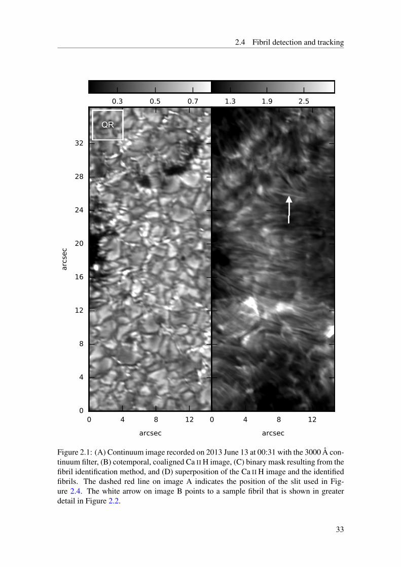
Figure 2.1: (A) Continuum image recorded on 2013 June 13 at 00:31 with the 3000 Å con-tinuum filter, (B) cotemporal, coaligned Ca II H image, (C) binary mask resulting from thefibril identification method, and (D) superposition of the Ca II H image and the identifiedfibrils. The dashed red line on image A indicates the position of the slit used in Fig-ure 2.4. The white arrow on image B points to a sample fibril that is shown in greaterdetail in Figure 2.2.
33
2 Paper I- Morphological properties of Ca II H slender fibrils
in Figure 2.1 B. To perform this identification we apply a series of image processing andcontrast enhancement techniques. We start by subtracting a boxcar-averaged version ofthe original image from itself to remove the low frequencies and to enhance the structurewith the typical dimensions of the fibrils. The size of the boxcar window is set to 20pixels, corresponding to approximately 0′′.4. Then, we apply a sharpening filter usingthe UNSHARP_MASK function from the Interactive Data Language (IDL, Exelis VisualInformation Solutions, Boulder, CO) to increase the global image contrast. This unsharpmask involves the following steps: (i) the original image is smoothed with a Gaussianfilter having a width of 10 pixels; (ii) this smoothed image is then subtracted from theoriginal image; and (iii) the resulting difference image is again added to the originalimage. In a next step, an adaptive histogram equalization is performed, described indetail by Pizer et al. (1987), again using the implementation in IDL (version 8.3) with thestandard parameter settings to further increase the contrast. Finally, we apply a boxcarsmoothing with a width of 3 pixels to remove frequencies beyond the spatial resolution ofSUNRISE, introduced by the steps described above.
The resulting contrast-enhanced images highlight most of the fibrils very well andallow the application of a binary mask with a threshold of 50% of its maximum intensity,separating the fibrils from their surroundings. The same threshold was used for the entireFOV of SUFI and for all frames in the time series, ensuring an unbiased determination ofthe length, width and shape of the identified fibrils.
Finally, we exclude all detected regions smaller than 200 pixels in area (correspondingto ≈0.1 arcsec2), which is approximately the area of a circle corresponding to a spatialresolution element close to the diffraction limit. An example of such a binary mask re-sulting from this process is shown in Figure 2.1 C.
The next step is to track individual fibrils in time to analyze their evolution. For thistask we take six consecutive frames and identify those regions where the binary maskmarks the presence of a fibril in at least 10 pixels at the same image position in at leastfive out of a total of six consecutive frames. After this, we assign each fibril a trackingindex. Then we advance one frame and repeat the same analysis, checking whether eachnewly identified fibril already has a tracking index. If so, it is counted as the temporalcontinuation of the fibril from the previous frame; if not, it is counted as a new fibril.
This method ensures, with a high level of confidence, that we catch the temporalevolution of individual fibrils. The method works very well for nicely separated fibrils,but it has some limitations in two special cases: (i) if a significant number of other fibrilscross the identified fibril, the binary mask will show either interruptions or the crossingfibrils are counted toward the identified fibril, and (ii) if the identified fibril has a hightransverse velocity (i.e., perpendicular to the fibril axis), it will move out of the detectionwindow in the next frame. The latter effect is particularly important in the regions ofmagnetic flux emergence (near x = 12′′, y = 9′′) where the fibrils are much more dynamicthan in the rest of the SUFI FOV.
Due to the large density of fibrils, about 80% of those detected fibrils suffer from thepresence of crossing or very close neighboring fibrils. The identified fibril and those cross-ing it are often misidentified as a single structure with a complex, frayed shape insteadof the expected linear, elongated one identified by the white arrow in Figure 2.1. If sucha complex shape does exist over several consecutive frames, a correct fibril identificationusing a binary mask is nearly impossible.
34
2.5 Fibril morphology
To address this problem we introduce the concept of a fibril’s reference backbone,which we define as the second-order polynomial best fitting the long axis of the fibriland therefore marking the ridge of maximum brightness. It is computed by first reducingthe fibril in every frame of the time series of Ca II H images to a shape that is a singlepixel in width. Each such pixel is equidistant from the fibril’s lateral boundaries (whichare the locations where the brightness drops below the threshold). The set of all such(single) pixels constitute the fibril’s backbone. Afterwards, the fibrils of the individualframes are fitted with a second-order polynomial. This polynomial is extended by theaverage width of this fibril (see Sect. 2.5.2), on both end points of the fibril to compensatefor the shortening due to the reduction of the fibril to a single pixel line. The resultingcurve we define as the reference backbone. Fibrils of complex shape, often produced byintersecting fibrils or by not well separated fibrils, are usually poorly fitted (χ2 valuesare higher than 6), and are excluded from this averaging. An example of this process isillustrated in Figure 2.2, where we show one identified fibril and its temporal evolution(left panels) and the overplotted fibril backbone (black line, right panels). The gray shadedarea around the skeleton displays the width of the fibril, computed in every single frameusing the method described inSect. 2.5.2.
The fibril is well identified in all six plotted time steps. However, its length may wellbe underestimated, as the detection method often fails to follow the fibril to its very end, ascan be seen by eye. Fibrils often become too faint near their ends to be reliably identifiedby our method. Being faint, they are also susceptible to interference from backgroundstructure and crossings by other fibrils. We have therefore not attempted to extend thelengths of the individual fibrils. Instead, we consider that the fibrils that we have identifiedare often in fact fibril fragments (see Pietarila et al. 2009), i.e., parts of longer fibrils. Forbrevity we will continue to call them fibrils (or SCFs) in the following, although in manycases we may be discussing only parts of the full fibrils.
We obtain a total of 598 fibrils in the SUFI FOV over the entire time series. Onesnapshot with the identified fibrils overlayed on top of the corresponding Ca II H image ispresented in panel D of Figure 2.1.
2.5 Fibril morphologyThe result of the fibril tracking allows for a statistical analysis of the SCFs and to computeseveral of their morphological properties. In this section we present the results obtainedfor lifetime, length, width, and curvature of SCFs extracted using information obtainedfrom the detection and tracking methods.
2.5.1 Lifetime
Visual inspection of the movie created from the time series of SUFI images (see onlinematerial, sufi.mp4) reveals the highly dynamical nature of the SCFs. The identificationof the individual fibrils over multiple time steps allows us to produce a lifetime histogramwith a lower limit of 35 s (corresponding to five consecutive frames, which is the mini-mum length of time we require for a fibril to survive to be identified as such) and an upperlimit given by the length of the time series (57 minutes). Only fibrils with a defined start-
35
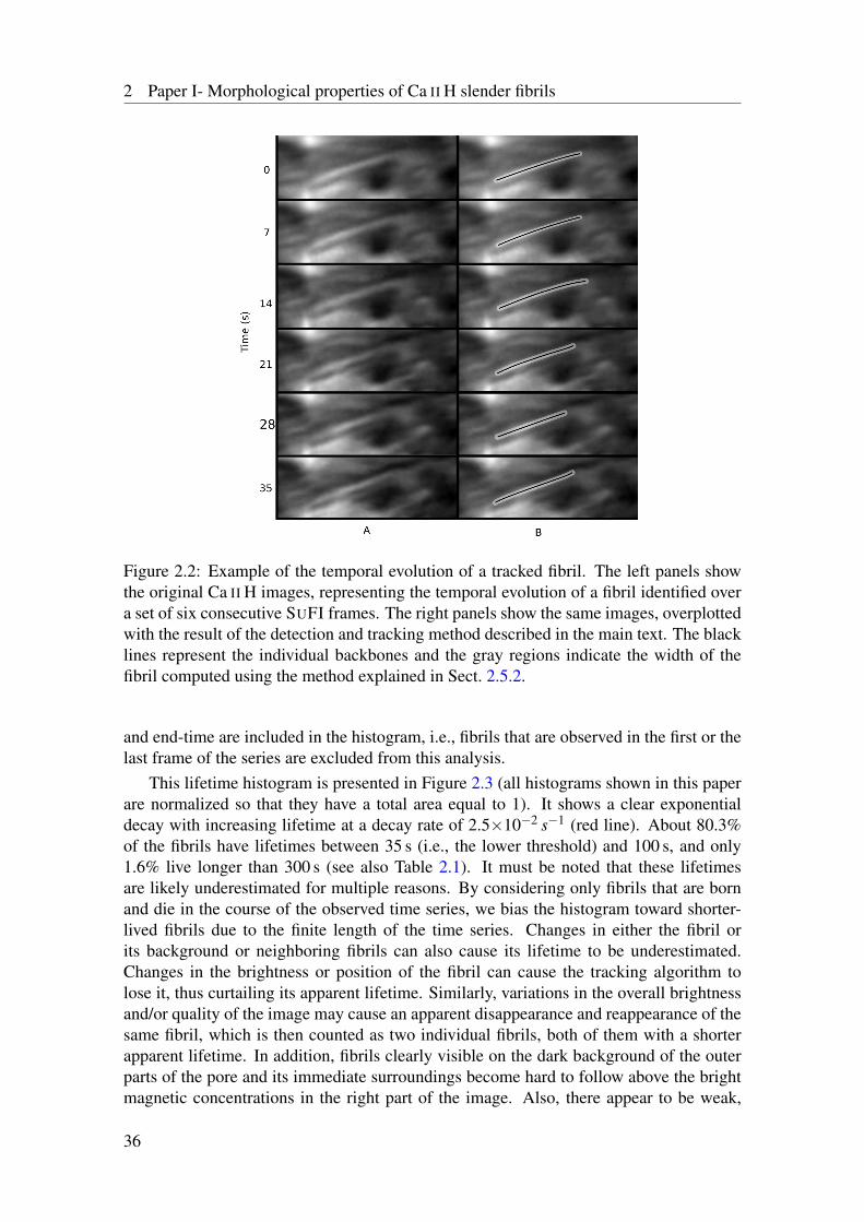
2 Paper I- Morphological properties of Ca II H slender fibrils
Figure 2.2: Example of the temporal evolution of a tracked fibril. The left panels showthe original Ca II H images, representing the temporal evolution of a fibril identified overa set of six consecutive SUFI frames. The right panels show the same images, overplottedwith the result of the detection and tracking method described in the main text. The blacklines represent the individual backbones and the gray regions indicate the width of thefibril computed using the method explained in Sect. 2.5.2.
and end-time are included in the histogram, i.e., fibrils that are observed in the first or thelast frame of the series are excluded from this analysis.
This lifetime histogram is presented in Figure 2.3 (all histograms shown in this paperare normalized so that they have a total area equal to 1). It shows a clear exponentialdecay with increasing lifetime at a decay rate of 2.5×10⁻² s−1 (red line). About 80.3%of the fibrils have lifetimes between 35 s (i.e., the lower threshold) and 100 s, and only1.6% live longer than 300 s (see also Table 2.1). It must be noted that these lifetimesare likely underestimated for multiple reasons. By considering only fibrils that are bornand die in the course of the observed time series, we bias the histogram toward shorter-lived fibrils due to the finite length of the time series. Changes in either the fibril orits background or neighboring fibrils can also cause its lifetime to be underestimated.Changes in the brightness or position of the fibril can cause the tracking algorithm tolose it, thus curtailing its apparent lifetime. Similarly, variations in the overall brightnessand/or quality of the image may cause an apparent disappearance and reappearance of thesame fibril, which is then counted as two individual fibrils, both of them with a shorterapparent lifetime. In addition, fibrils clearly visible on the dark background of the outerparts of the pore and its immediate surroundings become hard to follow above the brightmagnetic concentrations in the right part of the image. Also, there appear to be weak,
36
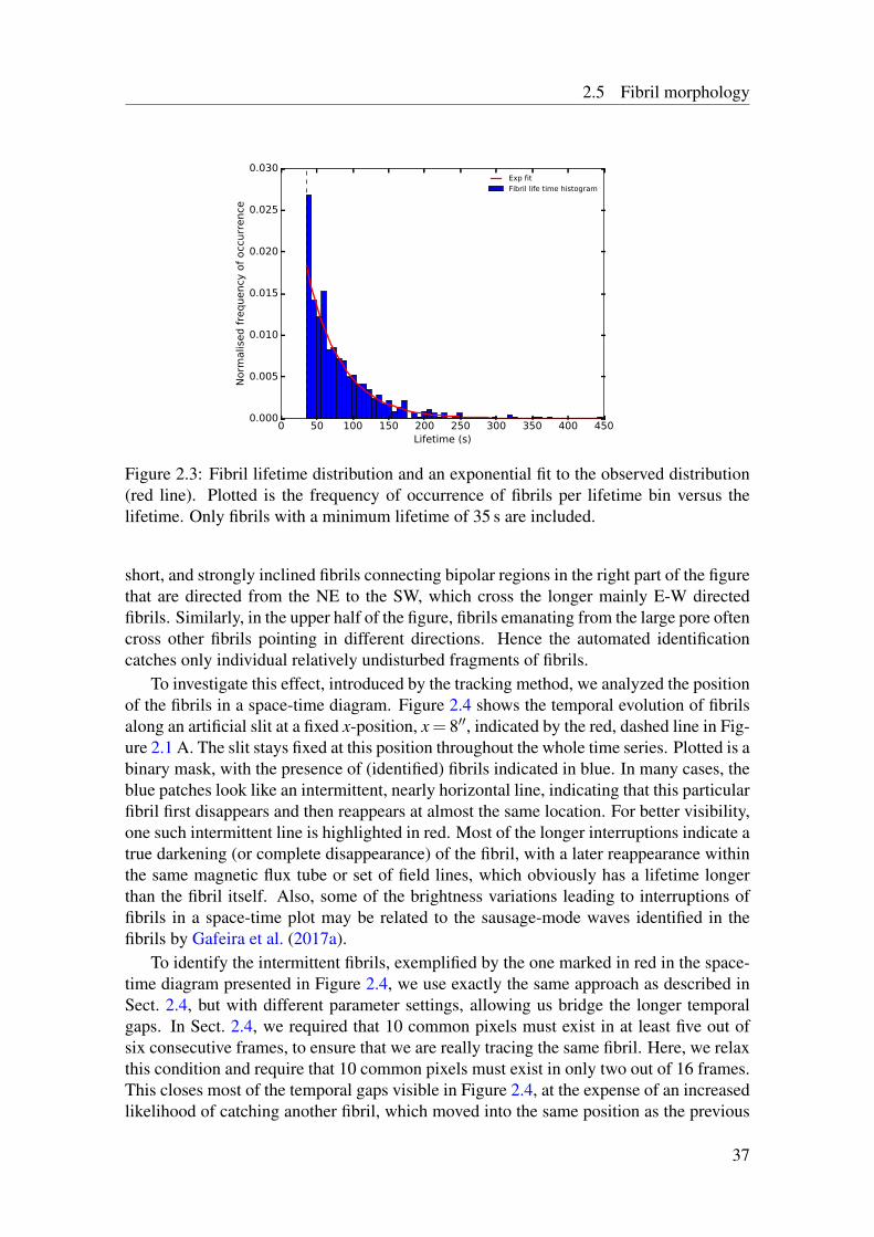
2.5 Fibril morphology
0 50 100 150 200 250 300 350 400 450Lifetime (s)
0.000
0.005
0.010
0.015
0.020
0.025
0.030
Norm
alised frequency of occurrence
Exp fit
Fibril life time histogram
Figure 2.3: Fibril lifetime distribution and an exponential fit to the observed distribution(red line). Plotted is the frequency of occurrence of fibrils per lifetime bin versus thelifetime. Only fibrils with a minimum lifetime of 35 s are included.
short, and strongly inclined fibrils connecting bipolar regions in the right part of the figurethat are directed from the NE to the SW, which cross the longer mainly E-W directedfibrils. Similarly, in the upper half of the figure, fibrils emanating from the large pore oftencross other fibrils pointing in different directions. Hence the automated identificationcatches only individual relatively undisturbed fragments of fibrils.
To investigate this effect, introduced by the tracking method, we analyzed the positionof the fibrils in a space-time diagram. Figure 2.4 shows the temporal evolution of fibrilsalong an artificial slit at a fixed x-position, x = 8′′, indicated by the red, dashed line in Fig-ure 2.1 A. The slit stays fixed at this position throughout the whole time series. Plotted is abinary mask, with the presence of (identified) fibrils indicated in blue. In many cases, theblue patches look like an intermittent, nearly horizontal line, indicating that this particularfibril first disappears and then reappears at almost the same location. For better visibility,one such intermittent line is highlighted in red. Most of the longer interruptions indicate atrue darkening (or complete disappearance) of the fibril, with a later reappearance withinthe same magnetic flux tube or set of field lines, which obviously has a lifetime longerthan the fibril itself. Also, some of the brightness variations leading to interruptions offibrils in a space-time plot may be related to the sausage-mode waves identified in thefibrils by Gafeira et al. (2017a).
To identify the intermittent fibrils, exemplified by the one marked in red in the space-time diagram presented in Figure 2.4, we use exactly the same approach as described inSect. 2.4, but with different parameter settings, allowing us bridge the longer temporalgaps. In Sect. 2.4, we required that 10 common pixels must exist in at least five out ofsix consecutive frames, to ensure that we are really tracing the same fibril. Here, we relaxthis condition and require that 10 common pixels must exist in only two out of 16 frames.This closes most of the temporal gaps visible in Figure 2.4, at the expense of an increasedlikelihood of catching another fibril, which moved into the same position as the previous
37
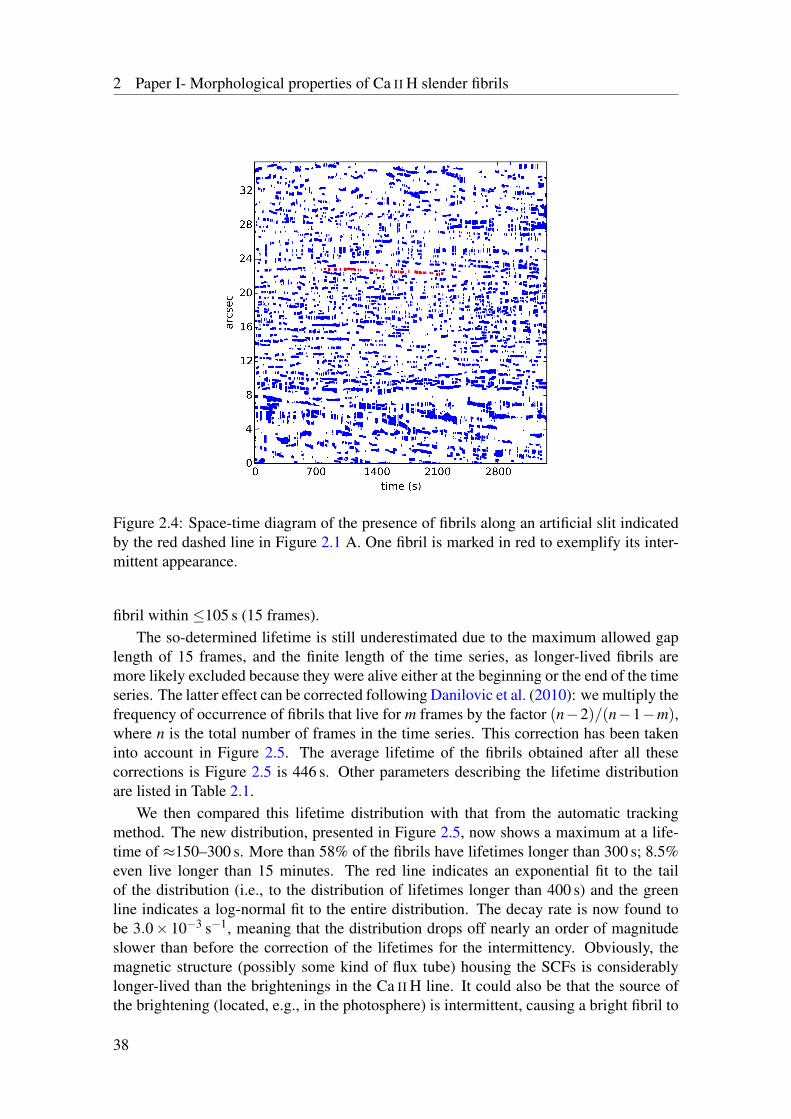
2 Paper I- Morphological properties of Ca II H slender fibrils
Figure 2.4: Space-time diagram of the presence of fibrils along an artificial slit indicatedby the red dashed line in Figure 2.1 A. One fibril is marked in red to exemplify its inter-mittent appearance.
fibril within ≤105 s (15 frames).The so-determined lifetime is still underestimated due to the maximum allowed gap
length of 15 frames, and the finite length of the time series, as longer-lived fibrils aremore likely excluded because they were alive either at the beginning or the end of the timeseries. The latter effect can be corrected following Danilovic et al. (2010): we multiply thefrequency of occurrence of fibrils that live for m frames by the factor (n−2)/(n−1−m),where n is the total number of frames in the time series. This correction has been takeninto account in Figure 2.5. The average lifetime of the fibrils obtained after all thesecorrections is Figure 2.5 is 446 s. Other parameters describing the lifetime distributionare listed in Table 2.1.
We then compared this lifetime distribution with that from the automatic trackingmethod. The new distribution, presented in Figure 2.5, now shows a maximum at a life-time of ≈150–300 s. More than 58% of the fibrils have lifetimes longer than 300 s; 8.5%even live longer than 15 minutes. The red line indicates an exponential fit to the tailof the distribution (i.e., to the distribution of lifetimes longer than 400 s) and the greenline indicates a log-normal fit to the entire distribution. The decay rate is now found tobe 3.0× 10⁻³ s−1, meaning that the distribution drops off nearly an order of magnitudeslower than before the correction of the lifetimes for the intermittency. Obviously, themagnetic structure (possibly some kind of flux tube) housing the SCFs is considerablylonger-lived than the brightenings in the Ca II H line. It could also be that the source ofthe brightening (located, e.g., in the photosphere) is intermittent, causing a bright fibril to
38
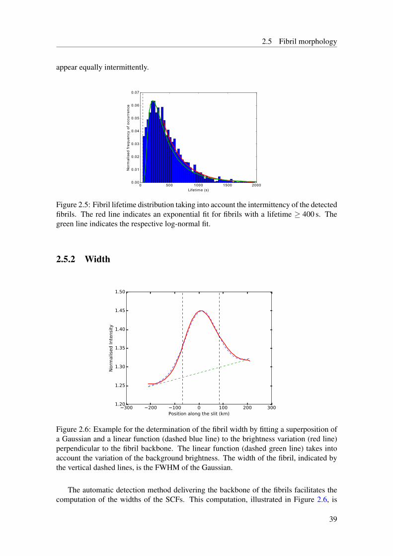
2.5 Fibril morphology
appear equally intermittently.
Figure 2.5: Fibril lifetime distribution taking into account the intermittency of the detectedfibrils. The red line indicates an exponential fit for fibrils with a lifetime ≥ 400 s. Thegreen line indicates the respective log-normal fit.
2.5.2 Width
Figure 2.6: Example for the determination of the fibril width by fitting a superposition ofa Gaussian and a linear function (dashed blue line) to the brightness variation (red line)perpendicular to the fibril backbone. The linear function (dashed green line) takes intoaccount the variation of the background brightness. The width of the fibril, indicated bythe vertical dashed lines, is the FWHM of the Gaussian.
The automatic detection method delivering the backbone of the fibrils facilitates thecomputation of the widths of the SCFs. This computation, illustrated in Figure 2.6, is
39
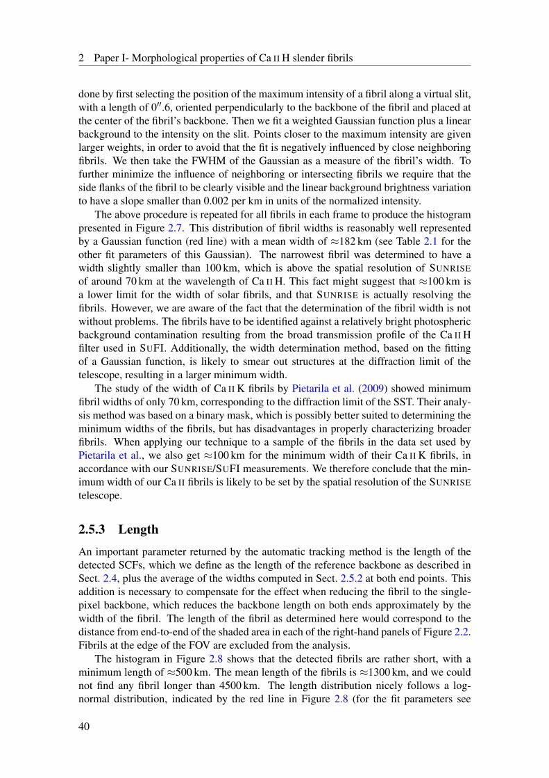
2 Paper I- Morphological properties of Ca II H slender fibrils
done by first selecting the position of the maximum intensity of a fibril along a virtual slit,with a length of 0′′.6, oriented perpendicularly to the backbone of the fibril and placed atthe center of the fibril’s backbone. Then we fit a weighted Gaussian function plus a linearbackground to the intensity on the slit. Points closer to the maximum intensity are givenlarger weights, in order to avoid that the fit is negatively influenced by close neighboringfibrils. We then take the FWHM of the Gaussian as a measure of the fibril’s width. Tofurther minimize the influence of neighboring or intersecting fibrils we require that theside flanks of the fibril to be clearly visible and the linear background brightness variationto have a slope smaller than 0.002 per km in units of the normalized intensity.
The above procedure is repeated for all fibrils in each frame to produce the histogrampresented in Figure 2.7. This distribution of fibril widths is reasonably well representedby a Gaussian function (red line) with a mean width of ≈182 km (see Table 2.1 for theother fit parameters of this Gaussian). The narrowest fibril was determined to have awidth slightly smaller than 100 km, which is above the spatial resolution of SUNRISE
of around 70 km at the wavelength of Ca II H. This fact might suggest that ≈100 km isa lower limit for the width of solar fibrils, and that SUNRISE is actually resolving thefibrils. However, we are aware of the fact that the determination of the fibril width is notwithout problems. The fibrils have to be identified against a relatively bright photosphericbackground contamination resulting from the broad transmission profile of the Ca II Hfilter used in SUFI. Additionally, the width determination method, based on the fittingof a Gaussian function, is likely to smear out structures at the diffraction limit of thetelescope, resulting in a larger minimum width.
The study of the width of Ca II K fibrils by Pietarila et al. (2009) showed minimumfibril widths of only 70 km, corresponding to the diffraction limit of the SST. Their analy-sis method was based on a binary mask, which is possibly better suited to determining theminimum widths of the fibrils, but has disadvantages in properly characterizing broaderfibrils. When applying our technique to a sample of the fibrils in the data set used byPietarila et al., we also get ≈100 km for the minimum width of their Ca II K fibrils, inaccordance with our SUNRISE/SUFI measurements. We therefore conclude that the min-imum width of our Ca II fibrils is likely to be set by the spatial resolution of the SUNRISE
telescope.
2.5.3 LengthAn important parameter returned by the automatic tracking method is the length of thedetected SCFs, which we define as the length of the reference backbone as described inSect. 2.4, plus the average of the widths computed in Sect. 2.5.2 at both end points. Thisaddition is necessary to compensate for the effect when reducing the fibril to the single-pixel backbone, which reduces the backbone length on both ends approximately by thewidth of the fibril. The length of the fibril as determined here would correspond to thedistance from end-to-end of the shaded area in each of the right-hand panels of Figure 2.2.Fibrils at the edge of the FOV are excluded from the analysis.
The histogram in Figure 2.8 shows that the detected fibrils are rather short, with aminimum length of ≈500 km. The mean length of the fibrils is ≈1300 km, and we couldnot find any fibril longer than 4500 km. The length distribution nicely follows a log-normal distribution, indicated by the red line in Figure 2.8 (for the fit parameters see
40
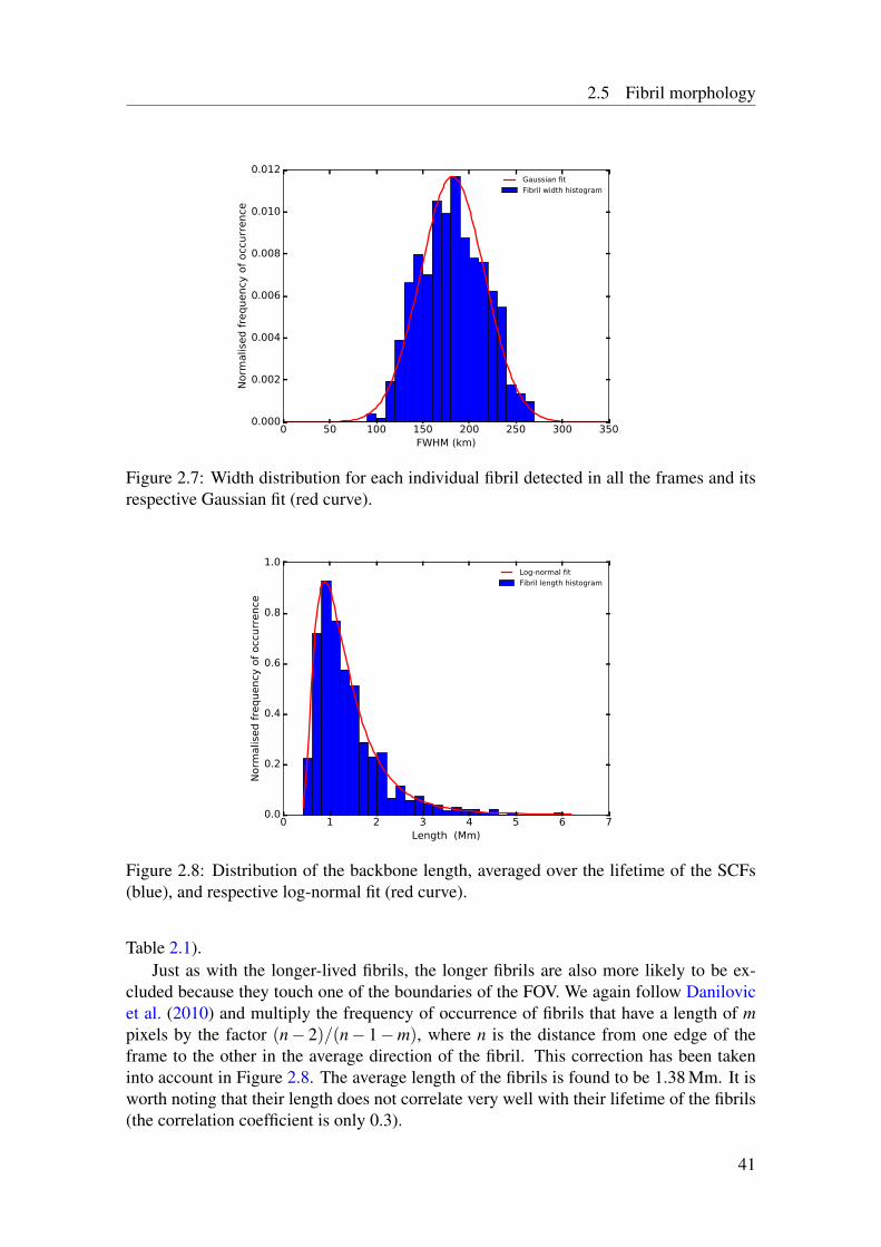
2.5 Fibril morphology
0 50 100 150 200 250 300 350FWHM (km)
0.000
0.002
0.004
0.006
0.008
0.010
0.012
Norm
alised frequency of occurrence
Gaussian fit
Fibril width histogram
Figure 2.7: Width distribution for each individual fibril detected in all the frames and itsrespective Gaussian fit (red curve).
0 1 2 3 4 5 6 7Length (Mm)
0.0
0.2
0.4
0.6
0.8
1.0
Norm
alis
ed fre
quency
of occ
urr
ence
Log-normal fit
Fibril length histogram
Figure 2.8: Distribution of the backbone length, averaged over the lifetime of the SCFs(blue), and respective log-normal fit (red curve).
Table 2.1).Just as with the longer-lived fibrils, the longer fibrils are also more likely to be ex-
cluded because they touch one of the boundaries of the FOV. We again follow Danilovicet al. (2010) and multiply the frequency of occurrence of fibrils that have a length of mpixels by the factor (n− 2)/(n− 1−m), where n is the distance from one edge of theframe to the other in the average direction of the fibril. This correction has been takeninto account in Figure 2.8. The average length of the fibrils is found to be 1.38 Mm. It isworth noting that their length does not correlate very well with their lifetime of the fibrils(the correlation coefficient is only 0.3).
41
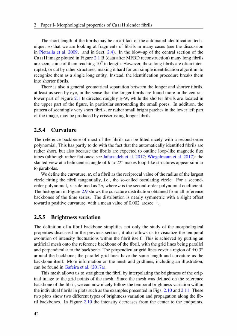
2 Paper I- Morphological properties of Ca II H slender fibrils
The short length of the fibrils may be an artifact of the automated identification tech-nique, so that we are looking at fragments of fibrils in many cases (see the discussionin Pietarila et al. 2009, and in Sect. 2.4). In the blow-up of the central section of theCa II H image plotted in Figure 2.1 B (data after MFBD reconstruction) many long fibrilsare seen, some of them reaching 10′′ in length. However, these long fibrils are often inter-rupted, or cut by other structures, making it hard for our simple identification algorithm torecognize them as a single long entity. Instead, the identification procedure breaks theminto shorter fibrils.
There is also a general geometrical separation between the longer and shorter fibrils,at least as seen by eye, in the sense that the longer fibrils are found more in the central-lower part of Figure 2.1 B directed roughly E-W, while the shorter fibrils are located inthe upper part of the figure, in particular surrounding the small pores. In addition, thepattern of seemingly very short fibrils, or rather small bright patches in the lower left partof the image, may be produced by crisscrossing longer fibrils.
2.5.4 CurvatureThe reference backbone of most of the fibrils can be fitted nicely with a second-orderpolynomial. This has partly to do with the fact that the automatically identified fibrils arerather short, but also because the fibrils are expected to outline loop-like magnetic fluxtubes (although rather flat ones; see Jafarzadeh et al. 2017; Wiegelmann et al. 2017): theslanted view at a heliocentric angle of θ ≈ 22 makes loop-like structures appear similarto parabolas.
We define the curvature, κ , of a fibril as the reciprocal value of the radius of the largestcircle fitting the fibril tangentially, i.e., the so-called osculating circle. For a second-order polynomial, κ is defined as 2a, where a is the second-order polynomial coefficient.The histogram in Figure 2.9 shows the curvature distribution obtained from all referencebackbones of the time series. The distribution is nearly symmetric with a slight offsettoward a positive curvature, with a mean value of 0.002 arcsec−1.
2.5.5 Brightness variationThe definition of a fibril backbone simplifies not only the study of the morphologicalproperties discussed in the previous section, it also allows us to visualize the temporalevolution of intensity fluctuations within the fibril itself. This is achieved by putting anartificial mesh onto the reference backbone of the fibril, with the grid lines being paralleland perpendicular to the backbone. The perpendicular grid lines cover a region of ±0.3′′
around the backbone; the parallel grid lines have the same length and curvature as thebackbone itself. More information on the mesh and gridlines, including an illustration,can be found in Gafeira et al. (2017a).
This mesh allows us to straighten the fibril by interpolating the brightness of the orig-inal image to the grid points of the mesh. Since the mesh was defined on the referencebackbone of the fibril, we can now nicely follow the temporal brightness variation withinthe individual fibrils in plots such as the examples presented in Figs. 2.10 and 2.11. Thesetwo plots show two different types of brightness variation and propagation along the fib-ril backbones. In Figure 2.10 the intensity decreases from the center to the endpoints,
42
2.5 Fibril morphology
−0.06 −0.04 −0.02 0.00 0.02 0.04 0.06Curvature (1/arcsec)
0
10
20
30
40
50
60
Norm
alised frequency of occurrence
Fibril curvature histogram
Figure 2.9: Curvature distribution of the fibril’s reference backbones.
whereas in Figure 2.11 the intensity decreases from the endpoints of the fibril to its cen-ter. After visual inspection of all fibrils we find that the first type is the more common(around 54% of the the fibrils are of this type), and the second type is observed in ≈25%of the fibrils. For the remaining ≈21% of the fibrils it is difficult to clearly categorize thedistribution of the brightness along the fibril axis, with only a very small fraction of thoseshowing a brightening at one endpoint only. We could not find any obvious correlationbetween the type of the brightening (central or endpoint) with other parameters of thefibrils (length, width, absolute value, lifetime). It can also be seen that the width of thefibrils is not constant along the the length of the fibril. In general, the fibrils are broaderat the locations where they are also brighter.
Note that in some cases, a fibril changes from having its brightness peak at its centerto having it near its ends. Obviously, the brightness of the fibril varies with time, as can beseen in Figs. 2.10 and 2.11. Gafeira et al. (2017a) have pointed out that these variationsare often periodic and occur mainly in (anti-)phase with oscillations in the width of thefibril. They identified these variations with sausage-mode waves.
43
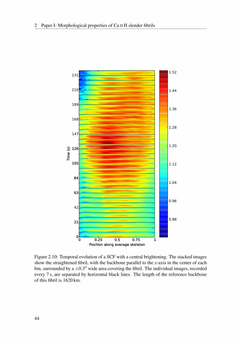
2 Paper I- Morphological properties of Ca II H slender fibrils
Figure 2.10: Temporal evolution of a SCF with a central brightening. The stacked imagesshow the straightened fibril, with the backbone parallel to the x-axis in the center of eachbin, surrounded by a±0.3′′ wide area covering the fibril. The individual images, recordedevery 7 s, are separated by horizontal black lines. The length of the reference backboneof this fibril is 1620 km.
44
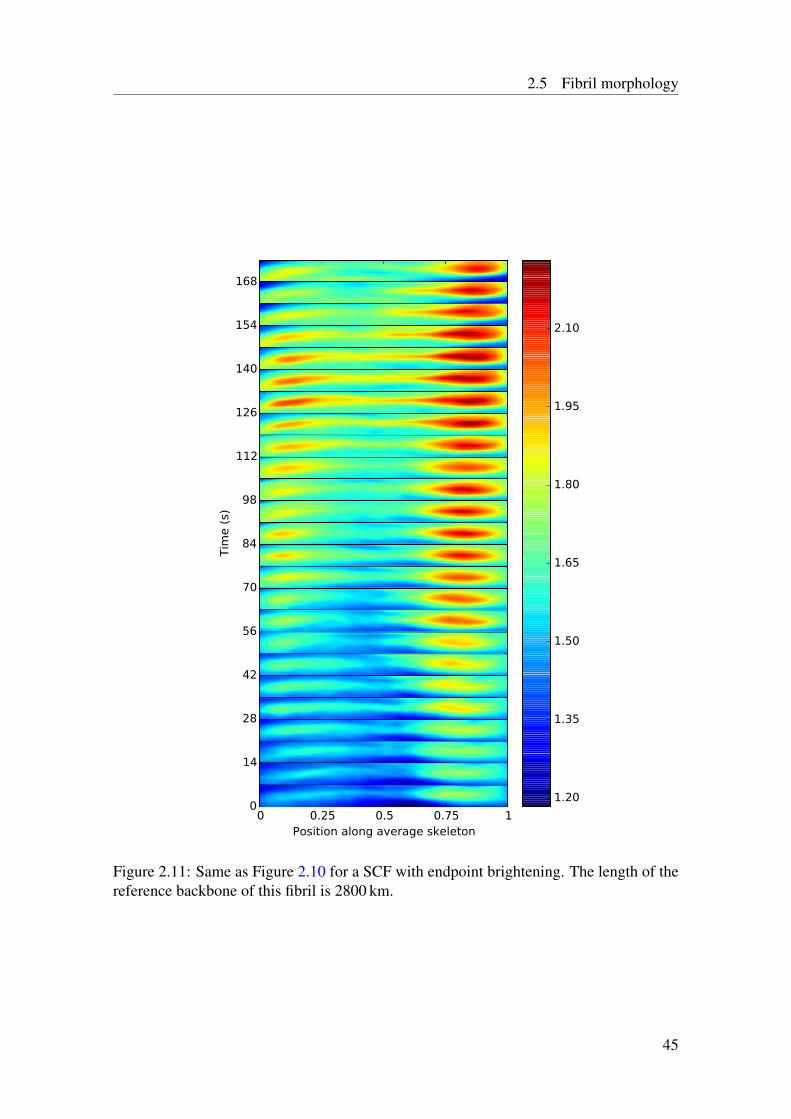
2.5 Fibril morphology
Figure 2.11: Same as Figure 2.10 for a SCF with endpoint brightening. The length of thereference backbone of this fibril is 2800 km.
45
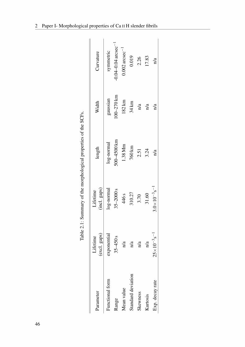
2 Paper I- Morphological properties of Ca II H slender fibrils
Tabl
e2.
1:Su
mm
ary
ofth
em
orph
olog
ical
prop
ertie
sof
the
SCFs
.
Para
met
erL
ifet
ime
(exc
l.ga
ps)
Lif
etim
e(i
ncl.
gaps
)le
ngth
Wid
thC
urva
ture
Func
tiona
lfor
mex
pone
ntia
llo
g-no
rmal
log-
norm
alga
ussi
ansy
mm
etri
c
Ran
ge35
–450
s35
–200
0s
500–
4500
km10
0–27
0km
-0.0
4–0.
04ar
csec−
1
Mea
nva
lue
n/a
446
s1.
38M
m18
2km
0.00
2ar
csec−
1
Stan
dard
devi
atio
nn/
a31
0.27
760
km34
km0.
019
Skew
ness
n/a
3.70
2.51
n/a
2.26
Kur
tosi
sn/
a31
.60
3.24
n/a
17.8
3
Exp
.dec
ayra
te25×
10−
3 s−1
3.0×
10−
3 s−1
n/a
n/a
n/a
46
2.6 Discussion and conclusions
2.6 Discussion and conclusions
In this paper we present a first quantitative study of the morphological properties ofSCFs aimed at measuring their parameters, such as lifetime, length, width, curvature,and brightness structure. We apply an automatic fibril detection algorithm based on sev-eral unsharp masking steps to identify the backbone of the fibrils (i.e., the curve followingthe central brightness ridge along the long-axis of the SCF). This allows us to identify,measure properties of, and perform a statistical analysis on 598 SCFs. We obtain valuesfor the lifetime between half a minute and half an hour (when taking into account theintermittency in fibril visibility), lengths between 0.5 and 4.5 Mm, and widths between100 and 270 km. The fibrils show a wide distribution of curvatures, with a slight pref-erence for a positive curvature, in agreement with the expected curvatures of low-lyingloops observed at a position away from the solar disk center. We also identify two dif-ferent morphologies of the evolution of the brightness within individual fibrils. In onetype the intensity increases starting from the center and moving to the edges, while in theother type the increase in intensity first becomes visible near one or both of the ends andexpands from there toward the center of the fibril.
Intersecting fibrils and not well separated fibrils cause problems in the automatictracking them, mainly leading to a failure in detecting fibrils longer than 4.5 Mm, al-though the visual inspection of the SUFI Ca II H images shows that such fibrils do exist.The contrast between the measured short lengths and the pattern of extended fibrils inparts of the SUFI FOV suggests that the automated technique is identifying relativelyundisturbed parts of fibrils as whole fibrils. Between these undisturbed fragments a givenlong fibril may be intersected by other fibrils, or disturbed by underlying bright points,reversed granulation, and acoustic grains. This complex picture may arise because at theheight of the SCFs, the Ca II H line may not be entirely optically thick, so that radiationfrom below can pass through possibly multiple layers of fibrils. This may have to do withthe 1.1 Å FWHM of the filter employed by SUFI, which includes not just the H2 and H3features of the line core, but also parts of the inner wings. The H2 and H3 features samplethe lower to middle chromosphere, while the inner wings are mainly sensitive to the upperphotosphere (see the heights of formation computed by Danilovic et al. 2014; Jafarzadehet al. 2017).
The results of the present analysis allow us to relate SCFs to small-scale elongated,chromospheric structures already known from the literature. In Table 2.2 we list the prop-erties of the SCFs together with those of type I and type II spicules (from Pereira et al.2012), and of Ca II K fibrils (as deduce by Pietarila et al. 2009). Spicules show consid-erable similarities to the SCFs with regard to the range of widths (although the Ca fibrilsstudied by us and, in particular, those by Pietarila et al. are on average narrower).
The difference in width between the fibrils seen by Pietarila et al. in Ca II K and thosestudied by us in Ca II H is puzzling. It has at least partly to do with the difference intechnique, as the application of our technique to a sample of fibrils identified by Pietarilaet al. (2009) returns larger widths than those found by those authors. Other factors mayalso contribute to the difference in width. Thus, it may have to do with different opticalthicknesses, or that our observations were recorded in a larger, more intensely activeregion.
Both types of known spicules are considerably longer than our SCFs, with even the
47
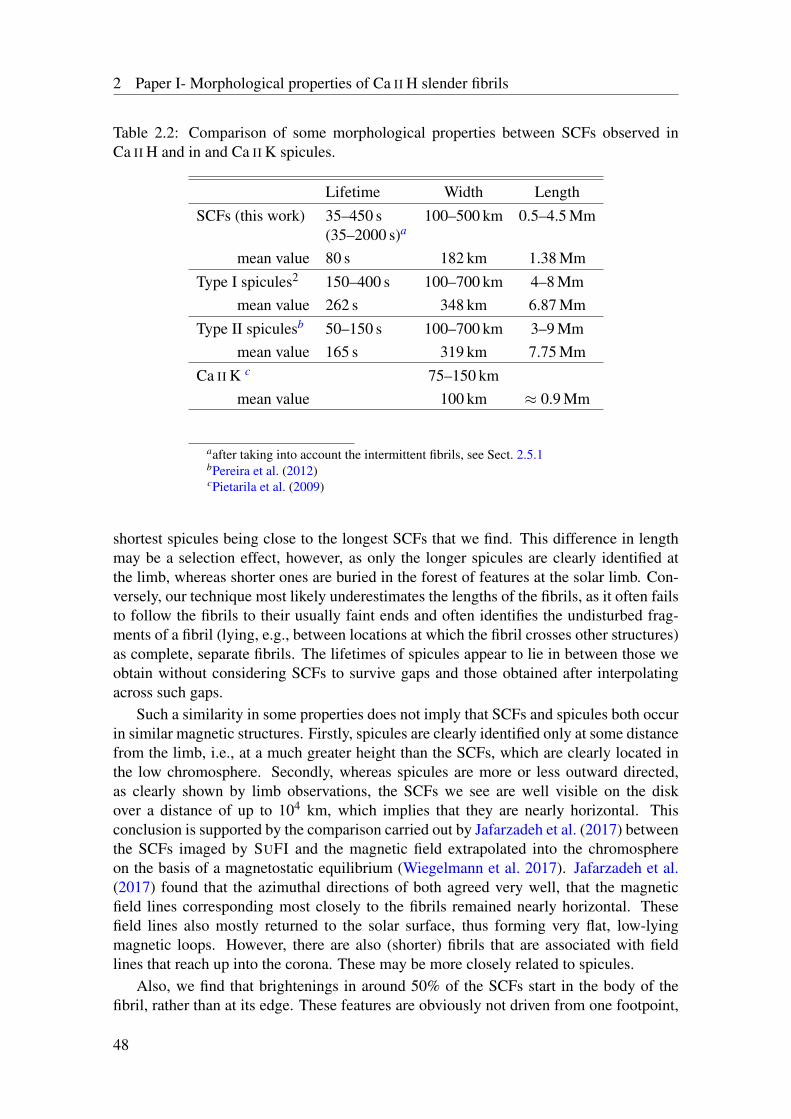
2 Paper I- Morphological properties of Ca II H slender fibrils
Table 2.2: Comparison of some morphological properties between SCFs observed inCa II H and in and Ca II K spicules.
Lifetime Width LengthSCFs (this work) 35–450 s
(35–2000 s)a100–500 km 0.5–4.5 Mm
mean value 80 s 182 km 1.38 MmType I spicules2 150–400 s 100–700 km 4–8 Mm
mean value 262 s 348 km 6.87 MmType II spiculesb 50–150 s 100–700 km 3–9 Mm
mean value 165 s 319 km 7.75 MmCa II K c 75–150 km
mean value 100 km ≈ 0.9 Mm
aafter taking into account the intermittent fibrils, see Sect. 2.5.1bPereira et al. (2012)cPietarila et al. (2009)
shortest spicules being close to the longest SCFs that we find. This difference in lengthmay be a selection effect, however, as only the longer spicules are clearly identified atthe limb, whereas shorter ones are buried in the forest of features at the solar limb. Con-versely, our technique most likely underestimates the lengths of the fibrils, as it often failsto follow the fibrils to their usually faint ends and often identifies the undisturbed frag-ments of a fibril (lying, e.g., between locations at which the fibril crosses other structures)as complete, separate fibrils. The lifetimes of spicules appear to lie in between those weobtain without considering SCFs to survive gaps and those obtained after interpolatingacross such gaps.
Such a similarity in some properties does not imply that SCFs and spicules both occurin similar magnetic structures. Firstly, spicules are clearly identified only at some distancefrom the limb, i.e., at a much greater height than the SCFs, which are clearly located inthe low chromosphere. Secondly, whereas spicules are more or less outward directed,as clearly shown by limb observations, the SCFs we see are well visible on the diskover a distance of up to 104 km, which implies that they are nearly horizontal. Thisconclusion is supported by the comparison carried out by Jafarzadeh et al. (2017) betweenthe SCFs imaged by SUFI and the magnetic field extrapolated into the chromosphereon the basis of a magnetostatic equilibrium (Wiegelmann et al. 2017). Jafarzadeh et al.(2017) found that the azimuthal directions of both agreed very well, that the magneticfield lines corresponding most closely to the fibrils remained nearly horizontal. Thesefield lines also mostly returned to the solar surface, thus forming very flat, low-lyingmagnetic loops. However, there are also (shorter) fibrils that are associated with fieldlines that reach up into the corona. These may be more closely related to spicules.
Also, we find that brightenings in around 50% of the SCFs start in the body of thefibril, rather than at its edge. These features are obviously not driven from one footpoint,
48
2.6 Discussion and conclusions
as are jet-like structures such as spicules. For another ≈25% of the SCFs, the brightnessvariation is similar to that presented in Figure 2.11, with the two edge-points of the SCFbeing brighter than the central part, which is also not compatible with a jet-like structure,where only one end of the structure is rooted in the photosphere, from where it pointstoward the upper layers of the atmosphere. All this suggests that our SCFs are more likelyto outline small, loop-like structures, an interpretation which is also supported by theanalysis of the curvature computed in the Sect. 2.5.4. The brightness enhancement at bothends of the SCFs may be a result of a footpoint heating process, although the structuremay simply reflect the fact that the broad Ca filter of SUFI allows the photospheric brightpoints to shine through. This is very similar to the structures seen by Pietarila et al. (2009),who also found many of their narrow fibrils to be rooted in underlying bright points.
The radiation transmitted through the SUFI 1.1 Å Ca II H filter comes from either thephotosphere, or the lower chromosphere (average height of 600–700 km). This is veryclose to the limit of the small-scale canopies created by the granulation (Wedemeyer-Böhm et al. 2008), which are also found by Jafarzadeh et al. (2017) on the basis of themagnetohydrodynamic-simulation assisted Stokes inversion output of Riethmüller et al.(2017). Some of the shorter SCFs may indeed be associated with the small-scale granularcanopies, with possible similarities to the seething horizontal magnetic fields describedin Harvey et al. (2007), or the horizontal fields detected by Hinode (Lites et al. 2008)and SUNRISE (Danilovic et al. 2010). However, the longer SCFs are likely more closelyrelated the larger-scale canopy found over the network by Jones and Giovanelli (1982)and modeled by Solanki and Steiner (1990). Such extended horizontal field lines werefound lying nearly parallel to the SCFs in the magnetostatic equilibrium computed byWiegelmann et al. (2017).
49

3 Paper II- Oscillations on width andintensity of slender Ca II H fibrils1
3.1 AbstractWe report the detection of oscillations in slender Ca II H fibrils (SCFs) from high-reso-lution observations acquired with the SUNRISE balloon-borne solar observatory. TheSCFs show obvious oscillations in their intensity, but also their width. The oscillatorybehaviors are investigated at several positions along the axes of the SCFs. A large ma-jority of fibrils show signs of oscillations in intensity. Their periods and phase speeds areanalyzed using a wavelet analysis. The width and intensity perturbations have overlappingdistributions of the wave period.
The obtained distributions have median values of the period of 32± 17 s and 36±25 s, respectively. We find that the fluctuations of both parameters propagate in the SCFswith speeds of 11+49
−11 km s−1 and 15+34−15 km s−1, respectively. Furthermore, the width and
intensity oscillations have a strong tendency to be either in anti phase or, to a smallerextent, in phase. This suggests that the oscillations of both parameters are caused bythe same wave mode and that the waves are likely propagating. Taking all the evidencetogether, the most likely wave mode to explain all measurements and criteria is the fastsausage mode.
3.2 IntroductionMagnetohydrodynamic (MHD) waves have been observed in various plasma structuresin the solar atmosphere, particularly in elongated features in the solar chromosphere andin the corona (for recent reviews see, e.g., Banerjee et al. 2007; Zaqarashvili and Erdélyi2009; Mathioudakis et al. 2013; Jess et al. 2015). According to the theory of MHD os-cillations, the waves may appear as a single mode or as a combination of several modes(i.e., kink, sausage, torsional, or longitudinal) with distinct properties and different ob-servational signatures (Edwin and Roberts 1983). These waves are often excited at pho-tospheric heights (e.g. by granular buffeting, Evans and Roberts 1990, or vortex motion,Kitiashvili et al. 2011), and either propagate away from their source or form a standingoscillation.
1This chapter reproduces the article Morphological properties of Ca II H slender fibrils by R. Gafeira,S.Jafarzadeh,S. K. Solanki, A. Lagg, M. van Noort, P. Barthol, J. Blanco Rodríguez, J. C. del Toro Iniesta,A. Gandorfer, L. Gizon, J. Hirzberger, M. Knölker, D. Orozco Suárez, T. L. Riethmüller, and W. Schmidt,published in ApJS, 229, 2017, DOI 10.3847/1538-4365/229/1/7. Reproduced with permission of ApJS
51
3 Paper II- Oscillations on width and intensity of slender Ca II H fibrils
While transverse waves such as kink or global Alfvénic modes cause the swayingof a flux tube or of an elongated feature, sausage-mode oscillations result in a periodicaxisymmetric expansion and contraction of the structure at one position. Torsional ortwisting motions are associated with torsional Alfvén waves propagating along the axisof fibrillar structures (e.g., Spruit 1982; Solanki 1993a).
The different wave modes in elongated structures have been mostly observed at coro-nal heights in, e.g., coronal loops (e.g., Aschwanden et al. 1999; De Moortel et al. 2002;Wang et al. 2002; Wang and Solanki 2004; Tomczyk et al. 2007; Srivastava et al. 2008;Nakariakov et al. 2012, see Nakariakov and Verwichte 2005 for a review), as well as atthe upper chromospheric levels in features such as filaments, fibrils, mottles, and spicules(De Pontieu et al. 2007; Lin et al. 2007; Okamoto and De Pontieu 2011; Pietarila et al.2011; Tsiropoula et al. 2012).
Images recorded in the Ca II K passband (with a filter width of 1.5 Å) with the 1 mSwedish Solar Telescope (Scharmer et al. 2003b) in an active region close to the solar diskcenter revealed the presence of slender, bright fibrils, extending seemingly horizontallyin the lower chromosphere (Pietarila et al. 2009). Only recently, the second flight of the1-m balloon-borne solar observatory SUNRISE (Solanki et al. 2010; Barthol et al. 2011;Berkefeld et al. 2011; Solanki et al. 2017) provided us with a high quality, seeing-freetime-series of Ca II H images (with a filter width of 1.1 Å). The relatively long duration ofthe observations (one hour) in an active region (close to disk center) enabled a thoroughstudy of properties of the slender fibrils (Gafeira et al. 2017b). In addition, Jafarzadehet al. (2017) have found ubiquitous transverse waves in the slender Ca II H fibrils (SCFs)in SUNRISE data. The SCFs have been shown to map the magnetic fields in the lowsolar chromosphere (Jafarzadeh et al. 2017). Earlier, (Pietarila et al. 2009) had shownthat the fibrils, or the magnetic canopy outlined by them, either suppressed oscillations orchanneled low frequency oscillations into the chromosphere, depending on their location.
In this paper we investigate width and intensity oscillations in the SCFs observed withSUNRISE. Periods of the fluctuations in individual SCFs are determined and the phasespeed of the waves propagating along the thin structures are quantified (Sect. 3.4). Wediscuss our results in Sect. 3.5, where we also conclude that the observed oscillations arelikely manifestations of sausage waves traveling along the fibrils.
3.3 Observations
For the present study we use the data set described in Gafeira et al. (2017b), Jafarzadehet al. (2017), and Solanki et al. (2017). The data set includes high spatial and tempo-ral resolution observations of an active region obtained in the Ca II H passband (with afull width at half maximum, FWHM, of ≈ 1.1 Å) of the SUNRISE Filter Imager (SUFI,Gandorfer et al. 2011) on the 1-meter SUNRISE balloon-borne solar observatory (Solankiet al. 2010; Barthol et al. 2011; Berkefeld et al. 2011) during its second science flight(Solanki et al. 2017). The observations were obtained between 23:39 UT on 2013 June12 and 00:38 UT on 2013 June 13 with a cadence of 7 s. These observations covered apart of NOAA AR 11768, mainly its following polarity that was dominated by a series ofpores, some of which lie at least partly within the SUFI field-of-view (FOV). The FOValso contained a number of plage elements and two granulation-scale flux emergences
52
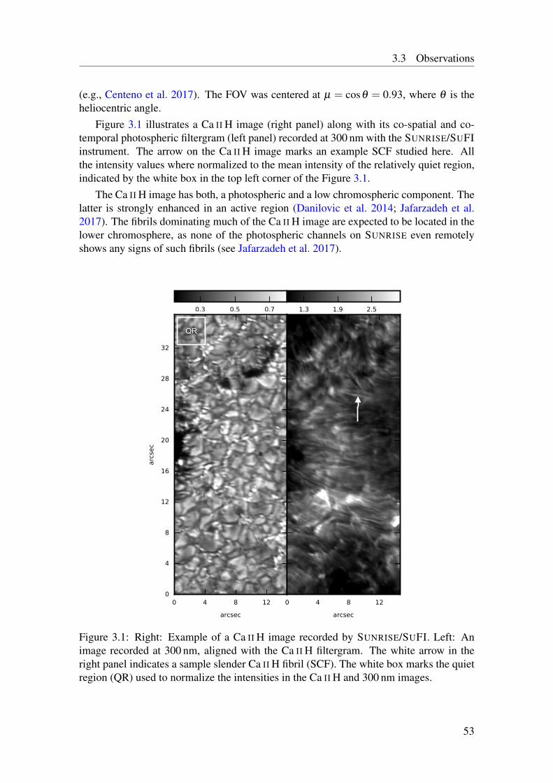
3.3 Observations
(e.g., Centeno et al. 2017). The FOV was centered at µ = cosθ = 0.93, where θ is theheliocentric angle.
Figure 3.1 illustrates a Ca II H image (right panel) along with its co-spatial and co-temporal photospheric filtergram (left panel) recorded at 300 nm with the SUNRISE/SUFIinstrument. The arrow on the Ca II H image marks an example SCF studied here. Allthe intensity values where normalized to the mean intensity of the relatively quiet region,indicated by the white box in the top left corner of the Figure 3.1.
The Ca II H image has both, a photospheric and a low chromospheric component. Thelatter is strongly enhanced in an active region (Danilovic et al. 2014; Jafarzadeh et al.2017). The fibrils dominating much of the Ca II H image are expected to be located in thelower chromosphere, as none of the photospheric channels on SUNRISE even remotelyshows any signs of such fibrils (see Jafarzadeh et al. 2017).
QR
Figure 3.1: Right: Example of a Ca II H image recorded by SUNRISE/SUFI. Left: Animage recorded at 300 nm, aligned with the Ca II H filtergram. The white arrow in theright panel indicates a sample slender Ca II H fibril (SCF). The white box marks the quietregion (QR) used to normalize the intensities in the Ca II H and 300 nm images.
53
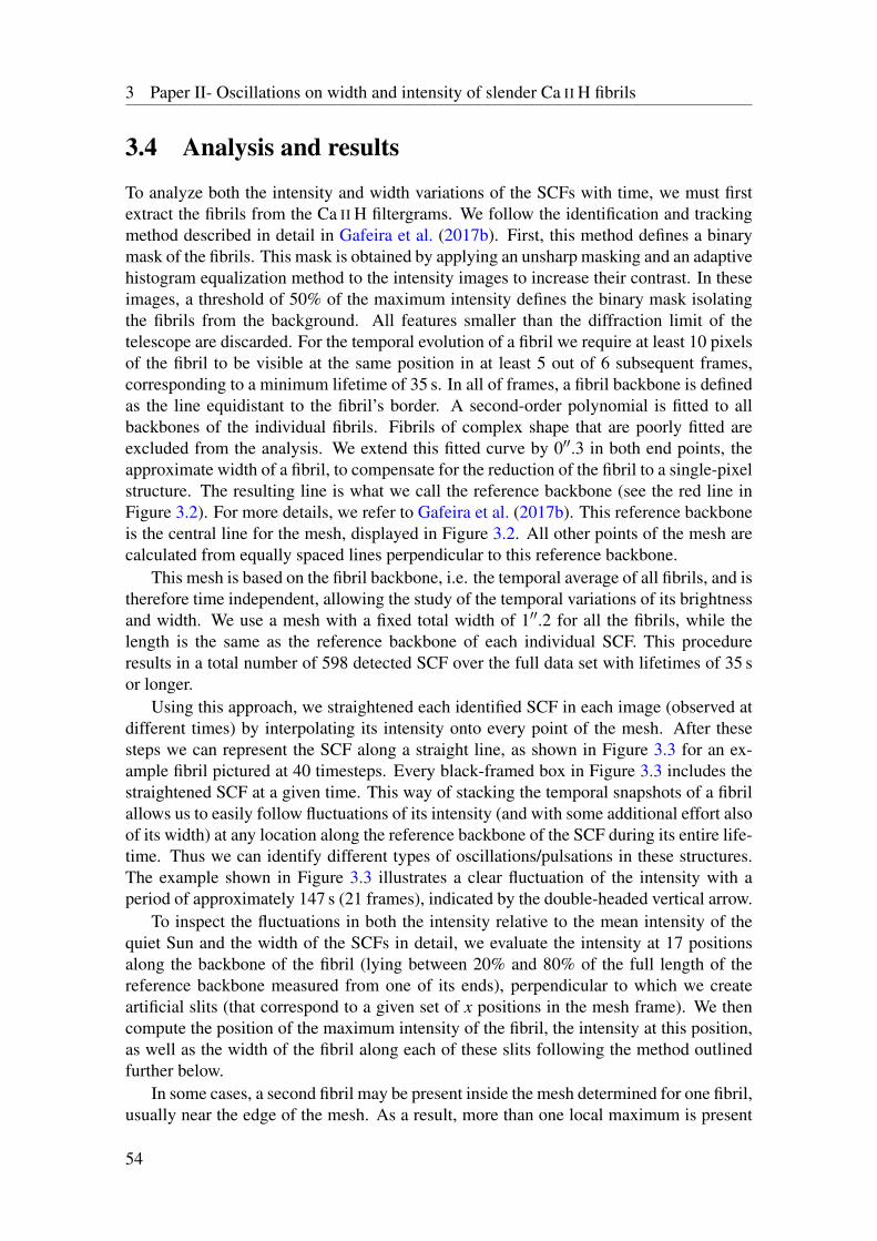
3 Paper II- Oscillations on width and intensity of slender Ca II H fibrils
3.4 Analysis and results
To analyze both the intensity and width variations of the SCFs with time, we must firstextract the fibrils from the Ca II H filtergrams. We follow the identification and trackingmethod described in detail in Gafeira et al. (2017b). First, this method defines a binarymask of the fibrils. This mask is obtained by applying an unsharp masking and an adaptivehistogram equalization method to the intensity images to increase their contrast. In theseimages, a threshold of 50% of the maximum intensity defines the binary mask isolatingthe fibrils from the background. All features smaller than the diffraction limit of thetelescope are discarded. For the temporal evolution of a fibril we require at least 10 pixelsof the fibril to be visible at the same position in at least 5 out of 6 subsequent frames,corresponding to a minimum lifetime of 35 s. In all of frames, a fibril backbone is definedas the line equidistant to the fibril’s border. A second-order polynomial is fitted to allbackbones of the individual fibrils. Fibrils of complex shape that are poorly fitted areexcluded from the analysis. We extend this fitted curve by 0′′.3 in both end points, theapproximate width of a fibril, to compensate for the reduction of the fibril to a single-pixelstructure. The resulting line is what we call the reference backbone (see the red line inFigure 3.2). For more details, we refer to Gafeira et al. (2017b). This reference backboneis the central line for the mesh, displayed in Figure 3.2. All other points of the mesh arecalculated from equally spaced lines perpendicular to this reference backbone.
This mesh is based on the fibril backbone, i.e. the temporal average of all fibrils, and istherefore time independent, allowing the study of the temporal variations of its brightnessand width. We use a mesh with a fixed total width of 1′′.2 for all the fibrils, while thelength is the same as the reference backbone of each individual SCF. This procedureresults in a total number of 598 detected SCF over the full data set with lifetimes of 35 sor longer.
Using this approach, we straightened each identified SCF in each image (observed atdifferent times) by interpolating its intensity onto every point of the mesh. After thesesteps we can represent the SCF along a straight line, as shown in Figure 3.3 for an ex-ample fibril pictured at 40 timesteps. Every black-framed box in Figure 3.3 includes thestraightened SCF at a given time. This way of stacking the temporal snapshots of a fibrilallows us to easily follow fluctuations of its intensity (and with some additional effort alsoof its width) at any location along the reference backbone of the SCF during its entire life-time. Thus we can identify different types of oscillations/pulsations in these structures.The example shown in Figure 3.3 illustrates a clear fluctuation of the intensity with aperiod of approximately 147 s (21 frames), indicated by the double-headed vertical arrow.
To inspect the fluctuations in both the intensity relative to the mean intensity of thequiet Sun and the width of the SCFs in detail, we evaluate the intensity at 17 positionsalong the backbone of the fibril (lying between 20% and 80% of the full length of thereference backbone measured from one of its ends), perpendicular to which we createartificial slits (that correspond to a given set of x positions in the mesh frame). We thencompute the position of the maximum intensity of the fibril, the intensity at this position,as well as the width of the fibril along each of these slits following the method outlinedfurther below.
In some cases, a second fibril may be present inside the mesh determined for one fibril,usually near the edge of the mesh. As a result, more than one local maximum is present
54
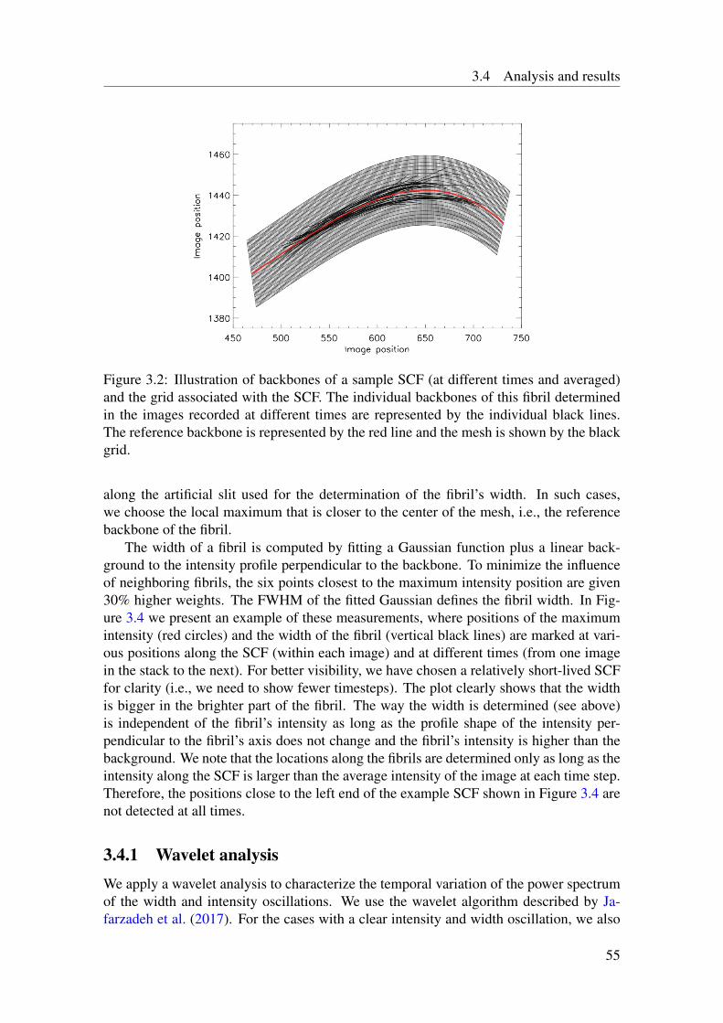
3.4 Analysis and results
Figure 3.2: Illustration of backbones of a sample SCF (at different times and averaged)and the grid associated with the SCF. The individual backbones of this fibril determinedin the images recorded at different times are represented by the individual black lines.The reference backbone is represented by the red line and the mesh is shown by the blackgrid.
along the artificial slit used for the determination of the fibril’s width. In such cases,we choose the local maximum that is closer to the center of the mesh, i.e., the referencebackbone of the fibril.
The width of a fibril is computed by fitting a Gaussian function plus a linear back-ground to the intensity profile perpendicular to the backbone. To minimize the influenceof neighboring fibrils, the six points closest to the maximum intensity position are given30% higher weights. The FWHM of the fitted Gaussian defines the fibril width. In Fig-ure 3.4 we present an example of these measurements, where positions of the maximumintensity (red circles) and the width of the fibril (vertical black lines) are marked at vari-ous positions along the SCF (within each image) and at different times (from one imagein the stack to the next). For better visibility, we have chosen a relatively short-lived SCFfor clarity (i.e., we need to show fewer timesteps). The plot clearly shows that the widthis bigger in the brighter part of the fibril. The way the width is determined (see above)is independent of the fibril’s intensity as long as the profile shape of the intensity per-pendicular to the fibril’s axis does not change and the fibril’s intensity is higher than thebackground. We note that the locations along the fibrils are determined only as long as theintensity along the SCF is larger than the average intensity of the image at each time step.Therefore, the positions close to the left end of the example SCF shown in Figure 3.4 arenot detected at all times.
3.4.1 Wavelet analysisWe apply a wavelet analysis to characterize the temporal variation of the power spectrumof the width and intensity oscillations. We use the wavelet algorithm described by Ja-farzadeh et al. (2017). For the cases with a clear intensity and width oscillation, we also
55
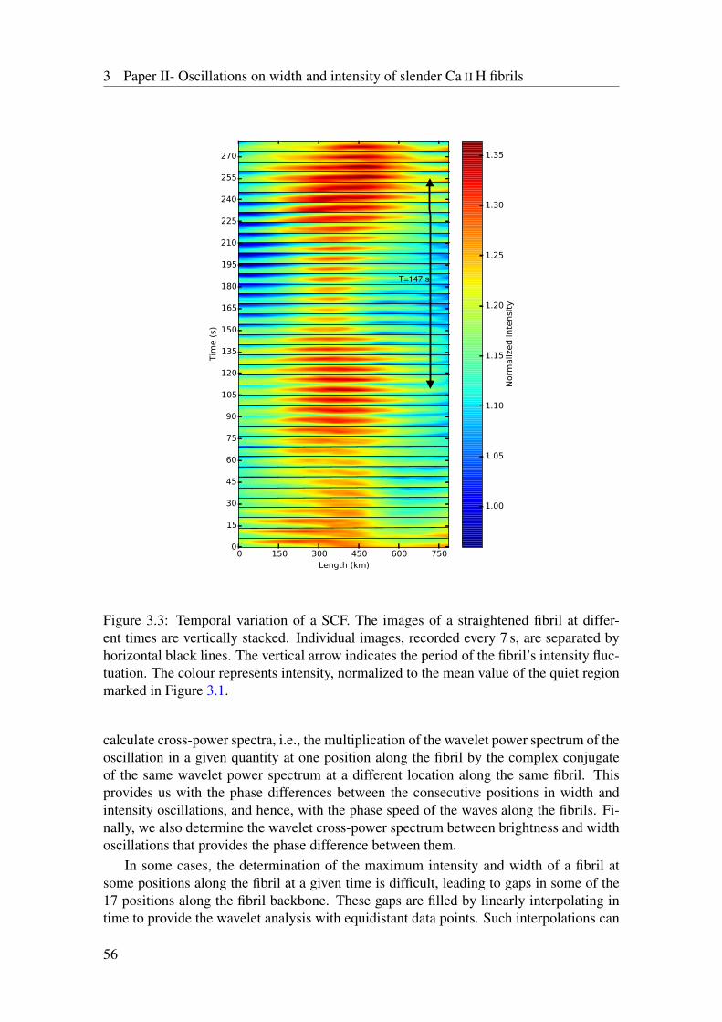
3 Paper II- Oscillations on width and intensity of slender Ca II H fibrils
T=147 s
Figure 3.3: Temporal variation of a SCF. The images of a straightened fibril at differ-ent times are vertically stacked. Individual images, recorded every 7 s, are separated byhorizontal black lines. The vertical arrow indicates the period of the fibril’s intensity fluc-tuation. The colour represents intensity, normalized to the mean value of the quiet regionmarked in Figure 3.1.
calculate cross-power spectra, i.e., the multiplication of the wavelet power spectrum of theoscillation in a given quantity at one position along the fibril by the complex conjugateof the same wavelet power spectrum at a different location along the same fibril. Thisprovides us with the phase differences between the consecutive positions in width andintensity oscillations, and hence, with the phase speed of the waves along the fibrils. Fi-nally, we also determine the wavelet cross-power spectrum between brightness and widthoscillations that provides the phase difference between them.
In some cases, the determination of the maximum intensity and width of a fibril atsome positions along the fibril at a given time is difficult, leading to gaps in some of the17 positions along the fibril backbone. These gaps are filled by linearly interpolating intime to provide the wavelet analysis with equidistant data points. Such interpolations can
56
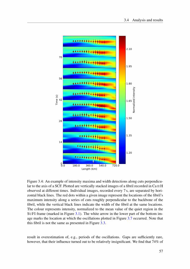
3.4 Analysis and results
14
28
42
56
70
Figure 3.4: An example of intensity maxima and width detections along cuts perpendicu-lar to the axis of a SCF. Plotted are vertically stacked images of a fibril recorded in Ca II Hobserved at different times. Individual images, recorded every 7 s, are separated by hori-zontal black lines. The red dots within a given image represent the locations of the fibril’smaximum intensity along a series of cuts roughly perpendicular to the backbone of thefibril, while the vertical black lines indicate the width of the fibril at the same locations.The colour represents intensity, normalized to the mean value of the quiet region in theSUFI frame (marked in Figure 3.1). The white arrow in the lower part of the bottom im-age marks the location at which the oscillations plotted in Figure 3.7 occurred. Note thatthis fibril is not the same as presented in Figure 3.3.
result in overestimation of, e.g., periods of the oscillations. Gaps are sufficiently rare,however, that their influence turned out to be relatively insignificant. We find that 74% of
57
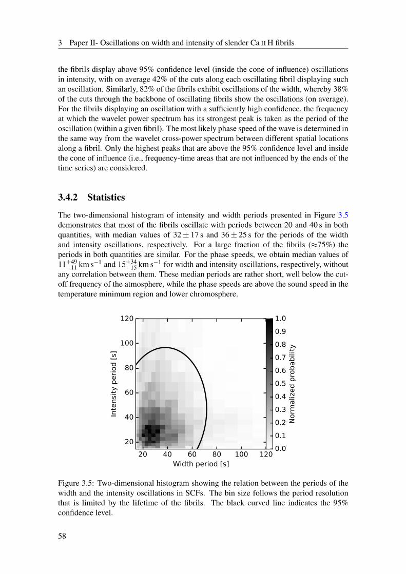
3 Paper II- Oscillations on width and intensity of slender Ca II H fibrils
the fibrils display above 95% confidence level (inside the cone of influence) oscillationsin intensity, with on average 42% of the cuts along each oscillating fibril displaying suchan oscillation. Similarly, 82% of the fibrils exhibit oscillations of the width, whereby 38%of the cuts through the backbone of oscillating fibrils show the oscillations (on average).For the fibrils displaying an oscillation with a sufficiently high confidence, the frequencyat which the wavelet power spectrum has its strongest peak is taken as the period of theoscillation (within a given fibril). The most likely phase speed of the wave is determined inthe same way from the wavelet cross-power spectrum between different spatial locationsalong a fibril. Only the highest peaks that are above the 95% confidence level and insidethe cone of influence (i.e., frequency-time areas that are not influenced by the ends of thetime series) are considered.
3.4.2 Statistics
The two-dimensional histogram of intensity and width periods presented in Figure 3.5demonstrates that most of the fibrils oscillate with periods between 20 and 40 s in bothquantities, with median values of 32± 17 s and 36± 25 s for the periods of the widthand intensity oscillations, respectively. For a large fraction of the fibrils (≈75%) theperiods in both quantities are similar. For the phase speeds, we obtain median values of11+49−11 km s−1 and 15+34
−15 km s−1 for width and intensity oscillations, respectively, withoutany correlation between them. These median periods are rather short, well below the cut-off frequency of the atmosphere, while the phase speeds are above the sound speed in thetemperature minimum region and lower chromosphere.
20 40 60 80 100 120Width period [s]
20
40
60
80
100
120
Inte
nsi
ty p
eri
od [
s]
0.0
0.1
0.2
0.3
0.4
0.5
0.6
0.7
0.8
0.9
1.0
Norm
aliz
ed p
robabili
ty
Figure 3.5: Two-dimensional histogram showing the relation between the periods of thewidth and the intensity oscillations in SCFs. The bin size follows the period resolutionthat is limited by the lifetime of the fibrils. The black curved line indicates the 95%confidence level.
58
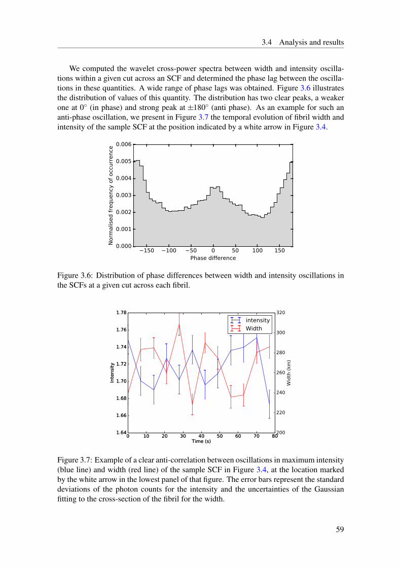
3.4 Analysis and results
We computed the wavelet cross-power spectra between width and intensity oscilla-tions within a given cut across an SCF and determined the phase lag between the oscilla-tions in these quantities. A wide range of phase lags was obtained. Figure 3.6 illustratesthe distribution of values of this quantity. The distribution has two clear peaks, a weakerone at 0 (in phase) and strong peak at 180 (anti phase). As an example for such ananti-phase oscillation, we present in Figure 3.7 the temporal evolution of fibril width andintensity of the sample SCF at the position indicated by a white arrow in Figure 3.4.
150 100 50 0 50 100 150Phase difference
0.000
0.001
0.002
0.003
0.004
0.005
0.006
Norm
alis
ed f
requency
of
occ
urr
ence
Figure 3.6: Distribution of phase differences between width and intensity oscillations inthe SCFs at a given cut across each fibril.
Figure 3.7: Example of a clear anti-correlation between oscillations in maximum intensity(blue line) and width (red line) of the sample SCF in Figure 3.4, at the location markedby the white arrow in the lowest panel of that figure. The error bars represent the standarddeviations of the photon counts for the intensity and the uncertainties of the Gaussianfitting to the cross-section of the fibril for the width.
59
3 Paper II- Oscillations on width and intensity of slender Ca II H fibrils
3.5 Discussion and conclusions
We have provided observational evidence for oscillations of the width of fibrils and ofintensity along SCFs in the lower chromosphere.
The high-resolution seeing-free images under study were recorded with SUNRISE/SUFI and revealed that such oscillations are almost ubiquitous all over the field of view,which covered part of NOAA AR 11768. Fluctuations in length of some of the SCFswere also observed, although it is not clear how independent this parameter is from theintensity.
The oscillatory behavior of both parameters (i.e., fibril width and intensity) was iden-tified in wavelet power spectra determined at a series of locations along the backbone ofeach detected SCF. The wavelet transform was employed to analyze the fluctuations fromwhich median periods of 32±17 s and 36±25 s were obtained for the width and intensityoscillations, respectively, with the uncertainty intervals representing the standard devi-ations of each distribution. Cross-power spectra between the perturbations at differentlocations along a given fibril revealed phase speeds of 11+49
−11 km s−1 and 15+34−15 km s−1
for the width and intensity fluctuations, respectively. Again, uncertainty intervals reflectstandard deviations. Given that these waves display brightness and width signatures, theyhave to be compressible, ruling out Alfvén waves. Simultaneous periodic fluctuations ofintensity and width in elongated structures are manifested by either slow-mode waves orfast sausage-mode waves (Van Doorsselaere et al. 2011; Su et al. 2012). In addition toobservations of the latter wave mode in the upper solar atmosphere (i.e., in the upper chro-mosphere and in the corona, Inglis et al. 2009), observations of sausage oscillations havealso been reported at lower atmospheric heights, in structures such as pores (Dorotovicet al. 2008; Morton et al. 2011).
To distinguish which wave modes are present in the SCFs we need to compare thephase speeds of the oscillations with the expected plasma Alfvén and sound speeds. Thevalues for the Alfvén and sound speeds were computed using the NC5 flux tube fromBruls and Solanki (1993) embedded in the VAL-A atmosphere (Vernazza et al. 1981).For a majority of the detected waves, these velocities are larger than the sound speedat the low chromospheric heights sampled by the SUFI 1.1 Å Ca II H filter, which liesaround 7 km s−1. The measured phase speeds are comparable to the local Alfvén speedfor this height region, with typical values in the range of 7–25 km s−1.
Interestingly, 20% of the SCFs show phase differences between −30 and +30, in-dicative of in-phase oscillations.
A strong peak was found at 180, with about 50% of all oscillations having a phasedifference within 30 of 180 (anti-phase oscillations). Phase differences of around ±90
are relatively uncommon.A phase difference in the range of |150−180|, as displayed by the example shown
in Figure 3.7, is consistent with the signature of sausage-mode oscillations in the SCFsunder the assumption of an optically thin plasma. The validity of this assumption is con-firmed by the fact that the observed intensity increases at the intersection points of cross-ing SCFs, suggesting that we can partly see through individual fibrils. The contractionof the fibril caused by the sausage-mode oscillation leads to a narrow fibril with a higherdensity. In an optically thin regime, a higher density implies an increased intensity. Thesubsequent expansion phase of the oscillation leads to an increase of the fibril’s width a
60
3.5 Discussion and conclusions
lower intensity. For such a plasma, the intensity follows the electron density. However, adetailed model of the brightening of these structures is required to determine the behaviorof the plasma under conditions typical of the lower chromosphere.
In about 25% of our SCFs we did not find a clear correlation between the fluctuationsin the two parameters. The intensity oscillations could also be caused by slow-modewaves, which are expected to be present inside strong-field magnetic features, such asflux tubes (although it is unclear to what extent the SCFs can be described as flux tubes).However, the median phase speeds obtained in our analysis are too high for slow-modewaves. Only for a few SCFs do we obtain low phase speeds that may well be compatiblewith the slow mode.
To our knowledge, our observations of sausage-mode oscillations in the SCFs are thefirst direct evidence of this wave mode in the lower solar chromosphere. Morton et al.(2012) inspected oscillations of width and intensity in Hα elongated fibrils and shortmottles (in the upper chromosphere). They found a phase speed of 67± 15 km s−1 fortheir MHD fast sausage waves, which is much larger than those we found in the SCFs.Like us, they also found a phase difference of 180 between their detected intensity andwidth perturbations. Dorotovic et al. (2008) and Morton et al. (2012) showed that theenergy these sausage waves carry is sufficient to contribute (around 10%) to the heatingof the chromosphere and/or the corona. Jess et al. (2012) claimed to see a fluctuation ofthe width of what they call a chromospheric spicule (observed on the disk as an Hα darkfibril). They interpret these fluctuations as sausage modes in the chromosphere.
This work points to a number of follow-up investigations to advance our knowledgeand understanding of the detected oscillations and waves. Firstly, measurements thatinclude velocities would help to distinguish better between different possible wave modes.Another important step is to compute MHD wave modes in simple models of fibrils,possibly described as flux tubes embedded in a magnetized gas. Such a study should notonly lead to new insights into the physics of these oscillations, but would also reveal theexpected behavior of different physical parameters, thus providing guidance for futureobservations and their interpretation. Finally, an investigation of the physical processesthat drive this oscillatory behavior of the SCFs would also be very useful.
61

4 Conclusion and Outlook
In this thesis, we present a detailed study of the morphological properties of slenderCa II H fibrils (SCFs) and their oscillatory behavior. It is composed of work presented intwo publications that appeared in the Astrophysical Journal Supplement Series in 2017, aspart of a SUNRISE special issue. In the first paper, reproduced in Chapter 2, we apply anautomatic detection algorithm to extract all the bright elongated structures present in theCa II H intensity maps. This algorithm is based on a series of unsharp mask proceduresand contrast enhancement technique that allow us to identify in total 598 SCFs for furtheranalysis in this thesis.
This analysis comprises of the study of the morphological properties of the SCFs andtheir statistics (see Table 2.1 for more details). We obtain lifetimes between 35 s and30 min (taking into account the intermittency in fibril visibility), maximum lengths from0.5 to 4.5 Mm, widths between 100 and 270 km and a slight preference for a positivecurvature. This preferential curvature agrees with the idea of these fibrils being part oflow-lying loops observed away from solar disk center.
We also compare our results with other studies of chromospheric small-scale elon-gated structures. In Table 2.2 we see that SCFs show some similarities with type I andtype II spicules (from Pereira et al. 2012), and with Ca II K fibrils (as deduced by Pietar-ila et al. 2009). We emphasize that despite these similarities SCFs, spicules, and Ca II Kfibrils might still outline different magnetic structures.
Two different types of the temporal evolution of the brightness of SCFs were alsoidentified. In one type the intensity increases starting from the center and propagates tothe edges, i.e., towards the footpoints of the loops outlined by the SCFs (around 50% ofthe cases). In the second type the increase in intensity starts at the edges and expandsfrom there towards the center (around 25%). A jet-like brightness variation, as observedin spicules of both types, is not compatible with either of the two cases, since the SCFsshow a symmetric brightness variation around their centers. 25% of the observed SCFsdo not show a clear pattern in the brightness variation.
The second part of this thesis is dedicated to the analysis of the oscillatory behaviorof SCFs. This topic is covered by the paper forming Chapter 3 and by the paper givenin the appendix. In chapter 3, we focus on the oscillations in width and intensity alongthe SCFs. We measure their intensities and widths at several positions along their axis asshown in Figure 3.4 and use a wavelet transform to compute the wave parameters period,phase speed and phase difference between the width and the intensity oscillations. Weobserve that the oscillations show periods with nearly identical median values of 32±17 sfor the width and 36± 25 s for the intensity, which are again equal within the errors.For the phase speed we obtain values of 11+49
−11 km s−1 for the width and 15+34−15 km s−1
for the intensity. All uncertainty intervals are standard deviations computed from the
63
4 Conclusion and Outlook
corresponding histograms. Due to the fact that the waves display these intensity andwidth oscillations, they have to be of magneto-acoustic type. We also observe in about50% of the cases the perturbation to oscillate in anti-phase and in 20% in phase (seeFigure 3.7). The facts that measured phase speeds are closer to the Alfvén speed (typicalrange for this height 7 to 25 km s−1) than to the sound speed (around 7 km s−1) and thatthe oscillations between the two properties are in anti-phase indicates that these waves areof fast sausage-mode type. For some of the examples, the phase speed is relatively low.In this case, they can be interpreted as slow sausage-mode waves, which are expected tobe present in strong magnetic field flux tubes.
As described in the appendix, we also performed an analysis of the transversal wavesin the SCFs (see Appendix A for more details). The transverse motions were measuredby placing fixed artificial slits along the fibril axis (see Figure A.5) and then comput-ing the transverse displacements, velocity amplitudes, periods and phase speeds of theoscillation. We obtained mean values of 33 km, 2.4 km s−1, 83 s, and 9 km s−1 respec-tively. In Table A.2 we compare these wave parameters with other structures describedin the literature. This showed that SCFs have, on average, smaller periods, transversedisplacement, velocity amplitude and phase speeds when compared to other on-disk chro-mospheric structures.
The observed transverse oscillations can be interpreted as a transverse wave propa-gating along the fibril axis compatible with a kink-mode wave. Such a wave, with theobtained parameters, can carry energy of around 15 kW m−2 which is of the same orderof magnitude as the energy needed to heat the solar chromosphere. This is also the regionwhere we expect the energy of the wave to be dissipated, since the SCFs are mainly ori-ented in a horizontal direction, and do not extend to higher layers Jafarzadeh et al. (2017).However, some of the SCFs trace more vertical field lines, allowing for the transport ofenergy to the higher layers, possibly contributing to coronal heating. However, from ourobservations it is impossible to tell how much of its energy the wave is dissipating to thesurroundings, if at all.
Outlook
The analysis mentioned above provides a wealth of information on the temporal evolution,the morphology and the statistical properties of the SCFs. However, there are still openquestions to be answered to deepen the understanding of the SCFs:
1. How are the SCFs magnetically connected to the underlying photosphere?
2. What is the magnetic topology of the SCFs?
3. What is the relevance of the detected waves in the SCFs for transporting energy tohigher layers of the solar atmosphere?
Answering these questions is important to conclude on the physical nature of thesestructures, e.g., if they are the possible on-disk counterparts of other chromospheric struc-tures like spicules or Ca II K fibrils.
An important step to answer these questions is to analyze the magnetic and veloc-ity properties of the SCFs, ideally also their height-dependence. This can be achieved
64
4 Conclusion and Outlook
by high-resolution, full-Stokes observations in the Ca II H&K lines, but also by lookingat other chromspheric observations, e.g., the He 10830 Å triplet and combining it withmeasurements of the photospheric magnetic field and velocity vectors. Correlating themeasurements from these two layers in the solar atmosphere will allow to clarify if thelong SCFs are related to the larger-scale canopy found over the internetwork (Giovanelliand Jones 1982; Solanki and Steiner 1990; Lagg et al. 2009), if they are low-lying, small-scale magnetic loops, or if they are the on-disk counterparts of spicules. Large-aperturesolar telescopes like GREGOR (Tenerife, Spain, Schmidt et al. (2012)) or the future 4-m telescope Daniel K. Inouye Telescope (DKIST, Hawaii, USA, Tritschler et al. (2016)),and also the planned reflight of the SUNRISE balloon-borne observatory with significantlyimproved instrumentation (multi-line full-Stokes observations in the near UV and visiblewavelengths) will offer the possibility for such measurements.
The measurement of the magnetic field with high temporal resolution in such struc-tures will help to perform a more detailed analysis of the observed oscillatory behavior.These measurements will put further constraints on the type of the observed wave andtherefore allow for their unambiguous identification. Modern instrumentation, like the2-dimensional full-Stokes spectropolarimeter (MiHI) or the Fast Solar Polarimeter (FSP),developed at MPS, will be ideally suited to accomplish this task. Height-dependent in-version codes will lift the restriction of local thermodynamic equlibrium (for exampleNICOLE (Socas-Navarro et al. 1998) or analytically computed response function inver-sion codes (Milic and van Noort 2017)). Such codes are needed to fully exploit the dataof the large-aperture telescopes and their attached instruments, providing the informationabout the conditions in the solar atmosphere from the deepest photospheric layers up tothe corona needed to attack the open questions.
65


Bibliography
Alissandrakis, C. E. and Macris, C. J.: 1971, Akademia Athenon Praktika 46, 107
Anan, T., Kitai, R., Kawate, T., Matsumoto, T., Ichimoto, K., Shibata, K., Hillier, A.,Otsuji, K., Watanabe, H., Ueno, S., Nagata, S., Ishii, T. T., Komori, H., Nishida, K.,Nakamura, T., Isobe, H., and Hagino, M.: 2010, PASJ 62, 871
Anusha, L. S., Solanki, S. K., Hirzberger, J., and Feller, A.: 2017, A&A 598, A47
Aschwanden, M. J., de Pontieu, B., Schrijver, C. J., and Title, A. M.: 2002, Sol. Phys.206, 99
Aschwanden, M. J., Fletcher, L., Schrijver, C. J., and Alexander, D.: 1999, ApJ 520, 880
Athay, R. G. (ed.): 1976, The solar chromosphere and corona: Quiet sun, Vol. 53 ofAstrophysics and Space Science Library
Banerjee, D., Erdélyi, R., Oliver, R., and O’Shea, E.: 2007, Sol. Phys. 246, 3
Banos, G. J. and Macris, C. J.: 1970, Sol. Phys. 12, 106
Barthol, P., Gandorfer, A., Solanki, S. K., Schüssler, M., Chares, B., Curdt, W., Deutsch,W., Feller, A., Germerott, D., Grauf, B., Heerlein, K., Hirzberger, J., Kolleck, M.,Meller, R., Müller, R., Riethmüller, T. L., Tomasch, G., Knölker, M., Lites, B. W., Card,G., Elmore, D., Fox, J., Lecinski, A., Nelson, P., Summers, R., Watt, A., MartínezPillet,V., Bonet, J. A., Schmidt, W., Berkefeld, T., Title, A. M., Domingo, V., GasentBlesa,J. L., del ToroIniesta, J. C., LópezJiménez, A., Álvarez-Herrero, A., Sabau-Graziati,L., Widani, C., Haberler, P., Härtel, K., Kampf, D., Levin, T., PérezGrande, I., Sanz-Andrés, A., and Schmidt, E.: 2011, Sol. Phys. 268(1), 1
Beck, C., Rezaei, R., and Puschmann, K. G.: 2013, A&A 556, A127
Beckers, J. M.: 1968, Sol. Phys. 3(3), 367
Beckers, J. M.: 1972, Annual Review of Astronomy and Astrophysics 10(1), 73
Bel, N. and Leroy, B.: 1977, A&A 55, 239
Berkefeld, T.: 2007, in Modern solar facilities-advanced solar science, p. 107
67
Bibliography
Berkefeld, T., Schmidt, W., Soltau, D., Bell, A., Doerr, H. P., Feger, B., Friedlein, R., Ger-ber, K., Heidecke, F., Kentischer, T., v.d. Lühe, O., Sigwarth, M., Wälde, E., Barthol,P., Deutsch, W., Gandorfer, A., Germerott, D., Grauf, B., Meller, R., Álvarez-Herrero,A., Knölker, M., Martínez Pillet, V., Solanki, S. K., and Title, A. M.: 2011, Sol. Phys.268(1), 103
Bogdan, T. J., Carlsson, M., Hansteen, V. H., McMurry, A., Rosenthal, C. S., Johnson,M., Petty-Powell, S., Zita, E. J., Stein, R. F., McIntosh, S. W., and Nordlund, Å.: 2003,ApJ 599, 626
Brandenburg, A., Rogachevskii, I., and Kleeorin, N.: 2016, New Journal of Physics18(12), 125011
Brandenburg, A. and Subramanian, K.: 2004, Phys. Rep. 417(1-4), 1
Bratsolis, E., Dialetis, D., and Alissandrakis, C. E.: 1993, A&A 274, 940
Bray, R. J. and Loughhead, R. E.: 1974, The solar chromosphere
Brown, D. S., Parnell, C. E., Deluca, E. E., Golub, L., and McMullen, R. A.: 2001,Sol. Phys. 201, 305
Bruls, J. H. M. J. and Solanki, S. K.: 1993, A&A 273, 293
Buehler, D., Lagg, A., Solanki, S. K., and van Noort, M.: 2015, A&A 576, A27
Carlsson, M., Hansteen, V. H., Gudiksen, B. V., Leenaarts, J., and De Pontieu, B.: 2016,A&A 585, A4
Carlsson, M. and Stein, R. F.: 1997, ApJ 481, 500
Cauzzi, G., Reardon, K. P., Uitenbroek, H., Cavallini, F., Falchi, A., Falciani, R., Janssen,K., Rimmele, T., Vecchio, A., and Wöger, F.: 2008, A&A 480, 515
Centeno, S., Blanco Rodríguez, J., Barthol, P., Del Toro Iniesta, J. C., and Sunrise team:2017, ApJS 229, 2
Charbonneau, P.: 2010, Living Rev. Solar Phys 7, 3
Cheung, M. C. M., Schüssler, M., and Moreno-Insertis, F.: 2007, A&A 461, 1163
Chitta, L. P., Peter, H., Solanki, S. K., Barthol, P., Gandorfer, A., Gizon, L., Hirzberger, J.,Riethmüller, T. L., van Noort, M., Rodríguez, J. B., Iniesta, J. C. D. T., Suárez, D. O.,Schmidt, W., Pillet, V. M., and Knölker, M.: 2017, ApJS 229(1), 4
Choudhuri, A. R., Auffret, H., and Priest, E. R.: 1993, Sol. Phys. 143, 49
Danilovic, S., Beeck, B., Pietarila, A., Schüssler, M., Solanki, S. K., Martínez Pillet, V.,Bonet, J. A., del Toro Iniesta, J. C., Domingo, V., Barthol, P., Berkefeld, T., Gandorfer,A., Knölker, M., Schmidt, W., and Title, A. M.: 2010, ApJ 723, L149
68
Bibliography
Danilovic, S., Hirzberger, J., Riethmüller, T. L., Solanki, S. K., Barthol, P., Berkefeld,T., Gandorfer, A., Gizon, L., Knölker, M., Schmidt, W., Blanco Rodríguez, J., and DelToro Iniesta, J. C.: 2014, ApJ 784, 20
Danilovic, S., Solanki, S. K., Barthol, P., Gandorfer, A., Gizon, L., Hirzberger, J., Ri-ethmüller, T. L., van Noort, M., Rodríguez, J. B., Iniesta, J. C. D. T., Suárez, D. O.,Schmidt, W., Pillet, V. M., and Knölker, M.: 2017, ApJS 229(1), 5
Daubechies, I.: 1990, IEEE Trans. Inf. Theory 36, 961
de la Cruz Rodríguez, J. and Socas-Navarro, H.: 2011, A&A 527, L8
De Moortel, I., Ireland, J., Hood, A. W., and Walsh, R. W.: 2002, A&A 387, L13
De Pontieu, B., Erdélyi, R., and James, S. P.: 2004, Nature 430, 536
De Pontieu, B., Hansteen, V. H., Rouppe van der Voort, L., van Noort, M., and Carlsson,M.: 2007, ApJ 655, 624
de Pontieu, B., McIntosh, S., Hansteen, V. H., Carlsson, M., Schrijver, C. J., Tarbell,T. D., Title, A. M., Shine, R. A., Suematsu, Y., Tsuneta, S., Katsukawa, Y., Ichimoto,K., Shimizu, T., and Nagata, S.: 2007, PASJ 59, S655
De Pontieu, B., McIntosh, S. W., Carlsson, M., Hansteen, V. H., Tarbell, T. D., Boerner,P., Martinez-Sykora, J., Schrijver, C. J., and Title, A. M.: 2011, Science 331, 55
De Pontieu, B., McIntosh, S. W., Carlsson, M., Hansteen, V. H., Tarbell, T. D., Schrijver,C. J., Title, A. M., Shine, R. A., Tsuneta, S., Katsukawa, Y., Ichimoto, K., Suematsu,Y., Shimizu, T., and Nagata, S.: 2007, Science 318, 1574
Defouw, R. J.: 1976, ApJ 209, 266
Dorotovic, I., Erdélyi, R., and Karlovský, V.: 2008, in R. Erdélyi and C. A.Mendoza-Briceno (eds.), Waves Oscillations in the Solar Atmosphere: Heating andMagneto-Seismology, Vol. 247 of IAU Symposium, p. 351
Edwin, P. M. and Roberts, B.: 1983, Sol. Phys. 88, 179
Erdélyi, R. and Fedun, V.: 2007, Science 318, 1572
Erdélyi, R., Malins, C., Tóth, G., and de Pontieu, B.: 2007, A&A 467, 1299
Evans, D. J. and Roberts, B.: 1990, ApJ 348, 346
Foukal, P.: 1971a, Sol. Phys. 20(2), 298
Foukal, P.: 1971b, Sol. Phys. 19(1), 59
Frazier, E. N. and Stenflo, J. O.: 1972, Sol. Phys. 27, 330
69
Bibliography
Gafeira, R., Jafarzadeh, S., Solanki, S. K., Lagg, A., van Noort, M., Barthol, P., Berkefeld,T., Blanco Rodríguez, J., del Toro Iniesta, J. C., Gandorfer, A., Gizon, L., Hirzberger,J., Knölker, M., Martínez Pillet, V., Orozco Suárez, D., Riethmüller, T. L., and Schmidt,W.: 2017a, ApJS 229, 6
Gafeira, R., Lagg, A., Solanki, S. K., Jafarzadeh, S., van Noort, M., Barthol, P., BlancoRodríguez, J., del Toro Iniesta, J. C., Gandorfer, A., Gizon, L., Hirzberger, J., Knölker,M., Orozco Suárez, D., Riethmüller, T. L., and Schmidt, W.: 2017b, ApJS 229, 6
Gandorfer, A., Grauf, B., Barthol, P., Riethmüller, T. L., Solanki, S. K., Chares, B.,Deutsch, W., Ebert, S., Feller, A., Germerott, D., Heerlein, K., Heinrichs, J., Hirche, D.,Hirzberger, J., Kolleck, M., Meller, R., Müller, R., Schäfer, R., Tomasch, G., Knölker,M., Martínez Pillet, V., Bonet, J. A., Schmidt, W., Berkefeld, T., Feger, B., Heidecke,F., Soltau, D., Tischenberg, A., Fischer, A., Title, A., Anwand, H., and Schmidt, E.:2011, Sol. Phys. 268, 35
Gary, G. A.: 2001, Sol. Phys. 203, 71
Giovanelli, R. G. and Jones, H. P.: 1982, Sol. Phys. 79, 267
Gold, T.: 1964, NASA Special Publication 50, 389
Gonsalves, R. A. and Chidlaw, R.: 1979, in A. G. Tescher (ed.), Applications of DigitalImage Processing III, Vol. 207 of SPIE Conf. Ser., p. 32
Goossens, M., Van Doorsselaere, T., Soler, R., and Verth, G.: 2013, ApJ 768, 191
Graham, J. P., Danilovic, S., and SchÃijssler, M.: 2009, ApJ 693(2), 1728
Grossmann-Doerth, U. and Schmidt, W.: 1992, A&A 264, 236
Hale, G. E.: 1908, ApJ 28, 315
Hansteen, V. H., De Pontieu, B., Rouppe van der Voort, L., van Noort, M., and Carlsson,M.: 2006, ApJ 647, L73
Harvey, J. W., Branston, D., Henney, C. J., Keller, C. U., SOLIS, and Teams, G.: 2007,ApJLetters 659(2), L177
Hasan, S. S. and van Ballegooijen, A. A.: 2008, ApJ 680, 1542
Hathaway, D. H., Wilson, R. M., and Reichmann, E. J.: 1994, Sol. Phys. 151, 177
He, J., Marsch, E., Tu, C., and Tian, H.: 2009, ApJ 705, L217
Henriques, V. M. J. and Kiselman, D.: 2013, A&A 557, A5
Henriques, V. M. J., Scullion, E., Mathioudakis, M., Kiselman, D., Gallagher, P. T., andKeenan, F. P.: 2015, A&A 574, A131
Hirzberger, J.: 2003, Astronomische Nachrichten 324, 344
70
Bibliography
Hirzberger, J., Feller, A., Riethmüller, T. L., Gandorfer, A., and Solanki, S. K.: 2011,A&A 529, A132
Hirzberger, J., Feller, A., Riethmüller, T. L., Schüssler, M., Borrero, J. M., Afram, N.,Unruh, Y. C., Berdyugina, S. V., Gandorfer, A., Solanki, S. K., Barthol, P., Bonet,J. A., Martínez Pillet, V., Berkefeld, T., Knölker, M., Schmidt, W., and Title, A. M.:2010, ApJ 723, L154
Howard, R. and Stenflo, J. O.: 1972, Sol. Phys. 22, 402
Inglis, A. R., Van Doorsselaere, T., Brady, C. S., and Nakariakov, V. M.: 2009, A&A503(2), 569
Jafarzadeh, S.: 2013, Ph.D. thesis, Georg-August-Universität Göttingen
Jafarzadeh, S., Rutten, R., Solanki, S. K., Wiegelmann, T., Riethmüller, T. L., van Noort,M., Szydlarsky, M., Blanco Rodríguez, J., Barthol, P., del Toro Iniesta, J. C., Gandorfer,A., Gizon, L., Hirzberger, J., Knölker, M., Martínez Pillet, V., Orozco Suárez, D., andSchmidt, W.: 2017, ApJS 229, 10
Jafarzadeh, S., Solanki, S. K., Cameron, R. H., Barthol, P., Rodríguez, J. B., del Toro Ini-esta, J. C., Gandorfer, A., Gizon, L., Hirzberger, J., Knölker, M., Pillet, V. M., Suárez,D. O., Riethmüller, T. L., Schmidt, W., and van Noort, M.: 2017, ApJS 229(1), 8
Jafarzadeh, S., Solanki, S. K., Feller, A., Lagg, A., Pietarila, A., Danilovic, S., Rieth-müller, T. L., and Martínez Pillet, V.: 2013, A&A 549, A116
Jafarzadeh, S., Solanki, S. K., Gafeira, R., Barthol, P., Berkefeld, T., Blanco Rodríguez, J.,del Toro Iniesta, J. C., Gandorfer, A., Gizon, L., Hirzberger, J., Knölker, M., MartínezPillet, V., Orozco Suárez, D., Riethmüller, T. L., Schmidt, W., and van Noort, M.: 2017,ApJS 229, 8
Jafarzadeh, S., Solanki, S. K., Lagg, A., Bellot Rubio, L. R., van Noort, M., Feller, A.,and Danilovic, S.: 2014, A&A 569, A105
Jafarzadeh, S., Solanki, S. K., Stangalini, M., Steiner, O., Cameron, R. H., and Danilovic,S.: 2017, ApJS 229, 9
Jess, D. B., Mathioudakis, M., Christian, D. J., Keenan, F. P., Ryans, R. S. I., and Crockett,P. J.: 2010, Sol. Phys. 261, 363
Jess, D. B., Mathioudakis, M., Erdélyi, R., Crockett, P. J., Keenan, F. P., and Christian,D. J.: 2009, Science 323, 1582
Jess, D. B., Morton, R. J., Verth, G., Fedun, V., Grant, S. D. T., and Giagkiozis, I.: 2015,Space Sci. Rev. 190, 103
Jess, D. B., Pascoe, D. J., Christian, D. J., Mathioudakis, M., Keys, P. H., and Keenan,F. P.: 2012, ApJ 744, L5
Jess, D. B. and Verth, G.: 2015, ArXiv e-prints
71
Bibliography
Jones, H. P. and Giovanelli, R. G.: 1982, Sol. Phys. 79, 247
Judge, P.: 2006, in J. Leibacher, R. F. Stein, and H. Uitenbroek (eds.), Solar MHD Theoryand Observations: A High Spatial Resolution Perspective, Vol. 354 of AstronomicalSociety of the Pacific Conference Series, p. 259
Judge, P. G. and Carlsson, M.: 2010, ApJ 719(1), 469
Judge, P. G., Tritschler, A., and Low, B. C.: 2011, ApJLetters 730(1), L4
Kahil, F., Riethmüller, T. L., and Solanki, S. K.: 2017, ApJS 229(1), 12
Kaithakkal, A. J., Riethmüller, T. L., Solanki, S. K., Lagg, A., Barthol, P., Gandorfer, A.,Gizon, L., Hirzberger, J., vanNoort, M., Rodríguez, J. B., Iniesta, J. C. D. T., Suárez,D. O., Schmidt, W., Pillet, V. M., and Knölker, M.: 2017, ApJS 229(1), 13
Keller, C. U. and von der Lühe, O.: 1992, A&A 261, 321
Khomenko, E. and Collados, M.: 2015, Living Rev. Solar Phys 12
Kitiashvili, I. N., Kosovichev, A. G., Mansour, N. N., and Wray, A. A.: 2011, ApJ 727,L50
Koza, J., Rutten, R. J., and Vourlidas, A.: 2009, A&A 499, 917
Kukhianidze, V., Zaqarashvili, T. V., and Khutsishvili, E.: 2006, A&A 449, L35
Kuridze, D., Morton, R. J., Erdélyi, R., Dorrian, G. D., Mathioudakis, M., Jess, D. B.,and Keenan, F. P.: 2012, ApJ 750, 51
Lagg, A., Ishikawa, R., Merenda, L., Wiegelmann, T., Tsuneta, S., and Solanki, S. K.:2009, in B. Lites, M. Cheung, T. Magara, J. Mariska, and K. Reeves (eds.), TheSecond Hinode Science Meeting: Beyond Discovery-Toward Understanding, Vol. 415of Astronomical Society of the Pacific Conference Series, p. 327
Langangen, Ã., Pontieu, B. D., Carlsson, M., Hansteen, V. H., Cauzzi, G., and Reardon,K.: 2008, ApJLetters 679(2), L167
Leenaarts, J., Carlsson, M., Hansteen, V., and Rouppe van der Voort, L.: 2009, ApJ 694,L128
Leenaarts, J., Carlsson, M., and Rouppe van der Voort, L.: 2012, ApJ 749, 136
Leenaarts, J., Carlsson, M., and Rouppe van der Voort, L.: 2015, ApJ 802, 136
Leighton, R. B., Noyes, R. W., and Simon, G. W.: 1962, ApJ 135, 474
Lin, Y., Engvold, O., Rouppe van der Voort, L. H. M., and van Noort, M.: 2007, Sol. Phys.246, 65
Lippincott, S. L.: 1957, Smithsonian Contributions to Astrophysics 2, 15
72
Bibliography
Lites, B. W., Kubo, M., Socas-Navarro, H., Berger, T., Frank, Z., Shine, R., Tarbell, T.,Title, A., Ichimoto, K., Katsukawa, Y., Tsuneta, S., Suematsu, Y., Shimizu, T., andNagata, S.: 2008, ApJ 672, 1237
Liu, Y., Zhang, H., Ai, G., Wang, H., and Zirin, H.: 1994, A&A 283, 215
Löfdahl, M. G.: 2002, in P. J. Bones, M. A. Fiddy, and R. P. Millane (eds.), ImageReconstruction from Incomplete Data, Vol. 4792 of Proc. SPIE, pp 146–155
Löfdahl, M. G. and Scharmer, G. B.: 1994, ApJS. 107, 243-264 (1994) 107
Marsh, K. A.: 1976, Sol. Phys. 50, 37
Martínez Pillet, V., Del Toro Iniesta, J. C., Álvarez-Herrero, A., Domingo, V., Bonet,J. A., González Fernández, L., López Jiménez, A., Pastor, C., Gasent Blesa, J. L.,Mellado, P., Piqueras, J., Aparicio, B., Balaguer, M., Ballesteros, E., Belenguer, T.,Bellot Rubio, L. R., Berkefeld, T., Collados, M., Deutsch, W., Feller, A., Girela, F.,Grauf, B., Heredero, R. L., Herranz, M., Jerónimo, J. M., Laguna, H., Meller, R.,Menéndez, M., Morales, R., Orozco Suárez, D., Ramos, G., Reina, M., Ramos, J. L.,Rodríguez, P., Sánchez, A., Uribe-Patarroyo, N., Barthol, P., Gandorfer, A., Knoelker,M., Schmidt, W., Solanki, S. K., and Vargas Domínguez, S.: 2011, Sol. Phys. 268, 57
Mathioudakis, M., Jess, D. B., and Erdélyi, R.: 2013, Space Sci. Rev. 175, 1
McIntosh, S. W., De Pontieu, B., Carlsson, M., Hansteen, V., Boerner, P., and Goossens,M.: 2011, Nature 475, 477
Michalitsanos, A. G.: 1973, Sol. Phys. 30, 47
Milic, I. and van Noort, M.: 2017, A&A 601, A100
Moore, R. L., Sterling, A. C., Cirtain, J. W., and Falconer, D. A.: 2011, ApJ 731, L18
Mooroogen, K., Morton, R. J., and Henriques, V.: 2017, A&A 607, A46
Morton, R. J., Erdélyi, R., Jess, D. B., and Mathioudakis, M.: 2011, ApJ 729, L18
Morton, R. J., Verth, G., Fedun, V., Shelyag, S., and Erdélyi, R.: 2013, ApJ 768, 17
Morton, R. J., Verth, G., Hillier, A., and Erdélyi, R.: 2014, ApJ 784, 29
Morton, R. J., Verth, G., Jess, D. B., Kuridze, D., Ruderman, M. S., Mathioudakis, M.,and Erdélyi, R.: 2012, Nature Communications 3, 1315
Nakariakov, V. M., Hornsey, C., and Melnikov, V. F.: 2012, ApJ 761, 134
Nakariakov, V. M. and Verwichte, E.: 2005, Living Rev. Solar Phys. 2, 3. URL:http://www.livingreviews.org/lrsp
Nakariakov, V. M. and Verwichte, E.: 2005, Living Rev. Solar Phys 2(3)
Narayanan, A. S.: 2013, An introduction to waves and oscillations in the Sun, Springer
73
Bibliography
Okamoto, T. J. and De Pontieu, B.: 2011, ApJ 736, L24
Okamoto, T. J., Tsuneta, S., Berger, T. E., Ichimoto, K., Katsukawa, Y., Lites, B. W.,Nagata, S., Shibata, K., Shimizu, T., Shine, R. A., Suematsu, Y., Tarbell, T. D., andTitle, A. M.: 2007, Science 318, 1577
Parker, E. N.: 1972, ApJ 174, 499
Pasachoff, J. M., Jacobson, W. A., and Sterling, A. C.: 2009, Sol. Phys. 260, 59
Pasachoff, J. M., Noyes, R. W., and Beckers, J. M.: 1968, Sol. Phys. 5(2), 131
Patsourakos, S., Gouttebroze, P., and Vourlidas, A.: 2007, ApJ 664, 1214
Paxman, R. G., Seldin, J. H., Loefdahl, M. G., Scharmer, G. B., and Keller, C. U.: 1996,ApJ 466, 1087
Pereira, T. M. D., De Pontieu, B., and Carlsson, M.: 2012, ApJ p. 17
Pereira, T. M. D., De Pontieu, B., Carlsson, M., Hansteen, V., Tarbell, T. D., Lemen,J., Title, A., Boerner, P., Hurlburt, N., Wülser, J. P., Martínez-Sykora, J., Kleint, L.,Golub, L., McKillop, S., Reeves, K. K., Saar, S., Testa, P., Tian, H., Jaeggli, S., andKankelborg, C.: 2014, ApJ 792, L15
Pereira, T. M. D., Rouppe van der Voort, L., and Carlsson, M.: 2016, ApJ 824, 65
Pereira, T. M. D., van der Voort, L. R., and Carlsson, M.: 2016, ApJ 824(2), 65
Pietarila, A., Cuadrado, R. A., Hirzberger, J., and Solanki, S. K.: 2011, Astrophys. J.739(2), 92
Pietarila, A., Hirzberger, J., Zakharov, V., and Solanki, S. K.: 2009, A&A 502(2), 647
Pietarila, A., Cameron, R., and Solanki, S. K.: 2010, A&A 518, A50
Pizer, S. M., Amburn, E. P., Austin, J. D., Cromartie, R., Geselowitz, A.,Greer, T., ter Haar Romeny, B., Zimmerman, J. B., and Zuiderveld, K.: 1987,Adaptive histogram equalization and its variations
Ploner, S. R. O. and Solanki, S. K.: 1999, A&A 345, 986
Priest, E.: 2014, Magnetohydrodynamics of the Sun
Reardon, K. P., Cauzzi, G., and Rimmele, T.: 2007, in P. Heinzel, I. Dorotovic, andR. J. Rutten (eds.), The Physics of Chromospheric Plasmas, Vol. 368 of AstronomicalSociety of the Pacific Conference Series, p. 151
Requerey, I. S., Cobo, B. R., Iniesta, J. C. D. T., Suárez, D. O., Rodríguez, J. B., Solanki,S. K., Barthol, P., Gandorfer, A., Gizon, L., Hirzberger, J., Riethmüller, T. L., vanNoort, M., Schmidt, W., Pillet, V. M., and Knölker, M.: 2017a, ApJS 229(1), 15
Requerey, I. S., Iniesta, J. C. D. T., Rubio, L. R. B., Pillet, V. M., Solanki, S. K., andSchmidt, W.: 2017b, ApJS 229(1), 14
74
Bibliography
Riethmüller, T. L., Solanki, S. K., Barthol, P., Berkefeld, T., Blanco Rodríguez, J., delToro Iniesta, J. C., Gandorfer, A., Gizon, L., Hirzberger, J., Knölker, M., MartínezPillet, V., Orozco Suárez, D., Riethmüller, T. L., Schmidt, W., and van Noort, M.:2017, ApJS 229, 15
Riethmüller, T. L., Solanki, S. K., Berdyugina, S. V., Schüssler, M., Martínez Pillet, V.,Feller, A., Gandorfer, A., and Hirzberger, J.: 2014, A&A 568, A13
Rimmele, T. R. and Marino, J.: 2011, Living Rev. Solar Phys 8(1), 2
Roberts, B.: 2004, in Lacoste, H. (ed.), SOHO 13 Waves, Oscillations and Small-ScaleTransients Events in the Solar Atmosphere: Joint View from SOHO and TRACE, Vol.547 of ESA Special Pub. (Paris: ESA), p. 1
Roberts, W. O.: 1945, ApJ 101, 136
Rouppe van der Voort, L., Leenaarts, J., de Pontieu, B., Carlsson, M., and Vissers, G.:2009, ApJ 705, 272
Rouppe van der Voort, L. H. M., De Pontieu, B., Hansteen, V. H., Carlsson, M., and vanNoort, M.: 2007, ApJ 660, L169
Rutten, R. J.: 2007, in Heinzel, P. and Dorotovic, I. and Rutten, R. J. (ed.), The Physicsof Chromospheric Plasmas, Vol. 368 of ASP Conf. Ser. (San Francisco: ASP), p. 27
Rutten, R. J.: 2012, Royal Society of London Philosophical Transactions Series A 370,3129
Rutten, R. J., de Wijn, A. G., and Sütterlin, P.: 2004, A&A 416, 333
Saha, S. K.: 2007, Diffraction-Limited Imaging With Large And Moderate Telescopes
Sawyer, C.: 1972, Sol. Phys. 24, 79
Scharmer, G. B., Bjelksjo, K., Korhonen, T. K., Lindberg, B., and Petterson, B.: 2003a,in S. L. Keil and S. V. Avakyan (eds.), Innovative Telescopes and Instrumentation forSolar Astrophysics, Vol. 4853 of Proc. SPIE, pp 341–350
Scharmer, G. B., Bjelksjo, K., Korhonen, T. K., Lindberg, B., and Petterson, B.: 2003b, inS. L. Keil and S. V. Avakyan (eds.), Society of Photo-Optical Instrumentation Engineers(SPIE) Conference Series, Vol. 4853 of SPIE Conf. Ser., p. 341
Scharmer, G. B., Narayan, G., Hillberg, T., de la Cruz Rodriguez, J., Löfdahl, M. G.,Kiselman, D., Sütterlin, P., van Noort, M., and Lagg, A.: 2008, ApJ 689, L69
Schmidt, W., von der Lühe, O., Volkmer, R., Denker, C., Solanki, S. K., Balthasar, H.,Bello Gonzalez, N., Berkefeld, T., Collados, M., Fischer, A., Halbgewachs, C., Hei-decke, F., Hofmann, A., Kneer, F., Lagg, A., Nicklas, H., Popow, E., Puschmann,K. G., Schmidt, D., Sigwarth, M., Sobotka, M., Soltau, D., Staude, J., Strassmeier,K. G., and Waldmann , T. A.: 2012, Astronomische Nachrichten 333, 796
75
Bibliography
Schrijver, C. J., Hagenaar, H. J., and Title, A. M.: 1997, ApJ 475, 328
Schüssler, M.: 1986, in Deinzer, W. and Knölker, M. and Voigt, H. H. (Göttingen:Vandenhoeck and Ruprecht) (ed.), Small Scale Magnetic Flux Concentrations in theSolar Photosphere, p. 103
Schüssler, M., Caligari, P., Ferriz-Mas, A., and Moreno-Insertis, F.: 1994, A&A 281, L69
Sekse, D. H., Rouppe van der Voort, L., and De Pontieu, B.: 2013, ApJ 764, 164
Shine, R. A., Title, A. M., Tarbell, T. D., Smith, K., Frank, Z. A., and Scharmer, G.: 1994,ApJ 430, 413
Smitha, H. N., Anusha, L. S., Solanki, S. K., and Riethmüller, T. L.: 2017, ApJS 229, 17
Socas-Navarro, H., Ruiz Cobo, B., and Trujillo Bueno, J.: 1998, ApJ 507, 470
Solanki, S. K.: 1993a, Space Sci. Rev. 63, 1
Solanki, S. K.: 1993b, Space Sci. Rev. 63, 1
Solanki, S. K., Barthol, P., Danilovic, S., Feller, A., Gandorfer, A., Hirzberger, J., Rieth-müller, T. L., Schüssler, M., Bonet, J. A., Pillet, V. M., del Toro Iniesta, J. C., Domingo,V., Palacios, J., Knölker, M., González, N. B., Berkefeld, T., Franz, M., Schmidt, W.,and Title, A. M.: 2010, ApJ 723(2), L127
Solanki, S. K., Inhester, B., and Schüssler, M.: 2006, Rep. Prog. in Phys. 69, 563
Solanki, S. K., Riethmüller, T. L., Barthol, P., Danilovic, S., Deutsch, W., Doerr, H. P.,Feller, A., Gandorfer, A., and Sunrise team: 2017, ApJS 229, 1
Solanki, S. K. and Steiner, O.: 1990, A&A 234, 519
Solanki, S. K., Steiner, O., and Uitenbroeck, H.: 1991, A&A 250, 220
Spruit, H. C.: 1976, Sol. Phys. 50, 269
Spruit, H. C.: 1981, A&A 98, 155
Spruit, H. C.: 1982, Sol. Phys. 75, 3
Srivastava, A. K., Zaqarashvili, T. V., Uddin, W., Dwivedi, B. N., and Kumar, P.: 2008,MNRAS 388, 1899
Stangalini, M., Giannattasio, F., and Jafarzadeh, S.: 2015, A&A 577, A17
Stenflo, J. O.: 1973, Sol. Phys. 32, 41
Sterling, A. C.: 2000, Sol. Phys. 196(1), 79
Su, J. T., Shen, Y. D., Liu, Y., Liu, Y., and Mao, X. J.: 2012, ApJ 755, 113
Suematsu, Y., Wang, H., and Zirin, H.: 1995, ApJ 450, 411
76
Bibliography
Tanaka, K.: 1974, in R. G. Athay (ed.), Chromospheric Fine Structure, Vol. 56 of IAUSymposium, p. 239
Tomczyk, S., McIntosh, S. W., Keil, S. L., Judge, P. G., Schad, T., Seeley, D. H., andEdmondson, J.: 2007, Science 317, 1192
Torrence, C. and Compo, G. P.: 1998, BAMS 79, 61
Tritschler, A., Rimmele, T. R., Berukoff, S., Casini, R., Kuhn, J. R., Lin, H., Rast, M. P.,McMullin, J. P., Schmidt, W., Wöger, F., and DKIST Team: 2016, AstronomischeNachrichten 337, 1064
Tsiropoula, G., Tziotziou, K., Kontogiannis, I., Madjarska, M. S., Doyle, J. G., and Sue-matsu, Y.: 2012, Space Sci. Rev. 169, 181
Tsuneta, S., Ichimoto, K., Katsukawa, Y., Nagata, S., Otsubo, M., Shimizu, T., Suematsu,Y., Nakagiri, M., Noguchi, M., Tarbell, T., Title, A., Shine, R., Rosenberg, W., Hoff-mann, C., Jurcevich, B., Kushner, G., Levay, M., Lites, B., Elmore, D., Matsushita, T.,Kawaguchi, N., Saito, H., Mikami, I., Hill, L. D., and Owens, J. K.: 2008, Sol. Phys.249, 167
van Ballegooijen, A. A., Asgari-Targhi, M., Cranmer, S. R., and DeLuca, E. E.: 2011,ApJ 736, 3
Van Doorsselaere, T., De Groof, A., Zender, J., Berghmans, D., and Goossens, M.: 2011,ApJ 740, 90
Van Doorsselaere, T., Gijsen, S. E., Andries, J., and Verth, G.: 2014, ApJ 795, 18
Van Doorsselaere, T., Nakariakov, V. M., and Verwichte, E.: 2008, ApJ 676, L73
van Noort, M., van Der Voort, L. R., and Löfdahl, M. G.: 2005, Sol. Phys. 228(1-2), 191
Vecchio, A., Cauzzi, G., Reardon, K. P., Janssen, K., and Rimmele, T.: 2007, A&A 461,L1
Vernazza, J. E., Avrett, E. H., and Loeser, R.: 1981, ApJS 45, 635
Verwichte, E., Nakariakov, V. M., Ofman, L., and Deluca, E. E.: 2004, Sol. Phys. 223, 77
Vissers, G. and Rouppe van der Voort, L.: 2012, ApJ 750, 22
Vögler, A. and Schüssler, M.: 2007, A&A 465, L43
Wang, H., Johannesson, A., Stage, M., Lee, C., and Zirin, H.: 1998, Sol. Phys. 178(1), 55
Wang, J., Wang, H., Tang, F., Lee, J. W., and Zirin, H.: 1995, Sol. Phys. 160, 277
Wang, T., Solanki, S. K., Curdt, W., Innes, D. E., and Dammasch, I. E.: 2002, ApJ 574,L101
Wang, T. J. and Solanki, S. K.: 2004, A&A 421, L33
77
Bibliography
Wedemeyer, S., Freytag, B., Steffen, M., Ludwig, H.-G., and Holweger, H.: 2004, A&A414, 1121
Wedemeyer-Böhm, S., Lagg, A., and Nordlund, A.: 2008, Space Sci. Rev. 144(1-4), 317
Wiegelmann, T., Neukirch, T., Nickeler, D. H., Solanki, S. K., Barthol, P., Gandorfer, A.,Gizon, L., Hirzberger, J., Riethmüller, T. L., van Noort, M., Blanco Rodríguez, J., delToro Iniesta, J. C., Orozco Suárez, D., Schmidt, W., Martínez Pillet, V., and Knölker,M.: 2017, ApJS 229, 17
Wiegelmann, T., Solanki, S. K., Borrero, J. M., Martínez Pillet, V., del Toro Iniesta, J. C.,Domingo, V., Bonet, J. A., Barthol, P., Gandorfer, A., Knölker, M., Schmidt, W., andTitle, A. M.: 2010, ApJ 723, L185
Withbroe, G. L. and Noyes, R. W.: 1977, ARA&A 15, 363
Wöger, F., Wedemeyer-Böhm, S., Uitenbroek, H., and Rimmele, T. R.: 2009, ApJ 706(1),148
Zaqarashvili, T. V. and Erdélyi, R.: 2009, Space Sci. Rev. 149, 355
Zaqarashvili, T. V., Khutsishvili, E., Kukhianidze, V., and Ramishvili, G.: 2007, A&A474, 627
Zirin, H.: 1974, Sol. Phys. 38, 91
78

Appendix

A Transverse Oscillations in SlenderCa II H Fibrils Observed withSUNRISE/SUFI
S. Jafarzadeh, S. K. Solanki, R. Gafeira, M. van Noort, P. Barthol, J. Blanco Rodríguez, J.C. del Toro Iniesta, A. Gandorfer, L. Gizon, J. Hirzberger, M. Knölker, D. Orozco Suárez,T. L. Riethmüller, and W. Schmidtpublished in ApJS, 229, 2017, DOI 10.3847/1538-4365/229/1/9. Reproduced with per-mission of ApJS
AbstractWe present observations of transverse oscillations in slender Ca II H fibrils (SCFs) in thelower solar chromosphere. We use a 1 hr long time series of high- (spatial and temporal-)resolution seeing-free observations in a 1.1 Å wide passband covering the line core ofCa II H 3969 Å from the second flight of the SUNRISE balloon-borne solar observatory.The entire field of view, spanning the polarity inversion line of an active region close tothe solar disk center, is covered with bright, thin, and very dynamic fine structures. Ouranalysis reveals the prevalence of transverse waves in SCFs with median amplitudes andperiods on the order of 2.4 ± 0.8 km s−1 and 83 ± 29 s, respectively (with standard de-viations given as uncertainties). We find that the transverse waves often propagate along(parts of) the SCFs with median phase speeds of 9 ± 14 km s−1. While the propaga-tion is only in one direction along the axis in some of the SCFs, propagating waves inboth directions, as well as standing waves are also observed. The transverse oscillationsare likely Alfvénic and are thought to be representative of magnetohydrodynamic kinkwaves. The wave propagation suggests that the rapid high-frequency transverse waves,often produced in the lower photosphere, can penetrate into the chromosphere with anestimated energy flux of ≈15 kW m−2. Characteristics of these waves differ from thosereported for other fibrillar structures, which, however, were observed mainly in the uppersolar chromosphere.
A.1 IntroductionThe solar chromosphere is a highly structured environment exhibiting elongated fea-tures at different spatial scales (Judge 2006; Rutten 2007; Wöger et al. 2009). Depend-
81
A Transverse Oscillations in Slender Ca II H Fibrils Observed with SUNRISE/SUFI
ing on their physical and dynamical properties, these thread-like structures have beengiven names such as fibrils, dynamic fibrils, mottles, straws, rosettes, spicules, or rapidblue/redshifted events (RBEs/RREs) in the literature (De Pontieu et al. 2007; Rutten 2007;Rouppe van der Voort et al. 2009); see Rutten (2012); see also Tsiropoula et al. (2012)for a recent review. Most of these structures often share some properties and appear to beassociated with photospheric concentrations of the magnetic field such as magnetic brightpoints and plages. These features have been mostly observed in Hα 6563 Å and Ca II
8542 Å images (representing the mid-to-upper chromosphere) on the solar disk (Vecchioet al. 2007; Cauzzi et al. 2008), and in Ca II 8542 Å, Ca II H/K, and Hα images off thelimb (e.g., Pasachoff et al. (2009); Pereira et al. (2016); see Pereira et al. (2014)).
In particular, internetwork fibrils (usually seen in Hα images) are relatively long andare often considered to outline the magnetic field lines in the chromosphere. They appearto constitute magnetic canopies in the mid-to-upper chromosphere, along which flowsmay reach to the transition region (with some signatures observed in, e.g., He II 304 Å;Rutten (2012)). Their correspondence to the chromospheric magnetic field topology hasbeen partly confirmed by comparisons with full Stokes observations in Ca II 8542 Å (dela Cruz Rodríguez and Socas-Navarro 2011). These elongated features are, however,shorter and more dynamic in and close to network and active regions and are sometimesseen extending into the upper atmosphere (Suematsu et al. 1995). The most dynamic ofthe active region elongated features are jet-like features seen in, e.g., Lyα observations(Patsourakos et al. 2007; Koza et al. 2009).
From observations in a 0.3 Å wide Ca II K passband, Zirin (1974) claimed the exis-tence of Ca II K bright fibrils matching dark fibrils in Hα filtergrams. Lifetime and lengthof those fibrils was thought to depend on the inclination of the field lines (Marsh 1976).
Investigating the on-disk Ca II H&K bright fibrils (in the lower chromospheric layers)has remained a challenging task. First, these very thin and bright features can only beidentified in relatively narrowband Ca II H&K filters (Reardon et al. 2007; Beck et al.2013). Thus, broader filters, such as that of Hinode/SOT Tsuneta et al. (2008); FWHMof 3.0 Å), sample a wide range in formation height, from the mid photosphere (in theirwings), at around the temperature minimum at the H1/K1 dip, reaching up to the midchromosphere at the H2/K2 emission peaks around their line-cores (Vernazza et al. 1981).Hence, the Hinode/SOT Ca II H filter is too broad to see the slender bright fibrils in thelower chromosphere. In addition, precise detection of the very thin and dynamic Ca II H/Kfibrils needs data with high spatial and temporal resolution (Pietarila et al. 2009).
Second, ground-based observations of temporal evolution of these fine structures with,e.g., the narrowband Ca II H filter (FWHM≈1.0 Å) of the Swedish Solar Telescope (SST;Scharmer et al. 2003a), need exceptional seeing conditions for a relatively long duration.
The only thorough study of such slender bright fibrils, to our knowledge, was providedby Pietarila et al. (2009) who demonstrated that these thin structures are ubiquitous in highspatial resolution and high-quality time series of images of a small active region recordedin a 1.5 Å Ca II H&K filter with the SST. We note that fibril-like structures (often dark)above sunspots have been also reported in observations of the SST narrowband Ca II Hfilter (Henriques and Kiselman 2013; Henriques et al. 2015).
A range of waves and oscillations that are thought to be important for heating the up-per solar atmosphere have been observed in these fibrillar structures (e.g., Lin et al. 2007;Pietarila et al. 2011; Tsiropoula et al. 2012, for a review). These waves are often produced
82
A.2 Observations
in the photosphere by, e.g., the buffeting of footpoints of their underlying magnetic ele-ments, and propagate (longitudinally or transversely) along the magnetic field lines ondifferent scales. The fibrils appear to act as a guide for the propagation of the MHDwaves (Hansteen et al. 2006; De Pontieu et al. 2007) whose leakage to the upper solaratmosphere depends on, e.g., the inclination angle of the fibrils (Michalitsanos 1973; Beland Leroy 1977). Thus, dissipation of energy carried by these MHD waves (of differenttypes) is of interest for the energy budget at different heights in the chromosphere and inthe corona ( De Pontieu et al. (2011), also see Jess et al. (2015) for a recent review).
In particular, transverse waves (in both standing and propagating states) have beenobserved in a number of features throughout the solar atmosphere, such as in magneticelements in the lower solar atmosphere (e.g., Stangalini et al. 2015; Jafarzadeh et al.2017), in spicules and filaments in the upper chromosphere (e.g., De Pontieu et al. 2007;Lin et al. 2007), and in prominences and loops in the corona (e.g., Aschwanden et al.1999; Okamoto et al. 2007). These transverse waves have often been interpreted as MHDkink and/or Alfvén waves (Spruit 1982; Nakariakov and Verwichte 2005; Erdélyi et al.2007). To date, however, these transverse waves have not been fully quantified in thelower solar chromosphere (e.g., in Ca II H/K fibrils).
In this paper, we present ubiquitous transverse oscillations in slender Ca II H fibrils(SCFs) from a high-quality and relatively long time series of images recorded at highspatial and temporal resolution (in a 1.1 Å narrowband filter) with the SUNRISE balloon-borne solar observatory. We quantify the oscillations by analyzing the swaying motionsin several spatial locations along their axes in the course of their lifetimes. We provideparameters of the oscillations/waves and suggest the role they may play in the localizedheating of the lower solar chromosphere.
A.2 Observations
Our analysis is based on high-resolution images in the Ca II H narrowband filter (FWHM≈ 1.1 Å) acquired with the SUNRISE Filter Imager (SUFI; Gandorfer et al. 2011) aboardthe 1-meter SUNRISE balloon-borne solar observatory (Solanki et al. 2010; Barthol et al.2011; Berkefeld et al. 2011) in June 2013, i.e., its second flight (see Solanki et al. 2017,for more details on the second flight of SUNRISE). The seeing-free, uninterrupted timeseries of images were recorded for ≈60 minutes (between 23:39 UT on 2013 June 12and 00:38 UT on 2013 June 13) with a cadence of 7 s. The Ca II H filtergrams covera field of view (FOV) of (15 × 38) arcsec2, after image restoration (Hirzberger et al.2010, 2011), in the immediate vicinity of an active region close to the solar disk center(with the cosine of heliocentric angle µ ≈ 0.93). The images include a few small poresand plages in their FOVs. These high-quality data were further corrected for wavefrontaberrations by means of multi-frame blind deconvolution (van Noort et al. 2005). Finally,the time series of images were corrected for field rotation by determining the rotationangle from the telescope pointing model (which depends on the position of the Sun onthe sky). Temporal misalignments were also corrected for, which included determiningthe geometrical shift and scale of each frame with respect to its preceding image, using across-correlation technique. There could still, however, remain residual alignment errorsbetween consecutive frames due to, e.g., some jitter from the telescope. Following Shine
83
A Transverse Oscillations in Slender Ca II H Fibrils Observed with SUNRISE/SUFI
et al. (1994), we employed a de-stretching approach to remove the variable distortionof the images. In short, each frame was divided into a grid of overlapping sub-imageswhose spatial misalignments with their corresponding ones in the following image weredetermined and corrected.
We note that in addition to the line core (sampling the low-to-mid chromosphericheights), the 1.1 Å Ca II H passband also includes a small portion of the inner line wingscontaminated by photospheric radiation. However, in the presence of strong magneticfields, the contribution of the line core (through further enhancement of the emissionpeaks) is much larger than that of the wings (Beck et al. 2013). Hence, our images mainlyrepresent chromospheric heights.
Additionally, the SUNRISE Imaging Magnetograph eXperiment (IMaX; Martínez Pil-let et al. 2011) undertook simultaneous full Stokes (I, Q, U, and V) observations of themagnetically sensitive Fe I 5250.2 Å line, which overlap with the first≈17 minutes of ourCa II H observations. The IMaX images cover a larger FOV of (51 × 51) arcsec2 and areused to identify the magnetic areas based on Stokes V observations.
Figure A.1 illustrates an example of the SUFI Ca II H image in a selected time stamp.Its co-spatial and co-temporal Stokes V image in the IMaX Fe i 5250.2 Å (an averageover four wavelength positions at ±80 and ±40 mÅ from the line center), as well as itsco-temporal Stokes I continuum frame (but with the full FOV of IMaX), are also plottedin panels (b) and (c), respectively. The FOV of the images in panels (a) and (b) is markedwith the red dashed box on the Stokes I continuum image. The yellow box in panel (a)includes the region of interest (ROI) whose analysis is discussed in Section 3. The ROIis chosen to include a region with a high density of fibrils, but excluding the pores. Wenote that the FOV of the images in Figure 1 is vertically flipped and slightly rotated withrespect to the true orientation on the Sun. For the correct orientation, see Solanki et al.(2017).
A.3 Analysis and Results
The study of individual SCFs embedded in the spatially dense forest of bright, extremelythin, and highly dynamic fibrillar structures observed in the SUFI narrowband Ca II Himage sequences needs several steps of image processing prior to the actual analysis. It isspecially important since, in addition to these bright structures, Ca II H images also exhibitextended bright background and/or other brightenings due to, e.g., shock waves and/orreversed granulation. We note that the latter has, however, less impact on our images,whose observations in a relatively narrowband filter within an active region sample higherchromospheric layers (with less imprint of the reversed granulation) compared to those inthe quiet Sun (see, e.g., Riethmüller et al. 2014).
After the image processing (described in the following subsection), the SCFs are thensegmented using a semi-automated procedure. This is followed by tracing the detectedSCFs in the times series of images and investigating possible transverse oscillations alongtheir axes. These oscillations are further quantified by determining their amplitudes, pe-riods, and transverse velocities. Phase speeds of propagating waves are also calculated,when possible.
84
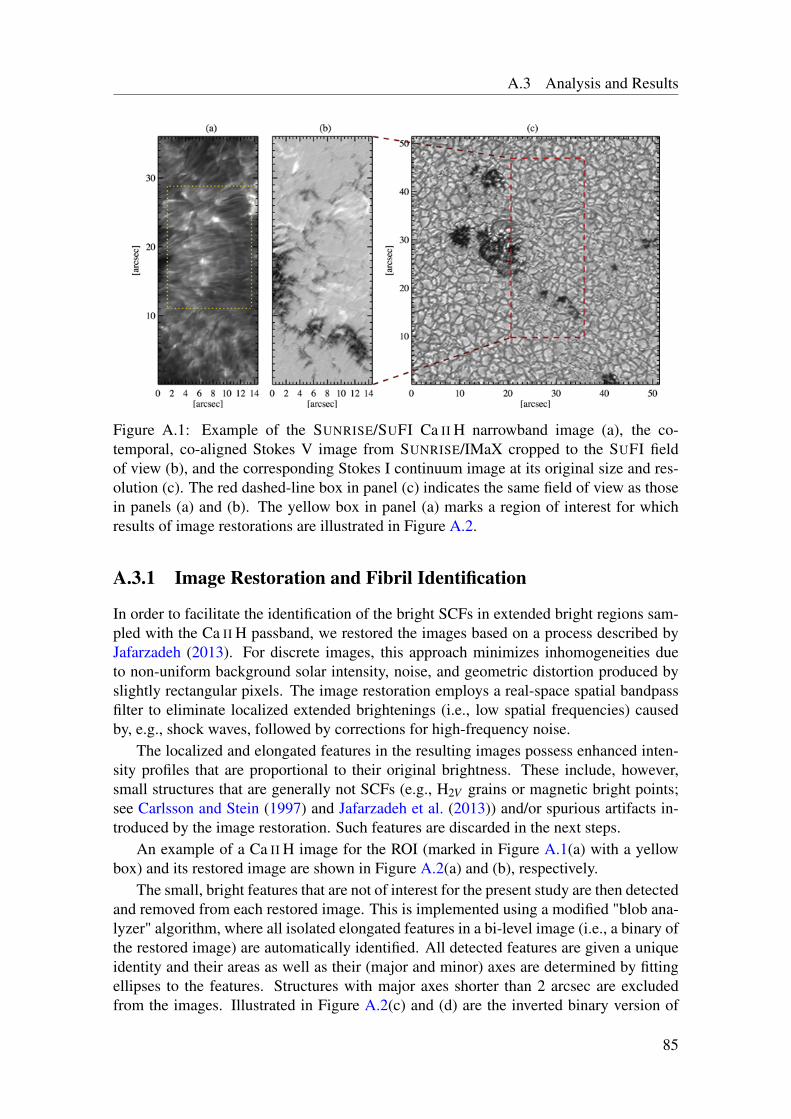
A.3 Analysis and Results
Figure A.1: Example of the SUNRISE/SUFI Ca II H narrowband image (a), the co-temporal, co-aligned Stokes V image from SUNRISE/IMaX cropped to the SUFI fieldof view (b), and the corresponding Stokes I continuum image at its original size and res-olution (c). The red dashed-line box in panel (c) indicates the same field of view as thosein panels (a) and (b). The yellow box in panel (a) marks a region of interest for whichresults of image restorations are illustrated in Figure A.2.
A.3.1 Image Restoration and Fibril Identification
In order to facilitate the identification of the bright SCFs in extended bright regions sam-pled with the Ca II H passband, we restored the images based on a process described byJafarzadeh (2013). For discrete images, this approach minimizes inhomogeneities dueto non-uniform background solar intensity, noise, and geometric distortion produced byslightly rectangular pixels. The image restoration employs a real-space spatial bandpassfilter to eliminate localized extended brightenings (i.e., low spatial frequencies) causedby, e.g., shock waves, followed by corrections for high-frequency noise.
The localized and elongated features in the resulting images possess enhanced inten-sity profiles that are proportional to their original brightness. These include, however,small structures that are generally not SCFs (e.g., H2V grains or magnetic bright points;see Carlsson and Stein (1997) and Jafarzadeh et al. (2013)) and/or spurious artifacts in-troduced by the image restoration. Such features are discarded in the next steps.
An example of a Ca II H image for the ROI (marked in Figure A.1(a) with a yellowbox) and its restored image are shown in Figure A.2(a) and (b), respectively.
The small, bright features that are not of interest for the present study are then detectedand removed from each restored image. This is implemented using a modified "blob ana-lyzer" algorithm, where all isolated elongated features in a bi-level image (i.e., a binary ofthe restored image) are automatically identified. All detected features are given a uniqueidentity and their areas as well as their (major and minor) axes are determined by fittingellipses to the features. Structures with major axes shorter than 2 arcsec are excludedfrom the images. Illustrated in Figure A.2(c) and (d) are the inverted binary version of
85
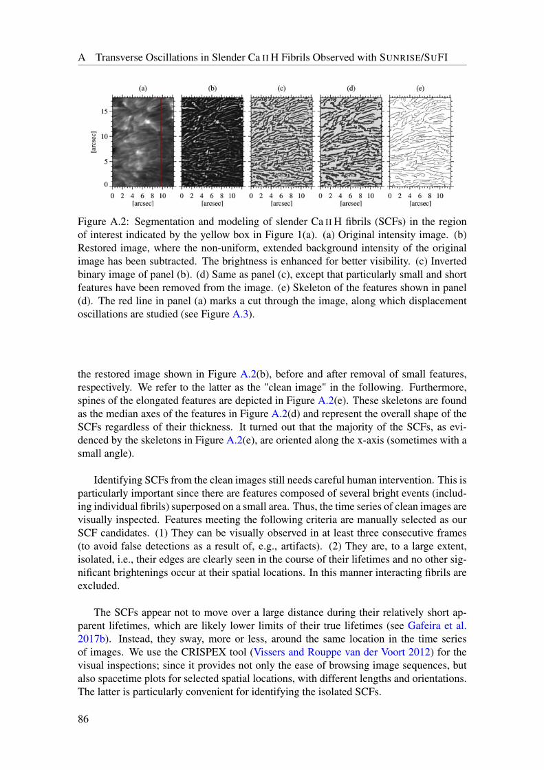
A Transverse Oscillations in Slender Ca II H Fibrils Observed with SUNRISE/SUFI
Figure A.2: Segmentation and modeling of slender Ca II H fibrils (SCFs) in the regionof interest indicated by the yellow box in Figure 1(a). (a) Original intensity image. (b)Restored image, where the non-uniform, extended background intensity of the originalimage has been subtracted. The brightness is enhanced for better visibility. (c) Invertedbinary image of panel (b). (d) Same as panel (c), except that particularly small and shortfeatures have been removed from the image. (e) Skeleton of the features shown in panel(d). The red line in panel (a) marks a cut through the image, along which displacementoscillations are studied (see Figure A.3).
the restored image shown in Figure A.2(b), before and after removal of small features,respectively. We refer to the latter as the "clean image" in the following. Furthermore,spines of the elongated features are depicted in Figure A.2(e). These skeletons are foundas the median axes of the features in Figure A.2(d) and represent the overall shape of theSCFs regardless of their thickness. It turned out that the majority of the SCFs, as evi-denced by the skeletons in Figure A.2(e), are oriented along the x-axis (sometimes with asmall angle).
Identifying SCFs from the clean images still needs careful human intervention. This isparticularly important since there are features composed of several bright events (includ-ing individual fibrils) superposed on a small area. Thus, the time series of clean images arevisually inspected. Features meeting the following criteria are manually selected as ourSCF candidates. (1) They can be visually observed in at least three consecutive frames(to avoid false detections as a result of, e.g., artifacts). (2) They are, to a large extent,isolated, i.e., their edges are clearly seen in the course of their lifetimes and no other sig-nificant brightenings occur at their spatial locations. In this manner interacting fibrils areexcluded.
The SCFs appear not to move over a large distance during their relatively short ap-parent lifetimes, which are likely lower limits of their true lifetimes (see Gafeira et al.2017b). Instead, they sway, more or less, around the same location in the time seriesof images. We use the CRISPEX tool (Vissers and Rouppe van der Voort 2012) for thevisual inspections; since it provides not only the ease of browsing image sequences, butalso spacetime plots for selected spatial locations, with different lengths and orientations.The latter is particularly convenient for identifying the isolated SCFs.
86
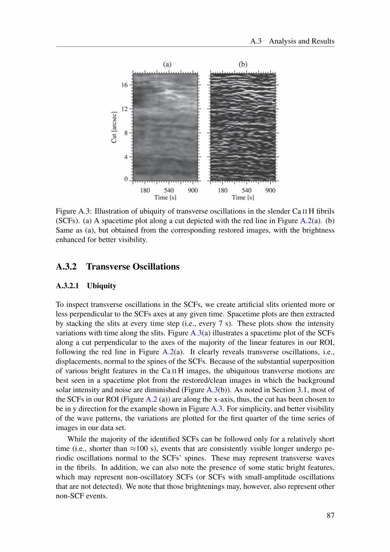
A.3 Analysis and Results
Figure A.3: Illustration of ubiquity of transverse oscillations in the slender Ca II H fibrils(SCFs). (a) A spacetime plot along a cut depicted with the red line in Figure A.2(a). (b)Same as (a), but obtained from the corresponding restored images, with the brightnessenhanced for better visibility.
A.3.2 Transverse Oscillations
A.3.2.1 Ubiquity
To inspect transverse oscillations in the SCFs, we create artificial slits oriented more orless perpendicular to the SCFs axes at any given time. Spacetime plots are then extractedby stacking the slits at every time step (i.e., every 7 s). These plots show the intensityvariations with time along the slits. Figure A.3(a) illustrates a spacetime plot of the SCFsalong a cut perpendicular to the axes of the majority of the linear features in our ROI,following the red line in Figure A.2(a). It clearly reveals transverse oscillations, i.e.,displacements, normal to the spines of the SCFs. Because of the substantial superpositionof various bright features in the Ca II H images, the ubiquitous transverse motions arebest seen in a spacetime plot from the restored/clean images in which the backgroundsolar intensity and noise are diminished (Figure A.3(b)). As noted in Section 3.1, most ofthe SCFs in our ROI (Figure A.2 (a)) are along the x-axis, thus, the cut has been chosen tobe in y direction for the example shown in Figure A.3. For simplicity, and better visibilityof the wave patterns, the variations are plotted for the first quarter of the time series ofimages in our data set.
While the majority of the identified SCFs can be followed only for a relatively shorttime (i.e., shorter than ≈100 s), events that are consistently visible longer undergo pe-riodic oscillations normal to the SCFs’ spines. These may represent transverse wavesin the fibrils. In addition, we can also note the presence of some static bright features,which may represent non-oscillatory SCFs (or SCFs with small-amplitude oscillationsthat are not detected). We note that those brightenings may, however, also represent othernon-SCF events.
87
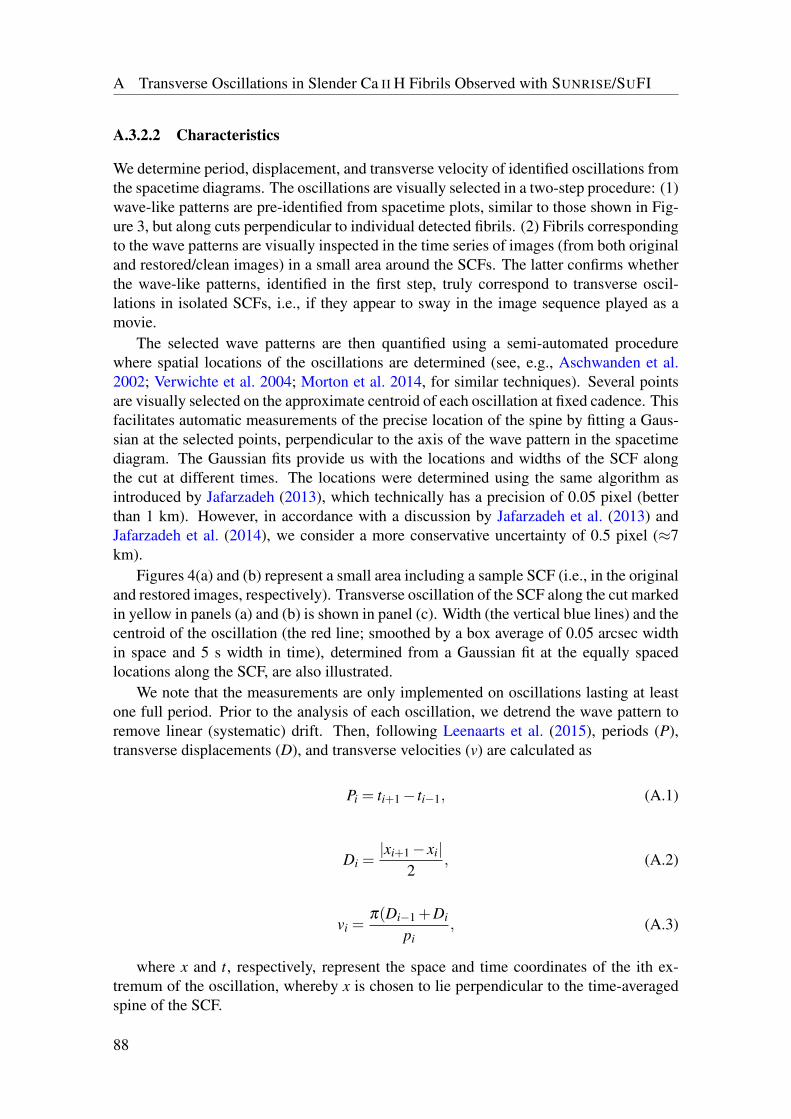
A Transverse Oscillations in Slender Ca II H Fibrils Observed with SUNRISE/SUFI
A.3.2.2 Characteristics
We determine period, displacement, and transverse velocity of identified oscillations fromthe spacetime diagrams. The oscillations are visually selected in a two-step procedure: (1)wave-like patterns are pre-identified from spacetime plots, similar to those shown in Fig-ure 3, but along cuts perpendicular to individual detected fibrils. (2) Fibrils correspondingto the wave patterns are visually inspected in the time series of images (from both originaland restored/clean images) in a small area around the SCFs. The latter confirms whetherthe wave-like patterns, identified in the first step, truly correspond to transverse oscil-lations in isolated SCFs, i.e., if they appear to sway in the image sequence played as amovie.
The selected wave patterns are then quantified using a semi-automated procedurewhere spatial locations of the oscillations are determined (see, e.g., Aschwanden et al.2002; Verwichte et al. 2004; Morton et al. 2014, for similar techniques). Several pointsare visually selected on the approximate centroid of each oscillation at fixed cadence. Thisfacilitates automatic measurements of the precise location of the spine by fitting a Gaus-sian at the selected points, perpendicular to the axis of the wave pattern in the spacetimediagram. The Gaussian fits provide us with the locations and widths of the SCF alongthe cut at different times. The locations were determined using the same algorithm asintroduced by Jafarzadeh (2013), which technically has a precision of 0.05 pixel (betterthan 1 km). However, in accordance with a discussion by Jafarzadeh et al. (2013) andJafarzadeh et al. (2014), we consider a more conservative uncertainty of 0.5 pixel (≈7km).
Figures 4(a) and (b) represent a small area including a sample SCF (i.e., in the originaland restored images, respectively). Transverse oscillation of the SCF along the cut markedin yellow in panels (a) and (b) is shown in panel (c). Width (the vertical blue lines) and thecentroid of the oscillation (the red line; smoothed by a box average of 0.05 arcsec widthin space and 5 s width in time), determined from a Gaussian fit at the equally spacedlocations along the SCF, are also illustrated.
We note that the measurements are only implemented on oscillations lasting at leastone full period. Prior to the analysis of each oscillation, we detrend the wave pattern toremove linear (systematic) drift. Then, following Leenaarts et al. (2015), periods (P),transverse displacements (D), and transverse velocities (v) are calculated as
Pi = ti+1− ti−1, (A.1)
Di =|xi+1− xi|
2, (A.2)
vi =π(Di−1 +Di
pi, (A.3)
where x and t, respectively, represent the space and time coordinates of the ith ex-tremum of the oscillation, whereby x is chosen to lie perpendicular to the time-averagedspine of the SCF.
88
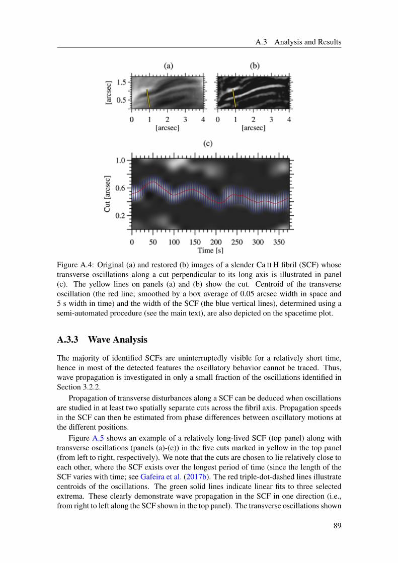
A.3 Analysis and Results
Figure A.4: Original (a) and restored (b) images of a slender Ca II H fibril (SCF) whosetransverse oscillations along a cut perpendicular to its long axis is illustrated in panel(c). The yellow lines on panels (a) and (b) show the cut. Centroid of the transverseoscillation (the red line; smoothed by a box average of 0.05 arcsec width in space and5 s width in time) and the width of the SCF (the blue vertical lines), determined using asemi-automated procedure (see the main text), are also depicted on the spacetime plot.
A.3.3 Wave Analysis
The majority of identified SCFs are uninterruptedly visible for a relatively short time,hence in most of the detected features the oscillatory behavior cannot be traced. Thus,wave propagation is investigated in only a small fraction of the oscillations identified inSection 3.2.2.
Propagation of transverse disturbances along a SCF can be deduced when oscillationsare studied in at least two spatially separate cuts across the fibril axis. Propagation speedsin the SCF can then be estimated from phase differences between oscillatory motions atthe different positions.
Figure A.5 shows an example of a relatively long-lived SCF (top panel) along withtransverse oscillations (panels (a)-(e)) in the five cuts marked in yellow in the top panel(from left to right, respectively). We note that the cuts are chosen to lie relatively close toeach other, where the SCF exists over the longest period of time (since the length of theSCF varies with time; see Gafeira et al. (2017b). The red triple-dot-dashed lines illustratecentroids of the oscillations. The green solid lines indicate linear fits to three selectedextrema. These clearly demonstrate wave propagation in the SCF in one direction (i.e.,from right to left along the SCF shown in the top panel). The transverse oscillations shown
89
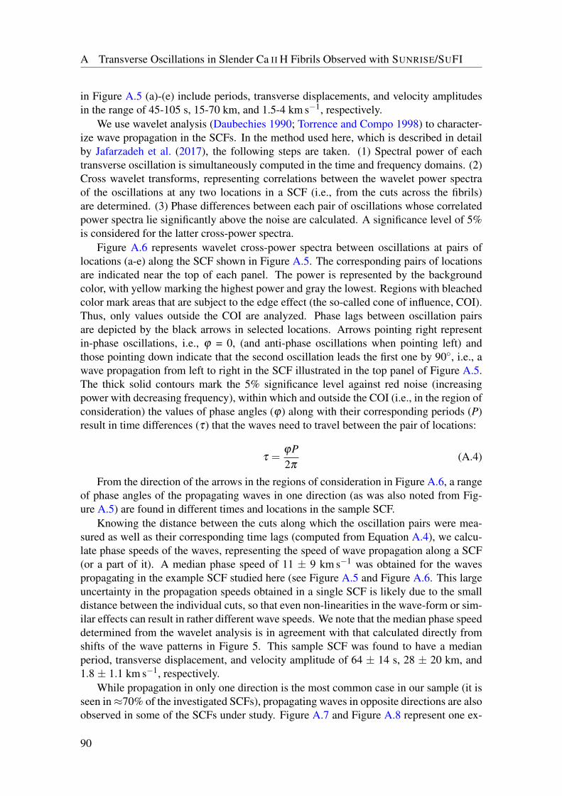
A Transverse Oscillations in Slender Ca II H Fibrils Observed with SUNRISE/SUFI
in Figure A.5 (a)-(e) include periods, transverse displacements, and velocity amplitudesin the range of 45-105 s, 15-70 km, and 1.5-4 km s−1, respectively.
We use wavelet analysis (Daubechies 1990; Torrence and Compo 1998) to character-ize wave propagation in the SCFs. In the method used here, which is described in detailby Jafarzadeh et al. (2017), the following steps are taken. (1) Spectral power of eachtransverse oscillation is simultaneously computed in the time and frequency domains. (2)Cross wavelet transforms, representing correlations between the wavelet power spectraof the oscillations at any two locations in a SCF (i.e., from the cuts across the fibrils)are determined. (3) Phase differences between each pair of oscillations whose correlatedpower spectra lie significantly above the noise are calculated. A significance level of 5%is considered for the latter cross-power spectra.
Figure A.6 represents wavelet cross-power spectra between oscillations at pairs oflocations (a-e) along the SCF shown in Figure A.5. The corresponding pairs of locationsare indicated near the top of each panel. The power is represented by the backgroundcolor, with yellow marking the highest power and gray the lowest. Regions with bleachedcolor mark areas that are subject to the edge effect (the so-called cone of influence, COI).Thus, only values outside the COI are analyzed. Phase lags between oscillation pairsare depicted by the black arrows in selected locations. Arrows pointing right representin-phase oscillations, i.e., ϕ = 0, (and anti-phase oscillations when pointing left) andthose pointing down indicate that the second oscillation leads the first one by 90, i.e., awave propagation from left to right in the SCF illustrated in the top panel of Figure A.5.The thick solid contours mark the 5% significance level against red noise (increasingpower with decreasing frequency), within which and outside the COI (i.e., in the region ofconsideration) the values of phase angles (ϕ) along with their corresponding periods (P)result in time differences (τ) that the waves need to travel between the pair of locations:
τ =ϕP2π
(A.4)
From the direction of the arrows in the regions of consideration in Figure A.6, a rangeof phase angles of the propagating waves in one direction (as was also noted from Fig-ure A.5) are found in different times and locations in the sample SCF.
Knowing the distance between the cuts along which the oscillation pairs were mea-sured as well as their corresponding time lags (computed from Equation A.4), we calcu-late phase speeds of the waves, representing the speed of wave propagation along a SCF(or a part of it). A median phase speed of 11 ± 9 km s−1 was obtained for the wavespropagating in the example SCF studied here (see Figure A.5 and Figure A.6. This largeuncertainty in the propagation speeds obtained in a single SCF is likely due to the smalldistance between the individual cuts, so that even non-linearities in the wave-form or sim-ilar effects can result in rather different wave speeds. We note that the median phase speeddetermined from the wavelet analysis is in agreement with that calculated directly fromshifts of the wave patterns in Figure 5. This sample SCF was found to have a medianperiod, transverse displacement, and velocity amplitude of 64 ± 14 s, 28 ± 20 km, and1.8 ± 1.1 km s−1, respectively.
While propagation in only one direction is the most common case in our sample (it isseen in≈70% of the investigated SCFs), propagating waves in opposite directions are alsoobserved in some of the SCFs under study. Figure A.7 and Figure A.8 represent one ex-
90
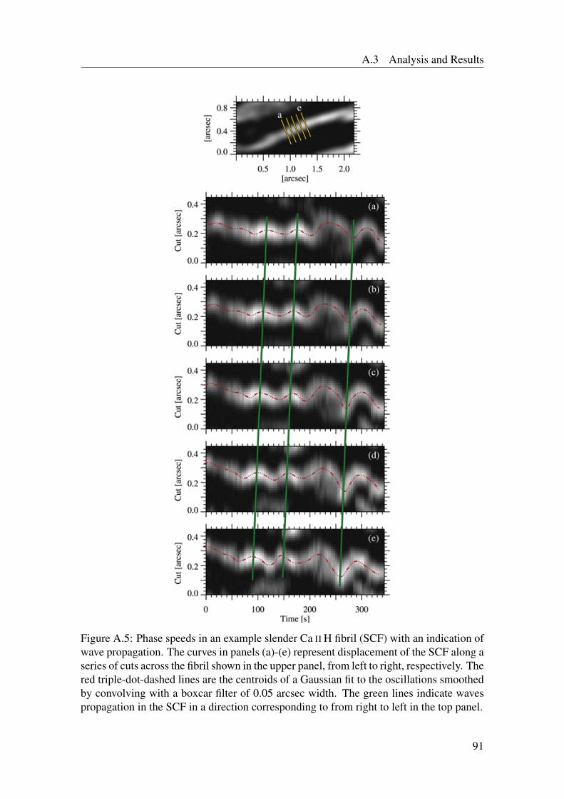
A.3 Analysis and Results
Figure A.5: Phase speeds in an example slender Ca II H fibril (SCF) with an indication ofwave propagation. The curves in panels (a)-(e) represent displacement of the SCF along aseries of cuts across the fibril shown in the upper panel, from left to right, respectively. Thered triple-dot-dashed lines are the centroids of a Gaussian fit to the oscillations smoothedby convolving with a boxcar filter of 0.05 arcsec width. The green lines indicate wavespropagation in the SCF in a direction corresponding to from right to left in the top panel.
91
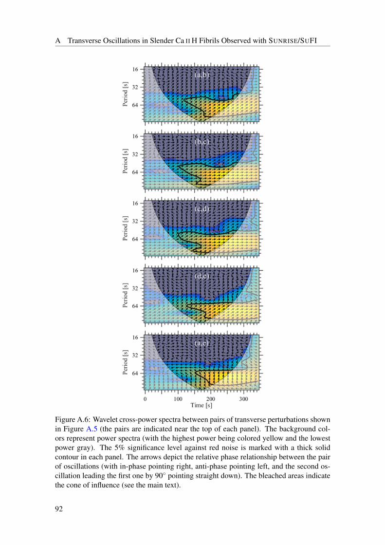
A Transverse Oscillations in Slender Ca II H Fibrils Observed with SUNRISE/SUFI
Figure A.6: Wavelet cross-power spectra between pairs of transverse perturbations shownin Figure A.5 (the pairs are indicated near the top of each panel). The background col-ors represent power spectra (with the highest power being colored yellow and the lowestpower gray). The 5% significance level against red noise is marked with a thick solidcontour in each panel. The arrows depict the relative phase relationship between the pairof oscillations (with in-phase pointing right, anti-phase pointing left, and the second os-cillation leading the first one by 90 pointing straight down). The bleached areas indicatethe cone of influence (see the main text).
92
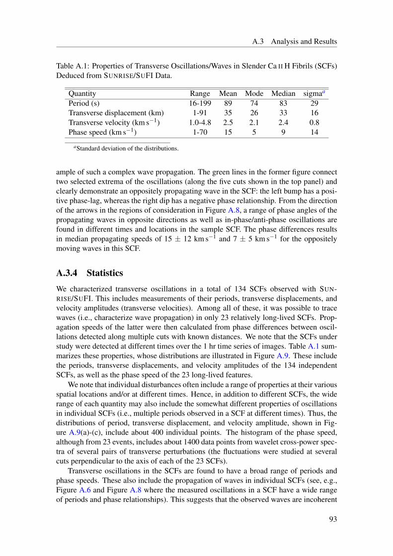
A.3 Analysis and Results
Table A.1: Properties of Transverse Oscillations/Waves in Slender Ca II H Fibrils (SCFs)Deduced from SUNRISE/SUFI Data.
Quantity Range Mean Mode Median sigmaa
Period (s) 16-199 89 74 83 29Transverse displacement (km) 1-91 35 26 33 16Transverse velocity (km s−1) 1.0-4.8 2.5 2.1 2.4 0.8Phase speed (km s−1) 1-70 15 5 9 14
aStandard deviation of the distributions.
ample of such a complex wave propagation. The green lines in the former figure connecttwo selected extrema of the oscillations (along the five cuts shown in the top panel) andclearly demonstrate an oppositely propagating wave in the SCF: the left bump has a posi-tive phase-lag, whereas the right dip has a negative phase relationship. From the directionof the arrows in the regions of consideration in Figure A.8, a range of phase angles of thepropagating waves in opposite directions as well as in-phase/anti-phase oscillations arefound in different times and locations in the sample SCF. The phase differences resultsin median propagating speeds of 15 ± 12 km s−1 and 7 ± 5 km s−1 for the oppositelymoving waves in this SCF.
A.3.4 Statistics
We characterized transverse oscillations in a total of 134 SCFs observed with SUN-RISE/SUFI. This includes measurements of their periods, transverse displacements, andvelocity amplitudes (transverse velocities). Among all of these, it was possible to tracewaves (i.e., characterize wave propagation) in only 23 relatively long-lived SCFs. Prop-agation speeds of the latter were then calculated from phase differences between oscil-lations detected along multiple cuts with known distances. We note that the SCFs understudy were detected at different times over the 1 hr time series of images. Table A.1 sum-marizes these properties, whose distributions are illustrated in Figure A.9. These includethe periods, transverse displacements, and velocity amplitudes of the 134 independentSCFs, as well as the phase speed of the 23 long-lived features.
We note that individual disturbances often include a range of properties at their variousspatial locations and/or at different times. Hence, in addition to different SCFs, the widerange of each quantity may also include the somewhat different properties of oscillationsin individual SCFs (i.e., multiple periods observed in a SCF at different times). Thus, thedistributions of period, transverse displacement, and velocity amplitude, shown in Fig-ure A.9(a)-(c), include about 400 individual points. The histogram of the phase speed,although from 23 events, includes about 1400 data points from wavelet cross-power spec-tra of several pairs of transverse perturbations (the fluctuations were studied at severalcuts perpendicular to the axis of each of the 23 SCFs).
Transverse oscillations in the SCFs are found to have a broad range of periods andphase speeds. These also include the propagation of waves in individual SCFs (see, e.g.,Figure A.6 and Figure A.8 where the measured oscillations in a SCF have a wide rangeof periods and phase relationships). This suggests that the observed waves are incoherent
93
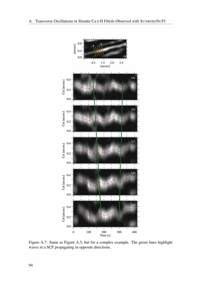
A Transverse Oscillations in Slender Ca II H Fibrils Observed with SUNRISE/SUFI
Figure A.7: Same as Figure A.5, but for a complex example. The green lines highlightwaves in a SCF propagating in opposite directions.
94
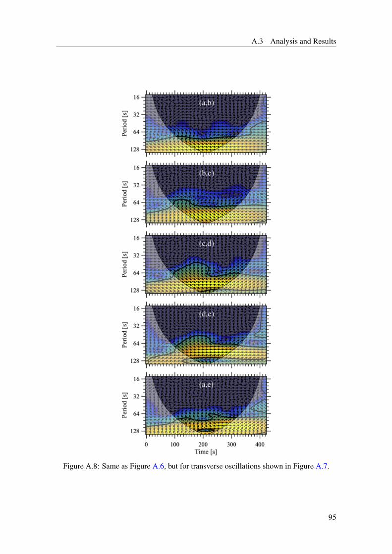
A.3 Analysis and Results
Figure A.8: Same as Figure A.6, but for transverse oscillations shown in Figure A.7.
95
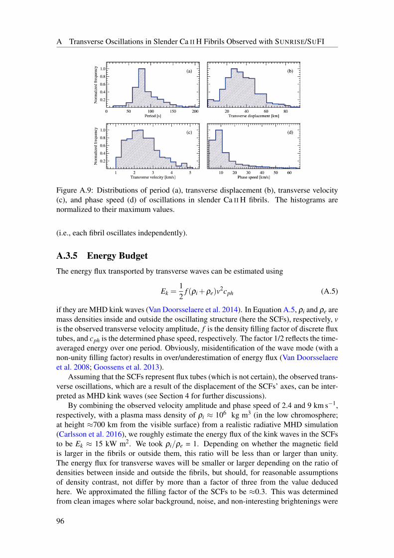
A Transverse Oscillations in Slender Ca II H Fibrils Observed with SUNRISE/SUFI
Figure A.9: Distributions of period (a), transverse displacement (b), transverse velocity(c), and phase speed (d) of oscillations in slender Ca II H fibrils. The histograms arenormalized to their maximum values.
(i.e., each fibril oscillates independently).
A.3.5 Energy BudgetThe energy flux transported by transverse waves can be estimated using
Ek =12
f (ρi +ρe)v2cph (A.5)
if they are MHD kink waves (Van Doorsselaere et al. 2014). In Equation A.5, ρi and ρe aremass densities inside and outside the oscillating structure (here the SCFs), respectively, vis the observed transverse velocity amplitude, f is the density filling factor of discrete fluxtubes, and cph is the determined phase speed, respectively. The factor 1/2 reflects the time-averaged energy over one period. Obviously, misidentification of the wave mode (with anon-unity filling factor) results in over/underestimation of energy flux (Van Doorsselaereet al. 2008; Goossens et al. 2013).
Assuming that the SCFs represent flux tubes (which is not certain), the observed trans-verse oscillations, which are a result of the displacement of the SCFs’ axes, can be inter-preted as MHD kink waves (see Section 4 for further discussions).
By combining the observed velocity amplitude and phase speed of 2.4 and 9 km s−1,respectively, with a plasma mass density of ρi ≈ 106 kg m3 (in the low chromosphere;at height ≈700 km from the visible surface) from a realistic radiative MHD simulation(Carlsson et al. 2016), we roughly estimate the energy flux of the kink waves in the SCFsto be Ek ≈ 15 kW m2. We took ρi/ρe = 1. Depending on whether the magnetic fieldis larger in the fibrils or outside them, this ratio will be less than or larger than unity.The energy flux for transverse waves will be smaller or larger depending on the ratio ofdensities between inside and outside the fibrils, but should, for reasonable assumptionsof density contrast, not differ by more than a factor of three from the value deducedhere. We approximated the filling factor of the SCFs to be ≈0.3. This was determinedfrom clean images where solar background, noise, and non-interesting brightenings were
96
A.4 Discussion and Conclusions
removed from the observed data (see Section 3.1). The ratio of the area filled by the SCFsto the total area (averaged over the entire time series of images) was taken as the fillingfactor. This would, however, be a lower limit for the filling factor, since many fibrils wereexcluded during the several steps of image restoration.
Also, we assume that the (magnetized) gas between the fibrils is not oscillating, whichis unlikely, as the shaking fibril should also excite oscillations in that gas. The assump-tion of a kink wave requires that the density (and/or the magnetic field strength) insidethe fibrils is different from that outside the fibrils. In the lower chromosphere, it is un-clear to what extent such differences occur, or if the fibrils are mainly visible becauseof, e.g., a horizontal temperature inhomogeneity in the lower chromosphere leading to aninhomogeneous optical depth scale where the Ca II H2 peaks are formed.
A.4 Discussion and ConclusionsWe have presented, for the first time to our knowledge, observations of transverse oscil-lations in SCFs. Seeing-free observations by the SUFI instrument onboard the SUNRISE
1 m solar telescope in a narrowband Ca II H filter have provided us with an excellent longtime series of images sampling the lower solar chromosphere. The observed area was partof active region AR11768. The strongly enhanced Ca II H brightness in the ROI (see Fig-ure 1) indicates a significant enhancement of the H2V /H2R emission in the core of Ca II H(due to the enhanced temperatures in the presence of strong magnetic fields Solanki et al.1991; Beck et al. 2013) so that the observed radiation contains significant contributionsfrom the lower chromosphere (Jafarzadeh et al. 2017).
Our analysis of the SUNRISE/SUFI Ca II H data revealed that the transverse oscilla-tions are ubiquitous in the lower solar chromosphere. To characterize the oscillationsreliably, we limited our study to a relatively small number of isolated SCFs not affectedby, e.g., the superposition of several SCFs and/or with other brightenings. Most SCFs arevisible only for a short time at a stretch, are highly dynamic, and display a high numberdensity in the studied area.
We found a wide range of periods, transverse displacements, velocity amplitudes, andphase speeds (when possible) for the oscillations/waves along the SCFs (see Figure A.9),with median values of 83 s, 33 km, 2.4 km s−1, and 9 km s−1, respectively (see Table A.1for all statistical values).
The SCFs are found to share some physical characteristics with, e.g., type II spiculesobserved in the upper chromosphere according to Gafeira et al. (2017b). Table A.2 sum-marizes properties of transverse oscillations (and waves) for various fibrillar structuresobserved in different chromospheric passbands reported in the literature, along with ourresults for the SCFs (see Jess et al. 2015, for a detailed overview).
97
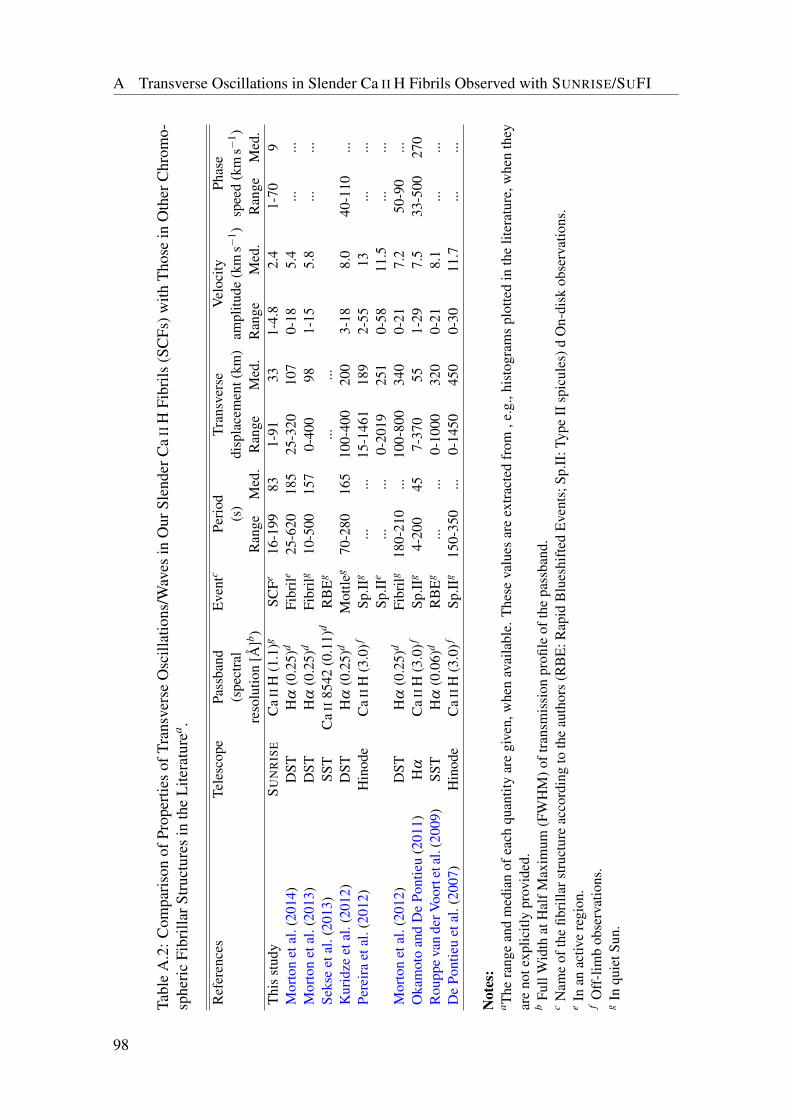
A Transverse Oscillations in Slender Ca II H Fibrils Observed with SUNRISE/SUFI
Tabl
eA
.2:C
ompa
riso
nof
Prop
ertie
sof
Tran
sver
seO
scill
atio
ns/W
aves
inO
urSl
ende
rCa
IIH
Fibr
ils(S
CFs
)with
Tho
sein
Oth
erC
hrom
o-sp
heri
cFi
brill
arSt
ruct
ures
inth
eL
itera
ture
a .
Ref
eren
ces
Tele
scop
ePa
ssba
ndE
vent
cPe
riod
Tran
sver
seV
eloc
ityPh
ase
(spe
ctra
l(s
)di
spla
cem
ent(
km)
ampl
itude
(km
s−1 )
spee
d(k
ms−
1 )re
solu
tion
[Å]b )
Ran
geM
ed.
Ran
geM
ed.
Ran
geM
ed.
Ran
geM
ed.
Thi
sst
udy
SU
NR
ISE
Ca
IIH
(1.1
)gSC
Fe16
-199
831-
9133
1-4.
82.
41-
709
Mor
ton
etal
.(20
14)
DST
Hα
(0.2
5)d
Fibr
ile25
-620
185
25-3
2010
70-
185.
4...
...M
orto
net
al.(
2013
)D
STH
α(0
.25)
dFi
brilg
10-5
0015
70-
400
981-
155.
8...
...Se
kse
etal
.(20
13)
SST
Ca
II85
42(0
.11)
dR
BE
g...
...K
urid
zeet
al.(
2012
)D
STH
α(0
.25)
dM
ottle
g70
-280
165
100-
400
200
3-18
8.0
40-1
10...
Pere
ira
etal
.(20
12)
Hin
ode
Ca
IIH
(3.0
)fSp
.IIg
......
15-1
461
189
2-55
13...
...Sp
.IIe
......
0-20
1925
10-
5811
.5...
...M
orto
net
al.(
2012
)D
STH
α(0
.25)
dFi
brilg
180-
210
...10
0-80
034
00-
217.
250
-90
...O
kam
oto
and
De
Pont
ieu
(201
1)H
αC
aII
H(3
.0)f
Sp.II
g4-
200
457-
370
551-
297.
533
-500
270
Rou
ppe
van
derV
oort
etal
.(20
09)
SST
Hα
(0.0
6)d
RB
Eg
......
0-10
0032
00-
218.
1...
...D
ePo
ntie
uet
al.(
2007
)H
inod
eC
aII
H(3
.0)f
Sp.II
g15
0-35
0...
0-14
5045
00-
3011
.7...
...
Not
es:
a The
rang
ean
dm
edia
nof
each
quan
tity
are
give
n,w
hen
avai
labl
e.T
hese
valu
esar
eex
trac
ted
from
,e.g
.,hi
stog
ram
spl
otte
din
the
liter
atur
e,w
hen
they
are
note
xplic
itly
prov
ided
.b
Full
Wid
that
Hal
fMax
imum
(FW
HM
)oft
rans
mis
sion
profi
leof
the
pass
band
.c
Nam
eof
the
fibri
llars
truc
ture
acco
rdin
gto
the
auth
ors
(RB
E:R
apid
Blu
eshi
fted
Eve
nts;
Sp.II
:Typ
eII
spic
ules
)dO
n-di
skob
serv
atio
ns.
eIn
anac
tive
regi
on.
fO
ff-l
imb
obse
rvat
ions
.g
Inqu
ietS
un.
98
A.4 Discussion and Conclusions
In addition to the ranges of different parameters of transverse oscillations in variouschromospheric structures, we have also provided the median values of their distributionsin Table A.2, when available. When not explicitly given, they were estimated from plotteddistributions. We do not use mean values of the parameters, since they can be susceptibleto the influence of outliers. The latter becomes particularly important in the case of fibril-lar structures because their precise detection is often a challenge (or they could be mixedwith other features of similar appearance). We stress that most of the other studies inves-tigated waves on fibrillar structures located higher in the solar atmosphere (the off-limbstudies even much higher), which might explain some of the differences seen in Table A.2and discussed below.
The SCFs are found to have transverse oscillation with shorter periods than their coun-terparts in the higher chromospheric layers (with the median period of the former beingshorter by a factor of ≈2 than the latter). The median period of type II spicules reportedby Okamoto and De Pontieu (2011) is, however, smaller than that of the SCFs (and otherchromospheric fibrillar events, including type II spicules from the other studies). Theauthors explained their very short periods as a result of their method of analysis.
Transverse displacement, velocity amplitude and phase speed of the SCFs studied hereare significantly smaller than those of the upper chromospheric elongated features (i.e.,Hα fibrils, type II spicules, mottles and Hα/Ca II 8542 Å RBEs). Transverse displace-ments of the relatively short-period type II spicules of Okamoto and De Pontieu (2011)are, however, comparable to (but slightly larger than) those we found for the SCFs (that isalso likely to be an influence of their detection method). One reason for this discrepancy,even with structures observed by Hinode in the same spectral line is the fact that many ofthe other observations in Ca II H were off-limb, whereas we are observing near solar diskcenter. This makes the SUFI observations mainly sensitive to much lower levels in thesolar atmosphere, where wave parameters, such as wave amplitudes, are expected to belower due to the higher gas density, assuming the total energy flux in the waves to be thesame at both layers. However, the higher spatial resolution of the SUFI data also allowssmaller wave amplitudes to be detected.
The structures listed in Table A.2 have been observed in various spectral lines in somecases off-limb so that they sample different heights in the solar chromosphere (Rutten2007; Leenaarts et al. 2009, 2012). In the vigorously dynamic Sun even individual linesmay obtain a contribution from a large range of heights (Rutten 2007). Hence, the linesused in the various observations may be affected by different local plasma properties,leading to subtle variations in the determined wave parameters (Jess and Verth 2015).
Hence, the chromospheric fibrillar structures sampled by the different observationscan be of intrinsically different types (Rutten 2007), with more upright fibrils (potentially)channeling energy to the corona and more slanted ones transferring energy mainly withindifferent parts of the chromosphere. The energies are likely generated in the photosphereas a result of the interactions between plasma and the magnetic field. Note that differentcharacteristics of these lines with respect to opacity causes limb observations to representmuch greater atmospheric heights compared to those on the disk. This is particularlythe case for observations of type II spicules in Ca II H off the limb. In that observinggeometry, the observed features lie in an upper chromospheric layer compared to on-diskobservations of, e.g., SCFs, using a similar, or even narrower bandpass. These eventsmay, however, share some apparent and/or physical characteristics (e.g., both types of
99
A Transverse Oscillations in Slender Ca II H Fibrils Observed with SUNRISE/SUFI
underlying fibrils are observed as short-lived, dynamic, thin and bright elongated featuresin the Ca II H passband). Jafarzadeh et al. (2017a) showed that the SUNRISE/SUFI SCFsmap the magnetic fields in the low solar chromosphere.
The observed transverse oscillations in the SCFs can clearly be described as wavespropagating along the axes of the SCFs (when phase relationship between different loca-tions along the fibril could be studied). In principle, both bulk Alfvén and kink waves canlead to transverse displacements. While some authors have interpreted transverse oscil-lations in chromospheric (and/or coronal) fibrillar structures, such as type II spicules, asAlfvénic waves (e.g., de Pontieu et al. 2007; Tomczyk et al. 2007; McIntosh et al. 2011),others have debated such interpretations and have explained them as a result of MHD kinkwaves (e.g., Van Doorsselaere et al. 2008, 2014; Goossens et al. 2013). In any case, theyare Alfvénic, i.e., largely incompressible transverse oscillations propagating along thefield lines, whose phase speed differs from the Alfvén speed only due to the inhomogene-ity of the atmosphere (see, e.g., Priest 2014, for a detailed description of the terminologyused here). The exact wave mode likely to be excited depends on the physical conditionsin the SCFs and their surroundings, which are still largely unexplored. The bulk (shear)Alfvén waves only exist in a homogeneous medium (Nakariakov and Verwichte 2005;Goossens et al. 2013), that is likely not the case in the solar atmosphere.
The SCFs are possibly a manifestation of plasma jets along horizontal flux tubes, thus,according to the MHD wave theory, the kink mode is the most appropriate interpretationof their swaying motions (Kukhianidze et al. 2006; Erdélyi et al. 2007; Zaqarashvili et al.2007). Note, however, that the fact that brightenings along the fibrils start more ofteninside the bulk of the fibrils than at one of their edges speaks against the interpretation ofthe fibrils as plasma jets. The incoherent oscillations among different SCFs disputes theoption of global (bulk) Alfvén waves (Zaqarashvili and Erdélyi 2009, in addition to theassumption of the non-uniform medium), although it is unclear how large the coherencelength must be to qualify as an Alfvén wave. A closer inspection would be necessary toconfirm whether such incoherency is also consistent between neighboring SCFs. Notethat incompressible, torsional Alfvén waves cannot displace flux tubes back and forth,hence they are unlikely to be responsible for the observed oscillations (Ploner and Solanki1999; Erdélyi and Fedun 2007; Van Doorsselaere et al. 2008; Jess et al. 2009). The MHDkink waves can be triggered by granular buffeting of footpoints of magnetic flux tubesat the base of the photosphere (e.g., Spruit 1981; Choudhuri et al. 1993; Hasan and vanBallegooijen 2008) or by small-scale magnetic reconnection (He et al. 2009). The wavescould also be generated as a result of wave coupling at plasma-β = 1 regions (e.g., Bogdanet al. 2003; Roberts 2004).
Excursions in the upper chromospheric fibrillar structures (such as mottles, spicules,and Hα dynamic fibrils) have been suggested to be produced by chromospheric shockwaves (De Pontieu et al. 2004; Hansteen et al. 2006). The chromospheric shocks areproduced with different strengths and periods that consequently result in a wide rangeof observed properties of transverse oscillations (Hansteen et al. 2006). This mechanismcould also be relevant for the origin of swaying motions in the SCFs, as shocks are alsopresent in the lower chromosphere (e.g., Wedemeyer et al. 2004).
We note that the ROI, within which the SCFs were studied, was located outsidepores, but in their immediate vicinity (see Figure A.1). Therefore, some of the wavesin our SCFs, particularly close to the left and bottom edges of the ROI, could be excited
100
A.4 Discussion and Conclusions
within the pores, or could at least be influenced by pore waves (e.g., Morton et al. 2012;Khomenko and Collados 2015).
The observed high-frequency kink waves were estimated to carry an energy flux oforder 15 kW m−2, which is comparable with what is needed to heat the (lower) solarchromosphere (Withbroe and Noyes 1977; Vernazza et al. 1981). Our observations can-not, however, clarify whether this energy is dissipated in the sampled atmospheric layers.The apparently almost horizontal orientation of the majority of the SCFs studied here,many of which connect back to the solar surface as low-lying loops (Jafarzadeh et al.2017, see), suggest that the waves propagating along them may not reach the upper atmo-sphere. Rather, they play a role in heating their local surroundings, if they release theirenergy at these layers. Jafarzadeh et al. (2017) showed with the help of the magnetostaticsolution of Wiegelmann et al. (2017) that the shorter SCFs map fields that are more ver-tical. A number of the transverse waves we have identified are found along these shortfibrils. These waves are likely capable of traveling upwards into the upper atmosphereand may even reach to the corona, contributing to the heating there.
To determine which mechanism can precisely explain the nature of bright and highlydynamic SCFs, analysis of high-resolution observations in a narrower Ca II H passband(e.g., from the upcoming SST/CHROMIS instrument) as well as realistic MHD simula-tions of this line will be necessary.
101

Publications
Refereed publications
• R. Gafeira, A. Lagg, S. K. Solanki, S. Jafarzadeh, M. van Noort, P. Barthol, J.Blanco Rodríguez, J. C. del Toro Iniesta, A. Gandorfer, L. Gizon, J. Hirzberger, M.Knölker, D. Orozco Suárez, T. L. Riethmüller, and W. Schmidt, published in ApJS,229, 2017, DOI 10.3847/1538-4365/229/1/6
• R. Gafeira,S. Jafarzadeh,S. K. Solanki, A. Lagg, M. van Noort, P. Barthol, J.Blanco Rodríguez, J. C. del Toro Iniesta, A. Gandorfer, L. Gizon, J. Hirzberger,M. Knölker, D. Orozco Suárez, T. L. Riethmüller, and W. Schmidt, published inApJS, 229, 2017, DOI 10.3847/1538-4365/229/1/7
• S. Jafarzadeh, S. K. Solanki, R. Gafeira, M. van Noort, P. Barthol, J. Blanco Ro-dríguez, J. C. del Toro Iniesta, A. Gandorfer, L. Gizon, J. Hirzberger, M. Knölker,D. Orozco Suárez, T. L. Riethmüller, and W. Schmidtpublished in ApJS, 229, 2017, DOI 10.3847/1538-4365/229/1/9.
103


Acknowledgements
My first thanks are going to my supervisors Sami Solanki and Andreas Lagg. Thanks toSami, for all his guidance, interesting discussions and support. Big thanks to Andreas forall his help and patience during the progress of my work, and infinite help in the processof writing the papers and thesis. Your help and our end of afternoon beneficial, efficient,extensive, refreshing meetings were essential to me to be able to finish my thesis. Thanksto Laurent for the valuable output and carefully reading my thesis.
Obrigado aos meus pais, Francisco e Graça e ao meu irmão Tiago e aos meus avosestarem sempre presentes e por serem a melhor família que alguém pode ter.
Thanks for all the good moments, and for the support and help to overpass the diffi-cult times to Filipa, Francisco Iglesias, David, Ivan, Alessandro, Michel, Azaymi, Iulia,Suzana, Isabel, and Pedro Lacerda that I have the luck to meet during this journey that Ihave the privilege to call friends.
Thanks to the ones who made my stay in Göttingen much nicer. Borys, Sabrina,Sihane, Marta, Gonçalo, Hans-Peter, Iker, Benjamin, Cátia, Belisa, Rita, Francisco, Luis,and so many others. Thanks to my old friends that even far away they were always presentfor me, Sara, Joana, Carina, Ricardo Vieira, Fabio, Tiago, Teresa, Peixinho, Sr. Claudino,Dr. Adriana, Dr. JoÃco Fernandes.
Thanks to Shahin for all his help during the thesis and support during my visit toInstitute of Theoretical Astrophysics in Oslo. To my officemates Mariangela, Patricio,Fabian, Chi Ju, and Farhad. To all SLAM members, in particular to Michiel, for the helpand availability to always answer to my question.
Thanks to the International Max Planck Research School (IMPRS) for Solar SystemScience at the University of Göttingen for the financial support and to the school coordi-nator Sonja Schuh for all the help.
This thesis is dedicated to my parents and my brother.
105

Curriculum vitae
Ricardo Jorge Maranhas GafeiraBorn in August 1987 in Guarda, PortugalPortugueseemail:[email protected]
Education
• 2014–today, PhD. Student, Max Planck Institute for Solar System Research andUniversity of Göttingen, Göttingen, Germany
• 2009–2011, M. Sc. in Astrophysics and Space Instrumentation, Faculty of Sciencesand Technology of University of Coimbra, Portugal
• 2005–2009, B. Sc. in Physics with a Space Sciences Minor, Faculty of Sciencesand Technology of University of Coimbra, Portugal
Selected oral presentations
• Small scale chromospheric fibrils observed by Sunrise II, R. Gafeira, A. Lagg, M.van Noort, S. K. Solanki, 4th SOLARNET meeting "The physics of the Sun fromthe interior to the outer atmosphere", 20-23 June of 2016, Arrecife, Lanzarote,Spain
• Small scale chromospheric fibrils observed by Sunrise II, R. Gafeira, A. Lagg, M.van Noort, S. K. Solanki, IRIS-6: The chromosphere, 16-20 January of 2016, Uni-versity of Stockholm,Stockholm,Sweden
• Temporal variations in small scale chromospheric fibrils observed by Sunrise II, R.Gafeira, A. Lagg, M. van Noort, S. K. Solanki, Ground based Solar Observationsin the Space Instrumentation Era, 05-09 October of 2015, University of Coimbra,Coimbra, Portugal
• Variation rate of sunspot area, R. Gafeira, A.Pais, C. Fonte, J. Fernandes,XXIINational meeting of Astronomy and Astrophysics, 23-25 September of 2012, Uni-versity of Porto, Porto, Portugal
107
Curriculum vitae
Poster communication
• Temporal variations in small scale chromospheric fibrils observed by Sunrise, R.Gafeira, A. Lagg, M. van Noort, S. K. Solanki, Annual Meeting of the Astronomis-che Gesellschaft, 22-26 September of 2014, University of Bamberg, Bamberg, Ger-many
• Variation rate of sunspot area, R. Gafeira, A.Pais, C. Fonte, J. Fernandes, EuropeanWeek of Astronomy and Space Science, 1-6 July, Pontificia Università Lateranense,Rome, Italy
• Solar filaments : Characteristics and Evolution , R. Gafeira, J. Fernandes, J.Aboudarham, XXI National meeting of Astronomy and Astrophysics7-10 Septem-ber of 2011, University of Coimbra, Coimbra, Portugal
Book Chapters
• Claudio Paulo, Joana Latas, Leonor Cabral, Lina Canas, Lucio Carvalho, Luis Car-doso, Manuel Penhor, Paula Furtado, Paulo Jorge Lourenco, Ricardo Gafeira, RitaGuerra, Rosa Doran, "Do Planeta Terra ao Espaco - Sugestoes de tarefas experi-mentais para dentro e fora da sala de aula", ISBN: 978-989-20-5053-9
Publications
• R. Gafeira, A. Lagg, S. K. Solanki, S. Jafarzadeh, M. van Noort, P. Barthol,J. Blanco Rodríguez, J. C. del Toro Iniesta, A. Gandorfer, L. Gizon, J. Hirzberger,M. Knölker, D. Orozco Suárez, T. L. Riethmüller, and W. Schmidt. MorphologicalProperties of Slender Ca II H Fibrils Observed by Sunrise II. The AstrophysicalJournal Supplement Series, 229:6, March 2017
• R. Gafeira, A. Lagg, S. K. Solanki, S. Jafarzadeh, M. van Noort, P. Barthol,J. Blanco Rodríguez, J. C. del Toro Iniesta, A. Gandorfer, L. Gizon, J. Hirzberger,M. Knölker, D. Orozco Suárez, T. L. Riethmüller, and W. Schmidt. MorphologicalProperties of Slender Ca II H Fibrils Observed by Sunrise II. The AstrophysicalJournal Supplement Series, 229:6, March 2017
• R. Gafeira, S. Jafarzadeh, S. K. Solanki, A. Lagg, M. van Noort, P. Barthol,J. Blanco Rodríguez, J. C. del Toro Iniesta, A. Gandorfer, L. Gizon, J. Hirzberger,M. Knölker, D. Orozco Suárez, T. L. Riethmüller, and W. Schmidt. Oscilla-tions on Width and Intensity of Slender Ca II H Fibrils from Sunrise/SuFI. TheAstrophysical Journal Supplement Series, 229:7, March 2017
• S. Jafarzadeh, S. K. Solanki, R. Gafeira, M. van Noort, P. Barthol, J. Blanco Ro-dríguez, J. C. del Toro Iniesta, A. Gandorfer, L. Gizon, J. Hirzberger, M. Knölker,D. Orozco Suárez, T. L. Riethmüller, and W. Schmidt. Transverse Oscillationsin Slender Ca II H Fibrils Observed with Sunrise/SuFI. The Astrophysical JournalSupplement Series, 229:9, March 2017 .
108
Curriculum vitae
• S. Carvalho, P. Pina, T. Barata, R. Gafeira, and A. Garcia. Ground-based Ob-servations of Sunspots from the Observatory of Coimbra: Evaluation of Differ-ent Automated Approaches to Analyse its Datasets. In I. Dorotovic, C. E. Fis-cher, and M. Temmer, editors, Coimbra Solar Physics Meeting: Ground-basedSolar Observations in the Space Instrumentation Era, volume 504 of AstronomicalSociety of the Pacific Conference Series, page 125, April 2016
• R Gafeira, CC Fonte, MA Pais, and J Fernandes. Temporal evolution of sunspotareas and estimation of related plasma flows. Solar Physics, 289(5):1531–1542,2014
• Gafeira, R., Patacas, C., and Fernandes, J. Mass-luminosity relation for fgk mainsequence stars: metallicity and age contributions. Astrophysics and Space Science,341:405–410, 2012
• Peixinho, N., Delsanti, A., Guilbert-Lepoutre, A., Gafeira, R., and Lacerda, P. Thebimodal colors of centaurs and small kuiper belt objects.A&A, 546:A86, 2012
109


![Literatur 26022019 test - TU Braunschweig · 2015 [1] Aizpurua Aldasoro, H.: On Gust Buffeting Design of Slender Chimneys – Building Interference and Fatigue. Dissertation April](https://img.pdfslide.org/doc/110x75/6068ec4d422fa2738f4f4587/literatur-26022019-test-tu-braunschweig-2015-1-aizpurua-aldasoro-h-on-gust.jpg)