Embed Size (px)
Citation preview
Universität Ulm | 89069 Ulm | Germany Fakultät für
Mathematik und
Wirtschaftswissenschaften
Institut für
Numerische Mathematik
Speech Signal Noise Reduction
with Wavelets
Diplomarbeit an der Universität Ulm
Vorgelegt von:
Bernhard [email protected]
am 9. Oktober 2009
Gutachter:
Prof. Dr. Karsten UrbanProf. Dr. Stefan Funken
Contents
1 Introduction and Motivation: Why Wavelets 1
1.1 Preliminaries . . . . . . . . . . . . . . . . . . . . . . . . . . . . . 1
1.2 Some Notes on Speech Signals . . . . . . . . . . . . . . . . . . . . 2
1.3 Motivation . . . . . . . . . . . . . . . . . . . . . . . . . . . . . . . 3
1.4 Outline and Structure . . . . . . . . . . . . . . . . . . . . . . . . 5
2 Wavelet and Fourier Transform 7
2.1 The Continuous Wavelet Transform . . . . . . . . . . . . . . . . . 7
2.2 The Discrete Fast Wavelet Transform . . . . . . . . . . . . . . . . 8
2.3 The Stationary Wavelet Transform . . . . . . . . . . . . . . . . . 11
2.4 The Fourier Transform . . . . . . . . . . . . . . . . . . . . . . . . 13
2.5 Comparison . . . . . . . . . . . . . . . . . . . . . . . . . . . . . . 14
3 A General Noise and Speech Model 18
3.1 Noisy Speech Signal Model . . . . . . . . . . . . . . . . . . . . . . 18
3.2 Noise Transformation . . . . . . . . . . . . . . . . . . . . . . . . . 19
3.3 Some Definitions and Notations . . . . . . . . . . . . . . . . . . . 21
4 Spectral Domain Denoising 23
4.1 Noise Reduction Filter Model . . . . . . . . . . . . . . . . . . . . 23
4.2 Wiener Filter . . . . . . . . . . . . . . . . . . . . . . . . . . . . . 24
4.3 Spectral Subtraction and Power Subtraction Filter . . . . . . . . . 27
4.4 Ephraim-Malah Filter . . . . . . . . . . . . . . . . . . . . . . . . 28
4.5 A priori SNR Estimation . . . . . . . . . . . . . . . . . . . . . . . 30
5 Lipschitz Denoising 32
5.1 Lipschitz Regularity . . . . . . . . . . . . . . . . . . . . . . . . . 32
5.2 Lipschitz Regularity Detection with the Wavelet Transform . . . . 35
5.3 Wavelet Transform Modulus Maxima . . . . . . . . . . . . . . . . 37
5.4 Denoising Based on Wavelet Maxima . . . . . . . . . . . . . . . . 44
i
CONTENTS ii
6 Diffusion Denoising 48
6.1 Introduction . . . . . . . . . . . . . . . . . . . . . . . . . . . . . . 48
6.2 Diffusion of Wavelet Coefficients . . . . . . . . . . . . . . . . . . . 49
6.3 Choice of Parameters . . . . . . . . . . . . . . . . . . . . . . . . . 52
7 Thresholding Methods 55
7.1 Hard and Soft Thresholding . . . . . . . . . . . . . . . . . . . . . 55
7.2 Selective Wavelet Reconstruction . . . . . . . . . . . . . . . . . . 56
7.3 VisuShrink . . . . . . . . . . . . . . . . . . . . . . . . . . . . . . . 57
7.4 Adapting to unknown smoothness . . . . . . . . . . . . . . . . . . 59
7.5 Minimax Threshold . . . . . . . . . . . . . . . . . . . . . . . . . . 63
7.6 Stein Unbiased Risk Estimate . . . . . . . . . . . . . . . . . . . . 68
7.7 Cross Validation . . . . . . . . . . . . . . . . . . . . . . . . . . . . 71
7.7.1 Ordinary Cross Validation . . . . . . . . . . . . . . . . . . 71
7.7.2 Generalized Cross Validation . . . . . . . . . . . . . . . . . 73
7.7.3 GCV Analysis . . . . . . . . . . . . . . . . . . . . . . . . . 75
7.8 SURE & GCV Minimization . . . . . . . . . . . . . . . . . . . . . 78
7.9 Level Dependent Thresholding . . . . . . . . . . . . . . . . . . . . 83
7.10 Inter & Intra Scale Thresholding . . . . . . . . . . . . . . . . . . 85
8 Tree Structured Thresholding 87
9 Sophisticated Thresholding 92
9.1 Optimal Thresholds . . . . . . . . . . . . . . . . . . . . . . . . . . 92
9.2 Sophisticated Thresholding . . . . . . . . . . . . . . . . . . . . . . 94
9.3 Sophisticated Thresholding, SURE and GCV . . . . . . . . . . . . 95
9.4 Comparison . . . . . . . . . . . . . . . . . . . . . . . . . . . . . . 98
9.5 Generalization and Improvement . . . . . . . . . . . . . . . . . . 102
9.6 Perspectives . . . . . . . . . . . . . . . . . . . . . . . . . . . . . . 106
10 Biased Risk Based Sound Improvement 108
10.1 Biased Risk Contribution . . . . . . . . . . . . . . . . . . . . . . . 108
10.2 Minimization Problem . . . . . . . . . . . . . . . . . . . . . . . . 110
11 Comparisons, Conclusions and Outlook 112
A Sound Examples: Specifications 124
Bibliography 127
List of Figures
1.1 Sounds “ a ”, “ n ”, “ t ” and “ s ” . . . . . . . . . . . . . . . . . . 2
1.2 Reconstructed and original German word “nichts” . . . . . . . . . 3
2.1 Window function gm,n and wavelet function ψj,k . . . . . . . . . . 15
2.2 STFT and FWT phase-space lattice . . . . . . . . . . . . . . . . . 16
4.1 General spectral domain denoising algorithm . . . . . . . . . . . . 25
4.2 Risk function for Wiener and power spectral filter . . . . . . . . . 28
5.1 Graph of√
|x| and its derivative . . . . . . . . . . . . . . . . . . 35
5.2 Colorbar: blue indicates smallest, red biggest values . . . . . . . . 40
5.3 Example 1: The step function . . . . . . . . . . . . . . . . . . . . 41
5.4 Example 2: Dirac delta function . . . . . . . . . . . . . . . . . . . 42
5.5 Example 3:√
|x| . . . . . . . . . . . . . . . . . . . . . . . . . . . 43
5.6 Example 4: Gaussian white noise . . . . . . . . . . . . . . . . . . 43
5.7 Lipschitz denoising: 100ms speech, σ = 0.05 . . . . . . . . . . . . 45
6.1 Diffusion of noisy sine function . . . . . . . . . . . . . . . . . . . 50
6.2 Diffusion denoising of pure noise . . . . . . . . . . . . . . . . . . . 53
7.1 Hard and Soft Thresholding . . . . . . . . . . . . . . . . . . . . . 56
7.2 Risk ρ(λ, S) and ρ(λopt(S), S) . . . . . . . . . . . . . . . . . . . . 66
7.3 Optimal threshold value λ with corresponding risk . . . . . . . . . 67
7.4 Sign of ∂/∂λ2(ρ(λ, S)) . . . . . . . . . . . . . . . . . . . . . . . . 79
7.5 MSE, SURE and GCV . . . . . . . . . . . . . . . . . . . . . . . 82
9.1 λopt(S) with corresponding risk and softλopt(S)(S) . . . . . . . . . 93
9.2 softλopt(S) and sophα,β(S) with α = 0.893 and β = 2.867α . . . . 95
9.3 soft, hard and sophisticated thresholding functions . . . . . . . . . 96
9.4 risk contribution of soft, hard and sophisticated thresholding . . . 99
9.5 risk contribution for S = 0 and σ2 = 1 as a function of λ . . . . . 100
9.6 risk contribution for fixed λ . . . . . . . . . . . . . . . . . . . . . 101
iii
LIST OF FIGURES iv
9.7 risk contribution with α = 2σ and β = 6α, σ = 1 . . . . . . . . . 102
9.8 optimal risk contribution for example of table 9.1, σ = 0.05 . . . . 105
9.9 Histogram of transformed German “ch” and “aa” . . . . . . . . . . 106
10.1 bias2 and variance for soft and sophisticated thresholding . . . . 110
List of Tables
7.1 Universal Threshold as a function of the number of samples . . . 59
7.2 Minimax vs VisuShrink for σ = 1 . . . . . . . . . . . . . . . . . . 68
8.1 Optimal threshold for CPRESS and speech example 4 . . . . . . 91
9.1 Comparison: Sophisticated Thresholding with different parameters 104
9.2 Comparison: hard, soft and sophisticated thresholding . . . . . . 105
10.1 Optimal thresholds for biased risk . . . . . . . . . . . . . . . . . . 111
10.2 Bias and variance for biased risk . . . . . . . . . . . . . . . . . . . 111
11.1 Explanations: σ = 0.0x . . . . . . . . . . . . . . . . . . . . . . . . 112
11.2 SNR Comparison: σ = 0.01 . . . . . . . . . . . . . . . . . . . . . 118
11.3 MSE Comparison: σ = 0.01, MSE = 1.000e− 4 . . . . . . . . . . 119
11.4 SNR Comparison: σ = 0.03 . . . . . . . . . . . . . . . . . . . . . 120
11.5 MSE Comparison: σ = 0.03, MSE = 9.000e− 4 . . . . . . . . . . 121
11.6 SNR Comparison: σ = 0.05 . . . . . . . . . . . . . . . . . . . . . 122
11.7 MSE Comparison: σ = 0.05, MSE = 2.500e− 3 . . . . . . . . . . 123
v
List of Sound Examples
1 arbeit.wav . . . . . . . . . . . . . . . . . . . . . . . . . . . . . . . 124
2 bursche.wav . . . . . . . . . . . . . . . . . . . . . . . . . . . . . . 124
3 illustrierte.wav . . . . . . . . . . . . . . . . . . . . . . . . . . . . 124
4 ironie.wav . . . . . . . . . . . . . . . . . . . . . . . . . . . . . . . 125
5 leer.wav . . . . . . . . . . . . . . . . . . . . . . . . . . . . . . . . 125
6 lieblingsmusik.wav . . . . . . . . . . . . . . . . . . . . . . . . . . 125
7 muecken.wav . . . . . . . . . . . . . . . . . . . . . . . . . . . . . 125
8 woche.wav . . . . . . . . . . . . . . . . . . . . . . . . . . . . . . . 126
9 worte.wav . . . . . . . . . . . . . . . . . . . . . . . . . . . . . . . 126
10 musicalnoise.wav . . . . . . . . . . . . . . . . . . . . . . . . . . . 126
11 diffusionnoise.wav . . . . . . . . . . . . . . . . . . . . . . . . . . . 126
vi
Chapter 1
Introduction and Motivation:
Why Wavelets
1.1 Preliminaries
Degradation of signals by noise is an omnipresent problem. In almost all fields
of signal processing the removal of noise is a key problem. For magnetic tapes,
analogue audio restoration techniques such as “Type A” Dolby Noise Reduction
have been already available and successful in the mid-1960s. Until the begin-
ning of the 1990s, digital audio processing had required expensive high-power
computers. Upcoming micro-chip improvements and affordable computers have
also led to more research on digital audio processing. Furthermore, the invention
of high quality digital audio media such as compact discs increased the general
awareness and expectation on sound quality. Later, especially digital speech de-
noising developed to be a more and more interesting field of study, since digital
communication via cell phones has become widely used.
In the past, beginning with the work of Norbert Wiener [35], several digital
denoising techniques based on Short Time Fourier Transform (STFT) algorithms
have been published (see chapter 4) and some reasonable results have already been
achieved. In this work I will introduce some denoising algorithms based on the
Fast Wavelet Transform (FWT) and develop some improvements. Let’s first take
a closer look on certain speech sound features before I provide some arguments
why wavelet transformations might be preferable to Fourier transform. In the
last part of this chapter, I provide the general outline and the structure of this
work.
1
CHAPTER 1. INTRODUCTION AND MOTIVATION: WHY WAVELETS 2
(a) sound “ a ” (b) sound “ n ”
(c) sound “ t ” (d) sound “ s ”
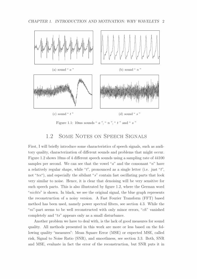
Figure 1.1: 10ms sounds “ a ”, “ n ”, “ t ” and “ s ”
1.2 Some Notes on Speech Signals
First, I will briefly introduce some characteristics of speech signals, such as audi-
tory quality, characterization of different sounds and problems that might occur.
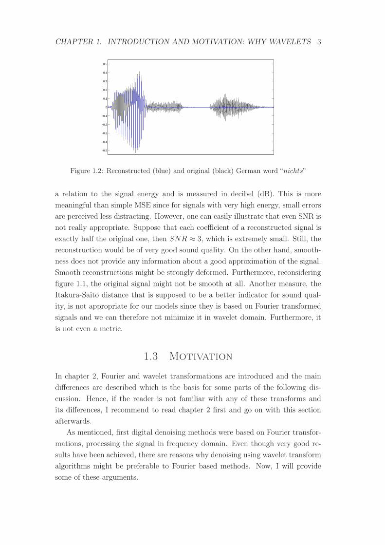
Figure 1.2 shows 10ms of 4 different speech sounds using a sampling rate of 44100
samples per second. We can see that the vowel “a” and the consonant “n” have
a relatively regular shape, while “t”, pronounced as a single letter (i.e. just “t”,
not “tee“), and especially the sibilant “s” contain fast oscillating parts that look
very similar to noise. Hence, it is clear that denoising will be very sensitive for
such speech parts. This is also illustrated by figure 1.2, where the German word
“nichts” is shown. In black, we see the original signal, the blue graph represents
the reconstruction of a noisy version. A Fast Fourier Transform (FFT) based
method has been used, namely power spectral filters, see section 4.3. While the
“ni”-part seems to be well reconstructed with only minor errors, “ch” vanished
completely and “ts” appears only as a small disturbance.
Another problem we have to deal with, is the lack of good measures for sound
quality. All methods presented in this work are more or less based on the fol-
lowing quality “measures”: Mean Square Error (MSE) or expected MSE, called
risk, Signal to Noise Ratio (SNR), and smoothness, see section 3.3. Both, SNR
and MSE, evaluate in fact the error of the reconstruction, but SNR puts it in
CHAPTER 1. INTRODUCTION AND MOTIVATION: WHY WAVELETS 3
−0.5
−0.4
−0.3
−0.2
−0.1
0
0.1
0.2
0.3
0.4
0.5
Figure 1.2: Reconstructed (blue) and original (black) German word “nichts”
a relation to the signal energy and is measured in decibel (dB). This is more
meaningful than simple MSE since for signals with very high energy, small errors
are perceived less distracting. However, one can easily illustrate that even SNR is
not really appropriate. Suppose that each coefficient of a reconstructed signal is
exactly half the original one, then SNR ≈ 3, which is extremely small. Still, the
reconstruction would be of very good sound quality. On the other hand, smooth-
ness does not provide any information about a good approximation of the signal.
Smooth reconstructions might be strongly deformed. Furthermore, reconsidering
figure 1.1, the original signal might not be smooth at all. Another measure, the
Itakura-Saito distance that is supposed to be a better indicator for sound qual-
ity, is not appropriate for our models since they is based on Fourier transformed
signals and we can therefore not minimize it in wavelet domain. Furthermore, it
is not even a metric.
1.3 Motivation
In chapter 2, Fourier and wavelet transformations are introduced and the main
differences are described which is the basis for some parts of the following dis-
cussion. Hence, if the reader is not familiar with any of these transforms and
its differences, I recommend to read chapter 2 first and go on with this section
afterwards.
As mentioned, first digital denoising methods were based on Fourier transfor-
mations, processing the signal in frequency domain. Even though very good re-
sults have been achieved, there are reasons why denoising using wavelet transform
algorithms might be preferable to Fourier based methods. Now, I will provide
some of these arguments.
CHAPTER 1. INTRODUCTION AND MOTIVATION: WHY WAVELETS 4
A. Auditory Perception: A sound signal that is received by the ear can be
described by a function s : R → R, where s(t) denotes the local pressure at the
corresponding time t. In some way, this one-dimensional signal is transformed
into a two-dimensional time-frequency plane, providing information about the oc-
currence of frequencies at any time, i.e. “when does which frequency occur” [17].
In fact, this is can be seen as a contradiction. Since pure frequencies are repre-
sented by complex exponentials eitω , they can not be associated with a certain
time point but last from −∞ to ∞. Vice versa, a certain time point, represented
by the Dirac delta function, contains all frequencies and it is not possible to asso-
ciate a special frequency. Hence, neither the signal itself nor its Fourier transform
provide the desired information and the hearing must be based on some compro-
mise between time localization and frequency localization [17]. Even though the
STFT provides such a compromise, wavelet transformations seem to come closer
to a more intuitive compromise, to rarely “update” low frequencies but to check
details, i.e. high frequencies, continuously. This is realized in some way by the
wavelet transformation since for high frequencies, the time resolution is much
finer than for low frequencies. Furthermore, the FWT treats frequencies in a
logarithmic way which is similar to acoustic perception [3].
B. Run-Time / Costs: The wavelet representation of a discretized signal of
length N can be obtained in O(N) whereas the STFT representation requires
O(N logM) where M denotes the sub-frame length of the used window. Hence,
the FWT algorithm might be preferable if the current application is very time sen-
sitive, i.e. for real time applications such as denoising communication transmitted
via radio. For example in helicopters, loud background noise is unavoidable and
makes communication difficult. Also high quality headphones try to remove back-
ground noise to enhance sound quality. However, it is clear that fast and effective
denoising techniques are needed.
C. Variety Of Wavelets: The wavelet transform is striking for its great
variety of different types and modifications. A whole host of different scaling and
wavelet functions (or scaling and wavelet coefficients) provide plenty of possible
adjustments and regulating variables. Examples are differentiability properties or
the number vanishing moments, symmetry features, complex or real wavelets,...
Some well known examples are the set of different Daubechies wavelets, Symmlets
and Coiflets. The corresponding scaling and wavelet coefficients can be found in
[4] or [34]. The Fourier Transform does not provide such a variety.
CHAPTER 1. INTRODUCTION AND MOTIVATION: WHY WAVELETS 5
D. Musical Noise Problem: Spectral domain denoising, Fourier based, of-
ten leads to special residual noise artifacts called musical noise or tonal noise,
sometimes regarded even more disturbing than the original Gaussian white noise.
An example of typical musical noise is provided by sound example 10. The way
musical noise occur can be explained considering a signal of pure noise. In spec-
tral domain, at each frame most of the frequencies will be removed. However,
some isolated frequencies will be preserved and perceived as tones. These isolated
frequencies randomly change from frame to frame, leading to rapidly time-varying
tones [14]. Hence, some post-processing might be necessary [15]. This compares
to the wavelet transform, which does not produce such artifacts due to better
time resolutions.
E. Image Processing: Wavelet transformation has been widely used for image
processing, such as edge or singularity detection [23], image compression (JPEG
2000) and especially image denoising [19], often outperforming existing algorithms
based on Fourier Transformations. Some of these algorithms have already been
used for the detection of abrupt changes in sound signals [16]. Hence, it is the
obvious thing to give wavelet transformations a trial for audio denoising as well.
We will try to modify some of the image processing algorithms, in particular the
image denoising methods, and test its applicability and performance on noisy
speech.
1.4 Outline and Structure
In chapter 2, I provide a brief introduction and comparison of different kinds of
wavelet and Fourier transformations. The Continuous Wavelet Transform (CWT)
will be only of theoretical interest, though, providing a better understanding of
the discrete transform as well as being used for some proofs in chapter 5. Before
several kinds of denoising techniques are presented, the general model of noisy
speech is given in chapter 3, together with some precise definitions of signal
goodness measures such as MSE, risk or SNR. Additionally, some notes on the
change of the behavior of transformed noise is provided.
The second part of this work, the presentation of several noise reduction meth-
ods, starts in chapter 4 with some well known and commonly used spectral filters,
i.e. Fourier transform based denoising filters, based on different noise reduction
assumptions. While the Wiener filter is based on risk minimization, spectral sub-
traction and power subtraction filters are based on rather intuitive approaches,
the removal of noise magnitudes. The Ephraim-Malah Filter however uses statisti-
CHAPTER 1. INTRODUCTION AND MOTIVATION: WHY WAVELETS 6
cal assumptions and conditional expectations to estimate the coefficient modulus.
The first wavelet transform based methods, introduced in chapter 5 and 6,
try to reconstruct the smoothness of the original signal. The idea of Lipschitz
denoising is to remove coefficients such that the produced outcome does not
contain negative Lipschitz singularities, i.e. the signal is uniformly Lipschitz
positive. Diffusion denoising performs several smoothing steps, each one can be
seen as an Euler step to solve a differential equation, modified in a way such that
important signal features are less smoothed than noise.
In chapter 7, the general thresholding concept is introduced. Except Visu
Shrink, introduced and analyzed in sections 7.3 and 7.4 with the objective to
produce smooth signal estimations, all thresholds are based on risk minimization.
In chapter 9, I develop some modifications of the soft thresholding function to
obtain better results. To reduce the occurrence of disturbing noise artifacts, i.e.
find a better compromise between smoothness and risk minimization, I develop
the idea of biased risk minimization in chapter 10. Tree structured thresholding,
presented in chapter 8, is based on the detection of important coefficients via
trees of wavelet detail coefficients, where “important” is in some way defined by
the used threshold value.
Finally, in chapter 11, a comprehensive comparison of the different denoising
results is provided. Corresponding implementations of all methods and tests for
several different speech examples can be found on the attached CD. All speech ex-
amples are specified in appendix A. Implementations for wavelet based methods
are provided in C++, spectral domain denoising is done in Matlab.
Chapter 2
Wavelet and Fourier
Transform
In this chapter, I will briefly introduce different wavelet transform concepts and
provide a general comparison with the Fourier transform, supporting the argu-
ments that have been mentioned in section 1.3 for the use of wavelet transforms
for denoising purposes instead of Fourier based spectral domain denoising. The
introduction will be as short as possible. First, the Continuous Wavelet Transform
(CWT) is presented. It is less restrictive than the definitions of the discrete trans-
formations — the Fast Wavelet Transform (FWT) and the Stationary Wavelet
Transform (SWT). For these transformations one first needs to introduce Mul-
tiresolution Analysis (MRA) to obtain consistent definitions. For more details
one may refer to [4], [25] [19] or [27].
2.1 The Continuous Wavelet Transform
For some mother wavelet function ψ(x), one generates a family of dilated and
shifted wavelets by
ψs,u(x) =1√|s|ψ
(x− u
s
)
with dilation s ∈ R\{0} and shift u ∈ R. It holds that ||ψ|| = ||ψs,u|| for all s, u.
The continuous wavelet transform of a real function f ∈ L2(R) is defined as the
7

CHAPTER 2. WAVELET AND FOURIER TRANSFORM 8
inner product of f and ψs,u, i.e.
Wf(s, u) := (f, ψs,u)
:=
∞∫
−∞
f(x)|s|−1/2ψ
(x− u
s
)dx (2.1)
for real Wavelets. Wf(s, u) provides information at scale s localized at position
u. In theory, all functions ψ can play the role of a wavelet function. For most
application one needs a reconstruction formula to recover the function f , though.
One can show that for mother wavelets ψ such that
Cψ := 2π
∞∫
−∞
|ψ(ω)|2|ω| dω <∞, (2.2)
where ψ denotes the Fourier transform of ψ, it holds that
f(x) =1
Cψ
∞∫
−∞
∞∫
−∞
Wf(s, u)1
s2ψs,u(x)ds du. (2.3)
Hence, one should restrict on mother wavelets ψ fulfilling (2.2). However, to
obtain the reconstruction formula (2.3), it is in most cases enough to require only
ψ(0) =
∞∫
−∞
ψ(x) dx = 0. (2.4)
Such function typically have oscillating properties. Hence the name Wavelets.
Some examples are the Morlet wavelet ψ(x) = eiω0xe−x2/2σ2
0 or the Mexican hat
wavelet ψ(x) = (1− x2)ex2/2. For more details and proofs of above assertions see
[4].
2.2 The Discrete Fast Wavelet Transform
Definition 2.2.1. Multiresolution Analysis (MRA)
A sequence of nested, closed subspaces of Vj ⊂ L2(R) is called Multiresolution
Analysis (MRA) if
(i) Vj ⊂ Vj+1 ∀j ∈ Z
(ii)⋃j∈Z Vj = L2(R)
CHAPTER 2. WAVELET AND FOURIER TRANSFORM 9
(iii)⋂j∈Z Vj = {0}
(iv) f(·) ∈ Vj ⇔ f(2·) ∈ Vj+1 ∀j ∈ Z
(v) f(·) ∈ V0 ⇔ f(·+ k) ∈ V0 ∀k ∈ Z
(vi) ∃ϕ ∈ V0 such that {ϕ(· − k)}k∈Z is a stable Riesz basis for V0
The function ϕ is sometimes called father or scaling function.
If ϕ is normalized, then {ϕjk(·) := 2j/2ϕ(2j · −k)}k∈Z is a normalized basis
of Vj . For a function f ∈ L2(R), let fj denote the projection of f into Vj, i.e.
fj ∈ Vj such that f − fj ∈ V ⊥j . Since Vj+1 ⊃ Vj , projections fj+1 into the finer
subspace Vj+1 obtain all information about f that is already provided by fj plus
some additional details . Hence, one can decompose Vj+1 into
Vj+1 = Vj ⊕Wj , j ∈ Z
where Wj denotes the so called detail space. We will only discuss the case of
orthonormal bases {ϕ(· − k)}k∈Z of V0. Similar results also hold for biorthognal
bases, see e.g. [29]. One can now proof that there is a function ψ such that
{ψj,k(·) := 2j/2ψ(2j · −k)}k∈Z form an orthonormal basis of the detail space Wj
[4]. The function ψ is called mother wavelet.
Since ϕ ∈ V0 ⊂ V1 and, as described above, {√2ϕ(2 · −k)}k∈Z denotes an
orthonormal basis of V1, it and follows that there is a sequence {ak}k∈Z ∈ l2(Z)
such that ϕ can be represented as the linear combination
ϕ(x) =√2∑
k∈Zakϕ(2x− k). (2.5)
Since W0 ⊂ V1, too, it follows in the same way that there is a sequence {bk}k∈Z ∈l2(Z) such that ψ can be represented as the linear combination
ψ(x) =√2∑
k∈Zbkϕ(2x− k). (2.6)
These equations are called dilation equations or two-scale relation, the sequences
{ak}k∈Z and {bk}k∈Z are called scaling sequence and wavelet sequence, respec-
tively, and characterize the corresponding scaling and wavelet function. With
their help we can define the Fast Wavelet Transform (FWT) and its inverse.
CHAPTER 2. WAVELET AND FOURIER TRANSFORM 10
Fast Wavelet Transform Let
fj+1(x) =∑
k∈Zcj+1,kϕj+1,k(x)
be the representation of the projection of a function f into Vj+1. One can decom-
pose this into Vj ⊕Wj by
fj+1(x) =∑
k∈Zcjkϕjk(x) +
∑
k∈Zdjkϕjk(x)
with
cjk =∑
l∈Zal−2kcj+1,l, (2.7)
djk =∑
l∈Zbl−2kcj+1,l. (2.8)
This decomposition is called Fast Wavelet Transform (FWT) and we call cj,k
approximation coefficients and dj,k detail coefficients. Furthermore, one can re-
construct cj+1 from cj and dj. This reconstruction is called Inverse Fast Wavelet
Transform (IFWT).
cj+1,k =∑
k∈Zal−2kcjk +
∑
k∈Zbl−2kdjk.
The proofs are easy and well known. They can be found e.g. in [19]. There is
a strong connection between the CWT and FWT. First, all Wavelet functions
obtained from a MRA are good candidates for the CWT, too. Additionally, let
{cJ,k}k=0,..,N−1, N = 2J , be some sequence that can be considered as a discretized
version of a function f , say cJ,k = (f, ϕJ,k), then we have
cj,k = (ϕj,k, f) =
∫2j/2ϕ(2jt− k)f(t) dt and (2.9)
dj,k = (ψj,k, f) =
∫2j/2ψ(2jt− k)f(t) dt, (2.10)
i.e. both coefficients can be seen as a CWT with s = 2−j and u = k2−j. Hence,
cj,k and dj,k provide information at scale 2J−j localized at position 2J−jk with
respect to the original sequence cJ that is considered as a representation at scale
CHAPTER 2. WAVELET AND FOURIER TRANSFORM 11
one, see [27]. Therefore, a representation of f is provided by
{c0, d0, d1, ..., dJ−1}. (2.11)
If only a finite number of coefficients ak and bk from (2.5) and (2.6), respectively,
are nonzero, the computation of the above representation (2.11) can be done in
O(N). Each coefficient vector dj and cj is of length O(2j), hence the total length
of the representation is O(N), too.
2.3 The Stationary Wavelet Transform
The Stationary Wavelet Transform (SWT) is a overrepresented form of the FWT.
The obtained representation is similar to (2.11), but now each coefficient vector
dj and cj is of length O(N), in case of periodic boundary conditions one obtains
a length of exactly N and the total number of coefficients is N log2(N) = J2J .
This is the reason why the SWT is also called non-decimated Wavelet Transform.
Let cJ be a discretized representation of a function f as described above, and
let {ak}k∈Z and {bk}k∈Z be the coefficients defined by (2.5) and (2.6), respectively.
Then, the SWT is defined as
cj,k =∑
l∈Za[J−j]l−k cj+1,l,
dj,k =∑
l∈Zb[J−j]l−k cj+1,l
where
a[r]k =
an , if k = 2rn
0 , otherwise .
As for the FWT we have a connection to the CWT, that is
cj,k =
∫2j/2ϕ(2jt− 2j−Jk)f(t) dt and (2.12)
dj,k =
∫2j/2ψ(2jt− 2j−Jk)f(t) dt. (2.13)
Now, cj,k and dj,k provide information of the function f at scale 2J−j, localized at
position k, in opposition to FWT coefficients where only localizations at 2J−jk
CHAPTER 2. WAVELET AND FOURIER TRANSFORM 12
are provided. The existence of coefficients at any position k = 0, ..., N − 1 at
each scale often facilitates the detection of correlations between different scales
and will be useful for some denoising algorithms (see section 7.9).
Nevertheless, the FWT is embedded in the SWT. Taking at each level j
only coefficients cj,k and dj,k such that k = n2J−j, n ∈ N, leads exactly to
the corresponding FWT coefficients. To confirm this, replace k in equations
(2.12) and (2.13) by n2J−j which leads to (2.9) and (2.10), respectively. In fact,
SWT can be seen as a rearrangement of all FWTs with shifted inputs. More
precisely, for shiftm(cJ,i) = cJ,i−m, the stationary wavelet transform contains all
coefficients of FWTs of shiftm(cJ), m = 0, ..., N − 1. Actually, this would lead
to N2 coefficients, however, several coefficients appear several times. Removing
this redundancy one obtains only O(N logN) coefficients and rearranging leads
to above representation. This procedure is also called cycle-spinning and further
explained and discussed in [2] and [27].
The inverse SWT can be done in several different ways. One possibility is to
take only the FWT coefficients and do the inverse FWT as described above. This
will be obtained using
cj+1,l =∑
l∈Za[J−j−1]l−2k cj,2k +
∑
l∈Zb[J−j−1]l−2k dj,2k.
In many cases a different approach might be better, though. Since we will pro-
cess all coefficient due to denoising issues, it might be better to use as well all
coefficients to compute the inverse SWT. These considerations lead to
cevenj+1,l =∑
l∈Za[J−j−1]l−2k cj,2k +
∑
l∈Zb[J−j−1]l−2k dj,2k
coddj+1,l =∑
l∈Za[J−j−1]l−2k cj,2k+1 +
∑
l∈Zb[J−j−1]l−2k dj,2k+1
cj+1,l =cevenj+1,l + coddj+1,l
2
which is the average of all inverse FWTs of coefficients obtained from FWTs
taking at each step either only odd or even coefficients. One can show that this
leads to the average of all N inverse FWTs of shifted inputs mentioned above. A
complete discussion and proofs are provided in [27].
CHAPTER 2. WAVELET AND FOURIER TRANSFORM 13
2.4 The Fourier Transform
Definition 2.4.1. The Continuous Fourier Transform (CFT) is defined as
F (ω) :=
∞∫
−∞
f(t)e−i2πtω dt. (2.14)
For signal analysis we need to introduce another form, the short-time Fourier
transform or windowed Fourier Transform which — for some window or frame
function g of compact support — is given by
F (ω, τ) :=
∞∫
−∞
f(t)g(t− τ)e−i2πtω dt. (2.15)
Definition 2.4.2. The Discrete Fourier Transform (DFT) is defined as
Xm =N−1∑
k=0
xke−i 2πkm
N (2.16)
where the sequence {xk}k=0,...,N−1 may represent a discretized function. The
discrete Short-Time Fourier Transform (STFT) for some window g is expressed
by
Xm,n =∑
k∈Zxkg(k − n)e−i
2πkmM , (2.17)
where g(k) 6= 0 only if k ∈ {0, ...,M − 1}. M is called sub-frame length. It
depends on the application if xk is assumed to be zero for k /∈ {0, ..., N − 1} or if
xk is extended periodically.
The windowed Fourier transform provides additional time resolution infor-
mation. This is essential for speech signal processing since different sounds, e.g.
vowels or consonants, lead to completely different frequency ranges, see also chap-
ter 1.2. The length of a typical speech processing window is usually chosen to
be between 20 to 40 milliseconds [12]. Furthermore, overlapping windows are
necessary for good denoising results. On the other hand it is too expensive to
evaluate Xm,n at each possible value of n. Hence, to obtain an overlap of 50-75%,
the actual time resolution will be at most 5ms, or N/4 in the discrete case.
For fixed n, the STFT coefficients Xm,n, m = 0, ...,M − 1, can be computed
in O(M logM) using the Fast Fourier Transform algorithm (FFT), presented for
CHAPTER 2. WAVELET AND FOURIER TRANSFORM 14
example in [14]. Hence, the complete Fourier representation with time resolution
as described can be obtained in O(N logM), where a full time resolution would
require O(NM logM).
A widely used class of windows, compactly supported on [0, 1] and with sub-
frame length M , is given by
gα(k) := α− (1− α)cos
(2πk
M
).
These functions are called generalized Hamming windows, named after Richard
Hamming. The frames for the most commonly used values of α are
α = 1 rectangular window
α = 0.5 Hann or Hanning window, named after Julius von Hann
α = 0.53836 Hamming window .
For more Details see [14].
2.5 Comparison
The idea of both, wavelet and Fourier transform, is based on the computations
of inner products of some function f and some analyzing functions to obtain a
time-frequency representation [3]. To illustrate this, let’s define
gm,n(k) := g(k − n)e−i2πkmM ,
the product of a shifted version of some window function g and a complex expo-
nential. Hence, similar to the inner product (2.10), we have
Xm,n = (gm,n, x)2,
even though the inner is now considered to be discrete. I.e., gm,n plays a similar
role than the wavelet function ψj,k. The first index of both functions refers to the
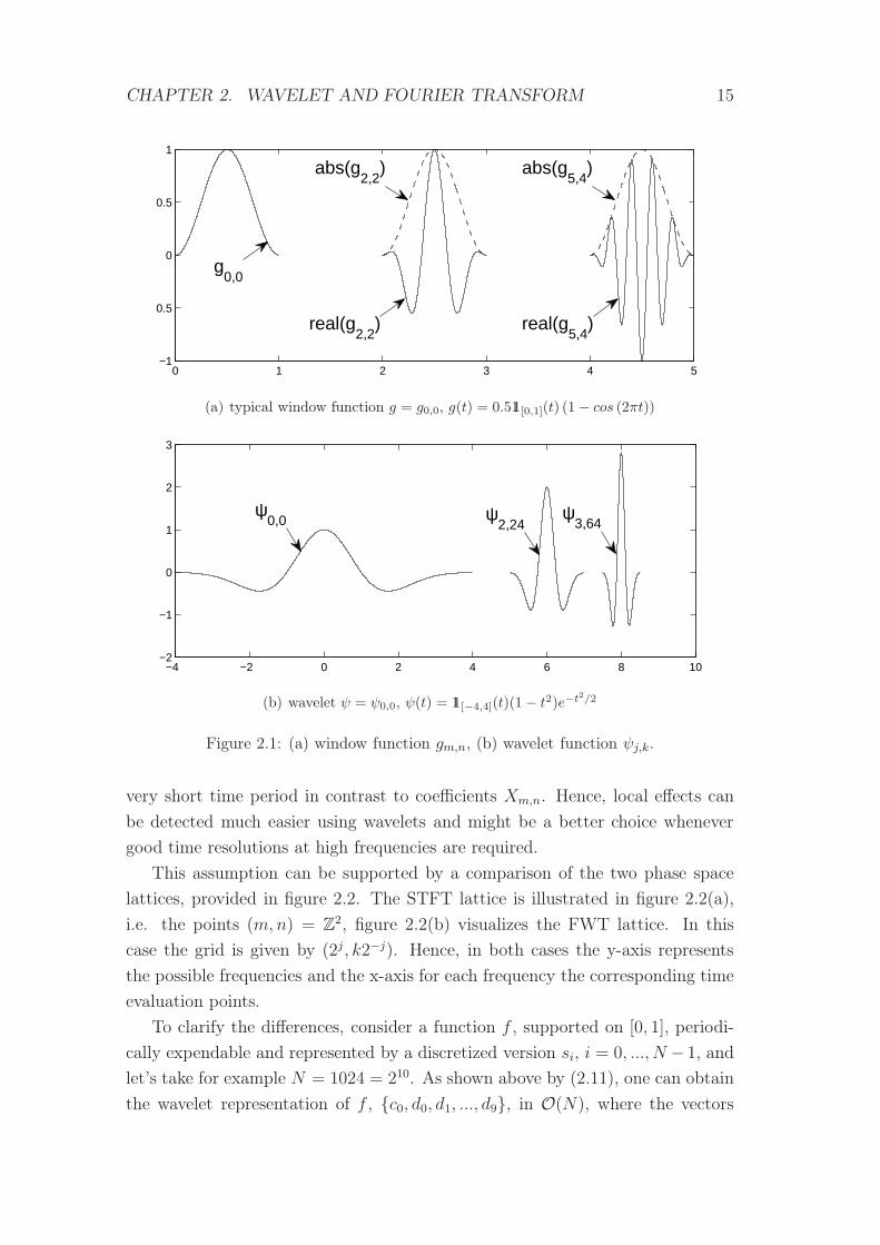
frequency and the second one to a time shift, as illustrated in figure 2.1.
However, the way the frequency is characterized differs. For large j, one can
see that the ψj,k is a strongly concentrated or shrunken version of itself whereas
g is not shrunken but “filled” with oscillations for large m. The support of ψj,k
is proportional to 2−j whereas indices m of gm,n are rather proportional to the
number of oscillations of real(g). I.e. the wavelet transform provides a kind of
“zoom in ” property, for large j coefficients dj,k contain only information about a
CHAPTER 2. WAVELET AND FOURIER TRANSFORM 15
0 1 2 3 4 5−1
−0.5
0
0.5
1
real(g5,4
)real(g2,2
)
g0,0
abs(g5,4
)abs(g2,2
)
(a) typical window function g = g0,0, g(t) = 0.511[0,1](t) (1− cos (2πt))
−4 −2 0 2 4 6 8 10−2
−1
0
1
2
3
ψ2,24
ψ3,64
ψ0,0
(b) wavelet ψ = ψ0,0, ψ(t) = 11[−4,4](t)(1− t2)e−t2/2
Figure 2.1: (a) window function gm,n, (b) wavelet function ψj,k.
very short time period in contrast to coefficients Xm,n. Hence, local effects can
be detected much easier using wavelets and might be a better choice whenever
good time resolutions at high frequencies are required.
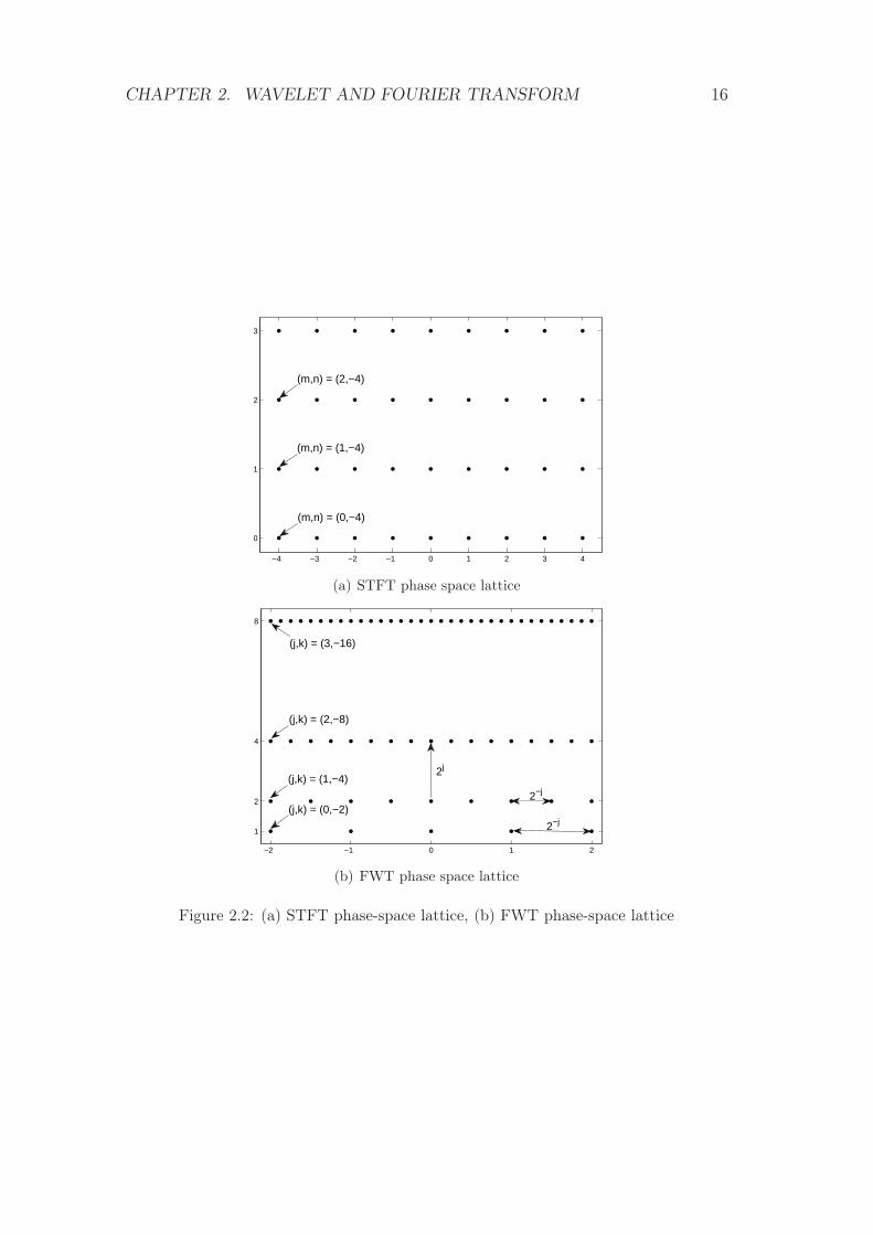
This assumption can be supported by a comparison of the two phase space
lattices, provided in figure 2.2. The STFT lattice is illustrated in figure 2.2(a),
i.e. the points (m,n) = Z2, figure 2.2(b) visualizes the FWT lattice. In this
case the grid is given by (2j, k2−j). Hence, in both cases the y-axis represents
the possible frequencies and the x-axis for each frequency the corresponding time
evaluation points.
To clarify the differences, consider a function f , supported on [0, 1], periodi-
cally expendable and represented by a discretized version si, i = 0, ..., N − 1, and
let’s take for example N = 1024 = 210. As shown above by (2.11), one can obtain
the wavelet representation of f , {c0, d0, d1, ..., d9}, in O(N), where the vectors
CHAPTER 2. WAVELET AND FOURIER TRANSFORM 16
−4 −3 −2 −1 0 1 2 3 4
0
1
2
3
(m,n) = (2,−4)
(m,n) = (1,−4)
(m,n) = (0,−4)
(a) STFT phase space lattice
−2 −1 0 1 2
1
2
4
8
(j,k) = (0,−2)
(j,k) = (1,−4)
(j,k) = (2,−8)
(j,k) = (3,−16)
2−j
2−j
2j
(b) FWT phase space lattice
Figure 2.2: (a) STFT phase-space lattice, (b) FWT phase-space lattice
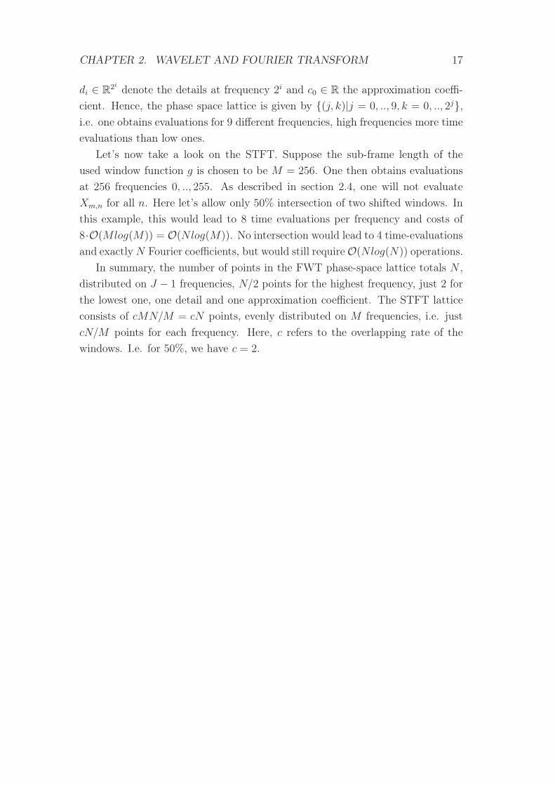
CHAPTER 2. WAVELET AND FOURIER TRANSFORM 17
di ∈ R2i denote the details at frequency 2i and c0 ∈ R the approximation coeffi-
cient. Hence, the phase space lattice is given by {(j, k)|j = 0, .., 9, k = 0, .., 2j},i.e. one obtains evaluations for 9 different frequencies, high frequencies more time
evaluations than low ones.
Let’s now take a look on the STFT. Suppose the sub-frame length of the
used window function g is chosen to be M = 256. One then obtains evaluations
at 256 frequencies 0, .., 255. As described in section 2.4, one will not evaluate
Xm,n for all n. Here let’s allow only 50% intersection of two shifted windows. In
this example, this would lead to 8 time evaluations per frequency and costs of
8·O(Mlog(M)) = O(Nlog(M)). No intersection would lead to 4 time-evaluations
and exactlyN Fourier coefficients, but would still require O(Nlog(N)) operations.
In summary, the number of points in the FWT phase-space lattice totals N ,
distributed on J − 1 frequencies, N/2 points for the highest frequency, just 2 for
the lowest one, one detail and one approximation coefficient. The STFT lattice
consists of cMN/M = cN points, evenly distributed on M frequencies, i.e. just
cN/M points for each frequency. Here, c refers to the overlapping rate of the
windows. I.e. for 50%, we have c = 2.
Chapter 3
A General Noise and Speech
Model
3.1 Noisy Speech Signal Model
Suppose a data vector y of finite length n is given and represents a combination
of an unknown speech signal and some as well unknown noise that is added to
the signal, i.e.
yi = si + ei, i = 0, ..., n− 1 (3.1)
where si refers to the unknown noise-free signal at time ti and ei is considered
to be the additional noise. Furthermore, for notational and algorithmic reasons,
we assume y to be periodic extensible, i.e. yi = yi+kn for all k ∈ Z, and n of the
form n = 2J for some J ∈ N. The periodicity is legitimated by considering only
signals s silent at the beginning and at the end.
From the observed data y we will try to estimate the original signal s. In the
following we assume s and e to be independent. For most denoising methods one
assumes e to be a vector of independent identically distributed (i.i.d.) normal
random numbers with ei ∼ N(0, σ2), i.e. Gaussian white noise with variance
σ2 that is not necessarily known. However, for some methods less restrictive
assumptions suffice. In any case we assume the expected noise to be zero, i.e.
E[e] = 0.
A second noise model is necessary for transformed coefficients. However, the
linearity of both, Fourier and Wavelet transform, leaves the additivity of model
(3.1) unchanged. Let’s denote the transformations of the data vector y and its
components s and e by Ypq, Spq and Epq, respectively, where p refers to the
18
CHAPTER 3. A GENERAL NOISE AND SPEECH MODEL 19
frequency and q stands for the time parameter, i.e. (p, q) = (m,n) in the Fourier
transform case and (p, q) = (j, k) in the wavelet transform case as described in
section 2.4. As mentioned, the linearity of both transformations leads to a second
noise model
Ypq = Spq + Epq, (p, q) ∈ I (3.2)
where I is the set of all possible indices in time-frequency domain. In the wavelet
case, Y , S and E may refer — if necessary — to both, approximation and detail
coefficients. However, most denoising algorithms leave approximation coefficients
unchanged and we do not consider the remaining approximation coefficients any-
way.
Let x be some data in time domain and X its transformation into time-
frequency domain. For orthogonal FWT it holds that ||x||2 = ||X||2, i.e. norms
in time and time-frequency domain are equal (see [19]). In the biorthogonal case
the Riesz basis property of (2.2.1) ensures equivalent norms. In the Fourier case it
holds that ||x||22 = 1n||X||22, also known as Parseval’s theorem. Hence, considering
norms in time domain is equivalent to restrict on norms in time-frequency domain,
especially minimizing in time-frequency domain minimizes (or nearly minimizes
in the biorthogonal Wavelet case) in time-domain.
3.2 Noise Transformation
One should pay some additional attention on the noise and its property change
after transformation. For E[e] = 0 it is clear that E[E] = 0 holds, too. Further
noise properties are given by its covariance matrix Q, i.e.
Qi,j = E [eiej ] ,
Q = E[eeT].
Since discrete Fourier and Wavelet transformations are linear, there is a matrix
A such that
Y = Ay, S = As, E = Ae
CHAPTER 3. A GENERAL NOISE AND SPEECH MODEL 20
and the new covariance matrix QW of E is obtained by
QA = E[EET
]
= E[AeeTAT
]
= AQAT .. (3.3)
In the Wavelet case it might be useful to derive the form of QA for some special
noise distributions and normalize the wavelet coefficients
Y newjk =
1√QAjk,jk
Yjk (3.4)
to obtain stationary noise [19].
First, for orthogonal Wavelet transformations, A is orthogonal, too. Now, if
e represents white noise, i.e. Q = σ2I where I is the identity matrix and σ2
the noise variance, then QA = σ2I, too. Hence, the noise remains uncorrelated,
stationary and the variance does not change either. No normalization is necessary.
Let’s now discuss a more general assumption. Suppose the original noise is
stationary and the correlation between two noise data points depends only on
their distance. Then, Q is a symmetric Toeplitz matrix and one can prove the
following lemma.
Lemma 3.2.1. Let Ejk, (j, k) ∈ I, represent wavelet coefficients obtained by ei-
ther orthogonal or biorthogonal FWT of stationary noise with symmetric Toeplitz
covariance matrix. Then, the variance of each coefficient depends only on the
level j, i.e.
E[E2j,k] = σ2
j (3.5)
Proof. Since Q is Toeplitz, we have Qu,v = q|u−v|. Using equation (2.8) one
obtains
E[EJ−1,kEJ−1,l] =∑
u
∑
v
bu−2kbv−2lE[euev]
=∑
u
∑
v
bu−2kbv−2lq|u−v|.
CHAPTER 3. A GENERAL NOISE AND SPEECH MODEL 21
Substituting m = u− 2k and n = v − 2l yields to
E[EJ−1,kEJ−1,l] =∑
m
∑
n
bmbnq|2(k−l)+m−n|
= E[EJ−1,k+rEJ−1,l+r].
The same holds for scaling coefficients using equation (2.7). Hence, at level J −1
the covariance matrices of detail and approximation coefficients are Toeplitz, too.
Thus, we have
E[E2J−1,k+r] = E[E2
J−1,k] = σ2J−1,
a constant variance at level J − 1. One can repeat this procedure for any other
level in exactly the same way.
In fact, the covariance matrix Q = σ2I for Gaussian white noise is a spe-
cial Toeplitz matrix, too. However, even though lemma 3.2.1 holds as well for
biorthogonal wavelet coefficients, Ej,k, (j, k) ∈ I, might be correlated and not
stationary (i.e. σj1 6= σj2 for j1 6= j2) in opposite to the case of orthogonal FWT.
3.3 Some Definitions and Notations
Let us now collect some definitions used later for the analysis of denoising meth-
ods and for the evaluation of denoised speech signals. The following “measures”
constitute a first set of possible evaluations of the goodness of signal approxima-
tions.
Definition 3.3.1. Given a certain denoising method called T , denote estimates
of s by sT . The following expected values refer to the unknown noise, often
assumed to be normally distributed. Let’s define
• Mean Square Error (MSE) of s and sT
MSE(s, sT ) =1
n||s− sT ||2
=1
n
n−1∑
i=0
|si − sTi |2 (3.6)
• Bias of s and sT
bias2(s, sT ) =1
n||s− EsT ||2 (3.7)
CHAPTER 3. A GENERAL NOISE AND SPEECH MODEL 22
• Variance of sT
var(sT ) =1
nE[||sT − EsT ||2
](3.8)
• Risk
risk(s, sT ) = E[MSE(s, sT )
](3.9)
=1
n
n−1∑
i=0
E[|si − sTi |2
]
= bias2(s, sT ) + var(sT ). (3.10)
the expected MSE for a given Method T . Some easy calculations lead to
equation (3.10) and are not specified here.
• Ideal Risk
R(s, T ) = infsTrisk(s, sT ) (3.11)
which is the infimum of all risks that can be achieved using method T .
• Signal to Noise Ratio (SNR)
SNR(s, sT ) = 10 ∗ log10||s||2
||s− sT ||2 or (3.12)
SNR(s, y) = 10 ∗ log10(||s||2/||e||2
)(3.13)
measured in decibels (dB).
All these definitions can be modified for transformed coefficients Y , S and
E, replacing n by the number of transformed coefficients, i.e. #(p, q) = |I|.For FWT and FFT and under the assumption of periodic functions we have
|I| = n, but not for STFT and SWT. All summations need to be done over all
possible indices (p, q) ∈ I. As mentioned above, the l2-norms in time and time-
frequency domain are equivalent, i.e. minimization in time domain is equivalent
to minimization in time-frequency domain.
Chapter 4
Spectral Domain Denoising
In this chapter we will briefly discuss some well known and widely used denoising
methods based on STFT, as described for example in [12], [13], [14], [31], [35].
Nevertheless, all these filters could be almost directly applied on wavelet detail
coefficients instead of STFT coefficients, too. Hence, I used the general nota-
tion introduced in chapter 3, referring to the Fourier transform only as much as
necessary. A comparison of these filters applied on STFT and FWT coefficients,
respectively, can be found in [13]. These experiments has been based only on
different SNR measures but not on human perception. However, it turned out
that these filters applied on Fourier transform coefficients provide better results
than applied on Wavelet detail coefficients. Hence, it will be necessary to create
different methods that benefit from special wavelet properties as mentioned in
chapter 1, e.g. the finer time resolution.
4.1 Noise Reduction Filter Model
First, I will introduce some further SNR definitions that are especially used for
theoretical analysis of spectral domain denoising methods, only defined for co-
efficients in time-frequency domain. Let X denote the transformation of some
sequence x, for variances RX(p, q) and RX denoted by
RX(p, q) = E[|Xpq|2]RX = E[||X||2]
one defines “a priori SNR”
ξpq =RS(p, q)
RE(p, q)(4.1)
23
CHAPTER 4. SPECTRAL DOMAIN DENOISING 24
and “a posteriori SNR”
γpq =RY (p, q)
RE(p, q). (4.2)
Due to the independence of S and E and for E[E] = 0, it is clear that RY =
RS +RE and hence
γpq = 1 + ξpq.
Some commonly used methods to determine ξpq are provided in section 4.5.
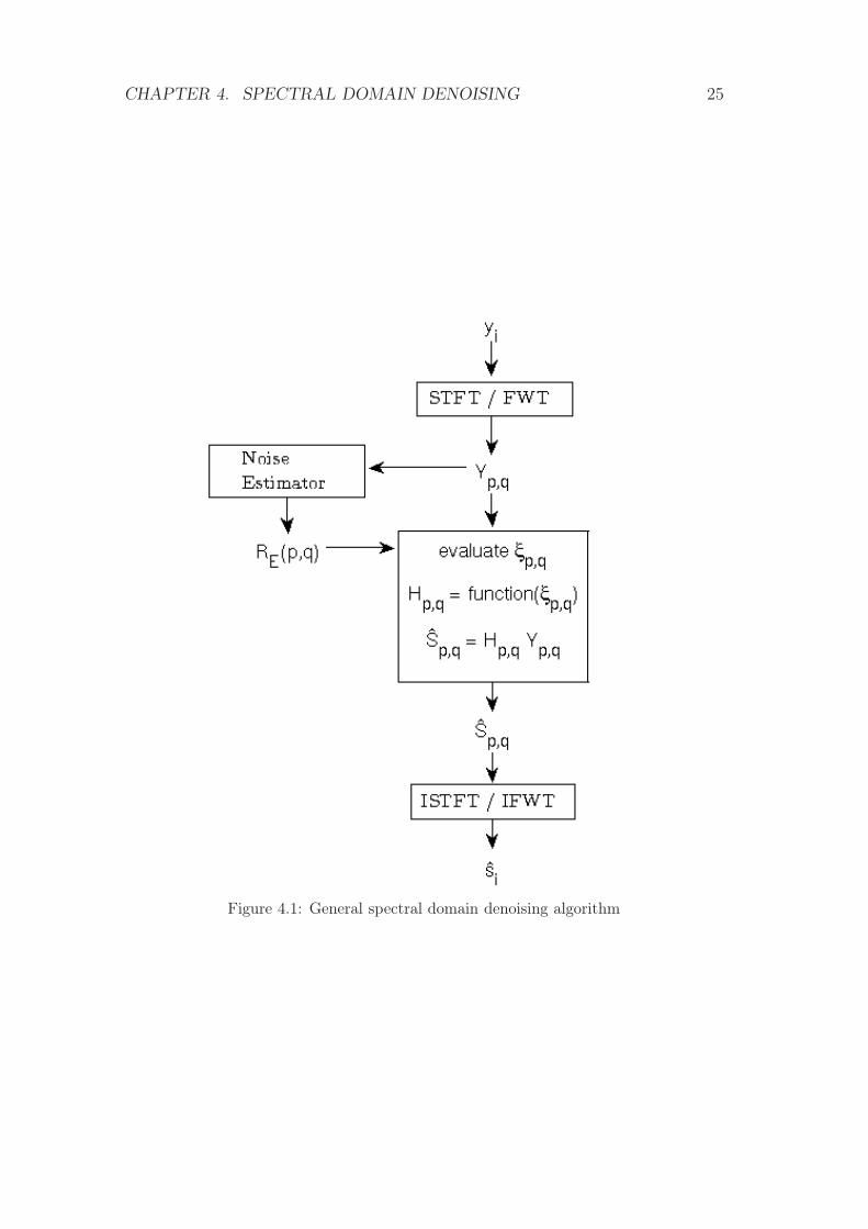
Considering noise models (3.1) and (3.2), spectral domain denoising can be
generalized as shown in figure 4.1. It is based on a so called gain or transfer
function H : R+ → [0, 1], a function of one parameter, the “a priori SNR” ξp,q.
The estimation Sp,q of Sp,q is given by
Sp,q = Hp,q · Yp,q (4.3)
where Hp,q := H(ξp,q). The fact that Hp,q ∈ [0, 1] ensures each coefficient is either
preserved or shrunken but not enlarged. To obtain ξp,q one needs to determine
the noise variance RE(p, q) which is constant for all (p, q) ∈ I for stationary noise,
for Gaussian white noise RE(p, q) ≡ σ2. Otherwise, some normalizations similar
to (3.4) might be useful to avoid current and expensive noise variance updating.
The actual gain function H depends on the used filter, i.e. the denoising method.
For the following filters, the gain function is chosen to be real even though
the transformed coefficients may be complex. Hence, these filters only change
the spectral amplitude but not phase. However, Ephraim and Malah show that
the optimal phase estimator is given by the phase of the noised transformed
coefficients [12]. Hence, real gain functions are sufficient.
4.2 Wiener Filter
One of the most common filters and basis for many others [14],[31],[12] is the
Wiener Filter (WF), published already in 1949 by Norbert Wiener [35]. We use
the noise model in spectral domain as described in (3.2), that is
Ypq = Spq + Epq,
CHAPTER 4. SPECTRAL DOMAIN DENOISING 25
Figure 4.1: General spectral domain denoising algorithm
CHAPTER 4. SPECTRAL DOMAIN DENOISING 26
and try to find an “optimal” gain function Hpq. The idea of the Wiener filter is to
minimize the Risk function (3.9) in spectral domain, i.e for n = |I| one minimizes
Risk(S, S) =E
[||S − S||2
]
n
=E [||S −HY ||2]
n.
Norbert Wiener proposed to use the zero of the risk’s partial derivative with
respect to H , i.e. to find a gain function H such that
n∂Risk(S, S)
∂H= 2E
[(S −HY )Y
]
= 2(E[SY]−HE
[||Y ||2
])
= 0.
Therefore, with RX = E [||X||2], one obtains
HWiener =E[SY]
RY
=E[(Y − E)Y
]
RY
=RY − E
[EY]
RY
=RY − E
[E(S + E)
]
RY
=RY −RE
RY,
applying the independence of E and S which implies E[ES] = 0 for E[E] = 0.
Using ξpq and γpq as defined by (4.1) and (4.2), respectively, the gain function is
given by
HWienerpq =
RY (p, q)−RE(p, q)
RY (p, q)
=γpq − 1
γpq=
ξpq1 + ξpq
(4.4)
and leads to estimations of Spq given by
SWienerpq = HWiener
pq Ypq. (4.5)
CHAPTER 4. SPECTRAL DOMAIN DENOISING 27
The fact that ξpq in (4.5) is positive ensures HWienerpq to be in [0, 1], i.e. Wiener
filtering can be considered as shrinking coefficients. Considering above equations,
one can see HWiener as both, a function of a priori SNR and a posteriori SNR.
However, in each case we need to find approximations for γpq or ξpq, respectively.
Some methods are presented in section 4.5. Assuming the knowledge of RS(p, q) =
S2pq and Epq ∼ N(0, σ2), a priori noise ξpq could be exactly evaluated and the risk
function would be given by
risk(S, SWiener) =1
|I|∑
(pq)∈I
S2pqσ
2
S2pq + σ2
. (4.6)
The proof is straightforward using simple calculations and the definition of MSE.
4.3 Spectral Subtraction and Power
Subtraction Filter
Some widely used alternatives are the Spectral Subtraction Filter (SSF) and the
Spectral Power Filter (PSF) [13], [14]. In contrast to the Wiener filter which
is based on a well-defined optimality criterion, i.e. the minimization of the risk
function, SSF and PSF use a rather intuitive approaches. The idea of SSF is to
remove the noise magnitude, i.e. simplified we have
|SSSFpq | = |Ypq| −√RE(p, q)
and
SSSFpq =|Ypq| −
√RE(p, q)
|Ypq|Ypq
This method is especially useful for systems using multiple microphones, one
recording noisy speech and another noise only. Assuming |Ypq| =√RY (p, q), one
can use above notations and with γpq = 1 + ξpq, one obtains
HSSFpq =
√RY (p, q)−
√RE(p, q)√
RY (p, q)
= 1−√
1
1 + ξpq(4.7)
SSSFpq = HSSFpq Ypq. (4.8)
CHAPTER 4. SPECTRAL DOMAIN DENOISING 28
0 0.5 1 1.5 2 2.50
0.2
0.4
0.6
0.8
1
Wiener Risk
PSF Risk
Figure 4.2: Risk function for Wiener and power spectral filter
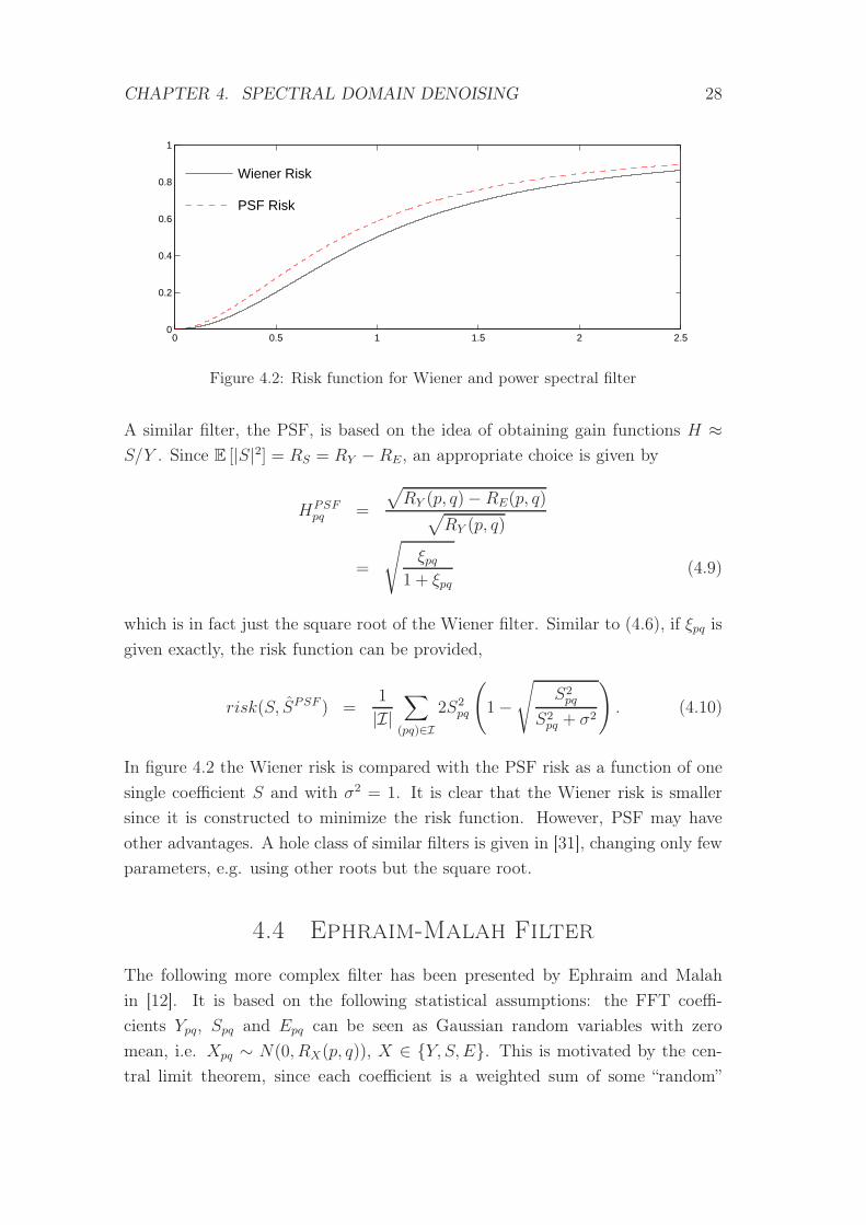
A similar filter, the PSF, is based on the idea of obtaining gain functions H ≈S/Y . Since E [|S|2] = RS = RY − RE, an appropriate choice is given by
HPSFpq =
√RY (p, q)− RE(p, q)√
RY (p, q)
=
√ξpq
1 + ξpq(4.9)
which is in fact just the square root of the Wiener filter. Similar to (4.6), if ξpq is
given exactly, the risk function can be provided,
risk(S, SPSF ) =1
|I|∑
(pq)∈I2S2
pq
(1−
√S2pq
S2pq + σ2
). (4.10)
In figure 4.2 the Wiener risk is compared with the PSF risk as a function of one
single coefficient S and with σ2 = 1. It is clear that the Wiener risk is smaller
since it is constructed to minimize the risk function. However, PSF may have
other advantages. A hole class of similar filters is given in [31], changing only few
parameters, e.g. using other roots but the square root.
4.4 Ephraim-Malah Filter
The following more complex filter has been presented by Ephraim and Malah
in [12]. It is based on the following statistical assumptions: the FFT coeffi-
cients Ypq, Spq and Epq can be seen as Gaussian random variables with zero
mean, i.e. Xpq ∼ N(0, RX(p, q)), X ∈ {Y, S, E}. This is motivated by the cen-
tral limit theorem, since each coefficient is a weighted sum of some “random”
CHAPTER 4. SPECTRAL DOMAIN DENOISING 29
variables. Sufficiently separated samples of the original signals are almost in-
dependent. Appropriate Windows (e.g. Hanning windows) reduces correlations
between widely separated coefficients but enlarges correlations between adjacent
coefficients. However, correlations between transformed coefficients approach zero
for large frame lengths. hence, we assume that the coefficients are pairwise inde-
pendent (or at least only weakly dependent). For more details see [12].
The Ephraim-Malah Filter (EMF) pursues the estimation of the spectral am-
plitude using conditional expectations, i.e. for
Spq = Apqeiαpq
Ypq = Bpqeiβpq ,
one estimates Apq based on the set of observations {Ypq|(p, q) ∈ I}. The pairwise
independence ensures that the estimation Apq of Apq depends only on Ypq, i.e.
only on coefficients of same time and frequency. More precise, the estimation is
given by the conditional expectation
Apq = E [Apq|Ypq]
=
∞∫0
2π∫0
apqP (Ypq|apq, αpq)P (apq, αpq) dαpqdapq∞∫0
2π∫0
P (Ypq|apq, αpq)P (apq, αpq) dαpqdapq
where P (·) denotes probability density functions
P (Y |a, α) =1
πREexp
(−|Y − aeiα|2
RE
)
P (a, α) =a
πRSexp
(− a2
RS
).
As shown in [12], substituting the above equations into the integral leads to
Apq =
√πξpq
1 + ξpqexp
(−ξpq
2
)((1 + ξpq)I0
(ξpq2
)+ ξpqI1
(ξpq2
))Bpq (4.11)
where In is the modified Bessel function of order n,
In(x) =1
2π
2π∫
0
cos(βn)excosβdβ.
As mentioned above, the optimal phase estimator αpq is given by βpq. For that
CHAPTER 4. SPECTRAL DOMAIN DENOISING 30
reason the EMF gain function and the estimator SEMFpq can now be obtained by
HEMFpq =
ApqBpq
(4.12)
SEMFpq = HEMF
pq Ypq
= HEMFpq Bpqe
iβpq
= Apqeiβpq . (4.13)
4.5 A priori SNR Estimation
The a priori SNR ξpq is given by the ration of signal spectral component variance
RS(p, q) and noise spectral component variance RE(p, q). Let’s take first a look
at the latter one. Then, I will provide some different methods of estimating ξpq
as shown for example in [12].
Noise Spectral Component Variance In practice this variance is esti-
mated using an interval without speech, hence only affected by noise. Assuming
the noise to be stationary, i.e. RE(p, q) ≡ const, it suffices to estimate RE only
one time. For a fixed window indicated by q0 with pure zero mean noise and n
samples, that is the sample variance
RE =1
n− 1
n−1∑
p=0
Y 2pq0.
However, it is not always easy to determine pure noise time intervals. Especially
for non-stationary noise, one needs to update RE regularly. Nevertheless it is
the most common method, also used in professional software, e.g. the open
source audio editor Audacity. For some applications like communication from a
helicopter, additional microphones are installed recording only noise, facilitating
the estimation of RE . We will see later that there are wavelet based denoising
methods that can be realized without explicit noise variance estimation.
A priori SNR Since RY (p, q) = E[|Ypq|2] = |Ypq|2 is known, with above esti-
mation of RE(p, q) one could use RS(p, q) = RY (p, q) − RE(p, q) leading to the
approximations
γpq = |Ypq|2/RE(p, q),
ξ(1)pq = γpq − 1.
CHAPTER 4. SPECTRAL DOMAIN DENOISING 31
However, using just one coefficient of the transformed input to estimate a priori
noise is probably too imprecise. Furthermore, as the name says, the variances
rather indicate a kind of volatility around (p, q) than an approximation of Ypq
or Spq, respectively. Hence, assuming only slowly in time varying variances RE
and RS, averaging several values Ypq might be preferable [12]. Let’s base the es-
timation on L consecutive observations Yp,q, Yp,q−1, ..., Yp,q−L+1 of same frequency
but in different time frames. One assumes these values to be independent, which
would be reasonable for non-overlapping frames. Now, one uses the sample vari-
ance of these values and obtains
RS(pq) =
1L
L−1∑l=0
|Yp,q−l|2 −RE(p, q) , if nonnegative
0 , otherwise
which leads to
ξ(2)pq =
1L
L−1∑l=0
γp,q−l − 1 , if nonnegative
0 , otherwise.
where as above γp,q−l =|Yp,q−l|2RE(p,q−l) . In practice, this average is replaced by a
recursive averaging,
γpq = αγp,q−1 + (1− α)γpqβ
where 0 ≤ α < 1, β ≥ 1. The choices of α and β depend on the used filter and
on auditory perception. Some examples can be found in [12]. Now, the estimator
for a priori SNR is given by
ξ(3)pq =
γpq − 1 , if nonnegative
0 , otherwise.
Another similar estimator, especially used in combination with the Wiener filter,
is given by
ξ(4)pq = αξ(4)p,q−1 + (1− α)11{γpq≥1}(γpq − 1)
with initial condition ξ(4)p,−1 = 1 which has been verified to be appropriate [12].
Chapter 5
Lipschitz Denoising
The idea of Lipschitz denoising is based on the detection of Lipschitz regularities
using local maxima of the wavelet transform. The same results can be obtained
using more general Besov regularities instead (see section 7.4). However, in this
case Lipschitz regularity is more illustrative and facilitates the understanding.
The presented method is based on the work of Mallat, Hwang and Zhong [22], [23],
[24]. It has been successfully applied on edge detection and image enhancement.
I will provide some examples of Lipschitz regularities and its detection with the
help of wavelets and investigate the usage of the presented methods in Audio
signal denoising.
5.1 Lipschitz Regularity
In the first section I will introduce the notion of Lipschitz regularity and its prac-
tical meaning as well as a definition of singularity based on Lipschitz regularities.
Furthermore I will provide some examples of different Lipschitz regularities for a
better understanding.
Definition 5.1.1. (Lipschitz Regularity)
(i) Let n ∈ N and α ∈ R such that n ≤ α ≤ n+1. A function f is called Lips-
chitz α at x0 if there exist constants A and h0 > 0 as well as a polynomial
Pn(h) of order n such that the following holds ∀ h < h0:
|f(x0 − h)− Pn(h)| ≤ A|h|α. (5.1)
(ii) The function is said to be uniformly Lipschitz α in the interval (a, b) if there
exists a constant A and for each x0 ∈ (a, b) there is a polynomial Pn(h) of
order n such that (5.1) is satisfied if x0 + h ∈ (a, b).
32
CHAPTER 5. LIPSCHITZ DENOISING 33
(iii) The Lipschitz regularity of f at x0 is defined as sup{α|f is Lipschitz α at
x0}.
(iv) We say that f is singular at x0 if it is not Lipschitz 1 at x0.
Lipschitz regularity gives an indication of differentiability. A function f that
is continuously differentiable at x0 is Lipschitz 1. If the derivative of f is not
continuous but bounded at x0, f is still Lipschitz 1, therefore according to 5.1.1
not singular at x0. Let n ∈ N and α > n. A function f that is Lipschitz α at x0 is
n times differentiable at x0 and Pn(h) is identical to the n-th Taylor polynomial
of f at x0. Lipschitz regularity provides even more information. Suppose the
Lipschitz regularity of f at x0 is α0 with n < α0 < n + 1, then f is n times
differentiable at x0 but its nth derivative is singular at x0. Furthermore, α0
characterizes this singularity.
Remark 5.1.2.
(i) One can prove that if f is Lipschitz α at x0 then its primitive is Lipschitz
α+ 1 at the same point.
(ii) The opposite is not true: Let a primitive F of a function f be Lipschitz α,
then f is not necessarily Lipschitz α−1. This is due to possible oscillations
as shown in [23].
However, if f is uniformly Lipschitz α on an interval (a, b) for α /∈ Z, α > 1
then its primitive is Lipschitz α + 1 on the same interval. By extending this
property one can define negative uniform Lipschitz exponents for tempered dis-
tributions. A tempered distribution can be characterized as “slow growing”, e.g.
locally integrable function with at most polynomial growth f(x) = O(|x|r) for
some r which includes all functions f ∈ Lp(R), p ≥ 1. A formal definition can
be found for example in [37] and many other fundamental books on functional
analysis.
Definition 5.1.3. For a tempered distribution f and for α ∈ RrZ a non-integer
real number and (a, b) ⊂ R a real interval, f is said to be uniformly Lipschitz α
on (a, b) if its primitive is uniformly Lipschitz α + 1 on (a, b).
Having this definition in mind we can redefine the notion of singularity in a
more general way than 5.1.1 (iv).
Definition 5.1.4. We will call a function f isolated singular at x0 if there is
no interval (a, b) with x0 ∈ (a, b) such that f is uniformly Lipschitz 1 but there
is an interval (a, b), x0 ∈ (a, b), such that f is uniformly Lipschitz 1 over any
subinterval of (a, b) that does not include x0.
CHAPTER 5. LIPSCHITZ DENOISING 34
I already mentioned that continuously differentiable functions and functions
with noncontinuous but bounded derivatives are Lipschitz 1 and therefore not
singular. I will provide some more examples for a better understanding of Lips-
chitz regularity. Later I will refer to these examples to demonstrate how to use
wavelet transform to detect singularities.
Example 1. (The step function)
The primitive of a step function
s(x) =
0 , if x < 0
1 , if x ≥ 0
is continuous but not differentiable at x = 0. However, since it is piecewise linear
the primitive is still Lipschitz 1 in a neighborhood of 0 and therefore uniformly
Lipschitz α0 for α0 < 1. Hence, the step function is uniformly Lipschitz α1 for
α1 < 0. Definition 5.1.3 is only defined for non-integer α, that’s why we can not
say that s is Lipschitz 0. Nevertheless it has an isolated Lipschitz α1 singularity
at x = 0.
Example 2. (The Dirac delta function)
The step function s is the primitive of the Dirac delta function, defined as
δ(x) =
∞ , if x = 0
0 , if x 6= 0.
Thus we can immediately conclude from definition 5.1.3 and the preceding exam-
ple that it is uniformly Lipschitz α for α < −1 in a neighborhood of x = 0, hence
singular at x = 0.
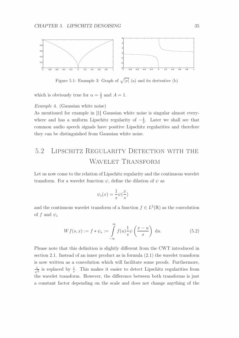
Example 3. (√
|x|)f(x) =
√|x| = |x| 12 is continuous and differentiable for all x 6= 0, but it is not
Lipschitz 1 since the derivative
f ′(x) = 0.5 ∗ sgn(x) ∗ |x|− 1
2 =
0.5 ∗ x− 1
2 , if x > 0
−0.5 ∗ (−x)− 1
2 , if x < 0.
is not bounded in any neighborhood of x = 0 (see figure 5.1). Thus, f is not Lip-
schitz 1 and it directly follows from definition 5.1.1 that the function is Lipschitz12. For n = 0 and Pn(h) ≡ 0 we get
∣∣∣|x0 + h| 12 − Pn(h)∣∣∣ = |h| 12 ≤ A|h|α
CHAPTER 5. LIPSCHITZ DENOISING 35
−1 −0.8 −0.6 −0.4 −0.2 0 0.2 0.4 0.6 0.8 10
0.2
0.4
0.6
0.8
1
−1 −0.8 −0.6 −0.4 −0.2 0 0.2 0.4 0.6 0.8 1−6
−4
−2
0
2
4
6
Figure 5.1: Example 3: Graph of√|x| (a) and its derivative (b)
which is obviously true for α = 12
and A = 1.
Example 4. (Gaussian white noise)
As mentioned for example in [1] Gaussian white noise is singular almost every-
where and has a uniform Lipschitz regularity of −12. Later we shall see that
common audio speech signals have positive Lipschitz regularities and therefore
they can be distinguished from Gaussian white noise.
5.2 Lipschitz Regularity Detection with the
Wavelet Transform
Let us now come to the relation of Lipschitz regularity and the continuous wavelet
transform. For a wavelet function ψ, define the dilation of ψ as
ψs(x) =1
sψ(x
s)
and the continuous wavelet transform of a function f ∈ L2(R) as the convolution
of f and ψs
Wf(s, x) := f ∗ ψs :=∞∫
−∞
f(u)1
sψ
(x− u
s
)du. (5.2)
Please note that this definition is slightly different from the CWT introduced in
section 2.1. Instead of an inner product as in formula (2.1) the wavelet transform
is now written as a convolution which will facilitate some proofs. Furthermore,1√s
is replaced by 1s. This makes it easier to detect Lipschitz regularities from
the wavelet transform. However, the difference between both transforms is just
a constant factor depending on the scale and does not change anything of the
CHAPTER 5. LIPSCHITZ DENOISING 36
general concept. We say that ψ has n vanishing moments if
∞∫
−∞
xkψ(x) dx = 0 (5.3)
for all nonnegative integers k < n. Obviously, this definition is the same for both
definitions of the CWT. The following theorem provides a way how to detect the
Lipschitz regularity of a function f with the help of the decay of the Wavelet
transform as a function of the scale s.
Theorem 5.2.1. Let ψ be a real wavelet function with compact support and n
vanishing moments. For f ∈ L2(R), [a, b] ⊂ R and 0 < α < n the following
statements are equivalent:
• For all ǫ > 0, f is uniformly Lipschitz α on (a+ ǫ, b− ǫ).
• There is a constant Aǫ such that for x ∈ (a+ ǫ, b− ǫ) and s > 0
|Wf(s, x)| ≤ Aǫsα. (5.4)
Proof. For only continuously differentiable wavelet functions and n = 1 a proof
of the theorem can be found in [18]. In the case of n vanishing moments, n > 1,
for any positive integer p < n there exists another wavelet function ψ1 such that
ψ(x) =dpψ1(x)
dxp
and, in the sense of weak derivatives, it holds that
Wf(s, x) = f ∗ ψs(x) (5.5)
=dp
dxp(f ∗ spψ1
s )(x) (5.6)
= sp(dpf
dxp∗ ψ1
s
)(x). (5.7)
Let p be an integer such that 0 < α−p < 1. The function f is uniformly Lipschitz
α if and only if dpf/dxp is uniformly Lipschitz α − p which is according to the
already proven case n = 1 equivalent to
∣∣∣∣dpf
dxp∗ ψ1
s(x)
∣∣∣∣ ≤ Aǫsα−p (5.8)
Eventually, using equation (5.7), this is equivalent to equation (5.4).
CHAPTER 5. LIPSCHITZ DENOISING 37
There is a similar result based on the Fourier transform, considering the scale
s “equivalent” to 1/ω for frequencies ω. A function f is uniformly Lipschitz α on
R if
∞∫
−∞
|f(ω)|(1 + |ω|α)dω <∞,
where f(ω) denotes the Fourier transform of f . This sufficient condition implies
that |f(ω)| has a decay “faster” than 1/ωα for large frequencies ω. In opposition
to the Fourier transform condition, (5.4) is sufficient and necessary as well as
localized on finite intervals.
Remark 5.2.2.
• If ψ has exactly n vanishing moments, the decay of |Wf(s, x)| does not tell
us anything about Lipschitz regularities α > n. For example sin(x) has
regularity +∞, but the decay of |Wf(s, x)| would be of order sn.
• For α < 0, α /∈ Z equation (5.4) remains valid to characterize uniform
Lipschitz exponents. This follows directly from definition 5.1.3 of negative
Lipschitz regularities.
However, to detect the Lipschitz regularity at a point x0 theorem 5.2.1 imposes
to measure the decay of Wf(s, x) in a whole two-dimensional neighborhood of
x0, which is useless for numerical computations. The next section will provide
numerically more efficient methods.
5.3 Wavelet Transform Modulus Maxima
In the following we suppose f and ψ to be real. Now, I will provide the exact
definition of the meaning of modulus maxima and maxima lines.
Definition 5.3.1.
• A modulus maxima is defined as a point (s0, x0) such that for any x in
a neighborhood of x0 we have |Wf(s0, x)| < |Wf(s0, x0)| . We still call
(s0, x0) a modulus maxima if the inequality is strict for only the right or
only the left side of the neighborhood of x0, i.e. if (s0, x0) is a strict extrema
on either the left or the right side of x0.
• A maxima line is defined as a connected curve in the scale space (s, x) along
all points are modulus maxima.
CHAPTER 5. LIPSCHITZ DENOISING 38
The next theorem shows that if there are no modulus maxima in a neigh-
borhood of x0 at fine scales, then the function is uniformly Lipschitz α in this
neighborhood for α < n.
Theorem 5.3.2. Let ψ be a n-times continuously differentiable wavelet function
with compact support and n vanishing moments and let f ∈ L1([a, b]).
• If there is a scale s0 > 0 such that |Wf(s, x)| has no local maxima for all
scales s < s0 and x ∈ (a, b), then ∀ǫ > 0 and α < n f is uniformly Lipschitz
α in (a+ ǫ, b− ǫ).
• If ψ is additionally the n-th derivative of a smoothing function θ, i.e. θ =
O( 11+x2
) and∫θ(x) dx 6= 0, then f is uniformly Lipschitz n on such an
interval.
Proof. The exact proof is very technical and can be found in [23]. In short, for
the first part one proves by induction that if |Wf(s, x)| has no maxima, for any
n and any ǫ > 0 there is a constant Aǫ,n such that
|Wf(s, x)| ≤ Aǫ,nsn (5.9)
holds for x ∈ (a + ǫ, b − ǫ) and s < s0. Then one can apply theorem 5.2.1. For
the second part of the proof, we write ψ = dnθ/dxn and get, in the weak sense of
derivatives,
|Wf(x, s)| = sndnf
dxn∗ θs(x).
The first part of the theorem and equation (5.9) now implies that for any ǫ > 0
and x ∈ (a + ǫ, b− ǫ) ∣∣∣∣dnf
dxn∗ θs(x)
∣∣∣∣ ≤ Aǫ,n.
Since the integral of θ(x) is not vanishing, this equation implies that dnf/dxn is
bounded by Aǫ,n and from definition 5.1.1 we get that f is uniformly Lipschitz n
on (a+ ǫ, b− ǫ).
In other words the theorem states that in any neighborhood where the wavelet
transform of f has no modulus maxima at fine scales, f can not be singular and
the closure of the set of points where f is not Lipschitz n is included in the
closure of the wavelet transform maxima of f . Hence, all singularities of f can
be detected by following the maxima lines when the scale goes to zero.
In the following we suppose that the function f has no fast oscillations. We
say a function f has fast oscillations if it is not Lipschitz α although its primitive
is Lipschitz α+1. One example of a fast oscillating function could be sin(1/x) in
CHAPTER 5. LIPSCHITZ DENOISING 39
the neighborhood of x = 0. However, such “fast oscillations” are not important
for our denoising models. The following theorem characterizes singularities from
the behavior of modulus maxima.
Theorem 5.3.3. Let ψ be of compact support, n times continuously differentiable
and the n-th derivative of a smoothing function. Furthermore let f be a tempered
distribution and x0 ∈ (a, b). We assume that ∃s0 > 0 and a constant C such that
for x ∈ (a, b) and s < s0, all modulus maxima belong to a cone defined by
|x− x0| ≤ Cs. (5.10)
Then the following statements hold:
• For any x1 ∈ (a, b), x1 6= x0, f is uniformly Lipschitz n in a neighborhood
of x1.
• Let α < n, α /∈ Z, then f is Lipschitz α at x0 if and only if there exists a
constant A such that at each modulus maxima (s, x) in the cone (5.10) it
holds that
|Wf(s, x)| ≤ Asα. (5.11)
Proof. One can prove the first part with the help of theorem 5.3.2. It follows
directly that f is Lipschitz n at all points x1 6= x0. For any ǫ > 0 such that
a + 2ǫ < x0 − 2ǫ there exits sǫ such that for s < sǫ and x ∈ (a + ǫ, x0 − ǫ)
the wavelet transform |Wf(s, x)| has no maxima (i.e. (s, x) is not in the cone
(5.10)). Hence, with theorem 5.3.2 one concludes that f is uniformly Lipschitz
n in a neighborhood of x1 ∈ (a, x0). Obviously, the same proof can be done for
x1 ∈ (x0, b).
The main difference between the second part of this theorem and theorem
5.2.1 is that we consider only points in the cone (5.10) and look only on modulus
maxima. However, the truth of equation (5.11) can be followed directly from
theorem 5.2.1. So it remains to prove that the Lipschitz regularity at x0 depends
only on the modulus maxima in the cone (5.10). Let x1 ∈ (a, x0) and x2 ∈ (x0, b).
Since f is Lipschitz n in the neighborhood of x1 and x2 one obtains from theorem
5.2.1 that there exists s0 > 0 such that for s < s0,
|Wf(s, x1)| ≤ A1sn and (5.12)
|Wf(s, x2)| ≤ A2sn. (5.13)
For x ∈ (x1, x2) and s < s0, |Wf(s, x)| is smaller or equal to |Wf(s, x1)|,|Wf(s, x2)| and all modulus maxima in the cone (5.10) for s < s0. Further-
CHAPTER 5. LIPSCHITZ DENOISING 40
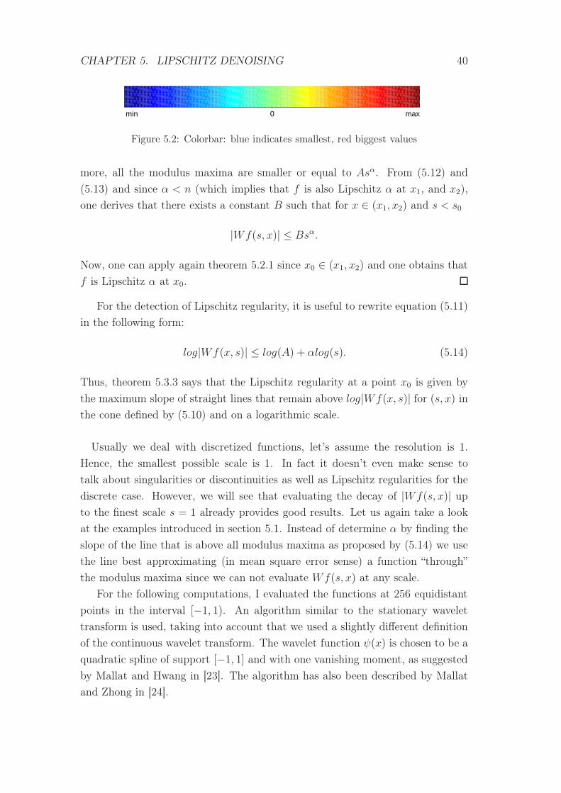
min 0 max
Figure 5.2: Colorbar: blue indicates smallest, red biggest values
more, all the modulus maxima are smaller or equal to Asα. From (5.12) and
(5.13) and since α < n (which implies that f is also Lipschitz α at x1, and x2),
one derives that there exists a constant B such that for x ∈ (x1, x2) and s < s0
|Wf(s, x)| ≤ Bsα.
Now, one can apply again theorem 5.2.1 since x0 ∈ (x1, x2) and one obtains that
f is Lipschitz α at x0.
For the detection of Lipschitz regularity, it is useful to rewrite equation (5.11)
in the following form:
log|Wf(x, s)| ≤ log(A) + αlog(s). (5.14)
Thus, theorem 5.3.3 says that the Lipschitz regularity at a point x0 is given by
the maximum slope of straight lines that remain above log|Wf(x, s)| for (s, x) in
the cone defined by (5.10) and on a logarithmic scale.
Usually we deal with discretized functions, let’s assume the resolution is 1.
Hence, the smallest possible scale is 1. In fact it doesn’t even make sense to
talk about singularities or discontinuities as well as Lipschitz regularities for the
discrete case. However, we will see that evaluating the decay of |Wf(s, x)| up
to the finest scale s = 1 already provides good results. Let us again take a look
at the examples introduced in section 5.1. Instead of determine α by finding the
slope of the line that is above all modulus maxima as proposed by (5.14) we use
the line best approximating (in mean square error sense) a function “through”
the modulus maxima since we can not evaluate Wf(s, x) at any scale.
For the following computations, I evaluated the functions at 256 equidistant
points in the interval [−1, 1). An algorithm similar to the stationary wavelet
transform is used, taking into account that we used a slightly different definition
of the continuous wavelet transform. The wavelet function ψ(x) is chosen to be a
quadratic spline of support [−1, 1] and with one vanishing moment, as suggested
by Mallat and Hwang in [23]. The algorithm has also been described by Mallat
and Zhong in [24].
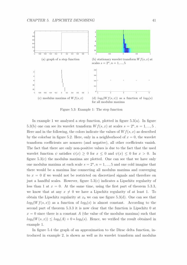
CHAPTER 5. LIPSCHITZ DENOISING 41
−1 −0.8 −0.6 −0.4 −0.2 0 0.2 0.4 0.6 0.8 1
0
0.2
0.4
0.6
0.8
1
(a) graph of a step function
2
4
8
16
32
−1 −0.5 0 0.5 1
(b) stationary wavelet transformWf(s, x) atscales s = 2n, n = 1, ..., 5
2
4
8
16
32
−1 −0.8 −0.6 −0.4 −0.2 0 0.2 0.4 0.6 0.8 1
(c) modulus maxima of Wf(s, x)
1 2 3 4 50
0.2
0.4
0.6
0.8
(d) log2(Wf(s, x)) as a function of log2(s)for all modulus maxima
Figure 5.3: Example 1: The step function
In example 1 we analyzed a step function, plotted in figure 5.3(a). In figure
5.3(b) one can see its wavelet transform Wf(s, x) at scales s = 2n, n = 1, ..., 5 .
Here and in the following, the colors indicate the values of Wf(s, x) as described
by the colorbar in figure 5.2. Here, only in a neighborhood of x = 0, the wavelet
transform coefficients are nonzero (and negative), all other coefficients vanish.
The fact that there are only non-positive values is due to the fact that the used
wavelet function ψ satisfies ψ(x) ≥ 0 for x ≤ 0 and ψ(x) ≤ 0 for x > 0. In
figure 5.3(c) the modulus maxima are plotted. One can see that we have only
one modulus maxima at each scale s = 2n, n = 1, ..., 5 and one cold imagine that
there would be a maxima line connecting all modulus maxima and converging
to x = 0 if we would not be restricted on discretized signals and therefore on
just a handful scales. However, figure 5.3(c) indicates a Lipschitz regularity of
less than 1 at x = 0. At the same time, using the first part of theorem 5.3.3,
we know that at any x 6= 0 we have a Lipschitz regularity of at least 1. To
obtain the Lipschitz regularity at x0 we can use figure 5.3(d). One can see that
log2(Wf(s, x)) as a function of log2(s) is almost constant. According to the
second part of theorem 5.3.3 it is now clear that the function is Lipschitz 0 at
x = 0 since there is a constant A (the value of the modulus maxima) such that
log2(W (s, x)) ≤ log2(A) + 0 ∗ log2(s). Hence, we verified the result obtained in
example 1.
In figure 5.4 the graph of an approximation to the Dirac delta function, in-
troduced in example 2, is shown as well as its wavelet transform and modulus
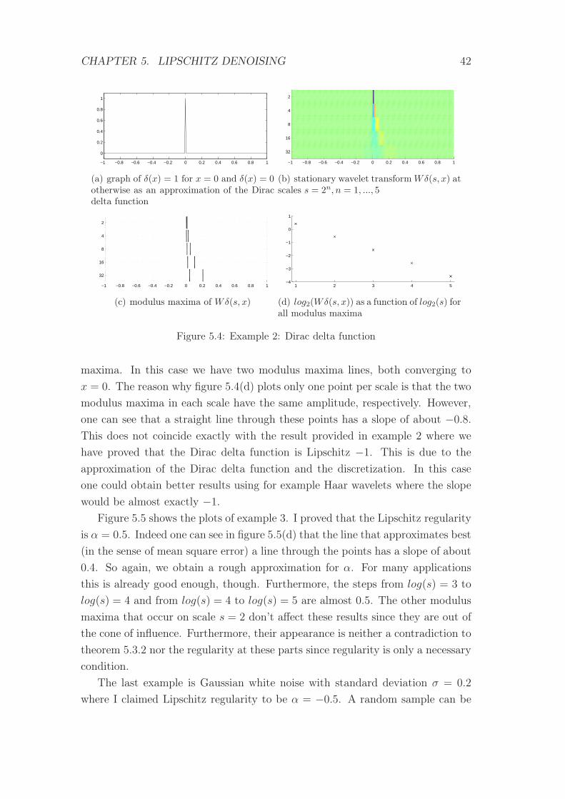
CHAPTER 5. LIPSCHITZ DENOISING 42
−1 −0.8 −0.6 −0.4 −0.2 0 0.2 0.4 0.6 0.8 1
0
0.2
0.4
0.6
0.8
1
(a) graph of δ(x) = 1 for x = 0 and δ(x) = 0otherwise as an approximation of the Diracdelta function
2
4
8
16
32
−1 −0.8 −0.6 −0.4 −0.2 0 0.2 0.4 0.6 0.8 1
(b) stationary wavelet transformWδ(s, x) atscales s = 2n, n = 1, ..., 5
2
4
8
16
32
−1 −0.8 −0.6 −0.4 −0.2 0 0.2 0.4 0.6 0.8 1
(c) modulus maxima of Wδ(s, x)
1 2 3 4 5−4
−3
−2
−1
0
1
(d) log2(Wδ(s, x)) as a function of log2(s) forall modulus maxima
Figure 5.4: Example 2: Dirac delta function
maxima. In this case we have two modulus maxima lines, both converging to
x = 0. The reason why figure 5.4(d) plots only one point per scale is that the two
modulus maxima in each scale have the same amplitude, respectively. However,
one can see that a straight line through these points has a slope of about −0.8.
This does not coincide exactly with the result provided in example 2 where we
have proved that the Dirac delta function is Lipschitz −1. This is due to the
approximation of the Dirac delta function and the discretization. In this case
one could obtain better results using for example Haar wavelets where the slope
would be almost exactly −1.
Figure 5.5 shows the plots of example 3. I proved that the Lipschitz regularity
is α = 0.5. Indeed one can see in figure 5.5(d) that the line that approximates best
(in the sense of mean square error) a line through the points has a slope of about
0.4. So again, we obtain a rough approximation for α. For many applications
this is already good enough, though. Furthermore, the steps from log(s) = 3 to
log(s) = 4 and from log(s) = 4 to log(s) = 5 are almost 0.5. The other modulus
maxima that occur on scale s = 2 don’t affect these results since they are out of
the cone of influence. Furthermore, their appearance is neither a contradiction to
theorem 5.3.2 nor the regularity at these parts since regularity is only a necessary
condition.
The last example is Gaussian white noise with standard deviation σ = 0.2
where I claimed Lipschitz regularity to be α = −0.5. A random sample can be
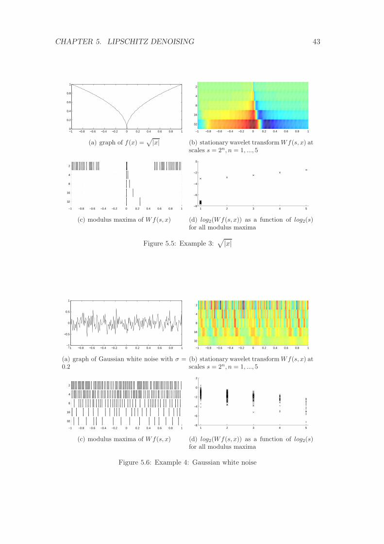
CHAPTER 5. LIPSCHITZ DENOISING 43
−1 −0.8 −0.6 −0.4 −0.2 0 0.2 0.4 0.6 0.8 10
0.2
0.4
0.6
0.8
1
(a) graph of f(x) =√|x|
2
4
8
16
32
−1 −0.8 −0.6 −0.4 −0.2 0 0.2 0.4 0.6 0.8 1
(b) stationary wavelet transformWf(s, x) atscales s = 2n, n = 1, ..., 5
2
4
8
16
32
−1 −0.8 −0.6 −0.4 −0.2 0 0.2 0.4 0.6 0.8 1
(c) modulus maxima of Wf(s, x)
1 2 3 4 5−8
−6
−4
−2
0
(d) log2(Wf(s, x)) as a function of log2(s)for all modulus maxima
Figure 5.5: Example 3:√
|x|
−1 −0.8 −0.6 −0.4 −0.2 0 0.2 0.4 0.6 0.8 1−1
−0.5
0
0.5
1
(a) graph of Gaussian white noise with σ =0.2
2
4
8
16
32
−1 −0.8 −0.6 −0.4 −0.2 0 0.2 0.4 0.6 0.8 1
(b) stationary wavelet transformWf(s, x) atscales s = 2n, n = 1, ..., 5
2
4
8
16
32
−1 −0.8 −0.6 −0.4 −0.2 0 0.2 0.4 0.6 0.8 1
(c) modulus maxima of Wf(s, x)
1 2 3 4 5−8
−6
−4
−2
0
2
(d) log2(Wf(s, x)) as a function of log2(s)for all modulus maxima
Figure 5.6: Example 4: Gaussian white noise
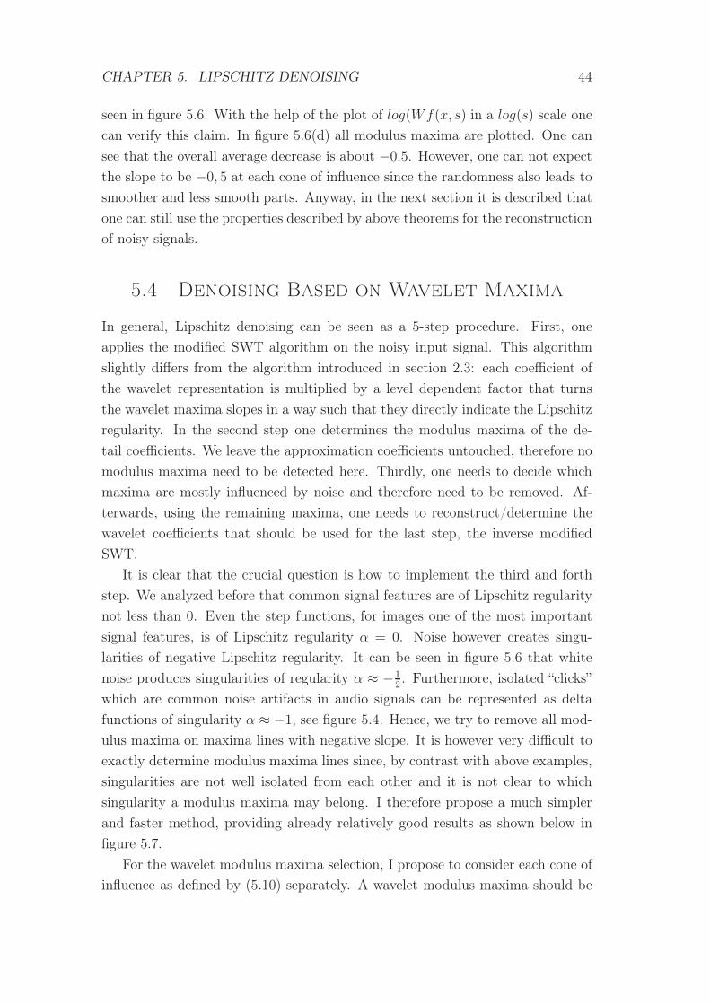
CHAPTER 5. LIPSCHITZ DENOISING 44
seen in figure 5.6. With the help of the plot of log(Wf(x, s) in a log(s) scale one
can verify this claim. In figure 5.6(d) all modulus maxima are plotted. One can
see that the overall average decrease is about −0.5. However, one can not expect
the slope to be −0, 5 at each cone of influence since the randomness also leads to
smoother and less smooth parts. Anyway, in the next section it is described that
one can still use the properties described by above theorems for the reconstruction
of noisy signals.
5.4 Denoising Based on Wavelet Maxima
In general, Lipschitz denoising can be seen as a 5-step procedure. First, one
applies the modified SWT algorithm on the noisy input signal. This algorithm
slightly differs from the algorithm introduced in section 2.3: each coefficient of
the wavelet representation is multiplied by a level dependent factor that turns
the wavelet maxima slopes in a way such that they directly indicate the Lipschitz
regularity. In the second step one determines the modulus maxima of the de-
tail coefficients. We leave the approximation coefficients untouched, therefore no
modulus maxima need to be detected here. Thirdly, one needs to decide which
maxima are mostly influenced by noise and therefore need to be removed. Af-
terwards, using the remaining maxima, one needs to reconstruct/determine the
wavelet coefficients that should be used for the last step, the inverse modified
SWT.
It is clear that the crucial question is how to implement the third and forth
step. We analyzed before that common signal features are of Lipschitz regularity
not less than 0. Even the step functions, for images one of the most important
signal features, is of Lipschitz regularity α = 0. Noise however creates singu-
larities of negative Lipschitz regularity. It can be seen in figure 5.6 that white
noise produces singularities of regularity α ≈ −12. Furthermore, isolated “clicks”
which are common noise artifacts in audio signals can be represented as delta
functions of singularity α ≈ −1, see figure 5.4. Hence, we try to remove all mod-
ulus maxima on maxima lines with negative slope. It is however very difficult to
exactly determine modulus maxima lines since, by contrast with above examples,
singularities are not well isolated from each other and it is not clear to which
singularity a modulus maxima may belong. I therefore propose a much simpler
and faster method, providing already relatively good results as shown below in
figure 5.7.
For the wavelet modulus maxima selection, I propose to consider each cone of
influence as defined by (5.10) separately. A wavelet modulus maxima should be
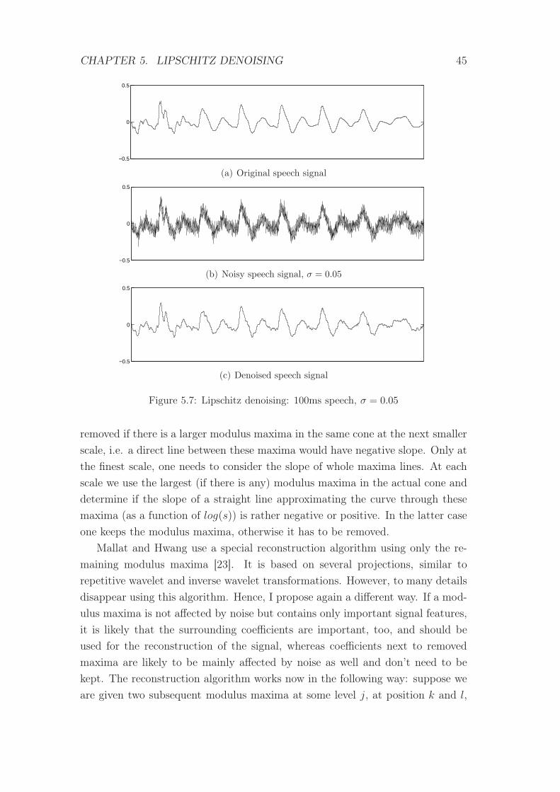
CHAPTER 5. LIPSCHITZ DENOISING 45
−0.5
0
0.5
(a) Original speech signal
−0.5
0
0.5
(b) Noisy speech signal, σ = 0.05
−0.5
0
0.5
(c) Denoised speech signal
Figure 5.7: Lipschitz denoising: 100ms speech, σ = 0.05
removed if there is a larger modulus maxima in the same cone at the next smaller
scale, i.e. a direct line between these maxima would have negative slope. Only at
the finest scale, one needs to consider the slope of whole maxima lines. At each
scale we use the largest (if there is any) modulus maxima in the actual cone and
determine if the slope of a straight line approximating the curve through these
maxima (as a function of log(s)) is rather negative or positive. In the latter case
one keeps the modulus maxima, otherwise it has to be removed.
Mallat and Hwang use a special reconstruction algorithm using only the re-
maining modulus maxima [23]. It is based on several projections, similar to
repetitive wavelet and inverse wavelet transformations. However, to many details
disappear using this algorithm. Hence, I propose again a different way. If a mod-
ulus maxima is not affected by noise but contains only important signal features,
it is likely that the surrounding coefficients are important, too, and should be
used for the reconstruction of the signal, whereas coefficients next to removed
maxima are likely to be mainly affected by noise as well and don’t need to be
kept. The reconstruction algorithm works now in the following way: suppose we
are given two subsequent modulus maxima at some level j, at position k and l,
CHAPTER 5. LIPSCHITZ DENOISING 46
then one distinguishes the following cases:
(i) both maxima are supposed to be removed, then
Sjk, ..., Sjl = 0
(ii) both maxima are supposed to be kept, then
Sjk = Yjk, ..., Sjl = Yjl
(iii) only the maxima at position k is supposed to be kept, then
Sji = Yji for k ≤ i ≤ k+l2
, Sji = 0 for k+l2< i ≤ l
(iv) only the maxima at position l is supposed to be kept, then
Sji = 0 for k ≤ i ≤ k+l2
, Sji = Yji for k+l2< i ≤ l
In fact, this selection algorithm denotes a “keep or kill” method. To obtain
additional smoothing, one may change cases (iii) and (iv). E.g. for a “smooth”
filter function f : {k, ..., l} → [0, 1] one can use
Sji = f(i) · Yji.
The function f should be chosen to be zero at the modulus maxima that is to be
removed and one for the the other maxima, strictly increasing or decreasing in
between. However, I tested several different filters, obtaining only minor changes
and no audible improvements.
Figure 5.7 provides a section of 100ms of speech example 4, Gaussian white
noise with σ = 0.05 has been added and denoised using Lipschitz denoising.
Experiments led to an optimal choice of J = 4, i.e. processing only 4 scales,
and orthogonal Daubechies wavelets with 7 vanishing moments. Furthermore,
the constant C of equation (5.10) has been chosen to be 10. Smaller values lead
to less noise reduction while larger values produce too much signal deformation.
One can see that a huge amount of noise has been reduced. Indeed, SNR has been
improved from 8.696dB to 16.149dB, MSE has been reduced from σ2 = 2.5e− 3
to 4.493e− 4. More examples and comparisons can be found in chapter 11.
However, some problems occur using Lipschitz denoising. First, since only 4
scales are used for the denoising algorithm, the remaining approximation coeffi-
cients still contain some noise, a constant background low frequency noise, like
the noise of a far away highway. Lipschitz denoising turned out to be incapable of
removing this noise artifact without strong signal deformation. Hence, an addi-
tional post-processing might be necessary, using one of the denoising algorithms
presented in the following chapters, applied only on the remaining approximation
coefficients. A second problem, similar though, is that signals with only small
CHAPTER 5. LIPSCHITZ DENOISING 47
amount of noise influence are too much deformed, see table 11.2. E.g. for the
same speech signal, but now adding Gaussian white noise of much smaller stan-
dard deviation σ = 0.01, the SNR even decreases from 22.672dB to 19.380dB.
Nevertheless, the sound quality has been improved a lot. This is in fact one of
the main problems in denoising, that SNR and other measures do not provide
enough information about auditory quality. A third problem is the denoising of
sibilants like “s”, “sh”, “z” and others. Lipschitz denoising treats some of them like
noise and strongly deforms, sometimes almost removes such sounds. However, on
balance, it already provides a very good denoising technique.
Chapter 6
Diffusion Denoising
6.1 Introduction
For the signal y(t) the Partial Differential Equation (PDE)
vu(t, u) =∂
∂t
(g(v2t (t, u))vt(t, u)
)(6.1)
v(t, 0) = y(t) (6.2)
(t, u) ∈ R× [0,+∞) (6.3)
describes a diffusion process v, embedding the signal y(·) into a family of functions
v(·, u). For constant diffusivity function g ≡ c this PDE is identical to the heat
equation vu = cvtt that can be interpreted as temperature at location t in some
body at time u. Eventually, (as u → ∞), the temperature of the body will
equalize. Hence, one can see v(t, u) as smoothed version of y(t) with smoothing
parameter u. In our case we consider t to be the signal time while u is called
diffusion time or smoothing parameter. The idea behind diffusion denoising is to
smooth noisy data y up to a certain level, i.e. up to a diffusion stopping time
U . Ones uses v(·, U) as an approximation of the original signal s. In their work
about edge detection using diffusion [28], Perona and Malik propose a diffusivity
function of the form
g(x2) =1
1 + x2
λ2
(6.4)
where λ denotes a threshold parameter. Suppose λ is in some way related to
the “derivative” of Gaussian noise, or discretized, to the difference between two
coefficients. Then, for derivatives much larger than λ, which is an indication for
important edges, g becomes small and less smoothing is done. Otherwise, one
48
CHAPTER 6. DIFFUSION DENOISING 49
expects the derivative to be influenced mainly by noise, hence g should be large
and strong smoothing is performed.
A discretized version of 6.1 based on Euler’s method is given by
vi(u+ τ) = vi(u) +τ
h
[g(v2i (u)
)vi(u)− g
(v2i−1(u)
)vi−1(u)
], (6.5)
where vi(u) = v(ti, u) with ti+1 − ti = h and τ the step sizes in signal time
and diffusion, respectively. The derivative vi(u) =δδtv(ti, u) can be obtained by
numerical differentiation, e.g.
vi(u) =1
h(vi+1(u)− vi(u)) .
Since we are not interested in precise solutions of PDE (6.1) but only in a
smoothed version of y, here, this simple one-step-method — namely Euler’s
method — is sufficient.
An example of smoothing by diffusion is shown in figure 6.1. Gaussian white
noise has been added to a sine function and denoised using the method described
above with constant diffusivity function g ≡ 1, diffusion time step size τ = 0.1
and signal time resolution h = 1:
vneui = vi + 0.1 (vi+1 − 2vi + vi−1) .
One can see in figures 6.1(a) and 6.1(b) that a view iterations are already sufficient
to achieve strong smoothing while differences between further iterations seem to
be rather small. Although the denoised version of figure 6.1(d) is very close to
the original sine function, as k approaches infinity the signal would converge to
constant 0, i.e. the integral or average value of the signal. Hence, a crucial ques-
tion will be when to stop the iteration or how to change the diffusivity function
g in a way such that v(t, u) leads to a good approximation of s(t).
6.2 Diffusion of Wavelet Coefficients
Even though it seems the results of the example provided above and illustrated
in figure 6.1 are close to the actual sine function, it is not enough to use such
simple smoothing algorithms. Small oscillatory details are usually smoothed first
by such smoothing filters. However, these details are one of the most important
features of audio signals [32]. To distinguish important audio signal features from
noise we apply (6.4) and (6.1) to the detail coefficients of a wavelet representation
of the signal. Hence, large derivatives lead to small changes of the new coefficient
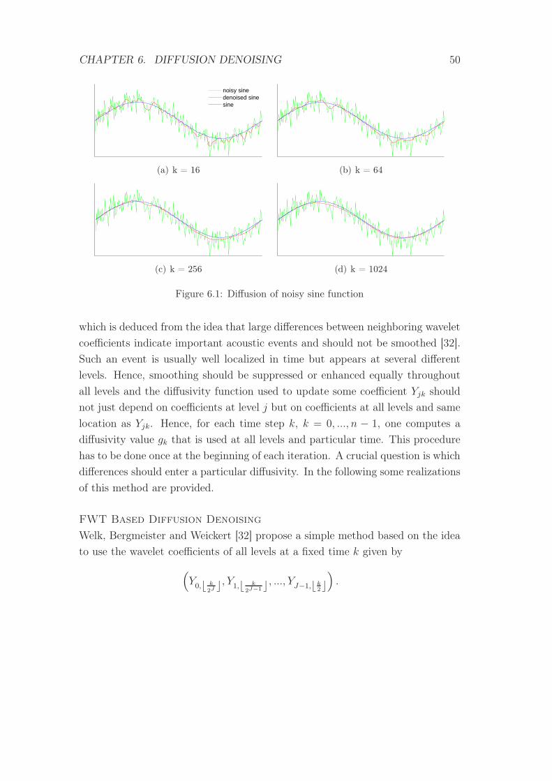
CHAPTER 6. DIFFUSION DENOISING 50
noisy sinedenoised sinesine
(a) k = 16 (b) k = 64
(c) k = 256 (d) k = 1024
Figure 6.1: Diffusion of noisy sine function
which is deduced from the idea that large differences between neighboring wavelet
coefficients indicate important acoustic events and should not be smoothed [32].
Such an event is usually well localized in time but appears at several different
levels. Hence, smoothing should be suppressed or enhanced equally throughout
all levels and the diffusivity function used to update some coefficient Yjk should
not just depend on coefficients at level j but on coefficients at all levels and same
location as Yjk. Hence, for each time step k, k = 0, ..., n − 1, one computes a
diffusivity value gk that is used at all levels and particular time. This procedure
has to be done once at the beginning of each iteration. A crucial question is which
differences should enter a particular diffusivity. In the following some realizations
of this method are provided.
FWT Based Diffusion Denoising
Welk, Bergmeister and Weickert [32] propose a simple method based on the idea
to use the wavelet coefficients of all levels at a fixed time k given by
(Y0,⌊ k
2J⌋, Y1,⌊ k
2J−1 ⌋, ..., YJ−1,⌊k2⌋).
CHAPTER 6. DIFFUSION DENOISING 51
Since gk should represent the difference between coefficients at time k and k − 1
the direct approach would be to use
gk := g
(J−1∑
j=0
(Yj,⌊ k
2J−j ⌋ − Yj,⌊ k−1
2J−j ⌋)2)
= g
(J−1∑
j=0
(Yj,⌊2jk/2J⌋ − Yj,⌊2j(k−1)/2J ⌋
)2). (6.6)
Vice versa, the associated time of some wavelet coefficient Yjk is supposed to be
2J−jk and therefore (6.5) can be modified to
Y neujk = Yjk +
τ
2J−j
(g2J−j(k+1)
Yj,k+1 − Yjk2J−j
− g2J−j(k)
Yjk − Yj,k−1
2J−j
)
= Yjk +τ
22(J−j)(g2J−j(k+1)[Yj,k+1 − Yjk]− g2J−j(k)[Yjk − dj,k−1]
)(6.7)
where 2J−j is the signal time step size at level j which holds under the assumption
of a signal time resolution h = 1. In fact, since 2J−jk is always even, it is only
necessary to compute gk for even values of k.
However, a point of criticism is that diffusivity at different locations depend
on different numbers of coefficients.The number of levels j where⌊
k2J−j
⌋=⌊k−12J−j
⌋
depends on k and therefore the number of terms on the sum of (6.6) that are
unequal zero depends on k, too. I therefore propose a slightly different diffusivity
function that ensures each summand to be nonzero, precisely
gk := g
J−1∑
j=0
(Yj,⌊ k
2J−j ⌋+1 − Yj,⌊ k
2J−j ⌋2J−j
)2 . (6.8)
The two coefficients Yj,⌊ k
2J−j ⌋+1 and Yj,⌊ k
2J−j ⌋ are chosen such that their corre-
sponding times enclose k, i.e.
2J−j(⌊
k
2J−j
⌋+ 1
)≥ k ≥ 2J−j
(⌊k
2J−j
⌋).
Furthermore, to normalize the differences, we need to divide by time step size
2J−j of the corresponding level j.
SWT Based Diffusion Denoising
An easier formula can be obtained using stationary wavelet transform coefficients.
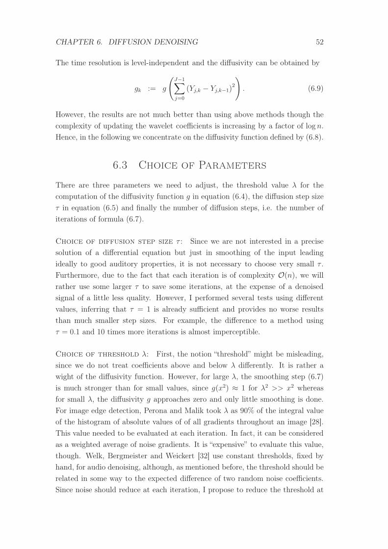
CHAPTER 6. DIFFUSION DENOISING 52
The time resolution is level-independent and the diffusivity can be obtained by
gk := g
(J−1∑
j=0
(Yj,k − Yj,k−1)2
). (6.9)
However, the results are not much better than using above methods though the
complexity of updating the wavelet coefficients is increasing by a factor of log n.
Hence, in the following we concentrate on the diffusivity function defined by (6.8).
6.3 Choice of Parameters
There are three parameters we need to adjust, the threshold value λ for the
computation of the diffusivity function g in equation (6.4), the diffusion step size
τ in equation (6.5) and finally the number of diffusion steps, i.e. the number of
iterations of formula (6.7).
Choice of diffusion step size τ : Since we are not interested in a precise
solution of a differential equation but just in smoothing of the input leading
ideally to good auditory properties, it is not necessary to choose very small τ .
Furthermore, due to the fact that each iteration is of complexity O(n), we will
rather use some larger τ to save some iterations, at the expense of a denoised
signal of a little less quality. However, I performed several tests using different
values, inferring that τ = 1 is already sufficient and provides no worse results
than much smaller step sizes. For example, the difference to a method using
τ = 0.1 and 10 times more iterations is almost imperceptible.
Choice of threshold λ: First, the notion “threshold” might be misleading,
since we do not treat coefficients above and below λ differently. It is rather a
wight of the diffusivity function. However, for large λ, the smoothing step (6.7)
is much stronger than for small values, since g(x2) ≈ 1 for λ2 >> x2 whereas
for small λ, the diffusivity g approaches zero and only little smoothing is done.
For image edge detection, Perona and Malik took λ as 90% of the integral value
of the histogram of absolute values of of all gradients throughout an image [28].
This value needed to be evaluated at each iteration. In fact, it can be considered
as a weighted average of noise gradients. It is “expensive” to evaluate this value,
though. Welk, Bergmeister and Weickert [32] use constant thresholds, fixed by
hand, for audio denoising, although, as mentioned before, the threshold should be
related in some way to the expected difference of two random noise coefficients.
Since noise should reduce at each iteration, I propose to reduce the threshold at
CHAPTER 6. DIFFUSION DENOISING 53
−0.2
−0.1
0
0.1
0.2
(a) pure noise
−0.2
−0.1
0
0.1
0.2
(b) noise after 100 iterations
−0.05
0
0.05
(c) noise after 1000 iterations
−0.05
0
0.05
(d) noise after 5000 iterations
Figure 6.2: Diffusion denoising of 50ms pure noise
each step, too. The variance of the difference of two independent and identically
distributed Gaussian random variables is given by two times the variance of the
original random variable, hence standard deviation is obtained by√2σ. Hence, I
propose to start with the universal threshold λdiff =√2σ
√2 logn = 2σ
√logn ,
introduced in chapter 7 and section 7.3. This value denotes, with high probability,
an upper bound for Gaussian random variables of variance 2σ2. We will use this
value although the difference of two Gaussian random variables is not Gaussian
anymore. However, I tested different thresholds, too, and λdiff seemed to be
an appropriate choice. Furthermore, several experiments leaded to a shrinking
factor of δ = 99% at each iteration to obtain relatively good results. Of course,
for diffusion step sizes τ 6= 1, one needs to adjust the shrinking factor.
Number of iterations: The choice of the shrinking factor solves in some way
the problem of the stopping time. Knowing δ and σ, it is clear that after some
iterations, the threshold will be too small to cause any significant signal change.
For the examples provided in chapter 11, I stopped after 80 iterations.
Diffusion denoising holds some problems, though. First, all assumptions and
choices of parameters are based on rather intuitive considerations and some ex-
periments. There is no guarantee that diffusion denoising indeed leads to good
results. Furthermore, as shown in figure 6.2, one can see that even pure noise
is not removed completely, even though for this plot no threshold shrinking has
CHAPTER 6. DIFFUSION DENOISING 54
been done. Instead, diffusion denoising produces signals containing a charac-
teristic constant background “noisy beeping”, an example is provided by sound
example 11.
However, the denoising results are similar to Lipschitz denoising, referred to
SNR and MSE measures. Only for signals with only little noise, diffusion de-
noising outperforms Lipschitz denoising significantly, see table 11.2 and 11.3. For
noisy speech with larger noise variance, using just SNR and MSE, no preference
can be recognized.
Chapter 7
Thresholding Methods
This chapter deals with different thresholding methods. Section 7.1 introduces the
most commonly used thresholding methods, hard and soft thresholding. Sections
7.3 to 7.9 are basically about the detection of “optimal” thresholds, where the
notion of optimality might differ at each section.
In the following we assume the noise ei of model (3.1) to be independent
Gaussian white noise with variance σ2, i.e.
ei ∼ N(0, σ2), i = 0, ..., n− 1.
Using orthogonal FWT, it holds that
Ejk ∼ N(0, σ2), (j, k) ∈ I,
as shown in section 3.1. Furthermore, we assume |I| = n to simplify notations.
7.1 Hard and Soft Thresholding
Hard thresholding is a typical “keep or kill” method, where all coefficients with
modulus less than threshold λ are set to be zero, the other coefficients remain
unchanged, i.e.
hardλ(x) = 11{|x|>λ} · x
=
x , if |x| > λ
0 , otherwise.(7.1)
The function hardλ(x) is plotted in figure 7.1(a), using the threshold value λ = 1.
Soft thresholding, shown in figure 7.1(b), is a little different since no coefficient
55
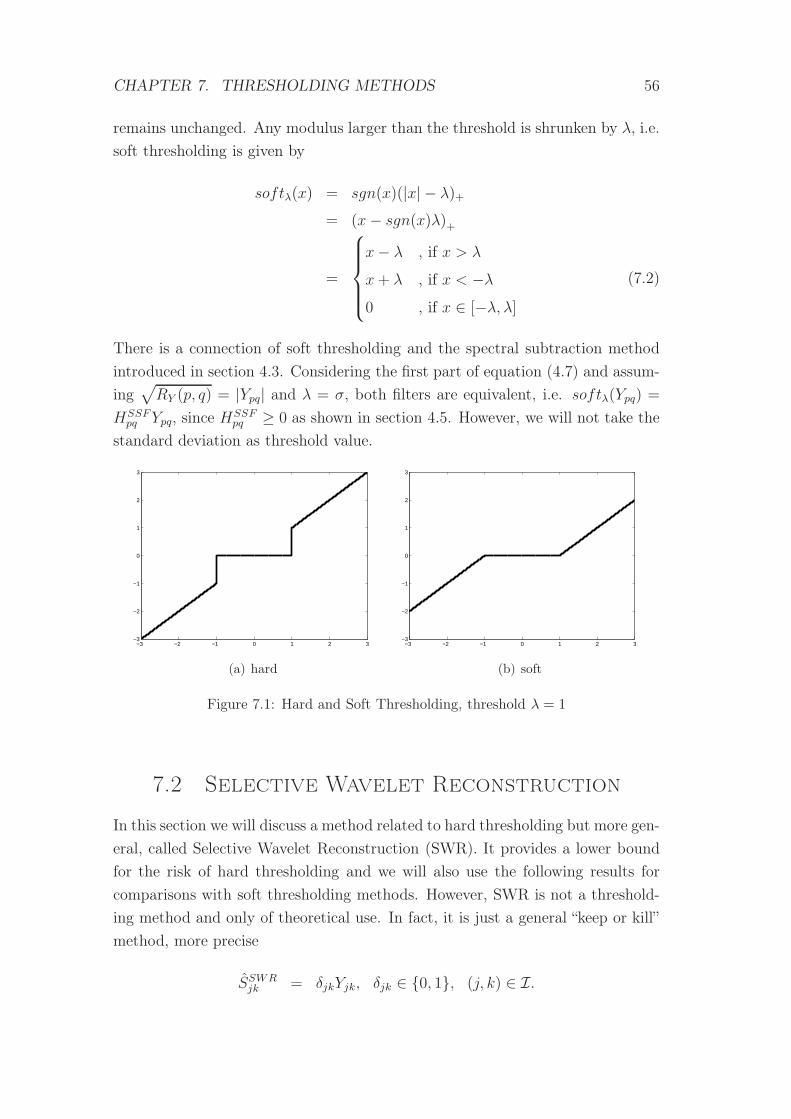
CHAPTER 7. THRESHOLDING METHODS 56
remains unchanged. Any modulus larger than the threshold is shrunken by λ, i.e.
soft thresholding is given by
softλ(x) = sgn(x)(|x| − λ)+
= (x− sgn(x)λ)+
=
x− λ , if x > λ
x+ λ , if x < −λ0 , if x ∈ [−λ, λ]
(7.2)
There is a connection of soft thresholding and the spectral subtraction method
introduced in section 4.3. Considering the first part of equation (4.7) and assum-
ing√RY (p, q) = |Ypq| and λ = σ, both filters are equivalent, i.e. softλ(Ypq) =
HSSFpq Ypq, since HSSF
pq ≥ 0 as shown in section 4.5. However, we will not take the
standard deviation as threshold value.
−3 −2 −1 0 1 2 3−3
−2
−1
0
1
2
3
(a) hard
−3 −2 −1 0 1 2 3−3
−2
−1
0
1
2
3
(b) soft
Figure 7.1: Hard and Soft Thresholding, threshold λ = 1
7.2 Selective Wavelet Reconstruction
In this section we will discuss a method related to hard thresholding but more gen-
eral, called Selective Wavelet Reconstruction (SWR). It provides a lower bound
for the risk of hard thresholding and we will also use the following results for
comparisons with soft thresholding methods. However, SWR is not a threshold-
ing method and only of theoretical use. In fact, it is just a general “keep or kill”
method, more precise
SSWRjk = δjkYjk, δjk ∈ {0, 1}, (j, k) ∈ I.
CHAPTER 7. THRESHOLDING METHODS 57
Given the knowledge of the original signal coefficients Sjk one could derive the
optimal values of δ, in the sense of minimizing the risk function.
Theorem 7.2.1. The optimal SWR estimator is obtained using
δoptjk = 11{|Sjk|>σ}
and the expected MSE of S and SSWR is given by the ideal risk
R(S, SWR) =1
n
∑
(jk)∈Imin(|Sjk|2, σ2)
Proof. Leaving a coefficient untouched, i.e. Sjk = Yjk, one obtains a risk contri-
bution of
E[(Sjk − Sjk)2] = E[(Sjk − Yjk)
2] = E[E2jk] = σ2.
Suppose |Sjk| > σ, then “killing”, i.e. Sjk = 0, would lead to the risk contribution
E[(Sjk − Sjk)2] = E[(Sjk)
2] > σ2
which would be worse than “keeping” the coefficient. In the same way, if |Sjk| ≤ σ,
it is better to remove the coefficient since
E[(Sjk − Sjk)2] = E[(Sjk)
2] ≤ σ2
is at least as good as leaving the coefficient untouched. Hence, at each coefficient
the above definition of δ leads to an expected MSE of min(|Sjk|2, σ2).
7.3 VisuShrink
The first and easiest thresholding method, called VisuShrink, is based on soft
thresholding using the so called universal threshold [8]
λV S = σ√
2 logn. (7.3)
The estimation SV Sjk is therefore given by
SV Sjk = softλV S(Yjk). (7.4)
CHAPTER 7. THRESHOLDING METHODS 58
Although the threshold does not depend on the input data (therefore “univer-
sal”), it provides already good results as illustrated by the following theorem.
Indeed, we can mimic SWR — which would require total knowledge of signal S
— essentially within a factor 2 logn.
Theorem 7.3.1. Using the universal threshold and soft thresholding as defined
above one obtains
risk(S, SV S) ≤ (2 logn + 1)
(σ2
n+R (Y, SWR)
)
Proof. I will provide only an outline of the proof. For more details see [8]. One
shows for X ∼ N(µ, 1) and λ =√2 logn with n ≥ 2 that
E[(softλ(X)− µ)2
]≤ (2 logn + 1)(1/n+min(µ2, 1))
holds. Summation leads to the deserved result. With
E[(softλ(X)− µ)2
]= 1− 2P (|X| < λ) + E
[min
(X2, λ2
)](7.5)
≤ 1 + λ2
≤ (1 + 2 logn)(1/n+ 1)
using min (X2, λ2) ≤ λ2 and
E[(softλ(X)− µ)2
]≤ 2− 2P (|X| < λ)
≤ 2P (|X| ≥ λ) + µ2
using min (X2, λ2) ≤ X2 it is enough to show that
2P (|X| ≥ λ) + µ2 ≤ (2 logn+ 1)(1/n+ µ2)
which can be done with the help of some simple statistical calculus [8].
It might be surprising that the threshold depends on the number of input data
such that joining two signals would change its value. However, the philosophy
behind the dependence on the signal length is rather taking more samples on
a given interval. Hence, adding more samples enhances redundancy and there
is less information in the additional data. Therefore, important coefficients are
concentrated in a very slowly growing data set while at the same time the signal
energy is the same in time and wavelet domain. For that reason one expects the
magnitude of these important coefficients to grow. Additionally, the dependence
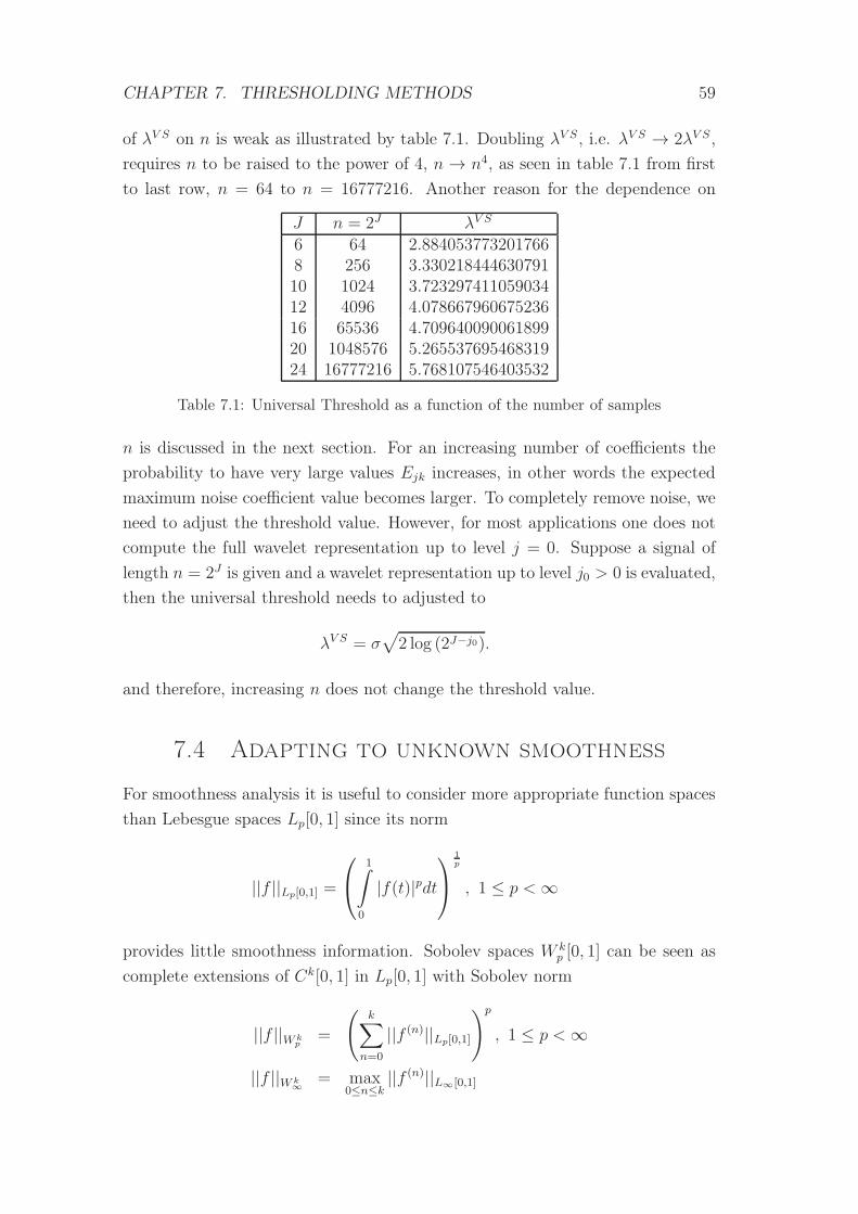
CHAPTER 7. THRESHOLDING METHODS 59
of λV S on n is weak as illustrated by table 7.1. Doubling λV S, i.e. λV S → 2λV S,
requires n to be raised to the power of 4, n → n4, as seen in table 7.1 from first
to last row, n = 64 to n = 16777216. Another reason for the dependence on
J n = 2J λV S
6 64 2.8840537732017668 256 3.33021844463079110 1024 3.72329741105903412 4096 4.07866796067523616 65536 4.70964009006189920 1048576 5.26553769546831924 16777216 5.768107546403532
Table 7.1: Universal Threshold as a function of the number of samples
n is discussed in the next section. For an increasing number of coefficients the
probability to have very large values Ejk increases, in other words the expected
maximum noise coefficient value becomes larger. To completely remove noise, we
need to adjust the threshold value. However, for most applications one does not
compute the full wavelet representation up to level j = 0. Suppose a signal of
length n = 2J is given and a wavelet representation up to level j0 > 0 is evaluated,
then the universal threshold needs to adjusted to
λV S = σ√
2 log (2J−j0).
and therefore, increasing n does not change the threshold value.
7.4 Adapting to unknown smoothness
For smoothness analysis it is useful to consider more appropriate function spaces
than Lebesgue spaces Lp[0, 1] since its norm
||f ||Lp[0,1] =
1∫
0
|f(t)|pdt
1
p
, 1 ≤ p <∞
provides little smoothness information. Sobolev spaces W kp [0, 1] can be seen as
complete extensions of Ck[0, 1] in Lp[0, 1] with Sobolev norm
||f ||W kp
=
(k∑
n=0
||f (n)||Lp[0,1]
)p
, 1 ≤ p <∞
||f ||W k∞
= max0≤n≤k
||f (n)||L∞[0,1]
CHAPTER 7. THRESHOLDING METHODS 60
where all derivatives are considered in weak sense [37]. Finally, there are even
more general spaces called Besov spaces [6], [9], [19]. For the r-th difference of a
Lp[0, 1]-function given by
∆rhf =
r∑
k=0
(r
k
)(−1)kf(t+ kh)
one defines the r-th modulus of smoothness of f
wr,p(f ; t) = suph≤t
||∆rhf ||Lp[0,1−rh]
and for r > α the Besov semi-norm
|f |Bαpq
=
1∫
0
(wr,p(f ; u)
uα
)qdu
u
1
q
, 1 ≤ q <∞
|f |Bαp∞
= sup0<t<1
wr,p(f ; h)
tα.
Eventually, the Besov norm is defined as
||f ||Bαpq= ||f ||Lp[0,1] + |f |Bα
pq. (7.6)
In this definition, α can be seen as an indication of smoothness. Functions of
Besov spaces are typically piecewise smooth. For a wavelet expansion
f(t) =
2J−1∑
k=0
cJkϕJk(t) +
∞∑
j=J
2j−1∑
k=0
djkψjk(t)
one defines the so called Besov sequence space [9], [6] given by the norm
||d||bαpq =
∞∑
j=J
2jβq
2j−1∑
k=0
|djk|p
q
p
1
q
, 1 ≤ q <∞
||d||bαp∞ = supj≥J
2jβ
2j−1∑
k=0
|djk|p
1
p
.
CHAPTER 7. THRESHOLDING METHODS 61
where β = α + 1/2 − 1/p. There are two constants c0(α, p, q) and c1(α, p, q)
independent of f such that
c0||f ||Bαpq≤ ||d||bαpq ≤ c1||f ||Bα
pq. (7.7)
This norm equivalence provides methods of measuring smoothness in wavelet
domain.
We will now show that VisuShrink produces reconstructed signals sV S that are
with high probability at least as smooth as the original signal s in the following
sense [6]:
Theorem 7.4.1. Let (si = s(ti))n−1i=0 represent a function in Besov space Bα
pq[0, 1]
and (sV Si )n−1i=0 its estimation using VisuShrink and an orthonormal wavelet basis.
There is a sequence πn independent of s and Bαpq with πn → 1 as n → ∞ and a
constant C(Bαpq) such that
P(||sV S||Bα
pq≤ C · ||s||Bα
pq
)≥ πn. (7.8)
For the proof of this theorem we first prove the following lemmas where πn is
determined. Furthermore, we show that with probability πn the estimated signal
wavelet coefficients are smaller (in absolute value) than the actual signal wavelet
coefficients.
Lemma 7.4.2. Let (zi)i∈N be i.i.d Gaussian random variables with z0 ∼ N(0, σ2).
For
πn := P
(max0≤i<n
(zi) ≤ σ√2 logn
)(7.9)
it holds that limn→∞
πn = 1.
Proof. We use the fact that
limn→∞
P
(max0≤i<n
(zi) ≤ x
)= e−a ⇔ lim
n→∞n(1− Φ(x)) = a
where Φ(x) is the distribution of zi. Furthermore, it holds that 1−Φ(x) ∼ σ2 φ(x)x
CHAPTER 7. THRESHOLDING METHODS 62
as x → ∞. Hence, for x = σ√2 logn we get
limn→∞
πn = 1
⇔ limn→∞
nσ2φ(σ√2 logn)
σ√2 logn
= 0
⇔ limn→∞
nσ2 1√2πσ
1
nσ√2 logn
= 0
which is obviously true.
Lemma 7.4.2 also ensures that for observed data containing only noise and no
signal information, i.e. si = 0, i = 0, ..., n− 1, noise is removed completely with
probability πn. Indeed, no noise can be heard listening to denoised signals using
VisuShrink. However, it is clear that signal information will be deformed, too.
The next lemma makes this even more clear.
Lemma 7.4.3. With πn as defined by (7.9)
P(|SV Sjk | ≤ |Sjk| ∀ (j, k) ∈ I
)≥ πn (7.10)
for all S ∈ Rn.
Proof. Let An denote the event
{max0≤i<n
(zi) ≤ σ√2 logn
}. We show that
An ⇒ |SV Sjk | ≤ |Sjk| ∀ (j, k) ∈ I.
Since P (An) ≥ πn, this will prove the lemma. If SV Sjk = 0 it is clear that the right
side holds. For each coordinate where SV Sjk 6= 0 we have
|SV Sjk | = |Yjk| − σ√
2 logn
and since An holds, |Yjk − Sjk| ≤ σ√2 logn which leads to
|Sjk| ≥ |Yjk| − σ√
2 logn = |SV Sjk |.
Proof of theorem 7.4.1. From (7.7) we get
c0||s||Bαpq≤ ||S||bαpq ≤ c1||s||Bα
pqand
c0||sV S||Bαpq≤ ||SV S||bαpq ≤ c1||sV S||Bα
pq
CHAPTER 7. THRESHOLDING METHODS 63
since c0 and c1 are independent of the used signal. Using Lemma 7.4.3 we get
with a probability greater or equal to πn.
||sV S||Bαpq
≤ 1
c0||SV S||bαpq
≤ 1
c0||S||bαpq
≤ c1c0||s||Bα
pq.
So theorem 7.4.1 holds for πn of lemma 7.4.2 and C = c1/c2.
7.5 Minimax Threshold
In the above section an easy threshold has been introduced that already provides
good visual and auditory results. However, it is based on the idea of removing
all noise without regarding possible signal destruction. In fact, those denoised
signals often sound dully since most of the high frequencies are removed, too. In
the following sections we will derive thresholds that minimize the risk function,
i.e. the expected mean square error. As already seen in (3.9) and (3.10), the risk
function can be seen as a sum of bias squared and variance. The best threshold
to minimize the variance is far away of being a good choice to make the bias
smaller, though. More precisely,
limλ→∞
var(Sλ) = limλ→∞
1
nE||Sλ − ESλ||2 = 0, (7.11)
limλ→∞
bias2(S, Sλ) = limλ→∞
1
n||S − ESλ||2 = 1
n||S||2. (7.12)
Hence, thresholds minimizing the risk function are best compromises between
variance and bias.
In this section we are interested in a minimax risk threshold, i.e. a threshold
λ∗ such that
supSrisk(S, Sλ)
becomes minimal, i.e.
supSrisk(S, Sλ
∗
) = infSλ
supSrisk(S, Sλ). (7.13)
In words, we are looking for a threshold that minimizes the risk assuming the
worst possible signal. Hence, it is not data adaptive. Let us first consider the
CHAPTER 7. THRESHOLDING METHODS 64
risk contribution of a single coefficient defined by
ρ(λ, S) = E[(softλ(Y )− S)2
]. (7.14)
Risk is then obtained by risk(λ) = 1n
∑ρ(λ, Sjk). In the following we always
assume noise to be Gaussian with density φ and distribution Φ,
φ(x) =1
σ√2πe
−x2
2σ2
Φ(x) =
x∫
−∞
φ(x)dx.
So far, we don’t know the value of ρ(λ, S) neither how to minimize it. The
following lemmas provide a form of ρ(λ, S) that requires only the evaluation of φ
and Φ. First, we introduce the expected error after soft thresholding and come
then to the computation of ρ(λ, S).
Lemma 7.5.1. Let Y = S+E ∼ N(S, σ2) and Sλ = softλ(Y ). Call Eλ = Sλ−Sthe bias of the thresholding method. It holds that
EEλ = S + Φ(λ− S)(λ− S)
+ Φ(λ + S)(−λ− S)
+ φ(λ− S)(σ2)
+ φ(λ+ S)(−σ2) (7.15)
CHAPTER 7. THRESHOLDING METHODS 65
Proof.
ESλ =
∞∫
−∞
softλ(x)φ(x− S)dx
=
∞∫
λ
(x− λ)φ(x− S)dx+
−λ∫
−∞
(x+ λ)φ(x− S)dx
=
∞∫
λ−S
(x+ S − λ)φ(x)dx+
−λ−S∫
−∞
(x+ S + λ)φ(x)dx
= (S − λ) [1− Φ(λ− S)] +
∞∫
λ−S
xφ(x)dx
+ (S + λ) [Φ(−λ− S)] +
−λ−S∫
−∞
xφ(x)dx
Using xφ(x) = −σ2φ′(x) and Φ(−x) = 1− Φ(x) one obtains
ESλ = 2S + Φ(λ− S)(λ− S)
+ Φ(λ + S)(−λ− S)
+ φ(λ− S)(σ2)
+ φ(λ+ S)(−σ2) (7.16)
Since EEλ = ESλ − S the proof is done.
Lemma 7.5.2. Using the assumptions of lemma 7.5.1 we have
ρ(λ, S) = E
[(Sλ − S)2
]
= 2σ2 + 2λ2 − S2
+ Φ(λ− S)(−σ2 − λ2 + S2)
+ Φ(λ + S)(−σ2 − λ2 + S2)
+ φ(λ− S)(−σ2(λ+ S))
+ φ(λ+ S)(−σ2(λ− S)) (7.17)
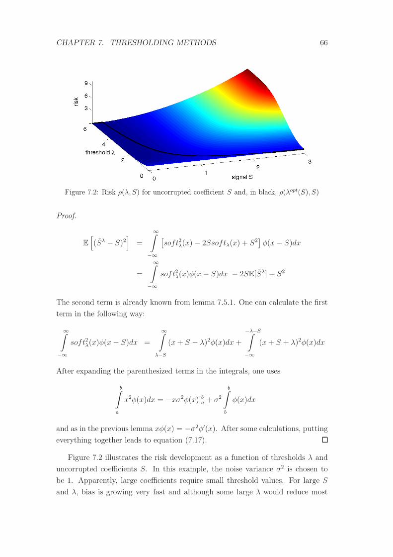
CHAPTER 7. THRESHOLDING METHODS 66
Figure 7.2: Risk ρ(λ, S) for uncorrupted coefficient S and, in black, ρ(λopt(S), S)
Proof.
E
[(Sλ − S)2
]=
∞∫
−∞
[soft2λ(x)− 2Ssoftλ(x) + S2
]φ(x− S)dx
=
∞∫
−∞
soft2λ(x)φ(x− S)dx − 2SE[Sλ] + S2
The second term is already known from lemma 7.5.1. One can calculate the first
term in the following way:
∞∫
−∞
soft2λ(x)φ(x− S)dx =
∞∫
λ−S
(x+ S − λ)2φ(x)dx+
−λ−S∫
−∞
(x+ S + λ)2φ(x)dx
After expanding the parenthesized terms in the integrals, one uses
b∫
a
x2φ(x)dx = −xσ2φ(x)|ba + σ2
b∫
b
φ(x)dx
and as in the previous lemma xφ(x) = −σ2φ′(x). After some calculations, putting
everything together leads to equation (7.17).
Figure 7.2 illustrates the risk development as a function of thresholds λ and
uncorrupted coefficients S. In this example, the noise variance σ2 is chosen to
be 1. Apparently, large coefficients require small threshold values. For large S
and λ, bias is growing very fast and although some large λ would reduce most
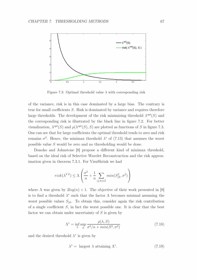
CHAPTER 7. THRESHOLDING METHODS 67
0 0.5 1 1.5 2 2.50
1
2
3
4
5
λopt(S)
risk( λopt(S), S )
Figure 7.3: Optimal threshold value λ with corresponding risk
of the variance, risk is in this case dominated by a large bias. The contrary is
true for small coefficients S. Risk is dominated by variance and requires therefore
large thresholds. The development of the risk minimizing threshold λopt(S) and
the corresponding risk is illustrated by the black line in figure 7.2. For better
visualization, λopt(S) and ρ(λopt(S), S) are plotted as functions of S in figure 7.3.
One can see that for large coefficients the optimal threshold tends to zero and risk
remains σ2. Hence, the minimax threshold λ∗ of (7.13) that assumes the worst
possible value S would be zero and no thresholding would be done.
Donoho and Johnstone [8] propose a different kind of minimax threshold,
based on the ideal risk of Selective Wavelet Reconstruction and the risk approx-
imation given in theorem 7.3.1. For VisuShrink we had
risk(λV S) ≤ Λ
σ
2
n+
1
n
∑
(j,k)∈Imin(S2
jk, σ2)
where Λ was given by 2log(n) + 1. The objective of their work presented in [8]
is to find a threshold λ∗ such that the factor Λ becomes minimal assuming the
worst possible values Sjk. To obtain this, consider again the risk contribution
of a single coefficient S, in fact the worst possible one. It is clear that the best
factor we can obtain under uncertainty of S is given by
Λ∗ = infλsupS
ρ(λ, S)
σ2/n+min(S2, σ2)(7.18)
and the desired threshold λ∗ is given by
λ∗ = largest λ attaining Λ∗. (7.19)
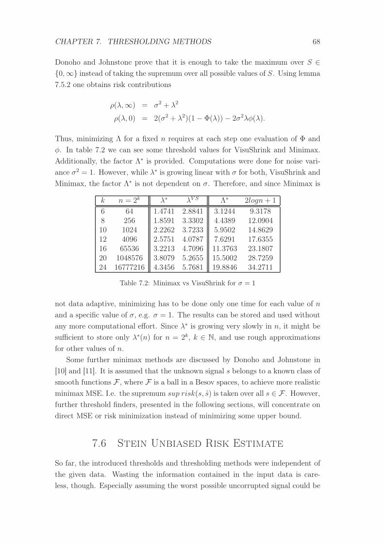
CHAPTER 7. THRESHOLDING METHODS 68
Donoho and Johnstone prove that it is enough to take the maximum over S ∈{0,∞} instead of taking the supremum over all possible values of S. Using lemma
7.5.2 one obtains risk contributions
ρ(λ,∞) = σ2 + λ2
ρ(λ, 0) = 2(σ2 + λ2)(1− Φ(λ))− 2σ2λφ(λ).
Thus, minimizing Λ for a fixed n requires at each step one evaluation of Φ and
φ. In table 7.2 we can see some threshold values for VisuShrink and Minimax.
Additionally, the factor Λ∗ is provided. Computations were done for noise vari-
ance σ2 = 1. However, while λ∗ is growing linear with σ for both, VisuShrink and
Minimax, the factor Λ∗ is not dependent on σ. Therefore, and since Minimax is
k n = 2k λ∗ λV S Λ∗ 2logn+ 1
6 64 1.4741 2.8841 3.1244 9.31788 256 1.8591 3.3302 4.4389 12.090410 1024 2.2262 3.7233 5.9502 14.862912 4096 2.5751 4.0787 7.6291 17.635516 65536 3.2213 4.7096 11.3763 23.180720 1048576 3.8079 5.2655 15.5002 28.725924 16777216 4.3456 5.7681 19.8846 34.2711
Table 7.2: Minimax vs VisuShrink for σ = 1
not data adaptive, minimizing has to be done only one time for each value of n
and a specific value of σ, e.g. σ = 1. The results can be stored and used without
any more computational effort. Since λ∗ is growing very slowly in n, it might be
sufficient to store only λ∗(n) for n = 2k, k ∈ N, and use rough approximations
for other values of n.
Some further minimax methods are discussed by Donoho and Johnstone in
[10] and [11]. It is assumed that the unknown signal s belongs to a known class of
smooth functions F , where F is a ball in a Besov spaces, to achieve more realistic
minimax MSE. I.e. the supremum sup risk(s, s) is taken over all s ∈ F . However,
further threshold finders, presented in the following sections, will concentrate on
direct MSE or risk minimization instead of minimizing some upper bound.
7.6 Stein Unbiased Risk Estimate
So far, the introduced thresholds and thresholding methods were independent of
the given data. Wasting the information contained in the input data is care-
less, though. Especially assuming the worst possible uncorrupted signal could be
CHAPTER 7. THRESHOLDING METHODS 69
considered as far too pessimistic. Knowing the input Y , it is rather unrealistic
to assume S to be either infinity or zero. In the following sections we will see
different approaches for data adaptive thresholding methods with the aim of risk
minimization and based on soft thresholding. In the subsequent chapter, I will
suggest a different kind of thresholding that is based on the idea not to use the
same threshold for all coefficients.
Let’s now denote the estimator of S using soft thresholding with threshold λ
by
Sλ = Ssoftλ
= softλ(Y ) (7.20)
and the MSE and risk of S and Sλ by
MSE(λ) = MSE(S, Sλ)
=1
n||Sλ − S||2,
risk(λ) = E[MSE(λ)]
Furthermore, for the measurement of the effect of thresholding, define
F (λ) =1
n||Sλ − Y ||2. (7.21)
The first MSE estimator we will discuss is called Stein Unbiased Risk Estimate
(SURE) and introduced by Donoho and Johnstone in [9]. Some additional anal-
ysis can be found in [19]. It is based on more general work of Charles Stein [30].
Although for a given threshold λ, both, Y and Sλ and therefore also F are known,
it is necessary to consider the expectation of this function to find approximations
of the expected MSE. I.e. one uses
E[F (λ)] =1
nE
[||Y − S||2 + ||S − Sλ||2 + 2(Y − S, S − Sλ)
]
= σ2 + risk(λ)− 2
nE[(E,Eλ)] (7.22)
where Eλ = Sλ−S denotes the remaining noise after thresholding. Lemmas 7.6.1
and 7.6.2 will lead to a more useful notation of the third term of equation (7.22).
CHAPTER 7. THRESHOLDING METHODS 70
Lemma 7.6.1. The derivative of Eλjk, seen as a function of Ejk, is given by
∂Eλjk
∂Ejk=
1 , if |Yjk| > λ
0 , otherwise
Proof. With the help of equation (7.2) we rewrite Eλ as
Eλ = softλ(Y )− S
=
(Y − λ)− S , if Y > λ
(Y + λ)− S , if Y < −λ−S , otherwise
=
E − λ , if Y > λ
E + λ , if Y < −λ−S , otherwise.
It is now easy to see that above claim holds.
Lemma 7.6.2. Let φ be the Gaussian density function with µ = 0. Then
E[EjkE
λjk
]= σ2P (|Yjk| > λ)
Proof. Since xφ(x) = −σ2φ′(x), we have
E[EjkE
λjk
]=
∞∫
−∞
EλjkEjkφ(Ejk)dEjk
= −σ2
∞∫
−∞
Eλjkφ
′(Ejk)dEjk
= −σ2[Eλjkφ(Ejk)
]∞−∞ + σ2
∞∫
−∞
∂Eλjk
∂Ejkφ(Ejk)dEjk
and with lemma 7.6.1 we get
E[EjkE
λjk
]= σ2P (|Yjk| > λ)
Now we need to find the probability P (|Yjk| > λ). Therefore we first define n0
as the number of wavelet coefficients that are shrunken to zero, i.e. the number
CHAPTER 7. THRESHOLDING METHODS 71
of wavelet coefficients whose modulus is less than or equal to the threshold,
n0 = |{(j, k) ∈ I|Y λjk = 0}|
= |{(j, k) ∈ I|Yjk ≤ λ}|. (7.23)
As shown in [19], it is the obvious choice to use P (|Yjk| > λ) = n−n0
nand one
obtains
E[(E,Eλ)] = σ2∑
(j,k)∈IP (|Yjk| > λ)
= σ2∑
(j,k)∈I
n− n0
n
= σ2(n− n0) (7.24)
Using equations (7.22) and (7.24) we construct the MSE approximation
SURE(λ) = F (λ)− σ2 + 2σ2n− n0
n, (7.25)
where SURE = risk = EMSE. Let’s mention again that, unlike Minimax,
SURE is adaptive, although it is as well derived from MSE expectation.
7.7 Cross Validation
In this section I will introduce Ordinary Cross Validation (OCV) and Generalized
Cross Validation (GCV) [26], [21], [20]. Like SURE, both of them can be seen
as a function of a threshold parameter λ and are estimates of the MSE function.
However, GCV evaluation only requires input data, no additional knowledge is
necessary. Estimations of noise variance is not needed either.
In short, the concept of cross validation is given by the construction of several
estimates, never using the whole data set. Using these estimates one predicts
what the expelled data could have been. Finally one compares the prediction
with the actual values of the expelled data.
7.7.1 Ordinary Cross Validation
Ordinary Cross Validation (OCV) is based on the assumption of in some way
smooth original data si. Hence, each value si can be approximated by linear
combinations of its neighbors. Let’s now define yi as a weighted average of the
observed data {y0, ..., yi−1, yi+1, ..., yn−1}. Noise in this component is smoothed,
CHAPTER 7. THRESHOLDING METHODS 72
and therefore it is considered to be relatively noise independent. Let’s denote
sλ,i := IFWT (softλ(FWT ({y0, ..., yi−1, yi, yi+1, ..., yn−1})))
the reproduced signal after soft thresholding using yi instead of yi. One considers
sλ,ii as a “prediction” of the coefficient yi and takes the distance |sλ,ii − yi| as a
measure of optimality of the threshold choice. The distance is dominated by noise
for small threshold values while large ones induce too much signal distortion. One
repeats the same procedure for each component, i.e. n transformations, threshold
procedures and inverse transformations are necessary. Then, one computes
OCV (λ) =1
n
n−1∑
i=0
(yi − sλ,ii )2 (7.26)
which is called “Ordinary Cross Validation” or “Leaving Out One - Ordinary Cross
Validation”. Now one could try to minimize OCV (λ) to obtain a near optimal
threshold. However, in this version each OCV evaluation in the minimization
procedure would contribute costs of O(n2). Hence, we need to find more advan-
tageous algorithms. To do so, let’s first discuss the choice of yi. A possible value
could be 12(yi−1 + yi+1) [26], however, to simplify the computation it is useful to
take yi in way such that
yi = sλ,ii . (7.27)
Thresholding has a leveling effect and it holds that ([19])
yi = maxiyi ⇒ sλ,ii ≤ yi
yi = miniyi ⇒ sλ,ii ≥ yi.
which proves the existence of this value. As before sλ denotes the reconstructed
signal after soft thresholding, i.e.
sλ := IFWT (softλ(FWT (y))).
Using the above choice of yi one has
yi − sλ,ii =yi − sλi1− ai
(7.28)
CHAPTER 7. THRESHOLDING METHODS 73
where ai is given by
ai =sλi − sλ,iiyi − sλ,ii
=sλi − sλ,iiyi − yi
≈ ∂sλi∂yi
. (7.29)
Assuming the knowledge of ai, one can approximate OCV (λ) in O(n), leading to
OCV (λ) =1
n
n−1∑
i=0
1
(1− ai)2(yi − sλi )
2 (7.30)
Hence, one needs to find a fast evaluable approximation of ai. As already indi-
cated by formula (7.29), the derivative ∂sλi /∂yi might be a good basis for such an
approximation. However, let’s introduce first
D(j1k1),(j2k2) :=∂Y λ
j1k1
∂Yj2k2
=∂
∂Yj2k2softλ(Yj1k1).
Using (7.2) one immediately sees that D(j1k1),(j2k2) = 0 for (j1, k1) 6= (j2, k2) and
D(jk),(jk) =
0 , if |Yjk| ≤ λ
1 , otherwise
Furthermore, let W denote a wavelet transform matrix and define A =W−1DW .
Now, one can see that
∂sλi∂yi
= Aii
and the evaluation requires only one forward and inverse wavelet transform.
Hence, one indeed obtains an approximation of the OCV function that can be
obtained in O(n), replacing ai in formula (7.30) by Aii.
7.7.2 Generalized Cross Validation
As discussed above, for each OCV evaluation in a minimization procedure, two
forward and inverse wavelet transforms are required. Additionally, for small
CHAPTER 7. THRESHOLDING METHODS 74
threshold values, most of the Aii are close to one and the algorithm could become
unstable. In this section we will see a similar function that can be minimized in
wavelet domain and that avoids the mentioned problems. The idea is to approxi-
mate ai of formula (7.26) using a constant value, say ai ≡ α for all i = 0, .., n−1.
In fact one uses the average of all values Aii [33], [21],
α =1
n
n−1∑
i=0
Aii
=1
n· tr(A),
where tr(A) is the trace of A. Since W is regular and A = W−1DW , recalling
the definition of D, one obtains
α =tr(D)
n=n− n0
n
where n0 is defined by (7.23). Applied to equation (7.26), one obtains the so
called generalized cross validation
GCV (λ) =1
n
1
(1− α)2
n−1∑
i=0
(yi − sλi )2
=1n||y − sλ||2(n0
n
)2 (7.31)
If the transform is orthogonal, this is equivalent to
GCV (λ) =1n||Y − Sλ||2(n0
n
)2
=F (λ)(n0
n
)2 (7.32)
Hence, it is now possible to minimize in wavelet domain and therefore, the com-
putation of GCV (λ) is much easier and faster than the evaluation of OCV (λ). A
special treatment needs to be implemented in the case of n0 = 0, although this
case is extremely unlikely for λ > 0. Especially in the presence of Gaussian white
noise we expect to shrink many coefficients to zero. However, one chooses in this
case GCV (λ) to be 2 ∗ σ2. A justification is provided in the next section where
a more rigorous analysis of the GCV procedure is done.
CHAPTER 7. THRESHOLDING METHODS 75
7.7.3 GCV Analysis
So far, we have no guarantee that GCV really approximates the MSE or risk
function. The assumptions for cross validations were rather rough and seem to be
very unsound. This section provides a relation of GCV and SURE that indeed
ensures the quality of the GCV function. Additionally, a result of asymptotic
behavior is provided. Let’s call n1 = n − n0 the number of wavelet coefficients
that have not been shrunken to zero. Note that n1/n should be rather small for
most applications since relatively smooth functions can be represented by just
a little number of coefficients. Hence, we omit terms of the order (n1/n)2 and
rewrite
GCV (λ) =F (λ)
(1− n1
n
)2
=F (λ)
1− 2n1
n+(n1
n
)2
≈ F (λ)
1− 2n1
n
≈ F (λ)
(1 +
2n1
n
)(7.33)
Using formulas (7.22) and (7.24) together with lemma 7.6.2 and assuming the
difference F (λ)− E[F (λ)] to be very small we have
F (λ) = E[F (λ)] + (F (λ)− E[F (λ)])
≈ σ2 + risk(λ)− σ2 2E[n1]
n(7.34)
and therefore, neglecting again terms of the order (n1/n)2, we obtain
GCV (λ) ≈ F (λ)
(1 +
2n1
n
)
≈ F (λ) +2n1
nσ2 +
2n1
nrisk(λ).
For threshold values near the minimum risk threshold, risk(λ) is much smaller
than σ2 = risk(0). So we omit the last term of the above equation, too. Now,
CHAPTER 7. THRESHOLDING METHODS 76
one can see the connection to the SURE formula (7.25):
GCV (λ) ≈ F (λ) +2n1
nσ2 (7.35)
= SURE(λ) + σ2 (7.36)
≈ MSE(λ) + σ2 (7.37)
However, for GCV evaluation there is no need to know the value of σ2, so no
additional noise variance approximation is necessary. This is useful especially for
signals with no “silent” parts that are only influenced by noise and would easily
provide noise variance approximations. For many applications, such silent parts
are hard to determine, anyway. Furthermore, for mean square error minimization
the constant term σ2 does not change anything and GCV should provide good
results (see also section 7.8). Formula (7.37) also justifies the choice of GCV (λ)
for n0 = 0. This case is only likely for very small threshold values and therefore
we choose GCV to be equal to GCV (0) ≈MSE(0) + σ2 = 2σ2.
Another interesting result is the asymptotic behavior of GCV . Let’s therefore
denote first λopt as the optimal threshold, i.e. the threshold that minimizes the
expected MSE function, λopt = argmin risk(λ) and λgcv the threshold that mini-
mizes the expected GCV function, λgcv = argmin EGCV (λ). The next theorem
states that risk(λopt) and risk(λgcv) have the same asymptotic behavior, i.e. for
large n both thresholds lead to almost the same risk. An outline of the proof is
provided.
Theorem 7.7.1. With λopt and λgcv as given above and for piecewise smooth
signals, it holds that
limn→∞
risk(λgcv)
risk(λopt)= 1 (7.38)
Proof. In the first part of the proof, an upper bound of risk(λgcv)/risk(λopt) is
derived. In the second part, I provide a less restrictive explanation why we can
expect this upper bound to converge to 1 for piecewise smooth signals. For a
detailed proof see [19].
In the following we call µ0 = E(n0/n) and µ1 = E(n1/n) = 1−µ0. Furthermore
we have, using (7.34),
EGCV (λ) = E
[F (λ)
(n0/n)2
]
=(risk(λ) + σ2 − 2σ2µ1
)/µ2
0
CHAPTER 7. THRESHOLDING METHODS 77
Now, we get
∣∣∣∣risk(λ)− (EGCV (λ)− σ2)
risk(λ)
∣∣∣∣ =
∣∣∣∣1−EGCV (λ)
risk(λ)+
σ2
risk(λ)
∣∣∣∣
=
∣∣∣∣1−risk(λ) + σ2 − 2σ2µ1
µ20 · risk(λ)
+σ2
risk(λ)
∣∣∣∣
=
∣∣∣∣1−1
µ20
+σ2
risk(λ)·(−1 + 2µ1
µ20
+ 1
)∣∣∣∣
=1
µ20
∣∣∣∣(µ20 − 1 +
σ2
risk(λ)µ21
)∣∣∣∣
≤ 1
µ20
(∣∣µ20 − 1
∣∣+∣∣∣∣σ2µ2
1
risk(λ)
∣∣∣∣)
=1
µ20
((1− µ2
0) +σ2µ2
1
risk(λ)
)
=: h(λ)
The function h(λ) leads directly to the upper bound of risk(λgcv)/risk(λopt):
risk(λgcv)(1− h(λgcv)) ≤ EGCV (λgcv)− σ2
≤ EGCV (λopt)− σ2
≤ risk(λopt)(1 + h(λopt))
and hence
1 ≤ risk(λgcv)
risk(λopt)≤ 1 + h(λopt)
1− h(λgcv)(7.39)
If we can show that limn→∞ h(λ) = 0 for both thresholds, the proof is done.
To obtain this, we have to show that µ1 → 0 (which infers µ0 → 1) and that
µ21/risk → 0. Let’s discuss the behavior of the risk first. In figure 7.2 the risk
contribution of a single coefficients with respect to λ is shown and total risk is
obtained by 1/n∑ρ(λ, Sjk). Since for large coefficients even optimal thresholds
produce a risk contribution of about σ2, we can assume for non-silent speech
signals that at least one signal wavelet coefficient S is large enough such that
ρ(λ, S) ≥ σ2. Hence, risk would be at least σ2/n. Therefore, it is now sufficient
to show that nµ21 → 0.
Let’s denote the set of indices where the original signal wavelet coefficients is
zero by
I0 = {(j, k) ∈ I|Sjk = 0}
CHAPTER 7. THRESHOLDING METHODS 78
and in the same way I1 = I −I0 the indices of original signal wavelet coefficients
unequal to zero. Suppose the original signal is piecewise polynomial, then the
number of nonzero coefficients is proportional to the number of levels, i.e. one
can say |I1| = O(log n), [19]. Then one obtains
µ1(λ) =1
n
∑
(j,k)∈IP (|Yjk| ≥ λ)
≤ 1
n
∑
(j,k)∈I1
1 +∑
(j,k)∈I0
P (|Ejk| ≥ λ)
=|I1|n
+|I0|nP (|Ejk| ≥ λ).
As n approaches infinity, we have λopt = O(√log n) for the optimal threshold
λopt, [19]. Since
1− Φ(x) ≈ σ2φ(x)
xas x→ ∞,
it holds that P (|Ejk| ≥ λ) = O(1/(n√log n)) for threshold values in the neigh-
borhood of λopt. In summary, we have in the piecewise polynomial case
µ1 = O(log n
n+
1
n√log n
)= O
(logn
n
)
and nµ21 = O(log2 (n)/n) → 0 for threshold values in the neighborhood of λopt.
Similar arguments hold for general piecewise smooth signals, where one can
not assume that most coefficients are exactly zero. However, using Iε0 = {(j, k) ∈I||Sjk| ≤ ελopt} instead of I0, similar arguments hold since one can show that
there is a level j0, such that all coefficients in higher levels that are not affected
by singularities are of modulus smaller than ελ∗, see [19].
7.8 SURE & GCV Minimization
Maarten Jansen assumes SURE and GCV to be convex functions in λ [19]. I
will now provide arguments based on the risk contribution function that support
this assumption. Nevertheless, one can show at the same time that there are
cases where the risk is not convex and so SURE and GCV cannot assumed to
be convex, either. These cases are very unlikely for speech signals, though.
A function is convex if and only if its second derivative is nonnegative. Simple
calculations, using again the fact that xφ(x) = −σ2φ(x), lead to the first and
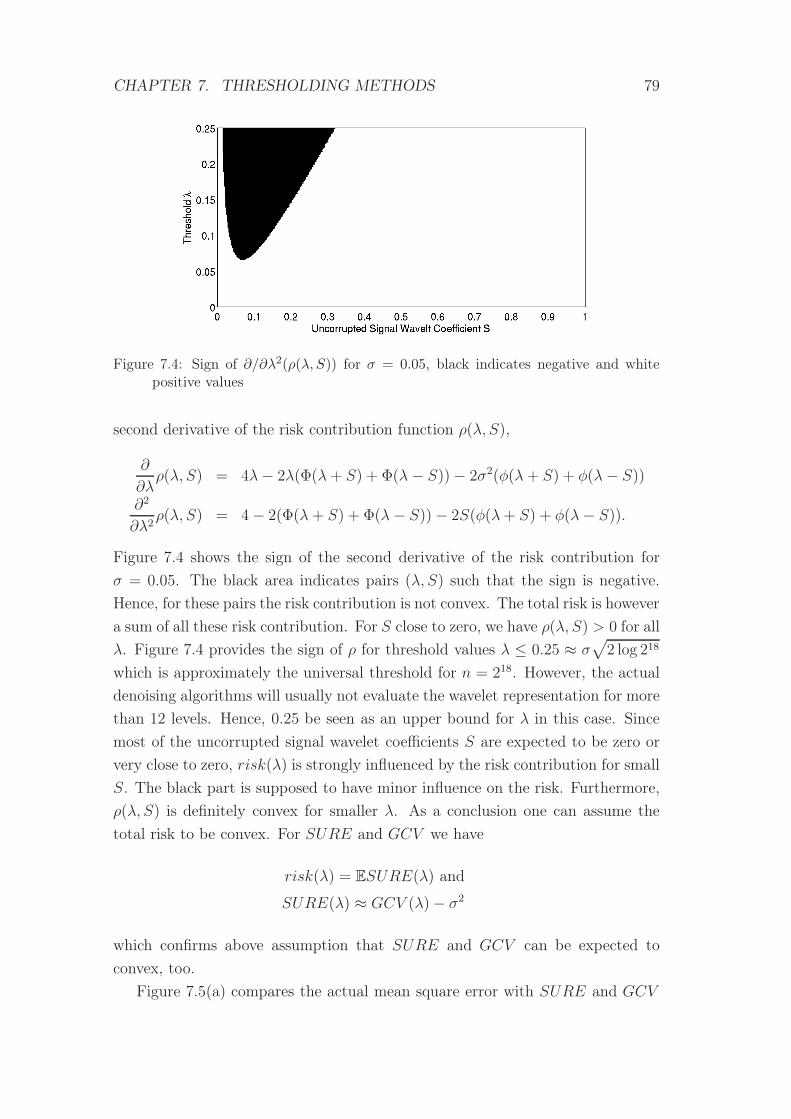
CHAPTER 7. THRESHOLDING METHODS 79
Figure 7.4: Sign of ∂/∂λ2(ρ(λ, S)) for σ = 0.05, black indicates negative and whitepositive values
second derivative of the risk contribution function ρ(λ, S),
∂
∂λρ(λ, S) = 4λ− 2λ(Φ(λ+ S) + Φ(λ− S))− 2σ2(φ(λ+ S) + φ(λ− S))
∂2
∂λ2ρ(λ, S) = 4− 2(Φ(λ+ S) + Φ(λ− S))− 2S(φ(λ+ S) + φ(λ− S)).
Figure 7.4 shows the sign of the second derivative of the risk contribution for
σ = 0.05. The black area indicates pairs (λ, S) such that the sign is negative.
Hence, for these pairs the risk contribution is not convex. The total risk is however
a sum of all these risk contribution. For S close to zero, we have ρ(λ, S) > 0 for all
λ. Figure 7.4 provides the sign of ρ for threshold values λ ≤ 0.25 ≈ σ√2 log 218
which is approximately the universal threshold for n = 218. However, the actual
denoising algorithms will usually not evaluate the wavelet representation for more
than 12 levels. Hence, 0.25 be seen as an upper bound for λ in this case. Since
most of the uncorrupted signal wavelet coefficients S are expected to be zero or
very close to zero, risk(λ) is strongly influenced by the risk contribution for small
S. The black part is supposed to have minor influence on the risk. Furthermore,
ρ(λ, S) is definitely convex for smaller λ. As a conclusion one can assume the
total risk to be convex. For SURE and GCV we have
risk(λ) = ESURE(λ) and
SURE(λ) ≈ GCV (λ)− σ2
which confirms above assumption that SURE and GCV can be expected to
convex, too.
Figure 7.5(a) compares the actual mean square error with SURE and GCV
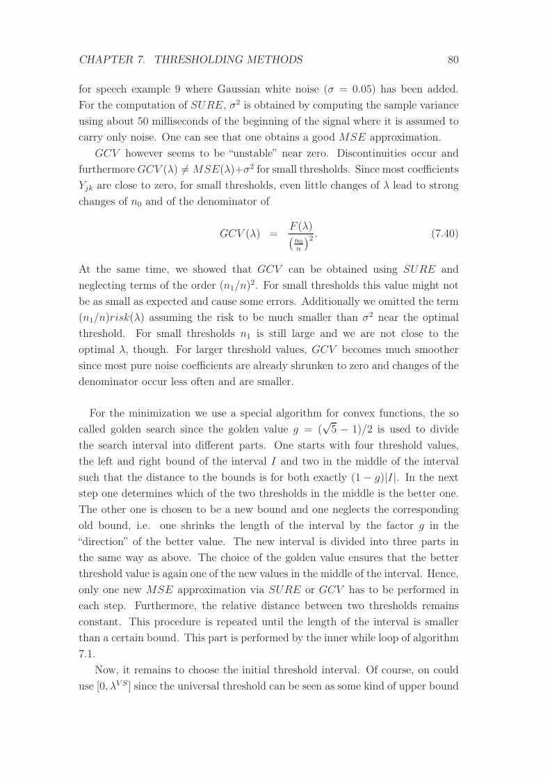
CHAPTER 7. THRESHOLDING METHODS 80
for speech example 9 where Gaussian white noise (σ = 0.05) has been added.
For the computation of SURE, σ2 is obtained by computing the sample variance
using about 50 milliseconds of the beginning of the signal where it is assumed to
carry only noise. One can see that one obtains a good MSE approximation.
GCV however seems to be “unstable” near zero. Discontinuities occur and
furthermoreGCV (λ) 6=MSE(λ)+σ2 for small thresholds. Since most coefficients
Yjk are close to zero, for small thresholds, even little changes of λ lead to strong
changes of n0 and of the denominator of
GCV (λ) =F (λ)(n0
n
)2 . (7.40)
At the same time, we showed that GCV can be obtained using SURE and
neglecting terms of the order (n1/n)2. For small thresholds this value might not
be as small as expected and cause some errors. Additionally we omitted the term
(n1/n)risk(λ) assuming the risk to be much smaller than σ2 near the optimal
threshold. For small thresholds n1 is still large and we are not close to the
optimal λ, though. For larger threshold values, GCV becomes much smoother
since most pure noise coefficients are already shrunken to zero and changes of the
denominator occur less often and are smaller.
For the minimization we use a special algorithm for convex functions, the so
called golden search since the golden value g = (√5 − 1)/2 is used to divide
the search interval into different parts. One starts with four threshold values,
the left and right bound of the interval I and two in the middle of the interval
such that the distance to the bounds is for both exactly (1 − g)|I|. In the next
step one determines which of the two thresholds in the middle is the better one.
The other one is chosen to be a new bound and one neglects the corresponding
old bound, i.e. one shrinks the length of the interval by the factor g in the
“direction” of the better value. The new interval is divided into three parts in
the same way as above. The choice of the golden value ensures that the better
threshold value is again one of the new values in the middle of the interval. Hence,
only one new MSE approximation via SURE or GCV has to be performed in
each step. Furthermore, the relative distance between two thresholds remains
constant. This procedure is repeated until the length of the interval is smaller
than a certain bound. This part is performed by the inner while loop of algorithm
7.1.
Now, it remains to choose the initial threshold interval. Of course, on could
use [0, λV S] since the universal threshold can be seen as some kind of upper bound
CHAPTER 7. THRESHOLDING METHODS 81
for optimal thresholds. However, first of all it would require the knowledge of σ,
which is not necessary for the evaluation of GCV and would eliminate one of
its advantages. Furthermore, the discontinuities of the GCV function near zero
could cause trouble. Therefore, one starts with rather too large values, i.e. an
interval shifted to the right. After the execution of above algorithm one checks if
it has changed the left bound of the interval. If so, the minimum of the convex
function is definitely in the interval produced by the algorithm. If not, the left
bound was too large and one starts again with a new interval until either the left
bound changes at some time or the right bound becomes too small. This part is
performed by the outer while loop of algorithm 7.1.
Algorithm 7.1 Golden Search Algorithm
1: g =√5−12
2: λ4 = max{|Sjk|}3: while λ4 > ǫ1 and λ1 unchanged do
4: λ1 = λ4/505: λ2 = λ1 + (1− g)(λ4 − λ1)6: λ3 = λ4 − (1− g)(λ4 − λ1)7: compute mse(λ2); compute mse(λ3);8: while {λ4 − λ1 > ǫ2} do
9: if mse(λ2) > mse(λ3) then
10: λ1 = λ2; λ2 = λ3; λ3 = λ4 − (λ2 − λ1);11: mse(λ2) = mse(λ3); compute mse(λ3);12: else
13: λ4 = λ3; λ3 = λ2; λ2 = λ1 + (λ4 − λ3);14: mse(λ3) = mse(λ2); compute mse(λ2);15: end if
16: end while
17: end while
It might be interesting what happens to signals that are not influenced by
noise. It would be desirable to have no or at least only very few changes of the
signal, i.e. a threshold as close to zero as possible. For σ2 = 0, SURE is given
by
SURE(λ) = F (λ) + σ2 − 2σ2n0
n
and clearly leads to an optimal threshold λ = 0. Only the first term does not
vanish. It is increasing in λ, though, and therefore the optimal threshold is
obtained. For GCV this is less clear. However, it also works surprisingly well.
The neglected terms are small even for small threshold values since σ2 = 0 and
most coefficients are already very close to zero, even before thresholding, and
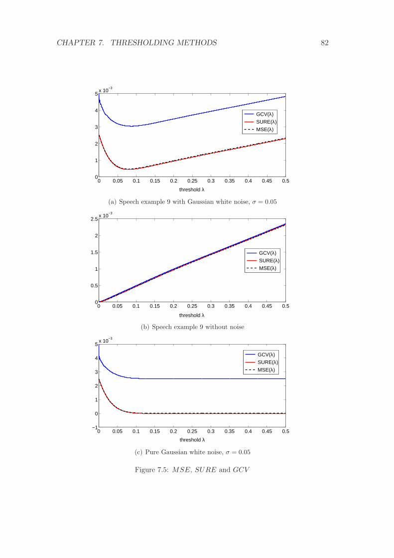
CHAPTER 7. THRESHOLDING METHODS 82
0 0.05 0.1 0.15 0.2 0.25 0.3 0.35 0.4 0.45 0.50
1
2
3
4
5x 10
−3
threshold λ
GCV(λ)
SURE(λ)
MSE(λ)
(a) Speech example 9 with Gaussian white noise, σ = 0.05
0 0.05 0.1 0.15 0.2 0.25 0.3 0.35 0.4 0.45 0.50
0.5
1
1.5
2
2.5x 10
−3
threshold λ
GCV(λ)
SURE(λ)
MSE(λ)
(b) Speech example 9 without noise
0 0.05 0.1 0.15 0.2 0.25 0.3 0.35 0.4 0.45 0.5−1
0
1
2
3
4
5x 10
−3
threshold λ
GCV(λ)
SURE(λ)
MSE(λ)
(c) Pure Gaussian white noise, σ = 0.05
Figure 7.5: MSE, SURE and GCV
CHAPTER 7. THRESHOLDING METHODS 83
for increasing thresholds, the denominator of equation 7.40 changes very slowly.
MSE, SURE and GCV in case of pure speech are plotted in figure 7.5(b), again
for speech example 9.
A second special case is pure noise, i.e. S = 0 for all coefficients. Correspond-
ing MSE, SURE and GCV are shown in figure 7.5(c). Large thresholds should
be preferred. Indeed, as λ approaches infinity, both, SURE and GCV , converge
to the minimum achievable risk value since n0 → n and F (λ) → σ2.
7.9 Level Dependent Thresholding
Until now, the introduced thresholding methods made no use of the multiscale
representation of the signal. Different levels represent different frequencies and
coefficients show different characteristics at different level, as shown in the previ-
ous chapter. In this and the following section we will see some suggestions how
to use dependencies between different levels [20].
So far we assumed noise to be Gaussian and white, i.e. stationary and uncor-
related noise coefficients. Otherwise, with the knowledge of the covariance matrix
Q, one could use formula (3.3) to normalize the wavelet coefficients
Y newjk =
1√QAjk,jk
Yjk.
But for all that, Q is generally unknown and hard to determine. Suppose noise is
stationary Gaussian but correlated in a way such that the correlation between two
points depend only on the distance of the points, one obtains a symmetric Toeplitz
covariance Matrix Q and in lemma 3.2.1 we have learned that the variance of the
transformed noise depends only on the level, i.e.
E[E2jk] = σ2
j ∀k ∈ Ij
where Ij denotes the set of indices of coefficients at level j. The wavelet transform
of stationary correlated noise is only stationery within a given level. Hence, a
single threshold for all levels makes no more sense. As mentioned above one could
normalize the wavelet coefficients to obtain stationary noise in wavelet domain,
too. However, even for this case it is not easy to find good approximations for
all values of σj . Uncorrelated noise variance can easily be estimated using either
very fine scales where little signal information is stored but still noise appears in
the same way as in all other scales, or one could use the original data y and try
to determine a “silent” part with no signal but corrupted by noise. Instead of the
CHAPTER 7. THRESHOLDING METHODS 84
determination of each σj , level dependent thresholding might be useful.
Level dependent thresholding can be applied very easily. One just performs
a GCV minimizing procedure at each level separately and obtains for each level
a different threshold value. GCV properties are not corrupted by correlated
noise. Correlations just lead to a different “sorting” of the coefficients which does
not change anything in the GCV computation since at a certain level the noise
variance is constant. In statistics this property is called homogeneity of variance.
Advantages: Level dependent thresholding is not only useful for the process-
ing of correlated noise. Using non-orthogonal wavelet transforms, wavelet noise
coefficients will be correlated and non-stationary as mentioned in section 3.1. Al-
though in this case the knowledge of the variance of the original noise coefficients
leads to the knowledge of the covariance matrix Q and one could apply (3.3),
level dependent thresholding might be easier.
Optimal thresholds do not only depend on the on the noise variance. Sig-
nal characteristics play an important role as well. As mentioned earlier, these
characteristics might change at different levels. As shown in chapter 5, impor-
tant coefficients do not necessarily show up at different levels with the same
magnitude. In low levels, i.e. at coarse scales, many coefficients contain much
information and are therefore large while at levels with finer resolution, large
coefficients are rare and most coefficients are influenced only by noise. Hence,
fine resolutions require rather large thresholds while at the same time for coarse
parts with much signal information, small thresholds are preferable. So even for
orthogonal wavelet transformation and stationary uncorrelated white noise, level
dependent thresholding might lead to better results. Hence, a single threshold is
already a compromise between coarse and fine levels.
Disadvantages: Level dependent thresholding leads to one important disad-
vantage. At coarse levels, one might not have enough coefficients to obtain good
MSE approximations via GCV since for n = 2J , level j consists of only about
2J−j coefficients. The solution could be the use of the stationary wavelet trans-
form (SWT) as described in section 2.3. For SWT, the homogeneity of variance
property holds, too. At each level one has n coefficients. Therefore, good MSE
approximations can be obtained at each level. Memory and time complexity is
now O(n logn), though. At each level, the proportion of noise free coefficients
remains the same as for FWT. Hence, at coarse scales most coefficients provide
signal information, the representation is not sparse there. Hence, it is not useful
to process too coarse levels. On the other side, finer levels are still sparse and
CHAPTER 7. THRESHOLDING METHODS 85
contain very few signal information. Additionally, inverse SWT provides an ad-
ditional smoothing as described in section 2.3 which might improve the output
signal quality in the sense of less noisy structures.
7.10 Inter & Intra Scale Thresholding
Xu, Weaver, Healy and Lu [36] describe a denoising method that - with slight
modification - can be seen as a thresholding method using inter scale dependen-
cies. It is based on the idea that important signal features show up not only at a
single scale but at a hole set of coefficients at the same location but subsequent
levels. This assumption has already been justified in chapter 5. To measure
if a coefficient should be kept or not, they propose not to use the coefficient
magnitude, but a inter scale correlation factor Corrl defined as the product of l
coefficient values at same location but subsequent coarser levels given by
corrjk(l) =l∏
i=0
Yj−i,k (7.41)
To simplify notation, a notion of stationary wavelet transform has been used
here, but it works in the same way using FWT coefficients instead. One just
needs to find the right coefficients at the same location. Xu et al propose to
select at each level the coefficients with largest correlation factors until the sum
of the squares of the selected coefficients exceeds a certain threshold value. This
threshold value can however be considered to be an upper bound of the signal
information and should be selected in a way such that the threshold represents
the expected amount of signal information provided at the given scale for the
uncorrupted signal.
Jansen modified this algorithm and created a kind of soft thresholding [19].
Now, the correlation factor is not only the measure if a coefficient should be
shrunken to zero or not, but it also influences the shrinking value:
Sλjk =
(1− λ
|corrjk(l)|
)
+
Yjk. (7.42)
For l = 0 this is exactly soft thresholding. Jansen states that already for l = 1,
this method outperforms the previous ones. Besides, GCV can be evaluated and
minimized in exactly the same way as mentioned in earlier sections. Comparisons
can be found in chapter 11. Modifications of inter level dependencies are however
possible. One could try using a sum of coefficients instead of the product in for-
CHAPTER 7. THRESHOLDING METHODS 86
mula (7.42), or selecting not only coefficients of coarser levels for the computation
of the correlation factor.
A method very similar to inter scale thresholding is called intra scale or block
thresholding. It is based on the idea that for an important signal coefficient, the
neighboring ones should be rather large and important, too, since except for Haar
wavelets, neighboring basis functions don’t have disjoint support. Block thresh-
olding, as the name indicates, keeps, shrinks or kills not only single coefficients
but complete blocks, based on the values of a superset of coefficients. I.e., let I0
be a set of indices of adjacent wavelet coefficients at a fixed level. Furthermore,
let I1 ⊃ I0 another set of indices of adjacent coefficients including I0. Let’s denote
µI1 by
µI1 =1
|I1|∑
(j,k)∈I1
Y 2jk. (7.43)
Similar to (7.42) we use a kind of soft thresholding defined by
Sjk =
(1− λ2
µI1
)
+
Yjk ∀(j, k) ∈ I0 (7.44)
for a given threshold λ. For |I0| = 1 each coefficient is processed separately.
However, the decision if it is better to keep or kill it is still based on information
provided by surrounding coefficients. A GCV procedure is again possible.
Block thresholding removes some additional spurious “blips” but inter scale
thresholding is still better. However, a variety of modifications and combinations
with other methods is possible.
Chapter 8
Tree Structured Thresholding
The method presented in this chapter uses again dependencies between coeffi-
cients of different levels. It is based on so called trees of wavelet coefficients and
introduced in the following definition:
Definition 8.0.1. For some wavelet coefficient Sj,k, a coefficient at level j + 1
is called son of Sj,k if it is positioned at the same location. Accordingly, Sj,k is
called parent of this coefficient. A wavelet tree is a set T of wavelet coefficients
such that
(i) there is exactly one coefficient Sj0,k0 ∈ T with no parent in T , i.e.
(ii) Sj1,k1 ∈ T , where (j1, k1) 6= (j0, k0), implies the existence of a parent in T
The coefficient Sj0,k0 is called root of the wavelet tree.
For n = 2J and for some discrete wavelet transform with periodic boundary
conditions, each wavelet coefficient Sjk, j < J − 1, has exactly two sons, given by
Sj+1,2k and Sj+1,2k+1 and we obtain a full binary tree.
We assume that inter-scale dependencies can be detected in such trees and
subtrees in the following way: If a coefficient Sjk is large since it contains signal
information, we expect coefficients at the same location but level greater than j
to be large as well. This fact has already been mentioned and used in chapter
5. At the same time, noise leads to rather local effects and a noise singularities
do not appear throughout many different levels. These assumptions are used for
tree structured thresholding [19]. One requires approximations Sjk of the original
signal wavelet coefficients to comply two conditions:
(i) Streejk ∈ {Yjk, 0}
87
CHAPTER 8. TREE STRUCTURED THRESHOLDING 88
(ii) Streejk = 0 implies each son to be zeros as well
The first condition indicates that we perform some kind of hard thresholding or
rather a “keep or kill” method. The second constraint requires each coefficient of
the subtree of a “killed” coefficient to be zero, too. Hence, a “killed” coefficient
produces a complete zero-subtree.
Similar to risk minimization methods like SURE or GCV , one tries to find
the best approximation of the signal as a compromise between closeness of fit and
sparseness, or in other words bias and variance. For a given threshold λ, we try
to find an approximation that minimizes
CPRESS(Stree) = ||Stree − Y ||2 + λ2n1
under above constraints. As before, n0 denotes the number of “killed” coefficients
and n1 the number of kept coefficients. The minimization problem can also be
considered in the following way: Find a coefficient selection vector x ∈ {0, 1}nsuch that
CPRESS(x) =∑
(j,k)∈I(1− xjk)Y
2jk − xjkλ
2 → min (8.1)
under the constraint that T = {xjk|xjk = 1} is a wavelet tree. Hence, for each
index (j, k) either λ2 or Y 2jk is added to the CPRESS value. David L. Donoho
describes a connection of tree structured thresholding and the best-ortho basis
algorithm [34]. It is shown that using Haar wavelets, both algorithms are equiv-
alent [5], [7]. However, in his work he also provides an algorithm called CART
(classification and regression trees), based on dynamic programming, that has
been modified and used for the CPRESS minimization.
Algorithm 8.1 provides a minimization method for CPRESS(x) that can be
done in O(n). Values CPRESSjk[0] denote the minimal CPRESS value of a
subtree with root Yjk under constraint Streejk = 0, while CPRESSjk[1] denotes
the minimal subtree value for Streejk = Yjk. I.e. the number in brackets denotes
the used value of xjk. Furthermore, Ij denotes the set of the indices of all wavelet
coefficients at level j. The algorithm can be subdivided into 4 parts, described
in the following paragraphs.
Part I: In the first part of the algorithm, the best CPRESS values of subtrees
consisting of only the root element are determined. Optimal xjk is given by
argmin(CPRESSJ−1,k(x)), i.e. for Y 2J−1,k > λ2 it is better to keep the coefficient
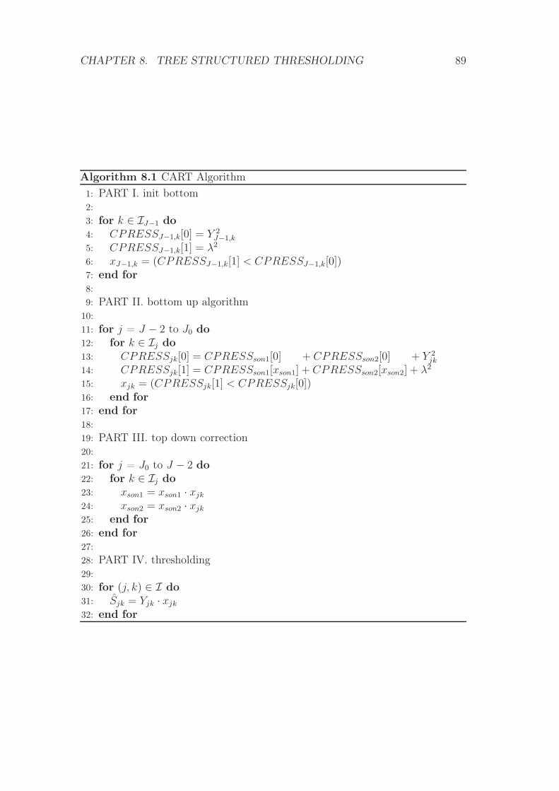
CHAPTER 8. TREE STRUCTURED THRESHOLDING 89
Algorithm 8.1 CART Algorithm
1: PART I. init bottom2:
3: for k ∈ IJ−1 do
4: CPRESSJ−1,k[0] = Y 2J−1,k
5: CPRESSJ−1,k[1] = λ2
6: xJ−1,k = (CPRESSJ−1,k[1] < CPRESSJ−1,k[0])7: end for
8:
9: PART II. bottom up algorithm10:
11: for j = J − 2 to J0 do
12: for k ∈ Ij do
13: CPRESSjk[0] = CPRESSson1[0] + CPRESSson2[0] + Y 2jk
14: CPRESSjk[1] = CPRESSson1[xson1] + CPRESSson2[xson2] + λ2
15: xjk = (CPRESSjk[1] < CPRESSjk[0])16: end for
17: end for
18:
19: PART III. top down correction20:
21: for j = J0 to J − 2 do
22: for k ∈ Ij do
23: xson1 = xson1 · xjk24: xson2 = xson2 · xjk25: end for
26: end for
27:
28: PART IV. thresholding29:
30: for (j, k) ∈ I do
31: Sjk = Yjk · xjk32: end for
CHAPTER 8. TREE STRUCTURED THRESHOLDING 90
to obtain a CPRESS contribution of equation (8.1) of only λ2. Hence, xJ−1,k = 1.
Part II: The second part is a bottom up algorithm that computes the minimal
CPRESS value for all subtrees and the optimal value of the coefficient selection
value xjk. CPRESS values can be obtained by the sum of the appropriate
CPRESS values of both sons. adding either λ2 or Y 2jk, depending on xjk. For
xjk = 0, due to condition (ii) above, xj1,k1 = 0 for all Yj1,k1 in the subtree with
root Yjk. Hence, one has to add CPRESS[0] for both sons and Y 2jk for the root.
In the other case, xjk = 1, one can decide for each son either to take CPRESS[0]
or CPRESS[1]. Obviously, we take the smaller ones, given by CPRESS[xson1]
and CPRESS[xson2], respectively, where son1 and son2 denote the index of the
two sons. The root contributes λ2 to the sum.
Part III: So far, we got for each coefficient Yjk the optimal coefficient selection
value xjk under the assumption that Yjk is the root of the tree. Furthermore, we
obtained the optimal CPRESS value for the complete tree (or in fact, if J0 6= 0,
for several trees). However, if the coefficient selection value of the parent of any
Yjk is zero, we need to adjust the coefficient selection values in the subtree. This
is done in the third part of the algorithm, starting at the lowest level, i.e. the top
of the tree.
Part IV: Finally, in the last part, the actual thresholding is done and one
obtains the approximation Stree.
For a given threshold λ, algorithm 8.1 provides an efficient way to find the
optimal tree. Nevertheless, the problem of finding an optimal threshold value
is still unsolved. CPRESS minimization procedures in terms of λ, e.g. golden
search introduced for SURE and GCV in 7.8, do not work here. In fact, the
minimum would be achieved for λ = 0 or λ = ∞. For both thresholds, one
obtains CPRESS(x) = 0. In the first case, the algorithm would lead to the
“optimal” coefficient selection values xjk = 0 for all (j, k) ∈ I which leads to
CPRESS(x) = 0. In the second case, λ = ∞, the algorithm leads to xjk = 1
for all (j, k) ∈ I and again CPRESS(x) = 0. Donoho proposes to use the
universal threshold σ√2 logn, [7]. For good MSE results this threshold is too
large, though. Differently from SURE and GCV values, CPRESS is no mea-
sure for good approximations, even though in all cases one may consider the
threshold value λ to be a weight to control sparsity. I.e., for large thresholds
it is less desirable to keep coefficients than for small ones. Hence, I claim that
thresholds produced by GCV or SURE are better candidates than the universal
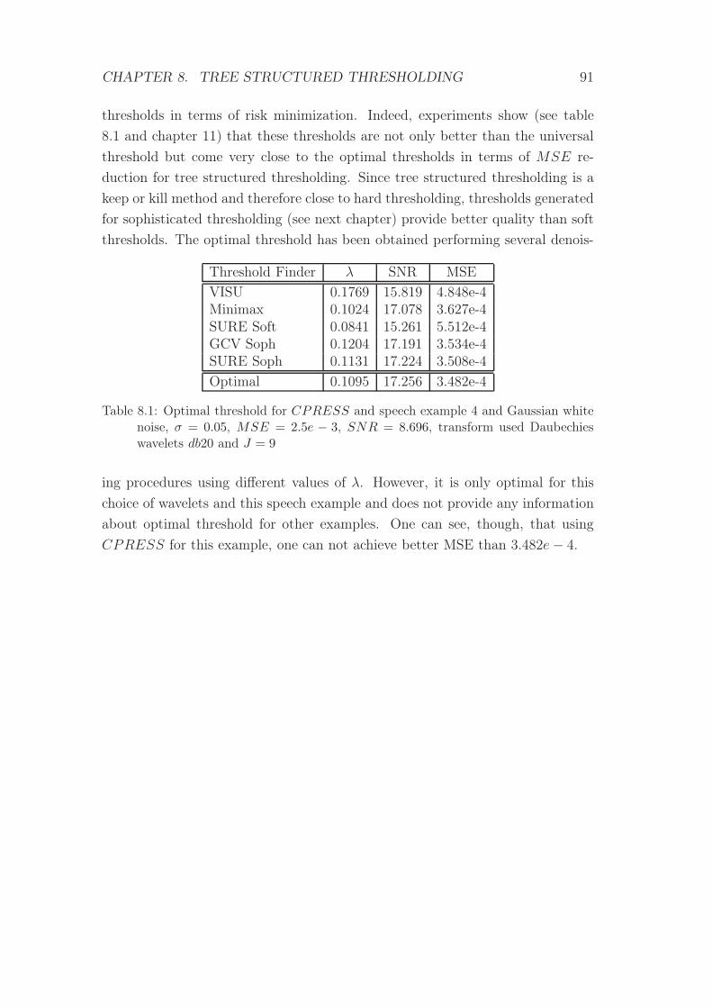
CHAPTER 8. TREE STRUCTURED THRESHOLDING 91
thresholds in terms of risk minimization. Indeed, experiments show (see table
8.1 and chapter 11) that these thresholds are not only better than the universal
threshold but come very close to the optimal thresholds in terms of MSE re-
duction for tree structured thresholding. Since tree structured thresholding is a
keep or kill method and therefore close to hard thresholding, thresholds generated
for sophisticated thresholding (see next chapter) provide better quality than soft
thresholds. The optimal threshold has been obtained performing several denois-
Threshold Finder λ SNR MSE
VISU 0.1769 15.819 4.848e-4Minimax 0.1024 17.078 3.627e-4SURE Soft 0.0841 15.261 5.512e-4GCV Soph 0.1204 17.191 3.534e-4SURE Soph 0.1131 17.224 3.508e-4
Optimal 0.1095 17.256 3.482e-4
Table 8.1: Optimal threshold for CPRESS and speech example 4 and Gaussian whitenoise, σ = 0.05, MSE = 2.5e − 3, SNR = 8.696, transform used Daubechieswavelets db20 and J = 9
ing procedures using different values of λ. However, it is only optimal for this
choice of wavelets and this speech example and does not provide any information
about optimal threshold for other examples. One can see, though, that using
CPRESS for this example, one can not achieve better MSE than 3.482e− 4.
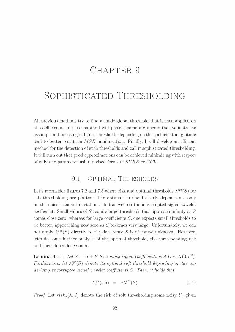
Chapter 9
Sophisticated Thresholding
All previous methods try to find a single global threshold that is then applied on
all coefficients. In this chapter I will present some arguments that validate the
assumption that using different thresholds depending on the coefficient magnitude
lead to better results in MSE minimization. Finally, I will develop an efficient
method for the detection of such thresholds and call it sophisticated thresholding.
It will turn out that good approximations can be achieved minimizing with respect
of only one parameter using revised forms of SURE or GCV .
9.1 Optimal Thresholds
Let’s reconsider figures 7.2 and 7.3 where risk and optimal thresholds λopt(S) for
soft thresholding are plotted. The optimal threshold clearly depends not only
on the noise standard deviation σ but as well on the uncorrupted signal wavelet
coefficient. Small values of S require large thresholds that approach infinity as S
comes close zero, whereas for large coefficients S, one expects small thresholds to
be better, approaching now zero as S becomes very large. Unfortunately, we can
not apply λopt(S) directly to the data since S is of course unknown. However,
let’s do some further analysis of the optimal threshold, the corresponding risk
and their dependence on σ.
Lemma 9.1.1. Let Y = S + E be a noisy signal coefficients and E ∼ N(0, σ2).
Furthermore, let λoptσ (S) denote its optimal soft threshold depending on the un-
derlying uncorrupted signal wavelet coefficients S. Then, it holds that
λoptσ (σS) = σλopt1 (S) (9.1)
Proof. Let riskσ(λ, S) denote the risk of soft thresholding some noisy Y , given
92
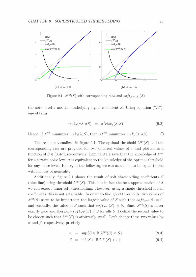
CHAPTER 9. SOPHISTICATED THRESHOLDING 93
0 1 2 30
1
2
3
id(S)
λopt(S)
softλopt(S)
risk( λopt(S), S)
(a) σ = 1.0
0 0.5 1 1.50
0.5
1
1.5
id(S)
λopt(S)
softλopt(S)
risk( λopt(S), S)
(b) σ = 0.5
Figure 9.1: λopt(S) with corresponding risk and softλopt(S)(S)
the noise level σ and the underlying signal coefficient S. Using equation (7.17),
one obtains
riskσ(σλ, σS) = σ2risk1(λ, S) (9.2)
Hence, if λopt1 minimizes risk1(λ, S), then σλopt1 minimizes riskσ(λ, σS).
This result is visualized in figure 9.1. The optimal threshold λopt(S) and the
corresponding risk are provided for two different values of σ and plotted as a
function of S ∈ [0, 4σ], respectively. Lemma 9.1.1 says that the knowledge of λopt
for a certain noise level σ is equivalent to the knowledge of the optimal threshold
for any noise level. Hence, in the following we can assume σ to be equal to one
without loss of generality.
Additionally, figure 9.1 shows the result of soft thresholding coefficients S
(blue line) using threshold λopt(S). This is is in fact the best approximation of S
we can expect using soft thresholding. However, using a single threshold for all
coefficients this is not attainable. In order to find good thresholds, two values of
λopt(S) seem to be important: the largest value of S such that softλopt(S) = 0,
and secondly, the value of S such that softλopt(S) ≈ S. Since λopt(S) is never
exactly zero and therefore softλopt(S) 6= S for alls S, I define the second value to
be chosen such that λopt(S) is arbitrarily small. Let’s denote these two values by
α and β, respectively, precisely
α = sup{S ∈ R|λopt(S) ≥ S} (9.3)
β = inf{S ∈ R|λopt(S) < ε}. (9.4)
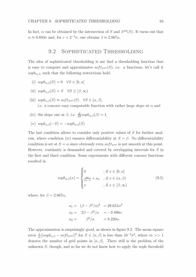
CHAPTER 9. SOPHISTICATED THRESHOLDING 94
In fact, α can be obtained by the intersection of S and λopt(S). It turns out that
α ≈ 0.893σ and, for ε = 2−5σ, one obtains β ≈ 2.867α.
9.2 Sophisticated Thresholding
The idea of sophisticated thresholding is use find a thresholding function that
is easy to compute and approximates softλopt(S), i.e. a functions, let’s call it
sophα,β, such that the following restrictions hold:
(i) sophα,β(S) = 0 ∀S ∈ [0, α]
(ii) sophα,β(S) = S ∀S ≥ [β,∞)
(iii) sophα,β(S) ≈ softλopt(S) ∀S ∈ [α, β],
i.e. a concave easy computable function with rather large slope at α and
(iv) the slope one at β, i.e. ∂∂Ssophα,β(β) = 1.
(v) sophα,β(−S) = −sophα,β(S)
The last condition allows to consider only positive values of S for further anal-
ysis, where condition (iv) ensures differentiability at S = β. No differentiability
condition is set at S = α since obviously even softλopt is not smooth at this point.
However, continuity is demanded and covered by overlapping intervals for S in
the first and third condition. Some experiments with different concave functions
resulted in
sophα,β(x) =
0 , if x ∈ [0, α]
a1a2−x + a3 , if x ∈ (α, β)
x , if x ∈ [β,∞)
(9.5)
where, for β = 2.867α,
a1 = (β − β2/α)2 = 28.651α2
a2 = 2β − β2/α = −2.486α
a3 = β2/α = 8.220α.
The approximation is surprisingly good, as shown in figure 9.2. The mean square
error 1m||sophα,β − softλopt||2 for S ∈ [α, β] is less than 10−3σ2, where m >> 1
denotes the number of grid points in [α, β]. There still is the problem of the
unknown S, though, and so far we do not know how to apply the soph threshold
CHAPTER 9. SOPHISTICATED THRESHOLDING 95
0 0.5 1 1.5 2 2.5 3
0
0.5
1
1.5
2
2.5
3
softλ
opt − sophα, β
sophα, β
softλ
opt
Figure 9.2: softλopt(S) and sophα,β(S) with α = 0.893 and β = 2.867α
function on noisy coefficients Y . Of course one could consider to apply the soph
function directly on Y instead S, but I will show that it is possible to achieve
much better results, using other values α than before.
9.3 Sophisticated Thresholding, SURE and
GCV
Let’s consider sophα := sophα,2.867α as a threshold function of a single parameter
α, similar to hard and soft thresholding in section 7.1. Figure 9.3 compares these
methods using λ = α = 1. One can see that sophisticated thresholding can bee
considered as a kind of compromise between soft and hard thresholding. For α =
β one would obtain hard thresholding while for α → ∞ it rather approximates
soft thresholding. Hence, one could try to use similar methods than before to find
optimal threshold values for sophisticated thresholding. We will see that SURE
and GCV , introduced in section 7.6 and 7.7, respectively, originally based on
soft thresholding, can be modified in order to use the MSE minimization for
sophisticated thresholding as well.
SURE: In section 7.6 we derived
risk(S, softλ(Y )) = E [F (λ)]− σ2 +2
nE[(E,Eλ)
]
where
F (λ) =1
n||softλ(Y )− Y ||2
Eλ = softλ(Y )− S
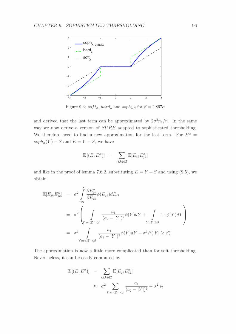
CHAPTER 9. SOPHISTICATED THRESHOLDING 96
−3 −2 −1 0 1 2 3−3
−2
−1
0
1
2
3
soph
λ, 2.867λ
hardλ
softλ
Figure 9.3: softλ, hardλ and sophλ,β for β = 2.867α
and derived that the last term can be approximated by 2σ2n1/n. In the same
way we now derive a version of SURE adapted to sophisticated thresholding.
We therefore need to find a new approximation for the last term. For Eα =
sophα(Y )− S and E = Y − S, we have
E [(E,Eα)] =∑
(j,k)∈IE[EjkE
αjk]
and like in the proof of lemma 7.6.2, substituting E = Y + S and using (9.5), we
obtain
E[EjkEαjk] = σ2
∞∫
−∞
∂Eαjk
∂Ejkφ(Ejk)dEjk
= σ2
∫
Y :α<|Y |<β
a1(a2 − |Y |)2φ(Y )dY +
∫
Y :|Y |≥β
1 · φ(Y )dY
= σ2
∫
Y :α<|Y |<β
a1(a2 − |Y |)2φ(Y )dY + σ2P (|Y | ≥ β).
The approximation is now a little more complicated than for soft thresholding.
Nevertheless, it can be easily computed by
E [(E,Eα)] =∑
(j,k)∈IE[EjkE
αjk]
≈ σ2∑
Y :α<|Y |<β
a1(a2 − |Y |)2 + σ2n2
CHAPTER 9. SOPHISTICATED THRESHOLDING 97
where n2 denotes the number of coefficients Y such that |Y | ≥ β which leads to
the approximation P (|Y | ≥ β) ≈ n2/n. Eventually the new SURE function is
given by
SURE(α) = F (α)− σ2 +2σ2
n
n2 +
∑
Y :α<|Y |<β
a1(a2 − |Y |)2
. (9.6)
The complexity is not much worse than for SURE based on soft thresholding.
For each Y such that α < |Y | < β, two extra divisions and additions have to be
performed and the total complexity is still O(n).
GCV: We use again the results of section 7.7.1 and 7.7.2. In formula (7.31) we
had
GCV (λ) =1
(1−D)2F (λ) (9.7)
where D denoted the average over all derivatives ∂Sλjk/∂Yjk, i.e
D =1
n
∑
(j,k)∈I
∂Sλjk∂Yjk
We can use exactly the same Formula for sophisticated thresholding, only the
computation of the derivatives is different and F (α) is of course obtained using
the soph function. The derivative is given by
soph′α,β(Y ) =
0 , if |Y | ∈ [0, α]
a1(a2−|Y |)2 , if |Y | ∈ (α, β)
1 , if |Y | ∈ [β,∞)
(9.8)
and therefore have
D ≈ 1
n
0 · n0 +
∑
Y :α<|Y |<β
a1(a2 − |Y |)2 + 1 · n2
(9.9)
where n0 = |{Y : |Y | ≤ α}| and n2 = |{Y : |Y | ≥ β}|. As before, there is not
much more computational effort than for soft thresholding.
CHAPTER 9. SOPHISTICATED THRESHOLDING 98
9.4 Comparison
The thresholding method introduced in the previous section is assumed to produce
less MSE. In this section I will verify this, comparing the risk contribution of a
single coefficient for soft, hard and sophisticated thresholding. The next lemma
provides the risk contribution for sophisticated and hard thresholding.
Lemma 9.4.1. The risk contribution of a single coefficient using sophisticated
thresholding is given by
ρsoph(α, β, S) = E[(sophα,β(Y )− S)2
]
= s2σ2 − S2
+ Φ(β − S)(−σ2 + S2) + Φ(β + S)(−σ2 + S2)
+ φ(β − S)(σ2(β − S)) + φ(β + S)(σ2(β + S))
+
β∫
α
(soph2α,β(x)− 2Ssophα,β(x)
)φ(x− S)dx
+
−α∫
−β
(soph2α,β(x)− 2Ssophα,β(x)
)φ(x− S)dx (9.10)
For hard thresholding we have
ρhard(λ, S) = E[(hardλ(Y )− S)2
]
= 2σ2 − S2
+ Φ(λ− S)(−σ2 + S2) + Φ(λ + S)(−σ2 + S2)
+ φ(λ− S)(σ2(λ− S)) + φ(λ+ S)(σ2(λ+ S)) (9.11)
Proof. Simple calculation similar to lemma 7.5.1 and lemma 7.5.2 lead to (9.10).
The second part of the proof is obtained using the fact that hard thresholding
can be seen as a special case of sophisticated thresholding with λ = α = β, i.e.
ρhard(λ, S) = ρsoph(λ, λ, S). Hence, hard thresholding is obtained by omitting the
integrals in equation (9.10).
There is no known analytic solution for the two integrals of (9.10). However,
for the subsequent analysis it is sufficient to leave them this way. With lemma
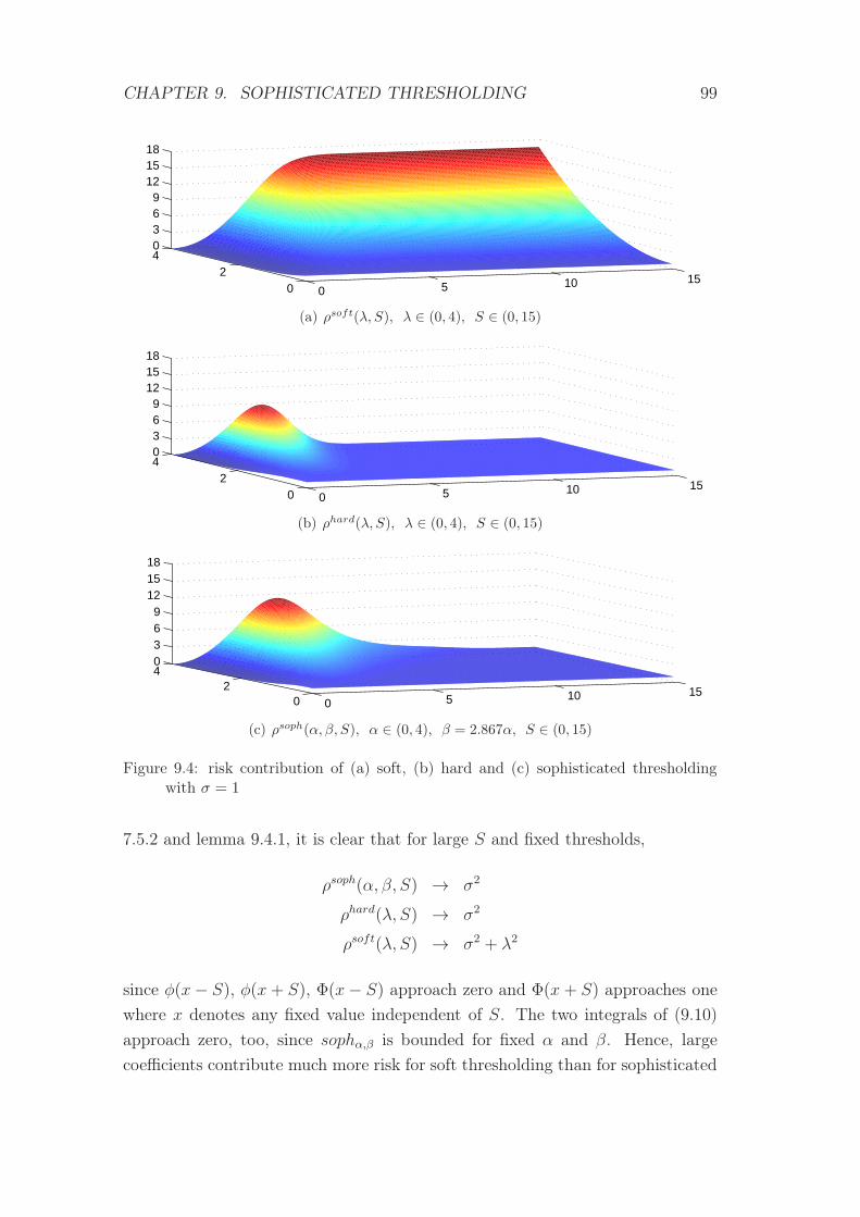
CHAPTER 9. SOPHISTICATED THRESHOLDING 99
0 5 10 150
240369
121518
(a) ρsoft(λ, S), λ ∈ (0, 4), S ∈ (0, 15)
0 5 10 150
240369
121518
(b) ρhard(λ, S), λ ∈ (0, 4), S ∈ (0, 15)
0 5 10 150
240369
121518
(c) ρsoph(α, β, S), α ∈ (0, 4), β = 2.867α, S ∈ (0, 15)
Figure 9.4: risk contribution of (a) soft, (b) hard and (c) sophisticated thresholdingwith σ = 1
7.5.2 and lemma 9.4.1, it is clear that for large S and fixed thresholds,
ρsoph(α, β, S) → σ2
ρhard(λ, S) → σ2
ρsoft(λ, S) → σ2 + λ2
since φ(x− S), φ(x+ S), Φ(x− S) approach zero and Φ(x + S) approaches one
where x denotes any fixed value independent of S. The two integrals of (9.10)
approach zero, too, since sophα,β is bounded for fixed α and β. Hence, large
coefficients contribute much more risk for soft thresholding than for sophisticated
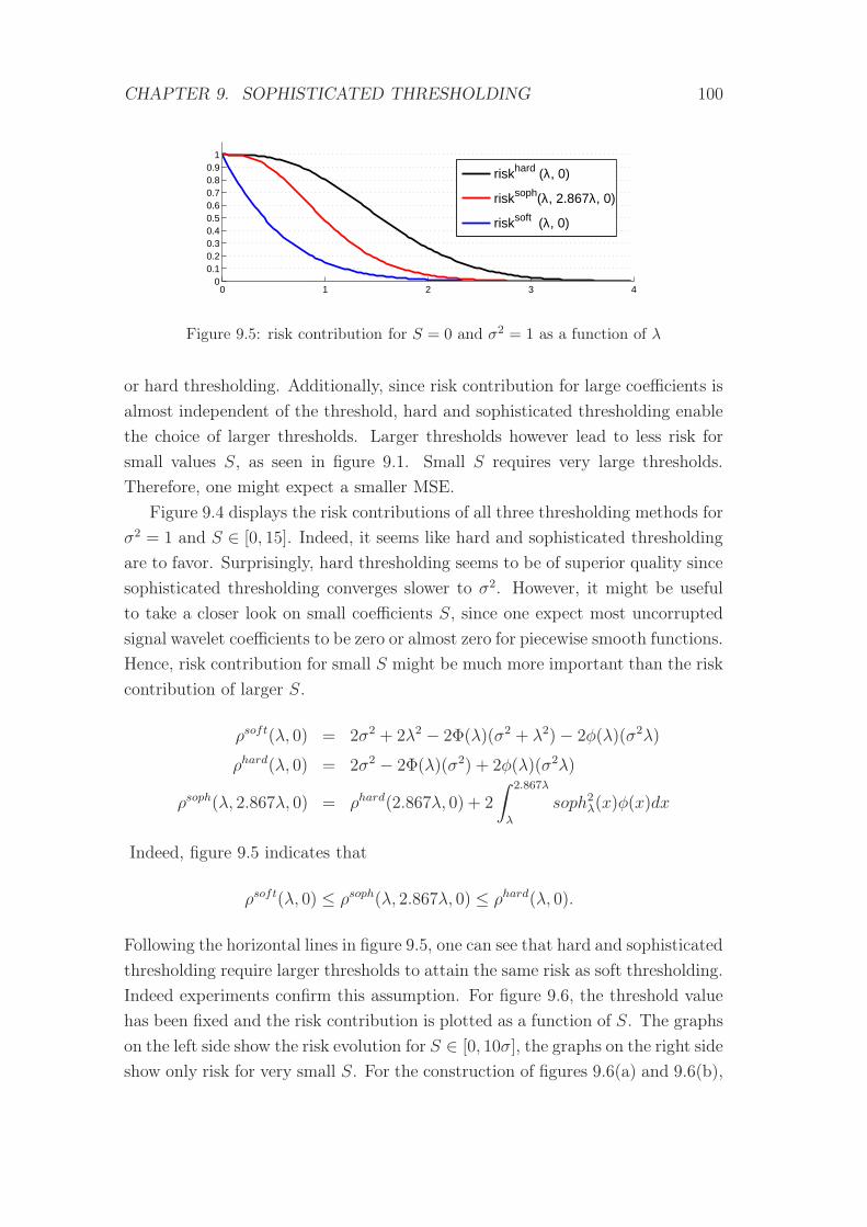
CHAPTER 9. SOPHISTICATED THRESHOLDING 100
0 1 2 3 40
0.10.20.30.40.50.60.70.80.9
1
riskhard (λ, 0)
risksoph(λ, 2.867λ, 0)
risksoft (λ, 0)
Figure 9.5: risk contribution for S = 0 and σ2 = 1 as a function of λ
or hard thresholding. Additionally, since risk contribution for large coefficients is
almost independent of the threshold, hard and sophisticated thresholding enable
the choice of larger thresholds. Larger thresholds however lead to less risk for
small values S, as seen in figure 9.1. Small S requires very large thresholds.
Therefore, one might expect a smaller MSE.
Figure 9.4 displays the risk contributions of all three thresholding methods for
σ2 = 1 and S ∈ [0, 15]. Indeed, it seems like hard and sophisticated thresholding
are to favor. Surprisingly, hard thresholding seems to be of superior quality since
sophisticated thresholding converges slower to σ2. However, it might be useful
to take a closer look on small coefficients S, since one expect most uncorrupted
signal wavelet coefficients to be zero or almost zero for piecewise smooth functions.
Hence, risk contribution for small S might be much more important than the risk
contribution of larger S.
ρsoft(λ, 0) = 2σ2 + 2λ2 − 2Φ(λ)(σ2 + λ2)− 2φ(λ)(σ2λ)
ρhard(λ, 0) = 2σ2 − 2Φ(λ)(σ2) + 2φ(λ)(σ2λ)
ρsoph(λ, 2.867λ, 0) = ρhard(2.867λ, 0) + 2
∫ 2.867λ
λ
soph2λ(x)φ(x)dx
Indeed, figure 9.5 indicates that
ρsoft(λ, 0) ≤ ρsoph(λ, 2.867λ, 0) ≤ ρhard(λ, 0).
Following the horizontal lines in figure 9.5, one can see that hard and sophisticated
thresholding require larger thresholds to attain the same risk as soft thresholding.
Indeed experiments confirm this assumption. For figure 9.6, the threshold value
has been fixed and the risk contribution is plotted as a function of S. The graphs
on the left side show the risk evolution for S ∈ [0, 10σ], the graphs on the right side
show only risk for very small S. For the construction of figures 9.6(a) and 9.6(b),
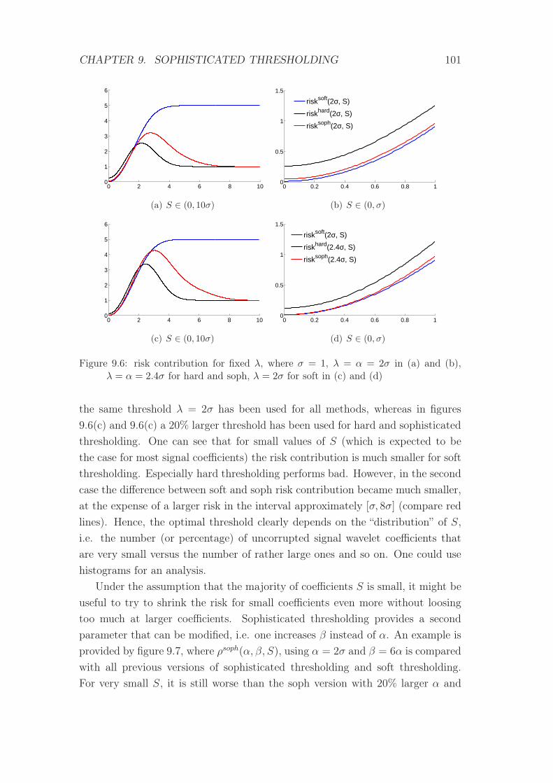
CHAPTER 9. SOPHISTICATED THRESHOLDING 101
0 2 4 6 8 100
1
2
3
4
5
6
(a) S ∈ (0, 10σ)
0 0.2 0.4 0.6 0.8 10
0.5
1
1.5
risksoft(2σ, S)
riskhard(2σ, S)
risksoph(2σ, S)
(b) S ∈ (0, σ)
0 2 4 6 8 100
1
2
3
4
5
6
(c) S ∈ (0, 10σ)
0 0.2 0.4 0.6 0.8 10
0.5
1
1.5
risksoft(2σ, S)
riskhard(2.4σ, S)
risksoph(2.4σ, S)
(d) S ∈ (0, σ)
Figure 9.6: risk contribution for fixed λ, where σ = 1, λ = α = 2σ in (a) and (b),λ = α = 2.4σ for hard and soph, λ = 2σ for soft in (c) and (d)
the same threshold λ = 2σ has been used for all methods, whereas in figures
9.6(c) and 9.6(c) a 20% larger threshold has been used for hard and sophisticated
thresholding. One can see that for small values of S (which is expected to be
the case for most signal coefficients) the risk contribution is much smaller for soft
thresholding. Especially hard thresholding performs bad. However, in the second
case the difference between soft and soph risk contribution became much smaller,
at the expense of a larger risk in the interval approximately [σ, 8σ] (compare red
lines). Hence, the optimal threshold clearly depends on the “distribution” of S,
i.e. the number (or percentage) of uncorrupted signal wavelet coefficients that
are very small versus the number of rather large ones and so on. One could use
histograms for an analysis.
Under the assumption that the majority of coefficients S is small, it might be
useful to try to shrink the risk for small coefficients even more without loosing
too much at larger coefficients. Sophisticated thresholding provides a second
parameter that can be modified, i.e. one increases β instead of α. An example is
provided by figure 9.7, where ρsoph(α, β, S), using α = 2σ and β = 6α is compared
with all previous versions of sophisticated thresholding and soft thresholding.
For very small S, it is still worse than the soph version with 20% larger α and
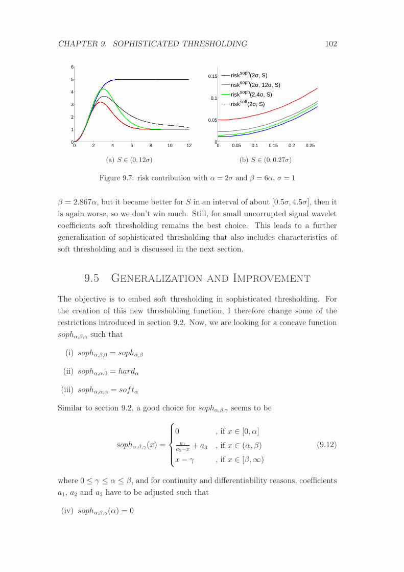
CHAPTER 9. SOPHISTICATED THRESHOLDING 102
0 2 4 6 8 10 120
1
2
3
4
5
6
(a) S ∈ (0, 12σ)
0 0.05 0.1 0.15 0.2 0.250
0.05
0.1
0.15
risksoph(2σ, S)
risksoph(2σ, 12σ, S)
risksoph(2.4σ, S)
risksoft(2σ, S)
(b) S ∈ (0, 0.27σ)
Figure 9.7: risk contribution with α = 2σ and β = 6α, σ = 1
β = 2.867α, but it became better for S in an interval of about [0.5σ, 4.5σ], then it
is again worse, so we don’t win much. Still, for small uncorrupted signal wavelet
coefficients soft thresholding remains the best choice. This leads to a further
generalization of sophisticated thresholding that also includes characteristics of
soft thresholding and is discussed in the next section.
9.5 Generalization and Improvement
The objective is to embed soft thresholding in sophisticated thresholding. For
the creation of this new thresholding function, I therefore change some of the
restrictions introduced in section 9.2. Now, we are looking for a concave function
sophα,β,γ such that
(i) sophα,β,0 = sophα,β
(ii) sophα,α,0 = hardα
(iii) sophα,α,α = softα
Similar to section 9.2, a good choice for sophα,β,γ seems to be
sophα,β,γ(x) =
0 , if x ∈ [0, α]
a1a2−x + a3 , if x ∈ (α, β)
x− γ , if x ∈ [β,∞)
(9.12)
where 0 ≤ γ ≤ α ≤ β, and for continuity and differentiability reasons, coefficients
a1, a2 and a3 have to be adjusted such that
(iv) sophα,β,γ(α) = 0
CHAPTER 9. SOPHISTICATED THRESHOLDING 103
(v) sophα,β,γ(β) = β − γ
(vi) soph′α,β,γ(β) = 1.
This leads to coefficients
a1 = (a2 − β)2
a2 = (β2 − 2αβ + αγ)/(γ − α)
a3 = −(a2 − β)2/(a2 − α).
Two cases seem to need special treatment. First assume a2 = α, then a3 is not
computable. However, one can easily show that this occurs if and only if α = β.
Now, a computation of a3 is no more necessary since the second case x ∈ (α, β) of
equation (9.12) is impossible. For α = γ the value a2 does not exist. One could
of course restrict on cases where α 6= γ but this would not allow to embed soft
thresholding any more. Hence, another condition has to be introduced,
(vii) allow α = γ only if α = β.
As before, for α = β = γ, we have x /∈ (α, β) and one obtains soft thresholding.
Knowing the distribution of S, i.e. the amount of coefficients Sjk of a certain
value and for a fixed σ, one could minimize the risk in α, β, and γ that is given
by formula 9.13 below. However, the SURE and GCV formulas introduced in
section 9.3 and given by (9.6) and (9.7),(9.9), respectively, can be applied in
exactly the same way, just using the coefficients a1, a2 and a3 provided in this
section.
Table 9.1 compares soft with sophisticated thresholding. For β I used in all
cases β = 2.867α and tried 4 different values of γ, also dependent on α to enable
minimization with respect of only one parameter, α. GCV has been used for both,
soft and sophisticated thresholding, to attain the best threshold value. Gaussian
white noise with σ = 0.05 has been added to a speech signal with 217 samples an a
sampling rate of 44100 samples per second. Hence, MSE before thresholding has
been about 2.5e−3 and SNR has been 6.340dB. I used Daubechies wavelets with
8 vanishing moments, periodic boundary conditions, and resolution up to level
J = 8. One can see that sophisticated thresholding outperforms soft thresholding.
Here, γ = 0.18α seemed to be optimal, MSE obtained by soft thresholding is
about 26% larger in this case. As in the sections before, one can find a direct
formula for the risk contribution. In fact, it embeds again risk contribution
formulas for soft, hard and the previous version of sophisticated thresholding. It
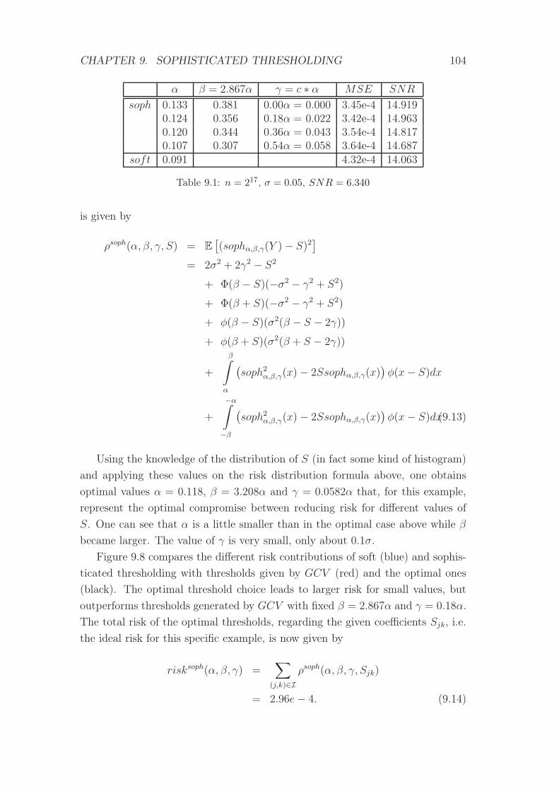
CHAPTER 9. SOPHISTICATED THRESHOLDING 104
α β = 2.867α γ = c ∗ α MSE SNR
soph 0.133 0.381 0.00α = 0.000 3.45e-4 14.9190.124 0.356 0.18α = 0.022 3.42e-4 14.9630.120 0.344 0.36α = 0.043 3.54e-4 14.8170.107 0.307 0.54α = 0.058 3.64e-4 14.687
soft 0.091 4.32e-4 14.063
Table 9.1: n = 217, σ = 0.05, SNR = 6.340
is given by
ρsoph(α, β, γ, S) = E[(sophα,β,γ(Y )− S)2
]
= 2σ2 + 2γ2 − S2
+ Φ(β − S)(−σ2 − γ2 + S2)
+ Φ(β + S)(−σ2 − γ2 + S2)
+ φ(β − S)(σ2(β − S − 2γ))
+ φ(β + S)(σ2(β + S − 2γ))
+
β∫
α
(soph2α,β,γ(x)− 2Ssophα,β,γ(x)
)φ(x− S)dx
+
−α∫
−β
(soph2α,β,γ(x)− 2Ssophα,β,γ(x)
)φ(x− S)dx(9.13)
Using the knowledge of the distribution of S (in fact some kind of histogram)
and applying these values on the risk distribution formula above, one obtains
optimal values α = 0.118, β = 3.208α and γ = 0.0582α that, for this example,
represent the optimal compromise between reducing risk for different values of
S. One can see that α is a little smaller than in the optimal case above while β
became larger. The value of γ is very small, only about 0.1σ.
Figure 9.8 compares the different risk contributions of soft (blue) and sophis-
ticated thresholding with thresholds given by GCV (red) and the optimal ones
(black). The optimal threshold choice leads to larger risk for small values, but
outperforms thresholds generated by GCV with fixed β = 2.867α and γ = 0.18α.
The total risk of the optimal thresholds, regarding the given coefficients Sjk, i.e.
the ideal risk for this specific example, is now given by
risksoph(α, β, γ) =∑
(j,k)∈Iρsoph(α, β, γ, Sjk)
= 2.96e− 4. (9.14)
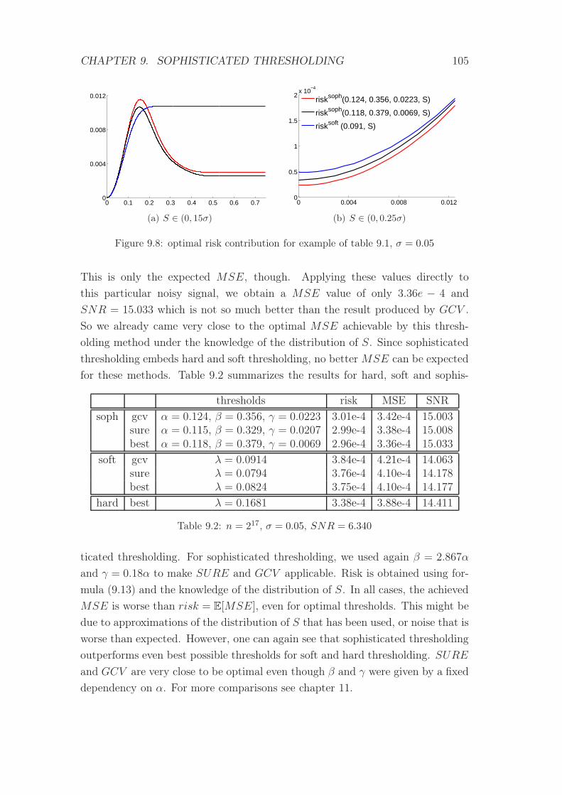
CHAPTER 9. SOPHISTICATED THRESHOLDING 105
0 0.1 0.2 0.3 0.4 0.5 0.6 0.70
0.004
0.008
0.012
(a) S ∈ (0, 15σ)
0 0.004 0.008 0.0120
0.5
1
1.5
2x 10
−4
risksoph(0.124, 0.356, 0.0223, S)
risksoph(0.118, 0.379, 0.0069, S)
risksoft (0.091, S)
(b) S ∈ (0, 0.25σ)
Figure 9.8: optimal risk contribution for example of table 9.1, σ = 0.05
This is only the expected MSE, though. Applying these values directly to
this particular noisy signal, we obtain a MSE value of only 3.36e − 4 and
SNR = 15.033 which is not so much better than the result produced by GCV .
So we already came very close to the optimal MSE achievable by this thresh-
olding method under the knowledge of the distribution of S. Since sophisticated
thresholding embeds hard and soft thresholding, no better MSE can be expected
for these methods. Table 9.2 summarizes the results for hard, soft and sophis-
thresholds risk MSE SNR
soph gcv α = 0.124, β = 0.356, γ = 0.0223 3.01e-4 3.42e-4 15.003sure α = 0.115, β = 0.329, γ = 0.0207 2.99e-4 3.38e-4 15.008best α = 0.118, β = 0.379, γ = 0.0069 2.96e-4 3.36e-4 15.033
soft gcv λ = 0.0914 3.84e-4 4.21e-4 14.063sure λ = 0.0794 3.76e-4 4.10e-4 14.178best λ = 0.0824 3.75e-4 4.10e-4 14.177
hard best λ = 0.1681 3.38e-4 3.88e-4 14.411
Table 9.2: n = 217, σ = 0.05, SNR = 6.340
ticated thresholding. For sophisticated thresholding, we used again β = 2.867α
and γ = 0.18α to make SURE and GCV applicable. Risk is obtained using for-
mula (9.13) and the knowledge of the distribution of S. In all cases, the achieved
MSE is worse than risk = E[MSE], even for optimal thresholds. This might be
due to approximations of the distribution of S that has been used, or noise that is
worse than expected. However, one can again see that sophisticated thresholding
outperforms even best possible thresholds for soft and hard thresholding. SURE
and GCV are very close to be optimal even though β and γ were given by a fixed
dependency on α. For more comparisons see chapter 11.
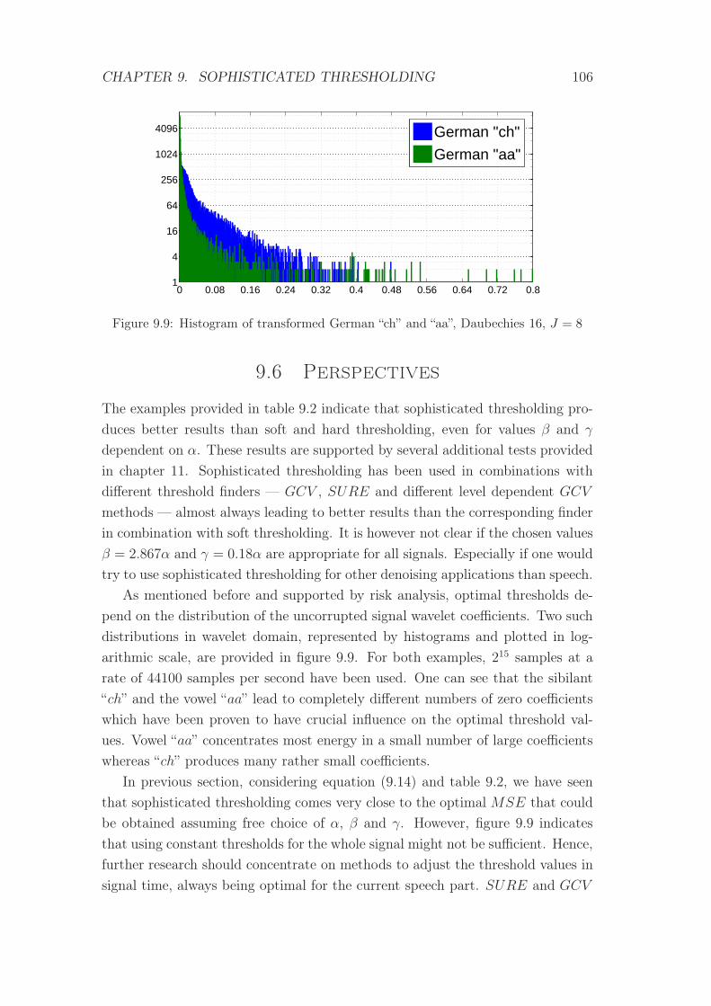
CHAPTER 9. SOPHISTICATED THRESHOLDING 106
0 0.08 0.16 0.24 0.32 0.4 0.48 0.56 0.64 0.72 0.81
4
16
64
256
1024
4096
German "ch"
German "aa"
Figure 9.9: Histogram of transformed German “ch” and “aa”, Daubechies 16, J = 8
9.6 Perspectives
The examples provided in table 9.2 indicate that sophisticated thresholding pro-
duces better results than soft and hard thresholding, even for values β and γ
dependent on α. These results are supported by several additional tests provided
in chapter 11. Sophisticated thresholding has been used in combinations with
different threshold finders — GCV , SURE and different level dependent GCV
methods — almost always leading to better results than the corresponding finder
in combination with soft thresholding. It is however not clear if the chosen values
β = 2.867α and γ = 0.18α are appropriate for all signals. Especially if one would
try to use sophisticated thresholding for other denoising applications than speech.
As mentioned before and supported by risk analysis, optimal thresholds de-
pend on the distribution of the uncorrupted signal wavelet coefficients. Two such
distributions in wavelet domain, represented by histograms and plotted in log-
arithmic scale, are provided in figure 9.9. For both examples, 215 samples at a
rate of 44100 samples per second have been used. One can see that the sibilant
“ch” and the vowel “aa” lead to completely different numbers of zero coefficients
which have been proven to have crucial influence on the optimal threshold val-
ues. Vowel “aa” concentrates most energy in a small number of large coefficients
whereas “ch” produces many rather small coefficients.
In previous section, considering equation (9.14) and table 9.2, we have seen
that sophisticated thresholding comes very close to the optimal MSE that could
be obtained assuming free choice of α, β and γ. However, figure 9.9 indicates
that using constant thresholds for the whole signal might not be sufficient. Hence,
further research should concentrate on methods to adjust the threshold values in
signal time, always being optimal for the current speech part. SURE and GCV
CHAPTER 9. SOPHISTICATED THRESHOLDING 107
are not appropriate, though. First of all, they both need too many coefficients
to obtain good results. Common sampling rates of 22050 or 44100 samples per
second do not provide enough data to enable separate treatment of each voice
tones like different vowels and consonants. Furthermore, the length of such sounds
vary and it is not clear how many samples should be used. A solution might be
to use larger intervals, putting in some way more weight on current coefficients.
However, after all it would be desirable to adjust β and γ, too, to obtain much
better results. Therefore, it will be necessary to find new methods to approximate
the distribution of uncorrupted signal wavelet coefficients.
Chapter 10
Biased Risk Based Sound
Improvement
In chapter 7 and 9 the main objective was to minimize the risk function that has
been introduced in chapter 3. However, the reconstructed signals carry a lot of
disturbing noise artifacts, sounding in some way like slight rain on a roof. Before,
we studied the universal threshold that produces smooth functions, completely
removing noise with high probability, on the expense of very large bias which
produces some kind of blurred signals. I will now try to find another approach
to obtain a good compromise of both, small risk and smooth signals. The risk
contribution of a signal wavelet coefficient can be expressed similarly to (3.9) by
ρ(α, β, γ, S) = E[S − Ssoph
]2
=(ESsoph − S
)2+ E
[ESsoph − Ssoph
]2
=(ESsoph − S
)2+(E(Ssoph)2 − (ESsoph)2
)(10.1)
= bias2 + variance. (10.2)
Hence, risk minimizing can be understood as finding a best compromise between
bias and variance [19]. So far, both have been weighted the same. The idea is
now to put more weight on the variance to achieve better noise removal quality
(at the expense of bias). In fact, shrinking the variance directly leads to smoother
signals.
10.1 Biased Risk Contribution
Let’s first introduce the definition of biased risk.
108
CHAPTER 10. BIASED RISK BASED SOUND IMPROVEMENT 109
Definition 10.1.1. For t ∈ (0, 1), we call
ρt(S, S) = t · bias2 + (2− t) · variance= t
((ES)2 − 2SES + S2
)+ (2− t)
(ES2 − (ES)2
)
= (2− t)ES2 + 2(t− 1)(ES)2 − 2tSES + tS2 (10.3)
biased risk contribution function.
For t = 1, one would obtain the original risk contribution function, whereas
values t > 1 lead to overweighted bias and hence the risk minimization results in
less biased but also less smooth estimated signal functions.
For the computation of biased risk we need the first and second moment of the
random variable Ssoph = sophα,β,γ(S + E). Simple calculations similar to those
done for the proofs of lemma 7.5.1 and lemma 7.5.2 lead to
ESsoph = 2S
− Φ(β − S)(S − γ) + φ(β − S)(σ2)
− Φ(β + S)(S + γ) + φ(β + S)(−σ2)
+
β∫
α
sophα,β,γ(x)φ(x− S)dx+
−α∫
−β
sophα,β,γ(x)φ(x− S)dx(10.4)
and
E(Ssoph)2 = 2σ2 + 2γ2 + 2S2
− Φ(β − S)(σ2 + (S − γ)2) + φ(β − S)(σ2(β + S − 2γ))
− Φ(β + S)(σ2 + (S + γ)2) + φ(β + S)(σ2(β − S − 2γ))
+
β∫
α
soph2α,β,γ(x)φ(x− S)dx+
−α∫
−β
soph2α,β,γ(x)φ(x− S)dx(10.5)
Let’s now take a separated look at the squared bias and the variance, respectively.
Using equations (10.2), (10.4) and (10.5), with β = cα, γ = dα for some constants
c ≥ 1, d ≥ 0, one obtains
limα→∞
bias2(Ssoph) = |S|2
limα→0
bias2(Ssoph) = 0
limα→∞
var(Ssoph) = 0
limα→0
var(Ssoph) = σ2.
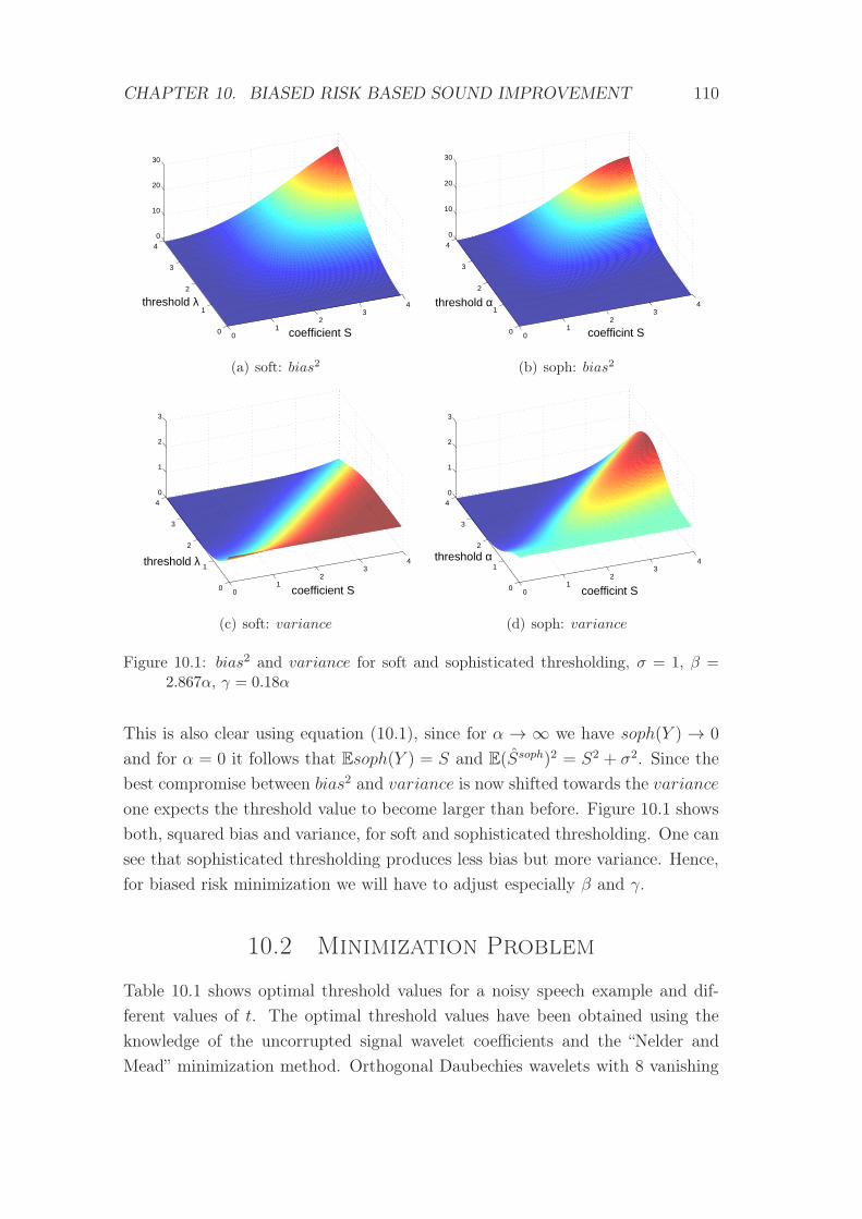
CHAPTER 10. BIASED RISK BASED SOUND IMPROVEMENT 110
01
23
4
0
1
2
3
40
10
20
30
coefficient S
threshold λ
(a) soft: bias2
01
23
4
0
1
2
3
4
0
10
20
30
coefficint S
threshold α
(b) soph: bias2
01
23
4
0
1
2
3
40
1
2
3
coefficient S
threshold λ
(c) soft: variance
01
23
4
0
1
2
3
40
1
2
3
coefficint S
threshold α
(d) soph: variance
Figure 10.1: bias2 and variance for soft and sophisticated thresholding, σ = 1, β =2.867α, γ = 0.18α
This is also clear using equation (10.1), since for α → ∞ we have soph(Y ) → 0
and for α = 0 it follows that Esoph(Y ) = S and E(Ssoph)2 = S2 + σ2. Since the
best compromise between bias2 and variance is now shifted towards the variance
one expects the threshold value to become larger than before. Figure 10.1 shows
both, squared bias and variance, for soft and sophisticated thresholding. One can
see that sophisticated thresholding produces less bias but more variance. Hence,
for biased risk minimization we will have to adjust especially β and γ.
10.2 Minimization Problem
Table 10.1 shows optimal threshold values for a noisy speech example and dif-
ferent values of t. The optimal threshold values have been obtained using the
knowledge of the uncorrupted signal wavelet coefficients and the “Nelder and
Mead” minimization method. Orthogonal Daubechies wavelets with 8 vanishing
CHAPTER 10. BIASED RISK BASED SOUND IMPROVEMENT 111
moments have been used and, the corresponding detail coefficients have been
evaluated at J = 8 levels. One can see that small t leads to, as expected, larger
thresholds α and γ, whereas β does not change much. While α increases ap-
proximately 28% from t = 1 to t = 0.2, the corresponding factor to obtain β
decreases about 25%. In fact, for t = 0.2, the threshold α is already very close
to the universal threshold λuniv = σ√
2 log (2J) = 0.1665. Table 10.2 provides
t α β γ riskt
1.00 0.1181 3.208α 0.0582α 2.961e-40.66 0.1317 2.987α 0.1628α 2.721e-40.50 0.1383 2.951α 0.2471α 2.489e-40.36 0.1457 2.810α 0.3916α 2.181e-40.20 0.1516 2.413α 0.6669α 1.791e-4
Table 10.1: Optimal thresholds for biased risk, n = 217, σ = 0.05, MSE = 3.5e − 3,SNR = 6.340
the corresponding risk, bias and variance for the thresholds given in table 10.1.
For t = 0.2, one can indeed see that the actual risk is almost only influenced by
bias, leading however to much worse MSE values. Hence, a good compromise
might be a choice of t ≈ 0.5, where variance is already shrunken much more than
bias, leading however to risk and MSE not much worse than optimal. So far, I
t risk bias2 variance MSE SNR
1.00 2.961e-4 1.687e-4 1.274e-4 3.364e-4 15.0330.66 3.088e-4 2.132e-4 9.562e-5 3.514e-4 14.8440.50 3.279e-4 2.455e-4 8.240e-5 3.712e-4 14.6060.36 3.661e-4 2.969e-4 6.921e-5 4.104e-4 14.1700.20 4.564e-4 4.021e-4 5.418e-5 5.024e-4 13.291
Table 10.2: Bias and variance for biased risk, n = 217, σ = 0.05, MSE = 3.5e − 3,SNR = 6.340
used the knowledge of the uncorrupted signal to find good threshold values. The
main problem is now to find good riskt minimization methods for t 6= 1. I tried
to develop generalizations of SURE and GCV , without success, though. Hence,
at the moment the best approximation of riskt minimization methods is to eval-
uate good thresholds using a known risk minimization method and adjusting the
results due to previous experiments. For the examples provided in chapter 11,
I performed a SURE minimizations, adjusting the results in the following way:
αt = 1.2α, βt = β, γt = 2γ. However, much more research need to be done to
improve biased risk minimization and replace the mentioned heuristic approach.
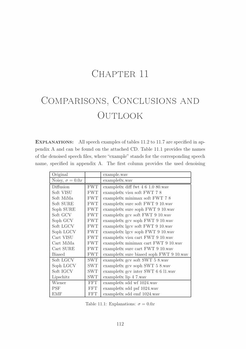
Chapter 11
Comparisons, Conclusions and
Outlook
Explanations: All speech examples of tables 11.2 to 11.7 are specified in ap-
pendix A and can be found on the attached CD. Table 11.1 provides the names
of the denoised speech files, where “example” stands for the corresponding speech
name, specified in appendix A. The first column provides the used denoising
Original example.wav
Noisy, σ = 0.0x example0x.wav
Diffusion FWT example0x diff fwt 4 6 1.0 80.wavSoft VISU FWT example0x visu soft FWT 7 8Soft MiMa FWT example0x minimax soft FWT 7 8Soft SURE FWT example0x sure soft FWT 9 10.wavSoph SURE FWT example0x sure soph FWT 9 10.wavSoft GCV FWT example0x gcv soft FWT 9 10.wavSoph GCV FWT example0x gcv soph FWT 9 10.wavSoft LGCV FWT example0x lgcv soft FWT 9 10.wavSoph LGCV FWT example0x lgcv soph FWT 9 10.wavCart VISU FWT example0x visu cart FWT 9 10.wavCart MiMa FWT example0x minimax cart FWT 9 10.wavCart SURE FWT example0x sure cart FWT 9 10.wavBiased FWT example0x sure biased soph FWT 9 10.wav
Soft LGCV SWT example0x gcv soft SWT 5 8.wavSoph LGCV SWT example0x gcv soph SWT 5 8.wavSoft IGCV SWT example0x gcv inter SWT 6 6 l1.wavLipschitz SWT example0x lip 4 7.wav
Wiener FFT example0x sdd wf 1024.wavPSF FFT example0x sdd psf 1024.wavEMF FFT example0x sdd emf 1024.wav
Table 11.1: Explanations: σ = 0.0x
112
CHAPTER 11. COMPARISONS, CONCLUSIONS AND OUTLOOK 113
method. For all thresholding methods, the first word describes the threshold-
ing method, the second word for the threshold or threshold finder, respectively.
“VISU” refers to the universal threshold, “MiMa” to the miinimax threshold. An
“L” at the threshold finder indicates level dependent thresholding, i.e. at each
level, a threshold has been evaluated separately. “Cart” refers to the algorithm for
tree structured thresholding, CPRESS. Furthermore, for “Cart SURE”, I used a
threshold obtained using SURE for sophisticated thresholding. “ICGV” refers to
inter scale GCV, as described in section 7.10, using coefficients of two subsequent
levels, i.e. l = 1. Diffusion denoising performes 80 iterations with diffusion step
size τ = 1, starting with a threshold 50% larger than universal. At each iteration,
the threshold has been shrunken by a factor of 0.99. Thresholds for biased risk
thresholding are obtained using “Soph SURE” thresholds, increasing α by a factor
of 1.2 and doubling γ. For all methods, I used orthogonal Daubechies wavelets.
The number of vanishing moments is provided in the fourth column of tables 11.2
to 11.7. For Fourier based methods, windows with a sub-frame length of 1024
samples are used, 75% overlapping.
On each speech example, Gaussian white noise with standard deviation σ =
0.01, σ = 0.03 and σ = 0.05 has been added. Tables 11.2 to 11.7 list MSE and
SNR before and after denoising. For each example, the best FWT based method
— in terms of MSE and SNR minimization — is marked blue. If any SWT based
procedure produces better results it is additionally marked green. There is no
case where FFT based methods are better than the best wavelet based method.
In the following, I will first compare the methods based only on MSE and SNR,
and try to provide some conclusions about favorable methods. Then, I will com-
pare the methods based on auditory behavior. However, clear and indisputable
results are not possible here, since each method produces its own characteristic
noise artifacts and signal deformations, diversely evaluated by different persons.
Hence, I recommend to listen to some of the speech examples on the attached
CD to form an own view, too. However, I will also try to provide an evaluation
which methods might be best for which speech sound, i.e. different preferences
for vocals, sibilants and other consonants.
MSE and SNR Comparison: First, I will compare the methods in gen-
eral, i.e. I try to find results that are true for all speech examples. Later I will
consider some special examples an analyze the best method. Diffusion denois-
ing, Lipschitz denoising and VISU shrink are for almost all examples the worst
methods. Only Lipschitz denoising outperforms in few cases some of the other
CHAPTER 11. COMPARISONS, CONCLUSIONS AND OUTLOOK 114
methods. This is however not surprising since all these methods are not based on
MSE minimization but rather on smoothing. Only for large noise magnitudes, i.e.
large σ, Lipschitz denoising yields some good results. In fact, compared to other
methods, the obtained SNR does not change much for decreasing noise magni-
tude, i.e. the absolute result is less dependent on noise. Although CPRESS is not
based on risk minimization, either, for a given threshold, the idea and the actual
outcome is not so much different to thresholding. Hence, using risk minimization
thresholds also leads to good results. Another remark should be done on biased
risk thresholding. Even though it is not directly based on risk minimization, in
fact we explicitly adjust thresholds to obtain more bias, it yields good results, not
much worse than others. Let’s now take a closer look on sophisticated threshold-
ing. We can see that for most cases, sophisticated thresholding produces better
results than corresponding threshold finders based on soft thresholding. Espe-
cially for level dependent GCV and FWT, there are some examples with very
large differences to soft thresholding. E.g. for speech 2 and σ = 0.01, the differ-
ence is over 3dB, i.e. MSE doubles from soph to soft. Furthermore, as mentioned
in chapter 9, it would be possible to obtain even better results if we were not
restricted on in some way fixed β and γ. Considering inter scale dependencies, I
cannot support the assumption, postulated by Maarten Jansen [19], that inter-
scale GCV thresholding yields better results than ordinary GCV. In fact, only
for few examples better SNR is obtained.
Let’s now consider speech example 1 and 2. In contrast to the other examples,
both consist of only 216 samples. It is remarkable that, independent of the noise
magnitude, CPRESS produces the best results. Especially for σ = 0.03, no other
method comes close to the MSE of CPRESS. The differences between SURE and
Minimax threshold is however small. In most cases, Minimax is a little better.
For all other examples, the optimal method depends on the noise magnitude.
For σ = 0.01, sophisticated thresholding linked with SURE seems to be the best
choice. Whenever it is not optimal, it is at least very close to optimal. If SURE is
not applicable because σ is not known, sophisticated GCV is second-best, either
ordinary or level dependent based on SWT. FWT based level dependent GCV
yields to much worse results for σ = 0.01. However, for larger noise magnitudes
the tide turns and for σ = 0.03 it is already the best method for some of the speech
examples, whereas others still prefer sophisticated SURE or Cart. Finally, for
σ = 0.05, it clearly is the optimal choice. Besides speech example 1 and 2, there
is only one other speech example that would prefer Cart. However, the SNR
difference to LGCV is rather small. LGCV is only outdone by “itself”, based
on SWT though. It is remarkable that for SWT, no clear preference between
CHAPTER 11. COMPARISONS, CONCLUSIONS AND OUTLOOK 115
sophisticated and soft thresholding can bee determined. Finally, the used FFT
based methods are outperformed by almost all wavelet based methods!
In summary, for small n, Cart seems to be appropriate. Otherwise, we need a
rough noise estimation to find good methods. For large noise magnitude, the best
choice is LGCV, based on SWT or FWT. For small noise amplitudes however,
LGCV performs much worse than SURE and GCV. For medial noise magnitudes,
the differences are small, and furthermore, Cart might be a good choice, too.
Sound Quality Comparison: Let’s now take a look at (or rather a listen
to) sound quality. The following conclusions are mainly based on my personal
perception of noise, i.e. on the evaluation which noise artifact is most disturbing.
Other readers may come to different conclusions. Additionally, I’ve been listening
to so much noise recently, such that I’ve got the feeling to become more and more
noise resistant.
However, let’s start with reconstructed signals for σ = 0.01. My clear favorite
is the universal threshold, i.e. Soft VISU. We have seen in chapter 7 that with
high probability, all noise is removed. Indeed, I can not hear much noisy distur-
bances. At the same time, since σ and therefore λ is relatively small compared
to uncorrupted signal coefficients, the signal deformation is still small. If σ can’t
be approximated, Lipschitz denoising provides relatively good quality, too. For
my perceptual experience, the constant low frequency background noise, charac-
teristic for Lipschitz denoising and described in chapter 5, is less distracting than
permanently changing small disturbances. For larger σ, VISU shrink yields much
more signal deformation and other methods are preferable.
For σ = 0.03 it is very hard to state a preference. For some examples, VISU
shrink still sounds good. For most examples I prefer Lipschitz denoising, though.
Even though many important signal features are kept by Diffusion denoising,
noise is not really removed but in some way smoothed to a constant high tone
background beeping, as already mentioned in chapter 6. However, also LGCV and
biased risk denoising yield to good results for some examples. Especially biased
risk seems to become much better than SURE or GCV methods for increasing σ.
Finally, for large σ, I would prefer biased risk thresholding and in some cases
Lispchitz denoising. Similar to VISU shrink, almost all noise is removed (be-
sides the mentioned low frequency background, sounding in some way like a far
away highway), but there is less signal distortion. However, Lipschitz denoising
produces now some additional disturbing swishing sounds, occuring at “s” and
similar sounds.
For all noise magnitudes, sophisticated and soft thresholding risk minimization
CHAPTER 11. COMPARISONS, CONCLUSIONS AND OUTLOOK 116
methods lead to different characteristic chirping and twittering. In my opinion,
the residual noise of sophisticated thresholding is a little less disturbing. How-
ever, for large noise magnitude these methods are outperformed by biased risk
denoising, leading indeed as desired to less “chirping” and about the same sig-
nal quality. Cart methods produce typical keep or kill problems. Soft or soph
thresholding leads to an additional smoothing by shrinking even large coefficients
by a certain amount. Hard thresholding, or in this case a tree structured keep
or kill method, yields to abrupt changes of the signal, sounding indeed in some
way “hard”. Furthermore, cart processes coefficients in blocks. Each tree of coef-
ficients is treated separately, i.e. for one tree most coefficients might be kept, in
the following one most might be killed, enhancing the effect of abrupt changes.
Finally, some additional remarks about the optimal method for some different
speech sounds. As mentioned in chapter 1, one expects reconstruction problems
for sibilant sounds like “s”, “ch” or “z”, since they sound and look similar to noise.
One can see in figure 1.1 that smoothness assumptions do not apply. Hence, it
is not surprising that especially smoothness based methods produce bad results.
Diffusion and Lipschitz denoising produce additional swishing or soughing arti-
facts whenever such sounds occur. Similar artifacts can also be observed for Visu
Shrink, but not as strong. Indeed, thresholding often produces much better qual-
ity, i.e. less signal deformation, on the expense of more audible residual noise.
The best result is obtained using level dependent thresholds. Also hard conso-
nants like “t” or “k” are, similar to sibilants, better preserved by thresholding
methods, again especially level dependent ones. The difference is much less con-
spicuous, though. However, other sounds, especially vowels, or sounds like “m”,
“l” and “r” that produce smooth curves are much better preserved using Lipschitz
denoising or Visu Shrink. Smooth signals produce sparser wavelet representations
of the original signal, and therefore, only few important but very large coefficients
remain. Hence, Visu Shrink, using very large thresholds to remove all pure noise
coefficients, does not kill or deform many important coefficients. For Lipschitz
denoising, the same fact facilitates the detection of noise coefficients that need to
be removed. For all other thresholding methods there is not much signal defor-
mation either, but much more residual noise since the selected thresholds are too
small. In fact, these results also support the statement made in chapter 9 that
large original signal coefficients prefer larger thresholds, i.e. global thresholds can
not be optimal.
However, as mentioned, I recommend to listen to some examples and decide
for yourself. For a very quick overview and comparison of the different residual
CHAPTER 11. COMPARISONS, CONCLUSIONS AND OUTLOOK 117
noise artifacts and denoising results, I recommend to select only Lipschitz, VISU,
biased, Soph LGCV and Soft SURE. Then, most typical artifacts are covered and
the audible differences to other methods are rather small.
Outlook, Perspectives: I have shown that wavelet based denoising meth-
ods can outperform some of the existing and commonly used Fourier based meth-
ods. However, some further improvements are possible. I will now give a brief
overview of possible enhancements. First of all, different wavelets may lead to
better results, without even changing a lot of the actual methods. For example,
Yu, Bacry and Mallat recently proposed to use complex wavelets in audio signal
processing to protect the phase of the signal [38]. Furthermore, I developed two
new denoising methods, sophisticated thresholding and biased risk thresholding.
However, for both methods the threshold finding procedure should be improved.
For sophisticated thresholding, we adjust in fact only one out of three parameters
for risk minimization purpose. Biased risk thresholding lacks of any appropriate
method to find good thresholds, using a simple heuristic approach so far. Addi-
tionally, as mentioned in chapter 9, it will be better not to use constant thresholds
for the whole signal but adjust it in accordance to the current signal features. In
fact, this bridges to speech recognition methods. In summary, we see that further
research is necessary to obtain satisfactorily results.
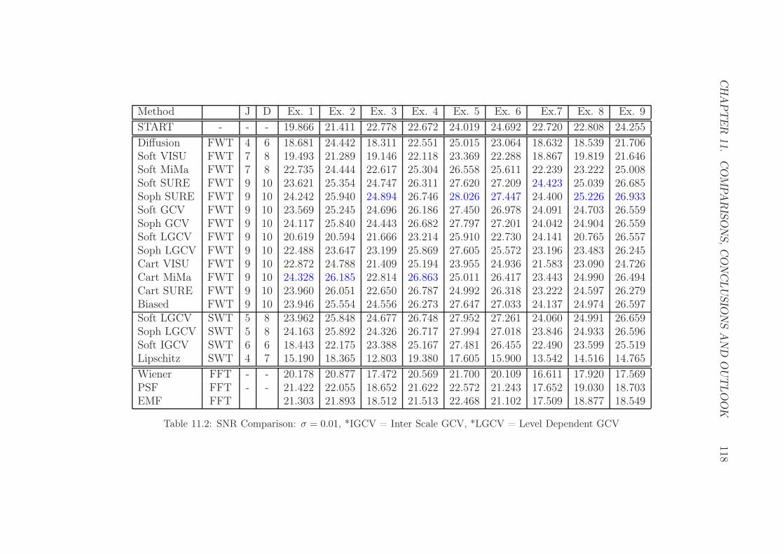
CH
AP
TE
R11.
CO
MPA
RIS
ON
S,C
ON
CLU
SIO
NS
AN
DO
UT
LO
OK
118
Method J D Ex. 1 Ex. 2 Ex. 3 Ex. 4 Ex. 5 Ex. 6 Ex.7 Ex. 8 Ex. 9
START - - - 19.866 21.411 22.778 22.672 24.019 24.692 22.720 22.808 24.255
Diffusion FWT 4 6 18.681 24.442 18.311 22.551 25.015 23.064 18.632 18.539 21.706Soft VISU FWT 7 8 19.493 21.289 19.146 22.118 23.369 22.288 18.867 19.819 21.646Soft MiMa FWT 7 8 22.735 24.444 22.617 25.304 26.558 25.611 22.239 23.222 25.008Soft SURE FWT 9 10 23.621 25.354 24.747 26.311 27.620 27.209 24.423 25.039 26.685Soph SURE FWT 9 10 24.242 25.940 24.894 26.746 28.026 27.447 24.400 25.226 26.933Soft GCV FWT 9 10 23.569 25.245 24.696 26.186 27.450 26.978 24.091 24.703 26.559Soph GCV FWT 9 10 24.117 25.840 24.443 26.682 27.797 27.201 24.042 24.904 26.559Soft LGCV FWT 9 10 20.619 20.594 21.666 23.214 25.910 22.730 24.141 20.765 26.557Soph LGCV FWT 9 10 22.488 23.647 23.199 25.869 27.605 25.572 23.196 23.483 26.245Cart VISU FWT 9 10 22.872 24.788 21.409 25.194 23.955 24.936 21.583 23.090 24.726Cart MiMa FWT 9 10 24.328 26.185 22.814 26.863 25.011 26.417 23.443 24.990 26.494Cart SURE FWT 9 10 23.960 26.051 22.650 26.787 24.992 26.318 23.222 24.597 26.279Biased FWT 9 10 23.946 25.554 24.556 26.273 27.647 27.033 24.137 24.974 26.597Soft LGCV SWT 5 8 23.962 25.848 24.677 26.748 27.952 27.261 24.060 24.991 26.659Soph LGCV SWT 5 8 24.163 25.892 24.326 26.717 27.994 27.018 23.846 24.933 26.596Soft IGCV SWT 6 6 18.443 22.175 23.388 25.167 27.481 26.455 22.490 23.599 25.519Lipschitz SWT 4 7 15.190 18.365 12.803 19.380 17.605 15.900 13.542 14.516 14.765
Wiener FFT - - 20.178 20.877 17.472 20.569 21.700 20.109 16.611 17.920 17.569PSF FFT - - 21.422 22.055 18.652 21.622 22.572 21.243 17.652 19.030 18.703EMF FFT 21.303 21.893 18.512 21.513 22.468 21.102 17.509 18.877 18.549
Table 11.2: SNR Comparison: σ = 0.01, *IGCV = Inter Scale GCV, *LGCV = Level Dependent GCV
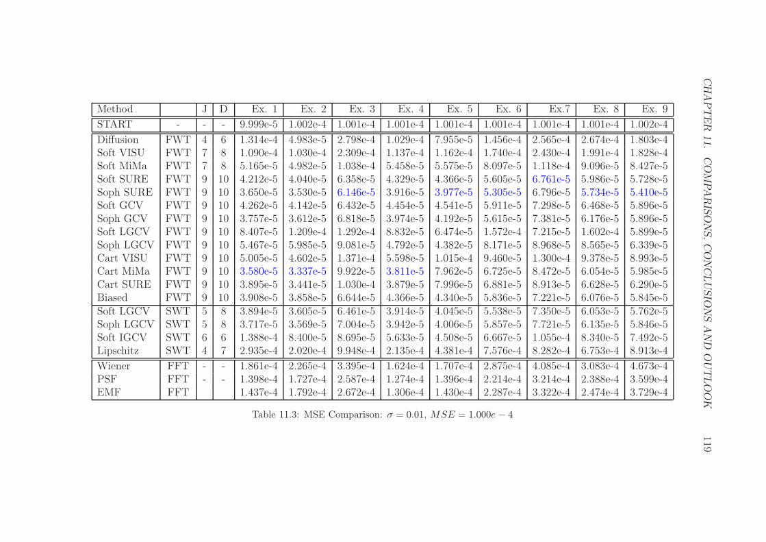
CH
AP
TE
R11.
CO
MPA
RIS
ON
S,C
ON
CLU
SIO
NS
AN
DO
UT
LO
OK
119
Method J D Ex. 1 Ex. 2 Ex. 3 Ex. 4 Ex. 5 Ex. 6 Ex.7 Ex. 8 Ex. 9
START - - - 9.999e-5 1.002e-4 1.001e-4 1.001e-4 1.001e-4 1.001e-4 1.001e-4 1.001e-4 1.002e-4
Diffusion FWT 4 6 1.314e-4 4.983e-5 2.798e-4 1.029e-4 7.955e-5 1.456e-4 2.565e-4 2.674e-4 1.803e-4Soft VISU FWT 7 8 1.090e-4 1.030e-4 2.309e-4 1.137e-4 1.162e-4 1.740e-4 2.430e-4 1.991e-4 1.828e-4Soft MiMa FWT 7 8 5.165e-5 4.982e-5 1.038e-4 5.458e-5 5.575e-5 8.097e-5 1.118e-4 9.096e-5 8.427e-5Soft SURE FWT 9 10 4.212e-5 4.040e-5 6.358e-5 4.329e-5 4.366e-5 5.605e-5 6.761e-5 5.986e-5 5.728e-5Soph SURE FWT 9 10 3.650e-5 3.530e-5 6.146e-5 3.916e-5 3.977e-5 5.305e-5 6.796e-5 5.734e-5 5.410e-5Soft GCV FWT 9 10 4.262e-5 4.142e-5 6.432e-5 4.454e-5 4.541e-5 5.911e-5 7.298e-5 6.468e-5 5.896e-5Soph GCV FWT 9 10 3.757e-5 3.612e-5 6.818e-5 3.974e-5 4.192e-5 5.615e-5 7.381e-5 6.176e-5 5.896e-5Soft LGCV FWT 9 10 8.407e-5 1.209e-4 1.292e-4 8.832e-5 6.474e-5 1.572e-4 7.215e-5 1.602e-4 5.899e-5Soph LGCV FWT 9 10 5.467e-5 5.985e-5 9.081e-5 4.792e-5 4.382e-5 8.171e-5 8.968e-5 8.565e-5 6.339e-5Cart VISU FWT 9 10 5.005e-5 4.602e-5 1.371e-4 5.598e-5 1.015e-4 9.460e-5 1.300e-4 9.378e-5 8.993e-5Cart MiMa FWT 9 10 3.580e-5 3.337e-5 9.922e-5 3.811e-5 7.962e-5 6.725e-5 8.472e-5 6.054e-5 5.985e-5Cart SURE FWT 9 10 3.895e-5 3.441e-5 1.030e-4 3.879e-5 7.996e-5 6.881e-5 8.913e-5 6.628e-5 6.290e-5Biased FWT 9 10 3.908e-5 3.858e-5 6.644e-5 4.366e-5 4.340e-5 5.836e-5 7.221e-5 6.076e-5 5.845e-5Soft LGCV SWT 5 8 3.894e-5 3.605e-5 6.461e-5 3.914e-5 4.045e-5 5.538e-5 7.350e-5 6.053e-5 5.762e-5Soph LGCV SWT 5 8 3.717e-5 3.569e-5 7.004e-5 3.942e-5 4.006e-5 5.857e-5 7.721e-5 6.135e-5 5.846e-5Soft IGCV SWT 6 6 1.388e-4 8.400e-5 8.695e-5 5.633e-5 4.508e-5 6.667e-5 1.055e-4 8.340e-5 7.492e-5Lipschitz SWT 4 7 2.935e-4 2.020e-4 9.948e-4 2.135e-4 4.381e-4 7.576e-4 8.282e-4 6.753e-4 8.913e-4
Wiener FFT - - 1.861e-4 2.265e-4 3.395e-4 1.624e-4 1.707e-4 2.875e-4 4.085e-4 3.083e-4 4.673e-4PSF FFT - - 1.398e-4 1.727e-4 2.587e-4 1.274e-4 1.396e-4 2.214e-4 3.214e-4 2.388e-4 3.599e-4EMF FFT 1.437e-4 1.792e-4 2.672e-4 1.306e-4 1.430e-4 2.287e-4 3.322e-4 2.474e-4 3.729e-4
Table 11.3: MSE Comparison: σ = 0.01, MSE = 1.000e − 4
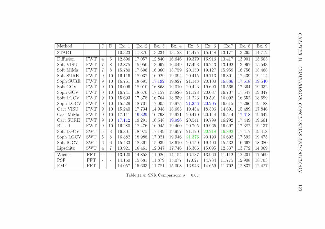
CH
AP
TE
R11.
CO
MPA
RIS
ON
S,C
ON
CLU
SIO
NS
AN
DO
UT
LO
OK
120
Method J D Ex. 1 Ex. 2 Ex. 3 Ex. 4 Ex. 5 Ex. 6 Ex.7 Ex. 8 Ex. 9
START - - - 10.323 11.870 13.234 13.128 14.475 15.148 13.177 13.265 14.712
Diffusion FWT 4 6 12.896 17.057 12.840 16.646 19.379 16.916 13.417 13.901 15.603Soft VISU FWT 7 8 12.875 15.050 13.092 16.049 17.493 16.243 13.192 13.967 15.543Soft MiMa FWT 7 8 15.780 17.696 16.060 18.759 20.150 19.127 15.959 16.756 18.468Soft SURE FWT 9 10 16.116 18.037 16.929 19.094 20.415 19.713 16.801 17.439 19.114Soph SURE FWT 9 10 16.761 18.695 17.192 19.827 21.148 20.100 16.886 17.618 19.540Soft GCV FWT 9 10 16.096 18.010 16.868 19.010 20.423 19.690 16.566 17.364 19.032Soph GCV FWT 9 10 16.741 18.676 17.157 19.826 21.128 20.087 16.707 17.547 19.347Soft LGCV FWT 9 10 15.693 17.378 16.764 18.959 21.223 19.591 16.092 16.652 18.699Soph LGCV FWT 9 10 15.529 18.701 17.005 19.975 21.356 20.205 16.615 17.266 19.188Cart VISU FWT 9 10 15.240 17.734 14.948 18.685 19.454 18.506 14.691 15.489 17.846Cart MiMa FWT 9 10 17.111 19.329 16.798 19.921 20.470 20.144 16.544 17.618 19.642Cart SURE FWT 9 10 17.112 19.291 16.548 19.996 20.541 19.799 16.292 17.449 19.601Biased FWT 9 10 16.280 18.476 16.945 19.460 20.765 19.965 16.697 17.382 19.137Soft LGCV SWT 5 8 16.801 18.975 17.149 19.957 21.120 20.218 16.892 17.417 19.418Soph LGCV SWT 5 8 16.882 18.988 17.021 19.946 21.376 20.193 16.692 17.592 19.475Soft IGCV SWT 6 6 15.433 18.361 15.939 18.610 20.150 19.400 15.532 16.662 18.380Lipschitz SWT 4 7 13.921 16.461 12.047 17.746 16.306 15.095 12.537 13.772 14.069
Wiener FFT - - 13.120 14.858 11.026 14.154 16.137 13.960 11.112 12.201 17.569PSF FFT - - 14.160 15.681 11.879 15.077 17.027 14.734 11.775 12.908 18.703EMF FFT 14.057 15.603 11.781 15.008 16.943 14.659 11.702 12.837 12.427
Table 11.4: SNR Comparison: σ = 0.03
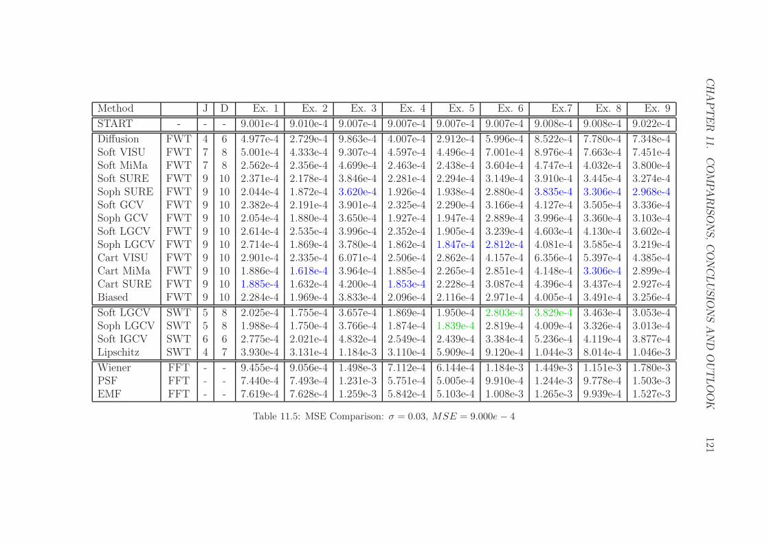
CH
AP
TE
R11.
CO
MPA
RIS
ON
S,C
ON
CLU
SIO
NS
AN
DO
UT
LO
OK
121
Method J D Ex. 1 Ex. 2 Ex. 3 Ex. 4 Ex. 5 Ex. 6 Ex.7 Ex. 8 Ex. 9
START - - - 9.001e-4 9.010e-4 9.007e-4 9.007e-4 9.007e-4 9.007e-4 9.008e-4 9.008e-4 9.022e-4
Diffusion FWT 4 6 4.977e-4 2.729e-4 9.863e-4 4.007e-4 2.912e-4 5.996e-4 8.522e-4 7.780e-4 7.348e-4Soft VISU FWT 7 8 5.001e-4 4.333e-4 9.307e-4 4.597e-4 4.496e-4 7.001e-4 8.976e-4 7.663e-4 7.451e-4Soft MiMa FWT 7 8 2.562e-4 2.356e-4 4.699e-4 2.463e-4 2.438e-4 3.604e-4 4.747e-4 4.032e-4 3.800e-4Soft SURE FWT 9 10 2.371e-4 2.178e-4 3.846e-4 2.281e-4 2.294e-4 3.149e-4 3.910e-4 3.445e-4 3.274e-4Soph SURE FWT 9 10 2.044e-4 1.872e-4 3.620e-4 1.926e-4 1.938e-4 2.880e-4 3.835e-4 3.306e-4 2.968e-4Soft GCV FWT 9 10 2.382e-4 2.191e-4 3.901e-4 2.325e-4 2.290e-4 3.166e-4 4.127e-4 3.505e-4 3.336e-4Soph GCV FWT 9 10 2.054e-4 1.880e-4 3.650e-4 1.927e-4 1.947e-4 2.889e-4 3.996e-4 3.360e-4 3.103e-4Soft LGCV FWT 9 10 2.614e-4 2.535e-4 3.996e-4 2.352e-4 1.905e-4 3.239e-4 4.603e-4 4.130e-4 3.602e-4Soph LGCV FWT 9 10 2.714e-4 1.869e-4 3.780e-4 1.862e-4 1.847e-4 2.812e-4 4.081e-4 3.585e-4 3.219e-4Cart VISU FWT 9 10 2.901e-4 2.335e-4 6.071e-4 2.506e-4 2.862e-4 4.157e-4 6.356e-4 5.397e-4 4.385e-4Cart MiMa FWT 9 10 1.886e-4 1.618e-4 3.964e-4 1.885e-4 2.265e-4 2.851e-4 4.148e-4 3.306e-4 2.899e-4Cart SURE FWT 9 10 1.885e-4 1.632e-4 4.200e-4 1.853e-4 2.228e-4 3.087e-4 4.396e-4 3.437e-4 2.927e-4Biased FWT 9 10 2.284e-4 1.969e-4 3.833e-4 2.096e-4 2.116e-4 2.971e-4 4.005e-4 3.491e-4 3.256e-4
Soft LGCV SWT 5 8 2.025e-4 1.755e-4 3.657e-4 1.869e-4 1.950e-4 2.803e-4 3.829e-4 3.463e-4 3.053e-4Soph LGCV SWT 5 8 1.988e-4 1.750e-4 3.766e-4 1.874e-4 1.839e-4 2.819e-4 4.009e-4 3.326e-4 3.013e-4Soft IGCV SWT 6 6 2.775e-4 2.021e-4 4.832e-4 2.549e-4 2.439e-4 3.384e-4 5.236e-4 4.119e-4 3.877e-4Lipschitz SWT 4 7 3.930e-4 3.131e-4 1.184e-3 3.110e-4 5.909e-4 9.120e-4 1.044e-3 8.014e-4 1.046e-3
Wiener FFT - - 9.455e-4 9.056e-4 1.498e-3 7.112e-4 6.144e-4 1.184e-3 1.449e-3 1.151e-3 1.780e-3PSF FFT - - 7.440e-4 7.493e-4 1.231e-3 5.751e-4 5.005e-4 9.910e-4 1.244e-3 9.778e-4 1.503e-3EMF FFT - - 7.619e-4 7.628e-4 1.259e-3 5.842e-4 5.103e-4 1.008e-3 1.265e-3 9.939e-4 1.527e-3
Table 11.5: MSE Comparison: σ = 0.03, MSE = 9.000e − 4
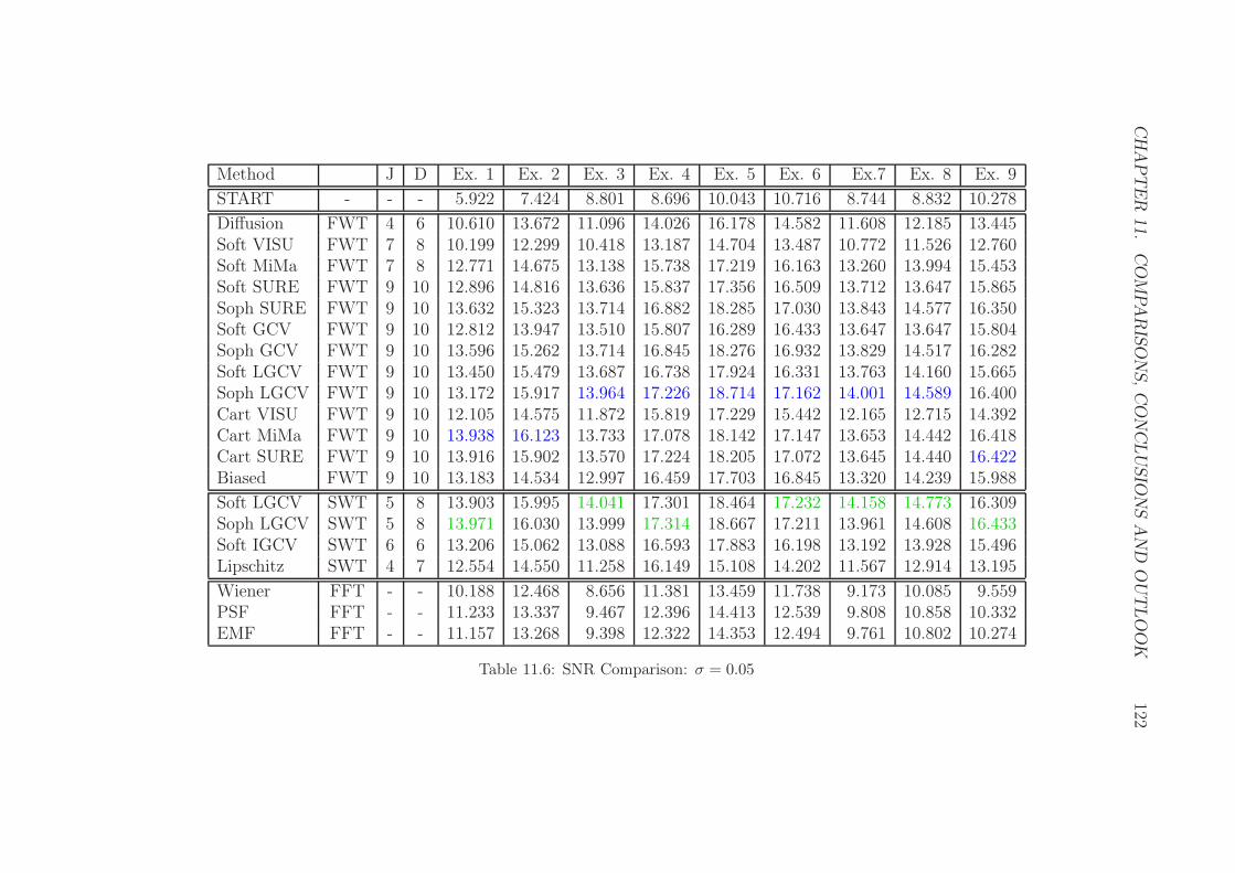
CH
AP
TE
R11.
CO
MPA
RIS
ON
S,C
ON
CLU
SIO
NS
AN
DO
UT
LO
OK
122
Method J D Ex. 1 Ex. 2 Ex. 3 Ex. 4 Ex. 5 Ex. 6 Ex.7 Ex. 8 Ex. 9
START - - - 5.922 7.424 8.801 8.696 10.043 10.716 8.744 8.832 10.278
Diffusion FWT 4 6 10.610 13.672 11.096 14.026 16.178 14.582 11.608 12.185 13.445Soft VISU FWT 7 8 10.199 12.299 10.418 13.187 14.704 13.487 10.772 11.526 12.760Soft MiMa FWT 7 8 12.771 14.675 13.138 15.738 17.219 16.163 13.260 13.994 15.453Soft SURE FWT 9 10 12.896 14.816 13.636 15.837 17.356 16.509 13.712 13.647 15.865Soph SURE FWT 9 10 13.632 15.323 13.714 16.882 18.285 17.030 13.843 14.577 16.350Soft GCV FWT 9 10 12.812 13.947 13.510 15.807 16.289 16.433 13.647 13.647 15.804Soph GCV FWT 9 10 13.596 15.262 13.714 16.845 18.276 16.932 13.829 14.517 16.282Soft LGCV FWT 9 10 13.450 15.479 13.687 16.738 17.924 16.331 13.763 14.160 15.665Soph LGCV FWT 9 10 13.172 15.917 13.964 17.226 18.714 17.162 14.001 14.589 16.400Cart VISU FWT 9 10 12.105 14.575 11.872 15.819 17.229 15.442 12.165 12.715 14.392Cart MiMa FWT 9 10 13.938 16.123 13.733 17.078 18.142 17.147 13.653 14.442 16.418Cart SURE FWT 9 10 13.916 15.902 13.570 17.224 18.205 17.072 13.645 14.440 16.422Biased FWT 9 10 13.183 14.534 12.997 16.459 17.703 16.845 13.320 14.239 15.988
Soft LGCV SWT 5 8 13.903 15.995 14.041 17.301 18.464 17.232 14.158 14.773 16.309Soph LGCV SWT 5 8 13.971 16.030 13.999 17.314 18.667 17.211 13.961 14.608 16.433Soft IGCV SWT 6 6 13.206 15.062 13.088 16.593 17.883 16.198 13.192 13.928 15.496Lipschitz SWT 4 7 12.554 14.550 11.258 16.149 15.108 14.202 11.567 12.914 13.195
Wiener FFT - - 10.188 12.468 8.656 11.381 13.459 11.738 9.173 10.085 9.559PSF FFT - - 11.233 13.337 9.467 12.396 14.413 12.539 9.808 10.858 10.332EMF FFT - - 11.157 13.268 9.398 12.322 14.353 12.494 9.761 10.802 10.274
Table 11.6: SNR Comparison: σ = 0.05
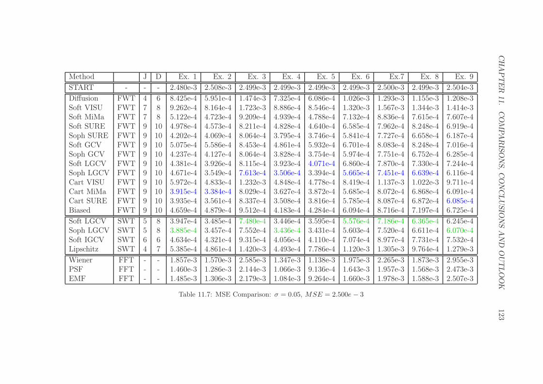
CH
AP
TE
R11.
CO
MPA
RIS
ON
S,C
ON
CLU
SIO
NS
AN
DO
UT
LO
OK
123
Method J D Ex. 1 Ex. 2 Ex. 3 Ex. 4 Ex. 5 Ex. 6 Ex.7 Ex. 8 Ex. 9
START - - - 2.480e-3 2.508e-3 2.499e-3 2.499e-3 2.499e-3 2.499e-3 2.500e-3 2.499e-3 2.504e-3
Diffusion FWT 4 6 8.425e-4 5.951e-4 1.474e-3 7.325e-4 6.086e-4 1.026e-3 1.293e-3 1.155e-3 1.208e-3Soft VISU FWT 7 8 9.262e-4 8.164e-4 1.723e-3 8.886e-4 8.546e-4 1.320e-3 1.567e-3 1.344e-3 1.414e-3Soft MiMa FWT 7 8 5.122e-4 4.723e-4 9.209e-4 4.939e-4 4.788e-4 7.132e-4 8.836e-4 7.615e-4 7.607e-4Soft SURE FWT 9 10 4.978e-4 4.573e-4 8.211e-4 4.828e-4 4.640e-4 6.585e-4 7.962e-4 8.248e-4 6.919e-4Soph SURE FWT 9 10 4.202e-4 4.069e-4 8.064e-4 3.795e-4 3.746e-4 5.841e-4 7.727e-4 6.658e-4 6.187e-4Soft GCV FWT 9 10 5.075e-4 5.586e-4 8.453e-4 4.861e-4 5.932e-4 6.701e-4 8.083e-4 8.248e-4 7.016e-4Soph GCV FWT 9 10 4.237e-4 4.127e-4 8.064e-4 3.828e-4 3.754e-4 5.974e-4 7.751e-4 6.752e-4 6.285e-4Soft LGCV FWT 9 10 4.381e-4 3.926e-4 8.115e-4 3.923e-4 4.071e-4 6.860e-4 7.870e-4 7.330e-4 7.244e-4Soph LGCV FWT 9 10 4.671e-4 3.549e-4 7.613e-4 3.506e-4 3.394e-4 5.665e-4 7.451e-4 6.639e-4 6.116e-4Cart VISU FWT 9 10 5.972e-4 4.833e-4 1.232e-3 4.848e-4 4.778e-4 8.419e-4 1.137e-3 1.022e-3 9.711e-4Cart MiMa FWT 9 10 3.915e-4 3.384e-4 8.029e-4 3.627e-4 3.872e-4 5.685e-4 8.072e-4 6.868e-4 6.091e-4Cart SURE FWT 9 10 3.935e-4 3.561e-4 8.337e-4 3.508e-4 3.816e-4 5.785e-4 8.087e-4 6.872e-4 6.085e-4Biased FWT 9 10 4.659e-4 4.879e-4 9.512e-4 4.183e-4 4.284e-4 6.094e-4 8.716e-4 7.197e-4 6.725e-4
Soft LGCV SWT 5 8 3.947e-4 3.485e-4 7.480e-4 3.446e-4 3.595e-4 5.576e-4 7.186e-4 6.365e-4 6.245e-4Soph LGCV SWT 5 8 3.885e-4 3.457e-4 7.552e-4 3.436e-4 3.431e-4 5.603e-4 7.520e-4 6.611e-4 6.070e-4Soft IGCV SWT 6 6 4.634e-4 4.321e-4 9.315e-4 4.056e-4 4.110e-4 7.074e-4 8.977e-4 7.731e-4 7.532e-4Lipschitz SWT 4 7 5.385e-4 4.861e-4 1.420e-3 4.493e-4 7.786e-4 1.120e-3 1.305e-3 9.764e-4 1.279e-3
Wiener FFT - - 1.857e-3 1.570e-3 2.585e-3 1.347e-3 1.138e-3 1.975e-3 2.265e-3 1.873e-3 2.955e-3PSF FFT - - 1.460e-3 1.286e-3 2.144e-3 1.066e-3 9.136e-4 1.643e-3 1.957e-3 1.568e-3 2.473e-3EMF FFT - - 1.485e-3 1.306e-3 2.179e-3 1.084e-3 9.264e-4 1.660e-3 1.978e-3 1.588e-3 2.507e-3
Table 11.7: MSE Comparison: σ = 0.05, MSE = 2.500e − 3
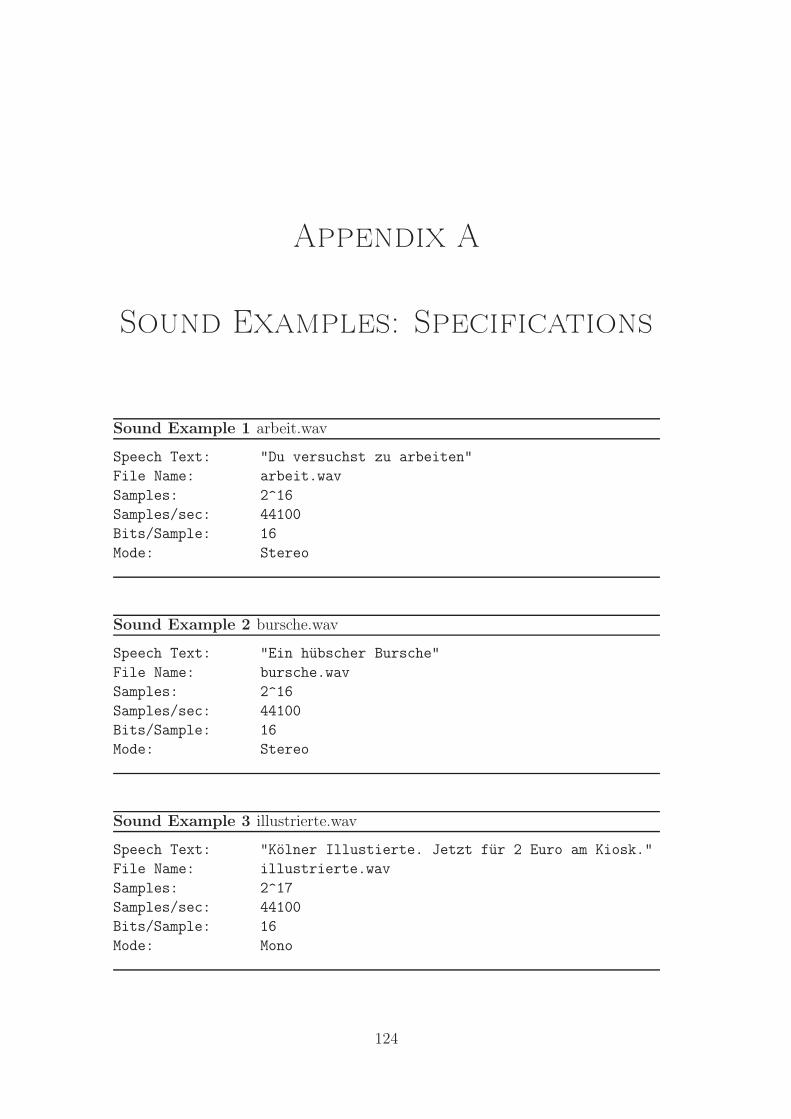
Appendix A
Sound Examples: Specifications
Sound Example 1 arbeit.wav
Speech Text: "Du versuchst zu arbeiten"
File Name: arbeit.wav
Samples: 2^16
Samples/sec: 44100
Bits/Sample: 16
Mode: Stereo
Sound Example 2 bursche.wav
Speech Text: "Ein hübscher Bursche"
File Name: bursche.wav
Samples: 2^16
Samples/sec: 44100
Bits/Sample: 16
Mode: Stereo
Sound Example 3 illustrierte.wav
Speech Text: "Kölner Illustierte. Jetzt für 2 Euro am Kiosk."
File Name: illustrierte.wav
Samples: 2^17
Samples/sec: 44100
Bits/Sample: 16
Mode: Mono
124
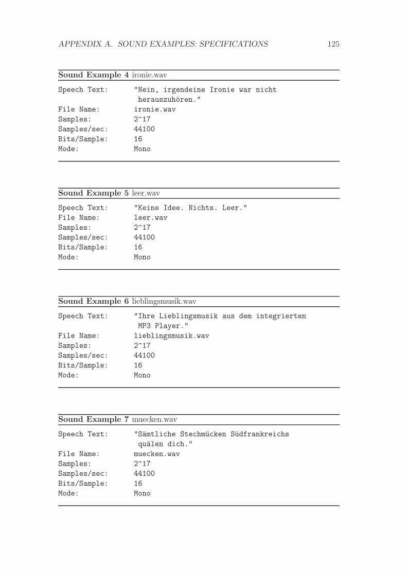
APPENDIX A. SOUND EXAMPLES: SPECIFICATIONS 125
Sound Example 4 ironie.wav
Speech Text: "Nein, irgendeine Ironie war nicht
herauszuhören."
File Name: ironie.wav
Samples: 2^17
Samples/sec: 44100
Bits/Sample: 16
Mode: Mono
Sound Example 5 leer.wav
Speech Text: "Keine Idee. Nichts. Leer."
File Name: leer.wav
Samples: 2^17
Samples/sec: 44100
Bits/Sample: 16
Mode: Mono
Sound Example 6 lieblingsmusik.wav
Speech Text: "Ihre Lieblingsmusik aus dem integrierten
MP3 Player."
File Name: lieblingsmusik.wav
Samples: 2^17
Samples/sec: 44100
Bits/Sample: 16
Mode: Mono
Sound Example 7 muecken.wav
Speech Text: "Sämtliche Stechmücken Südfrankreichs
quälen dich."
File Name: muecken.wav
Samples: 2^17
Samples/sec: 44100
Bits/Sample: 16
Mode: Mono
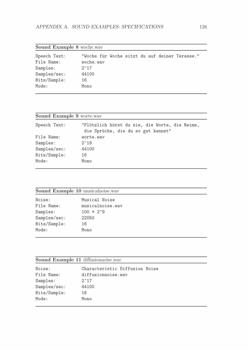
APPENDIX A. SOUND EXAMPLES: SPECIFICATIONS 126
Sound Example 8 woche.wav
Speech Text: "Woche für Woche sitzt du auf deiner Terasse."
File Name: woche.wav
Samples: 2^17
Samples/sec: 44100
Bits/Sample: 16
Mode: Mono
Sound Example 9 worte.wav
Speech Text: "Plötzlich hörst du sie, die Worte, die Reime,
die Sprüche, die du so gut kennst"
File Name: worte.wav
Samples: 2^18
Samples/sec: 44100
Bits/Sample: 16
Mode: Mono
Sound Example 10 musicalnoise.wav
Noise: Musical Noise
File Name: musicalnoise.wav
Samples: 100 * 2^9
Samples/sec: 22050
Bits/Sample: 16
Mode: Mono
Sound Example 11 diffusionnoise.wav
Noise: Characteristic Diffusion Noise
File Name: diffusionnoise.wav
Samples: 2^17
Samples/sec: 44100
Bits/Sample: 16
Mode: Mono
Bibliography
[1] Paul Bao and Lei Zhang. Noise reduction for magnetic resonance images via
adaptive multiscale products thresholding. IEEE Transactions on Medical
Imaging, 22(9):1089 – 1099, Sept. 2003.
[2] Ronald R. Coifman and David L. Donoho. Translation-invariant de-noising.
Technical report, Stanford University, Department of Statistics, 1995.
[3] Ingrid Daubechies. The wavelet transform, time-frequency localization and
signal analysis. IEEE Trans. Inform. Theory, 36(5):961–1005, 1990.
[4] Ingrid Daubechies. Ten lectures on wavelets, volume 61 of CBMS-NSF Re-
gional Conference Series in Applied Mathematics. Society for Industrial and
Applied Mathematics (SIAM), Philadelphia, PA, 1992.
[5] David L. Donoho. Cart and best-ortho-basis: A connection. Technical report,
Department of Statistics, Stanford University, October 1995.
[6] David L. Donoho. De-noising by soft-thresholding. IEEE Trans. Inform.
Theory, 41(3):613–627, 1995.
[7] David L. Donoho. CART and best-ortho-basis: a connection. Ann. Statist.,
25(5):1870–1911, 1997.
[8] David L. Donoho and Iain M. Johnstone. Ideal spatial adaptation by wavelet
shrinkage. Biometrika, 81(3):425–455, 1994.
[9] David L. Donoho and Iain M. Johnstone. Adapting to unknown smoothness
via wavelet shrinkage. J. Amer. Statist. Assoc., 90(432):1200–1224, 1995.
[10] David L. Donoho and Iain M. Johnstone. Minimax estimation via wavelet
shrinkage. Ann. Statist., 26(3):879–921, 1998.
[11] David L. Donoho and Iain M. Johnstone. Asymptotic minimaxity of wavelet
estimators with sampled data. Statist. Sinica, 9(1):1–32, 1999.
127
BIBLIOGRAPHY 128
[12] Yariv Ephraim and David Malah. Speech enhancement using a minimum-
mean square error short-time spectral amplitude estimator. Acoustics, Speech
and Signal Processing, IEEE Transactions on, 32(6):1109–1121, Dec 1984.
[13] Ningping Fan, Radu V. Balan, and Justinian Rosca. Comparison of wavelet-
and fft-based single-channel speech signal noise reduction techniques. volume
5607, pages 127–138. SPIE, 2004.
[14] Simon J. Godsill and Peter J.W. Rayner. Digital Audio Restoration - a
statistical model based approach. Springer-Verlag London, September 1998.
[15] Zenton Goh, Kah-Chye Tan, and T.G. Tan. Postprocessing method for
suppressing musical noise generated by spectral subtraction. Speech and
Audio Processing, IEEE Transactions on, 6(3):287–292, May 1998.
[16] A. Grossmann, M. Holschneider, R. Kronland-Martinet, and J. Morlet. De-
tection of abrupt changes in sound signals with the help of wavelet trans-
forms. In Inverse problems: an interdisciplinary study (Montpellier, ss1986),
Adv. Electron. Electron Phys., Suppl. 19, pages 289–306. Academic Press,
London, 1987.
[17] M. Holschneider. Wavelets. Oxford Mathematical Monographs. The Claren-
don Press Oxford University Press, New York, 1995. An analysis tool, Oxford
Science Publications.
[18] Matthias Holschneider and Philippe Tchamitchian. Régularite locale de la
fonction “non-différentiable” de Riemann. In Les ondelettes en 1989 (Or-
say, 1989), volume 1438 of Lecture Notes in Math., pages 102–124, 209–210.
Springer, Berlin, 1990.
[19] Maarten Jansen. Noise reduction by wavelet thresholding, volume 161 of
Lecture Notes in Statistics. Springer-Verlag, New York, 2001.
[20] Maarten Jansen and Adhemar Bultheel. Multiple wavelet threshold estima-
tion by generalized cross validation for images with correlated noise. IEEE
Trans. Image Process., 8(7):947–953, 1999.
[21] Maarten Jansen, Maurits Malfait, and Adhemar Bultheel. Generalized cross
validation for wavelet thresholding. Signal Processing, 56(1):33–44, 1997.
[22] Stephane Mallat. A Wavelet Tour of Signal Processing. Academic Press,
1998.
BIBLIOGRAPHY 129
[23] Stephane Mallat and Wen Liang Hwang. Singularity detection and processing
with wavelets. IEEE Trans. Inform. Theory, 38(2, part 2):617–643, 1992.
[24] Stephane Mallat and Sifen Zhong. Characterization of signals from multiscale
edges. IEEE Transactions on Pattern Analysis and Machine Intelligence,
14(7):710–732, July 1992.
[25] Yves Meyer. Wavelets: Algorithms & Applications. SIAM, 1993.
[26] Guy P. Nason. Wavelet shrinkage using cross-validation. J. Roy. Statist.
Soc. Ser. B, 58(2):463–479, 1996.
[27] Guy P. Nason and Bernard W. Silverman. The stationary wavelet transform
and some statistical applications. In Anestis Antoniadis and Georges Op-
penheim, editors, Wavelets and Statistics, number 103 in Lecture Notes in
Statistics, pages 281–300. Springer-Verlag, 1995.
[28] Pietro Perona and Jitendra Malik. Scale-space and edge detection using
anisotropic diffusion. Pattern Analysis and Machine Intelligence, IEEE
Transactions on, 12(7):629–639, Jul 1990.
[29] H. L. Resnikoff and R. O. Wells Jr. Wavelet Analysis, The Scalable Structure
of Information. Springer-Verlag, New York, 1998.
[30] Charles M. Stein. Estimation of the mean of a multivariate normal distribu-
tion. Ann. Statist., 9(6):1135–1151, 1981.
[31] Nathalie Virag. Single channel speech enhancement based on masking prop-
erties of the human auditory system. Speech and Audio Processing, IEEE
Transactions on, 7(2):126–137, March 1999.
[32] Martin Welk, Achim Bergmeister, and Joachim Weickert. Denoising of au-
dio data by nonlinear diffusion. In Ron Kimmel, Nir Sochen, and Joachim
Weickert, editors, Scale Space and PDE Methods in Computer Vision , 5th
International Conference, Scale-Space 2005, Hofgeismar, Germany, April 7-
9, 2005, Proceedings, volume 3459 of Lecture Notes in Computer Science,
pages 598–609. Springer Verlag Berlin / Heidelberg, 2005.
[33] Norman Weyrich and Gregory T. Warhola. Wavelet shrinkage and general-
ized cross validation for image denoising. Image Processing, IEEE Transac-
tions on, 7(1):82–90, Jan 1998.
[34] Mladen V. Wickerhauser. Adaptive Wavelet-Analysis: Theory and Software.
Vieweg & Sohn, 1993.
BIBLIOGRAPHY 130
[35] Norbert Wiener. Extrapolation, Interpolation, and Smoothing of Stationary
Time Series. With Engineering Applications. The Technology Press of the
Massachusetts Institute of Technology, Cambridge, Mass, 1949.
[36] Y. Xu, J. B. Weaver, D. M. Healy Jr., and J. Lu. Wavelet transform domain
filters: A spatially selective noise filtration technique. IEEE Transactions of
Image Processing, 3(6), November 1994.
[37] Kôsaku Yosida. Functional analysis. Second edition. Die Grundlehren der
mathematischen Wissenschaften, Band 123. Springer-Verlag New York Inc.,
New York, 1968.
[38] Guoshen Yu, Emmanuel Bacry, and Stephane Mallat. Audio signal denoising
with complex wavelets and adaptive block attenuation. Acoustics, Speech and
Signal Processing, 2007. ICASSP 2007. IEEE International Conference on,
3:III–869–III–872, April 2007.


![WAVELETS - Peopleblatter/Wavelets.pdf · bekannten Wavelet-Buch in deutscher Sprache, und im ,,Friendly guide to wavelets\ von Kaiser [K]. Fur weitere Quellen der Inspiration verweise](https://img.pdfslide.org/doc/110x75/5d5730af88c9935a158b5fcc/wavelets-people-blatterwaveletspdf-bekannten-wavelet-buch-in-deutscher-sprache.jpg)
![Speech Analysis: Barack Obama's speech on the …...SCHOOL-SCOUT Obama on Osama bin Laden’s Death Seite 5 von 8 Speech-analysis [Introduction: who is speaking, frame of reference]](https://img.pdfslide.org/doc/110x75/5f896c461c4c4b77c47b3b71/speech-analysis-barack-obamas-speech-on-the-school-scout-obama-on-osama-bin.jpg)