Embed Size (px)
Citation preview
Supercontinuum Generation by
Ghost Pulse
Dissertation
zur Erlangung des Grades eines
Doktors der Naturwissenschaften (Dr. rer. nat.)
am Fachbereich Physik
der Freien Universität Berlin
vorgelegt von
Xingwen Zhang
Berlin 2021

Erstgutachter/in: Prof. Dr. Karsten Heyne
Zweitgutachter/in: Prof. Dr. Holger Dau
Tag der Disputation: January 26, 2021
i
Kurzfassung
Diese Dissertation beschreibt eine neuartige Methode zur Erzeugung von
negativ gechirptem Superkontinuum (SC) und beschreibt detailliert das
Design, die Herstellung und die umfassende Charakterisierung der erzeugten
SC. Nach der SPM-Theorie sollte ein inverser Gaußscher Puls in der Lage sein,
negativ gechirpte SC zu erzeugen. In dieser Arbeit wird ein solcher inverser
Gaußscher Impuls als "Ghost pulse" bezeichnet. Jedoch ist es praktisch
unmöglich, einen inversen Gaußschen Puls zu erzeugen, da die Pulsintensität
nicht negativ sein kann. Um eine negativ gechirpte SC zu erzeugen, besteht
die erste schwierige Herausforderung daher darin, den gewünschten Ghost
pulse zu erhalten. In dieser Studie wurden ein 4f-Linien-
Impulsformungssystem und ein Summenfrequenzerzeugung-Setup (SFG)
aufgebaut und angewendet, um einen stabilen Ghost pulse zu erzeugen.
Aufgrund der Begrenzung durch die Fourier-Transformation entspricht eine
schmale spektrale Bandbreite einer langen Pulsdauer. Dadurch kann das 4f-
Linien-Pulsformungssystem einen Puls 𝐸4𝑓(𝑡) (𝜏𝑝 ≈ 2 𝑝𝑠) mit langer Dauer
erzeugen, indem es die spektrale Bandbreite des Eingangspulses verengt.
Anschließend wurde ein nichtlinearer Summenfrequenzerzeugungsprozess
(SFG) zwischen diesem langen Impuls 𝐸4𝑓(𝑡) und einem
Fundamentalimpuls 𝐸(𝑡) (𝜏𝑝 ≈ 200 𝑓𝑠 ) durchgeführt. Die Zentralenergie
des Pulses 𝐸4𝑓(𝑡) war aufgrund des SFG-Prozesses verringert und so wurde
ein Ghost pulse 𝐸𝑔ℎ𝑜𝑠𝑡(𝑡) erzeugt. Die Formung dieses Ghost pulse wurde
durch ein kommerzielles Autokorrelator-Gerät und eine selbst gebaute
frequenzaufgelöste optische Nachweismethode (FROG) verifiziert. Mit
diesem Ghost pulse konnten in YAG- und Saphirkristallen negativ gechirptes
SC erzeugt werden. Aus Kontrastgründen wurde auch ein Kontrollexperiment
mit einem Fundamentalpuls ( 𝜏𝑝 ≈ 200 𝑓𝑠 ) zur Erzeugung von SC
durchgeführt.
Die erzeugten SCs wurden experimentell mit Hilfe einer Vielzahl
verschiedener Techniken wie Autokorrelator, FROG und nicht-kollinearer
optischer parametrischer Verstärker (NOPA) charakterisiert. Die Validierung
der experimentellen Ergebnisse durch diese verschiedenen Strategien erlaubt
es uns, die Eigenschaften der erzeugten SC systematisch zu überprüfen. Die
Ergebnisse der NOPA und des Autokorrelators zeigen, dass die durch den
Ghost pulse erzeugte SC negativ gechirpt wird. Die FROG-Ergebnisse
demonstrieren direkt, dass der SC alleine durch den Ghost pulse erzeugt wird
und negativ gechirpt ist, während der durch Fundamentalimpulse erzeugte SC
positiv gechirpt ist.
ii
Abstract
This dissertation provides a novel method to generate negatively chirped
supercontinuum (SC) and details the design, fabrication and complete
characterization of the generated SC. According to the SPM theory, an inverse
Gaussian pulse should be able to generate negatively chirped SC. In this thesis
this kind of inverse Gaussian pulse is termed as “ghost pulse”. However, in
practice it is impossible to produce an inverse Gaussian pulse because the pulse
intensity can not be negative. Therefore, in order to generate negatively
chirped SC, the first difficult challenge is how to obtain the desired ghost pulse.
In this work, a 4f-line pulse shaping system and a sum-frequency generation
(SFG) setup were built and performed to produce a stable ghost pulse. Due to
the Fourier transform limit, narrow spectral bandwidth corresponds to long
pulse duration. Thereby, the 4f-line pulse shaping system can produce a long
duration pulse 𝐸4𝑓(𝑡) (𝜏𝑝 ≈ 2 𝑝𝑠 ) by narrowing the spectral bandwidth of
the input pulse. Afterwards, a sum-frequency generation (SFG) nonlinear
process was performed between this long pulse 𝐸4𝑓(𝑡) and a fundamental
pulse 𝐸(𝑡) ( 𝜏𝑝 ≈ 200 𝑓𝑠 ). The center energy of the pulse 𝐸4𝑓(𝑡) was
depleted due to the SFG process and thus a ghost pulse 𝐸𝑔ℎ𝑜𝑠𝑡(𝑡) was
obtained. The formation of this ghost pulse was verified by a commercial
autocorrelator device and a home-built FROG (frequency-resolved optical
gating) setup. Pumping by this ghost pulse and using YAG and sapphire
crystals as the working media, we have succeeded in generating negatively
chirped SC. For the sake of contrast, a control experiment using the
fundamental pulse (𝜏𝑝 ≈ 200 𝑓𝑠) to generate SC was also carried out.
The generated SCs were experimentally characterized with the help of
different techniques including autocorrelator, FROG and NOPA (non-collinear
optical parametric amplifier). The validation of the experimental results by
these different strategies allows us to check the properties of the generated SC
systematically. The NOPA and autocorrelator results reveal that the SC
generated by ghost pulse is negatively chirped in a round-about way. The
FROG results directly prove that the SC is purely generated by ghost pulse and
is clear negatively chirped, while the SC generated by fundamental pulse is
positively chirped.
iii
Contents
Kurzfassung ....................................................................................................................... i
Abstract ............................................................................................................................ ii
Chapter 1 Introduction ..................................................................................................... 1
Chapter 2 Fundamental physics ....................................................................................... 7
2.1 Ultrashort laser pulse ................................................................................................ 7
2.1.1 Pulse duration and pulse repetition rate ............................................................... 8
2.1.2 Relationship between pulse duration and spectral bandwidth............................... 9
2.1.3 Dispersion of optical pulses .............................................................................. 10
2.2 Nonlinear optics...................................................................................................... 11
2.2.1 Nonlinear polarization ...................................................................................... 11
2.2.2 Second harmonic generation............................................................................. 12
2.2.3 Sum frequency generation ................................................................................ 13
2.3 Pulse measurement techniques ................................................................................ 14
2.3.1 Autocorrelator and cross-correlator ................................................................... 15
2.3.2 Frequency-resolved optical gating technique .................................................... 17
2.4 Optical parametric amplifier.................................................................................... 20
2.4.1 Phase matching ................................................................................................ 20
2.4.2 Non-collinear optical parametric amplifier ........................................................ 23
2.5 Supercontinuum generation ..................................................................................... 24
2.5.1 Kerr effect ....................................................................................................... 24
2.5.2 Self-focusing ................................................................................................... 25
2.5.3 Plasma defocusing ........................................................................................... 26
2.5.4 Femtosecond filamentation............................................................................... 27
2.5.5 Self-phase modulation ...................................................................................... 28
2.5.6 Self-steepening ................................................................................................ 31
2.6 Summary ................................................................................................................ 31
Chapter 3 Negatively chirped supercontinuum generation by ghost pulse ................... 33
3.1 Introduction ............................................................................................................ 33
3.2 Experimental setups design ..................................................................................... 34
3.3 Supercontinuum generation by ghost pulse .............................................................. 40
3.3.1 Laser system .................................................................................................... 40
3.3.2 Second harmonic generation setup.................................................................... 42
3.3.3 4f-line pulse shaping and XFROG setups ......................................................... 43
3.3.4 Sum frequency generation process.................................................................... 50
3.3.5 Supercontinuum generation by ghost pulse and its characterization by XFROG
and NOPA-technique ................................................................................................ 53
3.4 Summary ................................................................................................................ 64
iv
Chapter 4 Two-stage non-collinear optical parametric amplifier .................................. 65
4.1 Introduction ............................................................................................................ 65
4.2 Acousto-optic programmable dispersive filter .......................................................... 66
4.3 Experimental setup of two-stage NOPA ................................................................... 69
4.3.1 Overview of the setup ...................................................................................... 69
4.3.2 Signal and pump beams for NOPA ................................................................... 71
4.3.3 Setup details..................................................................................................... 73
4.4 Results and discussion............................................................................................. 75
4.4.1 Broadband optical parametric amplification ...................................................... 75
4.4.2 Pulse compression using AOPDF ..................................................................... 77
4.5 Summary ................................................................................................................ 79
Chapter 5 Summary and outlook ................................................................................... 81
Literature ........................................................................................................................ 83
Acknowledgements ......................................................................................................... 99
Selbstständigkeitserklärung ......................................................................................... 101
Chapter 1 Introduction
1
Chapter 1
Introduction
Since the advent of laser, physicists are always exploring different
methods to optimize laser performance for achieving different goals, such as
new wavelength bands, maximum average output power, minimum output
pulse length [1-4], etc. In recent years, we have seen exciting development in
the generation of ultrashort laser sources and their important applications in a
variety of research fields [5-7]. Now it is convenient to find many kinds of
commercial laser devices which can output picosecond (ps, 10-12 s) pulses.
Several companies can also extend the duration time of pulse into the
femtosecond (fs, 10-15 s) time region. Some literatures have reported that they
can produce pulses consisting of just several optical cycles [8-10]. Many novel
instruments with extremely high temporal resolution have been invented based
on ultrashort laser pulses. These exciting progresses of ultrafast pulses permit
us to study and discover key processes unresolved in the past.
The great point about ultrafast laser pulses is that they have very high
intensity because all the energy is compressed into an ultrashort time. The
tremendous development of the ultrafast laser based on nonlinear optics is an
important branch of modern optics [11]. The nonlinear optics mainly studies
high intensity effects, e.g., second harmonic generation (SHG) process [12, 13]
which allows to obtain output light at double frequency and half wavelength,
or like optical parametric amplification (OPA) [14-16] which amplifies a
signal input by a higher frequency pump input and generates an idler wave,
etc.
Supercontinuum (SC) generation [17-19] is one of the most important and
amazing nonlinear optical processes, a phenomenon that intense laser can
dramatically broaden the input spectrum bandwidth in a transparent medium.
The first study on the SC generation dates back to 1968, when Alfano and
Shapiro observed the picosecond “white” continuum in the bulk of borosilicate
glass [20, 21]. With the high intensity laser pulses on the order of GW/cm2 in
the sample, the spectrum of laser pulses transmitted through the sample
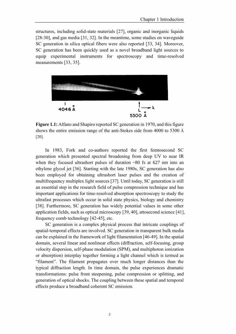
stretched from 400 to 700 nm. Fig. 1.1 presents the wavelength range of the
anti-Stokes side covering from 4000 to 5300 Å which was published by Alfano
and Shapiro in 1970 [20].
Soon afterwards, Alfano and Shapiro published SC generation
accompanied by the formation of thin laser radiation filaments in sodium
chloride, quartz, calcite, and various types of glass [22-26]. In the years of
1970s, experimental studies in SC generation demonstrated that the SC
generation can be achieved in various materials with different states and
Chapter 1 Introduction
2
structures, including solid-state materials [27], organic and inorganic liquids
[28-30], and gas media [31, 32]. In the meantime, some studies on waveguide
SC generation in silica optical fibers were also reported [33, 34]. Moreover,
SC generation has been quickly used as a novel broadband light sources to
equip experimental instruments for spectroscopy and time-resolved
measurements [33, 35].
Figure 1.1: Alfano and Shapiro reported SC generation in 1970, and this figure
shows the entire emission range of the anti-Stokes side from 4000 to 5300 Å
[20].
In 1983, Fork and co-authors reported the first femtosecond SC
generation which presented spectral broadening from deep UV to near IR
when they focused ultrashort pulses of duration ~80 fs at 627 nm into an
ethylene glycol jet [36]. Starting with the late 1980s, SC generation has also
been employed for obtaining ultrashort laser pulses and the creation of
multifrequency multiplex light sources [37]. Until today, SC generation is still
an essential step in the research field of pulse compression technique and has
important applications for time-resolved absorption spectroscopy to study the
ultrafast processes which occur in solid state physics, biology and chemistry
[38]. Furthermore, SC generation has widely potential values in some other
application fields, such as optical microscopy [39, 40], attosecond science [41],
frequency comb technology [42-45], etc.
SC generation is a complex physical process that intricate couplings of
spatial-temporal effects are involved. SC generation in transparent bulk media
can be explained in the framework of light filamentation [46-49]. In the spatial
domain, several linear and nonlinear effects (diffraction, self-focusing, group
velocity dispersion, self-phase modulation (SPM), and multiphoton ionization
or absorption) interplay together forming a light channel which is termed as
“filament”. The filament propagates over much longer distances than the
typical diffraction length. In time domain, the pulse experiences dramatic
transformations: pulse front steepening, pulse compression or splitting, and
generation of optical shocks. The coupling between these spatial and temporal
effects produce a broadband coherent SC emission.
Chapter 1 Introduction
3
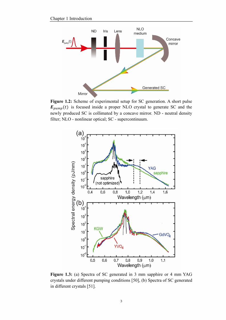
Figure 1.2: Scheme of experimental setup for SC generation. A short pulse
𝑬𝑝𝑢𝑚𝑝(𝑡) is focused inside a proper NLO crystal to generate SC and the
newly produced SC is collimated by a concave mirror. ND - neutral density
filter; NLO - nonlinear optical; SC - supercontinuum.
Figure 1.3: (a) Spectra of SC generated in 3 mm sapphire or 4 mm YAG
crystals under different pumping conditions [50], (b) Spectra of SC generated
in different crystals [51].
Chapter 1 Introduction
4
Although the physical mechanism of SC generation is complicate, the real
setup for SC generation is simple. As shown in Fig. 1.2, the setup involves just
a short pulse, a neutral density filter, an iris, a focusing lens, a suitable
nonlinear material and a collimating concave mirror (or a collimating lens).
The generated SC spectra and stability are determined by many
parameters, such as the wavelength and energy of the pumping pulse, the host
nonlinear medium, focusing conditions, etc. In general, the SC spectra is
defined by the wavelength of the pumping laser and the properties of the host
media, such as transparency range, energy bandgap and nonlinear index of
refraction. The SC stability is influenced by the beam size and intensity
distribution of the pumping pulse, focusing conditions and medium thickness.
Proper choice of these parameters is a key issue to guarantee the stable
generation of our desired SC source. Fig. 1.3 presents an example that SC
spectra are influenced by pumping conditions and media type.
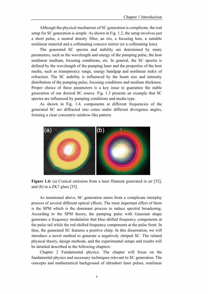
As shown in Fig. 1.4, components at different frequencies of the
generated SC are diffracted into cones under different divergence angles,
forming a clear concentric rainbow-like pattern.
Figure 1.4: (a) Conical emission from a laser filament generated in air [52],
and (b) in a ZK7 glass [53].
As mentioned above, SC generation stems from a complicate interplay
process of several different optical effects. The most important effect of them
is the SPM which is the dominant process to induce spectral broadening.
According to the SPM theory, the pumping pulse with Gaussian shape
generates a frequency modulation that blue-shifted frequency components at
the pulse tail while the red-shifted frequency components at the pulse front. In
thus, the generated SC features a positive chirp. In this dissertation, we will
introduce a novel method to generate a negatively chirped SC. The related
physical theory, design methods, and the experimental setups and results will
be detailed described in the following chapters:
Chapter 2 Fundamental physics. The chapter will focus on the
fundamental physics and necessary techniques relevant to SC generation. The
concepts and mathematical background of ultrashort laser pulses, nonlinear
Chapter 1 Introduction
5
optics and optical parametric amplifier will be described. Several widely used
techniques of pulse measurement such as autocorrelator, cross-correlator and
FROGs will be introduced. The relevant physics of SC generation will be also
presented.
Chapter 3 Negatively chirped supercontinuum generation by ghost pulse.
This chapter will present the experimental setup and results of SC generation
by ghost pulse. The experimental setup mainly consists of a 4f-line system,
SFG setup, SC generation, and SC characterization setups (NOPA/FROG).
The 4f-line is used to produce a long duration pulse. A subsequent SFG process
is performed between this long pulse and a short fundamental pulse to form a
desired ghost pulse. Afterwards, SC generation process is driven by the ghost
pulse. The generated SC is characterized by home-built NOPA or FROG setups.
Chapter 4 Two-stage non-collinear optical parametric amplifier. This
chapter will introduce the building of a two-stage NOPA setup and the
compression of the NOPA output by an AOPDF (Acousto-Optic
Programmable Dispersive Filter) device. The availability of this NOPA
supports for gap-free tuning covering from 650 to 1000 nm. By optimizing
pulse compression with different dispersion orders, we obtained a ~16 fs
ultrashort pulse.

Chapter 2 Fundamental physics
7
Chapter 2
Fundamental physics
Before delving into the details of the generation of negatively chirped
supercontinuum (SC), it is beneficial to systematically make an overview on
the relevant fundamental physics. Section 2.1 in this chapter will focus on the
concepts and mathematical background of ultrafast laser pulses, which is the
theoretical basis of the following content in this dissertation. Section 2.2 will
briefly introduce the basic aspects of the nonlinear optics, which is necessary
for understanding the SC generation theory and different pulse
characterization techniques in this work. Nonlinear optics include kinds of
different high-intensity effects and here we will mainly focus on the second
harmonic generation (SHG) and sum frequency generation (SFG) which are
the most widely used nonlinear effects. The third section 2.3 will be dedicated
to the methods of ultrashort pulse characterization. This part includes a general
description of the techniques of autocorrelator, cross-correlator and FROG.
These techniques will be applied to characterize the generated SC in this work
and more details will be described in the later chapters. The fourth section 2.4
will present a brief description of optical parametric amplifier which will also
be used to characterize the generated SC. The fifth section 2.5 of this chapter
will introduce the physics of SC generation which stems from a complicate
interplay process of different optical effects such as Kerr effect, self-focusing,
plasma defocusing, self-phase modulation, etc. SC generation by ghost pulse
is the main topic of this dissertation. In the end of the chapter, the contents of
this chapter will be briefly summarized.
2.1 Ultrashort laser pulse
An ultrashort laser pulse is an electromagnetic wave with duration time
of the order of a picosecond (ps, 10−12 s) or femtosecond (fs, 10−15 s). It can be
fully defined by the space and time dependent electric field. The propagation
of ultrashort pulse and its interaction with matter are described by Maxwell’s
equations. In this section, some necessary physical definitions and
mathematical formulas used throughout this dissertation will be discussed.
For the sake of simplicity, let us consider first the electric field is linearly
polarized. Because our main concern is the temporal features of the pulse, here
we can neglect its spatial dependence. The pulse electric field can be written
as [54]:
𝐸(𝑡) =1
2√𝐼(𝑡)𝑒{𝑖[𝜔0𝑡−𝜙(𝑡)]} + 𝑐. 𝑐. (2.1)
2.1 Ultrashort laser pulse
8
where 𝑡 is time, 𝜔0 - the carrier angular frequency, 𝐼(𝑡) - the time-
dependent intensity of the pulse, 𝜙(𝑡) - the phase of the pulse and "𝑐. 𝑐." - the
complex conjugate. However, it is not easy to access 𝐸(𝑡) directly for
ultrashort pulses. The pulse field in frequency domain is often more practical.
The Fourier transform of 𝐸(𝑡) is the pulse field in the frequency domain
�̃�(𝜔):
�̃�(𝜔) = ∫ 𝐸(𝑡)𝑒−𝑖𝜔𝑡𝑑𝑡∞
−∞ (2.2)
where the tilde (~) over a function indicates that it is the Fourier transform.
The inverse Fourier transform of �̃�(𝜔) is the pulse field in the time domain
𝐸(𝑡):
𝐸(𝑡) =1
2𝜋∫ �̃�(𝜔)𝑒𝑖𝜔𝑡𝑑𝜔
∞
−∞ (2.3)
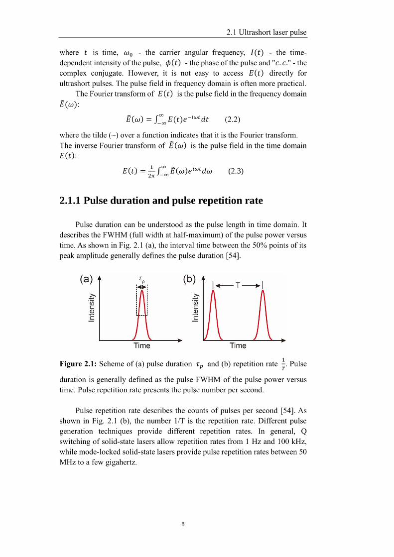
2.1.1 Pulse duration and pulse repetition rate
Pulse duration can be understood as the pulse length in time domain. It
describes the FWHM (full width at half-maximum) of the pulse power versus
time. As shown in Fig. 2.1 (a), the interval time between the 50% points of its
peak amplitude generally defines the pulse duration [54].
Figure 2.1: Scheme of (a) pulse duration 𝜏𝑝 and (b) repetition rate 1
𝑇. Pulse
duration is generally defined as the pulse FWHM of the pulse power versus
time. Pulse repetition rate presents the pulse number per second.
Pulse repetition rate describes the counts of pulses per second [54]. As
shown in Fig. 2.1 (b), the number 1/T is the repetition rate. Different pulse
generation techniques provide different repetition rates. In general, Q
switching of solid-state lasers allow repetition rates from 1 Hz and 100 kHz,
while mode-locked solid-state lasers provide pulse repetition rates between 50
MHz to a few gigahertz.
Chapter 2 Fundamental physics
9
2.1.2 Relationship between pulse duration and spectral
bandwidth
It is difficult to assert the precise pulse shape and thus here we select
standard waveforms. The temporal dependence of the most cited Gaussian
pulse is (with zero phase) [55, 56]:
𝐸(𝑡) = 𝐸0𝑒−(
𝑡
𝜏𝐻𝑊1 𝑒⁄)
2
= 𝐸0𝑒−2𝑙𝑛2(
𝑡
𝜏𝑝)2
,
where 𝐸0 is amplitude, 𝜏𝐻𝑊1 𝑒⁄ is the field half-width-half-maximum, and
𝜏𝑝 is the intensity full-width-half-maximum.
The intensity is:
𝐼(𝑡) = |𝐸(𝑡)|2 = |𝐸0|2𝑒
−4𝑙𝑛2(𝑡
𝜏𝑝)2
. (2.4)
Perform the Fourier transform on the Gaussian electric field 𝐸(𝑡):
𝐸(𝜔) = ℱ−1[𝐸(𝑡)] = ∫ 𝐸0𝑒−2𝑙𝑛2(
𝑡
𝜏𝑝)2
𝑒−𝑖𝜔𝑡∞
−∞𝑑𝑡. (2.5)
By utilizing the identity:
∫ 𝑒−𝑎𝑥2𝑒−2𝑏𝑥∞
−∞𝑑𝑥 = √
𝜋
𝑎𝑒
𝑏2
𝑎 , (a>0),
the Eq. (2.5) can be expressed as:
𝐸(𝜔) = 𝐸0√𝜋
2𝑙𝑛2𝜏𝑝𝑒
−𝜔2𝜏𝑝
2
8𝑙𝑛2 .
The intensity is:
𝐼(𝜔) = |𝐸(𝜔)|2 = |𝐸0|2 𝜋
2𝑙𝑛2𝜏𝑝
2𝑒−𝜔2𝜏𝑝
2
4𝑙𝑛2 . (2.6)
From Eqs. (2.4) and (2.6), we can derive the time bandwidth product
(TBP):
𝑇𝐵𝑃 ≥ ∆𝑓𝑝τ𝑝 =∆𝜔𝑝
2𝜋τ𝑝 =
4ln2
2π≥ 0.441, (2.7)
where ∆𝑓𝑝 is the frequency FWHM of the Gaussian pulse and ∆𝜔𝑝 is the
FWHM bandwidth of intensity 𝐼(𝜔).
According to the uncertainty principle, a Gaussian pulse with minimum
TBP value 0.441 is known as Fourier transform limited pulse. The TBP
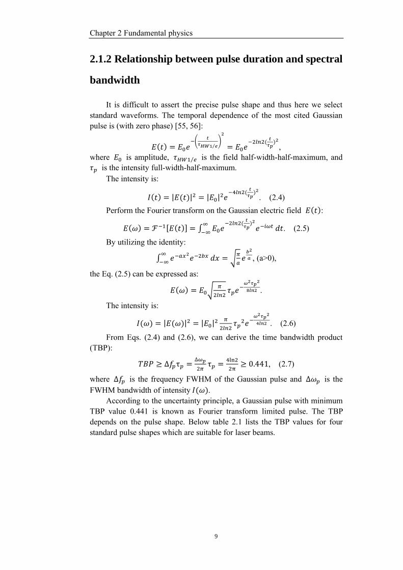
depends on the pulse shape. Below table 2.1 lists the TBP values for four
standard pulse shapes which are suitable for laser beams.
2.1 Ultrashort laser pulse
10
Table 2.1: TBP values for different standard pulse shapes [57].
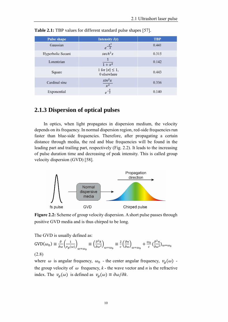
2.1.3 Dispersion of optical pulses
In optics, when light propagates in dispersion medium, the velocity
depends on its frequency. In normal dispersion region, red-side frequencies run
faster than blue-side frequencies. Therefore, after propagating a certain
distance through media, the red and blue frequencies will be found in the
leading part and trailing part, respectively (Fig. 2.2). It leads to the increasing
of pulse duration time and decreasing of peak intensity. This is called group
velocity dispersion (GVD) [58].
Figure 2.2: Scheme of group velocity dispersion. A short pulse passes through
positive GVD media and is thus chirped to be long.
The GVD is usually defined as:
GVD(𝜔0) ≡𝜕
𝜕𝜔(
1
𝑣𝑔(𝜔))𝜔=𝜔0
≡ (𝜕2𝑘
𝜕𝜔2)𝜔=𝜔0
≡2
𝑐(
𝜕𝑛
𝜕𝜔)𝜔=𝜔0
+𝜔0
𝑐(𝜕2𝑛
𝜕𝜔2)𝜔=𝜔0
(2.8)
where 𝜔 is angular frequency, 𝜔0 - the center angular frequency, 𝑣𝑔(𝜔) -
the group velocity of 𝜔 frequency, k - the wave vector and n is the refractive
index. The 𝑣𝑔(𝜔) is defined as 𝑣𝑔(𝜔) ≡ 𝜕𝜔/𝜕𝑘.
Chapter 2 Fundamental physics
11
2.2 Nonlinear optics
When light with low intensity, typical non-laser sources, passes through
a medium, the properties of this medium keep independent of the illumination.
When laser source is used, the incident light with extremely high intensity can
modify the properties of medium and thus light waves are able to interact with
each other to exchange energy and momentum. On this occasion, many
interesting high-intensity effects were discovered. Nonlinear optics is a
modern optical branch which studies precisely these high-intensity effects [11,
59].
2.2.1 Nonlinear polarization
The wave equation is the fundamental equation of optics [54]:
∂2𝑬
∂𝑧2 −1
𝑐02
∂2𝑬
∂𝑡2 = 𝜇0∂2𝑷
∂𝑡2 , (2.9)
where E is the real electric field, 𝑐0 - the speed of light in vacuum, 𝜇0 - the
magnetic permeability of free space, and P - the real induced polarization.
The induced polarization P contains linear and nonlinear optical effects. If the
strength of electric field E is low, the induced polarization P is proportional to
the electric field E [11, 59]:
𝑷 = 휀0𝜒(1)𝑬, (2.10)
where 휀0 is the electric permittivity of free space, and 𝜒(1) is the linear
susceptibility of the medium. The parameter 𝜒(1) describes the linear optics.
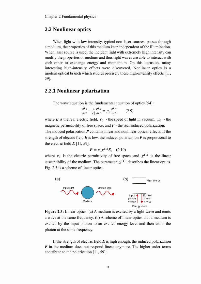
Fig. 2.3 is a scheme of linear optics.
Figure 2.3: Linear optics. (a) A medium is excited by a light wave and emits
a wave at the same frequency. (b) A scheme of linear optics that a medium is
excited by the input photon to an excited energy level and then emits the
photon at the same frequency.
If the strength of electric field E is high enough, the induced polarization
P in the medium does not respond linear anymore. The higher order terms
contribute to the polarization [11, 59]:
2.2 Nonlinear optics
12
𝑷 = 𝑷(1) + 𝑷(2) + 𝑷(3) + ⋯ = 휀0𝜒(1)𝑬 + 휀0𝜒
(2)𝑬2 + 휀0𝜒(3)𝑬3 + ⋯, (2.11)
where χ(n) denotes the n-th order component of electric susceptibility of the
medium.
We can express the i-th component for the vector P explicitly as:
𝑷𝑖 = 휀0𝜒𝑖𝑗(1)
𝑬𝑗 + 휀0𝜒𝑖𝑗𝑘(2)
𝑬𝑗𝑬𝑘 + 휀0𝜒𝑖𝑗𝑘𝑙(3)
𝑬𝑗𝑬𝑘𝑬𝑙 + ⋯, (2.12)
where i = 1, 2, 3.
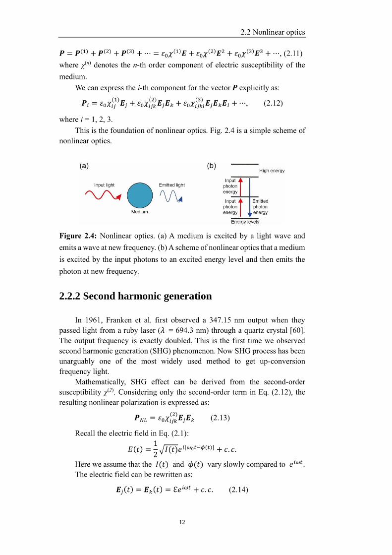
This is the foundation of nonlinear optics. Fig. 2.4 is a simple scheme of
nonlinear optics.
Figure 2.4: Nonlinear optics. (a) A medium is excited by a light wave and
emits a wave at new frequency. (b) A scheme of nonlinear optics that a medium
is excited by the input photons to an excited energy level and then emits the
photon at new frequency.
2.2.2 Second harmonic generation
In 1961, Franken et al. first observed a 347.15 nm output when they
passed light from a ruby laser (𝜆 = 694.3 nm) through a quartz crystal [60].
The output frequency is exactly doubled. This is the first time we observed
second harmonic generation (SHG) phenomenon. Now SHG process has been
unarguably one of the most widely used method to get up-conversion
frequency light.
Mathematically, SHG effect can be derived from the second-order
susceptibility χ(2). Considering only the second-order term in Eq. (2.12), the
resulting nonlinear polarization is expressed as:
𝑷𝑁𝐿 = 휀0𝜒𝑖𝑗𝑘(2)
𝑬𝑗𝑬𝑘 (2.13)
Recall the electric field in Eq. (2.1):
𝐸(𝑡) =1
2√𝐼(𝑡)𝑒𝑖[𝜔0𝑡−𝜙(𝑡)] + 𝑐. 𝑐.
Here we assume that the 𝐼(𝑡) and 𝜙(𝑡) vary slowly compared to 𝑒𝑖𝜔𝑡.
The electric field can be rewritten as:
𝑬𝑗(𝑡) = 𝑬𝑘(𝑡) = ℇ𝑒𝑖𝜔𝑡 + 𝑐. 𝑐. (2.14)
Chapter 2 Fundamental physics
13
where ℇ is the field amplitude.
Substituting the 𝑬𝑗(𝑡) and 𝑬𝑘(𝑡) into Eq. (2.13), we can get:
𝑷𝑁𝐿 = 휀0𝜒𝑖𝑗𝑘(2)
(ℇ2𝑒𝑖2𝜔𝑡 + ℇ∗2𝑒−𝑖2𝜔𝑡 + 2ℇℇ∗) (2.15)
From this equation we can find that the nonlinear polarization 𝑷𝑁𝐿
contains a component which radiates at double frequency of the input pulse. A
zero-frequency term is also included in the above 𝑷𝑁𝐿 expression, so light
contains a DC field. This effect is known as optical rectification which is
usually very weak. In the remaining, we will ignore this optical rectification
effect and just discuss the SHG effect.
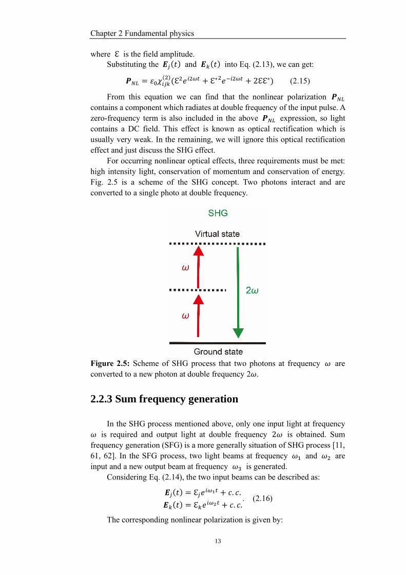
For occurring nonlinear optical effects, three requirements must be met:
high intensity light, conservation of momentum and conservation of energy.
Fig. 2.5 is a scheme of the SHG concept. Two photons interact and are
converted to a single photo at double frequency.
Figure 2.5: Scheme of SHG process that two photons at frequency 𝜔 are
converted to a new photon at double frequency 2𝜔.
2.2.3 Sum frequency generation
In the SHG process mentioned above, only one input light at frequency
𝜔 is required and output light at double frequency 2𝜔 is obtained. Sum
frequency generation (SFG) is a more generally situation of SHG process [11,
61, 62]. In the SFG process, two light beams at frequency 𝜔1 and 𝜔2 are
input and a new output beam at frequency 𝜔3 is generated.
Considering Eq. (2.14), the two input beams can be described as:
𝑬𝑗(𝑡) = ℇ𝑗𝑒𝑖𝜔1𝑡 + 𝑐. 𝑐.
𝑬𝑘(𝑡) = ℇ𝑘𝑒𝑖𝜔2𝑡 + 𝑐. 𝑐.
. (2.16)
The corresponding nonlinear polarization is given by:
2.3 Pulse measurement techniques
14
𝑷𝑁𝐿 = 휀0𝜒𝑖𝑗𝑘(2)
𝑬𝑗𝑬𝑘 = 휀0𝜒𝑖𝑗𝑘(2)
(ℇ𝑗ℇ𝑘𝑒𝑖(𝜔1+𝜔2)𝑡 + ℇ𝑗
∗ℇ𝑘∗𝑒−𝑖(𝜔1+𝜔2)𝑡 +
ℇ𝑗∗ℇ𝑘𝑒
𝑖(𝜔2−𝜔1)𝑡 + ℇ𝑗ℇ𝑘∗𝑒𝑖(𝜔1−𝜔2)𝑡) (2.17)
As shown in this expression that the nonlinear polarization 𝑷𝑁𝐿 contains
components at new frequency 𝜔3 = 𝜔1 + 𝜔2. This is SFG process.
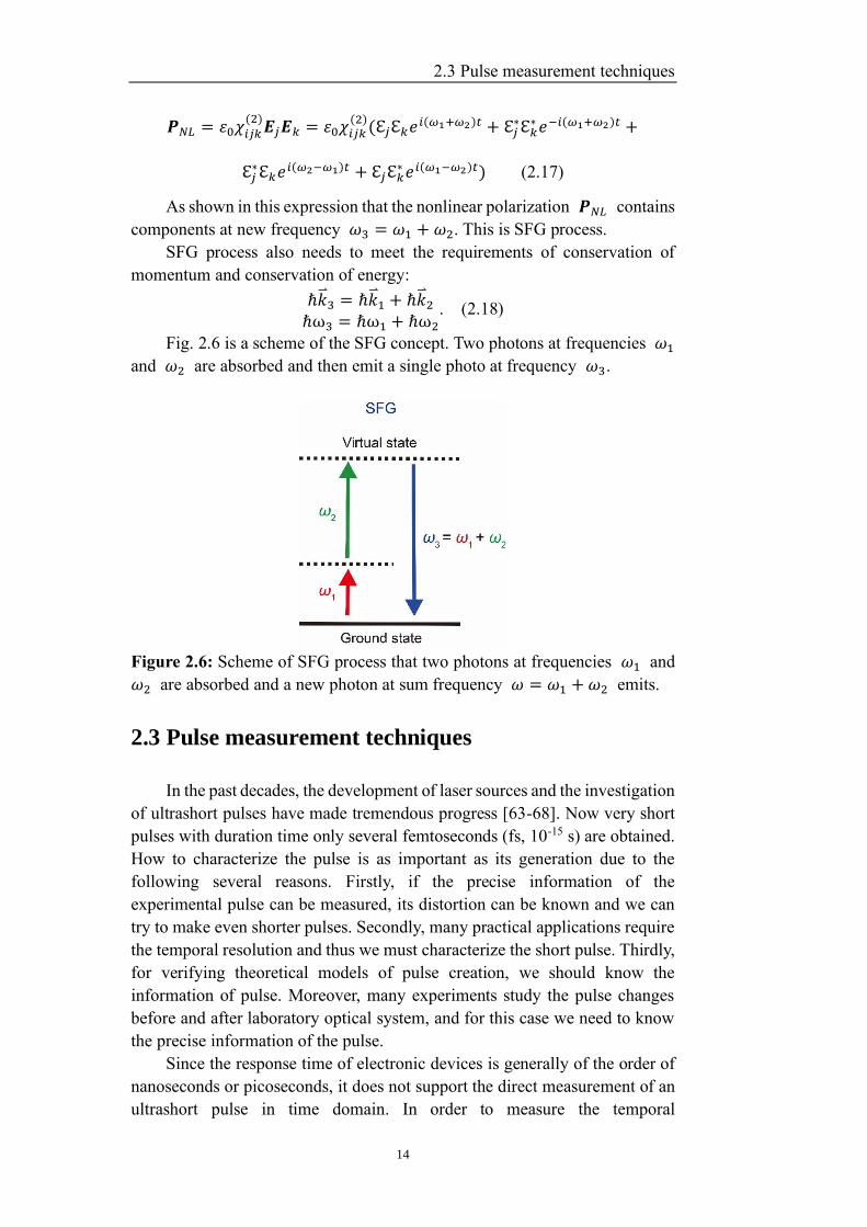
SFG process also needs to meet the requirements of conservation of
momentum and conservation of energy:
ℏ�⃑� 3 = ℏ�⃑� 1 + ℏ�⃑� 2ℏω3 = ℏω1 + ℏω2
. (2.18)
Fig. 2.6 is a scheme of the SFG concept. Two photons at frequencies 𝜔1
and 𝜔2 are absorbed and then emit a single photo at frequency 𝜔3.
Figure 2.6: Scheme of SFG process that two photons at frequencies 𝜔1 and
𝜔2 are absorbed and a new photon at sum frequency 𝜔 = 𝜔1 + 𝜔2 emits.
2.3 Pulse measurement techniques
In the past decades, the development of laser sources and the investigation
of ultrashort pulses have made tremendous progress [63-68]. Now very short
pulses with duration time only several femtoseconds (fs, 10-15 s) are obtained.
How to characterize the pulse is as important as its generation due to the
following several reasons. Firstly, if the precise information of the
experimental pulse can be measured, its distortion can be known and we can
try to make even shorter pulses. Secondly, many practical applications require
the temporal resolution and thus we must characterize the short pulse. Thirdly,
for verifying theoretical models of pulse creation, we should know the
information of pulse. Moreover, many experiments study the pulse changes
before and after laboratory optical system, and for this case we need to know
the precise information of the pulse.
Since the response time of electronic devices is generally of the order of
nanoseconds or picoseconds, it does not support the direct measurement of an
ultrashort pulse in time domain. In order to measure the temporal
Chapter 2 Fundamental physics
15
characteristics as short as few femtoseconds, we need an either shorter or the
same duration as the pulse itself. The only solution to directly measure a
femtosecond pulse in time domain, is to measure the pulse by itself. Up to now,
scientists have developed a vast variety of characterization techniques for the
measurement of ultrashort pulses [69, 70]. In this section, we will introduce
several popular techniques such as autocorrelator [71, 72], cross-correlator [73]
and FROG [74-81] (e.g., SHG FROG, XFROG, etc.).
2.3.1 Autocorrelator and cross-correlator
As discussed above, the pulse, like any light wave, can be defined by its
electric field as a function of time 𝐸(𝑡). Just consider the real part of 𝐸(𝑡)
and assume the pulse is linear polarized. The time-dependent component of
the pulse can be expressed as:
𝐸(𝑡) =1
2√𝐼(𝑡)𝑒𝑖[𝜔0𝑡−𝜙(𝑡)] (2.19)
where 𝐼(𝑡) is the time-dependent intensity, 𝜔0 the carrier frequency and
𝜑(𝑡) the time-dependent phase of the pulse.
The pulse instantaneous frequency is expressed as:
𝜔(𝑡) = 𝜔0 −𝑑𝜑
𝑑𝑡 (2.20)
The Fourier transform of 𝐸(𝑡) is:
�̃�(𝜔) = √𝐼(𝜔 − 𝜔0)𝑒�̃�(𝜔−𝜔0), (2.21)
where �̃�(𝜔) is the Fourier transform of 𝐸(𝑡), 𝐼(𝜔 − 𝜔0) is the intensity of
spectrum and �̃�(𝜔 − 𝜔0) is the spectral phase.
According to Eqs. (2.19) and (2.21), we must measure the intensity and
phase in time domain (or frequency domain) so that we can know the precise
information of 𝐸(𝑡) (or �̃�(𝜔)).
For the measurement of pulses in frequency domain, it is convenient to
use spectrometer. However, spectrometers can not measure the phase
information. For the measurement of pulses in time domain, the pulse is very
fast and much shorter than the time resolution of measurement devices. The
most widely used method to measure ultrashort pulse is the autocorrelator
proposed by Maier et al. (1966) [82]. As shown in Fig. 2.7, the test pulse passes
through a Michelson interferometer which divides the pulse into two replicas
with a relative time delay. These two replicas are focused into a 𝜒(2) NLO
crystal with an angle. We adjust the setup so that they can temporally and
spatially overlap inside the NLO crystal. The second harmonic signal
generated inside the NLO crystal comes from three sources: the SHG signal
from 𝐸(𝑡) , the SHG signal from 𝐸(𝑡 − 𝜏) and the SFG signal from both
𝐸(𝑡) and 𝐸(𝑡 − 𝜏) . According to the momentum conservation rule, these
three second harmonic signals propagate in different directions. We can use a
2.3 Pulse measurement techniques
16
spatial filter to block the two SHG signals and thus only the SFG signal can be
collected by photodiode device.
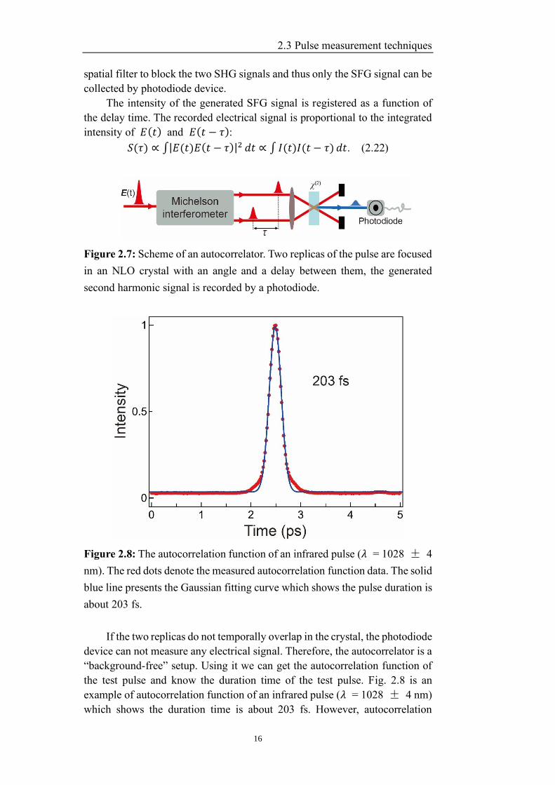
The intensity of the generated SFG signal is registered as a function of
the delay time. The recorded electrical signal is proportional to the integrated
intensity of 𝐸(𝑡) and 𝐸(𝑡 − 𝜏):
𝑆(𝜏) ∝ ∫|𝐸(𝑡)𝐸(𝑡 − 𝜏)|2 𝑑𝑡 ∝ ∫ 𝐼(𝑡)𝐼(𝑡 − 𝜏) 𝑑𝑡. (2.22)
Figure 2.7: Scheme of an autocorrelator. Two replicas of the pulse are focused
in an NLO crystal with an angle and a delay between them, the generated
second harmonic signal is recorded by a photodiode.
Figure 2.8: The autocorrelation function of an infrared pulse (𝜆 = 1028 ± 4
nm). The red dots denote the measured autocorrelation function data. The solid
blue line presents the Gaussian fitting curve which shows the pulse duration is
about 203 fs.
If the two replicas do not temporally overlap in the crystal, the photodiode
device can not measure any electrical signal. Therefore, the autocorrelator is a
“background-free” setup. Using it we can get the autocorrelation function of
the test pulse and know the duration time of the test pulse. Fig. 2.8 is an
example of autocorrelation function of an infrared pulse (𝜆 = 1028 ± 4 nm)
which shows the duration time is about 203 fs. However, autocorrelation
Chapter 2 Fundamental physics
17
function can not provide enough information on the pulse itself. For example,
two different pulses with different profile in time domain maybe gives the
same autocorrelation function and the autocorrelation function is always
symmetric in time. Moreover, the information below envelope can not be
measured by autocorrelator. In addition, we can not know the test pulse is
chirped or Fourier transform limited.
The autocorrelator device works well for simple pulses. However, it can
not measure complex pulses. For this case, we can use cross-correlation
method [73]. As shown in Fig. 2.9, the cross-correlation setup is nearly same
as the correlator. The only difference between them is that one replica is
replaced by a known reference short pulse 𝐸𝑟𝑒𝑓(𝑡).
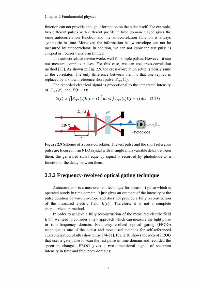
The recorded electrical signal is proportional to the integrated intensity
of 𝐸𝑟𝑒𝑓(𝑡) and 𝐸(𝑡 − 𝜏):
𝑆(𝜏) ∝ ∫|𝐸𝑟𝑒𝑓(𝑡)𝐸(𝑡 − 𝜏)|2𝑑𝑡 ∝ ∫ 𝐼𝑟𝑒𝑓(𝑡)𝐼(𝑡 − 𝜏) 𝑑𝑡. (2.23)
Figure 2.9 Scheme of a cross-correlator. The test pulse and the short reference
pulse are focused in an NLO crystal with an angle and a variable delay between
them, the generated sum-frequency signal is recorded by photodiode as a
function of the delay between them.
2.3.2 Frequency-resolved optical gating technique
Autocorrelator is a measurement technique for ultrashort pulse which is
operated purely in time domain. It just gives an estimate of the intensity or the
pulse duration of wave envelope and does not provide a fully reconstruction
of the measured electric field 𝐸(𝑡) . Therefore, it is not a complete
characterization method.
In order to achieve a fully reconstruction of the measured electric field
𝐸(𝑡), we need to consider a new approach which can measure the light pulse
in time-frequency domain. Frequency-resolved optical gating (FROG)
technique is one of the oldest and most used methods for self-referenced
characterization of ultrashort pulse [74-81]. Fig. 2.10 shows the idea of FROG
that uses a gate pulse to scan the test pulse in time domain and recorded the
spectrum changes. FROG gives a two-dimensional signal of spectrum
intensity in time and frequency domains:
2.3 Pulse measurement techniques
18
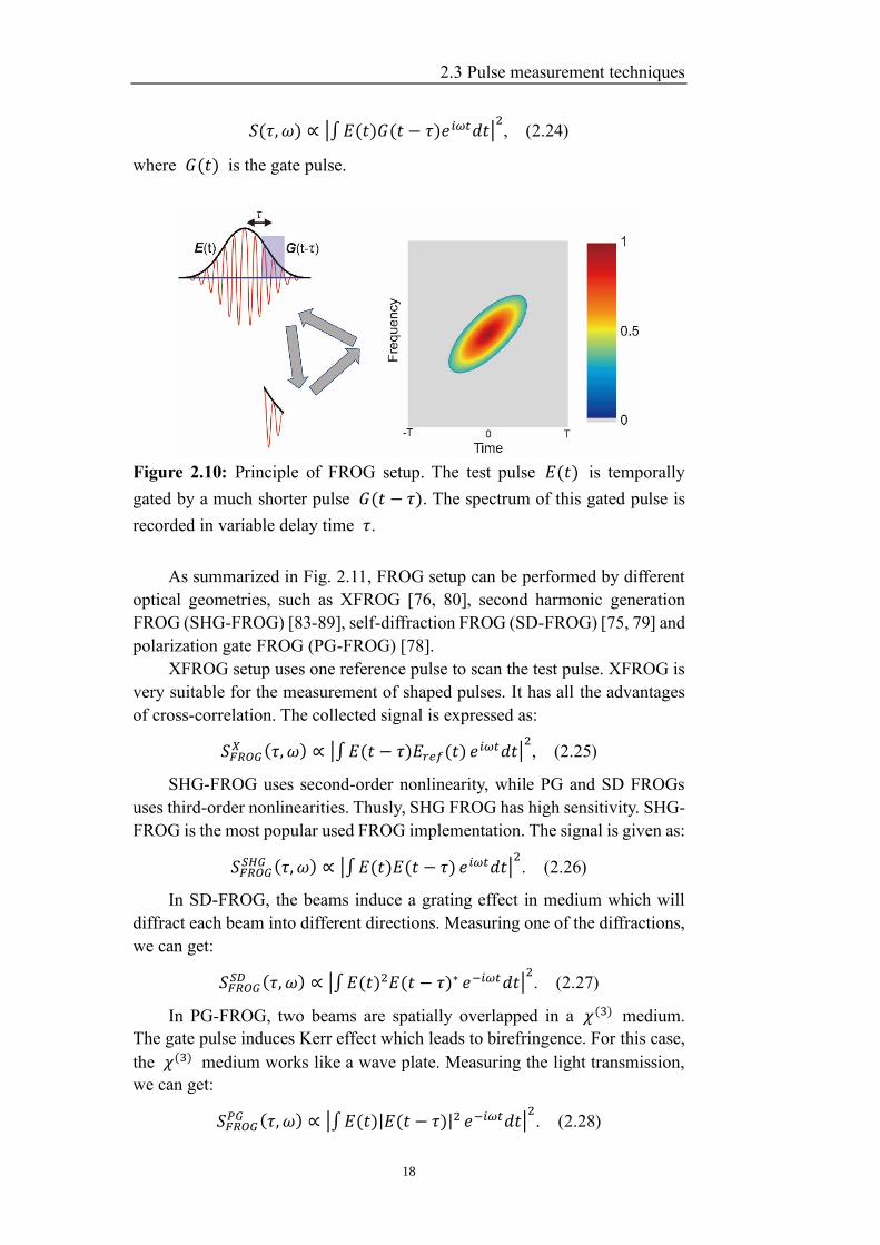
𝑆(𝜏, 𝜔) ∝ |∫𝐸(𝑡)𝐺(𝑡 − 𝜏)𝑒𝑖𝜔𝑡𝑑𝑡|2, (2.24)
where 𝐺(𝑡) is the gate pulse.
Figure 2.10: Principle of FROG setup. The test pulse 𝐸(𝑡) is temporally
gated by a much shorter pulse 𝐺(𝑡 − 𝜏). The spectrum of this gated pulse is
recorded in variable delay time 𝜏.
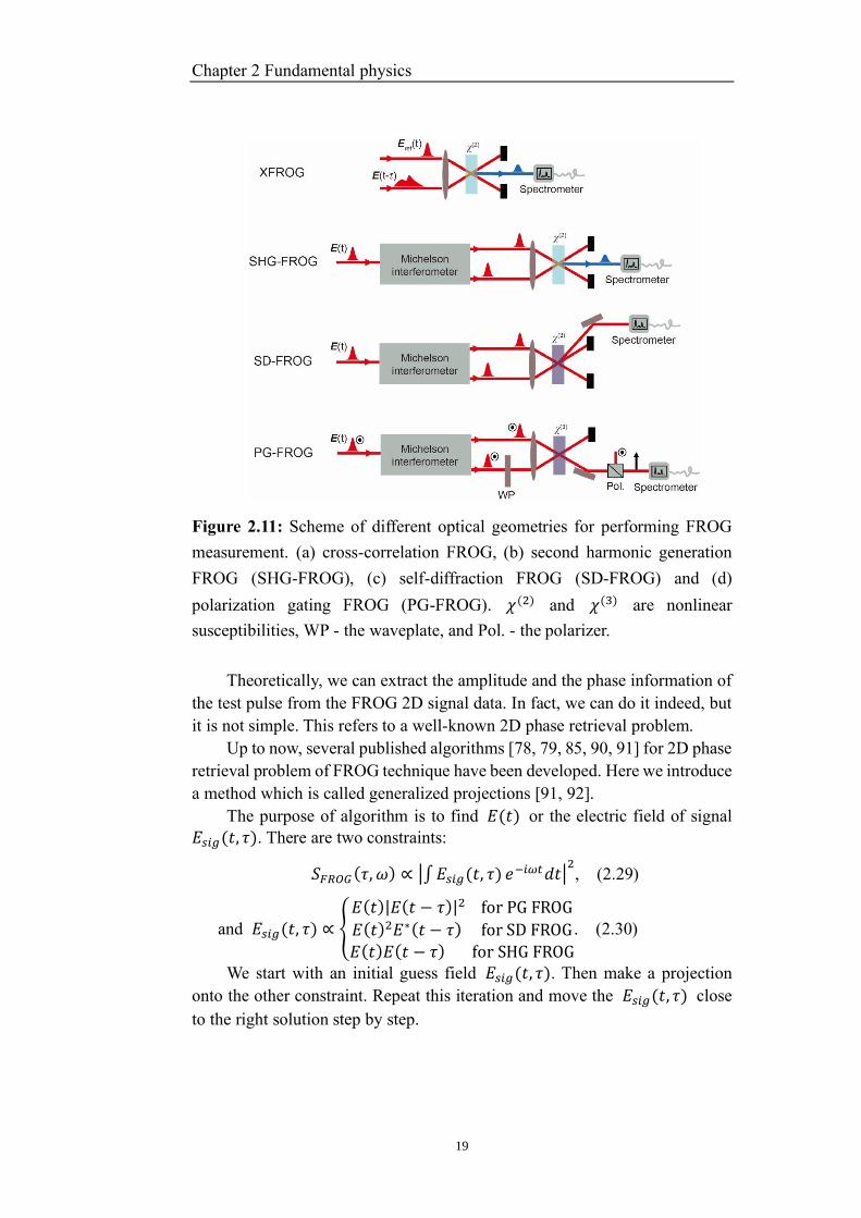
As summarized in Fig. 2.11, FROG setup can be performed by different
optical geometries, such as XFROG [76, 80], second harmonic generation
FROG (SHG-FROG) [83-89], self-diffraction FROG (SD-FROG) [75, 79] and
polarization gate FROG (PG-FROG) [78].
XFROG setup uses one reference pulse to scan the test pulse. XFROG is
very suitable for the measurement of shaped pulses. It has all the advantages
of cross-correlation. The collected signal is expressed as:
𝑆𝐹𝑅𝑂𝐺𝑋 (𝜏, 𝜔) ∝ |∫𝐸(𝑡 − 𝜏)𝐸𝑟𝑒𝑓(𝑡) 𝑒𝑖𝜔𝑡𝑑𝑡|
2, (2.25)
SHG-FROG uses second-order nonlinearity, while PG and SD FROGs
uses third-order nonlinearities. Thusly, SHG FROG has high sensitivity. SHG-
FROG is the most popular used FROG implementation. The signal is given as:
𝑆𝐹𝑅𝑂𝐺𝑆𝐻𝐺 (𝜏, 𝜔) ∝ |∫𝐸(𝑡)𝐸(𝑡 − 𝜏) 𝑒𝑖𝜔𝑡𝑑𝑡|
2. (2.26)
In SD-FROG, the beams induce a grating effect in medium which will
diffract each beam into different directions. Measuring one of the diffractions,
we can get:
𝑆𝐹𝑅𝑂𝐺𝑆𝐷 (𝜏, 𝜔) ∝ |∫𝐸(𝑡)2𝐸(𝑡 − 𝜏)∗ 𝑒−𝑖𝜔𝑡𝑑𝑡|
2. (2.27)
In PG-FROG, two beams are spatially overlapped in a 𝜒(3) medium.
The gate pulse induces Kerr effect which leads to birefringence. For this case,
the 𝜒(3) medium works like a wave plate. Measuring the light transmission,
we can get:
𝑆𝐹𝑅𝑂𝐺𝑃𝐺 (𝜏, 𝜔) ∝ |∫𝐸(𝑡)|𝐸(𝑡 − 𝜏)|2 𝑒−𝑖𝜔𝑡𝑑𝑡|
2. (2.28)
Chapter 2 Fundamental physics
19
Figure 2.11: Scheme of different optical geometries for performing FROG
measurement. (a) cross-correlation FROG, (b) second harmonic generation
FROG (SHG-FROG), (c) self-diffraction FROG (SD-FROG) and (d)
polarization gating FROG (PG-FROG). 𝜒(2) and 𝜒(3) are nonlinear
susceptibilities, WP - the waveplate, and Pol. - the polarizer.
Theoretically, we can extract the amplitude and the phase information of
the test pulse from the FROG 2D signal data. In fact, we can do it indeed, but
it is not simple. This refers to a well-known 2D phase retrieval problem.
Up to now, several published algorithms [78, 79, 85, 90, 91] for 2D phase
retrieval problem of FROG technique have been developed. Here we introduce
a method which is called generalized projections [91, 92].
The purpose of algorithm is to find 𝐸(𝑡) or the electric field of signal
𝐸𝑠𝑖𝑔(𝑡, 𝜏). There are two constraints:
𝑆𝐹𝑅𝑂𝐺(𝜏, 𝜔) ∝ |∫𝐸𝑠𝑖𝑔(𝑡, 𝜏) 𝑒−𝑖𝜔𝑡𝑑𝑡|2, (2.29)
and 𝐸𝑠𝑖𝑔(𝑡, 𝜏) ∝ {𝐸(𝑡)|𝐸(𝑡 − 𝜏)|2 for PG FROG
𝐸(𝑡)2𝐸∗(𝑡 − 𝜏) for SD FROG
𝐸(𝑡)𝐸(𝑡 − 𝜏) for SHG FROG
. (2.30)
We start with an initial guess field 𝐸𝑠𝑖𝑔(𝑡, 𝜏). Then make a projection
onto the other constraint. Repeat this iteration and move the 𝐸𝑠𝑖𝑔(𝑡, 𝜏) close
to the right solution step by step.
2.4 Optical parametric amplifier
20
2.4 Optical parametric amplifier
Optical parametric amplifier (OPA) exploiting second-order nonlinearity,
represents an easy way to transfer energy from a high intensity pump pulse at
a fixed frequency to weak signal/idler pulses at variable frequencies. In thus
OPA provides a tunable laser source over a broad frequency range [93-100].
Non-collinear OPA can act as broadband amplifiers under suitable conditions
and can thus shorten the achievable pulse duration to generate tunable
ultrashort laser pulses. Due to these unique advantages, OPAs are nowadays
widely used by not only physicists but also chemists and biologists.
2.4.1 Phase matching
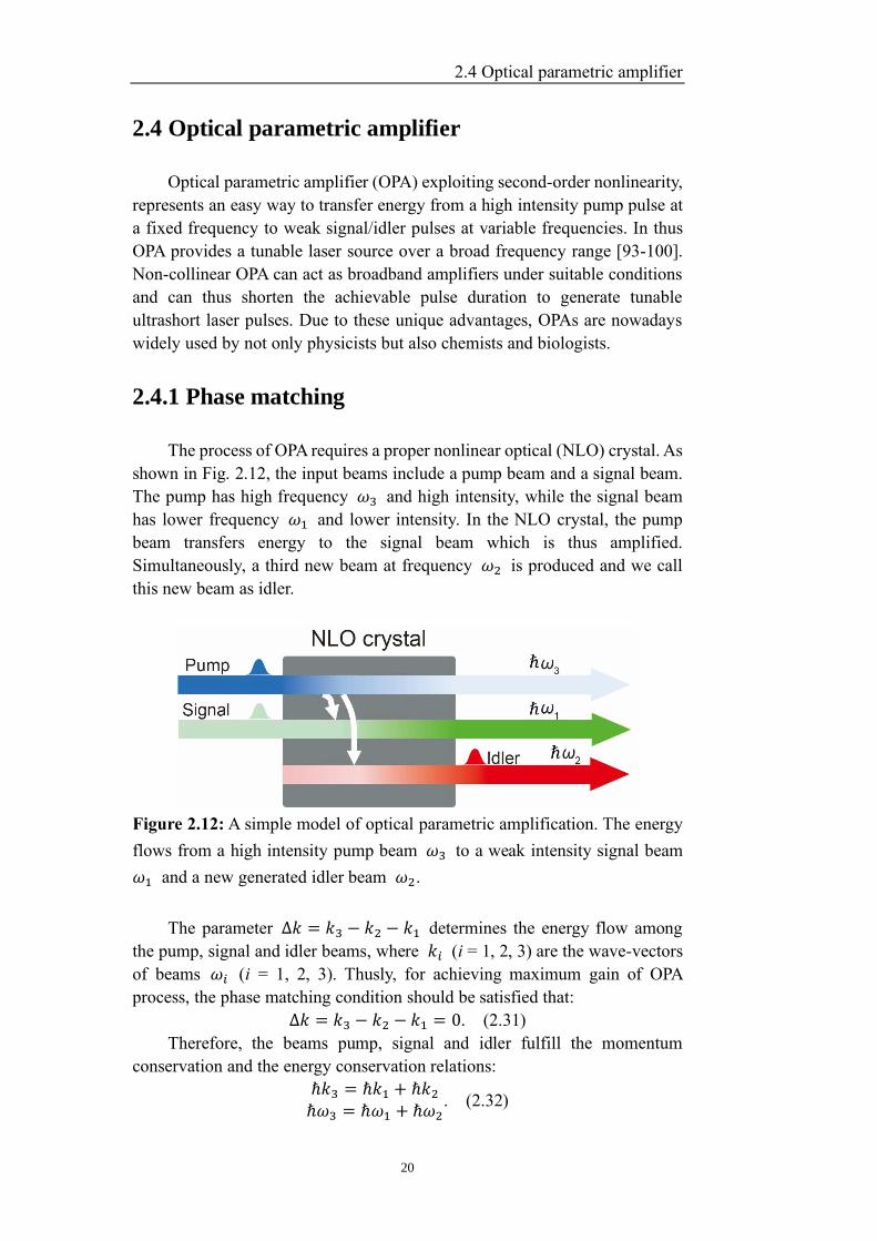
The process of OPA requires a proper nonlinear optical (NLO) crystal. As
shown in Fig. 2.12, the input beams include a pump beam and a signal beam.
The pump has high frequency 𝜔3 and high intensity, while the signal beam
has lower frequency 𝜔1 and lower intensity. In the NLO crystal, the pump
beam transfers energy to the signal beam which is thus amplified.
Simultaneously, a third new beam at frequency 𝜔2 is produced and we call
this new beam as idler.
Figure 2.12: A simple model of optical parametric amplification. The energy
flows from a high intensity pump beam 𝜔3 to a weak intensity signal beam
𝜔1 and a new generated idler beam 𝜔2.
The parameter ∆𝑘 = 𝑘3 − 𝑘2 − 𝑘1 determines the energy flow among
the pump, signal and idler beams, where 𝑘𝑖 (i = 1, 2, 3) are the wave-vectors
of beams 𝜔𝑖 (i = 1, 2, 3). Thusly, for achieving maximum gain of OPA
process, the phase matching condition should be satisfied that:
∆𝑘 = 𝑘3 − 𝑘2 − 𝑘1 = 0. (2.31)
Therefore, the beams pump, signal and idler fulfill the momentum
conservation and the energy conservation relations:
ℏ𝑘3 = ℏ𝑘1 + ℏ𝑘2
ℏ𝜔3 = ℏ𝜔1 + ℏ𝜔2. (2.32)
Chapter 2 Fundamental physics
21
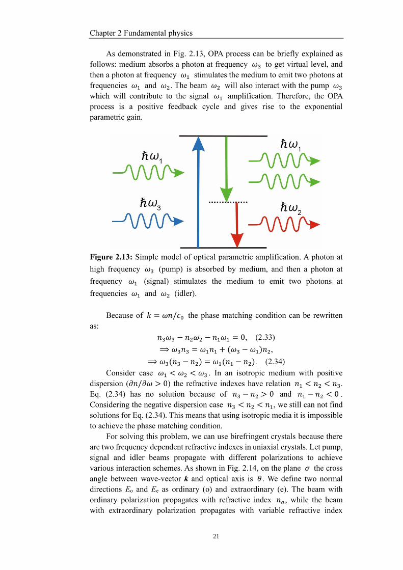
As demonstrated in Fig. 2.13, OPA process can be briefly explained as
follows: medium absorbs a photon at frequency 𝜔3 to get virtual level, and
then a photon at frequency 𝜔1 stimulates the medium to emit two photons at
frequencies 𝜔1 and 𝜔2. The beam 𝜔2 will also interact with the pump 𝜔3
which will contribute to the signal 𝜔1 amplification. Therefore, the OPA
process is a positive feedback cycle and gives rise to the exponential
parametric gain.
Figure 2.13: Simple model of optical parametric amplification. A photon at
high frequency 𝜔3 (pump) is absorbed by medium, and then a photon at
frequency 𝜔1 (signal) stimulates the medium to emit two photons at
frequencies 𝜔1 and 𝜔2 (idler).
Because of 𝑘 = 𝜔𝑛/𝑐0 the phase matching condition can be rewritten
as:
𝑛3𝜔3 − 𝑛2𝜔2 − 𝑛1𝜔1 = 0, (2.33)
⟹ 𝜔3𝑛3 = 𝜔1𝑛1 + (𝜔3 − 𝜔1)𝑛2,
⟹ 𝜔3(𝑛3 − 𝑛2) = 𝜔1(𝑛1 − 𝑛2). (2.34)
Consider case 𝜔1 < 𝜔2 < 𝜔3 . In an isotropic medium with positive
dispersion (𝜕𝑛/𝜕𝜔 > 0) the refractive indexes have relation 𝑛1 < 𝑛2 < 𝑛3.
Eq. (2.34) has no solution because of 𝑛3 − 𝑛2 > 0 and 𝑛1 − 𝑛2 < 0 .
Considering the negative dispersion case 𝑛3 < 𝑛2 < 𝑛1, we still can not find
solutions for Eq. (2.34). This means that using isotropic media it is impossible
to achieve the phase matching condition.
For solving this problem, we can use birefringent crystals because there
are two frequency dependent refractive indexes in uniaxial crystals. Let pump,
signal and idler beams propagate with different polarizations to achieve
various interaction schemes. As shown in Fig. 2.14, on the plane 𝜎 the cross
angle between wave-vector k and optical axis is 𝜃 . We define two normal
directions Eo and Ee as ordinary (o) and extraordinary (e). The beam with
ordinary polarization propagates with refractive index 𝑛𝑜 , while the beam
with extraordinary polarization propagates with variable refractive index
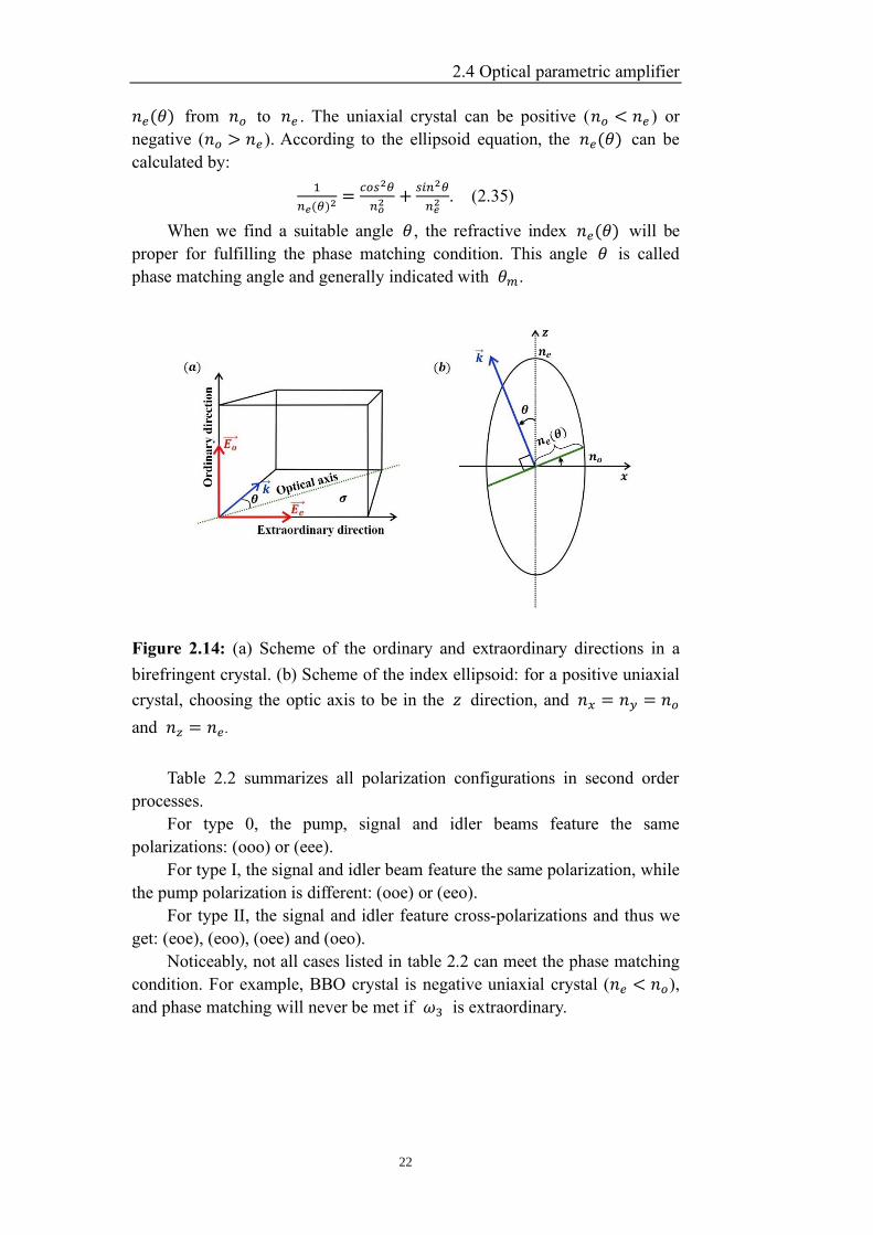
2.4 Optical parametric amplifier
22
𝑛𝑒(𝜃) from 𝑛𝑜 to 𝑛𝑒 . The uniaxial crystal can be positive (𝑛𝑜 < 𝑛𝑒 ) or
negative (𝑛𝑜 > 𝑛𝑒 ). According to the ellipsoid equation, the 𝑛𝑒(𝜃) can be
calculated by:
1
𝑛𝑒(𝜃)2=
𝑐𝑜𝑠2𝜃
𝑛𝑜2 +
𝑠𝑖𝑛2𝜃
𝑛𝑒2 . (2.35)
When we find a suitable angle 𝜃 , the refractive index 𝑛𝑒(𝜃) will be
proper for fulfilling the phase matching condition. This angle 𝜃 is called
phase matching angle and generally indicated with 𝜃𝑚.
Figure 2.14: (a) Scheme of the ordinary and extraordinary directions in a
birefringent crystal. (b) Scheme of the index ellipsoid: for a positive uniaxial
crystal, choosing the optic axis to be in the 𝑧 direction, and 𝑛𝑥 = 𝑛𝑦 = 𝑛𝑜
and 𝑛𝑧 = 𝑛𝑒.
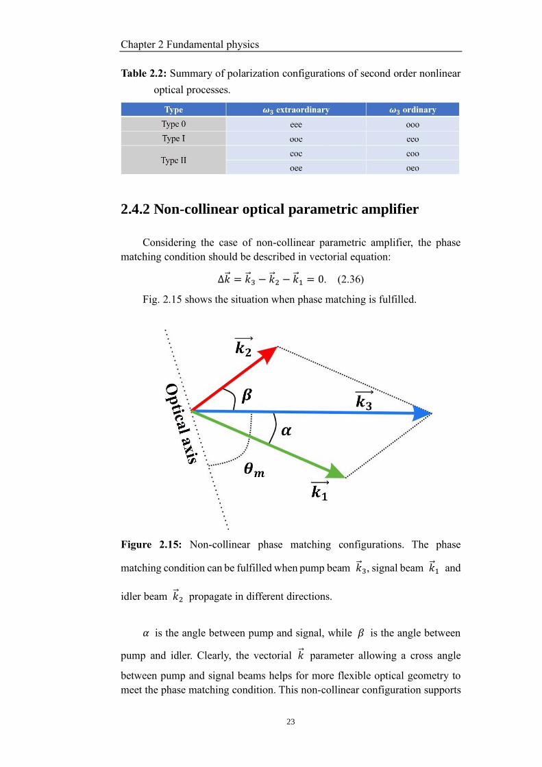
Table 2.2 summarizes all polarization configurations in second order
processes.
For type 0, the pump, signal and idler beams feature the same
polarizations: (ooo) or (eee).
For type I, the signal and idler beam feature the same polarization, while
the pump polarization is different: (ooe) or (eeo).
For type II, the signal and idler feature cross-polarizations and thus we
get: (eoe), (eoo), (oee) and (oeo).
Noticeably, not all cases listed in table 2.2 can meet the phase matching
condition. For example, BBO crystal is negative uniaxial crystal (𝑛𝑒 < 𝑛𝑜),
and phase matching will never be met if 𝜔3 is extraordinary.
Chapter 2 Fundamental physics
23
Table 2.2: Summary of polarization configurations of second order nonlinear
optical processes.
2.4.2 Non-collinear optical parametric amplifier
Considering the case of non-collinear parametric amplifier, the phase
matching condition should be described in vectorial equation:
∆�⃑� = �⃑� 3 − �⃑� 2 − �⃑� 1 = 0. (2.36)
Fig. 2.15 shows the situation when phase matching is fulfilled.
Figure 2.15: Non-collinear phase matching configurations. The phase
matching condition can be fulfilled when pump beam �⃑� 3, signal beam �⃑� 1 and
idler beam �⃑� 2 propagate in different directions.
𝛼 is the angle between pump and signal, while 𝛽 is the angle between
pump and idler. Clearly, the vectorial �⃑� parameter allowing a cross angle
between pump and signal beams helps for more flexible optical geometry to
meet the phase matching condition. This non-collinear configuration supports
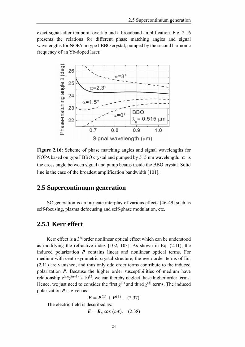
2.5 Supercontinuum generation
24
exact signal-idler temporal overlap and a broadband amplification. Fig. 2.16
presents the relations for different phase matching angles and signal
wavelengths for NOPA in type I BBO crystal, pumped by the second harmonic
frequency of an Yb-doped laser.
Figure 2.16: Scheme of phase matching angles and signal wavelengths for
NOPA based on type I BBO crystal and pumped by 515 nm wavelength. 𝛼 is
the cross angle between signal and pump beams inside the BBO crystal. Solid
line is the case of the broadest amplification bandwidth [101].
2.5 Supercontinuum generation
SC generation is an intricate interplay of various effects [46-49] such as
self-focusing, plasma defocusing and self-phase modulation, etc.
2.5.1 Kerr effect
Kerr effect is a 3rd order nonlinear optical effect which can be understood
as modifying the refractive index [102, 103]. As shown in Eq. (2.11), the
induced polarization P contains linear and nonlinear optical terms. For
medium with centrosymmetric crystal structure, the even order terms of Eq.
(2.11) are vanished, and thus only odd order terms contribute to the induced
polarization P. Because the higher order susceptibilities of medium have
relationship χ(n)/χ(n+1) ≈ 1012, we can thereby neglect these higher order terms.
Hence, we just need to consider the first χ(1) and third χ(3) terms. The induced
polarization P is given as:
𝑷 = 𝑷(1) + 𝑷(3). (2.37)
The electric field is described as:
𝑬 = 𝑬𝜔𝑐𝑜𝑠 (𝜔𝑡). (2.38)
Chapter 2 Fundamental physics
25
Thusly, the polarization P can be expressed as:
𝑷 = 휀0 (𝜒(1) +3
4𝜒(3)|𝑬𝜔|2)𝑬𝜔 𝑐𝑜𝑠(𝜔𝑡). (2.39)
Observing this Eq. (2.39), it looks like we can rewrite the χ into two
components, a linear susceptibility 𝜒𝐿 and an additional nonlinear term 𝜒𝑁𝐿:
𝜒 = 𝜒𝐿 + 𝜒𝑁𝐿 = 𝜒(1) +3𝜒(3)
4|𝑬𝜔|2. (2.40)
In an isotropic material, 𝜒(1) and refractive index 𝑛0 of material follow
this relationship:
𝑛0 = √1 + 𝜒(1) = √1 + 𝜒𝐿 . (2.41)
Now refractive index n can be described as:
𝑛 = √1 + 𝜒 = √1 + 𝜒𝐿 + 𝜒𝑁𝐿 ≃ 𝑛0(1 +1
2𝑛02 𝜒𝑁𝐿). (2.42)
Using Taylor expansion since 𝜒𝑁𝐿 ≪ 𝑛02 , we can get an intensity
dependent refractive index:
𝑛 = 𝑛0 +3𝜒(3)
8𝑛0|𝑬𝜔|2 = 𝑛0 + 𝑛2𝐼, (2.43)
where 𝑛2 is the 2nd order nonlinear refractive index, and I is the light intensity.
From this equation, we can know that the refractive index change is 𝑛2𝐼
which is proportional to the light intensity. As discussed above, the 3rd order
nonlinear optics will contribute to the intensity-dependent refractive index.
This effect is called as Kerr effect.
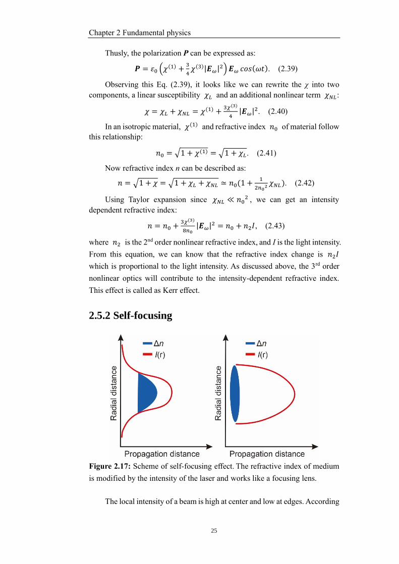
2.5.2 Self-focusing
Figure 2.17: Scheme of self-focusing effect. The refractive index of medium
is modified by the intensity of the laser and works like a focusing lens.
The local intensity of a beam is high at center and low at edges. According
2.5 Supercontinuum generation
26
to Eq. (2.43), we know that the change of refractive index is in direct
proportional to the local intensity. Therefore, medium works like a lens, which
can self-focus the incident beam. This nonlinear effect is called “self-focusing”
which is a natural phenomenon resulted from Kerr effect [104]. Fig. 2.17 is a
schematic diagram of self-focusing.
Self-focusing effect is determined by the input beam’s power and occurs
only if the beam power is high enough reaching the critical power [104-107].
J.H. Marburger et al. calculated the critical power Pcr for a standard Gaussian
beam [104, 107]:
𝑃cr =3.72𝜆0
2
8𝜋𝑛0𝑛2, (2.44)
where λ0 is the laser central wavelength.
Eq. (2.44) is valid for Gaussian beam shape. When the coefficient is equal
to 3.72 [105], diffraction and self-focusing effects are balanced. If the beams
feature other shapes, the coefficient 3.72 should be replaced by other values.
It should be noted that the critical power given by Eq. (2.44) is proper for both
ultrashort pulses and continuous wave lasers. However, for ultrashort pulses,
the peak power is very high and thus we should consider many other optical
effects such as group velocity dispersion, plasma defocusing and multiphoton
absorption. In this case, self-focusing process will be very complex.
If input beam power is higher than 𝑃cr, the collimated Gaussian beam
will self-focus at a distance [104]:
zsf =0.367zR
√[(P
Pcr)
12−0.852]2−0.0219
, (2.45)
which is called the nonlinear focus. Here zR is the diffraction length. This
equation is derived for the continuous wave laser beam, but it also gives an
accurate approximation in the case of ultrafast laser pulses as well.
2.5.3 Plasma defocusing
When the intensity of laser pulse is high enough, it will ionize the medium
and generate plasma. The generation of plasma can cause local reduction in
the refraction index. This effect is called “plasma defocusing” and the
refraction index is expressed as [108]:
𝑛 ≃ 𝑛0 −𝜌(𝑟,𝑡)
2𝜌𝑐, (2.46)
where 𝜌(𝑟, 𝑡) is the density of free electrons and 𝜌𝑐 is the critical plasma
density. The parameter 𝜌𝑐 is defined as
𝜌𝑐 ≡ 𝜖0𝑚𝑒𝜔02/𝑒2, (2.47)
where 𝜖0 is the permittivity of vacuum, 𝑚𝑒 - the electron mass and 𝑒 - the
electron charge.
Chapter 2 Fundamental physics
27
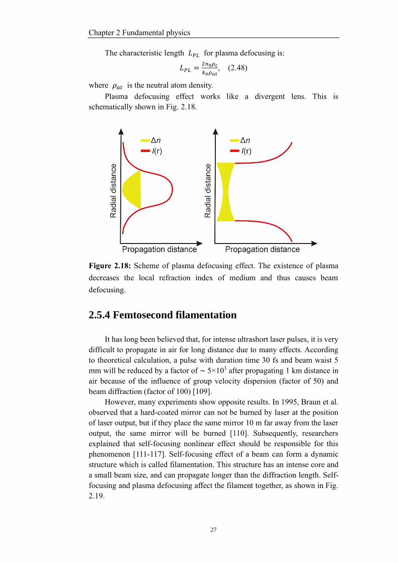
The characteristic length 𝐿𝑃𝐿 for plasma defocusing is:
𝐿𝑃𝐿 =2𝑛0𝜌𝑐
𝑘0𝜌𝑎𝑡, (2.48)
where 𝜌𝑎𝑡 is the neutral atom density.
Plasma defocusing effect works like a divergent lens. This is
schematically shown in Fig. 2.18.
Figure 2.18: Scheme of plasma defocusing effect. The existence of plasma
decreases the local refraction index of medium and thus causes beam
defocusing.
2.5.4 Femtosecond filamentation
It has long been believed that, for intense ultrashort laser pulses, it is very
difficult to propagate in air for long distance due to many effects. According
to theoretical calculation, a pulse with duration time 30 fs and beam waist 5
mm will be reduced by a factor of ∼ 5×10³ after propagating 1 km distance in
air because of the influence of group velocity dispersion (factor of 50) and
beam diffraction (factor of 100) [109].
However, many experiments show opposite results. In 1995, Braun et al.
observed that a hard-coated mirror can not be burned by laser at the position
of laser output, but if they place the same mirror 10 m far away from the laser
output, the same mirror will be burned [110]. Subsequently, researchers
explained that self-focusing nonlinear effect should be responsible for this
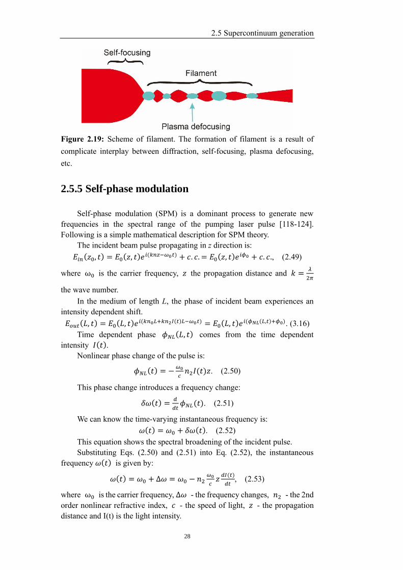
phenomenon [111-117]. Self-focusing effect of a beam can form a dynamic
structure which is called filamentation. This structure has an intense core and
a small beam size, and can propagate longer than the diffraction length. Self-
focusing and plasma defocusing affect the filament together, as shown in Fig.
2.19.
2.5 Supercontinuum generation
28
Figure 2.19: Scheme of filament. The formation of filament is a result of
complicate interplay between diffraction, self-focusing, plasma defocusing,
etc.
2.5.5 Self-phase modulation
Self-phase modulation (SPM) is a dominant process to generate new
frequencies in the spectral range of the pumping laser pulse [118-124].
Following is a simple mathematical description for SPM theory.
The incident beam pulse propagating in z direction is:
𝐸𝑖𝑛(𝑧0, 𝑡) = 𝐸0(𝑧, 𝑡)𝑒𝑖(𝑘𝑛𝑧−𝜔0𝑡) + 𝑐. 𝑐. = 𝐸0(𝑧, 𝑡)𝑒
𝑖𝜙0 + 𝑐. 𝑐., (2.49)
where ω0 is the carrier frequency, 𝑧 the propagation distance and 𝑘 =𝜆
2𝜋
the wave number.
In the medium of length L, the phase of incident beam experiences an
intensity dependent shift.
𝐸𝑜𝑢𝑡(𝐿, 𝑡) = 𝐸0(𝐿, 𝑡)𝑒𝑖(𝑘𝑛0𝐿+𝑘𝑛2𝐼(𝑡)𝐿−𝜔0𝑡) = 𝐸0(𝐿, 𝑡)𝑒
𝑖(𝜙𝑁𝐿(𝐿,𝑡)+𝜙0). (3.16)
Time dependent phase 𝜙𝑁𝐿(𝐿, 𝑡) comes from the time dependent
intensity 𝐼(𝑡).
Nonlinear phase change of the pulse is:
𝜙𝑁𝐿(𝑡) = −𝜔0
𝑐𝑛2𝐼(𝑡)𝑧. (2.50)
This phase change introduces a frequency change:
𝛿𝜔(𝑡) =𝑑
𝑑𝑡𝜙𝑁𝐿(𝑡). (2.51)
We can know the time-varying instantaneous frequency is:
𝜔(𝑡) = 𝜔0 + 𝛿𝜔(𝑡). (2.52)
This equation shows the spectral broadening of the incident pulse.
Substituting Eqs. (2.50) and (2.51) into Eq. (2.52), the instantaneous
frequency 𝜔(𝑡) is given by:
𝜔(𝑡) = 𝜔0 + ∆𝜔 = 𝜔0 − 𝑛2𝜔0
𝑐𝑧
𝑑𝐼(𝑡)
𝑑𝑡, (2.53)
where ω0 is the carrier frequency, ∆𝜔 - the frequency changes, 𝑛2 - the 2nd
order nonlinear refractive index, 𝑐 - the speed of light, 𝑧 - the propagation
distance and I(t) is the light intensity.
Chapter 2 Fundamental physics
29
The first term 𝜔0 in Eq. (2.53) is a constant which is determined by the
frequency of pumping laser. The second term ∆𝜔 is responsible to the
spectral broadening and only this term determines whether the instantaneous
frequency 𝜔(𝑡) shows blue-shifting or red-shifting. More specifically, it can
only be controlled by 𝑑𝐼(𝑡)
𝑑𝑡 because the other parameter 𝑛2
𝜔0
𝑐𝑧 is positive.
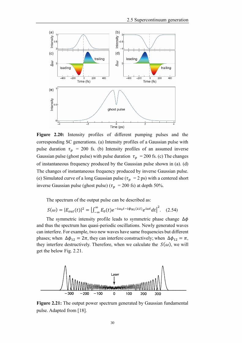
We first consider the general case where SC generation is performed using
conventional Gaussian shaped pumping pulse, as shown in Fig. 2.20(a). The
𝑑𝐼(𝑡)
𝑑𝑡 value features positive sign (+) during the front half time of the Gaussian
pulse, while the latter half part of the pulse results in minus (-) 𝑑𝐼(𝑡)
𝑑𝑡 value.
Thus, the instantaneous frequency 𝜔(𝑡) caused by SPM effect features a
negative frequency shift at the leading front of the pulse and a positive
frequency shift at the trailing front of the pulse, as depicted in Fig. 2.20(c). It
means the SC generated by a Gaussian pulse is positively chirped.
Now assume a case that we can obtain an inverse Gaussian pulse (see Fig.
2.20(b)) and use it to perform SC generation. We call this pulse a ghost pulse
since negative intensities are not possible. A more formal definition is that
ghost pulse is a short laser pulse (as normally defined), but with negative
intensity in a quasi constant intensity field. Ideally, the intensity of the constant
field is constant forever. Thus the (negative) intensity of the ghost pulse is
limited by the intensity of the constant field. In reality, the constant field is to
a very good approximation constant on the time-scale of the ghost pulse.
According to Eq. (2.53), this ghost pulse shown in Fig. 2.20(b) should
give rise to opposite 𝑑𝐼(𝑡)
𝑑𝑡 comparing with the case caused by Gaussian pulse.
Namely, the leading part of this ghost pulse will generate blue-shifted new
frequency components while the trailing part will produce red-shifted
frequency components, as depicted in Fig. 2.20(d). Therefore, using such kind
of ghost driving pulse (Fig. 2.20(b)) it should be able to generate negatively
chirped SC.
However, it is impossible to obtain a ghost pulse practically. An
achievable solution is that on top of a rather flat intensity level a ghost pulse
describes the sudden intensity loss, as shown in Fig. 2.20(e). The intensity
deduction in this proposed approach can be achieved by different nonlinear
effects, such as Kerr effect, SFG effect, etc.
2.5 Supercontinuum generation
30
Figure 2.20: Intensity profiles of different pumping pulses and the
corresponding SC generations. (a) Intensity profiles of a Gaussian pulse with
pulse duration 𝜏𝑝 = 200 fs. (b) Intensity profiles of an assumed inverse
Gaussian pulse (ghost pulse) with pulse duration 𝜏𝑝 = 200 fs. (c) The changes
of instantaneous frequency produced by the Gaussian pulse shown in (a). (d)
The changes of instantaneous frequency produced by inverse Gaussian pulse.
(e) Simulated curve of a long Gaussian pulse (𝜏𝑝 = 2 ps) with a centered short
inverse Gaussian pulse (ghost pulse) (𝜏𝑝 = 200 fs) at depth 50%.
The spectrum of the output pulse can be described as:
𝑆(𝜔) = |𝐸𝑜𝑢𝑡(𝑡)|2 = |∫ 𝐸0(𝑡)𝑒
−𝑖𝜔0𝑡−𝑖𝜙𝑁𝐿(𝑧,𝑡)𝑒𝑖𝜔𝑡𝑑𝑡∞
−∞|2. (2.54)
The symmetric intensity profile leads to symmetric phase change ∆𝜙
and thus the spectrum has quasi-periodic oscillations. Newly generated waves
can interfere. For example, two new waves have same frequencies but different
phases; when ∆𝜙12 = 2𝜋, they can interfere constructively; when ∆𝜙12 = 𝜋,
they interfere destructively. Therefore, when we calculate the 𝑆(𝜔), we will
get the below Fig. 2.21.
Figure 2.21: The output power spectrum generated by Gaussian fundamental
pulse. Adapted from [18].
Chapter 2 Fundamental physics
31
In this spectrum 𝑆(𝜔), the red-shifted and blue-shifted parts are Stokes
and anti-Stokes broadenings respectively. The Stokes and anti-Stokes parts are
symmetric.
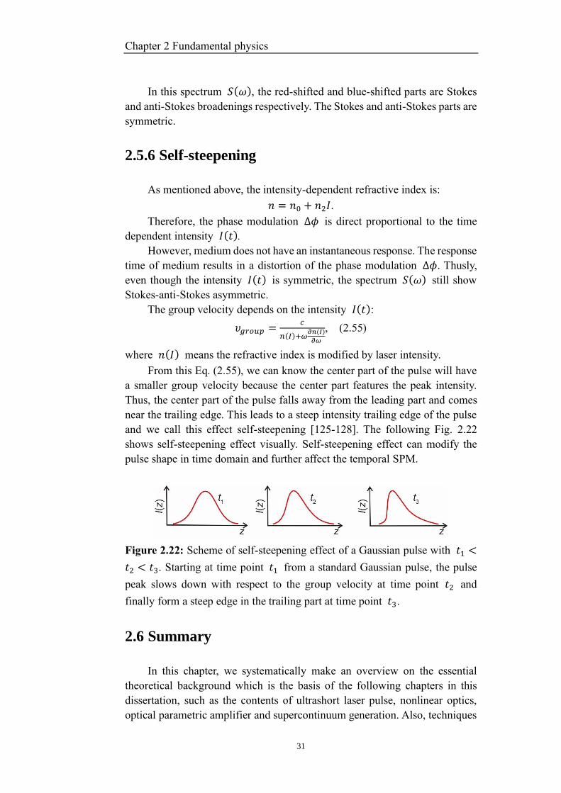
2.5.6 Self-steepening
As mentioned above, the intensity-dependent refractive index is:
𝑛 = 𝑛0 + 𝑛2𝐼.
Therefore, the phase modulation ∆𝜙 is direct proportional to the time
dependent intensity 𝐼(𝑡).
However, medium does not have an instantaneous response. The response
time of medium results in a distortion of the phase modulation ∆𝜙. Thusly,
even though the intensity 𝐼(𝑡) is symmetric, the spectrum 𝑆(𝜔) still show
Stokes-anti-Stokes asymmetric.
The group velocity depends on the intensity 𝐼(𝑡):
𝜐𝑔𝑟𝑜𝑢𝑝 =𝑐
𝑛(𝐼)+𝜔𝜕𝑛(𝐼)
𝜕𝜔
, (2.55)
where 𝑛(𝐼) means the refractive index is modified by laser intensity.
From this Eq. (2.55), we can know the center part of the pulse will have
a smaller group velocity because the center part features the peak intensity.
Thus, the center part of the pulse falls away from the leading part and comes
near the trailing edge. This leads to a steep intensity trailing edge of the pulse
and we call this effect self-steepening [125-128]. The following Fig. 2.22
shows self-steepening effect visually. Self-steepening effect can modify the
pulse shape in time domain and further affect the temporal SPM.
Figure 2.22: Scheme of self-steepening effect of a Gaussian pulse with 𝑡1 <
𝑡2 < 𝑡3. Starting at time point 𝑡1 from a standard Gaussian pulse, the pulse
peak slows down with respect to the group velocity at time point 𝑡2 and
finally form a steep edge in the trailing part at time point 𝑡3.
2.6 Summary
In this chapter, we systematically make an overview on the essential
theoretical background which is the basis of the following chapters in this
dissertation, such as the contents of ultrashort laser pulse, nonlinear optics,
optical parametric amplifier and supercontinuum generation. Also, techniques

2.6 Summary
32
for ultrashort pulse characterization which are widely used in modern optical
research field, are discussed in considerable detail. Sections 2.1 and 2.2 present
the contents of ultrashort laser pulse and nonlinear optics which are the
universal physics throughout the whole thesis. Sections 2.3 and 2.4 describe
the physics of pulse measurement techniques and optical parametric amplifier
which are used to characterize a test pulse. Section 2.5 presents the necessary
knowledge about the process of supercontinuum generation which is the core
content of this dissertation.
Chapter 3 Negatively chirped supercontinuum generation by ghost pulse
33
Chapter 3
Negatively chirped supercontinuum
generation by ghost pulse
This chapter is devoted to the negatively chirped supercontinuum (SC)
generation by ghost pulse which is the core content of this dissertation. The
chapter is organized as follows: Section 3.1 is a brief background introduction
of SC generation. Section 3.2 is an overview of experimental setups. It
describes the approach of the setup design and setup schemes used in this work.
The experimental setups mainly consist of 4f-line pulse shaping system, sum
frequency generator (SFG) setup, SC generation and SC characterization
setups. The 4f-line and SFG setups are used to produce stable ghost pulses. In
the Section 3.3 the key units of the SC generation and characterization setups
are described in detail, and the concerned experimental results are discussed.
Section 3.4 presents a summary and shows the potential applications of our
studies.
3.1 Introduction
Supercontinuum (SC) generation has been the research subject of
numerous investigations since its first observation by Alfano et al. in the 1970s
[20, 21]. Now it represents a unique technique to provide coherent light
sources with extremely broad tunable spectrum from near UV to far IR [17-
19]. The importance of SC generation is apparent for a variety of applications
including ultrafast spectroscopy [38], optical microscopy [39, 40], attosecond
science [41], frequency comb technology [42-45], etc. For example, SC
generation is on demand for time-resolved pump-probe spectroscopy [38] to
study the ultrafast molecular dynamics which occur in solid state physics,
chemistry and biology. Moreover, extremely broad SC spectrum is an
indispensable seeding source for optical parametric amplifiers [101] which has
become a standard tool for the generation of ultrashort pulses exceeding the
supporting range by conventional laser instruments.
The physics of SC generation is a subject of continuous in-depth research
and shows to be quite complicated. Detailed analyses suggest that SC
generation in bulk media arises from a complex interplay between self-
focusing, SPM (self-phase modulation) effect and multiphoton
absorption/ionization-induced free electron plasma [17-19]. Wherein, self-
focusing effect determines the propagation dynamics of the ultrashort laser
3.2 Experimental setups design
34
pumping laser pulses. SPM effect primarily governs the spectral broadening
which introduces new red-shifted and blue-shifted frequencies on the leading
and trailing fronts of the driving pulse respectively. However, both the self-
focusing and SPM effects are highly affected by the chromatic dispersion
which finally determines the extent and shape of the SC spectrum indirectly.
SPM theory suggests that the newly generated SC should feature positive
chirp, and thus on the subject of dispersion issue we usually just consider the
group velocity dispersion (GVD) of working media. Therefore, SC generation
is generally studied in two distinct cases defined by the sign of the media GVD.
In the region of normal GVD (positive GVD) of dielectric media, the input
pulse broadens temporally owing to GVD. New red-shifted and blue-shifted
frequencies generated by SPM effect appear on the leading and trailing fronts
of the pulse and are further dispersed. In the case of anomalous GVD (negative
GVD), the input wave packet is temporally shrinked leading to the formation
of self-compressed pulses and self-phase modulation, the newly generated SC
frequencies are swept back to the pulse center.
Before the present work, research attention of SC generation was mostly
paid on the comparations of different pump laser parameters, various dielectric
media used for SC generation, and normal/ anomalous GVD of working media.
For example, SC generation has been studied with different femtosecond laser
sources spanning pump wavelengths from UV to mid-IR [129-131], with
different pulse duration [132-134] and even with different shaped beams such
as Gaussian, Bessel [135], vortex [136], singular beams [137], etc. Different
wide bandgap dielectric media such as glasses [53, 130], water [138], YAG
[139], sapphire [140], etc. and normal/zero/anomalous GVD regions [141-143]
have also been theoretical studied by numerical simulation models of different
complexity, and afterwards confirmed experimentally. Although extensive
theoretical and experimental studies have been performed on SC generation,
however, no results on negatively chirped SC generation have been reported
so far, and the rich variety of GVD induced effects remain unexplored.
In this chapter, we describe a novel method to generate negatively chirped
supercontinuum by ghost pulse in normal GVD regime. The ghost pulse is
produced by a 4f-line pulse shaping setup and a following SFG process.
Driving by this ghost pulse, we have succeeded in generating negatively
chirped SC. XFROG and NOPA techniques have been built to characterize the
newly generated SC. To our knowledge, this is the first time generated a
negatively chirped SC in a material with normal GVD.
3.2 Experimental setups design
In this work, SC generation by ghost pulse has been performed with the
use of two kinds of experimental setups and the produced SC is characterized
by NOPA and XFROG techniques. A simple overview of the experimental
setups is presented in Fig. 3.1. The theoretical aspects of the experimental
Chapter 3 Negatively chirped supercontinuum generation by ghost pulse
35
design have been demonstrated in section 2.5.5. According to our design
approach, negatively chirped SC can be generated by ghost pulses. Therefore,
we need to obtain a ghost pule first. In the setups shown in Fig. 3.1, a 4f-line
system and an SFG process are responsible for the creation of the desired ghost
pulse. The generated SC are characterized by XFROG and NOPA techniques.
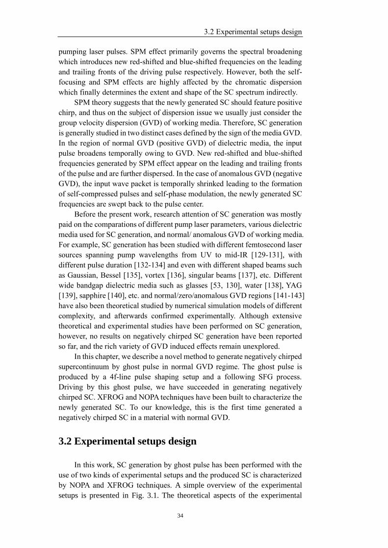
Figure 3.1: An overview of the experimental setups for SC generation by
ghost pulse and SC characterization. The red line represents the light path of
the fundamental 1028 nm laser beam, the green line denotes the second
harmonic of the fundamental pulse and the multicolor line denotes the
generated SC. BS - beam splitter; DM - dichroic mirror.
The 4f-line can produce a long pulse (𝜏𝑝 = 1 − 7 𝑝𝑠) by narrowing the
spectral bandwidth of the fundamental pulse (𝜏𝑝 ≈ 200 𝑓𝑠). The following
SFG process is used to create a ghost pulse by depleting the energy near the
center of the long pulse. In setup (a), the SFG process is performed using
beams at the same wavelength (𝜆0 = 1028 𝑛𝑚) but with different durations
(𝜏𝑝 ≈ 2 𝑝𝑠 and 200 𝑓𝑠). The generated SC is characterized by a home-built
XFROG setup. In the setup (b), an additional SHG process is added before the
4f-line to produce the second harmonic (𝜆0 = 514 𝑛𝑚) of the fundamental
beam, and in this case the SFG process is carried out between the fundamental
and the second harmonic beams. The generated SC is characterized by a NOPA
setup and a commercial autocorrelator is also adopted to further measure the
pulse duration of the NOPA output. The red, green and multicolor lines in Fig.
3.1 denote the paths of the fundamental 1028 nm laser beam, the second
harmonic 514 nm laser beam and the generated SC, respectively.
In this work, the setup in Fig. 3.1(a) was first built to implement the
generation of negatively chirped SC by ghost pulse. Fig. 3.2 presents a
simplified scheme of the experimental setup Fig. 3.1(a). The Yb:KGW laser
system delivers linearly polarized pulses of duration ~200 fs at 1028 nm with
2 kHz repetition rate. The initial laser pulse is divided into two beams 𝐸1(𝑡)
and 𝐸2(𝑡) by a beam splitter. As shown in Fig. 3.2, one beam 𝐸1(𝑡) is
guided into a 4f-line pulse shaping system which is built using a folded optical
geometry. The grating in 4f-line converts the input pulses from time domain to
frequency domain and thus all frequency components are spatially separated
in Fourier plane. Two metal plates are placed in the Fourier plane to form a
narrow slit. Only the central finite frequencies are not blocked by the plates
3.2 Experimental setups design
36
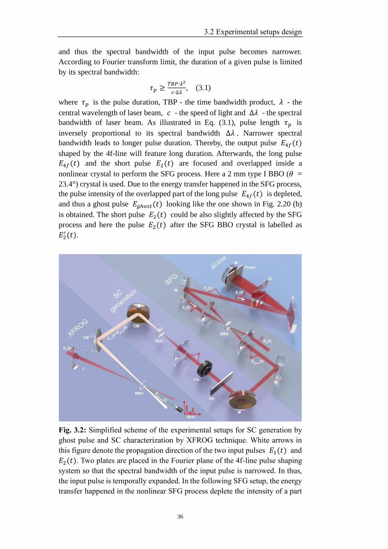
and thus the spectral bandwidth of the input pulse becomes narrower.
According to Fourier transform limit, the duration of a given pulse is limited
by its spectral bandwidth:
𝜏𝑝 ≥𝑇𝐵𝑃∙𝜆2
𝑐∙∆𝜆, (3.1)
where 𝜏𝑝 is the pulse duration, TBP - the time bandwidth product, 𝜆 - the
central wavelength of laser beam, 𝑐 - the speed of light and ∆𝜆 - the spectral
bandwidth of laser beam. As illustrated in Eq. (3.1), pulse length 𝜏𝑝 is
inversely proportional to its spectral bandwidth ∆𝜆 . Narrower spectral
bandwidth leads to longer pulse duration. Thereby, the output pulse 𝐸4𝑓(𝑡)
shaped by the 4f-line will feature long duration. Afterwards, the long pulse
𝐸4𝑓(𝑡) and the short pulse 𝐸2(𝑡) are focused and overlapped inside a
nonlinear crystal to perform the SFG process. Here a 2 mm type I BBO (𝜃 =
23.4°) crystal is used. Due to the energy transfer happened in the SFG process,
the pulse intensity of the overlapped part of the long pulse 𝐸4𝑓(𝑡) is depleted,
and thus a ghost pulse 𝐸𝑔ℎ𝑜𝑠𝑡(𝑡) looking like the one shown in Fig. 2.20 (b)
is obtained. The short pulse 𝐸2(𝑡) could be also slightly affected by the SFG
process and here the pulse 𝐸2(𝑡) after the SFG BBO crystal is labelled as
𝐸2′(𝑡).
Fig. 3.2: Simplified scheme of the experimental setups for SC generation by
ghost pulse and SC characterization by XFROG technique. White arrows in
this figure denote the propagation direction of the two input pulses 𝐸1(𝑡) and
𝐸2(𝑡). Two plates are placed in the Fourier plane of the 4f-line pulse shaping
system so that the spectral bandwidth of the input pulse is narrowed. In thus,
the input pulse is temporally expanded. In the following SFG setup, the energy
transfer happened in the nonlinear SFG process deplete the intensity of a part
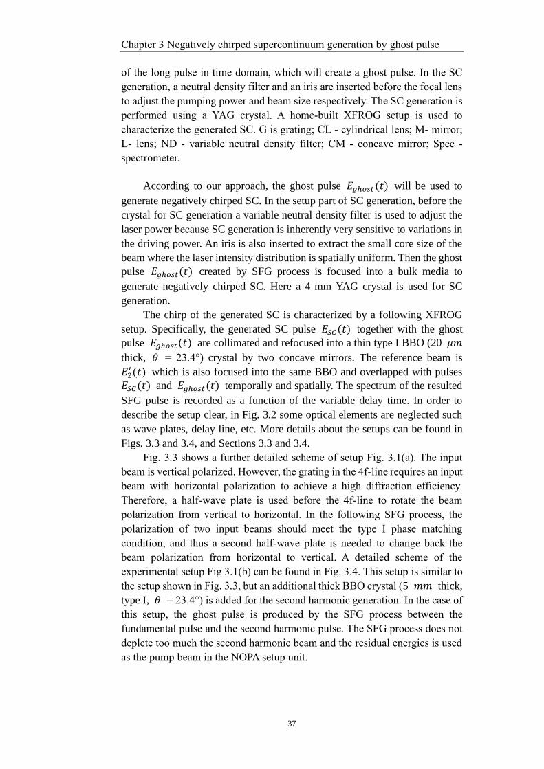
Chapter 3 Negatively chirped supercontinuum generation by ghost pulse
37
of the long pulse in time domain, which will create a ghost pulse. In the SC
generation, a neutral density filter and an iris are inserted before the focal lens
to adjust the pumping power and beam size respectively. The SC generation is
performed using a YAG crystal. A home-built XFROG setup is used to
characterize the generated SC. G is grating; CL - cylindrical lens; M- mirror;
L- lens; ND - variable neutral density filter; CM - concave mirror; Spec -
spectrometer.
According to our approach, the ghost pulse 𝐸𝑔ℎ𝑜𝑠𝑡(𝑡) will be used to
generate negatively chirped SC. In the setup part of SC generation, before the
crystal for SC generation a variable neutral density filter is used to adjust the
laser power because SC generation is inherently very sensitive to variations in
the driving power. An iris is also inserted to extract the small core size of the
beam where the laser intensity distribution is spatially uniform. Then the ghost
pulse 𝐸𝑔ℎ𝑜𝑠𝑡(𝑡) created by SFG process is focused into a bulk media to
generate negatively chirped SC. Here a 4 mm YAG crystal is used for SC
generation.
The chirp of the generated SC is characterized by a following XFROG
setup. Specifically, the generated SC pulse 𝐸𝑆𝐶(𝑡) together with the ghost
pulse 𝐸𝑔ℎ𝑜𝑠𝑡(𝑡) are collimated and refocused into a thin type I BBO (20 𝜇𝑚
thick, 𝜃 = 23.4°) crystal by two concave mirrors. The reference beam is
𝐸2′(𝑡) which is also focused into the same BBO and overlapped with pulses
𝐸𝑆𝐶(𝑡) and 𝐸𝑔ℎ𝑜𝑠𝑡(𝑡) temporally and spatially. The spectrum of the resulted
SFG pulse is recorded as a function of the variable delay time. In order to
describe the setup clear, in Fig. 3.2 some optical elements are neglected such
as wave plates, delay line, etc. More details about the setups can be found in
Figs. 3.3 and 3.4, and Sections 3.3 and 3.4.
Fig. 3.3 shows a further detailed scheme of setup Fig. 3.1(a). The input
beam is vertical polarized. However, the grating in the 4f-line requires an input
beam with horizontal polarization to achieve a high diffraction efficiency.
Therefore, a half-wave plate is used before the 4f-line to rotate the beam
polarization from vertical to horizontal. In the following SFG process, the
polarization of two input beams should meet the type I phase matching
condition, and thus a second half-wave plate is needed to change back the
beam polarization from horizontal to vertical. A detailed scheme of the
experimental setup Fig 3.1(b) can be found in Fig. 3.4. This setup is similar to
the setup shown in Fig. 3.3, but an additional thick BBO crystal (5 𝑚𝑚 thick,
type I, 𝜃 = 23.4°) is added for the second harmonic generation. In the case of
this setup, the ghost pulse is produced by the SFG process between the
fundamental pulse and the second harmonic pulse. The SFG process does not
deplete too much the second harmonic beam and the residual energies is used
as the pump beam in the NOPA setup unit.
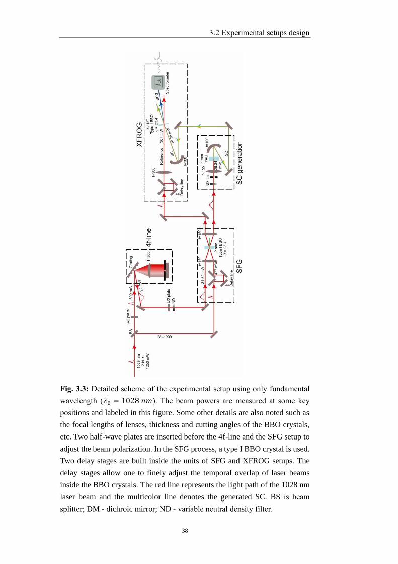
3.2 Experimental setups design
38
Fig. 3.3: Detailed scheme of the experimental setup using only fundamental
wavelength (𝜆0 = 1028 𝑛𝑚 ). The beam powers are measured at some key
positions and labeled in this figure. Some other details are also noted such as
the focal lengths of lenses, thickness and cutting angles of the BBO crystals,
etc. Two half-wave plates are inserted before the 4f-line and the SFG setup to
adjust the beam polarization. In the SFG process, a type I BBO crystal is used.
Two delay stages are built inside the units of SFG and XFROG setups. The
delay stages allow one to finely adjust the temporal overlap of laser beams
inside the BBO crystals. The red line represents the light path of the 1028 nm
laser beam and the multicolor line denotes the generated SC. BS is beam
splitter; DM - dichroic mirror; ND - variable neutral density filter.
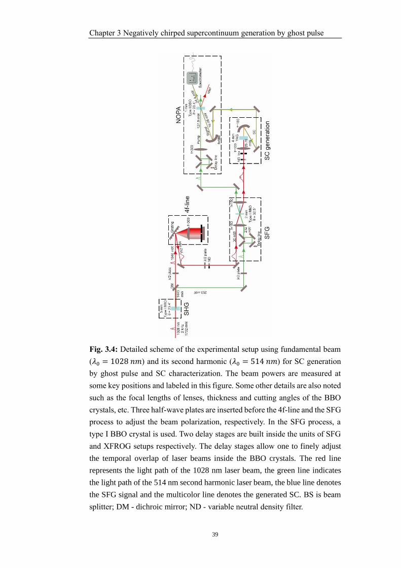
Chapter 3 Negatively chirped supercontinuum generation by ghost pulse
39
Fig. 3.4: Detailed scheme of the experimental setup using fundamental beam
(𝜆0 = 1028 𝑛𝑚) and its second harmonic (𝜆0 = 514 𝑛𝑚) for SC generation
by ghost pulse and SC characterization. The beam powers are measured at
some key positions and labeled in this figure. Some other details are also noted
such as the focal lengths of lenses, thickness and cutting angles of the BBO
crystals, etc. Three half-wave plates are inserted before the 4f-line and the SFG
process to adjust the beam polarization, respectively. In the SFG process, a
type I BBO crystal is used. Two delay stages are built inside the units of SFG
and XFROG setups respectively. The delay stages allow one to finely adjust
the temporal overlap of laser beams inside the BBO crystals. The red line
represents the light path of the 1028 nm laser beam, the green line indicates
the light path of the 514 nm second harmonic laser beam, the blue line denotes
the SFG signal and the multicolor line denotes the generated SC. BS is beam
splitter; DM - dichroic mirror; ND - variable neutral density filter.
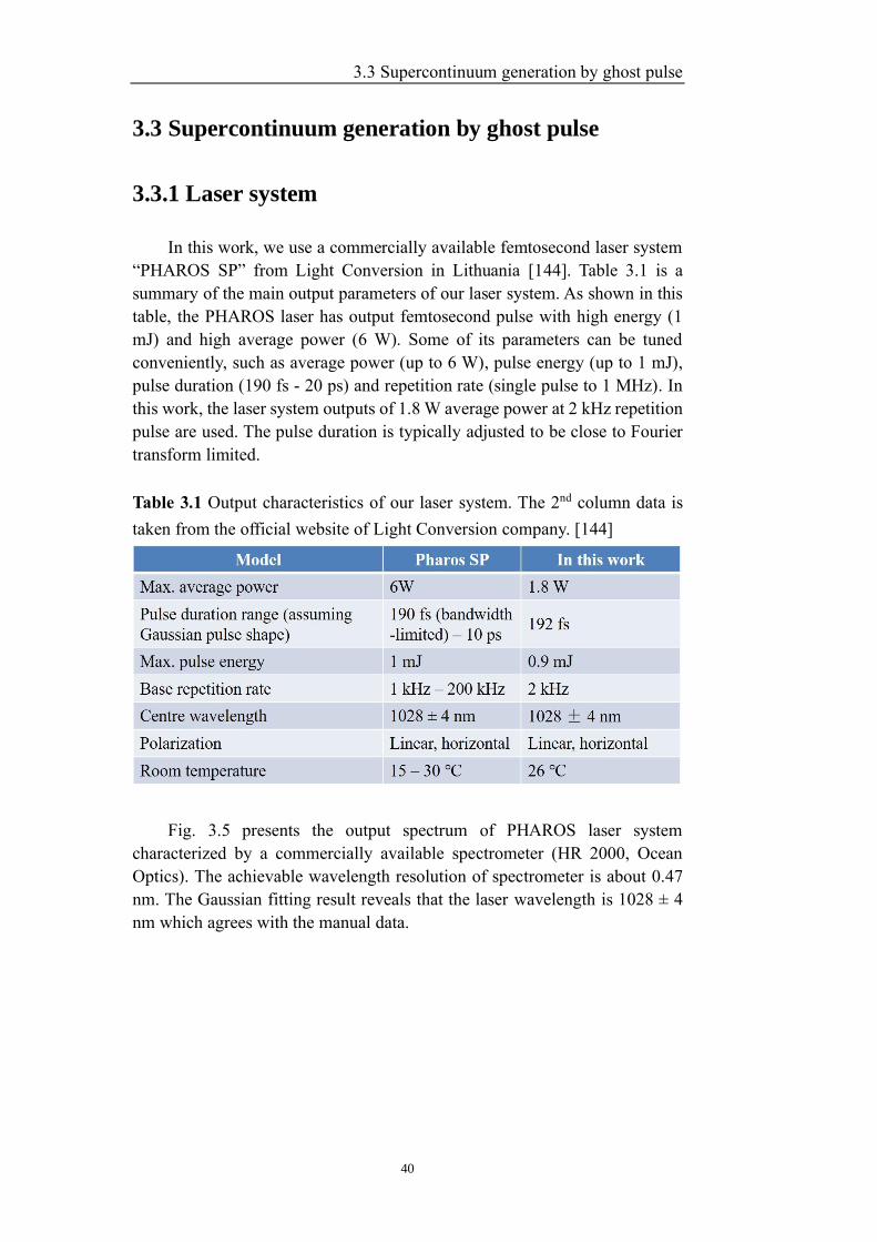
3.3 Supercontinuum generation by ghost pulse
40
3.3 Supercontinuum generation by ghost pulse
3.3.1 Laser system
In this work, we use a commercially available femtosecond laser system
“PHAROS SP” from Light Conversion in Lithuania [144]. Table 3.1 is a
summary of the main output parameters of our laser system. As shown in this
table, the PHAROS laser has output femtosecond pulse with high energy (1
mJ) and high average power (6 W). Some of its parameters can be tuned
conveniently, such as average power (up to 6 W), pulse energy (up to 1 mJ),
pulse duration (190 fs - 20 ps) and repetition rate (single pulse to 1 MHz). In
this work, the laser system outputs of 1.8 W average power at 2 kHz repetition
pulse are used. The pulse duration is typically adjusted to be close to Fourier
transform limited.
Table 3.1 Output characteristics of our laser system. The 2nd column data is
taken from the official website of Light Conversion company. [144]
Fig. 3.5 presents the output spectrum of PHAROS laser system
characterized by a commercially available spectrometer (HR 2000, Ocean
Optics). The achievable wavelength resolution of spectrometer is about 0.47
nm. The Gaussian fitting result reveals that the laser wavelength is 1028 ± 4
nm which agrees with the manual data.
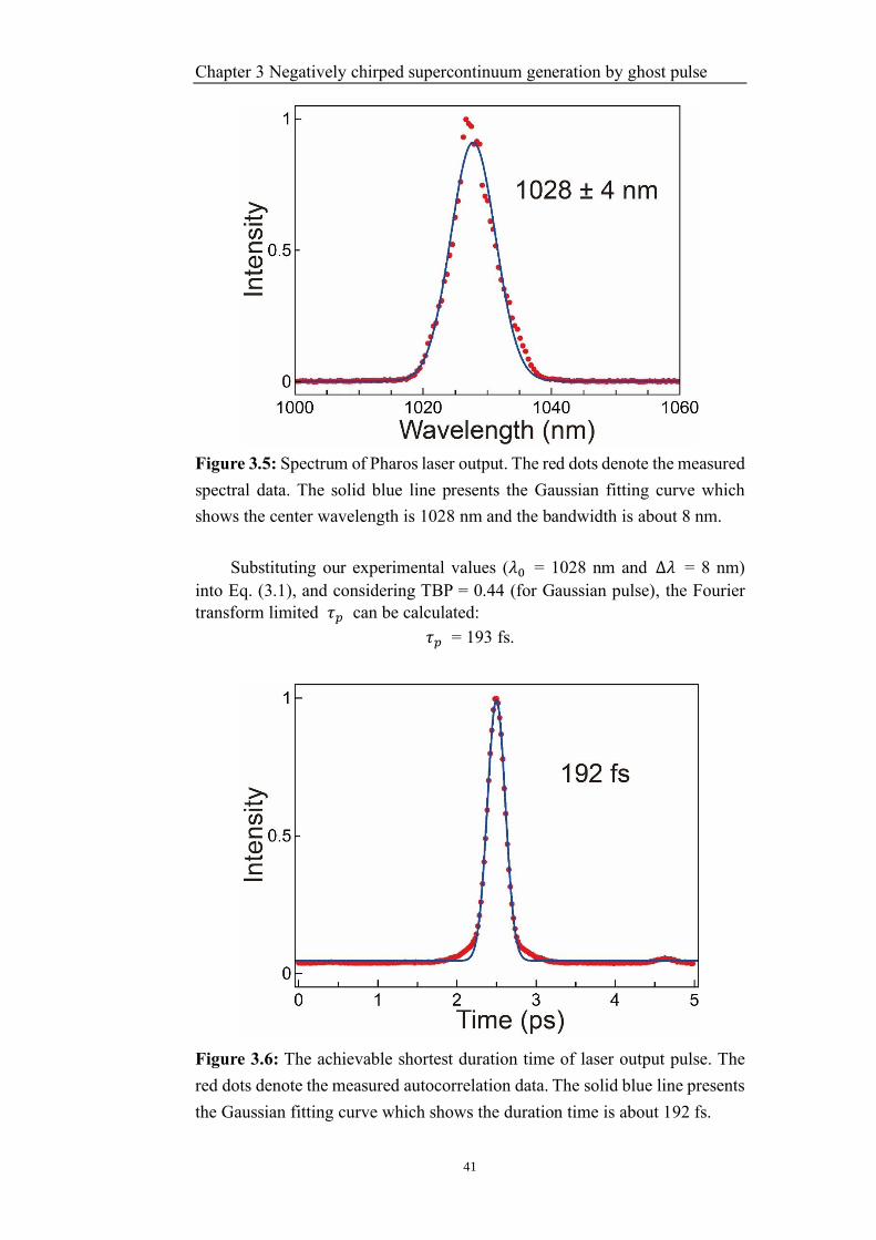
Chapter 3 Negatively chirped supercontinuum generation by ghost pulse
41
Figure 3.5: Spectrum of Pharos laser output. The red dots denote the measured
spectral data. The solid blue line presents the Gaussian fitting curve which
shows the center wavelength is 1028 nm and the bandwidth is about 8 nm.
Substituting our experimental values (𝜆0 = 1028 nm and ∆𝜆 = 8 nm)
into Eq. (3.1), and considering TBP = 0.44 (for Gaussian pulse), the Fourier
transform limited 𝜏𝑝 can be calculated:
𝜏𝑝 = 193 fs.
Figure 3.6: The achievable shortest duration time of laser output pulse. The
red dots denote the measured autocorrelation data. The solid blue line presents
the Gaussian fitting curve which shows the duration time is about 192 fs.
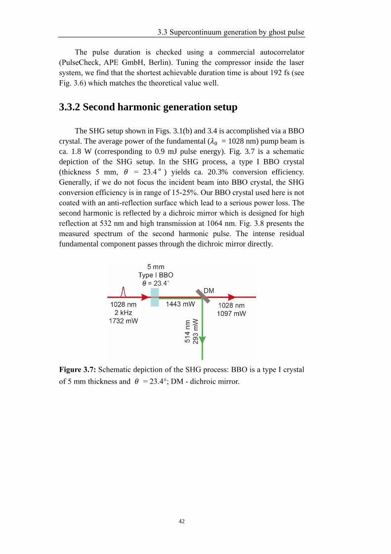
3.3 Supercontinuum generation by ghost pulse
42
The pulse duration is checked using a commercial autocorrelator
(PulseCheck, APE GmbH, Berlin). Tuning the compressor inside the laser
system, we find that the shortest achievable duration time is about 192 fs (see
Fig. 3.6) which matches the theoretical value well.
3.3.2 Second harmonic generation setup
The SHG setup shown in Figs. 3.1(b) and 3.4 is accomplished via a BBO
crystal. The average power of the fundamental (𝜆0 = 1028 nm) pump beam is
ca. 1.8 W (corresponding to 0.9 mJ pulse energy). Fig. 3.7 is a schematic
depiction of the SHG setup. In the SHG process, a type I BBO crystal
(thickness 5 mm, 𝜃 = 23.4 º ) yields ca. 20.3% conversion efficiency.
Generally, if we do not focus the incident beam into BBO crystal, the SHG
conversion efficiency is in range of 15-25%. Our BBO crystal used here is not
coated with an anti-reflection surface which lead to a serious power loss. The
second harmonic is reflected by a dichroic mirror which is designed for high
reflection at 532 nm and high transmission at 1064 nm. Fig. 3.8 presents the
measured spectrum of the second harmonic pulse. The intense residual
fundamental component passes through the dichroic mirror directly.
Figure 3.7: Schematic depiction of the SHG process: BBO is a type I crystal
of 5 mm thickness and 𝜃 = 23.4°; DM - dichroic mirror.
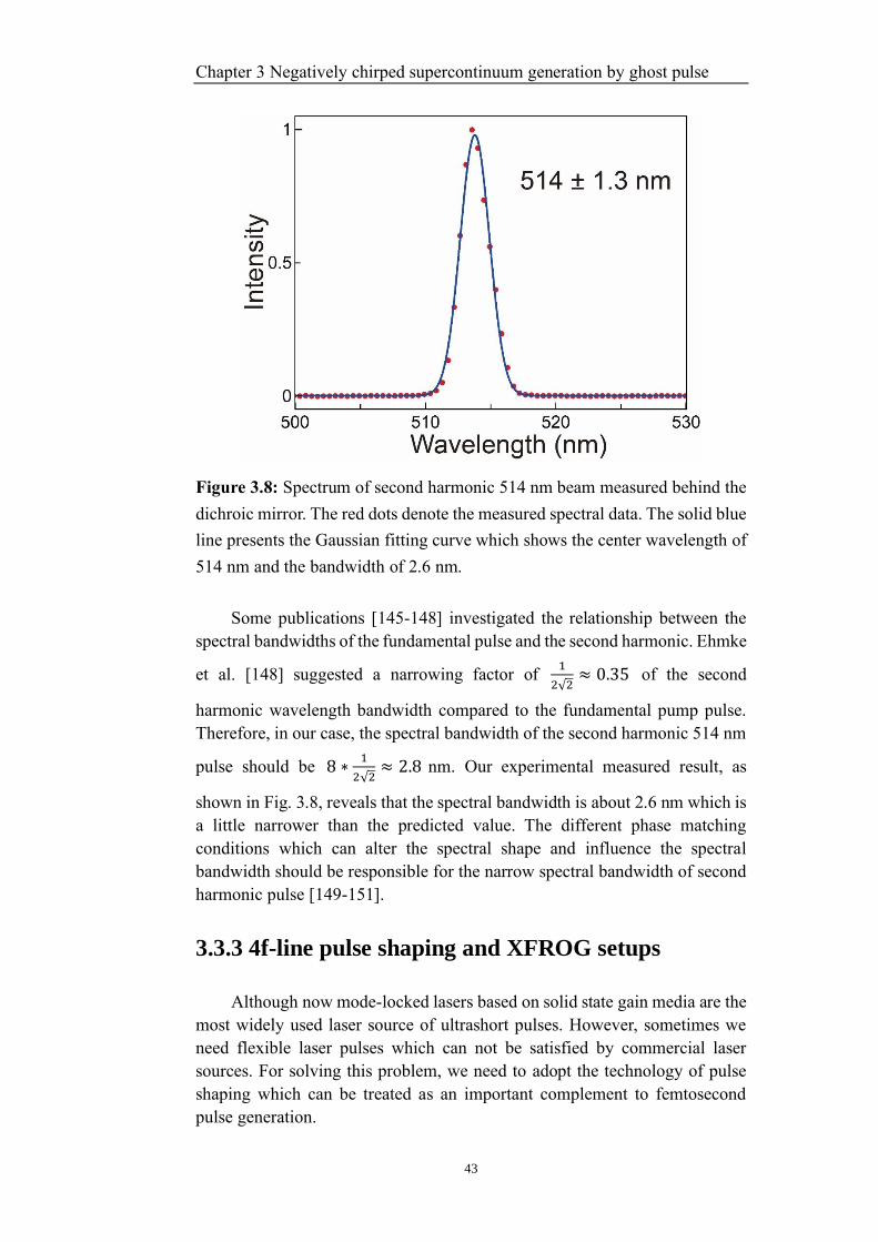
Chapter 3 Negatively chirped supercontinuum generation by ghost pulse
43
Figure 3.8: Spectrum of second harmonic 514 nm beam measured behind the
dichroic mirror. The red dots denote the measured spectral data. The solid blue
line presents the Gaussian fitting curve which shows the center wavelength of
514 nm and the bandwidth of 2.6 nm.
Some publications [145-148] investigated the relationship between the
spectral bandwidths of the fundamental pulse and the second harmonic. Ehmke
et al. [148] suggested a narrowing factor of 1
2√2≈ 0.35 of the second
harmonic wavelength bandwidth compared to the fundamental pump pulse.
Therefore, in our case, the spectral bandwidth of the second harmonic 514 nm
pulse should be 8 ∗1
2√2≈ 2.8 nm. Our experimental measured result, as
shown in Fig. 3.8, reveals that the spectral bandwidth is about 2.6 nm which is
a little narrower than the predicted value. The different phase matching
conditions which can alter the spectral shape and influence the spectral
bandwidth should be responsible for the narrow spectral bandwidth of second
harmonic pulse [149-151].
3.3.3 4f-line pulse shaping and XFROG setups
Although now mode-locked lasers based on solid state gain media are the
most widely used laser source of ultrashort pulses. However, sometimes we
need flexible laser pulses which can not be satisfied by commercial laser
sources. For solving this problem, we need to adopt the technology of pulse
shaping which can be treated as an important complement to femtosecond
pulse generation.
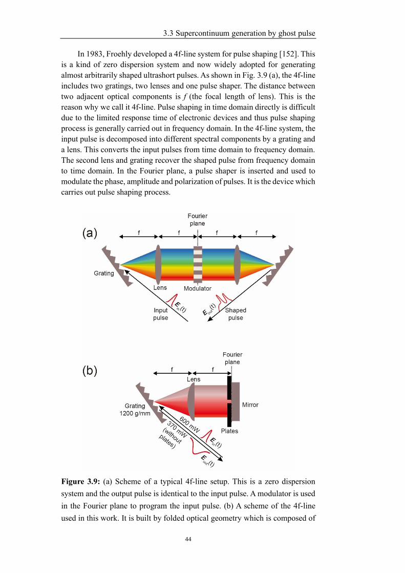
3.3 Supercontinuum generation by ghost pulse
44
In 1983, Froehly developed a 4f-line system for pulse shaping [152]. This
is a kind of zero dispersion system and now widely adopted for generating
almost arbitrarily shaped ultrashort pulses. As shown in Fig. 3.9 (a), the 4f-line
includes two gratings, two lenses and one pulse shaper. The distance between
two adjacent optical components is f (the focal length of lens). This is the
reason why we call it 4f-line. Pulse shaping in time domain directly is difficult
due to the limited response time of electronic devices and thus pulse shaping
process is generally carried out in frequency domain. In the 4f-line system, the
input pulse is decomposed into different spectral components by a grating and
a lens. This converts the input pulses from time domain to frequency domain.
The second lens and grating recover the shaped pulse from frequency domain
to time domain. In the Fourier plane, a pulse shaper is inserted and used to
modulate the phase, amplitude and polarization of pulses. It is the device which
carries out pulse shaping process.
Figure 3.9: (a) Scheme of a typical 4f-line setup. This is a zero dispersion
system and the output pulse is identical to the input pulse. A modulator is used
in the Fourier plane to program the input pulse. (b) A scheme of the 4f-line
used in this work. It is built by folded optical geometry which is composed of
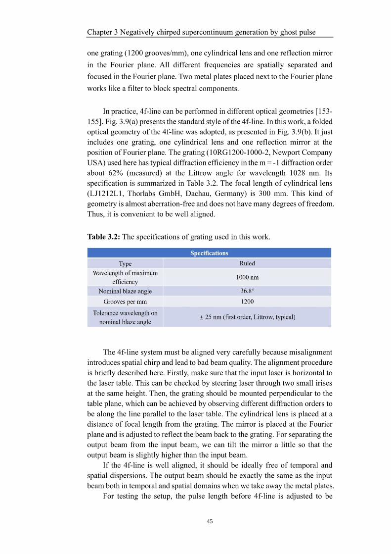
Chapter 3 Negatively chirped supercontinuum generation by ghost pulse
45
one grating (1200 grooves/mm), one cylindrical lens and one reflection mirror
in the Fourier plane. All different frequencies are spatially separated and
focused in the Fourier plane. Two metal plates placed next to the Fourier plane
works like a filter to block spectral components.
In practice, 4f-line can be performed in different optical geometries [153-
155]. Fig. 3.9(a) presents the standard style of the 4f-line. In this work, a folded
optical geometry of the 4f-line was adopted, as presented in Fig. 3.9(b). It just
includes one grating, one cylindrical lens and one reflection mirror at the
position of Fourier plane. The grating (10RG1200-1000-2, Newport Company
USA) used here has typical diffraction efficiency in the m = -1 diffraction order
about 62% (measured) at the Littrow angle for wavelength 1028 nm. Its
specification is summarized in Table 3.2. The focal length of cylindrical lens
(LJ1212L1, Thorlabs GmbH, Dachau, Germany) is 300 mm. This kind of
geometry is almost aberration-free and does not have many degrees of freedom.
Thus, it is convenient to be well aligned.
Table 3.2: The specifications of grating used in this work.
The 4f-line system must be aligned very carefully because misalignment
introduces spatial chirp and lead to bad beam quality. The alignment procedure
is briefly described here. Firstly, make sure that the input laser is horizontal to
the laser table. This can be checked by steering laser through two small irises
at the same height. Then, the grating should be mounted perpendicular to the
table plane, which can be achieved by observing different diffraction orders to
be along the line parallel to the laser table. The cylindrical lens is placed at a
distance of focal length from the grating. The mirror is placed at the Fourier
plane and is adjusted to reflect the beam back to the grating. For separating the
output beam from the input beam, we can tilt the mirror a little so that the
output beam is slightly higher than the input beam.
If the 4f-line is well aligned, it should be ideally free of temporal and
spatial dispersions. The output beam should be exactly the same as the input
beam both in temporal and spatial domains when we take away the metal plates.
For testing the setup, the pulse length before 4f-line is adjusted to be
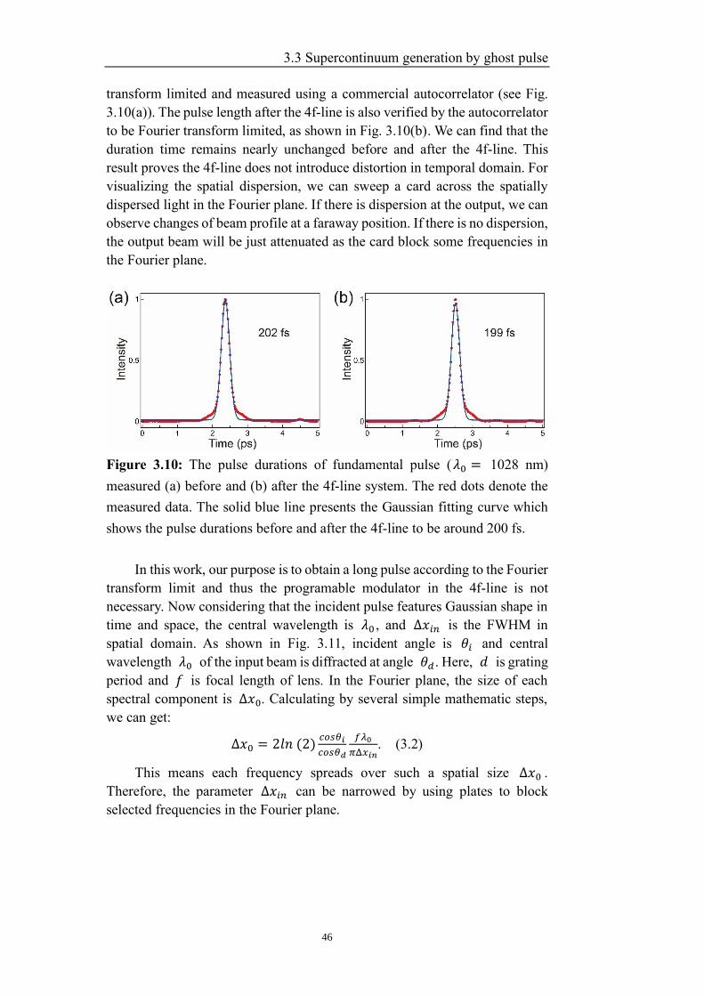
3.3 Supercontinuum generation by ghost pulse
46
transform limited and measured using a commercial autocorrelator (see Fig.
3.10(a)). The pulse length after the 4f-line is also verified by the autocorrelator
to be Fourier transform limited, as shown in Fig. 3.10(b). We can find that the
duration time remains nearly unchanged before and after the 4f-line. This
result proves the 4f-line does not introduce distortion in temporal domain. For
visualizing the spatial dispersion, we can sweep a card across the spatially
dispersed light in the Fourier plane. If there is dispersion at the output, we can
observe changes of beam profile at a faraway position. If there is no dispersion,
the output beam will be just attenuated as the card block some frequencies in
the Fourier plane.
Figure 3.10: The pulse durations of fundamental pulse (𝜆0 = 1028 nm)
measured (a) before and (b) after the 4f-line system. The red dots denote the
measured data. The solid blue line presents the Gaussian fitting curve which
shows the pulse durations before and after the 4f-line to be around 200 fs.
In this work, our purpose is to obtain a long pulse according to the Fourier
transform limit and thus the programable modulator in the 4f-line is not
necessary. Now considering that the incident pulse features Gaussian shape in
time and space, the central wavelength is 𝜆0 , and Δ𝑥𝑖𝑛 is the FWHM in
spatial domain. As shown in Fig. 3.11, incident angle is 𝜃𝑖 and central
wavelength 𝜆0 of the input beam is diffracted at angle 𝜃𝑑. Here, 𝑑 is grating
period and 𝑓 is focal length of lens. In the Fourier plane, the size of each
spectral component is Δ𝑥0. Calculating by several simple mathematic steps,
we can get:
Δ𝑥0 = 2𝑙𝑛 (2)𝑐𝑜𝑠𝜃𝑖
𝑐𝑜𝑠𝜃𝑑
𝑓𝜆0
𝜋Δ𝑥𝑖𝑛. (3.2)
This means each frequency spreads over such a spatial size Δ𝑥0 .
Therefore, the parameter Δ𝑥𝑖𝑛 can be narrowed by using plates to block
selected frequencies in the Fourier plane.

Chapter 3 Negatively chirped supercontinuum generation by ghost pulse
47
Figure 3.11: Scheme of a half 4f-line. The Fourier plane is located at the back
focal plane of the lens. 𝜃𝑖 denotes the incident angle on the grating; 𝜃𝑑 is
the diffraction angle; 𝑋 denotes the spatial coordinate of the Fourier plane;
𝑔(𝑋) represents the spatial size of a given frequency component.
As we have mentioned in Section 3.2, the minimum duration of a given
pulse is limited by its spectral bandwidth. Specifically, pulse duration is
inversely proportional to spectral bandwidth. Therefore, as we narrow the
spectral bandwidth of the input light by blocking frequency components in the
Fourier plane of the 4f-line, the pulse duration of the output light should
become longer. Fig. 3.12 shows a series of autocorrelation curves obtained by
gradually narrowing the spectrum’s FWHM. As it should be, narrower
spectrum leads to longer duration time.
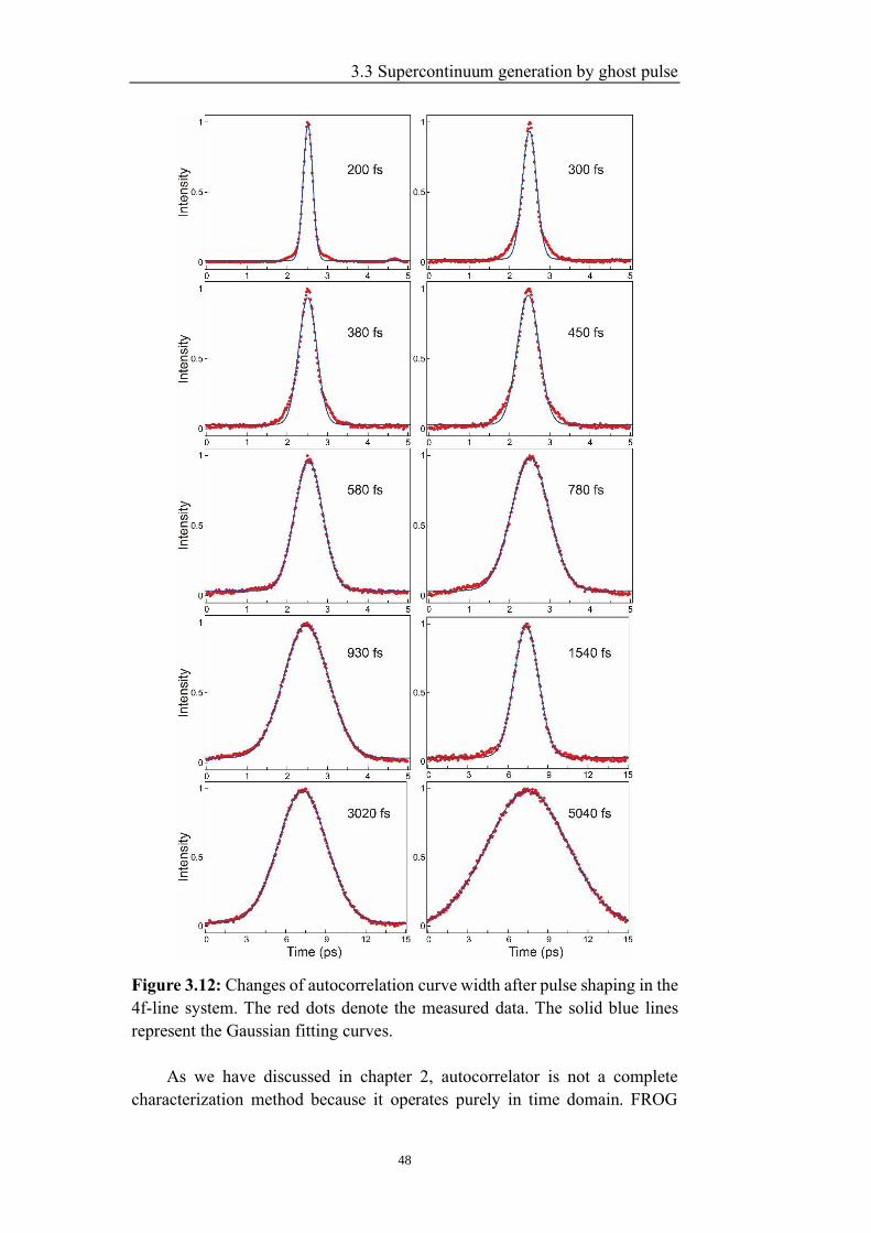
3.3 Supercontinuum generation by ghost pulse
48
Figure 3.12: Changes of autocorrelation curve width after pulse shaping in the
4f-line system. The red dots denote the measured data. The solid blue lines
represent the Gaussian fitting curves.
As we have discussed in chapter 2, autocorrelator is not a complete
characterization method because it operates purely in time domain. FROG
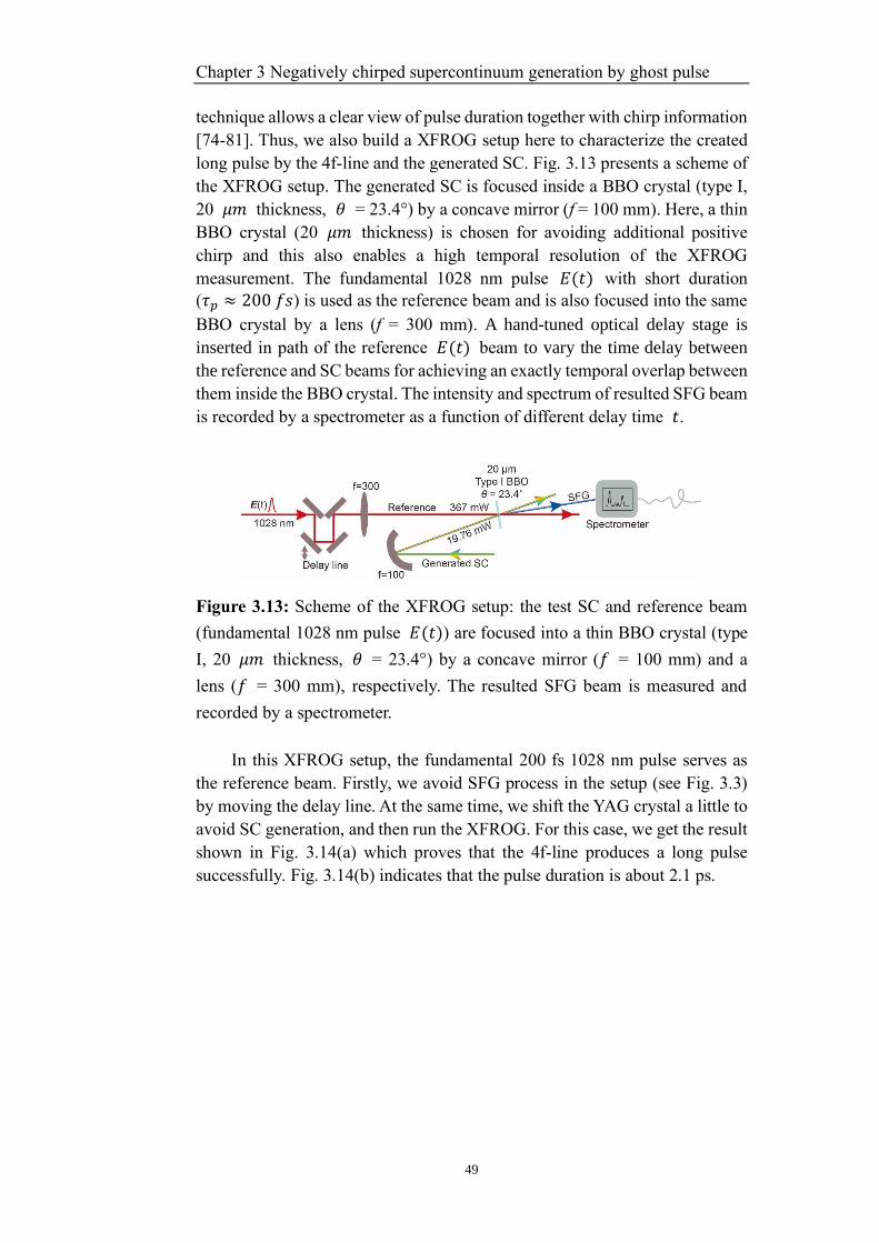
Chapter 3 Negatively chirped supercontinuum generation by ghost pulse
49
technique allows a clear view of pulse duration together with chirp information
[74-81]. Thus, we also build a XFROG setup here to characterize the created
long pulse by the 4f-line and the generated SC. Fig. 3.13 presents a scheme of
the XFROG setup. The generated SC is focused inside a BBO crystal (type I,
20 𝜇𝑚 thickness, 𝜃 = 23.4°) by a concave mirror (f = 100 mm). Here, a thin
BBO crystal (20 𝜇𝑚 thickness) is chosen for avoiding additional positive
chirp and this also enables a high temporal resolution of the XFROG
measurement. The fundamental 1028 nm pulse 𝐸(𝑡) with short duration
(𝜏𝑝 ≈ 200 𝑓𝑠) is used as the reference beam and is also focused into the same
BBO crystal by a lens (f = 300 mm). A hand-tuned optical delay stage is
inserted in path of the reference 𝐸(𝑡) beam to vary the time delay between
the reference and SC beams for achieving an exactly temporal overlap between
them inside the BBO crystal. The intensity and spectrum of resulted SFG beam
is recorded by a spectrometer as a function of different delay time 𝑡.
Figure 3.13: Scheme of the XFROG setup: the test SC and reference beam
(fundamental 1028 nm pulse 𝐸(𝑡)) are focused into a thin BBO crystal (type
I, 20 𝜇𝑚 thickness, 𝜃 = 23.4°) by a concave mirror (𝑓 = 100 mm) and a
lens (𝑓 = 300 mm), respectively. The resulted SFG beam is measured and
recorded by a spectrometer.
In this XFROG setup, the fundamental 200 fs 1028 nm pulse serves as
the reference beam. Firstly, we avoid SFG process in the setup (see Fig. 3.3)
by moving the delay line. At the same time, we shift the YAG crystal a little to
avoid SC generation, and then run the XFROG. For this case, we get the result
shown in Fig. 3.14(a) which proves that the 4f-line produces a long pulse
successfully. Fig. 3.14(b) indicates that the pulse duration is about 2.1 ps.
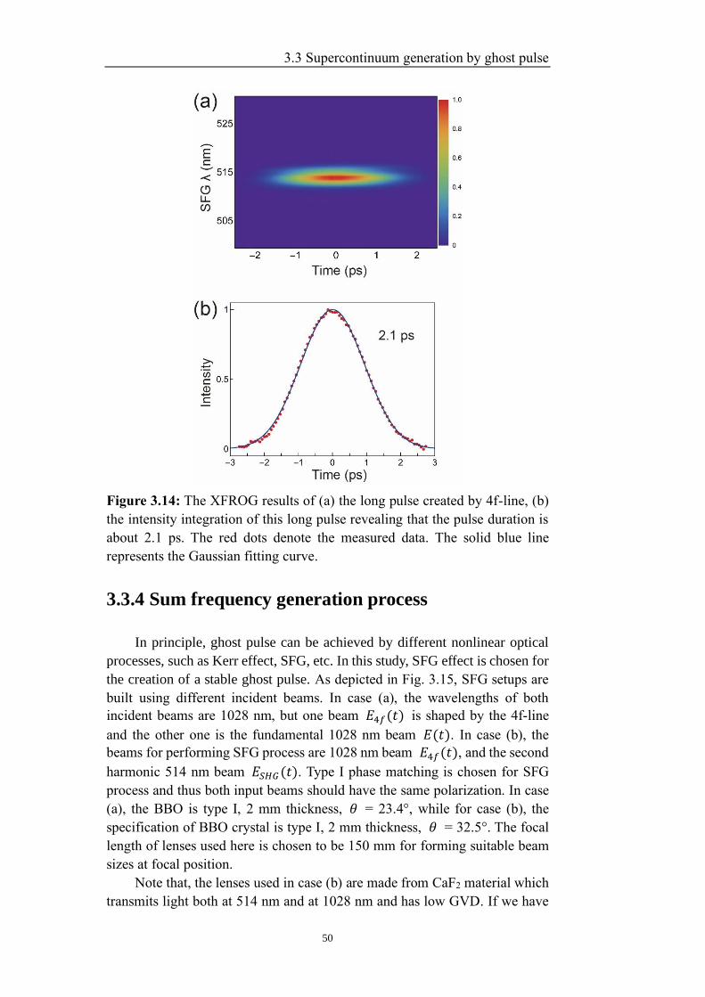
3.3 Supercontinuum generation by ghost pulse
50
Figure 3.14: The XFROG results of (a) the long pulse created by 4f-line, (b)
the intensity integration of this long pulse revealing that the pulse duration is
about 2.1 ps. The red dots denote the measured data. The solid blue line
represents the Gaussian fitting curve.
3.3.4 Sum frequency generation process
In principle, ghost pulse can be achieved by different nonlinear optical
processes, such as Kerr effect, SFG, etc. In this study, SFG effect is chosen for
the creation of a stable ghost pulse. As depicted in Fig. 3.15, SFG setups are
built using different incident beams. In case (a), the wavelengths of both
incident beams are 1028 nm, but one beam 𝐸4𝑓(𝑡) is shaped by the 4f-line
and the other one is the fundamental 1028 nm beam 𝐸(𝑡). In case (b), the
beams for performing SFG process are 1028 nm beam 𝐸4𝑓(𝑡), and the second
harmonic 514 nm beam 𝐸𝑆𝐻𝐺(𝑡). Type I phase matching is chosen for SFG
process and thus both input beams should have the same polarization. In case
(a), the BBO is type I, 2 mm thickness, 𝜃 = 23.4°, while for case (b), the
specification of BBO crystal is type I, 2 mm thickness, 𝜃 = 32.5°. The focal
length of lenses used here is chosen to be 150 mm for forming suitable beam
sizes at focal position.
Note that, the lenses used in case (b) are made from CaF2 material which
transmits light both at 514 nm and at 1028 nm and has low GVD. If we have
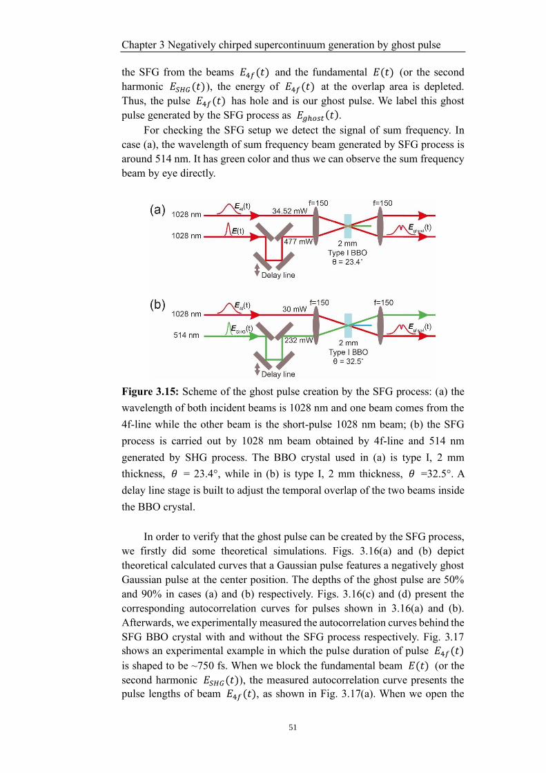
Chapter 3 Negatively chirped supercontinuum generation by ghost pulse
51
the SFG from the beams 𝐸4𝑓(𝑡) and the fundamental 𝐸(𝑡) (or the second
harmonic 𝐸𝑆𝐻𝐺(𝑡) ), the energy of 𝐸4𝑓(𝑡) at the overlap area is depleted.
Thus, the pulse 𝐸4𝑓(𝑡) has hole and is our ghost pulse. We label this ghost
pulse generated by the SFG process as 𝐸𝑔ℎ𝑜𝑠𝑡(𝑡).
For checking the SFG setup we detect the signal of sum frequency. In
case (a), the wavelength of sum frequency beam generated by SFG process is
around 514 nm. It has green color and thus we can observe the sum frequency
beam by eye directly.
Figure 3.15: Scheme of the ghost pulse creation by the SFG process: (a) the
wavelength of both incident beams is 1028 nm and one beam comes from the
4f-line while the other beam is the short-pulse 1028 nm beam; (b) the SFG
process is carried out by 1028 nm beam obtained by 4f-line and 514 nm
generated by SHG process. The BBO crystal used in (a) is type I, 2 mm
thickness, 𝜃 = 23.4°, while in (b) is type I, 2 mm thickness, 𝜃 =32.5°. A
delay line stage is built to adjust the temporal overlap of the two beams inside
the BBO crystal.
In order to verify that the ghost pulse can be created by the SFG process,
we firstly did some theoretical simulations. Figs. 3.16(a) and (b) depict
theoretical calculated curves that a Gaussian pulse features a negatively ghost
Gaussian pulse at the center position. The depths of the ghost pulse are 50%
and 90% in cases (a) and (b) respectively. Figs. 3.16(c) and (d) present the
corresponding autocorrelation curves for pulses shown in 3.16(a) and (b).
Afterwards, we experimentally measured the autocorrelation curves behind the
SFG BBO crystal with and without the SFG process respectively. Fig. 3.17
shows an experimental example in which the pulse duration of pulse 𝐸4𝑓(𝑡)
is shaped to be ~750 fs. When we block the fundamental beam 𝐸(𝑡) (or the
second harmonic 𝐸𝑆𝐻𝐺(𝑡)), the measured autocorrelation curve presents the
pulse lengths of beam 𝐸4𝑓(𝑡), as shown in Fig. 3.17(a). When we open the
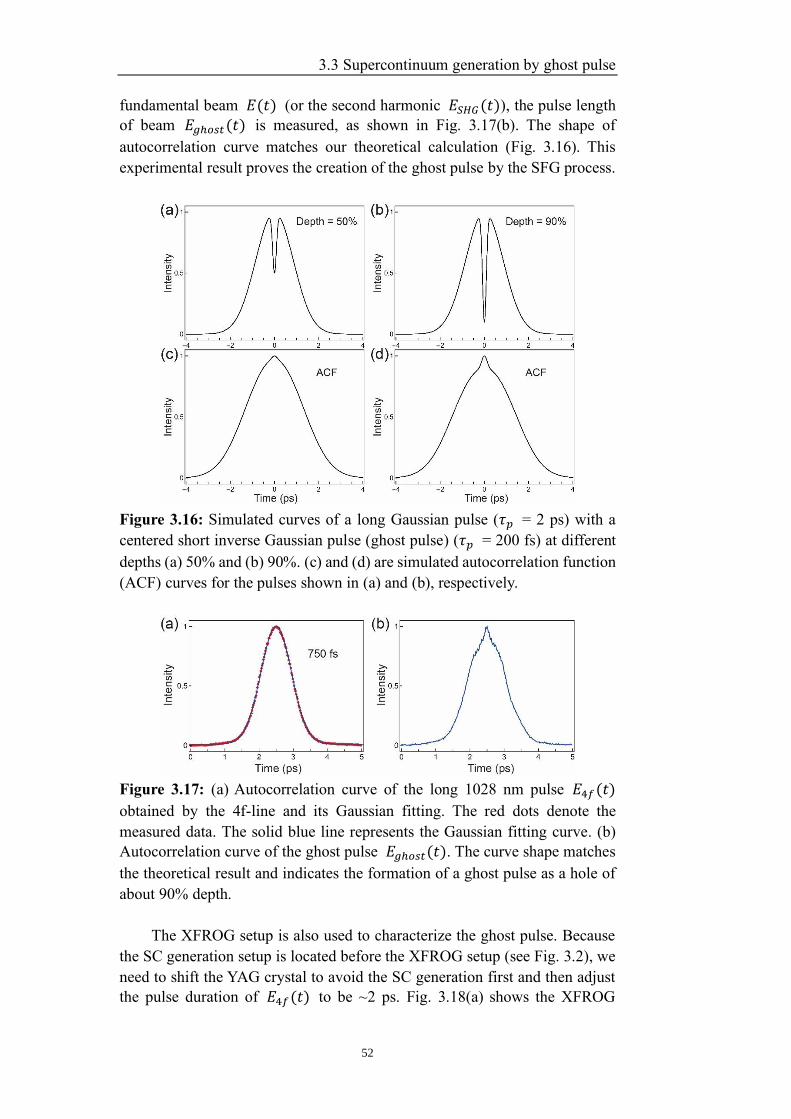
3.3 Supercontinuum generation by ghost pulse
52
fundamental beam 𝐸(𝑡) (or the second harmonic 𝐸𝑆𝐻𝐺(𝑡)), the pulse length
of beam 𝐸𝑔ℎ𝑜𝑠𝑡(𝑡) is measured, as shown in Fig. 3.17(b). The shape of
autocorrelation curve matches our theoretical calculation (Fig. 3.16). This
experimental result proves the creation of the ghost pulse by the SFG process.
Figure 3.16: Simulated curves of a long Gaussian pulse (𝜏𝑝 = 2 ps) with a
centered short inverse Gaussian pulse (ghost pulse) (𝜏𝑝 = 200 fs) at different
depths (a) 50% and (b) 90%. (c) and (d) are simulated autocorrelation function
(ACF) curves for the pulses shown in (a) and (b), respectively.
Figure 3.17: (a) Autocorrelation curve of the long 1028 nm pulse 𝐸4𝑓(𝑡)
obtained by the 4f-line and its Gaussian fitting. The red dots denote the
measured data. The solid blue line represents the Gaussian fitting curve. (b)
Autocorrelation curve of the ghost pulse 𝐸𝑔ℎ𝑜𝑠𝑡(𝑡). The curve shape matches
the theoretical result and indicates the formation of a ghost pulse as a hole of
about 90% depth.
The XFROG setup is also used to characterize the ghost pulse. Because
the SC generation setup is located before the XFROG setup (see Fig. 3.2), we
need to shift the YAG crystal to avoid the SC generation first and then adjust
the pulse duration of 𝐸4𝑓(𝑡) to be ~2 ps. Fig. 3.18(a) shows the XFROG
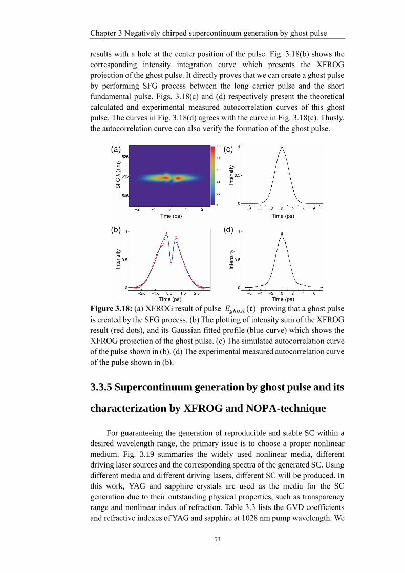
Chapter 3 Negatively chirped supercontinuum generation by ghost pulse
53
results with a hole at the center position of the pulse. Fig. 3.18(b) shows the
corresponding intensity integration curve which presents the XFROG
projection of the ghost pulse. It directly proves that we can create a ghost pulse
by performing SFG process between the long carrier pulse and the short
fundamental pulse. Figs. 3.18(c) and (d) respectively present the theoretical
calculated and experimental measured autocorrelation curves of this ghost
pulse. The curves in Fig. 3.18(d) agrees with the curve in Fig. 3.18(c). Thusly,
the autocorrelation curve can also verify the formation of the ghost pulse.
Figure 3.18: (a) XFROG result of pulse 𝐸𝑔ℎ𝑜𝑠𝑡(𝑡) proving that a ghost pulse
is created by the SFG process. (b) The plotting of intensity sum of the XFROG
result (red dots), and its Gaussian fitted profile (blue curve) which shows the
XFROG projection of the ghost pulse. (c) The simulated autocorrelation curve
of the pulse shown in (b). (d) The experimental measured autocorrelation curve
of the pulse shown in (b).
3.3.5 Supercontinuum generation by ghost pulse and its
characterization by XFROG and NOPA-technique
For guaranteeing the generation of reproducible and stable SC within a
desired wavelength range, the primary issue is to choose a proper nonlinear
medium. Fig. 3.19 summaries the widely used nonlinear media, different
driving laser sources and the corresponding spectra of the generated SC. Using
different media and different driving lasers, different SC will be produced. In
this work, YAG and sapphire crystals are used as the media for the SC
generation due to their outstanding physical properties, such as transparency
range and nonlinear index of refraction. Table 3.3 lists the GVD coefficients
and refractive indexes of YAG and sapphire at 1028 nm pump wavelength. We
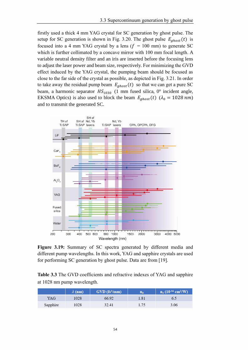
3.3 Supercontinuum generation by ghost pulse
54
firstly used a thick 4 mm YAG crystal for SC generation by ghost pulse. The
setup for SC generation is shown in Fig. 3.20. The ghost pulse 𝐸𝑔ℎ𝑜𝑠𝑡(𝑡) is
focused into a 4 mm YAG crystal by a lens (𝑓 = 100 mm) to generate SC
which is further collimated by a concave mirror with 100 mm focal length. A
variable neutral density filter and an iris are inserted before the focusing lens
to adjust the laser power and beam size, respectively. For minimizing the GVD
effect induced by the YAG crystal, the pumping beam should be focused as
close to the far side of the crystal as possible, as depicted in Fig. 3.21. In order
to take away the residual pump beam 𝐸𝑔ℎ𝑜𝑠𝑡(𝑡) so that we can get a pure SC
beam, a harmonic separator 𝐻𝑆1030 (1 mm fused silica, 0° incident angle,
EKSMA Optics) is also used to block the beam 𝐸𝑔ℎ𝑜𝑠𝑡(𝑡) (𝜆0 = 1028 𝑛𝑚)
and to transmit the generated SC.
Figure 3.19: Summary of SC spectra generated by different media and
different pump wavelengths. In this work, YAG and sapphire crystals are used
for performing SC generation by ghost pulse. Data are from [19].
Table 3.3 The GVD coefficients and refractive indexes of YAG and sapphire
at 1028 nm pump wavelength.
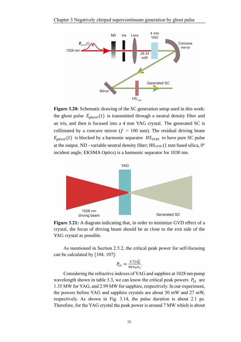
Chapter 3 Negatively chirped supercontinuum generation by ghost pulse
55
Figure 3.20: Schematic drawing of the SC generation setup used in this work:
the ghost pulse 𝐸𝑔ℎ𝑜𝑠𝑡(𝑡) is transmitted through a neutral density filter and
an iris, and then is focused into a 4 mm YAG crystal. The generated SC is
collimated by a concave mirror (𝑓 = 100 mm). The residual driving beam
𝐸𝑔ℎ𝑜𝑠𝑡(𝑡) is blocked by a harmonic separator 𝐻𝑆1030 to have pure SC pulse
at the output. ND - variable neutral density filter; HS1030 (1 mm fused silica, 0°
incident angle, EKSMA Optics) is a harmonic separator for 1030 nm.
Figure 3.21: A diagram indicating that, in order to minimize GVD effect of a
crystal, the focus of driving beam should be as close to the exit side of the
YAG crystal as possible.
As mentioned in Section 2.5.2, the critical peak power for self-focusing
can be calculated by [104, 107]:
𝑃cr =3.72𝜆0
2
8𝜋𝑛0𝑛2.
Considering the refractive indexes of YAG and sapphire at 1028 nm pump
wavelength shown in table 3.3, we can know the critical peak powers 𝑃cr are
1.35 MW for YAG, and 2.99 MW for sapphire, respectively. In our experiment,
the powers before YAG and sapphire crystals are about 30 mW and 27 mW,
respectively. As shown in Fig. 3.14, the pulse duration is about 2.1 ps.
Therefore, for the YAG crystal the peak power is around 7 MW which is about
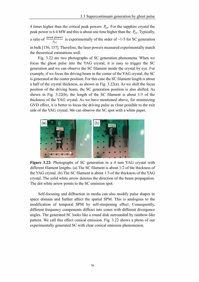
3.3 Supercontinuum generation by ghost pulse
56
4 times higher than the critical peak powers 𝑃cr. For the sapphire crystal the
peak power is 6.4 MW and this is about one time higher than the 𝑃cr. Typically,
a ratio of 𝑝𝑒𝑎𝑘 𝑝𝑜𝑤𝑒𝑟
𝑃𝑐𝑟 is experimentally of the order of ~1-5 for SC generation
in bulk [156, 157]. Therefore, the laser powers measured experimentally match
the theoretical estimations well.
Fig. 3.22 are two photographs of SC generation phenomena. When we
focus the ghost pulse into the YAG crystal, it is easy to trigger the SC
generation and we can observe the SC filament inside the crystal by eye. For
example, if we focus the driving beam in the center of the YAG crystal, the SC
is generated at the center position. For this case the SC filament length is about
a half of the crystal thickness, as shown in Fig. 3.22(a). As we shift the focus
position of the driving beam, the SC generation position is also shifted. As
shown in Fig. 3.22(b), the length of the SC filament is about 1/3 of the
thickness of the YAG crystal. As we have mentioned above, for minimizing
GVD effect, it is better to focus the driving pulse as close possible to the exit
side of the YAG crystal. We can observe the SC spot with a white paper.
Figure 3.22: Photographs of SC generation in a 4 mm YAG crystal with
different filament lengths. (a) The SC filament is about 1/2 of the thickness of
the YAG crystal. (b) The SC filament is about 1/3 of the thickness of the YAG
crystal. The solid white arrow denotes the direction of the beam propagation.
The dot white arrow points to the SC emission spot.
Self-focusing and diffraction in media can also modify pulse shapes in
space domain and further affect the spatial SPM. This is analogous to the
modification of temporal SPM by self-steepening effect. Consequently,
different frequency components diffract into cones with different divergence
angles. The generated SC looks like a round disk surrounded by rainbow-like
pattern. We call this effect conical emission. Fig. 3.22 shows a photo of our
experimentally generated SC with clear conical emission phenomenon.
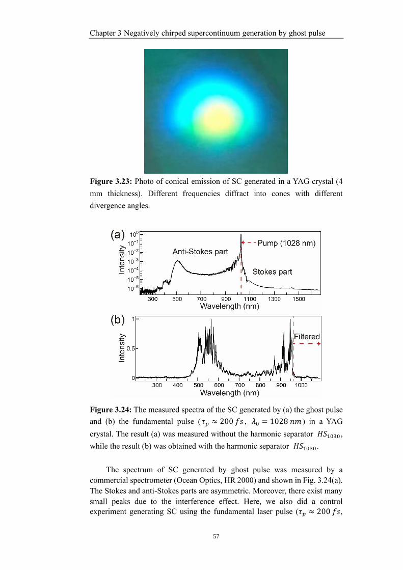
Chapter 3 Negatively chirped supercontinuum generation by ghost pulse
57
Figure 3.23: Photo of conical emission of SC generated in a YAG crystal (4
mm thickness). Different frequencies diffract into cones with different
divergence angles.
Figure 3.24: The measured spectra of the SC generated by (a) the ghost pulse
and (b) the fundamental pulse (𝜏𝑝 ≈ 200 𝑓𝑠 , 𝜆0 = 1028 𝑛𝑚 ) in a YAG
crystal. The result (a) was measured without the harmonic separator 𝐻𝑆1030 ,
while the result (b) was obtained with the harmonic separator 𝐻𝑆1030 .
The spectrum of SC generated by ghost pulse was measured by a
commercial spectrometer (Ocean Optics, HR 2000) and shown in Fig. 3.24(a).
The Stokes and anti-Stokes parts are asymmetric. Moreover, there exist many
small peaks due to the interference effect. Here, we also did a control
experiment generating SC using the fundamental laser pulse (𝜏𝑝 ≈ 200 𝑓𝑠,
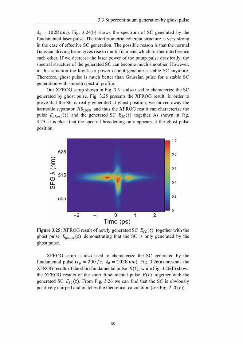
3.3 Supercontinuum generation by ghost pulse
58
𝜆0 = 1028 𝑛𝑚 ). Fig. 3.24(b) shows the spectrum of SC generated by the
fundamental laser pulse. The interferometric coherent structure is very strong
in the case of effective SC generation. The possible reason is that the normal
Gaussian driving beam gives rise to multi-filaments which further interference
each other. If we decrease the laser power of the pump pulse drastically, the
spectral structure of the generated SC can become much smoother. However,
in this situation the low laser power cannot generate a stable SC anymore.
Therefore, ghost pulse is much better than Gaussian pulse for a stable SC
generation with smooth spectral profile.
Our XFROG setup shown in Fig. 3.3 is also used to characterize the SC
generated by ghost pulse. Fig. 3.25 presents the XFROG result. In order to
prove that the SC is really generated at ghost position, we moved away the
harmonic separator 𝐻𝑆1030 and thus the XFROG result can characterize the
pulse 𝐸𝑔ℎ𝑜𝑠𝑡(𝑡) and the generated SC 𝐸𝑆𝐶(𝑡) together. As shown in Fig.
3.25, it is clear that the spectral broadening only appears at the ghost pulse
position.
Figure 3.25: XFROG result of newly generated SC 𝐸𝑆𝐶(𝑡) together with the
ghost pulse 𝐸𝑔ℎ𝑜𝑠𝑡(𝑡) demonstrating that the SC is only generated by the
ghost pulse.
XFROG setup is also used to characterize the SC generated by the
fundamental pulse (𝜏𝑝 ≈ 200 𝑓𝑠, 𝜆0 = 1028 𝑛𝑚). Fig. 3.26(a) presents the
XFROG results of the short fundamental pulse 𝐸(𝑡), while Fig. 3.26(b) shows
the XFROG results of the short fundamental pulse 𝐸(𝑡) together with the
generated SC 𝐸𝑆𝐶(𝑡). From Fig. 3.26 we can find that the SC is obviously
positively chirped and matches the theoretical calculation (see Fig. 2.20(c)).
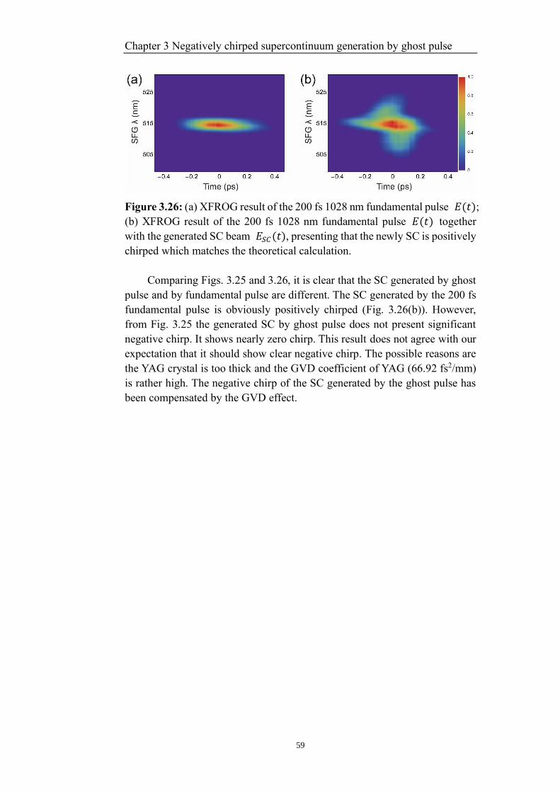
Chapter 3 Negatively chirped supercontinuum generation by ghost pulse
59
Figure 3.26: (a) XFROG result of the 200 fs 1028 nm fundamental pulse 𝐸(𝑡);
(b) XFROG result of the 200 fs 1028 nm fundamental pulse 𝐸(𝑡) together
with the generated SC beam 𝐸𝑆𝐶(𝑡), presenting that the newly SC is positively
chirped which matches the theoretical calculation.
Comparing Figs. 3.25 and 3.26, it is clear that the SC generated by ghost
pulse and by fundamental pulse are different. The SC generated by the 200 fs
fundamental pulse is obviously positively chirped (Fig. 3.26(b)). However,
from Fig. 3.25 the generated SC by ghost pulse does not present significant
negative chirp. It shows nearly zero chirp. This result does not agree with our
expectation that it should show clear negative chirp. The possible reasons are
the YAG crystal is too thick and the GVD coefficient of YAG (66.92 fs2/mm)
is rather high. The negative chirp of the SC generated by the ghost pulse has
been compensated by the GVD effect.
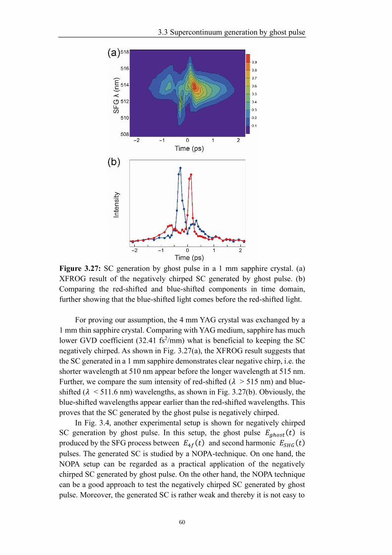
3.3 Supercontinuum generation by ghost pulse
60
Figure 3.27: SC generation by ghost pulse in a 1 mm sapphire crystal. (a)
XFROG result of the negatively chirped SC generated by ghost pulse. (b)
Comparing the red-shifted and blue-shifted components in time domain,
further showing that the blue-shifted light comes before the red-shifted light.
For proving our assumption, the 4 mm YAG crystal was exchanged by a
1 mm thin sapphire crystal. Comparing with YAG medium, sapphire has much
lower GVD coefficient (32.41 fs2/mm) what is beneficial to keeping the SC
negatively chirped. As shown in Fig. 3.27(a), the XFROG result suggests that
the SC generated in a 1 mm sapphire demonstrates clear negative chirp, i.e. the
shorter wavelength at 510 nm appear before the longer wavelength at 515 nm.
Further, we compare the sum intensity of red-shifted (𝜆 > 515 nm) and blue-
shifted (𝜆 < 511.6 nm) wavelengths, as shown in Fig. 3.27(b). Obviously, the
blue-shifted wavelengths appear earlier than the red-shifted wavelengths. This
proves that the SC generated by the ghost pulse is negatively chirped.
In Fig. 3.4, another experimental setup is shown for negatively chirped
SC generation by ghost pulse. In this setup, the ghost pulse 𝐸𝑔ℎ𝑜𝑠𝑡(𝑡) is
produced by the SFG process between 𝐸4𝑓(𝑡) and second harmonic 𝐸𝑆𝐻𝐺(𝑡)
pulses. The generated SC is studied by a NOPA-technique. On one hand, the
NOPA setup can be regarded as a practical application of the negatively
chirped SC generated by ghost pulse. On the other hand, the NOPA technique
can be a good approach to test the negatively chirped SC generated by ghost
pulse. Moreover, the generated SC is rather weak and thereby it is not easy to
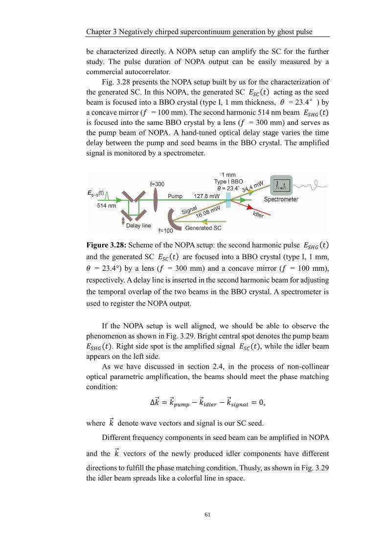
Chapter 3 Negatively chirped supercontinuum generation by ghost pulse
61
be characterized directly. A NOPA setup can amplify the SC for the further
study. The pulse duration of NOPA output can be easily measured by a
commercial autocorrelator.
Fig. 3.28 presents the NOPA setup built by us for the characterization of
the generated SC. In this NOPA, the generated SC 𝐸𝑆𝐶(𝑡) acting as the seed
beam is focused into a BBO crystal (type I, 1 mm thickness, 𝜃 = 23.4°) by
a concave mirror (𝑓 = 100 mm). The second harmonic 514 nm beam 𝐸𝑆𝐻𝐺(𝑡)
is focused into the same BBO crystal by a lens (𝑓 = 300 mm) and serves as
the pump beam of NOPA. A hand-tuned optical delay stage varies the time
delay between the pump and seed beams in the BBO crystal. The amplified
signal is monitored by a spectrometer.
Figure 3.28: Scheme of the NOPA setup: the second harmonic pulse 𝐸𝑆𝐻𝐺(𝑡)
and the generated SC 𝐸𝑆𝐶(𝑡) are focused into a BBO crystal (type I, 1 mm,
𝜃 = 23.4°) by a lens (𝑓 = 300 mm) and a concave mirror (𝑓 = 100 mm),
respectively. A delay line is inserted in the second harmonic beam for adjusting
the temporal overlap of the two beams in the BBO crystal. A spectrometer is
used to register the NOPA output.
If the NOPA setup is well aligned, we should be able to observe the
phenomenon as shown in Fig. 3.29. Bright central spot denotes the pump beam
𝐸𝑆𝐻𝐺(𝑡). Right side spot is the amplified signal 𝐸𝑆𝐶(𝑡), while the idler beam
appears on the left side.
As we have discussed in section 2.4, in the process of non-collinear
optical parametric amplification, the beams should meet the phase matching
condition:
∆�⃑� = �⃑� 𝑝𝑢𝑚𝑝 − �⃑� 𝑖𝑑𝑙𝑒𝑟 − �⃑� 𝑠𝑖𝑔𝑛𝑎𝑙 = 0,
where �⃑� denote wave vectors and signal is our SC seed.
Different frequency components in seed beam can be amplified in NOPA
and the �⃑� vectors of the newly produced idler components have different
directions to fulfill the phase matching condition. Thusly, as shown in Fig. 3.29
the idler beam spreads like a colorful line in space.
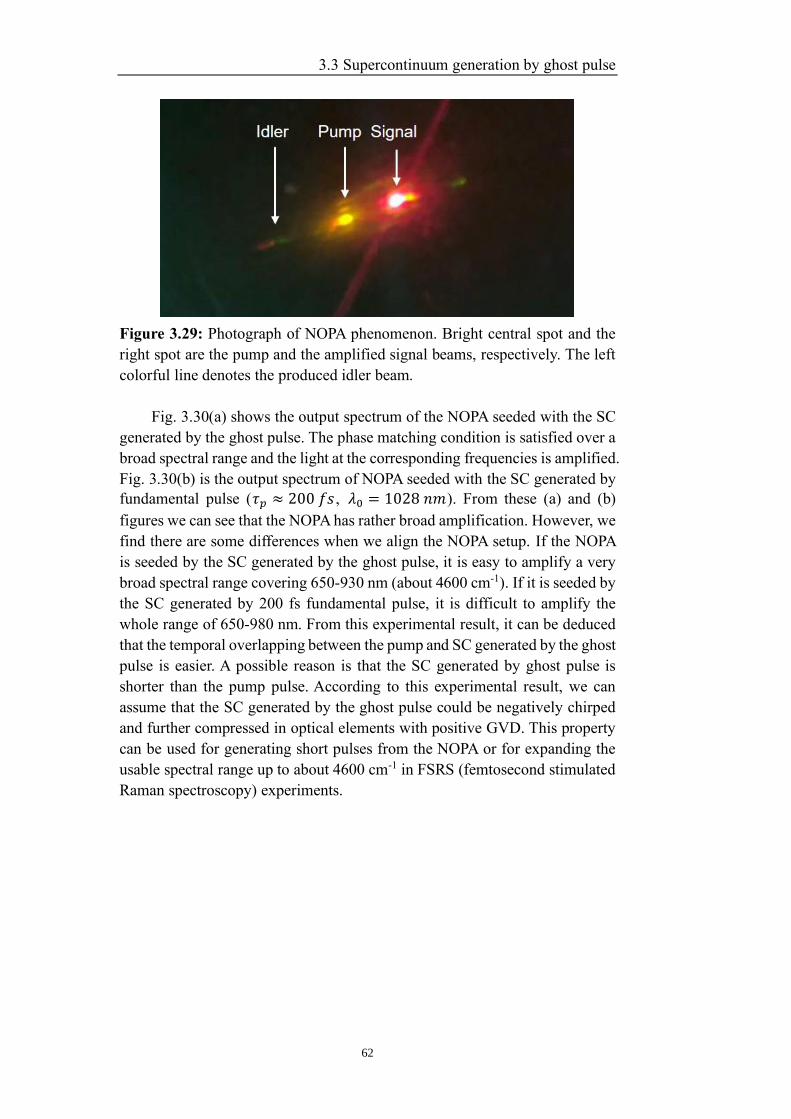
3.3 Supercontinuum generation by ghost pulse
62
Figure 3.29: Photograph of NOPA phenomenon. Bright central spot and the
right spot are the pump and the amplified signal beams, respectively. The left
colorful line denotes the produced idler beam.
Fig. 3.30(a) shows the output spectrum of the NOPA seeded with the SC
generated by the ghost pulse. The phase matching condition is satisfied over a
broad spectral range and the light at the corresponding frequencies is amplified.
Fig. 3.30(b) is the output spectrum of NOPA seeded with the SC generated by
fundamental pulse (𝜏𝑝 ≈ 200 𝑓𝑠 , 𝜆0 = 1028 𝑛𝑚 ). From these (a) and (b)
figures we can see that the NOPA has rather broad amplification. However, we
find there are some differences when we align the NOPA setup. If the NOPA
is seeded by the SC generated by the ghost pulse, it is easy to amplify a very
broad spectral range covering 650-930 nm (about 4600 cm-1). If it is seeded by
the SC generated by 200 fs fundamental pulse, it is difficult to amplify the
whole range of 650-980 nm. From this experimental result, it can be deduced
that the temporal overlapping between the pump and SC generated by the ghost
pulse is easier. A possible reason is that the SC generated by ghost pulse is
shorter than the pump pulse. According to this experimental result, we can
assume that the SC generated by the ghost pulse could be negatively chirped
and further compressed in optical elements with positive GVD. This property
can be used for generating short pulses from the NOPA or for expanding the
usable spectral range up to about 4600 cm-1 in FSRS (femtosecond stimulated
Raman spectroscopy) experiments.
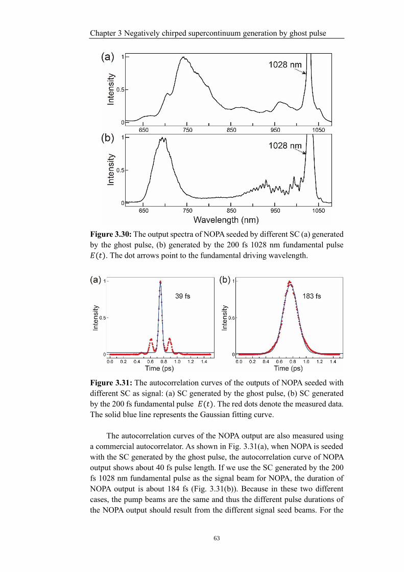
Chapter 3 Negatively chirped supercontinuum generation by ghost pulse
63
Figure 3.30: The output spectra of NOPA seeded by different SC (a) generated
by the ghost pulse, (b) generated by the 200 fs 1028 nm fundamental pulse
𝐸(𝑡). The dot arrows point to the fundamental driving wavelength.
Figure 3.31: The autocorrelation curves of the outputs of NOPA seeded with
different SC as signal: (a) SC generated by the ghost pulse, (b) SC generated
by the 200 fs fundamental pulse 𝐸(𝑡). The red dots denote the measured data.
The solid blue line represents the Gaussian fitting curve.
The autocorrelation curves of the NOPA output are also measured using
a commercial autocorrelator. As shown in Fig. 3.31(a), when NOPA is seeded
with the SC generated by the ghost pulse, the autocorrelation curve of NOPA
output shows about 40 fs pulse length. If we use the SC generated by the 200
fs 1028 nm fundamental pulse as the signal beam for NOPA, the duration of
NOPA output is about 184 fs (Fig. 3.31(b)). Because in these two different
cases, the pump beams are the same and thus the different pulse durations of
the NOPA output should result from the different signal seed beams. For the
3.4 Summary
64
case shown in Fig. 3.31(a), the seed SC pulse generated by the ghost pulse
must be very short, otherwise we should not obtain such short NOPA output.
Combining the XFROG results (see Figs. 3.26 and 3.27), it can be deduced
that the generated SC is negatively chirped and afterwards the chirp is
compensated in the optical elements, such as YAG, sapphire and BBO crystals.
When the SC arrives to the NOPA’s BBO crystal, the negative chirp of the SC
pulse could be good compensated and be shorter than the SC generated by the
fundamental pulse. This could explain short (39 fs) NOPA output.
3.4 Summary
This chapter is mainly devoted to the description of the negatively chirped
SC generation by the ghost pulse. We present the details of the experimental
setups, as well as analyze and discuss the experimental results. According to
the SPM theory, a ghost pulse should be able to generate a negatively chirped
SC. Motivated by this idea, specific experimental setups including several key
units such as 4f-line, SFG setup, SC generation and characterization setups
were built. The 4f-line and SFG setup are used to create the desired ghost pulse.
The formation of the ghost pulse was verified by a home-built FROG setup
and a commercial autocorrelator device. Afterwards, the ghost pulse is focused
into a YAG/sapphire crystal to produce negatively chirped SC. Finally, the
NOPA and XFROG techniques are used to characterize the negatively chirped
SC. From the NOPA result, we can deduce that the SC generated by ghost pulse
should be negatively chirped. The XFROG result gives more convinced proofs.
It verifies that the SC can be generated by the ghost pulse because the spectral
broadening appears just at the position of the ghost pulse. It also proves that
the generated SC in 1 mm sapphire by the ghost pulse is negatively chirped.
Chapter 4 Two-stage non-collinear optical parametric amplifier
65
Chapter 4
Two-stage non-collinear optical
parametric amplifier
In this chapter, a two-stage non-collinear optical parametric amplifier
(NOPA) pumped by the second harmonic (𝜆0 = 514 nm) of Yb:KGW laser
light is described. The NOPA output tuned from 650 to 1000 nm. Pulse
compression of the NOPA output is performed using an Acousto-Optic
Programmable Dispersive Filter (AOPDF).
4.1 Introduction
Ultrafast optics has become a major technology in many modern studies
of light-matter interaction [54, 63]. It is necessary to develop applicable laser
sources which can supply pulse with ultrashort duration, high peak power and
broad frequency bandwidth. For example, in the field of pump-probe
spectroscopy, the research objects (atom, molecule, etc.) are excited by a
“pump” pulse and then the sample’s subsequent evolution is monitored by
observing the pump-induced absorption change which is measured by a
delayed “probe” pulse [38]. For investigating some fast-physical process, the
probe pulse should have a very high temporal resolution which means the
duration time of probe pulse should be very short. Moreover, different study
samples require variable beam powers and frequencies of both pump and probe
pulses. Hence, for a long time the generation of a tunable ultrashort pulse is
one of the major challenges in the field of ultrafast optics.
Basing on Ti:sapphire and Yb:doped gain media, Kerr-lens mode-locking
and chirped-pulse amplification (CPA), rugged, reliable and power scalable
sources of ultrafast pulses have been developed [65-68]. Up to now, this
technology is still the mainstream method to generate ultrashort pulse.
However, such kind of laser source can not supply tunable output radiation and
is limited in a narrow range around the fundamental frequencies (1040 nm for
Yb and 800 nm for Ti:sapphire).
In most cases, optical parametric amplifier (OPA) using nonlinear optical
effect can achieve frequency tunability. Up to now, OPA has become a standard
tool for the generation of ultrashort pulses over the spectral range from UV to
IR [93-100]. Non-collinear OPA, namely NOPA, is able to achieve phase
matching conditions over a broad frequency range and thus an ultrabroad
amplification output can be obtained. In order to get ultrashort pulses,
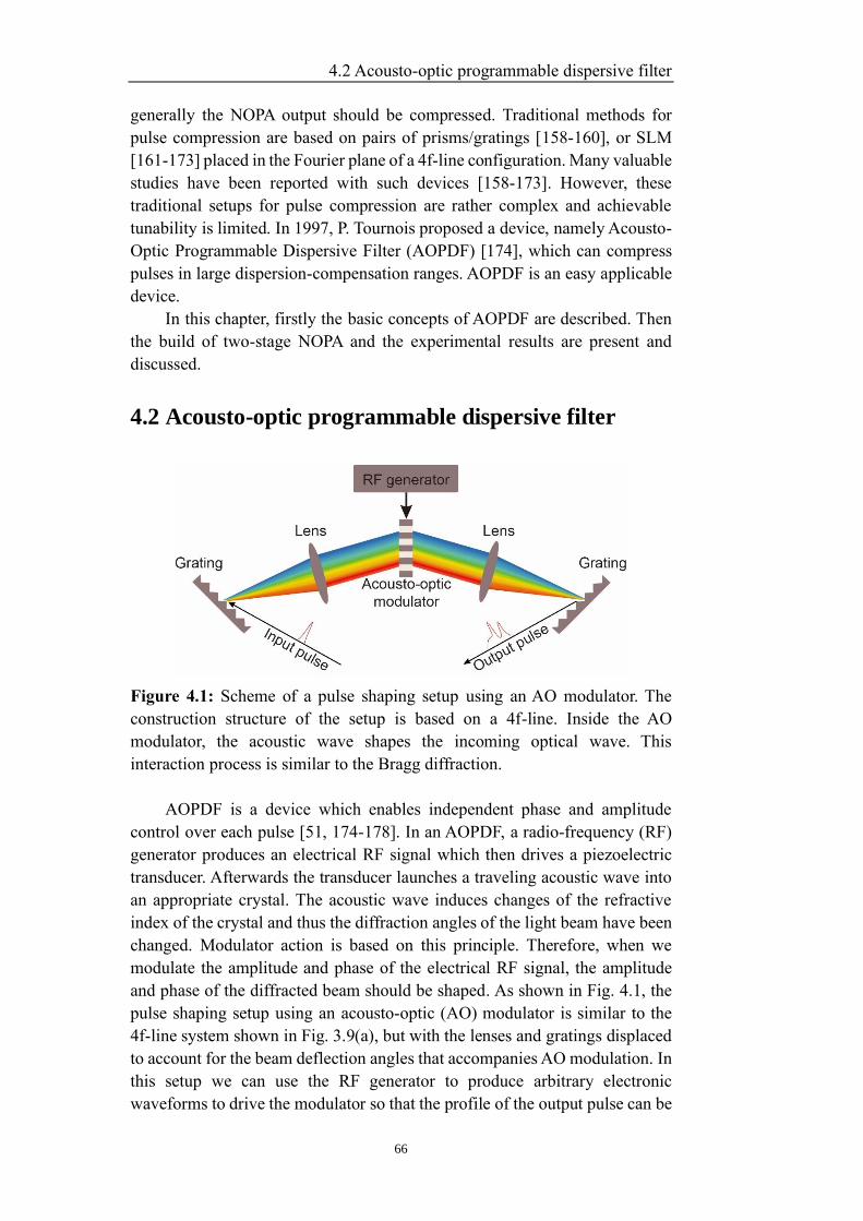
4.2 Acousto-optic programmable dispersive filter
66
generally the NOPA output should be compressed. Traditional methods for
pulse compression are based on pairs of prisms/gratings [158-160], or SLM
[161-173] placed in the Fourier plane of a 4f-line configuration. Many valuable
studies have been reported with such devices [158-173]. However, these
traditional setups for pulse compression are rather complex and achievable
tunability is limited. In 1997, P. Tournois proposed a device, namely Acousto-
Optic Programmable Dispersive Filter (AOPDF) [174], which can compress
pulses in large dispersion-compensation ranges. AOPDF is an easy applicable
device.
In this chapter, firstly the basic concepts of AOPDF are described. Then
the build of two-stage NOPA and the experimental results are present and
discussed.
4.2 Acousto-optic programmable dispersive filter
Figure 4.1: Scheme of a pulse shaping setup using an AO modulator. The
construction structure of the setup is based on a 4f-line. Inside the AO
modulator, the acoustic wave shapes the incoming optical wave. This
interaction process is similar to the Bragg diffraction.
AOPDF is a device which enables independent phase and amplitude
control over each pulse [51, 174-178]. In an AOPDF, a radio-frequency (RF)
generator produces an electrical RF signal which then drives a piezoelectric
transducer. Afterwards the transducer launches a traveling acoustic wave into
an appropriate crystal. The acoustic wave induces changes of the refractive
index of the crystal and thus the diffraction angles of the light beam have been
changed. Modulator action is based on this principle. Therefore, when we
modulate the amplitude and phase of the electrical RF signal, the amplitude
and phase of the diffracted beam should be shaped. As shown in Fig. 4.1, the
pulse shaping setup using an acousto-optic (AO) modulator is similar to the
4f-line system shown in Fig. 3.9(a), but with the lenses and gratings displaced
to account for the beam deflection angles that accompanies AO modulation. In
this setup we can use the RF generator to produce arbitrary electronic
waveforms to drive the modulator so that the profile of the output pulse can be
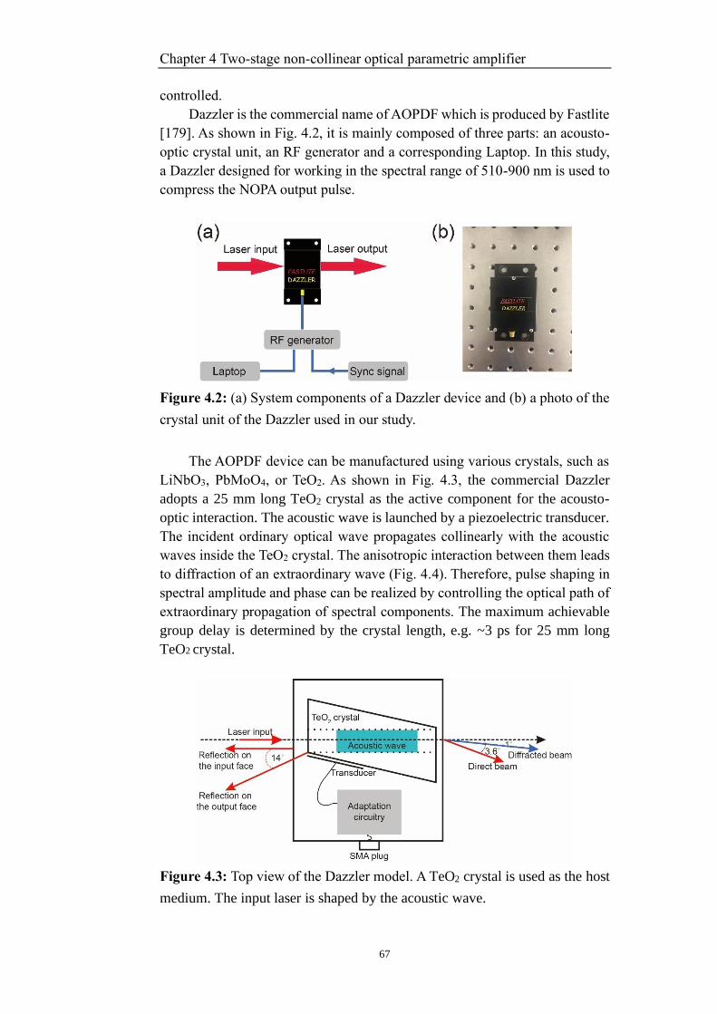
Chapter 4 Two-stage non-collinear optical parametric amplifier
67
controlled.
Dazzler is the commercial name of AOPDF which is produced by Fastlite
[179]. As shown in Fig. 4.2, it is mainly composed of three parts: an acousto-
optic crystal unit, an RF generator and a corresponding Laptop. In this study,
a Dazzler designed for working in the spectral range of 510-900 nm is used to
compress the NOPA output pulse.
Figure 4.2: (a) System components of a Dazzler device and (b) a photo of the
crystal unit of the Dazzler used in our study.
The AOPDF device can be manufactured using various crystals, such as
LiNbO3, PbMoO4, or TeO2. As shown in Fig. 4.3, the commercial Dazzler
adopts a 25 mm long TeO2 crystal as the active component for the acousto-
optic interaction. The acoustic wave is launched by a piezoelectric transducer.
The incident ordinary optical wave propagates collinearly with the acoustic
waves inside the TeO2 crystal. The anisotropic interaction between them leads
to diffraction of an extraordinary wave (Fig. 4.4). Therefore, pulse shaping in
spectral amplitude and phase can be realized by controlling the optical path of
extraordinary propagation of spectral components. The maximum achievable
group delay is determined by the crystal length, e.g. ~3 ps for 25 mm long
TeO2 crystal.
Figure 4.3: Top view of the Dazzler model. A TeO2 crystal is used as the host
medium. The input laser is shaped by the acoustic wave.
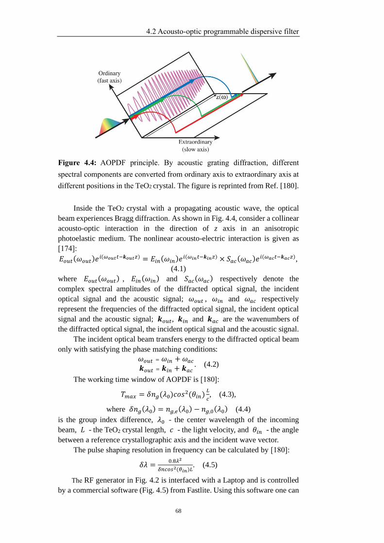
4.2 Acousto-optic programmable dispersive filter
68
Figure 4.4: AOPDF principle. By acoustic grating diffraction, different
spectral components are converted from ordinary axis to extraordinary axis at
different positions in the TeO2 crystal. The figure is reprinted from Ref. [180].
Inside the TeO2 crystal with a propagating acoustic wave, the optical
beam experiences Bragg diffraction. As shown in Fig. 4.4, consider a collinear
acousto-optic interaction in the direction of z axis in an anisotropic
photoelastic medium. The nonlinear acousto-electric interaction is given as
[174]:
𝐸𝑜𝑢𝑡(𝜔𝑜𝑢𝑡)𝑒𝑖(𝜔𝑜𝑢𝑡𝑡−𝒌𝑜𝑢𝑡𝑧) = 𝐸𝑖𝑛(𝜔𝑖𝑛)𝑒
𝑖(𝜔𝑖𝑛𝑡−𝒌𝑖𝑛𝑧) × 𝑆𝑎𝑐(𝜔𝑎𝑐)𝑒𝑖(𝜔𝑎𝑐𝑡−𝒌𝑎𝑐𝑧),
(4.1)
where 𝐸𝑜𝑢𝑡(𝜔𝑜𝑢𝑡) , 𝐸𝑖𝑛(𝜔𝑖𝑛) and 𝑆𝑎𝑐(𝜔𝑎𝑐) respectively denote the
complex spectral amplitudes of the diffracted optical signal, the incident
optical signal and the acoustic signal; 𝜔𝑜𝑢𝑡 , 𝜔𝑖𝑛 and 𝜔𝑎𝑐 respectively
represent the frequencies of the diffracted optical signal, the incident optical
signal and the acoustic signal; 𝒌𝑜𝑢𝑡, 𝒌𝑖𝑛 and 𝒌𝑎𝑐 are the wavenumbers of
the diffracted optical signal, the incident optical signal and the acoustic signal.
The incident optical beam transfers energy to the diffracted optical beam
only with satisfying the phase matching conditions:
𝜔𝑜𝑢𝑡 = 𝜔𝑖𝑛 + 𝜔𝑎𝑐
𝒌𝑜𝑢𝑡 = 𝒌𝑖𝑛 + 𝒌𝑎𝑐. (4.2)
The working time window of AOPDF is [180]:
𝑇𝑚𝑎𝑥 = 𝛿𝑛𝑔(𝜆0)𝑐𝑜𝑠2(𝜃𝑖𝑛)
𝐿
𝑐, (4.3),
where 𝛿𝑛𝑔(𝜆0) = 𝑛𝑔,𝑒(𝜆0) − 𝑛𝑔,0(𝜆0) (4.4)
is the group index difference, 𝜆0 - the center wavelength of the incoming
beam, 𝐿 - the TeO2 crystal length, 𝑐 - the light velocity, and 𝜃𝑖𝑛 - the angle
between a reference crystallographic axis and the incident wave vector.
The pulse shaping resolution in frequency can be calculated by [180]:
𝛿𝜆 =0.8𝜆2
𝛿𝑛𝑐𝑜𝑠2(𝜃𝑖𝑛)𝐿. (4.5)
The RF generator in Fig. 4.2 is interfaced with a Laptop and is controlled
by a commercial software (Fig. 4.5) from Fastlite. Using this software one can
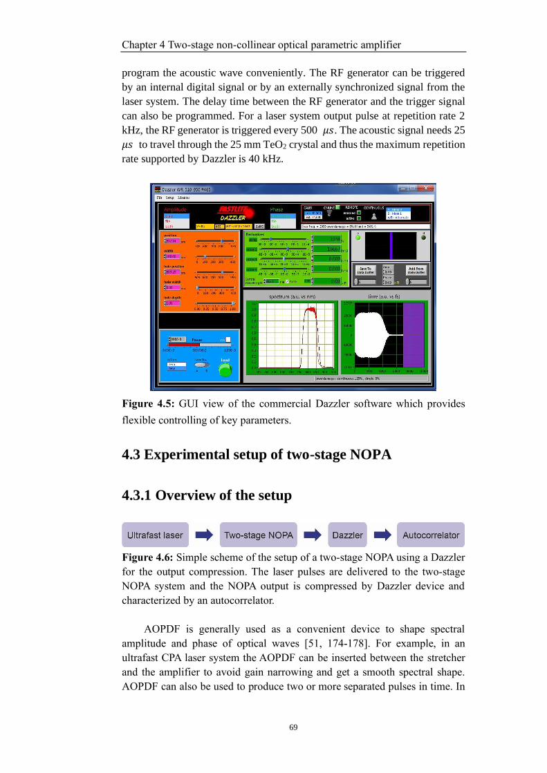
Chapter 4 Two-stage non-collinear optical parametric amplifier
69
program the acoustic wave conveniently. The RF generator can be triggered
by an internal digital signal or by an externally synchronized signal from the
laser system. The delay time between the RF generator and the trigger signal
can also be programmed. For a laser system output pulse at repetition rate 2
kHz, the RF generator is triggered every 500 𝜇𝑠. The acoustic signal needs 25
𝜇𝑠 to travel through the 25 mm TeO2 crystal and thus the maximum repetition
rate supported by Dazzler is 40 kHz.
Figure 4.5: GUI view of the commercial Dazzler software which provides
flexible controlling of key parameters.
4.3 Experimental setup of two-stage NOPA
4.3.1 Overview of the setup
Figure 4.6: Simple scheme of the setup of a two-stage NOPA using a Dazzler
for the output compression. The laser pulses are delivered to the two-stage
NOPA system and the NOPA output is compressed by Dazzler device and
characterized by an autocorrelator.
AOPDF is generally used as a convenient device to shape spectral
amplitude and phase of optical waves [51, 174-178]. For example, in an
ultrafast CPA laser system the AOPDF can be inserted between the stretcher
and the amplifier to avoid gain narrowing and get a smooth spectral shape.
AOPDF can also be used to produce two or more separated pulses in time. In
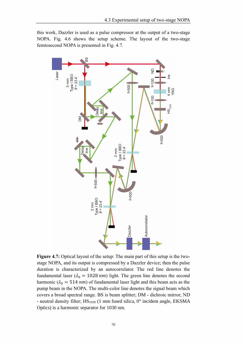
4.3 Experimental setup of two-stage NOPA
70
this work, Dazzler is used as a pulse compressor at the output of a two-stage
NOPA. Fig. 4.6 shows the setup scheme. The layout of the two-stage
femtosecond NOPA is presented in Fig. 4.7.
Figure 4.7: Optical layout of the setup: The main part of this setup is the two-
stage NOPA, and its output is compressed by a Dazzler device; then the pulse
duration is characterized by an autocorrelator. The red line denotes the
fundamental laser (𝜆0 = 1028 𝑛𝑚) light. The green line denotes the second
harmonic (𝜆0 = 514 𝑛𝑚) of fundamental laser light and this beam acts as the
pump beam in the NOPA. The multi-color line denotes the signal beam which
covers a broad spectral range. BS is beam splitter; DM - dichroic mirror; ND
- neutral density filter; HS1030 (1 mm fused silica, 0° incident angle, EKSMA
Optics) is a harmonic separator for 1030 nm.
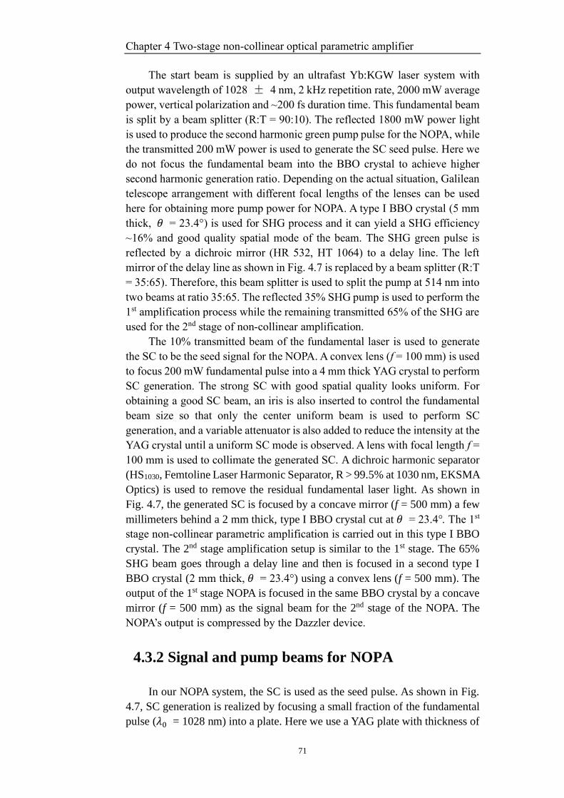
Chapter 4 Two-stage non-collinear optical parametric amplifier
71
The start beam is supplied by an ultrafast Yb:KGW laser system with
output wavelength of 1028 ± 4 nm, 2 kHz repetition rate, 2000 mW average
power, vertical polarization and ~200 fs duration time. This fundamental beam
is split by a beam splitter (R:T = 90:10). The reflected 1800 mW power light
is used to produce the second harmonic green pump pulse for the NOPA, while
the transmitted 200 mW power is used to generate the SC seed pulse. Here we
do not focus the fundamental beam into the BBO crystal to achieve higher
second harmonic generation ratio. Depending on the actual situation, Galilean
telescope arrangement with different focal lengths of the lenses can be used
here for obtaining more pump power for NOPA. A type I BBO crystal (5 mm
thick, 𝜃 = 23.4°) is used for SHG process and it can yield a SHG efficiency
~16% and good quality spatial mode of the beam. The SHG green pulse is
reflected by a dichroic mirror (HR 532, HT 1064) to a delay line. The left
mirror of the delay line as shown in Fig. 4.7 is replaced by a beam splitter (R:T
= 35:65). Therefore, this beam splitter is used to split the pump at 514 nm into
two beams at ratio 35:65. The reflected 35% SHG pump is used to perform the
1st amplification process while the remaining transmitted 65% of the SHG are
used for the 2nd stage of non-collinear amplification.
The 10% transmitted beam of the fundamental laser is used to generate
the SC to be the seed signal for the NOPA. A convex lens (f = 100 mm) is used
to focus 200 mW fundamental pulse into a 4 mm thick YAG crystal to perform
SC generation. The strong SC with good spatial quality looks uniform. For
obtaining a good SC beam, an iris is also inserted to control the fundamental
beam size so that only the center uniform beam is used to perform SC
generation, and a variable attenuator is also added to reduce the intensity at the
YAG crystal until a uniform SC mode is observed. A lens with focal length f =
100 mm is used to collimate the generated SC. A dichroic harmonic separator
(HS1030, Femtoline Laser Harmonic Separator, R > 99.5% at 1030 nm, EKSMA
Optics) is used to remove the residual fundamental laser light. As shown in
Fig. 4.7, the generated SC is focused by a concave mirror (f = 500 mm) a few
millimeters behind a 2 mm thick, type I BBO crystal cut at 𝜃 = 23.4° he 1st
stage non-collinear parametric amplification is carried out in this type I BBO
crystal. The 2nd stage amplification setup is similar to the 1st stage. The 65%
SHG beam goes through a delay line and then is focused in a second type I
BBO crystal (2 mm thick, 𝜃 = 23.4°) using a convex lens (f = 500 mm). The
output of the 1st stage NOPA is focused in the same BBO crystal by a concave
mirror (f = 500 mm) as the signal beam for the 2nd stage of the NOPA. The
NOPA’s output is compressed by the Dazzler device.
4.3.2 Signal and pump beams for NOPA
In our NOPA system, the SC is used as the seed pulse. As shown in Fig.
4.7, SC generation is realized by focusing a small fraction of the fundamental
pulse (𝜆0 = 1028 nm) into a plate. Here we use a YAG plate with thickness of
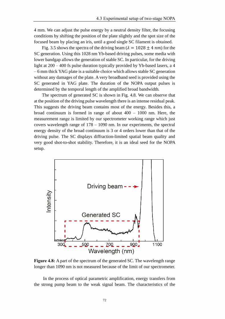
4.3 Experimental setup of two-stage NOPA
72
4 mm. We can adjust the pulse energy by a neutral density filter, the focusing
conditions by shifting the position of the plate slightly and the spot size of the
focused beam by placing an iris, until a good single SC filament is obtained.
Fig. 3.5 shows the spectra of the driving beam (𝜆 = 1028 ± 4 𝑛𝑚) for the
SC generation. Using this 1028 nm Yb-based driving pulses, some media with
lower bandgap allows the generation of stable SC. In particular, for the driving
light at 200 – 400 fs pulse duration typically provided by Yb-based lasers, a 4
– 6 mm thick YAG plate is a suitable choice which allows stable SC generation
without any damages of the plate. A very broadband seed is provided using the
SC generated in YAG plate. The duration of the NOPA output pulses is
determined by the temporal length of the amplified broad bandwidth.
The spectrum of generated SC is shown in Fig. 4.8. We can observe that
at the position of the driving pulse wavelength there is an intense residual peak.
This suggests the driving beam contains most of the energy. Besides this, a
broad continuum is formed in range of about 400 – 1000 nm. Here, the
measurement range is limited by our spectrometer working range which just
covers wavelength range of 178 – 1090 nm. In our experiments, the spectral
energy density of the broad continuum is 3 or 4 orders lower than that of the
driving pulse. The SC displays diffraction-limited spatial beam quality and
very good shot-to-shot stability. Therefore, it is an ideal seed for the NOPA
setup.
Figure 4.8: A part of the spectrum of the generated SC. The wavelength range
longer than 1090 nm is not measured because of the limit of our spectrometer.
In the process of optical parametric amplification, energy transfers from
the strong pump beam to the weak signal beam. The characteristics of the
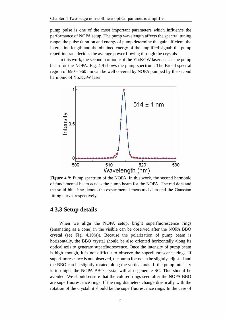
Chapter 4 Two-stage non-collinear optical parametric amplifier
73
pump pulse is one of the most important parameters which influence the
performance of NOPA setup. The pump wavelength affects the spectral tuning
range; the pulse duration and energy of pump determine the gain efficient, the
interaction length and the obtained energy of the amplified signal; the pump
repetition rate decides the average power flowing through the crystals.
In this work, the second harmonic of the Yb:KGW laser acts as the pump
beam for the NOPA. Fig. 4.9 shows the pump spectrum. The Broad spectral
region of 690 – 960 nm can be well covered by NOPA pumped by the second
harmonic of Yb:KGW laser.
Figure 4.9: Pump spectrum of the NOPA. In this work, the second harmonic
of fundamental beam acts as the pump beam for the NOPA. The red dots and
the solid blue line denote the experimental measured data and the Gaussian
fitting curve, respectively.
4.3.3 Setup details
When we align the NOPA setup, bright superfluorescence rings
(emanating as a cone) in the visible can be observed after the NOPA BBO
crystal (see Fig. 4.10(a)). Because the polarization of pump beam is
horizontally, the BBO crystal should be also oriented horizontally along its
optical axis to generate superfluorescence. Once the intensity of pump beam
is high enough, it is not difficult to observe the superfluorescence rings. If
superfluorescence is not observed, the pump focus can be slightly adjusted and
the BBO can be slightly rotated along the vertical axis. If the pump intensity
is too high, the NOPA BBO crystal will also generate SC. This should be
avoided. We should ensure that the colored rings seen after the NOPA BBO
are superfluorescence rings. If the ring diameters change drastically with the
rotation of the crystal, it should be the superfluorescence rings. In the case of

4.3 Experimental setup of two-stage NOPA
74
the colored rings generated due to supercontinuum, they remain constant under
crystal rotation.
Figure 4.10: Photographs of the output beams after the NOPA BBO crystal
pumped at 400 nm under different overlapping conditions. The central and
right-side bright spots denote the pump and signal beams, respectively. (a) The
pump beam induces multicolored parametric superfluorescence rings. (b) The
case that the pump and signal beams do not overlap well. (c) The case that the
phase matching is not completed. (d) The case that the phase matching
conditions have been satisfied completely. The figure is reprinted from Ref.
[181].
The crossing angle is determined by the pump wavelength and the signal
wavelengths that we want to amplify. Fig. 2.16 shows the theoretical phase
matching angle for NOPA using type I BBO crystal and central pump
wavelength of 514 nm. The white light seed and the green pump are crossed
at an angle of 2.3°, as can be seen in Fig. 2.16. It is worth noting that, the
crossing angle inside crystal is significantly different with the angle outside of
the BBO due to the influence of the high index of refraction of BBO.
The internal angle can be calculated based on the pump and signal
wavelengths and the phase matching conditions. The external angle is the
angle outside of the BBO crystal. When the pump and signal beams enter the
crystal, the high refractive index of the BBO crystal bends the beams’ path so
that the external angle is different with the internal angle. The external angle
can be calculated by Snell’s Law. At this angle, the white light can be seen
along the circumference of the superfluorescence ring and this is a good
guiding factor to ensure correct alignment. If the white light is not seen on the
circumference of the superfluorescence ring, the amplifier’s BBO can be
rotated slightly along its vertical axis to change the superfluorescence ring
diameter in order to overlap with the white light seed.
The delay between the seed and the green pump can be set to zero by
adjusting the delay line stage, as shown in Fig. 4.7. While adjusting the delay,
one can obtain a bright signal as shown in Figs. 4.10(c) and (d). The idler (in
the infrared region) can be easily seen on a screen in front of the amplifier
crystal around the zero delay, through an infrared viewer or using a webcam
(with IR filter removed) while adjusting the delay. The idler beam appears on
the left side of the ring and on the left side of the pump spot. The signal is the
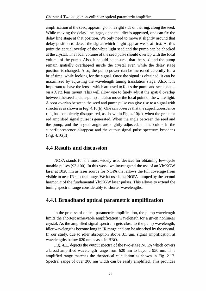
Chapter 4 Two-stage non-collinear optical parametric amplifier
75
amplification of the seed, appearing on the right side of the ring, along the seed.
While moving the delay line stage, once the idler is appeared, one can fix the
delay line stage at that position. We only need to move it slightly around that
delay position to detect the signal which might appear weak at first. At this
point the spatial overlap of the white light seed and the pump can be checked
at the crystal. The focal volume of the seed pulse should overlap with the focal
volume of the pump. Also, it should be ensured that the seed and the pump
remain spatially overlapped inside the crystal even while the delay stage
position is changed. Also, the pump power can be increased carefully for a
brief time, while looking for the signal. Once the signal is obtained, it can be
maximized by adjusting the wavelength tuning translation stage. Also, it is
important to have the lenses which are used to focus the pump and seed beams
on a XYZ lens mount. This will allow one to finely adjust the spatial overlap
between the seed and the pump and also move the focal point of the white light.
A poor overlap between the seed and pump pulse can give rise to a signal with
structures as shown in Fig. 4.10(b). One can observe that the superfluorescence
ring has completely disappeared, as shown in Fig. 4.10(d), when the green or
red amplified signal pulse is generated. When the angle between the seed and
the pump, and the crystal angle are slightly adjusted, all the colors in the
superfluorescence disappear and the output signal pulse spectrum broadens
(Fig. 4.10(d)).
4.4 Results and discussion
NOPA stands for the most widely used devices for obtaining few-cycle
tunable pulses [93-100]. In this work, we investigated the use of an Yb:KGW
laser at 1028 nm as laser source for NOPA that allows the full coverage from
visible to near IR spectral range. We focused on a NOPA pumped by the second
harmonic of the fundamental Yb:KGW laser pulses. This allows to extend the
tuning spectral range considerably to shorter wavelengths.
4.4.1 Broadband optical parametric amplification
In the process of optical parametric amplification, the pump wavelength
limits the shortest achievable amplification wavelength for a given nonlinear
crystal. As the amplified signal spectrum gets close to the pump wavelength,
idler wavelengths become long in IR range and can be absorbed by the crystal.
In our study, due to idler absorption above 3.1 µm, signal amplification at
wavelengths below 620 nm ceases in BBO.
Fig. 4.11 depicts the output spectra of the two-stage NOPA which covers
a broad amplified wavelength range from 620 nm to beyond 950 nm. This
amplified range matches the theoretical calculation as shown in Fig. 2.17.
Spectral range of over 200 nm width can be easily amplified. This provides
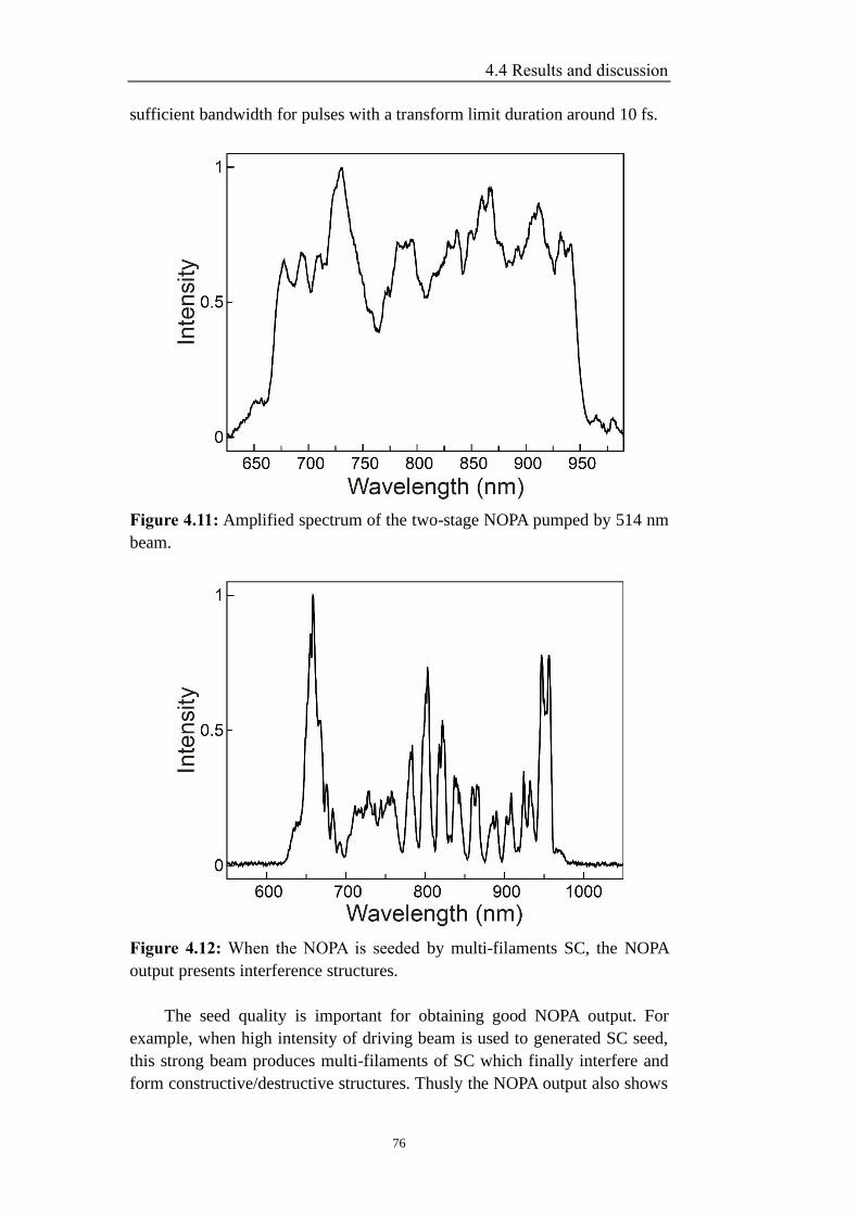
4.4 Results and discussion
76
sufficient bandwidth for pulses with a transform limit duration around 10 fs.
Figure 4.11: Amplified spectrum of the two-stage NOPA pumped by 514 nm
beam.
Figure 4.12: When the NOPA is seeded by multi-filaments SC, the NOPA
output presents interference structures.
The seed quality is important for obtaining good NOPA output. For
example, when high intensity of driving beam is used to generated SC seed,
this strong beam produces multi-filaments of SC which finally interfere and
form constructive/destructive structures. Thusly the NOPA output also shows
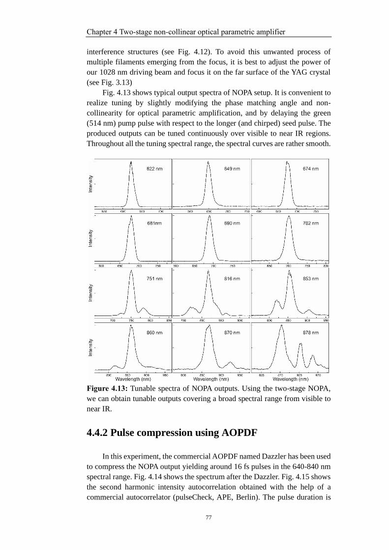
Chapter 4 Two-stage non-collinear optical parametric amplifier
77
interference structures (see Fig. 4.12). To avoid this unwanted process of
multiple filaments emerging from the focus, it is best to adjust the power of
our 1028 nm driving beam and focus it on the far surface of the YAG crystal
(see Fig. 3.13)
Fig. 4.13 shows typical output spectra of NOPA setup. It is convenient to
realize tuning by slightly modifying the phase matching angle and non-
collinearity for optical parametric amplification, and by delaying the green
(514 nm) pump pulse with respect to the longer (and chirped) seed pulse. The
produced outputs can be tuned continuously over visible to near IR regions.
Throughout all the tuning spectral range, the spectral curves are rather smooth.
Figure 4.13: Tunable spectra of NOPA outputs. Using the two-stage NOPA,
we can obtain tunable outputs covering a broad spectral range from visible to
near IR.
4.4.2 Pulse compression using AOPDF
In this experiment, the commercial AOPDF named Dazzler has been used
to compress the NOPA output yielding around 16 fs pulses in the 640-840 nm
spectral range. Fig. 4.14 shows the spectrum after the Dazzler. Fig. 4.15 shows
the second harmonic intensity autocorrelation obtained with the help of a
commercial autocorrelator (pulseCheck, APE, Berlin). The pulse duration is
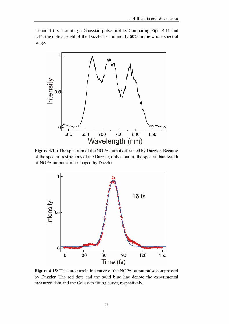
4.4 Results and discussion
78
around 16 fs assuming a Gaussian pulse profile. Comparing Figs. 4.11 and
4.14, the optical yield of the Dazzler is commonly 60% in the whole spectral
range.
Figure 4.14: The spectrum of the NOPA output diffracted by Dazzler. Because
of the spectral restrictions of the Dazzler, only a part of the spectral bandwidth
of NOPA output can be shaped by Dazzler.
Figure 4.15: The autocorrelation curve of the NOPA output pulse compressed
by Dazzler. The red dots and the solid blue line denote the experimental
measured data and the Gaussian fitting curve, respectively.
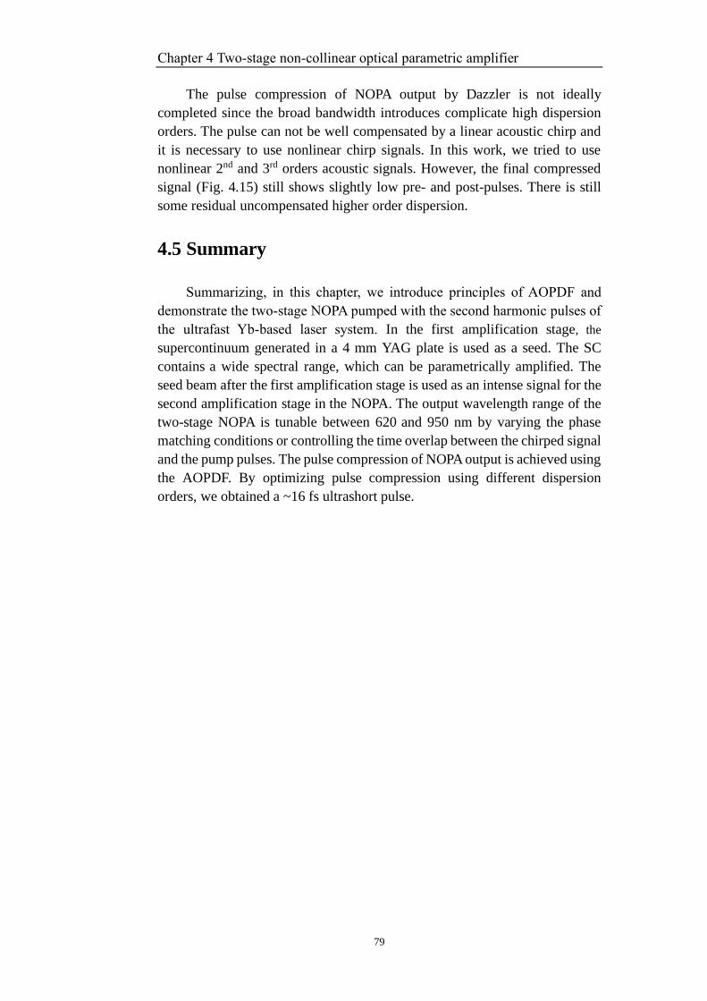
Chapter 4 Two-stage non-collinear optical parametric amplifier
79
The pulse compression of NOPA output by Dazzler is not ideally
completed since the broad bandwidth introduces complicate high dispersion
orders. The pulse can not be well compensated by a linear acoustic chirp and
it is necessary to use nonlinear chirp signals. In this work, we tried to use
nonlinear 2nd and 3rd orders acoustic signals. However, the final compressed
signal (Fig. 4.15) still shows slightly low pre- and post-pulses. There is still
some residual uncompensated higher order dispersion.
4.5 Summary
Summarizing, in this chapter, we introduce principles of AOPDF and
demonstrate the two-stage NOPA pumped with the second harmonic pulses of
the ultrafast Yb-based laser system. In the first amplification stage, the
supercontinuum generated in a 4 mm YAG plate is used as a seed. The SC
contains a wide spectral range, which can be parametrically amplified. The
seed beam after the first amplification stage is used as an intense signal for the
second amplification stage in the NOPA. The output wavelength range of the
two-stage NOPA is tunable between 620 and 950 nm by varying the phase
matching conditions or controlling the time overlap between the chirped signal
and the pump pulses. The pulse compression of NOPA output is achieved using
the AOPDF. By optimizing pulse compression using different dispersion
orders, we obtained a ~16 fs ultrashort pulse.

Chapter 5 Summary and outlook
81
Chapter 5
Summary and outlook
Supercontinuum (SC) generation represents a versatile and unique source
of coherent radiation and has become one of the hottest topics in optical and
photonic sciences. This dissertation provides a novel method to generate
negatively chirped SC by so called ghost pulse. Using the presented method,
we succeeded in generating negatively chirped SC in the optical range of
normal GVD of used materials.
The SC generation in bulk media is mostly due to the self-phase
modulation (SPM) effect which produces the light at new red-shifted and blue-
shifted frequencies on the leading and trailing fronts of the driving pulse
respectively. It means that the newly generated light features positive chirp. It
could be theoretically good explained and modeled using a Gaussian-shaped
pumping pulse. We proposed and developed the idea of negatively chirped SC
generation due to application as the pump pulse the one with a Gaussian-like
hole. In the dissertation we call such kind of pulse a ghost pulse because it has
a hole, or negative intensity, in the working time-interval of the SC generation.
To generate the ghost pulse we use the following procedure. A part of the
short-pulse radiation is directed into a 4f-line pulse shaping system to produce
picosecond long pulse, which cannot generate SC itself due to its low peak
power. Then the long pulse is combined with the short pulse or its second
harmonic in a type I BBO crystal to realize sum frequency generation (SFG)
process. Due to strong energy depletion of the long pulse in the range of
overlapping with the short one we create the intensity hole and, as result, our
ghost pulse.
In our case the beam of linearly polarized pulses of duration ~200 fs at
1028 nm with 2 kHz repetition rate is divided into two fractions by a beam
splitter. One beam after the 4f-line pulse shaping system, which is built using
a folded optical geometry, consists of 1-3 ps long pulses. Further, due to SFG
in a 2 mm BBO crystal we create the ghost pulse with the 50-70% depletion
intensity hole of about 150-300 fs duration. The formation of the ghost pulse
was verified by a home-built frequency-resolved optical gating (FROG) setup
and a commercial autocorrelator.
The chirp of the generated SC is characterized by a home-built XFROG
setup. The experimental results reveal that the SC can be generated by ghost
pulse and it differs from the SC generated by short Gaussian pulse. The SC
generated by a short pulse is positively chirped, so that the red-shifted
frequencies appear earlier than the blue-shifted frequencies like it should be
according to the SPM effect. The SC from the ghost pulse is generated in 1
Chapter 5 Summary and outlook
82
mm sapphire and 4 mm YAG crystals. The SC shows clear negative chirp,
which is stronger in sapphire crystal. It is explained by lower GVD coefficient
of this crystal in comparison with YAG.
We tested the effect of negatively chirped seed on the duration of output
pulses in non-collinear optical parametric amplifier (NOPA). Such NOPA
technique is also a good approach to test the negatively chirped SC generated
by ghost pulse.
When NOPA is seeded with the SC, generated by the ghost pulse, we
manage to get very short output pulses of about 40 fs of the NOPA without
pulse compression. In case of seeding the NOPA with the SC generated by the
200 fs at 1028 nm laser pulse, the duration of NOPA output pulse was about
180 fs.
This is a clear demonstration of negatively chirped seed generated by the
ghost pulse. Because of positive GVD in all optical elements and crystals in
visible and near infrared, we get some compression of the negatively chirped
seed and, as result, very short NOPA’s pulses.
Moreover, we built a two-stage NOPA. Its output wavelength could be
tuned between 620 and 950 nm. We use an acousto-optic programmable
dispersive filter (AOPDF) to compress the output pulse. We managed to obtain
in this case an ultrashort pulse of about 16 fs duration. Our study shows the
improvement of ultra-short pulse generation in a two-stage NOPA and very
good spectral tunability of our NOPA based on Yb laser source.
Our experiments inspire future studies in distinct fields. First, this work
presents a unique way to generate a negatively chirped SC, which is of
importance in the fields of broadband spectral laser sources for ultrafast
spectroscopy, optical imaging etc. Future experiments could be focused on
systematical investigation of the ghost-pulse shaping to control parameters of
the negatively chirped SC. It could help to get perfect compression of the seed
due to positive GVD in optical elements and generate ultra-short NOPA-pulses.
It is worth to develop the ghost-pulse technique for the laser sources with
relatively long pulses, that cannot generate SC by themselves. Introducing
very short ghost pulses using laser pulses at other wavelengths in these long
pulses, we could generate SC in the spectral range of the long pulses, e.g, IR
or UV.
Literature
83
Literature
1. J. Hecht: Beam: The Race to Make the Laser. Oxford University
Press (2005).
2. M. Csele: Fundamentals of Light Sources and Lasers. Wiley (2004).
3. M. Bertolotti: The History of the Laser. Institute of Physics (1999).
4. O. Svelto: Principles of Lasers (4th ed.). Springer (1998).
5. A. M. Weiner: Ultrafast Optics. Hoboken, NJ: Wiley (2009).
6. J. C. Diels and W. Rudolph: Ultrashort Laser Pulse phenomena.
New York, Academic (2006).
7. R. Paschotta: Encyclopedia of Laser Physics and Technology-
ultrashort pulses, femtosecond, laser. www.rp-photonics.com.
8. A. Baltuska, T. Fuji and T. Kobayashi: Visible pulse compression to
4 fs by optical parametric amplification and programmable
dispersion control. Opt. Lett. 27, 306-308 (2002).
9. A. Shirakawa, I. Sakane, M. Takasaka and T. Kobayashi: Sub-5-fs
visible pulse generation by pulse-front-matched noncollinear optical
parametric amplification. Appl. Phys. Lett., 74, 2268-2270 (1999).
10. M. Liebel, C. Schnedermann and P. Kukura: Sub-10-fs pulses
tunable from 480 to 980 nm from a NOPA pumped by an Yb:KGW
source. Opt. Lett. 39, 4112-4115 (2014).
11. R. Boyd: Nonlinear Optics (3rd ed.). Academic Press (2008).
12. P. Franken, A. Hill, C. Peters and G. Weinreich: Generation of
Optical Harmonics. Phys. Rev. Lett., 7, 118-119 (1961).
13. R. C. Eckardt and J. F. Reintjes: Phase Matching Limitations of High
Efficiency Second Harmonic Generation. IEEE J. Quantum
Electron., 20, 1178-1187 (1984).
14. J. A. Giordmaine and R. C. Miller: Tunable coherent parametric
oscillation in LiNO3 at optical frequencies. Phys. Rev. Lett. 14, 973-
Literature
84
976 (1965).
15. R. A. Baumgartner and R. Byer: Optical parametric amplification.
IEEE J. Quantum Electron. 15, 432-444 (1979).
16. D. Brida, et al.: Few-optical cycle pulses tunable from the visible to
the mid-infrared by optical parametric amplifiers. J. Opt. 12,
013001 (2010).
17. A. Dubietis and A. Couairon: Ultrafast Supercontinuum Generation in Transparent Solid-State Media. Springer (2019).
18. R. R. Alfano: The Supercontinuum Laser Source: Fundamentals with Updated References. Springer (2006).
19. A. Dubietis, et al.: Ultrafast supercontinuum generation in bulk
condensed media. Lith. J. Phys. 57, 113 (2017).
20. R. R. Alfano and S. L. Shapiro: Emission in the region 4000 to 7000 Å via four-photon coupling in glass. Phys. Rev. Lett. 24, 584-587 (1970).
21. R. R. Alfano and S. L. Shapiro: Observation of self-phase modulation and small-scale filaments in crystals and glasses. Phys. Rev. Lett. 24, 592-594 (1970).
22. R. R. Alfano, J. Gersten, G. Zawadzkas and N. Tzoar: Self-phase-modulation near the electronic resonances of a crystal. Phys. Rev. A 10, 698-708 (1974).
23. R. R. Alfano, P. Ho, P. Fleury and H. Guggeneheim: Nonlinear optical effects in antiferromagnetic KNiF3. Opt. Commun. 19, 261-264 (1976).
24. R. R. Alfano, et al.: Induced spectral broadening of a weak
picosecond pulse in glass produced by an intense picosecond pulse.
Opt. Lett. 11, 626-628 (1986).
25. R. R. Alfano, et al.: Induced spectral broadening about a second
harmonic generated by an intense primary ultrashort laser pulse in
ZnSe. Phys. Rev. A 35, 459-462 (1987).
26. R. R. Alfano, et al.: Harmonic cross-phasemodulation in ZnSe. App.
Phys. Lett, 54, 111-113 (1989).
27. W. Yu, R. R. Alfano, C. L. Sam and R. J. Seymour: Spectral
broadening of picosecond 1.06 µ pulse in KBr. Opt. Commun. 14,
344-347 (1975).
Literature
85
28. W. Werncke, et al.: An anomalous frequency broadening in water.
Opt. Commun. 4, 413-415 (1972).
29. A. Penzkofer, A. Laubereau and W. Kaiser: Stimulated Short-Wave
Radiation due to Single-Frequency Resonances of χ(3). Phys. Rev.
Lett. 31, 863-866 (1973).
30. W. L. Smith, P. Liu and N. Bloembergen: Superbroadening in H2O
and D2O by self-focused picosecond pulses from a YAlG: Nd laser.
Phys. Rev. A 15, 2396-2403 (1977).
31. P. B. Corkum, C. Rolland and T. Srinivasan-Rao: Supercontinuum
Generation in Gases. Phys. Rev. Lett. 57, 2268-2271 (1986).
32. J. H. Glownia, J. Misewich and P. P. Sorokin: Ultrafast ultraviolet
pump–probe apparatus. J. Opt. Soc. Am. B 3, 1573-1579 (1986).
33. C. Lin and R. H. Stolen: New nanosecond continuum for excited‐
state spectroscopy. Appl. Phys. Lett. 28, 216-218 (1976).
34. P. L. Baldeck and R. R. Alfano: Intensity effects on the stimulated
four photon spectra generated by picosecond pulses in optical fibers.
J. Lightwave Technol. 5, 1712-1715 (1987).
35. A. H. Zewail: Femtochemistry: atomic-scale dynamics of the
chemical bond. J. Phys. Chem. A 104, 5660-5694 (2000).
36. R. L. Fork, C. V. Shank, C. Hirlimann, R. Yen and W. J. Tomlinson:
Femtosecond white-light continuum pulses. Opt. Lett. 8, 1-3 (1983).
37. T. Morioka, K. Mori and M. Saruwatari: More than 100-wavelength-
channel picosecond optical pulse generation from single laser
source using supercontinuum in optical fibres. Electron. Lett. 29,
862-864 (1993).
38. T. Stensitzki, et al.: Acceleration of a ground-state reaction by selective femtosecond-infrared-laser-pulse excitation. Nature Chem. 10, 126-131, (2018).
39. K. Goda, K. K. Tsia and B. Jalali: Serial time-encoded amplified imaging for real-time observation of fast dynamic phenomena. Nature 458, 1145-1149 (2009).
40. D. Wildanger, E. Rittweger, L. Kastrup and S. W. Hell: STED microscopy with a supercontinuum laser source. Opt. Express 16, 9614-9621 (2008).
Literature
86
41. A. Wirth, et al.: Synthesized light transients. Science 334, 195-200 (2011).
42. S. A. Diddams, et al.: Direct link between microwave and optical frequencies with a 300 THz femtosecond laser comb. Phys. Rev. Lett. 84, 5102-5105 (2000).
43. D. J. Jones, et al.: Carrier-envelope phase control of femtosecond mode-locked lasers and direct optical frequency synthesis. Science 288, 635-639 (2000).
44. R. Holzwarth, et al.: Optical frequency synthesizer for precision spectroscopy. Phys. Rev. Lett. 85, 2264-2267 (2000).
45. N. R. Newbury: Searching for applications with a fine-tooth comb. Nat. Photonic 5, 186-188 (2011).
46. S. L. Chin, et al.: The propagation of powerful femtosecond laser
pulses in optical media: physics, applications, and new challenges.
Can. J. Phys. 83, 863-905 (2005).
47. M. Kolesik, G. Katona, J. V. Moloney and E.M. Wright: Physical
factors limiting the spectral extent and band gap dependence of
supercontinuum generation. Phys. Rev. Lett. 91, 043905 (2003).
48. L. Berge, et al.: Ultrashort filaments of light in weakly ionized,
optically transparent media. Rep. Prog. Phys. 70, 1633-1713 (2007).
49. V. P. Kandidov, S. A. Shlenov and O. G. Kosareva: Filamentation of
high-power femtosecond laser radiation. Quantum Electron. 39,
205-228 (2009).
50. M. Bradler, P. Baum and E. Riedle: Femtosecond continuum
generation in bulk laser host materials with sub-µJ pump pulses.
Appl. Phys. B 97, 561-574 (2009).
51. E. Riedle, et al.: Generation of 10 to 50 fs pulses tunable through all
of the visible and the NIR. Appl. Phys. B 71, 457-465 (2000).
52. E. T. J. Nibbering, et al.: Conical emission from self-guided
femtosecond pulses in air. Opt. Lett. 21, 62-64 (1996).
53. J. Yang and G. Mu: Multi-dimensional observation of white-light
filaments generated by femtosecond laser pulses in condensed
medium. Opt. Express 15, 4943-4952 (2007).
54. J. C. Diels and W. Rudolph: Ultrashort Laser Pulse Phenomena (2nd
Literature
87
ed.). Academic Press (2006).
55. G. L. Squires: Practical Physics (4 ed.). Cambridge University
Press (2001).
56. E. W. Weisstein: Fourier Transform-Gaussian. MathWorld (2013).
57. F. Träger: Handbook of Lasers and Optics. Springer (2007).
58. R. Paschotta: Encyclopedia of Laser Physics and Technology-group
velocity dispersion. www.rp-photonics.com (2016).
59. Y. R. Shen: The Principles of Nonlinear Optics. Wiley-Interscience
(2002).
60. P. Franken, A. Hill, C. Peters and G. Weinreich: Generation of
Optical Harmonics. Phys. Rev. Lett. 7, 118-119 (1961).
61. A. Morita: Theory of Sum Frequency Generation Spectroscopy.
Springer Singapore (2018).
62. F. Vidal and A. Tadjeddine: Sum-frequency generation spectroscopy
of interfaces. Rep. Prog. Phys. 68, 1095-1127 (2005).
63. A. Weiner: Ultrafast Optics. Wiley Series in Pure and Applied
Optics (2011).
64. R. L. Fork, B. I. Greene and C. V. Shank: Generation of optical
pulses shorter than 0.1 psec by colliding pulse mode locking. Appl.
Phys. Lett. 38, 671-672 (1981).
65. S. Backus, C. G. Durfee, M. M. Murnane, M. Margaret and H. C.
Kapteyn: High power ultrafast lasers. Rev. Sci. Instrum. 69, 1207-
1223 (1998).
66. T. Eidam, et al.: Femtosecond fiber CPA system emitting 830 W
average output power. Opt. Lett. 35, 94-96 (2010).
67. P. Russbueldt, T. Mans, J. Weitenberg, H. D. Hoffmann and R.
Poprawe: Compact diode-pumped 1.1 kW Yb:YAG Innoslab
femtosecond amplifier. Opt. Lett. 35, 4169–4171 (2010).
68. C. J. Saraceno, et al.: 275 W average output power from a
femtosecond thin disk oscillator operated in a vacuum environment.
Literature
88
Opt. Express 20, 23535–23541 (2012).
69. I. A. Walmsley and C. Dorrer: Characterization of ultrashort
electromagnetic pulses. Adv. Opt. Photon. 1, 308-437 (2009).
70. J. M. Dudley, I. A. Walmsley and R. Trebino: Measurement of
ultrashort electromagnetic pulses. J. Opt. Soc. Am. B 25, MU1-2
(2008).
71. K. Sala, G. Kenney-Wallace and G. Hall: Cw autocorrelation
measurements of picosecond laser pulses. IEEE J. Quantum
Electron. 16, 990-996 (1980).
72. J. M. Diels, J. J. Fontaine, I. C. McMichael and F. Simoni: Control
and measurement of ultrashort pulse shapes (in amplitude and phase)
with femtosecond accuracy. Appl. Opt. 24, 1270-1282 (1985).
73. A. Monmayrant, B. Chatel and B. Girard: Real time quantum state
holography using coherent transients. Opt. Commun. 264, 256-263
(2006).
74. R. Trebino: Frequency-Resolved Optical Gating: The Measurement
of Ultrashort Laser Pulses. Springer (2000).
75. D. J. Kane and R. Trebino: Characterization of arbitrary
femtosecond pulses using frequency-resolved optical gating. IEEE J.
Quantum Electron. 29, 571-579 (1993).
76. D. T. Reid, P. Loza-Alvarez, C. T. A. Brown, T. Beddard and W.
Sibbett: Amplitude and phase measurement of mid-infrared
femtosecond pulses by using cross-correlation frequency-resolved
optical gating. Opt. Lett. 25, 1478-1480 (2000).
77. P. O’Shea, M. Kimmel, X. Gu and R. Trebino: Highly simplified
device for ultrashort-pulse measurement. Opt. Lett. 26, 932-934
(2001).
78. D. J. Kane and R. Trebino: Single-shot measurement of the intensity
and phase of an arbitrary ultrashort pulse by using frequency-
resolved optical gating. Opt. Lett. 18, 823-825 (1993).
79. J. Paye, M. Ramaswamy, J. G. Fujimoto and E. P. Ippen:
Measurement of the amplitude and phase of ultrashort light pulses
from spectrally resolved autocorrelation. Opt. Lett. 18, 1946-1948
Literature
89
(1993).
80. J. Dudley, et al.: Cross-correlation frequency resolved optical gating
analysis of broadband continuum generation in photonic crystal
fiber: simulations and experiments. Opt. Express 10, 1215-1221
(2002).
81. T. Y. F. Tsang, M. A. Krumbugel, K. W. DeLong, D. N. Fittinghoff
and R. Trebino: Frequencyresolved optical-gating measurements of
ultrashort pulses using surface third-harmonic generation. Opt. Lett.
21, 1381-1383 (1996).
82. M. Maier, W. Kaiser and J. A. Giordmaine: Intense Light Bursts in
the Stimulated Raman Effect. Phys. Rev. Lett. 17, 1275-1277 (1966).
83. A. Monmayrant and B. Chatel: A new phase and amplitude high
resolution pulse shaper. Rev. Sci. Instrum. 75, 2668-2671 (2004).
84. K. W. DeLong, R. Trebino, J. Hunter and W. E. White: Frequency-
resolved optical gating with the use of second-harmonic generation.
J. Opt. Soc. Am. B 11, 2206-2215 (1994).
85. R. Trebino and D. J. Kane: Using phase retrieval to measure the
intensity and phase of ultrashort pulses: frequency-resolved optical
gating. J. Opt. Soc. Am. A 10, 1101-1111 (1993).
86. K. W. DeLong, R. Trebino and D. J. Kane: Comparison of
ultrashort-pulse frequency-resolved-optical-gating traces for three
common beam geometries. J. Opt. Soc. Am. B 11, 1595-1608 (1994).
87. G. Taft, et al.: Ultrashort optical waveform measurements using
frequency-resolved optical gating. Opt. Lett. 20, 743-745 (1995).
88. S. Akturk, et al.: Measuring several-cycle 1.5-m pulses using
frequency-resolved optical gating. Opt. Express 11, 3461-3466
(2003).
89. B. A. Richman, M. A. Krumbugel and R. Trebino: Temporal
characterization of mid IR free-electron-laser pulses by frequency-
resolved optical gating. Opt. Lett. 22, 721-723 (1997).
90. K. W. DeLong and R. Trebino: Improved ultrashort pulse-retrieval
algorithm for frequency-resolved optical gating. J. Opt. Soc. Am. A
11, 2429-2437 (1994).
Literature
90
91. K. W. DeLong, D. N. Fittinghoff, R. Trebino, B. Kohler and K.
Wilson: Pulse retrieval in frequency-resolved optical gating based
on the method of generalized projections. Opt. Lett. 19, 2152-2154
(1994).
92. D. J. Kane: Recent progress toward real-time measurement of
ultrashort laser pulses. IEEE J. Quantum Electron. 35, 421-431
(1999).
93. J. A. Giordmaine and R. C. Miller: Tunable coherent parametric
oscillation in LiNO3 at optical frequencies. Phys. Rev. Lett. 14, 973-
976 (1965).
94. R. A. Baumgartner and R. Byer: Optical parametric amplification.
IEEE J. Quantum Electron. 15, 432-444 (1979).
95. D. Brida, et al.: Few-optical cycle pulses tunable from the visible to
the mid-infrared by optical parametric amplifiers. J. Opt. 12,
013001 (2010).
96. D. Strickland and G. Mourou: Compression of amplified chirped
optical pulses. Opt. Commun. 56, 219-221 (1985).
97. A. Dubietis, G. Jonušauskas and A. Piskarskas: Powerful
femtosecond pulse generation by chirped and stretched pulse
parametric amplification in {BBO} crystal. Opt. Commun. 88, 437-
440 (1992).
98. H. Fattahi, et al.: Third-generation femtosecond technology. Optica
1, 45-63 (2014).
99. S. Witte and K. S. E. Eikema: Ultrafast optical parametric chirped-
pulse amplification. IEEE J. Sel. Top. Quantum Electron. 18, 296-
307 (2012).
100. D. Herrmann, et al.: Generation of sub-three cycle, 16 TW light
pulses by using noncollinear optical parametric chirped-pulse
amplification. Opt. Lett. 34, 2459-2461 (2009).
101. C. Manzoni and G. Cerullo: Design criteria for ultrafast optical
parametric amplifiers. J. Opt. 18, 103501 (2016).
102. P. Weinberger: John Kerr and his Effects Found in 1877 and 1878.
Philos. Mag. Lett. 88, 897-907 (2008).
Literature
91
103. M. Melnichuk and L. T. Wood: Direct Kerr electro-optic effect in
noncentrosymmetric materials. Phys. Rev. A. 82, 013821. (2010).
104. J. H. Marburger: Self-focusing: theory. Prog. Quantum Electron. 4,
35-110 (1975).
105. R. Y. Chiao, E. Garmire and C. H. Townes: Self-trapping of optical
beams. Phys. Rev. Lett. 13, 479-482 (1964).
106. M. A. Porras, A. Parola, D. Faccio, A. Couairon and P. Di Trapani:
Light-filament dynamics and the spatiotemporal instability of the
townes profile. Phys. Rev. A 76, 011803(R) (2007).
107. E. L. Dawes and J. H. Marburger: Computer studies in self-focusing.
Phys. Rev. 179, 862-868 (1969).
108. M. D. Feit and J. A. Fleck: Effect of refraction on spot-size
dependence of laser-induced breakdown. Appl. Phys. Lett. 24, 169-
172 (1974).
109. A. Couairon and A. Mysyrowicz: Femtosecond filamentation in
transparent media. Phys. Rep. 441, 47-189 (2007).
110. A. Braun, et al.: Self-channeling of high-peak-power femtosecond
laser pulses in air. Opt. Lett. 20, 73-75 (1995).
111. E. T. J. Nibbering, et al.: Conical emission from self-guided
femtosecond pulses in air. Opt. Lett. 2, 62-64 (1996).
112. B. La Fontaine, et al.: Filamentation of ultrashort pulse laser beams
resulting from their propagation over long distances in air. Phys.
Plasmas 6, 1615-1621 (1999).
113. G. Méchain, et al.: Long range self-channeling of infrared laser
pulses in air: a new propagation regime without ionization. Appl.
Phys. B 79, 379-382 (2004).
114. G. Méchain, et al.: Length of plasma filaments created in air by a
multiterawatt femtosecond laser. Opt. Commun. 247, 171-180
(2005).
115. L. Wöste, et al.: Femtosecond atmospheric lamp. Laser und
Optoelektronik 29, 51-53 (1997).
Literature
92
116. M. Rodriguez, et al.: Kilometric-range nonlinear propagation of
femtosecond laser pulses. Phys. Rev. E 69, 036607 (2004).
117. Y. Silberberg: Collapse of optical pulses. Opt. Lett. 15, 1282-1284
(1990).
118. N. Bloembergen and P. Lallemand: Complex intensity-dependent
index of refraction, frequency broadening of stimulated Raman lines,
and stimulated Rayleigh scattering. Phys. Rev. Lett. 16, 81-84
(1966).
119. R. G. Brewer: Frequency shifts in self-focusing light. Phys. Rev. Lett.
19, 8-10 (1967).
120. A. C. Cheung, D. M. Rank, R. Y. Chiao and C. H. Townes: Phase
modulation of Q-switched laser beams in small-scale filaments.
Phys. Rev. Lett. 20, 786-789 (1968).
121. P. Lallemand: Temperature variation of the width of stimulated
Raman lines in liquids. Appl. Phys. Lett. 8, 276-277 (1996).
122. W. J. Jones and B.P. Stoicheff: Inverse Raman Spectra: Induced
absorption at optical frequencies. Phys. Rev. Lett. 13, 657-659
(1964).
123. F. Shimizu: Frequency broadening in liquids by a short light pulse.
Phys. Rev. Lett. 19, 1097-1100 (1967).
124. B. P. Stoicheff: Characteristics of stimulated Raman radiation
generated by coherent light. Phys. Lett. 7, 186-188 (1963).
125. F. DeMartini, C. H. Townes, T. K. Gustafson and P. L. Kelley: Self-
steepening of light pulses. Phys. Rev. 164, 312-323 (1967).
126. J. E. Rothenberg: Space–time focusing: breakdown of the slowly
varying envelope approximation in the self-focusing of femtosecond
pulses. Opt. Lett. 17, 1340-1342 (1992).
127. G. Fibich and G. C. Papanicolaou: Self-focusing in the presence of
small time dispersion and nonparaxiality. Opt. Lett. 22, 1379-1381
(1997).
128. J. K. Ranka and A. L. Gaeta: Breakdown of the slowly varying
envelope approximation in the self-focusing of ultrashort pulses. Opt.
Literature
93
Lett. 23, 534-536 (1998).
129. M. Wittmann and A. Penzkofer: Spectral superbroadening of
femtosecond laser pulses. Opt. Commun. 126, 308-317 (1996).
130. C. Nagura, A. Suda, H. Kawano, M. Obara and K. Midorikawa:
Generation and characterization of ultrafast white-light continuum
in condensed media. Appl. Opt. 41, 3735-3742 (2002).
131. S. Tzortzakis, D. G. Papazoglou and I. Zergioti: Long-range
filamentary propagation of subpicosecond ultraviolet laser pulses in
fused silica. Opt. Lett. 31, 796-798 (2006).
132. A. L. Calendron, H. Çankaya, G. Cirmi and F. X. Kärtner: White-
light generation with sub-ps pulses. Opt. Express 23, 13866-13879
(2015).
133. H. Cankaya, et al.: 40-µJ passively CEP-stable seed source for
ytterbium-based high-energy optical waveform synthesizers. Opt.
Express 24, 25169-25180 (2016).
134. M. Schulz, et al.: Yb:YAG Innoslab amplifier: efficient high
repetition rate subpicosecond pumping system for optical
parametric chirped pulse amplification. Opt. Lett. 36, 2456-2458
(2011).
135. A. Dubietis, et al.: Axial emission and spectral broadening in self-
focusing of femtosecond Bessel beams. Opt. Express 15, 4168-4175
(2007).
136. D. N. Neshev, A. Dreischuh, G. Maleshkov, M. Samoc and Y. S.
Kivshar: Supercontinuum generation with optical vortices. Opt.
Express 18, 18368-18373 (2010).
137. G. Maleshkov, D. N. Neshev, E. Petrova and A. Dreischuh:
Filamentation and supercontinuum generation by singular beams in
self-focusing nonlinear media. J. Opt. 13, 064015 (2011).
138. A. Jarnac, et al.: Whole life cycle of femtosecond ultraviolet
filaments in water. Phys. Rev. A 89, 033809 (2014).
139. M. Bradler, P. Baum and E. Riedle: Femtosecond continuum
generation in bulk laser host materials with sub-μJ pump pulses.
Appl. Phys. B 97, 561-574 (2009).
Literature
94
140. D. Majus, V. Jukna, E. Pileckis, G. Valiulis and A. Dubietis: Rogue-
wave-like statistics in ultrafast white-light continuum generation in
sapphire. Opt. Express 19, 16317-16323 (2011).
141. A. A. Zozulya, S. A. Diddams, A. G. Van Engen and T. S. Clement:
Propagation dynamics of intense femtosecond pulses: multiple
splittings, Coalescence, and Continuum Generation. Phys. Rev. Lett.
82, 1430-1433 (1999).
142. K. D. Moll and A. L. Gaeta: Role of dispersion in multiple-collapse
dynamics. Opt. Lett. 29, 995-997 (2004).
143. J. Liu, R. Li and Z. Xu: Few-cycle spatiotemporal soliton wave
excited by filamentation of a femtosecond laser pulse in materials
with anomalous dispersion. Phys. Rev. A 74, 043801 (2006).
144. Light Conversion, Lithuania,
http://www.lightcon.com/Product/PHAROS.html.
145. P. J. Campagnola, et al.: Three-dimensional high resolution second-
harmonic generation imaging of endogenous structural proteins in
biological tissues. Biophys. J. 81, 493-508 (2002).
146. W. R. Zipfel, et al.: Live tissue intrinsic emission microscopy using
multiphoton-excited native fluorescence and second harmonic
generation. PNAS 100, 7075-7080 (2003).
147. W. Mohler, A. C. Millard and P. J. Campagnola: Second harmonic
generation imaging of endogenous structural proteins. Science
Direct - Methods 29, 97-109 (2003).
148. T. Ehmke, et al.: Spectral behavior of second harmonic signals from
organic and non-organic materials in multiphoton microscopy. AIP
Adv. 5, 084903 (2015).
149. J. Zhang, J. Y. Huang, H. Wang, K. S. Wong and G. K. Wong:
Second-harmonic generation from regeneratively amplified
femtosecond laser pulses in BBO and LBO crystals. J. Opt. Soc. Am.
B 15, 200-209 (1998).
150. J. P. Farrell, et al.: Influence of phase matching on the cooper
minimum in Ar high-order harmonic spectra. Phys. Rev. A 83,
023420 (2011).
Literature
95
151. R. LaComb, O. Nadiarnykh, S. S. Townsend and P. J. Campagnola:
Phase matching considerations in second harmonic generation from
tissues: Effects on emission directionality, conversion efficiency and
observed morphology. Opt. Commun. 281, 1823-1832 (2008).
152. C Froehly, B. Colombeau and M. Vampouille: Shaping and analysis
of picosecond light pulses. Progress in Optics (1983).
153. N. Dudovich, D. Oron and Y. Silberberg: Quantum control of the
angular momentum distribution in multiphoton absorption
processes. Phys. Rev. Lett. 92, 103003 (2004).
154. A. Efimov, C. Schaffer and D. H. Reitze: Programmable shaping of
ultrabroad-bandwidth pulses from a Ti:sapphire laser. J. Opt. Soc.
Am. 12, 1968-1980 (1995).
155. H. Wang, et al.: 20-fs pulse shaping with a 512-element phase-only
liquid crystal modulator. IEEE J. Sel. Top. Quantum Electron. 7,
718-727 (2001).
156. A. Brodeur and S. L. Chin: Ultrafast white-light continuum
generation and self-focusing in transparent condensed media. J. Opt.
Soc. Am. B 16, 637-650 (1999).
157. V. P. Kandidov, et al.: Self-transformation of a powerful femtosecond
laser pulse into a white-light laser pulse in bulk optical media (or
supercontinuum generation). Appl. Phys. B: Lasers Opt. 77, 149-
165 (2003).
158. I. Walmsley, L. Waxer and C. Dorrer: The role of dispersion in
ultrafast optics. Rev. Sci. Instrum. 72, 1-29 (2001).
159. E. B. Treacy: Optical pulse compression with diffraction gratings.
IEEE J. Quantum Electron. 5, 454-458 (1969).
160. O. E. Martinez: 3000 times grating compressor with positive group
velocity dispersion: application to fiber compensation in 1.3–1.6 μm
region. IEEE J. Quantum Electron. 23, 59-64 (1987).
161. T. Tanigawa, Y. Sakakibara, S. Fang, T. Sekikawa and M. Yamashita:
Spatial light modulator of 648 pixels with liquid crystal transparent
from ultraviolet to near-infrared and its chirp compensation
application. Opt. Lett. 34, 1696-1698 (2009).
Literature
96
162. D. Zeidler, T. Hornung, D. Proch and M. Motzkus: Adaptive
compression of tunable pulses from a non-collinear-type OPA to
below 16 fs by feedback-controlled pulse shaping. Appl. Phys. B 70,
S125 (2000).
163. A. Monmayrant and B. Chatel: A new phase and amplitude high
resolution pulse shaper. Rev. Sci. Instrum. 75, 2668-2671 (2004).
164. B. Pearson B and T. C. Weinacht: Shaped ultrafast laser pulses in
the deep ultraviolet. Opt. Express 17, 4385-4388 (2007).
165. H. S. Tan, W. S. Warren and E. Schreiber: Generation and
amplification of ultrashort shaped pulses in the visible by a two-
stage noncollinear optical parametric process. Opt. Lett. 26, 1812-
1814 (2001).
166. M. Roth, M. Mehendale, A. Bartelt and H. Rabitz: Acousto-optical
shaping of ultraviolet femtosecond pulses. Appl. Phys. B 80, 441-
444 (2005).
167. M. A. Dugan, J. X. Tull and W. S. Warren: High resolution acousto-
optic shaping of unamplified and amplified femtosecond laser pulses.
J. Opt. Soc. Am. 14, 2348-2358 (1997).
168. S. H. Shim, D. B. Strasfeld, E. C. Fulmer and M. T. Zanni:
Femtosecond pulse shaping directly in the mid IR using acousto-
optic modulation. Opt. Lett. 31, 838-840 (2006).
169. E. Zeek, et al.: Pulse compression by use of deformable mirrors. Opt.
Lett. 24, 493-495 (1999).
170. M. Hacker, et al.: Micromirror SLM for femtosecond pulse shaping
in the ultraviolet. Appl. Phys. B 76, 711-714 (2003).
171. A. Rondi, J. Extermann, L. Bonacina, S. Weber and J. P. Wolf:
Characterization of a MEMS-based pulse-shaping device in the
deep ultraviolet. Appl. Phys. B 96, 757-761 (2009).
172. J. C. Vaughan, T. Hornung, T. Feurer and K. A. Nelson: Diffraction-
based femtosecond pulse shaping with a two-dimensional spatial
light modulator. Opt. Lett. 30, 323-325 (2005).
173. E. Frumker and Y. Silberberg: Phase and amplitude pulse shaping
with two-dimensional phase-only spatial light modulators. J. Opt.
Literature
97
Soc. Am. B 24, 2940-2947 (2007).
174. P. Tournois: Acousto-optic programmable dispersive filter for
adaptive compensation of group delay time dispersion in laser
systems. Opt. Commun. 140, 245-249 (1997).
175. F. Verluise, V. Laude, Z. Cheng, C. Spielmann and P. Tournois:
Amplitude and phase control of ultrashort pulses by use of an
acousto-optic programmable dispersive filter: pulse compression
and shaping. Opt. Lett. 25, 575-577 (2000).
176. M. Pittman, et al.: Design and characterization of a near-diffraction-
limited femtosecond 100-TW 10-Hz high-intensity laser system.
Appl. Phys. B 74, 529-535 (2002).
177. A. Monmayrant, et al.: Time-domain interferometry for direct
electric-field reconstruction by use of an acousto-optic
programmable filter and a two-photon detector. Opt. Lett. 28, 278-
280 (2003).
178. B. Chatel, J. Degert, S. Stock and B. Girard: Competition between
sequential and direct paths in a two-photon transition. Phys. Rev. A
68, 041402R (2003).
179. Fastlite, France, https://www.fastlite.com/produits/dazzler/.
180. A. Monmayrant, S. Weberand and B. Chatel: A newcomer’s guide to
ultrashort pulse shaping and characterization. J. Phys. B: At. Mol.
Opt. Phys. 43, 103001 (2010).
181. S. K. Karthick Kumar, T. Goswami, I. Bhattacharyya and D.
Goswami: Visible 20-femtosecond pulse generation by double-pass
non-collinear optical parametric amplifier. Curr. Sci. 96, 1496-1500
(2009).

Acknowledgements
99
Acknowledgements
At this point, I want to emphasize that my past five years studying in
Germany has been an extremely memorable experience and make me grow up
in more ways than one.
Here, I want to thank all the people who helped me in Germany. All of
them supported me to overcome many difficulties and setbacks. Especially, I
want to thank the members of my group for the friendly and team work
atmosphere.
I would like to express my deep appreciations to my supervisor Prof.
Karsten Heyne for giving me opportunity to work in our group, for his
guidance, for his encouragement, and also for the financial support. He
acquainted me with the supercontinuum generation and also helped me gain a
deep insight into the ultrafast lasers.
I very appreciate my second supervisor Prof. Holger Dau for helpfulness
and for sharing his knowledge with me, and for the willingness to evaluate my
dissertation.
I would also like to thank my mentor Dr. Valeri for his comprehensive
guidance that saw me through these past five years in Free University of Berlin.
Without Valeri’s warm help and guidance, I would not have been able to
complete my experimental research and the final dissertation.
My sincere gratitude also goes to my colleague Frederik for his help about
the two photons microscopy and idea about the STED microscopy.
Many thanks go to Till for letting me benefit from his expertise in Python
programming.
Finally, I would like to thank my parents for their unconditional support
and patience over all these five years. Last but not least, a great deal of credit
goes to my wife Yuqing Su and my baby Beiyan who are my life motivation. I
definitely do not envision myself here today if it were not for them.

Selbstständigkeitserklärung
101
Selbstständigkeitserklärung
Name: Zhang
Vorname: Xingwen
Ich erkläre gegenüber der Freien Universität Berlin, dass ich die vorliegende
Dissertation selbstständig und ohne Benutzung anderer als der angegebenen
Quellen und Hilfsmittel angefertigt habe. Die vorliegende Arbeit ist frei von
Plagiaten. Alle Ausführungen, die wörtlich oder inhaltlich aus anderen
Schriften entnommen sind, habe ich als solche kenntlich gemacht. Diese
Dissertation wurde in gleicher oder ähnlicher Form noch in keinem früheren
Promotionsverfahren eingereicht.
Mit einer Prüfung meiner Arbeit durch ein Plagiatsprüfungsprogramm
erkläre ich mich einverstanden.
Datum: den 26. 01. 2021 Unterschrift: Xingwen Zhang
Declaration of authorship
Name: Zhang
First name: Xingwen
I declare to the Freie Universität Berlin that I have completed the submitted
dissertation independently and without the use of sources and aids other than
those indicated. The present thesis is free of plagiarism. I have marked as such
all statements that are taken literally or in content from other writings. This
dissertation has not been submitted in the same or similar form in any previous
doctoral procedure.
I agree to have my thesis examined by a plagiarism examination software.
Date: January 26, 2021 Signature: Xingwen Zhang