This note demonstrates that optimal tax calculations in ... · welfare maximization come at large costs for transitional cohorts which are not taken into account. ... in total savings

econstor www.econstor.eu

Der Open-Access-Publikationsserver der ZBW – Leibniz-Informationszentrum WirtschaftThe Open Access Publication Server of the ZBW – Leibniz Information Centre for Economics

Standard-Nutzungsbedingungen:

Die Dokumente auf EconStor dürfen zu eigenen wissenschaftlichenZwecken und zum Privatgebrauch gespeichert und kopiert werden.

Sie dürfen die Dokumente nicht für öffentliche oder kommerzielleZwecke vervielfältigen, öffentlich ausstellen, öffentlich zugänglichmachen, vertreiben oder anderweitig nutzen.

Sofern die Verfasser die Dokumente unter Open-Content-Lizenzen(insbesondere CC-Lizenzen) zur Verfügung gestellt haben sollten,gelten abweichend von diesen Nutzungsbedingungen die in der dortgenannten Lizenz gewährten Nutzungsrechte.

Terms of use:

Documents in EconStor may be saved and copied for yourpersonal and scholarly purposes.

You are not to copy documents for public or commercialpurposes, to exhibit the documents publicly, to make thempublicly available on the internet, or to distribute or otherwiseuse the documents in public.

If the documents have been made available under an OpenContent Licence (especially Creative Commons Licences), youmay exercise further usage rights as specified in the indicatedlicence.

zbw Leibniz-Informationszentrum WirtschaftLeibniz Information Centre for Economics

Fehr, Hans; Kindermann, Fabian

Working Paper

Optimal taxation with current and future cohorts

CESifo Working Paper: Public Finance, No. 3973

Provided in Cooperation with:Ifo Institute – Leibniz Institute for Economic Research at the University ofMunich

Suggested Citation: Fehr, Hans; Kindermann, Fabian (2012) : Optimal taxation with current andfuture cohorts, CESifo Working Paper: Public Finance, No. 3973

This Version is available at:http://hdl.handle.net/10419/65845

Optimal Taxation with Current and Future Cohorts

Hans Fehr Fabian Kindermann

CESIFO WORKING PAPER NO. 3973 CATEGORY 1: PUBLIC FINANCE

OCTOBER 2012

An electronic version of the paper may be downloaded • from the SSRN website: www.SSRN.com • from the RePEc website: www.RePEc.org

• from the CESifo website: Twww.CESifo-group.org/wp T

http://www.ssrn.com/

http://www.repec.org/

http://www.cesifo-group.de/

CESifo Working Paper No. 3973

Optimal Taxation with Current and Future Cohorts

Abstract This note demonstrates that optimal tax calculations in overlapping generations models should not be based exclusively on long-run welfare changes. As the latter represent a mix of efficiency and intergenerational redistribution effects, they typically favor policies which redistribute towards future cohorts. Taking the recent study of Conesa et al. (2009) as an example, we explicitly consider short- and long-run welfare effects and isolate the aggregate efficiency consequences of a tax reform. Based on this aggregate efficiency measure, we find a much lower capital income tax rate and a significantly less progressive labor income tax schedule than Conesa et al. (2009) to be optimal. As we demonstrate, the optimality of capital income taxation is explained by the low interest elasticity of precautionary savings compared to that of life-cycle savings.

JEL-Code: C680, H210, D910.

Keywords: stochastic OLG model, precautionary savings, intragenerational risk sharing and redistribution.

Hans Fehr Department of Economics University of Würzburg

Sanderring 2 Germany – 97070 Würzburg [email protected]

Fabian Kindermann Department of Economics University of Würzburg

Sanderring 2 Germany – 97070 Würzburg

[email protected]

September 2012 We thank participants at university seminars in Dortmund, Bonn and Groningen and Andras Simonovits for many useful comments and discussions. Financial support from the German Research Foundation (FE 377/ 5-2) is gratefully acknowledged.

1 Introduction

Optimal income taxation is one of the oldest, most controversial and most policy relevant topics inpublic finance. The discussion combines both the debate about the tax base, e.g. whether capitalincome should be taxed or not, and the question of the optimal tax schedule, especially its progres-sivity. Recent surveys by Mankiw et al. (2009) as well as Diamond and Saez (2011) in the Journal ofEconomic Perspectives document the ongoing debate and explain the logic underlying the seeminglycontradictory results. As the distribution of individual abilities, the life-cycle income process, and in-dividual preferences are the major determinants of the optimal income tax schedule, drawing robustconclusions from quantitative analyses is not a simple task.

Nevertheless, analyzing the optimal tax structure in numerical studies has a long tradition in theliterature. The majority of papers are testing the sensitivity of results with respect to certain modelassumptions. In contrast, we focus on what is an adequate measure of optimality. Our special inter-est lies with models of overlapping generations with households facing both borrowing constraintsand uncertainty about future labor earnings. Studies in this framework include Imrohoroglu (1998),Conesa and Krueger (2006) or Conesa et al. (2009) which all aim to quantitatively characterize theoptimal capital and/ or labor income tax. The latter of these studies finds that the optimal capitalincome tax rate is significantly positive at 36 percent and the optimal progressive labor income taxcombines a flat tax of 23 percent and a deduction of $ 7,200. A number of recent studies have extendedthe benchmark model of Conesa at al. (2009) in various directions in order to test the sensitivity oftheir results. Nakajima (2010) incorporates a housing asset and shows that in this case the optimalcapital income tax rate is close to zero. Kitao (2010) demonstrates that it may be optimal to reducethe capital income tax rate when labor supply rises. Fukushima (2010) highlights the optimality ofage- and history-dependent income taxes while Kumru and Piggott (2012) analyze the implicationsof means-tested pension benefits for optimal capital income taxation.

All studies discussed so far focus on steady states and derive the optimal tax system as the one thatmaximizes long-run welfare. Fukushima (2010) shows that this corresponds to maximizing a utilitar-ian social welfare function that places equal weights on all cohorts. However, focussing exclusivelyon long-run welfare and neglecting transitional cohorts is a very arbitrary welfare concept. It mayalso be misleading in economic terms, since welfare effects arising from efficiency and intergener-ational redistribution can not be isolated. Typically, optimal tax schedules derived from long-runwelfare maximization come at large costs for transitional cohorts which are not taken into account.To overcome this issue we therefore offer an alternative quantitative assessment of optimality whichexplicitly accounts for the welfare consequences of all generations, i.e. current and future, and iso-lates the effects of income redistribution across cohorts from aggregate efficiency.

As in the previous studiesmentioned above, we take themodel and calibration of Conesa et al. (2009)as a benchmark and start from the same initial equilibrium. Yet our simulation approach differs inthat we not only compute long-run equilibrium results of a policy change, but also the transition pathand the welfare effects of all current and future cohorts. We then derive the optimal policy schedulewith three different welfare concepts. The first one simply calculates the present value of welfarechanges along the transition path. The other two concepts follow Huang et al. (1997), Nishiyama andSmetters (2005, 2007) as well as Fehr and Habermann (2008) in isolating pure efficiency effects fromintergenerational redistribution by means of lump-sum transfers. Taking pure efficiency as measureof optimality, we still find a positive tax on capital income, but this rate is much lower at 14 percent.

1

In addition, the optimal income tax schedule turns out to be significantly less progressive with amarginal rate of 17 percent and a lump-sum tax of $ 712. The optimality of capital income taxation inour model is explained by the low interest elasticity of precautionary savings compared to life-cyclesavings. As a consequence, preferences and/ or policies that increase the fraction of life-cycle savingsin total savings will reduce the optimal capital income tax rate and vice versa.

The remainder of the paper is arranged as follows: the next section describes our model and itscalibration. Section 3 presents simulation results, section 4 concludes.

2 The model economy

The description of our simulation model’s structure and calibration follows closely that of Conesa etal. (2009).

2.1 Demographics

The model economy is populated by J overlapping generations. At any discrete point t in time anew generation is born, the mass of which grows at rate n. Agents survive from age j to age j+1with probability ψj, where ψJ = 0. Since we abstract from annuity markets, individuals may leaveaccidental bequests Trt that are distributed in a lump-sum manner across the currently alive. Agentsretire at age jr and start to receive social security payments SSt, which are financed by proportionalpayroll taxes at rate τSS,t that are paid up to an income threshold y. In the following, we omit thetime index t for simplicity reasons wherever possible.

2.2 Endowments and preferences

Individuals enter the economy with zero assets a1 = 0 and are not allowed to run into debt through-out their whole life, i.e. aj ≥ 0. During their working phase, they supply part of their maximumtime endowment of one unit per period as labor to the market. The remainder of time is consumedas leisure.

Households are heterogeneous along three dimensions that affect their labor productivity. First, av-erage labor productivity εj varies with age, governing the average wage of a cohort. Second, house-holds are born with permanent differences in productivity, standing in for differences in educationand innate abilities. We consider two ability types α1 and α2 with equal mass. Finally, workers ofsame age and ability face idiosyncratic shocks η ∈ E with respect to their individual labor produc-tivity. The stochastic process for labor productivity status is identical and independent across agentsand follows a finite-state Markov chain with stationary transitions over time, i.e.

Pr(η′ ∈ E|η) = Q(η, E). (1)

Since Q consists of strictly positive entries only, there exists a unique, strictly positive, invariant dis-tribution associated with Q denoted by Π. All individuals start their life with average stochasticproductivity η = ∑η ηΠ(η), where η ∈ E and Π(η) is the probability of η under the stationary distri-bution. Different realizations of the stochastic process then give rise to cross-sectional productivitydistributions that become more dispersed as a cohort ages.

2

At any given time households are characterized by (a, η, i, j), where a are current holdings of assets, η

is the stochastic labor productivity status, i is ability type, and j is age. A household of type (a, η, i, j)working l hours commands pre-tax labor income y = εjαiηlwt, where wt is the wage per efficiencyunit of labor. Let Φt(a, η, i, j) denote the measure of agents of type (a, η, i, j) at date t.

Preferences over consumption cj and and leisure 1− lj are assumed to be representable by a time-separable utility function of the form

W(c, 1− l) = E

{J

∑j=1

βj−1u(cj, 1− lj)},

where β is the time discount factor. Expectations are taken with respect to the stochastic processesgoverning idiosyncratic labor productivity and mortality. Due to additive separability, we can for-mulate the individual optimization problem recursively:

vt(a, η, i, j) = maxc,l,a′

{u(c, 1− l) + βψj

∫vt+1(a′, η′, i, j+ 1)Q(η, dη′)

}

The dynamic budget constraint reads

(1+ τc,t)c+ a′ = [1+ rt(1− τk,t)](a+ Trt) + y+ SSt − τSS,tmin{y, y} − Tt(ytax),where savings a′ and consumption expenditure (including consumption taxes) are financed out ofcurrent assets and inheritances (including capital income net of capital taxes at rate τk), gross incomefrom labor y or pensions SSt net of payroll taxes and income taxes according to the tax schedule Tt(·)in period t. ytax is taxable income, see below.

2.3 Technology

We let the production technology be represented by a Cobb-Douglas production function. The ag-gregate resource constraint is given by

Ct + Kt+1 − (1− δ)Kt + Gt ≤ Kαt N

1−αt , (2)

where Kt,Ct,Gt and Nt measure the aggregate capital stock, aggregate private and public consump-tion and aggregate labor input (in efficiency units) in period t, and α defines the capital share. Thedepreciation rate for physical capital is denoted by δ.

2.4 Government policy

In each period t, the government engages in three activities: it spends resources, levies taxes andruns a social security system. The social security system collects contributions up to a maximumlabor income level y from working households and pays benefits SSt to retirees, independent of theirearnings history. The payroll tax rate τSS,t is used to balance the budget of the system. The socialsecurity system is exogenously given and not subject to the optimization of the policymaker.

Furthermore the government faces an exogenously given consumption path {Gt}∞t=1. It finances

expenditure by means of a proportional tax τc,t on private consumption, taxes on capital and laborincome τk,t and Tt(·) and public debt Bt+1. The government’s budget constraint therefore reads

Gt + (1+ rt)Bt = τc,tCt +∫

[τkyr + Tt(ytax)]Φt(da× dη × di× dj) + (1+ n)Bt+1. (3)

3

The consumption tax rate is exogenously given, while the income tax schedule Tt(·) balances thebudget. Note that we assume the income tax schedule to be invariant along the transition, i.e. it onlycloses the intertemporal budget. The temporary budget is balanced by debt, where we assume aninitial debt level of 0.

Taxable labor income consists of labor earnings net of employer contributions to the pension systemyl = y− 0.5τSS,tmin{y, y}. Capital income is fully taxable yr = r(a+ Trt). In the initial equilibrium,henceforth denoted by t=0, the government taxes the sum of labor and capital income ytax = yl + yraccording to the schedule T0(·). There is no additional capital tax, i.e. τk,0 = 0. The policymakerchanges the tax schedule once and for all in the reform period t = 1. From that moment capitalincome is taxed at constant rate τk,t and labor income according to the schedule Tt(·), i.e. ytax = yl .The optimal tax structure (τk,t and Tt(·)) is the one that maximizes aggregate efficiency as definedbelow.

2.5 Functional forms and calibration

We use the very same calibration as Conesa et al. (2009) in their benchmark scenario. Households areborn at age 20 (model age 1), retire at age 65 (model age jr = 46) and may reach a maximum age of100 years (model age J = 81). Population grows at an annual rate of n = 0.011, conditional survivalprobabilities are taken from Bell and Miller (2002). We assume standard Cobb-Douglas preferences

u(c, 1− l) =(cγ(1− l)1−γ)1−σ

1− σ, (4)

where γ is a share parameter and σ determines the risk aversion of the household. We set σ = 4, β =1.001 and γ = 0.377 in order for the capital-output ratio to be 2.7 and the share of hours worked intotal time endowment to amount to 0.33.

We take Hansen’s (1993) age-productivity profile {εj}jrj=1. Abilities α1 and α2 are specified so as tomatch the cross-sectional variance of household labor income at age 22 reported in Støresletten etal. (2004). We assume the idiosyncratic part of the wage process to be a seven-state discretizedversion of an AR(1) process with persistence parameter ρ and unconditional variance σ2

η . Our choiceof these two parameters targets the cross-sectional household age-earnings variance profile reportedin Støresletten et al. (2004).

Both a capital share parameter of α = 0.36 and a depreciation rate of δ = 0.08 guarantee a realisticinvestment-output ratio. The payroll tax rate τSS,t is 12.4 percent and the maximum labor incomelevel y amounts to 2.5 times the average income. The social security benefit level is endogenous inthe initial equilibrium and balances the pension budget. We keep it constant in the reform periods.Government spending G accounts for 17 percent of GDP and remains constant per capita in all futureperiods. Consequently, the ratio G/ Y would decline, if output increased in consequence of a changein tax policy. We initially abstract from public debt and choose a consumption tax rate τc,t of 5 percent.Finally, the tax function is given by

T(ytax) = T(ytax, κ0, κ1, κ2) = κ0 [ytax − (y−κ1tax + κ2)−1/ κ1 ], (5)

where κi are parameters. This functional form proposed by Gouveia and Strauss (1994) is typicallyemployed in the quantitative finance literature. κ0 controls the level of the top marginal tax rateand κ1 determines the progressivity of the tax code. We yet extend out functional choice set in two

4

dimensions. We therefore let

T(ytax) =

{κ0 · ytax + κ2 for κ1 = 0

κ0 max[ytax − κ2, 0] for κ1 = ∞,(6)

i.e. in the first case we have a proportional tax paired with a lump-sum tax of κ2 and in the case ofκ1 = ∞ a flat tax with a deduction of κ2. In order to approximate the existing U.S. income tax systemwe set κ0 = 0.258 and κ1 = 0.768 in the initial equilibrium and adjust κ2 to balance the budget.

2.6 Welfare and efficiency calculation

We refer to current generations as generations having already been economically active in the initialequilibrium. Future generations are generations that enter the labor force in or after the reform year.We distinguish generations according to the year of their labor market entry t. Consequently, thegeneration that just entered the labor force in the reform year is indexed t= 1, the generation agedj=2 in the reform year is index t=0, the generation aged j=3 with t=−1, etc.

Given the specific form of the utility function, the welfare consequences of switching from the initialallocation (c0, 1− l0) to a new allocation (c∗, 1− l∗) for a specific current or future cohort t can becomputed from

CEVt =[W(c∗, 1− l∗)W(c0, 1− l0)

] 1γ(1−σ) − 1,

where W(c, 1 − l) is expected lifetime utility. CEVt is the percentage change in consumption at allages and all states of the world, which makes an individual in the initial allocation as well off as inthe new allocation. We can compare all current generations in the reform year t = 1 and all futurecohorts along the transition path with their respective counterparts in the initial equilibrium, sincetheir individual state variables are identical.

In order to derive an aggregate welfare measure for a specific policy, we compute the present valueof welfare changes for all existing and future cohorts along the transition path, i.e.

SW =∞

∑t=1−J

Rt(1+ n)1−t

· Wt(c∗, 1− l∗) −Wt(c0, 1− l0)λt

, where Rt =∏1k=t+1(1+ rk)

∏tk=2(1+ rk)

(7)

defines the discount factor and λt denotes the marginal utility of income of generation t. In thetables below, this sum is converted into an annuity and reported as a percentage of initial aggregateconsumption.

Assessing aggregate efficiency consequences is far more difficult. As mentioned above this includesseparating efficiency from intergenerational redistribution. We chose two different approaches tofulfill this task. The first follows Huang et al. (1997) and compute the present value of additionalwealth required to make all individuals along the transition path (i.e. current and future cohorts)indifferent to remaining under the initial system. Next, we derive an annuity from this stockmeasurewhich is payed out to any future generation. As final result all current generations face a welfarelevel equal to the one they experienced in the initial equilibrium.1 All future generations are at thesame utility level W∗. We call this level compensated expected utility and use it to calculate the

1 Their CEVc therefore is zero.

5

compensated relative consumption change CEVc. A positive CEVc indicates a Pareto improvement(after lump-sum compensation), a reform inducing a negative CEVc is Pareto inferior. Consequently,we may interpret CEVc as a measure of efficiency.

Compensating transfers induce behavioral reactions. Hence, factor markets and the governmentbudget are not in equilibrium anymore whenwe calculate compensatedwelfare changes. Our secondapproach overcomes this partial equilibrium (p.e.) framework and takes into account all generalequilibrium (g.e.) repercussions.2 Compensating transfers are computed in exactly the same wayas in the partial equilibrium framework. Yet, transfers between generations can only be processedthrough the asset market and therefore trigger price reactions. 3

3 Simulation results

We now want to study the optimal tax structure in our model. Following Conesa et al. (2009) weallow for a flexible labor income tax code and restrict capital income taxes to be proportional, i.e.

T(yl , κ0, κ1, κ2) + τkyr.

Thus the government optimizes four parameters (κ0, κ1, κ2, τk), where κ2 is determined by budgetbalance. Given a specific parameter choice we quantify the macroeconomic, welfare and efficiencyeffects along the transition path and in the new long-run equilibrium. The optimal tax structurethen is the one that maximizes our efficiency measure. We finally test the sensitivity of our resultswith respect to the openness of the economy, individual risk aversion and assumptions about initialgovernment debt.

3.1 The optimal tax system

Long-run welfare comparisons Taking long-run welfare as measure of optimality, Conesa et al. (2009)find a capital income tax rate τk of 36 percent as well as a labor income tax schedule with marginalrate of 23 percent (κ0 = 0.23) and a deduction of about $7,200 (which corresponds to κ1 ≈ 7 andκ2 = 34711) to be the optimal choice of the policy maker. The first column of Table 1 reports theresulting long-run changes in aggregate variables.4 Conesa et al. (2009) restrict their parameterchoice set to finite values for κ1. The flat tax case (i.e. κ1 = ∞) is only considered in the sensitivityanalysis of Table 6 (p. 47) yet without welfare calculations. However, this special case turns out to bethe optimal one in terms of long-run welfare maximization. The resulting tax schedule and long-runmacro- and welfare effects are shown in the second column of Table 1. A higher tax rate on capitalincome and a lower marginal tax rate on labor income induce individuals to work more and saveless compared to the Conesa et al. (2009) scenario. The long-run gain in equivalent consumptionincreases from 1.31 to 1.48 percent.

2 Note that this implies running the complete model twice: once without and once with compensating transfers.

3 The computation of compensating transfers in general equilibrium dates back to the work of Auerbach and Kotlikoff(1987, 62f.) and has recently been applied by Nishiyama and Smetters (2005, 2007) as well as Fehr and Habermann(2008) in similar stochastic frameworks.

4 The figures correspond to the ones in Table 2 (p. 36) of Conesa et al. (2009). Slight differences in values arise from adifferent computational method, see Appendix A.

6

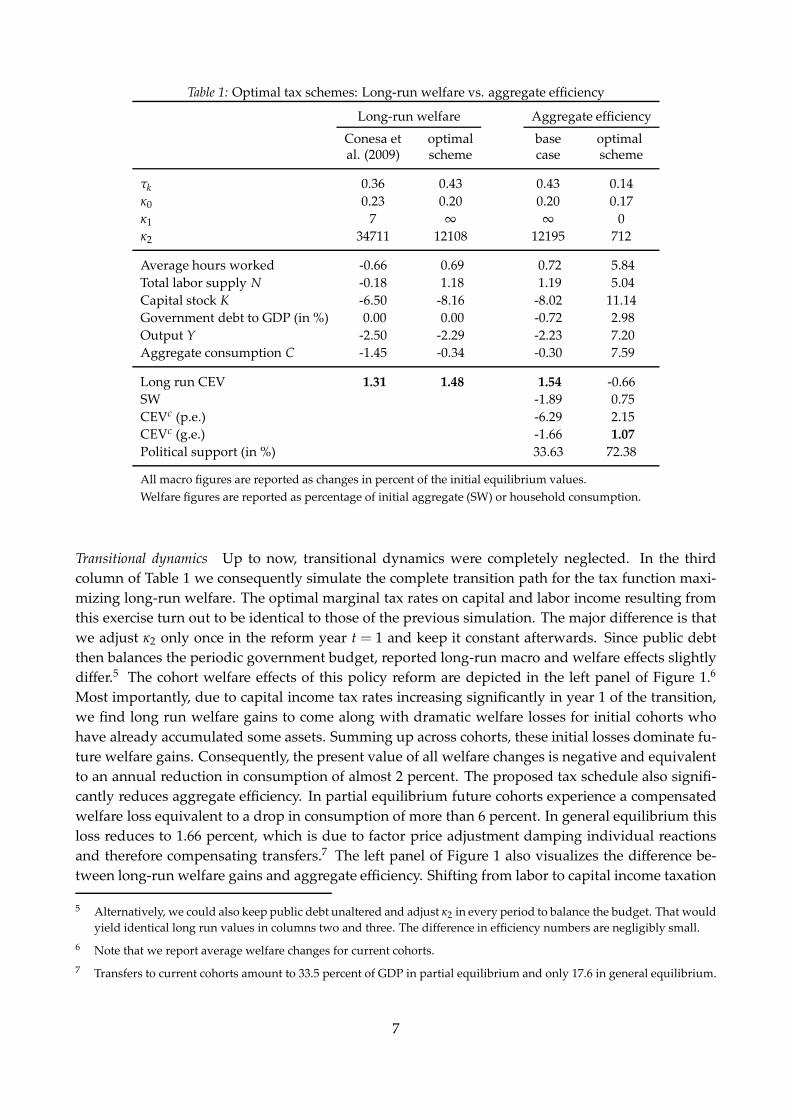
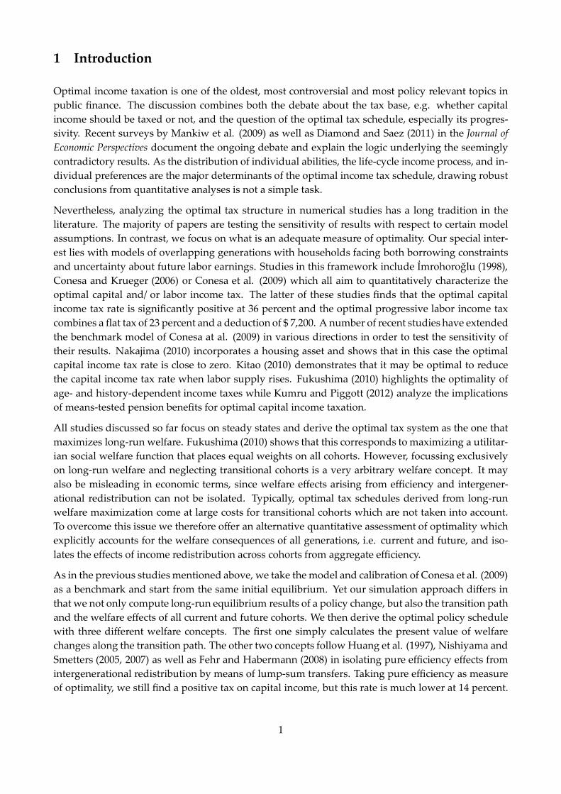
Table 1: Optimal tax schemes: Long-run welfare vs. aggregate efficiency

Long-run welfare Aggregate efficiency

Conesa et optimal base optimalal. (2009) scheme case scheme

τk 0.36 0.43 0.43 0.14κ0 0.23 0.20 0.20 0.17κ1 7 ∞ ∞ 0κ2 34711 12108 12195 712

Average hours worked -0.66 0.69 0.72 5.84Total labor supply N -0.18 1.18 1.19 5.04Capital stock K -6.50 -8.16 -8.02 11.14Government debt to GDP (in %) 0.00 0.00 -0.72 2.98Output Y -2.50 -2.29 -2.23 7.20Aggregate consumption C -1.45 -0.34 -0.30 7.59

Long run CEV 1.31 1.48 1.54 -0.66SW -1.89 0.75CEVc (p.e.) -6.29 2.15CEVc (g.e.) -1.66 1.07Political support (in %) 33.63 72.38

All macro figures are reported as changes in percent of the initial equilibrium values.Welfare figures are reported as percentage of initial aggregate (SW) or household consumption.

Transitional dynamics Up to now, transitional dynamics were completely neglected. In the thirdcolumn of Table 1 we consequently simulate the complete transition path for the tax function maxi-mizing long-run welfare. The optimal marginal tax rates on capital and labor income resulting fromthis exercise turn out to be identical to those of the previous simulation. The major difference is thatwe adjust κ2 only once in the reform year t = 1 and keep it constant afterwards. Since public debtthen balances the periodic government budget, reported long-run macro and welfare effects slightlydiffer.5 The cohort welfare effects of this policy reform are depicted in the left panel of Figure 1.6

Most importantly, due to capital income tax rates increasing significantly in year 1 of the transition,we find long run welfare gains to come along with dramatic welfare losses for initial cohorts whohave already accumulated some assets. Summing up across cohorts, these initial losses dominate fu-ture welfare gains. Consequently, the present value of all welfare changes is negative and equivalentto an annual reduction in consumption of almost 2 percent. The proposed tax schedule also signifi-cantly reduces aggregate efficiency. In partial equilibrium future cohorts experience a compensatedwelfare loss equivalent to a drop in consumption of more than 6 percent. In general equilibrium thisloss reduces to 1.66 percent, which is due to factor price adjustment damping individual reactionsand therefore compensating transfers.7 The left panel of Figure 1 also visualizes the difference be-tween long-run welfare gains and aggregate efficiency. Shifting from labor to capital income taxation

5 Alternatively, we could also keep public debt unaltered and adjust κ2 in every period to balance the budget. That wouldyield identical long run values in columns two and three. The difference in efficiency numbers are negligibly small.

6 Note that we report average welfare changes for current cohorts.

7 Transfers to current cohorts amount to 33.5 percent of GDP in partial equilibrium and only 17.6 in general equilibrium.

7

induces dramatic welfare losses for older current generations, while younger current and future co-horts benefit from reduced tax burdens. The compensation mechanism eliminates intergenerationalredistribution and reveals the aggregate efficiency loss. All initial cohorts, which experience risingburdens from capital income taxes, receive lump-sum transfers which bring them back to the welfarelevel of the initial equilibrium. Younger and future cohorts have to finance these transfers by meansof lump-sum taxes, so that they end up at a lower welfare level. Given the dramatic welfare lossesfor current cohorts, it is not surprising that the considered reform is quite unpopular. The last rowof Table 1 reveals that only one third of the population in the reform year experiences welfare gainsand therefore would vote in favor of such a reform.8

Figure 1: Intergenerational welfare effects: Base case vs. optimal scheme

Efficiency comparisons But what would an optimal scheme look like that takes aggregate efficiency asmeasure of optimality? The next column of Table 1 answers this question. It features both lower taxrates on capital and labor and comes along with a lump-sum tax of $ 712. This tax schedule inducesindividuals to work longer hours and save more. In consequence, long-run labor supply and capitalstock increase by more than 5 and 11 percent, respectively. The right panel of Figure 1 shows thatcurrent cohorts benefit from this tax structure while tax burdens on young and future generationsincrease. Long-run welfare therefore declines by an amount equivalent to 0.66 percent of consump-tion. Aggregating welfare changes across cohorts shows that initial welfare gains dominate futurewelfare losses. The present value of all welfare changes is now equivalent to an annual increase inconsumption of 0.75 percent. Applying our compensation mechanism now yields an aggregate effi-ciency gain of more than 2 percent of consumption in partial equilibrium and of more than 1 percentin general equilibrium. Note that since the optimal scheme balances efficiency losses from behav-ioral distortions and benefits arising from loosened liquidity constraints as well as the provision ofinsurance against labor market risk, it does not completely rely on lump-sum taxation. Lump-sumtaxes do not distort individual labor supply and savings, but enforce borrowing constraints at young

8 Of course, this political economy interpretation has to be taken with care. It is only valid if there is a one time vote withfull commitment to the reform ever after.

8

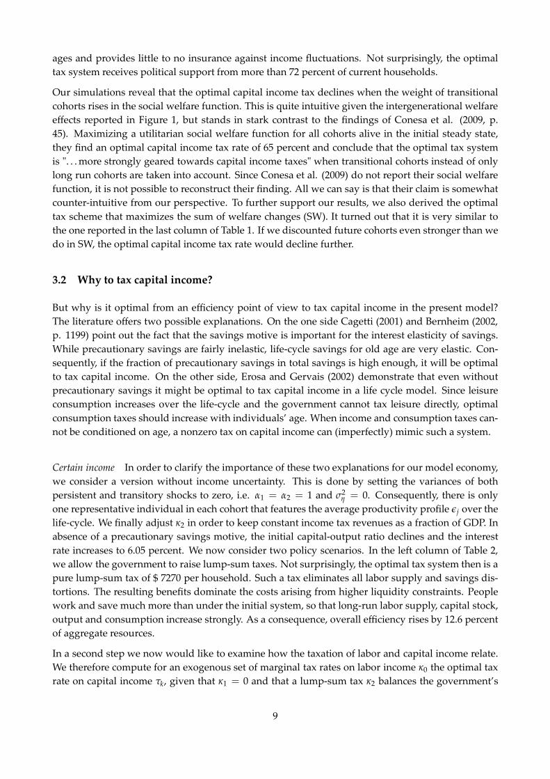
ages and provides little to no insurance against income fluctuations. Not surprisingly, the optimaltax system receives political support from more than 72 percent of current households.

Our simulations reveal that the optimal capital income tax declines when the weight of transitionalcohorts rises in the social welfare function. This is quite intuitive given the intergenerational welfareeffects reported in Figure 1, but stands in stark contrast to the findings of Conesa et al. (2009, p.45). Maximizing a utilitarian social welfare function for all cohorts alive in the initial steady state,they find an optimal capital income tax rate of 65 percent and conclude that the optimal tax systemis ". . .more strongly geared towards capital income taxes" when transitional cohorts instead of onlylong run cohorts are taken into account. Since Conesa et al. (2009) do not report their social welfarefunction, it is not possible to reconstruct their finding. All we can say is that their claim is somewhatcounter-intuitive from our perspective. To further support our results, we also derived the optimaltax scheme that maximizes the sum of welfare changes (SW). It turned out that it is very similar tothe one reported in the last column of Table 1. If we discounted future cohorts even stronger than wedo in SW, the optimal capital income tax rate would decline further.

3.2 Why to tax capital income?

But why is it optimal from an efficiency point of view to tax capital income in the present model?The literature offers two possible explanations. On the one side Cagetti (2001) and Bernheim (2002,p. 1199) point out the fact that the savings motive is important for the interest elasticity of savings.While precautionary savings are fairly inelastic, life-cycle savings for old age are very elastic. Con-sequently, if the fraction of precautionary savings in total savings is high enough, it will be optimalto tax capital income. On the other side, Erosa and Gervais (2002) demonstrate that even withoutprecautionary savings it might be optimal to tax capital income in a life cycle model. Since leisureconsumption increases over the life-cycle and the government cannot tax leisure directly, optimalconsumption taxes should increase with individuals’ age. When income and consumption taxes can-not be conditioned on age, a nonzero tax on capital income can (imperfectly) mimic such a system.

Certain income In order to clarify the importance of these two explanations for our model economy,we consider a version without income uncertainty. This is done by setting the variances of bothpersistent and transitory shocks to zero, i.e. α1 = α2 = 1 and σ2

η = 0. Consequently, there is onlyone representative individual in each cohort that features the average productivity profile εj over thelife-cycle. We finally adjust κ2 in order to keep constant income tax revenues as a fraction of GDP. Inabsence of a precautionary savings motive, the initial capital-output ratio declines and the interestrate increases to 6.05 percent. We now consider two policy scenarios. In the left column of Table 2,we allow the government to raise lump-sum taxes. Not surprisingly, the optimal tax system then is apure lump-sum tax of $ 7270 per household. Such a tax eliminates all labor supply and savings dis-tortions. The resulting benefits dominate the costs arising from higher liquidity constraints. Peoplework and save much more than under the initial system, so that long-run labor supply, capital stock,output and consumption increase strongly. As a consequence, overall efficiency rises by 12.6 percentof aggregate resources.

In a second step we now would like to examine how the taxation of labor and capital income relate.We therefore compute for an exogenous set of marginal tax rates on labor income κ0 the optimal taxrate on capital income τk, given that κ1 = 0 and that a lump-sum tax κ2 balances the government’s

9

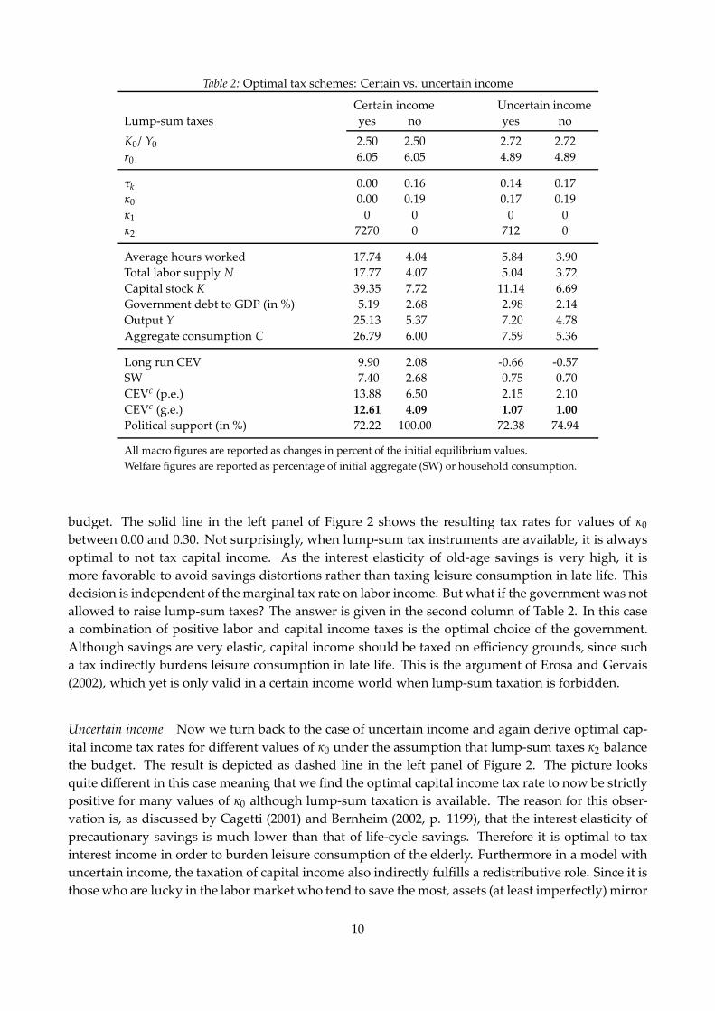
Table 2: Optimal tax schemes: Certain vs. uncertain income

Certain income Uncertain incomeLump-sum taxes yes no yes no

K0/ Y0 2.50 2.50 2.72 2.72r0 6.05 6.05 4.89 4.89

τk 0.00 0.16 0.14 0.17κ0 0.00 0.19 0.17 0.19κ1 0 0 0 0κ2 7270 0 712 0

Average hours worked 17.74 4.04 5.84 3.90Total labor supply N 17.77 4.07 5.04 3.72Capital stock K 39.35 7.72 11.14 6.69Government debt to GDP (in %) 5.19 2.68 2.98 2.14Output Y 25.13 5.37 7.20 4.78Aggregate consumption C 26.79 6.00 7.59 5.36

Long run CEV 9.90 2.08 -0.66 -0.57SW 7.40 2.68 0.75 0.70CEVc (p.e.) 13.88 6.50 2.15 2.10CEVc (g.e.) 12.61 4.09 1.07 1.00Political support (in %) 72.22 100.00 72.38 74.94


budget. The solid line in the left panel of Figure 2 shows the resulting tax rates for values of κ0between 0.00 and 0.30. Not surprisingly, when lump-sum tax instruments are available, it is alwaysoptimal to not tax capital income. As the interest elasticity of old-age savings is very high, it ismore favorable to avoid savings distortions rather than taxing leisure consumption in late life. Thisdecision is independent of themarginal tax rate on labor income. But what if the governmentwas notallowed to raise lump-sum taxes? The answer is given in the second column of Table 2. In this casea combination of positive labor and capital income taxes is the optimal choice of the government.Although savings are very elastic, capital income should be taxed on efficiency grounds, since sucha tax indirectly burdens leisure consumption in late life. This is the argument of Erosa and Gervais(2002), which yet is only valid in a certain income world when lump-sum taxation is forbidden.

Uncertain income Now we turn back to the case of uncertain income and again derive optimal cap-ital income tax rates for different values of κ0 under the assumption that lump-sum taxes κ2 balancethe budget. The result is depicted as dashed line in the left panel of Figure 2. The picture looksquite different in this case meaning that we find the optimal capital income tax rate to now be strictlypositive for many values of κ0 although lump-sum taxation is available. The reason for this obser-vation is, as discussed by Cagetti (2001) and Bernheim (2002, p. 1199), that the interest elasticity ofprecautionary savings is much lower than that of life-cycle savings. Therefore it is optimal to taxinterest income in order to burden leisure consumption of the elderly. Furthermore in a model withuncertain income, the taxation of capital income also indirectly fulfills a redistributive role. Since it isthosewho are lucky in the labor market who tend to save themost, assets (at least imperfectly) mirror

10

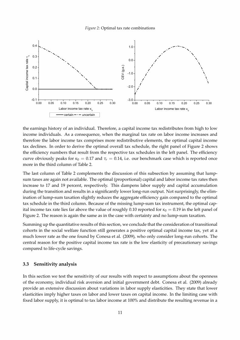
Figure 2: Optimal tax rate combinations

the earnings history of an individual. Therefore, a capital income tax redistributes from high to lowincome individuals. As a consequence, when the marginal tax rate on labor income increases andtherefore the labor income tax comprises more redistributive elements, the optimal capital incometax declines. In order to derive the optimal overall tax schedule, the right panel of Figure 2 showsthe efficiency numbers that result from the respective tax schedules in the left panel. The efficiencycurve obviously peaks for κ0 = 0.17 and τr = 0.14, i.e. our benchmark case which is reported oncemore in the third column of Table 2.

The last column of Table 2 complements the discussion of this subsection by assuming that lump-sum taxes are again not available. The optimal (proportional) capital and labor income tax rates thenincrease to 17 and 19 percent, respectively. This dampens labor supply and capital accumulationduring the transition and results in a significantly lower long-run output. Not surprisingly, the elim-ination of lump-sum taxation slightly reduces the aggregate efficiency gain compared to the optimaltax schedule in the third column. Because of the missing lump-sum tax instrument, the optimal cap-ital income tax rate lies far above the value of roughly 0.10 reported for κ0 = 0.19 in the left panel ofFigure 2. The reason is again the same as in the case with certainty and no lump-sum taxation.

Summing up the quantitative results of this section, we conclude that the consideration of transitionalcohorts in the social welfare function still generates a positive optimal capital income tax, yet at amuch lower rate as the one found by Conesa et al. (2009), who only consider long-run cohorts. Thecentral reason for the positive capital income tax rate is the low elasticity of precautionary savingscompared to life-cycle savings.

3.3 Sensitivity analysis

In this section we test the sensitivity of our results with respect to assumptions about the opennessof the economy, individual risk aversion and initial government debt. Conesa et al. (2009) alreadyprovide an extensive discussion about variations in labor supply elasticities. They state that lowerelasticities imply higher taxes on labor and lower taxes on capital income. In the limiting case withfixed labor supply, it is optimal to tax labor income at 100% and distribute the resulting revenue in a

11

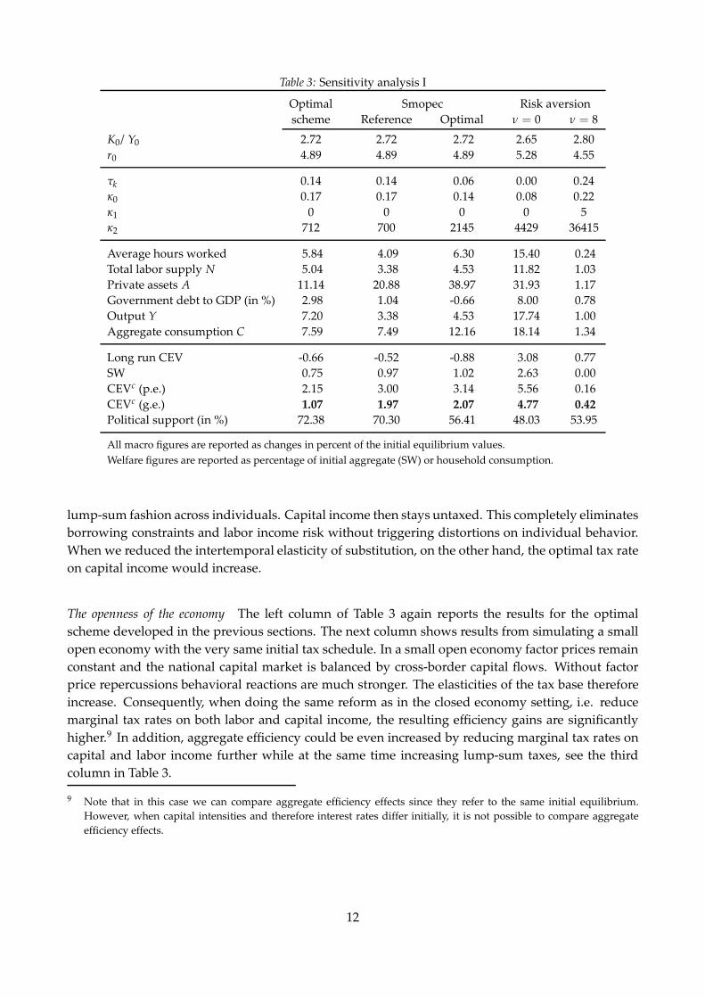
Table 3: Sensitivity analysis I

Optimal Smopec Risk aversionscheme Reference Optimal ν = 0 ν = 8

K0/ Y0 2.72 2.72 2.72 2.65 2.80r0 4.89 4.89 4.89 5.28 4.55

τk 0.14 0.14 0.06 0.00 0.24κ0 0.17 0.17 0.14 0.08 0.22κ1 0 0 0 0 5κ2 712 700 2145 4429 36415

Average hours worked 5.84 4.09 6.30 15.40 0.24Total labor supply N 5.04 3.38 4.53 11.82 1.03Private assets A 11.14 20.88 38.97 31.93 1.17Government debt to GDP (in %) 2.98 1.04 -0.66 8.00 0.78Output Y 7.20 3.38 4.53 17.74 1.00Aggregate consumption C 7.59 7.49 12.16 18.14 1.34

Long run CEV -0.66 -0.52 -0.88 3.08 0.77SW 0.75 0.97 1.02 2.63 0.00CEVc (p.e.) 2.15 3.00 3.14 5.56 0.16CEVc (g.e.) 1.07 1.97 2.07 4.77 0.42Political support (in %) 72.38 70.30 56.41 48.03 53.95


lump-sum fashion across individuals. Capital income then stays untaxed. This completely eliminatesborrowing constraints and labor income risk without triggering distortions on individual behavior.When we reduced the intertemporal elasticity of substitution, on the other hand, the optimal tax rateon capital income would increase.

The openness of the economy The left column of Table 3 again reports the results for the optimalscheme developed in the previous sections. The next column shows results from simulating a smallopen economy with the very same initial tax schedule. In a small open economy factor prices remainconstant and the national capital market is balanced by cross-border capital flows. Without factorprice repercussions behavioral reactions are much stronger. The elasticities of the tax base thereforeincrease. Consequently, when doing the same reform as in the closed economy setting, i.e. reducemarginal tax rates on both labor and capital income, the resulting efficiency gains are significantlyhigher.9 In addition, aggregate efficiency could be even increased by reducing marginal tax rates oncapital and labor income further while at the same time increasing lump-sum taxes, see the thirdcolumn in Table 3.

9 Note that in this case we can compare aggregate efficiency effects since they refer to the same initial equilibrium.However, when capital intensities and therefore interest rates differ initially, it is not possible to compare aggregateefficiency effects.

12

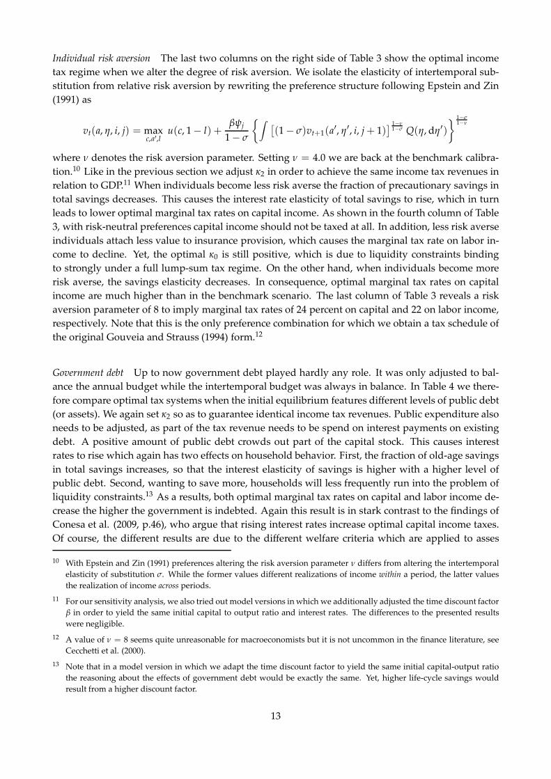
Individual risk aversion The last two columns on the right side of Table 3 show the optimal incometax regime when we alter the degree of risk aversion. We isolate the elasticity of intertemporal sub-stitution from relative risk aversion by rewriting the preference structure following Epstein and Zin(1991) as

vt(a, η, i, j) = maxc,a′,l

u(c, 1− l) +βψj

1− σ

{∫ [(1− σ)vt+1(a′, η′, i, j+ 1)

] 1−ν1−σ Q(η, dη′)

} 1−σ1−ν

where ν denotes the risk aversion parameter. Setting ν = 4.0 we are back at the benchmark calibra-tion.10 Like in the previous section we adjust κ2 in order to achieve the same income tax revenues inrelation to GDP.11 When individuals become less risk averse the fraction of precautionary savings intotal savings decreases. This causes the interest rate elasticity of total savings to rise, which in turnleads to lower optimal marginal tax rates on capital income. As shown in the fourth column of Table3, with risk-neutral preferences capital income should not be taxed at all. In addition, less risk averseindividuals attach less value to insurance provision, which causes the marginal tax rate on labor in-come to decline. Yet, the optimal κ0 is still positive, which is due to liquidity constraints bindingto strongly under a full lump-sum tax regime. On the other hand, when individuals become morerisk averse, the savings elasticity decreases. In consequence, optimal marginal tax rates on capitalincome are much higher than in the benchmark scenario. The last column of Table 3 reveals a riskaversion parameter of 8 to imply marginal tax rates of 24 percent on capital and 22 on labor income,respectively. Note that this is the only preference combination for which we obtain a tax schedule ofthe original Gouveia and Strauss (1994) form.12

Government debt Up to now government debt played hardly any role. It was only adjusted to bal-ance the annual budget while the intertemporal budget was always in balance. In Table 4 we there-fore compare optimal tax systemswhen the initial equilibrium features different levels of public debt(or assets). We again set κ2 so as to guarantee identical income tax revenues. Public expenditure alsoneeds to be adjusted, as part of the tax revenue needs to be spend on interest payments on existingdebt. A positive amount of public debt crowds out part of the capital stock. This causes interestrates to rise which again has two effects on household behavior. First, the fraction of old-age savingsin total savings increases, so that the interest elasticity of savings is higher with a higher level ofpublic debt. Second, wanting to save more, households will less frequently run into the problem ofliquidity constraints.13 As a results, both optimal marginal tax rates on capital and labor income de-crease the higher the government is indebted. Again this result is in stark contrast to the findings ofConesa et al. (2009, p.46), who argue that rising interest rates increase optimal capital income taxes.Of course, the different results are due to the different welfare criteria which are applied to asses

10 With Epstein and Zin (1991) preferences altering the risk aversion parameter ν differs from altering the intertemporalelasticity of substitution σ. While the former values different realizations of income within a period, the latter valuesthe realization of income across periods.

11 For our sensitivity analysis, we also tried out model versions inwhich we additionally adjusted the time discount factorβ in order to yield the same initial capital to output ratio and interest rates. The differences to the presented resultswere negligible.

12 A value of ν = 8 seems quite unreasonable for macroeconomists but it is not uncommon in the finance literature, seeCecchetti et al. (2000).

13 Note that in a model version in which we adapt the time discount factor to yield the same initial capital-output ratiothe reasoning about the effects of government debt would be exactly the same. Yet, higher life-cycle savings wouldresult from a higher discount factor.

13

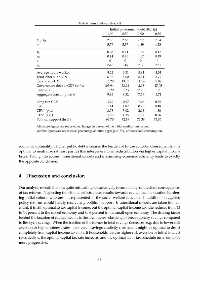
Table 4: Sensitivity analysis II

Initial government debt (B0/ Y0)1.00 0.50 0.00 -0.50

K0/ Y0 2.55 2.63 2.72 2.84r0 5.79 5.37 4.89 4.33

τk 0.08 0.11 0.14 0.17κ0 0.14 0.16 0.17 0.19κ1 0 0 0 0κ2 1548 945 712 270

Average hours worked 8.21 6.51 5.84 4.31Total labor supply N 6.92 5.60 5.04 3.77Capital stock K 16.28 13.07 11.14 7.87Government debt to GDP (in %) 103.94 53.92 2.98 -47.05Output Y 10.20 8.23 7.20 5.23Aggregate consumption C 9.95 8.32 7.59 5.71

Long run CEV -1.29 -0.97 -0.66 -0.56SW 1.14 1.07 0.75 0.48CEVc (p.e.) 3.78 3.02 2.15 1.30CEVc (g.e.) 1.95 1.15 1.07 0.56Political support (in %) 66.70 72.19 72.38 73.35


economic optimality. Higher public debt increases the burden of future cohorts. Consequently, it isoptimal to neutralize (at least partly) this intergenerational redistribution via higher capital incometaxes. Taking into account transitional cohorts and maximizing economic efficiency leads to exactlythe opposite conclusion.

4 Discussion and conclusion

Our analysis reveals that it is quite misleading to exclusively focus on long-run welfare consequencesof tax reforms. Neglecting transitional effects biases results towards capital income taxation burden-ing initial cohorts who are not represented in the social welfare function. In addition, suggestedpolicy reforms would hardly receive any political support. If transitional cohorts are taken into ac-count, it is still optimal to tax capital income, but the optimal capital income tax rate reduces from 43to 14 percent in the closed economy and to 6 percent in the small open economy. The driving factorbehind the taxation of capital income is the low interest elasticity of precautionary savings comparedto life-cycle savings. When the fraction of the former in total savings decreases, e.g. due to lower riskaversion or higher interest rates, the overall savings elasticity rises and it might be optimal to desistcompletely from capital income taxation. If households feature higher risk aversion or initial interestrates decline, the optimal capital tax rate increases and the optimal labor tax schedule turns out to bemore progressive.

14

Our results have to be interpreted with care, since they also depend on restrictions of the consideredtax system and various other assumptions about the economy and individual behavior. We haveassumed that the optimal tax scheme is set once at time zero and then maintained into perpetuity. Ofcourse, a full analysis would search for the best time-indexed sequences of labor and capital incometaxes across the transition that maximizes aggregate efficiency. However, this type of analysis ischallenging in the overlapping generation economy because it quickly runs up against the curse ofdimensionality. Furthermore, increasing uncertainty of the economic environment could result ina more progressive tax system. Uncertainty would for example rise, if unintended bequests weredistributed in proportion to ability or realized income, if the pension system was less progressiveor the income process more volatile. The progressivity of the optimal tax system will decline withrising labor supply elasticities. This includes considering household production or human capitalformation.

A final remark refers to linkages between and within generations due to one- or two-sided altruism.While our approach does not directly incorporate any bequest motive, our compensation mecha-nism can be interpreted as a system of private transfers neutralizing all intra- and intergenerationalredistribution effects. Effectively we are then in a Barro (1974) world, where successive generationsare linked by an operative altruistic bequest motive. With this interpretation our approach includesboth extremes, the standard overlapping generations model without intergenerational linkage andthe infinitely lived agent model, in which cohorts are perfectly linked via bequest motives.

15

A Computational appendix

We use two distinct solution algorithms: one to solve the household problem and one to solve formacroeconomic quantities and prices.

A.1 Solving the household problem

We first have to discretize continuous elements of the state space (a, η, i, j), respectively the asset di-mension. We therefore choose A = {a1, . . . , anA}. We then solve the household problem by backwardinduction, iterating on the following steps:

1. Compute household decisions at maximum age J for any (a, η, i, J). Since households are notallowed to work anymore and they die for sure in the next period, they consume all remainingresources.

2. Find the solution to the household optimization problem for all possible (a, η, i, j) recursivelyusing a line search method à la Powell, see Press et al. (2001, 406ff.). This algorithm requires acontinuous function to optimize. We therefore use an interpolated version of vt+1(a, η, i, j+1).Having computed the data vt+1(a, η, i, j+1) at any discrete asset grid point in the last iterationstep, we can find a piecewise polynomial function spt+1,j+1 satisfying the interpolation condi-tions

spt+1,j+1(ak, η, i, j+1) =∫vt+1(ak, η′, i, j+1)Q(η, dη′) (8)

for all k = 1, . . . , nA. We use the multidimensional spline interpolation algorithm described inHabermann and Kindermann (2007).

We choose nA = 25. We also tried higher values, but the results didn’t change.

A.2 The macroeconomic computational algorithm

We solve for quantities and prices using a Gauss-Seidel procedure in line with Auerbach and Kot-likoff (1987). Starting with a guess for quantities and government policy, we compute prices, optimalhousehold decisions, and value functions. Next we obtain the distribution of households on the statespace and new macroeconomic quantities. We then update the initial guesses. These steps are iter-ated until the initial guesses and the resulting values for quantities, prices and public policy havesufficiently converged.

A.3 Computational efficiency

Our algorithm turns out to be quite efficient. It differs from the one used in Conesa et al. (2009)in that we first apply a more efficient interpolation routine and second allow any choice dimension(consumption, leisure, and assets) to indeed be continuous. Minor differences in simulation resultsare the consequence. Solving for a long-run equilibrium in the original model of Conesa et al. (2009)takes about 10 to 15 minutes, depending on the calibration.14 Our simulation approach obtains the

14 We simulate our models on a regular PC with a Intel® Core™ i7-870 Processor with 2.93 GHz and 8M Cache.

16

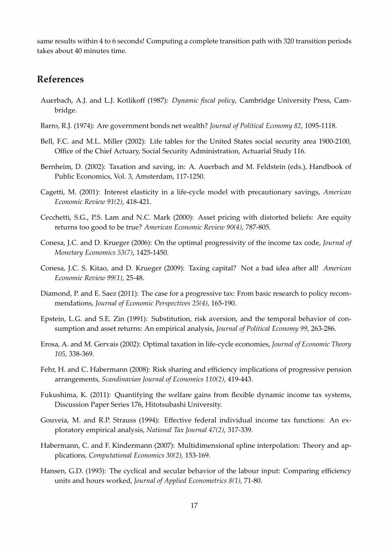
same results within 4 to 6 seconds! Computing a complete transition path with 320 transition periodstakes about 40 minutes time.

References

Auerbach, A.J. and L.J. Kotlikoff (1987): Dynamic fiscal policy, Cambridge University Press, Cam-bridge.

Barro, R.J. (1974): Are government bonds net wealth? Journal of Political Economy 82, 1095-1118.

Bell, F.C. and M.L. Miller (2002): Life tables for the United States social security area 1900-2100,Office of the Chief Actuary, Social Security Administration, Actuarial Study 116.

Bernheim, D. (2002): Taxation and saving, in: A. Auerbach and M. Feldstein (eds.), Handbook ofPublic Economics, Vol. 3, Amsterdam, 117-1250.

Cagetti, M. (2001): Interest elasticity in a life-cycle model with precautionary savings, AmericanEconomic Review 91(2), 418-421.

Cecchetti, S.G., P.S. Lam and N.C. Mark (2000): Asset pricing with distorted beliefs: Are equityreturns too good to be true? American Economic Review 90(4), 787-805.

Conesa, J.C. and D. Krueger (2006): On the optimal progressivity of the income tax code, Journal ofMonetary Economics 53(7), 1425-1450.

Conesa, J.C. S. Kitao, and D. Krueger (2009): Taxing capital? Not a bad idea after all! AmericanEconomic Review 99(1), 25-48.

Diamond, P. and E. Saez (2011): The case for a progressive tax: From basic research to policy recom-mendations, Journal of Economic Perspectives 25(4), 165-190.

Epstein, L.G. and S.E. Zin (1991): Substitution, risk aversion, and the temporal behavior of con-sumption and asset returns: An empirical analysis, Journal of Political Economy 99, 263-286.

Erosa, A. andM. Gervais (2002): Optimal taxation in life-cycle economies, Journal of Economic Theory105, 338-369.

Fehr, H. and C. Habermann (2008): Risk sharing and efficiency implications of progressive pensionarrangements, Scandinavian Journal of Economics 110(2), 419-443.

Fukushima, K. (2011): Quantifying the welfare gains from flexible dynamic income tax systems,Discussion Paper Series 176, Hitotsubashi University.

Gouveia, M. and R.P. Strauss (1994): Effective federal individual income tax functions: An ex-ploratory empirical analysis, National Tax Journal 47(2), 317-339.

Habermann, C. and F. Kindermann (2007): Multidimensional spline interpolation: Theory and ap-plications, Computational Economics 30(2), 153-169.

Hansen, G.D. (1993): The cyclical and secular behavior of the labour input: Comparing efficiencyunits and hours worked, Journal of Applied Econometrics 8(1), 71-80.

17

Huang, H., S. Imrohoroglu, and T. J. Sargent (1997): Two computations to fund social security,Macroeconomic Dynamics 1, 7-44.

Imrohoroglu, S. (1998): A quantitative analysis of capital income taxation, International EconomicReview 39(2), 307-328.

Kitao, S. (2010): Labor-dependent income taxation, Journal of Monetary Economics 57(8), 959-974.

Kumru, C. and J. Piggott (2012): Optimal capital income taxationwithmeans-tested benefits, CEPARWorking Paper 2012/ 13.

Mankiw, N.G., M. Weinzierl and D. Yagan (2009): Optimal taxation in theory and practice, Journal ofEconomic Perspectives 23(4), 147-174.

Nakajima, M. (2010): Optimal capital income taxation with housing, Working Paper No. 10-11,Federal Reserve Bank of Philadelphia.

Nishiyama, S. and K. Smetters (2005): Consumption taxes and economic efficiency with idiosyn-cratic wage shocks, Journal of Political Economy 113, 1088-1115.

Nishiyama, S. and K. Smetters (2007): Does social security privatization produce efficiency gains?Quarterly Journal of Economics xx, 1677-1719.

Press, W.H., S.A. Teukolsky, W.T. Vetterling and B.P. Flannery (2001): Numerical recipes in Fortran:The art of scientific computing, Cambridge University Press, Cambridge.

Støresletten, K., C. I. Telmer and A. Yaron (2004): Consumption and risk sharing over the life cycle,Journal of Monetary Economics 51(3), 609-633.

18