Embed Size (px)
Citation preview

econstor www.econstor.eu
Der Open-Access-Publikationsserver der ZBW – Leibniz-Informationszentrum WirtschaftThe Open Access Publication Server of the ZBW – Leibniz Information Centre for Economics
Standard-Nutzungsbedingungen:
Die Dokumente auf EconStor dürfen zu eigenen wissenschaftlichenZwecken und zum Privatgebrauch gespeichert und kopiert werden.
Sie dürfen die Dokumente nicht für öffentliche oder kommerzielleZwecke vervielfältigen, öffentlich ausstellen, öffentlich zugänglichmachen, vertreiben oder anderweitig nutzen.
Sofern die Verfasser die Dokumente unter Open-Content-Lizenzen(insbesondere CC-Lizenzen) zur Verfügung gestellt haben sollten,gelten abweichend von diesen Nutzungsbedingungen die in der dortgenannten Lizenz gewährten Nutzungsrechte.
Terms of use:
Documents in EconStor may be saved and copied for yourpersonal and scholarly purposes.
You are not to copy documents for public or commercialpurposes, to exhibit the documents publicly, to make thempublicly available on the internet, or to distribute or otherwiseuse the documents in public.
If the documents have been made available under an OpenContent Licence (especially Creative Commons Licences), youmay exercise further usage rights as specified in the indicatedlicence.
zbw Leibniz-Informationszentrum WirtschaftLeibniz Information Centre for Economics
Zoutman, Floris; Jacobs, Bas
Working Paper
Optimal Redistribution and Monitoring of Labor Effort
CESifo Working Paper, No. 4646
Provided in Cooperation with:Ifo Institute – Leibniz Institute for Economic Research at the University ofMunich
Suggested Citation: Zoutman, Floris; Jacobs, Bas (2014) : Optimal Redistribution andMonitoring of Labor Effort, CESifo Working Paper, No. 4646
This Version is available at:http://hdl.handle.net/10419/93467

Optimal Redistribution and Monitoring of Labor Effort
Floris T. Zoutman Bas Jacobs
CESIFO WORKING PAPER NO. 4646 CATEGORY 1: PUBLIC FINANCE
FEBRUARY 2014
An electronic version of the paper may be downloaded • from the SSRN website: www.SSRN.com • from the RePEc website: www.RePEc.org
• from the CESifo website: Twww.CESifo-group.org/wp T

CESifo Working Paper No. 4646
Optimal Redistribution and Monitoring of Labor Effort
Abstract This paper extends the Mirrlees (1971) model of optimal non-linear income taxation with a monitoring technology that allows the government to verify labor effort at a positive, but non-infinite cost. Monitored individuals receive a penalty, which increases if individuals earn a lower income (provide less work effort) or have a higher earning ability. We analyze the joint determination of the non-linear monitoring and tax schedules and the conditions under which these can be implemented. Monitoring of labor effort reduces the distortions created by income taxation and raises optimal marginal tax rates, possibly above 100 percent. The optimal intensity of monitoring increases with the marginal tax rate and the labor-supply elasticity. Our simulations demonstrate that monitoring strongly alleviates the trade-off between equity and efficiency as welfare gains of monitoring are around 1.4 percent of total output. The optimal intensity of monitoring follows a U-shaped pattern, similar to that of optimal marginal tax rates. Our paper explains why large welfare states optimally rely on work-dependent tax credits, active labor-market policies, benefit sanctions and work bonuses in welfare programs to redistribute income efficiently.
JEL-Code: H210, H260, H240, H310.
Keywords: optimal non-linear taxation, monitoring, costly verification ability/effort, optimal redistribution.
Floris T. Zoutman Department of Business and Management
Science / Norges Handelshøyskole Bergen / Norway
Bas Jacobs Erasmus School of Economics Erasmus Unitersity Rotterdam Rotterdam / The Netherlands
[email protected] January 17, 2014 The authors received the 2013 Young Economists Award of the International Institute for Public Finance for this paper. The authors would like to thank Katherine Cuff, Aart Gerritsen, Jean-Marie Lozachmeur, Luca Micheletto, Dominik Sachs, Dirk Schindler, and seminar and congress participants for useful suggestions and comments on an earlier version of this paper. All remaining errors are our own. The Matlab programs used for the computations in this paper are available from the authors on request.
“Informational frictions are a specification of a particular type of technology. Forexample, when we say “effort is hidden”, we are really saying that it is infinitelycostly for society to monitor effort. The desired approach would be to devise optimaltax systems for different specifications of the costs of monitoring different activitiesand/or individual attributes. To be able to implement this approach, we need to ...extend our modes of technical analysis to allow for costs of monitoring other thanzero or infinity.” Kocherlakota (2006, pp. 295-296)
1 Introduction
Redistribution of income is one of the most important tasks of modern welfare states. However,
redistribution is expensive as it distorts the incentives to provide work effort. As a result,
there is a trade-off between equity and efficiency. On a fundamental level, Mirrlees (1971)
demonstrates that the trade-off between equity and efficiency originates from an information
problem. Earnings ability and labor effort are private information, and the government cannot
condition redistributive taxes and transfers on earnings ability. Therefore, the government
cannot distinguish individuals that are unable to work from individuals that are unwilling to
work. Hence, redistribution from high-income to low-income earners inevitably distorts the
incentives to provide work effort.
In practice, labor effort is not completely non-verifiable, as assumed by Mirrlees (1971).
Indeed, some welfare states do condition the tax burden on some measure of labor supply. For
example, in the UK low-income individuals receive a tax credit if they work more than 30 hours.
This policy can only be implemented if the government is able to verify hours worked. Similar
restrictions apply to in-work tax credits in Ireland and New Zealand, see also OECD (2011).
Clearly, the assumption that work effort and earnings ability are not verifiable is a too strong
assumption. In the real world, the government does verify work effort of some individuals to
some extent, albeit at a cost. Consequently, the government can – to some extent – separate
shirking high-ability individuals from hard-working low-ability individuals.
This paper extends Mirrlees (1971) by allowing the government to operate a monitoring
technology. The monitoring technology allows the government to verify labor effort of an in-
dividual at a positive, but finite cost. If an individual is monitored, the government perfectly
verifies his/her labor effort and can thus deduce a worker’s ability. The government sets the
monitoring schedule as a function of gross income. That is, the probability that an individual
is monitored depends (possibly non-linearly) on his/her gross labor earnings. Monitoring work
effort provides incentives to individuals to adjust their labor supply in a direction that the
government desires. When individuals are monitored, they receive an exogenous penalty. The
penalty is increasing in ability as high-ability individuals are required to earn more income. The
penalty is decreasing in earnings, as a higher level of earnings indicates a higher labor effort for
given ability. The role of penalties should not be taken too literally. We could reformulate the
model such that individuals would receive a bonus or a tax credit when they adjust their labor
supply in the direction desired by the government.
Each individual is aware of the monitoring schedule and the penalty function before making
labor-supply decisions. Hence, individuals can alter their monitoring probability and penalties
1

by adjusting their labor effort. The total wedge on labor effort consists of the explicit income
tax rate and an implicit subsidy on labor effort due to monitoring. Monitoring of effort acts
as an implicit subsidy on labor supply for two reasons. First, the expected penalty decreases
with labor effort, since the penalty is assumed to be decreasing in gross earnings. Second,
the monitoring intensity, and therefore the probability of receiving a penalty, may decrease
with gross earnings, depending on the shape of the monitoring schedule. For a given tax rate,
monitoring can thus reduce the distortions of the income tax on labor effort, thereby increasing
both equity and efficiency.
The government maximizes social welfare by optimally setting the non-linear monitoring
intensity, alongside the optimal non-linear income tax. In our model, first-best can generally
not be obtained. Because the penalty function is exogenous, penalties are generally not sufficient
to ensure that all individuals supply the desired level of labor effort, and hence, some monitored
workers will receive a penalty.1 We solve for the optimal non-linear tax and monitoring schedules
by decentralizing the optimal, incentive-compatible direct mechanism that induces truthful
revelation of ability types. We do not deviate from Mirrlees (1971) in that individuals always
truthfully report earnings.2
The schedule of optimal non-linear labor wedges is affected in two important ways in compar-
ison to Mirrlees (1971). First, an increase in the labor wedge reduces labor supply, and hence,
increases marginal penalties for monitored individuals. Marginal penalties have the largest
impact on individuals’ labor-supply decisions when the probability of receiving a penalty is
high. Therefore, an increase in the monitoring intensity reduces the efficiency costs of the labor
wedge. Second, a decrease in labor supply directly increases the actual penalty. This increases
within-ability inequality between monitored and non-monitored individuals, since the monitored
individuals receive a penalty, whereas the unmonitored individuals do not. Therefore, higher
marginal taxes result in a distributional loss due to monitoring activities. The net effect of
monitoring on the optimal wedge is thus theoretically ambiguous.
In Mirrlees (1971) tax rates at, or above, 100 percent can never be optimal. In contrast
to Mirrlees (1971), we demonstrate that marginal tax rates could optimally be larger than 100
percent due to optimal monitoring. In particular, individuals may exert positive work effort
even if the marginal income tax rate is above 100 percent, as long as the total wedge on labor
remains below 100 percent. This could explain why effective marginal tax rates of close to, or
even higher than, 100 percent are observed in real-world tax-benefit systems in the phase-out
range of means-tested benefits. See Immervoll (2004), Spadaro (2005), Brewer et al. (2010) and
1If the government would be able to optimize the penalty function a trivial first-best outcome would resultby either raising the penalty to infinity or adjusting the penalty function such that the implicit subsidy on workexactly off-sets the explicit tax on work. It could be possible to endogenize both the penalty function and themonitoring function in our model if we assume that monitoring is imperfect. In such a setting, large penaltiesare undesirable, since hard-working individuals may inadvertently be monitored as shirking (see e.g. Stern, 1982,Diamond and Sheshinski, 1995 and Jacquet, forthcoming). However, extending our model to allow for imperfectmonitoring would complicate our analysis without affecting the key mechanism of our model – that monitoringalleviates the equity-efficiency trade-off.
2We realize that the assumption of truthful reporting of earnings is not always realistic due to, for example taxevasion and avoidance. This issue has been discussed in, amongst others, Cremer and Gahvari (1996), Schroyen(1997) and Chander and Wilde (1998). In most developed countries, however, firms are required to report grosslabor earnings directly to the tax authorities, which prevents underreporting of earnings for a very large fractionof labor earnings (see e.g. Kleven et al., 2011).
2

OECD (2011) for examples in OECD countries.
The non-linear monitoring schedule is set so as to equate the marginal cost of monitoring to
the marginal efficiency gain associated with monitoring at each gross income level. The efficiency
gain of monitoring is increasing in the distortion created by the wedge on labor. Therefore, the
optimal monitoring intensity increases with both the total labor wedge and the labor-supply
elasticity.
Unfortunately, there is no closed-form solution for the optimal tax and monitoring schedules.
Therefore, we resort to numerical simulations based on a realistic calibration of the model
to US data. Our simulations demonstrate that the optimal tax schedule follows a U-shape,
which closely resembles the simulations of Saez (2001). Moreover, the monitoring schedule
also follows a U-shape. This confirms that the monitoring intensity should indeed be large
when tax distortions on labor supply are large. The simulations demonstrate that the marginal
tax rates with monitoring are generally higher than without monitoring. Hence, monitoring
always results in more redistribution of income from high- to low-ability individuals, despite the
inequality within-ability groups that results due to monitoring and penalizing individuals.
Strikingly, our simulations demonstrate that the optimal tax rate at the bottom end of the
income scale is substantially above 100 percent. This implies that the implicit subsidy on work
due to monitoring is very effective in reducing the total tax wedge on labor effort at the lower end
of the income scale. Indeed, the optimal monitoring probability is close to one at the bottom, but
it drops substantially towards middle-income levels. There is a slight increase in the monitoring
probability towards the top, as tax rates increase. We conclude from our simulations that
monitoring is most important at the bottom of the income distribution. Strongly redistributive
governments should therefore optimally employ a high monitoring intensity at the low end of
the income scale, for example, via job-search requirements, benefit sanctions, work bonuses, and
active labor-market programs. Moreover, our findings suggest that work-dependent tax credits
for low-income earners, like those in the UK, Ireland and New Zealand, are indeed part of an
optimal redistributive tax policy.
The welfare gains of monitoring are shown to be large. Compared to the optimal non-linear
tax schedule without monitoring, monitoring increases average labor earnings by 1.35 percent
in our baseline simulation. Moreover, the transfer increases by about 4 percent. The monetized
welfare gain of monitoring is about 1.4 percent of total output. The optimal monitoring proba-
bility does not exceed 20 percent anywhere except at the lower end of the income distribution.
In our baseline simulations, the cost of monitoring and the average penalty are both only very
small fractions of average labor earnings. Extensive sensitivity analyses demonstrate that the
results are robust to parameter changes in the monitoring technology, on which little empirical
evidence exists.
The setup of the paper is the following. The next section gives a brief overview of the
related literature. The third section introduces the model and derives the conditions for first-
and second-order incentive compatibility. The fourth section derives the optimality conditions
for monitoring and redistribution. The fifth section presents the simulations. Finally, the sixth
section concludes.
3
2 Review of the literature
Our model builds upon two strands in the mechanism-design literature. Mirrlees (1971), Dia-
mond (1998) and Saez (2001) develop the theory of the optimal non-linear income tax under the
assumption that both effort and ability are completely private information, implicitly assuming
that verification of either effort or ability is infinitely costly. On the other hand, the literature
on costly state verification develops principal-agent models where the outcome of a project is
a function of both the state of the world and the action of the agent (see, e.g., Mirrlees, 1999,
1976, Holmstrom, 1979, and Townsend, 1979). The outcome is observed, but the action and
the state of the world can only be verified through costly monitoring. Monitoring can then
improve the ex-ante utility of both the principal and the agent. We apply the theory of costly
state verification to the Mirrlees (1971) model and show that monitoring of effort can increase
welfare significantly.
In a related paper, Armenter and Mertens (2010) study the effect of optimal monitoring of
ability types on the optimal tax schedule. They analyze a dynamic model of optimal taxation
where the government can use a monitoring technology to establish the ability of an agent. In
their model, the monitoring intensity is exogenous, while penalties are endogenous. In equilib-
rium, individuals do not misreport their ability, and are therefore never penalized. Indeed, the
economy is shown to converge to first best in an infinite-horizon setting. We instead analyze the
case where monitoring is endogenous and penalties are exogenously given. Because penalties are
exogenously given, individuals may misreport their ability type in equilibrium. Consequently,
our model does not converge to a first-best outcome. An advantage of allowing for an endoge-
nous monitoring intensity is that we do not need to worry about a tax-riot equilibrium in which
all individuals misreport their type when they expect other individuals to do the same (Bassetto
and Phelan, 2008).
The effect of monitoring has also been studied in the literature on tax evasion and the
literature on unemployment insurance. The literature on tax evasion (see, e.g., Allingham
and Sandmo, 1972, Sandmo, 1981, Mookherjee and Png, 1989, Slemrod, 1994, Cremer and
Gahvari, 1994, 1996, Chander and Wilde, 1998, and Slemrod and Kopczuk, 2002) extends the
Mirrlees (1971) framework by allowing individuals to underreport their earned income to the
tax authorities.3 Compared to the standard Mirrlees (1971) model, income taxation is more
distortionary, because it not only reduces labor supply, but also increases tax evasion. However,
the government can monitor individuals by auditing their tax returns and fine them when
they evade taxes. In a two-type economy with non-linear taxation and monitoring Cremer and
Gahvari (1994, 1996) show that the welfare-maximizing policy is to levy a positive marginal
tax rate on the bottom type and a zero tax rate at the top. All individuals reporting income
below a threshold level should be monitored with positive probability. The tax rate and the
monitoring schedules are strategic complements for the government, because a higher tax rate
induces an increase in tax evasion, thereby increasing the social value of monitoring.
In our model the only choice variable of individuals is their labor effort.4 The monitoring
3A comprehensive survey of the literature can be found in Slemrod and Yitzhaki (2002).4An alternative interpretation would be that individuals exogenously supply labor, but can use a costly evasion
technology.
4
instrument is therefore aimed at measuring effort instead of evasion. We extend the literature
by considering optimal non-linear tax and monitoring under a continuum of skill types. This
allows us to derive an elasticity-based formula for the optimal non-linear tax and monitoring
schedule in the spirit of Diamond (1998) and Saez (2001). Moreover, we can determine the
shape of non-linear tax and monitoring schedules over the entire income distribution through
simulations.
In the literature on unemployment insurance, Ljungqvist and Sargent (1995a,b) study the
effect of monitoring on equilibrium employment in welfare states.5 In their model, unemployed
workers may receive a job offer each period. In the absence of monitoring, the benefits in-
duce workers to decline an inefficiently large number of job offers. Monitoring can help raising
efficiency by punishing those workers who decline job offers. Simulations using Swedish data
demonstrate that welfare states with large benefits and progressive taxation can have low equi-
librium unemployment rates, provided the monitoring probability and sanctions are sufficiently
large. In a model of optimal income redistribution with search, Boadway and Cuff (1999) de-
termine the welfare-maximizing monitoring probability and demonstrate that it is increasing in
the level of the benefits. Boone and Van Ours (2006) and Boone et al. (2007) develop a search
model where the government can actively monitor and sanction job-search effort. They show
that monitoring and sanctioning may be more effective in reducing unemployment than cutting
the replacement rate. In addition, they show that monitoring may be effective, even when the
duration of unemployment benefits is limited. This literature has focused on monitoring the
search effort of unemployed workers. We contribute to this literature by studying the effect of
monitoring on employed workers.
Finally, we contribute to the literature on optimal non-linear tax simulations (see, for exam-
ple, Mirrlees, 1971, Tuomala, 1984, Saez, 2001, Brewer et al., 2010 and Zoutman et al., 2013).
We show that monitoring can lead to significant improvements in both equity and efficiency.
3 Model
3.1 Households
The setup of our model closely follows Mirrlees (1971). Individuals are heterogeneous in their
earnings ability, n, which denotes the productivity per hour worked. Ability is distributed
according to cumulative distribution function F (n) with support [n, n], where n could be infinite.
The density function is denoted by f(n). Workers are perfect substitutes in production and the
wage rate per efficiency unit of labor is constant and normalized to one. n therefore corresponds
to the number of efficiency units of labor of each worker. Gross labor income of an individual
is the product of his/her ability and his/her labor effort zn = nln.
Individuals derive utility from consumption cn and disutility from labor effort ln. Net
income is what remains of gross-labor income after taxes T (zn) and possibly a sanction, P , of
not supplying enough labor effort. All net income is consumed.
π(zn) is the probability that an individual with earnings zn is monitored by the government.
5A large literature exists on optimal unemployment insurance, see Fredriksson and Holmlund (2006) for asurvey of this literature. However, this literature typically does not consider monitoring of search effort.
5

It denotes the fraction of monitored individuals with gross earnings zn. π(zn) is also referred
to as the monitoring intensity. We assume the government receives a perfect signal of the
individual’s labor effort ln if an individual is monitored. The ability of a monitored individual
can then be inferred from the production relation: n = zn/ln.
Monitored individuals will receive a penalty or bonus depending on their observed earnings
zn and ability n:
P ≡ P (zn, n), P, Pn,−Pz ≥ 0, Pzn ≤ 0, ∀n, z. (1)
We will refer to P (·) as the penalty function. The penalty function P (·) is exogenously given
and assumed to be continuous and twice differentiable in both arguments. We restrict penalties
to be non-negative. Alternatively, we could have framed the model in terms of work bonuses
rather than penalties, where individuals receive a bonus (or negative penalty) when they earn
a higher income.6
For given gross income zn, penalties are assumed to be larger for individuals with higher
ability n: Pn > 0. Intuitively, a low-ability individual has to work harder to earn a given
gross income than a high-ability individual. Furthermore, penalties decrease in gross income
(Pz < 0), since an individual needs to supply more effort to earn a higher income for a given level
of ability. In addition, we make the logical assumption that the marginal penalty, −Pz, increases
in ability, such that Pzn ≤ 0. Hence, the government provides stronger work incentives to those
with higher earnings potential. Later, we will derive that this assumption helps to ensure
incentive compatibility.
As an example, a special case of the penalty function is P (zn, n) = P̂(znn
)= P̂ (ln), with
P̂ ′(·) < 0. In this case, individuals receive penalties strictly on the basis of the amount of
their work effort. With this penalty function, marginal penalties are increasing in ability if the
elasticity of the marginal penalty is smaller than one:
Pzn(·) ≤ 0⇐⇒ −dP̂ ′(ln)
dln
ln
P̂ ′(ln)≤ 1. (2)
That is, if a one-percent decrease in labor effort does not lead to an increase in the marginal
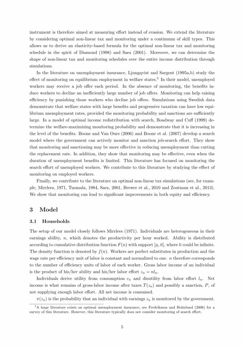
penalty of more than one percent. Figure 2 displays an example of penalties that are only a
function of labor effort. As can be seen, the penalty decreases quadratically in actual earnings
up to ln = l∗n, after which it remains constant at 0. Such a penalty function will be used in the
simulations later.
We assume that the penalty function P (zn, n) is exogenous and outside the control of the
redistributive government. The reason is that if P (zn, n) would be optimally set, the results
would become trivial. In particular, if the penalty function could be optimized, the optimal
penalty for any deviation of work effort from the first-best level would be infinity, so that all
individuals would choose to perform the first-best labor effort. We believe that constraining
P (zn, n) can be defended on legal grounds as the legal system imposes limitations on the gov-
6The main difference is that in our setting with positive penalties shirking individuals will adjust their laborsupply to avoid being monitored, whereas in a setting with bonuses hard-working individuals will adjust theirlabor supply in an attempt to get monitored. As such, the shape of the optimal monitoring schedule could bedifferent when the government provides bonuses instead of penalties. However, optimal second-best allocationswould be the same under the same informational and technological constraints.
6
Figure 1: Example of a penalty function
ernment’s ability to use infinite penalties. A more thorough discussion on these issues can be
found in Schroyen (1997), Mirrlees (1997), and Mirrlees (1999).
What is not outside the control of the tax authority is the determination of the tax rate and
monitoring probability. An individual with ability n is monitored with probability π(zn) and
not monitored with probability 1 − π(zn). The consumption of an unmonitored individual is
given by cUn ≡ zn− T (zn). The consumption of a monitored (and penalized) individual is given
by cPn ≡ zn − T (zn)− P (zn, n).
Individuals are assumed to maximize expected utility subject to their budget constraints in
monitored and unmonitored states. We follow Diamond (1998) by assuming that all individuals
have an identical quasi-linear expected utility function:
u(zn, n) ≡ π(zn)cPn + (1− π(zn))cUn − v(ln), v′(·) > 0, v′′(·) > 0, (3)
= zn − T (zn)− π(zn)P (zn, n)− v(zn/n), ∀n,
where we substituted the household budget constraint and ln = zn/n in the second line.
The first term in the first line represents the non-monitoring probability times the consump-
tion of an individual that is not monitored. The second term in the first line is the monitoring
probability times the consumption of an individual that is monitored. The last term in the first
line is the disutility of labor effort. An important analytical advantage of this quasi-linear-in-
consumption utility function is that individuals are risk-neutral.7
Individuals choose the optimal amount of gross income based on their productivity n, the
tax function T (·), the monitoring function π(·), and the penalty function P (·). An income level
zn is incentive compatible if it maximizes u(zn, n). The first-order condition for optimal labor
7We could allow for risk-aversion in the utility function. In that case we are only able to solve for the optimalnon-linear tax and monitoring schedules if the social welfare function is utilitarian. Intuitively, the problembecomes analytically untractable if the government has a different degree of risk-aversion – which is implied bya non-utilitarian social welfare function – than households. Without risk aversion, this problem is always absentand we can allow for any degree of inequality aversion in the social welfare function.
7
supply is given by:
v′(zn/n) = n(1− T ′(zn)− π′(zn)P (zn, n)− π(zn)Pz(zn, n)
), ∀n. (4)
On the right-hand side, we see that policy drives a wedge between the private and social benefits
of labor supply. The total labor wedge Wn is given by:
Wn ≡n− v′(zn/n)
n= T ′(zn)︸ ︷︷ ︸
explicit tax
+ π′(zn)P (zn, n) + π(zn)Pz(zn, n)︸ ︷︷ ︸implicit tax
, ∀n. (5)
In a laissez-faire equilibrium the right-hand side of eq. (4) equals n and the total labor wedgeWn
is zero. The total labor wedge consists of the explicit marginal tax on labor (T ′) and the implicit
marginal tax (subsidy) on labor due to monitoring (π′P + πPz). If T ′ + π′P + πPz > 0, the
redistributive tax and monitoring policy reduces optimal labor effort below the laissez-faire level,
and vice versa if it is smaller than zero. The wedge is naturally increasing in the explicit marginal
rate T ′. Furthermore, it increases in the marginal monitoring probability, π′, if penalties are
positive, P > 0. π′ gives the marginal increase in the monitoring probability as a function of
gross earnings. If the monitoring probability increases (decreases) with income, this reduces
(increases) the incentive to exert effort, because a higher labor income increases (decreases) the
probability of receiving a penalty. Therefore, an increase in the marginal monitoring probability
decreases the incentive to exert work effort.8
Proposition 1 shows that without loss of generality we can assume that expected consump-
tion, C(zn) ≡ zn − T (zn) − π(zn)P (zn, n), is non-decreasing in earnings zn. Consequently, the
total labor wedge Wn can never be larger than one, i.e. larger than 100 percent.
Proposition 1 All implementable continuous allocations can be implemented through a con-
tinuous non-decreasing expected consumption function C(zn), ∀n. If C(zn) is continuous and
differentiable, the wedge Wn can never exceed 1.
Proof. The proof directly follows Mirrlees (1971). Let C̃(z) be any continuous expected con-
sumption function. The individual maximization problem is given by:
zn = arg maxznC̃(zn)− v(zn/n), ∀n. (6)
Now consider function C(zn) = maxz̃n≤zn C̃(z̃n). Clearly, C(·) is non-decreasing and continuous,
because C̃(·) is continuous. Now, consider the maximization problem:
maxznC(zn)− v(zn/n) = max
zn
[maxz̃n≤zn
C̃(z̃n)
]− v(zn/n), ∀n. (7)
Assume zn is the solution to problem (6). The solution to this second maximization problem
must also be zn. To see this, evaluate C(·) at zn: C(zn) = maxz̃n≤zn C̃(z̃n). Either C(zn) = C̃(zn)
8Note that an equivalent wedge can be obtained using a bonus function instead of a penalty function.In particular, let B(zn, n) denote the bonus function, which gives a bonus B if an audited individual earn-ing zn is found to have ability n. Using the bonus function, the wedge on labor can be written as:Wn = T ′(zn) − π′(zn)B(zn, n) − π(zn)Bz(zn, n). Hence, the penalties and bonuses can achieve an identicallabor wedge π′(zn)B(zn, n) + π(zn)Bz(zn, n) = −π′(zn)P (zn, n)− π(zn)Pz(zn, n).
8
or C(zn) = C(z̄n) with z̄n < zn. In the first case, maximization problems (7) and (6) are
equivalent, and hence, they must have the same solution. In the second case, because v′(·) is
strictly increasing in zn, z̄n must give a higher value to the objective function in eq. (6) than does
zn. Hence, we arrive at a contradiction, because zn could not have been the solution to problem
(6) in the first place. Therefore, without loss of generality we can focus on non-decreasing
functions C(·). Now, suppose C(·) is differentiable and consider its derivative.
C′(zn) = 1− T ′(zn)− π′(zn)P (zn, n)− π(zn)Pz(zn, n) = 1−Wn, ∀n. (8)
C(zn) is non-decreasing if its derivative is greater than or equal to zero: C′(zn) ≥ 0⇔Wn ≤ 1.
Proposition 1 has an intuitive interpretation. Suppose, an individual has a budget constraint
such that expected consumption is decreasing in gross income over some interval. Then, this
individual will never choose gross income in this interval, because he can work less and consume
more, both yielding higher utility. Consequently, the government can never increase social
welfare by setting the wedgeWn above 1. The explicit marginal tax rate T ′(zn), however, could
be above 1, provided that monitoring implies a sufficiently large implicit marginal subsidy
on work, i.e. πPz + π′P < 0, such that the overall wedge remains below 1. This is the
case if the expected penalty decreases sufficiently fast in labor effort so that −π′P > πPz.
Therefore, monitoring can give incentives to provide work effort when the tax schedule reduces
the incentives to work.
3.2 Government
The government designs an optimal income tax system and monitoring schedule so as to maxi-
mize social welfare, subject to resource and incentive constraints. The government’s objective
function is a concave sum of individual utilities:
ˆ n
nG(u(zn))dF (n), G′(·) > 0, G′′(·) < 0. (9)
G(·) is the social welfare function. Redistribution from high-income individuals to low-income
individuals raises social welfare because the government is inequality averse. Due to quasi-
linearity of private utility there is no social desire to redistribute income if the social welfare
function is utilitarian. The government is constrained in its ability to redistribute income,
because the ability of individuals is private information. However, the government can infer
the ability of an individual from costly monitoring activities or it can induce self-selection by
sacrificing on redistribution.
The total cost of monitoring is given by:
ˆ n
nk(π(zn))dF (n), k(0) = 0, k′(·), k′′(·) > 0. (10)
The cost of monitoring is increasing and convex in the monitoring probability π. Since there is
a perfect mapping between skill n and labor earnings zn, we can also write π(·) as a function
9

of the skill level n, where we use the short-hand notation π(zn) = πn. However, π′(zn) ≡ dπndzn
always denotes the derivative of monitoring with respect to gross earnings.
The economy’s resource constraint implies that total labor earnings equal aggregate con-
sumption plus monitoring costs:
ˆ n
nzndF (n) =
ˆ n
n
((1− π(zn))cUn + π(zn)cPn + k(π(zn))
)dF (n). (11)
By defining unpenalized consumption as cn ≡ cUn = cPn + P (zn, n), we can write for aggregate
consumption:
ˆ n
n
((1− π(zn))cUn + π(zn)cPn
)dF (n) =
ˆ n
n(cn − π(zn)P (zn, n))dF (n). (12)
Hence, using eq. (12) the economy’s resource constraint (11) can be rewritten as:
ˆ n
n(zn + π(zn)P (zn, n))dF (n) =
ˆ n
n(cn + k(π(zn)))dF (n). (13)
We do not need to consider the government budget constraint, since it is automatically implied
by Walras’ law if the individual budget constraints and the economy’s resource constraint are
satisfied.
The timing of the model is as follows:
1. The government announces the exogenously given penalty function, as well as the optimal
non-linear income tax and monitoring schedules.
2. Each individual optimally chooses the amount of labor effort.
3. The government observes the labor incomes chosen by each individual and taxes income
and monitors individuals accordingly. The government penalizes all monitored individuals
according to the penalty function.
4. Individuals receive utility from consumption and leisure.
By the revelation principle any indirect mechanism can be replicated with an incentive-
compatible direct mechanism (Myerson, 1979; Harris and Townsend, 1981). Therefore, we
can find the optimal second-best allocation by maximizing welfare subject to feasibility and
incentive-compatibility constraints. We can decentralize the optimal second-best allocation as
a competitive market outcome through the non-linear tax and monitoring schedules.
3.3 First-order incentive compatibility
By using the envelope theorem we can derive a differential equation for the indirect utility
function un which is a necessary condition for incentive compatibility. The next subsection
derives the conditions under which the first-order condition is indeed sufficient. The incentive
10

compatibility constraint is found by totally differentiating eq. (3) with respect to n:
dundn
=∂u(zn, n)
∂n+∂u(zn, n)
∂zn
dzndn
=lnv′(ln)
n− π(zn)Pn(zn, n), ∀n, (14)
where ∂u(zn,n)∂zn
= 0 due to the individual’s first-order condition in eq. (4). Thus, if the optimal
allocation satisfies eq. (14), individuals’ first-order conditions for utility maximization are also
satisfied.
3.4 Second-order incentive compatibility
Without further restrictions we cannot be certain that the optimal allocation derived under
the first-order incentive compatibility constraint (14) is also implementable. An implementable
allocation should satisfy additional requirements to ensure that the first-order approach also
respects the second-order conditions for utility maximization. The next Lemma summarizes
the requirements for second-order incentive compatibility.
Lemma 1 Second-order conditions for utility maximization are satisfied under the first-order
approach if the following conditions hold at the optimal allocation for all n:
i) single-crossing conditions on the utility and penalty functions are satisfied:
∂(v′(ln)/n)
∂n+ π(zn)Pzn(zn, n) + π′(zn)Pn(zn, n) ≤ 0, (15)
ii) zn is non-decreasing in ability:dzndn≥ 0. (16)
Proof. The second-order condition for the utility-maximization problem (3) is given by:
∂2u(zn, n)
∂z2n
≤ 0, ∀n. (17)
This second-order condition can be rewritten in a number of steps. Totally differentiating the
first-order condition (4) gives:
∂2u(zn, n)
∂z2n
dzndn
+∂2u(zn, n)
∂zn∂n= 0, ∀n. (18)
Substitution of this result in eq. (17) implies that the second-order condition is equivalent to:
∂2u(zn, n)
∂zn∂n
(dzndn
)−1
≥ 0, ∀n. (19)
11
Differentiating the first-order condition (4) with respect to n and substituting the result yields:(∂(v′(ln)/n)
∂n+ π(zn)Pzn(zn, n) + π′(zn)Pn(zn, n)
)(dzndn
)−1
≤ 0, ∀n. (20)
The inequality holds if all conditions of the Lemma are satisfied.
The single-crossing condition and the monotonicity of gross earnings are well-known from
the Mirrlees model (Mirrlees, 1971; Ebert, 1992). The single-crossing condition ensures that
– at the same consumption-earnings bundle – individuals with a higher ability have a larger
marginal willingness to provide work effort. In our model, the single-crossing condition contains
three elements. The first is the standard Spence-Mirrlees condition on the utility function, i.e.∂(v′(ln)/n)
∂n . If this term is negative, the marginal disutility of work for individuals with a higher
ability level is lower. Most utility functions considered in the literature exhibit this property,
including our own. The second term is determined by Pzn(zn, n). As discussed before, the
assumption that Pzn ≤ 0 implies that marginal penalties do not decrease in ability. Hence,
high-ability individuals are more likely to self-select in higher income-consumption bundles if
the marginal penalty for earning less income increases with ability. The third term concerns
the slope of the monitoring schedule, π′(zn)Pn(zn, n) and its sign is determined by the the
monitoring schedule, since Pn > 0. If the marginal monitoring probability decreases in gross
earnings (π′(zn) < 0) individuals will work harder in order to decrease the probability of being
monitored and penalized. Whereas the first two terms feature uncontroversial signs, the last
term is determined by the endogenous monitoring schedule. Hence, high-ability individuals
can be induced to self-select into higher income-consumption bundles, unless the monitoring
probability increases too fast with ability.
A second requirement to induce self-selection is that gross earnings are indeed increasing
with ability at the optimal schedule. Consequently, a tax schedule that provides higher income
to higher ability individuals induces self-selection of higher ability types into higher income-
consumption bundles.
In the remainder we assume that all the conditions derived in Lemma 1 hold at the optimal
allocation. In our simulations, we check the second-order sufficiency conditions ex-post and we
always confirm that they are respected.
12

4 Optimal second-best allocation with monitoring
The optimization problem with monitoring can be specified formally as:
max
ˆ n
n[(1− πn)G(cn − v(zn/n)) + πnG(cn − P (zn, n)− v(zn/n))]f(n)dn, (21)
s.t.
ˆ n
n[zn + πnP (zn, n)− cn − k(πn)]f(n)dn = 0, (22)
dundn
=znv′(zn/n)
n2− πnPn(zn, n), (23)
un = cn − πnP (zn, n)− v(zn/n), ∀n, (24)
πn ≥ 0, ∀n. (25)
The final constraint assumes that the probability of monitoring cannot be smaller than zero.
We assume that the cost of monitoring is sufficiently large to ensure that the constraint πn ≤ 1
is never binding.
The Hamiltonian function of this problem is given by:
H ≡[(1− πn)G(uUn ) + πnG(uPn ) + λ(zn + πnP (zn, n)− cn − k(πn))
]f(n) (26)
−θn(znv′(zn/n)
n2− πnPn(zn, n)
)+ µn(un − cn + πnP (zn, n) + v(zn/n)) + ηnπn,
cn, zn and πn are control variables. un is a state variable with θn as its associated co-state
variable. uUn ≡ cn − v(zn/n) and uPn ≡ uUn − P (zn, n) denote the utility of the unpenalized and
penalized individuals, respectively. µn is the Lagrange multiplier for the definition of utility. λ is
the Lagrange multiplier of the economy’s resource constraint. ηn is the Kuhn-Tucker multiplier
of the non-negativity constraint on πn.
The first-order necessary conditions are given by:
∂H∂cn
= 0 :[(1− πn)G′(uUn ) + πnG
′(uPn )− λ]f(n)− µn = 0, ∀n, (27)
∂H∂zn
= 0 :
[−(1− πn)G′(uUn )
v′(·)n− πnG′(uPn )
(v′(·)n
+ Pz(·))
+ λ(1 + πnPz(·))]f(n) (28)
− θn(v′(·) + znv
′′(·)/nn2
− πnPzn(·))
+ µn
(v′(·)n
+ πnPz(·))
= 0, ∀n,
∂H∂πn
= 0 :[G(uPn )−G(uUn )− λ
(k′(πn)− P (·)
)]f(n) + θnPn(·) + µnP (·) + ηn = 0, ∀n,
(29)
∂H∂un
=dθndn
:dθndn
= µn, ∀n, (30)
ηnπn = 0, ηn ≥ 0, πn ≥ 0, ∀n, (31)
limn→n
θn = limn→n̄
θn = 0. (32)
Compared to the analysis of Mirrlees there are two new first-order conditions. Eq. (29) states
the optimal monitoring condition, and eqs. (31) state the Kuhn-Tucker conditions for the
13
non-negativity constraint on πn.
4.1 Optimal wedge on labor
Proposition 2 gives the conditions for optimal income redistribution.
Proposition 2 The optimal net marginal wedge on labor Wn at each ability level satisfies:
Wn
1−Wn= AnBnCn −Dn, ∀n, (33)
where
An ≡ 1 +1
εn+ πn
n
v′(zn/n)εPz , (34)
Bn ≡´ nn (1− gm)f(m)dm
1− F (n), (35)
Cn ≡ 1− F (n)
nf(n), (36)
Dn ≡ −Pz(zn, n)n
v′(zn/n)σn, (37)
σn ≡(1−πn)πn(G′(uPn )−G′(uUn ))
λ > 0 is a measure for the welfare cost of inequality between penalized
and unpenalized individuals at ability level n, εn ≡(lnv′′(ln)v′(ln)
)−1> 0 is the compensated wage
elasticity of labor supply, εPz ≡ − nPz
∂Pz∂n > 0 is the elasticity of the marginal penalty with respect
to ability, and gn ≡ (1−πn)G′(uUn )+πnG′(uPn )λ > 0 is the average, marginal social value of income,
expressed in money units, for individuals at ability level n.
Proof. Integrate eq. (30) using a transversality condition from eq. (32). If follows that
θn = λ´ nn (1 − gm)f(m)dm. Substitute this result and eq. (27) in eq. (28), use eq. (5), and
simplify to obtain the Proposition.
The An-term is related to the inverse of the efficiency cost of the labor wedge at income
level zn. The second term in An, 1/εn, is the inverse of the labor-supply elasticity and it enters
because the deadweight loss of the wedge increases in the labor-supply elasticity. The third
term represents the efficiency gains of monitoring. Penalties are more effective in seperating
high- and low-ability individuals if marginal penalties are strongly increasing in ability. That
is, if the elasticity of the marginal penalty with respect to ability, εPz , is larger. This effect
is stronger if the monitoring intensity π is larger. In addition, the third term decreases in
the marginal disutility of labor v′/n. Intuitively, the benefit of increasing earnings, in order
to reduce the marginal penalty, is smaller if the disutility of earning that additional income is
larger. Hence, in comparison to the optimal wedge without monitoring (cf. Diamond, 1998;
Saez, 2001) monitoring reduces the efficiency cost of taxation if marginal penalties increase in
ability.
The Bn-term measures the equity gain of an increase in the wedge at income level zn.
The first term, 1, captures the revenue gain of a larger marginal labor wedge at n, such that
individuals with an income level above zn pay one unit of extra income tax. The welfare loss
14

of extracting one unit of income from the individuals above n is gm for all individuals m ≥ n.
Therefore,´ nn (1− gm)dF (n) measures the redistributional gain of the labor wedge at n. The
Bn-term is not directly affected by monitoring. Since welfare weights gn are always declining
with income, Bn always rises with income, see also Diamond (1998).
Cn is the inverse relative hazard rate of the skill distribution. Its numerator is the fraction
of the population whose net income is decreased by increasing the wedge and its denominator
captures the size of the tax base that is distorted by the wedge. Hence, the numerator in Cn
gives weights to average equity gains in Bn and the denominator to average efficiency losses in
An – as in the model without monitoring. The numerator of Cn always declines with income;
there are fewer individuals paying marginal taxes if the tax rate is increased at a higher income
level. Hence, for a given Bn the total distributional benefits of raising the labor wedge fall as
the income level rises. For a unimodal skill distribution the denominator of Cn always increases
with income before the mode, since both n and f(n) are rising. Thus, labor wedges always
decrease with income before modal income. After the mode, f(n) falls, although n continues
to rise with income. Hence, it depends on the empirical distribution of n whether Cn rises or
falls with income after modal income. For most empirical distributions, Cn appears to rise after
the mode and converges to a constant at the top. See also Diamond (1998), Saez (2001) and
Zoutman et al. (2013).
Finally, Dn measures the welfare loss associated with within-ability inequality. If the labor
wedge increases, earnings at n decrease. Therefore, the penalty at n increases, which in turn
increases inequality between monitored and unmonitored individuals. σn measures the marginal
welfare cost of this within-ability inequality. The effect of a wedge on within-ability inequality
is increasing in the marginal penalty, −Pz. It decreases in the marginal cost of earning one unit
of additional income, v′/n, because, again, the relative effect of the penalty function on gross
earnings decreases if the disutility of labor earnings increases. Dn increases in the monitoring
probability for πn < .5 because the within-ability variance of monitoring is increasing in πn for
πn < .5. Finally, Dn is increasing in the concavity of the welfare function, because the difference
in welfare weights between penalized and unpenalized individuals, G′(upn)−G′(uun)λ , is larger if the
government is more inequality averse.
We can summarize the impact of monitoring on optimal labor wedges as follows. Monitor-
ing decreases the efficiency cost of setting a higher labor wedge, but introduces within-ability
inequality. Therefore, the total effect of monitoring on the optimal labor wedge is theoretically
ambiguous. Our simulations below demonstrate that the efficiency gains of monitoring outweigh
the distributional loss due to inequality between monitored and non-monitored individuals.
We can derive the non-linear tax function, which implements the second-best allocation as
the outcome of decentralized decision making in a competitive labor market. Substituting eq.
(4) into eq. (33) yields:
T ′(zn) + π′(zn)P (zn, n) + π(zn)Pz(zn, n)
1− T ′(zn)− π′(zn)P (zn, n)− π(zn)Pz(zn, n)= AnBnCn −Dn, ∀n. (38)
Thus, when we know the optimal monitoring schedule π(zn), this equation implicitly defines
the optimal non-linear income tax function T (zn).
15
4.2 Optimal monitoring
The next proposition derives the optimal monitoring schedule.
Proposition 3 The optimal level of monitoring at each ability level follows from:
k′(πn) + ∆n − gnP (·) ≥Wn
1−Wn+Dn
AnnPn(·) ∀n, (39)
where ∆n ≡ G(uUn )−G(uPn )λ is the welfare difference between a penalized and an unpenalized indi-
vidual expressed in money units. If πn > 0, the equation holds with equality.
Proof. Substitute eq. (27) into eq. (29), rearrange terms, employ the definitions for Bn and Cn,
and use the fact that ηn ≥ 0. Finally, substitute eq. (33) for BnCn to obtain the expression. By
eq. (31) ηn only equals zero if πn > 0 and therefore the equation holds with equality if πn > 0.
The first term on the left-hand side in condition (39) is the marginal cost of raising the
monitoring intensity. The second and third terms on the left-hand side jointly represent the
welfare effect of a compensated increase in the monitoring probability. That is, the welfare
effect of an increase in the monitoring probability, while keeping expected utility at skill level n
unchanged. The second term represents the uncompensated, direct welfare loss of an increase in
the monitoring probability. If the monitoring probability increases, there will be more penalized
and less unpenalized individuals. Therefore, the loss is equal to the welfare difference between
penalized and unpenalized individuals. The third term represents the welfare gain associated
with the compensation to keep expected utility unchanged if the monitoring probability is
increased. The compensation at ability level n requires a transfer of P and its associated
welfare effect is thus given by gnP . In Lemma 2 we derive how the compensated welfare effect
of monitoring changes with the monitoring probability for given levels of utility in monitored
and unmonitored states.
Lemma 2 The compensated welfare effect of the monitoring probability is decreasing in πn,
positive if πn = 0 and negative if πn = 1 for given levels of utility in penalized and unpenalized
states.
Proof. By a first-order Taylor expansion around uUn we can write ∆n as:
∆n =G(uUn )−G(uPn )
λ=G′(uUn )(uUn − uPn ) +R(P )
λ=G′(uUn )P
λ+R(P ). (40)
where R(P ) is a second-order remainder term. Similarly, a first-order Taylor expansion around
uP yields:
∆n =G′(uPn )P
λ− R̂(P ), (41)
where R̂(P ) is again a second-order remainder term. By concavity of G both remainder terms
are positive for P > 0: R(P ), R̂(P ) > 0. Now multiply eq. (40) with (1− πn) and eq. (41) with
πn and add them to find:
∆n − gnP = (1− πn)R(P )− πnR̂(P ). (42)
16

The right-hand side gives the compensated welfare effect of the monitoring probability, which
is decreasing in πn, always positive if πn = 0, and always negative if πn = 1, ceteris paribus.
The right-hand side of eq. (39) represents the marginal benefits of monitoring. The benefits
of monitoring increase in −Pn. This term can be interpreted as the power of the penalty
function. The penalty function is more powerful if penalties increase strongly in ability. In
addition, the marginal benefits of monitoring increase if labor-supply distortions are larger, i.e.
if the labor wedge Wn1−Wn
is larger or if the efficiency cost of taxation is larger, as captured by
1/An. The benefits of monitoring also increase in within-ability inequality Dn. Intuitively, as
more monitoring leads to higher labor effort, the expected penalty decreases. Hence, monitoring
helps to reduce within-ability inequality.
From Proposition 3 it follows that the government does not engage in monitoring if and only
if (evaluated at a no-monitoring equilibrium with πn = 0):
k′(0) + ∆n − gnP (·) ≥Wn
1−Wn+Dn
AnnPn(·), ∀n. (43)
That is, if the marginal cost of monitoring are higher than the marginal benefits for all types.
By evaluating eq. (33) at πn = 0 it easily follows that the optimal allocation is the allocation
derived in Mirrlees (1971). Mirrlees (1971) is thus a special case of our model where monitoring
is prohibitively expensive, such that the government never optimally monitors.
4.3 Boundary results
In the next Proposition we derive the optimal wedge and monitoring probability at the bottom
and the top of the ability distribution.9
Proposition 4 If the income distribution is bounded at the top, n <∞, the optimal wedge and
monitoring probabilities at the extremes are:
Wn =Wn = πn = πn = 0. (44)
If the penalties are zero at the first-best levels of earnings, marginal tax rates are also zero at
the endpoints:
T ′(zn) = T ′(zn) = 0. (45)
Proof. From eq. (33) it follows that(Wn
1−Wn+Dn
)/An = BnCn. The transversality conditions
(32) imply BnCn = BnCn = 0. At the extremes, the optimal monitoring condition (39),
therefore simplifies to: ∆n − gnP + k′(πn) ≥ 0. Evaluate this expression at π = 0:
∆n − gnP + k′(0) = R(P ) + k′(0) ≥ 0. (46)
where R(P ) > 0 is a second-order remainder term, and the second step follows from Lemma 2.
The condition is always satisfied at πn = 0. Hence, πn = 0 is optimal at the extremes. The
optimal wedges in eq. (33) at the extremes are zero, because the product BnCn is zero by the
9Due to the absence of income effects in labor supply, bunching at zero labor earnings is not an issue inderiving the boundary results, see also Seade (1977).
17
transversality conditions, and Dn is zero, since πn = 0. If the penalties are zero when labor
supply is at a first-best level, then P (·) = 0 at the endpoints, since labor effort is undistorted
if the wedges are zero. Using πn = P (·) = 0 in eq. (5) then demonstrates that Wn = Wn =
T ′(zn) = T ′(zn) = 0.
Proposition 4 establishes that the zero wedge result at the bottom and top result of the
model without monitoring carries over to the model with monitoring (Sadka, 1976; Seade, 1977).
Intuitively, the wedge at n redistributes income from individuals above n to the government, and,
hence indirectly to individuals below n. There are no individuals above n and no individuals
below n. Therefore, there are no benefits associated to a positive wedge at these points of
the ability distribution. However, the wedge does distort the labor-supply decision. Hence, the
optimal wedge must be zero. Because the wedge is zero, there is no efficiency gain of monitoring.
As a result, the optimal monitoring probability is also zero.
However, marginal tax rates at the endpoints do not necessarily need to be zero. This
critically depends on the penalty function. In particular, if the marginal monitoring probability
is non-zero at the end-points (π′(zn) 6= 0) and the expected penalty is positive, marginal tax
rates at the endpoints have to be non-zero in order to compensate for the distortion caused by
the change in monitoring intensity. In particular, marginal tax rates at the endpoints should
be positive (negative) if π′(zn)P (·) < 0 (> 0). However, if penalties are zero if earnings at
the end-points correspond to the first-best levels of earnings, then marginal tax rates at the
end-points are zero as well.
5 Simulations
In this section we use numerical simulations to establish the shape of the optimal tax and
monitoring schedules. The simulations require four main ingredients: the ability distribution,
the individual preferences, the social preferences and the monitoring technology. First, we
use the skill distribution from Mankiw et al. (2009). The hourly wage is used as a proxy for
earnings ability. We follow Mankiw et al. (2009) by assuming that wage rates follow a log-
normal distribution, which is extended with a Pareto distribution for the top tail of the wage
distribution. In addition, we assume that there is an exogenous fraction of 5 percent disabled
individuals having zero earning ability (n = 0), which is also based on Mankiw et al. (2009).
The earnings distribution is estimated from March 2007 CPS data. This resulted in a mean
log-ability of m = 2.76 and a standard deviation of log ability of s = 0.56. The Pareto tail starts
at the top 1 percent of the earnings distribution and features a Pareto parameter of α = 2. The
latter is in accordance with estimates of Saez (2001).
Second, a description of individual preferences is needed. For the purpose of our simulations
it is convenient if optimal labor effort is restricted between zero and one. In addition, we follow
the literature in assuming a constant elasticity of taxable income (see, e.g., Saez, 2001). The
following utility function abides both features:
u(cn, ln) = cn −n
1 + 1/εl1+1/εn , ε > 0. (47)
ε is the (un)compensated elasticity of taxable income. This utility function has been used in
18

Brewer et al. (2010).10 We follow the empirical literature estimating the elasticity of taxable
income (see, e.g., Saez et al., 2012) and set ε = 0.25.
The third ingredient is the social welfare function. We assume an Atkinson social-welfare
function featuring a constant elasticity of relative inequality aversion β:
G(un) =u1−βn
1− β, β ≥ 0, β 6= 1, (48)
G(un) = ln(un), β = 1.
The utilitarian objective is obtained by assuming β = 0. A Rawlsian social welfare function
results if β → ∞. The baseline assumes a moderately redistributive government with β =
0.99 ≈ 1. In the robustness analysis we also consider less redistributive governments (β = 0.5)
and more redistributive governments (β = 1.5).
Finally, we need to make specific assumptions on the monitoring technology and the penalty
function. Unfortunately, no empirical evidence is available that guides us to calibrate these func-
tions. However, our theoretical model provides some restrictions on the choice of the functions.
Also, we perform robustness checks on the parameter choices we have made for these functions.
In our theoretical model, the cost of monitoring needs to be increasing and convex in the
monitoring intensity π. We assume that the cost of monitoring is quadratic:
k(πn) =κ
2π2n, κ > 0, (49)
where κ is a cost parameter indicating the marginal cost of a higher monitoring probability.
In the baseline we assume κ = 1. In the robustness analysis we vary κ between 0.25 and
4. We provide economic justification for these parameter values by showing in the robustness
analysis that the change in the monitoring probability induced by the different values of κ is
relatively large. In addition, we show that in our calibration total monitoring cost is a small,
but significant fraction of total income earned in the economy.
In our baseline simulations, we assume that the reference level of labor effort l∗n equals:
l∗n = 1, ∀n > n, (50)
l∗n = 0, n = n = 0.
Therefore, all working individuals, i.e. those with positive earning ability (n > n), should exert
first-best labor effort to avoid being penalized. Individuals that cannot work (n = n = 0) are
not required to work. Desired labor earnings z∗n are thus a linear function of desired labor effort
l∗n:
z∗n = n, ∀n. (51)
In the robustness analysis we analyze the case where required work effort is only half of the
first-best effort level, i.e. l∗n = 0.5 for n > n. We will demonstrate that such changes result in
significant changes in the optimal monitoring intensity.
10We slightly deviate from the model in the previous sections by introducing heterogeneity in the preferencefor labor. This does not affect our results qualitatively, but it does simplify the numerical simulations.
19

Table 1: Calibration for simulations
Description Base value High value Low value
m Mean log ability 2.76 N/A N/As Standard deviation log ability 0.56 N/A N/Aα Pareto parameter 2.00 N/A N/Ad Fraction of disabled individuals 0.05 N/A N/Aε Compensated elasticity 0.25 N/A N/Ar Government revenue as fraction of GDP 0.10 N/A N/Aκ Cost of monitoring 1.00 0.25 4.00p Penalty parameter 3.00 5.00 1.00l∗ Reference labor effort 1.00 N/A 0.50β Relative inequality aversion 1.00 1.50 0.50
We assume that the penalty function is quadratic in labor effort ln and is given by:
P =p
2(min{0, ln − l∗n})
2, p > 0, (52)
where p is a parameter determining the severity of the penalty. The penalty is a function of the
reference level of labor effort l∗n. Each individual that faces a positive labor wedge supplies less
than the socially desired level of effort, and is therefore subject to a penalty when monitored,
and increasingly so if their labor effort deviates more from the reference level of work effort.
Consequently, monitoring will be effective in boosting labor effort at all income levels. In the
baseline we set p = 3. In the robustness checks we employ values of p = 1 and p = 5.
The government-revenue requirement is exogenous and set to 10 percent of labor earnings
in the baseline specification without monitoring, following Tuomala (1984) and Zoutman et al.
(2013). The choices for all the parameters can be found in Table 1.
In the table, the first column on the right-hand side gives the base value of the parameter.
In addition, we perform robustness checks with high and low parameter values for the welfare
function, all parameters of the penalty function and all parameters of the monitoring technology
to analyze the sensitivity of our results.
The numerical procedure we use to solve for the optimal allocation is a so-called shooting
method. We solve the differential equations (14) and (30) numerically for given initial values
θn, un, and λ. Subsequently, we “shoot” for initial values until we meet boundary conditions
(13) and (32). The wedge, tax, and monitoring schedule can be found using eq. (38). A more
detailed explanation of the numerical procedure can be found in the Appendix.
5.1 Results
Figure 2 gives the optimal wedge, tax and monitoring schedules as a function of yearly income in
US dollars. The fat solid line represents the optimal tax schedule with monitoring. The dashed
line is the optimal tax schedule without monitoring. The circled line is the optimal total labor
wedge with monitoring. And, the thin solid line is the optimal monitoring schedule. Recall that
the optimal tax schedule coincides with the optimal labor wedge if there is no monitoring.
As can be seen, the optimal labor wedge follows a U-shape both with and without monitoring.
20
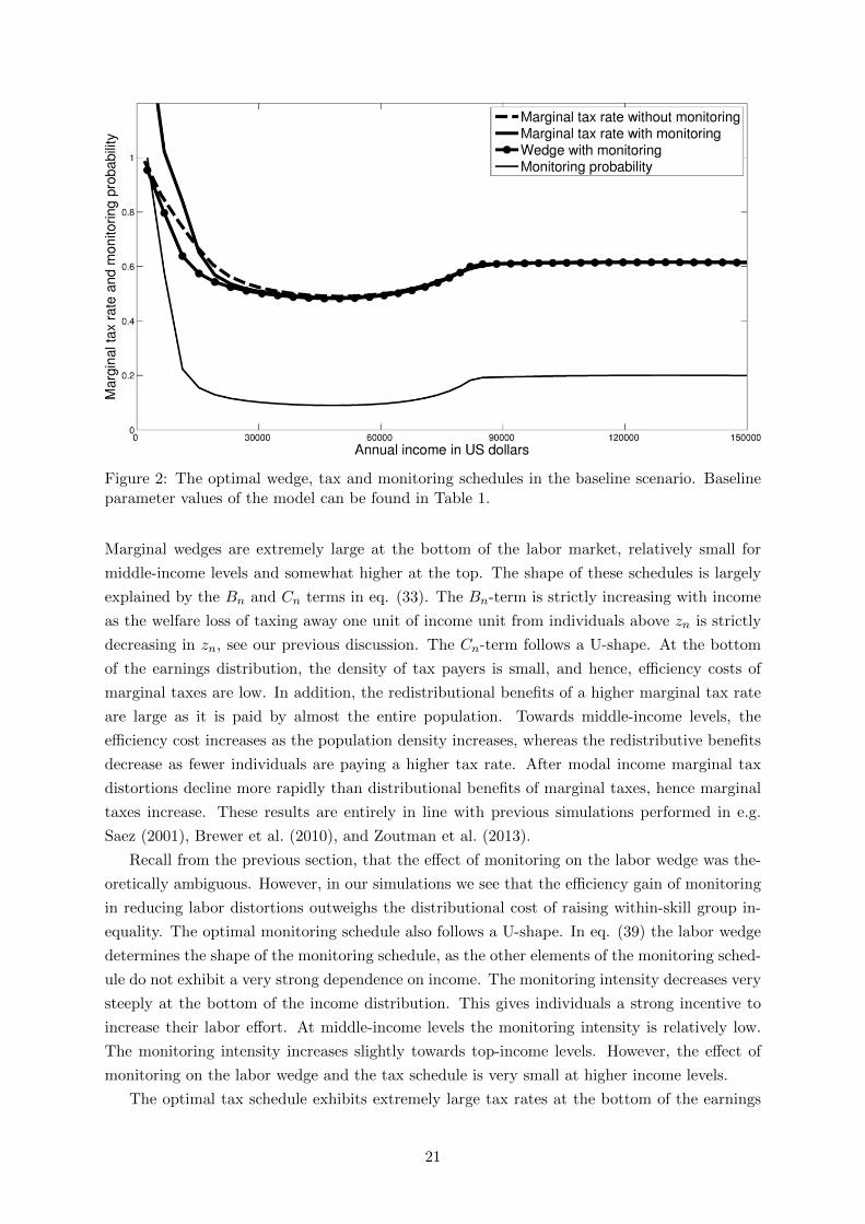
Figure 2: The optimal wedge, tax and monitoring schedules in the baseline scenario. Baselineparameter values of the model can be found in Table 1.
Marginal wedges are extremely large at the bottom of the labor market, relatively small for
middle-income levels and somewhat higher at the top. The shape of these schedules is largely
explained by the Bn and Cn terms in eq. (33). The Bn-term is strictly increasing with income
as the welfare loss of taxing away one unit of income unit from individuals above zn is strictly
decreasing in zn, see our previous discussion. The Cn-term follows a U-shape. At the bottom
of the earnings distribution, the density of tax payers is small, and hence, efficiency costs of
marginal taxes are low. In addition, the redistributional benefits of a higher marginal tax rate
are large as it is paid by almost the entire population. Towards middle-income levels, the
efficiency cost increases as the population density increases, whereas the redistributive benefits
decrease as fewer individuals are paying a higher tax rate. After modal income marginal tax
distortions decline more rapidly than distributional benefits of marginal taxes, hence marginal
taxes increase. These results are entirely in line with previous simulations performed in e.g.
Saez (2001), Brewer et al. (2010), and Zoutman et al. (2013).
Recall from the previous section, that the effect of monitoring on the labor wedge was the-
oretically ambiguous. However, in our simulations we see that the efficiency gain of monitoring
in reducing labor distortions outweighs the distributional cost of raising within-skill group in-
equality. The optimal monitoring schedule also follows a U-shape. In eq. (39) the labor wedge
determines the shape of the monitoring schedule, as the other elements of the monitoring sched-
ule do not exhibit a very strong dependence on income. The monitoring intensity decreases very
steeply at the bottom of the income distribution. This gives individuals a strong incentive to
increase their labor effort. At middle-income levels the monitoring intensity is relatively low.
The monitoring intensity increases slightly towards top-income levels. However, the effect of
monitoring on the labor wedge and the tax schedule is very small at higher income levels.
The optimal tax schedule exhibits extremely large tax rates at the bottom of the earnings
21
distribution. Indeed, the government can levy tax rates above 100 percent at the lowest income
earners. The sharp decrease in the monitoring intensity works as an implicit subsidy on work
effort and partially offsets the high explicit tax on labor supply. The poverty trap found in many
countries (see, e.g., Spadaro, 2005, Brewer et al., 2010 and OECD, 2011) can thus be optimal in
the presence of monitoring. Indeed, there may not be a poverty trap if the monitoring schedule
provides sufficient incentives, even if the tax-benefit system itself does not provide incentives to
supply labor.
Note that the optimal wedge and monitoring probability at the top do not equal zero, as
was derived in Proposition 4 for a bounded income distribution. Mirrlees (1971), Diamond
(1998), and Saez (2001) show theoretically that the optimal wedge converges to a constant if
the right tail of the ability distribution is Pareto distributed. In the Pareto tail of the earnings
distribution, the ratio of marginal distributional benefits and marginal efficiency costs of taxes
becomes constant, and the tax wedge converges to a constant. Our simulations confirm that
this result holds as well in the model with monitoring. In addition, we find that the optimal
monitoring probability also converges to a positive constant.
5.2 Sensitivity analysis
In this subsection we present the sensitivity analysis of the results obtained in the previous
subsection. We especially explore the sensitivity of our simulation outcomes with respect to the
monitoring technology and penalty function, on which little empirical evidence is available.
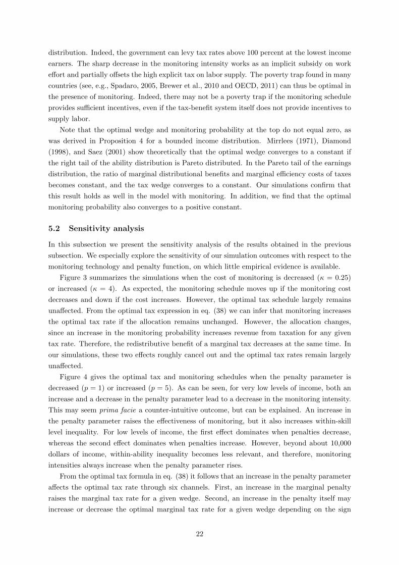
Figure 3 summarizes the simulations when the cost of monitoring is decreased (κ = 0.25)
or increased (κ = 4). As expected, the monitoring schedule moves up if the monitoring cost
decreases and down if the cost increases. However, the optimal tax schedule largely remains
unaffected. From the optimal tax expression in eq. (38) we can infer that monitoring increases
the optimal tax rate if the allocation remains unchanged. However, the allocation changes,
since an increase in the monitoring probability increases revenue from taxation for any given
tax rate. Therefore, the redistributive benefit of a marginal tax decreases at the same time. In
our simulations, these two effects roughly cancel out and the optimal tax rates remain largely
unaffected.
Figure 4 gives the optimal tax and monitoring schedules when the penalty parameter is
decreased (p = 1) or increased (p = 5). As can be seen, for very low levels of income, both an
increase and a decrease in the penalty parameter lead to a decrease in the monitoring intensity.
This may seem prima facie a counter-intuitive outcome, but can be explained. An increase in
the penalty parameter raises the effectiveness of monitoring, but it also increases within-skill
level inequality. For low levels of income, the first effect dominates when penalties decrease,
whereas the second effect dominates when penalties increase. However, beyond about 10,000
dollars of income, within-ability inequality becomes less relevant, and therefore, monitoring
intensities always increase when the penalty parameter rises.
From the optimal tax formula in eq. (38) it follows that an increase in the penalty parameter
affects the optimal tax rate through six channels. First, an increase in the marginal penalty
raises the marginal tax rate for a given wedge. Second, an increase in the penalty itself may
increase or decrease the optimal marginal tax rate for a given wedge depending on the sign
22

Figure 3: Optimal tax and monitoring schedules for high (κ = 4) and low (κ = 0.25) marginalcost of monitoring. All other parameters take baseline values, see Table 1.
Figure 4: Optimal tax and monitoring schedules for strong (p = 5) and weak (p = 1) penalties.All other parameters take baseline values, see Table 1.
23
of π′(zn). Third, an increase in the convexity of the penalty function decreases the efficiency
cost of a wedge. Fourth, the penalty affects the monitoring probability, although the effect
is ambiguous. Fifth, an increase in the penalty increases within skill-level inequality, which
decreases the optimal wedge. Finally, the allocation itself is affected, but it is a priori unclear
whether higher penalties lead to more or less redistribution. The simulation outcomes confirm
these theoretical ambiguities. The net effect is positive for very low income levels, negative for
medium-income levels, and negligible for higher income-levels.
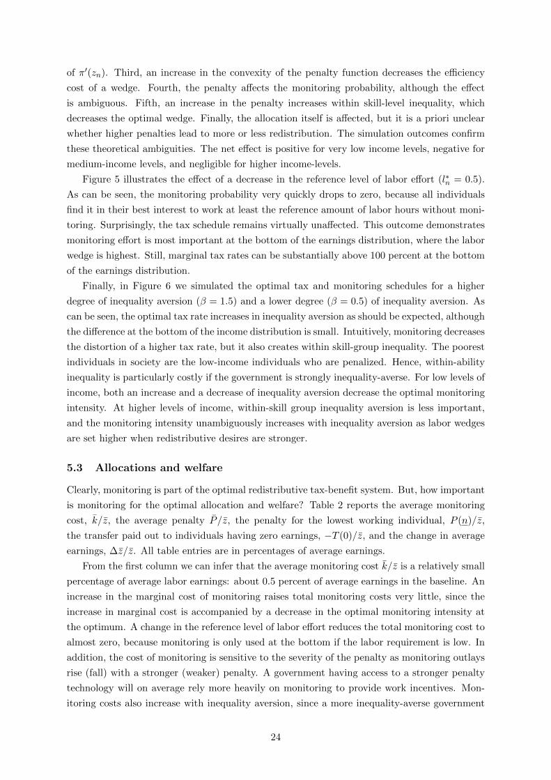
Figure 5 illustrates the effect of a decrease in the reference level of labor effort (l∗n = 0.5).
As can be seen, the monitoring probability very quickly drops to zero, because all individuals
find it in their best interest to work at least the reference amount of labor hours without moni-
toring. Surprisingly, the tax schedule remains virtually unaffected. This outcome demonstrates
monitoring effort is most important at the bottom of the earnings distribution, where the labor
wedge is highest. Still, marginal tax rates can be substantially above 100 percent at the bottom
of the earnings distribution.
Finally, in Figure 6 we simulated the optimal tax and monitoring schedules for a higher
degree of inequality aversion (β = 1.5) and a lower degree (β = 0.5) of inequality aversion. As
can be seen, the optimal tax rate increases in inequality aversion as should be expected, although
the difference at the bottom of the income distribution is small. Intuitively, monitoring decreases
the distortion of a higher tax rate, but it also creates within skill-group inequality. The poorest
individuals in society are the low-income individuals who are penalized. Hence, within-ability
inequality is particularly costly if the government is strongly inequality-averse. For low levels of
income, both an increase and a decrease of inequality aversion decrease the optimal monitoring
intensity. At higher levels of income, within-skill group inequality aversion is less important,
and the monitoring intensity unambiguously increases with inequality aversion as labor wedges
are set higher when redistributive desires are stronger.
5.3 Allocations and welfare
Clearly, monitoring is part of the optimal redistributive tax-benefit system. But, how important
is monitoring for the optimal allocation and welfare? Table 2 reports the average monitoring
cost, k̄/z̄, the average penalty P̄ /z̄, the penalty for the lowest working individual, P (n)/z̄,
the transfer paid out to individuals having zero earnings, −T (0)/z̄, and the change in average
earnings, ∆z̄/z̄. All table entries are in percentages of average earnings.
From the first column we can infer that the average monitoring cost k̄/z̄ is a relatively small
percentage of average labor earnings: about 0.5 percent of average earnings in the baseline. An
increase in the marginal cost of monitoring raises total monitoring costs very little, since the
increase in marginal cost is accompanied by a decrease in the optimal monitoring intensity at
the optimum. A change in the reference level of labor effort reduces the total monitoring cost to
almost zero, because monitoring is only used at the bottom if the labor requirement is low. In
addition, the cost of monitoring is sensitive to the severity of the penalty as monitoring outlays
rise (fall) with a stronger (weaker) penalty. A government having access to a stronger penalty
technology will on average rely more heavily on monitoring to provide work incentives. Mon-
itoring costs also increase with inequality aversion, since a more inequality-averse government
24
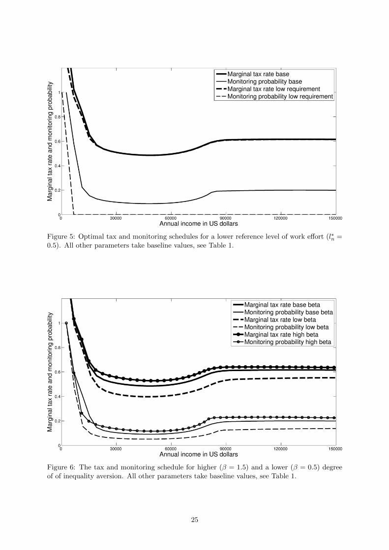
Figure 5: Optimal tax and monitoring schedules for a lower reference level of work effort (l∗n =0.5). All other parameters take baseline values, see Table 1.
Figure 6: The tax and monitoring schedule for higher (β = 1.5) and a lower (β = 0.5) degreeof of inequality aversion. All other parameters take baseline values, see Table 1.
25
relies on average more heavily on monitoring to alleviate the equity-efficiency trade-off.
Table 2: Change in allocation due to monitoring. (All numbersare in percentages of average earnings)
k̄z̄
P̄z̄
P (n)z̄
−T (0)z̄
∆z̄z̄
No Monitoring 0.00 0.00 0.00 29.46 0
Base scenario 0.49 0.35 7.83 33.65 1.35
Low monitoring cost 0.40 0.34 7.55 34.20 1.50
High monitoring cost 0.61 0.36 8.08 33.13 1.18
Low reference effort 0.03 0.02 5.63 34.85 1.07
Low penalty 0.24 0.14 3.53 29.67 0.43
High penalty 0.63 0.49 10.02 37.01 2.04
Low inequality aversion 0.32 0.23 8.20 30.25 5.55
High inequality aversion 0.61 0.42 7.62 35.23 −0.90
Note: z̄ is per capita labor income in the specified calibration, k̄ is theper capita monitoring cost, P̄ is the average penalty over the monitoredpopulation, P (n) is the penalty at the lowest skill level, −T (0) is thetransfer and ∆z̄ is the change in average labor earnings as comparedto the model without monitoring.
The second column represents the average penalty given to monitored individuals as a
percentage of average labor earnings P̄ /z̄. As can be seen, penalties are relatively small. In the
baseline, the average penalty equals 0.35 percent of average earnings. Penalties increase with
the monitoring cost, because monitoring decreases with its marginal cost, and as a consequence,
individuals work less and receive more severe penalties. The effects are very small, however.
In addition, the average penalty falls strongly when the reference level of labor effort is lower.
Similarly, the penalties increase (decrease) if the penalty parameter increases (decreases), as
expected. The penalty also increases (decreases) with stronger (weaker) inequality aversion
because a more (less) inequality-averse government sets higher (lower) wedges. The third column
represents the average penalty at the bottom of the income distribution P (n)/z̄. Penalties at
the bottom are relatively large, because the wedge at the bottom is large. Comparative-static
effects of the penalty at the bottom are roughly similar to the comparative statics of the average
penalty.
The fourth column represents the transfer as a fraction of earnings, −T (0)/z̄, and the
fifth column is the change in average labor earnings as compared to optimal taxation without
monitoring, ∆z̄/z̄. In almost all simulations, both the transfer and average labor earnings
increase, indicating an improvement in both equity and efficiency of the tax-transfer system.
This effect is surprisingly unsensitive to a change in the monitoring cost and to a change in the
reference level of labor effort. These outcomes can be explained by the fact that monitoring is
most effective at the bottom of the skill distribution. At this point in the earnings distribution,
monitoring costs are relatively unimportant as the density of monitored individuals is low. A
lower labor requirement is also unimportant, since individuals are working far less than any work
requirement at the bottom end of the income scale. Results are more sensitive to the size of the
26
penalty, because monitoring becomes less effective if the punishment technology is less effective.
However, even if penalties are relatively low, the increase in both average labor earnings and the
transfer is substantial. Finally, a change in the inequality aversion changes the emphasis given
to either equity (T (0)) or efficiency (average labor earnings). In our scenario with low inequality
aversion both increase. However, in the scenario with high inequality aversion average labor
earnings decreases slightly.
Table 3: Welfare effects of monitoring.
Marginal dead weight loss Welfare gain
No Monitoring 0.204 –
Base 0.203 1.421
Low monitoring cost 0.203 1.592
High monitoring cost 0.204 1.073
Low reference effort 0.203 0.969
Low penalty 0.204 0.267
High penalty 0.203 1.835
Low inequality aversion 0.170 1.015
High inequality aversion 0.214 1.76
Note: The marginal deadweight loss refers to the income-weighted average ofthe marginal deadweight loss of all households as a consequence of increasingthe labor wedge on labor with one percent. Welfare gains are obtained bycalculating the compensating variation as a percentage of average earnings inthe specified simulation.
Finally, Table 3 reports the welfare effects of monitoring. The first column represents the
income-weighted average of the marginal deadweight loss of increasing the marginal tax rate by
one percent. As can be seen, monitoring decreases the marginal deadweight loss by about 0.5
percent in our baseline simulation from 0.204 to 0.203. This result is robust in our sensitivity
analyses.
The last column reports the monetized welfare gain of monitoring. We compute the com-
pensating variation by calculating the amount of resources that have to be injected into an
economy without monitoring in order to attain the same social welfare as the economy with
optimal monitoring. In our base scenario, the welfare gain is about 1.4 percent of average labor
earnings, i.e. 1.4 percent of total output. The welfare gain increases if the cost of monitoring
are lower and if penalties are higher. Interestingly, the welfare gain is almost unaffected by a
lower reference level of labor effort. The reason is that reference labor effort is still generating
positive penalties at the bottom of the earnings distribution, where the benefits of monitoring
are highest. Also, an increase in inequality aversion increases the welfare gain of monitoring,
because the efficiency gain of monitoring is increasing in the optimal labor wedges, which are
larger when the government is more inequality averse. We find quantitatively substantial social
welfare gains in all scenarios.
27
6 Conclusions
In this paper we demonstrate that redistributive governments should optimally employ an effort-
monitoring technology in order to redistribute income at the lowest efficiency cost. Monitoring
of labor effort alleviates the equity-efficiency trade-off and raises equity, efficiency, or both.
The reason is that distortions from redistribution derive from the informational problem that
earning ability is private information. By using a monitoring technology this informational
asymmetry is reduced. A first-best outcome cannot be reached, however, because monitoring
is costly. Mirrlees (1971) is a special case of our model when monitoring is infinitely costly.
We demonstrated that monitoring works as an implicit subsidy on work effort, which par-
tially offsets the explicit tax on work effort. We derived conditions on the desirability of moni-
toring and demonstrated that the optimal non-linear monitoring schedule generally follows the
optimal labor wedge. Monitoring is more desirable when redistributive taxation creates larger
distortions in labor supply. Moreover, optimal labor taxes can optimally be above 100 percent
when monitoring is allowed for. At the endpoints of the earnings distribution labor wedges –
including taxes and the implicit subsidy on work due to monitoring – are zero in the absence
of bunching and with a finite skill level.
Simulations confirmed that the optimal monitoring intensity features a U-shaped pattern
with income; very high at the lower end of the earnings distribution, declining towards the
middle-income groups, increasing again towards the high-income groups, and becoming constant
at the top-income groups. Our simulations demonstrated that marginal tax rates will be higher
if the government monitors labor effort, while the labor wedges – including the explicit tax and
implicit subsidy of monitoring – decreases. Indeed, monitoring is very effective to alleviate the
equity efficiency trade-off.
In practice, monitoring is not infinitely costly as in Mirrlees (1971). By allowing for a mon-
itoring technology we can explain our why work-dependent tax credits for low-income earners,
that are employed in the UK, Ireland and New Zealand, are part of an optimal redistributive
tax policy. Our findings also show that sanctions for welfare recipients, bonuses for low-income
workers, and extensive monitoring of effort or working ability of low-earning individuals are
especially desirable in more generous welfare states. Moreover, we can also explain why (large)
penalties on low labor effort (or high bonuses on large labor effort) are more desirable when the
government desires to redistribute more income. Finally, we explain why marginal tax rates
larger than 100 percent at the lower end of the earnings distribution, as commonly observed in
many countries, can be optimal in the presence of monitoring of work effort.
References
Allingham, Micheal G., and Agmar Sandmo (1972) ‘Income tax evasion: A theoretical analysis.’
Journal of Public Economics 1(3-4), 323–338
Armenter, Roc, and Thomas M. Mertens (2010) ‘Fraud deterrence in dynamic Mirrleesian
economies.’ Federal Reserve Bank of Philadelphia Working Paper No. 10-7 Philadelphia
28
Bassetto, Marco, and Christopher Phelan (2008) ‘Tax riots.’ Review of Economic Studies
75(3), 649–669
Boadway, Robin, and Katherine Cuff (1999) ‘Monitoring job search as an instrument for tar-
geting transfers.’ International Tax and Public Finance 6(3), 317–337
Boone, Jan, and Jan C. Van Ours (2006) ‘Modeling financial incentives to get the unemployed
back to work.’ Journal of Institutional and Theoretical Economics 162(2), 227–252
Boone, Jan, Peter Fredriksson, Bertil Holmlund, and Jan C. Van Ours (2007) ‘Optimal unem-
ployment insurance with monitoring and sanctions.’ Economic Journal 117(518), 399–421
Brewer, Mike, Emmanuel Saez, and Andrew Shephard (2010) ‘Means-testing and tax rates on
earnings.’ In The Mirrlees Review – Dimensions of Tax Design, ed. James A. Mirrlees, Stuart
Adam, Timothy J. Besley, Richard Blundell, Steven Bond, Robert Chote, Malcolm Gammie,
Paul Johnson, Gareth D. Myles, and James M. Poterba (Oxford: Oxford University Press)
chapter 3, pp. 202–274
Chander, Parkash, and Louis L. Wilde (1998) ‘A general characterization of optimal income tax
enforcement.’ Review of Economic Studies 65(1), 165–183
Cremer, Helmuth, and Firouz Gahvari (1994) ‘Tax evasion, concealment and the optimal linear
income tax.’ Scandinavian Journal of Economics 2(96), 219–239
(1996) ‘Tax evasion and the optimum general income tax.’ Journal of Public Economics
60(2), 235–249
Diamond, Peter (1998) ‘Optimal income taxation: An example with a U-shaped pattern of
optimal marginal tax rates.’ American Economic Review 88(1), 83–95
Diamond, Peter, and Eytan Sheshinski (1995) ‘Economic aspects of optimal disability benefits.’
Journal of Public Economics 57(1), 1–23
Ebert, Udo (1992) ‘A reexamination of the optimal non-linear income tax.’ Journal of Public
Economics 49(1), 47–73
Fredriksson, Peter, and Bertil Holmlund (2006) ‘Improving incentives in unemployment insur-
ance: A review of recent research.’ Journal of Economic Surveys 20(3), 357–386
Harris, Milton, and Robert M. Townsend (1981) ‘Resource allocation under asymmetric infor-
mation.’ Econometrica 49(1), 33–64
Holmstrom, Bengt (1979) ‘Moral hazard and observability.’ Bell Journal of Economics 10(1), 74–
91
Immervoll, Herwig (2004) ‘Average and marginal effective tax rates facing workers in the EU: A
micro-level analysis of levels, distributions and driving factors.’ OECD Social, Employment
and Migration Working Papers, No. 19 Paris: OECD Publishing
29

Jacquet, Laurence (forthcoming) ‘Tagging and redistributive taxation with imperfect disability
monitoring.’ Social Choice and Welfare
Kleven, Henrik J., Martin B. Knudsen, Claus T. Kreiner, Soren Pedersen, and Emmanuel Saez
(2011) ‘Unwilling or unable to cheat? Evidence from a tax audit experiment in Denmark.’
Econometrica 79(3), 651–592
Kocherlakota, Narayana R. (2006) ‘Advances in dynamic optimal taxation.’ In Econometric
Society Monographs, ed. Richard Blundell, Whitney K. Newey, and Torsten Persson (Cam-
bridge: Cambridge University Press) chapter 7, pp. 269–297
Ljungqvist, Lars, and Thomas J. Sargent (1995a) ‘The Swedish unemployment experience.’
European Economic Review 39(5), 1043–1070
(1995b) ‘Welfare states and unemployment.’ Economic Theory 6(1), 143–160
Mankiw, N. Gregory, Matthew Weinzierl, and Danny Yagan (2009) ‘Optimal taxation in theory
and practice.’ Journal of Economic Perspectives 23(4), 147–174
Mirrlees, James A. (1971) ‘An exploration in the theory of optimum income taxation.’ Review
of Economic Studies 38(2), 175–208
(1976) ‘Optimal tax theory: A synthesis.’ Journal of Public Economics 6(4), 327–358
(1997) ‘Information and incentives: The economics of carrots and sticks.’ Economic Journal
107(444), 1311–1329
(1999) ‘The theory of moral hazard and unobservable behaviour: Part i.’ Review of Economic
Studies 66(1), 3–21
Mookherjee, Dilip, and Ivan Png (1989) ‘Optimal auditing, insurance, and redistribution.’ Quar-
terly Journal of Economics 104(2), 399–415
Myerson, Roger B. (1979) ‘Incentive compatibility and the bargaining problem.’ Econometrica
47(1), 61–73
OECD (2011) ‘Taxation and employment.’ OECD Tax Policy Studies, No.21 Paris
Sadka, Efraim (1976) ‘On income distribution, incentive effects and optimal income taxation.’
Review of Economic Studies 43(2), 261–267
Saez, Emmanuel (2001) ‘Using elasticities to derive optimal income tax rates.’ Review of Eco-
nomic Studies 68(1), 205–229
Saez, Emmanuel, Joel B. Slemrod, and Seth H. Giertz (2012) ‘The elasticity of taxable income
with respect to marginal tax rates: A critical review.’ Journal of Economic Literature 50(1), 3–
50
Sandmo, Agnar (1981) ‘Income tax evasion, labour supply, and the equity–efficiency tradeoff.’
Journal of Public Economics 16(3), 265–288
30
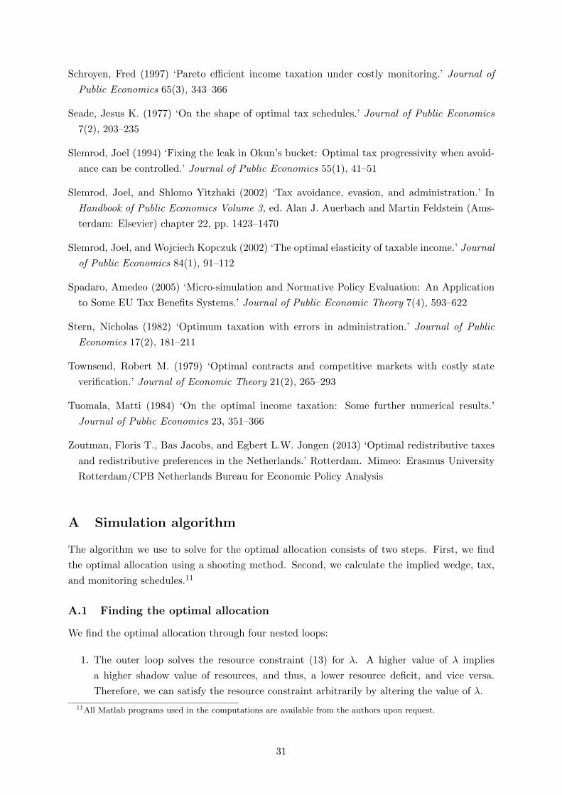
Schroyen, Fred (1997) ‘Pareto efficient income taxation under costly monitoring.’ Journal of
Public Economics 65(3), 343–366
Seade, Jesus K. (1977) ‘On the shape of optimal tax schedules.’ Journal of Public Economics
7(2), 203–235
Slemrod, Joel (1994) ‘Fixing the leak in Okun’s bucket: Optimal tax progressivity when avoid-
ance can be controlled.’ Journal of Public Economics 55(1), 41–51
Slemrod, Joel, and Shlomo Yitzhaki (2002) ‘Tax avoidance, evasion, and administration.’ In
Handbook of Public Economics Volume 3, ed. Alan J. Auerbach and Martin Feldstein (Ams-
terdam: Elsevier) chapter 22, pp. 1423–1470
Slemrod, Joel, and Wojciech Kopczuk (2002) ‘The optimal elasticity of taxable income.’ Journal
of Public Economics 84(1), 91–112
Spadaro, Amedeo (2005) ‘Micro-simulation and Normative Policy Evaluation: An Application
to Some EU Tax Benefits Systems.’ Journal of Public Economic Theory 7(4), 593–622
Stern, Nicholas (1982) ‘Optimum taxation with errors in administration.’ Journal of Public
Economics 17(2), 181–211
Townsend, Robert M. (1979) ‘Optimal contracts and competitive markets with costly state
verification.’ Journal of Economic Theory 21(2), 265–293
Tuomala, Matti (1984) ‘On the optimal income taxation: Some further numerical results.’
Journal of Public Economics 23, 351–366
Zoutman, Floris T., Bas Jacobs, and Egbert L.W. Jongen (2013) ‘Optimal redistributive taxes
and redistributive preferences in the Netherlands.’ Rotterdam. Mimeo: Erasmus University
Rotterdam/CPB Netherlands Bureau for Economic Policy Analysis
A Simulation algorithm
The algorithm we use to solve for the optimal allocation consists of two steps. First, we find
the optimal allocation using a shooting method. Second, we calculate the implied wedge, tax,
and monitoring schedules.11
A.1 Finding the optimal allocation
We find the optimal allocation through four nested loops:
1. The outer loop solves the resource constraint (13) for λ. A higher value of λ implies
a higher shadow value of resources, and thus, a lower resource deficit, and vice versa.
Therefore, we can satisfy the resource constraint arbitrarily by altering the value of λ.
11All Matlab programs used in the computations are available from the authors upon request.
31

2. The second loop solves the transversality condition at the top (32) for a given utility level
at the bottom un, and λ. The most important determinant in un is the transfer implied
by T (0). Therefore, one can think of this procedure as finding the intercept of the tax
function T (0). If the intercept is too low, the distortion at the top has to be positive to
finance the transfer, and vice versa if the intercept is set too high. As a consequence, by
varying the transfer T (0) we can satisfy the transversality condition arbitrarily closely.
3. The third loop solves the differential equations (14) and (30) for given un, λ, and θn using
a Runge-Kutta method to integrate over n.
4. The inner loop maximizes the Hamiltonian (26) with respect to πn and zn for a given
state un and costate variable θn at each n.
The above algorithm is known as a shooting method because it shoots for the initial values
of the differential equations that satisfy the boundary condition.
A.2 Finding the optimal wedge, tax, and monitoring schedules
The above algorithm gives us a numerical approximation of the allocation {un, θn, zn, πn} at
each n. π′(zn) can be approximated by taking the first difference:
π′(zn) ≈ ∆πn∆zn
. (53)
With π′(zn) we have all the information we need to find the optimal tax schedule using eq. (38).
32