Embed Size (px)
Citation preview
ISSN 1688-2806
Universidad de la RepublicaFacultad de Ingenierıa
Transient and steady-state componentseparation for audio signals
Tesis presentada a la Facultad de Ingenierıa de laUniversidad de la Republica por
Ignacio Irigaray Bayarres
en cumplimiento parcial de los requerimientospara la obtencion del tıtulo de
Magister en Ingenierıa Electrica.
Director de TesisDr. Luiz W. P. Biscainho Universidad Federal de
Rio de Janeiro
TribunalDr. Federico Lecumberry Universidad de la RepublicaDr. Pablo Belzarena Universidad de la Republica
Dr. Alvaro Pardo (Revisor externo) Universidad Catolica del Uruguay
Director AcademicoDr. Pablo Monzon Universidad de la Republica
Montevideo2 de octubre de 2014
Transient and steady-state component separation for audio signals, Ignacio IrigarayBayarres
ISSN 1688-2806
Esta tesis fue preparada en LATEX usando la clase iietesis (v1.0).Contiene un total de 88 paginas.Compilada el Monday 9th February, 2015.http://iie.fing.edu.uy/
Whitout analysis, we can never have a synthesis.
Hans-Joachim Koellreutter
Se me ocurre que la verdad profunda de las cosases necesariamente difusa, imprecisa, inexacta; queel espıritu se alimenta del misterio y huye y sedisuelve cuando lo que llamamos precision o rea-lidad intenta fijar las cosas en una forma deter-minada - o en un concepto.
Mario Levrero - Desplazamientos
Aside from weighty technical problem of collectivecoherent thinking, there is a very human, evensocial need for sympathy from all the members tobend for the common result.
Bill Evans - Improvisation in Jazz

ii
Abstract
In this work the problem of transient and steady-state component separation ofan audio signal was addressed. In particular, a recently proposed method for sep-aration of transient and steady-state components based on the median filter wasinvestigated. For a better understanding of the processes involved, a modifica-tion of the filtering stage of the algorithm was proposed. This modification wasevaluated subjectively by listening tests and objectively by an application-basedcomparison. Also some extensions to the model were presented in conjunction withdifferent possible applications for the transient and steady-state decomposition inthe area of audio editing and processing.
Esta tesis trata sobre la separacion de senales de audio en componentes tran-sitorios y estacionarios. En particular, se estudia un metodo reciente para laseparacion en componentes transitorios y estacionarios basado en la utilizacion defiltros de mediana. Para una mejor comprension de los procesos involucrados, sepropone una modificacion a la etapa de filtrado. La modificacion propuesta es eva-luada de forma subjetiva por medio de test de escucha y objetivamente mediantela comparacion de los resultado de algunas aplicaciones. Ademas, se presentan ex-tensiones al modelo en conjunto con diferentes aplicaciones en el area de la ediciony procesamiento de audio.

iv
Contents
Abstract iii
1 Introduction 1
1.1 Historical context . . . . . . . . . . . . . . . . . . . . . . . . . . . . 2
1.2 Motivation . . . . . . . . . . . . . . . . . . . . . . . . . . . . . . . 3
1.3 Thesis outline . . . . . . . . . . . . . . . . . . . . . . . . . . . . . . 4
2 Audio signal representation 5
2.1 Introduction . . . . . . . . . . . . . . . . . . . . . . . . . . . . . . . 6
2.2 Time-domain representations . . . . . . . . . . . . . . . . . . . . . 6
2.3 Frequency-domain representation . . . . . . . . . . . . . . . . . . . 6
2.4 Time-Frequency representation . . . . . . . . . . . . . . . . . . . . 7
2.4.1 Uncertainly principle . . . . . . . . . . . . . . . . . . . . . . 8
2.4.2 Short-Time Fourier Transform . . . . . . . . . . . . . . . . 9
2.4.3 Constant-Q Transform . . . . . . . . . . . . . . . . . . . . . 12
2.4.4 Sinusoidal Modeling . . . . . . . . . . . . . . . . . . . . . . 13
2.4.5 Non-Negative Matrix Factorization NMF . . . . . . . . . . 18
3 Transient and Steady-State separation 21
3.1 Model of transient and steady-state components . . . . . . . . . . 22
3.2 Separation Methods . . . . . . . . . . . . . . . . . . . . . . . . . . 22
3.2.1 Median Filter . . . . . . . . . . . . . . . . . . . . . . . . . . 24
3.2.2 SSE Filter . . . . . . . . . . . . . . . . . . . . . . . . . . . . 25
3.3 Extensions . . . . . . . . . . . . . . . . . . . . . . . . . . . . . . . 28
3.3.1 Iterative Filtering . . . . . . . . . . . . . . . . . . . . . . . 28
3.3.2 Relaxed components . . . . . . . . . . . . . . . . . . . . . . 29
3.3.3 Sub-Band processing . . . . . . . . . . . . . . . . . . . . . . 30
3.4 Reconstruction method . . . . . . . . . . . . . . . . . . . . . . . . 31
4 Tests & Applications 35
4.1 SSE and Median filter comparison . . . . . . . . . . . . . . . . . . 36
4.1.1 Data set description . . . . . . . . . . . . . . . . . . . . . . 36
4.1.2 Tests . . . . . . . . . . . . . . . . . . . . . . . . . . . . . . . 37
4.1.3 Beat Tracking . . . . . . . . . . . . . . . . . . . . . . . . . . 37
4.1.4 Pitch-tracking . . . . . . . . . . . . . . . . . . . . . . . . . . 40
Contents
4.2 Applications in audio editing . . . . . . . . . . . . . . . . . . . . . 444.2.1 Removing undesired transients . . . . . . . . . . . . . . . . 444.2.2 Percussion extraction and remixing . . . . . . . . . . . . . . 444.2.3 Noise Reduction . . . . . . . . . . . . . . . . . . . . . . . . 454.2.4 Transient shaping . . . . . . . . . . . . . . . . . . . . . . . 464.2.5 De-reverberation . . . . . . . . . . . . . . . . . . . . . . . . 474.2.6 Time/Pitch Modifications . . . . . . . . . . . . . . . . . . . 48
5 Conclusions and future work 515.1 Conclusions . . . . . . . . . . . . . . . . . . . . . . . . . . . . . . . 525.2 Future perspectives . . . . . . . . . . . . . . . . . . . . . . . . . . . 53
Appendix 54
A Subjective Quality Test Data 55
B Subjective Quality Test Interface 61
C Complete Beat-Tracking results 63
Bibliography 65
List of Figures 74
Indice de figuras 76
vi
Chapter 1
Introduction
Chapter 1. Introduction
This thesis is about sounds and music. Music is one of the most sophisticatedforms of communication ever created by humans. It finds the more diverse ap-plications, such as: social control, entertainment, religious rituals, marketing, andaesthetic pleasure, among others. Therefore, its detailed study under all the avail-able human knowledge becomes a worthwhile effort to undertake. The followingsection attempts to illustrate the relation between music and technology, and theimportance of the collaboration among musicians and engineers. This thesis is aneffort in this direction.
1.1 Historical contextFrom the beginning the humans are trying to understand and explain the sounds.The Marin Mersenne observation in [53] is worth quoting:
“The string struck and sounded freely makes at least five soundsat the same time, the first of which is the natural sound of the stringand serves as the foundation for the rest.”
Marsenne could not accept that the movement of one string could produce morethan one sound. Joseph Sauveur finds the explanation for overtones [70], which hepoetically resumes as:
“When a point of a calm surface of water is slightly agitated, cir-cular waves are formed and spread around it. When the surface isagitated at another point, new waves are formed and mix with the for-mer; they travel over the surface disturbed by the first wave as theywould do over a calm surface, so that they can be perfectly distinguishedin the mixture. What the eye perceives with respect to waves, the earperceives with respect to sounds or aerial vibrations, which travel si-multaneously without troubling each other and produce very distinctimpressions...”
In the year of 1807 Joseph Fourier releases his memories “On the Propagation ofHeat in Solid Bodies”, where he presents the theory of the Fourier Series. Mostof the works in audio signal processing are based on this foundational result, andthis thesis work is not the exception.1
Jumping in time to the early 20th century, the first electronic musical instru-ments were developed. The Dynamophone, also known as Thelarmonium, waspresented before the public in 1906: it weighted 200 tons and could delivery elec-tronic music through the telephone network. Approximately at the same time themusicians perceived the necessity of new instruments to express themselves. In1913 the Italian composer Luigi Russolo wrote [68]:
1This section is based [11], a complete reading of which is highly recommended.
2
1.2. Motivation
“Musical sound is too limited in qualitative variety of timbre. Themost complicated orchestra reduces themselves to four or five classesof instruments differing in timbre: instrument played with the bow,plucked instruments, brass-winds, wood-winds and percussion instru-ments... we must break out of this narrow circle of pure musical soundand conquer the infinite variety of noise sounds,”
and in 1916 the composer Edgar Varese stated:
“Our musical alphabet must be enriched... We also need new in-struments very badly... In my own works I have always felt the needfor new mediums of expression.”
The technological advances after the World War II2 inspired two differentaestethic movements, the musique concrete in Paris and the elektronische Musikin Cologne—the first exploring the creative possibilities of the tape recorder whilethe second the synthetic generation of sound by the utilization of electronic oscil-lators. The new mediums of expression that Varese advocated where created. Inbrief, as stated in [10]:
“Instrument and music can only develop together - and not as theyplease, but according to a concurrence: potential in the instrument,and need, in the player.”
The popularization of computers in universities in the sixties and the technolog-ical revolution brought by the introduction of the microprocessor in the seventieswere the foundation of software-synthesized music. In the following decades, withthe massification of personal computers, it became an indispensable tool in everystudio. The personal computer and the software that runs on it are the instrumentsof today.
1.2 MotivationAudio signal modeling has now decades of development and involves a vast liter-ature. To increment knowledge of the state of the art in this discipline is one ofthe principal motivations of this thesis. In particular, the transient and steady-state component separation problem is addressed. Along this work, transient com-ponents are considered as broad-band, with highly concentrated energy in time,whereas steady-state components are considered as discrete, narrow-band, withsmooth temporal behaviour. Such components connect with musical conceptssuch as beat and pitch, and some of these relations are explored in this work.Also, existing sound processing techniques can benefit from the utilization of thiskind of decomposition. For instance, the generation of artifacts can be reduced innoise-reduction applications and transients smearing can be avoided in time-scale
2And in particular, the end of the war.
3
Chapter 1. Introduction
modifications. Finally, the separation makes possible the precise control of eachcomponent separately, which enables artistic applications for musicians and com-posers. To explore applications of the separation techniques proposed is anothermotivation of the present work.
1.3 Thesis outlineThis document follows with an introduction of the principal concepts associatedwith time, frequency, and their relations in the signal processing context. Time,frequency, and joint time-frequency representations are presented and their limi-tations discussed in Chapter 2. Some of these representations are the foundationson which the transient and steady-state component separation relies. Next, inChapter 3 the transient/steady-state models are defined, an algorithm based onmedian filters is described, and a modification of its nonlinear filtering stage isproposed. The Chapter 4 has two principal sections: first, comparative subjectiveand objective evaluations between the proposed modification and the original algo-rithm are conducted and described. In the second part, various applications of thetransient/steady-state decomposition are presented and illustrated with examples.Finally, the document ends with some conclusions and ideas for future work inChapter 5.
4
Chapter 2
Audio signal representation
Chapter 2. Audio signal representation
2.1 IntroductionThis chapter describes some of the principal concepts associated with time, fre-quency and their relations in the signal processing context. Time, frequency andjoint time-frequency representation are presented and their limitations discussed.
2.2 Time-domain representationsSignals have various definitions: in the information theory context signal is de-fined as an entity that carries information, in electrical engineering a signal is ameasurable quantity that varies in time. In particular, sound signals represent thevariation of the air pressure along time. Time representation of audio signals isthe most intuitive, simple and common.
Although simple, useful information can be derived from the time-domain rep-resentation.
Given a signal s(t) its total energy can be defined as:
E =
∫ ∞−∞|s(t)|2dt. (2.1)
One can considerate |s(t)|2 as its instantaneous power, or density of energyexpressed along time. Thus the average time, that represents the time value aroundwhich this density is distributed, can be defined as follows:
< t >=
∫ ∞−∞
t|s(t)|2dt. (2.2)
In a similar way the standard deviation σt, which represents the effective du-ration of the signal, can be calculated as:
T 2 = σ2t =
∫ ∞−∞
(< t > −t)2|s(t)|2dt. (2.3)
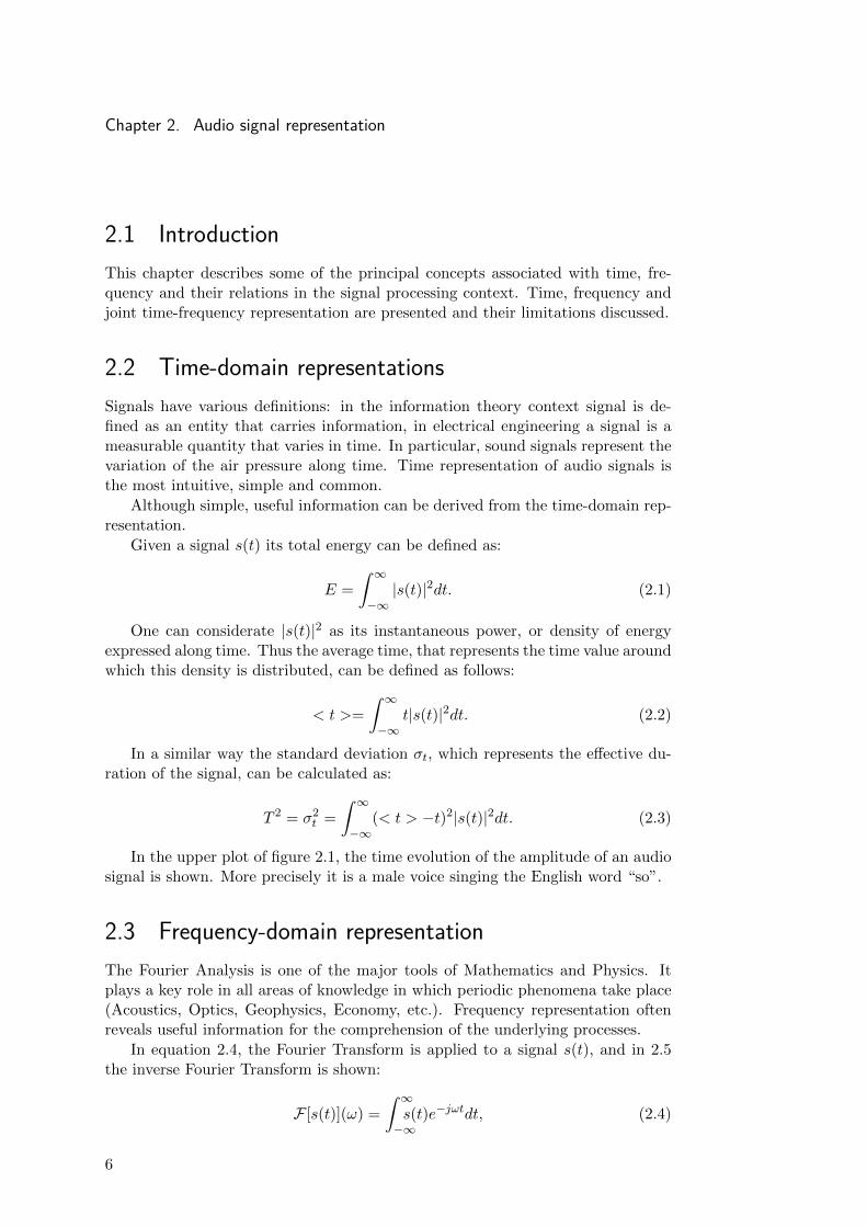
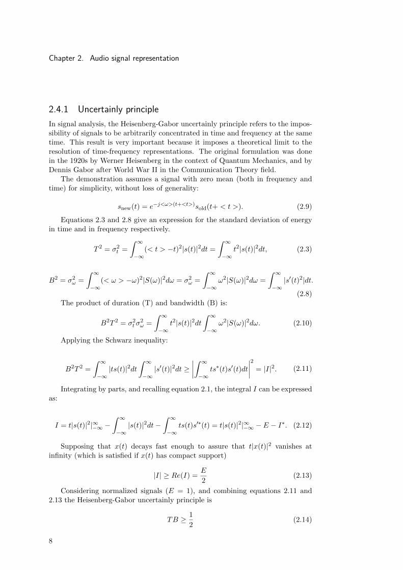
In the upper plot of figure 2.1, the time evolution of the amplitude of an audiosignal is shown. More precisely it is a male voice singing the English word “so”.
2.3 Frequency-domain representationThe Fourier Analysis is one of the major tools of Mathematics and Physics. Itplays a key role in all areas of knowledge in which periodic phenomena take place(Acoustics, Optics, Geophysics, Economy, etc.). Frequency representation oftenreveals useful information for the comprehension of the underlying processes.
In equation 2.4, the Fourier Transform is applied to a signal s(t), and in 2.5the inverse Fourier Transform is shown:
F [s(t)](ω) =
∫ ∞−∞s(t)e−jωtdt, (2.4)
6
2.4. Time-Frequency representation
0 0.2 0.4 0.6 0.8 1 1.2 1.4 1.6 1.8 2−0.4
−0.2
0
0.2
0.4Time representation
Time (s)
Am
plit
ude
−10 −8 −6 −4 −2 0 2 4 6 8 10−40
−20
0
20
40
60Frequency representation
Frequency (KHz)
Am
plit
ude (
dB
)
Figure 2.1: Time and frequency representation of an audio signal. A male voice singing “so”.Starts with the unvoiced consonant [s] and ends with the voiced vowel [o].
s(t) = F [S(ω)](t) =1
2π
∫ ∞−∞S(ω)ejωtdω. (2.5)
The signal s(t) is decomposed in complex exponentials (ejωt) of infinite dura-tion and frequency ω, each one contributing a relative amount indicated by S(ω).
One can interpret |S(ω)|2 as the energy per unit frequency at frequency ω, andthen derive via Parseval’s theorem the total energy:
E =
∫ ∞−∞|S(ω)|2dω =
∫ ∞−∞|s(t)|2dt. (2.6)
If |S(ω)|2 represents the density, the averages can be calculated as was done inthe time domain. The average frequency represents the frequency around whichthe energy is distributed, and is defined as:
< ω >=
∫ ∞−∞
ω|S(ω)|2dω. (2.7)
The standard deviation σω, often called the root mean squared bandwidth(denoted B), is calculated as:
B2 = σ2ω =
∫ ∞−∞
(< ω > −ω)2|S(ω)|2dω. (2.8)
The figure 2.1 depicts the module in decibels of the Fourier Transform (lower)and their correspondent time-domain signal (top).
2.4 Time-Frequency representationTime-Frequency Representations are one of the most important tools in audiosignal processing. The historical development of the theory was driven by variousdisciplines, such as Mathematics, Quantum Mechanics and Signal Processing.
7
Chapter 2. Audio signal representation
2.4.1 Uncertainly principleIn signal analysis, the Heisenberg-Gabor uncertainly principle refers to the impos-sibility of signals to be arbitrarily concentrated in time and frequency at the sametime. This result is very important because it imposes a theoretical limit to theresolution of time-frequency representations. The original formulation was donein the 1920s by Werner Heisenberg in the context of Quantum Mechanics, and byDennis Gabor after World War II in the Communication Theory field.
The demonstration assumes a signal with zero mean (both in frequency andtime) for simplicity, without loss of generality:
snew(t) = e−j<ω>(t+<t>)sold(t+ < t >). (2.9)
Equations 2.3 and 2.8 give an expression for the standard deviation of energyin time and in frequency respectively.
T 2 = σ2t =
∫ ∞−∞
(< t > −t)2|s(t)|2dt =
∫ ∞−∞
t2|s(t)|2dt, (2.3)
B2 = σ2ω =
∫ ∞−∞
(< ω > −ω)2|S(ω)|2dω = σ2ω =
∫ ∞−∞
ω2|S(ω)|2dω =
∫ ∞−∞|s′(t)2|dt.
(2.8)The product of duration (T) and bandwidth (B) is:
B2T 2 = σ2t σ2ω =
∫ ∞−∞
t2|s(t)|2dt∫ ∞−∞
ω2|S(ω)|2dω. (2.10)
Applying the Schwarz inequality:
B2T 2 =
∫ ∞−∞|ts(t)|2dt
∫ ∞−∞|s′(t)|2dt ≥
∣∣∣∣∫ ∞−∞
ts∗(t)s′(t)dt
∣∣∣∣2 = |I|2. (2.11)
Integrating by parts, and recalling equation 2.1, the integral I can be expressedas:
I = t|s(t)|2|∞−∞ −∫ ∞−∞|s(t)|2dt−
∫ ∞−∞
ts(t)s′∗(t) = t|s(t)|2|∞−∞ − E − I∗. (2.12)
Supposing that x(t) decays fast enough to assure that t|x(t)|2 vanishes atinfinity (which is satisfied if x(t) has compact support)
|I| ≥ Re(I) =E
2(2.13)
Considering normalized signals (E = 1), and combining equations 2.11 and2.13 the Heisenberg-Gabor uncertainly principle is
TB ≥ 1
2(2.14)
8
2.4. Time-Frequency representation
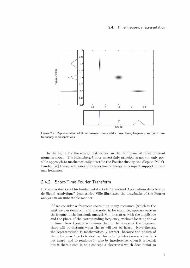
Figure 2.2: Representation of three Gaussian sinusoidal atoms: time, frequency and joint timefrequency representations.
In the figure 2.2 the energy distribution in the T-F plane of three differentatoms is shown. The Heisenberg-Gabor uncertainly principle is not the only pos-sible approach to mathematically describe the Fourier duality, the Slepian-Pollak-Landau [76] theory addresses the restriction of energy in compact support in timeand frequency.
2.4.2 Short-Time Fourier TransformIn the introduction of his fundamental article “Theorie et Applications de la Notionde Signal Analytique” Jean-Andre Ville illustrates the drawbacks of the Fourieranalysis in an unbeatable manner:
“If we consider a fragment containing many measures (which is theleast we can demand), and one note, la for example, appears once inthe fragment, the harmonic analysis will present us with the amplitudeand the phase of the corresponding frequency, without locating the lain time. Now then, it is obvious that in the course of the fragmentthere will be instants when the la will not be heard. Nevertheless,the representation is mathematically correct, because the phases ofthe notes near la acts to destroy this note by interference when la isnot heard, and to reinforce it, also by interference, when it is heard;but if there exists in this concept a cleverness which does honor to
9
Chapter 2. Audio signal representation
mathematical analysis, there is also a distortion of reality: in fact,when la is not heard, the true reason is that the la is not emitted.”
As seen in section 2.3, the Fourier Transform decompose signals as a combina-tion of sinusoids that last forever in time. Music never presents a strictly periodicbehaviour, by contrast its essence is the irregular variation over time. Althoughirregular, a lot of musical signals observed locally present a pseudo-periodic be-haviour.
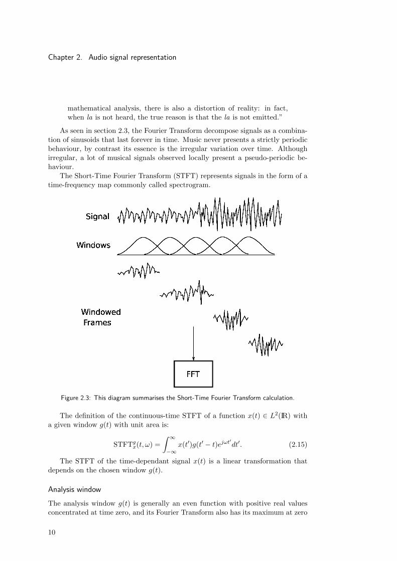
The Short-Time Fourier Transform (STFT) represents signals in the form of atime-frequency map commonly called spectrogram.
Figure 2.3: This diagram summarises the Short-Time Fourier Transform calculation.
The definition of the continuous-time STFT of a function x(t) ∈ L2(IR) witha given window g(t) with unit area is:
STFTgx(t, ω) =
∫ ∞−∞
x(t′)g(t′ − t)ejωt′dt′. (2.15)
The STFT of the time-dependant signal x(t) is a linear transformation thatdepends on the chosen window g(t).
Analysis windowThe analysis window g(t) is generally an even function with positive real valuesconcentrated at time zero, and its Fourier Transform also has its maximum at zero
10
2.4. Time-Frequency representation
frequency. The analysis window leaves unchanged the signal value at some instantt′ whereas attenuates the signal at distant times. One is looking at an excerpt ofthe entire signal, as is done with a landscape and a real window.
The STFT can be considered as a projection of the signal x(t) into a familyof atoms generated by time translations and frequency modulations of a givenwindow g(t):
gt,ω(t′) = g(t′ − t)e−jωt′ . (2.16)
If g(t) is an even, real-valued function, atom’s energy is concentrated in t, ω.Figure 2.2 shows three of such atoms with different time and frequency centres,and energy concentrations in the T-F plane.
Energy Conservation
The energy Ex of the signal can be calculated by integrating the STFT:
Ex =
∫ ∞−∞|x(t)|2dt =
∫ ∞−∞
∫ ∞−∞
STFT2(t, f)dfdt. (2.17)
This allows one to interpret the STFT as the distribution along the T-F planeof the density of energy. The demonstration of this property can be consulted in[29].
STFT Synthesis
The reconstruction formula given a STFTgx of a signal x is:
x(t′) =1
2π
∫ ∞−∞
∫ ∞−∞
STFTgx(t, ω)ejωt
′dωdt. (2.18)
Discrete Fourier Transform
In practice, the spectral analysis for audio signals is done in the discrete timedomain. In this domain, the STFT is defined as:
Xn[ejωk ] =
∞∑m=−∞
w[n−m]x[m]e−jωkm. (2.19)
Equation 2.19 has two equivalent interpretations: the overlapp-add (OLA) andthe filter bank summation (FBS).
The OLA interpretation consist in considering Xn[ejωk ] as a function of n, insuch a way that the STFT represents the Fourier transform of the moving signalcentered (and windowed) at time n.
In the filter bank summation interpretation, the signal x[m] is first frequencyshifted by e−jωkm so that the frequency ωk is moved to zero, and then low-passfiltered by a filter with impulse response w[n].
11
Chapter 2. Audio signal representation
2.4.3 Constant-Q TransformA representation with fixed frequency resolution (such as the STFT) has somelimitations when applied to music related signals. For example, if one considersthe register of a standard 88 key piano1, the first semitone is 1.6352-Hz wide,while the last one is 235-Hz wide. To discriminate two notes whose fundamentalfrequencies are separated by one semitone, a window with more than 27000-sample2 duration is needed. When using a constant resolution representation its resultsin oversampling at high frequencies. In 1991 Judith Brown presented in [4] aconstant Q spectral transform, where Q is the ratio of the center frequency to thebandwidth of each frequency bin.
The quality factor Q for a quarter-tone resolution is calculated as:
Q =f
δf=
f
( 24√
2− 1)f≈ 34, (2.20)
N [k] =S
δfk=
S
fkQ. (2.21)
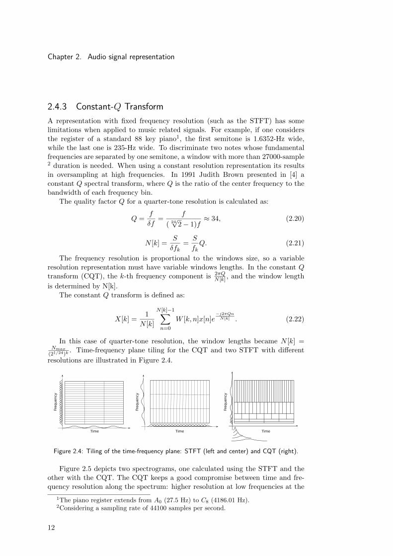
The frequency resolution is proportional to the windows size, so a variableresolution representation must have variable windows lengths. In the constant Qtransform (CQT), the k-th frequency component is 2πQ
N [k] , and the window length
is determined by N[k].The constant Q transform is defined as:
X[k] =1
N [k]
N [k]−1∑n=0
W [k, n]x[n]e−j2πQnN [k] . (2.22)
In this case of quarter-tone resolution, the window lengths became N [k] =Nmax
(21/24)k. Time-frequency plane tiling for the CQT and two STFT with different
resolutions are illustrated in Figure 2.4.
Time
Frequency
Frequency
Frequency
TimeTime
Figure 2.4: Tiling of the time-frequency plane: STFT (left and center) and CQT (right).
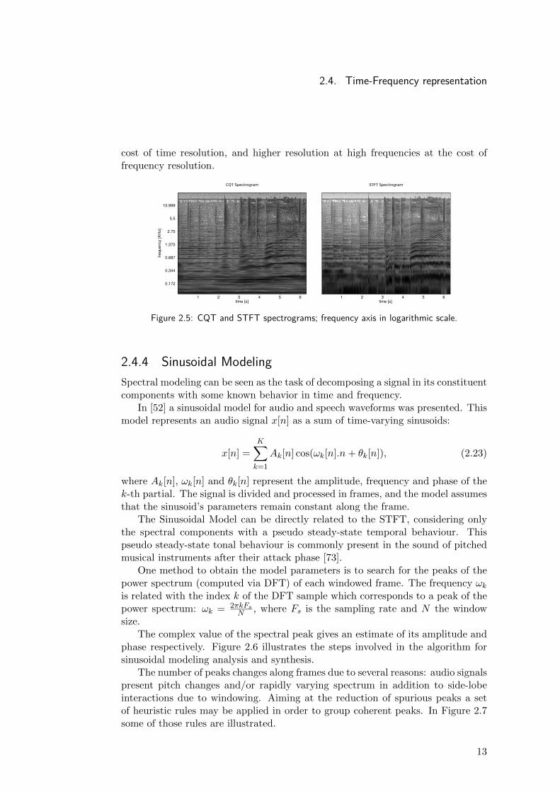
Figure 2.5 depicts two spectrograms, one calculated using the STFT and theother with the CQT. The CQT keeps a good compromise between time and fre-quency resolution along the spectrum: higher resolution at low frequencies at the
1The piano register extends from A0 (27.5 Hz) to C8 (4186.01 Hz).2Considering a sampling rate of 44100 samples per second.
12
2.4. Time-Frequency representation
cost of time resolution, and higher resolution at high frequencies at the cost offrequency resolution.
frequ
ency
[KH
z]
10.999
5.5
2.75
1.375
0.687
0.344
0.172
time [s]1 2 3 4 5 6
time [s]1 2 3 4 5 6
Figure 2.5: CQT and STFT spectrograms; frequency axis in logarithmic scale.
2.4.4 Sinusoidal ModelingSpectral modeling can be seen as the task of decomposing a signal in its constituentcomponents with some known behavior in time and frequency.
In [52] a sinusoidal model for audio and speech waveforms was presented. Thismodel represents an audio signal x[n] as a sum of time-varying sinusoids:
x[n] =K∑k=1
Ak[n] cos(ωk[n].n+ θk[n]), (2.23)
where Ak[n], ωk[n] and θk[n] represent the amplitude, frequency and phase of thek-th partial. The signal is divided and processed in frames, and the model assumesthat the sinusoid’s parameters remain constant along the frame.
The Sinusoidal Model can be directly related to the STFT, considering onlythe spectral components with a pseudo steady-state temporal behaviour. Thispseudo steady-state tonal behaviour is commonly present in the sound of pitchedmusical instruments after their attack phase [73].
One method to obtain the model parameters is to search for the peaks of thepower spectrum (computed via DFT) of each windowed frame. The frequency ωkis related with the index k of the DFT sample which corresponds to a peak of thepower spectrum: ωk = 2πkFs
N , where Fs is the sampling rate and N the windowsize.
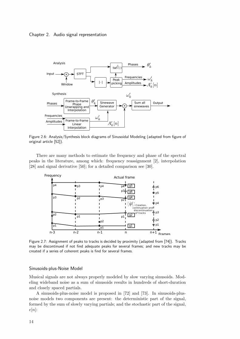
The complex value of the spectral peak gives an estimate of its amplitude andphase respectively. Figure 2.6 illustrates the steps involved in the algorithm forsinusoidal modeling analysis and synthesis.
The number of peaks changes along frames due to several reasons: audio signalspresent pitch changes and/or rapidly varying spectrum in addition to side-lobeinteractions due to windowing. Aiming at the reduction of spurious peaks a setof heuristic rules may be applied in order to group coherent peaks. In Figure 2.7some of those rules are illustrated.
13
Chapter 2. Audio signal representation
Figure 2.6: Analysis/Synthesis block diagrams of Sinusoidal Modeling (adapted from figure oforiginal article [52]).
There are many methods to estimate the frequency and phase of the spectralpeaks in the literature, among which: frequency reassignment [2], interpolation[28] and signal derivative [50]; for a detailed comparison see [30].
Figure 2.7: Assignment of peaks to tracks is decided by proximity (adapted from [74]). Tracksmay be discontinued if not find adequate peaks for several frames; and new tracks may becreated if a series of coherent peaks is find for several frames.
Sinusoids-plus-Noise ModelMusical signals are not always properly modeled by slow varying sinusoids. Mod-eling wideband noise as a sum of sinusoids results in hundreds of short-durationand closely spaced partials.
A sinusoids-plus-noise model is proposed in [72] and [73]. In sinusoids-plus-noise models two components are present: the deterministic part of the signal,formed by the sum of slowly varying partials; and the stochastic part of the signal,e[n]:
14
2.4. Time-Frequency representation
x[n] =
K∑k=1
Ak[n] cos(ωk[n].n+ θk[n]) + e[n]. (2.24)
The stochastic part e[n] can be described as filtered white noise:
e[n] =
∞∑k=−∞
hn[n− k]u[k], (2.25)
where u[k] is white noise and hn[k] is the impulse response of the time-varyingfrequency shaping filter at frame n.
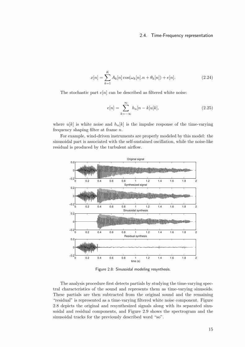
For example, wind-driven instruments are properly modeled by this model: thesinusoidal part is associated with the self-sustained oscillation, while the noise-likeresidual is produced by the turbulent airflow.
0 0.2 0.4 0.6 0.8 1 1.2 1.4 1.6 1.8 2−0.2
0
0.2Original signal
0 0.2 0.4 0.6 0.8 1 1.2 1.4 1.6 1.8 2−0.2
0
0.2Synthesized signal
0 0.2 0.4 0.6 0.8 1 1.2 1.4 1.6 1.8 2−0.2
0
0.2Sinusoidal synthesis
0 0.2 0.4 0.6 0.8 1 1.2 1.4 1.6 1.8 2−0.2
0
0.2
time (s)
Residual synthesis
Figure 2.8: Sinusoidal modeling resynthesis.
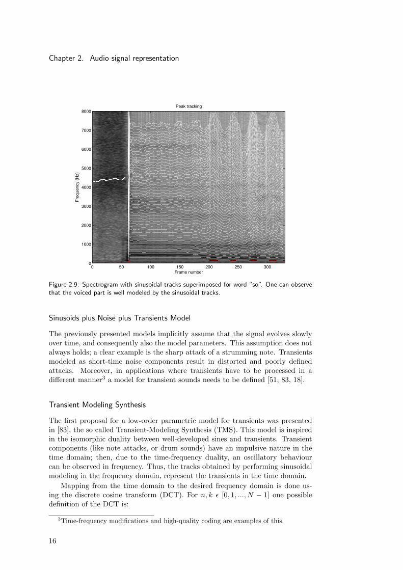
The analysis procedure first detects partials by studying the time-varying spec-tral characteristics of the sound and represents them as time-varying sinusoids.These partials are then subtracted from the original sound and the remaining“residual” is represented as a time-varying filtered white noise component. Figure2.8 depicts the original and resynthesized signals along with its separated sinu-soidal and residual components, and Figure 2.9 shows the spectrogram and thesinusoidal tracks for the previously described word “so”.
15
Chapter 2. Audio signal representation
Peak tracking
Frame number
Fre
quency (
Hz)
0 50 100 150 200 250 3000
1000
2000
3000
4000
5000
6000
7000
8000
Figure 2.9: Spectrogram with sinusoidal tracks superimposed for word “so”. One can observethat the voiced part is well modeled by the sinusoidal tracks.
Sinusoids plus Noise plus Transients Model
The previously presented models implicitly assume that the signal evolves slowlyover time, and consequently also the model parameters. This assumption does notalways holds; a clear example is the sharp attack of a strumming note. Transientsmodeled as short-time noise components result in distorted and poorly definedattacks. Moreover, in applications where transients have to be processed in adifferent manner3 a model for transient sounds needs to be defined [51, 83, 18].
Transient Modeling Synthesis
The first proposal for a low-order parametric model for transients was presentedin [83], the so called Transient-Modeling Synthesis (TMS). This model is inspiredin the isomorphic duality between well-developed sines and transients. Transientcomponents (like note attacks, or drum sounds) have an impulsive nature in thetime domain; then, due to the time-frequency duality, an oscillatory behaviourcan be observed in frequency. Thus, the tracks obtained by performing sinusoidalmodeling in the frequency domain, represent the transients in the time domain.
Mapping from the time domain to the desired frequency domain is done us-ing the discrete cosine transform (DCT). For n, k ε [0, 1, ..., N − 1] one possibledefinition of the DCT is:
3Time-frequency modifications and high-quality coding are examples of this.
16
2.4. Time-Frequency representation
C(k) = β(k)
N−1∑n=0
x(n) cos
[(2n+ 1)kπ
2N
],
where β(k) =√
1/N for k = 1, and β(k) =√
2/k otherwise.
−1
−0.5
0
0.5
1
Time domain
−1
−0.5
0
0.5
1
Frequency domain
0 0.5 1 1.5 2 2.5 3
−1
−0.5
0
0.5
1
Time (s)0 0.5 1 1.5 2 2.5 3
−1
−0.5
0
0.5
1
Normalized frequency
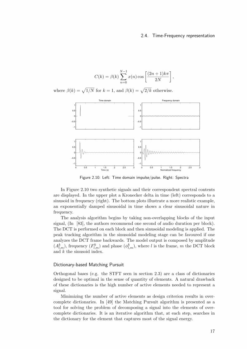
Figure 2.10: Left: Time domain impulse/pulse. Right: Spectra
In Figure 2.10 two synthetic signals and their correspondent spectral contentsare displayed. In the upper plot a Kronecker delta in time (left) corresponds to asinusoid in frequency (right). The bottom plots illustrate a more realistic example,an exponentially damped sinusoidal in time shows a clear sinusoidal nature infrequency.
The analysis algorithm begins by taking non-overlapping blocks of the inputsignal, (In [83], the authors recommend one second of audio duration per block).The DCT is performed on each block and then sinusoidal modeling is applied. Thepeak tracking algorithm in the sinusoidal modeling stage can be favoured if oneanalyzes the DCT frame backwards. The model output is composed by amplitude(Akl,m), frequency (F kl,m) and phase (φkl,m), where l is the frame, m the DCT blockand k the sinusoid index.
Dictionary-based Matching Pursuit
Orthogonal bases (e.g. the STFT seen in section 2.3) are a class of dictionariesdesigned to be optimal in the sense of quantity of elements. A natural drawbackof these dictionaries is the high number of active elements needed to represent asignal.
Minimizing the number of active elements as design criterion results in over-complete dictionaries. In [49] the Matching Pursuit algorithm is presented as atool for solving the problem of decomposing a signal into the elements of over-complete dictionaries. It is an iterative algorithm that, at each step, searches inthe dictionary for the element that captures most of the signal energy.
17
Chapter 2. Audio signal representation
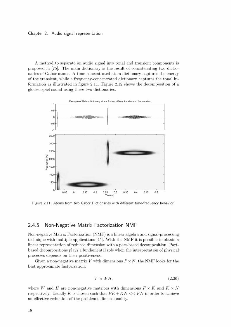
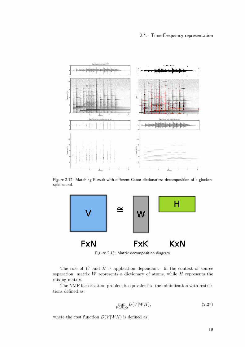
A method to separate an audio signal into tonal and transient components isproposed in [75]. The main dictionary is the result of concatenating two dictio-naries of Gabor atoms. A time-concentrated atom dictionary captures the energyof the transient, while a frequency-concentrated dictionary captures the tonal in-formation as illustrated in figure 2.11. Figure 2.12 shows the decomposition of aglockenspiel sound using these two dictionaries.
Figure 2.11: Atoms from two Gabor Dictionaries with different time-frequency behavior.
2.4.5 Non-Negative Matrix Factorization NMFNon-negative Matrix Factorization (NMF) is a linear algebra and signal-processingtechnique with multiple applications [45]. With the NMF it is possible to obtain alinear representation of reduced dimension with a part-based decomposition. Part-based decompositions plays a fundamental role when the interpretation of physicalprocesses depends on their positiveness.
Given a non-negative matrix V with dimensions F ×N , the NMF looks for thebest approximate factorization:
V ≈WH, (2.26)
where W and H are non-negative matrices with dimensions F × K and K × Nrespectively. Usually K is chosen such that FK+KN << FN in order to achievean effective reduction of the problem’s dimensionality.
18
2.4. Time-Frequency representation
−1
0
1Signal waverform and STFT
Time (s)
Fre
quency (
Hz)
1 2 3 4 5 6 0
5
10
15
20
−1
0
1Signal waverform and transient content
1 2 3 4 5 6
0
5
10
15
20
Time (s)
Fre
quency (
Hz)
−1
0
1Signal waverform and tonal content
1 2 3 4 5 6
0
5
10
15
20
Time (s)
Fre
quency (
Hz)
Figure 2.12: Matching Pursuit with different Gabor dictionaries: decomposition of a glocken-spiel sound.
Figure 2.13: Matrix decomposition diagram.
The role of W and H is application dependant. In the context of sourceseparation, matrix W represents a dictionary of atoms, while H represents themixing matrix.
The NMF factorization problem is equivalent to the minimization with restric-tions defined as:
minW,H≥0
D(V |WH), (2.27)
where the cost function D(V |WH) is defined as:
19
Chapter 2. Audio signal representation
D(V |WH) =F∑f=1
N∑n=1
d([V ]fn|[WH]fn) (2.28)
and function d(x|y) is a scalar divergence.Multiple divergences with different properties can be utilized with the NMF,
and the best choice depends on the application. The Euclidean (Eq. 2.29) and theKullback-Leibler (Eq. 2.30) are two common divergences.
dEUC(x|y) =1
2(x− y)2 (2.29)
dKL(x|y) = x log(x
y)− x+ y (2.30)
NMF in Audio ApplicationsIn the context of audio applications, the NMF algorithm is commonly applied tothe magnitude spectrogram4 [86].
The spectrogram is then decomposed in positive parts. The column wk of thedictionary matrix W represent the spectrum of the k-th base element, while thecorrespondent row hk of the activation matrix H represents the gain coefficientalong time frames. An important property is that the base elements wk belong tothe same space as the signal spectrum.
The product of the k-th column of W by the k-th row of H gives us an ap-proximation of the spectrogram of the k-th source Xk.
Xk = wk.hk (2.31)
To account for musical structure (e.g. time continuity, frequency sparseness),regularization can be added to the model [22], [85].
4Any non-negative T-F representation can be utilized with the NMF; the spectrogramis the most common.
20
Chapter 3
Transient and Steady-State separation
Chapter 3. Transient and Steady-State separation
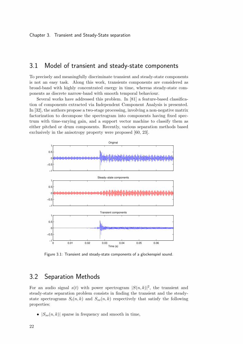
3.1 Model of transient and steady-state componentsTo precisely and meaningfully discriminate transient and steady-state componentsis not an easy task. Along this work, transients components are considered asbroad-band with highly concentrated energy in time, whereas steady-state com-ponents as discrete narrow-band with smooth temporal behaviour.
Several works have addressed this problem. In [81] a feature-based classifica-tion of components extracted via Independent Component Analysis is presented.In [32], the authors propose a two-stage processing, involving a non-negative matrixfactorization to decompose the spectrogram into components having fixed spec-trum with time-varying gain, and a support vector machine to classify them aseither pitched or drum components. Recently, various separation methods basedexclusively in the anisotropy property were proposed [60, 23].
−1
−0.5
0
0.5
1Original
−1
−0.5
0
0.5
1Steady−state components
0 0.01 0.02 0.03 0.04 0.05 0.06−1
−0.5
0
0.5
1Transient components
Time (s)
Figure 3.1: Transient and steady-state components of a glockenspiel sound.
3.2 Separation MethodsFor an audio signal s(t) with power spectrogram |S(n, k)|2, the transient andsteady-state separation problem consists in finding the transient and the steady-state spectrograms St(n, k) and Sss(n, k) respectively that satisfy the followingproperties:
• |Sss(n, k)| sparse in frequency and smooth in time,
22
3.2. Separation Methods
• |St(n, k)| sparse in time and smooth in frequency,
• |St(n, k)|+ |Sss(n, k)| = |S(n, k)|,
This problem can be formulated as the minimization of a cost function J withconstraints (as suggested in [65]) as follows:
J(|St|, |Sss|) =∑n,k
D [S(n, k), Sss(n, k) + St(n, k)]
+1
2σ2ss
∑n,k
(|Sss(n− 1, k)| − |Sss(n, k)|)
+1
2σ2t
∑n,k
(|St(n, k − 1)| − |St(n, k)|),
(3.1)
with the restrictions: |St| ≥ 0 and |Sss| ≥ 0 and being D a divergence. The firstterm measures the distance between |S(t)| and |St| + |Sss|, the second penalizesthe temporal discontinuity and the third measures the frequency smoothness. Thevalues σt and σss , determines the relative weights of the transient and steady-statecomponents in the cost function, respectively.
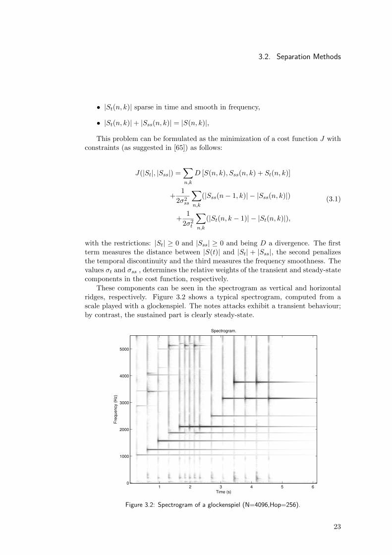
These components can be seen in the spectrogram as vertical and horizontalridges, respectively. Figure 3.2 shows a typical spectrogram, computed from ascale played with a glockenspiel. The notes attacks exhibit a transient behaviour;by contrast, the sustained part is clearly steady-state.
Fre
qu
en
cy (
Hz)
Time (s)
Spectrogram.
1 2 3 4 5 60
1000
2000
3000
4000
5000
Figure 3.2: Spectrogram of a glockenspiel (N=4096,Hop=256).
23

Chapter 3. Transient and Steady-State separation
The minimization of the previous cost function can be thought as a non-linearfilter which smooths the original spectrogram. It filters out the horizontal ridges,corresponding to transients, to obtain the magnitude of the steady-state spec-trogram |Sss|, and removes the vertical ridges, which corresponds to partials ofsteady-state components, to obtain the magnitude of the transient spectrogram|St|.
3.2.1 Median FilterAs seen in figure 3.2, along the time axis the transient components are atypicalevents, and thus can be considered as outliers, just as steady-state components canbe considered outliers along the frequency axis. A common procedure to eliminateoutliers is to use of a median filter.
Median filters are commonly used in signal processing for denoising, e.g. re-moving salt and pepper noise in image filtering [63] or removing noise from digitizedvinyl records in audio [39], [37]. The median filter consist in sliding a window ofsize 2N + 1 along the signal, replacing the centre value of each window by themedian of the samples within the window itself.
In [23] the utilization of median filters in the transient and steady-state com-ponent separation problem is proposed.
��������������
� � � �������
���
������ �� ���
������
����
��������������������
��������������
�
�
����������������
�� �
�� � t
ss
t
ss
ss
t
Figure 3.3: Diagram of the entire process.
The general procedure is illustrated in figure 3.3, and can be decomposed infour stages as follows:
1. Obtain a time-frequency representation for the digital audio signal, typicallya spectrogram computed via the Short-Term Fourier Transform (STFT):
S(n, k) =∑i
x(i).w(i− nT )e−j2πikN . (3.2)
2. Apply a median filter to the power spectrogram S along the frequency axisto eliminate steady-state components and obtain a “transient emphasized”spectrogram St, as well as along the time axis to eliminate transient peaksand obtain a “steady-state emphasized” spectrogram Sss:
St(n, k) = median(|S(n− l : n+ l, k)|), (3.3)
Sss(n, k) = median(|S(n, k − l : k + l)|). (3.4)
24
3.2. Separation Methods
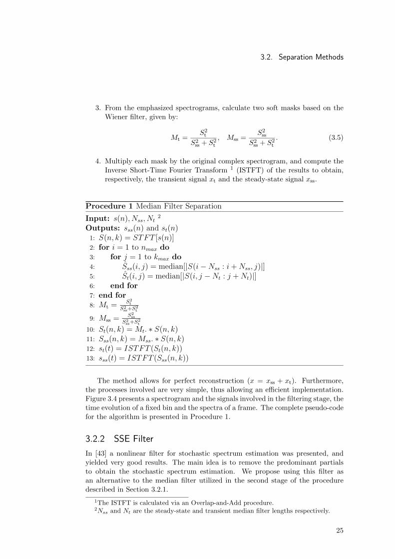
3. From the emphasized spectrograms, calculate two soft masks based on theWiener filter, given by:
Mt =S2t
S2ss + S2
t
, Mss =S2ss
S2ss + S2
t
. (3.5)
4. Multiply each mask by the original complex spectrogram, and compute theInverse Short-Time Fourier Transform 1 (ISTFT) of the results to obtain,respectively, the transient signal xt and the steady-state signal xss.
Procedure 1 Median Filter Separation
Input: s(n), Nss, Nt2
Outputs: sss(n) and st(n)1: S(n, k) = STFT [s(n)]2: for i = 1 to nmax do3: for j = 1 to kmax do4: Sss(i, j) = median[|S(i−Nss : i + Nss, j)|]5: St(i, j) = median[|S(i, j −Nt : j + Nt)|]6: end for7: end for8: Mt =
S2t
S2ss+S
2t
9: Mss = S2ss
S2ss+S
2t
10: St(n, k) = Mt. ∗ S(n, k)11: Sss(n, k) = Mss. ∗ S(n, k)12: st(t) = ISTFT (St(n, k))13: sss(t) = ISTFT (Sss(n, k))
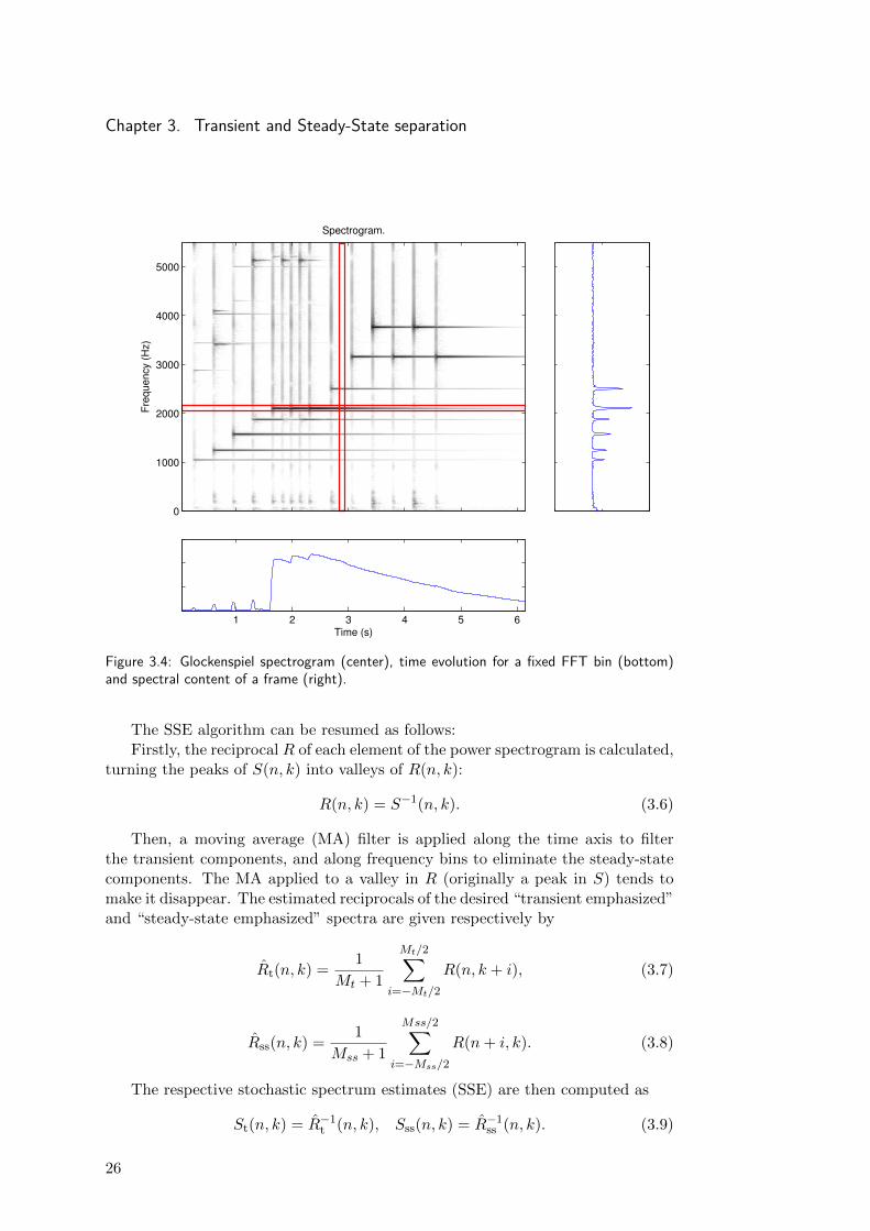
The method allows for perfect reconstruction (x = xss + xt). Furthermore,the processes involved are very simple, thus allowing an efficient implementation.Figure 3.4 presents a spectrogram and the signals involved in the filtering stage, thetime evolution of a fixed bin and the spectra of a frame. The complete pseudo-codefor the algorithm is presented in Procedure 1.
3.2.2 SSE FilterIn [43] a nonlinear filter for stochastic spectrum estimation was presented, andyielded very good results. The main idea is to remove the predominant partialsto obtain the stochastic spectrum estimation. We propose using this filter asan alternative to the median filter utilized in the second stage of the proceduredescribed in Section 3.2.1.
1The ISTFT is calculated via an Overlap-and-Add procedure.2Nss and Nt are the steady-state and transient median filter lengths respectively.
25
Chapter 3. Transient and Steady-State separationF
req
ue
ncy (
Hz)
Spectrogram.
0
1000
2000
3000
4000
5000
1 2 3 4 5 6Time (s)
Figure 3.4: Glockenspiel spectrogram (center), time evolution for a fixed FFT bin (bottom)and spectral content of a frame (right).
The SSE algorithm can be resumed as follows:Firstly, the reciprocal R of each element of the power spectrogram is calculated,
turning the peaks of S(n, k) into valleys of R(n, k):
R(n, k) = S−1(n, k). (3.6)
Then, a moving average (MA) filter is applied along the time axis to filterthe transient components, and along frequency bins to eliminate the steady-statecomponents. The MA applied to a valley in R (originally a peak in S) tends tomake it disappear. The estimated reciprocals of the desired “transient emphasized”and “steady-state emphasized” spectra are given respectively by
Rt(n, k) =1
Mt + 1
Mt/2∑i=−Mt/2
R(n, k + i), (3.7)
Rss(n, k) =1
Mss + 1
Mss/2∑i=−Mss/2
R(n+ i, k). (3.8)
The respective stochastic spectrum estimates (SSE) are then computed as
St(n, k) = R−1t (n, k), Sss(n, k) = R−1ss (n, k). (3.9)
26
3.2. Separation Methods
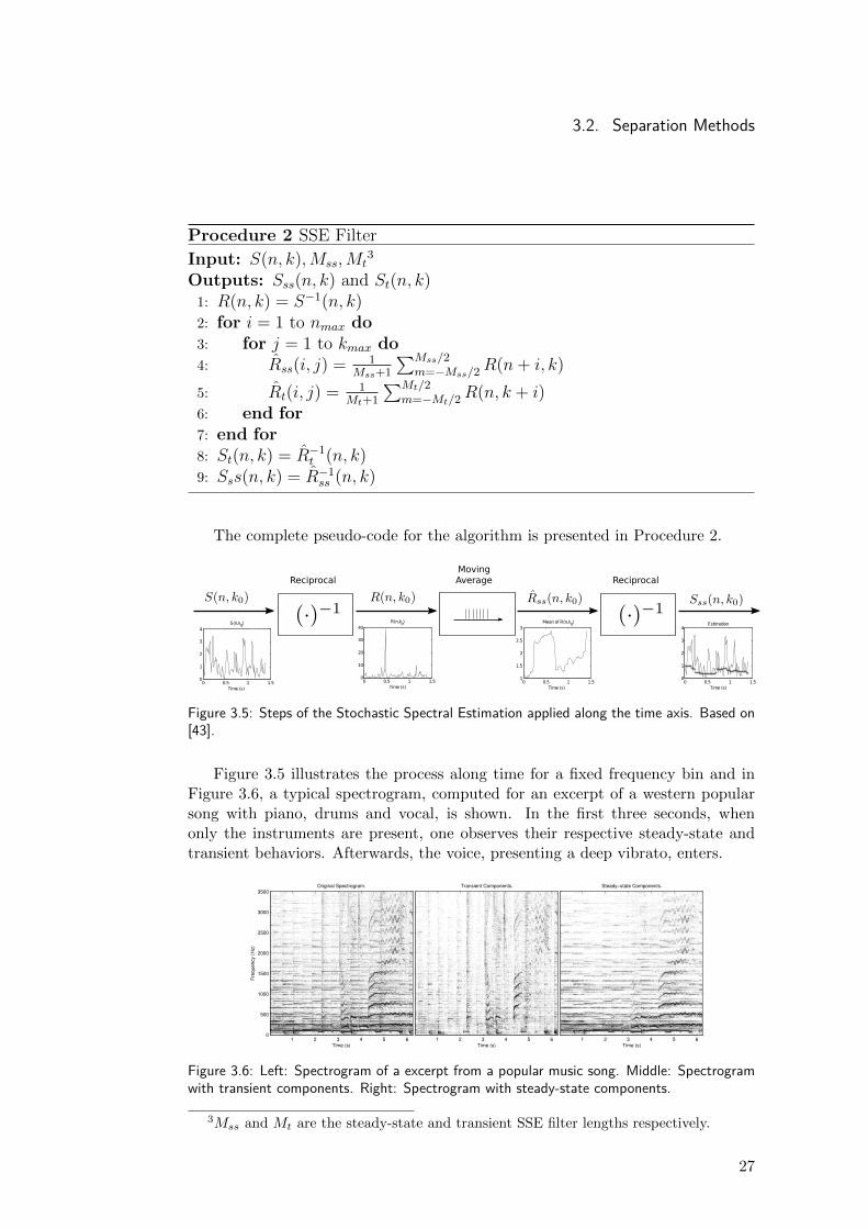
Procedure 2 SSE Filter
Input: S(n, k),Mss,Mt3
Outputs: Sss(n, k) and St(n, k)1: R(n, k) = S−1(n, k)2: for i = 1 to nmax do3: for j = 1 to kmax do4: Rss(i, j) = 1
Mss+1
∑Mss/2m=−Mss/2
R(n + i, k)
5: Rt(i, j) = 1Mt+1
∑Mt/2m=−Mt/2
R(n, k + i)6: end for7: end for8: St(n, k) = R−1t (n, k)9: Sss(n, k) = R−1ss (n, k)
The complete pseudo-code for the algorithm is presented in Procedure 2.
Figure 3.5: Steps of the Stochastic Spectral Estimation applied along the time axis. Based on[43].
Figure 3.5 illustrates the process along time for a fixed frequency bin and inFigure 3.6, a typical spectrogram, computed for an excerpt of a western popularsong with piano, drums and vocal, is shown. In the first three seconds, whenonly the instruments are present, one observes their respective steady-state andtransient behaviors. Afterwards, the voice, presenting a deep vibrato, enters.
Fre
qu
en
cy (
Hz)
Original Spectrogram.
Time (s)1 2 3 4 5 6
0
500
1000
1500
2000
2500
3000
3500
Time (s)
Transient Components.
1 2 3 4 5 6
Steady−state Components.
Time (s)1 2 3 4 5 6
Figure 3.6: Left: Spectrogram of a excerpt from a popular music song. Middle: Spectrogramwith transient components. Right: Spectrogram with steady-state components.
3Mss and Mt are the steady-state and transient SSE filter lengths respectively.
27
Chapter 3. Transient and Steady-State separation
One can observe in the first three seconds (when only drums and piano arepresent) that the separation is as expected, meeting the transient and steady-statemodels as defined, respectively. The deep vibrato voice that enters before secondthree is outside the defined model, and thus it not completely modeled by transientor steady-state components.
3.3 ExtensionsSome extensions can be proposed to overcome limitations of the previously de-scribed methods. The following sections present three extensions of the algorithmwhich allows the model to best fit some particular signals or applications.
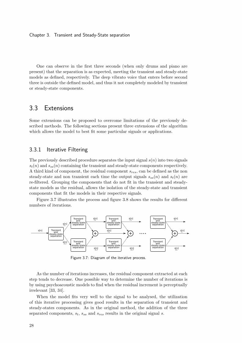
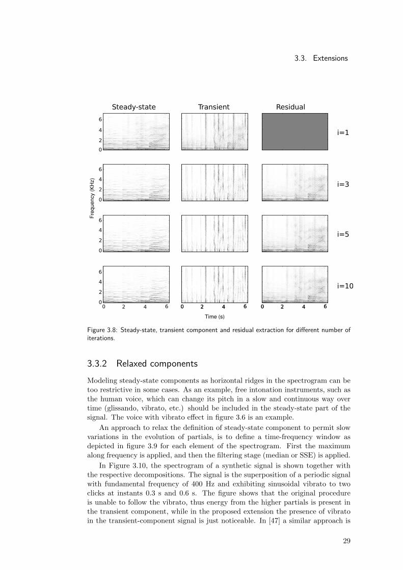
3.3.1 Iterative FilteringThe previously described procedure separates the input signal s(n) into two signalsst(n) and sss(n) containing the transient and steady-state components respectively.A third kind of component, the residual component sres, can be defined as the nonsteady-state and non transient each time the output signals sss(n) and st(n) arere-filtered. Grouping the components that do not fit in the transient and steady-state models as the residual, allows the isolation of the steady-state and transientcomponents that fit the models in their respective signals.
Figure 3.7 illustrates the process and figure 3.8 shows the results for differentnumbers of iterations.
Figure 3.7: Diagram of the iterative process.
As the number of iterations increases, the residual component extracted at eachstep tends to decrease. One possible way to determine the number of iterations isby using psychoacoustic models to find when the residual increment is perceptuallyirrelevant [33, 34].
When the model fits very well to the signal to be analysed, the utilizationof this iterative processing gives good results in the separation of transient andsteady-states components. As in the original method, the addition of the threeseparated components, st, sss and sres results in the original signal s.
28
3.3. Extensions
Figure 3.8: Steady-state, transient component and residual extraction for different number ofiterations.
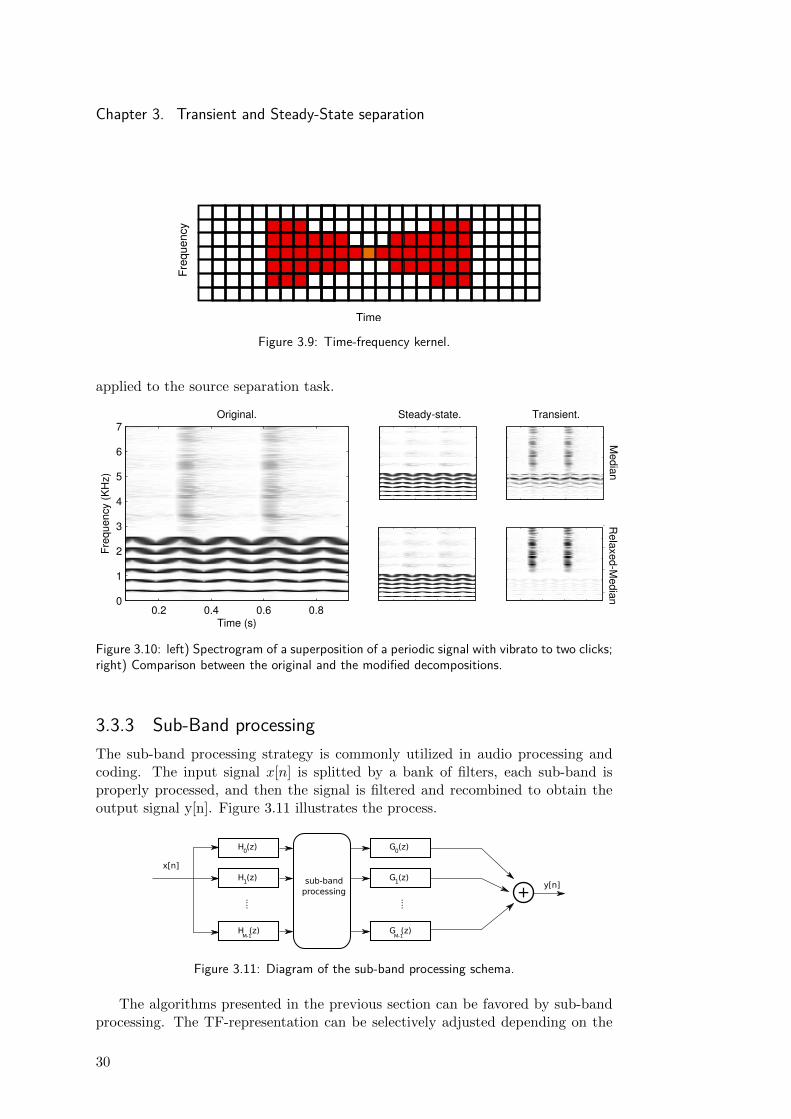
3.3.2 Relaxed componentsModeling steady-state components as horizontal ridges in the spectrogram can betoo restrictive in some cases. As an example, free intonation instruments, such asthe human voice, which can change its pitch in a slow and continuous way overtime (glissando, vibrato, etc.) should be included in the steady-state part of thesignal. The voice with vibrato effect in figure 3.6 is an example.
An approach to relax the definition of steady-state component to permit slowvariations in the evolution of partials, is to define a time-frequency window asdepicted in figure 3.9 for each element of the spectrogram. First the maximumalong frequency is applied, and then the filtering stage (median or SSE) is applied.
In Figure 3.10, the spectrogram of a synthetic signal is shown together withthe respective decompositions. The signal is the superposition of a periodic signalwith fundamental frequency of 400 Hz and exhibiting sinusoidal vibrato to twoclicks at instants 0.3 s and 0.6 s. The figure shows that the original procedureis unable to follow the vibrato, thus energy from the higher partials is present inthe transient component, while in the proposed extension the presence of vibratoin the transient-component signal is just noticeable. In [47] a similar approach is
29
Chapter 3. Transient and Steady-State separation
Figure 3.9: Time-frequency kernel.
applied to the source separation task.
Figure 3.10: left) Spectrogram of a superposition of a periodic signal with vibrato to two clicks;right) Comparison between the original and the modified decompositions.
3.3.3 Sub-Band processingThe sub-band processing strategy is commonly utilized in audio processing andcoding. The input signal x[n] is splitted by a bank of filters, each sub-band isproperly processed, and then the signal is filtered and recombined to obtain theoutput signal y[n]. Figure 3.11 illustrates the process.
Figure 3.11: Diagram of the sub-band processing schema.
The algorithms presented in the previous section can be favored by sub-bandprocessing. The TF-representation can be selectively adjusted depending on the
30
3.4. Reconstruction method
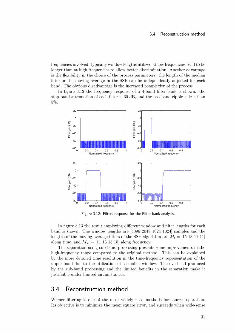
frequencies involved; typically window lengths utilized at low frequencies tend to belonger than at high frequencies to allow better discrimination. Another advantageis the flexibility in the choice of the process parameters: the length of the medianfilter or the moving average in the SSE can be independently adjusted for eachband. The obvious disadvantage is the increased complexity of the process.
In figure 3.12 the frequency response of a 4-band filter-bank is shown: thestop-band attenuation of each filter is 60 dB, and the passband ripple is less than5%.
0 0.2 0.4 0.6 0.8 1−80
−60
−40
−20
0
20
Normalized frequency
Filt
er
ga
in (
dB
)
0 0.2 0.4 0.6 0.8 1−80
−60
−40
−20
0
20
Normalized frequency
Filt
er
ga
in (
dB
)
0 0.2 0.4 0.6 0.8 1−80
−60
−40
−20
0
20
Normalized frequency
Filt
er
ga
in (
dB
)
0 0.2 0.4 0.6 0.8 1−80
−60
−40
−20
0
20
Normalized frequency
Filt
er
ga
in (
dB
)
Figure 3.12: Filters response for the Filter-bank analysis.
In figure 3.13 the result employing different window and filter lengths for eachband is shown. The window lengths are [4096 2048 1024 1024] samples and thelengths of the moving average filters of the SSE algorithm are Mt = [15 13 11 11]along time, and Mss = [11 13 15 15] along frequency.
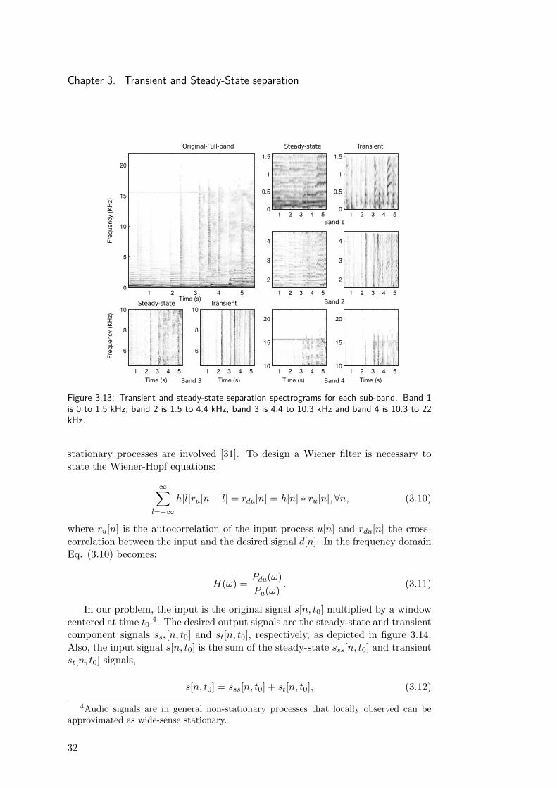
The separation using sub-band processing presents some improvements in thehigh-frequency range compared to the original method. This can be explainedby the more detailed time resolution in the time-frequency representation of theupper-band due to the utilization of a smaller window. The overhead producedby the sub-band processing and the limited benefits in the separation make itjustifiable under limited circumstances.
3.4 Reconstruction methodWiener filtering is one of the most widely used methods for source separation.Its objective is to minimize the mean square error, and succeeds when wide-sense
31
Chapter 3. Transient and Steady-State separation
Figure 3.13: Transient and steady-state separation spectrograms for each sub-band. Band 1is 0 to 1.5 kHz, band 2 is 1.5 to 4.4 kHz, band 3 is 4.4 to 10.3 kHz and band 4 is 10.3 to 22kHz.
stationary processes are involved [31]. To design a Wiener filter is necessary tostate the Wiener-Hopf equations:
∞∑l=−∞
h[l]ru[n− l] = rdu[n] = h[n] ∗ ru[n],∀n, (3.10)
where ru[n] is the autocorrelation of the input process u[n] and rdu[n] the cross-correlation between the input and the desired signal d[n]. In the frequency domainEq. (3.10) becomes:
H(ω) =Pdu(ω)
Pu(ω). (3.11)
In our problem, the input is the original signal s[n, t0] multiplied by a windowcentered at time t0
4. The desired output signals are the steady-state and transientcomponent signals sss[n, t0] and st[n, t0], respectively, as depicted in figure 3.14.Also, the input signal s[n, t0] is the sum of the steady-state sss[n, t0] and transientst[n, t0] signals,
s[n, t0] = sss[n, t0] + st[n, t0], (3.12)
4Audio signals are in general non-stationary processes that locally observed can beapproximated as wide-sense stationary.
32
3.4. Reconstruction method
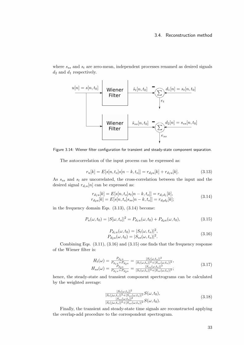
where sss and st are zero-mean, independent processes renamed as desired signalsd2 and d1 respectively.
Figure 3.14: Wiener filter configuration for transient and steady-state component separation.
The autocorrelation of the input process can be expressed as:
ru[k] = E[s[n, to]s[n− k, to]] = rd2u[k] + rd1u[k]. (3.13)
As sss and st are uncorrelated, the cross-correlation between the input and thedesired signal rdiu[n] can be expressed as:
rd1u[k] = E[s[n, to]st[n− k, to]] = rd1d1 [k],rd2u[k] = E[s[n, to]sss[n− k, to]] = rd2d2 [k];
(3.14)
in the frequency domain Eqs. (3.13), (3.14) become:
Pu(ω, t0) = |S[ω, to]|2 = Pd1u(ω, t0) + Pd2u(ω, t0), (3.15)
Pd1u(ω, t0) = |St(ω, to)|2,Pd2u(ω, t0) = |Sss(ω, to)|2.
(3.16)
Combining Eqs. (3.11), (3.16) and (3.15) one finds that the frequency responseof the Wiener filter is:
Ht(ω) =Pd1u
Pd1u+Pd2u= |St(ω,to)|2|St(ω,to)|2+|Sss(ω,to)|2 ,
Hss(ω) =Pd2u
Pd1u+Pd2u= |Sss(ω,to)|2|St(ω,to)|2+|Sss(ω,to)|2 ;
(3.17)
hence, the steady-state and transient component spectrograms can be calculatedby the weighted average:
|St(ω,to]|2|St(jω,to)|2+|Sss(ω,to)|2S(ω, t0),
|Sss(ω,to]|2|St(jω,to)|2+|Sss(ω,to)|2S(ω, t0).
(3.18)
Finally, the transient and steady-state time signals are reconstructed applyingthe overlap-add procedure to the correspondent spectrogram.
33

Chapter 3. Transient and Steady-State separation
34
Chapter 4
Tests & Applications
Chapter 4. Tests & Applications
This chapter is divided in two sections. In the first section, a comparison ofthe SSE and the Median filters as the non-linear filtering stage for the transient/ steady-state separation algorithm is performed. The second section describesdifferent applications and examples of audio editing that benefit from the decom-position in transient and steady-state components.
4.1 SSE and Median filter comparisonThe performance of the transient and steady-state separation algorithm is evalu-ated comparing the influence of the filtering stage when using the median and theSSE filter. Two different types of experiment are considered:
1. Systematic listening tests are conducted to compare the original and pro-posed methods as to their separation performances;
2. An application-based evaluation is carried out considering the beat-trackingand the pitch-tracking problems.
The listening tests and the application to the beat-tracking problem wherepresented at the “Congreso Internacional de Ciencia y Tecnologıa Musical CICTeM- 2013” [36]. For each type of experiment a different audio data set is used, bothdescribed in the following section.
4.1.1 Data set descriptionThree data sets were used in these tests, one for the subjective listening test andtwo others for the application-based evaluation. The audio files are mono and havea sampling rate of 44.1 kHz and 16-bit resolution.
The data set for the subjective listening tests consists of ten-seconds lengthexcerpts of thirteen pieces of North American popular music (rock, folk and blues)extracted from commercial records. It exhibits multiple combinations of transientand steady-state components in the sense of perceptual presence in the mix.
For the application-based evaluation, datasets from the Music Information Re-trieval Evaluation eXchange (MIREX) Contest [16, 15] were utilized. The MIREXis a community-based formal evaluation framework within the Music InformationRetrieval domain. To measure the performance of a beat-tracking algorithm theAudio Beat Tracking (MIREX 2006) data set was utilized. This data set is com-posed of twenty excerpts of western popular music of thirty-seconds duration. Thebeats of each recording have been annotated by 40 different listeners. For the per-formance of a pitch-tracking algorithm the Melody Extraction Contest (MIREX2004 and 2005) data sets [16] were utilized. The 2004 data set is composed oftwenty excerpts of western popular music of thirty-seconds duration and the 2005dataset is composed of thirteen excerpts with different durations (from 10 to 15 sec-onds). Each recording of the pitch-tracking datasets has a reference correspondingmelody frequency contour that was manually annotated.
36
4.1. SSE and Median filter comparison
4.1.2 TestsSubjective testIn order to measure the perceptual difference between utilizing the Median filterand utilizing the SSE filter, a set of formal subjective tests was designed and con-ducted following the recommendations suggested in [94]. Each participant shouldlisten and compare the separated steady-state and transient components producedby both non-linear filters.
For this purpose, a graphical user interface specifically designed to comply withthe requirements of this test was adapted from [71]; a screenshot of the interfaceis included in the annex BFor each song in the data set, the interface presents theoriginal signal as a reference together with the processed signals to be compared.The order of the compared signals is randomized to assure the blindness of thetest. The interface implements audio controls to play/stop any of the signals, andthe listener can also define loop points to allow an in-detail listening of certainparts of the audio.
Ten participants answered the next three questions for each transient andsteady-state output signal:* Q1: How much of the desired components has been properly separated?* Q2: How much of the undesired (residual) components has been left?* Q3: How would you rate the integrity (in the sense of naturalness) of the sepa-rated signal?
The questions were answered by controlling a slide bar that maps the responsesto values from 0 to 100. The complete individual results may be found in annexA. The answers presents a wide variation between participants making it difficultto be consistently compared. Then, the raw answers were thresholded to obtain abinary value. This value indicates which algorithm performs better or otherwiseif their results can be considered perceptually equivalent.
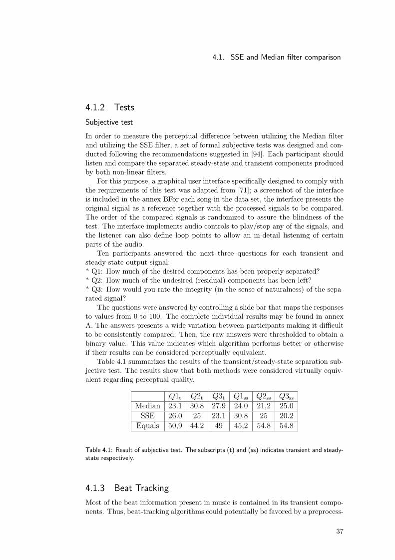
Table 4.1 summarizes the results of the transient/steady-state separation sub-jective test. The results show that both methods were considered virtually equiv-alent regarding perceptual quality.
Q1t Q2t Q3t Q1ss Q2ss Q3ss
Median 23.1 30.8 27.9 24.0 21,2 25.0SSE 26.0 25 23.1 30.8 25 20.2
Equals 50,9 44.2 49 45,2 54.8 54.8
Table 4.1: Result of subjective test. The subscripts (t) and (ss) indicates transient and steady-state respectively.
4.1.3 Beat TrackingMost of the beat information present in music is contained in its transient compo-nents. Thus, beat-tracking algorithms could potentially be favored by a preprocess-
37
Chapter 4. Tests & Applications
ing stage after which only transient components are left. Such hypothesis is testedby evaluating the performance of the state-of-the-art beat-tracking algorithm (pre-sented in [20]) on the 2006 MIREX audio beat-tracking test database [16].
Dynamic Programming based beat-tracking algorithm
The output of a beat-tracker is the sequence of time instants derived from the musicaudio signal that correspond to the instants in which a human listener would taphis foot. For the authors of the algorithm used in this work [20] the beat timesneed to satisfy two constraints: follow a regular rhythmic pattern, reflecting alocally constant inter-beat-interval; and correspond to a note onset played by oneof the instruments.
These constraints are expressed as two functions: the transition cost functionand a local onset strength.
The beats are then the set of time instants that minimize those cost functions.The best-scoring set of beats is found by Dynamic Programming, which decom-poses the entire problem (find the global optimum within a exponential-sized set)into simpler optimization problems at each step, finding the globally optimal beatsequence.
Performance evaluation
In order to perform an objective comparison of the beat-tracking algorithm withand without the preprocessing stage, the performance was evaluated with the BeatTracking Evaluation toolbox [14]. A brief description of each of the evaluationmethods implemented in the toolbox follows; for a complete survey, see [13, 12].
The F-measure is a generic performance measure in the information retrievalcontext. It is determined by the relation between the correctly estimated beats, thefalse positives and the false negatives. An estimated beat is considered correct if itfalls into a 70-ms wide tolerance window centered at each annotated beat. Cemgilet al [8] propose the utilization of a Gaussian error function to take into accountthe beats estimation accuracy . An error function is build centering a Gaussian ateach annotated beat. Then, the performance indicator is calculated as the sum ofthe values of the error function at the closest estimated beat of each annotation,normalized by the maximum between the number of annotations and the numberof estimated beats. In the PScore, the beat accuracy is determined by takingthe sum of the cross-correlation between two impulse trains, one representing theannotations and the other representing the extracted beats. Goto [26] proposesmeasuring the performance by evaluating the proportion of time in which the beatis correctly tracked. The classification of the beats as correctly tracked or notrelies on statistical properties of the difference to the annotated beats . CMLc,CMLt, AMLc, AMLt are continuity-based performance indicators computedover the correctly tracked regions. The CMLc and the CMLt are defined as theratio of the longest continuously tracked region or the total length of correctlytracked regions, respectively, to the total signal length. The AMLc and AMLtare defined in a similar way, but are more permissive in the definition of correctly
38
4.1. SSE and Median filter comparison
tracked beat, allowing off-beat estimation and beats at the double and half ofthe correct metrical level. To calculate the Information Gain, two timing errorhistograms are constructed, one between the annotated beats and the estimatedbeats and vice-versa. Then, the Information Gain is the minimum of the Kullback-Leibler divergence between the previously calculated histograms and an uniformlydistributed histogram.
In order to avoid unfair comparisons, we searched for the optimum performanceof each algorithm via a grid search over its respective parameters.
Results
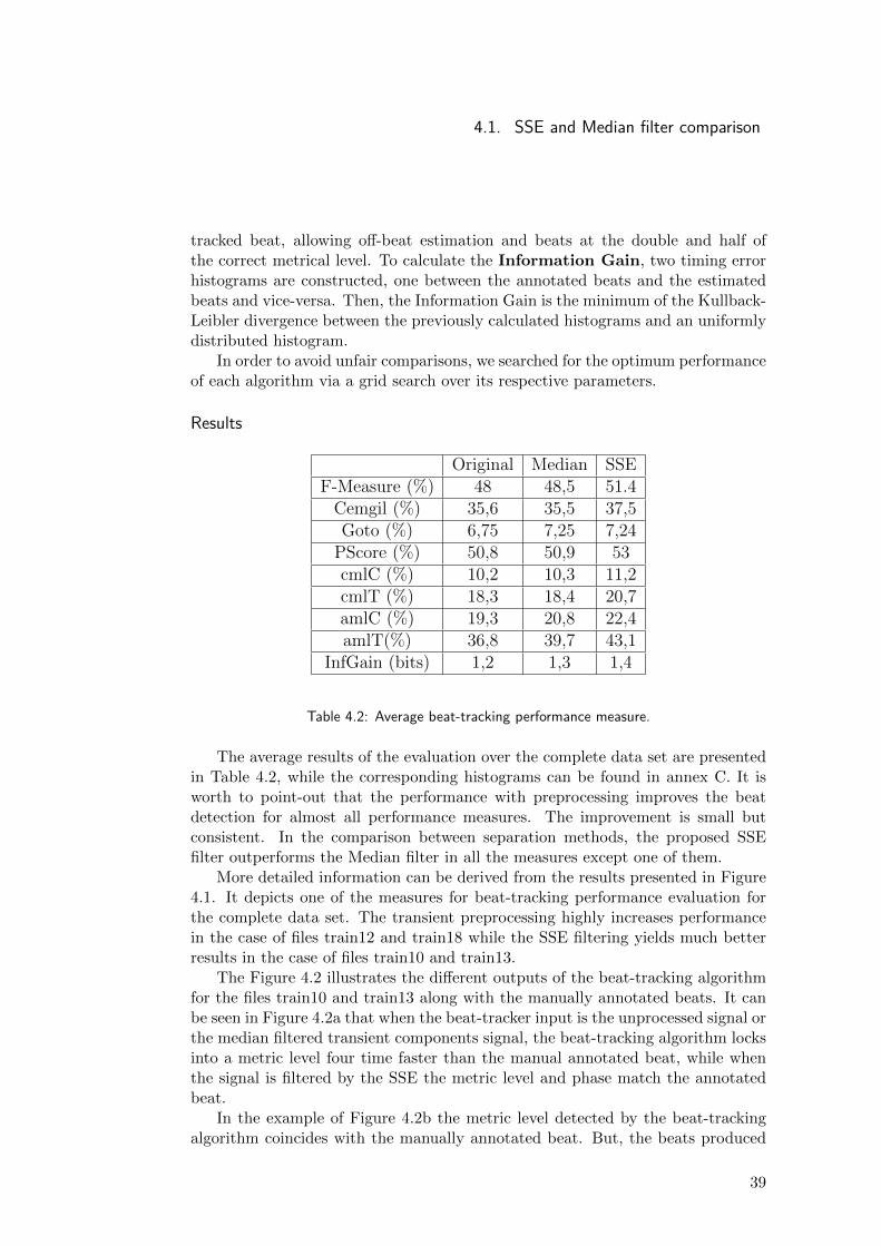
Original Median SSEF-Measure (%) 48 48,5 51.4
Cemgil (%) 35,6 35,5 37,5Goto (%) 6,75 7,25 7,24
PScore (%) 50,8 50,9 53cmlC (%) 10,2 10,3 11,2cmlT (%) 18,3 18,4 20,7amlC (%) 19,3 20,8 22,4amlT(%) 36,8 39,7 43,1
InfGain (bits) 1,2 1,3 1,4
Table 4.2: Average beat-tracking performance measure.
The average results of the evaluation over the complete data set are presentedin Table 4.2, while the corresponding histograms can be found in annex C. It isworth to point-out that the performance with preprocessing improves the beatdetection for almost all performance measures. The improvement is small butconsistent. In the comparison between separation methods, the proposed SSEfilter outperforms the Median filter in all the measures except one of them.
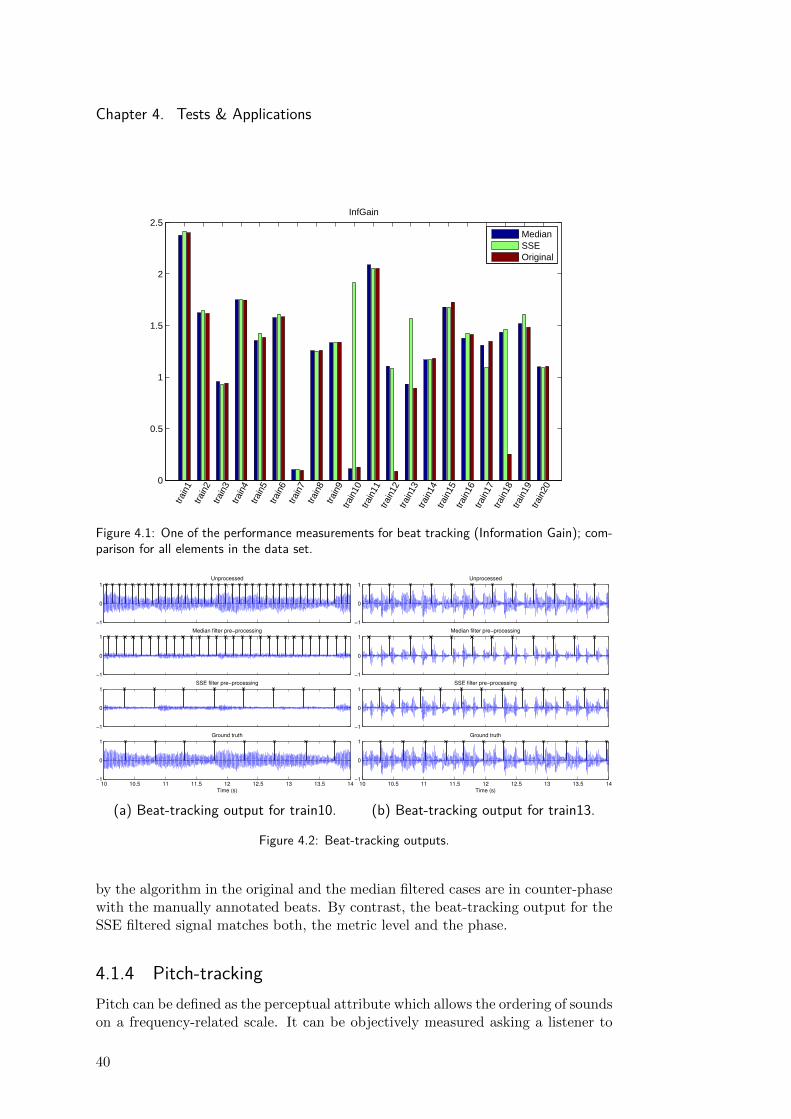
More detailed information can be derived from the results presented in Figure4.1. It depicts one of the measures for beat-tracking performance evaluation forthe complete data set. The transient preprocessing highly increases performancein the case of files train12 and train18 while the SSE filtering yields much betterresults in the case of files train10 and train13.
The Figure 4.2 illustrates the different outputs of the beat-tracking algorithmfor the files train10 and train13 along with the manually annotated beats. It canbe seen in Figure 4.2a that when the beat-tracker input is the unprocessed signal orthe median filtered transient components signal, the beat-tracking algorithm locksinto a metric level four time faster than the manual annotated beat, while whenthe signal is filtered by the SSE the metric level and phase match the annotatedbeat.
In the example of Figure 4.2b the metric level detected by the beat-trackingalgorithm coincides with the manually annotated beat. But, the beats produced
39
Chapter 4. Tests & Applications
0
0.5
1
1.5
2
2.5InfGain
train
1tra
in2
train
3tra
in4
train
5tra
in6
train
7tra
in8
train
9tra
in10
train
11tra
in12
train
13tra
in14
train
15tra
in16
train
17tra
in18
train
19tra
in20
MedianSSEOriginal
Figure 4.1: One of the performance measurements for beat tracking (Information Gain); com-parison for all elements in the data set.
−1
0
1Unprocessed
−1
0
1Median filter pre−processing
−1
0
1SSE filter pre−processing
10 10.5 11 11.5 12 12.5 13 13.5 14−1
0
1Ground truth
Time (s)
(a) Beat-tracking output for train10.
−1
0
1Unprocessed
−1
0
1Median filter pre−processing
−1
0
1SSE filter pre−processing
10 10.5 11 11.5 12 12.5 13 13.5 14−1
0
1Ground truth
Time (s)
(b) Beat-tracking output for train13.
Figure 4.2: Beat-tracking outputs.
by the algorithm in the original and the median filtered cases are in counter-phasewith the manually annotated beats. By contrast, the beat-tracking output for theSSE filtered signal matches both, the metric level and the phase.
4.1.4 Pitch-trackingPitch can be defined as the perceptual attribute which allows the ordering of soundson a frequency-related scale. It can be objectively measured asking a listener to
40
4.1. SSE and Median filter comparison
match the frequency of a sine wave with the tone of the target sound.
In [35] an Harmonic/Percussive separation algorithm (Harmonic PercussiveSound Separation - HPSS) is utilized as the first stage in a singing pitch extractionalgorithm, and good results are reported. The HPSS algorithm presented in [59]is also utilized in [77] to estimate the melodic line.
The “tonal” information can be assumed to be carried by the steady-state com-ponents of a signal. Analogously the performance improvement of beat-trackingalgorithms when tonal information is discarded, a pitch-tracking algorithm canbe favoured by the elimination of the transient components. We evaluate the ad-vantage of pre-processing a signal to eliminate the transient components beforeperforming the pitch-tracking, and compare the median filter to the proposed SSEfilter.
A state-of-the-art pitch-tracking algorithm presented in [69] was utilized. Thisalgorithm has been developed as a VAMP plug-in for the semantic visualizationsoftware Sonic Visualizer [7]. A brief description of the algorithm follows.
Pitch-tracking algorithm
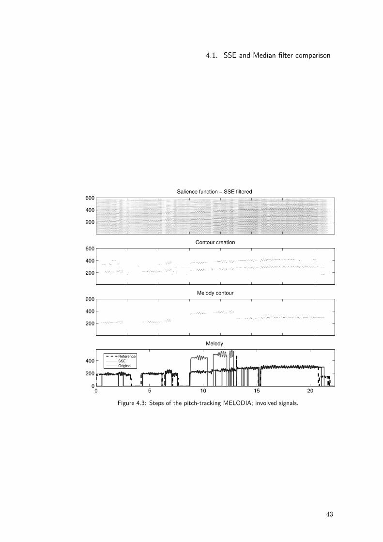
The MELODIA plug-in extracts the principal melody and respective F0 contourof polyphonic audio. The method is comprised of four main blocks:
The Sinusoid Extraction stage begins with an equal loudness filter to mimic thehuman auditory system sensitivity. It enhances the mid frequencies and attenuateslow frequencies. Then, the STFT of the result is computed with window lengthM = 2048, FFT length N = 8192 and hop size H = 128. Then, the estimation ofspectral peak frequencies is improved by a phase-vocoder based technique [40].
The previously calculated peaks are employed to compute the salience functionin the range from 55 Hz to 1760 Hz. For a given frequency, the salience functionis defined as a weighted sum of its harmonics’ energies.
For each frame of the salience function, the peaks are selected as potential F0candidates. Then the peaks are grouped into continuous pitch contours. Eachcontour has a limited time span and corresponds to a short phrase. Firstly, thepeaks are filtered by hard thresholding. Later, this peaks are grouped into contoursusing heuristics and auditory analysis cues.
A set of contour characteristics are calculated from the previously generatedcontours to determine which ones belong to the melody. The characteristics are:pitch mean, pitch deviation, contour mean salience, contour salience deviation,length and vibrato presence. Those contour characteristics are then utilized tofilter out the non melodic contours. Finally, the F0 melodic contour is selectedfrom the remaining contours.
Performance measures
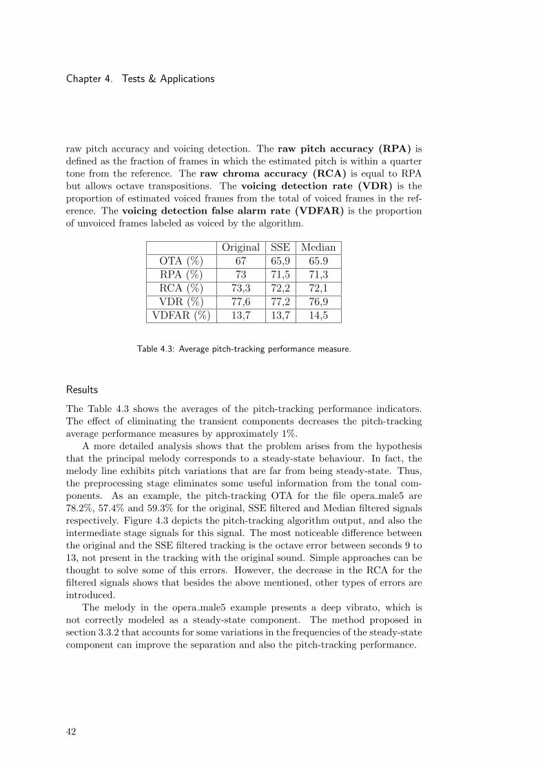
The evaluation metrics adopted are the ones used in the MIREX 2005 melodytranscription task, which are reviewed and described in [61]. The overall tran-scription accuracy (OTA) combines the pitch transcription and the voicingdetection task. It is defined as the proportion of frames correctly labelled with
41
Chapter 4. Tests & Applications
raw pitch accuracy and voicing detection. The raw pitch accuracy (RPA) isdefined as the fraction of frames in which the estimated pitch is within a quartertone from the reference. The raw chroma accuracy (RCA) is equal to RPAbut allows octave transpositions. The voicing detection rate (VDR) is theproportion of estimated voiced frames from the total of voiced frames in the ref-erence. The voicing detection false alarm rate (VDFAR) is the proportionof unvoiced frames labeled as voiced by the algorithm.
Original SSE MedianOTA (%) 67 65,9 65.9RPA (%) 73 71,5 71,3RCA (%) 73,3 72,2 72,1VDR (%) 77,6 77,2 76,9
VDFAR (%) 13,7 13,7 14,5
Table 4.3: Average pitch-tracking performance measure.
ResultsThe Table 4.3 shows the averages of the pitch-tracking performance indicators.The effect of eliminating the transient components decreases the pitch-trackingaverage performance measures by approximately 1%.
A more detailed analysis shows that the problem arises from the hypothesisthat the principal melody corresponds to a steady-state behaviour. In fact, themelody line exhibits pitch variations that are far from being steady-state. Thus,the preprocessing stage eliminates some useful information from the tonal com-ponents. As an example, the pitch-tracking OTA for the file opera male5 are78.2%, 57.4% and 59.3% for the original, SSE filtered and Median filtered signalsrespectively. Figure 4.3 depicts the pitch-tracking algorithm output, and also theintermediate stage signals for this signal. The most noticeable difference betweenthe original and the SSE filtered tracking is the octave error between seconds 9 to13, not present in the tracking with the original sound. Simple approaches can bethought to solve some of this errors. However, the decrease in the RCA for thefiltered signals shows that besides the above mentioned, other types of errors areintroduced.
The melody in the opera male5 example presents a deep vibrato, which isnot correctly modeled as a steady-state component. The method proposed insection 3.3.2 that accounts for some variations in the frequencies of the steady-statecomponent can improve the separation and also the pitch-tracking performance.
42
4.1. SSE and Median filter comparison
Figure 4.3: Steps of the pitch-tracking MELODIA; involved signals.
43
Chapter 4. Tests & Applications
4.2 Applications in audio editingThe transient and steady-state decomposition can be helpful in audio editing tasks.In the following sections some audio editing applications are described.
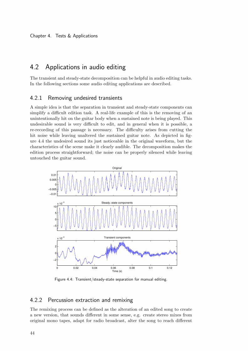
4.2.1 Removing undesired transientsA simple idea is that the separation in transient and steady-state components cansimplify a difficult edition task. A real-life example of this is the removing of anunintentionally hit on the guitar body when a sustained note is being played. Thisundesirable sound is very difficult to edit, and in general when it is possible, are-recording of this passage is necessary. The difficulty arises from cutting thehit noise while leaving unaltered the sustained guitar note. As depicted in fig-ure 4.4 the undesired sound its just noticeable in the original waveform, but thecharacteristics of the scene make it clearly audible. The decomposition makes theedition process straightforward; the noise can be properly silenced while leavinguntouched the guitar sound.
−0.01
−0.005
0
0.005
0.01
Original
−5
0
5
10x 10
−3 Steady−state components
0 0.02 0.04 0.06 0.08 0.1 0.12
−2
0
2
x 10−3 Transient components
Time (s)
Figure 4.4: Transient/steady-state separation for manual editing.
4.2.2 Percussion extraction and remixingThe remixing process can be defined as the alteration of an edited song to createa new version, that sounds different in some sense, e.g. create stereo mixes fromoriginal mono tapes, adapt for radio broadcast, alter the song to reach different
44
4.2. Applications in audio editing
−0.2
−0.1
0
0.1
0.2Original signal
−0.2
−0.1
0
0.1
0.2Steady−state component signal
0 0.1 0.2 0.3 0.4 0.5 0.6−0.2
−0.1
0
0.1
0.2Transient comopent signal
time (s)
(a) Transient and steady-state separation.
−0.4
−0.2
0
0.2
0.4Original signal
0 0.5 1 1.5 2 2.5 3 3.5 4 4.5 5−0.4
−0.2
0
0.2
0.46−dB gain for percussive sources
time (s)
(b) Transient component with 6dB gain.
Figure 4.5: Remixing application.
audiences, etc. Ideally, the raw material for remixing are the original multi-trackrecords. Often, this records are non-available or do not even exist, as in the caseof the recordings of the first half of the twentieth century. In some other cases, thenumber of tracks are very limited, for example, the first two Beatles’ albums wererecorded with two-track machines, since the eight-track recorders were introducedonly in 1968 [46].
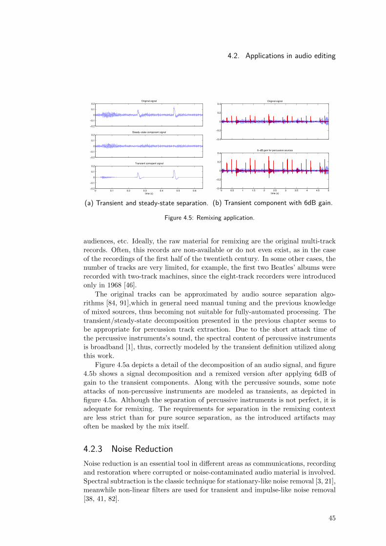
The original tracks can be approximated by audio source separation algo-rithms [84, 91],which in general need manual tuning and the previous knowledgeof mixed sources, thus becoming not suitable for fully-automated processing. Thetransient/steady-state decomposition presented in the previous chapter seems tobe appropriate for percussion track extraction. Due to the short attack time ofthe percussive instruments’s sound, the spectral content of percussive instrumentsis broadband [1], thus, correctly modeled by the transient definition utilized alongthis work.
Figure 4.5a depicts a detail of the decomposition of an audio signal, and figure4.5b shows a signal decomposition and a remixed version after applying 6dB ofgain to the transient components. Along with the percussive sounds, some noteattacks of non-percussive instruments are modeled as transients, as depicted infigure 4.5a. Although the separation of percussive instruments is not perfect, it isadequate for remixing. The requirements for separation in the remixing contextare less strict than for pure source separation, as the introduced artifacts mayoften be masked by the mix itself.
4.2.3 Noise ReductionNoise reduction is an essential tool in different areas as communications, recordingand restoration where corrupted or noise-contaminated audio material is involved.Spectral subtraction is the classic technique for stationary-like noise removal [3, 21],meanwhile non-linear filters are used for transient and impulse-like noise removal[38, 41, 82].
45
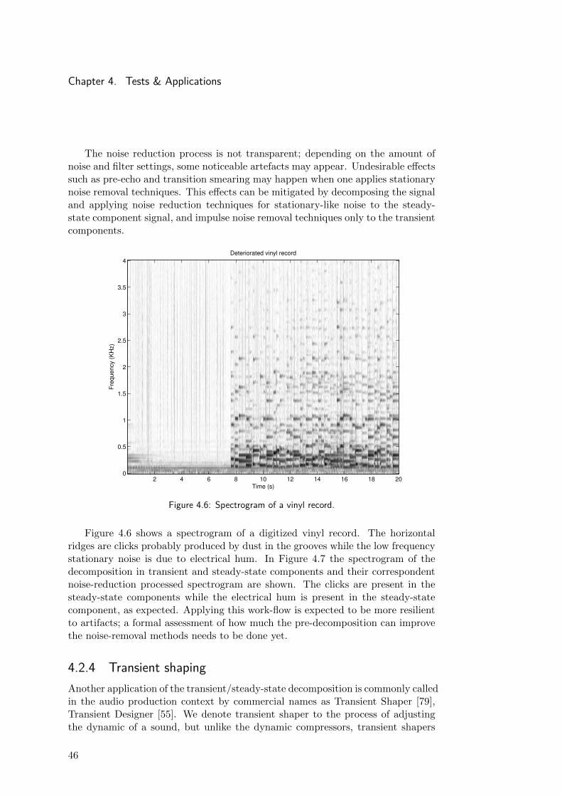
Chapter 4. Tests & Applications
The noise reduction process is not transparent; depending on the amount ofnoise and filter settings, some noticeable artefacts may appear. Undesirable effectssuch as pre-echo and transition smearing may happen when one applies stationarynoise removal techniques. This effects can be mitigated by decomposing the signaland applying noise reduction techniques for stationary-like noise to the steady-state component signal, and impulse noise removal techniques only to the transientcomponents.
Deteriorated vinyl record
Time (s)
Fre
quency (
KH
z)
2 4 6 8 10 12 14 16 18 200
0.5
1
1.5
2
2.5
3
3.5
4
Figure 4.6: Spectrogram of a vinyl record.
Figure 4.6 shows a spectrogram of a digitized vinyl record. The horizontalridges are clicks probably produced by dust in the grooves while the low frequencystationary noise is due to electrical hum. In Figure 4.7 the spectrogram of thedecomposition in transient and steady-state components and their correspondentnoise-reduction processed spectrogram are shown. The clicks are present in thesteady-state components while the electrical hum is present in the steady-statecomponent, as expected. Applying this work-flow is expected to be more resilientto artifacts; a formal assessment of how much the pre-decomposition can improvethe noise-removal methods needs to be done yet.
4.2.4 Transient shapingAnother application of the transient/steady-state decomposition is commonly calledin the audio production context by commercial names as Transient Shaper [79],Transient Designer [55]. We denote transient shaper to the process of adjustingthe dynamic of a sound, but unlike the dynamic compressors, transient shapers
46
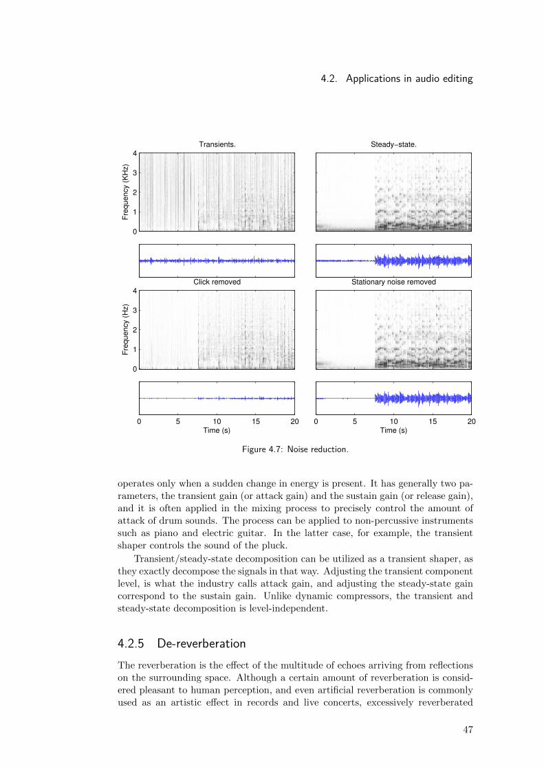
4.2. Applications in audio editing
Fre
qu
en
cy (
KH
z)
Transients.
0
1
2
3
4
Steady−state.
Fre
qu
en
cy (
Hz)
Click removed
0
1
2
3
4
Stationary noise removed
0 5 10 15 20Time (s)
0 5 10 15 20Time (s)
Figure 4.7: Noise reduction.
operates only when a sudden change in energy is present. It has generally two pa-rameters, the transient gain (or attack gain) and the sustain gain (or release gain),and it is often applied in the mixing process to precisely control the amount ofattack of drum sounds. The process can be applied to non-percussive instrumentssuch as piano and electric guitar. In the latter case, for example, the transientshaper controls the sound of the pluck.
Transient/steady-state decomposition can be utilized as a transient shaper, asthey exactly decompose the signals in that way. Adjusting the transient componentlevel, is what the industry calls attack gain, and adjusting the steady-state gaincorrespond to the sustain gain. Unlike dynamic compressors, the transient andsteady-state decomposition is level-independent.
4.2.5 De-reverberationThe reverberation is the effect of the multitude of echoes arriving from reflectionson the surrounding space. Although a certain amount of reverberation is consid-ered pleasant to human perception, and even artificial reverberation is commonlyused as an artistic effect in records and live concerts, excessively reverberated
47
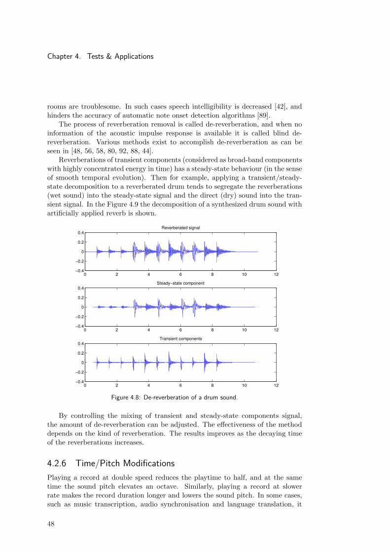
Chapter 4. Tests & Applications
rooms are troublesome. In such cases speech intelligibility is decreased [42], andhinders the accuracy of automatic note onset detection algorithms [89].
The process of reverberation removal is called de-reverberation, and when noinformation of the acoustic impulse response is available it is called blind de-reverberation. Various methods exist to accomplish de-reverberation as can beseen in [48, 56, 58, 80, 92, 88, 44].
Reverberations of transient components (considered as broad-band componentswith highly concentrated energy in time) has a steady-state behaviour (in the senseof smooth temporal evolution). Then for example, applying a transient/steady-state decomposition to a reverberated drum tends to segregate the reverberations(wet sound) into the steady-state signal and the direct (dry) sound into the tran-sient signal. In the Figure 4.9 the decomposition of a synthesized drum sound withartificially applied reverb is shown.
0 2 4 6 8 10 12−0.4
−0.2
0
0.2
0.4Reverberated signal
0 2 4 6 8 10 12−0.4
−0.2
0
0.2
0.4Steady−state component
0 2 4 6 8 10 12−0.4
−0.2
0
0.2
0.4Transient components
Figure 4.8: De-reverberation of a drum sound.
By controlling the mixing of transient and steady-state components signal,the amount of de-reverberation can be adjusted. The effectiveness of the methoddepends on the kind of reverberation. The results improves as the decaying timeof the reverberations increases.
4.2.6 Time/Pitch ModificationsPlaying a record at double speed reduces the playtime to half, and at the sametime the sound pitch elevates an octave. Similarly, playing a record at slowerrate makes the record duration longer and lowers the sound pitch. In some cases,such as music transcription, audio synchronisation and language translation, it
48
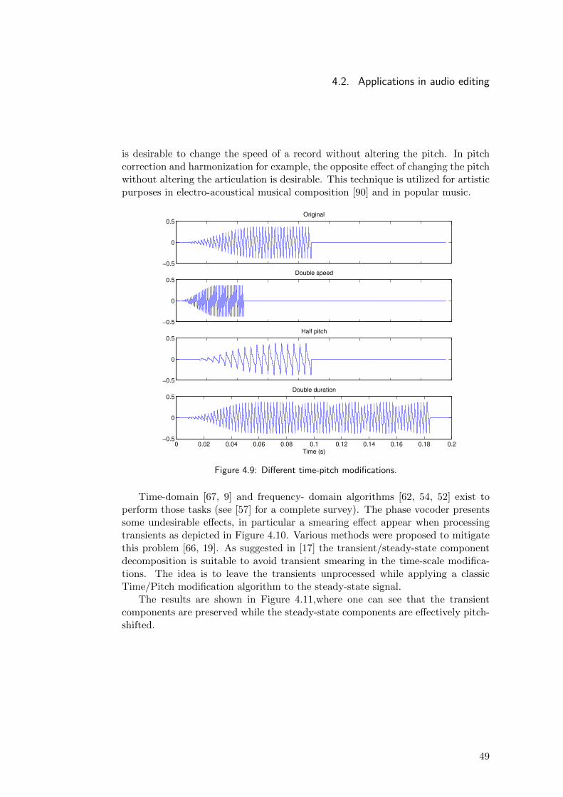
4.2. Applications in audio editing
is desirable to change the speed of a record without altering the pitch. In pitchcorrection and harmonization for example, the opposite effect of changing the pitchwithout altering the articulation is desirable. This technique is utilized for artisticpurposes in electro-acoustical musical composition [90] and in popular music.
−0.5
0
0.5Original
−0.5
0
0.5Double speed
−0.5
0
0.5Half pitch
0 0.02 0.04 0.06 0.08 0.1 0.12 0.14 0.16 0.18 0.2−0.5
0
0.5Double duration
Time (s)
Figure 4.9: Different time-pitch modifications.
Time-domain [67, 9] and frequency- domain algorithms [62, 54, 52] exist toperform those tasks (see [57] for a complete survey). The phase vocoder presentssome undesirable effects, in particular a smearing effect appear when processingtransients as depicted in Figure 4.10. Various methods were proposed to mitigatethis problem [66, 19]. As suggested in [17] the transient/steady-state componentdecomposition is suitable to avoid transient smearing in the time-scale modifica-tions. The idea is to leave the transients unprocessed while applying a classicTime/Pitch modification algorithm to the steady-state signal.
The results are shown in Figure 4.11,where one can see that the transientcomponents are preserved while the steady-state components are effectively pitch-shifted.
49
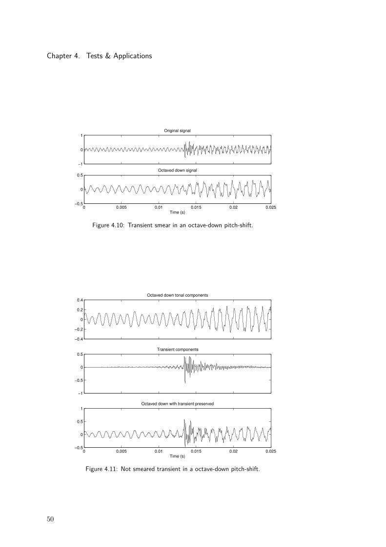
Chapter 4. Tests & Applications
−1
0
1Original signal
0 0.005 0.01 0.015 0.02 0.025−0.5
0
0.5
Time (s)
Octaved down signal
Figure 4.10: Transient smear in an octave-down pitch-shift.
−0.4
−0.2
0
0.2
0.4Octaved down tonal components
−1
−0.5
0
0.5Transient components
0 0.005 0.01 0.015 0.02 0.025−0.5
0
0.5
1Octaved down with transient preserved
Time (s)
Figure 4.11: Not smeared transient in a octave-down pitch-shift.
50

Chapter 5
Conclusions and future work
Chapter 5. Conclusions and future work
5.1 ConclusionsIn the preceding chapters, the transient/steady-state component separation prob-lem was studied. In particular, a recently proposed method for separating transientand steady-state components based on the median filter [23] was investigated. Fora best understanding of the processes involved, a modification of the filtering stageof the algorithm was proposed. The modification consisted in utilizing a non-linearfilter, originally devised to perform Stochastic Spectrum Estimation (SSE) [43], asthe filtering stage instead of the median filter.
To evaluate the perceptual quality of the decomposition, subjective listeningtests were designed and conducted. These tests allowed a perceptual comparisonbetween the original and the proposed filtering stage. The results indicated thatthere are no significant perceptual differences among them, both providing thesame quality of separation.
Besides, an application-based comparison was performed by applying the tran-sient and steady-state decomposition as a pre-processing stage for two Music In-formation Retrieval problems, namely the pitch-tracking and beat-tracking tasks.The hypothesis that the transient components carry the beat information whilethe steady-state components carry the pitch information was tested. The evalu-ation showed that the beat-tracking can benefit from the transient componentsextraction, notably increasing the performance in some cases. On the other hand,the pitch-tracking algorithm did not improved its performance by applying thepreprocessing. This seems to indicate that the partials of the melody line are notproperly captured as steady-state components, due to its frequency fluctuations.Part of this work was presented in a conference paper [36].
To overcome some of the model limitations that were identified, three exten-sions were delineated. First, an iterative filtering scheme was proposed, whichimplicitly defines the residual components as non-steady-state and non-transientcomponents. In other proposed extension, the definition of steady-state compo-nents was relaxed to allow for slow variations in partials’ evolution. This effect istypical of, but not limited to, free intonation instruments. Finally, to allow moreflexibility in the choice of the parameters of the algorithm, a sub-band processingtechnique was proposed. For each band, the window length, the hop size and thelength of the non-linear filters can be adjusted for a fine-tuning of the separation.
Another part of this work was to study possible applications of the decom-position into transient/steady-state components in the area of audio editing andprocessing. Six applications were surveyed and illustrated with real audio exam-ples. With this technique a very complex editing task such as the removal ofundesired transients in presence of steady-state sounds can be done in a simpleway. The transient/steady-state separation can also be used as a preprocess-ing stage to increase the performance of some audio processing techniques. Forinstance, it allows the application of specific noise-reduction algorithms to eachof the obtained components, such as stationary noise-removal techniques on thesteady-state signal, and impulse-like noise removal techniques on the transientsignal. Since each noise-reduction technique is applied to a signal which mainly
52
5.2. Future perspectives
contains the type of component for which it was devised, the number of undesiredartifacts is reduced. Analogously, the transient smearing effect that appears whentime/pitch modifications are applied can be avoided by modifying only the steady-state components while leaving the transients unchanged. In the other cases, bycontrolling the amount of transient and steady-state components in a mixture,different audio editing applications can be implemented. This was illustrated bysome examples, namely de-reverberation of percussive sound, transient shapingand percussive sound extraction for remixing.
5.2 Future perspectivesAll along this work, various topics that deserve further investigation were identifiedat different levels.
Although the STFT was the TF representation used in this work, it has somedrawbacks, such as constant time-frequency resolution. Therefore, other type ofrepresentation may be more suitable depending on the type of signal. For example,adaptive representations such as Fan Chirp Transform [6] seem to be useful whenharmonic signals with pitch fluctuations are involved.
On the other hand, the original definition of steady-state component provedto be too restrictive in some cases. An extension of the model was proposed inthis work to take into account pitch fluctuations commonly present in music signalsuch as the ones produced by glissando and vibrato. Its validity was illustratedby synthetic examples as a proof of concept, but further investigation is necessary.In future work, a systematic evaluation of the extensions proposed in Section 3.3will be conducted.
More audio processing applications for the transient/steady-state decomposi-tion could be developed. For example, lossy audio coding of transients tends togenerate undesired pre-echo effects that can be minimized by applying differentcoding schemes to the transient and the steady-state components [93, 87]. Further-more, it will be interesting to develop a real-time implementation of the algorithmsuitable for live performances. The algorithm latency in the current implementa-tion is in the order of 100 ms, which is not suitable for real-time. A low-latencycausal version of the algorithm will be developed in future work.
Finally, further developments of the present technique in collaboration withprofessional musicians will be encouraged. To do that, it is necessary to build user-friendly applications within popular frameworks such as Pure Data [64], SteinbergVirtual Studio Technologies [78] or LADSPA [25]. Musicians can contribute byfinely evaluating the quality of the separation and also by proposing novel appli-cations.
53
Chapter 5. Conclusions and future work
54
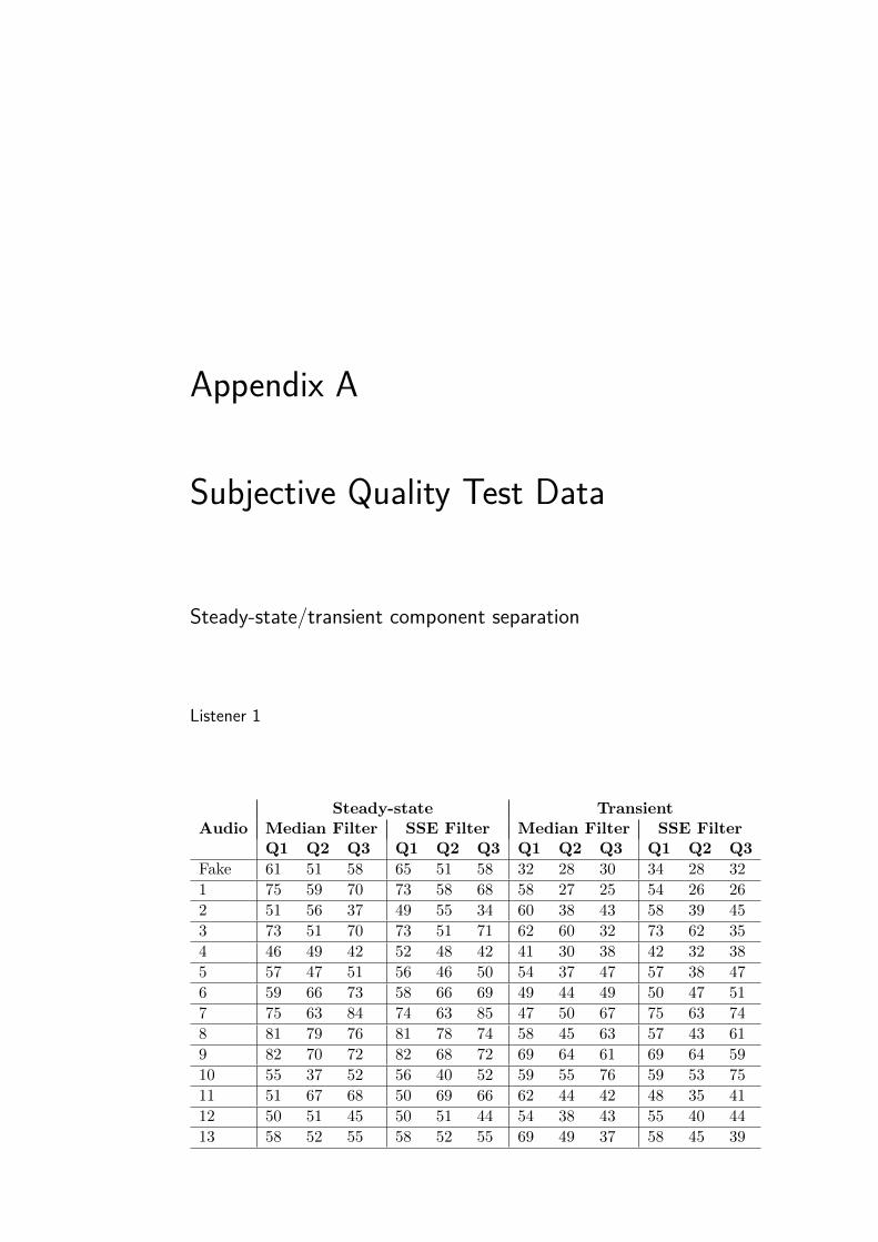
Appendix A
Subjective Quality Test Data
Steady-state/transient component separation
Listener 1
AudioSteady-state Transient
Median Filter SSE Filter Median Filter SSE FilterQ1 Q2 Q3 Q1 Q2 Q3 Q1 Q2 Q3 Q1 Q2 Q3
Fake 61 51 58 65 51 58 32 28 30 34 28 32
1 75 59 70 73 58 68 58 27 25 54 26 26
2 51 56 37 49 55 34 60 38 43 58 39 45
3 73 51 70 73 51 71 62 60 32 73 62 35
4 46 49 42 52 48 42 41 30 38 42 32 38
5 57 47 51 56 46 50 54 37 47 57 38 47
6 59 66 73 58 66 69 49 44 49 50 47 51
7 75 63 84 74 63 85 47 50 67 75 63 74
8 81 79 76 81 78 74 58 45 63 57 43 61
9 82 70 72 82 68 72 69 64 61 69 64 59
10 55 37 52 56 40 52 59 55 76 59 53 75
11 51 67 68 50 69 66 62 44 42 48 35 41
12 50 51 45 50 51 44 54 38 43 55 40 44
13 58 52 55 58 52 55 69 49 37 58 45 39
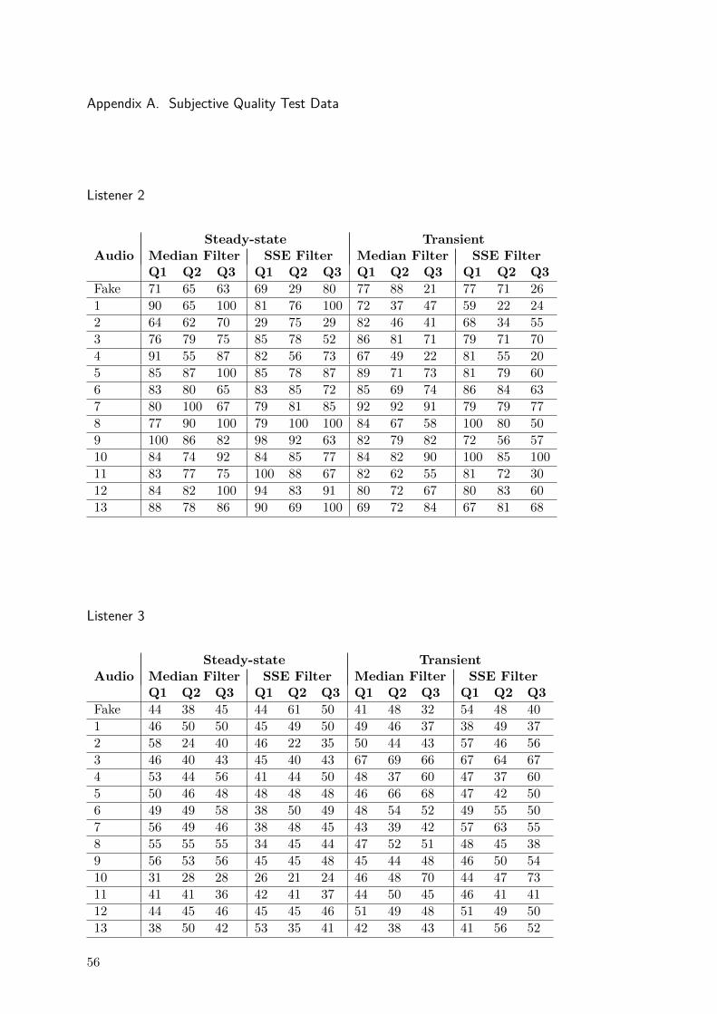
Appendix A. Subjective Quality Test Data
Listener 2
AudioSteady-state Transient
Median Filter SSE Filter Median Filter SSE FilterQ1 Q2 Q3 Q1 Q2 Q3 Q1 Q2 Q3 Q1 Q2 Q3
Fake 71 65 63 69 29 80 77 88 21 77 71 26
1 90 65 100 81 76 100 72 37 47 59 22 24
2 64 62 70 29 75 29 82 46 41 68 34 55
3 76 79 75 85 78 52 86 81 71 79 71 70
4 91 55 87 82 56 73 67 49 22 81 55 20
5 85 87 100 85 78 87 89 71 73 81 79 60
6 83 80 65 83 85 72 85 69 74 86 84 63
7 80 100 67 79 81 85 92 92 91 79 79 77
8 77 90 100 79 100 100 84 67 58 100 80 50
9 100 86 82 98 92 63 82 79 82 72 56 57
10 84 74 92 84 85 77 84 82 90 100 85 100
11 83 77 75 100 88 67 82 62 55 81 72 30
12 84 82 100 94 83 91 80 72 67 80 83 60
13 88 78 86 90 69 100 69 72 84 67 81 68
Listener 3
AudioSteady-state Transient
Median Filter SSE Filter Median Filter SSE FilterQ1 Q2 Q3 Q1 Q2 Q3 Q1 Q2 Q3 Q1 Q2 Q3
Fake 44 38 45 44 61 50 41 48 32 54 48 40
1 46 50 50 45 49 50 49 46 37 38 49 37
2 58 24 40 46 22 35 50 44 43 57 46 56
3 46 40 43 45 40 43 67 69 66 67 64 67
4 53 44 56 41 44 50 48 37 60 47 37 60
5 50 46 48 48 48 48 46 66 68 47 42 50
6 49 49 58 38 50 49 48 54 52 49 55 50
7 56 49 46 38 48 45 43 39 42 57 63 55
8 55 55 55 34 45 44 47 52 51 48 45 38
9 56 53 56 45 45 48 45 44 48 46 50 54
10 31 28 28 26 21 24 46 48 70 44 47 73
11 41 41 36 42 41 37 44 50 45 46 41 41
12 44 45 46 45 45 46 51 49 48 51 49 50
13 38 50 42 53 35 41 42 38 43 41 56 52
56
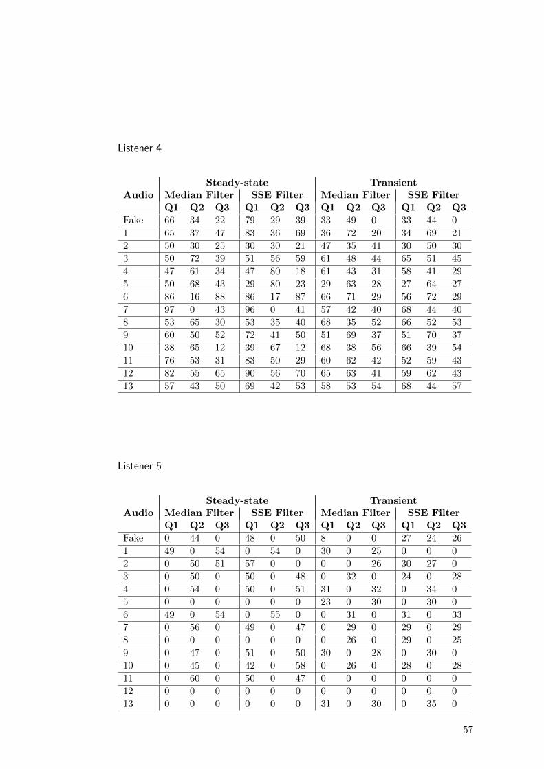
Listener 4
AudioSteady-state Transient
Median Filter SSE Filter Median Filter SSE FilterQ1 Q2 Q3 Q1 Q2 Q3 Q1 Q2 Q3 Q1 Q2 Q3
Fake 66 34 22 79 29 39 33 49 0 33 44 0
1 65 37 47 83 36 69 36 72 20 34 69 21
2 50 30 25 30 30 21 47 35 41 30 50 30
3 50 72 39 51 56 59 61 48 44 65 51 45
4 47 61 34 47 80 18 61 43 31 58 41 29
5 50 68 43 29 80 23 29 63 28 27 64 27
6 86 16 88 86 17 87 66 71 29 56 72 29
7 97 0 43 96 0 41 57 42 40 68 44 40
8 53 65 30 53 35 40 68 35 52 66 52 53
9 60 50 52 72 41 50 51 69 37 51 70 37
10 38 65 12 39 67 12 68 38 56 66 39 54
11 76 53 31 83 50 29 60 62 42 52 59 43
12 82 55 65 90 56 70 65 63 41 59 62 43
13 57 43 50 69 42 53 58 53 54 68 44 57
Listener 5
AudioSteady-state Transient
Median Filter SSE Filter Median Filter SSE FilterQ1 Q2 Q3 Q1 Q2 Q3 Q1 Q2 Q3 Q1 Q2 Q3
Fake 0 44 0 48 0 50 8 0 0 27 24 26
1 49 0 54 0 54 0 30 0 25 0 0 0
2 0 50 51 57 0 0 0 0 26 30 27 0
3 0 50 0 50 0 48 0 32 0 24 0 28
4 0 54 0 50 0 51 31 0 32 0 34 0
5 0 0 0 0 0 0 23 0 30 0 30 0
6 49 0 54 0 55 0 0 31 0 31 0 33
7 0 56 0 49 0 47 0 29 0 29 0 29
8 0 0 0 0 0 0 0 26 0 29 0 25
9 0 47 0 51 0 50 30 0 28 0 30 0
10 0 45 0 42 0 58 0 26 0 28 0 28
11 0 60 0 50 0 47 0 0 0 0 0 0
12 0 0 0 0 0 0 0 0 0 0 0 0
13 0 0 0 0 0 0 31 0 30 0 35 0
57
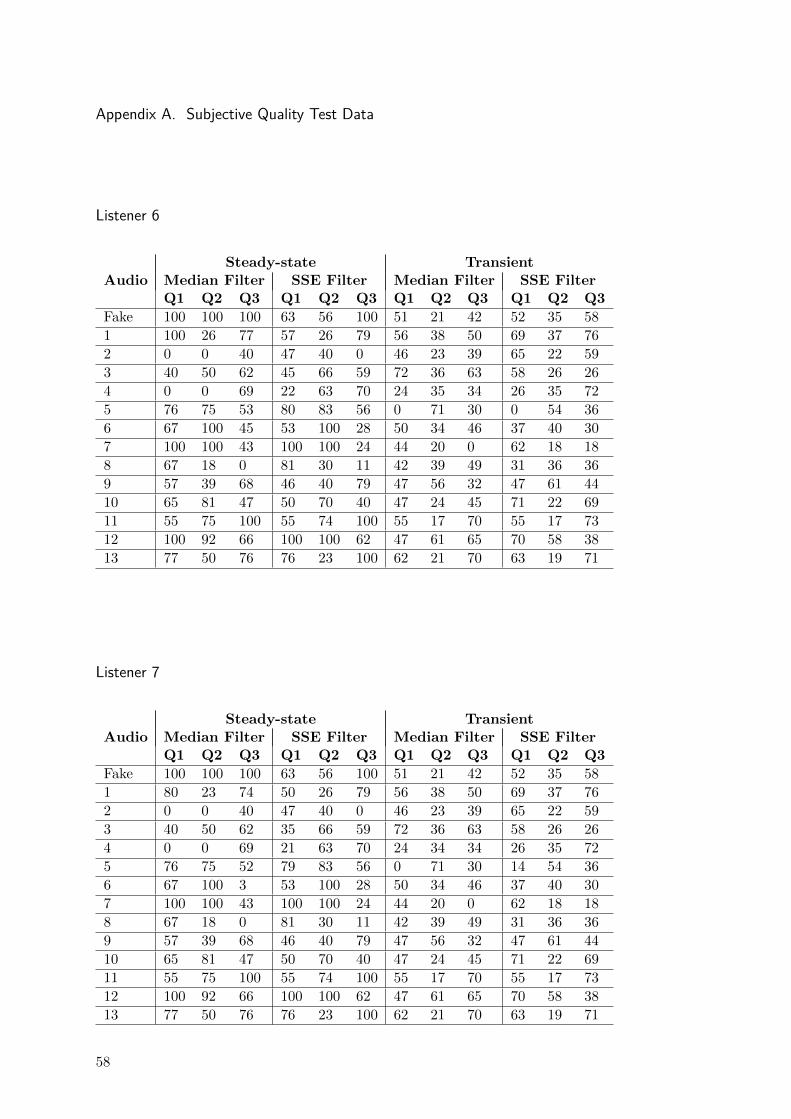
Appendix A. Subjective Quality Test Data
Listener 6
AudioSteady-state Transient
Median Filter SSE Filter Median Filter SSE FilterQ1 Q2 Q3 Q1 Q2 Q3 Q1 Q2 Q3 Q1 Q2 Q3
Fake 100 100 100 63 56 100 51 21 42 52 35 58
1 100 26 77 57 26 79 56 38 50 69 37 76
2 0 0 40 47 40 0 46 23 39 65 22 59
3 40 50 62 45 66 59 72 36 63 58 26 26
4 0 0 69 22 63 70 24 35 34 26 35 72
5 76 75 53 80 83 56 0 71 30 0 54 36
6 67 100 45 53 100 28 50 34 46 37 40 30
7 100 100 43 100 100 24 44 20 0 62 18 18
8 67 18 0 81 30 11 42 39 49 31 36 36
9 57 39 68 46 40 79 47 56 32 47 61 44
10 65 81 47 50 70 40 47 24 45 71 22 69
11 55 75 100 55 74 100 55 17 70 55 17 73
12 100 92 66 100 100 62 47 61 65 70 58 38
13 77 50 76 76 23 100 62 21 70 63 19 71
Listener 7
AudioSteady-state Transient
Median Filter SSE Filter Median Filter SSE FilterQ1 Q2 Q3 Q1 Q2 Q3 Q1 Q2 Q3 Q1 Q2 Q3
Fake 100 100 100 63 56 100 51 21 42 52 35 58
1 80 23 74 50 26 79 56 38 50 69 37 76
2 0 0 40 47 40 0 46 23 39 65 22 59
3 40 50 62 35 66 59 72 36 63 58 26 26
4 0 0 69 21 63 70 24 34 34 26 35 72
5 76 75 52 79 83 56 0 71 30 14 54 36
6 67 100 3 53 100 28 50 34 46 37 40 30
7 100 100 43 100 100 24 44 20 0 62 18 18
8 67 18 0 81 30 11 42 39 49 31 36 36
9 57 39 68 46 40 79 47 56 32 47 61 44
10 65 81 47 50 70 40 47 24 45 71 22 69
11 55 75 100 55 74 100 55 17 70 55 17 73
12 100 92 66 100 100 62 47 61 65 70 58 38
13 77 50 76 76 23 100 62 21 70 63 19 71
58
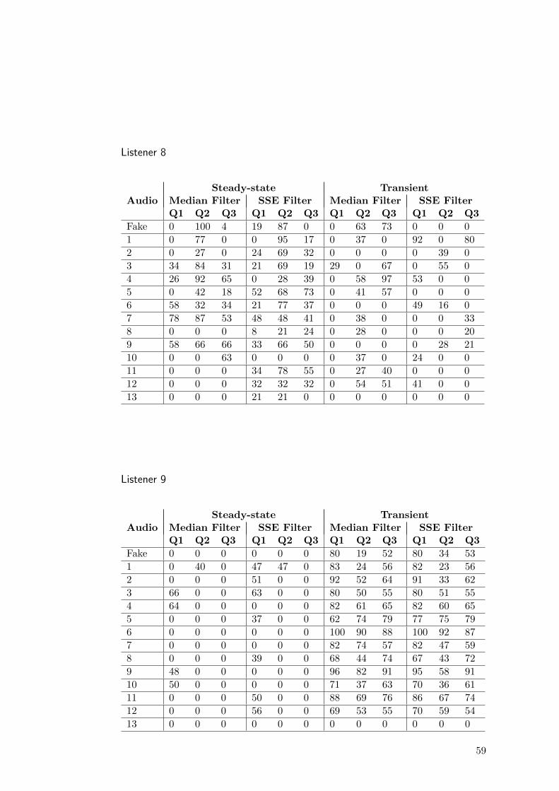
Listener 8
AudioSteady-state Transient
Median Filter SSE Filter Median Filter SSE FilterQ1 Q2 Q3 Q1 Q2 Q3 Q1 Q2 Q3 Q1 Q2 Q3
Fake 0 100 4 19 87 0 0 63 73 0 0 0
1 0 77 0 0 95 17 0 37 0 92 0 80
2 0 27 0 24 69 32 0 0 0 0 39 0
3 34 84 31 21 69 19 29 0 67 0 55 0
4 26 92 65 0 28 39 0 58 97 53 0 0
5 0 42 18 52 68 73 0 41 57 0 0 0
6 58 32 34 21 77 37 0 0 0 49 16 0
7 78 87 53 48 48 41 0 38 0 0 0 33
8 0 0 0 8 21 24 0 28 0 0 0 20
9 58 66 66 33 66 50 0 0 0 0 28 21
10 0 0 63 0 0 0 0 37 0 24 0 0
11 0 0 0 34 78 55 0 27 40 0 0 0
12 0 0 0 32 32 32 0 54 51 41 0 0
13 0 0 0 21 21 0 0 0 0 0 0 0
Listener 9
AudioSteady-state Transient
Median Filter SSE Filter Median Filter SSE FilterQ1 Q2 Q3 Q1 Q2 Q3 Q1 Q2 Q3 Q1 Q2 Q3
Fake 0 0 0 0 0 0 80 19 52 80 34 53
1 0 40 0 47 47 0 83 24 56 82 23 56
2 0 0 0 51 0 0 92 52 64 91 33 62
3 66 0 0 63 0 0 80 50 55 80 51 55
4 64 0 0 0 0 0 82 61 65 82 60 65
5 0 0 0 37 0 0 62 74 79 77 75 79
6 0 0 0 0 0 0 100 90 88 100 92 87
7 0 0 0 0 0 0 82 74 57 82 47 59
8 0 0 0 39 0 0 68 44 74 67 43 72
9 48 0 0 0 0 0 96 82 91 95 58 91
10 50 0 0 0 0 0 71 37 63 70 36 61
11 0 0 0 50 0 0 88 69 76 86 67 74
12 0 0 0 56 0 0 69 53 55 70 59 54
13 0 0 0 0 0 0 0 0 0 0 0 0
59
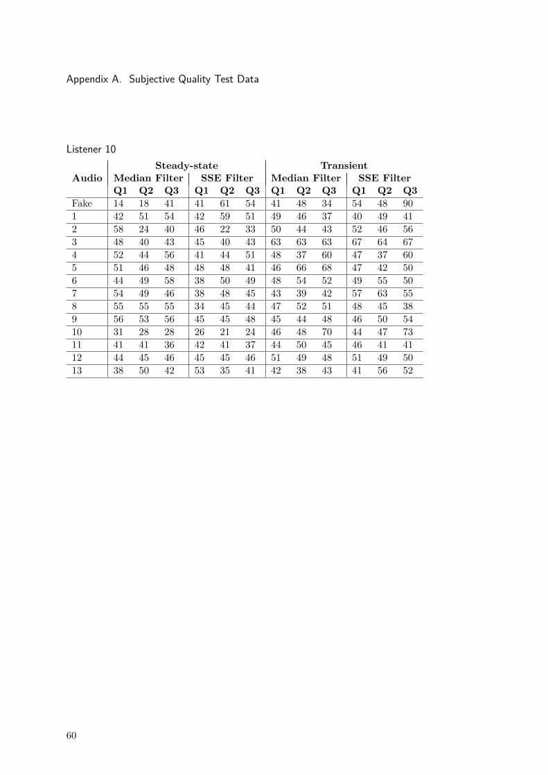
Appendix A. Subjective Quality Test Data
Listener 10
AudioSteady-state Transient
Median Filter SSE Filter Median Filter SSE FilterQ1 Q2 Q3 Q1 Q2 Q3 Q1 Q2 Q3 Q1 Q2 Q3
Fake 14 18 41 41 61 54 41 48 34 54 48 90
1 42 51 54 42 59 51 49 46 37 40 49 41
2 58 24 40 46 22 33 50 44 43 52 46 56
3 48 40 43 45 40 43 63 63 63 67 64 67
4 52 44 56 41 44 51 48 37 60 47 37 60
5 51 46 48 48 48 41 46 66 68 47 42 50
6 44 49 58 38 50 49 48 54 52 49 55 50
7 54 49 46 38 48 45 43 39 42 57 63 55
8 55 55 55 34 45 44 47 52 51 48 45 38
9 56 53 56 45 45 48 45 44 48 46 50 54
10 31 28 28 26 21 24 46 48 70 44 47 73
11 41 41 36 42 41 37 44 50 45 46 41 41
12 44 45 46 45 45 46 51 49 48 51 49 50
13 38 50 42 53 35 41 42 38 43 41 56 52
60
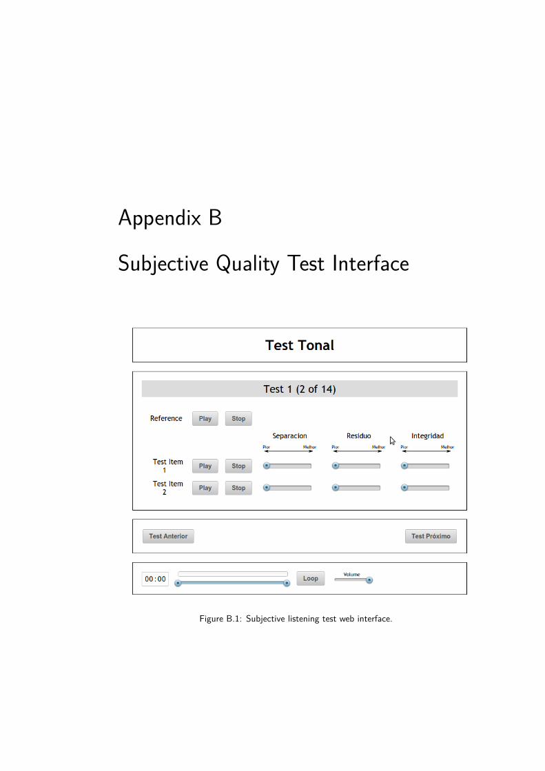
Appendix B
Subjective Quality Test Interface
Figure B.1: Subjective listening test web interface.
Appendix B. Subjective Quality Test Interface
62
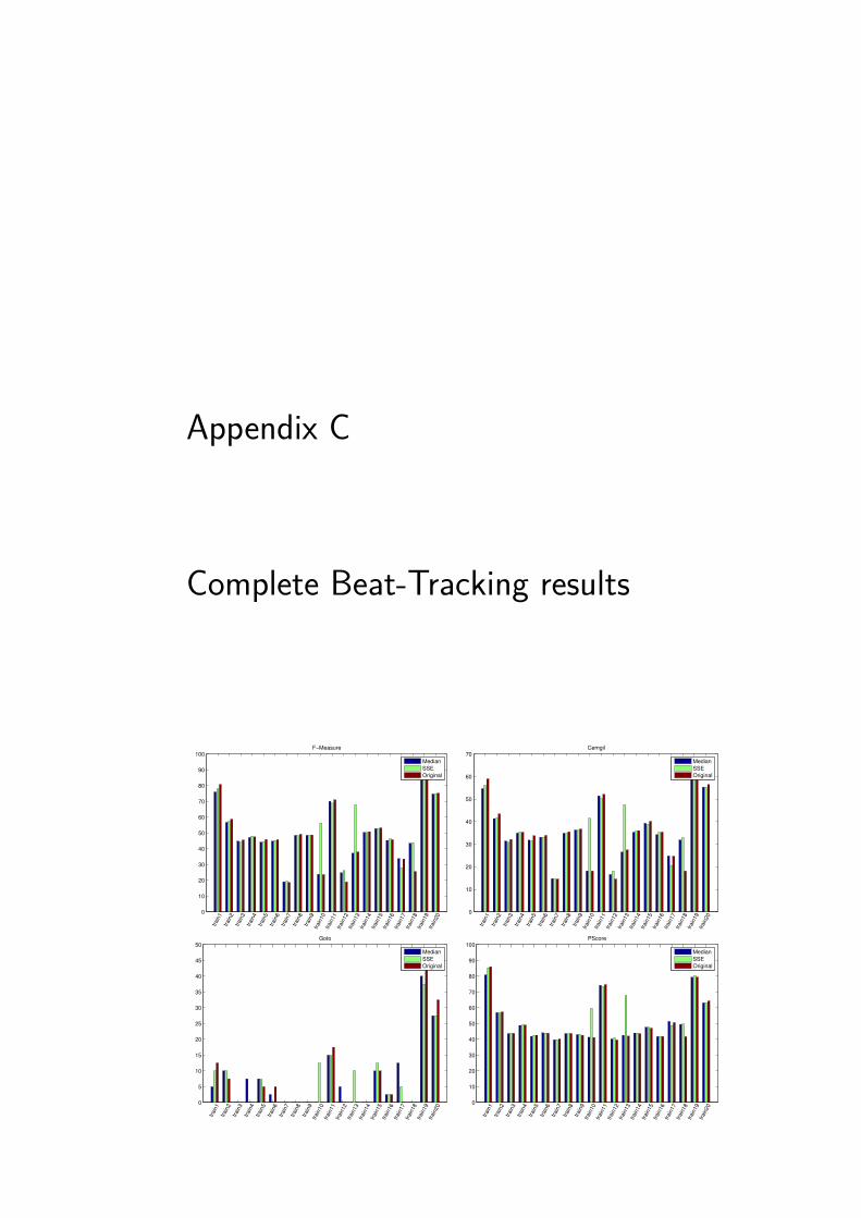
Appendix C
Complete Beat-Tracking results
0
10
20
30
40
50
60
70
80
90
100F−Measure
train
1train
2train
3train
4train
5train
6train
7train
8train
9train
10
train
11
train
12
train
13
train
14
train
15
train
16
train
17
train
18
train
19
train
20
Median
SSE
Original
0
10
20
30
40
50
60
70 Cemgil
train
1train
2train
3train
4train
5train
6train
7train
8train
9train
10
train
11
train
12
train
13
train
14
train
15
train
16
train
17
train
18
train
19
train
20
Median
SSE
Original
0
5
10
15
20
25
30
35
40
45
50Goto
train
1train
2train
3train
4train
5train
6train
7train
8train
9train
10
train
11
train
12
train
13
train
14
train
15
train
16
train
17
train
18
train
19
train
20
Median
SSE
Original
0
10
20
30
40
50
60
70
80
90
100PScore
train
1train
2train
3train
4train
5train
6train
7train
8train
9train
10
train
11
train
12
train
13
train
14
train
15
train
16
train
17
train
18
train
19
train
20
Median
SSE
Original
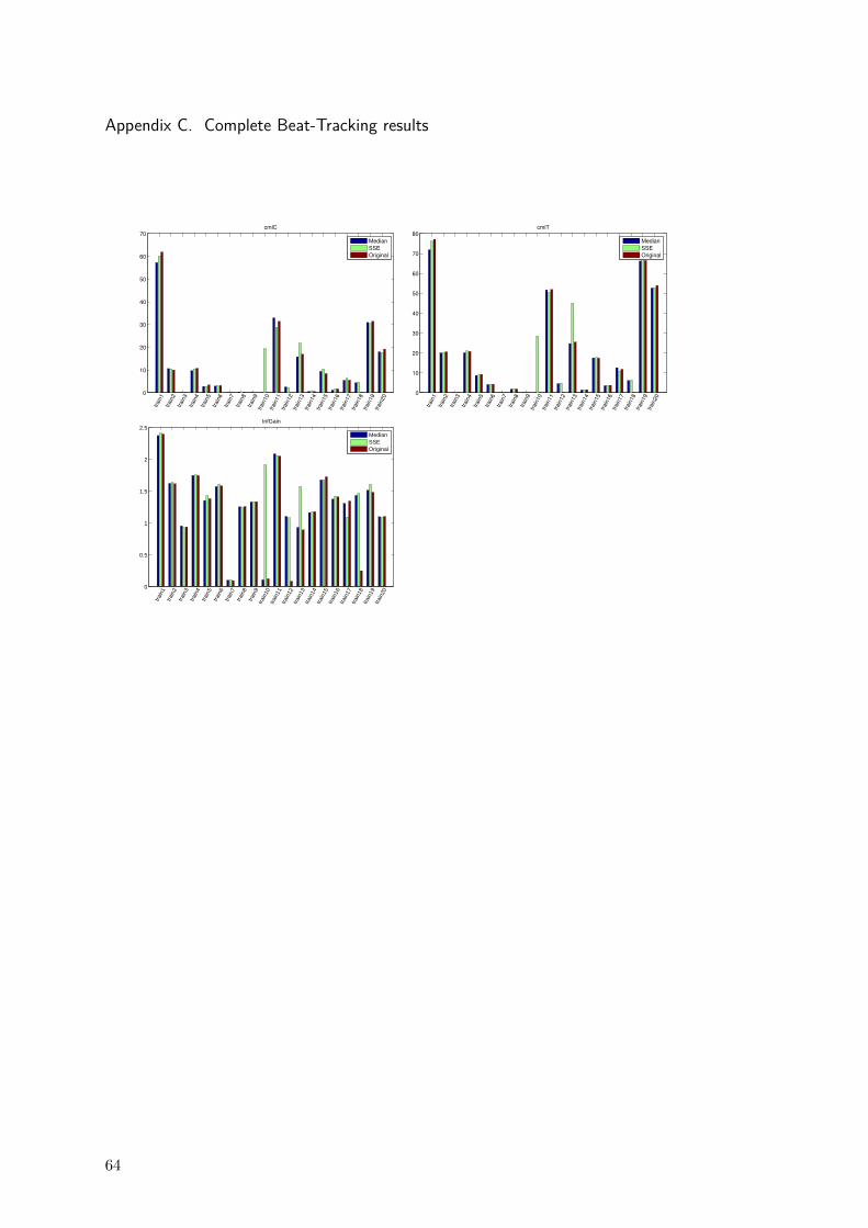
Appendix C. Complete Beat-Tracking results
0
10
20
30
40
50
60
70cmlC
train
1train
2train
3train
4train
5train
6train
7train
8train
9train
10
train
11
train
12
train
13
train
14
train
15
train
16
train
17
train
18
train
19
train
20
Median
SSE
Original
0
10
20
30
40
50
60
70
80cmlT
train
1train
2train
3train
4train
5train
6train
7train
8train
9train
10
train
11
train
12
train
13
train
14
train
15
train
16
train
17
train
18
train
19
train
20
Median
SSE
Original
0
0.5
1
1.5
2
2.5InfGain
train
1tra
in2
train
3tra
in4
train
5tra
in6
train
7tra
in8
train
9tra
in10
train
11tra
in12
train
13tra
in14
train
15tra
in16
train
17tra
in18
train
19tra
in20
MedianSSEOriginal
64
Bibliography
[1] Mitsuko Aramaki et al. “Synthesis and perceptual manipulation of per-cussive sounds”. In: International Computer Music Conference Pro-ceedings. ICMA. Barcelona, Spain, Sept. 2005, pp. 335–338.
[2] F. Auger and P. Flandrin. “Improving the readability of time-frequencyand time-scale representations by the reassignment method”. In: IEEETransactions on Signal Processing 43.5 (May 1995), pp. 1068–1089.
[3] Steven Boll. “Suppression of acoustic noise in speech using spectralsubtraction”. In: IEEE Transactions on Acoustics, Speech, and SignalProcessing 27.2 (Apr. 1979), pp. 113–120.
[4] Judith C. Brown. “Calculation of a constant Q spectral transform”.In: The Journal of the Acoustical Society of America 89.1 (Jan. 1991),pp. 425–434.
[5] Judith C. Brown and Miller S. Puckette. “An efficient algorithm forthe calculation of a constant Q transform”. In: The Journal of theAcoustical Society of America 92.5 (Nov. 1992), pp. 2698–2701.
[6] Pablo Cancela, Ernesto Lopez, and Martın Rocamora. “Fan chirp trans-form for music representation”. In: Proceedings of the 13th Interna-tional Conference on Digital Audio Effects (DAFx-10). Graz, Austria,Sept. 2010, pp. 1–8.
[7] Chris Cannam et al. “The sonic visualiser: A visualisation platformfor semantic descriptors from musical signals”. In: Proceedings of the7th International Conference on Music Information Retrieval (ISMIR2006). ISMIR. Victoria, Canada, Oct. 2006, pp. 324–327.
[8] Ali Taylan Cemgil et al. “On tempo tracking: Tempogram representa-tion and Kalman filtering”. In: Journal of New Music Research 29.4(2000), pp. 259–273.
[9] F. Charpentier and M. Stella. “Diphone synthesis using an overlap-addtechnique for speech waveforms concatenation”. In: Proceedings of theInternational Conference on Acoustics, Speech, and Signal Processing(ICASSP’86). Vol. 4. IEEE. Tokyo, Japan, Apr. 1986, pp. 2015–2018.
Bibliography
[10] Chris Cutler. “Technology, politics and contemporary music: necessityand choice in musical forms”. In: Popular Music 4 (Jan. 1984), pp. 279–300.
[11] Olivier Darrigol. “The acoustic origins of harmonic analysis”. In: Archivefor History of Exact Sciences 61.4 (July 2007), pp. 343–424.
[12] M. E. P. Davies and S. Bock. “Evaluating the evaluation measuresfor beat tracking”. In: Proceedings of the 15th International Society forMusic Information Retrieval Conference (ISMIR 2014). ISMIR. Taipei,Taiwan, Oct. 2014, pp. 637–642.
[13] M. E. P. Davies, N. Degara, and M. D. Plumbley. Evaluation Methodsfor Musical Audio Beat Tracking Algorithms. Technical Report C4DM-TR-09-06. London, UK: Queen Mary University, Centre for DigitalMusic, Oct. 2009.
[14] Matthew Davies and Adam Stark. Beat Tracking Evaluation Toolbox.2012. url: http://code.soundsoftware.ac.uk/projects/beat-evaluation/.
[15] J. Stephen Downie, Joe Futrelle, and David K. Tcheng. “The Inter-national Music Information Retrieval Systems Evaluation Laboratory:Governance, access and security”. In: Proceedings of the 5th Interna-tional Conference on Music Information Retrieval (ISMIR 2004). IS-MIR. Barcelona, Spain, Oct. 2004.
[16] J. Stephen Downie et al. “The 2005 music information retrieval evalu-ation exchange (MIREX 2005): Preliminary overview”. In: Proceedingsof the 6th International Conference on Music Information Retrieval(ISMIR 2005). ISMIR. London, UK, Sept. 2005, pp. 320–323.
[17] Jonathan Driedger, Meinard Muller, and Sebastian Ewert. “Improvingtime-scale modification of music signals using harmonic-percussive sep-aration”. In: IEEE Signal Processing Letters 21.1 (Jan. 2014), pp. 105–109.
[18] Chris Duxbury, Mike Davies, and Mark Sandler. “Separation of tran-sient information in musical audio using multiresolution analysis tech-niques”. In: Proceedings of the 4th Conference on Digital Audio Effects(DAFx-01). COST-G6. Limerick, Ireland, Dec. 2001.
[19] Chris Duxbury, Mike Davies, and Mark B. Sandler. “Improved time-scaling of musical audio using phase locking at transients”. In: 112thAudio Engineering Society Convention. Convention Paper 5530. AudioEngineering Society. 2002.
[20] Daniel P. W. Ellis. “Beat tracking by dynamic programming”. In: Jour-nal of New Music Research 36.1 (July 2007), pp. 51–60.
66
Bibliography
[21] Yariv Ephraim and David Malah. “Speech enhancement using a minimum-mean square error short-time spectral amplitude estimator”. In: IEEETransactions on Acoustics, Speech, and Signal Processing 32.6 (Dec.1984), pp. 1109–1121.
[22] C. Fevotte. “Itakura-Saito nonnegative factorizations of the power spec-trogram for music signal decomposition”. In: Machine Audition: Prin-ciples, Algorithms and Systems. Ed. by Wenwu Wang. Hershey, USA:IGI Global Press, 2010. Chap. 11, pp. 266–296.
[23] D. Fitzgerald. “Harmonic/percussive separation using median filter-ing”. In: Proceedings of the 13th International Conference on DiitalAudio Effects DAFx-10. Graz, Austria, Sept. 2010.
[24] Patrick Flandrin. Time-Frequency/Time-Scale Analysis. Vol. 10. WaveletAnalysis and Its Applications. San Diego, USA: Academic Press, 1999.
[25] Richard Furse. Linux audio developer’s simple plugin api (LADSPA).Apr. 2000. url: http://www.ladspa.org.
[26] Masataka Goto and Yoichi Muraoka. “Issues in evaluating beat trackingsystems”. In: Working Notes of the IJCAI-97 Workshop on Issues inAI and Music-Evaluation and Assessment. Nagoya, Japan, Aug. 1997,pp. 9–16.
[27] Masataka Goto and Yoichi Muraoka. “Real-time beat tracking for drum-less audio signals: Chord change detection for musical decisions”. In:Speech Communication 27.3 (Apr. 1999), pp. 311–335.
[28] Thomas Grandke. “Interpolation algorithms for discrete Fourier trans-forms of weighted signals”. In: IEEE Transactions on Instrumentationand Measurement 32.2 (June 1983), pp. 350–355.
[29] Karlheinz Grochenig. Foundations of Time-Frequency Analysis. Ap-plied and Numerical Harmonic Analysis. New York, USA: Springer,2001.
[30] Stephen Hainsworth and Malcolm Macleod. “On sinusoidal parameterestimation”. In: Proceedings of the 6th International Conference onDigital Audio Effects (DAFx-03). London, UK, Sept. 2003.
[31] Monson H. Hayes. Statistical Digital Signal Processing and Modeling.Hoboken, USA: John Wiley & Sons, 1996.
[32] Marko Helen and Tuomas Virtanen. “Separation of drums from poly-phonic music using non-negative matrix factorization and support vec-tor machine”. In: Proceedings of the 13th European Signal ProcessingConference (EUSIPCO 2005). EURASIP. Antalya, Turkey, Sept. 2005,pp. 1091–1094.
67
Bibliography
[33] Richard Heusdens, Renat Vafin, and W. Bastiaan Kleijn. “Sinusoidalmodeling using psychoacoustic-adaptive matching pursuits”. In: IEEESignal Processing Letters 9.8 (Aug. 2002), pp. 262–265.
[34] Richard Heusdens and Steven Van De Par. “Rate-distortion optimal si-nusoidal modeling of audio and speech using psychoacoustical matchingpursuits”. In: Proceedings of the International Conference on Acoustics,Speech, and Signal Processing (ICASSP’02). Vol. 2. IEEE. Orlando,USA, May 2002, pp. 1809–1812.
[35] C. Hsu and J. Jang. “Singing pitch extraction at MIREX 2010”. In:Proceedings of the 11th International Society for Music Information Re-trieval Conference (ISMIR 2010). ISMIR. Utrecht, Netherlands, Aug.2010.
[36] Ignacio Irigaray and Luiz W. P. Biscainho. “Transient and steady-statecomponent extration using nonlinear filtering”. In: Anales del I Con-greso Internacional de Ciencia y Tecnologıa Musical (CICTeM 2013).Buenos Aires, Argentina, Sept. 2013. url: http://iie.fing.edu.uy/publicaciones/2013/IB13.
[37] Mark Kahrs and Karlheinz Brandenburg, eds. Applications of DigitalSignal Processing to Audio and Acoustics. The Kluwer InternationalSeries in Engineering and Computer Science. New York, USA: Kluwer,2002.
[38] T. Kasparis and J. Lane. “Suppression of impulsive disturbances fromaudio signals”. In: Electronics Letters 29.22 (Oct. 1993), pp. 1926–1927.
[39] Takis Kasparis and John Lane. “Adaptive scratch noise filtering”. In:IEEE Transactions on Consumer Electronics 39.4 (Nov. 1993), pp. 917–922.
[40] Florian Keiler, Sylvain Marchand, et al. “Survey on extraction of si-nusoids in stationary sounds”. In: Proceedings of the 5th InternationalConference on Digital Audio Effects (DAFx-02). Hamburg, Germany,Sept. 2002, pp. 51–58.
[41] Seong Rag Kim and Adam Efron. “Adaptive robust impulse noise fil-tering”. In: IEEE Transactions on Signal Processing 43.8 (Aug. 1995),pp. 1855–1866.
[42] Maria Klatte, Thomas Lachmann, and Markus Meis. “Effects of noiseand reverberation on speech perception and listening comprehension ofchildren and adults in a classroom-like setting”. In: Noise and Health12.49 (Oct. 2010), p. 270.
68
Bibliography
[43] N. Laurenti, G. De Poli, and D. Montagner. “A nonlinear method forstochastic spectrum estimation in the modeling of musical sounds”. In:IEEE Transactions on Audio, Speech, and Language Processing 15.2(Feb. 2007), pp. 531–541.
[44] Katia Lebart, Jean-Marc Boucher, and P. N. Denbigh. “A new methodbased on spectral subtraction for speech dereverberation”. In: ActaAcustica united with Acustica 87.3 (May 2001), pp. 359–366.
[45] Daniel D Lee and H Sebastian Seung. “Learning the parts of objectsby non-negative matrix factorization”. In: Nature 401.6755 (Oct. 1999),pp. 788–791.
[46] Mark Lewisohn. The Beatles Recording Sessions. New York, USA: Har-mony Books, 1988.
[47] Antoine Liutkus et al. “Kernel additive models for source separation”.In: IEEE Transactions on Signal Processing 62.16 (Aug. 2014), pp. 4298–4310.
[48] Katariina Mahkonen et al. “Music dereverberation by spectral linearpredictiomn in live recordings”. In: Proceedings of the 16th Interna-tional Conference on Digital Audio Effects (DAFx-13). Maynooth, Ire-land, Sept. 2013.
[49] Stephane G Mallat and Zhifeng Zhang. “Matching pursuits with time-frequency dictionaries”. In: IEEE Transactions on Signal Processing41.12 (Dec. 1993), pp. 3397–3415.
[50] Sylvain Marchand. “Improving spectral analysis precision with an en-hanced phase vocoder using signal derivatives”. In: Proceedings of the1st Workshop on Digital Audio Effects (DAFx-98). COST-G6. Barcelona,Spain, Nov. 1998, pp. 114–118.
[51] Paul Masri and Andrew Bateman. “Improved modelling of attack tran-sients in music analysis-resynthesis”. In: Proceedings of the Interna-tional Computer Music Conference (ICMC’96). ICMA. Hong Kong,China, Aug. 1996, pp. 100–103.
[52] R. McAulay and T. Quatieri. “Speech analysis/synthesis based on a si-nusoidal representation”. In: IEEE Transactions on Acoustics, Speech,and Signal Processing 34.4 (Aug. 1986), pp. 744–754.
[53] Marin Mersenne. Harmonie Universelle: Contenant la Theorie et laPratique de la Musique. Vol. 2. Paris, France: Editions du Centre Na-tional de la Recherche Scientifique, 1637.
[54] Eric Moulines and Jean Laroche. “Non-parametric techniques for pitch-scale and time-scale modification of speech”. In: Speech Communication16.2 (Feb. 1995), pp. 175–205.
69
Bibliography
[55] Musiktechnik. SPL Transient Designer. Sept. 2014. url: http : / /
spl.info/de/produkte/analog- coder- plug- ins/transient-
designer/video.html.
[56] Patrick A. Naylor et al. “Models, measurement and evaluation”. In:Speech Dereverberation. Ed. by Patrick A. Naylor and Nikolay D. Gaubitch.Signals and Communication Technology. London, UK: Springer, 2010.Chap. 2, pp. 21–56.
[57] Brett Ninness and Soren J. Henriksen. “Time-scale modification ofspeech signals”. In: IEEE Transactions on Signal Processing 56.4 (Apr.2008), pp. 1479–1488.
[58] Takuma Okamoto, Yukio Iwaya, and Yoiti Suzuki. “Wide-band dere-verberation method based on multichannel linear prediction using prewhiten-ing filter”. In: Applied Acoustics 73.1 (Jan. 2012), pp. 50–55.
[59] Nobutaka Ono et al. “A real-time equalizer of harmonic and percus-sive components in music signals.” In: Proceedings of the 9th Inter-national Conference on Music Information Retrieval (ISMIR 2008).ISMIR. Philadelhia, USA, Sept. 2008, pp. 139–144.
[60] N. Ono et al. “Separation of a monaural audio signal into harmonic/percussivecomponents by complementary diffusion on spectrogram”. In: Proceed-ings of the 16th European Signal Processing Conference (EUSIPCO2008). EURASIP. Lausanne, Switzerland, Aug. 2008.
[61] Graham E. Poliner et al. “Melody transcription from music audio: Ap-proaches and evaluation”. In: IEEE Transactions on Audio, Speech,and Language Processing 15.4 (May 2007), pp. 1247–1256.
[62] Michael R. Portnoff. “Time-scale modification of speech based on short-time Fourier analysis”. In: IEEE Transactions on Acoustics, Speech andSignal Processing 29.3 (June 1981), pp. 374–390.
[63] William K. Pratt. Digital Image Processing. 4th ed. Hoboken, USA:John Wiley & Sons, Inc., 2007.
[64] Miller Puckette. “Pure Data: another integrated computer music envi-ronment”. In: Proceedings of the International Computer Music Con-ference (ICMC’96). ICMA. Hong Kong, China, Aug. 1996, pp. 37–41.
[65] Zbigniew W. Ras and Alicja Wieczorkowska, eds. Advances in MusicInformation Retrieval. Vol. 274. Studies in Computational Intelligence.Berlin, Germany: Springer, 2010.
[66] Axel Robel. “Transient detection and preservation in the phase vocoder”.In: Proceedings of the International Computer Music Conference (ICMC’03).ICMA. Singapore, 2003, pp. 247–250.
70
Bibliography
[67] Salim Roucos and Alexander Wilgus. “High quality time-scale modifi-cation for speech”. In: Proceedings of the International Conference onAcoustics, Speech, and Signal Processing (ICASSP’85). Vol. 10. IEEE.Tampa, USA, 1985, pp. 493–496.
[68] Luigi Russolo et al. The Art of Noise: Futurist Manifesto, 1913. NewYork, USA: Something Else Press, 1967.
[69] Justin Salamon and Emilia Gomez. “Melody extraction from poly-phonic music signals using pitch contour characteristics”. In: IEEETransactions on Audio, Speech, and Language Processing 20.6 (Aug.2012), pp. 1759–1770.
[70] Joseph Sauveur. Principes d’Acoustique et de Musique: ou, SystemeGeneral des Intervalles des Sons. Geneva, Switzerland: Editions Minkoff,1701.
[71] Kraft Sebastian. mushraJS. Mar. 2013. url: https://github.com/seebk/mushraJS.
[72] X. Serra and J. Smith III. “Spectral modeling synthesis: A sound anal-ysis/synthesis system based on a deterministic plus stochastic decom-position”. In: Computer Music Journal 4.14 (Winter 1990), pp. 12–24.
[73] Xavier Serra. A System for Sound Analysis/Transformation/SynthesisBased on a Deterministic Plus Stochastic Decomposition. Technical Re-port STAN-M-58. Stanford, USA: Stanford University, Center for Com-puter Research in Music and Acoustics, Oct. 1989.
[74] Xavier Serra. “Musical sound modeling with sinusoids plus noise”. In:Musical Signal Processing. Ed. by Curtis Roads et al. Studies on NewMusic Research. New York, USA: Routledge, 1997, pp. 91–122.
[75] Kai Siedenburg and Monika Dorfler. “Structured sparsity for audiosignals”. In: Proceedings of the 14th International Conference on DigitalAudio Effects (DAFx-11). Paris, France, Sept. 2011.
[76] David Slepian and Henry O. Pollak. “Prolate spheroidal wave functions,Fourier analysis and uncertainty—I”. In: The Bell System TechnicalJournal 40.1 (Jan. 1961), pp. 43–63.
[77] Hideyuki Tachibana et al. “Melody line estimation in homophonic mu-sic audio signals based on temporal-variability of melodic source”. In:Proceedings of the 35th International Conference on Acoustics, Speech,and Signal Processing (ICASSP’10). IEEE. Dallas, USA, Mar. 2010,pp. 425–428.
71
Bibliography
[78] George Tanev and Adrijan Bozinovski. “Virtual Studio Technologyinside Music Production”. In: ICT Innovations 2013: ICT Innova-tions and Education. Ed. by Vladimir Trajkovik and Anastas Mishev.Vol. 231. Advances in Intelligent Systems and Computing. Cham, Switzer-land: Springer, 2014, pp. 231–241.
[79] Schaack Audio Techonolgies. Transient Shaper. Sept. 2014. url: http://www.schaack-audio.com/transientshaper.html.
[80] Alexandros Tsilfidis and John Mourjopoulos. “Blind single-channel sup-pression of late reverberation based on perceptual reverberation model-ing”. In: The Journal of the Acoustical Society of America 129.3 (Mar.2011), pp. 1439–1451.
[81] Christian Uhle, Christian Dittmar, and Thomas Sporer. “Extractionof drum tracks from polyphonic music using Independent SubspaceAnalysis”. In: Proceedings of the 4th International Symposium on Inde-pendent Component Analysis and Blind Signal Separation (ICA2003).Nara, Japan, Apr. 2003, pp. 843–848.
[82] S. V. Vaseghi and P. J. W. Rayner. “Detection and suppression ofimpulsive noise in speech communication systems”. In: IEE ProceedingsI - Communications, Speech and Vision) 137.1 (Feb. 1990), pp. 38–46.
[83] T. Verma, S. Levine, and T. Meng. “Transient modeling synthesis: aflexible analysis/synthesis tool for transient signals”. In: Proceedingsof the International Computer Music Conference (ICMC’97). ICMA.Thessaloniki, Greece, Sept. 1997, pp. 164–167.
[84] Emmanuel Vincent et al. Blind Audio Source Separation. TechnicalReport C4DM-TR-05-01. London, UK: Queen Mary University, Centrefor Digital Music, Nov. 2005.
[85] Tuomas Virtanen. “Monaural sound source separation by nonnegativematrix factorization with temporal continuity and sparseness criteria”.In: IEEE Transactions on Audio, Speech, and Language Processing 15.3(Mar. 2007), pp. 1066–1074.
[86] Tuomas Virtanen. “Unsupervised learning methods for source sepa-ration in monaural music signals”. In: Signal Processing Methods forMusic Transcription. Ed. by Anssi Klapuri and Manuel Davy. NewYork, USA: Springer, 2006. Chap. 9, pp. 267–296.
[87] Jing Wang et al. “An adaptive window switching method for ITU-TG.719 transient coding in TDA domain”. In: Proceedings of the 3rd In-ternational Conference on Wireless, Mobile and Multimedia Networks(ICWMNN 2010). IET. Beijing, China, Sept. 2010, pp. 298–301.
72
Bibliography
[88] Thomas Wilmering, Mathieu Barthet, and Mark B. Sandler. “Dere-verberation of musical instrument recordings for improved note onsetdetection and instrument recognition”. In: 131st Audio Engineering So-ciety Convention. Convention Paper 8508. Audio Engineering Society.New York, USA, Oct. 2011.
[89] Thomas Wilmering, Gyorgy Fazekas, and Mark Sandler. “The effectsof reverberation on onset detection tasks”. In: 128th Audio Engineer-ing Society Convention. Convention Paper 8114. Audio EngineeringSociety. London, UK, May 2010.
[90] Trevor Wishart. “The Composition of “Vox-5””. In: Computer MusicJournal 12.4 (Winter 1988), pp. 21–27.
[91] John F. Woodruff, Bryan Pardo, and Roger B. Dannenberg. “Remixingstereo music with score-informed source separation”. In: Proceedingsof the 7th International Conference on Music Information Retrieval(ISMIR 2006). ISMIR. Victoria, Canada, Oct. 2006, pp. 314–319.
[92] Naoki Yasuraoka et al. “Music dereverberation using harmonic struc-ture source model and Wiener filter”. In: Proceedings of the 35th In-ternational Conference on Acoustics, Speech, and Signal Processing(ICASSP’10). IEEE. Dallas, USA, Mar. 2010, pp. 53–56.
[93] Tao Zhang, Wei Wang, and Jialin He. “On the pre-echo control methodin transient signal coding of AVS audio”. In: Proceedings of the 2008International Conference on Audio, Language and Image Processing(ICALIP 2008). IEEE. Shanghai, China, July 2008, pp. 242–246.
[94] Slawomir Zielinski and Francis Rumsey. “On some biases encounteredin modern audio quality listening tests-A Review”. In: Journal of theAudio Engineering Society 56 (June 2008), pp. 427–451.
73

Bibliography
74
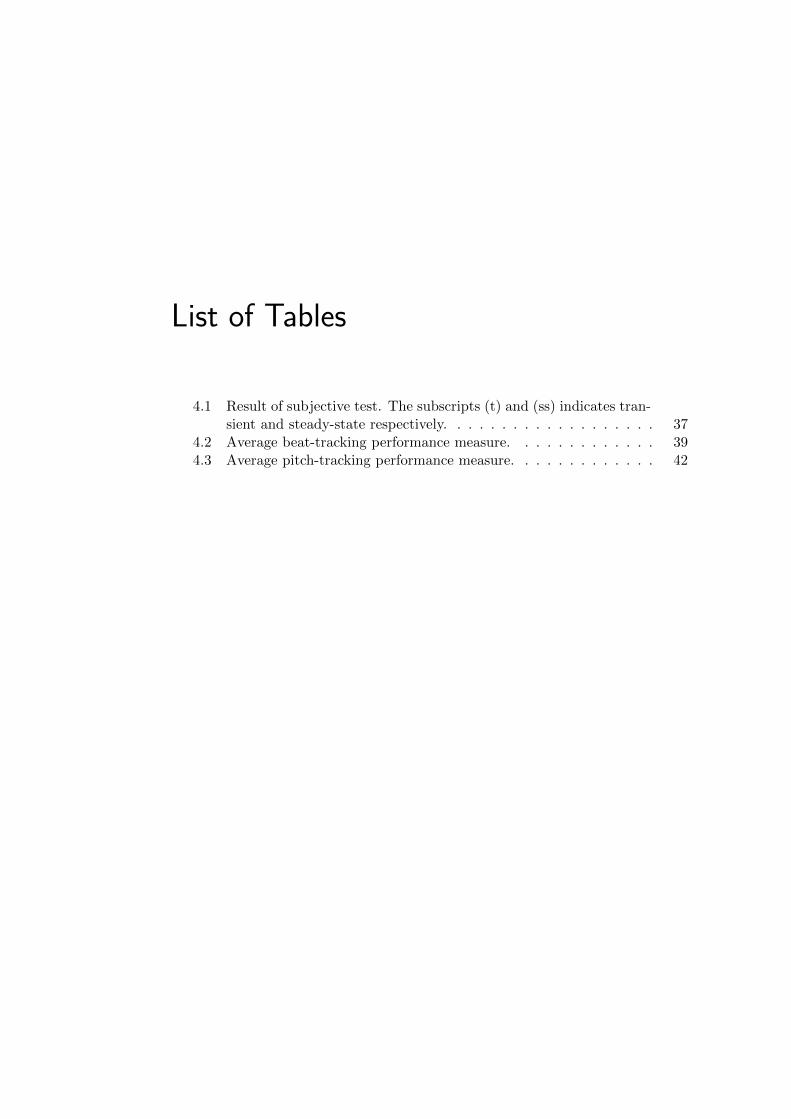
List of Tables
4.1 Result of subjective test. The subscripts (t) and (ss) indicates tran-sient and steady-state respectively. . . . . . . . . . . . . . . . . . . 37
4.2 Average beat-tracking performance measure. . . . . . . . . . . . . 394.3 Average pitch-tracking performance measure. . . . . . . . . . . . . 42
List of Tables
76
List of Figures
2.1 Time and frequency representation of an audio signal. A male voicesinging “so”. Starts with the unvoiced consonant [s] and ends withthe voiced vowel [o]. . . . . . . . . . . . . . . . . . . . . . . . . . . 7
2.2 Representation of three Gaussian sinusoidal atoms: time, frequencyand joint time frequency representations. . . . . . . . . . . . . . . . 9
2.3 This diagram summarises the Short-Time Fourier Transform calcu-lation. . . . . . . . . . . . . . . . . . . . . . . . . . . . . . . . . . . 10
2.4 Tiling of the time-frequency plane: STFT (left and center) andCQT (right). . . . . . . . . . . . . . . . . . . . . . . . . . . . . . . 12
2.5 CQT and STFT spectrograms; frequency axis in logarithmic scale. 13
2.6 Analysis/Synthesis block diagrams of Sinusoidal Modeling (adaptedfrom figure of original article [52]). . . . . . . . . . . . . . . . . . . 14
2.7 Assignment of peaks to tracks is decided by proximity (adaptedfrom [74]). Tracks may be discontinued if not find adequate peaksfor several frames; and new tracks may be created if a series ofcoherent peaks is find for several frames. . . . . . . . . . . . . . . . 14
2.8 Sinusoidal modeling resynthesis. . . . . . . . . . . . . . . . . . . . . 15
2.9 Spectrogram with sinusoidal tracks superimposed for word “so”.One can observe that the voiced part is well modeled by the sinu-soidal tracks. . . . . . . . . . . . . . . . . . . . . . . . . . . . . . . 16
2.10 Left: Time domain impulse/pulse. Right: Spectra . . . . . . . . . 17
2.11 Atoms from two Gabor Dictionaries with different time-frequencybehavior. . . . . . . . . . . . . . . . . . . . . . . . . . . . . . . . . 18
2.12 Matching Pursuit with different Gabor dictionaries: decompositionof a glockenspiel sound. . . . . . . . . . . . . . . . . . . . . . . . . 19
2.13 Matrix decomposition diagram. . . . . . . . . . . . . . . . . . . . . 19
3.1 Transient and steady-state components of a glockenspiel sound. . . 22
3.2 Spectrogram of a glockenspiel (N=4096,Hop=256). . . . . . . . . 23
3.3 Diagram of the entire process. . . . . . . . . . . . . . . . . . . . . . 24
3.4 Glockenspiel spectrogram (center), time evolution for a fixed FFTbin (bottom) and spectral content of a frame (right). . . . . . . . . 26
3.5 Steps of the Stochastic Spectral Estimation applied along the timeaxis. Based on [43]. . . . . . . . . . . . . . . . . . . . . . . . . . . . 27
List of Figures
3.6 Left: Spectrogram of a excerpt from a popular music song. Middle:Spectrogram with transient components. Right: Spectrogram withsteady-state components. . . . . . . . . . . . . . . . . . . . . . . . 27
3.7 Diagram of the iterative process. . . . . . . . . . . . . . . . . . . . 283.8 Steady-state, transient component and residual extraction for dif-
ferent number of iterations. . . . . . . . . . . . . . . . . . . . . . . 293.9 Time-frequency kernel. . . . . . . . . . . . . . . . . . . . . . . . . . 303.10 left) Spectrogram of a superposition of a periodic signal with vi-
brato to two clicks; right) Comparison between the original and themodified decompositions. . . . . . . . . . . . . . . . . . . . . . . . 30
3.11 Diagram of the sub-band processing schema. . . . . . . . . . . . . 303.12 Filters response for the Filter-bank analysis. . . . . . . . . . . . . . 313.13 Transient and steady-state separation spectrograms for each sub-
band. Band 1 is 0 to 1.5 kHz, band 2 is 1.5 to 4.4 kHz, band 3 is4.4 to 10.3 kHz and band 4 is 10.3 to 22 kHz. . . . . . . . . . . . 32
3.14 Wiener filter configuration for transient and steady-state componentseparation. . . . . . . . . . . . . . . . . . . . . . . . . . . . . . . . 33
4.1 One of the performance measurements for beat tracking (Informa-tion Gain); comparison for all elements in the data set. . . . . . . 40
4.2 Beat-tracking outputs. . . . . . . . . . . . . . . . . . . . . . . . . . 404.3 Steps of the pitch-tracking MELODIA; involved signals. . . . . . . 434.4 Transient/steady-state separation for manual editing. . . . . . . . 444.5 Remixing application. . . . . . . . . . . . . . . . . . . . . . . . . . 454.6 Spectrogram of a vinyl record. . . . . . . . . . . . . . . . . . . . . 464.7 Noise reduction. . . . . . . . . . . . . . . . . . . . . . . . . . . . . 474.8 De-reverberation of a drum sound. . . . . . . . . . . . . . . . . . . 484.9 Different time-pitch modifications. . . . . . . . . . . . . . . . . . . 494.10 Transient smear in an octave-down pitch-shift. . . . . . . . . . . . 504.11 Not smeared transient in a octave-down pitch-shift. . . . . . . . . . 50
B.1 Subjective listening test web interface. . . . . . . . . . . . . . . . 61
78

Esta es la ultima pagina.Compilado el Monday 9th February, 2015.
http://iie.fing.edu.uy/