Embed Size (px)
Citation preview
Two sample rank tests with adaptive score
functions using kernel density estimation
Dissertation
zur Erlangung des Doktorgrades
an den Naturwissenschaftlichen Fachbereichen
(Mathematik)
der Justus-Liebig-Universitat Gießen
vorgelegt von
Brandon Greene
betreut von
Prof. Dr. Winfried Stute
Marburg, Mai 2017

Acknowledgments
My sincerest gratitude and appreciation goes above all to my Doktorvater Professor Winfried Stute for all
of his excellent advice and guidance in this and other projects, his unquestioning generosity with his time,
his patience, and his willingness to give me a chance to begin studying mathematics in Gießen many years
ago. I would also like to thank all of my academic teachers from my time in Gießen, particularly Professor
Erich Hausler and Dr. Gerrit Eichner from the stochastics research group, for providing an invaluable
educational experience that gave me the knowledge and confidence needed to begin this undertaking.
My thanks also go to my family, especially to my wife Beate for her patience and encouragement during
times of frustration, and to my daughters for providing a much needed balance to work and study and
for asking the questions that continue to show me how much more there always is to learn.


Contents
Chapter 1. Introduction 1
Chapter 2. Main results 5
2.1. Definitions and notation 5
2.2. Results 6
Chapter 3. A modified test statistic 15
Chapter 4. A simulation study 29
Chapter 5. Proofs 41
5.1. Leading terms of SN 41
5.2. Negligible terms 55
5.2.1. Taylor rest terms from the expansion of SN 55
5.2.2. First bounded term 61
5.2.3. Second bounded term 85
5.2.4. Third bounded term 122
5.2.5. Fourth bounded term 128
5.3. Asymptotic variance under H0 141
Appendix A. Lemmata 153
Bibliography 165
iii

CHAPTER 1
Introduction
In the two-sample testing problem in its most general form we are interested in deciding between the
null hypothesis that two distributions F and G are equal H0 : F = G and the alternative that they
are different in some way H1 : F 6= G on the basis of two independently identically distributed samples
Xi ∼ F , 1 ≤ i ≤ m and Yk ∼ G, 1 ≤ k ≤ n from F and G respectively. If the testing problem is simplified
such that H1 contains only a single fixed alternative (i.e. (F,G) are a pair of known distribution functions
such that F 6= G and we may write H1 : (F,G)) which is to be compared against the null hypothesis
H0 : (F0, F0) that both of the samples are taken from the same distribution F0, and F , G and F0 possess
densities dFdµ , dGdµ and dF0
dµ with respect to some σ-finite measure µ, then the well-known classical Neyman-
Pearson lemma shows that the most powerful α-level test for comparing H0 and H1 may be found quite
easily by using the likelihood ratio ∏mi=1
dFdµ (Xi)×
∏nk=1
dGdµ (Yk)∏m
i=1dF0
dµ (Xi)×∏nk=1
dF0
dµ (Yk)
as a test statistic and setting the critical value as needed to ensure the level α is not exceeded.
In most practical applications, however, we are not willing to make such a strong assumption and specify
F , G and F0 completely. In the case of parametric tests we are willing to make assumptions about the
form of F and G, such as in the simple t-test, where it is assumed that F and G are normal with equal
variances, possibly differing in expectation (i.e. Xi ∼ N(µ1, σ2) and Yk ∼ N(µ2, σ
2)). In this case, the
testing problem becomes one of comparing hypotheses regarding whether certain parameters of the chosen
distributional family are equal or not in the case of F and G, while often some nuisance parameters, such
as the unknown common variance σ2 in the example of the t-test, must still be estimated from the data.
In some applications it is not feasible or possible to make any kind of assumption regarding the form of
the distributions F and G, beyond perhaps some degree of smoothness or symmetry. This leads us to
the use of nonparametric methods which comprise large classes of tests including permutation tests and
the rank tests, that we will be concerned with here.
By rank tests we mean tests which operate only on the basis of the ranks R11, R12, . . . , R1m and
R21, R22, . . . , R2n of the X1, X2, . . . , Xm and Y1, Y2, . . . , Yn respectively in the pooled sample. Thus,
test statistics of rank tests can be written as a function of the R1i and R2k alone, which brings many
advantages, since the distribution of the vector of ranks (R11, R12, . . . , R1m, R21, R22, . . . , R2n) is known
to be uniform under H0 regardless of the form of the underlying distribution F , meaning that any of the
(m+ n)! possible rank vectors in the combined sample is equally probable. This allows the distribution
of the test statistic under H0 to be determined exactly, independent of F .
There is, of course, a price to be paid for the ability to construct tests which require virtually no assump-
tions regarding the form of the underlying distributions to be made in order to be valid, which is put
succinctly by Hajek and Sidak (1967) in their seminal work Theory of Rank Tests.
1
2 1. INTRODUCTION
We have tried to organize the multitude of rank tests into a compact system. However,
we need to have some knowledge of the form of the unknown density in order to make
a rational selection from this system.
That is, although in a given testing situation all rank tests are identically distributed under H0 indepen-
dent of F , their efficiency in terms of power under the alternatives will indeed depend on the form of the
true underlying distributions.
Hajek and Sidak (1967) show, for example, that in a simple shift model where G(x) = F (x − θ) the
optimal - in the sense of locally most powerful - choice of rank tests in the case of normal F is given by
the statistic
SN =
m∑i=1
Φ−1(
R1i
m+ n+ 1
)while the well-known Wilcoxon rank-sum test (Wilcoxon (1945)), which simply sums the ranks of the
first sample
SN =
m∑i=1
R1i
is optimal for logistic F .
In the following we will re-visit an idea presented by K. Behnen and G. Neuhaus in a series of publications
(Behnen (1972); Behnen and Neuhaus (1983); Behnen et al. (1983); Behnen and Huskova (1984); Neuhaus
(1987); Behnen and Neuhaus (1989)) in which tests based on statistics of the form
SN (bN ) = m−1m∑i=1
bN
(R1i
N
)(1.1)
are proposed, where
HN =m
NF +
n
NG
with N = m+ n is the pooled distribution function and
bN = fN − gN
where fN and gN are the Lebesgue-densities of the HN (Xi) and HN (Yk) respectively.
In the works cited above the authors consider the broader class of nonparametric alternatives of the form
H1 : F 6= G rather than the simpler more restrictive shift model alternatives H1 : G(x) = F (x− θ), θ 6= 0.
In this context statistics of the form (1.1) can be motivated - among other ways - by considering the case of
testing a simple fixed alternative (i.e. Xi ∼ F and Yk ∼ G for a known pair (F,G) of distribution functions
with F 6= G) against the simple hypothesis H0 : Xi ∼ HN , Yk ∼ HN (i.e. both Xi and Yk come from the
pooled distribution HN ). Under the assumption that F and G are absolutely continuous with Lebesgue-
densities dFdµ and dG
dµ then HN = mN F + n
NG is absolutely continuous as well with Lebesgue-density dHN
dµ
and F = HN = G under H0 so that the optimal test is given according to the Neyman-Pearson lemma
by the likelihood - or equivalent log-likelihood - statistic:
log
[ ∏mi=1
dFdµ (Xi)×
∏nk=1
dGdµ (Yk)∏m
i=1dHN
dµ (Xi)×∏nk=1
dHN
dµ (Yk)
]. (1.2)
1. INTRODUCTION 3
HN obviously dominates F and G so there exist Radon-Nikodym derivatives dFdHN
and dGdHN
and we may
write (1.2) as
log
[m∏i=1
dFdµ (Xi)dHN
dµ (Xi)×
n∏k=1
dGdµ (Yk)dHN
dµ (Yk)
]
=
m∑i=1
log
(dF
dHN(Xi)
)+
n∑k=1
log
(dG
dHN(Yk)
)
=
m∑i=1
log(fN ◦HN (Xi)) +
n∑k=1
log(gN ◦HN (Yk))
=
m∑i=1
log[1 + nN−1 bN ◦HN (Xi)
]+
n∑k=1
log[1−mN−1 bN ◦HN (Yk)
]by using the fact that
fN =dF
dHN◦H−1N and gN =
dG
dHN◦H−1N
(see e.g. Behnen and Neuhaus (1989)) and
m
NfN +
n
NgN = 1
(see proof of lemma A.1). Replacing HN (Xi) and HN (Yk) by the natural empirical estimators HN (Xi) =
N−1R1i and HN (Yk) = N−1R2k leads to the rank statistic
m∑i=1
log[1 + nN−1 bN (N−1R1i)
]+
n∑k=1
log[1−mN−1 bN (N−1R2k)
]which can be approximated in local situations where ‖bN‖ → 0 (see Behnen and Neuhaus (1983)) by
m∑i=1
nN−1 bN (N−1R1i)−n∑k=1
mN−1 bN (N−1R2k)
=
m∑i=1
nN−1 bN (N−1R1i) +mN−1m∑i=1
bN (N−1R1i)
−mN−1m∑i=1
bN (N−1R1i)−n∑k=1
mN−1 bN (N−1R2k)
= (nN−1 +mN−1)
m∑i=1
bN (N−1R1i)−mN−1N∑i=1
bN (N−1i)
= m(SN (bN )−∫ 1
0
bN (u) du+ o(1))
= m(SN (bN ) + o(1))
since ∫ 1
0
bN (u) du =
∫ 1
0
fN (u) du−∫ 1
0
gN (u) du = 0.
In practical applications the problem remains, however, of how to estimate bN = fN − gN from the data.
Behnen and Neuhaus (1989) propose - among other approaches - to use kernel density estimators of the
4 1. INTRODUCTION
form
ˆfN (t) = m−1m∑i=1
KN
(t, N−1
(R1i −
1
2
))and ˆgN (t) = n−1
n∑k=1
KN
(t, N−1
(R2k −
1
2
))where
KN (t, s) = a−1N
[K
(t− saN
)+K
(t+ s
aN
)+K
(t− 2 + s
aN
)]which are essentially kernel density estimators using the shifted and scaled original ranks of the first and
second samples
R1i − 12
N, 1 ≤ i ≤ m and
R2k − 12
N, 1 ≤ k ≤ n,
each augmented by the artificial samples created by reflecting the N−1(R1i− 12 ) and N−1(R2k− 1
2 ) about
the points 0 and 1 respectively. This has the effect of making certain that ˆfN and ˆgN are, as the true fN
and gN , probability densities on [0, 1] with∫ 1
0ˆfN (u) du =
∫ 1
0ˆgN (u) du = 1 for all N . For this reason we
will refer to ˆfN and ˆgN as the restricted kernel density estimators that lead to the non-linear adaptive
rank statistic
SN (ˆbN ) = m−1m∑i=1
ˆbN
(R1i − 1
2
N
). (1.3)
Behnen and Huskova (1984) claim asymptotic normality of (1.3) under H0 : F = G after proper centering
and scaling
ma12
N SN (ˆbN )L−−→N
N(0, 1)
for K : [0, 1]→ R0 suitably smooth and 12 > aN → 0 such that Na6N →∞, so that it appears asymptotic
theory could be used to get critical values and p-values for SN (ˆbN ) for N suitably large. However,
extensive simulations showed that even for very large sample sizes (N = 2000) the resulting distribution
is neither centered, nor standardized, nor normal (see chapter 3).
In the present work we approach the estimation problem again using simple, non-restricted kernel density
estimators
fN (t) = m−1a−1N
m∑i=1
K
(t−N−1R1i
aN
)and gN (t) = n−1a−1N
n∑k=1
K
(t−N−1R2k
aN
).
As it will turn out, these will admit a linearization of SN (bN ) as a simple i.i.d. sum and negligible rest
terms for bandwidth sequences aN converging even more quickly to 0 (Na5N → ∞) from which we can
derive asymptotic normality under H0 as N →∞. Monte-carlo simulations in chapter 3 show that there
are still problems with centering and scaling under H0 which can be corrected by introducing appropriate
modifications to fN , improved variance estimates for Var[SN (bN )], and K other than the typical bell-
shaped kernels. However, further simulations in chapter 4 show that although aN → 0 more quickly, in
most cases there is a price to be paid when using the non-restricted kernel estimators fN and gN as far
as reduced power under H1.
CHAPTER 2
Main results
2.1. Definitions and notation
In order to work with the general two-sample testing problem of comparing distribution functions F and
G against stochastic alternatives
H0 : F = G versus H1 : F ≤ G, F ≥ G, F 6= G
using independent samples X1, X2, . . . , Xm i.i.d. from F and Y1, Y2, . . . , Yn i.i.d. from G, we will use
the following definitions, notation and assumptions throughout.
Let
Xi ∼ F , 1 ≤ i ≤ m, and Yk ∼ G, 1 ≤ k ≤ n (2.1)
be independent, real-valued random variables with continuous distribution functions F and G, and let
R11, R12, . . . , R1m and R21, R22, . . . , R2n (2.2)
be the ranks of X1, X2, . . . , Xm and Y1, Y2, . . . , Yn in the pooled sample respectively.
Further, let
N = m+ n and λN =m
N(2.3)
be the size of the pooled sample and the fraction of the pooled sample made up of the first sample, and
HN =m
NF +
n
NG (2.4)
be the continuous distribution function defined by the mixture of F and G with respect to the fractions
of the sample sizes.
In the sequel we will often work with the random variables HN (Xi) and HN (Yk). These can be shown
to have distribution functions F ◦H−1N and G ◦H−1N respectively (see Lemma A.1). Since F ◦H−1N and
G◦H−1N are dominated by the Lebesgue measure µ on the interval (0, 1) (see Behnen and Neuhaus (1989),
Chapter 1.3), we can define fN and gN to be the Lebesgue-densities of the random variables HN (Xi) and
HN (Yk):
fN =d(F ◦H−1N )
dµand gN =
d(G ◦H−1N )
dµ.
Later in our development of the test statistic, we will use kernel estimators of the densities fN and gN .
For this reason we will require a bandwidth sequence aN and a kernel K with the following properties:
aN <1
2∀ N, (2.5)
aN → 0 as N →∞, (2.6)
5
6 2. MAIN RESULTS
Na5N →∞ as N →∞, (2.7)
K is symmetric, (2.8)
K is zero outside of (−1, 1), (2.9)
K is twice continuously differentiable, (2.10)∫ 1
−1K(v) dv = 1. (2.11)
Now, we introduce the kernel estimators fN and gN
fN (t) = m−1a−1N
m∑i=1
K
(t−N−1R1i
aN
), (2.12)
gN (t) = n−1a−1N
n∑k=1
K
(t−N−1R2k
aN
). (2.13)
Since fN and gN are rank-based estimators and F and G are continuous, we may assume no ties without
loss of generality and the kernel estimators may be written as
fN (t) = m−1a−1N
m∑i=1
K
(t− HN (Xi)
aN
), (2.14)
gN (t) = n−1a−1N
n∑k=1
K
(t− HN (Yk)
aN
), (2.15)
where HN is the empirical distribution function of the pooled sample
HN =m
NFm +
n
NGn. (2.16)
At this point, we also define functions fN and gN
fN (t) = a−1N
∫K
(t−HN (y)
aN
)F (dy), 0 ≤ t ≤ 1, (2.17)
gN (t) = a−1N
∫K
(t−HN (y)
aN
)G(dy), 0 ≤ t ≤ 1, (2.18)
theoretical analogs to the empirical (2.12) and (2.13) which we will use frequently to center certain random
variables involving the kernel estimators fN and gN .
Lastly, define bN , bN and bN as differences
bN = fN − gN , bN = fN − gN and bN = fN − gN . (2.19)
In addition, all asymptotic results will be under the standard assumption that the ratio of the two sample
sizes converges to some constant, i.e.
λN → λ ∈ (0, 1) as N →∞. (2.20)
2.2. Results
In this chapter I will present the main results of my work with the test statistic SN (bN ) proposed below,
showing first a representation of SN (bN ) as a centered i.i.d sum, a negligible term, and a deterministic
2.2. RESULTS 7
term that vanishes under H0 : F = G but is responsible for the power of the test under H1. In a second
theorem I will show asymptotic normality of SN (bN ) under H0 after proper scaling and present a simple
representation of the asymptotic null variance, so that critical values and p-values for the asymptotic test
can be calculated quickly and easily from the standard normal distribution.
Theorem 2.1. Define the kernel estimators fN and gN as (2.12) and (2.13) and set bN = fN − gN .
Define the test statistic SN = SN (bN ) as
SN (bN ) = m−1m∑i=1
bN (N−1R1i)
and let the functions fN , gN be defined as in (2.17) and (2.18).
Then under the assumptions (2.5) through (2.7) on the bandwidth sequence aN as well as the assump-
tions (2.8) through (2.11) and (2.20) on the kernel function K, we have for any continuous distribution
functions F and G
SN (bN ) =
∫ [fN − gN
]◦HN (x)
[Fm(dx)− F (dx)
](2.21)
+
∫ [fN − gN
]′◦HN (x) ·
[HN (x)−HN (x)
]F (dx) (2.22)
+
∫fN ◦HN (x)
[Fm(dx)− F (dx)
](2.23)
−∫fN ◦HN (x)
[Gn(dx)−G(dx)
](2.24)
+
∫f ′N ◦HN (x) ·
[HN (x)−HN (x)
]F (dx) (2.25)
−∫f ′N ◦HN (x) ·
[HN (x)−HN (x)
]G(dx) (2.26)
+
∫ [fN − gN
]◦HN (x) F (dx) (2.27)
+OP (N−1a−2N ). (2.28)
We note that (2.21) through (2.26) are simple centered i.i.d. sums, while (2.27) is the non-random term
responsible for power under the alternative. The following is a result of Theorem 2.1 giving the asymptotic
null distribution of SN (bN ).
Theorem 2.2. Under the assumptions of Theorem 2.1, we have under the null hypothesis H0 : F = G
N12 a− 1
2
N · SN (bN )L−−→N
N(0, σ2
K,λ
)(2.29)
with
σ2K,λ = 2
[λ−1 + (1− λ)−1
] ∫ 0
−1
[ ∫ x
−1K(v) dv
]2dx. (2.30)
In order to prove Theorem 2.1, we will proceed by first deriving an integral representation of SN , which can
then be decomposed into terms which are either asymptotically negligible, responsible for the asymptotic
distribution or responsible for power.
8 2. MAIN RESULTS
Proof of Theorem 2.1.
SN (bN ) = m−1m∑i=1
bN (N−1R1i)
= m−1m∑i=1
[fN (N−1R1i)− gN (N−1R1i)
]
= m−1m∑i=1
[fN ◦ HN (Xi)− gN ◦ HN (Xi)
]=
∫ [fN − gN
]◦ HN (x) Fm(dx).
Next, we expand the integral representation by centering with functions fN and gN . This gives us
SN =
∫ [fN − gN − (fN − gN )
]◦ HN (x)
[Fm(dx)− F (dx)
](2.31)
+
∫ [fN − gN
]◦ HN (x)
[Fm(dx)− F (dx)
](2.32)
+
∫ [fN − gN
]◦ HN (x) F (dx) (2.33)
+
∫ [fN − gN − (fN − gN )
]◦ HN (x) F (dx) (2.34)
We further expand this by applying Taylor (see Remark 1) to (2.31), (2.32), (2.33) and (2.34) respectively,
which yields
SN =
∫ [fN − gN − (fN − gN )
]◦HN (x)
[Fm(dx)− F (dx)
](2.35)
+
∫ [fN − gN − (fN − gN )
]′◦HN (x) ·
[HN (x)−HN (x)
][Fm(dx)− F (dx)
](2.36)
+
∫ ∫ HN (x)
HN (x)
[fN − gN − (fN − gN )
]′′(t) ·
(HN (x)− t
)dt[Fm(dx)− F (dx)
](2.37)
+
∫ [fN − gN
]◦HN (x)
[Fm(dx)− F (dx)
](2.38)
+
∫ [fN − gN
]′◦HN (x) ·
[HN (x)−HN (x)
] [Fm(dx)− F (dx)
](2.39)
+
∫ ∫ HN (x)
HN (x)
[fN − gN
]′′(t) ·
(HN (x)− t
)dt[Fm(dx)− F (dx)
](2.40)
+
∫ [fN − gN
]◦HN (x) F (dx) (2.41)
+
∫ [fN − gN
]′◦HN (x) ·
[HN (x)−HN (x)
]F (dx) (2.42)
+
∫ ∫ HN (x)
HN (x)
[fN − gN
]′′(t) ·
(HN (x)− t
)dt F (dx) (2.43)
+
∫ [fN − gN − (fN − gN )
]◦HN (x) F (dx) (2.44)
+
∫ [fN − gN − (fN − gN )
]′◦HN (x) ·
[HN (x)−HN (x)
]F (dx) (2.45)
2.2. RESULTS 9
+
∫ ∫ HN (x)
HN (x)
[fN − gN − (fN − gN )
]′′(t) ·
(HN (x)− t
)dt F (dx). (2.46)
Lemmas 5.17, 5.24, 5.27 and 5.32 show that terms (2.35), (2.36), (2.39) and (2.45) are of the orders
OP(N−1a−2N ), OP(N−1a− 3
2
N ), OP(N−1a−2N ), and OP(N−1a−2N ) respectively and the combination of the
four Taylor rest terms (2.37), (2.40), (2.43) and (2.46) is shown in Lemma 5.10 to be asymptotically
negligible of the order OP(N−1a−2N ) as well. Altogether this yields
SN =
∫ [fN − gN
]◦HN (x)
[Fm(dx)− F (dx)
]+
∫ [fN − gN
]◦HN (x) F (dx)
+
∫ [fN − gN
]′◦HN (x) ·
[HN (x)−HN (x)
]F (dx)
+
∫ [fN − gN − (fN − gN )
]◦HN (x) F (dx)
+OP(N−1a−2N ).
Use Lemma 5.9 to write the last integral as the sum of four simple integrals and a negligible term and
rearrange terms to get the desired representation of SN :
SN (bN ) =
∫ [fN − gN
]◦HN (x)
[Fm(dx)− F (dx)
]+
∫ [fN − gN
]′◦HN (x) ·
[HN (x)−HN (x)
]F (dx)
+
∫fN ◦HN (x)
[Fm(dx)− F (dx)
]−∫fN ◦HN (x)
[Gn(dx)−G(dx)
]+
∫f ′N ◦HN (x) ·
[HN (x)−HN (x)
]F (dx)
−∫f ′N ◦HN (x) ·
[HN (x)−HN (x)
]G(dx)
+
∫ [fN − gN
]◦HN (x) F (dx)
+OP(N−1a−2N ).
�
Remark 1. Here – and later in further expansions of the leading terms (2.35), (2.36), (2.38), (2.39),
(2.41), (2.42), (2.44) and (2.45) as well – we will often use the integral form of the Taylor remainder (see
Chapter 14 of Konigsberger (2004)) rather than the Lagrange form, which will help us to more easily
achieve a sharper upper bound for the respective rest terms.
10 2. MAIN RESULTS
Proof of Theorem 2.2. Recall again the representation of SN shown in Theorem 2.1 to be valid under
H0 : F = G as well as under the alternative H1 : F 6= G:
SN (bN ) =
∫ [fN − gN
]◦HN (x)
[Fm(dx)− F (dx)
]( 2.21)
+
∫ [fN − gN
]′◦HN (x) ·
[HN (x)−HN (x)
]F (dx) ( 2.22)
+
∫fN ◦HN (x)
[Fm(dx)− F (dx)
]( 2.23)
−∫fN ◦HN (x)
[Gn(dx)−G(dx)
]( 2.24)
+
∫f ′N ◦HN (x) ·
[HN (x)−HN (x)
]F (dx) ( 2.25)
−∫f ′N ◦HN (x) ·
[HN (x)−HN (x)
]G(dx) ( 2.26)
+
∫ [fN − gN
]◦HN (x) F (dx) ( 2.27)
+OP(N−1a−2N ).
If we restrict ourselves to H0, then the terms (2.21), (2.22), (2.25), (2.26) and (2.27) vanish, since in this
case fN = gN , so that under H0 we have
SN (bN ) =
∫fN ◦HN (x)
[Fm(dx)− F (dx)
]−∫fN ◦HN (x)
[Gn(dx)−G(dx)
]+OP(N−1a−2N )
=
m∑i=1
m−1a−1N
[ ∫K(a−1N (HN (x)−HN (Xi))
)F (dx)
−∫∫
K(a−1N (HN (x)−HN (y))
)F (dy) F (dx)
](2.47)
−n∑k=1
n−1a−1N
[ ∫K(a−1N (HN (x)−HN (Yk))
)F (dx)
−∫∫
K(a−1N (HN (x)−HN (y))
)G(dy) F (dx)
](2.48)
+OP(N−1a−2N )
From this follows that the asymptotic null distribution of SN (bN ) will be completely determined by the
fairly simple i.i.d. sums (2.47) and (2.48) after proper scaling.
If we define wN as
wN (s) = a−1N
∫K(a−1N (HN (x)−HN (s))
)F (dx)
then we may write the sums (2.47) and (2.48) as
TN =
m∑i=1
m−1[wN (Xi)− E
[wN (X1)
]]−
n∑k=1
n−1[wN (Yk)− E
[wN (Y1)
]].
2.2. RESULTS 11
Now, we see immediately that the sequence of sums TN is formed by summing across rows of a triangular
array with centered, mutually independent summands m−1[wN (Xi) − E
[wN (X1)
]], 1 ≤ i ≤ m, and
−n−1[wN (Yk)− E
[wN (Y1)
]], 1 ≤ k ≤ n. Let
σ2N = Var
(TN).
Then
σ2N =
m∑i=1
Var(m−1
[wN (Xi)− E
[wN (X1)
]])+
n∑k=1
Var(n−1
[wN (Yk)− E
[wN (Y1)
]])=
m∑i=1
m−2 E[wN (X1)− E
[wN (X1)
]]2+
n∑k=1
n−2 E[wN (Y1)− E
[wN (Y1)
]]2= m−1 E
[wN (X1)− E
[wN (X1)
]]2+ n−1 E
[wN (Y1)− E
[wN (Y1)
]]2.
But under H0 we have X1 ∼ Y1, so this simplifies to
σ2N = (m−1 + n−1) E
[wN (X1)− E
[wN (X1)
]]2.
Thus, using Lemmas 5.33 and 5.34 we may write σ2N as
σ2N = (m−1 + n−1) E
[wN (X1)− E
[wN (X1)
]]2= (m−1 + n−1)
[E[a−1N
∫K(a−1N (HN (x)−HN (X1))
)F (dx)
]2−[a−1N
∫∫K(a−1N (HN (x)−HN (y))
)F (dx) F (dy)
]2]
= (m−1 + n−1)
[1 + 2 aN
∫ 0
−1
[∫ x
−1K(v) dv
]2dx− 4 aN
∫ 1
0
vK(v) dv
−[1− 4 aN
∫ 1
0
vK(v) dv + 4 a2N
[ ∫ 1
0
vK(v) dv
]2]]
= (m−1 + n−1)
[2 aN
∫ 0
−1
[ ∫ x
−1K(v) dv
]2dx− 4 a2N
[ ∫ 1
0
vK(v) dv
]2]
= N−1aN[λ−1N + (1− λN )−1
]·[2
∫ 0
−1
[ ∫ x
−1K(v) dv
]2dx− 4 aN
[ ∫ 1
0
vK(v) dv
]2].
From this representation we see that
limN
(Na−1N ) · σ2N = σ2
K,λ,
and thus that
σ2N = O(N−1aN ).
Now, the sequence σ−1N TN is a triangular array with centered, mutually independent summands
σ−1N m−1[wN (Xi)− E
[wN (X1)
]], 1 ≤ i ≤ m,
and
−σ−1N n−1[wN (Yk)− E
[wN (Y1)
]], 1 ≤ k ≤ n,
12 2. MAIN RESULTS
such thatm∑i=1
Var(σ−1N m−1
[wN (Xi)− E
[wN (X1)
]])+
n∑k=1
Var(σ−1N n−1
[wN (Yk)− E
[wN (Y1)
]])= 1.
Also, due to (A.2) in Lemma A.1, we can bound wN with a convergent sequence:∥∥wN∥∥ ≤ 2∥∥K∥∥(1 + nm−1),
so that
Var(wN (X1)) = E[wN (X1)− E
[wN (X1)
]]2≤ 8
∥∥K∥∥2(1 + nm−1)2.
This will allow us to easily show that the Lindeberg condition is satisfied since ∀ ε > 0
m∑i=1
E[[σ−1N m−1
[wN (Xi)− E
[wN (X1)
]]]2 · 1{|σ−1N m−1[wN (Xi)−E[wN (X1)]]|>ε}
]+
n∑k=1
E[[σ−1N n−1
[wN (Yk)− E
[wN (Y1)
]]]2 · 1{|σ−1N n−1[wN (Yk)−E[wN (Y1)]]|>ε}
]≤
m∑i=1
16∥∥K∥∥2(1 + nm−1)2 σ−2N m−2 · E
[1{|σ−1
N m−1[wN (Xi)−E[wN (X1)]]|>ε}]
+
n∑k=1
16∥∥K∥∥2(1 + nm−1)2 σ−2N n−2 · E
[1{|σ−1
N n−1[wN (Yk)−E[wN (Y1)]]|>ε}]
≤ 16∥∥K∥∥2(1 + nm−1)2 σ−2N m−1 · P
(∣∣wN (X1)− E[wN (X1)
]∣∣ > ε · σN m)
+ 16∥∥K∥∥2(1 + nm−1)2 σ−2N n−1 · P
(∣∣wN (Y1)− E[wN (Y1)
]∣∣ > ε · σN n)
≤ 16∥∥K∥∥2(1 + nm−1)2 σ−2N m−1 ·Var
(wN (X1)
)·(ε · σN m
)−2+ 16
∥∥K∥∥2(1 + nm−1)2 σ−2N n−1 ·Var(wN (Y1)
)·(ε · σN n
)−2≤ 128
∥∥K∥∥4(1 + nm−1)4 σ−4N m−3ε−2 + 128∥∥K∥∥4(1 + nm−1)4 σ−4N n−3ε−2
= O(N2 a−2N ) ·O(N−3)
= O(N−1a−2N ),
and N−1a−2N −→ 0, since we require that our bandwidth sequence aN converge to zero slowly enough
that Na5N −→∞.
Thus, we have (2.29) immediately by Slutsky’s Theorem and the Central Limit Theorem for triangular
arrays, since
N12 a− 1
2
N · SN (bN ) = N12 a− 1
2
N · (TN +OP(N−1a−2N ))
= N12 a− 1
2
N · TN +OP(N−12 a− 5
2
N )
and
N12 a− 1
2
N · TN = (N12 a− 1
2
N σN ) · (σ−1N TN )L−−→N
N(0, σ2
K,λ
).
�

2.2. RESULTS 13

CHAPTER 3
A modified test statistic
In this chapter, we will first use simulation results to highlight some problems with adaptive rank statistics
SN (bN ) of the form described in chapter 1 which lead to unexpected behavior under the null hypothesis
of equal distributions F = G. Then in further simulations we will use a heuristic approach to try to
isolate the source of these problems and propose some simple changes to bN and some modified variance
estimators that lead to improved behavior of the statistic under H0.
We begin by looking at simulations of SN (ˆbN ) for ˆbN = ˆfN − ˆgN with kernel estimators
ˆfN (t) = m−1m∑i=1
a−1N
[K
(t+
R1i− 12
N
aN
)+K
(t− R1i− 1
2
N
aN
)+K
(t− 2 +
R1i− 12
N
aN
)], (3.1)
ˆgN (t) = n−1n∑k=1
a−1N
[K
(t+
R2k− 12
N
aN
)+K
(t− R2k− 1
2
N
aN
)+K
(t− 2 +
R2k− 12
N
aN
)](3.2)
as proposed in Behnen et al. (1983) and Behnen and Huskova (1984) and using the centering and scaling
from Thereom 2.2 Behnen and Huskova (1984), where it is claimed that for SN (ˆbN ) with the kernel
estimators described above
m a12
N
[2
∫K2(x) dx
]− 12
·[SN (ˆbN )−m−1a−1N K(0)
]L−−→N
N(0, 1) (3.3)
under H0 for a kernel K fulfilling (2.8) through (2.11) and a bandwidth sequence aN such that 12 > aN → 0
and N a6N →∞.
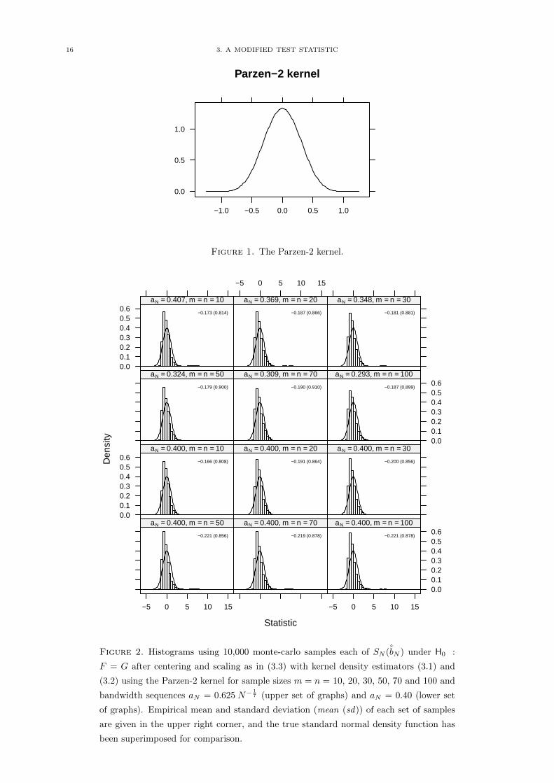
Each histogram in figure 2 shows the results of 10,000 monte-carlo simulations of the test statistic using
the centering and scaling shown above for increasing sample sizes of m = n = 10, 20, 30, 50, 70 and 100
with the true density function of the standard normal distribution N(0, 1) superimposed for comparison.
The upper set of simulations used a decreasing bandwidth sequence of aN = 0.625N−17 , while the lower
set used a constant bandwidth of aN = 0.40 as recommended in Behnen and Neuhaus (1989). The upper
right corner of each histogram includes the empirical mean and standard deviation of the simulated
samples.
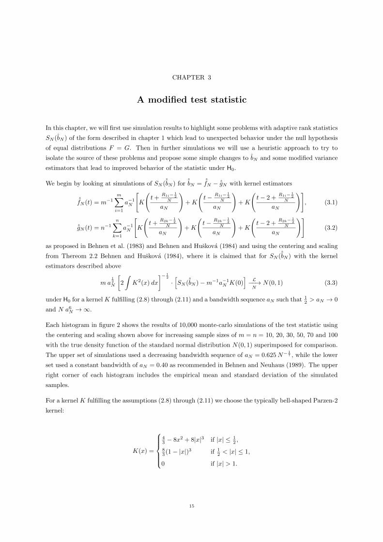
For a kernel K fulfilling the assumptions (2.8) through (2.11) we choose the typically bell-shaped Parzen-2
kernel:
K(x) =
43 − 8x2 + 8|x|3 if |x| ≤ 1
2 ,
83 (1− |x|)3 if 1
2 < |x| ≤ 1,
0 if |x| > 1.
15
16 3. A MODIFIED TEST STATISTIC
Parzen−2 kernel
0.0
0.5
1.0
−1.0 −0.5 0.0 0.5 1.0
Figure 1. The Parzen-2 kernel.
Statistic
Den
sity
0.00.10.20.30.40.50.6
−0.173 (0.814)
aN = 0.407, m = n = 10
−5 0 5 10 15
−0.187 (0.866)
aN = 0.369, m = n = 20
−0.181 (0.881)
aN = 0.348, m = n = 30
−0.179 (0.900)
aN = 0.324, m = n = 50
−0.190 (0.910)
aN = 0.309, m = n = 70
0.00.10.20.30.40.50.6
−0.187 (0.899)
aN = 0.293, m = n = 100
0.00.10.20.30.40.50.6
−0.166 (0.808)
aN = 0.400, m = n = 10
−0.191 (0.864)
aN = 0.400, m = n = 20
−0.200 (0.856)
aN = 0.400, m = n = 30
−5 0 5 10 15
−0.221 (0.856)
aN = 0.400, m = n = 50
−0.219 (0.878)
aN = 0.400, m = n = 70
−5 0 5 10 15
0.00.10.20.30.40.50.6
−0.221 (0.878)
aN = 0.400, m = n = 100
Figure 2. Histograms using 10,000 monte-carlo samples each of SN (ˆbN ) under H0 :
F = G after centering and scaling as in (3.3) with kernel density estimators (3.1) and
(3.2) using the Parzen-2 kernel for sample sizes m = n = 10, 20, 30, 50, 70 and 100 and
bandwidth sequences aN = 0.625 N−17 (upper set of graphs) and aN = 0.40 (lower set
of graphs). Empirical mean and standard deviation (mean (sd)) of each set of samples
are given in the upper right corner, and the true standard normal density function has
been superimposed for comparison.
3. A MODIFIED TEST STATISTIC 17
The simulations in figure 2 clearly show problems with centering and scaling in this case, as even for
quite large sample sizes of m = n = 100 the distribution still appears to be shifted too far to the left by
the centering term m−1a−1N K(0), and the mean does not appear to be approaching 0 as N increases. In
addition the distribution is obviously skewed to the right and the scaling factor of ma12
N (2∫K2(x)dx)−
12
seems to be overestimating the variance, although the standardized variance does appear to be moving
toward 1 for very large N .
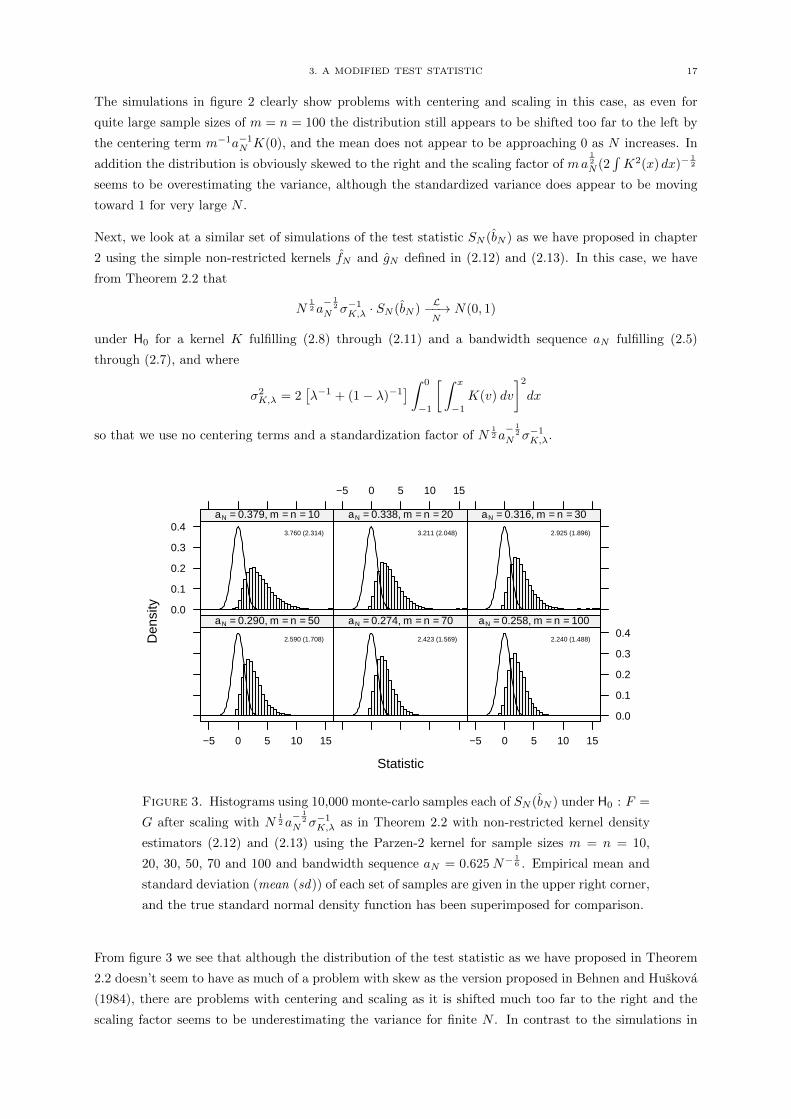
Next, we look at a similar set of simulations of the test statistic SN (bN ) as we have proposed in chapter
2 using the simple non-restricted kernels fN and gN defined in (2.12) and (2.13). In this case, we have
from Theorem 2.2 that
N12 a− 1
2
N σ−1K,λ · SN (bN )L−−→N
N(0, 1)
under H0 for a kernel K fulfilling (2.8) through (2.11) and a bandwidth sequence aN fulfilling (2.5)
through (2.7), and where
σ2K,λ = 2
[λ−1 + (1− λ)−1
] ∫ 0
−1
[ ∫ x
−1K(v) dv
]2dx
so that we use no centering terms and a standardization factor of N12 a− 1
2
N σ−1K,λ.
Statistic
Den
sity 0.0
0.1
0.2
0.3
0.43.760 (2.314)
aN = 0.379, m = n = 10
−5 0 5 10 15
3.211 (2.048)
aN = 0.338, m = n = 20
2.925 (1.896)
aN = 0.316, m = n = 30
−5 0 5 10 15
2.590 (1.708)
aN = 0.290, m = n = 50
2.423 (1.569)
aN = 0.274, m = n = 70
−5 0 5 10 15
0.0
0.1
0.2
0.3
0.42.240 (1.488)
aN = 0.258, m = n = 100
Figure 3. Histograms using 10,000 monte-carlo samples each of SN (bN ) under H0 : F =
G after scaling with N12 a− 1
2
N σ−1K,λ as in Theorem 2.2 with non-restricted kernel density
estimators (2.12) and (2.13) using the Parzen-2 kernel for sample sizes m = n = 10,
20, 30, 50, 70 and 100 and bandwidth sequence aN = 0.625 N−16 . Empirical mean and
standard deviation (mean (sd)) of each set of samples are given in the upper right corner,
and the true standard normal density function has been superimposed for comparison.
From figure 3 we see that although the distribution of the test statistic as we have proposed in Theorem
2.2 doesn’t seem to have as much of a problem with skew as the version proposed in Behnen and Huskova
(1984), there are problems with centering and scaling as it is shifted much too far to the right and the
scaling factor seems to be underestimating the variance for finite N . In contrast to the simulations in
18 3. A MODIFIED TEST STATISTIC
figure 2 there is notable improvement as N gets larger, but even for sample sizes as large as m = n = 100
the simulations indicate that the standard normal distribution obviously cannot be used to determine
critical values or get valid p-values even for large finite N .
The centering problem is due to the construction of the sum in
SN (bN ) = m−1m∑i=1
[fN − gN
]◦ HN (Xi)
which requires that fN be evaluated at each of the HN (Xi), 1 ≤ i ≤ m. Since fN (t) = m−1a−1N∑mj=1K(a−1N (t−
HN (Xj))) the result is a double sum over all 1 ≤ i ≤ m and 1 ≤ j ≤ m combinations, forcing the in-
clusion of the positive constant term m−1a−1N K(0) when i = j – in total m times – leading to a positive
shift in SN (bN ) of m−1a−1N K(0).
This is basically a nuisance constant independent of F and G which is present under H0 as well as H1,
doesn’t contribute to the power of the test and disappears asymptotically - even after scaling - as N →∞.
In this case the centering problem can be solved quickly by replacing fN by
f0N (t) = m(m− 1)−1fN (t)− (m− 1)−1a−1N K(0).
This drops the i = j terms from the double sum mentioned above and eliminates the shift in SN (bN ).
Using f0N in place of fN in SN (bN ), we can define
SN (b0N ) = m−1m∑i=1
[f0N − gN
]◦ (N−1R1i)
which is centered under H0 for all finite N , since for F = G we have
E[SN (b0N )
]= E
[m−1
m∑i=1
[f0N (N−1R1i)− gN (N−1R1i)
]]
= E
[m−1
m∑i=1
[m(m− 1)−1fN (N−1R1i)− (m− 1)−1a−1N K(0)
]−m−1
m∑i=1
gN (N−1R1i)
]
= E
[m−1
m∑i=1
[m(m− 1)−1m−1a−1N
m∑j=1
K(a−1N (HN (Xi)− HN (Xj))
)
− (m− 1)−1a−1N K(0)]−m−1
m∑i=1
n−1a−1N
n∑k=1
K(a−1N (HN (Xi)− HN (Yk))
)]
= E
[m−1(m− 1)−1a−1N
∑1≤i 6=j≤m
K(a−1N (HN (Xi)− HN (Xj))
)
−m−1n−1a−1Nm∑i=1
n∑k=1
K(a−1N (HN (Xi)− HN (Yk))
)]= m−1(m− 1)−1a−1N
∑1≤i 6=j≤m
E[K(a−1N (HN (Xi)− HN (Xj))
)]
−m−1n−1a−1Nm∑i=1
n∑k=1
E[K(a−1N (HN (Xi)− HN (Yk))
)]= a−1N E
[K(a−1N (HN (X1)− HN (X2))
)]− a−1N E
[K(a−1N (HN (X1)− HN (X2))
)]= 0.
3. A MODIFIED TEST STATISTIC 19
It is also easy to see that replacing SN (bN ) by SN (b0N ) and using the scaling factor N12 a− 1
2
N σ−1K,λ of
Theorem 2.2 results in an asymptotically equivalent test, as
E[SN (bN )− SN (b0N )
]2= E
[m−1
m∑i=1
[fN − gN
]◦ HN (Xi)−m−1
m∑i=1
[f0N − gN
]◦ HN (Xi)
]2
= E
[m−1
m∑i=1
[fN − f0N
]◦ HN (Xi)
]2
= E
[m−1
m∑i=1
−(m− 1)−1[fN (HN (Xi)) + a−1N K(0)
]]2
= E
[−m−1(m− 1)−1
m∑i=1
[m−1a−1N
m∑j=1
K(a−1N (HN (Xi)− HN (Xj))
)+ a−1N K(0)
]]2
= E
[m−2(m− 1)−1a−1N
m∑i=1
m∑j=1
[K(a−1N (HN (Xi)− HN (Xj))
)+K(0)
]]2
≤ E
[m−2(m− 1)−1a−1N
m∑i=1
m∑j=1
2 ‖K‖]2
= E[2 (m− 1)−1a−1N ‖K‖
]2= 4 (m− 1)−2a−2N ‖K‖
2
= O(N−2a−2N ),
and thus
N12 a− 1
2
N σ−1K,λ ·∣∣∣SN (bN )− SN (b0N )
∣∣∣= O(N
12 a− 1
2
N ) ·OP (N−1a−1N )
= OP (N−12 a− 3
2
N )
= oP (1).
Simulations using the modified SN (b0N ) with the scaling factor of N12 a− 1
2
N σ−1K,λ as in Theorem 2.2 are
shown in figure 4.
20 3. A MODIFIED TEST STATISTIC
Statistic
Den
sity 0.0
0.1
0.2
0.3
0.4−0.023 (2.482)
aN = 0.379, m = n = 10
−5 0 5 10 15
0.001 (2.135)
aN = 0.338, m = n = 20
0.025 (1.917)
aN = 0.316, m = n = 30
−5 0 5 10 15
0.012 (1.725)
aN = 0.290, m = n = 50
0.000 (1.617)
aN = 0.274, m = n = 70
−5 0 5 10 15
0.0
0.1
0.2
0.3
0.40.018 (1.537)
aN = 0.258, m = n = 100
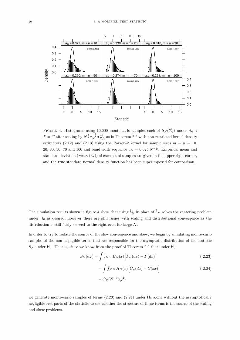
Figure 4. Histograms using 10,000 monte-carlo samples each of SN (b0N ) under H0 :
F = G after scaling by N12 a− 1
2
N σ−1K,λ as in Theorem 2.2 with non-restricted kernel density
estimators (2.12) and (2.13) using the Parzen-2 kernel for sample sizes m = n = 10,
20, 30, 50, 70 and 100 and bandwidth sequence aN = 0.625 N−16 . Empirical mean and
standard deviation (mean (sd)) of each set of samples are given in the upper right corner,
and the true standard normal density function has been superimposed for comparison.
The simulation results shown in figure 4 show that using b0N in place of bN solves the centering problem
under H0 as desired, however there are still issues with scaling and distributional convergence as the
distribution is still fairly skewed to the right even for large N .
In order to try to isolate the source of the slow convergence and skew, we begin by simulating monte-carlo
samples of the non-negligible terms that are responsible for the asymptotic distribution of the statistic
SN under H0. That is, since we know from the proof of Theorem 2.2 that under H0
SN (bN ) =
∫fN ◦HN (x)
[Fm(dx)− F (dx)
]( 2.23)
−∫fN ◦HN (x)
[Gn(dx)−G(dx)
]( 2.24)
+OP (N−1a−2N )
we generate monte-carlo samples of terms (2.23) and (2.24) under H0 alone without the asymptotically
negligible rest parts of the statistic to see whether the structure of these terms is the source of the scaling
and skew problems.
3. A MODIFIED TEST STATISTIC 21
Statistic
Den
sity 0.0
0.1
0.2
0.3
0.4 0.012 (0.887)
aN = 0.379, m = n = 10
−4 −2 0 2 4
0.013 (0.872)
aN = 0.338, m = n = 20
0.016 (0.876)
aN = 0.316, m = n = 30
−4 −2 0 2 4
−0.008 (0.888)
aN = 0.290, m = n = 50
−0.008 (0.897)
aN = 0.274, m = n = 70
−4 −2 0 2 4
0.0
0.1
0.2
0.3
0.4−0.009 (0.898)
aN = 0.258, m = n = 100
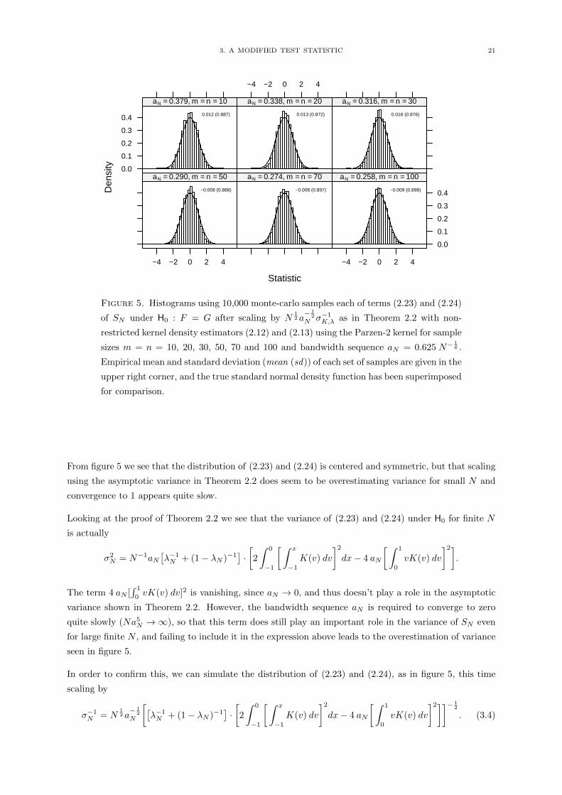
Figure 5. Histograms using 10,000 monte-carlo samples each of terms (2.23) and (2.24)
of SN under H0 : F = G after scaling by N12 a− 1
2
N σ−1K,λ as in Theorem 2.2 with non-
restricted kernel density estimators (2.12) and (2.13) using the Parzen-2 kernel for sample
sizes m = n = 10, 20, 30, 50, 70 and 100 and bandwidth sequence aN = 0.625 N−16 .
Empirical mean and standard deviation (mean (sd)) of each set of samples are given in the
upper right corner, and the true standard normal density function has been superimposed
for comparison.
From figure 5 we see that the distribution of (2.23) and (2.24) is centered and symmetric, but that scaling
using the asymptotic variance in Theorem 2.2 does seem to be overestimating variance for small N and
convergence to 1 appears quite slow.
Looking at the proof of Theorem 2.2 we see that the variance of (2.23) and (2.24) under H0 for finite N
is actually
σ2N = N−1aN
[λ−1N + (1− λN )−1
]·[2
∫ 0
−1
[ ∫ x
−1K(v) dv
]2dx− 4 aN
[ ∫ 1
0
vK(v) dv
]2].
The term 4 aN [∫ 1
0vK(v) dv]2 is vanishing, since aN → 0, and thus doesn’t play a role in the asymptotic
variance shown in Theorem 2.2. However, the bandwidth sequence aN is required to converge to zero
quite slowly (Na5N →∞), so that this term does still play an important role in the variance of SN even
for large finite N , and failing to include it in the expression above leads to the overestimation of variance
seen in figure 5.
In order to confirm this, we can simulate the distribution of (2.23) and (2.24), as in figure 5, this time
scaling by
σ−1N = N12 a− 1
2
N
[[λ−1N + (1− λN )−1
]·[2
∫ 0
−1
[ ∫ x
−1K(v) dv
]2dx− 4 aN
[ ∫ 1
0
vK(v) dv
]2]]− 12
. (3.4)
22 3. A MODIFIED TEST STATISTIC
Statistic
Den
sity 0.0
0.1
0.2
0.3
0.4 0.001 (1.056)
aN = 0.379, m = n = 10
−4 −2 0 2 4
−0.009 (1.025)
aN = 0.338, m = n = 20
0.000 (1.003)
aN = 0.316, m = n = 30
−4 −2 0 2 4
−0.021 (1.005)
aN = 0.290, m = n = 50
0.007 (1.007)
aN = 0.274, m = n = 70
−4 −2 0 2 4
0.0
0.1
0.2
0.3
0.40.011 (1.003)
aN = 0.258, m = n = 100
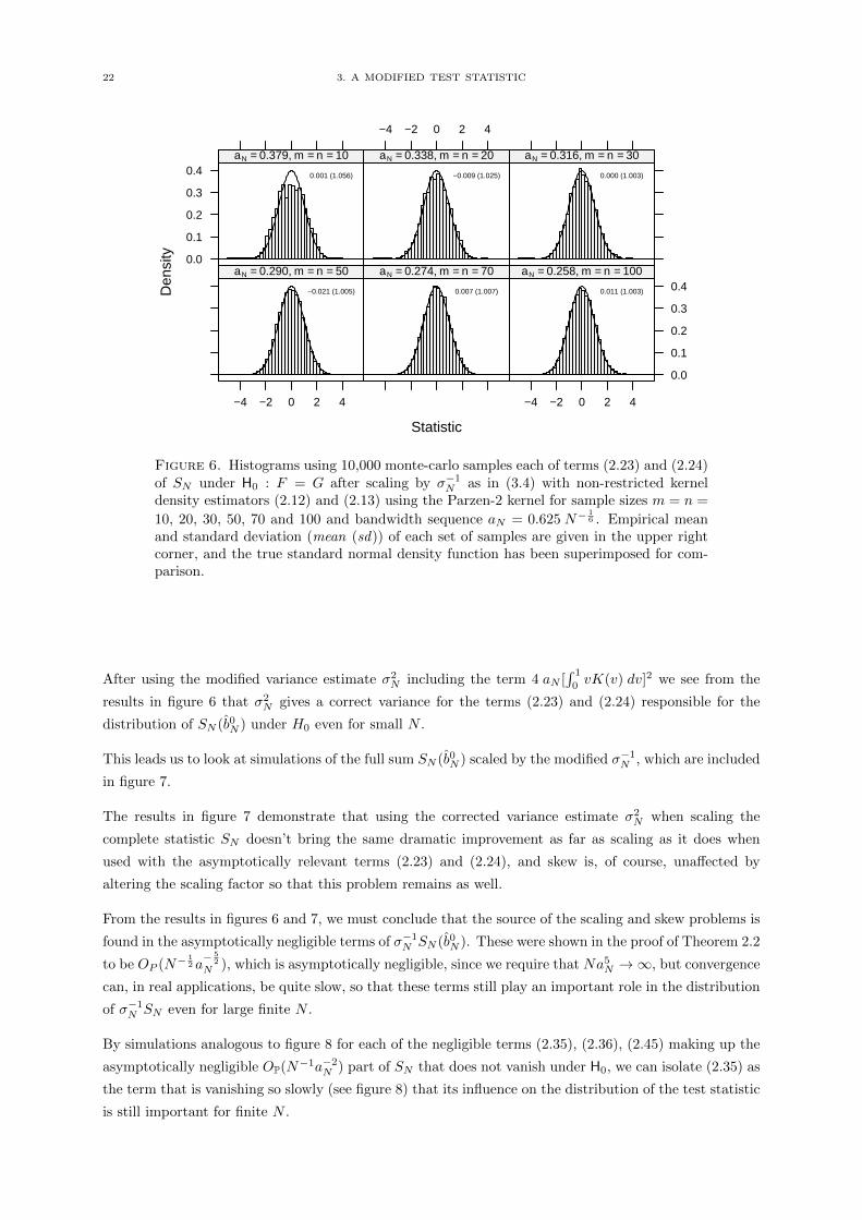
Figure 6. Histograms using 10,000 monte-carlo samples each of terms (2.23) and (2.24)of SN under H0 : F = G after scaling by σ−1N as in (3.4) with non-restricted kerneldensity estimators (2.12) and (2.13) using the Parzen-2 kernel for sample sizes m = n =
10, 20, 30, 50, 70 and 100 and bandwidth sequence aN = 0.625 N−16 . Empirical mean
and standard deviation (mean (sd)) of each set of samples are given in the upper rightcorner, and the true standard normal density function has been superimposed for com-parison.
After using the modified variance estimate σ2N including the term 4 aN [
∫ 1
0vK(v) dv]2 we see from the
results in figure 6 that σ2N gives a correct variance for the terms (2.23) and (2.24) responsible for the
distribution of SN (b0N ) under H0 even for small N .
This leads us to look at simulations of the full sum SN (b0N ) scaled by the modified σ−1N , which are included
in figure 7.
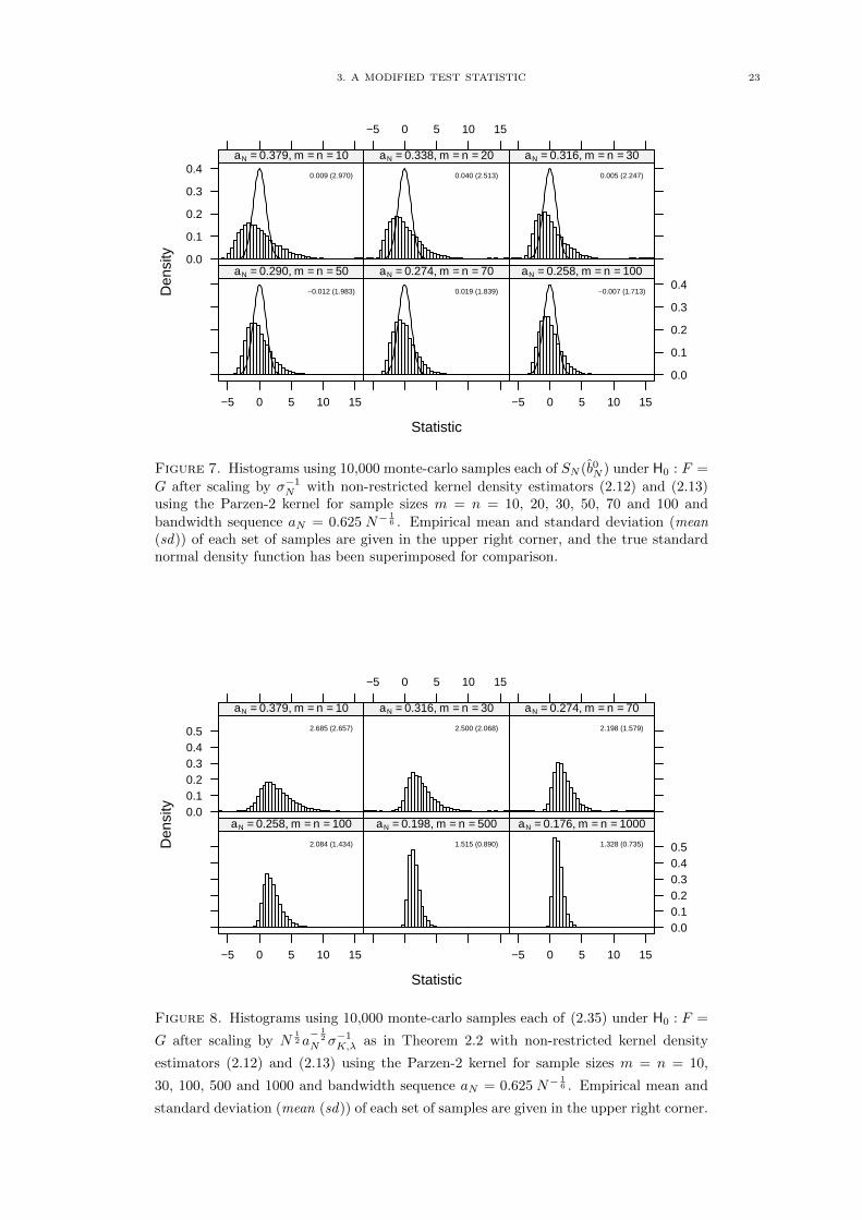
The results in figure 7 demonstrate that using the corrected variance estimate σ2N when scaling the
complete statistic SN doesn’t bring the same dramatic improvement as far as scaling as it does when
used with the asymptotically relevant terms (2.23) and (2.24), and skew is, of course, unaffected by
altering the scaling factor so that this problem remains as well.
From the results in figures 6 and 7, we must conclude that the source of the scaling and skew problems is
found in the asymptotically negligible terms of σ−1N SN (b0N ). These were shown in the proof of Theorem 2.2
to be OP (N−12 a− 5
2
N ), which is asymptotically negligible, since we require that Na5N →∞, but convergence
can, in real applications, be quite slow, so that these terms still play an important role in the distribution
of σ−1N SN even for large finite N .
By simulations analogous to figure 8 for each of the negligible terms (2.35), (2.36), (2.45) making up the
asymptotically negligible OP(N−1a−2N ) part of SN that does not vanish under H0, we can isolate (2.35) as
the term that is vanishing so slowly (see figure 8) that its influence on the distribution of the test statistic
is still important for finite N .
3. A MODIFIED TEST STATISTIC 23
Statistic
Den
sity 0.0
0.1
0.2
0.3
0.40.009 (2.970)
aN = 0.379, m = n = 10
−5 0 5 10 15
0.040 (2.513)
aN = 0.338, m = n = 20
0.005 (2.247)
aN = 0.316, m = n = 30
−5 0 5 10 15
−0.012 (1.983)
aN = 0.290, m = n = 50
0.019 (1.839)
aN = 0.274, m = n = 70
−5 0 5 10 15
0.0
0.1
0.2
0.3
0.4−0.007 (1.713)
aN = 0.258, m = n = 100
Figure 7. Histograms using 10,000 monte-carlo samples each of SN (b0N ) under H0 : F =
G after scaling by σ−1N with non-restricted kernel density estimators (2.12) and (2.13)using the Parzen-2 kernel for sample sizes m = n = 10, 20, 30, 50, 70 and 100 andbandwidth sequence aN = 0.625 N−
16 . Empirical mean and standard deviation (mean
(sd)) of each set of samples are given in the upper right corner, and the true standardnormal density function has been superimposed for comparison.
Statistic
Den
sity 0.0
0.10.20.30.40.5 2.685 (2.657)
aN = 0.379, m = n = 10
−5 0 5 10 15
2.500 (2.068)
aN = 0.316, m = n = 30
2.198 (1.579)
aN = 0.274, m = n = 70
−5 0 5 10 15
2.084 (1.434)
aN = 0.258, m = n = 100
1.515 (0.890)
aN = 0.198, m = n = 500
−5 0 5 10 15
0.00.10.20.30.40.51.328 (0.735)
aN = 0.176, m = n = 1000
Figure 8. Histograms using 10,000 monte-carlo samples each of (2.35) under H0 : F =
G after scaling by N12 a− 1
2
N σ−1K,λ as in Theorem 2.2 with non-restricted kernel density
estimators (2.12) and (2.13) using the Parzen-2 kernel for sample sizes m = n = 10,
30, 100, 500 and 1000 and bandwidth sequence aN = 0.625 N−16 . Empirical mean and
standard deviation (mean (sd)) of each set of samples are given in the upper right corner.
24 3. A MODIFIED TEST STATISTIC
The results in figure 8 show how (2.35) contributes to the variance and skew of the distribution of SN ,
and that although it is vanishing as N →∞, actual convergence is very slow with sizable variance even
for sample sizes as large as m = n = 1000.
Looking more closely at the form of (2.35) under H0 we find∫ [fN − gN − (fN − gN )
]◦HN (x)
[Fm(dx)− F (dx)
]=
∫ [fN − gN
]◦HN (x)
[Fm(dx)− F (dx)
]=
∫ [m−1a−1N
m∑j=1
K(a−1N (HN (x)− HN (Xj))
)
− n−1a−1Nn∑k=1
K(a−1N (HN (x)− HN (Yk))
)][Fm(dx)− F (dx)
]
=
∫m−1a−1N
m∑j=1
K(a−1N (HN (x)− HN (Xj))
)[Fm(dx)− F (dx)
]
−∫n−1a−1N
n∑k=1
K(a−1N (HN (x)− HN (Yk))
)[Fm(dx)− F (dx)
]
= m−1m∑i=1
[m−1a−1N
m∑j=1
K(a−1N (HN (Xi)− HN (Xj))
)
−∫m−1a−1N
m∑j=1
K(a−1N (HN (x)− HN (Xj))
)F (dx)
]
−m−1m∑i=1
[n−1a−1N
n∑k=1
K(a−1N (HN (Xi)− HN (Yk))
)−∫n−1a−1N
n∑k=1
K(a−1N (HN (x)− HN (Yk))
)F (dx)
]
= m−2a−1N
m∑i=1
m∑j=1
[K(a−1N (HN (Xi)− HN (Xj))
)−∫K(a−1N (HN (x)− HN (Xj))
)F (dx)
]
−m−1n−1a−1Nm∑i=1
n∑k=1
[K(a−1N (HN (Xi)− HN (Yk))
)−∫K(a−1N (HN (x)− HN (Yk))
)F (dx)
]
= m−2a−1N
m∑i=1
m∑j=1
[K(a−1N (HN (Xi)− HN (Xj))
)−∫K1
0
(a−1N (v − HN (Xj))
)dv
]
−m−1n−1a−1Nm∑i=1
n∑k=1
[K(a−1N (HN (Xi)− HN (Yk))
)−∫ 1
0
K(a−1N (v − HN (Yk))
)dv
].
From this, we see that the first sum above making up (2.35) comprises summands of the form
K(a−1N (HN (Xi)− HN (Xj))
)−∫ 1
0
K(a−1N (v − HN (Xj))
)dv
which is simply the difference between a kernel with bandwidth aN centered at HN (Xj) = N−1R1j
evaluated at HN (Xi) and the area under the same kernel contained within the interval [0, 1]. The form
of these summands turns out to be the source of the right skew and slow convergence to 0 of (2.35).
3. A MODIFIED TEST STATISTIC 25
In samples where, for example, the Xi occupy most of the smaller positions in the total sample (i.e. where
almost all R1i are smaller than the R2k) large portions of many of the kernels K(a−1N (t−N−1R1j)) will
not be contained on [0, 1] making∫ 1
0K(a−1N (v −N−1R1j)) dv small while at the same time many of the
HN (Xi) will be close to the centers of the bell-shaped kernels at N−1R1j where they reach their maximum
making the K(a−1N (HN (Xi)−N−1R1j)) large. The effect when Xi occupy most of the larger positions in
the total sample is the same by analogy. This allows (2.35) to become quite large and disappear slowly,
since such samples occur with some probability even under H0. Reducing the bandwidth aN in order to
allow more of the kernels K(a−1N (t − N−1R1j)) to be contained on [0, 1] unfortunately doesn’t improve
the situation, since a−1N is a factor in the sum as well leading immediately to kernels with higher peaks,
which can exacerbate the problem detailed above.
Since the convergence problem is, in essence, caused by the relative difference between the maximum
height of the bell-shaped K at its peak and areas like∫ 1
0K(a−1N (v − N−1R1j)) dv, we can attempt to
reduce these differences and improve convergence by switching from a fairly steep bell-shaped kernel like
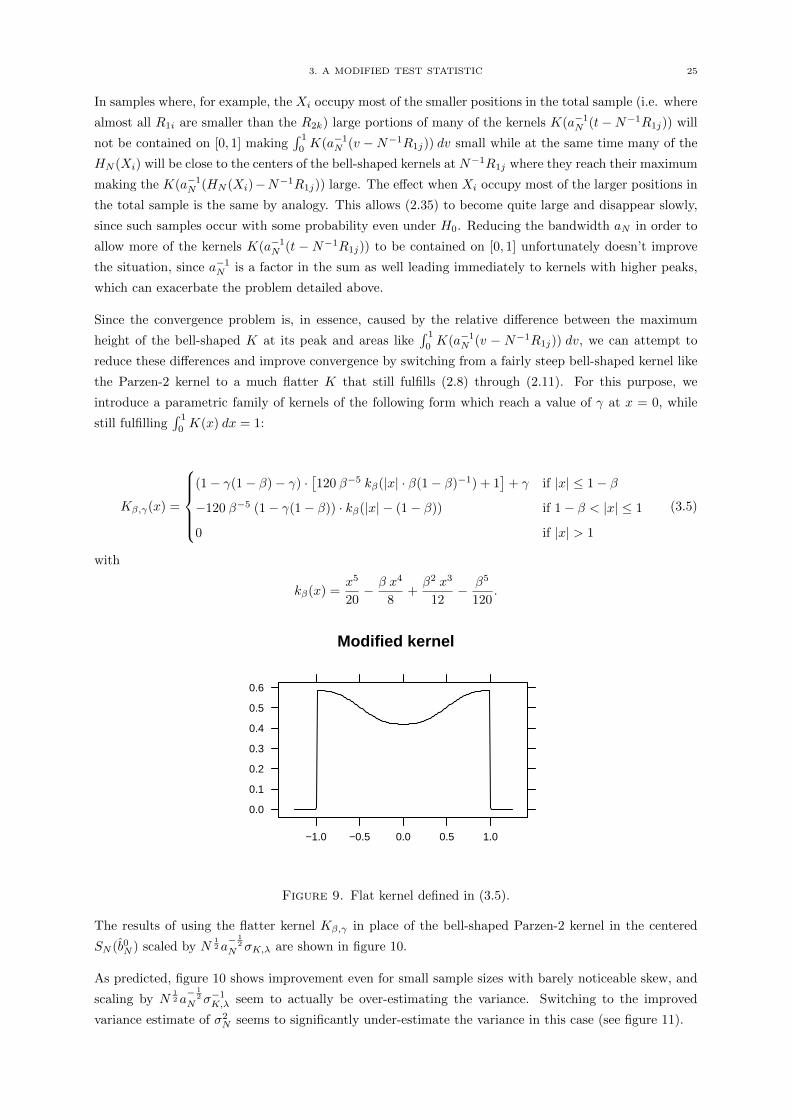
the Parzen-2 kernel to a much flatter K that still fulfills (2.8) through (2.11). For this purpose, we
introduce a parametric family of kernels of the following form which reach a value of γ at x = 0, while
still fulfilling∫ 1
0K(x) dx = 1:
Kβ,γ(x) =
(1− γ(1− β)− γ) ·
[120 β−5 kβ(|x| · β(1− β)−1) + 1
]+ γ if |x| ≤ 1− β
−120 β−5 (1− γ(1− β)) · kβ(|x| − (1− β)) if 1− β < |x| ≤ 1
0 if |x| > 1
(3.5)
with
kβ(x) =x5
20− β x4
8+β2 x3
12− β5
120.
Modified kernel
0.0
0.1
0.2
0.3
0.4
0.5
0.6
−1.0 −0.5 0.0 0.5 1.0
Figure 9. Flat kernel defined in (3.5).
The results of using the flatter kernel Kβ,γ in place of the bell-shaped Parzen-2 kernel in the centered
SN (b0N ) scaled by N12 a− 1
2
N σK,λ are shown in figure 10.
As predicted, figure 10 shows improvement even for small sample sizes with barely noticeable skew, and
scaling by N12 a− 1
2
N σ−1K,λ seem to actually be over-estimating the variance. Switching to the improved
variance estimate of σ2N seems to significantly under-estimate the variance in this case (see figure 11).

26 3. A MODIFIED TEST STATISTIC
Statistic
Den
sity 0.0
0.1
0.2
0.3
0.4−0.011 (1.055)
aN = 0.379, m = n = 10
−4 −2 0 2 4
−0.008 (0.981)
aN = 0.338, m = n = 20
0.003 (0.943)
aN = 0.316, m = n = 30
−4 −2 0 2 4
0.008 (0.925)
aN = 0.290, m = n = 50
0.018 (0.915)
aN = 0.274, m = n = 70
−4 −2 0 2 4
0.0
0.1
0.2
0.3
0.40.015 (0.914)
aN = 0.258, m = n = 100
Figure 10. Histograms using 10,000 monte-carlo samples each of SN (b0N ) under H0 :
F = G after scaling by N12 a− 1
2
N σ−1K,λ as in Theorem 2.2 with non-restricted kernel density
estimators (2.12) and (2.13) using the modified flattened kernel Kβ,γ with β = 0.01and γ = 0.42 for sample sizes m = n = 10, 20, 30, 50, 70 and 100 and bandwidthsequence aN = 0.625N−
16 . Empirical mean and standard deviation (mean (sd)) of each
set of samples are given in the upper right corner, and the true standard normal densityfunction has been superimposed for comparison.
Since we know that the distribution of SN (b0N ) is determined under H0 for finite N by the terms (2.23),
(2.24) and (2.35) we can try to find a more accurate variance estimate for SN (b0N ) by attempting to
incorporate the variance of (2.35) for finite N even though this term is asymptotically negligible. In
order to do this, define σ22N as the combined variance of (2.23) and (2.24) and the theoretical analog of
(2.35). That is, let
σ22N = Var
[ ∫fN ◦HN (x)
[Fm(dx)− F (dx)
]−∫fN ◦HN (x)
[Gn(dx)−G(dx)
](3.6)
+m−2a−1N
m∑i=1
m∑j=1
[K(a−1N (HN (Xi)−HN (Xj))
)−∫K(a−1N (HN (x)−HN (Xj))
)F (dx)
](3.7)
−m−1n−1a−1Nm∑i=1
n∑k=1
[K(a−1N (HN (Xi)−HN (Yk))
)−∫K(a−1N (HN (x)−HN (Yk))
)F (dx)
]](3.8)
under H0.
We already know from lemmas 5.33 and 5.34 that the variance of (3.6) is equal to σ2N . Lemma 5.36 shows
that the covariance between (3.6) and (3.7) (3.8) vanishes under H0 for all N and lemma 5.35 gives the
variance of (3.7) and (3.8) under H0, so that combining these results we have
σ22N = σ2
N +m−1(m− 1)−1[[a−1N
∫ 1
−1K2(v) dv − 2
∫ 1
0
vK2(v) dv
]
+ (2n+m− 1)n−1[1− 4 aN
∫ 1
0
vK(v) dv + 4 a2N
[ ∫ 1
0
vK(v) dv
]2]
3. A MODIFIED TEST STATISTIC 27
− (1 + 2n−1)
[1 + 2 aN
∫ 0
−1
[ ∫ x
−1K(v) dv
]2dx− 4 aN
∫ 1
0
vK(v) dv
]](3.9)
Statistic
Den
sity 0.0
0.1
0.2
0.3
0.40.000 (1.655)
aN = 0.379, m = n = 10
−4 −2 0 2 4
−0.006 (1.429)
aN = 0.338, m = n = 20
−0.013 (1.289)
aN = 0.316, m = n = 30
−4 −2 0 2 4
0.001 (1.222)
aN = 0.290, m = n = 50
0.011 (1.190)
aN = 0.274, m = n = 70
−4 −2 0 2 4
0.0
0.1
0.2
0.3
0.4−0.008 (1.154)
aN = 0.258, m = n = 100
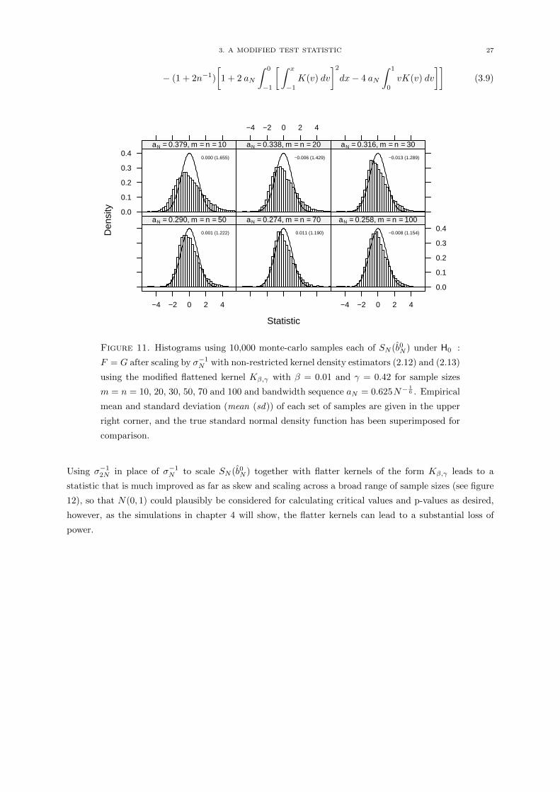
Figure 11. Histograms using 10,000 monte-carlo samples each of SN (b0N ) under H0 :
F = G after scaling by σ−1N with non-restricted kernel density estimators (2.12) and (2.13)
using the modified flattened kernel Kβ,γ with β = 0.01 and γ = 0.42 for sample sizes
m = n = 10, 20, 30, 50, 70 and 100 and bandwidth sequence aN = 0.625N−16 . Empirical
mean and standard deviation (mean (sd)) of each set of samples are given in the upper
right corner, and the true standard normal density function has been superimposed for
comparison.
Using σ−12N in place of σ−1N to scale SN (b0N ) together with flatter kernels of the form Kβ,γ leads to a
statistic that is much improved as far as skew and scaling across a broad range of sample sizes (see figure
12), so that N(0, 1) could plausibly be considered for calculating critical values and p-values as desired,
however, as the simulations in chapter 4 will show, the flatter kernels can lead to a substantial loss of
power.
28 3. A MODIFIED TEST STATISTIC
Statistic
Den
sity 0.0
0.1
0.2
0.3
0.4
0.50.003 (0.971)
aN = 0.379, m = n = 10
−4 −2 0 2 4
−0.008 (0.940)
aN = 0.338, m = n = 20
0.005 (0.933)
aN = 0.316, m = n = 30
−4 −2 0 2 4
0.007 (0.932)
aN = 0.290, m = n = 50
0.000 (0.961)
aN = 0.274, m = n = 70
−4 −2 0 2 4
0.0
0.1
0.2
0.3
0.4
0.50.021 (0.957)
aN = 0.258, m = n = 100
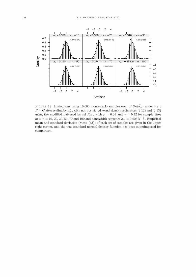
Figure 12. Histograms using 10,000 monte-carlo samples each of SN (b0N ) under H0 :
F = G after scaling by σ−12N with non-restricted kernel density estimators (2.12) and (2.13)using the modified flattened kernel Kβ,γ with β = 0.01 and γ = 0.42 for sample sizes
m = n = 10, 20, 30, 50, 70 and 100 and bandwidth sequence aN = 0.625N−16 . Empirical
mean and standard deviation (mean (sd)) of each set of samples are given in the upperright corner, and the true standard normal density function has been superimposed forcomparison.
CHAPTER 4
A simulation study
In the following we give the results of a series of simulations using different implementations of the
rank statistic SN with varying choices regarding the adaptive score function, scaling, kernel function K
and bandwidth sequence aN (see table 3). Of main interest will be comparisons between the statistic
SN (ˆbN ) using restricted kernel estimators (see (3.1) and (3.2)) as proposed by Behnen et al. (1983) and the
modified statistic SN (b0N ) as proposed in chapter 3 with scaling using the improved variance estimate σ22N
given in (3.9). We also include simulations using the fixed bandwidth sequence aN = 0.4 as recommended
in Behnen and Neuhaus (1989).
Since the simulations under H0 in chapter 3 clearly showed in almost all cases that the standard normal
distribution cannot be used to set valid critical values or calculate p-values, except where otherwise noted
critical values were determined either by calculating the exact distribution of the test statistic for small
sample sizes (m = n = 10) or by first using a set of 100,000 monte-carlo replications of the test statistic
under H0 to determine monte-carlo critical values for larger sample sizes (m = n = 20 or 30).
Table 4 shows the rejection rates of the various tests under H0. To explore the power of the proposed tests
under different kinds of non-trivial alternatives, we follow along the lines of Behnen and Neuhaus (1989)
and consider monte-carlo simulations under a collection of generalized shift alternatives that include the
classical exact shift model as well as alternatives that concentrate the shift between F and G in the lower,
central or upper part of the distribution (see figure 1).
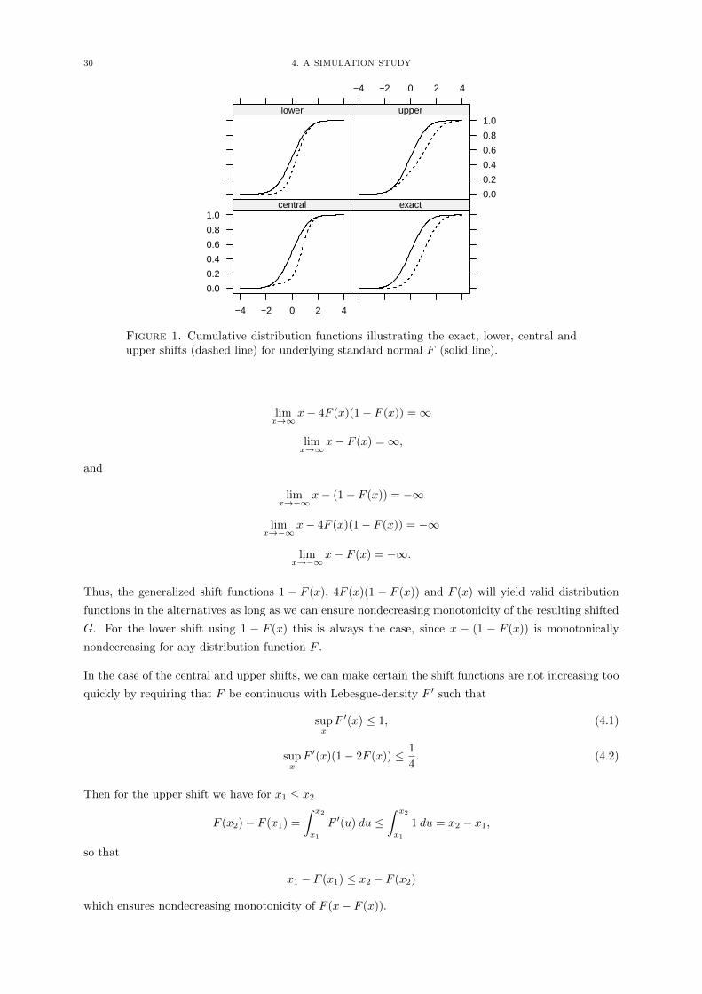
lower shift G(x) = F (x− (1− F (x)))
central shift G(x) = F (x− 4F (x)(1− F (x)))
upper shift G(x) = F (x− F (x))
exact shift G(x) = F (x− 1)
Table 1. Distribution functions of the lower, central, upper and exact shift alternatives
for an underlying distribution function F .
While the alternative G resulting from an exact shift is always a valid distribution function, this is not
immediately obvious for the other three generalized shifts. In the case of the lower, central and upper
shifts we see that as continous functions of the distribution function F , each of the alternative G are right
continuous with left limits, and that
limx→−∞
G(x) = 0 and limx→∞
G(x) = 1,
since
limx→∞
x− (1− F (x)) =∞
29
30 4. A SIMULATION STUDY
0.0
0.2
0.4
0.6
0.8
1.0
−4 −2 0 2 4
central exact
lower
−4 −2 0 2 4
0.0
0.2
0.4
0.6
0.8
1.0upper
Figure 1. Cumulative distribution functions illustrating the exact, lower, central andupper shifts (dashed line) for underlying standard normal F (solid line).
limx→∞
x− 4F (x)(1− F (x)) =∞
limx→∞
x− F (x) =∞,
and
limx→−∞
x− (1− F (x)) = −∞
limx→−∞
x− 4F (x)(1− F (x)) = −∞
limx→−∞
x− F (x) = −∞.
Thus, the generalized shift functions 1 − F (x), 4F (x)(1 − F (x)) and F (x) will yield valid distribution
functions in the alternatives as long as we can ensure nondecreasing monotonicity of the resulting shifted
G. For the lower shift using 1 − F (x) this is always the case, since x − (1 − F (x)) is monotonically
nondecreasing for any distribution function F .
In the case of the central and upper shifts, we can make certain the shift functions are not increasing too
quickly by requiring that F be continuous with Lebesgue-density F ′ such that
supxF ′(x) ≤ 1, (4.1)
supxF ′(x)(1− 2F (x)) ≤ 1
4. (4.2)
Then for the upper shift we have for x1 ≤ x2
F (x2)− F (x1) =
∫ x2
x1
F ′(u) du ≤∫ x2
x1
1 du = x2 − x1,
so that
x1 − F (x1) ≤ x2 − F (x2)
which ensures nondecreasing monotonicity of F (x− F (x)).
4. A SIMULATION STUDY 31
And in the case of the central shift with G(x) = F (x− 4F (x)(1− F (x))) we have for x1 ≤ x2
4[F (x2)(1− F (x2))− F (x1)(1− F (x1))
]= 4
∫ x2
x1
[F ′(u)(1− F (u)) + F (u)(−F ′(u))
]du
= 4
∫ x2
x1
F ′(u)(1− 2F (u)) du
≤ 4
∫ x2
x1
1
4du
= x2 − x1,
so that
x1 − 4F (x1)(1− F (x1)) ≤ x2 − 4F (x2)(1− F (x2))
which ensures monotonicity of F (x− 4F (x)(1− F (x))).
For the underlying distribution function F we use the standard normalN(0, 1), Logistic(0, 1) and Cauchy(0, 1)
distributions (see table 2). (4.1) is easily verified for these F , since their densities are symmetric about
0, attaining a maximum F ′(0) which is less than 1.
When verifying (4.2), we once again use the fact that each of the underlying F ′ are bounded by their
maximum at F ′(0).
For Logistic(0, 1) we actually have
F ′(0) =1
4,
so that (4.2) is fulfilled immediately, as 1− 2F (x) ≤ 1 everywhere.
For N(0, 1) and Cauchy(0, 1) we only need to be concerned with x such that x < F−1( 12 −
18F′(0)−1),
since for x ≥ F−1( 12 −
18F′(0)−1) we have
F ′(x)(1− 2F (x)) ≤ F ′(x)
[1− 2F
(F−1
(1
2− 1
8F ′(0)−1
))]≤ F ′(0)
[1− 2
(1
2− 1
8F ′(0)−1
)]= F ′(0)
1
4F ′(0)−1
=1
4.
For any x such that F ′(x) ≤ 14 we see that (4.2) is fulfilled as well, since 1 − 2F (x) ≤ 1 for all x. This
means that in the case of distributions such as N(0, 1) and Cauchy(0, 1) whose densities are monotonically
increasing on the interval (−∞, F−1(0)), (4.2) is fulfilled, when we can verify that the bound in (4.2)
holds for any x such that
inf
{x : F ′(x) ≥ 1
4
}< x < F−1
(1
2− 1
8F ′(0)−1
). (4.3)
As 1−2F (x) is monotonically nonincreasing everywhere and the three underlying densities used here are
monotonically increasing on the interval (−∞, F−1(0)), we know that on the interval (4.3)
F ′(x)(1− 2F (x)) ≤ F ′(F−1
(1
2− 1
8F ′(0)−1
))·[1− 2F
(inf
{x : F ′(x) ≥ 1
4
})],
32 4. A SIMULATION STUDY
which gives us an easy way to check (4.2).
For N(0, 1) we have
inf
{x : F ′(x) ≥ 1
4
}≈ −0.96664 and F−1
(1
2− 1
8F ′(0)−1
)≈ −0.890229,
so that
F ′(F−1
(1
2− 1
8F ′(0)−1
))·[1− 2F
(inf
{x : F ′(x) ≥ 1
4
})]≈ F ′(−0.8902299) · (1− 2F (−0.96664))
≈ 0.26842 · 0.66628
≤ 1
4.
And for Cauchy(0, 1) we have
inf
{x : F ′(x) ≥ 1
4
}≈ −0.5225 and F−1
(1
2− 1
8F ′(0)−1
)≈ −2.85329,
so that the interval in (4.3) is empty and (4.2) holds, since for all x either x ≥ F−1( 12 −
18F′(0)−1) or
F ′(x) ≤ 14 .
N(0, 1) F (x) =1√2π
∫ x
−∞exp
(− 1
2y2)dy
Logistic(0, 1) F (x) =exp(x)
1 + exp(x)
Cauchy(0, 1) F (x) =1
2+
1
πarctan(x)
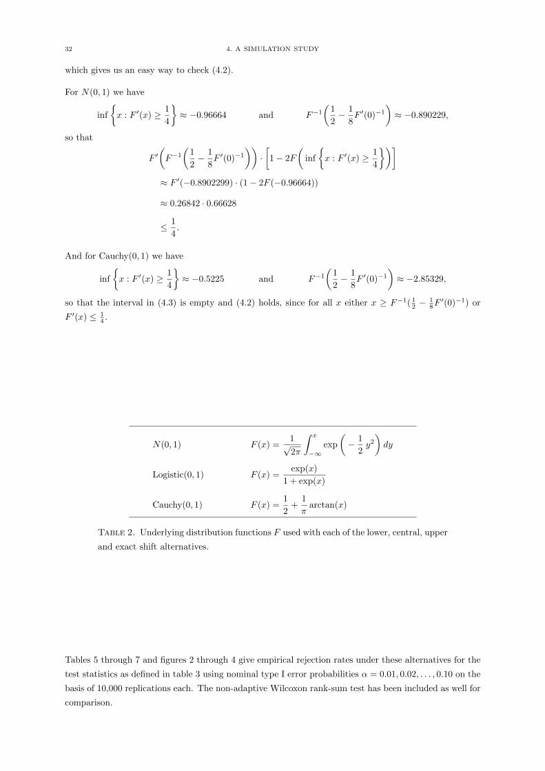
Table 2. Underlying distribution functions F used with each of the lower, central, upper
and exact shift alternatives.
Tables 5 through 7 and figures 2 through 4 give empirical rejection rates under these alternatives for the
test statistics as defined in table 3 using nominal type I error probabilities α = 0.01, 0.02, . . . , 0.10 on the
basis of 10,000 replications each. The non-adaptive Wilcoxon rank-sum test has been included as well for
comparison.
4. A SIMULATION STUDY 33
Legend Score function Scaling factor K aN Method
S1ˆbN ma
12
N [2∫K2(x) dx]−
12 Parzen-2 0.625 x−
17 exact (m = n = 10) or
monte-carlo (m = n =20, 30)
S2ˆbN ma
12
N [2∫K2(x) dx]−
12 Parzen-2 0.40 exact (m = n = 10) or
monte-carlo (m = n =20, 30)
S3 b0N N12 a− 1
2
N σ−1K,λ Parzen-2 0.625 x−16 exact (m = n = 10) or
monte-carlo (m = n =20, 30)
S4 b0N σ−12N Kγ,β 0.625 x−16 exact (m = n = 10) or
monte-carlo (m = n =20, 30)
S5 b0N σ−12N Kγ,β 0.625 x−16 asymptotic
S6 Rank-sum test exact (m = n = 10) orasymptotic (m = n =20, 30)
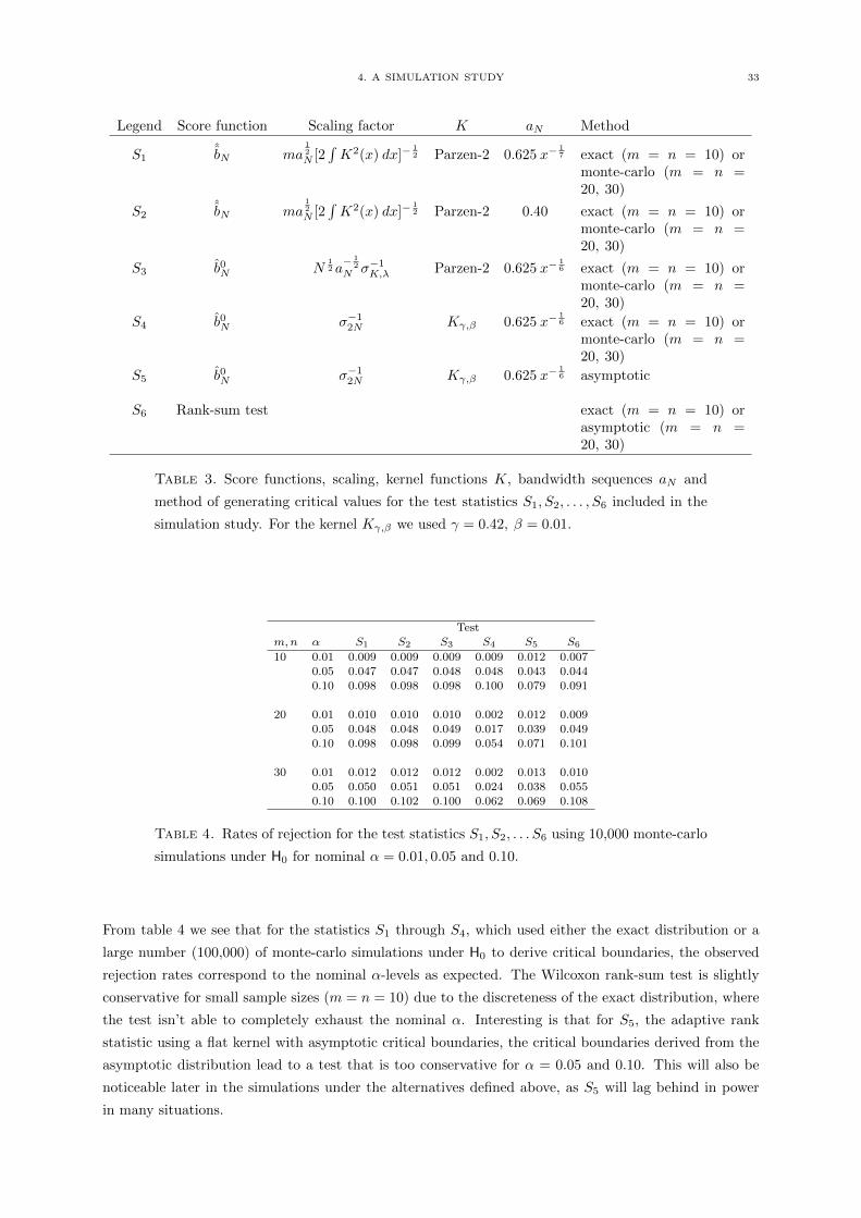
Table 3. Score functions, scaling, kernel functions K, bandwidth sequences aN and
method of generating critical values for the test statistics S1, S2, . . . , S6 included in the
simulation study. For the kernel Kγ,β we used γ = 0.42, β = 0.01.
Test
m,n α S1 S2 S3 S4 S5 S6
10 0.01 0.009 0.009 0.009 0.009 0.012 0.0070.05 0.047 0.047 0.048 0.048 0.043 0.044
0.10 0.098 0.098 0.098 0.100 0.079 0.091
20 0.01 0.010 0.010 0.010 0.002 0.012 0.009
0.05 0.048 0.048 0.049 0.017 0.039 0.049
0.10 0.098 0.098 0.099 0.054 0.071 0.101
30 0.01 0.012 0.012 0.012 0.002 0.013 0.010
0.05 0.050 0.051 0.051 0.024 0.038 0.0550.10 0.100 0.102 0.100 0.062 0.069 0.108
Table 4. Rates of rejection for the test statistics S1, S2, . . . S6 using 10,000 monte-carlo
simulations under H0 for nominal α = 0.01, 0.05 and 0.10.
From table 4 we see that for the statistics S1 through S4, which used either the exact distribution or a
large number (100,000) of monte-carlo simulations under H0 to derive critical boundaries, the observed
rejection rates correspond to the nominal α-levels as expected. The Wilcoxon rank-sum test is slightly
conservative for small sample sizes (m = n = 10) due to the discreteness of the exact distribution, where
the test isn’t able to completely exhaust the nominal α. Interesting is that for S5, the adaptive rank
statistic using a flat kernel with asymptotic critical boundaries, the critical boundaries derived from the
asymptotic distribution lead to a test that is too conservative for α = 0.05 and 0.10. This will also be
noticeable later in the simulations under the alternatives defined above, as S5 will lag behind in power
in many situations.
34 4. A SIMULATION STUDY
Significance level
Pow
er
0.0
0.2
0.4
0.6
● ● ● ● ● ● ● ● ● ●
● ● ● ● ● ● ● ● ● ●
m = n = 10lower shift
0.01 0.05 0.10
●● ● ●
● ● ● ● ● ●
●● ●
● ● ● ● ● ● ●
m = n = 20lower shift
●●
●●
●● ● ● ● ●
●●
●●
● ● ● ● ● ●
m = n = 30lower shift
●●
●●
●● ● ● ● ●
●●
● ● ●●
●●
● ●
m = n = 10central shift
●
●●
●●
●●
●● ●
●●
●●
●●
● ● ● ●
m = n = 20central shift
0.0
0.2
0.4
0.6
●
●
●●
●●
●●
● ●
●
●
●●
●●
●●
● ●
m = n = 30central shift
0.0
0.2
0.4
0.6
●● ● ● ● ● ● ● ● ●
●● ● ● ● ● ● ● ● ●
m = n = 10upper shift
●●
●●
●●
● ● ● ●
●●
●● ● ●
● ● ● ●
m = n = 20upper shift
●●
●●
●●
●● ● ●
●●
●●
●●
● ●● ●
m = n = 30upper shift
0.01 0.05 0.10
●●
●●
●● ● ●
● ●
●●
● ● ●●
●●
● ●
m = n = 10exact shift
●
●●
●●
●●
● ● ●
●
●
●●
●●
●● ●
●
m = n = 20exact shift
0.01 0.05 0.10
0.0
0.2
0.4
0.6
●
●
●●
●●
●● ● ●
●
●
●●
●●
●●
● ●
m = n = 30exact shift
S1 S2 S3 S4 S5 S6● ●
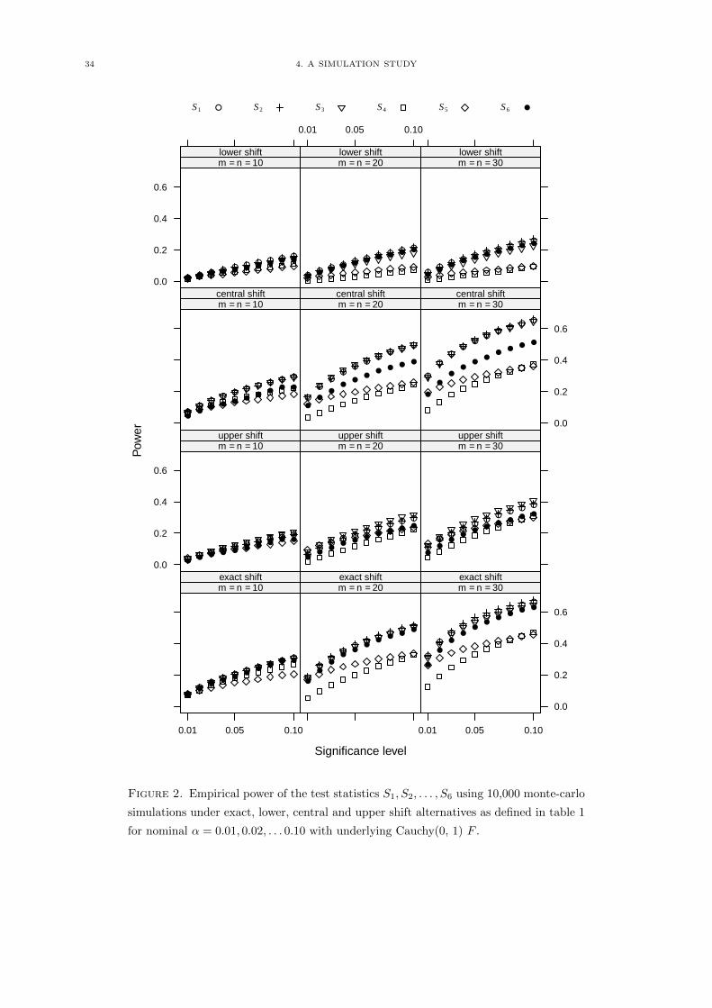
Figure 2. Empirical power of the test statistics S1, S2, . . . , S6 using 10,000 monte-carlo
simulations under exact, lower, central and upper shift alternatives as defined in table 1
for nominal α = 0.01, 0.02, . . . 0.10 with underlying Cauchy(0, 1) F .
4. A SIMULATION STUDY 35
Test
Shift m,n α S1 S2 S3 S4 S5 S6
lower 10 0.01 0.02 0.02 0.02 0.02 0.02 0.02
0.05 0.09 0.09 0.08 0.06 0.06 0.080.10 0.16 0.16 0.14 0.11 0.10 0.14
20 0.01 0.04 0.04 0.03 0.00 0.02 0.03
0.05 0.13 0.13 0.11 0.03 0.06 0.120.10 0.21 0.21 0.18 0.07 0.09 0.20
30 0.01 0.06 0.06 0.04 0.01 0.03 0.04
0.05 0.16 0.17 0.14 0.04 0.06 0.150.10 0.26 0.27 0.23 0.09 0.10 0.24
central 10 0.01 0.07 0.07 0.07 0.06 0.07 0.040.05 0.20 0.19 0.20 0.15 0.13 0.14
0.10 0.29 0.29 0.29 0.22 0.18 0.2320 0.01 0.16 0.16 0.17 0.04 0.12 0.11
0.05 0.36 0.36 0.37 0.14 0.20 0.27
0.10 0.49 0.49 0.50 0.25 0.26 0.3930 0.01 0.30 0.29 0.29 0.08 0.19 0.18
0.05 0.52 0.53 0.53 0.25 0.29 0.39
0.10 0.65 0.66 0.65 0.37 0.36 0.51
upper 10 0.01 0.03 0.03 0.04 0.04 0.04 0.02
0.05 0.11 0.11 0.13 0.12 0.10 0.090.10 0.19 0.19 0.21 0.20 0.15 0.16
20 0.01 0.06 0.07 0.08 0.02 0.09 0.05
0.05 0.19 0.19 0.21 0.12 0.17 0.160.10 0.29 0.30 0.32 0.22 0.24 0.25
30 0.01 0.11 0.11 0.12 0.04 0.13 0.080.05 0.26 0.27 0.29 0.19 0.23 0.22
0.10 0.38 0.39 0.41 0.31 0.30 0.32
exact 10 0.01 0.08 0.08 0.08 0.07 0.08 0.07
0.05 0.20 0.20 0.21 0.18 0.15 0.19
0.10 0.31 0.31 0.30 0.27 0.20 0.2920 0.01 0.18 0.19 0.18 0.05 0.17 0.16
0.05 0.39 0.39 0.38 0.20 0.27 0.36
0.10 0.51 0.52 0.51 0.33 0.34 0.4930 0.01 0.32 0.32 0.31 0.12 0.26 0.26
0.05 0.55 0.56 0.53 0.33 0.38 0.50
0.10 0.66 0.67 0.65 0.47 0.46 0.63
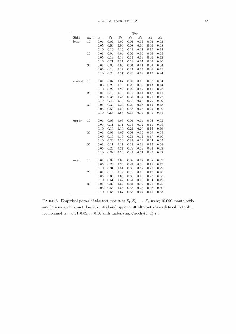
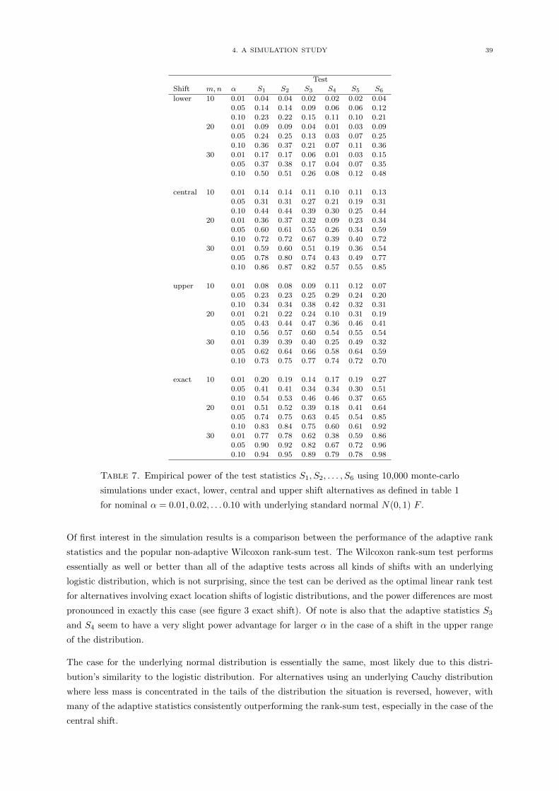
Table 5. Empirical power of the test statistics S1, S2, . . . , S6 using 10,000 monte-carlo
simulations under exact, lower, central and upper shift alternatives as defined in table 1
for nominal α = 0.01, 0.02, . . . 0.10 with underlying Cauchy(0, 1) F .
36 4. A SIMULATION STUDY
Significance level
Pow
er
0.0
0.2
0.4
0.6
● ● ● ● ● ● ● ● ● ●
● ● ● ● ● ● ● ● ● ●
m = n = 10lower shift
0.01 0.05 0.10
●● ● ● ● ● ● ● ● ●
●●
●● ● ● ● ● ● ●
m = n = 20lower shift
●●
●● ● ● ● ● ● ●
●●
●●
● ● ● ● ● ●
m = n = 30lower shift
●●
● ● ● ● ● ● ● ●
●●
● ● ● ●●
●● ●
m = n = 10central shift
●●
●●
●●
● ● ● ●
●
●●
●●
●● ● ● ●
m = n = 20central shift
0.0
0.2
0.4
0.6
●
●●
●●
●● ●
● ●
●
●●
●●
●●
●● ●
m = n = 30central shift
0.0
0.2
0.4
0.6
● ● ● ● ● ● ● ● ● ●
●● ● ● ● ● ● ● ● ●
m = n = 10upper shift
●●
●● ● ● ● ● ● ●
●●
●● ● ●
● ● ● ●
m = n = 20upper shift
●●
●●
●●
● ● ● ●
●●
●●
● ●● ● ● ●
m = n = 30upper shift
0.01 0.05 0.10
●●
●●
● ● ● ● ● ●
●●
●●
●●
●●
● ●
m = n = 10exact shift
●
●●
●●
●●
● ● ●
●
●
●●
●●
● ●● ●
m = n = 20exact shift
0.01 0.05 0.10
0.0
0.2
0.4
0.6
●
●●
●●
●● ●
● ●
●
●
●●
●●
●●
● ●
m = n = 30exact shift
S1 S2 S3 S4 S5 S6● ●
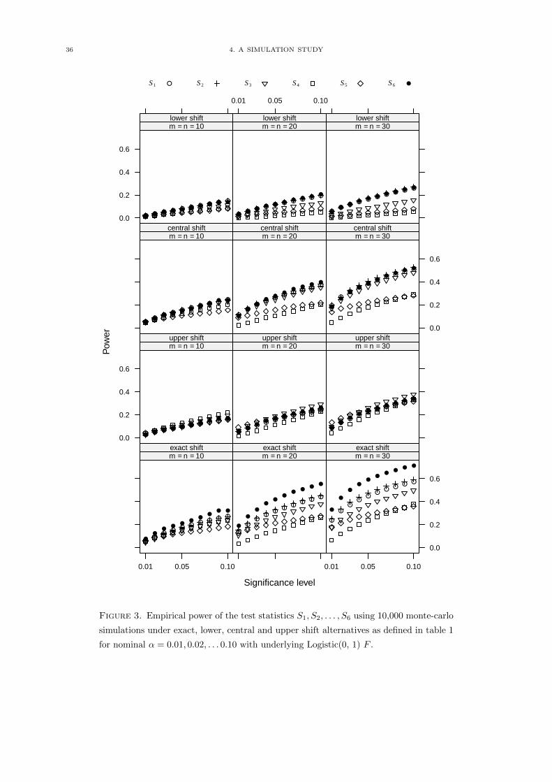
Figure 3. Empirical power of the test statistics S1, S2, . . . , S6 using 10,000 monte-carlo
simulations under exact, lower, central and upper shift alternatives as defined in table 1
for nominal α = 0.01, 0.02, . . . 0.10 with underlying Logistic(0, 1) F .

4. A SIMULATION STUDY 37
Test
Shift m,n α S1 S2 S3 S4 S5 S6
lower 10 0.01 0.02 0.02 0.01 0.01 0.02 0.02
0.05 0.08 0.08 0.06 0.05 0.04 0.080.10 0.15 0.15 0.11 0.09 0.08 0.14
20 0.01 0.03 0.03 0.02 0.00 0.02 0.03
0.05 0.12 0.12 0.07 0.02 0.05 0.120.10 0.19 0.20 0.13 0.05 0.08 0.21
30 0.01 0.06 0.06 0.03 0.00 0.02 0.05
0.05 0.16 0.17 0.09 0.02 0.04 0.170.10 0.26 0.27 0.15 0.05 0.08 0.27
central 10 0.01 0.05 0.05 0.05 0.05 0.05 0.050.05 0.16 0.15 0.15 0.12 0.11 0.15
0.10 0.25 0.24 0.23 0.20 0.15 0.2420 0.01 0.11 0.12 0.10 0.02 0.09 0.10
0.05 0.26 0.27 0.24 0.11 0.16 0.28
0.10 0.37 0.38 0.35 0.20 0.22 0.4030 0.01 0.19 0.20 0.17 0.05 0.14 0.18
0.05 0.39 0.40 0.36 0.18 0.22 0.39
0.10 0.51 0.53 0.48 0.29 0.28 0.52
upper 10 0.01 0.03 0.03 0.03 0.04 0.04 0.03
0.05 0.09 0.09 0.11 0.13 0.10 0.100.10 0.17 0.17 0.19 0.22 0.16 0.17
20 0.01 0.05 0.05 0.06 0.02 0.09 0.05
0.05 0.16 0.16 0.19 0.11 0.17 0.160.10 0.25 0.26 0.29 0.23 0.24 0.26
30 0.01 0.09 0.09 0.10 0.04 0.13 0.080.05 0.22 0.23 0.26 0.19 0.24 0.24
0.10 0.33 0.34 0.38 0.33 0.32 0.34
exact 10 0.01 0.06 0.06 0.05 0.06 0.06 0.08
0.05 0.18 0.17 0.15 0.15 0.13 0.21
0.10 0.27 0.27 0.24 0.24 0.18 0.3220 0.01 0.14 0.15 0.11 0.03 0.13 0.19
0.05 0.32 0.33 0.27 0.15 0.21 0.42
0.10 0.44 0.45 0.38 0.26 0.27 0.5530 0.01 0.24 0.25 0.17 0.07 0.18 0.33
0.05 0.45 0.48 0.37 0.24 0.29 0.59
0.10 0.57 0.59 0.50 0.38 0.36 0.71
Table 6. Empirical power of the test statistics S1, S2, . . . , S6 using 10,000 monte-carlo
simulations under exact, lower, central and upper shift alternatives as defined in table 1
for nominal α = 0.01, 0.02, . . . 0.10 with underlying Logistic(0, 1) F .
38 4. A SIMULATION STUDY
Significance level
Pow
er
0.0
0.2
0.4
0.6
0.8
1.0
● ● ● ● ● ● ● ● ● ●
● ● ● ● ● ● ● ● ● ●
m = n = 10lower shift
0.01 0.05 0.10
●●
●● ● ● ● ● ● ●
●●
●● ● ● ● ● ● ●
m = n = 20lower shift
●●
●●
●● ● ● ● ●
●●
●●
● ● ● ● ● ●
m = n = 30lower shift
●●
●● ● ● ● ● ● ●
●●
● ● ● ● ●● ● ●
m = n = 10central shift
●
●●
●● ● ● ● ● ●
●
●●
●●
●● ● ● ●
m = n = 20central shift
0.0
0.2
0.4
0.6
0.8
1.0
●
●●
● ● ● ● ● ● ●
●
●●
● ● ● ● ● ● ●
m = n = 30central shift
0.0
0.2
0.4
0.6
0.8
1.0
●●
● ●● ● ● ● ● ●
●●
● ● ● ● ● ● ● ●
m = n = 10upper shift
●
●●
●●
● ● ● ● ●
●
●●
● ●●
● ● ● ●
m = n = 20upper shift
●
●●
●●
● ● ● ● ●
●
●●
●● ● ● ● ● ●
m = n = 30upper shift
0.01 0.05 0.10
●
●●
●● ● ● ● ● ●
●
●●
●●
●●
●● ●
m = n = 10exact shift
●
●●
●● ● ● ● ● ●
●
●●
● ● ● ● ● ● ●
m = n = 20exact shift
0.01 0.05 0.10
0.0
0.2
0.4
0.6
0.8
1.0
●●
● ● ● ● ● ● ● ●
●● ● ● ● ● ● ● ● ●
m = n = 30exact shift
S1 S2 S3 S4 S5 S6● ●
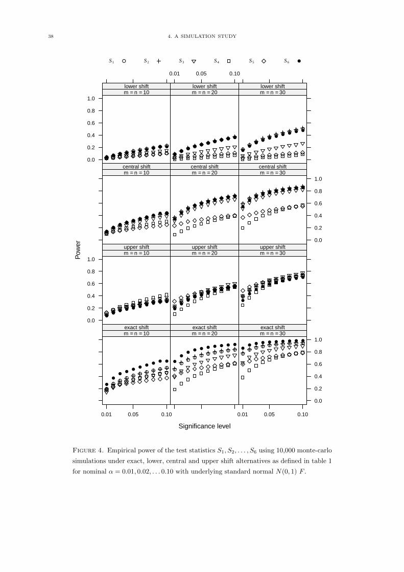
Figure 4. Empirical power of the test statistics S1, S2, . . . , S6 using 10,000 monte-carlo
simulations under exact, lower, central and upper shift alternatives as defined in table 1
for nominal α = 0.01, 0.02, . . . 0.10 with underlying standard normal N(0, 1) F .
4. A SIMULATION STUDY 39
Test
Shift m,n α S1 S2 S3 S4 S5 S6
lower 10 0.01 0.04 0.04 0.02 0.02 0.02 0.04
0.05 0.14 0.14 0.09 0.06 0.06 0.120.10 0.23 0.22 0.15 0.11 0.10 0.21
20 0.01 0.09 0.09 0.04 0.01 0.03 0.09
0.05 0.24 0.25 0.13 0.03 0.07 0.250.10 0.36 0.37 0.21 0.07 0.11 0.36
30 0.01 0.17 0.17 0.06 0.01 0.03 0.15
0.05 0.37 0.38 0.17 0.04 0.07 0.350.10 0.50 0.51 0.26 0.08 0.12 0.48
central 10 0.01 0.14 0.14 0.11 0.10 0.11 0.130.05 0.31 0.31 0.27 0.21 0.19 0.31
0.10 0.44 0.44 0.39 0.30 0.25 0.4420 0.01 0.36 0.37 0.32 0.09 0.23 0.34
0.05 0.60 0.61 0.55 0.26 0.34 0.59
0.10 0.72 0.72 0.67 0.39 0.40 0.7230 0.01 0.59 0.60 0.51 0.19 0.36 0.54
0.05 0.78 0.80 0.74 0.43 0.49 0.77
0.10 0.86 0.87 0.82 0.57 0.55 0.85
upper 10 0.01 0.08 0.08 0.09 0.11 0.12 0.07
0.05 0.23 0.23 0.25 0.29 0.24 0.200.10 0.34 0.34 0.38 0.42 0.32 0.31
20 0.01 0.21 0.22 0.24 0.10 0.31 0.19
0.05 0.43 0.44 0.47 0.36 0.46 0.410.10 0.56 0.57 0.60 0.54 0.55 0.54
30 0.01 0.39 0.39 0.40 0.25 0.49 0.320.05 0.62 0.64 0.66 0.58 0.64 0.59
0.10 0.73 0.75 0.77 0.74 0.72 0.70
exact 10 0.01 0.20 0.19 0.14 0.17 0.19 0.27
0.05 0.41 0.41 0.34 0.34 0.30 0.51
0.10 0.54 0.53 0.46 0.46 0.37 0.6520 0.01 0.51 0.52 0.39 0.18 0.41 0.64
0.05 0.74 0.75 0.63 0.45 0.54 0.85
0.10 0.83 0.84 0.75 0.60 0.61 0.9230 0.01 0.77 0.78 0.62 0.38 0.59 0.86
0.05 0.90 0.92 0.82 0.67 0.72 0.96
0.10 0.94 0.95 0.89 0.79 0.78 0.98
Table 7. Empirical power of the test statistics S1, S2, . . . , S6 using 10,000 monte-carlo
simulations under exact, lower, central and upper shift alternatives as defined in table 1
for nominal α = 0.01, 0.02, . . . 0.10 with underlying standard normal N(0, 1) F .
Of first interest in the simulation results is a comparison between the performance of the adaptive rank
statistics and the popular non-adaptive Wilcoxon rank-sum test. The Wilcoxon rank-sum test performs
essentially as well or better than all of the adaptive tests across all kinds of shifts with an underlying
logistic distribution, which is not surprising, since the test can be derived as the optimal linear rank test
for alternatives involving exact location shifts of logistic distributions, and the power differences are most
pronounced in exactly this case (see figure 3 exact shift). Of note is also that the adaptive statistics S3
and S4 seem to have a very slight power advantage for larger α in the case of a shift in the upper range
of the distribution.
The case for the underlying normal distribution is essentially the same, most likely due to this distri-
bution’s similarity to the logistic distribution. For alternatives using an underlying Cauchy distribution
where less mass is concentrated in the tails of the distribution the situation is reversed, however, with
many of the adaptive statistics consistently outperforming the rank-sum test, especially in the case of the
central shift.

40 4. A SIMULATION STUDY
Secondly, we would like to look at the differences between the various adaptive rank statistics S1 through
S5 proposed here. In general, the statistics S4 and S5 using the flattened kernels Kγ,β pay a heavy price
for the improved asymptotic behavior under H0 and suffer a significant loss of power compared to the
ranks-sum statistic and adaptive statistics using the bell-shaped Parzen-2 kernel. In most scenarios, the
differences become more severe as the nominal significance level α increases.
It is also interesting to note that in many cases it does not seem to matter much whether the restricted
kernel estimators ˆfN and ˆgN as proposed by Behnen et al. (1983) or the non-restricted kernel estimators
fN and gN proposed here are used when forming the test statistic SN , as long as we are using exact or
monte-carlo critical boundaries and are not concerned with asymptotics.
For an underlying Cauchy distribution, there were no real differences in the performance of S1 and S2
based on a score function ˆbN and S3 based on bN , and S3 even seemed to have a slight advantage over
the restricted estimators in the case of an upper shift. For underlying normal and logistic F the results
were much the same except for a distinct loss in power in S3 relative to S1 and S2 on the order of around
0.10 across all significance levels examined in the case of a lower or exact shift.
CHAPTER 5
Proofs
5.1. Leading terms of SN
In our proof of the representation of SN (bN ) shown in Theorem 2.1 we showed in a first step that SN (bN )
can be separated into a combination of leading terms that play a role in power and in the asymptotic
distribution of the test statistic and a collection of asymptotically negigible rest terms:
SN =
∫ [fN − gN
]◦HN (x)
[Fm(dx)− F (dx)
](2.38)
+
∫ [fN − gN
]◦HN (x) F (dx) (2.41)
+
∫ [fN − gN
]′◦HN (x) ·
[HN (x)−HN (x)
]F (dx) (2.42)
+
∫ [fN − gN − (fN − gN )
]◦HN (x) F (dx) (2.44)
+OP(a−2N ·N−1).
Of these leading terms (2.38) and (2.42) comprise i.i.d. sums, while (2.41) is a deterministic component
responsible for power under H1. Thus, it remains to work further with the remaining leading term (2.44)
to complete our linearization of SN .
In the following, we will show that (2.44) can also be written as a sum of i.i.d. variables plus negligible
rest. We can also note from the representation above that (2.38), (2.41) and (2.42) all vanish under H0,
so that (2.44) alone determines the asymptotic distribution of SN (bN ) under the null hypothesis.
Now, we can separate (2.44) into two simpler terms∫ [fN − gN − (fN − gN )
]◦HN (x) F (dx)
=
∫ [fN − fN
]◦HN (x) F (dx) (5.1)
−∫ [
gN − gN]◦HN (x) F (dx). (5.2)
In the following we will derive i.i.d sums from (5.1) and (5.2) and combine these to get an i.i.d. sum
for (2.44) plus negligible rest. All results in this section are proven using the same assumptions on K
and aN and definitions as in Theorem 2.1. We begin with (5.1). The work with (5.2) will be completely
analogous.
41
42 5. PROOFS
First, recall the definitions of the kernel estimators fN and gN of the densities fN and gN and the
functions fN and gN :
fN (t) = (aN ·m)−1 ·m∑i=1
K
(t− HN (Xi)
aN
),
gN (t) = (aN · n)−1 ·n∑k=1
K
(t− HN (Yk)
aN
),
fN (t) = a−1N
∫K
(t−HN (y)
aN
)F (dy), 0 ≤ t ≤ 1,
gN (t) = a−1N
∫K
(t−HN (y)
aN
)G(dy), 0 ≤ t ≤ 1.
Then ∫ [fN − fN
]◦HN (x) F (dx)
=
∫ [(m · aN )−1 ·
m∑i=1
K(a−1N (HN (x)− HN (Xi))
)− a−1N
∫K(a−1N (HN (x)−HN (y))
)F (dy)
]F (dx)
=
m∑i=1
(m · aN )−1[ ∫
K(a−1N (HN (x)− HN (Xi))
)F (dx)
−∫∫
K(a−1N (HN (x)−HN (y))
)F (dy) F (dx)
].
Using the Taylor expansion of the kernel function K about each of the a−1N (HN (x)−HN (Xi)) then yields
m∑i=1
(m · aN )−1[ ∫
K(a−1N (HN (x)−HN (Xi))
)F (dx)
−∫∫
K(a−1N (HN (x)−HN (y))
)F (dy) F (dx)
](5.3)
+ a−2N ·m−1 ·
m∑i=1
∫K ′(a−1N (HN (x)−HN (Xi))
)F (dx) ·
(HN (Xi)− HN (Xi)
)(5.4)
+ a−1N ·m−1 ·
m∑i=1
∫∫ a−1N (HN (x)−HN (Xi))
a−1N (HN (x)−HN (Xi))
(a−1N (HN (x)− HN (Xi))− t
)·K ′′(t) dt F (dx). (5.5)
It is immediately apparent that (5.3) is already a sum of centered i.i.d. variables. Thus, it remains to
work on deriving an i.i.d. sum from (5.4). Recalling the definition of the pooled empirical d.f. HN we
see that (5.4) is equal to
a−2N ·m−1 ·
m∑i=1
∫K ′(a−1N (HN (x)−HN (Xi))
)F (dx) ·
[HN (Xi)−N−1
[ m∑j=1
1{Xj≤Xi} +
n∑k=1
1{Yk≤Xi}
]]
= a−2N ·m−1 ·
m∑i=1
∫K ′(a−1N (HN (x)−HN (Xi))
)F (dx) ·HN (Xi)
5.1. LEADING TERMS OF SN 43
− a−2N ·m−1 ·
m∑i=1
∫K ′(a−1N (HN (x)−HN (Xi))
)F (dx) ·N−1 ·
m∑j=1
1{Xj≤Xi}
− a−2N ·m−1 ·
m∑i=1
∫K ′(a−1N (HN (x)−HN (Xi))
)F (dx) ·N−1 ·
n∑k=1
1{Yk≤Xi}
= a−2N ·m−1 ·
m∑i=1
∫K ′(a−1N (HN (x)−HN (Xi))
)F (dx) ·HN (Xi) (5.6)
− λN · a−2N ·m−2 ·
m∑i=1
∫K ′(a−1N (HN (x)−HN (Xi))
)F (dx) (5.7)
− λN · a−2N ·m−2 ·
∑1≤i 6=j≤m
∫K ′(a−1N (HN (x)−HN (Xi))
)F (dx) · 1{Xj≤Xi} (5.8)
− (1− λN ) · a−2N ·m−1n−1 ·
m∑i=1
n∑k=1
∫K ′(a−1N (HN (x)−HN (Xi))
)F (dx) · 1{Yk≤Xi}. (5.9)
We see that (5.6) is already an i.i.d. sum and (5.7) is negligible, since∣∣∣∣λN · a−2N ·m−2 · m∑i=1
∫K ′(a−1N (HN (x)−HN (Xi))
)F (dx)
∣∣∣∣≤ λN · a−2N ·m
−2 ·m∑i=1
∫ ∣∣K ′(a−1N (HN (x)−HN (Xi)))∣∣ F (dx)
≤ λN · a−2N ·m−2 ·
m∑i=1
∫ ∥∥K ′∥∥= λN
∥∥K ′∥∥ · a−2N ·m−1= O(a−2N ·N
−1). (5.10)
Further, (5.8) and (5.9) are a U -statistic and generalized U -statistic scaled by λN (m−1)m−1 and (1−λN )
respectively. We will proceed by finding projections of (5.8) and (5.9) onto the space of i.i.d. sums which
we can continue to work with.
Lemma 5.1.
a−2N ·m−2 ·
∑1≤i 6=j≤m
∫K ′(a−1N (HN (x)−HN (Xi))
)F (dx) · 1{Xj≤Xi} (5.11)
= a−2N ·m−1 ·
m∑i=1
[ ∫∫K ′(a−1N (HN (x)−HN (Xi))
)F (dx) · 1{y≤Xi} F (dy)
+
∫∫K ′(a−1N (HN (x)−HN (y))
)F (dx) · 1{Xi≤y} F (dy)
−∫∫∫
K ′(a−1N (HN (x)−HN (y))
)F (dx) · 1{z≤y} F (dy) F (dz)
]+OP(a−2N ·N
−1).
Proof. Define
uN (r, s) = a−2N
∫K ′(a−1N (HN (x)−HN (r))
)F (dx) · 1{s≤r},

44 5. PROOFS
and define the U -statistic Um as
Um = m−1(m− 1)−1 ·∑
1≤i 6=j≤m
uN (Xi, Xj).
Then
a−2N ·m−2 ·
∑1≤i 6=j≤m
∫K ′(a−1N (HN (x)−HN (Xi))
)F (dx) · 1{Xj≤Xi} = (m− 1)m−1 · Um.
Further, let Um be the Hajek projection of Um as defined in Lemma A.2:
Um = m−1 ·m∑i=1
[ ∫uN (Xi, y) F (dy) +
∫uN (z,Xi) F (dz)−
∫∫uN (y, z) F (dy) F (dz)
]
= a−2N ·m−1 ·
m∑i=1
[ ∫∫K ′(a−1N (HN (x)−HN (Xi))
)F (dx) · 1{y≤Xi} F (dy)
+
∫∫K ′(a−1N (HN (x)−HN (y))
)F (dx) · 1{Xi≤y} F (dy)
−∫∫∫
K ′(a−1N (HN (x)−HN (y))
)F (dx) · 1{z≤y} F (dy) F (dz)
].
In order to complete the proof it only remains to show that
E[(m− 1)m−1 · Um − Um
]2= O(a−4N ·N
−2).
Applying the inequality from Lemma A.2 we have
E[(m− 1)m−1 · Um − Um
]2= E
[(m− 1)m−1 · Um − Um + Um − Um
]2≤ 2 · E
[(m− 1)m−1 · Um − Um
]2+ 2 · E
[Um − Um
]2≤ 2m−2 · E
[Um]2
+ 4(m− 1)m−3 · E[u∗N (X1, X2)
]2for u∗N defined as
u∗N (r, s) = uN (r, s)−∫uN (r, y) F (dy)−
∫uN (z, s) F (dz) +
∫∫uN (z, y) F (dy) F (dz).
Now, the kernel function uN is uniformly bounded:∥∥uN∥∥ ≤ ∥∥K ′∥∥a−2Nwhich means for the first expectation we can write
E[Um]2
= E[m−1(m− 1)−1 ·
∑1≤i6=j≤m
uN (Xi, Xj)
]2≤∥∥uN∥∥2 ≤ ∥∥K ′∥∥2a−4N .
Thus, it remains only to bound the second expectation E[u∗N (X1, X2)
]2:
E[u∗N (X1, X2)
]2 ≤ 4 · E[[uN (X1, X2)
]2+
[ ∫uN (X1, y) F (dy)
]2+
[ ∫uN (z,X2) F (dz)
]2+
[ ∫∫uN (z, y) F (dy) F (dz)
]2]
5.1. LEADING TERMS OF SN 45
≤ 4 · E[[uN (X1, X2)
]2+
∫ [uN (X1, y)
]2F (dy)
+
∫ [uN (z,X2)
]2F (dz) +
∫∫ [uN (z, y)
]2F (dy) F (dz)
]≤ 4 · E
[4 ·[∥∥K ′∥∥a−2N ]2]
= 42∥∥K ′∥∥2a−4N .
Altogether this gives us
E[(m− 1)m−1 · Um − Um
]2≤ 2m−2 · E
[Um]2
+ 4(m− 1)m−3 · E[u∗N (X1, X2)
]2≤ 2m−2 ·
∥∥K ′∥∥2a−4N + 4(m− 1)m−3 · 42∥∥K ′∥∥2a−4N
= 2∥∥K ′∥∥2a−4N ·m−2 + 43
∥∥K ′∥∥2a−4N · (m− 1)m−3
= O(a−4N ·N−2)
which completes the proof. �
Using the following lemma, we can replace (5.9) by a projection as well.
Lemma 5.2.
a−2N ·m−1n−1 ·
m∑i=1
n∑k=1
∫K ′(a−1N (HN (x)−HN (Xi))
)F (dx) · 1{Yk≤Xi} (5.12)
= a−2N ·[m−1 ·
m∑i=1
∫∫K ′(a−1N (HN (x)−HN (Xi))
)F (dx) · 1{y≤Xi} G(dy)
+ n−1 ·n∑k=1
∫∫K ′(a−1N (HN (x)−HN (y))
)F (dx) · 1{Yk≤y} F (dy)
−∫∫∫
K ′(a−1N (HN (x)−HN (y))
)F (dx) · 1{z≤y} F (dy)G(dz)
]+OP(a−2N ·N
−1).
Proof. Define
uN (r, s) = a−2N
∫K ′(a−1N (HN (x)−HN (r))
)F (dx) · 1{s≤r},
and define the generalized U -statistic Um,n as
Um,n = m−1n−1 ·m∑i=1
n∑k=1
uN (Xi, Yk).
Then
a−2N ·m−1n−1 ·
m∑i=1
n∑k=1
∫K ′(a−1N (HN (x)−HN (Xi))
)F (dx) · 1{Yk≤Xi} = Um,n.
46 5. PROOFS
Further, let Um,n be the Hajek projection of Um,n as defined in Lemma A.3:
Um,n = m−1 ·m∑i=1
∫uN (Xi, y)G(dy) + n−1 ·
n∑k=1
∫uN (x, Yk) F (dx)−
∫∫uN (x, y) F (dx)G(dy)
= a−2N ·[m−1 ·
m∑i=1
∫∫K ′(a−1N (HN (x)−HN (Xi))
)F (dx) · 1{y≤Xi} G(dy)
+ n−1 ·n∑k=1
∫∫K ′(a−1N (HN (x)−HN (y))
)F (dx) · 1{Yk≤y} F (dy)
−∫∫∫
K ′(a−1N (HN (x)−HN (y))
)F (dx) · 1{z≤y} F (dy)G(dz)
].
In order to complete the proof it only remains to show that
E[Um,n − Um,n
]2= O(a−4N ·N
−2).
Applying the equality from Lemma A.3 we have
E[Um,n − Um,n
]2= m−1n−1 · E
[u∗N (X1, Y1)
]2for u∗N defined as
u∗N (r, s) = u(r, s)−∫u(r, y)G(dy)−
∫u(x, s) F (dx) +
∫∫u(x, y) F (dx)G(dy).
Since the kernel function uN is uniformly bounded:∥∥uN∥∥ ≤ ∥∥K ′∥∥a−2Nwe can write
E[u∗N (X1, Y1)
]2 ≤ 4 · E[[uN (X1, Y1)
]2+
[ ∫uN (X1, y)G(dy)
]2+
[ ∫uN (z, Y1) F (dz)
]2+
[ ∫∫uN (z, y)G(dy) F (dz)
]2]≤ 4 · E
[[uN (X1, Y1)
]2+
∫ [uN (X1, y)
]2G(dy)
+
∫ [uN (z, Y1)
]2F (dz) +
∫∫ [uN (z, y)
]2G(dy) F (dz)
]≤ 4 · E
[4 ·[∥∥K ′∥∥a−2N ]2]
= 42∥∥K ′∥∥2a−4N .
Altogether this gives us
E[Um,n − Um,n
]2= m−1n−1 · E
[u∗N (X1, Y1)
]2≤ m−1n−1 · 42
∥∥K ′∥∥2a−4N= 42
∥∥K ′∥∥2a−4N ·m−1n−1= O(a−4N ·N
−2)
5.1. LEADING TERMS OF SN 47
which completes the proof. �
Lemma 5.3.
a−1N ·m−1 ·
m∑i=1
∫∫ a−1N (HN (x)−HN (Xi))
a−1N (HN (x)−HN (Xi))
(a−1N (HN (x)− HN (Xi))− t
)·K ′′(t) dt F (dx) = OP(a−2N ·N
−1).
(5.13)
Proof.∣∣∣∣a−1N ·m−1 · m∑i=1
∫∫ a−1N (HN (x)−HN (Xi))
a−1N (HN (x)−HN (Xi))
(a−1N (HN (x)− HN (Xi))− t
)·K ′′(t) dt F (dx)
∣∣∣∣=
∣∣∣∣a−1N ·m−1 · m∑i=1
∫ 1
0
∫ a−1N (v−HN (Xi))
a−1N (v−HN (Xi))
(a−1N (v − HN (Xi))− t
)·K ′′(t) dt fN (v) dv
∣∣∣∣= a−1N ·m
−1 ·∣∣∣∣ ∑
1≤i≤mHN (Xi)>HN (Xi)
∫ 1
0
∫ 1
−11{a−1
N (v−HN (Xi))< t < a−1N (v−HN (Xi))}
×(a−1N (v − HN (Xi))− t
)·K ′′(t) dt fN (v) dv
+∑
1≤i≤mHN (Xi)≤HN (Xi)
∫ 1
0
∫ 1
−11{a−1
N (v−HN (Xi))< t < a−1N (v−HN (Xi))}
×(a−1N (v − HN (Xi))− t
)·K ′′(t) dt fN (v) dv
∣∣∣∣= a−1N ·m
−1 ·∣∣∣∣ ∑
1≤i≤mHN (Xi)>HN (Xi)
∫ 1
0
∫ 1
−11{HN (Xi))+aN ·t < v < HN (Xi))+aN ·t}
×(a−1N (v − HN (Xi))− t
)·K ′′(t) dt fN (v) dv
+∑
1≤i≤mHN (Xi)≤HN (Xi)
∫ 1
0
∫ 1
−11{HN (Xi))+aN ·t < v < HN (Xi))+aN ·t}
×(a−1N (v − HN (Xi))− t
)·K ′′(t) dt fN (v) dv
∣∣∣∣≤ a−1N ·m
−1 ·[ ∑
1≤i≤mHN (Xi)>HN (Xi)
∫ 1
−1
∫ 1
0
1{HN (Xi))+aN ·t < v < HN (Xi))+aN ·t}
×∣∣a−1N (v − HN (Xi))− t
∣∣ · fN (v) dv∣∣K ′′(t)∣∣ dt
+∑
1≤i≤mHN (Xi)≤HN (Xi)
∫ 1
−1
∫ 1
0
1{HN (Xi))+aN ·t < v < HN (Xi))+aN ·t}
×∣∣a−1N (v − HN (Xi))− t
∣∣ · fN (v) dv∣∣K ′′(t)∣∣ dt]
48 5. PROOFS
≤ a−1N ·m−1 ·
[ ∑1≤i≤m
HN (Xi)>HN (Xi)
∫ 1
−1
∥∥fN∥∥∫ 1
0
1{HN (Xi))+aN ·t < v < HN (Xi))+aN ·t}
×∣∣a−1N (v − HN (Xi))− t
∣∣ dv ∣∣K ′′(t)∣∣ dt+∑
1≤i≤mHN (Xi)≤HN (Xi)
∫ 1
−1
∥∥fN∥∥ ∫ 1
0
1{HN (Xi))+aN ·t < v < HN (Xi))+aN ·t}
×∣∣a−1N (v − HN (Xi))− t
∣∣ dv ∣∣K ′′(t)∣∣ dt]
≤ a−1N ·m−1 ·
∥∥fN∥∥ · [ ∑1≤i≤m
HN (Xi)>HN (Xi)
∫ 1
−1
∣∣a−1N (HN (Xi)− HN (Xi))∣∣
×∫ 1
0
1{HN (Xi))+aN ·t < v < HN (Xi))+aN ·t} dv∣∣K ′′(t)∣∣ dt
+∑
1≤i≤mHN (Xi)≤HN (Xi)
∫ 1
−1
∣∣a−1N (HN (Xi)− HN (Xi))∣∣ ∫ 1
0
1{HN (Xi))+aN ·t < v < HN (Xi))+aN ·t} dv∣∣K ′′(t)∣∣ dt]
≤ a−2N ·m−1 ·
∥∥fN∥∥ · [ ∑1≤i≤m
HN (Xi)>HN (Xi)
∣∣HN (Xi)− HN (Xi)∣∣
×∫ 1
−1
∫ 1
0
1{HN (Xi))+aN ·t < v < HN (Xi))+aN ·t} dv∣∣K ′′(t)∣∣ dt
+∑
1≤i≤mHN (Xi)≤HN (Xi)
∣∣HN (Xi)− HN (Xi)∣∣ · ∫ 1
−1
∫ 1
0
1{HN (Xi))+aN ·t < v < HN (Xi))+aN ·t} dv∣∣K ′′(t)∣∣ dt]
≤ a−2N ·m−1 ·
∥∥fN∥∥ · m∑i=1
∣∣HN (Xi)− HN (Xi)∣∣2 · 2∥∥K ′′∥∥
≤ 2∥∥K ′′∥∥a−2N · ∥∥fN∥∥ · ∥∥HN −HN
∥∥2= OP(a−2N ·N
−1),
due to the D-K-W bound on∥∥HN −HN
∥∥ and the fact that∥∥fN∥∥ = O(1) (see Lemma A.1). �
We can apply (5.3), (5.6) and (5.10) together with Lemmas 5.1, 5.2 and 5.3 to express (5.1) as an i.i.d
sum plus negligible rest terms, which we record in the following lemma.
Lemma 5.4.∫ [fN − fN
]◦HN (x) F (dx) =
= a−1N ·m−1 ·
m∑i=1
[ ∫K(a−1N (HN (x)−HN (Xi))
)F (dx)
−∫∫
K(a−1N (HN (x)−HN (y))
)F (dy) F (dx)
]

5.1. LEADING TERMS OF SN 49
− λN · a−2N ·m−1 ·
m∑i=1
[ ∫∫K ′(a−1N (HN (x)−HN (y))
)F (dx) · 1{Xi≤y} F (dy)
−∫∫
K ′(a−1N (HN (x)−HN (y))
)F (dx) · F (y) F (dy)
]
− (1− λN ) · a−2N · n−1 ·
n∑k=1
[ ∫∫K ′(a−1N (HN (x)−HN (y))
)F (dx) · 1{Yk≤y} F (dy)
−∫∫
K ′(a−1N (HN (x)−HN (y))
)F (dx) ·G(y) F (dy)
]+OP(a−2N ·N
−1).
Proof. Combine (5.3), (5.6) and (5.10) together with Lemmas 5.1 and 5.2 to get∫ [fN − fN
]◦HN (x) F (dx)
= a−1N ·m−1 ·
m∑i=1
[ ∫K(a−1N (HN (x)−HN (Xi))
)F (dx)
−∫∫
K(a−1N (HN (x)−HN (y))
)F (dy) F (dx)
]
+ a−2N ·m−1 ·
m∑i=1
∫K ′(a−1N (HN (x)−HN (Xi))
)F (dx) ·HN (Xi)
− λN · a−2N ·m−1 ·
m∑i=1
[ ∫∫K ′(a−1N (HN (x)−HN (Xi))
)F (dx) · 1{y≤Xi} F (dy)
+
∫∫K ′(a−1N (HN (x)−HN (y))
)F (dx) · 1{Xi≤y} F (dy)
−∫∫∫
K ′(a−1N (HN (x)−HN (y))
)F (dx) · 1{z≤y} F (dy) F (dz)
]
− (1− λN ) · a−2N ·[m−1 ·
m∑i=1
∫∫K ′(a−1N (HN (x)−HN (Xi))
)F (dx) · 1{y≤Xi} G(dy)
+ n−1 ·n∑k=1
∫∫K ′(a−1N (HN (x)−HN (y))
)F (dx) · 1{Yk≤y} F (dy)
−∫∫∫
K ′(a−1N (HN (x)−HN (y))
)F (dx) · 1{z≤y} F (dy)G(dz)
]+OP(a−2N ·N
−1)
= a−1N ·m−1 ·
m∑i=1
[ ∫K(a−1N (HN (x)−HN (Xi))
)F (dx)
−∫∫
K(a−1N (HN (x)−HN (y))
)F (dy) F (dx)
]
+ a−2N ·m−1 ·
m∑i=1
∫K ′(a−1N (HN (x)−HN (Xi))
)F (dx) ·HN (Xi)
− a−2N ·m−1 ·
m∑i=1
∫K ′(a−1N (HN (x)−HN (Xi))
)F (dx) · λNF (Xi)
50 5. PROOFS
− λN · a−2N ·m−1 ·
m∑i=1
∫∫K ′(a−1N (HN (x)−HN (y))
)F (dx) · 1{Xi≤y} F (dy)
+ λN · a−2N∫∫
K ′(a−1N (HN (x)−HN (y))
)F (dx) · F (y) F (dy)
− a−2N ·m−1 ·
m∑i=1
∫K ′(a−1N (HN (x)−HN (Xi))
)F (dx) · (1− λN )G(Xi)
− (1− λN ) · a−2N · n−1 ·
n∑k=1
∫∫K ′(a−1N (HN (x)−HN (y))
)F (dx) · 1{Yk≤y} F (dy)
+ (1− λN ) · a−2N∫∫
K ′(a−1N (HN (x)−HN (y))
)F (dx) ·G(y) F (dy)
+OP(a−2N ·N−1).
Now, since
a−2N ·m−1 ·
m∑i=1
∫K ′(a−1N (HN (x)−HN (Xi))
)F (dx) ·HN (Xi)
= a−2N ·m−1 ·
m∑i=1
∫K ′(a−1N (HN (x)−HN (Xi))
)F (dx) · λNF (Xi)
+ a−2N ·m−1 ·
m∑i=1
∫K ′(a−1N (HN (x)−HN (Xi))
)F (dx) · (1− λN )G(Xi)
this simplifies to∫ [fN − fN
]◦HN (x) F (dx)
= a−1N ·m−1 ·
m∑i=1
[ ∫K(a−1N (HN (x)−HN (Xi))
)F (dx)
−∫∫
K(a−1N (HN (x)−HN (y))
)F (dy) F (dx)
]
− λN · a−2N ·m−1 ·
m∑i=1
∫∫K ′(a−1N (HN (x)−HN (y))
)F (dx) · 1{Xi≤y} F (dy)
+ λN · a−2N∫∫
K ′(a−1N (HN (x)−HN (y))
)F (dx) · F (y) F (dy)
− (1− λN ) · a−2N · n−1 ·
n∑k=1
∫∫K ′(a−1N (HN (x)−HN (y))
)F (dx) · 1{Yk≤y} F (dy)
+ (1− λN ) · a−2N∫∫
K ′(a−1N (HN (x)−HN (y))
)F (dx) ·G(y) F (dy)
+OP(a−2N ·N−1)
= a−1N ·m−1 ·
m∑i=1
[ ∫K(a−1N (HN (x)−HN (Xi))
)F (dx)
−∫∫
K(a−1N (HN (x)−HN (y))
)F (dy) F (dx)
]

5.1. LEADING TERMS OF SN 51
− λN · a−2N ·m−1 ·
m∑i=1
[ ∫∫K ′(a−1N (HN (x)−HN (y))
)F (dx) · 1{Xi≤y} F (dy)
−∫∫
K ′(a−1N (HN (x)−HN (y))
)F (dx) · F (y) F (dy)
]
− (1− λN ) · a−2N · n−1 ·
n∑k=1
[ ∫∫K ′(a−1N (HN (x)−HN (y))
)F (dx) · 1{Yk≤y} F (dy)
−∫∫
K ′(a−1N (HN (x)−HN (y))
)F (dx) ·G(y) F (dy)
]+OP(a−2N ·N
−1)
which completes the proof. �
To derive an i.i.d sum from (5.2) we will use very similar arguments to those which we used to work with
(5.1). We begin by deriving a sum representation of (5.2).∫ [gN − gN
]◦HN (x) F (dx)
=
∫ [(n · aN )−1 ·
n∑k=1
K(a−1N (HN (x)− HN (Yk))
)− a−1N
∫K(a−1N (HN (x)−HN (y))
)G(dy)
]F (dx)
=
n∑k=1
(n · aN )−1[ ∫
K(a−1N (HN (x)− HN (Yk))
)F (dx)
−∫∫
K(a−1N (HN (x)−HN (y))
)G(dy) F (dx)
].
Using the Taylor expansion of the kernel function K about each of the a−1N (HN (x)−HN (Yk)) then yields
n∑k=1
(n · aN )−1[ ∫
K(a−1N (HN (x)−HN (Yk))
)F (dx)
−∫∫
K(a−1N (HN (x)−HN (y))
)G(dy) F (dx)
](5.14)
+ a−2N · n−1 ·
n∑k=1
∫K ′(a−1N (HN (x)−HN (Yk))
)F (dx) ·
(HN (Yk)− HN (Yk)
)(5.15)
+ a−1N · n−1 ·
n∑k=1
∫∫ a−1N (HN (x)−HN (Yk))
a−1N (HN (x)−HN (Yk))
(a−1N (HN (x)− HN (Yk))− t
)·K ′′(t) dt F (dx). (5.16)
It is immediately apparent that (5.14) is already a sum of centered i.i.d. variables. Thus, it remains to
work on deriving an i.i.d. sum from (5.15). Recalling the definition of the pooled empirical d.f. HN we
see that (5.15) is equal to
a−2N · n−1 ·
n∑k=1
∫K ′(a−1N (HN (x)−HN (Yk))
)F (dx) ·
[HN (Yk)−N−1
[ m∑j=1
1{Xj≤Yk} +
n∑l=1
1{Yl≤Yk}
]]
= a−2N · n−1 ·
n∑k=1
∫K ′(a−1N (HN (x)−HN (Yk))
)F (dx) ·HN (Yk)
52 5. PROOFS
− a−2N · n−1 ·
n∑k=1
∫K ′(a−1N (HN (x)−HN (Yk))
)F (dx) ·N−1 ·
m∑j=1
1{Xj≤Yk}
− a−2N · n−1 ·
n∑k=1
∫K ′(a−1N (HN (x)−HN (Yk))
)F (dx) ·N−1 ·
n∑l=1
1{Yl≤Yk}
= a−2N · n−1 ·
n∑k=1
∫K ′(a−1N (HN (x)−HN (Yk))
)F (dx) ·HN (Yk) (5.17)
− λN · a−2N ·m−1n−1 ·
n∑k=1
m∑j=1
∫K ′(a−1N (HN (x)−HN (Yk))
)F (dx) · 1{Xj≤Yk} (5.18)
− (1− λN ) · a−2N · n−2 ·
n∑k=1
∫K ′(a−1N (HN (x)−HN (Yk))
)F (dx) (5.19)
− (1− λN ) · a−2N · n−2 ·
∑1≤k 6=l≤m
∫K ′(a−1N (HN (x)−HN (Yk))
)F (dx) · 1{Yl≤Yk}. (5.20)
We see that (5.17) is already an i.i.d. sum and
(1− λN ) · a−2N · n−2 ·
n∑k=1
∫K ′(a−1N (HN (x)−HN (Yk))
)F (dx) = O(a−2N ·N
−1) (5.21)
by (5.10).
Further, (5.18) and (5.20) are a generalized U -statistic and U -statistic scaled by λN and (1−λN )·(n−1)n−1
respectively. We will proceed by finding projections of (5.18) and (5.20) onto the space of i.i.d. sums
which we can continue to work with.
Lemma 5.5.
a−2N ·m−1n−1 ·
n∑k=1
m∑j=1
∫K ′(a−1N (HN (x)−HN (Yk))
)F (dx) · 1{Xj≤Yk} (5.22)
= a−2N ·[m−1 ·
m∑i=1
∫∫K ′(a−1N (HN (x)−HN (y))
)F (dx) · 1{Xi≤y} G(dy)
+ n−1 ·n∑k=1
∫∫K ′(a−1N (HN (x)−HN (Yk))
)F (dx) · 1{y≤Yk} F (dy)
−∫∫∫
K ′(a−1N (HN (x)−HN (y))
)F (dx) · 1{z≤y} G(dy) F (dz)
]+OP(a−2N ·N
−1).
Proof. Define
uN (r, s) = a−2N
∫K ′(a−1N (HN (x)−HN (r))
)F (dx) · 1{s≤r},
and define the generalized U -statistic Um,n as
Um,n = m−1n−1 ·m∑i=1
n∑k=1
uN (Yk, Xi).
The rest of the proof is completely analogous to the proof of Lemma 5.2 with the kernel function
uN (Xi, Yk) replaced by uN (Yk, Xi). �
5.1. LEADING TERMS OF SN 53
Lemma 5.6.
a−2N · n−2 ·
∑1≤k 6=l≤m
∫K ′(a−1N (HN (x)−HN (Yk))
)F (dx) · 1{Yl≤Yk} (5.23)
= a−2N · n−1 ·
n∑k=1
[ ∫∫K ′(a−1N (HN (x)−HN (Yk))
)F (dx) · 1{y≤Yk} G(dy)
+
∫∫K ′(a−1N (HN (x)−HN (y))
)F (dx) · 1{Yk≤y} G(dy)
−∫∫∫
K ′(a−1N (HN (x)−HN (y))
)F (dx) · 1{z≤y} G(dy)G(dz)
]+OP(a−2N ·N
−1).
Proof. Define
uN (r, s) = a−2N
∫K ′(a−1N (HN (x)−HN (r))
)F (dx) · 1{s≤r},
and define the U -statistic Um as
Un = n−1(n− 1)−1 ·∑
1≤k 6=l≤m
uN (Yk, Yl).
Then
a−2N · n−2 ·
∑1≤k 6=l≤m
∫K ′(a−1N (HN (x)−HN (Yk))
)F (dx) · 1{Yl≤Yk} = (n− 1)n−1 · Un.
The rest of the proof is identical to the proof of Lemma 5.1 with m, i, j, Xi, Xj , F (dy) and F (dz)
replaced by n, k, l, Yk, Yl, G(dy) and G(dz) respectively. �
Lemma 5.7.
a−1N · n−1 ·
n∑k=1
∫∫ a−1N (HN (x)−HN (Yk))
a−1N (HN (x)−HN (Yk))
(a−1N (HN (x)− HN (Yk))− t
)·K ′′(t) dt F (dx) = OP(a−2N ·N
−1).
(5.24)
Proof. The proof is identical to the proof of Lemma 5.3 with k, n and Yk in place of i, m, and Xi. �
We can apply (5.14), (5.17) and (5.21) together with Lemmas 5.5, 5.6 and 5.7 to express (5.2) as an i.i.d
sum plus negligible rest terms:
Lemma 5.8.∫[gN − gN ] ◦HN (x) F (dx) =
= a−1N · n−1 ·
n∑k=1
[ ∫K(a−1N (HN (x)−HN (Yk))
)F (dx)
54 5. PROOFS
−∫∫
K(a−1N (HN (x)−HN (y))
)G(dy) F (dx)
]
− (1− λN ) · a−2N · n−1 ·
n∑k=1
[ ∫∫K ′(a−1N (HN (x)−HN (y))
)F (dx) · 1{Yk≤y} G(dy)
−∫∫
K ′(a−1N (HN (x)−HN (y))
)F (dx) ·G(y)G(dy)
]
− λN · a−2N ·m−1 ·
m∑i=1
[ ∫∫K ′(a−1N (HN (x)−HN (y))
)F (dx) · 1{Xi≤y} G(dy)
−∫∫
K ′(a−1N (HN (x)−HN (y))
)F (dx) · F (y)G(dy)
]+OP(a−2N ·N
−1).
Proof. Combine (5.14), (5.17) and (5.21) together with Lemmas 5.5 and 5.6. The proof is identical to
the proof of Lemma 5.4 with n, m, k, i, Yk, Xi, λN , (1 − λN ), G(dy), G(dz), and F (dy) in place of m,
n, i, k, Xi, Yk, λN and (1− λN ), F (dy), F (dz), and G(dy) respectively. �
Finally, we combine Lemmas 5.4 and 5.8 to get the desired i.i.d. sum representation for (2.44), which
yields
Lemma 5.9.∫ [fN − gN − (fN − gN )
]◦HN (x) F (dx)
= a−1N ·m−1 ·
m∑i=1
[ ∫K(a−1N (HN (x)−HN (Xi))
)F (dx) (5.25)
−∫∫
K(a−1N (HN (x)−HN (y))
)F (dy) F (dx)
](5.26)
− λN · a−2N ·m−1 ·
m∑i=1
[ ∫∫K ′(a−1N (HN (x)−HN (y))
)F (dx) · 1{Xi≤y} F (dy) (5.27)
−∫∫
K ′(a−1N (HN (x)−HN (y))
)F (dx) · F (y) F (dy)
](5.28)
− (1− λN ) · a−2N · n−1 ·
n∑k=1
[ ∫∫K ′(a−1N (HN (x)−HN (y))
)F (dx) · 1{Yk≤y} F (dy) (5.29)
−∫∫
K ′(a−1N (HN (x)−HN (y))
)F (dx) ·G(y) F (dy)
](5.30)
− a−1N · n−1 ·
n∑k=1
[ ∫K(a−1N (HN (x)−HN (Yk))
)F (dx) (5.31)
−∫∫
K(a−1N (HN (x)−HN (y))
)G(dy) F (dx)
](5.32)
+ (1− λN ) · a−2N · n−1 ·
n∑k=1
[ ∫∫K ′(a−1N (HN (x)−HN (y))
)F (dx) · 1{Yk≤y} G(dy) (5.33)
−∫∫
K ′(a−1N (HN (x)−HN (y))
)F (dx) ·G(y)G(dy)
](5.34)
5.2. NEGLIGIBLE TERMS 55
+ λN · a−2N ·m−1 ·
m∑i=1
[ ∫∫K ′(a−1N (HN (x)−HN (y))
)F (dx) · 1{Xi≤y} G(dy) (5.35)
−∫∫
K ′(a−1N (HN (x)−HN (y))
)F (dx) · F (y)G(dy)
](5.36)
+OP(a−2N ·N−1),
which can also be expressed more simply using integral notation as∫fN ◦HN (x)
[Fm(dx)− F (dx)
]−∫fN ◦HN (x)
[Gm(dx)−G(dx)
]+
∫f ′N ◦HN (x) ·
[HN (x)−HN (x)
][F (dx)−G(dx)
]+OP(a−2N ·N
−1).
5.2. Negligible terms
The proofs in this section will deal with terms which are asymptotically negligible under H1 as well as
under H0, meaning that they are stochastically bounded so that they converge in probability to 0 even
after SN (bN ) has been properly scaled to ensure convergence in distribution.
We begin by bounding the Taylor rest terms generated in our expansion of SN (bN ). The following sections
will deal with further terms from the expansion that turn out to be negligible as well.
5.2.1. Taylor rest terms from the expansion of SN . The following lemma shows that the four
Taylor rest terms (2.37), (2.40), (2.43) and (2.46) that appear in the expansion of SN (bN ) shown in the
proof of Theorem 2.1 can be combined into a simpler single integral representation which is shown to be
asymptotically negligible.
Lemma 5.10. Let F and G be continuous distribution functions and HN and HN be mixed theoretical
and empirical distribution functions for sample sizes m and n defined as in (2.4) and (2.16). Further,
let K be a kernel on (−1, 1) and aN a bandwidth sequence satisfying (2.5) through (2.11) and let fN and
gN be kernel estimators (2.12) and (2.13) and fN and gN be functions on the interval (0, 1) defined as
in (2.17) and (2.18) respectively. Then∫ ∫ HN (x)
HN (x)
[fN − gN − (fN − gN )
]′′(t) ·
(HN (x)− t
)dt[Fm(dx)− F (dx)
]
+
∫ ∫ HN (x)
HN (x)
[fN − gN
]′′(t) ·
(HN (x)− t
)dt[Fm(dx)− F (dx)
]
+
∫ ∫ HN (x)
HN (x)
[fN − gN
]′′(t) ·
(HN (x)− t
)dt F (dx)
56 5. PROOFS
+
∫ ∫ HN (x)
HN (x)
[fN − gN − (fN − gN )
]′′(t) ·
(HN (x)− t
)dt F (dx)
= OP(a−2N ·N−1).
Proof.∫ ∫ HN (x)
HN (x)
[fN − gN − (fN − gN )
]′′(t) ·
(HN (x)− t
)dt[Fm(dx)− F (dx)
]
+
∫ ∫ HN (x)
HN (x)
[fN − gN
]′′(t) ·
(HN (x)− t
)dt[Fm(dx)− F (dx)
]
+
∫ ∫ HN (x)
HN (x)
[fN − gN
]′′(t) ·
(HN (x)− t
)dt F (dx)
+
∫ ∫ HN (x)
HN (x)
[fN − gN − (fN − gN )
]′′(t) ·
(HN (x)− t
)dt F (dx)
=
∫ ∫ HN (x)
HN (x)
[fN − gN
]′′(t) ·
(HN (x)− t
)dt Fm(dx) (5.37)
= m−1 ·m∑i=1
∫ HN (Xi)
HN (Xi)
[fN − gN
]′′(t) ·
(HN (Xi)− t
)dt
= m−1 ·m∑i=1
∫ HN (Xi)
HN (Xi)
[a−3N ·m
−1 ·m∑j=1
K ′′(a−1N (t− HN (Xj))
)
− a−3N · n−1 ·
n∑k=1
K ′′(a−1N (t− HN (Yk))
)]·(HN (Xi)− t
)dt
= a−3N ·m−2 ·
m∑i=1
m∑j=1
∫ HN (Xi)
HN (Xi)
K ′′(a−1N (t− HN (Xj))
)·(HN (Xi)− t
)dt (5.38)
− a−3N ·m−1n−1 ·
m∑i=1
n∑k=1
∫ HN (Xi)
HN (Xi)
K ′′(a−1N (t− HN (Yk))
)·(HN (Xi)− t
)dt. (5.39)
We consider (5.38) and (5.39) in turn, showing that each are bounded by OP(a−2N ·N−1) sequences. For
(5.38) we have:
a−3N ·m−2 ·
m∑i=1
m∑j=1
∫ HN (Xi)
HN (Xi)
K ′′(a−1N (t− HN (Xj))
)·(HN (Xi)− t
)dt
= a−3N ·m−2 ·
m∑i=1
∫ HN (Xi)
HN (Xi)
K ′′(a−1N (t− HN (Xi))
)·(HN (Xi)− t
)dt (5.40)
+ a−3N ·m−2 ·
∑1≤i6=j≤m
∫ HN (Xi)
HN (Xi)
K ′′(a−1N (t− HN (Xj))
)·(HN (Xi)− t
)dt. (5.41)
Now bounding (5.40) we have∣∣∣∣a−3N ·m−2 · m∑i=1
∫ HN (Xi)
HN (Xi)
K ′′(a−1N (t− HN (Xi))
)·(HN (Xi)− t
)dt
∣∣∣∣
5.2. NEGLIGIBLE TERMS 57
=
∣∣∣∣a−3N ·m−2[ ∑1≤i≤m
HN (Xi)≤HN (Xi)
∫ HN (Xi)
HN (Xi)
K ′′(a−1N (t− HN (Xi))
)·(HN (Xi)− t
)dt
−∑
1≤i≤mHN (Xi)>HN (Xi)
∫ HN (Xi)
HN (Xi)
K ′′(a−1N (t− HN (Xi))
)·(HN (Xi)− t
)dt
]∣∣∣∣
≤ a−3N ·m−2[ ∑
1≤i≤mHN (Xi)≤HN (Xi)
∫ HN (Xi)
HN (Xi)
∣∣K ′′(a−1N (t− HN (Xi)))∣∣ · ∣∣HN (Xi)− t
∣∣ dt
+∑
1≤i≤mHN (Xi)>HN (Xi)
∫ HN (Xi)
HN (Xi)
∣∣K ′′(a−1N (t− HN (Xi)))∣∣ · ∣∣HN (Xi)− t
∣∣ dt]
≤ a−3N ·m−2[ ∑
1≤i≤mHN (Xi)≤HN (Xi)
∥∥K ′′∥∥ · ∫ HN (Xi)
HN (Xi)
∣∣HN (Xi)− t∣∣ dt
+∑
1≤i≤mHN (Xi)>HN (Xi)
∥∥K ′′∥∥ · ∫ HN (Xi)
HN (Xi)
∣∣HN (Xi)− t∣∣ dt]
≤ a−3N ·m−2 ·
m∑i=1
∥∥K ′′∥∥ · ∣∣HN (Xi)−HN (Xi)∣∣2
≤ a−3N ·m−1 ·
∥∥K ′′∥∥ · ∥∥HN −HN
∥∥2= OP(a−3N ·N
−2).
We use the L1 norm to show that (5.41) is OP(a−2N ·N−1). First, define H∗N to be equal to HN with X1,
X2, Y1 and Y2 removed from the sample. That is,
H∗N (x) = N−1 ·[ m∑i=3
1{Xi≤x} +
n∑k=3
1{Yk≤x}
].
Now recalling that K is zero outside of (−1, 1) we have for (5.41):
E[∣∣∣∣a−3N ·m−2 ·∑
1≤i 6=j≤m
∫ HN (Xi)
HN (Xi)
K ′′(a−1N (t− HN (Xj))
)·(HN (Xi)− t
)dt
∣∣∣∣]
≤ a−3N ·m−2 · E
[ ∑1≤i 6=j≤m
HN (Xi)≤HN (Xi)
∣∣∣∣ ∫ HN (Xi)
HN (Xi)
K ′′(a−1N (t− HN (Xj))
)·(HN (Xi)− t
)dt
∣∣∣∣+∑
1≤i 6=j≤mHN (Xi)>HN (Xi)
∣∣∣∣ ∫ HN (Xi)
HN (Xi)
K ′′(a−1N (t− HN (Xj))
)·(HN (Xi)− t
)dt
∣∣∣∣]
= a−3N ·m−2 · E
[ ∑1≤i 6=j≤m
HN (Xi)≤HN (Xi)
∣∣∣∣ ∫ HN (Xi)
HN (Xi)
1{HN (Xj)−aN < t < HN (Xj)+aN}
58 5. PROOFS
×K ′′(a−1N (t− HN (Xj))
)·(HN (Xi)− t
)dt
∣∣∣∣+∑
1≤i 6=j≤mHN (Xi)>HN (Xi)
∣∣∣∣ ∫ HN (Xi)
HN (Xi)
1{HN (Xj)−aN < t < HN (Xj)+aN} ·K′′(a−1N (t− HN (Xj))
)·(HN (Xi)− t
)dt
∣∣∣∣]
≤ a−3N ·m−2 · E
[ ∑1≤i6=j≤m
HN (Xi)≤HN (Xi)
∥∥K ′′∥∥ · ∫ HN (Xi)
HN (Xi)
1{HN (Xj)−aN < t < HN (Xj)+aN} ·∣∣HN (Xi)− t
∣∣ dt
+∑
1≤i 6=j≤mHN (Xi)>HN (Xi)
∥∥K ′′∥∥ · ∫ HN (Xi)
HN (Xi)
1{HN (Xj)−aN < t < HN (Xj)+aN} ·∣∣HN (Xi)− t
∣∣ dt]
=∥∥K ′′∥∥ · a−3N ·m−2 · [ ∑
1≤i6=j≤mHN (Xi)≤HN (Xi)
E[ ∫ HN (X1)
HN (X1)
1{HN (X2)−aN < t < HN (X2)+aN} ·∣∣HN (X1)− t
∣∣ dt]
+∑
1≤i 6=j≤mHN (Xi)>HN (Xi)
E[ ∫ HN (X1)
HN (X1)
1{HN (X2)−aN < t < HN (X2)+aN} ·∣∣HN (X1)− t
∣∣ dt]]
≤∥∥K ′′∥∥ · a−3N ·m−2 · [ ∑
1≤i6=j≤mHN (Xi)≤HN (Xi)
E[∣∣HN (X1)−HN (X1)
∣∣
×∫
1{HN (X1)< t < HN (X1)} · 1{HN (X2)−aN < t < HN (X2)+aN} dt
]+∑
1≤i 6=j≤mHN (Xi)>HN (Xi)
E[∣∣HN (X1)−HN (X1)
∣∣ · ∫ 1{HN (X1)< t < HN (X1)} · 1{HN (X2)−aN < t < HN (X2)+aN} dt
]]
≤∥∥K ′′∥∥ · a−3N ·m−2 · [ ∑
1≤i6=j≤mHN (Xi)≤HN (Xi)
E[[∣∣HN (X1)− H∗N (X1)
∣∣+∣∣H∗N (X1)−HN (X1)
∣∣]
×∫
1{HN (X1)< t < H∗N (X1)+|HN (X1)−H∗
N (X1)|} · 1{t−aN < HN (X2)< t+aN} dt
]+∑
1≤i 6=j≤mHN (Xi)>HN (Xi)
E[[∣∣HN (X1)− H∗N (X1)
∣∣+∣∣H∗N (X1)−HN (X1)
∣∣]
×∫
1{H∗N (X1)−|HN (X1)−H∗
N (X1)|< t < HN (X1)} · 1{t−aN < HN (X2)< t+aN} dt
]]≤∥∥K ′′∥∥ · a−3N ·m−2 · [ ∑
1≤i6=j≤mHN (Xi)≤HN (Xi)
E[[∥∥H∗N −HN
∥∥+ 4N−1]·∫
1{HN (X1)< t < H∗N (X1)+4N−1}
× 1{t−aN−|HN (X2)−H∗N (X2)|−|H∗
N (X2)−HN (X2)|<HN (X2)}
× 1{HN (X2)< t+aN+|HN (X2)−H∗N (X2)|+|H∗
N (X2)−HN (X2)|} dt
]
5.2. NEGLIGIBLE TERMS 59
+∑
1≤i 6=j≤mHN (Xi)>HN (Xi)
E[[∥∥H∗N −HN
∥∥+ 4N−1]·∫
1{H∗N (X1)−4N−1 < t < HN (X1)}
× 1{t−aN−|HN (X2)−H∗N (X2)|−|H∗
N (X2)−HN (X2)|<HN (X2)}
× 1{HN (X2)< t+aN+|HN (X2)−H∗N (X2)|+|H∗
N (X2)−HN (X2)|} dt
]]≤∥∥K ′′∥∥ · a−3N ·m−2 · [ ∑
1≤i 6=j≤mHN (Xi)≤HN (Xi)
E[[∥∥H∗N −HN
∥∥+ 4N−1]·∫
1{HN (X1)< t < H∗N (X1)+4N−1}
× 1{t−aN−‖HN−H∗N‖−4N−1 <HN (X2)< t+aN+‖HN−H∗
N‖+4N−1|} dt
]+∑
1≤i 6=j≤mHN (Xi)>HN (Xi)
E[[∥∥H∗N −HN
∥∥+ 4N−1]·∫
1{H∗N (X1)−4N−1 < t < HN (X1)}
× 1{t−aN−‖HN−H∗N‖−4N−1 <HN (X2)< t+aN+‖HN−H∗
N‖+4N−1|} dt
]]=∥∥K ′′∥∥ · a−3N ·m−2 · [ ∑
1≤i 6=j≤mHN (Xi)≤HN (Xi)
E[E[[∥∥H∗N −HN
∥∥+ 4N−1]·∫
1{HN (X1)< t < H∗N (X1)+4N−1}
× 1{t−aN−‖HN−H∗N‖−4N−1 <HN (X2)< t+aN+‖HN−H∗
N‖+4N−1|} dt
∣∣∣∣X1, X3, . . . , Xm, Y3, . . . , Yn
]]+∑
1≤i 6=j≤mHN (Xi)>HN (Xi)
E[E[[∥∥H∗N −HN
∥∥+ 4N−1]·∫
1{H∗N (X1)−4N−1 < t < HN (X1)}
× 1{t−aN−‖HN−H∗N‖−4N−1 <HN (X2)< t+aN+‖HN−H∗
N‖+4N−1|} dt
∣∣∣∣X1, X3, . . . , Xm, Y3, . . . , Yn
]]]
=∥∥K ′′∥∥ · a−3N ·m−2 · [ ∑
1≤i 6=j≤mHN (Xi)≤HN (Xi)
E[[∥∥H∗N −HN
∥∥+ 4N−1]·∫ 1
0
∫1{HN (X1)< t < H∗
N (X1)+4N−1}
× 1{t−aN−‖HN−H∗N‖−4N−1 < v < t+aN+‖HN−H∗
N‖+4N−1|} dt fN (v) dv
]
+∑
1≤i 6=j≤mHN (Xi)>HN (Xi)
E[[∥∥H∗N −HN
∥∥+ 4N−1]·∫ 1
0
∫1{H∗
N (X1)−4N−1 < t < HN (X1)}
× 1{t−aN−‖HN−H∗N‖−4N−1 < v < t+aN+‖HN−H∗
N‖+4N−1|} dt fN (v) dv
]]=∥∥K ′′∥∥ · a−3N ·m−2 · [ ∑
1≤i 6=j≤mHN (Xi)≤HN (Xi)
E[[∥∥H∗N −HN
∥∥+ 4N−1]·∫
1{HN (X1)< t < H∗N (X1)+4N−1}
×∫ 1
0
1{t−aN−‖HN−H∗N‖−4N−1 < v < t+aN+‖HN−H∗
N‖+4N−1|} · fN (v) dv dt
]+∑
1≤i 6=j≤mHN (Xi)>HN (Xi)
E[[∥∥H∗N −HN
∥∥+ 4N−1]·∫
1{H∗N (X1)−4N−1 < t < HN (X1)}
60 5. PROOFS
×∫ 1
0
1{t−aN−‖HN−H∗N‖−4N−1 < v < t+aN+‖HN−H∗
N‖+4N−1|} · fN (v) dv dt
]]≤∥∥K ′′∥∥ · a−3N ·m−2 · [ ∑
1≤i6=j≤mHN (Xi)≤HN (Xi)
E[[∥∥H∗N −HN
∥∥+ 4N−1]
×[H∗N (X1)−HN (X1) + 4N−1
]· 2∥∥fN∥∥ · [aN +
∥∥HN − H∗N∥∥+ 4N−1
]]+∑
1≤i 6=j≤mHN (Xi)>HN (Xi)
E[[∥∥H∗N −HN
∥∥+ 4N−1]
×[HN (X1)− H∗N (X1) + 4N−1
]· 2∥∥fN∥∥ · [aN +
∥∥HN − H∗N∥∥+ 4N−1
]]]≤∥∥K ′′∥∥ · a−3N ·m(m− 1)m−2 · E
[[∥∥H∗N −HN
∥∥+ 4N−1]2· 2∥∥fN∥∥ · [aN +
∥∥HN − H∗N∥∥+ 4N−1
]]≤∥∥K ′′∥∥ · a−3N ·m(m− 1)m−2 · 2
∥∥fN∥∥×[E[∥∥H∗N −HN
∥∥+ 4N−1]4] 1
2
·[E[aN +
∥∥HN − H∗N∥∥+ 4N−1
]2] 12
≤∥∥K ′′∥∥ · a−3N ·m(m− 1)m−2 · 2
∥∥fN∥∥×[8 E[∥∥H∗N −HN
∥∥4 + 4N−4]] 1
2
·[4 E[a2N +
∥∥HN − H∗N∥∥2 + 4N−2
]] 12
=∥∥K ′′∥∥ · a−3N ·m(m− 1)m−2 · 2
∥∥fN∥∥× 8
12
[E[∥∥H∗N −HN
∥∥]4 + 4N−4] 1
2
· 2[E[aN
]2+ E
[∥∥HN − H∗N∥∥]2 + 4N−2
] 12
=∥∥K ′′∥∥ · a−3N ·O(1) ·
[O(N−2) +O(N−4)
] 12 ·[O(a2N ) +O(N−1) +O(N−2)
] 12
= a−3N ·O(1) ·O(N−1) ·O(aN )
= O(a−2N ·N−1).
Thus, we have shown that (5.40) and (5.41) are OP(a−3N · N−2) and OP(a−2N · N−1) respectively so that
the first of the two sums that make up the total rest term (5.37) is OP(a−2N ·N−1).
To see that the second sum (5.39) is OP(a−2N · N−1) as well simply replace the scaled summation m−2 ·∑1≤i 6=j≤m with m−1n−1 ·
∑1≤i≤m, 1≤k≤n, and Xj , X2 and fN by Yk, Y1 and gN respectively in the
above proof showing that (5.41) is OP(a−2N ·N−1). Then, altogether, we have (5.37) is OP(a−2N ·N−1) as
claimed. �
The terms (2.35), (2.36), (2.39) and (2.45) are leading terms from the expansion of SN (bN ) in the proof
of Theorem 2.1 that will turn out to be negligible as well. In the following sections we will consider each
of these terms in turn and use similar techniques in each case to properly bound them.
5.2. NEGLIGIBLE TERMS 61
All results in this section are proven using the same assumptions on K and aN and definitions as in
Lemma 5.10.
5.2.2. First bounded term. Beginning with (2.35) we can write∫ [fN − gN − (fN − gN )
]◦HN (x)
[Fm(dx)− F (dx)
]=
∫ [fN − fN
]◦HN (x)
[Fm(dx)− F (dx)
](5.42)
−∫ [
gN − gN]◦HN (x)
[Fm(dx)− F (dx)
](5.43)
We will first work at bounding (5.42). The proof for (5.43) follows along similar lines. The approach
will be to show that our favorable choice of centering functions fN and gN will mean that (5.42) can be
written as a degenerate U -statistic plus a negligible rest.
Recall our definitions of fN and gN :
fN (t) = a−1N
∫K
(t−HN (y)
aN
)F (dy), 0 ≤ t ≤ 1, (5.44)
gN (t) = a−1N
∫K
(t−HN (y)
aN
)G(dy), 0 ≤ t ≤ 1. (5.45)
Then∫ [fN − fN
]◦HN (x)
[Fm(dx)− F (dx)
]= m−1 ·
m∑i=1
[[fN − fN
]◦HN (Xi)−
∫ [fN − fN
]◦HN (x) F (dx)
]
= m−1 ·m∑i=1
[(m · aN )−1 ·
m∑j=1
K(a−1N (HN (Xi)− HN (Xj))
)− fN ◦HN (Xi)
−∫
(m · aN )−1 ·m∑j=1
K(a−1N (HN (x)− HN (Xj))
)F (dx) +
∫fN ◦HN (x) F (dx)
]
= m−2 ·m∑i=1
m∑j=1
[a−1N K
(a−1N (HN (Xi)− HN (Xj))
)− fN ◦HN (Xi)
− a−1N∫K(a−1N (HN (x)− HN (Xj))
)F (dx) +
∫fN ◦HN (x) F (dx)
]
= m−2 ·m∑i=1
m∑j=1
[a−1N K
(a−1N (HN (Xi)− HN (Xj))
)− a−1N
∫K(a−1N (HN (Xi)−HN (y))
)F (dy)
− a−1N∫K(a−1N (HN (x)− HN (Xj))
)F (dx) + a−1N
∫∫K(a−1N (HN (x)−HN (y))
)F (dy) F (dx)
]
At this point we separate the summands with i = j and use the Taylor expansion of the kernel function
K about each of the a−1N (HN (Xi) −HN (Xj)) and a−1N (HN (x) −HN (Xj)) for the remaining summands
with i 6= j, which yields∫ [fN − fN
]◦HN (x)
[Fm(dx)− F (dx)
]
62 5. PROOFS
= a−1N ·m−2 ·
m∑i=1
[K(a−1N (HN (Xi)− HN (Xi))
)−∫K(a−1N (HN (Xi)−HN (y))
)F (dy)
−∫K(a−1N (HN (x)− HN (Xi))
)F (dx) +
∫∫K(a−1N (HN (x)−HN (y))
)F (dy) F (dx)
](5.46)
+ a−1N ·m−2 ·
∑1≤i 6=j≤m
[K(a−1N (HN (Xi)−HN (Xj))
)−∫K(a−1N (HN (Xi)−HN (y))
)F (dy)
−∫K(a−1N (HN (x)−HN (Xj))
)F (dx) +
∫∫K(a−1N (HN (x)−HN (y))
)F (dy) F (dx)
](5.47)
+ a−2N ·m−2 ·
∑1≤i 6=j≤m
[K ′(a−1N (HN (Xi)−HN (Xj))
)(HN (Xj)− HN (Xj)
)
−∫K ′(a−1N (HN (x)−HN (Xj))
)F (dx)
(HN (Xj)− HN (Xj)
)](5.48)
+ a−1N ·m−2 ·
∑1≤i 6=j≤m
[ ∫ a−1N (HN (Xi)−HN (Xj))
a−1N (HN (Xi)−HN (Xj))
(a−1N (HN (Xi)− HN (Xj))− t
)·K ′′(t) dt
−∫∫ a−1
N (HN (x)−HN (Xj))
a−1N (HN (x)−HN (Xj))
(a−1N (HN (x)− HN (Xj))− t
)·K ′′(t) dt F (dx)
](5.49)
Remark 2. In many of the following lemmas (e.g. Lemmas 5.11, 5.12 5.14 and 5.15) we eschew deriving
sharper bounds for the terms in question in favor of shorter, simpler proofs providing rough upper bounds.
We will invest more effort in deriving bounds for terms (5.49) and (5.76), since these converge more slowly
and thus play the role here of the “limiting” terms which determine the overall rates of convergence for
(5.42) and (5.43).
Since we have assumed that the kernel function K is bounded, it is easy to see that (5.46) is O(a−1N ·N−1),
since
=
∣∣∣∣a−1N ·m−2 · m∑i=1
[K(a−1N (HN (Xi)− HN (Xi))
)−∫K(a−1N (HN (Xi)−HN (y))
)F (dy)
−∫K(a−1N (HN (x)− HN (Xi))
)F (dx) +
∫∫K(a−1N (HN (x)−HN (y))
)F (dy) F (dx)
]∣∣∣∣≤ a−1N ·m
−1 · 4∥∥K∥∥. (5.50)
In the following lemmas we will derive bounds for the remaining three terms (5.47), (5.48) and (5.49).
Lemma 5.11.
a−1N ·m−2 ·
∑1≤i 6=j≤m
[K(a−1N (HN (Xi)−HN (Xj))
)−∫K(a−1N (HN (Xi)−HN (y))
)F (dy)
−∫K(a−1N (HN (x)−HN (Xj))
)F (dx) +
∫∫K(a−1N (HN (x)−HN (y))
)F (dy) F (dx)
]= OP (a−1N ·N
−1).

5.2. NEGLIGIBLE TERMS 63
Proof. Define
uN (s, t) = a−1N K(a−1N (HN (s)−HN (t))
),
and define the U -statistic Um as
Um = m−1(m− 1)−1 ·∑
1≤i 6=j≤m
uN (Xi, Xj).
Let Um be the Hajek projection of Um as defined in Lemma A.2. Then (5.47) is equal to
m− 1
m·[Um − Um
].
Applying the inequality in Lemma A.2 we have
E[Um − Um
]2≤ 2(m− 1)m−3 · E
[u∗N (X1, X2)
]2with u∗N defined as
u∗N (r, s) = uN (r, s)−∫uN (r, y) F (dy)−
∫uN (x, s) F (dx) +
∫∫uN (x, y) F (dx)F (dy).
Thus it remains only to bound the expectation E[u∗N (X1, X2)
]2:
E[u∗N (X1, X2)
]2= E
[a−1N
[K(a−1N (HN (X1)−HN (X2))
)−∫K(a−1N (HN (X1)−HN (y))
)F (dy)
−∫K(a−1N (HN (x)−HN (X2))
)F (dx) +
∫∫K(a−1N (HN (x)−HN (y))
)F (dy) F (dx)
]]2≤ a−2N · 4 · E
[[K(a−1N (HN (X1)−HN (X2))
)]2+
[ ∫K(a−1N (HN (X1)−HN (y))
)F (dy)
]2+
[ ∫K(a−1N (HN (x)−HN (X1))
)F (dx)
]2+
[ ∫∫K(a−1N (HN (x)−HN (y))
)F (dy) F (dx)
]2]≤ a−2N · 4 · E
[4 ·∥∥K∥∥2]
= 16∥∥K∥∥2 · a−2N .
Altogether, this yields
E[Um − Um
]2≤ 2(m− 1)m−3 · E
[u∗N (X1, X2)
]2≤ 2(m− 1)m−3 · 16
∥∥K∥∥2 · a−2N= 32
∥∥K∥∥2 · a−2N · (m− 1)m−3
= O(a−2N ·N−2).
so that (5.47) is
m− 1
m·[Um − Um
]= OP (a−1N ·N
−1)
which completes the proof. �
64 5. PROOFS
Lemma 5.12.
a−2N ·m−2 ·
∑1≤i 6=j≤m
[K ′(a−1N (HN (Xi)−HN (Xj))
)(HN (Xj)− HN (Xj)
)−∫K ′(a−1N (HN (x)−HN (Xj))
)F (dx)
(HN (Xj)− HN (Xj)
)]= OP (a−2N ·N
−1).
Proof. Define
uN (s, t) = a−2N ·[K ′(a−1N (HN (s)−HN (t))
)−∫K ′(a−1N (HN (x)−HN (t))
)F (dx)
].
Then
a−2N ·m−2 ·
∑1≤i 6=j≤m
[K ′(a−1N (HN (Xi)−HN (Xj))
)(HN (Xj)− HN (Xj)
)−∫K ′(a−1N (HN (x)−HN (Xj))
)F (dx)
(HN (Xj)− HN (Xj)
)]= m−2 ·
∑1≤i 6=j≤m
uN (Xi, Xj) ·[HN (Xj)− HN (Xj)
]
= m−2 ·∑
1≤i 6=j≤m
uN (Xi, Xj) ·[HN (Xj)−N−1
[ m∑l=1
1{Xl≤Xj} +
n∑k=1
1{Yk≤Xj}
]]
= m−2 ·∑
1≤i 6=j≤m
uN (Xi, Xj) ·HN (Xj)−m−2 ·∑
1≤i6=j≤m
uN (Xi, Xj) ·N−1m∑l=1
1{Xl≤Xj}
−m−2 ·∑
1≤i6=j≤m
uN (Xi, Xj) ·N−1n∑k=1
1{Yk≤Xj}
= m−2 ·∑
1≤i 6=j≤m
uN (Xi, Xj) ·HN (Xj)− λN ·m−3 ·∑
1≤i6=j≤m
m∑l=1
uN (Xi, Xj) · 1{Xl≤Xj}
− (1− λN ) ·m−2n−1 ·∑
1≤i 6=j≤m
n∑k=1
uN (Xi, Xj) · 1{Yk≤Xj}
= m−2 ·∑
1≤i 6=j≤m
uN (Xi, Xj) ·HN (Xj)− λN ·m−3 ·∑
1≤i, j, l≤mi 6=j, j 6=l and i 6=l
uN (Xi, Xj) · 1{Xl≤Xj}
− λN ·m−3 ·∑
1≤i 6=j≤m
uN (Xi, Xj) · 1{Xi≤Xj} − λN ·m−3 ·
∑1≤i 6=j≤m
uN (Xi, Xj)
− (1− λN ) ·m−2n−1 ·∑
1≤i 6=j≤m
n∑k=1
uN (Xi, Xj) · 1{Yk≤Xj}
Define the U -statistics U1m, U2
m and the generalized U -statistic U3m,n as
U1m = m−1(m− 1)−1 ·
∑1≤i 6=j≤m
uN (Xi, Xj) ·HN (Xj),

5.2. NEGLIGIBLE TERMS 65
U2m = m−1(m− 1)−1(m− 2)−1 ·
∑1≤i, j, l≤m
i 6=j, j 6=l and i 6=l
uN (Xi, Xj) · 1{Xl≤Xj},
U3m,n = m−1(m− 1)−1n−1 ·
∑1≤i 6=j≤m1≤k≤n
uN (Xi, Xj) · 1{Yk≤Xj},
and let U1m, U2
m and U3m,n be the Hajek projections of U1
m, U2m and U3
m,n respectively as defined in Lemmas
A.2, A.4 and A.5. Then (5.48) is equal to
m− 1
m· U1
m −λN · (m− 1)(m− 2)
m2· U2
m
− λN ·m−3 ·∑
1≤i6=j≤m
uN (Xi, Xj) · 1{Xi≤Xj} − λN ·m−3 ·
∑1≤i 6=j≤m
uN (Xi, Xj) (5.51)
− (1− λN ) · (m− 1)
m· U3
m,n.
Now, the kernel function uN is bounded: ∥∥uN∥∥ ≤ 2∥∥K ′∥∥a−2N .
Which means for the sums in (5.51) we can write∣∣∣∣− λN ·m−3 ·∑1≤i6=j≤m
uN (Xi, Xj) · 1{Xi≤Xj} − λN ·m−3 ·
∑1≤i 6=j≤m
uN (Xi, Xj)
∣∣∣∣≤ λN ·m−3 ·
∑1≤i 6=j≤m
∣∣uN (Xi, Xj) · 1{Xi≤Xj}∣∣+ λN ·m−3 ·
∑1≤i 6=j≤m
∣∣uN (Xi, Xj)∣∣
≤ λN ·m−3 ·∑
1≤i 6=j≤m
∥∥uN∥∥+ λN ·m−3 ·∑
1≤i 6=j≤m
∥∥uN∥∥=
2λN ·m(m− 1)
m3·∥∥uN∥∥
= O(a−2N ·N−1). (5.52)
Thus, we can partition (5.48) into the sum of three scaled U -statistics and a negligible rest:
m− 1
m· U1
m −λN · (m− 1)(m− 2)
m2· U2
m −(1− λN ) · (m− 1)
m· U3
m,n +O(a−2N ·N−1). (5.53)
In the following we will show that (5.53) is O(a−2N ·N−1) as well, which will complete the proof. Begin
by calculating each of the projections U1m, U2
m and U3m,n. Firstly,
U1m = m−1 ·
m∑i=1
[ ∫uN (Xi, y) ·HN (y) F (dy) +
∫uN (x,Xi) ·HN (Xi) F (dx)
−∫∫
uN (x, y) ·HN (y) F (dx)F (dy)
].
Nextly, for λN · U2m we have
λN · U2m = λN ·m−1 ·
m∑i=1
[ ∫∫uN (Xi, y) · 1{z≤y} F (dy)F (dz) +
∫∫uN (x,Xi) · 1{z≤Xi} F (dx)F (dz)
+
∫∫uN (x, y) · 1{Xi≤y} F (dx)F (dy)− 2
∫∫∫uN (x, y) · 1{z≤y} F (dx)F (dy)F (dz)
]
66 5. PROOFS
= m−1 ·m∑i=1
[ ∫uN (Xi, y) · λNF (y) F (dy) +
∫uN (x,Xi) · λNF (Xi) F (dx)
+ λN ·∫∫
uN (x, y) · 1{Xi≤y} F (dx)F (dy)− 2 ·∫∫
uN (x, y) · λNF (y) F (dx)F (dy)
]
= m−1 ·m∑i=1
[ ∫uN (Xi, y) · λNF (y) F (dy) +
∫uN (x,Xi) · λNF (Xi) F (dx)
−∫∫
uN (x, y) · λNF (y) F (dx)F (dy)
]
+ λN ·m−1 ·m∑i=1
[ ∫∫uN (x, y) · 1{Xi≤y} F (dx)F (dy)−
∫∫uN (x, y)F (y) F (dx)F (dy)
].
And lastly, for (1− λN ) · U3m,n we have
(1− λN ) · U3m,n
= (1− λN )
[m−1 ·
m∑i=1
[ ∫∫uN (Xi, y) · 1{z≤y} F (dy)G(dz) +
∫∫uN (x,Xi) · 1{z≤Xi} F (dx)G(dz)
]
+ n−1 ·n∑k=1
∫∫uN (x, y) · 1{Yk≤y} F (dx)F (dy)− 2
∫∫∫uN (x, y) · 1{z≤y} F (dx)F (dy)G(dz)
]
= m−1 ·m∑i=1
[ ∫uN (Xi, y) · (1− λN )G(y) F (dy) +
∫uN (x,Xi) · (1− λN )G(Xi) F (dx)
−∫∫
uN (x, y) · (1− λN )G(y) F (dx)F (dy)
]
+ (1− λN ) · n−1 ·n∑k=1
[ ∫∫uN (x, y) · 1{Yk≤y} F (dx)F (dy)−
∫∫uN (x, y)G(y) F (dx)F (dy)
].
Now, since
HN = λN · F + (1− λN ) ·G,
we see that
U1m − λN · U2
m − (1− λN ) · U3m,n
= −λN ·m−1 ·m∑i=1
[ ∫∫uN (x, y) · 1{Xi≤y} F (dx)F (dy)−
∫∫uN (x, y)F (y) F (dx)F (dy)
]
− (1− λN ) · n−1 ·n∑k=1
[ ∫∫uN (x, y) · 1{Yk≤y} F (dx)F (dy)−
∫∫uN (x, y)G(y) F (dx)F (dy)
]= 0
due to ∫uN (x, y) F (dx)
=
∫ [a−2N ·
[K ′(a−1N (HN (x)−HN (y))
)−∫K ′(a−1N (HN (z)−HN (y))
)F (dz)
]]F (dx)
5.2. NEGLIGIBLE TERMS 67
= a−2N ·[ ∫
K ′(a−1N (HN (x)−HN (y))
)F (dx)−
∫K ′(a−1N (HN (z)−HN (y))
)F (dz)
]= 0.
Thus, for (5.48) we have
m− 1
m· U1
m −λN · (m− 1)(m− 2)
m2· U2
m −(1− λN ) · (m− 1)
m· U3
m,n +O(a−2N ·N−1)
=m− 1
m·[U1m − λN · U2
m −2λNm· U2
m − (1− λN ) · U3m,n
]+O(a−2N ·N
−1)
=m− 1
m·[U1m − U1
m − λN ·[U2m − U2
m
]− 2λN
m· U2
m − (1− λN ) ·[U3m,n − U3
m,n
]]+O(a−2N ·N
−1),
and it remains only to bound[U1m − U1
m
],[U2m − U2
m
]and
[U3m,n − U3
m,n
]and 2λN
m · U2m. Firstly, using
Lemma A.2 we have
E[U1m − U1
m
]2≤ 2(m− 1)m−3 · E
[u∗1N (X1, X2)
]2for u∗1N defined as
u∗1N (r, s) = uN (r, s) ·HN (s)−∫uN (r, y) ·HN (y) F (dy)
−∫uN (x, s) ·HN (s) F (dx) +
∫∫uN (x, y) ·HN (y) F (dx)F (dy)
so that the expectation is easily bounded:
E[u∗1N (X1, X2)
]2≤ 4 · E
[[uN (X1, X2) ·HN (X2)
]2+
[ ∫uN (X1, y) ·HN (y) F (dy)
]2+
[ ∫uN (x,X2) ·HN (X2) F (dx)
]2+
[ ∫∫uN (x, y) ·HN (y) F (dx)F (dy)
]2]≤ 4 · E
[[uN (X1, X2)
]2+
∫ [uN (X1, y)
]2F (dy)
+
[ ∫uN (x,X2) F (dx)
]2+
[ ∫∫uN (x, y) F (dx) ·HN (y) F (dy)
]2]≤ 4 · E
[[2a−2N · ‖K
′‖]2
+
∫ [2a−2N · ‖K
′‖]2F (dy)
]≤ 32 ‖K ′‖2 · a−4N .
Altogether this yields
E[U1m − U1
m
]2≤ 2(m− 1)m−3 · E
[u∗1N (X1, X2)
]2≤ 2(m− 1)m−3 · 32
∥∥K ′∥∥2 · a−4N= 64
∥∥K ′∥∥2 · a−4N · (m− 1)m−3
= O(a−4N ·N−2). (5.54)
68 5. PROOFS
Similarly, using Lemmas A.4 and A.5 we have
E[U2m − U2
m
]2= O(m−2) ·
∥∥u∗2N∥∥2and
E[U3m,n − U3
m,n
]2=[O(m−1n−1) +O(m−2)
]·∥∥u∗3N∥∥2
for u∗2N and u∗3N defined as
u∗2N (r, s, t) = uN (r, s) · 1{t≤s} −∫∫
uN (r, y) · 1{z≤y} F (dy)F (dz)−∫∫
uN (x, s) · 1{z≤s} F (dx)F (dz)
−∫∫
uN (x, y) · 1{t≤y} F (dx)F (dy) + 2 ·∫∫∫
uN (x, y) · 1{z≤y} F (dx)F (dy)F (dz)
and
u∗3N (r, s, t) = uN (r, s) · 1{t≤s} −∫∫
uN (r, y) · 1{z≤y} F (dy)G(dz)−∫∫
uN (x, s) · 1{z≤s} F (dx)G(dz)
−∫∫
uN (x, y) · 1{t≤y} F (dx)F (dy) + 2 ·∫∫∫
uN (x, y) · 1{z≤y} F (dx)F (dy)G(dz).
Bounding u∗2N we obtain∣∣v∗2N (r, s, t)∣∣
=
∣∣∣∣uN (r, s) · 1{t≤s} −∫∫
uN (r, y) · 1{z≤y} F (dy)F (dz)−∫∫
uN (x, s) · 1{z≤s} F (dx)F (dz)
−∫∫
uN (x, y) · 1{t≤y} F (dx)F (dy) + 2 ·∫∫∫
uN (x, y) · 1{z≤y} F (dx)F (dy)F (dz)
∣∣∣∣=
∣∣∣∣uN (r, s) · 1{t≤s} −∫∫
uN (r, y) · 1{z≤y} F (dy)F (dz)−∫∫
uN (x, s) F (dx) · 1{z≤s} F (dz)
−∫∫
uN (x, y) F (dx) · 1{t≤y} F (dy) + 2 ·∫∫∫
uN (x, y) F (dx) · 1{z≤y} F (dy)F (dz)
∣∣∣∣≤∣∣uN (r, s)
∣∣+
∫∫ ∣∣uN (r, y)∣∣ F (dy)F (dz)
≤ 2a−2N ·∥∥K ′∥∥+ 2a−2N ·
∥∥K ′∥∥= 4a−2N ·
∥∥K ′∥∥.Completely analogous arguments show that∣∣v∗3N (r, s, t)
∣∣ ≤ 4a−2N ·∥∥K ′∥∥
as well. This gives us
E[U2m − U2
m
]2= O(m−2) ·
∥∥u∗2N∥∥2 = O(m−2) ·O(a−4N ) = O(a−4N ·N−2) (5.55)
and
E[U3m,n − U3
m,n
]2=[O(m−2)−O(m−1n−1)
]· ‖u∗3N‖
2= O(a−4N ·N
−2). (5.56)
5.2. NEGLIGIBLE TERMS 69
Lastly,
2λNm· U2
m =2λNm·m−1(m− 1)−1(m− 2)−1 ·
∑1≤i, j, l≤m
i 6=j, j 6=l and i 6=l
uN (Xi, Xj) · 1{Xl≤Xj}
≤ 2λNm2(m− 1)(m− 2)
·∑
1≤i, j, l≤mi 6=j, j 6=l and i 6=l
∥∥uN∥∥
=2λN ·
∥∥uN∥∥m
≤2λN · 2
∥∥K ′∥∥a−2Nm
= O(a−2N ·N−1). (5.57)
Combining (5.54), (5.55), (5.56) and (5.57) we see that (5.48) is equal to
m− 1
m·[OP (a−2N ·N
−1)− λN ·OP (a−2N ·N−1)−O(a−2N ·N
−1)
− (1− λN ) ·OP (a−2N ·N−1)
]+O(a−2N ·N
−1) = OP (a−2N ·N−1)
which completes the proof. �
Lemma 5.13.
a−1N ·m−2 ·
∑1≤i 6=j≤m
[ ∫ a−1N (HN (Xi)−HN (Xj))
a−1N (HN (Xi)−HN (Xj))
(a−1N (HN (Xi)− HN (Xj))− t
)·K ′′(t) dt
−∫∫ a−1
N (HN (x)−HN (Xj))
a−1N (HN (x)−HN (Xj))
(a−1N (HN (x)− HN (Xj))− t
)·K ′′(t) dt F (dx)
]= OP (a−3N ·N
− 54 ).
Proof. Begin by defining
uN (r, s) = a−1N ·[ ∫ a−1
N (HN (r)−HN (s))
a−1N (HN (r)−HN (s))
(a−1N (HN (r)− HN (s))− t
)·K ′′(t) dt
−∫∫ a−1
N (HN (x)−HN (s))
a−1N (HN (x)−HN (s))
(a−1N (HN (x)− HN (s))− t
)·K ′′(t) dt F (dx)
].
Then we may write (5.49) as
m−2 ·∑
1≤i6=j≤m
uN (Xi, Xj). (5.58)
Looking at the second moment of (5.58) in order to derive a bound for (5.49) we find
E[m−2 ·
∑1≤i 6=j≤m
uN (Xi, Xj)
]2= m−4 ·
[m(m− 1) · E
[uN (X1, X2)
]2(5.59)
70 5. PROOFS
+m(m− 1) · E[uN (X1, X2) · uN (X2, X1)
](5.60)
+ 2m(m− 1)(m− 2) · E[uN (X1, X2) · uN (X3, X1)
](5.61)
+m(m− 1)(m− 2) · E[uN (X1, X2) · uN (X1, X3)
](5.62)
+m(m− 1)(m− 2) · E[uN (X1, X2) · uN (X3, X2)
](5.63)
+m(m− 1)(m− 2)(m− 3) · E[uN (X1, X2) · uN (X3, X4)
]]. (5.64)
In order to derive bounds for some of the expectations in (5.59) through (5.64) we define H∗N to be equal
to HN with X1, X2, X3 and X4 removed from the sample. That is,
H∗N (x) = N−1 ·[ m∑i=5
1{Xi≤x} +
n∑k=1
1{Yk≤x}
]. (5.65)
Using H∗N we can derive a useful decomposition of uN . Define u∗1N , u∗2N and u∗3N as
u∗1N (r, s) = a−1N ·[ ∫ a−1
N (HN (r)−H∗N (s))
a−1N (HN (r)−HN (s))
(a−1N (HN (r)− H∗N (s))− t
)·K ′′(t) dt
−∫∫ a−1
N (HN (x)−H∗N (s))
a−1N (HN (x)−HN (s))
(a−1N (HN (x)− H∗N (s))− t
)·K ′′(t) dt F (dx)
], (5.66)
u∗2N (r, s) = a−1N ·[ ∫ a−1
N (HN (r)−H∗N (s))
a−1N (HN (r)−HN (s))
a−1N (H∗N (s)− HN (s)) ·K ′′(t) dt
−∫∫ a−1
N (HN (x)−H∗N (s))
a−1N (HN (x)−HN (s))
a−1N (H∗N (s)− HN (s)) ·K ′′(t) dt F (dx)
](5.67)
and
u∗3N (r, s) = a−1N ·[ ∫ a−1
N (HN (r)−HN (s))
a−1N (HN (r)−H∗
N (s))
(a−1N (HN (r)− HN (s))− t
)·K ′′(t) dt
−∫∫ a−1
N (HN (x)−HN (s))
a−1N (HN (x)−H∗
N (s))
a−1N(a−1N (HN (x)− HN (s))− t
)·K ′′(t) dt F (dx)
]. (5.68)
Then we may write uN as
uN = u∗1N + u∗2N + u∗3N ,
and for the expectation in (5.64) we may write
E[uN (X1, X2) · uN (X3, X4)
]= E
[[u∗1N (X1, X2) + u∗2N (X1, X2) + u∗3N (X1, X2)
]·[u∗1N (X3, X4) + u∗2N (X3, X4) + u∗3N (X3, X4)
]]= E
[u∗1N (X1, X2) · u∗1N (X3, X4)
]+ E
[u∗1N (X1, X2) · u∗2N (X3, X4)
]+ E
[u∗1N (X1, X2) · u∗3N (X3, X4)
]+ E
[u∗2N (X1, X2) · u∗1N (X3, X4)
]+ E
[u∗2N (X1, X2) · u∗2N (X3, X4)
]+ E
[u∗2N (X1, X2) · u∗3N (X3, X4)
]+ E
[u∗3N (X1, X2) · u∗1N (X3, X4)
]+ E
[u∗3N (X1, X2) · u∗2N (X3, X4)
]+ E
[u∗3N (X1, X2) · u∗3N (X3, X4)
]≤ E
[u∗1N (X1, X2) · u∗1N (X3, X4)
]+[E[u∗1N (X1, X2)
]2] 12 ·[E[u∗2N (X3, X4)
]2] 12
+[E[u∗1N (X1, X2)
]2] 12 ·[E[u∗3N (X3, X4)
]2] 12
5.2. NEGLIGIBLE TERMS 71
+[E[u∗2N (X1, X2)
]2] 12 ·[E[u∗1N (X3, X4)
]2] 12
+[E[u∗2N (X1, X2)
]2] 12 ·[E[u∗2N (X3, X4)
]2] 12
+[E[u∗2N (X1, X2)
]2] 12 ·[E[u∗3N (X3, X4)
]2] 12
+[E[u∗3N (X1, X2)
]2] 12 ·[E[u∗1N (X3, X4)
]2] 12
+[E[u∗3N (X1, X2)
]2] 12 ·[E[u∗2N (X3, X4)
]2] 12
+[E[u∗3N (X1, X2)
]2] 12 ·[E[u∗3N (X3, X4)
]2] 12
= E[u∗1N (X1, X2) · u∗1N (X3, X4)
]+ 2 ·
[E[u∗1N (X1, X2)
]2] 12 ·[E[u∗2N (X1, X2)
]2] 12
+ 2 ·[E[u∗1N (X1, X2)
]2] 12 ·[E[u∗3N (X1, X2)
]2] 12
+ E[u∗2N (X1, X2)
]2+ 2 ·
[E[u∗2N (X1, X2)
]2] 12 ·[E[u∗3N (X1, X2)
]2] 12
+ E[u∗3N (X1, X2)
]2.
This means we only need to bound the four expectations E[u∗1N (X1, X2)·u∗1N (X3, X4)
], E[u∗1N (X1, X2)
]2,
E[u∗2N (X1, X2)
]2and E
[u∗3N (X1, X2)
]2in order to bound the expectation in (5.64). Firstly,
E[u∗1N (X1, X2) · u∗1N (X3, X4)
]= E
[E[u∗1N (X1, X2) |X2, X3, · · · , Xm, Y1, Y2, · · · , Yn
]· u∗1N (X3, X4)
]= 0,
since for the inner expectation
E[u∗1N (X1, X2) |X2, X3, · · · , Xm, Y1, Y2, · · · , Yn
]= a−1N ·
[ ∫∫ a−1N (HN (x)−H∗
N (X2))
a−1N (HN (x)−HN (X2))
(a−1N (HN (x)− H∗N (X2))− t
)·K ′′(t) dt F (dx)
−∫∫ a−1
N (HN (x)−H∗N (X2))
a−1N (HN (x)−HN (X2))
(a−1N (HN (x)− H∗N (X2))− t
)·K ′′(t) dt F (dx)
]= 0,
so that the first expectation vanishes completely.
The other three expectations do not vanish, but can be bound adequately. Beginning with
E[u∗1N (X1, X2)
]2we have
E[u∗1N (X1, X2)
]2= E
[a−1N ·
[ ∫ a−1N (HN (X1)−H∗
N (X2))
a−1N (HN (X1)−HN (X2))
(a−1N (HN (X1)− H∗N (X2))− t
)·K ′′(t) dt
−∫∫ a−1
N (HN (x)−H∗N (X2))
a−1N (HN (x)−HN (X2))
(a−1N (HN (x)− H∗N (X2))− t
)·K ′′(t) dt F (dx)
]]2
≤ 2a−2N · E[[ ∫ a−1
N (HN (X1)−H∗N (X2))
a−1N (HN (X1)−HN (X2))
(a−1N (HN (X1)− H∗N (X2))− t
)·K ′′(t) dt
]2
+
[ ∫∫ a−1N (HN (x)−H∗
N (X2))
a−1N (HN (x)−HN (X2))
(a−1N (HN (x)− H∗N (X2))− t
)·K ′′(t) dt F (dx)
]2]
≤ 2a−2N · E[[∥∥K ′′∥∥∫ a−1
N (HN (X1)−H∗N (X2))
a−1N (HN (X1)−HN (X2))
∣∣a−1N (HN (X1)− H∗N (X2))− t∣∣ dt]2
72 5. PROOFS
+
[∥∥K ′′∥∥∫∫ a−1N (HN (x)−H∗
N (X2))
a−1N (HN (x)−HN (X2))
∣∣a−1N (HN (x)− H∗N (X2))− t∣∣ dt F (dx)
]2]
≤ 2a−2N · E[[∥∥K ′′∥∥ · ∣∣a−1N (HN (X2)− H∗N (X2))
∣∣ · ∫ a−1N (HN (X1)−H∗
N (X2))
a−1N (HN (X1)−HN (X2))
dt
]2
+
[∥∥K ′′∥∥ · ∣∣a−1N (HN (X2)− H∗N (X2))∣∣ · ∫∫ a−1
N (HN (x)−H∗N (X2))
a−1N (HN (x)−HN (X2))
dt F (dx)
]2]
≤ 2a−2N · E[[∥∥K ′′∥∥ · ∣∣a−1N (HN (X2)− H∗N (X2))
∣∣2]2+
[∥∥K ′′∥∥ · ∣∣a−1N (HN (X2)− H∗N (X2))∣∣2]2]
≤ 2a−2N · E[2
[∥∥K ′′∥∥ · ∣∣a−1N (HN (X2)− H∗N (X2))∣∣2]2]
≤ 4a−6N ·∥∥K ′′∥∥2 · E[[∣∣(HN (X2)− H∗N (X2))
∣∣2]2]≤ 4a−6N ·
∥∥K ′′∥∥2 · E[∥∥HN − H∗N∥∥4].
The expectation is O(N−2) by the well-known D-K-W bound on∥∥HN − HN
∥∥, so that altogether we have
E[u∗1N (X1, X2)
]2= O(a−6N ·N
−2). (5.69)
For the next expectation E[u∗2N (X1, X2)
]2we obtain
E[u∗2N (X1, X2)
]2= E
[a−1N ·
[ ∫ a−1N (HN (X1)−H∗
N (X2))
a−1N (HN (X1)−HN (X2))
a−1N (H∗N (X2)− HN (X2)) ·K ′′(t) dt
−∫∫ a−1
N (HN (x)−H∗N (X2))
a−1N (HN (x)−HN (X2))
a−1N (H∗N (X2)− HN (X2)) ·K ′′(t) dt F (dx)
]]2
≤ 2a−2N · E[[ ∫ a−1
N (HN (X1)−H∗N (X2))
a−1N (HN (X1)−HN (X2))
a−1N (H∗N (X2)− HN (X2)) ·K ′′(t) dt]2
+
[ ∫∫ a−1N (HN (x)−H∗
N (X2))
a−1N (HN (x)−HN (X2))
a−1N (H∗N (X2)− HN (X2)) ·K ′′(t) dt F (dx)
]2]
≤ 2a−2N · E[[∥∥K ′′∥∥∫ a−1
N (HN (X1)−H∗N (X2))
a−1N (HN (X1)−HN (X2))
∣∣a−1N (H∗N (X2)− HN (X2))∣∣ dt]2
+
[∥∥K ′′∥∥∫∫ a−1N (HN (x)−H∗
N (X2))
a−1N (HN (x)−HN (X2))
∣∣a−1N (H∗N (X2)− HN (X2))∣∣ dt F (dx)
]2]
≤ 2a−4N ·∥∥K ′′∥∥2 · E[[ ∫ a−1
N (HN (X1)−H∗N (X2))
a−1N (HN (X1)−HN (X2))
∣∣H∗N (X2)− HN (X2)∣∣ dt]2
+
[ ∫∫ a−1N (HN (x)−H∗
N (X2))
a−1N (HN (x)−HN (X2))
∣∣H∗N (X2)− HN (X2)∣∣ dt F (dx)
]2]
5.2. NEGLIGIBLE TERMS 73
≤ 4a−6N ·∥∥K ′′∥∥2 · E[∣∣H∗N (X2)− HN (X2)
∣∣ · ∣∣H∗N (X2)−HN (X2)∣∣]2
≤ 4a−6N ·∥∥K ′′∥∥2 · E[4N−1 · ∥∥H∗N −HN
∥∥]2≤ 64a−6N ·N
−2 ·∥∥K ′′∥∥2 · E[∥∥H∗N −HN
∥∥2].The expectation is O(N−1) by the D-K-W bound, so that altogether we have
E[u∗2N (X1, X2)
]2= O(a−6N ·N
−3). (5.70)
Lastly, for the expectation E[u∗3N (X1, X2)
]2we obtain
E[u∗3N (X1, X2)
]2= E
[a−1N ·
[ ∫ a−1N (HN (X1)−HN (X2))
a−1N (HN (X1)−H∗
N (X2))
(a−1N (HN (X1)− HN (X2))− t
)·K ′′(t) dt
−∫∫ a−1
N (HN (x)−HN (X2))
a−1N (HN (x)−H∗
N (X2))
a−1N(a−1N (HN (x)− HN (X2))− t
)·K ′′(t) dt F (dx)
]]2
≤ 2a−2N · E[[ ∫ a−1
N (HN (X1)−HN (X2))
a−1N (HN (X1)−H∗
N (X2))
(a−1N (HN (X1)− HN (X2))− t
)·K ′′(t) dt
]2
+
[ ∫∫ a−1N (HN (x)−HN (X2))
a−1N (HN (x)−H∗
N (X2))
a−1N(a−1N (HN (x)− HN (X2))− t
)·K ′′(t) dt F (dx)
]2]
≤ 2a−2N · E[[∥∥K ′′∥∥∫ a−1
N (HN (X1)−HN (X2))
a−1N (HN (X1)−H∗
N (X2))
∣∣a−1N (HN (X1)− HN (X2))− t∣∣ dt]2
+
[∥∥K ′′∥∥ ∫∫ a−1N (HN (x)−HN (X2))
a−1N (HN (x)−H∗
N (X2))
∣∣a−1N (HN (x)− HN (X2))− t∣∣ dt F (dx)
]2]
≤ 2a−2N · E[[∥∥K ′′∥∥ · ∣∣a−1N (H∗N (X2)− HN (X2))
∣∣ ∫ a−1N (HN (X1)−HN (X2))
a−1N (HN (X1)−H∗
N (X2))
dt
]2
+
[∥∥K ′′∥∥ · ∣∣a−1N (H∗N (X2)− HN (X2))∣∣ ∫∫ a−1
N (HN (x)−HN (X2))
a−1N (HN (x)−H∗
N (X2))
dt F (dx)
]2]
≤ 2a−2N ·∥∥K ′′∥∥2 · E[[∣∣a−1N (H∗N (X2)− HN (X2))
∣∣2]2 +
[∣∣a−1N (H∗N (X2)− HN (X2))∣∣2]2]
≤ 4a−2N ·∥∥K ′′∥∥2 · E[[∣∣a−1N (H∗N (X2)− HN (X2))
∣∣2]2]= 4a−6N ·
∥∥K ′′∥∥2 · E[∣∣H∗N (X2)− HN (X2)∣∣4]
≤ 4a−6N ·∥∥K ′′∥∥2 · E[(4N−1)4
]= 45
∥∥K ′′∥∥2 · a−6N ·N−4.
74 5. PROOFS
Thus, for the expectation we have
E[u∗3N (X1, X2)
]2= O(a−6N ·N
−4). (5.71)
Combining (5.69), (5.70) and (5.71), we have shown for the expectation in (5.64) that
E[uN (X1, X2) · uN (X3, X4)
]= 2 ·
[O(a−6N ·N
−2] 1
2 ·[O(a−6N ·N
−3)] 1
2
+ 2 ·[O(a−6N ·N
−2] 1
2 ·[O(a−6N ·N
−4] 1
2
+O(a−6N ·N−3)
+ 2 ·[O(a−6N ·N
−3] 1
2 ·[O(a−6N ·N
−4] 1
2
+O(a−6N ·N−4)
= O(a−6N ·N− 5
2 ) +O(a−6N ·N−3) +O(a−6N ·N
− 72 ) +O(a−6N ·N
−4)
= O(a−6N ·N− 5
2 ).
Using the Cauchy-Schwarz inequality, all of the other expectations in (5.59) through (5.63) are bound by
the expectation E[uN (X1, X2)
]2. Bounding this expression we have
E[uN (X1, X2)
]2= E
[a−1N ·
[ ∫ a−1N (HN (X1)−HN (X2))
a−1N (HN (X1)−HN (X2))
(a−1N (HN (X1)− HN (X2))− t
)·K ′′(t) dt
−∫∫ a−1
N (HN (x)−HN (X2))
a−1N (HN (x)−HN (X2))
(a−1N (HN (x)− HN (X2))− t
)·K ′′(t) dt F (dx)
]]2
≤ 2a−2N · E[[ ∫ a−1
N (HN (X1)−HN (X2))
a−1N (HN (X1)−HN (X2))
(a−1N (HN (X1)− HN (X2))− t
)·K ′′(t) dt
]2
+
[ ∫∫ a−1N (HN (x)−HN (X2))
a−1N (HN (x)−HN (X2))
(a−1N (HN (x)− HN (X2))− t
)·K ′′(t) dt F (dx)
]2]
≤ 2a−2N · E[[∥∥K ′′∥∥∫ a−1
N (HN (X1)−HN (X2))
a−1N (HN (X1)−HN (X2))
∣∣a−1N (HN (X1)− HN (X2))− t∣∣ dt]2
+
[∥∥K ′′∥∥∫∫ a−1N (HN (x)−HN (X2))
a−1N (HN (x)−HN (X2))
∣∣a−1N (HN (x)− HN (X2))− t∣∣ dt F (dx)
]2]
≤ 2a−2N · E[[∥∥K ′′∥∥ · ∣∣a−1N (HN (X2)− HN (X2))
∣∣ ∫ a−1N (HN (X1)−HN (X2))
a−1N (HN (X1)−HN (X2))
dt
]2
+
[∥∥K ′′∥∥ · ∣∣a−1N (HN (X2)− HN (X2))∣∣ ∫∫ a−1
N (HN (x)−HN (X2))
a−1N (HN (x)−HN (X2))
dt F (dx)
]2]
= 2a−2N ·∥∥K ′′∥∥2 · E[2∣∣a−1N (HN (X2)− HN (X2))
∣∣4]≤ 4a−6N ·
∥∥K ′′∥∥2 · E[∥∥HN − HN
∥∥4].
5.2. NEGLIGIBLE TERMS 75
The expectation is O(N−2) by the D-K-W bound, so that altogether we have
E[uN (X1, X2)
]2= O(a−6N ·N
−2), (5.72)
which means that the summands (5.59) through (5.63) are all O(a−6N · N−3). Combining this with the
fact that (5.64) is O(a−6N ·N−52 ) gives us a rate for (5.58), namely
m−2 ·∑
1≤i 6=j≤m
uN (Xi, Xj) = OP (a−3N ·N− 5
4 ) (5.73)
which completes the proof. �
To bound (5.43) we will use very similar arguments to those which we used to show that (5.42) is
OP (a−2N ·N−1). We begin by deriving a sum representation of (5.43).
∫ [gN − gN
]◦HN (x)
[Fm(dx)− F (dx)
]= m−1 ·
m∑i=1
[[gN − gN
]◦HN (Xi)−
∫ [gN − gN
]◦HN (x) F (dx)
]
= m−1 ·m∑i=1
[(n · aN )−1 ·
n∑k=1
K(a−1N (HN (Xi)− HN (Yk))
)− gN ◦HN (Xi)
−∫
(n · aN )−1 ·n∑k=1
K(a−1N (HN (x)− HN (Yk))
)F (dx) +
∫gN ◦HN (x) F (dx)
]
= m−1n−1 ·m∑i=1
n∑k=1
[a−1N K
(a−1N (HN (Xi)− HN (Yk))
)− gN ◦HN (Xi)
− a−1N∫K(a−1N (HN (x)− HN (Yk))
)F (dx) +
∫gN ◦HN (x) F (dx)
]
= m−1n−1 ·m∑i=1
n∑k=1
[a−1N K
(a−1N (HN (Xi)− HN (Yk))
)− a−1N
∫K(a−1N (HN (Xi)−HN (y))
)G(dy)
− a−1N∫K(a−1N (HN (x)− HN (Yk))
)F (dx) + a−1N
∫∫K(a−1N (HN (x)−HN (y))
)G(dy) F (dx)
]
Now using the Taylor expansion of the kernel function K about each of the a−1N (HN (Xi)−HN (Yk)) and
a−1N (HN (x)−HN (Yk)) then yields∫ [gN − gN
]◦HN (x)
[Fm(dx)− F (dx)
]= a−1N ·m
−1n−1 ·m∑i=1
n∑k=1
[K(a−1N (HN (Xi)−HN (Yk))
)−∫K(a−1N (HN (Xi)−HN (y))
)G(dy)
−∫K(a−1N (HN (x)−HN (Yk))
)F (dx) +
∫∫K(a−1N (HN (x)−HN (y))
)G(dy) F (dx)
](5.74)
+ a−2N ·m−1n−1 ·
m∑i=1
n∑k=1
[K ′(a−1N (HN (Xi)−HN (Yk))
)(HN (Yk)− HN (Yk)
)
76 5. PROOFS
−∫K ′(a−1N (HN (x)−HN (Yk))
)F (dx)
(HN (Xj)− HN (Yk)
)](5.75)
+ a−1N ·m−1n−1 ·
m∑i=1
n∑k=1
[ ∫ a−1N (HN (Xi)−HN (Yk))
a−1N (HN (Xi)−HN (Yk))
(a−1N (HN (Xi)− HN (Yk))− t
)·K ′′(t) dt
−∫∫ a−1
N (HN (x)−HN (Yk))
a−1N (HN (x)−HN (Yk))
(a−1N (HN (x)− HN (Yk))− t
)·K ′′(t) dt F (dx)
](5.76)
Lemma 5.14.
a−1N ·m−1n−1 ·
m∑i=1
n∑k=1
[K(a−1N (HN (Xi)−HN (Yk))
)−∫K(a−1N (HN (Xi)−HN (y))
)G(dy)
−∫K(a−1N (HN (x)−HN (Yk))
)F (dx) +
∫∫K(a−1N (HN (x)−HN (y))
)G(dy) F (dx)
]= OP (a−1N ·N
−1).
Proof. Define
uN (s, t) = a−1N K(a−1N (HN (s)−HN (t))
),
and define the generalized U -statistic Um,n as
Um,n = m−1n−1 ·∑
1≤i≤m1≤k≤n
uN (Xi, Yk),
and let Um,n be the Hajek projection of UU,n as defined in Lemma A.3. Then (5.74) is equal to Um,n−Um,n.
Applying the inequality in Lemma A.3 we have
E[Um,n − Um,n
]2= m−1n−1 · E
[u∗N (X1, Y1)
]2with u∗N defined as
u∗N (r, s) = uN (r, s)−∫uN (r, y)G(dy)−
∫uN (x, s) F (dx) +
∫∫uN (x, y) F (dx)G(dy).
Thus it remains to bound the expectation E[u∗N (X1, Y1)
]2:
E[u∗N (X1, Y1)
]2= E
[a−1N
[K(a−1N (HN (X1)−HN (Y1))
)−∫K(a−1N (HN (X1)−HN (y))
)G(dy)
−∫K(a−1N (HN (x)−HN (Y1))
)F (dx) +
∫∫K(a−1N (HN (x)−HN (y))
)G(dy) F (dx)
]]2= a−2N · E
[K(a−1N (HN (X1)−HN (Y1))
)−∫K(a−1N (HN (X1)−HN (y))
)G(dy)
−∫K(a−1N (HN (x)−HN (Y1))
)F (dx) +
∫∫K(a−1N (HN (x)−HN (y))
)G(dy) F (dx)
]2
5.2. NEGLIGIBLE TERMS 77
≤ a−2N · 4 · E[[K(a−1N (HN (X1)−HN (Y1))
)]2+
[ ∫K(a−1N (HN (X1)−HN (y))
)G(dy)
]2+
[ ∫K(a−1N (HN (x)−HN (Y1))
)F (dx)
]2+
[ ∫∫K(a−1N (HN (x)−HN (y))
)G(dy) F (dx)
]2]≤ a−2N · 4 · E
[4 ·∥∥K∥∥2]
≤ 16∥∥K∥∥2 · a−2N .
This yields
E[Um,n − Um,n
]2= m−1n−1 · E
[u∗N (X1, Y1)
]2≤ m−1n−1 · 16
∥∥K∥∥2 · a−2N= 16
∥∥K∥∥2 · a−2N ·m−1n−1= O(a−2N ·N
−2)
which completes the proof. �
Lemma 5.15.
a−2N ·m−1n−1 ·
m∑i=1
n∑k=1
[K ′(a−1N (HN (Xi)−HN (Yk))
)(HN (Yk)− HN (Yk)
)−∫K ′(a−1N (HN (x)−HN (Yk))
)F (dx)
(HN (Yk)− HN (Yk)
)]= OP (a−2N ·N
−1).
Proof. Define
uN (s, t) = a−2N ·[K ′(a−1N (HN (s)−HN (t))
)−∫K ′(a−1N (HN (x)−HN (t))
)F (dx)
].
Then
a−2N ·m−1n−1 ·
m∑i=1
n∑k=1
[K ′(a−1N (HN (Xi)−HN (Yk))
)(HN (Yk)− HN (Yk)
)−∫K ′(a−1N (HN (x)−HN (Yk))
)F (dx)
(HN (Yk)− HN (Yk)
)]
= m−1n−1 ·m∑i=1
n∑k=1
uN (Xi, Yk) ·[HN (Yk)− HN (Yk)
]= m−1n−1 ·
m∑i=1
n∑k=1
uN (Xi, Yk) ·[HN (Yk)−N−1
[ m∑j=1
1{Xj≤Yk} +
n∑q=1
1{Yq≤Yk}
]]
= m−1n−1 ·m∑i=1
n∑k=1
uN (Xi, Yk) ·HN (Yk)−m−1n−1 ·m∑i=1
n∑k=1
uN (Xi, Yk) ·N−1m∑j=1
1{Xj≤Yk}
−m−1n−1 ·m∑i=1
n∑k=1
uN (Xi, Yk) ·N−1n∑q=1
1{Yq≤Yk}
78 5. PROOFS
= m−1n−1 ·∑
1≤i≤m1≤k≤n
uN (Xi, Yk) ·HN (Yk)− λN ·m−2n−1 ·∑
1≤i 6=j≤m1≤k≤n
uN (Xi, Yk) · 1{Xj≤Yk}
− λN ·m−2n−1 ·∑
1≤i≤m1≤k≤n
uN (Xi, Yk) · 1{Xi≤Yk} − (1− λN ) ·m−1n−2 ·∑
1≤i≤m1≤k≤n
uN (Xi, Yk)
− (1− λN ) ·m−1n−2 ·∑
1≤i≤m1≤k 6=q≤n
uN (Xi, Yk) · 1{Yq≤Yk}
Define the generalized U -statistics U1m,n, U2
m,n, and U3m,n as
U1m,n = m−1n−1 ·
∑1≤i≤m1≤k≤n
uN (Xi, Yk) ·HN (Yk),
U2m,n = m−1(m− 1)−1n−1 ·
∑1≤i 6=j≤m1≤k≤n
uN (Xi, Yk) · 1{Xj≤Yk},
U3m,n = m−1n−1(n− 1)−1 ·
∑1≤i≤m
1≤k 6=q≤n
uN (Xi, Yk) · 1{Yq≤Yk}.
Then (5.75) is equal to
U1m,n −
λN · (m− 1)
m· U2
m,n
− λN ·m−2n−1 ·∑
1≤i≤m1≤k≤n
uN (Xi, Yk) · 1{Xi≤Yk} − (1− λN ) ·m−1n−2 ·∑
1≤i≤m1≤k≤n
uN (Xi, Yk) (5.77)
− (1− λN ) · (n− 1)
n· U3
m,n.
Now, the kernel function uN is bounded: ∥∥uN∥∥ ≤ 2∥∥K ′∥∥a−2N .
Which means for the sums in (5.77) we can write∣∣∣∣− λN ·m−2n−1 ·∑1≤i≤m1≤k≤n
uN (Xi, Yk) · 1{Xi≤Yk} − (1− λN ) ·m−1n−2 ·∑
1≤i≤m1≤k≤n
uN (Xi, Yk)
∣∣∣∣≤ λN ·m−2n−1 ·
∑1≤i≤m1≤k≤n
∣∣uN (Xi, Yk) · 1{Xi≤Yk}∣∣+ (1− λN ) ·m−1n−2 ·
∑1≤i≤m1≤k≤n
∣∣uN (Xi, Yk)∣∣
≤ λN ·m−2n−1 ·∑
1≤i≤m1≤k≤n
∥∥uN∥∥+ (1− λN ) ·m−1n−2 ·∑
1≤i≤m1≤k≤n
∥∥uN∥∥=[λN ·m−1 + (1− λN ) · n−1
]·∥∥uN∥∥
= O(a−2N ·N−1). (5.78)

5.2. NEGLIGIBLE TERMS 79
Thus, we can partition (5.75) into the sum of three scaled U -statistics and a negligible rest:
U1m,n −
λN · (m− 1)
m· U2
m,n −(1− λN ) · (n− 1)
n· U3
m,n +O(a−2N ·N−1). (5.79)
In the following we will show that (5.79) is O(a−2N ·N−1) as well, which will complete the proof. Begin
by calculating each of the projections U1m,n, U2
m,n and U3m,n. Firstly,
U1m,n = m−1 ·
m∑i=1
∫uN (Xi, y) ·HN (y)G(dy) + n−1 ·
n∑k=1
∫uN (x, Yk) ·HN (Yk) F (dx)
−∫∫
uN (x, y) ·HN (y) F (dx)G(dy).
Nextly, for λN · U2m,n we have
λN · U2m,n
= λN
[m−1 ·
m∑i=1
[ ∫∫uN (Xi, y) · 1{z≤y} G(dy)F (dz) +
∫∫uN (x, y) · 1{Xi≤y} F (dx)G(dz)
]
+ n−1 ·n∑k=1
∫∫uN (x, Yk) · 1{z≤Yk} F (dx)F (dz)− 2
∫∫∫uN (x, y) · 1{z≤y} F (dx)G(dy)F (dz)
]
= m−1 ·m∑i=1
∫uN (Xi, y) · λNF (y)G(dy) + n−1 ·
n∑k=1
∫uN (x, Yk) · λNF (Yk) F (dx)
−∫∫
uN (x, y) · λNF (y) F (dx)G(dy)
+ λN ·m−1 ·m∑i=1
[ ∫∫uN (x, y) · 1{Xi≤y} F (dx)G(dy)−
∫∫uN (x, y) · F (y) F (dx)G(dy)
].
And lastly, for (1− λN ) · U3m,n we have
(1− λN ) · U3m,n
= (1− λN )
[m−1 ·
m∑i=1
∫∫uN (Xi, y) · 1{w≤y} G(dy)G(dw)
+ n−1 ·n∑k=1
[ ∫∫uN (x, Yk) · 1{w≤Yk} F (dx)G(dw) +
∫∫uN (x, y) · 1{Yk≤y} F (dx)G(dy)
]
− 2
∫∫∫uN (x, y) · 1{w≤y} F (dx)G(dy)G(dw)
]
= m−1 ·m∑i=1
∫uN (Xi, y) · (1− λN )G(y)G(dy) + n−1 ·
n∑k=1
∫uN (x, Yk) · (1− λN )G(Yk) F (dx)
−∫∫
uN (x, y) · (1− λN )G(y) F (dx)G(dy)
+ (1− λN ) · n−1 ·n∑k=1
[ ∫∫uN (x, y) · 1{Yk≤y} F (dx)G(dy)−
∫∫uN (x, y) ·G(y) F (dx)G(dy)
]
Now, since
HN = λN · F + (1− λN ) ·G,

80 5. PROOFS
we see that
U1m,n − λN · U2
m,n − (1− λN ) · U3m,n
= −λN ·m−1 ·m∑i=1
[ ∫∫uN (x, y) · 1{Xi≤y} F (dx)G(dy)−
∫∫uN (x, y) · F (y) F (dx)G(dy)
]
− (1− λN ) · n−1 ·n∑k=1
[ ∫∫uN (x, y) · 1{Yk≤y} F (dx)G(dy)−
∫∫uN (x, y) ·G(y) F (dx)G(dy)
]= 0.
due to ∫uN (x, y) F (dx)
=
∫ [a−2N ·
[K ′(a−1N (HN (x)−HN (y))
)−∫K ′(a−1N (HN (z)−HN (y))
)F (dz)
]]F (dx)
= a−2N ·[ ∫
K ′(a−1N (HN (x)−HN (y))
)F (dx)−
∫K ′(a−1N (HN (z)−HN (y))
)F (dz)
]= 0.
Thus, for (5.75) we have
U1m,n −
λN · (m− 1)
m· U2
m,n −(1− λN ) · (n− 1)
n· U3
m,n +O(a−2N ·N−1)
= U1m,n − λN · U2
m,n +λNm· U2
m,n − (1− λN ) · U3m,n +
(1− λN )
n· U3
m,n +O(a−2N ·N−1)
= U1m,n − U1
m,n − λN ·[U2m,n − U2
m,n
]+λNm· U2
m,n − (1− λN ) ·[U3m,n − U3
m,n
]+
(1− λN )
n· U3
m,n +O(a−2N ·N−1),
and it remains only to bound[U1m,n− U1
m,n
],[U2m,n− U2
m,n
],[U3m,n− U3
m,n
], λN
m ·U2m,n and (1−λN )
n ·U3m,n.
Firstly, using Lemma A.3 we have
E[U1m,n − U1
m,n
]2= m−1n−1 · E
[u∗1N (X1, Y1)
]2for u∗1N defined as
u∗1N (r, s) = uN (r, s) ·HN (s)−∫uN (r, y) ·HN (y)G(dy)
−∫uN (x, s) ·HN (s) F (dx) +
∫∫uN (x, y) ·HN (y) F (dx)G(dy)
so that for the expectation we have
E[u∗1N (X1, Y1)
]2≤ 4 · E
[[uN (X1, Y1) ·HN (Y1)
]2+
[ ∫uN (X1, y) ·HN (y)G(dy)
]2+
[ ∫uN (x, Y1) ·HN (Y1) F (dx)
]2+
[ ∫∫uN (x, y) ·HN (y) F (dx)G(dy)
]2]

5.2. NEGLIGIBLE TERMS 81
≤ 4 · E[[uN (X1, Y1)
]2+
∫ [uN (X1, y)
]2G(dy)
+
[ ∫uN (x, Y1) F (dx)
]2+
[ ∫∫uN (x, y) F (dx) ·HN (y)G(dy)
]2]≤ 4 · E
[[2a−2N ·
∥∥K ′∥∥]2 +
∫ [2a−2N ·
∥∥K ′∥∥]2 F (dy)
]≤ 32
∥∥K ′∥∥2 · a−4N .
This yields
E[U1m,n − U1
m,n
]2= m−1n−1 · E
[u∗1N (X1, Y1)
]2≤ m−1n−1 · 32
∥∥K ′∥∥2 · a−4N= 32
∥∥K∥∥2 · a−4N ·m−1n−1= O(a−4N ·N
−2). (5.80)
Similarly, using Lemma A.5 we have
E[U2m,n − U2
m,n
]2=[O(m−1n−1 +O(m−2)
]·∥∥u∗2N∥∥2
and
E[U3m,n − U3
m,n
]2=[O(m−1n−1) +O(n−2)
]·∥∥u∗3N∥∥2
for u∗2N and u∗3N defined as
u∗2N (r, s, t) = uN (r, s) · 1{t≤s} −∫∫
uN (r, y) · 1{z≤y} G(dy)F (dz)−∫∫
uN (x, s) · 1{z≤s} F (dx)F (dz)
−∫∫
uN (x, y) · 1{t≤y} F (dx)G(dy) + 2 ·∫∫∫
uN (x, y) · 1{z≤y} F (dx)G(dy)F (dz),
and
u∗3N (r, s, t) = uN (r, s) · 1{t≤s} −∫∫
uN (r, y) · 1{z≤y} G(dy)G(dz)−∫∫
uN (x, s) · 1{z≤s} F (dx)G(dz)
−∫∫
uN (x, y) · 1{t≤y} F (dx)G(dy) + 2 ·∫∫∫
uN (x, y) · 1{z≤y} F (dx)G(dy)G(dz).
Bounding u∗2N we obtain∥∥u∗2N (r, s, t)∥∥
=∥∥uN (r, s) · 1{t≤s} −
∫∫uN (r, y) · 1{z≤y} G(dy)F (dz)−
∫∫uN (x, s) · 1{z≤s} F (dx)F (dz)
−∫∫
uN (x, y) · 1{t≤y} F (dx)G(dy) + 2 ·∫∫∫
uN (x, y) · 1{z≤y} F (dx)G(dy)F (dz)∥∥
=∥∥uN (r, s) · 1{t≤s} −
∫∫uN (r, y) · 1{z≤y} F (dy)F (dz)−
∫∫uN (x, s) F (dx) · 1{z≤s} F (dz)
−∫∫
uN (x, y) F (dx) · 1{t≤y} F (dy) + 2 ·∫∫∫
uN (x, y) F (dx) · 1{z≤y} F (dy)F (dz)∥∥
≤∥∥uN (r, s)
∥∥+
∫∫ ∥∥uN (r, y)∥∥ F (dy)F (dz)
82 5. PROOFS
≤ 2a−2N ·∥∥K ′∥∥+ 2a−2N ·
∥∥K ′∥∥= 4a−2N ·
∥∥K ′∥∥.Completely analogous arguments show that∥∥u∗3N (r, s, t)
∥∥ ≤ 4a−2N ·∥∥K ′∥∥
as well. This gives us
E[U2m,n − U2
m,n
]2=[O(m−1n−1) +O(m−2)
]·∥∥u∗2N∥∥2 = O(a−4N ·N
−2) (5.81)
and
E[U3m,n − U3
m,n
]2=[O(m−1n−1) +O(n−2)
]·∥∥u∗3N∥∥2 = O(a−4N ·N
−2). (5.82)
Lastly,
λNm· U2
m,n =λNm·m−1(m− 1)−1n−1 ·
∑1≤i 6=j≤m1≤k≤n
uN (Xi, Yk) · 1{Xj≤Yk}
≤ λNm2(m− 1)n
·∑
1≤i 6=j≤m1≤k≤n
∥∥uN∥∥
=λN ·
∥∥uN∥∥m
≤λN · 2
∥∥K ′∥∥a−2Nm
= O(a−2N ·N−1) (5.83)
and
(1− λN )
n· U3
m,n =(1− λN )
n·m−1n−1(n− 1)−1 ·
∑1≤i≤m
1≤k 6=q≤n
uN (Xi, Yk) · 1{Yq≤Yk}
≤ (1− λN )
n2(n− 1)m·∑
1≤i≤m1≤k 6=q≤n
∥∥uN∥∥
=(1− λN ) ·
∥∥uN∥∥n
≤(1− λN ) · 2
∥∥K ′∥∥a−2Nn
= O(a−2N ·N−1). (5.84)
Combining (5.80), (5.81), (5.82), (5.83) and (5.84) we see that (5.75) is equal to
OP (a−2N ·N−1)− λN ·OP (a−2N ·N
−1) +O(a−2N ·N−1)− (1− λN ) ·OP (a−2N ·N
−1)
+O(a−2N ·N−1) +OP (a−2N ·N
−1) = OP (a−2N ·N−1)
which completes the proof. �
5.2. NEGLIGIBLE TERMS 83
Lemma 5.16.
a−1N ·m−1n−1 ·
m∑i=1
n∑k=1
[ ∫ a−1N (HN (Xi)−HN (Yk))
a−1N (HN (Xi)−HN (Yk))
(a−1N (HN (Xi)− HN (Yk))− t
)·K ′′(t) dt
−∫∫ a−1
N (HN (x)−HN (Yk))
a−1N (HN (x)−HN (Yk))
(a−1N (HN (x)− HN (Yk))− t
)·K ′′(t) dt F (dx)
]= OP (a−3N ·N
− 54 ).
Proof. As in the proof that (5.49) is OP (a−3N ·N−54 ) begin by defining
uN (r, s) = a−1N ·[ ∫ a−1
N (HN (r)−HN (s))
a−1N (HN (r)−HN (s))
(a−1N (HN (r)− HN (s))− t
)·K ′′(t) dt
−∫∫ a−1
N (HN (x)−HN (s))
a−1N (HN (x)−HN (s))
(a−1N (HN (x)− HN (s))− t
)·K ′′(t) dt F (dx)
].
Then we may write (5.76) as
m−1n−1 ·m∑i=1
n∑k=1
uN (Xi, Yk). (5.85)
Looking at the second moment of (5.85) we find
E[m−1n−1 ·
m∑i=1
n∑k=1
uN (Xi, Yk)
]2= m−2n−2 ·
[mn · E
[uN (X1, Y1)
]2(5.86)
+m(m− 1)n · E[uN (X1, Y1) · uN (X2, Y1)
](5.87)
+mn(n− 1) · E[uN (X1, Y1) · uN (X1, Y2)
](5.88)
+m(m− 1)n(n− 1) · E[uN (X1, Y1) · uN (X2, Y2)
]]. (5.89)
In order to derive bounds for some of the expectations in (5.86) through (5.89) we define H∗N to be equal
to HN with X1 removed from the sample. That is,
H∗N (x) = N−1 ·[ m∑i=2
1{Xi≤x} +
n∑k=1
1{Yk≤x}
]. (5.90)
Using H∗N as defined above we use the same decomposition of uN as in the proof of Lemma 5.13 with
u∗1N , u∗2N and u∗3N defined as in (5.66), (5.67) and (5.68). Then, as before,
uN = u∗1N + u∗2N + u∗3N ,
and
E[uN (X1, Y1) · uN (Y1, Y2)
]≤ E
[u∗1N (X1, Y1) · u∗1N (X2, Y2)
]+ 2 ·
[E[u∗1N (X1, Y1)
]2] 12 ·[E[u∗2N (X1, Y1)
]2] 12
+ 2 ·[E[u∗1N (X1, Y1)
]2] 12 ·[E[u∗3N (X1, Y1)
]2] 12
+ E[u∗2N (X1, Y1)
]2
84 5. PROOFS
+ 2 ·[E[u∗2N (X1, Y1)
]2] 12 ·[E[u∗3N (X1, Y1)
]2] 12
+ E[u∗3N (X1, Y1)
]2.
This means we only need to bound the four expectations E[u∗1N (X1, Y1) · u∗1N (X2, Y2)
], E[u∗1N (X1, Y1)
]2,
E[u∗2N (X1, Y1)
]2and E
[u∗3N (X1, Y1)
]2in order to bound the expectation in (5.89). Firstly,
E[u∗1N (X1, X2) · u∗1N (X2, Y2)
]= E
[E[u∗1N (X1, Y1) |X2, X3, · · · , Xm, Y1, Y2, · · · , Yn
]· u∗1N (X2, Y2)
]= 0,
since for the inner expectation
E[u∗1N (X1, Y1) |X2, X3, · · · , Xm, Y1, Y2, · · · , Yn
]= a−1N ·
[ ∫∫ a−1N (HN (x)−H∗
N (Y1))
a−1N (HN (x)−HN (Y1))
(a−1N (HN (x)− H∗N (Y1))− t
)·K ′′(t) dt F (dx)
−∫∫ a−1
N (HN (x)−H∗N (Y1))
a−1N (HN (x)−HN (Y1))
(a−1N (HN (x)− H∗N (Y1))− t
)·K ′′(t) dt F (dx)
]= 0,
so that the first expectation vanishes completely.
The other three expectations do not vanish, but can be bound adequately. Altogether we have
E[u∗1N (X1, Y1)
]2= O(a−6N ·N
−2), (5.91)
E[u∗2N (X1, Y1)
]2= O(a−6N ·N
−3), (5.92)
and
E[u∗3N (X1, Y1)
]2= O(a−6N ·N
−4). (5.93)
The proof of (5.91), (5.92) and (5.93) is completely analogous to the proof showing the rates in (5.69),
(5.70) and (5.71) with Y1 in place of X2.
Combining (5.91), (5.92) and (5.93), we have shown for the expectation in (5.89) that
E[uN (X1, Y1) · uN (X2, Y2)
]= 2 ·
[O(a−6N ·N
−2] 1
2 ·[O(a−6N ·N
−3)] 1
2
+ 2 ·[O(a−6N ·N
−2] 1
2 ·[O(a−6N ·N
−4] 1
2
+O(a−6N ·N−3)
+ 2 ·[O(a−6N ·N
−3] 1
2 ·[O(a−6N ·N
−4] 1
2
+O(a−6N ·N−4)
= O(a−6N ·N− 5
2 ) +O(a−6N ·N−3) +O(a−6N ·N
− 72 ) +O(a−6N ·N
−4)
= O(a−6N ·N− 5
2 ).
5.2. NEGLIGIBLE TERMS 85
Using the Cauchy-Schwarz inequality, all of the other expectations in (5.86) through (5.88) are bound by
the expectation E[uN (X1, Y1)
]2. Bounding this expression we have
E[uN (X1, X2)
]2= O(a−6N ·N
−2), (5.94)
(proof completely analogous to the proof of (5.72) with Y1 in place of X2) which means that the summands
(5.86) through (5.88) are all O(a−6N · N−3). Combining this with the fact that (5.89) is O(a−6N · N−52 )
gives us a rate for (5.85), namely
m−1n−1 ·m∑i=1
n∑k=1
uN (Xi, Yk) = OP (a−3N ·N− 5
4 ). (5.95)
which completes the proof. �
Combining Lemmas 5.11, 5.12, 5.13, 5.14, 5.15 and 5.16 we have proven the following.
Lemma 5.17. ∫ [fN − fN
]◦HN (x)
[Fm(dx)− F (dx)
]= OP (a−2N ·N
−1), (5.96)∫ [gN − gN
]◦HN (x)
[Fm(dx)− F (dx)
]= OP (a−2N ·N
−1) (5.97)
and thus ∫ [fN − gN − (fN − gN )
]◦HN (x)
[Fm(dx)− F (dx)
]= OP (a−2N ·N
−1). (5.98)
5.2.3. Second bounded term. We continue our treatment of the asymptotically negligible terms
of the expansion by showing that the second term (2.36) is negligible as well. For (2.36) we can write∫ [fN − gN − (fN − gN )
]′◦HN (x) ·
[HN (x)−HN (x)
][Fm(dx)− F (dx)
]=
∫ [fN − fN
]′◦HN (x) ·
[HN (x)−HN (x)
][Fm(dx)− F (dx)
](5.99)
−∫ [
gN − gN]′◦HN (x) ·
[HN (x)−HN (x)
][Fm(dx)− F (dx)
](5.100)
We will first work at bounding (5.99). The proof for (5.100) follows along similar lines.
Recalling the definitions (2.12) and (2.18) of fN and fN , we can compute the first order derivatives of
these as
f ′N (t) = (a−2N ·m−1)
m∑j=1
K ′(t− HN (Xj)
aN
)and (5.101)
f ′N (t) = a−2N
∫K ′(t−HN (y)
aN
)F (dy) (5.102)
respectively, so that for (5.99) we may write∫ [fN − fN
]′◦HN (x) ·
[HN (x)−HN (x)
][Fm(dx)− F (dx)
]

86 5. PROOFS
= m−1 ·m∑i=1
[[a−2N ·m
−1 ·m∑j=1
K ′(a−1N (HN (Xi)− HN (Xj))
)− a−2N
∫K ′(a−1N (HN (Xi)−HN (y))
)F (dy)
]·(HN (Xi)−HN (Xi)
)−[a−2N ·m
−1∫ m∑
j=1
K ′(a−1N (HN (x)− HN (Xj))
)·(HN (x)−HN (x)
)F (dx)
− a−2N∫∫
K ′(a−1N (HN (x)−HN (y))
)F (dy)
(HN (x)−HN (x)
)F (dx)
]]
= a−2N ·m−2 ·
m∑i=1
m∑j=1
[[K ′(a−1N (HN (Xi)− HN (Xj))
)−∫K ′(a−1N (HN (Xi)−HN (y))
)F (dy)
]·(HN (Xi)−HN (Xi)
)−∫K ′(a−1N (HN (x)− HN (Xj))
)·(HN (x)−HN (x)
)F (dx)
+
∫∫K ′(a−1N (HN (x)−HN (y))
)F (dy)
(HN (x)−HN (x)
)F (dx)
].
At this point we separate the summands with i = j and use the Taylor expansion of the kernel function
K about each of the a−1N (HN (Xi) −HN (Xj)) and a−1N (HN (x) −HN (Xj)) for the remaining summands
with i 6= j, which yields∫ [fN − fN
]′◦HN (x) ·
[HN (x)−HN (x)
][Fm(dx)− F (dx)
]= a−2N ·m
−2 ·m∑i=1
[K ′(0) ·
(HN (Xi)−HN (Xi)
)−∫K ′(a−1N (HN (Xi)−HN (y))
)F (dy) ·
(HN (Xi)−HN (Xi)
)−∫K ′(a−1N (HN (x)−HN (Xi))
)·(HN (x)−HN (x)
)F (dx)
+
∫∫K ′(a−1N (HN (x)−HN (y))
)F (dy)
(HN (x)−HN (x)
)F (dx)
](5.103)
+ a−2N ·m−2 ·
∑1≤i 6=j≤m
[K ′(a−1N (HN (Xi)−HN (Xj))
)·(HN (Xi)−HN (Xi)
)−∫K ′(a−1N (HN (Xi)−HN (y))
)F (dy) ·
(HN (Xi)−HN (Xi)
)−∫K ′(a−1N (HN (x)−HN (Xj))
)·(HN (x)−HN (x)
)F (dx)
+
∫∫K ′(a−1N (HN (x)−HN (y))
)F (dy)
(HN (x)−HN (x)
)F (dx)
](5.104)
+ a−3N ·m−2 ·
∑1≤i 6=j≤m
[K ′′(a−1N (HN (Xi)−HN (Xj))
)·(HN (Xi)−HN (Xi)
)−∫K ′′(a−1N (HN (x)−HN (Xj))
)·(HN (x)−HN (x)
)F (dx)
]·(HN (Xj)− HN (Xj)
)(5.105)
5.2. NEGLIGIBLE TERMS 87
+1
2a−4N ·m
−2 ·∑
1≤i 6=j≤m
[K ′′′(ξij) ·
(HN (Xi)−HN (Xi)
)−∫K ′′′(τj) ·
(HN (x)−HN (x)
)F (dx)
]·(HN (Xj)− HN (Xj)
)2(5.106)
where ξij and τj are appropriate values between the two ratios.
Since the Kernel function K is assumed to be bounded, it is easy to see that (5.103) is O(a−2N · N−32 ),
since ∣∣∣∣a−2N ·m−2 · m∑i=1
[K ′(0) ·
(HN (Xi)−HN (Xi)
)−∫K ′(a−1N (HN (Xi)−HN (y))
)F (dy) ·
(HN (Xi)−HN (Xi)
)−∫K ′(a−1N (HN (x)−HN (Xi))
)·(HN (x)−HN (x)
)F (dx)
+
∫∫K ′(a−1N (HN (x)−HN (y))
)F (dy)
(HN (x)−HN (x)
)F (dx)
]∣∣∣∣≤ a−2N ·m
−1 · 4∥∥K ′∥∥ · ∥∥HN −HN
∥∥= OP (a−2N ·N
− 32 ) (5.107)
due to the D-K-W bound on∥∥HN −HN
∥∥.
In the following lemmas we will derive bounds for the remaining three terms (5.104), (5.105) and (5.106).
Lemma 5.18.
a−2N ·m−2 ·
∑1≤i 6=j≤m
[K ′(a−1N (HN (Xi)−HN (Xj))
)·(HN (Xi)−HN (Xi)
)−∫K ′(a−1N (HN (Xi)−HN (y))
)F (dy) ·
(HN (Xi)−HN (Xi)
)−∫K ′(a−1N (HN (x)−HN (Xj))
)·(HN (x)−HN (x)
)F (dx)
+
∫∫K ′(a−1N (HN (x)−HN (y))
)F (dy)
(HN (x)−HN (x)
)F (dx)
]= OP (a
− 32
N ·N−1).
Proof. Begin by defining
uN (r, s) = a−2N ·[K ′(a−1N (HN (r)−HN (s))
)·(HN (r)−HN (r)
)−∫K ′(a−1N (HN (r)−HN (y))
)F (dy) ·
(HN (r)−HN (r)
)−∫K ′(a−1N (HN (x)−HN (s))
)·(HN (x)−HN (x)
)F (dx)
+
∫∫K ′(a−1N (HN (x)−HN (y))
)F (dy)
(HN (x)−HN (x)
)F (dx)
].
88 5. PROOFS
Then we may write (5.104) as
m−2 ·∑
1≤i6=j≤m
uN (Xi, Xj). (5.108)
In order to derive bounds for (5.108) we look at the second moment and can use the standard expansion
to write
E[m−2 ·
∑1≤i 6=j≤m
uN (Xi, Xj)
]2= m−4 ·
[m(m− 1) · E
[uN (X1, X2)
]2(5.109)
+m(m− 1) · E[uN (X1, X2) · uN (X2, X1)
](5.110)
+ 2m(m− 1)(m− 2) · E[uN (X1, X2) · uN (X3, X1)
](5.111)
+m(m− 1)(m− 2) · E[uN (X1, X2) · uN (X1, X3)
](5.112)
+m(m− 1)(m− 2) · E[uN (X1, X2) · uN (X3, X2)
](5.113)
+m(m− 1)(m− 2)(m− 3) · E[uN (X1, X2) · uN (X3, X4)
]]. (5.114)
In order to derive bounds for some of the expectations in (5.109) through (5.114) we again define H∗N to
be equal to HN with X1, X2, X3 and X4 removed from the sample. That is,
H∗N (x) = N−1 ·[ m∑i=5
1{Xi≤x} +
n∑k=1
1{Yk≤x}
].
Also, define u∗N as uN with all occurrences of HN replaced by H∗N , and recall that for any Xi1 , Xi2 , Xi3
and Xi4 from the sample, we have
E[uN (Xi1 , Xi2) · uN (Xi3 , Xi4)
]= E
[((uN − u∗N )(Xi1 , Xi2) + u∗N (Xi1 , Xi2)
)·((uN − u∗N )(Xi3 , Xi4) + u∗N (Xi3 , Xi4)
)]= E
[(uN − u∗N )(Xi1 , Xi2) · (uN − u∗N )(Xi3 , Xi4)
]+ E
[(uN − u∗N )(Xi1 , Xi2) · u∗N (Xi3 , Xi4)
]+ E
[u∗N (Xi1 , Xi2) · (uN − u∗N )(Xi3 , Xi4)
]+ E
[u∗N (Xi1 , Xi2) · u∗N (Xi3 , Xi4)
], (5.115)
Since in our case i1 6= i2 and i3 6= i4, the Cauchy-inequality can be applied to the expectations on the
right to get the bound∣∣E[uN (Xi1 , Xi2) · uN (Xi3 , Xi4)]∣∣
≤ E[(uN − u∗N )(Xi1 , Xi2)
]2+ 2[E[u∗N (Xi1 , Xi2)
]2 · E[(uN − u∗N )(Xi1 , Xi2)]2] 1
2
+∣∣E[u∗N (Xi1 , Xi2) · u∗N (Xi3 , Xi4)
]∣∣ (5.116)
In the following, we will use the equation (5.115) and the inequality (5.116) to bound the expectations
in (5.111) through (5.114).
We begin by applying the inequality (5.116) to the expectations in (5.111), (5.112) and (5.113) and show
that for each of these the last expectation on the right hand side of the inequality vanishes. In the case
5.2. NEGLIGIBLE TERMS 89
of (5.111) we have
E[u∗N (X1, X2) · u∗N (X3, X1)
]= E
[E[u∗N (X1, X2)
∣∣ X1, X5, . . . , Xm, Y1, . . . , Yn]· E[u∗N (X3, X1)
∣∣ X1, X5, . . . , Xm, Y1, . . . , Yn]]
= 0,
since for the first inner expectation
E[u∗N (X1, X2)
∣∣ X1, X5, . . . , Xm, Y1, . . . , Yn]
= E[a−2N ·
[K ′(a−1N (HN (X1)−HN (X2))
)·(H∗N (X1)−HN (X1)
)−∫K ′(a−1N (HN (X1)−HN (y))
)F (dy) ·
(H∗N (X1)−HN (X1)
)−∫K ′(a−1N (HN (x)−HN (X2))
)·(H∗N (x)−HN (x)
)F (dx)
+
∫∫K ′(a−1N (HN (x)−HN (y))
)F (dy)
(H∗N (x)−HN (x)
)F (dx)
] ∣∣∣∣ X1, X5, . . . , Xm, Y1, . . . , Yn
]= a−2N ·
[ ∫K ′(a−1N (HN (X1)−HN (y))
)·(H∗N (X1)−HN (X1)
)F (dy)
−∫K ′(a−1N (HN (X1)−HN (y))
)F (dy) ·
(H∗N (X1)−HN (X1)
)−∫∫
K ′(a−1N (HN (x)−HN (y))
)·(H∗N (x)−HN (x)
)F (dx) F (dy)
+
∫∫K ′(a−1N (HN (x)−HN (y))
)F (dy)
(H∗N (x)−HN (x)
)F (dx)
]= 0.
The expectation in (5.112) is quickly seen to vanish as well, due to
E[u∗N (X1, X2) · u∗N (X1, X3)
]= E
[E[u∗N (X1, X2)
∣∣ X1, X5, . . . , Xm, Y1, . . . , Yn]· E[u∗N (X1, X3)
∣∣ X1, X5, . . . , Xm, Y1, . . . , Yn]]
= 0,
since we already know from the above that the first inner expectation vanishes.
Lastly, for the expectation in (5.113) we get
E[u∗N (X1, X2) · u∗N (X3, X2)
]= E
[E[u∗N (X1, X2)
∣∣ X2, X5, . . . , Xm, Y1, . . . , Yn]· E[u∗N (X3, X2)
∣∣ X2, X5, . . . , Xm, Y1, . . . , Yn]]
= 0,
since for the first inner expectation
E[u∗N (X1, X2)
∣∣ X2, X5, . . . , Xm, Y1, . . . , Yn]
= E[a−2N ·
[K ′(a−1N (HN (X1)−HN (X2))
)·(H∗N (X1)−HN (X1)
)
90 5. PROOFS
−∫K ′(a−1N (HN (X1)−HN (y))
)F (dy) ·
(H∗N (X1)−HN (X1)
)−∫K ′(a−1N (HN (x)−HN (X2))
)·(H∗N (x)−HN (x)
)F (dx)
+
∫∫K ′(a−1N (HN (x)−HN (y))
)F (dy)
(H∗N (x)−HN (x)
)F (dx)
] ∣∣∣∣ X2, X5, . . . , Xm, Y1, . . . , Yn
]= a−2N ·
[ ∫K ′(a−1N (HN (x)−HN (X2))
)·(H∗N (x)−HN (x)
)F (dx)
−∫∫
K ′(a−1N (HN (x)−HN (y))
)F (dy) ·
(H∗N (x)−HN (x)
)F (dx)
−∫K ′(a−1N (HN (x)−HN (X2))
)·(H∗N (x)−HN (x)
)F (dx)
+
∫∫K ′(a−1N (HN (x)−HN (y))
)F (dy)
(H∗N (x)−HN (x)
)F (dx)
]= 0.
Thus, using inequality (5.116) it remains only to bound the expectations E[(uN − u∗N )(X1, X2)
]2and
E[u∗N (X1, X2)
]2in order to derive bounds for the summands (5.111), (5.112) and (5.113). For the first
of these expectations note first that
HN (x)− H∗N (x)
= N−1 ·[ m∑i=1
1{Xi≤x} +
n∑k=1
1{Yk≤x}
]−N−1 ·
[ m∑i=5
1{Xi≤x} +
n∑k=1
1{Yk≤x}
]
= N−1 ·4∑i=1
1{Xi≤x},
so that
E[(uN − u∗N )(X1, X2)
]2= E
[a−2N ·
[K ′(a−1N (HN (X1)−HN (X2))
)·N−1 ·
4∑i=1
1{Xi≤X1}
−∫K ′(a−1N (HN (X1)−HN (y))
)F (dy) ·N−1 ·
4∑i=1
1{Xi≤X1}
−∫K ′(a−1N (HN (x)−HN (X2))
)·N−1 ·
4∑i=1
1{Xi≤x} F (dx)
+
∫∫K ′(a−1N (HN (x)−HN (y))
)F (dy)N−1 ·
4∑i=1
1{Xi≤x} F (dx)
]]2
= a−4N ·N−2 · E
[ 4∑i=1
[K ′(a−1N (HN (X1)−HN (X2))
)· 1{Xi≤X1}
−∫K ′(a−1N (HN (X1)−HN (y))
)F (dy) · 1{Xi≤X1}
−∫K ′(a−1N (HN (x)−HN (X2))
)· 1{Xi≤x} F (dx)
5.2. NEGLIGIBLE TERMS 91
+
∫∫K ′(a−1N (HN (x)−HN (y))
)F (dy) · 1{Xi≤x} F (dx)
]]2
≤ 4a−4N ·N−2 ·
4∑i=1
[E[K ′(a−1N (HN (X1)−HN (X2))
)· 1{Xi≤X1}
−∫K ′(a−1N (HN (X1)−HN (y))
)F (dy) · 1{Xi≤X1}
−∫K ′(a−1N (HN (x)−HN (X2))
)· 1{Xi≤x} F (dx)
+
∫∫K ′(a−1N (HN (x)−HN (y))
)F (dy) · 1{Xi≤x} F (dx)
]2]
≤ 42a−4N ·N−2 ·
4∑i=1
[E[K ′(a−1N (HN (X1)−HN (X2))
)· 1{Xi≤X1}
]2
+ E[ ∫
K ′(a−1N (HN (X1)−HN (y))
)F (dy) · 1{Xi≤X1}
]2+ E
[ ∫K ′(a−1N (HN (x)−HN (X2))
)· 1{Xi≤x} F (dx)
]2+ E
[ ∫∫K ′(a−1N (HN (x)−HN (y))
)F (dy) · 1{Xi≤x} F (dx)
]2]
≤ 43a−4N ·N−2 ·
[E[K ′(a−1N (HN (X1)−HN (X2))
)]2+ E
[ ∫K ′(a−1N (HN (X1)−HN (y))
)F (dy)
]2+ E
[ ∫ (K ′(a−1N (HN (x)−HN (X2))
))2F (dx)
]+ E
[ ∫∫ (K ′(a−1N (HN (x)−HN (y))
))2F (dy) F (dx)
]]≤ 44a−4N ·N
−2 ·∫∫ (
K ′(a−1N (HN (x)−HN (y))
))2F (dx) F (dy)
Using the bounds provided in (A.2) in Lemma A.1 this is less than or equal to
44a−4N ·N−2 · 2
∥∥K ′∥∥2 · aN(1 +n
m
)= 2 · 44
∥∥K ′∥∥2 · a−3N ·N−2(1 +n
m
).
Thus for E[(uN − u∗N )(X1, X2)
]2we may write
E[(uN − u∗N )(X1, X2)
]2 ≤ 2 · 44∥∥K ′∥∥2 · a−3N ·N−2(1 +
n
m
)= O(a−3N ·N
−2). (5.117)
Further, for the second expectation, E[u∗N (X1, X2)
]2, we have
E[u∗N (X1, X2)
]2= E
[a−2N ·
[K ′(a−1N (HN (X1)−HN (X2))
)·(H∗N (X1)−HN (X1)
)−∫K ′(a−1N (HN (X1)−HN (y))
)F (dy) ·
(H∗N (X1)−HN (X1)
)
92 5. PROOFS
−∫K ′(a−1N (HN (x)−HN (X2))
)·(H∗N (x)−HN (x)
)F (dx)
+
∫∫K ′(a−1N (HN (x)−HN (y))
)F (dy)
(H∗N (x)−HN (x)
)F (dx)
]]2≤ 4a−4N ·
[E[K ′(a−1N (HN (X1)−HN (X2))
)·(H∗N (X1)−HN (X1)
)]2+ E
[ ∫K ′(a−1N (HN (X1)−HN (y))
)F (dy) ·
(H∗N (X1)−HN (X1)
)]2+ E
[ ∫K ′(a−1N (HN (x)−HN (X2))
)·(H∗N (x)−HN (x)
)F (dx)
]2+ E
[ ∫∫K ′(a−1N (HN (x)−HN (y))
)F (dy)
(H∗N (x)−HN (x)
)F (dx)
]2]≤ 4a−4N ·
[E[ ∫ (
K ′(a−1N (HN (X1)−HN (y))
))2F (dy) ·
(H∗N (X1)−HN (X1)
)2]+ E
[ ∫ (K ′(a−1N (HN (X1)−HN (y))
))2F (dy) ·
(H∗N (X1)−HN (X1)
)2]+ E
[ ∫ (K ′(a−1N (HN (x)−HN (X2))
))2·(H∗N (x)−HN (x)
)2F (dx)
]+ E
[ ∫∫ (K ′(a−1N (HN (x)−HN (y))
))2F (dy)
(H∗N (x)−HN (x)
)2F (dx)
]].
Using the bounds from (A.2) in Lemma A.1 this is less than or equal to
4a−4N · 2∥∥K ′∥∥2 · aN(1 +
n
m
)·[E[H∗N (X1)−HN (X1)
]2+ E
[H∗N (X1)−HN (X1)
]2+ E
[∥∥H∗N −HN
∥∥2]+ E
[∥∥H∗N −HN
∥∥2]]≤ 2 · 42a−3N ·
∥∥K ′∥∥2 · (1 +n
m
)· E[∥∥H∗N −HN
∥∥2].Thus for E
[u∗N (X1, X2)
]2we may write
E[u∗N (X1, X2)
]2 ≤ 2 · 42a−3N ·∥∥K ′∥∥2 · (1 +
n
m) · E
[∥∥H∗N −HN
∥∥2]= O(a−3N ·N
−1). (5.118)
Using these bounds in the inequality (5.116) we have shown for the expectations in (5.111), (5.112) and
(5.113) that these are all less than or equal to
E[(uN − u∗N )(X1, X2)
]2+ 2[E[u∗N (X1, X2)
]2 · E[(uN − u∗N )(X1, X2)]2] 1
2
= O(a−3N ·N−2) +
[O(a−3N ·N
−1) ·O(a−3N ·N−2)] 1
2
= O(a−3N ·N−2) +O(a−3N ·N
− 32 )
= O(a−3N ·N− 3
2 ). (5.119)
5.2. NEGLIGIBLE TERMS 93
The expectation in the summand (5.110) is less than or equal to the expectation E[uN (X1, X2)
]2in
(5.109), so that we only need to bound this simpler expectation to bound both terms. Using (5.116),
(5.118) and (5.117) once again, we obtain
E[uN (X1, X2)
]2≤ E
[(uN − u∗N )(X1, X2)
]2+ 2[E[u∗N (X1, X2)
]2 · E[(uN − u∗N )(X1, X2)]2] 1
2
+∣∣E[u∗N (X1, X2) · u∗N (X1, X2)
]∣∣≤ E
[(uN − u∗N )(X1, X2)
]2+ 2[E[u∗N (X1, X2)
]2 · E[(uN − u∗N )(X1, X2)]2] 1
2
+ E[u∗N (X1, X2)
]2= O(a−3N ·N
−2) +[O(a−3N ·N
−1) ·O(a−3N ·N−2)] 1
2 +O(a−3N ·N−1)
= O(a−3N ·N−1).
Thus, the expectations in (5.109) and (5.110) are both of the order O(a−3N ·N−1), and it remains only to
bound the expectation in the last summand (5.114). In this case, we will use the equality (5.115), which
tells us that
E[uN (X1, X2) · uN (X3, X4)
]= E
[(uN − u∗N )(X1, X2) · (uN − u∗N )(X3, X4)
]+ E
[(uN − u∗N )(X1, X2) · u∗N (X3, X4)
]+ E
[u∗N (X1, X2) · (uN − u∗N )(X3, X4)
]+ E
[u∗N (X1, X2) · u∗N (X3, X4)
].
The last expectation vanishes immediately:
E[u∗N (X1, X2) · u∗N (X3, X4)
]= E
[E[u∗N (X1, X2)
∣∣ X5, . . . , Xm, Y1, . . . , Yn]· E[u∗N (X3, X4)
∣∣ X5, . . . , Xm, Y1, . . . , Yn]]
= 0,
since for the inner expectation
E[u∗N (X1, X2)
∣∣ X5, . . . , Xm, Y1, . . . , Yn]
= E[a−2N ·
[K ′(a−1N (HN (X1)−HN (X2))
)·(H∗N (X1)−HN (X1)
)−∫K ′(a−1N (HN (X1)−HN (y))
)F (dy) ·
(H∗N (X1)−HN (X1)
)−∫K ′(a−1N (HN (x)−HN (X2))
)·(H∗N (x)−HN (x)
)F (dx)
+
∫∫K ′(a−1N (HN (x)−HN (y))
)F (dy)
(H∗N (x)−HN (x)
)F (dx)
] ∣∣∣∣ X5, . . . , Xm, Y1, . . . , Yn
]= a−2N ·
[ ∫K ′(a−1N (HN (x)−HN (y))
)·(H∗N (x)−HN (x)
)F (dx) F (dy)
−∫K ′(a−1N (HN (x)−HN (y))
)F (dy) ·
(H∗N (x)−HN (x)
)F (dx)
94 5. PROOFS
−∫∫
K ′(a−1N (HN (x)−HN (y))
)·(H∗N (x)−HN (x)
)F (dx) F (dy)
+
∫∫K ′(a−1N (HN (x)−HN (y))
)F (dy)
(H∗N (x)−HN (x)
)F (dx)
]= 0.
Interestingly, unlike in the case of the other expectations in (5.111) through (5.113), we will find that
in the case of E[u∗N (X1, X2) · u∗N (X3, X4)
]the expectations E
[(uN − u∗N )(X1, X2) · u∗N (X3, X4)
]and
E[u∗N (X1, X2) · (uN − u∗N )(X3, X4)
]on the right hand side of (5.115) vanish as well.
Recall that HN (x) − H∗N (x) = N−1 ·∑4i=1 1{Xi≤x} . Then we can note that the expression (uN −
u∗N )(X1, X2) actually depends only on X1, X2, X3 and X4 and none of the rest of the sample, since
(uN − u∗N )(X1, X2) = a−2N ·[K ′(a−1N (HN (X1)−HN (X2))
)·N−1 ·
4∑i=1
1{Xi≤X1}
−∫K ′(a−1N (HN (X1)−HN (y))
)F (dy) ·N−1 ·
4∑i=1
1{Xi≤X1}
−∫K ′(a−1N (HN (x)−HN (X2))
)·N−1 ·
4∑i=1
1{Xi≤x} F (dx)
+
∫∫K ′(a−1N (HN (x)−HN (y))
)F (dy)N−1 ·
4∑i=1
1{Xi≤x} F (dx)
].
u∗N (X3, X4), on the other hand, is equal to
u∗N (X3, X4) = a−2N ·[K ′(a−1N (HN (X3)−HN (X4))
)·(H∗N (X3)−HN (X3)
)−∫K ′(a−1N (HN (X3)−HN (y))
)F (dy) ·
(H∗N (X3)−HN (X3)
)−∫K ′(a−1N (HN (x)−HN (X4))
)·(H∗N (x)−HN (x)
)F (dx)
+
∫∫K ′(a−1N (HN (x)−HN (y))
)F (dy)
(H∗N (x)−HN (x)
)F (dx)
]which depends on X3, X4, . . . , Xm and Y1, Y2, . . . , Yn, but not on X1 and X2, so that for the expectation
we may write
E[(uN − u∗N )(X1, X2) · u∗N (X3, X4)
]= E
[E[(uN − u∗N )(X1, X2)
∣∣ X3, X4
]· E[u∗N (X3, X4)
∣∣ X3, X4
]].
In the following we will show that the first inner expectation vanishes, since
E[(uN − u∗N )(X1, X2)
∣∣ X3, X4
]= E
[a−2N ·
[K ′(a−1N (HN (X1)−HN (X2))
)·N−1 ·
4∑i=1
1{Xi≤X1}
−∫K ′(a−1N (HN (X1)−HN (y))
)F (dy) ·N−1 ·
4∑i=1
1{Xi≤X1}

5.2. NEGLIGIBLE TERMS 95
−∫K ′(a−1N (HN (x)−HN (X2))
)·N−1 ·
4∑i=1
1{Xi≤x} F (dx)
+
∫∫K ′(a−1N (HN (x)−HN (y))
)F (dy)N−1 ·
4∑i=1
1{Xi≤x} F (dx)
] ∣∣∣∣ X3, X4
]
= a−2N ·N−1 · E
[ 4∑i=1
[K ′(a−1N (HN (X1)−HN (X2))
)· 1{Xi≤X1}
−∫K ′(a−1N (HN (X1)−HN (y))
)F (dy) · 1{Xi≤X1}
−∫K ′(a−1N (HN (x)−HN (X2))
)· 1{Xi≤x} F (dx)
+
∫∫K ′(a−1N (HN (x)−HN (y))
)F (dy) · 1{Xi≤x} F (dx)
] ∣∣∣∣ X3, X4
]= a−2N ·N
−1 · E[K ′(a−1N (HN (X1)−HN (X2))
)· 1{X1≤X1}
−∫K ′(a−1N (HN (X1)−HN (y))
)F (dy) · 1{X1≤X1}
−∫K ′(a−1N (HN (x)−HN (X2))
)· 1{X1≤x} F (dx)
+
∫∫K ′(a−1N (HN (x)−HN (y))
)F (dy) · 1{X1≤x} F (dx)
∣∣∣∣ X3, X4
]+ a−2N ·N
−1 · E[K ′(a−1N (HN (X1)−HN (X2))
)· 1{X2≤X1}
−∫K ′(a−1N (HN (X1)−HN (y))
)F (dy) · 1{X2≤X1}
−∫K ′(a−1N (HN (x)−HN (X2))
)· 1{X2≤x} F (dx)
+
∫∫K ′(a−1N (HN (x)−HN (y))
)F (dy) · 1{X2≤x} F (dx)
∣∣∣∣ X3, X4
]
+ a−2N ·N−1 ·
4∑i=3
E[K ′(a−1N (HN (X1)−HN (X2))
)· 1{Xi≤X1}
−∫K ′(a−1N (HN (X1)−HN (y))
)F (dy) · 1{Xi≤X1}
−∫K ′(a−1N (HN (x)−HN (X2))
)· 1{Xi≤x} F (dx)
+
∫∫K ′(a−1N (HN (x)−HN (y))
)F (dy) · 1{Xi≤x} F (dx)
∣∣∣∣ X3, X4
]= a−2N ·N
−1 ·[ ∫∫
K ′(a−1N (HN (w)−HN (z))
)F (dw) F (dz)
−∫∫
K ′(a−1N (HN (w)−HN (y))
)F (dy) F (dw)
−∫∫∫
K ′(a−1N (HN (x)−HN (z))
)· 1{w≤x} F (dx) F (dw) F (dz)
+
∫∫∫K ′(a−1N (HN (x)−HN (y))
)F (dy) · 1{w≤x} F (dx) F (dw)
]
96 5. PROOFS
+ a−2N ·N−1 ·
∫∫ [K ′(a−1N (HN (w)−HN (z))
)· 1{z≤w} F (dw) F (dz)
−∫∫∫
K ′(a−1N (HN (w)−HN (y))
)F (dy) · 1{z≤w} F (dw) F (dz)
−∫∫
K ′(a−1N (HN (x)−HN (z))
)· 1{z≤x} F (dx) F (dz)
+
∫∫∫K ′(a−1N (HN (x)−HN (y))
)F (dy) · 1{z≤x} F (dx) F (dz)
]
+ a−2N ·N−1 ·
4∑i=3
[ ∫∫K ′(a−1N (HN (w)−HN (z))
)· 1{Xi≤w} F (dw) F (dz)
−∫∫
K ′(a−1N (HN (w)−HN (y))
)F (dy) · 1{Xi≤w} F (dw)
−∫∫
K ′(a−1N (HN (x)−HN (z))
)· 1{Xi≤x} F (dx) F (dz)
+
∫∫K ′(a−1N (HN (x)−HN (y))
)F (dy) · 1{Xi≤x} F (dx)
]
= a−2N ·N−1 · 0 + a−2N ·N
−1 · 0 + a−2N ·N−1 ·
4∑i=3
0
= 0.
In the same manner we can show that the expectation E[u∗N (X1, X2) · (uN − u∗N )(X3, X4)
]vanishes as
well, since
E[u∗N (X1, X2) · (uN − u∗N )(X3, X4)
]= E
[E[u∗N (X1, X2)
∣∣ X1, X2
]· E[(uN − u∗N )(X3, X4)
∣∣ X1, X2
]],
and E[(uN − u∗N )(X3, X4)
∣∣ X1, X2
]= 0 (proof completely analogous to the proof above, that E
[(uN −
u∗N )(X1, X2)∣∣ X3, X4
]= 0).
Thus, altogether for E[uN (X1, X2) · uN (X3, X4)
]we have
E[uN (X1, X2) · uN (X3, X4)
]= E
[(uN − u∗N )(X1, X2) · (uN − u∗N )(X3, X4)
]≤ E
[(uN − u∗N )(X1, X2)
]2= O(a−3N ·N
−2).
We now have bounds on all of the expectations in the summands (5.109) through (5.114), so that for the
sum (5.108) we may write
E[m−2 ·
∑1≤i 6=j≤m
uN (Xi, Xj)
]2= m−4 ·
[m(m− 1) ·O(a−3N ·N
−1)
+m(m− 1) ·O(a−3N ·N−1)
+ 2m(m− 1)(m− 2) ·O(a−3N ·N− 3
2 )
+m(m− 1)(m− 2) ·O(a−3N ·N− 3
2 )
5.2. NEGLIGIBLE TERMS 97
+m(m− 1)(m− 2) ·O(a−3N ·N− 3
2 )
+m(m− 1)(m− 2)(m− 3) ·O(a−3N ·N−2)]
= O(a−3N ·N−2). (5.120)
making (5.108) OP (a− 3
2
N ·N−1) as claimed. �
Lemma 5.19.
a−3N ·m−2 ·
∑1≤i6=j≤m
[K ′′(a−1N (HN (Xi)−HN (Xj))
)·(HN (Xi)−HN (Xi)
)−∫K ′′(a−1N (HN (x)−HN (Xj))
)·(HN (x)−HN (x)
)F (dx)
]·(HN (Xj)− HN (Xj)
)= OP (a
− 52
N ·N− 54 ).
Proof. Begin by defining
uN (r, s) = a−3N ·[K ′′(a−1N (HN (r)−HN (s))
)·(HN (r)−HN (r)
)−∫K ′′(a−1N (HN (x)−HN (s))
)·(HN (x)−HN (x)
)F (dx)
]·(HN (s)− HN (s)
).
Then we may write (5.105) as
m−2 ·∑
1≤i6=j≤m
uN (Xi, Xj). (5.121)
Looking at the second moment of (5.121) to derive an upper bound we can use the standard expansion
to write
E[m−2 ·
∑1≤i 6=j≤m
uN (Xi, Xj)
]2= m−4 ·
[m(m− 1) · E
[uN (X1, X2)
]2(5.122)
+m(m− 1) · E[uN (X1, X2) · uN (X2, X1)
](5.123)
+ 2m(m− 1)(m− 2) · E[uN (X1, X2) · uN (X3, X1)
](5.124)
+m(m− 1)(m− 2) · E[uN (X1, X2) · uN (X1, X3)
](5.125)
+m(m− 1)(m− 2) · E[uN (X1, X2) · uN (X3, X2)
](5.126)
+m(m− 1)(m− 2)(m− 3) · E[uN (X1, X2) · uN (X3, X4)
]]. (5.127)
We construct a simple bound for∥∥uN∥∥, which will prove useful in deriving adequate bounds for the
expectations (5.122) through (5.126). For all r and s we have∣∣uN (r, s)∣∣ =
∣∣∣∣a−3N · [K ′′(a−1N (HN (r)−HN (s)))·(HN (r)−HN (r)
)−∫K ′′(a−1N (HN (x)−HN (s))
)·(HN (x)−HN (x)
)F (dx)
]·(HN (s)− HN (s)
)∣∣∣∣
98 5. PROOFS
= a−3N ·∣∣∣∣K ′′(a−1N (HN (r)−HN (s))
)·(HN (r)−HN (r)
)−∫K ′′(a−1N (HN (x)−HN (s))
)·(HN (x)−HN (x)
)F (dx)
∣∣∣∣ · ∣∣HN (s)− HN (s)∣∣
≤ a−3N ·[∣∣∣∣K ′′(a−1N (HN (r)−HN (s))
)·(HN (r)−HN (r)
)∣∣∣∣+
∣∣∣∣ ∫ K ′′(a−1N (HN (x)−HN (s))
)·(HN (x)−HN (x)
)F (dx)
∣∣∣∣] · ∥∥HN − HN
∥∥≤ a−3N · 2
∥∥K ′′∥∥ · ∥∥HN −HN
∥∥ · ∥∥HN − HN
∥∥,so that ∥∥uN∥∥ ≤ 2
∥∥K ′′∥∥ · a−3N · ∥∥HN −HN
∥∥2. (5.128)
Using (5.128) we obtain for the expectation in (5.122)
E[uN (X1, X2)
]2 ≤ 4∥∥K ′′∥∥2 · a−6N · E[∥∥HN −HN
∥∥2]2= O(a−6N ·N
−2). (5.129)
Also, since the expectations in the following four summands (5.123) through (5.126) are bound by the
expectation E[uN (X1, X2)
]2due to the Cauchy-inequality, these are all of the order O(a−6N ·N−2) as well.
Thus, it remains only to bound the last expectation in (5.127). In order to derive bounds for this
expectation we again define H∗N to be equal to HN with X1, X2, X3 and X4 removed from the sample.
That is,
H∗N (x) = N−1 ·[ m∑i=5
1{Xi≤x} +
n∑k=1
1{Yk≤x}
].
Also, as in the proof of the previous lemma, define u∗N as uN with all occurrences of HN replaced by H∗N .
To bound the expectation E[uN (X1, X2) · uN (X3, X4)
]we will again use the inequality (5.116), which in
this case gives us∣∣E[uN (X1, X2) · uN (X3, X4)]∣∣
≤ E[(uN − u∗N )(X1, X2)
]2+ 2[E[u∗N (X1, X2)
]2 · E[(uN − u∗N )(X1, X2)]2] 1
2
+∣∣E[u∗N (X1, X2) · u∗N (X3, X4)
]∣∣.For the last expectation on the right hand side we have
E[u∗N (X1, X2) · u∗N (X3, X4)
]= E
[E[u∗N (X1, X2)
∣∣ X2, . . . , Xm, Y1, . . . , Yn]· u∗N (X3, X4)
]= 0,
since for the inner expectation
E[u∗N (X1, X2)
∣∣ X2, . . . , Xm, Y1, . . . , Yn]
= E[a−3N ·
[K ′′(a−1N (HN (X1)−HN (X2))
)·(H∗N (X1)−HN (X1)
)−∫K ′′(a−1N (HN (x)−HN (X2))
)·(H∗N (x)−HN (x)
)F (dx)
]

5.2. NEGLIGIBLE TERMS 99
×(HN (X2)− H∗N (X2)
) ∣∣∣∣ X2, . . . , Xm, Y1, . . . , Yn
]= a−3N ·
[ ∫K ′′(a−1N (HN (x)−HN (X2))
)·(H∗N (x)−HN (x)
)F (dx)
−∫K ′′(a−1N (HN (x)−HN (X2))
)·(H∗N (x)−HN (x)
)F (dx)
]·(HN (X2)− H∗N (X2)
)= 0.
Thus, using inequality (5.116) it remains only to bound the expectations E[(uN − u∗N )(X1, X2)
]2and
E[u∗N (X1, X2)
]2in order to derive a bound for the summand (5.127). Now for the expression (uN −
u∗N )(X1, X2) we have
(uN − u∗N )(X1, X2)
= a−3N ·[K ′′(a−1N (HN (X1)−HN (X2))
)·(HN (X1)−HN (X1)
)−∫K ′′(a−1N (HN (x)−HN (X2))
)·(HN (x)−HN (x)
)F (dx)
]·(HN (X2)− HN (X2)
)− a−3N ·
[K ′′(a−1N (HN (X1)−HN (X2))
)·(H∗N (X1)−HN (X1)
)−∫K ′′(a−1N (HN (x)−HN (X2))
)·(H∗N (x)−HN (x)
)F (dx)
]·(HN (X2)− H∗N (X2)
)= a−3N ·
[K ′′(a−1N (HN (X1)−HN (X2))
)·[(HN (X1)− H∗N (X1)
)+(H∗N (X1)−HN (X1)
)]−∫K ′′(a−1N (HN (x)−HN (X2))
)·[(HN (x)− H∗N (x)
)+(H∗N (x)−HN (x)
)]F (dx)
]×[(HN (X2)− H∗N (X2)
)+(H∗N (X2)− HN (X2)
)]− a−3N ·
[K ′′(a−1N (HN (X1)−HN (X2))
)·(H∗N (X1)−HN (X1)
)−∫K ′′(a−1N (HN (x)−HN (X2))
)·(H∗N (x)−HN (x)
)F (dx)
]·(HN (X2)− H∗N (X2)
)= a−3N ·
[K ′′(a−1N (HN (X1)−HN (X2))
)·(HN (X1)− H∗N (X1)
)−∫K ′′(a−1N (HN (x)−HN (X2))
)·(HN (x)− H∗N (x)
)F (dx)
+K ′′(a−1N (HN (X1)−HN (X2))
)·(H∗N (X1)−HN (X1)
)−∫K ′′(a−1N (HN (x)−HN (X2))
)·(H∗N (x)−HN (x)
)F (dx)
]×[(HN (X2)− H∗N (X2)
)+(H∗N (X2)− HN (X2)
)]− a−3N ·
[K ′′(a−1N (HN (X1)−HN (X2))
)·(H∗N (X1)−HN (X1)
)−∫K ′′(a−1N (HN (x)−HN (X2))
)·(H∗N (x)−HN (x)
)F (dx)
]·(HN (X2)− H∗N (X2)
)

100 5. PROOFS
= a−3N ·[K ′′(a−1N (HN (X1)−HN (X2))
)·(HN (X1)− H∗N (X1)
)−∫K ′′(a−1N (HN (x)−HN (X2))
)·(HN (x)− H∗N (x)
)F (dx)
]·(HN (X2)− H∗N (X2)
)+ a−3N ·
[K ′′(a−1N (HN (X1)−HN (X2))
)·(HN (X1)− H∗N (X1)
)−∫K ′′(a−1N (HN (x)−HN (X2))
)·(HN (x)− H∗N (x)
)F (dx)
]·(H∗N (X2)− HN (X2)
)+ a−3N ·
[K ′′(a−1N (HN (X1)−HN (X2))
)·(H∗N (X1)−HN (X1)
)−∫K ′′(a−1N (HN (x)−HN (X2))
)·(H∗N (x)−HN (x)
)F (dx)
]·(H∗N (X2)− HN (X2)
),
so that for the expectation we have
E[(uN − u∗N )(X1, X2)
]2= E
[a−3N ·
[K ′′(a−1N (HN (X1)−HN (X2))
)·(HN (X1)− H∗N (X1)
)−∫K ′′(a−1N (HN (x)−HN (X2))
)·(HN (x)− H∗N (x)
)F (dx)
]·(HN (X2)− H∗N (X2)
)+ a−3N ·
[K ′′(a−1N (HN (X1)−HN (X2))
)·(HN (X1)− H∗N (X1)
)−∫K ′′(a−1N (HN (x)−HN (X2))
)·(HN (x)− H∗N (x)
)F (dx)
]·(H∗N (X2)− HN (X2)
)+ a−3N ·
[K ′′(a−1N (HN (X1)−HN (X2))
)·(H∗N (X1)−HN (X1)
)−∫K ′′(a−1N (HN (x)−HN (X2))
)·(H∗N (x)−HN (x)
)F (dx)
]·(H∗N (X2)− HN (X2)
)]2≤ 4a−6N ·
[E[[K ′′(a−1N (HN (X1)−HN (X2))
)·(HN (X1)− H∗N (X1)
)−∫K ′′(a−1N (HN (x)−HN (X2))
)·(HN (x)− H∗N (x)
)F (dx)
]·(HN (X2)− H∗N (X2)
)]2+ E
[[K ′′(a−1N (HN (X1)−HN (X2))
)·(HN (X1)− H∗N (X1)
)−∫K ′′(a−1N (HN (x)−HN (X2))
)·(HN (x)− H∗N (x)
)F (dx)
]·(H∗N (X2)− HN (X2)
)]2+ E
[[K ′′(a−1N (HN (X1)−HN (X2))
)·(H∗N (X1)−HN (X1)
)−∫K ′′(a−1N (HN (x)−HN (X2))
)·(H∗N (x)−HN (x)
)F (dx)
]·(H∗N (X2)− HN (X2)
)]2]≤ 4a−6N ·
[2 · E
[[K ′′(a−1N (HN (X1)−HN (X2))
)2 · (HN (X1)− H∗N (X1))2
+
[ ∫K ′′(a−1N (HN (x)−HN (X2))
)·(HN (x)− H∗N (x)
)F (dx)
]2]·(HN (X2)− H∗N (X2)
)2]

5.2. NEGLIGIBLE TERMS 101
+ 2 · E[[K ′′(a−1N (HN (X1)−HN (X2))
)2 · (HN (X1)− H∗N (X1))2
+
[ ∫K ′′(a−1N (HN (x)−HN (X2))
)·(HN (x)− H∗N (x)
)F (dx)
]2]·(H∗N (X2)− HN (X2)
)2]+ 2 · E
[[K ′′(a−1N (HN (X1)−HN (X2))
)2 · (H∗N (X1)−HN (X1))2
+
[ ∫K ′′(a−1N (HN (x)−HN (X2))
)·(H∗N (x)−HN (x)
)F (dx)
]2]·(H∗N (X2)− HN (X2)
)2]]≤ 4a−6N ·
[2 · E
[[K ′′(a−1N (HN (X1)−HN (X2))
)2 · 16N−2
+
[ ∫K ′′(a−1N (HN (x)−HN (X2))
)·(HN (x)− H∗N (x)
)F (dx)
]2]·∥∥HN − H∗N
∥∥2]+ 2 · E
[[K ′′(a−1N (HN (X1)−HN (X2))
)2 · 16N−2
+
[ ∫K ′′(a−1N (HN (x)−HN (X2))
)·(HN (x)− H∗N (x)
)F (dx)
]2]· 16N−2
]+ 2 · E
[[K ′′(a−1N (HN (X1)−HN (X2))
)2 · ∥∥H∗N −HN
∥∥2+
[ ∫K ′′(a−1N (HN (x)−HN (X2))
)·(H∗N (x)−HN (x)
)F (dx)
]2]· 16N−2
]]≤ 4a−6N ·
[2 · E
[[K ′′(a−1N (HN (X1)−HN (X2))
)2 · 16N−2
+
∫K ′′(a−1N (HN (x)−HN (X2))
)2 · (HN (x)− H∗N (x))2F (dx)
]·∥∥HN − H∗N
∥∥2]+ 2 · E
[[∥∥K ′′∥∥2 · 16N−2
+
∫K ′′(a−1N (HN (x)−HN (X2))
)2 · (HN (x)− H∗N (x))2F (dx)
]· 16N−2
]+ 2 · E
[[K ′′(a−1N (HN (X1)−HN (X2))
)2 · ∥∥H∗N −HN
∥∥2+
∫K ′′(a−1N (HN (x)−HN (X2))
)2 · (H∗N (x)−HN (x))2F (dx)
]· 16N−2
]]≤ 8a−6N ·
[E[[K ′′(a−1N (HN (X1)−HN (X2))
)2+
∫K ′′(a−1N (HN (x)−HN (X2))
)2 · F (dx)
]· 16N−2 ·
∥∥HN − H∗N∥∥2]
+ E[[∥∥K ′′∥∥2 · 16N−2 +
∥∥K ′′∥∥2 · 16N−2]· 16N−2
]+ E
[[K ′′(a−1N (HN (X1)−HN (X2))
)2+
∫K ′′(a−1N (HN (x)−HN (X2))
)2F (dx)
]·∥∥H∗N −HN
∥∥2 · 16N−2]]
= 8a−6N ·[2 · E
[[K ′′(a−1N (HN (X1)−HN (X2))
)2

102 5. PROOFS
+
∫K ′′(a−1N (HN (x)−HN (X2))
)2 · F (dx)
]· 16N−2 ·
∥∥HN − H∗N∥∥2]
+ 2∥∥K ′′∥∥2 · 162N−4
]= 162a−6N ·N
−2 · E[[K ′′(a−1N (HN (X1)−HN (X2))
)2+
∫K ′′(a−1N (HN (x)−HN (X2))
)2 · F (dx)
]·∥∥HN − H∗N
∥∥2]+ 163
∥∥K ′′∥∥2 · a−6N ·N−4= 162a−6N ·N
−2 ·[E[K ′′(a−1N (HN (X1)−HN (X2))
)2+
∫K ′′(a−1N (HN (x)−HN (X2))
)2 · F (dx)
]· E[∥∥HN − H∗N
∥∥2]]+ 163
∥∥K ′′∥∥2 · a−6N ·N−4= 162a−6N ·N
−2 ·[2 · E
[K ′′(a−1N (HN (X1)−HN (X2))
)2] · E[∥∥HN − H∗N∥∥2]]
+ 163∥∥K ′′∥∥2 · a−6N ·N−4
≤ 162a−6N ·N−2 · 4
∥∥K ′′∥∥2 · aN(1 +n
m
)· E[∥∥HN − H∗N
∥∥2]+ 163
∥∥K ′′∥∥2 · a−6N ·N−4,where we have used (A.2) to obtain the final inequality.
Thus, altogether for E[(uN − u∗N )(X1, X2)
]2we have
E[(uN − u∗N )(X1, X2)
]2 ≤ 162a−6N ·N−2 · 4
∥∥K ′′∥∥2 · aN(1 +n
m
)· E[∥∥HN − H∗N
∥∥2]+ 163
∥∥K ′′∥∥2 · a−6N ·N−4= O(a−5N ·N
−3) +O(a−6N ·N−4)
= O(a−5N ·N−3). (5.130)
Now, for the second expectation in the inequality (5.116) we have
E[u∗N (X1, X2)
]2= E
[a−3N ·
[K ′′(a−1N (HN (X1)−HN (X2))
)·(H∗N (X1)−HN (X1)
)−∫K ′′(a−1N (HN (x)−HN (X2))
)·(H∗N (x)−HN (x)
)F (dx)
]·(HN (X2)− H∗N (X2)
)]2≤ a−6N · E
[[K ′′(a−1N (HN (X1)−HN (X2))
)·(H∗N (X1)−HN (X1)
)−∫K ′′(a−1N (HN (x)−HN (X2))
)·(H∗N (x)−HN (x)
)F (dx)
]2·∥∥HN − H∗N
∥∥2]≤ a−6N · E
[2 ·[K ′′(a−1N (HN (X1)−HN (X2))
)2 · (H∗N (X1)−HN (X1))2

5.2. NEGLIGIBLE TERMS 103
+
[ ∫K ′′(a−1N (HN (x)−HN (X2))
)·(H∗N (x)−HN (x)
)F (dx)
]2]·∥∥HN − H∗N
∥∥2]≤ a−6N · E
[2 ·[K ′′(a−1N (HN (X1)−HN (X2))
)2 · ∥∥H∗N −HN
∥∥2+
∫K ′′(a−1N (HN (x)−HN (X2))
)2 · (H∗N (x)−HN (x))2F (dx)
]·∥∥HN − H∗N
∥∥2]≤ 2a−6N · E
[[K ′′(a−1N (HN (X1)−HN (X2))
)2+
∫K ′′(a−1N (HN (x)−HN (X2))
)2F (dx)
]·∥∥HN − H∗N
∥∥4]= 2a−6N · E
[K ′′(a−1N (HN (X1)−HN (X2))
)2+
∫K ′′(a−1N (HN (x)−HN (X2))
)2F (dx)
]· E[∥∥HN − H∗N
∥∥4]= 4a−6N · E
[ ∫K ′′(a−1N (HN (x)−HN (X2))
)2F (dx)
]· E[∥∥HN − H∗N
∥∥4]≤ 4a−6N · 2
∥∥K ′′∥∥2 · aN(1 +n
m
)· E[∥∥HN − H∗N
∥∥4],where we once again use (A.2) to obtain the last inequality.
Thus, altogether for E[u∗N (X1, X2)
]2we have
E[u∗N (X1, X2)
]2 ≤ 8∥∥K ′′∥∥2 · a−5N (1 +
n
m
)· E[∥∥HN − H∗N
∥∥4]= O(a−5N ) ·O(N−2)
= O(a−5N ·N−2). (5.131)
Combining (5.130) and (5.131) gives us a bound for the expectation in the last summand (5.127), namely∣∣E[uN (X1, X2) · uN (X3, X4)]∣∣
≤ E[(uN − u∗N )(X1, X2)
]2+ 2[E[u∗N (X1, X2)
]2 · E[(uN − u∗N )(X1, X2)]2] 1
2
= O(a−5N ·N−3) + 2
[O(a−5N ·N
−2) ·O(a−5N ·N−3)] 1
2
= O(a−5N ·N−3) +O(a−5N ·N
− 52 )
= O(a−5N ·N− 5
2 ). (5.132)
We now have bounds on all of the expectations in the summands (5.122) through (5.127), so that for the
sum (5.121) we may write
E[m−2 ·
∑1≤i 6=j≤m
uN (Xi, Xj)
]2= m−4 ·
[m(m− 1) ·O(a−6N ·N
−2)
+m(m− 1) ·O(a−6N ·N−2)
+ 2m(m− 1)(m− 2) ·O(a−6N ·N−2)
104 5. PROOFS
+m(m− 1)(m− 2) ·O(a−6N ·N−2)
+m(m− 1)(m− 2) ·O(a−6N ·N−2)
+m(m− 1)(m− 2)(m− 3) ·O(a−5N ·N− 5
2 )]
= O(a−5N ·N− 5
2 ). (5.133)
making (5.121) OP (a− 5
2
N ·N− 54 ) as claimed. �
Lemma 5.20.
1
2a−4N ·m
−2 ·∑
1≤i6=j≤m
[K ′′′(ξij) ·
(HN (Xi)−HN (Xi)
)−∫K ′′′(τj) ·
(HN (x)−HN (x)
)F (dx)
]·(HN (Xj)− HN (Xj)
)2= OP (a−4N ·N
− 32 ).
Proof.
1
2a−4N ·m
−2 ·∑
1≤i 6=j≤m
[K ′′′(ξij) ·
(HN (Xi)−HN (Xi)
)−∫K ′′′(τj) ·
(HN (x)−HN (x)
)F (dx)
]·(HN (Xj)− HN (Xj)
)2≤ 1
2a−4N ·m
−2 ·∑
1≤i6=j≤m
[∥∥K ′′′∥∥ · ∥∥HN −HN
∥∥+
∫ ∥∥K ′′′∥∥ · ∥∥HN −HN
∥∥ F (dx)
]·∥∥HN − HN
∥∥2=
1
2a−4N ·
m(m− 1)
m2· 2∥∥K ′′′∥∥ · ∥∥HN − HN
∥∥3=∥∥K ′′′∥∥ · a−4N · m(m− 1)
m2·∥∥HN − HN
∥∥3= OP (a−4N ·N
− 32 ).
�
To bound (5.100) we will use very similar arguments to those which we used to show that (5.99) is
OP (a− 3
2
N ·N−1). We begin by deriving a sum representation of (5.100).[gN − gN
]′◦HN (x) ·
[HN (x)−HN (x)
][Fm(dx)− F (dx)
]= m−1 ·
m∑i=1
[[a−2N · n
−1 ·n∑k=1
K ′(a−1N (HN (Xi)− HN (Yk))
)− a−2N
∫K ′(a−1N (HN (Xi)−HN (y))
)G(dy)
]·(HN (Xi)−HN (Xi)
)−[a−2N · n
−1∫ m∑
k=1
K ′(a−1N (HN (x)− HN (Yk))
)·(HN (x)−HN (x)
)F (dx)
− a−2N∫∫
K ′(a−1N (HN (x)−HN (y))
)G(dy)
(HN (x)−HN (x)
)F (dx)
]]
5.2. NEGLIGIBLE TERMS 105
= a−2N ·m−1n−1 ·
m∑i=1
n∑k=1
[[K ′(a−1N (HN (Xi)− HN (Yk))
)−∫K ′(a−1N (HN (Xi)−HN (y))
)G(dy)
]·(HN (Xi)−HN (Xi)
)−∫K ′(a−1N (HN (x)− HN (Yk))
)·(HN (x)−HN (x)
)F (dx)
+
∫∫K ′(a−1N (HN (x)−HN (y))
)G(dy)
(HN (x)−HN (x)
)F (dx)
]
Now using the Taylor expansion of K ′ about each of the a−1N (HN (Xi) − HN (Yk)) and a−1N (HN (x) −HN (Yk)) then yields[
gN − gN]′◦HN (x) ·
[HN (x)−HN (x)
][Fm(dx)− F (dx)
]= a−2N ·m
−1n−1 ·m∑i=1
n∑k=1
[K ′(a−1N (HN (Xi)−HN (Yk))
)·(HN (Xi)−HN (Xi)
)−∫K ′(a−1N (HN (Xi)−HN (y))
)G(dy) ·
(HN (Xi)−HN (Xi)
)−∫K ′(a−1N (HN (x)−HN (Yk))
)·(HN (x)−HN (x)
)F (dx)
+
∫∫K ′(a−1N (HN (x)−HN (y))
)G(dy)
(HN (x)−HN (x)
)F (dx)
](5.134)
+ a−3N ·m−1n−1 ·
m∑i=1
n∑k=1
[K ′′(a−1N (HN (Xi)−HN (Yk))
)·(HN (Xi)−HN (Xi)
)−∫K ′′(a−1N (HN (x)−HN (Yk))
)·(HN (x)−HN (x)
)F (dx)
]·(HN (Yk)− HN (Yk)
)(5.135)
+1
2a−4N ·m
−1n−1 ·m∑i=1
n∑k=1
[K ′′′(ξij) ·
(HN (Xi)−HN (Xi)
)−∫K ′′′(τj) ·
(HN (x)−HN (x)
)F (dx)
]·(HN (Yk)− HN (Yk)
)2(5.136)
where ξij and τj are appropriate values between the two ratios.
Lemma 5.21.
a−2N ·m−1n−1 ·
m∑i=1
n∑k=1
[K ′(a−1N (HN (Xi)−HN (Yk))
)·(HN (Xi)−HN (Xi)
)−∫K ′(a−1N (HN (Xi)−HN (y))
)G(dy) ·
(HN (Xi)−HN (Xi)
)−∫K ′(a−1N (HN (x)−HN (Yk))
)·(HN (x)−HN (x)
)F (dx)
+
∫∫K ′(a−1N (HN (x)−HN (y))
)G(dy)
(HN (x)−HN (x)
)F (dx)
]= OP (a
− 32
N ·N−1).
106 5. PROOFS
Proof. Begin by defining
uN (r, s) = a−2N ·[K ′(a−1N (HN (r)−HN (s))
)·(HN (r)−HN (r)
)−∫K ′(a−1N (HN (r)−HN (y))
)G(dy) ·
(HN (r)−HN (r)
)−∫K ′(a−1N (HN (x)−HN (s))
)·(HN (x)−HN (x)
)F (dx)
+
∫∫K ′(a−1N (HN (x)−HN (y))
)G(dy)
(HN (x)−HN (x)
)F (dx)
].
Then we may write (5.134) as
m−1n−1 ·m∑i=1
n∑k=1
uN (Xi, Yk). (5.137)
Looking at the second moment of (5.138) we can use the standard expansion to write
E[m−1n−1 ·
m∑i=1
n∑k=1
uN (Xi, Yk)
]2(5.138)
= m−2n−2 ·[mn · E
[uN (X1, Y1)
]2(5.139)
+m(m− 1)n · E[uN (X1, Y1) · uN (X2, Y1)
](5.140)
+mn(n− 1) · E[uN (X1, Y1) · uN (X1, Y2)
](5.141)
+m(m− 1)n(n− 1) · E[uN (X1, Y1) · uN (X2, Y2)
]]. (5.142)
To bound the expectation in (5.139) note that∥∥uN∥∥ ≤ 4∥∥K ′∥∥ · a−2N · ∥∥HN −HN
∥∥,so that
E[uN (X1, Y1)
]2 ≤ E[∥∥uN∥∥]2
≤ 16∥∥K ′∥∥2 · a−4N · E[∥∥HN −HN
∥∥2]= O(a−4N ·N
−1). (5.143)
In order to derive bounds for the expectations in (5.140) through (5.142) we define H∗N to be equal to
HN with X1, X2, Y1 and Y2 removed from the sample. That is,
H∗N (x) = N−1 ·[ m∑i=3
1{Xi≤x} +
n∑k=3
1{Yk≤x}
].
Also, define u∗N as uN with all occurrences of HN replaced by H∗N , and recall that for any Xi1 , Xi2 , Yk1
and Yk2 from the sample, we have
E[uN (Xi1 , Yk1) · uN (Xi2 , Yk2)
]= E
[((uN − u∗N )(Xi1 , Yk1) + u∗N (Xi1 , Yk1)
)·((uN − u∗N )(Xi2 , Yk2) + u∗N (Xi2 , Yk2)
)]= E
[(uN − u∗N )(Xi1 , Yk1) · (uN − u∗N )(Xi2 , Yk2)
]+ E
[(uN − u∗N )(Xi1 , Yk1) · u∗N (Xi2 , Yk2)
]
5.2. NEGLIGIBLE TERMS 107
+ E[u∗N (Xi1 , Yk1) · (uN − u∗N )(Xi2 , Yk2)
]+ E
[u∗N (Xi1 , Yk1) · u∗N (Xi2 , Yk2)
], (5.144)
and the Cauchy-inequality can be applied to the expectations on the right to get the bound∣∣E[uN (Xi1 , Yk1) · uN (Xi2 , Yk2)]∣∣
≤ E[(uN − u∗N )(Xi1 , Yk1)
]2+ 2[E[u∗N (Xi1 , Yk1)
]2 · E[(uN − u∗N )(Xi1 , Yk1)]2] 1
2
+∣∣E[u∗N (Xi1 , Yk1) · u∗N (Xi2 , Yk2)
]∣∣ (5.145)
In the following, we will use the equation (5.144) and the inequality (5.145) to bound the expectations in
(5.140) through (5.142). We begin by applying (5.145) to the expectations in (5.140) and (5.141). In each
of these cases, the last expectation on the right hand side of (5.145) vanishes. Beginning with (5.140) we
see
E[u∗N (X1, Y1) · u∗N (X2, Y1)
]= E
[E[u∗N (X1, Y1)
∣∣ X2, . . . , Xm, Y1, . . . , Yn]· u∗N (X2, Y1)
]= 0,
since for the inner expectation
E[u∗N (X1, Y1)
∣∣ X2, . . . , Xm, Y1, . . . , Yn]
= E[a−2N ·
[K ′(a−1N (HN (X1)−HN (Y1))
)·(H∗N (X1)−HN (X1)
)−∫K ′(a−1N (HN (X1)−HN (y))
)G(dy) ·
(H∗N (X1)−HN (X1)
)−∫K ′(a−1N (HN (x)−HN (Y1))
)·(H∗N (x)−HN (x)
)F (dx)
+
∫∫K ′(a−1N (HN (x)−HN (y))
)G(dy)
(H∗N (x)−HN (x)
)F (dx)
] ∣∣∣∣ X2, . . . , Xm, Y1, . . . , Yn
]= a−2N ·
[ ∫K ′(a−1N (HN (x)−HN (Y1))
)·(H∗N (x)−HN (x)
)F (dx)
−∫∫
K ′(a−1N (HN (x)−HN (y))
)G(dy) ·
(H∗N (x)−HN (x)
)F (dx)
−∫K ′(a−1N (HN (x)−HN (Y1))
)·(H∗N (x)−HN (x)
)F (dx)
+
∫∫K ′(a−1N (HN (x)−HN (y))
)G(dy)
(H∗N (x)−HN (x)
)F (dx)
]= 0.
Further, in the case of (5.141) we have
E[u∗N (X1, Y1) · u∗N (X1, Y2)
]= E
[E[u∗N (X1, Y1)
∣∣ X1, . . . , Xm, Y2, . . . , Yn]· u∗N (X1, Y2)
]= 0,
since for the inner expectation
E[u∗N (X1, Y1)
∣∣ X1, . . . , Xm, Y2, . . . , Yn]
= E[a−2N ·
[K ′(a−1N (HN (X1)−HN (Y1))
)·(H∗N (X1)−HN (X1)
)−∫K ′(a−1N (HN (X1)−HN (y))
)G(dy) ·
(H∗N (X1)−HN (X1)
)
108 5. PROOFS
−∫K ′(a−1N (HN (x)−HN (Y1))
)·(H∗N (x)−HN (x)
)F (dx)
+
∫∫K ′(a−1N (HN (x)−HN (y))
)G(dy)
(H∗N (x)−HN (x)
)F (dx)
] ∣∣∣∣ X1, . . . , Xm, Y2, . . . , Yn
]= a−2N ·
[ ∫K ′(a−1N (HN (X1)−HN (z))
)·(H∗N (X1)−HN (X1)
)G(dz)
−∫K ′(a−1N (HN (X1)−HN (y))
)G(dy) ·
(H∗N (X1)−HN (X1)
)−∫∫
K ′(a−1N (HN (x)−HN (z))
)·(H∗N (x)−HN (x)
)F (dx)G(dz)
+
∫∫K ′(a−1N (HN (x)−HN (y))
)G(dy)
(H∗N (x)−HN (x)
)F (dx)
]= 0.
Thus, using inequality (5.145) it remains only to bound the expectations E[(uN − u∗N )(X1, Y1)
]2and
E[u∗N (X1, Y1)
]2in order to derive bounds for the summands (5.140) and (5.141). For the first of these
expectations note first that
HN (x)− H∗N (x)
= N−1 ·[ m∑i=1
1{Xi≤x} +
n∑k=1
1{Yk≤x}
]−N−1 ·
[ m∑i=3
1{Xi≤x} +
n∑k=3
1{Yk≤x}
]
= N−1 ·[ 2∑i=1
1{Xi≤x} +
2∑k=1
1{Yk≤x}
],
so that
E[(uN − u∗N )(X1, Y1)
]2= E
[a−2N ·
[K ′(a−1N (HN (X1)−HN (Y1))
)·N−1 ·
[ 2∑i=1
1{Xi≤X1} +
2∑k=1
1{Yk≤X1}
]
−∫K ′(a−1N (HN (X1)−HN (y))
)G(dy) ·N−1 ·
[ 2∑i=1
1{Xi≤X1} +
2∑k=1
1{Yk≤X1}
]
−∫K ′(a−1N (HN (x)−HN (Y1))
)·N−1 ·
[ 2∑i=1
1{Xi≤x} +
2∑k=1
1{Yk≤x}
]F (dx)
+
∫∫K ′(a−1N (HN (x)−HN (y))
)G(dy) ·N−1 ·
[ 2∑i=1
1{Xi≤x} +
2∑k=1
1{Yk≤x}
]F (dx)
]]2
= a−4N ·N−2 · E
[ 2∑i=1
[K ′(a−1N (HN (X1)−HN (Y1))
)· 1{Xi≤X1}
−∫K ′(a−1N (HN (X1)−HN (y))
)G(dy) · 1{Xi≤X1}
−∫K ′(a−1N (HN (x)−HN (Y1))
)· 1{Xi≤x} F (dx)
+
∫∫K ′(a−1N (HN (x)−HN (y))
)G(dy) · 1{Xi≤x} F (dx)
]
5.2. NEGLIGIBLE TERMS 109
+
2∑k=1
[K ′(a−1N (HN (X1)−HN (Y1))
)· 1{Yk≤X1}
−∫K ′(a−1N (HN (X1)−HN (y))
)G(dy) · 1{Yk≤X1}
−∫K ′(a−1N (HN (x)−HN (Y1))
)· 1{Yk≤x} F (dx)
+
∫∫K ′(a−1N (HN (x)−HN (y))
)G(dy) · 1{Yk≤x} F (dx)
]]2
≤ 4a−4N ·N−2 ·
[ 2∑i=1
E[K ′(a−1N (HN (X1)−HN (Y1))
)· 1{Xi≤X1}
−∫K ′(a−1N (HN (X1)−HN (y))
)G(dy) · 1{Xi≤X1}
−∫K ′(a−1N (HN (x)−HN (Y1))
)· 1{Xi≤x} F (dx)
+
∫∫K ′(a−1N (HN (x)−HN (y))
)G(dy) · 1{Xi≤x} F (dx)
]2
+
2∑k=1
E[K ′(a−1N (HN (X1)−HN (Y1))
)· 1{Yk≤X1}
−∫K ′(a−1N (HN (X1)−HN (y))
)G(dy) · 1{Yk≤X1}
−∫K ′(a−1N (HN (x)−HN (Y1))
)· 1{Yk≤x} F (dx)
+
∫∫K ′(a−1N (HN (x)−HN (y))
)G(dy) · 1{Yk≤x} F (dx)
]2]
≤ 16a−4N ·N−2 ·
[ 2∑i=1
E[K ′(a−1N (HN (X1)−HN (Y1))
)· 1{Xi≤X1}
]2
+ E[ ∫
K ′(a−1N (HN (X1)−HN (y))
)G(dy) · 1{Xi≤X1}
]2+ E
[ ∫K ′(a−1N (HN (x)−HN (Y1))
)· 1{Xi≤x} F (dx)
]2+ E
[ ∫∫K ′(a−1N (HN (x)−HN (y))
)G(dy) · 1{Xi≤x} F (dx)
]2
+
2∑k=1
E[K ′(a−1N (HN (X1)−HN (Y1))
)· 1{Yk≤X1}
]2
+ E[ ∫
K ′(a−1N (HN (X1)−HN (y))
)G(dy) · 1{Yk≤X1}
]2+ E
[ ∫K ′(a−1N (HN (x)−HN (Y1))
)· 1{Yk≤x} F (dx)
]2+ E
[ ∫∫K ′(a−1N (HN (x)−HN (y))
)G(dy) · 1{Yk≤x} F (dx)
]2]

110 5. PROOFS
≤ 16a−4N ·N−2 ·
[ 2∑i=1
E[K ′(a−1N (HN (X1)−HN (Y1))
)2]
+ E[ ∫
K ′(a−1N (HN (X1)−HN (y))
)2G(dy)
]+ E
[ ∫K ′(a−1N (HN (x)−HN (Y1))
)2F (dx)
]+ E
[ ∫∫K ′(a−1N (HN (x)−HN (y))
)2G(dy) F (dx)
]
+
2∑k=1
E[K ′(a−1N (HN (X1)−HN (Y1))
)2]
+ E[ ∫
K ′(a−1N (HN (X1)−HN (y))
)2G(dy)
]+ E
[ ∫K ′(a−1N (HN (x)−HN (Y1))
)2F (dx)
]+ E
[ ∫∫K ′(a−1N (HN (x)−HN (y))
)2G(dy) F (dx)
]]= 162a−4N ·N
−2 ·∫∫
K ′(a−1N (HN (x)−HN (y))
)2G(dy) F (dx)
≤ 162a−4N ·N−2 · 2
∥∥K ′∥∥2 · aN(1 +m
n
)= 512
∥∥K ′∥∥2a−3N ·N−2 · (1 +m
n
),
where we have used (A.2) to obtain the last inequality.
Thus for E[(uN − u∗N )(X1, Y1)
]2we may write
E[(uN − u∗N )(X1, Y1)
]2= O(a−3N ·N
−2). (5.146)
For the second of these expectations we have
E[u∗N (X1, Y1)
]2= E
[a−2N ·
[K ′(a−1N (HN (X1)−HN (Y1))
)·(H∗N (X1)−HN (X1)
)−∫K ′(a−1N (HN (X1)−HN (y))
)G(dy) ·
(H∗N (X1)−HN (X1)
)−∫K ′(a−1N (HN (x)−HN (Y1))
)·(H∗N (x)−HN (x)
)F (dx)
+
∫∫K ′(a−1N (HN (x)−HN (y))
)G(dy) ·
(H∗N (x)−HN (x)
)F (dx)
]]2≤ 4a−4N ·
[E[K ′(a−1N (HN (X1)−HN (Y1))
)·(H∗N (X1)−HN (X1)
)]2+ E
[ ∫K ′(a−1N (HN (X1)−HN (y))
)G(dy) ·
(H∗N (X1)−HN (X1)
)]2+ E
[ ∫K ′(a−1N (HN (x)−HN (Y1))
)·(H∗N (x)−HN (x)
)F (dx)
]2

5.2. NEGLIGIBLE TERMS 111
+ E[ ∫∫
K ′(a−1N (HN (x)−HN (y))
)G(dy) ·
(H∗N (x)−HN (x)
)F (dx)
]2]≤ 4a−4N ·
[E[ ∫ (
K ′(a−1N (HN (X1)−HN (y))
))2G(dy) ·
(H∗N (X1)−HN (X1)
)2]+ E
[ ∫ (K ′(a−1N (HN (X1)−HN (y))
))2G(dy) ·
(H∗N (X1)−HN (X1)
)2]+ E
[ ∫ (K ′(a−1N (HN (x)−HN (Y1))
))2·(H∗N (x)−HN (x)
)2F (dx)
]+ E
[ ∫∫ (K ′(a−1N (HN (x)−HN (y))
))2G(dy) ·
(H∗N (x)−HN (x)
)2F (dx)
]]≤ 4a−4N · 2
∥∥K ′∥∥2 · aN(1 +m
n
)·[E[H∗N (X1)−HN (X1)
]2+ E
[H∗N (X1)−HN (X1)
]2+ E
[∥∥H∗N −HN
∥∥2]+ E
[∥∥H∗N −HN
∥∥2]]≤ 32a−3N ·
∥∥K ′∥∥2 · (1 +m
n
)· E[∥∥H∗N −HN
∥∥2],once again using (A.2) to obtain the penultimate inequality.
Thus for E[u∗N (X1, Y1)
]2we may write
E[u∗N (X1, Y1)
]2 ≤ 32a−3N ·∥∥K ′∥∥2 · (1 +
m
n
)· E[∥∥H∗N −HN
∥∥2]= O(a−3N ·N
−1). (5.147)
Using the bounds (5.146) and (5.147) in the inequality (5.145) we have shown for the expectations in
(5.140) and (5.141) that these are all less than or equal to
E[(uN − u∗N )(X1, Y1)
]2+ 2[E[u∗N (X1, Y1)
]2 · E[(uN − u∗N )(X1, Y1)]2] 1
2
= O(a−3N ·N−2) +
[O(a−3N ·N
−1) ·O(a−3N ·N−2)] 1
2
= O(a−3N ·N−2) +O(a−3N ·N
− 32 )
= O(a−3N ·N− 3
2 ). (5.148)
Thus, it remains only to bound the expectation in the last summand (5.142). In this case, we will use
the equation (5.144), which tells us that
E[uN (X1, Y1) · uN (X2, Y2)
]= E
[(uN − u∗N )(X1, Y1) · (uN − u∗N )(X2, Y2)
]+ E
[(uN − u∗N )(X1, Y1) · u∗N (X2, Y2)
]+ E
[u∗N (X1, Y1) · (uN − u∗N )(X2, Y2)
]+ E
[u∗N (X1, Y1) · u∗N (X2, Y2)
].
The last expectation vanishes immediately:
E[u∗N (X1, Y1) · u∗N (X2, Y2)
]= E
[E[u∗N (X1, Y1)
∣∣ X2, . . . , Xm, Y1, . . . , Yn]· u∗N (X2, Y2)
]= 0,
112 5. PROOFS
as we have already shown above that the inner expectation is 0.
Now, unlike in the case of the other expectations in (5.140) and (5.141), we will find that in the case of
E[u∗N (X1, Y1) · u∗N (X2, Y2)
]the expectations E
[(uN − u∗N )(X1, Y1) · u∗N (X2, Y2)
]and E
[u∗N (X1, Y1) · (uN −
u∗N )(X2, Y2)]
on the right hand side of (5.144) vanish as well.
Recall that HN (x) − H∗N (x) = N−1 ·[∑2
i=1 1{Xi≤x} +∑2k=1 1{Yk≤x}
]. Then we can note that the
expression (uN − u∗N )(X1, Y1) actually depends only on X1, X2, Y1 and Y2 and none of the rest of the
sample, since
(uN − u∗N )(X1, Y1)
= a−2N ·[K ′(a−1N (HN (X1)−HN (Y1))
)·N−1 ·
[ 2∑i=1
1{Xi≤X1} +
2∑k=1
1{Yk≤X1}
]
−∫K ′(a−1N (HN (X1)−HN (y))
)G(dy) ·N−1 ·
[ 2∑i=1
1{Xi≤X1} +
2∑k=1
1{Yk≤X1}
]
−∫K ′(a−1N (HN (x)−HN (Y1))
)·N−1 ·
[ 2∑i=1
1{Xi≤x} +
2∑k=1
1{Yk≤x}
]F (dx)
+
∫∫K ′(a−1N (HN (x)−HN (y))
)G(dy) ·N−1 ·
[ 2∑i=1
1{Xi≤x} +
2∑k=1
1{Yk≤x}
]F (dx)
].
u∗N (X2, Y2), on the other hand, is equal to
u∗N (X2, Y2) = a−2N ·[K ′(a−1N (HN (X2)−HN (Y2))
)·(H∗N (X2)−HN (X2)
)−∫K ′(a−1N (HN (X2)−HN (y))
)G(dy) ·
(H∗N (X2)−HN (X2)
)−∫K ′(a−1N (HN (x)−HN (Y2))
)·(H∗N (x)−HN (x)
)F (dx)
+
∫∫K ′(a−1N (HN (x)−HN (y))
)G(dy)
(H∗N (x)−HN (x)
)F (dx)
]which depends on X2, . . . , Xm and Y2, . . . , Yn, but not on X1 and Y1, so that for the expectation we may
write
E[(uN − u∗N )(X1, Y1) · u∗N (X2, Y2)
]= E
[E[(uN − u∗N )(X1, Y1)
∣∣ X2, Y2]· E[u∗N (X2, Y2)
∣∣ X2, Y2]].
In the following we show that the first inner expectation vanishes:
E[(uN − u∗N )(X1, Y1)
∣∣ X2, Y2]
= E[a−2N ·
[K ′(a−1N (HN (X1)−HN (Y1))
)·N−1 ·
[ 2∑i=1
1{Xi≤X1} +
2∑k=1
1{Yk≤X1}
]
−∫K ′(a−1N (HN (X1)−HN (y))
)G(dy) ·N−1 ·
[ 2∑i=1
1{Xi≤X1} +
2∑k=1
1{Yk≤X1}
]
−∫K ′(a−1N (HN (x)−HN (Y1))
)·N−1 ·
[ 2∑i=1
1{Xi≤x} +
2∑k=1
1{Yk≤x}
]F (dx)

5.2. NEGLIGIBLE TERMS 113
+
∫∫K ′(a−1N (HN (x)−HN (y))
)G(dy) ·N−1 ·
[ 2∑i=1
1{Xi≤x} +
2∑k=1
1{Yk≤x}
]F (dx)
] ∣∣∣∣ X2, Y2
]
= a−2N ·N−1 · E
[ 2∑i=1
[K ′(a−1N (HN (X1)−HN (Y1))
)· 1{Xi≤X1}
−∫K ′(a−1N (HN (X1)−HN (y))
)G(dy) · 1{Xi≤X1}
−∫K ′(a−1N (HN (x)−HN (Y1))
)· 1{Xi≤x} F (dx)
+
∫∫K ′(a−1N (HN (x)−HN (y))
)G(dy) · 1{Xi≤x} F (dx)
+
2∑k=1
[K ′(a−1N (HN (X1)−HN (Y1))
)· 1{Yk≤X1}
−∫K ′(a−1N (HN (X1)−HN (y))
)G(dy) · 1{Yk≤X1}
−∫K ′(a−1N (HN (x)−HN (Y1))
)· 1{Yk≤x} F (dx)
+
∫∫K ′(a−1N (HN (x)−HN (y))
)G(dy) · 1{Yk≤x} F (dx)
] ∣∣∣∣ X2, Y2
]= a−2N ·N
−1 · E[K ′(a−1N (HN (X1)−HN (Y1))
)· 1{X1≤X1}
−∫K ′(a−1N (HN (X1)−HN (y))
)G(dy) · 1{X1≤X1}
−∫K ′(a−1N (HN (x)−HN (Y1))
)· 1{X1≤x} F (dx)
+
∫∫K ′(a−1N (HN (x)−HN (y))
)G(dy) · 1{X1≤x} F (dx)
∣∣∣∣ X2, Y2
]+ a−2N ·N
−1 · E[K ′(a−1N (HN (X1)−HN (Y1))
)· 1{X2≤X1}
−∫K ′(a−1N (HN (X1)−HN (y))
)G(dy) · 1{X2≤X1}
−∫K ′(a−1N (HN (x)−HN (Y1))
)· 1{X2≤x} F (dx)
+
∫∫K ′(a−1N (HN (x)−HN (y))
)G(dy) · 1{X2≤x} F (dx)
∣∣∣∣ X2, Y2
]+ a−2N ·N
−1 · E[K ′(a−1N (HN (X1)−HN (Y1))
)· 1{Y1≤X1}
−∫K ′(a−1N (HN (X1)−HN (y))
)G(dy) · 1{Y1≤X1}
−∫K ′(a−1N (HN (x)−HN (Y1))
)· 1{Y1≤x} F (dx)
+
∫∫K ′(a−1N (HN (x)−HN (y))
)G(dy) · 1{Y1≤x} F (dx)
∣∣∣∣ X2, Y2
]+ a−2N ·N
−1 · E[K ′(a−1N (HN (X1)−HN (Y1))
)· 1{Y2≤X1}

114 5. PROOFS
−∫K ′(a−1N (HN (X1)−HN (y))
)G(dy) · 1{Y2≤X1}
−∫K ′(a−1N (HN (x)−HN (Y1))
)· 1{Y2≤x} F (dx)
+
∫∫K ′(a−1N (HN (x)−HN (y))
)G(dy) · 1{Y2≤x} F (dx)
∣∣∣∣ X2, Y2
]= a−2N ·N
−1 ·[ ∫∫
K ′(a−1N (HN (w)−HN (y))
)F (dw)G(dy)
−∫∫
K ′(a−1N (HN (w)−HN (y))
)G(dy) F (dw)
−∫∫∫
K ′(a−1N (HN (x)−HN (y))
)· 1{w≤x} F (dx) F (dw)G(dy)
+
∫∫∫K ′(a−1N (HN (x)−HN (y))
)G(dy) · 1{w≤x} F (dx) F (dw)
]+ a−2N ·N
−1 ·∫∫ [
K ′(a−1N (HN (w)−HN (y))
)· 1{X2≤w} F (dw)G(dy)
−∫∫
K ′(a−1N (HN (w)−HN (y))
)G(dy) · 1{X2≤w} F (dw)
−∫∫
K ′(a−1N (HN (x)−HN (y))
)· 1{X2≤x} F (dx)G(dy)
+
∫∫K ′(a−1N (HN (x)−HN (y))
)G(dy) · 1{X2≤x} F (dx)
]+ a−2N ·N
−1 ·[ ∫∫
K ′(a−1N (HN (w)−HN (y))
)· 1{y≤w} F (dw)G(dy)
−∫∫∫
K ′(a−1N (HN (w)−HN (y))
)G(dy) · 1{z≤w} F (dw)G(dz)
−∫∫
K ′(a−1N (HN (x)−HN (y))
)· 1{y≤x} F (dx)G(dy)
+
∫∫∫K ′(a−1N (HN (x)−HN (y))
)G(dy) · 1{z≤x} F (dx)G(dz)
]+ a−2N ·N
−1 ·[ ∫∫
K ′(a−1N (HN (w)−HN (y))
)· 1{Y2≤w} F (dw)G(dy)
−∫∫
K ′(a−1N (HN (w)−HN (y))
)G(dy) · 1{Y2≤w} F (dw)
−∫∫
K ′(a−1N (HN (x)−HN (y))
)· 1{Y2≤x} F (dx)G(dy)
+
∫∫K ′(a−1N (HN (x)−HN (y))
)G(dy) · 1{Y2≤x} F (dx)
]= 0 + 0 + 0 + 0.
In the same manner we can show that the expectation E[u∗N (X1, Y1) · (uN − u∗N )(X2, Y2)
]vanishes as
well, since
E[u∗N (X1, Y1) · (uN − u∗N )(X2, Y2)
]= E
[E[u∗N (X1, Y1)
∣∣ X1, Y1]· E[(uN − u∗N )(X2, Y2)
∣∣ X1, Y1]],
5.2. NEGLIGIBLE TERMS 115
and E[(uN − u∗N )(X2, Y2)
∣∣ X1, Y1]
= 0 (proof completely analogous to the proof above, that E[(uN −
u∗N )(X1, Y1)∣∣ X2, Y2
]= 0).
Thus, altogether for E[uN (X1, Y1) · uN (X2, Y2)
]we have
E[uN (X1, Y1) · uN (X2, Y2)
]= E
[(uN − u∗N )(X1, Y1) · (uN − u∗N )(X2, Y2)
]≤ E
[(uN − u∗N )(X1, Y1)
]2= O(a−3N ·N
−2). (5.149)
Using (5.143), (5.148) and (5.149) we now have bounds on all of the summands (5.139) through (5.142)
so that for the sum (5.138) we may write
E[m−1n−1 ·
m∑i=1
n∑k=1
uN (Xi, Yk)
]2= m−2n−2 ·
[mn ·O(a−4N ·N
−1)
+m(m− 1)n ·O(a−3N ·N− 3
2 )
+mn(n− 1) ·O(a−3N ·N− 3
2 )
+m(m− 1)n(n− 1) ·O(a−3N ·N−2)]
= O(a−3N ·N−2).
This gives us
m−1n−1 ·m∑i=1
n∑k=1
uN (Xi, Yk) = OP (a− 3
2
N ·N−1),
which completes the proof. �
Lemma 5.22.
a−3N ·m−1n−1 ·
m∑i=1
n∑k=1
[K ′′(a−1N (HN (Xi)−HN (Yk))
)·(HN (Xi)−HN (Xi)
)−∫K ′′(a−1N (HN (x)−HN (Yk))
)·(HN (x)−HN (x)
)F (dx)
]·(HN (Yk)− HN (Yk)
)= OP (a
− 52
N ·N− 54 ).
Proof. As in the proof of Lemma 5.19 begin by defining
uN (r, s) = a−3N ·[K ′′(a−1N (HN (r)−HN (s))
)·(HN (r)−HN (r)
)−∫K ′′(a−1N (HN (x)−HN (s))
)·(HN (x)−HN (x)
)F (dx)
]·(HN (s)− HN (s)
).
Then we may write (5.135) as
m−1n−1 ·m∑i=1
n∑k=1
uN (Xi, Yk) (5.150)
116 5. PROOFS
Looking at the second moment of (5.150) we can use the standard expansion to write
E[m−1n−1 ·
m∑i=1
n∑k=1
uN (Xi, Yk)
]2(5.151)
= m−2n−2 ·[mn · E
[uN (X1, Y1)
]2(5.152)
+m(m− 1)n · E[uN (X1, Y1) · uN (X2, Y1)
](5.153)
+mn(n− 1) · E[uN (X1, Y1) · uN (X1, Y2)
](5.154)
+m(m− 1)n(n− 1) · E[uN (X1, Y1) · uN (X2, Y2)
]]. (5.155)
In (5.128) (see proof of Lemma 5.19) we already constructed a simple bound for ‖uN‖, which we can
again use to quickly derive adequate bounds for the expectations (5.152) through (5.154), namely∥∥uN∥∥ ≤ 2∥∥K ′′∥∥ · a−3N · ∥∥HN −HN
∥∥2.Using (5.128) we obtain for the expectation in (5.152)
E[uN (X1, Y1)
]2 ≤ 4∥∥K ′′∥∥2 · a−6N · E[∥∥HN −HN
∥∥2]2= O(a−6N ·N
−2). (5.156)
Also, since the expectations in the following two summands (5.153) and (5.154) are bound by the expec-
tation E[uN (X1, Y1)
]2due to the Cauchy-inequality, these are all of the order O(a−6N ·N−2) as well.
Thus, it remains only to bound the last expectation in (5.155). In order to derive bounds for this
expectation we again define H∗N to be equal to HN with X1, X2, Y1 and Y2 removed from the sample.
That is,
H∗N (x) = N−1 ·[ m∑i=3
1{Xi≤x} +
n∑k=3
1{Yk≤x}
].
Also, as in the proof of the previous lemma, define u∗N as uN with all occurrences of HN replaced by H∗N .
To bound the expectation E[uN (X1, Y1) · uN (X2, Y2)
]we will again use the inequality (5.145), which in
this case gives us∣∣E[uN (X1, Y1) · uN (X2, Y2)]∣∣
≤ E[(uN − u∗N )(X1, Y1)
]2+ 2[E[u∗N (X1, Y1)
]2 · E[(uN − u∗N )(X1, Y1)]2] 1
2
+∣∣E[u∗N (X1, Y1) · u∗N (X2, Y2)
]∣∣For the last expectation on the right hand side we have
E[u∗N (X1, Y1) · u∗N (X2, Y2)
]= E
[E[u∗N (X1, Y1)
∣∣ X2, . . . , Xm, Y1, . . . , Yn]· u∗N (X2, Y2)
]= 0,
since for the inner expectation
E[u∗N (X1, Y1)
∣∣ X2, . . . , Xm, Y1, . . . , Yn]
= E[a−3N ·
[K ′′(a−1N (HN (X1)−HN (Y1))
)·(H∗N (X1)−HN (X1)
)
5.2. NEGLIGIBLE TERMS 117
−∫K ′′(a−1N (HN (x)−HN (Y1))
)·(H∗N (x)−HN (x)
)F (dx)
]×(HN (Y1)− H∗N (Y1)
) ∣∣∣∣ X2, . . . , Xm, Y1, . . . , Yn
]= a−3N ·
[ ∫K ′′(a−1N (HN (x)−HN (Y1))
)·(H∗N (x)−HN (x)
)F (dx)
−∫K ′′(a−1N (HN (x)−HN (Y1))
)·(H∗N (x)−HN (x)
)F (dx)
]·(HN (Y1)− H∗N (Y1)
)= 0.
Thus, using inequality (5.145) it remains only to bound the expectations E[(uN − u∗N )(X1, Y1)
]2and
E[u∗N (X1, Y1)
]2in order to derive a bound for the summand (5.155). Now we can derive a similar
representation of the expression (uN − u∗N )(X1, Y1) as the one derived for (uN − u∗N )(X1, X2) in the proof
of Lemma 5.19 (see proof for details), which gives us
(uN − u∗N )(X1, Y1)
= a−3N ·[K ′′(a−1N (HN (X1)−HN (Y1))
)·(HN (X1)− H∗N (X1)
)−∫K ′′(a−1N (HN (x)−HN (Y1))
)·(HN (x)− H∗N (x)
)F (dx)
]·(HN (Y1)− H∗N (Y1)
)+ a−3N ·
[K ′′(a−1N (HN (X1)−HN (Y1))
)·(HN (X1)− H∗N (X1)
)−∫K ′′(a−1N (HN (x)−HN (Y1))
)·(HN (x)− H∗N (x)
)F (dx)
]·(H∗N (Y1)− HN (Y1)
)+ a−3N ·
[K ′′(a−1N (HN (X1)−HN (Y1))
)·(H∗N (X1)−HN (X1)
)−∫K ′′(a−1N (HN (x)−HN (Y1))
)·(H∗N (x)−HN (x)
)F (dx)
]·(H∗N (Y1)− HN (Y1)
),
so that for the expectation we have
E[(uN − u∗N )(X1, Y1)
]2= E
[a−3N ·
[K ′′(a−1N (HN (X1)−HN (Y1))
)·(HN (X1)− H∗N (X1)
)−∫K ′′(a−1N (HN (x)−HN (Y1))
)·(HN (x)− H∗N (x)
)F (dx)
]·(HN (Y1)− H∗N (Y1)
)+ a−3N ·
[K ′′(a−1N (HN (X1)−HN (Y1))
)·(HN (X1)− H∗N (X1)
)−∫K ′′(a−1N (HN (x)−HN (Y1))
)·(HN (x)− H∗N (x)
)F (dx)
]·(H∗N (Y1)− HN (Y1)
)+ a−3N ·
[K ′′(a−1N (HN (X1)−HN (Y1))
)·(H∗N (X1)−HN (X1)
)−∫K ′′(a−1N (HN (x)−HN (Y1))
)·(H∗N (x)−HN (x)
)F (dx)
]·(H∗N (Y1)− HN (Y1)
)]2≤ 4a−6N ·
[E[[K ′′(a−1N (HN (X1)−HN (Y1))
)·(HN (X1)− H∗N (X1)
)

118 5. PROOFS
−∫K ′′(a−1N (HN (x)−HN (Y1))
)·(HN (x)− H∗N (x)
)F (dx)
]·(HN (Y1)− H∗N (Y1)
)]2+ E
[[K ′′(a−1N (HN (X1)−HN (Y1))
)·(HN (X1)− H∗N (X1)
)−∫K ′′(a−1N (HN (x)−HN (Y1))
)·(HN (x)− H∗N (x)
)F (dx)
]·(H∗N (Y1)− HN (Y1)
)]2+ E
[[K ′′(a−1N (HN (X1)−HN (Y1))
)·(H∗N (X1)−HN (X1)
)−∫K ′′(a−1N (HN (x)−HN (Y1))
)·(H∗N (x)−HN (x)
)F (dx)
]·(H∗N (Y1)− HN (Y1)
)]2]≤ 4a−6N ·
[2 · E
[[K ′′(a−1N (HN (X1)−HN (Y1))
)2 · (HN (X1)− H∗N (X1))2
+
[ ∫K ′′(a−1N (HN (x)−HN (Y1))
)·(HN (x)− H∗N (x)
)F (dx)
]2]·(HN (Y1)− H∗N (Y1)
)2]+ 2 · E
[[K ′′(a−1N (HN (X1)−HN (Y1))
)2 · (HN (X1)− H∗N (X1))2
+
[ ∫K ′′(a−1N (HN (x)−HN (Y1))
)·(HN (x)− H∗N (x)
)F (dx)
]2]·(H∗N (Y1)− HN (Y1)
)2]+ 2 · E
[[K ′′(a−1N (HN (X1)−HN (Y1))
)2 · (H∗N (X1)−HN (X1))2
+
[ ∫K ′′(a−1N (HN (x)−HN (Y1))
)·(H∗N (x)−HN (x)
)F (dx)
]2]·(H∗N (Y1)− HN (Y1)
)2]]≤ 4a−6N ·
[2 · E
[[K ′′(a−1N (HN (X1)−HN (Y1))
)2 · 16N−2
+
[ ∫K ′′(a−1N (HN (x)−HN (Y1))
)·(HN (x)− H∗N (x)
)F (dx)
]2]·∥∥HN − H∗N
∥∥2]+ 2 · E
[[K ′′(a−1N (HN (X1)−HN (Y1))
)2 · 16N−2
+
[ ∫K ′′(a−1N (HN (x)−HN (Y1))
)·(HN (x)− H∗N (x)
)F (dx)
]2]· 16N−2
]+ 2 · E
[[K ′′(a−1N (HN (X1)−HN (Y1))
)2 · ∥∥H∗N −HN
∥∥2+
[ ∫K ′′(a−1N (HN (x)−HN (Y1))
)·(H∗N (x)−HN (x)
)F (dx)
]2]· 16N−2
]]≤ 4a−6N ·
[2 · E
[[K ′′(a−1N (HN (X1)−HN (Y1))
)2 · 16N−2
+
∫K ′′(a−1N (HN (x)−HN (Y1))
)2 · (HN (x)− H∗N (x))2F (dx)
]·∥∥HN − H∗N
∥∥2]+ 2 · E
[[∥∥K ′′∥∥2 · 16N−2
+
∫K ′′(a−1N (HN (x)−HN (Y1))
)2 · (HN (x)− H∗N (x))2F (dx)
]· 16N−2
]

5.2. NEGLIGIBLE TERMS 119
+ 2 · E[[K ′′(a−1N (HN (X1)−HN (Y1))
)2 · ∥∥H∗N −HN
∥∥2+
∫K ′′(a−1N (HN (x)−HN (Y1))
)2 · (H∗N (x)−HN (x))2F (dx)
]· 16N−2
]]≤ 8a−6N ·
[E[[K ′′(a−1N (HN (X1)−HN (Y1))
)2+
∫K ′′(a−1N (HN (x)−HN (Y1))
)2 · F (dx)
]· 16N−2 ·
∥∥HN − H∗N∥∥2]
+ E[[∥∥K ′′∥∥2 · 16N−2 +
∥∥K ′′∥∥2 · 16N−2]· 16N−2
]+ E
[[K ′′(a−1N (HN (X1)−HN (Y1))
)2+
∫K ′′(a−1N (HN (x)−HN (Y1))
)2F (dx)
]·∥∥H∗N −HN
∥∥2 · 16N−2]]
= 8a−6N ·[2 · E
[[K ′′(a−1N (HN (X1)−HN (Y1))
)2+
∫K ′′(a−1N (HN (x)−HN (Y1))
)2 · F (dx)
]· 16N−2 ·
∥∥HN − H∗N∥∥2]
+ 2∥∥K ′′∥∥2 · 162N−4
]= 162a−6N ·N
−2 · E[[K ′′(a−1N (HN (X1)−HN (Y1))
)2+
∫K ′′(a−1N (HN (x)−HN (Y1))
)2 · F (dx)
]·∥∥HN − H∗N
∥∥2]+ 163
∥∥K ′′∥∥2 · a−6N ·N−4= 162a−6N ·N
−2 ·[E[K ′′(a−1N (HN (X1)−HN (Y1))
)2+
∫K ′′(a−1N (HN (x)−HN (Y1))
)2 · F (dx)
]· E[∥∥HN − H∗N
∥∥2]]+ 163
∥∥K ′′∥∥2 · a−6N ·N−4= 162a−6N ·N
−2 ·[2 · E
[K ′′(a−1N (HN (X1)−HN (Y1))
)2] · E[∥∥HN − H∗N∥∥2]]
+ 163∥∥K ′′∥∥2 · a−6N ·N−4
≤ 162a−6N ·N−2 · 4
∥∥K ′′∥∥2 · aN(1 +n
m
)· E[∥∥HN − H∗N
∥∥2]+ 163
∥∥K ′′∥∥2 · a−6N ·N−4,where (A.2) was used as before to obtain the final inequality.
Thus, altogether for E[(uN − u∗N )(X1, Y1)
]2we have
E[(uN − u∗N )(X1, Y1)
]2 ≤ 162a−6N ·N−2 · 4
∥∥K ′′∥∥2 · aN(1 +n
m
)· E[∥∥HN − H∗N
∥∥2]+ 163
∥∥K ′′∥∥2 · a−6N ·N−4= O(a−5N ·N
−3) +O(a−6N ·N−4)

120 5. PROOFS
= O(a−5N ·N−3). (5.157)
Now, for the second expectation in the inequality (5.145) we have
E[u∗N (X1, Y1)
]2= E
[a−3N ·
[K ′′(a−1N (HN (X1)−HN (Y1))
)·(H∗N (X1)−HN (X1)
)−∫K ′′(a−1N (HN (x)−HN (Y1))
)·(H∗N (x)−HN (x)
)F (dx)
]·(HN (Y1)− H∗N (Y1)
)]2≤ a−6N · E
[[K ′′(a−1N (HN (X1)−HN (Y1))
)·(H∗N (X1)−HN (X1)
)−∫K ′′(a−1N (HN (x)−HN (Y1))
)·(H∗N (x)−HN (x)
)F (dx)
]2·∥∥HN − H∗N
∥∥2]≤ a−6N · E
[2 ·[K ′′(a−1N (HN (X1)−HN (Y1))
)2 · (H∗N (X1)−HN (X1))2
+
[ ∫K ′′(a−1N (HN (x)−HN (Y1))
)·(H∗N (x)−HN (x)
)F (dx)
]2]·∥∥HN − H∗N
∥∥2]≤ a−6N · E
[2 ·[K ′′(a−1N (HN (X1)−HN (Y1))
)2 · ∥∥H∗N −HN
∥∥2+
∫K ′′(a−1N (HN (x)−HN (Y1))
)2 · (H∗N (x)−HN (x))2F (dx)
]·∥∥HN − H∗N
∥∥2]≤ 2a−6N · E
[[K ′′(a−1N (HN (X1)−HN (Y1))
)2+
∫K ′′(a−1N (HN (x)−HN (Y1))
)2F (dx)
]·∥∥HN − H∗N
∥∥4]= 2a−6N · E
[K ′′(a−1N (HN (X1)−HN (Y1))
)2+
∫K ′′(a−1N (HN (x)−HN (Y1))
)2F (dx)
]· E[∥∥HN − H∗N
∥∥4]= 4a−6N · E
[ ∫K ′′(a−1N (HN (x)−HN (Y1))
)2F (dx)
]· E[∥∥HN − H∗N
∥∥4]≤ 4a−6N · 2
∥∥K ′′∥∥2 · aN(1 +n
m
)· E[∥∥HN − H∗N
∥∥4].Thus, altogether for E
[u∗N (X1, Y1)
]2we have
E[u∗N (X1, Y1)
]2 ≤ 8∥∥K ′′∥∥2 · a−5N (1 +
n
m
)· E[∥∥HN − H∗N
∥∥4]= O(a−5N ) ·O(N−2)
= O(a−5N ·N−2). (5.158)
Combining (5.157) and (5.158) gives us a bound for the expectation in the last summand (5.155), namely∣∣E[uN (X1, Y1) · uN (X2, Y2)]∣∣
≤ E[(uN − u∗N )(X1, Y1)
]2+ 2[E[u∗N (X1, Y1)
]2 · E[(uN − u∗N )(X1, Y1)]2] 1
2
5.2. NEGLIGIBLE TERMS 121
= O(a−5N ·N−3) + 2
[O(a−5N ·N
−2) ·O(a−5N ·N−3)] 1
2
= O(a−5N ·N−3) +O(a−5N ·N
− 52 )
= O(a−5N ·N− 5
2 ). (5.159)
We now have bounds on all of the expectations in the summands (5.152) through (5.155), so that for the
sum (5.150) we may write
E[m−1n−1 ·
m∑i=1
n∑k=1
uN (Xi, Yk)
]2= m−2n−2 ·
[mn ·O(a−6N ·N
−2)
+m(m− 1)n ·O(a−6N ·N−2)
+mn(n− 1) ·O(a−6N ·N−2)
+m(m− 1)n(n− 1) ·O(a−5N ·N− 5
2 )]
= O(a−5N ·N− 5
2 ). (5.160)
This gives us
m−1n−1 ·m∑i=1
n∑k=1
uN (Xi, Yk) = OP (a− 5
2
N ·N− 54 )
as claimed. �
Lemma 5.23.
1
2a−4N ·m
−1n−1 ·m∑i=1
n∑k=1
[K ′′′(ξij) ·
(HN (Xi)−HN (Xi)
)−∫K ′′′(τj) ·
(HN (x)−HN (x)
)F (dx)
]·(HN (Yk)− HN (Yk)
)2= OP (a−4N ·N
− 32 ).
Proof.
1
2a−4N ·m
−1n−1 ·m∑i=1
n∑k=1
[K ′′′(ξij) ·
(HN (Xi)−HN (Xi)
)−∫K ′′′(τj) ·
(HN (x)−HN (x)
)F (dx)
]·(HN (Yk)− HN (Yk)
)2≤ 1
2a−4N ·m
−2 ·m∑i=1
m∑j=1
[∥∥K ′′′∥∥ · ∥∥HN −HN
∥∥+
∫ ∥∥K ′′′∥∥ · ∥∥HN −HN
∥∥ F (dx)
]·∥∥HN − HN
∥∥2=
1
2a−4N · 2
∥∥K ′′′∥∥ · ∥∥HN − HN
∥∥3=∥∥K ′′′∥∥ · a−4N · ∥∥HN − HN
∥∥3= OP (a−4N ·N
− 32 ).
122 5. PROOFS
�
Combining Lemmas 5.18, 5.19, 5.20, 5.21, 5.22 and 5.23 we have proven the following.
Lemma 5.24.∫ [fN − fN
]′◦HN (x) ·
[HN (x)−HN (x)
][Fm(dx)− F (dx)
]= OP (a
− 32
N ·N−1), (5.161)∫ [fN − fN
]′◦HN (x) ·
[HN (x)−HN (x)
][Fm(dx)− F (dx)
]= OP (a
− 32
N ·N−1) (5.162)
and thus∫ [fN − gN − (fN − gN )
]′◦HN (x) ·
[HN (x)−HN (x)
][Fm(dx)− F (dx)
]= OP (a
− 32
N ·N−1). (5.163)
5.2.4. Third bounded term. We continue our treatment of the asymptotically negligible terms of
the expansion by showing that the term (2.39) is negligible as well. For (2.39) we can write∫ [fN − gN
]′◦HN (x) ·
[HN (x)−HN (x)
][Fm(dx)− F (dx)
]=
∫f ′N ◦HN (x) ·
[HN (x)−HN (x)
][Fm(dx)− F (dx)
](5.164)
−∫g′N ◦HN (x) ·
[HN (x)−HN (x)
][Fm(dx)− F (dx)
](5.165)
We will first work at bounding (5.164). The proof for (5.165) follows along similar lines.
Recalling the first order derivatives f ′N and g′N (see (5.102)), we have for (5.164):∫f ′N ◦HN (x) ·
[HN (x)−HN (x)
][Fm(dx)− F (dx)
]= m−1 ·
m∑i=1
[f ′N ◦HN (Xi) ·
[HN (Xi)−HN (Xi)
]−∫f ′N ◦HN (x) ·
[HN (x)−HN (x)
]F (dx)
]
= m−1 ·m∑i=1
[a−2N ·
∫K ′(a−1N (HN (Xi)−HN (y))
)F (dy) ·
[HN (Xi)−HN (Xi)
]− a−2N ·
∫∫K ′(a−1N (HN (x)−HN (y))
)F (dy) ·
[HN (x)−HN (x)
]F (dx)
]
In contrast to our development of terms (2.35) and (2.36) we won’t need to use the Taylor expansion of
the kernel function K ′ here, since there are no occurrences of the random empirical distribution function
HN in the arguments of K ′. Instead, we can move directly to deriving a bound for (5.164) in the following
lemma.
Lemma 5.25.
m−1 ·m∑i=1
[a−2N ·
∫K ′(a−1N (HN (Xi)−HN (y))
)F (dy) ·
[HN (Xi)−HN (Xi)
]
5.2. NEGLIGIBLE TERMS 123
− a−2N ·∫∫
K ′(a−1N (HN (x)−HN (y))
)F (dy) ·
[HN (x)−HN (x)
]F (dx)
]= OP (a−2N ·N
−1).
Proof. Define
uN (s) = a−2N ·∫K ′(a−1N (HN (s)−HN (y))
)F (dy).
Then
m−1 ·m∑i=1
[a−2N ·
∫K ′(a−1N (HN (Xi)−HN (y))
)F (dy) ·
[HN (Xi)−HN (Xi)
]− a−2N ·
∫∫K ′(a−1N (HN (x)−HN (y))
)F (dy) ·
[HN (x)−HN (x)
]F (dx)
]
= m−1 ·m∑i=1
[uN (Xi) ·
[HN (Xi)−HN (Xi)
]−∫uN (x) ·
[HN (x)−HN (x)
]F (dx)
]
= m−1 ·m∑i=1
[uN (Xi) ·
[N−1
[ m∑j=1
1{Xj≤Xi} +
n∑k=1
1{Yk≤Xi}
]−HN (Xi)
]
−∫uN (x) ·
[N−1
[ m∑j=1
1{Xj≤x} +
n∑k=1
1{Yk≤x}
]−HN (x)
]F (dx)
]
= m−1 ·m∑i=1
uN (Xi) ·N−1m∑j=1
1{Xj≤Xi} +m−1 ·m∑i=1
uN (Xi) ·N−1n∑k=1
1{Yk≤Xi}
−m−1 ·m∑i=1
uN (Xi) ·HN (Xi)
−∫uN (x) ·N−1 ·
m∑j=1
1{Xj≤x} F (dx)−∫uN (x) ·N−1 ·
n∑k=1
1{Yk≤x} F (dx)
+
∫uN (x) ·HN (x) F (dx)
= λN ·m−2 ·m∑i=1
m∑j=1
uN (Xi) · 1{Xj≤Xi} + (1− λN ) ·m−1n−1 ·m∑i=1
n∑k=1
uN (Xi) · 1{Yk≤Xi}
−m−1 ·m∑i=1
uN (Xi) ·HN (Xi)
− λN ·m−1 ·m∑j=1
∫uN (x) · 1{Xj≤x} F (dx)− (1− λN ) · n−1 ·
n∑k=1
∫uN (x) · 1{Yk≤x} F (dx)
+
∫uN (x) ·HN (x) F (dx)
= λN ·m−2 ·∑
1≤i 6=j≤m
uN (Xi) · 1{Xj≤Xi} + (1− λN ) ·m−1n−1 ·m∑i=1
n∑k=1
uN (Xi) · 1{Yk≤Xi}
+ λN ·m−2 ·m∑i=1
uN (Xi)−m−1 ·m∑i=1
uN (Xi) ·HN (Xi)
− λN ·m−1 ·m∑j=1
∫uN (x) · 1{Xj≤x} F (dx)− (1− λN ) · n−1 ·
n∑k=1
∫uN (x) · 1{Yk≤x} F (dx)
124 5. PROOFS
+
∫uN (x) ·HN (x) F (dx)
Define the U -statistic U1m and the generalized U -statistic U2
m,n as
U1m = m−1(m− 1)−1 ·
∑1≤i 6=j≤m
uN (Xi) · 1{Xj≤Xi},
U2m,n = m−1n−1 ·
∑1≤i≤m1≤k≤n
uN (Xi) · 1{Yk≤Xi},
and let U1m and U2
m,n be the Hajek projections of U1m and U2
m,n respectively as defined in Lemmas A.2
and A.3. Then (5.164) is equal to
λN (m− 1)
m· U1
m + (1− λN ) · U2m,n + λN ·m−2 ·
m∑i=1
uN (Xi)−m−1 ·m∑i=1
uN (Xi) ·HN (Xi)
− λN ·m−1 ·m∑j=1
∫uN (x) · 1{Xj≤x} F (dx)− (1− λN ) · n−1 ·
n∑k=1
∫uN (x) · 1{Yk≤x} F (dx)
+
∫uN (x) ·HN (x) F (dx).
Now, the kernel function uN is bounded: ∥∥uN∥∥ ≤ 2∥∥K ′∥∥a−2N .
Which means for the third sum λN ·m−2 ·∑mi=1 uN (Xi) we can write∣∣∣∣λN ·m−2 · m∑
i=1
uN (Xi)
∣∣∣∣ ≤ λN ·m−2 · m∑i=1
∣∣uN (Xi)∣∣
≤ λN ·m−2 ·m∑i=1
∥∥uN∥∥= λN ·m−1 ·
∥∥uN∥∥= O(a−2N ·N
−1). (5.166)
Thus, we can partition (5.164) into the sum of two scaled U -statistics, some i.i.d. sequences and a
negligible rest:
λN (m− 1)
m· U1
m + (1− λN ) · U2m,n +O(a−2N ·N
−1)−m−1 ·m∑i=1
uN (Xi) ·HN (Xi)
− λN ·m−1 ·m∑j=1
∫uN (x) · 1{Xj≤x} F (dx)− (1− λN ) · n−1 ·
n∑k=1
∫uN (x) · 1{Yk≤x} F (dx)
+
∫uN (x) ·HN (x) F (dx). (5.167)
In the following we will show that (5.167) is O(a−2N ·N−1) as well, which will complete the proof. Begin
by calculating each of the projections U1m and U2
m,n. Firstly, for λN · U1m
λN · U1m = λN ·m−1 ·
m∑i=1
[ ∫uN (Xi) · 1{x≤Xi} F (dx) +
∫uN (x) · 1{Xi≤x} F (dx)
5.2. NEGLIGIBLE TERMS 125
−∫∫
uN (x) · 1{y≤x} F (dx)F (dy)
]
= m−1 ·m∑i=1
uN (Xi) · λN · F (Xi) + λN ·m−1 ·m∑i=1
∫uN (x) · 1{Xi≤x} F (dx)
−∫uN (x) · λN · F (x) F (dx).
Nextly, for (1− λN ) · U2m,n we have
(1− λN ) · U2m = (1− λN ) ·
[m−1 ·
m∑i=1
∫uN (Xi) · 1{x≤Xi} G(dx) + n−1 ·
n∑k=1
∫uN (x) · 1{Yk≤x} F (dx)
−∫∫
uN (x) · 1{y≤x} F (dx)G(dy)
]
= m−1 ·m∑i=1
uN (Xi) · (1− λN ) ·G(Xi) + (1− λN ) · n−1 ·n∑k=1
∫uN (x) · 1{Yk≤x} F (dx)
−∫uN (x) · (1− λN ) ·G(x) F (dx).
Now, since
HN = λN · F + (1− λN ) ·G,
we see that
λN · U1m + (1− λN ) · U2
m,n
= m−1 ·m∑i=1
uN (Xi) ·HN (Xi)
+ λN ·m−1 ·m∑i=1
∫uN (x) · 1{Xi≤x} F (dx) + (1− λN ) · n−1 ·
n∑k=1
∫uN (x) · 1{Yk≤x} F (dx)
−∫uN (x) ·HN (x) F (dx).
so that
λN · U1m + (1− λN ) · U2
m,n −m−1 ·m∑i=1
uN (Xi) ·HN (Xi)
− λN ·m−1 ·m∑j=1
∫uN (x) · 1{Xj≤x} F (dx)− (1− λN ) · n−1 ·
n∑k=1
∫uN (x) · 1{Yk≤x} F (dx)
+
∫uN (x) ·HN (x) F (dx)
= 0.
Thus, for the representation (5.167) of (5.164) we have
λN (m− 1)
m· U1
m + (1− λN ) · U2m,n +O(a−2N ·N
−1)−m−1 ·m∑i=1
uN (Xi) ·HN (Xi)
126 5. PROOFS
− λN ·m−1 ·m∑j=1
∫uN (x) · 1{Xj≤x} F (dx)− (1− λN ) · n−1 ·
n∑k=1
∫uN (x) · 1{Yk≤x} F (dx)
+
∫uN (x) ·HN (x) F (dx)
=
[λN · U1
m + (1− λN ) · U2m,n −m−1 ·
m∑i=1
uN (Xi) ·HN (Xi)
− λN ·m−1 ·m∑j=1
∫uN (x) · 1{Xj≤x} F (dx)− (1− λN ) · n−1 ·
n∑k=1
∫uN (x) · 1{Yk≤x} F (dx)
+
∫uN (x) ·HN (x) F (dx) +O(a−2N ·N
−1)
]− λN
m· U1
m
=
[λN ·
[U1m − U1
m
]+ (1− λN ) ·
[U2m,n − U2
m,n
]+O(a−2N ·N
−1)
]− λN
m· U1
m,
and it remains only to bound[U1m− U1
m
],[U2m,n− U2
m,n
]and λN
m ·U1m. Firstly, using Lemma A.2 we have
E[U1m − U1
m
]2≤ 2(m− 1)m−3 · E
[u∗1N (X1, X2)
]2for u∗1N defined as
u∗1N (r, s) = uN (r) · 1{s≤r} −∫uN (r) · 1{y≤r} F (dy)
−∫uN (x) · 1{s≤x} F (dx) +
∫∫uN (x) · 1{y≤x} F (dx)F (dy)
so that the expectation is easily bounded:
E[u∗1N (X1, X2)
]2≤ 4 · E
[[uN (X1) · 1{X2≤X1}
]2+
[ ∫uN (X1) · 1{y≤X1} F (dy)
]2+
[ ∫uN (x) · 1{X2≤x} F (dx)
]2+
[ ∫∫uN (x) · 1{y≤x} F (dx)F (dy)
]2]≤ 4 · E
[[uN (X1)
]2+[uN (X1)
]2+
∫ [uN (x)
]2F (dx) +
[ ∫uN (x) · F (x) F (dy)
]2]≤ 4 · E
[4 ·[2a−2N · ‖K
′‖]2]
≤ 42 · 2 ‖K ′‖2 · a−4N .
Altogether this yields
E[U1m − U1
m
]2≤ 2(m− 1)m−3 · E
[u∗1N (X1, X2)
]2≤ 2(m− 1)m−3 · 42 · 2 ‖K ′‖2 · a−4N
= 43∥∥K ′∥∥2 · a−4N · (m− 1)m−3
= O(a−4N ·N−2). (5.168)
5.2. NEGLIGIBLE TERMS 127
Similarly, using Lemma A.3 we have
E[U2m,n − U2
m,n
]2= m−1n−1 · E
[u∗2N (X1, Y1)
]2for u∗2N defined as
u∗2N (r, s) = uN (r) · 1{s≤r} −∫uN (r) · 1{s≤y} G(dy)
−∫uN (x) · 1{s≤x} F (dx) +
∫∫uN (x) · 1{y≤x} F (dx)G(dy).
Bounding E[u∗2N (X1, Y1)
]2we obtain
E[u∗2N (X1, Y1)
]2 ≤ 42 · 2 ‖K ′‖2 · a−4N
(proof completely analogous to the above showing that E[u∗2N (X1, X2)
]2 ≤ 42 · 2 ‖K ′‖2 · a−4N ). which
gives us
E[U2m,n − U2
m,n
]2= O(m−1n−1) ·O(a−4N ) = O(a−4N ·N
−2) (5.169)
Lastly,
λNm· U1
m =λNm·m−1(m− 1)−1 ·
∑1≤i6=j≤m
uN (Xi) · 1{Xj≤Xi}
≤ λNm2(m− 1)
·∑
1≤i 6=j≤m
∥∥uN∥∥=λN ·
∥∥uN∥∥m
≤2λN · 2
∥∥K ′∥∥a−2Nm
= O(a−2N ·N−1). (5.170)
Combining (5.168), (5.169) and (5.170) we see that (5.164) is equal to[λN ·
[U1m − U1
m
]+ (1− λN ) ·
[U2m,n − U2
m,n
]+O(a−2N ·N
−1)
]− λN
m· U1
m
=
[OP (a−2N ·N
−1) +OP (a−2N ·N−1) +O(a−2N ·N
−1)
]−O(a−2N ·N
−1)
= OP (a−2N ·N−1)
which completes the proof. �
To bound (5.165) we will use very similar arguments to those which we used to show that (5.164) is
OP (a−2N ·N−1). We begin by deriving a sum representation of (5.165).Recalling the first order derivative
g′N (see (5.102)), we have for (5.165):∫g′N ◦HN (x) ·
[HN (x)−HN (x)
][Fm(dx)− F (dx)
]= m−1 ·
m∑i=1
[g′N ◦HN (Xi) ·
[HN (Xi)−HN (Xi)
]−∫g′N ◦HN (x) ·
[HN (x)−HN (x)
]F (dx)
]

128 5. PROOFS
= m−1 ·m∑i=1
[a−2N ·
∫K ′(a−1N (HN (Xi)−HN (y))
)G(dy) ·
[HN (Xi)−HN (Xi)
]− a−2N ·
∫∫K ′(a−1N (HN (x)−HN (y))
)G(dy) ·
[HN (x)−HN (x)
]F (dx)
]
Lemma 5.26.
m−1 ·m∑i=1
[a−2N ·
∫K ′(a−1N (HN (Xi)−HN (y))
)G(dy) ·
[HN (Xi)−HN (Xi)
]− a−2N ·
∫∫K ′(a−1N (HN (x)−HN (y))
)G(dy) ·
[HN (x)−HN (x)
]F (dx)
]= OP (a−2N ·N
−1).
Proof. Define
uN (s) = a−2N ·∫K ′(a−1N (HN (s)−HN (y))
)G(dy).
Then the rest of the proof is identical to the proof of Lemma 5.25, which depends only on the fact that
uN is uniformly bounded: ∥∥uN∥∥ ≤ 2∥∥K ′∥∥a−2N
which is the case for uN defined here as well. �
Combining Lemmas 5.25 and 5.26 we have proven the following.
Lemma 5.27. ∫f ′N ◦HN (x) ·
[HN (x)−HN (x)
][Fm(dx)− F (dx)
]= OP (a−2N ·N
−1), (5.171)∫g′N ◦HN (x) ·
[HN (x)−HN (x)
][Fm(dx)− F (dx)
]= OP (a−2N ·N
−1) (5.172)
and thus∫ [fN − gN
]′◦HN (x) ·
[HN (x)−HN (x)
][Fm(dx)− F (dx)
]= OP (a−2N ·N
−1). (5.173)
5.2.5. Fourth bounded term. We continue our treatment of the asymptotically negligible terms
of the expansion by showing that the term (2.45) is negligible as well. For (2.45) we can write∫ [fN − gN − (fN − gN )
]′◦HN (x) ·
[HN (x)−HN (x)
]F (dx)
=
∫ [fN − fN
]′◦HN (x) ·
[HN (x)−HN (x)
]F (dx) (5.174)
−∫ [
gN − gN]′◦HN (x) ·
[HN (x)−HN (x)
]F (dx) (5.175)
We will first work at bounding (5.174). The proof for (5.175) follows along similar lines.

5.2. NEGLIGIBLE TERMS 129
Recalling (5.101) and (5.102) for (5.174) we may write∫ [fN − fN
]′◦HN (x) ·
[HN (x)−HN (x)
]F (dx)
= a−2N ·m−1∫ m∑
j=1
K ′(a−1N (HN (x)− HN (Xj))
)·(HN (x)−HN (x)
)F (dx)
− a−2N∫∫
K ′(a−1N (HN (x)−HN (y))
)F (dy)
(HN (x)−HN (x)
)F (dx)
= a−2N ·m−1 ·
m∑j=1
[ ∫K ′(a−1N (HN (x)− HN (Xj))
)·(HN (x)−HN (x)
)F (dx)
−∫∫
K ′(a−1N (HN (x)−HN (y))
)F (dy)
(HN (x)−HN (x)
)F (dx)
].
At this point we use the Taylor expansion of the kernel functionK about each of the a−1N (HN (x)−HN (Xj))
which yields∫ [fN − fN
]′◦HN (x) ·
[HN (x)−HN (x)
]F (dx)
= a−2N ·m−1 ·
m∑j=1
[ ∫K ′(a−1N (HN (x)−HN (Xj))
)·(HN (x)−HN (x)
)F (dx)
−∫∫
K ′(a−1N (HN (x)−HN (y))
)F (dy)
(HN (x)−HN (x)
)F (dx)
](5.176)
+ a−3N ·m−1 ·
m∑j=1
∫K ′′(a−1N (HN (x)−HN (Xj))
)·(HN (x)−HN (x)
)F (dx) ·
(HN (Xj)− HN (Xj)
)(5.177)
+1
2a−4N ·m
−1 ·m∑j=1
∫K ′′′(τj) ·
(HN (x)−HN (x)
)F (dx) ·
(HN (Xj)− HN (Xj)
)2(5.178)
where τj are appropriate values between the two ratios.
In the following lemmas we will derive bounds for the three terms (5.176), (5.177) and (5.178).
Lemma 5.28.
a−2N ·m−1 ·
m∑j=1
[ ∫K ′(a−1N (HN (x)−HN (Xj))
)·(HN (x)−HN (x)
)F (dx)
−∫∫
K ′(a−1N (HN (x)−HN (y))
)F (dy)
(HN (x)−HN (x)
)F (dx)
]= OP (a−2N ·N
−1).
Proof. Define
uN (s, t) = a−2N ·[K ′(a−1N (HN (s)−HN (t))
)−∫K ′(a−1N (HN (s)−HN (y))
)F (dy)
].
130 5. PROOFS
Then
a−2N ·m−1 ·
m∑j=1
[ ∫K ′(a−1N (HN (x)−HN (Xj))
)·(HN (x)−HN (x)
)F (dx)
−∫∫
K ′(a−1N (HN (x)−HN (y))
)F (dy)
(HN (x)−HN (x)
)F (dx)
]
= m−1 ·m∑j=1
∫uN (x,Xj) ·
[HN (x)−HN (x)
]F (dx)
= m−1 ·m∑j=1
∫uN (x,Xj) ·
[N−1
[ m∑i=1
1{Xi≤x} +
n∑k=1
1{Yk≤x}
]−HN (x)
]F (dx)
= m−1 ·m∑j=1
∫uN (x,Xj) ·N−1
m∑i=1
1{Xi≤x} F (dx)
+m−1 ·m∑j=1
∫uN (x,Xj) ·N−1
n∑k=1
1{Yk≤x} F (dx)
−m−1 ·m∑j=1
∫uN (x,Xj) ·HN (x) F (dx)
= λN ·m−2 ·∑
1≤i6=j≤m
∫uN (x,Xj) · 1{Xi≤x} F (dx) + λN ·m−2 ·
m∑i=1
∫uN (x,Xi) · 1{Xi≤x} F (dx)
+ (1− λN ) ·m−1n−1 ·m∑j=1
n∑k=1
∫uN (x,Xj) · 1{Yk≤x} F (dx)
−m−1 ·m∑j=1
∫uN (x,Xj) ·HN (x) F (dx).
Define the U -statistic U1m and the generalized U -statistic U2
m,n as
U1m = m−1(m− 1)−1 ·
∑1≤i 6=j≤m
∫uN (x,Xj) · 1{Xi≤x} F (dx),
U2m,n = m−1n−1 ·
m∑j=1
n∑k=1
∫uN (x,Xj) · 1{Yk≤x} F (dx),
and let U1m and U2
m,n be the Hajek projections of U1m and U2
m,n respectively as defined in Lemmas A.2
and A.3. Then (5.176) is equal to
λN · (m− 1)
m· U1
m + λN ·m−2 ·m∑i=1
∫uN (x,Xi) · 1{Xi≤x} F (dx) (5.179)
+ (1− λN ) · U2m,n −m−1 ·
m∑j=1
∫uN (x,Xj) ·HN (x) F (dx).
Now, the kernel function uN is bounded: ∥∥uN∥∥ ≤ 2∥∥K ′∥∥a−2N .

5.2. NEGLIGIBLE TERMS 131
Which means for the second sum in (5.179) we can write∣∣∣∣λN ·m−2 · m∑i=1
∫uN (x,Xi) · 1{Xi≤x} F (dx)
∣∣∣∣≤ λN ·m−2 ·
m∑i=1
∣∣∣∣ ∫ uN (x,Xi) · 1{Xi≤x} F (dx)
∣∣∣∣≤ λN ·m−2 ·
m∑i=1
∥∥uN∥∥= λN ·m−1
∥∥uN∥∥= O(a−2N ·N
−1). (5.180)
Thus, we can partition (5.176) into the sum of two scaled U -statistics, an i.i.d sum and a negligible rest:
λN · (m− 1)
m· U1
m + (1− λN ) · U2m,n −m−1 ·
m∑j=1
∫uN (x,Xj) ·HN (x) F (dx) +O(a−2N ·N
−1). (5.181)
In the following we will show that (5.181) is O(a−2N ·N−1) as well, which will complete the proof. Begin
by calculating each of the projections U1m and U2
m,n. Firstly,
λN · U1m = λN ·m−1 ·
m∑i=1
[ ∫∫uN (x,Xi) · 1{y≤x} F (dx) F (dy) +
∫∫uN (x, y) · 1{Xi≤x} F (dx) F (dy)
−∫∫∫
uN (x, y) · 1{z≤x} F (dx) F (dy) F (dz)
]
= m−1 ·m∑i=1
[ ∫uN (x,Xi) · λNF (x) F (dx) + λN ·
∫∫uN (x, y) · 1{Xi≤x} F (dx) F (dy)
−∫∫
uN (x, y) · λNF (x) F (dx) F (dy)
].
Nextly, for (1− λN ) · U2m,n we have
(1− λN ) · U2m,n = (1− λN ) ·
[m−1 ·
m∑i=1
∫∫uN (x,Xi) · 1{y≤x} F (dx)G(dy)
+ n−1 ·n∑k=1
∫∫uN (x, y) · 1{Yk≤x} F (dx) F (dy)
−∫∫∫
uN (x, z) · 1{y≤x} F (dx)G(dy) F (dz)
]
= m−1 ·m∑i=1
∫uN (x,Xi) · (1− λN )G(x) F (dx)
+ (1− λN ) · n−1 ·n∑k=1
∫∫uN (x, y) · 1{Yk≤x} F (dx) F (dy)
−∫∫
uN (x, z) · (1− λN )G(x) F (dx) F (dz).

132 5. PROOFS
Now, since
HN = λN · F + (1− λN ) ·G,
we see that
λN · U1m + (1− λN ) · U2
m,n −m−1 ·m∑j=1
∫uN (x,Xj) ·HN (x) F (dx)
= m−1 ·m∑i=1
[λN ·
∫∫uN (x, y) · 1{Xi≤x} F (dx) F (dy)−
∫∫uN (x, y) · λNF (x) F (dx) F (dy)
]
+ (1− λN ) ·[n−1 ·
n∑k=1
∫∫uN (x, y) · 1{Yk≤x} F (dx) F (dy)−
∫∫uN (x, z) ·G(x) F (dx) F (dz)
]= 0
due to ∫uN (x, y) F (dy)
=
∫a−2N ·
[K ′(a−1N (HN (x)−HN (y))
)−∫K ′(a−1N (HN (x)−HN (z))
)F (dz)
]F (dy)
= a−2N ·[ ∫
K ′(a−1N (HN (x)−HN (y))
)F (dy)−
∫K ′(a−1N (HN (x)−HN (z))
)F (dz)
]= 0.
Thus, for (5.176) we have
λN · (m− 1)
m· U1
m + (1− λN ) · U2m,n −m−1 ·
m∑j=1
∫uN (x,Xj) ·HN (x) F (dx) +O(a−2N ·N
−1)
= λN · U1m +
λNm· U1
m + (1− λN ) · U2m,n −m−1 ·
m∑j=1
∫uN (x,Xj) ·HN (x) F (dx) +O(a−2N ·N
−1)
= λN ·[U1m − U1
m
]+λNm· U1
m + (1− λN ) ·[U2m,n − U2
m,n
]+O(a−2N ·N
−1)
and it remains only to bound[U1m− U1
m
],[U2m,n− U2
m,n
]and λN
m ·U1m. Firstly, using Lemma A.2 we have
E[U1m − U1
m
]2≤ 2(m− 1)m−3 · E
[u∗1N (X1, X2)
]2for u∗1N defined as
u∗1N (r, s) =
∫uN (x, s) · 1{r≤x} F (dx)−
∫∫uN (x, y) · 1{r≤x} F (dx) F (dy)
−∫∫
uN (x, s) · 1{y≤x} F (dx) F (dy) +
∫∫∫uN (x, y) · 1{z≤x} F (dx) F (dy) F (dz)
so that the expectation is easily bounded:
E[u∗1N (X1, X2)
]2≤ 4 · E
[[ ∫uN (x,X2) · 1{X1≤x} F (dx)
]2+
[ ∫∫uN (x, y) · 1{X1≤x} F (dx) F (dy)
]2+
[ ∫∫uN (x,X2) · 1{z≤x} F (dx) F (dz)
]2+
[ ∫∫∫uN (x, y) · 1{z≤x} F (dx) F (dy) F (dz)
]2]
5.2. NEGLIGIBLE TERMS 133
≤ 4 · E[ ∫ [
uN (x,X2)]2F (dx) + 0 +
∫∫ [uN (x,X2)
]2F (dx) F (dz) + 0
]≤ 4 · E
[ ∫ [2a−2N · ‖K
′‖]2F (dx) +
∫∫ [2a−2N · ‖K
′‖]2F (dx) F (dz)
]= 32 ‖K ′‖2 · a−4N .
Altogether this yields
E[U1m − U1
m
]2≤ 2(m− 1)m−3 · E
[u∗1N (X1, X2)
]2≤ 2(m− 1)m−3 · 32
∥∥K ′∥∥2 · a−4N= 64
∥∥K ′∥∥2 · a−4N · (m− 1)m−3
= O(a−4N ·N−2). (5.182)
Similarly, since the kernel functions of U1m and U2
m,n are equal, using Lemma A.3 for U2m,n we can write
E[U2m,n − U2
m,n
]2= m−1n−1 · E
[u∗2N (X1, Y1)
]2for u∗2N defined as
u∗2N (r, s) =
∫uN (x, s) · 1{r≤x} F (dx)−
∫∫uN (x, y) · 1{r≤x} F (dx)G(dy)
−∫∫
uN (x, s) · 1{y≤x} F (dx) F (dy) +
∫∫∫uN (x, y) · 1{z≤x} F (dx)G(dy) F (dz)
so that the expectation is easily bounded:
E[u∗2N (X1, Y1)
]2≤ 4 · E
[[ ∫uN (x, Y1) · 1{X1≤x} F (dx)
]2+
[ ∫∫uN (x, y) · 1{X1≤x} F (dx)G(dy)
]2+
[ ∫∫uN (x, Y1) · 1{z≤x} F (dx) F (dz)
]2+
[ ∫∫∫uN (x, y) · 1{z≤x} F (dx)G(dy) F (dz)
]2]≤ 4 · E
[ ∫ [uN (x, Y1)
]2F (dx) +
∫∫ [uN (x, y)
]2F (dx)G(dy)
+
∫∫ [uN (x, Y1)
]2F (dx) F (dz) +
∫∫∫ [uN (x, y)
]2F (dx)G(dy) F (dz)
]≤ 4 · E
[4 ·[2a−2N ·
∥∥K ′∥∥]2]= 64
∥∥K ′∥∥2 · a−4N .
Altogether this yields
E[U2m,n − U2
m,n
]2= m−1n−1 · E
[u∗2N (X1, Y1)
]2≤ m−1n−1 · 64
∥∥K ′∥∥2 · a−4N= 64
∥∥K ′∥∥2 · a−4N ·m−1n−1= O(a−4N ·N
−2). (5.183)
134 5. PROOFS
Lastly,
λNm· U1
m = λN ·m−2(m− 1)−1 ·∑
1≤i6=j≤m
∫uN (x,Xj) · 1{Xi≤x} F (dx)
≤ λN ·m−1 ·∥∥uN∥∥
≤ λN ·m−1 · 2∥∥K ′∥∥a−2N
= O(a−2N ·N−1). (5.184)
Combining (5.182), (5.183) and (5.184) we see that (5.176) is equal to
λN ·OP (a−2N ·N−1) +O(a−2N ·N
−1) + (1− λN ) ·OP (a−2N ·N−1) +O(a−2N ·N
−1) = OP (a−2N ·N−1)
which completes the proof. �
Lemma 5.29.
a−3N ·m−1 ·
m∑j=1
∫K ′′(a−1N (HN (x)−HN (Xj))
)·(HN (x)−HN (x)
)F (dx) ·
(HN (Xj)− HN (Xj)
)= OP (a−2N ·N
−1)
and
1
2a−4N ·m
−1 ·m∑j=1
∫K ′′′(τj) ·
(HN (x)−HN (x)
)F (dx) ·
(HN (Xj)− HN (Xj)
)2= OP (a−2N ·N
−1).
Proof. For the first expression we have∣∣∣∣a−3N ·m−1 m∑j=1
∫K ′′(a−1N (HN (x)−HN (Xj))
)·(HN (x)−HN (x)
)F (dx) ·
(HN (Xj)− HN (Xj)
)∣∣∣∣≤ a−3N ·m
−1m∑j=1
∫ ∣∣K ′′(a−1N (HN (x)−HN (Xj)))·(HN (x)−HN (x)
)∣∣ F (dx) ·∣∣HN (Xj)− HN (Xj)
∣∣≤ a−3N ·m
−1m∑j=1
∫ ∣∣K ′′(a−1N (HN (x)−HN (Xj)))∣∣ · ∥∥HN −HN
∥∥ F (dx) ·∣∣HN (Xj)− HN (Xj)
∣∣≤ a−3N ·m
−1 ·∥∥HN −HN
∥∥2 · m∑j=1
∫ ∣∣K ′′(a−1N (HN (x)−HN (Xj)))∣∣ F (dx).
Since∣∣K ′′∣∣ is bounded and equal to zero outside of ( -1, 1), we can apply the bound in Lemma A.1 to
obtain ∫ ∣∣K ′′(a−1N (HN (x)−HN (Xj)))∣∣ F (dx) ≤ 2
∥∥K ′′∥∥ · aN(1 +n
m
).
For (5.177) this gives us a bound of
a−3N ·m−1 ·
∥∥HN −HN
∥∥2 · m∑j=1
2∥∥K ′′∥∥ · aN(1 +
n
m
)= 2∥∥K ′′∥∥ · a−2N (1 +
n
m
)·∥∥HN −HN
∥∥2

5.2. NEGLIGIBLE TERMS 135
= 2∥∥K ′′∥∥ · a−2N (1 +
n
m
)·OP (N−1)
= OP (a−2N ·N−1)
using the D-K-W bound.
For the second expression we have∣∣∣∣12a−4N ·m−1 ·m∑j=1
∫K ′′′(τj) ·
(HN (x)−HN (x)
)F (dx) ·
(HN (Xj)− HN (Xj)
)2∣∣∣∣≤ 1
2a−4N ·m
−1 ·m∑j=1
∫ ∣∣K ′′′(τj) · (HN (x)−HN (x))∣∣ F (dx) ·
∣∣HN (Xj)− HN (Xj)∣∣2
≤ 1
2a−4N ·m
−1 ·m∑j=1
∫ ∥∥K ′′′∥∥ · ∥∥HN −HN
∥∥ F (dx) ·∥∥HN − HN
∥∥2=
1
2
∥∥K ′′′∥∥ · a−4N · ∥∥HN − HN
∥∥3= OP (a−4N ·N
−32 )
using the D-K-W bound.
Since we require that aN → 0 slowly enough that a6N ·N →∞, the second expression is OP (a−2N ·N−1),
as a−4N ·N−32 =
(a−2N ·N−
12
)·(a−2N ·N−1
), and a−2N ·N−
12 → 0. �
To bound (5.175) we will use very similar arguments to those which we used to show that (5.174) is
OP (a−2N ·N−1). We begin by deriving a sum representation of (5.175):
∫ [gN − gN
]′◦HN (x) ·
[HN (x)−HN (x)
]F (dx)
= a−2N · n−1∫ n∑
k=1
K ′(a−1N (HN (x)− HN (Yk))
)·(HN (x)−HN (x)
)F (dx)
− a−2N∫∫
K ′(a−1N (HN (x)−HN (y))
)G(dy)
(HN (x)−HN (x)
)F (dx)
= a−2N · n−1 ·
n∑k=1
[ ∫K ′(a−1N (HN (x)− HN (Yk))
)·(HN (x)−HN (x)
)F (dx)
−∫∫
K ′(a−1N (HN (x)−HN (y))
)G(dy)
(HN (x)−HN (x)
)F (dx)
].
At this point we use the Taylor expansion of the kernel function K about each of the a−1N (HN (x)−HN (Yk))
which yields∫ [gN − gN
]′◦HN (x) ·
[HN (x)−HN (x)
]F (dx)
= a−2N · n−1 ·
n∑k=1
[ ∫K ′(a−1N (HN (x)−HN (Yk))
)·(HN (x)−HN (x)
)F (dx)
136 5. PROOFS
−∫∫
K ′(a−1N (HN (x)−HN (y))
)G(dy)
(HN (x)−HN (x)
)F (dx)
](5.185)
+ a−3N · n−1 ·
n∑k=1
∫K ′′(a−1N (HN (x)−HN (Yk))
)·(HN (x)−HN (x)
)F (dx) ·
(HN (Yk)− HN (Yk)
)(5.186)
+1
2a−4N · n
−1 ·n∑k=1
∫K ′′′(τk) ·
(HN (x)−HN (x)
)F (dx) ·
(HN (Yk)− HN (Yk)
)2(5.187)
where τk are appropriate values between the two ratios.
In the following lemmas we will derive bounds for the three terms (5.185), (5.186) and (5.187).
Lemma 5.30.
a−2N · n−1 ·
n∑k=1
[ ∫K ′(a−1N (HN (x)−HN (Yk))
)·(HN (x)−HN (x)
)F (dx)
−∫∫
K ′(a−1N (HN (x)−HN (y))
)G(dy)
(HN (x)−HN (x)
)F (dx)
]= OP (a−2N ·N
−1).
Proof. Define
uN (s, t) = a−2N ·[K ′(a−1N (HN (s)−HN (t))
)−∫K ′(a−1N (HN (s)−HN (y))
)G(dy)
].
Then
a−2N · n−1 ·
n∑k=1
[ ∫K ′(a−1N (HN (x)−HN (Yk))
)·(HN (x)−HN (x)
)F (dx)
−∫∫
K ′(a−1N (HN (x)−HN (y))
)G(dy)
(HN (x)−HN (x)
)F (dx)
]
= n−1 ·n∑k=1
∫uN (x, Yk) ·
[HN (x)−HN (x)
]F (dx)
= n−1 ·n∑k=1
∫uN (x, Yk) ·
[N−1
[ m∑i=1
1{Xi≤x} +
n∑l=1
1{Yl≤x}
]−HN (x)
]F (dx)
= n−1 ·n∑k=1
∫uN (x, Yk) ·N−1
m∑i=1
1{Xi≤x} F (dx)
+ n−1 ·n∑k=1
∫uN (x, Yk) ·N−1
n∑l=1
1{Yl≤x} F (dx)
− n−1 ·n∑k=1
∫uN (x, Yk) ·HN (x) F (dx)
= λN · n−1m−1 ·n∑k=1
m∑i=1
∫uN (x, Yk) · 1{Xi≤x} F (dx)
+ (1− λN ) · n−2 ·∑
1≤k 6=l≤m
∫uN (x, Yk) · 1{Yl≤x} F (dx)
5.2. NEGLIGIBLE TERMS 137
+ (1− λN ) · n−2 ·n∑k=1
∫uN (x, Yk) · 1{Yk≤x} F (dx)− n−1 ·
n∑k=1
∫uN (x, Yk) ·HN (x) F (dx).
Define the U -statistic U1n and the generalized U -statistic U2
m,n as
U1n = n−1(n− 1)−1 ·
∑1≤k 6=l≤n
∫uN (x, Yk) · 1{Yl≤x} F (dx),
U2m,n = n−1m−1 ·
n∑k=1
m∑i=1
∫uN (x, Yk) · 1{Xi≤x} F (dx),
and let U1m and U2
m,n be the Hajek projections of U1m and U2
m,n respectively as defined in Lemmas A.2
and A.3. Then (5.185) is equal to
λN · U2m,n +
(1− λN ) · (n− 1)
n· U1
n + (1− λN ) · n−2 ·n∑k=1
∫uN (x, Yk) · 1{Yk≤x} F (dx)
− n−1 ·n∑k=1
∫uN (x, Yk) ·HN (x) F (dx). (5.188)
Now, the kernel function uN is bounded: ∥∥uN∥∥ ≤ 2∥∥K ′∥∥a−2N .
Which means for the third sum in (5.188) we can write∣∣∣∣(1− λN ) · n−2 ·n∑k=1
∫uN (x, Yk) · 1{Yk≤x} F (dx)
∣∣∣∣≤ (1− λN ) · n−2 ·
n∑k=1
∣∣∣∣ ∫ uN (x, Yk) · 1{Yk≤x} F (dx)
∣∣∣∣≤ (1− λN ) · n−2 ·
n∑k=1
∥∥uN∥∥= (1− λN ) · n−1
∥∥uN∥∥= O(a−2N ·N
−1). (5.189)
Thus, we can partition (5.185) into the sum of two scaled U -statistics, an i.i.d sum and a negligible rest:
λN · U2m,n +
(1− λN ) · (n− 1)
n· U1
n − n−1 ·n∑k=1
∫uN (x, Yk) ·HN (x) F (dx) +O(a−2N ·N
−1). (5.190)
In the following we will show that (5.190) is O(a−2N ·N−1) as well, which will complete the proof. Begin
by calculating each of the projections U1n and U2
m,n. Firstly,
(1− λN ) · U1n = (1− λN ) · n−1 ·
n∑k=1
[ ∫∫uN (x, Yk) · 1{y≤x} F (dx)G(dy)
+
∫∫uN (x, y) · 1{Yk≤x} F (dx)G(dy)−
∫∫∫uN (x, y) · 1{z≤x} F (dx)G(dy)G(dz)
]
= n−1 ·n∑k=1
[ ∫uN (x, Yk) · (1− λN )G(x) F (dx)
138 5. PROOFS
+ (1− λN ) ·∫∫
uN (x, y) · 1{Yk≤x} F (dx)G(dy)
−∫∫
uN (x, y) · (1− λN )G(x) F (dx)G(dy)
].
Nextly, for λN · U2m,n we have
λN · U2m,n = λN ·
[n−1 ·
n∑k=1
∫∫uN (x, Yk) · 1{y≤x} F (dx) F (dy)
+m−1 ·m∑i=1
∫∫uN (x, y) · 1{Xi≤x} F (dx)G(dy)
−∫∫∫
uN (x, z) · 1{y≤x} F (dx) F (dy)G(dz)
]
= n−1 ·n∑k=1
∫uN (x, Yk) · λNF (x) F (dx) + λN ·m−1 ·
m∑i=1
∫∫uN (x, y) · 1{Xi≤x} F (dx)G(dy)
−∫∫
uN (x, z) · λNF (x) F (dx)G(dz).
Now, since
HN = λN · F + (1− λN ) ·G,
we see that
λN · U2m,n + (1− λN ) · U1
n − n−1 ·n∑k=1
∫uN (x, Yk) ·HN (x) F (dx)
= m−1 ·m∑i=1
[λN ·
∫∫uN (x, y) · 1{Xi≤x} F (dx)G(dy)−
∫∫uN (x, z) · λNF (x) F (dx)G(dz)
]
+ (1− λN ) ·[n−1 ·
n∑k=1
∫∫uN (x, y) · 1{Yk≤x} F (dx)G(dy)−
∫∫uN (x, y) ·G(x) F (dx)G(dy)
]= 0
due to ∫uN (x, y)G(dy)
=
∫a−2N ·
[K ′(a−1N (HN (x)−HN (y))
)−∫K ′(a−1N (HN (x)−HN (z))
)G(dz)
]G(dy)
= a−2N ·[ ∫
K ′(a−1N (HN (x)−HN (y))
)G(dy)−
∫K ′(a−1N (HN (x)−HN (z))
)G(dz)
]= 0.
Thus, for (5.185) we have
λN · U2m,n +
(1− λN ) · (n− 1)
n· U1
n − n−1 ·n∑k=1
∫uN (x, Yk) ·HN (x) F (dx) +O(a−2N ·N
−1)
= λN · U2m,n + (1− λN ) · U1
n −1− λNn
· U1n − n−1 ·
n∑k=1
∫uN (x, Yk) ·HN (x) F (dx) +O(a−2N ·N
−1)
5.2. NEGLIGIBLE TERMS 139
= λN ·[U2m,n − U2
m,n
]+ (1− λN ) ·
[U1n − U1
n
]+
1− λNn
· U1n +O(a−2N ·N
−1)
and it remains only to bound[U1n − U1
n
],[U2m,n − U2
m,n
]and 1−λN
n · U1n.
Using Lemmas A.2 and A.3 we have
E[U1n − U1
n
]2≤ 2(n− 1)n−3 · E
[u∗1N (Y1, Y2)
]2,
E[U2m,n − U2
m,n
]2= m−1n−1 · E
[u∗2N (X1, Y1)
]2for u∗1N and u∗2N defined as
u∗1N (r, s) =
∫uN (x, s) · 1{r≤x} F (dx)−
∫∫uN (x, y) · 1{r≤x} F (dx)G(dy)
−∫∫
uN (x, s) · 1{y≤x} F (dx)G(dy) +
∫∫∫uN (x, y) · 1{z≤x} F (dx)G(dy)G(dz)
u∗2N (r, s) =
∫uN (x, s) · 1{r≤x} F (dx)−
∫∫uN (x, y) · 1{r≤x} F (dx)G(dy)
−∫∫
uN (x, s) · 1{y≤x} F (dx) F (dy) +
∫∫∫uN (x, y) · 1{z≤x} F (dx)G(dy) F (dz).
From (5.183) we already know
E[U2m,n − U2
m,n
]2= m−1n−1 · E
[u∗2N (X1, Y1)
]2≤ m−1n−1 · 64
∥∥K ′∥∥2 · a−4N= 64
∥∥K ′∥∥2 · a−4N ·m−1n−1= O(a−4N ·N
−2). (5.191)
The other expectation can be bounded similarly as well:
E[u∗1N (Y1, Y2)
]2≤ 4 · E
[[ ∫uN (x, Y2) · 1{Y1≤x} F (dx)
]2+
[ ∫∫uN (x, y) · 1{Y1≤x} F (dx)G(dy)
]2+
[ ∫∫uN (x, Y2) · 1{z≤x} F (dx)G(dz)
]2+
[ ∫∫∫uN (x, y) · 1{z≤x} F (dx)G(dy)G(dz)
]2]≤ 4 · E
[ ∫ [uN (x, Y2)
]2F (dx) + 0 +
∫∫ [uN (x, Y2)
]2F (dx)G(dz) + 0
]≤ 4 · E
[ ∫ [2a−2N · ‖K
′‖]2F (dx) +
∫∫ [2a−2N · ‖K
′‖]2F (dx)G(dz)
]= 32 ‖K ′‖2 · a−4N .
Altogether this yields
E[U1n − U1
n
]2≤ 2(n− 1)n−3 · E
[u∗1N (Y1, Y2)
]2≤ 2(n− 1)n−3 · 32
∥∥K ′∥∥2 · a−4N= 64
∥∥K ′∥∥2 · a−4N · (n− 1)n−3
140 5. PROOFS
= O(a−4N ·N−2). (5.192)
Lastly,
1− λNn
· U1n = (1− λN ) · n−2(n− 1)−1 ·
∑1≤k 6=l≤n
∫uN (x, Yk) · 1{Yl≤x} F (dx)
≤ (1− λN ) · n−1 ·∥∥uN∥∥
≤ (1− λN ) · n−1 · 2∥∥K ′∥∥a−2N
= O(a−2N ·N−1). (5.193)
Combining (5.192), (5.191) and (5.193) we see that (5.185) is equal to
λN ·OP (a−2N ·N−1) + (1− λN ) ·OP (a−2N ·N
−1) +O(a−2N ·N−1) +O(a−2N ·N
−1) = OP (a−2N ·N−1)
which completes the proof. �
Lemma 5.31.
a−3N · n−1 ·
n∑k=1
∫K ′′(a−1N (HN (x)−HN (Yk))
)·(HN (x)−HN (x)
)F (dx) ·
(HN (Yk)− HN (Yk)
)= OP (a−2N ·N
−1)
and
1
2a−4N · n
−1 ·n∑k=1
∫K ′′′(τk) ·
(HN (x)−HN (x)
)F (dx) ·
(HN (Yk)− HN (Yk)
)2= OP (a−2N ·N
−1).
Proof. The proof is completely analogous to the proof of Lemma 5.29 with m, j and Xj replaced by n,
k and Yk repectively. �
Combining Lemmas 5.28, 5.29,5.30, and 5.31 we have proven the following.
Lemma 5.32. ∫ [fN − fN
]′◦HN (x) ·
[HN (x)−HN (x)
]F (dx) = OP (a−2N ·N
−1), (5.194)∫ [gN − gN
]′◦HN (x) ·
[HN (x)−HN (x)
]F (dx) = OP (a−2N ·N
−1) (5.195)
and thus∫ [fN − gN − (fN − gN )
]′◦HN (x) ·
[HN (x)−HN (x)
]F (dx) = OP (a−2N ·N
−1). (5.196)
5.3. ASYMPTOTIC VARIANCE UNDER H0 141
5.3. Asymptotic variance under H0
The lemmas in this section deal with the expectations that determine the asymptotic variance of the test
statistic under H0. The asymptotic variance under H0 does not depend on the underlying distributions
F and G, which is as we would expect when dealing with rank statistics. In this sense the test is
distribution free. It is interesting to note, that the variance terms dealt with in the following lemmas do
depend, however, on the bandwidth aN and the choice of the kernel function K.
Lemma 5.33. Let F and G be continuous distribution functions and HN be defined as in (2.4). Further,
let K be a kernel on (−1, 1) satisfying (2.8) through (2.11) then under H0 : F = G
E[a−1N ·
∫K(a−1N (HN (x)−HN (X1))
)F (dx)
]2= 1 + 2 · aN
∫ 0
−1
[∫ x
−1K(v) dv
]2dx− 4 · aN
∫ 1
0
vK(v) dv. (5.197)
Proof. Firstly, we define a funtion ϕ as the squared antiderivative of the Kernel K:
ϕ(x) =
[ ∫ x
−1K(v) dv
]2. (5.198)
Now, recall that under H0: F = G we have HN = mN F + n
NG = F = G for all N , so that the HN (X1)
are uniformly distributed on the intervall (0, 1), and have density fN = 1(0,1). Then
E[a−1N ·
∫K(a−1N (HN (x)−HN (X1))
)F (dx)
]2=
∫ [a−1N ·
∫K(a−1N (HN (x)−HN (y))
)F (dx)
]2F (dy)
=
∫ [a−1N ·
∫ 1
0
K(a−1N (w −HN (y))
)dw
]2F (dy)
=
∫ [ ∫ a−1N (1−HN (y))
−a−1N HN (y)
K(v) dv
]2F (dy)
=
∫ 1
0
[ ∫ a−1N (1−w)
−a−1N w
K(v) dv
]2dw
=
∫ 1
0
[1− 1{a−1
N (1−w)<1} ·∫ 1
a−1N (1−w)
K(v) dv − 1{−a−1N w>−1} ·
∫ −a−1N w
−1K(v) dv
]2dw
=
∫ 1
0
[1 + 1{a−1
N (1−w)<1} ·[ ∫ 1
a−1N (1−w)
K(v) dv
]2+ 1{−a−1
N w>−1} ·[ ∫ −a−1
N w
−1K(v) dv
]2
− 2 · 1{a−1N (1−w)<1} ·
∫ 1
a−1N (1−w)
K(v) dv − 2 · 1{−a−1N w>−1} ·
∫ −a−1N w
−1K(v) dv
+ 2 · 1{a−1N (1−w)<1} · 1{−a−1
N w>−1} ·∫ 1
a−1N (1−w)
K(v) dv ·∫ −a−1
N w
−1K(v) dv
]dw.
142 5. PROOFS
We require of our bandwidth sequence that aN < 12 ∀ N , so that 1{a−1
N (1−w)<1} · 1{−a−1N w>−1} vanishes,
leaving∫ 1
0
dw +
∫ 1
0
1{w>1−aN} ·[ ∫ 1
a−1N (1−w)
K(v) dv
]2dw +
∫ 1
0
1{w<aN} ·[ ∫ −a−1
N w
−1K(v) dv
]2dw
− 2 ·∫ 1
0
1{w>1−aN} ·∫ 1
a−1N (1−w)
K(v) dv dw − 2 ·∫ 1
0
1{w<aN} ·∫ −a−1
N w
−1K(v) dv dw
= 1 +
∫ 1
1−aN
[ ∫ a−1N (w−1)
−1K(v) dv
]2dw +
∫ aN
0
[ ∫ −a−1N w
−1K(v) dv
]2dw
− 2 ·∫ 1
−1K(v)
∫ 1
0
1{w>1−aN} · 1{a−1N (1−w)<v} dw dv
− 2 ·∫ 1
−1K(v)
∫ 1
0
1{w<aN} · 1{v<−a−1N w} dw dv
= 1 +
∫ 1
1−aNϕ(a−1N (w − 1)) dw +
∫ aN
0
ϕ(−a−1N w) dw
− 2 ·∫ 1
0
K(v)
∫ 1
0
1{w>1−aNv}dw dv − 2 ·∫ 1
0
K(v)
∫ 1
0
1{w<aNv}dw dv
= 1 +
∫ 0
−1aN · ϕ(x) dx−
∫ −10
aN · ϕ(x) dx
− 2 · aN ·∫ 1
0
vK(v) dv − 2 · aN ·∫ 1
0
vK(v) dv
= 1 + 2 · aN∫ 0
−1ϕ(x) dx− 4 · aN ·
∫ 1
0
vK(v) dv
= 1 + 2 · aN∫ 0
−1
[ ∫ x
−1K(v) dv
]2dx− 4 · aN
∫ 1
0
vK(v) dv.
�
Lemma 5.34. Let F and G be continuous distribution functions and HN be defined as in (2.4). Further,
let K be a kernel on (−1, 1) satisfying (2.8) through (2.11) then under H0 : F = G[a−1N ·
∫∫K(a−1N (HN (x)−HN (y))
)F (dx)F (dy)
]2= 1− 4 · aN
∫ 1
0
vK(v) dv + 4 · a2N[ ∫ 1
0
vK(v) dv
]2.
Proof. [a−1N ·
∫∫K(a−1N (HN (x)−HN (y))
)F (dx)F (dy)
]2=
[a−1N ·
∫ ∫ 1
0
K(a−1N (w −HN (y))
)dw F (dy)
]2
=
[ ∫ ∫ a−1N (1−HN (y))
−a−1N HN (y)
K(v) dv F (dy)
]2
5.3. ASYMPTOTIC VARIANCE UNDER H0 143
=
[ ∫ 1
0
∫ a−1N (1−w)
−a−1N w
K(v) dv dw
]2
=
[ ∫ 1
0
∫ 1
−11{−a−1
N w<v<a−1N (1−w)}K(v) dv dw
]2=
[ ∫ 1
−1K(v)
∫ 1
0
1{−aNv<w<v<1−aNv} dw dv
]2=
[ ∫ 0
−1K(v)
∫ 1
0
1{−aNv<w} dw dv +
∫ 1
0
K(v)
∫ 1
0
1{w<v<1−aNv} dw dv
]2=
[ ∫ 0
−1K(v)(1 + aNv) dv +
∫ 1
0
K(v)(1− aNv) dv
]2=
[ ∫ 0
−1K(v) dv + aN ·
∫ 0
−1vK(v) dv +
∫ 1
0
K(v) dv − aN ·∫ 1
0
vK(v) dv
]2=
[ ∫ 1
−1K(v) dv + aN ·
[ ∫ 0
−1vK(v) dv −
∫ 1
0
vK(v) dv
]]2=
[1− 2 · aN ·
∫ 1
0
vK(v) dv
]2= 1− 4 · aN
∫ 1
0
vK(v) dv + 4 · a2N[ ∫ 1
0
vK(v) dv
]2.
�
Lemma 5.35. Let F and G be continuous distribution functions and HN be defined as in (2.4). Further,
let K be a kernel on (−1, 1) satisfying (2.8) through (2.11) and let 0 < aN < 12 .
Then for
uN (s, t) = a−1N K(a−1N (HN (s)−HN (t))
)− a−1N
∫K(a−1N (HN (x)−HN (t))
)F (dx),
under H0 : F = G we have
Var
[m−1(m− 1)−1 ·
∑1≤i6=j≤m
uN (Xi, Xj)−m−1n−1 ·m∑i=1
n∑k=1
uN (Xi, Yk)
]
= m−1(m− 1)−1[[a−1N
∫ 1
−1K2(v) dv − 2
∫ 1
0
vK2(v) dv
]
+ (2n+m− 1)n−1[1− 4 · aN
∫ 1
0
vK(v) dv + 4 · a2N[ ∫ 1
0
vK(v) dv
]2]
− (1 + 2n−1)
[1 + 2 · aN
∫ 0
−1
[∫ x
−1K(v) dv
]2dx− 4 · aN
∫ 1
0
vK(v) dv
]].
Proof.
Var
[m−1(m− 1)−1 ·
∑1≤i 6=j≤m
uN (Xi, Xj)−m−1n−1 ·m∑i=1
n∑k=1
uN (Xi, Yk)
]
= Var
[m−1(m− 1)−1 ·
∑1≤i 6=j≤m
uN (Xi, Xj)
]
144 5. PROOFS
− 2 · Cov[m−1(m− 1)−1 ·
∑1≤i6=j≤m
uN (Xi, Xj), m−1n−1 ·
∑1≤i≤m1≤k≤n
uN (Xi, Yk)
]
+ Var
[m−1n−1 ·
∑1≤i≤m1≤k≤n
uN (Xi, Yk)
]
= E
[m−1(m− 1)−1 ·
∑1≤i6=j≤m
uN (Xi, Xj)
]2(5.199)
− 2 · E[[m−1(m− 1)−1 ·
∑1≤i 6=j≤m
uN (Xi, Xj)
]·[m−1n−1 ·
∑1≤i≤m1≤k≤n
uN (Xi, Yk)
]](5.200)
+ E
[m−1n−1 ·
∑1≤i≤m1≤k≤n
uN (Xi, Yk)
]2(5.201)
In the following we will expand each of the three expectations (5.199), (5.200) and (5.201) and combine
the results to get a simpler expression for the overall variance. Beginning with (5.199) we get
E
[m−1(m− 1)−1 ·
∑1≤i 6=j≤m
uN (Xi, Xj)
]2= m−2(m− 1)−2
[m(m− 1)(m− 2)(m− 3) · E
[uN (X1, X2) · uN (X3, X4)
](5.202)
+m(m− 1)(m− 2) ·[E[uN (X1, X2) · uN (X1, X3)
](5.203)
+ 2 · E[uN (X1, X2) · uN (X3, X1)
](5.204)
+ E[uN (X1, X2) · uN (X3, X2)
]](5.205)
+m(m− 1) ·[E[uN (X1, X2) · uN (X2, X1)
](5.206)
+ E[uN (X1, X2)
]2]]. (5.207)
Clearly, E[uN (X1, X2)
]= 0, so (5.202) vanishes immediately. Additionally, the expectation in (5.204)
vanishes due to
E[uN (X1, X2) · uN (X3, X1)
]= E
[E[uN (X1, X2) | X1
]· E[uN (X3, X1) | X1
]],
since for the inner expectation
E[uN (X3, X1) |X1
]= a−1N
∫K(a−1N (HN (x)−HN (X1))
)F (dx)− a−1N
∫K(a−1N (HN (x)−HN (X1))
)F (dx)
= 0. (5.208)
(5.208) implies directly that (5.205) vanishes as well, since
E[uN (X1, X2) · uN (X3, X2)
]= E
[E[uN (X1, X2) | X2
]· E[uN (X3, X2) | X2
]],
5.3. ASYMPTOTIC VARIANCE UNDER H0 145
so that we have
E
[m−1(m− 1)−1 ·
∑1≤i 6=j≤m
uN (Xi, Xj)
]2= m−2(m− 1)−2
[m(m− 1)(m− 2) · E
[uN (X1, X2) · uN (X1, X3)
]+m(m− 1) ·
[E[uN (X1, X2) · uN (X2, X1)
]+ E
[uN (X1, X2)
]2]].
Now, for the second expectation (5.200) we have
E
[[m−1(m− 1)−1 ·
∑1≤i 6=j≤m
uN (Xi, Xj)
]·[m−1n−1 ·
∑1≤i≤m1≤k≤n
uN (Xi, Yk)
]]
= m−2(m− 1)−1n−1[m(m− 1)(m− 2)n · E
[uN (X1, X2) · uN (X3, Y1)
](5.209)
+m(m− 1)n ·[E[uN (X1, X2) · uN (X1, Y1)
](5.210)
+ E[uN (X1, X2) · uN (X2, Y1)
]]](5.211)
Clearly, E[uN (X1, X2)
]= 0, so (5.209) vanishes immediately. Additionally, the expectation in (5.211)
vanishes due to
E[uN (X1, X2) · uN (X2, Y1)
]= E
[E[uN (X1, X2) | X2
]· E[uN (X2, Y1) | X2
]],
since we know from (5.208) that the second inner expectation vanishes, so that we have
E
[[m−1(m− 1)−1 ·
∑1≤i6=j≤m
uN (Xi, Xj)
]·[m−1n−1 ·
∑1≤i≤m1≤k≤n
uN (Xi, Yk)
]]
= m−2(m− 1)−1n−1 ·m(m− 1)n · E[uN (X1, X2) · uN (X1, Y1)
]= m−1 · E
[uN (X1, X2) · uN (X1, Y1)
].
Lastly, for the third expectation (5.201) we have
E
[m−1n−1 ·
∑1≤i≤m1≤k≤n
uN (Xi, Yk)
]2
= m−2n−2[m(m− 1)n(n− 1) · E
[uN (X1, Y1) · uN (X2, Y2)
](5.212)
+mn(n− 1) · E[uN (X1, Y1) · uN (X1, Y2)
](5.213)
+m(m− 1)n · E[uN (X1, Y1) · uN (X2, Y1)
](5.214)
+mn · E[uN (X1, Y1)
]2]. (5.215)
Clearly, E[uN (X1, Y1)
]= 0, so (5.212) vanishes immediately. Additionally, the expectation in (5.214)
vanishes due to
E[uN (X1, Y1) · uN (X2, Y1)
]= E
[E[uN (X1, Y1) | Y1
]· E[uN (X2, Y1) | X1
]],
146 5. PROOFS
since for the inner expectation
E[uN (X1, Y1) | Y1
]= a−1N
∫K(a−1N (HN (x)−HN (Y1))
)F (dx)− a−1N
∫K(a−1N (HN (x)−HN (Y1))
)F (dx)
= 0.
Then altogether for the expectation (5.201) we have
E
[m−1n−1 ·
∑1≤i≤m1≤k≤n
uN (Xi, Yk)
]2= m−2n−2
[mn(n− 1) · E
[uN (X1, Y1) · uN (X1, Y2)
]
+mn · E[uN (X1, Y1)
]2].
At this point, we can combine our expressions for the expectations (5.199), (5.200) and (5.201) to get
Var
[m−1(m− 1)−1 ·
∑1≤i 6=j≤m
uN (Xi, Xj)−m−1n−1 ·m∑i=1
n∑k=1
uN (Xi, Yk)
]
= m−2(m− 1)−2[m(m− 1)(m− 2) · E
[uN (X1, X2) · uN (X1, X3)
]+m(m− 1) ·
[E[uN (X1, X2) · uN (X2, X1)
]+ E
[uN (X1, X2)
]2]]− 2 ·m−1 · E
[uN (X1, X2) · uN (X1, Y1)
]+m−2n−2
[mn(n− 1) · E
[uN (X1, Y1) · uN (X1, Y2)
]+mn · E
[uN (X1, Y1)
]2],
which, under H0, simplifies to
m−1(m− 1)−1(m− 2) · E[uN (X1, X2) · uN (X1, X3)
]+m−1(m− 1)−1 · E
[uN (X1, X2) · uN (X2, X1)
]+m−1(m− 1)−1 · E
[uN (X1, X2)
]2− 2 ·m−1 · E
[uN (X1, X2) · uN (X1, X3)
]+m−1n−1(n− 1) · E
[uN (X1, X2) · uN (X1, X3)
]+m−1n−1 · E
[uN (X1, X2)
]2= m−1((m− 1)−1(m− 2) + n−1(n− 1)− 2) · E
[uN (X1, X2) · uN (X1, X3)
](5.216)
+m−1((m− 1)−1 + n−1) · E[uN (X1, X2)
]2(5.217)
+m−1(m− 1)−1 · E[uN (X1, X2) · uN (X2, X1)
]. (5.218)
At this point introduce the function
vN (s, t) = a−1N K(a−1N (HN (s)−HN (t))
),
5.3. ASYMPTOTIC VARIANCE UNDER H0 147
which is symmetric in its two arguments s and t, since we require K to be a symmetric kernel.
Then we may write the expectation in (5.216) as
E[uN (X1, X2) · uN (X1, X3)
]= E
[[vN (X1, X2)− E
[vN (X1, X2) | X2
]]·[vN (X1, X3)− E
[vN (X1, X3) | X3
]]]= E
[vN (X1, X2) · vN (X1, X2)
]− E
[vN (X1, X2) · E
[vN (X1, X3) | X3
]]− E
[vN (X1, X3) · E
[vN (X1, X2) | X2
]]+ E
[E[vN (X1, X2) | X2
]· E[vN (X1, X3) | X3
]]= E
[vN (X1, X2)
]2 − [E[vN (X1, X2)]]2
.
Using the symmetry in vN the expectation in (5.217) becomes
E[uN (X1, X2)
]2= E
[vN (X1, X2)− E
[vN (X1, X2) | X2
]]2= E
[vN (X1, X2)
]2 − 2 · E[vN (X1, X2) · E
[vN (X1, X2) | X2
]]+ E
[E[vN (X1, X2) | X2
]]2= E
[vN (X1, X2)
]2 − E[E[vN (X1, X2) | X2
]]2= E
[vN (X1, X2)
]2 − E[E[vN (X1, X2) | X2
]· E[vN (X1, X2) | X2
]]= E
[vN (X1, X2)
]2 − E[E[vN (X1, X2) | X2
]· E[vN (X3, X2) | X2
]]= E
[vN (X1, X2)
]2 − E[vN (X1, X2) · vN (X3, X2)
]= E
[vN (X1, X2)
]2 − E[vN (X1, X2) · vN (X1, X3)
]Finally, the expectation in (5.218) becomes
E[uN (X1, X2) · uN (X2, X1)
]= E
[[vN (X1, X2)− E
[vN (X1, X2) | X2
]]·[vN (X2, X1)− E
[vN (X2, X1) | X1
]]]= E
[vN (X1, X2) · vN (X2, X1)
]− E
[vN (X1, X2) · E
[vN (X2, X1) | X1
]]− E
[vN (X2, X1) · E
[vN (X1, X2) | X2
]]+ E
[E[vN (X1, X2) | X2
]· E[vN (X2, X1) | X1
]]= E
[vN (X1, X2)
]2 − 2 · E[E[vN (X1, X2) | X1
]· E[vN (X2, X1) | X1
]]+[E[vN (X1, X2)
]]2= E
[vN (X1, X2)
]2 − 2 · E[vN (X1, X2) · vN (X1, X3)
]+[E[vN (X1, X2)
]]2Taken together, this means that we can write the variance we are interested in as a function of the three
fairly simple expectations E[vN (X1, X2)]2, E[vN (X1, X2) · vN (X1, X3)] and [E[vN (X1, X2)]]2.
Under H0 the integral
E[vN (X1, X2) · vN (X1, X3)
]= E
[E[vN (X1, X2) | X1
]· E[vN (X1, X3) | X1
]]
148 5. PROOFS
= E[E[vN (X1, X2) | X1
]· E[vN (X1, X2) | X1
]]= E
[E[vN (X1, X2) | X1
]]2= E
[E[vN (X2, X1) | X1
]]2= E
[a−1N
∫K(a−1N (HN (x)−HN (X2))
)F (dx)
]2has already been dealt with above in lemma 5.33.
Likewise, the integral[E[vN (X1, X2)
]]2=
[a−1N
∫∫K(a−1N (HN (x)−HN (y))
)F (dx)F (dy)
]2has already been handled above in lemma 5.34.
Thus it remains only to evaluate the remaining expectation:
E[vN (X1, X2)
]2= E
[a−1N K
(a−1N (HN (X1)−HN (X2))
)]2= a−2N
∫∫K2(a−1N (HN (x)−HN (y))
)F (dx)F (dy)
= a−2N
∫ 1
0
∫ 1
0
K2(a−1N (HN (v)−HN (w))
)dv dw
= a−1N
∫ 1
0
∫ a−1N (1−w)
−a−1N w
K2(u) du dw
= a−1N
∫ 1
−1
∫ 1
0
1{−aN ·u<w<1−aN ·u}K2(u) dw du
= a−1N ·[ ∫ 0
−1
∫ 1
0
1{−aN ·u<w} dw K2(u) du+
∫ 1
0
∫ 1
0
1{w<1−aN ·u} dw K2(u) du
]
= a−1N ·[ ∫ 0
−1(1 + aN · u)K2(u) du+
∫ 1
0
(1− aN · u)K2(u) du
]
= a−1N ·[ ∫ 0
−1K2(u) du+ aN
∫ 0
−1uK2(u) du+
∫ 1
0
K2(u) du− aN∫ 1
0
uK2(u) du
]
= a−1N ·[ ∫ 1
−1K2(u) du− 2 · aN
∫ 1
0
uK2(u) du
]
= a−1N
∫ 1
−1K2(u) du− 2
∫ 1
0
uK2(u) du.
Combining the integrals we have calculated for the expectations in (5.216), (5.217) and (5.218), we get
the simplified representation of the total variance as claimed.
Var
[m−1(m− 1)−1 ·
∑1≤i 6=j≤m
uN (Xi, Xj)−m−1n−1 ·m∑i=1
n∑k=1
uN (Xi, Yk)
]= m−1((m− 1)−1(m− 2) + n−1(n− 1)− 2) · E
[uN (X1, X2) · uN (X1, X3)
]
5.3. ASYMPTOTIC VARIANCE UNDER H0 149
+m−1((m− 1)−1 + n−1) · E[uN (X1, X2)
]2+m−1(m− 1)−1 · E
[uN (X1, X2) · uN (X2, X1)
]= m−1((m− 1)−1(m− 2) + n−1(n− 1)− 2) ·
[E[vN (X1, X2)
]2 − [E[vN (X1, X2)]]2]
+m−1((m− 1)−1 + n−1) ·[E[vN (X1, X2)
]2 − E[vN (X1, X2) · vN (X1, X3)
]]+m−1(m− 1)−1 ·
[E[vN (X1, X2)
]2 − 2 · E[vN (X1, X2) · vN (X1, X3)
]+[E[vN (X1, X2)
]]2]= m−1
((m− 1)−1(m− 2) + n−1(n− 1)− 2 + (m− 1)−1 + n−1 + (m− 1)−1
)· E[vN (X1, X2)
]2+m−1
((m− 1)−1 − (m− 1)−1(m− 2)− n−1(n− 1) + 2
)·[E[vN (X1, X2)
]]2−m−1
((m− 1)−1 + 2 · n−1(m− 1)−1
)· E[vN (X1, X2) · vN (X1, X3)
]= m−1(m− 1)−1 · E
[vN (X1, X2)
]2+m−1
((m− 1)−1(3−m)− n−1(n− 1) + 2
)·[E[vN (X1, X2)
]]2−m−1
((m− 1)−1(1 + 2 · n−1)
)· E[vN (X1, X2) · vN (X1, X3)
]= m−1(m− 1)−1 ·
[E[vN (X1, X2)
]2+((3−m)− (m− 1)n−1(n− 1) + 2(m− 1)
)·[E[vN (X1, X2)
]]2− (1 + 2 · n−1) · E
[vN (X1, X2) · vN (X1, X3)
]]= m−1(m− 1)−1
[[a−1N
∫ 1
−1K2(v) dv − 2
∫ 1
0
vK2(v) dv
]
+ (2n+m− 1)n−1[1− 4 · aN
∫ 1
0
vK(v) dv + 4 · a2N[ ∫ 1
0
vK(v) dv
]2]
− (1 + 2 · n−1)
[1 + 2 · aN
∫ 0
−1
[∫ x
−1K(v) dv
]2dx− 4 · aN
∫ 1
0
vK(v) dv
]].
�
Lemma 5.36. Let F and G be continuous distribution functions and HN be defined as in (2.4). Further,
let K be a kernel on (−1, 1) satisfying (2.8) through (2.11) and let 0 < aN < 12 .
Then for
uN (s, t) = a−1N K(a−1N (HN (s)−HN (t)
)under H0 : F = G we have
Covar
[m−1
m∑i=1
[E[uN (X1, Xi) |Xi
]− E
[uN (X1, X2)
]]
− n−1n∑k=1
[E[uN (X1, Yk) | Yk
]− E
[uN (X1, Y1)
]],
150 5. PROOFS
m−1(m− 1)−1∑
1≤i 6=j≤m
[uN (Xi, Xj)− E
[uN (X1, Xj) |Xj
]]
−m−1n−1∑
1≤i≤m1≤k≤n
[uN (Xi, Yk)− E
[uN (X1, Yk) | Yk
]]]= 0.
Proof. The individual summands are obviously centered so that the covariance becomes
E
[m−1
m∑i=1
[E[uN (X1, Xi) |Xi
]− E
[uN (X1, X2)
]]
− n−1n∑k=1
[E[uN (X1, Yk) | Yk
]− E
[uN (X1, Y1)
]]]
×[m−1(m− 1)−1
∑1≤i 6=j≤m
[uN (Xi, Xj)− E
[uN (X1, Xj) |Xj
]]
−m−1n−1∑
1≤i≤m1≤k≤n
[uN (Xi, Yk)− E
[uN (X1, Yk) | Yk
]]]
= m−1 ·m−1(m− 1)−1m∑i=1
∑1≤j 6=l≤m
E
[[E[uN (X1, Xi) |Xi
]− E
[uN (X1, X2)
]]
×[uN (Xj , Xl)− E
[uN (X1, Xl) |Xl
]]](5.219)
−m−1 ·m−1n−1m∑i=1
∑1≤l≤m1≤k≤n
E
[[E[uN (X1, Xi) |Xi
]− E
[uN (X1, X2)
]]
×[uN (Xl, Yk)− E
[uN (X1, Yk) | Yk
]]](5.220)
− n−1 ·m−1(m− 1)−1n∑k=1
∑1≤i 6=j≤m
E
[[E[uN (X1, Yk) | Yk
]− E
[uN (X1, Y1)
]]
×[uN (Xi, Xj)− E
[uN (X1, Xj) |Xj
]]](5.221)
+ n−1 ·m−1n−1n∑k=1
∑1≤i≤m1≤l≤n
E
[[E[uN (X1, Yk) | Yk
]− E
[uN (X1, Y1)
]]
×[uN (Xi, Yl)− E
[uN (X1, Yl) | Yl
]]]. (5.222)
The expectation in (5.221) vanishes immediately, due to the independence of the Xi and Yk, so that we
are only concerned with the expectations in (5.219), (5.220) and (5.222).
Beginning with (5.219), we have
m∑i=1
∑1≤j 6=l≤m
E
[[E[uN (X1, Xi) |Xi
]− E
[uN (X1, X2)
]]
×[uN (Xj , Xl)− E
[uN (X1, Xl) |Xl
]]]
5.3. ASYMPTOTIC VARIANCE UNDER H0 151
= m(m− 1)(m− 2)E
[[E[uN (X1, X3) |X3
]− E
[uN (X1, X2)
]]×[uN (X4, X5)− E
[uN (X1, X5) |X5
]]]+m(m− 1)E
[[E[uN (X1, X3) |X3
]− E
[uN (X1, X2)
]]×[uN (X3, X4)− E
[uN (X1, X4) |X4
]]]+m(m− 1)E
[[E[uN (X1, X3) |X3
]− E
[uN (X1, X2)
]]×[uN (X4, X3)− E
[uN (X1, X3) |X3
]]]= m(m− 1)(m− 2) · 0
+m(m− 1)E
[E[uN (X1, X3) |X3
]· uN (X3, X4)
− E[uN (X1, X3) |X3
]· E[uN (X1, X4) |X4
]− E
[uN (X1, X2)
]· uN (X3, X4)
+ E[uN (X1, X2)
]· E[uN (X1, X4) |X4
]]+m(m− 1)E
[[E[uN (X1, X3) |X3
]− E
[uN (X1, X2)
]]× E
[uN (X4, X3)− E
[uN (X1, X3) |X3
] ∣∣∣X3
]]= m(m− 1)
[E[E[uN (X1, X3) |X3
]· uN (X4, X3)
]−[E[uN (X1, X2)
]]2]+m(m− 1)E
[[E[uN (X1, X3) |X3
]− E
[uN (X1, X2)
]]× 0
]= m(m− 1)
[E[E[uN (X1, X2) |X2
]]2−[E[uN (X1, X2)
]]2].
Turning to (5.220) we find
m∑i=1
∑1≤l≤m1≤k≤n
E
[[E[uN (X1, Xi) |Xi
]− E
[uN (X1, X2)
]]·[uN (Xl, Yk)− E
[uN (X1, Yk) | Yk
]]]
= m(m− 1)n · E[[E[uN (X1, X3) |X3
]− E
[uN (X1, X2)
]]·[uN (X4, Y1)− E
[uN (X1, Y1) | Y1
]]]+mn · E
[[E[uN (X1, X3) |X3
]− E
[uN (X1, X2)
]]·[uN (X3, Y1)− E
[uN (X1, Y1) | Y1
]]]= m(m− 1)n · 0
+mn · E[E[uN (X1, X3) |X3
]· uN (X3, Y1)− E
[uN (X1, X3) |X3
]· E[uN (X1, Y1) | Y1
]− E
[uN (X1, X2)
]· uN (X3, Y1) + E
[uN (X1, X2)
]· E[uN (X1, Y1) | Y1
]]= mn ·
[E[[uN (X1, X3) |X3
]· uN (Y1, X3)
]− E
[uN (X1, X2)
]· E[uN (X1, Y1)
]
152 5. PROOFS
− E[uN (X1, X2)
]· E[uN (X1, Y1)
]+ E
[uN (X1, X2)
]· E[uN (X1, Y1)
]]= mn ·
[E[[uN (X1, X3) |X3
]· E[uN (Y1, X3) |X3
]]− E
[uN (X1, X2)
]· E[uN (X1, Y1)
]]which under H0 is equal to
mn ·[E[E[uN (X1, X2) |X2
]]2−[E[uN (X1, X2)
]]2].
Finally, for (5.222) we have
n∑k=1
∑1≤i≤m1≤l≤n
E
[[E[uN (X1, Yk) | Yk
]− E
[uN (X1, Y1)
]]·[uN (Xi, Yl)− E
[uN (X1, Yl) | Yl
]]]
= nm(n− 1) · E[[E[uN (X1, Y2) | Y2
]− E
[uN (X1, Y1)
]]·[uN (X1, Y3)− E
[uN (X1, Y3) | Y3
]]]+ nm · E
[[E[uN (X1, Y2) | Y2
]− E
[uN (X1, Y1)
]]·[uN (X1, Y2)− E
[uN (X1, Y2) | Y2
]]]= nm(n− 1) · 0
+ nm · E[[E[uN (X1, Y2) | Y2
]− E
[uN (X1, Y1)
]]· E[uN (X1, Y2)− E
[uN (X1, Y2) | Y2
] ∣∣∣ Y2]]= nm · E
[[E[uN (X1, Y2) | Y2
]− E
[uN (X1, Y1)
]]· 0
]= 0.
Combining our results for (5.219), (5.220) and (5.222) we have
E
[m−1
m∑i=1
[E[uN (X1, Xi) |Xi
]− E
[uN (X1, X2)
]]
− n−1n∑k=1
[E[uN (X1, Yk) | Yk
]− E
[uN (X1, Y1)
]]]
×[m−1(m− 1)−1
∑1≤i6=j≤m
[uN (Xi, Xj)− E
[uN (X1, Xj) |Xj
]]
−m−1n−1∑
1≤i≤m1≤k≤n
[uN (Xi, Yk)− E
[uN (X1, Yk) | Yk
]]]
= m−1 ·m−1(m− 1)−1 ·m(m− 1)[E[E[uN (X1, X2) |X2
]]2−[E[uN (X1, X2)
]]2]−m−1 ·m−1n−1 ·mn
[E[E[uN (X1, X2) |X2
]]2−[E[uN (X1, X2)
]]2]= m−1 ·
[E[E[uN (X1, X2) |X2
]]2−[E[uN (X1, X2)
]]2]−m−1 ·
[E[E[uN (X1, X2) |X2
]]2−[E[uN (X1, X2)
]]2]= 0.
which completes the proof. �
APPENDIX A
Lemmata
Lemma A.1. Let X1, X2, . . . , Xm and Y1, Y2, . . . , Yn be independent real-valued random variables such
that
Xi ∼ F , 1 ≤ i ≤ m, and Yk ∼ G, 1 ≤ k ≤ n
for continuous distribution functions F and G, and let
N = m+ n
be the size of the pooled sample, and
HN =m
NF +
n
NG
be the pooled theoretical (not empirical!) distribution function. Let fN be the Lebesgue-density of the
random variables HN (Xi) and gN be the Lebesgue-density of the HN (Yk) and define
bN = fN − gN .
Further, let φ be any integrable bounded function with φ = 0 outside of the interval (−1, 1).
Then the following inequalities hold for all sample sizes m and n:
‖fN‖ ≤ 1 +n
m, ‖gN‖ ≤ 1 +
m
n, and −N
n≤ bN ≤
N
m. (A.1)
and ∣∣∣∣ ∫ φ(a−1N (HN (x)−HN (y))
)F (dx)
∣∣∣∣ ≤ 2 ‖φ‖ · aN(
1 +n
m
)and∣∣∣∣ ∫ φ
(a−1N (HN (x)−HN (y))
)G(dx)
∣∣∣∣ ≤ 2 ‖φ‖ · aN(
1 +m
n
)for x, y ∈ R. (A.2)
Proof. We can derive the distribution functions of the HN (Xi) and HN (Yk), since for all real y
P (HN (X1) < y) = 1− P (HN (X1) ≥ y)
= 1− P (X1 ≥ H−1N (y))
= 1−[1− F ◦H−1N (y)
]= F ◦H−1N (y).
We can see immediately that F ◦ H−1N is left-continuous and admits limits from the right, since F is
continuous and H−1N is left-continuous with limits from the right on (0, 1) as the generalized inverse of
the cumulative distribution function HN .
153
154 A. LEMMATA
We can also show that F ◦H−1N is right-continuous as well, even when H−1N is not. To see this let u ∈ (0, 1)
be a point where H−1N is not right-continuous, meaning there is a jump at u with
H−1N (u) < limv↓u
H−1N (v),
where limv↓uH−1N (v) is the right-hand limit of H−1N at u.
From the continuity of HN we have
HN ◦H−1N (u) = u = limv↓u
v = limv↓u
HN ◦H−1N (v) = HN (limv↓u
H−1N (v)),
so that HN must be constant equal to u on the interval [H−1N (u), limv↓uH−1N (v)], which can only be the
case if F and G are constant on this interval as well, which gives us the right-hand continuity of F ◦H−1Nin u, since
limv↓u
F ◦H−1N (v) = F (limv↓u
H−1N (v)) = F ◦H−1N (u).
Using the continuity of F ◦H−1N , we then have
P (HN (X1) ≤ y) = limx↓y
P (HN (X1) < x) = limx↓y
F ◦H−1N (x) = F ◦H−1N (y).
Analogously
P (HN (Y1) ≤ y) = G ◦H−1N (y).
Thus for the Lebesgue-densities fN and gN we may write,
fN =d(F ◦H−1N )
dµand gN =
d(G ◦H−1N )
dµ.
From the definition of HN we get
Id = HN ◦H−1N =m
NF ◦H−1N +
n
NG ◦H−1N ,
which implies
1 =m
NfN +
n
NgN .
This can be used to bound bN :
m
N· bN =
m
N·[fN − gN
]= 1− n
N· gN −
m
N· gN = 1− gN ≤ 1,
and
− nN· bN =
n
N·[gN − fN
]= 1− m
N· fN −
n
N· fN = 1− fN ≤ 1,
so that
−Nn≤ bN ≤
N
m.
Further,
0 ≤ fN =m
N· fN +
n
N· fN =
[1− n
N· gN
]+n
N· fN = 1 +
n
N· bN ≤ 1 +
n
m,
and
0 ≤ gN =m
N· gN +
n
N· gN =
m
N· gN +
[1− m
N· fN
]= 1− m
N· bN ≤ 1 +
m
n,

A. LEMMATA 155
so that
‖fN‖ ≤ 1 +n
mand ‖gN‖ ≤ 1 +
m
n
as claimed.
Regarding (A.2) it is easy to see that∫φ(a−1N (HN (x)−HN (y))
)F (dx) =
∫ 1
0
φ(a−1N (w −HN (y))
)· fN (w) dw
= aN
∫ a−1N (1−HN (y))
−a−1N HN (y)
φ(u)fN (HN (y) + aN · u) du,
so that ∣∣∣∣ ∫ φ(a−1N (HN (x)−HN (y))
)F (dx)
∣∣∣∣ ≤ aN · ‖fN‖ ∫ a−1N (1−HN (y))
−a−1N HN (y)
∣∣φ(u)∣∣ du
≤ 2 ‖φ‖ · aN (1 +n
m).
The proof for the second inequality in (A.2) with G(dx) in place of F (dx) is completely analogous using
the bound ‖gN‖ ≤ 1 + mn in the final inequality. �
Lemma A.2. Let X1, X2, . . . , Xn ∼ F be an i.i.d. sample and let
Un = n−1(n− 1)−1 ·∑
1≤i6=j≤n
u(Xi, Xj)
be a U -statistic of degree 2 with kernel u such that
E[u(X1, X2)
]2<∞.
Further, define
Un = n−1 ·n∑i=1
[ ∫u(Xi, y) F (dy) +
∫u(x,Xi) F (dx)−
∫∫u(x, y) F (dx)F (dy)
]
= n−1(n− 1)−1 ·∑
1≤i 6=j≤n
[ ∫u(Xi, y) F (dy) +
∫u(x,Xj) F (dx)−
∫∫u(x, y) F (dx)F (dy)
]to be the Hajek projection of Un and u∗ as
u∗(r, s) = u(r, s)−∫u(r, y) F (dy)−
∫u(x, s) F (dx) +
∫∫u(x, y) F (dx)F (dy).
Then
E[Un − Un
]2≤ 2n−1(n− 1)−1 · E
[u∗(X1, X2)
]2.
Proof.
E[Un − Un
]2= E
[n−1(n− 1)−1 ·
∑1≤i 6=j≤n
u∗(Xi, Xj)
]2
= n−2(n− 1)−2 · E[ ∑
1≤i, j, k, l≤ni 6=j, k 6=l
u∗(Xi, Xj) · u∗(Xk, Xl)
].
156 A. LEMMATA
Expanding the expectation this is equal to
n−2(n− 1)−2[n(n− 1)(n− 2)(n− 3) · E
[u∗(X1, X2) · u∗(X3, X4)
](A.3)
+ n(n− 1)(n− 2) ·[E[u∗(X1, X2) · u∗(X1, X3)
](A.4)
+ 2 · E[u∗(X1, X2) · u∗(X2, X3)
](A.5)
+ E[u∗(X1, X2) · u∗(X3, X2)
]](A.6)
+ n(n− 1) ·[E[u∗(X1, X2) · u∗(X2, X1)
](A.7)
+ E[u∗(X1, X2)
]2]]. (A.8)
Clearly, E[u∗(X1, X2)
]= 0, so (A.3) vanishes immediately. Additionally, the expectation in (A.4) van-
ishes due to
E[u∗(X1, X2) · u∗(X1, X3)
]= E
[E[u∗(X1, X2) |X1
]· E[u∗(X1, X3) |X1
]],
since for the inner expectation
E[u∗(X1, X2) |X1
]=
∫v(X1, y)F (dy)−
∫v(X1, y)F (dy)−
∫∫v(y, z)F (dy)F (dz) +
∫∫v(y, z)F (dy)F (dz)
= 0. (A.9)
(A.9) implies directly that (A.5) vanishes as well, since
E[u∗(X1, X2) · u∗(X2, X3)
]= E
[E[u∗(X1, X2) |X2
]· E[u∗(X2, X3) |X2
]].
Analogously, (A.6) vanishes as well, since
E[u∗(X1, X2) · u∗(X3, X2)
]= E
[E[u∗(X1, X2) |X2
]· E[u∗(X3, X2) |X2
]]and the inner expectation is
E[u∗(X1, X2) |X2
]=
∫v(y,X2)F (dy)−
∫∫v(z, y)F (dy)F (dz)−
∫v(y,X2)F (dy) +
∫∫v(y, z)F (dy)F (dz)
= 0. (A.10)
The expectation in (A.7) is bounded by the expectation in (A.8):∣∣E[u∗(X1, X2) · u∗(X2, X1)]∣∣ ≤ [E[u∗(X1, X2)
]2] 12 ·[E[u∗(X2, X1)
]2] 12
= E[u∗(X1, X2)
]2,
so that we have
n−2(n− 1)−2 · E[ ∑
1≤i, j, k, l≤ni 6=j, k 6=l
u∗(Xi, Xj) · u∗(Xk, Xl)
]
A. LEMMATA 157
≤ 2n−1(n− 1)−1 · E[u∗(X1, X2)
]2.
�
Lemma A.3. Let X1, X2, . . . , Xm ∼ F and Y1, Y2, . . . , Yn ∼ G be two independent i.i.d. samples and
let
Um,n = m−1n−1 ·∑
1≤i≤m1≤k≤n
u(Xi, Yk)
be a generalized U -statistic of degree 2 with kernel u such that
E[u(X1, Y1)
]2<∞.
Further, define
Um,n = m−1 ·m∑i=1
∫u(Xi, y)G(dy) + n−1 ·
n∑k=1
∫u(x, Yk) F (dx)−
∫∫u(x, y) F (dx)G(dy)
= m−1n−1 ·∑
1≤i≤m1≤k≤n
[ ∫u(Xi, y)G(dy) +
∫u(x, Yk) F (dx)−
∫∫u(x, y) F (dx)G(dy)
]
to be the Hajek projection of Um,n and u∗ as
u∗(r, s) = u(r, s)−∫u(r, y)G(dy)−
∫u(x, s) F (dx) +
∫∫u(x, y) F (dx)G(dy).
Then
E[Um,n − Um,n
]2= m−1n−1 · E
[u∗(X1, Y1)
]2.
Proof.
E[Um,n − Um,n
]2= E
[m−1n−1 ·
∑1≤i≤m1≤k≤n
u∗(Xi, Yk)
]2
= m−2n−2 · E[ ∑1≤i≤m1≤k≤n
∑1≤j≤m1≤l≤n
u∗(Xi, Yk) · u∗(Xj , Yl)
].
Expanding the expectation this is equal to
m−2n−2[m(m− 1)n(n− 1) · E
[u∗(X1, Y1) · u∗(X2, Y2)
](A.11)
+mn(n− 1) · E[u∗(X1, Y1) · u∗(X1, Y2)
](A.12)
+m(m− 1)n · E[u∗(X1, Y1) · u∗(X2, Y1)
](A.13)
+mn · E[u∗(X1, Y1)
]2]. (A.14)
Clearly, E [u∗(X1, Y1)] = 0, so the expectation in (A.11) vanishes immediately due to the independence
of u∗(X1, Y1) and u∗(X2, Y2). Furthermore, the expectation in (A.12) vanishes due to
E[u∗(X1, Y1) · u∗(X1, Y2)
]= E
[E[u∗(X1, Y1) |X1
]· E[u∗(X1, Y2) |X1
]],
158 A. LEMMATA
since for the inner expectation
E[u∗(X1, Y1) |X1
]=
∫v(X1, y)G(dy)−
∫v(X1, y)G(dy)−
∫∫v(x, y)F (dx)G(dy) +
∫∫v(x, y)F (dx)G(dy)
= 0.
Analogously, (A.13) vanishes as well, since
E[u∗(X1, Y1) · u∗(X2, Y1)
]= E
[E[u∗(X1, Y1) | Y1
]· E[u∗(X2, Y1) | Y1
]],
and the inner expectation is
E[u∗(X1, Y1) | Y1
]=
∫v(x, Y1) F (dx)−
∫∫v(x, y) F (dx)G(dy)−
∫v(x, Y1) F (dx) +
∫∫v(x, y) F (dx)G(dy)
= 0.
This leaves us with
m−2n−2 · E[ ∑1≤i≤m1≤k≤n
∑1≤j≤m1≤l≤n
u∗(Xi, Yk) · u∗(Xj , Yl)
]= m−1n−1 · E
[u∗(X1, Y1)
]2.
�
Lemma A.4. Let X1, X2, . . . , Xn ∼ F be an i.i.d. sample and let
Un = n−1(n− 1)−1(n− 2)−1 ·∑
1≤i, j, k≤ni 6=j, j 6=k, i 6=k
u(Xi, Xj , Xk)
be a U -statistic of degree 3 with kernel u such that E[u(X1, X2, X3)
]2<∞. Further, define
Un = n−1 ·n∑i=1
[ ∫∫u(Xi, y, z) F (dy)F (dz) +
∫∫u(x,Xi, z) F (dx)F (dz)
+
∫∫u(x, y,Xi) F (dx)F (dy)− 2 ·
∫∫∫u(x, y, z) F (dx)F (dy)F (dz)
]= n−1(n− 1)−1(n− 2)−1 ·
∑1≤i, j, k≤ni 6=j, j 6=k, i 6=k
[ ∫∫u(Xi, y, z) F (dy)F (dz) +
∫∫u(x,Xj , z) F (dx)F (dz)
+
∫∫u(x, y,Xk) F (dx)F (dy)− 2 ·
∫∫∫u(x, y, z) F (dx)F (dy)F (dz)
]to be the Hajek projection of Un and u∗ as
u∗(r, s, t) = u(r, s, t)−∫∫
u(r, y, z) F (dy)F (dz)−∫∫
u(x, s, z) F (dx)F (dz)
−∫∫
u(x, y, t) F (dx)F (dy) + 2 ·∫∫∫
u(x, y, z) F (dx)F (dy)F (dz).
A. LEMMATA 159
Then
E[Un − Un
]2≤[
18(n− 3) + 6
n(n− 1)(n− 2)
]· E[u∗(X1, X2, X3)
]2= O(n−2) · E
[u∗(X1, X2, X3)
]2.
Proof.
E[Un − Un
]2(A.15)
= E[n−1(n− 1)−1(n− 2)−1 ·
∑1≤i, j, k≤ni 6=j, j 6=k, i 6=k
u∗(Xi, Xj , Xk)
]2
= E[n−2(n− 1)−2(n− 2)−2 ·
∑1≤i1, i2, i3≤n
i1 6=i2, i2 6=i3, i1 6=i3
∑1≤i4, i5, i6≤n
i4 6=i5, i5 6=i6, i4 6=i6
u∗(Xi1 , Xi2 , Xi3) · u∗(Xi4 , Xi5 , Xi6)
]
= n−2(n− 1)−2(n− 2)−2 ·
[ ∑1≤i1, i2, i3, i4, i5, i6≤n
i1 6=i2, i2 6=i3, i1 6=i3 and i4 6=i5, i5 6=i6, i4 6=i6|{i1,i2,i3}∩{i4,i5,i6}|=0
E[u∗(Xi1 , Xi2 , Xi3) · u∗(Xi4 , Xi5 , Xi6)
](A.16)
+∑
1≤i1, i2, i3, i4, i5, i6≤ni1 6=i2, i2 6=i3, i1 6=i3 and i4 6=i5, i5 6=i6, i4 6=i6
|{i1,i2,i3}∩{i4,i5,i6}|=1
E[u∗(Xi1 , Xi2 , Xi3) · u∗(Xi4 , Xi5 , Xi6)
](A.17)
+∑
1≤i1, i2, i3, i4, i5, i6≤ni1 6=i2, i2 6=i3, i1 6=i3 and i4 6=i5, i5 6=i6, i4 6=i6
|{i1,i2,i3}∩{i4,i5,i6}|=2
E[u∗(Xi1 , Xi2 , Xi3) · u∗(Xi4 , Xi5 , Xi6)
](A.18)
+∑
1≤i1, i2, i3, i4, i5, i6≤ni1 6=i2, i2 6=i3, i1 6=i3 and i4 6=i5, i5 6=i6, i4 6=i6
|{i1,i2,i3}∩{i4,i5,i6}|=3
E[u∗(Xi1 , Xi2 , Xi3) · u∗(Xi4 , Xi5 , Xi6)
]]. (A.19)
(A.16) is made up of n(n− 1)(n− 2)(n− 3)(n− 4)(n− 5) summands which are all equal to zero, due to
the independence of the X1, . . . , Xn and since
E[u∗(X1, X2, X3)
]= E
[u(X1, X2, X3)−
∫∫u(X1, y, z) F (dy)F (dz)−
∫∫u(x,X2, z) F (dx)F (dz)
−∫∫
u(x, y,X3) F (dx)F (dy) + 2 ·∫∫∫
u(x, y, z) F (dx)F (dy)F (dz)
]=
∫∫∫u(x, y, z) F (dx)F (dy)F (dz)−
∫∫∫u(x, y, z) F (dy)F (dz)F (dx)
−∫∫∫
u(x, y, z) F (dx)F (dz)F (dy)−∫∫∫
u(x, y, z) F (dx)F (dy)F (dz)
+ 2 ·∫∫∫
u(x, y, z) F (dx)F (dy)F (dz)
= 0.
160 A. LEMMATA
Each of the expectations in (A.17) has the form
E[u∗(Xi1 , Xi2 , Xi3) · u∗(Xi4 , Xi5 , Xi6)
]such that exactly one of the {Xi1 , Xi2 , Xi3} is equal to exactly one of the {Xi4 , Xi5 , Xi6}. In the case
that Xi1 ∈ {Xi4 , Xi5 , Xi6} we can write
E[u∗(Xi1 , Xi2 , Xi3) · u∗(Xi4 , Xi5 , Xi6)
]= E
[E[u∗(Xi1 , Xi2 , Xi3) |Xi1
]· u∗(Xi4 , Xi5 , Xi6)
]= 0,
since for the inner expectation
E[u∗(Xi1 , Xi2 , Xi3) |Xi1
]= E
[u(Xi1 , Xi2 , Xi3)−
∫∫u(Xi1 , y, z) F (dy)F (dz)−
∫∫u(x,Xi2 , z) F (dx)F (dz)
−∫∫
u(x, y,Xi3) F (dx)F (dy) + 2 ·∫∫∫
u(x, y, z) F (dx)F (dy)F (dz) |Xi1
]=
∫∫u(Xi1 , y, z) F (dy)F (dz)−
∫∫u(Xi1 , y, z) F (dy)F (dz)
−∫∫∫
u(x, y, z) F (dx)F (dz)F (dy)−∫∫∫
u(x, y, z) F (dx)F (dy)F (dz)
+ 2 ·∫∫∫
u(x, y, z) F (dx)F (dy)F (dz)
= 0.
In the case that Xi2 ∈ {Xi4 , Xi5 , Xi6} or Xi3 ∈ {Xi4 , Xi5 , Xi6} completely analogous arguments show
that the expectations are equal to zero as well, so that we have shown that the sums (A.16) and (A.17)
both vanish completely.
There are 18·n!(n−4)! summands in (A.18) and 6n!
(n−3)! summands in (A.19) all of which are bounded by
E[u∗(X1, X2, X3)
]2due to the Cauchy-Schwarz inequality, so that altogether
E[Un − Un
]2≤ n−2(n− 1)−2(n− 2)−2 ·
[18 · n!
(n− 4)!+
6n!
(n− 3)!
]· E[u∗(X1, X2, X3)
]2=
[18n(n− 1)(n− 2)(n− 3) + 6 · n(n− 1)(n− 2)
n2(n− 1)2(n− 2)2
]· E[u∗(X1, X2, X3)
]2=
[18(n− 3) + 6
n(n− 1)(n− 2)
]· E[u∗(X1, X2, X3)
]2= O(n−2) · E
[u∗(X1, X2, X3)
]2.
�
Lemma A.5. Let X1, X2, . . . , Xm ∼ F and Y1, Y2, . . . , Yn ∼ G be two independent i.i.d. samples and
let
Um,n = m−1(m− 1)−1n−1 ·∑
1≤i 6=j≤m1≤k≤n
u(Xi, Xj , Yk)
A. LEMMATA 161
be a generalized U -statistic of degree 3 with kernel u such that E[u(X1, X2, Y1)
]2<∞. Further, define
Um,n = m−1 ·m∑i=1
[ ∫∫u(Xi, y, z) F (dy)G(dz) +
∫∫u(x,Xi, z) F (dx)G(dz)
]
+ n−1n∑k=1
∫∫u(x, y, Yk) F (dx)F (dy)− 2 ·
∫∫∫u(x, y, z) F (dx)F (dy)G(dz)
= m−1(m− 1)−1n−1 ·∑
1≤i6=j≤m1≤k≤n
[ ∫∫u(Xi, y, z) F (dy)G(dz) +
∫∫u(x,Xj , z) F (dx)G(dz)
+
∫∫u(x, y, Yk) F (dx)F (dy)− 2 ·
∫∫∫u(x, y, z) F (dx)F (dy)G(dz)
]to be the Hajek projection of Um,n and u∗ as
u∗(r, s, t) = u(r, s, t)−∫∫
u(r, y, z) F (dy)G(dz)−∫∫
u(x, s, z) F (dx)G(dz)
−∫∫
u(x, y, t) F (dx)F (dy) + 2 ·∫∫∫
u(x, y, z) F (dx)F (dy)G(dz).
Then
E[Um,n − Um,n
]2≤[
4(m− 2) + 2n
m−1(m− 1)−1n−1
]· E[u∗(X1, X2, Y1)
]2=[O(m−1n−1) +O(m−2)
]· E[u∗(X1, X2, Y1)
]2.
Proof.
E[Um,n − Um,n
]2= E
[m−1(m− 1)−1n−1 ·
∑1≤i 6=j≤m1≤k≤n
u∗(Xi, Xj , Yk)
]2
= E[m−2(m− 1)−2n−2 ·
∑1≤i1 6=i2≤m
1≤i3≤n
∑1≤i4 6=i5≤m
1≤i6≤n
u∗(Xi1 , Xi2 , Yi3) · u∗(Xi4 , Xi5 , Yi6)
]
= m−2(m− 1)−2n−2 ·
[ ∑1≤i1, i2, i4, i5≤m and 1≤i3, i6≤n
i1 6=i2, i4 6=i5 and i3=i6
|{i1,i2}∩{i4,i5}|=0
E[u∗(Xi1 , Xi2 , Yi3) · u∗(Xi4 , Xi5 , Yi6)
](A.20)
+∑
1≤i1, i2, i4, i5≤m and 1≤i3, i6≤ni1 6=i2, i4 6=i5 and i3=i6
|{i1,i2}∩{i4,i5}|=1
E[u∗(Xi1 , Xi2 , Yi3) · u∗(Xi4 , Xi5 , Yi6)
](A.21)
+∑
1≤i1, i2, i4, i5≤m and 1≤i3, i6≤ni1 6=i2, i4 6=i5 and i3=i6
|{i1,i2}∩{i4,i5}|=2
E[u∗(Xi1 , Xi2 , Yi3) · u∗(Xi4 , Xi5 , Yi6)
](A.22)
+∑
1≤i1, i2, i4, i5≤m and 1≤i3, i6≤ni1 6=i2, i4 6=i5 and i3 6=i6|{i1,i2}∩{i4,i5}|=0
E[u∗(Xi1 , Xi2 , Yi3) · u∗(Xi4 , Xi5 , Yi6)
](A.23)
162 A. LEMMATA
+∑
1≤i1, i2, i4, i5≤m and 1≤i3, i6≤ni1 6=i2, i4 6=i5 and i3 6=i6|{i1,i2}∩{i4,i5}|=1
E[u∗(Xi1 , Xi2 , Yi3) · u∗(Xi4 , Xi5 , Yi6)
](A.24)
+∑
1≤i1, i2, i4, i5≤m and 1≤i3, i6≤ni1 6=i2, i4 6=i5 and i3 6=i6|{i1,i2}∩{i4,i5}|=2
E[u∗(Xi1 , Xi2 , Yi3) · u∗(Xi4 , Xi5 , Yi6)
]]. (A.25)
(A.23) is made up of m(m− 1)(m− 2)(m− 3)n(n− 1) summands which are all equal to zero, due to the
independence of the X1, . . . , Xm and Y1, . . . , Yn and since
E[u∗(X1, X2, Y3)
]= E
[u(X1, X2, Y3)−
∫∫u(X1, y, z) F (dy)G(dz)−
∫∫u(x,X2, z) F (dx)G(dz)
−∫∫
u(x, y, Y3) F (dx)F (dy) + 2 ·∫∫∫
u(x, y, z) F (dx)F (dy)G(dz)
]=
∫∫∫u(x, y, z) F (dx)F (dy)G(dz)−
∫∫∫u(x, y, z) F (dy)G(dz)F (dx)
−∫∫∫
u(x, y, z) F (dx)G(dz)F (dy)−∫∫∫
u(x, y, z) F (dx)F (dy)G(dz)
+ 2 ·∫∫∫
u(x, y, z) F (dx)F (dy)G(dz)
= 0.
Each of the expectations in (A.20) has the form
E[u∗(Xi1 , Xi2 , Yi3) · u∗(Xi4 , Xi5 , Yi6)
]such that the {Xi1 , Xi2 , Xi4 , Xi5} are all unique, and Yi3 = Yi6 . In this case we may write
E[u∗(Xi1 , Xi2 , Yi3) · u∗(Xi4 , Xi5 , Yi6)
]= E
[E[u∗(Xi1 , Xi2 , Yi3) | Yi3
]· u∗(Xi4 , Xi5 , Yi6)
]= 0,
since for the inner expectation
E[u∗(Xi1 , Xi2 , Yi3) | Yi3
]= E
[u(Xi1 , Xi2 , Yi3)−
∫∫u(Xi1 , y, z) F (dy)G(dz)−
∫∫u(x,Xi2 , z) F (dx)G(dz)
−∫∫
u(x, y, Yi3) F (dx)F (dy) + 2 ·∫∫∫
u(x, y, z) F (dx)F (dy)G(dz) | Yi3]
=
∫∫u(x, y, Yi3) F (dx)F (dy)−
∫∫∫u(x, y, z) F (dy)G(dz)F (dx)
−∫∫∫
u(x, y, z) F (dx)G(dz)F (dy)−∫∫
u(x, y, Yi3) F (dx)F (dy)
+ 2 ·∫∫∫
u(x, y, z) F (dx)F (dy)G(dz)
= 0.
A. LEMMATA 163
Further, each of the expectations in (A.24) has the form
E[u∗(Xi1 , Xi2 , Yi3) · u∗(Xi4 , Xi5 , Yi6)
]such that exactly one of the {Xi1 , Xi2} is equal to exactly one of the {Xi4 , Xi5}, and Yi3 6= Yi6 . In the
case that Xi1 ∈ {Xi4 , Xi5} the expectation vanishes since
E[u∗(Xi1 , Xi2 , Yi3) · u∗(Xi4 , Xi5 , Yi6)
]= E
[E[u∗(Xi1 , Xi2 , Yi3) |Xi1
]· u∗(Xi4 , Xi5 , Yi6)
],
and for the inner expectation
E[u∗(Xi1 , Xi2 , Yi3) |Xi1
]= E
[u(Xi1 , Xi2 , Yi3)−
∫∫u(Xi1 , y, z) F (dy)G(dz)−
∫∫u(x,Xi2 , z) F (dx)G(dz)
−∫∫
u(x, y, Yi3) F (dx)F (dy) + 2 ·∫∫∫
u(x, y, z) F (dx)F (dy)G(dz) |Xi1
]=
∫∫u(Xi1 , y, z) F (dy)G(dz)−
∫∫u(Xi1 , y, z) F (dy)G(dz)
−∫∫∫
u(x, y, z) F (dx)G(dz)F (dy)−∫∫∫
u(x, y, z) F (dx)F (dy)G(dz)
+ 2 ·∫∫∫
u(x, y, z) F (dx)F (dy)G(dz)
= 0.
In the case that Xi2 ∈ {Xi4 , Xi5} completely analogous arguments show that the expectations are equal
to zero as well, so that we have shown that the sums (A.20), (A.23) and (A.24) all vanish completely.
There are 4·m!·n(m−3)! summands in (A.21) and 2m!·n
(m−2)! summands in (A.22) and 2·m!·n!(m−2)!(n−2)! summands in
(A.25) all of which are bounded by E[u∗(X1, X2, Y1)
]2due to the Cauchy-Schwarz inequality, so that
altogether
E[Um,n − Um,n
]2≤ m−2(m− 1)−2n−2 ·
[4m! · n
(m− 3)!+
2m! · n(m− 2)!
+2m! · n!
(m− 2)!(n− 2)!
]· E[u∗(X1, X2, Y1)
]2= m−2(m− 1)−2n−2 ·
[4m(m− 1)(m− 2)n+ 2m(m− 1)n+ 2m(m− 1)n(n− 1)
]× E
[u∗(X1, X2, Y1)
]2=
[4(m− 2) + 2 + 2(n− 1)
m−1(m− 1)−1n−1
]· E[u∗(X1, X2, Y1)
]2=
[4(m− 2) + 2n
m−1(m− 1)−1n−1
]· E[u∗(X1, X2, Y1)
]2=[O(m−1n−1) +O(m−2)
]· E[u∗(X1, X2, Y1)
]2.
�


Bibliography
Behnen, K. (1972). A characterization of certain rank-order tests with bounds for the asymptotic relative
efficiency. The Annals of Mathematical Statistics, 43(6):1839–51.
Behnen, K. and Huskova, M. (1984). A simple algorithm for the adaptation of scores and power behavior
of the corresponding rank test. Communications in Statistics - Theory and Methods, 13(3):305–25.
Behnen, K. and Neuhaus, G. (1983). Galton’s test as a linear rank test with estimated scores and its
local asymptotic efficiency. The Annals of Statistics, 11(2):588–99.
Behnen, K. and Neuhaus, G. (1989). Rank Tests with Estimated Scores and Their Application. Teubner,
Stuttgart.
Behnen, K., Neuhaus, G., and Ruymgaart, F. (1983). Two sample rank estimators of optimal nonpara-
metric score-functions and corresponding adaptive rank statistics. The Annals of Statistics, 11(4):1175–
1189.
Hajek, J. and Sidak, Z. (1967). Theory of Rank Tests. Academic Press, New York, 1st edition.
Konigsberger, K. (2004). Analysis 1. Springer Verlag, Berlin/Heidelberg, 6th edition.
Neuhaus, G. (1987). Local asymptotics for linear rank statistics with estimated score functions. The
Annals of Statistics, 15(2):491–512.
Wilcoxon, F. (1945). Individual comparisons by ranking methods. Biometrics Bulletin, 1(6):80–83.
165


Eidesstattliche Erklarung
Ich erklare: Ich habe die vorgelegte Dissertation selbstandig und ohne unerlaubte fremde Hilfe und nur
mit den Hilfen angefertigt, die ich in der Dissertation angegeben habe. Alle Textstellen, die wortlich
oder sinngemaß aus veroffentlichten Schriften entnommen sind, und alle Angaben, die auf mundlichen
Auskunften beruhen, sind als solche kenntlich gemacht. Ich stimme einer evtl. Uberprufung meiner
Dissertation durch eine Antiplagiat-Software zu.
Bei den von mir durchgefuhrten und in der Dissertation erwahnten Untersuchungen habe ich die Grund-
satze guter wissenschaftlicher Praxis, wie sie in der Satzung der Justus-Liebig-Universitat Gießen zur
Sicherung guter wissenschaftlicher Praxis niedergelegt sind, eingehalten.
Marburg, den 06. Januar 2017
Brandon Greene