Embed Size (px)
Citation preview
Dissertation
National Energy Demand Projections and Analysis of Nepal
ausgeführt zum Zwecke der Erlangung des akademischen Grades eines
Doktors der technischen Wissenschaften unter der Leitung von
Univ. Prof. Dr.- Ing. Christian Bauer
E302
Institut für Energietechnik und Thermodynamik
eingereicht an der Technischen Universität Wien
Fakultät für Maschinenwesen und Betriebswissenschaften
von
Nawraj Bhattarai, M.Sc.
e1129963
1200 Wien, Brigittenauer Lände 6648
Wien, im März 2015
ii
Acknowledgement
I am sincerely grateful to Univ. Prof. Dr.-Ing. Christian Bauer for supervising this
dissertation as well as providing all kinds of support needed during my study in Vienna,
Austria. Without his proper guidance, support and encouragement; this study could not
have been materialized. Similarly I am greatly thankful to Ass. Prof. Dr. Eduard Doujak
for his continuous supports and encouragements during the study. Likewise, I am greatly
pleased to Univ. Prof. Dr.-Ing. Wolfgang Gawlik, Institut für Energiesysteme und
Elektrische Antriebe for being the external reviewer of this dissertation. I am also
thankful to Prof. Dr. Tri Ratna Bajracharya, Institute of Engineering, Tribhuvan
University for providing continuous academic as well as moral supports during the
study.
I extend my deep gratitude to Austrian Partnership Programme in Higher Education and
Research for Development (appear) for providing me financial support for my study in
Austria. Similarly, I would like to express my appreciation to all friends in TU-Wien,
Vienna, Austria and in Nepal for their continuous supports and encouragements.
Likewise, special gratitude goes to Tribhuvan University of Nepal, for providing me
study leave for this research. Further, special thanks go to Prof. Dr. J.R. Pokharel, Prof.
Dr. G.R. Pokharel, Prof. Dr. B.B. Ale, Prof. Dr. J.N. Shrestha, Prof. A.M. Nakarmi, Prof.
R. C. Sapkota, Dr. R. Shrestha, Mr. M.C.Luitel, Mr. R.P. Singh, Mr. H. Darlami, Mr. I.
Bajracharya, Mr. R.P. Dhital, Mr. S. Sapkota, Mr. N.R. Dhakal, Mr.R.B.Thapa, Mr. M.
Ghimire, Mr. P. Aryal, Mr. N. Aryal, Mr. K.Gawali, Ms. M. Manandhar, and Mrs. K.
Gautam for providing various kinds of supports during this research. Their kind supports
are greatly appreciated.
Finally, I would like to thank and express my deep love to my wife Deewa who
supported me in every moment of my life and without her continuous encouragement
and support; I would perhaps be impossible for me to complete the study. Similarly, I am
greatly thankful to my parents, my son Shaarav, daughter Saanvi, brothers, sisters, and
all relatives for their continuous encouragements and supports during my study. At last
but not the least, special thanks also goes to sister in law Mrs. T. Pokharel and brother in
law Mr. D.R. Dahal for their continuous effort in grammatical corrections of the
dissertation.
iii
Kurzfassung
Eine realistische Prognose des Energiebedarfs ist eine Voraussetzung für nachhaltige
Nutzung der heimischen Energieressourcen eines Landes. Das Ziel dieser Studie ist es,
den langfristigen Energiebedarf Nepals zu analysieren und Prognosen für dessen
zukünftigen Verlauf zu erstellen. In dieser Studie wird das Energiebedarfsmodell in
Sektoren unterteilt und die verfügbaren Informationen über den Energieverbrauch des
Landes einbezogen. Zur Ermittlung des künftigen Energiebedarfs wurden vier jährliche
Wachstumsszenarien der Nationalwirtschaft, sowie ein immer wechselndes
demographisches Bild herangezogen. Aus diesen Szenarien wurde das
Mittelwachstumsszenario ausgesucht um politische Eingriffe bei dem Wohn- und
Industriesektor des Landes anzunehmen.
Die Studienergebnisse zeigen, dass bei den projektierten Szenarien im Wohnsektor die
Energienachfrage am Meisten ansteigen wird, gefolgt vom Transport-, Gewerbe-,
Industrie-, Agrar- und Restsektor. In allen untersuchten Szenarien zeigt sich, dass die
Nachfrage nach fester Biomasse abnimmt während die Nachfrage nach Erdölprodukten,
Strom, Kohle und Biogas ansteigen wird. Von allen Energieformen wird die
Preiserhöhungsrate der Erdölprodukte am höchstens sein, gefolgt von jener des Stroms,
des Biogases beziehungsweise der Kohle. Ebenfalls wurde beobachtet, dass die
Nachfrage nach fester Biomasse für das höchste Wachstumsszenario rascher absinkt als
in den anderen Wachstumsszenarien.
Die projizierten nationalen Energieindikatoren wie zum Beispiel der Pro-Kopf
Stromverbrauch, der Pro-Kopf Energieverbrauch, der Teil des regionalen
Energieverbrauchs und der strukturelle Teil des immer ansteigenden Kraftstoffkonsums
sind wichtige Faktoren zum Planen und Vergleichen der heimischen Energieressourcen
eines Landes. Wenn das obengenannte Strategieszenario im Wohnsektor eintritt, würde
dies zu einem jährlich signifikant ansteigenden Energiebedarf führen. Die Studie des
Industriebereichs hat ergeben, dass durch strategische Maßnahmen eine beträchtliche
Menge an Energie eingespart werden kann.
iv
Abstract
A reliable future energy demand projection is a prerequisite condition for sustainable
utilization of local energy resources of a country. The purpose of this study is to project
and analyze the long term national energy demands of the country - Nepal. In this study,
sector wise nation’s energy demand model has been developed by incorporating
available energy consumptions information of the country. For capturing the future
energy demands, this study has considered four annual growth scenarios of national
economy along with changing demographic situations of the country. Among the
selected growth scenarios, the medium growth scenario has been selected for further
policy interventions on the residential and industrial sectors of the country.
The finding from this research provides the evidence that in all of the projected
scenarios, residential sector will be the main energy demanding sector, followed by
transport, industrial, commercial, agricultural and others respectively. In coming years,
the share of national demand of solid biomass will be decreased, while the demanding
shares of petroleum products, electricity, coal and biogas will be increased in all of the
projected scenarios. Among the fuels, the growth rates of the petroleum products will be
the highest, followed by electricity, biogas and coal. It has also been observed that for
the highest growth scenario, the demand of solid biomass will be decreased more rapidly
in comparison with the other growth scenarios.
The projected national level energy indicators like per capita electricity consumption, per
capita total energy consumption, shares of sectoral energy demand and structure of
demanding fuels shares will be the useful parameters for comparing and planning of
local energy resources of the country. If the mentioned policy scenario on the residential
sector will be followed then annually, a significant amount of reliable local electricity
demand will be generated within the country. Similarly, in the industrial sector, the study
has also figured out that the quantities of energy can be saved through the
implementation of the suggested sectoral policy measures of the country.
v
Acronyms and Abbreviations
AAGR : Annual Average Growth Rate
AEPC : Alternative Energy Promotion Centre
AIM : Asia-Pacific Integrated Energy Model
ATF : Aviation Turbine Fuel
BA : Business as Usual
CBS : Centre Bureau of Statistics
CDR : Central Development Region
CH : Central Hill
CM : Central Mountain
CT : Central Terai
EDR : Eastern Development Region
EFOM : Energy Flow Optimization Model
EH : Eastern Hill
EI : Energy Intensity
EM : Eastern Mountain
ENPEP : Energy and Power Evaluation Program
ET : Eastern Terai
FSU : Former Soviet Union
FSU : Former Soviet Union
FWDR : Far Western Development Region
FWH : Far Western Hill
FWM : Far Western Mountain
FWT : Far Western Terai
GDP : Gross Domestic Product
GHG : Green House Gas
HDV : Heavy Duty Vehicle
HG : High Growth
IAEA : International Atomic Energy Agency
IIASA : International Institute for Applied Systems
Analysis
IVA : Industrial Value Added
LDV : Light Duty Vehicle
LEAP : Long Range Energy Alternative Planning
LG : Low Growth
vi
LPG : Liquefied Petroleum Gas
MADE : Model for Analysis of Energy Demand
MADEE : Modele d’Evolution de la Demande
d’energie
MARKAL : MARKet ALlocation
MESAP : Modular Energy System Analysis and Planning
MESSAGE : Model for Energy Supply Strategy Alternative and
their General Environmental Impact
MG : Medium Growth
MIS : Macroeconomic Information System
MOEV : Ministry of Environment
Mote : Million tons of oil equivalents
MWDR : Mid Western Development Region
MWH : Mid Western Hill
MWM : Mid Western Mountain
MWT : Mid Western Terai
NCL : Nepal Coal Limited
NEA : Nepal Electricity Authority
NLSS : Nepal Living Standard Survey
NOC : Nepal Oil Corporation
NRB : Nepal Rastra Bank
NRs : Nepali Rupees
OPEC : Organization of the Petroleum Exporting Countries
RE : Renewable Energy
SSVA : Service Sector Value Added
USA : United State of America
WASP : Wien Automatic System Planning
WB : World Bank
WDR : Western Development Region
WECS : Water and Energy Commission Secretariat
WH : Western Hill
WM : Western Mountain
WT : Western Terai
vii
Nomenclatures
Ab : Activity level
b : Branch
b׳ : Parent of branch b
b״ : Grandparent of branch b
D : Energy demand
E : Fuel economy
EI : Energy intensity
i : Vehicle type
j : Fuel type
k : Age of vehicle
P : Probability
R : Number of soled vehicle
s : Scenario
S : Survival rate of vehicle
T : Characteristics service life of vehicle
t : Year
TA : Total activity
V : Total number of actually plying vehicle
VKT : Annual average distance travelled
α,β : Failure steepness
viii
Table of Contents
Acknowledgement……………………………………………………………………..ii
Kurzfassung…………………………………………………………………………...iii
Abstract……………………………………………………………………………......iv
Acronyms and Abbreviations.......................................................................................v
Nomenclatures………………………………………………………………………..vii
1. Chapter 1: Introduction……………………………………………………..…....1
1.1. Background…………………………...…………………………….………….1
1.1.1. Energy Security….………………...……………………….…………...3
1.1.2. National Energy Consumption and Policy Overview of Nepal………..4
1.2. Problem Statement…………………………………………………...….……..7
1.3. Motivation for the Study……………………………………………...….…….8
1.4. Objectives of the Study……………….…………………………………….....10
1.5. Scope of the Study………………………………………………………….....10
1.6. Structure of the Dissertation……………………………………………...…...11
2. Chapter 2: Energy Situation in Nepal………………………………………......12
2.1. Country Information…………………...……………………………………...12
2.2. Energy Consumption Scenario of the Country…...……………………….….13
2.2.1. Energy Consumption in Residential Sector……………….…………..15
2.2.2. Energy Consumption in Industrial Sector……………...……………. .19
2.2.3. Energy Consumption in Transport Sector….……………………….....19
2.2.4. Energy Consumption in Commercial Sector………...………………...20
2.2.5. Energy Consumption in Agriculture Sector…………………………...20
2.2.6. Energy Consumption in Others Sector………………………………...20
2.3. Energy Planning Models……………………………………………………....21
2.3.1. Classification of Energy Models…………………………………...…..22
2.3.2. Energy Information Systems…………………………………………...26
2.3.3. Macro Economic Models……………………………………………....26
2.3.4. Energy Demand Models……………………………………………......26
2.3.5. Modular Packages……………………………………………………...27
2.3.6. Selection of Energy Modeling Tools………………………………......28
2.4. Economic Growth of the Country……….……………………………………30
2.5. Population Structure of the Country…………………………………....….….34
2.6. Previous Studies Related to Energy Demand of the Country………………...37
ix
3. Chapter 3: Research Methodology ………………………...…………………....38
3.1. Approach And Scenario Developments..............................................................38
3.2. Formulation of the models……………………………………….…................39
3.2.1. Model for Residential Sector………………………….………….….....39
3.2.2. Model for Industrial Sector………………………………………..…....41
3.2.3. Model for Commercial Sector…………………………………….….....42
3.2.4. Model for Transport Sector……………………………………….….....44
3.2.5. Model for Agriculture Sector……………………………………….…..46
3.2.6. Model for Others Sector…………………………………………….......47
3.3. Sources of Data…………………………………………………………….......48
3.4. Key Drivers Projections and Boundaries………………………………….......48
3.4.1. Demographic Developments………………………….…………….......48
3.4.2. Economic Growth Targets………………………….………………......50
3.4.3. Energy Demand Intensities………………………….……………….....53
3.5. Calibration and Validation of Models…………………………….……….…..53
3.6. Boundary of the Study…………………………………………….…………...54
4. Chapter 4: Results and Findings…………………………….…………….….....55
4.1. Sectoral Energy Demand Projections…...…………………….………….……55
4.1.1. Energy Demand for Residential Sector…………………………….…..55
4.1.2. Energy Demand for Industrial Sector………………………...…….…..60
4.1.3. Energy Demand for Commercial Sector...………………………….......62
4.1.4. Energy Demand for Transport Sector…………………………….….....63
4.1.5. Energy Demand for Agriculture Sector…………………………….......65
4.1.6. Energy Demand for Others Sector……………………………….……..65
4.2. National Energy Demand Projections……………………….………................66
4.3. Policy Scenarios………………………………………….…………….............73
4.3.1. LPG Substitution Scenarios in Residential Sector….………….............74
4.3.2. Energy Saving Scenarios in Industrial Sector……….………………....78
4.4. Discussion on Results and Findings……………………….………………......79
5. Chapter 5: Conclusions and Recommendations…………….………………......84
5.1. Conclusions……………………………………………….…………………...84
5.2. Recommendations…………………………………………………………......86
Bibliographies………………………………………………………………………....87
Appendices
1
Chapter 1
Introduction
1.1 Background
The consumption of energy is a crucial indicator for measuring social and economic
growth of a society. To meet the growth, the global primary energy demand had been
increased from 83.95 million GWh in 1980 to 141.1 million GWh in 2009. It has been
further projected to 212.9 million GWh in 2035 under a policy scenario [1], [2], [3]. The
total global primary energy supply in 2009 was 146.7 million GWh in which the
contribution of fossil, renewable and nuclear fuels were 78%, 17% and 5% respectively.
Among the renewable energy, the contributing share of biomass was 7.5%, followed by
hydro electricity 6.2%, and the share from solar, wind, modern biomass, geothermal, and
ocean energy was only 3.3% [4]. Although the contribution of fossil fuel is major in the
world’s primary energy supply, but the global proven conventional reserves of oil and
natural gas would be exhausted in coming 41 to 45 and 54 to 62 years, except coal which
will be available for more than 100 years [5],[6]. It has been estimated that the amount of
uranium in the world is insufficient for massive long-term deployment for nuclear power
generation [5]. Energy is related to development; therefore, its sustainable consumption
will be needed for meeting the future demand [7]. Sustainable development is defined as
the development which meets the needs of the present without compromising the ability
of future generations [8]. Thus, the current global energy supply scenario and its
continuity seem unsustainable in future. For sustainable development, It is necessary to
address its three dimensions of the development approaches which are economic
development, social development, and environmental improvement in the process of
development [9]. Globally, the wide sprayed energy hungers especially in Asia and
Africa have been created the global sustainability problem, although the world has made
little progress for implementing programs and policies towards improve the lives of the
poor [10]. There is a big challenge for planning future energy supply to match the global
demand. In global perspective, the energy system-supply, transformation, delivery and
uses are the dominant contributor to climate change, representing around sixty percent of
total greenhouse gas emissions [11]. The main primary source of world’s energy demand
has been fulfilled by fossil fuel which itself is not sustainable and one reason for climate
2
change. It was estimated that about 1.5 billion people did not have access to electricity in
the year 2008 which was more than one-fifth of the world’s population. Among them,
about 85 percent were living in rural area mainly in Sub-Saharan Africa and South Asia
[1]. To address the problem of access to electricity, the clear message for low income
countries are, that they need to expand access to modern energy services considerably in
order to meet the needs of the several billion people who experience serve energy
poverty in terms of inadequate and unreliable access to energy services and reliance on
traditional biomass. The access to modern energy services need to supply in such a way
that it will be economically viable, affordable, efficient, and release the least amount of
GHG [12]. From one side, there has been an alarming pictured of fossil energy supply to
cope the future global energy demand, on the other side there has also been growing an
international concern about the issue of modern energy accessibility to the poor. In
connection to this, the United Nations had declared 2012 to be the “International Year of
Sustainable Energy for All” and targeted for the year 2030 are universal access to
modern energy, double energy efficiency improvement, and double renewable share in
final energy [13].
One of the best options of the energy for all initiative is to increase the utilization of
renewable energy sources in energy supply. The renewable energy technologies are
energy-providing technologies that utilize the energy sources in such a way that they do
not deplete the earth’s natural resources and are environmental friendly. The use of
renewable energy ensures sustainable development of a country by lowering oil import,
diversify energy uses, increase local jobs, as well as reduce GHG emissions [14].
Renewable energy in 2010 supplied an estimated 16.7% of global final energy
consumption. Of the total, an estimated 8.2% came from modern renewable energy—
counting hydropower, wind, solar, geothermal, bio-fuels, and modern biomass.
Traditional biomass, which is used primarily for cooking and heating in rural areas of
developing countries, and that could be considered renewable, accounted for
approximately 8.5% of total final energy. Hydropower supplied about 3.3% of global
final energy consumption, and hydro capacity is growing steadily in recent years. All
other modern renewable provided approximately 4.9% of the final energy consumption
in the year 2010, and have been experienced rapid growth in many developed and
developing countries. [15].
3
1.1.1 Energy Security
It is an uninterrupted provision of vital energy services and is a critical concern for
sustainable energy planning process of a country. For industrialized countries, the key
energy security challenges are dependence on imported fossil fuels and reliability of
infrastructures. The many emerging economic countries have additional vulnerabilities,
such as insufficient power generation capacity, high energy intensity, and rapid demand
growth. In many low-income countries, multiple vulnerabilities of energy systems
overlap, making them especially insecure [4]. Although, the fossil energy has been major
commodity in most of the nations, but the production of fossil fuels is highly
concentrated in few regions, like more than 60% of coal reserves are located in United
State of America (USA), China, and Former Soviet Union (FSU) [5]. Over 75% of
natural gas reserves are held by Organization of the Petroleum Exporting Countries
(OPEC) and 80% of the global gas markets are supplied by the top ten exporters [2]. The
heavy concentration of energy sources creates a dependency for importers and also raises
the risk of energy supply disruptions [16]. Due to the universally distribution of
renewable energy resources and increasing uses of them permit countries to substitute
away from the use of fossil fuels such that existing reserves of fossil fuels will be
depleted less rapidly in the future [17]. In addition to this, renewable energy sources
contribute to diversify the portfolio of supply options and reduce an economy’s
vulnerability to price volatility represents opportunities to enhance energy security at the
global, the national as well as the local levels [18],[19].
The impacts of higher oil prices on low income countries and the poor oil importing
developing countries are significantly high [20]. Examples of the uses of RE in India,
Nepal and parts of Africa indicates that it can stimulate local economic and social
development [21]. It has been figured out that the certain minimum amount of energy is
required to assure an acceptable standard of living for human being. It has been
suggested that about 42 GJ (i.e, 11.7 MWh) per capita per year energy is required, after
which raising energy consumption yields marginal improvements for the quality of life
[22]. Thus, there are the emerging issues of sustainable development and energy security
while planning national energy system. In this connection, two paths are suggested for
supplying the energy services [23]:
4
1. The hard path or unsustainable path continues with heavy reliance on
unsustainable fossil fuel or nuclear power. This leads to serious pollution
problems and disposal of radioactive waste problems.
2. The soft or sustainable path relies on energy efficiency and renewable resources
to meet the energy requirements.
By proper addressing the potential of available renewable resources including
hydropower, Nepal can meet the growing demand with enhancing energy security
through sustainable manner. The utilization of clean energy resources for long term
energy planning process not only stands for sustainable development of the country but
also helps to low carbon pathway to address global partnership common agenda for
environmental protection.
1.1.2 National Energy Consumption and Policy Overview of Nepal
The total energy consumption of the country was about 111.3 TWh in 2009, out of which
87% were derived from traditional resources (mostly from fuel wood, agricultural
residue and animal dung), 12% from commercial sources (electricity, petroleum
products, and coal) and less than 1% from the alternative sources (biogas, micro hydro
power, solar etc.). Out of the 111.3 TWh energy consumption, the share of residential
sector was highest (89.1%) followed by transport (5.2%), industrial (3.3%), commercial
(1.3%), agricultural (0.9%) and others (0.2%) sectors respectively [24].
Hydropower is the only commercial indigenous source of energy in Nepal. It’s
theoretical and economic potential are about 83 GW and 42 GW respectively [24]. The
other studies have also shown different resource estimation of total generation capacity
of the country like 200 GW and 53.9 GW respectively [25] [26]. Although there are 42
GW economically feasible hydropower resources in the country, however, less than 2%
has been exploited at present [27]. All the petroleum products consumed in Nepal have
been imported. Nepal Oil Corporation (NOC) is the only one state owned organization
responsible to import and distribute of the products across the country. Before 1993,
Nepal Coal Limited (NCL) was the sole responsible agency to import the coal in the
country. After 1993, NCL became inactive and private enterprises taking part for import
and distribution of it. The majority of energy supply fuels have been derived from
traditional resources in the country. The traditional resources include fuel wood, dung
and agricultural residues. Among the traditional resources fuel wood is the major
contributor for national energy supply mix. The fuel wood consumption in the year 2010
5
was 86.9 TWh, whereas the sustainable supply was only about 75.8 TWh. The
unsustainable consumption of the fuel wood has been indicated that there is over
exploitation of the forest resources across the country [24], [28], [29].
Nepal Electricity Authority (NEA) was established in the year 1985 with the objectives
to generate, transmit and distribute adequate, reliable and affordable power supply option
across the country. One of the major responsibilities of the NEA is to recommend long
and short- term plans and policies regarding national power sector development of the
nation [30]. Although, the country has large potential of hydropower resource and the
NEA has the mandate for formulation and recommendation of the policies regarding the
sectoral development of the country, but the scheduled power cuts (so- called load-
shedding), become a part of power supply in the country since last years. Especially
during dry-season country’s dependence on hydropower become obvious, forcing the
NEA to cut power in Kathmandu up to 16 hours per day (as in April 2011) [24].
However, Nepal is lagging for the development of hydropower but the European
country, Norway has already demonstrated that the hydropower resources as, “the white
coal”, for its industrialization process [31].
In Nepal, the periodic national planning process of the country had been started in the
year 1956 however; the fifth plan (1975-1980) policy statement of the government was
the first specific energy sector policy statement of the country. In the plan, the
government emphasized the need to reduce heavy dependence on traditional source of
biomass and imported fossil fuels, along with the rise of renewable energy sources
including hydropower to meet the growing energy demand of the country [32]. The main
aims of electricity development in the sixth plan (1980-1985) were to produce enough
electricity power to meet the growing demands of the country, to extensively widen the
domestic use of electricity with a view to stop future depletion of the forest, and to
supply the required power for electrifying the transport system as a substitute of
petroleum products [33].
The first comprehensive alternative energy development policy for developing
Renewable Energy Technology (RET) was adopted during the eighth national
development plan (1992-1997). In 1997, an Alternative Energy Promotion Center
(AEPC) was formed with the main objective for developing and promoting
renewable/alternative energy technologies in the country [34].
6
The tenth five year plan (2002-2007) aimed to develop hydroelectricity as exportable
items of the country through low cost harnessing [35]. Further, the three year interim
plan (2008-2010) also intended to develop the hydropower potential of the country as an
expert commodity along with expanding its development to the rural areas and providing
quality services with low investment [36]. Similarly, in the following three year plan
(2011-2013), the objectives were set to access modern energy services in the country
through generation, transmission and distribution of hydropower in the country. The
policy document also aimed to develop the sector as the exportable commodity of the
country [37]. Recently planned, the three years approach paper (2014-2016) has also
expected to increase public access of reliable and good quality electricity services by
encouraging production of hydropower resources across the country [38].
The target has been taken for long term (up to 2027) generation of 4 GW of hydro
electricity to meet the domestic demand of the country according to the national water
plan 2005. In the plan, it has been targeted that about 75 % of the population will be
accessed through national grid, next 20 % through non grid (small and micro hydro) and
remaining 5 % of population through alternative sources [39]. In connection to this, for
domestic consumption and export by 2030, a medium term hydropower developments
plan to develop 25 GW of hydropower capacity has also been formulated [40].
Additional to the plans and policies, following are some main rule and regulations for
guiding the energy sector development including hydropower resources of the country:
Hydropower Development Policies 1992 and 2001
Water Resources Strategy 2002 and National Water Plan 2005
National Electricity Crisis Resolution Action Plan 2008
Local Self-Government Act,1999
Rural Energy Policy 2006
Forest Sector policies and Forest Act, 1992
National Transport Policy 2001
Task force for Hydropower Development 2008
Rural Energy Policy 2006
Subsidy Delivery Mechanism 2006.
For addressing the sustainable development issue of the country, the climate change
policy 2011 has already been introduced in the country. There are concrete objectives in
7
the policy to promote and use of clean and renewable energy resources of the country to
meet the long term energy demand by adopting a low carbon development path [41].
Although there are various rules, regulations and periodic plans for governing the energy
sector of the country but the achievements are limited and are not encouraging [32-37].
1.2 Problem Statement
The national energy consumption demand of the country has been increased and will be
also increased in future along with changing structure of demanding fuels. Thus, the
reliable demand projections of the fuels are a crucial pre- requisite requirement for
supply side planning of the country.
Due to continuous rise in consumption of imported fossil fuels has not only created
economical burden of the country, but also raise the issues of energy security and
sustainable development of the nation. Thus, it is necessary to know qualitative and
quantitative amount of demanding fuels such that the necessary reliable supply measures
can be planned.
For meeting the energy demand of the growing population and changing socio-economic
condition of the country, per capita energy consumption of the people will be a particular
concerned for national development.
There is an urgent need to find out sector wise energy demand of the country in terms of
demanding fuels, and also need to examine the additional demand of the clean local
hydropower resource by substituting the imported liquefied petroleum gas (LPG) in
residential sector and the possible amount of energy saving in industrial sector to
facilitate the further secure energy system planning of the country.
It is needed to change the present energy consumption mix dominated by traditional and
imported fuels to a more desirable energy mix having higher share of local clean
renewable energy resources. For this purpose, first the prediction of actual demand of the
demanding fuels are necessary and afterwards, the essential policy measures can be
formulated to path the future national energy supply system of the country.
In connection to this, a proper combination of sectoral energy demand models of the
country must be formulated for determining the national energy demand of the country.
For this purpose, in this study, Long Range Energy Alternative Planning (LEAP)
8
framework has been selected for residential, industrial, commercial, agriculture and road
transport sectors whereas econometric modeling approach to the aviation transport and
others sector energy demand models respectively. Further, the residential and industrial
sectors models are again expanded to analyze the LPG substitution by electrical fuel in
residential sector and energy saving opportunities in industrial sector of the country
through the proper policy interventions in these sectors.
1.3 Motivation of the Study
The total energy consumption of the country was 81.1 TWh in 1996 and reached to
111.3 TWh in 2009.There was not only rise in total national consumption demand of the
country but also changes of contributing fuels for meeting the demand. Then, it is
important to know about the possible future structure of demanding fuels. The reliable
future demand projections of the fuels are a crucial pre- requisite requirement for supply
side planning of the country. Hence, one of the motivation factors of this study is to find
the answer about the total energy demand of the country along with demanding fuels and
per capita energy consumption by the end of the projection year 2030.
The residential sector’s share on national energy consumption demand has been
dominated. In the year 2009, the demanding shares of residential, transport, industrial,
commercial, agriculture and others sectors were 89.1%, 5.2 %, 3.3 %, 1.3%, 0.9% and
0.2% respectively. Thus, the future contributing scenarios of those energy demanding
sectors will be needed for their efficient supply side planning process.
In 1996, 6.1 TWh of petroleum products was consumed in the country. The consumption
was increased by 1.5 fold and reached to 9.2 TWh in the year 2009. Within the
petroleum products, the liquid petroleum product (i.e., oil products) consumption was
increased by 1.3 fold and reached to 7.6 TWh in 2009 ,while the LPG consumption (i.e.,
gases fuel) was grown from 0.3 TWh in 1996 to 1.6 TWh by increasing 5.3 fold during
the period. The total petroleum product contribution on national energy system was 7.4%
in 1996 and increased to 8.24% in 2009. It is noticeable that country had spent only 19%
of national exports’ earning in 2001 whiles in the year 2013 the amount money spent has
been raised to 142.2% of the earning just for importing the products [42], [43], [44]. The
price of crude oil which is the raw material for all petroleum products has been increased
in international market. In 2001, the price was $23.12 per barrel, while it soared to
$105.87 per barrel in the year 2013 [45]. Hence, the current consumptions of the
9
products on the country have already been made the national energy mix unsustainable
and further growth of their demands will be more vulnerable for national economy. A
study has also pointed out that the impacts of higher oil prices on low income countries
and the poor oil importing developing countries are significantly affected by oil price
[20]. In one side, the formulated plans and policies of the country emphasize to
utilization of local clean hydropower resource of the country to meet the growing
demand, but in existing scenario of national energy supply mix, the consumptions of
imported fossil fuels have been increased annually in all of the energy demanding sectors
of the country. The growing consumption demand of fossil fuel like LPG in residential
sector has been created alarming situation for the sectoral energy security. The
consumption of LPG in residential sector alone is more than half of total LPG
consumption of the country. Thus, to address the country’s adopted policies and plans, it
is necessary to examine the additional demand of clean local hydropower resource by
substituting the imported fossil fuel (i.e., LPG) in the sector. It is noticeable matter that;
despite the huge potential of hydropower resources in the country, the share of electricity
in the national energy system is less than 2% [24].
A study on the selected industries of the country has shown that there is a potential of
energy saving in industries [46]. Thus, it is necessary to figure out the amount of energy
that can be saved through intervention of an appropriate policy scenario in the sector.
There is a crucial need to change the present energy consumption mix dominated by
traditional and imported fossil fuel to a more desirable energy mix with higher share of
electricity derived from clean local hydropower resources. For this reason, first the
reliable future consumption demands of the fuels are necessary then through policy
interventions, the substitution of required fuels will be planned for making national
energy system more efficient and secure in days to come.
By proper addressing the potential of renewable energy resources including hydropower
resource, Nepal can meet the growing energy demand of the country. The utilization of
clean energy resources for long term energy planning process of the country not only
stands for its sustainable development but, also helps to grasp low carbon pathway for
environmental protection. To demonstrate the future energy demand and supply options
in quantitative and qualitative terms, it is necessary to carry out energy planning work by
projecting different scenarios for demand and corresponding supplies alternatives.
10
The design of present study has been initiated based on the mentioned issues, and
motivation of this study has been raised for finding the solution of the issues. But, due to
the importance of work and available timeframe, this study has been focused only on the
national energy demand projections and analysis of the country.
1.4 Objectives of the Study
The main objective of the study is to project and analyze the national energy demand of
the country. Apart from the main objective, following are the specific objectives of this
study:
1. To study existing energy consumption pattern of the country.
2. To project and analyze sector wise energy demand of the country.
3. To evaluate the change in electricity demand through substitution of LPG fuel in
residential sector.
4. To figure out change in energy demand in industrial sector through intervention
of energy saving opportunities.
5. To evaluate and compare per capita energy consumption of the country.
1.5 Scope of the Study
Sector wise nation’s energy demand model has been developed by incorporating
available energy consumption information of the country. The outcomes of the study will
be helpful for formulating necessary policy measures for policy makers and concerned
stakeholders in the sector. The policy makers can use the information from this study to
adopt necessary actions for sustainable utilization of the local energy resources to avoid
any negative implications for national energy systems. This study provides the possible
structure of national energy demand with contributing demanding fuels. It also provides
the necessary information of the energy demand inputs for supply side energy planning
of the country. It is highly expected that, these outcomes will support for future energy
planning process of the country through proper utilization of available resources in
sustainable manner.
11
1.6 Structure of the Dissertation
Chapter 1 covers the introductory information including background, problem statement,
motivation, objective and scope of the study. Chapter 2 deals with energy situation in
Nepal related to energy consumption of the country, energy planning tools and related
past studies. The chapter further deals with revision of energy planning tools, national
economic growths, and demographic situations of the country. Chapter 3 explains for
adopted methodological approach of the research in order to be able to response the
research objectives. The chapter furthermore deals with the key selected drivers, their
projections, boundary conditions and approaches for calibration and validation of the
research outputs. Chapter 4 illustrates figures and describes the results and findings of
the projected energy demands under the four anticipated growth scenarios of national
economy along with policy scenarios related to LPG substitution in residential sector and
energy saving opportunities in industrial sector. Finally, Chapter 5 deals with
conclusions and recommendations of the research.
12
Chapter 2
Energy Situation in Nepal
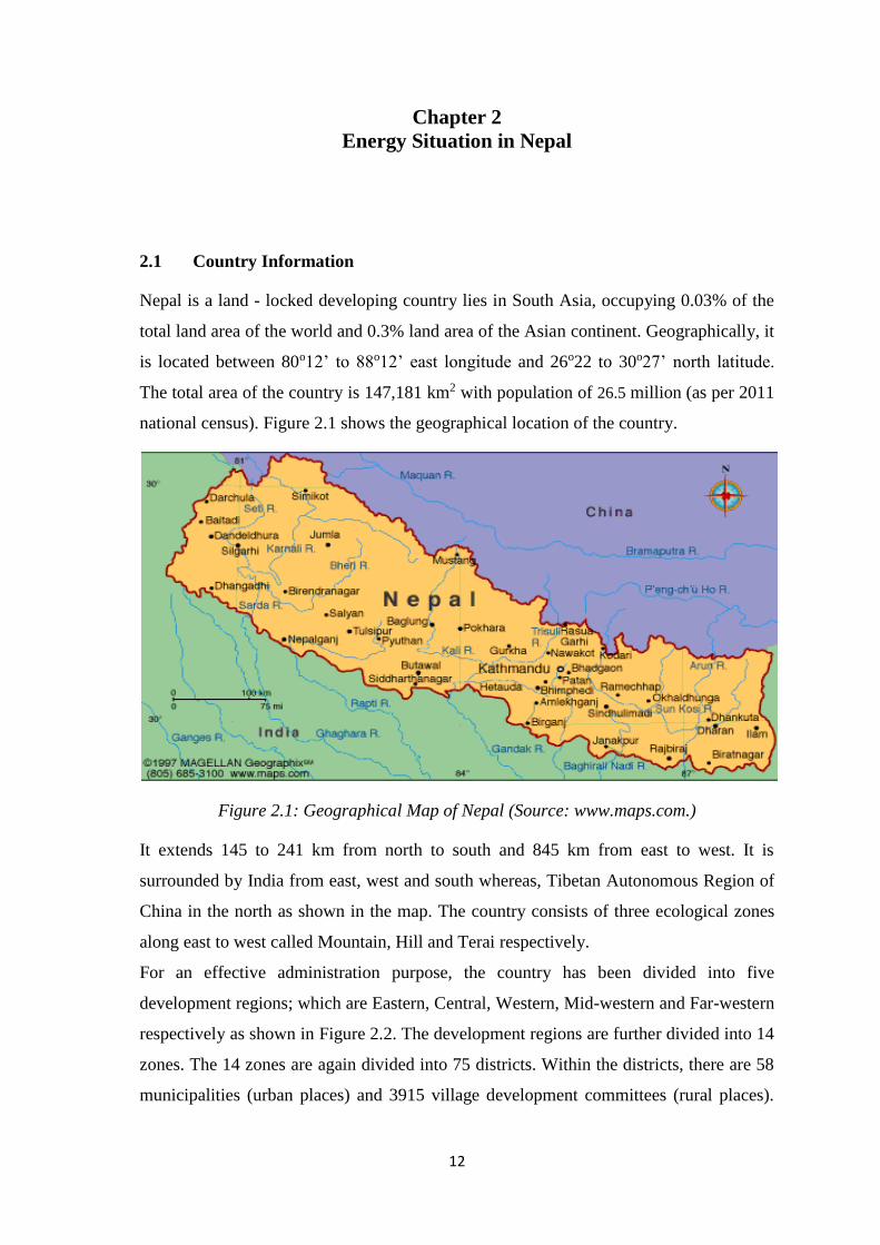
2.1 Country Information
Nepal is a land - locked developing country lies in South Asia, occupying 0.03% of the
total land area of the world and 0.3% land area of the Asian continent. Geographically, it
is located between 80o12’ to 88o12’ east longitude and 26o22 to 30o27’ north latitude.
The total area of the country is 147,181 km2 with population of 26.5 million (as per 2011
national census). Figure 2.1 shows the geographical location of the country.
Figure 2.1: Geographical Map of Nepal (Source: www.maps.com.)
It extends 145 to 241 km from north to south and 845 km from east to west. It is
surrounded by India from east, west and south whereas, Tibetan Autonomous Region of
China in the north as shown in the map. The country consists of three ecological zones
along east to west called Mountain, Hill and Terai respectively.
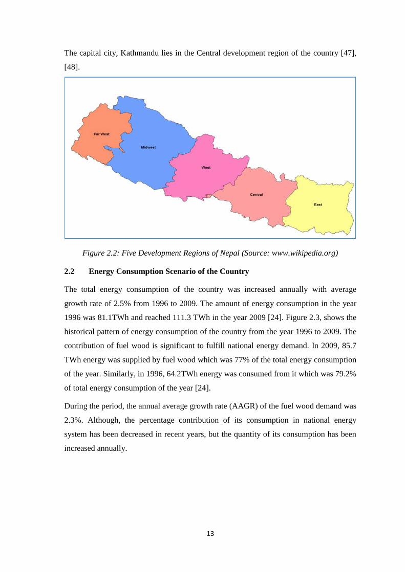
For an effective administration purpose, the country has been divided into five
development regions; which are Eastern, Central, Western, Mid-western and Far-western
respectively as shown in Figure 2.2. The development regions are further divided into 14
zones. The 14 zones are again divided into 75 districts. Within the districts, there are 58
municipalities (urban places) and 3915 village development committees (rural places).
13
The capital city, Kathmandu lies in the Central development region of the country [47],
[48].
Figure 2.2: Five Development Regions of Nepal (Source: www.wikipedia.org)
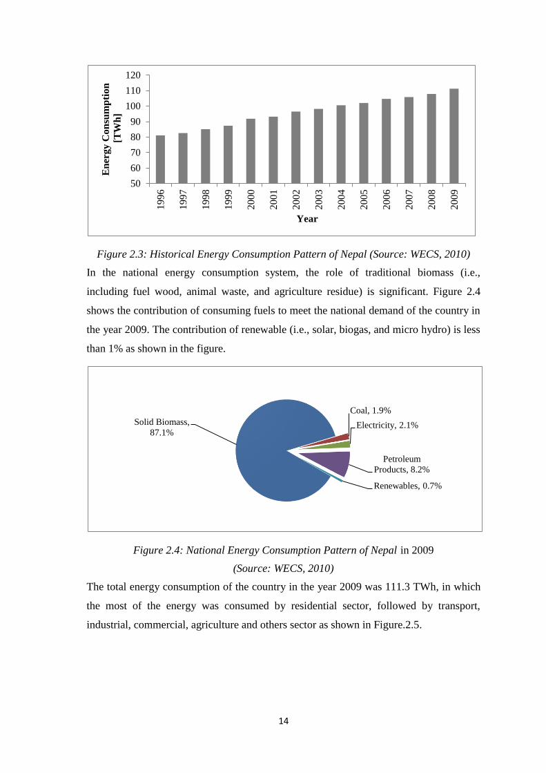
2.2 Energy Consumption Scenario of the Country
The total energy consumption of the country was increased annually with average
growth rate of 2.5% from 1996 to 2009. The amount of energy consumption in the year
1996 was 81.1TWh and reached 111.3 TWh in the year 2009 [24]. Figure 2.3, shows the
historical pattern of energy consumption of the country from the year 1996 to 2009. The
contribution of fuel wood is significant to fulfill national energy demand. In 2009, 85.7
TWh energy was supplied by fuel wood which was 77% of the total energy consumption
of the year. Similarly, in 1996, 64.2TWh energy was consumed from it which was 79.2%
of total energy consumption of the year [24].
During the period, the annual average growth rate (AAGR) of the fuel wood demand was
2.3%. Although, the percentage contribution of its consumption in national energy
system has been decreased in recent years, but the quantity of its consumption has been
increased annually.
14
Figure 2.3: Historical Energy Consumption Pattern of Nepal (Source: WECS, 2010)
In the national energy consumption system, the role of traditional biomass (i.e.,
including fuel wood, animal waste, and agriculture residue) is significant. Figure 2.4
shows the contribution of consuming fuels to meet the national demand of the country in
the year 2009. The contribution of renewable (i.e., solar, biogas, and micro hydro) is less
than 1% as shown in the figure.
Figure 2.4: National Energy Consumption Pattern of Nepal in 2009
(Source: WECS, 2010)
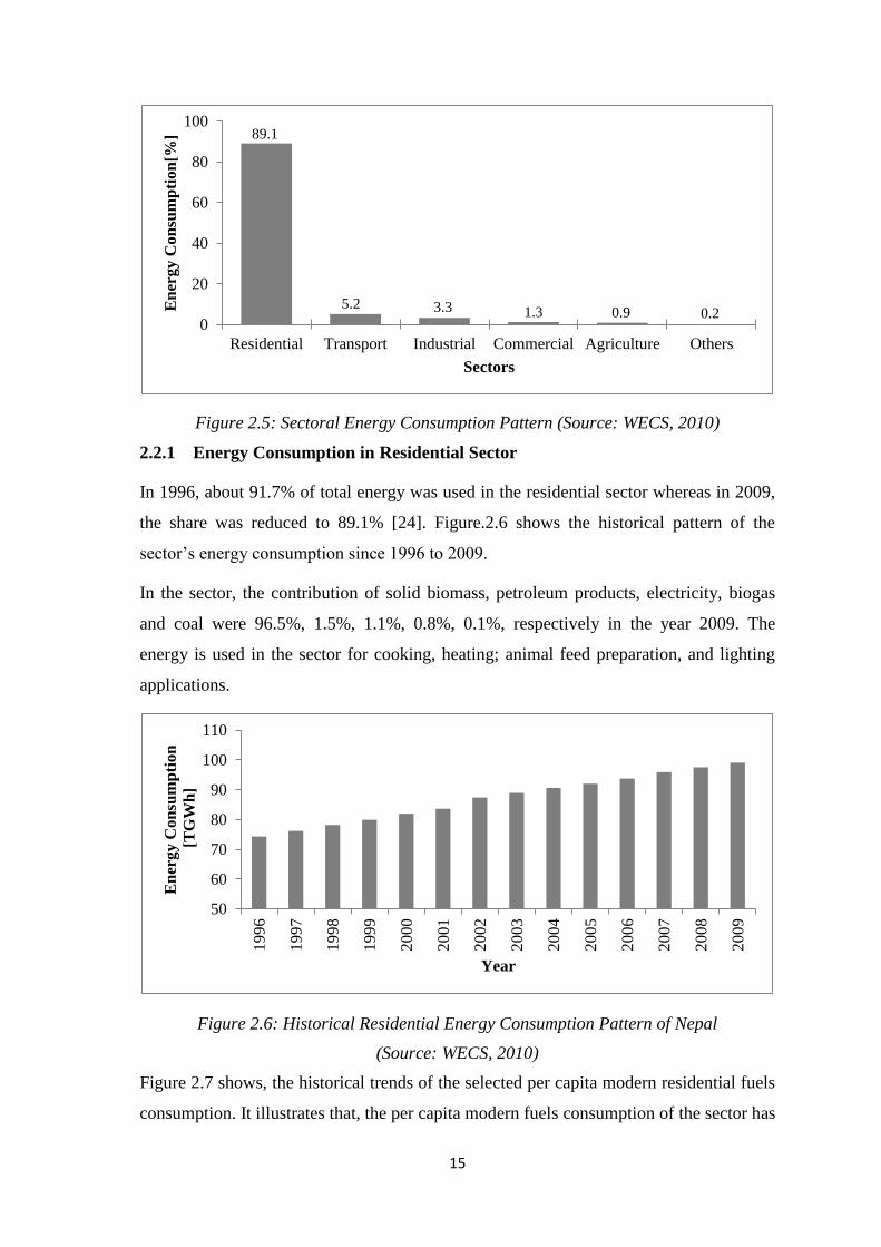
The total energy consumption of the country in the year 2009 was 111.3 TWh, in which
the most of the energy was consumed by residential sector, followed by transport,
industrial, commercial, agriculture and others sector as shown in Figure.2.5.
50
60
70
80
90
100
110
120
19
96
19
97
19
98
19
99
2000
20
01
20
02
20
03
20
04
20
05
20
06
20
07
2008
20
09
En
erg
y C
on
sum
pti
on
[TW
h]
Year
Solid Biomass,
87.1%
Coal, 1.9%
Electricity, 2.1%
Petroleum
Products, 8.2%
Renewables, 0.7%
15
Figure 2.5: Sectoral Energy Consumption Pattern (Source: WECS, 2010)
2.2.1 Energy Consumption in Residential Sector
In 1996, about 91.7% of total energy was used in the residential sector whereas in 2009,
the share was reduced to 89.1% [24]. Figure.2.6 shows the historical pattern of the
sector’s energy consumption since 1996 to 2009.
In the sector, the contribution of solid biomass, petroleum products, electricity, biogas
and coal were 96.5%, 1.5%, 1.1%, 0.8%, 0.1%, respectively in the year 2009. The
energy is used in the sector for cooking, heating; animal feed preparation, and lighting
applications.
Figure 2.6: Historical Residential Energy Consumption Pattern of Nepal
(Source: WECS, 2010)
Figure 2.7 shows, the historical trends of the selected per capita modern residential fuels
consumption. It illustrates that, the per capita modern fuels consumption of the sector has
89.1
5.2 3.3 1.3 0.9 0.20
20
40
60
80
100
Residential Transport Industrial Commercial Agriculture Others
En
erg
y C
on
sum
pti
on
[%]
Sectors
50
60
70
80
90
100
110
19
96
19
97
19
98
19
99
20
00
20
01
20
02
20
03
20
04
20
05
20
06
20
07
20
08
20
09
En
erg
y C
on
sum
pti
on
[TG
Wh
]
Year
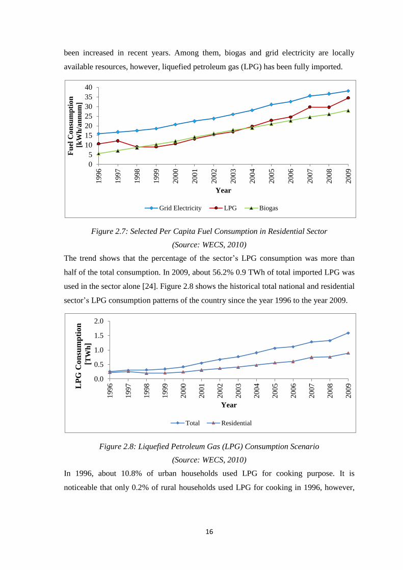
16
been increased in recent years. Among them, biogas and grid electricity are locally
available resources, however, liquefied petroleum gas (LPG) has been fully imported.
Figure 2.7: Selected Per Capita Fuel Consumption in Residential Sector
(Source: WECS, 2010)
The trend shows that the percentage of the sector’s LPG consumption was more than
half of the total consumption. In 2009, about 56.2% 0.9 TWh of total imported LPG was
used in the sector alone [24]. Figure 2.8 shows the historical total national and residential
sector’s LPG consumption patterns of the country since the year 1996 to the year 2009.
Figure 2.8: Liquefied Petroleum Gas (LPG) Consumption Scenario
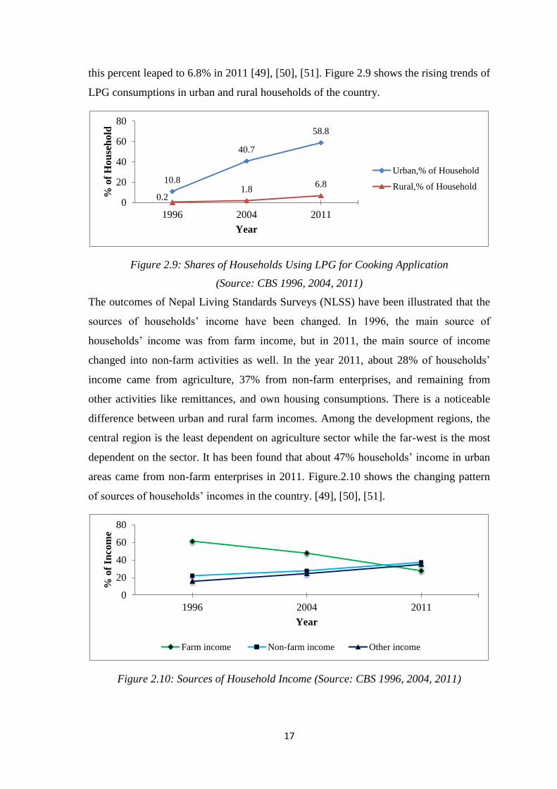
(Source: WECS, 2010)
In 1996, about 10.8% of urban households used LPG for cooking purpose. It is
noticeable that only 0.2% of rural households used LPG for cooking in 1996, however,
0
5
10
15
20
25
30
35
40
19
96
19
97
19
98
19
99
20
00
20
01
20
02
20
03
20
04
20
05
20
06
20
07
20
08
20
09
Fu
el C
on
sum
pti
on
[kW
h/a
nn
um
]
Year
Grid Electricity LPG Biogas
0.0
0.5
1.0
1.5
2.0
1996
1997
1998
1999
2000
2001
2002
2003
2004
2005
2006
2007
2008
2009LP
G C
on
sum
pti
on
[TW
h]
Year
Total Residential
17
this percent leaped to 6.8% in 2011 [49], [50], [51]. Figure 2.9 shows the rising trends of
LPG consumptions in urban and rural households of the country.
Figure 2.9: Shares of Households Using LPG for Cooking Application
(Source: CBS 1996, 2004, 2011)
The outcomes of Nepal Living Standards Surveys (NLSS) have been illustrated that the
sources of households’ income have been changed. In 1996, the main source of
households’ income was from farm income, but in 2011, the main source of income
changed into non-farm activities as well. In the year 2011, about 28% of households’
income came from agriculture, 37% from non-farm enterprises, and remaining from
other activities like remittances, and own housing consumptions. There is a noticeable
difference between urban and rural farm incomes. Among the development regions, the
central region is the least dependent on agriculture sector while the far-west is the most
dependent on the sector. It has been found that about 47% households’ income in urban
areas came from non-farm enterprises in 2011. Figure.2.10 shows the changing pattern
of sources of households’ incomes in the country. [49], [50], [51].
Figure 2.10: Sources of Household Income (Source: CBS 1996, 2004, 2011)
10.8
40.7
58.8
0.21.8
6.8
0
20
40
60
80
1996 2004 2011
% o
f H
ou
seh
old
Year
Urban,% of Household
Rural,% of Household
0
20
40
60
80
1996 2004 2011
% o
f In
com
e
Year
Farm income Non-farm income Other income
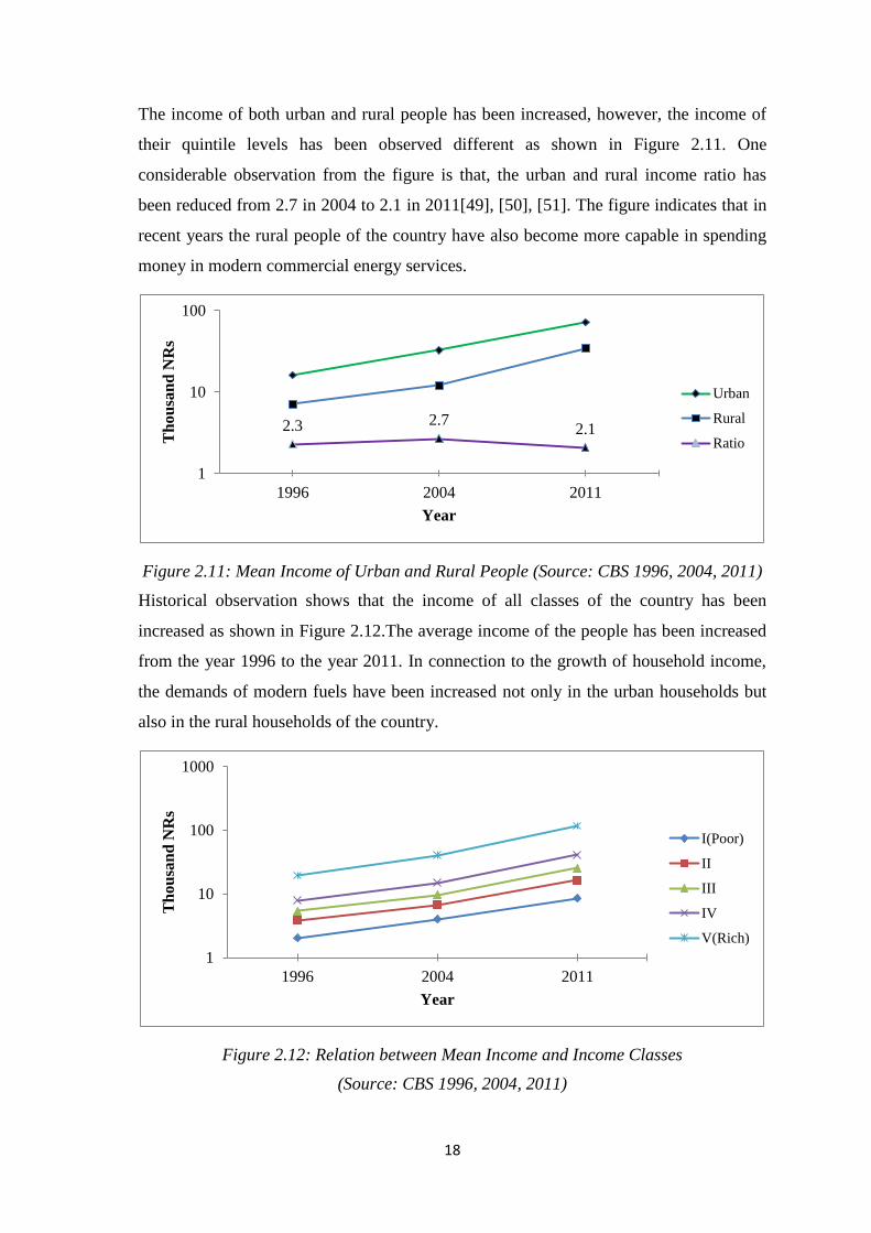
18
The income of both urban and rural people has been increased, however, the income of
their quintile levels has been observed different as shown in Figure 2.11. One
considerable observation from the figure is that, the urban and rural income ratio has
been reduced from 2.7 in 2004 to 2.1 in 2011[49], [50], [51]. The figure indicates that in
recent years the rural people of the country have also become more capable in spending
money in modern commercial energy services.
Figure 2.11: Mean Income of Urban and Rural People (Source: CBS 1996, 2004, 2011)
Historical observation shows that the income of all classes of the country has been
increased as shown in Figure 2.12.The average income of the people has been increased
from the year 1996 to the year 2011. In connection to the growth of household income,
the demands of modern fuels have been increased not only in the urban households but
also in the rural households of the country.
Figure 2.12: Relation between Mean Income and Income Classes
(Source: CBS 1996, 2004, 2011)
2.3 2.72.1
1
10
100
1996 2004 2011
Th
ou
san
d N
Rs
Year
Urban
Rural
Ratio
1
10
100
1000
1996 2004 2011
Th
ou
san
d N
Rs
Year
I(Poor)
II
III
IV
V(Rich)
19
2.2.2 Energy Consumption in Industrial Sector
The industrial sector’s energy consumption was about 3.3% of total national energy
consumption of the country in 2009. In 1996, about 34.2% of the total sectoral energy
consumption demand was supplied from coal followed by 21.2% from electricity, 19.6%
from petroleum products, 16.5% from biomass and 8.5% from fuel wood. But in the
year 2009, the energy consumption data shows that about 57.9% of the sector energy
consumption was supplied from coal, followed by 23.2 % from electricity, 3.5% from
petroleum products, 10.0 % from biomass and 5.4 % from fuel wood [24]. During the
period, the contribution of coal, and electricity had been increased while the contribution
of other fuels had been decreased. The coal has been used for heating in boiler and kiln.
Hence, the consumption of coal in the sector is major. The wood and other biomass fuels
have been used in the sector for ignition of fire as well as for heating purposes.
There are five end uses in the sector which are process heat, motive power, boiler,
lighting and others. Boiler end use application has used most of the energy (37%) that is
why coal is heavily consumed in the sector. Other end uses for energy consumption are
motive power (31%), process heat (30%) and lighting (2%) respectively [24]. In this
sector, many traditional and small scale industries were closed due to unstable political
situation and being unable to compete with international market [23], [52]. As a result,
the contribution of this sector to national economy has been decreased.
2.2.3 Energy Consumption in Transport Sector
Transport sector includes mainly road and air transport in Nepal. The energy
consumption in this sector deals with fuels used by vehicles and planes (i.e., air transport
devices) for passenger and freight transport. The total energy consumption on the sector
in 2009 was about 5.8 TWh which was raised from 2.4 TWh in the year 1996. During
the period, about 6.9 % of AAGR of the energy demand was observed in the sector. In
the year 2009, about 9.2 TWh was supplied by petroleum product which was 8.2 % of
total energy consumption of the year. The sectoral consumption of petroleum products
was about 63.3% in the year 2009. It has been observed that the road transport demand
was increased with AAGR of 7.4% while, the air transport demand was increased with
AAGR of 4.2% respectively during the period. From 1996 to 2009, average 84.5% of the
sector’s energy demand was consumed in road transport alone, and remaining in air
transport. In the year 2009, the demand was supplied mainly by diesel (67.1%), followed
20
by gasoline (19.8%), ATF (11.9%), LPG (1.1%) and electricity (0.1%) fuels respectively
[24], [52].
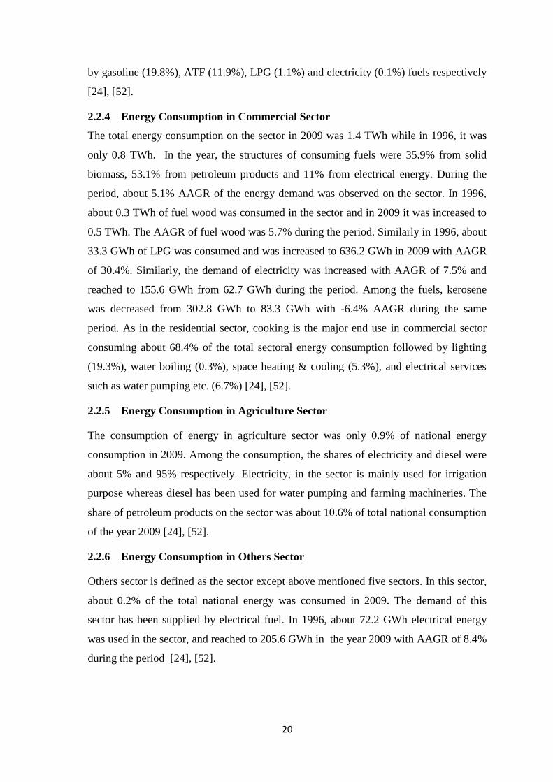
2.2.4 Energy Consumption in Commercial Sector
The total energy consumption on the sector in 2009 was 1.4 TWh while in 1996, it was
only 0.8 TWh. In the year, the structures of consuming fuels were 35.9% from solid
biomass, 53.1% from petroleum products and 11% from electrical energy. During the
period, about 5.1% AAGR of the energy demand was observed on the sector. In 1996,
about 0.3 TWh of fuel wood was consumed in the sector and in 2009 it was increased to
0.5 TWh. The AAGR of fuel wood was 5.7% during the period. Similarly in 1996, about
33.3 GWh of LPG was consumed and was increased to 636.2 GWh in 2009 with AAGR
of 30.4%. Similarly, the demand of electricity was increased with AAGR of 7.5% and
reached to 155.6 GWh from 62.7 GWh during the period. Among the fuels, kerosene
was decreased from 302.8 GWh to 83.3 GWh with -6.4% AAGR during the same
period. As in the residential sector, cooking is the major end use in commercial sector
consuming about 68.4% of the total sectoral energy consumption followed by lighting
(19.3%), water boiling (0.3%), space heating & cooling (5.3%), and electrical services
such as water pumping etc. (6.7%) [24], [52].
2.2.5 Energy Consumption in Agriculture Sector
The consumption of energy in agriculture sector was only 0.9% of national energy
consumption in 2009. Among the consumption, the shares of electricity and diesel were
about 5% and 95% respectively. Electricity, in the sector is mainly used for irrigation
purpose whereas diesel has been used for water pumping and farming machineries. The
share of petroleum products on the sector was about 10.6% of total national consumption
of the year 2009 [24], [52].
2.2.6 Energy Consumption in Others Sector
Others sector is defined as the sector except above mentioned five sectors. In this sector,
about 0.2% of the total national energy was consumed in 2009. The demand of this
sector has been supplied by electrical fuel. In 1996, about 72.2 GWh electrical energy
was used in the sector, and reached to 205.6 GWh in the year 2009 with AAGR of 8.4%
during the period [24], [52].
21
2.3 Energy Planning Models
Kahen (1995) defined energy planning as a matter of assessing the supply and demand
for energy and attempting to balance them from present to future [53]. The energy
planning is a way of managing the available resources and, is a process oriented activity.
According to Van Beeck (2003), a planning process is the process of making choice
between available alternatives [54]. Planning for future is basically done through
projecting the scenarios based on present and past information. Energy planning is a
dynamic and complex approach for considering the policies and strategies of energy
systems, therefore, energy models are used for the planning process. For energy planning
purpose, energy models were first developed in 1970s as a result of the increasing
availability of computer and the growing concern of environmental consciousness [55].
The importance of developing countries in energy planning began after the first oil crisis
in 1973, when the high oil prices suddenly caused trade unbalance of many oil-
importing countries [54],[56]. Only after the crisis, the sufficient attention was given for
rational utilization of energy resources, and felt the importance of long-term energy
planning [57]. Literatures show, energy planning is done for different time horizons.
Klein et al. (1984) refer to four years or less as short term, from five to nine years as
medium term and ten or more than ten years as long term respectively [58].
Different models have came in practice for addressing the energy system planning like
MESSAGE, WASP and MARKAL for supply side, whereas MADEE and MADE for
demand side. It has been found that about 80% contribution of the total global
greenhouse effect was due to energy related activities [59]. Knowing the fact, the scope
of environmental planning along with energy and economics rose - up and the
importance of the new dimension of planning was realized and afterwards,
environmental dimension was also integrated for the planning process. Therefore, the
existing energy planning tools are continuously enhanced to address the energy,
economic and environment aspects of the energy planning process.
22
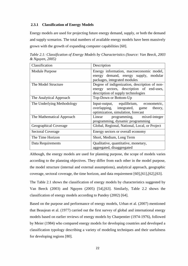
2.3.1 Classification of Energy Models
Energy models are used for projecting future energy demand, supply, or both the demand
and supply scenarios. The total numbers of available energy models have been massively
grown with the growth of expanding computer capabilities [60].
Table 2.1: Classification of Energy Models by Characteristics (Source: Van Beeck, 2003
& Nguyen, 2005)
Classification Description
Module Purpose Energy information, macroeconomic model,
energy demand, energy supply, modular
packages, integrated modules
The Model Structure Degree of indigenization, description of non-
energy sectors, description of end-uses,
description of supply technologies
The Analytical Approach Top-Down or Bottom-Up
The Underlying Methodology Input-output, equilibrium, econometric,
overlapping, integrated, game theory,
optimization, simulation, forecast
The Mathematical Approach Linear programming, mixed-integer
programming, dynamic programming
Geographical Coverage Global, Regional, National, Local, or Project
Sectoral Coverage Energy sectors or overall economy
The Time Horizon Short, Medium, Long Term
Data Requirements Qualitative, quantitative, monetary,
aggregated, disaggregated
Although, the energy models are used for planning purpose, the scope of models varies
according to the planning objectives. They differ from each other in the model purpose,
the model structure (internal and external assumptions), analytical approach, geographic
coverage, sectoral coverage, the time horizon, and data requirement [60],[61],[62],[63].
The Table 2.1 shows the classification of energy models by characteristics suggested by
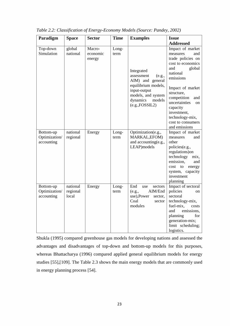
Van Beeck (2003) and Nguyen (2005) [54],[63]. Similarly, Table 2.2 shows the
classification of energy models according to Pandey (2002) [64].
Based on the purpose and performance of energy models, Urban et al. (2007) mentioned
that Beaujean et al. (1977) carried out the first survey of global and international energy
models based on earlier reviews of energy models by Charpentier (1974-1976), followed
by Meier (1984) who compared energy models for developing countries and developed a
classification typology describing a variety of modeling techniques and their usefulness
for developing regions [80].
23
Table 2.2: Classification of Energy-Economy Models (Source: Pandey, 2002)
Paradigm Space Sector Time Examples Issue
Addressed Top-down
Simulation
global
national
Macro-
economic
energy
Long-
term
Integrated
assessment (e.g.,
AIM) and general
equilibrium models,
input-output
models, and system
dynamics models
(e.g.,FOSSIL2)
Impact of market
measures and
trade policies on
cost to economics
and global
national
emissions
Impact of market
structure,
competition and
uncertainties on
capacity
investment,
technology-mix,
cost to consumers
and emissions
Bottom-up
Optimization/
accounting
national
regional
Energy Long-
term
Optimization(e.g.,
MARKAL,EFOM)
and accounting(e.g.,
LEAP)models
Impact of market
measures and
other
policies(e.g.,
regulations)on
technology mix,
emission, and
cost to energy
system, capacity
investment
planning
Bottom-up
Optimization/
accounting
national
regional
local
Energy Long-
term
End use sectors
(e.g., AIM/End
use),Power sector,
Coal sector
modules
Impact of sectoral
policies on
sectoral
technology-mix,
fuel-mix, costs
and emissions,
planning for
generation-mix;
limit scheduling;
logistics.
Shukla (1995) compared greenhouse gas models for developing nations and assessed the
advantages and disadvantages of top-down and bottom-up models for this purposes,
whereas Bhattacharya (1996) compared applied general equilibrium models for energy
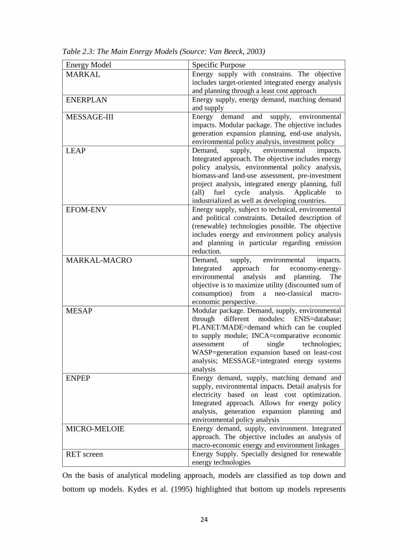
studies [55],[109]. The Table 2.3 shows the main energy models that are commonly used
in energy planning process [54].
24
Table 2.3: The Main Energy Models (Source: Van Beeck, 2003)
Energy Model Specific Purpose
MARKAL Energy supply with constrains. The objective
includes target-oriented integrated energy analysis
and planning through a least cost approach
ENERPLAN Energy supply, energy demand, matching demand
and supply
MESSAGE-III Energy demand and supply, environmental
impacts. Modular package. The objective includes
generation expansion planning, end-use analysis,
environmental policy analysis, investment policy
LEAP Demand, supply, environmental impacts.
Integrated approach. The objective includes energy
policy analysis, environmental policy analysis,
biomass-and land-use assessment, pre-investment
project analysis, integrated energy planning, full
(all) fuel cycle analysis. Applicable to
industrialized as well as developing countries.
EFOM-ENV Energy supply, subject to technical, environmental
and political constraints. Detailed description of
(renewable) technologies possible. The objective
includes energy and environment policy analysis
and planning in particular regarding emission
reduction.
MARKAL-MACRO Demand, supply, environmental impacts.
Integrated approach for economy-energy-
environmental analysis and planning. The
objective is to maximize utility (discounted sum of
consumption) from a neo-classical macro-
economic perspective.
MESAP Modular package. Demand, supply, environmental
through different modules: ENIS=database;
PLANET/MADE=demand which can be coupled
to supply module; INCA=comparative economic
assessment of single technologies;
WASP=generation expansion based on least-cost
analysis; MESSAGE=integrated energy systems
analysis
ENPEP Energy demand, supply, matching demand and
supply, environmental impacts. Detail analysis for
electricity based on least cost optimization.
Integrated approach. Allows for energy policy
analysis, generation expansion planning and
environmental policy analysis
MICRO-MELOIE Energy demand, supply, environment. Integrated
approach. The objective includes an analysis of
macro-economic energy and environment linkages
RET screen Energy Supply. Specially designed for renewable
energy technologies
On the basis of analytical modeling approach, models are classified as top down and
bottom up models. Kydes et al. (1995) highlighted that bottom up models represents
25
different activities like energy supply process, conversion technologies and end- use
demand pattern in detail [65]. On the other hand, Pandey (2002) argued that the top
down models can answer energy policy questions regarding macroeconomic indicators
and energy-wide emissions, due to their clear inclusion of inter-linkages between energy
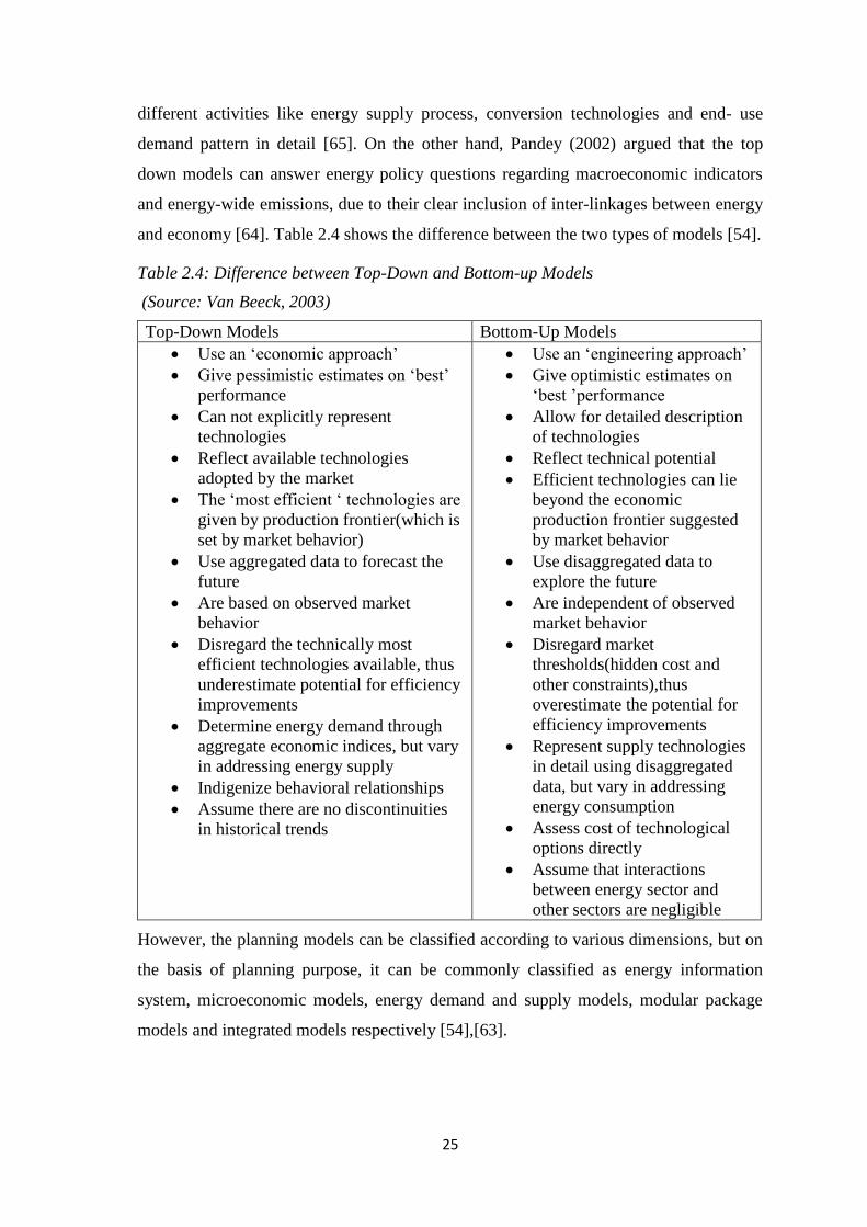
and economy [64]. Table 2.4 shows the difference between the two types of models [54].
Table 2.4: Difference between Top-Down and Bottom-up Models
(Source: Van Beeck, 2003)
Top-Down Models Bottom-Up Models
Use an ‘economic approach’
Give pessimistic estimates on ‘best’
performance
Can not explicitly represent
technologies
Reflect available technologies
adopted by the market
The ‘most efficient ‘ technologies are
given by production frontier(which is
set by market behavior)
Use aggregated data to forecast the
future
Are based on observed market
behavior
Disregard the technically most
efficient technologies available, thus
underestimate potential for efficiency
improvements
Determine energy demand through
aggregate economic indices, but vary
in addressing energy supply
Indigenize behavioral relationships
Assume there are no discontinuities
in historical trends
Use an ‘engineering approach’
Give optimistic estimates on
‘best ’performance
Allow for detailed description
of technologies
Reflect technical potential
Efficient technologies can lie
beyond the economic
production frontier suggested
by market behavior
Use disaggregated data to
explore the future
Are independent of observed
market behavior
Disregard market
thresholds(hidden cost and
other constraints),thus
overestimate the potential for
efficiency improvements
Represent supply technologies
in detail using disaggregated
data, but vary in addressing
energy consumption
Assess cost of technological
options directly
Assume that interactions
between energy sector and
other sectors are negligible
However, the planning models can be classified according to various dimensions, but on
the basis of planning purpose, it can be commonly classified as energy information
system, microeconomic models, energy demand and supply models, modular package
models and integrated models respectively [54],[63].
26
2.3.2 Energy Information Systems
Energy information systems are typically database for management and presentation of
statistic and technical data in graphical and table formats. Apart from the management
and presentation of the data, some databases offer opportunities to analyze and compare
technologies. Some common examples of these databases are CO2DB, DECPAC, and
IKARUS etc. [63].
2.3.3 Macro Economic Models
Macroeconomic models are an analytical tools design to describe for a question on how
the price and availability of energy influence the economy in terms of gross domestic
product (GDP), employment and inflation rate and vice versa, of a country or a region.
They are related to the level of outputs and prices based on the interactions between
aggregate demand and supply. Two examples under this category are MACRO and MIS
models [63].
1. MACRO: The MACRO model was developed by the International Institute of
Applied System Analysis (IIASA). The model has eleven regional versions and is
widely used to compute size of economy, investment flows, and demand for
electric and non electric energy. The model’s strength is that it treats the
economy of coherent regions of the world in an integrated fashion and estimates
energy demand. Its weakness is that the model has little resolution of
technological choices and the choice of technologies determines emissions and
environmental impacts [66].
2. Macroeconomic information system (MIS): It was developed by University of
Oldenburg as a module in IKARUS2 project. The system provides framework
data for the economic consistency. It is based on dynamic input/output approach.
The overall economy of Germany is aggregated into 30 sectors, 9 of which are
energy sectors, corresponding to the functional structure. The MIS system
consists of an input/output generator, a growth-model and several sub-models,
namely electricity, transport and dwelling [63],[67].
2.3.4 Energy Demand Models
The energy demand models are used to forecast the energy demand for a specified time
horizon. They are used either for specific sector or entire economy of a region (i.e., local
27
level, regional level, national or international). Among the energy demand models, the
techno-economic models are widespread, but econometric models are also used.
Popularly known energy demand models are MADEE, and MAED. The MAED was
developed based on earlier version of MEDEE by IAEA into its present form, while
MADEE remains the model of the original authors and is supported by their energy
consulting firm ENERDATA [68].
1. MEDEE: Modele d’ Evaluation de la Demande En Energie (MEDEE) was
developed by the Institute of Energy Policy and Economics, Grenoble, France. It
is a techno-economic bottom – up model for forecasting the demand of a region
or a country. In the model, the aggregate demand of the economy is
disaggregated into standardized subgroups (like agriculture, industry etc.). By
addressing the direct and indirect determinates of these subgroups demands, the
model is able to evaluate the future energy demand of the region or a country.
[63].
2. MAED: The Model for Analysis of Energy Demand (MAED) is developed by
International Atomic Agency for estimation of the demand for different time
horizons of a region or a country. The simulation model needs various technical
and political parameters as model inputs; such as varying social needs of people,
policy measures of a county for development & industrialization etc. The demand
is first determined at the disaggregated level and then added up to obtain the
overall final demand. It uses a bottom-up approach to project future energy
demand based on medium to long term scenarios of socio-economic,
technological and demographic development of the region or a country [69].
2.3.5 Modular Packages
Modular package incorporates different kind of models like a macro-economic
component, an energy supply and demand balance, an energy demand alone, etc. within
the package. Based on the scope and required application, user can choose the particular
module application from the package. Some of the well known tools are ENPEP, LEAP
and MESAP.
1. ENPEP: The Energy and Power Evaluation Program (ENPEP) is a simulation
type of model. It is developed by the Argonne National Laboratory in the USA. It
is used to model a country’s entire energy system. The model incorporates the
28
dynamics of market processes related to energy by an explicit representation of
market equilibrium, i.e., the balancing of supply and demand. It consists of an
executive module and ten technical modules. The main module is BALANCE.
This module uses a non-linear and market-based equilibrium approach to
determine energy supply and demand balance for the entire energy system [70].
Equilibrium is reached when ENPEN-BALANCE finds a set of market cleaning
prices and quantities that satisfy all relevant equations and inequalities. Connolly
et al. (2010) mentioned that the model has been used for Mexico’s future energy
needs and estimated the corresponding environment burdens, green house-gas
emission projections for Turkey and GHS mitigation analysis for Bulgaria [71].
2. MESAP: The Modular Energy System Analysis and Planning (MESAP) model
is developed for integrated energy and environment planning. Baumhogger et al.
(1998) developed it not only for energy and environmental management on local
and regional scales but also in global scale. It consists of general information
system based on relation database theory that is linked to different modeling
tools. It supports energy phase of the structural analysis procedure to assist the
decision-making process in a pragmatic way. The model is used for demand
analysis, integrated resource planning, and demand side management purposes.
[72], [73].
3. LEAP: LEAP means Long-range Energy Alternatives Planning System and is
developed by the Stockholm Environment Institute in Boston, USA. It is an
energy and environmental policy analysis tool for planning medium to long-term
time horizon. Various scenarios (business as usual, policy, alternative) can be
created using the tool. The energy requirements, their social costs & benefits, and
their environmental impacts can be evaluated and compared for different
scenarios by using the tool [74].
2.3.6 Selection of Energy Modeling Tool
Although there are different types of models available for energy planning purpose, but
the selection of particular modeling tool for a country is a difficult task. For selection of
a model for planning purposes, Rath-Nagel (1981) suggested that there are no models
which can provide the answer to all questions due to the complexity of energy policy and
energy strategy issues; therefore, it will be required several models with different
29
objectives and specifications in order to effectively support the development of energy
policies and planning [75]. Van Beeck (2003) realized for capturing impossibility to
every aspect of reality in a model and informed that the best model addresses maximum
degree of a simplified representation of reality [54]. The examination of model quality is
difficult, hence IIASA (2005) stated that a model quality cannot be measured exactly and
further suggested that an important assessment criterion of long-term models is that their
ability to handle uncertainties and adequately map the real-world system [76].
The selection of a proper model for energy planning process is a tradeoff between
availability of planning models and their characteristics and capabilities. Shukla (1995)
mentioned that the most of the energy models were built and used in industrialized
countries, and it was also assumed that the development of energy systems of developing
countries would be followed the same pattern like industrialized countries [55]. The
required data for modeling based on model is also challenge for developing countries
like Nepal. Worrell et al. (2004) highlighted a number of modeling challenges like data
quality, capturing technological potential and technological penetration [77]. According
to Jung et al. (2000), the development trajectory of developing countries will be
followed the path of the industrialized countries, first a decline of the agriculture sector,
then heavily growing industry and later a shift towards the service sector [78]. But in
India, it has been observed that the development trajectory has followed a modest
industry sector towards the service sector [79]. Thus, the energy system path of
developing countries like India has been shown that the path of development is different
than the predefined path of developed countries. According to Urban et al. (2007) the
main issues for developing countries’ energy system are the informal economy, supply
shortages, poor performance of power sector, structural economic change, electrification,
traditional bio-fuels and urban-rural division [80]. Being a developing country, those
characteristics are easily observed in Nepalese energy system too. In addition, the
unavailability of appropriate database is also a crucial issue for long term Nepalese
energy sector’s modeling and planning.
Urban et al. (2007) illustrated that based on the number of characteristics of developing
countries address per model, the LEAP model address a large number of characteristics
whereas MARKAL model address a medium number of characteristics. It has been
concluded that none of the present-day energy models fulfill all requirements adequately
by addressing the energy systems and economics of developing countries [80]. Seebregts
30
et al. (2001) emphasized that the MARKAL model is the most widely used and best
known in the family of optimization models for supply side planning [81].
The LEAP model has been adopted by thousand of organizations in more than 190
countries worldwide, including governmental agencies, academics, non-governmental
organizations, consulting companies and energy utilities [74]. Similarly, MARKAL
model has been used more than 70 countries and 230 institutions for energy planning
purposes [82]. In connection with this, there are number of studies that have been
conducted using LEAP, and MARKAL tools in the world from highly developed to list
developed countries and their methodologies are well established and worldwide
accepted.
The economic growth and energy demand are closely related [83]. Evan Lau et al.
(2011), found that there is casual linkage exist from GDP to energy consumption for
seventeen selected Asian countries, including Nepal [84]. Similarly, Ozturk et al. (2012)
showed that there is a bidirectional casual linkage between them in the case of India
[85].
2.4 Economic Growth of the Country
After the establishment of democratic government in 1991, Nepal adopted open
economic policies and started promoting private sectors involvement in business [86].
To demonstrate the adopted policy, government privatized many public enterprises
during 1990s. As a result, an accelerated economic growth was observed in some years
but, it could not be continued later [87]. In 1996, armed conflict began in the country
which caused political instability. The process of economic reforms came in low priority
of the nation due to shift of its focus for addressing the solution of emerged new
challenge of law and order situation across the country. The armed conflict was ended
through comprehensive peace accord between concerned stakeholders in 2006. In 2008,
the people elected constitutional assembly and the assembly abolished monarchy and
established the country as a federal democratic republic. Unfortunately, the
constitutional assembly also could not promulgate constitution thus, it was dissolved.
After then, again a new constitutional assembly election was held in 2013, and the newly
elected constitutional assembly is under the process for formulating the new constitution
of the country.
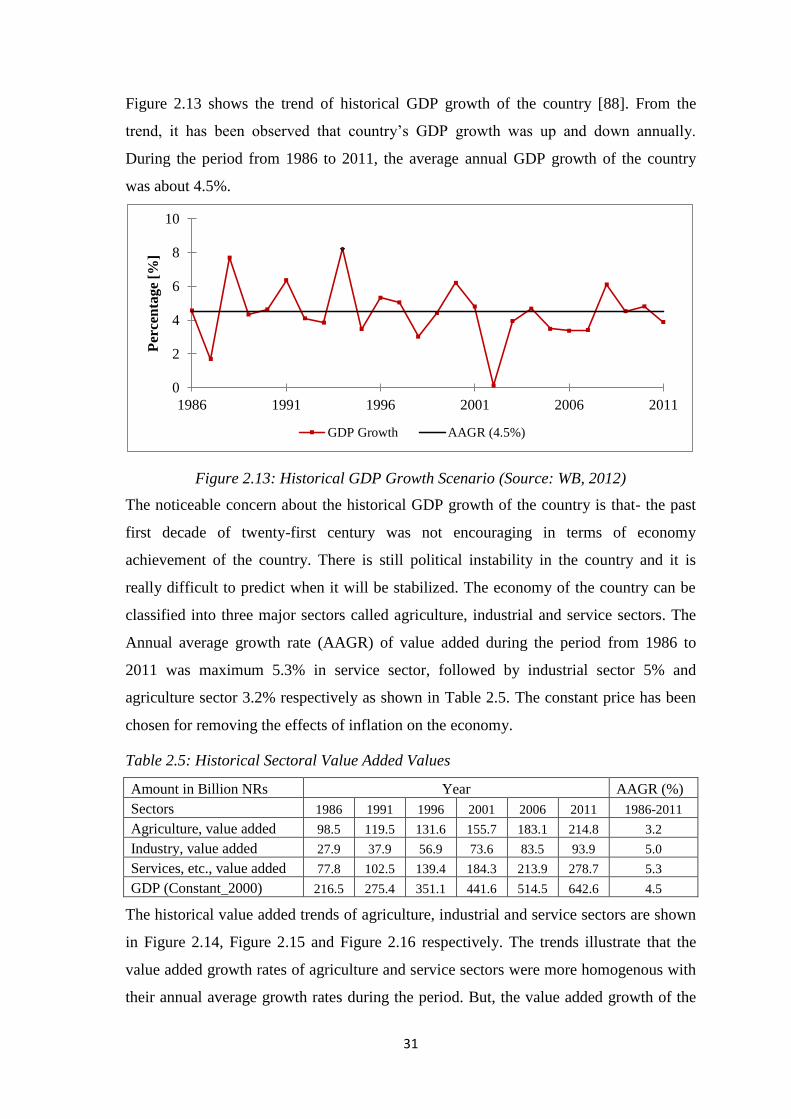
31
Figure 2.13 shows the trend of historical GDP growth of the country [88]. From the
trend, it has been observed that country’s GDP growth was up and down annually.
During the period from 1986 to 2011, the average annual GDP growth of the country
was about 4.5%.
Figure 2.13: Historical GDP Growth Scenario (Source: WB, 2012)
The noticeable concern about the historical GDP growth of the country is that- the past
first decade of twenty-first century was not encouraging in terms of economy
achievement of the country. There is still political instability in the country and it is
really difficult to predict when it will be stabilized. The economy of the country can be
classified into three major sectors called agriculture, industrial and service sectors. The
Annual average growth rate (AAGR) of value added during the period from 1986 to
2011 was maximum 5.3% in service sector, followed by industrial sector 5% and
agriculture sector 3.2% respectively as shown in Table 2.5. The constant price has been
chosen for removing the effects of inflation on the economy.
Table 2.5: Historical Sectoral Value Added Values
Amount in Billion NRs Year AAGR (%)
Sectors 1986 1991 1996 2001 2006 2011 1986-2011
Agriculture, value added 98.5 119.5 131.6 155.7 183.1 214.8 3.2
Industry, value added 27.9 37.9 56.9 73.6 83.5 93.9 5.0
Services, etc., value added 77.8 102.5 139.4 184.3 213.9 278.7 5.3
GDP (Constant_2000) 216.5 275.4 351.1 441.6 514.5 642.6 4.5
The historical value added trends of agriculture, industrial and service sectors are shown
in Figure 2.14, Figure 2.15 and Figure 2.16 respectively. The trends illustrate that the
value added growth rates of agriculture and service sectors were more homogenous with
their annual average growth rates during the period. But, the value added growth of the
0
2
4
6
8
10
1986 1991 1996 2001 2006 2011
Per
cen
tag
e [
%]
GDP Growth AAGR (4.5%)
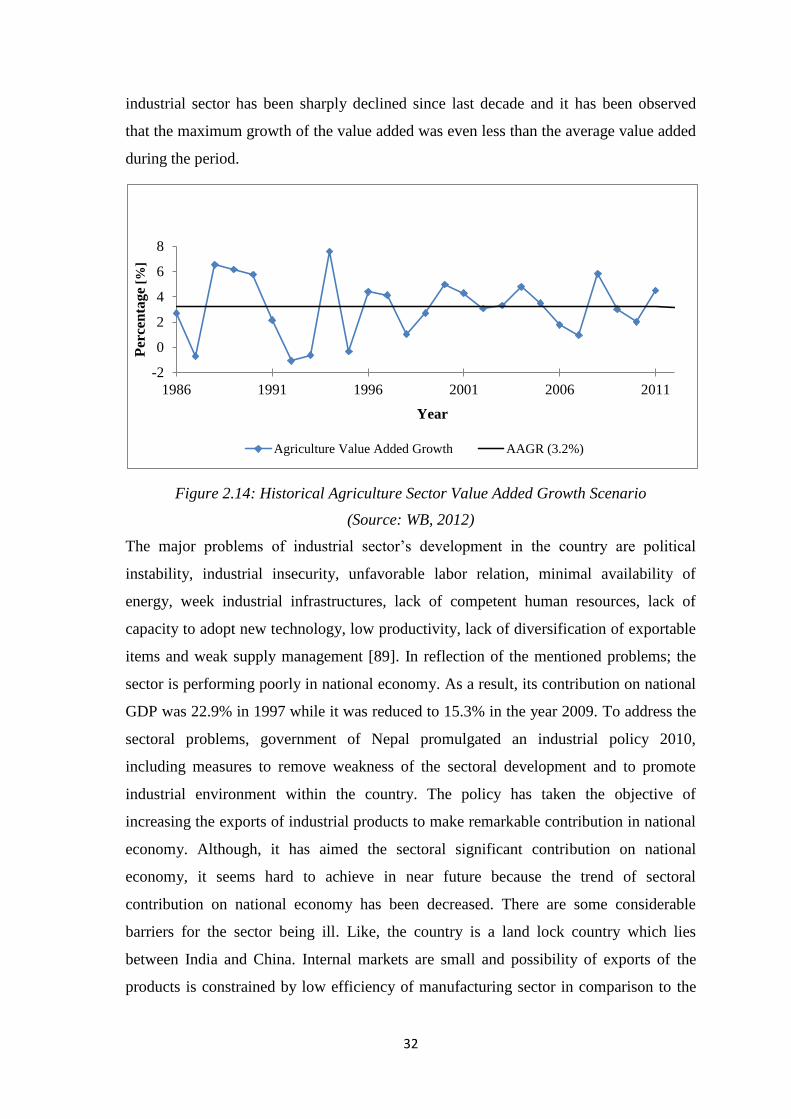
32
industrial sector has been sharply declined since last decade and it has been observed
that the maximum growth of the value added was even less than the average value added
during the period.
Figure 2.14: Historical Agriculture Sector Value Added Growth Scenario
(Source: WB, 2012)
The major problems of industrial sector’s development in the country are political
instability, industrial insecurity, unfavorable labor relation, minimal availability of
energy, week industrial infrastructures, lack of competent human resources, lack of
capacity to adopt new technology, low productivity, lack of diversification of exportable
items and weak supply management [89]. In reflection of the mentioned problems; the
sector is performing poorly in national economy. As a result, its contribution on national
GDP was 22.9% in 1997 while it was reduced to 15.3% in the year 2009. To address the
sectoral problems, government of Nepal promulgated an industrial policy 2010,
including measures to remove weakness of the sectoral development and to promote
industrial environment within the country. The policy has taken the objective of
increasing the exports of industrial products to make remarkable contribution in national
economy. Although, it has aimed the sectoral significant contribution on national
economy, it seems hard to achieve in near future because the trend of sectoral
contribution on national economy has been decreased. There are some considerable
barriers for the sector being ill. Like, the country is a land lock country which lies
between India and China. Internal markets are small and possibility of exports of the
products is constrained by low efficiency of manufacturing sector in comparison to the
-2
0
2
4
6
8
1986 1991 1996 2001 2006 2011
Per
cen
tag
e [
%]
Year
Agriculture Value Added Growth AAGR (3.2%)
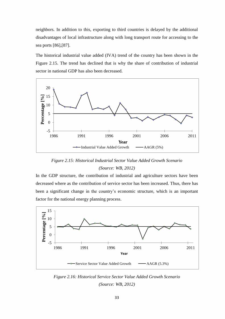
33
neighbors. In addition to this, exporting to third countries is delayed by the additional
disadvantages of local infrastructure along with long transport route for accessing to the
sea ports [86],[87].
The historical industrial value added (IVA) trend of the country has been shown in the
Figure 2.15. The trend has declined that is why the share of contribution of industrial
sector in national GDP has also been decreased.
Figure 2.15: Historical Industrial Sector Value Added Growth Scenario
(Source: WB, 2012)
In the GDP structure, the contribution of industrial and agriculture sectors have been
decreased where as the contribution of service sector has been increased. Thus, there has
been a significant change in the country’s economic structure, which is an important
factor for the national energy planning process.
Figure 2.16: Historical Service Sector Value Added Growth Scenario
(Source: WB, 2012)
-5
0
5
10
15
20
1986 1991 1996 2001 2006 2011
Per
cen
tage
[%]
YearIndustrial Value Added Growth AAGR (5%)
-5
0
5
10
15
1986 1991 1996 2001 2006 2011
Per
cen
tage
[%]
Year
Service Sector Value Added Growth AAGR (5.3%)
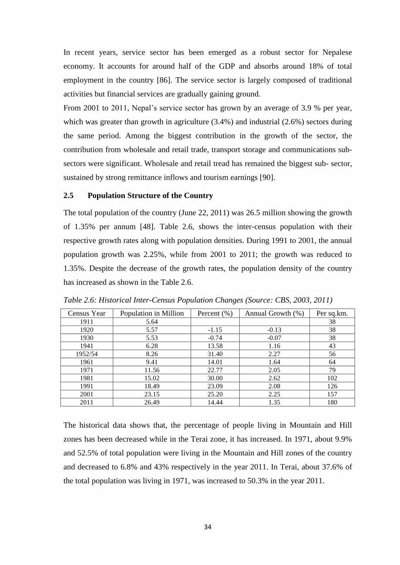
34
In recent years, service sector has been emerged as a robust sector for Nepalese
economy. It accounts for around half of the GDP and absorbs around 18% of total
employment in the country [86]. The service sector is largely composed of traditional
activities but financial services are gradually gaining ground.
From 2001 to 2011, Nepal’s service sector has grown by an average of 3.9 % per year,
which was greater than growth in agriculture (3.4%) and industrial (2.6%) sectors during
the same period. Among the biggest contribution in the growth of the sector, the
contribution from wholesale and retail trade, transport storage and communications sub-
sectors were significant. Wholesale and retail tread has remained the biggest sub- sector,
sustained by strong remittance inflows and tourism earnings [90].
2.5 Population Structure of the Country
The total population of the country (June 22, 2011) was 26.5 million showing the growth
of 1.35% per annum [48]. Table 2.6, shows the inter-census population with their
respective growth rates along with population densities. During 1991 to 2001, the annual
population growth was 2.25%, while from 2001 to 2011; the growth was reduced to
1.35%. Despite the decrease of the growth rates, the population density of the country
has increased as shown in the Table 2.6.
Table 2.6: Historical Inter-Census Population Changes (Source: CBS, 2003, 2011)
Census Year Population in Million Percent (%) Annual Growth (%) Per sq.km. 1911 5.64
38
1920 5.57 -1.15 -0.13 38
1930 5.53 -0.74 -0.07 38
1941 6.28 13.58 1.16 43
1952/54 8.26 31.40 2.27 56
1961 9.41 14.01 1.64 64
1971 11.56 22.77 2.05 79
1981 15.02 30.00 2.62 102
1991 18.49 23.09 2.08 126
2001 23.15 25.20 2.25 157
2011 26.49 14.44 1.35 180
The historical data shows that, the percentage of people living in Mountain and Hill
zones has been decreased while in the Terai zone, it has increased. In 1971, about 9.9%
and 52.5% of total population were living in the Mountain and Hill zones of the country
and decreased to 6.8% and 43% respectively in the year 2011. In Terai, about 37.6% of
the total population was living in 1971, was increased to 50.3% in the year 2011.
35
The population growth rate of Terai is greater in comparison to other two zones. From
1971 to 1981, the population growth rate of the Mountain, Hill and Terai zones were
1.4%, 1.7% and 4.1% respectively. Again in these zones, following two inter census
(1981-1991), the growth rates were 1.1%, 1.6% and 2.8% respectively. Similarly, during
the census (1991 - 2000) the growths rates of population in these three corresponding
zones were 1.6%, 2.0% and 2.6% respectively. According to census 2011, the growths
were recorded 0.5%, 1.1% and 1.7% annually from 2001 to 2011 for the regions. The
historical data shows that there has been a decline in growth rates of population not only
in the Mountain and Hill zones, but also in Terai zone of the country. Table 2.7 shows
the structure of population on the three ecological zones of the country. The table
demonstrates that the percentage of population living in the Mountain and Hill has
decreased while the percentage of population living in the Terai has increased.
According to the 2011 census, there was more than half of total national population
living in Terai zone of the country alone, which holds only 17% land area of the country
having major agricultural purpose [48],[91].
Table 2.7: Structure of Population in Ecological Zone of Nepal
(Source: CBS, 2003, 2011)
Census Year Mountain (%) Hill (%) Terai (%)
1971 9.9 52.5 37.6
1981 8.7 47.7 43.6
1991 7.8 45.5 46.7
2001 7.3 44.3 48.4
2011 6.7 43.0 50.3
The shares of people living in the five development regions of the country are not
uniform and varying in nature. The tabulated historical data in Table 2.8, shows that
there has been a change in structure of population among the development regions.
According to the table, the percentage shares of people living in Eastern Development
Region (EDR) and Western Development Region (WDR) have decreased while the
shares of people living in remaining Centre Development Region (CDR), Mid Western
Region (MWD), and Far Western Development Region (FWDR) have increased.
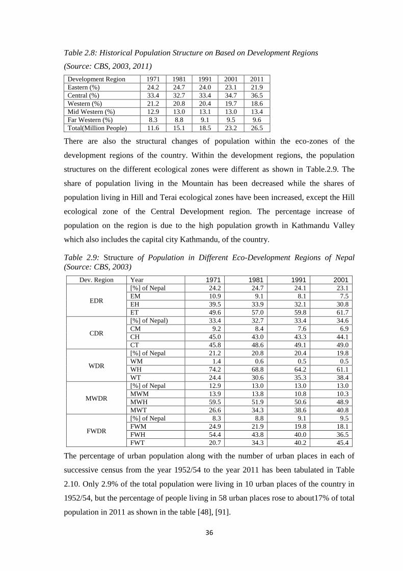
36
Table 2.8: Historical Population Structure on Based on Development Regions
(Source: CBS, 2003, 2011)
Development Region 1971 1981 1991 2001 2011
Eastern (%) 24.2 24.7 24.0 23.1 21.9
Central (%) 33.4 32.7 33.4 34.7 36.5
Western (%) 21.2 20.8 20.4 19.7 18.6
Mid Western (%) 12.9 13.0 13.1 13.0 13.4
Far Western (%) 8.3 8.8 9.1 9.5 9.6
Total(Million People) 11.6 15.1 18.5 23.2 26.5
There are also the structural changes of population within the eco-zones of the
development regions of the country. Within the development regions, the population
structures on the different ecological zones were different as shown in Table.2.9. The
share of population living in the Mountain has been decreased while the shares of
population living in Hill and Terai ecological zones have been increased, except the Hill
ecological zone of the Central Development region. The percentage increase of
population on the region is due to the high population growth in Kathmandu Valley
which also includes the capital city Kathmandu, of the country.
Table 2.9: Structure of Population in Different Eco-Development Regions of Nepal
(Source: CBS, 2003)
Dev. Region Year 1971 1981 1991 2001
EDR
[%] of Nepal 24.2 24.7 24.1 23.1
EM 10.9 9.1 8.1 7.5
EH 39.5 33.9 32.1 30.8
ET 49.6 57.0 59.8 61.7
CDR
[%] of Nepal) 33.4 32.7 33.4 34.6
CM 9.2 8.4 7.6 6.9
CH 45.0 43.0 43.3 44.1
CT 45.8 48.6 49.1 49.0
WDR
[%] of Nepal 21.2 20.8 20.4 19.8
WM 1.4 0.6 0.5 0.5
WH 74.2 68.8 64.2 61.1
WT 24.4 30.6 35.3 38.4
MWDR
[%] of Nepal 12.9 13.0 13.0 13.0
MWM 13.9 13.8 10.8 10.3
MWH 59.5 51.9 50.6 48.9
MWT 26.6 34.3 38.6 40.8
FWDR
[%] of Nepal 8.3 8.8 9.1 9.5
FWM 24.9 21.9 19.8 18.1
FWH 54.4 43.8 40.0 36.5
FWT 20.7 34.3 40.2 45.4
The percentage of urban population along with the number of urban places in each of
successive census from the year 1952/54 to the year 2011 has been tabulated in Table
2.10. Only 2.9% of the total population were living in 10 urban places of the country in
1952/54, but the percentage of people living in 58 urban places rose to about17% of total
population in 2011 as shown in the table [48], [91].
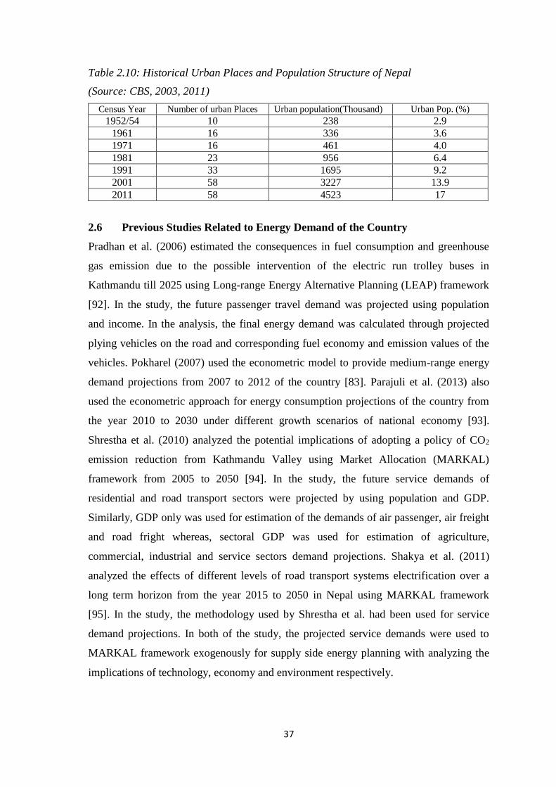
37
Table 2.10: Historical Urban Places and Population Structure of Nepal
(Source: CBS, 2003, 2011)
Census Year Number of urban Places Urban population(Thousand) Urban Pop. (%)
1952/54 10 238 2.9
1961 16 336 3.6
1971 16 461 4.0
1981 23 956 6.4
1991 33 1695 9.2
2001 58 3227 13.9
2011 58 4523 17
2.6 Previous Studies Related to Energy Demand of the Country
Pradhan et al. (2006) estimated the consequences in fuel consumption and greenhouse
gas emission due to the possible intervention of the electric run trolley buses in
Kathmandu till 2025 using Long-range Energy Alternative Planning (LEAP) framework
[92]. In the study, the future passenger travel demand was projected using population
and income. In the analysis, the final energy demand was calculated through projected
plying vehicles on the road and corresponding fuel economy and emission values of the
vehicles. Pokharel (2007) used the econometric model to provide medium-range energy
demand projections from 2007 to 2012 of the country [83]. Parajuli et al. (2013) also
used the econometric approach for energy consumption projections of the country from
the year 2010 to 2030 under different growth scenarios of national economy [93].
Shrestha et al. (2010) analyzed the potential implications of adopting a policy of CO2
emission reduction from Kathmandu Valley using Market Allocation (MARKAL)
framework from 2005 to 2050 [94]. In the study, the future service demands of
residential and road transport sectors were projected by using population and GDP.
Similarly, GDP only was used for estimation of the demands of air passenger, air freight
and road fright whereas, sectoral GDP was used for estimation of agriculture,
commercial, industrial and service sectors demand projections. Shakya et al. (2011)
analyzed the effects of different levels of road transport systems electrification over a
long term horizon from the year 2015 to 2050 in Nepal using MARKAL framework
[95]. In the study, the methodology used by Shrestha et al. had been used for service
demand projections. In both of the study, the projected service demands were used to
MARKAL framework exogenously for supply side energy planning with analyzing the
implications of technology, economy and environment respectively.
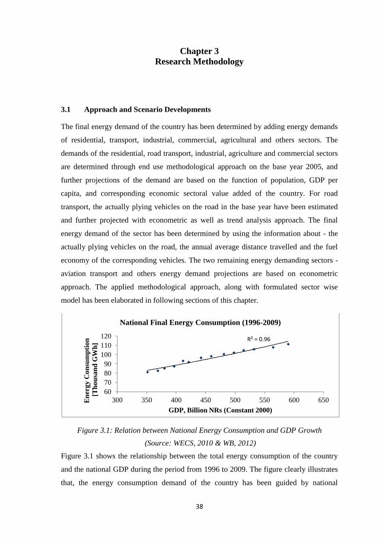
38
Chapter 3
Research Methodology
3.1 Approach and Scenario Developments
The final energy demand of the country has been determined by adding energy demands
of residential, transport, industrial, commercial, agricultural and others sectors. The
demands of the residential, road transport, industrial, agriculture and commercial sectors
are determined through end use methodological approach on the base year 2005, and
further projections of the demand are based on the function of population, GDP per
capita, and corresponding economic sectoral value added of the country. For road
transport, the actually plying vehicles on the road in the base year have been estimated
and further projected with econometric as well as trend analysis approach. The final
energy demand of the sector has been determined by using the information about - the
actually plying vehicles on the road, the annual average distance travelled and the fuel
economy of the corresponding vehicles. The two remaining energy demanding sectors -
aviation transport and others energy demand projections are based on econometric
approach. The applied methodological approach, along with formulated sector wise
model has been elaborated in following sections of this chapter.
Figure 3.1: Relation between National Energy Consumption and GDP Growth
(Source: WECS, 2010 & WB, 2012)
Figure 3.1 shows the relationship between the total energy consumption of the country
and the national GDP during the period from 1996 to 2009. The figure clearly illustrates
that, the energy consumption demand of the country has been guided by national
R² = 0.96
60
70
80
90
100
110
120
300 350 400 450 500 550 600 650En
erg
y C
on
sum
pti
on
[Th
ou
san
d G
Wh
]
GDP, Billion NRs (Constant 2000)
National Final Energy Consumption (1996-2009)
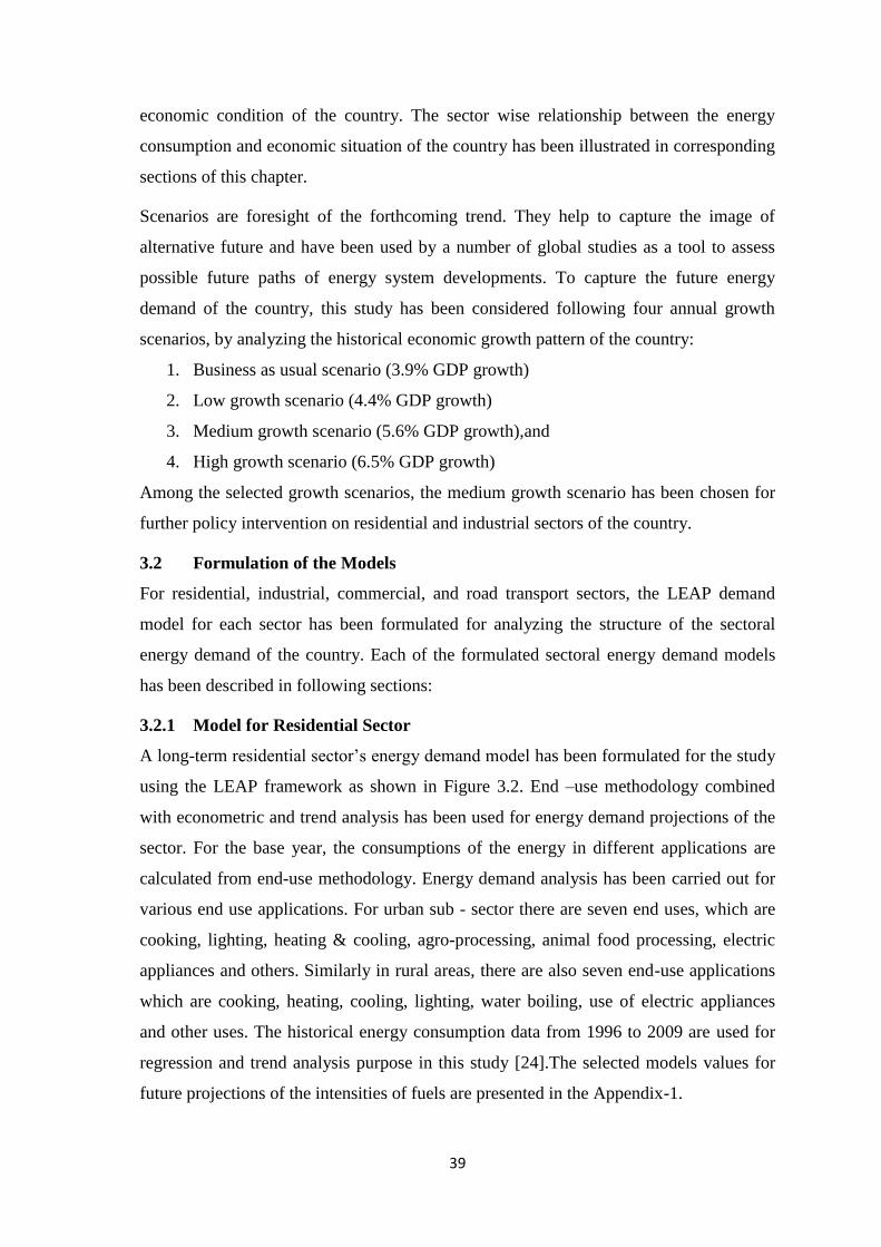
39
economic condition of the country. The sector wise relationship between the energy
consumption and economic situation of the country has been illustrated in corresponding
sections of this chapter.
Scenarios are foresight of the forthcoming trend. They help to capture the image of
alternative future and have been used by a number of global studies as a tool to assess
possible future paths of energy system developments. To capture the future energy
demand of the country, this study has been considered following four annual growth
scenarios, by analyzing the historical economic growth pattern of the country:
1. Business as usual scenario (3.9% GDP growth)
2. Low growth scenario (4.4% GDP growth)
3. Medium growth scenario (5.6% GDP growth),and
4. High growth scenario (6.5% GDP growth)
Among the selected growth scenarios, the medium growth scenario has been chosen for
further policy intervention on residential and industrial sectors of the country.
3.2 Formulation of the Models
For residential, industrial, commercial, and road transport sectors, the LEAP demand
model for each sector has been formulated for analyzing the structure of the sectoral
energy demand of the country. Each of the formulated sectoral energy demand models
has been described in following sections:
3.2.1 Model for Residential Sector
A long-term residential sector’s energy demand model has been formulated for the study
using the LEAP framework as shown in Figure 3.2. End –use methodology combined
with econometric and trend analysis has been used for energy demand projections of the
sector. For the base year, the consumptions of the energy in different applications are
calculated from end-use methodology. Energy demand analysis has been carried out for
various end use applications. For urban sub - sector there are seven end uses, which are
cooking, lighting, heating & cooling, agro-processing, animal food processing, electric
appliances and others. Similarly in rural areas, there are also seven end-use applications
which are cooking, heating, cooling, lighting, water boiling, use of electric appliances
and other uses. The historical energy consumption data from 1996 to 2009 are used for
regression and trend analysis purpose in this study [24].The selected models values for
future projections of the intensities of fuels are presented in the Appendix-1.
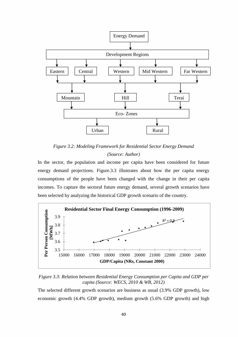
40
Figure 3.2: Modeling Framework for Residential Sector Energy Demand
(Source: Author)
In the sector, the population and income per capita have been considered for future
energy demand projections. Figure.3.3 illustrates about how the per capita energy
consumptions of the people have been changed with the change in their per capita
incomes. To capture the sectoral future energy demand, several growth scenarios have
been selected by analyzing the historical GDP growth scenario of the country.
Figure 3.3: Relation between Residential Energy Consumption per Capita and GDP per
capita (Source: WECS, 2010 & WB, 2012)
The selected different growth scenarios are business as usual (3.9% GDP growth), low
economic growth (4.4% GDP growth), medium growth (5.6% GDP growth) and high
R² = 0.9
3.5
3.6
3.7
3.8
3.9
15000 16000 17000 18000 19000 20000 21000 22000 23000 24000Per
Per
son
Con
sum
pti
on
[MW
h]
GDP/Capita (NRs, Constant 2000)
Residential Sector Final Energy Consumption (1996-2009)
Energy Demand
Development Regions
Far Western Mid Western Western Central Eastern
Terai Mountain Hill
Eco- Zones
Rural Urban
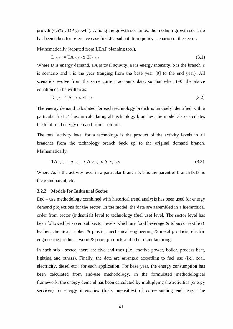
41
growth (6.5% GDP growth). Among the growth scenarios, the medium growth scenario
has been taken for reference case for LPG substitution (policy scenario) in the sector.
Mathematically (adopted from LEAP planning tool),
D b, s, t = TA b, s, t x EI b, s, t (3.1)
Where D is energy demand, TA is total activity, EI is energy intensity, b is the branch, s
is scenario and t is the year (ranging from the base year [0] to the end year). All
scenarios evolve from the same current accounts data, so that when t=0, the above
equation can be written as:
D b, 0 = TA b, 0 x EI b, 0 (3.2)
The energy demand calculated for each technology branch is uniquely identified with a
particular fuel . Thus, in calculating all technology branches, the model also calculates
the total final energy demand from each fuel.
The total activity level for a technology is the product of the activity levels in all
branches from the technology branch back up to the original demand branch.
Mathematically,
TA b, s, t = A b', s, t x A b'', s, t x A b''', s, t X (3.3)
Where Ab is the activity level in a particular branch b, b' is the parent of branch b, b'' is
the grandparent, etc.
3.2.2 Models for Industrial Sector
End – use methodology combined with historical trend analysis has been used for energy
demand projections for the sector. In the model, the data are assembled in a hierarchical
order from sector (industrial) level to technology (fuel use) level. The sector level has
been followed by seven sub sector levels which are food beverage & tobacco, textile &
leather, chemical, rubber & plastic, mechanical engineering & metal products, electric
engineering products, wood & paper products and other manufacturing.
In each sub - sector, there are five end uses (i.e., motive power, boiler, process heat,
lighting and others). Finally, the data are arranged according to fuel use (i.e., coal,
electricity, diesel etc.) for each application. For base year, the energy consumption has
been calculated from end-use methodology. In the formulated methodological
framework, the energy demand has been calculated by multiplying the activities (energy
services) by energy intensities (fuels intensities) of corresponding end uses. The
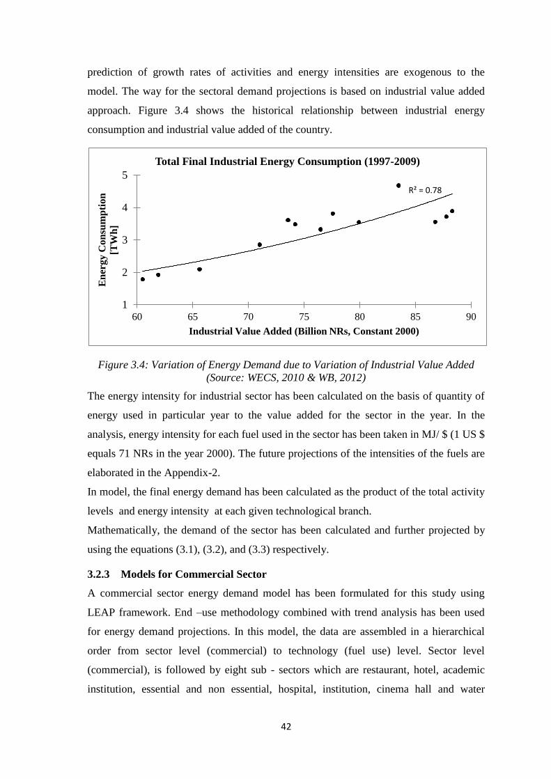
42
prediction of growth rates of activities and energy intensities are exogenous to the
model. The way for the sectoral demand projections is based on industrial value added
approach. Figure 3.4 shows the historical relationship between industrial energy
consumption and industrial value added of the country.
Figure 3.4: Variation of Energy Demand due to Variation of Industrial Value Added
(Source: WECS, 2010 & WB, 2012)
The energy intensity for industrial sector has been calculated on the basis of quantity of
energy used in particular year to the value added for the sector in the year. In the
analysis, energy intensity for each fuel used in the sector has been taken in MJ/ $ (1 US $
equals 71 NRs in the year 2000). The future projections of the intensities of the fuels are
elaborated in the Appendix-2.
In model, the final energy demand has been calculated as the product of the total activity
levels and energy intensity at each given technological branch.
Mathematically, the demand of the sector has been calculated and further projected by
using the equations (3.1), (3.2), and (3.3) respectively.
3.2.3 Models for Commercial Sector
A commercial sector energy demand model has been formulated for this study using
LEAP framework. End –use methodology combined with trend analysis has been used
for energy demand projections. In this model, the data are assembled in a hierarchical
order from sector level (commercial) to technology (fuel use) level. Sector level
(commercial), is followed by eight sub - sectors which are restaurant, hotel, academic
institution, essential and non essential, hospital, institution, cinema hall and water
R² = 0.78
1
2
3
4
5
60 65 70 75 80 85 90
En
ergy C
on
sum
pti
on
[TW
h]
Industrial Value Added (Billion NRs, Constant 2000)
Total Final Industrial Energy Consumption (1997-2009)
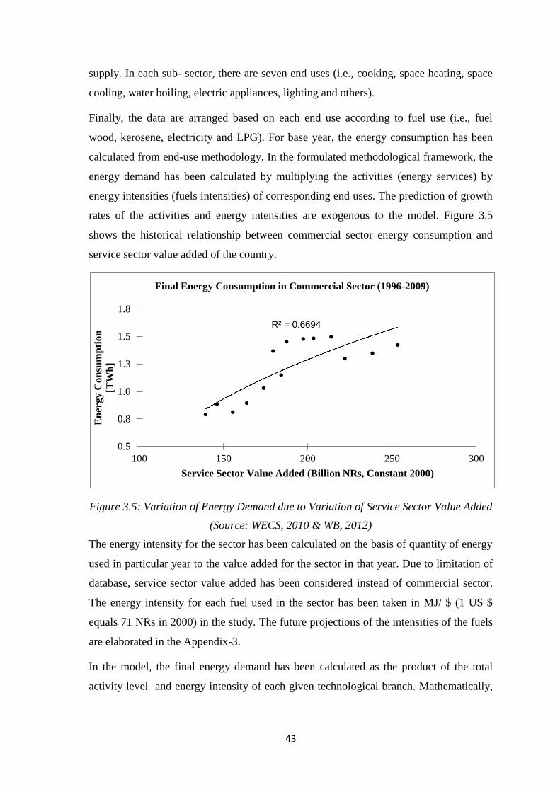
43
supply. In each sub- sector, there are seven end uses (i.e., cooking, space heating, space
cooling, water boiling, electric appliances, lighting and others).
Finally, the data are arranged based on each end use according to fuel use (i.e., fuel
wood, kerosene, electricity and LPG). For base year, the energy consumption has been
calculated from end-use methodology. In the formulated methodological framework, the
energy demand has been calculated by multiplying the activities (energy services) by
energy intensities (fuels intensities) of corresponding end uses. The prediction of growth
rates of the activities and energy intensities are exogenous to the model. Figure 3.5
shows the historical relationship between commercial sector energy consumption and
service sector value added of the country.
Figure 3.5: Variation of Energy Demand due to Variation of Service Sector Value Added
(Source: WECS, 2010 & WB, 2012)
The energy intensity for the sector has been calculated on the basis of quantity of energy
used in particular year to the value added for the sector in that year. Due to limitation of
database, service sector value added has been considered instead of commercial sector.
The energy intensity for each fuel used in the sector has been taken in MJ/ $ (1 US $
equals 71 NRs in 2000) in the study. The future projections of the intensities of the fuels
are elaborated in the Appendix-3.
In the model, the final energy demand has been calculated as the product of the total
activity level and energy intensity of each given technological branch. Mathematically,
R² = 0.6694
0.5
0.8
1.0
1.3
1.5
1.8
100 150 200 250 300
En
ergy C
on
sum
pti
on
[TW
h]
Service Sector Value Added (Billion NRs, Constant 2000)
Final Energy Consumption in Commercial Sector (1996-2009)
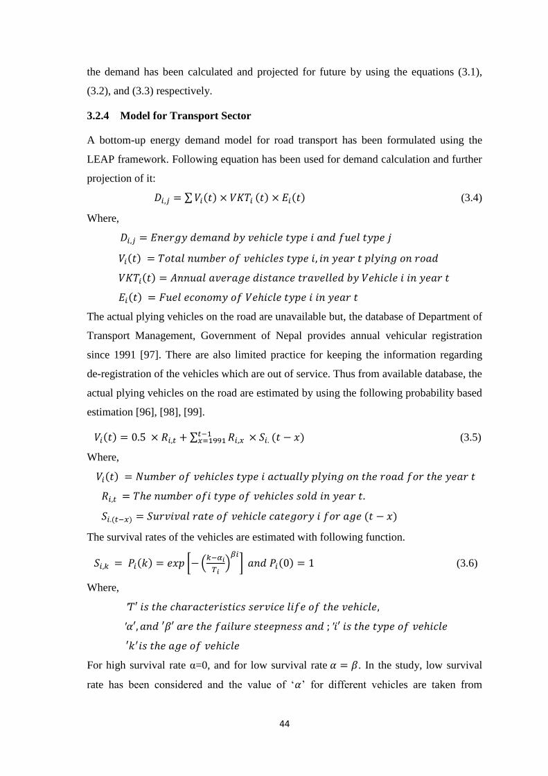
44
the demand has been calculated and projected for future by using the equations (3.1),
(3.2), and (3.3) respectively.
3.2.4 Model for Transport Sector
A bottom-up energy demand model for road transport has been formulated using the
LEAP framework. Following equation has been used for demand calculation and further
projection of it:
𝐷𝑖,𝑗 = ∑ 𝑉𝑖(𝑡) × 𝑉𝐾𝑇𝑖 (𝑡) × 𝐸𝑖(𝑡) (3.4)
Where,
𝐷𝑖,𝑗 = 𝐸𝑛𝑒𝑟𝑔𝑦 𝑑𝑒𝑚𝑎𝑛𝑑 𝑏𝑦 𝑣𝑒ℎ𝑖𝑐𝑙𝑒 𝑡𝑦𝑝𝑒 𝑖 𝑎𝑛𝑑 𝑓𝑢𝑒𝑙 𝑡𝑦𝑝𝑒 𝑗
𝑉𝑖(𝑡) = 𝑇𝑜𝑡𝑎𝑙 𝑛𝑢𝑚𝑏𝑒𝑟 𝑜𝑓 𝑣𝑒ℎ𝑖𝑐𝑙𝑒𝑠 𝑡𝑦𝑝𝑒 𝑖, 𝑖𝑛 𝑦𝑒𝑎𝑟 𝑡 𝑝𝑙𝑦𝑖𝑛𝑔 𝑜𝑛 𝑟𝑜𝑎𝑑
𝑉𝐾𝑇𝑖(𝑡) = 𝐴𝑛𝑛𝑢𝑎𝑙 𝑎𝑣𝑒𝑟𝑎𝑔𝑒 𝑑𝑖𝑠𝑡𝑎𝑛𝑐𝑒 𝑡𝑟𝑎𝑣𝑒𝑙𝑙𝑒𝑑 𝑏𝑦 𝑉𝑒ℎ𝑖𝑐𝑙𝑒 𝑖 𝑖𝑛 𝑦𝑒𝑎𝑟 𝑡
𝐸𝑖(𝑡) = 𝐹𝑢𝑒𝑙 𝑒𝑐𝑜𝑛𝑜𝑚𝑦 𝑜𝑓 𝑉𝑒ℎ𝑖𝑐𝑙𝑒 𝑡𝑦𝑝𝑒 𝑖 𝑖𝑛 𝑦𝑒𝑎𝑟 𝑡
The actual plying vehicles on the road are unavailable but, the database of Department of
Transport Management, Government of Nepal provides annual vehicular registration
since 1991 [97]. There are also limited practice for keeping the information regarding
de-registration of the vehicles which are out of service. Thus from available database, the
actual plying vehicles on the road are estimated by using the following probability based
estimation [96], [98], [99].
𝑉𝑖(𝑡) = 0.5 × 𝑅𝑖,𝑡 + ∑ 𝑅𝑖,𝑥 × 𝑆𝑖.𝑡−1𝑥=1991 (𝑡 − 𝑥) (3.5)
Where,
𝑉𝑖(𝑡) = 𝑁𝑢𝑚𝑏𝑒𝑟 𝑜𝑓 𝑣𝑒ℎ𝑖𝑐𝑙𝑒𝑠 𝑡𝑦𝑝𝑒 𝑖 𝑎𝑐𝑡𝑢𝑎𝑙𝑙𝑦 𝑝𝑙𝑦𝑖𝑛𝑔 𝑜𝑛 𝑡ℎ𝑒 𝑟𝑜𝑎𝑑 𝑓𝑜𝑟 𝑡ℎ𝑒 𝑦𝑒𝑎𝑟 𝑡
𝑅𝑖,𝑡 = 𝑇ℎ𝑒 𝑛𝑢𝑚𝑏𝑒𝑟 𝑜𝑓𝑖 𝑡𝑦𝑝𝑒 𝑜𝑓 𝑣𝑒ℎ𝑖𝑐𝑙𝑒𝑠 𝑠𝑜𝑙𝑑 𝑖𝑛 𝑦𝑒𝑎𝑟 𝑡.
𝑆𝑖.(𝑡−𝑥) = 𝑆𝑢𝑟𝑣𝑖𝑣𝑎𝑙 𝑟𝑎𝑡𝑒 𝑜𝑓 𝑣𝑒ℎ𝑖𝑐𝑙𝑒 𝑐𝑎𝑡𝑒𝑔𝑜𝑟𝑦 𝑖 𝑓𝑜𝑟 𝑎𝑔𝑒 (𝑡 − 𝑥)
The survival rates of the vehicles are estimated with following function.
𝑆𝑖,𝑘 = 𝑃𝑖(𝑘) = 𝑒𝑥𝑝 [− (𝑘−𝛼𝑖
𝑇𝑖)
𝛽𝑖
] 𝑎𝑛𝑑 𝑃𝑖(0) = 1 (3.6)
Where,
′𝑇′ 𝑖𝑠 𝑡ℎ𝑒 𝑐ℎ𝑎𝑟𝑎𝑐𝑡𝑒𝑟𝑖𝑠𝑡𝑖𝑐𝑠 𝑠𝑒𝑟𝑣𝑖𝑐𝑒 𝑙𝑖𝑓𝑒 𝑜𝑓 𝑡ℎ𝑒 𝑣𝑒ℎ𝑖𝑐𝑙𝑒,
′𝛼′, 𝑎𝑛𝑑 ′𝛽′ 𝑎𝑟𝑒 𝑡ℎ𝑒 𝑓𝑎𝑖𝑙𝑢𝑟𝑒 𝑠𝑡𝑒𝑒𝑝𝑛𝑒𝑠𝑠 𝑎𝑛𝑑 ; ′𝑖′ 𝑖𝑠 𝑡ℎ𝑒 𝑡𝑦𝑝𝑒 𝑜𝑓 𝑣𝑒ℎ𝑖𝑐𝑙𝑒
′𝑘′𝑖𝑠 𝑡ℎ𝑒 𝑎𝑔𝑒 𝑜𝑓 𝑣𝑒ℎ𝑖𝑐𝑙𝑒
For high survival rate α=0, and for low survival rate 𝛼 = 𝛽. In the study, low survival
rate has been considered and the value of ‘𝛼’ for different vehicles are taken from
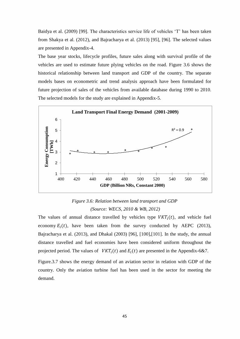
45
Baidya et al. (2009) [99]. The characteristics service life of vehicles ‘T’ has been taken
from Shakya et al. (2012), and Bajracharya et al. (2013) [95], [96]. The selected values
are presented in Appendix-4.
The base year stocks, lifecycle profiles, future sales along with survival profile of the
vehicles are used to estimate future plying vehicles on the road. Figure 3.6 shows the
historical relationship between land transport and GDP of the country. The separate
models bases on econometric and trend analysis approach have been formulated for
future projection of sales of the vehicles from available database during 1990 to 2010.
The selected models for the study are explained in Appendix-5.
Figure 3.6: Relation between land transport and GDP
(Source: WECS, 2010 & WB, 2012)
The values of annual distance travelled by vehicles type 𝑉𝐾𝑇𝑖(𝑡), and vehicle fuel
economy 𝐸𝑖(𝑡), have been taken from the survey conducted by AEPC (2013),
Bajracharya et al. (2013), and Dhakal (2003) [96], [100],[101]. In the study, the annual
distance travelled and fuel economies have been considered uniform throughout the
projected period. The values of 𝑉𝐾𝑇𝑖(𝑡) and 𝐸𝑖(𝑡) are presented in the Appendix-6&7.
Figure.3.7 shows the energy demand of an aviation sector in relation with GDP of the
country. Only the aviation turbine fuel has been used in the sector for meeting the
demand.
R² = 0.9
1
2
3
4
5
6
400 420 440 460 480 500 520 540 560 580
En
ergy C
on
sum
pti
on
[TW
h]
GDP (Billion NRs, Constant 2000)
Land Transport Final Energy Demand (2001-2009)
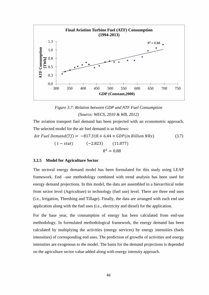
46
Figure 3.7: Relation between GDP and ATF Fuel Consumption
(Source: WECS, 2010 & WB, 2012)
The aviation transport fuel demand has been projected with an econometric approach.
The selected model for the air fuel demand is as follows:
𝐴𝑖𝑟 𝐹𝑢𝑒𝑙 𝐷𝑒𝑚𝑎𝑛𝑑(𝑇𝐽) = −817.318 + 6.44 × 𝐺𝐷𝑃(𝑖𝑛 𝐵𝑖𝑙𝑙𝑖𝑜𝑛 𝑁𝑅𝑠) (3.7)
( 𝑡 − 𝑠𝑡𝑎𝑡) (−2.823) (11.077)
𝑅2 = 0.88
3.2.5 Model for Agriculture Sector
The sectoral energy demand model has been formulated for this study using LEAP
framework. End –use methodology combined with trend analysis has been used for
energy demand projections. In this model, the data are assembled in a hierarchical order
from sector level (Agriculture) to technology (fuel use) level. There are three end uses
(i.e., Irrigation, Threshing and Tillage). Finally, the data are arranged with each end use
application along with the fuel uses (i.e., electricity and diesel) for the application.
For the base year, the consumption of energy has been calculated from end-use
methodology. In formulated methodological framework, the energy demand has been
calculated by multiplying the activities (energy services) by energy intensities (fuels
intensities) of corresponding end uses. The prediction of growths of activities and energy
intensities are exogenous to the model. The basis for the demand projections is depended
on the agriculture sector value added along with energy intensity approach.
R² = 0.88
0.0
0.3
0.5
0.8
1.0
1.3
300 350 400 450 500 550 600 650 700 750
AT
F C
on
sum
pti
on
[TW
h]
GDP (Constant,2000)
Final Aviation Turbine Fuel (ATF) Consumption
(1994-2013)
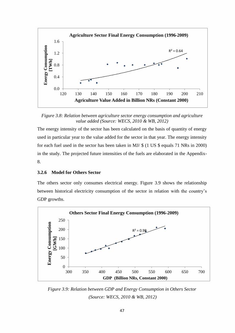
47
Figure 3.8: Relation between agriculture sector energy consumption and agriculture
value added (Source: WECS, 2010 & WB, 2012)
The energy intensity of the sector has been calculated on the basis of quantity of energy
used in particular year to the value added for the sector in that year. The energy intensity
for each fuel used in the sector has been taken in MJ/ $ (1 US $ equals 71 NRs in 2000)
in the study. The projected future intensities of the fuels are elaborated in the Appendix-
8.
3.2.6 Model for Others Sector
The others sector only consumes electrical energy. Figure 3.9 shows the relationship
between historical electricity consumption of the sector in relation with the country’s
GDP growths.
Figure 3.9: Relation between GDP and Energy Consumption in Others Sector
(Source: WECS, 2010 & WB, 2012)
R² = 0.64
0.0
0.4
0.8
1.2
1.6
120 130 140 150 160 170 180 190 200 210
En
erg
y C
on
sum
pti
on
[TW
h]
Agriculture Value Added in Billion NRs (Constant 2000)
Agriculture Sector Final Energy Consumption (1996-2009)
R² = 0.98
0
50
100
150
200
250
300 350 400 450 500 550 600 650 700
En
ergy
Con
sum
pti
on
[GW
h]
GDP (Billion NRs, Constant 2000)
Others Sector Final Energy Consumption (1996-2009)
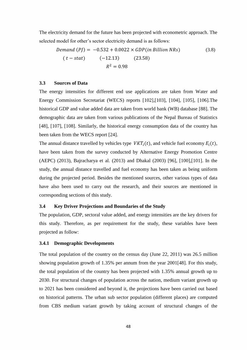
48
The electricity demand for the future has been projected with econometric approach. The
selected model for other’s sector electricity demand is as follows:
𝐷𝑒𝑚𝑎𝑛𝑑 (𝑃𝐽) = −0.532 + 0.0022 × 𝐺𝐷𝑃(𝑖𝑛 𝐵𝑖𝑙𝑙𝑖𝑜𝑛 𝑁𝑅𝑠) (3.8)
( 𝑡 − 𝑠𝑡𝑎𝑡) (−12.13) (23.58)
𝑅2 = 0.98
3.3 Sources of Data
The energy intensities for different end use applications are taken from Water and
Energy Commission Secretariat (WECS) reports [102],[103], [104], [105], [106].The
historical GDP and value added data are taken from world bank (WB) database [88]. The
demographic data are taken from various publications of the Nepal Bureau of Statistics
[48], [107], [108]. Similarly, the historical energy consumption data of the country has
been taken from the WECS report [24].
The annual distance travelled by vehicles type 𝑉𝐾𝑇𝑖(𝑡), and vehicle fuel economy 𝐸𝑖(𝑡),
have been taken from the survey conducted by Alternative Energy Promotion Centre
(AEPC) (2013), Bajracharya et al. (2013) and Dhakal (2003) [96], [100],[101]. In the
study, the annual distance travelled and fuel economy has been taken as being uniform
during the projected period. Besides the mentioned sources, other various types of data
have also been used to carry out the research, and their sources are mentioned in
corresponding sections of this study.
3.4 Key Driver Projections and Boundaries of the Study
The population, GDP, sectoral value added, and energy intensities are the key drivers for
this study. Therefore, as per requirement for the study, these variables have been
projected as follow:
3.4.1 Demographic Developments
The total population of the country on the census day (June 22, 2011) was 26.5 million
showing population growth of 1.35% per annum from the year 2001[48]. For this study,
the total population of the country has been projected with 1.35% annual growth up to
2030. For structural changes of population across the nation, medium variant growth up
to 2021 has been considered and beyond it, the projections have been carried out based
on historical patterns. The urban sub sector population (different places) are computed
from CBS medium variant growth by taking account of structural changes of the
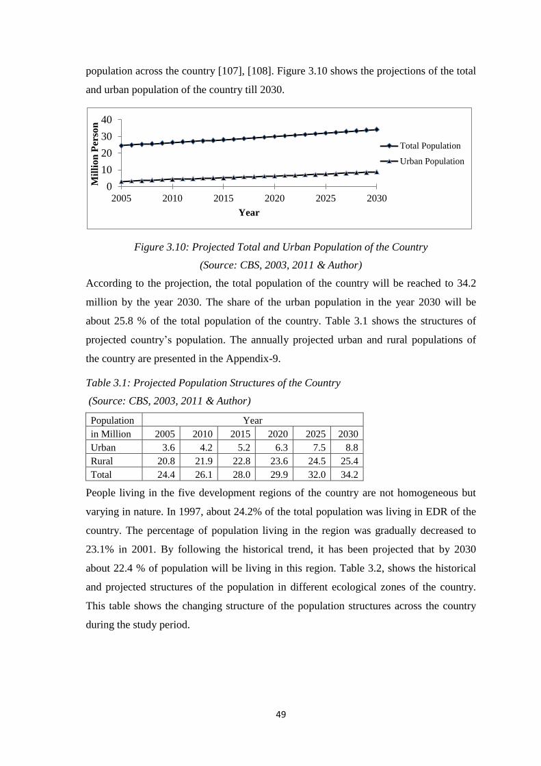
49
population across the country [107], [108]. Figure 3.10 shows the projections of the total
and urban population of the country till 2030.
Figure 3.10: Projected Total and Urban Population of the Country
(Source: CBS, 2003, 2011 & Author)
According to the projection, the total population of the country will be reached to 34.2
million by the year 2030. The share of the urban population in the year 2030 will be
about 25.8 % of the total population of the country. Table 3.1 shows the structures of
projected country’s population. The annually projected urban and rural populations of
the country are presented in the Appendix-9.
Table 3.1: Projected Population Structures of the Country
(Source: CBS, 2003, 2011 & Author)
Population Year
in Million 2005 2010 2015 2020 2025 2030
Urban 3.6 4.2 5.2 6.3 7.5 8.8
Rural 20.8 21.9 22.8 23.6 24.5 25.4
Total 24.4 26.1 28.0 29.9 32.0 34.2
People living in the five development regions of the country are not homogeneous but
varying in nature. In 1997, about 24.2% of the total population was living in EDR of the
country. The percentage of population living in the region was gradually decreased to
23.1% in 2001. By following the historical trend, it has been projected that by 2030
about 22.4 % of population will be living in this region. Table 3.2, shows the historical
and projected structures of the population in different ecological zones of the country.
This table shows the changing structure of the population structures across the country
during the study period.
0
10
20
30
40
2005 2010 2015 2020 2025 2030
Mil
lio
n P
erso
n
Year
Total Population
Urban Population
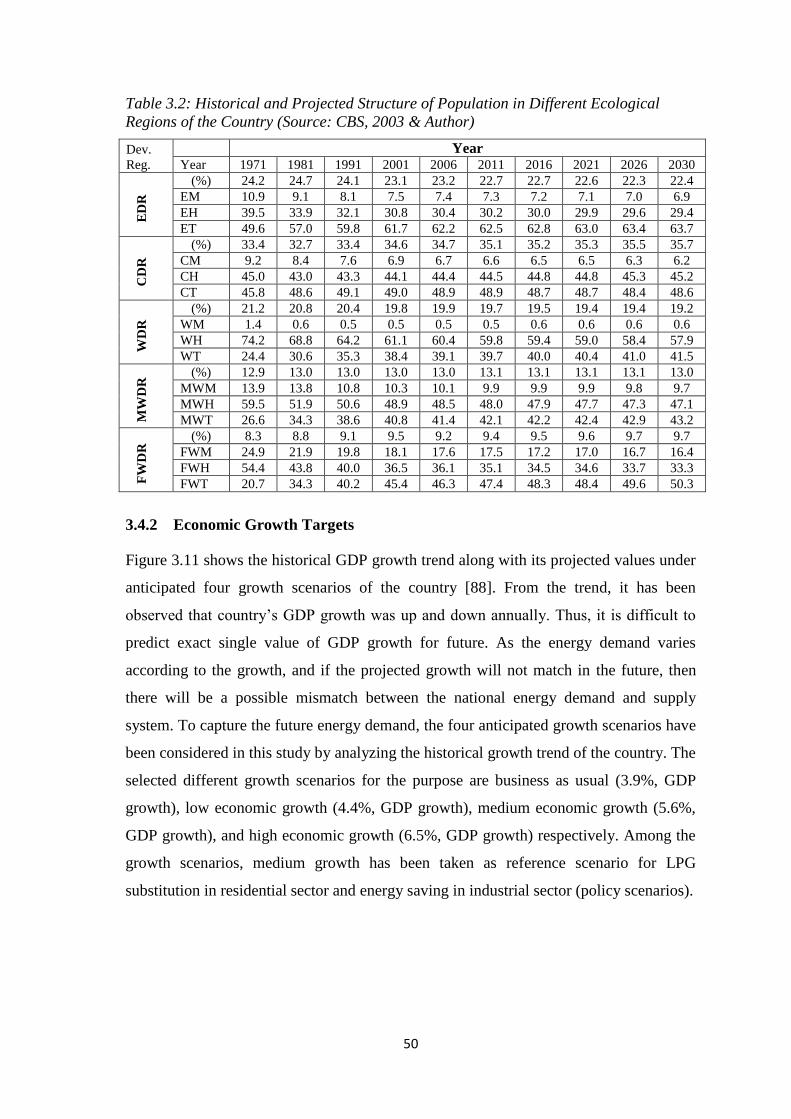
50
Table 3.2: Historical and Projected Structure of Population in Different Ecological
Regions of the Country (Source: CBS, 2003 & Author)
Dev.
Reg. Year
Year 1971 1981 1991 2001 2006 2011 2016 2021 2026 2030
ED
R
(%) 24.2 24.7 24.1 23.1 23.2 22.7 22.7 22.6 22.3 22.4
EM 10.9 9.1 8.1 7.5 7.4 7.3 7.2 7.1 7.0 6.9
EH 39.5 33.9 32.1 30.8 30.4 30.2 30.0 29.9 29.6 29.4
ET 49.6 57.0 59.8 61.7 62.2 62.5 62.8 63.0 63.4 63.7
CD
R
(%) 33.4 32.7 33.4 34.6 34.7 35.1 35.2 35.3 35.5 35.7
CM 9.2 8.4 7.6 6.9 6.7 6.6 6.5 6.5 6.3 6.2
CH 45.0 43.0 43.3 44.1 44.4 44.5 44.8 44.8 45.3 45.2
CT 45.8 48.6 49.1 49.0 48.9 48.9 48.7 48.7 48.4 48.6
WD
R
(%) 21.2 20.8 20.4 19.8 19.9 19.7 19.5 19.4 19.4 19.2
WM 1.4 0.6 0.5 0.5 0.5 0.5 0.6 0.6 0.6 0.6
WH 74.2 68.8 64.2 61.1 60.4 59.8 59.4 59.0 58.4 57.9
WT 24.4 30.6 35.3 38.4 39.1 39.7 40.0 40.4 41.0 41.5
MW
DR
(%) 12.9 13.0 13.0 13.0 13.0 13.1 13.1 13.1 13.1 13.0
MWM 13.9 13.8 10.8 10.3 10.1 9.9 9.9 9.9 9.8 9.7
MWH 59.5 51.9 50.6 48.9 48.5 48.0 47.9 47.7 47.3 47.1
MWT 26.6 34.3 38.6 40.8 41.4 42.1 42.2 42.4 42.9 43.2
FW
DR
(%) 8.3 8.8 9.1 9.5 9.2 9.4 9.5 9.6 9.7 9.7
FWM 24.9 21.9 19.8 18.1 17.6 17.5 17.2 17.0 16.7 16.4
FWH 54.4 43.8 40.0 36.5 36.1 35.1 34.5 34.6 33.7 33.3
FWT 20.7 34.3 40.2 45.4 46.3 47.4 48.3 48.4 49.6 50.3
3.4.2 Economic Growth Targets
Figure 3.11 shows the historical GDP growth trend along with its projected values under
anticipated four growth scenarios of the country [88]. From the trend, it has been
observed that country’s GDP growth was up and down annually. Thus, it is difficult to
predict exact single value of GDP growth for future. As the energy demand varies
according to the growth, and if the projected growth will not match in the future, then
there will be a possible mismatch between the national energy demand and supply
system. To capture the future energy demand, the four anticipated growth scenarios have
been considered in this study by analyzing the historical growth trend of the country. The
selected different growth scenarios for the purpose are business as usual (3.9%, GDP
growth), low economic growth (4.4%, GDP growth), medium economic growth (5.6%,
GDP growth), and high economic growth (6.5%, GDP growth) respectively. Among the
growth scenarios, medium growth has been taken as reference scenario for LPG
substitution in residential sector and energy saving in industrial sector (policy scenarios).
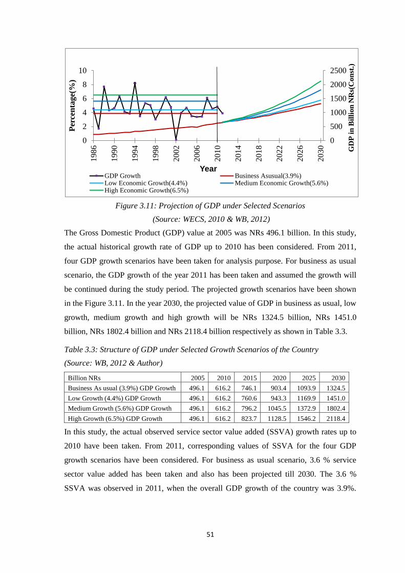
51
Figure 3.11: Projection of GDP under Selected Scenarios
(Source: WECS, 2010 & WB, 2012)
The Gross Domestic Product (GDP) value at 2005 was NRs 496.1 billion. In this study,
the actual historical growth rate of GDP up to 2010 has been considered. From 2011,
four GDP growth scenarios have been taken for analysis purpose. For business as usual
scenario, the GDP growth of the year 2011 has been taken and assumed the growth will
be continued during the study period. The projected growth scenarios have been shown
in the Figure 3.11. In the year 2030, the projected value of GDP in business as usual, low
growth, medium growth and high growth will be NRs 1324.5 billion, NRs 1451.0
billion, NRs 1802.4 billion and NRs 2118.4 billion respectively as shown in Table 3.3.
Table 3.3: Structure of GDP under Selected Growth Scenarios of the Country
(Source: WB, 2012 & Author)
Billion NRs 2005 2010 2015 2020 2025 2030
Business As usual (3.9%) GDP Growth 496.1 616.2 746.1 903.4 1093.9 1324.5
Low Growth (4.4%) GDP Growth 496.1 616.2 760.6 943.3 1169.9 1451.0
Medium Growth (5.6%) GDP Growth 496.1 616.2 796.2 1045.5 1372.9 1802.4
High Growth (6.5%) GDP Growth 496.1 616.2 823.7 1128.5 1546.2 2118.4
In this study, the actual observed service sector value added (SSVA) growth rates up to
2010 have been taken. From 2011, corresponding values of SSVA for the four GDP
growth scenarios have been considered. For business as usual scenario, 3.6 % service
sector value added has been taken and also has been projected till 2030. The 3.6 %
SSVA was observed in 2011, when the overall GDP growth of the country was 3.9%.
0
500
1000
1500
2000
2500
0
2
4
6
8
10
19
86
19
90
19
94
19
98
20
02
20
06
20
10
20
14
20
18
20
22
20
26
20
30 GD
P i
n B
illi
on
NR
s(C
on
st.)
Per
cen
tage(
%)
YearGDP Growth Business Asusual(3.9%)Low Economic Growth(4.4%) Medium Economic Growth(5.6%)High Economic Growth(6.5%)
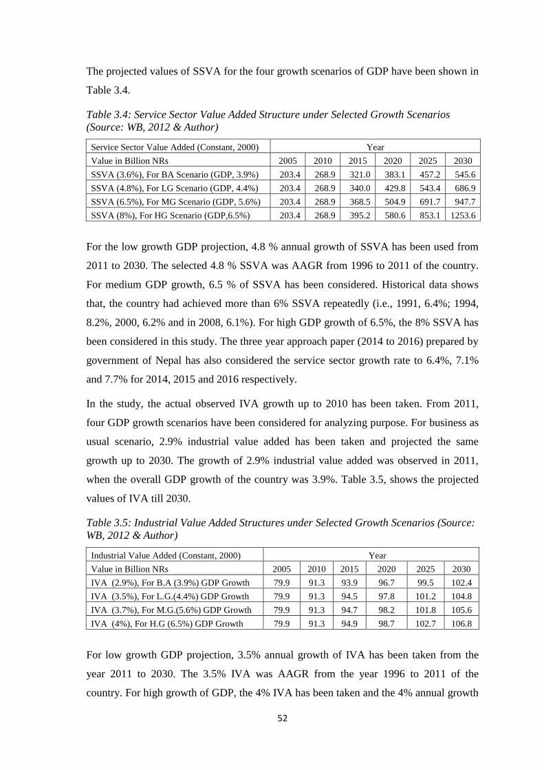
52
The projected values of SSVA for the four growth scenarios of GDP have been shown in
Table 3.4.
Table 3.4: Service Sector Value Added Structure under Selected Growth Scenarios
(Source: WB, 2012 & Author)
Service Sector Value Added (Constant, 2000) Year
Value in Billion NRs 2005 2010 2015 2020 2025 2030
SSVA (3.6%), For BA Scenario (GDP, 3.9%) 203.4 268.9 321.0 383.1 457.2 545.6
SSVA (4.8%), For LG Scenario (GDP, 4.4%) 203.4 268.9 340.0 429.8 543.4 686.9
SSVA (6.5%), For MG Scenario (GDP, 5.6%) 203.4 268.9 368.5 504.9 691.7 947.7
SSVA (8%), For HG Scenario (GDP,6.5%) 203.4 268.9 395.2 580.6 853.1 1253.6
For the low growth GDP projection, 4.8 % annual growth of SSVA has been used from
2011 to 2030. The selected 4.8 % SSVA was AAGR from 1996 to 2011 of the country.
For medium GDP growth, 6.5 % of SSVA has been considered. Historical data shows
that, the country had achieved more than 6% SSVA repeatedly (i.e., 1991, 6.4%; 1994,
8.2%, 2000, 6.2% and in 2008, 6.1%). For high GDP growth of 6.5%, the 8% SSVA has
been considered in this study. The three year approach paper (2014 to 2016) prepared by
government of Nepal has also considered the service sector growth rate to 6.4%, 7.1%
and 7.7% for 2014, 2015 and 2016 respectively.
In the study, the actual observed IVA growth up to 2010 has been taken. From 2011,
four GDP growth scenarios have been considered for analyzing purpose. For business as
usual scenario, 2.9% industrial value added has been taken and projected the same
growth up to 2030. The growth of 2.9% industrial value added was observed in 2011,
when the overall GDP growth of the country was 3.9%. Table 3.5, shows the projected
values of IVA till 2030.
Table 3.5: Industrial Value Added Structures under Selected Growth Scenarios (Source:
WB, 2012 & Author)
Industrial Value Added (Constant, 2000) Year
Value in Billion NRs 2005 2010 2015 2020 2025 2030
IVA (2.9%), For B.A (3.9%) GDP Growth 79.9 91.3 93.9 96.7 99.5 102.4
IVA (3.5%), For L.G.(4.4%) GDP Growth 79.9 91.3 94.5 97.8 101.2 104.8
IVA (3.7%), For M.G.(5.6%) GDP Growth 79.9 91.3 94.7 98.2 101.8 105.6
IVA (4%), For H.G (6.5%) GDP Growth 79.9 91.3 94.9 98.7 102.7 106.8
For low growth GDP projection, 3.5% annual growth of IVA has been taken from the
year 2011 to 2030. The 3.5% IVA was AAGR from the year 1996 to 2011 of the
country. For high growth of GDP, the 4% IVA has been taken and the 4% annual growth
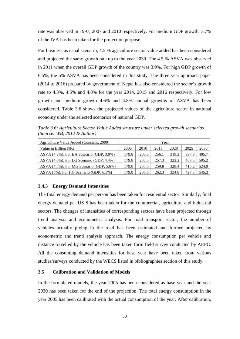
53
rate was observed in 1997, 2007 and 2010 respectively. For medium GDP growth, 3.7%
of the IVA has been taken for the projection purpose.
For business as usual scenario, 4.5 % agriculture sector value added has been considered
and projected the same growth rate up to the year 2030. The 4.5 % ASVA was observed
in 2011 when the overall GDP growth of the country was 3.9%. For high GDP growth of
6.5%, the 5% ASVA has been considered in this study. The three year approach paper
(2014 to 2016) prepared by government of Nepal has also considered the sector’s growth
rate to 4.3%, 4.5% and 4.8% for the year 2014, 2015 and 2016 respectively. For low
growth and medium growth 4.6% and 4.8% annual growths of ASVA has been
considered. Table 3.6 shows the projected values of the agriculture sector in national
economy under the selected scenarios of national GDP.
Table 3.6: Agriculture Sector Value Added structure under selected growth scenarios
(Source: WB, 2012 & Author)
Agriculture Value Added (Constant, 2000) Year
Value in Billion NRs 2005 2010 2015 2020 2025 2030
ASVA (4.5%), For BA Scenario (GDP, 3.9%) 179.8 205.5 256.1 319.2 397.8 495.7
ASVA (4.6%), For LG Scenario (GDP, 4.4%) 179.8 205.5 257.3 322.2 403.5 505.2
ASVA (4.8%), For MG Scenario (GDP, 5.6%) 179.8 205.5 259.8 328.4 415.2 524.9
ASVA (5%), For HG Scenario (GDP, 6.5%) 179.8 205.5 262.3 334.8 427.3 545.3
3.4.3 Energy Demand Intensities
The final energy demand per person has been taken for residential sector. Similarly, final
energy demand per US $ has been taken for the commercial, agriculture and industrial
sectors. The changes of intensities of corresponding sectors have been projected through
trend analysis and econometric analysis. For road transport sector, the number of
vehicles actually plying in the road has been estimated and further projected by
econometric and trend analysis approach. The energy consumption per vehicle and
distance travelled by the vehicle has been taken form field survey conducted by AEPC.
All the consuming demand intensities for base year have been taken from various
studies/surveys conducted by the WECS listed in bibliographies section of this study.
3.5 Calibration and Validation of Models
In the formulated models, the year 2005 has been considered as base year and the year
2030 has been taken for the end of the projection. The total energy consumption in the
year 2005 has been calibrated with the actual consumption of the year. After calibration,
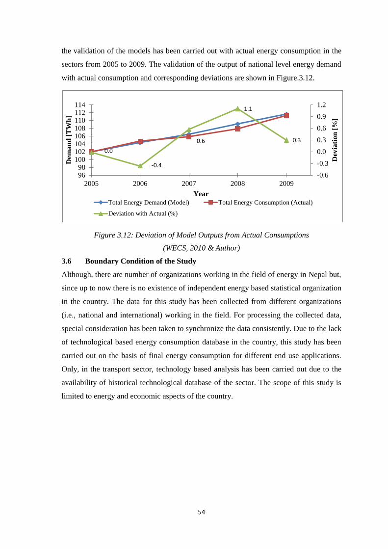
54
the validation of the models has been carried out with actual energy consumption in the
sectors from 2005 to 2009. The validation of the output of national level energy demand
with actual consumption and corresponding deviations are shown in Figure.3.12.
Figure 3.12: Deviation of Model Outputs from Actual Consumptions
(WECS, 2010 & Author)
3.6 Boundary Condition of the Study
Although, there are number of organizations working in the field of energy in Nepal but,
since up to now there is no existence of independent energy based statistical organization
in the country. The data for this study has been collected from different organizations
(i.e., national and international) working in the field. For processing the collected data,
special consideration has been taken to synchronize the data consistently. Due to the lack
of technological based energy consumption database in the country, this study has been
carried out on the basis of final energy consumption for different end use applications.
Only, in the transport sector, technology based analysis has been carried out due to the
availability of historical technological database of the sector. The scope of this study is
limited to energy and economic aspects of the country.
0.0
-0.4
0.6
1.1
0.3
-0.6
-0.3
0.0
0.3
0.6
0.9
1.2
9698
100102104106108110112114
2005 2006 2007 2008 2009
Dev
iati
on
[%
]
Dem
an
d [
TW
h]
Year
Total Energy Demand (Model) Total Energy Consumption (Actual)
Deviation with Actual (%)
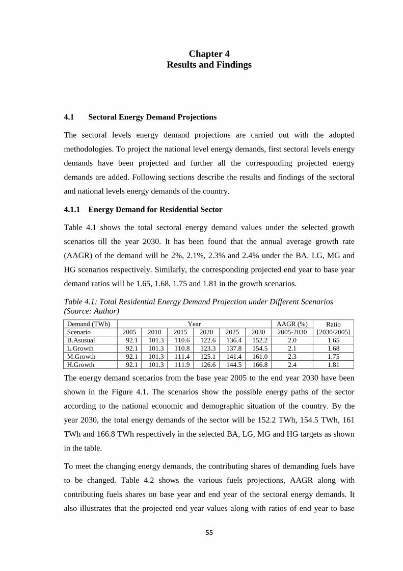
55
Chapter 4
Results and Findings
4.1 Sectoral Energy Demand Projections
The sectoral levels energy demand projections are carried out with the adopted
methodologies. To project the national level energy demands, first sectoral levels energy
demands have been projected and further all the corresponding projected energy
demands are added. Following sections describe the results and findings of the sectoral
and national levels energy demands of the country.
4.1.1 Energy Demand for Residential Sector
Table 4.1 shows the total sectoral energy demand values under the selected growth
scenarios till the year 2030. It has been found that the annual average growth rate
(AAGR) of the demand will be 2%, 2.1%, 2.3% and 2.4% under the BA, LG, MG and
HG scenarios respectively. Similarly, the corresponding projected end year to base year
demand ratios will be 1.65, 1.68, 1.75 and 1.81 in the growth scenarios.
Table 4.1: Total Residential Energy Demand Projection under Different Scenarios
(Source: Author)
Demand (TWh) Year AAGR (%) Ratio
[2030/2005] Scenario 2005 2010 2015 2020 2025 2030 2005-2030
B.Asusual 92.1 101.3 110.6 122.6 136.4 152.2 2.0 1.65
L.Growth 92.1 101.3 110.8 123.3 137.8 154.5 2.1 1.68
M.Growth 92.1 101.3 111.4 125.1 141.4 161.0 2.3 1.75
H.Growth 92.1 101.3 111.9 126.6 144.5 166.8 2.4 1.81
The energy demand scenarios from the base year 2005 to the end year 2030 have been
shown in the Figure 4.1. The scenarios show the possible energy paths of the sector
according to the national economic and demographic situation of the country. By the
year 2030, the total energy demands of the sector will be 152.2 TWh, 154.5 TWh, 161
TWh and 166.8 TWh respectively in the selected BA, LG, MG and HG targets as shown
in the table.
To meet the changing energy demands, the contributing shares of demanding fuels have
to be changed. Table 4.2 shows the various fuels projections, AAGR along with
contributing fuels shares on base year and end year of the sectoral energy demands. It
also illustrates that the projected end year values along with ratios of end year to base
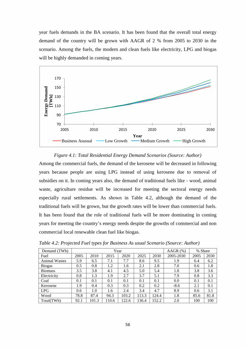
56
year fuels demands in the BA scenario. It has been found that the overall total energy
demand of the country will be grown with AAGR of 2 % from 2005 to 2030 in the
scenario. Among the fuels, the modern and clean fuels like electricity, LPG and biogas
will be highly demanded in coming years.
Figure 4.1: Total Residential Energy Demand Scenarios (Source: Author)
Among the commercial fuels, the demand of the kerosene will be decreased in following
years because people are using LPG instead of using kerosene due to removal of
subsidies on it. In coming years also, the demand of traditional fuels like - wood, animal
waste, agriculture residue will be increased for meeting the sectoral energy needs
especially rural settlements. As shown in Table 4.2, although the demand of the
traditional fuels will be grown, but the growth rates will be lower than commercial fuels.
It has been found that the role of traditional fuels will be more dominating in coming
years for meeting the country’s energy needs despite the growths of commercial and non
commercial local renewable clean fuel like biogas.
Table 4.2: Projected Fuel types for Business As usual Scenario (Source: Author)
Demand (TWh) Year AAGR (%) % Share
Fuel 2005 2010 2015 2020 2025 2030 2005-2030 2005 2030
Animal Wastes 5.9 6.5 7.1 7.7 8.6 9.5 1.9 6.4 6.2
Biogas 0.5 0.8 1.2 1.6 2.1 2.8 7.0 0.6 1.8
Biomass 3.5 3.8 4.1 4.5 5.0 5.4 1.8 3.8 3.6
Electricity 0.8 1.3 1.9 2.7 3.7 5.1 7.9 0.8 3.3
Coal 0.1 0.1 0.1 0.1 0.1 0.1 0.0 0.1 0.1
Kerosene 1.9 0.4 0.3 0.3 0.2 0.2 -8.6 2.1 0.1
LPG 0.6 1.0 1.6 2.4 3.4 4.7 8.9 0.6 3.1
Wood 78.8 87.4 94.3 103.2 113.3 124.4 1.8 85.6 81.8
Total(TWh) 92.1 101.3 110.6 122.6 136.4 152.2 2.0 100 100
70
90
110
130
150
170
2005 2010 2015 2020 2025 2030
En
erg
y D
ema
nd
[TW
h]
Year
Business Asusual Low Growth Medium Growth High Growth
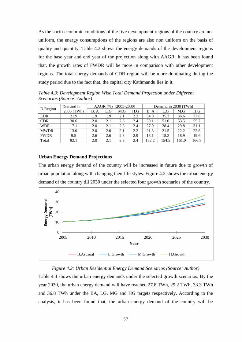
57
As the socio-economic conditions of the five development regions of the country are not
uniform, the energy consumptions of the regions are also non uniform on the basis of
quality and quantity. Table 4.3 shows the energy demands of the development regions
for the base year and end year of the projection along with AAGR. It has been found
that, the growth rates of FWDR will be more in comparison with other development
regions. The total energy demands of CDR region will be more dominating during the
study period due to the fact that, the capital city Kathmandu lies in it.
Table 4.3: Development Region Wise Total Demand Projection under Different
Scenarios (Source: Author)
D.Region Demand in
2005 (TWh)
AAGR (%) [2005-2030] Demand in 2030 (TWh)
B. A L.G M.G H.G B. A L.G M.G H.G
EDR 21.9 1.9 1.9 2.1 2.2 34.8 35.3 36.6 37.8
CDR 30.6 2.0 2.1 2.3 2.4 50.1 51.0 53.5 55.7
WDR 17.1 2.0 2.1 2.3 2.4 27.9 28.4 29.8 31.1
MWDR 13.0 2.0 2.0 2.1 2.2 21.3 21.5 22.2 22.6
FWDR 9.5 2.6 2.6 2.8 2.9 18.1 18.3 18.9 19.6
Total 92.1 2.0 2.1 2.3 2.4 152.2 154.5 161.0 166.8
Urban Energy Demand Projections
The urban energy demand of the country will be increased in future due to growth of
urban population along with changing their life styles. Figure 4.2 shows the urban energy
demand of the country till 2030 under the selected four growth scenarios of the country.
Figure 4.2: Urban Residential Energy Demand Scenarios (Source: Author)
Table 4.4 shows the urban energy demands under the selected growth scenarios. By the
year 2030, the urban energy demand will have reached 27.8 TWh, 29.2 TWh, 33.3 TWh
and 36.8 TWh under the BA, LG, MG and HG targets respectively. According to the
analysis, it has been found that, the urban energy demand of the country will be
0
10
20
30
40
2005 2010 2015 2020 2025 2030
Ene
rgy
De
man
d[T
Wh
]
Year
B.Asusual L.Growth M.Growth H.Growth
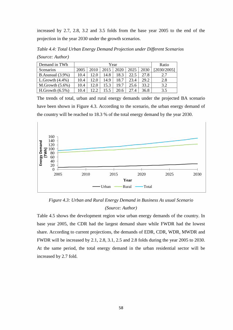
58
increased by 2.7, 2.8, 3.2 and 3.5 folds from the base year 2005 to the end of the
projection in the year 2030 under the growth scenarios.
Table 4.4: Total Urban Energy Demand Projection under Different Scenarios
(Source: Author)
Demand in TWh Year Ratio
[2030/2005] Scenarios 2005 2010 2015 2020 2025 2030
B.Asusual (3.9%) 10.4 12.0 14.8 18.3 22.5 27.8 2.7
L.Growth (4.4%) 10.4 12.0 14.9 18.7 23.4 29.2 2.8
M.Growth (5.6%) 10.4 12.0 15.3 19.7 25.6 33.2 3.2
H.Growth (6.5%) 10.4 12.2 15.5 20.6 27.4 36.8 3.5
The trends of total, urban and rural energy demands under the projected BA scenario
have been shown in Figure 4.3. According to the scenario, the urban energy demand of
the country will be reached to 18.3 % of the total energy demand by the year 2030.
Figure 4.3: Urban and Rural Energy Demand in Business As usual Scenario
(Source: Author)
Table 4.5 shows the development region wise urban energy demands of the country. In
base year 2005, the CDR had the largest demand share while FWDR had the lowest
share. According to current projections, the demands of EDR, CDR, WDR, MWDR and
FWDR will be increased by 2.1, 2.8, 3.1, 2.5 and 2.8 folds during the year 2005 to 2030.
At the same period, the total energy demand in the urban residential sector will be
increased by 2.7 fold.
020406080
100120140160
2005 2010 2015 2020 2025 2030
Ene
rgy
De
man
d[T
Wh
]
Year
Urban Rural Total
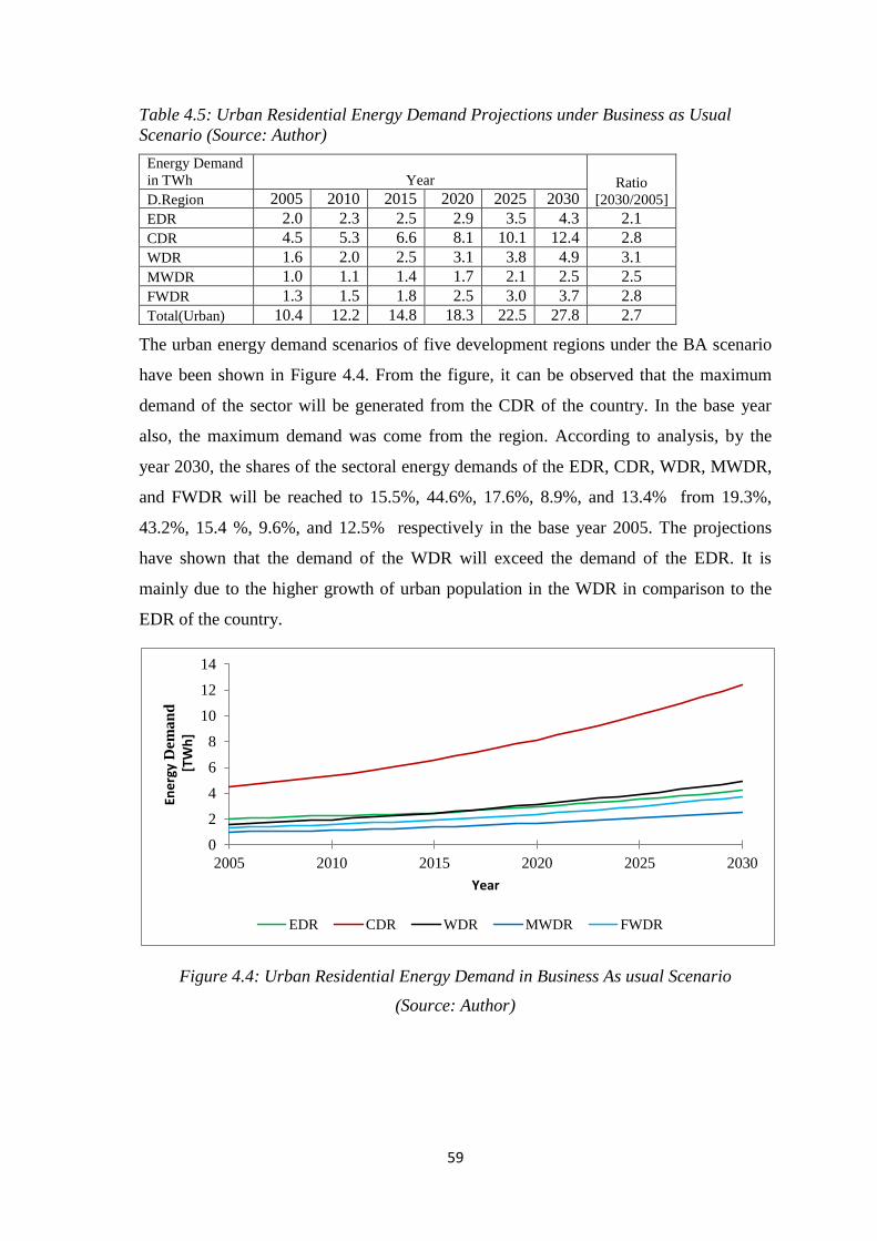
59
Table 4.5: Urban Residential Energy Demand Projections under Business as Usual
Scenario (Source: Author)
Energy Demand
in TWh Year Ratio
[2030/2005] D.Region 2005 2010 2015 2020 2025 2030
EDR 2.0 2.3 2.5 2.9 3.5 4.3 2.1
CDR 4.5 5.3 6.6 8.1 10.1 12.4 2.8
WDR 1.6 2.0 2.5 3.1 3.8 4.9 3.1
MWDR 1.0 1.1 1.4 1.7 2.1 2.5 2.5
FWDR 1.3 1.5 1.8 2.5 3.0 3.7 2.8
Total(Urban) 10.4 12.2 14.8 18.3 22.5 27.8 2.7
The urban energy demand scenarios of five development regions under the BA scenario
have been shown in Figure 4.4. From the figure, it can be observed that the maximum
demand of the sector will be generated from the CDR of the country. In the base year
also, the maximum demand was come from the region. According to analysis, by the
year 2030, the shares of the sectoral energy demands of the EDR, CDR, WDR, MWDR,
and FWDR will be reached to 15.5%, 44.6%, 17.6%, 8.9%, and 13.4% from 19.3%,
43.2%, 15.4 %, 9.6%, and 12.5% respectively in the base year 2005. The projections
have shown that the demand of the WDR will exceed the demand of the EDR. It is
mainly due to the higher growth of urban population in the WDR in comparison to the
EDR of the country.
Figure 4.4: Urban Residential Energy Demand in Business As usual Scenario
(Source: Author)
0
2
4
6
8
10
12
14
2005 2010 2015 2020 2025 2030
Ene
rgy
Dem
an
d
[TW
h]
Year
EDR CDR WDR MWDR FWDR
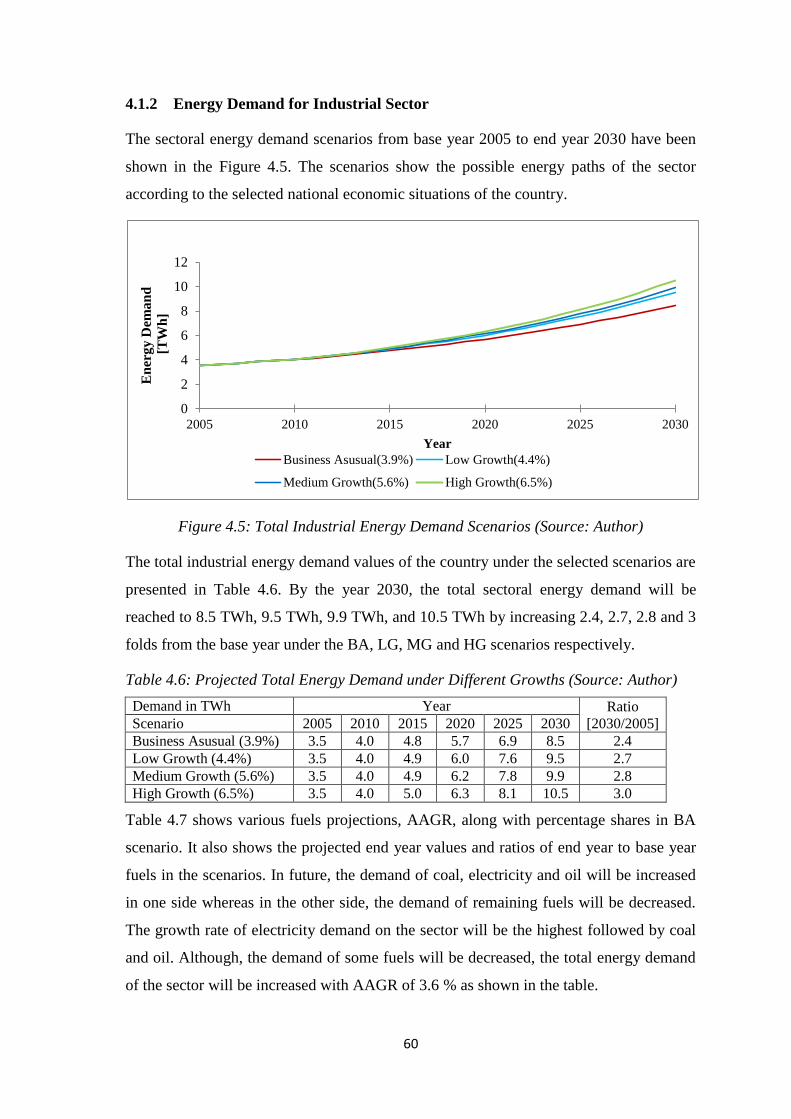
60
4.1.2 Energy Demand for Industrial Sector
The sectoral energy demand scenarios from base year 2005 to end year 2030 have been
shown in the Figure 4.5. The scenarios show the possible energy paths of the sector
according to the selected national economic situations of the country.
Figure 4.5: Total Industrial Energy Demand Scenarios (Source: Author)
The total industrial energy demand values of the country under the selected scenarios are
presented in Table 4.6. By the year 2030, the total sectoral energy demand will be
reached to 8.5 TWh, 9.5 TWh, 9.9 TWh, and 10.5 TWh by increasing 2.4, 2.7, 2.8 and 3
folds from the base year under the BA, LG, MG and HG scenarios respectively.
Table 4.6: Projected Total Energy Demand under Different Growths (Source: Author)
Demand in TWh Year Ratio
[2030/2005] Scenario 2005 2010 2015 2020 2025 2030
Business Asusual (3.9%) 3.5 4.0 4.8 5.7 6.9 8.5 2.4
Low Growth (4.4%) 3.5 4.0 4.9 6.0 7.6 9.5 2.7
Medium Growth (5.6%) 3.5 4.0 4.9 6.2 7.8 9.9 2.8
High Growth (6.5%) 3.5 4.0 5.0 6.3 8.1 10.5 3.0
Table 4.7 shows various fuels projections, AAGR, along with percentage shares in BA
scenario. It also shows the projected end year values and ratios of end year to base year
fuels in the scenarios. In future, the demand of coal, electricity and oil will be increased
in one side whereas in the other side, the demand of remaining fuels will be decreased.
The growth rate of electricity demand on the sector will be the highest followed by coal
and oil. Although, the demand of some fuels will be decreased, the total energy demand
of the sector will be increased with AAGR of 3.6 % as shown in the table.
0
2
4
6
8
10
12
2005 2010 2015 2020 2025 2030
En
erg
y D
ema
nd
[TW
h]
Year
Business Asusual(3.9%) Low Growth(4.4%)
Medium Growth(5.6%) High Growth(6.5%)
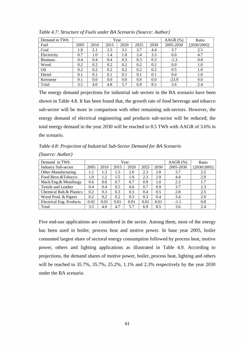
61
Table 4.7: Structure of Fuels under BA Scenario (Source: Author)
Demand in TWh Year AAGR (%) Ratio
[2030/2005] Fuel 2005 2010 2015 2020 2025 2030 2005-2030
Coal 1.8 2.1 2.5 3.1 3.7 4.4 3.7 2.5
Electricity 0.7 1.0 1.4 1.8 2.4 3.3 6.0 4.7
Biomass 0.4 0.4 0.4 0.3 0.3 0.3 -1.3 0.8
Wood 0.2 0.2 0.2 0.2 0.2 0.2 0.0 1.0
Oil 0.2 0.2 0.2 0.2 0.2 0.2 0.5 1.0
Diesel 0.1 0.1 0.1 0.1 0.1 0.1 0.0 1.0
Kerosene 0.1 0.0 0.0 0.0 0.0 0.0 -23.9 0.0
Total 3.5 4.0 4.8 5.7 6.9 8.5 3.6 2.4
The energy demand projections for industrial sub sectors in the BA scenario have been
shown in Table 4.8. It has been found that, the growth rate of food beverage and tobacco
sub-sector will be more in comparison with other remaining sub-sectors. However, the
energy demand of electrical engineering and products sub-sector will be reduced; the
total energy demand in the year 2030 will be reached to 8.5 TWh with AAGR of 3.6% in
the scenario.
Table 4.8: Projection of Industrial Sub-Sector Demand for BA Scenario
(Source: Author)
Demand in TWh Year AAGR (%) Ratio
[2030/2005] Industry Sub-sector 2005 2010 2015 2020 2025 2030 2005-2030
Other Manufacturing 1.1 1.3 1.5 2.0 2.3 2.8 3.7 2.5
Food Beve.&Tobacco 1.0 1.2 1.5 1.8 2.3 2.9 4.4 2.9
Mach Eng.& Metallurgy 0.6 0.6 0.7 0.7 0.9 1.0 2.3 1.7
Textile and Leather 0.4 0.4 0.5 0.6 0.7 0.9 3.7 2.3
Chemical Rub.& Plastics 0.2 0.3 0.3 0.3 0.4 0.5 2.8 2.5
Wood Prod. & Papers 0.2 0.2 0.2 0.3 0.3 0.4 3.4 2.0
Electrical Eng. Products 0.02 0.01 0.01 0.01 0.01 0.01 -1.1 0.8
Total 3.5 4.0 4.7 5.7 6.9 8.5 3.6 2.4
Five end-use applications are considered in the sector. Among them, most of the energy
has been used in boiler, process heat and motive power. In base year 2005, boiler
consumed largest share of sectoral energy consumption followed by process heat, motive
power, others and lighting applications as illustrated in Table 4.9. According to
projections, the demand shares of motive power, boiler, process heat, lighting and others
will be reached to 35.7%, 35.7%, 25.2%, 1.1% and 2.3% respectively by the year 2030
under the BA scenario.
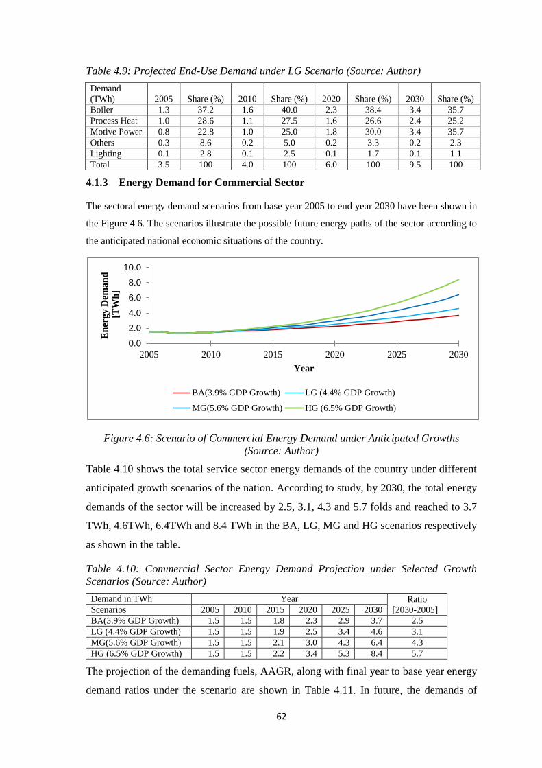
62
Table 4.9: Projected End-Use Demand under LG Scenario (Source: Author)
Demand
(TWh) 2005 Share (%) 2010 Share (%) 2020 Share (%) 2030 Share (%)
Boiler 1.3 37.2 1.6 40.0 2.3 38.4 3.4 35.7
Process Heat 1.0 28.6 1.1 27.5 1.6 26.6 2.4 25.2
Motive Power 0.8 22.8 1.0 25.0 1.8 30.0 3.4 35.7
Others 0.3 8.6 0.2 5.0 0.2 3.3 0.2 2.3
Lighting 0.1 2.8 0.1 2.5 0.1 1.7 0.1 1.1
Total 3.5 100 4.0 100 6.0 100 9.5 100
4.1.3 Energy Demand for Commercial Sector
The sectoral energy demand scenarios from base year 2005 to end year 2030 have been shown in
the Figure 4.6. The scenarios illustrate the possible future energy paths of the sector according to
the anticipated national economic situations of the country.
Figure 4.6: Scenario of Commercial Energy Demand under Anticipated Growths
(Source: Author)
Table 4.10 shows the total service sector energy demands of the country under different
anticipated growth scenarios of the nation. According to study, by 2030, the total energy
demands of the sector will be increased by 2.5, 3.1, 4.3 and 5.7 folds and reached to 3.7
TWh, 4.6TWh, 6.4TWh and 8.4 TWh in the BA, LG, MG and HG scenarios respectively
as shown in the table.
Table 4.10: Commercial Sector Energy Demand Projection under Selected Growth
Scenarios (Source: Author)
Demand in TWh Year Ratio
[2030-2005] Scenarios 2005 2010 2015 2020 2025 2030
BA(3.9% GDP Growth) 1.5 1.5 1.8 2.3 2.9 3.7 2.5
LG (4.4% GDP Growth) 1.5 1.5 1.9 2.5 3.4 4.6 3.1
MG(5.6% GDP Growth) 1.5 1.5 2.1 3.0 4.3 6.4 4.3
HG (6.5% GDP Growth) 1.5 1.5 2.2 3.4 5.3 8.4 5.7
The projection of the demanding fuels, AAGR, along with final year to base year energy
demand ratios under the scenario are shown in Table 4.11. In future, the demands of
0.0
2.0
4.0
6.0
8.0
10.0
2005 2010 2015 2020 2025 2030
En
ergy D
ema
nd
[TW
h]
Year
BA(3.9% GDP Growth) LG (4.4% GDP Growth)
MG(5.6% GDP Growth) HG (6.5% GDP Growth)
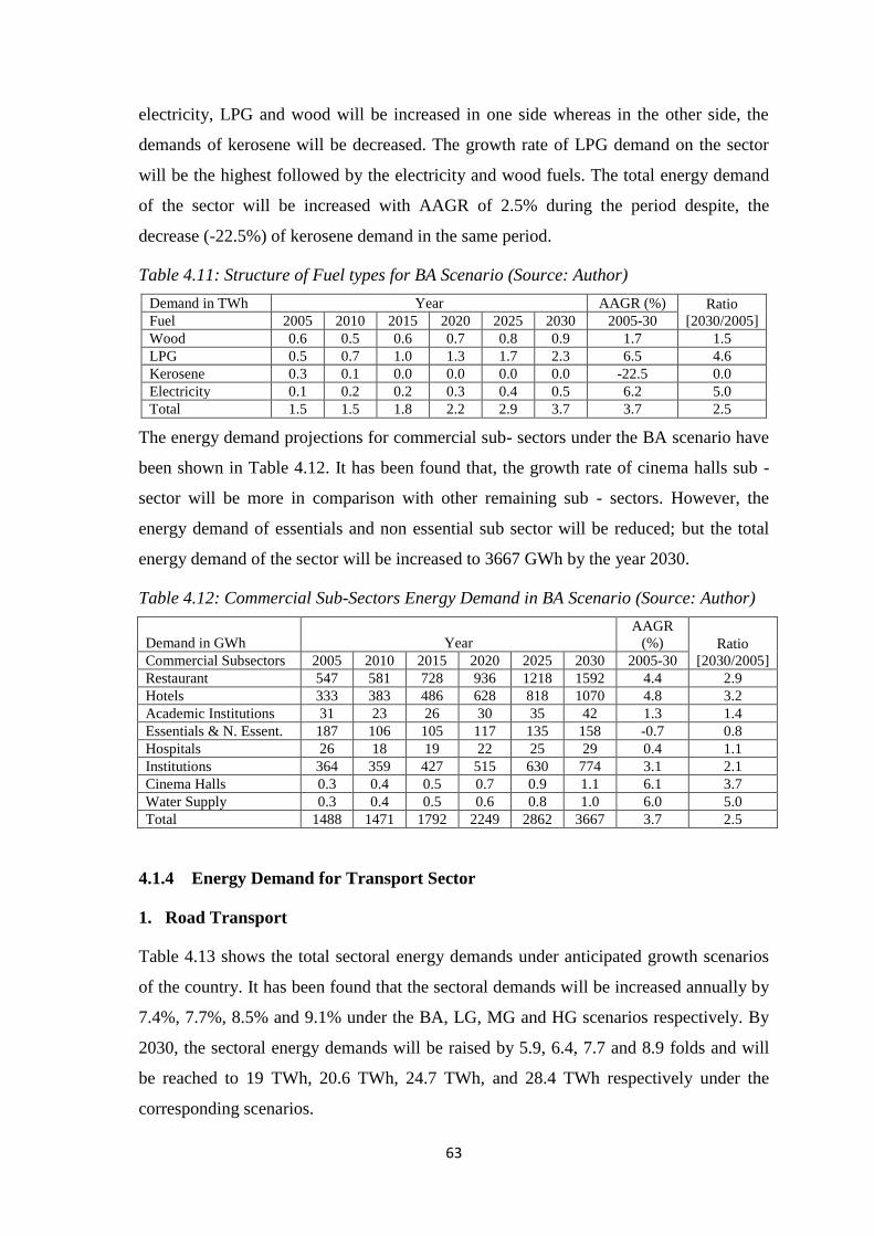
63
electricity, LPG and wood will be increased in one side whereas in the other side, the
demands of kerosene will be decreased. The growth rate of LPG demand on the sector
will be the highest followed by the electricity and wood fuels. The total energy demand
of the sector will be increased with AAGR of 2.5% during the period despite, the
decrease (-22.5%) of kerosene demand in the same period.
Table 4.11: Structure of Fuel types for BA Scenario (Source: Author)
Demand in TWh Year AAGR (%) Ratio
[2030/2005] Fuel 2005 2010 2015 2020 2025 2030 2005-30
Wood 0.6 0.5 0.6 0.7 0.8 0.9 1.7 1.5
LPG 0.5 0.7 1.0 1.3 1.7 2.3 6.5 4.6
Kerosene 0.3 0.1 0.0 0.0 0.0 0.0 -22.5 0.0
Electricity 0.1 0.2 0.2 0.3 0.4 0.5 6.2 5.0
Total 1.5 1.5 1.8 2.2 2.9 3.7 3.7 2.5
The energy demand projections for commercial sub- sectors under the BA scenario have
been shown in Table 4.12. It has been found that, the growth rate of cinema halls sub -
sector will be more in comparison with other remaining sub - sectors. However, the
energy demand of essentials and non essential sub sector will be reduced; but the total
energy demand of the sector will be increased to 3667 GWh by the year 2030.
Table 4.12: Commercial Sub-Sectors Energy Demand in BA Scenario (Source: Author)
Demand in GWh Year
AAGR
(%) Ratio
[2030/2005] Commercial Subsectors 2005 2010 2015 2020 2025 2030 2005-30
Restaurant 547 581 728 936 1218 1592 4.4 2.9
Hotels 333 383 486 628 818 1070 4.8 3.2
Academic Institutions 31 23 26 30 35 42 1.3 1.4
Essentials & N. Essent. 187 106 105 117 135 158 -0.7 0.8
Hospitals 26 18 19 22 25 29 0.4 1.1
Institutions 364 359 427 515 630 774 3.1 2.1
Cinema Halls 0.3 0.4 0.5 0.7 0.9 1.1 6.1 3.7
Water Supply 0.3 0.4 0.5 0.6 0.8 1.0 6.0 5.0
Total 1488 1471 1792 2249 2862 3667 3.7 2.5
4.1.4 Energy Demand for Transport Sector
1. Road Transport
Table 4.13 shows the total sectoral energy demands under anticipated growth scenarios
of the country. It has been found that the sectoral demands will be increased annually by
7.4%, 7.7%, 8.5% and 9.1% under the BA, LG, MG and HG scenarios respectively. By
2030, the sectoral energy demands will be raised by 5.9, 6.4, 7.7 and 8.9 folds and will
be reached to 19 TWh, 20.6 TWh, 24.7 TWh, and 28.4 TWh respectively under the
corresponding scenarios.
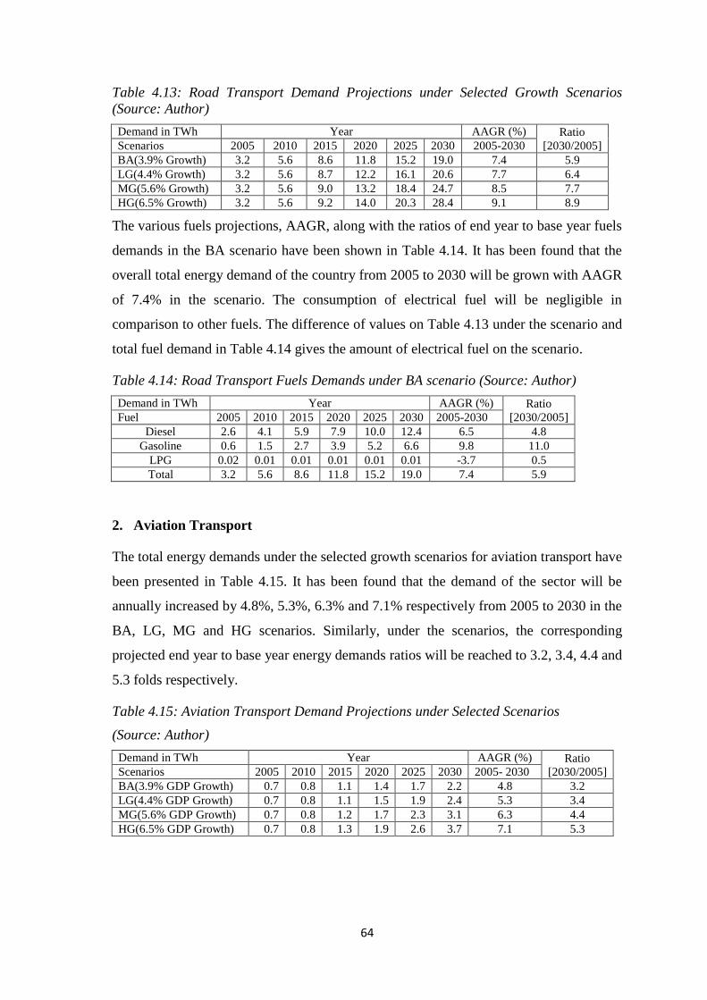
64
Table 4.13: Road Transport Demand Projections under Selected Growth Scenarios
(Source: Author)
Demand in TWh Year AAGR (%) Ratio
[2030/2005] Scenarios 2005 2010 2015 2020 2025 2030 2005-2030
BA(3.9% Growth) 3.2 5.6 8.6 11.8 15.2 19.0 7.4 5.9
LG(4.4% Growth) 3.2 5.6 8.7 12.2 16.1 20.6 7.7 6.4
MG(5.6% Growth) 3.2 5.6 9.0 13.2 18.4 24.7 8.5 7.7
HG(6.5% Growth) 3.2 5.6 9.2 14.0 20.3 28.4 9.1 8.9
The various fuels projections, AAGR, along with the ratios of end year to base year fuels
demands in the BA scenario have been shown in Table 4.14. It has been found that the
overall total energy demand of the country from 2005 to 2030 will be grown with AAGR
of 7.4% in the scenario. The consumption of electrical fuel will be negligible in
comparison to other fuels. The difference of values on Table 4.13 under the scenario and
total fuel demand in Table 4.14 gives the amount of electrical fuel on the scenario.
Table 4.14: Road Transport Fuels Demands under BA scenario (Source: Author)
Demand in TWh Year AAGR (%) Ratio
[2030/2005] Fuel 2005 2010 2015 2020 2025 2030 2005-2030
Diesel 2.6 4.1 5.9 7.9 10.0 12.4 6.5 4.8
Gasoline 0.6 1.5 2.7 3.9 5.2 6.6 9.8 11.0
LPG 0.02 0.01 0.01 0.01 0.01 0.01 -3.7 0.5
Total 3.2 5.6 8.6 11.8 15.2 19.0 7.4 5.9
2. Aviation Transport
The total energy demands under the selected growth scenarios for aviation transport have
been presented in Table 4.15. It has been found that the demand of the sector will be
annually increased by 4.8%, 5.3%, 6.3% and 7.1% respectively from 2005 to 2030 in the
BA, LG, MG and HG scenarios. Similarly, under the scenarios, the corresponding
projected end year to base year energy demands ratios will be reached to 3.2, 3.4, 4.4 and
5.3 folds respectively.
Table 4.15: Aviation Transport Demand Projections under Selected Scenarios
(Source: Author)
Demand in TWh Year AAGR (%) Ratio
[2030/2005] Scenarios 2005 2010 2015 2020 2025 2030 2005- 2030
BA(3.9% GDP Growth) 0.7 0.8 1.1 1.4 1.7 2.2 4.8 3.2
LG(4.4% GDP Growth) 0.7 0.8 1.1 1.5 1.9 2.4 5.3 3.4
MG(5.6% GDP Growth) 0.7 0.8 1.2 1.7 2.3 3.1 6.3 4.4
HG(6.5% GDP Growth) 0.7 0.8 1.3 1.9 2.6 3.7 7.1 5.3
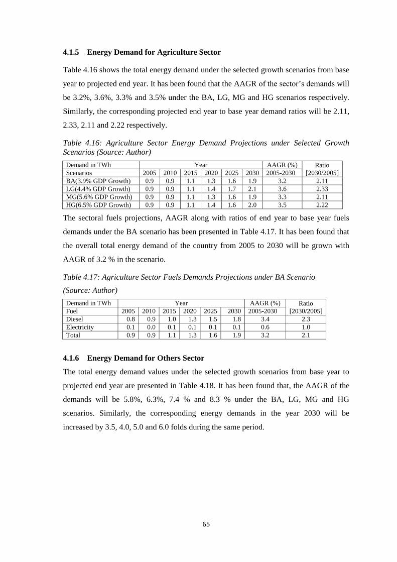
65
4.1.5 Energy Demand for Agriculture Sector
Table 4.16 shows the total energy demand under the selected growth scenarios from base
year to projected end year. It has been found that the AAGR of the sector’s demands will
be 3.2%, 3.6%, 3.3% and 3.5% under the BA, LG, MG and HG scenarios respectively.
Similarly, the corresponding projected end year to base year demand ratios will be 2.11,
2.33, 2.11 and 2.22 respectively.
Table 4.16: Agriculture Sector Energy Demand Projections under Selected Growth
Scenarios (Source: Author)
Demand in TWh Year AAGR (%) Ratio
[2030/2005] Scenarios 2005 2010 2015 2020 2025 2030 2005-2030
BA(3.9% GDP Growth) 0.9 0.9 1.1 1.3 1.6 1.9 3.2 2.11
LG(4.4% GDP Growth) 0.9 0.9 1.1 1.4 1.7 2.1 3.6 2.33
MG(5.6% GDP Growth) 0.9 0.9 1.1 1.3 1.6 1.9 3.3 2.11
HG(6.5% GDP Growth) 0.9 0.9 1.1 1.4 1.6 2.0 3.5 2.22
The sectoral fuels projections, AAGR along with ratios of end year to base year fuels
demands under the BA scenario has been presented in Table 4.17. It has been found that
the overall total energy demand of the country from 2005 to 2030 will be grown with
AAGR of 3.2 % in the scenario.
Table 4.17: Agriculture Sector Fuels Demands Projections under BA Scenario
(Source: Author)
Demand in TWh Year AAGR (%) Ratio
[2030/2005] Fuel 2005 2010 2015 2020 2025 2030 2005-2030
Diesel 0.8 0.9 1.0 1.3 1.5 1.8 3.4 2.3
Electricity 0.1 0.0 0.1 0.1 0.1 0.1 0.6 1.0
Total 0.9 0.9 1.1 1.3 1.6 1.9 3.2 2.1
4.1.6 Energy Demand for Others Sector
The total energy demand values under the selected growth scenarios from base year to
projected end year are presented in Table 4.18. It has been found that, the AAGR of the
demands will be 5.8%, 6.3%, 7.4 % and 8.3 % under the BA, LG, MG and HG
scenarios. Similarly, the corresponding energy demands in the year 2030 will be
increased by 3.5, 4.0, 5.0 and 6.0 folds during the same period.
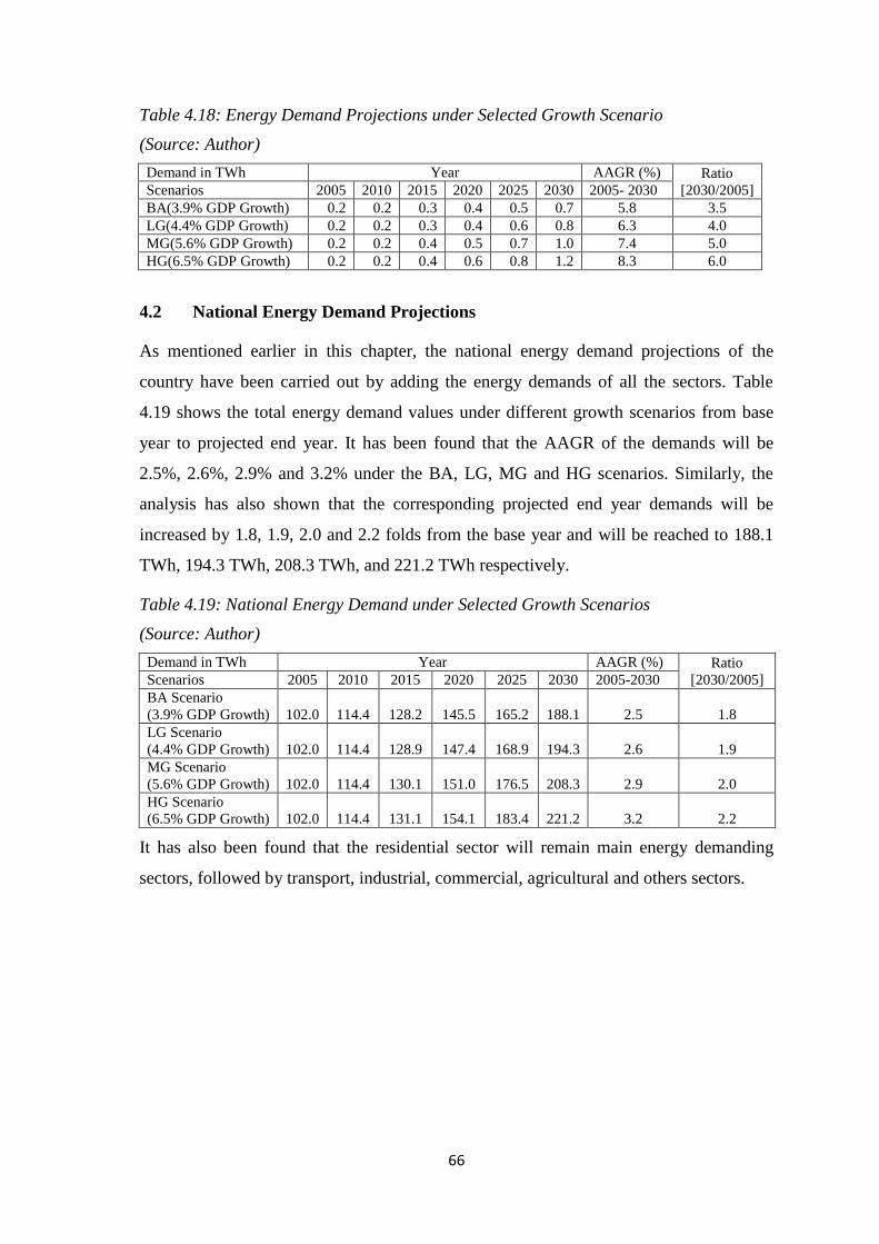
66
Table 4.18: Energy Demand Projections under Selected Growth Scenario
(Source: Author)
Demand in TWh Year AAGR (%) Ratio
[2030/2005] Scenarios 2005 2010 2015 2020 2025 2030 2005- 2030
BA(3.9% GDP Growth) 0.2 0.2 0.3 0.4 0.5 0.7 5.8 3.5
LG(4.4% GDP Growth) 0.2 0.2 0.3 0.4 0.6 0.8 6.3 4.0
MG(5.6% GDP Growth) 0.2 0.2 0.4 0.5 0.7 1.0 7.4 5.0
HG(6.5% GDP Growth) 0.2 0.2 0.4 0.6 0.8 1.2 8.3 6.0
4.2 National Energy Demand Projections
As mentioned earlier in this chapter, the national energy demand projections of the
country have been carried out by adding the energy demands of all the sectors. Table
4.19 shows the total energy demand values under different growth scenarios from base
year to projected end year. It has been found that the AAGR of the demands will be
2.5%, 2.6%, 2.9% and 3.2% under the BA, LG, MG and HG scenarios. Similarly, the
analysis has also shown that the corresponding projected end year demands will be
increased by 1.8, 1.9, 2.0 and 2.2 folds from the base year and will be reached to 188.1
TWh, 194.3 TWh, 208.3 TWh, and 221.2 TWh respectively.
Table 4.19: National Energy Demand under Selected Growth Scenarios
(Source: Author)
Demand in TWh Year AAGR (%) Ratio
[2030/2005] Scenarios 2005 2010 2015 2020 2025 2030 2005-2030
BA Scenario
(3.9% GDP Growth) 102.0 114.4 128.2 145.5 165.2 188.1 2.5 1.8
LG Scenario
(4.4% GDP Growth) 102.0 114.4 128.9 147.4 168.9 194.3 2.6 1.9
MG Scenario
(5.6% GDP Growth) 102.0 114.4 130.1 151.0 176.5 208.3 2.9 2.0
HG Scenario
(6.5% GDP Growth) 102.0 114.4 131.1 154.1 183.4 221.2 3.2 2.2
It has also been found that the residential sector will remain main energy demanding
sectors, followed by transport, industrial, commercial, agricultural and others sectors.
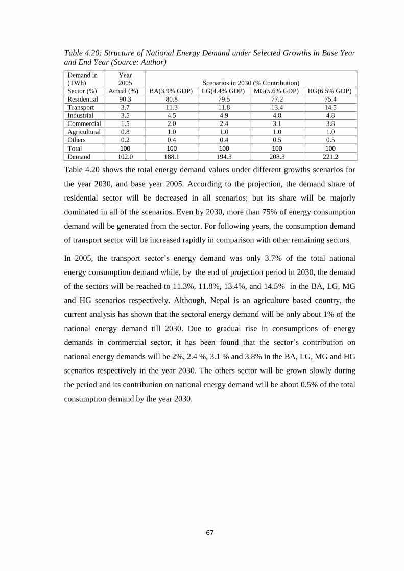
67
Table 4.20: Structure of National Energy Demand under Selected Growths in Base Year
and End Year (Source: Author)
Demand in
(TWh)
Year
2005 Scenarios in 2030 (% Contribution)
Sector (%) Actual (%) BA(3.9% GDP) LG(4.4% GDP) MG(5.6% GDP) HG(6.5% GDP)
Residential 90.3 80.8 79.5 77.2 75.4
Transport 3.7 11.3 11.8 13.4 14.5
Industrial 3.5 4.5 4.9 4.8 4.8
Commercial 1.5 2.0 2.4 3.1 3.8
Agricultural 0.8 1.0 1.0 1.0 1.0
Others 0.2 0.4 0.4 0.5 0.5
Total 100 100 100 100 100 Demand 102.0 188.1 194.3 208.3 221.2
Table 4.20 shows the total energy demand values under different growths scenarios for
the year 2030, and base year 2005. According to the projection, the demand share of
residential sector will be decreased in all scenarios; but its share will be majorly
dominated in all of the scenarios. Even by 2030, more than 75% of energy consumption
demand will be generated from the sector. For following years, the consumption demand
of transport sector will be increased rapidly in comparison with other remaining sectors.
In 2005, the transport sector’s energy demand was only 3.7% of the total national
energy consumption demand while, by the end of projection period in 2030, the demand
of the sectors will be reached to 11.3%, 11.8%, 13.4%, and 14.5% in the BA, LG, MG
and HG scenarios respectively. Although, Nepal is an agriculture based country, the
current analysis has shown that the sectoral energy demand will be only about 1% of the
national energy demand till 2030. Due to gradual rise in consumptions of energy
demands in commercial sector, it has been found that the sector’s contribution on
national energy demands will be 2%, 2.4 %, 3.1 % and 3.8% in the BA, LG, MG and HG
scenarios respectively in the year 2030. The others sector will be grown slowly during
the period and its contribution on national energy demand will be about 0.5% of the total
consumption demand by the year 2030.
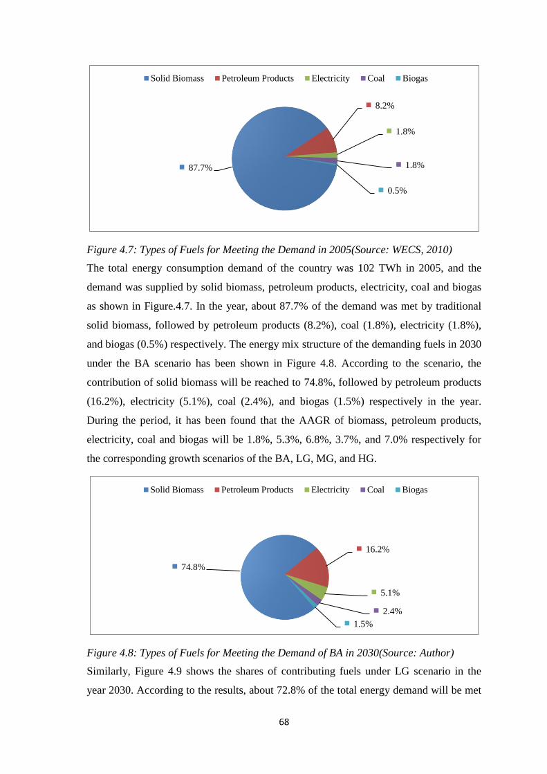
68
Figure 4.7: Types of Fuels for Meeting the Demand in 2005(Source: WECS, 2010)
The total energy consumption demand of the country was 102 TWh in 2005, and the
demand was supplied by solid biomass, petroleum products, electricity, coal and biogas
as shown in Figure.4.7. In the year, about 87.7% of the demand was met by traditional
solid biomass, followed by petroleum products (8.2%), coal (1.8%), electricity (1.8%),
and biogas (0.5%) respectively. The energy mix structure of the demanding fuels in 2030
under the BA scenario has been shown in Figure 4.8. According to the scenario, the
contribution of solid biomass will be reached to 74.8%, followed by petroleum products
(16.2%), electricity (5.1%), coal (2.4%), and biogas (1.5%) respectively in the year.
During the period, it has been found that the AAGR of biomass, petroleum products,
electricity, coal and biogas will be 1.8%, 5.3%, 6.8%, 3.7%, and 7.0% respectively for
the corresponding growth scenarios of the BA, LG, MG, and HG.
Figure 4.8: Types of Fuels for Meeting the Demand of BA in 2030(Source: Author)
Similarly, Figure 4.9 shows the shares of contributing fuels under LG scenario in the
year 2030. According to the results, about 72.8% of the total energy demand will be met
87.7%
8.2%
1.8%
1.8%
0.5%
Solid Biomass Petroleum Products Electricity Coal Biogas
74.8%
16.2%
5.1%
2.4%
1.5%
Solid Biomass Petroleum Products Electricity Coal Biogas
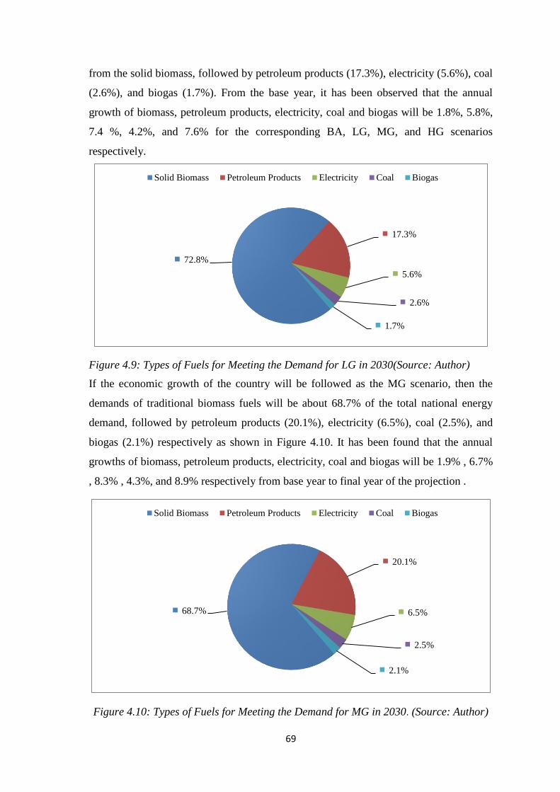
69
from the solid biomass, followed by petroleum products (17.3%), electricity (5.6%), coal
(2.6%), and biogas (1.7%). From the base year, it has been observed that the annual
growth of biomass, petroleum products, electricity, coal and biogas will be 1.8%, 5.8%,
7.4 %, 4.2%, and 7.6% for the corresponding BA, LG, MG, and HG scenarios
respectively.
Figure 4.9: Types of Fuels for Meeting the Demand for LG in 2030(Source: Author)
If the economic growth of the country will be followed as the MG scenario, then the
demands of traditional biomass fuels will be about 68.7% of the total national energy
demand, followed by petroleum products (20.1%), electricity (6.5%), coal (2.5%), and
biogas (2.1%) respectively as shown in Figure 4.10. It has been found that the annual
growths of biomass, petroleum products, electricity, coal and biogas will be 1.9% , 6.7%
, 8.3% , 4.3%, and 8.9% respectively from base year to final year of the projection .
Figure 4.10: Types of Fuels for Meeting the Demand for MG in 2030. (Source: Author)
72.8%
17.3%
5.6%
2.6%
1.7%
Solid Biomass Petroleum Products Electricity Coal Biogas
68.7%
20.1%
6.5%
2.5%
2.1%
Solid Biomass Petroleum Products Electricity Coal Biogas
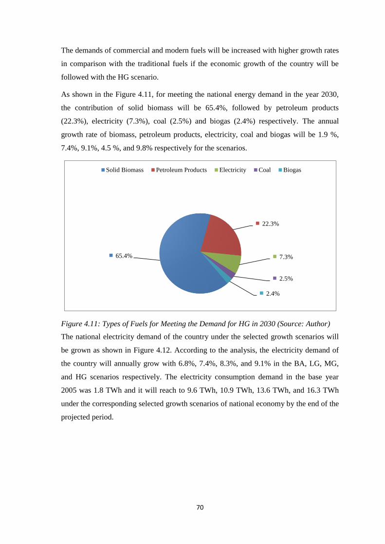
70
The demands of commercial and modern fuels will be increased with higher growth rates
in comparison with the traditional fuels if the economic growth of the country will be
followed with the HG scenario.
As shown in the Figure 4.11, for meeting the national energy demand in the year 2030,
the contribution of solid biomass will be 65.4%, followed by petroleum products
(22.3%), electricity (7.3%), coal (2.5%) and biogas (2.4%) respectively. The annual
growth rate of biomass, petroleum products, electricity, coal and biogas will be 1.9 %,
7.4%, 9.1%, 4.5 %, and 9.8% respectively for the scenarios.
Figure 4.11: Types of Fuels for Meeting the Demand for HG in 2030 (Source: Author)
The national electricity demand of the country under the selected growth scenarios will
be grown as shown in Figure 4.12. According to the analysis, the electricity demand of
the country will annually grow with 6.8%, 7.4%, 8.3%, and 9.1% in the BA, LG, MG,
and HG scenarios respectively. The electricity consumption demand in the base year
2005 was 1.8 TWh and it will reach to 9.6 TWh, 10.9 TWh, 13.6 TWh, and 16.3 TWh
under the corresponding selected growth scenarios of national economy by the end of the
projected period.
65.4%
22.3%
7.3%
2.5%
2.4%
Solid Biomass Petroleum Products Electricity Coal Biogas
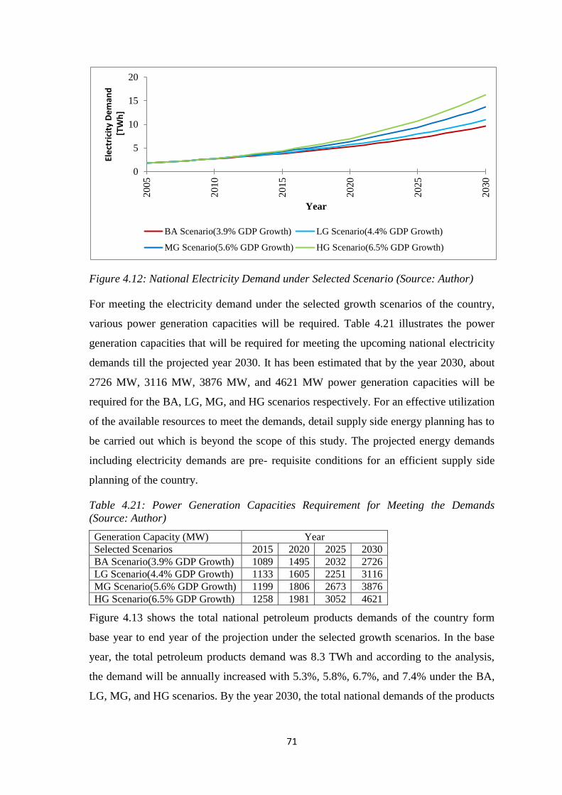
71
Figure 4.12: National Electricity Demand under Selected Scenario (Source: Author)
For meeting the electricity demand under the selected growth scenarios of the country,
various power generation capacities will be required. Table 4.21 illustrates the power
generation capacities that will be required for meeting the upcoming national electricity
demands till the projected year 2030. It has been estimated that by the year 2030, about
2726 MW, 3116 MW, 3876 MW, and 4621 MW power generation capacities will be
required for the BA, LG, MG, and HG scenarios respectively. For an effective utilization
of the available resources to meet the demands, detail supply side energy planning has to
be carried out which is beyond the scope of this study. The projected energy demands
including electricity demands are pre- requisite conditions for an efficient supply side
planning of the country.
Table 4.21: Power Generation Capacities Requirement for Meeting the Demands
(Source: Author)
Generation Capacity (MW) Year
Selected Scenarios 2015 2020 2025 2030
BA Scenario(3.9% GDP Growth) 1089 1495 2032 2726
LG Scenario(4.4% GDP Growth) 1133 1605 2251 3116
MG Scenario(5.6% GDP Growth) 1199 1806 2673 3876
HG Scenario(6.5% GDP Growth) 1258 1981 3052 4621
Figure 4.13 shows the total national petroleum products demands of the country form
base year to end year of the projection under the selected growth scenarios. In the base
year, the total petroleum products demand was 8.3 TWh and according to the analysis,
the demand will be annually increased with 5.3%, 5.8%, 6.7%, and 7.4% under the BA,
LG, MG, and HG scenarios. By the year 2030, the total national demands of the products
0
5
10
15
20
20
05
20
10
20
15
20
20
20
25
20
30
Ele
ctri
city
De
man
d[T
Wh
]
Year
BA Scenario(3.9% GDP Growth) LG Scenario(4.4% GDP Growth)
MG Scenario(5.6% GDP Growth) HG Scenario(6.5% GDP Growth)
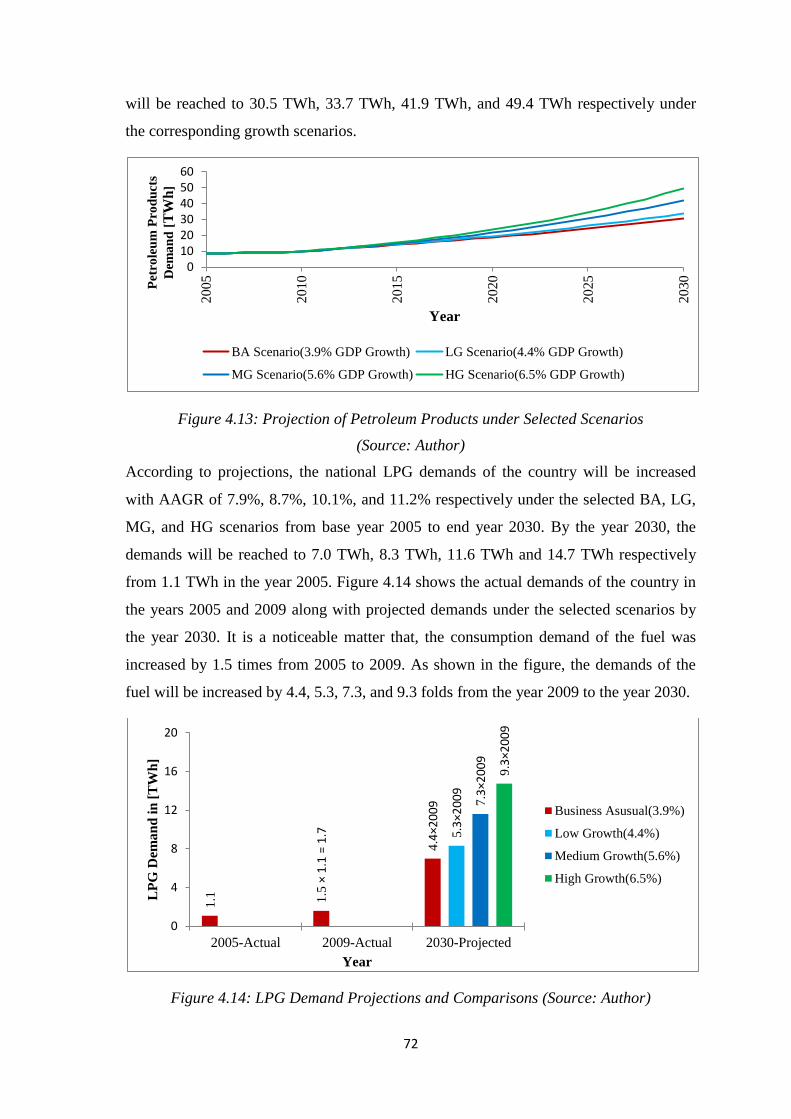
72
will be reached to 30.5 TWh, 33.7 TWh, 41.9 TWh, and 49.4 TWh respectively under
the corresponding growth scenarios.
Figure 4.13: Projection of Petroleum Products under Selected Scenarios
(Source: Author)
According to projections, the national LPG demands of the country will be increased
with AAGR of 7.9%, 8.7%, 10.1%, and 11.2% respectively under the selected BA, LG,
MG, and HG scenarios from base year 2005 to end year 2030. By the year 2030, the
demands will be reached to 7.0 TWh, 8.3 TWh, 11.6 TWh and 14.7 TWh respectively
from 1.1 TWh in the year 2005. Figure 4.14 shows the actual demands of the country in
the years 2005 and 2009 along with projected demands under the selected scenarios by
the year 2030. It is a noticeable matter that, the consumption demand of the fuel was
increased by 1.5 times from 2005 to 2009. As shown in the figure, the demands of the
fuel will be increased by 4.4, 5.3, 7.3, and 9.3 folds from the year 2009 to the year 2030.
Figure 4.14: LPG Demand Projections and Comparisons (Source: Author)
0102030405060
20
05
20
10
20
15
20
20
2025
20
30
Pet
role
um
Pro
du
cts
Dem
an
d [
TW
h]
Year
BA Scenario(3.9% GDP Growth) LG Scenario(4.4% GDP Growth)
MG Scenario(5.6% GDP Growth) HG Scenario(6.5% GDP Growth)
1.1 1.5
×1
.1 =
1.7
4.4×2
00
9
5.3×2
00
9
7.3×2
00
9
9.3×2
00
9
0
4
8
12
16
20
2005-Actual 2009-Actual 2030-Projected
LP
G D
eman
d i
n [
TW
h]
Year
Business Asusual(3.9%)
Low Growth(4.4%)
Medium Growth(5.6%)
High Growth(6.5%)
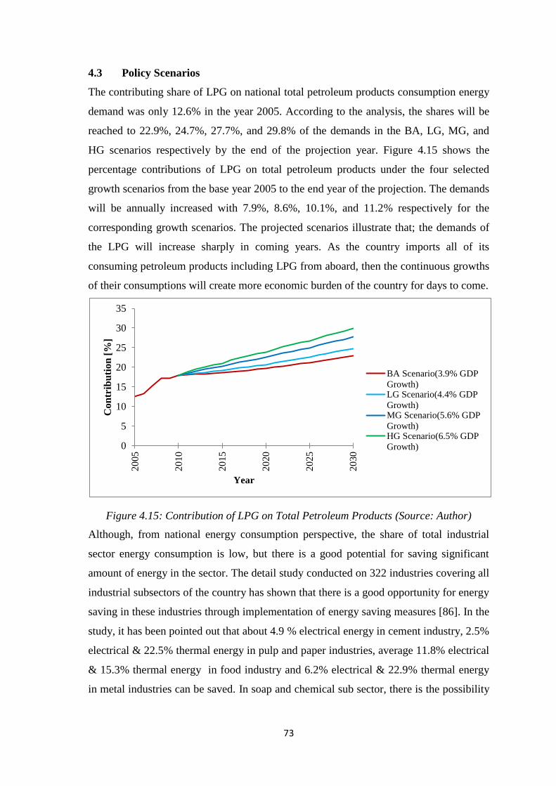
73
4.3 Policy Scenarios
The contributing share of LPG on national total petroleum products consumption energy
demand was only 12.6% in the year 2005. According to the analysis, the shares will be
reached to 22.9%, 24.7%, 27.7%, and 29.8% of the demands in the BA, LG, MG, and
HG scenarios respectively by the end of the projection year. Figure 4.15 shows the
percentage contributions of LPG on total petroleum products under the four selected
growth scenarios from the base year 2005 to the end year of the projection. The demands
will be annually increased with 7.9%, 8.6%, 10.1%, and 11.2% respectively for the
corresponding growth scenarios. The projected scenarios illustrate that; the demands of
the LPG will increase sharply in coming years. As the country imports all of its
consuming petroleum products including LPG from aboard, then the continuous growths
of their consumptions will create more economic burden of the country for days to come.
Figure 4.15: Contribution of LPG on Total Petroleum Products (Source: Author)
Although, from national energy consumption perspective, the share of total industrial
sector energy consumption is low, but there is a good potential for saving significant
amount of energy in the sector. The detail study conducted on 322 industries covering all
industrial subsectors of the country has shown that there is a good opportunity for energy
saving in these industries through implementation of energy saving measures [86]. In the
study, it has been pointed out that about 4.9 % electrical energy in cement industry, 2.5%
electrical & 22.5% thermal energy in pulp and paper industries, average 11.8% electrical
& 15.3% thermal energy in food industry and 6.2% electrical & 22.9% thermal energy
in metal industries can be saved. In soap and chemical sub sector, there is the possibility
0
5
10
15
20
25
30
35
2005
2010
2015
2020
2025
2030
Con
trib
uti
on
[%
]
Year
BA Scenario(3.9% GDP
Growth)LG Scenario(4.4% GDP
Growth)MG Scenario(5.6% GDP
Growth)HG Scenario(6.5% GDP
Growth)
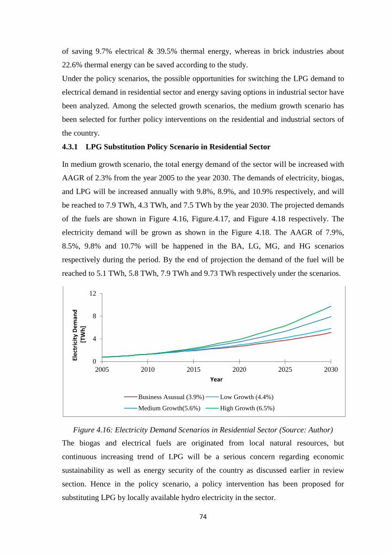
74
of saving 9.7% electrical & 39.5% thermal energy, whereas in brick industries about
22.6% thermal energy can be saved according to the study.
Under the policy scenarios, the possible opportunities for switching the LPG demand to
electrical demand in residential sector and energy saving options in industrial sector have
been analyzed. Among the selected growth scenarios, the medium growth scenario has
been selected for further policy interventions on the residential and industrial sectors of
the country.
4.3.1 LPG Substitution Policy Scenario in Residential Sector
In medium growth scenario, the total energy demand of the sector will be increased with
AAGR of 2.3% from the year 2005 to the year 2030. The demands of electricity, biogas,
and LPG will be increased annually with 9.8%, 8.9%, and 10.9% respectively, and will
be reached to 7.9 TWh, 4.3 TWh, and 7.5 TWh by the year 2030. The projected demands
of the fuels are shown in Figure 4.16, Figure.4.17, and Figure 4.18 respectively. The
electricity demand will be grown as shown in the Figure 4.18. The AAGR of 7.9%,
8.5%, 9.8% and 10.7% will be happened in the BA, LG, MG, and HG scenarios
respectively during the period. By the end of projection the demand of the fuel will be
reached to 5.1 TWh, 5.8 TWh, 7.9 TWh and 9.73 TWh respectively under the scenarios.
Figure 4.16: Electricity Demand Scenarios in Residential Sector (Source: Author)
The biogas and electrical fuels are originated from local natural resources, but
continuous increasing trend of LPG will be a serious concern regarding economic
sustainability as well as energy security of the country as discussed earlier in review
section. Hence in the policy scenario, a policy intervention has been proposed for
substituting LPG by locally available hydro electricity in the sector.
0
4
8
12
2005 2010 2015 2020 2025 2030
Ele
ctri
city
De
man
d[T
Wh
]
Year
Business Asusual (3.9%) Low Growth (4.4%)
Medium Growth(5.6%) High Growth (6.5%)
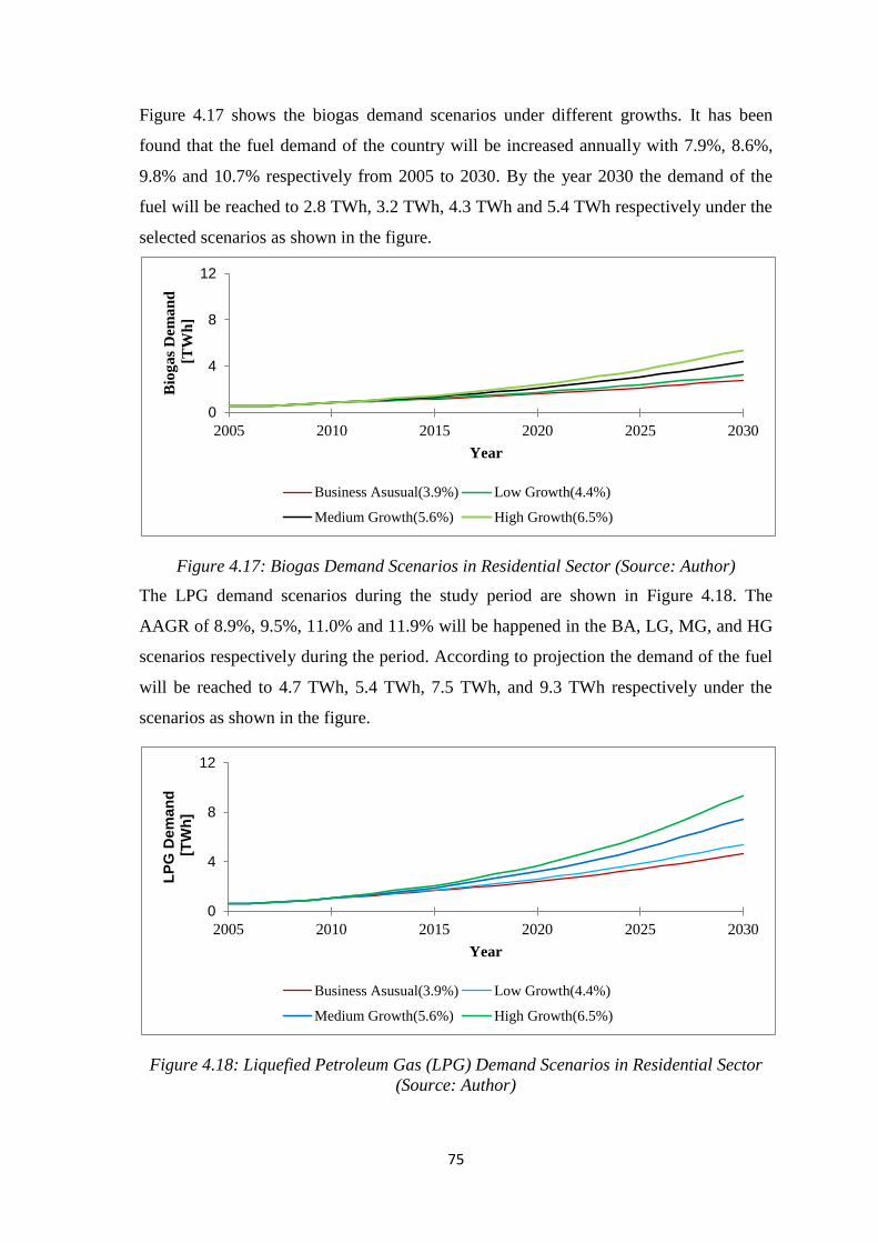
75
Figure 4.17 shows the biogas demand scenarios under different growths. It has been
found that the fuel demand of the country will be increased annually with 7.9%, 8.6%,
9.8% and 10.7% respectively from 2005 to 2030. By the year 2030 the demand of the
fuel will be reached to 2.8 TWh, 3.2 TWh, 4.3 TWh and 5.4 TWh respectively under the
selected scenarios as shown in the figure.
Figure 4.17: Biogas Demand Scenarios in Residential Sector (Source: Author)
The LPG demand scenarios during the study period are shown in Figure 4.18. The
AAGR of 8.9%, 9.5%, 11.0% and 11.9% will be happened in the BA, LG, MG, and HG
scenarios respectively during the period. According to projection the demand of the fuel
will be reached to 4.7 TWh, 5.4 TWh, 7.5 TWh, and 9.3 TWh respectively under the
scenarios as shown in the figure.
Figure 4.18: Liquefied Petroleum Gas (LPG) Demand Scenarios in Residential Sector
(Source: Author)
0
4
8
12
2005 2010 2015 2020 2025 2030
Bio
ga
s D
ema
nd
[TW
h]
Year
Business Asusual(3.9%) Low Growth(4.4%)
Medium Growth(5.6%) High Growth(6.5%)
0
4
8
12
2005 2010 2015 2020 2025 2030
LP
G D
em
an
d[T
Wh
]
Year
Business Asusual(3.9%) Low Growth(4.4%)
Medium Growth(5.6%) High Growth(6.5%)
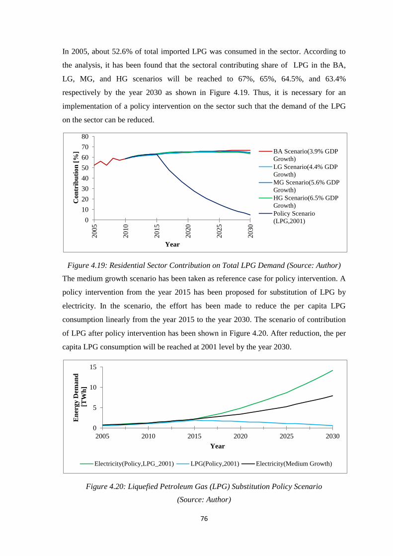
76
In 2005, about 52.6% of total imported LPG was consumed in the sector. According to
the analysis, it has been found that the sectoral contributing share of LPG in the BA,
LG, MG, and HG scenarios will be reached to 67%, 65%, 64.5%, and 63.4%
respectively by the year 2030 as shown in Figure 4.19. Thus, it is necessary for an
implementation of a policy intervention on the sector such that the demand of the LPG
on the sector can be reduced.
Figure 4.19: Residential Sector Contribution on Total LPG Demand (Source: Author)
The medium growth scenario has been taken as reference case for policy intervention. A
policy intervention from the year 2015 has been proposed for substitution of LPG by
electricity. In the scenario, the effort has been made to reduce the per capita LPG
consumption linearly from the year 2015 to the year 2030. The scenario of contribution
of LPG after policy intervention has been shown in Figure 4.20. After reduction, the per
capita LPG consumption will be reached at 2001 level by the year 2030.
Figure 4.20: Liquefied Petroleum Gas (LPG) Substitution Policy Scenario
(Source: Author)
0
10
20
30
40
50
60
70
80
2005
2010
2015
2020
2025
2030
Co
ntr
ibu
tio
n [
%]
Year
BA Scenario(3.9% GDP
Growth)
LG Scenario(4.4% GDP
Growth)
MG Scenario(5.6% GDP
Growth)
HG Scenario(6.5% GDP
Growth)
Policy Scenario
(LPG,2001)
0
5
10
15
2005 2010 2015 2020 2025 2030
En
ergy D
eman
d
[TW
h]
Year
Electricity(Policy,LPG_2001) LPG(Policy,2001) Electricity(Medium Growth)
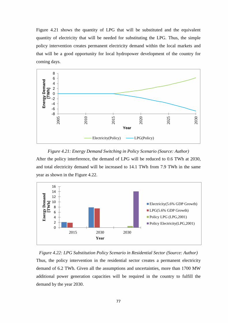
77
Figure 4.21 shows the quantity of LPG that will be substituted and the equivalent
quantity of electricity that will be needed for substituting the LPG. Thus, the simple
policy intervention creates permanent electricity demand within the local markets and
that will be a good opportunity for local hydropower development of the country for
coming days.
Figure 4.21: Energy Demand Switching in Policy Scenario (Source: Author)
After the policy interference, the demand of LPG will be reduced to 0.6 TWh at 2030,
and total electricity demand will be increased to 14.1 TWh from 7.9 TWh in the same
year as shown in the Figure 4.22.
Figure 4.22: LPG Substitution Policy Scenario in Residential Sector (Source: Author)
Thus, the policy intervention in the residential sector creates a permanent electricity
demand of 6.2 TWh. Given all the assumptions and uncertainties, more than 1700 MW
additional power generation capacities will be required in the country to fulfill the
demand by the year 2030.
-8
-6
-4
-2
0
2
4
6
8
20
05
20
10
20
15
20
20
20
25
20
30
En
erg
y D
em
an
d[T
Wh
]
Year
Electricity(Policy) LPG(Policy)
0
2
4
6
8
10
12
14
16
2015 2030 2030
En
ergy D
eman
d
[TW
h]
Year
Electricity(5.6% GDP Growth)
LPG(5.6% GDP Growth)
Policy LPG (LPG,2001)
Policy Electricity(LPG,2001)
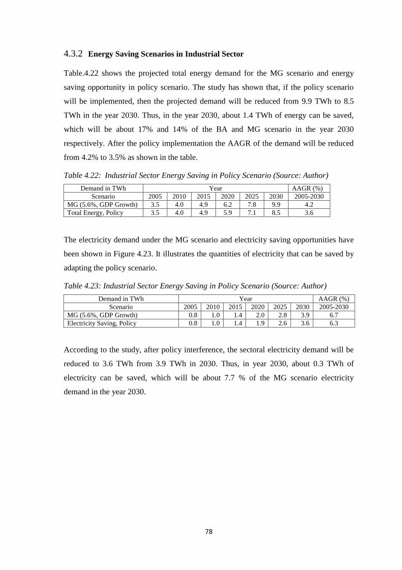
78
4.3.2 Energy Saving Scenarios in Industrial Sector
Table.4.22 shows the projected total energy demand for the MG scenario and energy
saving opportunity in policy scenario. The study has shown that, if the policy scenario
will be implemented, then the projected demand will be reduced from 9.9 TWh to 8.5
TWh in the year 2030. Thus, in the year 2030, about 1.4 TWh of energy can be saved,
which will be about 17% and 14% of the BA and MG scenario in the year 2030
respectively. After the policy implementation the AAGR of the demand will be reduced
from 4.2% to 3.5% as shown in the table.
Table 4.22: Industrial Sector Energy Saving in Policy Scenario (Source: Author)
Demand in TWh Year AAGR (%)
Scenario 2005 2010 2015 2020 2025 2030 2005-2030
MG (5.6%, GDP Growth) 3.5 4.0 4.9 6.2 7.8 9.9 4.2
Total Energy, Policy 3.5 4.0 4.9 5.9 7.1 8.5 3.6
The electricity demand under the MG scenario and electricity saving opportunities have
been shown in Figure 4.23. It illustrates the quantities of electricity that can be saved by
adapting the policy scenario.
Table 4.23: Industrial Sector Energy Saving in Policy Scenario (Source: Author)
Demand in TWh Year AAGR (%)
Scenario 2005 2010 2015 2020 2025 2030 2005-2030
MG (5.6%, GDP Growth) 0.8 1.0 1.4 2.0 2.8 3.9 6.7
Electricity Saving, Policy 0.8 1.0 1.4 1.9 2.6 3.6 6.3
According to the study, after policy interference, the sectoral electricity demand will be
reduced to 3.6 TWh from 3.9 TWh in 2030. Thus, in year 2030, about 0.3 TWh of
electricity can be saved, which will be about 7.7 % of the MG scenario electricity
demand in the year 2030.
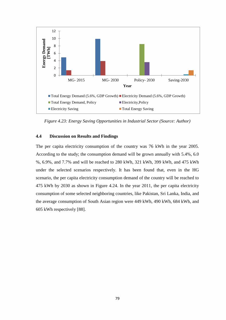
79
Figure 4.23: Energy Saving Opportunities in Industrial Sector (Source: Author)
4.4 Discussion on Results and Findings
The per capita electricity consumption of the country was 76 kWh in the year 2005.
According to the study; the consumption demand will be grown annually with 5.4%, 6.0
%, 6.9%, and 7.7% and will be reached to 280 kWh, 321 kWh, 399 kWh, and 475 kWh
under the selected scenarios respectively. It has been found that, even in the HG
scenario, the per capita electricity consumption demand of the country will be reached to
475 kWh by 2030 as shown in Figure 4.24. In the year 2011, the per capita electricity
consumption of some selected neighboring countries, like Pakistan, Sri Lanka, India, and
the average consumption of South Asian region were 449 kWh, 490 kWh, 684 kWh, and
605 kWh respectively [88].
0
2
4
6
8
10
12
MG- 2015 MG- 2030 Policy- 2030 Saving-2030
En
erg
y D
ema
nd
[TW
h]
Year
Total Energy Demand (5.6%, GDP Growth) Electricity Demand (5.6%, GDP Growth)
Total Energy Demand, Policy Electricity,Policy
Electricity Saving Total Energy Saving
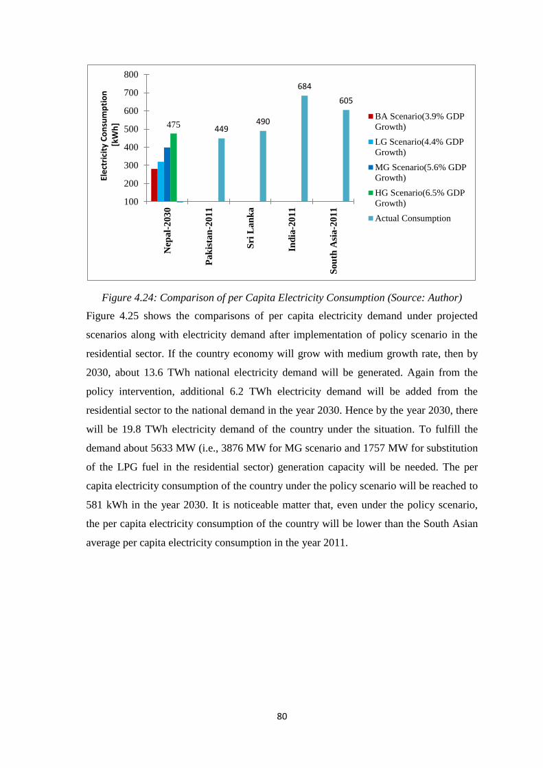
80
Figure 4.24: Comparison of per Capita Electricity Consumption (Source: Author)
Figure 4.25 shows the comparisons of per capita electricity demand under projected
scenarios along with electricity demand after implementation of policy scenario in the
residential sector. If the country economy will grow with medium growth rate, then by
2030, about 13.6 TWh national electricity demand will be generated. Again from the
policy intervention, additional 6.2 TWh electricity demand will be added from the
residential sector to the national demand in the year 2030. Hence by the year 2030, there
will be 19.8 TWh electricity demand of the country under the situation. To fulfill the
demand about 5633 MW (i.e., 3876 MW for MG scenario and 1757 MW for substitution
of the LPG fuel in the residential sector) generation capacity will be needed. The per
capita electricity consumption of the country under the policy scenario will be reached to
581 kWh in the year 2030. It is noticeable matter that, even under the policy scenario,
the per capita electricity consumption of the country will be lower than the South Asian
average per capita electricity consumption in the year 2011.
475 449490
684
605
100
200
300
400
500
600
700
800
Nep
al-
203
0
Pa
kis
tan
-201
1
Sri
La
nk
a
Ind
ia-2
01
1
Sou
th A
sia
-20
11
Ele
ctri
city
Co
nsu
mp
tio
n[k
Wh
]BA Scenario(3.9% GDP
Growth)
LG Scenario(4.4% GDP
Growth)
MG Scenario(5.6% GDP
Growth)
HG Scenario(6.5% GDP
Growth)
Actual Consumption
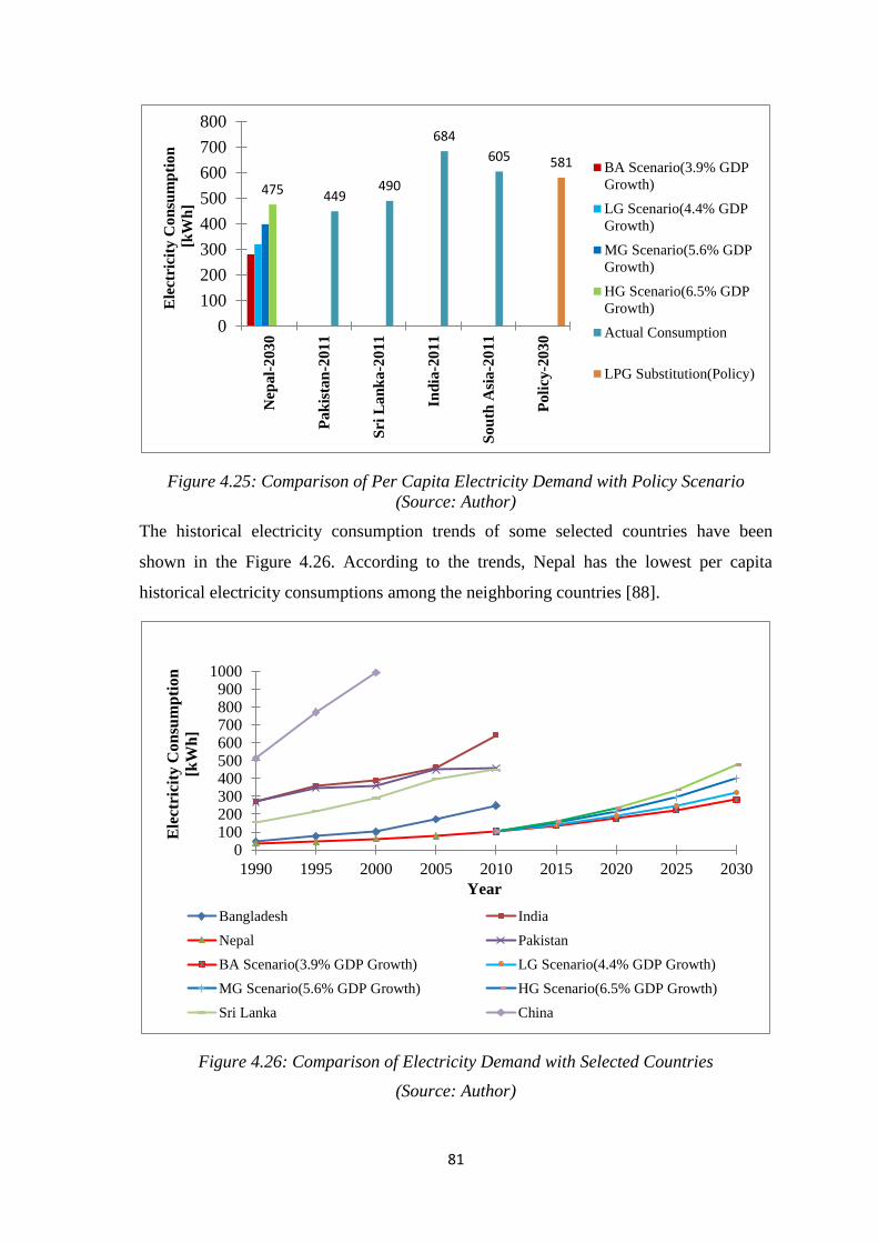
81
Figure 4.25: Comparison of Per Capita Electricity Demand with Policy Scenario
(Source: Author)
The historical electricity consumption trends of some selected countries have been
shown in the Figure 4.26. According to the trends, Nepal has the lowest per capita
historical electricity consumptions among the neighboring countries [88].
Figure 4.26: Comparison of Electricity Demand with Selected Countries
(Source: Author)
475 449490
684
605 581
0
100
200
300
400
500
600
700
800
Nep
al-
203
0
Pa
kis
tan
-201
1
Sri
La
nk
a-2
011
Ind
ia-2
01
1
Sou
th A
sia
-20
11
Po
licy
-20
30
Ele
ctri
city
Con
sum
pti
on
[kW
h]
BA Scenario(3.9% GDP
Growth)
LG Scenario(4.4% GDP
Growth)
MG Scenario(5.6% GDP
Growth)
HG Scenario(6.5% GDP
Growth)
Actual Consumption
LPG Substitution(Policy)
0100200300400500600700800900
1000
1990 1995 2000 2005 2010 2015 2020 2025 2030
Ele
ctri
city
Con
sum
pti
on
[kW
h]
Year
Bangladesh India
Nepal Pakistan
BA Scenario(3.9% GDP Growth) LG Scenario(4.4% GDP Growth)
MG Scenario(5.6% GDP Growth) HG Scenario(6.5% GDP Growth)
Sri Lanka China
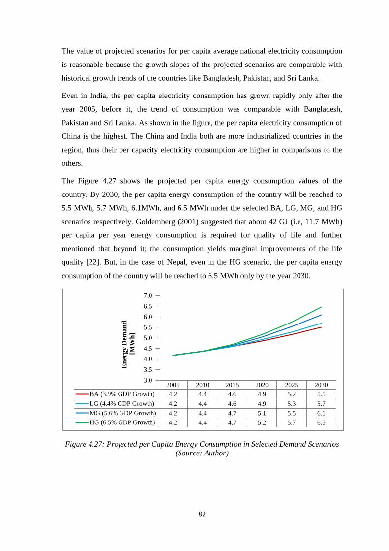
82
The value of projected scenarios for per capita average national electricity consumption
is reasonable because the growth slopes of the projected scenarios are comparable with
historical growth trends of the countries like Bangladesh, Pakistan, and Sri Lanka.
Even in India, the per capita electricity consumption has grown rapidly only after the
year 2005, before it, the trend of consumption was comparable with Bangladesh,
Pakistan and Sri Lanka. As shown in the figure, the per capita electricity consumption of
China is the highest. The China and India both are more industrialized countries in the
region, thus their per capacity electricity consumption are higher in comparisons to the
others.
The Figure 4.27 shows the projected per capita energy consumption values of the
country. By 2030, the per capita energy consumption of the country will be reached to
5.5 MWh, 5.7 MWh, 6.1MWh, and 6.5 MWh under the selected BA, LG, MG, and HG
scenarios respectively. Goldemberg (2001) suggested that about 42 GJ (i.e, 11.7 MWh)
per capita per year energy consumption is required for quality of life and further
mentioned that beyond it; the consumption yields marginal improvements of the life
quality [22]. But, in the case of Nepal, even in the HG scenario, the per capita energy
consumption of the country will be reached to 6.5 MWh only by the year 2030.
Figure 4.27: Projected per Capita Energy Consumption in Selected Demand Scenarios
(Source: Author)
2005 2010 2015 2020 2025 2030
BA (3.9% GDP Growth) 4.2 4.4 4.6 4.9 5.2 5.5
LG (4.4% GDP Growth) 4.2 4.4 4.6 4.9 5.3 5.7
MG (5.6% GDP Growth) 4.2 4.4 4.7 5.1 5.5 6.1
HG (6.5% GDP Growth) 4.2 4.4 4.7 5.2 5.7 6.5
3.0
3.5
4.0
4.5
5.0
5.5
6.0
6.5
7.0
En
ergy D
eman
d
[MW
h]
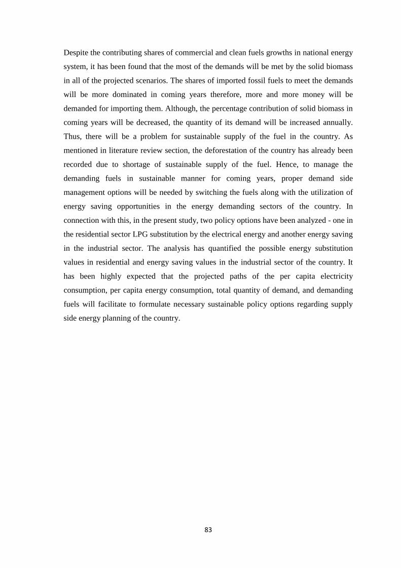
83
Despite the contributing shares of commercial and clean fuels growths in national energy
system, it has been found that the most of the demands will be met by the solid biomass
in all of the projected scenarios. The shares of imported fossil fuels to meet the demands
will be more dominated in coming years therefore, more and more money will be
demanded for importing them. Although, the percentage contribution of solid biomass in
coming years will be decreased, the quantity of its demand will be increased annually.
Thus, there will be a problem for sustainable supply of the fuel in the country. As
mentioned in literature review section, the deforestation of the country has already been
recorded due to shortage of sustainable supply of the fuel. Hence, to manage the
demanding fuels in sustainable manner for coming years, proper demand side
management options will be needed by switching the fuels along with the utilization of
energy saving opportunities in the energy demanding sectors of the country. In
connection with this, in the present study, two policy options have been analyzed - one in
the residential sector LPG substitution by the electrical energy and another energy saving
in the industrial sector. The analysis has quantified the possible energy substitution
values in residential and energy saving values in the industrial sector of the country. It
has been highly expected that the projected paths of the per capita electricity
consumption, per capita energy consumption, total quantity of demand, and demanding
fuels will facilitate to formulate necessary sustainable policy options regarding supply
side energy planning of the country.
84
Chapter 5
Conclusions and Recommendations
5.1 Conclusions
The different types of energy planning tools for the national energy system planning
have been reviewed. In this study, Long Range Energy Alternative Planning (LEAP) tool
has been selected for residential, industrial, commercial, agriculture and road transport
sectors whereas, econometric modeling approach has been selected for the aviation
transport and others sector respectively. The LEAP tool has been selected because there
are number of studies that have been conducted using it in the world from highly
developed to list developed countries and their methodologies are well established and
worldwide accepted.
In the study, the final energy demand of the country has been determined by adding
energy demands of residential, transport, industrial, commercial, agricultural and others
sectors respectively. In the formulated models, the year 2005 has been considered as
base year and the year 2030 has been taken for the end of the projection. The total
energy consumption in the year 2005 has been calibrated with the actual consumption of
the year. After calibration, the validation of the model has been carried out with actual
energy consumption of the country from the year 2005 to the year 2009. After calibration
and validation, the model has been further used to project the national energy demand of
the country by the year 2030.
The demands of the residential, transport, industrial, agriculture and commercial sectors
are determined through end use methodological approach on the base year 2005, and
further projections of the demand are based on the function of population, GDP per
capita, and corresponding economic sectoral value added of the country. For road
transport, the actually plying vehicles on the road in the base year have been estimated
and further projected with econometric as well as trend analysis approach. The final
energy demand of the sector has been determined by using the information about - the
actually plying vehicles on the road, the annual average distance travelled and the fuel
economy of the corresponding vehicles.
85
Further, the residential and industrial sectors models are again expanded to analyze the
LPG fuel substitution by electrical fuel in residential sector and energy saving
opportunities in industrial sector of the country through the proper policy interventions
on the sectors.
The finding from this research provides the evidence that in all of the projected
scenarios, residential sector will be the main energy demanding sector, followed by
transport, industrial, commercial, agricultural and others sectors respectively. In coming
years, the share of national demand of solid biomass will be decreased, while the
demanding shares of petroleum products, electricity, coal and biogas will be increased in
all of the projected scenarios. Among the fuels, the growth rates of the petroleum
products will be the highest, followed by electricity, biogas and coal. It has also been
observed that for the highest growth scenario, the demand of solid biomass will be
decreased more rapidly in comparison with the other growth scenarios. Although, the
total energy consumption of the country will be increased but even in the HG scenario,
the per capita energy consumption of the country will be far less than the suggested
acceptable benchmark level.
The projected national level energy indicators like per capita electricity consumption, per
capita total energy consumption, share of sectoral energy demand, and structure of
demanding fuels shares will be the useful parameters for comparing and planning of the
local energy resources of the country. If the mentioned policy scenario on the residential
sector will be followed, then annually a significant amount of reliable local electricity
demand will be generated within the country. This would reduce the expenditure
presently being spent for importing the LPG fossil fuel by greater extent and contribute
towards the opportunity to invest the development of the local hydro resources.
Similarly, in the industrial sector, the study has also quantified the quantities of energy
that can be saved through the implementation of the suggested sectoral policy measures.
The projected structures of energy consumption mix shows that the consumption demand
of the country will be dominated by traditional and imported fuels, thus a proper supply
side planning can be done for achieving more desirable energy mix having higher share
of local clean renewable energy resources. The utilization of the clean energy resources
for long term energy planning process not only stands for sustainable development of the
86
country but also helps to low carbon pathway to address global partnership for
environmental protection and access to modern energy.
5.2 Recommendations
The outcomes of the study will be helpful for formulating necessary policy measures for
policy makers and concerned stakeholders in the sector. The policy makers can use the
information from this study to adopt necessary actions for sustainable utilization of the
local energy resources for avoiding any negative implications for national energy
system. Although, the results of the formulated objectives are obtained through the
adopted methodologies, there are always some opportunities for further improvements.
Therefore, following are the few recommendations for the improvements:
Due to the lack of end use technological stocks, the current study has been
carried out on the basis of fuels consumptions for various end use applications in
the residential, industrial, commercial, and agriculture sectors. Therefore, it has
been recommended to do further research on the sectors by carrying out the
proper assessments of the technological stocks.
The formulated models can be further used for analyzing the environmental
aspects of the study.
The current study is limited to demand side energy analysis; however, supply
side energy planning can be done through utilizing the outputs of these models
exogenously to the other proper supply side energy planning tools.
87
Bibliographies
1. IEA, 2009, World Energy Outlook, 2009, International Energy Agency, France.
2. IEA, 2010, World Energy Outlook, 2010, International Energy Agency, France.
3. IEA, 2011, World Energy Outlook, 2011, International Energy Agency, France.
4. IIASA, 2012, Global Energy Assessment, Towards a Sustainable Future,
International Institute for Applied Systems Analysis, Luxemburg, Austria.
5. BP, 2010, Statistical Review of World Energy, London, UK.
6. WCE, 2010, Survey of Energy Resources. World Energy Council (WEC),
London.
7. Adil Najam et al., 2003, Energy and Sustainable Development at Global
Environmental Summits: An Evolving Agenda. Environment, Development and
Sustainability 5: 1117-138, Kluwer Academic Publishers, printed in the
Netherlands.
8. WCED, 1997, Our Commission Future, the World Commission on Environment
and Development, Oxford University Press, USA, 1997.
9. UN, 2000, The General Assembly, United Nations Millennium Declaration,
United Nations.
10. Moyo, D., 2009. Dead Aid: Why Aid is Not Working and How there is a Better
Way for Africa. New York: Farrar, Straus and Giroux.
11. AGECC, 2010, The Secretary-General’s Advisory Group on Energy and Climate
Change Summary Report and Recommendations, New-Work, 2010.
12. UN, 2010, Energy for a Sustainable Future, Report and Recommendations, 2010,
United Nations, New York.
13. UN, 2012, Sustainable Energy for All, Technical Report of Task Force 1, in
Support of the Objective to Achieve Universal Access to Modern Energy
Services by 2030.
14. Renewable Energy Association (2009), Energy and environment. At
http://www.r-e-a.net/info/energy-info(accessed 14 April 2010).
15. REN 21, 2011, Renewable 2011, Global Status Report, Paris, France.
16. E. Gupta, 2008: Oil vulnerability index of oil importing countries. Energy
Policy., The Energy and Resources Institute, Darbari Seth Block, Habitat Place,
New Delhi 110003, India.
17. Kruyt, B. et al. 2009, Indicators for energy security, Energy Policy, 37,2166-
2181 pp.
88
18. Awebuch,S.,2006,Portfolio-based electricity generation planning, policy
implications for renewable and energy security. Mitigation and Adaptation
Strategies for Global Change,(113),693-710 pp.
19. Bazilian M. et al., 2008, Analytical Approaches to Quantify and Value Fuel Mix
Diversity, Elsevier.
20. ESMAP, 2005: The Impacts of Higher Oil Price on Low Income Countries and
the Poor: Impacts and Policies: Energy Sector Management Assistance Program,
World Bank, Washington DC, USA.
21. IPCC, 2012, Renewable Energy Sources and Climate Change Mitigation, Special
Report of the Intergovernmental Panel on Climate Change, Cambridge
University.
22. Goldemberg, J.,2001, Energy and Human Well Being .Human Development
Occasional paper HDOCPA-2001-02, United Nations Development Program,
New York, USA.
23. Dabrase.S, et al., 2000, Integrated Renewable Energy System- Perspectives and
Issues, Millennium International Conference on Renewable Energy
Technologies, IIT, Chennai 9-11 Feburary, 2000.
24. WECS, 2010, Energy Synopsis Report, Water and Energy Commission
Secretariat Ministry of Water Resources, Kathmandu, Nepal.
25. Pradhan.GL, 2009, Electricity: domestic consumption versus export. Hydro
Nepal, 2009, 1-3pp.
26. Jha. R., 2010, Total run-of-river type hydropower potential of Nepal. Hydro
Nepal, 8-13pp.
27. Sharma. RH. et al., 2013, Hydropower Development in Nepal. Science Direct,
684-693pp.
28. MoF, 2012, Economic Survey, 2012, Ministry of Finance, Government of Nepal,
Kathmandu, Nepal.
29. MFSC, 1987, Master Plan for Forestry Sector Nepal: The Forest Resources of
Nepal, ADB T.A.No 670.
30. NEAA, 1984, Nepal Electricity Authority Act, 2041(1984). Government of
Nepal
31. Skjold, D.O., 2009, Power for Generations: The Development of Statkraft and
the Role of the state in Norwegian Electrification 1830-2009.
Universitetsforlaget, Oslo, Norway, 284 pp.
89
32. NPC,1975, Fifth Plan (1975-1980), National Planning Commission, Government
of Nepal, Kathmandu, Nepal
33. NPC,1980, Sixth Plan (1980-1985), National Planning Commission Government
of Nepal, Kathmandu, Nepal
34. NPC, 1992, Eighth Plan (1992-1997), National Planning Commission,
Government of Nepal, Kathmandu, Nepal.
35. NPC, 2002, Tenth Plan (2002-2007), National Planning Commission,
Government of Nepal, Kathmandu, Nepal.
36. NPC, 2007, Three Year Interim Plan (FY 2007/08-2009/10), National Planning
Commission, Government of Nepal, Kathmandu, Nepal.
37. NPC, 2010, Three Year Plan (FY 2010/11-2012/13), National Planning
Commission, Government of Nepal, Kathmandu, Nepal.
38. NPC, 2013, An Approach Paper to The Thirteenth Plan (FY 2013/14-2015/16),
National Planning Commission, Government of Nepal, Kathmandu, Nepal.
39. WECS, 2005, National Water Plan 2005, Water and Energy Commission
Secretariat, Ministry of Water Resources, Government of Nepal, Kathamndu,
Nepal.
40. MOE, 2010, Ministry of Energy, Twenty-year Hydropower Development Plan
Implementation Task Force, Government of Nepal, Kathmandu.
41. MOEV, 2010, Climate Change Policy, Ministry of Environment Government of
Nepal, Kathmandu, Nepal.
42. NRB, 2007, Macroeconomic Indicators of Nepal, Nepal Rastra Bank,
Kathmandu, Nepal.
43. NRB, 2011, Macroeconomic Indicators of Nepal, Nepal Rastra Bank,
Kathmandu, Nepal.
44. Economic Survey, 2007, Ministry of Finance, Government of Nepal, Kathmandu,
Nepal.
45. OPEC, 2014, Annual Statistical Bulletin 2013, Organization of Petroleum
Exporting Countries.
46. Nepal Energy Efficiency Programme (NEEP), Final Report, Baseline Study of
Selected Industries to access the potentials for more efficient use of energy, 2012,
Kathmandu, Nepal
47. District Development Profile of Nepal, 2011, A Socio- Economic Development
Database of Nepal, Mega Publication and Research Centre, Kathmandu, Nepal.
90
48. CBS,2012, National Population and Housing Census 2011, Central Bureau of
Statistics National Planning Commission Secretariats, Government of Nepal
,Kathmandu, Nepal
49. CBS, 1996, Nepal Living Standards Survey, Central Bureau of Statistics National
Planning Commission Secretariat, Government of Nepal.
50. CBS, 2004, Nepal Living Standards Survey, Central Bureau of Statistics,
National Planning Commission Secretariat, Government of Nepal.
51. CBS, 2011, Nepal Living Standards Survey, Central Bureau of Statistics,
National Planning Commission Secretariat, Government of Nepal.
52. WECS, Energy Synopsis Report: Nepal 2006, Water and Energy Commission
Secretariat, Ministry of Water Resources, Kathmandu, Nepal.
53. Kahen G., 1995, Integrated Energy Planning and Techno-Economic
Development: A Solid Basis for the Assessment and Transfer of Energy
Technology to Developing Countries, Imperial College, University of London.
54. Van Beeck Nicole 2003, A new decision support method for local energy
planning in developing countries, Tilburg University, ISBN 90-5668-116-8.
55. Shukla, P.R., 1995, Greenhouse gas models and abatement costs for developing
nations. A critical Assessment, Energy Policy, Volume 8, 677-687pp.
56. Sanchez-Sierra, Gabrie 1991, Electricity Planning for Developing Countries’ in
ATAS(Advanced Technology Assessment System), Bulletin, Issue 6: Energy
Systems, Environment, and Development: A Reader. New York: United Nations,
Centre for Science and Technology for Development.
57. Mathur.J, 2001, Development of a modified dynamic energy and greenhouse gas
reduction planning approach through the case of Indian power sector,
Dissertation,Fachbereich12,Maschinenwesen-Energietechnik-Verfahrenstechnik,
University of Essen,2001.
58. Klein, et al. 1984, Environmental assessment: An international study of corporate
practice, Journal of Business Strategy, Vol.5, pages 66-75pp.
59. WRI, 1999, World Resources: A guide to the global Environment 1998-1999,
joint publication of World Resource Institute, UNEP, World Bank, Published by
World Bank, New Delhi, India.
60. Beeck. N, 1999, Classification of Energy Models, Tilburg University and
Endhoven University of Technology.
61. Schlen 98, Schlenzig, C.; PlaNet 1998, Ein entscheidungsunterstützendes System
für die Energie-used Umweltplanung(a decision supported system for energy and
91
environment planning), Dissertation, Institute für Energiewirtschaft und
Rationelle Energieanwendung( Institute of energy economics and rational use of
energy,Juli,1998)
62. Kem et al., 1997 :Volkswirtschaftliche Modelle im Vergleich.
63. Nguyen K.Q., 2005, Long- term optimization of energy supply and demand in
Vietnam with special reference to the potential of renewable energy. Dissertation,
University of Oldenburg.
64. Pandey R., 2002 Energy policy modeling: agenda for developing countries.
Energy Policy 30:97-106 pp.
65. Kydes et al, 1995, Beyond the horizon: recent directions in long-term energy
modeling. Energy 20, 131-149pp.
66. Grubler A, et al, 1999, Dynamics of energy technologies and global change.
Energy Policy 27, 247-280 pp.
67. Pfaff.Pfaffenberger,W.,Ströbele,W.:ProjektIkarus1995Makroökonomische
Einbettung(Ikraus project-Macroeconomic embedding),Band 1, Oldenburg.
68. World Bank, 2009, Energy Demand Models for Policy Formulation, A
Comparative Study of Energy Demand Models. Development Research Group
Environment and Energy Team.
69. Omer Yuksek et al., 2006, The role of hydropower in meeting Turkey’s electric
energy demand, Energy Policy 34, 3093-3103 pp.
70. Khalaquzzaman. M. et al., 2008, Long Term Sustainable Energy Supply and
Mitigation of Greenhouse Gas Emission in Bangladesh, International Energy
Journal, Volume 9, Issue 2.
71. Connolly D, et al., 2010, A review of computer tools for analyzing the
integration of renewable energy into various energy systems. Appl. Energy 87:
1059-1082pp.
72. Baumhögger et al., 1998, Manual MESAP, Version 3.1, Institute of Energy
Economics and the Rational Use of Energy, Germany.
73. Ramachandra.T.V, 2009, Regional integrated energy plan, Renewable and
Sustainable Energy Review, Science Direct, 13, 285-317pp.
74. LEAP, 2011, Long Range Energy Alternatives Planning System, A tool for
energy policy analysis and climate mitigation assessment, Stockholm
Environment Institute, USA.
75. Rath-Nagel S. and Voss A.1981, Energy models for planning and policy
assessment, European Journal of Operational Research, Vol.8, No.2, 99-114 pp.
92
76. IIASA, 2005, Leo Schrattenholzer, Energy Planning Methodologies and Tools,
IIASA, Austria
77. Wirrel. E.S. et al., 2004, Advances in Energy Forecasting Models based on
Engineering Economics, Ann Environ Resources, Vol 29, 345 to 381pp.
78. Jung, T.Y.et al., 2000, Structural changes in developing countries and their
implication for energy-related CO2 emission. Technological Forecasting and
Social Change 63,111-136pp.
79. Urban, F. et al., 2006. Modeling transitions to renewable energy in developing
countries. In Sastry, E.V.R., Reddy, D.N.(Eds.), International Congress on
Renewable Energy ICORE 2006 Proceedings. Allied Publications Pvt. Ltd.,
Hyderabad, India, 497-502 pp.
80. F.Uraban et al., 2007, Modeling Energy Systems for Developing Countries,
Energy Policy 35, 3473-3482 pp.
81. Seebregts, A.J. et al., 2001, Energy/environmental modeling with MARKAL
family of models, in Operations Research Proceedings 2001-Selected Papers of
the International Conference on Operations Research(QR2001).
82. Goldstein G. and Tosato G. 2008, Global Energy Systems and Common
Analysis: Final report of annex X (2005-2008), ETSAP, International Energy
Agency.
83. Pokharel, S., 2007, An Econometric analysis of energy consumption in Nepal,
Energy Policy, 350-361pp.
84. Lau.E.et al., 2011, Energy – Growth Causality: Asian Countries Revisited,
International Journal of Energy Economics and Policy, Vol.1, No.4, 140-149 pp.,
ISSN: 2146-4553.
85. Ozturk.I.et al., 2012, Causality among Carbon Emission, Energy Consumption
and Growth in India, Economic Research, Vol-25,752-775pp.
86. WTO, 2012, Trade Policy Review Report by Nepal, World Trade Organization.
87. MoICS, 2002, Industrial Development Perspective Plan: Vision 2020, Analytical
Report, Ministry of Industry, Commerce and Supplies, Government of Nepal,
Kathmandu, Nepal.
88. WB, 2012, World Bank Data, Nepal, Accessed: September 5, 2012,
http://data.worldbank.org/country/nepal.
89. MoI, 2010, Industrial Policy 2010, Ministry of Industry Government of Nepal,
Kathmandu, Nepal.
90. ADB, 2013, The Service Sector in Lower- Income Asian Economies, Asian
Development Bank.
93
91. CBS, 2003, Population Monograph of Nepal, Central Bureau of Statistics,
National Planning Commission Secretariat, Kathmandu, Nepal.
92. Pradhan, et al., 2006, Mitigation potential of greenhouse gas emission and
implications on fuel consumption due to clean energy vehicles as public
passenger transport in Kathmandu Valley of Nepal: A case study of trolley buses
in Ring Road. Energy 31, 1748-1760 pp.
93. Parajuli.R.et al., 2013, Energy consumption projection of Nepal: An econometric
approach, Science Direct, 432-444 pp.
94. Shrestha R.M et al., 2010, Energy and environment implications of carbon
emission reduction targets: Case of Kathmandu Valley, Nepal, Energy policy
Vol.38, 4818-4827pp.
95. Shakya.SR et al., 2011, Transport sector electrification in a hydropower resource
rich developing country: Energy security, environmental and climate change co-
benefits, Science Direct, 147-159 pp.
96. Bajracharya et al., 2013, Scenario Analysis of Road Transport Energy
Consumption and Greenhouse Gas Emission in Nepal, proceeding of IoE
Graduate Conference, Tribhuvan University, Lalitpur, Nepal.
97. DoTM, 2014, Government of Nepal, Department of Transport Management.
Accessed:March18,2014,<http://www.dotm.gov.np/uploads/files/vechicle%20reg
istration.pdf >
98. Zachariadis, T., et al. 2001, The effect of age and technological change on motor
vehicle emissions. Transportation Research Part D 6, 221 – 227 pp.
99. Bidya.S. et al., 2009, Atmospheric emissions from road transportation of India,
Energy Policy 37, 3812 – 3822 pp.
100. Dhakal, S., 2003, Implications of transportation policies and environment in
Kathmandu Valley, Nepal. Energy Policy 31, 1493 – 1507 pp.
101. AEPC,2013, Formulation of Low Carbon Economic Development Strategy for
Nepal, Alternative Energy Promotion Centre, Ministry of Science, Technology
and Environment, Government of Nepal.
102. WECS, 2005, Detail Energy Consumption Survey in Urban Residential Sector
of Nepal, Kathmandu, Nepal.
103. WECS, 1997, Update and Compilation of Energy Resources and Consumption
Profile of Nepal, Final Report, Volume-I, II, &III, Kathmandu, Nepal.
104. WECS, 2013, Final Report, Final Report, National Survey of Energy Resources
and Consumption Profile of Nepal, Kathmandu, Nepal.
94
105. WECS, 2001, Agriculture Sector Energy Consumption in Nepal, Water and
Energy Commission Secretariat, Government of Nepal, Kathmandu, Nepal.
106. WECS, 1999, Detail Energy Consummation Survey in the Commercial Sector
of Nepal, Water and Energy Commission Secretariat, Government of Nepal,
Kathmandu, Nepal.
107. CBS, 2003, Population Monograph of Nepal, Central Bureau of Statistics,
National Planning Commission Secretariat, Kathmandu, Nepal.
108. CBS, 2003, Population Projections for Nepal 2001 to 2021. Central Bureau of
Statistics, National Planning Commission Secretariat, Kathmandu, Nepal.
Publication from this Study
Bhattarai, N., Bauer. C, Doujak. E, 2014, “Residential Sector Energy Demand
Projections and Analysis of Nepal for Sustainable Utilization of Local
Hydropower Resources.” Published in the Proceeding of Innovations and
Development Needs for Sustainable Growth of Hydropower, 18th International
Seminar on Hydropower Plants, 26-28 November 2014, Vienna, Austria.
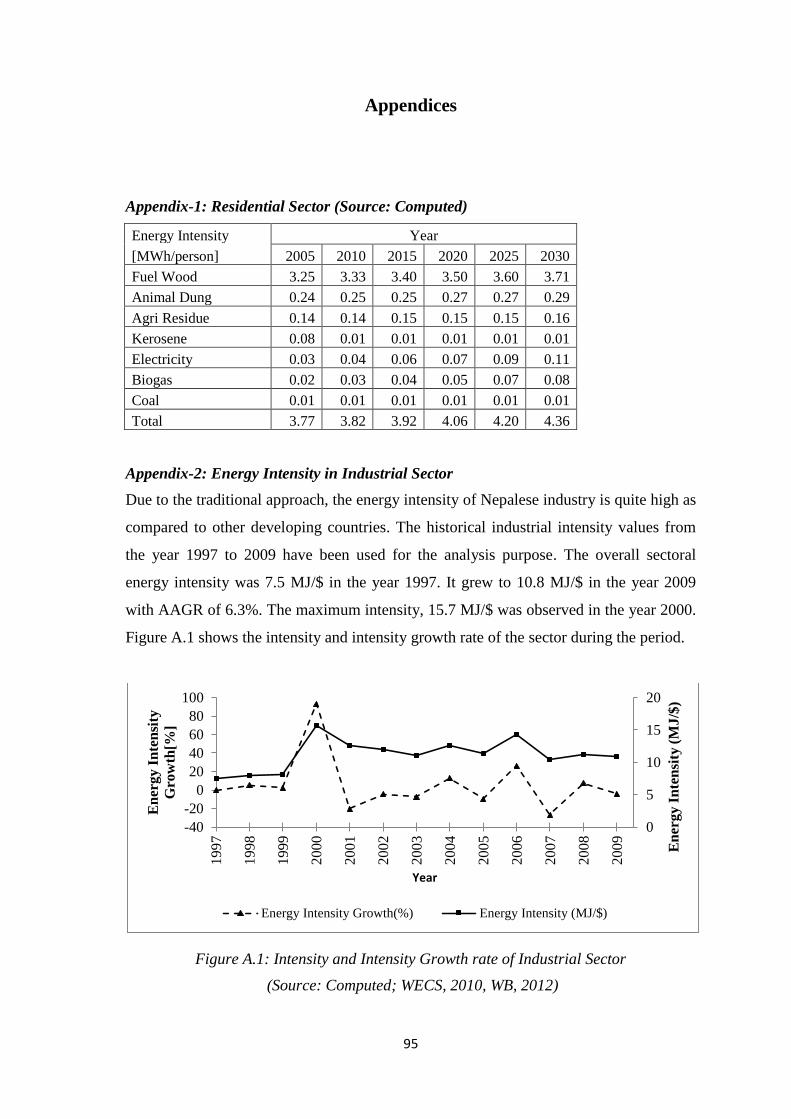
95
Appendices
Appendix-1: Residential Sector (Source: Computed)
Energy Intensity Year
[MWh/person] 2005 2010 2015 2020 2025 2030
Fuel Wood 3.25 3.33 3.40 3.50 3.60 3.71
Animal Dung 0.24 0.25 0.25 0.27 0.27 0.29
Agri Residue 0.14 0.14 0.15 0.15 0.15 0.16
Kerosene 0.08 0.01 0.01 0.01 0.01 0.01
Electricity 0.03 0.04 0.06 0.07 0.09 0.11
Biogas 0.02 0.03 0.04 0.05 0.07 0.08
Coal 0.01 0.01 0.01 0.01 0.01 0.01
Total 3.77 3.82 3.92 4.06 4.20 4.36
Appendix-2: Energy Intensity in Industrial Sector
Due to the traditional approach, the energy intensity of Nepalese industry is quite high as
compared to other developing countries. The historical industrial intensity values from
the year 1997 to 2009 have been used for the analysis purpose. The overall sectoral
energy intensity was 7.5 MJ/$ in the year 1997. It grew to 10.8 MJ/$ in the year 2009
with AAGR of 6.3%. The maximum intensity, 15.7 MJ/$ was observed in the year 2000.
Figure A.1 shows the intensity and intensity growth rate of the sector during the period.
Figure A.1: Intensity and Intensity Growth rate of Industrial Sector
(Source: Computed; WECS, 2010, WB, 2012)
0
5
10
15
20
-40
-20
0
20
40
60
80
100
19
97
19
98
1999
20
00
20
01
20
02
20
03
20
04
20
05
20
06
20
07
2008
20
09
En
ergy I
nte
nsi
ty (
MJ
/$)
En
erg
y I
nte
nsi
ty
Gro
wth
[%]
Year
Energy Intensity Growth(%) Energy Intensity (MJ/$)
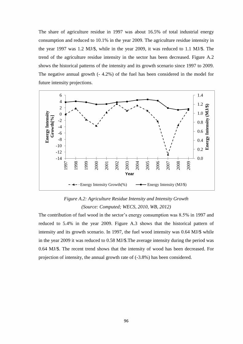
96
The share of agriculture residue in 1997 was about 16.5% of total industrial energy
consumption and reduced to 10.1% in the year 2009. The agriculture residue intensity in
the year 1997 was 1.2 MJ/$, while in the year 2009, it was reduced to 1.1 MJ/$. The
trend of the agriculture residue intensity in the sector has been decreased. Figure A.2
shows the historical patterns of the intensity and its growth scenario since 1997 to 2009.
The negative annual growth (- 4.2%) of the fuel has been considered in the model for
future intensity projections.
Figure A.2: Agriculture Residue Intensity and Intensity Growth
(Source: Computed; WECS, 2010, WB, 2012)
The contribution of fuel wood in the sector’s energy consumption was 8.5% in 1997 and
reduced to 5.4% in the year 2009. Figure A.3 shows that the historical pattern of
intensity and its growth scenario. In 1997, the fuel wood intensity was 0.64 MJ/$ while
in the year 2009 it was reduced to 0.58 MJ/$.The average intensity during the period was
0.64 MJ/$. The recent trend shows that the intensity of wood has been decreased. For
projection of intensity, the annual growth rate of (-3.8%) has been considered.
0.0
0.2
0.4
0.6
0.8
1.0
1.2
1.4
-14
-12
-10
-8
-6
-4
-2
0
2
4
6
19
97
19
98
19
99
20
00
20
01
20
02
20
03
20
04
20
05
20
06
20
07
20
08
20
09
En
erg
y I
nte
nsi
ty (
MJ/$
)
En
erg
y I
nte
nsi
ty
Gro
wth
[%]
Year
Energy Intensity Growth(%) Energy Intensity (MJ/$)
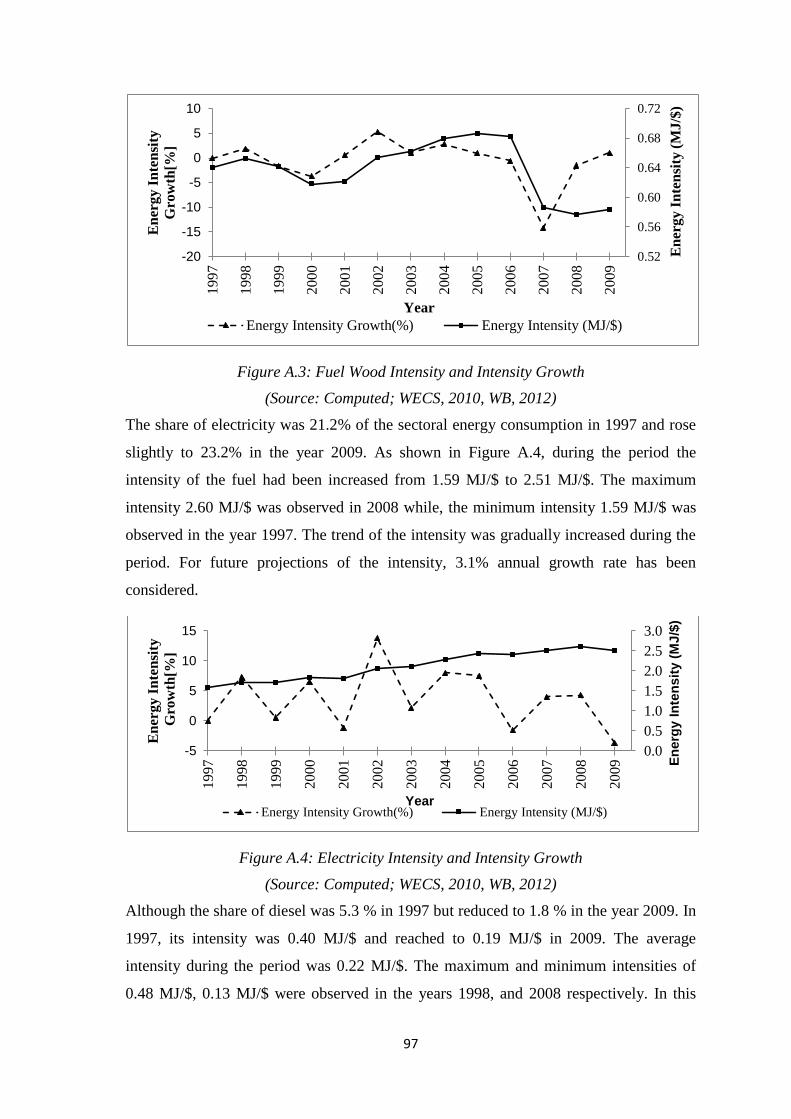
97
Figure A.3: Fuel Wood Intensity and Intensity Growth
(Source: Computed; WECS, 2010, WB, 2012)
The share of electricity was 21.2% of the sectoral energy consumption in 1997 and rose
slightly to 23.2% in the year 2009. As shown in Figure A.4, during the period the
intensity of the fuel had been increased from 1.59 MJ/$ to 2.51 MJ/$. The maximum
intensity 2.60 MJ/$ was observed in 2008 while, the minimum intensity 1.59 MJ/$ was
observed in the year 1997. The trend of the intensity was gradually increased during the
period. For future projections of the intensity, 3.1% annual growth rate has been
considered.
Figure A.4: Electricity Intensity and Intensity Growth
(Source: Computed; WECS, 2010, WB, 2012)
Although the share of diesel was 5.3 % in 1997 but reduced to 1.8 % in the year 2009. In
1997, its intensity was 0.40 MJ/$ and reached to 0.19 MJ/$ in 2009. The average
intensity during the period was 0.22 MJ/$. The maximum and minimum intensities of
0.48 MJ/$, 0.13 MJ/$ were observed in the years 1998, and 2008 respectively. In this
0.52
0.56
0.60
0.64
0.68
0.72
-20
-15
-10
-5
0
5
10
19
97
19
98
19
99
20
00
20
01
20
02
20
03
20
04
20
05
20
06
20
07
20
08
20
09
En
ergy I
nte
nsi
ty (
MJ/$
)
En
erg
y I
nte
nsi
ty
Gro
wth
[%]
Year
Energy Intensity Growth(%) Energy Intensity (MJ/$)
0.0
0.5
1.0
1.5
2.0
2.5
3.0
-5
0
5
10
15
1997
1998
1999
2000
2001
2002
2003
2004
2005
2006
2007
2008
2009 E
nerg
y I
nte
nsit
y (
MJ/$
)
En
ergy
In
ten
sity
Gro
wth
[%]
YearEnergy Intensity Growth(%) Energy Intensity (MJ/$)
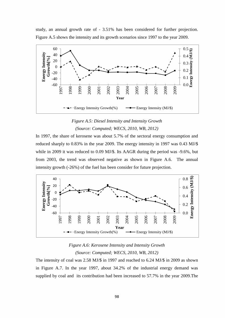
98
study, an annual growth rate of - 3.51% has been considered for further projection.
Figure A.5 shows the intensity and its growth scenarios since 1997 to the year 2009.
Figure A.5: Diesel Intensity and Intensity Growth
(Source: Computed; WECS, 2010, WB, 2012)
In 1997, the share of kerosene was about 5.7% of the sectoral energy consumption and
reduced sharply to 0.83% in the year 2009. The energy intensity in 1997 was 0.43 MJ/$
while in 2009 it was reduced to 0.09 MJ/$. Its AAGR during the period was -9.6%, but
from 2003, the trend was observed negative as shown in Figure A.6. The annual
intensity growth (-26%) of the fuel has been consider for future projection.
Figure A.6: Kerosene Intensity and Intensity Growth
(Source: Computed; WECS, 2010, WB, 2012)
The intensity of coal was 2.58 MJ/$ in 1997 and reached to 6.24 MJ/$ in 2009 as shown
in Figure A.7. In the year 1997, about 34.2% of the industrial energy demand was
supplied by coal and its contribution had been increased to 57.7% in the year 2009.The
0.0
0.1
0.2
0.3
0.4
0.5
-60
-40
-20
0
20
40
60
19
97
19
98
1999
20
00
20
01
2002
20
03
20
04
2005
20
06
20
07
20
08
20
09 E
ner
gy
In
ten
sity
(M
J/$
)
En
erg
y I
nte
nsi
ty
Gro
wth
[%]
Year
Energy Intensity Growth(%) Energy Intensity (MJ/$)
0.0
0.2
0.4
0.6
0.8
-60
-40
-20
0
20
40
1997
19
98
19
99
2000
20
01
20
02
20
03
20
04
20
05
20
06
20
07
20
08
20
09 En
erg
y I
nte
nsi
ty (
MJ
/$)
En
ergy I
nte
nsi
ty
Gro
wth
[%]
YearEnergy Intensity Growth(%) Energy Intensity (MJ/$)
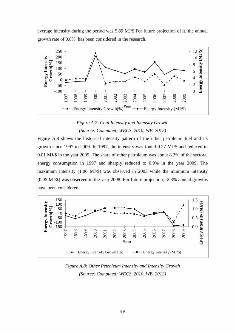
99
average intensity during the period was 5.89 MJ/$.For future projection of it, the annual
growth rate of 0.8% has been considered in the research.
Figure A.7: Coal Intensity and Intensity Growth
(Source: Computed; WECS, 2010, WB, 2012)
Figure A.8 shows the historical intensity pattern of the other petroleum fuel and its
growth since 1997 to 2009. In 1997, the intensity was found 0.27 MJ/$ and reduced to
0.01 MJ/$ in the year 2009. The share of other petroleum was about 8.3% of the sectoral
energy consumption in 1997 and sharply reduced to 0.9% in the year 2009. The
maximum intensity (1.06 MJ/$) was observed in 2003 while the minimum intensity
(0.05 MJ/$) was observed in the year 2008. For future projection, -2.3% annual growths
have been considered.
Figure A.8: Other Petroleum Intensity and Intensity Growth
(Source: Computed; WECS, 2010, WB, 2012)
0
2
4
6
8
10
12
-100
-50
0
50
100
150
200
250
19
97
1998
19
99
20
00
2001
20
02
20
03
2004
20
05
20
06
2007
20
08
20
09
En
erg
y I
nte
nsi
ty (
MJ
/$)
En
erg
y I
nte
nsi
ty
Gro
wth
[%]
YearEnergy Intensity Growth(%) Energy Intensity (MJ/$)
0.0
0.5
1.0
1.5
-150-100
-500
50100150
19
97
19
98
19
99
20
00
20
01
20
02
20
03
20
04
20
05
20
06
20
07
20
08
20
09
En
erg
y I
nte
nsit
y (
MJ/$
)
En
ergy I
nte
nsi
ty
Gro
wth
[%]
Year
Energy Intensity Growth(%) Energy Intensity (MJ/$)
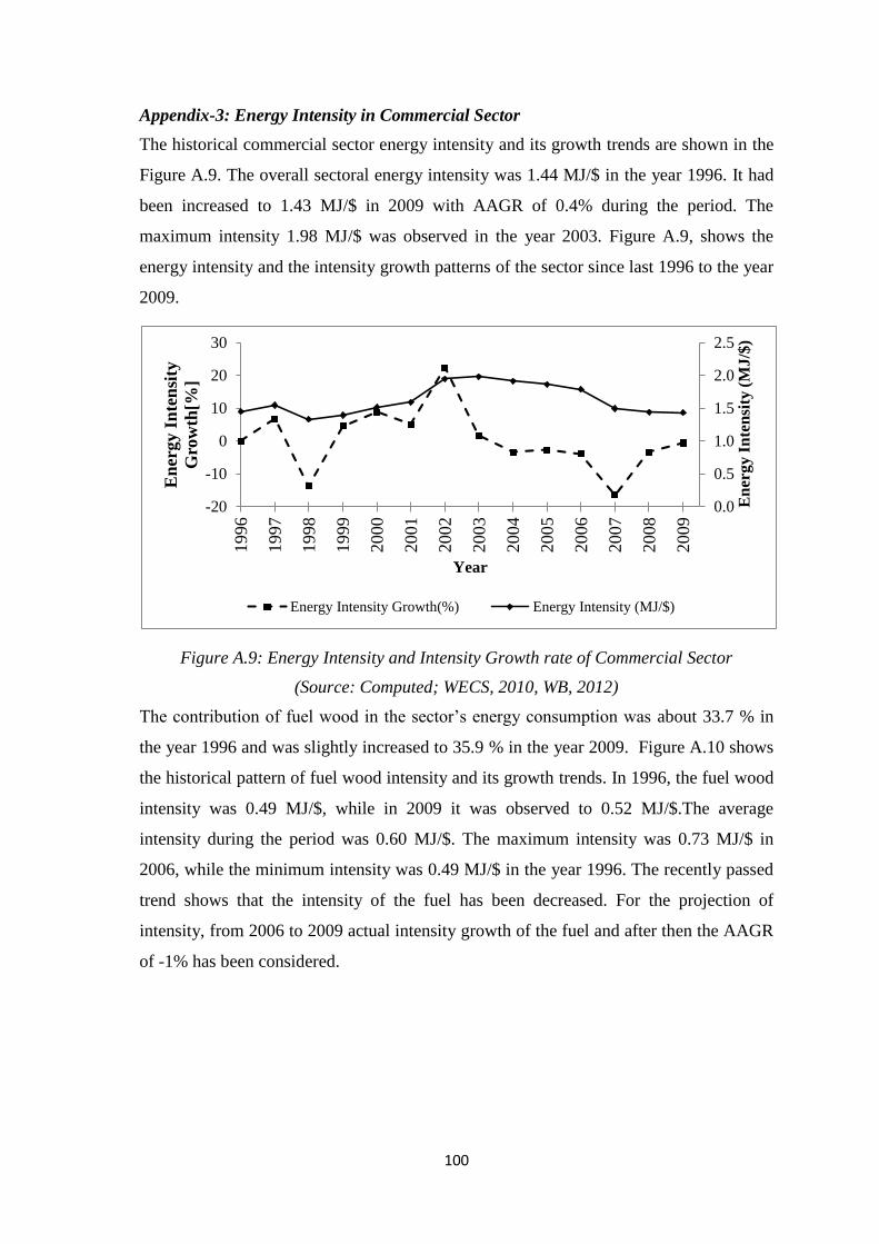
100
Appendix-3: Energy Intensity in Commercial Sector
The historical commercial sector energy intensity and its growth trends are shown in the
Figure A.9. The overall sectoral energy intensity was 1.44 MJ/$ in the year 1996. It had
been increased to 1.43 MJ/$ in 2009 with AAGR of 0.4% during the period. The
maximum intensity 1.98 MJ/$ was observed in the year 2003. Figure A.9, shows the
energy intensity and the intensity growth patterns of the sector since last 1996 to the year
2009.
Figure A.9: Energy Intensity and Intensity Growth rate of Commercial Sector
(Source: Computed; WECS, 2010, WB, 2012)
The contribution of fuel wood in the sector’s energy consumption was about 33.7 % in
the year 1996 and was slightly increased to 35.9 % in the year 2009. Figure A.10 shows
the historical pattern of fuel wood intensity and its growth trends. In 1996, the fuel wood
intensity was 0.49 MJ/$, while in 2009 it was observed to 0.52 MJ/$.The average
intensity during the period was 0.60 MJ/$. The maximum intensity was 0.73 MJ/$ in
2006, while the minimum intensity was 0.49 MJ/$ in the year 1996. The recently passed
trend shows that the intensity of the fuel has been decreased. For the projection of
intensity, from 2006 to 2009 actual intensity growth of the fuel and after then the AAGR
of -1% has been considered.
0.0
0.5
1.0
1.5
2.0
2.5
-20
-10
0
10
20
30
1996
1997
1998
1999
2000
2001
2002
2003
2004
2005
2006
2007
2008
2009
En
ergy I
nte
nsi
ty (
MJ/$
)
En
ergy I
nte
nsi
ty
Gro
wth
[%]
Year
Energy Intensity Growth(%) Energy Intensity (MJ/$)
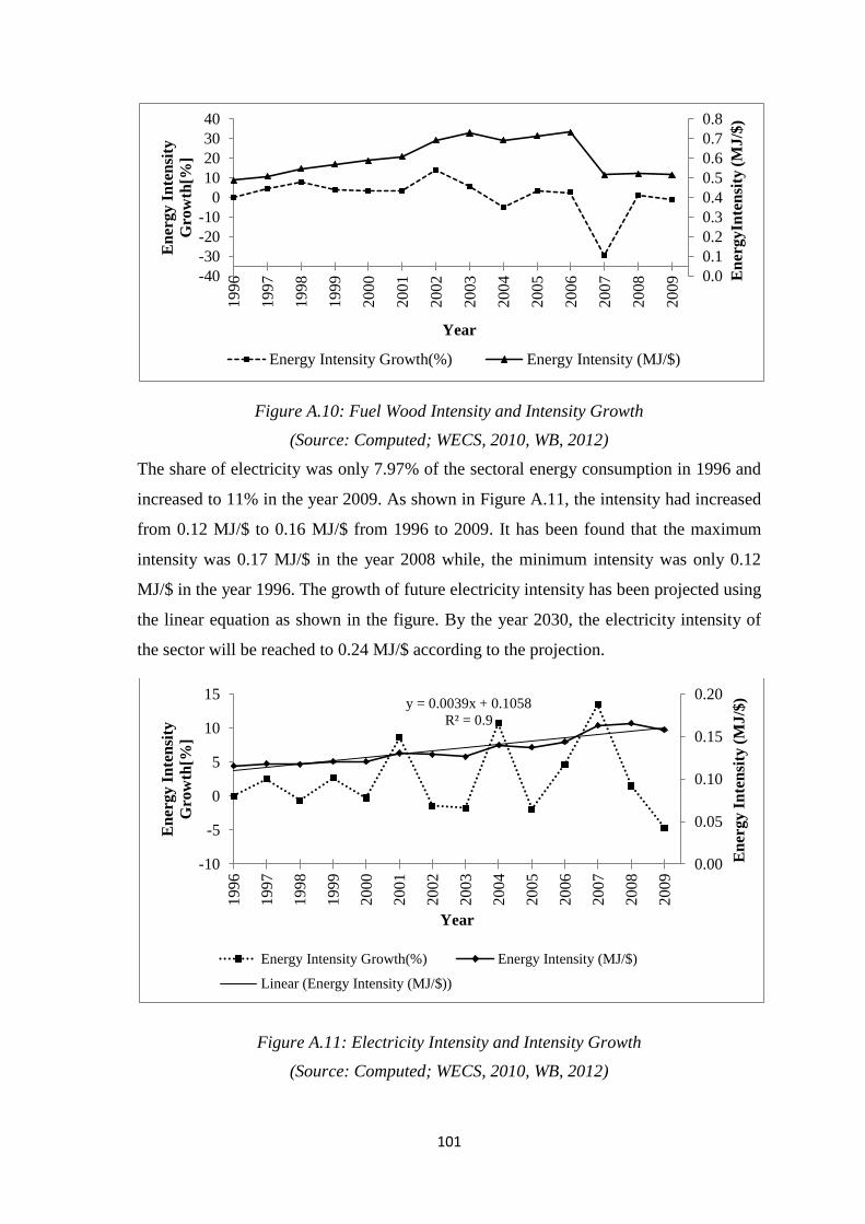
101
Figure A.10: Fuel Wood Intensity and Intensity Growth
(Source: Computed; WECS, 2010, WB, 2012)
The share of electricity was only 7.97% of the sectoral energy consumption in 1996 and
increased to 11% in the year 2009. As shown in Figure A.11, the intensity had increased
from 0.12 MJ/$ to 0.16 MJ/$ from 1996 to 2009. It has been found that the maximum
intensity was 0.17 MJ/$ in the year 2008 while, the minimum intensity was only 0.12
MJ/$ in the year 1996. The growth of future electricity intensity has been projected using
the linear equation as shown in the figure. By the year 2030, the electricity intensity of
the sector will be reached to 0.24 MJ/$ according to the projection.
Figure A.11: Electricity Intensity and Intensity Growth
(Source: Computed; WECS, 2010, WB, 2012)
0.0
0.1
0.2
0.3
0.4
0.5
0.6
0.7
0.8
-40
-30
-20
-10
0
10
20
30
40
19
96
19
97
19
98
1999
20
00
20
01
20
02
20
03
2004
20
05
20
06
20
07
20
08
20
09 E
ner
gyIn
ten
sity
(M
J/$
)
En
erg
y I
nte
nsi
ty
Gro
wth
[%]
Year
Energy Intensity Growth(%) Energy Intensity (MJ/$)
y = 0.0039x + 0.1058
R² = 0.9
0.00
0.05
0.10
0.15
0.20
-10
-5
0
5
10
15
19
96
19
97
19
98
19
99
20
00
20
01
20
02
2003
20
04
20
05
20
06
20
07
20
08
20
09
En
erg
y I
nte
nsi
ty (
MJ
/$)
En
ergy I
nte
nsi
ty
Gro
wth
[%]
Year
Energy Intensity Growth(%) Energy Intensity (MJ/$)
Linear (Energy Intensity (MJ/$))
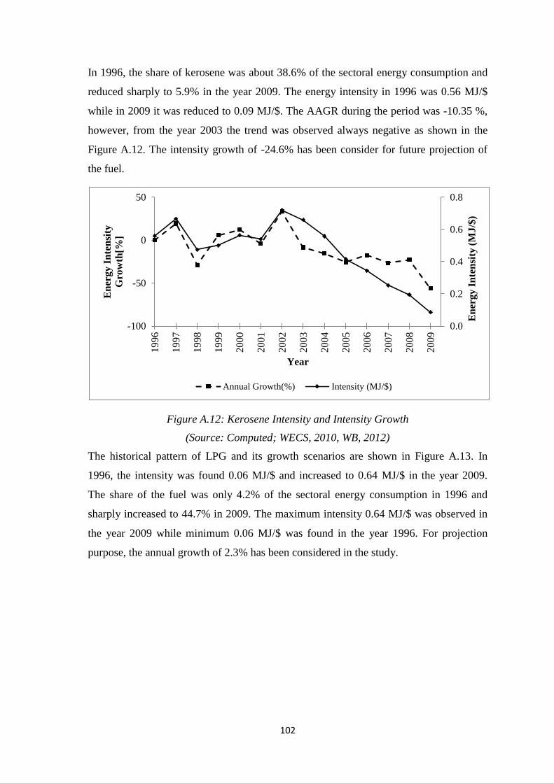
102
In 1996, the share of kerosene was about 38.6% of the sectoral energy consumption and
reduced sharply to 5.9% in the year 2009. The energy intensity in 1996 was 0.56 MJ/$
while in 2009 it was reduced to 0.09 MJ/$. The AAGR during the period was -10.35 %,
however, from the year 2003 the trend was observed always negative as shown in the
Figure A.12. The intensity growth of -24.6% has been consider for future projection of
the fuel.
Figure A.12: Kerosene Intensity and Intensity Growth
(Source: Computed; WECS, 2010, WB, 2012)
The historical pattern of LPG and its growth scenarios are shown in Figure A.13. In
1996, the intensity was found 0.06 MJ/$ and increased to 0.64 MJ/$ in the year 2009.
The share of the fuel was only 4.2% of the sectoral energy consumption in 1996 and
sharply increased to 44.7% in 2009. The maximum intensity 0.64 MJ/$ was observed in
the year 2009 while minimum 0.06 MJ/$ was found in the year 1996. For projection
purpose, the annual growth of 2.3% has been considered in the study.
0.0
0.2
0.4
0.6
0.8
-100
-50
0
50
1996
1997
1998
1999
2000
2001
2002
2003
2004
2005
2006
2007
2008
2009
En
ergy I
nte
nsi
ty (
MJ/$
)
En
erg
y I
nte
nsi
ty
Gro
wth
[%]
Year
Annual Growth(%) Intensity (MJ/$)
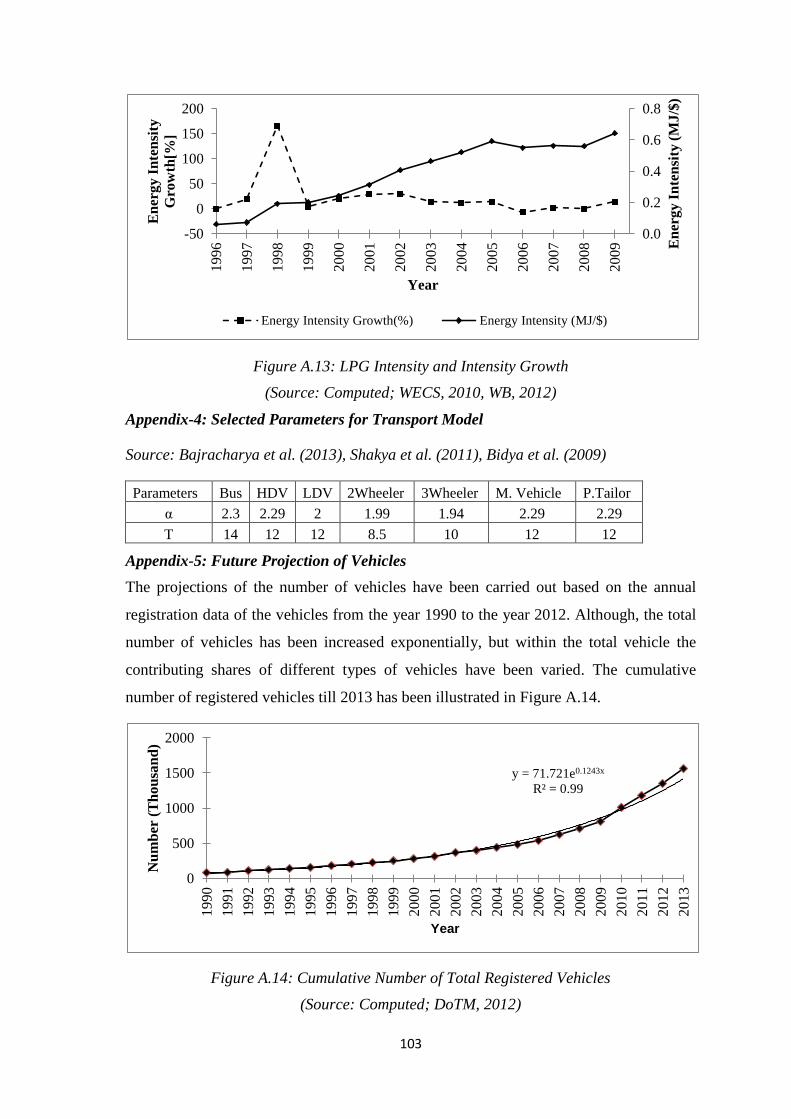
103
Figure A.13: LPG Intensity and Intensity Growth
(Source: Computed; WECS, 2010, WB, 2012)
Appendix-4: Selected Parameters for Transport Model
Source: Bajracharya et al. (2013), Shakya et al. (2011), Bidya et al. (2009)
Parameters Bus HDV LDV 2Wheeler 3Wheeler M. Vehicle P.Tailor
α 2.3 2.29 2 1.99 1.94 2.29 2.29
T 14 12 12 8.5 10 12 12
Appendix-5: Future Projection of Vehicles
The projections of the number of vehicles have been carried out based on the annual
registration data of the vehicles from the year 1990 to the year 2012. Although, the total
number of vehicles has been increased exponentially, but within the total vehicle the
contributing shares of different types of vehicles have been varied. The cumulative
number of registered vehicles till 2013 has been illustrated in Figure A.14.
Figure A.14: Cumulative Number of Total Registered Vehicles
(Source: Computed; DoTM, 2012)
0.0
0.2
0.4
0.6
0.8
-50
0
50
100
150
200
19
96
19
97
1998
19
99
2000
20
01
20
02
20
03
20
04
20
05
20
06
20
07
20
08
20
09 E
ner
gy I
nte
nsi
ty (
MJ/$
)
En
erg
y I
nte
nsi
ty
Gro
wth
[%]
Year
Energy Intensity Growth(%) Energy Intensity (MJ/$)
y = 71.721e0.1243x
R² = 0.99
0
500
1000
1500
2000
19
90
19
91
19
92
19
93
19
94
19
95
19
96
19
97
19
98
19
99
20
00
20
01
20
02
20
03
20
04
20
05
2006
20
07
20
08
2009
20
10
20
11
2012
20
13
Nu
mb
er (
Th
ou
san
d)
Year
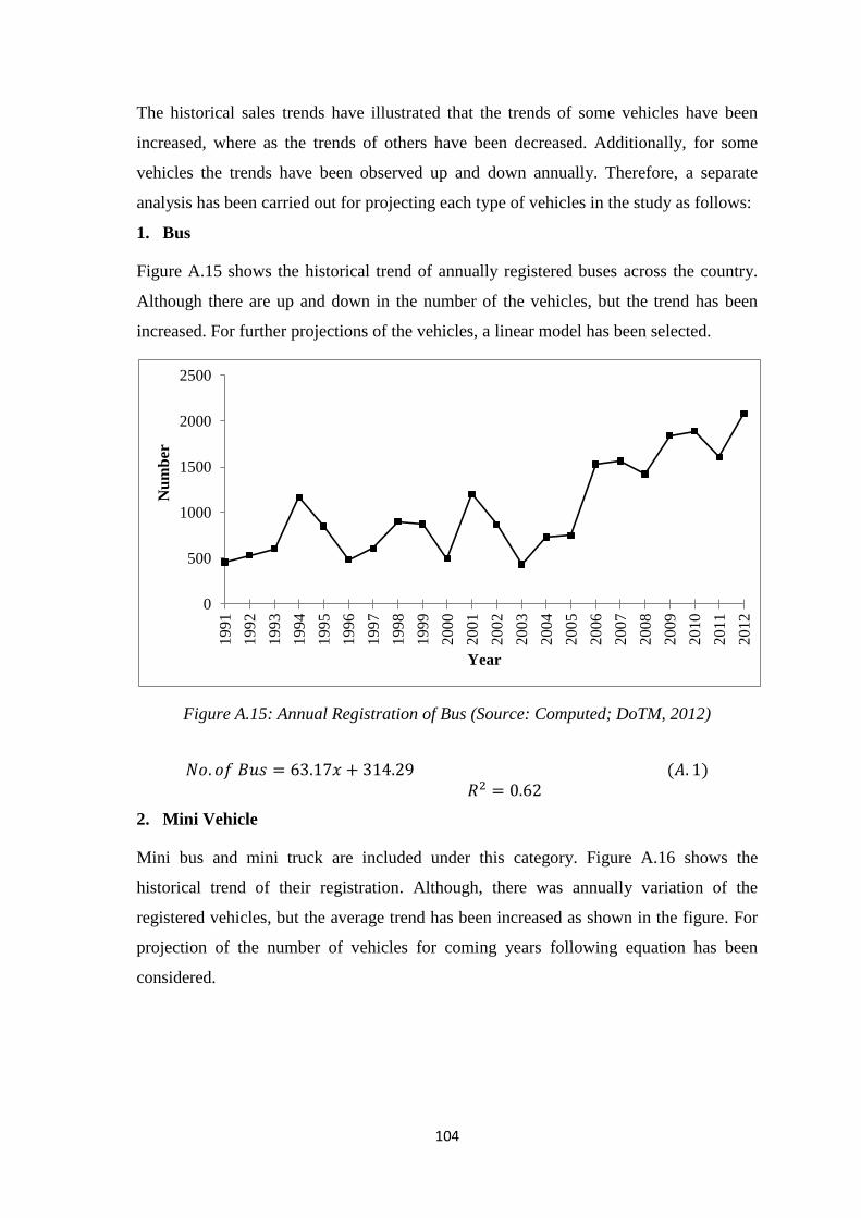
104
The historical sales trends have illustrated that the trends of some vehicles have been
increased, where as the trends of others have been decreased. Additionally, for some
vehicles the trends have been observed up and down annually. Therefore, a separate
analysis has been carried out for projecting each type of vehicles in the study as follows:
1. Bus
Figure A.15 shows the historical trend of annually registered buses across the country.
Although there are up and down in the number of the vehicles, but the trend has been
increased. For further projections of the vehicles, a linear model has been selected.
Figure A.15: Annual Registration of Bus (Source: Computed; DoTM, 2012)
𝑁𝑜. 𝑜𝑓 𝐵𝑢𝑠 = 63.17𝑥 + 314.29 (𝐴. 1)
𝑅2 = 0.62
2. Mini Vehicle
Mini bus and mini truck are included under this category. Figure A.16 shows the
historical trend of their registration. Although, there was annually variation of the
registered vehicles, but the average trend has been increased as shown in the figure. For
projection of the number of vehicles for coming years following equation has been
considered.
0
500
1000
1500
2000
2500
1991
1992
1993
1994
1995
1996
1997
1998
1999
2000
2001
2002
2003
2004
2005
2006
2007
2008
2009
2010
2011
2012
Nu
mb
er
Year
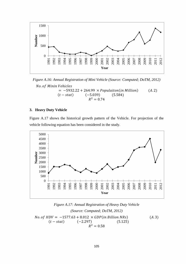
105
Figure A.16: Annual Registration of Mini Vehicle (Source: Computed; DoTM, 2012)
𝑁𝑜. 𝑜𝑓 𝑀𝑖𝑛𝑖𝑛 𝑉𝑒ℎ𝑖𝑐𝑙𝑒𝑠= −5932.22 + 264.99 × 𝑃𝑜𝑝𝑢𝑙𝑎𝑖𝑡𝑜𝑛(𝑖𝑛 𝑀𝑖𝑙𝑙𝑖𝑜𝑛) (𝐴. 2)
(𝑡 − 𝑠𝑡𝑎𝑡) (−5.039) (5.584) 𝑅2 = 0.74
3. Heavy Duty Vehicle
Figure A.17 shows the historical growth pattern of the Vehicle. For projection of the
vehicle following equation has been considered in the study.
Figure A.17: Annual Registration of Heavy Duty Vehicle
(Source: Computed; DoTM, 2012)
𝑁𝑜. 𝑜𝑓 𝐻𝐷𝑉 = −1577.63 + 8.012 × 𝐺𝐷𝑃(𝑖𝑛 𝐵𝑖𝑙𝑙𝑖𝑜𝑛 𝑁𝑅𝑠) (𝐴. 3) (𝑡 − 𝑠𝑡𝑎𝑡) (−2.297) (5.125)
𝑅2 = 0.58
0
500
1000
1500
19
91
19
92
1993
19
94
19
95
19
96
19
97
19
98
19
99
20
00
20
01
20
02
20
03
2004
20
05
20
06
20
07
20
08
20
09
20
10
20
11
20
12
Nu
mb
er
Year
0
500
1000
1500
2000
2500
3000
3500
4000
4500
5000
19
91
19
92
1993
19
94
19
95
19
96
19
97
19
98
19
99
20
00
20
01
20
02
20
03
2004
20
05
20
06
20
07
20
08
20
09
20
10
20
11
20
12
Nu
mb
er
Year
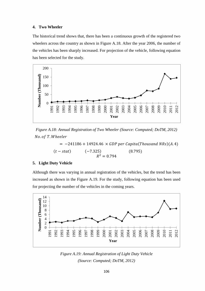
106
4. Two Wheeler
The historical trend shows that, there has been a continuous growth of the registered two
wheelers across the country as shown in Figure A.18. After the year 2006, the number of
the vehicles has been sharply increased. For projection of the vehicle, following equation
has been selected for the study.
Figure A.18: Annual Registration of Two Wheeler (Source: Computed; DoTM, 2012)
𝑁𝑜. 𝑜𝑓 𝑇. 𝑊ℎ𝑒𝑒𝑙𝑒𝑟
= −241186 + 14924.46 × 𝐺𝐷𝑃 𝑝𝑒𝑟 𝐶𝑎𝑝𝑖𝑡𝑎(𝑇ℎ𝑜𝑢𝑠𝑎𝑛𝑑 𝑁𝑅𝑠)(𝐴. 4)
(𝑡 − 𝑠𝑡𝑎𝑡) (−7.325) (8.795) 𝑅2 = 0.794
5. Light Duty Vehicle
Although there was varying in annual registration of the vehicles, but the trend has been
increased as shown in the Figure A.19. For the study, following equation has been used
for projecting the number of the vehicles in the coming years.
Figure A.19: Annual Registration of Light Duty Vehicle
(Source: Computed; DoTM, 2012)
0
50
100
150
200
19
91
19
92
19
93
19
94
19
95
19
96
19
97
1998
19
99
20
00
20
01
20
02
2003
20
04
20
05
20
06
20
07
20
08
20
09
20
10
20
11
20
12N
um
ber
(T
ho
usa
nd
)
Year
0
24
6
8
10
12
14
19
91
19
92
19
93
1994
19
95
19
96
19
97
19
98
1999
20
00
20
01
20
02
20
03
20
04
20
05
2006
20
07
20
08
20
09
20
10
20
11
20
12N
um
ber
(T
ho
usa
nd
)
Year
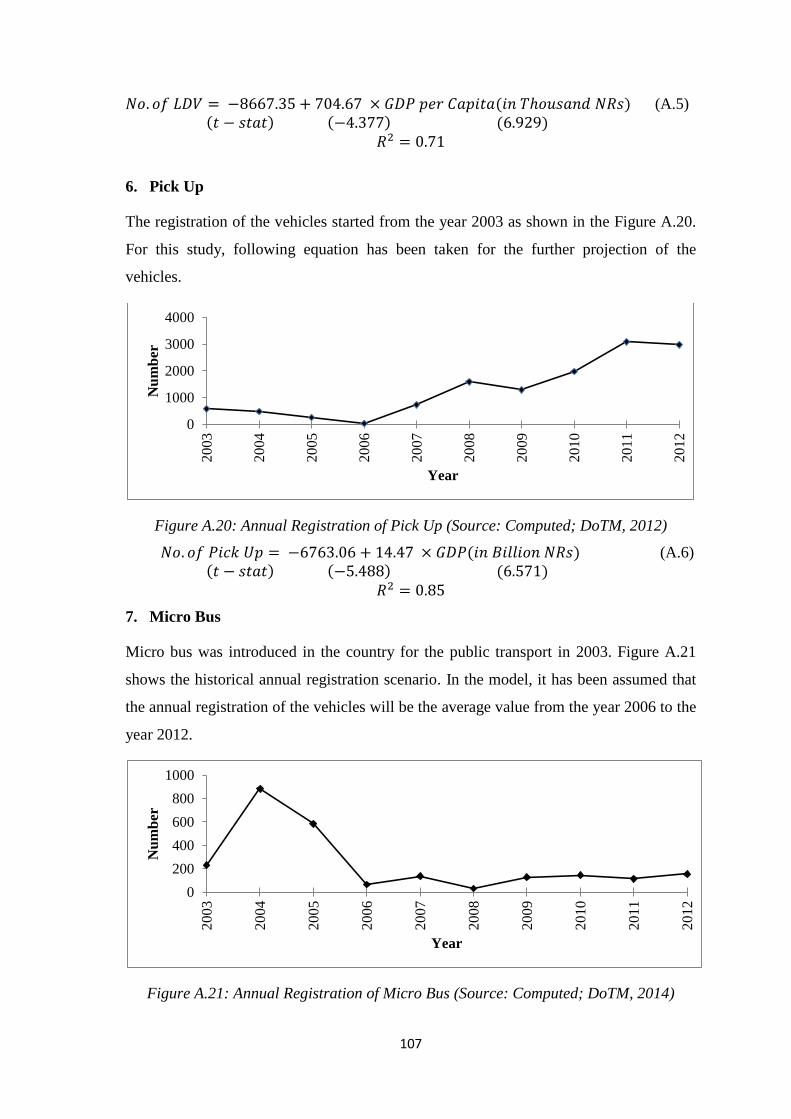
107
𝑁𝑜. 𝑜𝑓 𝐿𝐷𝑉 = −8667.35 + 704.67 × 𝐺𝐷𝑃 𝑝𝑒𝑟 𝐶𝑎𝑝𝑖𝑡𝑎(𝑖𝑛 𝑇ℎ𝑜𝑢𝑠𝑎𝑛𝑑 𝑁𝑅𝑠) (A.5)
(𝑡 − 𝑠𝑡𝑎𝑡) (−4.377) (6.929) 𝑅2 = 0.71
6. Pick Up
The registration of the vehicles started from the year 2003 as shown in the Figure A.20.
For this study, following equation has been taken for the further projection of the
vehicles.
Figure A.20: Annual Registration of Pick Up (Source: Computed; DoTM, 2012)
𝑁𝑜. 𝑜𝑓 𝑃𝑖𝑐𝑘 𝑈𝑝 = −6763.06 + 14.47 × 𝐺𝐷𝑃(𝑖𝑛 𝐵𝑖𝑙𝑙𝑖𝑜𝑛 𝑁𝑅𝑠) (A.6)
(𝑡 − 𝑠𝑡𝑎𝑡) (−5.488) (6.571) 𝑅2 = 0.85
7. Micro Bus
Micro bus was introduced in the country for the public transport in 2003. Figure A.21
shows the historical annual registration scenario. In the model, it has been assumed that
the annual registration of the vehicles will be the average value from the year 2006 to the
year 2012.
Figure A.21: Annual Registration of Micro Bus (Source: Computed; DoTM, 2014)
0
1000
2000
3000
4000
2003
2004
2005
2006
2007
2008
2009
2010
2011
2012
Nu
mb
er
Year
0
200
400
600
800
1000
20
03
20
04
20
05
20
06
20
07
20
08
20
09
20
10
20
11
20
12
Nu
mb
er
Year
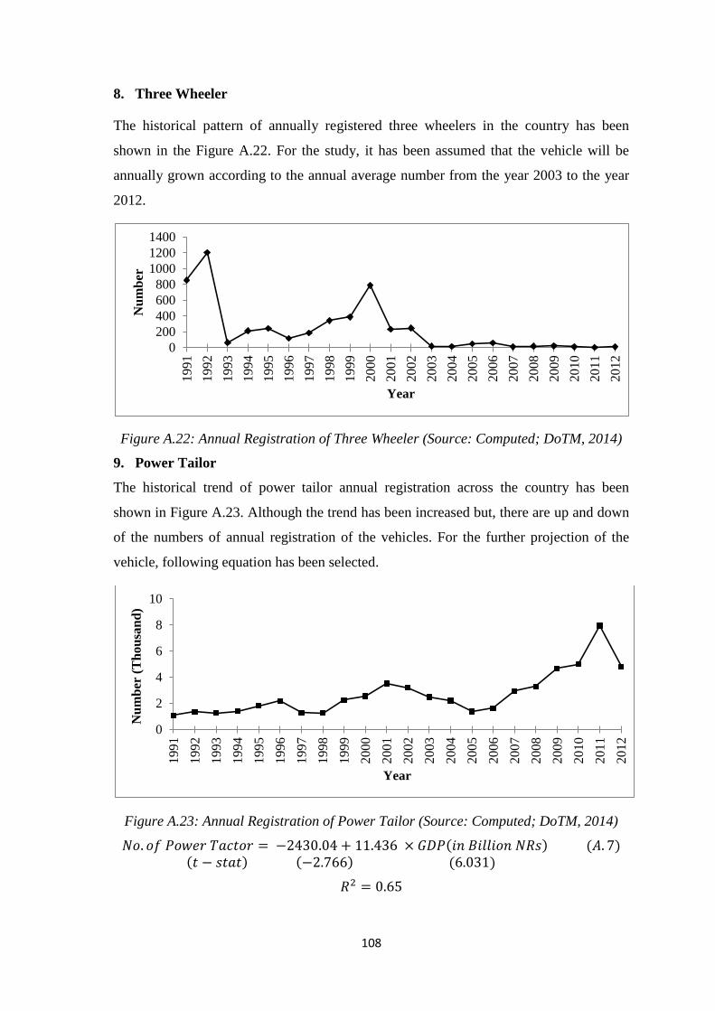
108
8. Three Wheeler
The historical pattern of annually registered three wheelers in the country has been
shown in the Figure A.22. For the study, it has been assumed that the vehicle will be
annually grown according to the annual average number from the year 2003 to the year
2012.
Figure A.22: Annual Registration of Three Wheeler (Source: Computed; DoTM, 2014)
9. Power Tailor
The historical trend of power tailor annual registration across the country has been
shown in Figure A.23. Although the trend has been increased but, there are up and down
of the numbers of annual registration of the vehicles. For the further projection of the
vehicle, following equation has been selected.
Figure A.23: Annual Registration of Power Tailor (Source: Computed; DoTM, 2014)
𝑁𝑜. 𝑜𝑓 𝑃𝑜𝑤𝑒𝑟 𝑇𝑎𝑐𝑡𝑜𝑟 = −2430.04 + 11.436 × 𝐺𝐷𝑃(𝑖𝑛 𝐵𝑖𝑙𝑙𝑖𝑜𝑛 𝑁𝑅𝑠) (𝐴. 7) (𝑡 − 𝑠𝑡𝑎𝑡) (−2.766) (6.031)
𝑅2 = 0.65
0
200
400
600
800
1000
1200
1400
19
91
19
92
19
93
19
94
1995
1996
1997
1998
1999
2000
2001
2002
2003
20
04
20
05
20
06
20
07
20
08
20
09
20
10
20
11
20
12
Nu
mb
er
Year
0
2
4
6
8
10
19
91
19
92
19
93
19
94
19
95
19
96
19
97
19
98
19
99
20
00
20
01
20
02
20
03
20
04
2005
20
06
20
07
20
08
2009
20
10
20
11
20
12
Nu
mb
er (
Th
ou
san
d)
Year
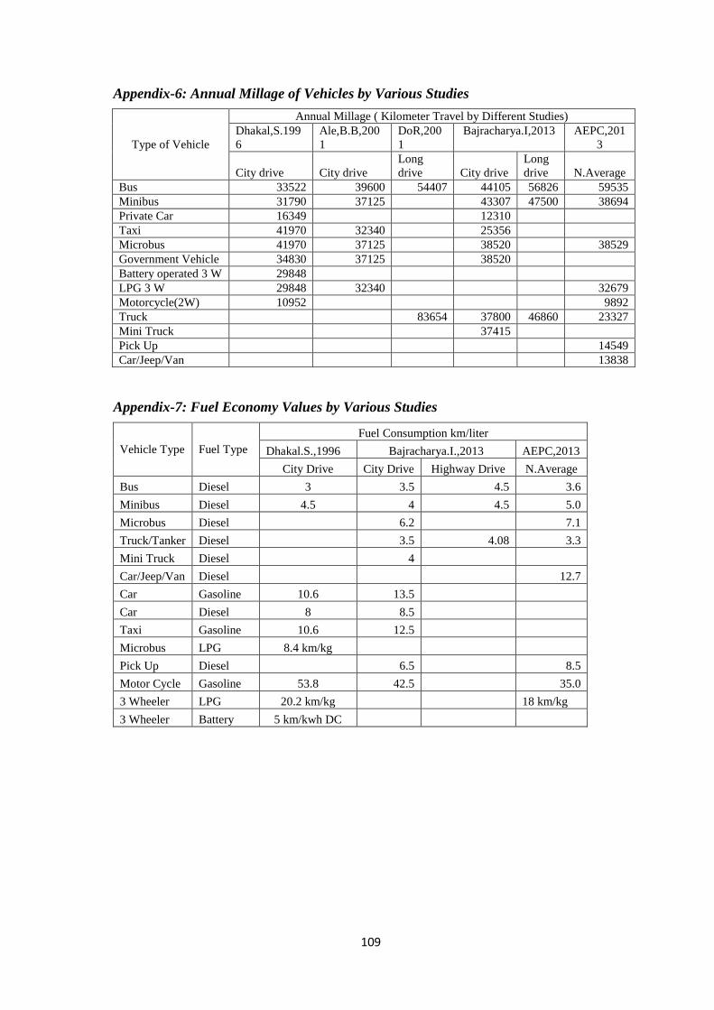
109
Appendix-6: Annual Millage of Vehicles by Various Studies
Type of Vehicle
Annual Millage ( Kilometer Travel by Different Studies)
Dhakal,S.199
6
Ale,B.B,200
1
DoR,200
1
Bajracharya.I,2013
AEPC,201
3
City drive City drive
Long
drive City drive
Long
drive N.Average
Bus 33522 39600 54407 44105 56826 59535
Minibus 31790 37125 43307 47500 38694
Private Car 16349 12310
Taxi 41970 32340 25356
Microbus 41970 37125 38520 38529
Government Vehicle 34830 37125 38520
Battery operated 3 W 29848
LPG 3 W 29848 32340 32679
Motorcycle(2W) 10952 9892
Truck 83654 37800 46860 23327
Mini Truck 37415
Pick Up 14549
Car/Jeep/Van 13838
Appendix-7: Fuel Economy Values by Various Studies
Vehicle Type Fuel Type
Fuel Consumption km/liter
Dhakal.S.,1996 Bajracharya.I.,2013 AEPC,2013
City Drive City Drive Highway Drive N.Average
Bus Diesel 3 3.5 4.5 3.6
Minibus Diesel 4.5 4 4.5 5.0
Microbus Diesel 6.2 7.1
Truck/Tanker Diesel 3.5 4.08 3.3
Mini Truck Diesel 4
Car/Jeep/Van Diesel 12.7
Car Gasoline 10.6 13.5
Car Diesel 8 8.5
Taxi Gasoline 10.6 12.5
Microbus LPG 8.4 km/kg
Pick Up Diesel 6.5 8.5
Motor Cycle Gasoline 53.8 42.5 35.0
3 Wheeler LPG 20.2 km/kg 18 km/kg
3 Wheeler Battery 5 km/kwh DC
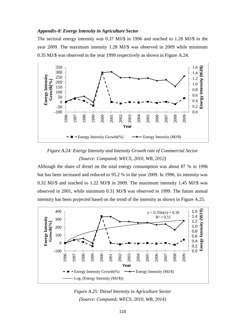
110
Appendix-8: Energy Intensity in Agriculture Sector
The sectoral energy intensity was 0.37 MJ/$ in 1996 and reached to 1.28 MJ/$ in the
year 2009. The maximum intensity 1.28 MJ/$ was observed in 2009 while minimum
0.35 MJ/$ was observed in the year 1999 respectively as shown in Figure A.24.
Figure A.24: Energy Intensity and Intensity Growth rate of Commercial Sector
(Source: Computed; WECS, 2010, WB, 2012)
Although the share of diesel on the total energy consumption was about 87 % in 1996
but has been increased and reduced to 95.2 % in the year 2009. In 1996, its intensity was
0.32 MJ/$ and reached to 1.22 MJ/$ in 2009. The maximum intensity 1.45 MJ/$ was
observed in 2001, while minimum 0.31 MJ/$ was observed in 1999. The future annual
intensity has been projected based on the trend of the intensity as shown in Figure A.25.
Figure A.25: Diesel Intensity in Agriculture Sector
(Source: Computed; WECS, 2010, WB, 2014)
0.0
0.2
0.4
0.6
0.8
1.0
1.2
1.4
1.6
-100-50
050
100150200250300350
19
96
19
97
19
98
19
99
20
00
20
01
20
02
20
03
20
04
20
05
20
06
20
07
20
08
20
09
En
erg
y I
nte
nsit
y (
MJ/$
)
En
erg
y I
nte
nsi
ty
Gro
wth
[%]
Year
Energy Intensity Growth(%) Energy Intensity (MJ/$)
y = 0.35ln(x) + 0.30
R² = 0.51
0.0
0.2
0.4
0.6
0.8
1.0
1.2
1.4
1.6
-100
0
100
200
300
400
1996
1997
1998
1999
2000
2001
2002
2003
2004
2005
2006
2007
2008
2009
En
ergy I
nte
nsi
ty (
MJ/$
)
En
ergy I
nte
nsi
ty
Gro
wth
[%]
Year
Energy Intensity Growth(%) Energy Intensity (MJ/$)
Log. (Energy Intensity (MJ/$))
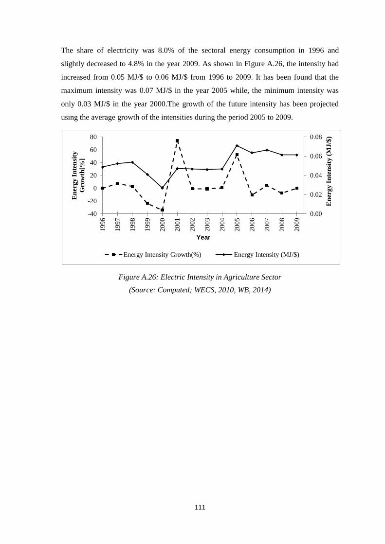
111
The share of electricity was 8.0% of the sectoral energy consumption in 1996 and
slightly decreased to 4.8% in the year 2009. As shown in Figure A.26, the intensity had
increased from 0.05 MJ/$ to 0.06 MJ/$ from 1996 to 2009. It has been found that the
maximum intensity was 0.07 MJ/$ in the year 2005 while, the minimum intensity was
only 0.03 MJ/$ in the year 2000.The growth of the future intensity has been projected
using the average growth of the intensities during the period 2005 to 2009.
Figure A.26: Electric Intensity in Agriculture Sector
(Source: Computed; WECS, 2010, WB, 2014)
0.00
0.02
0.04
0.06
0.08
-40
-20
0
20
40
60
80
1996
1997
1998
1999
2000
2001
2002
2003
2004
2005
2006
2007
2008
2009
En
erg
y I
nte
nsi
ty (
MJ
/$)
En
erg
y I
nte
nsi
ty
Gro
wth
[%]
Year
Energy Intensity Growth(%) Energy Intensity (MJ/$)
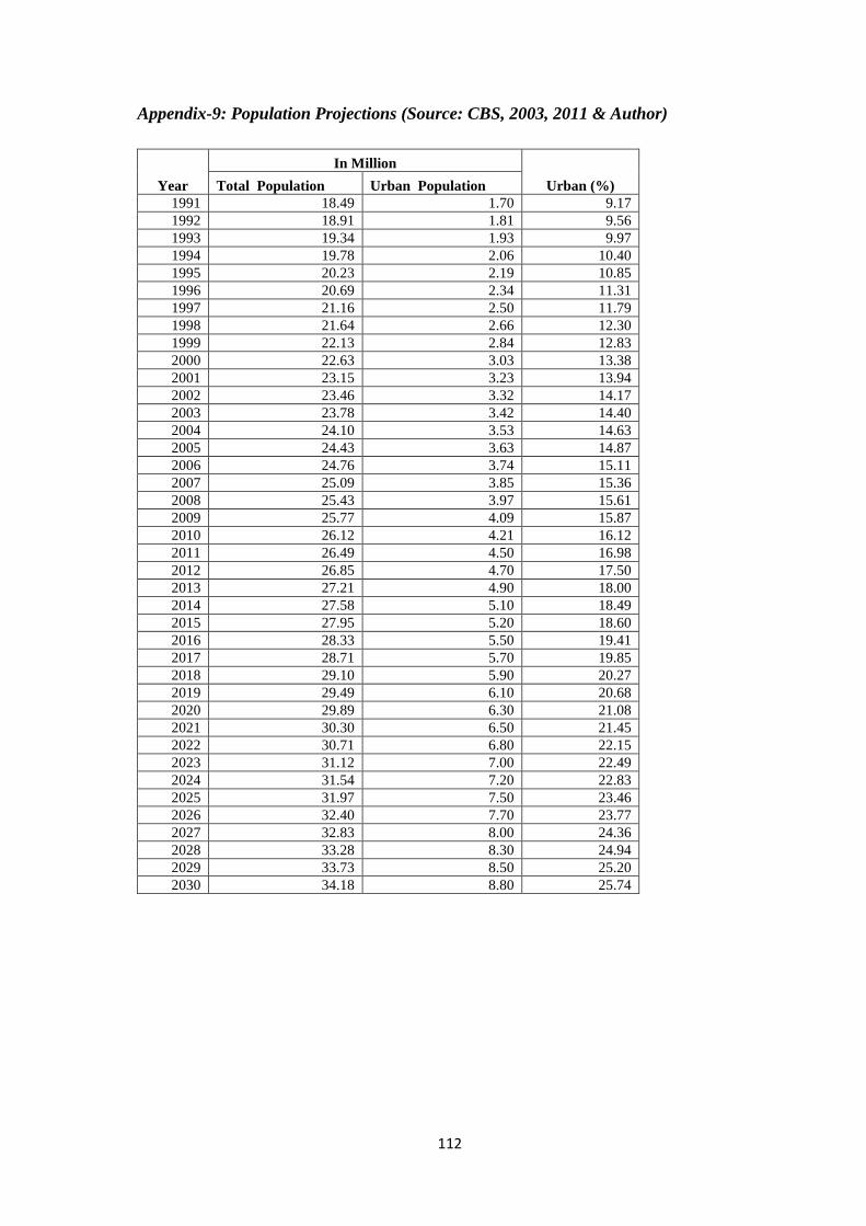
112
Appendix-9: Population Projections (Source: CBS, 2003, 2011 & Author)
Year
In Million
Urban (%) Total Population Urban Population
1991 18.49 1.70 9.17
1992 18.91 1.81 9.56
1993 19.34 1.93 9.97
1994 19.78 2.06 10.40
1995 20.23 2.19 10.85
1996 20.69 2.34 11.31
1997 21.16 2.50 11.79
1998 21.64 2.66 12.30
1999 22.13 2.84 12.83
2000 22.63 3.03 13.38
2001 23.15 3.23 13.94
2002 23.46 3.32 14.17
2003 23.78 3.42 14.40
2004 24.10 3.53 14.63
2005 24.43 3.63 14.87
2006 24.76 3.74 15.11
2007 25.09 3.85 15.36
2008 25.43 3.97 15.61
2009 25.77 4.09 15.87
2010 26.12 4.21 16.12
2011 26.49 4.50 16.98
2012 26.85 4.70 17.50
2013 27.21 4.90 18.00
2014 27.58 5.10 18.49
2015 27.95 5.20 18.60
2016 28.33 5.50 19.41
2017 28.71 5.70 19.85
2018 29.10 5.90 20.27
2019 29.49 6.10 20.68
2020 29.89 6.30 21.08
2021 30.30 6.50 21.45
2022 30.71 6.80 22.15
2023 31.12 7.00 22.49
2024 31.54 7.20 22.83
2025 31.97 7.50 23.46
2026 32.40 7.70 23.77
2027 32.83 8.00 24.36
2028 33.28 8.30 24.94
2029 33.73 8.50 25.20
2030 34.18 8.80 25.74
113
Curriculum Vitae
Family Name : Bhattarai
Name : Nawraj
Date of Birth : 02 September, 1975
Marital Status : Married with Deewa Pokharel, 2 children
(Son-Shaarav & Daughter- Saanvi)
Address : Hariwon-4, Sarlahi, Nepal
E-mail : [email protected]
Academic Qualification
Master of Science (M.Sc.) in Renewable Energy Engineering from Institute of
Engineering, Tribhuvan University, Nepal in 2004.
Bachelor of Engineering (B.E.) in Mechanical Engineering from Institute of
Engineering, Tribhuvan University, Nepal in 2000.
Job Experiences
Working as an Assistant Professor since 2004 and toughed several subjects in
Mechanical Engineering, Pulchowk Campus, Institute of Engineering, Tribhuvan
University, Nepal.
Deputy Head (2008-2010) in Department of Mechanical Engineering, Pulchowk
Campus, Institute of Engineering, Tribhuvan University, Nepal.
Deputy Director (2010-2011) in Centre for Energy Studies, Institute of
Engineering, Tribhuvan University, Nepal.
Academic Research Supervision (M.Sc. Level)
1. 2006, Performance Study on Tabular and Compact Fluorescent Lamps used in
Solar Home System in Nepal.
2. 2009, Computer Based Analysis, Design and Fabrication of Diffuser Type
Portable Wood Gasifier to Develop a Preliminary Lab Setup for Performance
Test.
3. 2009, Rural Electrification Options for Kaldhar Village Nepal.
4. 2010, Study on Techno-Socio and Financial Impact of Biogas Plants in Kavre
District of Nepal.
5. 2010, Wind Energy Resource Assessment and Feasibility Study of Wind Farm in
Mustang of Nepal.
114
6. 2010, A Study on Operation and Maintenance of Electro- Mechanical Parts of
Kulakhani Second Hydropower Plant of Nepal.
7. 2010, Performance Test of Residential Cook Stove and Modification of a Metal
Stove.
8. 2011, Policy and Study of Grid Connected PV System in Nepal.
9. 2011, Study on Erosion Behavior of Runner and Guide Vane and its Rectification
in Hydropower Station ( A case of Middle Marsyangdi Hydropower Station)
10. 2012, Energy Analysis of Green Building and Setting-up Building code for
Different Parts of Nepal.
Academic Publications
1. 2006, Performance Analysis of DC Tubular Lamps and Compact Fluorescents
Lamps used in Solar Home System in Nepal, in first National Conference on
Renewable Energy Technology for Rural Development in Kathmandu, Nepal.
2. 2006, Development of Liquid Bio-fuel out of the Traditional Biomass Resources
to Generate Renewable Fuel for Rural Development in Nepal, in first National
Conference on Renewable Energy Technology for Rural Development in
Kathmandu, Nepal.
3. 2008, Emission of Pollutants under Different Traffic Load Condition in
Kathmandu Valley, in Better Air Quality Conference, Bangkok, Thailand.
4. 2009, Knowledge Management System for Sustainable Modern Biomass Based
Energy Development in Nepal, Asian Institute of Technology International
Conference on Knowledge Management, Kathmandu, Nepal.
5. 2009, Relation between Air Pollution and Climate Change, in Nepal Engineer’s
Association 11th Convention, Kathmandu, Nepal.
6. 2009, Institutional Gasifier Stove: A Sustainable Prospect for Institutional
Cooking, Journal of the Institute of Engineering, Vol 7, No, 1, 142-149.
7. 2009, Barrier for Implementation of Improved Cook Stove Program in Nepal,
Institutional Gasifier Stove: A Sustainable Prospect for Institutional Cooking,
Journal of the Institute of Engineering, Vol 7, No, 1, 116-120
8. 2011, Wind Energy Resource Assessment and Feasibility Study of Wind Farm in
Mustang, Journal of the Institute of Engineering, Vol 8, No, 1-2, 93-104.
9. 2011, Biomethanation of Organic Waste under Psychrophilic Conditions,
International Conference on Addressing Climate Change for Sustainable
Development through Up-Scaling Renewable Energy Technologies, Kathmandu,
Nepal.
Course Manual Writing (for International Level only)
1. 2009, Biomass and design/construction for cooking stoves, Department of
Alternative Energy, Tumba College of Technology, Rwanda, Africa.