Embed Size (px)
Citation preview
Bachelor’s Thesis
Untersuchung vonModellierungsunsicherheiten in
tt̄-Paarproduktion am ATLAS-Experiment
Study of modelling uncertainties in tt̄ pairproduction at the ATLAS experiment
prepared by
Jun Huangfrom Wuhan
at the II. Physikalisches Institut
Thesis number: II.Physik-UniGö-BSc-2020/03
Thesis period: 1st April 2020 until 6th July 2014
First referee: Prof. Dr. Arnulf Quadt
Second referee: Prof. Dr. Ariane Frey

Contents
1 Introduction 1
2 Theoretical Background 22.1 Standard Model . . . . . . . . . . . . . . . . . . . . . . . . . . . . . . . . . 22.2 The Top Quark . . . . . . . . . . . . . . . . . . . . . . . . . . . . . . . . . 3
2.2.1 Top Quarks at the LHC . . . . . . . . . . . . . . . . . . . . . . . . 3
3 Experimental Setup 63.1 Detector . . . . . . . . . . . . . . . . . . . . . . . . . . . . . . . . . . . . . 63.2 ATLAS . . . . . . . . . . . . . . . . . . . . . . . . . . . . . . . . . . . . . 63.3 ALTAS detector . . . . . . . . . . . . . . . . . . . . . . . . . . . . . . . . . 7
3.3.1 Inner Detector . . . . . . . . . . . . . . . . . . . . . . . . . . . . . . 83.3.2 Calorimeter . . . . . . . . . . . . . . . . . . . . . . . . . . . . . . . 93.3.3 Muon Detector . . . . . . . . . . . . . . . . . . . . . . . . . . . . . 93.3.4 Data processing analysis system . . . . . . . . . . . . . . . . . . . . 9
4 Introduction to top quark analysis 114.1 Monte Carlo simulation . . . . . . . . . . . . . . . . . . . . . . . . . . . . . 114.2 Monte Carlo samples . . . . . . . . . . . . . . . . . . . . . . . . . . . . . . 12
5 Comparison between the FSR and ISR uncertainties estimation in oldand new approach 145.1 Comparison between up and down impact of each variation in ISR and FSR 14
5.1.1 Explanation . . . . . . . . . . . . . . . . . . . . . . . . . . . . . . . 145.1.2 HT and Njets multiplicity distributions for individual variations of
both ISR and FSR for single electron . . . . . . . . . . . . . . . . . 155.1.3 HT and Njets multiplicity distributions for individual variations of
both ISR and FSR for single muon . . . . . . . . . . . . . . . . . . 205.1.4 Discussion . . . . . . . . . . . . . . . . . . . . . . . . . . . . . . . . 25
ii
Contents
5.2 Comparison of histogram total uncertainty and ratio total uncertainty be-tween 4 variations . . . . . . . . . . . . . . . . . . . . . . . . . . . . . . . . 265.2.1 Comparing and Discussion . . . . . . . . . . . . . . . . . . . . . . . 26
5.3 Comparison of nominal histograms with modified error in the new approach 265.3.1 Explanation . . . . . . . . . . . . . . . . . . . . . . . . . . . . . . . 275.3.2 Comparison of variations contributions to the uncertainty on nom-
inal histograms in lepton+jets event . . . . . . . . . . . . . . . . . . 275.3.3 Discussion . . . . . . . . . . . . . . . . . . . . . . . . . . . . . . . . 37
5.4 Comparison of ISR/FSR uncertainties in the new/old approach with thelargest impact variation . . . . . . . . . . . . . . . . . . . . . . . . . . . . 375.4.1 Explanation . . . . . . . . . . . . . . . . . . . . . . . . . . . . . . . 375.4.2 Comparison of ISR/FSR uncertainties in the new/old approach with
largest impacted variation in e+jet event . . . . . . . . . . . . . . . 385.4.3 Comparison of ISR/FSR uncertainties in the new/old approach with
largest impacted variation in µ+jet event . . . . . . . . . . . . . . . 425.4.4 Discussion . . . . . . . . . . . . . . . . . . . . . . . . . . . . . . . . 46
6 Conclusion and outlook 516.1 Summary . . . . . . . . . . . . . . . . . . . . . . . . . . . . . . . . . . . . 51
6.1.1 On total uncertainty level . . . . . . . . . . . . . . . . . . . . . . . 516.1.2 On 4 variations level . . . . . . . . . . . . . . . . . . . . . . . . . . 516.1.3 On "up" and "down" variation level . . . . . . . . . . . . . . . . . . 52
6.2 Outlook . . . . . . . . . . . . . . . . . . . . . . . . . . . . . . . . . . . . . 53
iii

1 Introduction
About 2,500 years ago, Greek philosophers believed that after being divided innumerabletimes, matter would eventually become too small to be indivisible. The word atom isderived from Greek and means "indivisible".
In 1897, the first subatomic particle, the electron, was discovered by J.J Thomson. In1911, Rutherford discovered that each atom contained a positively charged nucleus, andlater in 1919 he discovered positively charged protons inside the nucleus. In 1932, un-charged neutrons were discovered by Chadwick. Prior to the 1950s, it was generallybelieved that atoms were composed of electrons, protons and neutrons, and these wereconsidered the most basic units of matter.
With the development of particle accelerators and particle detectors, scientists have dis-covered that neutrons and protons are one type of hadrons, composed of smaller quarkparticles. The Standard Model of particle physics was developed in parallel to theoreti-cally describe the interaction between elementary particles at the subatomic level.
To examine the theory both physical experiment and computer simulation are made.This thesis will mainly focus on the uncertainty in the computer simulation.
1
2 Theoretical Background
2.1 Standard Model
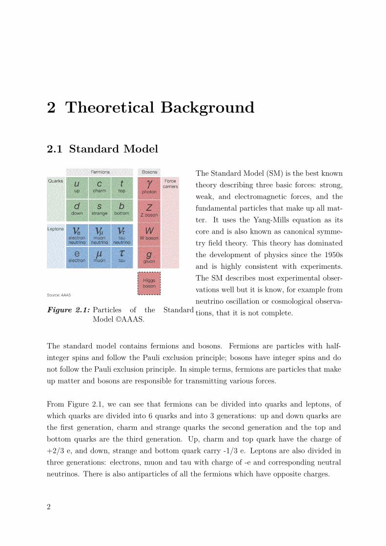
Figure 2.1: Particles of the StandardModel ©AAAS.
The Standard Model (SM) is the best knowntheory describing three basic forces: strong,weak, and electromagnetic forces, and thefundamental particles that make up all mat-ter. It uses the Yang-Mills equation as itscore and is also known as canonical symme-try field theory. This theory has dominatedthe development of physics since the 1950sand is highly consistent with experiments.The SM describes most experimental obser-vations well but it is know, for example fromneutrino oscillation or cosmological observa-tions, that it is not complete.
The standard model contains fermions and bosons. Fermions are particles with half-integer spins and follow the Pauli exclusion principle; bosons have integer spins and donot follow the Pauli exclusion principle. In simple terms, fermions are particles that makeup matter and bosons are responsible for transmitting various forces.
From Figure 2.1, we can see that fermions can be divided into quarks and leptons, ofwhich quarks are divided into 6 quarks and into 3 generations: up and down quarks arethe first generation, charm and strange quarks the second generation and the top andbottom quarks are the third generation. Up, charm and top quark have the charge of+2/3 e, and down, strange and bottom quark carry -1/3 e. Leptons are also divided inthree generations: electrons, muon and tau with charge of -e and corresponding neutralneutrinos. There is also antiparticles of all the fermions which have opposite charges.
2
2.2 The Top Quark
Bosons are the particles which mediate forces between the fermions. Photons mediatethe electromagnetic force, gluons mediate the strong force, and Z bosons and W bosonsmediate the weak force. The higgs mechanism describes how particles obtain there massesby interacting with a so-called higgs-field. A consequence if this field is a scalaer bosons,the higgs-boson, which was discovered in 2012 by the ATLAS and CMS experiments atthe LHC.
2.2 The Top Quark
The top quark was discovered by the CDF and D0 experiments at Fermilab in 1995 [1][2]and is currently the heaviest known quark, its mass is 173.0 ± 0.4GeV [3]. Like otherquarks, top quarks belong to fermions, have a spin of 1
2 , and have a charge of +2/3 e.The top quark interacts with other elementary particles through the strong force. Thelife time of the top quark is very short, only 5 × 10⁻²⁵ s. Before it has the time to formhadrons, it decays into a W boson and a bottom quark through the weak force.
2.2.1 Top Quarks at the LHC
Because the mass of the top quark is very large, according to Einstein’s formula for massand energy, we know that higher mass requires higher energy. Thus, top quarks couldonly be produced at the Tevatron and the LHC till now by pair production via the stronginteraction or as single top quark via the weak interaction.
At the LHC top-quark pairs are usually produced by gluon fusion. Top quarks can alsobe produced via the weak interaction, which is related to W boson exchanges (s-channel,t-channel, Wt-channel).
Top quarks decay via the weak interaction, usually top quarks will decay into a W bosonand a bottom quark, after that the W boson would rapidly decay into lepton and neutrinoor quark and antiquark. When both W bosons decay into quarks, we could observe 6 jets(bb̄ quarks and quarks from W boson decay); when both W bosons decay into leptons andneutrinos, we could observe 2 jets (b quarks) with 2 charged leptons; when only one oftwo W bosons decays into lepton and neutrino while the other one decays into quark andantiquark, we could observe 4 jets (b quarks and quark antiquark from W boson decay)and 1 charged lepton. The resulting decay modes are summarized in Table 2.1.
3
2 Theoretical Background
jet lepton reaction
all jets 6 0 tt̄→ bb̄W+W− → bb̄q1q̄2q3q̄4
jets with lepton 4 1 tt̄→ bb̄W+W− → bb̄q1q̄2lv̄l / bb̄q1q̄2l̄vl
dilepton 2 2 tt̄→ bb̄W+W− → l1v̄l1 l̄2vl2
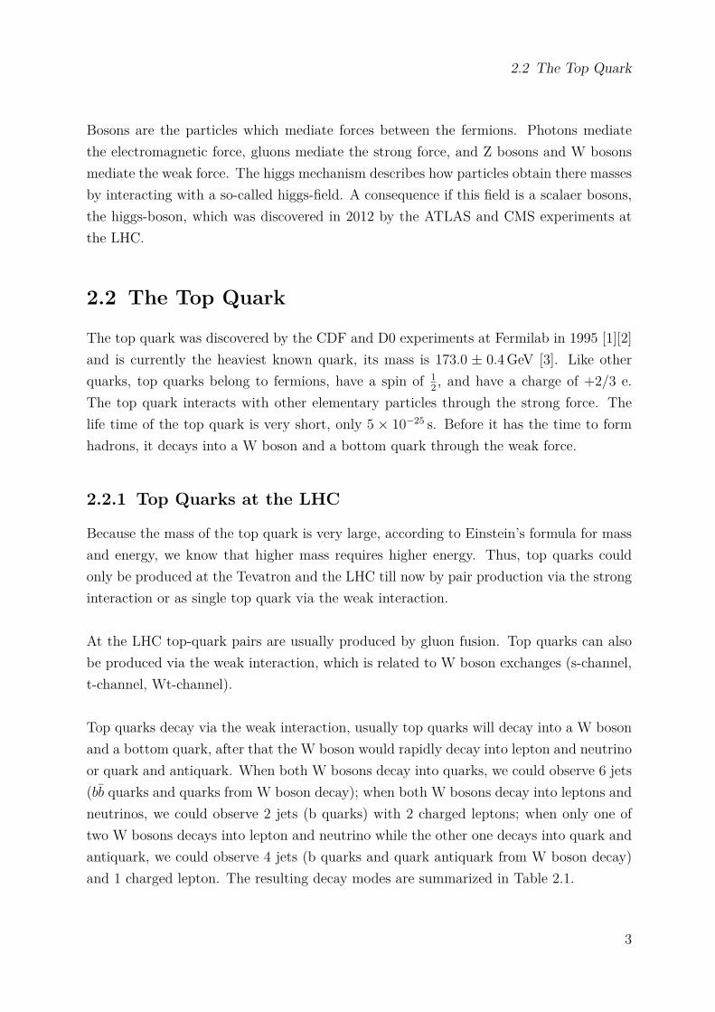
Table 2.1: Top quarks decays after pair production.
The predicted cross section of top quark pair production at the LHC at different ener-gies is given in Table 2.2 :
energy cross section√s= 7 TeV σtt̄ = 177.3+4.6+9.0
−6.0−9.0 pb
√s= 8 TeV σtt̄ = 252.9+6.4+11.5
−8.6−11.5 pb
√s= 13 TeV σtt̄ = 831.8+19.8+35.1
−29.2−35.1 pb
√s= 14 TeV σtt̄ = 984.5+23.2+41.3
−34.7−41.3 pb
Table 2.2: Cross section theoretical prediction for tt̄ pair production at the LHC assum-ing a top-quark mass of 172.5 GeV/c2 [4]
The measurement of the tt̄ production cross-section in the lepton+jets channel at√s=13
TeV with the ATLAS experiment using a data sample of L= 139 fb−1 yields σtt̄ =830± 0.4(stat.)+38.2
−37.0(syst.) pb [5].The systematic uncertainties are summarized in Table 2.3 [5]:
4
2.2 The Top Quark
Experimental luminosity, pile up, lepton identification,uncertainties reconstruction, isolation and trigger,
lepton momentum scale and resolution,jet energy scale, jet energy resolution,
jet-vertex-tagger(JVT) efficiency, flavour tagging,missing transverse energy scale and resolution
Signal top quark pT reweighting, scale uncertainties,modelling parton distribution functions(PDFs),
parton shower and hadronisation
Background multijet, single-top, W+jets,modelling other background processes
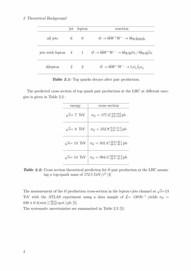
Table 2.3: Uncertainties of the cross section in tt̄ pair production at the LHC.
5

3 Experimental Setup
3.1 Detector
The 27 km long Large Hadron Collider (LHC) causes two beams of protons to collide. Eachbeam has an energy of 6.5 TeV. High-energy particles made by particle accelerators mustbe observed by particle detectors. In order to detect the phenomena produced, particledetector must be able to detect these particles and measure their mass, momentum,energy, charge, and spin. In order to identify each particle made by the collision at theinteraction point, the particle detectors must usually be designed in different layers eachdedicated for a specific purpose. Different types of detectors make up different detectionlayers, and each type of detector is specialized in detecting a specific type of particles.The information left by the particles in different detection layers can be used to confirmthe identity of the particles and accurately measure their energy and momentum. Therole of each detection layer in the detector will be discussed in Section 3.3. The size ofdetector is huge due to high resolution and multiplicity functions. At the LHC, ATLASis the largest particle detector with other detectors such as CMS, Alice and LHCb. Withtheir help, scientists successfully discovered the Higgs particle at the LHC in 2012.
3.2 ATLAS
The ATLAS (A Toroidal LHC ApparatuS) [6] detector is a multipurpose particle detectorwith a height of 25 m and a length of 44 m (see Figure 3.1). When a proton beam madeby the Large Hadron Collider (LHC) performs scattering experiments at the centre ofthe detector, many kinds of particles with different energies are generated. The ATLASdetector is not focused on a specific physical process. It is designed to detect a widerange of possible signals. ALTAS measure the deposited energies and tracks of the decayproducts1. The unique challenges faced by the Large Hadron Collider unprecedented highenergy and extremely high collision frequencies require ATLAS to be larger and morecomplex than previously built detectors.
1ATLAS can not measure neutrinos.
6
3.3 ALTAS detector
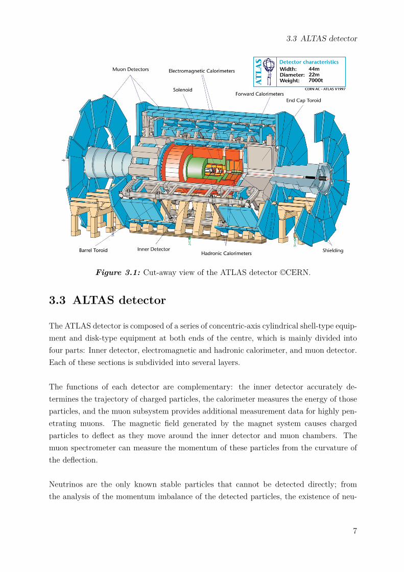
Figure 3.1: Cut-away view of the ATLAS detector ©CERN.
3.3 ALTAS detector
The ATLAS detector is composed of a series of concentric-axis cylindrical shell-type equip-ment and disk-type equipment at both ends of the centre, which is mainly divided intofour parts: Inner detector, electromagnetic and hadronic calorimeter, and muon detector.Each of these sections is subdivided into several layers.
The functions of each detector are complementary: the inner detector accurately de-termines the trajectory of charged particles, the calorimeter measures the energy of thoseparticles, and the muon subsystem provides additional measurement data for highly pen-etrating muons. The magnetic field generated by the magnet system causes chargedparticles to deflect as they move around the inner detector and muon chambers. Themuon spectrometer can measure the momentum of these particles from the curvature ofthe deflection.
Neutrinos are the only known stable particles that cannot be detected directly; fromthe analysis of the momentum imbalance of the detected particles, the existence of neu-
7
3 Experimental Setup
trinos can be inferred. In order to achieve the above goals, the detector must be a 4πdetector, i.e. all particles except neutrinos must be detected to avoid any detection blindspots.
3.3.1 Inner Detector
By detecting the interaction of scattered charged particles with materials at differentpositions, the movement of these particles can be tracked. Because the inner detector[6] is immersed in a 2 Tesla magnetic field, the charged particles moving in its space willbe deflected, its direction shows the electrical properties of the charged particles, and itsangle shows the momentum of the particles. The starting point of the trajectory canprovide useful information for particle identification. For example, if the initial point of aseries of particle trajectories is not the collision point of protons, this indicates that theseparticles originate from the decay of a bottom quark. The inner detector has three parts,which will be explained in detail below.
Pixel Detector
The pixel detector is the innermost part of the detector. Four precise positions can begiven for each particle trajectory. The pixel detector has a total of more than 100 milliondata readout channels.
Semi Conductor Tracker
The Semiconductor Tracker (SCT) is the middle part of the inner detector. It can give atleast four precise positions for each particle trajectory. In contrast to the pixel detector,the SCT uses silicon strips to measure particle trajectories.
Transition Radiation Tracker
The Transition Radiation Tracker (TRT) is the outermost part of the inner detector. It is acombination of a straw tracker and a transition radiation detector. Transitional radiationtrackers have two main functions: Accurately track charged particles and correctly identifyelectrons. Each straw is filled with a Xenon gas mixture, and when the charged particlespass through, the gas mixture is ionised and the straw generates a current pulse (signal).By analysing the patterns formed by these pulsed wires, the trajectory of ion movementcan be determined.
8

3.3 ALTAS detector
3.3.2 Calorimeter
The solenoid carrying the current is placed outside the inner detector, and the calorimeter[6] is located outside the solenoid. The purpose of the calorimeter is to measure the energyof the particles by absorbing them. There are two basic types of calorimetric systems:the Electromagnetic Calorimeter is the inner calorimeter and the Hadron Calorimeter isthe outer one (see Figure 3.1). Both are sampling calorimeters.
In a sampling calorimeter, the material that absorbs the particle energy to generate aparticle shower is different from the material that measures the shower energy and isseparated in different areas.
Electromagnetic Calorimeter
An electromagnetic calorimeter absorbs energy from particles involved in electromagneticinteractions. This includes elecctrons and photons. The material used to absorb theenergy to generate the particle shower is lead and stainless steel, and the material for thesampling layers is liquid Argon.
Hadron Calorimeter
Particles that do not loose a significant amount of enegry in the electromagnetic calorimter,mostly hadrons, will interact in the hadronic calorimeter. The Hadron calorimeter usescopper and tungsten as absorbers, the sampling material is steel.
3.3.3 Muon Detector
The muon spectrometer works similarly to the inner detector, the momentum of muonscan be determined by the muon trajectory deflected by the magnetic field. This is impor-tant for the accurate measurement of the total momentum and analysis of neutrino-relateddata.
The muon spectrometer is used in the trigger system, which selects a pre-defined choiceof events of interest which is motivated by physics arguments.
3.3.4 Data processing analysis system
Detectors can generate massive amounts of data that are difficult to store, the triggersystem uses simple information to identify those interesting events in real time and retain
9

3 Experimental Setup
their information for detailed analysis. All events that are permanently stored will bereconstructed offline, which will regularly convert the signals obtained by the detectorinto physical objects, such as jets, photons and leptons.
10

4 Introduction to top quark analysis
At the LHC experiments, a lot of data is obtained by many different processes. Within thedetectors, only the final state products, such as the final decay products of a top-quark,are observed. These have to be reconstructed to gain insight of the initial productionprocess. In general, the following approach is being used: first use computer simulationsto generate artificial events and then compare the measured events to the simulation toinfer the process.
The analytical solution are unavailable to make predictions for the hard scattering processso numerical integration is required. However, Newton or Gaussian integration can onlydeal with a small number of final states, therefore numerical sampling of Monte Carloevents are used as experimental predictions based on the event probability distribution.
4.1 Monte Carlo simulation
Almost all analyses of the LHC are using event generators. In these predictions, a fixed-order of the matrix element is used, and a consistent matching or merging is performedbetween the matrix element and the parton shower contribution. The components of thisprediction are based on approximations, so it is necessary to estimate their reliability,which is part of this thesis.
For a fixed order (matrix elements), the uncertainty estimate comes from changing thecommon factorisation (µF ) and renormalisation (µR) scales, an additional uncertaintycomes from the choice of the parton distribution function (PDF)1. Uncertainties in otherparts of the prediction (such as parton showers, multi parton interactions and hadroni-sation) are difficult to estimate and require tuning of the used shower and hadronisation
1Parton distribution function (PDF) describes probability density for finding a particle with a certainlongitudinal momentum fraction at resolution scales.
11
4 Introduction to top quark analysis
algorithms (see also Signal Modelling in Table 2.3).
To estimate systematic uncertainties on the modelling in an analysis, a set of MC sam-ples with varied parameters is used to make new predictions for the process under study.Because each of these new simulations makes a different particle-level prediction, eachgenerated event must pass a detector simulation which is computationally time consum-ing. Some uncertainties like the one on µR and µF can already be estimated using are-weighting of the nominal MC simulation.
A new approach to estimate systematic uncertainties on the scale choice in the genertionof MC events has recently been developed [7]. The uncertainties are estimated by re-weighting the nominal MC simulation. For each generated event, a vector of alternativeweights is provided for the uncertainty variations. The estimation of modelling uncer-tainties via reweighting is computationaly less expensive than generating new samples foreach uncertainty. For the first time, the scale uncertainties are correlated between partonshower and PDF. The re-weighting also preserves the physical splittings in the partonshower and the total cross section.
4.2 Monte Carlo samples
The studies presented in this thesis focus on tt̄ MC samples and the systematic uncertain-ties due to variations of the parton shower. The generator is Powheg+Pythia8: Powhegis used for the matrix element, Pythia8 for the showering and hadronisation.
The old approach to evaluate scale uncertainties was, to make just individual changesof Var3c for intial state radiation (ISR) and αS for final state radiation (FSR).
The new approach is to use kernel splitting weights, i.e. each splitting in the showeris evaluated for changes in αF SR
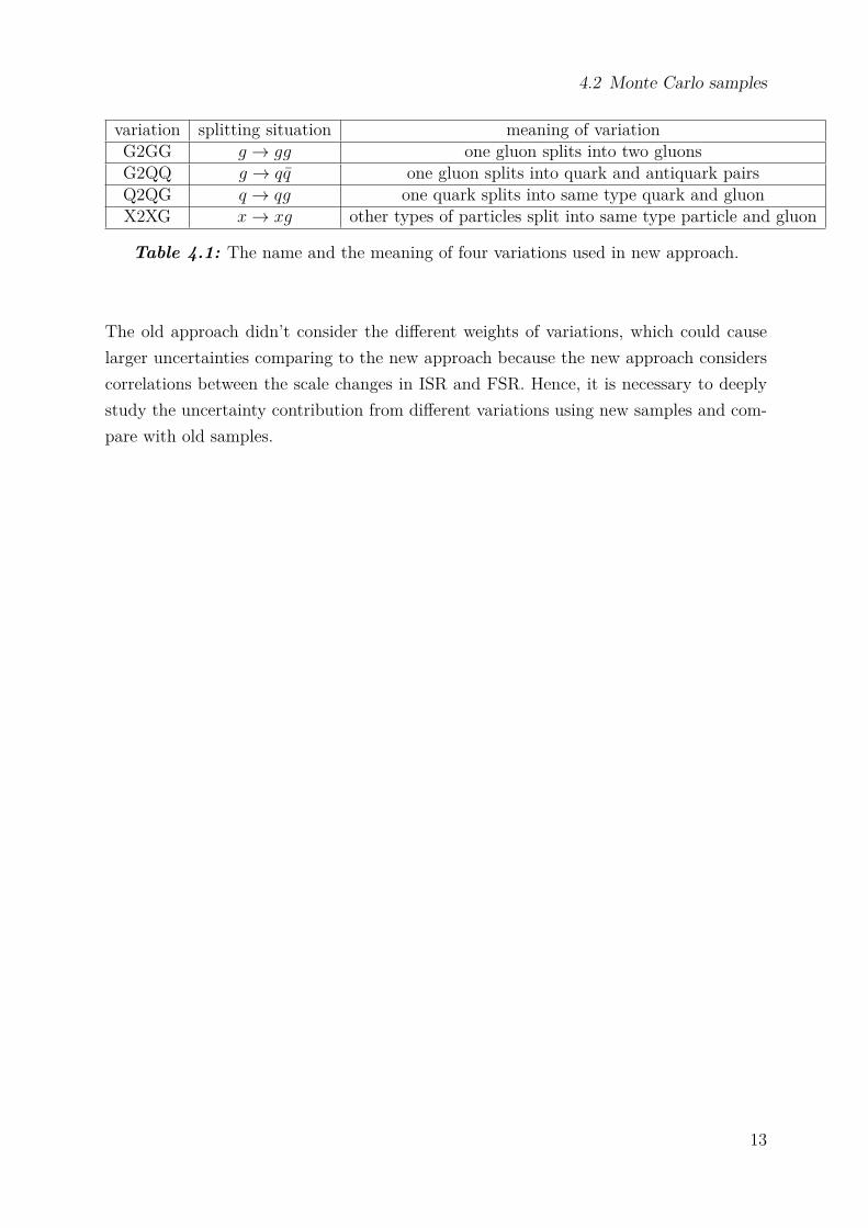
S (strong coupling constant). This is done for each kind ofsplitting individually. During the splitting four variations are used to separate differentsplitting situations. Table 4.1 shows the four variations and the meaning of them.
in particular, the meaning of X in X2XG is that the bottom quark or top quark since thenumber of flavours have been adjusted to be included in Q (u/d/s/c) to be 4 rather than5. Therefore X2XG could be simply considered as a gluon bremsstrahlung off bottomquark or top quark.
12
4.2 Monte Carlo samples
variation splitting situation meaning of variationG2GG g → gg one gluon splits into two gluonsG2QQ g → qq̄ one gluon splits into quark and antiquark pairsQ2QG q → qg one quark splits into same type quark and gluonX2XG x→ xg other types of particles split into same type particle and gluon
Table 4.1: The name and the meaning of four variations used in new approach.
The old approach didn’t consider the different weights of variations, which could causelarger uncertainties comparing to the new approach because the new approach considerscorrelations between the scale changes in ISR and FSR. Hence, it is necessary to deeplystudy the uncertainty contribution from different variations using new samples and com-pare with old samples.
13
5 Comparison between the FSR andISR uncertainties estimation inold and new approach
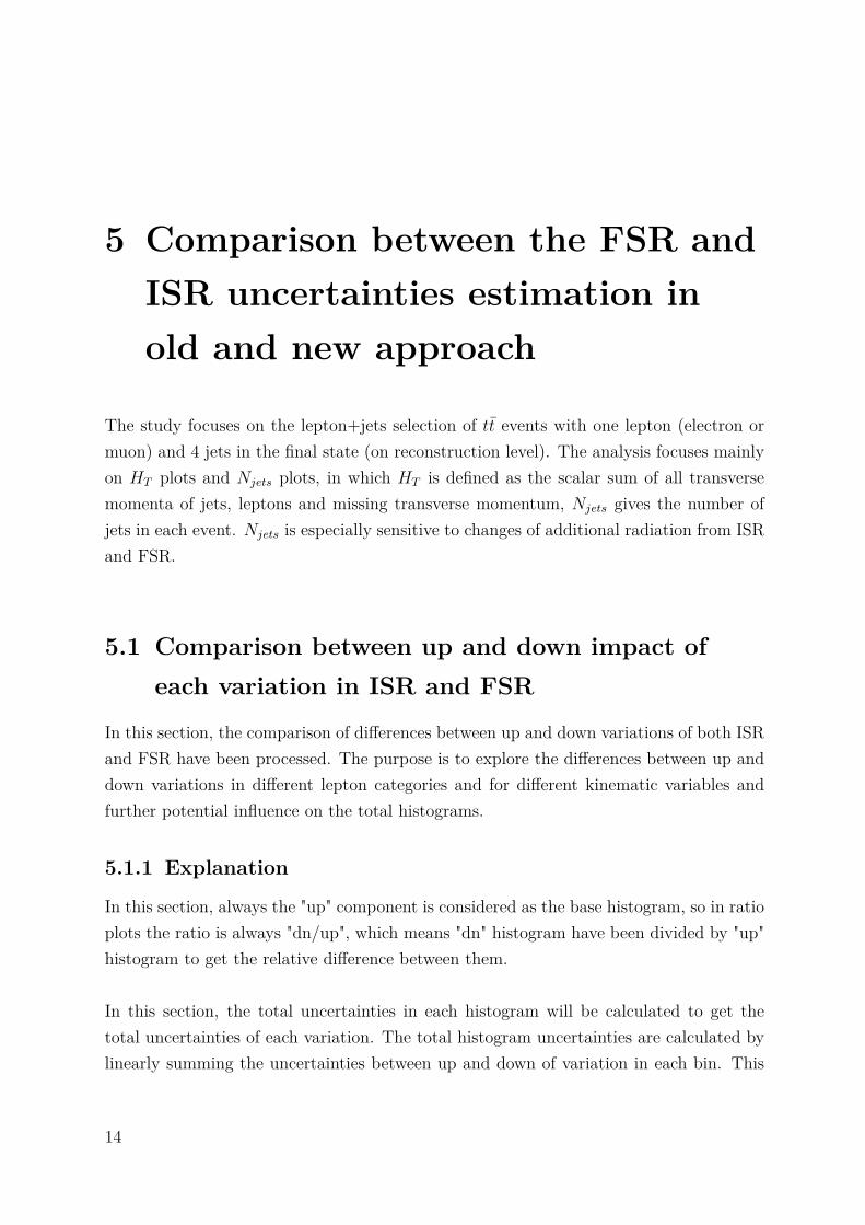
The study focuses on the lepton+jets selection of tt̄ events with one lepton (electron ormuon) and 4 jets in the final state (on reconstruction level). The analysis focuses mainlyon HT plots and Njets plots, in which HT is defined as the scalar sum of all transversemomenta of jets, leptons and missing transverse momentum, Njets gives the number ofjets in each event. Njets is especially sensitive to changes of additional radiation from ISRand FSR.
5.1 Comparison between up and down impact ofeach variation in ISR and FSR
In this section, the comparison of differences between up and down variations of both ISRand FSR have been processed. The purpose is to explore the differences between up anddown variations in different lepton categories and for different kinematic variables andfurther potential influence on the total histograms.
5.1.1 Explanation
In this section, always the "up" component is considered as the base histogram, so in ratioplots the ratio is always "dn/up", which means "dn" histogram have been divided by "up"histogram to get the relative difference between them.
In this section, the total uncertainties in each histogram will be calculated to get thetotal uncertainties of each variation. The total histogram uncertainties are calculated bylinearly summing the uncertainties between up and down of variation in each bin. This
14

5.1 Comparison between up and down impact of each variation in ISR and FSR
is shown at the legend of each plot as " histo total uncertainty ".During the calculation selections should also be made because for some bins only "up"or "down" exist, in this case the bin should be selected out of calculation otherwise theuncertainty of this bin is not the difference between "up" and "down", but the bin contentof "up" or "down". Then the uncertainty would increase giantly.
In this section, the ratio total uncertainties will also be calculated to get the relativeuncertainties of the ratio plots. The ratio total uncertainties are calculated by adding theuncertainties between up and down of each bin in quadrature and are then divided by thetotal number of bins. This is shown at the legend of each plot as "ratio total uncertainty".
Because for different variation the ratio of "dn/up" is different, so for a certain ratiorange some plots could be out of range, while the others do not show much variation inthis certain range. Therefore, 3 ratio ranges are selected for both large and small uncer-tainties, i.e. [0.9:1.1] , [0.95:1.05], [0.99:1.01]. These three ratio ranges are used in orderto take into consideration the spread of the ratio down/up values of different variations,and to make the plots more meaningful.
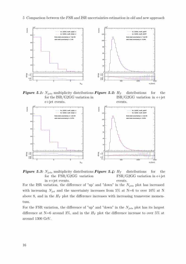
5.1.2 HT and Njets multiplicity distributions for individualvariations of both ISR and FSR for single electron
Electron-G2GG
Here the Njets and HT comparison of G2GG variations between up and down in the singleelectron channel for ISR and FSR is shown:
15
5 Comparison between the FSR and ISR uncertainties estimation in old and new approach
100
200
300
400
500
310×E
vent
s
isr_G2GG_muR_up/jet_n
isr_G2GG_muR_dn/jet_n
histo total uncertainty is 7.4e+03
ratio total uncertainty is 1.4%
4 6 8
jetsN
0.90.95
11.05
1.1
dn/u
p
Figure 5.1: Njets multiplicity distributionsfor the ISR/G2GG variation ine+jet events.
0
20
40
60
80
100
120
310×
Eve
nts
isr_G2GG_muR_up/HT
isr_G2GG_muR_dn/HT
histo total uncertainty is 7.4e+03
ratio total uncertainty is 0.19%
0 500 1000 1500
/[GeV]TH
0.960.98
11.021.04
dn/u
p
Figure 5.2: HT distributions for theISR/G2GG variation in e+jetevents.
100
200
300
400
500
310×
Eve
nts
fsr_G2GG_muR_up/jet_n
fsr_G2GG_muR_dn/jet_n
histo total uncertainty is 1.3e+04
ratio total uncertainty is 0.37%
4 6 8
jetsN
0.960.98
11.021.04
dn/u
p
Figure 5.3: Njets multiplicity distributionsfor the FSR/G2GG variationin e+jet events.
0
20
40
60
80
100
120
310×
Eve
nts
fsr_G2GG_muR_up/HT
fsr_G2GG_muR_dn/HT
histo total uncertainty is 1.3e+04
ratio total uncertainty is 0.22%
0 500 1000 1500
/[GeV]TH
0.90.95
11.05
1.1
dn/u
p
Figure 5.4: HT distributions for theFSR/G2GG variation in e+jetevents.
For the ISR variation, the difference of "up’ and "down" in the Njets plot has increasedwith increasing Njet and the uncertainty increases from 5% at N=6 to over 10% at Nabove 8, and in the HT plot the difference increases with increasing transverse momen-tum.For the FSR variation, the difference of "up" and "down" in the Njets plot has its largestdifference at N=6 around 3%, and in the HT plot the difference increase to over 5% ataround 1300 GeV.
16

5.1 Comparison between up and down impact of each variation in ISR and FSR
Electron-G2QQ
Here the Njets and HT comparison of G2QQ variations between up and down in the singleelectron channel for ISR and FSR is shown:
100
200
300
400
500
310×
Eve
nts
isr_G2QQ_muR_up/jet_n
isr_G2QQ_muR_dn/jet_n
histo total uncertainty is 7.2e+02
ratio total uncertainty is 0.11%
4 6 8
jetsN
0.990.995
11.005
1.01
dn/u
p
Figure 5.5: Njets multiplicity distributionsfor the ISR/G2QQ variation ine+jet events.
0
20
40
60
80
100
120
310×
Eve
nts
isr_G2QQ_muR_up/HT
isr_G2QQ_muR_dn/HT
histo total uncertainty is 7.2e+02
ratio total uncertainty is 0.025%
0 500 1000 1500
/[GeV]TH
0.990.995
11.005
1.01
dn/u
p
Figure 5.6: HT distributions for theISR/G2QQ variation in e+jetevents.
100
200
300
400
500
310×
Eve
nts
fsr_G2QQ_muR_up/jet_n
fsr_G2QQ_muR_dn/jet_n
histo total uncertainty is 9.3e+03
ratio total uncertainty is 0.69%
4 6 8
jetsN
0.90.95
11.05
1.1
dn/u
p
Figure 5.7: Njets multiplicity distributionsfor the FSR/G2QQ variationin e+jet events.
0
20
40
60
80
100
120
310×
Eve
nts
fsr_G2QQ_muR_up/HT
fsr_G2QQ_muR_dn/HT
histo total uncertainty is 9.3e+03
ratio total uncertainty is 0.18%
0 500 1000 1500
/[GeV]TH
0.960.98
11.021.04
dn/u
p
Figure 5.8: HT distributions for theFSR/G2QQ variation in e+jetevents.
For the ISR variation, the difference of "up’ and "down" in the Njets plot has increasedas N increases and reaches 1% at N=9. And in the HT plot the differences are relativelysmall, most below 0.5%.For the FSR variation, the difference of "up" and "down" in the Njets plot has increasedwith increasing N and reach around 6% at N=9, and in theHT plot the difference increases
17
5 Comparison between the FSR and ISR uncertainties estimation in old and new approach
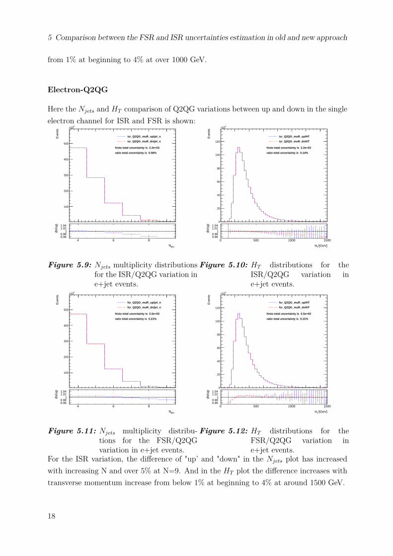
from 1% at beginning to 4% at over 1000 GeV.
Electron-Q2QG
Here the Njets and HT comparison of Q2QG variations between up and down in the singleelectron channel for ISR and FSR is shown:
100
200
300
400
500
310×
Eve
nts
isr_Q2QG_muR_up/jet_n
isr_Q2QG_muR_dn/jet_n
histo total uncertainty is 2.2e+03
ratio total uncertainty is 0.56%
4 6 8
jetsN
0.960.98
11.021.04
dn/u
p
Figure 5.9: Njets multiplicity distributionsfor the ISR/Q2QG variation ine+jet events.
0
20
40
60
80
100
120
310×
Eve
nts
isr_Q2QG_muR_up/HT
isr_Q2QG_muR_dn/HT
histo total uncertainty is 2.2e+03
ratio total uncertainty is 0.14%
0 500 1000 1500
/[GeV]TH
0.960.98
11.021.04
dn/u
p
Figure 5.10: HT distributions for theISR/Q2QG variation ine+jet events.
100
200
300
400
500
310×
Eve
nts
fsr_Q2QG_muR_up/jet_n
fsr_Q2QG_muR_dn/jet_n
histo total uncertainty is 5.5e+03
ratio total uncertainty is 0.21%
4 6 8
jetsN
0.960.98
11.021.04
dn/u
p
Figure 5.11: Njets multiplicity distribu-tions for the FSR/Q2QGvariation in e+jet events.
0
20
40
60
80
100
120
310×
Eve
nts
fsr_Q2QG_muR_up/HT
fsr_Q2QG_muR_dn/HT
histo total uncertainty is 5.5e+03
ratio total uncertainty is 0.11%
0 500 1000 1500
/[GeV]TH
0.960.98
11.021.04
dn/u
p
Figure 5.12: HT distributions for theFSR/Q2QG variation ine+jet events.
For the ISR variation, the difference of "up’ and "down" in the Njets plot has increasedwith increasing N and over 5% at N=9. And in the HT plot the difference increases withtransverse momentum increase from below 1% at beginning to 4% at around 1500 GeV.
18
5.1 Comparison between up and down impact of each variation in ISR and FSR
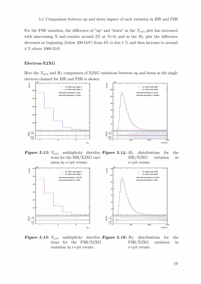
For the FSR variation, the difference of "up" and "down" in the Njets plot has increasedwith nincreasing N and reaches around 2% at N=9, and in the HT plot the differencedecreases at beginning (below 200 GeV) from 4% to less 1 % and then increase to around4 % above 1000 GeV.
Electron-X2XG
Here the Njets and HT comparison of X2XG variations between up and down in the singleelectron channel for ISR and FSR is shown:
100
200
300
400
500
310×
Eve
nts
isr_X2XG_muR_up/jet_n
isr_X2XG_muR_dn/jet_n
histo total uncertainty is 4e+02
ratio total uncertainty is 0.034%
4 6 8
jetsN
0.990.995
11.005
1.01
dn/u
p
Figure 5.13: Njets multiplicity distribu-tions for the ISR/X2XG vari-ation in e+jet events.
0
20
40
60
80
100
120
310×
Eve
nts
isr_X2XG_muR_up/HT
isr_X2XG_muR_dn/HT
histo total uncertainty is 4e+02
ratio total uncertainty is 0.0082%
0 500 1000 1500
/[GeV]TH
0.990.995
11.005
1.01
dn/u
p
Figure 5.14: HT distributions for theISR/X2XG variation ine+jet events.
100
200
300
400
500
600
310×
Eve
nts
fsr_X2XG_muR_up/jet_n
fsr_X2XG_muR_dn/jet_n
histo total uncertainty is 5.6e+04
ratio total uncertainty is 0.99%
4 6 8
jetsN
0.90.95
11.05
1.1
dn/u
p
Figure 5.15: Njets multiplicity distribu-tions for the FSR/X2XGvariation in e+jet events.
0
20
40
60
80
100
120
140
310×
Eve
nts
fsr_X2XG_muR_up/HT
fsr_X2XG_muR_dn/HT
histo total uncertainty is 5.6e+04
ratio total uncertainty is 0.39%
0 500 1000 1500
/[GeV]TH
0.90.95
11.05
1.1
dn/u
p
Figure 5.16: HT distributions for theFSR/X2XG variation ine+jet events.
19
5 Comparison between the FSR and ISR uncertainties estimation in old and new approach
For the ISR variation, the difference of "up’ and "down" in both the Njets and the HT plotare extremely small that they do not show any uncertainties. Both of the uncertaintiesare below 0.2%.In FSR, the difference of "up" and "down" in the Njets plot has decreased with increasingN from 8% at N=4 to 2% at N=9, and in the HT plot the difference rapidly increases to7% around 200 GeV and are stable above 5% until 1500 GeV.
5.1.3 HT and Njets multiplicity distributions for individualvariations of both ISR and FSR for single muon
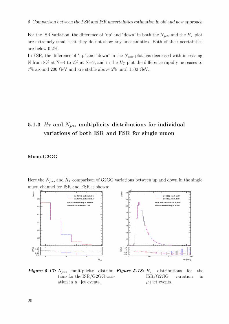
Muon-G2GG
Here the Njets and HT comparison of G2GG variations between up and down in the singlemuon channel for ISR and FSR is shown:
100
200
300
400
500
600
310×
Eve
nts
isr_G2GG_muR_up/jet_n
isr_G2GG_muR_dn/jet_n
histo total uncertainty is 6.8e+03
ratio total uncertainty is 1.4%
4 6 8
jetsN
0.90.95
11.05
1.1
dn/u
p
Figure 5.17: Njets multiplicity distribu-tions for the ISR/G2GG vari-ation in µ+jet events.
0
20
40
60
80
100
120
140
160
310×
Eve
nts
isr_G2GG_muR_up/HT
isr_G2GG_muR_dn/HT
histo total uncertainty is 6.8e+03
ratio total uncertainty is 0.17%
0 500 1000 1500
/[GeV]TH
0.960.98
11.021.04
dn/u
p
Figure 5.18: HT distributions for theISR/G2GG variation inµ+jet events.
20
5.1 Comparison between up and down impact of each variation in ISR and FSR
100
200
300
400
500
600
310×E
vent
s
fsr_G2GG_muR_up/jet_n
fsr_G2GG_muR_dn/jet_n
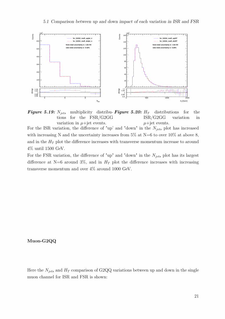
histo total uncertainty is 1.8e+04
ratio total uncertainty is 0.42%
4 6 8
jetsN
0.960.98
11.021.04
dn/u
p
Figure 5.19: Njets multiplicity distribu-tions for the FSR/G2GGvariation in µ+jet events.
0
20
40
60
80
100
120
140
160
310×
Eve
nts
fsr_G2GG_muR_up/HT
fsr_G2GG_muR_dn/HT
histo total uncertainty is 1.8e+04
ratio total uncertainty is 0.26%
0 500 1000 1500
/[GeV]TH
0.90.95
11.05
1.1
dn/u
p
Figure 5.20: HT distributions for theISR/G2GG variation inµ+jet events.
For the ISR variation, the difference of "up’ and "down" in the Njets plot has increasedwith increasing N and the uncertainty increases from 5% at N=6 to over 10% at above 8,and in the HT plot the difference increases with transverse momentum increase to around4% until 1500 GeV.For the FSR variation, the difference of "up" and "down" in the Njets plot has its largestdifference at N=6 around 3%, and in HT plot the difference increases with increasingtransverse momentum and over 4% around 1000 GeV.
Muon-G2QQ
Here the Njets and HT comparison of G2QQ variations between up and down in the singlemuon channel for ISR and FSR is shown:
21

5 Comparison between the FSR and ISR uncertainties estimation in old and new approach
100
200
300
400
500
600
310×E
vent
s
isr_G2QQ_muR_up/jet_n
isr_G2QQ_muR_dn/jet_n
histo total uncertainty is 6.8e+02
ratio total uncertainty is 0.091%
4 6 8
jetsN
0.990.995
11.005
1.01
dn/u
p
Figure 5.21: Njets multiplicity distribu-tions for the ISR/G2QQ vari-ation in µ+jet events.
0
20
40
60
80
100
120
140
160
310×
Eve
nts
isr_G2QQ_muR_up/HT
isr_G2QQ_muR_dn/HT
histo total uncertainty is 6.8e+02
ratio total uncertainty is 0.021%
0 500 1000 1500
/[GeV]TH
0.990.995
11.005
1.01
dn/u
p
Figure 5.22: HT distributions for theISR/G2QQ variation inµ+jet events.
100
200
300
400
500
600
310×
Eve
nts
fsr_G2QQ_muR_up/jet_n
fsr_G2QQ_muR_dn/jet_n
histo total uncertainty is 1e+04
ratio total uncertainty is 0.75%
4 6 8
jetsN
0.90.95
11.05
1.1
dn/u
p
Figure 5.23: Njets multiplicity distribu-tions for the FSR/G2QQvariation in µ+jet events.
0
20
40
60
80
100
120
140
160
310×
Eve
nts
fsr_G2QQ_muR_up/HT
fsr_G2QQ_muR_dn/HT
histo total uncertainty is 1e+04
ratio total uncertainty is 0.18%
0 500 1000 1500
/[GeV]TH
0.960.98
11.021.04
dn/u
p
Figure 5.24: HT distributions for theFSR/G2QQ variation inµ+jet events.
For the ISR variation, the difference of "up’ and "down" in the Njets plot has increased asN increases and around 0.8% at N=9. And in the HT plot the differences are relativelysmall, i.e. below 0.5%.For the FSR variation, the difference of "up" and "down" in the Njets plot has increasedwith increasing N and over 5% at N=9, and in the HT plot the differences increase from1% at beginning to 5% at over 1000 GeV.
22
5.1 Comparison between up and down impact of each variation in ISR and FSR
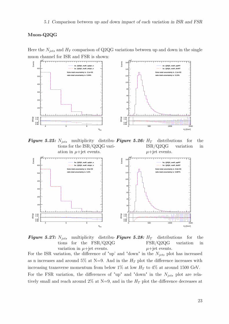
Muon-Q2QG
Here the Njets and HT comparison of Q2QG variations between up and down in the singlemuon channel for ISR and FSR is shown:
100
200
300
400
500
600
310×
Eve
nts
isr_Q2QG_muR_up/jet_n
isr_Q2QG_muR_dn/jet_n
histo total uncertainty is 2.1e+03
ratio total uncertainty is 0.54%
4 6 8
jetsN
0.960.98
11.021.04
dn/u
p
Figure 5.25: Njets multiplicity distribu-tions for the ISR/Q2QG vari-ation in µ+jet events.
0
20
40
60
80
100
120
140
160
310×
Eve
nts
isr_Q2QG_muR_up/HT
isr_Q2QG_muR_dn/HT
histo total uncertainty is 2.1e+03
ratio total uncertainty is 0.13%
0 500 1000 1500
/[GeV]TH
0.960.98
11.021.04
dn/u
p
Figure 5.26: HT distributions for theISR/Q2QG variation inµ+jet events.
100
200
300
400
500
600
310×
Eve
nts
fsr_Q2QG_muR_up/jet_n
fsr_Q2QG_muR_dn/jet_n
histo total uncertainty is 6.6e+03
ratio total uncertainty is 0.2%
4 6 8
jetsN
0.960.98
11.021.04
dn/u
p
Figure 5.27: Njets multiplicity distribu-tions for the FSR/Q2QGvariation in µ+jet events.
0
20
40
60
80
100
120
140
160
310×
Eve
nts
fsr_Q2QG_muR_up/HT
fsr_Q2QG_muR_dn/HT
histo total uncertainty is 6.6e+03
ratio total uncertainty is 0.087%
0 500 1000 1500
/[GeV]TH
0.960.98
11.021.04
dn/u
p
Figure 5.28: HT distributions for theFSR/Q2QG variation inµ+jet events.
For the ISR variation, the difference of "up’ and "down" in the Njets plot has increasedas n increases and around 5% at N=9. And in the HT plot the difference increases withincreasing transverse momentum from below 1% at low HT to 4% at around 1500 GeV.For the FSR variation, the differences of "up" and "down" in the Njets plot are rela-tively small and reach around 2% at N=9, and in the HT plot the difference decreases at
23
5 Comparison between the FSR and ISR uncertainties estimation in old and new approach
HT < 200 GeV from 4% to less 1 % and then increases to around 2 % at above 1000 GeV.
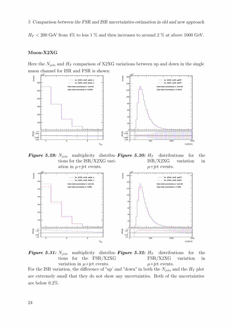
Muon-X2XG
Here the Njets and HT comparison of X2XG variations between up and down in the singlemuon channel for ISR and FSR is shown:
100
200
300
400
500
600
310×
Eve
nts
isr_X2XG_muR_up/jet_n
isr_X2XG_muR_dn/jet_n
histo total uncertainty is 4.3e+02
ratio total uncertainty is 0.033%
4 6 8
jetsN
0.990.995
11.005
1.01
dn/u
p
Figure 5.29: Njets multiplicity distribu-tions for the ISR/X2XG vari-ation in µ+jet events.
0
20
40
60
80
100
120
140
160
310×
Eve
nts
isr_X2XG_muR_up/HT
isr_X2XG_muR_dn/HT
histo total uncertainty is 4.3e+02
ratio total uncertainty is 0.011%
0 500 1000 1500
/[GeV]TH
0.990.995
11.005
1.01
dn/u
p
Figure 5.30: HT distributions for theISR/X2XG variation inµ+jet events.
100
200
300
400
500
600
700310×
Eve
nts
fsr_X2XG_muR_up/jet_n
fsr_X2XG_muR_dn/jet_n
histo total uncertainty is 6.4e+04
ratio total uncertainty is 0.98%
4 6 8
jetsN
0.90.95
11.05
1.1
dn/u
p
Figure 5.31: Njets multiplicity distribu-tions for the FSR/X2XGvariation in µ+jet events.
0
20
40
60
80
100
120
140
160
310×
Eve
nts
fsr_X2XG_muR_up/HT
fsr_X2XG_muR_dn/HT
histo total uncertainty is 6.4e+04
ratio total uncertainty is 0.39%
0 500 1000 1500
/[GeV]TH
0.90.95
11.05
1.1
dn/u
p
Figure 5.32: HT distributions for theFSR/X2XG variation inµ+jet events.
For the ISR variation, the difference of "up’ and "down" in both the Njets and the HT plotare extremely small that they do not show any uncertainties. Both of the uncertaintiesare below 0.2%.
24

5.1 Comparison between up and down impact of each variation in ISR and FSR
For the FSR variation, the difference of "up" and "down" in the Njets plot has decreasedwith increasing N from 8% at N=4 to 2% at N=9, and in the HT plot the differencerapidly increases at beginning to 7% at around 1200 GeV and are stable above 5% atuntil 1500 GeV.
5.1.4 Discussion
The maximal uncertainties between up and down in both Njets and HT plots of 4 varia-tions of ISR and FSR in e+jet event and µ+jet event are summarised in Table 5.1.
variation e+jet Njets plot µ+jet Njets plot e+jet HT plot µ+jet HT plotISR-G2GG over 10% over 10% around 4% around 4%FSR-G2GG under 3% around 3% over 5% over 4%ISR-G2QQ under 1% around 0.8% under 0.5% under 0.5%FSR-G2QQ around 6% over 5% around 4% around 5%ISR-Q2QG over 5% around 5% around 4% around 4%FSR-Q2QG around 2% around 2% around 4% around 2%ISR-X2XG around 0.2% around 0.2% under 0.2% under 0.2%FSR-X2XG around 8% around 8% above 5% above 5%
Table 5.1: Summarising table of maximal uncertainties between up and down of eachvariation of ISR and FSR in e+jet or µ+jet events.
Comparing the uncertainties in e+jet and µ+jet events at same variation and also theshape of them in plots, it can be concluded that in general single electron and single muonevents have similar shape for both Njets and HT plots for ISR and FSR variation. Theuncertainties of them do not differ too much. So electron and muon could be included assingle lepton in the analysis.
This section shows how the difference between "up" and "down" single lepton is related todifferent jet multiplicity and to the transverse momentum of jets. To get which variationhas contributed the most uncertainties to the total part, it is required to compare between4 variations.
25
5 Comparison between the FSR and ISR uncertainties estimation in old and new approach
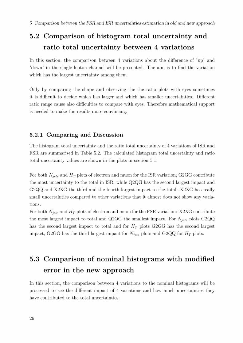
5.2 Comparison of histogram total uncertainty andratio total uncertainty between 4 variations
In this section, the comparison between 4 variations about the difference of "up" and"down" in the single lepton channel will be presented. The aim is to find the variationwhich has the largest uncertainty among them.
Only by comparing the shape and observing the the ratio plots with eyes sometimesit is difficult to decide which has larger and which has smaller uncertainties. Differentratio range cause also difficulties to compare with eyes. Therefore mathematical supportis needed to make the results more convincing.
5.2.1 Comparing and Discussion
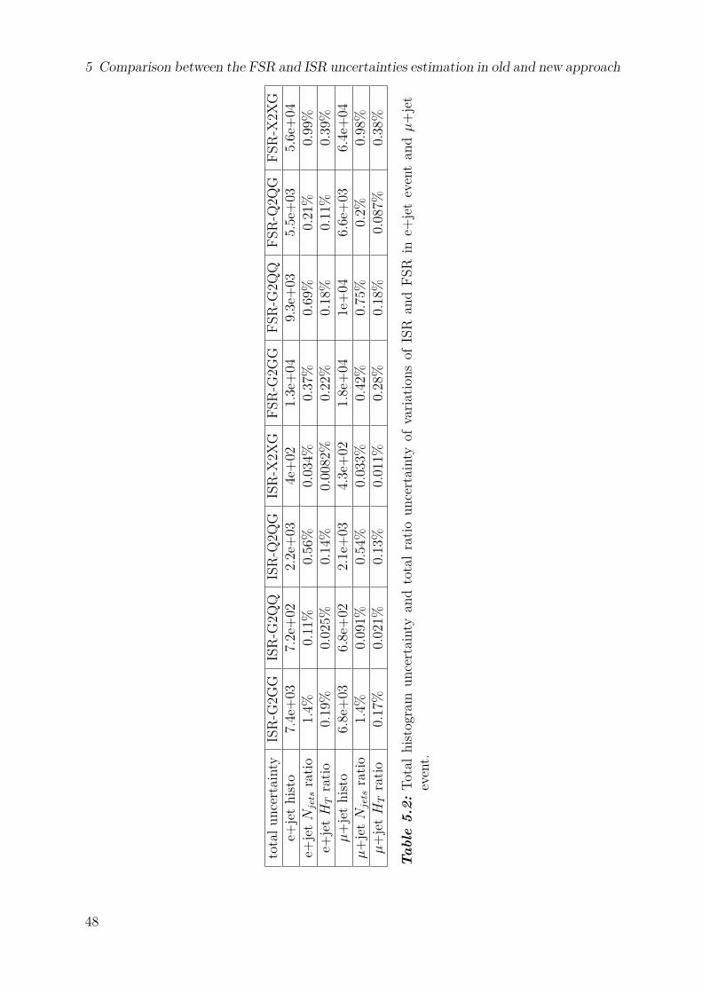
The histogram total uncertainty and the ratio total uncertainty of 4 variations of ISR andFSR are summarised in Table 5.2. The calculated histogram total uncertainty and ratiototal uncertainty values are shown in the plots in section 5.1.
For both Njets and HT plots of electron and muon for the ISR variation, G2GG contributethe most uncertainty to the total in ISR, while Q2QG has the second largest impact andG2QQ and X2XG the third and the fourth largest impact to the total. X2XG has reallysmall uncertainties compared to other variations that it almost does not show any varia-tions.For both Njets andHT plots of electron and muon for the FSR variation: X2XG contributethe most largest impact to total and Q2QG the smallest impact. For Njets plots G2QQhas the second largest impact to total and for HT plots G2GG has the second largestimpact, G2GG has the third largest impact for Njets plots and G2QQ for HT plots.
5.3 Comparison of nominal histograms with modifiederror in the new approach
In this section, the comparison between 4 variations to the nominal histograms will beprocessed to see the different impact of 4 variations and how much uncertainties theyhave contributed to the total uncertainties.
26
5.3 Comparison of nominal histograms with modified error in the new approach
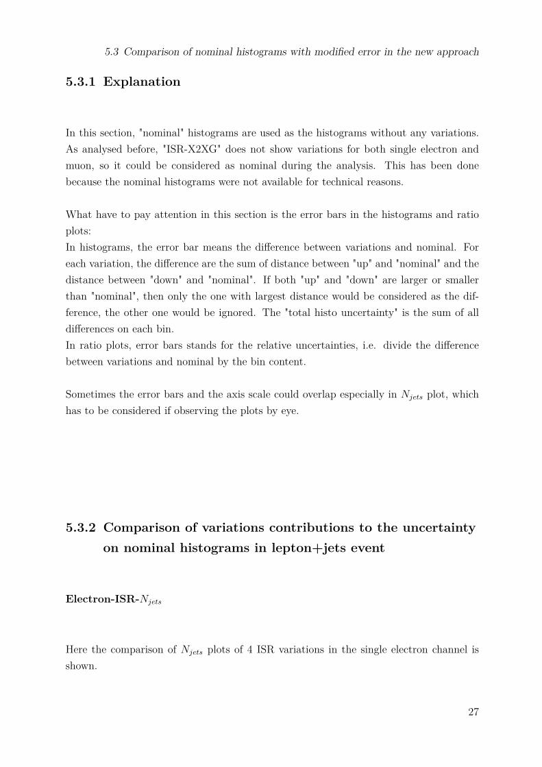
5.3.1 Explanation
In this section, "nominal" histograms are used as the histograms without any variations.As analysed before, "ISR-X2XG" does not show variations for both single electron andmuon, so it could be considered as nominal during the analysis. This has been donebecause the nominal histograms were not available for technical reasons.
What have to pay attention in this section is the error bars in the histograms and ratioplots:In histograms, the error bar means the difference between variations and nominal. Foreach variation, the difference are the sum of distance between "up" and "nominal" and thedistance between "down" and "nominal". If both "up" and "down" are larger or smallerthan "nominal", then only the one with largest distance would be considered as the dif-ference, the other one would be ignored. The "total histo uncertainty" is the sum of alldifferences on each bin.In ratio plots, error bars stands for the relative uncertainties, i.e. divide the differencebetween variations and nominal by the bin content.
Sometimes the error bars and the axis scale could overlap especially in Njets plot, whichhas to be considered if observing the plots by eye.
5.3.2 Comparison of variations contributions to the uncertaintyon nominal histograms in lepton+jets event
Electron-ISR-Njets
Here the comparison of Njets plots of 4 ISR variations in the single electron channel isshown.
27

5 Comparison between the FSR and ISR uncertainties estimation in old and new approach
Figure 5.33: Njets multiplicity distribu-tions with modified error onnominal histograms for theISR/G2GG variation in thee+jet events.
Figure 5.34: Njets multiplicity distribu-tions with modified error onnominal histograms for theISR/G2QQ variation in thee+jet events.
Figure 5.35: Njets multiplicity distribu-tions with modified error onnominal histograms for theISR/Q2QG variation in thee+jet events.
Figure 5.36: Njets multiplicity distribu-tions with modified error onnominal histograms for theISR/X2XG variation in thee+jet events.
Comparing the histogram total uncertainties and error bars in ratio plots, the relation of4 variations contribution to the uncertainty on nominal histograms could be shown below:
For electron-ISR-Njets: G2GG > Q2QG > G2QQ > X2XG
28
5.3 Comparison of nominal histograms with modified error in the new approach
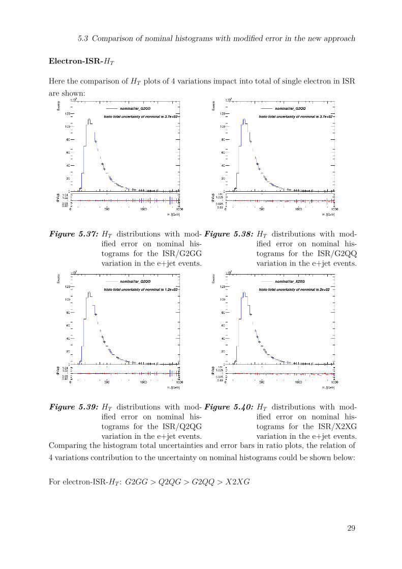
Electron-ISR-HT
Here the comparison of HT plots of 4 variations impact into total of single electron in ISRare shown:
Figure 5.37: HT distributions with mod-ified error on nominal his-tograms for the ISR/G2GGvariation in the e+jet events.
Figure 5.38: HT distributions with mod-ified error on nominal his-tograms for the ISR/G2QQvariation in the e+jet events.
Figure 5.39: HT distributions with mod-ified error on nominal his-tograms for the ISR/Q2QGvariation in the e+jet events.
Figure 5.40: HT distributions with mod-ified error on nominal his-tograms for the ISR/X2XGvariation in the e+jet events.
Comparing the histogram total uncertainties and error bars in ratio plots, the relation of4 variations contribution to the uncertainty on nominal histograms could be shown below:
For electron-ISR-HT : G2GG > Q2QG > G2QQ > X2XG
29

5 Comparison between the FSR and ISR uncertainties estimation in old and new approach
Electron-FSR-Njets
Here the comparison of Njets plots of 4 variations impact into total of single electron inFSR are shown:
Figure 5.41: Njets multiplicity distribu-tions with modified error onnominal histograms for theFSR/G2GG variation in thee+jet events.
Figure 5.42: Njets multiplicity distribu-tions with modified error onnominal histograms for theFSR/G2QQ variation in thee+jet events.
Figure 5.43: Njets multiplicity distribu-tions with modified error onnominal histograms for theFSR/Q2QG variation in thee+jet events.
Figure 5.44: Njets multiplicity distribu-tions with modified error onnominal histograms for theFSR/X2XG variation in thee+jet events.
Comparing the histogram total uncertainties and error bars in ratio plots, the relation of4 variations contribution to the uncertainty on nominal histograms could be shown below:
30

5.3 Comparison of nominal histograms with modified error in the new approach
For electron-FSR-Njets: X2XG > G2GG > G2QQ > Q2QG
Electron-FSR-HT
Here the comparison of HT plots of 4 variations impact into total of single electron inFSR are shown:
Figure 5.45: HT distributions with mod-ified error on nominal his-tograms for the FSR/G2GGvariation in the e+jet events.
Figure 5.46: HT distributions with mod-ified error on nominal his-tograms for the FSR/G2QQvariation in the e+jet events.
Figure 5.47: HT distributions with mod-ified error on nominal his-tograms for the FSR/Q2QGvariation in the e+jet events.
Figure 5.48: HT distributions with mod-ified error on nominal his-tograms for the FSR/X2XGvariation in the e+jet events.
Comparing the histogram total uncertainties and error bars in ratio plots, the relation of4 variations contribution to the uncertainty on nominal histograms could be shown below:
31
5 Comparison between the FSR and ISR uncertainties estimation in old and new approach
For electron-FSR-HT : X2XG > G2GG > G2QQ > Q2QG
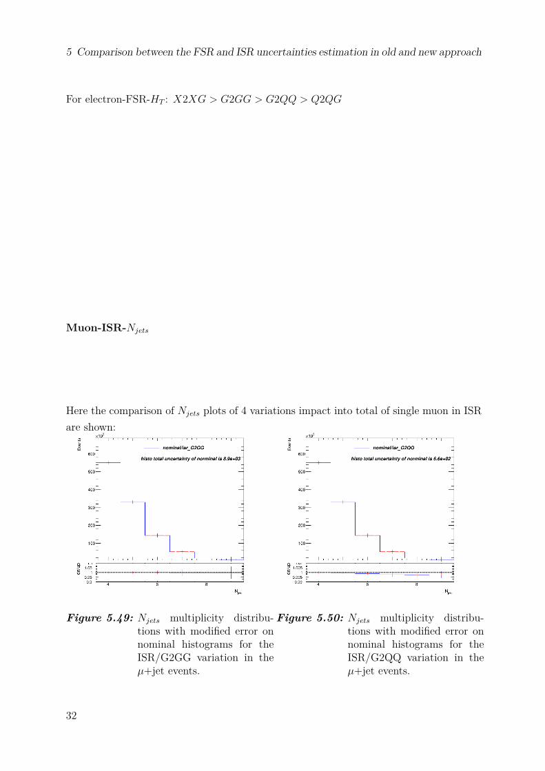
Muon-ISR-Njets
Here the comparison of Njets plots of 4 variations impact into total of single muon in ISRare shown:
Figure 5.49: Njets multiplicity distribu-tions with modified error onnominal histograms for theISR/G2GG variation in theµ+jet events.
Figure 5.50: Njets multiplicity distribu-tions with modified error onnominal histograms for theISR/G2QQ variation in theµ+jet events.
32
5.3 Comparison of nominal histograms with modified error in the new approach
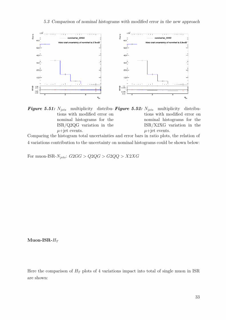
Figure 5.51: Njets multiplicity distribu-tions with modified error onnominal histograms for theISR/Q2QG variation in theµ+jet events.
Figure 5.52: Njets multiplicity distribu-tions with modified error onnominal histograms for theISR/X2XG variation in theµ+jet events.
Comparing the histogram total uncertainties and error bars in ratio plots, the relation of4 variations contribution to the uncertainty on nominal histograms could be shown below:
For muon-ISR-Njets: G2GG > Q2QG > G2QQ > X2XG
Muon-ISR-HT
Here the comparison of HT plots of 4 variations impact into total of single muon in ISRare shown:
33
5 Comparison between the FSR and ISR uncertainties estimation in old and new approach
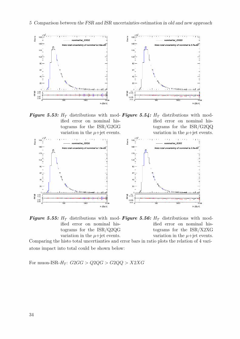
Figure 5.53: HT distributions with mod-ified error on nominal his-tograms for the ISR/G2GGvariation in the µ+jet events.
Figure 5.54: HT distributions with mod-ified error on nominal his-tograms for the ISR/G2QQvariation in the µ+jet events.
Figure 5.55: HT distributions with mod-ified error on nominal his-tograms for the ISR/Q2QGvariation in the µ+jet events.
Figure 5.56: HT distributions with mod-ified error on nominal his-tograms for the ISR/X2XGvariation in the µ+jet events.
Comparing the histo total uncertianties and error bars in ratio plots the relation of 4 vari-atons impact into total could be shown below:
For muon-ISR-HT : G2GG > Q2QG > G2QQ > X2XG
34
5.3 Comparison of nominal histograms with modified error in the new approach
Muon-FSR-Njets
Here the comparison of Njets 4 plots of 4 variations impact into total of single muon inFSR are shown:
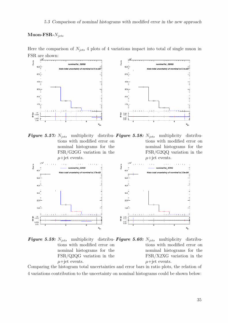
Figure 5.57: Njets multiplicity distribu-tions with modified error onnominal histograms for theFSR/G2GG variation in theµ+jet events.
Figure 5.58: Njets multiplicity distribu-tions with modified error onnominal histograms for theFSR/G2QQ variation in theµ+jet events.
Figure 5.59: Njets multiplicity distribu-tions with modified error onnominal histograms for theFSR/Q2QG variation in theµ+jet events.
Figure 5.60: Njets multiplicity distribu-tions with modified error onnominal histograms for theFSR/X2XG variation in theµ+jet events.
Comparing the histogram total uncertainties and error bars in ratio plots, the relation of4 variations contribution to the uncertainty on nominal histograms could be shown below:
35

5 Comparison between the FSR and ISR uncertainties estimation in old and new approach
For muon-FSR-Njets: X2XG > G2GG > G2QQ > Q2QG
Muon-FSR-HT
Here the comparison of HT plots of 4 variations impact into total of single muon in FSRare shown:
Figure 5.61: HT distributions with mod-ified error on nominal his-tograms for the FSR/G2GGvariation in the µ+jet events.
Figure 5.62: HT distributions with mod-ified error on nominal his-tograms for the FSR/G2QQvariation in the µ+jet events.
Figure 5.63: HT distributions with mod-ified error on nominal his-tograms for the FSR/Q2QGvariation in the µ+jet events.
Figure 5.64: HT distributions with mod-ified error on nominal his-tograms for the FSR/X2XGvariation in the µ+jet events.
Comparing the histogram total uncertainties and error bars in ratio plots, the relation of4 variations contribution to the uncertainty on nominal histograms could be shown below:
36
5.4 Comparison of ISR/FSR uncertainties in the new/old approach with the largest impact variation
For muon-FSR-HT : X2XG > G2GG > G2QQ > Q2QG
5.3.3 Discussion
The histogram total uncertainty and the maximal relative uncertainty of 4 variations con-tributing to nominal histograms are summarised in Table 5.3.Looking at the error bars on histograms and on ratio plots, the impact of 4 variations
could be observed and the variations which has the largest uncertainties to nominal his-tograms and contribute the largest uncertainties to total could be informed.Comparing the relation of 4 variations contributing uncertainties into total histogramsand the relation of 4 variations uncertainties between up and down single lepton: thosevariations, which have the largest uncertainties between up and down have also the largestuncertainties impact into the total histograms. And those variations which have smallestuncertainty between up and down single lepton have also the smallest uncertainty impactinto total histograms.
5.4 Comparison of ISR/FSR uncertainties in thenew/old approach with the largest impactvariation
In this section, the uncertainties comparison of old and new samples will be processed tosee which approach has smaller uncertainty and how much uncertainty has the variation,which has the largest impact, contributed to total histograms.
5.4.1 Explanation
The old samples are plotted nominal histograms with up and down variations and mean-while the error bars on histograms and ratio plots to show the uncertainties of them.In ratio plots the ratio between up and down variation is not the main point in compari-son, but the error bars on ratio plots, which shows the relative uncertainties of each bin.
In this section, histograms called "total" are produced to summarise 4 variations togetherto get the whole uncertainties of using new approach.For total histograms, the bin content are the sum of 4 variations and the error bars for
37

5 Comparison between the FSR and ISR uncertainties estimation in old and new approach
both histograms and ratio plots are the quadrature summed error from 4 variations. i.e.quadrature sum the difference between 4 variations and nominal histograms, which showsthe whole uncertainties influence of 4 variations together on nominal histograms.
5.4.2 Comparison of ISR/FSR uncertainties in the new/oldapproach with largest impacted variation in e+jet event
Electron-ISR-Njets
Here the comparison of nominal histograms from old and new samples with total uncer-tainties are processed with also the variation which contributes the largest uncertaintiesimpact into total:
Figure 5.65: Nominal histograms of newsamples with total uncertain-ties.
Figure 5.66: Nominal histograms of oldsamples with total uncertain-ties.
38
5.4 Comparison of ISR/FSR uncertainties in the new/old approach with the largest impact variation
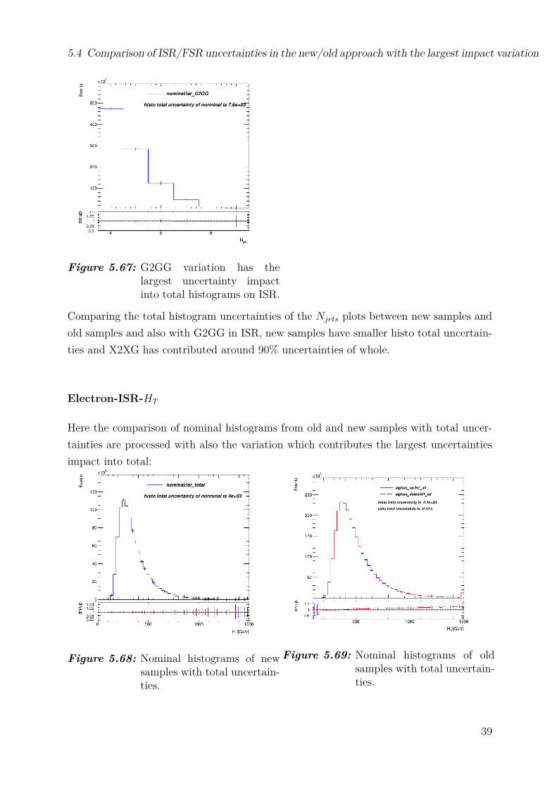
Figure 5.67: G2GG variation has thelargest uncertainty impactinto total histograms on ISR.
Comparing the total histogram uncertainties of the Njets plots between new samples andold samples and also with G2GG in ISR, new samples have smaller histo total uncertain-ties and X2XG has contributed around 90% uncertainties of whole.
Electron-ISR-HT
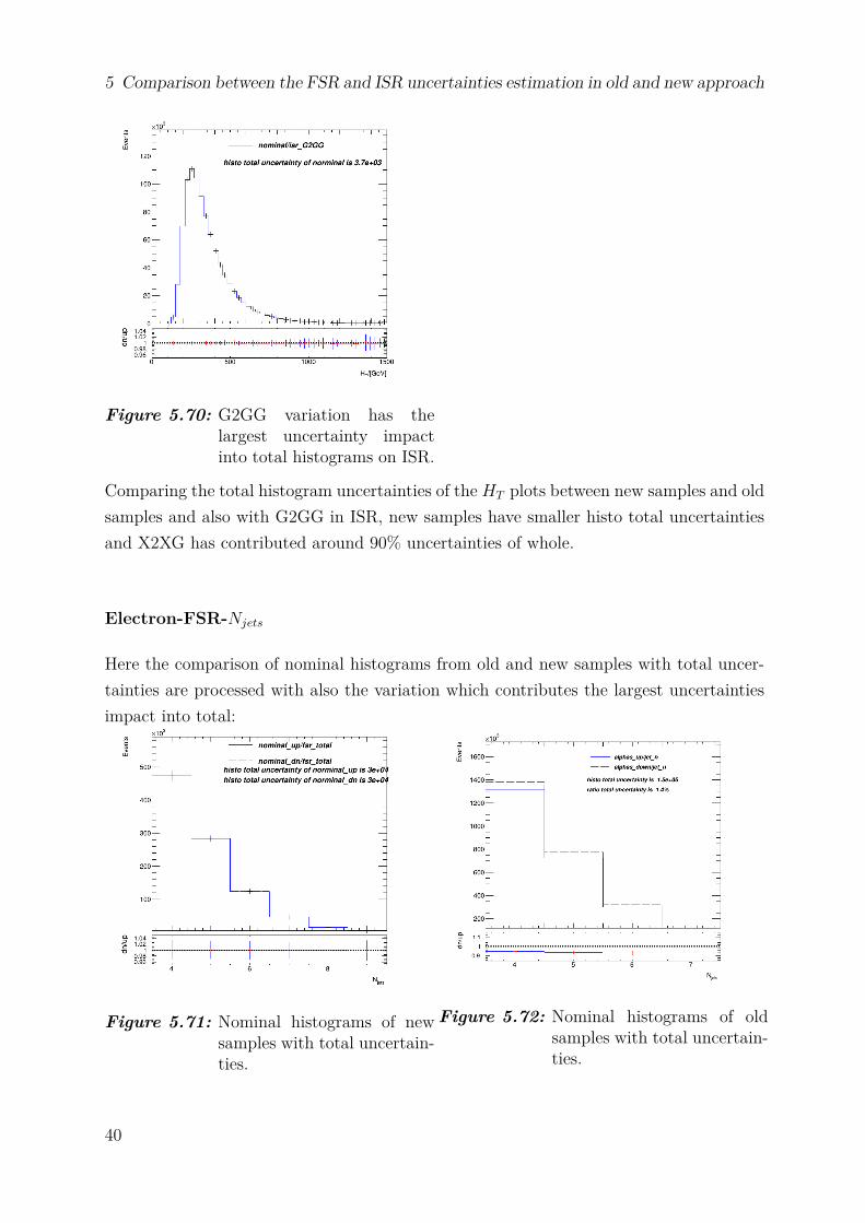
Here the comparison of nominal histograms from old and new samples with total uncer-tainties are processed with also the variation which contributes the largest uncertaintiesimpact into total:
Figure 5.68: Nominal histograms of newsamples with total uncertain-ties.
Figure 5.69: Nominal histograms of oldsamples with total uncertain-ties.
39
5 Comparison between the FSR and ISR uncertainties estimation in old and new approach
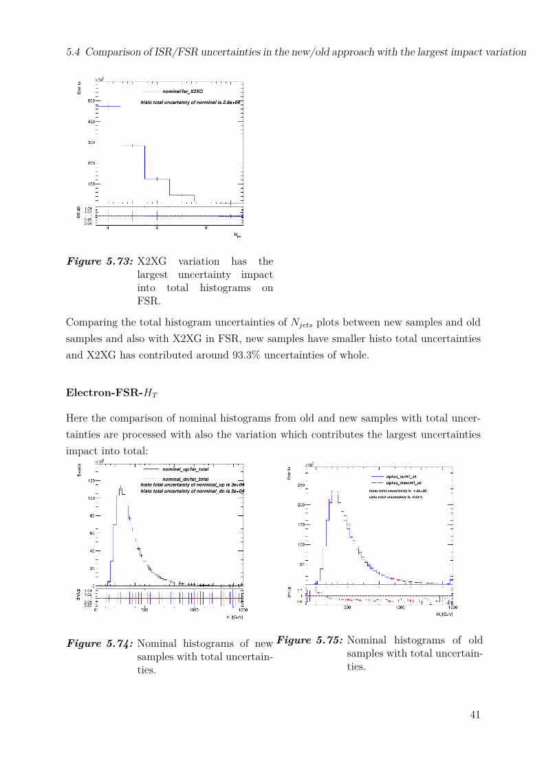
Figure 5.70: G2GG variation has thelargest uncertainty impactinto total histograms on ISR.
Comparing the total histogram uncertainties of the HT plots between new samples and oldsamples and also with G2GG in ISR, new samples have smaller histo total uncertaintiesand X2XG has contributed around 90% uncertainties of whole.
Electron-FSR-Njets
Here the comparison of nominal histograms from old and new samples with total uncer-tainties are processed with also the variation which contributes the largest uncertaintiesimpact into total:
Figure 5.71: Nominal histograms of newsamples with total uncertain-ties.
Figure 5.72: Nominal histograms of oldsamples with total uncertain-ties.
40
5.4 Comparison of ISR/FSR uncertainties in the new/old approach with the largest impact variation
Figure 5.73: X2XG variation has thelargest uncertainty impactinto total histograms onFSR.
Comparing the total histogram uncertainties of Njets plots between new samples and oldsamples and also with X2XG in FSR, new samples have smaller histo total uncertaintiesand X2XG has contributed around 93.3% uncertainties of whole.
Electron-FSR-HT
Here the comparison of nominal histograms from old and new samples with total uncer-tainties are processed with also the variation which contributes the largest uncertaintiesimpact into total:
Figure 5.74: Nominal histograms of newsamples with total uncertain-ties.
Figure 5.75: Nominal histograms of oldsamples with total uncertain-ties.
41

5 Comparison between the FSR and ISR uncertainties estimation in old and new approach
Figure 5.76: X2XG variation has thelargest uncertainty impactinto total histograms onFSR.
Comparing the total histogram uncertainties of HT plots between new samples and oldsamples and also with X2XG in FSR, new samples have smaller histo total uncertaintiesand X2XG has contributed around 93.3% uncertainties of whole.
5.4.3 Comparison of ISR/FSR uncertainties in the new/oldapproach with largest impacted variation in µ+jet event
Muon-ISR-Njets
Here the comparison of nominal histograms from old and new samples with total un-certainties are made with also the variation which contributes the largest uncertaintiesimpact into total:
42
5.4 Comparison of ISR/FSR uncertainties in the new/old approach with the largest impact variation
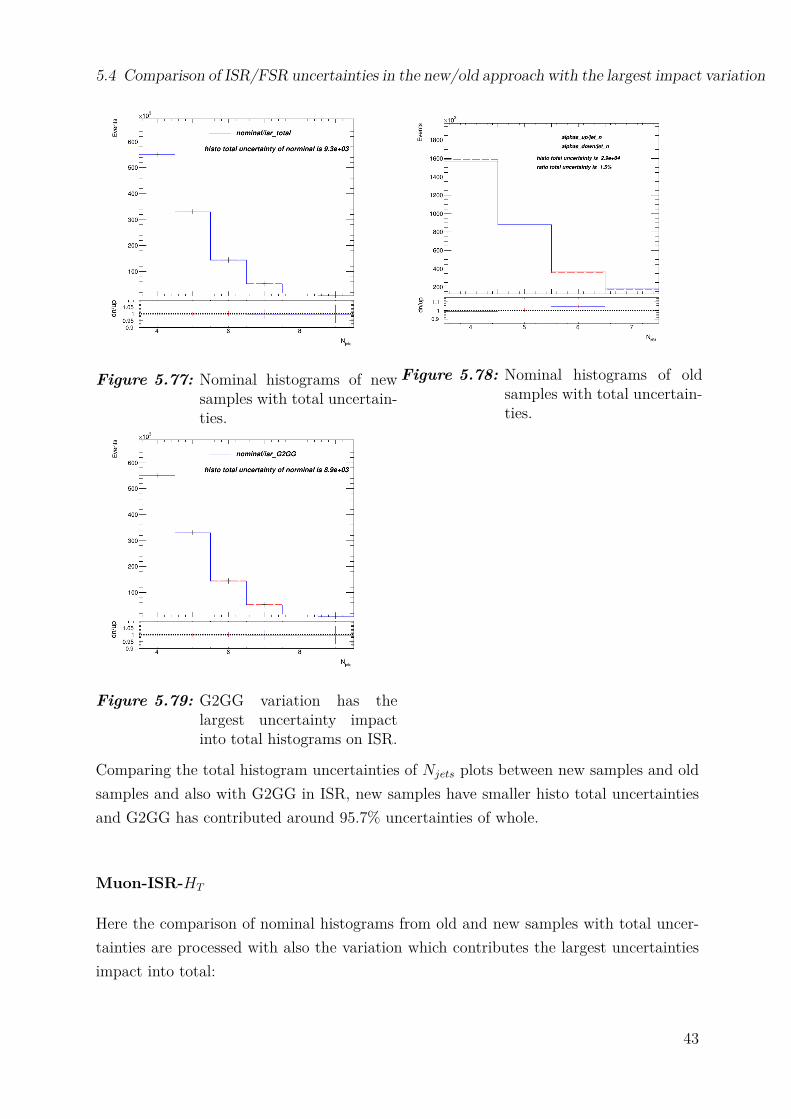
Figure 5.77: Nominal histograms of newsamples with total uncertain-ties.
Figure 5.78: Nominal histograms of oldsamples with total uncertain-ties.
Figure 5.79: G2GG variation has thelargest uncertainty impactinto total histograms on ISR.
Comparing the total histogram uncertainties of Njets plots between new samples and oldsamples and also with G2GG in ISR, new samples have smaller histo total uncertaintiesand G2GG has contributed around 95.7% uncertainties of whole.
Muon-ISR-HT
Here the comparison of nominal histograms from old and new samples with total uncer-tainties are processed with also the variation which contributes the largest uncertaintiesimpact into total:
43

5 Comparison between the FSR and ISR uncertainties estimation in old and new approach
Figure 5.80: Nominal histograms of newsamples with total uncertain-ties.
Figure 5.81: Nominal histograms of oldsamples with total uncertain-ties.
Figure 5.82: G2GG variation has thelargest uncertainty impactinto total histograms on ISR.
Comparing the total histogram uncertainties of HT plots between new samples and oldsamples and also with G2GG in ISR, new samples have smaller histo total uncertaintiesand G2GG has contributed around 90% uncertainties of whole.
Muon-FSR-Njets
Here the comparison of nominal histograms from old and new samples with total uncer-tainties are processed with also the variation which contributes the largest uncertaintiesimpact into total:
44

5.4 Comparison of ISR/FSR uncertainties in the new/old approach with the largest impact variation
Figure 5.83: Nominal histograms of newsamples with total uncertain-ties.
Figure 5.84: Nominal histograms of oldsamples with total uncertain-ties.
Figure 5.85: X2XG variation has thelargest uncertainty impactinto total histograms onFSR.
Comparing the total histogram uncertainties of Njets plots between new samples and oldsamples and also with X2XG in FSR, new samples have smaller histo total uncertaintiesand X2XG has contributed over 90% uncertainties of whole.
Muon-FSR-HT
Here the comparison of nominal histograms from old and new samples with total uncer-tainties are processed with also the variation which contributes the largest uncertaintiesimpact into total:
45

5 Comparison between the FSR and ISR uncertainties estimation in old and new approach
Figure 5.86: Nominal histograms of newsamples with total uncertain-ties.
Figure 5.87: Nominal histograms of oldsamples with total uncertain-ties.
Figure 5.88: X2XG variation has thelargest uncertainty impactinto total histograms onFSR.
Comparing the total histogram uncertainties of HT plots between new samples and oldsamples and also with X2XG in FSR, new samples have smaller histo total uncertaintiesand X2XG has contributed over 90% uncertainties of whole.
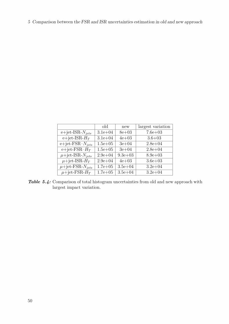
5.4.4 Discussion
The total histogram uncertainties of old and new approach with the largest variationcontribution into total histogram are summarised in Table 5.4. Comparing old with newsamples: the uncertainties from new approach are smaller than uncertainties from old
46

5.4 Comparison of ISR/FSR uncertainties in the new/old approach with the largest impact variation
approach. And during comparing it is also observed that G2GG variation has contributedthe most uncertainties of total uncertainties in ISR and X2XG has contributed the mostuncertainties in FSR.
47
5 Comparison between the FSR and ISR uncertainties estimation in old and new approach
totalu
ncertainty
ISR-G
2GG
ISR-G
2QQ
ISR-Q
2QG
ISR-X
2XG
FSR-G
2GG
FSR-G
2QQ
FSR-Q
2QG
FSR-X
2XG
e+jethisto
7.4e+03
7.2e+02
2.2e+03
4e+02
1.3e+04
9.3e+03
5.5e+03
5.6e+04
e+jetN
jetsratio
1.4%
0.11%
0.56%
0.034%
0.37%
0.69%
0.21%
0.99%
e+jetH
Tratio
0.19%
0.025%
0.14%
0.0082%
0.22%
0.18%
0.11%
0.39%
µ+jethisto
6.8e+03
6.8e+02
2.1e+03
4.3e+02
1.8e+04
1e+04
6.6e+03
6.4e+04
µ+jetN
jetsratio
1.4%
0.091%
0.54%
0.033%
0.42%
0.75%
0.2%
0.98%
µ+jetH
Tratio
0.17%
0.021%
0.13%
0.011%
0.28%
0.18%
0.087%
0.38%
Tab
le5.
2:To
talh
istogram
uncertaintyan
dtotalr
atio
uncertaintyof
varia
tions
ofISR
andFS
Rin
e+jeteventan
dµ+jet
event.
48

5.4 Comparison of ISR/FSR uncertainties in the new/old approach with the largest impact variation
uncertainty
ISR-G
2GG
ISR-G
2QQ
ISR-Q
2QG
ISR-X
2XG
FSR-G
2GG
FSR-G
2QQ
FSR-Q
2QG
FSR-X
2XG
e+jetN
jets
histo
7.6e+03
6.2e+02
2.4e+03
2e+02
6.5e+03
4.7e+03
3.2e+03
2.8e+04
e+jetN
jets
relativ
e5%
0.4%
2%0.2%
0.7%
3%1%
4%e+
jetH
Thisto
3.7e+03
3.7e+02
1.2e+03
2e+02
6.5e+03
4.7e+03
3.9e+03
2.8e+04
e+jetH
Trelativ
e3%
0.5%
2%0.1%
5%3%
1%4%
µ+jetN
jets
histo
8.9e+03
6.6e+02
2.7e+03
2.2e+02
9.1e+03
5.1e+03
3.7e+03
3.2e+04
µ+jetN
jets
relativ
e7%
0.5%
2%0.2%
1%4%
1%4%
µ+jetH
Thisto
3.6e+03
3.7e+02
1.3e+03
2.2e+02
9e+03
5.1e+03
4.6e+03
3.2e+04
µ+jetH
Trelativ
e3%
0.2%
2%0.2%
1%3%
1%4%
Tab
le5.
3:To
talh
istogram
uncertaintyan
drelativ
eun
certaintyof
varia
tions
ofISR
andFS
Rin
e+jete
vent
andµ+jete
vent.
49
5 Comparison between the FSR and ISR uncertainties estimation in old and new approach
old new largest variatione+jet-ISR-Njets 3.1e+04 8e+03 7.6e+03e+jet-ISR-HT 3.1e+04 4e+03 3.6+03
e+jet-FSR–Njets 1.5e+05 3e+04 2.8e+04e+jet-FSR–HT 1.5e+05 3e+04 2.8e+04µ+jet-ISR-Njets 2.9e+04 9.3e+03 8.9e+03µ+jet-ISR-HT 2.9e+04 4e+03 3.6e+03µ+jet-FSR-Njets 1.7e+05 3.5e+04 3.2e+04µ+jet-FSR-HT 1.7e+05 3.5e+04 3.2e+04
Table 5.4: Comparison of total histogram uncertainties from old and new approach withlargest impact variation.
50
6 Conclusion and outlook
6.1 Summary
6.1.1 On total uncertainty level
Comparing the total uncertainty generated by the new and old approaches which are in-troduced in section ??, it was found that using the new approach can significantly reducethe total uncertainty and the total uncertainty generated by the new approach in a singlelepton channel is about only 20% of the old approach. In the new approach, the variable,which is introduced in Table 4.1, with the most uncertainty contributes more than 90%of the total uncertainty. In ISR, the variable with the most uncertainty is G2GG, and inFSR it is X2XG.What also to pay attention to is the relative uncertainty of 4 variation impact on totalhistograms. For the ISR variation, the relative uncertainty of Njets plots and HT plotsfor G2GG is all over 3% and reaches 7% sometime and for Q2QG is all over 2%. Onthe contrary, the relative uncertainty for G2QQ are under 0.5% and especially for X2XGunder 0.2%.For the FSR variation, the situation is completely reversed. For both, G2QQ and X2XG,the relative uncertainties are above 3% and for G2GG and Q2QG, the relative uncertain-ties are under 1%. But there is one exception in particular, the HT plot for FSR/G2GGhas the maximum relative uncertainty around 5% at 1400 GeV. Out of this peak therelative uncertainties of the remaining bins are under 2%, which is relatively small.
6.1.2 On 4 variations level
Comparing the 4 variations in the new approach, the difference of the uncertainty between"up" and "down" variation also causes the large uncertainty which finally leads to the totaluncertainty.For the ISR variation, G2GG and Q2QG have large histogram uncertainties and ratio
51

6 Conclusion and outlook
uncertainties and G2QQ and X2XG have small uncertainties, which is consistent withtheir performance on the total uncertainties.For the FSR variation, X2XG and G2QQ have large uncertainties while Q2QG has smalluncertainties, which is also consistent with their performance in the total uncertainties.The exception here is also the G2GG variation, which has sometimes the second largesthistograms in both Njets and HT plots and for ratio uncertainties the second in HT plotsand the third in Njets plots. The main reason for that is the large uncertainty at around1400 GeV.
6.1.3 On "up" and "down" variation level
In general, the single electron channel and the single muon channel do not show muchdifference, so it is reasonable to combine them into single lepton channel. Looking at Njets
and HT plots of 4 variations in both ISR and FSR variations in single lepton channel,some observalous can also be summarized.For Njets plots, the difference between up and down in ratio plots has increased withincreasing N. Exception here is FSR/G2GG and FSR/X2XG. The difference between upand down in ratio plots is, that for FSR/G2GG the uncertainties first increase and reach amaximum 3% at N=6 and afterwards decrease and for FSR/X2XG has largest differencearound 6% at N=4, and after that constantly decrease to 2% at N=9.For HT plots, the difference between up and down in the ratio plots normally increases asthe transverse momentum increases and for G2GG and G2QQ variation, there is alwaysa peak at around 1400 GeV, which increases total ratio uncertainties. The exceptionhere is FSR/Q2QG and FSR/X2XG. The difference between up and down in ratio plotsfor FSR/Q2QG has a decrease from 4% at around 125 GeV to 1% at 200 GeV at thebeginning, and for FSR/X2XG the uncertainties has increased extremely rapidly to 6%at 200 GeV. Therefore, for transverse momentum under 200 GeV in the FSR variation,Q2QG has contributed the largest uncertainty among 4 variations and above 200 GeV,X2XG has contributed the most uncertainty. The physical explaintion for this observationis, at low momentum, i.e. transverse momentum under 200 GeV, the uncertainties ofanalysis mainly come from one quark (in this analysis means up, down, charm or strangequark) splitting into same type quark and gluon and for momentum above 200 GeV, theuncertainties mainly comes from other types of particles (in this analysis means bottomor top quark) splitting into same type particle and gluon.
52
6.2 Outlook
6.2 Outlook
By analysing the relation of uncertainties from 4 variations contributed into total his-tograms and also the uncertainties of up and down variation for 4 variations in the newapproach has been summarised in section 6.1. But during the analysis there are also someproblems remaining which need to be studied deeply to understand the cause of the largeuncertainty.Comparing the histogram total uncertainties in the Njets and HT plots of 4 variations indifferent state radiation (ISR and FSR) in the new approach from Table 5.2 and Table 5.3,it could be observed that not only the uncertainties between "up" and ’down" variationof 4 variations in single lepton+jets events but also the uncertainties of 4 variations innominal histograms, FSR has always larger impact on the tt̄ systematic model in analysisthan ISR.To explore the reason of the large uncertainty contribution in the FSR variation, it is nec-essary to dig further about which impact the large uncertainty on the total uncertaintyin the new approach. The main problem which needs to be investigated further is thelarge uncertainty around 1400 GeV in the HT plots, which causes the large uncertaintiesin G2GG and G2QQ variations in the FSR variation. Deeply understanding this problemmay lead to a solution why FSR has larger uncertainties on the tt̄ systematic model in tt̄cross section analysis than the ISR one.Another problem which needs to be considered is the large uncertainties at low HT val-ues. In the new approach, the selection of momentum is above 25 GeV. During makingthe plots, some bins at low HT values have bin content of 0, which would cause troubleby calculating the ratio total uncertainty if they are not selected out, and they alwayshave larger uncertainties comparing to bins above 200 GeV. This is shown in compar-ison plots of "up" and "down" variations in both new approach and old approach. Byreasonably increasing the selection standard, the total ratio uncertainties could rapidlydecrease without the bins which cause large uncertainties and the analysis may becomemore meaningful and accurate.It would be necessary to study the impact of the new uncertainties in the signal regions ofthe tt̄ single lepton+jets cross-section measurement. This includes not only the variationof the three fit variables, but also the impact of the uncertainties in the profile likelihoodfit that is used to extract the cross-section and its uncertainties.
53
Bibliography
[1] S. Abachi, et al. (DØ), Observation of the top quark, Phys. Rev. Lett. 74, 2632 (1995)
[2] F. Abe, et al. (CDF), Observation of top quark production in p̄p collisions, Phys. Rev.Lett. 74, 2626 (1995)
[3] M. Tanabashi, et al. (Particle Data Group), Review of Particle Physics, Phys. Rev.D98(3), 030001 (2018)
[4] M. Czakon, P. Fiedler, A. Mitov, Total Top-Quark Pair-Production Cross Section atHadron Colliders Through O(α 4
S), Phys. Rev. Lett. 110, 252004 (2013)
[5] Measurement of the tt̄ production cross-section in the lepton+jets channel at√s = 13
TeV with the ATLAS experiment, Technical Report ATLAS-CONF-2019-044, CERN,Geneva (2019)
[6] G. Aad, et al. (ATLAS), The ATLAS Experiment at the CERN Large Hadron Collider,JINST 3, S08003 (2008)
[7] S. Mrenna, P. Skands, Automated Parton-Shower Variations in Pythia 8, Phys. Rev.D94(7), 074005 (2016)
54

Acknowledgements
First of all, I want to thank my parents. Without their unselfish emotional and financialsupport, I cannot successfully complete my thesis, especially during the virus pandemic.I also want to thank my girlfriend for taking care of me and helping to deal with dailymatters when I am busy at work.
Secondly, I would like to thank many people who supported me in my work. First, Iwant to express my sincere thanks to Dr.Thomas Peiffer, who has given me inestimablehelp and support from the beginning to the end, from software support, the plan, thespecific algorithm to the final modification work. I can’t solve many problems and com-plete this paper without his help. Secondly, I would like to express my sincere gratitudeto Marcel Niemeyer and Prof. Dr. Baida Achkar, who gave me meticulous help to guideme to finally solve all kinds of problems encountered. In the early stage of work, MarcelNiemeyer guided me meticulously and patiently at work and answered many of my verybasic questions, and also helped me organize the code to make it more readable and stan-dardized. Later in the work, Professor Baida was very patient and meticulous and gaveme a lot of help and clarified the next goal. At the same time, she also provided me witha lot of information and codes to help me better understand and carry out my work. Ofcourse, I also want to express my gratitude to Ishan Pokharel, Fabian Sohns, Dr. TomasDado and Dr. Elizaveta Shabalina, who have helped me in my work and answered andpointed out many questions.
Finally, I want to express my sincere thanks to Prof. Dr.Arnulf Quadt and the Universityof Göttingen for giving me the opportunity to study in depth. It not only enriched myknowledge but also deepened my interest and desire for further exploration in the field ofparticle physics.
55
Erklärung nach §13(9) der Prüfungsordnung für den Bachelor-Studiengang Phy-sik und den Master-Studiengang Physik an der Universität Göttingen:Hiermit erkläre ich, dass ich diese Abschlussarbeit selbständig ver-fasst habe, keine anderen als die angegebenen Quellen und Hilfsmittelbenutzt habe und alle Stellen, die wörtlich oder sinngemäß aus veröf-fentlichten Schriften entnommen wurden, als solche kenntlich gemachthabe.Darüberhinaus erkläre ich, dass diese Abschlussarbeit nicht, auchnicht auszugsweise, im Rahmen einer nichtbestandenen Prüfung andieser oder einer anderen Hochschule eingereicht wurde.
Göttingen, den 30. Juli 2020
(Jun Huang)