econstor www.econstor.eu

Der Open-Access-Publikationsserver der ZBW – Leibniz-Informationszentrum WirtschaftThe Open Access Publication Server of the ZBW – Leibniz Information Centre for Economics

Standard-Nutzungsbedingungen:

Die Dokumente auf EconStor dürfen zu eigenen wissenschaftlichenZwecken und zum Privatgebrauch gespeichert und kopiert werden.

Sie dürfen die Dokumente nicht für öffentliche oder kommerzielleZwecke vervielfältigen, öffentlich ausstellen, öffentlich zugänglichmachen, vertreiben oder anderweitig nutzen.

Sofern die Verfasser die Dokumente unter Open-Content-Lizenzen(insbesondere CC-Lizenzen) zur Verfügung gestellt haben sollten,gelten abweichend von diesen Nutzungsbedingungen die in der dortgenannten Lizenz gewährten Nutzungsrechte.

Terms of use:

Documents in EconStor may be saved and copied for yourpersonal and scholarly purposes.

You are not to copy documents for public or commercialpurposes, to exhibit the documents publicly, to make thempublicly available on the internet, or to distribute or otherwiseuse the documents in public.

If the documents have been made available under an OpenContent Licence (especially Creative Commons Licences), youmay exercise further usage rights as specified in the indicatedlicence.

zbw Leibniz-Informationszentrum WirtschaftLeibniz Information Centre for Economics

Rosendahl, Knut Einar; Strand, Jon

Working Paper

Emissions Trading with Offset Markets and FreeQuota Allocations

CESifo Working Paper, No. 4603

Provided in Cooperation with:Ifo Institute – Leibniz Institute for Economic Research at the University ofMunich

Suggested Citation: Rosendahl, Knut Einar; Strand, Jon (2014) : Emissions Trading with OffsetMarkets and Free Quota Allocations, CESifo Working Paper, No. 4603

This Version is available at:http://hdl.handle.net/10419/93441

Emissions Trading with Offset Markets and Free Quota Allocations

Knut Einar Rosendahl Jon Strand

CESIFO WORKING PAPER NO. 4603 CATEGORY 9: RESOURCE AND ENVIRONMENT ECONOMICS

JANUARY 2014

Presented at CESifo Area Conference on Energy & Climate Economics, October 2013

An electronic version of the paper may be downloaded • from the SSRN website: www.SSRN.com • from the RePEc website: www.RePEc.org

• from the CESifo website: Twww.CESifo-group.org/wp T

CESifo Working Paper No. 4603

Emissions Trading with Offset Markets and Free Quota Allocations

Abstract We study optimal climate policy for a “policy bloc” of countries facing a market where emissions offsets can be purchased from a non-policy “fringe” of countries (such as for the CDM). Policy-bloc firms benefit from free quota allocations whose quantity is updated according to firms’ past emissions, or their outputs. We show that the resulting abatement and its allocation between policy bloc and fringe are both inefficient. When firms buy offsets directly from the fringe and all quotas are traded at a single price, the policy bloc chooses to either not constrain the offset market, or ban offsets completely. The former (latter) case occurs when free allocation of quotas is not (very) generous, and the offset market is large (small). It is preferable for policy-bloc countries’ governments to instead buy offsets directly from the fringe at a quota price below marginal damage cost of emissions, while the policy-bloc quota price will be above this cost. With maximization of global welfare and a unified quota price, this price is higher, and offsets constrained in fewer cases, but the solution still inefficient. Full efficiency then requires a higher quota price in the policy bloc than in the fringe.

JEL-Code: F640, H230, Q540, Q580.

Keywords: emissions quotas, offset market, quota allocation.

Knut Einar Rosendahl Norwegian University of Life Sciences

Ås / Norway knut.einar.rosendahl@umb.no

Jon Strand Development Research Group

The World Bank Washington DC / USA

jstrand1@worldbank.org A previous version of this paper was presented at the CESifo conference on Climate and Energy Economics, in Munich, 11-12 October 2013. We thank conference participants for helpful comments. Viewpoints and conclusions in this paper are those of the authors only and not necessarily of the World Bank, its management or member countries.

2

1. Introduction

Free emissions rights or quotas are a standard feature of most existing emission trading schemes. In

particular, within the EU’s Emissions Trading System (EU ETS) for greenhouse gases (GHGs), 99.9 % of

emissions rights were on average handed out for free to participating entities from the start (Convery et

al., 2008). This share was reduced somewhat in the second period, but has been well above the minimum

requirement of 90 %. From 2013 on, the share is scheduled to be reduced to below 50%; a more complete

phase-out is however not yet on the horizon.

Free allocation of quotas has four major impacts in our context, three negative and one potentially

positive. The first, very well recognized, is that substantial revenue is foregone for governments (see, e.g.,

Goulder et al., 1999); this includes the fact that the polluter pays principle is more or less abandoned. Two

further issues have until recently been less recognized, but are no less detrimental. One is that free

allocations may reduce firms’ incentives to abate. This follows mainly because current activity (emissions

or production) may serve as the basis for current of future free allocations, thus acting as an effective

premium on emissions (directly, or indirectly as a premium on output). This “raises the bar” with respect

to abatement that is privately efficient for emitters, since more abatement may reduce the extent of future

free allocations. The other issue, the main focus of this paper, is that free allocations can make offset

markets less efficient. In fact, when firms’ gains from free allocations are sufficiently high, we find that

policy-country governments may choose to ban the offset market completely. But even when the offset

market is allowed to operate, it will do so inefficiently. The fourth and potentially positive effect of free

allocation is that it may alleviate carbon leakage and improve the competitiveness of trade-exposed

sectors. In addition to the third issue, we will also touch upon the second and the fourth issue.

Two alternative mechanisms for allocating emissions quotas could here be at play. The first is based on

updating of quota allocations according to past emissions, as these may be taken as an indication of

future quota “needs”. This issue has been treated in the literature, e.g. by Böhringer and Lange (2005),

Rosendahl (2008), Harstad and Eskeland (2010) and Rosendahl and Storrøsten (2011), who have shown

that when free allocations are updated in such a fashion, much of the incentive to abate could be removed

from emitters. Furthermore, the quota price will exceed firms’ marginal mitigation costs. However, it has

also been shown that such allocations at least in principle can provide a cost-effective solution, in the

context of a “closed system” with no offset market and identical updating rules and price expectations

across emitting firms (Böhringer and Lange, 2005). A second type of allocation mechanism entails that

free allocations are based on output of the relevant entities, using then a “benchmark” emissions intensity

index for the industry (“output-based allocation”). Under this mechanism a high level of output will

secure a large amount of free allocations (on the presumption that the “need” for free allocations is

proportional to output). In this case the distortion to incentives will be in the direction of too high output,

and in consequence also too high emissions. However, for sectors that are highly exposed to carbon

leakage, i.e., increased output and corresponding emissions abroad, output-based allocation could in fact

be superior to no free allocation if the effects on foreign emissions are also considered (see e.g. Böhringer

et al., 2010). Carbon leakage exposure is the main argument put forward by the EU for continuing with

free allocation in the EU ETS. Strand and Rosendahl (2012) show that the Clean Development

Mechanism (CDM), the key “offset” mechanism under the Kyoto protocol, may similarly create

incentives for excessive production.

3

This paper discusses the effects of free quota allocations in an emission trading system comprising a

“policy bloc” of countries, which faces a “fringe” of (non-policy) countries. We assume that an offset

market is established, whereby emissions in policy bloc countries can be offset through emissions

reductions executed in the fringe, and purchased by entities in the policy bloc. In the context of the Kyoto

Protocol (under which the EU ETS is established), the CDM serves such a role; it will be useful for the

reader to have this mechanism in mind in the following. A main purpose of this paper is to study how free

quota allocations to firms in policy-bloc countries interact with the working of the offset market.

We study two separate cases by which emissions are limited through a market of tradable emissions

quotas in policy bloc countries, and where a fraction of these quotas are given away for free by

governments to emitters. In the first case, we assume that emitters may buy offsets directly from the

fringe, which mimics the current situation with respect to the EU ETS and the CDM. Further, offsets

substitute perfectly with domestic quotas. In this case, the price of offsets must be equal to the quota price

in the policy bloc.2

In the second case, the quota markets in the policy bloc and fringe are kept apart. There is, as in the first

case, free trading of emissions quotas within the policy bloc. The difference is that, in this case, free

trading with offsets among market participants is not allowed. Instead, offset purchases from the fringe

are made directly by policy countries’ governments, at an offset price that may differ from (and is

typically lower than) the quota price prevailing in the policy bloc countries. Strand (2013) has recently

shown, in a model with such separate markets (but without free quota allocations), that it is optimal for

the policy bloc to set a lower quota (and offset) price in the fringe, so that fringe emitters face an

emissions price that is lower than that facing policy bloc emitters.

We first consider a unified quota market with updating of free allocations, free trading of emissions

quotas among firms, and no fringe and thus no potential offset market. For this case we briefly replicate,

in Section 2, some important results demonstrated in earlier studies (see above). In Sections 3-4 we

extend this model to include an offset market with free trading of quotas among all market participants, so

that the trading price of offsets is the same as the internal quota price in the policy bloc.

In Section 3 we consider free updated quota allocations based on emissions. When the quota allocation is

“not too beneficial” to firms, we show that it is optimal for the policy-bloc not to constrain the use of

offsets. Due to the updating rule, the marginal mitigation cost of policy-bloc firms will be below that of

the fringe. This will lead to an excessive share of offsets. However, we show that the optimal emissions

price at the same time is below (the policy bloc’s value of) marginal environmental costs, meaning that

there will be inefficiently low volumes of abatement both in the policy bloc and in the fringe. For

gradually more generous quota allocation rules, at some point it is optimal for the policy-bloc to switch,

discretely, from free use of offsets to banning offsets completely. This implies no abatement in the fringe

whatsoever, and is also clearly inefficient.

2 In our analysis we disregard factors such as uncertainty and restrictions on the use of CDM credits, which may

explain why prices of CDM credits are usually below the quota price in the EU ETS.

4

In Section 4 we assume instead that free allocations are based on firms’ past outputs. The solution is also

in this case inefficient for both the offset market and policy bloc. With no carbon leakage, output of

policy bloc firms is always inefficiently high. This conclusion can however be changed when there is

leakage. The policy chosen by the policy bloc could here as in Section 3 entail inclusion of an offset

market with emission prices below marginal environmental costs (when the implicit output subsidy is

“not too large”); or it could entail a higher quota price but no offset trading permitted when the output

subsidy is larger.

A basic assumption in Sections 3-4 is that all emissions quotas must be traded at a quota price which is

common for the policy bloc and in the offset market. This is the basic principal policy applied to the

CDM today. In Section 5 we instead assume that an institution set up by the policy-bloc countries has a

monopsony on offset purchases from the fringe, behaving as a non-discriminating monopsonist with no

knowledge of project-specific abatement costs in the fringe. We then show that this institution will set a

(unified) offset price below marginal environmental damage cost. The optimal quota price within the

policy bloc is set such that marginal damage costs equal marginal abatement cost (as in the case of no

offset market); thus the quota price may well exceed marginal damage costs. The consequence could be a

large difference between the internal quota price and the external offset price. Moreover, the use of offsets

will be inefficiently low, but suboptimal from the policy bloc perspective, due to the coordinated,

monopsonistic behavior of the policy countries versus the fringe.

Section 6 studies a case where global (and not as in sections 3-4 only the policy bloc’s) welfare is

maximized, given that free allocations depend on past emissions and assuming that the quota price cannot

be differentiated (as in section 3). We then show that the (constrained optimally) chosen quota price will

be higher as global and not regional externalities are considered. Also, free offset purchases are chosen

more often than in section 3, as such purchases are no longer a net fiscal cost (instead, a transfer from the

policy bloc to the fringe).

Section 7 concludes, and indicates scope and topics for future research.

2. A Basic Model with Emissions Trading and Updated Allocations

Consider a “policy bloc” of countries which initiates and issues emissions quotas for GHGs, to a large

extent given out for free to emitters within the bloc. It is also possible to purchase emissions rights from

“non-policy countries” (the “fringe”). Assume that the offset market works perfectly in the sense that all

offsets are additional and efficient. In the policy bloc, there are a given number of firms with aggregate

revenue function R1(E1, X1), where E1 and X1 denote respectively emissions and production from the

policy bloc. We have R1E′ > 0 for E1(t) < E10(t) and R1X

′ > 0 for X1(t) < X10(t), where E10(t) and X10(t) are

the BaU emissions and production levels. The probability that any given firm survives to the next period

is β (same for all firms and such that firm exits are random events).

Assume that free allocation of emissions rights follow an “updated grandfather” rule whereby the number

of free quotas awarded to firms with emissions E(t) and production X(t) in period t equals αE(t) + γX(t) in

period t+1. That is, allocation of quotas is based on firms’ past emissions and/or production, where the

updating parameters α and γ are assumed to lie between zero and unity. In the two first phases of the EU

ETS (2005-2012), α has been closer to one while γ has been mostly zero. In the third phase (2013-2020),

5

however, α is mostly zero except in some sectors,3 while γ is close to one in exposed sectors but smaller

(or zero) in other sectors (cf. the discussion in Section 4).

Denote the discount factor between periods by δ, and assume that firms have a potentially infinite life

span. The discounted value of net returns for a representative firm in the policy bloc, V1(t), can then be

expressed as

(1) 2 2

1 1 1 1( ) ( ) ( 1) ( 2) ....V t W t W t W t

where W1(t) denotes net returns in period t. W1(t) is in turn given by4

(2) 1 1 1 1 1( ) ( ( ), ( )) ( )( ( ) ( 1) ( 1))W t R E t X t q t E t E t X t ,

where q(t) is the quota price in period t. We note that αE1(t-1) + γX1(t-1) represents the amounts of free

allocations of emissions rights available to the representative firm in period t. This amount is exogenous

to the firm when period t arrives. However, the firm looks ahead to future periods, in which the payoff

will be affected by current emissions through the updating mechanism. Inserting from (2) into (1) we may

write

(1a) 1 1 1 1 1 1 1

2 2

1 1 1 1 1 1 1

( ) ( ( ), ( )) ( )( ( ) ( 1) ( 1))

[ ( ( 1), ( 1)) ( 1)( ( 1) ( ) ( ))] ( 2)

V t R E t X t q t E t E t X t

R E t X t q t E t E t X t V t

.

The representative firm seeks to maximize V1(t) with respect to current emissions and production levels,

E1(t) and X1(t). This yields the following first-order conditions:

(3) 11 1 1

1

( )'( ( ), ( )) ( ) ( 1) 0

( )E

dV tR E t X t q t q t

dE t

and

(4) 11 1 1

1

( )'( ( ), ( )) ( 1) 0

( )X

dV tR E t X t q t

dX t

and thus

(3a) 1 1 1'( ( ), ( )) ( ) ( 1)ER E t X t q t q t .

3 Although output-based allocation will be the main allocation rule in the third phase (75-80% of freely allocated

quotas), for several products the allocation will be based on either past energy input or past (process) emissions for

the individual firm. Energy input is closely related to emissions, except for the possibility of fuel switching. For

further discussion see Lecourt (2012).

4 A condition for (2) to hold is E1(t) ≥ αE1(t-1), which we assume to hold (in particular, it holds in steady state).

6

(4a) 1 1 1'( ( ), ( )) ( 1)XR E t X t q t .

Because of the sequential (Bellman-type) nature of each firm’s decision problem, E1(t) and X1(t) here

enter into V1(t+1), but not into V1(t+2). This drastically simplifies the problem as we do not need to

explicitly consider V1(t+2) or higher-order value function terms in deriving the optimal solution. Focusing

on steady-state cases, with constant revenue functions, constant number of firms (so that a fraction β of all

firms are replaced by entering firms in any given period), and a constant overall emissions cap, we have

q(t) = q(t+1) = q. (3a) and (4a) may then be written as

(3b) 1 1 1'( ( ), ( )) (1 ) (1 )ER E t X t q a q .

(4b) 1 1 1'( ( ), ( ))XR E t X t q bq .

where a=αβδ and b=γβδ. The parenthesis on the right-hand side of (3b) expresses the “net price” paid for

emissions quotas by policy country firms in a steady state. This price is lower than the “gross” price q

since the free quota allocation is an increasing function of past emissions. The difference between the

“net” and the “gross” price depends on the product of three parameters: the updating share (α); the

probability of firm survival to the next period (β); and the discount factor (δ). All these three parameters

might be close to unity; in that case their product will also be relatively close to unity. The effective quota

price could then be much lower than the statutory price, q.

Similarly, the right-hand side of (4b) expresses the implicit subsidy per unit production by an output-

based allocation where γ>0.5 Note that this subsidy is proportional to the quota price.

As stated in the introduction, our analysis so far is just a restatement of already known results from the

literature. Our innovation here is to embed it in an emissions trading market where also offsets are

allowed. The main difference between offsets and regular emissions quotas within the policy bloc in our

context is that offsets are not directly affected by the types of incentives that affect policy bloc firms, as

represented by (3b). Instead, for the offset market, the “statutory” quota price, q, is also the effective

quota price for offsetting units. This implies an asymmetry between the regular (internal) quota market,

and the (external) offset market; with an effective favoring of emitters operating in the former of these

markets.

In the next section we will assume that γ=0, and focus on the case with emissions-based allocation (α>0).

In Section 4 we consider output-based allocation and set α=0 (and γ>0). To simplify notation, we skip

X(t) in the expressions in Section 3.

3. Offset Policies with Emissions-Based Allocation of Quotas

Consider the offset market in the fringe countries. This market has an aggregate revenue function

R2(E2(t)) in period t, and can be viewed as operating on a period-by-period basis. We assume

5 To be precise, the right-hand side expresses the implicit tax. However, since this is negative in our case, we have

an implicit subsidy.

7

(conservatively) that all offsets represent real emissions reductions in the offsetting region, where the

comparison benchmark is overall emissions in the absence of offsets.6 Define this benchmark by E20(t) in

period t, given by

(5) 2 20'( ( )) 0R E t .

We assume that quotas and offsets can be traded freely by all actors in the carbon markets, both within the

policy bloc, within the fringe, and between the policy bloc and the fringe. Such free trading implies that

there exists a single trading price q for all quotas (including offsets). Fringe market participants have no

incentives to buy quotas except for resale; this we can ignore here. In Section 5 we consider alternative

assumptions with different quota trading prices within the policy bloc and in the offset market.

Define next the maximal (potential) supply of offsets from the fringe, for a given offset price q, by 2ˆ ( )Q t .

This supply corresponds to the difference between the benchmark emissions 20 ( )E t and the emissions

level 2ˆ ( )E t given by

(6) 2 2ˆ'( ( ))R E t q .

As shown below, it may be optimal for the policy bloc to restrict the number of offsets. Let k denote the

share of offset supply from the fringe that is utilized in the policy bloc, and let Q2k denote the

corresponding offset purchases. We then have

(7) 2 2 20 2ˆ ˆ( ) ( ) ( ( ) ( ))kQ t kQ t k E t E t .

We assume that the sales of offsets are regulated on a first-come-first-served basis, meaning that realized

offsets are a random draw among all potential offset suppliers (so that each has probability k of

successfully selling offsets, and the cost distribution for realized offsets is the same as for all potential

offsets).7 We show below that it is optimal for policy-bloc country governments to choose either k = 0 or

k = 1, so this potential challenge turns out to be irrelevant.

It is clear that mitigation cannot be overall optimal, under our assumptions. The reason is that policy bloc

firms and fringe firms face different effective mitigation costs, with lower costs for policy bloc firms than

for fringe firms (compare (3b) with (6)). Thus, there exist some firms in the fringe that mitigate to the

level where marginal mitigation cost equals q, whereas no mitigation options in the policy bloc with

6 There are several reasons why not all offsets need to reduce global net emissions. Two are leakage (see Rosendahl

and Strand (2011)), and baseline manipulation and output inflation under “relative baselines” with incentives to

increase emissions (see Fischer (2005), Germain et al (2007), Strand and Rosendahl (2012)).

7 This need not be the case. Since low-cost projects imply more rent to project sponsors, these will have greater

incentives than others to promote their projects thus attracting more attention from policy bloc firms. Rent sharing

between contracting parties, ignored here but studied by Brechet, Meniere and Picard (2011), would also make low

cost projects more directly attractive to policy bloc parties.

8

marginal cost between (1-a)q and q are realized. Hence, mitigation through offsets is on average more

costly (and inefficiently so) than mitigation by the policy bloc. This inefficiency can however to some

degree be counteracted by reducing the overall volume of offsets, given by (7), by lowering the “purchase

rate” parameter k. The distribution of mitigation within the fringe will still remain inefficient, since

abatement costs in the fringe are then not minimized for given abatement.

We now search for optimal combinations of q and k, i.e., the quota price and the share of potential offsets

to be purchased, and study how these depend on the parameter a (=αβδ) which we treat as exogenously

given.8 Equivalently, we could search for optimal combinations of E* and k, where E* is the emissions

cap level in the policy bloc.9 We have

(8) 1 2 1 20 2

ˆ* ( ( ) ( ))kE E Q E k E t E t

E20 is assumed given and unaffected by the model parameters.10

What is an “optimal” offset policy is here not obvious. We postulate in sections 3-5 the following simple

objective function, defined by the policy bloc only (defining all relevant variables as functions of the

policy variables q and k):

(9) 1 1 1 20 2ˆ( , ) ( ( )) ( , ) ( ( ))B q k R E q cE q k qk E E q .

The first term is simply the aggregate revenue function, the second term accounts for the environmental

damages from global emissions (E), valued at a constant unit cost c, and the last term represents costs of

buying offsets from the fringe.11

E1 and 2E are here both simple functions of q only (from (3b) and (6) respectively). For E we have the

following accounting definition:

(10) 1 20 20 2 1 20 2ˆ ˆ( ) (1 )E E E k E E E k E kE .

We can now insert into (9) from (10) for E, which yields

(9a) 1 1 1 1 2 20ˆ( , ) ( ( )) ( ) ( ) ( ) [ (1 ) ] .B q k R E q cE q c q kE q c k qk E

8 β and δ are non-policy parameters, whereas α is clearly a policy parameter.

9 For a given combination of E* and k, a corresponding level of q follows (and vice versa for a given combination of

q and k). Furthermore, instead of regulating k directly, which is difficult, the bloc could regulate the total number of

offsets Q2k.

10 This requires that there is no (positive or negative) emissions “leakage” from the policy bloc to the fringe. In

Section 4 we return to this issue.

11 Note that only welfare for the policy bloc is considered, so that welfare for the fringe is excluded. In section 6

below we will instead take a “welfare maximizing” view, where also the fringe’s welfare is included.

9

This expression can be maximized with respect to q and k, yielding the following general first-order

conditions for internal solution:

(11) 1 1 21 20 2

ˆ( , ) ˆ( ' ) ( ) ( ) 0B q k E E

R c k c q k E Eq q q

(12) 120 2

( , ) ˆ( )( ) 0B q k

c q E Ek

,

(11) and (12) determine optimal levels of q and k. Consider first how optimal k depends on q. From (12),

since 20 2ˆ 0E E , an internal solution for k is not feasible unless q = c, in which case any value of k

fulfills (11).12

Without loss of generality we assume that k is set to zero whenever q = c, as B1 is then

independent of k. If q < c is optimal, k = 1 as B1 then increases in k for any k. On the other hand, if q > c is

optimal, k = 0 (B1 is then decreasing in k). Intuitively, we know that E1 only depends on q, i.e., emissions

in the policy bloc are independent of k, for given q. Hence, k only determines how many offsets, or

emissions reductions, the policy bloc purchases from the fringe. Consequently, it is optimal for the policy

bloc to buy offsets from the fringe if and only if the costs of buying offsets (q) are lower than the damage

costs of emissions (c), which then represents the benefits of buying offsets.

What about the optimal level of q? At first glance, one would expect the optimal q to be set equal to the

marginal damage costs c. However, there are two reasons why it may be optimal to deviate from this

standard result, which we come back to below.

From the reasoning above, we must either have q ≥ c and k = 0, or q < c and k = 1. Let us characterize

these two potential outcomes of the policy bloc’s optimization.

In the first case there is no offset market available for the firms since k = 0. From (11) we then have the

standard optimality condition R1′ = c. Then there is no inefficiency within the policy bloc, but not using

offsets at all is inefficient since cheap abatement options are foregone. Still, it may be a second-best

solution for the policy bloc. This outcome implies, from (3b) and (11):

(13) 1

cq c

a

.

Thus, an optimal solution with k = 0 requires that the quota price be set higher than the marginal damage

cost of emissions, c, as long as a > 0. This is just as in Böhringer and Lange (2005) and Rosendahl

(2008), who show that the quota price is driven up by the updating rule (for a given emissions constraint).

A high quota price in this case makes it too expensive for the policy bloc to purchase offsets. Note that

when a is relatively close to unity, the mark-up relative to c could be large.

12

We have assumed linear environmental damage costs, represented by the marginal costs c. If we rather assume

convex damage costs C(E), we would still have q = C′(E) as the only internal solution. However, in this case E and

thus C′(E) is a function of both q and k, and so the choice of k is no longer irrelevant under an internal solution.

10

Consider next the outcome where q < c and k = 1. q = 0 cannot be optimal (cf. (11)), so only internal

solutions are feasible. We may write (11) as follows, inserting from (3b):

(11b) 1 1 220 2

ˆˆ( ( )) ( )

E E Eaq E E q c q

q q q

The LHS and the first term on the RHS are here both positive for a, q > 0, whereas the second term on the

RHS is negative for q < c. We distinguish between the following three cases:

a) 120 2

ˆ ( )E

aq E E qq

for any q < c. In this case, equation (11b) has no solution when q < c,

and thus it is optimal to increase q until q ≥ c (cf. (11)). But then we are back to the case with k =

0 and q determined by (13), as described above. The intuition here is that the ability of the offset

market to profitably deliver offsets to the policy bloc (RHS of the inequality) is relatively small.

The solution is then determined out of a concern for the domestic mitigation market. Notice that

the higher a is (e.g., the higher the allocation rate α is), the more likely this case is. Further,

without the updating rule (i.e., a = 0) this case can never occur.

b) 120 2

ˆ ( )E

aq E E qq

for q = c. In this case, equation (11b) must have (at least one) internal

solution with q < c.13

The ability of the offset market to profitably deliver offsets is now greater.

This implies that the quota price may be determined more out of a direct concern for the offset

market, and less out of a concern for the domestic mitigation market in the policy bloc. However,

we cannot conclude in general whether or not this solution with q < c and k = 1 is preferred over

the solution with k = 0 and q determined by (13). The former case utilizes relatively cheap

abatement options in the offset market, but abatement in the policy bloc is far too low as R1′(E1) <

q < c. In the latter case, mitigation in the policy bloc is optimized, but none of the abatement

options in the offset market are utilized.

c) 120 2

ˆ ( )E

aq E E qq

for some q < c (but not for q = c). In this case we may or may not have

an internal solution of (11b). For instance, the fringe may be quite able to deliver profitable

offsets relative to emissions reductions in the policy bloc at low levels of q, but not at higher

levels of q. The policy bloc does not want the quota price to be too low, however, due to the

environmental concern. Hence, it may be optimal to increase q until q ≥ c, i.e., similar to a).

However, we may also have an internal solution similar to b).

To sum up so far, it is optimal for the policy bloc to either ban offsets completely, and let the quota price

be given by (13), or to not restrict offsets, implying R1′(E1) < q = R2

′(E2) < c. Further, the higher is a, and

13

If emissions in the two regions are convex (or linear) in q, we can show that the second order condition of (12) is

fulfilled for q ≤ c. Thus, there is just one internal solution which is optimal given q ≤ c.

11

the lower is the offset potential relative to domestic emissions reductions, the more likely it is that offsets

are banned.

Let us investigate case b) further. We first notice that if a = 0, i.e., no updating rule, then q < c and k = 1

is preferred over the alternative solution q = c and k = 0. The reason is that the latter outcome is

equivalent with q = c and k = 1 (see above). But then we know from the investigation of case b) that

reducing q below c will be beneficial. This case, i.e., without any updating rule, has already been

analyzed in Strand (2012). In other words, without updating it is never optimal to put any restrictions on

offset purchases (given our model assumptions), and the optimal quota price should be below the

marginal damage cost. The latter conclusion is seen by replacing R1′(E1) by q and setting k = 1 in (11). At

q = c the RHS is negative as the policy bloc, acting as a monopsonist, benefits from reducing q due to

lower costs of importing quotas.

When a is marginally increased from zero, i.e., if a mild updating rule is introduced, the optimal q will

increase. This is shown in the appendix in the case of quadratic mitigation costs. The reason is that

introducing updating increases the deviation between the marginal costs of abatement, given by (3b), and

the marginal costs of emissions, c, for given q. Thus, it is optimal to increase q even though the policy

bloc’s costs of buying offsets increase. As long as k = 1, introducing updating will then increase the

optimal level of offsets at low levels of a. However, at some point, a further increase in a will reduce the

optimal q (cf. the appendix), thus also reducing the use of offsets. The reason is, as explained above, that

the policy bloc ideally would like to see a lower q in the offset market in order to reduce the costs of

buying offsets. This matter becomes relatively more important when a is high, and hence the optimal q

declines. Finally, when a becomes sufficiently high, it becomes optimal to stop buying offsets

whatsoever, i.e., switch from k = 1 to k = 0.

Although the optimal quota price increases when a is increased from zero, abatement in the policy bloc

declines (at least, this is the case with quadratic mitigation costs, cf. the appendix). The reason is that for

abatement to stay constant within the policy bloc when a increases, (13) would need to be fulfilled; while

we find that q falls relative to that level. In other words, the effects of higher a dominate the effects of

higher (optimal) q in equation (3b), so that E1 increases. Moreover, global emissions increase, too, when a

is increased, as the higher emissions in the policy bloc (“region 1”) will always dominate the (initially)

lower emissions in the fringe (“region 2”; see the appendix). This holds only as long as k = 1, however, as

when a becomes so high that k = 0 is optimal, q jumps to the level given by (13). Then emissions in both

regions are insensitive to a further increase in a (which then only affects q, from (13)).

In the appendix we show that, given quadratic mitigation costs, welfare in region 1 decreases

monotonically in the level of a as long as offsets are used. Thus, introducing (or intensifying the level of)

updating in a quota system with access to offsets will unambiguously reduce welfare in the policy bloc.

Updating then increases the deviation between the desired domestic quota price and the desired offset

price. It also becomes optimal to switch to no offsets exactly when global emissions are the same with

and without offsets (see the appendix). It follows that increasing the level of a will always increase global

emissions as long as offsets are used initially. A partial explanation for this result, which may not hold

with other specifications than quadratic mitigation costs, is that the policy bloc wants to minimize global

emissions, and hence has incentives to pick the alternative where these are lowest.

12

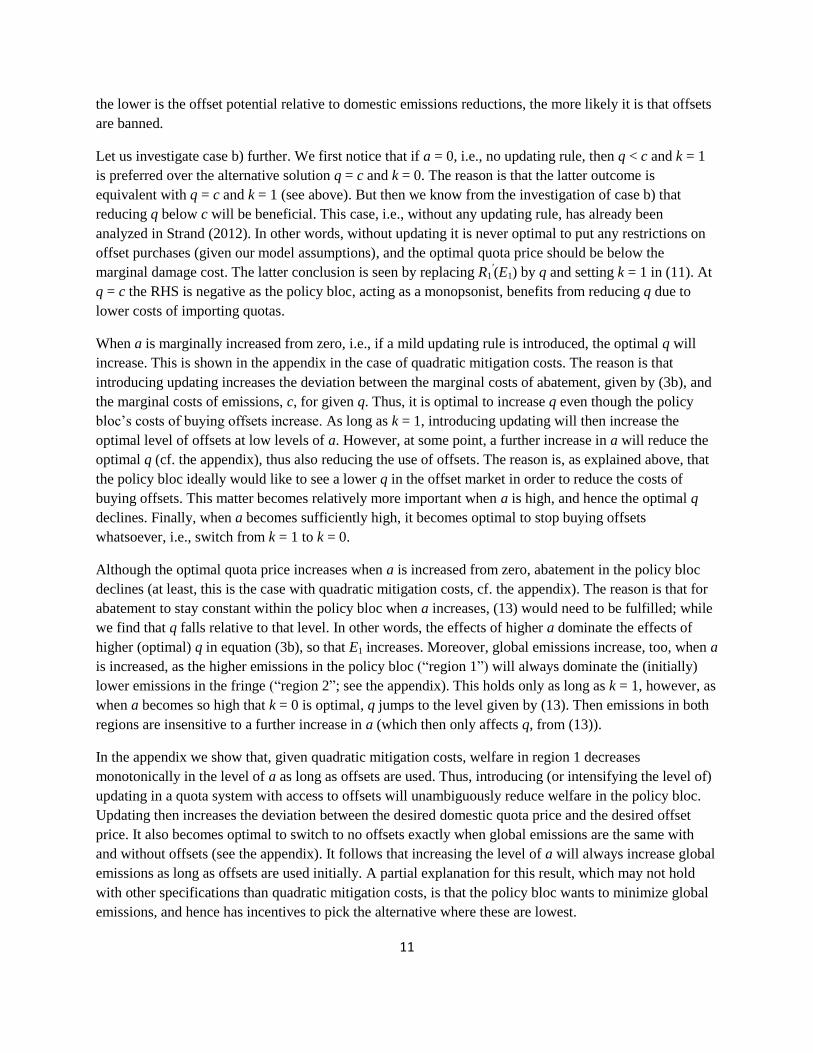
Figure 1. Emissions in the policy bloc, the fringe and total emissions as a function of a

0

0.25

0.5

0.75

1

1.25

1.5

1.75

0 0.1 0.2 0.3 0.4 0.5 0.6 0.7 0.8 0.9 1

a

E1 (k=1) E1 (k=0) E2 (k=1) E2 (k=0) E (k=1) E (k=0)E1 (k=1) E1 (k=0) E2 (k=1) E (k=1) E (k=0)

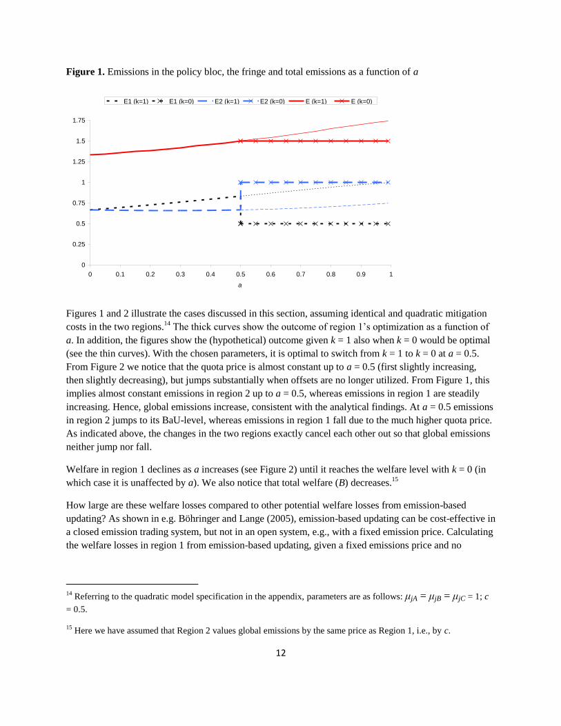
Figures 1 and 2 illustrate the cases discussed in this section, assuming identical and quadratic mitigation

costs in the two regions.14

The thick curves show the outcome of region 1’s optimization as a function of

a. In addition, the figures show the (hypothetical) outcome given k = 1 also when k = 0 would be optimal

(see the thin curves). With the chosen parameters, it is optimal to switch from k = 1 to k = 0 at a = 0.5.

From Figure 2 we notice that the quota price is almost constant up to a = 0.5 (first slightly increasing,

then slightly decreasing), but jumps substantially when offsets are no longer utilized. From Figure 1, this

implies almost constant emissions in region 2 up to a = 0.5, whereas emissions in region 1 are steadily

increasing. Hence, global emissions increase, consistent with the analytical findings. At a = 0.5 emissions

in region 2 jumps to its BaU-level, whereas emissions in region 1 fall due to the much higher quota price.

As indicated above, the changes in the two regions exactly cancel each other out so that global emissions

neither jump nor fall.

Welfare in region 1 declines as a increases (see Figure 2) until it reaches the welfare level with k = 0 (in

which case it is unaffected by a). We also notice that total welfare (B) decreases.15

How large are these welfare losses compared to other potential welfare losses from emission-based

updating? As shown in e.g. Böhringer and Lange (2005), emission-based updating can be cost-effective in

a closed emission trading system, but not in an open system, e.g., with a fixed emission price. Calculating

the welfare losses in region 1 from emission-based updating, given a fixed emissions price and no

14

Referring to the quadratic model specification in the appendix, parameters are as follows: μjA = μjB = μjC = 1; c

= 0.5.

15 Here we have assumed that Region 2 values global emissions by the same price as Region 1, i.e., by c.

13

emission changes outside this region, these are up to 11 percent when a = 1. The corresponding welfare

losses in Figure 2 amount to 6 percent for region 1 (B1) and 12 percent for both regions combined (B).

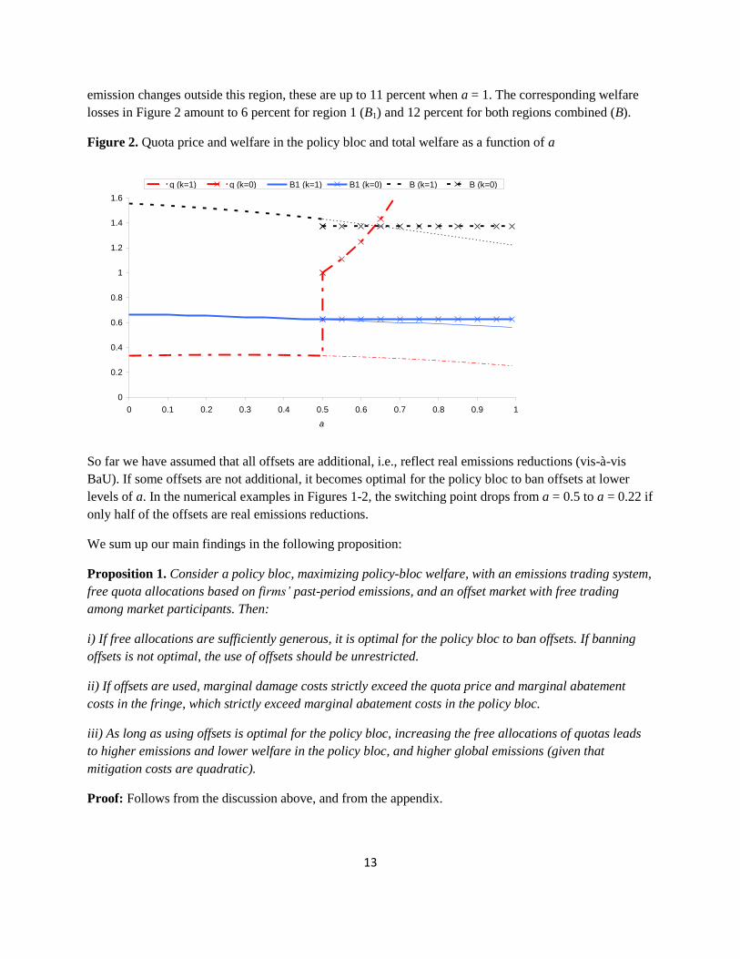
Figure 2. Quota price and welfare in the policy bloc and total welfare as a function of a

0

0.2

0.4

0.6

0.8

1

1.2

1.4

1.6

0 0.1 0.2 0.3 0.4 0.5 0.6 0.7 0.8 0.9 1

a

q (k=1) q (k=0) B1 (k=1) B1 (k=0) B (k=1) B (k=0)B (k=1) B (k=0) B1 (k=1) B1 (k=0) q (k=0) q (k=1)

So far we have assumed that all offsets are additional, i.e., reflect real emissions reductions (vis-à-vis

BaU). If some offsets are not additional, it becomes optimal for the policy bloc to ban offsets at lower

levels of a. In the numerical examples in Figures 1-2, the switching point drops from a = 0.5 to a = 0.22 if

only half of the offsets are real emissions reductions.

We sum up our main findings in the following proposition:

Proposition 1. Consider a policy bloc, maximizing policy-bloc welfare, with an emissions trading system,

free quota allocations based on firms’ past-period emissions, and an offset market with free trading

among market participants. Then:

i) If free allocations are sufficiently generous, it is optimal for the policy bloc to ban offsets. If banning

offsets is not optimal, the use of offsets should be unrestricted.

ii) If offsets are used, marginal damage costs strictly exceed the quota price and marginal abatement

costs in the fringe, which strictly exceed marginal abatement costs in the policy bloc.

iii) As long as using offsets is optimal for the policy bloc, increasing the free allocations of quotas leads

to higher emissions and lower welfare in the policy bloc, and higher global emissions (given that

mitigation costs are quadratic).

Proof: Follows from the discussion above, and from the appendix.

14

4. Offset Policies with Output-Based Allocation of Quotas

In the previous section we assumed that free quotas are based only on firms’ past emissions. As explained

in Section 2, the EU ETS is now moving more towards output-based allocations of quotas, although

emissions-based allocations will still be used in some sectors (see footnote 3). Output-based allocations

are also highly relevant for regions such as Australia, New Zealand and California (see e.g. Hood, 2010).

A main justification for this switch is the fear of “carbon leakage” through the markets for emission-

intensive, trade-exposed goods. The underlying problem is that lower output of such goods in one region,

due to unilateral climate policy, leads to greater output and emissions in regions with more lenient climate

policies.16

With output-based allocations, an “emission intensity benchmark” is defined for each product,

based on e.g. an average standard of all or the best firms in the industry. This would, at least in principle,

make this “benchmark” independent of the emissions of any one given firm.17

To account for such effects we will in this section focus on output-based allocations, so that γ > 0 and α =

0. From (3b), absent an offset market, emissions within the policy bloc are then “optimal” in the sense

that marginal value of emissions equals the quota price, which is set equal to marginal damage cost. On

the other hand, from (4b) and with no carbon leakage, output is excessive: Optimality would here entail

(net) marginal value equal to zero. Emissions from fossil energy are then likely also excessive, given that

(as is reasonable) output and energy use are complementary.

We now introduce offsets into this alternative model. Instead of (9a) we then have the following

alternative objective function for the policy bloc:

(14) 1 1 1 1 1 2 1 20 1ˆ( , ) ( ( ), ( )) ( ) ( ) ( , ( )) [ (1 ) ] ( ( )).B q k R E q X q cE q c q kE q X q c k qk E X q

Following the discussion above, we assume that in the absence of free allocation (γ=0), 1 / 0X q and

2 1ˆ / 0E X . The first of these derivatives simply expresses that a higher quota price (or emission cost)

reduces energy-intensive output in the policy bloc if no quotas are allocated for free. Note, however, that

with output-based allocation (γ>0), the positive effect on output through higher implicit subsidy may

dominate the negative effect through reduced emissions – this depends on the size of γ and the

complementarity of E and X (we return to this below).

The second of the derivatives states that when output is reduced in energy-intensive sectors in the policy

bloc, fringe emissions will shift up, presumably as related industrial activity is shifted to this region.

Both these conditions are intuitive for emission-intensive, trade-exposed industries, and are preconditions

for having a leakage problem in our context. The size of 1 /X q determines how sensitive domestic

16

There is a large literature on emissions leakage (e.g., Hoel, 1996; Rosendahl and Strand, 2011; Böhringer et al.,

2011). Leakage may occur through the international markets for fossil fuels, and through the markets for emission-

intensive, trade-exposed goods. Here we focus on the latter channel.

17 In the EU ETS, benchmarks for the period 2013-2020 are mainly determined based on the ten per cent least

emission-intensive installations.

15

output is to the quota price, whereas 2 1

ˆ /E X determines “leakage exposure” for domestic firms. To

simplify assume 2 1 20 1ˆ / /E X E X , so that leakage is independent of offset projects.

Maximizing (14) with respect to q and then reorganizing yields in this case:

(15) 1 1 2 2 120 2

1

ˆ ˆ( , ) ˆ( ) ( ) ( ) 0B q k E E E X

q c k c q k E E bq cq q q X q

(12) still holds, so we must either have q ≥ c and k = 0, or q < c and k = 1.

Reasonably, the value of free allocations is likely related to the costs of leakage exposure; this may be

because the authorities are inclined to compensate firms, in terms of reduced quota costs, for their loss of

competitive position when subject to climate policy. Such effects are captured by the two terms inside the

parenthesis of the last term on the RHS. The first is the expected value of future allocations per unit

output today (where b=γβδ), i.e., the implicit output subsidy. The second is the environmental cost of

leakage due to a marginal reduction in domestic output. Assume first that this parenthesis is zero. Then

we are back to (11) (remember that R1E′ = q). From Section 3 with a =0, we know that the optimal

solution is characterized by q < c and k = 1. This further implies that for the parenthesis to be zero (in the

optimal solution), we must have b > 2 1ˆ /E X . Let q

* denote the optimal quota price in this case.

If the last term in (15) is negative, e.g., because ( 2 1ˆ /E X ) is large compared to b (and 1 / 0X q ),

it is optimal to reduce the quota price below q*. The reason is that leakage reduces the environmental

effectiveness of climate policy in the policy bloc, and hence the optimal quota price falls.

If the last term is positive, the optimal quota price is higher than q*. This occurs if firms are given free

quotas even when leakage exposure is negligible (b >> 2 1ˆ /E X ), and output is declining in the quota

price (despite γ being large). Intuitively, the free quota allocation stimulates output too much, and so the

optimal (second-best) response is to increase the price of emissions to moderate output.18

If this effect,

represented by the last term of (15), is big compared to the offset potential, represented by the third term

of (15), it is optimal to increase q at least up to q = c (the two first terms in (15) are both positive for q <

c). But then we know from above that k = 0, i.e., banning offsets is optimal.

As explained above, however, if γ is large the sign of 1 /X q may turn positive, in which case the last

term becomes negative when b >> 2 1ˆ /E X . Hence, excessive allocation may not necessarily imply

that the quota price should exceed q* – hence banning offsets may not be optimal even if the offset

18

Obviously, the first-best response would be to lower b, but this might be difficult for political reasons.

16

potential is limited. In order for q* to exceed c in (15), we must have a combination of excessive

allocation, output decreasing in the quota price, and limited offset potential.19

Let us now discuss the sign of the last term in (15), and in particular the size of b and 2 1ˆ /E X , based

on the allocation rules of the EU-ETS. For the most highly exposed sectors in the EU ETS, which account

for most of industry emissions in the EU, γ = b/(βδ) is set close to E1/X1 (almost 100% compensation at

the sector level). This means that, if reductions in domestic output are replaced one-to-one by foreign

output, and emissions intensities are similar inside and outside the policy bloc, 2 1ˆ/( ) /b E X .

More likely, however, the output replacement is less than 100%. But since emissions intensities are often

higher in the fringe, it is still difficult to judge whether b could be higher or lower than 2 1ˆ /E X , at

least for the highly exposed sectors.

The EU has been criticized for allocating too many free quotas also to sectors that are only slightly

exposed to leakage (see e.g. Martin et al., 2012). This relates both to sectors given 100% compensation

(e.g., fossil fuel extraction), and to the remaining sectors which initially receive 70% compensation.

Hence, sectors can probably be found where b exceeds 2 1ˆ /E X , and possibly also b >> 2 1

ˆ /E X .

This could be explained by strong industry lobbying groups. Still, since 1 /X q may turn positive when

b becomes large, the sign of the last term in (15) is ambiguous.

To sum up, free output-based allocations to leakage-exposed sectors have ambiguous effects on the

optimal quota price when an offset market is available. This price will most likely be below marginal

environmental cost. However, if sectors with limited leakage exposure are granted substantial free quotas

and the offset potential is limited, the policy bloc may choose to ban offsets completely.

We sum up our main findings from the discussion above in the following proposition:

Proposition 2. Consider a policy bloc with an emissions trading system, free quota allocations based on

firms’ past-period output, and an offset market with free trading among market participants. Then:

i) If allocation is not too generous relative to the leakage exposure (b ≤ 2 1ˆ /E X ), and output is

declining in the quota price ( 1 / 0X q ), it is not optimal to put any restrictions on the use of offsets.

ii) If allocation is generous relative to the leakage exposure (b >> 2 1ˆ /E X ), output is declining in the

quota price ( 1 / 0X q ), and the offset potential 20 2ˆE E is sufficiently limited, it is optimal for the

policy bloc to ban the use of offsets.

19

The last term in (15) can also be positive if 0 < b < 2 1ˆ( / ) /c E X q , and 1 / 0X q , in which case a

higher quota price reduces leakage. If offset potential is limited, banning offsets may be optimal. We find this

alternative less realistic. As under case b) and c) in Section 3, we may also have cases where the internal solution to

(15) entails q < c, but still k = 0 is better than k = 1. See the discussion in Section 3 for details.

17

iii) If offsets are used, marginal damage costs strictly exceed the quota price and marginal abatement

costs in the fringe and in the policy bloc (which are all equal).

We see by comparing Propositions 1 and 2 that banning offsets is less likely to be optimal under output-

based allocation than under emissions-based allocation, even if leakage exposure is limited. To shed more

light into this question, we have performed simulations on a simple numerical model with the following

revenue function for region 1:

(14b) 2 2

1 1 0 1 1 1 1 1 1( , ) 1 ( / 2) / 2R E X E E X X E X

φ > 0 determines the relative importance of emissions in the revenue function, while θ ≥ 0 determines to

what degree E and X are complements. The lower is θ, the easier emissions can be reduced without

affecting output. Region 2 is assumed to have the same revenue function, except for the size of the region

given by σ. Let 2 1ˆ /E X denote an exogenous leakage parameter. For more details, see the

appendix.

We can now investigate the importance of respectively the leakage exposure (represented by ζ), the extent

of free allocation (represented by b), the complementarity between X and E (represented by θ), and the

offset potential (represented by σ).

As a benchmark, consider first σ = 1, φ = 1 and θ = 0.25, and ζ = 0, 0.5 and 1. The BaU emission intensity

is then unity, so ζ = 1 means substantial leakage exposure.

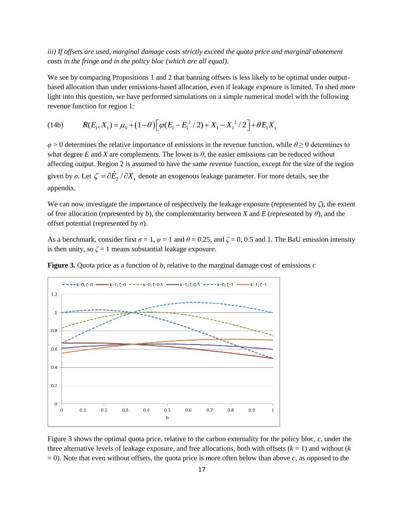
Figure 3. Quota price as a function of b, relative to the marginal damage cost of emissions c

Figure 3 shows the optimal quota price, relative to the carbon externality for the policy bloc, c, under the

three alternative levels of leakage exposure, and free allocations, both with offsets (k = 1) and without (k

= 0). Note that even without offsets, the quota price is more often below than above c, as opposed to the

18

case with emission-based allocation. Moreover, the optimal quota price seems to fall in b for high b, both

with and without offsets. This is due to the indirect subsidy effect explained above.

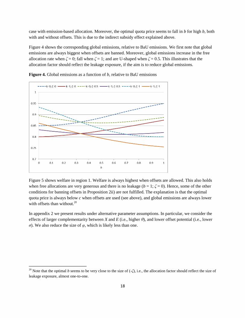
Figure 4 shows the corresponding global emissions, relative to BaU emissions. We first note that global

emissions are always biggest when offsets are banned. Moreover, global emissions increase in the free

allocation rate when ζ = 0; fall when ζ = 1; and are U-shaped when ζ = 0.5. This illustrates that the

allocation factor should reflect the leakage exposure, if the aim is to reduce global emissions.

Figure 4. Global emissions as a function of b, relative to BaU emissions

Figure 5 shows welfare in region 1. Welfare is always highest when offsets are allowed. This also holds

when free allocations are very generous and there is no leakage (b = 1; ζ = 0). Hence, some of the other

conditions for banning offsets in Proposition 2ii) are not fulfilled. The explanation is that the optimal

quota price is always below c when offsets are used (see above), and global emissions are always lower

with offsets than without.20

In appendix 2 we present results under alternative parameter assumptions. In particular, we consider the

effects of larger complementarity between X and E (i.e., higher θ), and lower offset potential (i.e., lower

σ). We also reduce the size of φ, which is likely less than one.

20

Note that the optimal b seems to be very close to the size of (-ζ), i.e., the allocation factor should reflect the size of

leakage exposure, almost one-to-one.

19

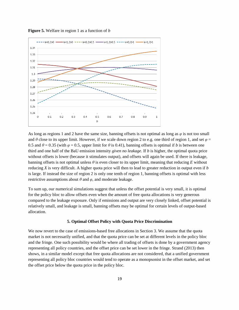
Figure 5. Welfare in region 1 as a function of b

As long as regions 1 and 2 have the same size, banning offsets is not optimal as long as φ is not too small

and θ close to its upper limit. However, if we scale down region 2 to e.g. one third of region 1, and set φ =

0.5 and θ = 0.35 (with φ = 0.5, upper limit for θ is 0.41), banning offsets is optimal if b is between one

third and one half of the BaU emission intensity given no leakage. If b is higher, the optimal quota price

without offsets is lower (because it stimulates output), and offsets will again be used. If there is leakage,

banning offsets is not optimal unless θ is even closer to its upper limit, meaning that reducing E without

reducing X is very difficult. A higher quota price will then to lead to greater reduction in output even if b

is large. If instead the size of region 2 is only one tenth of region 1, banning offsets is optimal with less

restrictive assumptions about θ and φ, and moderate leakage.

To sum up, our numerical simulations suggest that unless the offset potential is very small, it is optimal

for the policy bloc to allow offsets even when the amount of free quota allocations is very generous

compared to the leakage exposure. Only if emissions and output are very closely linked, offset potential is

relatively small, and leakage is small, banning offsets may be optimal for certain levels of output-based

allocation.

5. Optimal Offset Policy with Quota Price Discrimination

We now revert to the case of emissions-based free allocations in Section 3. We assume that the quota

market is not necessarily unified, and that the quota price can be set at different levels in the policy bloc

and the fringe. One such possibility would be where all trading of offsets is done by a government agency

representing all policy countries, and the offset price can be set lower in the fringe. Strand (2013) then

shows, in a similar model except that free quota allocations are not considered, that a unified government

representing all policy bloc countries would tend to operate as a monopsonist in the offset market, and set

the offset price below the quota price in the policy bloc.

20

We will here model a similar case, assuming updated quota allocations. Assume that the government

representing the policy bloc is required to set one single offset price at which offset quotas can be

purchased from the fringe. While this may seem as a natural limitation to impose on the policy bloc, it is

still not fully optimal for this bloc. The reason is that price discrimination in the offset market, whereby

quotas can be purchased “cheaper” from “fringe” firms with lower abatement costs, is thereby precluded.

Such price discrimination probably takes place at least to some degree in the CDM market today. Our

assumption is akin to assuming an extreme version of asymmetric information about abatement costs,

where low-cost firms will in general have incentives to mimic as high-cost. If such mimicking is fully

successful, no type revelation will take place in equilibrium.21

The problem is now formally similar to that in Section 3 except that we have two quota prices, q1 for the

policy bloc, and q2 for the offset market (in the fringe), instead of just a single price, q. Define now the

policy bloc’s objective function in similar fashion to (9a), by

(16) 1 2 1 1 1 1 1 2 2 2 2 20ˆ( , , ) ( ( )) ( ) ( ) ( ) [ (1 ) ] .B q q k R E q cE q c q kE q c k q k E

(16) is maximized with respect to q1, q2 and k, yielding the first-order conditions:

(17) 1 2 11

1 1

( , , )( ' ) 0

B q q k ER c

q q

(18) 22 20 2 2

2 2

ˆˆ( ) ( ( )) 0

EBk c q k E E q

q q

(19) 1 22 20 2 2

( , , ) ˆ( )( ( )) 0B q q k

c q E E qk

.

From (17), R1′ = c: mitigation is optimal in the policy bloc. This implies that q1, given from (13), exceeds

marginal damage cost from emissions as long as a > 0.

Consider next q2. From (18) we find

(20) 20 22

2 2

ˆ( )

ˆ

E Eq c c

E q

.

The optimal quota price, at which quotas are purchased from the offset market, is now below marginal

damage cost of emissions. This is a standard monopsony solution where a unified policy bloc government

(acting as a monopsonist in the offset market) trades off an environmental efficiency aspect (“too little”

mitigation) against a fiscal cost aspect (expenditure on the purchase of offset quotas). It results in too little

mitigation through offsets, but the gain for the policy bloc is that quota expenditures are reduced.

21

For an introduction to the game theoretic basis for such an equilibrium, see e.g. Gibbons (1992), Chapter 3.

21

The main difference between mitigation policy towards domestic firms versus firms in fringe countries is

that government payments to domestic firms, but not to foreign firms, are part of net social welfare for the

policy bloc. The government thereby wishes to limit the latter payments, doing so in (constrained)

optimal, monopsonistic, fashion.

The quota price facing policy bloc countries, q1, is here greater than marginal damage cost; while the

quota price facing firms in fringe countries, q2, is lower than this damage. The difference between the

internal and external quota prices, q1 and q2, can be substantial. In our model, quota prices can differ only

because private actors are not allowed to trade in the offset markets. Admittedly, it is unrealistic to

assume that governments-sponsored purchases of offsets will lead to such strong discrimination in

disfavor of offset sellers; and that offsets are always purchased at a given price. Our analysis must be

viewed as a first cut at this issue, so that further research is warranted.22

Using c – q2 > 0, (19) must hold with inequality, so that k = 1 at the optimal solution. The reason is that

the policy bloc, in implementing its desired volume of offsets at minimum cost, finds it preferable to

reduce the offset price, rather than restrict offset purchases by setting k < 1.

We sum up these results as follows.

Proposition 3. Consider a policy bloc with a domestic emissions trading system, free quota allocations

based on firms’ past-period emissions, and an offset market fully controlled by policy-bloc governments.

Then:

i) Within the policy bloc, the equilibrium quota price exceeds firms’ marginal abatement costs

which in turn equal marginal damage cost, so that abatement is efficient within the policy

bloc.

ii) Offsets are always used.

iii) The equilibrium offset price is lower than marginal damage cost; thus abatement in the fringe is

inefficiently low.

Proof: The results follow from the discussion above.

For the policy bloc countries, the solution in this section is preferable to a unified quota market.

Efficiency loss still occurs due to the wedge between marginal damage cost and marginal mitigation cost

in the fringe, leading to too little mitigation. On the other hand, the policy bloc now always finds it

optimal to utilize the offset market, which is not necessarily the case under a unified market. Moreover, if

offsets are used under a unified market, the amount of domestic mitigation is too low. Both types of

solutions thus entail inefficiencies, which are quite different. Although price discrimination is preferred

22

Price differences exist today between the CDM market and the EU ETS, and within the CDM market, for a

variety of reasons beyond our simple model. Among these are 1) transaction costs and other imperfections in the

offset market; 2) uncertain delivery of effective offsets from the point of view of offset purchasers (not all offsets are

actually achieved and credited); and 3) bilateral bargaining or monopsonistic power by buyers in the offset markets.

22

by the policy bloc, we cannot easily say which of the two solutions is preferable from a global efficiency

perspective.

It is also ambiguous which solution is more favorable to fringe countries. The solution with different

quota prices in the two regions is clearly more favorable to fringe countries than the solution with k = 0 in

Section 3 above, i.e., when the offset market is not utilized at all by the policy bloc. Price discrimination

can in fact also be more favorable to fringe countries when the offset market is used in the case without

price discrimination.23

The solution possibilities sketched in Section 3, with a unified quota price, are also easier to understand

when viewed in the context of the current solution. In particular, when the offset market is

overwhelmingly important compared to the domestic mitigation market, as it may be under case b) in

Section 3 above, the unified solution for q will be close to that found in (23). The quota price will then be

below the marginal damage cost of emissions, also for the domestic mitigation market. By contrast, when

the domestic mitigation market is overwhelmingly important compared to the offset market, as under case

a) in Section 3, the unified solution for q would entail that the quota price be set by (13) and there would

be no offset market.

Can the solution in this section be implemented as a decentralized market solution where emitters in the

policy bloc also trade with the offset market? Any such trading must be subject to a price difference q1 –

q2 facing policy bloc actors versus fringe actors. Focusing on policy bloc actors, the price of all quotas

facing these must be the same.

There are at least two ways of implementing such a solution. One entails that the government imposes an

(excise) tax per quota purchased in the offset market, equal to tq = q1 – q2.24

Given such a tax, the

government needs not impose other restrictions on quota sales (all possible offsets ought to be realized

given this tax).

The other solution, from Malik et al (1993), Mignone et al (2009), Castro and Michaelowa (2010), and

discussed analytically by, among others, Bushnell (2011), Klemick (2012) and Strand (2013a), is

“discounting” offsets by giving them less value to purchasers per ton CO2 actually offset. Such discounts

can be justified, on independent grounds, by inherent problems in the offset markets (such as lack of

additionality) not focused on here; see discussions of such issues in Montero (1999, 2000), Wear and

Murray (2004), Gan and McCarl (2007), Wara (2008). Note also that a similar solution is implemented

when the rate at which offset quotas are “discounted” (or reduced in value relative to domestic

abatement), call it λ, equals (q1 – q2)/q1. When buying one unit of offset from the fringe, a policy bloc firm

is t hen credited with only q2/q1 units of actual offset. One difference between the two solutions is that, in

the first, the government would raise revenue (q1 – q2)Q2, where Q2 is the amount of abatement taking

place in the fringe; and this abatement would all be credited to policy bloc firms. In the second case, the

government would raise no revenue. However, if the government auctions off λQ2 quotas, we get exactly

23

This depends among other things on whether the amount of offsets purchased is smaller or greater. This however

needs further study, and we refer to the discussion in Strand (2013).

24 We thank Ian Parry for suggesting this solution.

23

the same outcome with respect to emissions, costs and government revenues as in the former case.25

Both

solutions are very similar to the optimal price discrimination solution under a carbon tax, in Strand

(2013a).

Note that giving the policy bloc the ability to discriminate between quota prices resolves some problems

of inefficiency, but not all. There is still inefficiency due to the policy bloc not incorporating the fringe’s

utility in the objective function that is maximized; this will be discussed in section 6.

6. Global Welfare Considered

So far we have assumed that the objective function to be maximized is determined solely by the policy

bloc, so that welfare in the fringe is ignored. We will now instead assume that welfare of the fringe is

fully incorporated in the objective function being maximized. We return to the case of section 3, assuming

a common quota price and free allocations according to past emissions. The relevant objective may now

be formulated as

(21) 1 1 2 20 2 2 1 20 2ˆ ˆ( , ) ( ( )) (1 ) ( ) ( ( )) ( ) (1 ) ( )TB q k R E q k R E kR E q c E q E k kE q

where now cT denotes the global climate externality (experienced by both the policy bloc and fringe), so

that cT > c. Note that, on the right-hand side of (21), two terms representing the fringe enter with weights

(1-k) (the share of firms that are not allowed to sell offsets) and k (the share of firms that sell offsets).

Also, as different from (9), the fringe’s net revenue function is included in the objective. Maximizing (21)

with respect to q and k now yields

(22) 1 21 2 2

ˆ( , ) ˆ( ' ) [ '( ) ] 0T T

E EB q kR c k R E c

q q q

(23) 2 2 2 20 20 2

( , ) ˆ ˆ( ) ( ) ( )T

B q kR E R E c E E

k

.

We still have R1′ = (1-a)q, and R2′(E2) = q. Since partial derivatives of E1 and E2 with respect to q are

both negative, given k > 0, (22) must for any a where 0 < a < 1, imply that q > cT.

Consider next determination of k. Note that we here need to be careful in interpreting R2(E2), since the

offset payment q(E20 – E2) should not be included in this expression (since it is not part of the social

surplus). Thus generally 2 20 2 2ˆ( ) ( ) 0R E R E . Moreover, as long as R2′′≤ 0 (increasing marginal

mitigation costs), 2 20 2 2 20 2ˆ ˆ( ) ( ) ( )R E R E q E E . In the case of quadratic mitigation costs (cf sections

25

Note that in the ”discount” case, policy bloc emissions will be lower than in the “tax” case if the overall cap of the

emissions trading system in the policy bloc is the same in the two cases. By increasing the cap by λQ2 units,

emissions will be the same both in the fringe and in the policy bloc. It is straightforward to see that the revenue from

selling λQ2 quotas is (q1 – q2)Q2.

24

3-4), (23) becomes 20 2

ˆ( , ) / ( 0.5 )( )TB q k k c q E E . Hence, if the quota price is close to marginal

damage costs, the expression is positive, and k = 1 is optimal. This will be the case if a is not too high (a

≤ 0.5 is a sufficient condition), or the offset potential is not too small. On the other hand, if a is large and

the offset potential is limited, it may be optimal with a quota price more than two times higher than cT. If

so, offsets should be banned, as it is more important to set the incentives correctly in the policy bloc.26

Simulations indicate that it is never optimal with an interior solution for k in this case either. It can here

be shown that ( , ) / 0B q k k for 0 < k < 1 corresponds to a local minimum point, meaning that both k

= 0 and k = 1 are better solutions.

We can formulate the following Proposition:

Proposition 4: Consider a policy bloc maximizing global welfare, but is otherwise subject to the same

conditions as under Proposition 1. Then

i) The optimal quota price always exceeds global marginal damage cost from emissions

ii) It may be optimal to ban offsets if allocation is very generous, and the offset potential is limited.

Here, the optimal quota price implies a tradeoff between an inefficiently low (suboptimal) mitigation

activity in the policy bloc (corresponding to a suboptimal emissions price), and an over-optimal

mitigation activity in the fringe (corresponding to an over-optimal emissions price), so as to optimally

balance these two. The over-optimal emissions price in the fringe explains why offsets may be banned

even when maximizing global welfare.

Overall, the quota price q is substantially higher here than in the case of k = 1 in subsection 3.1. There are

two reasons for this. First, in determining optimal mitigation one now considers the higher, global, carbon

emissions cost cT, instead of only c in the previous case. Secondly, the policy bloc no longer constrained

in its (now considerably higher) offset payments by any fiscal concern, as payments to the fringe are now

a pure transfer and not a loss.

Note that incorporating fringe welfare resolves some inefficiency problems, but not all. The problem that

policy bloc and fringe firms choose different marginal abatement cost levels still persists in this case. A

fully efficient solution can be implemented only when an aggregate welfare function is maximized, and

quota price discrimination is allowed as in Section 5. It is easily verified that this results in an overall

optimal (first-best) solution, where q2 = cT for the fringe, and q1 = cT/(1-a) for the policy bloc.

7. Conclusions

This paper studies (constrained) optimal climate policies of a “policy bloc” of countries enforcing an

emissions trading system with free quota allocations to its domestic firms; combined with an offset

market where emissions reductions are purchased from a “fringe” of (non-policy) countries, as under the

26

Given the numerical specification in section 3, it is never optimal to ban offsets if the two regions are identical. On

the other hand, if for instance the size of region 2 is one fifth of region 1 (μ2C = 5), it is optimal to ban offsets if a >

0.6.

25

CDM. We consider two separate ways of organizing this market. For most of the analysis, only the policy

bloc’s utility enters the objective function of the policy maker, here then a unified government of all

countries in the policy bloc. These solutions are however also, in section 6, confronted with a global

welfare-maximizing solution.

We first assume a unified market for emissions reductions in the policy bloc and fringe, allowing market

participants to trade emissions quotas in both blocs. In the second case, all offsets are assumed to be

purchased directly from the fringe by a central unit in the policy bloc countries, at an offset price below

the price charged to policy bloc emitters. A key feature of our analysis is that a large share of emission

quotas are given away for free to participating firms, based on their emissions and/or output in the

preceding period. The combined policy-bloc and offset market is then always inefficient, in both models.

One reason for inefficiency is that the free emissions rights tend to raise the preferred quota price above

marginal mitigation cost of firms in the policy bloc, but not in the “fringe”. Given a single quota price, the

marginal abatement cost is substantially higher in the fringe than in the policy bloc. Moreover, purchasing

offsets from the fringe is a net fiscal outlay and thus expensive for the policy bloc. When the fringe

dominates the overall quota market, and/or the effect of free allocations on the quota price is not too great,

the policy bloc prefers to set a low quota price. Offsets are then inexpensive, and the main inefficiency is

too little abatement within the policy bloc. When the fringe becomes less significant, and/or there is a

large effect of free allocations on the domestic quota price, policy-bloc countries instead prefer to ban the

offset market altogether. Offsets are then too expensive to be worthwhile. However, if quotas are

allocated in proportion to output and not emissions, and the allocation is not too generous relative to

leakage exposure, it is never optimal to ban the use of offsets.

In the second model, with full government control of offset purchases, the policy bloc acts as a

monopsonist in limiting the number of offsets, and sets a lower quota price for offsets than that resulting

in the domestic market. The inefficiency then takes the form of too little abatement in the fringe. The

quota price in the policy bloc is then always higher than, and the offset price always lower than, the

marginal abatement cost in the policy bloc.

Section 6 considers maximization of global welfare, but still conditioned on a common quota price and

free allocations tied to past emissions as in section 3. It may then still be optimal to ban offsets if the

offset potential is limited and allocation is generous. However, the quota price then always exceeds

(global) marginal damage cost. Emissions are lower and the quota price higher than when the policy

bloc’s utility only is maximized, perhaps substantially so. There are two factors behind these differences.

First, when global welfare is maximized, offset payments are not a net cost but instead a transfer from the

policy bloc to the fringe; this makes offsets more attractive. Secondly, the global and not regional (for the

policy bloc) carbon externality is considered in setting climate policy, making it stricter. Still, however, a

first-best solution cannot result as long as there is a unified quota price for the policy bloc and fringe. This

would require the quota price to be differentiated, as in section 5.

The analysis shows that providing free quota allocations to participating firms based on updating schemes

is, quite generally, problematic for the functioning of offset markets. When offsets are traded freely at a

price identical to the emissions quota price in the policy bloc, the equilibrium solution can even be that

policy countries ban trading in the offset market entirely. Possible measures to reduce these problems are

26

to eliminate or reduce the value of free allocations; make the updating rules less distortive; separate the

domestic quota market and the offset market, thus not allowing free trading across these markets; or tax

offsets making the policy bloc’s optimal price discrimination solution implementable for the offset

market.

Several extensions of this work can be visualized. One is to more explicitly consider non-competitive

behavior among firms, and the processes by which entry and exit of firms are affected by features

(including generosity) of the quota allocation market; see the related analyses by Rosendahl and

Storrøsten (2011), and Anouliès (2013). Another is to more explicitly consider features of the offset

markets that cause trouble here, including asymmetric information (adverse selection and moral hazard), e

g in Bushnell (2011), and the related applications to REDD markets by Benthem and Kerr (2013) and

Mason and Plantinga (2013); and basic reluctance of lower-income countries to engage in mitigation

action, see Strand (2014). Additionality of GHG mitigation, which concerns both offsets and the basic

policy bloc quota market (see, e. g., Fischer (2005), and Strand and Rosendahl (2012)), is then a key

issue. Furthermore, a global welfare analysis is called for: this requires that the welfare effects of

mitigation are evaluated based on a “global carbon cost” and not the cost only to the policy bloc region, as

here. Regardless of the immediate apparent relevance of offset markets (which currently may appear

moderate), such issues will be important for the foreseeable future.

References

Anouliès, L. (2013), Heterogeneous Firms in a Cap-and-Trade Program. Working Paper, Université de

Paris Sud.

Benthem, A. V. and Kerr, S. 2013. Scale and Transfers in International Emissions Offset Programs.

Journal of Public Economics, 107, 31-46.

Böhringer, C., Fischer, C. and Rosendahl, K.E. (2010): The Global Effects of Subglobal Climate Policies,

The B.E. Journal of Economic Analysis & Policy 10 (2) (Symposium), Article 13.

Böhringer, C. and Lange, A. (2005), On the Design of Optimal Grandfathering Schemes for Emissions

Allowances. European Economic Review, 49, 2041-2055.

Brechet, T., Meniere, Y. and Picard, P. M. (2011), The Clean Development Mechanism in a Globalized

Carbon Market. Center for Research in Economic Analysis Working Paper, no 2011-12, University of

Luxemburg.

Bushnell, J. (2011), Adverse Selection and Emissions Offsets. Working Paper, Department of Economics,

Iowa State University.

Castro, P. and Michaelowa, A. (2010), The Impact of Discounting Emission Credits on the

Competitiveness of Different CDM Host Countries. Ecological Economics, 70, 34-42.

Convery, F., De Perthuis, C. and Ellerman, D. (2008), The European Carbon Market in Action: Lessons

from the First Trading Period. Interim Report, CEEPR Working Papers WP-2008-002, March 2008, MIT.

Fischer, C. (2005), Project-based Mechanisms for Emissions Reductions: Balancing Trade-offs with

Baselines. Energy Policy, 33, 1807-1823.

27

Fowlie, M. (2010), Updating the Allocation of Greenhouse Gas Emissions Permits in a Federal Cap-and-

Trade Program. NBER working paper no. 16307.

Gan, J. and McCarl, B. (2007), Measuring Transnational Leakage of Forest Conservation. Ecological

Economics, 64, 423-432.

Germain, M., Magnus, A. and Steenberghe, V. van (2007), How to Design and Use the Clean

Development Mechanism under the Kyoto Protocol? A Developing Country Perspective. Environmental

and Resource Economics, 38, 13-30

Gibbons, Robert (1992): A Primer on Game Theory. New York: Prentice-Hall.

Goulder, L. H., Parry, I. W. H.,Williams, R. C. III and Burtraw, D. (1999): The cost-effectiveness of

alternative instruments for environmental protection in a second-best setting, Journal of Public

Economics, 72, 329-360.

Harstad, B. and Eskeland, G. (2010), Trading for the Future: Signaling in Permit Markets. Journal of

Public Economics, 94, 749-760.

Hoel, M. O. (1996), Should a Carbon Tax be Differentiated Across Sectors?" Journal of Public

Economics, 59, 17-32.

Hood, C. (2010): Reviewing Existing and Proposed Emissions Trading Systems, OECD/IEA, 2010.

https://www.iea.org/publications/freepublications/publication/ets_paper2010.pdf

Klemick, H. (2012): What is the Optimal Offsets Discount under a Second-Best Can and Trade Policy?

National Center for Environmental Economics Working Paper # 12-04. Washington, D. C.: U.S.

Environmental Protection Agency.

Lecourt, S. (2012): The EU ETS Phase 3 Preliminary Amounts of Free Allowances. Information and

Debate Series no 16, Climate Economics Chair, Paris-Dauphine University, June 2012.

Malik, A., Letson, D. and Cructhfield, S. (1993), Point/Nonpoint Source Trading of Pollution Abatement:

Choosing the Right Trading Ratio. American Journal of Agricultural Economics, 75, 959-967.

Martin, R., M. M. Muûls, L.B. de Preux and U.J. Wagner (2012): Industry Compensation Under The Risk

of Relocation: A Firm-level Analysis Of The EU Emissions Trading Scheme (April 3, 2012). Available at

SSRN: http://ssrn.com/abstract=2033683.

Mason, C. F. and Plantinga, A. J. 2013. The Additionality Problem with Offsets: Optimal Contracts for

Carbon Sequestration in Forests. Journal of Environmental Economics and Management, 66, 1-14.

Mignone, B., Hurteau, M., Chen Y. and Sohngen, B. (2009), Carbon Offsets, Reversal Risk and U.S.

Climate Policy. Carbon Balance and Management, 4 no 3.

Montero, J.-P. (1999), Voluntary Compliance with Market-Based Environmental Policy: Evidcned from

the U.S. Acid Rain Program. Journal of Political Economy, 107, 998-1033.

Montero, J.-P. (2000), Optimal Design of a Phase-In Emissions Trading Program. Journal of Public

Economics, 75, 273-291.

Rosendahl, K. E. (2008), Incentives and prices in an emissions trading scheme with updating, Journal of

Environmental Economics and Management, 56, 69-82.

28

Rosendahl, K.E. and Storrøsten, H. (2011): Emissions trading with updated allocation: Effects on

entry/exit and distribution, Environmental and Resource Economics 49, 243-261.

Rosendahl, K. E. and Strand, J. (2011), Leakage from the Clean Development Mechanism. The Energy

Journal, 32 no 4, 2011, 27-50.

Strand, J. (2013), Strategic Climate Policy with Offsets and Incomplete Abatement: Carbon Taxes Versus

Cap-and-Trade. Journal of Environmental Economics and Management, 66, 202-218.

Strand, J. (2014), Mitigation Incentives with Future Climate Finance and Treaty Options. Unpublished,

Development Research Group, World Bank.

Strand, J. and Rosendahl, K. E. (2012), Global Emissions Effects of CDM Projects with Relative

Baselines. Resource and Energy Economics, 34, 533-548.

Wara, N, (2008), Measuring the Clean Development Mechanism’s Performance and Potential. UCLA Law

Review, 55, 1759-1803.

Wear, D. and Murray, B. (2004), Federal Timber Restrictions, Interregional Spillovers, and the Impact on

U.S. Softwoord Markets. Journal of Environmental Economics and Management, 47, 307-330.

Wirl, F., Huber, C. and Walker, I. O. (1998), Joint Implementation: Strategic Reactions and Possible

Remedies. Environmental and Resource Economics, 12, 203-224.

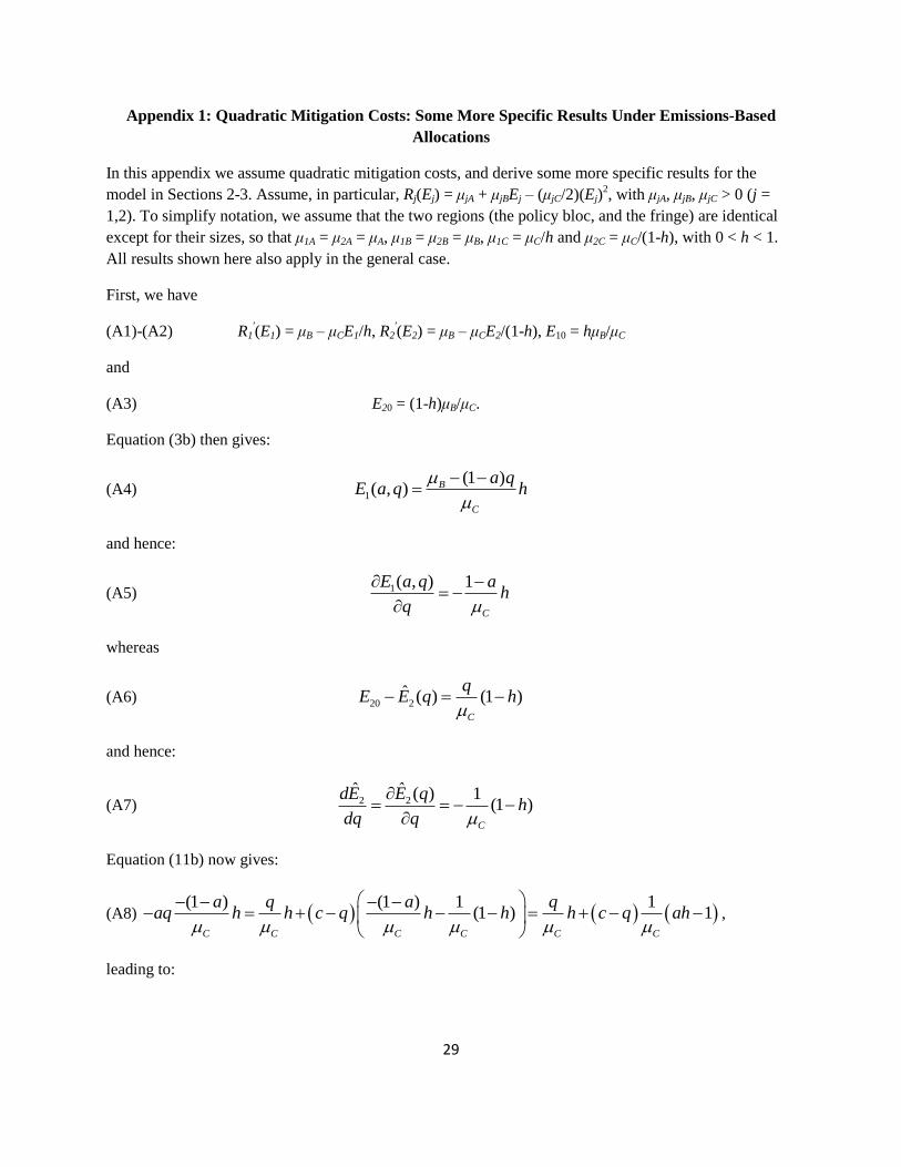
29

Appendix 1: Quadratic Mitigation Costs: Some More Specific Results Under Emissions-Based

Allocations

In this appendix we assume quadratic mitigation costs, and derive some more specific results for the

model in Sections 2-3. Assume, in particular, Rj(Ej) = μjA + μjBEj – (μjC/2)(Ej)2, with μjA, μjB, μjC > 0 (j =

1,2). To simplify notation, we assume that the two regions (the policy bloc, and the fringe) are identical

except for their sizes, so that μ1A = μ2A = μA, μ1B = μ2B = μB, μ1C = μC/h and μ2C = μC/(1-h), with 0 < h < 1.

All results shown here also apply in the general case.

First, we have

(A1)-(A2) R1′(E1) = μB – μCE1/h, R2

′(E2) = μB – μCE2/(1-h), E10 = hμB/μC

and

(A3) E20 = (1-h)μB/μC.

Equation (3b) then gives:

(A4) 1

(1 )( , ) B

C

a qE a q h

and hence:

(A5) 1( , ) 1

C

E a q ah

q

whereas

(A6) 20 2ˆ ( ) (1 )

C

qE E q h

and hence:

(A7) 2 2ˆ ˆ ( ) 1

(1 )C

dE E qh

dq q

Equation (11b) now gives:

(A8) (1 ) (1 ) 1 1

(1 ) 1C C C C C C

a q a qaq h h c q h h h c q ah

,

leading to:

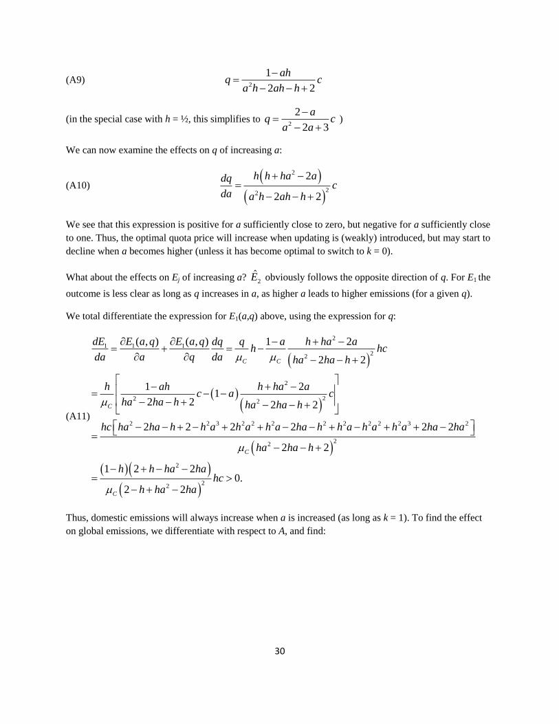
30

(A9) 2

1

2 2

ahq c

a h ah h

(in the special case with h = ½, this simplifies to 2

2

2 3

aq c

a a

)

We can now examine the effects on q of increasing a:

(A10)

2

22

2

2 2

h h ha adqc

da a h ah h

We see that this expression is positive for a sufficiently close to zero, but negative for a sufficiently close

to one. Thus, the optimal quota price will increase when updating is (weakly) introduced, but may start to

decline when a becomes higher (unless it has become optimal to switch to k = 0).

What about the effects on Ej of increasing a? 2E obviously follows the opposite direction of q. For E1 the

outcome is less clear as long as q increases in a, as higher a leads to higher emissions (for a given q).

We total differentiate the expression for E1(a,q) above, using the expression for q:

(A11)

2

1 1 1

22

2

22 2

2 2 3 2 2 2 2 2 2 2 2 3 2

22

( , ) ( , ) 1 2

2 2

1 21

2 2 2 2

2 2 2 2 2 2

2 2

1 2

C C

C

C

dE E a q E a q dq q a h ha ah hc

da a q da ha ha h

h ah h ha ac a c

ha ha h ha ha h

hc ha ha h h a h a h a ha h h a h a h a ha ha

ha ha h

h

2

22

20.

2 2C

h ha hahc

h ha ha

Thus, domestic emissions will always increase when a is increased (as long as k = 1). To find the effect

on global emissions, we differentiate with respect to A, and find:

31

(A12)

2 2

1 2

2 22 2

2 2

22

2

22

ˆ 1 2 2 21

2 2 2 2

(1 )2 2 2

2 2

2(1 )1 0.

2 2

CC

C

C

h h ha ha h h ha adE dEdE dq hhc c

da da dq da h ha ha h ha ha

h hch ha ha h ha a

h ha ha

h hca ha ha

h ha ha

Hence, global emissions will unambiguously increase when a is increased as long as offsets are used. We

can also show, given a = 0, that global emissions are lower if offsets are used than if they are not.

Updating will then increase global emissions, regardless of the optimality of offsets.

Furthermore, we can show that welfare is decreasing in the level of a as long as offsets are used (k = 1),

cf. equation (9):

(A13)

1 21 20 2

1 21

1

ˆˆ

ˆ (1 )

1 2(1 )

CB

CB

C

C

dE dEdB dqE c c q E E

da h da da da

dE dE q h dqE c c q

h da dq da

h c qdE dqa q c

da da

The first term in the last line of (A13) is negative due to the 1.o.c. in (3b). The bracket in the second term

is also negative, as q > 2c (cf. the expression of q above). Thus, since q increases in a for sufficiently low

levels of a, we know that B must decrease when a is increased starting at zero, and as long as dq/da is

positive. Furthermore, consider a level of a where dq/da is negative. Assume that a is increased from a1 to

a2, so that q(a1) > q(a2). Consider the suboptimal pair a1 and q(a2). We know that B(a1,q(a1)) is higher

than B(a1,q(a2)), since q(a1) is the optimal quota price given a1. What about the comparison between

B(a1,q(a2)) and B(a2,q(a2))? Obviously, emissions in region 2 are the same in these two cases, and thus the

two last terms in (10a) are identical. Moreover, emissions in region 1 are lowest when a is lowest (given

the same q). Since R1′(E1) < c whenever offsets are used, B must be highest when E1 is lowest. Thus,

B(a1,q(a2)) > B(a2,q(a2)). But then we have shown that B is decreasing in a also when q is decreasing in a.

A higher level of a will therefore unambiguously reduce welfare whenever offsets are used.

Finally, we can show that it is optimal to switch to no offsets exactly when global emissions are the same

with and without offsets. To see this, we first calculate the level of a where global emissions are identical

with and without offsets. Then we must have:

32

(A14)

1 0

1 1 20 2

2

2 2 2 2 2 2

ˆ (1 )

(1 )(1 )

1 (1 )

11 (1 )

2 2

1 2 2 2

1

2

k k

C

B B

C C C

qE E E E h

a q c qh h h

q h a h ch

ahc h a h ch

a h ah h

ha h a h a h a h h

ha

h

We denote this level of a as â. It follows straightforwardly that:

(A15) 2

( )1

hq a c

h

We next calculate the difference in welfare with and without offsets when global emissions are the same:

(A16)

1 0 1 0

1 1 1 1 20 2

2 21 0 1 0

1 1 1 1

2 2 2 2 2 2 2 2 2 2 2 2 2

4

2 2 2 2 2

2

2

ˆ( ) ( )

(1 )2

(1 )

(1 ) 2 2 (1 ) 2 (1 )

2

12

2

C

k k k k

k k k kCB

C

B

C

B C C C B C B C C

C

B B

C

C

h

B B R E R E q E E

qE E E E q h

h

qq h

h c h q h c h q h h cq h h

h c h c h

h

2 2 2 2 2 2 2 2 2 2

2 2 2 2 2 2

22

2 2 2 (1 )

2 2 (1 ) 2 (1 ) 2

2( 1 ) 2 (1 )

2 (1 ) 10

2 2

B B B

B B B B

C C

hq h q hq h q h c h q h

c h q h h cqh h h c h c h

hq h c ch h

q q h q ch h h

h h

Thus, we have shown that, when global emissions are the same with and without offsets, welfare is also

the same with and without offsets. As welfare is monotonically decreasing in the level of a, and global

emissions are monotonically increasing in the level of a, it must be optimal to switch to no offsets exactly

when global emissions are the same in the two cases.

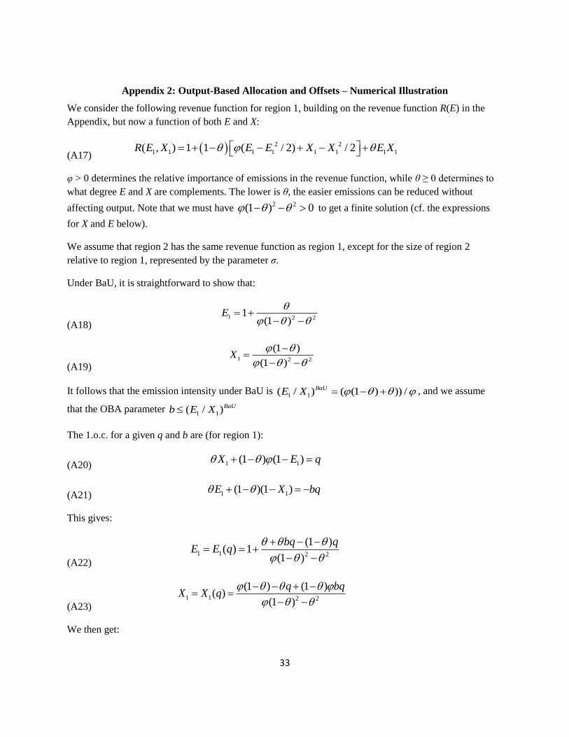
33

Appendix 2: Output-Based Allocation and Offsets – Numerical Illustration

We consider the following revenue function for region 1, building on the revenue function R(E) in the

Appendix, but now a function of both E and X:

(A17) 2 2

1 1 1 1 1 1 1 1( , ) 1 1 ( / 2) / 2R E X E E X X E X

φ > 0 determines the relative importance of emissions in the revenue function, while θ ≥ 0 determines to

what degree E and X are complements. The lower is θ, the easier emissions can be reduced without

affecting output. Note that we must have 2 2(1 ) 0 to get a finite solution (cf. the expressions

for X and E below).

We assume that region 2 has the same revenue function as region 1, except for the size of region 2

relative to region 1, represented by the parameter σ.

Under BaU, it is straightforward to show that:

(A18) 1 2 2

1(1 )

E

(A19) 1 2 2

(1 )

(1 )X

It follows that the emission intensity under BaU is 1 1( / ) ( (1 ) )) /BaUE X , and we assume

that the OBA parameter 1 1( / )BaUb E X

The 1.o.c. for a given q and b are (for region 1):

(A20) 1 1(1 ) (1 )X E q

(A21) 1 1(1 )(1 )E X bq

This gives:

(A22) 1 1 2 2

(1 )( ) 1

(1 )

bq qE E q

(A23) 1 1 2 2

(1 ) (1 )( )

(1 )

q bqX X q

We then get:

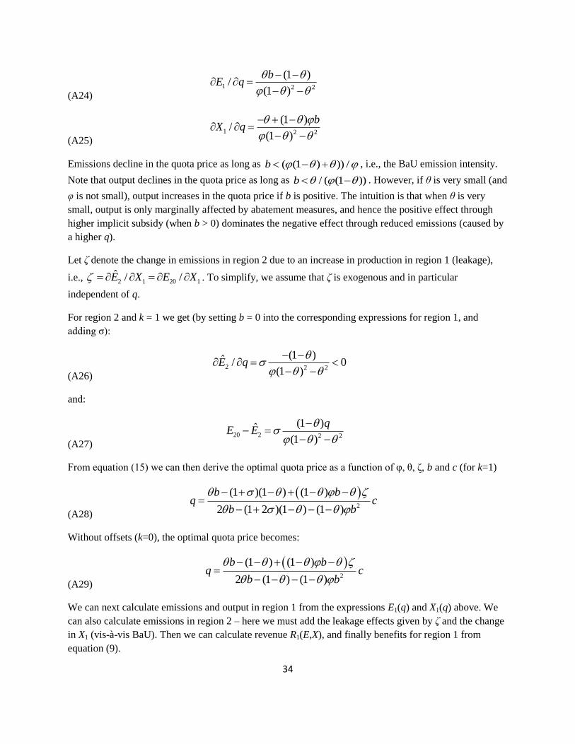
34

(A24) 1 2 2

(1 )/

(1 )

bE q

(A25) 1 2 2

(1 )/

(1 )

bX q

Emissions decline in the quota price as long as ( (1 ) )) /b , i.e., the BaU emission intensity.

Note that output declines in the quota price as long as / ( (1 ))b . However, if θ is very small (and

φ is not small), output increases in the quota price if b is positive. The intuition is that when θ is very

small, output is only marginally affected by abatement measures, and hence the positive effect through

higher implicit subsidy (when b > 0) dominates the negative effect through reduced emissions (caused by

a higher q).

Let ζ denote the change in emissions in region 2 due to an increase in production in region 1 (leakage),

i.e., 2 1 20 1ˆ / /E X E X . To simplify, we assume that ζ is exogenous and in particular

independent of q.

For region 2 and k = 1 we get (by setting b = 0 into the corresponding expressions for region 1, and

adding σ):

(A26) 2 2 2

(1 )ˆ / 0(1 )

E q

and:

(A27) 20 2 2 2

(1 )ˆ(1 )

qE E

From equation (15) we can then derive the optimal quota price as a function of φ, θ, ζ, b and c (for k=1)

(A28)

2

(1 )(1 ) (1 )

2 (1 2 )(1 ) (1 )

b bq c

b b

Without offsets (k=0), the optimal quota price becomes:

(A29)

2

(1 ) (1 )

2 (1 ) (1 )

b bq c

b b

We can next calculate emissions and output in region 1 from the expressions E1(q) and X1(q) above. We

can also calculate emissions in region 2 – here we must add the leakage effects given by ζ and the change

in X1 (vis-à-vis BaU). Then we can calculate revenue R1(E,X), and finally benefits for region 1 from

equation (9).

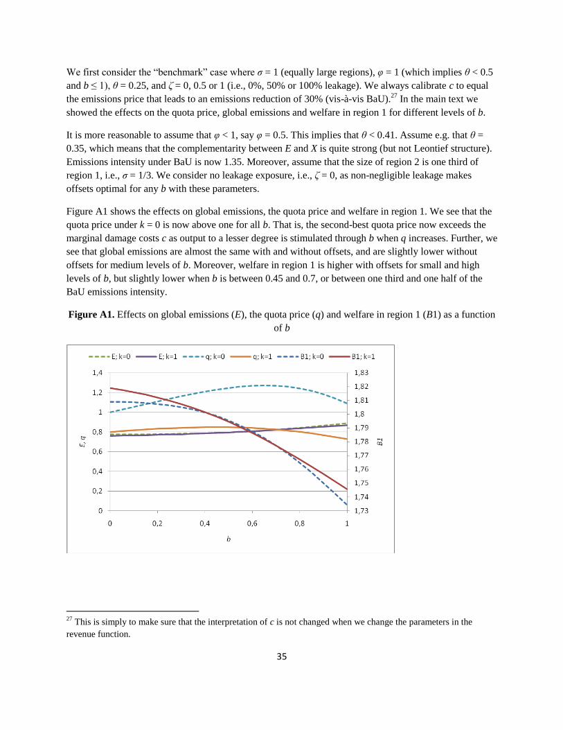
35

We first consider the “benchmark” case where σ = 1 (equally large regions), φ = 1 (which implies θ < 0.5

and b ≤ 1), θ = 0.25, and ζ = 0, 0.5 or 1 (i.e., 0%, 50% or 100% leakage). We always calibrate c to equal

the emissions price that leads to an emissions reduction of 30% (vis-à-vis BaU).27

In the main text we

showed the effects on the quota price, global emissions and welfare in region 1 for different levels of b.

It is more reasonable to assume that φ < 1, say φ = 0.5. This implies that θ < 0.41. Assume e.g. that θ =

0.35, which means that the complementarity between E and X is quite strong (but not Leontief structure).

Emissions intensity under BaU is now 1.35. Moreover, assume that the size of region 2 is one third of

region 1, i.e., σ = 1/3. We consider no leakage exposure, i.e., ζ = 0, as non-negligible leakage makes

offsets optimal for any b with these parameters.

Figure A1 shows the effects on global emissions, the quota price and welfare in region 1. We see that the

quota price under k = 0 is now above one for all b. That is, the second-best quota price now exceeds the

marginal damage costs c as output to a lesser degree is stimulated through b when q increases. Further, we

see that global emissions are almost the same with and without offsets, and are slightly lower without

offsets for medium levels of b. Moreover, welfare in region 1 is higher with offsets for small and high

levels of b, but slightly lower when b is between 0.45 and 0.7, or between one third and one half of the

BaU emissions intensity.

Figure A1. Effects on global emissions (E), the quota price (q) and welfare in region 1 (B1) as a function

of b

27

This is simply to make sure that the interpretation of c is not changed when we change the parameters in the

revenue function.