
1
Supplementary Information for 1
In-situ study of the formation mechanism of two-2
dimensional superlattices from PbSe nanocrystals 3
Jaco J. Geuchies1,5a†, Carlo van Overbeek1†, Wiel H. Evers2,3, Bart Goris4, Annick de Backer4, Anjan P. 4 Gantapara6, Freddy. T. Rabouw1, Jan Hilhorst5b, Joep L. Peters1, Oleg Konovalov5a, Andrei V. 5 Petukhov7,8, Marjolein Dijkstra6, Laurens D.A. Siebbeles2, Sandra van Aert4, Sara Bals4 and Daniel 6 Vanmaekelbergh1* 7 8
*Corresponding author. E-mail: [email protected] 9
10
This supplement contains: 11
Supplementary figure S1…………………………………………………………………………………………………………….……….…………..…p. 3 12
Supplementary figure S2………………………………………………………………………………………………………….…..………....…………p. 3 13
Supplementary figure S3……………………………………………………………………………………………………………………..…..…………p. 4 14
Supplementary figure S4………………………………………………………………………………………………………………………..…..………p. 4 15
Supplementary figure S5…………………………………………………………………………………………………………….…..……..…..………p. 5 16
Supplementary figure S6………………………………………………………………………………………………………..…….……………….……p. 5 17
Supplementary figure S7…………………………………………………………………………………………………..………….…………………....p. 6 18
Supplementary figure S8……………………………………………………………………………………………………..……….………………..…..p. 6 19
Supplementary figure S9…………………………………………………………………………………………………..……….…………………….…p. 7 20
Supplementary figure S10…………………………………………………………………………………………………..……….…………………..…p. 7 21
Supplementary figure S11………………………………………………………………………………………………………………………………..…p. 7 22
Supplementary methods 1: calculation of the X-ray penetration depth………………………………...……….…………….……p. 9 23
Supplementary figure S12…………………………………………………………………………………………………………………...………..……p. 9 24
Supplementary methods 2: computer aided image analysis……………………………….……………….………………………..……p. 10 25
Supplementary figure S13……………………………………………………………………………………………..…..…………….………….…..…p. 10 26
Supplementary figure S14……………………………………………………………………………………………..…..…………….………….…..…p. 11 27
Supplementary figure S15……………………………………………………………………………………………..…..…………….………….…..…p. 11 28
Supplementary figure S16…………………………………………………………………………………………………….….…………………......…p. 12 29
Supplementary methods 3: modelling of GISAXS patterns for hexagonal, rhombic and square superlattices……..p. 13 30
Supplementary figure S17……………………………………………….…………………………….……………………………………….……….…..p. 14 31
Supplementary methods 4: calculation of the position of the atomic reflections on the GIWAXS detector……......p. 15 32
Supplementary figure S18……………………………………………….…………………………….……………………………….……….…….…….p. 16 33
Supplementary methods 5: peak width of atomically aligned, but not attached, nanocrystals……………………….…...p. 17 34
In situ study of the formation mechanism of two-dimensional superlattices from PbSe nanocrystals
SUPPLEMENTARY INFORMATIONDOI: 10.1038/NMAT4746
NATURE MATERIALS | www.nature.com/naturematerials 1
© 2016 Macmillan Publishers Limited, part of Springer Nature. All rights reserved.
2
Supplementary figure S19……………………………………………….…………………………….………………………………………….………….p. 17 35
Supplementary figure S20……………………………………………….…………………………….………………………………………….………….p. 18 36
Supplementary methods 6: azimuthal and radial peak widths in electron diffraction………………………….…….…….…..p. 20 37
Supplementary figure S21……………………………………………….…………………………….……………………………………..…..………….p. 20 38
Supplementary figure S22……………………………………………….…………………………….……………………………………..….….……….p. 21 39
Supplementary figure S23……………………………………………….…………………………….……………………………………...….………….p. 21 40
Supplementary methods 7: Coulombic and Van Der Waals interactions between nanocrystals.………….….……….…..p. 22 41
Supplementary figure S24……………………………………………….…………………………….……………………………………...….………….p. 22 42
Supplementary figure S25.............................................................................................................................................p. 23 43
References………………………………………………………………….…………………………..…………………………………….…....……..………..p. 24 44
2 NATURE MATERIALS | www.nature.com/naturematerials
SUPPLEMENTARY INFORMATION DOI: 10.1038/NMAT4746
© 2016 Macmillan Publishers Limited, part of Springer Nature. All rights reserved.
3
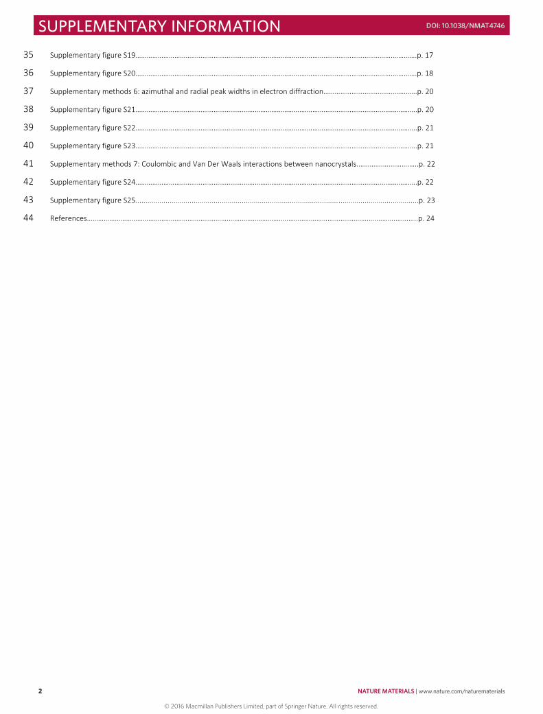
Figure S1: Schematic of the in-situ GISAXS/GIWAXS study of nanocrystal assembly at the liquid/air 45 interface. (a) An atomic model of the PbSe truncated nanocubes, showing the different facets of the 46 NC. Blue indicates the {100} facets, yellow the {110} facets and green the {111} facets. (b) Schematic 47 of the setup used for in-situ GISAXS/WAXS experiments. A dispersion of NCs in toluene evaporates in 48 a liquid sample cell. We examine the process of assembly and attachment using grazing-incidence x-49 ray scattering, by simultaneously monitoring the atomic order on the wide-angle detector and 50 nanoscale order on the small-angle detector. 51
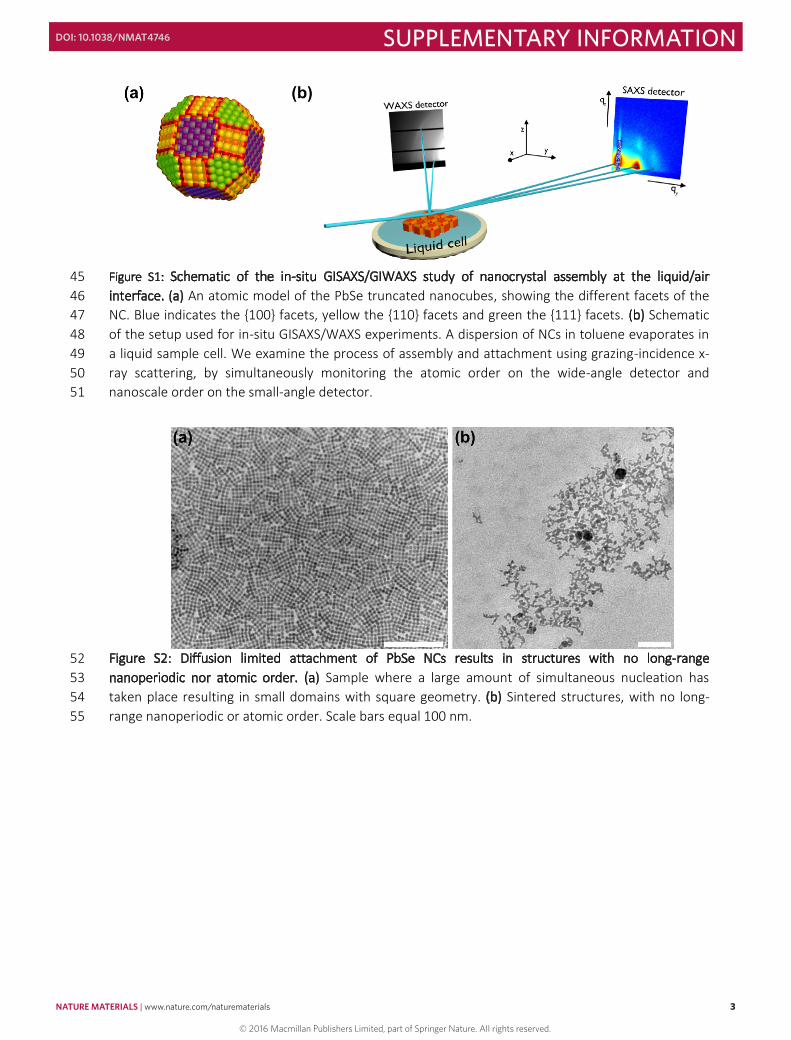
Figure S2: Diffusion limited attachment of PbSe NCs results in structures with no long-range 52 nanoperiodic nor atomic order. (a) Sample where a large amount of simultaneous nucleation has 53 taken place resulting in small domains with square geometry. (b) Sintered structures, with no long-54 range nanoperiodic or atomic order. Scale bars equal 100 nm. 55
NATURE MATERIALS | www.nature.com/naturematerials 3
SUPPLEMENTARY INFORMATIONDOI: 10.1038/NMAT4746
© 2016 Macmillan Publishers Limited, part of Springer Nature. All rights reserved.
4
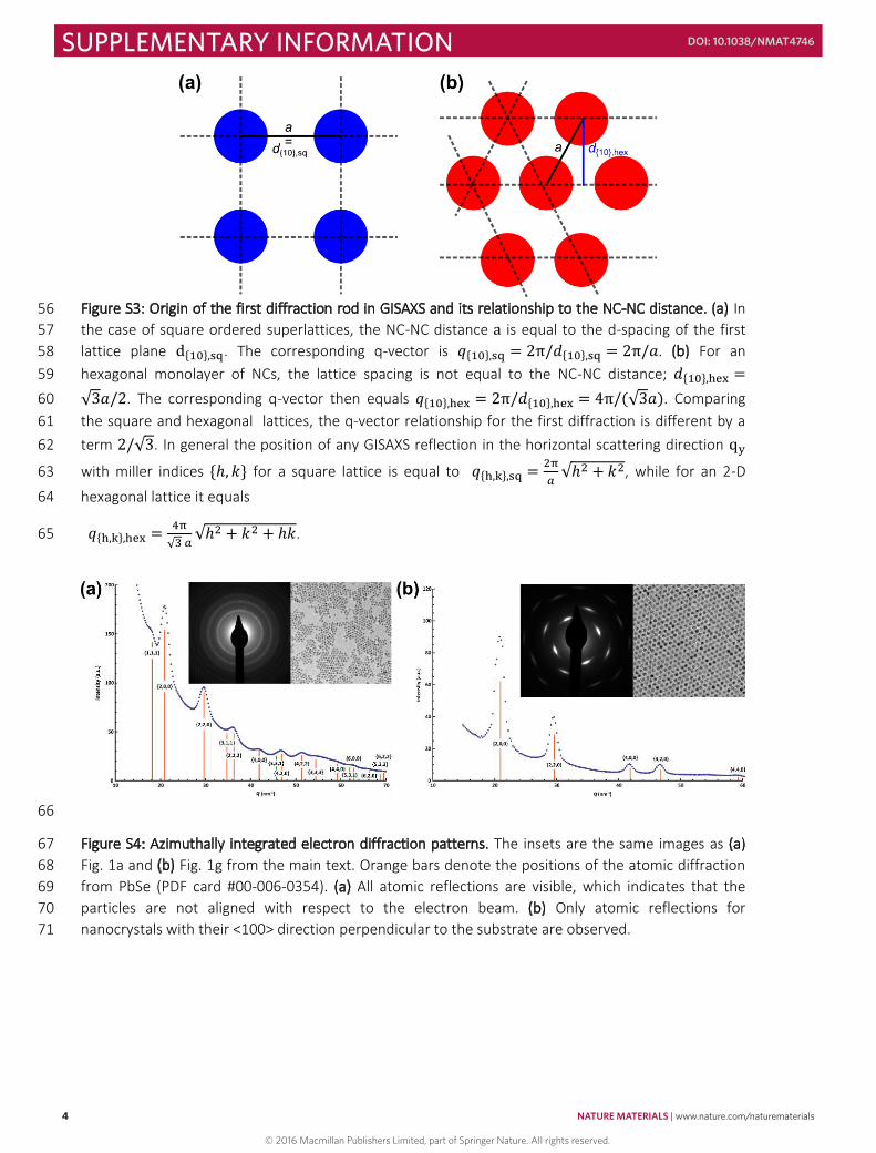
Figure S3: Origin of the first diffraction rod in GISAXS and its relationship to the NC-NC distance. (a) In 56 the case of square ordered superlattices, the NC-NC distance a is equal to the d-spacing of the first 57 lattice plane d{10},sq. The corresponding q-vector is 𝑞𝑞{10},sq = 2π/𝑑𝑑{10},sq = 2π/𝑎𝑎. (b) For an 58 hexagonal monolayer of NCs, the lattice spacing is not equal to the NC-NC distance; 𝑑𝑑{10},hex =59
√3𝑎𝑎/2. The corresponding q-vector then equals 𝑞𝑞{10},hex = 2π/𝑑𝑑{10},hex = 4π/(√3𝑎𝑎). Comparing 60 the square and hexagonal lattices, the q-vector relationship for the first diffraction is different by a 61 term 2/√3. In general the position of any GISAXS reflection in the horizontal scattering direction qy 62
with miller indices {ℎ, 𝑘𝑘} for a square lattice is equal to 𝑞𝑞{h,k},sq = 2π𝑎𝑎 √ℎ2 + 𝑘𝑘2, while for an 2-D 63
hexagonal lattice it equals 64
𝑞𝑞{h,k},hex = 4π√3 𝑎𝑎 √ℎ2 + 𝑘𝑘2 + ℎ𝑘𝑘. 65
66
Figure S4: Azimuthally integrated electron diffraction patterns. The insets are the same images as (a) 67 Fig. 1a and (b) Fig. 1g from the main text. Orange bars denote the positions of the atomic diffraction 68 from PbSe (PDF card #00-006-0354). (a) All atomic reflections are visible, which indicates that the 69 particles are not aligned with respect to the electron beam. (b) Only atomic reflections for 70 nanocrystals with their <100> direction perpendicular to the substrate are observed. 71
4 NATURE MATERIALS | www.nature.com/naturematerials
SUPPLEMENTARY INFORMATION DOI: 10.1038/NMAT4746
© 2016 Macmillan Publishers Limited, part of Springer Nature. All rights reserved.
5
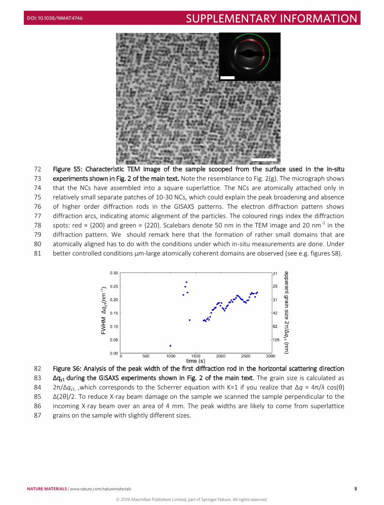
Figure S5: Characteristic TEM image of the sample scooped from the surface used in the in-situ 72 experiments shown in Fig. 2 of the main text. Note the resemblance to Fig. 2(g). The micrograph shows 73 that the NCs have assembled into a square superlattice. The NCs are atomically attached only in 74 relatively small separate patches of 10-30 NCs, which could explain the peak broadening and absence 75 of higher order diffraction rods in the GISAXS patterns. The electron diffraction pattern shows 76 diffraction arcs, indicating atomic alignment of the particles. The coloured rings index the diffraction 77 spots: red = {200} and green = {220}. Scalebars denote 50 nm in the TEM image and 20 nm-1 in the 78 diffraction pattern. We should remark here that the formation of rather small domains that are 79 atomically aligned has to do with the conditions under which in-situ measurements are done. Under 80 better controlled conditions µm-large atomically coherent domains are observed (see e.g. figures S8). 81
Figure S6: Analysis of the peak width of the first diffraction rod in the horizontal scattering direction 82 Δqy1 during the GISAXS experiments shown in Fig. 2 of the main text. The grain size is calculated as 83 2π/Δqy1, ,which corresponds to the Scherrer equation with K=1 if you realize that Δq = 4π/λ cos(θ) 84 Δ(2θ)/2. To reduce X-ray beam damage on the sample we scanned the sample perpendicular to the 85 incoming X-ray beam over an area of 4 mm. The peak widths are likely to come from superlattice 86 grains on the sample with slightly different sizes. 87
NATURE MATERIALS | www.nature.com/naturematerials 5
SUPPLEMENTARY INFORMATIONDOI: 10.1038/NMAT4746
© 2016 Macmillan Publishers Limited, part of Springer Nature. All rights reserved.
6
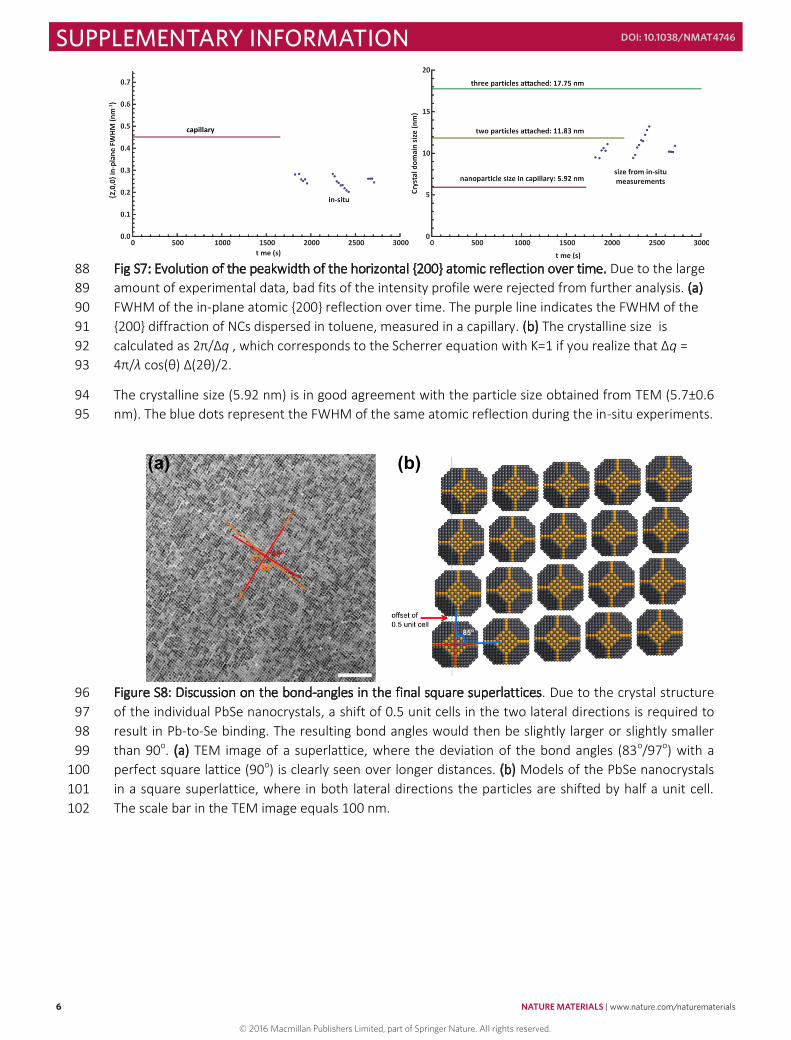
Fig S7: Evolution of the peakwidth of the horizontal {200} atomic reflection over time. Due to the large 88 amount of experimental data, bad fits of the intensity profile were rejected from further analysis. (a) 89 FWHM of the in-plane atomic {200} reflection over time. The purple line indicates the FWHM of the 90 {200} diffraction of NCs dispersed in toluene, measured in a capillary. (b) The crystalline size is 91 calculated as 2π/Δq , which corresponds to the Scherrer equation with K=1 if you realize that Δq = 92 4π/λ cos(θ) Δ(2θ)/2. 93
The crystalline size (5.92 nm) is in good agreement with the particle size obtained from TEM (5.7±0.6 94 nm). The blue dots represent the FWHM of the same atomic reflection during the in-situ experiments. 95
Figure S8: Discussion on the bond-angles in the final square superlattices. Due to the crystal structure 96 of the individual PbSe nanocrystals, a shift of 0.5 unit cells in the two lateral directions is required to 97 result in Pb-to-Se binding. The resulting bond angles would then be slightly larger or slightly smaller 98 than 90o. (a) TEM image of a superlattice, where the deviation of the bond angles (83o/97o) with a 99 perfect square lattice (90o) is clearly seen over longer distances. (b) Models of the PbSe nanocrystals 100 in a square superlattice, where in both lateral directions the particles are shifted by half a unit cell. 101 The scale bar in the TEM image equals 100 nm. 102
6 NATURE MATERIALS | www.nature.com/naturematerials
SUPPLEMENTARY INFORMATION DOI: 10.1038/NMAT4746
© 2016 Macmillan Publishers Limited, part of Springer Nature. All rights reserved.
7
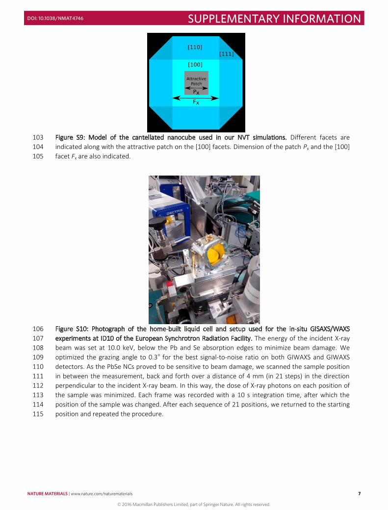
Figure S9: Model of the cantellated nanocube used in our NVT simulations. Different facets are 103 indicated along with the attractive patch on the [100] facets. Dimension of the patch Px and the [100] 104 facet Fx are also indicated. 105
Figure S10: Photograph of the home-built liquid cell and setup used for the in-situ GISAXS/WAXS 106 experiments at ID10 of the European Synchrotron Radiation Facility. The energy of the incident X-ray 107 beam was set at 10.0 keV, below the Pb and Se absorption edges to minimize beam damage. We 108 optimized the grazing angle to 0.3o for the best signal-to-noise ratio on both GIWAXS and GIWAXS 109 detectors. As the PbSe NCs proved to be sensitive to beam damage, we scanned the sample position 110 in between the measurement, back and forth over a distance of 4 mm (in 21 steps) in the direction 111 perpendicular to the incident X-ray beam. In this way, the dose of X-ray photons on each position of 112 the sample was minimized. Each frame was recorded with a 10 s integration time, after which the 113 position of the sample was changed. After each sequence of 21 positions, we returned to the starting 114 position and repeated the procedure. 115
NATURE MATERIALS | www.nature.com/naturematerials 7
SUPPLEMENTARY INFORMATIONDOI: 10.1038/NMAT4746
© 2016 Macmillan Publishers Limited, part of Springer Nature. All rights reserved.
8
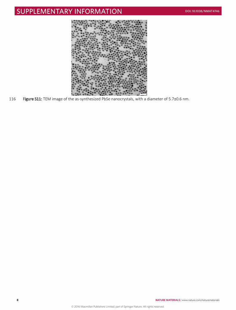
Figure S11: TEM image of the as-synthesized PbSe nanocrystals, with a diameter of 5.7±0.6 nm. 116
8 NATURE MATERIALS | www.nature.com/naturematerials
SUPPLEMENTARY INFORMATION DOI: 10.1038/NMAT4746
© 2016 Macmillan Publishers Limited, part of Springer Nature. All rights reserved.
9
Supplementary methods 1: calculation of the X-ray penetration depth 117
The incident X-ray energy of 10 keV corresponds to a wavelength λ0 = 0.124 nm and a wavevector of 118 magnitude 𝑘𝑘0 = 2𝜋𝜋/𝜆𝜆0 = 50.7 nm-1 in air. For our experiments we used a grazing angle of incidence 119 of 0.3o, slightly larger than the critical angle for total external reflection of bulk PbSe. Since the 120 refractive index of any material is negative at X-ray frequencies (𝑛𝑛 = 1 − 𝛿𝛿 + 𝑖𝑖𝑖𝑖), the wavevector 121 inside the sample 𝑘𝑘 = 𝑛𝑛𝑘𝑘0 is smaller than in air. Upon transmission of the beam into the sample, the 122 wavevector component parallel to the air–sample interface 𝑘𝑘|| = 𝑘𝑘0cos (𝛼𝛼𝑖𝑖) is conserved. The 123 wavevector component perpendicular to the sample is 124
𝑘𝑘𝑧𝑧 = √𝑘𝑘2 − 𝑘𝑘||2 = 𝑘𝑘0√𝑛𝑛2 − cos2(𝛼𝛼𝑖𝑖)
Since n is complex, kz is complex. The imaginary part of kz describes how quickly the X-ray intensity 125 decays when going deeper into the sample. The penetration depth d, defined as the depth at which 126 the X-ray intensity is lower by a factor e than at the interface, is given by 127
𝑑𝑑 = 12 Im(𝑘𝑘𝑧𝑧)
δ β PbSe 1.292x10⁻⁵ 8.430x10⁻⁷ Toluene 1.964x10⁻⁶ 1.750x10⁻⁹ Ethylene glycol 2.539x10⁻⁶ 4.188x10⁻⁹
Supplementary table S1: Values of the real (δ) and imaginary (β) part of the refractive-index 128 decrement at 10keV for the materials used in these experiments. δ and β define refraction and 129 absorption in a material accordingly. 130
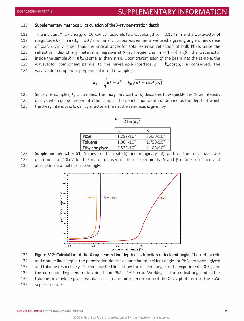
Figure S12: Calculation of the X-ray penetration depth as a function of incident angle. The red, purple 131 and orange lines depict the penetration depths as function of incident angle for PbSe, ethylene glycol 132 and toluene respectively. The blue dashed lines show the incident angle of the experiments (0.3o) and 133 the corresponding penetration depth for PbSe (16.3 nm). Working at the critical angle of either 134 toluene or ethylene glycol would result in a minute penetration of the X-ray photons into the PbSe 135 superstructure. 136
NATURE MATERIALS | www.nature.com/naturematerials 9
SUPPLEMENTARY INFORMATIONDOI: 10.1038/NMAT4746
© 2016 Macmillan Publishers Limited, part of Springer Nature. All rights reserved.
10
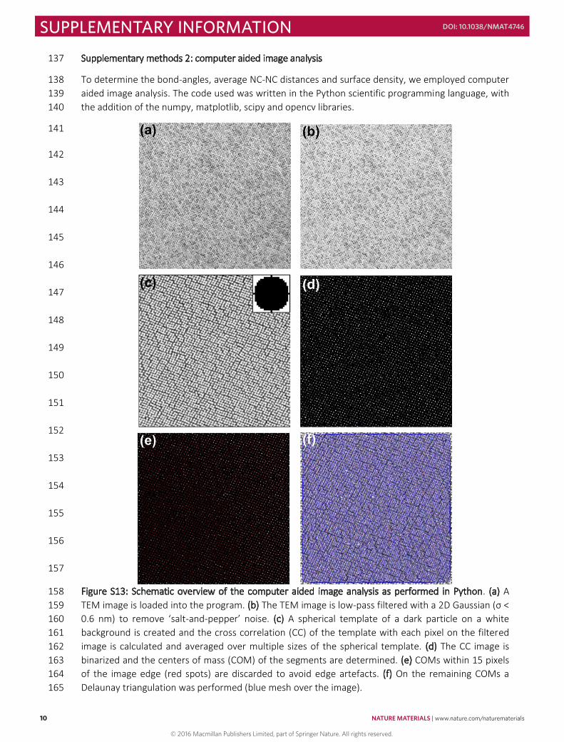
Supplementary methods 2: computer aided image analysis 137
To determine the bond-angles, average NC-NC distances and surface density, we employed computer 138 aided image analysis. The code used was written in the Python scientific programming language, with 139 the addition of the numpy, matplotlib, scipy and opencv libraries. 140
141
142
143
144
145
146
147
148
149
150
151
152
153
154
155
156
157
Figure S13: Schematic overview of the computer aided image analysis as performed in Python. (a) A 158 TEM image is loaded into the program. (b) The TEM image is low-pass filtered with a 2D Gaussian (σ < 159 0.6 nm) to remove ‘salt-and-pepper’ noise. (c) A spherical template of a dark particle on a white 160 background is created and the cross correlation (CC) of the template with each pixel on the filtered 161 image is calculated and averaged over multiple sizes of the spherical template. (d) The CC image is 162 binarized and the centers of mass (COM) of the segments are determined. (e) COMs within 15 pixels 163 of the image edge (red spots) are discarded to avoid edge artefacts. (f) On the remaining COMs a 164 Delaunay triangulation was performed (blue mesh over the image). 165
10 NATURE MATERIALS | www.nature.com/naturematerials
SUPPLEMENTARY INFORMATION DOI: 10.1038/NMAT4746
© 2016 Macmillan Publishers Limited, part of Springer Nature. All rights reserved.
11
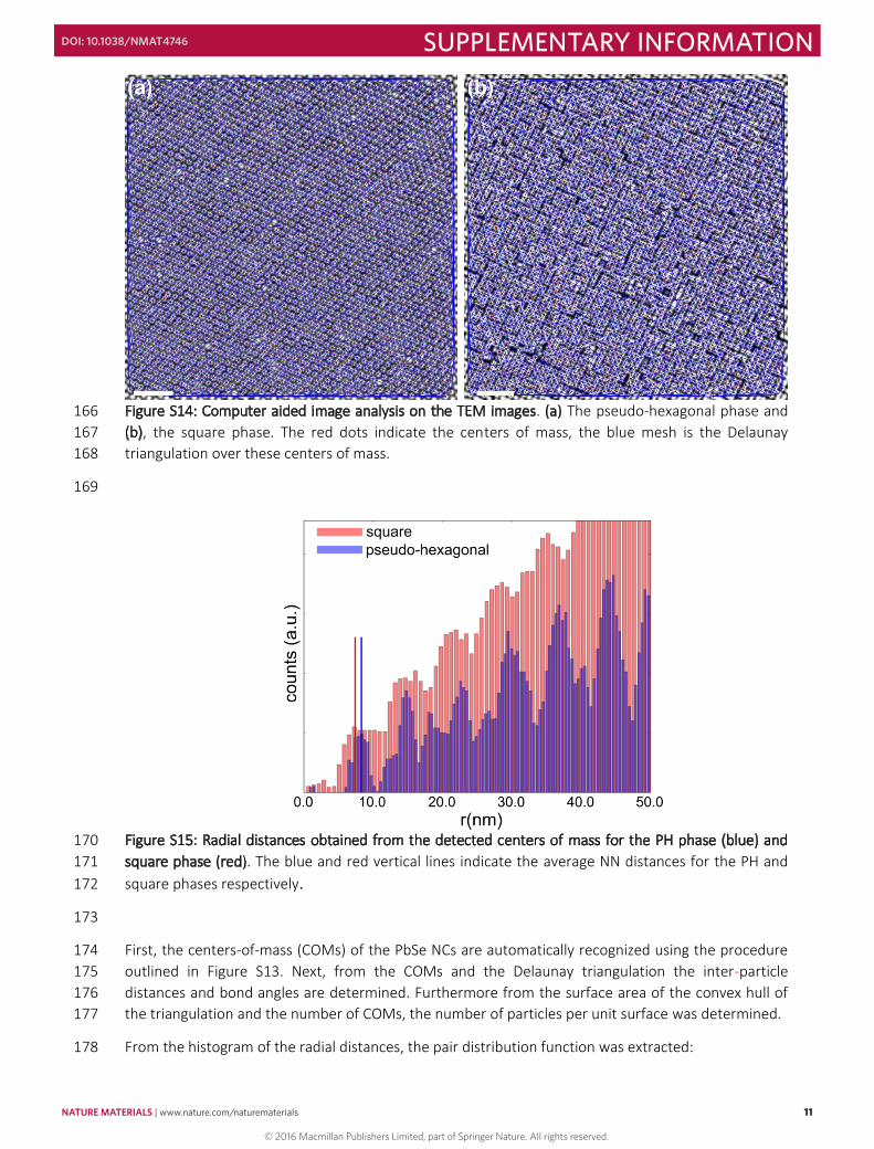
Figure S14: Computer aided image analysis on the TEM images. (a) The pseudo-hexagonal phase and 166 (b), the square phase. The red dots indicate the centers of mass, the blue mesh is the Delaunay 167 triangulation over these centers of mass. 168
169
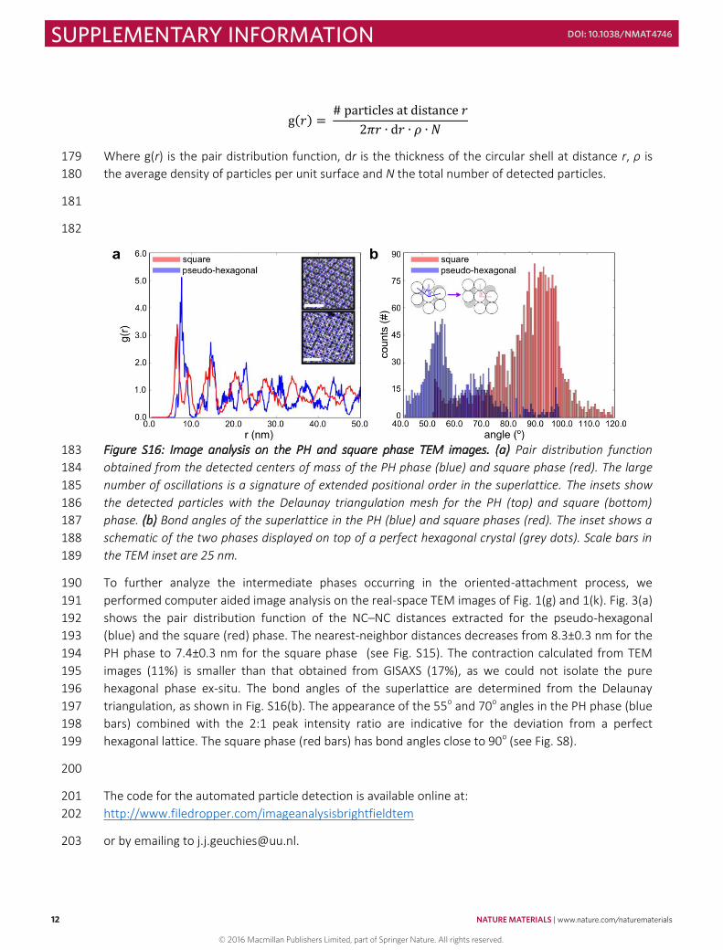
Figure S15: Radial distances obtained from the detected centers of mass for the PH phase (blue) and 170 square phase (red). The blue and red vertical lines indicate the average NN distances for the PH and 171 square phases respectively. 172
173
First, the centers-of-mass (COMs) of the PbSe NCs are automatically recognized using the procedure 174 outlined in Figure S13. Next, from the COMs and the Delaunay triangulation the inter-particle 175 distances and bond angles are determined. Furthermore from the surface area of the convex hull of 176 the triangulation and the number of COMs, the number of particles per unit surface was determined. 177
From the histogram of the radial distances, the pair distribution function was extracted: 178
NATURE MATERIALS | www.nature.com/naturematerials 11
SUPPLEMENTARY INFORMATIONDOI: 10.1038/NMAT4746
© 2016 Macmillan Publishers Limited, part of Springer Nature. All rights reserved.
12
g(𝑟𝑟) = # particles at distance 𝑟𝑟2𝜋𝜋𝑟𝑟 ∙ d𝑟𝑟 ∙ 𝜌𝜌 ∙ 𝑁𝑁
Where g(r) is the pair distribution function, dr is the thickness of the circular shell at distance r, ρ is 179 the average density of particles per unit surface and N the total number of detected particles. 180
181
182
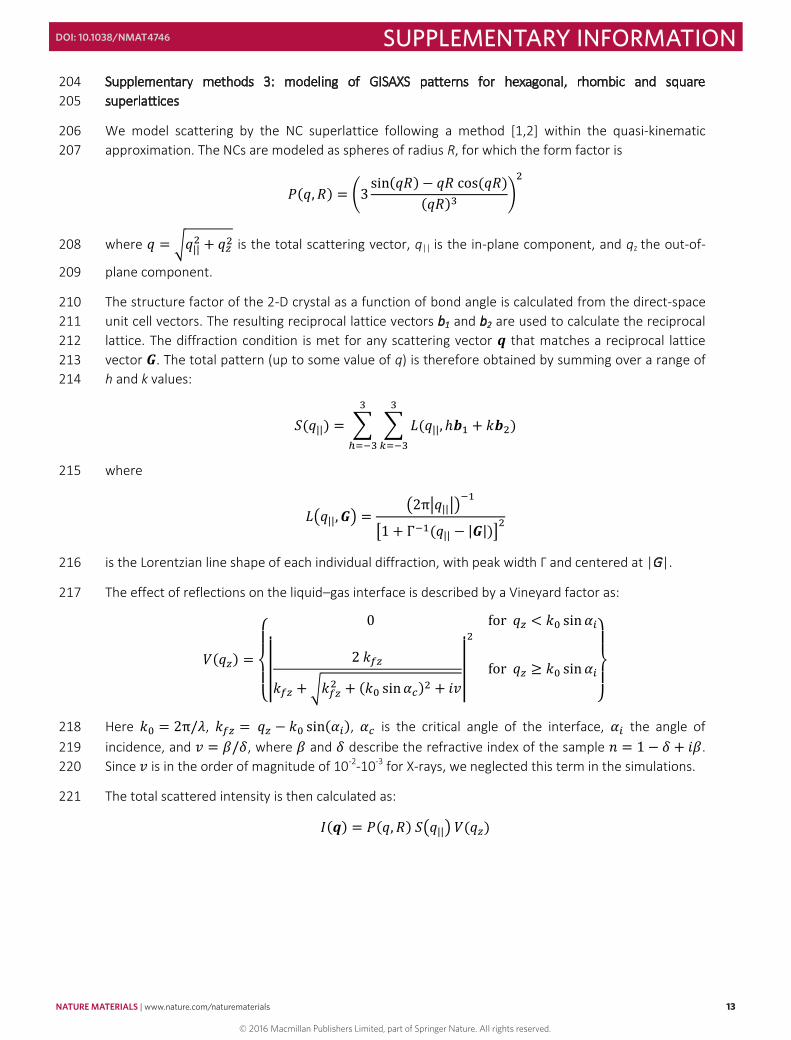
Figure S16: Image analysis on the PH and square phase TEM images. (a) Pair distribution function 183 obtained from the detected centers of mass of the PH phase (blue) and square phase (red). The large 184 number of oscillations is a signature of extended positional order in the superlattice. The insets show 185 the detected particles with the Delaunay triangulation mesh for the PH (top) and square (bottom) 186 phase. (b) Bond angles of the superlattice in the PH (blue) and square phases (red). The inset shows a 187 schematic of the two phases displayed on top of a perfect hexagonal crystal (grey dots). Scale bars in 188 the TEM inset are 25 nm. 189
To further analyze the intermediate phases occurring in the oriented-attachment process, we 190 performed computer aided image analysis on the real-space TEM images of Fig. 1(g) and 1(k). Fig. 3(a) 191 shows the pair distribution function of the NC–NC distances extracted for the pseudo-hexagonal 192 (blue) and the square (red) phase. The nearest-neighbor distances decreases from 8.3±0.3 nm for the 193 PH phase to 7.4±0.3 nm for the square phase (see Fig. S15). The contraction calculated from TEM 194 images (11%) is smaller than that obtained from GISAXS (17%), as we could not isolate the pure 195 hexagonal phase ex-situ. The bond angles of the superlattice are determined from the Delaunay 196 triangulation, as shown in Fig. S16(b). The appearance of the 55o and 70o angles in the PH phase (blue 197 bars) combined with the 2:1 peak intensity ratio are indicative for the deviation from a perfect 198 hexagonal lattice. The square phase (red bars) has bond angles close to 90o (see Fig. S8). 199
200
The code for the automated particle detection is available online at: 201 http://www.filedropper.com/imageanalysisbrightfieldtem 202
or by emailing to [email protected]. 203
12 NATURE MATERIALS | www.nature.com/naturematerials
SUPPLEMENTARY INFORMATION DOI: 10.1038/NMAT4746
© 2016 Macmillan Publishers Limited, part of Springer Nature. All rights reserved.
13
Supplementary methods 3: modeling of GISAXS patterns for hexagonal, rhombic and square 204 superlattices 205
We model scattering by the NC superlattice following a method [1,2] within the quasi-kinematic 206 approximation. The NCs are modeled as spheres of radius R, for which the form factor is 207
𝑃𝑃(𝑞𝑞, 𝑅𝑅) = (3 sin(𝑞𝑞𝑅𝑅) − 𝑞𝑞𝑅𝑅 cos (𝑞𝑞𝑅𝑅)
(𝑞𝑞𝑅𝑅)3 )2
where 𝑞𝑞 = √𝑞𝑞||2 + 𝑞𝑞𝑧𝑧2 is the total scattering vector, q|| is the in-plane component, and qz the out-of-208
plane component. 209
The structure factor of the 2-D crystal as a function of bond angle is calculated from the direct-space 210 unit cell vectors. The resulting reciprocal lattice vectors b1 and b2 are used to calculate the reciprocal 211 lattice. The diffraction condition is met for any scattering vector 𝒒𝒒 that matches a reciprocal lattice 212 vector 𝑮𝑮. The total pattern (up to some value of q) is therefore obtained by summing over a range of 213 h and k values: 214
𝑆𝑆(𝑞𝑞||) = ∑ ∑ 𝐿𝐿(𝑞𝑞||, ℎ𝒃𝒃1 + 𝑘𝑘𝒃𝒃2)3
𝑘𝑘=−3
3
ℎ=−3
where 215
𝐿𝐿(𝑞𝑞||, 𝑮𝑮) =(2π|𝑞𝑞|||)
−1
[1 + Γ−1(𝑞𝑞|| − |𝑮𝑮|)]2
is the Lorentzian line shape of each individual diffraction, with peak width Γ and centered at |G|. 216
The effect of reflections on the liquid–gas interface is described by a Vineyard factor as: 217
𝑉𝑉(𝑞𝑞𝑧𝑧) =
{ 0 for 𝑞𝑞𝑧𝑧 < 𝑘𝑘0 sin𝛼𝛼𝑖𝑖
||2 𝑘𝑘𝑓𝑓𝑧𝑧
𝑘𝑘𝑓𝑓𝑧𝑧 + √𝑘𝑘𝑓𝑓𝑧𝑧2 + (𝑘𝑘0 sin𝛼𝛼𝑐𝑐)2 + 𝑖𝑖𝑖𝑖||
2
for 𝑞𝑞𝑧𝑧 ≥ 𝑘𝑘0 sin𝛼𝛼𝑖𝑖}
Here 𝑘𝑘0 = 2π/𝜆𝜆, 𝑘𝑘𝑓𝑓𝑧𝑧 = 𝑞𝑞𝑧𝑧 − 𝑘𝑘0 sin(𝛼𝛼𝑖𝑖), 𝛼𝛼𝑐𝑐 is the critical angle of the interface, 𝛼𝛼𝑖𝑖 the angle of 218 incidence, and 𝑖𝑖 = 𝛽𝛽/𝛿𝛿, where 𝛽𝛽 and 𝛿𝛿 describe the refractive index of the sample 𝑛𝑛 = 1 − 𝛿𝛿 + 𝑖𝑖𝛽𝛽. 219 Since 𝑖𝑖 is in the order of magnitude of 10-2-10-3 for X-rays, we neglected this term in the simulations. 220
The total scattered intensity is then calculated as: 221
𝐼𝐼(𝒒𝒒) = 𝑃𝑃(𝑞𝑞, 𝑅𝑅) 𝑆𝑆(𝑞𝑞||) 𝑉𝑉(𝑞𝑞𝑧𝑧)
NATURE MATERIALS | www.nature.com/naturematerials 13
SUPPLEMENTARY INFORMATIONDOI: 10.1038/NMAT4746
© 2016 Macmillan Publishers Limited, part of Springer Nature. All rights reserved.
14
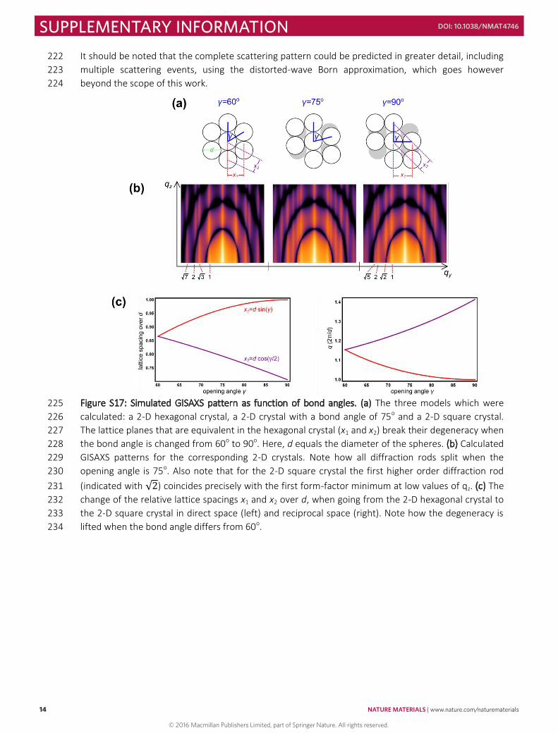
It should be noted that the complete scattering pattern could be predicted in greater detail, including 222 multiple scattering events, using the distorted-wave Born approximation, which goes however 223 beyond the scope of this work. 224
Figure S17: Simulated GISAXS pattern as function of bond angles. (a) The three models which were 225 calculated: a 2-D hexagonal crystal, a 2-D crystal with a bond angle of 75o and a 2-D square crystal. 226 The lattice planes that are equivalent in the hexagonal crystal (x1 and x2) break their degeneracy when 227 the bond angle is changed from 60o to 90o. Here, d equals the diameter of the spheres. (b) Calculated 228 GISAXS patterns for the corresponding 2-D crystals. Note how all diffraction rods split when the 229 opening angle is 75o. Also note that for the 2-D square crystal the first higher order diffraction rod 230 (indicated with √2) coincides precisely with the first form-factor minimum at low values of qz. (c) The 231 change of the relative lattice spacings x1 and x2 over d, when going from the 2-D hexagonal crystal to 232 the 2-D square crystal in direct space (left) and reciprocal space (right). Note how the degeneracy is 233 lifted when the bond angle differs from 60o. 234
14 NATURE MATERIALS | www.nature.com/naturematerials
SUPPLEMENTARY INFORMATION DOI: 10.1038/NMAT4746
© 2016 Macmillan Publishers Limited, part of Springer Nature. All rights reserved.
15
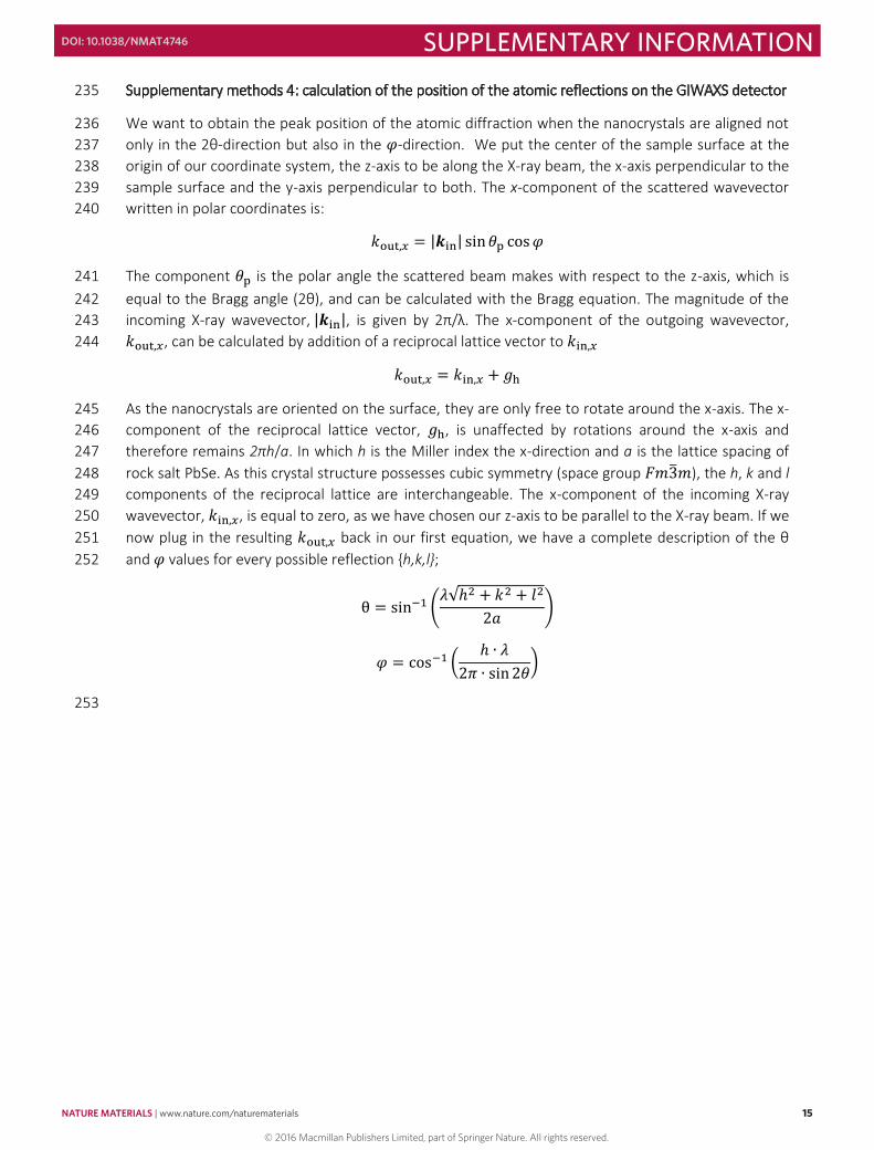
Supplementary methods 4: calculation of the position of the atomic reflections on the GIWAXS detector 235
We want to obtain the peak position of the atomic diffraction when the nanocrystals are aligned not 236 only in the 2θ-direction but also in the 𝜑𝜑-direction. We put the center of the sample surface at the 237 origin of our coordinate system, the z-axis to be along the X-ray beam, the x-axis perpendicular to the 238 sample surface and the y-axis perpendicular to both. The x-component of the scattered wavevector 239 written in polar coordinates is: 240
𝑘𝑘out,𝑥𝑥 = |𝒌𝒌in| sin 𝜃𝜃p cos 𝜑𝜑
The component 𝜃𝜃p is the polar angle the scattered beam makes with respect to the z-axis, which is 241 equal to the Bragg angle (2θ), and can be calculated with the Bragg equation. The magnitude of the 242 incoming X-ray wavevector, |𝒌𝒌in|, is given by 2π/λ. The x-component of the outgoing wavevector, 243 𝑘𝑘out,𝑥𝑥, can be calculated by addition of a reciprocal lattice vector to 𝑘𝑘in,𝑥𝑥 244
𝑘𝑘out,𝑥𝑥 = 𝑘𝑘in,𝑥𝑥 + 𝑔𝑔h
As the nanocrystals are oriented on the surface, they are only free to rotate around the x-axis. The x-245 component of the reciprocal lattice vector, 𝑔𝑔h, is unaffected by rotations around the x-axis and 246 therefore remains 2πh/a. In which h is the Miller index the x-direction and a is the lattice spacing of 247 rock salt PbSe. As this crystal structure possesses cubic symmetry (space group 𝐹𝐹𝐹𝐹3̅𝐹𝐹), the h, k and l 248 components of the reciprocal lattice are interchangeable. The x-component of the incoming X-ray 249 wavevector, 𝑘𝑘in,𝑥𝑥, is equal to zero, as we have chosen our z-axis to be parallel to the X-ray beam. If we 250 now plug in the resulting 𝑘𝑘out,𝑥𝑥 back in our first equation, we have a complete description of the θ 251 and 𝜑𝜑 values for every possible reflection {h,k,l}; 252
θ = sin−1 (𝜆𝜆√ℎ2 + 𝑘𝑘2 + 𝑙𝑙2
2𝑎𝑎 )
𝜑𝜑 = cos−1 ( ℎ ∙ 𝜆𝜆2𝜋𝜋 ∙ sin 2𝜃𝜃)
253
NATURE MATERIALS | www.nature.com/naturematerials 15
SUPPLEMENTARY INFORMATIONDOI: 10.1038/NMAT4746
© 2016 Macmillan Publishers Limited, part of Springer Nature. All rights reserved.
16
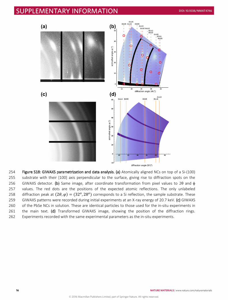
Figure S18: GIWAXS parametrization and data analysis. (a) Atomically aligned NCs on top of a Si-(100) 254 substrate with their [100] axis perpendicular to the surface, giving rise to diffraction spots on the 255 GIWAXS detector. (b) Same image, after coordinate transformation from pixel values to 2θ and 256 values. The red dots are the positions of the expected atomic reflections. The only unlabeled 257 diffraction peak at (2𝜃𝜃, 𝜑𝜑) = (32𝑜𝑜, 28𝑜𝑜) corresponds to a Si reflection, the sample substrate. These 258 GIWAXS patterns were recorded during initial experiments at an X-ray energy of 20.7 keV. (c) GIWAXS 259 of the PbSe NCs in solution. These are identical particles to those used for the in-situ experiments in 260 the main text. (d) Transformed GIWAXS image, showing the position of the diffraction rings. 261 Experiments recorded with the same experimental parameters as the in-situ experiments. 262
16 NATURE MATERIALS | www.nature.com/naturematerials
SUPPLEMENTARY INFORMATION DOI: 10.1038/NMAT4746
© 2016 Macmillan Publishers Limited, part of Springer Nature. All rights reserved.
17
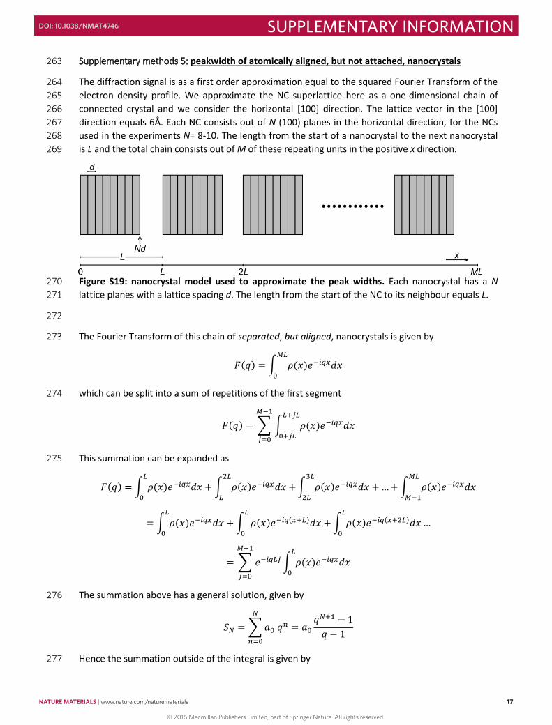
Supplementary methods 5: peakwidth of atomically aligned, but not attached, nanocrystals 263
The diffraction signal is as a first order approximation equal to the squared Fourier Transform of the 264 electron density profile. We approximate the NC superlattice here as a one-dimensional chain of 265 connected crystal and we consider the horizontal [100] direction. The lattice vector in the [100] 266 direction equals 6Å. Each NC consists out of N (100) planes in the horizontal direction, for the NCs 267 used in the experiments N= 8-10. The length from the start of a nanocrystal to the next nanocrystal 268 is L and the total chain consists out of M of these repeating units in the positive x direction. 269
Figure S19: nanocrystal model used to approximate the peak widths. Each nanocrystal has a N 270 lattice planes with a lattice spacing d. The length from the start of the NC to its neighbour equals L. 271
272
The Fourier Transform of this chain of separated, but aligned, nanocrystals is given by 273
𝐹𝐹(𝑞𝑞) = ∫ 𝜌𝜌(𝑥𝑥)𝑒𝑒−𝑖𝑖𝑖𝑖𝑖𝑖𝑑𝑑𝑥𝑥𝑀𝑀𝑀𝑀
0
which can be split into a sum of repetitions of the first segment 274
𝐹𝐹(𝑞𝑞) = ∑ ∫ 𝜌𝜌(𝑥𝑥)𝑒𝑒−𝑖𝑖𝑖𝑖𝑖𝑖𝑑𝑑𝑥𝑥𝑀𝑀+𝑗𝑗𝑀𝑀
0+𝑗𝑗𝑀𝑀
𝑀𝑀−1
𝑗𝑗=0
This summation can be expanded as 275
𝐹𝐹(𝑞𝑞) = ∫ 𝜌𝜌(𝑥𝑥)𝑒𝑒−𝑖𝑖𝑖𝑖𝑖𝑖𝑑𝑑𝑥𝑥𝑀𝑀
0+ ∫ 𝜌𝜌(𝑥𝑥)𝑒𝑒−𝑖𝑖𝑖𝑖𝑖𝑖𝑑𝑑𝑥𝑥 +
2𝑀𝑀
𝑀𝑀∫ 𝜌𝜌(𝑥𝑥)𝑒𝑒−𝑖𝑖𝑖𝑖𝑖𝑖𝑑𝑑𝑥𝑥 +
3𝑀𝑀
2𝑀𝑀… + ∫ 𝜌𝜌(𝑥𝑥)𝑒𝑒−𝑖𝑖𝑖𝑖𝑖𝑖𝑑𝑑𝑥𝑥
𝑀𝑀𝑀𝑀
𝑀𝑀−1
= ∫ 𝜌𝜌(𝑥𝑥)𝑒𝑒−𝑖𝑖𝑖𝑖𝑖𝑖𝑑𝑑𝑥𝑥𝑀𝑀
0+ ∫ 𝜌𝜌(𝑥𝑥)𝑒𝑒−𝑖𝑖𝑖𝑖(𝑖𝑖+𝑀𝑀)𝑑𝑑𝑥𝑥 + ∫ 𝜌𝜌(𝑥𝑥)𝑒𝑒−𝑖𝑖𝑖𝑖(𝑖𝑖+2𝑀𝑀)𝑑𝑑𝑥𝑥
𝑀𝑀
0…
𝑀𝑀
0
= ∑ 𝑒𝑒−𝑖𝑖𝑖𝑖𝑀𝑀𝑗𝑗𝑀𝑀−1
𝑗𝑗=0∫ 𝜌𝜌(𝑥𝑥)𝑒𝑒−𝑖𝑖𝑖𝑖𝑖𝑖𝑑𝑑𝑥𝑥
𝑀𝑀
0
The summation above has a general solution, given by 276
𝑆𝑆𝑁𝑁 = ∑ 𝑎𝑎0 𝑞𝑞𝑛𝑛𝑁𝑁
𝑛𝑛=0= 𝑎𝑎0
𝑞𝑞𝑁𝑁+1 − 1𝑞𝑞 − 1
Hence the summation outside of the integral is given by 277
NATURE MATERIALS | www.nature.com/naturematerials 17
SUPPLEMENTARY INFORMATIONDOI: 10.1038/NMAT4746
© 2016 Macmillan Publishers Limited, part of Springer Nature. All rights reserved.
18
∑ 𝑒𝑒−𝑖𝑖𝑖𝑖𝑖𝑖𝑖𝑖𝑀𝑀−1
𝑖𝑖=0= 𝑒𝑒−𝑖𝑖𝑖𝑖𝑀𝑀𝑖𝑖 − 1
𝑒𝑒−𝑖𝑖𝑖𝑖𝑖𝑖 − 1
The integral itself, which runs over a single segment of length L can be evaluated in an equivalent 278 manner: 279
∫ 𝜌𝜌(𝑥𝑥)𝑒𝑒−𝑖𝑖𝑖𝑖𝑖𝑖𝑑𝑑𝑥𝑥𝑖𝑖
0= ∫ 𝜌𝜌(𝑥𝑥)𝑒𝑒−𝑖𝑖𝑖𝑖𝑖𝑖𝑑𝑑𝑥𝑥
𝑁𝑁𝑁𝑁
0+ ∫ 𝜌𝜌(𝑥𝑥)𝑒𝑒−𝑖𝑖𝑖𝑖𝑖𝑖𝑑𝑑𝑥𝑥
𝑖𝑖
𝑁𝑁𝑁𝑁
The second integral is equal to zero as there is no electron density in between the nanocrystals. The 280 second integral is evaluated equivalently to the summation over all nanocrystals and gives 281
∫ 𝜌𝜌(𝑥𝑥)𝑒𝑒−𝑖𝑖𝑖𝑖𝑖𝑖𝑑𝑑𝑥𝑥𝑁𝑁𝑁𝑁
0= 𝑒𝑒−𝑖𝑖𝑖𝑖𝑁𝑁𝑁𝑁 − 1
𝑒𝑒−𝑖𝑖𝑖𝑖𝑁𝑁 − 1 ∫ 𝜌𝜌(𝑥𝑥)𝑒𝑒−𝑖𝑖𝑖𝑖𝑖𝑖𝑑𝑑𝑥𝑥𝑁𝑁
0= 𝑒𝑒−𝑖𝑖𝑖𝑖𝑁𝑁𝑁𝑁 − 1
𝑒𝑒−𝑖𝑖𝑖𝑖𝑁𝑁 − 1 𝑆𝑆𝑛𝑛
Where we treat the Fourier Transform of the electron density in between the lattice planes, 𝑆𝑆𝑛𝑛, as a 282 constant. 283
The intensity is measured as |𝐹𝐹(𝑞𝑞)|2 and can now be approximated by: 284
𝐼𝐼(𝑞𝑞) ∝sin2 (𝑞𝑞𝑞𝑞𝑞𝑞
2 )
sin2 (𝑞𝑞𝑞𝑞2 )
sin2 (𝑞𝑞𝑞𝑞𝑑𝑑2 )
sin2 (𝑞𝑞𝑑𝑑2 )
We assume a perfect positioning of the nanocrystals in the above derivation. This situation is not 285 realistic, but can be improved by assuming a Gaussian distribution of the nanocrystal positions: 286
𝐼𝐼(𝑞𝑞) ∝ ∫ 𝑒𝑒−12(𝑖𝑖−𝑖𝑖0
𝜎𝜎𝑖𝑖 )2
sin2 (𝑞𝑞𝑞𝑞𝑞𝑞
2 )
sin2 (𝑞𝑞𝑞𝑞2 )
sin2 (𝑞𝑞𝑞𝑞𝑑𝑑2 )
sin2 (𝑞𝑞𝑑𝑑2 )
∞
0𝑑𝑑𝑞𝑞
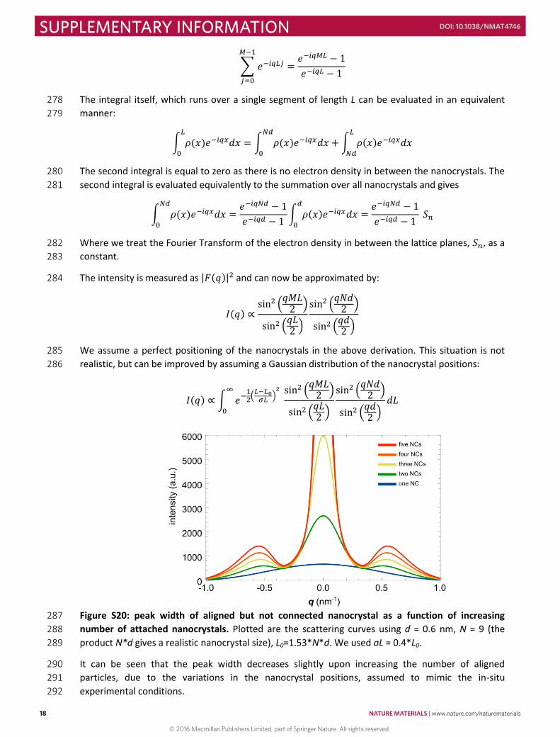
Figure S20: peak width of aligned but not connected nanocrystal as a function of increasing 287 number of attached nanocrystals. Plotted are the scattering curves using d = 0.6 nm, N = 9 (the 288 product N*d gives a realistic nanocrystal size), L0=1.53*N*d. We used σL = 0.4*L0. 289
It can be seen that the peak width decreases slightly upon increasing the number of aligned 290 particles, due to the variations in the nanocrystal positions, assumed to mimic the in-situ 291 experimental conditions. 292
18 NATURE MATERIALS | www.nature.com/naturematerials
SUPPLEMENTARY INFORMATION DOI: 10.1038/NMAT4746
© 2016 Macmillan Publishers Limited, part of Springer Nature. All rights reserved.

19
The approximation used above is only accounting for a variation in the particle positions. When we 293 assume further disorder by considering the NC rotational freedom along all three Cartesian axes, the 294 peak width of the diffracted signals will decrease even less. 295
Upon perfect alignment of the particles (no rotational misalignment, no distribution in the particle 296 positions) the peak width decreases. However, we consider the latter situation to be unrealistic and 297 do assign the decrease in atomic peak width to be due to particle attachment. 298
NATURE MATERIALS | www.nature.com/naturematerials 19
SUPPLEMENTARY INFORMATIONDOI: 10.1038/NMAT4746
© 2016 Macmillan Publishers Limited, part of Springer Nature. All rights reserved.
20
Supplementary methods 6: azimuthal and radial peakwidths in electron diffraction 299
300
301
302
303
304
305
306
307
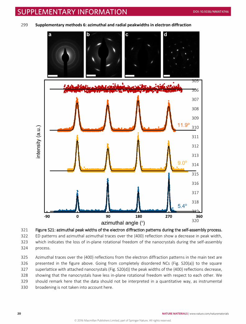
308
309
310
311
312
313
314
315
316
317
318
319
320
Figure S21: azimuthal peak widths of the electron diffraction patterns during the self-assembly process. 321 ED patterns and azimuthal azimuthal traces over the {400} reflection show a decrease in peak width, 322 which indicates the loss of in-plane rotational freedom of the nanocrystals during the self-assembly 323 process. 324
Azimuthal traces over the {400} reflections from the electron diffraction patterns in the main text are 325 presented in the figure above. Going from completely disordered NCs (Fig. S20(a)) to the square 326 superlattice with attached nanocrystals (Fig. S20(d)) the peak widths of the {400} reflections decrease, 327 showing that the nanocrystals have less in-plane rotational freedom with respect to each other. We 328 should remark here that the data should not be interpreted in a quantitative way, as instrumental 329 broadening is not taken into account here. 330
20 NATURE MATERIALS | www.nature.com/naturematerials
SUPPLEMENTARY INFORMATION DOI: 10.1038/NMAT4746
© 2016 Macmillan Publishers Limited, part of Springer Nature. All rights reserved.
21
331 Figure S22: Conservation of nanocrystalline order on mesoscopic length scales. From left to right 332 consecutive zoomed in TEM images are displayed, which show a very long-range periodicity. Even 333 though the atomic coherency throughout the complete lattice is conserved over several nanocrystals, 334 this does not perturb the long-range nano-crystalline order. From the widths of the {100}-superlattice 335 reflections in the Fourier transforms we obtain nanocrystal coherence lengths for the superlattice of 336 39.3 nm, 34.3 nm and 35.9 nm from left to right. Scale bars from left to right images are 2μm, 500nm, 337 200nm and 20 nm respectively and 1 nm-1 for all Fourier transform insets. 338
Figure S23: HAADF-STEM and atom counting reconstruction on attached NCs. (a) HAADF-STEM image 339 of NCs attached in a square superlattice. The atomic periodicity is continued from a given NC to its 340 neighbors. Slight misorientations can also be observed. (b) Results from the atom counting procedure, 341 using (a) as an input image. The color bar represents the number of detected atoms in each vertical 342 column. (c) Top-view and (d) side-view of the reconstructed atomic model. 343
NATURE MATERIALS | www.nature.com/naturematerials 21
SUPPLEMENTARY INFORMATIONDOI: 10.1038/NMAT4746
© 2016 Macmillan Publishers Limited, part of Springer Nature. All rights reserved.
22
Supplementary methods 7: Coulomb and Van Der Waals interactions between nanocrystals 344
We model the interaction between two PbSe nanocrystal cubes (consisting out of 3375 atoms) 345 through electrostatic and Van Der Waals interactions. We assume an ionic model for rocksalt PbSe. 346 For the calculation of the Coulomb potential between two nanocrystals, we sum the Coulomb 347 potentials of each ion in nanocrystal 1 in interaction with all ions in nanocrystal ‘2’. This is performed 348 for a given relative position of nanocrystal 1 with respect to nanocrystal 2. Hence the Coulomb 349 interaction is given by: 350
𝑉𝑉𝑐𝑐𝑐𝑐𝑐𝑐𝑐𝑐𝑐𝑐𝑐𝑐𝑐𝑐 =1
4𝜋𝜋𝜀𝜀0∑∑
𝑞𝑞𝑖𝑖𝑞𝑞𝑗𝑗𝑟𝑟𝑖𝑖𝑗𝑗
𝑁𝑁𝑗𝑗
𝑗𝑗
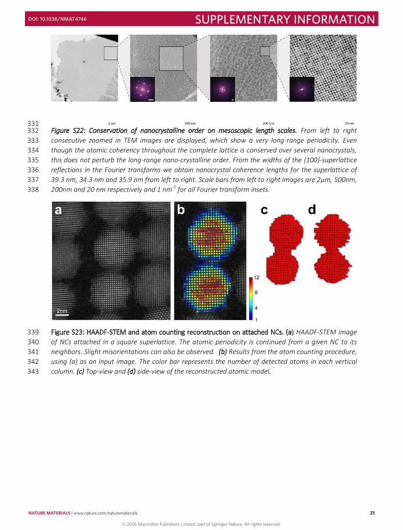
𝑁𝑁𝑖𝑖
𝑖𝑖
Where With ε0 the vacuum permittivity, qi and qj the charges on atom 1 (located in nanocrystal 1) and 351 atom 2 (located in nanocrystal 2). The double sum runs over all pairs of atoms in nanocrystal i and 352 nanocrystal j. 353
The Van Der Waals interaction is calculated as spontaneous dipole-induced dipole (otherwise known 354 as London or dispersion interactions); 355
𝑉𝑉𝑉𝑉𝑉𝑉𝑉𝑉 = −32∑∑
𝐼𝐼𝑖𝑖𝐼𝐼𝑗𝑗𝐼𝐼𝑖𝑖 + 𝐼𝐼𝑗𝑗
𝛼𝛼𝑖𝑖𝛼𝛼𝑗𝑗𝑟𝑟𝑖𝑖𝑗𝑗6
𝑁𝑁𝑗𝑗
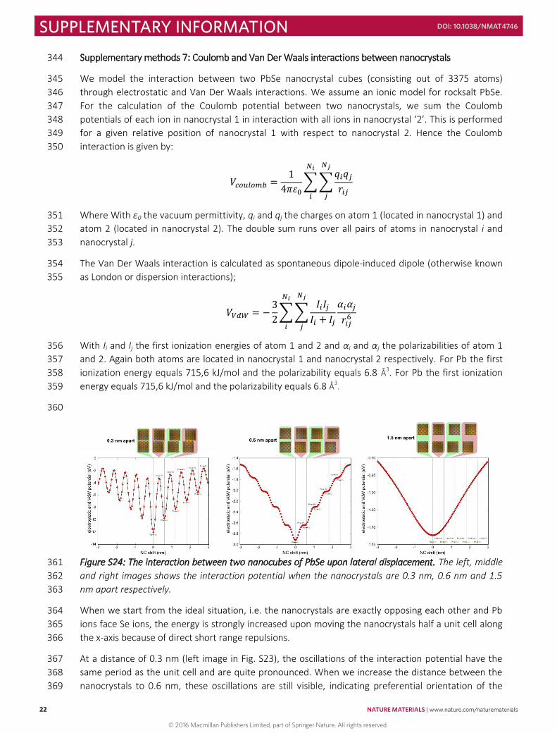
𝑗𝑗
𝑁𝑁𝑖𝑖
𝑖𝑖
With Ii and Ij the first ionization energies of atom 1 and 2 and αi and αj the polarizabilities of atom 1 356 and 2. Again both atoms are located in nanocrystal 1 and nanocrystal 2 respectively. For Pb the first 357 ionization energy equals 715,6 kJ/mol and the polarizability equals 6.8 Å3. For Pb the first ionization 358 energy equals 715,6 kJ/mol and the polarizability equals 6.8 Å3. 359
360
Figure S24: The interaction between two nanocubes of PbSe upon lateral displacement. The left, middle 361 and right images shows the interaction potential when the nanocrystals are 0.3 nm, 0.6 nm and 1.5 362 nm apart respectively. 363
When we start from the ideal situation, i.e. the nanocrystals are exactly opposing each other and Pb 364 ions face Se ions, the energy is strongly increased upon moving the nanocrystals half a unit cell along 365 the x-axis because of direct short range repulsions. 366
At a distance of 0.3 nm (left image in Fig. S23), the oscillations of the interaction potential have the 367 same period as the unit cell and are quite pronounced. When we increase the distance between the 368 nanocrystals to 0.6 nm, these oscillations are still visible, indicating preferential orientation of the 369
22 NATURE MATERIALS | www.nature.com/naturematerials
SUPPLEMENTARY INFORMATION DOI: 10.1038/NMAT4746
© 2016 Macmillan Publishers Limited, part of Springer Nature. All rights reserved.
23
atomic lattices favoring Pb-to-Se alignment. The 0.6 nm distance approaches realistic experimental 370 conditions. When we further increase the distance to 1.5 nm, the oscillations disappear, but there is a 371 general potential minimum when the nanocrystal [100] facets have maximum overlap. Such a 372 potential leads an attractive driving force between the nanocrystals for maximum {100} to{100} facet 373 overlap, be it with half a unit cell mismatch to maximize the interactions between ions of opposite 374 charge. 375
In the simulations of the hexagonal to square phase transitions, the above potential is mimicked by 376 attractive patches centered on the vertical {100} facets of each nanocrystal, representing a similar 377 driving force for maximal facet-to-facet overlap as following from the atomistic calculations. 378
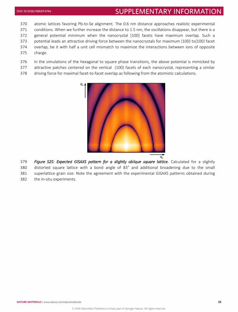
Figure S25: Expected GISAXS pattern for a slightly oblique square lattice. Calculated for a slightly 379 distorted square lattice with a bond angle of 83o and additional broadening due to the small 380 superlattice grain size. Note the agreement with the experimental GISAXS patterns obtained during 381 the in-situ experiments. 382
NATURE MATERIALS | www.nature.com/naturematerials 23
SUPPLEMENTARY INFORMATIONDOI: 10.1038/NMAT4746
© 2016 Macmillan Publishers Limited, part of Springer Nature. All rights reserved.

24
References 383
1. Heitsch, A. T., Patel, R. N., Goodfellow, B. W., Smilgies, D.-M. & Korgel, B. A. GISAXS 384 Characterization of Order in Hexagonal Monolayers of FePt Nanocrystals. J. Phys. Chem. C 385 114, 14427–14432 (2010). 386
2. Smilgies, D.-M., Heitsch, A. T. & Korgel, B. A. Stacking of hexagonal nanocrystal layers during 387 Langmuir-Blodgett deposition. J. Phys. Chem. B 116, 6017–6026 (2012). 388
24 NATURE MATERIALS | www.nature.com/naturematerials
SUPPLEMENTARY INFORMATION DOI: 10.1038/NMAT4746
© 2016 Macmillan Publishers Limited, part of Springer Nature. All rights reserved.
Recommended