Embed Size (px)
Citation preview

Dual-Pivot Quicksort and BeyondAnalysis of Multiway Partitioning and Its Practical Potential
Sebastian Wild
Vortrag zur wissenschaftlichen Aussprache
im Rahmen des Promotionsverfahrens
8. Juli 2016
Sebastian Wild Dual-Pivot Quicksort and Beyond 2016-07-08 1 / 17

Dual-P??? Q?????? and BeyondAnalysis of Multi??? P??????? and Its Practical Potential
Sebastian Wild
Vortrag zur wissenschaftlichen Aussprache
im Rahmen des Promotionsverfahrens
8. Juli 2016
Sebastian Wild Dual-Pivot Quicksort and Beyond 2016-07-08 1 / 17

Dual-Pivot Quicksort and BeyondAnalysis of Multiway Partitioning and Its Practical Potential
Sebastian Wild
Vortrag zur wissenschaftlichen Aussprache
im Rahmen des Promotionsverfahrens
8. Juli 2016
Sebastian Wild Dual-Pivot Quicksort and Beyond 2016-07-08 1 / 17

What is sorting?
What do you think when you hear sorting?
Sebastian Wild Dual-Pivot Quicksort and Beyond 2016-07-08 2 / 17
What is sorting?
What do you think when you hear sorting?
Sebastian Wild Dual-Pivot Quicksort and Beyond 2016-07-08 2 / 17
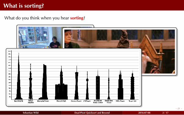
What is sorting?
What do you think when you hear sorting?
Sebastian Wild Dual-Pivot Quicksort and Beyond 2016-07-08 2 / 17
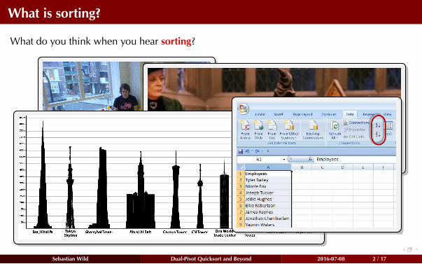
What is sorting?
What do you think when you hear sorting?
Sebastian Wild Dual-Pivot Quicksort and Beyond 2016-07-08 2 / 17
What is sorting?
What do you think when you hear sorting?
Sebastian Wild Dual-Pivot Quicksort and Beyond 2016-07-08 2 / 17
What is sorting?
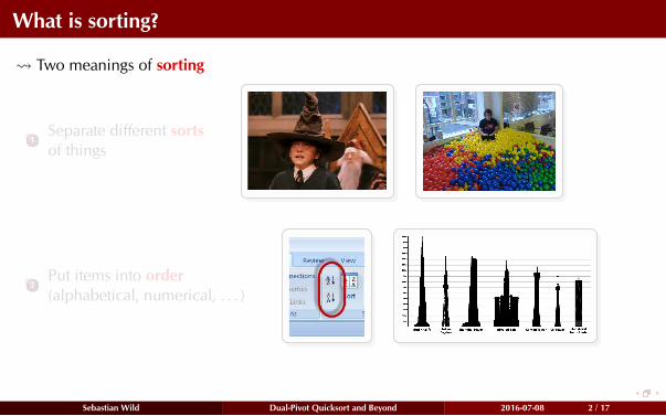
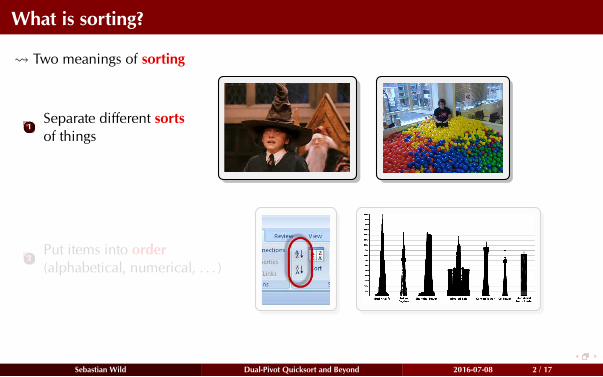
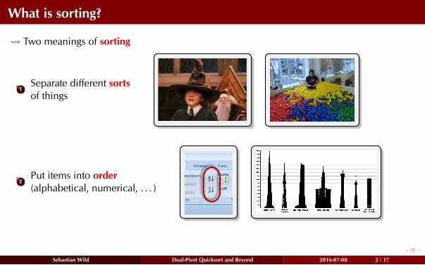
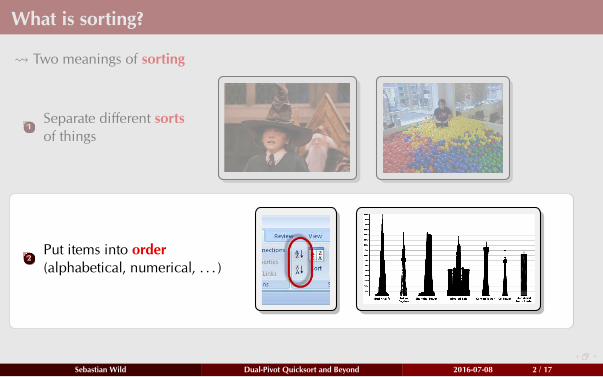
Two meanings of sorting
1Separate different sorts
of things
2Put items into order
(alphabetical, numerical, . . . )
Sebastian Wild Dual-Pivot Quicksort and Beyond 2016-07-08 2 / 17
What is sorting?
Two meanings of sorting
1Separate different sorts
of things
2Put items into order
(alphabetical, numerical, . . . )
Sebastian Wild Dual-Pivot Quicksort and Beyond 2016-07-08 2 / 17
What is sorting?
Two meanings of sorting
1Separate different sorts
of things
2Put items into order
(alphabetical, numerical, . . . )
Sebastian Wild Dual-Pivot Quicksort and Beyond 2016-07-08 2 / 17
What is sorting?
Two meanings of sorting
1Separate different sorts
of things
2Put items into order
(alphabetical, numerical, . . . )
Sebastian Wild Dual-Pivot Quicksort and Beyond 2016-07-08 2 / 17
Model of Computation
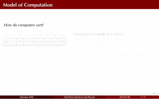
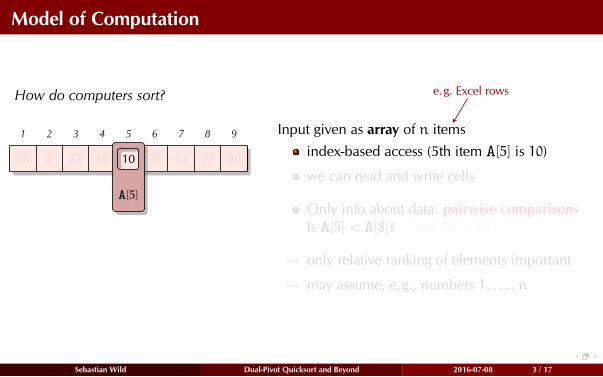
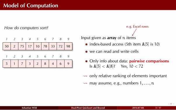
How do computers sort?
1 2 3 4 5 6 7 8 9
50 2 75 17 10 78 33 72 98
Input given as array of n items
index-based access (5th item A[5] is 10)
we can read and write cells
Only info about data: pairwise comparisons
Is A[5] < A[8]? Yes, 10 < 72
only relative ranking of elements important
may assume, e.g., numbers 1, . . . , n
Sebastian Wild Dual-Pivot Quicksort and Beyond 2016-07-08 3 / 17
Model of Computation
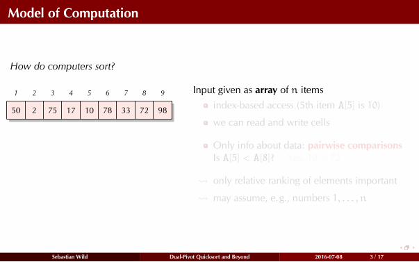
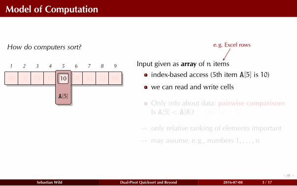
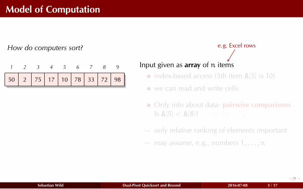
How do computers sort?
1 2 3 4 5 6 7 8 9
50 2 75 17 10 78 33 72 98
Input given as array of n items
e.g. Excel rows
index-based access (5th item A[5] is 10)
we can read and write cells
Only info about data: pairwise comparisons
Is A[5] < A[8]? Yes, 10 < 72
only relative ranking of elements important
may assume, e.g., numbers 1, . . . , n
Sebastian Wild Dual-Pivot Quicksort and Beyond 2016-07-08 3 / 17
Model of Computation
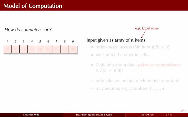
How do computers sort?
1 2 3 4 5 6 7 8 9
50 2 75 17 10 78 33 72 98
Input given as array of n items
e.g. Excel rows
index-based access (5th item A[5] is 10)
we can read and write cells
Only info about data: pairwise comparisons
Is A[5] < A[8]? Yes, 10 < 72
only relative ranking of elements important
may assume, e.g., numbers 1, . . . , n
Sebastian Wild Dual-Pivot Quicksort and Beyond 2016-07-08 3 / 17
Model of Computation
How do computers sort?
1 2 3 4 5 6 7 8 9
50 2 75 17 10 78 33 72 98
A[5]
10
Input given as array of n items
e.g. Excel rows
index-based access (5th item A[5] is 10)
we can read and write cells
Only info about data: pairwise comparisons
Is A[5] < A[8]? Yes, 10 < 72
only relative ranking of elements important
may assume, e.g., numbers 1, . . . , n
Sebastian Wild Dual-Pivot Quicksort and Beyond 2016-07-08 3 / 17

Model of Computation
How do computers sort?
1 2 3 4 5 6 7 8 9
50 2 75 17 10 78 33 72 98
A[5]
10
A[8]
72
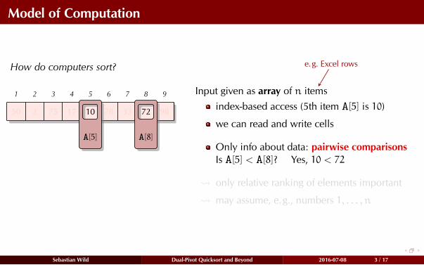
Input given as array of n items
e.g. Excel rows
index-based access (5th item A[5] is 10)
we can read and write cells
Only info about data: pairwise comparisons
Is A[5] < A[8]? Yes, 10 < 72
only relative ranking of elements important
may assume, e.g., numbers 1, . . . , n
Sebastian Wild Dual-Pivot Quicksort and Beyond 2016-07-08 3 / 17
Model of Computation
How do computers sort?
1 2 3 4 5 6 7 8 9
50 2 75 17 10 78 33 72 98
A[5]
10
A[8]
72
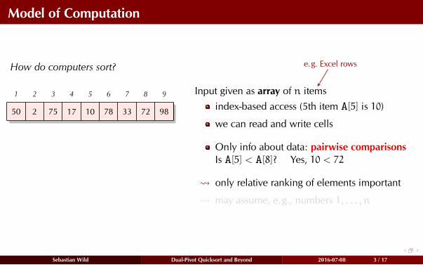
Input given as array of n items
e.g. Excel rows
index-based access (5th item A[5] is 10)
we can read and write cells
Only info about data: pairwise comparisons
Is A[5] < A[8]? Yes, 10 < 72
only relative ranking of elements important
may assume, e.g., numbers 1, . . . , n
Sebastian Wild Dual-Pivot Quicksort and Beyond 2016-07-08 3 / 17
Model of Computation
How do computers sort?
1 2 3 4 5 6 7 8 9
50 2 75 17 10 78 33 72 98
1 2 3 4 5 6 7 8 9
5 1 7 3 2 8 4 6 9
Input given as array of n items
e.g. Excel rows
index-based access (5th item A[5] is 10)
we can read and write cells
Only info about data: pairwise comparisons
Is A[5] < A[8]? Yes, 10 < 72
only relative ranking of elements important
may assume, e.g., numbers 1, . . . , n
Sebastian Wild Dual-Pivot Quicksort and Beyond 2016-07-08 3 / 17

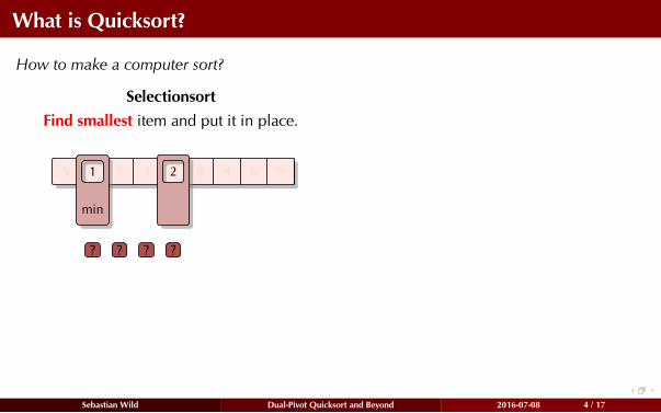
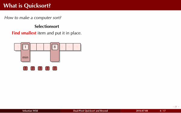
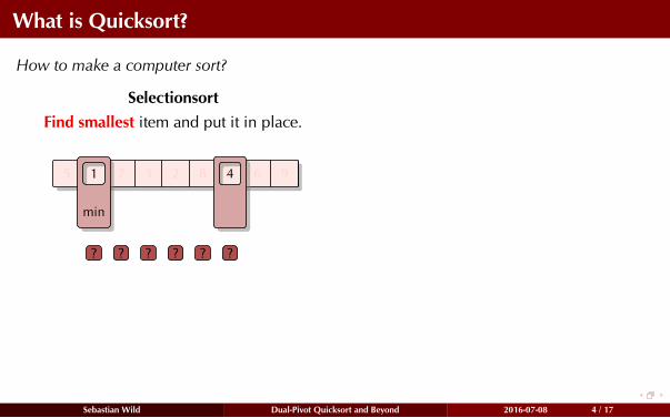
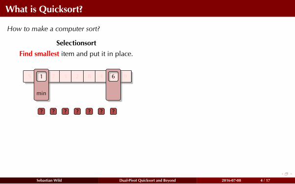
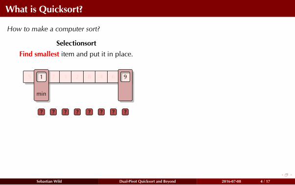
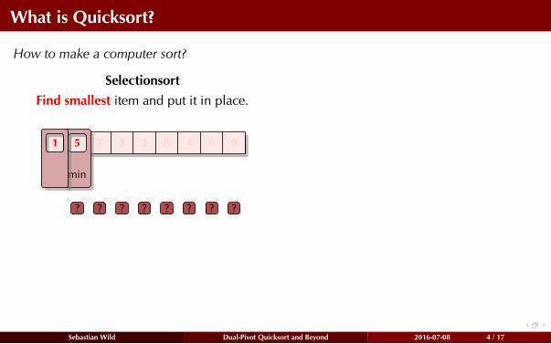
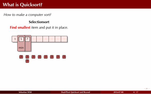
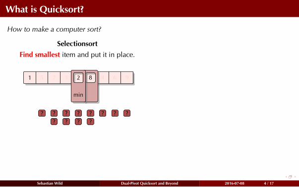
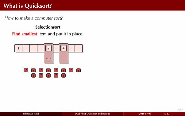
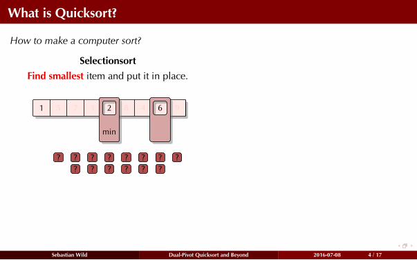
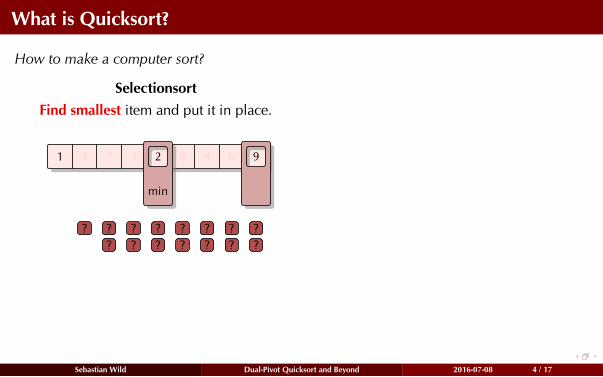
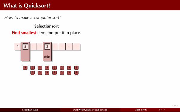
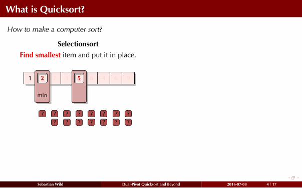
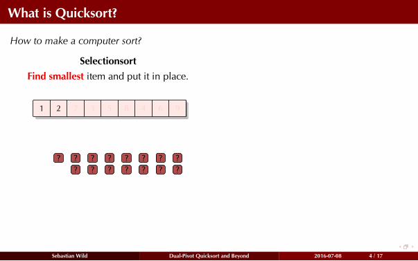
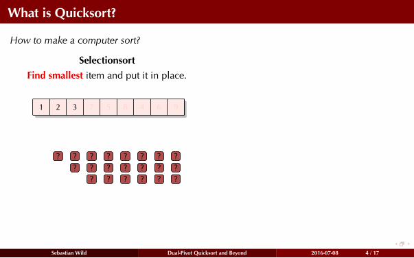
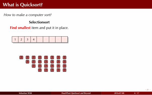
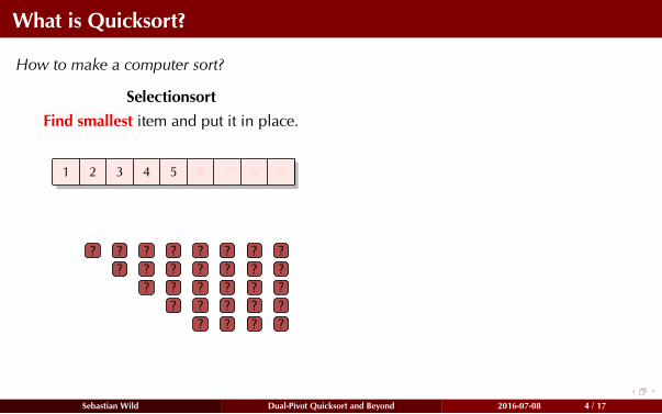
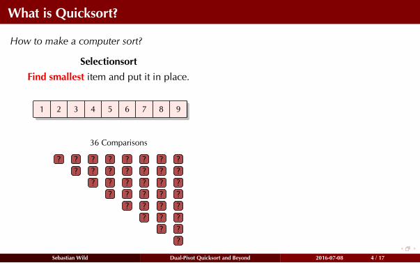
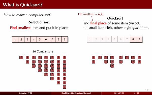
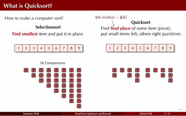
What is Quicksort?
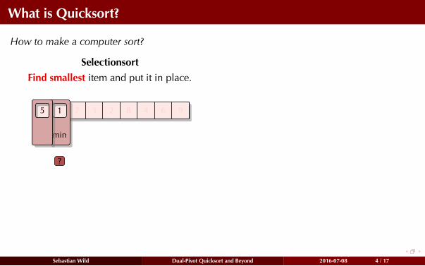
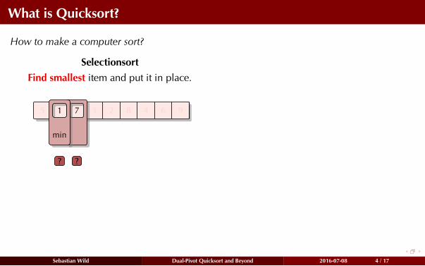
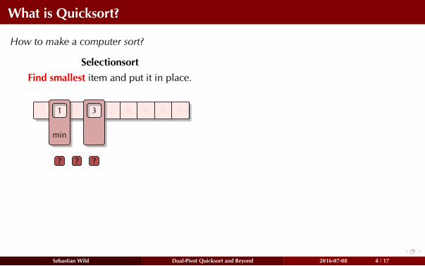
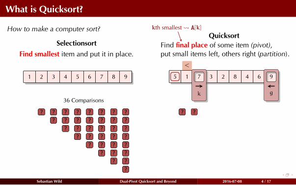
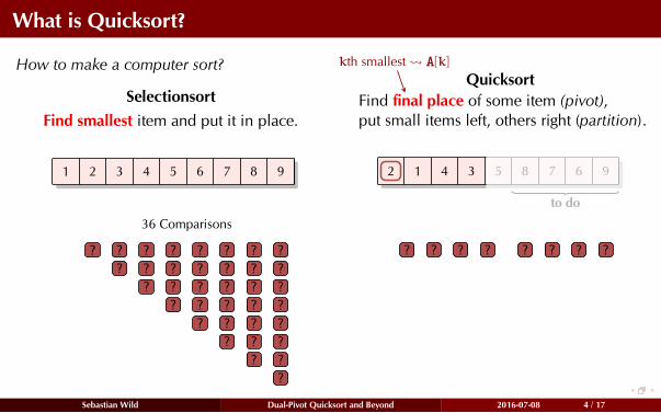
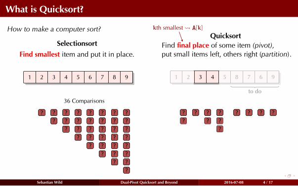
How to make a computer sort?
Selectionsort
Find smallest item and put it in place.
5 1 7 3 2 8 4 6 9
Sebastian Wild Dual-Pivot Quicksort and Beyond 2016-07-08 4 / 17

What is Quicksort?
How to make a computer sort?
Selectionsort
Find smallest item and put it in place.
5 1 7 3 2 8 4 6 915
min
?
Sebastian Wild Dual-Pivot Quicksort and Beyond 2016-07-08 4 / 17
What is Quicksort?
How to make a computer sort?
Selectionsort
Find smallest item and put it in place.
5 1 7 3 2 8 4 6 9
?
1
min
5
Sebastian Wild Dual-Pivot Quicksort and Beyond 2016-07-08 4 / 17
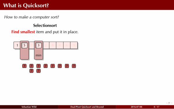
What is Quicksort?
How to make a computer sort?
Selectionsort
Find smallest item and put it in place.
5 1 7 3 2 8 4 6 9
?
71
min
?
Sebastian Wild Dual-Pivot Quicksort and Beyond 2016-07-08 4 / 17
What is Quicksort?
How to make a computer sort?
Selectionsort
Find smallest item and put it in place.
5 1 7 3 2 8 4 6 9
? ?
31
min
?
Sebastian Wild Dual-Pivot Quicksort and Beyond 2016-07-08 4 / 17
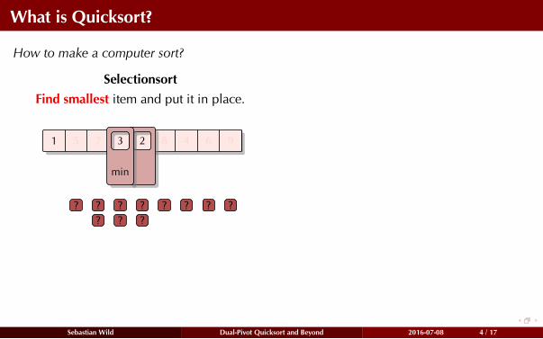
What is Quicksort?
How to make a computer sort?
Selectionsort
Find smallest item and put it in place.
5 1 7 3 2 8 4 6 9
? ? ?
21
min
?
Sebastian Wild Dual-Pivot Quicksort and Beyond 2016-07-08 4 / 17
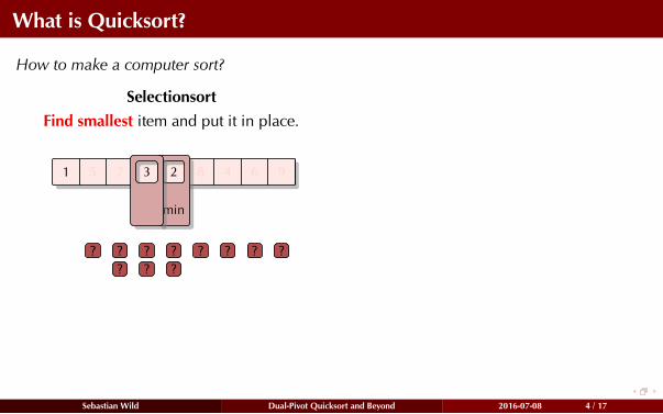
What is Quicksort?
How to make a computer sort?
Selectionsort
Find smallest item and put it in place.
5 1 7 3 2 8 4 6 9
? ? ? ?
81
min
?
Sebastian Wild Dual-Pivot Quicksort and Beyond 2016-07-08 4 / 17
What is Quicksort?
How to make a computer sort?
Selectionsort
Find smallest item and put it in place.
5 1 7 3 2 8 4 6 9
? ? ? ? ?
41
min
?
Sebastian Wild Dual-Pivot Quicksort and Beyond 2016-07-08 4 / 17
What is Quicksort?
How to make a computer sort?
Selectionsort
Find smallest item and put it in place.
5 1 7 3 2 8 4 6 9
? ? ? ? ? ?
61
min
?
Sebastian Wild Dual-Pivot Quicksort and Beyond 2016-07-08 4 / 17
What is Quicksort?
How to make a computer sort?
Selectionsort
Find smallest item and put it in place.
5 1 7 3 2 8 4 6 9
? ? ? ? ? ? ?
91
min
?
Sebastian Wild Dual-Pivot Quicksort and Beyond 2016-07-08 4 / 17

What is Quicksort?
How to make a computer sort?
Selectionsort
Find smallest item and put it in place.
5 1 7 3 2 8 4 6 9
? ? ? ? ? ? ? ?
1
min
5
Sebastian Wild Dual-Pivot Quicksort and Beyond 2016-07-08 4 / 17
What is Quicksort?
How to make a computer sort?
Selectionsort
Find smallest item and put it in place.
5 1 7 3 2 8 4 6 9
? ? ? ? ? ? ? ?
5 7 3 2 8 4 6 95
min
1
Sebastian Wild Dual-Pivot Quicksort and Beyond 2016-07-08 4 / 17
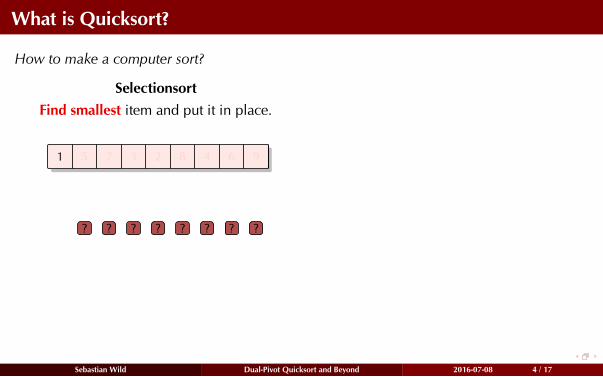
What is Quicksort?
How to make a computer sort?
Selectionsort
Find smallest item and put it in place.
? ? ? ? ? ? ? ?
5 7 3 2 8 4 6 91
Sebastian Wild Dual-Pivot Quicksort and Beyond 2016-07-08 4 / 17
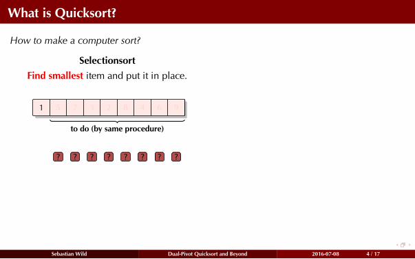
What is Quicksort?
How to make a computer sort?
Selectionsort
Find smallest item and put it in place.
? ? ? ? ? ? ? ?
5 7 3 2 8 4 6 91
to do (by same procedure)
Sebastian Wild Dual-Pivot Quicksort and Beyond 2016-07-08 4 / 17
What is Quicksort?
How to make a computer sort?
Selectionsort
Find smallest item and put it in place.
? ? ? ? ? ? ? ?
5 7 3 2 8 4 6 91 75
min
?
Sebastian Wild Dual-Pivot Quicksort and Beyond 2016-07-08 4 / 17

What is Quicksort?
How to make a computer sort?
Selectionsort
Find smallest item and put it in place.
? ? ? ? ? ? ? ?
5 7 3 2 8 4 6 91
?
35
min
?
Sebastian Wild Dual-Pivot Quicksort and Beyond 2016-07-08 4 / 17
What is Quicksort?
How to make a computer sort?
Selectionsort
Find smallest item and put it in place.
? ? ? ? ? ? ? ?
5 7 3 2 8 4 6 91
? ?
5 3
min
Sebastian Wild Dual-Pivot Quicksort and Beyond 2016-07-08 4 / 17
What is Quicksort?
How to make a computer sort?
Selectionsort
Find smallest item and put it in place.
? ? ? ? ? ? ? ?
5 7 3 2 8 4 6 91
? ?
23
min
?
Sebastian Wild Dual-Pivot Quicksort and Beyond 2016-07-08 4 / 17
What is Quicksort?
How to make a computer sort?
Selectionsort
Find smallest item and put it in place.
? ? ? ? ? ? ? ?
5 7 3 2 8 4 6 91
? ? ?
2
min
3
Sebastian Wild Dual-Pivot Quicksort and Beyond 2016-07-08 4 / 17
What is Quicksort?
How to make a computer sort?
Selectionsort
Find smallest item and put it in place.
? ? ? ? ? ? ? ?
5 7 3 2 8 4 6 91
? ? ?
82
min
?
Sebastian Wild Dual-Pivot Quicksort and Beyond 2016-07-08 4 / 17
What is Quicksort?
How to make a computer sort?
Selectionsort
Find smallest item and put it in place.
? ? ? ? ? ? ? ?
5 7 3 2 8 4 6 91
? ? ? ?
42
min
?
Sebastian Wild Dual-Pivot Quicksort and Beyond 2016-07-08 4 / 17
What is Quicksort?
How to make a computer sort?
Selectionsort
Find smallest item and put it in place.
? ? ? ? ? ? ? ?
5 7 3 2 8 4 6 91
? ? ? ? ?
62
min
?
Sebastian Wild Dual-Pivot Quicksort and Beyond 2016-07-08 4 / 17
What is Quicksort?
How to make a computer sort?
Selectionsort
Find smallest item and put it in place.
? ? ? ? ? ? ? ?
5 7 3 2 8 4 6 91
? ? ? ? ? ?
92
min
?
Sebastian Wild Dual-Pivot Quicksort and Beyond 2016-07-08 4 / 17
What is Quicksort?
How to make a computer sort?
Selectionsort
Find smallest item and put it in place.
? ? ? ? ? ? ? ?
5 7 3 2 8 4 6 91
? ? ? ? ? ? ?
2
min
5
Sebastian Wild Dual-Pivot Quicksort and Beyond 2016-07-08 4 / 17
What is Quicksort?
How to make a computer sort?
Selectionsort
Find smallest item and put it in place.
? ? ? ? ? ? ? ?
1
? ? ? ? ? ? ?
7 3 5 8 4 6 952
min
Sebastian Wild Dual-Pivot Quicksort and Beyond 2016-07-08 4 / 17
What is Quicksort?
How to make a computer sort?
Selectionsort
Find smallest item and put it in place.
? ? ? ? ? ? ? ?
1
? ? ? ? ? ? ?
7 3 5 8 4 6 92
Sebastian Wild Dual-Pivot Quicksort and Beyond 2016-07-08 4 / 17
What is Quicksort?
How to make a computer sort?
Selectionsort
Find smallest item and put it in place.
? ? ? ? ? ? ? ?
1
? ? ? ? ? ? ?
2 3 7 5 8 4 6 9
? ? ? ? ? ?
Sebastian Wild Dual-Pivot Quicksort and Beyond 2016-07-08 4 / 17
What is Quicksort?
How to make a computer sort?
Selectionsort
Find smallest item and put it in place.
? ? ? ? ? ? ? ?
1
? ? ? ? ? ? ?
2
? ? ? ? ? ?
3 4 5 8 7 6 9
? ? ? ? ?
Sebastian Wild Dual-Pivot Quicksort and Beyond 2016-07-08 4 / 17
What is Quicksort?
How to make a computer sort?
Selectionsort
Find smallest item and put it in place.
? ? ? ? ? ? ? ?
1
? ? ? ? ? ? ?
2
? ? ? ? ? ?
? ? ? ? ?
3 4 5 8 7 6 9
? ? ? ?
Sebastian Wild Dual-Pivot Quicksort and Beyond 2016-07-08 4 / 17

What is Quicksort?
How to make a computer sort?
Selectionsort
Find smallest item and put it in place.
? ? ? ? ? ? ? ?
1
? ? ? ? ? ? ?
2
? ? ? ? ? ?
? ? ? ? ?
? ? ? ?
3 4 5 6 7 8 9
? ? ?
? ?
?
Sebastian Wild Dual-Pivot Quicksort and Beyond 2016-07-08 4 / 17

What is Quicksort?
How to make a computer sort?
Selectionsort
Find smallest item and put it in place.
? ? ? ? ? ? ? ?
1
? ? ? ? ? ? ?
2
? ? ? ? ? ?
? ? ? ? ?
? ? ? ?
3 4 5 6 7 8 9
? ? ?
? ?
?
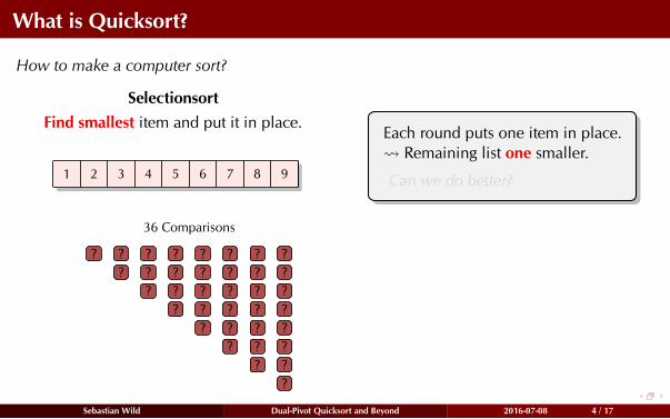
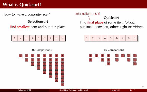
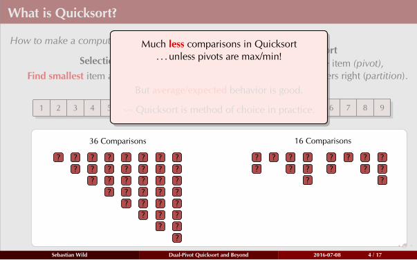
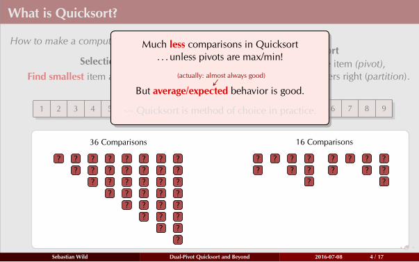
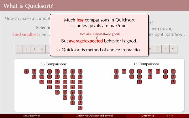
36 Comparisons
Sebastian Wild Dual-Pivot Quicksort and Beyond 2016-07-08 4 / 17
What is Quicksort?
How to make a computer sort?
Selectionsort
Find smallest item and put it in place.
? ? ? ? ? ? ? ?
1
? ? ? ? ? ? ?
2
? ? ? ? ? ?
? ? ? ? ?
? ? ? ?
3 4 5 6 7 8 9
? ? ?
? ?
?
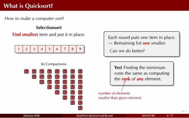
36 Comparisons
Each round puts one item in place.
Remaining list one smaller.
Can we do better?
Sebastian Wild Dual-Pivot Quicksort and Beyond 2016-07-08 4 / 17

What is Quicksort?
How to make a computer sort?
Selectionsort
Find smallest item and put it in place.
? ? ? ? ? ? ? ?
1
? ? ? ? ? ? ?
2
? ? ? ? ? ?
? ? ? ? ?
? ? ? ?
3 4 5 6 7 8 9
? ? ?
? ?
?
36 Comparisons
Each round puts one item in place.
Remaining list one smaller.
Can we do better?
Sebastian Wild Dual-Pivot Quicksort and Beyond 2016-07-08 4 / 17
What is Quicksort?
How to make a computer sort?
Selectionsort
Find smallest item and put it in place.
? ? ? ? ? ? ? ?
1
? ? ? ? ? ? ?
2
? ? ? ? ? ?
? ? ? ? ?
? ? ? ?
3 4 5 6 7 8 9
? ? ?
? ?
?
36 Comparisons
Each round puts one item in place.
Remaining list one smaller.
Can we do better?
Yes! Finding the minimum
costs the same as computing
the rank
number of elements
smaller than given element
of any element.
Sebastian Wild Dual-Pivot Quicksort and Beyond 2016-07-08 4 / 17
What is Quicksort?
How to make a computer sort?
Selectionsort
Find smallest item and put it in place.
? ? ? ? ? ? ? ?
1
? ? ? ? ? ? ?
2
? ? ? ? ? ?
? ? ? ? ?
? ? ? ?
3 4 5 6 7 8 9
? ? ?
? ?
?
36 Comparisons
Sebastian Wild Dual-Pivot Quicksort and Beyond 2016-07-08 4 / 17

What is Quicksort?
How to make a computer sort?
Selectionsort
Find smallest item and put it in place.
? ? ? ? ? ? ? ?
1
? ? ? ? ? ? ?
2
? ? ? ? ? ?
? ? ? ? ?
? ? ? ?
3 4 5 6 7 8 9
? ? ?
? ?
?
36 Comparisons
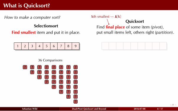
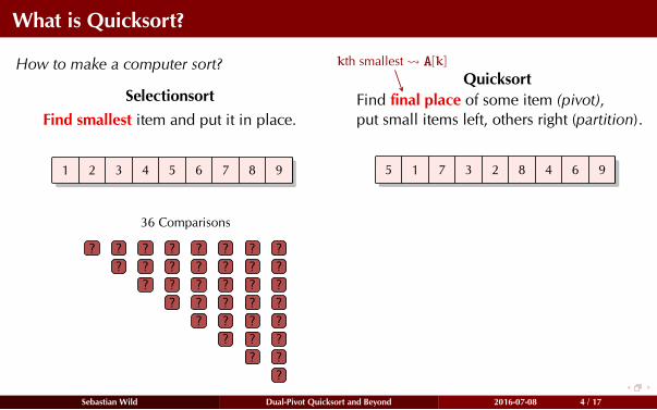
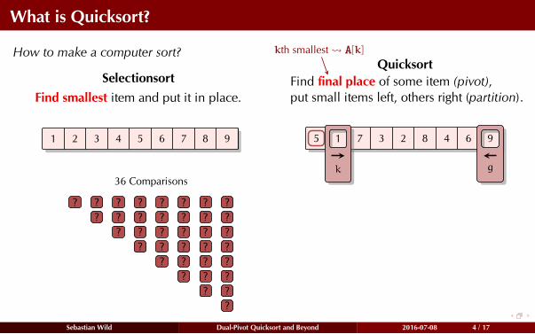
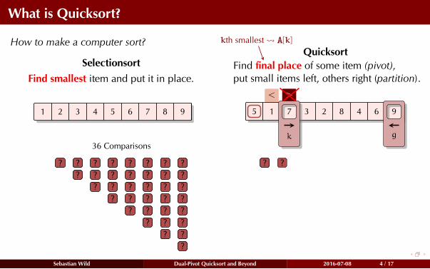
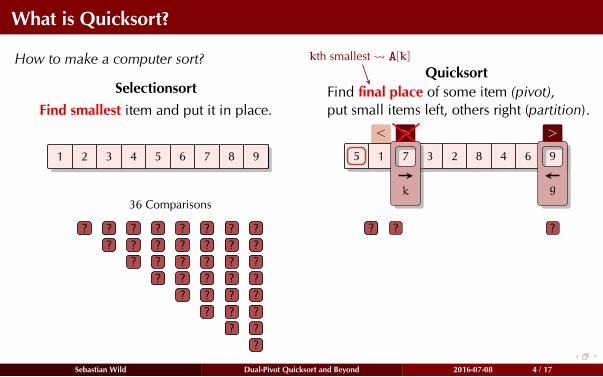
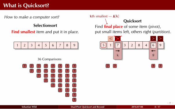
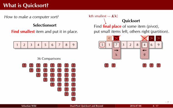
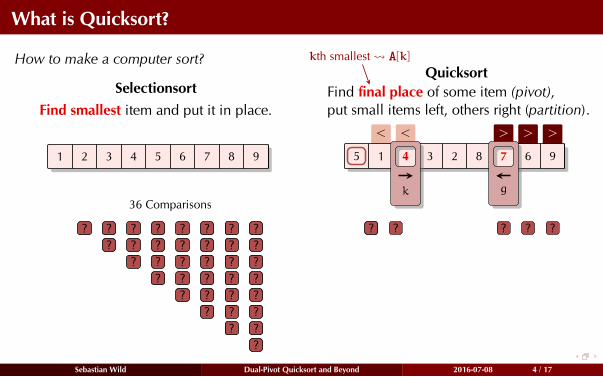
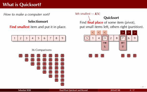
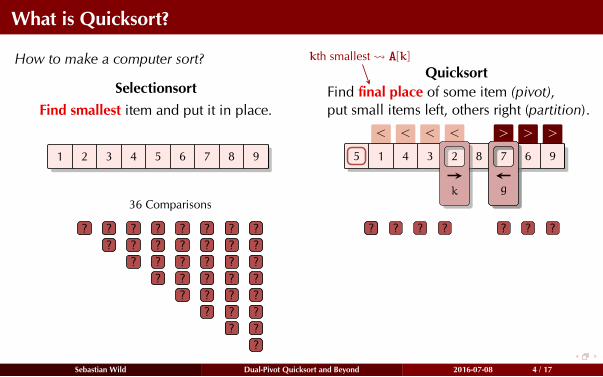
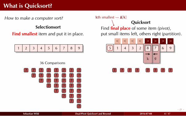
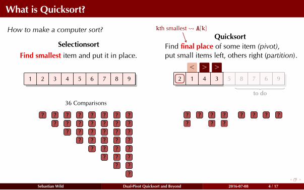
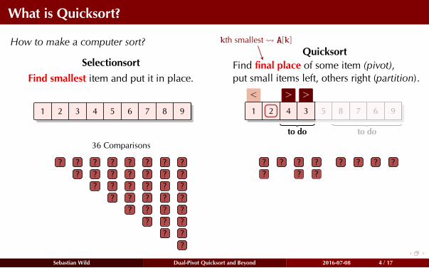
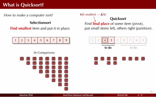
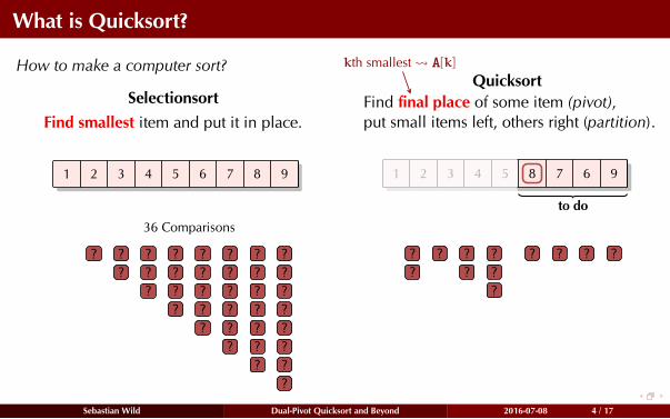
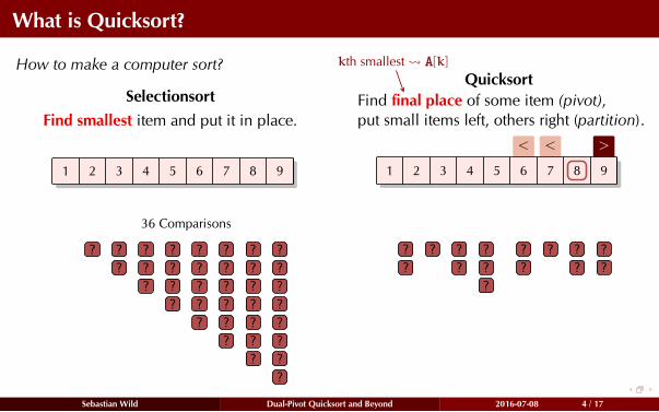
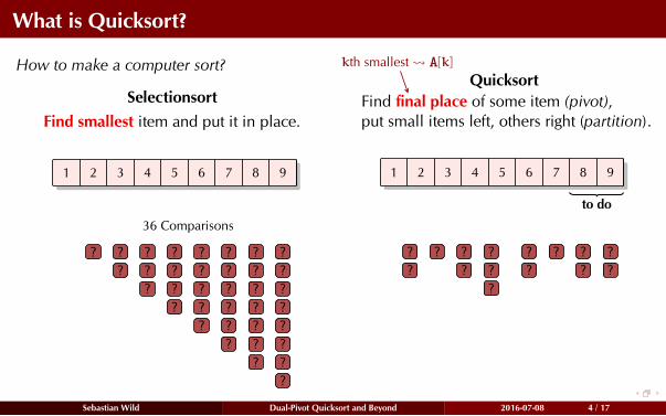
Quicksort
Find final place of some item (pivot),
put small items left, others right (partition).
Sebastian Wild Dual-Pivot Quicksort and Beyond 2016-07-08 4 / 17
What is Quicksort?
How to make a computer sort?
Selectionsort
Find smallest item and put it in place.
? ? ? ? ? ? ? ?
1
? ? ? ? ? ? ?
2
? ? ? ? ? ?
? ? ? ? ?
? ? ? ?
3 4 5 6 7 8 9
? ? ?
? ?
?
36 Comparisons
Quicksort
Find final
kth smallest A[k]
place of some item (pivot),
put small items left, others right (partition).
5 1 7 3 2 8 4 6 9
Sebastian Wild Dual-Pivot Quicksort and Beyond 2016-07-08 4 / 17
What is Quicksort?
How to make a computer sort?
Selectionsort
Find smallest item and put it in place.
? ? ? ? ? ? ? ?
1
? ? ? ? ? ? ?
2
? ? ? ? ? ?
? ? ? ? ?
? ? ? ?
3 4 5 6 7 8 9
? ? ?
? ?
?
36 Comparisons
Quicksort
Find final
kth smallest A[k]
place of some item (pivot),
put small items left, others right (partition).
5 1 7 3 2 8 4 6 9
k g
Sebastian Wild Dual-Pivot Quicksort and Beyond 2016-07-08 4 / 17

What is Quicksort?
How to make a computer sort?
Selectionsort
Find smallest item and put it in place.
? ? ? ? ? ? ? ?
1
? ? ? ? ? ? ?
2
? ? ? ? ? ?
? ? ? ? ?
? ? ? ?
3 4 5 6 7 8 9
? ? ?
? ?
?
36 Comparisons
Quicksort
Find final
kth smallest A[k]
place of some item (pivot),
put small items left, others right (partition).
<
5 1 7 3 2 8 4 6 9
k g
?
Sebastian Wild Dual-Pivot Quicksort and Beyond 2016-07-08 4 / 17

What is Quicksort?
How to make a computer sort?
Selectionsort
Find smallest item and put it in place.
? ? ? ? ? ? ? ?
1
? ? ? ? ? ? ?
2
? ? ? ? ? ?
? ? ? ? ?
? ? ? ?
3 4 5 6 7 8 9
? ? ?
? ?
?
36 Comparisons
Quicksort
Find final
kth smallest A[k]
place of some item (pivot),
put small items left, others right (partition).
<
5 1 7 3 2 8 4 6 9
?
k g
Sebastian Wild Dual-Pivot Quicksort and Beyond 2016-07-08 4 / 17
What is Quicksort?
How to make a computer sort?
Selectionsort
Find smallest item and put it in place.
? ? ? ? ? ? ? ?
1
? ? ? ? ? ? ?
2
? ? ? ? ? ?
? ? ? ? ?
? ? ? ?
3 4 5 6 7 8 9
? ? ?
? ?
?
36 Comparisons
Quicksort
Find final
kth smallest A[k]
place of some item (pivot),
put small items left, others right (partition).
<
5 1 7 3 2 8 4 6 9
?
k g
?
Sebastian Wild Dual-Pivot Quicksort and Beyond 2016-07-08 4 / 17
What is Quicksort?
How to make a computer sort?
Selectionsort
Find smallest item and put it in place.
? ? ? ? ? ? ? ?
1
? ? ? ? ? ? ?
2
? ? ? ? ? ?
? ? ? ? ?
? ? ? ?
3 4 5 6 7 8 9
? ? ?
? ?
?
36 Comparisons
Quicksort
Find final
kth smallest A[k]
place of some item (pivot),
put small items left, others right (partition).
< >
5 1 7 3 2 8 4 6 9
?
k g
?
Sebastian Wild Dual-Pivot Quicksort and Beyond 2016-07-08 4 / 17
What is Quicksort?
How to make a computer sort?
Selectionsort
Find smallest item and put it in place.
? ? ? ? ? ? ? ?
1
? ? ? ? ? ? ?
2
? ? ? ? ? ?
? ? ? ? ?
? ? ? ?
3 4 5 6 7 8 9
? ? ?
? ?
?
36 Comparisons
Quicksort
Find final
kth smallest A[k]
place of some item (pivot),
put small items left, others right (partition).
< > >
5 1 7 3 2 8 4 6 9
?
k g
? ?
Sebastian Wild Dual-Pivot Quicksort and Beyond 2016-07-08 4 / 17
What is Quicksort?
How to make a computer sort?
Selectionsort
Find smallest item and put it in place.
? ? ? ? ? ? ? ?
1
? ? ? ? ? ? ?
2
? ? ? ? ? ?
? ? ? ? ?
? ? ? ?
3 4 5 6 7 8 9
? ? ?
? ?
?
36 Comparisons
Quicksort
Find final
kth smallest A[k]
place of some item (pivot),
put small items left, others right (partition).
< > >>
5 1 7 3 2 8 4 6 9
? ? ?
k g
?
Sebastian Wild Dual-Pivot Quicksort and Beyond 2016-07-08 4 / 17
What is Quicksort?
How to make a computer sort?
Selectionsort
Find smallest item and put it in place.
? ? ? ? ? ? ? ?
1
? ? ? ? ? ? ?
2
? ? ? ? ? ?
? ? ? ? ?
? ? ? ?
3 4 5 6 7 8 9
? ? ?
? ?
?
36 Comparisons
Quicksort
Find final
kth smallest A[k]
place of some item (pivot),
put small items left, others right (partition).
< > >><
5 1 7 3 2 8 4 6 9
? ? ??
k g
?
Sebastian Wild Dual-Pivot Quicksort and Beyond 2016-07-08 4 / 17
What is Quicksort?
How to make a computer sort?
Selectionsort
Find smallest item and put it in place.
? ? ? ? ? ? ? ?
1
? ? ? ? ? ? ?
2
? ? ? ? ? ?
? ? ? ? ?
? ? ? ?
3 4 5 6 7 8 9
? ? ?
? ?
?
36 Comparisons
Quicksort
Find final
kth smallest A[k]
place of some item (pivot),
put small items left, others right (partition).
< >>< >
? ? ??
k g
?
5 1 3 2 8 6 94 7
Sebastian Wild Dual-Pivot Quicksort and Beyond 2016-07-08 4 / 17
What is Quicksort?
How to make a computer sort?
Selectionsort
Find smallest item and put it in place.
? ? ? ? ? ? ? ?
1
? ? ? ? ? ? ?
2
? ? ? ? ? ?
? ? ? ? ?
? ? ? ?
3 4 5 6 7 8 9
? ? ?
? ?
?
36 Comparisons
Quicksort
Find final
kth smallest A[k]
place of some item (pivot),
put small items left, others right (partition).
< >>< ><
? ? ??
g
?
5 1 4 3 2 8 7 6 9
k g
?
Sebastian Wild Dual-Pivot Quicksort and Beyond 2016-07-08 4 / 17
What is Quicksort?
How to make a computer sort?
Selectionsort
Find smallest item and put it in place.
? ? ? ? ? ? ? ?
1
? ? ? ? ? ? ?
2
? ? ? ? ? ?
? ? ? ? ?
? ? ? ?
3 4 5 6 7 8 9
? ? ?
? ?
?
36 Comparisons
Quicksort
Find final
kth smallest A[k]
place of some item (pivot),
put small items left, others right (partition).
< >>< >< <
? ? ??
g
?
5 1 4 3 2 8 7 6 9
?
k g
?
Sebastian Wild Dual-Pivot Quicksort and Beyond 2016-07-08 4 / 17
What is Quicksort?
How to make a computer sort?
Selectionsort
Find smallest item and put it in place.
? ? ? ? ? ? ? ?
1
? ? ? ? ? ? ?
2
? ? ? ? ? ?
? ? ? ? ?
? ? ? ?
3 4 5 6 7 8 9
? ? ?
? ?
?
36 Comparisons
Quicksort
Find final
kth smallest A[k]
place of some item (pivot),
put small items left, others right (partition).
< >>< >< < >
? ? ???
5 1 4 3 2 8 7 6 9
? ?
gk
?
Sebastian Wild Dual-Pivot Quicksort and Beyond 2016-07-08 4 / 17

What is Quicksort?
How to make a computer sort?
Selectionsort
Find smallest item and put it in place.
? ? ? ? ? ? ? ?
1
? ? ? ? ? ? ?
2
? ? ? ? ? ?
? ? ? ? ?
? ? ? ?
3 4 5 6 7 8 9
? ? ?
? ?
?
36 Comparisons
Quicksort
Find final
kth smallest A[k]
place of some item (pivot),
put small items left, others right (partition).
< >>< >< < >
? ? ???
5 1 4 3 2 8 7 6 9
? ? ?
Sebastian Wild Dual-Pivot Quicksort and Beyond 2016-07-08 4 / 17

What is Quicksort?
How to make a computer sort?
Selectionsort
Find smallest item and put it in place.
? ? ? ? ? ? ? ?
1
? ? ? ? ? ? ?
2
? ? ? ? ? ?
? ? ? ? ?
? ? ? ?
3 4 5 6 7 8 9
? ? ?
? ?
?
36 Comparisons
Quicksort
Find final
kth smallest A[k]
place of some item (pivot),
put small items left, others right (partition).
< >>< >< ><
? ? ???? ? ?
1 4 3 8 7 6 92 5
Sebastian Wild Dual-Pivot Quicksort and Beyond 2016-07-08 4 / 17
What is Quicksort?
How to make a computer sort?
Selectionsort
Find smallest item and put it in place.
? ? ? ? ? ? ? ?
1
? ? ? ? ? ? ?
2
? ? ? ? ? ?
? ? ? ? ?
? ? ? ?
3 4 5 6 7 8 9
? ? ?
? ?
?
36 Comparisons
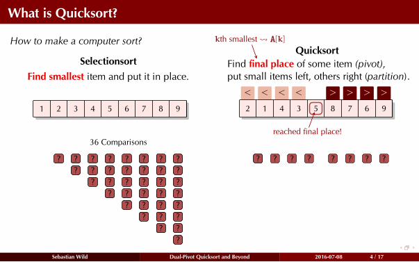
Quicksort
Find final
kth smallest A[k]
place of some item (pivot),
put small items left, others right (partition).
< >>< >< ><
? ? ???? ? ?
2 1 4 3 8 7 6 95
reached final place!
Sebastian Wild Dual-Pivot Quicksort and Beyond 2016-07-08 4 / 17
What is Quicksort?
How to make a computer sort?
Selectionsort
Find smallest item and put it in place.
? ? ? ? ? ? ? ?
1
? ? ? ? ? ? ?
2
? ? ? ? ? ?
? ? ? ? ?
? ? ? ?
3 4 5 6 7 8 9
? ? ?
? ?
?
36 Comparisons
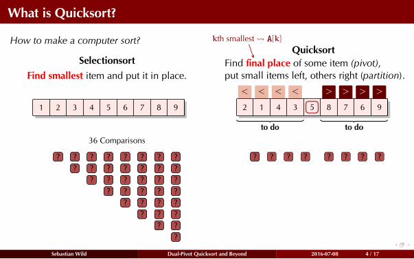
Quicksort
Find final
kth smallest A[k]
place of some item (pivot),
put small items left, others right (partition).
< >>< >< ><
? ? ???? ? ?
2 1 4 3 8 7 6 95
to do to do
Sebastian Wild Dual-Pivot Quicksort and Beyond 2016-07-08 4 / 17
What is Quicksort?
How to make a computer sort?
Selectionsort
Find smallest item and put it in place.
? ? ? ? ? ? ? ?
1
? ? ? ? ? ? ?
2
? ? ? ? ? ?
? ? ? ? ?
? ? ? ?
3 4 5 6 7 8 9
? ? ?
? ?
?
36 Comparisons
Quicksort
Find final
kth smallest A[k]
place of some item (pivot),
put small items left, others right (partition).
? ? ???? ? ?
2 1 4 3 8 7 6 95
to do
Sebastian Wild Dual-Pivot Quicksort and Beyond 2016-07-08 4 / 17
What is Quicksort?
How to make a computer sort?
Selectionsort
Find smallest item and put it in place.
? ? ? ? ? ? ? ?
1
? ? ? ? ? ? ?
2
? ? ? ? ? ?
? ? ? ? ?
? ? ? ?
3 4 5 6 7 8 9
? ? ?
? ?
?
36 Comparisons
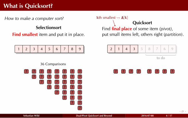
Quicksort
Find final
kth smallest A[k]
place of some item (pivot),
put small items left, others right (partition).
< > >
? ? ???? ? ?
2 1 4 3 8 7 6 95
to do
? ? ?
Sebastian Wild Dual-Pivot Quicksort and Beyond 2016-07-08 4 / 17
What is Quicksort?
How to make a computer sort?
Selectionsort
Find smallest item and put it in place.
? ? ? ? ? ? ? ?
1
? ? ? ? ? ? ?
2
? ? ? ? ? ?
? ? ? ? ?
? ? ? ?
3 4 5 6 7 8 9
? ? ?
? ?
?
36 Comparisons
Quicksort
Find final
kth smallest A[k]
place of some item (pivot),
put small items left, others right (partition).
< > >
? ? ???? ? ?
to do
? ? ?
1 2 4 3 5 8 7 6 9
to do
Sebastian Wild Dual-Pivot Quicksort and Beyond 2016-07-08 4 / 17
What is Quicksort?
How to make a computer sort?
Selectionsort
Find smallest item and put it in place.
? ? ? ? ? ? ? ?
1
? ? ? ? ? ? ?
2
? ? ? ? ? ?
? ? ? ? ?
? ? ? ?
3 4 5 6 7 8 9
? ? ?
? ?
?
36 Comparisons
Quicksort
Find final
kth smallest A[k]
place of some item (pivot),
put small items left, others right (partition).
? ? ???? ? ?
to do
? ? ?
1 2 3 4 5 8 7 6 9
?
Sebastian Wild Dual-Pivot Quicksort and Beyond 2016-07-08 4 / 17

What is Quicksort?
How to make a computer sort?
Selectionsort
Find smallest item and put it in place.
? ? ? ? ? ? ? ?
1
? ? ? ? ? ? ?
2
? ? ? ? ? ?
? ? ? ? ?
? ? ? ?
3 4 5 6 7 8 9
? ? ?
? ?
?
36 Comparisons
Quicksort
Find final
kth smallest A[k]
place of some item (pivot),
put small items left, others right (partition).
< < >
? ? ???? ? ?
? ? ?
1 2 3 4 5 8 7 6 9
?
? ? ?
Sebastian Wild Dual-Pivot Quicksort and Beyond 2016-07-08 4 / 17
What is Quicksort?
How to make a computer sort?
Selectionsort
Find smallest item and put it in place.
? ? ? ? ? ? ? ?
1
? ? ? ? ? ? ?
2
? ? ? ? ? ?
? ? ? ? ?
? ? ? ?
3 4 5 6 7 8 9
? ? ?
? ?
?
36 Comparisons
Quicksort
Find final
kth smallest A[k]
place of some item (pivot),
put small items left, others right (partition).
< < >
? ? ???? ? ?
? ? ?
?
? ? ?
1 2 3 4 5 6 7 8 9
Sebastian Wild Dual-Pivot Quicksort and Beyond 2016-07-08 4 / 17
What is Quicksort?
How to make a computer sort?
Selectionsort
Find smallest item and put it in place.
? ? ? ? ? ? ? ?
1
? ? ? ? ? ? ?
2
? ? ? ? ? ?
? ? ? ? ?
? ? ? ?
3 4 5 6 7 8 9
? ? ?
? ?
?
36 Comparisons
Quicksort
Find final
kth smallest A[k]
place of some item (pivot),
put small items left, others right (partition).
? ? ???? ? ?
? ? ?
?
? ? ?
1 2 3 4 5 6 7 8 9
to do
Sebastian Wild Dual-Pivot Quicksort and Beyond 2016-07-08 4 / 17
What is Quicksort?
How to make a computer sort?
Selectionsort
Find smallest item and put it in place.
? ? ? ? ? ? ? ?
1
? ? ? ? ? ? ?
2
? ? ? ? ? ?
? ? ? ? ?
? ? ? ?
3 4 5 6 7 8 9
? ? ?
? ?
?
36 Comparisons
Quicksort
Find final
kth smallest A[k]
place of some item (pivot),
put small items left, others right (partition).
? ? ???? ? ?
? ? ?
?
? ? ?
1 2 3 4 5 6 7 8 9
?
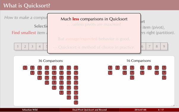
16 Comparisons
Sebastian Wild Dual-Pivot Quicksort and Beyond 2016-07-08 4 / 17
What is Quicksort?
How to make a computer sort?
Selectionsort
Find smallest item and put it in place.
? ? ? ? ? ? ? ?
1
? ? ? ? ? ? ?
2
? ? ? ? ? ?
? ? ? ? ?
? ? ? ?
3 4 5 6 7 8 9
? ? ?
? ?
?
36 Comparisons
Quicksort
Find final
kth smallest A[k]
place of some item (pivot),
put small items left, others right (partition).
? ? ???? ? ?
? ? ?
?
? ? ?
1 2 3 4 5 6 7 8 9
?
16 Comparisons
Much less comparisons in Quicksort
. . . unless pivots are max/min!
But average/expected behavior is good.
Quicksort is method of choice in practice.
Sebastian Wild Dual-Pivot Quicksort and Beyond 2016-07-08 4 / 17
What is Quicksort?
How to make a computer sort?
Selectionsort
Find smallest item and put it in place.
? ? ? ? ? ? ? ?
1
? ? ? ? ? ? ?
2
? ? ? ? ? ?
? ? ? ? ?
? ? ? ?
3 4 5 6 7 8 9
? ? ?
? ?
?
36 Comparisons
Quicksort
Find final
kth smallest A[k]
place of some item (pivot),
put small items left, others right (partition).
? ? ???? ? ?
? ? ?
?
? ? ?
1 2 3 4 5 6 7 8 9
?
16 Comparisons
Much less comparisons in Quicksort
. . . unless pivots are max/min!
But average/expected
(actually: almost always good)
behavior is good.
Quicksort is method of choice in practice.
Sebastian Wild Dual-Pivot Quicksort and Beyond 2016-07-08 4 / 17
Variants of Quicksort
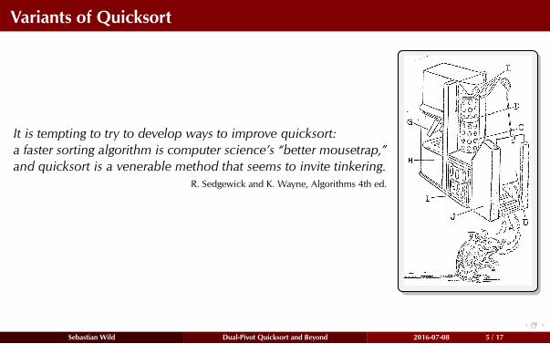
It is tempting to try to develop ways to improve quicksort:
a faster sorting algorithm is computer science’s “better mousetrap,”
and quicksort is a venerable method that seems to invite tinkering.
R. Sedgewick and K. Wayne, Algorithms 4th ed.
Sebastian Wild Dual-Pivot Quicksort and Beyond 2016-07-08 5 / 17
Variants of Quicksort
It is tempting to try to develop ways to improve quicksort:
a faster sorting algorithm is computer science’s “better mousetrap,”
and quicksort is a venerable method that seems to invite tinkering.
R. Sedgewick and K. Wayne, Algorithms 4th ed.
Many variants tried
Two important tuning options:
1 Choose pivots wisely (pivot sampling)
for example: middle element of three (median-of-three)
pivot never min or max!
2 Split into s > 2 subproblems at once (multiway partitioning)
for example: 2 pivots 3 classes: small, medium and large
subproblems are smaller,
but partitioning is more expensive.
Sebastian Wild Dual-Pivot Quicksort and Beyond 2016-07-08 5 / 17
Variants of Quicksort
It is tempting to try to develop ways to improve quicksort:
a faster sorting algorithm is computer science’s “better mousetrap,”
and quicksort is a venerable method that seems to invite tinkering.
R. Sedgewick and K. Wayne, Algorithms 4th ed.
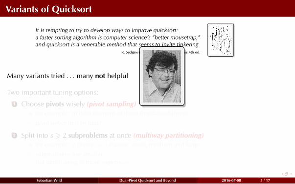
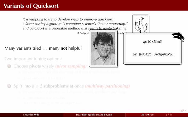
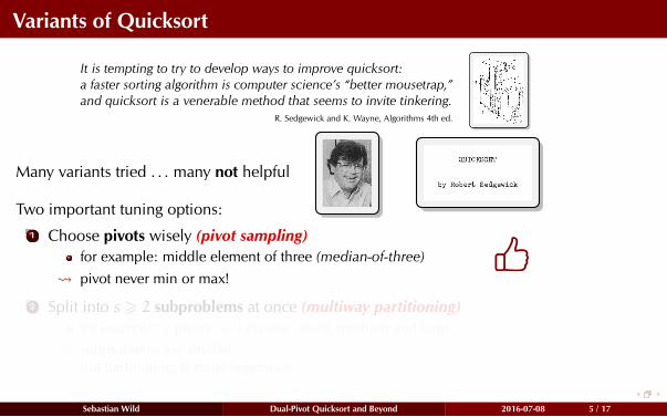
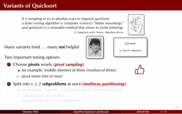
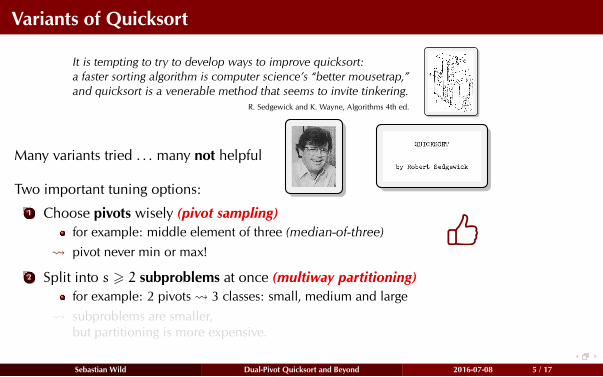
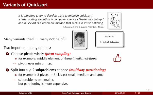
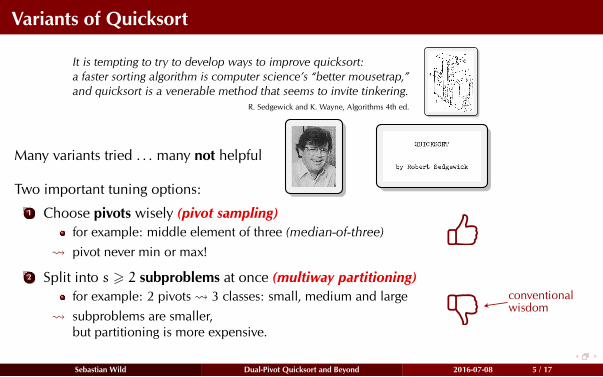
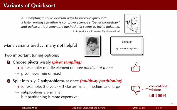
Many variants tried . . . many not helpful
Two important tuning options:
1 Choose pivots wisely (pivot sampling)
for example: middle element of three (median-of-three)
pivot never min or max!
2 Split into s > 2 subproblems at once (multiway partitioning)
for example: 2 pivots 3 classes: small, medium and large
subproblems are smaller,
but partitioning is more expensive.
Sebastian Wild Dual-Pivot Quicksort and Beyond 2016-07-08 5 / 17
Variants of Quicksort
It is tempting to try to develop ways to improve quicksort:
a faster sorting algorithm is computer science’s “better mousetrap,”
and quicksort is a venerable method that seems to invite tinkering.
R. Sedgewick and K. Wayne, Algorithms 4th ed.
Many variants tried . . . many not helpful
Two important tuning options:
1 Choose pivots wisely (pivot sampling)
for example: middle element of three (median-of-three)
pivot never min or max!
2 Split into s > 2 subproblems at once (multiway partitioning)
for example: 2 pivots 3 classes: small, medium and large
subproblems are smaller,
but partitioning is more expensive.
conventionalwisdom
till 2009!
Sebastian Wild Dual-Pivot Quicksort and Beyond 2016-07-08 5 / 17
Java 7’s Dual-Pivot Quicksort
What happened in 2009? Java
used e.g. for Android apps
7 sorting method was released!
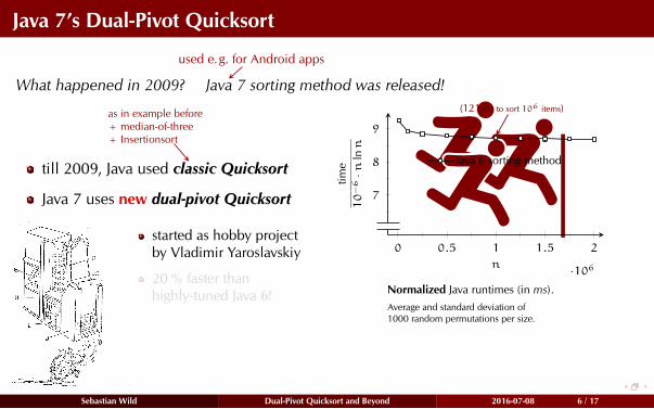
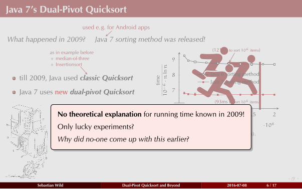
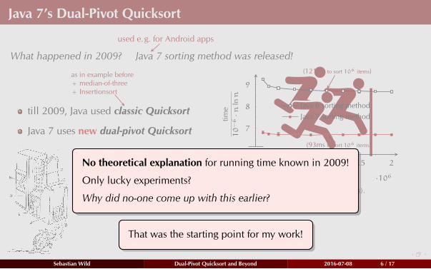
till 2009, Java used classic Quicksort
Java 7 uses new dual-pivot Quicksort
started as hobby project
by Vladimir Yaroslavskiy
20 % faster than
highly-tuned Java 6!
Sebastian Wild Dual-Pivot Quicksort and Beyond 2016-07-08 6 / 17
Java 7’s Dual-Pivot Quicksort
What happened in 2009? Java
used e.g. for Android apps
7 sorting method was released!
till 2009, Java used classic
as in example before
+ median-of-three
+ Insertionsort
Quicksort
Java 7 uses new dual-pivot Quicksort
started as hobby project
by Vladimir Yaroslavskiy
20 % faster than
highly-tuned Java 6!
Sebastian Wild Dual-Pivot Quicksort and Beyond 2016-07-08 6 / 17
Java 7’s Dual-Pivot Quicksort
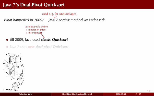
What happened in 2009? Java
used e.g. for Android apps
7 sorting method was released!
till 2009, Java used classic
as in example before
+ median-of-three
+ Insertionsort
Quicksort
Java 7 uses new dual-pivot Quicksort
started as hobby project
by Vladimir Yaroslavskiy
20 % faster than
highly-tuned Java 6!
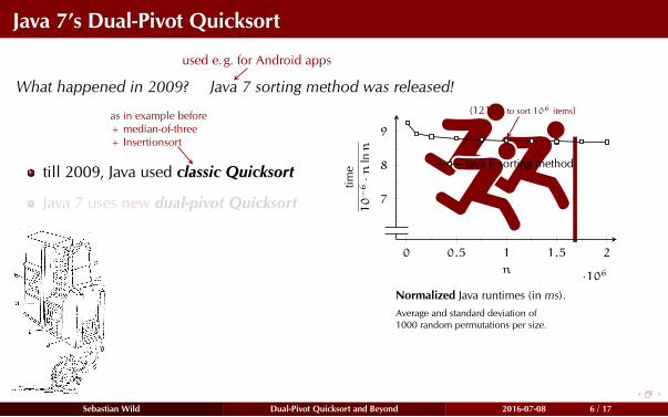
0 0.5 1 1.5 2
·106
7
8
9
n
tim
e
10−6·n
lnn
Java 6 sorting method
(121ms to sort 106 items)
Normalized Java runtimes (in ms).
Average and standard deviation of
1000 random permutations per size.
Sebastian Wild Dual-Pivot Quicksort and Beyond 2016-07-08 6 / 17
Java 7’s Dual-Pivot Quicksort
What happened in 2009? Java
used e.g. for Android apps
7 sorting method was released!
till 2009, Java used classic
as in example before
+ median-of-three
+ Insertionsort
Quicksort
Java 7 uses new dual-pivot Quicksort
started as hobby project
by Vladimir Yaroslavskiy
20 % faster than
highly-tuned Java 6!
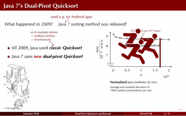
0 0.5 1 1.5 2
·106
7
8
9
n
tim
e
10−6·n
lnn
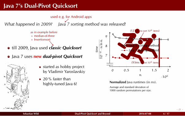
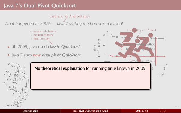
Java 6 sorting method
Java 7 sorting method
(121ms to sort 106 items)
(93ms to sort 106 items)
Normalized Java runtimes (in ms).
Average and standard deviation of
1000 random permutations per size.
Sebastian Wild Dual-Pivot Quicksort and Beyond 2016-07-08 6 / 17
Java 7’s Dual-Pivot Quicksort
What happened in 2009? Java
used e.g. for Android apps
7 sorting method was released!
till 2009, Java used classic
as in example before
+ median-of-three
+ Insertionsort
Quicksort
Java 7 uses new dual-pivot Quicksort
started as hobby project
by Vladimir Yaroslavskiy
20 % faster than
highly-tuned Java 6!
0 0.5 1 1.5 2
·106
7
8
9
n
tim
e
10−6·n
lnn
Java 6 sorting method
Java 7 sorting method
(121ms to sort 106 items)
(93ms to sort 106 items)
Normalized Java runtimes (in ms).
Average and standard deviation of
1000 random permutations per size.
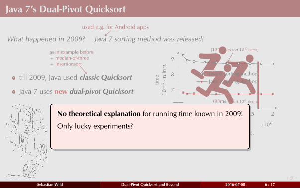
No theoretical explanation for running time known in 2009!
Sebastian Wild Dual-Pivot Quicksort and Beyond 2016-07-08 6 / 17
Java 7’s Dual-Pivot Quicksort
What happened in 2009? Java
used e.g. for Android apps
7 sorting method was released!
till 2009, Java used classic
as in example before
+ median-of-three
+ Insertionsort
Quicksort
Java 7 uses new dual-pivot Quicksort
started as hobby project
by Vladimir Yaroslavskiy
20 % faster than
highly-tuned Java 6!
0 0.5 1 1.5 2
·106
7
8
9
n
tim
e
10−6·n
lnn
Java 6 sorting method
Java 7 sorting method
(121ms to sort 106 items)
(93ms to sort 106 items)
Normalized Java runtimes (in ms).
Average and standard deviation of
1000 random permutations per size.
No theoretical explanation for running time known in 2009!
Only lucky experiments?
Why did no-one come up with this earlier?
That was the starting point for my work!
Sebastian Wild Dual-Pivot Quicksort and Beyond 2016-07-08 6 / 17

Overview of my work
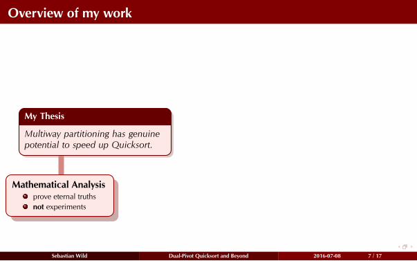
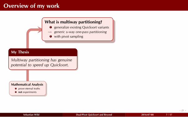
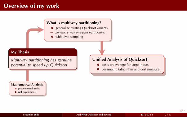
My Thesis
Multiway partitioning has genuine
potential to speed up Quicksort.
Sebastian Wild Dual-Pivot Quicksort and Beyond 2016-07-08 7 / 17
Overview of my work
My Thesis
Multiway partitioning has genuine
potential to speed up Quicksort.
Mathematical Analysisprove eternal truths
not experiments
Mathematical Analysisprove eternal truths
not experiments
Sebastian Wild Dual-Pivot Quicksort and Beyond 2016-07-08 7 / 17
Overview of my work
My Thesis
Multiway partitioning has genuine
potential to speed up Quicksort.
Mathematical Analysisprove eternal truths
not experiments
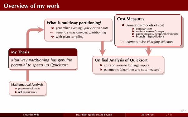
What is multiway partitioning?generalize existing Quicksort variants
generic s-way one-pass partitioning
with pivot sampling
What is multiway partitioning?generalize existing Quicksort variants
generic s-way one-pass partitioning
with pivot sampling
Sebastian Wild Dual-Pivot Quicksort and Beyond 2016-07-08 7 / 17
Overview of my work
My Thesis
Multiway partitioning has genuine
potential to speed up Quicksort.
Mathematical Analysisprove eternal truths
not experiments
What is multiway partitioning?generalize existing Quicksort variants
generic s-way one-pass partitioning
with pivot sampling
Unified Analysis of Quicksortcosts on average for large inputs
parametric (algorithm and cost measure)
Unified Analysis of Quicksortcosts on average for large inputs
parametric (algorithm and cost measure)
Sebastian Wild Dual-Pivot Quicksort and Beyond 2016-07-08 7 / 17
Overview of my work
My Thesis
Multiway partitioning has genuine
potential to speed up Quicksort.
Mathematical Analysisprove eternal truths
not experiments
What is multiway partitioning?generalize existing Quicksort variants
generic s-way one-pass partitioning
with pivot sampling
Unified Analysis of Quicksortcosts on average for large inputs
parametric (algorithm and cost measure)
Cost Measures
generalize models of costcomparisonswrite accesses / swapscache misses / scanned elementsbranch mispredictions
element-wise charging schemes
Cost Measures
generalize models of costcomparisonswrite accesses / swapscache misses / scanned elementsbranch mispredictions
element-wise charging schemes
Sebastian Wild Dual-Pivot Quicksort and Beyond 2016-07-08 7 / 17
Overview of my work
My Thesis
Multiway partitioning has genuine
potential to speed up Quicksort.
Mathematical Analysisprove eternal truths
not experiments
What is multiway partitioning?generalize existing Quicksort variants
generic s-way one-pass partitioning
with pivot sampling
Unified Analysis of Quicksortcosts on average for large inputs
parametric (algorithm and cost measure)
Cost Measures
generalize models of costcomparisonswrite accesses / swapscache misses / scanned elementsbranch mispredictions
element-wise charging schemes
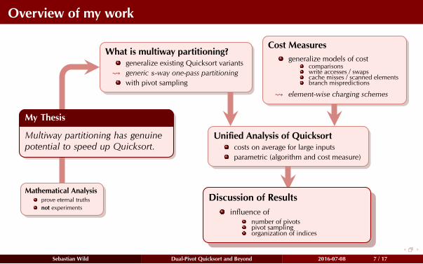
Discussion of Results
influence ofnumber of pivotspivot samplingorganization of indices
Discussion of Results
influence ofnumber of pivotspivot samplingorganization of indices
Sebastian Wild Dual-Pivot Quicksort and Beyond 2016-07-08 7 / 17
Overview of my work
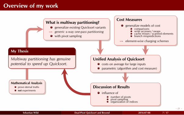
My Thesis
Multiway partitioning has genuine
potential to speed up Quicksort.
Mathematical Analysisprove eternal truths
not experiments
What is multiway partitioning?generalize existing Quicksort variants
generic s-way one-pass partitioning
with pivot sampling
Unified Analysis of Quicksortcosts on average for large inputs
parametric (algorithm and cost measure)
Cost Measures
generalize models of costcomparisonswrite accesses / swapscache misses / scanned elementsbranch mispredictions
element-wise charging schemes
Discussion of Results
influence ofnumber of pivotspivot samplingorganization of indices
Sebastian Wild Dual-Pivot Quicksort and Beyond 2016-07-08 7 / 17
Entropy
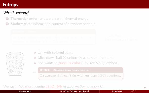
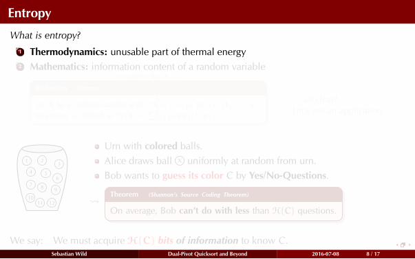
What is entropy?
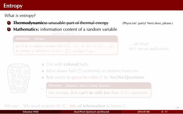
1 Thermodynamics: unusable part of thermal energy
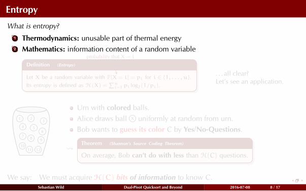
2 Mathematics: information content of a random variable
Definition (Entropy)
Let X be a random variable with P[X = i] = pi for i ∈ {1, . . . ,u}.
Its entropy is defined as H(X) =∑u
i=1 pi log2(1/pi).
probability that X = i
. . . all clear?
Let’s see an application.
1 23
4 56
7 8 9
1011 12
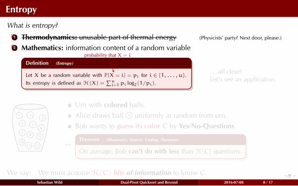
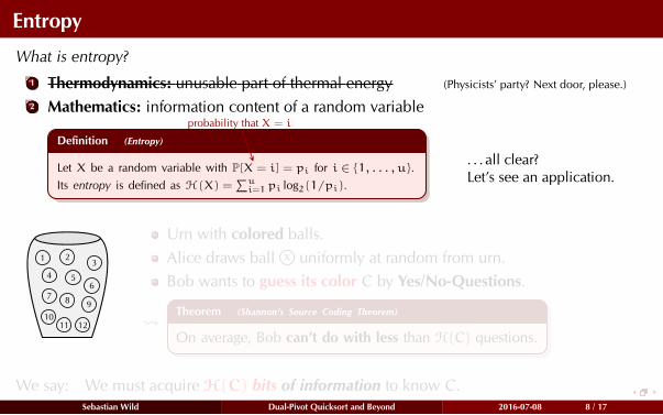
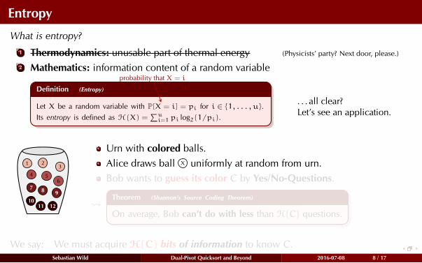
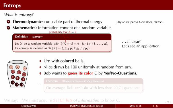
Urn with colored balls.
Alice draws ball X uniformly at random from urn.
Bob wants to guess its color C by Yes/No-Questions.
Theorem (Shannon’s Source Coding Theorem)
On average, Bob can’t do with less than H(C) questions.
We say: We must acquire H(C) bits of information to know C.
Sebastian Wild Dual-Pivot Quicksort and Beyond 2016-07-08 8 / 17
Entropy
What is entropy?
1 Thermodynamics: unusable part of thermal energy
2 Mathematics: information content of a random variable
Definition (Entropy)
Let X be a random variable with P[X = i] = pi for i ∈ {1, . . . ,u}.
Its entropy is defined as H(X) =∑u
i=1 pi log2(1/pi).
probability that X = i
. . . all clear?
Let’s see an application.
1 23
4 56
7 8 9
1011 12
Urn with colored balls.
Alice draws ball X uniformly at random from urn.
Bob wants to guess its color C by Yes/No-Questions.
Theorem (Shannon’s Source Coding Theorem)
On average, Bob can’t do with less than H(C) questions.
We say: We must acquire H(C) bits of information to know C.
Sebastian Wild Dual-Pivot Quicksort and Beyond 2016-07-08 8 / 17
Entropy
What is entropy?
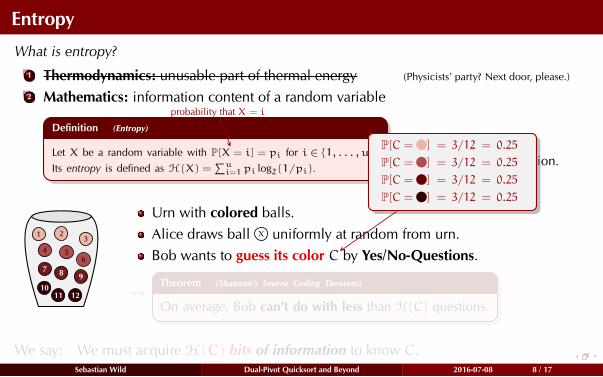
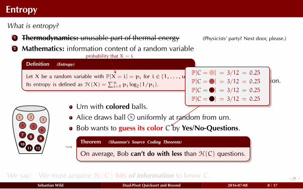
1 Thermodynamics: unusable part of thermal energy (Physicists’ party? Next door, please.)
2 Mathematics: information content of a random variable
Definition (Entropy)
Let X be a random variable with P[X = i] = pi for i ∈ {1, . . . ,u}.
Its entropy is defined as H(X) =∑u
i=1 pi log2(1/pi).
probability that X = i
. . . all clear?
Let’s see an application.
1 23
4 56
7 8 9
1011 12
Urn with colored balls.
Alice draws ball X uniformly at random from urn.
Bob wants to guess its color C by Yes/No-Questions.
Theorem (Shannon’s Source Coding Theorem)
On average, Bob can’t do with less than H(C) questions.
We say: We must acquire H(C) bits of information to know C.
Sebastian Wild Dual-Pivot Quicksort and Beyond 2016-07-08 8 / 17
Entropy
What is entropy?
1 Thermodynamics: unusable part of thermal energy (Physicists’ party? Next door, please.)
2 Mathematics: information content of a random variable
Definition (Entropy)
Let X be a random variable with P[X = i] = pi for i ∈ {1, . . . ,u}.
Its entropy is defined as H(X) =∑u
i=1 pi log2(1/pi).
probability that X = i
. . . all clear?
Let’s see an application.
1 23
4 56
7 8 9
1011 12
Urn with colored balls.
Alice draws ball X uniformly at random from urn.
Bob wants to guess its color C by Yes/No-Questions.
Theorem (Shannon’s Source Coding Theorem)
On average, Bob can’t do with less than H(C) questions.
We say: We must acquire H(C) bits of information to know C.
Sebastian Wild Dual-Pivot Quicksort and Beyond 2016-07-08 8 / 17
Entropy
What is entropy?
1 Thermodynamics: unusable part of thermal energy (Physicists’ party? Next door, please.)
2 Mathematics: information content of a random variable
Definition (Entropy)
Let X be a random variable with P[X = i] = pi for i ∈ {1, . . . ,u}.
Its entropy is defined as H(X) =∑u
i=1 pi log2(1/pi).
probability that X = i
. . . all clear?
Let’s see an application.
1 23
4 56
7 8 9
1011 12
Urn with colored balls.
Alice draws ball X uniformly at random from urn.
Bob wants to guess its color C
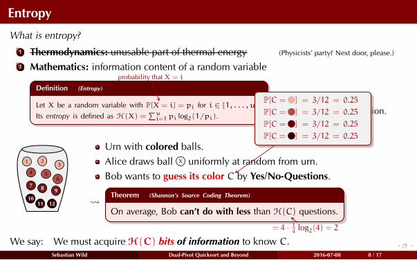
P[C = ] = 3/12 = 0.25
P[C = ] = 3/12 = 0.25
P[C = ] = 3/12 = 0.25
P[C = ] = 3/12 = 0.25
by Yes/No-Questions.
Theorem (Shannon’s Source Coding Theorem)
On average, Bob can’t do with less than H(C) questions.
We say: We must acquire H(C) bits of information to know C.
Sebastian Wild Dual-Pivot Quicksort and Beyond 2016-07-08 8 / 17
Entropy
What is entropy?
1 Thermodynamics: unusable part of thermal energy (Physicists’ party? Next door, please.)
2 Mathematics: information content of a random variable
Definition (Entropy)
Let X be a random variable with P[X = i] = pi for i ∈ {1, . . . ,u}.
Its entropy is defined as H(X) =∑u
i=1 pi log2(1/pi).
probability that X = i
. . . all clear?
Let’s see an application.
1 23
4 56
7 8 9
1011 12
Urn with colored balls.
Alice draws ball X uniformly at random from urn.
Bob wants to guess its color C
P[C = ] = 3/12 = 0.25
P[C = ] = 3/12 = 0.25
P[C = ] = 3/12 = 0.25
P[C = ] = 3/12 = 0.25
by Yes/No-Questions.
Theorem (Shannon’s Source Coding Theorem)
On average, Bob can’t do with less than H(C) questions.
We say: We must acquire H(C) bits of information to know C.
Sebastian Wild Dual-Pivot Quicksort and Beyond 2016-07-08 8 / 17

Entropy
What is entropy?
1 Thermodynamics: unusable part of thermal energy (Physicists’ party? Next door, please.)
2 Mathematics: information content of a random variable
Definition (Entropy)
Let X be a random variable with P[X = i] = pi for i ∈ {1, . . . ,u}.
Its entropy is defined as H(X) =∑u
i=1 pi log2(1/pi).
probability that X = i
. . . all clear?
Let’s see an application.
1 23
4 56
7 8 9
1011 12
Urn with colored balls.
Alice draws ball X uniformly at random from urn.
Bob wants to guess its color C
P[C = ] = 3/12 = 0.25
P[C = ] = 3/12 = 0.25
P[C = ] = 3/12 = 0.25
P[C = ] = 3/12 = 0.25
by Yes/No-Questions.
Theorem (Shannon’s Source Coding Theorem)
On average, Bob can’t do with less than H(C) questions.
= 4 · 14
log2(4) = 2
We say: We must acquire H(C) bits of information to know C.
Sebastian Wild Dual-Pivot Quicksort and Beyond 2016-07-08 8 / 17
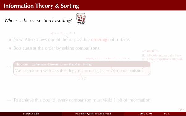
Information Theory & Sorting
Where is the connection to sorting?
1 23
4 56
7 8 9
1011 12
Now, Alice draws one of the n!
n(n− 1) · · · 2 · 1
possible orderings of n items.
Bob guesses the order by asking comparisons.
Theorem (Information-Theoretic Lower Bound for Sorting)
We cannot sort with less than log2(n!) = n log2(n)±O(n) comparisons.
Assumptions:
(1) All orderings equally likely.
(2) Only comparisons allowed.asymptotic error term for n → ∞
H(C)
To achieve this bound, every comparison must yield 1 bit of information!
Sebastian Wild Dual-Pivot Quicksort and Beyond 2016-07-08 9 / 17
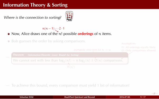
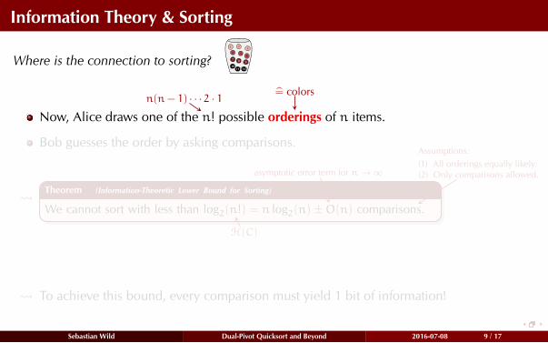
Information Theory & Sorting
Where is the connection to sorting?
1 23
4 56
7 8 9
1011 12
Now, Alice draws one of the n!
n(n− 1) · · · 2 · 1
possible orderings
=̂ colors
of n items.
Bob guesses the order by asking comparisons.
Theorem (Information-Theoretic Lower Bound for Sorting)
We cannot sort with less than log2(n!) = n log2(n)±O(n) comparisons.
Assumptions:
(1) All orderings equally likely.
(2) Only comparisons allowed.asymptotic error term for n → ∞
H(C)
To achieve this bound, every comparison must yield 1 bit of information!
Sebastian Wild Dual-Pivot Quicksort and Beyond 2016-07-08 9 / 17
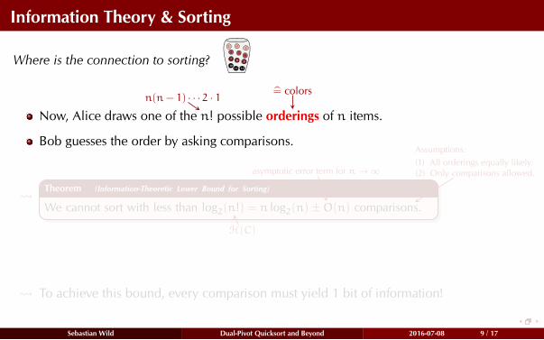
Information Theory & Sorting
Where is the connection to sorting?
1 23
4 56
7 8 9
1011 12
Now, Alice draws one of the n!
n(n− 1) · · · 2 · 1
possible orderings
=̂ colors
of n items.
Bob guesses the order by asking comparisons.
Theorem (Information-Theoretic Lower Bound for Sorting)
We cannot sort with less than log2(n!) = n log2(n)±O(n) comparisons.
Assumptions:
(1) All orderings equally likely.
(2) Only comparisons allowed.asymptotic error term for n → ∞
H(C)
To achieve this bound, every comparison must yield 1 bit of information!
Sebastian Wild Dual-Pivot Quicksort and Beyond 2016-07-08 9 / 17
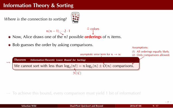
Information Theory & Sorting
Where is the connection to sorting?
1 23
4 56
7 8 9
1011 12
Now, Alice draws one of the n!
n(n− 1) · · · 2 · 1
possible orderings
=̂ colors
of n items.
Bob guesses the order by asking comparisons.
Theorem (Information-Theoretic Lower Bound for Sorting)
We cannot sort with less than log2(n!) = n log2(n)±O(n) comparisons.
Assumptions:
(1) All orderings equally likely.
(2) Only comparisons allowed.asymptotic error term for n → ∞
H(C)
To achieve this bound, every comparison must yield 1 bit of information!
Sebastian Wild Dual-Pivot Quicksort and Beyond 2016-07-08 9 / 17
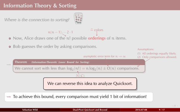
Information Theory & Sorting
Where is the connection to sorting?
1 23
4 56
7 8 9
1011 12
Now, Alice draws one of the n!
n(n− 1) · · · 2 · 1
possible orderings
=̂ colors
of n items.
Bob guesses the order by asking comparisons.
Theorem (Information-Theoretic Lower Bound for Sorting)
We cannot sort with less than log2(n!) = n log2(n)±O(n) comparisons.
Assumptions:
(1) All orderings equally likely.
(2) Only comparisons allowed.asymptotic error term for n → ∞
H(C)
To achieve this bound, every comparison must yield 1 bit of information!
We can reverse this idea to analyze Quicksort.
Sebastian Wild Dual-Pivot Quicksort and Beyond 2016-07-08 9 / 17
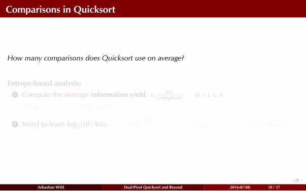
Comparisons in Quicksort
How many comparisons does Quicksort use on average?
Entropy-based analysis:
1 Compute the average information yield: x bitcomparison . (0 < x 6 1)
What is x? . . . stay tuned.
2 Need to learn log2(n!) bits Uselog2(n!)
x=
1
xn log2(n)±O(n) comparisons.
Sebastian Wild Dual-Pivot Quicksort and Beyond 2016-07-08 10 / 17
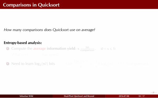
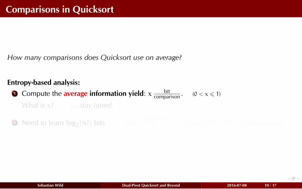
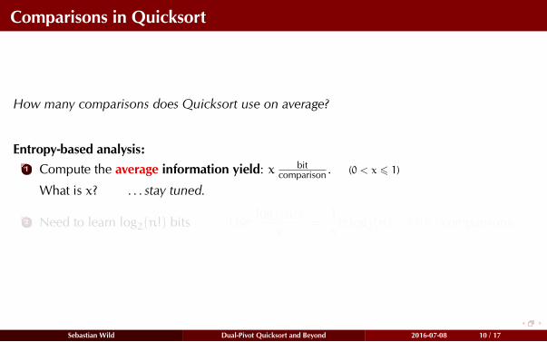
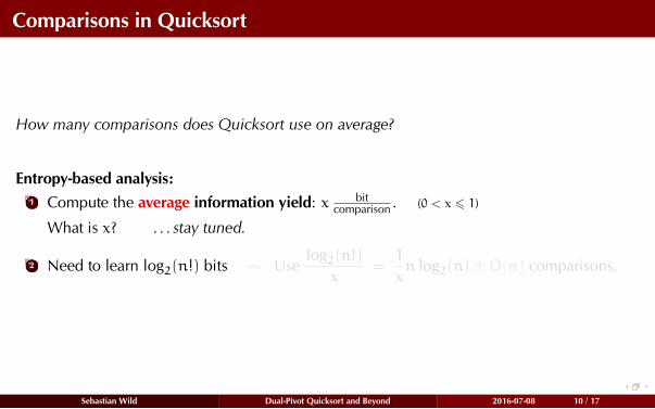
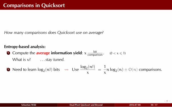
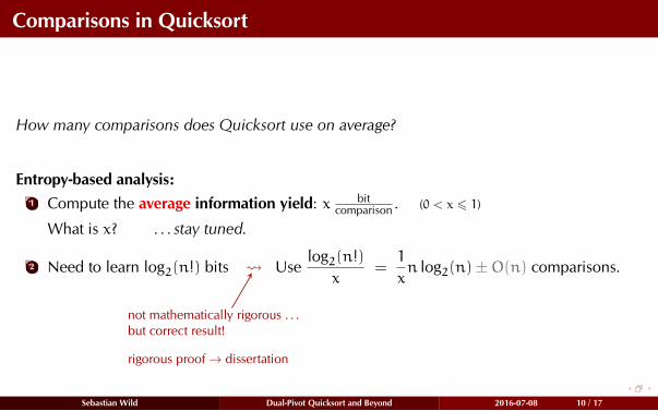
Comparisons in Quicksort
How many comparisons does Quicksort use on average?
Entropy-based analysis:
1 Compute the average information yield: x bitcomparison . (0 < x 6 1)
What is x? . . . stay tuned.
2 Need to learn log2(n!) bits
not mathematically rigorous . . .
but correct result!
rigorous proof → dissertation
Uselog2(n!)
x=
1
xn log2(n)±O(n) comparisons.
Sebastian Wild Dual-Pivot Quicksort and Beyond 2016-07-08 10 / 17

Partitioning Entropy
What is x?
Classic Quicksort:
Always compare with the pivot P
< < < < > > > >
2 1 4 3 5 8 7 6 9
Outcome C is either small or large .
Information yield is H(C) =
−P[ < ] log2(P[ < ]) − P[ > ] log2(P[ > ])
Sebastian Wild Dual-Pivot Quicksort and Beyond 2016-07-08 11 / 17
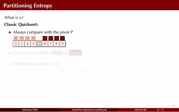
Partitioning Entropy
What is x?
Classic Quicksort:
Always compare with the pivot P
< < < < > > > >
2 1 4 3 5 8 7 6 9
Outcome C is either small or large .
Information yield is H(C) =
−P[ < ] log2(P[ < ]) − P[ > ] log2(P[ > ])
Sebastian Wild Dual-Pivot Quicksort and Beyond 2016-07-08 11 / 17
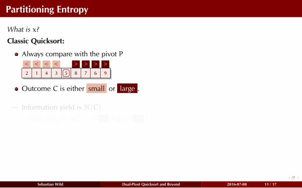
Partitioning Entropy
What is x?
Classic Quicksort:
Always compare with the pivot P
< < < < > > > >
2 1 4 3 5 8 7 6 9
Outcome C is either small or large .
Information yield is H(C) =
−P[ < ] log2(P[ < ]) − P[ > ] log2(P[ > ])
Sebastian Wild Dual-Pivot Quicksort and Beyond 2016-07-08 11 / 17
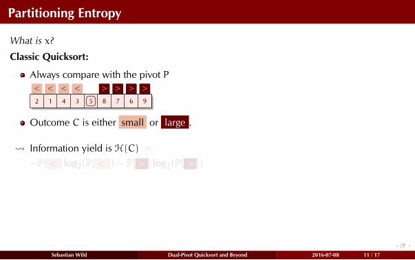
Partitioning Entropy
What is x?
Classic Quicksort:
Always compare with the pivot P
< < < < > > > >
2 1 4 3 5 8 7 6 9
Outcome C is either small or large .
Information yield is H(C) =
−P[ < ] log2(P[ < ]) − P[ > ] log2(P[ > ])
Sebastian Wild Dual-Pivot Quicksort and Beyond 2016-07-08 11 / 17
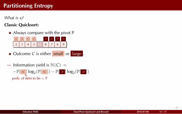
Partitioning Entropy
What is x?
Classic Quicksort:
Always compare with the pivot P
< < < < > > > >
2 1 4 3 5 8 7 6 9
Outcome C is either small or large .
Information yield is H(C) =
−P[ < ]
prob. of item to be < P
log2(P[ < ]) − P[ > ] log2(P[ > ])
Sebastian Wild Dual-Pivot Quicksort and Beyond 2016-07-08 11 / 17
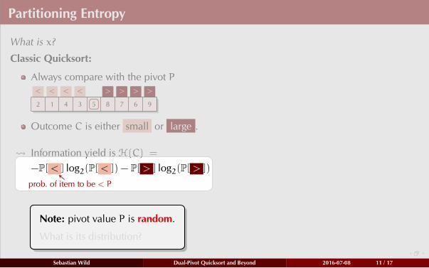
Partitioning Entropy
What is x?
Classic Quicksort:
Always compare with the pivot P
< < < < > > > >
2 1 4 3 5 8 7 6 9
Outcome C is either small or large .
Information yield is H(C) =
−P[ < ]
prob. of item to be < P
log2(P[ < ]) − P[ > ] log2(P[ > ])
Note: pivot value P is random.
What is its distribution?
Sebastian Wild Dual-Pivot Quicksort and Beyond 2016-07-08 11 / 17
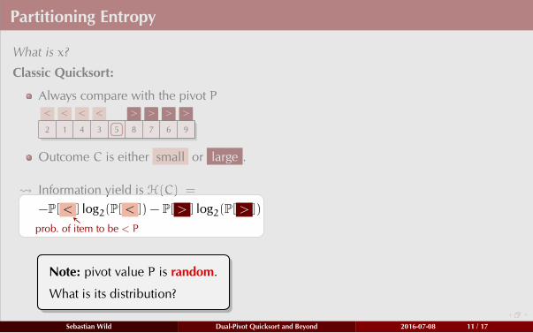
Partitioning Entropy
What is x?
Classic Quicksort:
Always compare with the pivot P
< < < < > > > >
2 1 4 3 5 8 7 6 9
Outcome C is either small or large .
Information yield is H(C) =
−P[ < ]
prob. of item to be < P
log2(P[ < ]) − P[ > ] log2(P[ > ])
Note: pivot value P is random.
What is its distribution?
Sebastian Wild Dual-Pivot Quicksort and Beyond 2016-07-08 11 / 17
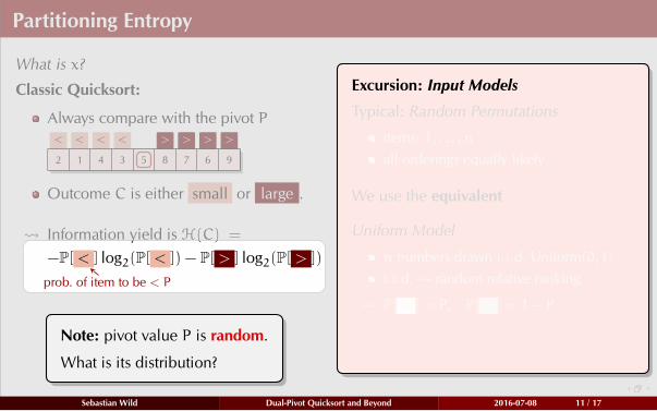
Partitioning Entropy
What is x?
Classic Quicksort:
Always compare with the pivot P
< < < < > > > >
2 1 4 3 5 8 7 6 9
Outcome C is either small or large .
Information yield is H(C) =
−P[ < ]
prob. of item to be < P
log2(P[ < ]) − P[ > ] log2(P[ > ])
Note: pivot value P is random.
What is its distribution?
Excursion: Input Models
Typical: Random Permutations
items: 1, . . . , n
all orderings equally likely
We use the equivalent
Uniform Model
n numbers drawn i. i.d. Uniform(0, 1)
i. i.d. random relative ranking
P[ < ] = P, P[ > ] = 1− P
Sebastian Wild Dual-Pivot Quicksort and Beyond 2016-07-08 11 / 17
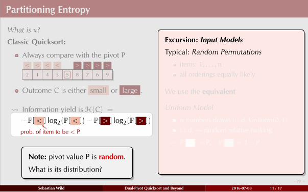
Partitioning Entropy
What is x?
Classic Quicksort:
Always compare with the pivot P
< < < < > > > >
2 1 4 3 5 8 7 6 9
Outcome C is either small or large .
Information yield is H(C) =
−P[ < ]
prob. of item to be < P
log2(P[ < ]) − P[ > ] log2(P[ > ])
Note: pivot value P is random.
What is its distribution?
Excursion: Input Models
Typical: Random Permutations
items: 1, . . . , n
all orderings equally likely
We use the equivalent
Uniform Model
n numbers drawn i. i.d. Uniform(0, 1)
i. i.d. random relative ranking
P[ < ] = P, P[ > ] = 1− P
Sebastian Wild Dual-Pivot Quicksort and Beyond 2016-07-08 11 / 17
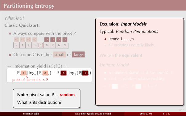
Partitioning Entropy
What is x?
Classic Quicksort:
Always compare with the pivot P
< < < < > > > >
2 1 4 3 5 8 7 6 9
Outcome C is either small or large .
Information yield is H(C) =
−P[ < ]
prob. of item to be < P
log2(P[ < ]) − P[ > ] log2(P[ > ])
Note: pivot value P is random.
What is its distribution?
Excursion: Input Models
Typical: Random Permutations
items: 1, . . . , n
all orderings equally likely
We use the equivalent
Uniform Model
n numbers drawn i. i.d. Uniform(0, 1)
i. i.d. random relative ranking
P[ < ] = P, P[ > ] = 1− P
Sebastian Wild Dual-Pivot Quicksort and Beyond 2016-07-08 11 / 17
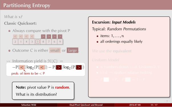
Partitioning Entropy
What is x?
Classic Quicksort:
Always compare with the pivot P
< < < < > > > >
2 1 4 3 5 8 7 6 9
Outcome C is either small or large .
Information yield is H(C) =
−P[ < ]
prob. of item to be < P
log2(P[ < ]) − P[ > ] log2(P[ > ])
Note: pivot value P is random.
What is its distribution?
Excursion: Input Models
Typical: Random Permutations
items: 1, . . . , n
all orderings equally likely
We use the equivalent
Uniform Model
n numbers drawn i. i.d. Uniform(0, 1)
i. i.d. random relative ranking
P[ < ] = P, P[ > ] = 1− P
Sebastian Wild Dual-Pivot Quicksort and Beyond 2016-07-08 11 / 17
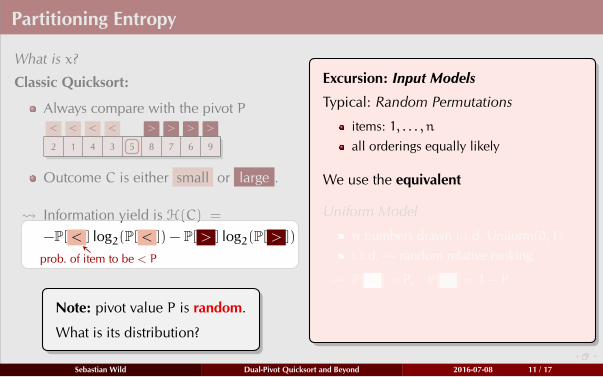
Partitioning Entropy
What is x?
Classic Quicksort:
Always compare with the pivot P
< < < < > > > >
2 1 4 3 5 8 7 6 9
Outcome C is either small or large .
Information yield is H(C) =
−P[ < ]
prob. of item to be < P
log2(P[ < ]) − P[ > ] log2(P[ > ])
Note: pivot value P is random.
What is its distribution?
Excursion: Input Models
Typical: Random Permutations
items: 1, . . . , n
all orderings equally likely
We use the equivalent
Uniform Model
n numbers drawn i. i.d. Uniform(0, 1)
i. i.d. random relative ranking
P[ < ] = P, P[ > ] = 1− P
Sebastian Wild Dual-Pivot Quicksort and Beyond 2016-07-08 11 / 17
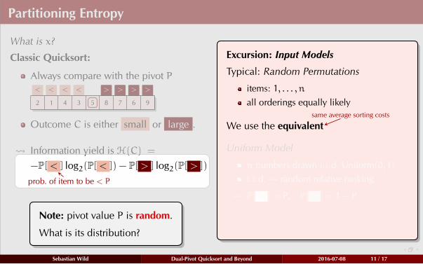
Partitioning Entropy
What is x?
Classic Quicksort:
Always compare with the pivot P
< < < < > > > >
2 1 4 3 5 8 7 6 9
Outcome C is either small or large .
Information yield is H(C) =
−P[ < ]
prob. of item to be < P
log2(P[ < ]) − P[ > ] log2(P[ > ])
Note: pivot value P is random.
What is its distribution?
Excursion: Input Models
Typical: Random Permutations
items: 1, . . . , n
all orderings equally likely
We use the equivalent
Uniform Model
n numbers drawn i. i.d. Uniform(0, 1)
i. i.d. random relative ranking
P[ < ] = P, P[ > ] = 1− P
same average sorting costs
Sebastian Wild Dual-Pivot Quicksort and Beyond 2016-07-08 11 / 17
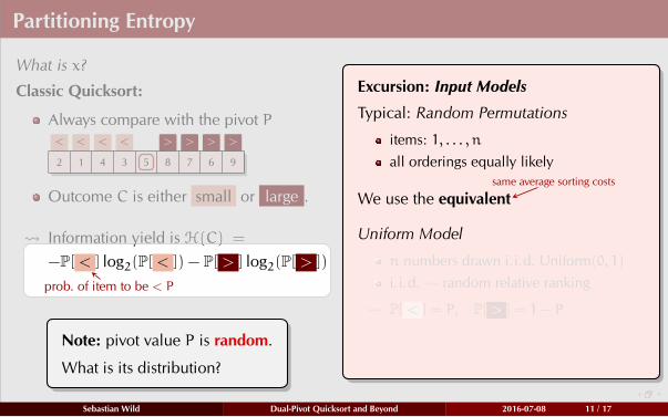
Partitioning Entropy
What is x?
Classic Quicksort:
Always compare with the pivot P
< < < < > > > >
2 1 4 3 5 8 7 6 9
Outcome C is either small or large .
Information yield is H(C) =
−P[ < ]
prob. of item to be < P
log2(P[ < ]) − P[ > ] log2(P[ > ])
Note: pivot value P is random.
What is its distribution?
Excursion: Input Models
Typical: Random Permutations
items: 1, . . . , n
all orderings equally likely
We use the equivalent
Uniform Model
n numbers drawn i. i.d. Uniform(0, 1)
i. i.d. random relative ranking
P[ < ] = P, P[ > ] = 1− P
same average sorting costs
Sebastian Wild Dual-Pivot Quicksort and Beyond 2016-07-08 11 / 17
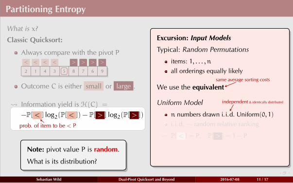
Partitioning Entropy
What is x?
Classic Quicksort:
Always compare with the pivot P
< < < < > > > >
2 1 4 3 5 8 7 6 9
Outcome C is either small or large .
Information yield is H(C) =
−P[ < ]
prob. of item to be < P
log2(P[ < ]) − P[ > ] log2(P[ > ])
Note: pivot value P is random.
What is its distribution?
Excursion: Input Models
Typical: Random Permutations
items: 1, . . . , n
all orderings equally likely
We use the equivalent
Uniform Model
n numbers drawn i. i.d. Uniform(0, 1)
i. i.d. random relative ranking
P[ < ] = P, P[ > ] = 1− P
same average sorting costs
independent & identically distributed
Sebastian Wild Dual-Pivot Quicksort and Beyond 2016-07-08 11 / 17
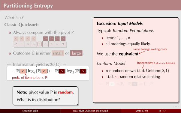
Partitioning Entropy
What is x?
Classic Quicksort:
Always compare with the pivot P
< < < < > > > >
2 1 4 3 5 8 7 6 9
Outcome C is either small or large .
Information yield is H(C) =
−P[ < ]
prob. of item to be < P
log2(P[ < ]) − P[ > ] log2(P[ > ])
Note: pivot value P is random.
What is its distribution?
Excursion: Input Models
Typical: Random Permutations
items: 1, . . . , n
all orderings equally likely
We use the equivalent
Uniform Model
n numbers drawn i. i.d. Uniform(0, 1)
i. i.d. random relative ranking
P[ < ] = P, P[ > ] = 1− P
same average sorting costs
independent & identically distributed
Sebastian Wild Dual-Pivot Quicksort and Beyond 2016-07-08 11 / 17
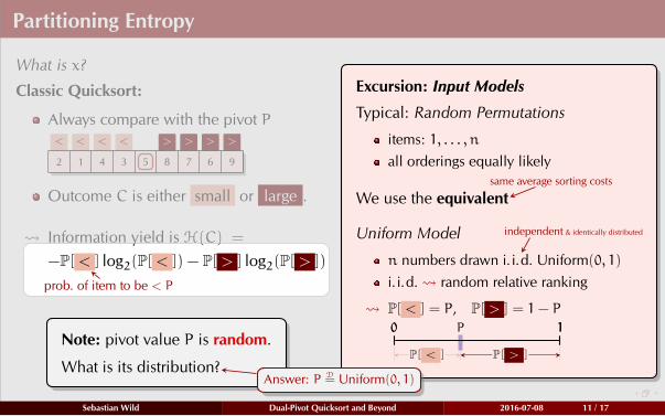
Partitioning Entropy
What is x?
Classic Quicksort:
Always compare with the pivot P
< < < < > > > >
2 1 4 3 5 8 7 6 9
Outcome C is either small or large .
Information yield is H(C) =
−P[ < ]
prob. of item to be < P
log2(P[ < ]) − P[ > ] log2(P[ > ])
Note: pivot value P is random.
What is its distribution?
Excursion: Input Models
Typical: Random Permutations
items: 1, . . . , n
all orderings equally likely
We use the equivalent
Uniform Model
n numbers drawn i. i.d. Uniform(0, 1)
i. i.d. random relative ranking
P[ < ] = P, P[ > ] = 1− P
0 1P0 1
P[ < ] P[ > ]
same average sorting costs
independent & identically distributed
Answer: PD= Uniform(0, 1)
Sebastian Wild Dual-Pivot Quicksort and Beyond 2016-07-08 11 / 17

Partitioning Entropy
What is x?
Classic Quicksort:
Always compare with the pivot P
< < < < > > > >
2 1 4 3 5 8 7 6 9
Outcome C is either small or large .
Information yield is H(C) =
−P[ < ] log2(P[ < ]) − P[ > ] log2(P[ > ])
Excursion: Input Models
Typical: Random Permutations
items: 1, . . . , n
all orderings equally likely
We use the equivalent
Uniform Model
n numbers drawn i. i.d. Uniform(0, 1)
i. i.d. random relative ranking
P[ < ] = P, P[ > ] = 1− P
0 1P0 1
P[ < ] P[ > ]
same average sorting costs
independent & identically distributed
E
Average over P
[H(C)] = E
[−P log2(P) − (1− P) log2(1− P)
]
= −2
∫1
0
z log2(z)dz
=1
2log2(e) ≈ 0.721348
Sebastian Wild Dual-Pivot Quicksort and Beyond 2016-07-08 11 / 17
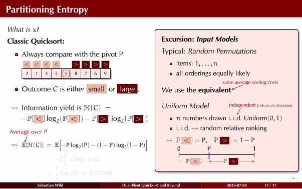
Partitioning Entropy
What is x?
Classic Quicksort:
Always compare with the pivot P
< < < < > > > >
2 1 4 3 5 8 7 6 9
Outcome C is either small or large .
Information yield is H(C) =
−P[ < ] log2(P[ < ]) − P[ > ] log2(P[ > ])
Excursion: Input Models
Typical: Random Permutations
items: 1, . . . , n
all orderings equally likely
We use the equivalent
Uniform Model
n numbers drawn i. i.d. Uniform(0, 1)
i. i.d. random relative ranking
P[ < ] = P, P[ > ] = 1− P
0 1P0 1
P[ < ] P[ > ]
same average sorting costs
independent & identically distributed
E
Average over P
[H(C)] = E
[−P log2(P) − (1− P) log2(1− P)
]
= −2
∫1
0
z log2(z)dz
=1
2log2(e) ≈ 0.721348
Sebastian Wild Dual-Pivot Quicksort and Beyond 2016-07-08 11 / 17
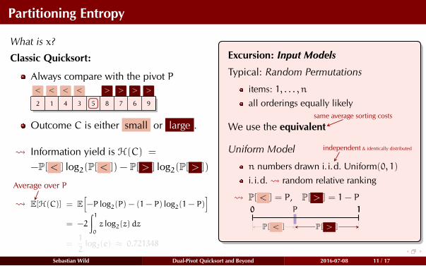
Partitioning Entropy
What is x?
Classic Quicksort:
Always compare with the pivot P
< < < < > > > >
2 1 4 3 5 8 7 6 9
Outcome C is either small or large .
Information yield is H(C) =
−P[ < ] log2(P[ < ]) − P[ > ] log2(P[ > ])
Excursion: Input Models
Typical: Random Permutations
items: 1, . . . , n
all orderings equally likely
We use the equivalent
Uniform Model
n numbers drawn i. i.d. Uniform(0, 1)
i. i.d. random relative ranking
P[ < ] = P, P[ > ] = 1− P
0 1P0 1
P[ < ] P[ > ]
same average sorting costs
independent & identically distributed
E
Average over P
[H(C)] = E
[−P log2(P) − (1− P) log2(1− P)
]
= −2
∫1
0
z log2(z)dz
=1
2log2(e) ≈ 0.721348
Sebastian Wild Dual-Pivot Quicksort and Beyond 2016-07-08 11 / 17
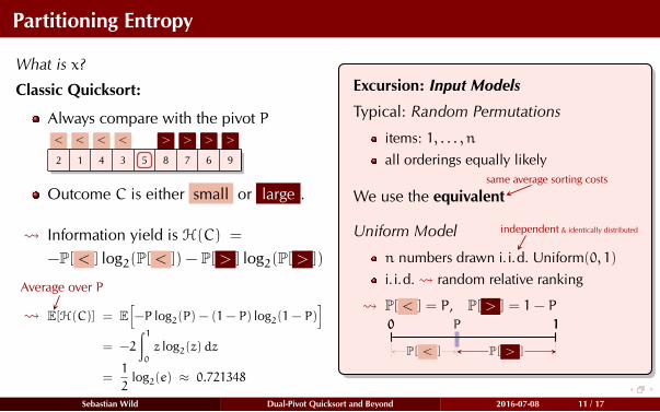
Partitioning Entropy
What is x?
Classic Quicksort:
Always compare with the pivot P
< < < < > > > >
2 1 4 3 5 8 7 6 9
Outcome C is either small or large .
Information yield is H(C) =
−P[ < ] log2(P[ < ]) − P[ > ] log2(P[ > ])
Excursion: Input Models
Typical: Random Permutations
items: 1, . . . , n
all orderings equally likely
We use the equivalent
Uniform Model
n numbers drawn i. i.d. Uniform(0, 1)
i. i.d. random relative ranking
P[ < ] = P, P[ > ] = 1− P
0 1P0 1
P[ < ] P[ > ]
same average sorting costs
independent & identically distributed
E
Average over P
[H(C)] = E
[−P log2(P) − (1− P) log2(1− P)
]
= −2
∫1
0
z log2(z)dz
=1
2log2(e) ≈ 0.721348
Sebastian Wild Dual-Pivot Quicksort and Beyond 2016-07-08 11 / 17
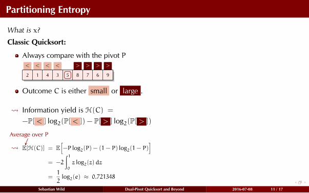
Partitioning Entropy
What is x?
Classic Quicksort:
Always compare with the pivot P
< < < < > > > >
2 1 4 3 5 8 7 6 9
Outcome C is either small or large .
Information yield is H(C) =
−P[ < ] log2(P[ < ]) − P[ > ] log2(P[ > ])
E
Average over P
[H(C)] = E
[−P log2(P) − (1− P) log2(1− P)
]
= −2
∫1
0
z log2(z)dz
=1
2log2(e) ≈ 0.721348
Sebastian Wild Dual-Pivot Quicksort and Beyond 2016-07-08 11 / 17
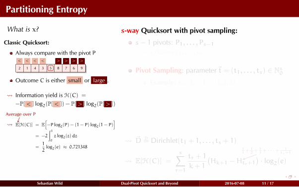
Partitioning Entropy
What is x?
Classic Quicksort:
Always compare with the pivot P
< < < < > > > >
2 1 4 3 5 8 7 6 9
Outcome C is either small or large .
Information yield is H(C) =
−P[ < ] log2(P[ < ]) − P[ > ] log2(P[ > ])
E
Average over P
[H(C)] = E
[−P log2(P) − (1− P) log2(1− P)
]
= −2
∫1
0
z log2(z)dz
=1
2log2(e) ≈ 0.721348
s-way Quicksort with pivot sampling:
s− 1 pivots: P1, . . . , Ps−1
s classes c1, . . . , cs
Pivot Sampling: parameter~t = (t1, . . . , ts) ∈ Ns0
Example: s = 3, ~t = (1, 2, 3)
choose pivots from k = 8 sample items
0 10 1
~DD= Dirichlet(t1 + 1, . . . , ts + 1)
E[H(C)] =
s∑
r=1
tr + 1
k+ 1
(Hk+1 −H
1
1+1
2+1
3+ · · ·+ 1
tr+1
tr+1
)· log2(e)
Sebastian Wild Dual-Pivot Quicksort and Beyond 2016-07-08 11 / 17
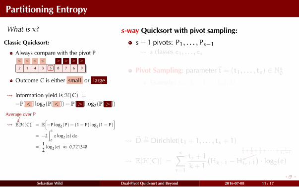
Partitioning Entropy
What is x?
Classic Quicksort:
Always compare with the pivot P
< < < < > > > >
2 1 4 3 5 8 7 6 9
Outcome C is either small or large .
Information yield is H(C) =
−P[ < ] log2(P[ < ]) − P[ > ] log2(P[ > ])
E
Average over P
[H(C)] = E
[−P log2(P) − (1− P) log2(1− P)
]
= −2
∫1
0
z log2(z)dz
=1
2log2(e) ≈ 0.721348
s-way Quicksort with pivot sampling:
s− 1 pivots: P1, . . . , Ps−1
s classes c1, . . . , cs
Pivot Sampling: parameter~t = (t1, . . . , ts) ∈ Ns0
Example: s = 3, ~t = (1, 2, 3)
choose pivots from k = 8 sample items
0 10 1
~DD= Dirichlet(t1 + 1, . . . , ts + 1)
E[H(C)] =
s∑
r=1
tr + 1
k+ 1
(Hk+1 −H
1
1+1
2+1
3+ · · ·+ 1
tr+1
tr+1
)· log2(e)
Sebastian Wild Dual-Pivot Quicksort and Beyond 2016-07-08 11 / 17
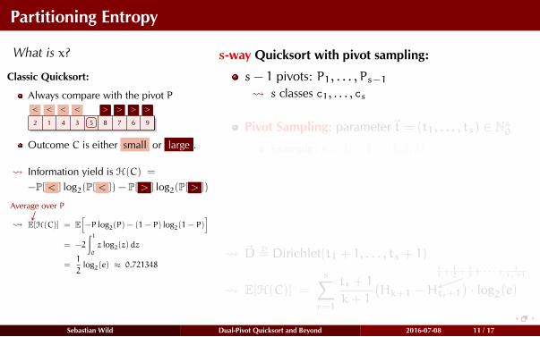
Partitioning Entropy
What is x?
Classic Quicksort:
Always compare with the pivot P
< < < < > > > >
2 1 4 3 5 8 7 6 9
Outcome C is either small or large .
Information yield is H(C) =
−P[ < ] log2(P[ < ]) − P[ > ] log2(P[ > ])
E
Average over P
[H(C)] = E
[−P log2(P) − (1− P) log2(1− P)
]
= −2
∫1
0
z log2(z)dz
=1
2log2(e) ≈ 0.721348
s-way Quicksort with pivot sampling:
s− 1 pivots: P1, . . . , Ps−1
s classes c1, . . . , cs
Pivot Sampling: parameter~t = (t1, . . . , ts) ∈ Ns0
Example: s = 3, ~t = (1, 2, 3)
choose pivots from k = 8 sample items
0 10 1
~DD= Dirichlet(t1 + 1, . . . , ts + 1)
E[H(C)] =
s∑
r=1
tr + 1
k+ 1
(Hk+1 −H
1
1+1
2+1
3+ · · ·+ 1
tr+1
tr+1
)· log2(e)
Sebastian Wild Dual-Pivot Quicksort and Beyond 2016-07-08 11 / 17
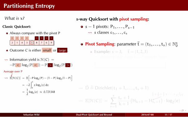
Partitioning Entropy
What is x?
Classic Quicksort:
Always compare with the pivot P
< < < < > > > >
2 1 4 3 5 8 7 6 9
Outcome C is either small or large .
Information yield is H(C) =
−P[ < ] log2(P[ < ]) − P[ > ] log2(P[ > ])
E
Average over P
[H(C)] = E
[−P log2(P) − (1− P) log2(1− P)
]
= −2
∫1
0
z log2(z)dz
=1
2log2(e) ≈ 0.721348
s-way Quicksort with pivot sampling:
s− 1 pivots: P1, . . . , Ps−1
s classes c1, . . . , cs
Pivot Sampling: parameter~t = (t1, . . . , ts) ∈ Ns0
Example: s = 3, ~t = (1, 2, 3)
choose pivots from k = 8 sample items
0 10 1
~DD= Dirichlet(t1 + 1, . . . , ts + 1)
E[H(C)] =
s∑
r=1
tr + 1
k+ 1
(Hk+1 −H
1
1+1
2+1
3+ · · ·+ 1
tr+1
tr+1
)· log2(e)
Sebastian Wild Dual-Pivot Quicksort and Beyond 2016-07-08 11 / 17
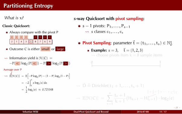
Partitioning Entropy
What is x?
Classic Quicksort:
Always compare with the pivot P
< < < < > > > >
2 1 4 3 5 8 7 6 9
Outcome C is either small or large .
Information yield is H(C) =
−P[ < ] log2(P[ < ]) − P[ > ] log2(P[ > ])
E
Average over P
[H(C)] = E
[−P log2(P) − (1− P) log2(1− P)
]
= −2
∫1
0
z log2(z)dz
=1
2log2(e) ≈ 0.721348
s-way Quicksort with pivot sampling:
s− 1 pivots: P1, . . . , Ps−1
s classes c1, . . . , cs
Pivot Sampling: parameter~t = (t1, . . . , ts) ∈ Ns0
Example: s = 3, ~t = (1, 2, 3)
choose pivots from k = 8 sample items
0 10 1
~DD= Dirichlet(t1 + 1, . . . , ts + 1)
E[H(C)] =
s∑
r=1
tr + 1
k+ 1
(Hk+1 −H
1
1+1
2+1
3+ · · ·+ 1
tr+1
tr+1
)· log2(e)
Sebastian Wild Dual-Pivot Quicksort and Beyond 2016-07-08 11 / 17
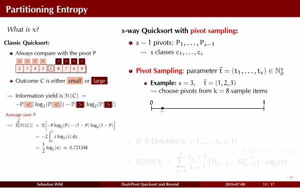
Partitioning Entropy
What is x?
Classic Quicksort:
Always compare with the pivot P
< < < < > > > >
2 1 4 3 5 8 7 6 9
Outcome C is either small or large .
Information yield is H(C) =
−P[ < ] log2(P[ < ]) − P[ > ] log2(P[ > ])
E
Average over P
[H(C)] = E
[−P log2(P) − (1− P) log2(1− P)
]
= −2
∫1
0
z log2(z)dz
=1
2log2(e) ≈ 0.721348
s-way Quicksort with pivot sampling:
s− 1 pivots: P1, . . . , Ps−1
s classes c1, . . . , cs
Pivot Sampling: parameter~t = (t1, . . . , ts) ∈ Ns0
Example: s = 3, ~t = (1, 2, 3)
choose pivots from k = 8 sample items
0 1
U1
0 1
~DD= Dirichlet(t1 + 1, . . . , ts + 1)
E[H(C)] =
s∑
r=1
tr + 1
k+ 1
(Hk+1 −H
1
1+1
2+1
3+ · · ·+ 1
tr+1
tr+1
)· log2(e)
Sebastian Wild Dual-Pivot Quicksort and Beyond 2016-07-08 11 / 17

Partitioning Entropy
What is x?
Classic Quicksort:
Always compare with the pivot P
< < < < > > > >
2 1 4 3 5 8 7 6 9
Outcome C is either small or large .
Information yield is H(C) =
−P[ < ] log2(P[ < ]) − P[ > ] log2(P[ > ])
E
Average over P
[H(C)] = E
[−P log2(P) − (1− P) log2(1− P)
]
= −2
∫1
0
z log2(z)dz
=1
2log2(e) ≈ 0.721348
s-way Quicksort with pivot sampling:
s− 1 pivots: P1, . . . , Ps−1
s classes c1, . . . , cs
Pivot Sampling: parameter~t = (t1, . . . , ts) ∈ Ns0
Example: s = 3, ~t = (1, 2, 3)
choose pivots from k = 8 sample items
0 1
U1 U2
0 1
~DD= Dirichlet(t1 + 1, . . . , ts + 1)
E[H(C)] =
s∑
r=1
tr + 1
k+ 1
(Hk+1 −H
1
1+1
2+1
3+ · · ·+ 1
tr+1
tr+1
)· log2(e)
Sebastian Wild Dual-Pivot Quicksort and Beyond 2016-07-08 11 / 17

Partitioning Entropy
What is x?
Classic Quicksort:
Always compare with the pivot P
< < < < > > > >
2 1 4 3 5 8 7 6 9
Outcome C is either small or large .
Information yield is H(C) =
−P[ < ] log2(P[ < ]) − P[ > ] log2(P[ > ])
E
Average over P
[H(C)] = E
[−P log2(P) − (1− P) log2(1− P)
]
= −2
∫1
0
z log2(z)dz
=1
2log2(e) ≈ 0.721348
s-way Quicksort with pivot sampling:
s− 1 pivots: P1, . . . , Ps−1
s classes c1, . . . , cs
Pivot Sampling: parameter~t = (t1, . . . , ts) ∈ Ns0
Example: s = 3, ~t = (1, 2, 3)
choose pivots from k = 8 sample items
0 1
U1 U2U3
0 1
~DD= Dirichlet(t1 + 1, . . . , ts + 1)
E[H(C)] =
s∑
r=1
tr + 1
k+ 1
(Hk+1 −H
1
1+1
2+1
3+ · · ·+ 1
tr+1
tr+1
)· log2(e)
Sebastian Wild Dual-Pivot Quicksort and Beyond 2016-07-08 11 / 17

Partitioning Entropy
What is x?
Classic Quicksort:
Always compare with the pivot P
< < < < > > > >
2 1 4 3 5 8 7 6 9
Outcome C is either small or large .
Information yield is H(C) =
−P[ < ] log2(P[ < ]) − P[ > ] log2(P[ > ])
E
Average over P
[H(C)] = E
[−P log2(P) − (1− P) log2(1− P)
]
= −2
∫1
0
z log2(z)dz
=1
2log2(e) ≈ 0.721348
s-way Quicksort with pivot sampling:
s− 1 pivots: P1, . . . , Ps−1
s classes c1, . . . , cs
Pivot Sampling: parameter~t = (t1, . . . , ts) ∈ Ns0
Example: s = 3, ~t = (1, 2, 3)
choose pivots from k = 8 sample items
0 1
U1 U2U3 U4
0 1
~DD= Dirichlet(t1 + 1, . . . , ts + 1)
E[H(C)] =
s∑
r=1
tr + 1
k+ 1
(Hk+1 −H
1
1+1
2+1
3+ · · ·+ 1
tr+1
tr+1
)· log2(e)
Sebastian Wild Dual-Pivot Quicksort and Beyond 2016-07-08 11 / 17

Partitioning Entropy
What is x?
Classic Quicksort:
Always compare with the pivot P
< < < < > > > >
2 1 4 3 5 8 7 6 9
Outcome C is either small or large .
Information yield is H(C) =
−P[ < ] log2(P[ < ]) − P[ > ] log2(P[ > ])
E
Average over P
[H(C)] = E
[−P log2(P) − (1− P) log2(1− P)
]
= −2
∫1
0
z log2(z)dz
=1
2log2(e) ≈ 0.721348
s-way Quicksort with pivot sampling:
s− 1 pivots: P1, . . . , Ps−1
s classes c1, . . . , cs
Pivot Sampling: parameter~t = (t1, . . . , ts) ∈ Ns0
Example: s = 3, ~t = (1, 2, 3)
choose pivots from k = 8 sample items
0 1
U1 U2U3 U4U5
0 1
~DD= Dirichlet(t1 + 1, . . . , ts + 1)
E[H(C)] =
s∑
r=1
tr + 1
k+ 1
(Hk+1 −H
1
1+1
2+1
3+ · · ·+ 1
tr+1
tr+1
)· log2(e)
Sebastian Wild Dual-Pivot Quicksort and Beyond 2016-07-08 11 / 17

Partitioning Entropy
What is x?
Classic Quicksort:
Always compare with the pivot P
< < < < > > > >
2 1 4 3 5 8 7 6 9
Outcome C is either small or large .
Information yield is H(C) =
−P[ < ] log2(P[ < ]) − P[ > ] log2(P[ > ])
E
Average over P
[H(C)] = E
[−P log2(P) − (1− P) log2(1− P)
]
= −2
∫1
0
z log2(z)dz
=1
2log2(e) ≈ 0.721348
s-way Quicksort with pivot sampling:
s− 1 pivots: P1, . . . , Ps−1
s classes c1, . . . , cs
Pivot Sampling: parameter~t = (t1, . . . , ts) ∈ Ns0
Example: s = 3, ~t = (1, 2, 3)
choose pivots from k = 8 sample items
0 1
U1 U2U3 U4U5 U6
0 1
~DD= Dirichlet(t1 + 1, . . . , ts + 1)
E[H(C)] =
s∑
r=1
tr + 1
k+ 1
(Hk+1 −H
1
1+1
2+1
3+ · · ·+ 1
tr+1
tr+1
)· log2(e)
Sebastian Wild Dual-Pivot Quicksort and Beyond 2016-07-08 11 / 17

Partitioning Entropy
What is x?
Classic Quicksort:
Always compare with the pivot P
< < < < > > > >
2 1 4 3 5 8 7 6 9
Outcome C is either small or large .
Information yield is H(C) =
−P[ < ] log2(P[ < ]) − P[ > ] log2(P[ > ])
E
Average over P
[H(C)] = E
[−P log2(P) − (1− P) log2(1− P)
]
= −2
∫1
0
z log2(z)dz
=1
2log2(e) ≈ 0.721348
s-way Quicksort with pivot sampling:
s− 1 pivots: P1, . . . , Ps−1
s classes c1, . . . , cs
Pivot Sampling: parameter~t = (t1, . . . , ts) ∈ Ns0
Example: s = 3, ~t = (1, 2, 3)
choose pivots from k = 8 sample items
0 1
U1 U2U3 U4U5 U6 U7
0 1
~DD= Dirichlet(t1 + 1, . . . , ts + 1)
E[H(C)] =
s∑
r=1
tr + 1
k+ 1
(Hk+1 −H
1
1+1
2+1
3+ · · ·+ 1
tr+1
tr+1
)· log2(e)
Sebastian Wild Dual-Pivot Quicksort and Beyond 2016-07-08 11 / 17

Partitioning Entropy
What is x?
Classic Quicksort:
Always compare with the pivot P
< < < < > > > >
2 1 4 3 5 8 7 6 9
Outcome C is either small or large .
Information yield is H(C) =
−P[ < ] log2(P[ < ]) − P[ > ] log2(P[ > ])
E
Average over P
[H(C)] = E
[−P log2(P) − (1− P) log2(1− P)
]
= −2
∫1
0
z log2(z)dz
=1
2log2(e) ≈ 0.721348
s-way Quicksort with pivot sampling:
s− 1 pivots: P1, . . . , Ps−1
s classes c1, . . . , cs
Pivot Sampling: parameter~t = (t1, . . . , ts) ∈ Ns0
Example: s = 3, ~t = (1, 2, 3)
choose pivots from k = 8 sample items
0 1
U1 U2U3 U4U5 U6 U7U8
0 1
~DD= Dirichlet(t1 + 1, . . . , ts + 1)
E[H(C)] =
s∑
r=1
tr + 1
k+ 1
(Hk+1 −H
1
1+1
2+1
3+ · · ·+ 1
tr+1
tr+1
)· log2(e)
Sebastian Wild Dual-Pivot Quicksort and Beyond 2016-07-08 11 / 17
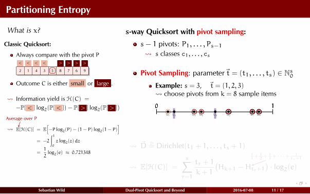
Partitioning Entropy
What is x?
Classic Quicksort:
Always compare with the pivot P
< < < < > > > >
2 1 4 3 5 8 7 6 9
Outcome C is either small or large .
Information yield is H(C) =
−P[ < ] log2(P[ < ]) − P[ > ] log2(P[ > ])
E
Average over P
[H(C)] = E
[−P log2(P) − (1− P) log2(1− P)
]
= −2
∫1
0
z log2(z)dz
=1
2log2(e) ≈ 0.721348
s-way Quicksort with pivot sampling:
s− 1 pivots: P1, . . . , Ps−1
s classes c1, . . . , cs
Pivot Sampling: parameter~t = (t1, . . . , ts) ∈ Ns0
Example: s = 3, ~t = (1, 2, 3)
choose pivots from k = 8 sample items
0 1
U1 U2U3 U4U5 U6 U7U8
0 1
~DD= Dirichlet(t1 + 1, . . . , ts + 1)
E[H(C)] =
s∑
r=1
tr + 1
k+ 1
(Hk+1 −H
1
1+1
2+1
3+ · · ·+ 1
tr+1
tr+1
)· log2(e)
Sebastian Wild Dual-Pivot Quicksort and Beyond 2016-07-08 11 / 17

Partitioning Entropy
What is x?
Classic Quicksort:
Always compare with the pivot P
< < < < > > > >
2 1 4 3 5 8 7 6 9
Outcome C is either small or large .
Information yield is H(C) =
−P[ < ] log2(P[ < ]) − P[ > ] log2(P[ > ])
E
Average over P
[H(C)] = E
[−P log2(P) − (1− P) log2(1− P)
]
= −2
∫1
0
z log2(z)dz
=1
2log2(e) ≈ 0.721348
s-way Quicksort with pivot sampling:
s− 1 pivots: P1, . . . , Ps−1
s classes c1, . . . , cs
Pivot Sampling: parameter~t = (t1, . . . , ts) ∈ Ns0
Example: s = 3, ~t = (1, 2, 3)
choose pivots from k = 8 sample items
0 1
U1 U2U3 U4U5 U6 U7U8
P1 P20 1
~DD= Dirichlet(t1 + 1, . . . , ts + 1)
E[H(C)] =
s∑
r=1
tr + 1
k+ 1
(Hk+1 −H
1
1+1
2+1
3+ · · ·+ 1
tr+1
tr+1
)· log2(e)
Sebastian Wild Dual-Pivot Quicksort and Beyond 2016-07-08 11 / 17
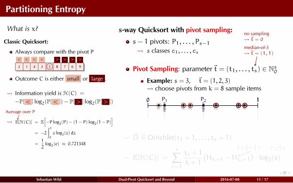
Partitioning Entropy
What is x?
Classic Quicksort:
Always compare with the pivot P
< < < < > > > >
2 1 4 3 5 8 7 6 9
Outcome C is either small or large .
Information yield is H(C) =
−P[ < ] log2(P[ < ]) − P[ > ] log2(P[ > ])
E
Average over P
[H(C)] = E
[−P log2(P) − (1− P) log2(1− P)
]
= −2
∫1
0
z log2(z)dz
=1
2log2(e) ≈ 0.721348
s-way Quicksort with pivot sampling:
s− 1 pivots: P1, . . . , Ps−1
s classes c1, . . . , cs
Pivot Sampling: parameter~t = (t1, . . . , ts
no sampling
~t = 0
median-of-3
~t = (1,1)
) ∈ Ns0
Example: s = 3, ~t = (1, 2, 3)
choose pivots from k = 8 sample items
0 1
U1 U2U3 U4U5 U6 U7U8
P1 P20 1
~DD= Dirichlet(t1 + 1, . . . , ts + 1)
E[H(C)] =
s∑
r=1
tr + 1
k+ 1
(Hk+1 −H
1
1+1
2+1
3+ · · ·+ 1
tr+1
tr+1
)· log2(e)
Sebastian Wild Dual-Pivot Quicksort and Beyond 2016-07-08 11 / 17
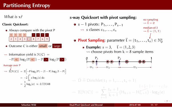
Partitioning Entropy
What is x?
Classic Quicksort:
Always compare with the pivot P
< < < < > > > >
2 1 4 3 5 8 7 6 9
Outcome C is either small or large .
Information yield is H(C) =
−P[ < ] log2(P[ < ]) − P[ > ] log2(P[ > ])
E
Average over P
[H(C)] = E
[−P log2(P) − (1− P) log2(1− P)
]
= −2
∫1
0
z log2(z)dz
=1
2log2(e) ≈ 0.721348
s-way Quicksort with pivot sampling:
s− 1 pivots: P1, . . . , Ps−1
s classes c1, . . . , cs
Pivot Sampling: parameter~t = (t1, . . . , ts
no sampling
~t = 0
median-of-3
~t = (1,1)
) ∈ Ns0
Example: s = 3, ~t = (1, 2, 3)
choose pivots from k = 8 sample items
0 1
U1 U2U3 U4U5 U6 U7U8
P1 P20 1
D1 D2 D3
~DD= Dirichlet(t1 + 1, . . . , ts + 1)
E[H(C)] =
s∑
r=1
tr + 1
k+ 1
(Hk+1 −H
1
1+1
2+1
3+ · · ·+ 1
tr+1
tr+1
)· log2(e)
Sebastian Wild Dual-Pivot Quicksort and Beyond 2016-07-08 11 / 17
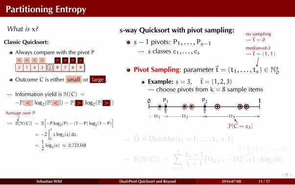
Partitioning Entropy
What is x?
Classic Quicksort:
Always compare with the pivot P
< < < < > > > >
2 1 4 3 5 8 7 6 9
Outcome C is either small or large .
Information yield is H(C) =
−P[ < ] log2(P[ < ]) − P[ > ] log2(P[ > ])
E
Average over P
[H(C)] = E
[−P log2(P) − (1− P) log2(1− P)
]
= −2
∫1
0
z log2(z)dz
=1
2log2(e) ≈ 0.721348
s-way Quicksort with pivot sampling:
s− 1 pivots: P1, . . . , Ps−1
s classes c1, . . . , cs
Pivot Sampling: parameter~t = (t1, . . . , ts
no sampling
~t = 0
median-of-3
~t = (1,1)
) ∈ Ns0
Example: s = 3, ~t = (1, 2, 3)
choose pivots from k = 8 sample items
0 1
U1 U2U3 U4U5 U6 U7U8
P1 P20 1
D1 D2 D3
P[C = c3]
~DD= Dirichlet(t1 + 1, . . . , ts + 1)
E[H(C)] =
s∑
r=1
tr + 1
k+ 1
(Hk+1 −H
1
1+1
2+1
3+ · · ·+ 1
tr+1
tr+1
)· log2(e)
Sebastian Wild Dual-Pivot Quicksort and Beyond 2016-07-08 11 / 17
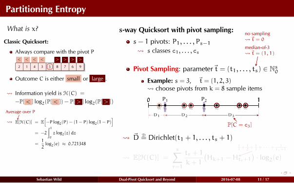
Partitioning Entropy
What is x?
Classic Quicksort:
Always compare with the pivot P
< < < < > > > >
2 1 4 3 5 8 7 6 9
Outcome C is either small or large .
Information yield is H(C) =
−P[ < ] log2(P[ < ]) − P[ > ] log2(P[ > ])
E
Average over P
[H(C)] = E
[−P log2(P) − (1− P) log2(1− P)
]
= −2
∫1
0
z log2(z)dz
=1
2log2(e) ≈ 0.721348
s-way Quicksort with pivot sampling:
s− 1 pivots: P1, . . . , Ps−1
s classes c1, . . . , cs
Pivot Sampling: parameter~t = (t1, . . . , ts
no sampling
~t = 0
median-of-3
~t = (1,1)
) ∈ Ns0
Example: s = 3, ~t = (1, 2, 3)
choose pivots from k = 8 sample items
0 1
U1 U2U3 U4U5 U6 U7U8
P1 P20 1
D1 D2 D3
P[C = c3]
~DD= Dirichlet(t1 + 1, . . . , ts + 1)
E[H(C)] =
s∑
r=1
tr + 1
k+ 1
(Hk+1 −H
1
1+1
2+1
3+ · · ·+ 1
tr+1
tr+1
)· log2(e)
Sebastian Wild Dual-Pivot Quicksort and Beyond 2016-07-08 11 / 17
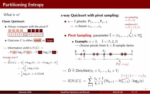
Partitioning Entropy
What is x?
Classic Quicksort:
Always compare with the pivot P
< < < < > > > >
2 1 4 3 5 8 7 6 9
Outcome C is either small or large .
Information yield is H(C) =
−P[ < ] log2(P[ < ]) − P[ > ] log2(P[ > ])
E
Average over P
[H(C)] = E
[−P log2(P) − (1− P) log2(1− P)
]
= −2
∫1
0
z log2(z)dz
=1
2log2(e) ≈ 0.721348
s-way Quicksort with pivot sampling:
s− 1 pivots: P1, . . . , Ps−1
s classes c1, . . . , cs
Pivot Sampling: parameter~t = (t1, . . . , ts
no sampling
~t = 0
median-of-3
~t = (1,1)
) ∈ Ns0
Example: s = 3, ~t = (1, 2, 3)
choose pivots from k = 8 sample items
0 1
U1 U2U3 U4U5 U6 U7U8
P1 P20 1
D1 D2 D3
P[C = c3]
~DD= Dirichlet(t1 + 1, . . . , ts + 1)
E[H(C)] =
s∑
r=1
tr + 1
k+ 1
(Hk+1 −H
1
1+1
2+1
3+ · · ·+ 1
tr+1
tr+1
)· log2(e)
Sebastian Wild Dual-Pivot Quicksort and Beyond 2016-07-08 11 / 17
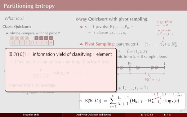
Partitioning Entropy
What is x?
Classic Quicksort:
Always compare with the pivot P
< < < < > > > >
2 1 4 3 5 8 7 6 9
Outcome C is either small or large .
Information yield is H(C) =
−P[ < ] log2(P[ < ]) − P[ > ] log2(P[ > ])
E
Average over P
[H(C)] = E
[−P log2(P) − (1− P) log2(1− P)
]
= −2
∫1
0
z log2(z)dz
=1
2log2(e) ≈ 0.721348
s-way Quicksort with pivot sampling:
s− 1 pivots: P1, . . . , Ps−1
s classes c1, . . . , cs
Pivot Sampling: parameter~t = (t1, . . . , ts
no sampling
~t = 0
median-of-3
~t = (1,1)
) ∈ Ns0
Example: s = 3, ~t = (1, 2, 3)
choose pivots from k = 8 sample items
0 1
U1 U2U3 U4U5 U6 U7U8
P1 P20 1
D1 D2 D3
P[C = c3]
~DD= Dirichlet(t1 + 1, . . . , ts + 1)
E[H(C)] =
s∑
r=1
tr + 1
k+ 1
(Hk+1 −H
1
1+1
2+1
3+ · · ·+ 1
tr+1
tr+1
)· log2(e)
E[H(C)] = information yield of classifying 1 element
If we need a comparisons for that, Quicksort uses
a
E[H(C)]· n log2(n) ± O(n)
comparisons on average.
Sebastian Wild Dual-Pivot Quicksort and Beyond 2016-07-08 11 / 17
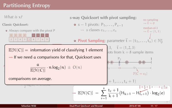
Partitioning Entropy
What is x?
Classic Quicksort:
Always compare with the pivot P
< < < < > > > >
2 1 4 3 5 8 7 6 9
Outcome C is either small or large .
Information yield is H(C) =
−P[ < ] log2(P[ < ]) − P[ > ] log2(P[ > ])
E
Average over P
[H(C)] = E
[−P log2(P) − (1− P) log2(1− P)
]
= −2
∫1
0
z log2(z)dz
=1
2log2(e) ≈ 0.721348
s-way Quicksort with pivot sampling:
s− 1 pivots: P1, . . . , Ps−1
s classes c1, . . . , cs
Pivot Sampling: parameter~t = (t1, . . . , ts
no sampling
~t = 0
median-of-3
~t = (1,1)
) ∈ Ns0
Example: s = 3, ~t = (1, 2, 3)
choose pivots from k = 8 sample items
0 1
U1 U2U3 U4U5 U6 U7U8
P1 P20 1
D1 D2 D3
P[C = c3]
~DD= Dirichlet(t1 + 1, . . . , ts + 1)
E[H(C)] =
s∑
r=1
tr + 1
k+ 1
(Hk+1 −H
1
1+1
2+1
3+ · · ·+ 1
tr+1
tr+1
)· log2(e)
E[H(C)] = information yield of classifying 1 element
If we need a comparisons for that, Quicksort uses
a
E[H(C)]· n log2(n) ± O(n)
comparisons on average.
Sebastian Wild Dual-Pivot Quicksort and Beyond 2016-07-08 11 / 17

Binary vs. Multiway Partitioning
Now, does multiway partitioning perform better? Let’s try an example.
4-way Quicksort
<
< >
>
< >
<P2
<P1
c1 c2
<P3
c3 c4
Need a = 2 comparisons to
classify 1 item.
2413
≈ 1.846
n ln(n) comparisons
(without sampling)
Classic Quicksort
2n ln(n) comparisons
(without sampling)
Sebastian Wild Dual-Pivot Quicksort and Beyond 2016-07-08 12 / 17
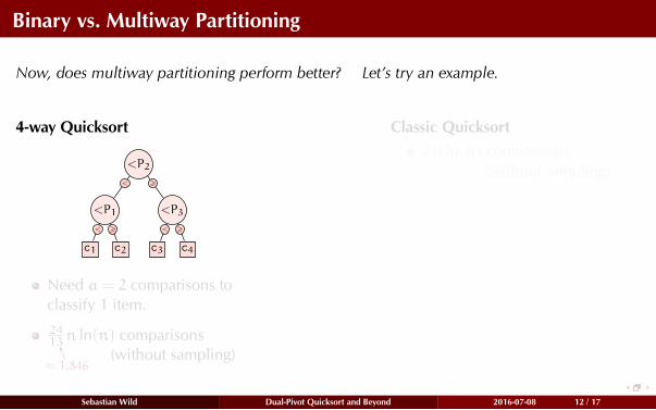
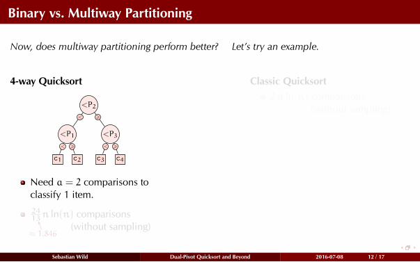
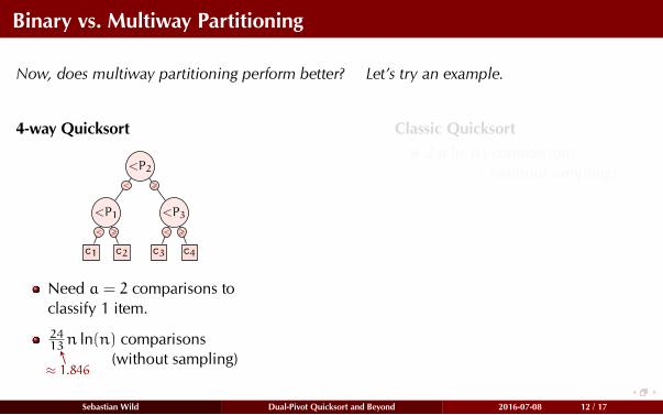
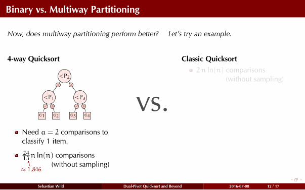
Binary vs. Multiway Partitioning
Now, does multiway partitioning perform better? Let’s try an example.
4-way Quicksort
<
< >
>
< >
<P2
<P1
c1 c2
<P3
c3 c4
Need a = 2 comparisons to
classify 1 item.
2413
≈ 1.846
n ln(n) comparisons
(without sampling)
vs.
Classic Quicksort
2n ln(n) comparisons
(without sampling)
Sebastian Wild Dual-Pivot Quicksort and Beyond 2016-07-08 12 / 17
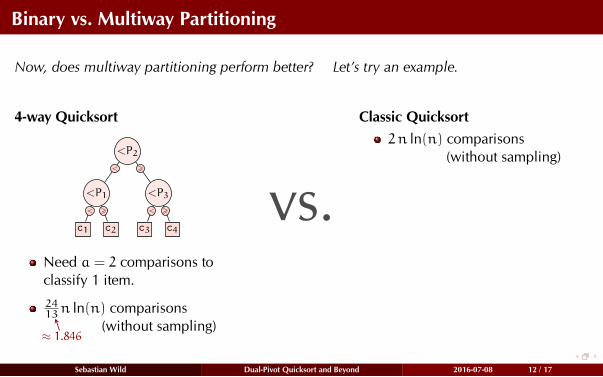
Binary vs. Multiway Partitioning
Now, does multiway partitioning perform better? Let’s try an example.
4-way Quicksort
<
< >
>
< >
<P2
<P1
c1 c2
<P3
c3 c4
Need a = 2 comparisons to
classify 1 item.
2413
≈ 1.846
n ln(n) comparisons
(without sampling)
vs.
Classic Quicksort
2n ln(n) comparisons
(without sampling)
Sebastian Wild Dual-Pivot Quicksort and Beyond 2016-07-08 12 / 17
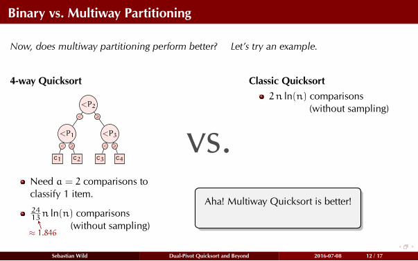
Binary vs. Multiway Partitioning
Now, does multiway partitioning perform better? Let’s try an example.
4-way Quicksort
<
< >
>
< >
<P2
<P1
c1 c2
<P3
c3 c4
Need a = 2 comparisons to
classify 1 item.
2413
≈ 1.846
n ln(n) comparisons
(without sampling)
vs.
Classic Quicksort
2n ln(n) comparisons
(without sampling)
Aha! Multiway Quicksort is better!
Sebastian Wild Dual-Pivot Quicksort and Beyond 2016-07-08 12 / 17
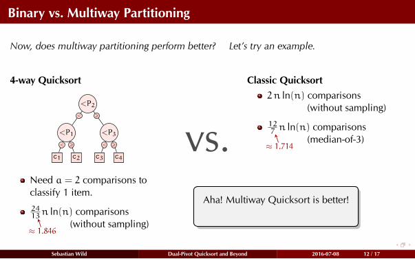
Binary vs. Multiway Partitioning
Now, does multiway partitioning perform better? Let’s try an example.
4-way Quicksort
<
< >
>
< >
<P2
<P1
c1 c2
<P3
c3 c4
Need a = 2 comparisons to
classify 1 item.
2413
≈ 1.846
n ln(n) comparisons
(without sampling)
vs.
Classic Quicksort
2n ln(n) comparisons
(without sampling)
Aha! Multiway Quicksort is better!
127
≈ 1.714
n ln(n) comparisons
(median-of-3)
Sebastian Wild Dual-Pivot Quicksort and Beyond 2016-07-08 12 / 17
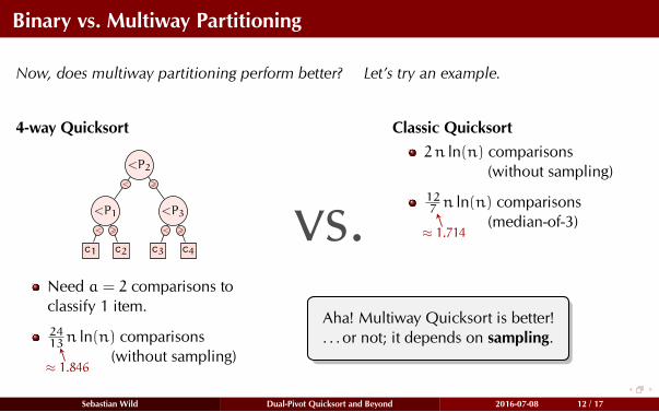
Binary vs. Multiway Partitioning
Now, does multiway partitioning perform better? Let’s try an example.
4-way Quicksort
<
< >
>
< >
<P2
<P1
c1 c2
<P3
c3 c4
Need a = 2 comparisons to
classify 1 item.
2413
≈ 1.846
n ln(n) comparisons
(without sampling)
vs.
Classic Quicksort
2n ln(n) comparisons
(without sampling)
Aha! Multiway Quicksort is better!
. . . or not; it depends on sampling.
127
≈ 1.714
n ln(n) comparisons
(median-of-3)
Sebastian Wild Dual-Pivot Quicksort and Beyond 2016-07-08 12 / 17
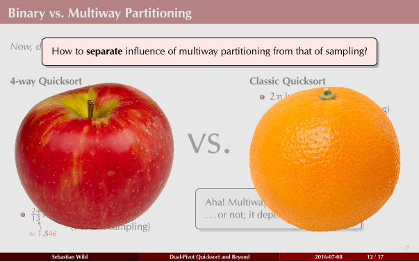
Binary vs. Multiway Partitioning
Now, does multiway partitioning perform better? Let’s try an example.
4-way Quicksort
<
< >
>
< >
<P2
<P1
c1 c2
<P3
c3 c4
Need a = 2 comparisons to
classify 1 item.
2413
≈ 1.846
n ln(n) comparisons
(without sampling)
vs.
Classic Quicksort
2n ln(n) comparisons
(without sampling)
Aha! Multiway Quicksort is better!
. . . or not; it depends on sampling.
127
≈ 1.714
n ln(n) comparisons
(median-of-3)
How to separate influence of multiway partitioning from that of sampling?
Sebastian Wild Dual-Pivot Quicksort and Beyond 2016-07-08 12 / 17
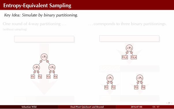
Entropy-Equivalent Sampling
Key Idea: Simulate by binary partitioning.
One round of 4-way partitioning . . .
(without sampling)
<
< >
>
< >
<P2
<P1
c1 c2
<P3
c3 c4
. . . corresponds to three binary partitionings.
< >
<P2
c1,2 c3,4
< >
<P1
c1 c2
< >
<P3
c3 c4
Sebastian Wild Dual-Pivot Quicksort and Beyond 2016-07-08 13 / 17
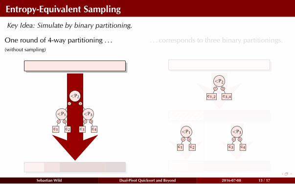
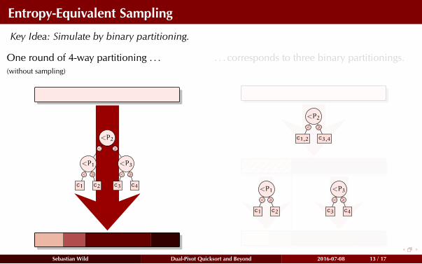
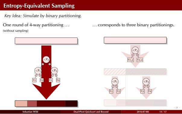
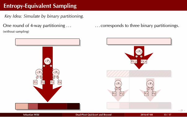
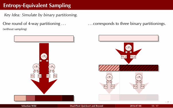
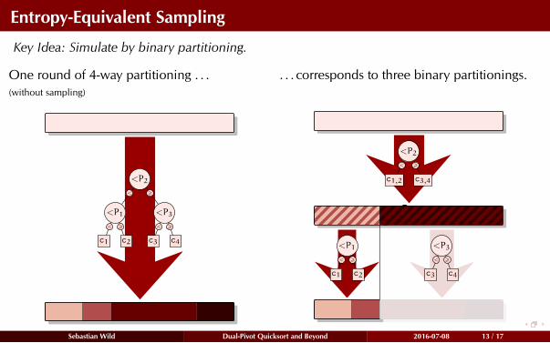
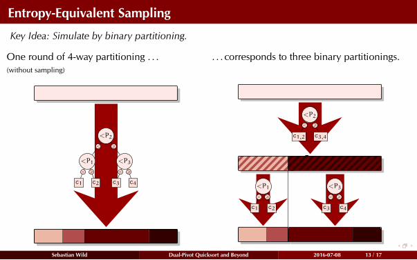
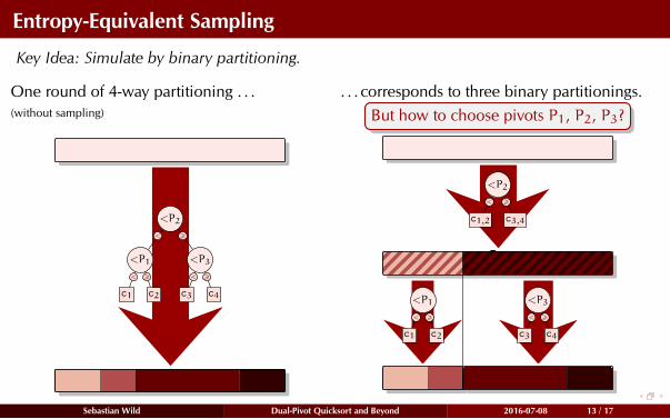
Entropy-Equivalent Sampling
Key Idea: Simulate by binary partitioning.
One round of 4-way partitioning . . .
(without sampling)
<
< >
>
< >
<P2
<P1
c1 c2
<P3
c3 c4
. . . corresponds to three binary partitionings.
< >
<P2
c1,2 c3,4
< >
<P1
c1 c2
< >
<P3
c3 c4
But how to choose pivots P1, P2, P3?
Sebastian Wild Dual-Pivot Quicksort and Beyond 2016-07-08 13 / 17
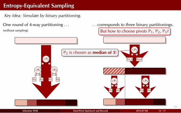
Entropy-Equivalent Sampling
Key Idea: Simulate by binary partitioning.
One round of 4-way partitioning . . .
(without sampling)
<
< >
>
< >
<P2
<P1
c1 c2
<P3
c3 c4
. . . corresponds to three binary partitionings.
< >
<P2
c1,2 c3,4
< >
<P1
c1 c2
< >
<P3
c3 c4
But how to choose pivots P1, P2, P3?
P2 is chosen as median of 3!
Sebastian Wild Dual-Pivot Quicksort and Beyond 2016-07-08 13 / 17
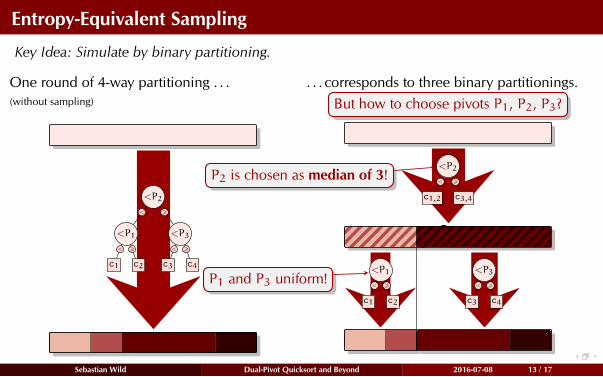
Entropy-Equivalent Sampling
Key Idea: Simulate by binary partitioning.
One round of 4-way partitioning . . .
(without sampling)
<
< >
>
< >
<P2
<P1
c1 c2
<P3
c3 c4
. . . corresponds to three binary partitionings.
< >
<P2
c1,2 c3,4
< >
<P1
c1 c2
< >
<P3
c3 c4
But how to choose pivots P1, P2, P3?
P2 is chosen as median of 3!
P1 and P3 uniform!
Sebastian Wild Dual-Pivot Quicksort and Beyond 2016-07-08 13 / 17
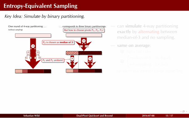
Entropy-Equivalent Sampling
Key Idea: Simulate by binary partitioning.
One round of 4-way partitioning . . .
(without sampling)
<
< >
>
< >
<P2
<P1
c1 c2
<P3
c3 c4
. . . corresponds to three binary partitionings.
< >
<P2
c1,2 c3,4
< >
<P1
c1 c2
< >
<P3
c3 c4
But how to choose pivots P1, P2, P3?
P2 is chosen as median of 3!
P1 and P3 uniform!
can simulate 4-way partitioning
exactly by alternating between
median-of-3 and no sampling.
same on average:1 flip a fair coin
2
{median-of-3 for heads
no sampling for tails
random-parameter pivot sampling
Sebastian Wild Dual-Pivot Quicksort and Beyond 2016-07-08 13 / 17
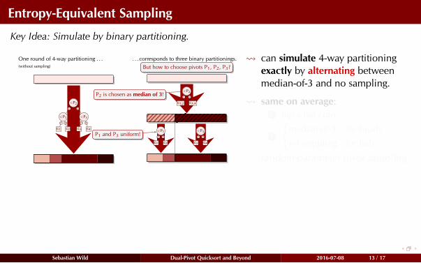
Entropy-Equivalent Sampling
Key Idea: Simulate by binary partitioning.
One round of 4-way partitioning . . .
(without sampling)
<
< >
>
< >
<P2
<P1
c1 c2
<P3
c3 c4
. . . corresponds to three binary partitionings.
< >
<P2
c1,2 c3,4
< >
<P1
c1 c2
< >
<P3
c3 c4
But how to choose pivots P1, P2, P3?
P2 is chosen as median of 3!
P1 and P3 uniform!
can simulate 4-way partitioning
exactly by alternating between
median-of-3 and no sampling.
same on average:1 flip a fair coin
2
{median-of-3 for heads
no sampling for tails
random-parameter pivot sampling
Sebastian Wild Dual-Pivot Quicksort and Beyond 2016-07-08 13 / 17
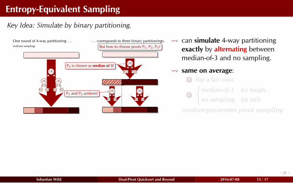
Entropy-Equivalent Sampling
Key Idea: Simulate by binary partitioning.
One round of 4-way partitioning . . .
(without sampling)
<
< >
>
< >
<P2
<P1
c1 c2
<P3
c3 c4
. . . corresponds to three binary partitionings.
< >
<P2
c1,2 c3,4
< >
<P1
c1 c2
< >
<P3
c3 c4
But how to choose pivots P1, P2, P3?
P2 is chosen as median of 3!
P1 and P3 uniform!
can simulate 4-way partitioning
exactly by alternating between
median-of-3 and no sampling.
same on average:1 flip a fair coin
2
{median-of-3 for heads
no sampling for tails
random-parameter pivot sampling
Sebastian Wild Dual-Pivot Quicksort and Beyond 2016-07-08 13 / 17
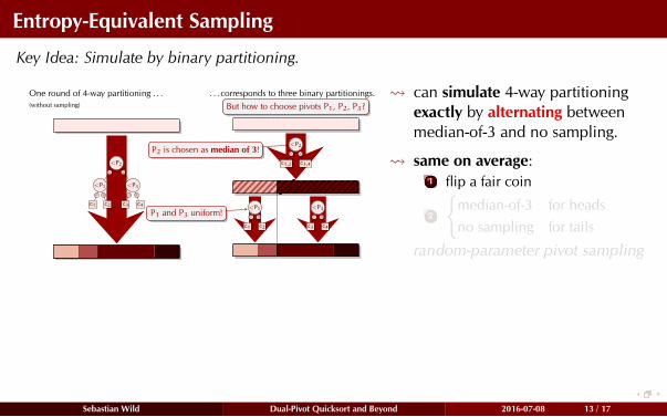
Entropy-Equivalent Sampling
Key Idea: Simulate by binary partitioning.
One round of 4-way partitioning . . .
(without sampling)
<
< >
>
< >
<P2
<P1
c1 c2
<P3
c3 c4
. . . corresponds to three binary partitionings.
< >
<P2
c1,2 c3,4
< >
<P1
c1 c2
< >
<P3
c3 c4
But how to choose pivots P1, P2, P3?
P2 is chosen as median of 3!
P1 and P3 uniform!
can simulate 4-way partitioning
exactly by alternating between
median-of-3 and no sampling.
same on average:1 flip a fair coin
2
{median-of-3 for heads
no sampling for tails
random-parameter pivot sampling
Sebastian Wild Dual-Pivot Quicksort and Beyond 2016-07-08 13 / 17
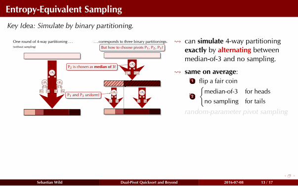
Entropy-Equivalent Sampling
Key Idea: Simulate by binary partitioning.
One round of 4-way partitioning . . .
(without sampling)
<
< >
>
< >
<P2
<P1
c1 c2
<P3
c3 c4
. . . corresponds to three binary partitionings.
< >
<P2
c1,2 c3,4
< >
<P1
c1 c2
< >
<P3
c3 c4
But how to choose pivots P1, P2, P3?
P2 is chosen as median of 3!
P1 and P3 uniform!
can simulate 4-way partitioning
exactly by alternating between
median-of-3 and no sampling.
same on average:1 flip a fair coin
2
{median-of-3 for heads
no sampling for tails
random-parameter pivot sampling
Sebastian Wild Dual-Pivot Quicksort and Beyond 2016-07-08 13 / 17
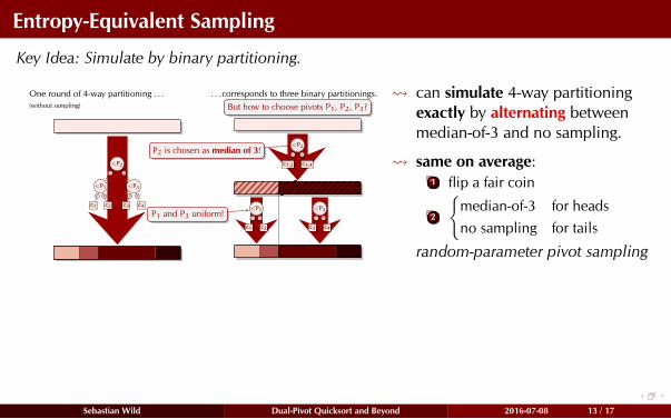
Entropy-Equivalent Sampling
Key Idea: Simulate by binary partitioning.
One round of 4-way partitioning . . .
(without sampling)
<
< >
>
< >
<P2
<P1
c1 c2
<P3
c3 c4
. . . corresponds to three binary partitionings.
< >
<P2
c1,2 c3,4
< >
<P1
c1 c2
< >
<P3
c3 c4
But how to choose pivots P1, P2, P3?
P2 is chosen as median of 3!
P1 and P3 uniform!
can simulate 4-way partitioning
exactly by alternating between
median-of-3 and no sampling.
same on average:1 flip a fair coin
2
{median-of-3 for heads
no sampling for tails
random-parameter pivot sampling
Sebastian Wild Dual-Pivot Quicksort and Beyond 2016-07-08 13 / 17
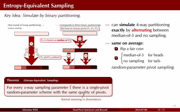
Entropy-Equivalent Sampling
Key Idea: Simulate by binary partitioning.
One round of 4-way partitioning . . .
(without sampling)
<
< >
>
< >
<P2
<P1
c1 c2
<P3
c3 c4
. . . corresponds to three binary partitionings.
< >
<P2
c1,2 c3,4
< >
<P1
c1 c2
< >
<P3
c3 c4
But how to choose pivots P1, P2, P3?
P2 is chosen as median of 3!
P1 and P3 uniform!
can simulate 4-way partitioning
exactly by alternating between
median-of-3 and no sampling.
same on average:1 flip a fair coin
2
{median-of-3 for heads
no sampling for tails
random-parameter pivot sampling
Theorem (Entropy-Equivalent Sampling)
For every s-way sampling parameter~t there is a single-pivot
random-parameter scheme with the same quality of pivots.
(formal meaning in dissertation)
Sebastian Wild Dual-Pivot Quicksort and Beyond 2016-07-08 13 / 17
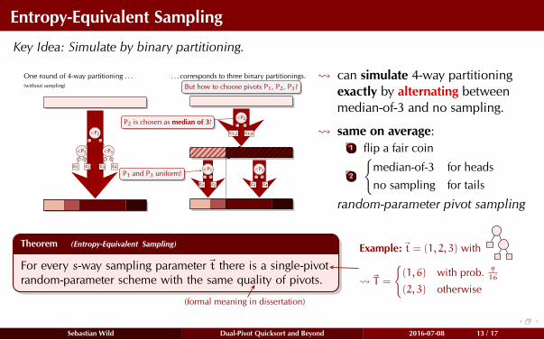
Entropy-Equivalent Sampling
Key Idea: Simulate by binary partitioning.
One round of 4-way partitioning . . .
(without sampling)
<
< >
>
< >
<P2
<P1
c1 c2
<P3
c3 c4
. . . corresponds to three binary partitionings.
< >
<P2
c1,2 c3,4
< >
<P1
c1 c2
< >
<P3
c3 c4
But how to choose pivots P1, P2, P3?
P2 is chosen as median of 3!
P1 and P3 uniform!
can simulate 4-way partitioning
exactly by alternating between
median-of-3 and no sampling.
same on average:1 flip a fair coin
2
{median-of-3 for heads
no sampling for tails
random-parameter pivot sampling
Theorem (Entropy-Equivalent Sampling)
For every s-way sampling parameter~t there is a single-pivot
random-parameter scheme with the same quality of pivots.
(formal meaning in dissertation)
Example:~t = (1, 2, 3) with
~T =
{(1, 6) with prob. 9
16
(2, 3) otherwise
What does that mean?
1 Can simulate any multiway method by binary partitioning.
2 In terms of comparisons, this can only get better!
Sebastian Wild Dual-Pivot Quicksort and Beyond 2016-07-08 13 / 17
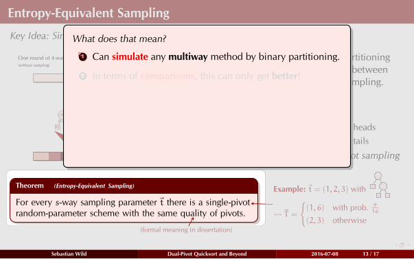
Entropy-Equivalent Sampling
Key Idea: Simulate by binary partitioning.
One round of 4-way partitioning . . .
(without sampling)
<
< >
>
< >
<P2
<P1
c1 c2
<P3
c3 c4
. . . corresponds to three binary partitionings.
< >
<P2
c1,2 c3,4
< >
<P1
c1 c2
< >
<P3
c3 c4
But how to choose pivots P1, P2, P3?
P2 is chosen as median of 3!
P1 and P3 uniform!
can simulate 4-way partitioning
exactly by alternating between
median-of-3 and no sampling.
same on average:1 flip a fair coin
2
{median-of-3 for heads
no sampling for tails
random-parameter pivot sampling
Theorem (Entropy-Equivalent Sampling)
For every s-way sampling parameter~t there is a single-pivot
random-parameter scheme with the same quality of pivots.
(formal meaning in dissertation)
Example:~t = (1, 2, 3) with
~T =
{(1, 6) with prob. 9
16
(2, 3) otherwise
What does that mean?
1 Can simulate any multiway method by binary partitioning.
2 In terms of comparisons, this can only get better!
Sebastian Wild Dual-Pivot Quicksort and Beyond 2016-07-08 13 / 17
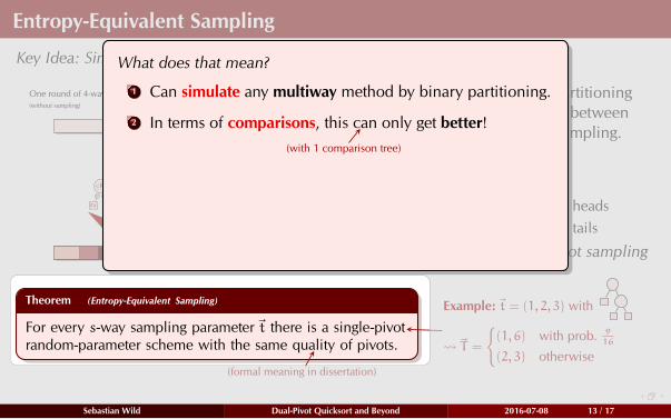
Entropy-Equivalent Sampling
Key Idea: Simulate by binary partitioning.
One round of 4-way partitioning . . .
(without sampling)
<
< >
>
< >
<P2
<P1
c1 c2
<P3
c3 c4
. . . corresponds to three binary partitionings.
< >
<P2
c1,2 c3,4
< >
<P1
c1 c2
< >
<P3
c3 c4
But how to choose pivots P1, P2, P3?
P2 is chosen as median of 3!
P1 and P3 uniform!
can simulate 4-way partitioning
exactly by alternating between
median-of-3 and no sampling.
same on average:1 flip a fair coin
2
{median-of-3 for heads
no sampling for tails
random-parameter pivot sampling
Theorem (Entropy-Equivalent Sampling)
For every s-way sampling parameter~t there is a single-pivot
random-parameter scheme with the same quality of pivots.
(formal meaning in dissertation)
Example:~t = (1, 2, 3) with
~T =
{(1, 6) with prob. 9
16
(2, 3) otherwise
What does that mean?
1 Can simulate any multiway method by binary partitioning.
2 In terms of comparisons, this can only get better!
(with 1 comparison tree)
Sebastian Wild Dual-Pivot Quicksort and Beyond 2016-07-08 13 / 17
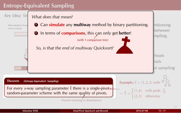
Entropy-Equivalent Sampling
Key Idea: Simulate by binary partitioning.
One round of 4-way partitioning . . .
(without sampling)
<
< >
>
< >
<P2
<P1
c1 c2
<P3
c3 c4
. . . corresponds to three binary partitionings.
< >
<P2
c1,2 c3,4
< >
<P1
c1 c2
< >
<P3
c3 c4
But how to choose pivots P1, P2, P3?
P2 is chosen as median of 3!
P1 and P3 uniform!
can simulate 4-way partitioning
exactly by alternating between
median-of-3 and no sampling.
same on average:1 flip a fair coin
2
{median-of-3 for heads
no sampling for tails
random-parameter pivot sampling
Theorem (Entropy-Equivalent Sampling)
For every s-way sampling parameter~t there is a single-pivot
random-parameter scheme with the same quality of pivots.
(formal meaning in dissertation)
Example:~t = (1, 2, 3) with
~T =
{(1, 6) with prob. 9
16
(2, 3) otherwise
What does that mean?
1 Can simulate any multiway method by binary partitioning.
2 In terms of comparisons, this can only get better!
So, is that the end of multiway Quicksort?
(with 1 comparison tree)
Sebastian Wild Dual-Pivot Quicksort and Beyond 2016-07-08 13 / 17
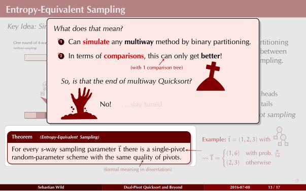
Entropy-Equivalent Sampling
Key Idea: Simulate by binary partitioning.
One round of 4-way partitioning . . .
(without sampling)
<
< >
>
< >
<P2
<P1
c1 c2
<P3
c3 c4
. . . corresponds to three binary partitionings.
< >
<P2
c1,2 c3,4
< >
<P1
c1 c2
< >
<P3
c3 c4
But how to choose pivots P1, P2, P3?
P2 is chosen as median of 3!
P1 and P3 uniform!
can simulate 4-way partitioning
exactly by alternating between
median-of-3 and no sampling.
same on average:1 flip a fair coin
2
{median-of-3 for heads
no sampling for tails
random-parameter pivot sampling
Theorem (Entropy-Equivalent Sampling)
For every s-way sampling parameter~t there is a single-pivot
random-parameter scheme with the same quality of pivots.
(formal meaning in dissertation)
Example:~t = (1, 2, 3) with
~T =
{(1, 6) with prob. 9
16
(2, 3) otherwise
What does that mean?
1 Can simulate any multiway method by binary partitioning.
2 In terms of comparisons, this can only get better!
So, is that the end of multiway Quicksort?
No! . . . stay tuned
(with 1 comparison tree)
Sebastian Wild Dual-Pivot Quicksort and Beyond 2016-07-08 13 / 17
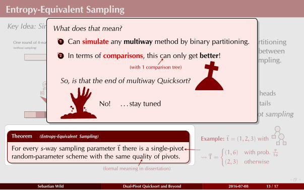
Entropy-Equivalent Sampling
Key Idea: Simulate by binary partitioning.
One round of 4-way partitioning . . .
(without sampling)
<
< >
>
< >
<P2
<P1
c1 c2
<P3
c3 c4
. . . corresponds to three binary partitionings.
< >
<P2
c1,2 c3,4
< >
<P1
c1 c2
< >
<P3
c3 c4
But how to choose pivots P1, P2, P3?
P2 is chosen as median of 3!
P1 and P3 uniform!
can simulate 4-way partitioning
exactly by alternating between
median-of-3 and no sampling.
same on average:1 flip a fair coin
2
{median-of-3 for heads
no sampling for tails
random-parameter pivot sampling
Theorem (Entropy-Equivalent Sampling)
For every s-way sampling parameter~t there is a single-pivot
random-parameter scheme with the same quality of pivots.
(formal meaning in dissertation)
Example:~t = (1, 2, 3) with
~T =
{(1, 6) with prob. 9
16
(2, 3) otherwise
What does that mean?
1 Can simulate any multiway method by binary partitioning.
2 In terms of comparisons, this can only get better!
So, is that the end of multiway Quicksort?
No! . . . stay tuned
(with 1 comparison tree)
Sebastian Wild Dual-Pivot Quicksort and Beyond 2016-07-08 13 / 17

The Memory Wall
Comparisons =̂ CPU effort, but we also need to load items from memory.
Sebastian Wild Dual-Pivot Quicksort and Beyond 2016-07-08 14 / 17

The Memory Wall
Comparisons =̂ CPU effort, but we also need to load items from memory.
Sebastian Wild Dual-Pivot Quicksort and Beyond 2016-07-08 14 / 17
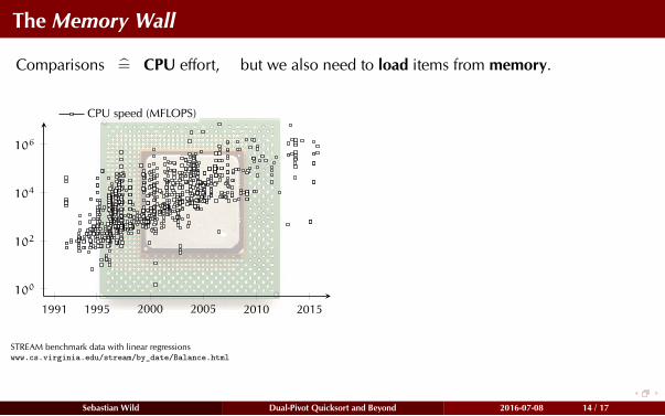
The Memory Wall
Comparisons =̂ CPU effort, but we also need to load items from memory.
1991 1995 2000 2005 2010 2015
100
102
104
106
CPU speed (MFLOPS)
STREAM benchmark data with linear regressionswww.cs.virginia.edu/stream/by_date/Balance.html
Sebastian Wild Dual-Pivot Quicksort and Beyond 2016-07-08 14 / 17
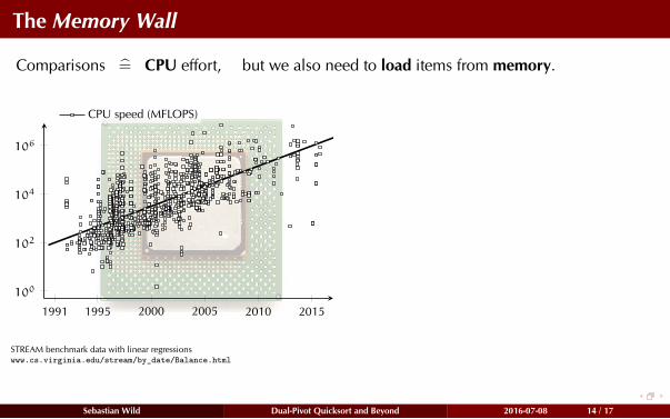
The Memory Wall
Comparisons =̂ CPU effort, but we also need to load items from memory.
1991 1995 2000 2005 2010 2015
100
102
104
106
CPU speed (MFLOPS)
STREAM benchmark data with linear regressionswww.cs.virginia.edu/stream/by_date/Balance.html
Sebastian Wild Dual-Pivot Quicksort and Beyond 2016-07-08 14 / 17
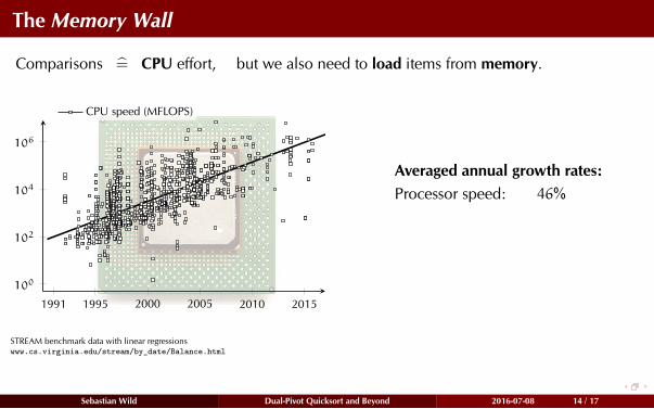
The Memory Wall
Comparisons =̂ CPU effort, but we also need to load items from memory.
1991 1995 2000 2005 2010 2015
100
102
104
106
CPU speed (MFLOPS)
STREAM benchmark data with linear regressionswww.cs.virginia.edu/stream/by_date/Balance.html
Averaged annual growth rates:
Processor speed: 46%
Sebastian Wild Dual-Pivot Quicksort and Beyond 2016-07-08 14 / 17
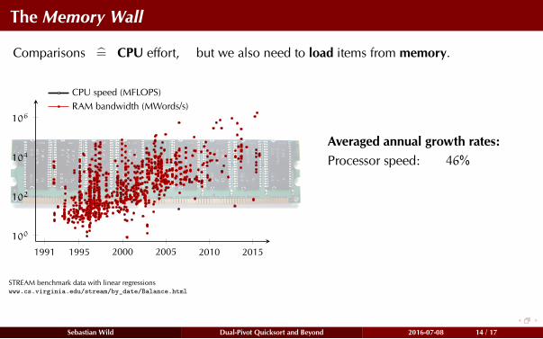
The Memory Wall
Comparisons =̂ CPU effort, but we also need to load items from memory.
1991 1995 2000 2005 2010 2015
100
102
104
106
CPU speed (MFLOPS)
RAM bandwidth (MWords/s)
STREAM benchmark data with linear regressionswww.cs.virginia.edu/stream/by_date/Balance.html
Averaged annual growth rates:
Processor speed: 46%
Sebastian Wild Dual-Pivot Quicksort and Beyond 2016-07-08 14 / 17
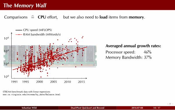
The Memory Wall
Comparisons =̂ CPU effort, but we also need to load items from memory.
1991 1995 2000 2005 2010 2015
100
102
104
106
CPU speed (MFLOPS)
RAM bandwidth (MWords/s)
STREAM benchmark data with linear regressionswww.cs.virginia.edu/stream/by_date/Balance.html
Averaged annual growth rates:
Processor speed: 46%
Memory Bandwidth: 37%
Sebastian Wild Dual-Pivot Quicksort and Beyond 2016-07-08 14 / 17
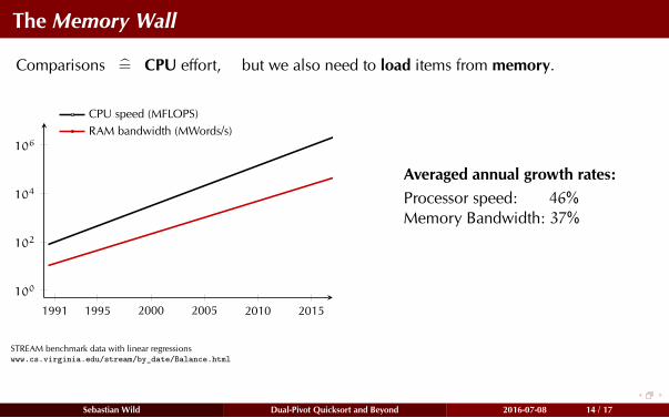
The Memory Wall
Comparisons =̂ CPU effort, but we also need to load items from memory.
1991 1995 2000 2005 2010 2015
100
102
104
106
CPU speed (MFLOPS)
RAM bandwidth (MWords/s)
STREAM benchmark data with linear regressionswww.cs.virginia.edu/stream/by_date/Balance.html
Averaged annual growth rates:
Processor speed: 46%
Memory Bandwidth: 37%
Sebastian Wild Dual-Pivot Quicksort and Beyond 2016-07-08 14 / 17
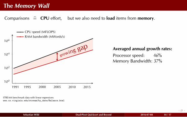
The Memory Wall
Comparisons =̂ CPU effort, but we also need to load items from memory.
1991 1995 2000 2005 2010 2015
100
102
104
106
growing gap
CPU speed (MFLOPS)
RAM bandwidth (MWords/s)
STREAM benchmark data with linear regressionswww.cs.virginia.edu/stream/by_date/Balance.html
Averaged annual growth rates:
Processor speed: 46%
Memory Bandwidth: 37%
Sebastian Wild Dual-Pivot Quicksort and Beyond 2016-07-08 14 / 17
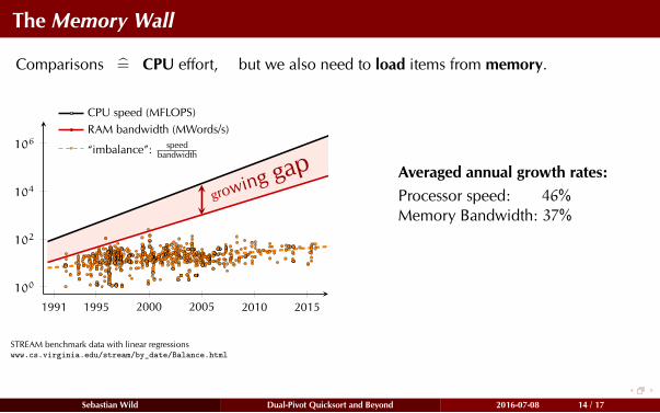
The Memory Wall
Comparisons =̂ CPU effort, but we also need to load items from memory.
1991 1995 2000 2005 2010 2015
100
102
104
106
growing gap
CPU speed (MFLOPS)
RAM bandwidth (MWords/s)
“imbalance”: speedbandwidth
STREAM benchmark data with linear regressionswww.cs.virginia.edu/stream/by_date/Balance.html
Averaged annual growth rates:
Processor speed: 46%
Memory Bandwidth: 37%
Sebastian Wild Dual-Pivot Quicksort and Beyond 2016-07-08 14 / 17
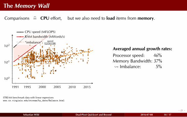
The Memory Wall
Comparisons =̂ CPU effort, but we also need to load items from memory.
1991 1995 2000 2005 2010 2015
100
101
102
CPU speed (MFLOPS)
RAM bandwidth (MWords/s)
“imbalance”: speedbandwidth
STREAM benchmark data with linear regressionswww.cs.virginia.edu/stream/by_date/Balance.html
Averaged annual growth rates:
Processor speed: 46%
Memory Bandwidth: 37%
Imbalance: 5%
Sebastian Wild Dual-Pivot Quicksort and Beyond 2016-07-08 14 / 17
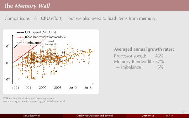
The Memory Wall
Comparisons =̂ CPU effort, but we also need to load items from memory.
1991 1995 2000 2005 2010 2015
100
101
102
CPU speed (MFLOPS)
RAM bandwidth (MWords/s)
“imbalance”: speedbandwidth
STREAM benchmark data with linear regressionswww.cs.virginia.edu/stream/by_date/Balance.html
Averaged annual growth rates:
Processor speed: 46%
Memory Bandwidth: 37%
Imbalance: 5%
Sebastian Wild Dual-Pivot Quicksort and Beyond 2016-07-08 14 / 17
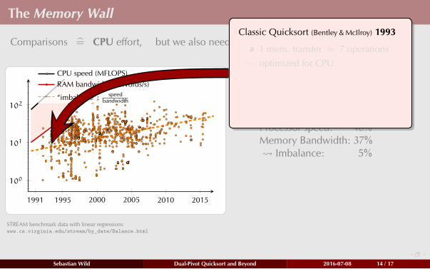
The Memory Wall
Comparisons =̂ CPU effort, but we also need to load items from memory.
1991 1995 2000 2005 2010 2015
100
101
102
CPU speed (MFLOPS)
RAM bandwidth (MWords/s)
“imbalance”: speedbandwidth
STREAM benchmark data with linear regressionswww.cs.virginia.edu/stream/by_date/Balance.html
Averaged annual growth rates:
Processor speed: 46%
Memory Bandwidth: 37%
Imbalance: 5%
Classic Quicksort (Bentley & McIlroy) 1993
1 mem. transfer ≈ 7 operations
optimized for CPU
Sebastian Wild Dual-Pivot Quicksort and Beyond 2016-07-08 14 / 17
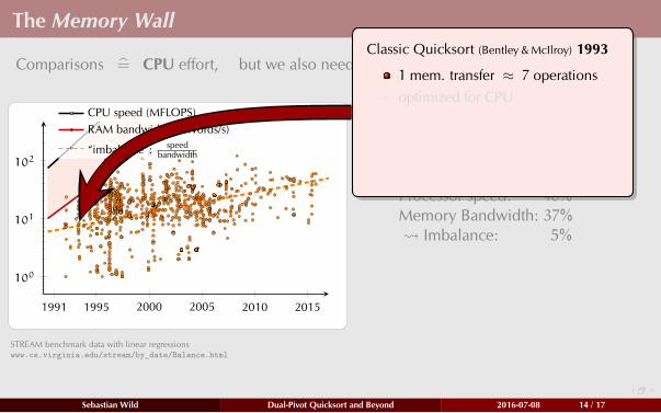
The Memory Wall
Comparisons =̂ CPU effort, but we also need to load items from memory.
1991 1995 2000 2005 2010 2015
100
101
102
CPU speed (MFLOPS)
RAM bandwidth (MWords/s)
“imbalance”: speedbandwidth
STREAM benchmark data with linear regressionswww.cs.virginia.edu/stream/by_date/Balance.html
Averaged annual growth rates:
Processor speed: 46%
Memory Bandwidth: 37%
Imbalance: 5%
Classic Quicksort (Bentley & McIlroy) 1993
1 mem. transfer ≈ 7 operations
optimized for CPU
Sebastian Wild Dual-Pivot Quicksort and Beyond 2016-07-08 14 / 17
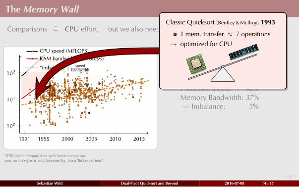
The Memory Wall
Comparisons =̂ CPU effort, but we also need to load items from memory.
1991 1995 2000 2005 2010 2015
100
101
102
CPU speed (MFLOPS)
RAM bandwidth (MWords/s)
“imbalance”: speedbandwidth
STREAM benchmark data with linear regressionswww.cs.virginia.edu/stream/by_date/Balance.html
Averaged annual growth rates:
Processor speed: 46%
Memory Bandwidth: 37%
Imbalance: 5%
Classic Quicksort (Bentley & McIlroy) 1993
1 mem. transfer ≈ 7 operations
optimized for CPU
Sebastian Wild Dual-Pivot Quicksort and Beyond 2016-07-08 14 / 17
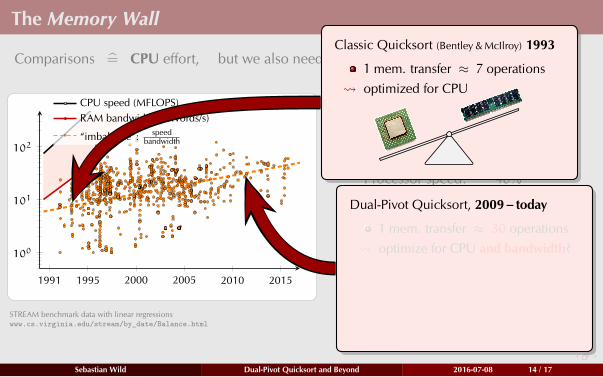
The Memory Wall
Comparisons =̂ CPU effort, but we also need to load items from memory.
1991 1995 2000 2005 2010 2015
100
101
102
CPU speed (MFLOPS)
RAM bandwidth (MWords/s)
“imbalance”: speedbandwidth
STREAM benchmark data with linear regressionswww.cs.virginia.edu/stream/by_date/Balance.html
Averaged annual growth rates:
Processor speed: 46%
Memory Bandwidth: 37%
Imbalance: 5%
Classic Quicksort (Bentley & McIlroy) 1993
1 mem. transfer ≈ 7 operations
optimized for CPU
Dual-Pivot Quicksort, 2009 – today
1 mem. transfer ≈ 30 operations
optimize for CPU and bandwidth?
Sebastian Wild Dual-Pivot Quicksort and Beyond 2016-07-08 14 / 17
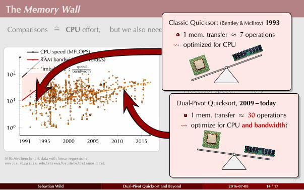
The Memory Wall
Comparisons =̂ CPU effort, but we also need to load items from memory.
1991 1995 2000 2005 2010 2015
100
101
102
CPU speed (MFLOPS)
RAM bandwidth (MWords/s)
“imbalance”: speedbandwidth
STREAM benchmark data with linear regressionswww.cs.virginia.edu/stream/by_date/Balance.html
Averaged annual growth rates:
Processor speed: 46%
Memory Bandwidth: 37%
Imbalance: 5%
Classic Quicksort (Bentley & McIlroy) 1993
1 mem. transfer ≈ 7 operations
optimized for CPU
Dual-Pivot Quicksort, 2009 – today
1 mem. transfer ≈ 30 operations
optimize for CPU and bandwidth?
Sebastian Wild Dual-Pivot Quicksort and Beyond 2016-07-08 14 / 17
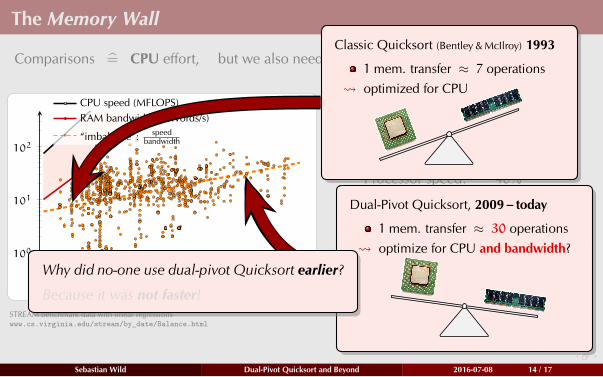
The Memory Wall
Comparisons =̂ CPU effort, but we also need to load items from memory.
1991 1995 2000 2005 2010 2015
100
101
102
CPU speed (MFLOPS)
RAM bandwidth (MWords/s)
“imbalance”: speedbandwidth
STREAM benchmark data with linear regressionswww.cs.virginia.edu/stream/by_date/Balance.html
Averaged annual growth rates:
Processor speed: 46%
Memory Bandwidth: 37%
Imbalance: 5%
Classic Quicksort (Bentley & McIlroy) 1993
1 mem. transfer ≈ 7 operations
optimized for CPU
Dual-Pivot Quicksort, 2009 – today
1 mem. transfer ≈ 30 operations
optimize for CPU and bandwidth?
Why did no-one use dual-pivot Quicksort earlier?
Because it was not faster!
Sebastian Wild Dual-Pivot Quicksort and Beyond 2016-07-08 14 / 17
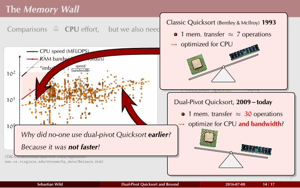
The Memory Wall
Comparisons =̂ CPU effort, but we also need to load items from memory.
1991 1995 2000 2005 2010 2015
100
101
102
CPU speed (MFLOPS)
RAM bandwidth (MWords/s)
“imbalance”: speedbandwidth
STREAM benchmark data with linear regressionswww.cs.virginia.edu/stream/by_date/Balance.html
Averaged annual growth rates:
Processor speed: 46%
Memory Bandwidth: 37%
Imbalance: 5%
Classic Quicksort (Bentley & McIlroy) 1993
1 mem. transfer ≈ 7 operations
optimized for CPU
Dual-Pivot Quicksort, 2009 – today
1 mem. transfer ≈ 30 operations
optimize for CPU and bandwidth?
Why did no-one use dual-pivot Quicksort earlier?
Because it was not faster!
Sebastian Wild Dual-Pivot Quicksort and Beyond 2016-07-08 14 / 17

Scanned Elements
How to analyze bandwidth consumption?
Need good cost measure!
Proposal: count scanned elements
Access to array only through iterators
(no random access!)5
1
1
2
7
3
4
4
2
5
8
6
Iterators can
head left or right (one-directional!)
advance to next position
read and write current cell
Cost: number of advances
≈ cache misses, but hardware independent
Costs of Partitioning
Classic Quicksort
k g
n scanned elements
(array scanned once)
4-way Quicksort
k2 g2
k g
1.5n scanned elements
(on average without sampling)
Sebastian Wild Dual-Pivot Quicksort and Beyond 2016-07-08 15 / 17
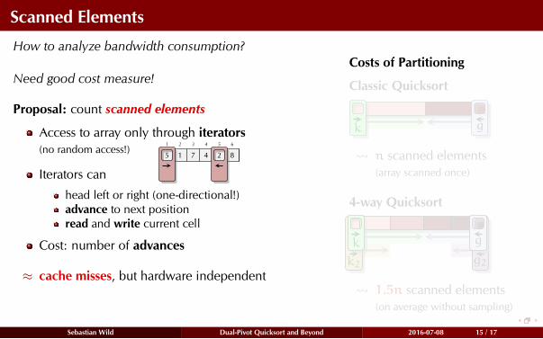
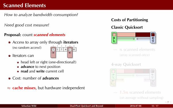
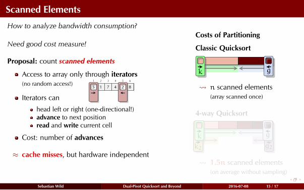
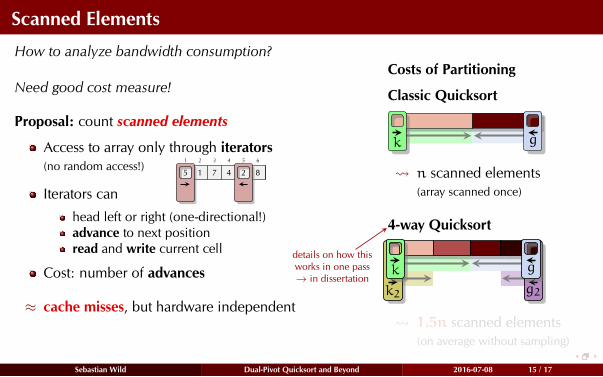
Scanned Elements
How to analyze bandwidth consumption?
Need good cost measure!
Proposal: count scanned elements
Access to array only through iterators
(no random access!)5
1
1
2
7
3
4
4
2
5
8
6
Iterators can
head left or right (one-directional!)
advance to next position
read and write current cell
Cost: number of advances
≈ cache misses, but hardware independent
Costs of Partitioning
Classic Quicksort
k g
n scanned elements
(array scanned once)
4
details on how this
works in one pass
→ in dissertation
-way Quicksort
k2 g2
k g
1.5n scanned elements
(on average without sampling)
Sebastian Wild Dual-Pivot Quicksort and Beyond 2016-07-08 15 / 17
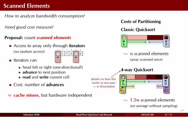
Scanned Elements
How to analyze bandwidth consumption?
Need good cost measure!
Proposal: count scanned elements
Access to array only through iterators
(no random access!)5
1
1
2
7
3
4
4
2
5
8
6
Iterators can
head left or right (one-directional!)
advance to next position
read and write current cell
Cost: number of advances
≈ cache misses, but hardware independent
Costs of Partitioning
Classic Quicksort
k g
n scanned elements
(array scanned once)
4
details on how this
works in one pass
→ in dissertation
-way Quicksort
k2 g2
k g
1.5n scanned elements
(on average without sampling)
Sebastian Wild Dual-Pivot Quicksort and Beyond 2016-07-08 15 / 17
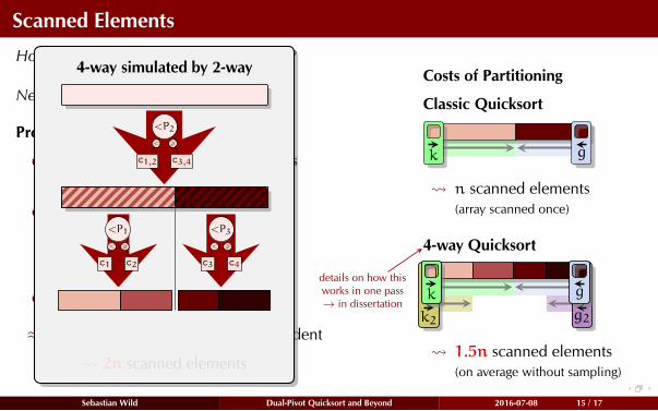
Scanned Elements
How to analyze bandwidth consumption?
Need good cost measure!
Proposal: count scanned elements
Access to array only through iterators
(no random access!)5
1
1
2
7
3
4
4
2
5
8
6
Iterators can
head left or right (one-directional!)
advance to next position
read and write current cell
Cost: number of advances
≈ cache misses, but hardware independent
Costs of Partitioning
Classic Quicksort
k g
n scanned elements
(array scanned once)
4
details on how this
works in one pass
→ in dissertation
-way Quicksort
k2 g2
k g
1.5n scanned elements
(on average without sampling)
4-way simulated by 2-way
< >
<P2
c1,2 c3,4
< >
<P1
c1 c2
< >
<P3
c3 c4
2n scanned elements
Sebastian Wild Dual-Pivot Quicksort and Beyond 2016-07-08 15 / 17
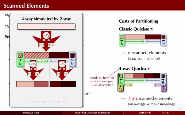
Scanned Elements
How to analyze bandwidth consumption?
Need good cost measure!
Proposal: count scanned elements
Access to array only through iterators
(no random access!)5
1
1
2
7
3
4
4
2
5
8
6
Iterators can
head left or right (one-directional!)
advance to next position
read and write current cell
Cost: number of advances
≈ cache misses, but hardware independent
Costs of Partitioning
Classic Quicksort
k g
n scanned elements
(array scanned once)
4
details on how this
works in one pass
→ in dissertation
-way Quicksort
k2 g2
k g
1.5n scanned elements
(on average without sampling)
4-way simulated by 2-way
< >
<P2
c1,2 c3,4
< >
<P1
c1 c2
< >
<P3
c3 c4
k g
2n scanned elements
Sebastian Wild Dual-Pivot Quicksort and Beyond 2016-07-08 15 / 17
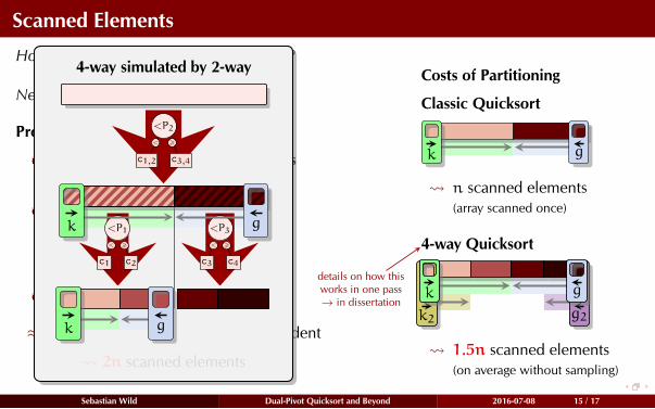
Scanned Elements
How to analyze bandwidth consumption?
Need good cost measure!
Proposal: count scanned elements
Access to array only through iterators
(no random access!)5
1
1
2
7
3
4
4
2
5
8
6
Iterators can
head left or right (one-directional!)
advance to next position
read and write current cell
Cost: number of advances
≈ cache misses, but hardware independent
Costs of Partitioning
Classic Quicksort
k g
n scanned elements
(array scanned once)
4
details on how this
works in one pass
→ in dissertation
-way Quicksort
k2 g2
k g
1.5n scanned elements
(on average without sampling)
4-way simulated by 2-way
< >
<P2
c1,2 c3,4
< >
<P1
c1 c2
< >
<P3
c3 c4
k g
k g
2n scanned elements
Sebastian Wild Dual-Pivot Quicksort and Beyond 2016-07-08 15 / 17
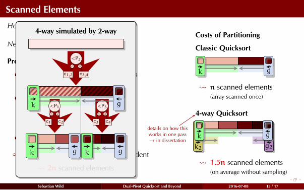
Scanned Elements
How to analyze bandwidth consumption?
Need good cost measure!
Proposal: count scanned elements
Access to array only through iterators
(no random access!)5
1
1
2
7
3
4
4
2
5
8
6
Iterators can
head left or right (one-directional!)
advance to next position
read and write current cell
Cost: number of advances
≈ cache misses, but hardware independent
Costs of Partitioning
Classic Quicksort
k g
n scanned elements
(array scanned once)
4
details on how this
works in one pass
→ in dissertation
-way Quicksort
k2 g2
k g
1.5n scanned elements
(on average without sampling)
4-way simulated by 2-way
< >
<P2
c1,2 c3,4
< >
<P1
c1 c2
< >
<P3
c3 c4
k g
k g k g
2n scanned elements
Sebastian Wild Dual-Pivot Quicksort and Beyond 2016-07-08 15 / 17
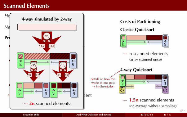
Scanned Elements
How to analyze bandwidth consumption?
Need good cost measure!
Proposal: count scanned elements
Access to array only through iterators
(no random access!)5
1
1
2
7
3
4
4
2
5
8
6
Iterators can
head left or right (one-directional!)
advance to next position
read and write current cell
Cost: number of advances
≈ cache misses, but hardware independent
Costs of Partitioning
Classic Quicksort
k g
n scanned elements
(array scanned once)
4
details on how this
works in one pass
→ in dissertation
-way Quicksort
k2 g2
k g
1.5n scanned elements
(on average without sampling)
4-way simulated by 2-way
< >
<P2
c1,2 c3,4
< >
<P1
c1 c2
< >
<P3
c3 c4
k g
k g k g
2n scanned elements
Sebastian Wild Dual-Pivot Quicksort and Beyond 2016-07-08 15 / 17
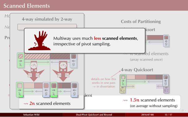
Scanned Elements
How to analyze bandwidth consumption?
Need good cost measure!
Proposal: count scanned elements
Access to array only through iterators
(no random access!)5
1
1
2
7
3
4
4
2
5
8
6
Iterators can
head left or right (one-directional!)
advance to next position
read and write current cell
Cost: number of advances
≈ cache misses, but hardware independent
Costs of Partitioning
Classic Quicksort
k g
n scanned elements
(array scanned once)
4
details on how this
works in one pass
→ in dissertation
-way Quicksort
k2 g2
k g
1.5n scanned elements
(on average without sampling)
4-way simulated by 2-way
< >
<P2
c1,2 c3,4
< >
<P1
c1 c2
< >
<P3
c3 c4
k g
k g k g
2n scanned elements
Multiway uses much less scanned elements,
irrespective of pivot sampling.
Sebastian Wild Dual-Pivot Quicksort and Beyond 2016-07-08 15 / 17
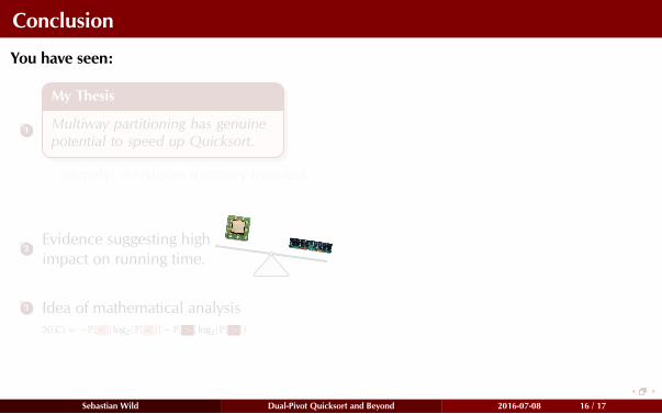
Conclusion
You have seen:
1
My Thesis
Multiway partitioning has genuine
potential to speed up Quicksort.
. . . namely: it reduces memory transfers.
2Evidence suggesting high
impact on running time.
3 Idea of mathematical analysis
H(C) = −P[ < ] log2(P[ < ]) − P[ > ] log2(P[ > ])
Sebastian Wild Dual-Pivot Quicksort and Beyond 2016-07-08 16 / 17
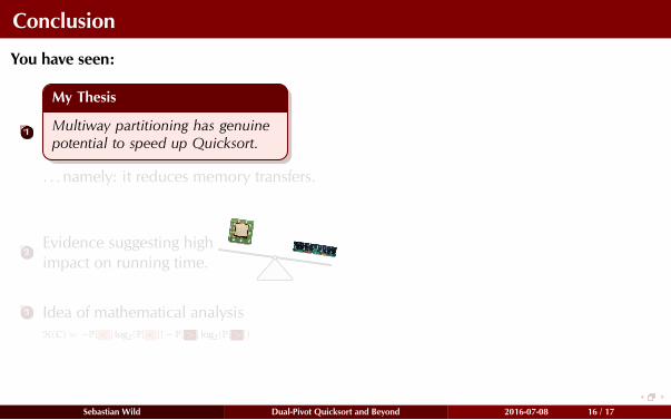
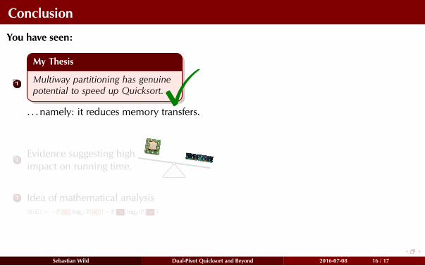
Conclusion
You have seen:
1
My Thesis
Multiway partitioning has genuine
potential to speed up Quicksort.X. . . namely: it reduces memory transfers.
2Evidence suggesting high
impact on running time.
3 Idea of mathematical analysis
H(C) = −P[ < ] log2(P[ < ]) − P[ > ] log2(P[ > ])
Sebastian Wild Dual-Pivot Quicksort and Beyond 2016-07-08 16 / 17
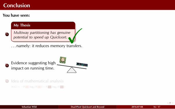
Conclusion
You have seen:
1
My Thesis
Multiway partitioning has genuine
potential to speed up Quicksort.X. . . namely: it reduces memory transfers.
2Evidence suggesting high
impact on running time.
3 Idea of mathematical analysis
H(C) = −P[ < ] log2(P[ < ]) − P[ > ] log2(P[ > ])
Sebastian Wild Dual-Pivot Quicksort and Beyond 2016-07-08 16 / 17
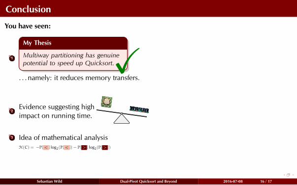
Conclusion
You have seen:
1
My Thesis
Multiway partitioning has genuine
potential to speed up Quicksort.X. . . namely: it reduces memory transfers.
2Evidence suggesting high
impact on running time.
3 Idea of mathematical analysis
H(C) = −P[ < ] log2(P[ < ]) − P[ > ] log2(P[ > ])
Sebastian Wild Dual-Pivot Quicksort and Beyond 2016-07-08 16 / 17
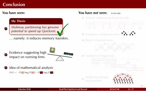
Conclusion
You have seen:
1
My Thesis
Multiway partitioning has genuine
potential to speed up Quicksort.X. . . namely: it reduces memory transfers.
2Evidence suggesting high
impact on running time.
3 Idea of mathematical analysis
H(C) = −P[ < ] log2(P[ < ]) − P[ > ] log2(P[ > ])
You have not seen: (in this talk)
Generic multiway partitioning code
k⌈m⌉ k2 k ≡ k1 g ≡ g1 g2 gs−⌊m⌋
s⌈m⌉ . . . s1 ? l1 . . . ls−⌊m⌋
. . . . . .left right
Using two comparison trees
Branch mispredictions
1taken
2taken
3not t.
4not t.
taken
not t.
not t.
not t. not t.
taken
taken
taken
Treatment of equal keys4 2 1 3 3 5 4 4 3 5 2
2 1 2 4 5 4 4 533 3
5 54 442 1 2
5 5
4 2 1 3 3 5 4 4 3 5 2
3
4
5 5
2 1 2
Intriguing interplay
of parameters
Sebastian Wild Dual-Pivot Quicksort and Beyond 2016-07-08 16 / 17
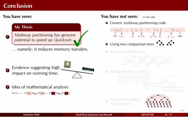
Conclusion
You have seen:
1
My Thesis
Multiway partitioning has genuine
potential to speed up Quicksort.X. . . namely: it reduces memory transfers.
2Evidence suggesting high
impact on running time.
3 Idea of mathematical analysis
H(C) = −P[ < ] log2(P[ < ]) − P[ > ] log2(P[ > ])
You have not seen: (in this talk)
Generic multiway partitioning code
k⌈m⌉ k2 k ≡ k1 g ≡ g1 g2 gs−⌊m⌋
s⌈m⌉ . . . s1 ? l1 . . . ls−⌊m⌋
. . . . . .left right
Using two comparison trees
Branch mispredictions
1taken
2taken
3not t.
4not t.
taken
not t.
not t.
not t. not t.
taken
taken
taken
Treatment of equal keys4 2 1 3 3 5 4 4 3 5 2
2 1 2 4 5 4 4 533 3
5 54 442 1 2
5 5
4 2 1 3 3 5 4 4 3 5 2
3
4
5 5
2 1 2
Intriguing interplay
of parameters
Sebastian Wild Dual-Pivot Quicksort and Beyond 2016-07-08 16 / 17
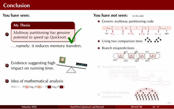
Conclusion
You have seen:
1
My Thesis
Multiway partitioning has genuine
potential to speed up Quicksort.X. . . namely: it reduces memory transfers.
2Evidence suggesting high
impact on running time.
3 Idea of mathematical analysis
H(C) = −P[ < ] log2(P[ < ]) − P[ > ] log2(P[ > ])
You have not seen: (in this talk)
Generic multiway partitioning code
k⌈m⌉ k2 k ≡ k1 g ≡ g1 g2 gs−⌊m⌋
s⌈m⌉ . . . s1 ? l1 . . . ls−⌊m⌋
. . . . . .left right
Using two comparison trees
Branch mispredictions
1taken
2taken
3not t.
4not t.
taken
not t.
not t.
not t. not t.
taken
taken
taken
Treatment of equal keys4 2 1 3 3 5 4 4 3 5 2
2 1 2 4 5 4 4 533 3
5 54 442 1 2
5 5
4 2 1 3 3 5 4 4 3 5 2
3
4
5 5
2 1 2
Intriguing interplay
of parameters
Sebastian Wild Dual-Pivot Quicksort and Beyond 2016-07-08 16 / 17
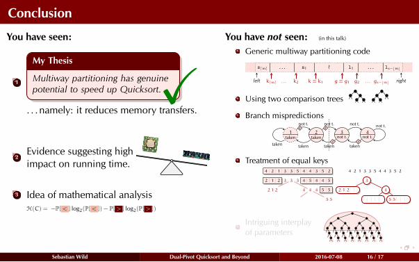
Conclusion
You have seen:
1
My Thesis
Multiway partitioning has genuine
potential to speed up Quicksort.X. . . namely: it reduces memory transfers.
2Evidence suggesting high
impact on running time.
3 Idea of mathematical analysis
H(C) = −P[ < ] log2(P[ < ]) − P[ > ] log2(P[ > ])
You have not seen: (in this talk)
Generic multiway partitioning code
k⌈m⌉ k2 k ≡ k1 g ≡ g1 g2 gs−⌊m⌋
s⌈m⌉ . . . s1 ? l1 . . . ls−⌊m⌋
. . . . . .left right
Using two comparison trees
Branch mispredictions
1taken
2taken
3not t.
4not t.
taken
not t.
not t.
not t. not t.
taken
taken
taken
Treatment of equal keys4 2 1 3 3 5 4 4 3 5 2
2 1 2 4 5 4 4 533 3
5 54 442 1 2
5 5
4 2 1 3 3 5 4 4 3 5 2
3
4
5 5
2 1 2
Intriguing interplay
of parameters
Sebastian Wild Dual-Pivot Quicksort and Beyond 2016-07-08 16 / 17
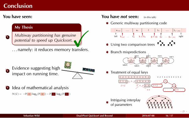
Conclusion
You have seen:
1
My Thesis
Multiway partitioning has genuine
potential to speed up Quicksort.X. . . namely: it reduces memory transfers.
2Evidence suggesting high
impact on running time.
3 Idea of mathematical analysis
H(C) = −P[ < ] log2(P[ < ]) − P[ > ] log2(P[ > ])
You have not seen: (in this talk)
Generic multiway partitioning code
k⌈m⌉ k2 k ≡ k1 g ≡ g1 g2 gs−⌊m⌋
s⌈m⌉ . . . s1 ? l1 . . . ls−⌊m⌋
. . . . . .left right
Using two comparison trees
Branch mispredictions
1taken
2taken
3not t.
4not t.
taken
not t.
not t.
not t. not t.
taken
taken
taken
Treatment of equal keys4 2 1 3 3 5 4 4 3 5 2
2 1 2 4 5 4 4 533 3
5 54 442 1 2
5 5
4 2 1 3 3 5 4 4 3 5 2
3
4
5 5
2 1 2
Intriguing interplay
of parameters
Sebastian Wild Dual-Pivot Quicksort and Beyond 2016-07-08 16 / 17

Sebastian Wild Dual-Pivot Quicksort and Beyond 2016-07-08 17 / 17

Image sources
Icons by Freepik and Gregor Cresnar from www.flaticon.com.
Ball Pit: https://www.flickr.com/photos/davidsingleton/2175975083/
Sorting Hat: http://harrypotter.wikia.com/wiki/Sorting_Hat
Highest Towers: WikimediaMouse Trap: bobbleheaddad.comRobert Sedgewick: http://www.cs.princeton.edu/~rs/
Apple: WikimediaOrange: WikimediaCPU Die: WikimediaRAM: Wikimedia
Sebastian Wild Dual-Pivot Quicksort and Beyond 2016-07-08 18 / 17