Embed Size (px)
Citation preview
Geometric Electroelasticity
Dissertationzur Erlangung des akademischen Grades
”doctor rerum naturalium”(Dr. rer. nat)
in der Wissenschaftsdisziplin ”Geometrie”
eingereicht an derMathematisch-Naturwissenschaftlichen Fakultat
der Universitat Potsdam
vonRamona Ziese
Betreuer: Prof. Dr. Christian Bar
eingereicht am 29. April 2014,verteidigt am 26. September 2014
Published online at the Institutional Repository of the University of Potsdam: URL http://opus.kobv.de/ubp/volltexte/2014/7250/ URN urn:nbn:de:kobv:517-opus-72504 http://nbn-resolving.de/urn:nbn:de:kobv:517-opus-72504
Danksagung
Zuallererst danke ich Prof. Dr. Christian Bar fur die Vergabe des Themas und fur seineBetreuung und Unterstutzung.Dann mochte ich mich ganz herzlich bei Dr. Christoph Stephan bedanken, fur unzahligeaußerst produktive Diskussionen sowie seine Geduld und Zeit und gelegentliche Ermu-tigungen. Weiterhin danke ich Dr. Florian Hanisch und Claudia Grabs fur so manchewertvolle Diskussion.Als nachstes mochte ich mich bei Ariane Beier, Viktoria Rothe und Dr. Volker Brandingbedanken; bei Ariane und Viktoria fur das Korrekturlesen und bei allen dreien fur eineschone Zeit in unserem gemeinsamen Buro.Des Weiteren mochte ich mich bei Dr. Stefan Fredenhagen, Dr. Axel Kleinschmidt undDr. Oliver Schlotterer fur die Organisation der IMPRS-Seminare und -Exkursionen sowiefur ihre Ermutigungen danken. Außerdem danke ich dem Albert-Einstein Institut fur diefinanzielle Unterstutzung wahrend der letzten Jahre.Fur ihre moralische Unterstutzung sowie ihre stets fur mich offenen Ohren mochte ichNicole Mucke meinen Dank aussprechen.Mein ganz besonderer Dank gilt David Kappel fur seinen Beistand und seine Geduld sowieaußerst hilfreiche Diskussionen und seine unglaublich sorgfaltigen und umfangreichenKorrekturanmerkungen.
iii

Contents
Introduction 1
1 Geometric Setup and Basic Definitions 51.1 Deformations . . . . . . . . . . . . . . . . . . . . . . . . . . . . . . . . . . 5
The substantial derivative . . . . . . . . . . . . . . . . . . . . . . . . . . . 71.2 Deformation Tensors . . . . . . . . . . . . . . . . . . . . . . . . . . . . . . 121.3 The Master Balance Law . . . . . . . . . . . . . . . . . . . . . . . . . . . 19
1.3.1 The Spatial Master Balance Law . . . . . . . . . . . . . . . . . . . 191.3.2 The Material Master Balance Law . . . . . . . . . . . . . . . . . . 241.3.3 Consequences of Conservation of Mass . . . . . . . . . . . . . . . . 28
2 Electrodynamics 332.1 Maxwell’s equations . . . . . . . . . . . . . . . . . . . . . . . . . . . . . . 332.2 Galilei-invariants and the Lorentz force . . . . . . . . . . . . . . . . . . . . 352.3 Maxwell’s Equations in terms of differential forms . . . . . . . . . . . . . 382.4 Polarization and Magnetization . . . . . . . . . . . . . . . . . . . . . . . . 402.5 The electromagnetic fields along the map φt . . . . . . . . . . . . . . . . . 43
3 The Balance Laws on Bt 453.1 Conservation of Mass . . . . . . . . . . . . . . . . . . . . . . . . . . . . . . 463.2 Balance of Momentum . . . . . . . . . . . . . . . . . . . . . . . . . . . . . 473.3 Balance of Angular Momentum . . . . . . . . . . . . . . . . . . . . . . . . 523.4 Balance of Energy . . . . . . . . . . . . . . . . . . . . . . . . . . . . . . . 55
3.4.1 Special case: S = R3 with the Euclidean metric . . . . . . . . . . 563.4.2 The general case . . . . . . . . . . . . . . . . . . . . . . . . . . . . 61
3.5 The balance laws for the general case . . . . . . . . . . . . . . . . . . . . . 62
4 The Balance Laws on B 734.1 Conservation of mass . . . . . . . . . . . . . . . . . . . . . . . . . . . . . . 734.2 Balance of Momentum . . . . . . . . . . . . . . . . . . . . . . . . . . . . . 734.3 Balance of Angular Momentum . . . . . . . . . . . . . . . . . . . . . . . . 754.4 Balance of Energy . . . . . . . . . . . . . . . . . . . . . . . . . . . . . . . 764.5 The Equation of motion and the Doyle-Ericksen formula . . . . . . . . . . 78
5 The Properties of the material: Constitutive relations 815.1 Constitutive relations . . . . . . . . . . . . . . . . . . . . . . . . . . . . . 815.2 Thermoelasticity . . . . . . . . . . . . . . . . . . . . . . . . . . . . . . . . 84
v
Contents
5.3 Thermoelectromagnetoelasticity . . . . . . . . . . . . . . . . . . . . . . . . 915.4 Electroelastic materials . . . . . . . . . . . . . . . . . . . . . . . . . . . . 101
6 The equation of motion for Neo-electroelastic materials 1036.1 The initial boundary value problem for simple bodies . . . . . . . . . . . . 103
vi
Introduction
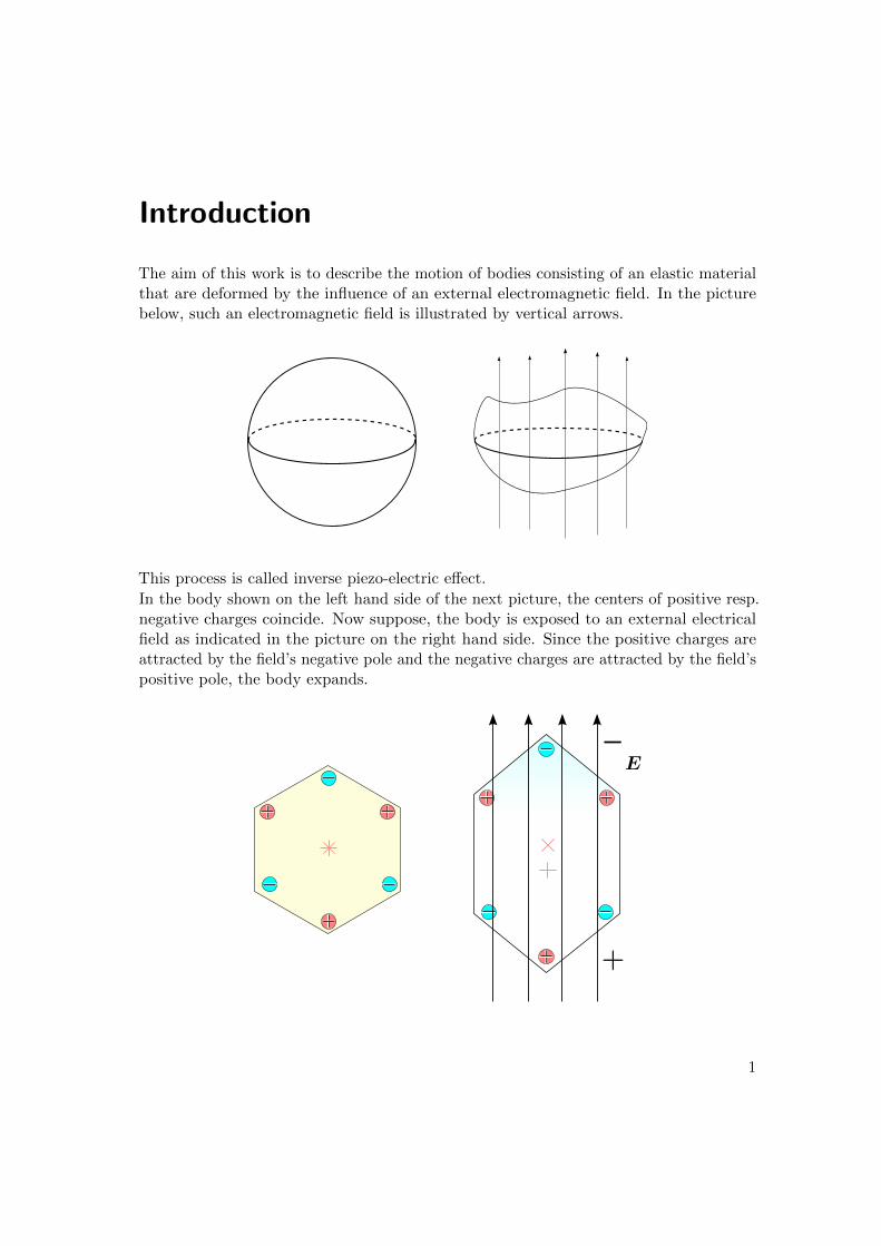
The aim of this work is to describe the motion of bodies consisting of an elastic materialthat are deformed by the influence of an external electromagnetic field. In the picturebelow, such an electromagnetic field is illustrated by vertical arrows.
This process is called inverse piezo-electric effect.
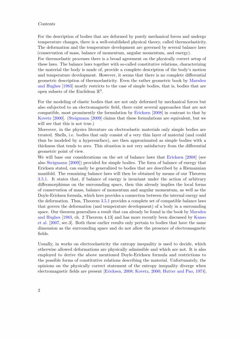
In the body shown on the left hand side of the next picture, the centers of positive resp.negative charges coincide. Now suppose, the body is exposed to an external electricalfield as indicated in the picture on the right hand side. Since the positive charges areattracted by the field’s negative pole and the negative charges are attracted by the field’spositive pole, the body expands.
1
Contents
For the description of bodies that are deformed by purely mechanical forces and undergotemperature changes, there is a well-established physical theory, called thermoelasticity.The deformation and the temperature development are governed by several balance laws(conservation of mass, balance of momentum, angular momentum, and energy).
For thermoelastic processes there is a broad agreement on the physically correct setup ofthese laws. The balance laws together with so-called constitutive relations, characterizingthe material the body is made of, provide a complete description of the body’s motionand temperature development. However, it seems that there is no complete differentialgeometric description of thermoelasticity. Even the rather geometric book by Marsdenand Hughes [1983] mostly restricts to the case of simple bodies, that is, bodies that areopen subsets of the Euclidean R3.
For the modeling of elastic bodies that are not only deformed by mechanical forces butalso subjected to an electromagnetic field, there exist several approaches that are notcompatible, most prominently the formulation by Ericksen [2008] in contrast to that byKovetz [2000]. (Steigmann [2009] claims that these formulations are equivalent, but wewill see that this is not true.)
Moreover, in the physics literature on electroelastic materials only simple bodies aretreated. Shells, i.e. bodies that only consist of a very thin layer of material (and couldthus be modeled by a hypersurface), are then approximated as simple bodies with athickness that tends to zero. This situation is not very satisfactory from the differentialgeometric point of view.
We will base our considerations on the set of balance laws that Ericksen [2008] (seealso Steigmann [2009]) provided for simple bodies. The form of balance of energy thatEricksen stated, can easily be generalized to bodies that are described by a Riemannianmanifold. The remaining balance laws will then be obtained by means of our Theorem3.5.1. It states that, if balance of energy is invariant under the action of arbitrarydiffeomorphisms on the surrounding space, then this already implies the local formsof conservation of mass, balance of momentum and angular momentum, as well as theDoyle-Ericksen formula, which here provides a connection between the internal energy andthe deformation. Thus, Theorem 3.5.1 provides a complete set of compatible balance lawsthat govern the deformation (and temperature development) of a body in a surroundingspace. Our theorem generalizes a result that can already be found in the book by Marsdenand Hughes [1983, ch. 2 Theorem 4.13] and has more recently been discussed by Kansoet al. [2007, sec.3]. Both these earlier results only pertain to bodies that have the samedimension as the surrounding space and do not allow the presence of electromagneticfields.
Usually, in works on electroelasticity the entropy inequality is used to decide, whichotherwise allowed deformations are physically admissible and which are not. It is alsoemployed to derive the above mentioned Doyle-Ericksen formula and restrictions tothe possible forms of constitutive relations describing the material. Unfortunately, theopinions on the physically correct statement of the entropy inequality diverge whenelectromagnetic fields are present [Ericksen, 2008; Kovetz, 2000; Hutter and Pao, 1974].
2
Contents
A further problem in the formulation of an electroelastic theory on manifolds is that theentropy inequality, as it relies on the entropy flux to be tangential to the deformed body,is only applicable to simple bodies. For general bodies, in particular if they are subjectedto an electromagnetic field, this needs not to be the case.
In order to replace the entropy inequality from the outset, we demand that for a givenprocess, balance of energy is invariant under the action of arbitrary diffeomorphisms onthe surrounding space and under linear rescalings of the temperature (see Theorem 5.3.4).This generalizes a theorem of Marsden and Hughes [1983]. This time, our result is, liketheirs, only valid for simple bodies, but it could possibly be generalized to arbitrary bodies.Moreover, in the physics literature one usually starts with quite strong assumptions onthe form of the constitutive relations and deduces a number of further restrictions onits form by means of the entropy inequality. By means of Theorem 5.3.4 we are able todeduce the same restrictions using much weaker assumptions.
Finally, we shortly present the partial differential equation that governs the motion of asimple body that is made from a Neo-electroelastic material.
In the first chapter we reproduce some basic notions and concepts of classical elasticitytheory. We explain what the deformation and the motion of a body are and give geometricdefinitions of the body’s velocity and acceleration. For that purpose we have to definethe substantial derivative that provides the time derivative of a moved continuous body.
Moreover, we recall the definition of certain tensors that describe, in what way thegeometry (lengths, angles) of the body is deformed during its motion.
Furthermore we study important general aspects of balance laws.
In the second chapter we recall some basics of electrodynamics that will be needed lateron. We state Maxwell’s equations in terms of vector fields and also in terms of differentialforms. Moreover we discuss Galilei transformations as well as Galilei invariants andintroduce the notions of polarization and magnetization.
The third chapter comprises the formulation of the balance laws for electroelasticity.We introduce the Cauchy stress tensor that provides a measure for the forces that thedeformation causes inside the body. Some of these laws are formulated at first only forthe case that the surrounding space is the Euclidean R3.
The central theorem of this chapter is Theorem 3.5.1. It provides among other thingslocal forms of balance of momentum and angular momentum that are also valid if thebody and the surrounding space are arbitrary Riemannian manifolds, as well as theafore-mentioned Doyle-Ericksen formula. Since the motion of the body is governed bybalance of momentum, Theorem 3.5.1 now provides the means to determine (in principle)the body’s motion.
In the fourth chapter we reformulate the balance laws and the Doyle-Ericksen formulathat we have obtained in the third chapter in terms of the coordinates on the undeformed
3
Contents
body. This makes their study much easier.
The fifth chapter discusses certain properties of the material. These are encoded in theso-called constitutive relations providing a connection between the exterior influences(for example the electromagnetic field) and material quantities (for example the internalenergy).We recall the notion of thermoelastic materials, i.e. materials for which the materialquantities only depend on the deformation and the temperature as well as their derivativesup to a certain order. Then we cite a result of Marsden and Hughes [1983] that providessome restrictions to the constitutive relations resulting from covariance assumptions andbalance of energy. In contrast to section 3.5 we do not consider all processes, but rather alltransformations of a given process. Next, material symmetries and in particular isotropicmaterials are discussed. As particular materials the Mooney-Rivlin and Neo-Hookeanmaterials are considered.Then we define thermoelectromagnetoelastic materials and deduce by means of Theorem5.3.4 quite strong restrictions to the possible forms of constitutive relations for suchmaterials. This generalizes a result of Marsden and Hughes [1983] that was given forthermoelastic materials.After that we discuss constitutive relations for Neo-electroelastic materials, ie. for mate-rials that can interact with an external electric field. They are defined as a generalizationof the Neo-Hookean materials that are known from classical elasticity theory.
Finally, in the sixth chapter we shortly present the partial differential equation thatgoverns the motion of a simple body that is made from a Neo-electroelastic material.
4
1 Geometric Setup and Basic Definitions
In this chapter we reproduce some basic notions and concepts of classical elasticity theory.We explain what the deformation and the motion of a body are and give geometricdefinitions of the body’s velocity and acceleration. For that purpose we have to definethe substantial derivative that provides the time derivative of a moved continuous body.
Moreover, we recall the definition of certain tensors that describe in what way thegeometry (length, arcs) of the body is deformed during its motion. Later on, in chapter3, we will establish a number of balance laws, like for example balance of momentum,that govern the body’s motion. Since all of these laws have essentially the same form, itis convenient to study them in general. This is done in section 1.3. In anticipation ofchapter 3, we will already treat conservation of mass, for the treatment of all the otherbalance laws will become easier, if conservation of mass is valid. Most of the material forthis introductory chapter is taken from Bar [2014] and Marsden and Hughes [1983].
1.1 Deformations
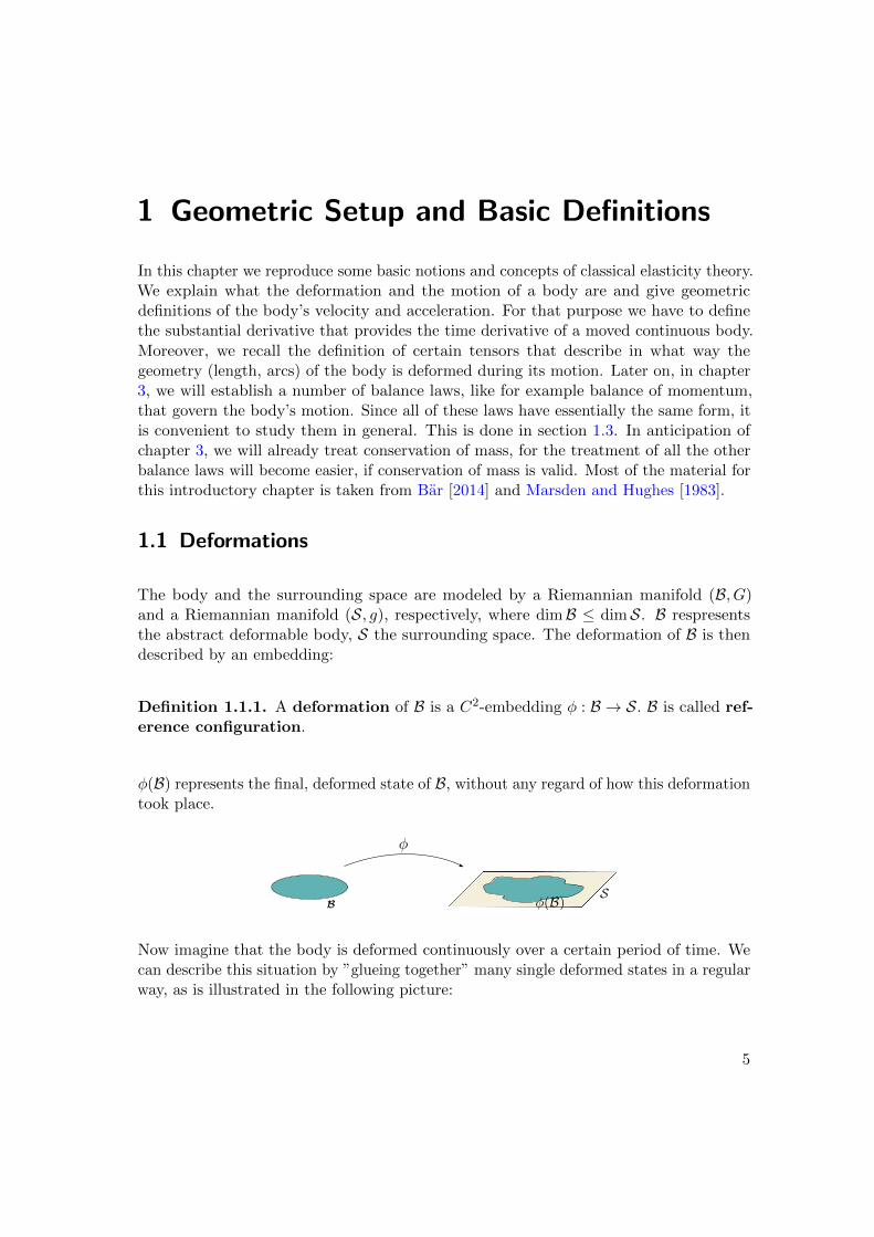
The body and the surrounding space are modeled by a Riemannian manifold (B, G)and a Riemannian manifold (S, g), respectively, where dimB ≤ dimS. B respresentsthe abstract deformable body, S the surrounding space. The deformation of B is thendescribed by an embedding:
Definition 1.1.1. A deformation of B is a C2-embedding φ : B → S. B is called ref-erence configuration.
φ(B) represents the final, deformed state of B, without any regard of how this deformationtook place.
Now imagine that the body is deformed continuously over a certain period of time. Wecan describe this situation by ”glueing together” many single deformed states in a regularway, as is illustrated in the following picture:
5
1 Geometric Setup and Basic Definitions
More formally, we define:
Definition 1.1.2. Denote by D(B) the set of all deformations of B in S, and let I ⊂ Rbe an open interval. A motion of a body B in S is a curve in D(B), that is, a C2-map
φ : B × I → D(B)
(X, t) 7→ φ(X, t),
such that for each t ∈ I the map φt := φ(·, t) is a deformation.
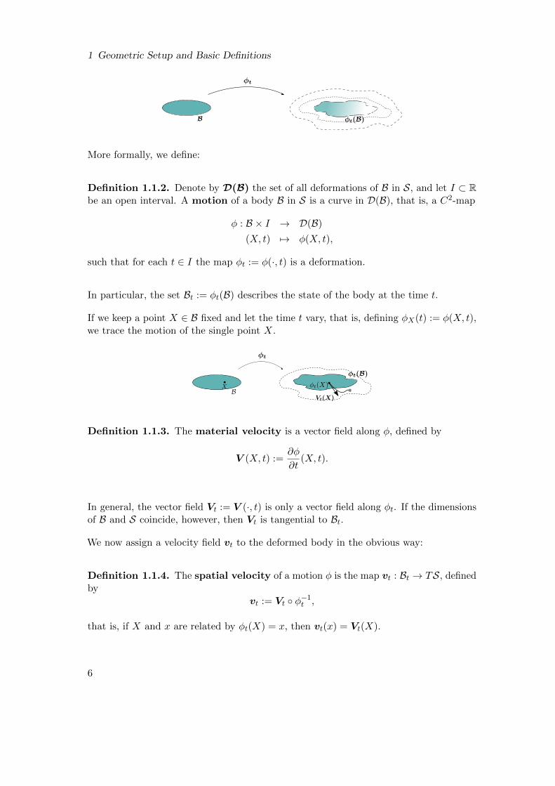
In particular, the set Bt := φt(B) describes the state of the body at the time t.
If we keep a point X ∈ B fixed and let the time t vary, that is, defining φX(t) := φ(X, t),we trace the motion of the single point X.
Definition 1.1.3. The material velocity is a vector field along φ, defined by
V (X, t) :=∂φ
∂t(X, t).
In general, the vector field Vt := V (·, t) is only a vector field along φt. If the dimensionsof B and S coincide, however, then Vt is tangential to Bt.
We now assign a velocity field vt to the deformed body in the obvious way:
Definition 1.1.4. The spatial velocity of a motion φ is the map vt : Bt → TS, definedby
vt := Vt φ−1t ,
that is, if X and x are related by φt(X) = x, then vt(x) = Vt(X).
6
1.1 Deformations
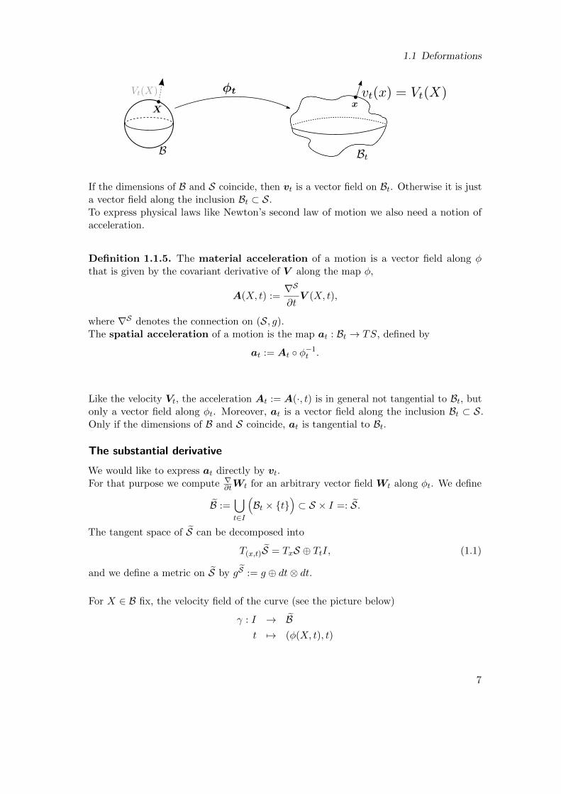
If the dimensions of B and S coincide, then vt is a vector field on Bt. Otherwise it is justa vector field along the inclusion Bt ⊂ S.To express physical laws like Newton’s second law of motion we also need a notion ofacceleration.
Definition 1.1.5. The material acceleration of a motion is a vector field along φthat is given by the covariant derivative of V along the map φ,
A(X, t) :=∇S
∂tV (X, t),
where ∇S denotes the connection on (S, g).The spatial acceleration of a motion is the map at : Bt → TS, defined by
at := At φ−1t .
Like the velocity Vt, the acceleration At := A(·, t) is in general not tangential to Bt, butonly a vector field along φt. Moreover, at is a vector field along the inclusion Bt ⊂ S.Only if the dimensions of B and S coincide, at is tangential to Bt.
The substantial derivative
We would like to express at directly by vt.For that purpose we compute ∇∂tWt for an arbitrary vector field Wt along φt. We define
B :=⋃t∈I
(Bt × t
)⊂ S × I =: S.
The tangent space of S can be decomposed into
T(x,t)S = TxS ⊕ TtI, (1.1)
and we define a metric on S by gS := g ⊕ dt⊗ dt.
For X ∈ B fix, the velocity field of the curve (see the picture below)
γ : I → Bt 7→ (φ(X, t), t)
7
1 Geometric Setup and Basic Definitions
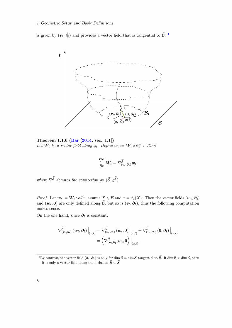
is given by (vt,∂∂t) and provides a vector field that is tangential to B. 1
Theorem 1.1.6 (Bar [2014, sec. 1.1])Let Wt be a vector field along φt. Define wt := Wt φ−1
t . Then
∇S
∂tWt = ∇S(vt,∂t)wt,
where ∇S denotes the connection on (S, gS).
Proof. Let wt := Wt φ−1t , assume X ∈ B and x = φt(X). Then the vector fields (wt,∂t)
and (wt,0) are only defined along B, but so is (vt,∂t), thus the following computationmakes sense.
On the one hand, since ∂t is constant,
∇S(vt,∂t) (wt,∂t)∣∣∣(x,t)
= ∇S(vt,∂t) (wt,0)∣∣∣(x,t)
+∇S(vt,∂t) (0,∂t)∣∣∣(x,t)
=
Å∇S(vt,∂t)wt,0
ã ∣∣∣(x,t)
.
1By contrast, the vector field (at,∂t) is only for dimB = dimS tangential to B. If dimB < dimS, then
it is only a vector field along the inclusion B ⊂ S.
8
1.1 Deformations
On the other hand, (vt,∂t) is the velocity field of the curve γ and hence
∇S(vt,∂t) (wt,∂t)∣∣∣(x,t)
=∇S
∂t(wt,∂t)
∣∣∣(x,t)
=∇S
∂t(wt,0)
∣∣∣(x,t)
+∇S
∂t(0,∂t)
∣∣∣(x,t)
=
Ç∇S
∂twt,0
å ∣∣∣(x,t)
=
Ç∇S
∂tWt(X),0
å,
where we have used again that ∂t is constant.
Comparing both expressions for ∇S(vt,∂t) (wt,∂t)∣∣∣(x,t)
, we conclude that
∇S
∂tWt = ∇S(vt,∂t)wt.
If the dimensions of the body and the surrounding space coincide, then not only (vt,∂t)is tangential to B, but (vt,0) and (0,∂t) are tangential to B, too. Then we are allowed
to decompose ∇S(vt,∂t)wt into
∇S(vt,∂t)wt = ∇S(vt,0)wt +∇S(0,∂t)wt. (1.2)
Now we can use the decomposition (1.1) and obtain
∇S(vt,0)wt = ∇Svtwt
∇S(0,∂t)wt =∇wt
∂t.
Thus,
∇S
∂tWt =
∇wt
∂t+∇Svtwt.
If dim B < dim S, then (vt,0) and (0,∂t) are not necessarily tangential to B. Thus the de-
composition (1.2) does not make sense, since the single summands∇S(vt,0)wt and∇S(0,∂t)wt
are not defined. In this case, we use the orthogonal projection tan : T(x,t)S → T(x,t)Bonto the tangent space T(x,t)B and write
∇S
∂tWt = ∇S(vt,∂t)wt
= ∇Stan(vt,∂t)wt
= ∇Stan(vt,0)wt +∇Stan(0,∂t)wt.
9
1 Geometric Setup and Basic Definitions
Definition 1.1.7. The vector field
wt := ∇S(vt,∂t)wt = ∇Stan(0,∂t)wt +∇Stan(vt,0)wt.
is called substantial (or material) derivative of wt. If the dimensions of B and Scoincide, then the projections are redundant and
wt =∇wt
∂t+∇Svtwt.
Thus, we have in particular
at =∇S
∂tVt φ−1
t = vt.
Let us consider the directional derivative ∂(vt,∂t)f of a function f ∈ C∞Ä‹B,Rä. This
derivative is well-defined, since (vt,∂t) is tangential to B. If the dimensions of B andS coincide, then (vt,0) and (0,∂t) are tangential to B, too, and we are allowed todecompose ∂(vt,∂t)f into
∂(vt,∂t)f = ∂(vt,0)f + ∂(0,∂t)f. (1.3)
Again, we can use the decomposition (1.1) and obtain
∂(vt,0)f = g(gradxf,vt)
∂(0,∂t)f =∂f
∂t,
where gradxf denotes the spatial gradient of f , that is, gradxf is tangential to Bt.Thus,
∂(vt,∂t)f =∂f
∂t+ g(gradxf,vt). (1.4)
If dim B < dim S, then the decomposition (1.3) does not make sense, since the singlesummands ∂(vt,0)f and ∂(0,∂t)f are not defined. Thus, we use again the orthogonal
projection tan : T(x,t)S → T(x,t)B onto the tangent space T(x,t)B and write
∂(vt,∂t)f = ∂tan(vt,∂t)f
= ∂tan(vt,0)f + ∂tan(0,∂t)f.
Definition 1.1.8. For any function f ∈ C∞ÄB,R
ä,
f := ∂(vt,∂t)f = ∂tan(0,∂t)f + ∂tan(vt,0)f
10
1.1 Deformations
is called substantial derivative of f . If the dimensions of B and S coincide, then thissimplifies to
f =∂f
∂t+ g(gradxf,vt).
Lemma 1.1.9The substantial derivative satisfies:
1) For any functions f, h ∈ C∞(B,R)
·f · h = f h+ f h.
2) Let Wt and Zt be vector fields along φt. Define wt := Wt φ−1t and zt := Zt φ−1
t .Then
·˝g(wt, zt) = g(wt, zt) + g(wt, zt).
Proof.
1) This follows immediately from the definition of the substantial derivative.
·f · h = ∂(vt,∂t)(f · h)
= (∂(vt,∂t)f) · h+ f · (∂(vt,∂t)h)
= f h+ f h.
2) A direct computation yields
·˝g(wt, zt) = ∂(vt,∂t)g(wt, zt)
= ∂(vt,∂t)gS(wt ⊕ 0, zt ⊕ 0)
= gSÄ∇S(vt,∂t)(wt ⊕ 0), zt ⊕ 0
ä+ gS
Äwt ⊕ 0,∇S(vt,∂t)(zt ⊕ 0)
ä= gS
Ä(∇S(vt,∂t)wt)⊕ 0, zt ⊕ 0
ä+ gS
Äwt ⊕ 0, (∇S(vt,∂t)zt)⊕ 0
ä= gÄ∇S(vt,∂t)wt, zt
ä+ gÄwt,∇S(vt,∂t)zt
ä= g(wt, zt) + g(wt, zt).
11
1 Geometric Setup and Basic Definitions
Remark 1.1.10. Assume that f : B → R is differentiable. Let us define a correspondingfunction F : B × I → R by
F (X, t) := f(φ(X, t), t).
Let ψ : B × I → B be given by (X, t)ψ7→ (φ(X, t), t). Then for x = φt(X),
f(x, t) = ∂(vt,∂t)f∣∣∣(x,t)
= df∣∣∣(x,t)
(vt,∂t)
=
ïdF∣∣∣ψ−1(x,t)
dψ−1∣∣∣(x,t)
ò(vt,∂t)
= dF∣∣∣(X,t)
(∂t)
=∂F
∂t(X, t).
Thus, the time derivatives of F and f are related by
∂F
∂t= f ψ. (1.5)
Notation 1.1.11. In accordance with standard notation of elasticity, points in B orother geometrical expressions concerning B are denoted by capital letters, whereas quan-tities concerning S are denoted by small letters. Bold letters are used for vector andtensors fields, calligraphic letters for tensor fields coming from elasticity theory. Notethat a list of symbols can be found in the index at the end of this work.
Occasionally we will consider bodies for which the substantial derivatives and later theequations governing the motion of the body are especially simple:
Definition 1.1.12. A simple body is the closure Ω of a bounded, open, connectedsubset Ω ⊂ R3.
1.2 Deformation Tensors
The contents of the first part of this section are taken from Marsden and Hughes [1983].
Definition 1.2.1. Let φ : B → S be a deformation. The deformation gradient F ofφ is given by the differential of φ:
F |X := dφ|X .
12
1.2 Deformation Tensors
Remark 1.2.2. Let XA and xa denote local coordinates on B and S, respectively.Then in components,
FaA(X) =∂φa
∂XA(X).
The coordinates of the transpose, FT , are given byÄFTäA
a(x) = gab(x)FbB(X)GAB(X),
where x = φ(X).
For the deformation φ : B → R3 of a simple body B,
φ(x+ h)− φ(x) = F(h) + o(h)
and hence
‖φ(x+ h)− φ(x)‖2 = ‖F(h)‖2 + oÄ‖h‖2
ä=¨h,FTF(h)
∂+ oÄ‖h‖2
ä.
Thus, we expect FTF to be a measure for local changes of the body’s form. Hence wemake the following definition.
Definition 1.2.3. The tensor
C∣∣∣x
: TXB → TXB
V 7→ C|X(V ) := (F |X)TF |X(V ).
is called deformation or (right Cauchy-Green) strain tensor.
Theorem 1.2.4 (Marsden and Hughes [1983, ch.1, Prop. 3.6])C is symmetric and positive definite and in particular invertible.
Proof. For V ,W ∈ TXB
G(C(V ),W ) = GÄFT F(V ),W
ä= G
ÄV ,FT F(W )
ä= G(V ,C(W )),
so C is symmetric. Since G(C(V ),V ) = g(F(V ),F(V )) ≥ 0, C is non-negative.
Assume now G(C(V ),V ) = 0. Then g(F(V ),F(V )) = 0. Since φ is an embedding, Fis one-to-one, and the last equation implies that V must be zero.
13
1 Geometric Setup and Basic Definitions
Remark 1.2.5. C can also be defined, if φ is not an embedding, but only smooth. ThenC will still be symmetric, but it will only be non-negative and thus not invertible ingeneral.
Remark 1.2.6 (Marsden and Hughes [1983], ch.1, Prop. 4.13).The deformation tensor is related to the metric g by C[ = φ∗g:
C[(W1,W2) = G(C(W1),W2) = G(FTF(W1),W2) = g(F(W1),F(W2))
= (φ∗g)(W1,W2).
If XA and xa denote local coordinate systems on B and S, respectively, then incomponents,
(C[|X)AB = gab|x(F|X)aA (F|X)bB = gab|x∂φa
∂XA
∂φb
∂XB.
Recall that the length of a piecewise C1-curve γ : [a, b]→ B is given by
l(γ) =
b∫a
∥∥γ′(s)∥∥ ds.
Theorem 1.2.7 (Marsden and Hughes [1983, ch.1, Prop. 3.16])Let γ be a C1-curve in B and let φ be a deformation of B in S. Let γ = φ γ be theimage of γ under φ. Then
l (γ) =
b∫a
√GÄγ′(s),C (γ′(s))
äds.
In particular, the length of γ only depends on the deformation tensor C and γ.
Proof. By the chain rule, γ′(s) = F |γ(s) (γ′(s)). Thus,∣∣γ′(s)∣∣2 = gÄF(γ′(s)
),F
(γ′(s)
) ä= G
Äγ′(s),FTF
(γ′(s)
) ä= G
Äγ′(s),C
(γ′(s)
) ä.
This yields
l (γ) =
b∫a
√GÄγ′(s),C (γ′(s))
äds.
14
1.2 Deformation Tensors
We have just seen that for some curve γ on B and some fixed deformation φ the defor-mation tensor C relates the length of γ with the length of φ(γ). The following tensordescribes how the angle between the images of tangent vectors on B changes during amotion φ : B × I → S.
Definition 1.2.8. The tensor D|(X,t) : TXB → TXB, defined by
D|(X,t) :=1
2
∂C∂t|(X,t)
is called material rate of deformation tensor.
Theorem 1.2.9 (Marsden and Hughes [1983, ch.1, Prop. 3.30])D is a measure for the geodesic deviation caused by the deformation φt:Let W1,W2 ∈ TXB and wi(t) := F |(X,t)(Wi), i = 1, 2. Then
d
dtgÄw1(t),w2(t)
ä= G
ÄW1, 2D|(X,t)(W2)
ä.
That is, D measures the change of the angle between w1(t) and w2(t) with time.
Proof. Let W1,W2 ∈ TXB and wi(t) := F |(X,t)(Wi), i = 1, 2. Then
d
dtgÄw1(t),w2(t)
ä=
d
dtgÄF |(X,t)(W1),F |(X,t)(W2)
ä=
d
dtGÄW1, (F |(X,t))TF |(X,t)(W2)
ä=
d
dtG(W1,C|(X,t)(W2))
= GÄW1, 2D|(X,t)(W2)
ä.
We would like to express D directly in terms of the motion.
Theorem 1.2.10 (Marsden and Hughes [1983, ch. 1, Prop. 5.14])The rate of deformation tensor satisfies
D[ =1
2
∂
∂t
Äφ∗t gä
=1
2φ∗t
((∇Sv)[ +
î(∇Sv)[
óT).
To prove this theorem we need to compute the time derivative of F t := dφt.
15
1 Geometric Setup and Basic Definitions
Lemma 1.2.11Let us define F t := dφt. Then
d
dtF t = (∇Sv) F t.
Proof. Assume thatW ∈ TXB. Let γ : (−a, a)→ B be a curve on B, such that γ(0) = W .Then
dF t
dt(W ) =
∇∂t
(F t(W ))
=∇∂t
(dφt(W ))
=∇∂t
Åd
ds(φt γ)|s=0
ã=∇∂s
Å∂
∂t(φt γ)
ã|s=0
=∇∂s
(Vt γ(s)) |s=0
= ∇WV= ∇Sdφt(W )v.
Here, ∇WV denotes the covariant derivative of V in the direction of W along the mapφt. Thus, d
dt F t = (∇Sv) F t.
Proof of Theorem 1.2.10. By Remark 1.2.6,
2D[ =∂
∂tC[ =
∂
∂t
Äφ∗t gä.
Let W1,W2 ∈ TB. Then
∂
∂t
Äφ∗t gä(W1,W2) =
∂
∂t(g(F t(W1),F t(W2)))
= g
ÅdF t
dt(W1),F t(W2)
ã+ g
ÅF(W1),
dF t
dt(W2)
ãEmploying Lemma 1.2.11 we obtain
∂
∂t
Äφ∗t gä(W1,W2) = g
Ä∇Sdφt(W1)v, dφt(W2)
ä+ gÄdφt(W1),∇Sdφt(W2)v
ä= φ∗t (∇Sv)[(W1,W2) + φ∗t
î(∇Sv)[
óT(W1,W2).
16
1.2 Deformation Tensors
Definition 1.2.12. We define the spatial rate of deformation tensor d : T B → T Bby
d[ := φ∗D[ =1
2Lvg.
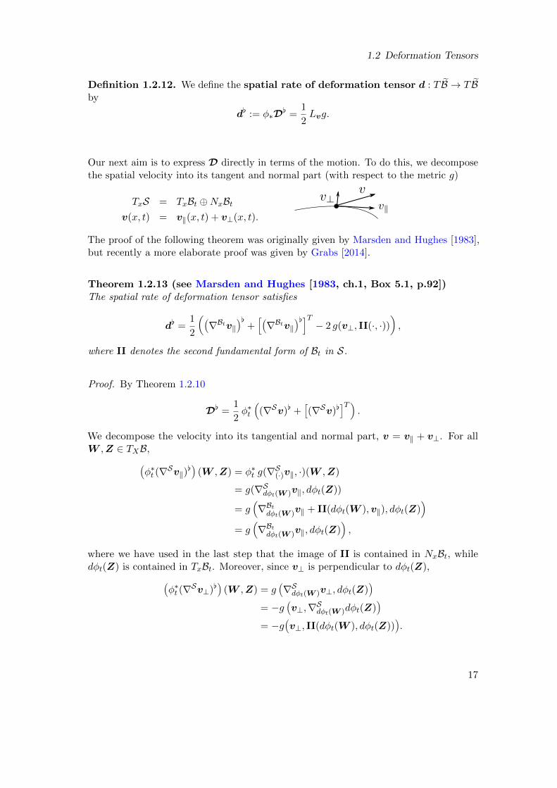
Our next aim is to express D directly in terms of the motion. To do this, we decomposethe spatial velocity into its tangent and normal part (with respect to the metric g)
TxS = TxBt ⊕NxBtv(x, t) = v‖(x, t) + v⊥(x, t).
The proof of the following theorem was originally given by Marsden and Hughes [1983],but recently a more elaborate proof was given by Grabs [2014].
Theorem 1.2.13 (see Marsden and Hughes [1983, ch.1, Box 5.1, p.92])The spatial rate of deformation tensor satisfies
d[ =1
2
ÅÄ∇Btv‖
ä[+[Ä∇Btv‖
ä[]T − 2 g(v⊥, II(·, ·))ã,
where II denotes the second fundamental form of Bt in S.
Proof. By Theorem 1.2.10
D[ =1
2φ∗t
((∇Sv)[ +
î(∇Sv)[
óT).
We decompose the velocity into its tangential and normal part, v = v‖ + v⊥. For allW ,Z ∈ TXB,Ä
φ∗t (∇Sv‖)[ä
(W ,Z) = φ∗t g(∇S(·)v‖, ·)(W ,Z)
= g(∇Sdφt(W )v‖, dφt(Z))
= g(∇Btdφt(W )v‖ + II(dφt(W ),v‖), dφt(Z)
)= g
(∇Btdφt(W )v‖, dφt(Z)
),
where we have used in the last step that the image of II is contained in NxBt, whiledφt(Z) is contained in TxBt. Moreover, since v⊥ is perpendicular to dφt(Z),Ä
φ∗t (∇Sv⊥)[ä
(W ,Z) = gÄ∇Sdφt(W )v⊥, dφt(Z)
ä= −g
Äv⊥,∇Sdφt(W )dφt(Z)
ä= −g
Äv⊥, II(dφt(W ), dφt(Z))
ä.
17
1 Geometric Setup and Basic Definitions
Thus, φ∗tÄ(∇Sv)[
ä: TXB × TXB → R is given by
φ∗tÄ(∇Sv)[
ä= φ∗t
Ä(∇Btv‖)[ − g(v⊥, II(·, ·))
äHence,
d[ =1
2
((∇Btv‖)[ − g(v⊥, II(·, ·)) +
î(∇Btv‖)[ − g(v⊥, II(·, ·))
óT)=
1
2
((∇Btv‖)[ +
î(∇Btv‖)[
óT − 2 g(v⊥, II(·, ·))).
Notation 1.2.14.Let S be a (p, q) tensor and T be a (r, s) tensor, where p+ q = r + s. Then we definethe scalar product of S and T as the contraction of S] and T [ on all entries. That is, ifE1, . . . , Em is a basis of TXB and E1, . . . , Em is the corresponding dual basis, then
〈S,T 〉 := S](EA1 , . . . , EAp , EB1 , . . . , EBq)T [(EA1 , . . . , EAp , EB1 , . . . , EBq).
In components,
〈S,T 〉 = SA1...ApB1...BqTA1...ApB1...Bq .
This definition is independent of the choice of the basis E1, . . . , Em.If E1, . . . , Em is an orthonormal basis, then we may also write
〈S,T 〉 = S[(EA1 , . . . , EAp , EB1 , . . . , EBq)T [(EA1 , . . . , EAp , EB1 , . . . , EBq),
or in components,
〈S,T 〉 =m∑
A1,...,Bs=1
SA1...ApB1...BqTA1...ArB1...Bs .
Moreover, if S and T are (1, 1) tensors, then 〈S,T 〉 coincides with
tr(S T ) =m∑A=1
g(S T (EA), EA).
If Vt and Wt are vector fields along the deformation φt and x = φt(X), then
〈Vt,Wt〉(X) = (Vt)a (Wt)a = gab(x) (Vt)
a(X) (Wt)b(X) = gx(Vt(X),Wt(X)).
For vector fields v and w on S
〈v,w〉 = vawa = gab vawb = g(v,w).
18
1.3 The Master Balance Law
1.3 The Master Balance Law
1.3.1 The Spatial Master Balance Law
Let φt : B → S be a time-dependent deformation. The metric g of S can be restricted toa metric gt on Bt, which induces the volume element volt on Bt.For each subset U of B we define Ut := φt(U). We will call a set U ⊂ B nice if it is openand relatively compact with piecewise C1-boundary.
The motion of B is governed by a system of partial differential equations that consists ofbalance laws including the acting forces and exchanged energies. All of these balancelaws are essentially of the following form:
Definition 1.3.1 (Marsden and Hughes [1983]). Let a, b : Bt × I → R be scalarfunctions on Bt and c be a scalar function on the unit tangent bundle of Bt × I.
We say that a, b, and c satisfy the (spatial) master balance law, if for any nice setU ⊂ B
i) the integrals in iii) exist,
ii)∫Ut
avolt is differentiable in t,
iii) andd
dt
∫Ut
avolt =
∫Ut
bvolt +
∫∂Ut
cÄx, t,n
ävol∂Ut , (1.6)
where n is the unit outward normal field to ∂Ut.
Remark 1.3.2. Sloppily said, the master balance law states that the rate of increaseof a over the volume Ut is equal to sources b inside of Ut inducing the growth of a andsome inflow c through the boundary of Ut.
If the body is isolated (which means that b = 0 and that c = 0 on ∂Ut), then a is constantin time.
The following theorem is one of the most fundamental theorems of elasticity theory. Itcan be found, for example, in the book of [Marsden and Hughes, 1983, ch.2, Th. 1.9].Here, we state it in a form that is similar to the one presented in Bar [2014].
Let St ⊂ TBt be the unit tangent bundle. Similar to the construction of B in section 1.1,we define the sphere bundle SB over B by
SB :=⋃t∈I
(St × t
)→⋃t∈I
(Bt × t
)= B
19
1 Geometric Setup and Basic Definitions
Theorem 1.3.3 (Cauchy’s Theorem, Bar [2014, Satz 2.2.1])Let a, b : B → R be C2 functions and assume that c : SB → R is C2. Moreover, assumethat a, b, and c satisfy the master balance law, which means for all nice sets U b B
d
dt
∫Ut
a(x, t) volt =
∫Ut
b(x, t) volt +
∫∂Ut
c(x, t,n) vol∂Ut ,
where n is the unit outward normal to ∂Ut. Then for every (x, t) ∈ B the function c ison TxBt the restriction of a linear function. In particular, there is a unique vector field con ∂Ut, such that
c(x, t,n) = gt(c(x, t),n).
Corollary 1.3.4a, b, and c as defined in Theorem 1.3.3 satisfy the spatial master balance law if and onlyif
d
dt
∫Ut
avolt =
∫Ut
bvolt +
∫∂Ut
gt(c(x, t),n) vol∂Ut . (1.7)
To find a local form form of the master balance law, we have to pull the derivative ddt into
the integral∫Uta(x, t) volt, keeping in mind that the domain of integration also depends
on t. The Transport Theorem below will explain how this can be done.
The Transport Theorem
Let VOL be the volume element induced on B by G. Let φt : B → S be a time-dependentconfiguration, and for each X ∈ B define as usual x ∈ Bt by x = φt(X).
Definition 1.3.5. We define J : B × I → R by
φ∗t (volt|x) = J (X, t) VOL|X .
Then, for every integrable function f : Bt → R and U ⊂ B∫Ut
f volt =
∫U
(f φt)J (·, t) VOL. (1.8)
By the transformation formula from integration theory,
J (X, t) = det(I dφt∣∣∣X
),
20
1.3 The Master Balance Law
where I : TxBt → TXB is an arbitrary isometry, such that I dφt∣∣∣X
: TXB → TXB is
orientation-preserving.
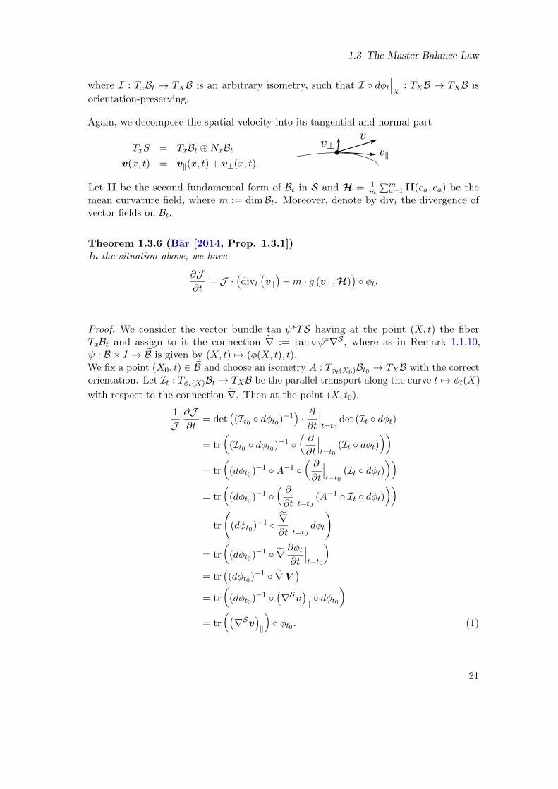
Again, we decompose the spatial velocity into its tangential and normal part
TxS = TxBt ⊕NxBtv(x, t) = v‖(x, t) + v⊥(x, t).
Let II be the second fundamental form of Bt in S and H = 1m
∑ma=1 II(ea, ea) be the
mean curvature field, where m := dimBt. Moreover, denote by divt the divergence ofvector fields on Bt.
Theorem 1.3.6 (Bar [2014, Prop. 1.3.1])In the situation above, we have
∂J∂t
= J ·Ädivt
Äv‖ä−m · g (v⊥,H)
ä φt.
Proof. We consider the vector bundle tan ψ∗TS having at the point (X, t) the fiberTxBt and assign to it the connection ‹∇ := tan ψ∗∇S , where as in Remark 1.1.10,ψ : B × I → B is given by (X, t) 7→ (φ(X, t), t).We fix a point (X0, t) ∈ B and choose an isometry A : Tφt(X0)Bt0 → TXB with the correctorientation. Let It : Tφt(X)Bt → TXB be the parallel transport along the curve t 7→ φt(X)
with respect to the connection ‹∇. Then at the point (X, t0),
1
J∂J∂t
= detÄ(It0 dφt0)−1
ä· ∂∂t
∣∣∣t=t0
det (It dφt)
= tr
Å(It0 dφt0)−1
Å∂
∂t
∣∣∣t=t0
(It dφt)ãã
= tr
Å(dφt0)−1 A−1
Å∂
∂t
∣∣∣t=t0
(It dφt)ãã
= tr
Å(dφt0)−1
Å∂
∂t
∣∣∣t=t0
(A−1 It dφt)ãã
= tr
((dφt0)−1
‹∇∂t
∣∣∣t=t0
dφt
)
= tr
Å(dφt0)−1 ‹∇ ∂φt
∂t
∣∣∣t=t0
ã= tr
Ä(dφt0)−1 ‹∇V ä
= tr
Å(dφt0)−1
Ä∇Sv
ä‖ dφt0
ã= tr
ÅÄ∇Sv
ä‖
ã φt0 . (1)
21
1 Geometric Setup and Basic Definitions
Let ea, a = 1, . . . ,m, be a local orthonormal frame for TBt. Then
tr
ÅÄ∇Sv
ä‖
ã φt0 =
m∑a=1
gÄ∇Seav, ea
ä φt0
=m∑a=1
îgÄ∇Seav‖, ea
ä+ gÄ∇Seav⊥, ea
äó φt0 (2)
Now we compute
m∑a=1
gÄ∇Seav‖, ea
ä=
m∑a=1
ÄgÄ∇Bteav‖, ea
ä+ gÄII(ea,v‖), ea
ää= divt v‖ (3)
and
m∑a=1
gÄ∇Seav⊥, ea
ä=
m∑a=1
Ä∂eag(v⊥, ea)− g(v⊥,∇Seaea)
ä= −
m∑a=1
gÄv⊥,∇Bteaea + II(ea, ea)
ä= −mg(v⊥,H). (4)
where we have used in the last step thatm∑a=1
II(ea, ea) = mH. Thus, by inserting (3) and
(4) into (2) and by use of (1), we obtain
∂J∂t
= J ·Ädivt v‖ −m · g (v⊥,H)
ä φt0 .
With the knowledge of ∂J∂t we immediately obtain the variation of the volume of the
deformed body.
Corollary 1.3.7 (Bar [2014, Satz 1.3.2 and Bem. 1.3.3])Assume that B is compact and that φ : B×I → S is a motion. Then the volume variationof B is given by
d
dtvol(Bt) =
∫Bt
Ädivt v‖ −m · g (v⊥,H)
ävolt.
22
1.3 The Master Balance Law
Proof. Theorem 1.3.6 implies that for each nice subset U of B and its image Ut,
d
dtvol(Bt) =
d
dt
∫Bt
volt
=d
dt
∫B
J (·, t) VOL
=
∫B
∂J∂t
VOL
=
∫B
îÄdivt
Äv‖ä−m · g (v⊥,H)
ä φtóJ (·, t) VOL
=
∫Bt
Ädivt
Äv‖ä−m · g (v⊥,H)
ävolt.
Theorem 1.3.8 (Transport Theorem, [see Bar, 2014, Kor. 1.3.4])Let f : B → R be smooth and assume that each f(·, t) is compactly supported. Then forthe image Ut := φt(B) of each nice set U ⊂ B,
d
dt
∫Ut
f(x, t) volt =
∫Ut
Äf + f · divt v‖ −mf · g (v⊥,H)
ävolt.
In particular, if dimB = dimS, then
d
dt
∫Ut
f(x, t) volt =
∫Ut
Äf + f · divt v
ävolt
=
∫Ut
Å∂f
∂t+ divt(fv)
ãvolt.
Proof.1) By (1.8) and Theorem 1.3.6,
d
dt
∫Ut
f(x, t) volt(x) =d
dt
∫U
f (φt(X), t) · J (X, t) VOL(X)
=
∫U
∂
∂t
(f (φt(X), t) · J (X, t)
)VOL(X)
=
∫U
Äf + f · divt
Äv‖ä−mf · g (v⊥,H)
ä(φt(X)) · J (X, t) VOL(X)
23
1 Geometric Setup and Basic Definitions
=
∫Ut
Äf + f · divt
Äv‖ä−mf · g (v⊥,H)
ä(x) volt(x).
2) If dimB = dimS, then v = v‖ while v⊥ = 0. In this case
f + f · divt(v) =∂f
∂t+ g(gradf,v) + f · divt(v) =
∂f
∂t+ divt(f · v).
Now we can use the Transport Theorem (Theorem 1.3.8) to obtain a local form of theMaster Balance Law:
Theorem 1.3.9 (Spatial Localization Theorem)Let a, b : B → R be scalar functions and c a vector field on B. Assume that a and c areC1 and b is C0. Then a, b, and c satisfy the master balance law if and only if
a+ a · divt(v‖)−mag(v⊥,H) = b+ divtc.
In particular, if dimB = dimS, then
∂a
∂t+ divt(av) = b+ divtc.
Proof. By the Transport Theorem (1.3.8), the master balance law is equivalent to∫Ut
[a+ a · divt(v‖)−ma · g (v⊥,H)
]volt =
∫Ut
bvolt +
∫Ut
divtcvolt
for the image Ut of any nice U ⊂ B. Thus, the first asserted formula follows immediately.
If the dimensions of B and S coincide, then v = v‖ and v⊥ is zero. In this case
a+ a · divt(v‖)−ma · g (v⊥,H) =∂a
∂t+ g(grad a,v) + a · divt(v)
=∂a
∂t+ divt(av).
1.3.2 The Material Master Balance Law
As we have already seen in Remark 1.1.10, it is much easier to compute time derivativeson the undeformed body. Hence we would like to transform the spatial Master BalanceLaw to a balance law that is formulated in terms of functions and vector fields definedon B × I. That is, we would like to replace
d
dt
∫Ut
avolt =
∫Ut
bvolt +
∫∂Ut
g(c,n) volt (1.9)
24
1.3 The Master Balance Law
by a balance law
d
dt
∫U
AVOL =
∫U
BVOL +
∫∂U
G(C,N) VOL∂U
on B, where N is the unit normal vector field on ∂U , and A, B, C are somehow connectedwith a, b, c, where we still have to determine how exactly they are related.
Because of the relation volt(x) = J (X, t) VOL(X) we can easily see that we could justdefine
A(X, t) := J (X, t) a(x, t) and B(X, t) := J(X, t) b(x, t),
where x = φt(X). Then∫Ut
a(x, t) volt(x) =
∫U
a(φ(X, t), t)J (X, t) VOL(X) =
∫U
A(X, t) VOL(X)
and analogously∫Ut
b(x, t) volt(x) =
∫U
B(X, t) VOL(X).
But how do we define C in such a way that the last term in (1.9) keeps its form ? Wewill see that c and C have to be related by a Piola transformation.
Recall that each φt : B → Bt is a diffeomorphism and that the pull-back of a vector fieldw on Bt to a vector field on B is given by
φ∗twt := dφ−1t wt φt.
Definition 1.3.10. The vector field
Wt := J (·, t) · (φ∗twt)
is called the Piola transformation of w.
Lemma 1.3.11 (Marsden and Hughes [1983, ch.1, Th. 7.19])A vector field Wt on B is the Piola transformation of a vector field wt on Bt if and onlyif
φ∗t (iwtvolt) = iWtVOL.
25
1 Geometric Setup and Basic Definitions
Proof. For each vector field wt that is tangential to Bt,
φ∗t (iwtvolt) = iφ∗twt (φ∗tvolt)
= iφ∗twt (J (·, t) ·VOL)
= iJ (·,t)·φ∗twtVOL.
Thus, Wt = J (·, t) · (φ∗twt) is equivalent to φ∗t (iwtvolt) = iWtVOL.
Theorem 1.3.12 (Piola Identity, [Marsden and Hughes, 1983, ch. 1, Th. 7.20])If Wt is the Piola transformation of wt, then
DIV(Wt) = J (·, t) · (divt(wt) φt).
Proof. For each nice U ⊂ B, ∫U
DIV(Wt) VOL =
∫∂U
iWtVOL (1)
and ∫U
J (·, t) · (divt(wt) φt) VOL =
∫Ut
divt(wt) volt
=
∫∂Ut
iwtvolt
=
∫∂U
φ∗t (iwtvolt) (2)
If Wt is the Piola transformation of wt, then by Lemma 1.3.11 the right hand sides of(1) and (2) coincide. Since U is arbitrary, we conclude that
DIV(Wt) = J (·, t) · (divt(wt) φt).
As an immediate consequence of Theorem 1.3.12 we obtain
Theorem 1.3.13Let a, b : Bt × I → R be scalar functions and let ct be a vector field on Bt.Let A,B : B × I → R be scalar functions and let Ct be a vector field on B. Assume thatA, B, Ct and a, b, ct are related by
A(X, t) = J (X, t) a(x, t)
B(X, t) = J (X, t) b(x, t)
Ct(X) = J (X, t)F−1(X, t)ct(x), i.e., Ct is the Piola transformation of ct.
26
1.3 The Master Balance Law
Then a, b, ct satisfy the spatial master balance law if and only if A, B, Ct satisfy
d
dt
∫U
AVOL =
∫U
BVOL +
∫∂U
〈Ct,N〉VOL∂U .
Remark 1.3.14. Marsden and Hughes [1983] define the scalar functions A and Bwithout using the factor J and thus give a slightly different version of this theorem (seetheir Prop. 1.6 in ch.2).
Proof. As we have already seen,
d
dt
∫Ut
avolt =d
dt
∫U
AVOL,
∫Ut
bvolt =
∫U
BVOL.
Moreover, by Theorem 1.3.12,∫∂U
〈Ct,N〉VOL∂U =
∫U
DIVCt VOL =
∫U
J · (divt ct) φt VOL
=
∫Ut
divt ct volt =
∫∂Ut
〈ct,n〉vol∂Ut .
Thus we define the notion of a master balance law on B as follows:
Definition 1.3.15. Let A,B : B× I → R be scalar functions and Ct a vector field on B.We say that A, B, and Ct satisfy the material master balance law, if for any niceset U ∈ B
i) the integrals in the following equation exist,
ii)∫U
AVOL is differentiable in t,
iii) andd
dt
∫U
AVOL =
∫U
BVOL +
∫∂U
〈Ct,N〉VOL∂U ,
where N is the unit outward normal to ∂U .
The local version of the Material Master Balance Law is easily found:
27
1 Geometric Setup and Basic Definitions
Theorem 1.3.16 (Material Localization Theorem)Let A,B : B × I → R be scalar functions and Ct a vector field on B. Assume that A and
B are C0, ∂A∂t exists, and Ct is C1. Then A, B, and Ct satisfy the master balance law if
and only if∂A
∂t= B + DIVCt. (1.10)
Proof. A direct differentiation under the integral sign and the Theorem of Stokes providethe stated equation.
Remark 1.3.17. The form of the Material Localization Theorem, given by Theorem1.3.16, slightly differs from the one given by Marsden and Hughes [1983] (see their Th.1.5 in ch.2).
1.3.3 Consequences of Conservation of Mass
If conservation of mass is given, then the Transport Theorem and the LocalizationTheorem can be considerably simplified.
Assume we are given a smooth mass density ρ : B → R.
Definition 1.3.18. The mass M of a nice set Ut ⊂ Bt is given by the integral of themass density
M(Ut) =
∫Ut
ρ(x, t) volt.
We say that ρ obeys conservation of mass, if for all nice Ut ⊂ Bt,
d
dt
∫Ut
ρ(x, t) volt = 0.
Conservation of mass states that the mass of any nice subset of U ⊂ B is constant intime.
We get at once from the spatial localization theorem (1.3.9) the local form of conservationof mass:
Theorem 1.3.19Conservation of mass is equivalent to the continuity equation
ρ+ ρdivt(v‖)−mρg(v⊥,H) = 0,
28
1.3 The Master Balance Law
where v denotes the body’s spatial velocity, m is the body’s dimension and H denotes themean curvature field.In particular, if dimB = dimS, then conservation of mass is equivalent to
∂ρ
∂t+ div (ρv) = 0.
It is now convenient to refer the quantities a and b in the spatial master balance law(Corollary 1.3.4) to the mass density ρ, that is, to consider instead of
d
dt
∫Ut
a(x, t) volt =
∫Ut
b(x, t) volt +
∫∂Ut
〈ct(x, t),n〉vol∂Ut
the balance law
d
dt
∫Ut
a(x, t)ρ(x, t) volt =
∫Ut
b(x, t)ρ(x, t) volt +
∫∂Ut
〈ct(x, t),n〉vol∂Ut .
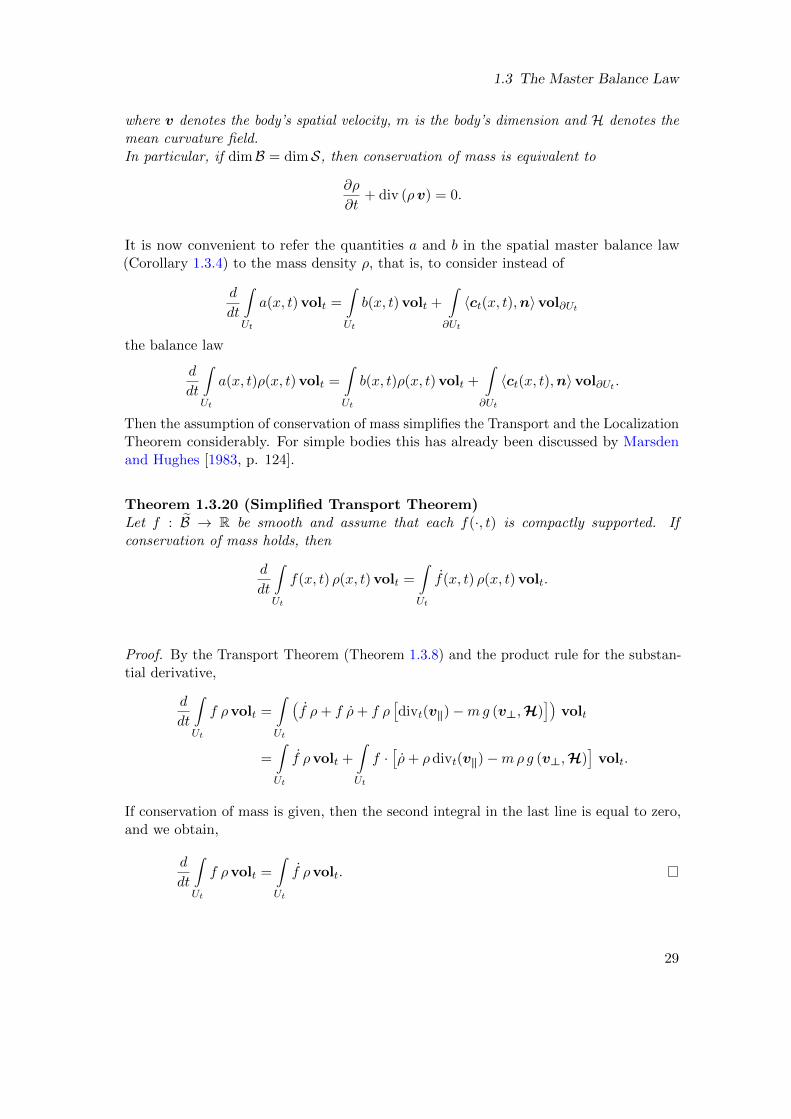
Then the assumption of conservation of mass simplifies the Transport and the LocalizationTheorem considerably. For simple bodies this has already been discussed by Marsdenand Hughes [1983, p. 124].
Theorem 1.3.20 (Simplified Transport Theorem)Let f : B → R be smooth and assume that each f(·, t) is compactly supported. Ifconservation of mass holds, then
d
dt
∫Ut
f(x, t) ρ(x, t) volt =
∫Ut
f(x, t) ρ(x, t) volt.
Proof. By the Transport Theorem (Theorem 1.3.8) and the product rule for the substan-tial derivative,
d
dt
∫Ut
f ρvolt =
∫Ut
Äf ρ+ f ρ+ f ρ
îdivt(v‖)−mg (v⊥,H)
óävolt
=
∫Ut
f ρvolt +
∫Ut
f ·îρ+ ρ divt(v‖)−mρg (v⊥,H)
óvolt.
If conservation of mass is given, then the second integral in the last line is equal to zero,and we obtain,
d
dt
∫Ut
f ρvolt =
∫Ut
f ρvolt.
29
1 Geometric Setup and Basic Definitions
Now we immediately obtain a simpler version of the Spatial Localization Theorem (1.3.9).A similar proof as the one given for Theorem 1.3.9 shows:
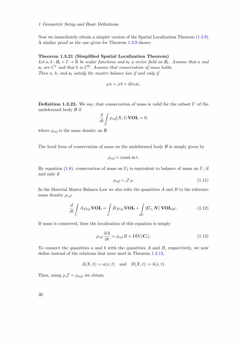
Theorem 1.3.21 (Simplified Spatial Localization Theorem)Let a, b : Bt × I → R be scalar functions and ct a vector field on Bt. Assume that a andct are C1 and that b is C0. Assume that conservation of mass holds.
Then a, b, and ct satisfy the master balance law if and only if
ρ a = ρ b+ divtct.
Definition 1.3.22. We say, that conservation of mass is valid for the subset U of theundeformed body B if
d
dt
∫U
ρref(X, t) VOL = 0,
where ρref is the mass density on B.
The local form of conservation of mass on the undeformed body B is simply given by
ρref = const.in t.
By equation (1.8), conservation of mass on Ut is equivalent to balance of mass on U , ifand only if
ρref = J ρ. (1.11)
In the Material Master Balance Law we also refer the quantities A and B to the referencemass density ρref:
d
dt
∫U
Aρref VOL =
∫U
B ρref VOL +
∫∂U
〈Ct,N〉VOL∂U . (1.12)
If mass is conserved, then the localization of this equation is simply
ρref∂A
∂t= ρrefB + DIV(Ct). (1.13)
To connect the quantities a and b with the quantities A and B, respectively, we nowdefine instead of the relations that were used in Theorem 1.3.13,
A(X, t) := a(x, t) and B(X, t) := b(x, t).
Then, using ρJ = ρref, we obtain
30
1.3 The Master Balance Law
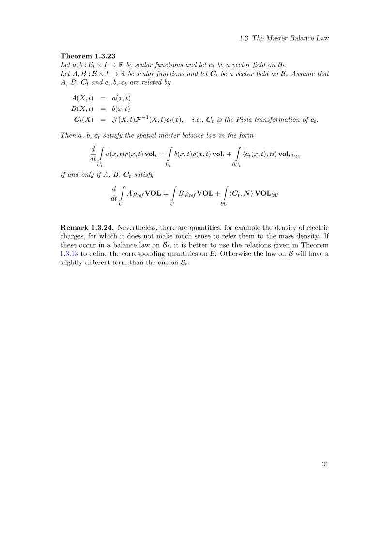
Theorem 1.3.23Let a, b : Bt × I → R be scalar functions and let ct be a vector field on Bt.Let A,B : B × I → R be scalar functions and let Ct be a vector field on B. Assume thatA, B, Ct and a, b, ct are related by
A(X, t) = a(x, t)
B(X, t) = b(x, t)
Ct(X) = J (X, t)F−1(X, t)ct(x), i.e., Ct is the Piola transformation of ct.
Then a, b, ct satisfy the spatial master balance law in the form
d
dt
∫Ut
a(x, t)ρ(x, t) volt =
∫Ut
b(x, t)ρ(x, t) volt +
∫∂Ut
〈ct(x, t),n〉vol∂Ut ,
if and only if A, B, Ct satisfy
d
dt
∫U
Aρref VOL =
∫U
B ρref VOL +
∫∂U
〈Ct,N〉VOL∂U
Remark 1.3.24. Nevertheless, there are quantities, for example the density of electriccharges, for which it does not make much sense to refer them to the mass density. Ifthese occur in a balance law on Bt, it is better to use the relations given in Theorem1.3.13 to define the corresponding quantities on B. Otherwise the law on B will have aslightly different form than the one on Bt.
31

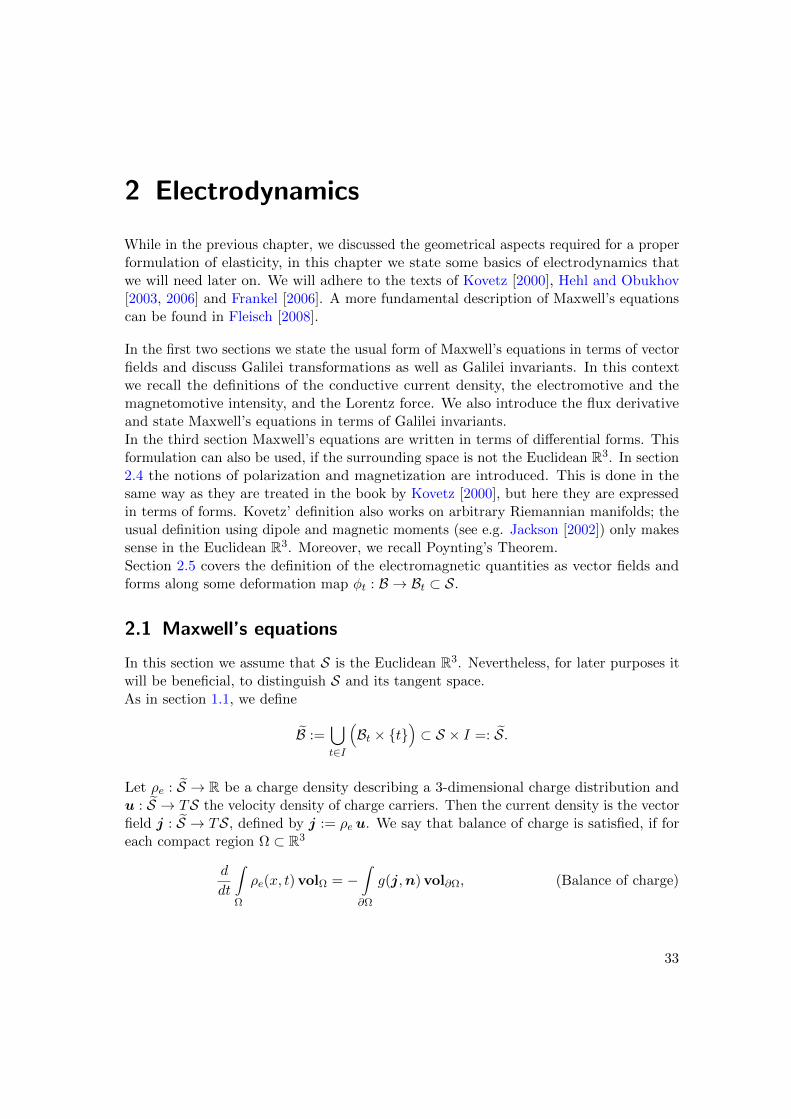
2 Electrodynamics
While in the previous chapter, we discussed the geometrical aspects required for a properformulation of elasticity, in this chapter we state some basics of electrodynamics thatwe will need later on. We will adhere to the texts of Kovetz [2000], Hehl and Obukhov[2003, 2006] and Frankel [2006]. A more fundamental description of Maxwell’s equationscan be found in Fleisch [2008].
In the first two sections we state the usual form of Maxwell’s equations in terms of vectorfields and discuss Galilei transformations as well as Galilei invariants. In this contextwe recall the definitions of the conductive current density, the electromotive and themagnetomotive intensity, and the Lorentz force. We also introduce the flux derivativeand state Maxwell’s equations in terms of Galilei invariants.
In the third section Maxwell’s equations are written in terms of differential forms. Thisformulation can also be used, if the surrounding space is not the Euclidean R3. In section2.4 the notions of polarization and magnetization are introduced. This is done in thesame way as they are treated in the book by Kovetz [2000], but here they are expressedin terms of forms. Kovetz’ definition also works on arbitrary Riemannian manifolds; theusual definition using dipole and magnetic moments (see e.g. Jackson [2002]) only makessense in the Euclidean R3. Moreover, we recall Poynting’s Theorem.
Section 2.5 covers the definition of the electromagnetic quantities as vector fields andforms along some deformation map φt : B → Bt ⊂ S.
2.1 Maxwell’s equations
In this section we assume that S is the Euclidean R3. Nevertheless, for later purposes itwill be beneficial, to distinguish S and its tangent space.
As in section 1.1, we define
B :=⋃t∈I
(Bt × t
)⊂ S × I =: S.
Let ρe : S → R be a charge density describing a 3-dimensional charge distribution andu : S → TS the velocity density of charge carriers. Then the current density is the vectorfield j : S → TS, defined by j := ρe u. We say that balance of charge is satisfied, if foreach compact region Ω ⊂ R3
d
dt
∫Ω
ρe(x, t) volΩ = −∫∂Ω
g(j,n) vol∂Ω, (Balance of charge)
33
2 Electrodynamics
where n denotes the (outer) unit normal vector field on ∂Ω.Let d : S → TS be the electric flux density. Then by Gauss’ Law, for any compact regionΩ ⊂ R3, ∫
∂Ω
〈d,n〉vol∂Ω =
∫Ω
ρe volΩ. (Gauss’ Law)
Let us denote by b : S → TS the magnetic flux density. Then the conservation law ofmagnetic flux states that for each compact oriented region Ω ⊂ R3,∫
∂Ω
〈b,n〉vol∂Ω = 0. (Conservation of magnetic flux)
Moreover, let e : S → TS be the electric field. By Faraday’s Induction Law, for eachcompact oriented surface Σ,∫
∂Σ
〈e, ξ〉vol∂Σ = −∫Σ
¨∂b∂t,n∂
volΣ. (Faraday’s Induction Law)
Here, ξ denotes the unit tangent vector field to ∂Σ. Furthermore, let us denote byh : S → TS the magnetic field. Ampere’s Law states that for each compact 2-sidedsurface Σ with prescribed normal n,∫
∂Σ
〈h, ξ〉vol∂Σ =
∫Σ
〈j,n〉volΣ +
∫Σ
¨∂d∂t,n∂
volΣ. (Ampere’s Law)
It is important to note that the balance of charge as well as Maxwell’s equations arethree-dimensional concepts and that the electromagnetic fields are in a sense a propertyof the surrounding space. If one wants to formulate balance of charge for a hypersurfaceor a one-dimensional body, one has to work with distributions. But here we will notneed to do that. Our present aim is just the statement of Maxwell’s equations for thesurrounding space.Later on, we are only interested in what happens inside the deformed body. Thus, werestrict the charge density and the electromagnetic fields to B and demand that the mapsρe : B → R, u : B → TS, j : B → TS as well as d : B → TS, b : B → TS, e : B → TSand h : B → TS are C2. Note that the flux density j is in general not tangential to Bt,we will discuss that later on.Then the local form of Maxwell’s equations states that on B
divd = ρe (Gauss’ Law)
div b = 0 (Conservation of magnetic flux)
rot e = −∂b∂t
(Faraday’s Induction Law)
rot h = j +∂d
∂t. (Ampere’s Law)
34
2.2 Galilei-invariants and the Lorentz force
The local expression for the balance of charge is given by
∂ρe∂t
+ div j = 0. (Balance of charge)
Remark 2.1.1. In Notation 1.1.11 we have stipulated to denote all quantities that aredefined on Bt or B by small letters, whereas quantities that are defined on B or B × I aredenoted by capital letters. d, b, e and h are vector fields on the surrounding space andcan be evaluated along B. Thus, in contrast to the classical literature on electrodynamics,we denote all the electromagnetic quantities by small letters.
2.2 Galilei-invariants and the Lorentz force
In this section we recall some material on Galilei transformations. Maxwell’s equationsare Lorentz invariant. But in the following chapters we will use notions and concepts fromthermodynamics. Unfortunately, it seems that a generally accepted theory of relativisticthermodynamics does not (yet) exist (see for instance Nakamura [2012] and Requardt[2008]).Moreover, we will need in the proof of Theorem 3.5.1 the splitting of the energy densityinto the internal energy density and the (macroscopic) kinetic energy. But relativistically,this splitting is not covariant.Thus, we will always restrict our considerations to motions with velocities that are smallcompared to the speed of light.
We continue to assume that S is the Euclidean R3. Let Σ′ be a coordinate system thatmoves with some constant small (compared to the speed of light) velocity w : S → TSwith respect to a given coordinate system Σ. Then the coordinates x′ and x of somepoint of S with respect to the systems Σ′ and Σ, respectively, are related by a Galileitransformation, usually stated as
x′ = x−w t. (2.1)
Velocities v′ and v that are measured in the primed and unprimed system are thereforeconnected by
v′ = v −w. (2.2)
On a deformed body Bt we can at each tangent space TxBt consider a different Galileitransformation with the velocity wt(x), demanding that these Galilei transformationsdepend smoothly on the point x, in other words, demanding that wt : Bt → TS is C∞.Then velocities in the primed and in the unprimed system are related by
v′(x′, t) = v(x, t)−w(x, t). (2.3)
The charge density, the electric flux density, and the magnetic flux density are invari-ant under Galilei transformations, that is, ρ′e(x
′, t) = ρe(x, t), d′(x′, t) = d(x, t), and
35
2 Electrodynamics
b′(x′, t) = b(x, t), whereas the current density, the electric field e, and the magnetic fieldh are not invariant. Recall that for charge carriers with the density ρe moving with thevelocity u : B → TS with respect to Σ, the current density j : B → TS is given by
j = ρe u.
The current densities in the primed and the unprimed system are related by
j′ = ρ′e u′ = ρe (u−w) = j − ρew.
Assume now that the material moves with the spatial velocity field v : B → TS. Wewould like to construct a current density that is Galilei-invariant. The obvious way to dois to take at each point the current density as it is seen in the system that moves alongwith the material in that point. That is, in the co-moved system Σ′ the material has thevelocity v′ = 0. Hence, the velocity of Σ′ with respect to Σ is given by w = v. Thus, wedefine the convective current density j : B → TS as
j := j − ρe v.
j is Galilei-invariant. The convective current density can be seen as a more fundamentalnotion than the current density j: It gives the current as it is seen from the material’spoint of view. Thus, j(·, t) is by definition tangential to Bt, otherwise the charge carrierswould leave the material. The current density j(·, t) = j(·, t) + ρe(·, t)v(·, t), however, isin general not tangential to Bt. It describes the motion of the material’s charge carriersfrom the point of view of an external observer, and for this observer the velocity of theirmotion inside the material and the motion of the material itself superimpose.
Recall that the electric fields as seen in the primed and the unprimed system, resp., areconnected by
e′ = e+w × b.
Again, we would like to define a quantity that is Galilei-invariant. If the material moveswith the velocity field v, then we take at each point of the material the electric field asit is seen in the co-moved frame, in which the material is at rest. Then w = v and wedefine the electromotive intensity e : S → TS as
e := e+ v × b.
Similarly, the magnetic fields in the primed and the unprimed system, resp., are connectedby
h′ = h−w × d,
and we can construct a Galilei-invariant version h : S → TS of h, the magnetomotiveintensity, by
h := h− v × d.
36
2.2 Galilei-invariants and the Lorentz force
Up to now we have not specified how electromagnetic fields act upon charged particlesmoving with the velocity u. This connection is provided by the Lorentz force. TheLorentz force fL : B → TS is defined as
fL = ρe e′′,
where e′′ : B → T S is now the electric field as it is seen from the charge carrier’s pointof view, that is, in a frame Σ′′ that moves with respect to Σ with the velocity w = u.Thus, e′′ = e+ u× b. Using j = ρe u, we obtain
fL = ρe e+ j × b.
This definition of the Lorentz force is Galilei-invariant. We might also express fL com-pletely in terms of Galilei-invariants (i.e. give the Lorentz force as it is seen from thematerial’s point of view) and write
fL = ρe e+ j × b.
Of course, one could also exchange the roles of the primed and the unprimed system andwrite
x′ = x+w t. (2.4)
Then the velocities, current densities and electric fields measured in the primed and theunprimed system are related by
v′ = v +w (2.5)
j′ = j + ρew
e′ = e−w × b.
Nevertheless, the definition of the Galilean invariants j, e and fL stays the same: If weobserve the current density and the electric field from the co-moved system, in whichthe velocity of the material is v′ = 0, then the velocity of this system is w = −v, andwe obtain again that j = j − ρe v and e = e + v × b. If we observe the electric fieldfrom the co-moved system Σ′′ of charge carriers moving with the velocity field u, thenthe velocity of Σ′′ with respect to Σ is given by w = −u, and we obtain once more thatfL = ρe e+ j × b.
It will turn out to be convenient to express the vectorial form of Maxwell’s equationscompletely in terms of the Galilei-invariants d, b, e, h, as well as ρe and j:
divd = ρe (Gauss’s Law)
div b = 0 (Conservation of magnetic flux)
rot e = −∗b (Faraday’s Induction Law)
rot h = j +∗d. (Ampere’s Law)
37
2 Electrodynamics
Here, the star denotes the flux derivative [Kovetz, 2000, see sections 25 and 54]. For
any vector field b on S, its flux derivative∗b : S → TS is defined by
d
dt
∫∂Ut
〈b,n〉vol∂Ut =
∫∂Ut
〈∗b,n〉vol∂Ut .
It can be shown that∗b is given by
∗b =
∂b
∂t+ (div b)v − rot (v × b),
where v denotes the spatial velocity of the deformation. Using the identity
rot (v × b) = (div b)v − (div v)b+∇Sbv −∇Svb,
we see that∗b and the material derivative b are related by
∗b = b+ (div v) b−∇Sbv. (2.6)
2.3 Maxwell’s Equations in terms of differential forms
If the body and the surrounding space are arbitrary manifolds, then we regard theelectromagnetic fields as differential forms.
Let us denote the volume form of S by vol and the induced volume form on Bt by volt.We can think of the charge density as a 3-form σe on B, related to the scalar chargedensity ρe : S → R by σe(·, t) = ρe(·, t) vol.
The current density can be considered either as a C1 map j : S → Ω2S, or as vector fieldj : S → TS, where both notions are related by j = ijvol.
Moreover, the electric flux density and the electric field are regarded as maps d : S → Ω2Sand e : S → Ω1S, respectively. The magnetic flux density and the magnetic field canbe taken as maps b : S → Ω2S and h : S → Ω1S, respectively. (This distinction in themathematical structure is usually ignored in the standard vectorial formulation.)
As in section 2.1 we restrict the charge density and the electromagnetic fields to B anddemand that these restrictions are C2.
Then Maxwell’s equations state that on B,
dd = σe (Gauss’ Law)
db = 0 (Conservation of magnetic flux)
de = −∂b∂t
(Faraday’s Induction Law)
dh = j +∂d
∂t. (Ampere’s Law)
38
2.3 Maxwell’s Equations in terms of differential forms
The electric flux density and the magnetic flux density are related with the electric andthe magnetic field via the so-called aether relations
d = ε0 ∗ e
h =1
µ0∗ b, (Aether relations)
where ∗ denotes the Hodge star operator. ε0 and µ0 are constants, called the vacuumpermittivity and the vacuum permeability, respectively. The local expression for thebalance of charge is given by
∂σe∂t
+ dj = 0. (Balance of charge)
In the usual vectorial formulation, the electric flux density and the magnetic flux densityare related with the electric and the magnetic field via
d = ε0 e
h =1
µ0b. (Aether relations)
This is an extremely awkward situation, since on the level of forms it is obvious that d ande or b and h, respectively, are completely different objects with a different transformationbehavior. This blurring of their differences is the source of much distress in physicaltexts, in particular, when Maxwell’s equations are to be transferred to the undeformedbody.
Assume once more that the material moves with the velocity field v. Then we define theelectromotive intensity as the C2 map e : S → Ω1S that is given by
e := e− ivb.
while the magnetomotive intensity, seen as a C2 map h : S → Ω1S is defined as
h := h + ivd.
Both these objects are Galilei-invariant. The Lorentz force fL : B → Ω1S is defined by
fL = ρe e− ijb.
or in terms of Galilei-invariants, by
fL = ρe e− ijb.
39
2 Electrodynamics
2.4 Polarization and Magnetization
In most texts on electrodynamics, balance of charge is seen as a consequence of Gauss’Law and Ampere’s Law. Alternatively, one might take it as a postulate and deduce fromit the laws of Gauss and Ampere under the additional assumption of covariance. [Kovetz,2000] Then the charge density σe is seen as the source of the electric flux density d, whilethe current density j and the temporal change of the electric flux density generate themagnetic field h. We adopt the second point of view to define the polarization and themagnetization of the material:
Experiments have shown that many materials react to an external electromagnetic fieldby setting up charge and current distributions. These contributions are usually calledbound charge and current distributions and are denoted by (σe)b and jb, respectively.But the bound charges and currents not necessarily constitute the total charge that iscontained in the material or the total current passing through it. We call the othercharges and currents free and denote them by (σe)f and jf . Thus the total charge densityand the total current density are given by
σe = (σe)b + (σe)f and j = jb + jf ,
respectively. We now assume that not only the total charges, but also the bound charges(and hence the free charges, too) are conserved (see [Hehl and Obukhov, 2003]):
∂(σe)b∂t
+ djb = 0. (2.7)
The total charge σe gave rise to the potential d. Similarly, (σe)b generates the potentialdb : B → Ω2S, that is,
ddb = (σe)b. (Gauss Law for bound charges)
By Ampere’s Law, currents and temporal changes of the electric flux density generate amagnetic field. The bound current density jb and temporal changes of the electric fluxdensity generated by bound charges induce a magnetic field hb : B → Ω1S, that is,
dhb = jb +∂db∂t
(Ampere’s Law for bound charges)
The negative of the bound part of d is called polarization and denoted by p, the boundpart of h is called magnetization and denoted by m,
db =: −phb =: m.
We may now define the parts of d and h that are generated by the free charges andcurrents. Using the aether relations, we obtain
df := d− db = ε0 ∗ e + p,
hf := h− hb =1
µ0∗ b−m. (2.8)
40
2.4 Polarization and Magnetization
Then we can write Maxwell’s equations in a way that only uses the free charges andcurrents
ddf = (σe)f
db = 0
de = −∂b∂t
dhf = jf +∂df∂t
. (2.9)
but we have to complement them by the relations (2.8).It is common practice to omit the index f in the relations (2.9), but here we will not doso.
The polarization is a Galilei-invariant, the magnetization is not. If the body moves withthe velocity v, then we construct a Galilei-invariant version of m by
m := m− ivp.
If S is the Euclidean R3, then we can also give a vectorial formulation of (2.9): Expressedsolely in terms of free charges and currents, Maxwell’s equations take on the form
divdf = (ρe)f (Gauss’ Law)
div b = 0 (Conservation of magnetic flux)
rot e = −∂b∂t
(Faraday’s Induction Law)
rot hf = jf +∂df∂t
. (Ampere’s Law)
The connections between the electric flux density and the polarization and between themagnetic flux density and the magnetization are then given by
df = ε0 e+ p
hf =1
µ0b−m.
Again, this is an awkward situation, since e and p as well as b and m have completelydifferent properties which can be easily seen if they are considered as differential forms.This constitutes an extremely annoying source of confusion in the literature. If, forexample (in the case of a simple body), Maxwell’s equations are pulled back to B × I,then some authors (e.g. Dorfmann and Ogden [2005]) wonder what the correct trans-formation of p might be. Shall it behave like d, whose counterpart D on B × I is givenby D = J F−1 d, or rather like e, whose counterpart ‹E is given by ‹E = FT (e) ? Ofcourse, when seen as forms, it is clear that p must behave like d, so its counterpart ‹P onB × I must be defined by ‹P = J F−1p.
41
2 Electrodynamics
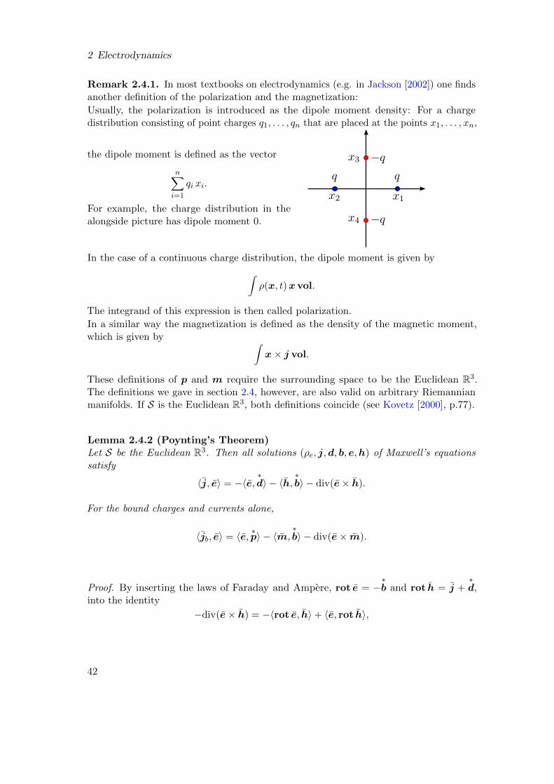
Remark 2.4.1. In most textbooks on electrodynamics (e.g. in Jackson [2002]) one findsanother definition of the polarization and the magnetization:
Usually, the polarization is introduced as the dipole moment density: For a chargedistribution consisting of point charges q1, . . . , qn that are placed at the points x1, . . . , xn,
the dipole moment is defined as the vector
n∑i=1
qi xi.
For example, the charge distribution in thealongside picture has dipole moment 0.
In the case of a continuous charge distribution, the dipole moment is given by∫ρ(x, t)xvol.
The integrand of this expression is then called polarization.
In a similar way the magnetization is defined as the density of the magnetic moment,which is given by ∫
x× j vol.
These definitions of p and m require the surrounding space to be the Euclidean R3.The definitions we gave in section 2.4, however, are also valid on arbitrary Riemannianmanifolds. If S is the Euclidean R3, both definitions coincide (see Kovetz [2000], p.77).
Lemma 2.4.2 (Poynting’s Theorem)Let S be the Euclidean R3. Then all solutions (ρe, j,d, b, e,h) of Maxwell’s equationssatisfy
〈j, e〉 = −〈e,∗d〉 − 〈h,
∗b〉 − div(e× h).
For the bound charges and currents alone,
〈jb, e〉 = 〈e, ∗p〉 − 〈m,∗b〉 − div(e× m).
Proof. By inserting the laws of Faraday and Ampere, rot e = −∗b and rot h = j +
∗d,
into the identity
−div(e× h) = −〈rot e, h〉+ 〈e, rot h〉,
42
2.5 The electromagnetic fields along the map φt
we immediately obtain the first of the asserted formulas. By inserting the laws of Faraday
and Ampere for bound charges instead, rot e = −∗b and rot m = jb −
∗p, we obtain the
second one.
2.5 The electromagnetic fields along the map φt
In chapter 3, we will establish balance laws (like for instance balance of momentum andenergy) that govern the motion of B. Of course, these laws contain electromagneticquantities. For example, balance of momentum contains the Lorentz force fL, and balanceof energy contains the term (j, e), where (·, ·) denotes the dual pairing of vector fieldsand 1-forms. As we have already seen in section 1.3.2, it is advisable to express theselaws in terms of the coordinates on the undeformed body. Thus, we will, starting inchapter 4, regard the electromagnetic quantities as vector fields or forms along the mapφt : B → Bt ⊂ S, defining
ρe(X, t) := J (X, t) ρe(x, t)
J(X, t) := J (X, t) j(x, t)
E(X, t) := e(x, t)
B(X, t) := b(x, t)
P(X, t) := J (X, t) p(x, t).
Then we obtain
J (j, e) = (J ,E), (2.10)
which will be helpful in chapter 4 for expressing balance of energy in terms of thecoordinates on B. Moreover, the vector fields or forms along the map φt : B → Bt ⊂ S,defined by
J := J − ρe VE := E− iVB
FL := ρe E + iJB
satisfy the following relations, that we will need in chapter 4:
J(X, t) = J (X, t) j(x, t) (2.11)
E(X, t) = e(x, t) (2.12)
FL(X, t) = J (X, t) fL(x, t), (2.13)
and
J (j, e) = (J , E). (2.14)
43

3 The Balance Laws on Bt
The motion of B is governed by a system of partial differential equations that consists ofthe conservation of mass and the balance laws for momentum, angular momentum, andenergy.
For simple elastic bodies that are not exposed to an electromagnetic field, there is abroad agreement on how these balance laws must be formulated (see for example Liu[2002] or Chadwick [1999]). Marsden and Hughes [1983] even discuss the balance lawsfor the case that B and S are manifolds, but they mostly restrict to the case, where thebody has the same dimension as the surrounding space.
For electromagnetic fields alone, that is, without any matter that is moved or deformedunder the influence of these fields, there are also statements on balance of momentumand energy. [Griffiths, 2008]
But for the modeling of elastic bodies that are subjected to an electromagnetic field,there exist several approaches that are not compatible, most prominently the formulationby Ericksen [2008] in contrast to that by Kovetz [2000]. Steigmann [2009] claims thatthese formulations are equivalent, but we will see that this is not true (see Remark 3.5.3).Other formulations that also involve so-called surface couples, can be found in Eringenand Maugin [1990], Hutter et al. [2006], Hutter and Pao [1974], and Maugin [1988].
Moreover, in the physics literature on electroelastic materials only simple bodies aretreated. Shells, i.e. bodies that only consist of a very thin layer of material (and couldthus be modeled by a hypersurface), are then approximated as simple bodies with athickness that tends to zero.
Usually, in works on electroelasticity the entropy inequality is used to decide, whichotherwise allowed deformations are physically admissible and which are not. It is alsoemployed to derive the Doyle-Ericksen formula that provides an important connectionbetween the free energy density of the material and the deformation. Unfortunately,the opinions on the physically correct statement of the entropy inequality diverge whenelectromagnetic fields are present [Ericksen, 2008; Kovetz, 2000; Hutter and Pao, 1974].A further problem in the formulation of an electroelastic theory on manifolds is that theentropy inequality, as it relies on the entropy flux to be tangential to the deformed body,is only applicable to simple bodies. For general bodies, in particular if they are subjectedto an electromagnetic field, this needs not to be the case.
If the balance laws are to be formulated for general bodies, one has to decide upona setup that is physically acceptable and at the same time can be carried over to amanifold. We will base our considerations on the set of balance laws that Ericksen[2008](see also Steigmann [2009]) provided for simple bodies. The form of balance of
45
3 The Balance Laws on Bt
energy that Ericksen stated, can be easily generalized to bodies that are described bya Riemannian manifold. The other balance laws will then be obtained by means ofour Theorem 3.5.1. It states that, if balance of energy is invariant under the action ofarbitrary diffeomorphisms on the surrounding space, then this already implies the localforms of conservation of mass, balance of momentum and angular momentum, as well asthe Doyle-Ericksen formula which here provides a connection between the internal energyand the deformation. Theorem 3.5.1 generalizes a result that can already be found inthe book by Marsden and Hughes [1983, ch. 2, Th. 4.13], and has more recently beendiscussed by Kanso et al. [2007, sec.3]. Both earlier statements of this result only pertainto bodies that have the same dimension as the surrounding space and do not allow thepresence of electromagnetic fields.Of course, it is also desirable from the physical point of view to have this invarianceof balance of energy; it meets the demand that physics is independent of the choice ofcoordinate system. The proof of Theorem 3.5.1, however, does not work nicely for othersetups of the balance laws that were suggested in the literature.The formulation by Hutter and Pao [1974] is not suitable, since it uses transformationsof the electromagnetic fields that are neither Galilean nor Lorentzian, but something inbetween.The formulation by Kovetz [2000] is quite elegant, but it does not tell how the singlecontributions to the energy density depend on the velocity. But this knowledge is vitalto the proof of Theorem 3.5.1. Furthermore, Kovetz uses the Poynting vector in hisstatement of balance of energy. Unfortunately, this vector is in general not tangentialto the deformed body and thus hardly usable if one wants to find a description of thebalance laws that works on a manifold.
As before, we will denote by Bt the state of B at the time t, i.e., Bt := φt(B), and forsome subset U ⊂ B of the undeformed body, Ut := φt(U) denotes the state of U at thetime t.
3.1 Conservation of Mass
Recall from section 1.3.3 that the mass M of a nice set Ut ⊂ Bt is given by the integralof the (smooth) mass density ρ : B → R,
M(Ut) =
∫Ut
ρ(x, t) volt,
and that ρ obeys conservation of mass, if for all nice Ut ⊂ Bt,d
dt
∫Ut
ρ(x, t) volt = 0.
By Theorem 1.3.19, the local form of conservation of mass is
ρ+ ρ divtÄv‖ä−mρg(v⊥,H) = 0,
46
3.2 Balance of Momentum
where v denotes the body’s spatial velocity, m is the body’s dimension and H denotesthe mean curvature field. If the dimension of B coincides with the dimension of thesurrounding space (and so in particular for simple bodies), then this simplifies to
∂ρ
∂t+ div (ρv) = 0.
3.2 Balance of Momentum
By Newton’s second law, the change of momentum P of a point mass is equal to theapplied force F :
dP
dt= F .
To set up balance of momentum in electroelasticity, we have to define, what momentumand force are in the case of a continuum.
The formulations of balance of momentum and angular momentum that are used in thisand the following section only make sense if the surrounding space is the Euclidean R3.Later on in section 3.5 we will justify why the local forms of the laws that we obtain hereare also valid on arbitrary Riemannian manifolds.
Definition 3.2.1. The momentum P of a part Ut ⊂ Bt in the motion φ is given bythe integral of the momentum density ρv,
P(Ut) :=
∫Ut
ρ(x, t)v volt,
where ρ : B → R denotes the mass density and v : B → S the velocity.
Forces
There are two kinds of forces acting on matter. On the one hand there are long-rangeforces (for example gravity and external electromagnetic forces) which decrease slowlywhen the distance between the interacting particles grows. If such a force acts from theoutside on a part U of B, it is capable of passing through the interior of U . The totalforce is proportional to the size of the concerned volume. Thus, long-range forces arealso called volume or body forces.
On the other hand, there are forces that have only a short range and that decreaseextremely rapidly when the distance between the interacting parts grows. They arecalled surface forces or contact forces and are negligible unless there is direct mechanicalcontact between the interacting parts. If a part U of B is acted on by short-range forcesarising from reactions with the material outside U , these forces can act only on a thin
47
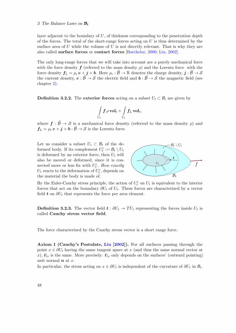
3 The Balance Laws on Bt
layer adjacent to the boundary of U , of thickness corresponding to the penetration depthof the forces. The total of the short-range forces acting on U is thus determined by thesurface area of U while the volume of U is not directly relevant. That is why they arealso called surface forces or contact forces [Batchelor, 2000; Liu, 2002].
The only long-range forces that we will take into account are a purely mechanical forcewith the force density f (referred to the mass density ρ) and the Lorentz force with theforce density fL = ρe e+ j × b. Here ρe : B → R denotes the charge density, j : B → Sthe current density, e : B → S the electric field and b : B → S the magnetic field (seechapter 2).
Definition 3.2.2. The exterior forces acting on a subset Ut ⊂ Bt are given by∫Ut
f ρvolt +
∫Ut
fL volt,
where f : B → S is a mechanical force density (referred to the mass density ρ) andfL = ρe e+ j × b : B → S is the Lorentz force.
Let us consider a subset Ut ⊂ Bt of the de-formed body. If its complement U ct := Bt \ Utis deformed by an exterior force, then Ut willalso be moved or deformed, since it is con-nected more or less fix with U ct . How exactlyUt reacts to the deformation of U ct , depends onthe material the body is made of.
By the Euler-Cauchy stress principle, the action of U ct on Ut is equivalent to the interiorforces that act on the boundary ∂Ut of Ut. These forces are characterized by a vectorfield t on ∂Ut that represents the force per area element.
Definition 3.2.3. The vector field t : ∂Ut → TUt representing the forces inside Ut iscalled Cauchy stress vector field.
The force characterized by the Cauchy stress vector is a short range force.
Axiom 1 (Cauchy’s Postulate, Liu [2002]). For all surfaces passing through thepoint x ∈ ∂Ut having the same tangent space at x (and thus the same normal vector atx), t|x is the same. More precisely: t|x only depends on the surfaces’ (outward pointing)unit normal n at x.
In particular, the stress acting on x ∈ ∂Ut is independent of the curvature of ∂Ut in Bt.
48
3.2 Balance of Momentum
Thus, the interior force or the stress that is caused inside Ut by the deformation of thebody is given by ∫
∂Ut
t(x, t,n) vol∂Ut .
Definition 3.2.4. The total force acting on a part Ut ⊂ Bt is given by
F :=
∫Ut
(f ρ+ fL) volt +
∫∂Ut
tvol∂Ut ,
where the Cauchy stress t depends on the unit normal field n of ∂Ut.
Now we can formulate the balance of momentum:
Definition 3.2.5. We say that balance of momentum is satisfied, if for every niceset U ⊂ B,
d
dt
∫Ut
ρv volt =
∫Ut
(f ρ+ fL) volt +
∫∂Ut
tvol∂Ut , (3.1)
where Ut = φt(U), f : B → S is a mechanical force density (referred to the mass densityρ), fL = ρe e+ j × b : B → S is the Lorentz force and where the Cauchy stress t dependson the (outward) unit normal field n of ∂Ut.
Theorem 3.2.6Let t(x, t,n) be a continuous function of its arguments. Moreover, assume that balance ofmomentum holds. Then there is a unique (1, 1)-tensor field σ on Bt, called the Cauchystress tensor field, such that
t(x, t,n) = σ(n)(x, t).
That is, in local coordinates on Bt, the components of the vector t are given by
ta = σ(n)a = σab nb.
Proof. Let ea, a = 1, . . . ,m, be a local frame for the tangent space of Bt, and let Ei,i = 1, 2, 3, be the Euclidean base of the surrounding R3. Moreover, we denote by gBt themetric that is induced on Bt by the restriction of g to Bt. The i-th component of (3.1),
d
dt
∫Ut
vi ρvolt =
∫Ut
[f i ρ+ f iL]volt +
∫∂Ut
ti vol∂Ut ,
49
3 The Balance Laws on Bt
is a conservation law for the i-th component of the momentum. By Cauchy’s Theorem(1.3.3) it follows that there is a vector field σi, such that ti = gBt(σi,n), and hence
t = tiEi = gBt(σi,n)Ei. (1)
Thus, t depends linearly on n. Hence, there must be a (1, 1)-tensor field σ on Bt suchthat t = σ(n). By (1)
σ(n) = gBt(σi,n)Ei.
Consider a fixed point x ∈ Bt. For each vector field wt ∈ TxBt we can find a subsetUt ⊂ Bt, such that wt is a multiple of the outward unit normal vector n of ∂Ut in x.Thus, we define σ by
σ(wt) = gBt(σi,wt)Ei for all wt ∈ TBt. (2)
Thus, balance of momentum can also be expressed by
d
dt
∫Ut
ρv volt =
∫Ut
(f ρ+ fL) volt +
∫∂Ut
σ(n) vol∂Ut . (3.2)
Theorem 3.2.7 (Equations of Motion)Assume that conservation of mass and balance of momentum hold. Then
ρa = ρf + fL + divtσ + trIIσ, (3.3)
with a = v and fL = ρe e+ j × b. trIIσ denotes the trace of σ with respect to II, i.e., ife1, . . . , em is a local orthonormal basis of TxBt, then
trIIσ =m∑a=1
II(ea,σ(ea)).
If Bt is a hypersurface in S, then
ρa = ρf + fL + divtσ + tr(Sν σ)ν,
where ν denotes the (outer) unit normal vector field of Bt and Sν is the correspondingWeingarten map.
Some parts of the following proof are taken from Grabs [2014].
50
3.2 Balance of Momentum
Proof. We consider some arbitrary point x ∈ Ut. Let e1(x), . . . , em(x) be an orthonormalbasis of TxBt, and extend it to a synchronous frame e1, . . . , em around x. Let E1, E2, E3
be the standard basis of the surrounding R3. For reasons of clarity we denote by gS themetric on S and by gBt the metric that is induced on Bt by the restriction of gS to Bt.Once more, we consider the i-th component of (3.1),
d
dt
∫Ut
vi ρvolt =
∫Ut
[f i ρ+ f iL]volt +
∫∂Ut
ti vol∂Ut . (1)
In the course of the proof of Theorem 3.2.6 we have seen that if balance of momentum isgiven, then the i-th component of t can be expressed by
ti = gBt(σi,n).
Hence, according to Theorem 1.3.21, the local form of (1) is given by
ρ·Ùvi = ρ f i + f iL + divt σ
i, (2)
where·Ùvi denotes the substantial derivative of vi. Here the surrounding space is the
Euclidean R3, thus the substantial derivative of any vector field wt = wit Ei that isdefined along φt satisfies
·wt =
·ıwit Ei.(In other words,
·ıwit = wti, i.e., the substantial derivative of the i-th component of wt is
equal to the i-th component of the substantial derivative of wt.) This can be seen asfollows:Since the Ei are constant,
wt = ∇S(vt,∂t)(wit Ei)
=î∂(vt,∂t)w
it
óEi
=
·ıwit Ei.(Note that this step really requires S to be Euclidean.) Thus multiplying (2) by Ei andsumming over i yields
ρ v = ρf + fL + (divt σi)Ei. (3)
Using the synchronicity of e1, . . . , em, we obtain at the point x
divtσi =
m∑a=1
gBtÄ∇Bteaσ
i, eaä
=m∑a=1
∂ea gBtÄσi, ea
ä.
51
3 The Balance Laws on Bt
Using (2) from the proof of Theorem 3.2.6, we obtain
divtσi =
m∑a=1
∂ea gS(σ(ea), Ei)
=m∑a=1
gS(∇SeaÄσ(ea)
ä, Ei
),
where we have used that the Ei are constant. In particular, ∇SeaEi = 0 for all a = 1, . . . ,mand all i = 1, . . . , 3. Now we can decompose ∇S into its tangent and normal part withrespect to Bt and obtain
divtσi =
m∑a=1
gS(∇BteaÄσ(ea)
ä+ II
Äea,σ(ea)
ä, Ei
)=
m∑a=1
gS(Ä∇Bteaσ
ä(ea) + II
Äea,σ(ea)
ä, Ei
),
where we have used again that the ea are synchronous with respect to x. Thus,
divt(σi)Ei = divt σ +
m∑a=1
II(ea,σ(ea)).
Inserting this into (3) yields
ρ v = ρf + fL + divtσ +m∑a=1
II(ea,σ(ea)).
If Bt is a hypersurface in S, then we may write II(ξ,η) = g(Sν(ξ),η)ν, where ξ,η ∈ TBt,and ν denotes the (outer) unit normal vector field of Bt ⊂ S. Then, using the symmetryof the Weingarten map Sν , we obtain
m∑a=1
IIÄea,σ(ea)
ä=
m∑a=1
gÄSν(ea),σ(ea)
äν
=m∑a=1
gÄ(Sν σ)(ea), ea
äν
= tr(Sν σ)ν.
This completes the proof.
3.3 Balance of Angular Momentum
By Newton’s Law for a rigid body the change of angular momentum L0 is equal to theapplied torque M0:
dL0
dt= M0.
52
3.3 Balance of Angular Momentum
In the case of a point particle the angular momentum (with respect to a point x0) isgiven by (x−x0)×p, where x denotes the position and p the momentum of the particle.The torque that is caused by a force f is given by (x− x0)× f . For a continuous bodythis is replaced by the following definition.
Definition 3.3.1. We define the angular momentum with respect to some pointx0 ∈ Ut of a part Ut ⊂ Bt in the motion φ by
L0(Ut,x0) :=
∫Ut
(x− x0)× v ρvolt.
and the torque acting on a part Ut by
M0(Ut,x0) :=
∫Ut
(x− x0)× f ρvolt +
∫Ut
(x− x0)× fL volt +
∫∂Ut
(x− x0)× tvol∂Ut .
Here, as usual, f : B → S is a mechanical force density (referred to the mass density ρ),fL = ρe e+ j × b : B → S is the Lorentz force density, and t is the Cauchy stress vector.
Thus, for a continuous body, balance of angular momentum has the following form.
Definition 3.3.2. We say that balance of angular momentum is satisfied, if forevery nice U ⊂ B,
d
dt
∫Ut
(x− x0)× v ρvolt =
∫Ut
(x− x0)× f ρvolt +
∫Ut
(x− x0)× fL volt
+
∫∂Ut
(x− x0)× tvol∂Ut , (3.4)
where Ut = φt(U), f : B → S is a mechanical force density (referred to the mass densityρ), fL = ρe e + j × b : B → S is the Lorentz force density, and t is the Cauchy stressvector.
In the following we set x0 to 0.
Theorem 3.3.3Assume that conservation of mass and balance of momentum hold. Then balance ofangular momentum holds if and only if
σ = σT .
53
3 The Balance Laws on Bt
Proof. Let E1, E2, E3 be the Euclidean base of the surrounding R3. Again, for reasonsof clarity, we denote by gS the (Euclidean) metric on S and by gBt the metric that isinduced on Bt by the restriction of gS to Bt.We consider the i-th component of (3.4):
d
dt
∫Ut
(x× v)i ρvolt =
∫Ut
(x× f)i ρvolt +
∫Ut
(x× fL)i volt +
∫∂Ut
(x× t)i vol∂Ut . (1)
If balance of momentum is valid, then by Theorem 3.2.6 there is a vector field σk,tangential to Bt, such that tk = gBt(σk,n). Then
(x× t)i = εijk xj tk = gBt(εijk x
j σk,n),
where ε denotes the Levi-Civita symbol. Thus, using conservation of mass and
divt(xj σk) = gBt(gradxj ,σk) + xj divt σ
k,
by Theorem 1.3.21 the localization of (1) is
ρ
·˝(x× v)i = ρ (x× f)i + (x× fL)i + εijkîgBt(gradxj ,σk) + xj divt σ
kó. (2)
For the term on the left hand side of (2) we compute
ρ
·˝(x× v)i = ρ
·˝εijk xj vk
= ρ εijk
[ ·ıxj vk + xj·ıvk].
xj is a function on B. Let us define as in Remark 1.1.10 the function ψ : B × I → B by
(X, t)ψ7→ (φ(X, t), t). Then
·ıxj ψ =∂φj
∂t= V j = vj ψ.
Moreover, in the course of the proof of Theorem 3.2.7, we have seen that
·ıvk = vk, i.e.,the substantial derivative of the k-th component of v is equal to the k-th component ofthe substantial derivative of v. (Of course, this works only with components with respectto the standard Euclidean basis.) Thus,
ρ
·˝(x× v)i = ρ [v × v + x× v]i
= ρ [x× v]i . (3)
54
3.4 Balance of Energy
We have also seen in the same proof that balance of momentum can be formulated asρ v = ρf + fL + divt σ
lEl. Inserting this into (3) gives
ρ
·˝(x× v)i = ρ (x× f)i + (x× fL)i + divtσl [x× El]i
= ρ (x× f)i + (x× fL)i + εijk xj divtσ
k. (4)
Combining (2) and (4), we obtain
εijk gBt(gradxj ,σk) = 0. (5)
Let ea, a = 1, . . . ,m, be a local frame for the tangent space of Bt. Then
gradxj = gab ∂ea(xj) eb
= gab (ea)iEi(x
j) eb
= gab (ea)i δi
j eb
= gab (ea)j eb.
We have derived in the proof of Theorem 3.2.6 that gBt(σk,w) = gS(σ(w), Ek) for eachvector w that is tangential to Bt. Thus,
gBt(gradxj ,σk) = gab (ea)j gBt(σk, eb)
= gab (ea)j gS(σ(eb), Ek)
= gab (ea)j σcb (ec)
k
= σba (ea)j (eb)
k.
Hence, (5) is equivalent to
σba ea × eb = 0.
Using the anti-symmetry of the vector product, we can rewrite this to
1
2(σba − σab) ea × eb = 0,
from which we conclude that σ is symmetric.
3.4 Balance of Energy
The next balance law, balance of energy, is a scalar law and can be formulated, if B andS are Riemannian manifolds. But for the computation of its local form we will needbalance of momentum and angular momentum, and up to now we have only establishedthem for the case that S is the Euclidean R3. Thus, we will at first demand that S isthe Euclidean R3. At the end of this section, we will formulate balance of energy for
55
3 The Balance Laws on Bt
the general setting and derive balance of momentum and angular momentum from theassumption that balance of energy is invariant under arbitrary spatial diffeomorphisms.
The first law of thermodynamics states that the change of energy E equals the power Πof the work that is done by body and surface forces and the exchanged amount of heatQ:
dE
dt= Π + Q + Wdiss,
where E denotes the energy, Π the power, Q the exchanged amount of heat, and Wdiss rep-resents some dissipative work. The energy is the sum of internal energy and (macroscopic)kinetic energy. Thus we define in the continuous case:
Definition 3.4.1. The energy E of a part Ut ⊂ Bt in the motion φ is given by
E (Ut) :=
∫Ut
Åu+
1
2g(v,v)
ãρvolt.
Here, u : B → R is the internal energy density including among other things the energywhich is stored microscopically inside the body in form of binding energy and the energyof molecular translations, rotations, and vibrations.
3.4.1 Special case: S = R3 with the Euclidean metric
The power is equal to the scalar product of the applied forces with the velocity field.Here, as before, the applied forces are a purely mechanical force with the force density f ,stress forces inside the body, encoded in the stress vector t, and the Lorentz force densityfL.
Definition 3.4.2. The power Π of the forces acting on a part Ut ⊂ Bt in the motion φis given by
Π(Ut) :=
∫Ut
g(ρf + fL,v) volt +
∫∂Ut
g(t,v) vol∂Ut ,
where as usual, f : B → S is a mechanical force density (referred to the mass density ρ),fL = ρe e+ j × b : B → S is the Lorentz force, and t is the Cauchy stress vector.
Heat can be exchanged by an external heat supply with the density rθ : B → R, and bysome gain or loss of heat through the boundary of Ut, encoded in some functionh, depending on the outward unit normal vector field n of ∂Ut.
56
3.4 Balance of Energy
Definition 3.4.3. We define the exchanged amount of heat Q of a part Ut ⊂ Bt inthe motion φ by
Q(Ut) :=
∫Ut
rθ ρvolt +
∫∂Ut
h(x, t,n) vol∂Ut ,
with the heat supply density rθ : B → R and the gain or loss of heat through the boundaryh.
If B does not have the same dimension as the surrounding space, then we could collecta possible heat flux between the body and its surrounding space into the heat supplydensity rθ.
The only dissipative work that we take into account is the Joule heating. It is definedas g(j, e) where j := j − ρe v is the conduction current density and e := e + v × b isthe electromotive intensity (see chapter 2). The Joule heating represents the amount ofenergy that charge carriers inside the material transfer during collisions to the rest ofthe material. For this process only the velocity of the charge carriers with respect tothe material and the electric field as seen from the material’s point of view are relevant.Hence the expression for the Joule heating involves the Galilei invariants j and e, i.e.the current density and the electric field as they are seen from the material’s point ofview and not the corresponding fields that might be perceived by another observer.
Definition 3.4.4. The dissipative work that occurs inside some part Ut ⊂ Bt duringthe motion φ is given by
Wdiss(Ut) :=
∫Ut
g(j, e) volt,
where j : B → S denotes the convective current density and e : B → S the electromotiveintensity.
Definition 3.4.5 (Balance of Energy). We say that balance of energy holds if forevery nice open set U ⊂ B,
d
dt
∫Ut
Åu+
1
2g(v,v)
ãρvolt
=
∫Ut
(g(f ,v) + rθ)ρvolt +
∫Ut
g(fL,v) volt +
∫Ut
g(j, e) volt +
∫∂Ut
(g(t,v) + h
)vol∂Ut ,
57
3 The Balance Laws on Bt
where as usual Ut = φt(U), f : B → S is a mechanical force density (referred to the massdensity ρ), fL = ρe e+ j × b : B → S is the Lorentz force, and t is the Cauchy stressvector. Moreover, u : B → R denotes the internal energy, rθ : B → R the heat supply, hthe gain/loss of heat through the boundary, and j : B → S and e : B → S denote theconvective current density and the electromotive intensity, respectively. This is equivalentto
d
dt
∫Ut
Åu+
1
2g(v,v)
ãρvolt
=
∫Ut
Äg(f ,v) + rθ
äρvolt +
∫Ut
g(j, e)volt +
∫∂Ut
Äg(t,v) + h
ävol∂Ut ,
with the current density j : B → S and the electric field e : B → S.
Remark 3.4.6. One part of the gained energy, the kinetic energy, is used for thedeformation of the body, while the other part increases the internal energy of the body.
Theorem 3.4.7 (Marsden and Hughes [1983])Assume that t(x, t,n) = σ(x,t)(n) for a (1, 1) tensor field σ on Bt, where n denotes theoutward unit normal vector field along ∂Ut. (This is given, if balance of momentumholds.)
Then balance of energy implies the existence of a unique vector field qθ on Bt, such thatfor all n,
h(x, t,n) = −g(qθ(x, t),n).
We call qθ the heat flux vector.
Proof. We define c := 〈t,v〉+ h. By Cauchy’s Theorem (1.3.3) there exists a vector fieldc on Ut, such that c = g(c,n). Hence,
h = g(c,n)− g(t,v).
If t = σ(n) for a (1, 1) tensor field σ on Bt, then
g(t,v) = gBt(σ(n),v‖) = gBt(σT (v‖),n)
and thus
h = g(c− σT (v‖),n).
Now we can define qθ by −qθ = c− σT (v‖).
58
3.4 Balance of Energy
Remark 3.4.8. The minus sign in the definition of qθ is just a matter of convention:It leads to h = −g(qθ,n) where n is the outward unit normal field to ∂Ut. Thus, if qθpoints into the same direction as −n, then the contribution of the heat flux is positive.
An immediate consequence of Theorem 3.4.7 is
Corollary 3.4.9If balance of momentum holds, then balance of energy is equivalent to
d
dt
∫Ut
Åu+
1
2g(v,v)
ãρvolt =
∫Ut
Äg(f ,v) + rθ
äρvolt +
∫Ut
g(fL,v) volt
+
∫Ut
g(j, e) volt +
∫∂Ut
gÄσT (v‖)− qθ,n
ävol∂Ut .
Theorem 3.4.10 (Local spatial form of balance of energy)Assume that conservation of mass and balance of momentum hold.Then the local form of balance of energy is given by
ρ u = 〈σ,∇Btv‖〉 − g (trIIσ,v) + ρ rθ + g(j, e)− divt qθ. (3.5)
Here, ∇Bt denotes the Levi-Civita connection on (Bt, gBt) and 〈σ,∇Btv‖〉 the scalar
product of the (1, 1) tensor fields σ and ∇Btv‖ on Bt (see Notation 1.2.14). If moreover,balance of angular momentum holds, then this simplifies to
ρ u = 〈σ,d〉+ ρ rθ + g(j, e)− divt qθ, (3.6)
where d is the rate of deformation tensor field we defined in section 1.2 (see Definition1.2.12).
Proof. Since by assumption balance of momentum holds, it is sufficient to localize theequation from corollary 3.4.9.Since conservation of mass holds, we can apply Theorem 1.3.21. Thus, balance of energyis equivalent to
ρ u+1
2ρ
·˚g(v,v) = ρ g(f ,v) + ρ rθ + g(fL,v) + g(j, e) + divtÄσT (v‖)
ä− divt qθ. (1)
By Lemma 1.1.9,
1
2ρ
·˚g(v,v) = ρ g(v, v) = ρ g(v,a).
59
3 The Balance Laws on Bt
Inserting this and balance of momentum (see Theorem 3.2.7),
ρa = ρf + fL + divtσ + trIIσ
into (1) while using that divt σ is tangential, gives
ρ u+ g(divtσ,v‖) + g (trIIσ,v) = ρ rθ + g(j, e) + divtÄσT (v‖)
ä− divt qθ. (1’)
Consider some arbitrary point x ∈ Bt. Let e1(x), . . . , em(x) be an orthonormal basis ofTxBt and extend it to a synchronous frame e1, . . . , em around x. Then in x
divtÄσT (v‖)
ä= gÄ∇BteaÄσT v‖
ä, eaä
= ∂eagÄσT v‖, ea
ä= ∂eag
Äσ(ea),v‖
ä= gÄÄ∇Bteaσ
ä(ea),v‖
ä+ gÄσ(ea),∇Bteav‖
ä= g(divtσ,v‖) + g
ÄσT ∇Btv‖(ea), ea
ä= g(divtσ,v‖) + trg(σ
T ∇Btv‖)= g(divtσ,v‖) + 〈σ,∇Btv‖〉.
Thus, (1’) becomes
ρ u = 〈σ,∇Btv‖〉 − g (trIIσ,v) + ρ rθ + g(j, e)− divt qθ. (1”)
If balance of angular momentum is given, then σ is symmetric and hence,
〈σ,∇Btv‖〉 =1
2
î〈σ,∇Btv‖〉+ 〈σT , (∇Btv‖)T 〉
ó=
1
2〈σ,∇Btv‖ + (∇Btv‖)T 〉
=1
2〈σ, (∇Btv‖)[ +
î(∇Btv‖)[
óT 〉.Moreover, the symmetry of σ implies
g(trIIσ,v) =m∑a=1
g (II(ea,σ(ea)),v)
=m∑a=1
g(σ(ea), eb) g (II(ea, eb),v⊥)
=m∑a=1
σ[(ea, eb) g (II(ea, eb),v⊥)
= 〈σ, g(II(·, ·),v⊥)〉.
60
3.4 Balance of Energy
Thus, by the definition of the rate of deformation tensor d (see Definition 1.2.12) andTheorem 1.2.13,
〈σ,∇Btv‖〉 − g(trIIσ,v) =¨σ,
1
2
î(∇Btv‖)[ + ((∇Btv‖)[)T
ó− g(II(·, ·),v⊥)
∂= 〈σ,d〉,
and (1”) becomesρ u = 〈σ,d〉+ ρ rθ + g(j, e)− divt qθ.
3.4.2 The general case
On general manifolds we regard the mechanical force and the Lorentz force as 1-forms fand fL and write fL = ρe e− ijb, where e and b denote the electric field 1-form and themagnetic flux 2-form, respectively.Then the power Π of the forces acting on a part Ut ⊂ Bt in the motion φ can be expressedby
Π(Ut) =
∫Ut
(ρ f + fL,v) volt +
∫∂Ut
g(t,v) vol∂Ut ,
where (f,v) denotes the dual pairing of the vector field v and the 1-form f.The scalar product g(j, e) can be replaced by the pairing (j, e) with e = e− ivb. Thenthe dissipative work for a part Ut ⊂ Bt in the motion φ is given by
Wdiss(Ut) :=
∫Ut
(j, e) volt.
Altogether we formulate balance of energy as follows:
Definition 3.4.11 (Balance of Energy in the general setting). We say that bal-ance of energy holds if for every nice open set U ⊂ B,
d
dt
∫Ut
Åu+
1
2g(v,v)
ãρvolt
=
∫Ut
Ä(f,v) + rθ
äρvolt +
∫Ut
(fL,v) volt +
∫Ut
(j, e) volt +
∫∂Ut
(g(t,v) + h
)vol∂Ut ,
with fL = ρe e− ijb. This is equivalent to
d
dt
∫Ut
Åu+
1
2g(v,v)
ãρvolt
=
∫Ut
Ä(f,v) + rθ
äρvolt +
∫Ut
(j, e) volt +
∫∂Ut
Äg(t,v) + h
ävol∂Ut ,
61
3 The Balance Laws on Bt
with notation as in Def. 3.4.5 but adapted to forms.
3.5 The balance laws for the general case
Conservation of mass and balance of energy are scalar laws and can be easily formulatedeven if the body and the surrounding space are Riemannian manifolds: Conservation ofmass is given if (see section 3.1)
d
dt
∫Ut
ρvolt = 0,
or locally,
ρ+ ρdivt(v‖)−mρg(v⊥,H) = 0. (3.7)
Balance of energy is given, if (see Def. 3.4.11)
d
dt
∫Ut
(u+
1
2g(v,v)
)ρvolt
=
∫Ut
((f,v) + rθ) ρvolt +
∫Ut
(j, e) volt +
∫∂Ut
g(t,v) vol∂Ut +
∫∂Ut
hvol∂Ut .
(3.8)
For the balance laws of momentum and angular momentum there is a problem: For thesimple case, where S is the Euclidean R3, we have derived local formulations of theselaws in sections 3.2 and 3.3:
ρa = ρf + fL + divtσ + trIIσ (3.9)
σ = σT . (3.10)
(where we have already used conservation of mass) and with their help a local form ofbalance of energy. But to derive these laws we explicitly used the Euclidian structure ofthe surrounding space. So why should these laws also be valid if B and S are arbitraryRiemannian manifolds ?
In this section we will show that the demand that balance of energy is invariant underthe action of arbitrary diffeomorphisms on the surrounding space together with somephysical assumptions already implies (3.9), (3.10), and also (3.7). Then, by use of (3.7),(3.9), and (3.10) we also obtain the local form of balance of energy as we know it fromTheorem 3.4.10. As a nice by-product we obtain the Doyle-Ericksen formula that provides
62
3.5 The balance laws for the general case
a connection between the stress tensor, the internal energy, and the metric.
By Theorem 1.3.8 and Lemma 1.1.9, equation (3.8) is equivalent to∫Ut
[u+ g(v,a)] ρvolt +
∫Ut
ïu+
1
2g(v,v)
òρvolt
+
∫Ut
ïu+
1
2g(v,v)
òρîdivt(v‖)−mg(v⊥,H)
óvolt
=
∫Ut
[(f,v) + rθ] ρvolt +
∫Ut
(j, e) volt +
∫∂Ut
g(t,v) vol∂Ut +
∫∂Ut
hvol∂Ut . (1)
Axiom 2. Balance of energy is invariant under the action of spatial diffeomorphismsξt : S → S. That is, on U ′t = ξt(Ut) = φ′t(U), where φ′t := ξt φt, balance of energy isgiven by∫U ′t
îu′ + g′(v′,a′)
óρ′ vol′t +
∫U ′t
ïu′ +
1
2g′(v′,v′)
òρ ′ vol′t
+
∫U ′t
ïu′ +
1
2g′(v′,v′)
òρ′îdiv′t(v
′‖)−mg′(v′⊥,H′)
óvol′t
=
∫U ′t
[(f′,v′) + r′θ
]ρ′ vol′t +
∫U ′t
(j′, e′) vol′t +
∫∂U ′t
g′(t′,v′) vol′∂U ′t+
∫∂U ′t
h′ vol′∂U ′t. (2)
The coordinates in the primed and the unprimed systems are related by x′ = ξt(x). Thecorresponding expressions for the metric satisfy
g = ξ∗t g′,
the volume forms of Ut and U ′t are related by
volt = ξ∗t vol′t.
Let w be the velocity of ξt. Then differentiating φ′t = ξt φt gives
v′(x′, t) = (ξt)∗v(x, t) +w(x, t).
Let p be an arbitrary point on Bt. Let e′1, . . . , e′m be an orthonormal basis of TpBt with
respect to the coordinates x′. Then e1, . . . , em, defined by e′a = ξt∗ea, a = 1, . . . ,m, is abasis of TpBt with respect to the coordinates x. Thus, in p,
div′t(v′‖) =
m∑a=1
g′(∇Bte′av′‖, e′a)
=m∑a=1
((ξ−1t )∗g)
(∇Bt(ξt∗ea)((ξt)∗v‖ +w‖), ξt∗ea
).
63
3 The Balance Laws on Bt
We make the following assumptions:
1) The mass density, the heat supply density and the heat flow through the boundarysatisfy
ρ′(x′, t) = ρ(x, t)
r′θ(x′, t) = rθ(x, t)
h′(x′, t,n′) = h(x, t,n).
2) The forces are transformed classically, i.e., they are transformed in the same wayas the accelerations. Thus, f ′ − a′ = (ξt)∗(f − a), or equivalently,
f− a[ = ξ∗tÄf′ − a′ [
ä.
3) The stress vectors that act along the boundaries of Ut and U ′t, respectively, arerelated by
t′(x′, t,n′) = (ξt)∗t(x, t,n).
4) The internal energy contains among other contributions the energy that is storedinside the material in the form of molecular rotations and vibrations. These energiesdepend on the distance of the molecules and thus on the metric of the surroundingspace. Hence, the internal energy density u should depend on the metric g. Weassume the simplest possible transformation
u′(x′, t, g) = u(x, t, ξ∗t g).
This assumption is often called assumption of ”minimal coupling”.
5) If t = t0, the velocities satisfy v′ = v +w. Thus, for t = t0,
j′ = j + ρew
e′ = e + iwb,
(see chapter 2).
We collect the relations between the primed and the unprimed quantitites at t = t0:
vol′t(x′) = volt(x),
H(x′) = H(x),
h′(x′, t,n′) = h(x, t,n),
t′(x′, t,n′) = t(x, t,n).
64
3.5 The balance laws for the general case
Moreover,
v′ = v +w,
div′t(v′‖) = divt(v‖) + divt(w‖),
ρ′ = ρ,
r′θ = rθ,
f′ − a′ [ = f− a[,u′ = u,
j′ = j + ρew,
e′ = e + iwb,
and
〈v′,a′〉 = 〈v +w,a′〉,
u′|t=t0 = u+¨ ∂u
∂(ξ∗t g),d
dt(ξ∗t g)|t=t0
∂= u+
¨∂u∂g, Lwg
∂, (3.11)
where the primed quantities are evaluated at (x′, t) while the unprimed quantities areevaluated at (x, t).
Now we are ready to state one of the central theorems in this work:
Theorem 3.5.1Let the body (B, G) and the surrounding space (S, g) be arbitrary Riemannian mani-folds. Suppose, balance of energy is satisfied and invariant under the action of spatialdiffeomorphisms ξt : S → S (Axiom 2) with the transformations that were stated above.Then there exists a (1, 1)-tensor field σ on Bt, such that t = σ(n) and a vector field qθon Bt, such that h(x, t,n) = −g(qθ,n).Moreover, conservation of mass is satisfied,
ρ+ ρ divt(v‖)−mρg(v⊥,H) = 0,
as well as
ρa[ = ρ f + ρe e− (ijb) + (divtσ)[ + trIIσ[, (3.12)
σ = σT , (3.13)
and the Doyle-Ericksen formula,
σ] = 2 ρ∂u
∂g.
Furthermore, the local form of balance of energy is given by
ρ u = 〈σ,d〉+ ρ rθ + (j, e)− divt qθ.
65
3 The Balance Laws on Bt
We identify (3.12) and (3.13) as balance of momentum and angular momentum, sincethey coincide with the local expressions (3.9) and (3.10) we had derived for the case thatS is the Euclidean R3.
Remark 3.5.2. Theorem 3.5.1 provides a complete set of compatible balance laws thatgovern the deformation (and temperature development) of a body in a surrounding space.These balance laws are also valid, if the body and the surrounding space are arbitrarymanifolds. Moreover, the Doyle-Ericksen formula states that the internal energy servesas a potential function for the stress tensor. In classical elasticity theory materials forwhich such a potential function exists are called hyperelastic. Thus, we have seen that thedemand that the balance of energy is invariant under arbitrary spatial diffeomorphisms(together with some reasonable physical assumptions), already implies that the materialthe body consists of, must be hyperelastic. This is remarkable since we did not specifythe kind of material yet.
As we have already mentioned, 3.5.1 generalizes a result by Marsden and Hughes [1983,ch. 2 Theorem 4.13] and Kanso et al. [2007, sec.3]. Both these earlier results only pertainto bodies that have the same dimension as the surrounding space and do not allow thepresence of electromagnetic fields.
Proof. If t = t0, then by use of the relations (3.11), balance of energy in the primedcoordinates (2) becomes
∫Ut
Åu+¨∂u∂g, Lwg
∂ãρvolt +
∫Ut
ïu+
1
2g(v +w,v +w)
ò îρ+ ∂(wt,∂t)ρ
óvolt
+
∫Ut
ïu+
1
2g(v +w,v +w)
òρîdivt(v‖ +w‖)−mg(v⊥ +w⊥,H)
óvolt
=
∫Ut
Ä(f− a[,v +w) + rθ
äρvolt +
∫Ut
[(j, e) + (ρe e− ijb,w)] volt
+
∫∂Ut
g(t,v +w) vol∂Ut +
∫∂Ut
hvol∂Ut , (3)
where we also used that
(j′, e′) = (j + ρew, e + iwb)
= (j, e) + (j, iwb) + (ρew, e) + (ρew, iwb)︸ ︷︷ ︸= 0
= (j, e) + (ρe e− ijb,w).
66
3.5 The balance laws for the general case
Substracting (1) from (3) gives∫Ut
¨∂u∂g, Lwg
∂ρvolt +
∫Ut
1
2g(w,w)
îρ+ ρdivt(v‖)−mρg(v⊥,H)
óvolt
+
∫Ut
g(v,w)îρ+ ρ divt(v‖)−mρg(v⊥,H)
óvolt
+
∫Ut
1
2g(w,w)
î∂(wt,∂t)ρ+ ρdivt(w‖)−mρg(w⊥,H)
óvolt
+
∫Ut
Åu+
1
2g(v,v)
ã î∂(wt,∂t)ρ+ ρdivt(w‖)−mρg(w⊥,H)
óvolt
+
∫Ut
1
2g(v,v)
î∂(wt,∂t)ρ+ ρ divt(w‖)−mρg(w⊥,H)
óvolt
=
∫Ut
(f− a[,w) ρvolt +
∫Ut
(ρe e− ijb,w) volt +
∫∂Ut
g(t,w) vol∂Ut . (4)
The only summand in this equation, in which w occurs in the third order, is the summandin the third line. Thus, a rescaling argument provides
∂(wt,∂t)ρ+ ρdivt(w‖)−mρg(w⊥,H) = 0.
Hence, (4) simplifies to∫Ut
¨∂u∂g, Lwg
∂ρvolt +
∫Ut
1
2g(w,w)
îρ+ ρdivt(v‖)−mρg(v⊥,H)
óvolt
+
∫Ut
g(v,w)îρ+ ρ divt(v‖)−mρg(v⊥,H)
óvolt
=
∫Ut
(f− a[,w) ρvolt +
∫Ut
(ρe e− ijb,w) volt +
∫∂Ut
g(t,w) vol∂Ut . (4’)
The only summand in (4’), in which w occurs quadratically, is the second summand inthe first line. Thus, we conclude that
ρ+ ρ divt(v‖)−mρg(v⊥,H) = 0.
This is the local form of conservation of mass. Hence, (4’) simplifies to∫Ut
¨∂u∂g, Lwg
∂ρvolt =
∫Ut
(ρ f− ρa[ + ρe e− ijb,w) volt +
∫∂Ut
g(t,w) vol∂Ut . (4”)
In a similar way as in the proof of Theorem 3.2.6 we can apply Cauchy’s Theorem to(4”) and deduce the existence of a vector field ζ that is tangential to Bt and satisfies
g(t,w) = g(ζ,n).
67
3 The Balance Laws on Bt
The left hand side of this equation depends linearly on w‖, so the ζ on the right handside must also depend linearly on w‖. Thus, there is a (1, 1)-tensor field “σ on Bt, suchthat ζ = “σ(w‖) and hence
g(t,w) = g(t,w‖) = g(“σ(w‖),n) = g(“σT (n),w‖).
We now define σ := “σT and obtain t = σ(n). As in the proof of Theorem 3.4.7 it followsfrom (1) that h = −g(qθ,n) for a vector field qθ on Ut. Moreover, (4”) can be replacedby ∫
Ut
¨∂u∂g, Lwg
∂ρvolt =
∫Ut
(ρ f− ρa[ + ρe e− ijb,w) volt +
∫Ut
divt(σTw‖) volt,
or, locally,
ρ¨∂u∂g, Lwg
∂= (ρ f− ρa[ + ρe e− ijb,w) + divt(σ
Tw‖). (5)
We reformulate the last term of (5). We have already computed in the proof of Theorem3.4.10 that
divt(σTw‖) = g(divtσ,w‖) + 〈σ], (∇Btw‖)[〉.
We can also write this as
divt(σTw‖) = g(divtσ,w‖) +
1
2
¨σ], (∇Btw‖)[ +
î(∇Btw‖)[
óT ∂+ 〈σ],α〉
with
α :=1
2
[(∇Btw‖)[ −
î(∇Btw‖)[
óT ].
By Definition 1.2.12 and Theorem 1.2.13,
(∇Btw‖)[ +î(∇Btw‖)[
óT= Lwg + 2 g(w⊥, II(·, ·)),
where Lw denotes the Lie derivative with respect to w. Moreover, divtσ is tangential toBt. Hence,
divt(σTw‖) = g(divtσ,w) +
1
2〈σ], Lwg〉+
¨σ], g(w⊥, II(·, ·))
∂+ 〈σ],α〉.
Consider an arbitrary point x ∈ Ut. Let e1(x), . . . , em(x) be an orthonormal basis ofTxUt and extend it to a local frame e1, . . . , em around x. Then at x¨σ], g(w⊥, II(·, ·))
∂=
m∑a,b=1
σ[(ea, eb) g(w⊥, II(ea, eb)) =m∑
a,b=1
g(σ[(ea, eb) II(ea, eb),w),
68
3.5 The balance laws for the general case
since each II(ea, eb) is normal to Bt. Thus,
divt(σTw‖) =
m∑a,b=1
gÄdivtσ + σ[(ea, eb) II(ea, eb),w
ä+
1
2
¨σ], Lwg
∂+ 〈σ],α〉
and (5) becomes¨ρ∂u
∂g− 1
2σ], Lwg
∂= (ρ f− ρa[ + ρe e− ijb + (divtσ)[
+m∑
a,b=1
σ[(ea, eb) (II(ea, eb))[,w) + 〈σ],α〉. (6)
This equation shall be valid for each diffeomorphism ξt : S → S and hence for eachvelocity w.We now consider (6) in an arbitrary point x ∈ Bt. In the coordinates of the surroundingspace, the Lie derivative of g is given by
(Lwg)ij =∂gij∂t
+ gij;k wk + wi;j + wj;i.
g does not depend on t. From now on we use Riemannian normal coordinates around x.Then in x all gij;k are 0. In these coordinates,
Lwg = (∇Sw)[ +î(∇Sw)[
óT.
We now choose a ξt, such that w‖ = 0 and ∇Sw⊥ = 0. Then ∇Btw‖ = 0 and
∇Sw = ∇Sw⊥ = 0. Thus, (6) implies
(ρ f⊥ − ρa[⊥ + ρe e⊥ − (ijb)⊥ +m∑
a,b=1
σ[(ea, eb) (II(ea, eb))[,w⊥) = 0
and hence
ρa[⊥ = ρ f⊥ + ρe e⊥ − (ijb)⊥ +m∑
a,b=1
σ[(ea, eb) (II(ea, eb))[. (7)
On the other hand, if we choose a ξt, such that w⊥ = 0 and ∇Sw‖ = 0, then this implies
∇Sw = 0 and ∇Sηw‖ = ∇Btη w‖ + II(η,w‖) = 0 for each η that is tangential to Bt. Since
∇Btη w‖ is tangential to Bt, while II(η,w‖) is normal, both must be equal to 0. Thus,
∇Btw‖ = 0. Hence, (6) implies,
(ρ f‖ − ρa[‖ + ρe e‖ − (ijb)‖ + (divtσ)[,w‖) = 0,
and thus, since w‖ 6= 0,
ρa[‖ = ρ f‖ + ρe e‖ − (ijb)‖ + (divtσ)[. (8)
69
3 The Balance Laws on Bt
Adding (7) and (8) yields
ρa[ = ρ f + ρe e− (ijb) + (divtσ)[ +m∑
a,b=1
σ[(ea, eb) (II(ea, eb))[. (9)
Thus, (6) simplifies to ¨ρ∂u
∂g− 1
2σ], Lwg
∂= 〈σ],α〉, (10)
Now we choose ξt in such a way that w‖ = 0 while the normal velocity w⊥ is arbitrary.Then (10) becomes ¨
ρ∂u
∂g− 1
2σ], Lw⊥g
∂= 0.
By the arbitrariness of w⊥ we deduce that
σ] = 2 ρ∂u
∂g. (11)
The only remnant of (6) is 〈σ],α〉 = 0. Since α is skew-symmetric, this implies that σ issymmetric,
σ = σT . (12)
Thus, we can rewrite the last term of (9) by
m∑a,b=1
σ[(ea, eb) II(ea, eb) =m∑
a,b=1
g(σ(ea), eb) II(ea, eb)
=m∑
a,b=1
II(ea,σ(ea))
= trIIσ.
Hence, (9) becomes
ρa[ = ρ f + ρe e− (ijb) + (divtσ)[ + trIIσ[. (13)
Using conservation of mass, (13), (12), as well as the relations t = σ(n) and h = −g(qθ,n),we can compute the local form of (1) as in the proof of Theorem 3.4.10. We obtain
ρ u = 〈σ,d〉+ ρ rθ + (j, e)− divt qθ.
70
3.5 The balance laws for the general case
Remark 3.5.3. We have based our formulations of the balance laws on the ansatz byEricksen [2008], but we used the reformulation that was provided by Steigmann [2009]and carried it over to manifolds.
Steigmann [2009] claims that Kovetz’ ansatz for the balance laws can be rephrased togive the formulation by Ericksen. But this is not true. Their formulations of balance ofenergy are different. Ericksen’s ansatz contains an additional term divt(e× m), wheree denotes the electromotive intensity and m the magnetization that we introduced inchapter 2. It might be possible that Steigmann has overlooked that Kovetz [2000] startingfrom p. 81 solely uses Maxwell’s equations in a form that contains only free charges andcurrents, without indicating this by use of the index f .
71

4 The Balance Laws on B
In chapter 3 we have found a set of balance laws that govern the deformation of the bodyin the surrounding space. All of these laws were formulated on the deformed body, i.e.they were expressed by functions, vector and tensor fields (or forms) defined on Bt. Insection 1.3.1 we have called such laws spatial balance laws. In section 1.3.2, we havealready seen that it is convenient to transform such spatial balance laws to materialbalance laws, i.e. to laws that are formulated in terms of quantities that are defined onB × I. It is the aim of this chapter to provide a material version of conservation of mass,balance of momentum, angular momentum, and energy.
For simple bodies that are not exposed to an external electromagnetic field the followingmaterial balance laws were already given by Marsden and Hughes [1983].
4.1 Conservation of mass
Recall from section 1.3.3 that conservation of mass on some subset U of the undeformedbody is given by
d
dt
∫U
ρref(X, t) VOL = 0,
where ρref is the mass density on B. The local form of conservation of mass is simply
ρref = const. in t. (4.1)
Conservation of mass on Ut is equivalent to conservation of mass on U , if and only if
ρref = J ρ, (4.2)
where J : B × I → R denotes the factor of volume deformation (see Def. 1.3.5) andρ : B → R the mass density.
4.2 Balance of Momentum
For simple bodies the integral form of balance of momentum was found to read
d
dt
∫Ut
ρv volt =
∫Ut
(f ρ+ fL) volt +
∫∂Ut
σ(n) vol∂Ut (4.3)
for the image Ut = φt(U) of any nice subset U of B (see section 3.2).
73
4 The Balance Laws on B
In section 3.5 we have seen that the local form of balance of momentum on any body,simple or not, is given by
ρa[ = ρ f + fL + (divtσ)[ + trIIσ[, (4.4)
where fL = ρe e− ijb.
The expression σ(x,t)(n) in (4.3) gives the force per unit of deformed area. Now we usethe Piola transformation to define a stress tensor field P on B such that P(N) gives theforce per unit of undeformed area, where N denotes the outer unit normal vector fieldon B.
Definition 4.2.1. The first Piola-Kirchhoff stress tensor P : TXB → TxBt, wherex = φt(X), is defined by
P = J σ (F−1)T . (4.5)
In components, this means
PaA = J σab (F−1)Ab.
The components of the corresponding tensor field P] : T ∗xBt × T ∗XB → R are given by
PaA = J (F−1)Ab σab.
Hence, some authors define the first Piola-Kirchhoff tensor by ”applying a Piola transfor-mation (see Definition 1.3.10) on the second index of σ”.
By use of the Piola Identity (Theorem 1.3.12), we see that
J divtσ φt = DIVP . (4.6)
Using the first Piola-Kirchhoff tensor we can rewrite (4.3) to arrive at
d
dt
∫U
V ρref VOL =
∫U
F ρref VOL +
∫U
FLVOL +
∫∂U
P(N) VOL∂U
for any nice open set, where V (X, t) = v(x, t), F (X, t) = f(x, t), and FL(X, t) =J (X, t)fL(x, t).
For simple bodies, we could now obtain the local form of this equation with an argumen-tation similar to the proof of Theorem 3.2.7.
But we would like to have a local form of this law that is valid for arbitrary Riemannianmanifolds. Thus, we multiply the local spatial form (4.4) that we had derived for anybody (under assumption of conservation of mass) by J and express all quantities in
74
4.3 Balance of Angular Momentum
terms of the coordinates on the undeformed body: Using
J (X, t) ρ(x, t) = ρref(X, t) (see eq. (4.2))
FL(X, t) = J (X, t) fL(x, t), (see eq. (2.13))
J divtσ φt = DIVP (see eq. (4.6))
J trIIσ = trII(P FT ) (see eq. (4.5))
as well as V (X, t) = v(x, t) and F(X, t) = f(x, t), we obtain
ρrefA[ = ρref F + FL + (DIVP)[ +
îtrII(P FT )
ó[ φ,where A denotes the material acceleration that we defined in section 1.1 (see Definition1.1.5). If Bt is a hypersurface with normal unit field ν, then J trIIσ = trg(Sν P FT )and balance of momentum can be expressed by
ρrefA[ = ρref F + FL + (DIVP)[ +
îtrg(Sν P FT )
ó[ν φ,
where Sν denotes the Weingarten map.
Thus, we have shown
Theorem 4.2.2The material form of balance of momentum, equivalent to (4.4) is
ρrefA[ = ρref F + FL + (DIVP)[ +
îtrII(P FT )
ó[ φ.For hypersurfaces this becomes
ρrefA[ = ρref F + FL + (DIVP)[ +
îtrg(Sν P FT )
ó[ν φ.
4.3 Balance of Angular Momentum
We can now give a material version of balance of angular momentum. According toTheorem 1.3.23, for simple bodies it is given by
Theorem 4.3.1 (Material Balance of Angular Momentum)In material form, the integral formulation of balance of angular momentum for simplebodies reads
d
dt
∫U
X×V ρref VOL =
∫U
X×F ρref VOL+
∫U
X×FL VOL+
∫∂U
X×(P(N))VOL∂U
for any nice U ⊂ B, where F (X, t) := f(x, t), FL(X, t) := J fL(x, t), and P is the firstPiola-Kirchhoff tensor.
75
4 The Balance Laws on B
Definition 4.3.2. The second Piola-Kirchhoff tensor S : TXB → TXB is definedby
S = F−1 P = J F−1 σ (F−1)T .
In components,
SAB = J (F−1)Aa σab (F−1)Bb.
The components of the corresponding (2, 0) tensor field S] : T ∗XB × T ∗XB → R are givenby
SAB = J (F−1)Aa σab (F−1)Bb.
In other words, S] = J φ∗tσ].
Theorem 4.3.3 (Material Balance of Angular Momentum, Local Form)Assume that Axiom 2) holds with the transformations that were stated above Theorem3.5.1. Then balance of angular momentum holds if and only if
S = ST .
Proof. Under the given assumptions by Theorem 3.5.1 the local form of balance of angularmomentum is given by the symmetry of σ. By the definition of S, S is symmetric if andonly if σ is symmetric.
4.4 Balance of Energy
Under the assumption that the spatial form of balance of energy is invariant under theaction of arbitrary spatial diffeomorphisms, we have balance of momentum and angularmomentum at our disposal (see Theorem 3.5.1) and can express the spatial form ofbalance of energy by
d
dt
∫Ut
Åu+
1
2g(v,v)
ãρvolt
=
∫Ut
Äg(f ,v) + rθ
äρvolt +
∫Ut
(j, e) volt +
∫∂Ut
gÄσT (v‖)− qθ,n
ävol∂Ut . (4.7)
Theorem 4.4.1 (Material Balance of Energy)Define U(X, t) := u(x, t), F (X, t) := f(x, t), Rθ(X, t) := rθ(x, t), Qθ(X, t) := J (X, t) ·F−1(qθ(x, t)), and as in section 2.5, J(X, t) := J (X, t) · j(x, t), E(X, t) = e(x, t).
76
4.4 Balance of Energy
Then the material form of balance of energy, equivalent to (4.7), is
d
dt
∫U
ÅU +
1
2〈V ,V 〉
ãρref VOL
=
∫U
Ä〈F ,V 〉+Rθ
äρref VOL +
∫U
(J ,E)VOL +
∫∂U
G(PT (V‖)−Qθ,N) VOL∂U .
Proof. We just apply Theorem 1.3.13 to (4.7). To do this, we need to determine thePiola transformation of σT (v‖). It follows immediately from the definition of the firstPiola-Kirchhoff tensor P that
J F−1σT (v‖) = PT (v‖).
Writing v‖(x, t) = V‖(X, t), we obtain that the Piola transformation of σT (v‖) is
PT (V‖).
Theorem 4.4.2 (Balance of Energy - local material form)Assume that conservation of mass, balance of momentum and balance of angular momen-tum hold. Then the local form of balance of energy is given by
ρref∂U
∂t= 〈S,D〉+ ρrefRθ + (J , E)−DIVQθ,
where as in section 2.5, J(X, t) := J (X, t) j(x, t) and E(X, t) := e(x, t).
Proof. We immediately obtain from S] = J φ∗tσ] and D[ = φ∗td[ that
J 〈σ,d〉 = 〈S,D〉.
We multiply the local form of balance of energy
ρ u = 〈σ,d〉+ ρ rθ + (j, e)− divt qθ,
from Theorem 3.5.1 by J and express all terms in dependence on X and t: In Theorem4.4.1 we have defined U and u by U(X, t) = u(x, t) and Rθ(X, t) = rθ(x, t), respec-tively. Moreover, Qθ was defined as the Piola transformation of qθ, thus by the Piolaidentity (Theorem 1.3.12) J divt qθ = DIVQθ. Furthermore, as in section 2.5 we de-fine J(X, t) := J (X, t) · j(x, t) and E(X, t) = e(x, t). By (4.2), J ρ = ρref. Thus weimmediately obtain
ρref∂U
∂t= 〈S,D〉+ ρrefRθ + (J , E)−DIVQθ.
77
4 The Balance Laws on B
4.5 The Equation of motion and the Doyle-Ericksen formula
We can also provide material versions of the Doyle-Ericksen formula σ] = 2 ρ ∂u∂g (seeTheorem 3.5.1) that links the internal energy u and the metric g of the surrounding spaceto the stress tensor σ.
Theorem 4.5.1The Doyle-Ericksen formula σ] = 2 ρ ∂u∂g is equivalent to each of the following relations
S] = 2 ρref∂U
∂C[, i.e., SAB = 2ρref
∂U
∂CAB, (4.8)
P] = 2 ρrefF∂U
∂C[PaB = 2ρrefFaA
∂U
∂CAB(4.9)
P] = g] ρref∂U
∂F , PaA = gab ρref∂U
∂FbA. (4.10)
Here, U is the material expression for the internal energy. P and S denote the first andthe second Piola-Kirchhoff tensor, respectively. Moreover, F is the deformation gradient(see Def. 1.2.1) and C the deformation tensor (see Def. 1.2.3).
Parts of the proof of this theorem are taken from the proofs of Proposition 2.11 andProposition 2.12 in Marsden and Hughes [1983, see ch. 3].
Proof. By use of the chain rule and C[ = φ∗g (Remark 1.2.6), we see thatÅ∂u
∂g
ãab=
∂u
∂gab=
∂U
∂CAB∂CAB∂gab
=∂U
∂CABFa
AF bB =
Åφ∗
∂U
∂C[ãab
,
or short, ∂u∂g = φ∗
∂U∂C[ . Thus, the Doyle-Ericksen formula is equivalent to
σ] = 2 ρ φ∗∂U
∂C[.
We multiplicate this equation by J and apply φ∗. Since J φ∗σ] = S] and J ρ = ρref,(see p. 76 and eq. 4.2) we obtain equation (4.8),
S] = 2 ρref∂U
∂C[.
Applying now the deformation gradient F to both sides using the definition of S,immediately provides equation (4.9),
P] = 2 ρrefF∂U
∂C[.
78
4.5 The Equation of motion and the Doyle-Ericksen formula
To show the equivalence of (4.9) and (4.10), we compute g] ∂U∂F : In components,Åg]∂U
∂F
ãaA= gab
∂U
∂CBC∂CBC∂FbA
.
By use of ∂CBC
∂FbA
= gbcÄδAB FcC + FcB δAC
äand the symmetry of C we obtainÅ
g]∂U
∂F
ãaA= FaB
∂U
∂CAB+ FaB
∂U
∂CBA
= 2FaBÅ∂U
∂C
ãBA,
or in short, g] ∂U∂F = 2F ∂U∂C[ . Thus,
2 ρrefF∂U
∂C[= g] ρref
∂U
∂F ,
whence the equivalence of (4.9) and (4.10) is proved.
By use of (4.10) and A = ∇∂t∂φ∂t we can rewrite the material form of balance of momentum
(see Theorem 4.2.2) to
ρref∇∂t
∂φ
∂t= ρref F + FL + DIV
Åρref
∂U
∂F
ã+ ρref trII
Å∂U
∂F FTã φ.
If we knew, how the internal energy U depends on the deformation φ and thus on thedeformation gradient F , we could start immediately with the study of the equation ofmotion as a partial differential equation. We could make now an ad hoc assumption onthis dependence and get started. But it is advisable, to reflect on how such a connectionbetween U und F could look like at all and whether it might be restricted by somereasonable physical demands. This will be the topic of the next chapter.
79

5 The Properties of the material:Constitutive relations
From here on, we always assume that balance of energy is invariant under diffeomorphismsacting on the surrounding space (see Axiom 2, section 3.5). Only then we have the localforms of balance of momentum, angular momentum, and energy at our disposal.
5.1 Constitutive relations
In material coordinates, the local forms of conservation of mass, balance of angularmomentum, and balance of energy were given by
ρref = const. in t, (see eq. (4.1))
S = ST , (see Th. 4.3.3)
ρref∂U
∂t= 〈S,D〉+ ρrefRθ + (J , E)−DIVQθ. (see Th. 4.4.2)
The body’s motion is governed by balance of momentum,
ρrefA[ = ρref F + FL + (DIVP)[ +
îtrII(P FT )
ó[ φ, (see Th. 4.2.2)
or in spatial coordinates,
ρa[ = ρ f + fL + (divtσ)[ + trIIσ[. (see Th. 3.5.1)
Assume we are given the initial values of the mass density, the deformation, and thevelocity
ρref(X, 0), φ(X, 0), and V (X, 0),
as well as the external force F and the electromagnetic fields E and B. Can we determinethe motion of B ?
Indeed, the equations that we have summarized above, are not sufficient to determinethe motion of B. There are the following problems:
1) We have more unknowns than relations. According to Theorem 3.5.1 and Theorem4.5.1, the first Piola-Kirchhoff tensor is related to the motion φ and the internalenergy U by the Doyle-Ericksen formula
P] = g] ρref∂U
∂F .
81
5 The Properties of the material: Constitutive relations
But we do not know yet, how the internal energy depends on F and the externalinfluences.
2) Up to now, we have not taken the material the body is made of into account. Butwe should certainly do so, since we would expect the body to behave differentlyaccording to how elastic or stiff it is.
To solve these problems we introduce constitutive relations that encode the substanceconstituting B and its inner structure, and hence specify the materials’ properties. Ofcourse, only the quantities that actually depend on the kind of material will be given bya constitutive relation. These are
• the internal energy U , since it encodes the molecular structure of the material,
• the first Piola Kirchhoff tensor P, since it describes how one part of B reacts ifanother part of B is moved. This reaction clearly depends on the material,
• and the heat flux vector Qθ which states, how well B can conduct heat.
If we are given a constitutive relation for the internal energy, then by use of the Doyle-Ericksen formula we can compute the first Piola-Kirchhoff tensor.The external mechanical force F , the heat supply Rθ and the electromagnetic fields Eand B, however, are purely external influences.
Remark 5.1.1.
1) It is easier to formulate constitutive laws on B and not on Bt, since then the domainof the quantities is fixed.
2) Here we are not interested in the development of the body’s temperature. It isgoverned by balance of energy and depends on a constitutive relation for the heatflux vector Qθ.
Recall that D(B) denotes the set of all deformations of B in S.
Definition 5.1.2 (see Marsden and Hughes [1983, ch.3, Def. 1.3]).Let F ∈ Cr(B) be a scalar function describing a material property (for instance, the inter-nal energy density). A thermoelectromagnetoelastic (TEM-elastic) constitutiverelation for F is a map“F : D(B)× Cr(B,R+)× Γk(B, T ∗S)× Γk(B, T ∗S)→ Cr(B).
The function F associated to “F , the motion φ, the temperature field Θ, the electric fieldE, and the magnetic flux B, is then given by
F (X, t) = “FÄφt,Θt, Et,Bt
ä(X), (5.1)
82
5.1 Constitutive relations
where φt(X) = φ(X, t), Θt(X) = Θ(X, t), Et(X) = E(X, t) and Bt(X) = B(X, t).
Materials with such a kind of constitutive relation are called thermoelectromagnetoe-lastic.
The relation (5.1) means that F depends on the functions and vector fields φt, Θt, Et,and Bt as a whole. For instance, F could depend on spatial or temporal derivatives ofφt, Θt, Et, and Bt.
Similar definitions can be given for the TEM-elastic constitutive relations of materialproperties characterized by vector fields or tensor fields (e.g. the heat flux Qθ and thesecond Piola-Kirchhoff tensor S).
It could be possible that the value of some material property F at the time t not onlydepends on the values of φ, Θ, E, and B at the time t, but on the values these quantitieshad at earlier times. In such a case one says that there are memory effects. Here we haveexcluded such a behavior and only consider the simplest possible case: In the constitutiverelations all quantities are evaluated at the same time t. That is, to define the currentvalue of F , only the current values of the deformation φt, the temperature θt and theelectromagnetic fields Et and Bt are necessary, their earlier values are irrelevant.
Remark 5.1.3. In particular the stress tensor σ (and thus P and S) at each pointx ∈ Bt is determined only by the current state of deformation. The stress does notdepend on the path of deformation that was taken to achieve the current state Bt.Materials with such a simple dependence of the stress on the deformation are calledCauchy elastic materials [Ogden, 1984, p.175 ff.]. Nevertheless the work done by theinterior forces could still depend on the past states of deformation, i.e. even for thesematerials, σ can in general not be derived from a scalar potential function. If, however,the stress can be computed as the derivative of some potential function with respectto the deformation, then the material is called hyperelastic. The potential function isthen called strain-energy function, and the corresponding relation between the stressand the deformation is called stress-deformation relation.
We only want to consider materials for which all balance laws are available on a mani-fold. But then, according to Theorem 3.5.1, the Doyle-Ericksen formula σ] = 2ρ ∂u∂g or
P = ρref∂U∂F , resp., holds, so the internal energy is a potential function for the stress.
Thus, to have a theory of electroelasticity on a manifold, the material under considerationmust be hyperelastic.
In section 5.3 we will set up a particular constitutive relation describing a certain elec-troelastic material that we want to study. But before we do that we will considerconstitutive relations in general. We will make some (physically) reasonable demands tothese relations and will see that they already restrict the form of the dependence of the
83
5 The Properties of the material: Constitutive relations
material quantities on the deformation and the external influences.
5.2 Thermoelasticity
In this section, we recollect some results on thermoelastic materials.
Again we assume that we can always assign a well-defined (absolute) temperaturefield θt : Bt → R+ to Bt. Moreover, we define the temperature Θ : B → R+ on theundeformed body by
Θ(X, t) := θ(x, t).
Definition 5.2.1 (see Marsden and Hughes [1983, ch.3, Def. 1.3]).Let F ∈ Cr(B) be a scalar function describing a material property (for instance, theinternal energy density). A thermoelastic constitutive relation for F is a map“F : D(B)× Cr(B,R+)→ Cr(B).
The function F associated to “F , the motion φ and the temperature field Θ is then givenby
F (X, t) = “FÄφt,Θt
ä(X), (5.2)
where φt(X) = φ(X, t) and Θt(X) = Θ(X, t).Materials with this kind of constitutive relation are called thermoelastic.
Definition 5.2.2 (Locality, Marsden and Hughes [1983], ch.3, Def. 2.1).Let “F : D(B)× Cr(B,R+)→ F (B) be a constitutive function for thermoelasticity, whereF stands for the scalar functions, the smooth vector fields or the (0, 2) tensor fields onB, respectively. Let φ1, φ2 ∈ D(B) and Θ1,Θ2 ∈ Cr(B,R+).“F is called local, if for any open set U ⊂ B
φ1 = φ2 on U
Θ1 = Θ2 on U
already implies that “F (φ1,Θ1) = “F (φ2,Θ2) on U.
Definition 5.2.3. Let “F : D(B)× Cr(B,R+)→ F (B) be a constitutive function forthermoelasticity, where F stands for the scalar functions, the smooth vector fields or the(0, 2) tensor fields on B, respectively. We say that “F is strongly local, if the value of “Fat X only depends on the values of φ and Θ and their derivatives up to a certain order kat X.
84
5.2 Thermoelasticity
In particular, each strongly local constitutive relation is also local.
Axiom 3 (see Marsden and Hughes [1983, ch.3, p. 202]). For thermoelastic ma-terials all constitutive functions are strongly local.
Definition 5.2.4. We assume that the entropy S on Ut is given by the integral ofsome entropy density s : Bt → R that is referred to the mass density ρ:
S (Ut) =
∫Ut
s ρvolt.
We define the free energy density ψ on Bt by
ψ := u− θ s.
As before u is the internal energy, θ the temperature, and ρ the mass density.
We also define a corresponding free energy density on the undeformed body: In section4.4 we have already defined the internal energy on B, by U(X, t) := u(x, t). Analogouslywe define the entropy density on the undeformed body by
S(X, t) := s(x, t)
Thus, the free energy density Ψ on B, defined by Ψ(X, t) := ψ(x, t), satisfies
Ψ = U −ΘS. (5.3)
“Ψ is a material property and thus characterized by a constitutive relation.
Definition 5.2.5. A (thermoelastic) process is a tuple (φ,Θ), where φ : B × I → S isa motion of B in S and Θ : B × I → R a temperature distribution.
Let us denote by Dφ“Ψ the partial derivative of “Ψ with respect to φ in the Frechet sense,
see Marsden and Hughes [1983, ch.3, Box 1.1].
We will now deduce some restrictions to the constitutive relations that result fromcovariance assumptions and balance of energy. In contrast to section 3.5, we do notconsider all processes, but rather all transformations of a given process.
As before, we consider coordinate changes ξ : S → S of the surrounding space, but herewe additionally use linear temperature rescalings.
85
5 The Properties of the material: Constitutive relations
Definition 5.2.6. A linear rescaling of the temperature is a monotone increasing lineardiffeomorphism r : R+ → R+. Moreover, we set
R = r : R+ → R+ | r is a temperature rescaling.C = ξ : S → S | ξ is a diffeomorphism.
The following axiom is a reformulation of an axiom that has been given by Marsden andHughes [1983].
Axiom 4 (see Marsden and Hughes [1983], ch.3, p. 202).Let (φ, Θ) be a process, where we assume that φ and Θ are as often continuouslydifferentiable, as is needed to have the partial derivatives Dφ
“Ψ and DΘ“Ψ well-defined.
1) For each time t, the tuple (φt, Θt) satisfies balance of energy (see Th. 4.4.2)
ρref∂U
∂t= 〈S,D〉+ ρrefRθ −DIVQθ.
2) There is a mapˆΨ : D(B) ×Og × Cr(B) × R+ → Cr(B), such that for any diffeo-
morphism ξ : S → S and any temperature rescaling r : R+ → R+,“Ψ(φt,Θt) =ˆΨ(ξ φt, ξ∗g, rΘt, r).
3) For curves in C and in R, given by
I → C, t 7→ ξt and I → R, t 7→ rt,
respectively, we assume that φ′t := ξt φt and Θ′t := rtΘt satisfy balance of energy.We demand that the primed and unprimed quantities are related by
S′ = S
Ψ′ = Ψ.
(Rθ)′t −Θ′t
∂S′t∂t
= (Rθ)t −Θt∂St∂t
(5.4)
(Qθ)′t = rt · (ξt)∗(Qθ)t
t′ = (ξt)∗t.
Formula (5.4) accounts for the apparent heat supply due to some additional entropyproduction.The following theorem was provided by Marsden and Hughes [1983], but we restrict itsassertion to simple bodies to ensure the well-definedness of the partial derivatives Dφ
“Ψand DΘ
“Ψ that are needed for its proof.
86
5.2 Thermoelasticity
Theorem 5.2.7 (see Marsden and Hughes [1983, ch.3, Theorem 3.6])Let B be a simple body. Then under the assumptions of axiom 3 and axiom 4 the con-
stitutive function “Ψ for the free energy density depends only on the point values of thedeformation tensor C and the temperature Θ. Moreover, the entropy S and the firstPiola-Kirchhoff tensor P can be obtained from “Ψ by
S = −∂“Ψ∂Θ
P] = g] ρref∂“Ψ∂F = 2 ρrefF
∂“Ψ∂C[
.
In section 5.3 we will give a version of this theorem that includes electromagnetic fields.
Remark 5.2.8. Observe that Theorem 5.2.7 provides no information on the dependenceof Qθ on φ and Θ. In the literature on thermoelasticity it is often just assumed that Qθdepends only on the point values of C, Θ and GRAD Θ at X (Marsden and Hughes[1983, p. 193]; Kovetz [2000, p. 229]).A material with such a simple constitutive relation is called grade (1, 1) material.
If the material possesses symmetries, then the constitutive relations can be furthersimplified.
Definition 5.2.9 (Marsden and Hughes [1983], ch.3, Def. 5.1).A material symmetry for the free energy density Ψ at a point X0 ∈ B is a linearisometry λ : TX0B → TX0B, such that“Ψ(X0,C,Θ) = “Ψ(X0, λ
∗C,Θ),
where C is an arbitrary symmetric positive-definite (0, 2) tensor field on B.The material symmetry group of “Ψ in X0 consists of all material symmetries of “Ψ inX0 and is denoted by SX0(“Ψ).
Theorem 5.2.10 (Marsden and Hughes [1983], ch.3, Prop. 5.4)Assume that “S = 2 ρref
∂Ψ∂C . Then for each material symmetry λ ∈ SX0(“Ψ),“S(X0, λ
∗C,Θ) = λ∗“S(X0,C,Θ).
Definition 5.2.11 (Marsden and Hughes [1983], ch.3, Def. 5.6). Let B be a sim-ple body. Then the material B is made of, is called isotropic at a point X0 ∈ B, if its
87
5 The Properties of the material: Constitutive relations
constitutive relation for the free energy density in X0 is invariant under the action ofSO(3), that is, if SO(TX0B) = SO(3) ⊂ SX0(“Ψ).
A material is called isotropic, if it is isotropic at every point.
Theorem 5.2.12 (Marsden and Hughes [1983], ch.3, Prop. 5.10)Let C be an arbitrary symmetric m×m matrix.
Then a scalar function f of C is invariant under orthogonal transformations if and onlyif f depends on C only by its elementary symmetric functions Ia, i.e. by
Ia(C) =∑
1≤i1<i2<...<ia≤mλi1 · . . . · λia a = 1, . . . ,m = dim B,
where λ1, . . . , λm denote the eigenvalues of C.
Remark 5.2.13. Recall that I1(C) = tr(C) and Im(C) = det(C).
Definition 5.2.14 (Marsden and Hughes [1983], ch.3, p.220). The thermoelasticconstitutive function “Ψ for the free energy density is called materially covariant, if forall diffeomorphisms Ξ : B → B,
Ξ∗(“Ψ(G,C,Θ)) = “Ψ(Ξ∗G,Ξ∗C,Ξ∗Θ),
where G denotes the Riemannian metric on B.
Theorem 5.2.15 (Marsden and Hughes [1983], ch.3, Prop. 5.7)Assume that “Ψ is materially covariant. Then for each X0 ∈ B, SO(TX0B) ⊂ SX0(“Ψ).
In particular, any materially covariant body in R3 is isotropic.
Let “Ψ be an thermoelastic constitutive function for the free energy density. If “Ψ ismaterially covariant, then, motivated by Theorems 5.2.15 and 5.2.12, we regard it as afunction of I1(C), . . . , Im(C) and Θ.
There are several definitions concerning the constitutive laws of specified elastic materials.In the following we essentially adhere to the definitions as they are given by Ogden [1984,ch. 4.3.5], but we rewrite the definitions given there in terms of the elementary symmetricfunctions of C and also provide a version of these relations for shells.
In the following we disregard temperature dependencies and consider the purely elasticcase. Assume for the moment that the dimension of the body is three. Since for amaterially covariant material the free energy density only depends on the elementarysymmetric functions of C, we assume that Ψ is smooth with respect to I1(C), I2(C), and
88
5.2 Thermoelasticity
I3(C), and that we can expand it to an infinite power series
ΨîI1(C), I2(C), I3(C)
ó=
∞∑p,q,r=0
cpqrÄI1(C)− 3
äp ÄI2(C)− 3
äq ÄI3(C)− 1
är. (5.5)
The coefficients cpqr are assumed to be independent of the deformation.If the stress inside the body is zero, then C = Id and thus I1(C) = I2(C) = 3 whileI3(C) = 1. In this case Ψ[I1(C), I2(C), I3(C)] = c000.
Remark 5.2.16. Ogden [1984] considers not explicitly the free energy, but an abstractfunction W , called ”stored energy function” that serves as a potential for the first Piola-Kirchhoff tensor. To Ogden, W is just ”a measure of the energy stored in the material asa result of deformation”. That is why he demands that c000 = 0, which implies that Wvanishes if there is no deformation.In our setting this demand does not make sense: If we as above disregard the temperature,then Ψ coincides with the internal energy. But a vanishing internal energy is only possibleif there is no material at all.However, keeping a non-vanishing c000 has no impact in the following anyway; in thefollowing deductions we will only consider the derivative of Ψ with respect to C.Ogden’s stored energy function W might be characterized as the change of internalenergy due to deformation.
Definition 5.2.17. A material is called incompressible, if the factor of volume defor-mation J is constant and equal to 1.
For an incompressible material I3(C) = J 2 = 1, and the power series (5.5) simplifies to
ΨîI1(C), I2(C), I3(C)
ó=
∞∑p,q=0
cpqÄI1(C)− 3
äp ÄI2(C)− 3
äq. (5.6)
The simplest examples of isotropic materials are the Mooney-Rivlin and the Neo-Hookeanmaterials. Their free energy density is obtained by using only some of the first terms ofthe power series (5.6).
Definition 5.2.18. Assume that the body is three-dimensional.A Mooney-Rivlin material is a material with a constitutive law of the form
Ψ =µ1
2(I1(C)− 3) +
µ2
2(I2(C)− 3) + µ3,
where I1(C) and I2(C) denote the first and the second elementary symmetric functionsof C. µ1, µ2, µ3 are constants, and we demand that µ1 > 0.
89
5 The Properties of the material: Constitutive relations
A Neo-Hookean material is a material with the constitutive law
Ψ =µ
2(I1(C)− 3) + τ,
where µ > 0 and τ are constants.
Remark 5.2.19.
1) By definition, the Mooney-Rivlin and the Neo-Hookean materials are incompressible.
2) The isotropy of the material is reflected in the fact that µ1 and µ2 are (constant)functions and not (non-trivial) tensors.
3) µ1 and µ2 (or µ) can be determined experimentally. µ1 is called shear modulus.and is always positive. Materials with a high shear modulus are harder to deformthan materials with a low shear modulus.
In two dimensions the power series (5.5) has to be replaced by
ΨîI1(C), I2(C)
ó=
∞∑p,q=0
cpqÄI1(C)− 2
äp ÄI2(C)− 1
äq. (5.7)
If the material is incompressible, then this simplifies to
ΨîI1(C), I2(C)
ó=∞∑p=0
cpÄI1(C)− 2
äp. (5.8)
In three dimensions we have defined Mooney-Rivlin and Neo-Hookean materials by settingin (5.6) all coefficients with the exception of c00, c10 and c01 to zero. The analogy hereis to set all coefficients cp equal to zero with the exception of c0 and c1. But then, fortwo-dimensional bodies Mooney-Rivlin and Neo-Hookean materials are the same:
Definition 5.2.20. Assume that the body is two-dimensional.A Mooney-Rivlin material/Neo-Hookean material is a material with a constitutivelaw of the form
Ψ =µ
2(I1(C)− 2) + τ,
where I1(C) denotes the first elementary symmetric functions of C, that is, I1(C) = tr(C).µ > 0 and ν are constants.
For one-dimensional bodies C is a scalar, and we write
Ψ[C] =∞∑p=0
cpÄC − 1
äp. (5.9)
90
5.3 Thermoelectromagnetoelasticity
But now it makes no sense to assume that the material is incompressible. In particularthere are no one-dimensional Mooney-Rivlin or Neo-Hookean materials. To have a simplemodel for a one-dimensional body we can just take the first two summands of the powerseries (5.9) and work with
Ψ[C] =µ
2
ÄC − 1
ä+ τ
where µ > 0 and τ are constants.
Remark 5.2.21. If the material is incompressible, then the Transport Theorem (Th.1.3.8), the Spatial Localization Theorem (1.3.9), and the conservation of mass becomemuch simpler. The first equation in the Transport Theorem (Theorem 1.3.8) is replacedby
d
dt
∫Ut
f(x, t) volt =
∫Ut
f(x, t) volt(x),
the local form of
d
dt
∫Ut
a(x, t) volt =
∫Ut
b(x, t) volt +
∫∂Ut
g(c(x, t),n) vol∂Ut
becomes (see Theorem 1.3.9)
a = b+ divtc,
and hence conservation of mass (see Th. 1.3.19) simplifies to ρ = 0.
5.3 Thermoelectromagnetoelasticity
We repeat the definition of TEM-elastic materials that was already stated in section 5.1.
Definition 5.3.1 (see Marsden and Hughes [1983, ch. 3, Def. 1.3]).Let F ∈ Cr(B) be a scalar function describing a material property (for instance, the inter-nal energy density). A thermoelectromagnetoelastic (TEM-elastic) constitutiverelation for F is a map“F : D(B)× Cr(B,R+)× Γk(B, T ∗S)× Γk(B, T ∗S)→ Cr(B).
The function F associated to “F , a motion φ, a temperature field Θ, an electric field Eand a magnetic field B, is then given by
F (X, t) = “FÄφt,Θt, Et,Bt
ä(X), (5.10)
91
5 The Properties of the material: Constitutive relations
where φt(X) = φ(X, t), Θt(X) = Θ(X, t), Et(X) = E(X, t) and Bt(X) = B(X, t).Materials with such a kind of constitutive relation are called thermoelectromagnetoe-lastic (TEM-elastic).
We extend the notion of locality as stated in definition 5.2.2 to TEM-elastic materials.
Axiom 5. We assume that for TEM-elastic materials all constitutive functions arestrongly local.
Definition 5.3.2. We define the free energy density ψ on Bt by
ψ := u− θ s− 1
ρ(e,p).
e is the electromotive intensity, p denotes the polarization that we introduced in chapter2.Again, we define a corresponding free energy density on the undeformed body: In sec-tion 4.4 we have already defined the electromotive intensity on B, by E(X, t) := e(x, t).Analogously we define the polarization on the undeformed body by
P (X, t) := J (X, t)p(x, t).
Thus, the free energy density Ψ on B, defined by Ψ(X, t) := ψ(x, t), satisfies
Ψ = U −ΘS − 1
ρref〈E,P 〉. (5.11)
Definition 5.3.3. A (TEM-elastic) process is a tuple (φ,Θ, E,B), where φ : B×I → Sis a motion in S, Θ : B × I → R a temperature distribution, E : B × I → T ∗S anelectromotive intensity and B : B × I → T ∗S a magnetic flux density.
Recall that C denotes the set of all diffeomorphisms on S and that R denotes the set ofall linear temperature rescalings r : R+ → R+.
We now generalize axiom 4 to arrive at an axiom that also includes the presence ofelectromagnetic fields.
Axiom 6.Let (φ, Θ, E,B) be a given process, where we assume that φ, Θ, E, B are as oftencontinuously differentiable, as is needed to have the partial derivatives DφΨ, DΘΨ, DEΨand DBΨ well-defined.
92
5.3 Thermoelectromagnetoelasticity
1) For each time t, the tuple (φt,Θt, Et,Bt) satisfies balance of energy (see Th. 4.4.2)
ρref∂U
∂t= 〈S,D〉+ ρrefRθ + (J , E)−DIVQθ.
2) There is a mapˆΨ : D(B)×Og×Cr(B)×R+×Γ(B, T ∗S)×Γ(B, T ∗S)→ Cr(B), such
that for any diffeomorphism ξ : S → S and any temperature rescaling r : R+ → R+,“Ψ(φt,Θt, Et,Bt) =ˆΨ(ξ φt, ξ∗g, rΘt, r, ξ∗Et, ξ∗Bt).
3) For curves in C and in R, given by
I → C, t 7→ ξt and I → R, t 7→ rt,
respectively, we assume that φ′t := ξt φt and Θ′t := rtΘt satisfy balance of energy.We demand that the primed and unprimed quantities are related by
S′ = S
Ψ′ = Ψ.
(Rθ)′t −Θ′t
∂S′t∂t
= (Rθ)t −Θt∂St∂t
(Qθ)′t = rt · (ξt)∗(Qθ)t
t′ = (ξt)∗t.
Let us assume that at the time t = t0, ξt and r are the identity. Then for t = t0
J ′ = J ,
E′ = E,
P ′ = P ,
(see chapter 2).
The following central theorem generalizes Theorem 5.2.7 to TEM-materials.
Theorem 5.3.4Assume that B is a simple body and suppose that the axioms 5 and 6 hold.
Then the constitutive function “Ψ for the free energy density depends only on the pointvalues of F , Θ, E and B. Moreover, the entropy, the temperature, the polarization, andthe magnetization can be obtained as partial derivatives of “Ψ:
S = −∂Ψ
∂Θ(5.12)
P = −ρref∂Ψ
∂E(5.13)
M = −ρref∂Ψ
∂B(5.14)
93
5 The Properties of the material: Constitutive relations
and
P = ρref∂“Ψ∂F +
î〈M ,B〉 Id− M ⊗B + E ⊗ P
ó ÄFTä−1
, (5.15)
that is,
P = ρref∂“Ψ∂F + 〈M ,B〉
ÄFTä−1 − 〈B, (FT )−1( · )〉M + 〈P , (FT )−1( · )〉 E. (5.16)
Here we have identified vector fields and 1-forms along φt.
If “Ψ depends on E and B only by |E|2 and |B|2, then “Ψ depends on φ only be thedeformation tensor C.
Remark 5.3.5. By means of the entropy inequality Kovetz [2000, see p.230] provides asimilar result, but he uses much stronger assumptions: Concerning the electromagneticfields he already assumes that “Ψ depends only on the point values of E and B. Moreoverhe already assumes that the dependence on the deformation φ is at most given bythe point values of the deformation gradient F and the velocity. For the temperaturedependence he assumes that “Ψ only depends on the point values of the temperatureitself and on the temperature gradient. Then he shows that under these assumptionsthe free energy density is indeed independent from the velocity and the temperaturegradient. Moreover he derives the same relations for the entropy, the polarization, andthe magnetization that we obtained in Theorem 5.3.4 and also provides a connection forthe Cauchy stress tensor that is similar to eq. (5.15).
Proof of Theorem 5.3.4. We have already seen in the course of the proof of Theorem4.4.2 that 〈S,D〉 = J 〈σ,d〉. For simple bodies, the spatial rate of deformation tensor dis given by
d[ =1
2
ÅÄ∇Btv
ä[+[Ä∇Btv
ä[]Tã.
(see Theorem 1.2.13) and thus, 〈S,D〉 = J 〈σ,∇Btv〉. The definition of the first Piola-Kirchhoff tensor (see 4.2.1) now provides J σ = P FT . Moreover, for simple bodies∇Bt = ∇S . Thus,
〈S,D〉 = 〈P FT ,∇Sv〉
Using this and the definition of Ψ, (see (5.11)), we express balance of energy in terms ofΨ:
ρref
Ådψ
dt+∂Θ
∂tS + Θ
∂S
∂t
ã+¨∂E∂t
,P∂
+¨E,
∂P
∂t
∂= ρrefRΘ + 〈P FT ,∇Sv〉+ 〈J , E〉 −DIVQθ.
94
5.3 Thermoelectromagnetoelasticity
Assuming Ψ = “Ψ(φ, θ, E,B) gives
ρref
Ç(Dφ“Ψ)V + (DΘ
“Ψ)∂Θ
∂t+ (DE
“Ψ)∂E
∂t+ (DB“Ψ)
∂B
∂t+ S
∂Θ
∂t+ Θ
∂S
∂t
å+¨P ,
∂E
∂t
∂+¨E,
∂P
∂t
∂= ρrefRΘ + 〈P FT ,∇Sv〉+ 〈J , E〉 −DIVQθ. (1)
We rewrite 〈E, ∂P∂t 〉. We had defined P (X, t) = J (X, t)p(x, t) and E(X, t) = e(x, t).
Using that for simple bodies ∂J∂t = J div v (see Th. 1.3.6), the connection (2.6) between
the flux derivative and the substantial derivative as well as Poynting’s Theorem for boundcharges (see Lemma 2.4.2), we obtain¨
E,∂P
∂t
∂=∂J∂t〈e,p〉+ J 〈e, p〉
=¨M ,
∂B
∂t
∂+ 〈Jb, E〉+ J div(e× m) + J div v 〈m, b〉 − J 〈m,∇Sbv〉
+ J 〈e,∇Spv〉,
Here we used that B(X, t) = b(x, t) (without the factor J ). Employing div v = 〈Id,∇Sv〉as well as 〈e,∇Spv〉 = 〈e⊗ p,∇Sv〉 and 〈m,∇Sbv〉 = 〈m⊗ b,∇Sv〉 gives¨
E,∂P
∂t
∂=¨M ,
∂B
∂t
∂+ 〈Jb, E〉+ J div(e× m)
+ J¨〈m, b〉 Id− m⊗ b+ e⊗ p,∇Sv
∂.
Here, e⊗ p denotes the (1, 1)-tensor field that is defined by (e⊗ p)(v) = 〈p,v〉 e for allv ∈ TBt and 〈e⊗ p,∇Sv〉 denotes the scalar product of the (1, 1) tensor fields as it wasintroduced in Notation 1.2.14. Thus, (1) becomes
ρref
Ç(Dφ“Ψ)V + (DΘ
“Ψ)∂Θ
∂t+ (DE
“Ψ)∂E
∂t+ (DB“Ψ)
∂B
∂t+ S
∂Θ
∂t+ Θ
∂S
∂t
å+¨P ,
∂E
∂t
∂+¨M ,
∂B
∂t
∂+ J div(e× m)
= ρrefRΘ + 〈T FT ,∇Sv〉+ 〈Jf , E〉 −DIVQθ (1’)
with the electromagnetic stress tensor
T := P + Jî− 〈m, b〉 Id + m⊗ b− e⊗ p
óÄFTä−1
, (5.17)
or, equivalently,
T = P − 〈M ,B〉ÄFTä−1
+ 〈B, (FT )−1( · )〉M − 〈P , (FT )−1( · )〉 E.
95
5 The Properties of the material: Constitutive relations
After the change of coordinates ξt and the temperature rescaling rt, (1’) becomes
ρref
Ç(Dφ′
“Ψ′)V ′ + (DΘ′“Ψ′) ∂Θ′
∂t+ (DE′
“Ψ′) ∂E′∂t
+ (DB′“Ψ′) ∂B′∂t
+ S′∂Θ′
∂t+ Θ′
∂S′
∂t
å+¨P ′,
∂E′
∂t
∂+¨M ′,
∂B′
∂t
∂+ J ′ div′(e′ × m′)
= ρrefR′Θ + 〈T ′F ′T ,∇Sv′〉+ 〈J ′f , E′〉 −DIV′Q′θ. (2)
Let w be the velocity of ξt. If at the time t = t0, ξt is the identity, then the primed andthe unprimed velocities are related by (see the discussion above Theorem 3.5.1)
v′(x′, t) = v(x, t) +w(x, t) or
V ′(X, t) = V (X, t) +W (X, t),
where W (X, t) := w(x, t). (Since x and x′ are the images under φt and φ′t of the samepoint X ∈ B, both the velocities V and V ′ depend on X.) E, P , B and J are Galileiinvariants. Thus, for t = t0,
E′(X, t) = E(X, t),
P ′(X, t) = P (X, t),
B′(X, t) = B(X, t)
J ′(X, t) = J(X, t).
But the derivatives of these fields depend on the velocity w. Consider for example themagnetic field B. Its time derivative along the deformed body is given by b = ∂b
∂t +∇Svb.In the primed system, at t = t0,
b′(x′, t) =∂b′
∂t(x′, t) +∇Sv′b′ (x′, t)
=∂b
∂t(x, t) +
î∇Svb+∇Swb
ó(x, t)
= b(x, t) +∇Swb (x, t).
In the coordinates of the undeformed body, this can be expressed by
∂B′
∂t(X, t) =
∂B
∂t(X, t) +∇Swb (x, t).
Next, we discuss the transformation behavior of the term T FT :
By Def. 4.2.1, P FT = J σ. If t = t0, then by Axiom 6 t′ = t and σ′ = σ. Thus ift = t0, then
P ′ (F ′)T (x′, t) = P ′ (F ′)T (x, t).
96
5.3 Thermoelectromagnetoelasticity
Moreover, the second part of T FT , given by
Jî− 〈m, b〉 Id + m⊗ b− e⊗ p
ó,
involves only Galilei invariants. Thus, if t = t0, then
T ′ (F ′)T (x, t) = T FT (x, t).
Let u = drtdt be the velocity of the temperature rescaling rt. If for t = t0 rt is the identity,
then∂Θ′
∂t= u ·Θ +
∂Θ
∂t.
In summary, the above considerations provide that for t = t0, equation (2) becomes
ρref
Ç(Dφ“Ψ) (V +w) + (DΘ
“Ψ)
ÅuΘ +
∂Θ
∂t
ã+ (DE
“Ψ)
Ç∂E
∂t+∇Swe
å+(DB“Ψ)
Å∂B
∂t+∇Swb
ã+ S
ÅuΘ +
∂Θ
∂t
ã+ Θ
∂S
∂t
ã+¨P ,
∂E
∂t
∂+ 〈p,∇Swe〉+
¨M ,
∂B
∂t
∂+ 〈m,∇Swb〉+ J div(e× m)
= ρrefRΘ + 〈T FT ,∇S(v +w)〉+ 〈Jf , E〉 −DIVQθ. (3)
Subtracting (1’) from (3) gives
ρrefÄ(Dφ“Ψ)w + (DΘ
“Ψ)uΘ + (DE“Ψ)∇Swe+ (DB“Ψ)∇Swb+ S uΘ
ä+ 〈p,∇Swe〉+ 〈m,∇Swb〉
= ρrefRΘ + 〈T FT ,∇Sw〉.
This equation is valid for all diffeomorphisms ξt : S → S and all rescalings rt : R+ → R+.Since ξt and rt are arbitrary and do not depend on each other, we deduce that indepen-dently
ρrefÄ(Dφ“Ψ)w + (DE
“Ψ)∇Swe+ (DB“Ψ)∇Swbä
+ 〈p,∇Swe〉+ 〈m,∇Swb〉
= 〈T FT ,∇Sw〉 (4)
and
ρrefÄ(DΘ
“Ψ)uΘ + S uΘä
= 0. (5)
Keep in mind that T also contains the point values of e and b.Now consider (4) at an arbitrary point x0 ∈ S. We can change e and b in such a waythat their values in x0 stay the same, but their derivatives ∇Swe and ∇Swb in the pointx0 are changed independently of each other. Thus, (4) can only hold, if in x0
ρref (Dφ“Ψ)w = 〈T FT ,∇Sw〉 (4a)
ρref (DE“Ψ)∇Swe+ 〈p,∇Swe〉 = 0 (4b)
ρref (DB“Ψ)∇Swb+ 〈m,∇Swb〉 = 0 (4c)
97
5 The Properties of the material: Constitutive relations
Since x0 and the diffeomorphism ξt were arbitrarily chosen, the relations (4a)-(4c) mustbe valid in each point and for each ξt : S → S.
1) Consider a fix point X0 ∈ B and fix Θ, E, and B. Let φ0 and φ1 be two configura-tions, such that
φ0(X0) = φ1(X0)
F0(X0) = F1(X0).
We define a motion φ by
φ(X, t) := φ0(X) + t(φ1(X)− φ0(X))
for a sufficiently small neighborhood U of X0 and small t. Outside this neighborhoodwe continuate φ in a regular but otherwise arbitrary way. By the locality of “Ψ thechoice of continuation does not influence the values of “Ψ inside the neighborhood.
The velocity and deformation gradient of the motion φ satisfy
Vt(X0) = φ1(X0)− φ0(X0) = 0,
∂F∂t
(X0) = dφ1(X0)− dφ0(X0) = 0.
Now we consider a particular coordinate transformation ξt : S → S that is givenon U by
ξt(x) = φÄφ−1
1 (x), tä
= φ0
Äφ−1
1 (x)ä
+ tÄx− φ0(φ−1
1 (x))ä
and continuated regularly. Then
wt(x0) = 0 = Vt(X0)
and (see Lemma 1.2.11) ∇Swt(x0) = ddt dξt(x0) = 0. Hence, (4a) implies that at
the point X0,
ρref (Dφ“Ψ)V (X0, t) = 0.
Thus,d
dt“Ψ[φt,Θ, E,B](X0, t) = 0
and “Ψ[φ0,Θ, E,B](X0, t) = “Ψ[φ1,Θ, E,B](X0, t).
Thus, we have shown: If Θ, E, and B are kept fixed and the deformation gradientsof two deformations coincide in X0, then the corresponding free energy densitiescoincide in X0, too. In other words, “Ψ depends on φ only by the point values of F .
98
5.3 Thermoelectromagnetoelasticity
Hence, using Lemma 1.2.11 we can replace the term (Dφ“Ψ)V in (1) by
〈 ∂“Ψ
∂F ,∂F∂t〉 = 〈 ∂
“Ψ∂F ,∇Sv F〉.
Retracing the steps that led from (1) to (4a), we see that we can replace (4a) by¨ρref
∂“Ψ∂F FT − T FT ,∇Sw
∂= 0
and conclude that T = ρref∂Ψ∂F . Thus, by the definition of T ,
P = ρref∂“Ψ∂F − J
î− 〈m, b〉 Id + m⊗ b− e⊗ p
ó ÄFTä−1
or, in terms of vector fields along φt,
P = ρref∂“Ψ∂F +
î〈M ,B〉 Id− M ⊗B + E ⊗ P
ó ÄFTä−1
.
2) Let rt be a rescaling of the temperature, such that in t = t0 the derivative u = 0.(That is, the rescaling is the identity in a small neighborhood around t = t0. Thisis admissible; we had only demanded that for each fix t the rescaling rt : R+ → R+
is a diffeomorphism.) Then in each point of B, S uΘ = 0. Hence, (5) implies that“Ψ depends on Θ only by the point values of Θ, and not by higher derivatives.
Thus, we can replace (5) by
ρref
(∂“Ψ∂Θ
+ S
)uΘ = 0.
Using ρref 6= 0, we conclude that S = −∂Ψ∂Θ .
3) Let x0 ∈ S be fix. We choose a diffeomorphism ξt : S → S, such that ∇Swe (x0) = 0.Then (4b) implies that “Ψ depends on E only by the point values of E.
Thus, we can replace (4b) by ¨ρref
∂“Ψ∂E
+ P ,∇Swe∂
and conclude that P = −ρref ∂Ψ∂E
.
The statements concerning B can be deduced in exactly the same way from (4c).
4) By the items 1)-3) we have established that “Ψ depends only on X, the point valuesof Θ, E, and B and it depends on φ only by the deformation gradient F . Let usnow assume that “Ψ depends on E and B only by |E|2 and |B|2. Then the secondassumption in Axiom 6 implies the following:
99
5 The Properties of the material: Constitutive relations
Let ξ : S → S be an invertible, orientation-preserving map taking x to x′, suchthat dξ|x is an isometry from TxS to Tx′S. Then“Ψ(X,F ,Θ, |E|2, |B|2) = “Ψ(X,F ′,Θ, |E|2, |B|2), (5.18)
where F : TXB → TxS, F ′ : TXB → Tx′S and F ′ = ξ∗F = dξ F .
x and x′ can be either regarded as different coordinates for one and the same pointof φt(B), or x can be regarded as the image of X by a deformation φ while x′ isthe image of X by a deformation φ′.
Let F : TXB → TxS and F ′ : TXB → Tx′S be deformation gradients such that theresulting deformation tensors FTF and (F ′)TF ′ coincide:
C := FTF = (F ′)TF ′.
If we can show that this implies “Ψ(X,F ,Θ, E,B) = “Ψ(X,F ′,Θ, E,B), then “Ψfollows to depend only on C, but not on the values of F resp. F ′ themselves.
We had assumed our deformations to be diffeomorphisms, so F and F ′ are invert-ible. Thus, there is a regular map ξ : S → S, with ξ(x) = x′, such that dξ|xF = F ′.Now we show that dξ|x is an isometry: For all tangent vectors V,W ∈ TXB,¨
dξ|x ·F |X(V ), dξ|x ·F |X(W )∂
=¨F ′|X(V ),F ′|X(W )
∂=¨F ′|TXF ′|X(V ),W
∂Since we had assumed that FTF = (F ′)TF ′, it follows that¨
dξ|x ·F |X(V ), dξ|x ·F |X(W )∂
=¨F |TXF |X(V ),W
∂=¨F |X(V ),F |X(W )
∂.
Thus, ξ is an isometry, so by (5.18), “Ψ(X,F ,Θ, |E|2, |B|2) = “Ψ(X,F ′,Θ, |E|2, |B|2).
Remark 5.3.6. The electromagnetic stress tensor T that we defined in (5.17) alsooccurs in other texts on electroelasticity, e.g. in Kovetz [2000, p.221]. Ericksen [2007, seepage 95-96] criticizes the use of this tensor, claiming that it does not vanish outside matter.T indeed contains the electromotive intensity e and the magnetic flux density b, both ofwhich also exist outside matter. But outside matter, the Piola-Kirchhoff tensor vanishesas do the polarization and the magnetization (at least in classical electrodynamics), so invacuum, the electromagnetic stress tensor does vanish.
100
5.4 Electroelastic materials
Remark 5.3.7. In physics it is a fundamental demand that at no instant during themotion φ the entropy inequality is violated. That is, by use of the entropy inequality onecan rule out motions that are not physically possible. Kovetz [2000] and Ericksen [2008]use disagreeing entropy inequalities, and so obtain different classes of possible motions.Again Steigmann [2009] claims that the formulations of Kovetz and Ericksen are equivalent,but again this is not true. Kovetz assumes that
ρ θ s ≥ ρ rθ − θ divt
Åqθθ
ã,
where s denotes the entropy density, while Ericksen makes the ansatz
ρ θ s ≥ ρ rθ − θ divt
Åqθ + e× m
θ
ã.
5.4 Electroelastic materials
Finally, we now consider a setting in which we neglect temperature dependencies andwhere the body is only exposed to a pure electric field. We assume that the experimentalsetup ensures that all magnetic influences are negligible. Then in particular E = E.
Definition 5.4.1. Let F ∈ Cr(B) be a scalar function describing a material property.An electroelastic constitutive relation for F is a map“F : D(B)× Γk(B, T ∗S)→ Cr(B).
The function F associated to “F , the motion φ and the electric field E, is then given by
F (X, t) = “FÄφt,Etä(X), (5.19)
where φt(X) = φ(X, t) and Et(X) = E(X, t).Materials with such a kind of constitutive relation are called electroelastic.
We would now like to build a constitutive law for electroelastic materials that generalizesthe Neo-Hookean law we formulated for purely elastic materials. Thus, if the electricfield vanishes, the law to be constructed should simplify to
Ψ =µ
2(I1(C)− dim B) + τ, (5.20)
with the shear modulus µ = const. > 0 and some τ = const.
We assume that the free energy density Ψ depends on the electric field only by the traceof a symmetric (0, 2)-tensor that can be constructed from E. A convenient choice is
101
5 The Properties of the material: Constitutive relations
tr(E⊗ E) = |E|2g. Note that for simple bodies, Theorem 5.3.4 then already implies that“Ψ depends on φ only by the point values of C.To obtain a law that simplifies for E = 0 to the Neo-Hookean law we make the shearmodulus µ dependent on |E|2g and define
Definition 5.4.2. A Neo-electroelastic material is a material with a constitutive law ofthe form
Ψ =µ(|E|2g)
2(tr(C)− dim B) + ν(|E|2g) + τ, (5.21)
where µ : C0(Bt) → R+, ν : C0(Bt) → R+0 , and τ ∈ R+ is constant. If E = 0, then
µ is supposed to coincide with the constant shear modulus of a classical Neo-Hookeanmaterial and ν ≡ 0.
Remark 5.4.3. For simple bodies the constitutive law of definition 5.4.2 is a simpli-fication of a law that also occurs in the physics literature, for instance in the work ofDorfmann and Ogden [2005, p.177, eq. (76)].
102
6 The equation of motion forNeo-electroelastic materials
In section 4.2 we have obtained as the equation of motion (see Theorem 4.2.2)
ρrefA[ = ρref F + FL + (DIVP)[ +
îtrII(P FT )
ó[ φ.For purely electroelastic problems B = 0 and thus E = E and FL = ρe E. If we moreoverexpress the acceleration by the motion φ, then this equation becomes
ρref
Å∇∂t
∂φ
∂t
ã[= ρref F + ρe E + (DIVP)[ +
îtrII(P FT )
ó[ φ.The first Piola-Kirchhoff tensor P is characterized by the material the body is madeof. We would now like to set up the equation of motion for Neo-electroelastic materials.According to Def. 5.4.2 they are characterized by“Ψ =
µ(|E|2g)2
(tr(C)− dim B) + ν(|E|2g) + τ. (6.1)
To compute the divergence of P and trII(P FT ) with the help of (6.1), we need toknow how the first Piola-Kirchhoff tensor can be derived from the free energy density.Unfortunately, our Theorem 5.3.4 provides this knowledge only for simple bodies.
6.1 The initial boundary value problem for simple bodies
For simple bodies, Theorem 5.3.4 provides that
P] = g] ρref∂“Ψ∂F +E ⊗ P
ÄFTä−1
= ρref
(2F ∂“Ψ
∂C[−E ⊗ ∂“Ψ
∂E
ÄFTä−1
),
where we have also used that g] ∂Ψ∂F = 2F ∂Ψ
∂C[ . (We have already seen an analogous
statement for the internal energy density in Theorem 4.5.1). Using ∂tr(C)∂C = Id and (6.1),
we compute that for Neo-electroelastic materials
DIV
(2 ρrefF
∂“Ψ∂C[
)= DIV
(ρref µ
Ä|E|2g
äF).
103
6 The equation of motion for Neo-electroelastic materials
Moreover, for Neo-electroelastic materials
∂“Ψ∂E
=1
2(tr(C)− dimB)
∂µ
∂|E|22|E| 〈E, · 〉+ 2
∂ν
∂|E|2|E| 〈E, · 〉
= 2 |E|Ç
1
2
Ätr(C)− dimB
ä ∂µ
∂|E|2+
∂ν
∂|E|2
å〈E, · 〉.
Hence,
DIV
(ρrefE ⊗
∂“Ψ∂E
ÄFTä−1
)
= 2 DIV
Çρref |E|
Ç1
2
Ätr(C)− dimB
ä ∂µ
∂|E|2+
∂ν
∂|E|2
å¨E,ÄFTä−1
( · )∂E
å.
Thus, for simple bodies made of a Neo-electroelastic material, the equation of motionreads
ρref∂2φ
∂t2= ρref F + ρeE + DIV
Äρref µ
Ä|E|2g
äFä
− 2 DIV
Çρref |E|
Ç1
2
Ätr(C)− dimB
ä ∂µ
∂|E|2+
∂ν
∂|E|2
å¨E,ÄFTä−1
( · )∂E
å,
(6.2)
where F = dφ is the deformation gradient and C = FT F the deformation tensor.
This equation is a system of non-linear inhomogeneous partial differential equationsof second order. Observe that here, for simple bodies, all the single equations for thecomponents of φ decouple. The mass density ρref and the shear modulus µ are alwayspositive, so if it were not for the last term, each of these partial differential equationswould be hyperbolic.
Eq. (6.2) has to be supplemented by initial and boundary conditions. As initial conditionswe might prescribe the values of φ and V = ∂φ
∂t for some initial time t = t0. Suitableboundary conditions can be [Marsden and Hughes, 1983, ch.3, Def. 4.9]
1) displacement - φ is prescribed on ∂B, the boundary of B,
2) traction - the stress vector field T = P(N) is prescribed on ∂B
3) mixed - φ is prescribed on a part ∂BD of ∂B and the stress vector field T = P(N) isprescribed on the remaining part of ∂B, where ∂BD∪∂BT = ∂B and ∂BD∩∂BT = ∅.
The condition 2) is non-linear: “P depends on C = FTF and is thus a non-linear functionof φ.
104
6.1 The initial boundary value problem for simple bodies
Definition 6.1.1. Assume that the exterior mechanical force F , the electric field E andone of the boundary conditions 1)-3) above are given. Moreover, prescribe the values ofφ and V = ∂φ
∂t for some initial time t = t0.Then the initial boundary value problem of Neo-electroelasticity consists infinding φ, such that it satisfies (6.2) and also the boundary and initial conditions.
105


Index
(vt,∂∂t), 8
∗, 39
< S,T >, 18
A, material acceleration, 7
At, material acceleration, 7
at, spatial acceleration, 7
B, body, 5
b, magnetic flux density, 48
b, magnetic flux 2-form, 61
B, 7∗b, flux derivative of b, 38
Bt, state of B at the time t, 6
c, 20
C, deformation tensor, 13
D, material rate of deformation tensor,15
D(B), set of all deformations, 6
d, spatial rate of deformation tensor, 17
df , 41
df , 40
divt, divergence on Bt, 21
e, electric field, 48
e, electric field 1-form, 61
e, electromotive intensity form, 39
E, 77
e, electromotive intensity, 36, 57
E , energy, 56
E, 43
E, 43
f, force 1-form, 61
f , external mechanical force density, 48
fL, Lorentz force, 37
fL, Lorentz force density, 48
fL, Lorentz force 1-form, 61
fL, Lorentz force, 39
F , deformation gradient, 12
F , total force, 49
gS , metric on S, 7
h, gain or loss of heat, 56
h, magnetomotive intensity, 36
h, magnetomotive intensity, 39
hf , 41
H, mean curvature field, 21
hf , 40
II, second fundamental form, 17, 21
J , determinant of det dφ, 20
j, current density, 48
j, convective current density, 36
J , 77
J , 43
j, conduction current density, 57
L0, angular momentum, 53
m, magnetization, 41
M, mass, 28
m, dimension of B, 21
m, magnetization, 41
MO, torque, 53
m, magnetization form, 40
∇S , connection on S, 7
ν, unit normal vector field of Bt, 50
Ω, simple body, 12
p, polarization, 41
Π, power, 56, 61
P , first Piola-Kirchhoff tensor, 74
P, momentum, 47
p, polarization form, 40
φ, deformation, 5, 6
φX , 6
107
Index
φt, 6
φ∗t , pull-back, 25
Ψ, free energy on B, 85, 92
ψ, free energy density, 85, 92
Q, amount of heat, 57
qθ, heat flux vector, 58
ρ, mass density on Bt, 28
ρe, 43
ρref, mass density on B, 30
rθ, heat supply density, 56
S, surrounding space, 5
S, second Piola-Kirchhoff tensor, 76
s, entropy density, 85
S, entropy on B, 85
S, 7
Sν , Weingarten map, 50, 75
S , entropy, 85
σ, (Cauchy) stress tensor, 49
SB, sphere bundle over B, 19
T , electromagnetic stress tensor, 95
t, Cauchy stress vector field, 48
Θ, temperature on B, 84
θ, absolute temperature, 84
u, internal energy density, 56
Ut = φt(U), 19
V , material velocity, 6
VOL, volume element on B, 20
v⊥, 17, 21
vt, spatial velocity, 6
volt, volume element on Bt, 19
w, 63
Wdiss, dissipative work, 56, 57
absolute temperature, 84
acceleration
material, 7
spatial, 7
amount of heat, 57
angular momentum, 53
balance of
angular momentum, 53
energy, 55, 57, 59, 61
momentum, 49
body force, 47body, simple, 12bound charge, 40bound current, 40
Cauchy elastic material, 83Cauchy stress tensor, 49Cauchy’s Postulate, 48Cauchy’s Theorem, 20Cauchy-Green strain tensor, 13charge, bound, 40charge, free, 40conduction current density, 57constitutive relation, electroelastic, 101constitutive relation, thermoelastic, 84constitutive relation, thermoelectromag-
netoelastic, 82, 91contact force, 48continuity equation
for conservation of mass, 28convective current density, 36covariant, materially, 88current density, 48current density, convective, 36current, bound, 40current, free, 40
deformation, 5deformation gradient, 12deformation tensor, 13dissipative work, 57Doyle-Ericksen formula, 65, 66, 83
electric field, 48electroelastic material, 101electromagnetic stress tensor, 95electromotive intensity, 36, 39, 57elementary symmetric functions, 88energy, 56entropy, 85entropy density, 85equations of motion, 50exterior forces, 48
First Law of Thermodynamics, 56
108
Index
force density, external mechanical, 48force density, Lorentz ∼, 48force, total, 49forces, exterior, 48free charge, 40free current, 40free energy density, 85, 92
Galilei transformation, 35
heat flux vector, 58heat supply, 56hyperelastic material, 66, 83
incompressible material, 89isotropic material, 88
Joule heating, 57, 61
local constitutive relation, 84locality, 84localization theorem
material, 28spatial, 24
Lorentz force, 37, 39Lorentz force density, 48
magnetization, 40mass density on Bt, 28master balance law
material, 27spatial, 19, 20
materialthermoelectromagnetoelastic, 92
material acceleration, 7material derivative
of a vector field, 10material localization theorem, 28material symmetry, 87material symmetry group, 87material velocity, 6materially covariant, 88materials
electroelastic, 101thermoelastic, 84
mechanical force density, 48momentum, 47momentum density, 47momentum, angular, 53Mooney-Rivlin material, 89Mooney-Rivlin material, in 2 dimensions,
90motion, 6
Neo-Hookean material, 90Neo-Hookean material, in 2 dimensions,
90nice set, 19
Piola Identity, 26Piola transformation, 25Piola-Kirchhoff stress tensor, first, 74Piola-Kirchhoff tensor, second, 76polarization, 40pull-back, 25
rate of deformation tensor, material, 15rate of deformation tensor, spatial, 17reference configuration, 5
second Piola-Kirchhoff tensor, 76shear modulus, 90simple body, 12simplified spatial localization theorem, 30simplified transport theorem, 29spatial acceleration, 7spatial localization theorem, 24
simplified, 30spatial velocity, 6strain tensor, 13strain-energy function, 83stress, 49stress tensor, electromagnetic, 95stress-deformation relation, 83strong locality, 84strongly local constitutive relation, 84substantial derivative
of a function, 11of a vector field, 10
surface force, 48
109
Index
TEM-elastic material, 83, 92temperature, 84thermoelastic, 84thermoelastic materials, 84thermoelectromagnetoelastic material, 83,
92torque, 53total force, 49transport theorem, 23
simplified, 29
velocitymaterial, 6spatial, 6
volume force, 47
110
Bibliography
Bar, C. (2010/2014). Geometrische Elastizitatstheorie. unpublished. University ofPotsdam.
Batchelor, G. (2000). An Introduction to Fluid Dynamics. Cambridge University Press.
Chadwick, P. (1999). Continuum Mechanics: Concise Theory and Problems. DoverPublications.
Dorfmann, A. and Ogden, R. (2005). Nonlinear electroelasticity. Acta Mechanica,174:167–183.
Ericksen, J. (2007). On formulating and assessing continuum theories of electromagneticfields in elastic materials. Journal of Elasticity, 87:95–108.
Ericksen, J. (2008). Magnetizable and polarizable elastic materials. Mathematics andMechanics of Solids, 13:38–54.
Eringen, A. C. and Maugin, G. A. (1990). Electrodynamics of Continua. Springer.
Fleisch, D. (2008). A Student’s Guide to Maxwell’s Equations. Cambridge UniversityPress.
Frankel, T. (2006). The geometry of physics: an introduction. Cambridge UniversityPress.
Grabs, C. (2014). Geometrische Behandlung eines Problems aus der Elastostatik. DiplomaThesis, University of Potsdam.
Griffiths, D. J. (2008). Introduction to Electrodynamics. Pearson.
Hehl, F. W. and Obukhov, Y. N. (2003). Foundations of Classical Electrodynamics -Charge, Flux and Metric. Birkhauser.
Hehl, F. W. and Obukhov, Y. N. (2006). Spacetime metric from local and linearelectrodynamics: A new axiomatic scheme. Lecture Notes in Physics, 702:163–187.
Hutter, K. and Pao, Y.-H. (1974). A dynamic theory for magnetizable elastic solids withthermal and electrical conduction. Journal of Elasticity, 4(2):89–114.
Hutter, K., van de Ven, Alfons, A., and Ursescu, A. (2006). Electromagnetic FieldInteractions in Thermoelastic Solids and Viscous Fluids. Springer.
111
Bibliography
Jackson, J. D. (2002). Klassische Elektrodynamik. Walter de Gruyter.
Kanso, E., Arroyo, M., Tong, Y., Yavari, A., Marsden, J. E., and Desbrun, M. (2007). Onthe geometric character of stress in continuum mechanics. Zeitschrift fur angewandteMathematik und Physik, 58:1–14.
Kovetz, A. (2000). Electromagnetic theory. Oxford University Press.
Liu, I.-S. (2002). Continuum Mechanics. Springer.
Marsden, J. E. and Hughes, T. J. (1983). Mathematical Foundations of Elasticity. DoverPublications, New York.
Maugin, G. A. (1988). Continuum Mechanics of Electromagnetic Solids, volume 33 ofApplied Mathematics and Mechanics. North Holland, Elsevier.
Nakamura, T. K. (2012). Three views of a Secret in relativistic thermodynamics. Progressof Theoretical Physics, 128(3):463–475.
Ogden, R. (1984). Non-linear elastic deformations. Ellis Harwood, Ltd. and HalstedPress/John Wiley and Sons.
Requardt, M. (2008). Thermodynamics meets Special Relativity - or what is real inPhysics ? arXiv:0801.2639v1 [gr-qc].
Steigmann, D. J. (2009). On the formulation of balance laws for electromagnetic continua.Mathematics and Mechanics of Solids, 14:390–402.
112
Hiermit erklare ich, dass diese Arbeit an keiner anderen Hochschule eingereicht sowieselbstandig von mir und nur mit den angegebenen Mitteln angefertigt wurde.
Potsdam, den 29. April 2014
113