6. Vektorautoregressive Modelle - uni-potsdam.de · Dann ist ln y vielleicht schon stationär (Reduktion großer Varianzen), ... Akaike Info. Criterion 397.2043 Schwarz Bayesian Crit

Universität Potsdam -Wirtschafts- und Sozialwissenschaftliche Fakultät - Lehrstuhl für Statistik und Ökonometrie -Prof. H.-G. Strohe

6.1

6. Vektorautoregressive Modelle

In bisherigen Modellen Festlegung von exogenen Variablen notwendig.

Streng genommen gibt es keine vollständig exogenen Variablen.

Beispiel: Selbst die „exogene“ Anhebung des Leit-zinssatzes war durch andere wirtschaftliche Einflussfaktoren notwendig geworden

In VARs sind alle Variablen potentiell endogen.


6.2

6.1 VAR-Modelle ohne Restriktionen

Wiederholung: Zeitreihenanalyse u. Ökonometrie I

AR(p)-Prozess:

yt = (ß +) f 1 yt-1 + f 2 yt-2 + ... +f p yt-p + ut

wobei ut ein reiner Zufallsprozess, ein white noise, ist mit

,const ,0)E( 2 == utu σ


6.3

Voraussetzung: yt (schwach) stationärer stochastischer Prozess

D.h. zeitkonstante(r) Erwartungswert und Autokovarianzfunktion ?(t ):

[ ] )()()(E

)E(

τγµµ

µ

τ =−⋅−

=

−tt

t

yy

y

Varianz ebenfalls zeitkonstant und endlich. Warum?


6.4

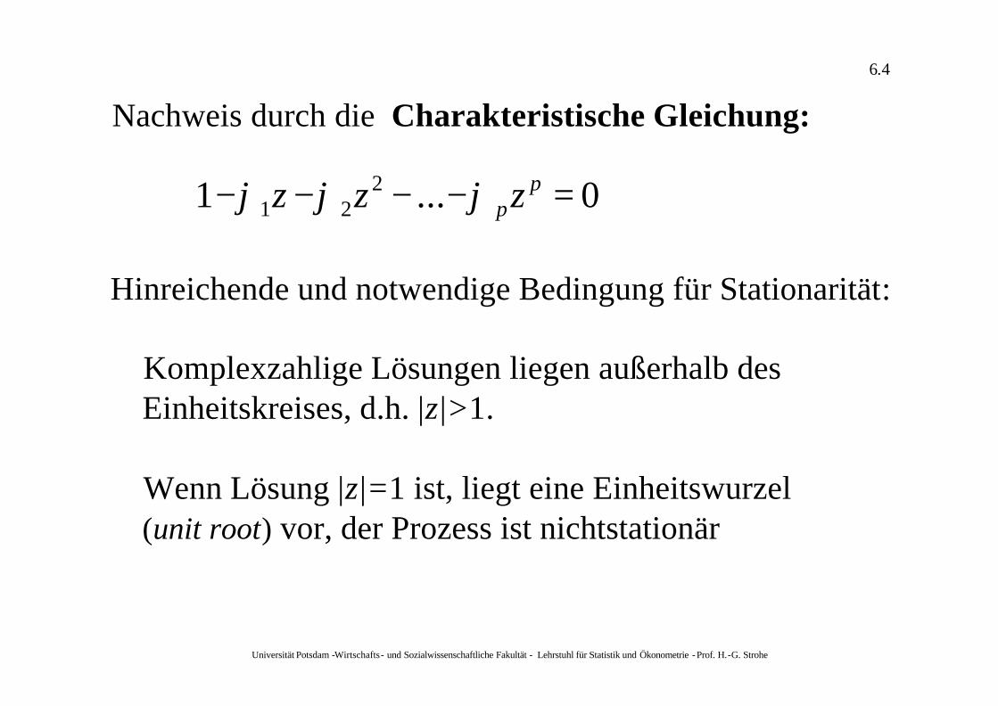
Nachweis durch die Charakteristische Gleichung:

01 221 =−−−− p

pz...zz ϕϕϕ

Hinreichende und notwendige Bedingung für Stationarität:

Komplexzahlige Lösungen liegen außerhalb des Einheitskreises, d.h. |z|>1.

Wenn Lösung |z|=1 ist, liegt eine Einheitswurzel (unit root) vor, der Prozess ist nichtstationär


6.5

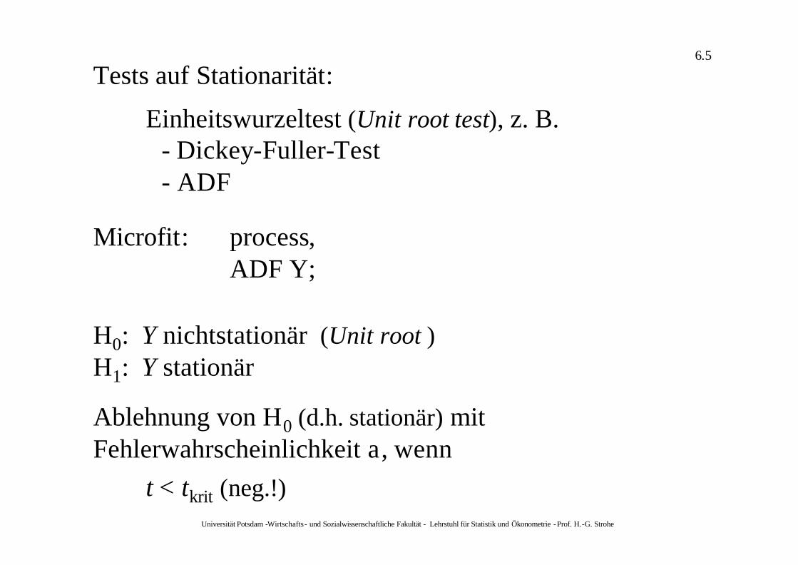
Tests auf Stationarität:

Einheitswurzeltest (Unit root test), z. B.- Dickey-Fuller-Test- ADF

Microfit: process, ADF Y;

H0: Y nichtstationär (Unit root )H1: Y stationär

Ablehnung von H0 (d.h. stationär) mit Fehlerwahrscheinlichkeit a, wenn

t < tkrit (neg.!)


6.6

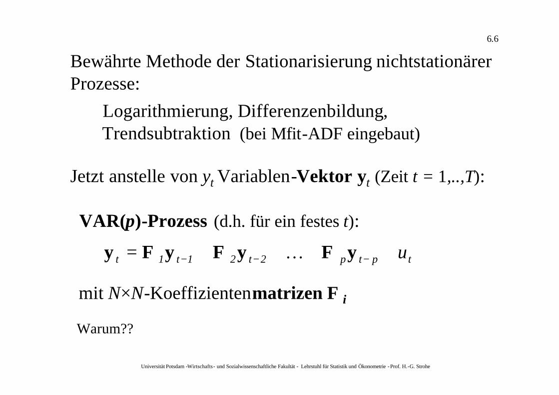
Bewährte Methode der Stationarisierung nichtstationärer Prozesse:

Logarithmierung, Differenzenbildung, Trendsubtraktion (bei Mfit-ADF eingebaut)

Jetzt anstelle von yt Variablen-Vektor yt (Zeit t = 1,..,T):

VAR(p)-Prozess (d.h. für ein festes t):

tptp2t21t1t u++++= −−− yyyy ΦΦΦ K

mit N×N-Koeffizientenmatrizen F i

Warum??


6.7

NtpNtNNpptNpNtNNtNNt

ntpNtnNpptnpNtnNtnnt

tpNtNpptpNtNtt

uyyyyy

uyyyyy

uyyyyy

+++++++=

+++++++=

+++++++=

−−−−

−−−−

−−−−

,11,1,1111,1

,11,1,1111,1

11,111,11,11111,11

ϕϕϕϕ

ϕϕϕϕ

ϕϕϕϕ

KKKKK

KKKKK

KKK

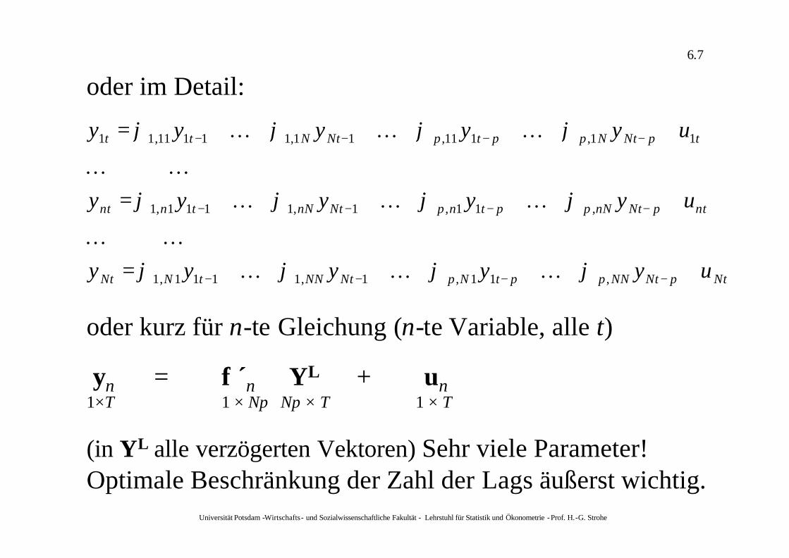
oder kurz für n-te Gleichung (n-te Variable, alle t)

yn = f ń YL + un1×T 1 × Np Np × T 1 × T

(in YL alle verzögerten Vektoren) Sehr viele Parameter! Optimale Beschränkung der Zahl der Lags äußerst wichtig.

oder im Detail:


6.8

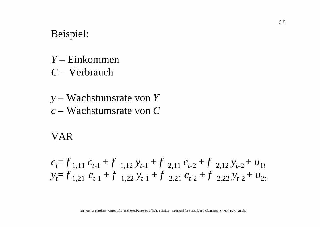
Beispiel:

Y – EinkommenC – Verbrauch

y – Wachstumsrate von Yc – Wachstumsrate von C

VAR

ct= f 1,11 ct-1 + f 1,12 yt-1 + f 2,11 ct-2 + f 2,12 yt-2 + u1tyt= f 1,21 ct-1 + f 1,22 yt-1 + f 2,21 ct-2 + f 2,22 yt-2 + u2t


6.9

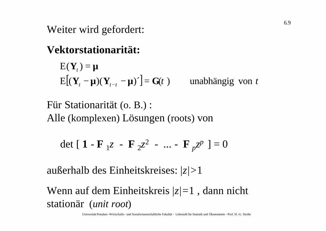
Weiter wird gefordert:

Vektorstationarität:

[ ] tttt

t

von unabhängig)()´)((E

)(E

τGµYµY

µY

=−−=

−

Für Stationarität (o. B.) :Alle (komplexen) Lösungen (roots) von

det [ 1 - F 1z - F 2z2 - ... - F pzp ] = 0

außerhalb des Einheitskreises: |z|>1

Wenn auf dem Einheitskreis |z|=1 , dann nicht stationär (unit root)


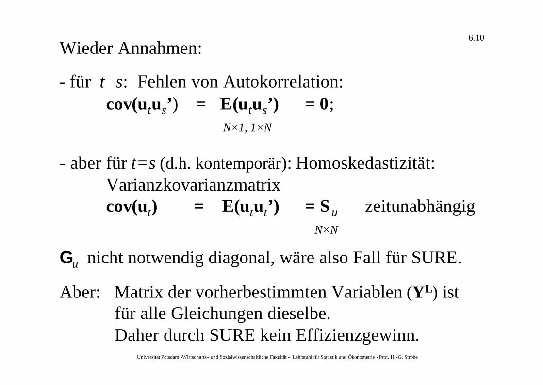
6.10Wieder Annahmen:

- für tÖs: Fehlen von Autokorrelation:cov(utus’) = E(utus’) = 0;

N×1, 1×N

- aber für t=s (d.h. kontemporär): Homoskedastizität: Varianzkovarianzmatrixcov(ut) = E(utut’) = Su zeitunabhängig

N×N

Gu nicht notwendig diagonal, wäre also Fall für SURE.

Aber: Matrix der vorherbestimmten Variablen (YL) ist für alle Gleichungen dieselbe. Daher durch SURE kein Effizienzgewinn.


6.11

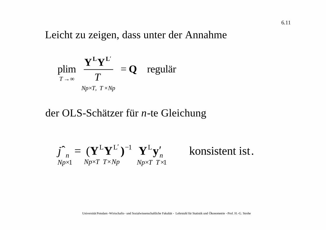
Leicht zu zeigen, dass unter der Annahme

regulärplim QYY LL

=

××

′

∞→NpT, TNp

T T

der OLS-Schätzer für n-te Gleichung

.ist konsistent(ˆ1

L

1LL

1 ××××

−′

×′=

T TNpn

NpT TNpNpn yY)YYϕ


6.12

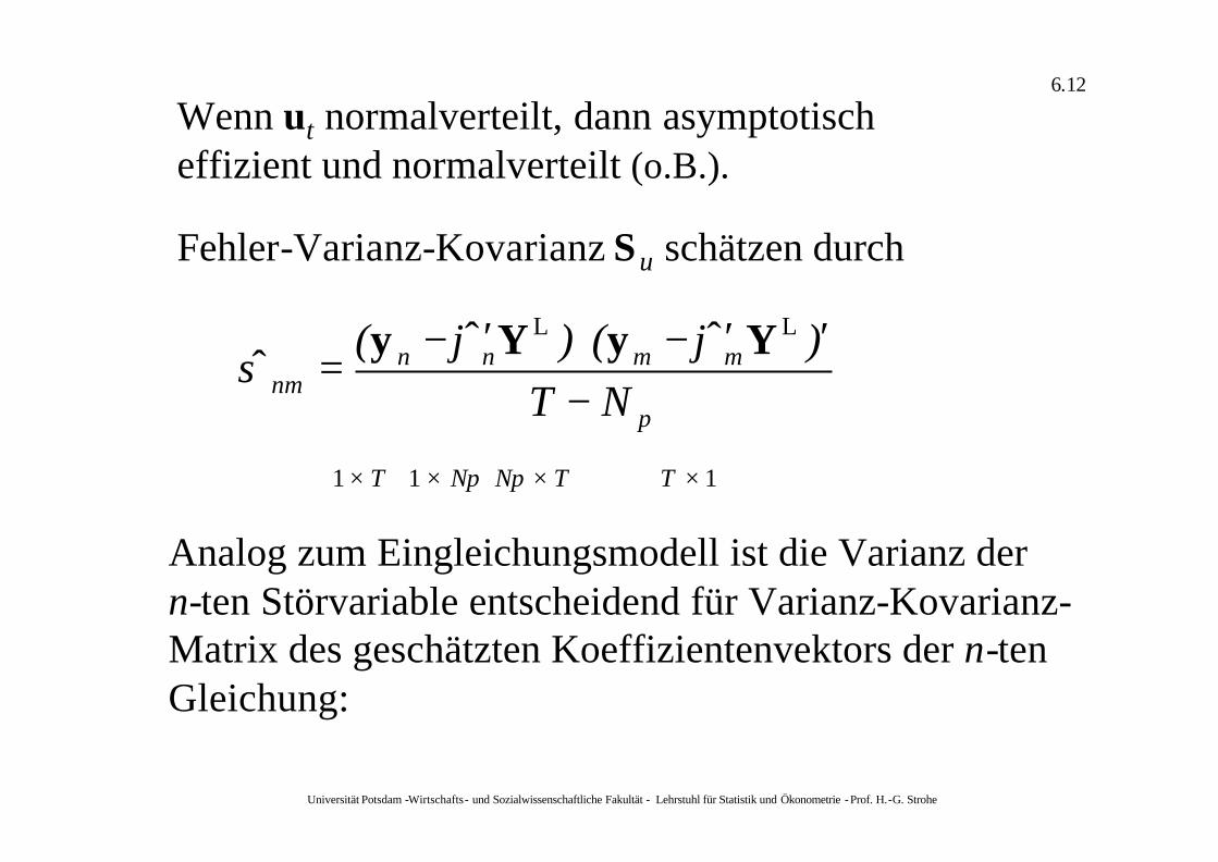
Wenn ut normalverteilt, dann asymptotisch effizient und normalverteilt (o.B.).

Fehler-Varianz-Kovarianz Su schätzen durch

1 1 1

LL

ˆˆˆ

××××

−′′−⋅′−

=

TT NpNpT

p

mmnnnm NT

)()( YyYy ϕϕσ

Analog zum Eingleichungsmodell ist die Varianz der n-ten Störvariable entscheidend für Varianz-Kovarianz-Matrix des geschätzten Koeffizientenvektors der n-ten Gleichung:


6.13

NpTT NpNp Np

nnn TTn

×××

−−

=

=

1

2

1

ˆ

´ˆ

´ˆ

LLLL YYYYS σσϕ

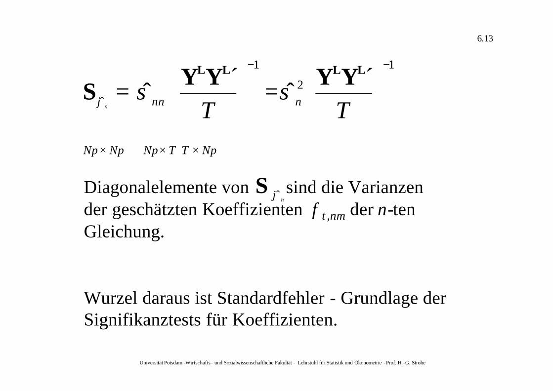
Diagonalelemente von sind die Varianzender geschätzten Koeffizienten f t ,nm der n-ten Gleichung.

Wurzel daraus ist Standardfehler - Grundlage der Signifikanztests für Koeffizienten.

nϕ̂S


6.14

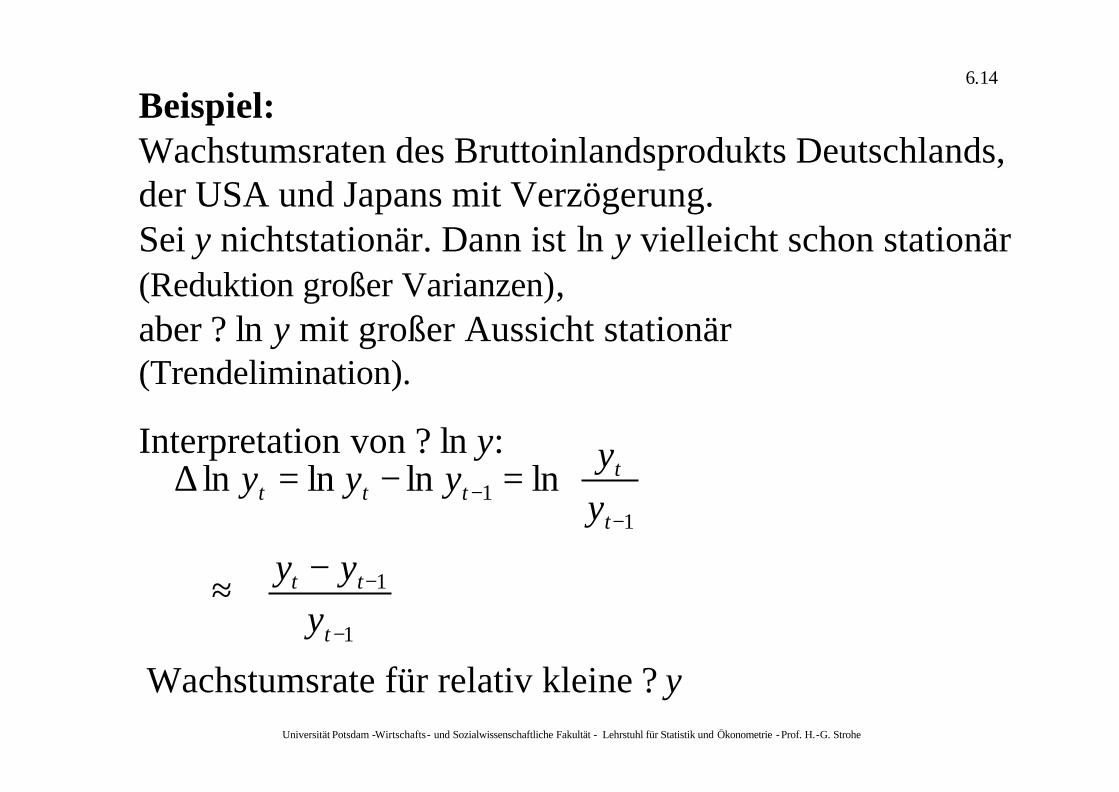
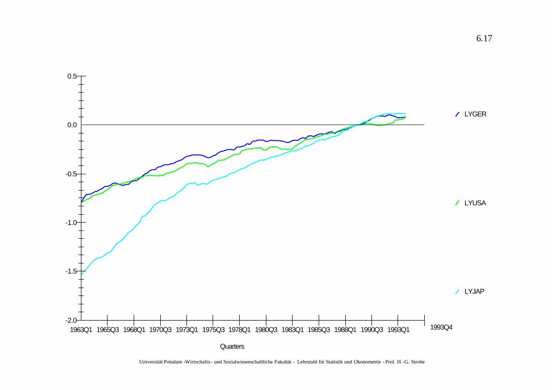
Beispiel:Wachstumsraten des Bruttoinlandsprodukts Deutschlands, der USA und Japans mit Verzögerung.Sei y nichtstationär. Dann ist ln y vielleicht schon stationär (Reduktion großer Varianzen), aber ? ln y mit großer Aussicht stationär (Trendelimination).

Interpretation von ? ln y:

1

1

11 lnlnlnln

−

−

−−

−≈

=−=∆

t

tt

t

tttt

yyy

yy

yyy

Wachstumsrate für relativ kleine ? y


6.15

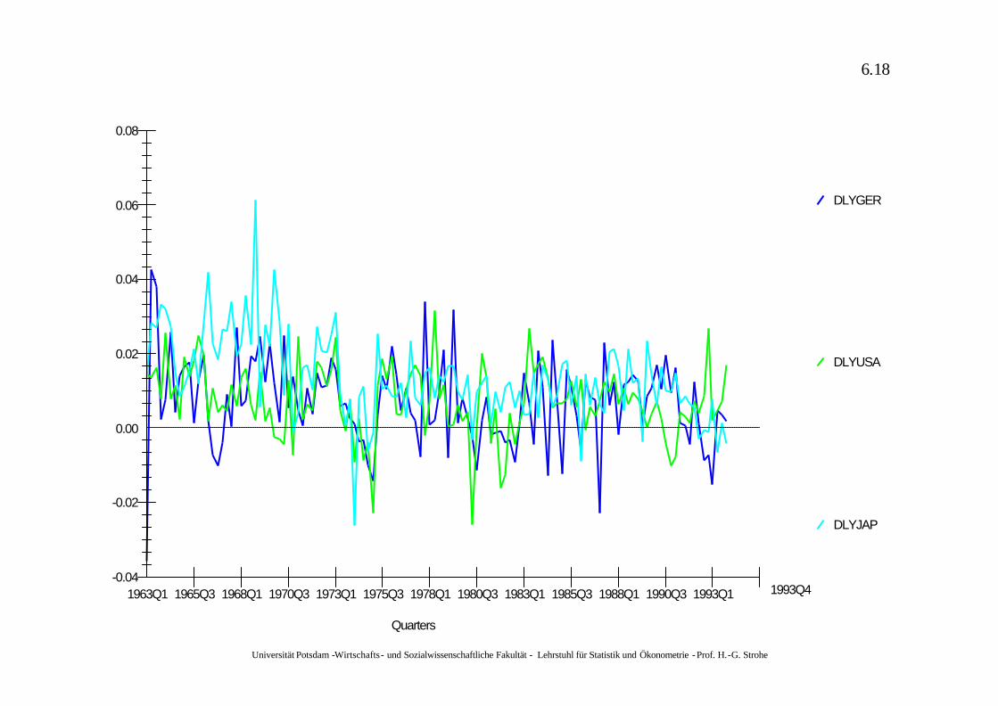
Daher als Wachstumsraten der BIPs jetzt als stationär angenommene Reihen ? ln Yt.

In Mfit: DLY mit Kennz. GER, USA, JAP (aus G7GDP.fit)

Vorgehen: Multivariate; Unrestricted VAR;

Lag-Ordnung (p) eingeben (z.B. 2); Variable eingeben.


6.16

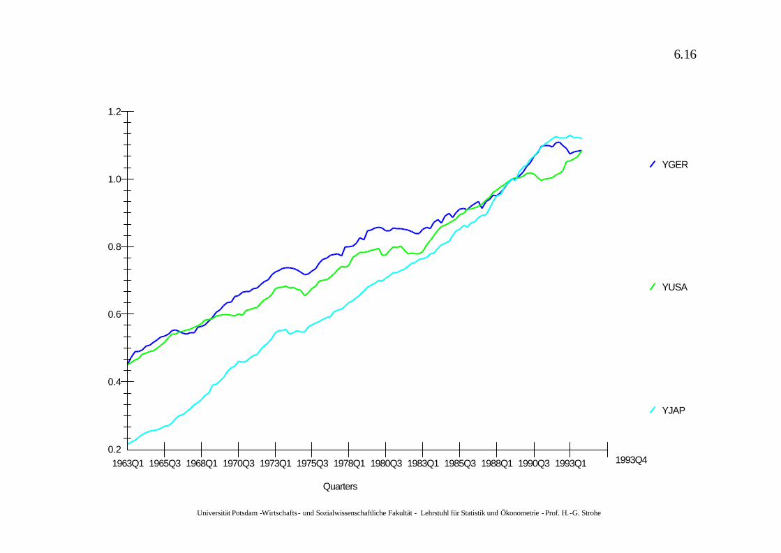
YGER

YUSA

YJAP

Quarters

0.2

0.4

0.6

0.8

1.0

1.2

1963Q1 1965Q3 1968Q1 1970Q3 1973Q1 1975Q3 1978Q1 1980Q3 1983Q1 1985Q3 1988Q1 1990Q3 1993Q1 1993Q4


6.17

LYGER

LYUSA

LYJAP

Quarters

-0.5

-1.0

-1.5

-2.0

0.0

0.5

1963Q1 1965Q3 1968Q1 1970Q3 1973Q1 1975Q3 1978Q1 1980Q3 1983Q1 1985Q3 1988Q1 1990Q3 1993Q1 1993Q4


6.18

DLYGER

DLYUSA

DLYJAP

Quarters

-0.02

-0.04

0.00

0.02

0.04

0.06

0.08

1963Q1 1965Q3 1968Q1 1970Q3 1973Q1 1975Q3 1978Q1 1980Q3 1983Q1 1985Q3 1988Q1 1990Q3 1993Q1 1993Q4


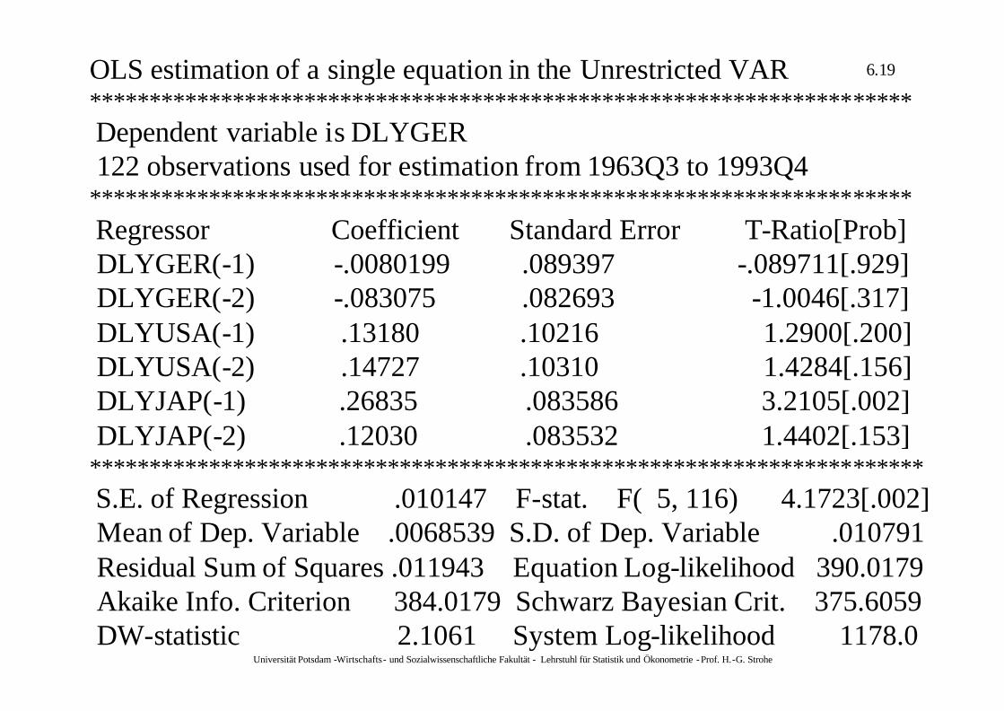
6.19OLS estimation of a single equation in the Unrestricted VAR *********************************************************************Dependent variable is DLYGER 122 observations used for estimation from 1963Q3 to 1993Q4

*********************************************************************Regressor Coefficient Standard Error T-Ratio[Prob]DLYGER(-1) -.0080199 .089397 -.089711[.929]DLYGER(-2) -.083075 .082693 -1.0046[.317]DLYUSA(-1) .13180 .10216 1.2900[.200]DLYUSA(-2) .14727 .10310 1.4284[.156]DLYJAP(-1) .26835 .083586 3.2105[.002]DLYJAP(-2) .12030 .083532 1.4402[.153]

**********************************************************************S.E. of Regression .010147 F-stat. F( 5, 116) 4.1723[.002]Mean of Dep. Variable .0068539 S.D. of Dep. Variable .010791Residual Sum of Squares .011943 Equation Log-likelihood 390.0179Akaike Info. Criterion 384.0179 Schwarz Bayesian Crit. 375.6059DW-statistic 2.1061 System Log-likelihood 1178.0


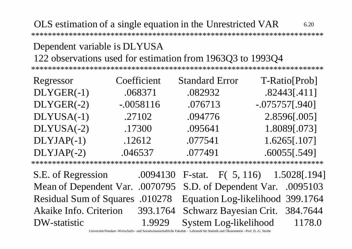
6.20OLS estimation of a single equation in the Unrestricted VAR**********************************************************************Dependent variable is DLYUSA 122 observations used for estimation from 1963Q3 to 1993Q4

**********************************************************************Regressor Coefficient Standard Error T-Ratio[Prob]DLYGER(-1) .068371 .082932 .82443[.411]DLYGER(-2) -.0058116 .076713 -.075757[.940]DLYUSA(-1) .27102 .094776 2.8596[.005]DLYUSA(-2) .17300 .095641 1.8089[.073]DLYJAP(-1) .12612 .077541 1.6265[.107]DLYJAP(-2) .046537 .077491 .60055[.549]

**********************************************************************S.E. of Regression .0094130 F-stat. F( 5, 116) 1.5028[.194]Mean of Dependent Var. .0070795 S.D. of Dependent Var. .0095103Residual Sum of Squares .010278 Equation Log-likelihood 399.1764Akaike Info. Criterion 393.1764 Schwarz Bayesian Crit. 384.7644DW-statistic 1.9929 System Log-likelihood 1178.0


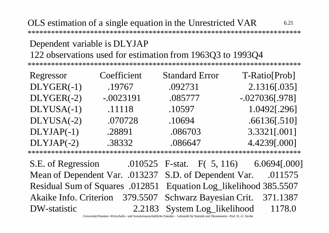
6.21OLS estimation of a single equation in the Unrestricted VAR **********************************************************************Dependent variable is DLYJAP 122 observations used for estimation from 1963Q3 to 1993Q4

**********************************************************************Regressor Coefficient Standard Error T-Ratio[Prob]DLYGER(-1) .19767 .092731 2.1316[.035]DLYGER(-2) -.0023191 .085777 -.027036[.978]DLYUSA(-1) .11118 .10597 1.0492[.296]DLYUSA(-2) .070728 .10694 .66136[.510]DLYJAP(-1) .28891 .086703 3.3321[.001]DLYJAP(-2) .38332 .086647 4.4239[.000]

**********************************************************************S.E. of Regression .010525 F-stat. F( 5, 116) 6.0694[.000]Mean of Dependent Var. .013237 S.D. of Dependent Var. .011575Residual Sum of Squares .012851 Equation Log_likelihood 385.5507Akaike Info. Criterion 379.5507 Schwarz Bayesian Crit. 371.1387DW-statistic 2.2183 System Log_likelihood 1178.0


6.22

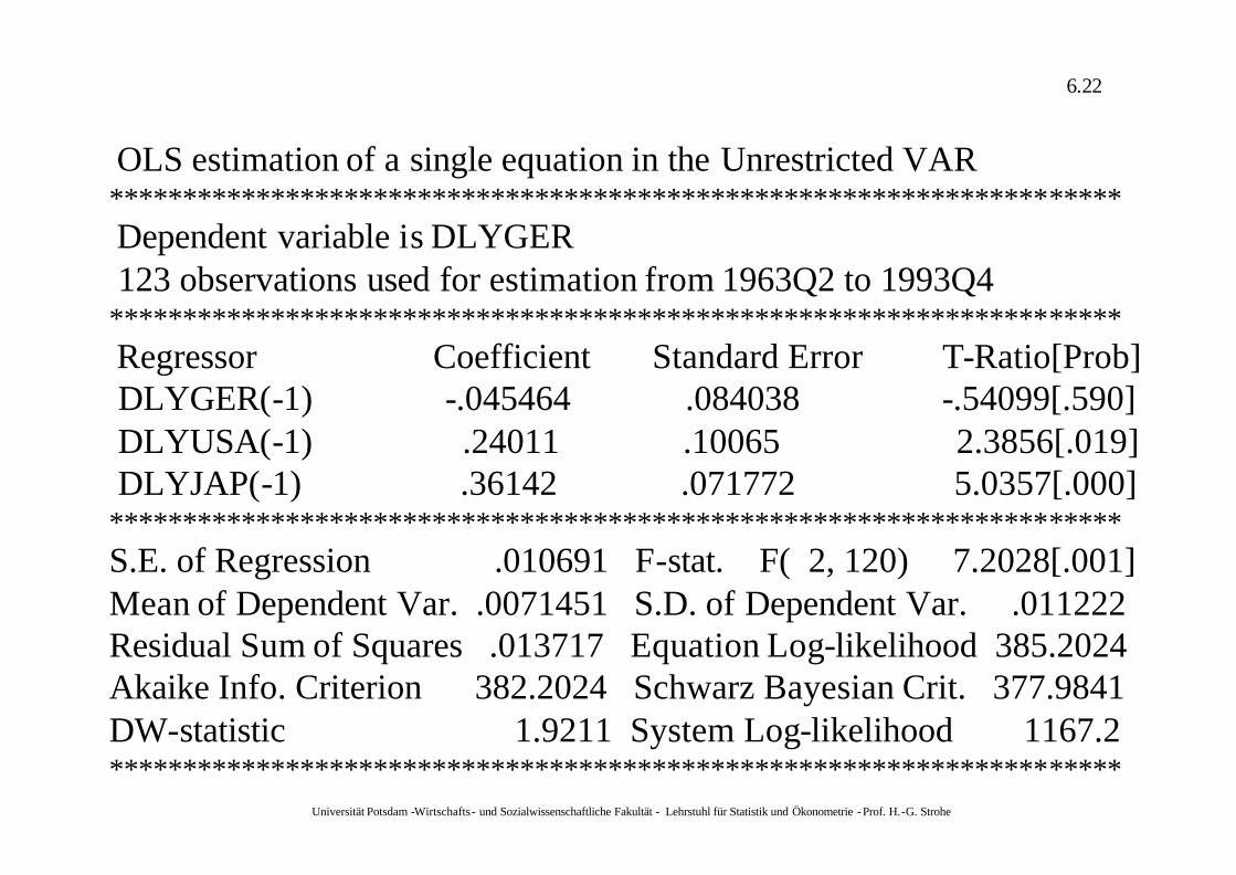
OLS estimation of a single equation in the Unrestricted VAR *********************************************************************Dependent variable is DLYGER 123 observations used for estimation from 1963Q2 to 1993Q4

*********************************************************************Regressor Coefficient Standard Error T-Ratio[Prob]DLYGER(-1) -.045464 .084038 -.54099[.590]DLYUSA(-1) .24011 .10065 2.3856[.019]DLYJAP(-1) .36142 .071772 5.0357[.000]

*********************************************************************S.E. of Regression .010691 F-stat. F( 2, 120) 7.2028[.001]Mean of Dependent Var. .0071451 S.D. of Dependent Var. .011222Residual Sum of Squares .013717 Equation Log-likelihood 385.2024Akaike Info. Criterion 382.2024 Schwarz Bayesian Crit. 377.9841DW-statistic 1.9211 System Log-likelihood 1167.2*********************************************************************


6.23

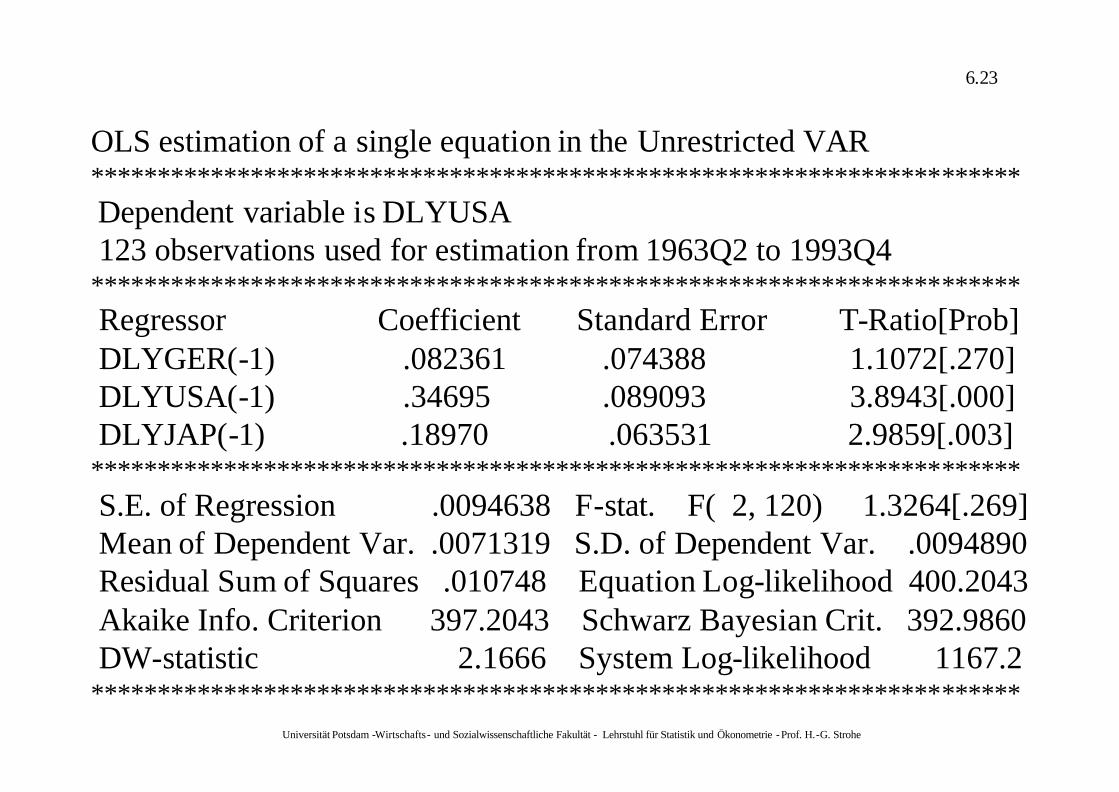
OLS estimation of a single equation in the Unrestricted VAR**********************************************************************Dependent variable is DLYUSA 123 observations used for estimation from 1963Q2 to 1993Q4

**********************************************************************Regressor Coefficient Standard Error T-Ratio[Prob]DLYGER(-1) .082361 .074388 1.1072[.270]DLYUSA(-1) .34695 .089093 3.8943[.000]DLYJAP(-1) .18970 .063531 2.9859[.003]

**********************************************************************S.E. of Regression .0094638 F-stat. F( 2, 120) 1.3264[.269]Mean of Dependent Var. .0071319 S.D. of Dependent Var. .0094890Residual Sum of Squares .010748 Equation Log-likelihood 400.2043Akaike Info. Criterion 397.2043 Schwarz Bayesian Crit. 392.9860DW-statistic 2.1666 System Log-likelihood 1167.2

**********************************************************************


6.24

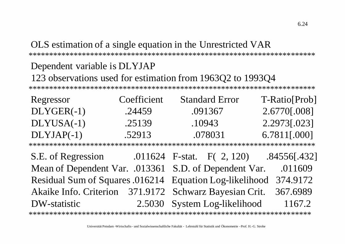
OLS estimation of a single equation in the Unrestricted VAR**********************************************************************Dependent variable is DLYJAP 123 observations used for estimation from 1963Q2 to 1993Q4

**********************************************************************Regressor Coefficient Standard Error T-Ratio[Prob]DLYGER(-1) .24459 .091367 2.6770[.008]DLYUSA(-1) .25139 .10943 2.2973[.023]DLYJAP(-1) .52913 .078031 6.7811[.000]

**********************************************************************S.E. of Regression .011624 F-stat. F( 2, 120) .84556[.432]Mean of Dependent Var. .013361 S.D. of Dependent Var. .011609Residual Sum of Squares .016214 Equation Log-likelihood 374.9172Akaike Info. Criterion 371.9172 Schwarz Bayesian Crit. 367.6989DW-statistic 2.5030 System Log-likelihood 1167.2

*********************************************************************


6.25

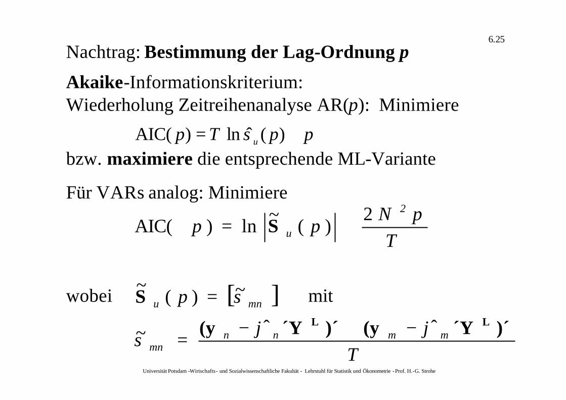
Nachtrag: Bestimmung der Lag-Ordnung p

Akaike-Informationskriterium:Wiederholung Zeitreihenanalyse AR(p): Minimiere

[ ]

Ts

sp

TpN

pp

mmnnmn

mnu

2

u

)´Ý(y )´Ý(y

S

S

LL ϕϕ ˆˆ~

~)(~

2)(

~ln)AIC(

−⋅−=

=

+=

ppsT p u += )(ˆln)AIC(

Für VARs analog: Minimiere

wobei mit

bzw. maximiere die entsprechende ML-Variante


6.26

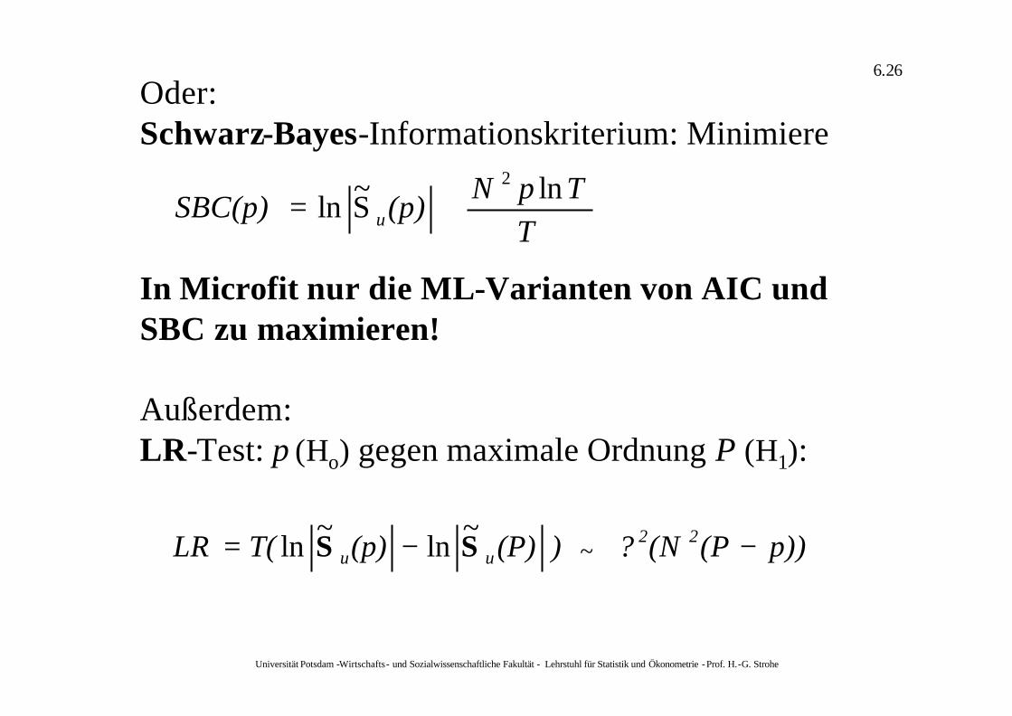
Oder:Schwarz-Bayes-Informationskriterium: Minimiere

TTpN(p)SBC(p) u

lnS~ln2

+=

In Microfit nur die ML-Varianten von AIC und SBC zu maximieren!

Außerdem:LR-Test: p (Ho) gegen maximale Ordnung P (H1):

~

ln~

ln p))(P(N?) (P)(p)T(LR 22uu −−= SS ~


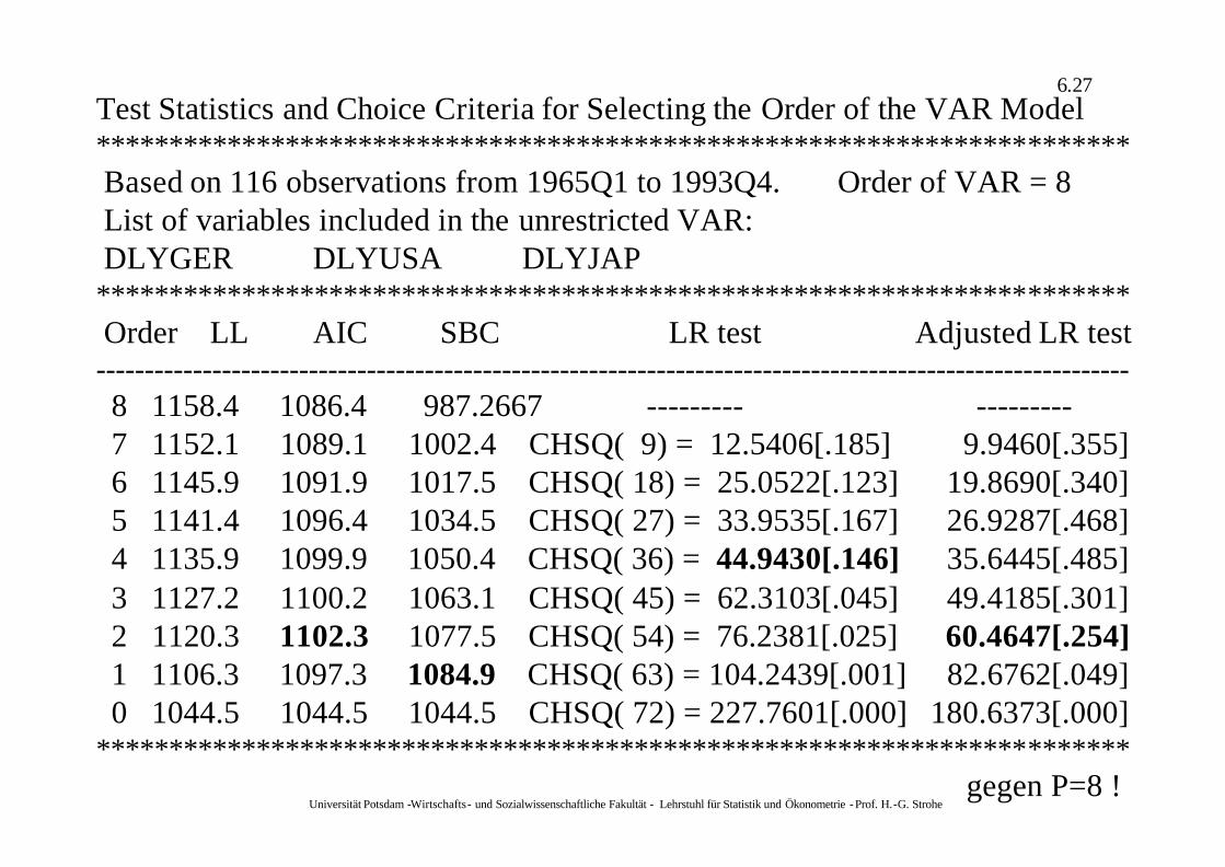
6.27Test Statistics and Choice Criteria for Selecting the Order of the VAR Model ***********************************************************************Based on 116 observations from 1965Q1 to 1993Q4. Order of VAR = 8 List of variables included in the unrestricted VAR: DLYGER DLYUSA DLYJAP

***********************************************************************Order LL AIC SBC LR test Adjusted LR test

-----------------------------------------------------------------------------------------------------------8 1158.4 1086.4 987.2667 --------- ---------7 1152.1 1089.1 1002.4 CHSQ( 9) = 12.5406[.185] 9.9460[.355]6 1145.9 1091.9 1017.5 CHSQ( 18) = 25.0522[.123] 19.8690[.340]5 1141.4 1096.4 1034.5 CHSQ( 27) = 33.9535[.167] 26.9287[.468]4 1135.9 1099.9 1050.4 CHSQ( 36) = 44.9430[.146] 35.6445[.485]3 1127.2 1100.2 1063.1 CHSQ( 45) = 62.3103[.045] 49.4185[.301]2 1120.3 1102.3 1077.5 CHSQ( 54) = 76.2381[.025] 60.4647[.254]1 1106.3 1097.3 1084.9 CHSQ( 63) = 104.2439[.001] 82.6762[.049]0 1044.5 1044.5 1044.5 CHSQ( 72) = 227.7601[.000] 180.6373[.000]

***********************************************************************gegen P=8 !


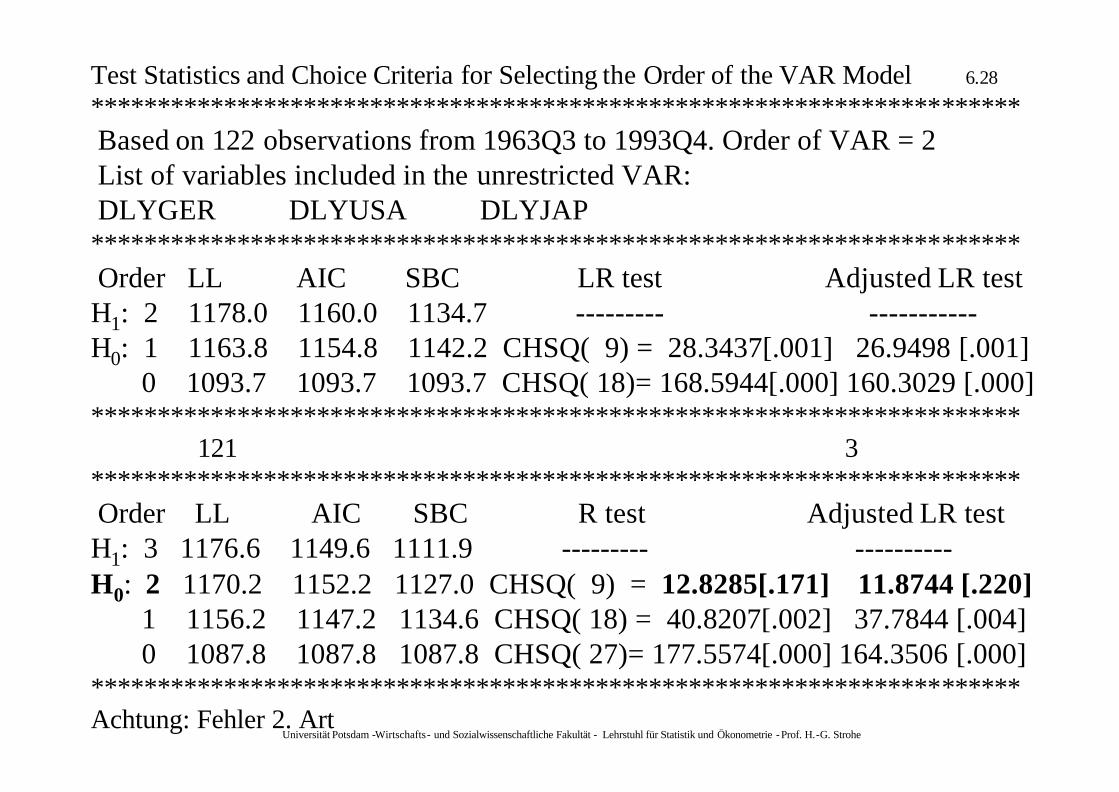
6.28Test Statistics and Choice Criteria for Selecting the Order of the VAR Model **********************************************************************Based on 122 observations from 1963Q3 to 1993Q4. Order of VAR = 2 List of variables included in the unrestricted VAR: DLYGER DLYUSA DLYJAP

**********************************************************************Order LL AIC SBC LR test Adjusted LR test H1: 2 1178.0 1160.0 1134.7 --------- -----------H0: 1 1163.8 1154.8 1142.2 CHSQ( 9) = 28.3437[.001] 26.9498 [.001]

0 1093.7 1093.7 1093.7 CHSQ( 18)= 168.5944[.000] 160.3029 [.000]**********************************************************************

121 3**********************************************************************Order LL AIC SBC R test Adjusted LR test H1: 3 1176.6 1149.6 1111.9 --------- ----------H0: 2 1170.2 1152.2 1127.0 CHSQ( 9) = 12.8285[.171] 11.8744 [.220]

1 1156.2 1147.2 1134.6 CHSQ( 18) = 40.8207[.002] 37.7844 [.004]0 1087.8 1087.8 1087.8 CHSQ( 27)= 177.5574[.000] 164.3506 [.000]

**********************************************************************Achtung: Fehler 2. Art

Documents

6. Vektorautoregressive Modelle - uni-potsdam.de · Dann ist ln y vielleicht schon stationär (Reduktion großer Varianzen), ... Akaike Info. Criterion 397.2043 Schwarz Bayesian Crit