On the Endogeneity of anExogenous OCA-Criterion:The Impact of Specialisationon the Synchronisation ofRegional Business Cycles inEurope

Ansgar BelkeJens M. Heine

HWWA DISCUSSION PAPER

119HWWA-Institut für Wirtschaftsforschung-Hamburg

2001ISSN 1616-4814

The HWWA is a member of:

• Wissenschaftsgemeinschaft Gottfried Wilhelm Leibniz (WGL)• Arbeitsgemeinschaft deutscher wirtschaftswissenschaftlicher Forschungsinstitute (ARGE)• Association d‘Instituts Européens de Conjoncture Economique (AIECE)

On the Endogeneity of anExogenous OCA-Criterion:The Impact of Specialisationon the Synchronisation ofRegional Business Cycles inEurope

Ansgar BelkeJens M. Heine

A first draft of this paper was presented at the Annual HWWA-Conference, May 2000,and on the International Thünen-Conference, September 2000. The authors would liketo thank seminar participants and especially Marius Brülhart for helpful comments.

HWWA DISCUSSION PAPER

Edited by the DepartmentEUROPEAN INTEGRATIONHead: Dr. Konrad Lammers

Hamburgisches Welt-Wirtschafts-Archiv (HWWA)Hamburg Institute of International EconomicsÖffentlichkeitsarbeitNeuer Jungfernstieg 21 - 20347 HamburgTelefon: 040/428 34 355Telefax: 040/428 34 451e-mail: hwwa@hwwa.deInternet: http://www.hwwa.de/

Ansgar BelkeUniversity of ViennaInstitut für WirtschaftswissenschaftBrünner Str. 721210 WienTel.: 0043-1-4277-37431Fax: 0043-1-4277-37498email: ansgar.belke@univie.ac.at

Jens M. HeineRuhr-University BochumFakultät für WirtschaftswissenschaftLehrstuhl für Theoretische VWL 1Gebäude GC 3/150Universitätsstrasse 15044801 BochumTel.: 0049-234-32-28888Fax: 0049-234-32-14258email: jens.heine@ruhr-uni-bochum.de

Contents

Page1 Introduction 72 Theoretical Background 83 The Specialisation Indices, Data and Stylised Facts 13 3.1 The Specialisation Indices 13 3.2 Data 14 3.3 Stylised Facts 164 Estimation 20 4.1 Procedure 21 4.2 Results 23 4.2.1 Individual Equation Estimations 23 4.2.2 Pooled Estimations 26 4.2.3 Testing for robustness of the pooled estimation results 295 Conclusions 31References 34Annex I 37Annex II 56

TablesTable 1: Indicators as measures of the degreee of specialisation 13Table 2: French and German NUTS 1 Regions 15Table 3a: Regression results based on the conformity index CON Annex IITable 3b: Regression results based on the Finger-Kreinin index FIN Annex IITable 3c: Regression results based on the specialisation index SPEC Annex IITable 3d: Regression results based on the Balassa-Aquino-Index BAL Annex IITable 4a: Pooled Least Squares (conformity index CON) 26Table 4b: Pooled Least Squares (Finger-Kreinin index Fin) 27Table 4c: Pooled Least Squares (specialisation index SPEC) 27Table 4d: Pooled Least Squares (Balassa-Aquino index BAL) 28Table 5: The impact of specialisation on the synchronisation of cycles:

Testing for robustness 30

FiguresFigure 1: The relationship and the interdependences between the degree of

specialisation and the synchronisation of regional business cycles 9Figure 2: Within-France region pair correlations 18Figure 3: Within-Germany region pair correlations 19Figure 4: Cross-country region pair correlations 20

Summary

This paper empirically assesses the impact of specialisation on the synchronisation ofregional business cycles in two core countries of EMU, namely France and Germany.Several specialisation indices are introduced and some first stylised facts about inter-regional business cycle correlations are derived. Second, region pair specific and pooledestimations are enacted and tested for robustness in order to calculate the impact of spe-cialisation on the degree of business cycle synchronisation. However, our regression re-sults confirm the hypothesis of a positive impact only partly, but they underline theproblem of a common monetary policy for uncommon regions which has already ex-isted in the DM- and in the Franc-zone before.

Zusammenfassung

Der vorliegende empirische Beitrag untersucht die Auswirkungen realwirtschaftlicherVeränderungen auf den konjunkturellen Gleichlauf regionaler Konjunkturzyklen. In ei-nem ersten Schritt werden zunächst verschiedene Maßzahlen zur Bestimmung der regi-onalen Spezialisierung sowie einige stilisierte Fakten bezüglich des Synchronisations-verhaltens regionaler Konjunkturzyklen vorgestellt. In einem zweiten Schritt wird aufder Basis ökonometrischer Verfahren der quantitative Einfluss von Strukturveränderun-gen auf den Synchronisationsgrad ermittelt. Zwar kann die aufgestellte Hypothese einermessbaren Einwirkung nur partiell bestätigt werden, die Resultate reflektieren jedochdas schon in der DM- und Franc-Zone bestehende Problem einer gemeinsamen Geldpo-litik für unterschiedliche Regionen.

JEL-Codes: E32, F15, R23

Keywords: Agglomeration, Specialisation, Regional Employment, EuropeanMonetary Union, Regional Business Cycles, Synchronisation

7

1 INTRODUCTION

One obvious caveat against EMU is that for example its one size fits all monetary pol-icy cannot do justice to such a heterogeneous area as the EMU11. There has been con-siderable theoretical and empirical research on this general issue, but the latter has usu-ally emphasised differences across countries, assuming implicitly (instead of testingexplicitly) that countries are homogenous entities. However, the implicit assumption ofhomogenous entities is not warranted. The general concern about the cost of having acommon policy for a heterogeneous area mainly stems from two aspects:

1) The common monetary policy stance might not be optimal for all regions becausethe latter might be at different stages of the business cycle.

2) The common monetary policy might have quite different effects in regions with alow degree of intra-industrial trade. In both cases, regionally asymmetric shockswould result and raise the claim for stabilising transfer mechanisms (Belke and Gros1998).

Several authors tried to find (exogenous) factors endogenising the OCA-criterion de-gree of synchronisation, e.g., Frankel and Rose (1998), Imbs (1999) among others. Inour paper, we go one step further and endogenise the degree of the regional businesscycle synchronisation by the former exogenous OCA-criterion degree of specialisa-tion, approximated by several specialisation indices.

The structure of our paper is as follows: In the first chapter we introduce the theoreticalbackground, combining the empirical literature of the European national and regionalbusiness cycles with the New Economic Geography. After explaining the used data indetail, the method of constructing the “specialisation index” and the estimation proce-dures, we will have a short view on the descriptive statistics of the synchronisation ofregional business cycles in the core EMU countries France and Germany. In chapterfour we will discuss the empirical results of our individual and our pooled regressions.Chapter five concludes.

8

2 THEORETICAL BACKGROUND

Increasing synchronisation of national business cycles within Europe was investigatedempirically by many authors. As the main reasons, the shaping of the European Mone-tary System in 1979 (Artis and Zhang 1997), increasing international trade (Frankel andRose 1997), identical income and sectoral structures between two economies (Imbs1999) or the existence of a common border (Clark and Wincoop 1999) have been identi-fied.

Artis and Zhang (1997) investigate the filtered time series of industrial production indifferent countries (national cycles) and regress these filtered series on the filtered U.S.and German benchmark cycle. As their main result, these authors emphasise that thecontinental European countries display a business cycle behaviour which has becomeincreasingly synchronous to the German and less so to the U.S. cycle after the creationof the EMS in 1979. Based on his own analysis, Fatás (1997) concludes that the syn-chronisation of regional business cycles to an European aggregate has increased sincethe start of the EMS. He applies the growth rate of employment within a region as anindicator of its business cycle stance and makes use of the fact that the first differencesfilter of logarithms approximately correspond to the realisations of the growth rate.Fatás as well as Forni and Reichlin (1997) were the first who stressed the potential im-portance of the regional dimension. Both Fatás as well as Artis and Zhang emphasisethe role of the exchange rate regime, i.e. the EMS, in determining the cyclical behav-iour of macroeconomic time series and the degree of bilateral correlation of the businesscycles. By this, they merely focus on the role of a nominal variable. However, the im-pact of real variables on the degree of synchronisation is still neglected.

Focusing on different real impact variables, Frankel and Rose (1998) examine the im-pact of aggregated foreign trade on the synchronisation of national business cycles.They draw the conclusion that an increase in foreign trade generally leads to more syn-chronicity of the cyclical movements of the national economic time series. However,Imbs (1999) qualifies the main result gained by Frankel and Rose. His results signifi-cantly reduce the potential role of foreign trade in explaining co-movement of nationalbusiness cycle indicators. Instead, he finds that relative economic structures, relativesectoral production patterns and relative total economy incomes are the main de-terminants of the degree of synchronisation of national business cycles. Clark and Win-coop (1999) investigate the evidence of the within-country and across-countries busi-

ness cycle synchronisation for Europe and the U.S. As one result, the correlation ofeconomic variables within the U.S. were higher than in Europe. They conclude thatthese differences were due to the existence of (national) borders, but there seems to beevidence that this border effect has become smaller in Europe in the eighties of the lastcentury.

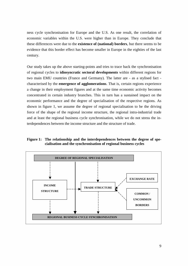
Our study takes up the above starting-points and tries to trace back the synchronisationof regional cycles to idiosyncratic sectoral developments within different regions fortwo main EMU countries (France and Germany). The latter are - as a stylised fact -characterised by the emergence of agglomerations. That is, certain regions experiencea change in their employment figures and at the same time economic activity becomesconcentrated in certain industry branches. This in turn has a sustained impact on theeconomic performance and the degree of specialisation of the respective regions. Asshown in figure 1, we assume the degree of regional specialisation to be the drivingforce of the shape of the regional income structure, the regional intra-industrial tradeand at least the regional business cycle synchronisation, while we do not stress the in-terdependences between the income structure and the structure of trade.

Figure 1: The relationship and the interdependences between the degree of spe-cialisation and the synchronisation of regional business cycles

DEGREE OF REGIONAL SPECIALISATION

INCOME

STRUCTURETRADE STRUCTURE

COMMON /

UNCOMMON

BORDERS

REGIONAL BUSINESS CYCLE SYNCHRONISATION

EXCHANGE RATE

9

10

In order to examine the nature of the relationship between the degree of regional spe-cialisation and the fluctuation of the regional business cycle, we intend to quantify thesectoral change caused by European integration for the last two decades. For this pur-pose, we construct several annual indices (in the following called specialisation indi-ces) for two core EMU countries, which we will introduce in section 3. Since it is gen-erally acknowledged that a disaggregated representation of a business cycle displayshigher informational contents than its aggregated representation (different regional de-velopments cancel out at the aggregated level) and the agglomeration phenomenon canmore accurately be grasped by a higher resolution we decided to choose the regionaldimension as emphasised and focused on by Fatás (1997), Forni and Reichlin (1997)and Clark and Wincoop (1999) as well.

Our paper is motivated by the seminal study of Artis and Zhang who for the first timeexplicitly tested for the synchronisation of European business cycles dependent on theexchange rate regime. However, our analysis differs from the latter in several respects.First, in contrast to Artis and Zhang, our procedure is not limited to the analysis ofbenchmark cycles but we correlate all possible region pairs. Second, we emphasise theregional dimension in the same way as Fatás (NUTS1) by approximating the regionalcycle by the growth rate of total regional employment. Third, we do not emphasisethe role of nominal impact variables, as e.g. the exchange rate regime, in determiningthe cyclical behaviour of macroeconomic time series. Finally, we dispense with investi-gating the correlation between regional cycles and national or European cycles. Instead,we focus on the impacts of a change in the regional sectoral pattern of production onthe degree of correlation of regional employment cycles. Supplementary, we are inter-ested in a solution to the empirical issue whether the probability of asymmetric shockswill increase in the light of EMU if the industries will agglomerate in several regions.

All above cited papers investigate the sources of the co-fluctuations empirically, butonly a few (Fatás, Clark and Wincoop) deliver a detailed analysis of the regional level.However, one of the latter exceptions is the study by Clark and Wincoop who identifycorrelations between regional cycles based on border effects and on a measure of thenational specialisation. In other words, they apply the same national measure for eachregion of the respective nation.

In this contribution, we focus on the degree of regional specialisation determining thesynchronisation of the regional business cycles. However, we do not believe that this

11

specialisation pattern is given as an exogenous variable – instead we suppose that thedegree of specialisation will be an endogenous variable as well. One theory which triesto explain the choice of an industry to locate in a certain region is the so-called NewEconomic Geography. The latter explicitly conveys us some detailed theoretical in-formation about the impact of by increasing economic integration on the developmentof industrial structures. Moreover, it implicitly gives some information about the re-sulting degree of specialisation. Assuming increasing returns in the production of dif-ferentiated goods as well as monopolistic competition, models of the New EconomicGeography type endogenise the initially given factor endowment further – endogenouscore-periphery patterns will be the result.

If firms find themselves a situation of increasing economic integration, there will be ad-vantages for firms of one industry to cluster in a certain region – this agglomerationforces can further be reinforced by themselves and will tend to encourage concentrationof industrial activity by cumulative causations. There are two mechanisms which po-tentially lead to these cumulative causations. The first example is Krugman (1991) whoassumes highly mobile workers, while Venables (1996) or Krugman and Venables(1996) focuses on high firm mobility (we pick up this assumption later for choosing thevariable which measures our specialisation index).

Centripetal or centrifugal forces are commonly regarded as the main reasons for thiscumulative causations (for a survey see, e.g., Krugman 1998). These forces have an im-pact on the decision of mobile production factors to agglomerate or deglomerate geo-graphically. However, these forces are themselves determined by the degree of integra-tion or, even better, by the magnitude of transportation costs. The advantages of ag-glomerating geographically (centripetal forces) may be seen in larger markets offeringintermediate goods. Besides other aspects, this might result in lower production costsfor the sectors which produce final goods and/or in technological and knowledge spill-overs between equal specialised firms or home market effects. Both of these conceptsare generally known as the forward linkages and the backward linkages. When de-glomeration is observed (centrifugal forces), this may be caused by increasing costs ofenvironment pollution, decreasing scale effects or lower factor costs in the periphery or,equivalently and more generally, by a utility of agglomeration which is smaller than itscosts. Even when the produced goods are homogeneous, price competition pressure isincreasing when firms agglomerate, so there is an incentive to migrate to peripheral re-gions. The degree of economic integration plays an important role with respect to the

12

balance of power between both forces. Starting from a situation of low integration, anincrease of the latter will lead to industrial concentration in order to profit from the up-coming trade centres. If this increase continues, the incentives of producing goods in theperiphery and transporting them to the markets will raise. Deglomeration is the conse-quence and the centrifugal forces may dominate the centripetal ones (Krugman 1998).

However, some recent studies reveal that the relationship between agglomeration andthe degree of specialisation is far from being purely monotonic. Examples are, e.g.,Ricci (1999) and Puga (1999). The latter combines the assumptions of labour mobility(in the tradition of Krugman) and of firm mobility (in this respect following Venables)in a two regions and two sectors model in order to get a more realistic model. Based onhis model he demonstrates how the industrial structure will change if economic integra-tion increases. In a situation with low integration, the industries will distribute symmet-rically over the two regions. This would imply a low degree of specialisation. Increasingintegration strengthens the centripetal forces and leads to agglomeration of the industrialsector in just one region, so the degree of specialisation will increase too. This degreewill again decrease if the economic integration will further increase, strengthening thecentrifugal forces. Thus, he is able to identify a theoretically founded relationship be-tween the process of economic integration, the agglomeration of industries in certainregions and the degree of specialisation. Thus, our assumption that the OCA-criteriondegree of specialisation is an endogenous variable is not rejected by these model basedconsiderations.

In Europe, the integration of nations is now an issue since four decades. With respect tothe national level, there exists a variety of empirical studies on the level of national spe-cialisation, the sources of national business cycles and the importance of industry-specific shocks, especially when they are classified as asymmetric. As indicated above,some studies combine regional measures of the national specialisation with the co-movement of regional cycles. However, we want to stress the relationship between re-gional cycles and regional industrial specialisation. Our main innovation is to use somefeatures of the New Economic Geography in order to construct several regional spe-cialisation indices. We investigate the impacts of these indices on a representative re-gional business cycle indicator, namely (growth of) total regional employment. In thenext chapter we explain the construction of the respective indices, and in chapter fourthe business cycle impacts of the latter are estimated via some regressions.

13

3 THE SPECIALISATION INDICES, DATA AND STYLISEDFACTS

3.1 The Specialisation Indices

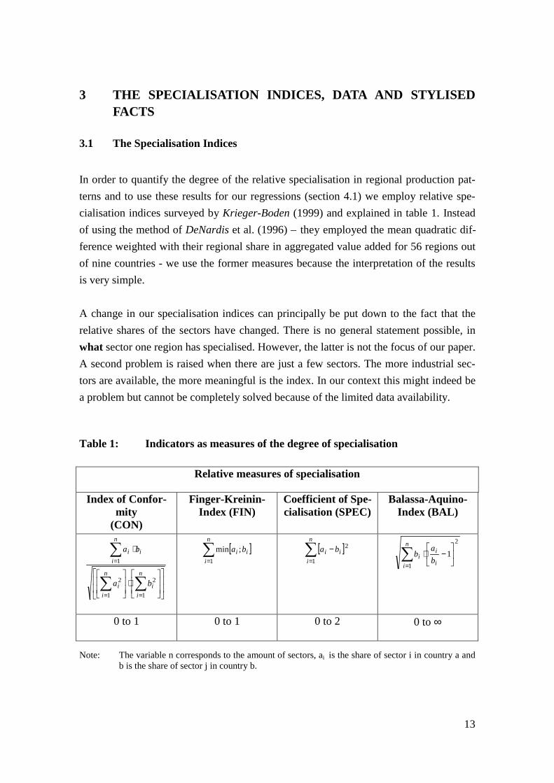
In order to quantify the degree of the relative specialisation in regional production pat-terns and to use these results for our regressions (section 4.1) we employ relative spe-cialisation indices surveyed by Krieger-Boden (1999) and explained in table 1. Insteadof using the method of DeNardis et al. (1996) – they employed the mean quadratic dif-ference weighted with their regional share in aggregated value added for 56 regions outof nine countries - we use the former measures because the interpretation of the resultsis very simple.

A change in our specialisation indices can principally be put down to the fact that therelative shares of the sectors have changed. There is no general statement possible, inwhat sector one region has specialised. However, the latter is not the focus of our paper.A second problem is raised when there are just a few sectors. The more industrial sec-tors are available, the more meaningful is the index. In our context this might indeed bea problem but cannot be completely solved because of the limited data availability.

Table 1: Indicators as measures of the degree of specialisation

Relative measures of specialisation

Index of Confor-mity

(CON)

Finger-Kreinin-Index (FIN)

Coefficient of Spe-cialisation (SPEC)

Balassa-Aquino-Index (BAL)

��

�

�

��

�

�

��

�

�

��

�

�⋅

��

�

�

��

�

�

⋅

��

�

==

=

n

ii

n

ii

n

iii

ba

ba

1

2

1

2

1

[ ]�=

n

iii ba

1

;min [ ]�=

−n

iii ba

1

22

1

1�=

��

���

�−⋅

n

i i

ii b

ab

0 to 1 0 to 1 0 to 2 0 to ∞

Note: The variable n corresponds to the amount of sectors, ai is the share of sector i in country a andb is the share of sector j in country b.

14

As a first index we employ the index of conformity, used, e.g., by Imbs (1999) in orderto measure the degree of national specialisation. It is constructed analogously to theusual correlation coefficient without consideration of the statistical mean. The resultsare values between zero (perfect specialisation) and one (perfect diversification). Sec-ond, the Finger-Kreinin index is used (see, e.g., Amiti 1997) which is defined as thesum of the minima of the industrial shares of two regions. The higher the value of thisindex (maximum 1), the more identical sectoral patterns the both regions realise. Thethird index we apply is the specialisation coefficient, e.g., proposed by Krugman(1993) and Clark and Wincoop (1999). However, in order to stress differences in per-formance between two regions (which might not come out as clearly as appropriate) wecalculate the quadratic difference instead of the total amount of the differences of therelative shares. Finally, the Balassa-Aquino index, constructed as the standard error ofthe Balassa index weighted with sector shares, is the last index we use. Its interpretationis more difficult than with respect to the three ones discussed before, because in the caseof total specialisation of both regions the value of this index will raise to infinity. Thismay lead to problems for our estimation, because in this case the index might not bestationary from a time series point of view.1

3.2 Data

The first variable which has to be defined is the specialisation index. In order to con-struct four variants of this index, we use the time series of the nominal gross valueadded for 16 European regions from 1975 to 1994 instead of the time series of the na-tional gross value added (mill. ECU) as used in Clark and Wincoop. The data for theregional gross value added and regional GDP were taken from EUROSTAT for theyears 1975 to 1995 respectively 1980 to 1997. Our choice of this variable significantlydeviates from Imbs (1999) who estimates a specialisation index based on the sectoraltotal employment. We do not use employment data because they are level merely avail-able for three sectors on the regional such that the specialisation index would not bevery meaningful. In order to avoid such kind of problems inherent in the use of an indexof sectoral total employment, we decided to use the regional gross value added for six

1 An additional popular approach is to calculate Gini coefficients after constructing a Lorenz curve.

The Gini coefficient is widely used in the economic literature, but as commonly known neither twointersecting Lorenz curves nor the corresponding Gini coefficients may be interpreted. For this reasonwe just use the four above explained indices.

15

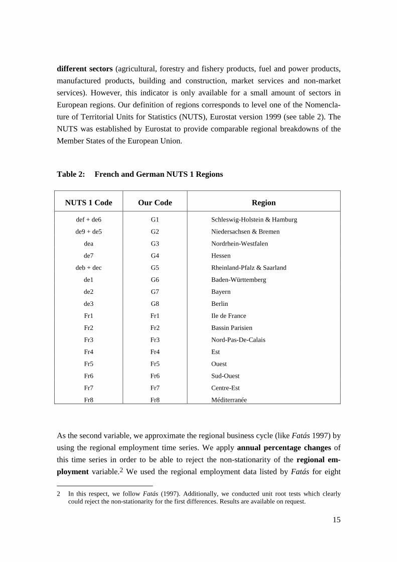
different sectors (agricultural, forestry and fishery products, fuel and power products,manufactured products, building and construction, market services and non-marketservices). However, this indicator is only available for a small amount of sectors inEuropean regions. Our definition of regions corresponds to level one of the Nomencla-ture of Territorial Units for Statistics (NUTS), Eurostat version 1999 (see table 2). TheNUTS was established by Eurostat to provide comparable regional breakdowns of theMember States of the European Union.

Table 2: French and German NUTS 1 Regions

NUTS 1 Code Our Code Region

def + de6 G1 Schleswig-Holstein & Hamburg

de9 + de5 G2 Niedersachsen & Bremen

dea G3 Nordrhein-Westfalen

de7 G4 Hessen

deb + dec G5 Rheinland-Pfalz & Saarland

de1 G6 Baden-Württemberg

de2 G7 Bayern

de3 G8 Berlin

Fr1 Fr1 Ile de France

Fr2 Fr2 Bassin Parisien

Fr3 Fr3 Nord-Pas-De-Calais

Fr4 Fr4 Est

Fr5 Fr5 Ouest

Fr6 Fr6 Sud-Ouest

Fr7 Fr7 Centre-Est

Fr8 Fr8 Méditerranée

As the second variable, we approximate the regional business cycle (like Fatás 1997) byusing the regional employment time series. We apply annual percentage changes ofthis time series in order to be able to reject the non-stationarity of the regional em-ployment variable.2 We used the regional employment data listed by Fatás for eight

2 In this respect, we follow Fatás (1997). Additionally, we conducted unit root tests which clearly

could reject the non-stationarity for the first differences. Results are available on request.

16

German and eight French regions for the years 1970 to 1997. Reducing the elevenWest-German regions should avoid using the so-called city-states in Germany beingonly large cities.3 Both the availability of a fairly large time span ranging from 1970 to1997 and the procyclical behaviour of this variable make this procedure appear highlyadvantageous for our purposes.4 When we test for the robustness of our regression re-sults we implement the difference in relative income between two regions as an addi-tional explaining control variable. This is done by means of the CPI deflated regionalGDP, divided by the European (here consisting solely of Germany and France) GDP-aggregate in order to normalise the size of the regional income. Missing values for theFrench regions in 1981 were interpolated.

3.3 Stylised Facts

A variety of stylised facts for business cycles are accepted as valid for the nationallevel by many scholars, but for the regional level such relatively indisputable facts aremissing. In particular, this could be caused by the fact that adequate regional time seriesare not available or not existent. First steps in this direction are undertaken by Fatás andClark and Wincoop; in their investigations they find that the co-movements of economicvariables between European regions are decreasing (analogously to the results gainedby us later on in this section) but not to a statistically significant extent. On the contrary,the correlations of national cycles within Europe seem to be increasing significantly ac-cording to several studies.

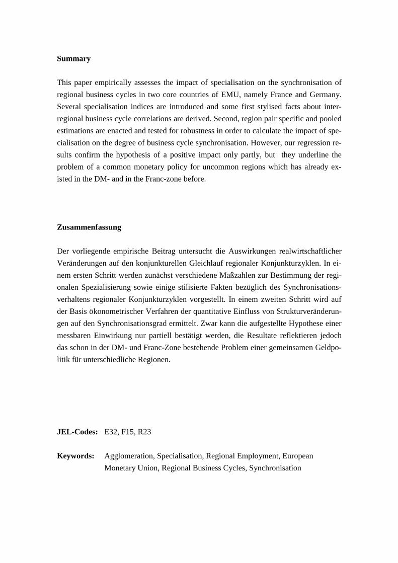
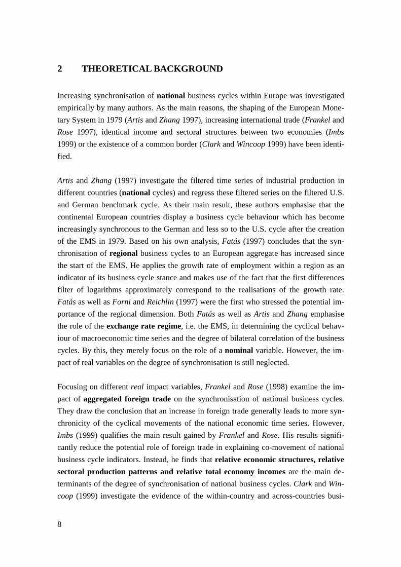
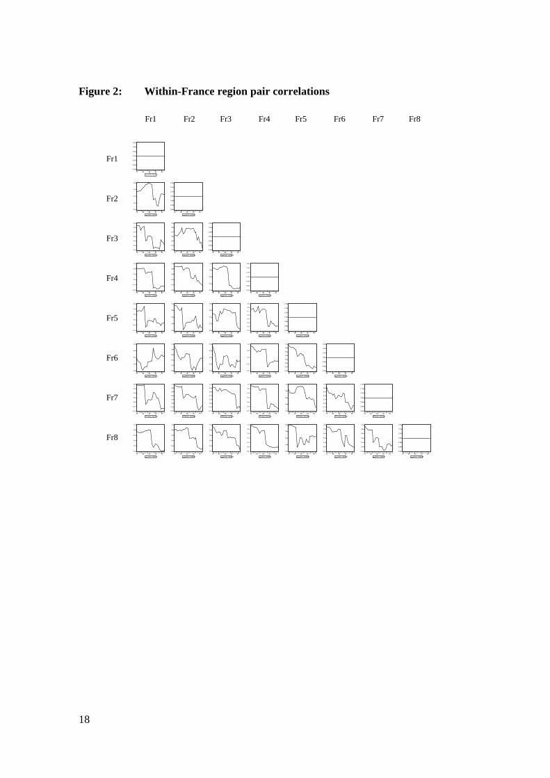
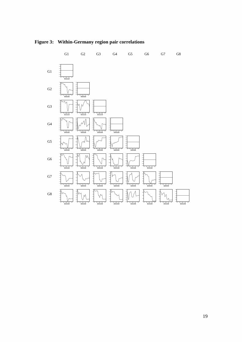
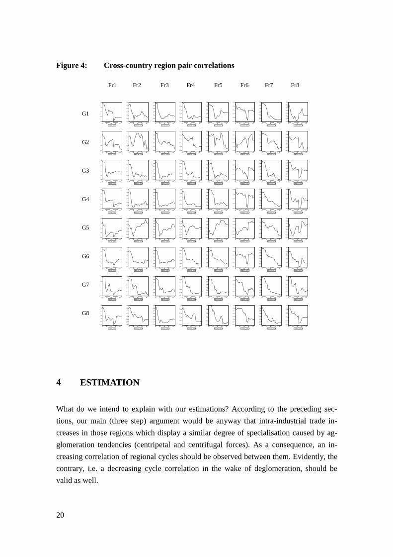
In order to get some stylised facts with respect to the within- and across-country corre-lation between regional business cycles, we calculate correlations between bilateral an-nual percentage growth rates of the regional total employment, which are displayedgraphically in the figures 1 to 3. For every possible pair of regions, we generate rollingcorrelations by a stepwise procedure5, as depicted detailed by our estimation algo-rithm in the appendix I. We let the sample grow in annual steps, each time calculating

3 The data of regional employment for 1970 until 1992 were kindly provided by Clark, for the years

1993 to 1997 from EUROSTAT.4 Using alternative filter methods in order to induce stationarity properties of the variables lead to

similar results which are available on request by the authors5 In this final version of the paper, we dispense with using ten-years windows for constructing the

rolling correlation coefficient (as, e.g., ECB 1999) in order to avoid loosing ten degrees of freedom ofour sample. Nevertheless we calculated these coefficients, but there were no differences in the results.

17

the corresponding correlation coefficient (beginning with regional correlations for thesample from 1971 to 1975 and then continuing with calculations for 1971 to 1976, 1971to 1977 and so on).6 However, we finally refused to use some alternative procedureswhich could have been potentially applicable, too. Neither splitting the total sample intwo or more subsamples, nor creating a rolling window is favoured by us. The reasonsto proceed in that way have been (1) that we only have annual data available and thussuffer from low degrees of freedom7, and (2) that the choice of the window (for exam-ple letting consecutive 10-year subsamples cover an additional one-year period minusthe first one, see Caporale et al. (1999) would appear to be rather arbitrary.

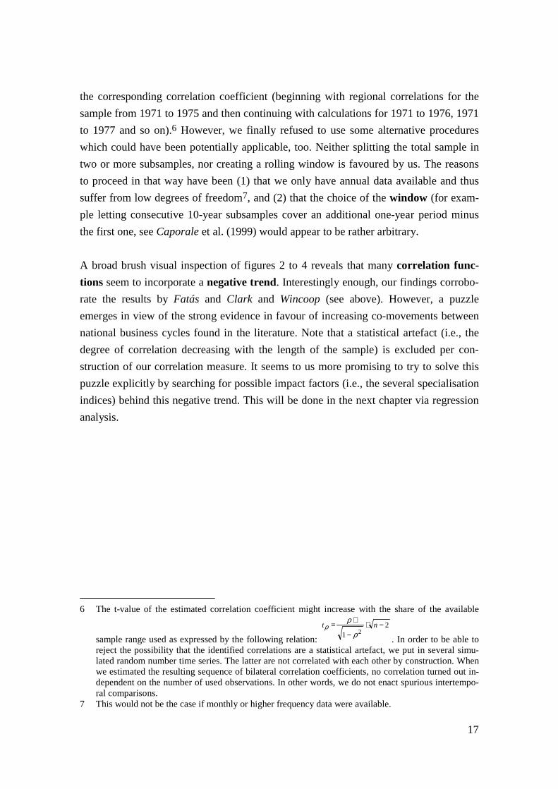
A broad brush visual inspection of figures 2 to 4 reveals that many correlation func-tions seem to incorporate a negative trend. Interestingly enough, our findings corrobo-rate the results by Fatás and Clark and Wincoop (see above). However, a puzzleemerges in view of the strong evidence in favour of increasing co-movements betweennational business cycles found in the literature. Note that a statistical artefact (i.e., thedegree of correlation decreasing with the length of the sample) is excluded per con-struction of our correlation measure. It seems to us more promising to try to solve thispuzzle explicitly by searching for possible impact factors (i.e., the several specialisationindices) behind this negative trend. This will be done in the next chapter via regressionanalysis.

6 The t-value of the estimated correlation coefficient might increase with the share of the available

sample range used as expressed by the following relation: 2

1 2−⋅

−

⋅= ntρ

ρρ

. In order to be able toreject the possibility that the identified correlations are a statistical artefact, we put in several simu-lated random number time series. The latter are not correlated with each other by construction. Whenwe estimated the resulting sequence of bilateral correlation coefficients, no correlation turned out in-dependent on the number of used observations. In other words, we do not enact spurious intertempo-ral comparisons.

7 This would not be the case if monthly or higher frequency data were available.

18

Figure 2: Within-France region pair correlations

Fr1 Fr2 Fr3 Fr4 Fr5 Fr6 Fr7 Fr8

Fr1

Fr2

Fr3

Fr4

Fr5

Fr6

Fr7

Fr8

0.94

0.96

0.98

1.00

1.02

1.04

1.06

75 80 85 90 95

KOR_FR1FR1

0.0

0.2

0.4

0.6

0.8

75 80 85 90 95

KOR_FR2FR1

0.94

0.96

0.98

1.00

1.02

1.04

1.06

75 80 85 90 95

KOR_FR2FR2

0.3

0.4

0.5

0.6

0.7

0.8

0.9

75 80 85 90 95

KOR_FR3FR1

0.3

0.4

0.5

0.6

0.7

0.8

0.9

75 80 85 90 95

KOR_FR3FR2

0.94

0.96

0.98

1.00

1.02

1.04

1.06

75 80 85 90 95

KOR_FR3FR3

-0.8

-0.4

0.0

0.4

0.8

1.2

75 80 85 90 95

KOR_FR4FR1

0.0

0.2

0.4

0.6

0.8

1.0

75 80 85 90 95

KOR_FR4FR2

0.2

0.4

0.6

0.8

1.0

75 80 85 90 95

KOR_FR4FR3

0.94

0.96

0.98

1.00

1.02

1.04

1.06

75 80 85 90 95

KOR_FR4FR4

-0.4

-0.2

0.0

0.2

0.4

0.6

75 80 85 90 95

KOR_FR5FR1

0.2

0.4

0.6

0.8

1.0

75 80 85 90 95

KOR_FR5FR2

0.0

0.2

0.4

0.6

0.8

75 80 85 90 95

KOR_FR5FR3

0.2

0.3

0.4

0.5

0.6

0.7

0.8

0.9

75 80 85 90 95

KOR_FR5FR4

0.94

0.96

0.98

1.00

1.02

1.04

1.06

75 80 85 90 95

KOR_FR5FR5

0.2

0.4

0.6

0.8

1.0

75 80 85 90 95

KOR_FR6FR1

0.0

0.2

0.4

0.6

0.8

1.0

75 80 85 90 95

KOR_FR6FR2

0.0

0.2

0.4

0.6

0.8

75 80 85 90 95

KOR_FR6FR3

-1.0

-0.5

0.0

0.5

1.0

75 80 85 90 95

KOR_FR6FR4

-0.4

-0.2

0.0

0.2

0.4

0.6

0.8

1.0

75 80 85 90 95

KOR_FR6FR5

0.94

0.96

0.98

1.00

1.02

1.04

1.06

75 80 85 90 95

KOR_FR6FR6

-0.4

-0.2

0.0

0.2

0.4

0.6

0.8

75 80 85 90 95

KOR_FR7FR1

-0.4

-0.2

0.0

0.2

0.4

0.6

0.8

1.0

75 80 85 90 95

KOR_FR7FR2

-0.4

-0.2

0.0

0.2

0.4

0.6

0.8

1.0

75 80 85 90 95

KOR_FR7FR3

-0.2

0.0

0.2

0.4

0.6

0.8

1.0

75 80 85 90 95

KOR_FR7FR4

0.2

0.4

0.6

0.8

1.0

75 80 85 90 95

KOR_FR7FR5

-0.4

-0.2

0.0

0.2

0.4

0.6

0.8

1.0

75 80 85 90 95

KOR_FR7FR6

0.94

0.96

0.98

1.00

1.02

1.04

1.06

75 80 85 90 95

KOR_FR7FR7

0.0

0.2

0.4

0.6

0.8

1.0

75 80 85 90 95

KOR_FR8FR1

0.0

0.2

0.4

0.6

0.8

1.0

75 80 85 90 95

KOR_FR8FR2

0.0

0.2

0.4

0.6

0.8

1.0

75 80 85 90 95

KOR_FR8FR3

-0.2

0.0

0.2

0.4

0.6

0.8

1.0

75 80 85 90 95

KOR_FR8FR4

0.0

0.2

0.4

0.6

0.8

75 80 85 90 95

KOR_FR8FR5

-0.2

0.0

0.2

0.4

0.6

0.8

1.0

75 80 85 90 95

KOR_FR8FR6

-0.2

0.0

0.2

0.4

0.6

0.8

1.0

75 80 85 90 95

KOR_FR8FR7

0.94

0.96

0.98

1.00

1.02

1.04

1.06

75 80 85 90 95

KOR_FR8FR8

19

Figure 3: Within-Germany region pair correlations

G1 G2 G3 G4 G5 G6 G7 G8

G1

G2

G3

G4

G5

G6

G7

G8

0.94

0.96

0.98

1.00

1.02

1.04

1.06

75 80 85 90 95

KOR_G1G1

0.3

0.4

0.5

0.6

0.7

0.8

0.9

75 80 85 90 95

KOR_G2G1

0.94

0.96

0.98

1.00

1.02

1.04

1.06

75 80 85 90 95

KOR_G2G2

0.2

0.3

0.4

0.5

0.6

0.7

0.8

75 80 85 90 95

KOR_G3G1

0.50

0.55

0.60

0.65

0.70

0.75

75 80 85 90 95

KOR_G3G2

0.94

0.96

0.98

1.00

1.02

1.04

1.06

75 80 85 90 95

KOR_G3G3

0.50

0.55

0.60

0.65

0.70

0.75

0.80

75 80 85 90 95

KOR_G4G1

0.52

0.54

0.56

0.58

0.60

0.62

0.64

0.66

0.68

75 80 85 90 95

KOR_G4G2

0.70

0.75

0.80

0.85

0.90

0.95

1.00

75 80 85 90 95

KOR_G4G3

0.94

0.96

0.98

1.00

1.02

1.04

1.06

75 80 85 90 95

KOR_G4G4

0.1

0.2

0.3

0.4

0.5

75 80 85 90 95

KOR_G5G1

0.50

0.55

0.60

0.65

0.70

75 80 85 90 95

KOR_G5G2

0.2

0.3

0.4

0.5

0.6

0.7

0.8

75 80 85 90 95

KOR_G5G3

0.1

0.2

0.3

0.4

0.5

0.6

0.7

75 80 85 90 95

KOR_G5G4

0.94

0.96

0.98

1.00

1.02

1.04

1.06

75 80 85 90 95

KOR_G5G5

0.3

0.4

0.5

0.6

0.7

75 80 85 90 95

KOR_G6G1

0.48

0.52

0.56

0.60

0.64

75 80 85 90 95

KOR_G6G2

0.70

0.75

0.80

0.85

0.90

0.95

1.00

75 80 85 90 95

KOR_G6G3

0.75

0.80

0.85

0.90

0.95

75 80 85 90 95

KOR_G6G4

0.3

0.4

0.5

0.6

0.7

0.8

75 80 85 90 95

KOR_G6G5

0.94

0.96

0.98

1.00

1.02

1.04

1.06

75 80 85 90 95

KOR_G6G6

-0.2

0.0

0.2

0.4

0.6

0.8

1.0

75 80 85 90 95

KOR_G7G1

0.0

0.2

0.4

0.6

0.8

75 80 85 90 95

KOR_G7G2

0.0

0.2

0.4

0.6

0.8

1.0

75 80 85 90 95

KOR_G7G3

0.2

0.3

0.4

0.5

0.6

0.7

0.8

75 80 85 90 95

KOR_G7G4

0.1

0.2

0.3

0.4

0.5

0.6

75 80 85 90 95

KOR_G7G5

0.4

0.5

0.6

0.7

0.8

0.9

75 80 85 90 95

KOR_G7G6

0.94

0.96

0.98

1.00

1.02

1.04

1.06

75 80 85 90 95

KOR_G7G7

-0.2

0.0

0.2

0.4

0.6

0.8

1.0

75 80 85 90 95

KOR_G8G1

0.1

0.2

0.3

0.4

0.5

0.6

0.7

75 80 85 90 95

KOR_G8G2

0.0

0.2

0.4

0.6

0.8

1.0

75 80 85 90 95

KOR_G8G3

0.0

0.2

0.4

0.6

0.8

1.0

75 80 85 90 95

KOR_G8G4

-0.2

-0.1

0.0

0.1

0.2

0.3

0.4

75 80 85 90 95

KOR_G8G5

0.2

0.4

0.6

0.8

1.0

75 80 85 90 95

KOR_G8G6

0.0

0.2

0.4

0.6

0.8

1.0

75 80 85 90 95

KOR_G8G7

0.94

0.96

0.98

1.00

1.02

1.04

1.06

75 80 85 90 95

KOR_G8G8

20

Figure 4: Cross-country region pair correlations

Fr1 Fr2 Fr3 Fr4 Fr5 Fr6 Fr7 Fr8

G1

G2

G3

G4

G5

G6

G7

G8

0.0

0.2

0.4

0.6

0.8

75 80 85 90 95

KOR_G1FR1

0.0

0.1

0.2

0.3

0.4

0.5

0.6

75 80 85 90 95

KOR_G1FR2

-0.2

0.0

0.2

0.4

0.6

0.8

1.0

75 80 85 90 95

KOR_G1FR3

-0.2

0.0

0.2

0.4

0.6

0.8

75 80 85 90 95

KOR_G1FR4

-0.4

-0.2

0.0

0.2

0.4

0.6

75 80 85 90 95

KOR_G1FR5

-0.2

0.0

0.2

0.4

0.6

0.8

75 80 85 90 95

KOR_G1FR6

-0.4

-0.2

0.0

0.2

0.4

0.6

0.8

75 80 85 90 95

KOR_G1FR7

0.3

0.4

0.5

0.6

0.7

0.8

0.9

1.0

75 80 85 90 95

KOR_G1FR8

0.4

0.5

0.6

0.7

0.8

75 80 85 90 95

KOR_G2FR1

0.1

0.2

0.3

0.4

0.5

75 80 85 90 95

KOR_G2FR2

0.0

0.2

0.4

0.6

0.8

1.0

75 80 85 90 95

KOR_G2FR3

-0.2

0.0

0.2

0.4

0.6

0.8

75 80 85 90 95

KOR_G2FR4

-0.2

-0.1

0.0

0.1

0.2

0.3

75 80 85 90 95

KOR_G2FR5

0.1

0.2

0.3

0.4

0.5

0.6

75 80 85 90 95

KOR_G2FR6

-0.2

0.0

0.2

0.4

0.6

0.8

75 80 85 90 95

KOR_G2FR7

-0.2

0.0

0.2

0.4

0.6

0.8

1.0

75 80 85 90 95

KOR_G2FR8

0.0

0.2

0.4

0.6

0.8

1.0

75 80 85 90 95

KOR_G3FR1

0.0

0.2

0.4

0.6

0.8

1.0

75 80 85 90 95

KOR_G3FR2

-0.2

0.0

0.2

0.4

0.6

0.8

1.0

75 80 85 90 95

KOR_G3FR3

-0.2

0.0

0.2

0.4

0.6

0.8

1.0

75 80 85 90 95

KOR_G3FR4

-0.2

0.0

0.2

0.4

0.6

0.8

75 80 85 90 95

KOR_G3FR5

0.2

0.4

0.6

0.8

1.0

75 80 85 90 95

KOR_G3FR6

-0.2

0.0

0.2

0.4

0.6

0.8

1.0

75 80 85 90 95

KOR_G3FR7

-0.4

-0.2

0.0

0.2

0.4

0.6

0.8

1.0

75 80 85 90 95

KOR_G3FR8

0.0

0.2

0.4

0.6

0.8

1.0

75 80 85 90 95

KOR_G4FR1

0.1

0.2

0.3

0.4

0.5

0.6

0.7

75 80 85 90 95

KOR_G4FR2

-0.2

0.0

0.2

0.4

0.6

0.8

1.0

75 80 85 90 95

KOR_G4FR3

0.0

0.2

0.4

0.6

0.8

1.0

75 80 85 90 95

KOR_G4FR4

-0.1

0.0

0.1

0.2

0.3

0.4

0.5

75 80 85 90 95

KOR_G4FR5

0.0

0.2

0.4

0.6

0.8

75 80 85 90 95

KOR_G4FR6

-0.4

-0.2

0.0

0.2

0.4

0.6

0.8

1.0

75 80 85 90 95

KOR_G4FR7

0.0

0.2

0.4

0.6

0.8

75 80 85 90 95

KOR_G4FR8

0.0

0.2

0.4

0.6

0.8

75 80 85 90 95

KOR_G5FR1

-0.2

-0.1

0.0

0.1

0.2

0.3

0.4

75 80 85 90 95

KOR_G5FR2

-0.1

0.0

0.1

0.2

0.3

0.4

0.5

0.6

75 80 85 90 95

KOR_G5FR3

-0.2

-0.1

0.0

0.1

0.2

0.3

0.4

0.5

75 80 85 90 95

KOR_G5FR4

-0.4

-0.3

-0.2

-0.1

0.0

0.1

0.2

75 80 85 90 95

KOR_G5FR5

-0.6

-0.4

-0.2

0.0

0.2

0.4

0.6

75 80 85 90 95

KOR_G5FR6

-0.4

-0.2

0.0

0.2

0.4

0.6

75 80 85 90 95

KOR_G5FR7

-0.3

-0.2

-0.1

0.0

0.1

0.2

0.3

0.4

75 80 85 90 95

KOR_G5FR8

0.0

0.2

0.4

0.6

0.8

1.0

75 80 85 90 95

KOR_G6FR1

0.0

0.2

0.4

0.6

0.8

1.0

75 80 85 90 95

KOR_G6FR2

-0.2

0.0

0.2

0.4

0.6

0.8

1.0

75 80 85 90 95

KOR_G6FR3

-0.2

0.0

0.2

0.4

0.6

0.8

1.0

75 80 85 90 95

KOR_G6FR4

-0.2

0.0

0.2

0.4

0.6

0.8

75 80 85 90 95

KOR_G6FR5

0.0

0.2

0.4

0.6

0.8

1.0

75 80 85 90 95

KOR_G6FR6

-0.4

-0.2

0.0

0.2

0.4

0.6

0.8

1.0

75 80 85 90 95

KOR_G6FR7

0.0

0.2

0.4

0.6

0.8

1.0

75 80 85 90 95

KOR_G6FR8

0.0

0.2

0.4

0.6

0.8

75 80 85 90 95

KOR_G7FR1

0.0

0.2

0.4

0.6

0.8

1.0

75 80 85 90 95

KOR_G7FR2

-0.2

0.0

0.2

0.4

0.6

0.8

1.0

75 80 85 90 95

KOR_G7FR3

-0.2

0.0

0.2

0.4

0.6

0.8

1.0

75 80 85 90 95

KOR_G7FR4

-0.4

-0.2

0.0

0.2

0.4

0.6

0.8

1.0

75 80 85 90 95

KOR_G7FR5

0.0

0.2

0.4

0.6

0.8

1.0

75 80 85 90 95

KOR_G7FR6

-0.4

-0.2

0.0

0.2

0.4

0.6

0.8

1.0

75 80 85 90 95

KOR_G7FR7

0.0

0.2

0.4

0.6

0.8

1.0

75 80 85 90 95

KOR_G7FR8

-0.2

0.0

0.2

0.4

0.6

0.8

1.0

75 80 85 90 95

KOR_G8FR1

-0.6

-0.4

-0.2

0.0

0.2

0.4

0.6

0.8

75 80 85 90 95

KOR_G8FR2

-0.4

-0.2

0.0

0.2

0.4

0.6

0.8

1.0

75 80 85 90 95

KOR_G8FR3

-0.8

-0.4

0.0

0.4

0.8

1.2

75 80 85 90 95

KOR_G8FR4

-0.4

-0.2

0.0

0.2

0.4

0.6

75 80 85 90 95

KOR_G8FR5

-0.4

-0.2

0.0

0.2

0.4

0.6

0.8

1.0

75 80 85 90 95

KOR_G8FR6

-0.4

-0.2

0.0

0.2

0.4

0.6

0.8

1.0

75 80 85 90 95

KOR_G8FR7

-0.8

-0.4

0.0

0.4

0.8

1.2

75 80 85 90 95

KOR_G8FR8

4 ESTIMATION

What do we intend to explain with our estimations? According to the preceding sec-tions, our main (three step) argument would be anyway that intra-industrial trade in-creases in those regions which display a similar degree of specialisation caused by ag-glomeration tendencies (centripetal and centrifugal forces). As a consequence, an in-creasing correlation of regional cycles should be observed between them. Evidently, thecontrary, i.e. a decreasing cycle correlation in the wake of deglomeration, should bevalid as well.

21

In order to be able to test for a significant relationship between the relative business cy-cle performance of two selected regions and the relative bilateral specialisation index,we have applied several methods:

1. estimations for single individual pairs of regions instead of pooling regions in orderto avoid too rigid (OCA) assumptions (see point 2),

2. regressions of the correlation coefficient between two regional business cycles on acertain measure of relative concentration via a pooled analysis (under the relativelyrigid (OCA) assumption that all region pairs in the pool react in the same manner onchanges in the concentration measure), and

3. augmentation of the benchmark estimations by dummies for common borders, Ger-man reunification and relative differences between regional income.8

4.1 Procedure

Since our variables are stationary by definition, we run our regressions in levels. Forexample, realisations of the correlation coefficient KOR by definition fall into a rangeof –1 to +1. table 1 clearly demonstrates the existence of finite upper and lower boundsfor the realisations of the specialisation indices. The same is valid with respect to thecommon border, reunification dummies (both between zero and one) and the relative in-come variable (RELINC) which essentially represents a share and therefore takes valuesbetween zero and one.9 In the following, one representative regression is displayed forthe case of the specialisation measure SPEC in order to convey an impression of ourproceedings. The equations estimated by us have the following structure. The correla-tion coefficient (KOR) of unemployment growth rates between two regions is regressedon a constant (C), on its own past (KOR(-1)), on the specific specialisation index (SSI)and, if necessary, on a deterministic trend (TREND) and/or a dummy (DUMMY) for aspecial year:

8 Regressions of the change of the annual correlation coefficient on the change of relative concentra-

tion did not lead to significant results in both individual and pooled estimations. The same was thecase with respect to considering EMS membership explicitly in our estimation via sample splits.

9 The only possible exception could be the Balassa-Aquino index. However, a visual inspection of theseries reveals that its realisations fall in a relatively narrow band.

22

(1) KOR = c(1) + c(2)*KOR(-1) + c(3)*SSI + c(4)*TREND+ c(5)*DUMMY.

We estimated these kind of regressions for all region pairs and all four different spe-cialisation indices via individual equation and pooled equation estimation techniques.The latter are based on equation 1 as well. However, the only difference consists of thefact that variables in our second step refer to a pool of region pairs. Lagged endoge-nous variables (i.e. lagged realisations of KOR) should be no problem in our contextbecause estimates are still consistent as long as the absence of residual autocorrelation is– as in our case – not rejected (see above all Wasmer and Weil (2000). The final specifi-cation of the underlying regression equations is based on the usual diagnostics com-bined with the Schwarz Bayesian Information Criterion (SCH). The latter is chosenas our primary model selection criterion since it asymptotically leads to the correctmodel choice (if the true model is among the models under investigation, Lütkepohl1991). The regression which reveals the lowest SCH-value and at the same time fulfilsthe usual diagnostic residual criteria is selected and finally tabulated by us. However,one important precondition for their application we take into account is the same num-ber of observations for the alternative specifications (Banerjee et al. 1993, p. 286, Mills1990, p. 139, Schwarz 1978).

The sample has been chosen to be 1971 to 1997 (if available) in order to exploit allavailable information. The procedure is exactly the same for each region pair such thatwe never intervene to exercise a discretionary judgment. As usual, we add country spe-cific dummies from time to time in order to account for possible breaks in the bi-regional relations. Significant dummies are added only if they are economically mean-ingful, if they improve the SCH statistics (higher informational contents even if a pen-alty for the extra dummy is taken into account) and lead to a non-rejection of the nor-mality assumption of the residuals (Jarque and Bera 1987). At the same time theyshould contribute to fulfil the criteria on the residuals, especially those on normality.However, none of our results is essentially due to the implementation of these dummies.

With respect to the coefficients of the explaining ”specialisation indices” in our regres-sions we expect the following conditions to hold:

(2)

0>∂∂CONKOR ;

0≤CON≤1

0>∂∂

FINKOR ;

0≤FIN≤1

0<∂∂SPECKOR ;

0≤SPEC≤6

0<∂∂

BALKOR ;

0≤BAL≤∞

23

Note that the numbers of necessary regressions depends on the chosen specialisation in-dex (BAL: 240 relevant region pairs; CON, FIN, SPEC: 120 relevant region pairs) andon the specific pair of regions (France-France, Germany-Germany, France-Germany,Germany-France (our estimations are based on EViews)). With these facts in mind, wewould now like to turn to an introduction to our results.

4.2 Results

4.2.1 Individual Equation Estimations

In the following tables 3a to 3d, for each region pair the coefficient estimate of our spe-cialisation index (*/**/*** corresponding to α=0.1/0.05/0.01), the R-squared and theempirical realisation of the α-probability of the LM-autocorrelation F-test (2 lags) aredisplayed. The dark-shaded fields denote significant coefficient estimates of our indi-cators, if the sign corresponds to our theoretical expectations expressed in eq. 2. Thegrey-shaded areas represent significant estimates of the same variable, if their sign iscontrary to intuition. As a consequence of our method of constructing the specialisa-tion indices, tables 3a to 3c are symmetric. For this reason, we only display the relevantpart of the matrix of results. However, symmetry is not valid with respect to table 3dwhere the reference region now matters (see the different results for, e.g., FR3FR4 ver-sus FR4FR3) and the whole matrix is displayed.

According to our results, in case of CON and SPEC around one quarter (but just onesixth in case of FIN) of the region pair-specific regressions lead to the theoretically ex-pected signs of significant coefficient estimates of the “specialisation index”. In the caseof the asymmetric matrix for the Balassa-Aquino index, this valid for 51 region pairsout of a maximum possible 240.

Let us now turn to a more detailed analysis of the results gained on the basis of the firstthree indices CON, FIN and SPEC. It appears to be useful in a first step to take a look atthe share of theoretically correct signs in all significant relationships. The latter amountsto 70 percent in the case of CON and SPEC and 60 percent for FIN. Second, it seems tobe worthwhile to examine potential regional cumulations of corroborations of our theo-retical priors derived in sections 3 and 4.1 before. A certain clustering of significant re-sults with the expected sign can above all be observed within France. Especially for the

24

regions Nord-Pas-De-Calais (FR3) and less so for the regions Ouest (FR5) and Sud-Ouest (FR6) we are able to reject the null hypothesis that the specialisation index doesnot have an impact on the degree of synchronisation of regional business (employment)cycles. A considerable number of seven region pairs proves to be significant with theexpected sign, independent of the chosen index.

Table 3a: Regression results based on the conformity index CON(Appendix II)

Table 3b: Regression results based on the Finger-Kreinin index FIN(Appendix II)

Table 3c: Regression results based on the specialisation index SPEC(Appendix II)

Table 3d: Regression results based on the Balassa-Aquino index BAL(Appendix II)

However, the corresponding pattern of results is less clear within Germany where theabsolute number of black-shaded fields is much lower. Moreover, in the case of Ger-many only two region pairs are significant throughout, independent of the chosen index(Rheinland-Pfalz/Saarland and Bayern (G5G7) and Niedersachsen/Bremen with Baden-Württemberg (G2G6)).

Concerning the relationship between German and French regions, more significant coef-ficients with the expected sign emerge as compared to the within-German region pairs.The numbers for France are exceeded by three in case of SPEC. However, in the casesof FIN and SPEC the respective numbers fall below the French numbers by two. Fourregion pairs (Schleswig-Holstein/Hamburg vis-à-vis Bassin Parisien (G1FR2),Schleswig-Holstein/Hamburg vis-à-vis Nord-Pas-de-Calais (G1FR3), Bayern vis-à-visBassin Parisien (G7FR2) and Bayern vis-à-vis Sud-Ouest (G7FR6)) come out as sig-nificant with the expected sign, independent of the respective index.

We conclude our analysis of the single regression results with a closer investigation ofthe results for the Balassa-Aquino index BAL. First, within Germany we find twice as

25

much significant correlation pairs with the expected signs than within France (20 com-pared to 10). Second, across both countries, i.e. with respect to correlations betweenGerman and French regions, 21 significant correct specifications can be identified. Seenon the whole, 82 of the total of 240 regressions lead to significant estimated coefficientsfor the specialisation indices. Even more important, 51 of those 82 regressions, i.e.nearly 65 percent, lead to theoretically consistent estimates. This leads us to concludealso in the case of the Balassa-Aquino index that there is some evidence in favour of asignificant impact of ‘specialisation indices’ on the extent of correlation between re-gional business cycles in two core countries of EMU.

However, one important caveat with respect to our estimations of individual pairs of re-gions may be constituted by the fact that only a limited sample (consisting of a maxi-mum of 27 annual observations) is available for single European regions fromEUROSTAT. In the light of the recent debate on the extent to which Euroland repre-sents an optimum currency area, another potential extension of our above cross-sectionspecific regressions deserves attention as well. It might be useful to test empiricallywhether region pairs can be treated as identical cross-section identifiers in the sense thatone can impose the same characteristics/parameters on each cross-section unit of thesample. This sample is represented in our investigations by a large part of core EMU,i.e. France and Germany. In other more concrete terms, it would be an interesting exer-cise to test whether consistent and reasonable regression results hold with respect to theimpact of specialisation indices on the synchronisation of business cycles if one ignoresall cross-section specific features. By this one would assume regions respectively regionpairs to be homogenous entities (as is implicitly done so far by some proponents ofEMU). This can also be interpreted as an effort to test whether a certain common impactof specialisation on the synchronisation of regional business cycles is valid on average.An empirical non-rejection of this view would point to a similar pattern of endogeneityof synchronisation and, thus, towards a non-increasing probability of asymmetric shocksunder EMU.

These aspects motivated us to pool our data and to do some pooled estimation exer-cises in the next section in order to enhance our available degrees of freedom and in or-der to test the degree. Another purpose is to test the degree of homogeneity of endoge-neity of the OCA-criterion business cycle synchronisation in a straightforward way.

26

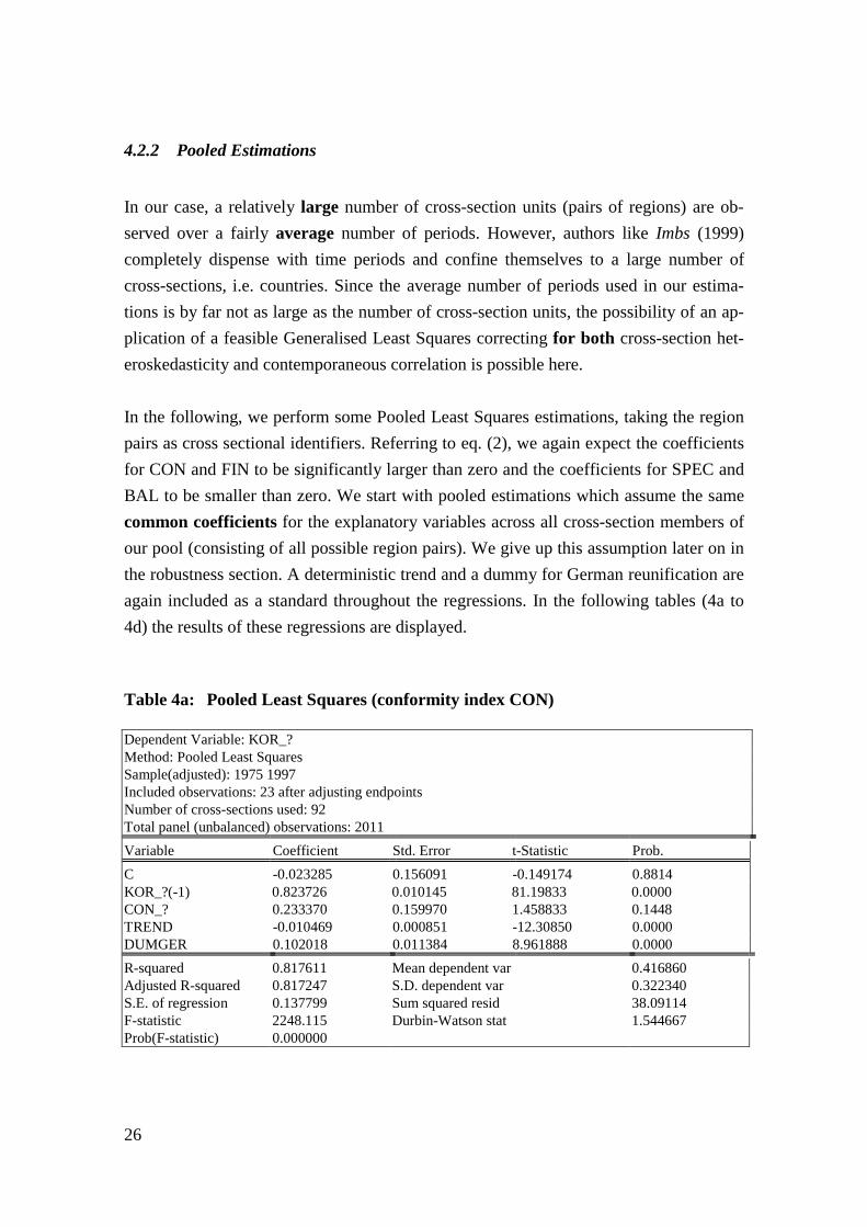
4.2.2 Pooled Estimations

In our case, a relatively large number of cross-section units (pairs of regions) are ob-served over a fairly average number of periods. However, authors like Imbs (1999)completely dispense with time periods and confine themselves to a large number ofcross-sections, i.e. countries. Since the average number of periods used in our estima-tions is by far not as large as the number of cross-section units, the possibility of an ap-plication of a feasible Generalised Least Squares correcting for both cross-section het-eroskedasticity and contemporaneous correlation is possible here.

In the following, we perform some Pooled Least Squares estimations, taking the regionpairs as cross sectional identifiers. Referring to eq. (2), we again expect the coefficientsfor CON and FIN to be significantly larger than zero and the coefficients for SPEC andBAL to be smaller than zero. We start with pooled estimations which assume the samecommon coefficients for the explanatory variables across all cross-section members ofour pool (consisting of all possible region pairs). We give up this assumption later on inthe robustness section. A deterministic trend and a dummy for German reunification areagain included as a standard throughout the regressions. In the following tables (4a to4d) the results of these regressions are displayed.

Table 4a: Pooled Least Squares (conformity index CON)

Dependent Variable: KOR_?Method: Pooled Least SquaresSample(adjusted): 1975 1997Included observations: 23 after adjusting endpointsNumber of cross-sections used: 92Total panel (unbalanced) observations: 2011Variable Coefficient Std. Error t-Statistic Prob.C -0.023285 0.156091 -0.149174 0.8814KOR_?(-1) 0.823726 0.010145 81.19833 0.0000CON_? 0.233370 0.159970 1.458833 0.1448TREND -0.010469 0.000851 -12.30850 0.0000DUMGER 0.102018 0.011384 8.961888 0.0000R-squared 0.817611 Mean dependent var 0.416860Adjusted R-squared 0.817247 S.D. dependent var 0.322340S.E. of regression 0.137799 Sum squared resid 38.09114F-statistic 2248.115 Durbin-Watson stat 1.544667Prob(F-statistic) 0.000000

27

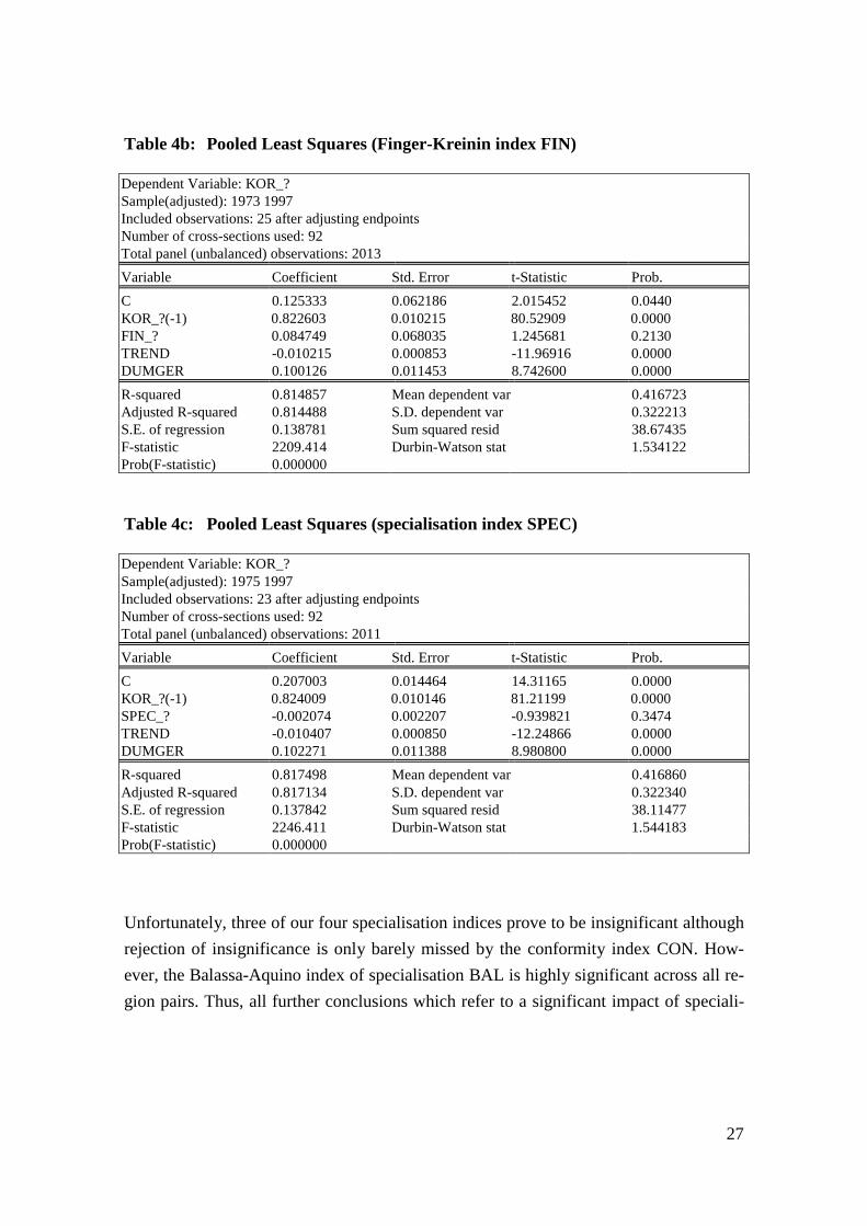
Table 4b: Pooled Least Squares (Finger-Kreinin index FIN)

Dependent Variable: KOR_?Sample(adjusted): 1973 1997Included observations: 25 after adjusting endpointsNumber of cross-sections used: 92Total panel (unbalanced) observations: 2013Variable Coefficient Std. Error t-Statistic Prob.C 0.125333 0.062186 2.015452 0.0440KOR_?(-1) 0.822603 0.010215 80.52909 0.0000FIN_? 0.084749 0.068035 1.245681 0.2130TREND -0.010215 0.000853 -11.96916 0.0000DUMGER 0.100126 0.011453 8.742600 0.0000R-squared 0.814857 Mean dependent var 0.416723Adjusted R-squared 0.814488 S.D. dependent var 0.322213S.E. of regression 0.138781 Sum squared resid 38.67435F-statistic 2209.414 Durbin-Watson stat 1.534122Prob(F-statistic) 0.000000

Table 4c: Pooled Least Squares (specialisation index SPEC)

Dependent Variable: KOR_?Sample(adjusted): 1975 1997Included observations: 23 after adjusting endpointsNumber of cross-sections used: 92Total panel (unbalanced) observations: 2011Variable Coefficient Std. Error t-Statistic Prob.C 0.207003 0.014464 14.31165 0.0000KOR_?(-1) 0.824009 0.010146 81.21199 0.0000SPEC_? -0.002074 0.002207 -0.939821 0.3474TREND -0.010407 0.000850 -12.24866 0.0000DUMGER 0.102271 0.011388 8.980800 0.0000R-squared 0.817498 Mean dependent var 0.416860Adjusted R-squared 0.817134 S.D. dependent var 0.322340S.E. of regression 0.137842 Sum squared resid 38.11477F-statistic 2246.411 Durbin-Watson stat 1.544183Prob(F-statistic) 0.000000

Unfortunately, three of our four specialisation indices prove to be insignificant althoughrejection of insignificance is only barely missed by the conformity index CON. How-ever, the Balassa-Aquino index of specialisation BAL is highly significant across all re-gion pairs. Thus, all further conclusions which refer to a significant impact of speciali-

28

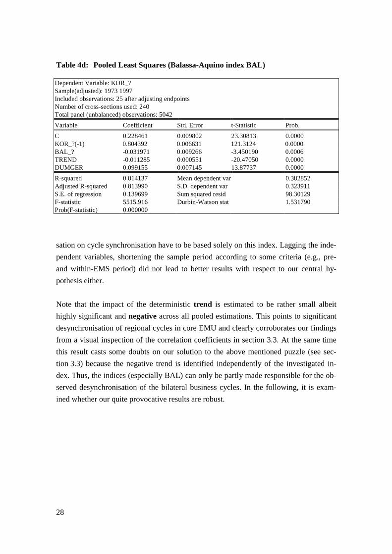
Table 4d: Pooled Least Squares (Balassa-Aquino index BAL)

Dependent Variable: KOR_?Sample(adjusted): 1973 1997Included observations: 25 after adjusting endpointsNumber of cross-sections used: 240Total panel (unbalanced) observations: 5042Variable Coefficient Std. Error t-Statistic Prob.C 0.228461 0.009802 23.30813 0.0000KOR_?(-1) 0.804392 0.006631 121.3124 0.0000BAL_? -0.031971 0.009266 -3.450190 0.0006TREND -0.011285 0.000551 -20.47050 0.0000DUMGER 0.099155 0.007145 13.87737 0.0000R-squared 0.814137 Mean dependent var 0.382852Adjusted R-squared 0.813990 S.D. dependent var 0.323911S.E. of regression 0.139699 Sum squared resid 98.30129F-statistic 5515.916 Durbin-Watson stat 1.531790Prob(F-statistic) 0.000000

sation on cycle synchronisation have to be based solely on this index. Lagging the inde-pendent variables, shortening the sample period according to some criteria (e.g., pre-and within-EMS period) did not lead to better results with respect to our central hy-pothesis either.

Note that the impact of the deterministic trend is estimated to be rather small albeithighly significant and negative across all pooled estimations. This points to significantdesynchronisation of regional cycles in core EMU and clearly corroborates our findingsfrom a visual inspection of the correlation coefficients in section 3.3. At the same timethis result casts some doubts on our solution to the above mentioned puzzle (see sec-tion 3.3) because the negative trend is identified independently of the investigated in-dex. Thus, the indices (especially BAL) can only be partly made responsible for the ob-served desynchronisation of the bilateral business cycles. In the following, it is exam-ined whether our quite provocative results are robust.

29

4.2.3 Testing for robustness of the pooled estimation results

In order to avoid an omitted-variable bias we conduct several test for robustness, eachconsidering different aspects and including additional explaining variables.10 First, wefollow Clark and Wincoop (1999) including dummies for common regional borders(see our algorithm in the appendix for the identification of common borders). Like Imbs(1999), we also implement the relative income variable in order to grasp the income ef-fect on regional trade and co-movement. We include these variables separately (a) and(b) and jointly (c).

Second, we test – as usual in such kind of studies - for robustness with respect tochanges in the sample. Here we follow two approaches: (d) in order to limit our analy-sis to the available, i.e. not estimated (see section 3.2), data we confine ourselves to asample ranging from 1975 to 1994. This can be interpreted as another test for robustnessof our results. (e) in order to conclude observations only if data on all variables areavailable for all cross-sections in the same period, we employ data from a balancedsample ranging from 1975 to 1990.

Third, we use alternative specifications of the constant in the pooled regression esti-mation. By this, we dispense with our initial assumption of common coefficients (iden-tical intercepts for all pool members). Here we consider the case of no intercepts (f) anda case of fixed effects, i.e. specific (and possibly different) intercepts for each regionpair as a pool member (g).

Fourth, we estimate a feasible Generalized Least Squares (instead of an OLS) specifi-cation (h) assuming the presence of cross-section heteroskedasticity but the absence ofcontemporaneous correlation of the residuals (inclusion of lagged dependent variable!).Finally, we omit the German unification dummy (i). The following table displays thecoefficient estimates of our four specialisation indices together with the realisation ofthe α-probability (*/**/*** corresponding to α=0.1/0.05/0.01) and the corresponding R-squared for each of the robustness test specifications.

10 With this testing up-strategy we exactly follow, e.g., Belke and Gros (1998a). One objection might be

that exactly this procedure possibly leads to an omitted-variable bias. However, the empirical realisa-tions of the relevant test statistics do not reveal - as already discussed above – any misspecificationlike, e.g. serial, correlation of the residuals.

30

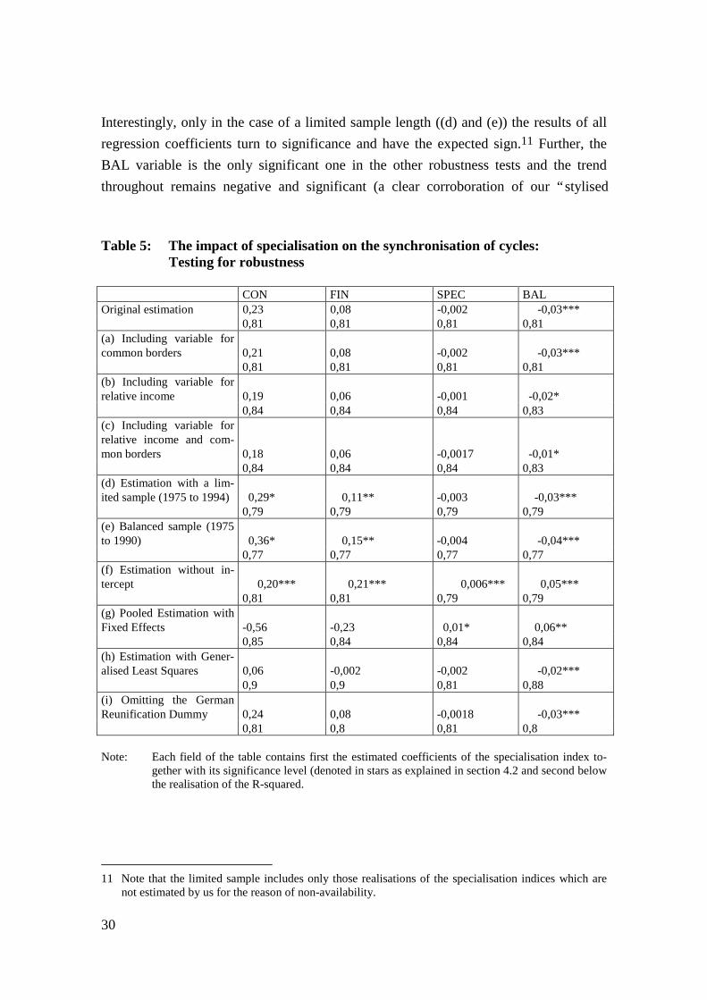
Interestingly, only in the case of a limited sample length ((d) and (e)) the results of allregression coefficients turn to significance and have the expected sign.11 Further, theBAL variable is the only significant one in the other robustness tests and the trendthroughout remains negative and significant (a clear corroboration of our “stylised

Table 5: The impact of specialisation on the synchronisation of cycles:Testing for robustness

CON FIN SPEC BALOriginal estimation 0,23 0,08 -0,002 -0,03***

0,81 0,81 0,81 0,81(a) Including variable forcommon borders 0,21 0,08 -0,002 -0,03*** 0,81 0,81 0,81 0,81(b) Including variable forrelative income 0,19 0,06 -0,001 -0,02* 0,84 0,84 0,84 0,83(c) Including variable forrelative income and com-mon borders 0,18 0,06 -0,0017 -0,01* 0,84 0,84 0,84 0,83(d) Estimation with a lim-ited sample (1975 to 1994) 0,29* 0,11** -0,003 -0,03***

0,79 0,79 0,79 0,79(e) Balanced sample (1975to 1990) 0,36* 0,15** -0,004 -0,04***

0,77 0,77 0,77 0,77(f) Estimation without in-tercept 0,20*** 0,21*** 0,006*** 0,05***

0,81 0,81 0,79 0,79(g) Pooled Estimation withFixed Effects -0,56 -0,23 0,01* 0,06**

0,85 0,84 0,84 0,84(h) Estimation with Gener-alised Least Squares 0,06 -0,002 -0,002 -0,02***

0,9 0,9 0,81 0,88(i) Omitting the GermanReunification Dummy 0,24 0,08 -0,0018 -0,03***

0,81 0,8 0,81 0,8

Note: Each field of the table contains first the estimated coefficients of the specialisation index to-gether with its significance level (denoted in stars as explained in section 4.2 and second belowthe realisation of the R-squared.

11 Note that the limited sample includes only those realisations of the specialisation indices which are

not estimated by us for the reason of non-availability.

31

facts”, but not shown in table 5). If we estimate the pool regression without intercept (f),the coefficients of the variables CON and FIN reveal the expected sign significantlylarger than zero, but the coefficients of FIN and BAL are now positive and not signifi-cant. For the relative income variable we clearly cannot reject the hypothesis that thisvariable does not have an impact on the co-movement of bilateral regional business cy-cles. Seen on the whole, the results of the robustness tests do not change our conclu-sions on the relationship between specialisation and synchronisation of regional busi-ness cycles significantly.12

5 CONCLUSIONS

In the preceding chapters we were able to derive some tentative answers to the questionof the impact of specialisation on the synchronisation of regional business cycles inEurope. We list the most important ones below:

1) In the case of regions whose sectoral composition has changed into the same direc-tion because of increasing specialisation, we expected higher synchronisation of theregional cycles. This lets regions turning into “high-tech” or “developing” ones.However, a necessary condition for this, a positive impact of increasing similarity ofsectoral composition on synchronisation could be corroborated only partly. Only forsome regions and some indicators we were able to detect that kind of impact whichis expected from theory.

At the same time, some regions have to be considered which will develop differ-ently. This can also be traced back to agglomeration, i.e. the emigration of industriesand labour. In this case, we forecasted a decreasing degree of correlation. Again, thecorresponding negative impact of increasing similarity of sectoral composition onsynchronisation could only be observed for some regions and some indicators.

2) Relying on those of our results which correspond the most closely to theory, oneforecast would be that core-EMU will tend to change into two-class pairs of regions.

12 Constructing a rolling window as a second method of mapping the correlation function and using this

variable to test for a relationship between this variable and the specialisation indices proved to befruitless efforts in the case of the individual region pair regressions as well as with respect to thepooled estimation procedure.

32

On the one hand, there will be regions which converge to each other and display in-creasingly synchronous business cycles and enhance their regional income by intra-industrial trade. On the other hand, there will be regions which will lose by agglom-eration. Seen on the whole, this could lead to a more uneven distribution of regionswith respect to their business cycle stance (regional GDP).

3) Our section 3.3 on stylised facts revealed that the degree of synchronisation of re-gional business cycles has decreased in the past for a majority of region pairs. Thisresult stands in contrast to many studies indicating an increasingly closer correlationof business cycles between countries which are now members of EMU (e.g. Artisand Zhang 1997, Christodoulakis et al. 1995). However, our evidence in favour of adecreasing synchronisation of regional cycles is implicitly backed by other studieswith a regional focus (Fatás 1997, Clark and Wincoop 1999). Moreover, alreadyBelke and Gros (1998) detailedly worked out that regional asymmetries do not nec-essarily constitute a strong argument against the OCA-property of Euroland. Instead,one could argue (and this can be clearly read off the data in chapter 3) that regionalasymmetries caused, e.g., by an increasing desynchronisation of regional cycleshave already been a problem of existing currency unions like France and Germanyin the past.

4) What kind of impact should our results have on the design of monetary and fiscalpolicy? The general concern about the cost of having a common policy for a hetero-geneous area like EMU is corroborated by our results in a very subtle sense. Let usfirst base our arguments on those of our empirical results which confirm the stan-dard theoretical considerations. Since those results indicate a negative impact of lessspecialisation on the synchronisation of regional cycles, the common monetary pol-icy stance in Euroland might not be optimal for many regions because they mightfind themselves at increasingly different stages of their business cycle (commonmonetary policy for uncommon regions). However, since the common monetarypolicy might at the same time have benefits for some regions with a high degree ofintra-industrial trade and therefore high business cycle synchronisation, the overallresult is not unambiguously negative. Instead, our estimates even allow a guess - orbetter a founded speculation - which regions will loose and which regions willbenefit from increasing specialisation. Insofar as the speed of specialisation is en-hanced by EMU, a forecast of the regional distribution of some real gains and somelosses from EMU appears feasible as well.

33

These conclusions might be disputed on technical grounds, because by far not all em-pirical results corresponded to our theoretical expectations. A lot of regressions for cer-tain region pairs and specific specialisation indices revealed a negative or even an insig-nificant impact of specialisation on the synchronisation of cycles. Moreover, future re-search should try to investigate why the results on the four specialisation indices are sodifferent. However, even if one abstracts from the regression results in chapter 4, onecan still stick to the main stylised fact found in chapter 3, namely that of an on averagedecreasing degree of cycle correlation between important core EMU regions. Thisfinding underlines the problem of a common monetary policy for uncommon regionswhich, however, has already existed in the DM- and in the Franc-zone before.

Seen on the whole, thus, our empirical results indicate that regionally asymmetricshocks cannot be excluded for EMU in the future. This might raise the claim for stabi-lising insurance mechanisms (Belke and Gros (1998)). On the regional level, however,the performance of weaker regions should be strengthened by tax incentives and bymeasures to promote the establishing of certain industries.

34

References

Amiti, M., 1997Specialisation Patterns in Europe, in: Weltwirtschaftliches Archiv, 135, 573-593

Aquino, A., 1978Intra-Industry Trade and Inter-Industry Specialisation as Concurrent Sources ofInternational Trade in Manufactures, in: Weltwirtschaftliches Archiv, 114, 275-296

Artis, M. J.; Zhang, W., 1997International Business Cycles and the ERM: Is there a European Business Cycle?,in: International Journal of Finance and Economics, Vol. 2, 1-16

Balassa, B., 1965Trade Liberalization and ‘Revealed’ Comparative Advantage, in: The ManchesterSchool of Economic and Social Sciences, 33, 99-123

Banerjee, A. et al., 1993Co-Integration, Error Correction, and the Econometric Analysis of Non-StationaryData, Oxford.

Belke, A.; Gros, D., 1998Asymmetric Shocks and EMU: Is There a Need for a Stability Fund?, in: Intere-conomics - Review of International Trade and Development, Vol. 33, Novem-ber/December, 274 - 288.

Belke, A.; Gros, D., 1998aEvidence on the Costs of Intra-European Exchange Rate Variability, in: CentER forEconomic Research Discussion Papers, No. 9814, Tilburg/Netherlands (forthcom-ing in: Open Economic Review)

Caporale, G. M.; Pittis, N.; Prodromidis, K., 1999Is Europe an Optimum Currency Area? Business Cycles in Europe, in: Journal ofEconomic Integration, 14 (2), June 1999, 169-202

Christodoulakis, N.; Dimelis, S. P.; Kollintzas, T., 1995Comparisons of Business Cycles in the EC: Idiosyncrasies and Regularities, in:Economica, Vol. 62, 1-27

Clark, T. E.; Wincoop, E. van, 1999Borders and Business Cycles, in: Federal Reserve Bank of Kansas City, ResearchWorking Paper RWP 99-07

DeNardis, S.; Goglio, A.; Malgarini, M., 1996Regional Specialisation and Shocks in Europe: Some Evidence from RegionalData, in: Weltwirtschaftliches Archiv 132 (2), 197-214

Ellison, G.; Glaeser, E. L., 1999The Geographic Concentration of Industry: Does Natural Advantage Explain Ag-glomeration?, in: American Economic Review Papers and Proceedings, Vol. 89,311-316

European Central Bank, 1999Monthly Bulletin, July 1999, S. 35-58

35

Fatás, A., 1997Countries or Regions? Lessons from the EMS Experience, in: European EconomicReview, Vol. 41, 743-751

Finger, J. M.; Kreinin, M. E., 1979A Measure of ‚Export Similarity’ and its Possible Uses, in: Economic Journal, 89,905-912

Forni, M.; Reichlin, L., 1997National Policies and Local Economies: Europe and the United States, in: CEPRDiscussion Paper No. 1632

Frankel, J. A.; Rose, A. K., 1998The Endogeneity of the Optimum Currency Area Criteria, in: The Economic Jour-nal, Vol. 108, No. 449, 1009 – 1025

Fujita, M.; Thisse, J. F., 1996Economics of Agglomeration, in: Journal of the Japanese and International Eco-nomics, 10, 339-378

Imbs, J., 1999Co-Fluctuations, in: CEPR Discussion Paper No. 2267

Krieger-Boden, Ch., 1999Nationale und regionale Spezialisierungsmuster im europäischen Integrationspro-zess, in: Die Weltwirtschaft, 234-254

Krugman, P., 1991Increasing Returns and Economic Geography, in: Journal of Political Economy,Vol. 99, No. 3, 483-499

Krugman, P., 1993Lessons for Massachusetts for EMU, in: Torres, F. and F. Giavazzi (Hrsg.), Ad-justment and Growth in the European Monetary Union”, Cambridge UniversityPress, Cambridge

Krugman, P., 1998What’s New about the New Economic Geography, Oxford Review of EconomicPolicy, Vol. 14, 7-17

Krugman, P.; Venables, A. J., 1996Integration, Specialization and Adjustment, in: European Economic Review, Vol.40, 959-967

Lütkepohl, H., 1991Introduction to Multiple Time Series Analysis, New York: Springer

Mills, T. C., 1990Time Series Techniques for Economists, Cambridge et al.: Cambridge UniversityPress.

Ottaviano, G. I. P.; Puga, D., 1997Agglomeration in the Global Economy: A Survey of the ‘New Economic Geogra-phy’, in: CEPR Discussion Paper Nr. 1699

36

Puga, D., 1999The rise and fall of regional inequalities, in: European Economic Review, Vol. 43,303-334

Quantitative Micro Software, 1997EViews – Command and Reference, Irvine, California

Ricci, L. A., 1999Economic Geography and comparative advantage: Agglomeration versus speciali-zation, in: European Economic Review, Vol. 43, 357-377

Schmutzler, A., 1999The New Economic Geography, in: Journal of Economic Surveys, Vol. 13, Nr. 4,355-379

Schwarz, G., 1978Estimating the Dimension of a Model, in: Annals of Statistics 6, 461-464.

Venables, A. J., 1996Equilibrium Locations of Vertically Linked Industries, in: International EconomicReview, 37, 341-359

Wasmer, J.; Weil, P., 2000The Macroeconomics of Labor and Credit Market Imperfections, mimeo, Ecaresand MIT

37

APPENDIX I

38

‘ESTIMATION PROCEDURE’

SMPL 1971 1997

FOR !1=1 TO 26

SMPL 1971 1971+!1

‘Defining a Group of Variables'

group corr growth_fr1 growth_fr2 growth_fr3 growth_fr4 growth_fr5 growth_fr6 growth_fr7

growth_fr8 growth_g1 growth_g2 growth_g3 growth_g4 growth_g5 growth_g6 growth_g7

growth_g8

'Matrix Representation of this Group'

stom(corr,m1)

'Matrix of Correlations between Columns of Matrix'

matrix m2 = @cor(m1)

'Generate 'Rolling' Correlations for every possible Pair of Regions'

SMPL 1971+!1 1971+!1

FOR !2=1 TO 8

FOR !3=1 TO 8

'France-France'

genr kor_fr!2fr!3=0

'Germany-France'

genr kor_g!2fr!3=0

'France-Germany'

genr kor_fr!2g!3=0

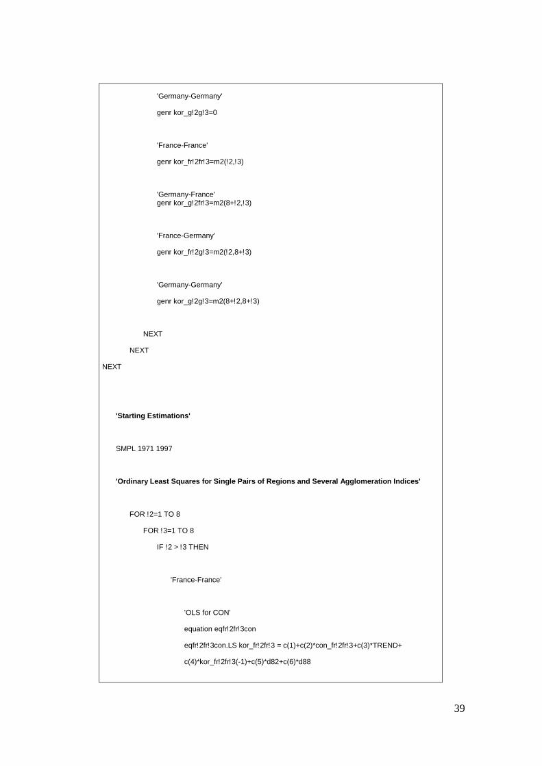
39

'Germany-Germany'

genr kor_g!2g!3=0

'France-France'

genr kor_fr!2fr!3=m2(!2,!3)

'Germany-France'genr kor_g!2fr!3=m2(8+!2,!3)

'France-Germany'

genr kor_fr!2g!3=m2(!2,8+!3)

'Germany-Germany'

genr kor_g!2g!3=m2(8+!2,8+!3)

NEXT

NEXT

NEXT

'Starting Estimations'

SMPL 1971 1997

'Ordinary Least Squares for Single Pairs of Regions and Several Agglomeration Indices'

FOR !2=1 TO 8

FOR !3=1 TO 8

IF !2 > !3 THEN

'France-France'

'OLS for CON'

equation eqfr!2fr!3con

eqfr!2fr!3con.LS kor_fr!2fr!3 = c(1)+c(2)*con_fr!2fr!3+c(3)*TREND+

c(4)*kor_fr!2fr!3(-1)+c(5)*d82+c(6)*d88

40

'OLS for SPEC'

equation eqfr!2fr!3spec

eqfr!2fr!3spec.LS kor_fr!2fr!3 = c(1)+c(2)*spec_fr!2fr!3+c(3)*TREND+

c(4)*kor_fr!2fr!3(-1)+c(5)*d82+c(6)*d88

'OLS for FIN'

equation eqfr!2fr!3FIN

eqfr!2fr!3fin.LS kor_fr!2fr!3 = c(1)+c(2)*FIN_fr!2fr!3+C(3)*TREND+

c(4)*kor_fr!2fr!3(-1)+c(5)*d82+c(6)*d88

'Germany-Germany'

'OLS for CON'

equation eqg!2g!3con

eqg!2g!3con.LS kor_g!2g!3 = c(1)+c(2)*con_g!2g!3+c(3)*DUMGER+

C(4)*TREND+ c(5)*kor_g!2g!3(-1)

'OLS for SPEC'

equation eqg!2g!3spec

eqg!2g!3spec.LS kor_g!2g!3 = c(1)+c(2)*spec_g!2g!3+c(3)*DUMGER+

C(4)*TREND+c(5)*kor_g!2g!3(-1)

'OLS for FIN'

equation eqg!2g!3FIN

eqg!2g!3fin.LS kor_g!2g!3 = c(1)+c(2)*FIN_g!2g!3+c(3)*DUMGER+

C(4)*TREND+ c(5)*kor_g!2g!3(-1)

ENDIF

'Germany-France'

'OLS for CON'

equation eqg!2fr!3con

eqg!2fr!3con.LS kor_g!2fr!3 = c(1)+c(2)*con_g!2fr!3+ c(3)*kor_g!2fr!3(-1)

41

'OLS for SPEC'

equation eqg!2fr!3spec

eqg!2fr!3spec.LS kor_g!2fr!3 = c(1)+c(2)*spec_g!2fr!3+

c(3)*kor_g!2fr!3(-1)+c(4)*trend

'OLS for FIN'

equation eqg!2fr!3FIN

eqg!2fr!3fin.LS kor_g!2fr!3 = c(1)+c(2)*FIN_g!2fr!3+c(3)*kor_g!2fr!3(-1)

'OLS for BAL'

IF !2 <> !3 THEN

'for France-France'

equation eqfr!2fr!3BAL

eqfr!2fr!3BAL.LS kor_fr!2fr!3 = c(1)+c(2)*BAL_fr!2fr!3+C(3)*TREND+

c(4)*kor_fr!2fr!3(-1)+c(5)*d82+c(6)*d88

'for Germany-Germany'

equation eqg!2g!3BAL

eqg!2g!3BAL.LS kor_g!2g!3 = c(1)+c(2)*BAL_g!2g!3+c(3)*TREND+

c(4)*kor_g!2g!3(-1)

ENDIF

'for Germany-France'

equation eqg!2fr!3BAL

eqg!2fr!3BAL.LS kor_g!2fr!3 = c(1)+c(2)*BAL_g!2fr!3+c(3)*DUMGER+

C(4)*TREND+c(5)*kor_g!2fr!3(-1)

'for France-Germany'

equation eqfr!2g!3BAL

eqfr!2g!3BAL.LS kor_fr!2g!3 = c(1)+c(2)*BAL_fr!2g!3+C(3)*TREND+

c(4)*kor_fr!2g!3(-1)+c(5)*D81+c(6)*D88

42

NEXT

NEXT

‘Identification of Several Dummies’

SMPL 1971 1997

'German Unification'

GENR DUMGER=0

SMPL 1990 1997

DUMGER =1

‘Dummies for Country-Specific Shocks’

SMPL 1971 1997

genr d79=0

genr d81=0

genr d82=0

genr d88=0

SMPL 1979 1979

genr d79=1

smpl 1981 1981

genr d81=1

smpl 1982 1982

genr d82=1

smpl 1988 1988

genr d88=1

'Regressions for Pool of Region Pairs'

SMPL 1971 1997

'Pool Regressions for CON'

DELETE EMUCORECON

POOL EMUCORECON

43

FOR !2=1 TO 8

FOR !3=1 TO 8

IF !2 > !3 THEN

EMUCORECON.ADD fr!2fr!3 g!2g!3

ENDIF

IF !2 >= !3 THEN

EMUCORECON.ADD g!2fr!3

ENDIF

EMUCORECON.LS KOR_? C KOR_?(-1) CON_? TREND DUMGER

NEXT

NEXT

'Pool Regressions for FIN'

DELETE EMUCOREFIN

POOL EMUCOREFIN

FOR !2=1 TO 8

FOR !3=1 TO 8

IF !2 > !3 THEN

EMUCOREFIN.ADD fr!2fr!3 g!2g!3

ENDIF

IF !2 >= !3 THEN

EMUCOREFIN.ADD g!2fr!3

ENDIF

EMUCOREFIN.LS KOR_? C KOR_?(-1) FIN_? TREND DUMGER

44

NEXT

NEXT

'Pool Regressions for SPEC'

DELETE EMUCORESPEC

POOL EMUCORESPEC

FOR !2=1 TO 8

FOR !3=1 TO 8

IF !2 > !3 THEN

EMUCORESPEC.ADD fr!2fr!3 g!2g!3

ENDIF

IF !2 >= !3 THEN

EMUCORESPEC.ADD g!2fr!3

ENDIF

EMUCORESPEC.LS KOR_? C KOR_?(-1) SPEC_? TREND DUMGER

NEXT

NEXT

'Pool Regressions for BAL'

DELETE EMUCOREBAL

POOL EMUCOREBAL

FOR !2=1 TO 8

FOR !3=1 TO 8

45

IF !2 <> !3 THEN

EMUCOREBAL.ADD fr!2fr!3 g!2g!3

ENDIF

EMUCOREBAL.ADD g!2fr!3 fr!2g!3

EMUCOREBAL.LS KOR_? C KOR_?(-1) BAL_? TREND DUMGER

NEXT

NEXT

'Testing for Robustness'

'Limiting the Cross Sections'

'Only French Regions'

'pool regressions for CON'

DELETE EMUCORECONFR

POOL EMUCORECONFR

FOR !2=1 TO 8

FOR !3=1 TO 8

IF !2 > !3 THEN

EMUCORECONFR.ADD fr!2fr!3

ENDIF

EMUCORECONFR.LS KOR_? C KOR_?(-1) CON_? TREND DUMGER

46

'Only German Regions'

'pool regressions for CON'

DELETE EMUCORECONG

POOL EMUCORECONG

FOR !2=1 TO 8

FOR !3=1 TO 8

IF !2 > !3 THEN

EMUCORECON.ADD g!2g!3

ENDIF

EMUCORECONG.LS KOR_? C KOR_?(-1) CON_? TREND DUMGER

'Specification of Robustness Variables'

'Dummies for Common Borders'

FOR !2=1 TO 8

FOR !3=1 TO 8

GENR DUM_fr!2fr!3=0

GENR DUM_g!2g!3=0

GENR DUM_g!2fr!3=0

GENR DUM_fr!2g!3=0

NEXT

NEXT

47

'Common Borders in Germany'

GENR dum_g1g2=1

GENR dum_g2g3=1

GENR dum_g2g4=1

GENR dum_g3g2=1

GENR dum_g3g4=1

GENR dum_g3g5=1

GENR dum_g4g2=1

GENR dum_g4g3=1

GENR dum_g4g5=1

GENR dum_g4g6=1

GENR dum_g4g7=1

GENR dum_g5g3=1

GENR dum_g5g4=1

GENR dum_g5g6=1

GENR dum_g6g4=1

GENR dum_g6g5=1

GENR dum_g6g7=1

GENR dum_g7g6=1

GENR dum_g7g4=1

'Common Borders in France'

GENR dum_fr5fr3=1

GENR dum_fr3fr5=1

GENR dum_fr5fr6=1

GENR dum_fr6fr5=1

GENR dum_fr3fr4=1

GENR dum_fr4fr3=1

GENR dum_fr4fr7=1

GENR dum_fr7fr4=1

GENR dum_fr4fr8=1

GENR dum_fr8fr4=1

GENR dum_fr6fr7=1

GENR dum_fr7fr6=1

48

GENR dum_fr1fr2=1

GENR dum_fr2fr1=1

GENR dum_fr1fr5=1

GENR dum_fr1fr3=1

GENR dum_fr1fr4=1

GENR dum_fr1fr6=1

GENR dum_fr1fr7=1

GENR dum_fr5fr1=1

GENR dum_fr3fr1=1

GENR dum_fr4fr1=1

GENR dum_fr6fr1=1

GENR dum_fr7fr1=1

'Common Borders Germany France / France-Germany'

GENR dum_fr4g5=1

GENR dum_g5fr4=1

GENR dum_fr4g6=1

GENR dum_g6fr4=1

'Relative Income between the Regions'

FOR !2=1 TO 8

FOR !3=1 TO 8

genr relinc_fr!2fr!3=0

genr relinc_g!2g!3=0

genr relinc_fr!2g!3=0

genr relinc_g!2fr!3=0

genr relinc_fr!2fr!3=@abs(ry_fr!2-ry_fr!3)

genr relinc_g!2g!3=@abs(ry_g!2-ry_g!3)

genr relinc_fr!2g!3=@abs(ry_fr!2-ry_g!3)

genr relinc_g!2fr!3=@abs(ry_g!2-ry_fr!3)

49

NEXT

NEXT

'Implementing the Robustness Variables in Pool Regressions'

'Robustness of Pool Regressions for CON'

DELETE EMUCORECON1

POOL EMUCORECON1

FOR !2=1 TO 8

FOR !3=1 TO 8

IF !2 > !3 THEN

EMUCORECON1.ADD fr!2fr!3 g!2g!3

ENDIF

IF !2 >= !3 THEN

EMUCORECON1.ADD g!2fr!3

ENDIF

EMUCORECON1.LS KOR_? C KOR_?(-1) CON_? TREND

DUMGER RELINC_?

NEXT

NEXT

DELETE EMUCORECON2

POOL EMUCORECON2

FOR !2=1 TO 8

FOR !3=1 TO 8

50

IF !2 > !3 THEN

EMUCORECON2.ADD fr!2fr!3 g!2g!3

ENDIF

IF !2 >= !3 THEN

EMUCORECON2.ADD g!2fr!3

ENDIF

EMUCORECON2.LS KOR_? C KOR_?(-1) CON_? TREND DUMGER DUM_?

NEXT

NEXT

DELETE EMUCORECON3

POOL EMUCORECON3

FOR !2=1 TO 8

FOR !3=1 TO 8

IF !2 > !3 THEN

EMUCORECON2.ADD fr!2fr!3 g!2g!3

ENDIF

IF !2 >= !3 THEN

EMUCORECON3.ADD g!2fr!3

ENDIF

EMUCORECON3.LS KOR_? C KOR_?(-1) CON_? TREND DUMGER

RELINC_? DUM_?

NEXT

NEXT

51

'Robustness of Pool Regressions for FIN'

DELETE EMUCOREFIN1

POOL EMUCOREFIN1

FOR !2=1 TO 8

FOR !3=1 TO 8

IF !2 > !3 THEN

EMUCOREFIN1.ADD fr!2fr!3 g!2g!3

ENDIF

IF !2 >= !3 THEN

EMUCOREFIN1.ADD g!2fr!3

ENDIF

EMUCOREFIN1.LS KOR_? C KOR_?(-1) FIN_? TREND DUMGER RELINC_?

NEXT

NEXT

DELETE EMUCOREFIN2

POOL EMUCOREFIN2

FOR !2=1 TO 8

FOR !3=1 TO 8

IF !2 > !3 THEN

EMUCOREFIN2.ADD fr!2fr!3 g!2g!3

ENDIF

IF !2 >= !3 THEN

EMUCOREFIN2.ADD g!2fr!3

ENDIF

52

EMUCOREFIN2.LS KOR_? C KOR_?(-1) FIN_? TREND DUMGER DUM_?

NEXT

NEXT

DELETE EMUCOREFIN3

POOL EMUCOREFIN3

FOR !2=1 TO 8

FOR !3=1 TO 8

IF !2 > !3 THEN

EMUCOREFIN3.ADD fr!2fr!3 g!2g!3

ENDIF

IF !2 >= !3 THEN

EMUCOREFIN3.ADD g!2fr!3

ENDIF

EMUCOREFIN3.LS KOR_? C KOR_?(-1) FIN_? TREND DUMGER

RELINC_? DUM_?

NEXT

NEXT

'Robustness of Pool Regressions for SPEC'

DELETE EMUCORESPEC1

POOL EMUCORESPEC1

FOR !2=1 TO 8 FOR !3=1 TO 8

IF !2 > !3 THEN

EMUCORESPEC1.ADD fr!2fr!3 g!2g!3

ENDIF

53

IF !2 >= !3 THEN

EMUCORESPEC1.ADD g!2fr!3

ENDIF

EMUCORESPEC1.LS KOR_? C KOR_?(-1) SPEC_? TREND DUMGER

RELINC_?

NEXT

NEXT

DELETE EMUCORESPEC2

POOL EMUCORESPEC2

FOR !2=1 TO 8

FOR !3=1 TO 8

IF !2 > !3 THEN

EMUCORESPEC2.ADD fr!2fr!3 g!2g!3

ENDIF

IF !2 >= !3 THEN

EMUCORESPEC2.ADD g!2fr!3

ENDIF

EMUCORESPEC2.LS KOR_? C KOR_?(-1) SPEC_? TREND DUMGER

DUM_?

NEXT

NEXT

DELETE EMUCORESPEC3

POOL EMUCORESPEC3

54

FOR !2=1 TO 8

FOR !3=1 TO 8

IF !2 > !3 THEN

EMUCORESPEC1.ADD fr!2fr!3 g!2g!3

ENDIF

IF !2 >= !3 THEN

EMUCORESPEC3.ADD g!2fr!3

ENDIF

EMUCORESPEC3.LS KOR_? C KOR_?(-1) SPEC_? TREND DUMGER

RELINC_? DUM_?

NEXT

NEXT

'Robustness of Pool Regressions for BAL'

DELETE EMUCOREBAL1

POOL EMUCOREBAL1

FOR !2=1 TO 8

FOR !3=1 TO 8

IF !2 <> !3 THEN

EMUCOREBAL1.ADD fr!2fr!3 g!2g!3

ENDIF

EMUCOREBAL1.ADD g!2fr!3 fr!2g!3

EMUCOREBAL1.LS KOR_? C KOR_?(-1) BAL_? RELINC_? TREND

DUMGER

NEXT

55

NEXT

DELETE EMUCOREBAL2

POOL EMUCOREBAL2

FOR !2=1 TO 8

FOR !3=1 TO 8

IF !2 <> !3 THEN

EMUCOREBAL2.ADD fr!2fr!3 g!2g!3

ENDIF

EMUCOREBAL2.ADD g!2fr!3 fr!2g!3

EMUCOREBAL2.LS KOR_? C KOR_?(-1) BAL_? DUM_? TREND

NEXT

NEXT

DELETE EMUCOREBAL3

POOL EMUCOREBAL3

FOR !2=1 TO 8

FOR !3=1 TO 8

IF !2 <> !3 THEN

EMUCOREBAL3.ADD fr!2fr!3 g!2g!3

ENDIF

EMUCOREBAL3.ADD g!2fr!3 fr!2g!3

EMUCOREBAL3.LS KOR_? C KOR_?(-1) BAL_? RELINC_? DUM_? TREND

DUMGER

NEXT

NEXT

56

APPENDIX II

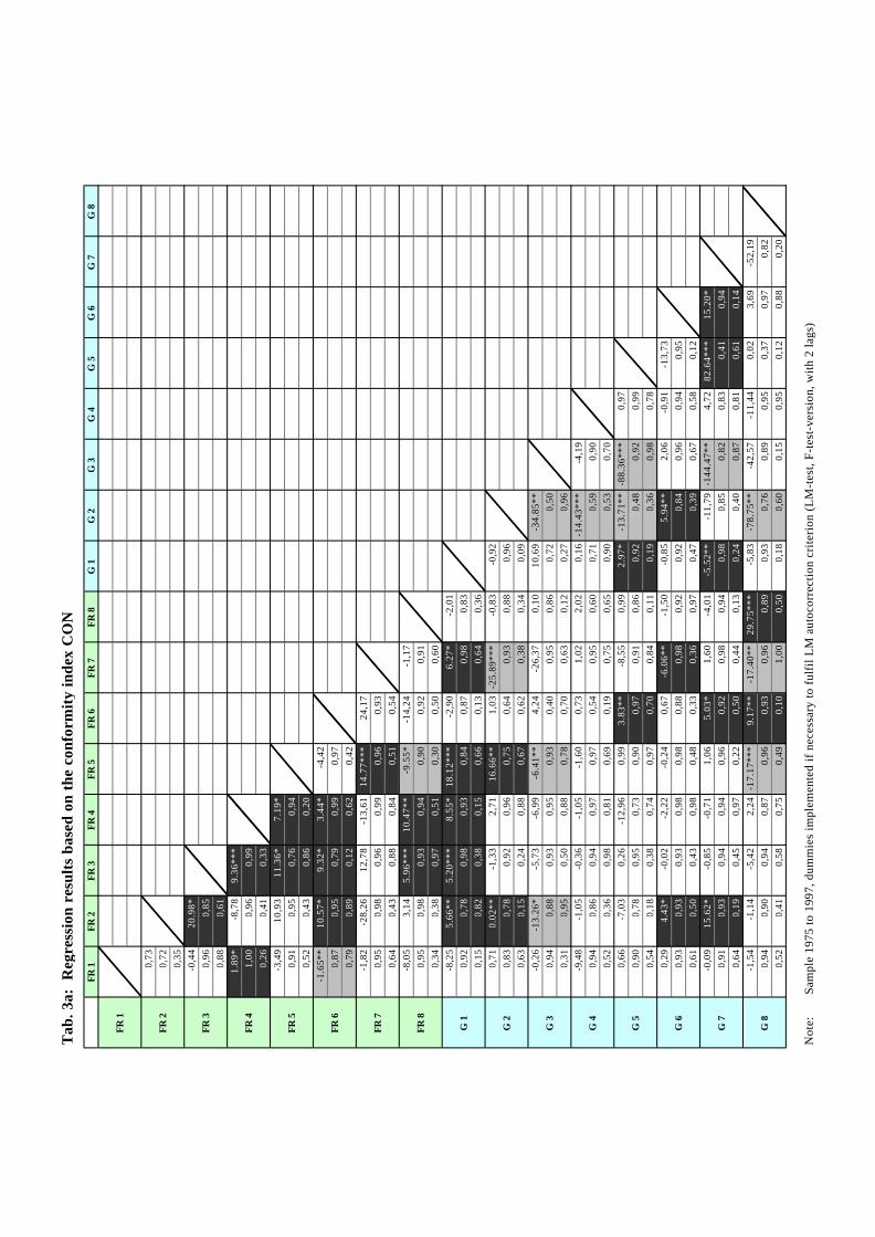
Tab

. 3a:

Reg

ress

ion

resu

lts b

ased

on

the

conf

orm

ity in

dex

CO

NFR

1FR

2FR

3FR

4FR

5FR

6FR

7FR

8G

1G

2G

3G

4G

5G

6G

7G

8

0,73

0,72

0,35

-0,4

420

.98*

0,96

0,85

0,88

0,61

1.89

*-8

,78

9.36

***

1,00

0,96

0,99

0,26

0,41

0,33

-3,4

910

,93

11.3

6*7.

19*

0,91

0,95

0,76

0,94

0,52

0,43

0,86

0,20

-1.6

5**

10.5

7*9.

32*

3.44

*-4

,42

0,87

0,95

0,79

0,99

0,97

0,79

0,89

0,12

0,62

0,42

-1,8

2-2

8,26

12,7

8-1

3,61

14.7

7***

24,1

70,

950,

980,

960,

990,

960,

930,

640,

430,

880,

840,

510,

54-8

,05

3,14

5.96

***

10.4

7**

-9.5

5*-1

4,24

-1,1

70,

950,

980,

930,

940,

900,

920,

910,

340,

380,

970,

510,

300,

500,

60-8

,25

5.66

**5.

20**

*8.

55*

18.1

2***

-2,9

06.

27*

-2,0

10,

920,

780,

980,

930,

840,

870,

980,

830,

150,

820,

380,

150,

660,

130,

640,

360,

710.

02**

-1,3

32,

7116

.66*

*1,

03-2

5.89

***

-0,8

3-0

,92

0,83

0,78

0,92

0,96

0,75

0,64

0,93

0,88

0,96

0,63

0,15

0,24

0,88

0,67

0,62

0,38

0,34

0,09

-0,2

6-1

3.26

*-5

,73

-6,9

9-6

.41*

*4,

24-2

6,37

0,10

10,6

9-3

4.85

**0,

940,

880,

930,

950,

930,

400,

950,

860,

720,

500,

310,

950,

500,

880,

780,

700,

630,

120,

270,

96-9

,48

-1,0

5-0

,36

-1,0

5-1

,60

0,73

1,02

2,02

0,16

-14.

43**

*-4

,19

0,94

0,86

0,94

0,97

0,97

0,54

0,95

0,60

0,71

0,59

0,90

0,52

0,36

0,98

0,81

0,69

0,19

0,75

0,65

0,90

0,53

0,70

0,66

-7,0

30,

26-1

2,96

0,99

3.83

**-8

,55

0,99

2.97

*-1

3.71

**-8

8.36

***

0,97

0,90

0,78

0,95

0,73

0,90

0,97

0,91

0,86

0,92

0,48

0,92

0,99

0,54

0,18

0,38

0,74

0,97

0,70

0,84

0,11

0,19

0,36

0,98

0,78

0,29

4.43

*-0

,02

-2,2

2-0

,24

0,67

-6.0

6**

-1,5

0-0

,85

5.94

**2,

06-0

,91

-13,

730,

930,

930,

930,

980,

980,

880,

980,

920,

920,

840,

960,

940,

950,

610,

500,

430,

980,

480,

330,

360,

970,

470,

390,

670,

580,

12-0

,09

15.6

2*-0

,85

-0,7

11,

065.

03*

1,60

-4,0

1-5

.52*

*-1

1,79

-144

.47*

*4,

7282

.64*

**15

.20*

0,91

0,93

0,94

0,94

0,96

0,92

0,98

0,94

0,98

0,85

0,82

0,83

0,41

0,94

0,64

0,19

0,45

0,97

0,22

0,50

0,44

0,13

0,24

0,40

0,87

0,81

0,61

0,14

-1,5

4-1

,14

-5,4

22,

24-1

7.17

***

9.17

**-1

7.40

**29

.75*

**-5

,83

-78.

75**

-42,

57-1

1,44

0,02

3,69

-52,

190,

940,

900,

940,

870,

960,

930,

960,

890,

930,

760,

890,

950,

370,

970,

820,

520,

410,

580,

750,

490,

101,

000,

500,

180,

600,

150,

950,

120,

880,

20

Not

e:

Sam

ple

1975

to 1

997,

dum

mie

s im

plem

ente

d if

nece

ssar

y to

fulfi

l LM

aut

ocor

rect

ion

crite

rion

(LM

-test

, F-te

st-v

ersi

on, w

ith 2

lags

)

G 8

G 4

G 5

G 6

G 7

FR 8

G 1

G 2

G 3

FR 1

FR 2

FR 3

FR 4

FR 5

FR 7

FR 6

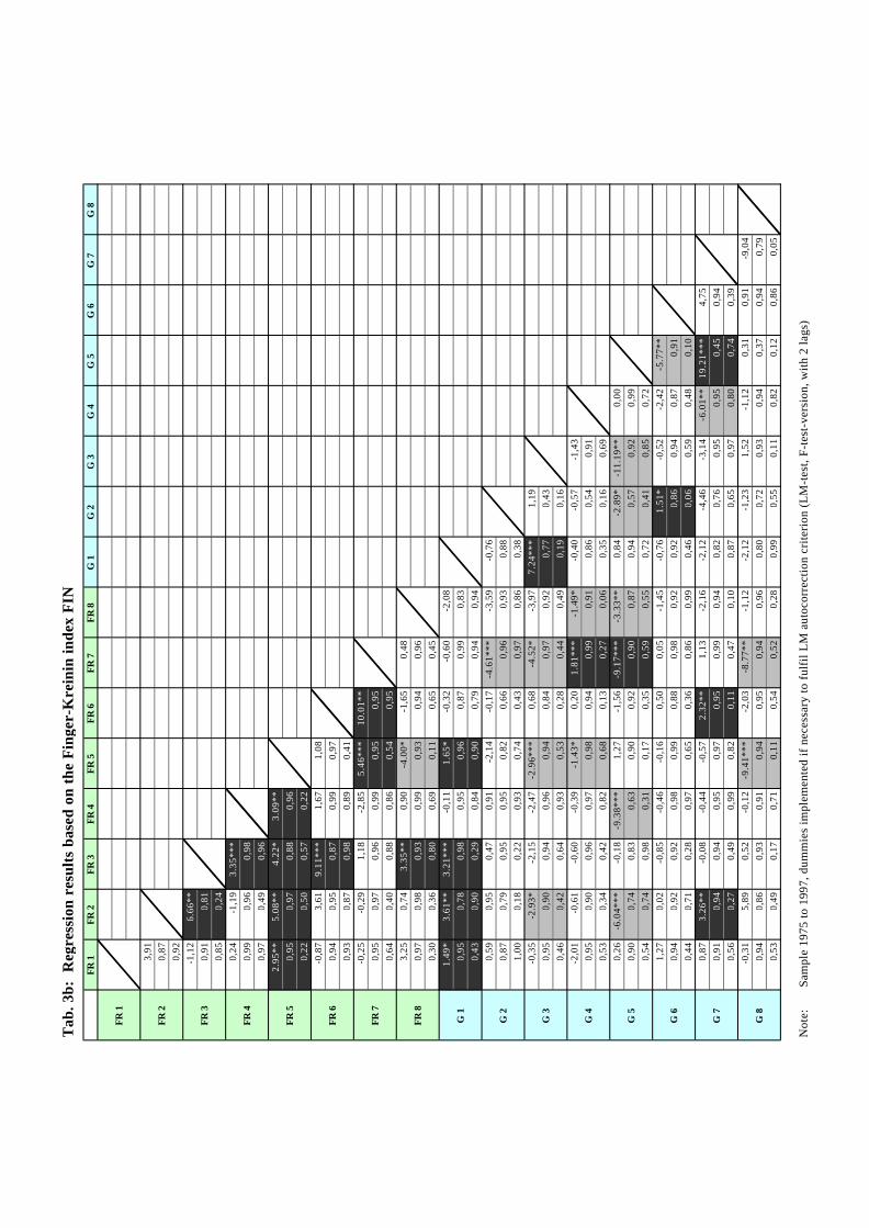
Tab

. 3b:

Reg

ress

ion

resu

lts b

ased

on

the

Fing

er-K

rein

in in

dex

FIN

FR 1

FR 2

FR 3

FR 4

FR 5

FR 6

FR 7

FR 8

G 1

G 2

G 3

G 4

G 5

G 6

G 7

G 8

3,91

0,87

0,92

-1,1

26.

66**

0,91

0,81

0,85

0,24

0,24

-1,1

93.

35**

*0,

990,

960,

980,

970,

490,

962.

95**

5.08

**4.

22*

3.09

**0,

950,

970,

880,

960,

220,

500,

570,

22-0

,87

3,61

9.11

***

1,67

1,08

0,94

0,95

0,87

0,99

0,97

0,93

0,87

0,98

0,89

0,41

-0,2

5-0

,29

1,18

-2,8

55.

46**

*10

.01*

*0,

950,

970,

960,

990,

950,

950,

640,

400,

880,

860,

540,

953,

250,

743.

35**

0,90

-4.0

0*-1

,65

0,48

0,97

0,98

0,93

0,99

0,93

0,94

0,96

0,30

0,36

0,80

0,69

0,11

0,65

0,45

1.49

*3.

61**

3.21

***

-0,1

11.

65*

-0,3

2-0

,60

-2,0

80,

950,

780,

980,

950,

960,

870,

990,

830,

430,

900,

290,

840,

900,

790,

940,

940,

590,

950,

470,

91-2

,14

-0,1

7-4

.61*

**-3

,59

-0,7

60,

870,

790,

950,

950,

820,

660,

960,

930,

881,

000,

180,

220,

930,

740,

430,

970,

860,

38-0

,35

-2.9

3*-2

,15

-2,4

7-2

.96*

**0,

68-4

.52*

-3,9

77.

24**

*1,

190,

950,

900,

940,

960,

940,

840,

970,

920,

770,

430,

460,

420,

640,

930,

530,

280,

440,

490,

190,

16-2

,01

-0,6

1-0

,60

-0,3

9-1

.43*

0,20

1.81

***

-1.4

9*-0

,40

-0,5

7-1

,43

0,95

0,90

0,96

0,97

0,98

0,94

0,99

0,91

0,86

0,54

0,91

0,53

0,34

0,42

0,82

0,68

0,13

0,27

0,06

0,35

0,16

0,69

0,26

-6.0

4***

-0,1

8-9

.38*

**1,

27-1

,56

-9.1

7***

-3.3

3**

0,84

-2.8

9*-1

1.19

**0,

000,

900,

740,

830,

630,

900,

920,

900,

870,

940,

570,

920,

990,

540,

740,

980,

310,

170,

350,

590,

550,

720,

410,

850,

721,

270,

02-0

,85

-0,4

6-0

,16

0,50

0,05

-1,4

5-0

,76

1.51

*-0

,52

-2,4

2-5

.77*

*0,

940,

920,

920,

980,

990,

880,

980,

920,

920,

860,

940,

870,

910,

440,

710,

280,

970,

650,

360,

860,

990,

460,

060,

590,

480,

100,

873.

26**

-0,0

8-0

,44

-0,5

72.

32**

1,13

-2,1

6-2

,12

-4,4

6-3

,14

-6.0

1**

19.2

1***

4,75

0,91

0,94

0,94

0,95

0,97

0,95

0,99

0,94

0,82

0,76

0,95

0,95

0,45

0,94

0,56

0,27

0,49

0,99

0,82

0,11

0,47

0,10

0,87

0,65

0,97

0,80

0,74

0,39

-0,3

15,

890,

52-0

,12

-9.4

1***

-2,0

3-8

.77*

*-1

,12

-2,1

2-1

,23

1,52

-1,1

20,

310,

91-9

,04

0,94

0,86

0,93

0,91

0,94

0,95

0,94

0,96

0,80

0,72

0,93

0,94

0,37

0,94

0,79

0,53

0,49

0,17

0,71

0,11

0,54

0,52

0,28

0,99

0,55

0,11

0,82

0,12

0,86

0,05

Not

e:

Sam

ple

1975

to 1

997,

dum

mie

s im

plem

ente

d if

nece

ssar

y to

fulfi

l LM

aut

ocor

rect

ion

crite

rion

(LM

-test

, F-te

st-v

ersi

on, w

ith 2

lags

)

G 8

G 4

G 5

G 6

G 7

FR 8

G 1

G 2

G 3

FR 1

FR 2

FR 3

FR 4

FR 5

FR 7

FR 6

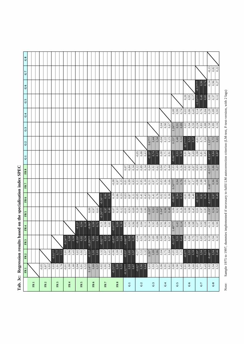
Tab

. 3c:

Reg

ress

ion

resu

lts b

ased

on

the

spec

ialis

atio

n in

dex

SPE

CFR

1FR

2FR

3FR

4FR

5FR

6FR

7FR

8G

1G

2G

3G

4G

5G

6G

7G

8

-0,0

50,

870,

930,

03-0

.61*

*0,

910,

770,

780,

11-0

,01

0,01

-0.2

4**

0,99

0,96

0,98

1,00

0,43

0,98

0,04

0,02

-0.1

9*-0

.12*

0,91

0,92

0,82

0,94

0,52

0,17

0,56

0,18

0.14

**-0

.11*

-0.2

9***

-0.0

6*0,

000,

890,

950,

860,

990,

970,

570,

830,

610,

720,

610,

020,

32-0

.82*

*0,

21-0

.26*

**-0

.38*

**0,

950,

970,

850,

990,

970,

960,

640,

410,

350,

820,

460,

50-0

.25*

*-0

,06

-0.0

7*-0

.07*

*0,

070,

19-0

,08

0,99

0,99

0,91

0,99

0,33

0,86

0,97

0,33

0,66

0,64

0,39

0,12

0,53

0,35

-0.3

2***

-0.0

3*-0

.06*

*0,

02-0

,01

0,03

0,01

0,07

0,93

0,85

0,98

0,93

0,93

0,87

0,99

0,84

0,67

0,97

0,29

0,96

0,69

0,11

0,93

0,34

-0.0

2*-0

,27

-0,0

4-0

,06

0,20

-0,0

50,

110,

12-0

,05

0,90

0,53

0,91

0,84

0,60

0,41

0,95

0,89

0,88

0,64

0,32

0,19

0,11

0,80

0,43

0,18

0,34

0,63

0,03

0.26

*0,

500,

140.

10*

-0,0

70,

510,

04-0

.19*

0.67

**0,

930,

890,

890,

950,

930,

410,

970,

920,

740,

440,

570,

860,

880,

840,

830,

760,

730,

620,

170,

340,

060,

040,

000,

910.

04*

0,02

0,03

0,04

0,00

-0,0

40,

040,

950,

750,

940,

960,

960,

550,

960,

730,

710,

220,

900,

610,

840,

970,

510,

480,

300,

660,

440,

910,

150,

670,

00-0

,05

-0.1

3**

1.48

***

0,06

-0.0

8**

0.50

***

0,03

-0.0

6***

0.23

*1.

26**

0,00

0,90

0,93

0,93

0,43

0,92

0,94

0,94

0,69

0,93

0,48

0,91

0,99

0,45

0,25

0,41

0,14

0,26

0,15

0,76

0,56

0,30

0,33

0,89

0,74

0,01

-0.0

7*0,

000,

040,

00-0

,01

0,06

0,02

0,01

-0.1

7***

0,02

0,03

0,20

0,90

0,93

0,84

0,98

0,98

0,88

0,97

0,92

0,87

0,51

0,94

0,86

0,95

0,66

0,59

0,75

0,98

0,45

0,40

0,17

0,97

0,69

0,37

0,59

0,43

0,17

0,01

-0.1

9*0,

120,

070,

01-0

.11*

*-0

,08

0,03

0,08

-0,0

1-0

,24

0,14

-1.5

5***

-0.3

7***

0,77

0,94

0,85

0,93

0,97

0,91

0,98

0,81

0,81

0,75

0,83

0,76

0,46

0,96

0,43

0,23

0,55

0,68

0,85

0,26

0,48

0,32

0,85

0,69

0,88

0,84

0,85

0,74

0,02

-0.4

8**

0,10

-0,1

10.

19*

-0.1

7***

0.48

***

-0.3

1**

-0.1

9**

1.12

**0,

580,

200,

00-0

,14

-0,1

30,

940,

940,

940,

890,

940,

970,

960,

860,

840,

720,

890,

890,

370,

960,

820,

520,

460,

320,

990,

570,

490,

990,

270,

870,

650,

160,

950,

120,

270,

22

Not

e:

Sam

ple

1975

to 1

997,

dum

mie

s im

plem

ente

d if

nece

ssar

y to

fulfi

l LM

aut

ocor

rect

ion

crite

rion

(LM

-test

, F-te

st-v

ersi

on, w

ith 2

lags

)

G 5

G 6

G 7

G 8

G 1

G 2

G 3

G 4

FR 5

FR 7

FR 6

FR 8

FR 1

FR 2

FR 3

FR 4

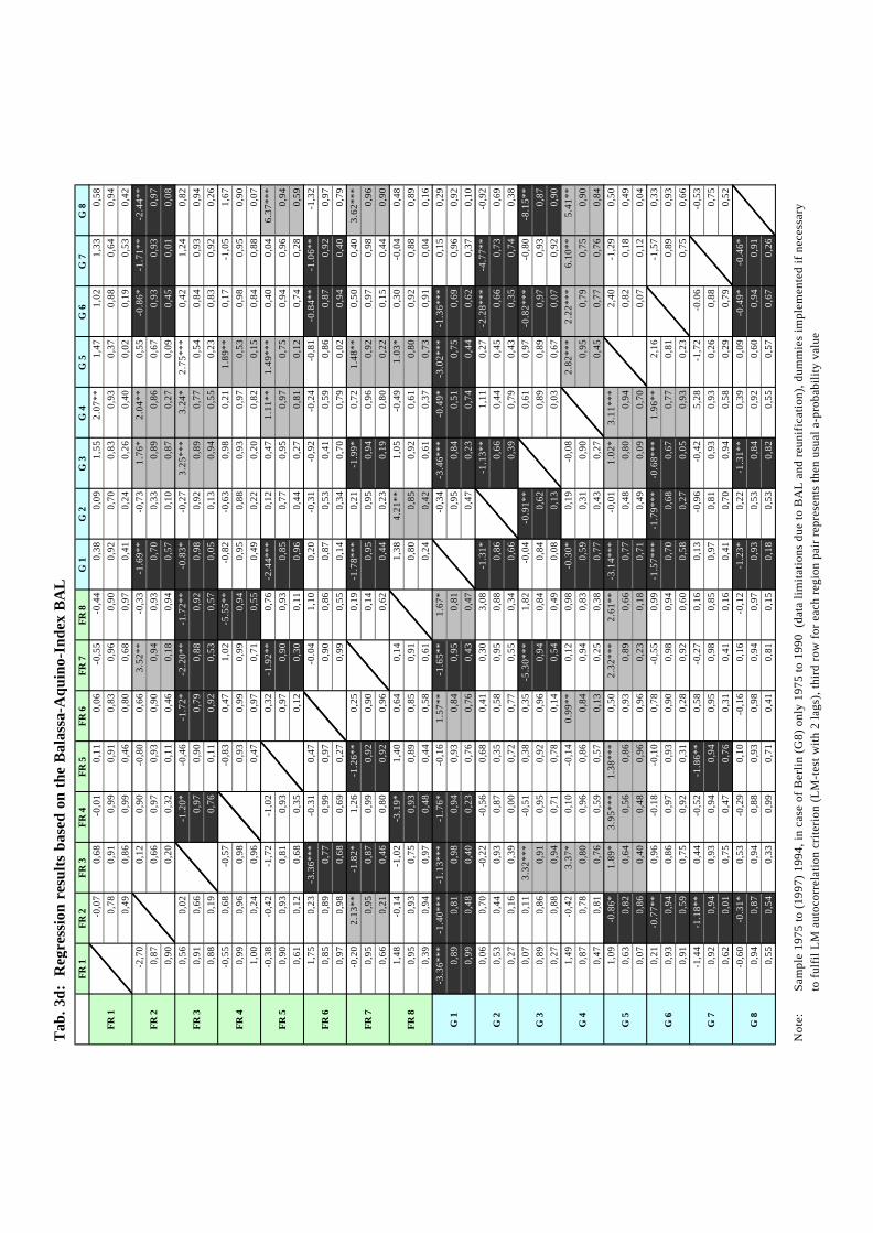
Tab

. 3d:

Reg

ress

ion

resu

lts b

ased

on

the

Bal

assa

-Aqu

ino-

Inde

x B

AL

FR 1

FR 2

FR 3

FR 4

FR 5

FR 6

FR 7

FR 8

G 1

G 2

G 3

G 4

G 5

G 6

G 7

G 8

-0,0

70,

68-0

,01

0,11

0,06

-0,5

5-0

,44

0,38

0,09

1,55

2.07

**1,

471,

021,

330,

580,

780,

910,

990,

910,

830,

960,

900,

920,

700,

830,

930,

370,

880,

640,

940,

490,

860,

990,

460,

800,

680,

970,

410,

240,

260,

400,

020,

190,

530,

42-2

,70

0,12

0,90

-0,8

00,

663.

52**

-0,3

3 -1

.69*

*-0

,73

1.76

*2.

04**

0,55

-0.8

6* -1

.71*

* -2

.44*

*0,

870,

660,

970,

930,

900,

940,

930,

700,

330,

890,

860,

670,

930,

930,

970,

900,

200,

320,

110,

460,

180,

940,

570,

100,

870,

270,

090,

450,

010,

080,

560,

02 -1

.20*

-0,4

6 -1

.72*

-2.2

0**

-1.7

2**

-0.8

3*-0

,27

3.25

***

3.24

*2.

75**

*0,

421,

240,

820,

910,

660,

970,

900,

790,

880,

920,

980,

920,

890,

770,

540,

840,

930,

940,

880,

190,

760,

110,

920,

530,

570,

050,

130,

940,

550,

230,

830,

920,

26-0

,55

0,68

-0,5

7-0

,83

0,47

1,02

-5.5

5**

-0,8

2-0

,63

0,98

0,21

1.89

**0,

17-1

,05

1,67

0,99

0,96

0,98

0,93

0,99

0,99

0,94

0,95

0,88

0,93

0,97

0,53

0,98

0,95

0,90

1,00

0,24

0,96

0,47

0,97

0,71

0,55

0,49

0,22

0,20

0,82

0,15

0,84

0,88

0,07

-0,3

8-0

,42

-1,7

2-1

,02

0,32

-1.9

2**

0,76

-2.4

4***

0,12

0,47

1.11

**1.

49**

*0,

400,

046.

37**

*0,

900,

930,

810,

930,

970,

900,

930,

850,

770,

950,

970,

750,

940,

960,

940,

610,

120,

680,

350,

120,

300,

110,

960,

440,

270,

810,

120,

740,

280,

591,

750,

23-3

.36*

**-0

.31

0,47

-0.0

41,

100,

20-0

,31

-0,9

2-0

,24

-0,8

1 -0

.84*

* -1

.06*

*-1

,32

0,85

0,89

0,77

0,99

0,97

0,90

0,86

0,87

0,53

0,41

0,59

0,86

0,87

0,92

0,97

0,97

0,98

0,68

0,69

0,27

0,99

0,55

0,14

0,34

0,70

0,79

0,02

0,94

0,40

0,79

-0,2

02.

13**

-1.8

2*1,

26 -1

.26*

*0,

250,

19 -1

.78*

**0,

21 -1

.99*

0,72

1.48

**0,

500,

403.

62**

*0,

950,

950,

870,

990,

920,

900,

140,

950,

950,

940,

960,

920,

970,

980,

960,

660,

210,

460,

800,

920,

960,

620,

440,

230,

190,

800,

220,

150,

440,

901,

48-0

,14

-1,0

2 -3

.19*

1,40

0,64

0,14

1,38

4.21

**1,

05-0

,49

1.03

*0,

30-0

,04

0,48

0,95

0,93

0,75

0,93

0,89

0,85

0,91

0,80

0,85

0,92

0,61

0,80

0,92

0,88

0,89

0,39

0,94

0,97

0,48

0,44

0,58

0,61

0,24

0,42

0,61

0,37

0,73

0,91

0,04

0,16

-3.3

6***

-1.4

0***

-1.1

3***

-1.7

6*-0

,16

1.57

** -1

.65*

*1.

67*

-0,3

4 -3

.46*

** -0

.49*

-3.0

2***

-1.3

6***

0,15

0,29

0,89

0,81

0,98

0,94

0,93

0,84

0,95

0,81

0,95

0,84

0,51

0,75

0,69

0,96

0,92

0,99

0,48

0,40

0,23

0,76

0,76

0,43

0,47

0,47

0,23

0,74

0,44

0,62

0,37

0,10

0,06

0,70

-0,2

2-0

,56

0,68

0,41

0,30

3,08

-1.3

1* -1

.13*

*1,

110,

27 -2

.28*

** -4

.77*

*-0

,92

0,53

0,44

0,93

0,87

0,35

0,58

0,95

0,88

0,86

0,66

0,44

0,45

0,66

0,73

0,69

0,27

0,16

0,39

0,00

0,72

0,77

0,55

0,34

0,66

0,39

0,79

0,43

0,35

0,74

0,38

0,07

0,11

3.32

***

-0,5

10,

380,

35 -5

.30*

**1,

82-0

,04

-0.9

1**

0,61

0,97

-0.8

2***

-0,8

0 -8

.15*

*0,

890,

860,

910,

950,

920,

960,

940,

840,

840,

620,

890,

890,

970,

930,

870,

270,

880,

940,

710,

780,

140,

540,

490,

080,

130,

030,

670,

070,

920,

901,

49-0

,42

3.37

*0,

10-0

,14

0.99

**0,

120,

98 -0

.30*

0,19

-0,0

82.

82**

*2.

22**

*6.

10**

5.41

**0,

870,

780,

800,

960,

860,

840,

940,

830,

590,

310,

900,

950,

790,

750,

900,

470,

810,

760,

590,

570,

130,

250,

380,

770,

430,

270,

450,

770,

760,

841,

09-0

.86*

1.89

*3.

95**

*1.

38**

*0,

502.

32**

*2.

61**

-3.1

4***

-0,0

11.

02*

3.11

***

2,40

-1,2

90,

500,

630,

820,

640,

560,

860,

930,

890,

660,

770,

480,

800,

940,

820,

180,

490,

070,

860,

400,

480,

960,

960,

230,

180,

710,

490,

090,

700,

070,

120,

040,

21-0

.77*

*0,

96-0

.18

-0,1

00,

78-0

,55

0,99

-1.5

7***

-1.7

9***

-0.6

8***

1.96

**2,

16-1

,57

0,33

0,93

0,94

0,86

0,97

0,93

0,90

0,98

0,94

0,70

0,68

0,67

0,77

0,81

0,89

0,93

0,91

0,59

0,75

0,92

0,31

0,28

0,92

0,60

0,58

0,27

0,05

0,93

0,23

0,75

0,66

-1,4

4-1

.18*

*0,

44-0

,52

-1.8

6**

0,58

-0,2

70,

160,

13-0

,96

-0,4

25,

28-1

,72

-0.0

6-0

,53

0,92

0,94

0,93

0,94

0,94

0,95

0,98

0,85

0,97

0,81

0,93

0,93

0,26

0,88

0,75

0,62

0,01

0,75

0,47

0,76

0,31

0,41

0,16

0,41

0,70

0,94

0,58

0,29

0,79

0,52

-0,6

0-0

.31*

0,53

-0,2

90,

10-0

,16

0,16

-0,1

2-1

.23*

0,22

-1.3

1**

0,39

0,09

-0.4

9*-0

.46*

0,94

0,87

0,94

0,88

0,93

0,98

0,94

0,97

0,93

0,53

0,84

0,92

0,60

0,94

0,91

0,55

0,54

0,33

0,99

0,71

0,41

0,81

0,15

0,18

0,53

0,82

0,55

0,57

0,67

0,26

Not

e:

Sam

ple

1975

to (1

997)

199

4, in

cas

e of

Ber

lin (G

8) o

nly

1975

to 1

990

(dat

a lim

itatio

ns d

ue to

BA

L an

d re

unifi

catio

n), d

umm

ies

impl

emen

ted

if ne

cess

ary

to fu

lfil L

M a

utoc

orre

latio

n cr

iterio

n (L

M-te

st w

ith 2

lags

), th

ird ro

w fo

r eac

h re

gion

pai

r rep

rese

nts

then

usu

al a

-pro

babi

lity

valu

e

FR 1

FR 2

FR 3

FR 4

FR 5

FR 7

FR 6

FR 8

G 1

G 2

G 3

G 4

G 5

G 6

G 7

G 8