Springba k CompensationforIn remental Sheet Metal Forming Appli ationsJ. Zettler1, H. Rezai1, G. Hirt21 EADS Deuts hland GmbH, Mün hen2 Institut für Bildsame Formgebung der RWTH Aa hen, Aa henAbstra t. In remental CNC sheet forming (ISF) and in remental sheet forming with in remental die(ISFID) are relatively new sheet metal forming pro ess for small bat h produ tion and prototyping. In thesepro esses, a blank is shaped by the CNC movements of simple tools in ombination with a simpli�ed die orwithout die at all. The standard forming strategies for the traditional ISF pro ess normally use some kind ofdie in order to in rease the a ura y of the �nal part. However the ISF pro ess and the ISFID introdu e greatresidual stresses to the sheet during the forming whi h lead to geometri al deviations after releasing the�xation of the sheet. These residual stresses vary based on material sele tion and geometry of the formedpart.This paper deals with a pro edure to a ount for the geometri al deviations based on the residual stresses byapplying a ompensation to them with a software tool whi h takes are of spe ial ISF and ISFID requirementslike maximum wall angle or minimal radii. As this software tool is part of a software designed for ISFID atEADS Innovation Works, several links and spe ialities of this pro ess variation are used for the ompensationtool des ribed in this paper and might not be appli able to the standard and traditional ISF pro ess.

2008 Copyright by DYNAmore GmbH

7. LS-DYNA Anwenderforum, Bamberg 2008 Metallumformung I

C - I - 21

1 Introdu tionThe geometri deviations related to residual stresses are a ommon problem in old sheet metal formingpro esses. After removing the sheet from the shaping tools or the blank holder the elasti energy inside thesheet vanishes and as a result the sheet begins to distort. This distortion, often alled springba k, leads toa geometri al deviation ompared to the desired CAD shape.To ompensate the springba k espe ially for deep drawing pro esses a lot of e�orts have been spent during thelast years and numerous papers and resear h results exist already [6℄. The ISFID and the ISF pro ess howeverare still in a ni he but growing and some resear hers already tried to reuse the basi ideas of springba k ompensation based on a omparison and s aled mirroring of the CAD geometry and the geometry after theforming ( [3℄). In this paper we will fo us on a new developed software within EADS Innovation Works whi hallows for a ompensation of the springba k after ISFID and ISF. The pro edure di�ers mainly from thatof other resear h a tivities by taking are of ISFID and ISF hara teristi s whi h have been implemented inthe software. These hara teristi s in lude maximum forming angle and minimum radii of the forming part.The software an either be used in a FE simulation based springba k ompensation loop or in an iterativetrial series. In �gure 1 the basi prin iple of the software is shown.We have a CAD geometry whi h represents the target of the ompensation. In ISF and ISFID we need a toolpath to form our part. Therefore the �rst step is to generate a tool path based on the CAD geometry. Afterforming the part either by FE simulation with LS-DYNA (see [7℄) or by real trials, the �nal geometry afterspringba k is measured. For the simulation output this is not ne essary but for the real trials an optim almeasurement system alled ATOS from the ompany GOM is used. The next step, Best-Fit, is one of themost important steps in the whole pro edure as it is responsible for how mu h deviation we will measure indi�erent areas of the part. In se tion 2 we will explain in more detail the exa t pro edure we use here.CAD-Model

Surface

reconstruction

Compare

Geometry-

measurement

compensated

CAD-Model

Springback

compensation

< TOL„perfect“ part

formedtrue

false

Tool Path

Generation

Tool Path

Generation

Forming of the

part

Forming of the

part

Manufacturing Simulation

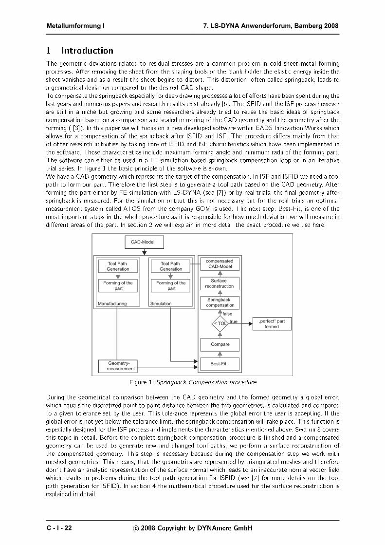
Best-FitFigure 1: Springba k Compensation pro edureDuring the geometri al omparison between the CAD geometry and the formed geometry a global error,whi h equals the dis retized point to point distan e between the two geometries, is al ulated and omparedto a given toleran e set by the user. This toleran e represents the global error the user is a epting. If theglobal error is not yet below the toleran e limit, the springba k ompensation will take pla e. This fun tion isespe ially designed for the ISF pro ess and implements the hara teristi s mentioned above. Se tion 3 oversthis topi in detail. Before the omplete springba k ompensation pro edure is �nished and a ompensatedgeometry an be used to generate new and hanged tool paths, we perform a surfa e re onstru tion ofthe ompensated geometry. This step is ne essary be ause during the ompensation step we work withmeshed geometries. This means, that the geometries are represented by triangulated meshes and thereforedon�t have an analyti representation of the surfa e normal whi h leads to an ina urate normal ve tor �eldwhi h results in problems during the tool path generation for ISFID (see [7℄ for more details on the toolpath generation for ISFID). In se tion 4 the mathemati al pro edure used for the surfa e re onstru tion isexplained in detail. 2008 Copyright by DYNAmore GmbH

Metallumformung I 7. LS-DYNA Anwenderforum, Bamberg 2008

C - I - 22

After the surfa e re onstru tion is �nished the ompensated surfa e an be used for the next iteration loopuntil the global error is below the error toleran e set by the user.2 Best FitAfter the forming, either virtually by FE simulation or in trials, we get a triangulated geometry representationof the formed part. To al ulate the geometri al deviation between this geometry and our desired CADgeometry we have to make sure that the relative position of the CAD geometry and our formed geometry isaligned to ea h other in a proper way. We all this pro edure �Best Fit� as we sear h for the optimal relativeposition between two di�erent geometries whi h have similar and representative regions. For the ISF pro essit is often ne essary to take into a ount spe ial areas of the geometry whi h should be preferred by thealignment pro edure. An example for su h a spe ial area is the region in whi h the die or the blank holder isa ting. With our algorithm this area an be weighted di�erently than the other parts of the geometry and the�Best Fit� will lead to a slightly better positioning towards the prefered areas. For our algorithm we �rst haveto triangulate our CAD model to speed up the whole pro edure. This triangulation is dire tly implemented inour software as well. Afterwards we now assume two given triangulations. One from the CAD model alledDS with the point-set Q = fqigi=1;:::;m and D of the formed geometry with the point-set P = fpigi=1;:::;n .The algorithm uses a weighted version of the ICP-Method (ICP =̂ Iterative Closest Point) wi h is used to�nd the perfe t mat h between the both triangulations. A detailed des ription of this method an be foundin [4℄. The aim of this method is to ompute a ombination of rotations and translations of the point set Pwi h minimizes the square-distan es between the two point sets Q andP . As already mentioned above, byusing weights for single points of the point set P the user an in�uen e the resulting orientation. In Fig. 2di�erent weights have been used and the hanged �Best Fit� position of the formed geometry an be seen.

−150 −100 −50 0 50 100 150

−40

−35

−30

−25

−20

−15

−10

−5

0

x−coordinate

z−co

ord

inat

e

CAD model

Best Fit without weights

Best Fit with weightsFigure 2: Cut through a CAD geometry ompared to two �Best Fit� formed geometries with and withoutweights on the boundary of the geometryIn our implementation we allow a presele tion and de�nition of weights for single regions of the CAD modelby dire tly sele ting CAD B-Spline pat hes. Internally we take all the nodes of the CAD triangulation whi hrefer to the B-Spline pat h and apply the desired weight to them.To ensure a robust and fast onvergen e of the algorithm, it is ne essary to start with a oarse orientationof the triangulation D ompared to DS . For this reason, before starting the ICP-algorithm, we omputethe prin ipal axes of the two point sets Q andP and transform D in a way that the pri ipal axes �t to ea hother . The prin ipal axes an be omputed by setting up a ovarianz matrix of the point sets Q andP andusing the hara teristi polynomial of that matrix to a quire the Eigenve tors and Eigenvalues. They alreadyrepresent the prin ipal axes.After the oarse alignment we an ompute an assignment : Q ! P̂ � P between the two point setsQ andP by using a nearest-neighbour-sear h-algorithm. With the given weights wi ; i = 1; : : : ; m we haveto solve the following nonlinear minimization problemm∑i=1 wikrik22 �! min ; ri := R � (qi) + t � qiwith a 3� 3 rotational matrix R and a translation-ve tor t 2 R3 . 2008 Copyright by DYNAmore GmbH

7. LS-DYNA Anwenderforum, Bamberg 2008 Metallumformung I

C - I - 23

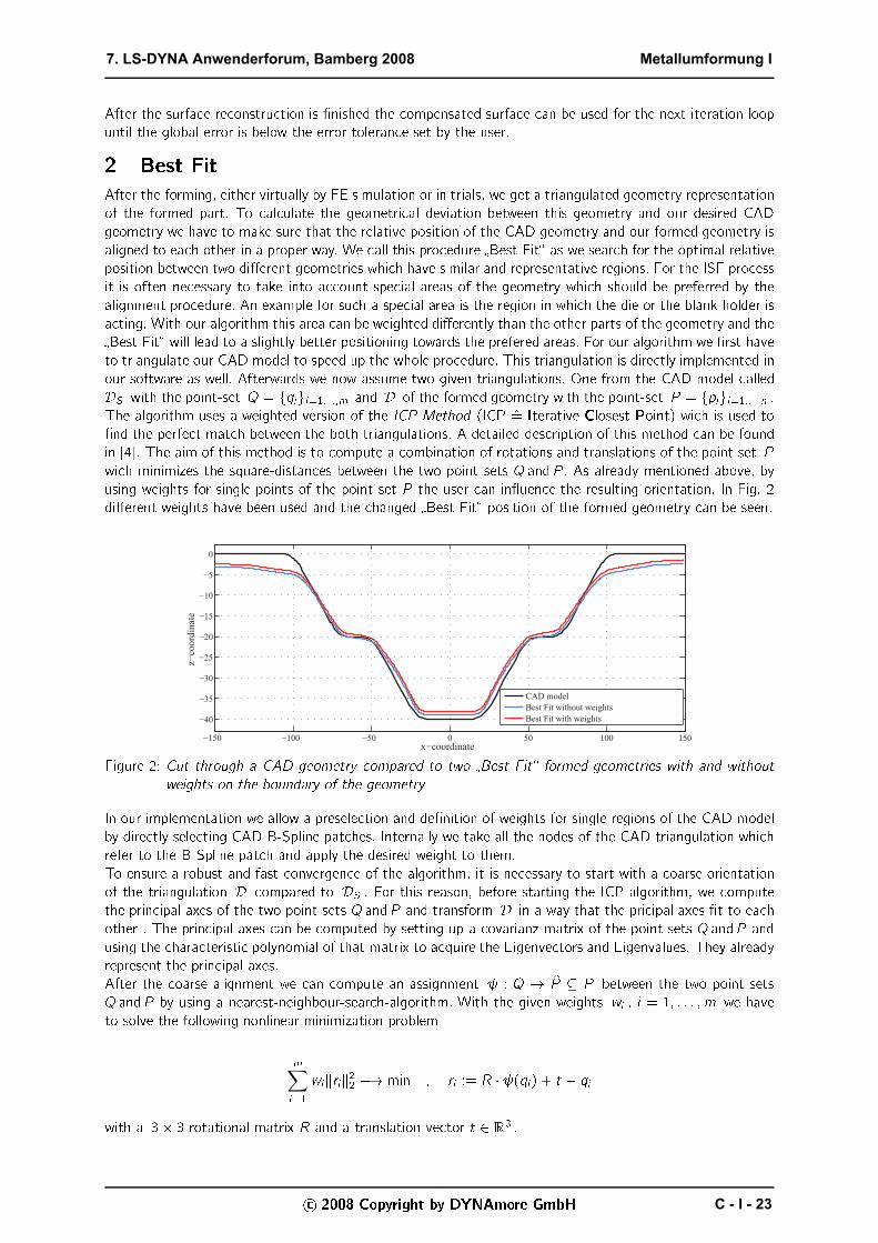
The solution is found by using the Levenberg-Marquardt-Algorithm. Afterwards the mesh will be transformedwith the solution and the assignment is omputed again for the transformend point-set. The iterationwill be an elled if the average square distan e errorE = 1m m∑i=1kqi � (qi )k22has no signi� ant hange in omparison to the previous iteration step. In �gure 3 the speed of the algorithmis shown. Already after around 10-20 iterations the average error is nearly minimized.

0 10 20 30 40 50 60 70 80 90 1000

5

10

15

20

25

30

35

40

Iteration step

av

erag

e er

ror

(E)

Figure 3: Average Error in relation to the �Best Fit� iteration steps (left) and resulting overall error in [mm℄of the �Best Fit� positioning for an example part with more weights on the boundary (right)

2008 Copyright by DYNAmore GmbH

Metallumformung I 7. LS-DYNA Anwenderforum, Bamberg 2008

C - I - 24

3 Springba k CompensationAfter the formed geometry is �Best Fit� towards the CAD part with the user set weights in spe ial areas, thea tual springba k ompensation is performed. This algorithm is optimised for the ISF pro ess and thereforedi�erent from state of the art springba k ompensation methods des ribed in [6℄. The main di�eren e is,that the geometry after the springba k ompensation is still formable by the ISF pro ess without any tool hange. This is a hieved by taking are that the ompensated geometry will never result in wall angles greaterthen a user de�ned value �TOL and also radii will never be less then the forming tool radius. These spe ialISF related restri tions an be extra ted from the urvature information of the CAD model and atta hed tothe CAD mesh DS . As during the ompensation pro edure the distan e between the CAD geometry and theformed geometry has to be measured we also need the analyti al surfa e normal of the CAD geometry andatta h it to our CAD mesh DS at the proper nodes qi 2 Q . For further explanations let V := f1; : : : ; mg ontain the index values of the point set Q and Vb � V represents the point indi es within the boundaryregion of the CAD-model.The single steps of the ompensation pro edure an be summarised as follows:� For every knot i 2 V of the mesh DS with the analyti al unit normal ve tor ni from the CADgeometry, ompute a distan e ve tor fi 2 R3 through interse tion with D in normal dire tion.� After omputing a urvature based bound si � 0 for every knot i 2 V , taking into a ount themaximum allowable wall angle �TOL , all nodal points qi 2 Q will be transformed (global o�set) usingq�i = qi � � � �i � fiwith � 2 [0; 1℄ and �i 2 [0; 1℄ . � represents the s aling fa tor. If we would mirror the al ulated andmeasured error this fa tor will be 1.0. Based on experien es this fa tor usually varies between 0.8 and1.0 (see [3℄).� Determine onne ted regions of triangles based on the triangle normals whi h an be moved furtherwithout ex eeding the angle toleran e �TOL (lo al o�set) and transform ea h of these separateregions separately.� The last step in ludes a smoothing pro edure of the transformed triangulations DS to obtain a smoothintera tion between the lo al o�setted areas and the global o�setted areas.3.1 Global O�setThe CAD unit normal ve tors ni at the nodal points qi 2 Q determine the dire tion of the node movementand are also ne essary to ompute the distan e to the triangulation D by interse tioning it. As alreadymentioned above, for a ura y reasons, these normals will be omputed dire tly on the parametri CADsurfa e S(u; v) with ni := Su(ui ; vi )� Sv (ui ; vi )kSu(ui ; vi )� Sv (ui ; vi )k2 ; (ui ; vi ) := S�1(qi)The surfa e parameters (ui ; vi ) 2 R2 are stored during the triangulation pro ess of the CAD surfa e andwe assume them to be given.The key aspe t of the introdu ed algorithm is the omputation of an upper bound si � 0 for the translationamount. Based on the prin ipal urvatures of the CAD model at all knots i 2 V the upper bound si will bedetermined in a way, that the approximative omputed radii of urvature of the ompensated geometry willnot ex eed the tool radii set by the user. The paramater ��TOL 2 [0; 1℄ is omputed, based on the trianglenormals of all knots i 2 V . To ensure that the triangles of the deformed triangulation will not ex eed theangle toleran e �TOL .The distan e ve tor fi is always ollinear to ni and the magnitude in the �rst iteration step equates to theeu lidean distan e to D . To ensure a ontinous improvement during the iterative pro ess of the springba k ompensation, all pre ending ompensation loops will be added at this stage (in luding the signs) to thea tual distan e ve tor fi . 2008 Copyright by DYNAmore GmbH

7. LS-DYNA Anwenderforum, Bamberg 2008 Metallumformung I

C - I - 25

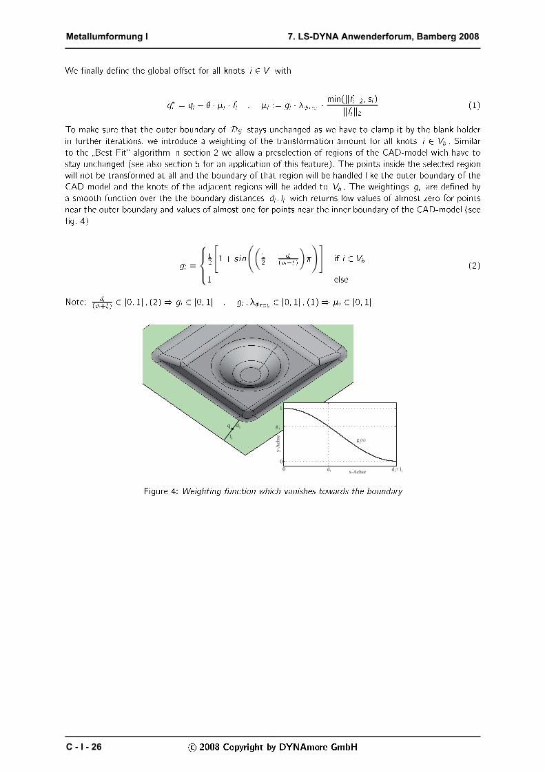
We �nally de�ne the global o�set for all knots i 2 V withq�i = qi � � � �i � fi ; �i := gi � ��TOL � min(kfik2; si )kfik2 (1)To make sure that the outer boundary of DS stays un hanged as we have to lamp it by the blank holderin further iterations, we introdu e a weighting of the transformation-amount for all knots i 2 Vb . Similarto the �Best Fit� algorithm in se tion 2 we allow a presele tion of regions of the CAD-model wi h have tostay un hanged (see also se tion 5 for an appli ation of this feature). The points inside the sele ted regionwill not be transformed at all and the boundary of that region will be handled like the outer boundary of theCAD-model and the knots of the adja ent regions will be added to Vb . The weightings gi are de�ned bya smooth fun tion over the the boundary distan es di ; li wi h returns low values of almost zero for pointsnear the outer boundary and values of almost one for points near the inner boundary of the CAD-model (see�g. 4) gi =

12[1 + sin(( 12 � di(di+li ))�)] if i 2 Vb1 else (2)Note: di(di+li ) 2 [0; 1℄ ; (2)) gi 2 [0; 1℄ ; gi ; ��TOL 2 [0; 1℄ ; (1)) �i 2 [0; 1℄q

idi

li

g i

di d + li i0

0

1

g (x)

x-Achse

y-A

chse

iFigure 4: Weighting fun tion whi h vanishes towards the boundary

2008 Copyright by DYNAmore GmbH

Metallumformung I 7. LS-DYNA Anwenderforum, Bamberg 2008

C - I - 26

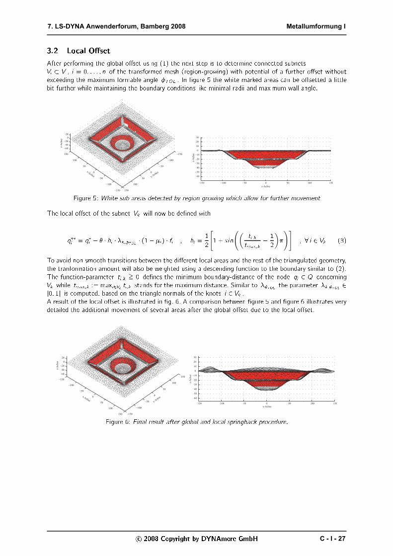
3.2 Lo al O�setAfter performing the global o�set using (1) the next step is to determine onne ted subnetsVi � V ; i = 0; : : : ; n of the transformed mesh (region-growing) with potential of a further o�set withoutex eeding the maximum formable angle �TOL . In �gure 5 the white marked areas an be o�setted a littlebit further while maintaining the boundary onditions like minimal radii and maximum wall angle.

−150

−100

−50

0

50

100

150 −150

−100

−50

0

50

100

150

−60

−40

−20

0

20

z-A

chse

−150 −100 −50 0 50 100 150

−60

−50

−40

−30

−20

−10

0

10

20

30

z-A

chse

x-Achse y-Ach

se

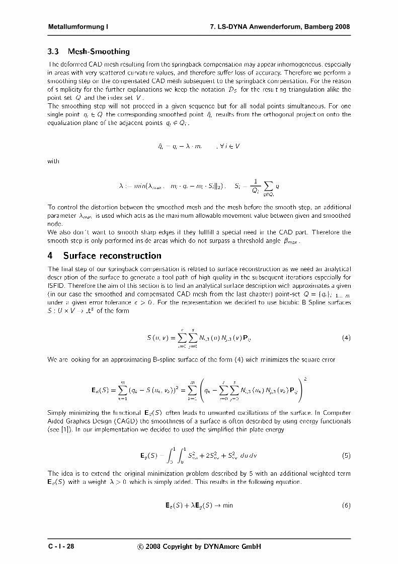
y-AchseFigure 5: White sub areas dete ted by region growing whi h allow for further movementThe lo al o�set of the subnet Vk will now be de�ned withq��i = q�i � � � hi � �k;�TOL � (1� �i ) � fi ; hi = 12[1 + sin(( ti ;ktmax;k � 12)�)] ; 8 i 2 Vk (3)To avoid non smooth transitions between the di�erent lo al areas and the rest of the triangulated geometry,the tranformation amount will also be weighted using a des ending fun tion to the boundary similar to (2).The fun tion-parameter ti ;k = 0 de�nes the minimum boundary-distan e of the node qi 2 Q on erningVk while tmax;k := maxi2Vk ti ;k stands for the maximum distan e. Similar to ��TOL the parameter �k;�TOL 2[0; 1℄ is omputed, based on the triangle normals of the knots i 2 Vk .A result of the lo al o�set is illustrated in �g. 6. A omparison between �gure 5 and �gure 6 illustrates verydetailed the additional movement of several areas after the global o�set due to the lo al o�set.−150

−100

−50

0

50

100

150 −150

−100

−50

0

50

100

150−60

−40

−20

0

20

−150 −100 −50 0 50 100 150

−60

−50

−40

−30

−20

−10

0

10

20

30

z-A

chse

x-Achsey-A

chse

z-A

chse

x-AchseFigure 6: Final result after global and lo al springba k pro edure.

2008 Copyright by DYNAmore GmbH

7. LS-DYNA Anwenderforum, Bamberg 2008 Metallumformung I

C - I - 27

3.3 Mesh-SmoothingThe deformed CAD mesh resulting from the springba k ompensation may appear inhomogeneous, espe iallyin areas with very s attered urvature values, and therefore su�er loss of a ura y. Therefore we perform asmoothing step on the ompensated CAD mesh subsequent to the springba k ompensation. For the reasonof simpli ity for the further explanations we keep the notation DS for the resulting triangulation alike thepoint set Q and the index set V .The smoothing step will not pro eed in a given sequen e but for all nodal points simultaneous. For onesingle point qi 2 Q the orresponding smoothed point q̂i results from the orthogonal proje tion onto theequalization plane of the adja ent points qj 2 Qi .q̂i = qi � � �mi ; 8 i 2 Vwith � := min(�max ; kmi � qi �mi � Sik2) ; Si = 1jQi j ∑q2Qi qTo ontrol the distortion between the smoothed mesh and the mesh before the smooth step, an additionalparameter �max is used whi h a ts as the maximum allowable movement value between given and smoothednode.We also don�t want to smooth sharp edges if they full�ll a spe ial need in the CAD part. Therefore thesmooth step is only performed inside areas whi h do not surpass a threshold angle �max .4 Surfa e re onstru tionThe �nal step of our springba k ompensation is related to surfa e re onstru tion as we need an analyti aldes ription of the surfa e to generate a tool path of high quality in the subsequent iterations espe ially forISFID. Therefore the aim of this se tion is to �nd an analyti al surfa e des ription wi h approximates a given(in our ase the smoothed and ompensated CAD mesh from the last hapter) point-set Q = fqigi=1;:::;munder a given error-toleran e � > 0 . For the representation we de ided to use bi ubi B-Spline surfa esS : U � V ! R3 of the form S (u; v) = r∑i=0 s

∑j=0 Ni ;3 (u)Nj;3 (v)Pi j (4)We are looking for an approximating B-spline surfa e of the form (4) wi h minimizes the square errorEd(S) = m∑k=1 (qk � S (uk ; vk))2 = m

∑k=1qk � r∑i=0 s

∑j=0 Ni ;3 (uk)Nj;3 (vk)Pi j2Simply minimizing the fun tional Ed(S) often leads to unwanted os illations of the surfa e. In ComputerAided Graphi s Design (CAGD) the smoothness of a surfa e is often des ribed by using energy fun tionals(see [1℄). In our implementation we de ided to used the simpli�ed thin plate energyEg(S) = ∫ 10 ∫ 10 S2uu + 2S2uv + S2vv du dv (5)The idea is to extend the original minimization problem des ribed by 5 with an additional weighted termEd(S) with a weight � > 0 whi h is simply added. This results in the following equation.Ed(S) + �Eg(S)! min (6) 2008 Copyright by DYNAmore GmbH

Metallumformung I 7. LS-DYNA Anwenderforum, Bamberg 2008

C - I - 28

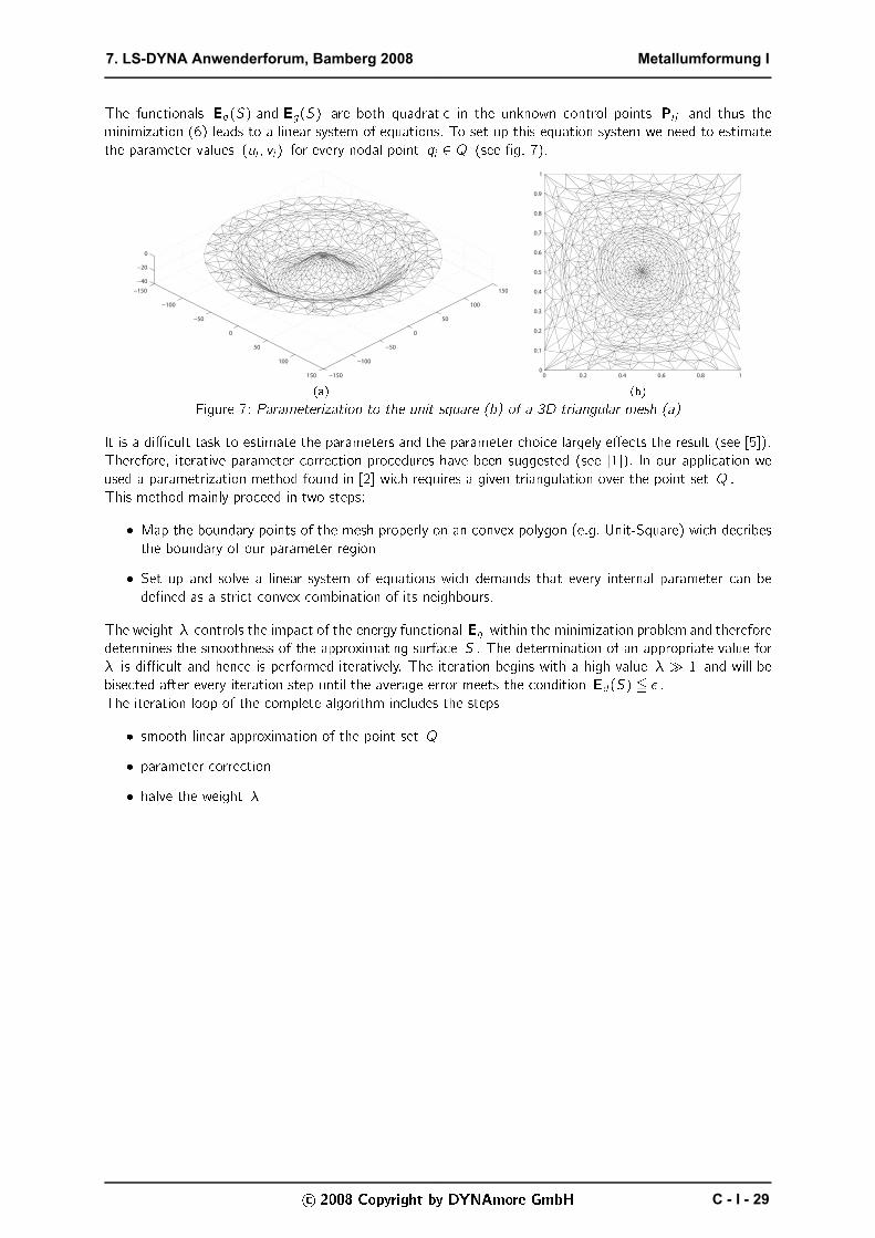
The fun tionals Ed(S) and Eg(S) are both quadrati in the unknown ontrol points Pi j and thus theminimization (6) leads to a linear system of equations. To set up this equation system we need to estimatethe parameter values (ui ; vi ) for every nodal point qi 2 Q (see �g. 7).−150

−100

−50

0

50

100

150 −150

−100

−50

0

50

100

150

−40

−20

0

(a) 0 0.2 0.4 0.6 0.8 10

0.1

0.2

0.3

0.4

0.5

0.6

0.7

0.8

0.9

1

(b)Figure 7: Parameterization to the unit-square (b) of a 3D triangular mesh (a)It is a di� ult task to estimate the parameters and the parameter hoi e largely e�e ts the result (see [5℄).Therefore, iterative parameter orre tion pro edures have been suggested (see [1℄). In our appli ation weused a parametrization method found in [2℄ wi h requires a given triangulation over the point set Q .This method mainly pro eed in two steps:� Map the boundary points of the mesh properly on an onvex polygon (e.g. Unit-Square) wi h de ribesthe boundary of our parameter region� Set up and solve a linear system of equations wi h demands that every internal parameter an bede�ned as a stri t onvex ombination of its neighbours.The weight � ontrols the impa t of the energy fun tional Eg within the minimization problem and thereforedetermines the smoothness of the approximating surfa e S . The determination of an appropriate value for� is di� ult and hen e is performed iteratively. The iteration begins with a high value � � 1 and will bebise ted after every iteration step until the average error meets the ondition Ed(S) 5 � .The iteration loop of the omplete algorithm in ludes the steps� smooth linear approximation of the point set Q� parameter orre tion� halve the weight �

2008 Copyright by DYNAmore GmbH

7. LS-DYNA Anwenderforum, Bamberg 2008 Metallumformung I

C - I - 29

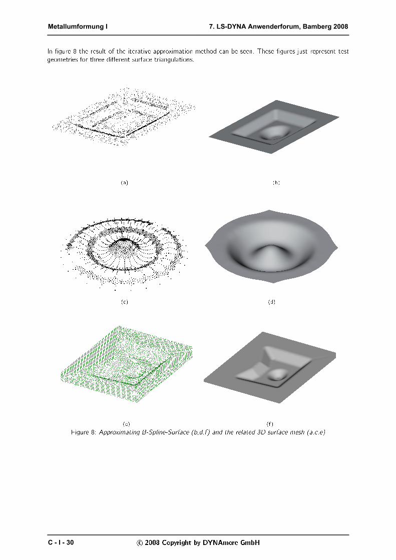
In �gure 8 the result of the iterative approximation method an be seen. These �gures just represent testgeometries for three di�erent surfa e triangulations.

(a) (b)

( ) (d)

(e) (f)Figure 8: Approximating B-Spline-Surfa e (b,d,f) and the related 3D surfa e mesh (a, ,e)

2008 Copyright by DYNAmore GmbH

Metallumformung I 7. LS-DYNA Anwenderforum, Bamberg 2008

C - I - 30

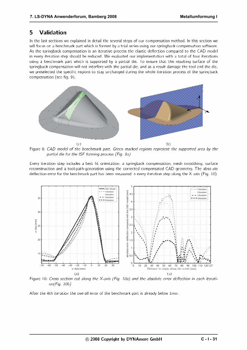
5 ValidationIn the last se tions we explained in detail the several steps of our ompensation method. In this se tion wewill fo us on a ben hmark part whi h is formed by a trial series using our springba k ompensation software.As the springba k ompensation is an iterative pro ess the elasti de�e tion ompared to the CAD modelin every iteration step should be redu ed. We evaluated our implementation with a total of four iterationsusing a ben hmark part whi h is supported by a partial die. To ensure that the resulting surfa e of thespringba k ompensation will not interfere with the partial die, and as a result damage the tool and the die,we presele ted the spe i� regions to stay un hanged during the whole iteration pro ess of the springba k ompensation (see �g. 9).

(a)O

x y

z

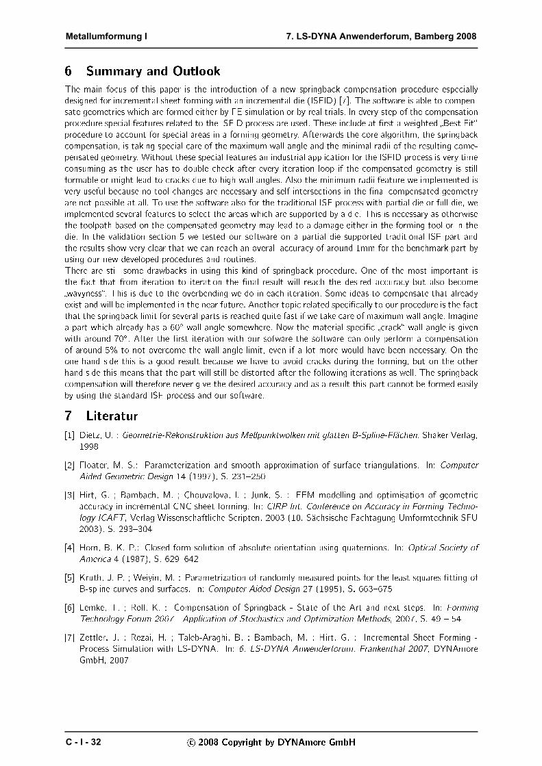
(b)Figure 9: CAD model of the ben hmark part. Green marked regions represent the supported area by thepartial die for the ISF forming pro ess (Fig. 9a)Every iteration step in ludes a best �t orientation, a springba k ompensation, mesh smoothing, surfa ere onstru tion and a tool-path-generation using the orre ted ompensated CAD geometry. The absolutede�e tion error for the ben hmark part has been measured in every iteration step along the X-axis (Fig. 10).

−70 −60 −50 −40 −30 −20 −10 0 10 20 30

15

20

25

30

35

x−Axis [mm]

z−A

xis

[m

m]

CAD−Model

1.Iteration

2.Iteration

3.Iteration

4.Iteration

(a) 0 10 20 30 40 50 60 70 80 90 100 110 120 1270

0.5

1

1.5

2

2.5

3

3.5

4

4.5

5

Distance to origin along the x-axis [mm]

ab

solu

te e

rro

r−d

e"

ect

ion

co

mp

are

d w

ith

th

e C

AD

−m

od

el [

mm

]

1.Iteration

2.Iteration

3.Iteration

4.Iteration

(b)Figure 10: Cross se tion ut along the X-axis (Fig. 10a) and the absolute error de�e tion in ea h iterati-on(Fig. 10b)After the 4th iteration the overall error of the ben hmark part is already below 1mm. 2008 Copyright by DYNAmore GmbH

7. LS-DYNA Anwenderforum, Bamberg 2008 Metallumformung I

C - I - 31

6 Summary and OutlookThe main fo us of this paper is the introdu tion of a new springba k ompensation pro edure espe iallydesigned for in remental sheet forming with an in remental die (ISFID) [7℄. The software is able to ompen-sate geometries whi h are formed either by FE simulation or by real trials. In every step of the ompensationpro edure spe ial features related to the ISFID pro ess are used. These in lude at �rst a weighted �Best Fit�pro edure to a ount for spe ial areas in a forming geometry. Afterwards the ore algorithm, the springba k ompensation, is taking spe ial are of the maximum wall angle and the minimal radii of the resulting ome-pensated geometry. Without these spe ial features an industrial appli ation for the ISFID pro ess is very time onsuming as the user has to double he k after every iteration loop if the ompensated geometry is stillformable or might lead to ra ks due to high wall angles. Also the minimum radii feature we implemented isvery useful be ause no tool hanges are ne essary and self interse tions in the �nal ompensated geometryare not possible at all. To use the software also for the traditional ISF pro ess with partial die or full die, weimplemented several features to sele t the areas whi h are supported by a die. This is ne essary as otherwisethe toolpath based on the ompensated geometry may lead to a damage either in the forming tool or in thedie. In the validation se tion 5 we tested our software on a partial die supported traditional ISF part andthe results show very lear that we an rea h an overall a ura y of around 1mm for the ben hmark part byusing our new developed pro edures and routines.There are still some drawba ks in using this kind of springba k pro edure. One of the most important isthe fa t that from iteration to iteration the �nal result will rea h the desired a ura y but also be ome�wavyness�. This is due to the overbending we do in ea h iteration. Some ideas to ompensate that alreadyexist and will be implemented in the near future. Another topi related spe i� ally to our pro edure is the fa tthat the springba k limit for several parts is rea hed quite fast if we take are of maximum wall angle. Imaginea part whi h already has a 60Æ wall angle somewhere. Now the material spe i� � ra k� wall angle is givenwith around 70Æ. After the �rst iteration with our sofware the software an only perform a ompensationof around 5% to not over ome the wall angle limit, even if a lot more would have been ne essary. On theone hand side this is a good result be ause we have to avoid ra ks during the forming, but on the otherhand side this means that the part will still be distorted after the following iterations as well. The springba k ompensation will therefore never give the desired a ura y and as a result this part annot be formed easilyby using the standard ISF pro ess and our software.7 Literatur[1℄ Dietz, U. : Geometrie-Rekonstruktion aus Meÿpunktwolken mit glatten B-Spline-Flä hen. Shaker Verlag,1998[2℄ Floater, M. S.: Parameterization and smooth approximation of surfa e triangulations. In: ComputerAided Geometri Design 14 (1997), S. 231�250[3℄ Hirt, G. ; Bamba h, M. ; Chouvalova, I. ; Junk, S. : FEM modelling and optimisation of geometri a ura y in in remental CNC sheet forming. In: CIRP Int. Conferen e on A ura y in Forming Te hno-logy ICAFT, Verlag Wissens haftli he S ripten, 2003 (10. Sä hsis he Fa htagung Umformte hnik SFU2003), S. 293�304[4℄ Horn, B. K. P.: Closed-form solution of absolute orientation using quaternions. In: Opti al So iety ofAmeri a 4 (1987), S. 629�642[5℄ Kruth, J. P. ; Weiyin, M. : Parametrization of randomly measured points for the least squares �tting ofB-spline urves and surfa es. In: Computer Aided Design 27 (1995), S. 663�675[6℄ Lemke, T. ; Roll, K. : Compensation of Springba k - State of the Art and next steps. In: FormingTe hnology Forum 2007 - Appli ation of Sto hasti s and Optimization Methods, 2007, S. 49 � 54[7℄ Zettler, J. ; Rezai, H. ; Taleb-Araghi, B. ; Bamba h, M. ; Hirt, G. : In remental Sheet Forming -Pro ess Simulation with LS-DYNA. In: 6. LS-DYNA Anwenderforum, Frankenthal 2007, DYNAmoreGmbH, 2007 2008 Copyright by DYNAmore GmbH

Metallumformung I 7. LS-DYNA Anwenderforum, Bamberg 2008

C - I - 32