This work has been digitalized and published in 2013 by Verlag Zeitschrift für Naturforschung in cooperation with the Max Planck Society for the Advancement of Science under a Creative Commons Attribution4.0 International License.

Dieses Werk wurde im Jahr 2013 vom Verlag Zeitschrift für Naturforschungin Zusammenarbeit mit der Max-Planck-Gesellschaft zur Förderung derWissenschaften e.V. digitalisiert und unter folgender Lizenz veröffentlicht:Creative Commons Namensnennung 4.0 Lizenz.

Boundary-Value Problem for Electromagnetic Fields in Cylindrical Conductor with Circumferential Electrodes Excited by AC-CurrentH. E. Wilhelm*, S. H. Hong**, and D. A. BoonzaierD epartm ent of Bioengineering and Groote Schuur Hospital, University of Cape Town,Cape Town, Republic of South Africa

Z. Naturforsch. 83 a, 1161 — 1168 (1978); received June 12, 1978

The bounardy-value problem for the electromagnetic fields E(r, t) = {Er (r, z, t),0, Ez (r, z, t)} and B(r, t) = {0, Bg(r, z, <),0} in an electrically conducting cylinder of radius r = a and infinite length (— oo ^ 2 ^ -f- oo) is treated, which are excited by a periodic ac-current I(t) = I 0cosojt entering and leaving the cylinder through circumferential electrodes a t r = a and z = ± c. Solu­tions for E(r, t ) and B(r, t) are obtained in term s of Fourier integrals which are reduced to in­finite series by means of the residue theorem. Graphical presentations of the fields E(r, z, t) and B(r, z, t) versus 2 and r for times lot = 0 and n j2 are given which show the relative amplitude and phase relations of the fields. An application of the results to medical physics is discussed con­cerning the measurement of the electrical conductivity of the tissue of limbs.

Introduction

In a classical investigation, Sommerfeld evaluated the electromagnetic field of an infinitely long wire carrying a periodic electric current [1 ]. We treat a similar, though more complex boundary-value prob­lem for the electromagnetic field in a cylindrical conductor of infinite length X — oo, which is sup­plied with a periodic current I (t) = I q c o s cot through circumferential electrodes located on the surface r = a of the conductor at the axial positions z = ± c (Figure 1). For the case of electrodes of non-vanishing width, |z l z |> 0 , and quasi-infinite conductivity, the electric potential within the elec­trode contact surface and the radial potential gra­dient within the remaining surface of the conductor are given as boundary conditions. Mixed boundary- value problems of this type lead to dual integral equations which cannot, in general, be solved in closed form [2]. This is probably the reason why the fundamental electromagnetic boundary-value problem under consideration has not been solved in the literature.

Under the assumption that the axial width Az of the electrodes is small compared with all charac­teristic dimensions of the system, | Az | a < oo and

R eprint requests to Prof. Dr. H. E. WTilhelm, Dept, of Electrical Engineering, Colorado State University, F ort Collins, CO 80523, U.S.A.

* On sabbatical leave from the D epartm ent of Electrical Engineering, Colorado State University, Fort Collins, Colo­rado.

* * Departm ent of Electrical Engineering, Colorado StateUniversity, Fort Collins, Colorado.

| Az | <| L = oo, the injected current distributions at the electrode surfaces can be represent as Dirac functions. This approximation permits us to reduce the mixed boundary-value problem to a Dirichlet problem. I t is remarkable that the mixed boundary

r

. A\ f ,

3

rrFig. 1. Geometry of conducting cylinder of radius r — a with circumferential electrodes a t r = a, z — ± c.

conditions for electrodes of nonvanishing width | Az | > 0 could be taken into account rigorously by means of a continuous superposition of Dirac func­tions a t axial positions z within the electrode sur­face. This approach would represent an alternative to the solution of mixed boundary-value problems based on distribution theory.

This electromagnetic boundary-value problem arose in connection with the evaluation of the zero- order response of a cylindrical model for a limb (a ^ 1 0 _ 1 mho m-1) subject to an ac-current via ring electrodes of frequency v = 1 0 5 sec- 1 and inten­sity I o = 10- 3 amps. The resulting potential differ­ence observed at the surface r = a of the limb allows determination of the impedance of the limb at the frequency v. The (weak) conductivity pulses caused by the pulsating blood flow give rise to a small perturbation of the electric potential from which the speed of the blood flow can be determined [3, 4].

1162 H. E. W ilhelm et al. • Boundary-Value Problem for Electromagnetic F ields in Cylindrical Conductors

Boundary-Value Problem

In general, the electromagnetic fields E(r, I) and B (r, t) produced by a current density j ( r , t ) are determined by Maxwell’s equations with displace­ment current 8 = /uedE/dt (/u, e = magnetic and electrical permeability). The electromagnetic field propagates approximately with the speed of light uq = 1/jue ^ 3 X 108 m sec- 1 along the conductor[1 ]. Accordingly, if the frequency co of the periodic current source is small compared to

wo/A, A ~ max (a, c),

the electromagnetic field can be assumed to adjust itself quasi-instantaneously to the relatively slow changes of j (r , t ) . In this situation, the theory <f quasi-stationary currents is applicable, i.e. Max­well’s equations without displacement current [5]:

V x E = - d B / d t , V ■£ — 0, (1)

V x f l = /<J, V -B = 0, (2)

wherej = o E (3)

is Ohm’s law for an isotropic conductor of relaxa­tion time rc co- 1 in a frame of reference in which the conductor is at rest. For example, for

2 ~ c = l m > a and co = 2 n X 105 sec-1 ,

the condition for neglecting the displacement cur­rent is well satisfied,

co X ~ 2 7i X 105 m sec- 1 uq ^ 3 X 108 m sec-1 .

The system under consideration is a cylindrical conductor of radius a, length L = oo. and homoge­neous conductivity a. An ac-current

I(t) = I 0 c o s cot = Iq Re exp{ico£} (4)

is injected through the central segment 2 c of this conductor by means of ring electrodes a t r = a and z = ± c, which are assumed to be of vanishing width (Figure 1). The injected current density entering the surface of the cylinder is, therefore, radial and given byj r(r = a,z, t) = — dBe{r --- a, z, t)/dz

= (/o/27ra) cos cot[<5(z + c) — d(z — c)]. (5)

The electromagnetic field in the conductor is of the form

B(r, t ) = {0, B 0(r,z,t), 0},E{r, t) = {Er(r, z, t), 0, E z(r, z, t,)} (6 )

whereE = D { — dBo/dz, 0, r~l 0(r2?e)/0r} (7)

by Eqs. (2) —(3), and D is the diffusion coefficient of the electromagnetic field.

D = l/ju c[m 2 sec-1] . (8 )

In accordance with Eqs. (1) —(8 ), the complex dimensionless version &( q, £ , t) of the azimuthal magnetic field Be(r,z, t) is described by the com­plex, parabolic boundary-value problem:

m 0 2̂ 1 0J 1 ® 0 2̂“ e 7 = ~e^2“ + ~ z Q ~ ~ ~Qi + >

— [0#(e,C»T)/0£]c=*= e^[6(C + c ) - d ( C - c ) ] , | C | ^ o o , (10)

d[Q@{Q, C, T)]/0g->O, |C| -> OO , (11)

where

0 = rl(D/(o)1''2, 0 5S q 5S « ,ä = o/(D/ft))i/2 , (1 2 )

C = z/(/)/ft>)1/2 , — oo 5S £ ^ -f- OO , c = cftDI co)1/2, (13)

t = co t , 0 ^ r ^ o o , (14)

andR e 88(o, £, r) = B e(r,z,t)IB0,B 0 = juIo^Tia . (15)

E q u a t io n (9) represents the diffusion equation for the magnetic field in the quasi-stationary approxi­mation [5]. Equation (10) is the boundary condition corresponding to Equation (5). Equation (11) is an improper boundary condition considering that the axial current density vanishes at infinity,

jz cr, z, t) = /X-1 0 [r Be (r, z, <)]/r 0r -* 0,1 Z | —>■ oo .

By Eqs. (2) —(3), the electric field components are obtained from the solution for 88 (q, £, r) as

E r (r, z,t) = — E q Re {0J 1 {q, f , r)/0£}, E z(r,z,t) = + E 0 ~Re{d[Q@(Q,t, t )]Iqöq},E q = (Deo)1'2 i l l q/2 7i a. (16)

Analytical Solution

The partial solutions of the boundary-value prob­lem in Eqs. (9) —(11) are oscillations at the dimen-

H. E. W ilhelm et al. • Boundary-Yalue Problem for Electrom agnetic Fields in Cylindrical Conductors 1163

sionless frequency a> — 1 , and are of the form

^a({?,C, t) oc Ii(]/i + a2£>) co saC ex p (ir) ,

since d&(g, £, t )/0£ is asymmetric with respect to the plane £ = 0 by Equation (10). Accordingly, the general solution of Eqs. (9) —(11) should be repre­sentable by the Fourier integral over the continuous eigenvalues a ( |£ | sS co),

OO

&{q, £, t ) — ei r \ A (a) Ii(]/i + a2@) cos a£da (17) o

whereOO

j A (a) a I i {]/i + a 2 ä) sin a C daö

OO

= — (2 /7r) J s in a c s in a^ d a (18)o

by the boundary condition (10). In Eq. (18) the Dirac functions <5 (£± c) of Eq. (10) have been ex­panded as Fourier integrals,

d(t + c ) - d ( t - c )OO

= — (2 /tt) J s in a c s in a C d a . (19)o

Application of the inverse Hankel transform to Eq. (18) gives for the Fourier amplitudes

2 sinac - 1 ______A(cc) = -------------- 11 (1H + a 2 ä ) . (2 0 )n a r

Combining of Eqs. (17) and (20) yields the general solution for the magnetic field in complex, dimen- sionles representation:

@(Q,t ,T)= (21)OO

2 f s inac cl2 q)------e ™ ----------- 7— .... cos a C da.n J a 7i(J/t + a 2 a)

o

As will be shown, this solution satisfies also the improper boundary condition (11). By means of Eq. (16), one derives from Eq. (2 1 ) the complex, dimensionless solutions for the electric field:

r) = (22)

2 f • - h { ) / i + a.2Q) .— — eir sin a c T , > - - ■ sm a Q d a , n J 7i(|/i + a 2 a)o

k i Q ’ C, t ) = (23)

2 C ,_____sinac io(lA + a2p)— elT / )/* + oc2 --------- T /W. , ==-^cosa£ d a .71 a 7 i(|/i + a2ä)

The integrands in Eqs. (21) —(23) are even in a, so that the Fourier integral solutions can be rewritten, in the complex a-plane, as (sgn(:r) = i 1 , 0 ; sgn (a;) = 0 , x = 0 ):

& ( q , C , t ) = -z— J [sgn (c + C) eia |c + (24)- 71 -oo

r_fi, + a2£>) da-j-sgn(c — £) eia^/ i ( j / i + a 2 ä) a

e ir + °°

" TT _ oo

r: d a ,

T) =

I i { ] / i + a 2 ä)T + ° °

J y i + a 2 [sgn(c -f- £) et0£lff+^

(25)

. . 7o(l/i + a 2 p) da + 8g n (c -C )e* “lc- t l ] T ^ = | ( — (26)

Comparison of Eqs. (24) and (26) with Eqs. (21) and (23) respectively indicates that poles have been generated a t a = 0 by replacing the trigometric functions by complex exponential functions. The path of integration for the integrals in Eqs. (24) and (26) has to be intended through a semi-circle C&o because of the pole at a = 0 (Fig. 2a), whereas the closed contour for the integral in Eq. (25) is a straight line along the real axis closed by the semi­circle (Figure 2 b). The contribution to the in-

a) b)Fig. 2. Paths of integration a) and b) in the complex plane.

tegrals from the pole a t a = 0is — tu Res (a = 0) in the limit —> 0 , the negative sign being due to the negative sense of the semi-circle C&0. The inte­gral along the semi-circle 0t<x, in Eq. (24) tends to zero in the limit 0too -> 0 by Jordan’s lemma. The zeros of the modified Bessel function of order one in the denominator of Eqs. (24)—(26) produce poles in the upper half-plane at

a = -f- i |A + olv2 = uv + ivv , v = 1 , 2 , 3 , , (27)

whereuv = _ 2 - i /2 [ - a „ 2 + ( 1 + a „ 4)1 /2]1 /2 -> 0 ,av -> oo , (28)

1164 H. E. W ilhelm et al. • Boundary-Value Problem for Electrom agnetic F ields in Cylindrical Conductors

Vv = + 2 - i /2 [ - a „ 2 + (l + a „ 4)1 /2]- 1 /2 -^a„ , xv -> oo , (29)

andJ i ( a vä) = 0, v = l , 2 , 3 , . . . (30)

determines avä ^ 0 as the roots of the ordinary Bessel function of order one. In accordance with the residue theorem, the Fourier integrals for the electromagnetic fields in Eqs. (24) —(26) reduce to sums over one half of the residue of the pole at a = 0 and the infinitely many residues of the poles a t a = i \ / i + <xv2(dQä = 1 ; 0 for q = ä; 4 =ä):

1 «7i(ge*35*/4)

+ sgn(c — £)] eir (31)

@(Q, t, T) [sgn (c + C)

1 “ <xv(ccv2 — i) J i {olvq)+ av4 Jo (avä)' - -F V(C, r),

>g{Q, C, t) = - (5cfl[a(C - c) - <5(£ + c)] e*T (32)1 “ ccv {pv igv) J i ( y . v g )7- Z ■ - 9 - 7 - , - „ T) ,

rc(e»C,T) =

ä „= i i>r2 + g»-2 Jo{<xvä)

i J 0 (ec<8*/4)[sgn (c + C)

2 Ji(äe*'3*/4)+ s g n ( c — £ ) ] e*(T+3?l/4)

1 “ av2(ay2 — t) Jo(a,.{>)(33)

a l -f- a?4 Jo(y.vd)~ F V(£, r ) ,

where

and

p v = 2 - i /2 [av2 + ( 1 + a , 4 ) 1 /2]-*-1 /2 - a?+1,ay > 1, (34)

= 2 - i /2 [a, 2 + ( 1 + a , 4) 1 /2] “ 1 /2 - a , " 1 , a,» > 1, (35)

jPr (C, r) = sgn(c + C)' exp[—p v | c + C| + i { r — qv \c + £\)]

+ sgn(c — C)exp[—p v \c - £| ++ i ( t — gv | c £ | )], (36)

G,(C, r) = sgn2(c + C)• exp[—p v \c + £| + i{r — qv \c + C|)]

— sgn2(c — C) exp[—jp„|c — £|-f- i (r — qv | c C | )] • (37)

Finally, by taking the real parts of the Eqs. (31) to (33), we find the dimensionless, real electromagnetic

fields inside the conductor,0 <Lo — oo ^ - f oo:

Re & (o, C, r) = — [sgn (c + C) + sgn (c — £)] (38)

V / x 1 v a ’’ Ji(a»>e)•*i e, r - - - z 1 r ~ 4~ T »a „"j 1 + a v4 Jo (av a)

Re (g, C, r) = - ögi [d (C - c) - (5 (C + c)] (39)

1 ~ CLV JliXvQ)-VdviC, r) ,COS T - 7 2 .ä v= i^ 2r + 9V2 Jo{*vä)

Re f (g, C, t) = — [sgn (c + C) + sgn(c — £)] (40)

a ,.2 Jo(a„g)■ h ( Q , r ) ------ 2 : > 7 ~ - r fv(C, t) ,a v“ i 1 + av4 J 0(apa)

whereJo (x e*37l/4) = ber (z) + i bei (#), J i (a; e*3^/4) _ beri i bej1 , (41)

andÄ! (g, t) = 2-1 [ben 2 (a) + beii2 (o)]~i (42)

• {[beri (ä) cos r + beii (ä) sin r] •beri (q) + [beii (ä) cos r — beri (ä)• sin t] beii(p)},

h(g, r) = — 2 _3/2 [beri2 (a) + beii2 (a) ] - 1

• {[beri(ä) cos r + beii (ä) sin r]• [ber(g) + bei(g)] (43)— [beii (ä) cos r — beri (ä) sin r]• [ber(g) — bei(g)]},

fv{£, r) = sgn(c + £) [a»-2 cos(r — qv \c + C|) + sin(r — qv \c + C|)]• exp{ — p v \c + C | } + sgn (c — C)• [ar2 cos(t — qv \c — £|) (44) + sin(r — qv \c — C | )]• exp{— | c — C|},

gr,(C, r) = sgn2 (c + C)[^>-cos(t — q, \c + £\) + q v s in(r — 2„|c + C |)]• ex p { — p v \c + C | } — sgn2 (c — Q■ [pv cos(r — qv \c — C|) (45) + ?„sin(T — qv |c — C|)]•exp{—Pv\c — C|}.

It is seen that the azimuthal magnetic field [Eq. (38)] is symmetrical with respect to the central plan £ = 0 ,i.e.,

@{q, — C, r) = &{q, +C, t ) .

H. E. Wilhelm et al. • Boundary-Value Problem for Electrom agnetic F ields in Cylindrical Conductors 1165

The radial electric field [Eq. (39)] is asymmetrical with respect to the central plane, i.e.,

S e(o, — £, r) = — £ e{g, + £, t) .

The axial electric field [Eq. (40)] is symmetrical with respect to the plane £ = 0 , i.e.,

#t(Q, — C.t) = ^c(o, + £, r ) .

The electromagnetic field oscillates with the fre­quency a) in time t, and any of the field components 3P(g, £, t) in Eqs. (38) —(40) has the period A r = 2n,

^(g ,C , r + 2nn ) = ^ (g ,C , r ) , (46)n = 0 , i 1 , i 2 , —

Furthermore, it is recognized th a t the electromag­netic field components in Eqs. (38) —(40) satisfy the improper boundary condition

J^(g,C,r) ->0, |£ |-» -oo .

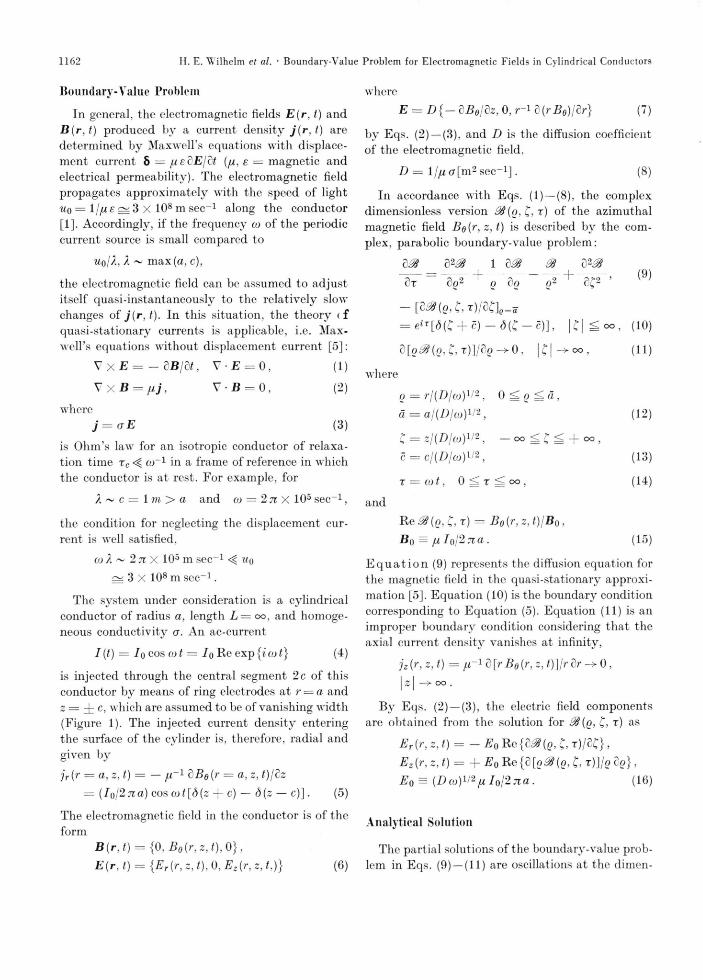
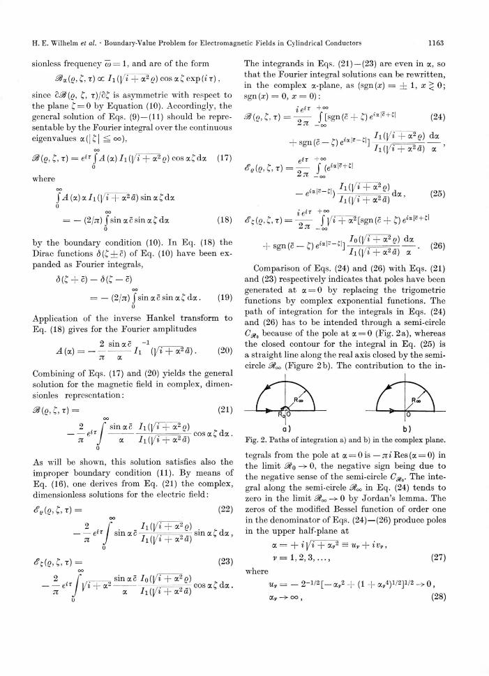
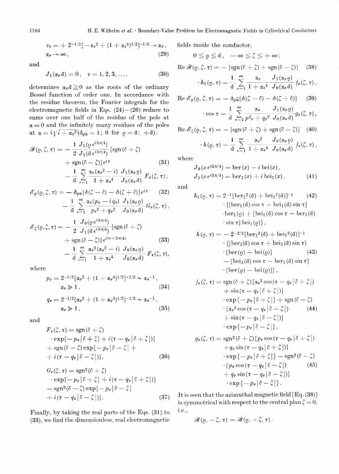
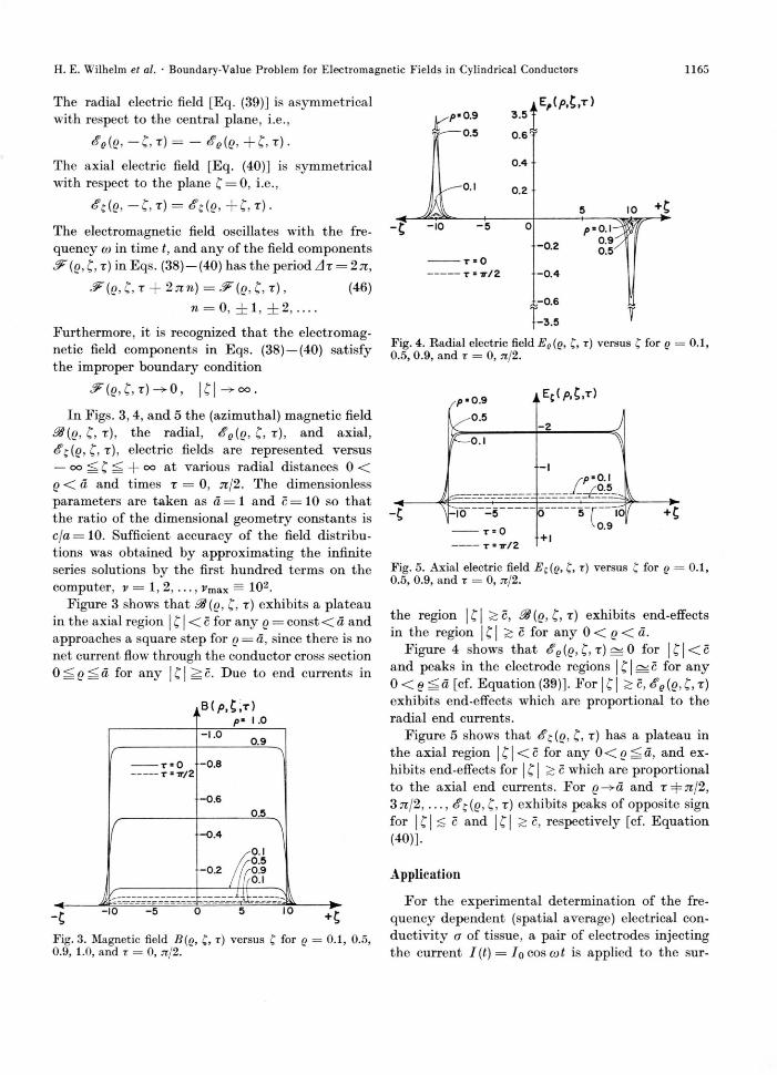
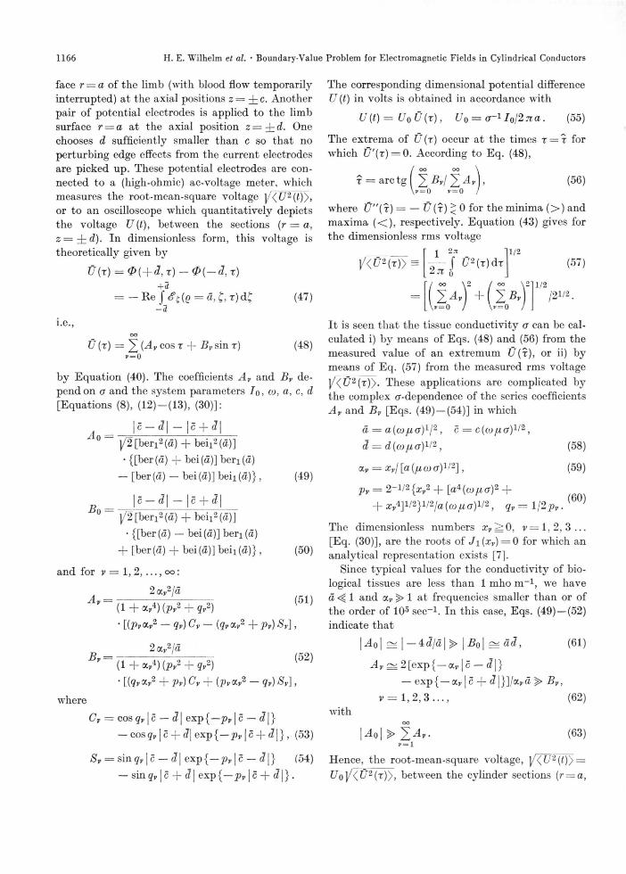
In Figs. 3, 4, and 5 the (azimuthal) magnetic field 38 (g, £, r), the radial, &Q(g, £, t), and axial, < ? t ( g , £ , t ) , electric fields are represented versus— oo ^ + o° a t various radial distances 0 < g < d and times r = 0, jr/2. The dimensionless parameters are taken as d = 1 and c = 1 0 so that the ratio of the dimensional geometry constants is c/a = 10. Sufficient accuracy of the field distribu­tions was obtained by approximating the infinite series solutions by the first hundred terms on the computer, v = 1 , 2 , . . . , r max = 1 0 2.

Figure 3 shows th a t 38 {g, £, r) exhibits a plateau in the axial region | £ | < c for any g = const < d and approaches a square step for g = d, since there is no net current flow through the conductor cross section0 ^ g fS d for any | £ | ^ c. Due to end currents in

Fig. 3. Magnetic field B ( q, £, r) versus £ for q = 0.1, 0.5, 0.9, 1.0, and r — 0, n/2.

Fig. 4. Radial electric field E e(g, £, r) versus £ for q — 0.1, 0.5, 0.9, and r = 0, n/2.

Fig. 5. Axial electric field E$(q, £, r) versus £ for q = 0.1, 0.5, 0.9, and r = 0, ji/2.

the region |£ | > c, 38 (g, £, r) exhibits end-effects in the region | £ | > c for any 0 < g < d.

Figure 4 shows th a t S‘e(g, £, r) ^ 0 for |£ |< c and peaks in the electrode regions | £ | ^ c for any0 < g fS d [cf. Equation (39)]. For | £ | > c, (f>Q (g, £, r) exhibits end-effects which are proportional to the radial end currents.

Figure 5 shows that <f>t(g, £, t) has a plateau in the axial region | £ | < c for any 0 < g ^ d, and ex­hibits end-effects for | £ | > c which are proportional to the axial end currents. For g ^ d and T=f=7r/2 , 3jt/2, . . . , $z{g, £, t) exhibits peaks of opposite sign for |£ | < c and | £ | > c, respectively [cf. Equation (40)].

Application

For the experimental determination of the fre­quency dependent (spatial average) electrical con­ductivity a of tissue, a pair of electrodes injecting the current I ( t ) = I q c o s w t is applied to the sur­

1166 H. E. W ilhelm et al. • Boundary-Value Problem for Electrom agnetic F ields in Cylindrical Conductors

face r = a of the limb (with blood flow temporarily interrupted) a t the axial positions z = i c . Another pair of potential electrodes is applied to the limb surface r = a a t the axial position z — ^ d . One chooses d sufficiently smaller than c so that no perturbing edge effects from the current electrodes are picked up. These potential electrodes are con­nected to a (high-ohmic) ac-voltage meter, which measures the root-mean-square voltage J/<t/2(£)>, or to an oscilloscope which quantitatively depicts the voltage U (t), between the sections (r = a, z = ± d ) . In dimensionless form, this voltage is theoretically given by

Ü (t ) = 0 ( Jr d , r ) — 0 ( — d, r )-\-d

i.e.,

= — Re J = ä, C, r) d£

Ü (t ) = 2 {Av cos r -f- B v sin t ) v = 0

(47)

(48)

by Equation (40). The coefficients A v and B v de­pend on a and the system parameters I o, a>, a, c, d [Equations (8 ), (12) —(13), (30)]:

A o =\c — d | — |c -f- d\

B 0 =

| / 2 [beri2 (ä) -f beii2 (ä)]* {[ber(ä) + bei(ä)] beri(ä)

— [ber(ä) — bei(ä)] beii(ä)} , (49)

| c — <71 — |c -f- d \

/̂2 [beri2 (ä) -f- beii2 (ä)]• {[ber(ä) — bei(ä)] beri(ä)

+ [ber(ä) -f- bei(ä)] beii(ä)} , (50)

and for v — 1 , 2 , . . . , oo:

2 a v2jäAy ' (1 + a,4) (p v2 + qv2)

■ [(Prccv2 — qv) C v — {qv ct-v2 + Pv) S v] ,

(51)

Bv =2 ccv2/ ä

(52)

where

(1 + ay4) (p v2 + qv2)

• [{qvy-v2 + Pv) Cv + {pvZv2 — qv) Sv],

Cv = cos qv | c — d | exp {— p v | c — d |}— cosqv | c -j- d\ exp{—p v | c -f- d|} , (53)

S v = sin qv | c — d\ exp{—p v \ c — c?|} (54)— sin qv | c -(- d\ exp{—p v \ c -f- d\] .

The corresponding dimensional potential difference U (t) in volts is obtained in accordance with

U ( t ) = U o Ü { r ) , Uo = (T- 1 I o l ^ n a . (55)

The extrema of Ü (r) occur a t the times r = x for which £7'(t) = 0. According to Eq. (48),

/ OO OO \

x = arc tg I 2 Bvl 2 ) ’ (56)\v = 0 » = 0

where Ü"(r) = — Ü {r) < 0 for the minima (> ) and maxima (< ) , respectively. Equation (43) gives for the dimensionless rms voltage

V < Ü 2 { t )> =2 71

f Ü2 (r) d r1/2

(57)

»> = 0

OO \ Z / oo

2 ^ „) + ( 2 ^\v = 0

1/2/2 1 /-2 .

I t is seen th a t the tissue conductivity a can be cal­culated i) by means of Eqs. (48) and (56) from the measured value of an extremum Ü(r), or ii) by means of Eq. (57) from the measured rms voltage|/<?72 (t)>. These applications are complicated by the complex ^-dependence of the series coefficients A v and B v [Eqs. (49) —(54)] in which

ä = a (co/zcr)1/2, c = c(cojua)1/2, d — d((o/j,a)xl2 ,

clv = xvl [a (/u, eo cr)1/2] ,

p v — 2~1/2{xv2 -f [a* (co [a o)2 ++ x v̂ ]1l2}1l2la((jo [xa)1!2, qv = 1 / 2 p v.

(58)

(59)

(60)

The dimensionless numbers xv^ 0 , v = l , 2 , 3 ... [Eq. (30)], are the roots of Ji(xv) — 0 for which an analytical representation exists [7].

Since typical values for the conductivity of bio­logical tissues are less than 1 mho m-1, we have ä 1 and <xv 1 a t frequencies smaller than or of the order of 105 sec-1. In this case, Eqs. (49) —(52) indicate th a t

|^ o | = | — 4 J /a | > | .ßo| ^ äd, (61)

A v ^ 2 [exp{— car | c — d\}— exp{—ar | c + d\}]la.vä > B v,

v = 1 , 2 ,3 , (62)with

(63)

Hence, the root-mean-square voltage, \ / (U2(t)') = u 0y< ü H t ) ) , between the cylinder sections (r = a ,

H. E. W ilhelm et al. • Boundary-Value Problem for Electromagnetic Fields in Cylindrical Conductors 1167

z = ± d ) is approximately [Eqs. (55), (57) and (61)]

This expression corresponds to the voltage between two equipotential end surfaces of a cylindrical con­ductor a, of cross sectional area j ia2 and length 2d, carrying a homogeneous current /o/|/2 . I t should be noted th a t the simple result in Eq. (64) is ap­plicable only to poor conductors such as biological tissues.

The rms voltage U (d) = j / ( U 2) on the surface of a human thigh of average radius a = 0.079 m was measured for various distances 2 d of the voltage electrodes and a fixed current of Iq — 2.27 j/2 x 10- 3

amp and frequency co = 2 n x 105 sec-1. The latter was injected by means of current electrodes just above the knee and below the hip so that there separation distance was 2c = 0.35 m. The current and voltage electrodes were circumferential elec­trodes of width 0.01 m. The experimental values Ü (d) and the tissue conductivities a calculated by iteration of Eq. (57), with the first iteration value of a determined by means of Eq. (64), are presented in Table 1.

The experimental data indicate th a t U (d) in­creases stronger than proportional to d at large distances 2d and U(d) oc d for small distances 2d. For this reason, larger tissue conductivities a are obtained for small values of d than for large values of d. The observed conductivities are, however, of the correct magnitude for human tissue [3, 4]. Evi­dently, for separation distances 2 d which are of the same magnitude-of-order as the width of the voltage electrodes, these perturb each other considerably so that the idealized theory which assumes circum­ferential electrodes of vanishing width is no longer applicable. Furthermore, for small distances 2d, the thigh resembles better a cylindrical conductor of radius a than for large distances 2d when the thigh resembles more a conoid cylinder. The apparent dependence of a on d for fixed values of a, c, I q,

Table I.

d\m\ U (d ) [volt] a [mho/m]

0.025 0.010 0.6900.075 0.066 0.3140.125 0.155 0.2240.150 0.224 0.190

and co shall be studied in more detail in an experi­mental investigation.

Appendix to Eqs. (31) —(33)

Equation (31) is directly obtained by integration of Eq. (24) with the help of the Cauchy integral theorem for the path of integration in Fig. 2 a, since the integral along the semi-circle vanishes in the limit 0toQ -> oo. Since

— — 0^ / 0£ and = £- 1 0 (^ ^ ) /0^

by Eq. (7), it is simpler to derive Eqs. (32) and (33) by partial differentiation of Eq. (31) than to in­tegrate Eqs. (25) and (26). The ^-derivative of the sgn (c±C) functions in the first expression and the r-sum of Eq. (31) produce terms linear in the Dirac functions (5(£±c), which combine to the first ex­pression of Equation (32). This is readily shown by means of the following theorem for Bessel functions.

In accordance with the Cauchy integral theorem, the closed integral in the complex plane a = u + i v of Fig. 2 a,

I i i ^ i + ol2 q ) d a i i ( j / i + a 2ä) a

OO

= 2 n i 2 Res (a = i j/i + <xv2)

( A l )

0 < q < ä,

can be expressed in terms of the residues of its poles at a = i\Ji + a?2, v — 1 ,2 , . . . oo. Noting th a t the integral along the semi-circle i?o is —7ii Res(a = 0 ) in the limit R q 0, Eq. (A l) becomes

+ u2q) dwu2ä) u

Of + a 2 e) d a

L i “ J 7 i ( | / r + Ä ) a

— 7i i Res (a = 0)

(A2)

= 2 7i i 2 Res (a = i ]/i + ccv2) , 0 < q < ä .v = i

The dw- and da-integrals in Eq. (A2) vanish since the integrand of the former is odd in u and the integrand of the latter vanishes in the limit Roo oo. Thus Eq. (A2) reduces to

OO

Res (a = 0) + 2 2 R es (a = i y i + ccv2) = 0,V= 1

0 < q < ä . (A3)