A residual distribution method using dis ontinuous elements forthe omputation of possibly non smooth ows.Rémi AbgrallTeam Ba hus, INRIA Bordeaux Sud-Ouestand Institut de Mathématiques de Bordeaux, Université Bordeaux I341 ours de la Liberation33405 Talen e Cedex, Fran eJune 19, 2010Abstra tIn this paper, we des ribe a residual distribution (RD) method where, ontrarily to standardthis type s hemes, the mesh is not ne essarily onformal. It also enable to use dis ontinuous elements, ontrarily to the standard ase where ontinuous elements are requested. More over, if ontinuityis for ed, the s heme be omes similar to the standard RD ase. Hen e, the situation be omes omparable with the Dis ontinuous Galerkin (DG) method, but it is simpler to implement than DGand has guaranteed L∞ bounds. We fo us on the se ond order ase, but the method an be easilygeneralized to higher degree polynomials.1 Introdu tionThis paper is devoted to the design of an approximation method for steady hyperboli problems bymeans of a s heme whi h enjoys the most possible ompa t sten il. There exist many similar methods,for example the Dis ontinuous Galerkin method, or the ontinuous Residual Distribution s hemes. Inthe rst ase, the solution is represented in ea h element of the mesh by polynomial fun tions where no ontinuity is enfor ed at the element boundaries. Hen e, the method is very exible sin e the mesh doesnot need to be onformal, nor the polynomial degree be the same in ea h element. Other approximationte hniques than lo al polynomial representations an be hosen In our opinion, one of its disadvantagesis its omplexity, espe ially when one onsiders mixed hyperboli /ellipti problems su h as the NavierStokes equations. Moreover, and this is the point we are interested in here, when dis ontinuous solutionsare omputed, the non linear non os illatory stabilization me hanisms are not ompletely satisfa torybe ause they depend on parameters or are quite omplex to design, see [1, 2, 3, 4 for example. Eitherthey are very omplex to set up, or they introdu e too mu h dissipation.In the ase of the residual distribution (RD) methods, the solution is also approximated by pie e-wise polynomial fun tions, but here the approximation is globally ontinuous. Hen e, the algorithmi omplexity is lower (in term of memory espe ially). Another property is that there exists a very generaland systemati method that enables us to guaranty a ura y formal O(hk+1) a ura y, even at lo alextrema, and L∞ stability. However, the mesh must be onformal, see [5, 6, 7 among several others.In this note, we des ribe a residual distribution method where the fun tional representation doesnot need to be ontinuous a ross edges. The method is general and ould be extended to any order ofa ura y, following the lines of [8, but here, we have only developed it for a lo al P 1 interpolation inea h element to present the ideas. Contrary to the lassi al RD s hemes, the ontinuity a ross edges isno longer enfor ed. This method is simpler than the one des ribed in [9. Indeed, the s heme redu es tothe one of [5, 10 and [6 if ontinuity is enfor ed a ross edges. Compared with standard DG methods,the s heme non os illatory properties are obtained without any parameter.The paper is organized as follows. We rst des ribe the method for a s alar problem. Then themethod is extended to the Euler equations for uid dynami s. The extension to 3D is straightforwardas well as on non onformal meshes. This paper opens the road for h − p adaptation for RD s hemes.1

This paper is a translation of a 2007 report written in fren h, [11, with some improvements. In themeantime, M. Hubbard [12 has published a similar te hnique. However, the similarity starts and ends inthat we both use dis ontinuous elements. Hubbard then develops his method using an extension of theN s heme. We have used Lax Friedri hs method, but following [13, any standard nite volume s heme an be rewritten as a RD s heme, and hen e an be plugged into our framework. The method is alsomu h simpler than [9.2 The s alar aseLet us onsider the following problem, dened in Ω ⊂ R2 to make the presentation simplerdiv f(u) = 0 if x ∈ Ω

u = g if x ∈ Γ−,(1)

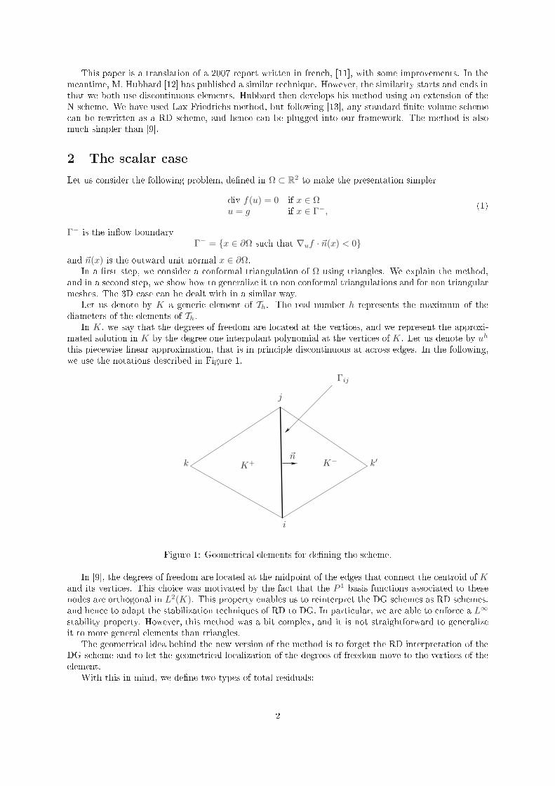
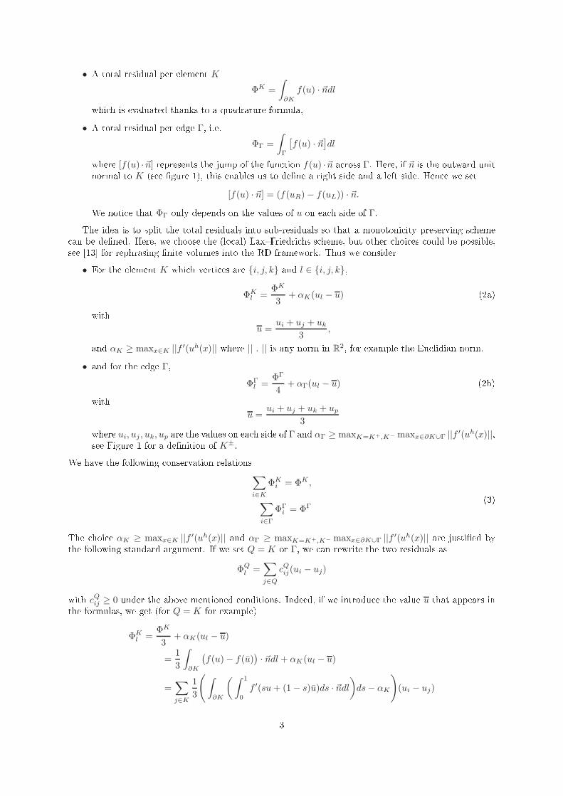
Γ− is the inow boundaryΓ− = x ∈ ∂Ω su h that ∇uf · ~n(x) < 0and ~n(x) is the outward unit normal x ∈ ∂Ω.In a rst step, we onsider a onformal triangulation of Ω using triangles. We explain the method,and in a se ond step, we show how to generalize it to non onformal triangulations and for non triangularmeshes. The 3D ase an be dealt with in a similar way.Let us denote by K a generi element of Th. The real number h represents the maximum of thediameters of the elements of Th.In K, we say that the degrees of freedom are lo ated at the verti es, and we represent the approxi-mated solution in K by the degree one interpolant polynomial at the verti es of K. Let us denote by uhthis pie ewise linear approximation, that is in prin iple dis ontinuous at a ross edges. In the following,we use the notations des ribed in Figure 1.

PSfrag repla ementsK+ K−k

i

j

k′

Γij

~n

Figure 1: Geometri al elements for dening the s heme.In [9, the degrees of freedom are lo ated at the midpoint of the edges that onne t the entroid of Kand its verti es. This hoi e was motivated by the fa t that the P 1 basis fun tions asso iated to thesenodes are orthogonal in L2(K). This property enables us to reinterpret the DG s hemes as RD s hemes,and hen e to adapt the stabilization te hniques of RD to DG. In parti ular, we are able to enfor e a L∞stability property. However, this method was a bit omplex, and it is not straightforward to generalizeit to more general elements than triangles.The geometri al idea behind the new version of the method is to forget the RD interpretation of theDG s heme and to let the geometri al lo alization of the degrees of freedom move to the verti es of theelement.With this in mind, we dene two types of total residuals:2

• A total residual per element K

ΦK =

∫

∂K

f(u) · ~ndlwhi h is evaluated thanks to a quadrature formula,• A total residual per edge Γ, i.e.

ΦΓ =

∫

Γ

[

f(u) · ~n]

dlwhere [f(u) ·~n] represents the jump of the fun tion f(u) ·~n a ross Γ. Here, if ~n is the outward unitnormal to K (see gure 1), this enables us to dene a right side and a left side. Hen e we set[f(u) · ~n] = (f(uR) − f(uL)) · ~n.We noti e that ΦΓ only depends on the values of u on ea h side of Γ.The idea is to split the total residuals into sub-residuals so that a monotoni ity preserving s heme an be dened. Here, we hoose the (lo al) LaxFriedri hs s heme, but other hoi es ould be possible,see [13 for rephrasing nite volumes into the RD framework. Thus we onsider

• For the element K whi h verti es are i, j, k and l ∈ i, j, k,ΦK

l =ΦK

3+ αK(ul − u) (2a)with

u =ui + uj + uk

3,and αK ≥ maxx∈K ||f ′(uh(x)|| where || . || is any norm in R

2, for example the Eu lidian norm.• and for the edge Γ,

ΦΓl =

ΦΓ

4+ αΓ(ul − u) (2b)with

u =ui + uj + uk + up

3where ui, uj , uk, up are the values on ea h side of Γ and αΓ ≥ maxK=K+,K− maxx∈∂K∪Γ ||f ′(uh(x)||,see Figure 1 for a denition of K±.We have the following onservation relations∑

i∈K

ΦKi = ΦK ,

∑

i∈Γ

ΦΓi = ΦΓ

(3)The hoi e αK ≥ maxx∈K ||f ′(uh(x)|| and αΓ ≥ maxK=K+,K− maxx∈∂K∪Γ ||f ′(uh(x)|| are justied bythe following standard argument. If we set Q = K or Γ, we an rewrite the two residuals asΦQ

l =∑

j∈Q

cQij(ui − uj)with cQ

ij ≥ 0 under the above mentioned onditions. Indeed, if we introdu e the value u that appears inthe formulas, we get (for Q = K for example)ΦK

l =ΦK

3+ αK(ul − u)

=1

3

∫

∂K

(

f(u) − f(u))

· ~ndl + αK(ul − u)

=∑

j∈K

1

3

(

∫

∂K

(∫ 1

0

f ′(su + (1 − s)u)ds · ~ndl

)

ds − αK

)

(ui − uj)3

whi h proves the result.We get a rst order s heme by determining uh the solution of: nd uh linear in ea h triangle K su hthat for any degree of freedom i (i.e. vertex of the triangulation),∑

K,i∈K

ΦKi +

∑

Γ,i∈Γ

ΦΓi = 0. (4)We spe ify later the boundary onditions.Using standard arguments, as dening uh as the limit of the solution of

un+1

i = uni − ωi

(

∑

K,i∈K

ΦKi +

∑

Γ,i∈Γ

ΦΓi

)withωi

(

∑

K,i∈K

cKij +

∑

Γ,i∈Γ

cΓij

)

≤ 1,we see that we have a maximum prin iple.It is possible to onstru t a s heme that is formally se ond order a urate by settingΦK,⋆

i = βKi ΦK and ΦΓ,⋆

i = βΓi ΦK (5)with, setting

xKi =

ΦKi

ΦK, xΓ

i =ΦΓ

i

ΦΓ,and

βKi =

max(xKi , 0)

∑

j∈K

max(xKj , 0)

, βΓi =

max(xΓi , 0)

∑

j∈K

max(xΓj , 0)

. (6)As in the lassi al RD framework, the oe ients β are well dened thanks to the onservationrelations (3). The s heme writes as (4) where the residuals ΦKi (resp. ΦΓ

i ) are repla ed by ΦK,⋆i (resp.

ΦΓ,⋆i .Boundary onditions. If Γ is an inow boundary edge, we need to set weakly the boundary ondition

u = g. Consider a numeri al ux, say an upwind ux, denoted by F(uh, g, ~n(x)). We onsider theboundary residualΦΓ =

∫

Γ

(F(uh, g, ~n(x)) − f(uh) · ~n)dlthat we split into two parts following the same pro edure as above. If l and l′ are the two verti es of Γ,we have dened ΦΓl and ΦΓ

l′ , andΦΓ

l + ΦΓl′ = ΦΓ.The s heme, when we take into a ount the boundary onditions, is again (4) where the list of edgestakes into a ount the boundary edges, if needed.Conservation and a ura y issues. In [9, we have shown that a s heme of the type (4) where theresidual satises the onservation onstraints (3) (in luding on the boundary) and standard stabilityassumptions (as in the Lax Wendro theorem) is onvergent and the limit solution is a weak solution ofthe PDE (1).The a ura y onstraint (5) and (6) are also analyzed in the same referen e [9. In that ase, theassumption that the problem is steady is essential in showing that the residuals (in luding the boundaryresiduals) satises

ΦQ(uh) = O(hd+1)where uh is the interpolant of the exa t solution (assuming it is smooth) and d is the dimension of Q:d = 2 for a triangle and d = 1 for an edge. 4

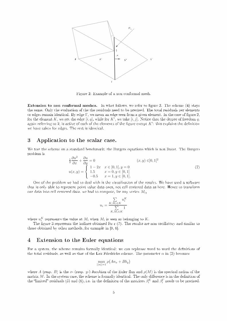
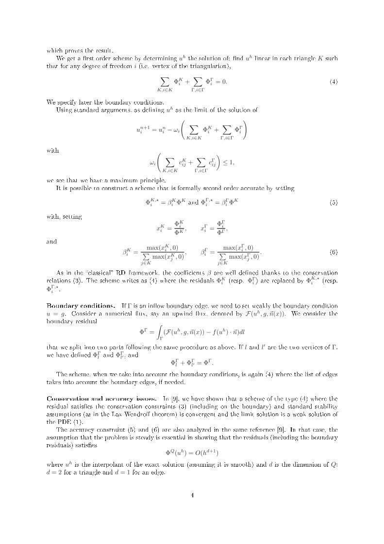
Figure 2: Example of a non onformal mesh.Extension to non onformal meshes. In what follows, we refer to gure 2. The s heme (4) staysthe same. Only the evaluation of the the residuals need to be pre ised. The total residuals per elementsor edges remain identi al. By edge Γ, we mean an edge seen from a given element. In the ase of gure 2,for the element K, we get the edge [i, q], while for K ′, we take [i, j]. Noti e that the degree of freedom q,again referring to 2, is a tive of ea h of the elements of the gure ex ept K ′: this explains the denitionwe have taken for edges. The rest is identi al.3 Appli ation to the s alar ase.We test the s heme on a standard ben hmark: the Burgers equations whi h is non linear. The Burgersproblem is1

2

∂u2

∂x+

∂u

∂y= 0 (x, y) ∈]0, 1[2

u(x, y) =

1 − 2x x ∈ [0, 1], y = 01.5 x = 0, y ∈ [0, 1]−0.5 x = 1, y ∈ [0, 1].

(7)One of the problem we had to deal with is the visualization of the results. We have used a softwarethat is only able to represent point value data ones, not ell entered data as here. Hen e to transformour data into ell entered data, we had to ompute, for any vertex Mi,ui =

∑

K,Mi∈K

uKi

∑

K,Mi∈K

1where uKi represents the value at Mi when Mi is seen as belonging to K.The gure 3 represents the isolines obtained for r (7). The results are non os illatory and similar tothose obtained by other methods, for example in [9, 6.4 Extension to the Euler equationsFor a system, the s heme remains formally identi al: we an rephrase word to word the denitions ofthe total residuals, as well as that of the Lax Friedri hs s heme. The parameter α in (2) be omes

max||n||=1

ρ(

Anx + Bby

)where A (resp. B) is the x- (resp. y-) Ja obian of the Euler ux and ρ(M) is the spe tral radius of thematrix M . In the system ase, the s heme is formally identi al. The only dieren e is in the denition ofthe limited residuals (5) and (6), i.e. in the denition of the matri es βKi and βΓ

i needs to be pre ised.5

x

y

0 0.2 0.4 0.6 0.8 10

0.2

0.4

0.6

0.8

1

Figure 3: Results obtained for (7).The methods is the one des ribed by [5 that we re all. The Euler equations write∂U

∂t+

∂F (U)

∂x+

∂G(U)

∂y= 0where the ve tor of onserved variables is

U =

ρρuρvE

,and the uxes F and G areF (U) =

ρuρu2 + p

ρuvu(E + p)

, G(U) =

ρvρuv

ρv2 + pv(E + p)

.Here, as usual, ρ represents the density, u and v are the two omponents of the velo ity ve tor, E is thetotal energy and p is the pressure. The system is losed by an equation of state, here we assume thatthe uid is a alori aly perfe t gas,p = (γ − 1)

(

E −1

2ρ(u2 + v2)

)

.The ratio of spe i heats γ is set to 1.4.Let us onsider a dire tion (in pra ti e the velo ity ve tor) ~n whi h omponents are nx and ny.Denoting A and B the Ja obian matri es of the ux F and G with respe t to U , we know that thematrixAnx + Bny6

is diagonalizable with distin t real eigenvalues: the system is stri tly hyperboli . The eigenvalues areλ1 = ~u · ~n whi h is double and λ± = ~u · ~n ± c. As usual, c represents the speed of sound,

c2 = γp

ρ.Let us denote by r1, r2 the eigenve tors asso iated to λ1 and r3,4 those asso iated to λ±. More pre isely,if H represents the total enthalpy, un = ~u · ~n and ut = −nyu + nxv, we have

r1 =

1uv

u2+v2

2

, r2 =

0−ny

nx

ut

, r3 =

1u − cnx

v − cny

H − unc

, r4 =

1u + cnx

v + cny

H + unc

.By itself, the hoi e of the eigenve tors is not important, what is important is that these eigenve tors areorthonormal for the quadrati form dened by the Hessian of the entropy. Here, the quantities involvedin the denition of the eigenve tors, i.e. the speed of sound, the velo ity, the enthalpy, are evaluated atan average state. Many hoi es have been tested, and these experien es have revealed that the hoi eis not very important. We have taken a state dened by the primitive variables that are the arithmeti averages of the states at the verti es of K or Γ, the elements for whi h we are omputing the se ondorder residuals.On e this is done, we pro eed as follows, for the element Q = K or Γ.1. We de ompose ΦQl , l = 1, . . . , N (N=3 for a triangle, 4 for an edge), in the eigen-basis

ΦQl =

∑

ℓ=1,4

(ΦQl )ℓrℓ,2. For ea h parameter ℓ (hen e for any eigenve tor rℓ), we noti e that

N∑

l=1

(ΦQl )ℓ = (ΦQ)ℓand we dene (ΦQ

l )⋆ℓ by

(ΦQl )⋆

ℓ =

(

(ΦQl )ℓ/(ΦQ)ℓ

)+

N∑

j=1

(

(ΦQj )ℓ/(ΦQ)ℓ

)+(ΦQ)ℓ,with x+ = max(x, 0).3. Then

(ΦQl )⋆ =

4∑

ℓ=1

(ΦQl )⋆

ℓrℓ.In any of the results that we have obtained, we have not added any ltering term as it was ne essaryin [6. For the moment, it is not possible to tell if su h a term is needed or not for the following reason:The graphi software we have used needs data at the verti es of the mesh. Here, a vertex arries severaldegrees of freedom (one per element), and we have made an arithmeti average. This ertainly smoothesthe results.We have run a quite omplex ase, that has been already do umented in [6. It is a s ramjet whi h onditions are• Left and right boundary: supersoni inow and outow onditions. The inow onditions are

ρ = 1.4, u = 3.6, v = 0, p = 1.

• The other boundaries are solid walls. 7

x

y

0 2 4 6 8 100

0.5

1

1.5

2

2.5

3

x

y

0 2 4 6 8 100

0.5

1

1.5

2

2.5

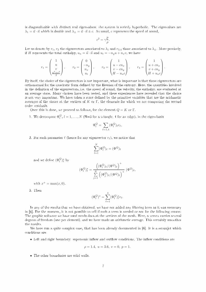
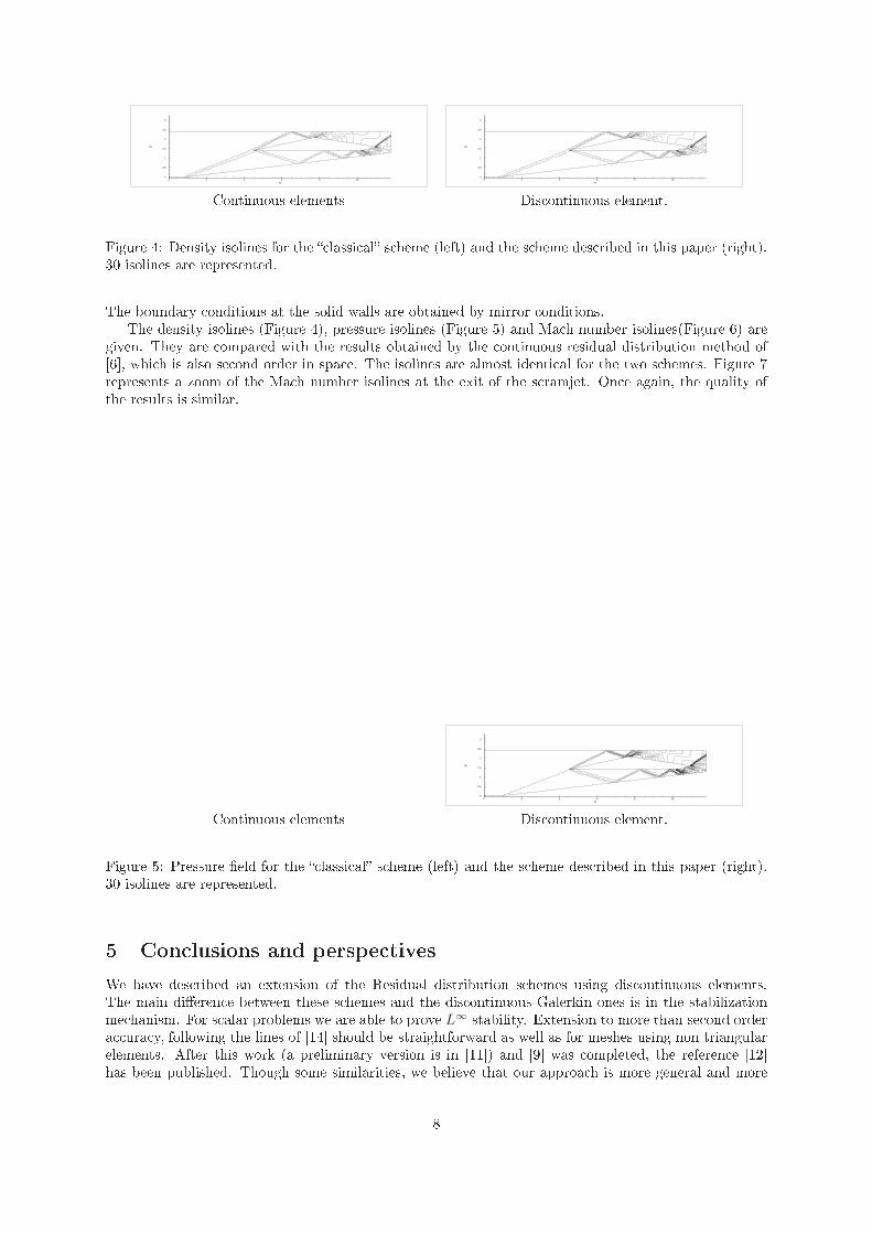
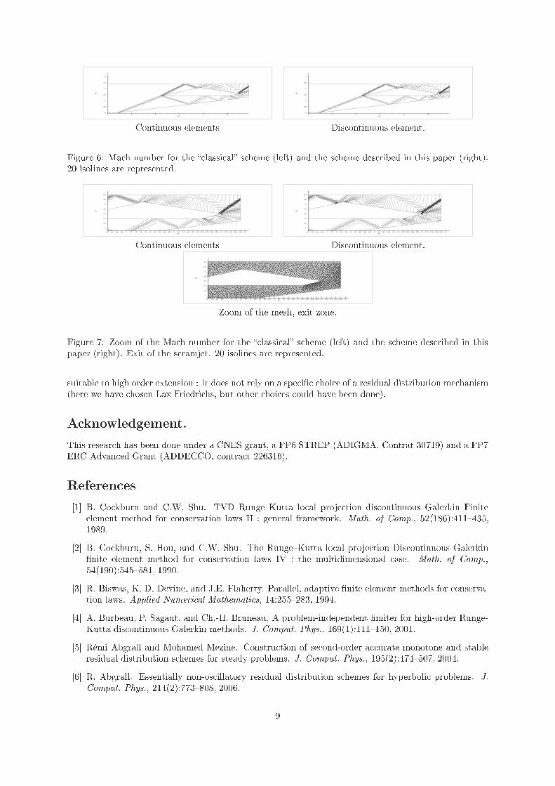
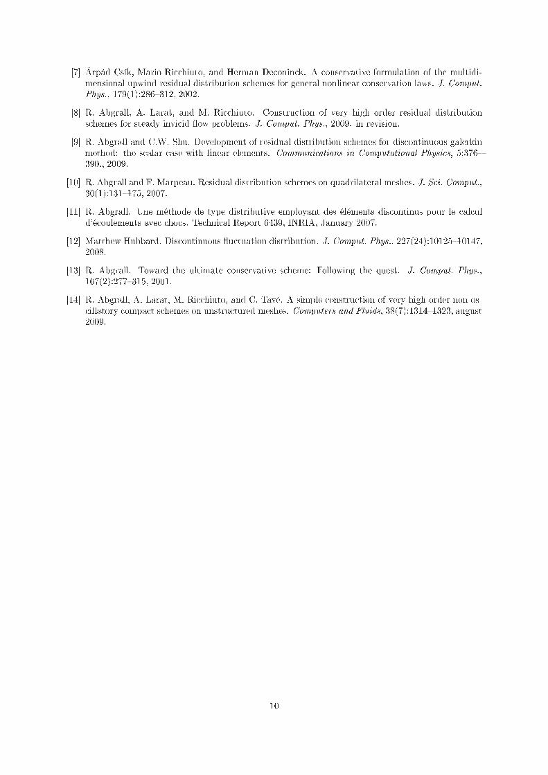
3Continuous elements Dis ontinuous element.Figure 4: Density isolines for the lassi al s heme (left) and the s heme des ribed in this paper (right).30 isolines are represented.The boundary onditions at the solid walls are obtained by mirror onditions.The density isolines (Figure 4), pressure isolines (Figure 5) and Ma h number isolines(Figure 6) aregiven. They are ompared with the results obtained by the ontinuous residual distribution method of[6, whi h is also se ond order in spa e. The isolines are almost identi al for the two s hemes. Figure 7represents a zoom of the Ma h number isolines at the exit of the s ramjet. On e again, the quality ofthe results is similar.

x

y

0 2 4 6 8 100

0.5

1

1.5

2

2.5

3Continuous elements Dis ontinuous element.Figure 5: Pressure eld for the lassi al s heme (left) and the s heme des ribed in this paper (right).30 isolines are represented.5 Con lusions and perspe tivesWe have des ribed an extension of the Residual distribution s hemes using dis ontinuous elements.The main dieren e between these s hemes and the dis ontinuous Galerkin ones is in the stabilizationme hanism. For s alar problems we are able to prove L∞ stability. Extension to more than se ond ordera ura y, following the lines of [14 should be straightforward as well as for meshes using non triangularelements. After this work (a preliminary version is in [11) and [9 was ompleted, the referen e [12has been published. Though some similarities, we believe that our approa h is more general and more8

x

y

0 2 4 6 8 100

0.5

1

1.5

2

2.5

3

x

y

0 2 4 6 8 100

0.5

1

1.5

2

2.5

3Continuous elements Dis ontinuous element.Figure 6: Ma h number for the lassi al s heme (left) and the s heme des ribed in this paper (right).20 isolines are represented.x

y

6.2 6.4 6.6 6.8 7 7.2 7.4 7.6 7.8 8 8.2 8.4 8.6 8.8 9 9.2 9.4 9.6 9.8 10 10.2 10.4 10.6 10.8 11 11.2 11.4 11.6 11.8 12

1

1.2

1.4

1.6

1.8

2

2.2

2.4

x

y

6.2 6.4 6.6 6.8 7 7.2 7.4 7.6 7.8 8 8.2 8.4 8.6 8.8 9 9.2 9.4 9.6 9.8 10 10.2 10.4 10.6 10.8 11 11.2 11.4 11.6 11.8 12

1

1.2

1.4

1.6

1.8

2

2.2

2.4Continuous elements Dis ontinuous element.x

y

6.2 6.4 6.6 6.8 7 7.2 7.4 7.6 7.8 8 8.2 8.4 8.6 8.8 9 9.2 9.4 9.6 9.8 10 10.2 10.4 10.6 10.8 11 11.2 11.4 11.6 11.8 12

1

1.2

1.4

1.6

1.8

2

2.2

2.4 Zoom of the mesh, exit zone.Figure 7: Zoom of the Ma h number for the lassi al s heme (left) and the s heme des ribed in thispaper (right). Exit of the s ramjet. 20 isolines are represented.suitable to high order extension : it does not rely on a spe i hoi e of a residual distribution me hanism(here we have hosen Lax Friedri hs, but other hoi es ould have been done).A knowledgement.This resear h has been done under a CNES grant, a FP6 STREP (ADIGMA, Contrat 30719) and a FP7ERC Advan ed Grant (ADDECCO, ontra t 226316).Referen es[1 B. Co kburn and C.W. Shu. TVD Runge Kutta lo al proje tion dis ontinuous Galerkin Finiteelement method for onservation laws II : general framework. Math. of Comp., 52(186):411435,1989.[2 B. Co kburn, S. Hou, and C.W. Shu. The RungeKutta lo al proje tion Dis ontinuous Galerkinnite element method for onservation laws IV : the multidimensional ase. Math. of Comp.,54(190):545581, 1990.[3 R. Biswas, K. D. Devine, and J.E. Flaherty. Parallel, adaptive nite element methods for onserva-tion laws. Applied Numeri al Mathemati s, 14:255283, 1994.[4 A. Burbeau, P. Sagaut, and Ch.-H. Bruneau. A problem-independent limiter for high-order Runge-Kutta dis ontinuous Galerkin methods. J. Comput. Phys., 169(1):111150, 2001.[5 Rémi Abgrall and Mohamed Mezine. Constru tion of se ond-order a urate monotone and stableresidual distribution s hemes for steady problems. J. Comput. Phys., 195(2):474507, 2004.[6 R. Abgrall. Essentially non-os illatory residual distribution s hemes for hyperboli problems. J.Comput. Phys., 214(2):773808, 2006. 9

[7 Árpád Csík, Mario Ri hiuto, and Herman De onin k. A onservative formulation of the multidi-mensional upwind residual distribution s hemes for general nonlinear onservation laws. J. Comput.Phys., 179(1):286312, 2002.[8 R. Abgrall, A. Larat, and M. Ri hiuto. Constru tion of very high order residual distributions hemes for steady invi id ow problems. J. Comput. Phys., 2009. in revision.[9 R. Abgrall and C.W. Shu. Development of residual distribution s hemes for dis ontinuous galerkinmethod: the s alar ase with linear elements. Communi ations in Computational Physi s, 5:376390., 2009.[10 R. Abgrall and F. Marpeau. Residual distribution s hemes on quadrilateral meshes. J. S i. Comput.,30(1):131175, 2007.[11 R. Abgrall. Une méthode de type distributive employant des éléments dis ontinus pour le al uld'é oulements ave ho s. Te hni al Report 6439, INRIA, January 2007.[12 Matthew Hubbard. Dis ontinuous u tuation distribution. J. Comput. Phys., 227(24):1012510147,2008.[13 R. Abgrall. Toward the ultimate onservative s heme: Following the quest. J. Comput. Phys.,167(2):277315, 2001.[14 R. Abgrall, A. Larat, M. Ri hiuto, and C. Tavé. A simple onstru tion of very high order non os- illatory ompa t s hemes on unstru tured meshes. Computers and Fluids, 38(7):13141323, august2009.

10