Embed Size (px)
Citation preview

Regina Dittrich and Brian Francis Seminar Institut für Statistik, Universität Innsbruck 24 Jänner, 2003
Analyse von unvollständigen Rangreihungen mit Hilfe von
Paarvergleichsmethoden :
Eine Untersuchung von Wertorientierungen in Europa
Regina Dittrich Brian Francis
Institut für Statistik,Wirtschaftsuniversität,Wien
Centre for Applied Statistics,Lancaster University
Eine gemeinsame Arbeit mit
Reinhold HatzingerInstitut für Statistik, Wirtschaftsuniversität, Wien
Roger Penn,Department of Sociology, Lancaster University

Regina Dittrich and Brian Francis Seminar Institut für Statistik, Universität Innsbruck 24 Jänner, 2003
Ein sehr langer Titel!
Drei Komponenten
Analyse von unvollständigen Rangreihungen mit Hilfe
Paarvergleichsmethoden :
Eine Untersuchung von Werteorientierungen in Europa

Regina Dittrich and Brian Francis Seminar Institut für Statistik, Universität Innsbruck 24 Jänner, 2003
Werteorientierungen
International Social Survey Program 1993
• Sozialwissenschaftliche Studien die jährlich seit 1984 durchgeführt werden
• Jedes Jahr wird eine anderes Thema untersucht. 1993 war es ‘Environmentand green issues’.
• 21 Länder wurden 1993 untersucht . Hauptsächlich Europa, aber auch USA,Kanada, Australien , Neu Seeland, Japan, Israel und die Philippinen. Eswurden dieselben Fragen in jedem Land verwendet.
• Daten verfügbar im Zentral Archiv, Köln.
• Wir analysieren fünf europäische Länder und konzentrieren uns auf denInglehart Index. Inglehart index ist ein wichtiges Erhebungsinstrument fürSoziologen – er wird in vielen modernen sozialwissenschaftlichen Studienerhoben. Oftmals Verwendung sehr einfacher Analysemethoden .
Regina Dittrich and Brian Francis Seminar Institut für Statistik, Universität Innsbruck 24 Jänner, 2003
Wertorientierung
International Social Survey Program 1993
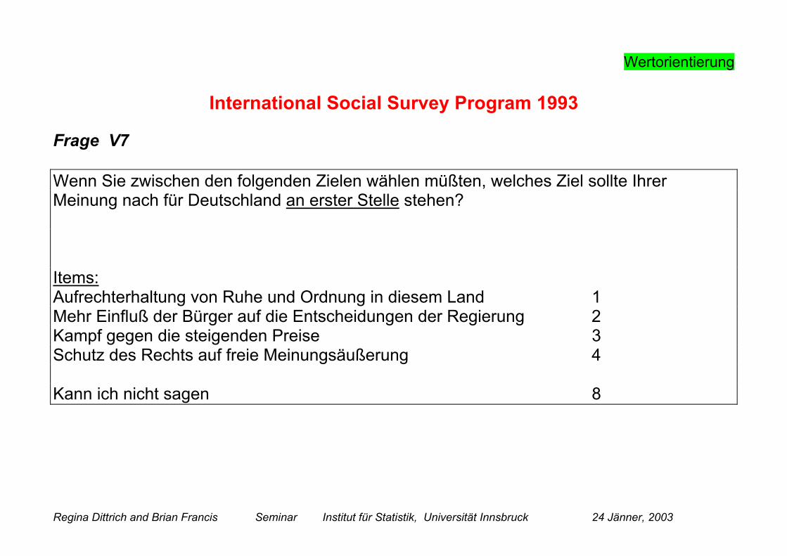
Frage V7
Wenn Sie zwischen den folgenden Zielen wählen müßten, welches Ziel sollte IhrerMeinung nach für Deutschland an erster Stelle stehen?
Items:Aufrechterhaltung von Ruhe und Ordnung in diesem Land 1Mehr Einfluß der Bürger auf die Entscheidungen der Regierung 2Kampf gegen die steigenden Preise 3Schutz des Rechts auf freie Meinungsäußerung 4
Kann ich nicht sagen 8
Regina Dittrich and Brian Francis Seminar Institut für Statistik, Universität Innsbruck 24 Jänner, 2003
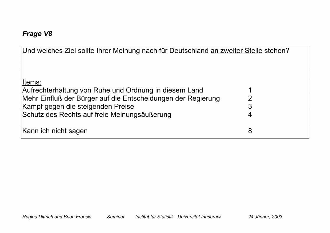
Frage V8
Und welches Ziel sollte Ihrer Meinung nach für Deutschland an zweiter Stelle stehen?
Items:Aufrechterhaltung von Ruhe und Ordnung in diesem Land 1Mehr Einfluß der Bürger auf die Entscheidungen der Regierung 2Kampf gegen die steigenden Preise 3Schutz des Rechts auf freie Meinungsäußerung 4
Kann ich nicht sagen 8

Regina Dittrich and Brian Francis Seminar Institut für Statistik, Universität Innsbruck 24 Jänner, 2003
WertorientierungenHintergrund
Die Fragen wurden von Ingelhart (1990) entwickelt ’Cultural shift in Advanced IndustrialSociety’ um postmaterialistische und materialistische Werte zu erfassen.
Postmaterialistische Werte werden definiert als :“social equality, life style choices, participation, concern for environmental quality”
Ingelhart bezeichnet jene mit Item 2 und 4 als höchste Prioritäten als Postmaterialisten‘mehr Einfluß auf Regierung ’ ‘freie Meinungsäußerung’
jene mit Item 1 und 3 als höchste Prioritäten als Materialisten‘Aufrechterhaltung von Ordnung’ 'Kampf gegen steigende Preise’
Alle anderen werden als ‘Mixed’ bezeichnet.

Regina Dittrich and Brian Francis Seminar Institut für Statistik, Universität Innsbruck 24 Jänner, 2003
Untersuchungsfragen:
“Jüngere Europäer sind in Zeiten relativen Wohlstands aufgewachsen und tendieren daherzu postmaterialistischen Werten”
“Postmaterialistische Werte sind in Großbritannien weniger stark entwickelt” Inglehart(1990,1997)
Ist dies vereinfachend? Gibt es die postmaterialistischen -materialistischenWerte?Erfolgt die Veränderung für beide postmaterialistischen Items in gleicher Weise?Welche anderen Kovariaten neben Ländereffekten beeinflussen Antworten auf die IngelhartSkala? Wie variieren die Antworten mit Alter?

Regina Dittrich and Brian Francis Seminar Institut für Statistik, Universität Innsbruck 24 Jänner, 2003
Wie können solche Daten analysiert werden?
Daten sind unvollständige Rangreihungen. Die Befragten wurden nur gebeten die zweiwichtigsten Items von vier möglichen Items zu nennen.
Wie kann man solche Daten analysieren?Einfache Ansätze:
⇒ Man könnte Prozentsätze berechnen, wie oft die 4 Items an erster Stelle gereihtwurden. Hier werden nicht alle Daten berücksichtigt.
⇒ Man könnte jedem Item den Rangwert zuordnen und ‘Normal linear models’ (z.B.Varianzanalysen) rechnen. Aber man müsste auch Scores für die nicht gereihtenund ausgelassenen Items vergeben (3?, 4?). Nicht gut weil viele nur eine Fragebeantworten. Zuviele Annahmen notwendig.
⇒ Man kann Rangkombinationen verwenden, die auf soziologischen Theorien beruhen (Inglehart,nächste Folie). Nicht gut weil viele nur eine Frage beantworten.
⇒ Außerdem....⇒ Interessiert uns, wie die einzelnen Antworten mit verschiedenen Personen
Kovariaten und Länderzugehörigkeit zusammenhängen.⇒ Möglicherweise nicht-lineare Effekte von Alter. Potentiell komplexe Modelle

Regina Dittrich and Brian Francis Seminar Institut für Statistik, Universität Innsbruck 24 Jänner, 2003
Frühere Arbeit
Dalton and Rohrschneider (1994) betrachteten die %werte von Materialisten undPostmaterialisten in 6 westeuropäischen Ländern und präsentierten folgende Tabelle:
Postmaterialisten%
Materialisten%
Differenz
West Deutschland 23 24 -1Niederland 16 23 -7Italien 13 25 -12Irland 13 26 -13Britain 12 26 -14Spanien 12 31 -19
“Materialists outnumber postmaterialists in Britain by 14 points, making Britain morematerialist than every other country except Spain.”
“West Germany and Netherlands are most post-materialist”.
Wie auch immer, im Durchschnitt sind ca. 60% aller Antworten MIXED!
Regina Dittrich and Brian Francis Seminar Institut für Statistik, Universität Innsbruck 24 Jänner, 2003

Regina Dittrich and Brian Francis Seminar Institut für Statistik, Universität Innsbruck 24 Jänner, 2003
Andere Ansätze :
Bean and Papadakis verwendeten Hauptkomponenten Analyse um materialistische –postmaterialistische Dimensionen aufzufinden.
Klein (1995) verwendete logistische Regression um POST vs (MIX, MAT) zu modellieren

Regina Dittrich and Brian Francis Seminar Institut für Statistik, Universität Innsbruck 24 Jänner, 2003
Unsere Lösung
• Umwandlung von unvollständigen Rangreihungen in Paarvergleiche . Dadurch kann dieWertigkeit (Worth) bzw. der Nutzen jedes Items geschätzt werden. Somit werden 36mögliche Antwortmuster in 4 Worthparameter konvertiert. Weiters kann untersuchtwerden, inwiefern sich verschiedene individuelle Eigenschaften der beurteilendenPersonen auf die Wertigkeit der 4 Items auswirken.
• Analyse der Paarvergleiche mittels Bradley-Terry Modell.
• Modell muss erweitert werden, um Eigenschaften auf individuellem Niveauberücksichtigen zu können; hinzufügen von Glättungsfunktionen für Alters-effekte.
Wir untersuchen 5 europäische Länder
West Deutschland Ost Deutschland Großbritannien Polen Italien
West und Ost Deutschland wurden getrennt analysiert, obwohl die Wiedervereinigung vor1993 stattgefunden hat.

Regina Dittrich and Brian Francis Seminar Institut für Statistik, Universität Innsbruck 24 Jänner, 2003
Rankings and orderings
Ignoriert man die fehlenden Werte gibt es vier Items zur Auswahl. Wir fixieren die Anordnung der Items wie sie im Fragebogen verwendet wird: (ORDNUNG, EINFLUSS, PREISE, MEINUNG).
Ein individuelles Antwortmuster kann entweder als Rang Vektor oder als Order Vektordefiniert werden:
Zum Beispiel, EINFLUSS 1ste Wahl und MEINUNG 2te Wahl kann definiert werden als:
• Order Vektor – welches Item war 1ste Wahl 2te Wahl
(EINFLUSS, MEINUNG, -,-) or (2,4,-,-) or (2,4)
• Rang Vektor – welches Item hat welchen RangORDNUNG, EINFLUSS, PREISE, MEINUNG Item1 Item2 Item3 Item4
( - 1 - 2 )
Für fehlende Werte verwenden wir - im Rang und Order Vektor.

Regina Dittrich and Brian Francis Seminar Institut für Statistik, Universität Innsbruck 24 Jänner, 2003
Antworten auf Inglehart Index Items für alle 5 Länder gemeinsam.
2te Wahl 1ste Wahl Ordnung Einfluss Preise Meinung Un-
entschiedenFehlend Total
Ordnung 72 722 1110 347 42 4 2297
Einfluss 699 73 594 407 26 4 1803
Preise 645 375 72 99 43 3 1237
Meinung 149 168 70 4 5 4 400
Unent-schieden
15 8 14 4 93 0 134
Fehlend 7 1 5 2 0 30 45
Total 1587 1347 1865 863 209 45 5916
MaterialistenPostmaterialisten

Regina Dittrich and Brian Francis Seminar Institut für Statistik, Unversität Innsbruck 24 Jänner, 2003
Die verschiedenen Antwortarten.
Die häufigste Antwort ist eine materialistische mit dem Order Vektor (ORDNUNG, PREISE) sowohl für alle 5 Länder gemeinsam als auch für jedeseinzelne Land.
Die zweithäufigste Antwort ist eine Mixed Antwort (MEINUNG, ORDNUNG)
Es gibt auch noch• Partielle Antworten (1ste Wahl, keine zweite Wahl) 131 Personen
• Wiederholte Antworten ( 1ste Wahl gleich wie zweite Wahl) 221 Personen
• Ungültige Antworten ( keine 1ste Wahl, 2te Wahl getroffen) 56 Personen
• Fehlende Antworten (keine Wahl getroffen) 123 Personen
Alle Arten von Antworten müssen behandelt werden.

Regina Dittrich and Brian Francis Seminar Institut für Statistik, Unversität Innsbruck 24 Jänner, 2003
Umwandlung der Order Vektoren in PaarvergleicheJeder Typ eines Order Vektor ergibt ein Set von Paarvergleichen. Wir behandeln hierUnentschieden als Fehlend, obwohl komplexere Modelle auch unentschieden Antwortenmitberücksichtigen können.Order Vektor Rang Vektor Paarvergleiche
8....unentschieden9....fehlend
-....fehlend 1.... erstes Item bevorzugt 2.... zweites Item bevorzugt-...... fehlend
V7 V8 I1 I2 I3 I4 (12) (13) (23) (14) (24) (34)e.g.Gültig 1 3 1 - 2 - 1 1 2 1 - 1
Fehlend 9 9 - - - - - - - - - -
Partiell 2 9 - 1 - - 2 - 1 - 1 -
Ungültig 9 2 - - - - - - - - - -
Wieder-holt
1 1 1 - - - 1 1 - 1 - -
Eine Antwort von (1,3) impliziert (1, 3, {2&4})1 wichtiger als 2 1 wichtiger als 3 3 wichtiger als 2 1 wichtiger als 43 wichtiger als 4 aber keine INFORMATION über Vergleich (24)
Regina Dittrich and Brian Francis Seminar Institut für Statistik, Unversität Innsbruck 24 Jänner, 2003
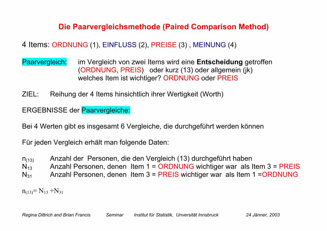
Die Paarvergleichsmethode (Paired Comparison Method)
4 Items: ORDNUNG (1), EINFLUSS (2), PREISE (3) , MEINUNG (4)
Paarvergleich: im Vergleich von zwei Items wird eine Entscheidung getroffen(ORDNUNG, PREIS) oder kurz (13) oder allgemein (jk)welches Item ist wichtiger? ORDNUNG oder PREIS
ZIEL: Reihung der 4 Items hinsichtlich ihrer Wertigkeit (Worth)
ERGEBNISSE der Paarvergleiche:
Bei 4 Werten gibt es insgesamt 6 Vergleiche, die durchgeführt werden können
Für jeden Vergleich erhält man folgende Daten:
n(13) Anzahl der Personen, die den Vergleich (13) durchgeführt habenN13 Anzahl Personen, denen Item 1 = ORDNUNG wichtiger war als Item 3 = PREIS N31 Anzahl Personen, denen Item 3 = PREIS wichtiger war als Item 1 =ORDNUNG
n(13)= N13 +N31

Regina Dittrich and Brian Francis Seminar Institut für Statistik, Unversität Innsbruck 24 Jänner, 2003
Basis Bradley- Terry Modell
Wir definieren 13p als Wahrscheinlichkeit, dass Item 1 (ORDNUNG) wichtiger ist als Item 3 (PREIS) im Vergleich (13)
• Wir modellieren p13 durch Worthparameter π1 , π3
113
1 3p =
+p
p p und 3
311 3
p =+p
p p
Je größer π1 im Verhältnis zu π3 , desto größer die Wahrscheinlichkeit, dass das Item ORDNUNG wichtiger ist als das Item PREIS
• Wir könnten die Chance 13 13 1
31 13 3
p p = = p 1-p
ππ
durch π1 , π3 modellieren
die Chance, dass ORDNUNG wichtiger ist als PREIS als das Verhältnis der Worthparameter von ORDNUNG zu PREIS

Regina Dittrich and Brian Francis Seminar Institut für Statistik, Unversität Innsbruck 24 Jänner, 2003
Die logit Form des Bradley-Terry Modells
• Wir modellieren die log Chance
13 1 3 1 1logit p = - wobei = log g g g p
als Differenz der log Worth-parameter von ORDNUNG und PREIS
Vorausetzungen, dass die γ-Parameter für die 4 Items ORDNUNG,EINFLUSS; PREIS, MEINUNG, geschätzt werden können:
N13 ist binomialverteilt mit der Wahrscheinlichkeit p13 und Stichprobengröße n(13)Annahme: Vergleiche unabhängig mit konstanten Wahrscheinlichkeiten
Zur Identifizierbarkeit der γ-Parameter setzen wir den letzten Null γ4= 0 undwir beschränken die Worthparameter, dass sie in Summe 1 ergeben (zwischen 0 und 1 liegen)
∑ =j
j 1π , ergibt ( )( )∑
=j j
jj γ
γπ
expexp
Regina Dittrich and Brian Francis Seminar Institut für Statistik, Unversität Innsbruck 24 Jänner, 2003
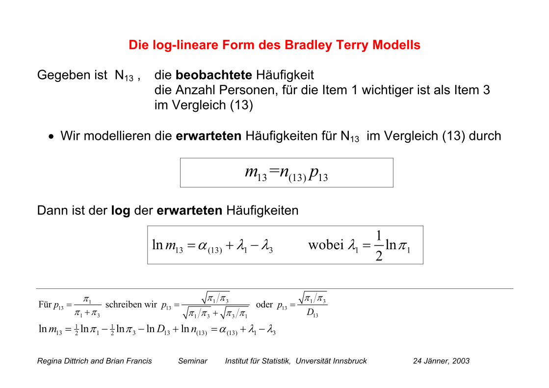
Die log-lineare Form des Bradley Terry Modells
Gegeben ist N13 , die beobachtete Häufigkeit die Anzahl Personen, für die Item 1 wichtiger ist als Item 3im Vergleich (13)
• Wir modellieren die erwarteten Häufigkeiten für N13 im Vergleich (13) durch
13 (13) 13=m n p
Dann ist der log der erwarteten Häufigkeiten
1 3 1 3113 13 13
1 3 131 3 3 1
Für schreiben wir oder p p pD
π π π πππ π π π π π
= = =+ +
1 113 1 3 13 (13) (13) 1 32 2ln ln ln ln lnm D nπ π α λ λ= − − + = + −
13 (13) 1 3 1 11ln wobei ln 2
m α λ λ λ π= + − =

Regina Dittrich and Brian Francis Seminar Institut für Statistik, Unversität Innsbruck 24 Jänner, 2003
Annahme: Njk und Nkj sind poissonverteilt, bedingt auf fixe n(jk) mit Erwartungswerten mjk and mkj und mjk = n(jk)pjk
Die Worthparameter sind jetzt :
( )( )
exp 2exp 2
jj
jj
lp
l=
å
Dieses Modell ist komplexer als das logit Modell, aber es eignet sich besser fürweitere Entwicklungen

Regina Dittrich and Brian Francis Seminar Institut für Statistik, Unversität Innsbruck 24 Jänner, 2003
Für alle 5 Länder gemeinsam
VergleichjkN Häufigkeiten
( )jkα 1λ 2λ 3λ 4λ
ORDNUNG EINFLUSS PREIS MEINUNG
(12)12N 722+72 1 1 -1
(12)21N 699+73 1 -1 1
(13)13N 1110+72 2 1 -1
(13)31N 645+72 2 -1 1
(23)23N 594+73 3 1 -1
(23)32N 375+72 3 -1 1
(14)14N 347+72 4 1 -1
(14)41N 149+4 4 -1 1
(24)24N 407+73 5 1 -1
(42)42N 168+4 5 -1 1
(34)34N 99+72 6 1 -1
(34)43N 70+4 6 -1 1

Regina Dittrich and Brian Francis Seminar Institut für Statistik, Unversität Innsbruck 24 Jänner, 2003
Für Westdeutschland
VergleichjkN Häufigkeiten
( )jkα 1λ 2λ 3λ 4λ
ORDNUNG EINFLUSS PREIS MEINUNG
(12)12N 439 1 1 -1
(12)21N 477 1 -1 1
(13)13N 494 2 1 -1
(13)31N 248 2 -1 1
(23)23N 535 3 1 -1
(23)32N 309 3 -1 1
(14)14N 523 4 1 -1
(14)41N 268 4 -1 1
(24)24N 515 5 1 -1
(42)42N 213 5 -1 1
(34)34N 383 6 1 -1
(34)43N 314 6 -1 1

Regina Dittrich and Brian Francis Seminar Institut für Statistik, Unversität Innsbruck 24 Jänner, 2003
BeobachteteHäufigkeiten
jkN
ErwarteteHäufigkeiten
jkm439 444.2 477 471.8 494 474.4 248 267.6 535 551.2 309 292.8 523 537.4 268 253.6 515 504.0 213 224.0 383 379.6 314 317.4

Regina Dittrich and Brian Francis Seminar Institut für Statistik, Unversität Innsbruck 24 Jänner, 2003
Modell Anpassung für West Deutschland
[o] scaled deviance = 5.8003 at cycle 3[o] residual df = 3
estimate
ils.e. parameter worth
0.3755 0.027 ORDNUNG 0.320.4056 0.030 EINFLUSS 0.340.0893 0.027 PREIS 0.180.000 aliased MEINUNG 0.156.126 0.033 ALPHA(1)5.876 0.037 ALPHA(2)5.996 0.035 ALPHA(3)5.911 0.037 ALPHA(4)5.817 0.039 ALPHA(5)5.850 0.0380 ALPHA(6)

Regina Dittrich and Brian Francis Seminar Institut für Statistik, Unversität Innsbruck 24 Jänner, 2003
Adding subject covariates to the PC model
We have already seen that there are differences between countries in the worthsof the four items.
However, we are also interested in how the items are changing according to age,gender, educational level and so on.
As every case is likely to have a unique combination of these variables, we look atdata at the individual subject level. For each subject, we form a set of pairedcomparisons, and list the covariates.
Assume there are a total of nS subjects with a total of t paired comparisons overall subjects.For subject i, Ni,jk + Ni,jk =1, with:
Ni,jk =1 if j is preferred to k in the comparison (jk), and zero otherwise.Ni,kj =1 if k is preferred to j in the comparison (jk), and zero otherwise.
We thus have a separate table for each case.
Regina Dittrich and Brian Francis Seminar Institut für Statistik, Unversität Innsbruck 24 Jänner, 2003
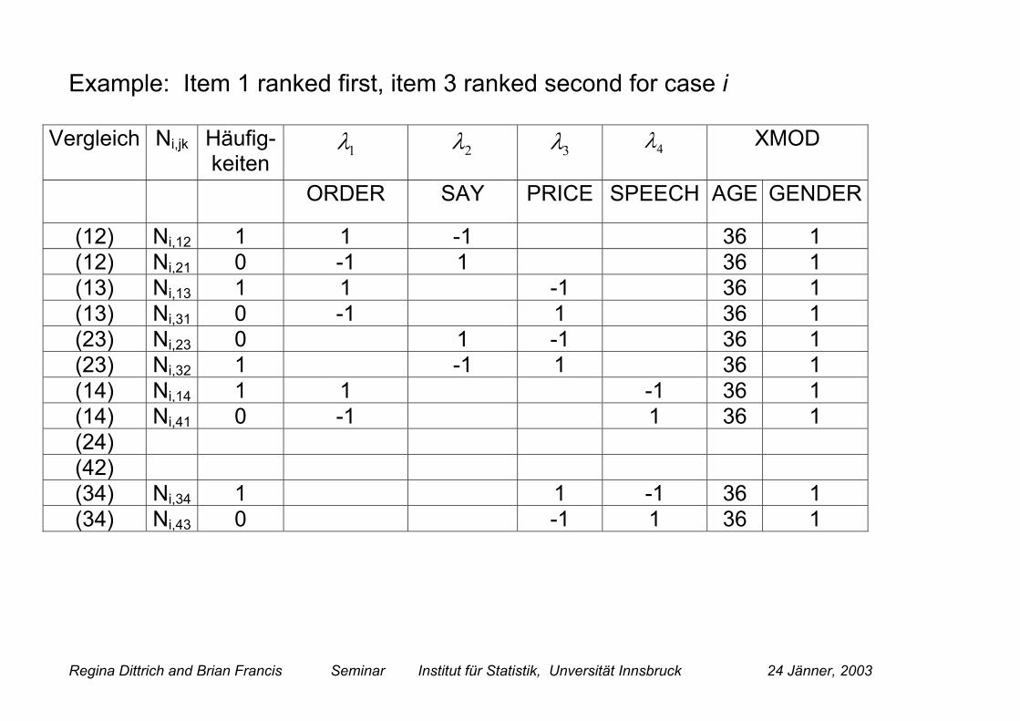
Example: Item 1 ranked first, item 3 ranked second for case i
Vergleich Ni,jk Häufig-keiten
1λ 2λ 3λ 4λ XMOD
ORDER SAY PRICE SPEECH AGE GENDER
(12) Ni,12 1 1 -1 36 1(12) Ni,21 0 -1 1 36 1(13) Ni,13 1 1 -1 36 1(13) Ni,31 0 -1 1 36 1(23) Ni,23 0 1 -1 36 1(23) Ni,32 1 -1 1 36 1(14) Ni,14 1 1 -1 36 1(14) Ni,41 0 -1 1 36 1(24)(42)(34) Ni,34 1 1 -1 36 1(34) Ni,43 0 -1 1 36 1

Regina Dittrich and Brian Francis Seminar Institut für Statistik, Unversität Innsbruck 24 Jänner, 2003
Adding subject covariates to the PC model
Assume a set of continuous covariates and factors at the individual level whichform a covariate model XMOD, with design matrix X (2t by Q).
Q gives the number of predictor variables (including dummy variables) in themodel.
What is XMOD? Simply an R (or STATA or GLIM) model formulasuch as AGE+GENDER+COUNTRY, which generates a
design matrix.

Regina Dittrich and Brian Francis Seminar Institut für Statistik, Unversität Innsbruck 24 Jänner, 2003
Adding subject covariates to the PC model (2)
Remember the log-linear model without covariates:
kjjkjkm λλα −+= )(ln
With data at the individual level, we now have
kijijkijkijki pm ,,)(,,, lnln λλα −+==
and we model λi,j by 0,1
,, =+= ∑=
Ji
Q
qiqjqjji x λβλλ
This gives:
The αi,(jk) are a set of t nuisance parameters – one for each paired comparison foreach individual.
∑=
−+−+=Q
qiqkqjqkjjkijki xm
1,)(,, )(ln ββλλα

Regina Dittrich and Brian Francis Seminar Institut für Statistik, Unversität Innsbruck 24 Jänner, 2003
Defining the linear structure of the model.
For each object j there is a separate set of β parameters which describe the effectof the covariates on that item.
With four items, we can define item covariates
ITEM1, ITEM2, ITEM3, ITEM4.
ITEMj = 1 if in the comparison (j,k) j is preferred = -1 if in the comparison (j,k) k is preferred = 0 if j is not one of the two objects being compared.
Then we can write the model as
ALPHA + ITEM1+ITEM2 +ITEM3 +ITEM4 + XMOD.(ITEM1+ITEM2+ITEM3+ITEM4)
Overparameterised - Estimates for ITEM4 will be unestimable and are set to 0.

Regina Dittrich and Brian Francis Seminar Institut für Statistik, Unversität Innsbruck 24 Jänner, 2003
Adding smooth effects of covariates to paired comparison models (1)
We want to assess effect of some subset of covariates q=1…M (such as AGE) as smoothnon-linear functions fjq for each item. We might choose to do this for a subset of continuouscovariates where we suspect the relationship is not linear.
What does this mean? Consider linear regression, (or a generalised linear model), with theresult of a response Y against AGE as follows:
The graph shows a steep increasing relationshipwith X until X=8, then a decline, followed by alevelling off past X=15.
2.5 5.0 7.5 10.0 12.5 15.0 17.5 20.0
4
5
6
7
8
9
10
11
12
Regina Dittrich and Brian Francis Seminar Institut für Statistik, Unversität Innsbruck 24 Jänner, 2003
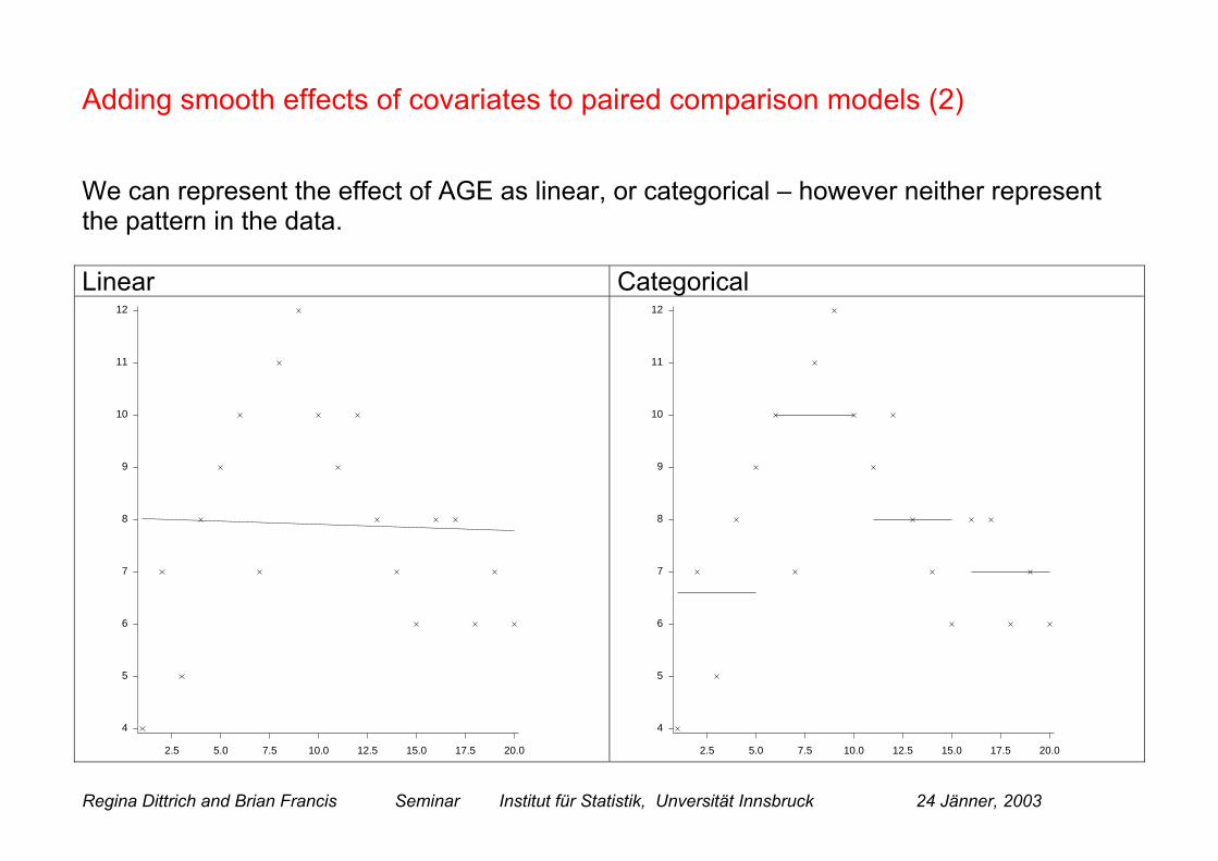
Adding smooth effects of covariates to paired comparison models (2)
We can represent the effect of AGE as linear, or categorical – however neither representthe pattern in the data.
Linear Categorical
2.5 5.0 7.5 10.0 12.5 15.0 17.5 20.0
4
5
6
7
8
9
10
11
12
2.5 5.0 7.5 10.0 12.5 15.0 17.5 20.0
4
5
6
7
8
9
10
11
12

Regina Dittrich and Brian Francis Seminar Institut für Statistik, Unversität Innsbruck 24 Jänner, 2003
Adding smooth effects of covariates to paired comparison models (3)
Non-linear effects can be introduced by fitting quadratic, cubic functions.etc
The graph here shows a quadratic function, butthis also fails to represent the data.
One possibility is to use a smoothing curve torepresent the pattern. The smoothing curve isnon-parametric and data-dependent.
One of the simplest smoothers is a running meansmoother. This looks at the average of each datapoints and its K nearest neighbours.
2.5 5.0 7.5 10.0 12.5 15.0 17.5 20.0
4
5
6
7
8
9
10
11
12

Regina Dittrich and Brian Francis Seminar Institut für Statistik, Unversität Innsbruck 24 Jänner, 2003
Adding smooth effects of covariates to paired comparison models (4)
A smoother is defined by the smoothing matrix Swhich is applied to the raw data y – this gives thefitted values Sy. For example, the running mean smoother withK=1, taking the average of the point and itsnearest neighbour, has an S matrix which mightlook like S y
1/2 1/2 0 0 0 0 0 0 y10 1/2 1/2 0 0 0 0 0 y20 1/2 1/2 0 0 0 0 0 y30 0 0 1/2 1/2 0 0 0 y40 0 0 0 1/2 1/2 0 0 y50 0 0 0 0 1/2 1/2 0 y60 0 0 0 0 0 1/2 1/2 y7... ... ... ... ... ... ...
The equivalent degrees of freedom of thesmoother is the trace of this matrix S, (or more exactly, 1.25 Trace (S))
A smooth fit with 3 df.
2.5 5.0 7.5 10.0 12.5 15.0 17.5 20.0
4
5
6
7
8
9
10
11
12
Regina Dittrich and Brian Francis Seminar Institut für Statistik, Unversität Innsbruck 24 Jänner, 2003

Regina Dittrich and Brian Francis Seminar Institut für Statistik, Unversität Innsbruck 24 Jänner, 2003
Generalised additive models
Hastie and Tibshirani (1990) showed that smoothers can be incorporated into the linearcomponent of a generalised linear model (GLM) by using the backfitting algorithm - extrastep in the weighted least squares cycle. Basically, we smooth the residuals after fitting thelinear part of the model. This is known as a generalised additive model.
How do we incorporate smooth terms into the paired comparison model?
Paired comparison models are GLMs but with negative terms.
kijijkijkijki pm ,,)(,,, lnln λλα −+==
and we now model λi,j by
0)( ,1
,1
,, =++= ∑∑+==
Ji
Q
Mqiqjq
M
qiqjqjji xxf λβλλ

Regina Dittrich and Brian Francis Seminar Institut für Statistik, Unversität Innsbruck 24 Jänner, 2003
This gives
As before, estimation of ßs is easy: -ßx = ß(-x).
But –f(x) is not necessarily equal to f(-x)……
Our trick, which replaces negative parameter estimates with negative terms in thedesign matrix does not work for the smoothing component.
∑
∑
+=
=
−
+−+−+=
Q
Mqiqkqjq
iqkq
M
qiqjqkjjkijki
x
xfxfp
1,
,1
,)(,,
)(
))()((ln
ββ
λλα

Regina Dittrich and Brian Francis Seminar Institut für Statistik, Unversität Innsbruck 24 Jänner, 2003
Reparametrisation
The solution is to use a reparametrisation.Define a new set of nuisance parameters
Then
giving
Sum of positive terms – works! Reparametrisation possible with log-linear form,not with logistic form. The worth parameters are
kijijkijki ,,)(,*
)(,λλαα −−=
ji
kijijkijki
jki
p
,*
,,)(,,
2
ln
)(,λα
λλα
+=
−+=
∑∑+==
+++=Q
Mqiqjq
M
qiqjqjjki xxfp
jki1
,1
,*
)(, 2)(22ln)(,
βλα
∑=
jji
jiji }2exp{
}2exp{
,
,, λ
λπ

Regina Dittrich and Brian Francis Seminar Institut für Statistik, Unversität Innsbruck 24 Jänner, 2003
Estimation issues
Log-linear model with smoothers- can be fitted as a complex generalised additivemodel, using R, GLIM, STATA(?) etc.
Problems are:
Number of smoothers – have J-1 smoothers for each of M desired covariates.Complex to interpret.
Large number of nuisance parameters. In our example, there are t=27981separate paired comparisons. Each comparison has a nuisance parameter.
Need powerful computer, but there are also numerical techniques that can invertSSP matrices which are partially generated by a factor with a large number oflevels.
e.g. ELIMINATE directive in GLIM. Not implemented in R or STATA yet.

Regina Dittrich and Brian Francis Seminar Institut für Statistik, Unversität Innsbruck 24 Jänner, 2003
Inclusion of covariates.
We examined AGE, GENDER, EDUCATION, RELIGION and COUNTRY.Would like to have looked at INCOME but information not collected for every country.SOCIAL CLASS also differs from country to country.
Different level of information collected on each variable in each country.
EDUCATION RELIGION GENDER COUNTRY1= Low (less than 11 years) 1=Catholic, Orthodox 1=Male 1=West Germany2= Medium (11, 12 or 13 yrs) 2=Protestant 2=Female 2=East Germany3= High (14 or more years) 3= Non-believer 3=Britain
4=Other AGE (range 16 – 80) 4=ItalySmooth continuous 5=Poland
Label items as
ORD maintain order in nationPMS give people more say in governmentPFS protect freedom of speechFRP fight rising prices

Regina Dittrich and Brian Francis Seminar Institut für Statistik, Unversität Innsbruck 24 Jänner, 2003
Model fitting strategy
We expect to find strong country to country differences. Covariates will act differently ineach country. So we :
• Fit each country separately
• Fit all covariates and determine the level of smoothing by using AIC. (Akaike InformationCriterion), using the trace of the smoothing matrix S as a measure of the equivalentdegrees of fredom
• Remove non-significant covariates.
modellinear in parameters of no. tr(S)1.25w2w)ˆ;( ,,,
+=+= ∑ jkijkijki
pNDevAIC
Model formula changes from (AGE+SEX+RELI+EDUC)*(PMS+ORD+FRP+PFS)covariates items
tosmooth(AGE.PMS) + smooth(AGE.ORD) + smooth(AGE.FRP) +smooth(AGE.PFS) +(SEX+RELI+EDUC)*(PMS+ORD+FRP+PFS)Overparametrized - set smooth(AGE.PFS) to zero (arbitrary)
Also fit all countries combined, with COUNTRY as an additional factor
Regina Dittrich and Brian Francis Seminar Institut für Statistik, Unversität Innsbruck 24 Jänner, 2003
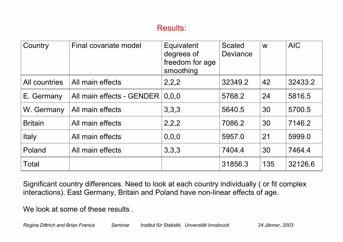
Results:
Country Final covariate model Equivalentdegrees offreedom for agesmoothing
ScaledDeviance
w AIC
All countries All main effects 2,2,2 32349.2 42 32433.2
E. Germany All main effects - GENDER 0,0,0 5768.2 24 5816.5
W. Germany All main effects 3,3,3 5640.5 30 5700.5
Britain All main effects 2,2,2 7086.2 30 7146.2
Italy All main effects 0,0,0 5957.0 21 5999.0
Poland All main effects 3,3,3 7404.4 30 7464.4
Total 31856.3 135 32126.6
Significant country differences. Need to look at each country individually ( or fit complexinteractions). East Germany, Britain and Poland have non-linear effects of age.
We look at some of these results .

Regina Dittrich and Brian Francis Seminar Institut für Statistik, UnversitätInnsbruck 24 Jänner, 2003
West Germany – effect of ageplotting the lambda’s (no smoothing)
20 30 40 50 60 70 80 90
0.0
0.2
0.4
0.6
0.8
1.0
1.2
1.4
1.6
1.8
2.0
West Germany
age
maintain order
more say in govt
fight rising prices
freedom of speech
Difficulty with this plot is that freedom of speech is defined tobe zero for every age – all other effects are relative to
‘freedom of speech’

Regina Dittrich and Brian Francis Seminar Institut für Statistik, UnversitätInnsbruck 24 Jänner, 2003
West Germany – effect of agethe ‘worth’ effects

Regina Dittrich and Brian Francis Seminar Institut für Statistik, UnversitätInnsbruck 24 Jänner, 2003
20 30 40 50 60 70 80 900.0
0.1
0.2
0.3
0.4
0.5
0.6
0.7
0.8
0.9West Germany
age
ORDER
SAY
PRICES
SPEECH
Results for male Catholic with lower level of education.
Freedom of speech not important. More to say ingovernment, and maintain order strongly related to age.However, ORDER is important for older respondents, and‘more to say’ for younger respondents.
Regina Dittrich and Brian Francis Seminar Institut für Statistik, UnversitätInnsbruck 24 Jänner, 2003
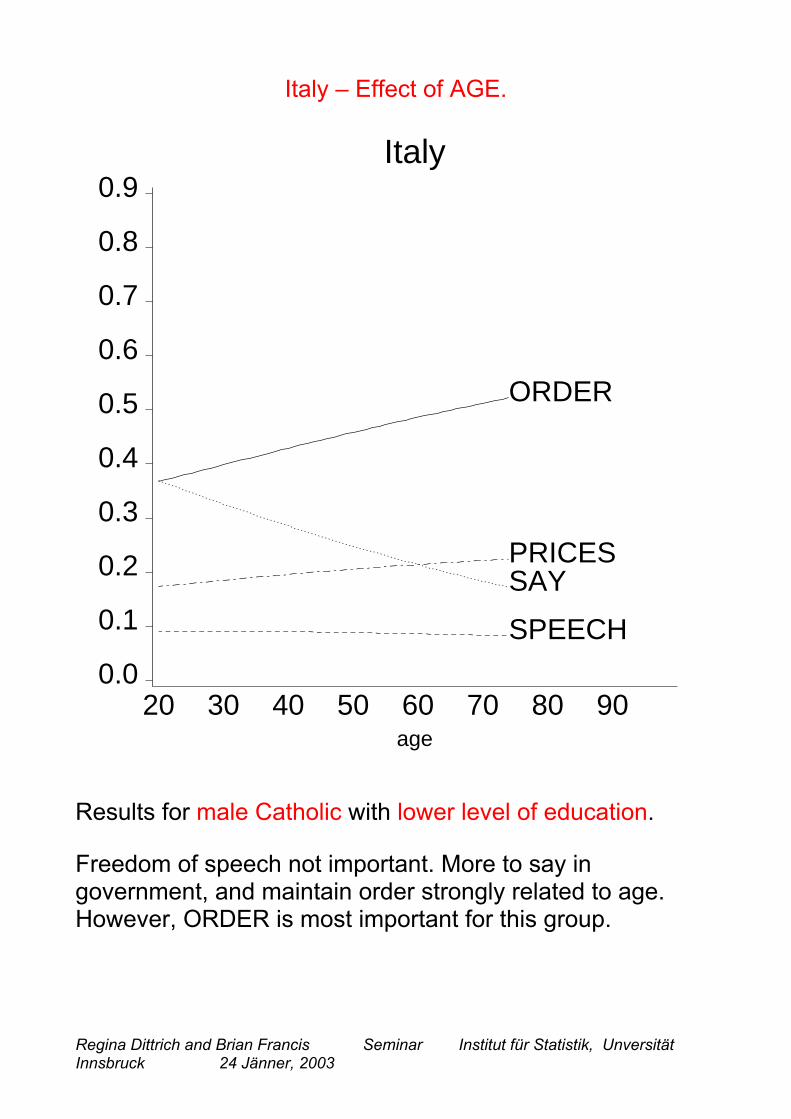
Italy – Effect of AGE.
20 30 40 50 60 70 80 900.0
0.1
0.2
0.3
0.4
0.5
0.6
0.7
0.8
0.9Italy
age
ORDER
SAYPRICES
SPEECH
Results for male Catholic with lower level of education.
Freedom of speech not important. More to say ingovernment, and maintain order strongly related to age.However, ORDER is most important for this group.
Regina Dittrich and Brian Francis Seminar Institut für Statistik, UnversitätInnsbruck 24 Jänner, 2003
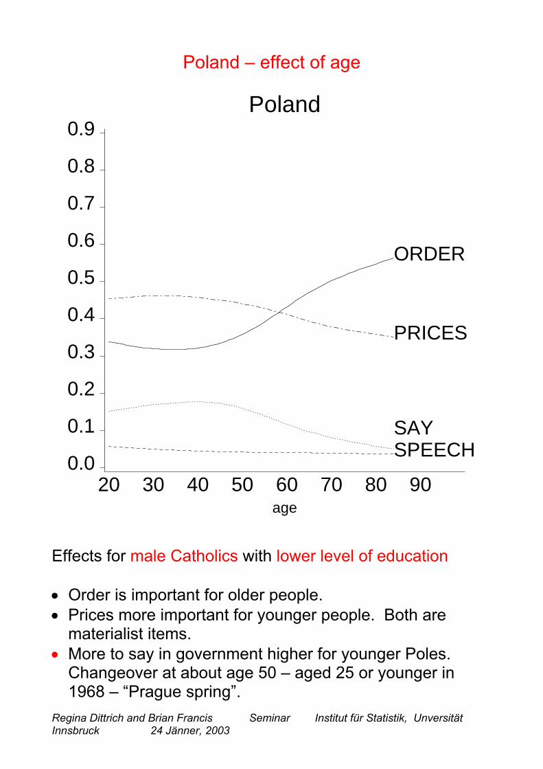
Poland – effect of age
20 30 40 50 60 70 80 900.0
0.1
0.2
0.3
0.4
0.5
0.6
0.7
0.8
0.9Poland
age
ORDER
SAY
PRICES
SPEECH
Effects for male Catholics with lower level of education
• Order is important for older people. • Prices more important for younger people. Both are
materialist items. • More to say in government higher for younger Poles.
Changeover at about age 50 – aged 25 or younger in1968 – “Prague spring”.

Regina Dittrich and Brian Francis Seminar Institut für Statistik, UnversitätInnsbruck 24 Jänner, 2003
Regina Dittrich and Brian Francis Seminar Institut für Statistik, UnversitätInnsbruck 24 Jänner, 2003
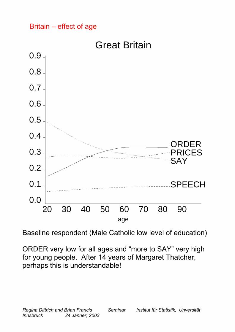
Britain – effect of age
20 30 40 50 60 70 80 900.0
0.1
0.2
0.3
0.4
0.5
0.6
0.7
0.8
0.9Great Britain
age
ORDER
SAYPRICES
SPEECH
Baseline respondent (Male Catholic low level of education)
ORDER very low for all ages and “more to SAY” very highfor young people. After 14 years of Margaret Thatcher,perhaps this is understandable!

Regina Dittrich and Brian Francis Seminar Institut für Statistik, UnversitätInnsbruck 24 Jänner, 2003
West Germany – effect of education
0-10 11-13 14 or more0.0
0.1
0.2
0.3
0.4
0.5
0.6West Germany
years of education
ORDER
SAY
PRICE
SPEECH
Effects are for male Catholic aged 30
Freedom of speech has a worth which increases witheducation.
Those with more education rate postmaterialist items higher“more to say in government” and “freedom of speech”.

Regina Dittrich and Brian Francis Seminar Institut für Statistik, UnversitätInnsbruck 24 Jänner, 2003
Italy – effect of Education
0-10 11-13 14 or more0.0
0.1
0.2
0.3
0.4
0.5
0.6Italy
years of education
ORDER
SAY
PRICESSPEECH
Effects are for male Catholic aged 30
Those with more education rate postmaterialist items higher“more to say in government” and “freedom of speech”.
Regina Dittrich and Brian Francis Seminar Institut für Statistik, UnversitätInnsbruck 24 Jänner, 2003
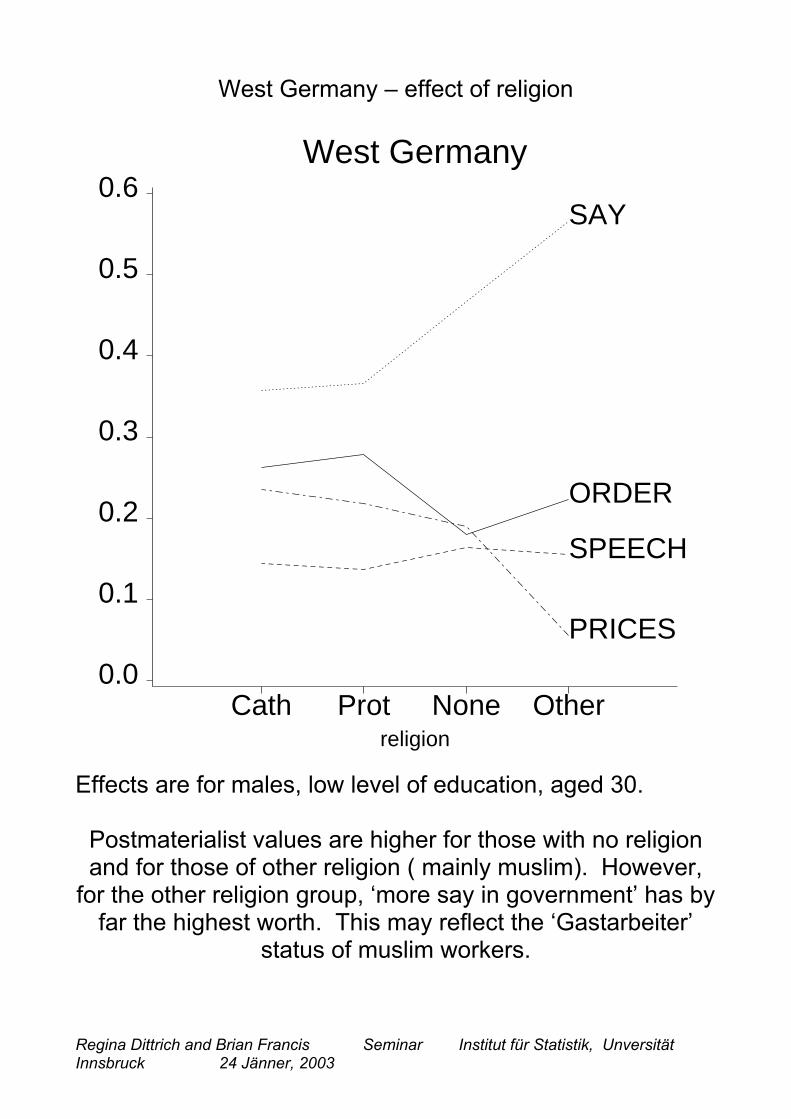
West Germany – effect of religion
Cath Prot None Other0.0
0.1
0.2
0.3
0.4
0.5
0.6West Germany
religion
ORDER
SAY
PRICES
SPEECH
Effects are for males, low level of education, aged 30.
Postmaterialist values are higher for those with no religionand for those of other religion ( mainly muslim). However,
for the other religion group, ‘more say in government’ has byfar the highest worth. This may reflect the ‘Gastarbeiter’
status of muslim workers.
Regina Dittrich and Brian Francis Seminar Institut für Statistik, UnversitätInnsbruck 24 Jänner, 2003
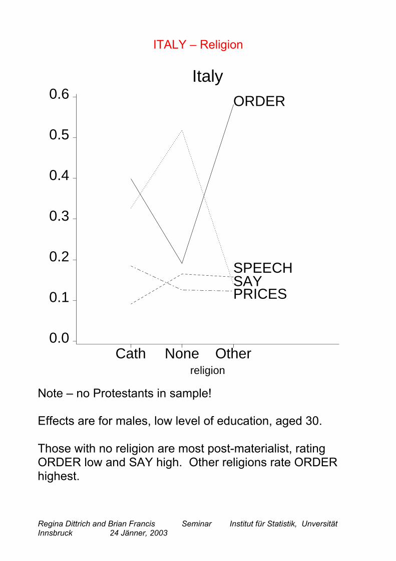
ITALY – Religion
Cath None Other0.0
0.1
0.2
0.3
0.4
0.5
0.6Italy
religion
ORDER
SAYPRICES
SPEECH
Note – no Protestants in sample!
Effects are for males, low level of education, aged 30.
Those with no religion are most post-materialist, ratingORDER low and SAY high. Other religions rate ORDERhighest.

Regina Dittrich and Brian Francis Seminar Institut für Statistik, UnversitätInnsbruck 24 Jänner, 2003
ITALY – effect of gender.
Males desire ORDER more than females.
Females are more concerned with PRICES than males.
Contrast with Poland, where women rate both materialistitems (PRICES, ORDER) higher than men.

Regina Dittrich and Brian Francis Seminar Institut für Statistik, Unversität Innsbruck 24 Jänner, 2003
Calculating the probability of materialism and postmaterialism
Materialist responses will rank items 1 and 3 in first and second place.
So
)2,4,1,3()4,2,1,3()2,4,3,1()4,2,3,1()4,2,3,1()1,3()3,1()(
iiiii
iii
PPPPPPPMATP
++++=+=
and we can estimate each of these probabilities by decomposing the rank orders intopaired comparisons.
Similarly, we can estimate Pi(POST) and Pi(MIXED) for any set of covariates
04,
12,
21,
33,
24,14,12,34,32,31,)4,2,1,3(
iiii
iiiiiii
K
ppppppCP
ππππ=
=
Regina Dittrich and Brian Francis Seminar Institut für Statistik, UnversitätInnsbruck 24 Jänner, 2003
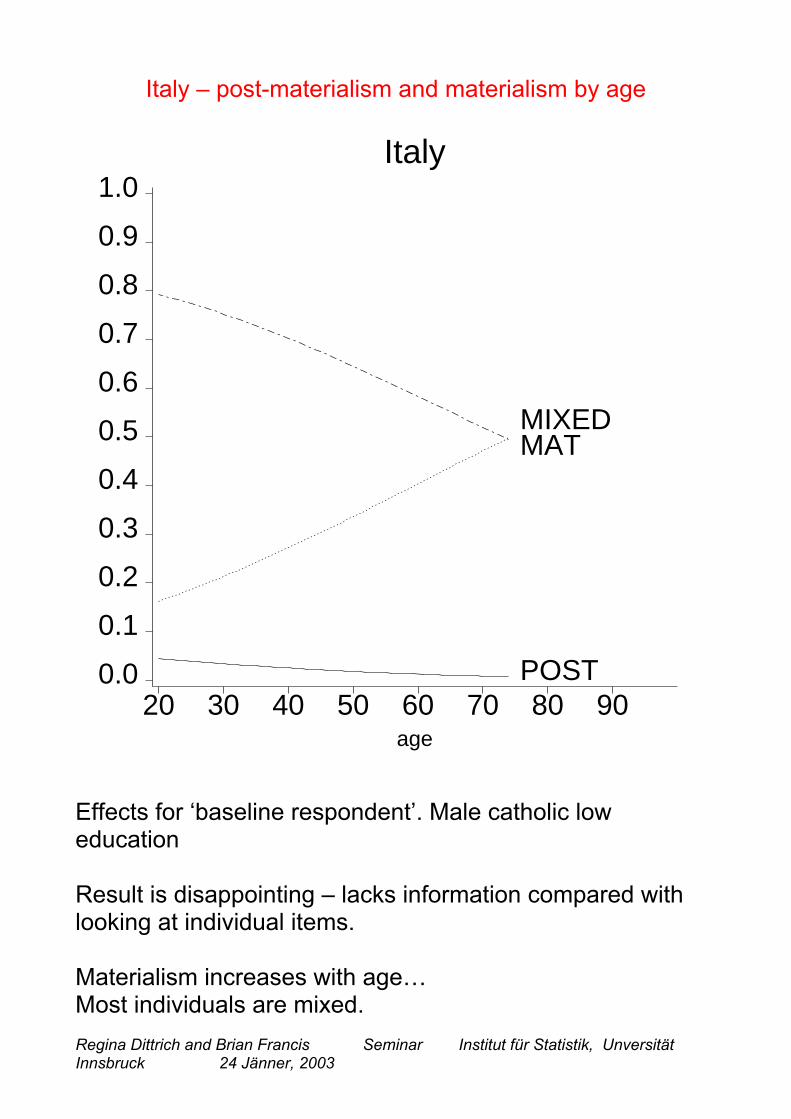
Italy – post-materialism and materialism by age
20 30 40 50 60 70 80 900.0
0.1
0.2
0.3
0.4
0.5
0.6
0.7
0.8
0.9
1.0Italy
age
POST
MIXEDMAT
Effects for ‘baseline respondent’. Male catholic loweducation
Result is disappointing – lacks information compared withlooking at individual items.
Materialism increases with age…Most individuals are mixed.
Regina Dittrich and Brian Francis Seminar Institut für Statistik, Unversität Innsbruck 24 Jänner, 2003
CONCLUSIONS
• Assumes decisions made by individuals can be decomposed into a set of pairedcomparisons, and these are independent.
Methods exist for dealing with dependencies (Francis and Dittrich, 2000; Dittrich andKatzenbeisser, 2002) but have not been extended into smooth covariate models.
• Would like to separate out generation (birth cohort) effects from age effects. Doindividuals become more materialist as they age, or does a new generation havedifferent values to the previous generation?
• Interactions between covariates can be included, but models will become more complex.Varying coefficient models would play a role here in considering interactions with AGE.
• Individual items give far more information than a simple post-materialist- materialist split.
• Every country appears to be different. Not a simple East- West or North-South split!Viva la differenza!Es lebe der kleine Unterschied!