Embed Size (px)
Citation preview
Analysis of Electronic Medical Records of RheumatoidArthritis Patients on Biological Therapies
A Reuma.pt Study
João Pedro Bento Machado Marques de Freitas
Thesis to obtain the Master of Science Degree in
Biomedical Engineering
Supervisors: Prof. Alexandra Sofia Martins de Carvalho
Dr. Helena Cristina de Matos Canhao
Examination Committee
Chairperson: Prof. João Pedro Estrela Rodrigues Conde
Supervisor: Dr. Helena Cristina de Matos Canhão
Member of the Committee: Dr. Helena Isabel Aidos Lopes
June 2015

Dedico este trabalho a minha famılia.
ii

Acknowledgments
First of all I would like to express my sincere thanks to my co-supervisor Prof. Dr. Helena Canhao for
providing data from Reuma.pt for this thesis. I would also like to thank to my university supervisors, Prof.
Dr. Alexandra Carvalho and Prof. Dr. Susana Vinga, who provided me with their opinions, proofread the
draft material and with whom I had many meetings during this thesis.
I am also thankful for the opportunity that my supervisors gave me of having a grant to work on the
FCT project InteleGen (PTDC/DTP-FTO/1747/2012) and I also want to thank for the availability of Prof.
Dr. Conceicao Amado.
Finally, I would like to thank to my family for all the support they gave to me.
iii
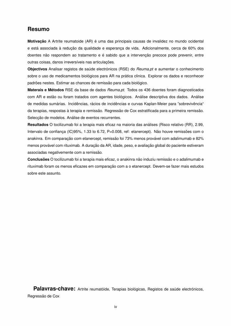
Resumo
Motivacao A Artrite reumatoide (AR) e uma das principais causas de invalidez no mundo ocidental
e esta associada a reducao da qualidade e esperanca de vida. Adicionalmente, cerca de 60% dos
doentes nao respondem ao tratamento e e sabido que a intervencao precoce pode prevenir, entre
outras coisas, danos irreversıveis nas articulacoes.
Objectivos Analisar registos de saude electronicos (RSE) do Reuma.pt e aumentar o conhecimento
sobre o uso de medicamentos biologicos para AR na pratica clinica. Explorar os dados e reconhecer
padroes nestes. Estimar as chances de remissao para cada biologico.
Materais e Metodos RSE da base de dados Reuma.pt. Todos os 436 doentes foram diagnosticados
com AR e estao ou foram tratados com agentes biologicos. Analise descriptiva dos dados. Analise
de medidas sumarias. Incidencias, racios de incidencias e curvas Kaplan-Meier para ”sobrevivencia“
da terapias, respostas a terapia e remissao. Regressao de Cox estratificada para a primeira remissao.
Seleccao de modelos. Analise de eventos recurrentes.
Resultados O tocilizumab foi a terapia mais eficaz na maioria das analises (Risco relativo (RR), 2.99,
Intervalo de confianca (IC)95%, 1.33 to 6.72, P=0.008, ref: etanercept). Nao houve remissoes com o
anakinra. Em comparacao com etanercept, remissao foi 73% menos provavel com adalimumab e 82%
menos provavel com rituximab. A duracao da AR, idade, peso, e avaliacao global do paciente estiveram
associadas negativemente com a remissao.
Conclusoes O tocilizumab foi a terapia mais eficaz, o anakinra nao induziu remissao e o adalimumab e
rituximab foram os menos eficazes em comparacao com a o etanercept. Devem-se fazer mais estudos
sobre este assunto.
Palavras-chave: Artrite reumatoide, Terapias biologicas, Registos de saude electronicos,
Regressao de Cox
iv
Abstract
Motivation Rheumatoid arthritis (RA) is one of the lead causes of disability in the western world and is
linked with reduced life quality and expectancy. In addition, about 60% of the patients fail treatment and
is known that early intervention might prevent, among other things, irreversible damages to the joints.
Objectives Investigate Electronic medical records (EMR) from Reuma.pt and increase the base knowl-
edge about the use of biologic drugs for RA in clinical-practice. Explore the data and find meaningful
patterns in it. Estimate the chances of remission for the different biologics.
Materials & Methods EMR from Reuma.pt database. All the 436 patients are diagnosed with RA
and are or were treated with biological agents. Descriptive analysis of the data. Summary measures
analysis. Incidence rates, incidence density rates and Kaplan-Meier curves for drug ”survival“, therapy
response and remission. Stratified Cox proportional hazards regression for the first remission. Model
selection. Recurrent events analysis.
Findings Tocilizumab was the most efficacious therapy in most of the analysis (Hazard Ratio (HR),
2.99, 95% Confidence interval (CI), 1.33 to 6.72, P=0.008, ref: etanercept). There was no remissions
with anakinra. In comparison to etanercept, remission was 73% less likely with adalimumab and 82%
less likely with rituximab. RA duration, age, weight and patient global assessment VAS at baseline were
negatively associated with remission.
Conclusions Tocilizumab was the most efficacious therapy and anakinra had no remission and ritux-
imab and adalimumab were less efficacious comparing to etanercept. Further studies need to be done.
Keywords: Rheumatoid arthritis, Biological therapies, Electronic medical records, Cox regres-
sion
v

vi
Contents
Acknowledgments . . . . . . . . . . . . . . . . . . . . . . . . . . . . . . . . . . . . . . . . . . . iii
Resumo . . . . . . . . . . . . . . . . . . . . . . . . . . . . . . . . . . . . . . . . . . . . . . . . . iv
Abstract . . . . . . . . . . . . . . . . . . . . . . . . . . . . . . . . . . . . . . . . . . . . . . . . . v
List of Tables . . . . . . . . . . . . . . . . . . . . . . . . . . . . . . . . . . . . . . . . . . . . . . ix
List of Figures . . . . . . . . . . . . . . . . . . . . . . . . . . . . . . . . . . . . . . . . . . . . . xi
Nomenclature xiii
Nomenclature . . . . . . . . . . . . . . . . . . . . . . . . . . . . . . . . . . . . . . . . . . . . . . 1
Glossary . . . . . . . . . . . . . . . . . . . . . . . . . . . . . . . . . . . . . . . . . . . . . . . . 1
1 Introduction 3
1.1 Motivation . . . . . . . . . . . . . . . . . . . . . . . . . . . . . . . . . . . . . . . . . . . . . 3
1.2 Data mining . . . . . . . . . . . . . . . . . . . . . . . . . . . . . . . . . . . . . . . . . . . . 5
1.3 Objectives . . . . . . . . . . . . . . . . . . . . . . . . . . . . . . . . . . . . . . . . . . . . . 5
1.4 Thesis outline . . . . . . . . . . . . . . . . . . . . . . . . . . . . . . . . . . . . . . . . . . . 6
2 Rheumatoid Arthritis 7
2.1 Description . . . . . . . . . . . . . . . . . . . . . . . . . . . . . . . . . . . . . . . . . . . . 7
2.2 Disease activity scores . . . . . . . . . . . . . . . . . . . . . . . . . . . . . . . . . . . . . . 9
2.3 Measuring functional disability . . . . . . . . . . . . . . . . . . . . . . . . . . . . . . . . . 10
2.4 Remission criteria . . . . . . . . . . . . . . . . . . . . . . . . . . . . . . . . . . . . . . . . 10
2.5 Response criteria . . . . . . . . . . . . . . . . . . . . . . . . . . . . . . . . . . . . . . . . . 11
2.6 Treatment of rheumatoid arthritis . . . . . . . . . . . . . . . . . . . . . . . . . . . . . . . . 11
3 Materials and Methodology 15
3.1 Data . . . . . . . . . . . . . . . . . . . . . . . . . . . . . . . . . . . . . . . . . . . . . . . . 15
3.2 Methods . . . . . . . . . . . . . . . . . . . . . . . . . . . . . . . . . . . . . . . . . . . . . . 18
3.2.1 Smoothing . . . . . . . . . . . . . . . . . . . . . . . . . . . . . . . . . . . . . . . . 19
3.2.2 Summary measures . . . . . . . . . . . . . . . . . . . . . . . . . . . . . . . . . . . 19
3.2.3 Measures of occurrence and association . . . . . . . . . . . . . . . . . . . . . . . 19
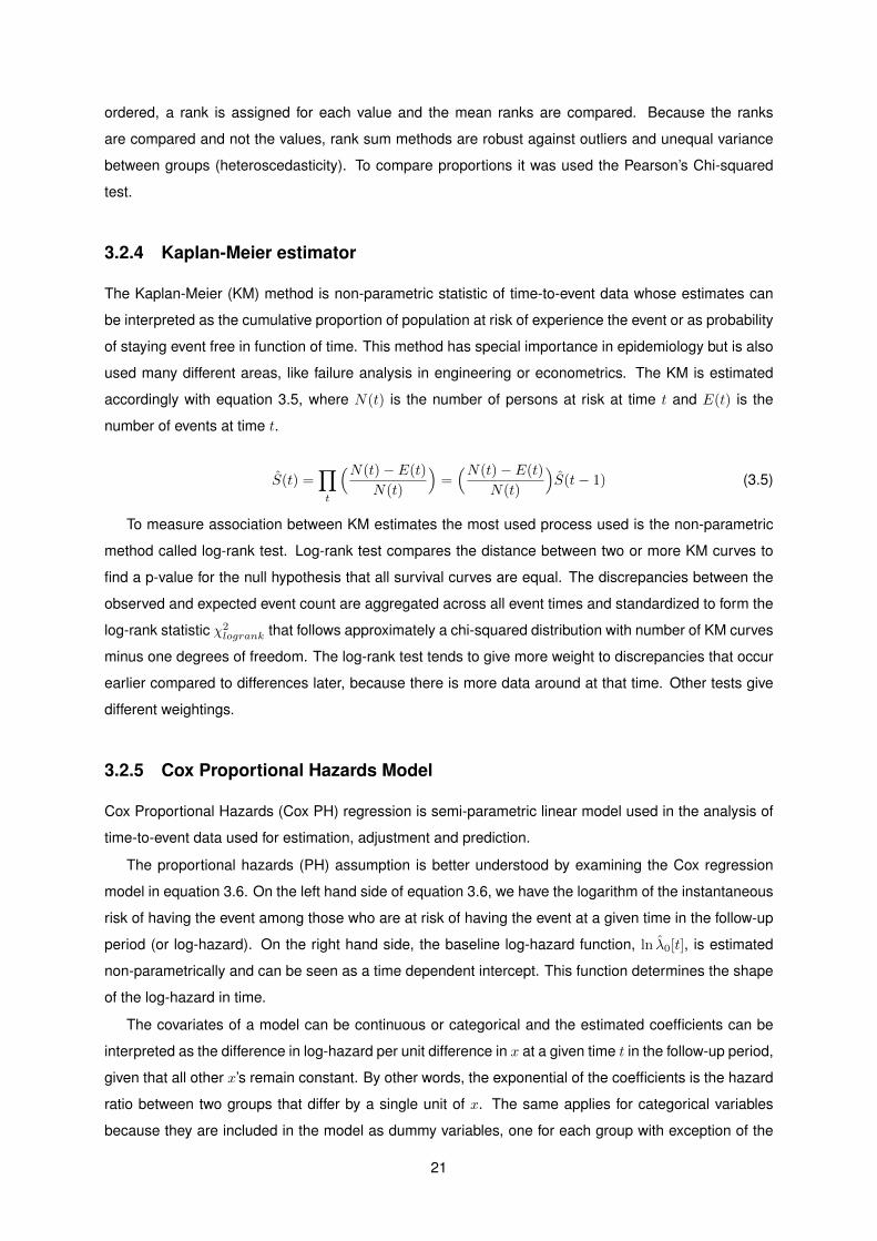
3.2.4 Kaplan-Meier estimator . . . . . . . . . . . . . . . . . . . . . . . . . . . . . . . . . 21
3.2.5 Cox Proportional Hazards Model . . . . . . . . . . . . . . . . . . . . . . . . . . . . 21
vii
3.3 Data Analysis . . . . . . . . . . . . . . . . . . . . . . . . . . . . . . . . . . . . . . . . . . . 25
3.3.1 Descriptive analysis . . . . . . . . . . . . . . . . . . . . . . . . . . . . . . . . . . . 26
3.3.2 Summary measures analysis . . . . . . . . . . . . . . . . . . . . . . . . . . . . . . 26
3.3.3 Incidence density rates . . . . . . . . . . . . . . . . . . . . . . . . . . . . . . . . . 26
3.3.4 Kaplan-Meier estimates . . . . . . . . . . . . . . . . . . . . . . . . . . . . . . . . . 26
3.3.5 Cox proportional hazards regression . . . . . . . . . . . . . . . . . . . . . . . . . . 27
4 Results 29
4.1 Descriptive analysis . . . . . . . . . . . . . . . . . . . . . . . . . . . . . . . . . . . . . . . 29
4.2 Summary measures analysis . . . . . . . . . . . . . . . . . . . . . . . . . . . . . . . . . . 35
4.3 Incidence density rates . . . . . . . . . . . . . . . . . . . . . . . . . . . . . . . . . . . . . 36
4.4 Kaplan-Meier estimates . . . . . . . . . . . . . . . . . . . . . . . . . . . . . . . . . . . . . 40
4.5 Cox regression analysis . . . . . . . . . . . . . . . . . . . . . . . . . . . . . . . . . . . . . 40
4.5.1 Model selection . . . . . . . . . . . . . . . . . . . . . . . . . . . . . . . . . . . . . . 41
4.5.2 Recurrent events analysis . . . . . . . . . . . . . . . . . . . . . . . . . . . . . . . . 47
5 Conclusions 51
5.1 Descriptive analysis . . . . . . . . . . . . . . . . . . . . . . . . . . . . . . . . . . . . . . . 51
5.2 Summary measures analysis . . . . . . . . . . . . . . . . . . . . . . . . . . . . . . . . . . 53
5.3 Incidence density rates . . . . . . . . . . . . . . . . . . . . . . . . . . . . . . . . . . . . . 53
5.4 Kaplan-Meier estimates . . . . . . . . . . . . . . . . . . . . . . . . . . . . . . . . . . . . . 54
5.5 Cox regression analysis . . . . . . . . . . . . . . . . . . . . . . . . . . . . . . . . . . . . . 54
5.5.1 Model Selection . . . . . . . . . . . . . . . . . . . . . . . . . . . . . . . . . . . . . 54
5.5.2 Recurrent events analysis . . . . . . . . . . . . . . . . . . . . . . . . . . . . . . . . 56
5.6 Limitations . . . . . . . . . . . . . . . . . . . . . . . . . . . . . . . . . . . . . . . . . . . . 56
5.7 Achievements . . . . . . . . . . . . . . . . . . . . . . . . . . . . . . . . . . . . . . . . . . . 58
5.8 Future Work . . . . . . . . . . . . . . . . . . . . . . . . . . . . . . . . . . . . . . . . . . . . 59
Bibliography 65
A Kaplan-Meier Estimates 67
viii
List of Tables
2.1 Disease activity scores formulae table. . . . . . . . . . . . . . . . . . . . . . . . . . . . . . 9
2.2 ACR/EULAR boolean and index based definition of remission for clinical trials and clinical
practice. . . . . . . . . . . . . . . . . . . . . . . . . . . . . . . . . . . . . . . . . . . . . . . 10
2.3 EULAR response criteria . . . . . . . . . . . . . . . . . . . . . . . . . . . . . . . . . . . . 11
2.4 Guidelines for biological therapies approved for Rheumatoid Arthritis . . . . . . . . . . . . 13
3.1 Number of patients per biologic number. . . . . . . . . . . . . . . . . . . . . . . . . . . . . 17
3.2 Percentage (number) of patients per drug in cohort dataset. . . . . . . . . . . . . . . . . 18
3.3 Data layouts for different recurrent event models using two hypothetical subjects. . . . . . 24
4.1 Baseline table. . . . . . . . . . . . . . . . . . . . . . . . . . . . . . . . . . . . . . . . . . . 30
4.2 Summary measures table. . . . . . . . . . . . . . . . . . . . . . . . . . . . . . . . . . . . . 30
4.3 Incidence rate by drug per 1000 person-months over the follow-up period of 4 years. . . . 37
4.4 IRR and 95% CI of tocilizumab (TCZ) comparing to etanercept (ETN) by age quartile. . . 39
4.5 Cox Proportional Hazards regression results for predictors of remission, Hazard Ratio
(95% CI). . . . . . . . . . . . . . . . . . . . . . . . . . . . . . . . . . . . . . . . . . . . . . 42
4.6 Magnitude of confounding table. . . . . . . . . . . . . . . . . . . . . . . . . . . . . . . . . 42
4.7 Best models obtained. Swollen joint count (SJC), rheumatoid factor (RF), extra articular
manifestations (EA Manif.). . . . . . . . . . . . . . . . . . . . . . . . . . . . . . . . . . . . 46
4.8 Cox Proportional Hazards models for recurrent events. . . . . . . . . . . . . . . . . . . . . 49
4.9 Grambsch-Therneau test p-values for the PWP-CP model covariates . . . . . . . . . . . . 49
ix

x
List of Figures
2.1 The American College of Rheumatology treatment algorithm after rheumatoid arthritis
diagnosis. . . . . . . . . . . . . . . . . . . . . . . . . . . . . . . . . . . . . . . . . . . . . . 12
3.1 Patients time-line. . . . . . . . . . . . . . . . . . . . . . . . . . . . . . . . . . . . . . . . . 16
4.1 Body distribution of the swollen and tender joints at baseline. . . . . . . . . . . . . . . . . 29
4.2 Hands and feet distribution of the swollen and tender joints at therapy baseline. . . . . . . 31
4.3 DAS28 by drug, over the 4 years follow-up period. . . . . . . . . . . . . . . . . . . . . . . 32
4.4 HAQ, 4 years follow-up. . . . . . . . . . . . . . . . . . . . . . . . . . . . . . . . . . . . . . 33
4.5 Disease activity conditional density estimate by therapy. . . . . . . . . . . . . . . . . . . . 34
4.6 Boxplots of the therapy duration. . . . . . . . . . . . . . . . . . . . . . . . . . . . . . . . . 35
4.7 Summary measures plots. . . . . . . . . . . . . . . . . . . . . . . . . . . . . . . . . . . . . 36
4.8 Kaplan Meier estimates stratified by biologic drug. . . . . . . . . . . . . . . . . . . . . . . 37
4.9 Unadjusted incidence rate ratio of the other drugs in comparison with etarnecept and
stratified by age, concomitant DMARD, descent and time since onset of disease. . . . . . 39
4.10 Evolution of different scores during backward elimination with different data sets and dif-
ferent criteria to eliminate a variable. . . . . . . . . . . . . . . . . . . . . . . . . . . . . . . 45
4.11 Kaplan Meier estimate for recurrent events. . . . . . . . . . . . . . . . . . . . . . . . . . . 48
A.1 Kaplan-Meier of remission between naive and non-naive patients. . . . . . . . . . . . . . 67
A.2 Kaplan-Meier of drug switch between naive and non-naive patients. . . . . . . . . . . . . 68
A.3 Kaplan-Meier of remission between patients with DMARD and without DMARD at baseline. 68
xi

xii
Nomenclature
L Likelihood
n Number of observations
p Number of parameters
S(t) Survival function
t Time
ABT Abatacept
ACR American College for Rheumatology
ADA Adalimumab
AG Andersen and Gill counting process indepeendent increment model
AIC Akaike information criterion
AICc Akaike information criterion corrected
AKR Anakinra
bDMARD Biologic disease modifying anti-rheumatic drugs
BIC Bayesian information crterion
CCP cyclic citrullinated peptide
CDAI Clinical disease activity index
Cox PH Cox Proportional Hazards
CP Counting processes
CRP C-reactive protein
DAS Disease activity score
DAS28 Disease activity score for 28 joints
xiii
DGS Portuguese Directorate-General of Health
DMARD Disease modifying anti-rheumatic drugs
EMR Electronic Medical Records
ESR erythrocytes sedimentation rate
ETN Etanercept
EULAR European League Against Rheumatism
GC Glucocorticoid
GLM Golimumab
GT Gap time
HAQ Health assessment questionnaire
HAQ-DI Health assessment questionnaire disabilityy index
HCQ Hydroxychloroquine
IFX Infliximab
MTX Methotrexate
NSAID Nonsteroidal anti-inflammatory drug
PtGA Patient global assessment
PWP Prentice, Williams and Peterson conditional model
RA Rheumatoid Arthritis
RTX Rituximab
SDAI Simplified disease activity index
SJC Swollen joint count
SPR Portuguese Society of Rheumatology
SSZ Sulfasalazine
TCZ Tocilizumab
TJC Tender joint count
TNF Tumor necrosis factor
TT-R Total time-restricted
VAS Visual analog scale
WLW Wei, Lin and Weissfeld model marginal model
1

2
Chapter 1
Introduction
1.1 Motivation
Rheumatoid Arthritis (RA) is one of the leading causes of disability in the western world and is linked
with reduce life quality, decreased life expectancy and increased risk of cardiovascular diseases [1].
Moreover, RA affects 0.5% to 1% of the general population worldwide being the most common inflam-
matory arthritis [2]. Because therapy aims not only to control the symptoms during flares of increased
disease activity but also to prevent irreversible damage to the joints, early recognition and intervention
can improve function, slow structural progression, mortality and also reduce the financial burden for the
patients and society.
Today’s therapies are estimated to work only in 60% of the patients, the therapy selection follows
no specific criteria and the causes for RA remains unknown. Furthermore, the time used to find an
effective therapy, or therapies, for each patient is of special importance since it may give opportunity for
the disease to cause irreversible damage in the joints and bone erosion. However, many studies have
helped us understand which factors enhance the disease expression in individuals who have RA [2] and
in the future they might help us to find the right therapy for the right patient.
The ultimate goal of epidemiology, biostatistics and other sciences that use statistics or computational
methods to deal with biomedical data is to provide evidence that can be used not only for policy making
on public health but also on daily clinical practice to support clinical decisions. In the past, the impact of
such measures went well beyond public health and had deep reverberation in society and economy.
Nowadays, the developed countries face increasingly aging demographic with rising health care costs
consuming increasing portion of the nation’s gross domestic product [3]. This gives data sciences a re-
inforced role on the organization, strategic planning and optimization of the allocation of resource. Ulti-
mately, the new evidences should translated to new public health policies in a way that the sustainability,
universality and equity of the health systems are preserved.
Plataforma Mais Saude, an association of rheumatic diseases patients in Portugal, states that rheumatic
diseases are the first cause for early retirement and that an untreated or late diagnosed patient is two
times and a half more costly for the Portuguese State than a early diagnosed [4]. In Portugal, the
3
rheumatic diseases are responsible for 43% of the cases of work absenteeism and Portugal is one of
the countries that more spends per capita with drugs used in the treatment of this group of diseases
[5]. In fact, the emergence of biological therapies for RA increased the cost of treatment of rheumatic
diseases. However, they yield better results than their synthetic counterparts and have important clinical
benefits for the patients.
This thesis focus on studying biological therapies for RA. This relatively new drugs are called this
way because they are produced in other organisms by recombining human genes of antibodies against
a specific target. This genetically engineered organism are used to produce these molecules because
they are too large and complex to be produced synthetically. In the case of RA this antibodies act as
inhibitors of a group of molecules responsible for the cell signaling and activation of the immune system
cells and the autoimmune response. Because of their production method the price is much higher than
the synthetically produced disease modifying anti-rheumatic drugs (DMARDs). For example, a 25 mg
tab of methotrexate can cost 600 times more than a etanercept 25 mg vial [2]. For this reason, and also
because of the increased risk of infection, they are only used after therapy with DMARDs has failed.
Electronic medical records (EMR) are the technological successor of the paper-based medical records.
EMRs centralize and accumulate the medical history data and any other information relevant for the
medical domain in databases to provide informed and planned patient care. The data stored in EMRs is
more accessible, usable and exists in larger quantities. In addition, EMRs can also guide the decision
making process by enabling tools that can instantly help the physician visualize and analyze the data.
Another application of EMRs is to monitor the quality of care and for conducting scientific research that
deals with important clinical problems.
Since June 2008, the Rheumatic Diseases Portuguese Register (Reuma.pt) is collecting data from
rheumatic patients receiving biological therapies or synthetic DMARDs. This register was created by
the Portuguese Society of Rheumatology (SPR) and includes patients with RA, ankylosing spondylitis,
psoriatic arthritis and juvenile idiopathic arthritis. At each visit demographic and anthropometric data,
life style habits, work status, co-morbidities, disease activity and functional assessment scores, previous
and current therapies, adverse events, reasons for discontinuation and laboratory measurements are
registered. The register includes all Rheumatology departments assigned to the Portuguese National
Health Service, a public-private partnership and some private centers [6]. Reuma.pt goal is to keep
track of the patients’ disease progression, to support the clinical practice on a daily basis and to provide
data for studies about therapies’ efficacy and safety.
The main focus of this thesis is a data set from EMR data extracted from Reuma.pt obtained on
mid-June 2014 that includes patients from two health centers with a total of 9305 observations and 426
patients. All the patients are diagnosed as having RA and are being or were treated with biological
therapies. Since all subjects were treated with biologics the analysis will be mostly about this new drugs.
4
1.2 Data mining
Data mining is considered a step of several analysis processes for databases, including the Knowl-
edge Discovery in Databases (KDD) process and the Cross-Industry Standard Process for Data Mining
(CRISP-DM) developed by a consortium of European companies and currently used by IBM [7, 8]. The
goal of data mining is to find patterns of interest in databases using methods from fields like artificial
intelligence, machine learning and statistics. The most striking difference between data mining and
statistics is that the first analyzes data without any a priori hypothesis and analyzes mostly observa-
tional data from databases without any kind of experimental designed or measurement control. Data
mining seems to be a rebranding that comprises many fields that already existed.
The objective of experimental design is to collect data in a way that represents best the underlying
population. The main way to accomplish it is by randomization and by diving the experimental units in
similar groups (blocks) to reduce sources of heterogeneity and control for confounding variables.
In a statistical study one has a well-defined hypothesis that will be investigated, a specifically chosen
population, carefully collected data, control for confounding variables and a set of methods inference
tools with well know properties used to generalize the results from a sample to the studied population.
The last decade notoriety of data mining is due in part to the growing quantity of information stored in
databases and with how little companies know what to do with it. This phenomenon has even more been
pronounced by the promise from some software solutions that the investment will create huge returns.
1.3 Objectives
This study investigates EMR data collected in the Reuma.pt and aims to increase the base knowledge
about the use of biologic drugs for RA in clinical-practice. More precisely, it aims to measure the effect
of the different biologic treatments and to discover what other factors might influence the progression of
the disease activity and functional disability on patients with RA.
This work also aims to study the drug discontinuation, since it is a overall marker of the success of a
treatment and depends on the efficacy of the drug, its side effects and doctor and patient preferences.
Ultimately, we also hope to be determine what therapy is more likely to succeed according to the
characteristics of the data.
In order to meet this aims, the beginning of this thesis will focus on defining the grounds and contex-
tualizing the rest of the work by reviewing some of the literature about rheumatoid arthritis, its treatments,
guidelines, epidemiology, genetics and current criteria used to assessment of disease activity and func-
tional ability.
Then it is paramount to find appropriate ways to analyze Reuma.pt data and to understand the
implications and limitations of the results that will be produced. For this reason, it will be reviewed
literature about epidemiology, longitudinal data analysis, survival analysis, machine learning and other
data sciences or methods.
Next, the data processing and data analysis have to be outlined and prepared. This step consists of
5
plan and script all steps on the data processing and analysis to produce the results in the form of figures
and tables. From the processing of the original data it will be created multiple datasets that are suitable
for most of the methods chosen. Thus, R statistical software and other appropriate tools will be used.
Specifically, we want to explore the dataset with a set of summary measures and plots that can be
easily understandable and interpretable. In addition, we wan to describe the evolution in time of key
variables by drug.
Then, we want to measure the effect of the different biologic treatments and other factors on the
progression of the disease activity on the patients with RA. Assess the effectiveness of the biologic
therapies with and without DMARDs and compare the therapy response between biological therapies’
naıve and non-naıve patients.
After the results are presented clearly and systematically, conclusions can be drawn from the re-
search, methods implications and limitations can be discussed and ideas for future work can be referred.
1.4 Thesis outline
Chapter 1 gives the motivations, aims and objectives of this thesis.
Chapter 2 is about rheumatoid arthritis disease, its treatments and Portuguese and European guide-
lines. The conditions for introduction in biologic therapies are described and the background for our data
is established.
In Chapter 3 we can find the methodology, which is divided in three sections: Data, Method and
Data Analysis. On the first section the structure of the original data set and the processing methods to
construct the other data sets is described. The second section gives a theoretical review of the methods
used in this work and the third section describes how the results in Chapter 4 were obtained.
Chapter 4 starts by representing the data with some descriptive statistics and summaries. Then, it
presents the estimates for the effect of the different therapies and variables on remission for the different
analysis.
Chapter 5 summarizes and interprets the results in light of the initial objectives, discusses the advan-
tages and limitations of the proposed solutions and also refers possible applications and future work.
6
Chapter 2
Rheumatoid Arthritis
In this chapter we describe the background inherent with the data used in this work. By other words, the
disease, treatments and guidelines are analyzed with the objective of understanding the posed problem
and to elicit good solutions to analyze the data.
2.1 Description
RA is a systemic inflammatory disease that causes a chronic inflammatory response of the synovial
membrane with consequent cartilage destruction and bone erosion within the joint. The main clinical
manifestations of the disease are joint pain, stiffness and excess synovial fluid in symmetrical joints
causing swelling of the synovium, mostly, on the hands and feet. The disability in RA patients develops
most rapidly during the first 2 years of disease when the constant insult to the synovium leads to the
gradual replacement of this tissue by fibrous tissue.
Nonetheless, the cause of RA and why the synovium is the primary target remains unknown. How-
ever, it is believed that repeated inflammatory insults in a genetically susceptible individual might con-
tribute to decline of tolerance and subsequent autoimmunity. These insults can be environmental factors,
such as smoking or infectious agents that can contribute to the initiation and perpetuation of RA [2].
While RA prevalence ranges from 0.5-1.0% in the general population, in women it is two to three
time higher than in men. According to the Portuguese Directorate-General of Health (DGS), in Portugal
this proportion is 4:1 [9]. Consequently, the hormonal part in the development of RA have been widely
studied to understand what factor might cause RA.
For reasons not yet fully elucidated, the oral contraceptive pill may have a protective effect on the
development of RA, even if different levels of female sex hormones does not increase the risk of RA.
Moreover, men who have RA present lower testosterone levels and higher incidence of RA development
occurs at the beginning of menopause and during the postpartum period after the first pregnancy, spe-
cially for women that breastfeed. This suggests that RA may be related with an increase in prolactin or
an abnormal response to it [10, 11].
Diet also seems to be relevant in reducing the incidence of RA. One study states that the intake
7
of vitamin D is inversely associated with RA [12], while another states that a vegetarian diet produced
significant general improvement of the patients [13]. However, there are not many studies that associate
the incidence of RA with the dietary behavior.
On the other hand, many evidence have been found that support the existence of genetics suscepti-
bility and severity factors of RA. For example, chinese and japanese populations have a lower prevalence
of RA (0.2-0.3%) and studies in Africa failed to find any RA cases, while native populations from North
America, like the Pima indians (5.3%) and Chippewa Indians (6.8%), have higher prevalences [2].
In addition, the class II major histocompatibility complex (MHC) genes, specifically the genotypes of
the hypervariable region of the human leukocyte antigen-DR4 (HLA-DR4) has been associated to an
increased risk of RA and also to the severity of the disease. The risk of having RA is 4 to 5 greater in
individuals with the HLA-DR4 genotype. However, it is estimated that only 50% of the genetic contribu-
tion to RA can be explained by HLA genotype. In addition, the alleles of the tumor necrosis factor (TNF)
and many other genes have also been investigated but their contribution to the disease are yet not well
defined [2, 10].
RA can also affect other organs and systems with manifestations on the eyes, lungs and cardiovascu-
lar system. One of the main characteristics of RA patients is anemia caused by the chronic inflammation
[11]. In a 40 years prospective study, a cohort of 100 patients with RA had increased mortality with a
median life expectancy reduced by 10 years for men and 11 years for women compared to the general
population. Also in this study, the primary cause of death was cardiovascular disease [14]. Other factors
that also contribute for the excess mortality among RA patients are infections, renal disease and respi-
ratory failure [2]. For this reasons, early suppression the RA inflammation process can not only have
impact on the morbidity of affected population but too on its mortality.
Inflammation, infection or tissues necrosis causes the production by the liver of group of proteins
known as the acute-phase proteins that characterize what is known as the acute-phase response. The
presence of this acute-phase proteins, as well as increased age or anemia, promotes the erythrocytes
aggregation. So, the erythrocytes sedimentation rate (ESR) is an indirect and non-specif way of as-
sessing the patient acute-phase response. The measurement of the level of C-reactive protein, an
acute-phase protein, has the advantage that they increase and decrease rapidly compared to ESR in
the presence and absence of inflammation [11].
The rheumatoid factors (RF) and anti-cyclic citrullinated peptide antibodies (anti-CCP) are antibodies
directed against proteins of the own individual. The RF is found in 70% to 90% of the RA patients and
the anti-CCP is found in 75% of the same [11]. Other autoantibodies that recognize either joint antigens
or systemic antigens are related with RA, but RF and anti-CCP are the only biomarkers with significant
sensitivity and specificity to be considered useful for RA prognostic and diagnostic in clinical practice . It
is known that cartilage and bone erosion are more common in RF-positive or anti-CCP-positive patients
and that autoimmunity can be present before the unveiling of the first symptoms [2].
8
2.2 Disease activity scores
A score gives a value to the quantity being measure by gathering quantitative evidence about the patient
state that can be later used to monitor the disease activity and decide the best treatment strategy. Scores
like the disease activity score (DAS), the simplified disease activity index (SDAI) and the clinical disease
activity index (CDAI) try to provide maximum information about the disease activity using a minimal
number of variables. The scores on Table 2.1 are of great importance to clinical practice as well as
to clinical trials because they provide standard measures and remission criteria that can be used and
compared across studies.
Score Formula Cutpoints(Range) REM/LDA/MDA/HDA
DAS 0.54√RAI + 0.065
√SJC44 + 0.33 lnESR+
0.0072GH< 1.6/ ≤ 2.4/ ≤ 3.7/ > 3.7(0-12.2)
DAS28 0.56√TJC28 + 0.28
√SJC28 +
0.70 lnESR+ 0.014GH< 2.6/ ≤ 3.2/ ≤ 5.1/ > 5.1(0-9.8)
SDAITJC28 + SJC28 + PtGA+ PhGA+ CRP ≤ 3.3/ ≤ 11/ ≤ 26/ > 26(0-86)
CDAITJC28 + SJC28 + PtGA+ PhGA ≤ 2.8/ ≤ 10/ ≤ 22/ > 22(0-76)
Table 2.1: Disease activity score (DAS and DAS28); simplified disease activity index (SDAI); clinicaldisease activity index (CDAI). Ritchie articular index (RAI); Tender joint count (TJC); swollen joint count(SJC). DAS joint counts is determined using 44 joints and DAS28, SDAI and CDAI using 28 joints. C-reactive protein (CRP) in mg/dL; erythrocyte sedimentation rate (ESR) in mm/h. DAS and DAS28 usethe general health (GH) or patient global assessment (PtGA) on a 0 to 100mm visual analog scale (VAS)while SDAI and CDAI use the PtGA and the physician global assessment (PhGA) of disease activity ona 0-10cm VAS. Remission(REM); low disease activity (LDA); moderate disease activity (MDA) and highdisease activity (HDA).
While swollen joint count (SJC) reflects the amount of inflamed synovial tissue, the tender joint count
(TJC) is associated with the level of pain on the joints.
The Ritchie articular index (RAI) is an articular measurement for the assessment of joint tenderness
in patients with RA. The RAI is the sum of the grades of tenderness of 52 evaluated joints (0 for not
tender, 1 for tender, 2 for tender and causes wince and 3 for tender, causes wince and effort to withdraw)
obtained by applying pressure over the joint margin of articular joints [15].
DAS and DAS28 have also modified formulae that include CRP instead of ESR and a constant
that substitute the patient global assessment (PtGA) in case it is missing from the appointment register.
Nevertheless, these scores have limitations and can not express all characteristics of the disease. While
the mechanisms behind RA are not fully understand, the variables used in the scores will not describe
completely the activity of the disease or the treatment effect in RA, too.
9
2.3 Measuring functional disability
The health assessment questionnaire (HAQ) measures the extent of the functional damage caused by
the disease. HAQ has been validated in patients with a wide variety of rheumatic diseases including RA
and so, it is not considered disease specific.
The HAQ has two versions, the full HAQ and the 2-page HAQ that contains the HAQ Disability Index
(HAQ-DI), pain scale, and global health status scale. The HAQ-DI assesses the patient’s level of func-
tional ability through 8 categories of questions about fine movements of the upper extremity, locomotor
activities of the lower extremity, and activities that involve both upper and lower extremities. These cate-
gories are dressing and grooming, arising, eating, walking, hygiene, reach, grip and activities. A HAQ-DI
score cannot be calculated validly when there are scores for less than six of the eight categories.
The HAQ pain scale and the global health status scale are both visual analog scales (VAS) that
assesses the patient condition over the past week in a 15-centimeter, double-anchored horizontal scale
that starts at 0 (very well) and goes to 100 (very poor) [16, 17]. Bruce and Fries state in [17] that some
researchers consider a difference of 0.10 on the HAQ-DI as clinically important. Others consider 0.22
the minimal clinical important difference.
2.4 Remission criteria
Remission is the state of lessening of disease symptoms without reaching cure and with the possibility
of relapse. Remission criteria are fundamental decision boundaries in clinical trials and clinical practice.
It is sought from remission criteria that the probability of relapse is minimal but as long as there is not
complete understanding of the pathophysiology or a biomarker that describes completely the disease
activity, these criteria will not be perfect. However, letting the patient know they are in remission may
lead to periods of under treatment by giving the patients and physicians a false sense of security [18].
Some remission criteria were already presented in Table 2.1, but many others exist. For this reason,
in 2011 a joint initiative from American College of Rheumatology (ACR), the European League Against
Rheumatism (EULAR) and the Outcome Measures in Rheumatology Initiative (OMERACT) met to define
a uniform remission criterion for RA in trials and practice. ACR/EULAR committee came up with the
criteria presented in Table 2.2. Furthermore, ACR also recommends to include the feet and ankle joints
extra to the 28-joint count when evaluating remission [19, 20].
ACR/EULAR Boolean-based Index-based
Clinical trials SJC, TJS, PtGA, CRP all ≤1 SDAI ≤3.3
Clinical practice SJC, TJS, PtGA all ≤1 CDAI ≤2.8
Table 2.2: ACR/EULAR boolean and index based definition of remission for clinical trials and clinicalpractice. Swollen joint count (SJC) using 28 joints, tender joint count (TJS) using 28 joints, patientglobal assessment (PtGA) on a 0 to 10 scale, C-reactive protein (CRP) in mg/dL, simplified diseaseactivity index (SDAI), clinical disease activity index (CDAI) [19, 21].
Regarding DAS28 remission criterion defined in Table 2.1 (DAS28<2.6), the EULAR recommenda-
10
tions consider that it is not enough strict [22]. Additionally, the DAS28 remission definition does not
predict radiographic outcomes as well as the other remission criteria [19].
As explained in [23], the boolean-based criteria present a disadvantage because the PtGA is not only
influenced by the RA disease activity. For this reason, many patients did not meet the boolean remission
criteria even though they did not have signs of disease activity. Consequently, it is better to use index
based criteria since they provide more flexible criteria for remission.
Nevertheless, in current clinical practice states of remission are frequently not kept over long periods
and a more feasible goal might be to reach and sustain a state of very low disease activity, as defined
by the score’s cut-points in Table 2.1. Ultimately there is still no consensus in what is best the definition
for remission in RA and these criteria are still being validated.
2.5 Response criteria
The response criteria, validated and developed by the EULAR is present in Table 2.3.
Current DAS28 DAS28 change from baseline (∆DAS28)>1.2 0.6-1.2 ≤0.6
≤3.2 good response moderate response no response3.2-5.1 moderate response moderate response no response>5.1 moderate response no response no response
Table 2.3: EULAR response criteria
The developers of the EULAR response criterion considered that a good responder must have a low
disease activity, accordingly with the DAS28 cut-points, and that the score must decrease of 1.2 to be
statistically significant. The 1.2 value comes from the fact that the variables used to calculate the DAS28
were transformed to have a Gaussian distribution and that this change is two times the measurement
error (95% confidence).
2.6 Treatment of rheumatoid arthritis
Early identification and aggressive intervention in RA is fundamental to minimize the irreversible func-
tional damage in the joints. Accordingly with the EULAR recommendations [22], the initial therapy ap-
proach for RA patients should consist of conventional synthetic disease-modifying antirheumatic drugs
(csDMARDs or simply DMARDs), alone or in combination of two or three, as soon as the disease is
diagnosed. On the first 6 months of disease, non-steroidal anti-inflammatory (NSAID) and low-dose glu-
corticoids can be considered but they should be reduced the sooner the possible. The treatment target
to achieve is remission by the ACR/EULAR criteria or low disease activity as defined by the different
scores cut-points on Tables 2.2 and 2.1.
Therapy generally begins with methotrexate (MTX), the most commonly prescribed DMARD. In case
of contraindications or intolerance, sulfasalazine (SSZ) or hydroxychloroquine (HCQ) are alternatives.
11
After initiating a DMARD, patients need to be monitored for potential side effects of the medications. If
there is no improvement after three months of therapy the therapy should be adjusted to another DMARD
or to a combination of DMARDs. In case remission or low disease activity has not been reached after
six months, therapy should be adjusted. In case of poor prognostic the therapy should be adjusted to a
biologic DMARD (bDMARD, biological therapy or biologic) in monotherapy or with DMARD(s).
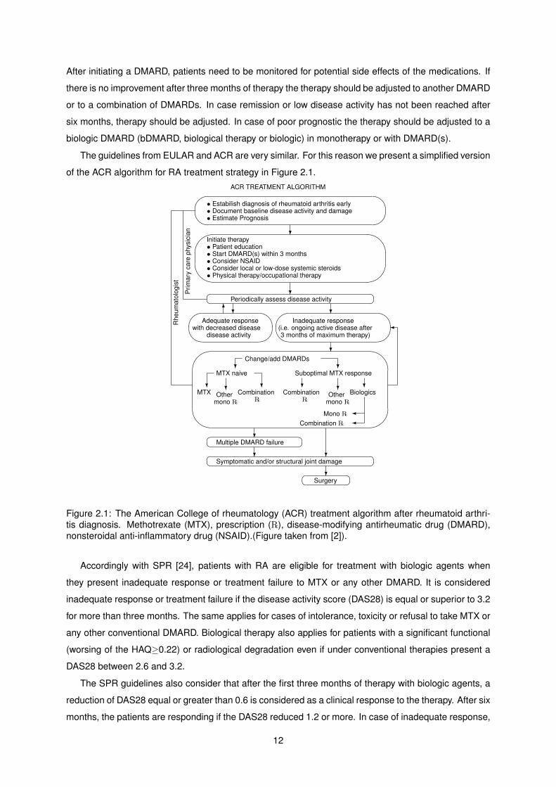
The guidelines from EULAR and ACR are very similar. For this reason we present a simplified version
of the ACR algorithm for RA treatment strategy in Figure 2.1.ACR TREATMENT ALGORITHM�
���
• Estabilish diagnosis of rheumatoid arthritis early• Document baseline disease activity and damage• Estimate Prognosis
?'
&
$
%Initiate therapy• Patient education• Start DMARD(s) within 3 months• Consider NSAID• Consider local or low-dose systemic steroids• Physical therapy/occupational therapy
?�� ��Periodically assess disease activity
6?��
��
Adequate responsewith decreased disease
disease activity
?��
��
Inadequate response(i.e. ongoing active disease after3 months of maximum therapy)
?'
&
$
%
Change/add DMARDs?
MTX naive
?MTX
?Other
mono �
?Combination
�
?Suboptimal MTX response
?Combination
�
?Other
mono �
?Biologics
�Mono ��Combination �
?�� ��Multiple DMARD failure
? ?�� ��Symptomatic and/or structural joint damage
?�� ��Surgery
�
Prim
ary
care
phys
icia
n
Rhe
umat
olog
ist
Figure 2.1: The American College of rheumatology (ACR) treatment algorithm after rheumatoid arthri-tis diagnosis. Methotrexate (MTX), prescription (�), disease-modifying antirheumatic drug (DMARD),nonsteroidal anti-inflammatory drug (NSAID).(Figure taken from [2]).
Accordingly with SPR [24], patients with RA are eligible for treatment with biologic agents when
they present inadequate response or treatment failure to MTX or any other DMARD. It is considered
inadequate response or treatment failure if the disease activity score (DAS28) is equal or superior to 3.2
for more than three months. The same applies for cases of intolerance, toxicity or refusal to take MTX or
any other conventional DMARD. Biological therapy also applies for patients with a significant functional
(worsing of the HAQ≥0.22) or radiological degradation even if under conventional therapies present a
DAS28 between 2.6 and 3.2.
The SPR guidelines also consider that after the first three months of therapy with biologic agents, a
reduction of DAS28 equal or greater than 0.6 is considered as a clinical response to the therapy. After six
months, the patients are responding if the DAS28 reduced 1.2 or more. In case of inadequate response,
12
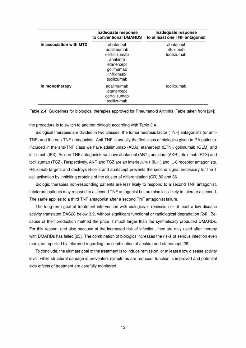
Inadequate response Inadequate responseto conventional DMARDS to at least one TNF antagonist
In association with MTX abatacept abataceptadalimumab rituximabcertolizumab tocilizumab
anakinraetanerceptgolimumabinfliximab
tocilizumab
In monotherapy adalimumab tocilizumabetanercept
certolizumabtocilizumab
Table 2.4: Guidelines for biological therapies approved for Rheumatoid Arthritis (Table taken from [24]).
the procedure is to switch to another biologic according with Table 2.4.
Biological therapies are divided in two classes: the tumor necrosis factor (TNF) antagonists (or anti-
TNF) and the non-TNF antagonists. Anti-TNF is usually the first class of biologics given to RA patients.
Included in the anti-TNF class we have adalimumab (ADA), etanercept (ETN), golimumab (GLM) and
infliximab (IFX). As non-TNF antagonists we have abatacept (ABT), anakinra (AKR), rituximab (RTX) and
tocilizumab (TCZ). Respectively, AKR and TCZ are an interleukin-1 (IL-1) and IL-6 receptor antagonists.
Rituximab targets and destroys B-cells and abatacept prevents the second signal necessary for the T
cell activation by inhibiting proteins of the cluster of differentiation (CD) 80 and 86.
Biologic therapies non-responding patients are less likely to respond to a second TNF antagonist.
Intolerant patients may respond to a second TNF antagonist but are also less likely to tolerate a second.
The same applies to a third TNF antagonist after a second TNF antagonist failure.
The long-term goal of treatment intervention with biologics is remission or at least a low disease
activity translated DAS28 below 3.2, without significant functional or radiological degradation [24]. Be-
cause of their production method the price is much larger than the synthetically produced DMARDs.
For this reason, and also because of the increased risk of infection, they are only used after therapy
with DMARDs has failed [25]. The combination of biologics increases the risks of serious infection even
more, as reported by Infarmed regarding the combination of anakira and etanercept [26].
To conclude, the ultimate goal of the treatment is to induce remission, or at least a low disease activity
level, while structural damage is prevented, symptoms are reduced, function is improved and potential
side effects of treatment are carefully monitored.
13

14
Chapter 3
Materials and Methodology
The object of study of this thesis is EMR extracted in June of 2014 from the Reuma.pt database. The
patients records come from observational data from two health centers registered in Reuma.pt. There
are 9305 observations from a total of 436 patients, 78 of which had already started biological therapies
before the follow-up start. All the patients are diagnosed with RA and are or were treated with biological
agents.
3.1 Data
The data consists of demographic information, pharmaceutical records, disease activity and disability
indicators, response to biological therapy and other clinical data. The data can be described as retro-
spective observational and as an unbalanced longitudinal, also known as unbalanced panel data. The
last description means that the patients have repeated measures during the follow-up period but there is
not the same number of observations per patient. In addition, a patient can switch between therapies or
be unenrolled on therapy during the follow-up period. As mentioned in Chapter 2, remission in RA, the
primary outcome on this work, is not an easy outcome to access since subjects experience periods of
disease remission and frequent relapses. The largest follow-up time for a patient in the data was almost
15 years and the smallest was just one appointment. See Figure 3.1 for a real example of the structure
of the data.
Since it does not exist a control/reference group on placebo, DMARDs or a defined golden standard
for the biologics, etanercept will be chosen as the reference group for comparisons between drugs in
this work, due to the fact that it was the most prescribed drug. On all work the DAS28 used was the
version with four variables and with the ESR.
In this work, the information about the various DMARDs and GCs was spread across different vari-
ables. This variables were collapsed to form a unique variable for the DMARDs and GCs. Furthermore,
the dates of the appointments was encoded according with the season of the year to investigate possible
seasonality of the disease flare or remission. Variables with a big number of levels were recategorized
to ease the analysis and because some groups did not have enough observations for the methods to
15
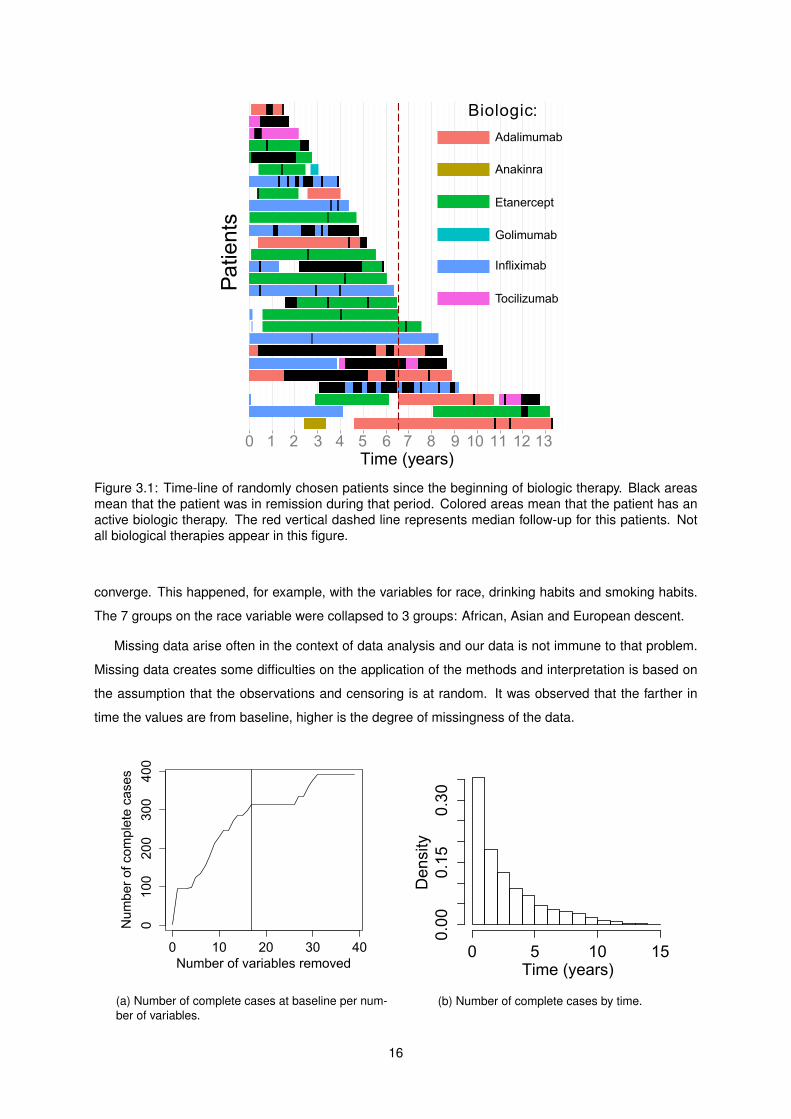
Figure 3.1: Time-line of randomly chosen patients since the beginning of biologic therapy. Black areasmean that the patient was in remission during that period. Colored areas mean that the patient has anactive biologic therapy. The red vertical dashed line represents median follow-up for this patients. Notall biological therapies appear in this figure.
converge. This happened, for example, with the variables for race, drinking habits and smoking habits.
The 7 groups on the race variable were collapsed to 3 groups: African, Asian and European descent.
Missing data arise often in the context of data analysis and our data is not immune to that problem.
Missing data creates some difficulties on the application of the methods and interpretation is based on
the assumption that the observations and censoring is at random. It was observed that the farther in
time the values are from baseline, higher is the degree of missingness of the data.
(a) Number of complete cases at baseline per num-ber of variables.
(b) Number of complete cases by time.
16
The original data was used to design a number of studies in order to investigate the association of the
different variables to therapy response and disease remission. On a longitudinal dataset, the continuous
and categorical variables can also be classified as time dependent and time independent, accordingly
if they change or not with time. From a time-depended variable, like the number of days since the start
of a particular therapy, and an event variable, like the disease activity or the drug switch, we can extract
from the original dataset time-to-event data and analyze it accordingly with the time a subject remained
event free or was lost to follow-up.
By observing different estimates for disease activity, there were few subjects at risk and almost no
new events after 4 years. Machin et al. [27] suggests to limit the follow-up time to a certain time when
the number of patients at risk is less than 15 or the Kaplan-Meier estimate starts to form a ”plateau“
with relatively big gaps between events. Therefore, the follow-up time was limited to 4 years and it was
considered up to four recurrent remissions.
Having in attention that most of the subjects experienced different drugs at different times, only one
of the drugs per subject was selected. This was done because the observations of the same subject
for different drugs are correlated and the assumption of independent observations that many of the
conventional methods in data analysis use needed to be followed. For example, if observations of the
same subject is present in different groups being compared this groups are depended of each other.
This choice has the disadvantage that we discard a great part of the data but the advantage that
making possible to study the effect of the therapies with a greater variety of methods and less restrictions
and assumptions.
Biologic Biologic numberDrug 0 1 2 3 4 5 6
Abatacept 1 5 9 10 2 1 0Adalimumab 61 26 8 1 0 2 0
Anakinra 8 0 1 1 1 0 0Etanercept 144 71 10 1 0 0 0Golimumab 30 9 2 0 1 1 0Infliximab 110 24 3 1 0 0 0Rituximab 5 31 27 8 1 0 0
Tocilizumab 34 16 23 13 5 0 1
Total 393 182 83 35 10 4 1
Table 3.1: Number of patients per biologic number.
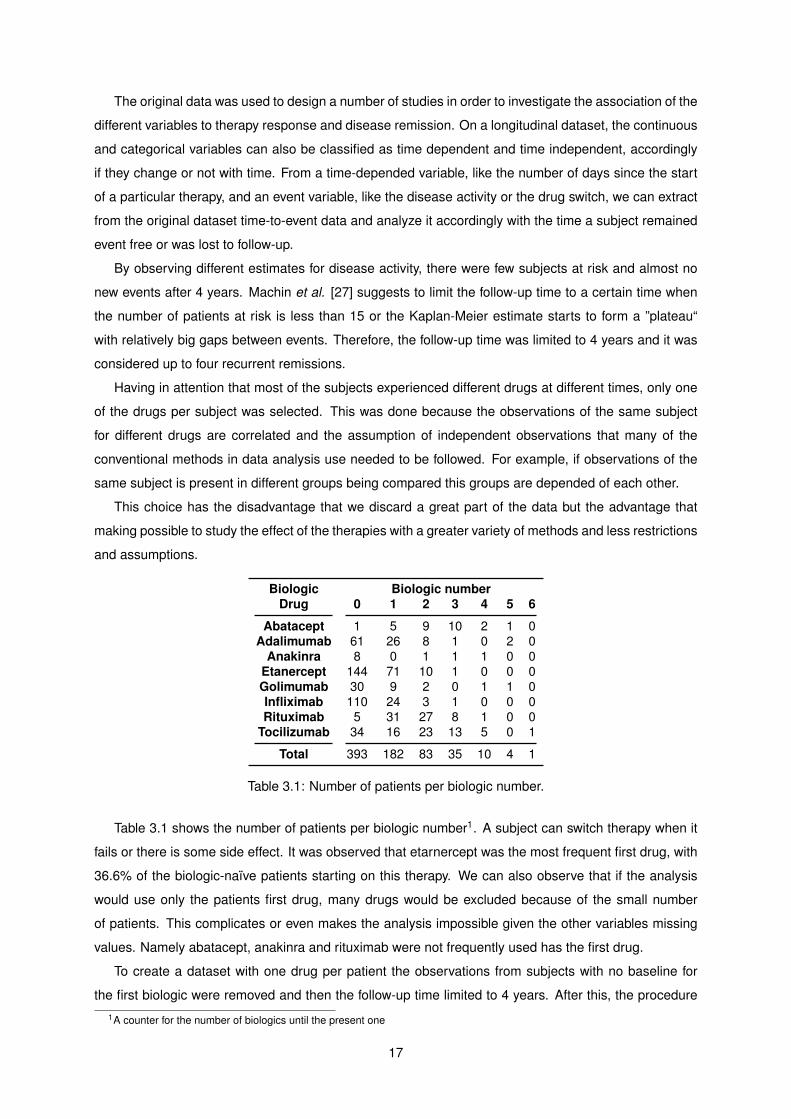
Table 3.1 shows the number of patients per biologic number1. A subject can switch therapy when it
fails or there is some side effect. It was observed that etarnercept was the most frequent first drug, with
36.6% of the biologic-naıve patients starting on this therapy. We can also observe that if the analysis
would use only the patients first drug, many drugs would be excluded because of the small number
of patients. This complicates or even makes the analysis impossible given the other variables missing
values. Namely abatacept, anakinra and rituximab were not frequently used has the first drug.
To create a dataset with one drug per patient the observations from subjects with no baseline for
the first biologic were removed and then the follow-up time limited to 4 years. After this, the procedure
1A counter for the number of biologics until the present one
17
consisted of picking the subjects from the less frequent drug to the more frequent drug without repetition
of subjects between drugs.
This dataset, cohort dataset, was used in all comparison between the drugs and consists of 394
subjects distributed by the different drugs accordingly with Table 3.2. It was named cohort dataset
because for each subject it was select only one of the therapies experienced by him and then they were
divided into groups/cohorts that share a particular drug exposure.
Table 3.2 shows the percentage and number of patients per drug on cohort dataset and we can
see that with this procedure the number of patients gets more evenly distributed across the different
therapies and makes possible the inclusion of the least frequent first drugs in the study. The number of
patients increases in comparison with Table 3.1 because a patient can be included in the analysis even
if he does not have baseline for the first drug.
Abatacept Adalimumab Anakinra Etanercept Golimumab Infliximab Rituximab Tocilizumab
6.35% (25) 16.50% (65) 2.54% (10) 23.86% (94) 8.88% (35) 14.72% (58) 14.21% (56) 12.94% (51)
Table 3.2: Percentage (number) of patients per drug in cohort dataset.
From this cohort dataset we extracted the information needed for the analysis of time to remission
(dataset A and dataset B), time to discontinuation and time to response. On these datasets the follow-
up time starts with the beginning of the subject biological therapy and ends when one of these events
happens or the subject is lost to follow-up. The current biologic number, a counter for the number of
biologic the patient experienced, was included as a covariate to control the effect of previous therapy
failures.
The criterion for remission was the index-based ACR/EULAR criterion for clinical trials, Table 2.2
(See page 10). The definitions of event for the time to response data was having at least moderate
response or at least good response, according to the EULAR response criteria, Table 2.3 (see page 11).
Dataset B characteristics are in all aspects similar to dataset A but the follow-up period was reduce
to just one year. In addition, dataset C was created and consists of time to remission data extracted
from the original data. In this dataset, each drug of each patient there is an observation for the time to
the first remission.
3.2 Methods
The main problems with longitudinal data are: the sample population might differ between the beginning
of the follow-up and the end of study, exists within-subject correlation of the observations and the time
varying variables might influence the effect of an exposure in time. On this chapter we list some methods
appropriate to deal with this problems given the data collected and review part of them.
The bulk of the theory on this section came from the books Fundamentals of Biostatistics [28] and
Survival Analysis a Practical Approach [27] and R packages documentation and vignettes. The analysis
of recurrent events was based on the theory presented on the book Modeling Survival Data - Extending
the Cox Model [29] and several articles [30, 31, 32, 33].
18
3.2.1 Smoothing
When scatterplots interpretation is troublesome, fitting the data can help visualization and interpretation.
Locally weighted scatterplot smoothing (LOWESS or LOESS) are methods that perform linear regres-
sions on local data subsets and then combine them to estimate overall smoothed trend of the dependent
variable. Each of this local subsets of data contains neighboring data points that are weighted according
to the distance to the ”center“ of that regression.
Kernel density estimation, is non-parametric way of estimating the probability density function of a
random variable sample and can be considered as a smoothed version of histograms. The method
consists of estimating a function for each histogram bin, sum all this functions and normalize the overall
result to obtain estimated probability density function.
On this work, both the kernel density estimation and LOESS were made using the methods of the
ggplot2 package. The kernels were Gaussian and the bandwidth and other parameters were found
using the default methods used in these implementations.
3.2.2 Summary measures
One of the simplest and most effective ways of analyzing longitudinal data is to combine the multiple
observations of each subject over time into a summary measure or several summary measures. The
data from each subject is this way reduced to a single observation and this can be used to compare the
response between groups. Typical summaries are the mean, the slope of a regression line, area under
the curve, maximum/minimum value and time to the maximum/minimum response.
For example, in analgesics drugs trials the total pain relief (TOTPAR) and the Sum of Pain Intensity
Difference (SPID) are used to summarize the treatment response over time. However, the area under
the curve, the minimum value and time to minimum value are no longer comparable if the subjects have
different follow-up times, like it happens with our data.
Inside these summaries measures we can also include time-to-event data but an alternative is to use
more traditional methods and compare cross-sectional statistics of different time points.
The limitation of this methods is that not all available information per subject is being used. However,
that also does not mean that methods that use more information will provide better results.
3.2.3 Measures of occurrence and association
Evaluations of the disease progression and therapy response are made at 3 months and 6 months after
the start of therapy, as stated by the EULAR/ACR guidelines for biological drugs and by the SPR as
well. A way of comparing the efficacy of each drug is by estimating the prevalence of remission for
each therapy at this time points. Prevalence is no more than the proportion of a population with some
condition at a particular time point or period. Prevalence is a common measure of occurrence used in
cross-sectional studies and can be used to describe prevalence’s odds ratio, absolute risk and relative
risks.
19
Different types of studies have different types of measures of occurrence and association. For ex-
ample in the case of cohort studies, a type of observational study, the proportion of events or risk is
the measures of occurrence used to calculate the relative risk, the ratio of risks between the exposed
groups. The problem with risks in our case is that it gives to all persons the same influence when the
amount of time at risk of the event to happen during the study period varies from person to person. Inci-
dence rate (or incidence density rate) can be thought of as a risk measure that incorporates differences
in subject follow-up times into the comparison. In general, incidence rates (IR) are the number of new
cases per number of person per time unit over the follow-up time.
IR =Number of events
Person-time at risk2 (3.1)
Equation 3.1 gives the estimator for IR. This equation assumes that the event rate is constant across
the entire follow-up time. For this reason. IR may be less meaningful if calculated for long time periods.
When a incidence rate varies over time is better to use hazard rates, which are kind of a ”instantaneous“
incidence rate. The hazard is the instantaneous probability (risk) of having and event among those who
are at risk of having the event at a given time in the follow-up time period, so, it can be interpreted as the
number of events per time unit.
The confidence interval (CI) is a range of plausible values for a parameter of interested, that depends
of a chosen significance level. The significance level determines how often the interval contains the true
value of the parameter of interest. In other words, for one hundred random samples of the same size,
the 100%(1-α) CI created will contain the true value of the parameter of interest 100(1-α) times.
Confidence limits for incidence rates are obtained for the expected number of events based on the
Poisson distribution and then divided by the total person-time at risk. For 10 events or more the it was
considered that the normal approximation to the Poisson distribution did hold (equation 3.2). For less
than 10 events were estimated the exact Poisson confidence limits that explore the relation between the
Chi-squared distribution and the Poisson distribution (Equation 3.3) [28, 34].
100%(1− α) CI = IR± Z1−α/2IR√N
(3.2)
100%(1− α) CI =(χ2
2N,α/2
2T,χ22(N+1),1−α/2
2T
)(3.3)
By assuming approximate normality for log of the incidence rate ratio (IRR) we can obtain the interval
estimates as follows in Equation 3.4. The IRR confidence interval gives a range of possible values for
the true incidence ratio for the population being compared by the two samples.
IRR 100%(1− α) CI = exp{
ln IRR± Z1−α/2
√1
N1+
1
N2
}(3.4)
Means comparisons of continuous variables that might not follow the Gaussian distribution can be done
by using the non-parametric Kruskal-Wallis rank sum test. On this kind of methods, the values are
2Sum of the amount of at risk time each person contributes.
20
ordered, a rank is assigned for each value and the mean ranks are compared. Because the ranks
are compared and not the values, rank sum methods are robust against outliers and unequal variance
between groups (heteroscedasticity). To compare proportions it was used the Pearson’s Chi-squared
test.
3.2.4 Kaplan-Meier estimator
The Kaplan-Meier (KM) method is non-parametric statistic of time-to-event data whose estimates can
be interpreted as the cumulative proportion of population at risk of experience the event or as probability
of staying event free in function of time. This method has special importance in epidemiology but is also
used many different areas, like failure analysis in engineering or econometrics. The KM is estimated
accordingly with equation 3.5, where N(t) is the number of persons at risk at time t and E(t) is the
number of events at time t.
S(t) =∏t
(N(t)− E(t)
N(t)
)=(N(t)− E(t)
N(t)
)S(t− 1) (3.5)
To measure association between KM estimates the most used process used is the non-parametric
method called log-rank test. Log-rank test compares the distance between two or more KM curves to
find a p-value for the null hypothesis that all survival curves are equal. The discrepancies between the
observed and expected event count are aggregated across all event times and standardized to form the
log-rank statistic χ2logrank that follows approximately a chi-squared distribution with number of KM curves
minus one degrees of freedom. The log-rank test tends to give more weight to discrepancies that occur
earlier compared to differences later, because there is more data around at that time. Other tests give
different weightings.
3.2.5 Cox Proportional Hazards Model
Cox Proportional Hazards (Cox PH) regression is semi-parametric linear model used in the analysis of
time-to-event data used for estimation, adjustment and prediction.
The proportional hazards (PH) assumption is better understood by examining the Cox regression
model in equation 3.6. On the left hand side of equation 3.6, we have the logarithm of the instantaneous
risk of having the event among those who are at risk of having the event at a given time in the follow-up
period (or log-hazard). On the right hand side, the baseline log-hazard function, ln λ0[t], is estimated
non-parametrically and can be seen as a time dependent intercept. This function determines the shape
of the log-hazard in time.
The covariates of a model can be continuous or categorical and the estimated coefficients can be
interpreted as the difference in log-hazard per unit difference in x at a given time t in the follow-up period,
given that all other x’s remain constant. By other words, the exponential of the coefficients is the hazard
ratio between two groups that differ by a single unit of x. The same applies for categorical variables
because they are included in the model as dummy variables, one for each group with exception of the
21
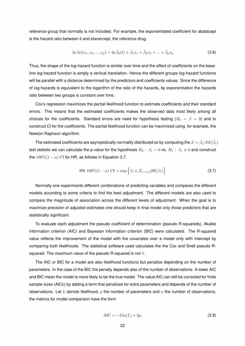
reference group that normally is not included. For example, the exponentiated coefficient for abatacept
is the hazard ratio between it and etanercept, the reference drug.
ln λ(t|x1, x2, ..., xp) = ln λ0(t) + β1x1 + β2x2 + ...+ βpxp (3.6)
Thus, the shape of the log-hazard function is similar over time and the effect of coefficients on the base-
line log-hazard function is simply a vertical translation. Hence the different groups log-hazard functions
will be parallel with a distance determined by the predictors and coefficients values. Since the difference
of log-hazards is equivalent to the logarithm of the ratio of the hazards, by exponentiation the hazards
ratio between two groups is constant over time.
Cox’s regression maximizes the partial likelihood function to estimate coefficients and their standard
errors. This means that the estimated coefficients makes the observed data most likely among all
choices for the coefficients. Standard errors are need for hypothesis testing (H0 = β = 0) and to
construct CI for the coefficients. The partial likelihood function can be maximized using, for example, the
Newton-Raphson algorithm.
The estimated coefficients are asymptotically normality distributed so by computing the Z = βi/SE(βi)
test statistic we can calculate the p-value for the hypothesis H0 : β1 = 0 vs. H1 : β1 6= 0 and construct
the 100%(1− α) CI for HR, as follows in Equation 3.7.
HR 100%(1− α) CI = exp{βi ± Z1−α/2SE(βi)
}(3.7)
Normally one experiments different combinations of predicting variables and compares the different
models according to some criteria to find the best adjustment. The different models are also used to
compare the magnitude of association across the different levels of adjustment. When the goal is to
maximize precision of adjusted estimates one should keep in final model only those predictors that are
statistically significant.
To evaluate each adjustment the pseudo coefficient of determination (pseudo R-squareds), Akaike
information criterion (AIC) and Bayesian information criterion (BIC) were calculated. The R-squared
value reflects the improvement of the model with the covariates over a model only with intercept by
comparing both likelihoods. The statistical software used calculates the the Cox and Snell pseudo R-
squared. The maximum value of the pseudo R-squared is not 1.
The AIC or BIC for a model are also likelihood functions but penalize depending on the number of
parameters. In the case of the BIC the penalty depends also of the number of observations. A lower AIC
and BIC mean the model is more likely to be the true model. The value AIC can still be corrected for finite
sample sizes (AICc) by adding a term that penalizes for extra parameters and depends of the number of
observations. Let L denote likelihood, p the number of parameters and n the number of observations,
the metrics for model comparison have the form
AIC = −2 ln(L) + 2p, (3.8)
22
AICc = AIC +2p(p+ 1)
(n− p− 1), (3.9)
BIC = −2 ln(L) + p lnn. (3.10)
Non-proportionality occurs when the relationship between the outcome and the continuous predictors
is not linear or the HR is not constant over time causing the shape of the hazards curves to be very
different or to cross between groups.
A way to assess PH is to plot the complementary log transformation, or log(− logS(t)), against log(t).
If the hazard rate does not change with time then plot will seem approximately linear. We did not present
this results because there was many strata and extract any information about this plots was difficult.
Another way to assess PH is to visualize or fit the scaled Schoenfeld residual [35] for each individual
and covariate. Schoenfeld residual ”are based on the individual contributions to the derivative of the log
partial likelihoo“ for a specific covariate [36].
Therefore, a significant regression slope coefficient for the fit of the residuals indicates that the true
HR changes over time and the PH assumption does not hold. This method is known as the Grambsch-
Therneau test of trend in Schoenfeld residuals and is available using the cox.zph function of the survival
package [35]. The Cox.zph function also allows for a global chi-square test for the model and provides
a correlation coefficient (r) between transformed survival time and the scaled Schoenfeld residuals to
assess if the HR are increasing or decreasing over time.
In case of non-proportionality for a continuous predictor, we can categorize the concerned predictors.
Some authors state that when the PH assumption is not met we can interpret the Cox PH results as the
average HR over the follow-up time [27, 35].
Cox PH model has different extension to allow for time-dependent variables, stratified analysis and
clustered data. Time-dependent variables can be introduced by adding an interaction term between one
of the covariates and a function of time, normally ln t or by having multiple observations per subject
with corresponding time at risk for each value. A stratified Cox model fits a separate baseline hazard
functions for each strata. For this reason the the partial likelihood functions for each strata depends
only on the observations for each strata. After the maximization of the partial likelihood the effect of the
strata is removed without making the assumption of proportional hazards. This is particularly useful if
the stratifying variable does not follow this assumption but it is not useful if the effects of this variable are
of scientific interest, like the case of the biological therapies.
Statistical independence of the observations is a important assumption that needs to be present for
most statistical methods. The independence assumption is violated when some observations are more
similar to each other than from other observations. By adding a cluster term to the Cox regression
model the correlated observations are identified as belonging to a particular cluster. Each cluster forms
a stratum and the model considers that the observations are conditional independent within the clusters.
The coefficients are estimated assuming independence within cluster and the variance is estimated
using robust sandwich variance estimators. This method corrects the variance estimation assuming
correlation between different observations but does not correct the estimate of the coefficients.
23
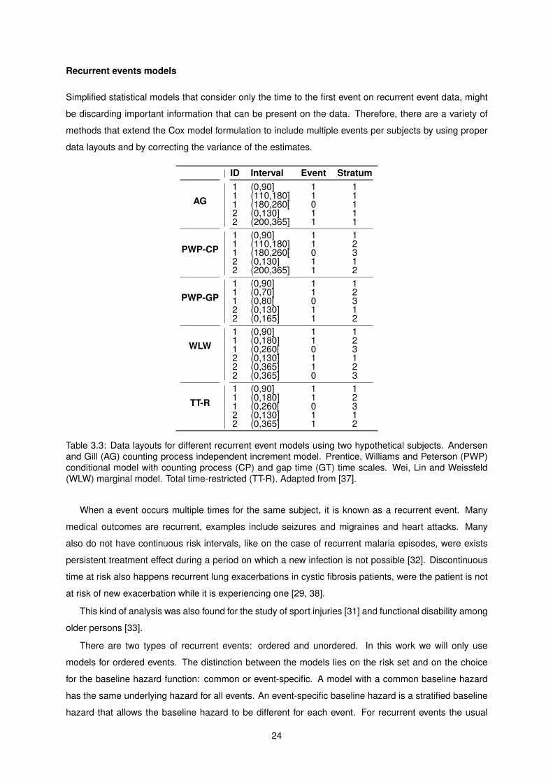
Recurrent events models
Simplified statistical models that consider only the time to the first event on recurrent event data, might
be discarding important information that can be present on the data. Therefore, there are a variety of
methods that extend the Cox model formulation to include multiple events per subjects by using proper
data layouts and by correcting the variance of the estimates.
ID Interval Event Stratum
AG1 (0,90] 1 11 (110,180] 1 11 (180,260[ 0 12 (0,130] 1 12 (200,365] 1 1
PWP-CP1 (0,90] 1 11 (110,180] 1 21 (180,260[ 0 32 (0,130] 1 12 (200,365] 1 2
PWP-GP1 (0,90] 1 11 (0,70] 1 21 (0,80[ 0 32 (0,130] 1 12 (0,165] 1 2
WLW1 (0,90] 1 11 (0,180] 1 21 (0,260[ 0 32 (0,130] 1 12 (0,365] 1 22 (0,365] 0 3
TT-R1 (0,90] 1 11 (0,180] 1 21 (0,260[ 0 32 (0,130] 1 12 (0,365] 1 2
Table 3.3: Data layouts for different recurrent event models using two hypothetical subjects. Andersenand Gill (AG) counting process independent increment model. Prentice, Williams and Peterson (PWP)conditional model with counting process (CP) and gap time (GT) time scales. Wei, Lin and Weissfeld(WLW) marginal model. Total time-restricted (TT-R). Adapted from [37].
When a event occurs multiple times for the same subject, it is known as a recurrent event. Many
medical outcomes are recurrent, examples include seizures and migraines and heart attacks. Many
also do not have continuous risk intervals, like on the case of recurrent malaria episodes, were exists
persistent treatment effect during a period on which a new infection is not possible [32]. Discontinuous
time at risk also happens recurrent lung exacerbations in cystic fibrosis patients, were the patient is not
at risk of new exacerbation while it is experiencing one [29, 38].
This kind of analysis was also found for the study of sport injuries [31] and functional disability among
older persons [33].
There are two types of recurrent events: ordered and unordered. In this work we will only use
models for ordered events. The distinction between the models lies on the risk set and on the choice
for the baseline hazard function: common or event-specific. A model with a common baseline hazard
has the same underlying hazard for all events. An event-specific baseline hazard is a stratified baseline
hazard that allows the baseline hazard to be different for each event. For recurrent events the usual
24
approaches to generalize the Cox’s framework model are on Table 3.3.
Andersen and Gill (AG) [39] model breaks the follow-up time into segments defined by the events
and has a common baseline hazard for all events. This model treat the events as being independent
because does not differentiate between the first and subsequent events.
Prentice, Williams and Peterson (PWP) [40] model is called conditional because a subject is assumed
not to be at risk for the next events until the prior events have occurred. The stratum variable keeps track
of the event number. For this model is possible to have two different time scales: the counting process
(CP) and gap time (GT) time scales. Gap time scale corresponds to the time since entry or last event.
Wei, Lin, Weissfeld (WLW) [41] model each event is considered as separated process. All subjects
are considered at risk for all events, regardless of how many events they actually experience. For
this reason the number of observations per subject depends of the maximum of events a subject has
experienced in the dataset.
Total Time-Restricted (TT-R) [42] is a model similar to the WLW. This model uses the same intervals
as WLW, but deletes the strata for which no additional follow up time is added.
On this models the coefficients are estimated ignoring the existing correlation between the events and
the correction for the dependency is done by estimating a corrected variance, similar to the sandwich
estimator. As well as in single-event Cox regression, censoring must be independent of the events. In
our case time at risk is discontinuous because makes no sense that while on remission periods the
subjects are at risk of being in remission.
3.3 Data Analysis
A research project normally consists of five phases: the planning/design of the study, data collection,
data analysis, presentation, interpretation and discussion of the results. This thesis is concerned with
analyzing the data, interpret it and discussion of the results. The role of data analysis or statistics is to
learn the characteristics of a population via samples collected and analyzed so that true characteristics
of the data are observable.
During this work, the central tendency of continuous data was expressed as means. When is ex-
pected that the variables not follow a Gaussian distribution it was used the median. The dispersion
tendency was measured by the standard deviation or by the first and third quartile.
Categorical data is expressed by absolute and relative frequencies distributions and Kaplan–Meier
survival analysis was used to assess the proportion of subjects that remain event/outcome free.
All comparisons of groups were done using the Kruskal-Wallis rank sum test, a non-parametric test
that allows for variables that do not follow a Gaussian distribution. Comparison of proportions was made
with Pearson’s Chi-squared test.
Cox multivariate regression models were used to assess potential predictors of remission, adjust for
confounding variables and estimate hazards ratios.
There was no data imputation and when comparing models it was always used the dataset defined
by the complete cases of covariates of the larger model.
25
Categorical variables where recategorized when necessary because of the small number counts and
continuous variables were categorized when necessary to stratify the analysis or when the proportional
hazard assumption was not met.
The significance level (α) used in this work was 0.05 (5%) calculated with two-sided tests. This
means that for samples of the same size drawn from the same population the chance of finding estimates
outside the CI is 5 in 100. When relevant the 95% CI were calculated.
All statistical analysis in this work was conducted with the use of the statistical software R [43]. The
dplyr package helped with the data processing and most of the figures and tables were made using
ggplot2 and xtable package, respectively [44, 45, 46]. The survival analysis was performed using R’s
survival package [47, 29].
3.3.1 Descriptive analysis
The first part of descriptive analysis used the original data set. It was given focus to rare occurrences that
would be difficult to study or include in a model. Textual description of those and other observations was
made. The different combinations of DMARDs, anatomical distribution of the affected joints at baseline
were also some of the results extracted from the original data set.
Cohort dataset was the source for Table 4.1, used to compare across the multiple cohorts baseline
values. Mean smooth estimates and kernel density estimates for the evolution of the disease activity
were also produced for each drug as well as boxplots for the duration of each therapy.
3.3.2 Summary measures analysis
On the summary analysis, each one of the subjects DAS28’s evolution over time was fitted with a simple
linear model and then the mean and 95% CI of the slope and p-values was presented. It were only used
observations from the first 6 months to take advantage of the approximate linearity of the period after
the start of the drug.
3.3.3 Incidence density rates
IR and IRR with 95% CI were calculated for dataset A, time to drug discontinuation and time to response
data. Then, the data was stratified by drug and other factors to investigate for possible interactions with
the therapies.
3.3.4 Kaplan-Meier estimates
Kaplan-Meier estimates for the therapies were presented using dataset A along with the result from the
log-rank test for this estimates. The same was made for the comparison of biologic agents persistence.
In some articles this kind if analysis is also called ”drug survival“ or medication persistence. Drug
persistence is defined as ”the duration of time from initiation to discontinuation of therapy´´ [48] and is
an overall marker of the success of a treatment and depends on the efficacy of the drug, its side effects
26
and doctor and patient preferences. Remission was defined using the ACR/EULAR remission criteria
for clinical trials.
Nevertheless, because there are many different therapies and other factors of interest that should be
investigated, a regression method is more appropriate than KM estimates.
3.3.5 Cox proportional hazards regression
In this work Cox proportional hazards regressions were used to assess potential predictors of remis-
sion and adjust for confounding variables. Another advantage of having one drug per subject (cohort
dataset) is that the KM estimates and the Cox regressions come from the same data.
With the regression models were investigated the following variables: biological therapy, sex, age,
weight at baseline, height, body mass index, alcohol, smoking, race, years of education, age of onset,
DAS28 at baseline, SDAI at baseline, time since onset, season, DMARD therapy, GCs therapy, extra ar-
ticular manifestations, patient VAS evaluation, physician VAS evaluation, pain VAS evaluation, HAQ, ery-
throcytes sedimentation rate, reactive C-protein, rheumatoid factor, anti-CCP, number of swollen joints,
number of tender joints, erosive and biologic number.
The rest of the variables were excluded because of the number of missing values, were redundant,
monotonous in some of the therapies or to keep the number of variables in the models relatively small
comparing to the number of observations. For example, the indicator for each of the HAQ questions or
for each one the joints was not used, just the resulting values for the score and count.
The estimated hazard ratios and 95% confidence intervals, provide adjustment for potential system-
atic differences between our therapy groups (confounding factors) and identify risk factors for decrease
of therapy efficacy.
Model selection
First, the unadjusted HR of each candidate covariates was estimated with on univariate Cox model.
Second, the non-statistically significant covariates for a level of 10% were discarded and the remaining
were included on a multivariate Cox model. Third, it was used backward elimination, eliminating always
the least significant variable. Finally, the models were compared according to the AIC, BIC and R2
scores. All the models, univariate and multivariate, were also tested for proportional hazards using
Grambsch-Therneau test of trend in Schoenfeld residuals.
The second method for model selection consisted of including 25 of the most relevant variables in
the model and subsequently remove the one of the variables according with four different criteria. It was
only used 25 variables because of the missing values. The first criterion was the same as previous one:
remove the least significant variable. The three other criteria consisted of removing the the variable that
will produce the best model according with a measures of quality of the statistical models used for model
selection (AIC, AICc and BIC). The therapy variable was forcibly kept in the models even if removing it
would produce a better model.
These 25 variables were: therapy, sex, descent, disease duration, weight, height, season, age RA
27
onset, erosive indicator, ESR, CRP, RF, age, SJC, TJC, extra articular manifestations, patient VAS, pain
VAS, doctor VAS, DAS28, SDAI, HAQ, years of education, DMARD(s) indicator and biologic number.
Recurrent event analysis
The recurrent event analysis was performed using the Andersen and Gill (AG) counting process inde-
pendent increment model, the Prentice, Williams and Peterson (PWP) conditional model with counting
process (CP) and gap time (GT) time scales, the Wei, Lin and Weissfeld (WLW) marginal model and the
total time-restricted (TT-R). The covariates used were the ones from the first model of the second model
selection method for the first event Cox regression (Method 2) and the comparison of models was made
with the same metrics.
28
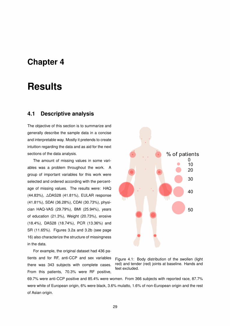
Chapter 4
Results
4.1 Descriptive analysis
Figure 4.1: Body distribution of the swollen (lightred) and tender (red) joints at baseline. Hands andfeet excluded.
The objective of this section is to summarize and
generally describe the sample data in a concise
and interpretable way. Mostly it pretends to create
intuition regarding the data and as aid for the next
sections of the data analysis.
The amount of missing values in some vari-
ables was a problem throughout the work. A
group of important variables for this work were
selected and ordered according with the percent-
age of missing values. The results were: HAQ
(44.83%), ∆DAS28 (41.81%), EULAR response
(41.81%), SDAI (36.28%), CDAI (30.73%), physi-
cian HAQ-VAS (29.79%), BMI (25.94%), years
of education (21.3%), Weight (20.73%), erosive
(18.4%), DAS28 (18.74%), PCR (13.36%) and
SR (11.65%). Figures 3.2a and 3.2b (see page
16) also characterize the structure of missingness
in the data.
For example, the original dataset had 436 pa-
tients and for RF, anti-CCP and sex variables
there was 343 subjects with complete cases.
From this patients, 70.3% were RF positive,
69.7% were anti-CCP positive and 85.4% were women. From 366 subjects with reported race, 87.7%
were white of European origin, 6% were black, 3.6% mulatto, 1.6% of non-European origin and the rest
of Asian origin.
29
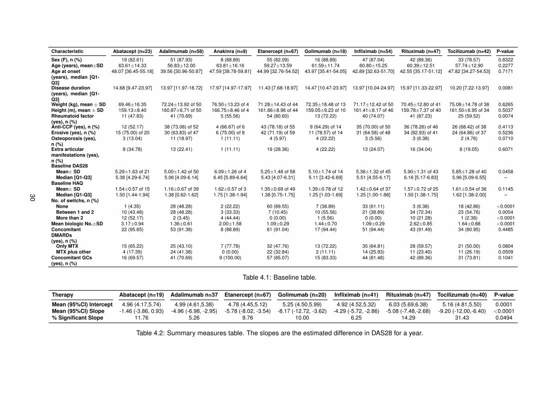
Characteristic Abatacept (n=23) Adalimumab (n=58) Anakinra (n=9) Etanercept (n=67) Golimumab (n=18) Infliximab (n=54) Rituximab (n=47) Tocilizumab (n=42) P-value
Sex (F), n (%) 19 (82.61) 51 (87.93) 8 (88.89) 55 (82.09) 16 (88.89) 47 (87.04) 42 (89.36) 33 (78.57) 0.8322Age (years), mean±SD 63.61±14.33 56.83±12.00 63.81±16.16 59.27±13.59 61.59±11.74 60.80±15.25 60.39±12.51 57.74±12.90 0.2277Age at onset(years), median [Q1-Q3]
48.07 [36.45-55.18] 39.56 [30.96-50.87] 47.59 [38.78-59.81] 44.99 [32.76-54.52] 43.97 [35.41-54.05] 42.89 [32.63-51.70] 42.55 [35.17-51.12] 47.82 [34.27-54.53] 0.7171
Disease duration(years), median [Q1-Q3]
14.68 [9.47-23.97] 13.97 [11.97-18.72] 17.97 [14.97-17.97] 11.43 [7.68-18.97] 14.47 [10.47-23.97] 13.97 [10.04-24.97] 15.97 [11.33-22.97] 10.20 [7.22-13.97] 0.0081
Weight (kg), mean ± SD 69.46±16.35 72.24±13.92 of 50 76.50±13.23 of 4 71.28±14.43 of 44 72.35±18.48 of 13 71.17±12.42 of 50 70.45±12.80 of 41 75.08±14.78 of 38 0.6265Height (m), mean ± SD 159.13±8.40 160.87±6.71 of 50 166.75±8.46 of 4 161.86±8.96 of 44 159.05±9.23 of 10 161.41±8.17 of 46 159.78±7.37 of 40 161.50±6.95 of 34 0.5037Rheumatoid factor(yes), n (%)
11 (47.83) 41 (70.69) 5 (55.56) 54 (80.60) 13 (72.22) 40 (74.07) 41 (87.23) 25 (59.52) 0.0074
Anti-CCP (yes), n (%) 12 (52.17) 38 (73.08) of 52 4 (66.67) of 6 43 (78.18) of 55 9 (64.29) of 14 35 (70.00) of 50 36 (78.26) of 46 26 (68.42) of 38 0.4113Erosive (yes), n (%) 15 (75.00) of 20 30 (63.83) of 47 6 (75.00) of 8 42 (71.19) of 59 11 (78.57) of 14 31 (64.58) of 48 34 (82.93) of 41 24 (64.86) of 37 0.5236Osteoporosis (yes),n (%)
3 (13.04) 11 (18.97) 1 (11.11) 4 (5.97) 4 (22.22) 3 (5.56) 3 (6.38) 2 (4.76) 0.0710
Extra articularmanifestations (yes),n (%)
8 (34.78) 13 (22.41) 1 (11.11) 19 (28.36) 4 (22.22) 13 (24.07) 16 (34.04) 8 (19.05) 0.6071
Baseline DAS28Mean± SD 5.29±1.63 of 21 5.00±1.42 of 50 6.09±1.26 of 4 5.25±1.48 of 58 5.10±1.74 of 14 5.36±1.32 of 45 5.90±1.31 of 43 5.85±1.28 of 40 0.0458Median [Q1-Q3] 5.38 [4.29-6.74] 5.06 [4.09-6.14] 6.45 [5.89-6.64] 5.43 [4.07-6.31] 5.11 [3.42-6.69] 5.51 [4.55-6.17] 6.16 [5.17-6.83] 5.96 [5.09-6.55] –
Baseline HAQMean± SD 1.54±0.57 of 15 1.16±0.67 of 39 1.62±0.57 of 3 1.35±0.69 of 49 1.39±0.78 of 12 1.42±0.64 of 37 1.57±0.72 of 25 1.61±0.54 of 36 0.1145Median [Q1-Q3] 1.50 [1.44-1.94] 1.38 [0.62-1.62] 1.75 [1.38-1.94] 1.38 [0.75-1.75] 1.25 [1.03-1.69] 1.25 [1.00-1.88] 1.50 [1.38-1.75] 1.62 [1.38-2.00] –
No. of switchs, n (%)None 1 (4.35) 28 (48.28) 2 (22.22) 60 (89.55) 7 (38.89) 33 (61.11) 3 (6.38) 18 (42.86) <0.0001Between 1 and 2 10 (43.48) 28 (48.28) 3 (33.33) 7 (10.45) 10 (55.56) 21 (38.89) 34 (72.34) 23 (54.76) 0.0054More than 2 12 (52.17) 2 (3.45) 4 (44.44) 0 (0.00) 1 (5.56) 0 (0.00) 10 (21.28) 1 (2.38) <0.0001
Mean biologic No.±SD 3.17±0.94 1.36±0.61 2.00±1.58 1.09±0.29 1.44±0.70 1.09±0.29 2.62±0.85 1.64±0.88 <0.0001ConcomitantDMARDs(yes), n (%)
22 (95.65) 53 (91.38) 8 (88.89) 61 (91.04) 17 (94.44) 51 (94.44) 43 (91.49) 34 (80.95) 0.4485
Only MTX 15 (65.22) 25 (43.10) 7 (77.78) 32 (47.76) 13 (72.22) 35 (64.81) 28 (59.57) 21 (50.00) 0.0804MTX plus other 4 (17.39) 24 (41.38) 0 (0.00) 22 (32.84) 2 (11.11) 14 (25.93) 11 (23.40) 11 (26.19) 0.0509
Concomitant GCs(yes), n (%)
16 (69.57) 41 (70.69) 9 (100.00) 57 (85.07) 15 (83.33) 44 (81.48) 42 (89.36) 31 (73.81) 0.1041
Table 4.1: Baseline table.
Therapy Abatacept (n=19) Adalimumab n=37 Etanercept (n=67) Golimumab (n=20) Infliximab (n=41) Rituximab (n=47) Tocilizumab (n=40) P-value
Mean (95%CI) Intercept 4.96 (4.17,5.74) 4.99 (4.61,5.38) 4.78 (4.45,5.12) 5.25 (4.50,5.99) 4.92 (4.52,5.32) 6.03 (5.69,6.38) 5.16 (4.81,5.50) 0.0001Mean (95%CI) Slope -1.46 (-3.86, 0.93) -4.96 (-6.98, -2.95) -5.78 (-8.02, -3.54) -8.17 (-12.72, -3.62) -4.29 (-5.72, -2.86) -5.08 (-7.48,-2.68) -9.20 (-12.00,-6.40) <0.0001% Significant Slope 11.76 5.26 9.76 10.00 6.25 14.29 31.43 0.0494
Table 4.2: Summary measures table. The slopes are the estimated difference in DAS28 for a year.
30
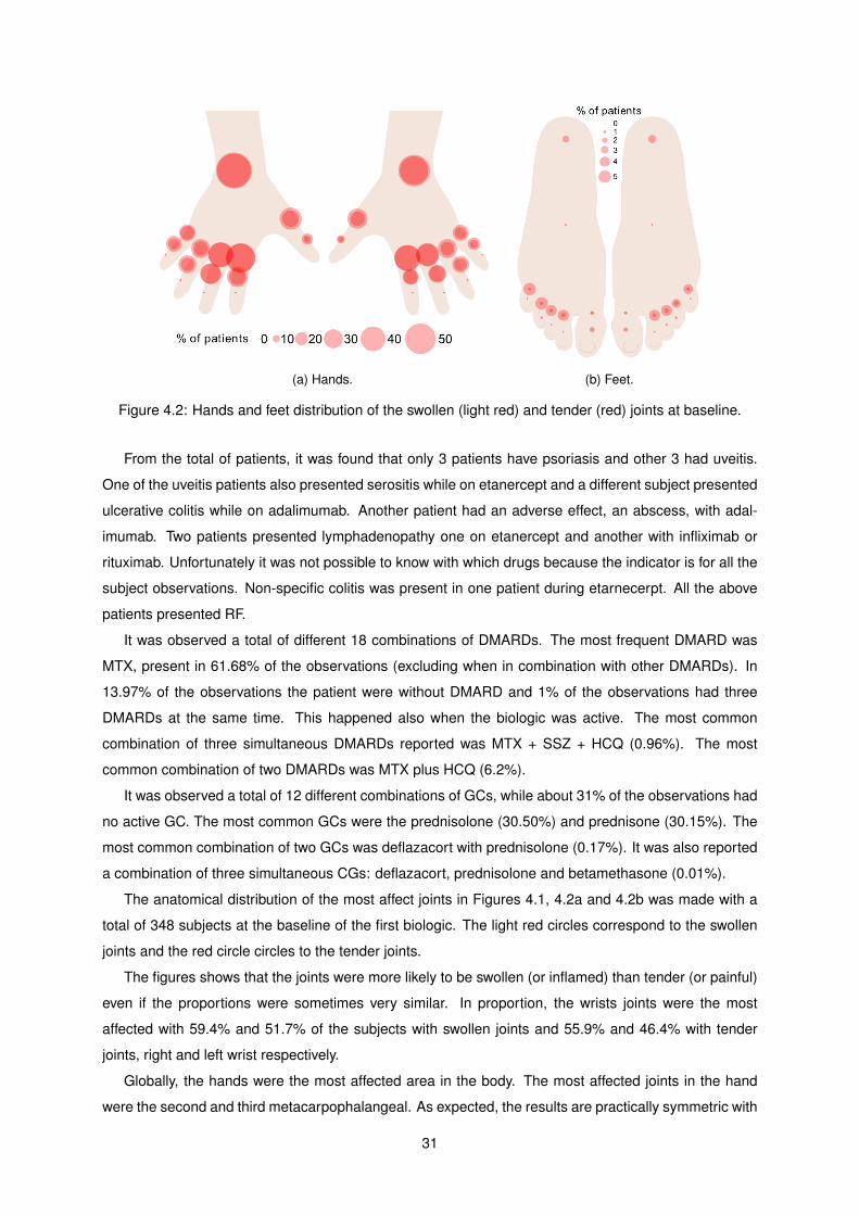
(a) Hands. (b) Feet.
Figure 4.2: Hands and feet distribution of the swollen (light red) and tender (red) joints at baseline.
From the total of patients, it was found that only 3 patients have psoriasis and other 3 had uveitis.
One of the uveitis patients also presented serositis while on etanercept and a different subject presented
ulcerative colitis while on adalimumab. Another patient had an adverse effect, an abscess, with adal-
imumab. Two patients presented lymphadenopathy one on etanercept and another with infliximab or
rituximab. Unfortunately it was not possible to know with which drugs because the indicator is for all the
subject observations. Non-specific colitis was present in one patient during etarnecerpt. All the above
patients presented RF.
It was observed a total of different 18 combinations of DMARDs. The most frequent DMARD was
MTX, present in 61.68% of the observations (excluding when in combination with other DMARDs). In
13.97% of the observations the patient were without DMARD and 1% of the observations had three
DMARDs at the same time. This happened also when the biologic was active. The most common
combination of three simultaneous DMARDs reported was MTX + SSZ + HCQ (0.96%). The most
common combination of two DMARDs was MTX plus HCQ (6.2%).
It was observed a total of 12 different combinations of GCs, while about 31% of the observations had
no active GC. The most common GCs were the prednisolone (30.50%) and prednisone (30.15%). The
most common combination of two GCs was deflazacort with prednisolone (0.17%). It was also reported
a combination of three simultaneous CGs: deflazacort, prednisolone and betamethasone (0.01%).
The anatomical distribution of the most affect joints in Figures 4.1, 4.2a and 4.2b was made with a
total of 348 subjects at the baseline of the first biologic. The light red circles correspond to the swollen
joints and the red circle circles to the tender joints.
The figures shows that the joints were more likely to be swollen (or inflamed) than tender (or painful)
even if the proportions were sometimes very similar. In proportion, the wrists joints were the most
affected with 59.4% and 51.7% of the subjects with swollen joints and 55.9% and 46.4% with tender
joints, right and left wrist respectively.
Globally, the hands were the most affected area in the body. The most affected joints in the hand
were the second and third metacarpophalangeal. As expected, the results are practically symmetric with
31
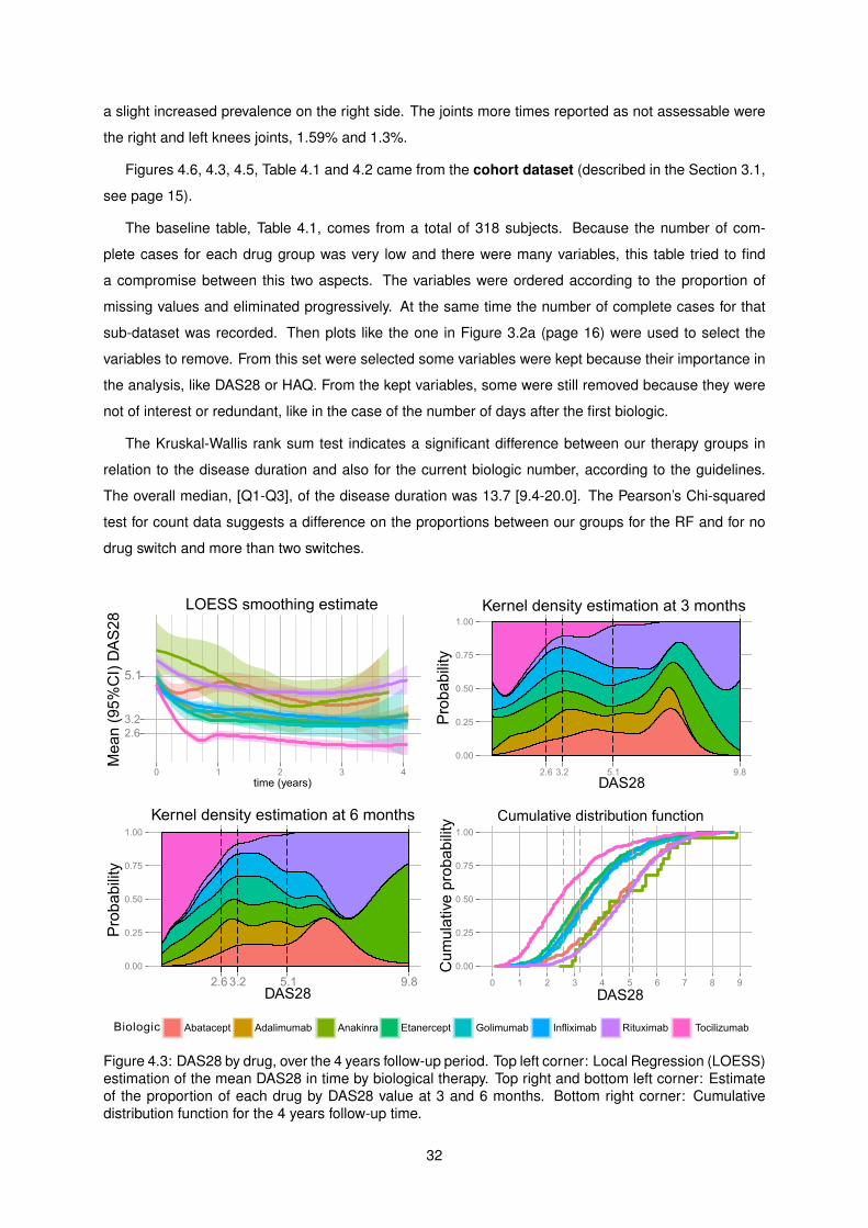
a slight increased prevalence on the right side. The joints more times reported as not assessable were
the right and left knees joints, 1.59% and 1.3%.
Figures 4.6, 4.3, 4.5, Table 4.1 and 4.2 came from the cohort dataset (described in the Section 3.1,
see page 15).
The baseline table, Table 4.1, comes from a total of 318 subjects. Because the number of com-
plete cases for each drug group was very low and there were many variables, this table tried to find
a compromise between this two aspects. The variables were ordered according to the proportion of
missing values and eliminated progressively. At the same time the number of complete cases for that
sub-dataset was recorded. Then plots like the one in Figure 3.2a (page 16) were used to select the
variables to remove. From this set were selected some variables were kept because their importance in
the analysis, like DAS28 or HAQ. From the kept variables, some were still removed because they were
not of interest or redundant, like in the case of the number of days after the first biologic.
The Kruskal-Wallis rank sum test indicates a significant difference between our therapy groups in
relation to the disease duration and also for the current biologic number, according to the guidelines.
The overall median, [Q1-Q3], of the disease duration was 13.7 [9.4-20.0]. The Pearson’s Chi-squared
test for count data suggests a difference on the proportions between our groups for the RF and for no
drug switch and more than two switches.
Figure 4.3: DAS28 by drug, over the 4 years follow-up period. Top left corner: Local Regression (LOESS)estimation of the mean DAS28 in time by biological therapy. Top right and bottom left corner: Estimateof the proportion of each drug by DAS28 value at 3 and 6 months. Bottom right corner: Cumulativedistribution function for the 4 years follow-up time.
32
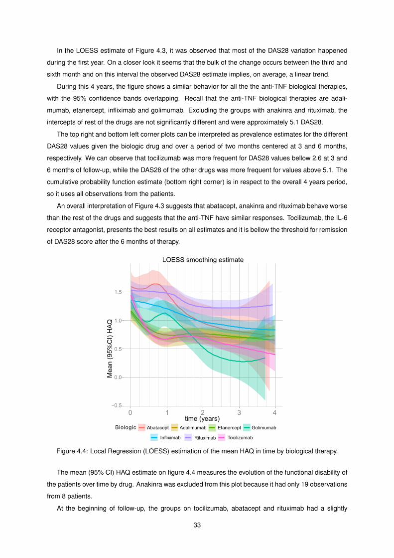
In the LOESS estimate of Figure 4.3, it was observed that most of the DAS28 variation happened
during the first year. On a closer look it seems that the bulk of the change occurs between the third and
sixth month and on this interval the observed DAS28 estimate implies, on average, a linear trend.
During this 4 years, the figure shows a similar behavior for all the the anti-TNF biological therapies,
with the 95% confidence bands overlapping. Recall that the anti-TNF biological therapies are adali-
mumab, etanercept, infliximab and golimumab. Excluding the groups with anakinra and rituximab, the
intercepts of rest of the drugs are not significantly different and were approximately 5.1 DAS28.
The top right and bottom left corner plots can be interpreted as prevalence estimates for the different
DAS28 values given the biologic drug and over a period of two months centered at 3 and 6 months,
respectively. We can observe that tocilizumab was more frequent for DAS28 values bellow 2.6 at 3 and
6 months of follow-up, while the DAS28 of the other drugs was more frequent for values above 5.1. The
cumulative probability function estimate (bottom right corner) is in respect to the overall 4 years period,
so it uses all observations from the patients.
An overall interpretation of Figure 4.3 suggests that abatacept, anakinra and rituximab behave worse
than the rest of the drugs and suggests that the anti-TNF have similar responses. Tocilizumab, the IL-6
receptor antagonist, presents the best results on all estimates and it is bellow the threshold for remission
of DAS28 score after the 6 months of therapy.
Figure 4.4: Local Regression (LOESS) estimation of the mean HAQ in time by biological therapy.
The mean (95% CI) HAQ estimate on figure 4.4 measures the evolution of the functional disability of
the patients over time by drug. Anakinra was excluded from this plot because it had only 19 observations
from 8 patients.
At the beginning of follow-up, the groups on tocilizumab, abatacept and rituximab had a slightly
33
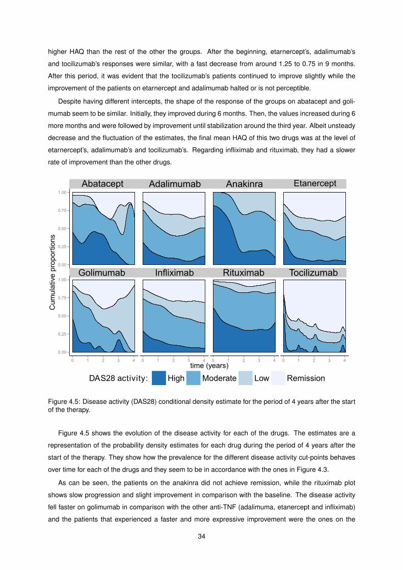
higher HAQ than the rest of the other the groups. After the beginning, etarnercept’s, adalimumab’s
and tocilizumab’s responses were similar, with a fast decrease from around 1.25 to 0.75 in 9 months.
After this period, it was evident that the tocilizumab’s patients continued to improve slightly while the
improvement of the patients on etarnercept and adalimumab halted or is not perceptible.
Despite having different intercepts, the shape of the response of the groups on abatacept and goli-
mumab seem to be similar. Initially, they improved during 6 months. Then, the values increased during 6
more months and were followed by improvement until stabilization around the third year. Albeit unsteady
decrease and the fluctuation of the estimates, the final mean HAQ of this two drugs was at the level of
etarnercept’s, adalimumab’s and tocilizumab’s. Regarding infliximab and rituximab, they had a slower
rate of improvement than the other drugs.
Figure 4.5: Disease activity (DAS28) conditional density estimate for the period of 4 years after the startof the therapy.
Figure 4.5 shows the evolution of the disease activity for each of the drugs. The estimates are a
representation of the probability density estimates for each drug during the period of 4 years after the
start of the therapy. They show how the prevalence for the different disease activity cut-points behaves
over time for each of the drugs and they seem to be in accordance with the ones in Figure 4.3.
As can be seen, the patients on the anakinra did not achieve remission, while the rituximab plot
shows slow progression and slight improvement in comparison with the baseline. The disease activity
fell faster on golimumab in comparison with the other anti-TNF (adalimuma, etanercept and infliximab)
and the patients that experienced a faster and more expressive improvement were the ones on the
34
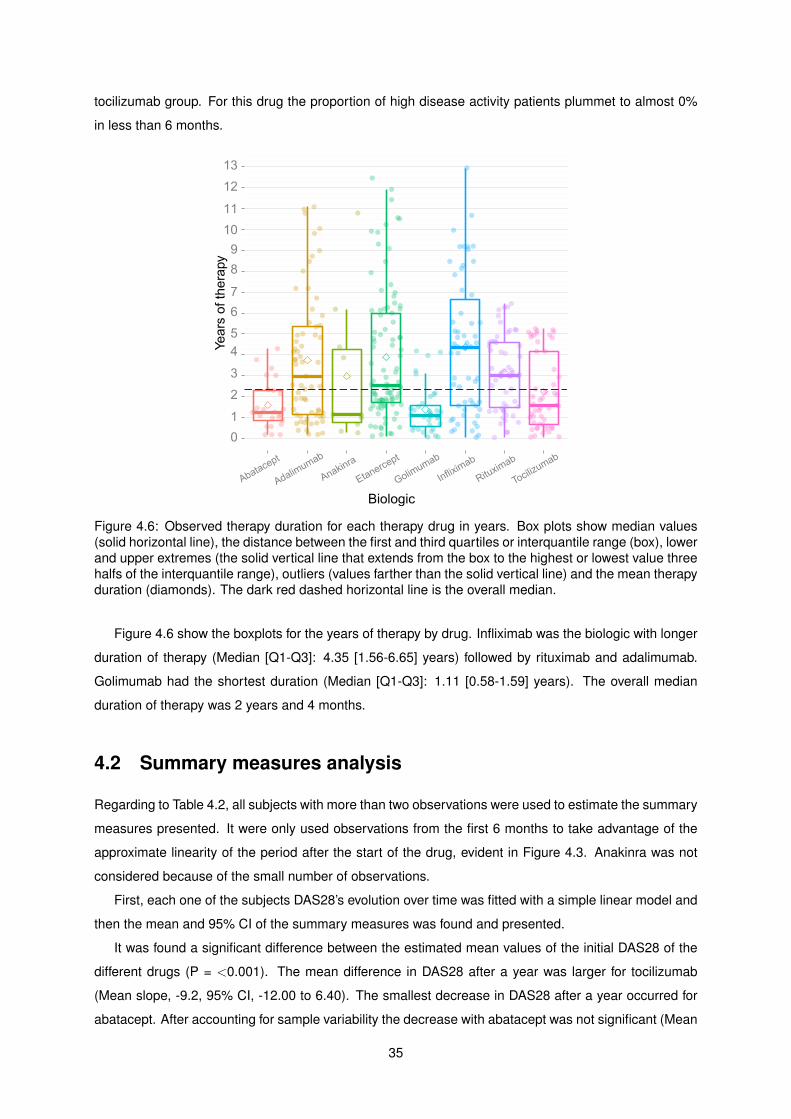
tocilizumab group. For this drug the proportion of high disease activity patients plummet to almost 0%
in less than 6 months.
Figure 4.6: Observed therapy duration for each therapy drug in years. Box plots show median values(solid horizontal line), the distance between the first and third quartiles or interquantile range (box), lowerand upper extremes (the solid vertical line that extends from the box to the highest or lowest value threehalfs of the interquantile range), outliers (values farther than the solid vertical line) and the mean therapyduration (diamonds). The dark red dashed horizontal line is the overall median.
Figure 4.6 show the boxplots for the years of therapy by drug. Infliximab was the biologic with longer
duration of therapy (Median [Q1-Q3]: 4.35 [1.56-6.65] years) followed by rituximab and adalimumab.
Golimumab had the shortest duration (Median [Q1-Q3]: 1.11 [0.58-1.59] years). The overall median
duration of therapy was 2 years and 4 months.
4.2 Summary measures analysis
Regarding to Table 4.2, all subjects with more than two observations were used to estimate the summary
measures presented. It were only used observations from the first 6 months to take advantage of the
approximate linearity of the period after the start of the drug, evident in Figure 4.3. Anakinra was not
considered because of the small number of observations.
First, each one of the subjects DAS28’s evolution over time was fitted with a simple linear model and
then the mean and 95% CI of the summary measures was found and presented.
It was found a significant difference between the estimated mean values of the initial DAS28 of the
different drugs (P = <0.001). The mean difference in DAS28 after a year was larger for tocilizumab
(Mean slope, -9.2, 95% CI, -12.00 to 6.40). The smallest decrease in DAS28 after a year occurred for
abatacept. After accounting for sample variability the decrease with abatacept was not significant (Mean
35
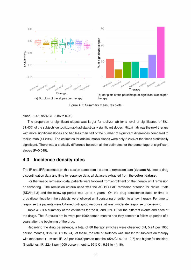
(a) Boxplots of the slopes per therapy.(b) Bar plots of the percentage of significant slopes pertherapy.
Figure 4.7: Summary measures plots.
slope, -1.46, 95% CI, -3.86 to 0.93).
The proportion of significant slopes was larger for tocilizumab for a level of significance of 5%.
31.43% of the subjects on tocilizumab had statistically significant slopes. Rituximab was the next therapy
with more significant slopes and had less than half of the number of significant differences compared to
tocilizumab (14.29%). The estimates for adalimumab’s slopes were only 5.26% of the times statistically
significant. There was a statically difference between all the estimates for the percentage of significant
slopes (P=0.049).
4.3 Incidence density rates
The IR and IRR estimates on this section came from the time to remission data (dataset A), time to drug
discontinuation data and time to response data, all datasets extracted from the cohort dataset.
For the time to remission data, patients were followed from enrollment on the therapy until remission
or censoring. The remission criteria used was the ACR/EULAR remission criterion for clinical trials
(SDAI≤3.3) and the follow-up period was up to 4 years. On the drug persistence data, or time to
drug discontinuation, the subjects were followed until censoring or switch to a new therapy. For time to
response the patients were followed until good response, at least moderate response or censoring.
Table 4.3 is a summary of the estimates for the IR and 95% CI for the different events and each of
the drugs. The IR results are in event per 1000 person-months and they concern a follow-up period of 4
years after the beginning of the drug.
Regarding the drug persistence, a total of 80 therapy switches were observed (IR, 5.24 per 1000
person-months, 95% CI, 4.1 to 6.4); of these, the rate of switches was smaller for subjects on therapy
with etanercept (1 switch, IR, 2.3 per 10000 person-months, 95% CI, 0.1 to 12.7) and higher for anakinra
(8 switches, IR, 22.41 per 1000 person-months, 95% CI, 9.68 to 44.16).
36
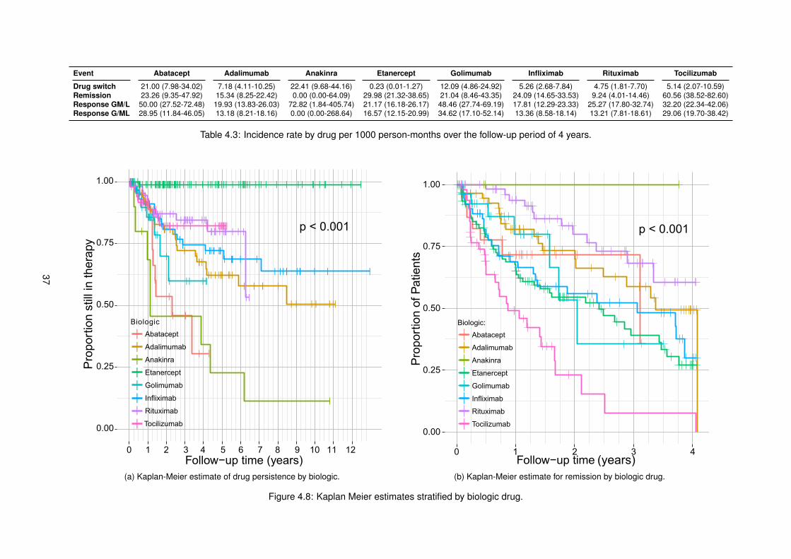
Event Abatacept Adalimumab Anakinra Etanercept Golimumab Infliximab Rituximab Tocilizumab
Drug switch 21.00 (7.98-34.02) 7.18 (4.11-10.25) 22.41 (9.68-44.16) 0.23 (0.01-1.27) 12.09 (4.86-24.92) 5.26 (2.68-7.84) 4.75 (1.81-7.70) 5.14 (2.07-10.59)Remission 23.26 (9.35-47.92) 15.34 (8.25-22.42) 0.00 (0.00-64.09) 29.98 (21.32-38.65) 21.04 (8.46-43.35) 24.09 (14.65-33.53) 9.24 (4.01-14.46) 60.56 (38.52-82.60)Response GM/L 50.00 (27.52-72.48) 19.93 (13.83-26.03) 72.82 (1.84-405.74) 21.17 (16.18-26.17) 48.46 (27.74-69.19) 17.81 (12.29-23.33) 25.27 (17.80-32.74) 32.20 (22.34-42.06)Response G/ML 28.95 (11.84-46.05) 13.18 (8.21-18.16) 0.00 (0.00-268.64) 16.57 (12.15-20.99) 34.62 (17.10-52.14) 13.36 (8.58-18.14) 13.21 (7.81-18.61) 29.06 (19.70-38.42)
Table 4.3: Incidence rate by drug per 1000 person-months over the follow-up period of 4 years.
(a) Kaplan-Meier estimate of drug persistence by biologic. (b) Kaplan-Meier estimate for remission by biologic drug.
Figure 4.8: Kaplan Meier estimates stratified by biologic drug.
37
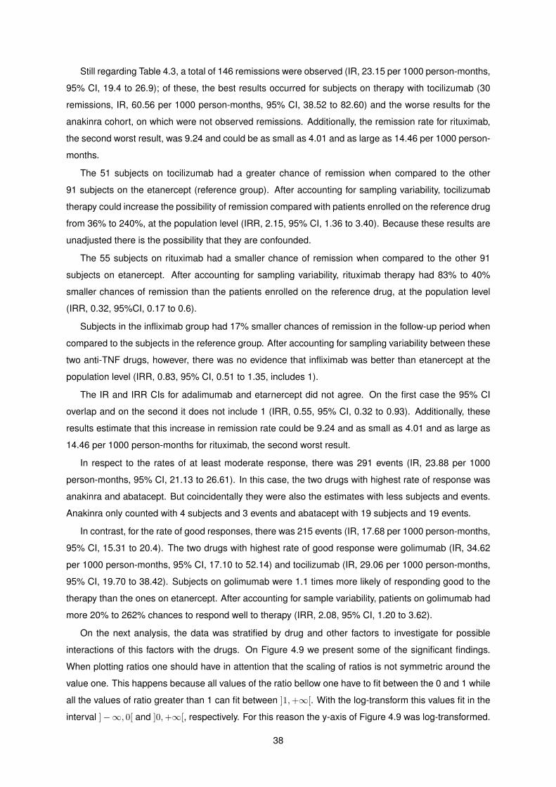
Still regarding Table 4.3, a total of 146 remissions were observed (IR, 23.15 per 1000 person-months,
95% CI, 19.4 to 26.9); of these, the best results occurred for subjects on therapy with tocilizumab (30
remissions, IR, 60.56 per 1000 person-months, 95% CI, 38.52 to 82.60) and the worse results for the
anakinra cohort, on which were not observed remissions. Additionally, the remission rate for rituximab,
the second worst result, was 9.24 and could be as small as 4.01 and as large as 14.46 per 1000 person-
months.
The 51 subjects on tocilizumab had a greater chance of remission when compared to the other
91 subjects on the etanercept (reference group). After accounting for sampling variability, tocilizumab
therapy could increase the possibility of remission compared with patients enrolled on the reference drug
from 36% to 240%, at the population level (IRR, 2.15, 95% CI, 1.36 to 3.40). Because these results are
unadjusted there is the possibility that they are confounded.
The 55 subjects on rituximab had a smaller chance of remission when compared to the other 91
subjects on etanercept. After accounting for sampling variability, rituximab therapy had 83% to 40%
smaller chances of remission than the patients enrolled on the reference drug, at the population level
(IRR, 0.32, 95%CI, 0.17 to 0.6).
Subjects in the infliximab group had 17% smaller chances of remission in the follow-up period when
compared to the subjects in the reference group. After accounting for sampling variability between these
two anti-TNF drugs, however, there was no evidence that infliximab was better than etanercept at the
population level (IRR, 0.83, 95% CI, 0.51 to 1.35, includes 1).
The IR and IRR CIs for adalimumab and etarnercept did not agree. On the first case the 95% CI
overlap and on the second it does not include 1 (IRR, 0.55, 95% CI, 0.32 to 0.93). Additionally, these
results estimate that this increase in remission rate could be 9.24 and as small as 4.01 and as large as
14.46 per 1000 person-months for rituximab, the second worst result.
In respect to the rates of at least moderate response, there was 291 events (IR, 23.88 per 1000
person-months, 95% CI, 21.13 to 26.61). In this case, the two drugs with highest rate of response was
anakinra and abatacept. But coincidentally they were also the estimates with less subjects and events.
Anakinra only counted with 4 subjects and 3 events and abatacept with 19 subjects and 19 events.
In contrast, for the rate of good responses, there was 215 events (IR, 17.68 per 1000 person-months,
95% CI, 15.31 to 20.4). The two drugs with highest rate of good response were golimumab (IR, 34.62
per 1000 person-months, 95% CI, 17.10 to 52.14) and tocilizumab (IR, 29.06 per 1000 person-months,
95% CI, 19.70 to 38.42). Subjects on golimumab were 1.1 times more likely of responding good to the
therapy than the ones on etanercept. After accounting for sample variability, patients on golimumab had
more 20% to 262% chances to respond well to therapy (IRR, 2.08, 95% CI, 1.20 to 3.62).
On the next analysis, the data was stratified by drug and other factors to investigate for possible
interactions of this factors with the drugs. On Figure 4.9 we present some of the significant findings.
When plotting ratios one should have in attention that the scaling of ratios is not symmetric around the
value one. This happens because all values of the ratio bellow one have to fit between the 0 and 1 while
all the values of ratio greater than 1 can fit between ]1,+∞[. With the log-transform this values fit in the
interval ]−∞, 0[ and ]0,+∞[, respectively. For this reason the y-axis of Figure 4.9 was log-transformed.
38
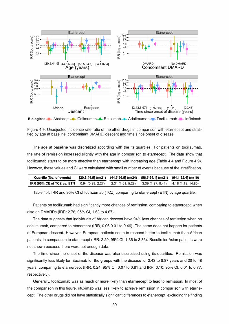
Figure 4.9: Unadjusted incidence rate ratio of the other drugs in comparison with etarnecept and strati-fied by age at baseline, concomitant DMARD, descent and time since onset of disease.
The age at baseline was discretized according with the its quartiles. For patients on tocilizumab,
the rate of remission increased slightly with the age in comparison to etarnecept. The data show that
tocilizumab starts to be more effective than etarnercept with increasing age (Table 4.4 and Figure 4.9).
However, these values and CI were calculated with small number of events because of the stratification.
Quartile (No. of events) [20.8,44.5] (n=21) (44.5,56.5] (n=24) (56.5,64.1] (n=21) (64.1,82.4] (n=10)
IRR (95% CI) of TCZ vs. ETN 0.94 (0.39, 2.27) 2.31 (1.01, 5.28) 3.39 (1.37, 8.41) 4.18 (1.18, 14.80)
Table 4.4: IRR and 95% CI of tocilizumab (TCZ) comparing to etanercept (ETN) by age quartile.
Patients on tocilizumab had significantly more chances of remission, comparing to etanercept, when
also on DMARDs (IRR: 2.76, 95% CI, 1.63 to 4.67).
The data suggests that individuals of African descent have 94% less chances of remission when on
adalimumab, compared to etanercept (IRR, 0.06 0.01 to 0.46). The same does not happen for patients
of European descent. However, European patients seem to respond better to tocilizumab than African
patients, in comparison to etanercept (IRR: 2.29, 95% CI, 1.36 to 3.85). Results for Asian patients were
not shown because there were not enough data.
The time since the onset of the disease was also discretized using its quartiles. Remission was
significantly less likely for rituximab for the groups with the disease for 2.43 to 8.87 years and 20 to 48
years, comparing to etarnercept (IRR, 0.24, 95% CI, 0.07 to 0.81 and IRR, 0.10, 95% CI, 0.01 to 0.77,
respectively).
Generally, tocilizumab was as much or more likely than etarnercept to lead to remission. In most of
the comparison in this figure, rituximab was less likely to achieve remission in comparison with etarne-
cept. The other drugs did not have statistically significant differences to etanercept, excluding the finding
39
regarding adalimumab and subjects of African descent.
4.4 Kaplan-Meier estimates
The Kaplan-Meier estimates on this section came from dataset A and time to drug discontinuation data.
Figure 4.8a shows a smaller therapy duration for anakinra and abatacept and almost no drug switches
for etanercept. There was a significant difference between the Kaplan-Meier estimates (P < 0.001). The
median persistence for anakinra was one year and two month months.
On Figure 4.8b, it was observed that the curves for abatacept and golimumab crossed the others
curves and there were no remissions on anakinra. The intersection of the survival curves is an indication
of non-proportionality of the hazards, however, these curves were estimated with few observations and
the intersection of the curves could be associated with the larger uncertainty of the estimates for a small
sample and not be meaningful of non-proportionality.
The etanercept curve overlaps with the infliximab curve during the first two years and the golimumab
curve overlapping with the adalimumab curve during the first year. At the end of the first year, 50% of
the patients on tocilizumab already reached remission. In fact, it seems that we could limit the follow-up
period even more, to just one year, and avoid the apparent non-proportionality of the hazards. However,
this would mean to discard even more data. The log-rank test gave a significant difference between the
Kaplan-Meier estimates (P < 0.001).
In the appendix A of this work there are the KM estimates for remission and drug switch between
patients on DMARD(s) and without DMARD(s) at baseline. There is also the KM for remission between
patients naive to biologic drugs and at least in second biologic. None of this estimates was significantly
different.
4.5 Cox regression analysis
On this section Cox proportional hazards regression was used for variable selection and estimate the
adjusted HR of remission. Likewise, the reference group for the therapies was etanercept.
The HR are obtained by exponentiation of the coefficients of the regression. For categorical variables
the HR is the relative risk between considered level and the reference group. For continuous predictors,
the HR is the relative risk between two groups who differ by one unit. The estimated HRs are constant
regardless of time for any two group of the same variable. The estimated HRs are constant regardless
of time for any two group of the same variable and if the HR change over time it is considered that the
estimate is the average risk during the follow-up period.
For this analysis the variables investigated using Cox regression were: biologic therapy, sex, age,
race, weight at baseline, height, body mass index, alcohol, smoking, years of education, age of onset,
DAS28 at baseline, SDAI at baseline, time since onset, season, DMARD therapy, GCs therapy, extra ar-
ticular manifestations, patient VAS evaluation, physician VAS evaluation, pain VAS evaluation, HAQ, ery-
throcytes sedimentation rate, reactive C-protein, rheumatoid factor, anti-CCP, number of swollen joints,
40
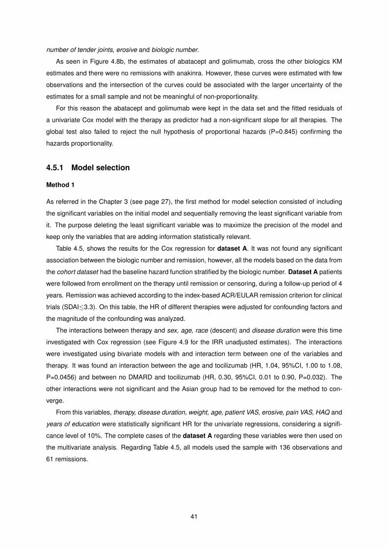
number of tender joints, erosive and biologic number.
As seen in Figure 4.8b, the estimates of abatacept and golimumab, cross the other biologics KM
estimates and there were no remissions with anakinra. However, these curves were estimated with few
observations and the intersection of the curves could be associated with the larger uncertainty of the
estimates for a small sample and not be meaningful of non-proportionality.
For this reason the abatacept and golimumab were kept in the data set and the fitted residuals of
a univariate Cox model with the therapy as predictor had a non-significant slope for all therapies. The
global test also failed to reject the null hypothesis of proportional hazards (P=0.845) confirming the
hazards proportionality.
4.5.1 Model selection
Method 1
As referred in the Chapter 3 (see page 27), the first method for model selection consisted of including
the significant variables on the initial model and sequentially removing the least significant variable from
it. The purpose deleting the least significant variable was to maximize the precision of the model and
keep only the variables that are adding information statistically relevant.
Table 4.5, shows the results for the Cox regression for dataset A. It was not found any significant
association between the biologic number and remission, however, all the models based on the data from
the cohort dataset had the baseline hazard function stratified by the biologic number. Dataset A patients
were followed from enrollment on the therapy until remission or censoring, during a follow-up period of 4
years. Remission was achieved according to the index-based ACR/EULAR remission criterion for clinical
trials (SDAI≤3.3). On this table, the HR of different therapies were adjusted for confounding factors and
the magnitude of the confounding was analyzed.
The interactions between therapy and sex, age, race (descent) and disease duration were this time
investigated with Cox regression (see Figure 4.9 for the IRR unadjusted estimates). The interactions
were investigated using bivariate models with and interaction term between one of the variables and
therapy. It was found an interaction between the age and tocilizumab (HR, 1.04, 95%CI, 1.00 to 1.08,
P=0.0456) and between no DMARD and tocilizumab (HR, 0.30, 95%CI, 0.01 to 0.90, P=0.032). The
other interactions were not significant and the Asian group had to be removed for the method to con-
verge.
From this variables, therapy, disease duration, weight, age, patient VAS, erosive, pain VAS, HAQ and
years of education were statistically significant HR for the univariate regressions, considering a signifi-
cance level of 10%. The complete cases of the dataset A regarding these variables were then used on
the multivariate analysis. Regarding Table 4.5, all models used the sample with 136 observations and
61 remissions.
41
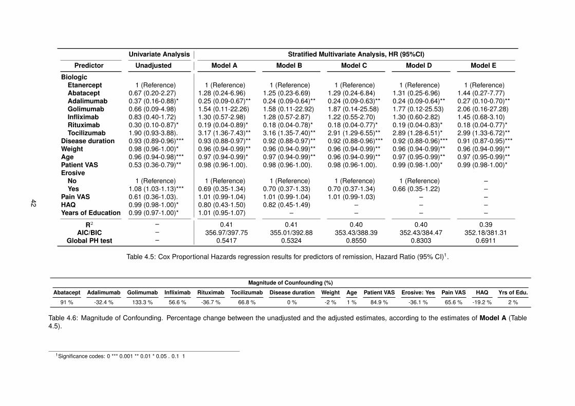
Univariate Analysis Stratified Multivariate Analysis, HR (95%CI)
Predictor Unadjusted Model A Model B Model C Model D Model E
BiologicEtanercept 1 (Reference) 1 (Reference) 1 (Reference) 1 (Reference) 1 (Reference) 1 (Reference)Abatacept 0.67 (0.20-2.27) 1.28 (0.24-6.96) 1.25 (0.23-6.69) 1.29 (0.24-6.84) 1.31 (0.25-6.96) 1.44 (0.27-7.77)Adalimumab 0.37 (0.16-0.88)* 0.25 (0.09-0.67)** 0.24 (0.09-0.64)** 0.24 (0.09-0.63)** 0.24 (0.09-0.64)** 0.27 (0.10-0.70)**Golimumab 0.66 (0.09-4.98) 1.54 (0.11-22.26) 1.58 (0.11-22.92) 1.87 (0.14-25.58) 1.77 (0.12-25.53) 2.06 (0.16-27.28)Infliximab 0.83 (0.40-1.72) 1.30 (0.57-2.98) 1.28 (0.57-2.87) 1.22 (0.55-2.70) 1.30 (0.60-2.82) 1.45 (0.68-3.10)Rituximab 0.30 (0.10-0.87)* 0.19 (0.04-0.89)* 0.18 (0.04-0.78)* 0.18 (0.04-0.77)* 0.19 (0.04-0.83)* 0.18 (0.04-0.77)*Tocilizumab 1.90 (0.93-3.88). 3.17 (1.36-7.43)** 3.16 (1.35-7.40)** 2.91 (1.29-6.55)** 2.89 (1.28-6.51)* 2.99 (1.33-6.72)**
Disease duration 0.93 (0.89-0.96)*** 0.93 (0.88-0.97)** 0.92 (0.88-0.97)** 0.92 (0.88-0.96)*** 0.92 (0.88-0.96)*** 0.91 (0.87-0.95)***Weight 0.98 (0.96-1.00)* 0.96 (0.94-0.99)** 0.96 (0.94-0.99)** 0.96 (0.94-0.99)** 0.96 (0.94-0.99)** 0.96 (0.94-0.99)**Age 0.96 (0.94-0.98)*** 0.97 (0.94-0.99)* 0.97 (0.94-0.99)** 0.96 (0.94-0.99)** 0.97 (0.95-0.99)** 0.97 (0.95-0.99)**Patient VAS 0.53 (0.36-0.79)** 0.98 (0.96-1.00). 0.98 (0.96-1.00). 0.98 (0.96-1.00). 0.99 (0.98-1.00)* 0.99 (0.98-1.00)*Erosive
No 1 (Reference) 1 (Reference) 1 (Reference) 1 (Reference) 1 (Reference) –Yes 1.08 (1.03-1.13)*** 0.69 (0.35-1.34) 0.70 (0.37-1.33) 0.70 (0.37-1.34) 0.66 (0.35-1.22) –
Pain VAS 0.61 (0.36-1.03). 1.01 (0.99-1.04) 1.01 (0.99-1.04) 1.01 (0.99-1.03) – –HAQ 0.99 (0.98-1.00)* 0.80 (0.43-1.50) 0.82 (0.45-1.49) – – –Years of Education 0.99 (0.97-1.00)* 1.01 (0.95-1.07) – – – –
R2 – 0.41 0.41 0.40 0.40 0.39AIC/BIC – 356.97/397.75 355.01/392.88 353.43/388.39 352.43/384.47 352.18/381.31
Global PH test – 0.5417 0.5324 0.8550 0.8303 0.6911
Table 4.5: Cox Proportional Hazards regression results for predictors of remission, Hazard Ratio (95% CI)1.
Magnitude of Counfounding (%)
Abatacept Adalimumab Golimumab Infliximab Rituximab Tocilizumab Disease duration Weight Age Patient VAS Erosive: Yes Pain VAS HAQ Yrs of Edu.
91 % -32.4 % 133.3 % 56.6 % -36.7 % 66.8 % 0 % -2 % 1 % 84.9 % -36.1 % 65.6 % -19.2 % 2 %
Table 4.6: Magnitude of Confounding. Percentage change between the unadjusted and the adjusted estimates, according to the estimates of Model A (Table4.5).
1Significance codes: 0 *** 0.001 ** 0.01 * 0.05 . 0.1 1
42
The multivariate models estimation considered different baseline hazard functions for the number of
the present biologic (biologic number ), for this reason they were stratified multivariate Cox regressions.
After accounting for the information of all predictors, just adalimumab, rituximab, tocilizumab, disease
duration, weight and age remained significantly associated with remission at the population level.
A simple way of determining if there is confounding factors that may bias the result is by measur-
ing the percentage change of magnitude of measure of association between the unadjusted and the
adjusted estimate. If the percentage difference is larger than 10%, confounding is present. Otherwise,
there was little confounding and is not meaningful [49].
Table 4.6, shows the confounding magnitudes according to the unadjusted estimates and the ad-
justed estimates of Model A (Table 4.5). The treatment effect of the majority of the biologics was
underestimated in the univariate analysis. The HR for the indicator of erosiveness and HAQ was over-
estimated while the the patient and pain VAS were overestimated. Years of education, weight, age and
disease duration barely changed in magnitude in comparison with the unadjusted counterparts. There-
fore, there was no indication that the relationship between remission and therapy was confounded by
this variables, nor that the relationship between this group of variables was confounded by treatment.
In Table 4.5, it should be noted that the maximum possible R-squared for this models was 0.947 and
that the definition of a good R-square depends of the field one is working on. The Grambsch-Therneau
test of trend in Schoenfeld residual failed to reject the null hypothesis in all variables and models, with
exception of HAQ in Model B. According to the AIC and the BIC, the model more likely to be the true
model was Model E (AIC=352.18). By continuing eliminating the least significant variable, patient VAS
would have been eliminated and the resulting model would have an increased AIC equal to 354.12. The
next model would have a even higher AIC of 360.84.
Model E, counted with 136 observations like all the other models on this table and was the HR and
95% CI were adjusted for disease duration, weight and age. From 136 observations, 62 remissions
occurred and the pseudo coefficient of determination was 0.39.
On this model, there was an increased association of infliximab with remission, comparing to etan-
ercept. However, this finding was not statistically significant (HR, 1.45, 95% CI, 0.68 to 3.10, P=0.341).
The same happened for golimumab (HR, 2.06, 95% CI, 0.16 to 27.28, P=0.583) and abatacept (HR,
1.44, 95% CI, 0.27 to 7.77, P=0.672).
Subjects receiving adalimumab had 73% less chances of remission than subjects on etanercept. Af-
ter accounting for sample variability the result was significant, and patients on adalimumab had between
30% to 90% less chances of remission (HR, 0.27, 95% CI, 0.10 to 0.70, P=0.007). Tocilizumab was
again the biologic that provided best chances of remission, this time with adjusted estimates. Subjects
on tocilizumab were 2.99 times more likely of achieving remission in comparison the reference group
(HR, 2.99, 95% CI, 1.33 to 6.72, P=0.008).
The time since the onset of the disease at baseline (disease duration) was negatively associated
with remission (HR, 0.91, 95% CI, 0.87 to 0.95, P<0.001). For each year of RA the chances of remis-
sion decrease on average 5% to 13%. The weight was also negatively associated with remission. An
increase of a kilogram reduces the chances of remission between 1% and 6% (HR, 0.96, 95% CI, 0.94
43
to 0.99, P=0.002).
The results also show a significant negative association of age with remission. For every year of age,
remission is 3% less likely (HR, 0.97, 95% CI, 0.95 to 0.99, P=0.03). It should be noted that the HR for
age and disease duration increase over time (r=0.20).
The value of the patient VAS self-evaluation at baseline, or PtGA, had also a negative effect on
achieving remission. A centimeter difference represents a decrease of 12% of the chances of remission
(HR, 0.99, 95% CI, 0.98 to 1.00, P=0.496).
The estimates for the remaining variables were not significant on the other models. Nevertheless,
each unit increase of HAQ at baseline reduces the chances of remission by circa 20% and the presence
of bone erosion at baseline gives the prognosis of less 30% chances of remission.
Method 2
The next method consisted of including 25 of the most relevant variables in the model and subsequently
remove the one of the variables according with four different criteria. The number of variables was limited
to 25 to increase the number of complete cases in the data. The first criterion was the same as previous
one: remove the least significant variable. The three other criteria consisted of removing the the variable
that will produce the best model according with a measures of quality of the statistical models used
for model selection (AIC, AICc and BIC). The therapy variable was forcibly kept in the models even if
removing it would produce a better model.
In addition, this experiment was performed for three datasets extracted from the original but with
different characteristics. Dataset A is the dataset already used on the previous analysis and is based on
the cohort dataset, where the patients are uniquely divided in groups that share a particular drug and
the follow-up period is 4 years. Again on this analysis, it was used only the time to the first remission of
each subject.
At the end of the first year of follow-up it was already apparent differences of the KM estimates and
to avoid the apparent non-proportionality of golimumab and adalimumab (Figure 4.8b) it was created
dataset B. Dataset B characteristics are in all aspects similar to dataset A but the follow-up period was
reduce to just one year.
Dataset C consists of time to remission data extracted from the original data. For each drug of each
patient there is an observation for the time to the first remission. As result of the repeated measures
for each subject the variance models used for this data were corrected to account for within-subject
correlation of the observations. Like all other models, the baseline hazard function was also stratified by
the biologic number.
Figures 4.10a, 4.10b and 4.10c, show the evolution of the AIC, AICc and BIC values during the back-
ward elimination for each one of the criteria. Subjects on anakinra were excluded from the data because
there were no remissions. The p-value criterion was only used for dataset A because it produced mostly
the same results than the other criteria and the choice of the least significant variable was ambiguous
when comparing the significance of the categorical variables levels with continuous variables.
The figures show that most of the criteria produced the same results. Concerning the scores, it can
44
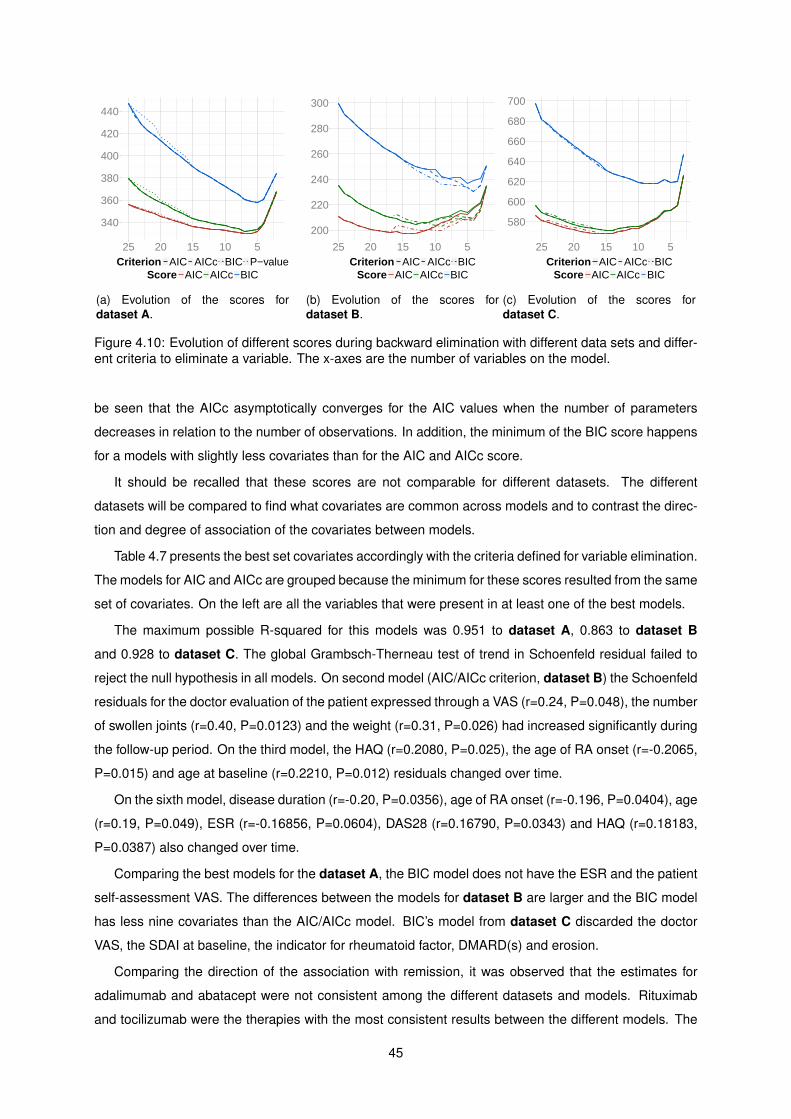
340
360
380
400
420
440
25 20 15 10 5Criterion AIC AICc BIC P−value
Score AIC AICc BIC
(a) Evolution of the scores fordataset A.
200
220
240
260
280
300
25 20 15 10 5Criterion AIC AICc BIC
Score AIC AICc BIC
(b) Evolution of the scores fordataset B.
580
600
620
640
660
680
700
25 20 15 10 5Criterion AIC AICc BIC
Score AIC AICc BIC
(c) Evolution of the scores fordataset C.
Figure 4.10: Evolution of different scores during backward elimination with different data sets and differ-ent criteria to eliminate a variable. The x-axes are the number of variables on the model.
be seen that the AICc asymptotically converges for the AIC values when the number of parameters
decreases in relation to the number of observations. In addition, the minimum of the BIC score happens
for a models with slightly less covariates than for the AIC and AICc score.
It should be recalled that these scores are not comparable for different datasets. The different
datasets will be compared to find what covariates are common across models and to contrast the direc-
tion and degree of association of the covariates between models.
Table 4.7 presents the best set covariates accordingly with the criteria defined for variable elimination.
The models for AIC and AICc are grouped because the minimum for these scores resulted from the same
set of covariates. On the left are all the variables that were present in at least one of the best models.
The maximum possible R-squared for this models was 0.951 to dataset A, 0.863 to dataset B
and 0.928 to dataset C. The global Grambsch-Therneau test of trend in Schoenfeld residual failed to
reject the null hypothesis in all models. On second model (AIC/AICc criterion, dataset B) the Schoenfeld
residuals for the doctor evaluation of the patient expressed through a VAS (r=0.24, P=0.048), the number
of swollen joints (r=0.40, P=0.0123) and the weight (r=0.31, P=0.026) had increased significantly during
the follow-up period. On the third model, the HAQ (r=0.2080, P=0.025), the age of RA onset (r=-0.2065,
P=0.015) and age at baseline (r=0.2210, P=0.012) residuals changed over time.
On the sixth model, disease duration (r=-0.20, P=0.0356), age of RA onset (r=-0.196, P=0.0404), age
(r=0.19, P=0.049), ESR (r=-0.16856, P=0.0604), DAS28 (r=0.16790, P=0.0343) and HAQ (r=0.18183,
P=0.0387) also changed over time.
Comparing the best models for the dataset A, the BIC model does not have the ESR and the patient
self-assessment VAS. The differences between the models for dataset B are larger and the BIC model
has less nine covariates than the AIC/AICc model. BIC’s model from dataset C discarded the doctor
VAS, the SDAI at baseline, the indicator for rheumatoid factor, DMARD(s) and erosion.
Comparing the direction of the association with remission, it was observed that the estimates for
adalimumab and abatacept were not consistent among the different datasets and models. Rituximab
and tocilizumab were the therapies with the most consistent results between the different models. The
45
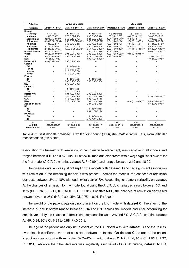
Criterion AIC/AICc Models BIC Models
Predictor Dataset A (n=124) Dataset B (n=118) Dataset C (n=239) Dataset A (n=124) Dataset B (n=118) Dataset C (n=239)
BiologicEtanercept 1 (Reference) 1 (Reference) 1 (Reference) 1 (Reference) 1 (Reference) 1 (Reference)Abatacept 1.24 (0.23-6.71) 0.70 (0.07-7.50) 1.83 (0.45-7.44) 1.08 (0.22-5.38) 0.42 (0.06-2.93) 2.46 (0.50-12.17)Adalimumab 0.27 (0.10-0.69)** 0.59 (0.13-2.76) 1.24 (0.67-2.32) 0.24 (0.09-0.64)** 0.48 (0.13-1.77) 1.09 (0.60-1.98)Golimumab 4.59 (0.21-102.44) 1.58 (0.00-37988.09) 3.60 (0.69-18.72) 3.31 (0.20-55.90) 2.70 (0.11-65.79) 7.48 (1.67-33.54)**Infliximab 1.13 (0.52-2.47) 2.43 (0.72-8.21) 2.52 (1.36-4.65)** 1.28 (0.59-2.79) 1.94 (0.71-5.34) 2.47 (1.36-4.48)**Rituximab 0.12 (0.03-0.58)** 0.42 (0.03-5.23) 0.48 (0.14-1.68) 0.14 (0.03-0.59)** 0.12 (0.01-1.17). 0.57 (0.13-2.43)Tocilizumab 2.12 (0.89-5.06). 18.09 (3.68-88.94)*** 3.57 (1.87-6.82)*** 2.28 (1.00-5.19)* 5.14 (1.76-14.96)** 3.85 (2.04-7.25)***
Disease duration 0.92 (0.88-0.97)*** – 0.82 (0.75-0.91)*** 0.92 (0.88-0.96)*** – 0.83 (0.75-0.91)***Weight 0.96 (0.94-0.98)*** 0.94 (0.91-0.98)*** 0.98 (0.97-1.00)* 0.96 (0.93-0.98)*** 0.96 (0.93-0.98)** –Age 0.97 (0.94-0.99)** 0.96 (0.93-0.99)* 1.14 (1.03-1.27)* 0.97 (0.95-0.99)** – 1.15 (1.04-1.27)**ESR 1.01 (1.00-1.02). – 1.02 (1.01-1.03)*** – – 1.01 (1.00-1.03)**Patient VAS 0.98 (0.97-1.00)* 0.95 (0.91-0.98)** – – – –Season
Fall – 1 (Reference) – – – –Spring – 0.10 (0.02-0.44)** – – – –Summer – 0.15 (0.03-0.71)* – – – –Winter – 0.16 (0.04-0.64)** – – – –
ErosiveNo – 1 (Reference) 1 (Reference) – – –Yes – 0.33 (0.13-0.87)* 0.62 (0.40-0.96)* – – –
SJC – 0.79 (0.64-0.98)* – – – –EA Manif.
No – 1 (Reference) – – – –Yes – 0.18 (0.05-0.62)** – – – –
Doctor VAS – 1.04 (1.00-1.09). 0.98 (0.96-1.00). – – –DAS28 – 0.45 (0.21-0.96)* 0.45 (0.30-0.69)*** – – 0.70 (0.57-0.86)***SDAI – 1.15 (1.03-1.28)* 1.06 (1.02-1.11)** – – –HAQ – 0.27 (0.10-0.74)* 0.62 (0.41-0.92)* – 0.28 (0.14-0.56)*** 0.54 (0.37-0.80)**Age of RA onset – – 0.87 (0.78-0.96)** – – 0.86 (0.78-0.95)**RF
No – – 1 (Reference) – – –Yes – – 1.84 (1.09-3.12)* – – –
DMARD(s)Yes – – 1 (Reference) – – –No – – 2.70 (1.44-5.08)** – – –
R2 0.41 0.47 0.33 0.38 0.30 0.27AIC/BIC 329.55/360.57 197.06/249.70 567.90/630.47 332.09/357.48 207.96/230.12 575.87/617.59
Global PH test 0.8807 0.0601 0.3058 0.7765 0.4303 0.3391
Table 4.7: Best models obtained. Swollen joint count (SJC), rheumatoid factor (RF), extra articularmanifestations (EA Manif.).
association of rituximab with remission, in comparison to etanercept, was negative in all models and
ranged between 0.12 and 0.57. The HR of tocilizumab and etanercept was always significant except for
the first model (AIC/AICc criteria, dataset A, P=0.091) and ranged between 2.12 and 18.09.
The disease duration was just not kept on the models with dataset B and had significant association
with remission in the remaining models it was present. Across the models, the chances of remission
decrease between 8% to 18% with each extra year of RA. Accounting for sample variability on dataset
A, the chances of remission for the model found using the AIC/AICc criteria decreased between 3% and
12% (HR, 0.92, 95% CI, 0.88 to 0.97, P<0.001). For dataset C, the chances of remission decreased
between 9% and 25% (HR, 0.82, 95% CI, 0.75 to 0.91, P<0.001)
The weight of the patient was only not present on the BIC model with dataset C. The effect of the
increase of one kilogram ranged between 0.94 and 0.98 across the models and after accounting for
sample variability the chances of remission decreased between 2% and 6% (AIC/AICc criteria, dataset
A: HR, 0.96, 95% CI, 0.94 to 0.98, P<0.001).
The age of the patient was only not present on the BIC model with with dataset B and the results,
even though significant, were not consistent between datasets. On dataset C the age of the patient
is positively associated with remission (AIC/AICc criteria, dataset C: HR, 1.14, 95% CI, 1.03 to 1.27,
P=0.011), while on the other datasets was negatively associated (AIC/AICc criteria, dataset A: HR,
46
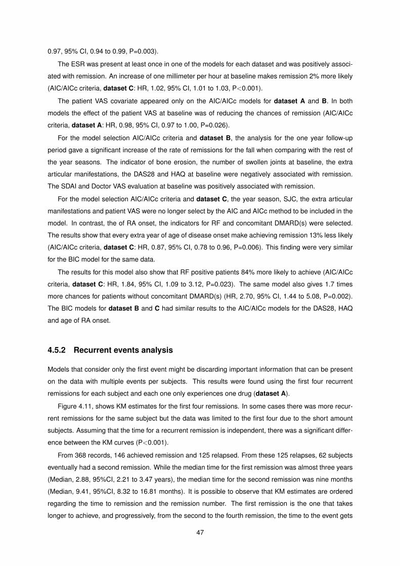
0.97, 95% CI, 0.94 to 0.99, P=0.003).
The ESR was present at least once in one of the models for each dataset and was positively associ-
ated with remission. An increase of one millimeter per hour at baseline makes remission 2% more likely
(AIC/AICc criteria, dataset C: HR, 1.02, 95% CI, 1.01 to 1.03, P<0.001).
The patient VAS covariate appeared only on the AIC/AICc models for dataset A and B. In both
models the effect of the patient VAS at baseline was of reducing the chances of remission (AIC/AICc
criteria, dataset A: HR, 0.98, 95% CI, 0.97 to 1.00, P=0.026).
For the model selection AIC/AICc criteria and dataset B, the analysis for the one year follow-up
period gave a significant increase of the rate of remissions for the fall when comparing with the rest of
the year seasons. The indicator of bone erosion, the number of swollen joints at baseline, the extra
articular manifestations, the DAS28 and HAQ at baseline were negatively associated with remission.
The SDAI and Doctor VAS evaluation at baseline was positively associated with remission.
For the model selection AIC/AICc criteria and dataset C, the year season, SJC, the extra articular
manifestations and patient VAS were no longer select by the AIC and AICc method to be included in the
model. In contrast, the of RA onset, the indicators for RF and concomitant DMARD(s) were selected.
The results show that every extra year of age of disease onset make achieving remission 13% less likely
(AIC/AICc criteria, dataset C: HR, 0.87, 95% CI, 0.78 to 0.96, P=0.006). This finding were very similar
for the BIC model for the same data.
The results for this model also show that RF positive patients 84% more likely to achieve (AIC/AICc
criteria, dataset C: HR, 1.84, 95% CI, 1.09 to 3.12, P=0.023). The same model also gives 1.7 times
more chances for patients without concomitant DMARD(s) (HR, 2.70, 95% CI, 1.44 to 5.08, P=0.002).
The BIC models for dataset B and C had similar results to the AIC/AICc models for the DAS28, HAQ
and age of RA onset.
4.5.2 Recurrent events analysis
Models that consider only the first event might be discarding important information that can be present
on the data with multiple events per subjects. This results were found using the first four recurrent
remissions for each subject and each one only experiences one drug (dataset A).
Figure 4.11, shows KM estimates for the first four remissions. In some cases there was more recur-
rent remissions for the same subject but the data was limited to the first four due to the short amount
subjects. Assuming that the time for a recurrent remission is independent, there was a significant differ-
ence between the KM curves (P<0.001).
From 368 records, 146 achieved remission and 125 relapsed. From these 125 relapses, 62 subjects
eventually had a second remission. While the median time for the first remission was almost three years
(Median, 2.88, 95%CI, 2.21 to 3.47 years), the median time for the second remission was nine months
(Median, 9.41, 95%CI, 8.32 to 16.81 months). It is possible to observe that KM estimates are ordered
regarding the time to remission and the remission number. The first remission is the one that takes
longer to achieve, and progressively, from the second to the fourth remission, the time to the event gets
47
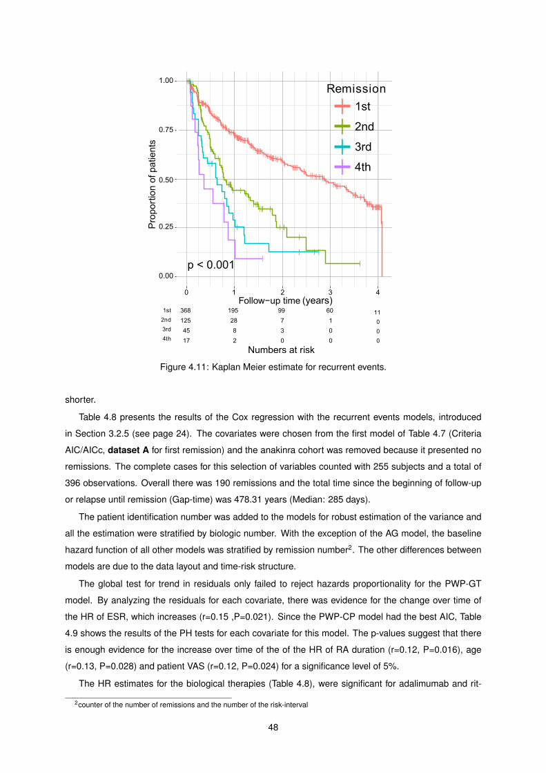
Figure 4.11: Kaplan Meier estimate for recurrent events.
shorter.
Table 4.8 presents the results of the Cox regression with the recurrent events models, introduced
in Section 3.2.5 (see page 24). The covariates were chosen from the first model of Table 4.7 (Criteria
AIC/AICc, dataset A for first remission) and the anakinra cohort was removed because it presented no
remissions. The complete cases for this selection of variables counted with 255 subjects and a total of
396 observations. Overall there was 190 remissions and the total time since the beginning of follow-up
or relapse until remission (Gap-time) was 478.31 years (Median: 285 days).
The patient identification number was added to the models for robust estimation of the variance and
all the estimation were stratified by biologic number. With the exception of the AG model, the baseline
hazard function of all other models was stratified by remission number2. The other differences between
models are due to the data layout and time-risk structure.
The global test for trend in residuals only failed to reject hazards proportionality for the PWP-GT
model. By analyzing the residuals for each covariate, there was evidence for the change over time of
the HR of ESR, which increases (r=0.15 ,P=0.021). Since the PWP-CP model had the best AIC, Table
4.9 shows the results of the PH tests for each covariate for this model. The p-values suggest that there
is enough evidence for the increase over time of the of the HR of RA duration (r=0.12, P=0.016), age
(r=0.13, P=0.028) and patient VAS (r=0.12, P=0.024) for a significance level of 5%.
The HR estimates for the biological therapies (Table 4.8), were significant for adalimumab and rit-
2counter of the number of remissions and the number of the risk-interval
48
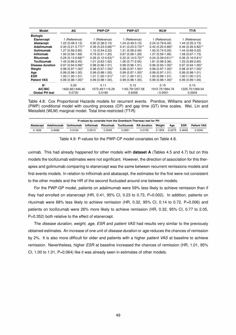
Model AG PWP-CP PWP-GT WLW TT-R
BiologicEtanercept 1 (Reference) 1 (Reference) 1 (Reference) 1 (Reference) 1 (Reference)Abatacept 1.22 (0.48-3.13) 0.90 (0.38-2.15) 1.24 (0.49-3.15) 2.24 (0.79-6.40) 1.44 (0.55-3.73)Adalimumab 0.40 (0.21-0.77)** 0.39 (0.23-0.68)*** 0.41 (0.23-0.73)** 0.42 (0.20-0.89)* 0.46 (0.26-0.82)**Golimumab 1.27 (0.56-2.85) 1.10 (0.54-2.22) 1.21 (0.58-2.49) 1.93 (0.74-5.05) 1.44 (0.69-3.02)Infliximab 1.00 (0.58-1.69) 0.79 (0.51-1.20) 0.87 (0.58-1.29) 1.07 (0.59-1.95) 1.08 (0.67-1.73)Rituximab 0.29 (0.13-0.68)** 0.28 (0.12-0.63)** 0.32 (0.14-0.72)** 0.24 (0.09-0.61)** 0.36 (0.16-0.81)*Tocilizumab 1.45 (0.86-2.45) 1.01 (0.63-1.62) 1.26 (0.77-2.05) 1.81 (0.98-3.36). 1.53 (0.89-2.60)
Disease duration 0.97 (0.94-0.99)* 0.98 (0.96-1.01) 0.98 (0.96-1.01) 0.96 (0.93-1.00)* 0.97 (0.94-1.00)*Weight 0.98 (0.97-1.00)* 0.98 (0.97-1.00)* 0.98 (0.97-1.00)* 0.98 (0.97-1.00)* 0.98 (0.97-1.00)*Age 0.99 (0.98-1.00) 0.99 (0.98-1.00). 0.99 (0.97-1.00)* 0.99 (0.97-1.01) 0.99 (0.98-1.01)ESR 1.00 (1.00-1.01) 1.01 (1.00-1.01)* 1.01 (1.00-1.01). 1.00 (0.99-1.01) 1.00 (1.00-1.01)Patient VAS 0.99 (0.98-1.00)* 0.99 (0.98-1.00). 0.99 (0.98-1.00). 0.99 (0.98-1.00)* 0.99 (0.99-1.00)
R2 0.20 0.11 0.13 0.15 0.13AIC/BIC 1402.66/1446.46 1072.49/1116.29 1163.79/1207.58 1910.75/1964.76 1225.75/1269.54
Global PH test 0.0730 0.0180 0.6358 <0.0001 0.0004
Table 4.8: Cox Proportional Hazards models for recurrent events. Prentice, Williams and Peterson(PWP) conditional model with counting process (CP) and gap time (GT) time scales. Wei, Lin andWeissfeld (WLW) marginal model. Total time-restricted (TT-R)
P-values by covariate from the Grambsch-Therneau test for PH
Abatacept Adalimumab Golimumab Infliximab Rituximab Tocilizumab RA duration Weight Age ESR Patient VAS
0.1626 0.9466 0.9164 0.6513 0.3545 0.0951 0.0155 0.1854 0.0275 0.4645 0.0240
Table 4.9: P-values for the PWP-CP model covariates on Table 4.8.
uximab. This had already happened for other models with dataset A (Tables 4.5 and 4.7) but on this
models the tocilizumab estimates were not significant. However, the direction of association for this ther-
apies and golimumab comparing to etanercept was the same between recurrent remissions models and
first events models. In relation to infliximab and abatacept, the estimates for the first were not consistent
to the other models and the HR of the second fluctuated around one between models.
For the PWP-GP model, patients on adalimumab were 59% less likely to achieve remission than if
they had enrolled on etanercept (HR, 0.41, 95% CI, 0.23 to 0.73, P=0.002). In addition, patients on
rituximab were 68% less likely to achieve remission (HR, 0.32, 95% CI, 0.14 to 0.72, P=0.006) and
patients on tocilizumab were 26% more likely to achieve remission (HR, 0.32, 95% CI, 0.77 to 2.05,
P=0.352) both relative to the effect of etanercept.
The disease duration, weight, age, ESR and patient VAS had results very similar to the previously
obtained estimates. An increase of one unit of disease duration or age reduces the chances of remission
by 2%. It is also more difficult for older and patients with a higher patient VAS at baseline to achieve
remission. Nevertheless, higher ESR at baseline increased the chances of remission (HR, 1.01, 95%
CI, 1.00 to 1.01, P=0.064) like it was already seen in estimates of other models.
49

50
Chapter 5
Conclusions
This chapter summarizes and interprets the main findings of this thesis in light of the of the investigation
on EMR data from RA patients enrolled in biological therapies and the initial objectives. In addition, it will
be discussed the advantages and limitations of the proposed solutions, possible applications and future
work.
In this work the problem of analyzing EMR data from RA patients enrolled in biological therapies was
addressed with success. First, literature was reviewed about the the disease, treatments, guidelines,
scores, remission criteria and kind of methods used in this kind of study.
Then, from the original raw dataset were extracted multiple datasets to allow for the different analyzes
throughout this work. This was done to overcome the difficulties of dealing with real life data without a
specific type of study design during the data collection phase, multiple observations and no specific
pattern for the drug switches.
After finding the appropriate ways to analyze Reuma.pt data and of understanding the implications
and limitations of the methods, the methodology allowed to represent the data, summarize it and quantify
the relative chances of remission (relative risk of remission) for the different therapy, other factors and
also to adjust for possible confounding variables.
Every analysis in this work including tables and figures was scripted in R, a free software widely used
for statistical computing.
5.1 Descriptive analysis
Despite the simple nature of the descriptive analysis (Section 4.1, page 29) a lot meaningful and easily
interpretable results were found and can be discussed.
The data exploration showed that some of the most relevant variables that characterize the disease
activity and functional disability had a high degree of missingness and alarmed for the difficulties regard-
ing missing values that could be found in the rest of the work.
The proportion of women on this sample of Reuma.pt was almost 6 times greater than of men.
However, the prevalence for women is estimated to be two to three time higher than in men and in
51
Portugal this proportion is 4:1 [10, 9]. This probably happened because there was more women failing
the conventional therapies than men. Regarding RF and anti-CCP, there was about 2 times more patient
with it than without. This values are similar to the prevalences found in the general population [11].
It was also found a considerable variety of combinations of DMARDs (n=18) and 1% of the observa-
tions had three DMARDs combined. It was also found a combination of three GCs on the 12 different
combinations found.
Drugs combination and their interaction is a matter that is difficult to study because of the amount of
possible combinations of drugs and the high cost of such an investigations. The drug interaction might
cause a exacerbated effect of the drug or decreased effect when the interaction is antagonistic. For this
reason, this is still not well studied and more research should be done regarding this area.
The observation of anatomical distribution of the swollen and tender joints at baseline showed that
a joint was more likely to be swollen than tender, the distribution is almost symmetric as expected
in RA and the wrists and the hands joints are the most affect. In the hands, the second and third
metacarpophalangeal joints were the most affected.
On the next part, it was represented the change of disease activity, functional disability over time by
therapy groups. It should be noted that this estimates are biased because the windows for the smoothing
and kernel estimation might contain more than one observation per patient, but since observations from
the same patient are not expected to be found close to one another the effect of this was not relevant.
It is not relevant because this estimates serve only the purpose of data visualization and for aiding
on the interpretation of the data, and not for statistical inference of the therapies effects on the popu-
lation of patients. Descriptive statistics and analysis is concerned only with properties of the sample,
while inferential statistics tries to extrapolate the properties found in the data sample to the underlying
population.
Also on this analysis, it was of interest to describe each drug effect near the third and sixth month
after the therapy start because those are the decision time points.
The results show that most of the disease activity variation occurred for the first 6 to 12 months after
the therapy start.
Given the consistence of the results regarding the anti-TNF drug and the lack of significant difference
in treatment effects between anti-TNF drugs, the descriptive analysis suggests that these drugs are
equivalent.
The overwhelming difference of the estimates and the faster and larger improvements for tocilizumab,
comparing to the other drugs, suggests that this drug produces the best results. Rituximab and anakinra
had the worst results both for the progression of disease activity and functional disability. It became
evident early in this work that the best therapy response came from patients on tocilizumab. This finding
turned to be reinforced through out the work for the cohort dataset but also for other datasets with data
from all the biologics each patient was exposed.
52
5.2 Summary measures analysis
The baseline characteristics of each cohort were compared on Table 4.1 and then it was presented the
results for the analysis of the data summaries on Table 4.2, both on page 30.
Globally, tocilizumab was the therapy with better results. It had the highest mean rate of decrease of
disease activity and the highest percentage significant changes of disease activity. Others summaries
like the AUC and the minimum activity or time to minimum activity were not possible to use because the
subjects do not have equal follow-up times making this measurement incomparable.
5.3 Incidence density rates
The study of drug persistence was difficult in this work. It should be note that the drugs were not
introduced in the market at the same time and some of these drugs were already authorized for some
years when others were approved in the Portuguese market. For example, according to Infarmed,
tocilizumab was only authorized in 2010. It was not possible to precise when the others drugs were
authorized but is mentioned that adalimumab, anakinra, etanercept, infliximab and rituximab did not
have a cost-effectiveness analysis because they were authorized to enter in the market in prior to 2006.
This was the year that this analysis started to be mandatory for this drugs. For golimumab was made a
cost-effectiveness analysis and for abatacept is only mentioned that should be used by RA adults [50].
Since drug persistence does not depend only of the overall success of the therapy or of the doctor
and patient preferences. For all this factors and not having enough elements to control for them, it was
chosen to limit the analysis to descriptive statistics and unadjusted estimates like the KMs, IRs and
IRRs.
It was observed that the therapy duration was greater than the overall median of two years and four
months for adalimumab, etanercept, inflixumab and rituximab. Etanercept was the most persistence
drug with about two drug switches by 10000 person-months and this was also visible on the KM curve.
Anakinra and abatacept had highest rates of drug switch.
The IR of remission was best for tocilizumab and worse for anakinra and rituximab. Subjects on
tocilizumab had about two times more chances of remission than the ones on etanercept. After ac-
counting for sample variability the subject had 36% to 240% more chances of remission with tocilizumab
when with etanercept. This results was statistically significant because the 95% CI did not cross one.
In relation to etanercept, it was observed that the chances of remission increases gradually with age
for patients on tocilizumab. In addition, tocilizumab performed better than etanercept when in combina-
tion with one or more DMARDs and adalimumab decreased the chances of remission in comparison to
etanercept for people of African descent. At last, rituximab was generally worse than etanercept.
There is the possbility that this results are confounded because they are unadjusted estimates.
The therapy response using the EULAR criterion for therapy response was difficult because the
criterion has three cut-points (good response, moderate response and low response) and by comparing
different levels groupings some of the results were contradictory. In addition, the DAS28 variation was
53
one of the variable with more missing values and is used to determined the patient response.
5.4 Kaplan-Meier estimates
Tocilizumab’s KM estimate for remission was clearly isolated from the other drugs. The intersection of
the survival curves for abatacept and golimumab was probably result of the small number of observations
for this drugs and it can not be said with certainty that the hazard are non-proportional. For this reason,
further investigation was done when applying the Cox proportional hazards regression.
The median persistence for anakinra was one year and two month months. In contrast, the median
persistence for tocilizumab was one year and eight months.
Given the characteristics of the outcomes in the data, it was found that the disease activity is a
better outcome than the therapy persistence or the therapy response. DAS28 and SDAI are two good
measures of the disease activity. While DAS28 was developed to be normally distributed, SDAI is the
current score used to define remission.
5.5 Cox regression analysis
Cox proportional hazards regressions were used to assess potential predictors of remission and adjust
for variables correlated both with the outcome and other covariates. This variables, also called con-
founding variables or confounders, are one of the main problems with non-randomized studies and can
cause associations between to the outcome that are not true if it is not performed proper adjustment
for them. However, it is not possible to know if all confounders are in the data, we are adjusting for all
of them or the method is flexible enough permit for the proper adjustment. So, the best way to achieve
maximum strength of causality association between the exposures and the outcome and protect the
sample against confounding is to do a randomized study.
5.5.1 Model Selection
Method 1
To find a the most probable to represent the data were compared different models. The first procedure
was to fit an univariate Cox model for each candidate predictors of remission. Then the insignificant
covariates for a level of 10% were discarded and the remaining were included on a multivariate Cox
model. At last, it was used backward elimination, eliminating always the least significant variable.
The aim of deleting the least significant variable was to maximize the precision of the model and
keep only the variables that are adding information statistically. Combinations of other covariates were
also experimented.
Years of education was statistically significant on the univariate model. This possible relation with re-
mission could be connected with the socioeconomic characteristics of the patients: alimentation, stress
54
access to complementary therapies, and the care that more informed patient might give to treatment.
However, this was not confirmed on the multivariate models.
There was indication that the relationship between therapy and remission was confounded by patient
VAS, erosiveness, pain VAS, years of education and HAQ, and that the effect of these variables was
also confounded by therapy.
The model most likely to represent this data included therapy, disease duration, weight, age and
patient VAS as predictors of remission. Also there was not enough evidence of non-proportionality of
the hazards, even including the abatacept and golimumab cohorts.
It should be noted that the HR for age and disease duration increase over time (r=0.20). This results
was expected because the HR for one year difference when one is in their thirties does not have the
same impact in the HR of when one is in their sixties.
In all the models, subjects tocilizumab had the highest chances of remission in relation to the etan-
ercept. These subject were about 3 times more likely to achieve remission. For the same reference,
subjects on adalimumab had 73% less chances of remission and on rituximab 82%. RA duration, weight
and age had significant negative effects.
Every year since the beginning of RA and of age decreases the chances of remission 8% and 1%,
respectively. One more kilogram of weight makes 4% more likely. It was also found, with exception of
adalimumab, that there was not a statistically difference between the anti-TNF.
Method 2
Another criteria for model selection were tried but this time with more variables. Namely, it was again
used backward elimination, but this time it was removed the variable that provided the best model ac-
cordingly to the AIC, AICc or BIC. It were also used different datasets. Dataset A was again used for
this method. Dataset B, like dataset A, comes from cohort dataset but has a 1 year follow-up period.
Dataset C has the time to remission or censoring for each biologic therapy of each subject.
It was found that this model selection method does not depend much of the criterion for variable
elimination but of the score used to find the best model. For example for dataset A, the model with
minimum AIC is equal for both the AIC or BIC criterion. The same happened using the p-value criterion.
In addition, the minimum of the BIC score happens for smaller models.
Therapy was the only variable that was present in all models. However, therapy was never a can-
didate for elimination of the models. The remission predictors present in three or more models were:
disease duration, weight, age, ESR and HAQ.
On the best models for dataset C the effect of age was positive regarding remission and the DAS28
and SDAI scores were included and considered statistically significant. One possible explanation for the
first case to happen is that every time the patient switches drug the age is correspondent to the moment
of beginning of the new drug. So, the age increases for every new drug and also the the likelihood of
remission, because the therapy was adjusted. The same happens for the ESR, DAS28 and SDAI values
and a better way is to make this variable time-independent and include only the overall baseline value in
all the observations from the same subject.
55
This systematic technique was simpler and easier way of selecting covariates than trying all possible
combinations of covariates.
By comparing the results for the best models of the three datasets for the different criteria (minimum
AIC for AIC criterion, etc.) it was found that the greatest effect on remission was from tocilizumab. The
estimated HR of tocilizumab in relation to etanercept across the different models was between 2.12 and
18.09.
The strikingly higher frequency of remission among patients on tocilizumab in our data and across
different models suggests an important effect of this drug on the reduction of the RA activity and remis-
sion induction. This results reinforce the relevance of the IL-6 as pro-inflammatory cytokine in RA.
The effect of disease duration, weight and age was also consistent with previous models and of the
same magnitude.
5.5.2 Recurrent events analysis
Remission does not last long in RA and relapses and flares of disease activity are common. For this
reasons it were used and compared several methodologies for recurrent events.
For recurrent events, it was found that for half the subjects the time for the first remission can be
3.67 times greater than the time for the subsequent remissions. It was also observed that the mean
remission-time decreases for every new remission.
For the recurrent events analysis, the effect of tocilizumab was not statistically significant even if
positive and consistent with the other results. On other hand, the effects of adalimumab and rituximab
was statistically significant and negative. Subject on adalimumab had 60% less chances of remission
and the ones on rituximab were 71% less likely than the ones on etanercept. However, there was
evidence of violation of the hazards proportionality assumption on this models.
The Cochrane overview on biologics for RA [51] compared the efficay of abatacept, adalimumab,
anakinra, etanercept, infliximab, and rituximab. They found that anakinra was less efficacious than
etanercept (RR, 0.44, 95%CI, 0.23 to 0.85, P=0.014), rituximab and adalimumab and that the rest
therapies had similar effects between them. This results are consistent with with the findings in this
thesis for anakinra and the anti-TNF drugs.
5.6 Limitations
The understanding of the sampling procedure of the data is an important aspect because with it we can
determine to whom the results may apply and how well we can extrapolate the results from the sample
to the population of RA patients.
One of the factors that might cause a systematic difference between the sample and the population
of interest is the non-random assignment of the therapy. The guidelines [24] recommend to prescribe
first the anti-TNF class of biologics and on this group there were some drugs more frequent than others.
Namely, etarnercept (41.5%), infliximab (31.6%), adalimumab (18.3%) and golimumab (6.6%). This can
56
be due to some drugs only being available recently.
Knowing that non-responders to the first therapy are more likely to not respond for a second drug,
this might bias the results in favor of the first therapies. In addition, patients that start a biological therapy
already failed the conventional therapies, for this reason the results will only apply to the population that
already failed therapy with DMARDs and not to the complete population of RA patients.
Furthermore, it is expected that some patients avoid going to the doctor when they have no com-
plains. For this reason, it can be expect that the loss to follow-up might not be completely at random,
even different between treatment groups and changing these groups characteristics with time. Since
the data comes from two health centers that might have populations with different accessibilities and
socio-economics aspects, the access and quality of health care might be different between centers.
Consideration has been given to the possibility that the results could have been produce by selection
of an unsuitable group of patients, by patients with unusual exacerbation of RA activity and unresponsive
to the current therapies. This is supported by the fact that the sampling procedure created a selection
bias of both patients and therapy and the data is also convenience sample.
There are superior methodologies to find evidence of association of particular variable to the out-
come, establish a stronger causal relationship between the exposure and outcomes and avoid system-
atic difference between the exposure groups other then the outcome of interest (confounding). Namely,
randomization eliminates systematic confounding and and appropriate observational study design can
be used to increase the chances of a good representation of the population of interest by the sample.
On non-random samples same elements might not reflect the makeup of the population of patients.
Being EMR data there was not a rigorous control of the data collection as in a randomized or typical
observational study and, as seen, there was many missing values in the data. Furthermore some
therapies, like anakinra, had small groups of subjects and could not be analyzed.
It exists a great number of joints to observe, so the results regarding this matter might be influenced
by the 28 joints count for DAS28 or by the personal choice of joints to be examined by the doctor.
Another limitation of this work was the non-existence of a clear reference group for the therapies, like
a placebo group or group only not on biological therapies.
One of the biggest drawbacks of the time-to-event analysis is the issue of non-informative censoring.
To satisfy this assumption, the design of study must ensure that the mechanisms giving rise to censoring
of individual subjects are not related to the probability of an event occurring. For example, the continu-
ation of follow-up must not depend of the patient condition. This assumption can not be guaranteed in
our data since there are many factor that can influence this. Violation of this assumption can invalidates
both KM estimates and Cox models.
It should be taken into account that lack of statistical significance, is not the same as lack of scientific
significance. The scientific significance depends of the context of the study and of the sample size.
Small samples can produce non-significant results even though the magnitude of the association at
the population is relevant. What happens is that our study can not detected it because does not have
enough statistical power. The opposite also holds and not rejecting the null hypothesis is not equivalent
to accepting the null hypothesis as the truth.
57
A limitation of the CI for the IR and IRR estimates is that they tent to work worse for small sample
sizes and what would be expected to be a 95% CI has in fact a coverage smaller than 95%. This
happens because the central limit theorem only works asymptotically. In addition, the p-values for the
Chi-squared approximation may be inaccurate because of small sample size and the null hypothesis can
be false, but erroneously fails to be rejected (type II error).
A group of methods suited to analyze longitudinal data are mixed effects models. Mixed models are
statistical methods that contain both fixed effects and random effects and can deal with missing values
and repeat measures of the same subject on the data. However, the linear mixed effect models and
Cox regression with a frailty term experimented during this study had many times difficulty converging.
For this reason their results were not included. Probably this happened because many subjects had few
observations and that difficult the convergence of the iterative methods used.
Cohort dataset was created because most of the subjects start with anti-TNF biologics like it is
advised on SPR guidelines [24] and by using only the first therapy the other types of biologics would be
under represented on the analysis. In alternative, if it was used all patient’s therapies the observations
for different drugs would be correlated, like it happened with dataset C.
This choice has the disadvantage that we discard a great part of the data but the advantage that
making possible to study the effect of the therapies with a greater variety of methods and less restrictions
and assumptions. For example, this makes possible to present correct KM and Cox models from the
same data and eliminates the difficulty of comparing the effect of therapies when the same subject is in
two different groups.
A limitation of the remission criteria is the amount of relapses and that they just state the criteria must
be fulfilled ”at any time point“. This makes possible to call remission to very short periods of disease
inactivity and creates difficulties in defining the remission for prospective studies since the relapse rate
is very high.
Linear methods are easy to use and most of all are easily interpretable. However, in the case that the
hazard of a predictor changes over time and the hazards proportionality does not hold, some authors
considered that the estimate can be interpreted had the average HR over the follow-up time [27, 35]. If
the information is not representable by linear combination of variables or features, other methods are
more appropriate.
5.7 Achievements
As is know, RA is one of the leading causes of disability and is associated with decreased life expectancy.
Furthermore, precious time is lost looking for an effective therapy while it is given opportunity for the
disease to cause irreversible joint destruction on the RA patients.
Therefore, some of the literature about rheumatoid arthritis, its treatments, guidelines, epidemiology,
genetics and current criteria used to assess disease activity and functional ability were reviewed. Then,
to construct a methodology for this work, literature about epidemiology, longitudinal data analysis, sur-
vival analysis, machine learning and other data sciences or methods were studied, paying attention to
58

the possible limitation to our case.
It should be mentioned that even though machine learning techniques were studied and tried on this
data, the structure of the data limits a lot what kind of analysis can be made and the results would be
less meaningful and interpretable than the results of this work.
Finally, this study investigated EMR data from Reuma.pt register and with it was able to extract
important information about the sample and contributed the base knowledge about biological therapies
for RA in clinical-practice. To achieve that, it was found the best set of predictors for different datasets
and the estimates from the different models were compared. The model selection procedure contributed
for the development of the best model to fit the this kind data.
More precisely, it was measured the effect on the disease activity of different biologic treatments and
of factors like the disease duration, weight and age. In addition, it was found what therapy was more
likely to succeed and which one was is more likely to fail according with the characteristics of the data
using population based estimates. Other outcomes, like drug persistence and therapy response, were
also investigated.
One of the biggest challenges in this work was to adapt real-world data to methods that were devel-
oped for dataset with a specific set of characteristics and assumptions.
This thesis gave me the opportunity to work with data on a real world context with all the inherent
difficulties of such challenge. Since the beginning of this thesis I could learn to program with R, bash
script and work with Weka. I could also deepen my knowledge about many data sciences areas, such
as epidemiology, statistics and machine learning.
5.8 Future Work
This work can be used as a guide for future work on Reuma.pt and the estimates might be useful
to design future studies and to compute the sample size for a desired statistical power. As is know,
preliminary observational studies are first done to develop evidence for the possibility of doing larger
and perhaps more costly randomized trials.
In addition, the covariates from the selected models can be later be used for future models and
prediction of the hazards in new data.
Some of the therapies in this work did not have a cost-effectiveness study because it was not manda-
tory at the time they were authorized in the market. Namely, adalimumab, anakinra, etanercept, inflix-
imab and rituximab. The optimization of the resource allocation is an important factor on the context of
the sustainability of the health systems. Given the high costs of biologic therapies and the results of this
work, future work should be done to analyze the cost-effectiveness of these medications.
In future work can instead use forward selection of covariates to select the best model or be centered
on prediction and development of a recommendation system. Interactions between covariates and in
time can be further investigated and the results adjusted for confounding variables.
A simple recommendation system that can be easily implemented is based on the K-nearest neigh-
bors. Using a distance measure that uses both categorical, continuous variables, time dependent and
59
time-independent variables, the subjects can be ranked for each therapy. From this ranks the nearest
K subjects are averaged to predict the response of the new subject and the best therapy with the best
response is chosen.
Bayesian networks and other recommendation systems also have several applications in health care.
Disease diagnosis, selection of optimal therapy, outcome prediction, health care management, construc-
tion of diseases models in clinical epidemiology and discovery of functional models through expression
data are some of the possible applications in health care [52]. This methods do not need to have explicit
representation of time, instead the time-dependent predictor can be represent by creating features that
describe the temporal evolution over time, like it was done in the summarized analysis in this work.
Bayesian networks have also been extended to what is called an influence diagram and used in
decision theory contexts. An influence diagram is a generalization of a Bayesian network, in which
probabilistic inference is used to solve decision making problems by means of maximizing the expected
utility. The utility function can depend of multiple factors and reflects the preferences of the agent about
decisions that involve uncertainty. Depends on the attitude to risk of the agent and normally is not linear.
This kind of system can be used, for example, to select the optimal treatment alternatives.
A group of methods that can be used in the future are the mixed-effects models and an alternative
for Cox regression and recurrent events is to use Poisson regression.
To conclude, this study has developed a general methodology for the representation and analysis of
Reuma.pt data. It has been demonstrated that some therapies are significantly more efficacious than
others and that the time since the onset of the disease, age and weight affect the chances of remission.
Further methods should be applied and this data can will be subject of more research.
60
Bibliography
[1] D.P. Symmons and S.E. Gabriel. Epidemiology of CVD in rheumatic disease, with a focus on RA
and SLE. Nature Reviews Rheumatology, 7:399–408, 2001.
[2] G.S. Firestein, R.C. Budd, E.D. Harris, I.B. McInnes, S. Ruddy, and J.S. Sergent. Kelley’s Textbook
of Rheumatology, volume vol. 1, chapter Rheumatoid Arthritis. Saunders/Elsevier, 8th ed. edition,
2009.
[3] Pedro Pita Barros. Pela Sua Saude. Fundacao Francisco Manuel dos Santos, 2013.
[4] Associacao de Farmacias de Portugal. Doentes rejeitam limitacoes no acesso a medicamen-
tos biologicos. http://www.portaldasfarmacias.com/noticia_detalhe.php?id=196, 2015. Ac-
cessed: 10 March 2015.
[5] Pedro Laires, Miguel Gouveia, and Jaime Branco. O impacto economico das doencas Reumaticas.
Technical report, Observatorio Nacional de Doencas Reumaticas, 2013.
[6] Elsa Vieira-Sousa, J A Pereira Silva, Maria Jose Santos, J Canas Silva, J A Melo Gomes, Catia
Duarte, Jose Antonio Silva, Luıs Cunha-miranda, Ana Teixeira, Walter Castelao, Jaime Branco,
Jose Antonio Costa, Domingos Araujo, Teresa Novoa, Guilherme Figueiredo, Herberto Jesus, Al-
berto Quintal, Ana Rita Cravo, Graca Sequeira, Patrıcia Pinto, Rui Andre, Miguel Bernardes, Fran-
cisco Ventura, Ines Cunha, Anabela Barcelos, Patrıcia Nero, and Margarida Cruz. Reuma.pt - The
Rheumatic Diseases Portuguese Register. Technical report, Sociedade Portuguesa de Reumatolo-
gia, 2011.
[7] Usama Fayyad, Gregory Piatetsky-shapiro, and Padhraic Smyth. From Data Mining to Knowledge
Discovery in Databases. AI Magazine, 17:37–54, 1996.
[8] K.J. Cios, W. Pedrycz, Swiniarski, and L. R.W., Kurgan. Data Mining - A Knowledge Discovery
Approach. Springer, 2007. ISBN 978-0-387-36795-8.
[9] Direccao Geral de Saude. Programa Nacional Contra as Doencas Reumaticas. http://www.dgs.
pt/upload/membro.id/ficheiros/i006345.pdf, 2004. Accessed: 15 April 2015.
[10] Alan Silman and Jacqueline Pearson. Epidemiology and genetics of rheumatoid arthritis. Arthritis
Res, 4(Suppl 3):S265–S272, 2002. London, UK. 24-26 June 2002.
61
[11] Joao Eurico Cabral da Fonseca, Helena Canhao, and Mario Viana de Queiroz. Reumatologia
Fundamental. LIDEL, 2013. ISBN 978-972-757-905-1.
[12] Linda A Merlino and et al. Vitamin D Intake Is Inversely Associated With Rheumatoid Arthritis.
Arthritis & Rheumatism, 50(1):72–72, 2004.
[13] J Kjeldsen-Kragh and et al. Controlled trial of fasting and one-year vegetarian diet in rheumatoid
arthritis. The Lancet, 338(8772):899–92, 1991.
[14] Nicola J Minaur, Richard K Jacoby, John A Cosh, Gordon Taylor, and Johannes J Rasker. Out-
come after 40 years with rheumatoid arthritis: a prospective study of function, disease activity, and
mortality. The Journal of Rheumatology, 69:3–8, 2004.
[15] Ozlem Pala and Frank L Cavaliere. Joint Counts. http://www.rheumatology.org/assets/0/116/
401/408/419/420/d49d771a-8035-469f-b7a4-65838f9fcfef.pdf, 2006. Accessed: 15 February
2015.
[16] Ministry of Heatlh - British Columbia. Rheumatoid Arthritis: Diagnosis, Management and Monitor-
ing, 2012.
[17] Bonnie Bruce and James F Fries. The Stanford Health Assessment Questionnaire: Dimensions
and Practical Applications. Health and Quality of Life Outcomes, 1, 2003.
[18] RaniaM. Shammas, VeenaK. Ranganath, and HaroldE. Paulus. Remission in rheumatoid arthritis.
Current Rheumatology Reports, 12(5):355–362, 2010.
[19] David T Felson, Josef S Smolen, George Wells, Bin Zhang, Lilian H D van Tuyl, Julia Funovits,
Daniel Aletaha, Cornelia F Allaart, Joan Bathon, Stefano Bombardieri, Peter Brooks, Andrew
Brown, Marco Matucci-Cerinic, Hyon Choi, Bernard Combe, Maarten de Wit, Maxime Dougados,
Paul Emery, Daniel Furst, Juan Gomez-Reino, Gillian Hawker, Edward Keystone, Dinesh Khanna,
John Kirwan, Tore K. Kvien, Robert Landewe, Joachim Listing, Kaleb Michaud, Emilio Martin-
Mola, Pamela Montie, Theodore Pincus, Pamela Richards, Jeffrey N Siegel, Lee S Simon, Tuulikki
Sokka, Vibeke Strand, Peter Tugwell, Alan Tyndall, Desiree van der Heijde, Suzan Verstappen,
Barbara White, Frederick Wolfe, Angela Zink, and Maarten Boers. American College of Rheuma-
tology/European League Against Rheumatism Provisional Definition of Remission in Rheumatoid
Arthritis for Clinical Trials. Annals of the Rheumatic Diseases, 70(3):404–413, 2011.
[20] American College of Rheumatology. The 2011 ACR/EULAR definitions of remission in rheumatoid
arthritis clinical trials. https://www.rheumatology.org/practice/clinical/classification/
ra/ra_remission_2011.asp, 2015. Accessed: 9 February 2015.
[21] ACR and EULAR. Defining Remission in Rheumatoid Arthritis. http://www.eular.org/
myUploadData/files/RA%20Remission%20Slides-Web.pdf, 2015. Accessed: 9 February 2015.
[22] Josef S Smolen, Robert Landewe, Ferdinand C Breedveld, Maya Buch, Gerd Burmester, Maxime
Dougados, Paul Emery, Cecile Gaujoux-Viala, Laure Gossec, Jackie Nam, Sofia Ramiro, Kevin
62
Winthrop, Maarten de Wit, Daniel Aletaha, Neil Betteridge, Johannes W J Bijlsma, Maarten Boers,
Frank Buttgereit, Bernard Combe, Maurizio Cutolo, Nemanja Damjanov, Johanna M W Hazes, Mar-
ios Kouloumas, Tore K Kvien, Xavier Mariette, Karel Pavelka, Piet L C M van Riel, Andrea Rubbert-
Roth, Marieke Scholte-Voshaar, David L Scott, Tuulikki Sokka-Isler, John B Wong, and Desiree
van der Heijde. Eular recommendations for the management of rheumatoid arthritis with synthetic
and biological disease-modifying antirheumatic drugs: 2013 update. Annals of the Rheumatic Dis-
eases, 2013.
[23] Msc. Marloes Vermeer, Hillechina H. Kuper, Arie E. van der Bijl, Drs. Henriette Baan, Marcel D.
Posthumus, Herman L.M. Brus, Piet L.C.M. van Riel, and Prof.dr. Mart A.F.J. van de Laar. The
provisional ACR/EULAR definition of remission in RA: a comment on the patient global assessment
criterion. Rheumatology, 51:1076 – 1080, 2012.
[24] Joao Eurico Fonseca, Miguel Bernardes, Helena Canhao, Maria Jose Santos, Alberto Quintal,
Armando Malcata, Adriano Neto, Ana Cordeiro, Ana Rodrigues, Ana Filipa Mourao, Ana Sofia
Ribeiro, Ana Rita Cravo, Anabela Barcelos, Anabela Cardoso, Antonio Vilar, Arecili Brana, Armando
Malcata, Augusto Faustino, Candida Silva, Catia Duarte, Domingos Araujo, Dolores Nour, Elsa
Sousa, Eugenia Simoes, Fatima Godinho, Filipe Brandao, Francisco Ventura, Graca Sequeira,
Guilherme Figueiredo, Ines Cunha, J Alves De Matos, Jaime Branco, Joao Ramos, Jose Antonio
Costa, Jose Antonio, Melo Gomes, Jose Pinto, Jose Canas, J A Pereira, Jose Vaz Patto, Lucia
Costa, Luıs Cunha Miranda, Luıs Ines, Luıs Maurıcio Santos, Margarida Cruz, Maria Joao Salvador,
Maria Julia Ferreira, Maria Rial, Mario Viana De Queiroz, Monica Bogas, Paula Araujo, Paulo Reis,
Pedro Abreu, Pedro Machado, Patrıcia Pinto, Rui Andre, Rui Melo, Sandra Garces, Sara Cortes,
Sergio Alcino, Sofia Ramiro, and Susana Capela. Portuguese guidelines for the use of biological
agents in Rheumatoid Arthritis - Octorber 2011 update. Technical report, Sociedade Portuguesa
de Reumatologia, 2011.
[25] C Salliot, M Dougados, and L Gossec. Risk of serious infections during rituximab, abatacept and
anakinra treatments for rheumatoid arthritis: meta-analyses of randomised placebo-controlled tri-
als. Annals of the Rheumatic Diseases, 68(1):25–32, 2009.
[26] Infarmed. Risco acrescido de infeccoes graves e neutropenia em doentes com terapeutica
concomitantemente de Kineret r(anakinra) e Enbrel r(etanercept). http://www.infarmed.
pt/portal/page/portal/INFARMED/MAIS_ALERTAS/DETALHE_ALERTA?itemid=44758, 2015. Ac-
cessed: 4 February 2015.
[27] David Machin, Yin Bun Cheung, and Mahesh K.B. Parmar. Survival Analysis A Practical Approach.
John Wiley & Sons, second edition, 2006.
[28] B.A. Rosner. Fundamentals of Biostatistics. Thomson-Brooks/Cole, 2006.
[29] Terry M. Therneau and Patricia M. Grambsch. Modeling Survival Data: Extending the Cox Model.
Springer, New York, 2000.
63
[30] Jos W R Twisk, Nynke Smidt, and Wieke de Vente. Applied analysis of recurrent events: a practical
overview. Journal of Epidemiology and Community Health, 59(8):706–710, 2005.
[31] Shahid Ullah, Tim J Gabbett, and Caroline F Finch. Statistical modelling for recurrent events: an
application to sports injuries. British Journal of Sports Medicine, 48(17):1287–1293, 2014.
[32] Issaka Sagara, Roch Giorgi, Ogobara Doumbo, Renaud Piarroux, and Jean Gaudart. Modelling
recurrent events: comparison of statistical models with continuous and discontinuous risk intervals
on recurrent malaria episodes data. Malaria Journal, 13(1):293, 2014.
[33] Z. Guo, T. M. Gill, and H. G. Allore. Modeling Repeated Time-to-event Health Conditions with
Discontinuous Risk Intervals - An Example of a Longitudinal Study of Functional Disability among
Older Persons. Methods of Information in Medicine, 47(2):107–116, 2008.
[34] K. ULM. Simple method to calculate the confidence interval of a standardized mortality ratio (smr).
American Journal of Epidemiology, 131(2):373–375, 1990.
[35] Patricia M. Grambsch and Terry M. Therneau. Proportional hazards tests and diagnostics based
on weighted residuals. Biometrika, 81(3):515–526, 1994.
[36] David W. Hosmer, Stanley Lemeshow, and Susanne May. Assessment of Model Adequacy, pages
169–206. John Wiley & Sons, Inc., 2008.
[37] D.W. Hosmer and S. Lemeshow. Applied Survival Analysis: Time-to-Event. A Wiley-Interscience
publication. Wiley, 1999.
[38] Henry J. Fuchs, Drucy S. Borowitz, David H. Christiansen, Edward M. Morris, Martha L. Nash, Bon-
nie W. Ramsey, Beryl J. Rosenstein, Arnold L. Smith, and Mary Ellen Wohl. Effect of Aerosolized
Recombinant Human DNase on Exacerbations of Respiratory Symptoms and on Pulmonary Func-
tion in Patients with Cystic Fibrosis. New England Journal of Medicine, 331(10):637–642, 1994.
PMID: 7503821.
[39] P. K. Andersen and R. D. Gill. Cox’s regression model for counting processes: A large sample
study. Ann. Statist., 10(4):1100–1120, 12 1982.
[40] Prentice, R. L., Williams, B. J., and Peterson, A. V. On the Regression Analysis of Multivariate
Failure Time Data. Biometrika, 68(2):373–379, August 1981.
[41] L. J. Wei, D. Y. Lin, and L. Weissfield. Regression analysis of multivariate incomplete failure time
data by modelling marginal distributions. Journal of the American Statistical Association, 84:1065–
1073, 1989.
[42] Patrick J. Kelly and Lynette L-Y. Lim. Survival analysis for recurrent event data: an application to
childhood infectious diseases. Statistics in Medicine, 19(1):13–33, 2000.
[43] R Core Team. R: A Language and Environment for Statistical Computing. R Foundation for Statis-
tical Computing, Vienna, Austria, 2014.
64
[44] Hadley Wickham and Romain Francois. dplyr: A Grammar of Data Manipulation, 2014. R package
version 0.3.0.2.
[45] Hadley Wickham. ggplot2: elegant graphics for data analysis. Springer New York, 2009.
[46] David B. Dahl. xtable: Export tables to LaTeX or HTML, 2014. R package version 1.7-4.
[47] Terry M Therneau. A Package for Survival Analysis in S, 2015. version 2.38.
[48] Joyce A. Cramer, Anuja Roy, Anita Burrell, Carol J. Fairchild, Mahesh J. Fuldeore, Daniel A. Ol-
lendorf, and Peter K. Wong. Medication compliance and persistence: Terminology and definitions.
Value in Health, 11(1):44 – 47, 2008.
[49] Boston University - School of Public Health. Confounding and Effect Measure Modi-
fication. http://sphweb.bumc.bu.edu/otlt/MPH-Modules/BS/BS704-EP713_Confounding-EM/
BS704-EP713_Confounding-EM_print.html, 2015. Accessed: 1 April 2015.
[50] Comissao Nacional de Farmacia e Terapeutica. Utilizacao de medicamento biologicos em doencas
reumaticas, psorıase e doenca inflamatoria intestinal. http://www.infarmed.pt/portal/page/
portal/SOBRE_O_INFARMED/ESTRUTURA_E_ORGANIZACAO/CTE/Comissao_Nacional_de_Farmacia_
Terapeutica/FNM/Medicamentos%20Biologicos%20em%20Reumatologia%20DII%20e%20Psor%
EDase%20CNFT%20Aprovado.pdf, 2014. Accessed: 20 April 2015.
[51] Jasvinder A. Singh, Robin Christensen, George A. Wells, Maria E. Suarez-Almazor, Rachelle Buch-
binder, Maria Angeles Lopez-Olivo, Elizabeth Tanjong Ghogomu, and Peter Tugwell. Biologics for
rheumatoid arthritis: an overview of Cochrane reviews. Sao Paulo Medical Journal, 128:309 – 310,
00 2010.
[52] Peter J F Lucas, Linda C van der Gaag, and Ameen Abu-Hanna. Bayesian networks in biomedicine
and health-care. Artificial intelligence in medicine, 30(3):201–14, March 2004.
65

66
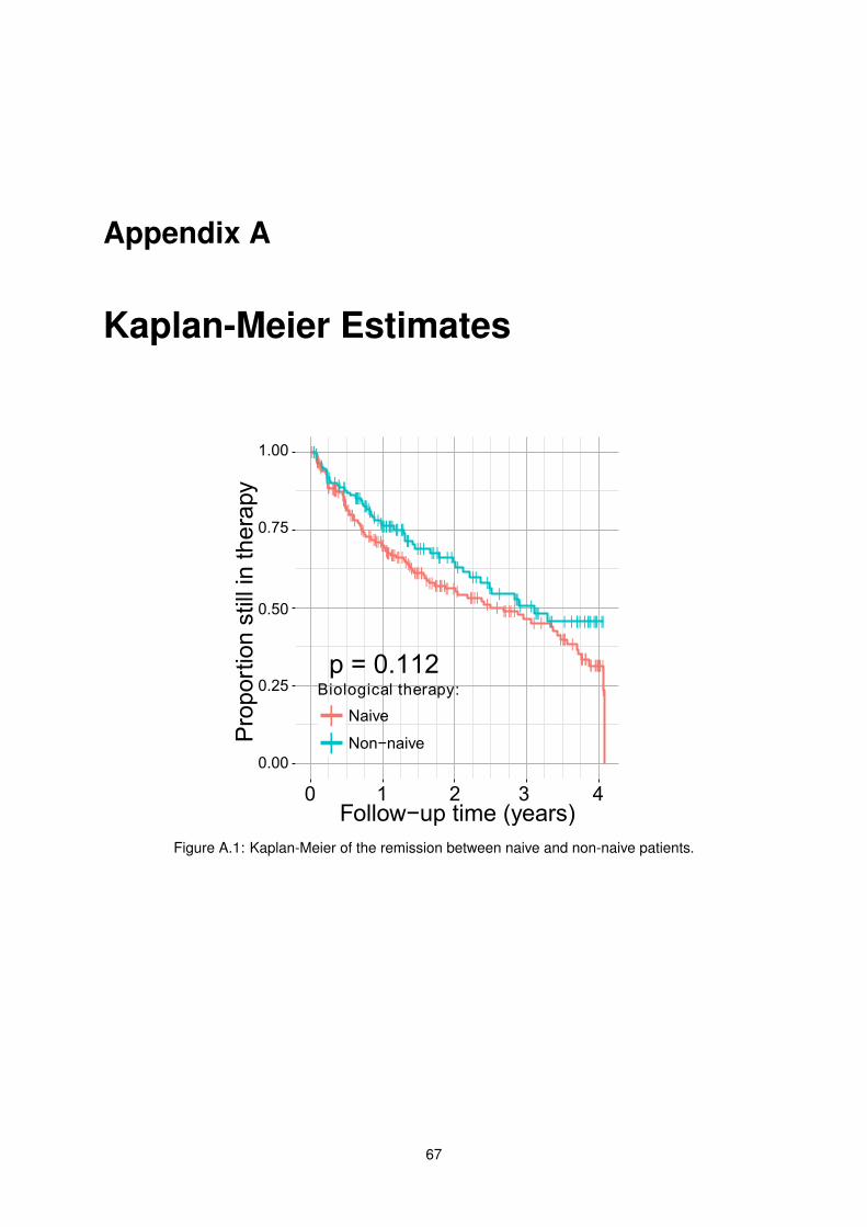
Appendix A
Kaplan-Meier Estimates
Figure A.1: Kaplan-Meier of the remission between naive and non-naive patients.
67
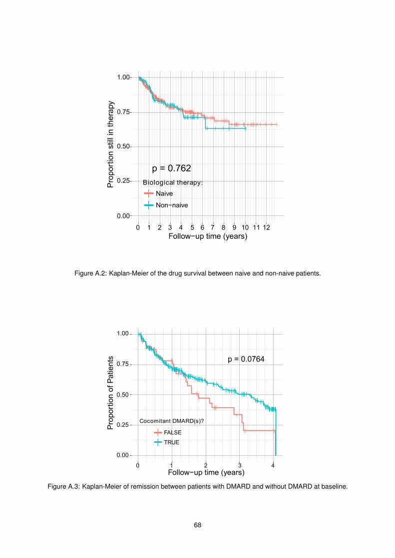
Figure A.2: Kaplan-Meier of the drug survival between naive and non-naive patients.
Figure A.3: Kaplan-Meier of remission between patients with DMARD and without DMARD at baseline.
68
![Die Effektivität von Behandlung der Halswirbelsäu · Der PDI (Pain Disability Index)[9, 22, 27, 54, 61] und der NDI (Neck Disability Index)[21, 67] wurden zur Beurteilung der Funktion](https://img.pdfslide.org/doc/110x75/60b8e64374c191662a718ad3/die-effektivitt-von-behandlung-der-halswirbelsu-der-pdi-pain-disability-index9.jpg)