Embed Size (px)
Citation preview

Werner Raza, Bernhard Tröster, Rudi von Arnim
ASSESS_CETA: ASSESSing ThE ClAimEd bEnEfiTS of ThE EU-CAnAdA TrAdE AgrEEmEnT (CETA)
CETA: ÖkonomiSChE bEwErTUng dEr prognoSTiziErTEn EffEkTE dES EU-kAnAdA frEihAndElSAbkommEnSCommissioned by the Chamber of Labour Vienna
August 2016
GerechtiGkeit muss sein

Impressum
Medieninhaber: Kammer für Arbeiter und Angestellte für Wien,Prinz Eugen Straße 20-22, 1040 Wien, Telefon: (01) 501 65 0Offenlegung gem. § 25 MedienG: siehe wien.arbeiterkammer.at/impressumZulassungsnummer: AK Wien 02Z34648 MISBN: 978-3-7063-0620-1Redaktion: Werner Raza, Bernhard Tröster, Rudi von Arnim
Grafik und Druck: AK Wien, 1040 WienVerlags- und Herstellungsort: Wien© 2016 bei AK Wien
Stand August 2016Im Auftrag der Kammer für Arbeiter und Angestellte für Wien
Demnächst steht auf EU Ebene die Ent-scheidung an, ob das ausverhandelte Freihandelsabkommen CETA zwischen der EU und Kanada angenommen wird. Die Europäische Kommission, aber auch andere BefürworterInnen werben für das Abkommen mit der Förderung des Außen-handels, mit einem höheren Wirtschafts-wachstum, steigenden Einkommen und der Schaffung von Arbeitsplätzen. Die AK hat bei der Österreichischen Forschungs-stiftung für Internationale Entwicklung (ÖFSE) eine Studie in Auftrag gegeben, die prognostizierten Effekte einer Über-prüfung auf fundierter wissenschaftlicher Basis zu unterziehen. Dazu gehörte auch, alle bisherigen Untersuchungen und Stu-dien zu beurteilen und ihre Annahmen und Ergebnisse auf Plausibilität zu prüfen. In einem zweiten Schritt wurden eigene Modellberechnungen angestellt, um zu aktuelleren und zusätzlichen Schlüssen
zu gelangen. Die Ergebnisse der Studie erhärten die Fakten, dass für Österreich keine bis extrem geringe positive wirt-schaftliche Effekte aus CETA zu erwar-ten sind. Nicht berücksichtigt in diesen ökonomi-schen Modellen werden aber gesamtwirt-schaftliche Kosten, die durch die Ände-rungen, Senkungen oder gar durch den gänzlichen Entfall von Regulierungen für die BürgerInnen, KonsumentInnen, ArbeitnehmerInnen oder die Umwelt ent-stehen können. Solch eine Berücksichti-gung des gesellschaftlichen Nutzens von Regulierungen fehlt zudem, wenn es um den Wert hoher Standards bei öffentlicher Daseinsvorsorge und Infrastruktur geht. Auch die Kosten, die durch das Inves-tor-Staat-Streitbeilegungsverfahren ent-stehen, können – wie die Erfahrung in Ka-nada und anderen Staaten zeigt – enorme Ausmaße annehmen. Das droht auch eu-ropäischen Staaten, denn an den privile-gierten Klagsrechten ändert auch das neu verhandelte CETA Tribunal nichts.Wenn wir nun also den Nutzen und die Risiken bzw. Kosten, die durch das Freihandelsabkommen CETA bestehen, gegenüberstellen, dann ist das Ergebnis eindeutig. Es gibt keine bzw. margina-le positive Effekte für den Handel, aber große Risiken bzw. Kosten für die Allge-meinheit. Diese Rechnung geht also klar ins Minus.
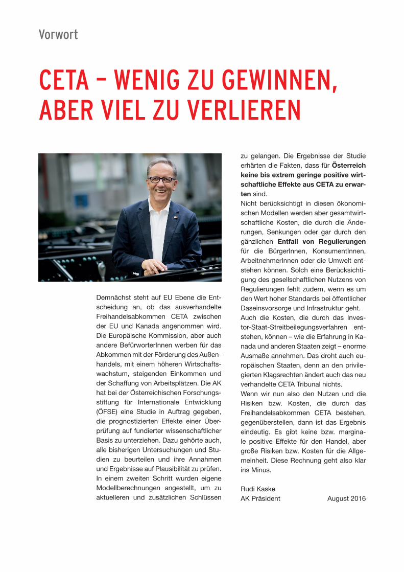
Rudi KaskeAK Präsident August 2016
Vorwort
CETA – wEnig zu gEwinnEn, AbEr ViEl zu VErliErEn
AUSTRIAN FOUNDATION FOR
DEVELOPMENT RESEARCH
ASSESS_CETA: Assessing the claimed benefits of the
EU-Canada Trade Agreement (CETA)
Updated Final Report, 03 August 2016
Werner Raza, Bernhard Tröster (ÖFSE)
Rudi von Arnim (University of Utah, USA)
A report commissioned by Arbeiterkammer Wien
Research 2
CONTENTS
Zusammenfassung ......................................................................................................... 3
Executive Summary ....................................................................................................... 7
1. Context and Motivation ................................................................................................. 11
2. Current Trade Relations with Canada .......................................................................... 12
3. The pro-CETA Reports – Summary and Discussion ..................................................... 14
4. Alternative Simulation Results with ÖFSE Global Trade Model ................................... 26
5. Conclusions.................................................................................................................. 43
References .................................................................................................................. 44
Appendix ...................................................................................................................... 46
About the Authors ........................................................................................................ 48
Research 3
ZUSAMMENFASSUNG
Im Herbst 2016 steht auf EU-Ebene die Entscheidung an, ob das ausverhandelte Freihan-
delsabkommen CETA zwischen der EU und Kanada angenommen wird. Die Europäische
Kommission (EK) wirbt für das Abkommen mit der Förderung von Handelsbeziehungen
und der Schaffung von Arbeitsplätzen. Jedoch kommen auch die von der EU-
Kommission beauftragten Studien nur zu einer verschwindend geringen Steigerung
der Wirtschaftsleistung durch CETA von 0,03% bis 0,08% für die gesamte EU. Dies ent-
spricht nach einer mehrjährigen Implementierungsphase des Abkommens einem einmali-
gen Einkommensgewinn von 20 Euro pro EU-BürgerIn.
Zudem gilt es, die Annahmen und Modelle hinter diesen Ergebnissen zu hinterfragen
und die nicht beachteten Risiken und Anpassungskosten offenzulegen. Dies ist umso
wichtiger, als nicht zuletzt die EU-Kommission selbst die Neuartigkeit des Abkommens be-
tont, durch das in vielen Bereichen die Zusammenarbeit in Regulierungsfragen intensiviert
und der Investorenschutz durch die vieldiskutierte Investor-Staat-Streitbeilegung (Invest-
ment Court System, ICS) ausgebaut wird. CETA gilt damit als eine Vorreiterin für die künfti-
ge Handelspolitik der EU, in der Themen wie Regulierung, Liberalisierung des öffentlichen
Beschaffungswesens und Schutz von Investitionen im Mittelpunkt stehen.
In dieser Studie werden drei Hauptaspekte behandelt:
1) Die bekannten Studien zu ökonomischen Effekten von CETA werden zusammen-
gefasst und kritisch überprüft. Dabei werden unzureichende Modellannahmen
problematisiert und fehlende Risiken und Anpassungskosten dargestellt.
2) Basierend auf dem ÖFSE Global Trade Model werden die ökonomischen Effekte
von CETA auf die Mitglieder des Abkommens und andere Weltregionen – aber auch
speziell für Österreich – geschätzt. Das verwendete Modell erlaubt dabei im Gegen-
satz zu herkömmlichen Ansätzen auch Aussagen zu Effekten auf Beschäftigung,
Löhne, Budgetdefizit und Leistungsbilanz.
3) Modellbasierte Analysen zu den wirtschaftlichen Effekten von Handelsabkommen
sind immer mit gewissen Unsicherheiten verbunden, da bestimmte Parameter nicht
exakt abzuschätzen sind. In den Handelsabkommen der neuen Generation wie CETA
wird dies durch die Bedeutung von nicht-tarifären Handelshemmnissen wie Regulie-
rungen und technische Standards noch verstärkt, da ex-ante unklar ist, wie stark
Handelskosten durch regulatorische Zusammenarbeit gesenkt werden können. Des-
halb wird mithilfe einer Sensitivitätsanalyse die Schwankungsbreite der Ergeb-
nisse aufgrund der Variation von wichtigen Parametern aufgezeigt.
Kritik an bestehender Studien
Zu den wichtigen Studien zu CETA zählen die „Joint Study by the European Commission
and the Government of Canada“ (Joint Study, 2008) und das EU Sustainability Impact As-
sessment (SIA, 2011), die beide von der EK beauftragt wurden. Außerdem ist die Studie
von Francois/Pindyuk (2013) mit Fokus auf Österreich von Relevanz. Die in diesen Studien
verwendeten Modelle beruhen alle auf angebotsseitigen, neoklassischen Annahmen und
können nur bedingt Aussagen über wichtige makroökonomische Variablen wie insbesonde-
re Beschäftigungseffekte machen.
Research 4
Alle drei Studien zeigen positive Effekte für die EU, Österreich und Kanada. So zum
Beispiel:
BIP Steigerung von 0,03% bis zu 0,08% für die gesamte EU; bis zu 0,22% für
Österreich (jeweils nach einem Anpassungszeitraum von 6 bis 10 Jahren)
Steigerung der EU-Exporte nach Kanada um 17% (Joint Study), österreichische
Exporte nach Kanada +50% (Francois/Pindyuk)
Reallohnsteigerungen um 0,06% (EU) bis 0,13% (Österreich)
Mögliche Effekte aus der Liberalisierung des öffentlichen Beschaffungswesens für europäi-
sche Unternehmen werden von den Studien – soweit behandelt – als gering eingeschätzt.
Die große Bandbreite der Ergebnisse hängt von den verwendeten Modellen ab. So ver-
wenden die Joint Study (2008) und Francois/Pindyuk (2013) eine dynamische Modellie-
rung, aufgrund derer sich die statischen Einkommenseffekte um das Fünffache erhö-
hen. Die dafür unterstellte Kausalitätskette (Ramsey-Struktur) ist allerdings nicht über-
zeugend, wird doch angenommen, dass steigende Einkommen durch Exporte die gesamt-
wirtschaftliche Ersparnis erhöhen, was in Folge die Investitionen und den Kapitalbestand
erhöht. Dieser Zusammenhang gilt allerdings nur unter der unrealistischen Annahme der
Vollbeschäftigung. In diesem Sinne betont die Ramsey-Modellstruktur die Bedeutung der
problematischen Vollbeschäftigungsannahme noch mehr als das Standardmodell, und
muss sich derselben Kritik aussetzen.
Obwohl die berichteten Effekte nur langfristig gelten, berücksichtigen die Studien kurz- und
mittelfristige Anpassungskosten nicht. Eine grobe Berechnung auf Grund der in Fran-
cois/Pindyuk (2013) angegebenen sektoralen Verschiebungen auf dem österreichischen
Arbeitsmarkt ergibt eine temporäre Arbeitslosigkeit in Höhe von rund 4.300 Stellen. Die
dadurch entstehenden volkswirtschaftlichen Kosten (Arbeitslosengeld, Ausfall von Steu-
er- und Sozialversicherungseinnahmen) schätzen wir auf ca. 127 Millionen Euro. Die ent-
spricht rund 20% der von Francois/Pindyuk (2013) genannten Zugewinne in der Höhe von
ca. 600 Millionen Euro durch CETA in Österreich.
Für die EU insgesamt ergeben sich Anpassungskosten aufgrund von temporärer Ar-
beitslosigkeit und den damit verbunden Mehrausgaben für Arbeitslosigkeit bzw. Minderein-
nahmen bei Steuern und Sozialausgaben sowie durch entfallenden Zolleinnahmen von bis
zu EUR 5,5 Mrd. über den Anpassungszeitraum von 10 Jahren. Dem gegenüber stehen
mögliche Einkommensgewinne durch CETA in der Größenordnung von EUR 4 Mrd. (SIA,
2011) bis EUR 12 Mrd. (Joint Study, 2008).
ÖFSE Simulation der Effekte von CETA
Mit dem ÖFSE Global Trade Model ist es möglich die ökonomischen Effekte von CETA
auf einzelne EU-Länder und Regionen sowie Kanada, USA und andere Weltregionen und
für 20 Sektoren zu berechnen. In diesem nachfragebasierten Modell werden explizit Be-
schäftigungseffekte und makroökonomische Einflussgrößen ausgewiesen. Es werden
insgesamt vier Szenarien berücksichtigt1, wobei es zum einen um die Reduktion der ver-
bliebenen Zölle im bilateralen Handel und zum anderen um die Angleichung unterschiedli-
cher Standards, Normen und Regulierungen – sog. Nicht-Tarifärer Handelshemmnisse
(NTM) – geht. Daraus ergeben sich für alle CETA-Mitgliedstaaten positive, aber sehr
geringe Effekte (langfristiges Szenario):
1 Szenario 1: Zollreduktion zwischen EU und Kanada um 100%; Szenario 2: Reduktion der nicht-tarifären Handels-
hemmnisse (NTM) im bilateralen Handel um 25%; Szenario 3 (Kurzfristiges Szenario): Zollreduktion um 75% und NTM-Reduktion um 10%; Szenario 4 (Langfristiges Szenario): Zollreduktion um 100% und NTM-Reduktion um 50%.
Research 5
Wachstum des BIP um 0,023% in der gesamten EU und 0,062% in Kanada. Diese
Zuwächse sind als langfristiger Niveaueffekt zu verstehen, d.h. erhöhen das BIP
einmalig während des Umsetzungszeitraums von CETA von rund 10-20 Jahren.
Stärkere Effekte für große EU-Länder (Deutschland, Frankreich, Italien) führen da-
zu, dass andere EU-Länder wie Österreich anteilig am EU-BIP verlieren.
Auf EU-Ebene, profitieren vor allem die Sektoren Nahrungsmittel (+0,13%) und Au-
tomobil (+0,08%).
Die Beschäftigung steigt in der gesamten EU leicht um +0,018%. Die Reallöhne
sinken für ArbeitnehmerInnen mit geringer Qualifikation um -0,011%, bzw. steigen um
+0,014% für ArbeitnehmerInnen mit höherer Qualifikation.
Für Österreich ergibt sich ein realer Einkommenszuwachs von 0,016% oder
knapp 50 Millionen Euro, das sind 6 Euro pro ÖsterreicherIn. Die Veränderung
liegt damit unter dem EU-Durchschnitt.
Die Effekte stammen sowohl aus dem Abbau von Zöllen als auch von NTM, die
Wirkung von NTM-Anpassungen ist allerdings für die meisten EU-Länder und auch
Österreich etwas weniger relevant.
Auf sektoraler Ebene können in Österreich vor allem die Sektoren Automobil
(+0,10%), Nahrungsmittel (+0,06%) und Maschinenbau (+0,03%) leicht profitie-
ren. In Dienstleistungssektoren kommt es zu sehr geringen Veränderungen (ca.
0,01%).
Die Veränderungen auf die Beschäftigung in Österreich bleiben mit einem Zu-
wachs von rund 450 Vollzeitstellen (+0,013%) gering und folgen damit der leicht
positiven Entwicklung des BIP.
Bei den österreichischen Reallöhnen ergibt sich eine leicht negative Veränderung
bei Beschäftigten mit niedrigerem Ausbildungsstand (-0,0023%); Reallöhne von
besser ausgebildeten Beschäftigen steigen minimal (0,009%).
Diese Ergebnisse sollten als ‚Best Case Szenario‘ interpretiert werden, da eine deutliche
Senkung von Handelskosten aus nicht-tarifären Handelshemmnissen (NTM) von 50% an-
genommen wird. Zudem wird in diesem Modell aus methodischen Gründen davon ausge-
gangen, dass die Senkung von Handelskosten aus nicht-tarifären Handelshemmnissen nur
positive ökonomische Effekte bringt. Mögliche Kosten, die bei der Anpassung von Stan-
dards entstehen, sowie allfällige soziale Kosten der Senkung von Standards sind nicht be-
rücksichtigt.
Weitere mögliche Anpassungskosten können während der Implementierungsphase
durch vorübergehende sektorale Arbeitsplatzverluste entstehen. Eine dynamische Simula-
tion des ÖFSE Global Trade Models, ergibt aufgrund der insgesamt äußerst geringen
Wachstumseffekte nur minimale Anpassungskosten auf dem Arbeitsmarkt. Letztere hängen
somit stark von der gewählten Modellstruktur ab. Je höher die erwarteten Effekte auf das
BIP, desto größer auch die zu erwartenden Anpassungskosten auf dem Arbeitsmarkt.
Dementsprechend schwanken die Schätzungen zur vorübergehenden Arbeitslosigkeit
zwischen nahezu Null (ÖFSE Weltmodell), rund 4.300 Stellen in Österreich (unsere
Schätzung auf Basis von Francois/Pindyuk 2013) und 167.000 Stellen in der gesamten
EU (unsere Schätzung auf Basis von SIA 2011).
Research 6
Sensitivitätsanalyse
Die angegebenen Modellergebnisse sind mit einer Unsicherheit verbunden, da einige
wichtige Parameter für die Modellanalyse geschätzt werden müssen. Besonders die Schät-
zungen zu den Handelskosten der nicht-tarifären Handelshemmnisse (NTM) variieren in
den untersuchten Studien stark. Eine Sensitivitätsanalyse unserer diesbezüglichen Ergeb-
nisse zeigt deutlich, dass diese einer beträchtlichen Schwankung unterliegen. Für Öster-
reich bedeutet dies konkret:
Die BIP Veränderungen schwanken zwischen -0,01% und 0,015%.
Auf sektoraler Ebene sind negative BIP-Effekte für alle Sektoren möglich.
Für die Beschäftigungseffekte ergibt sich eine Schwankungsbreite von +/- 300
Vollzeitstellen aus NTM Veränderungen.
In Kombination mit den leicht positiven Effekten aus Zollsenkungen für Österreich
(+325 Jobs), ist somit eine Bandbreite der Beschäftigungseffekte von nahezu Null
bis knapp 600 Vollzeitstellen möglich.
Insgesamt kann man also davon ausgehen, dass auch im positiven Fall die wirtschaftli-
chen Effekte von CETA für Österreich gering sind. Im Gegensatz dazu können potenzi-
ell negative Effekte aus NTM Veränderungen die Gesamteffekte Richtung Null brin-
gen.
Auf EU-Ebene gilt ebenfalls für alle EU Länder und Regionen, dass das BIP je nach Re-
duktion der Handelskosten durch NTMs um bis zu +/- 0,05% schwanken kann. Am
deutlichsten zeigt sich dies für Großbritannien, wo negative Veränderungen bis zu -0,05%
auftreten können. Die Beschäftigungseffekte für Großbritannien sind etwas geringer und
liegen im Bereich von -0,03% und 0,04%. Die Veränderungen in BIP und Beschäftigung für
die anderen EU-Länder bzw. Regionen sind zum Teil deutlich geringer.
Research 7
EXECUTIVE SUMMARY
In late 2016, a decision will be made by the Council of the European Union whether to
launch the ratification process of the free trade agreement between the EU and Canada
(CETA). The European Commission (EC) is promoting the agreement with the prospects of
more trade, stronger economic relations and job creation. However, studies on the
economic impact of CETA report only marginal effects on GDP of 0.03% to 0.08% for
the whole of the EU. In other words, CETA is expected to generate a one-time income ef-
fect of around 20 EUR per EU citizen after a 10 years implementation period.
Despite these small effects by CETA, it is worthwhile to question models and assump-
tions that stand behind these estimations and show neglected risks and adjustment
costs. This task is highly relevant, given that the EC is stressing the innovative character of
the agreement as it includes intensive regulatory cooperation and strengthens investor pro-
tection via the controversially discussed investor arbitration mechanism. CETA is therefore
considered the blueprint of the future EU trade policy that focuses on new topics such as
regulation, liberalization of public procurement and the promotion and protection of invest-
ment.
This report consists of three major parts:
1) The results of often-cited reports on the economic impacts of CETA are summarized
and critically assessed. The problematic model assumptions and the neglected
risks and adjustment costs are analyzed.
2) Based on the ÖFSE Global Trade Model, the economic effects of CETA for the
member countries – with a focus on Austria – and on non-parties are estimated. In
contrast to standard trade models, we are able to report effects on employment,
wages, budget deficits and current accounts.
3) Model-based analysis on the economic impacts of free trade agreements are always
subject to a level of uncertainty given that certain model parameters have to be esti-
mated. This is specifically relevant for trade agreements of the ‘new generation’ with
their focus on non-tariff measures (NTMs) such as regulations and standards, as it
ambiguous ex-ante by how much trade costs related to NTMs can be reduced. Based
on a sensitivity analysis, the variability of our model outcomes is assessed.
Critique on existing CETA studies
The reports on CETA include the „Joint Study by the European Commission and the Gov-
ernment of Canada“ (Joint Study, 2008) and the EU Sustainability Impact Assessment (SIA,
2011), which were both commissioned by the EC. In addition, a study of Francois/Pindyuk
(2013) is assessed that focuses on Austria. All of these studies use models that are based
on supply-side, neoclassical assumptions and cannot speak to important macroeconomic
variables such as employment.
All three studies show positive effects for the EU, Austria and Canada. For instance:
Real GDP growth ranges from 0.03% to 0.08% for the EU and up to 0.22% for Aus-
tria (after an implementation period of 6 to 10 years).
Research 8
Increase in EU exports to Canada by 17% (Joint Study), in Austrian exports to Can-
ada by 50% (Francois/Pindyuk).
Real wage gains by 0.06% (EU) and up to 0.13% (Austria).
Potential effects from the liberalization of public procurement are estimated to have margin-
al effects on European companies.
The wide range of results highly depends on the applied type of model. As the Joint Study
(2008) and Francois/Pindyuk (2013) use a long run model with capital accumulation,
their dynamic results for income exceed static effects by a factor of five. These results
rely on a controversial chain of causation – the so-called “Ramsey-structure” – as it is
assumed that growing income from exports leads to higher overall savings, which in turn
creates investment and higher capital stocks. However, this relation is only valid if full em-
ployment is assumed. In this sense, the ‘Ramsey structure’ compounds the problematic
assumptions of price-clearing markets (specifically labor markets) made in the base-
line static neoclassical CGE models.
Even though the reported effects are long-term gains, the studies do not consider short-
and medium term adjustment cost. A rough calculation based on inter-sectoral displace-
ments in the Austrian labor market reported by Francois/Pindyuk (2013), shows that
4,300 full-time jobs are threatened by temporary unemployment. This amounts to ad-
justment costs (unemployment benefits and foregone taxes and social contributions) of
around EUR 127 million. This is equivalent to about 20% of the gains from CETA of
around EUR 600 million for the Austrian economy reported by Francois/Pindyuk (2013).
For the EU, adjustment costs due to inter-sectoral job displacements and foregone tax
and social security contributions and tariff revenues could sum up to EUR 5.5 billion over
a ten year implementation period, against estimated gains from CETA between EUR 4
billion (SIA, 2011) to EUR 12 billion (Joint Study, 2008).
ÖFSE Simulations on CETA Effects
Based on the ÖFSE Global Trade Model, it is possible to estimate economic effects of
CETA on specific EU countries and regions as well as on Canada, USA and other world
regions and for 20 sectors in each country. The demand-based model explicitly reports
employment effects and changes to macro-economic variables. In total, four scenari-
os are considered2 that include the reduction of tariffs in EU-Canada trade and the effects
of regulatory alignment of so called non-tariff measures.
Our results show positive, but marginally low effects for all CETA-member states in the
long run scenario:
Real GDP grows by 0.023% for the EU and 0.062% for Canada; these changes
represent long run level effects, meaning that the GDP changes occur over a 10-20
year implementation period.
2 Tariff scenario: tariff reduction between EU and Canada by 100%; NTM scenario: Reduction of NTMs by 25%; Short run
scenario: tariff reductions by 75% and NTM reductions by 10%; Long run scenario: Tariff reduction by 100% and NTM re-ductions by 50%
Research 9
Stronger effects occur in the larger EU countries (Germany, France, Italy), mean-
ing the other EU countries such as Austria are losing ground relative to these EU
partners.
On the EU level, above-average gains appear in the sectors ‘processed foods’
(+0.13%) und ‘motor vehicles’ (+0.08%).
EU employment increases slightly by +0.018%. However, real wages shrink slightly
for lower skilled workers (-0.011%), whereas small gains for high skilled workers are
possible (+0,014%).
For Austria, real income effects amount to 0.016% or EUR 50 million, which is
roughly 6 EUR per Austrian citizen. These effects are below EU average.
The effects are caused both by tariff and NTM reductions; NTM trade cost reductions
are crucial for Canada but of less importance for EU countries and Austria.
On the sectoral level in Austria, the sectors ‘motor vehicles’ (+0.10%), ‘processed
foods’ (+0.06%) and ‘other machinery’ (+0.03%) show above-average gains. In the
service sectors only small changes appear (around 0.01%). Changes in employ-
ment in Austria (+450 full-time jobs or 0.013%) are small and follow the small posi-
tive gains in GDP.
Changes in Austrian real wages are different for the two skill-levels. While the real
wage of high skilled workers increases slightly (0.009%), lower skilled workers see
declines in real wages (-0.0023%).
These results should be interpreted as a ‘best case scenario’, since the long run version
includes reduction of NTM trade costs of 50%. Effects of changes in NTMs that are poten-
tially trade facilitating, are not modeled here. Further, potential costs associated with the
alignment of regulations and standards as well as social costs of lower standards are not
considered in this model.
Adjustment costs caused by temporary unemployment during the implementation period
of CETA are possible. However, due to the small growth effects, a dynamic simulation of
the ÖFSE Global Trade Model shows only marginal adjustment costs in the EU and Austri-
an labor markets. Thus, these costs are related to the magnitude of overall changes due to
trade liberalization. Higher effects on GDP also cause higher adjustment costs. Therefore,
the estimates for these costs range from close to zero (ÖFSE Model) to around 4.300
jobs in Austria (our estimates based on Francois/Pindyuk 2013) and 167.000 jobs in the
whole EU (our estimates based on SIA 2011).
Sensitivity Analysis
The reported model results are subject to uncertainty, as a wide range of parameters
have to be applied. Particularly the estimations regarding trade costs of NTMs vary sub-
stantially in the analyzed studies. A sensitivity analysis of our results shows that changes in
NTM reductions can increase the range of variation of our results substantially. For Austria
this means:
GDP changes range from -0.01% to 0.015%.
On a sector level, negative effects on value added are possible in all sectors.
Research 10
For employment, the range of variation is +/- 300 full time jobs due to NTM varia-
tions.
In combination with the small gains from tariff reductions for Austria (+ 325 jobs), total
employment effects range from close to zero up to 600 additional jobs.
Overall, this analysis underlines that the economic effects of CETA for the Austrian
economy are marginal, even in the most positive scenario. Contrary, potentially nega-
tive effects from NTM reductions might bring down overall outcomes to zero.
On the EU level, GDP effects in all EU member states are also subject to variations of
+/- 0.05%, if changes in the NTM trade cost reductions are allowed for. These negative
impacts are most pronounced for the UK with -0.05% on the downside and +0.05% on the
upside. Employment effects in the UK are smaller and range from -0.03% to 0.04%. GDP
and employment effects are less pronounced for all other EU countries.
Research 11
1. CONTEXT AND MOTIVATION
Free Trade Agreements (FTAs) have become an increasingly popular policy instrument
during recent years. The WTO reports that the number of active bilateral or regional FTAs
has increased from around 50 in 1990 to more than 400 in 2015. Likewise, the EU is cur-
rently engaged in a number of FTA negotiations, inter alia with MERCOSUR, ASEAN, the
ACP group of countries, Japan, and most importantly, with the US on TTIP. However, the
first third generation FTA is not TTIP, but the Comprehensive Economic and Trade Agree-
ment (CETA) between the EU and Canada. Negotiations started already in June 2009, and
were concluded in September 2014. Discussion and, eventually, the launching of the ratifi-
cation process of the agreement are scheduled for fall 2016 in the European Parliament.
As many commentators believe, in many regards CETA serves as a blueprint for the TTIP
negotiations. Crucial and, notably, extremely controversial features of TTIP, in particular
investor-to-state-dispute settlement and regulatory cooperation prominently feature already
in CETA.
The decisive question for policy-makers when confronted with FTA negotiations is of
course: Cui bono? More precisely: What are the effects of trade liberalization on economic
growth, the structure of the economy and the distribution of income? These questions have
preoccupied trade policy-makers throughout, in fact, modern history. While advocates of
free trade have traditionally emphasized the positive welfare gains of trade, it is well-known
that trade liberalization leads to a – often sizable – redistribution of income between owners
of production factors. Those negatively affected will eventually resist trade liberalization,
making it difficult for governments to pursue a pro-liberalization agenda. Thus there exists a
political need to base political decisions about trade liberalization upon reliable empirical
information about the likely impacts of a particular FTA on the countries involved.
In an effort to promote the political debate on CETA, several ex-ante reports have been
published by the European Commission and others, that try to shed light on what the
agreement would mean in terms of economic benefits to be expected (see below for de-
tails). In general, the studies find comparatively small but positive effects on trade and in-
come. So far, these reports have been instrumental in delivering a message that there are
substantial, and above all, easy gains to be harvested. In times of economic crisis, this is
indeed an appealing message to the general public.
The standard tool for ex-ante assessments of the impacts of trade liberalisation are so-
called Computable General Equilibrium (CGE) models. The latter have become a routine
element of the Trade Sustainability Impact Assessments of the European Commission, and
are also the methodological backbone of most of the pro-CETA studies produced so far.
However, most of these CGE studies are constructed upon a methodology that is heavily
biased towards demonstrating the positive effects, while sidelining potential negative effects
of the agreement. The lack of providing information on central macroeconomic variables
like employment, government balances or the current account, has to be seen as a severe
shortcoming of mainstream CGE-models. The neoclassical, and also New Keynesian, justi-
fications that all possible adjustment costs, such as job losses due to trade liberalisation,
are short-term and will eventually disappear, as the economy moves towards a new equilib-
rium, are certainly not convincing, neither from a theoretical point of view, nor on empirical
grounds. In order to tackle any negative impacts in due time, from a policy-making perspec-
tive it is therefore imperative to identify them as precisely as possible. Only afterwards can
appropriate remedies be designed and implemented. Furthermore, it is not the case that
any adjustment costs are short-term and temporary. There may well be persistent impacts
on employment, or on the environment. These need to be identified and taken into consid-
eration, before taking far-reaching decisions about trade negotiations.
Research 12
It should thus come as no surprise that the results of most CGE-modelling exercises, in-
cluding those performed by the pro-CETA studies, have been biased towards presenting
overly optimistic predictions on the welfare and growth enhancing effects of trade liberaliza-
tion. What is needed instead is an alternative methodology, which takes relevant policy var-
iables such as unemployment, the distribution of income, public finances, or the external
balance explicitly into account and is hence equipped to present a more realistic picture of
trade liberalization impacts. Only with this information can informed decisions about the
appropriate design of trade agreements be achieved.
In order to rebalance the political debate on CETA, we will in the following critically examine
the beneficial claims made by these reports, lay open their methodological foundations and
biases, and provide an alternative assessment of the potential economic effects of the TTIP
upon key indicators of public interest, in particular income, employment, wages, the public
household and the current account.
2. CURRENT TRADE RELATIONS WITH CANADA
2.1. Trade patterns
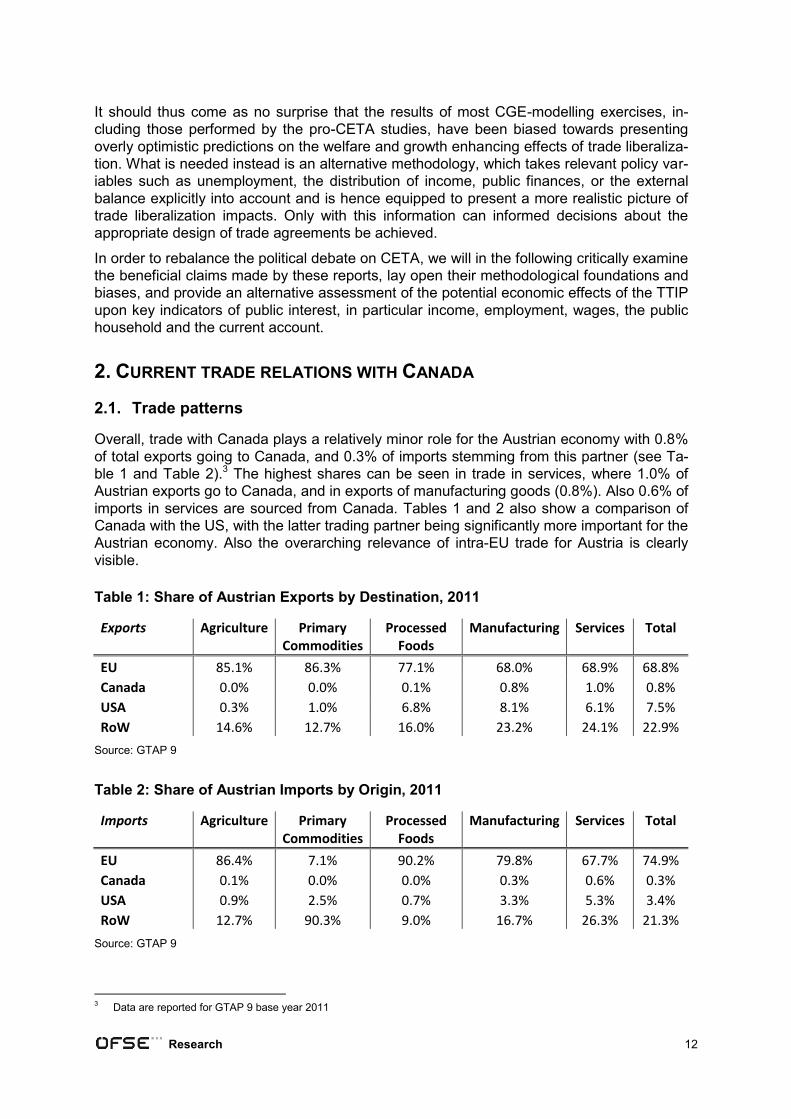
Overall, trade with Canada plays a relatively minor role for the Austrian economy with 0.8%
of total exports going to Canada, and 0.3% of imports stemming from this partner (see Ta-
ble 1 and Table 2).3 The highest shares can be seen in trade in services, where 1.0% of
Austrian exports go to Canada, and in exports of manufacturing goods (0.8%). Also 0.6% of
imports in services are sourced from Canada. Tables 1 and 2 also show a comparison of
Canada with the US, with the latter trading partner being significantly more important for the
Austrian economy. Also the overarching relevance of intra-EU trade for Austria is clearly
visible.
Table 1: Share of Austrian Exports by Destination, 2011
Exports
Agriculture Primary Commodities
Processed Foods
Manufacturing Services Total
EU 85.1% 86.3% 77.1% 68.0% 68.9% 68.8%
Canada 0.0% 0.0% 0.1% 0.8% 1.0% 0.8%
USA 0.3% 1.0% 6.8% 8.1% 6.1% 7.5%
RoW 14.6% 12.7% 16.0% 23.2% 24.1% 22.9%
Source: GTAP 9
Table 2: Share of Austrian Imports by Origin, 2011
Imports
Agriculture Primary Commodities
Processed Foods
Manufacturing Services Total
EU 86.4% 7.1% 90.2% 79.8% 67.7% 74.9%
Canada 0.1% 0.0% 0.0% 0.3% 0.6% 0.3%
USA 0.9% 2.5% 0.7% 3.3% 5.3% 3.4%
RoW 12.7% 90.3% 9.0% 16.7% 26.3% 21.3%
Source: GTAP 9
3 Data are reported for GTAP 9 base year 2011
Research 13
On an EU-28 level, trade relations with Canada are more intense with an overall export
share of more than 1.1% and an import share of 0.9%. Particularly the EU trade in services
with Canada is relevant (export share of 1.9% and import share of 1.2%). Also imports from
Canada in agricultural (share of 1.2%) and primary commodities (share of 1.1%) play a cer-
tain role, while EU exports in processed foods to Canada (share of 0.9%) are more pro-
nounced on the EU-level compared to Austrian trade data (see Table 3 and Table 4).
Table 3: Share of EU Exports by Destination, 2011
Exports
Agriculture Primary Commodities
Processed Foods
Manufacturing Services Total
EU 76.2% 64.0% 72.0% 60.7% 54.6% 60.3%
Canada 0.2% 1.3% 0.9% 0.8% 1.9% 1.1%
USA 1.2% 1.9% 5.0% 7.4% 10.2% 7.7%
RoW 22.4% 32.8% 22.1% 31.1% 33.4% 31.0%
Source: GTAP 9
Table 4: Share of EU Imports by Origin, 2011
Imports
Agriculture Primary Commodities
Processed Foods
Manufacturing Services Total
EU 58.0% 7.3% 77.7% 63.6% 55.3% 57.4%
Canada 1.2% 1.1% 0.3% 0.7% 1.2% 0.9%
USA 4.1% 1.2% 1.9% 6.5% 12.3% 7.0%
RoW 36.7% 90.4% 20.1% 29.2% 31.2% 34.7%
Source: GTAP 9
UN Comtrade data on Austrian trade in goods for 2014 show that Canada is ranked as the
23rd most important destination of Austrian goods exports. On the import side, Canada is
only ranked on position 41. In goods exports to Canada, the most important sectors are
machinery and equipment (here named ‘other machinery’) with a share of 37% in 2014,
followed by chemicals (13%) and motor vehicles (10%). This pattern changed over time, as
‘motor vehicles’ were the most important Austrian export sector in 2004 with a share of
29%. On the import side, transport equipment and metals are the most important Canadian
sectors with a share of 34% and 19%, respectively. Similar to the exports side, the rele-
vance of the motor vehicles sector declined substantially as it accounted for 30% of imports
from Canada in 2003 and decreased to 2% in 2014 (Source: UN Comtrade Database).
For the whole EU-28 similar sectoral patterns are visible in the exports to Canada, with the
sectors machinery and equipment (23%), chemicals (20%) and motor vehicles being most
relevant in 2014. On the imports side, additional sectors are crucial compared to the Austri-
an trade patterns. Besides metals (23%) and transport equipment (12%), also minerals
(11%), crude oil (6%) and wheat (3%) have a crucial share in EU goods imports from Can-
ada (Source: UN Comtrade Database).
Overall, Austrian trade with Canada developed dynamically in recent years. In particular
goods exports increased from USD 520 million in 2002 to more than USD 1.3 billion in
2014. Imports from Canada to Austria increased as well from USD 304 million to 407 million
over the same period. Consequently, the strong export expansion created a substantial
surplus in goods trade for Austria against Canada in recent years. Taking also service trade
Research 14
into account inflates the Austrian trade surplus even more. The same trend is true for the
EU-28, however the surplus is as distinct as in the Austrian case with goods exports to
Canada amounting to around USD 41 billion and imports to more than USD 35 billion in
2014 (Source: UN Comtrade Database).
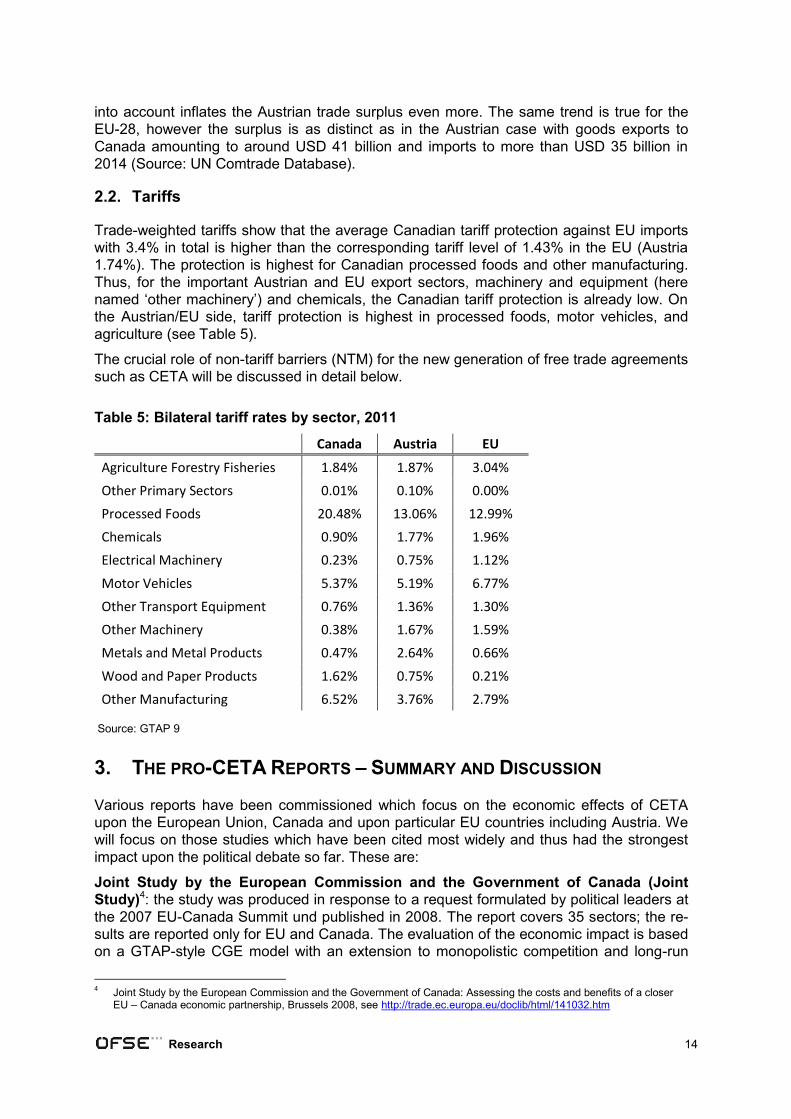
2.2. Tariffs
Trade-weighted tariffs show that the average Canadian tariff protection against EU imports
with 3.4% in total is higher than the corresponding tariff level of 1.43% in the EU (Austria
1.74%). The protection is highest for Canadian processed foods and other manufacturing.
Thus, for the important Austrian and EU export sectors, machinery and equipment (here
named ‘other machinery’) and chemicals, the Canadian tariff protection is already low. On
the Austrian/EU side, tariff protection is highest in processed foods, motor vehicles, and
agriculture (see Table 5).
The crucial role of non-tariff barriers (NTM) for the new generation of free trade agreements
such as CETA will be discussed in detail below.
Table 5: Bilateral tariff rates by sector, 2011
Canada Austria EU
Agriculture Forestry Fisheries 1.84% 1.87% 3.04%
Other Primary Sectors 0.01% 0.10% 0.00%
Processed Foods 20.48% 13.06% 12.99%
Chemicals 0.90% 1.77% 1.96%
Electrical Machinery 0.23% 0.75% 1.12%
Motor Vehicles 5.37% 5.19% 6.77%
Other Transport Equipment 0.76% 1.36% 1.30%
Other Machinery 0.38% 1.67% 1.59%
Metals and Metal Products 0.47% 2.64% 0.66%
Wood and Paper Products 1.62% 0.75% 0.21%
Other Manufacturing 6.52% 3.76% 2.79%
Source: GTAP 9
3. THE PRO-CETA REPORTS – SUMMARY AND DISCUSSION
Various reports have been commissioned which focus on the economic effects of CETA
upon the European Union, Canada and upon particular EU countries including Austria. We
will focus on those studies which have been cited most widely and thus had the strongest
impact upon the political debate so far. These are:
Joint Study by the European Commission and the Government of Canada (Joint
Study)4: the study was produced in response to a request formulated by political leaders at
the 2007 EU-Canada Summit und published in 2008. The report covers 35 sectors; the re-
sults are reported only for EU and Canada. The evaluation of the economic impact is based
on a GTAP-style CGE model with an extension to monopolistic competition and long-run
4 Joint Study by the European Commission and the Government of Canada: Assessing the costs and benefits of a closer
EU – Canada economic partnership, Brussels 2008, see http://trade.ec.europa.eu/doclib/html/141032.htm
Research 15
investment dynamics. The results show absolute gains in GDP and welfare for both, EU
and Canada, with higher GDP percentage changes occurring for Canada (0.77%; EU:
0.08%). However, negative sectoral output changes appear mainly in the Canadian econo-
my.
EU Sustainability Impact Assessment (SIA):5 the report was commissioned by the Euro-
pean Commission and published in 2011. Besides an economic assessment, the study
analyses social and environmental impacts of CETA. Trade cost reductions due to NTM
alignments follow the approach by the Joint Study (2008). The CGE model, however, does
not include capital accumulation, meaning that economic effects are positive but lower
compared to the Joint Study results with GDP changes ranging from 0.03% for the EU and
0.36% for Canada. The study also reports effects on non-CETA countries/regions and de-
tailed sectoral results. In total 57 sectors are covered. The report also shows potentially
negative, but small, impacts on non-CETA countries and regions.
Francois/Pindyuk (F/P):6 this study focuses on the impact of three free trade agreements
(EU-US, EU-Canada and EU-Moldova/Georgia/Armenia) on the Austrian economy and was
published as FIW-Research Report in 2013. The effects of regulatory alignment are based
on specific NTM trade cost estimations. Importantly, Francois/Pindyuk (2013) apply a long-
run, dynamic model that incorporates effects resulting from capital accumulation. Overall,
this leads to accelerated national income gains of 0.215% from CETA in Austria. In addi-
tion, employment and real wages are expected to increase. However, most results are re-
ported for Austria only and use 21 sectors.
3.1. Economic effects of CETA in detail
Even though a direct comparison of study results should be taken with care due to the dif-
ferences in database, base year, baseline assumptions, as well as scenario design and
other factors, in the following we present a summary of results from the three selected stud-
ies.
National Income/GDP Impacts
All three studies report changes in national income which is measured by equivalent varia-
tions (EV). This measure reports a change in real income that allows consumers to obtain
the same utility level after a change in prices, due to trade liberalization, for example, as
before, but at the original relative prices.7
In the case of the comparative-static (short-run) model results, the Joint Study (2008) re-
ports higher EV effects for Canada (EUR 4,100 million) compared to EU gains (EUR 2,527
million) (see Table 6). In contrast, SIA (2011) sees higher EVs on the EU side (EUR 3,400
million) than for Canada (EUR 2,932 million). However, in the dynamic model of the Joint
Study (2008), the static gains are lifted by factors 2 to 4, leaving higher EVs for the EU
(EUR 10,539 million) compared to Canada (EUR 8,364 million). This significant dynamic
investment effect is also reported by Francois/Pindyuk (2013) with total long-run gains ex-
ceeding static gains by a factor of 5. The EV for Austria amounts to USD 684 million.
5 Development Solutions: A Trade SIA relating to the negotiations of a comprehensive economic and trade agreement
between the EU and Canada, Final Report, Study commissioned by the European Commission, Trade 10/B3/B06, June 2011, see: http://ec.europa.eu/trade/policy/policy-making/analysis/sustainability-impact-assessments/assessments/#study-geo-14 Listed as Kirkpatrick et al. (2011) in the references
6 Francois, J./Pindyuk, O: Modeling the Effects of Free Trade Agreements between the EU and Canada, USA and Moldo-
va/Georgia/Armenia on the Austrian Economy: Model Simulations for Trade Policy Analysis, FIW Research Report 2012/13 N° 03, Vienna, January 2013, see: http://www.fiw.ac.at/fileadmin/Documents/Publikationen/Studien_2012_13/03-ResearchReport-FrancoisPindyuk.pdf
7 Potential problems with the EV measure due to the lack of empirical substance as well as the concept of welfare itself are
discussed in Raza et al. (2014, p.45) in more detail.
Research 16
Table 6: National Income effects (EV), in million EUR
EU / Austria Canada
Joint Study 2,527 (Stat)
10,539 (Dyn) 4,100 (Stat) 8,364 (Dyn)
SIA 3,400 2,932
F/P 684 (USD) -
Notes: Changes in million EUR; ‘Stat’ refers to changes in comparative-static (short-run) model, ‘Dyn’ refers to chang-es in dynamic model; Francois/Pindyuk results for Austria only.
The contribution to national income changes due to tariff and NTM reductions in goods and
services varies among the studies due to different trade cost estimates of NTMs. While the
Joint Study (2008) and the SIA (2011) gains follow from tariff and services NTM reduction,
Francois/Pindyuk (2013, Table 15, p.19) see around two thirds of higher national income in
Austria coming from reductions in goods NTMs.
The absolute changes should however be related to effects per household or capita, as the
population in the EU-28 (508.3 million people in 2014, source: World Development Indica-
tors) exceeds the Canadian population (35.5 million people in 2014) by a factor of more
than 14. Thus the most optimistic estimates in the Joint Study (2008) would be equal to
additional income of about 20 EUR per EU citizen and about 235 EUR per Canadian citi-
zen. This size-effect also shows up in percentage GDP changes.
In contrast to the absolute effects, the percentage changes in GDP show large differences
between the CETA-member states. While the EU sees only minor effects ranging from 0.03
to 0.08%, the Canadian GDP increases by 0.36 or 0.77%, respectively (see Table 7). The
difference between the upper and lower bounds is again related to the application of dy-
namic and static models. Overall, all studies show a positive impact of CETA on GDP and
national income. However the effects are marginal for the EU and moderate for Canada,
even if all long-run dynamic and variety/specialization gains are included.
Table 7: Changes in GDP, in percent
EU Canada
Joint Study 0.08 (Dyn) 0.77 (Dyn)
SIA 0.03 (Stat) 0.36 (Stat)
F/P 0.215* (Dyn) -
Note: * Francois/Pindyuk report changes in national income
Sectoral Output Impacts
Even though aggregate GDP effects might be minor, sectoral output impacts are more dif-
ferentiated, specifically for Canada. All three studies report sectoral output changes with the
highest degree of detail included in the SIA (2011). However, similar patterns among declin-
ing and expanding sectors can be identified only to a limited degree in the Joint Study
(2008) and SIA (2011). The sectoral results for Austrian output in Francois/Pindyuk (2013)
are an exception as they are throughout positive for all sectors except one. This reflects
also the different modelling approaches.
The Joint Study (2008) sees substantial sectoral changes in the Canadian economy rang-
ing from a decline of -6.0% in the processed foods sector to gains of 11.0% in the metals
sector as a result of the relative sizes of the two economies. Most Canadian manufacturing
Research 17
sectors benefit significantly from CETA, while effects for the Canadian service sectors are
mixed and contractions are reported for processed foods and beverages & tobacco. On the
EU-side, negative changes are notable in a number of manufacturing sectors (metals,
transport equipment and machinery & equipment with up to -0.7%). All other sectors show
marginal and slightly positive output changes, with the processed foods sector seeing the
strongest expansion (+0.6%).
The static model results in the SIA (2011) show less pronounced sectoral output effects
compared to the Joint Study (2008). However, it underlines the pattern of stronger changes
for Canada and the mixed results in the manufacturing sector on both sides. The main dif-
ferences in the sectoral results appear in the agricultural and processed foods sectors. The
disaggregated sectoral effects in the SIA see most EU sub-sectors such as wheat, red meat
and other meat products as loosing sectors due to CETA, while the corresponding Canadi-
an sectors gain from the agreement. The reverse effect is reported for the dairy sector with
substantial losses in the Canadian dairy sector of more than -12.5%, while the EU-dairy
sector gains close to 1%. Thus, the SIA (2011, p.15) highlights potentially large CETA ef-
fects in sensitive food products.
The sectoral output changes due to CETA for the Austrian economy in Francois/Pindyuk
(2013, p.15, Table 10) are positive for all sectors except for the ‘other goods’ sector. All
other sectors increase production ranging from 0.05% in chemicals up to 0.74% in motor
vehicles. The positive output effects reflect the dynamic investment impacts assumed in the
model which leads to broad increases across most sectors. Corresponding effects for Can-
ada are not reported.
Trade Impacts
In the studies, output changes are related to changes in trade due to the trade liberalisation.
These changes reflect the reductions in trade costs that come from elimination of tariffs and
trade costs related to NTMs.
Only SIA (2011) reports changes in total exports with a marginal increase of 0.07% for the
whole EU and 1.56% for Canada in their most comprehensive scenario D. This results in an
improvement of the EU’s balance of trade of close to USD 200 million, meaning that growth
in EU’s exports exceeds growth in imports by that amount. This is largely driven by effects
from service liberalisation (SIA 2011, p.45, Figure 3). For Canada, the balance of trade im-
proves by almost USD 500 million as Canada also benefits from tariff cuts (SIA 2011, p.45,
Figure 4).
Changes in bilateral trade are reported in the Joint Study (2008, for EU-Canada) and by
Francois/Pindyuk (2013, for Austria-Canada) (see Table 8). In the Joint Study (2008) per-
centage changes in bilateral trade are almost identical with 16.8% in EU exports to Canada
and 16.5% in Canadian exports to the EU. Based on the different initial trade volumes, this
leads to a higher absolute change in exports by EUR 11.5 billion in the case of EU exports
to Canada compared to increased exports from Canada to the EU by EUR 6.4 billion.
Changes in EU exports exceed corresponding Canadian exports in both industrial goods
and services. In addition EU exports in processed foods contribute significantly to higher
EU exports with an increase of more than EUR 5.5 billion or 326%.
Table 8: Changes in bilateral exports, in percent
EU / Austria Canada
Joint Study 16.8 16.5
F/P 50.3 71.9
Research 18
Francois/Pindyuk (2013) see higher positive bilateral export effects for Canadian exports to
Austria. With an increase of 71.9%, the trade gains for Canadian exports exceed changes
of 50.3% for Austrian exports to Canada. In absolute terms, the translates to export gains
for the Austrian economy of USD 586 million while imports from Canada grow by 2.1 billion
and therefore exceed export growth by a factor of 3.6.8 Austrian export gains appear mainly
in manufacturing sectors (motor vehicles and textiles) as well as processed foods. Exports
to Canada in agriculture/fishery/forestry even decline slightly. In service sectors, Austrian
export gains exceed the corresponding growth rates for Canadian exports. Otherwise, Ca-
nadian sectoral export changes generally surpass Austrian export changes in the primary
and manufacturing sectors. Overall, this would result in substantial negative trade impacts
for the Austrian economy, with a negative change in the bilateral trade balance of around
USD 1.5 billion according to Francois/Pindyuk. That the authors nonetheless report positive
changes in output shows the relevance of dynamic investment effects in their model.
Wages and Employment Impacts
Commonly used macroeconomic closures in standard CGE models require holding con-
stant either real wages or employment. In the Joint Study (2008) no results on wages and
employment are reported. In the SIA (2011) results for changes in real wages are shown
(see Table 9). In accordance to percentage changes in output, changes for both skill levels
are higher in the Canadian economy. For the whole EU, the changes in real wages are mi-
nor. Due to the application of a static CGE model, employment supply is fixed in the SIA
(2011) analysis.
Francois/Pindyuk (2013) report changes in both variables for the Austrian economy. Real
wage changes amount to around 0.13%. In addition, changes in employment are reported
with an increase of 0.065% in unskilled employment and 0.064% in skilled employment due
to CETA as Francois/Pindyuk assume an upward sloping labor supply curve following Dee
et al. (2011). Employment changes are however smaller compared to changes in national
income and capital formation.
Table 9: Changes in real wages by skill level, in percent
unskilled skilled
EU / Austria Canada EU / Austria Canada
SIA 0.06 0.52 0.07 0.49
F/P 0.131 - 0.129 -
Public Procurement
In recent years, the EU Commission has been pushing for the inclusion of far-reaching pub-
lic procurement clauses in FTAs, given that potential benefits from cost reductions and
trade facilitation are expected. Even though OECD data suggest that procurement spending
often amounts to more than 10% of GDP in developed countries, the international dimen-
sion of these expenditures is ambiguous (Cernat/Kutlina-Dimitrova, 2015). As a substantial
part of public procurement such as e.g. in social services and in specific sectors and goods
(military) are not tradable or too sensitive for negotiations, the relevance of public procure-
ment in FTAs is arguably limited. Therefore, none of the CETA studies estimates specific
8 Reported percentage and absolute changes in Francois/Pindyuk imply that bilateral trade flows in 2011 would amount to
USD 1.16 billion (USD 586 million / 0.503) in Austrian exports and USD 2.92 billion (USD 2.1 billion / 0.719) in Austrian imports from Canada. These data are not in accordance to any other trade data source where Austria has a positive trade balance with Canada.
Research 19
economic effects based on public procurement provisions.9 Nevertheless, the Joint Study
(2008) and SIA (2011) emphasize that liberalization would potentially benefit the EU, as the
WTO Agreement on Government Procurement (GPA) already provides Canadian compa-
nies broad access to EU procurement processes. Canada, however, still excludes its sub-
central government entities from international competition, also from the US. Thus, liberali-
zation and increased competition would occur on the Canadian side and not on the already
comparatively open EU market. However, it is highlighted in the SIA (2011, p.258) that it
would be EU companies with existing foreign subsidiaries, hence multinational firms, that
would benefit from Canadian procurement liberalization first and foremost.
With regard to the procurement chapter in the consolidated CETA text, thresholds have
been implemented, which range from SDR 130,000 (equivalent to current EU threshold
EUR 135,000) for goods and services procurement to SDR 5 million (equivalent to current
EU threshold of EUR 5.225 million) for construction projects, thus limiting the access for
foreign bidders and concomitantly the economic gains to be expected.
Overall, this indicates that potential effects for the EU from public procurement provisions of
CETA are rather limited. This conclusion is further supported by the fact that Canada is
about to open up its public procurement via TPP and other FTAs – which would intensify
competition for EU companies in the Canadian market.
3.2. Discussion of the Methodologies applied in the pro-CETA Studies
CETA is set up as a free trade agreement aiming at ‘deep integration’ of the trading part-
ners’ economies. This necessarily involves the reduction of trade costs associated with
non-traditional barriers to trade, so called non-tariff measures (NTMs). However, many
components of these trade costs are unobservable. In recent years, econometric analysis
based on gravity models has evolved as the standard approach to derive the size of these
barriers to trade. Berden/Francois (2015, p.3) define the resulting trade cost equivalents of
NTMs in bilateral trade as the quantified difference in regulatory systems between the trad-
ing partners. Consequently, a reduction of NTM trade costs is equal to the “lowering of the
differences between regulatory systems” (Berden/Francois 2015, p.4) either through har-
monization, mutual recognition or elimination of standards. Such a process is managed via
the institutionialization of ‘regulatory cooperation’ in the agreement. An alignment of regula-
tory divergence does therefore not necessarily lead to a lowering of standards. However, it
is likely that the process involves at least adjustment costs for different actors in the econ-
omy (see also Raza et al., 2016a).
Besides the absolute size of NTM trade cost estimations, the actionability of NTMs is cru-
cial. The term ‘actionability’ expresses the possibility to change current regulations and
standards in order to facilitate trade. Based on expert interviews Ecorys (2009) conclude
that roughly 50% of existing NTMs are potentially ‘actionable’ and recent trade impact as-
sessments on TTIP (for instance CEPR 2013) typically assume that half of these actionable
regulatory divergences can be reduced in a bilateral FTA. This yields a NTM trade cost re-
duction of 25% which can be deducted from the estimated trade cost equivalents. Alterna-
tively, other studies apply an approach that uses the intra-EU integration towards the single
market as a benchmark for potential trade effects through regulatory convergence.
9 Estimation by CEPR (2013) on TTIP could serve as upper bound estimation. According this study public procurement
liberalization contributes 1/10th to the overall benefits. The size of the Canadian market and the one-sided liberalization
might reduce these effects even more.
Research 20
On NTM Reductions
In the Joint Study (2008), two different approaches are used for NTM trade cost estimations
and reductions in the goods and service sectors. While in non-commodity goods sectors
trade costs generated by NTMs are reduced simply by a uniform cut of 2% of the value of
trade, all commodity sectors (coal, oil, gas, minerals) as well as primary agriculture are ex-
cluded from NTM trade cost reductions and only tariff cuts apply for these sector. The au-
thors justify their assumed reduction rate of 2% by “anecdotal evidence” (p.41) without cit-
ing specific studies supporting this assumption.
For the service sectors, the impact of the intra-EU liberalisation on intra-EU service trade
flows are used as an upper-bound solution that is assumed to be achievable also in the EU-
Canada context. According to results of other studies co-authored by Joseph Francois, the
level of intra-EU trade in services is 35% higher compared to a non-EU scenario. To
achieve similar increases in EU-Canada service sector trade, bilateral trade costs have to
be reduced by 2 to 10% depending on the specific sector. In this context, the total trade
cost estimates are also reported. These range from 24 - 52% for trade in services into Can-
ada and from 18 to 24% for trade in services into the EU. This means that NTM trade cost
equivalents are reduced by 16% for EU exports to Canada and by 22% for Canadian ex-
ports to the EU.
Given the larger trade cost reductions in service sectors compared to the goods sectors,
the growth in national income and GDP in the Joint Study (2008) is largely determined by
service trade. This is also the case in the SIA (2011) as the latter’s scenarios explicitly refer
to Joint Study NTM reductions in the service sectors. Importantly, SIA (2011) includes only
reductions in tariffs and service sector NTMs to varying degrees in their four scenarios; re-
ductions in goods NTMs are not considered.
The NTM reductions in Francois/Pindyuk (2013) refer also to the Joint Study (2008), but the
reported reductions for the service sector differ from the original data in the Joint Study. As
Francois/Pindyuk (2013, p.10) reduce actionable barriers to trade by 25%, they assume a
higher rate of reduction compared to 16% (Canada) and 22% (EU) in the Joint Study
(2008). However the underlying magnitude of trade cost estimations are not reported.10 It is
also unclear, if the reported EU-27 NTM reductions refer to changes in relation to the US,
Canada or Moldova/Georgia/Armenia, or if all three FTA partners are taken into account.
Francois/Pindyuk (2013) see the highest trade cost reductions in the Canadian motor vehi-
cles (12.3%), transportation equipment (9.4%) and construction sectors (8.6%). On the EU
side the insurance sector (15.0%), motor vehicles (12.5%) and finance (9.6%) liberalize the
most. Overall, the reductions in goods sectors with 5.2% for exports to Canada and 6.2%
for export to the EU are notably higher than the assumed uniform reduction of 2% in the
Joint Study (2008). Consequently, the NTM reductions in goods contribute most (two thirds)
to the gains for the Austrian economy from CETA.
All three studies uniformly see NTMs only as barriers to trade that involve costs for produc-
ers and consumers as well as efficiency losses. However, quantity-based approaches
(gravity models) to estimate trade cost equivalents also show negative results meaning that
regulations have trade-facilitating effects.11 The intuition behind this idea is that certain
standards and regulations such as quality or fair trade certifications address consumer con-
cerns in the importing country with respect to health, environmental and safety issues and
thus have a positive effect on trade. This can be particularly relevant for agricultural goods
and food. For instance, Bratt (2014) and Beghin et al. (2012) estimate that about 46% and
10
The reference to an OECD report by Dee et al. (2011) reveals that unpublished survey data by Ecorys (2009) were used to construct NTM indices and trade cost equivalents also for the EU-Canada trade relations. However, details are missing in in Dee et al. (2011) and Francois/Pindyuk (2013).
11 In contrast, a prominent study on NTMs by Kee et al. (2009) sets AVE to be non-negative by construction.
Research 21
39%, respectively, of the product lines affected by NTMs exhibit negative tariff equivalents
(AVEs). Also Dean et al. (2009), using a price-based NTM quantification methodology, see
partial positive correlations between NTM restrictiveness and country income, given that
regulatory barriers can also reflect income sensitive demand for higher consumer protection
for instance in food products. So far, approaches to include these potential trade-facilitating
effects of NTMs are not included in the standard NTM estimations used in the standard
impact assessments.
On dynamic CGE Models
As described in section 3.1., the magnitude of reported results crucially depends on the
application of ‘dynamic’ or ‘long-run’ CGE models. In contrast to ‘static’ or ‘short-run’ CGE
models, the former type of models include changes in factor utilization (accumulation). Im-
portantly, the term ‘dynamic’ in standard CGE modelling – as applied in the Joint Study
(2008) and Francois/Pindyuk (2013) – does not imply that the model is actually solved as a
system of differential equations. Rather, it merely renders factor use endogenous. Specifi-
cally, a dynamic CGE model, according to this terminology, includes capital accumulation.
Traditional (static) models feature fixed factor endowments (Shoven/Whalley, 1984). As
standard CGE models usually yield positive efficiency gains from trade liberalisation, addi-
tional changes in capital stocks will further exaggerate the overall results. In the case of
Francois/Pindyuk (2013) dynamic results are five times higher than the static gains.
These mechanisms are controversial, as growth effects are introduced through the back-
door (Rodrik, 2015). Moreover, the implied causal chain is subject to criticism, as it is as-
sumed that growing income through higher exports can generate higher savings and there-
fore lead to higher investments. This, however, depends again on the unrealistic assump-
tion of full employment.
In sharp contrast, in the ÖFSE Global Trade Model the term ‘dynamic’ has the standard
meaning: the system of simultaneous equations consists of differential equations, and solu-
tions for endogenous variables are functions of time (see section 4.3 for a further discus-
sion).
Dynamic CGE modelling approaches are rooted in economic growth models à la Solow and
Ramsey. The basic idea of these models on capital accumulation and steady states are
also included in Francois/McDonald/Nordström (1996). In this paper, which serves as refer-
ence for the models in the Joint Study (2008) and Francois/Pindyuk (2013), capital accumu-
lation in CGE models is differentiated between a static case and two steady-state, dynamic
closures. These three cases also show up in the standard descriptions of CGE models à la
Francois in Francois/Pindyuk (2013, p.28): “For investment demand, in the short run, we
assume a fixed savings rate. In the long-run, the model can alternatively incorporate a fixed
savings rate, or a rate that adjusts to meet steady state conditions in a basic Ramsey struc-
ture with constant relative risk aversion (CRRA) preferences.”
In the short run, the ratio of income going to savings is fixed. However, the capital stock is
not allowed to change as efficiency gains are simply realized by more efficient allocation of
given production factors (labor and capital). In the long run, two possibilities are given in
these models. Firstly, the savings rate remains fixed but the whole model is assumed to
change until a steady state is reached. Implicitly, this is based on the assumption that all
regions are initially in a steady state which also Francois/McDonald/Nordström (1996, p.9)
call “a convenient although admittedly unrealistic assumption”. Similar to the mechanisms in
a Solow growth model, efficiency gains through trade liberalization shift output (=income),
and therefore savings, up. As a consequence, the capital stock expands until savings and
investment are just enough to replace depreciated capital. In other words, a fixed proportion
Research 22
of the static gains flows into savings and investment. This generates additional income,
which in turn is saved and invested until a steady state is reached. In this case, induced
investment is simply a multiple of the static gain. The magnitude of the multiplier depends
on the output-capital elasticity and increases with higher capital shares in the production
function (Francois/McDonald/Nordström 1996, p.4).
Secondly, a dynamic closure is possible that allows for endogenous savings rates and en-
dogenous capital stocks as it is applied in Francois/Pindyuk (2013). In this case the savings
rate is determined via optimization of consumption over time ‘in a basic Ramsey structure’.
The Ramsey problem refers to the optimal inter-temporal allocation of consumption (see
Blanchard/Fisher, 1989, chapter 2 and Taylor, 2004, chapter 3). There are infinitely-living
households that trade off consumption levels of future and current generations in order to
maximise overall utility stemming from consumption. In the absence of technological pro-
gress, this optimization process results in a steady state with constant levels of consump-
tion and capital stock per worker. In contrast to the well-known golden-rule condition à la
Solow with the marginal product of capital being equal to the rate of depreciation plus popu-
lation growth, a rate of time preference is included in the inter-temporal Ramsey structure,
setting the steady state below the golden rule level. This rate of time preference – or rate of
time discount or rate of impatience – expresses the desire to consume now instead of at a
future point in time. Thus, the more patient a representative household is in order to post-
pone consumption to later points in time, the smaller is the rate of time preference and the
smaller is the difference to the golden rule steady state as higher investment levels are
available in the current time period. This also means that the marginal product of capital
(and therefore, in competitive factor markets, the real interest rate) is determined by tastes
towards timing of consumption, while technology determines the capital stock that is con-
sistent with the interest rate (Blanchard/Fisher, 1989, p.45).
As noted above, this steady state condition is commonly assumed to hold in a standard
CGE model in the base year (Francois/McDonald/Nordström,1996). In the case of a shock,
all variables are adjusted in order to achieve a new steady state à la Ramsey. As optimiza-
tion problems in CGE models are solved via the equation of prices and marginal costs, it is
the price of capital in terms of consumption goods (return to capital), showing up in the dy-
namic Francois model in equation (24) (Francois/Pindyuk 2013, p.30). It is then this price of
capital that is determined by the rate of time preference (discount) and the rate of deprecia-
tion, which allow the savings rate to be determined endogenously. With this flexible savings
rate the optimality condition of equivalence between the marginal cost of capital formation
and the return to investment can be guaranteed. This is achieved as initially boosted re-
turns to capital due to trade liberalisation initiate capital accumulation via savings and in-
vestments until the marginal return to capital falls back to the steady state level.
The application of a Ramsey structure therefore allows for changes in the capital stock –
which are ultimately determined by a jump from one steady state condition to another. As
Taylor (2004, p.101) notes, it is not the uncertain trajectory between the two steady states
that is interesting for mainstream economists, but the unique event of a jump between the
equilibrium states. This of course requires full rationality. Further, the optimization process
depends on perfect competition as well as full employment of factors, both of which are
rather stringent and unrealistic assumptions. Nevertheless, the Ramsey structure is com-
monly applied in CGE models as it creates an automatic mechanism for capital accumula-
tion to occur if trade liberalisation boosts returns to capital. This is seen as an enhanced
way to integrate potential endogenous linkages between trade policy, investment, and
steady-state growth (Francois/McDonald/Nordström, 1996, p.1)
Research 23
In their numerical example Francois/McDonald/Nordström (1996) show that the second
steady-state closure generates higher changes in real GDP and welfare than the first option
for most countries. In addition, the inclusion of monopolistic competition and therefore in-
creasing returns to scale play a role in lifting up model results. In the case of the Fran-
cois/Pindyuk (2013) study for Austria, the second steady-state closure with endogenous
savings rates and sectors with monopolistic competition is applied. This implies that the
authors assume “an interaction of investment and variety/specialization gains” (Dee et al.
2011, p.41) in the long-run which is able to boost results by a factor of five compared to the
outcomes in the static version. Crucial factors for the magnitude of dynamic effects are the
assumptions on the rate of preferences and the rate of depreciation that determine the price
of capital. The smaller one assumes these rates, the stronger is the capital accumulation
effect. However, values of these rates are usually not published in the study. In addition,
Francois/Pindyuk (2013) also include a long-run labor market closure based on Dee et al.
(2011) which allows for an expansion in labor supply if wages go up. Therefore, Fran-
cois/Pindyuk (2013) are able to report growth in real wages and employment. However, the
changes in capital stock of 0.481% due to CETA are higher than changes in employment
(0.065% for less skilled labor and 0.064% in more skilled labor) which indicates a clear cap-
ital-friendly effect of a CETA trade liberalization. There is no detailed model description
available for the Joint Study (2008), only a short technical background on the modelling
framework is provided (pp.50-51).
In summary: the ‘basic Ramsey structure’ compounds the problematic assumptions made
in the baseline static neoclassical CGE model. Recall that the static model calculates effi-
ciency gains from trade liberalization under the assumption of price-clearing markets. Es-
pecially (but not only) in labor markets, this assumption is deeply flawed, and renders mod-
el results irrelevant for the most pressing questions policy makers have. Further, the size of
calculated gains depends on the size of trade barriers removed and the magnitude of elas-
ticities applied. As discussed elsewhere, assumed (and removed) NTM barriers as well as
elasticities are likely vast overestimates. Last but not least, models do not calculate costs
versus benefits – as the implicit assumption always is that regulations that underlie NTMs
represent only costs to society. For all of these reasons, calculated gains are an extremely
optimistic upper bound of the likely effects of “new trade agreements.”
The ‘basic Ramsey structure’ further exaggerates these highly optimistic results. It does so
based on the assumption that base year as well as post-liberalization equilibria represent
inter-temporal steady states. In such steady states, all factors are in full employment, and
the economy experiences balanced growth. These assumptions are obviously not satisfied
in reality, but it provides an operational route to multiply static gains.
3.3. Potential Adjustment Costs
Trade agreements have effects on the structure of an economy as well as the well-being
and behavior of all actors in the public and private sectors. The economic effects of trade
liberalization are commonly assumed to be positive in the aggregate. However, two crucial
aspects are often neglected in the discussion: (1) Long-run outcomes can be unevenly dis-
tributed among countries/regions and social groups within a country; (2) There can be tran-
sitory adjustment costs involved until effects are achieved in the long run. While we concen-
trate on the latter aspect here, we also want to point towards the discussion on social costs
of regulatory changes associated with the ‘deep integration’ approach in the new generation
of free trade agreements (see for more details: Raza et al. 2014 and Raza et al. 2016a).
Research 24
Labor Market Adjustment Costs
Conventional theory postulates gains from trade due to comparative advantage, as coun-
tries specialize and accumulate production factors in specific sectors while labor and capital
is withdrawn in less competitive sectors. These specialization effects typically show up in
the results of standard CGE models as changes in employment by sector. Given fixed labor
supply as an assumption of standard CGE models, a certain number of jobs switch from
less productive to more productive sectors, leading to a more efficient distribution of labor
and production. Based on these insights it is possible to calculate a replacement index that
indicates how many workers have to change jobs due to trade liberalization, following the
approach by CEPR (2013, p.77). Based on this index, we provide a rough estimation of
costs stemming from potential unemployment in the transition process and foregone public
income from taxes and social contributions for Austria and the EU similar to the calculation
in Raza et al. (2014, pp.17-19).
For Austria, Francois/Pindyuk (2013, Tables 11 and 12) report changes in employment by
sector due to CETA. According to their results, employment in 14 out of 21 sectors increas-
es, led by motor vehicle (+0.48%) and electric machinery (+0.33%). However, in seven sec-
tors employment is falling, with the sectors other goods (-0.23%) and transport (-0.15%)
being most affected.12 Overall this results in a displacement index of approximately 0.12,
meaning that 12 workers out of 10,000 have to find jobs in other sectors. Given a number of
3.6 million full-time equivalents (2011, Statistik Austria), this implies that roughly 4,300 jobs
are affected by labor displacement due to CETA in Austria. For the EU, SIA (2011) provides
estimates changes in employment by sector in their Appendix. Based on these data an EU
displacement index of 0.069 is calculated, meaning that roughly 7 jobs out of 10,000 switch
sectors. Given that in 2011, 242 million people were employed in the EU, almost 167,000
jobs would be affected.
Given the difficult labor market situation in many EU countries and in Austria, we assume
that 10% of displaced persons will not find another (full-time) job and will thus become long-
term unemployed. We assume that the average length of their unemployment is five years
during the ten year implementation period of CETA. In accordance with most national un-
employment benefit schemes, we further assume that during the first year workers will re-
ceive a higher net replacement rate (66% in Austria and 65% in the EU) than for the follow-
ing four years (57% in Austria and 43% in the EU). For annual wages and replacement
rates we use averages derived from OECD statistics. We assume that 90% of displaced
workers will become re-employed after six months on average, without a loss compared to
their pre-CETA wage level – again we are on the optimistic side. We also consider the fore-
gone public income from taxes and social security contributions from unemployment. Upon
that basis, we calculate cumulative adjustment costs of CETA during the ten year imple-
mentation period.
Our rough calculations show that even these small displacement effects based on the opti-
mistic outcomes by Francois/Pindyuk (2013) could cause adjustment costs on the Austrian
labor market of more than EUR 127 million (see Table 10 Part I). In relation to the reported
economic gains of USD 684 million, (or around EUR 600 million), these costs amount to
around 20% of total benefits expected for Austria. For the whole EU, labor market adjust-
ment costs cumulate to more than EUR 2.4 billion which would be a large offset of pro-
claimed static benefits of 0.03% of GDP (or around EUR 4 billion) according to SIA (2011).
Even if these amounts are only an approximation, the omission of these costs in economic
12
Francois/Pindyuk (2013) report changes in employment by sector according to skill level. The percentage changes are very similar, however.
Research 25
impact analyses can lead to simplified and overly optimistic assessments of benefits from
free trade agreements.
Table 10: Potential Adjustment Costs, in EUR
Part I Austria
Cumulative - 10 year period
a. Unemployment Benefits
430 long-term unemployed post-CETA (Year 1) 8,542,120
430 long-term unemployed post-CETA (Year 2 - 5) 29,518,599
3,870 short term unemployed (6 months) 38,439,540
Sub-Total 76,500,259
b. Foregone Public Income from Taxes and Social Contributions 430 long-term unemployed post-CETA (Year 2 - 5) 26,830,092
3,870 short term unemployed (6 months) 24,147,083
Sub-Total 50,977,176
Cumulative Adjustment Costs – TOTAL (EUR) 127,477,435
Part II EU
Cumulative - 10 year period
a. Unemployment Benefits
16.698 long-term unemployed post-CETA (Year 1) 266,700,914
16.698 long-term unemployed post-CETA (Year 2 - 5) 712,928,286
150.282 short term unemployed (6 months) 30,905,873
Sub-Total 1,010,535,073
b. Foregone Public Income from Taxes and Social Contributions 16.698 long-term unemployed post-CETA (Year 2 - 5) 737,608,253
150.282 short term unemployed (6 months) 663,847,428
Sub-Total 1,401,455,682
Cumulative Adjustment Costs – TOTAL (EUR) 2,411,990,754
Sources: OECD Employment Statistics, Benefits and wages statistics, http://www.oecd.org/els/benefits-and-wages-statistics.htm (02/06/2016); Eurostat Labour Market Statistics
Assumptions: Average duration of long-term unemployment during TTIP implementation phase: 5 years; Average duration of short-term unemployment during TTIP implementation phase: 0.5 years; Number of displaced persons post-CETA ratification: in Austria 4,300 (based on displacement index calculated based on Francois/Pindyuk, 2013) and in the EU 167,000 (SIA, 2011) – 90% of unemployment is short-term, 10% long-term; Average annual net income per worker (simple average 4 family types, 100% Average Wage, 2014): 30,070 EUR (AUT), 24,473 EUR (EU); Net Replacement Rate (60 month unemployed, simple average 6 family types and 100% Average Wage): 57% (AUT), 44% (EU); Net Replacement Rate (initial unemployment phase, simple average 6 family types and 100% Average Wage): 66% (AUT), 65%(EU); Implicit tax rate on labor (2012): 41.5% (AUT), 36.1% (EU).
Research 26
Foregone tariff revenues
As 75% of all customs duties collected from the member states are transferred to the EU
revenue for customs duties amounts to more than 10% of the EU budget. In 2014, total
customs duties in the EU summed up to around EUR 21.9 billion of which EUR 16.5 billion
became part of the EU Budget.13 In the case of CETA, the EU Commission (2016) esti-
mates that foregone tariff revenues from Canadian imports into the EU are EUR 158 million
per year from industrial goods alone. When tariffs on other goods (agricultural and food
products) are added, the foregone revenue for the EU would increase to around EUR 330
million per year or EUR 3.3 billion over a implementation period of 10 years (UNCTAD-
TRAINS data, average 2010-2014).
Even though these results are only a rough calculation, data on potential adjustment costs
and foregone public revenue are lacking in CETA assessments. These potential downsides
are even more relevant in the case of marginal benefits as reported for CETA. Again, po-
tential gains range from EUR 4 billion (SIA, 2011) to EUR 12 billion (Joint Study, 2008) after
an implementation period of up to 10 years. In contrast, adjustment costs on EU labor mar-
kets and foregone tariff revenues would sum up to more than EUR 5.5 billion during the
same time period.
4. ALTERNATIVE SIMULATION RESULTS WITH THE ÖFSE GLOBAL
TRADE MODEL
In this part, a new assessment of the economic costs and benefits to Canada and the EU
based on the ÖFSE Global Trade Model, a structuralist CGE Model, is provided. The dis-
tinct difference of our model to standard CGE models is the macroeconomic causality we
apply. In our model, output and income are determined by aggregate demand. Another cen-
tral feature of the model is that labor market clearance is not required. Therefore, the labor
market features unemployment. The pricing power of firms is included as output prices are
mark-ups on nominal unit labor costs. Also distributional aspects are considered by way of
including a wage bargaining process. However, changes in imports and exports are func-
tions of relative prices and demand, in standard fashion. Thus, as in standard CGE models,
imports react to changes in trade costs via tariff reductions and NTM alignments (see Raza
et al. (2016b) for details).
In the following, we briefly discuss the database, model calibration and policy scenarios. In
subsequent sections, we present simulation results for four scenarios, discuss the possibil-
ity of economic adjustment costs in the transition to the post-liberalization equilibrium, and
document various exercises on sensitivity analysis, so as to contextualize results.
4.1. Aggregation, calibration and scenarios
The database is disaggregated into eleven countries and regions, and twenty sectors. The
eleven regions are five EU countries – Germany, France, Italy, Austria and UK – and two
sub-regions, Northern Europe (NE) and Southern & Eastern Europe (SEE). Canada and the
US are two further individual countries. Remaining countries are disaggregated into “other
OECD” and the rest of the world (ROW). In total, 20 sectors per country/region are included
with sectoral breakdowns defined by GTAP (all details included in Table A in the Annex).
13
Source: http://ec.europa.eu/taxation_customs/customs/policy_issues/facts_and_figures/customs_mean_revenue_en.htm (01/06/2016)
Research 27
The database feeding this aggregation is the GTAP standard (version 9, base year 2011),
which includes data on tariffs. Non-tariff measures (NTMs) are inexorably difficult to esti-
mate. Available estimates are sparse, and not easily reconcilable, as the methodological
analysis of other studies shows. Ecorys (2009)14 represents a standard source. These data
are, however, not available for Canada. Thus we assume that US NTMs vis-à-vis EU ex-
ports also apply to Canada. The presumption is that the Canadian regulatory structure (as a
NAFTA partner) is not radically different than the US’s. As this is necessarily an assumption
subject to some uncertainty, we conduct simulations with different NTMs to gauge robust-
ness of results to the Ecorys data. These exercises are discussed in more detail in the
chapter on sensitivity analysis (see section 4.4).
As is well known, parameter choices strongly affect simulation results. We apply the GTAP
trade price elasticity structure, albeit at empirically defensible magnitudes. Choices on other
parameter values build on the “baseline calibration” discussed in more detail in Raza et.al.
(2016b). Import price elasticities, tariffs and ad-valorem equivalents of NTMs are reported in
Table B in the Appendix.
Four different scenarios are investigated:
1) Tariff scenario
In this scenario, all remaining tariffs between EU member countries and Canada are
reduced to 0. The scenario wants to investigate the effect of a full removal of all re-
maining tariffs. This is substantiated by the results of the CETA negotiations. Accord-
ing to the consolidated CETA agreement text, the tariffs for 98.6% of all Canadian tar-
iff lines and 98.7% of all EU tariff lines will be fully eliminated within a period of up to 7
years.
2) NTM scenario
In this scenario, Ecorys NTMs are reduced by 25%. CETA aims at the alignment of
NTM through an institutionalized process of regulatory cooperation. In this scenario
we assume that 25% of all actionable regulations will be removed over the medium
term through this process and thus specifically look upon the effects of NTM align-
ment.
3) Short run scenario
The short run scenario presumes that 75% of all remaining tariffs are removed, and
10% of Ecorys NTMs are removed. This scenario tries to gauge the short-term impact
of CETA during the first years of its implementation, given that first a number of tariff
lines in both the EU and Canada will not be reduced to 0 in the short run or exempted
from tariff elimination altogether, and second that NTM reduction in the short run will
at best achieve some alignment in selected industries.
4) Long run scenario
In the long run scenario, all tariffs are reduced to 0, and Ecorys NTMs are reduced by
an ambitious 50%. This scenario tries to envisage a very optimistic upper bound of
achievable liberalization results over a long term period of up to 20 years.
The next section presents simulation results.
14
Listed as Berden et al. (2009) in the references. Ecorys data are used in CEPR (2013) on TTIP; CEPR (2013) is listed as Francois et al. (2013).
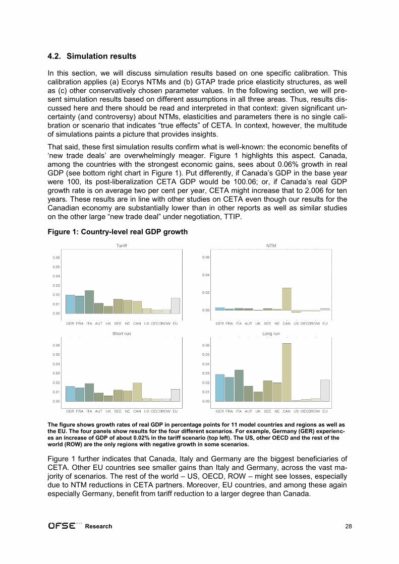
Research 28
4.2. Simulation results
In this section, we will discuss simulation results based on one specific calibration. This
calibration applies (a) Ecorys NTMs and (b) GTAP trade price elasticity structures, as well
as (c) other conservatively chosen parameter values. In the following section, we will pre-
sent simulation results based on different assumptions in all three areas. Thus, results dis-
cussed here and there should be read and interpreted in that context: given significant un-
certainty (and controversy) about NTMs, elasticities and parameters there is no single cali-
bration or scenario that indicates “true effects” of CETA. In context, however, the multitude
of simulations paints a picture that provides insights.
That said, these first simulation results confirm what is well-known: the economic benefits of
‘new trade deals’ are overwhelmingly meager. Figure 1 highlights this aspect. Canada,
among the countries with the strongest economic gains, sees about 0.06% growth in real
GDP (see bottom right chart in Figure 1). Put differently, if Canada’s GDP in the base year
were 100, its post-liberalization CETA GDP would be 100.06; or, if Canada’s real GDP
growth rate is on average two per cent per year, CETA might increase that to 2.006 for ten
years. These results are in line with other studies on CETA even though our results for the
Canadian economy are substantially lower than in other reports as well as similar studies
on the other large “new trade deal” under negotiation, TTIP.
Figure 1: Country-level real GDP growth
The figure shows growth rates of real GDP in percentage points for 11 model countries and regions as well as the EU. The four panels show results for the four different scenarios. For example, Germany (GER) experienc-es an increase of GDP of about 0.02% in the tariff scenario (top left). The US, other OECD and the rest of the world (ROW) are the only regions with negative growth in some scenarios.
Figure 1 further indicates that Canada, Italy and Germany are the biggest beneficiaries of
CETA. Other EU countries see smaller gains than Italy and Germany, across the vast ma-
jority of scenarios. The rest of the world – US, OECD, ROW – might see losses, especially
due to NTM reductions in CETA partners. Moreover, EU countries, and among these again
especially Germany, benefit from tariff reduction to a larger degree than Canada.
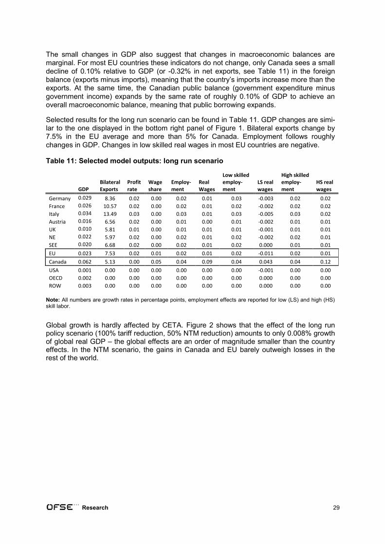
Research 29
The small changes in GDP also suggest that changes in macroeconomic balances are
marginal. For most EU countries these indicators do not change, only Canada sees a small
decline of 0.10% relative to GDP (or -0.32% in net exports, see Table 11) in the foreign
balance (exports minus imports), meaning that the country’s imports increase more than the
exports. At the same time, the Canadian public balance (government expenditure minus
government income) expands by the same rate of roughly 0.10% of GDP to achieve an
overall macroeconomic balance, meaning that public borrowing expands.
Selected results for the long run scenario can be found in Table 11. GDP changes are simi-
lar to the one displayed in the bottom right panel of Figure 1. Bilateral exports change by
7.5% in the EU average and more than 5% for Canada. Employment follows roughly
changes in GDP. Changes in low skilled real wages in most EU countries are negative.
Table 11: Selected model outputs: long run scenario
GDP Bilateral Exports
Profit rate
Wage share
Employ-ment
Real Wages
Low skilled employ-ment
LS real wages
High skilled employ-ment
HS real wages
Germany 0.029 8.36 0.02 0.00 0.02 0.01 0.03 -0.003 0.02 0.02
France 0.026 10.57 0.02 0.00 0.02 0.01 0.02 -0.002 0.02 0.02
Italy 0.034 13.49 0.03 0.00 0.03 0.01 0.03 -0.005 0.03 0.02
Austria 0.016 6.56 0.02 0.00 0.01 0.00 0.01 -0.002 0.01 0.01
UK 0.010 5.81 0.01 0.00 0.01 0.01 0.01 -0.001 0.01 0.01
NE 0.022 5.97 0.02 0.00 0.02 0.01 0.02 -0.002 0.02 0.01
SEE 0.020 6.68 0.02 0.00 0.02 0.01 0.02 0.000 0.01 0.01
EU 0.023 7.53 0.02 0.01 0.02 0.01 0.02 -0.011 0.02 0.01
Canada 0.062 5.13 0.00 0.05 0.04 0.09 0.04 0.043 0.04 0.12
USA 0.001 0.00 0.00 0.00 0.00 0.00 0.00 -0.001 0.00 0.00
OECD 0.002 0.00 0.00 0.00 0.00 0.00 0.00 0.000 0.00 0.00
ROW 0.003 0.00 0.00 0.00 0.00 0.00 0.00 0.000 0.00 0.00
Note: All numbers are growth rates in percentage points, employment effects are reported for low (LS) and high (HS) skill labor.
Global growth is hardly affected by CETA. Figure 2 shows that the effect of the long run policy scenario (100% tariff reduction, 50% NTM reduction) amounts to only 0.008% growth of global real GDP – the global effects are an order of magnitude smaller than the country effects. In the NTM scenario, the gains in Canada and EU barely outweigh losses in the rest of the world.
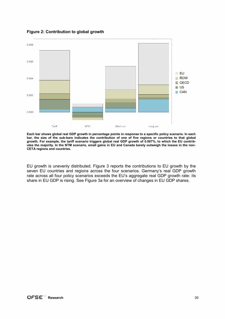
Research 30
Figure 2: Contribution to global growth
Each bar shows global real GDP growth in percentage points in response to a specific policy scenario. In each bar, the size of the sub-bars indicates the contribution of one of five regions or countries to that global growth. For example, the tariff scenario triggers global real GDP growth of 0.007%, to which the EU contrib-utes the majority. In the NTM scenario, small gains in EU and Canada barely outweigh the losses in the non-CETA regions and countries.
EU growth is unevenly distributed. Figure 3 reports the contributions to EU growth by the seven EU countries and regions across the four scenarios. Germany’s real GDP growth rate across all four policy scenarios exceeds the EU’s aggregate real GDP growth rate: its share in EU GDP is rising. See Figure 3a for an overview of changes in EU GDP shares.
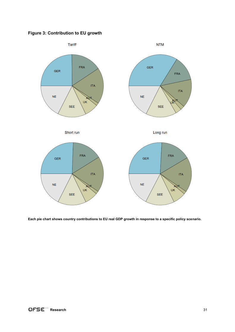
Research 31
Figure 3: Contribution to EU growth
Each pie chart shows country contributions to EU real GDP growth in response to a specific policy scenario.
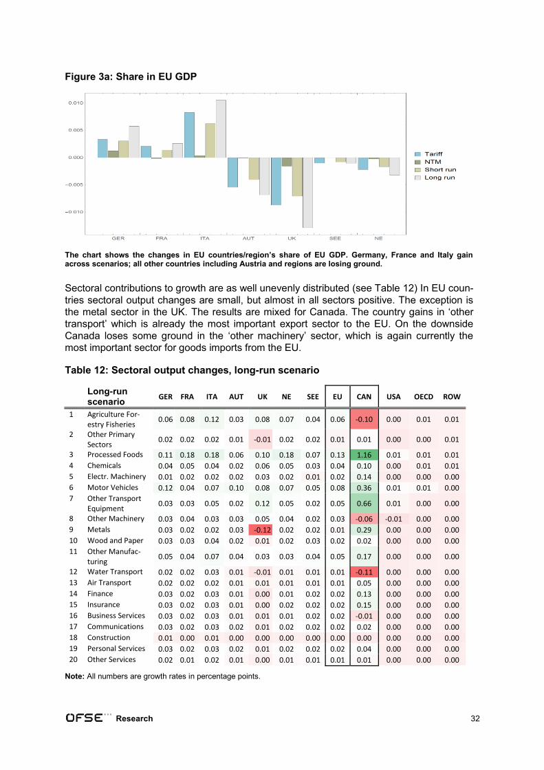
Research 32
Figure 3a: Share in EU GDP
The chart shows the changes in EU countries/region’s share of EU GDP. Germany, France and Italy gain across scenarios; all other countries including Austria and regions are losing ground.
Sectoral contributions to growth are as well unevenly distributed (see Table 12) In EU coun-
tries sectoral output changes are small, but almost in all sectors positive. The exception is
the metal sector in the UK. The results are mixed for Canada. The country gains in ‘other
transport’ which is already the most important export sector to the EU. On the downside
Canada loses some ground in the ‘other machinery’ sector, which is again currently the
most important sector for goods imports from the EU.
Table 12: Sectoral output changes, long-run scenario
Long-run scenario
GER FRA ITA AUT UK NE SEE EU CAN USA OECD ROW
1 Agriculture For-estry Fisheries
0.06 0.08 0.12 0.03 0.08 0.07 0.04 0.06 -0.10 0.00 0.01 0.01
2 Other Primary Sectors
0.02 0.02 0.02 0.01 -0.01 0.02 0.02 0.01 0.01 0.00 0.00 0.01
3 Processed Foods 0.11 0.18 0.18 0.06 0.10 0.18 0.07 0.13 1.16 0.01 0.01 0.01
4 Chemicals 0.04 0.05 0.04 0.02 0.06 0.05 0.03 0.04 0.10 0.00 0.01 0.01
5 Electr. Machinery 0.01 0.02 0.02 0.02 0.03 0.02 0.01 0.02 0.14 0.00 0.00 0.00
6 Motor Vehicles 0.12 0.04 0.07 0.10 0.08 0.07 0.05 0.08 0.36 0.01 0.01 0.00
7 Other Transport Equipment
0.03 0.03 0.05 0.02 0.12 0.05 0.02 0.05 0.66 0.01 0.00 0.00
8 Other Machinery 0.03 0.04 0.03 0.03 0.05 0.04 0.02 0.03 -0.06 -0.01 0.00 0.00
9 Metals 0.03 0.02 0.02 0.03 -0.12 0.02 0.02 0.01 0.29 0.00 0.00 0.00
10 Wood and Paper 0.03 0.03 0.04 0.02 0.01 0.02 0.03 0.02 0.02 0.00 0.00 0.00
11 Other Manufac-turing
0.05 0.04 0.07 0.04 0.03 0.03 0.04 0.05 0.17 0.00 0.00 0.00
12 Water Transport 0.02 0.02 0.03 0.01 -0.01 0.01 0.01 0.01 -0.11 0.00 0.00 0.00
13 Air Transport 0.02 0.02 0.02 0.01 0.01 0.01 0.01 0.01 0.05 0.00 0.00 0.00
14 Finance 0.03 0.02 0.03 0.01 0.00 0.01 0.02 0.02 0.13 0.00 0.00 0.00
15 Insurance 0.03 0.02 0.03 0.01 0.00 0.02 0.02 0.02 0.15 0.00 0.00 0.00
16 Business Services 0.03 0.02 0.03 0.01 0.01 0.01 0.02 0.02 -0.01 0.00 0.00 0.00
17 Communications 0.03 0.02 0.03 0.02 0.01 0.02 0.02 0.02 0.02 0.00 0.00 0.00
18 Construction 0.01 0.00 0.01 0.00 0.00 0.00 0.00 0.00 0.00 0.00 0.00 0.00
19 Personal Services 0.03 0.02 0.03 0.02 0.01 0.02 0.02 0.02 0.04 0.00 0.00 0.00
20 Other Services 0.02 0.01 0.02 0.01 0.00 0.01 0.01 0.01 0.01 0.00 0.00 0.00
Note: All numbers are growth rates in percentage points.
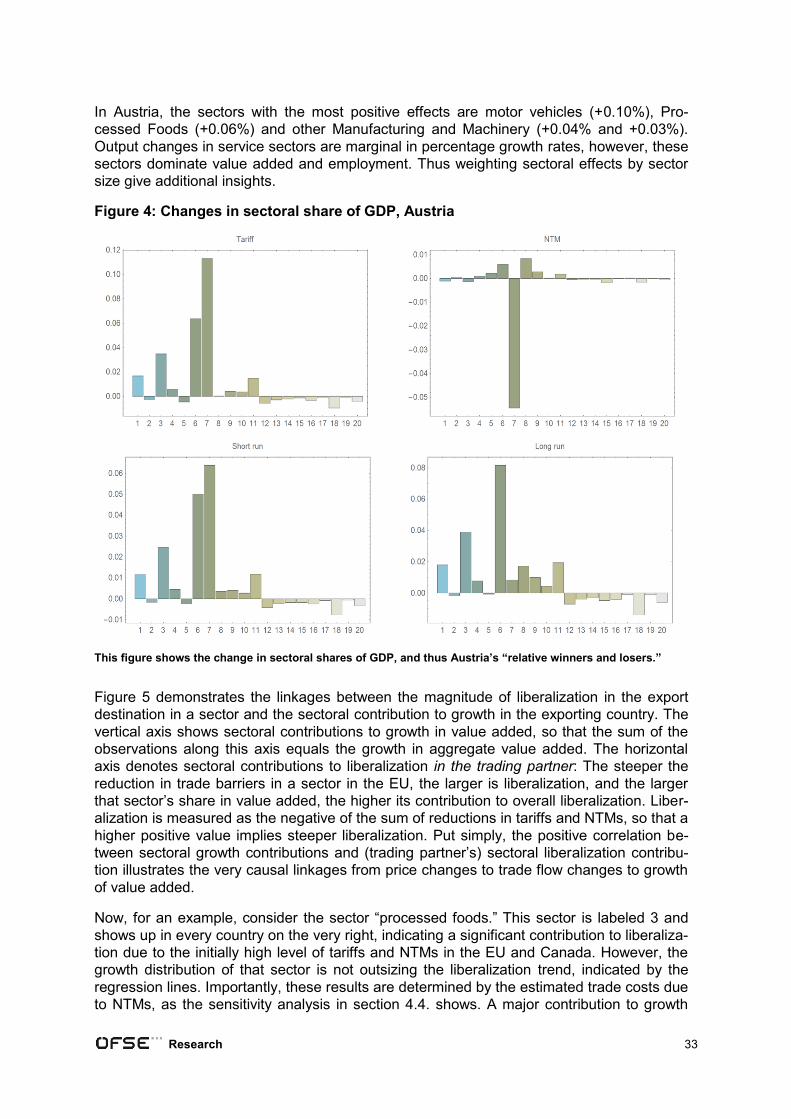
Research 33
In Austria, the sectors with the most positive effects are motor vehicles (+0.10%), Pro-
cessed Foods (+0.06%) and other Manufacturing and Machinery (+0.04% and +0.03%).
Output changes in service sectors are marginal in percentage growth rates, however, these
sectors dominate value added and employment. Thus weighting sectoral effects by sector
size give additional insights.
Figure 4: Changes in sectoral share of GDP, Austria
This figure shows the change in sectoral shares of GDP, and thus Austria’s “relative winners and losers.”
Figure 5 demonstrates the linkages between the magnitude of liberalization in the export
destination in a sector and the sectoral contribution to growth in the exporting country. The
vertical axis shows sectoral contributions to growth in value added, so that the sum of the
observations along this axis equals the growth in aggregate value added. The horizontal
axis denotes sectoral contributions to liberalization in the trading partner: The steeper the
reduction in trade barriers in a sector in the EU, the larger is liberalization, and the larger
that sector’s share in value added, the higher its contribution to overall liberalization. Liber-
alization is measured as the negative of the sum of reductions in tariffs and NTMs, so that a
higher positive value implies steeper liberalization. Put simply, the positive correlation be-
tween sectoral growth contributions and (trading partner’s) sectoral liberalization contribu-
tion illustrates the very causal linkages from price changes to trade flow changes to growth
of value added.
Now, for an example, consider the sector “processed foods.” This sector is labeled 3 and
shows up in every country on the very right, indicating a significant contribution to liberaliza-
tion due to the initially high level of tariffs and NTMs in the EU and Canada. However, the
growth distribution of that sector is not outsizing the liberalization trend, indicated by the
regression lines. Importantly, these results are determined by the estimated trade costs due
to NTMs, as the sensitivity analysis in section 4.4. shows. A major contribution to growth
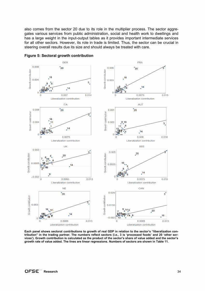
Research 34
also comes from the sector 20 due to its role in the multiplier process. The sector aggre-
gates various services from public administration, social and health work to dwellings and
has a large weight in the input-output tables as it provides important intermediate services
for all other sectors. However, its role in trade is limited. Thus, the sector can be crucial in
steering overall results due its size and should always be treated with care.
Figure 5: Sectoral growth contribution
Each panel shows sectoral contributions to growth of real GDP in relation to the sector’s “liberalization con-tribution” in the trading partner. The numbers reflect sectors (i.e., 3 is ‘processed foods’ and 20 ‘other ser-vices’). Growth contribution is calculated as the product of the sector’s share of value added and the sector’s growth rate of value added. The lines are linear regressions. Numbers of sectors are shown in Table 11.
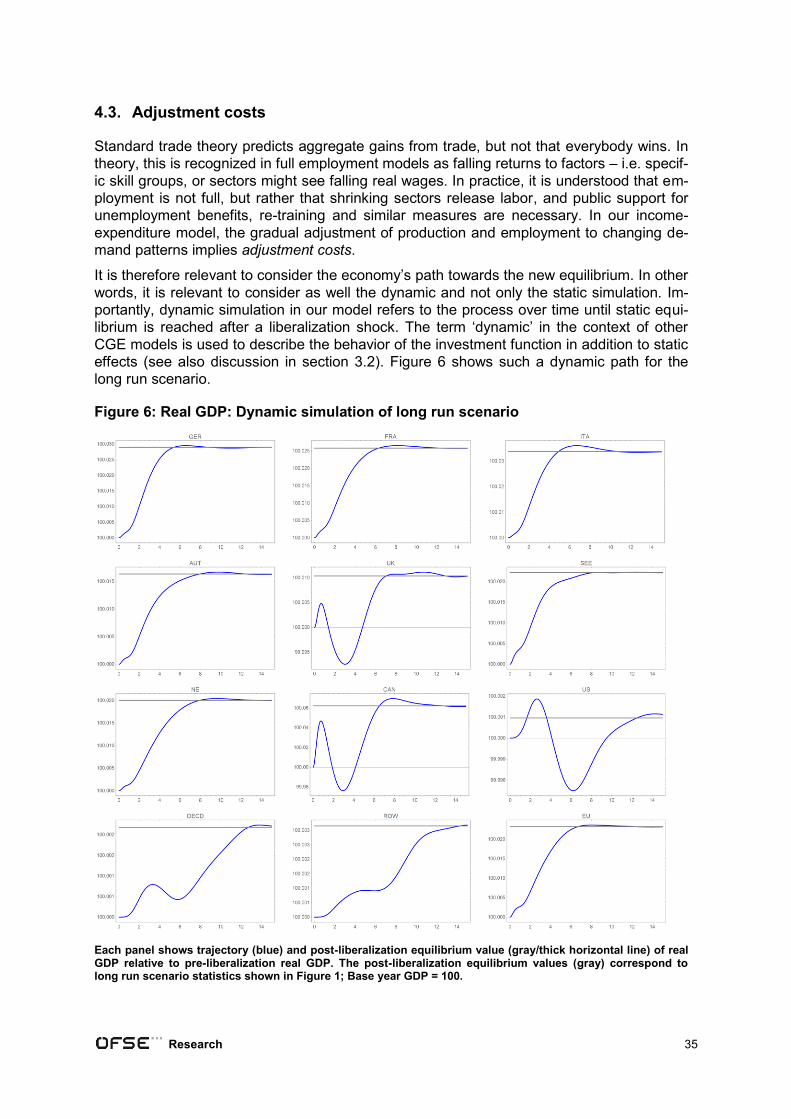
Research 35
4.3. Adjustment costs
Standard trade theory predicts aggregate gains from trade, but not that everybody wins. In
theory, this is recognized in full employment models as falling returns to factors – i.e. specif-
ic skill groups, or sectors might see falling real wages. In practice, it is understood that em-
ployment is not full, but rather that shrinking sectors release labor, and public support for
unemployment benefits, re-training and similar measures are necessary. In our income-
expenditure model, the gradual adjustment of production and employment to changing de-
mand patterns implies adjustment costs.
It is therefore relevant to consider the economy’s path towards the new equilibrium. In other
words, it is relevant to consider as well the dynamic and not only the static simulation. Im-
portantly, dynamic simulation in our model refers to the process over time until static equi-
librium is reached after a liberalization shock. The term ‘dynamic’ in the context of other
CGE models is used to describe the behavior of the investment function in addition to static
effects (see also discussion in section 3.2). Figure 6 shows such a dynamic path for the
long run scenario.
Figure 6: Real GDP: Dynamic simulation of long run scenario
Each panel shows trajectory (blue) and post-liberalization equilibrium value (gray/thick horizontal line) of real GDP relative to pre-liberalization real GDP. The post-liberalization equilibrium values (gray) correspond to long run scenario statistics shown in Figure 1; Base year GDP = 100.
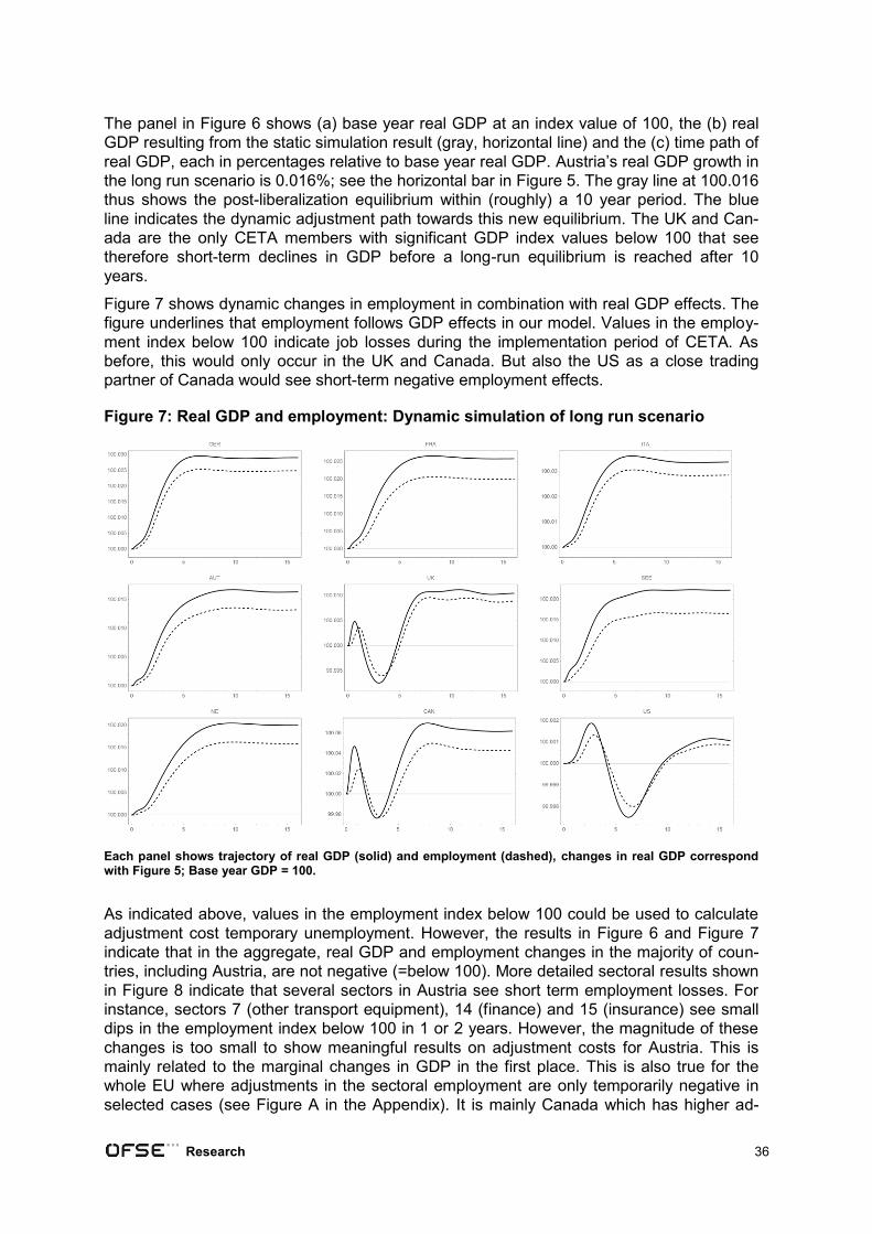
Research 36
The panel in Figure 6 shows (a) base year real GDP at an index value of 100, the (b) real
GDP resulting from the static simulation result (gray, horizontal line) and the (c) time path of
real GDP, each in percentages relative to base year real GDP. Austria’s real GDP growth in
the long run scenario is 0.016%; see the horizontal bar in Figure 5. The gray line at 100.016
thus shows the post-liberalization equilibrium within (roughly) a 10 year period. The blue
line indicates the dynamic adjustment path towards this new equilibrium. The UK and Can-
ada are the only CETA members with significant GDP index values below 100 that see
therefore short-term declines in GDP before a long-run equilibrium is reached after 10
years.
Figure 7 shows dynamic changes in employment in combination with real GDP effects. The
figure underlines that employment follows GDP effects in our model. Values in the employ-
ment index below 100 indicate job losses during the implementation period of CETA. As
before, this would only occur in the UK and Canada. But also the US as a close trading
partner of Canada would see short-term negative employment effects.
Figure 7: Real GDP and employment: Dynamic simulation of long run scenario
Each panel shows trajectory of real GDP (solid) and employment (dashed), changes in real GDP correspond with Figure 5; Base year GDP = 100.
As indicated above, values in the employment index below 100 could be used to calculate
adjustment cost temporary unemployment. However, the results in Figure 6 and Figure 7
indicate that in the aggregate, real GDP and employment changes in the majority of coun-
tries, including Austria, are not negative (=below 100). More detailed sectoral results shown
in Figure 8 indicate that several sectors in Austria see short term employment losses. For
instance, sectors 7 (other transport equipment), 14 (finance) and 15 (insurance) see small
dips in the employment index below 100 in 1 or 2 years. However, the magnitude of these
changes is too small to show meaningful results on adjustment costs for Austria. This is
mainly related to the marginal changes in GDP in the first place. This is also true for the
whole EU where adjustments in the sectoral employment are only temporarily negative in
selected cases (see Figure A in the Appendix). It is mainly Canada which has higher ad-
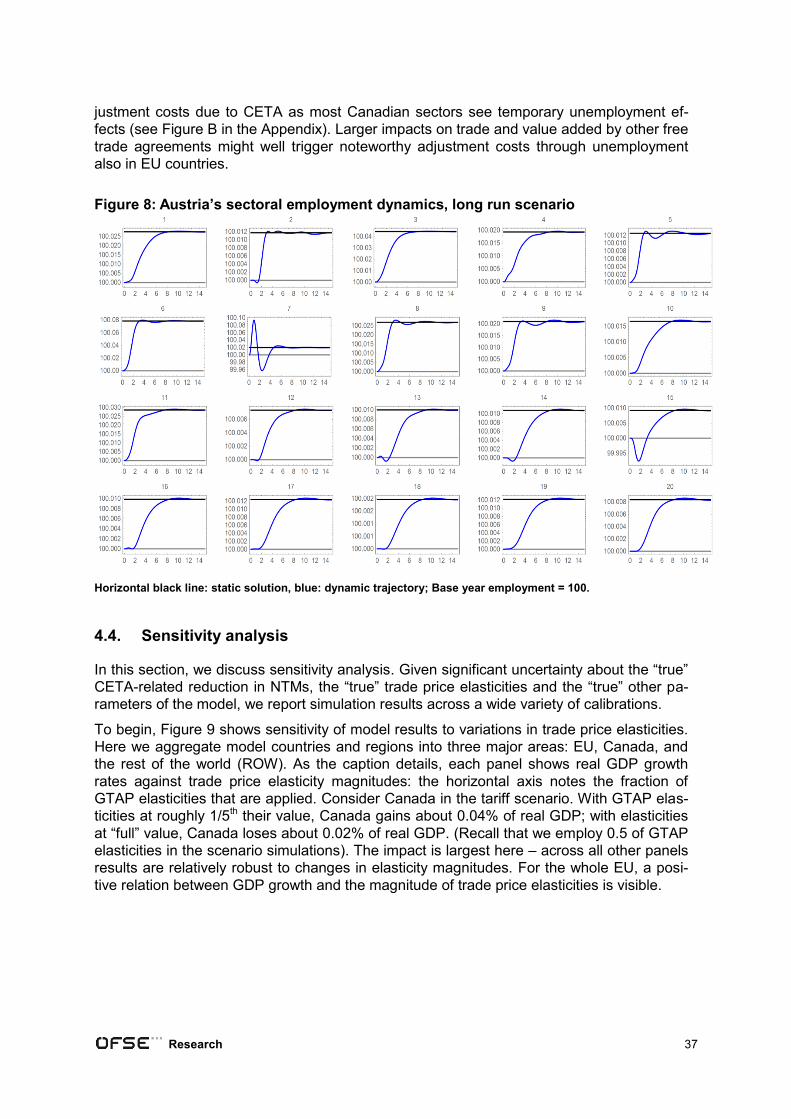
Research 37
justment costs due to CETA as most Canadian sectors see temporary unemployment ef-
fects (see Figure B in the Appendix). Larger impacts on trade and value added by other free
trade agreements might well trigger noteworthy adjustment costs through unemployment
also in EU countries.
Figure 8: Austria’s sectoral employment dynamics, long run scenario
Horizontal black line: static solution, blue: dynamic trajectory; Base year employment = 100.
4.4. Sensitivity analysis
In this section, we discuss sensitivity analysis. Given significant uncertainty about the “true”
CETA-related reduction in NTMs, the “true” trade price elasticities and the “true” other pa-
rameters of the model, we report simulation results across a wide variety of calibrations.
To begin, Figure 9 shows sensitivity of model results to variations in trade price elasticities.
Here we aggregate model countries and regions into three major areas: EU, Canada, and
the rest of the world (ROW). As the caption details, each panel shows real GDP growth
rates against trade price elasticity magnitudes: the horizontal axis notes the fraction of
GTAP elasticities that are applied. Consider Canada in the tariff scenario. With GTAP elas-
ticities at roughly 1/5th their value, Canada gains about 0.04% of real GDP; with elasticities
at “full” value, Canada loses about 0.02% of real GDP. (Recall that we employ 0.5 of GTAP
elasticities in the scenario simulations). The impact is largest here – across all other panels
results are relatively robust to changes in elasticity magnitudes. For the whole EU, a posi-
tive relation between GDP growth and the magnitude of trade price elasticities is visible.
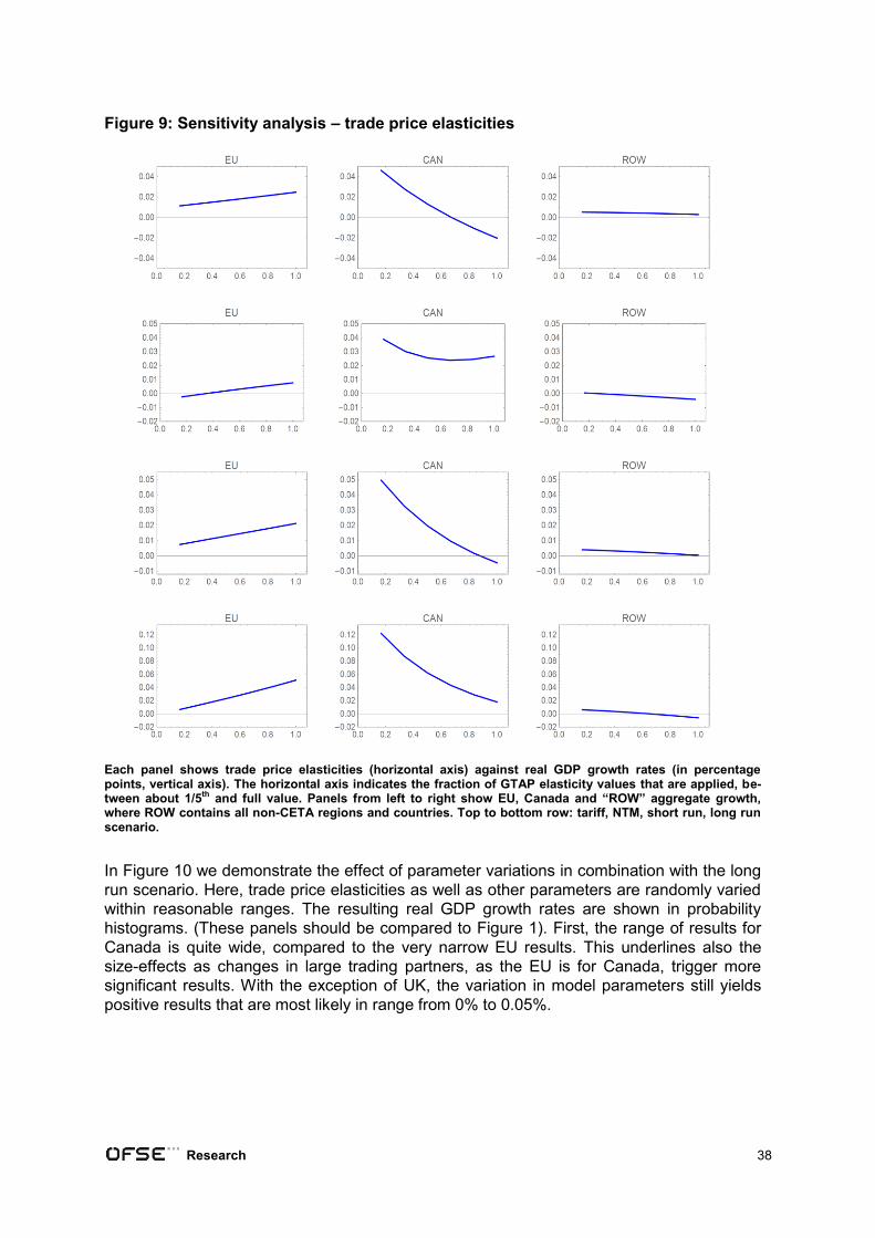
Research 38
Figure 9: Sensitivity analysis – trade price elasticities
Each panel shows trade price elasticities (horizontal axis) against real GDP growth rates (in percentage points, vertical axis). The horizontal axis indicates the fraction of GTAP elasticity values that are applied, be-tween about 1/5th and full value. Panels from left to right show EU, Canada and “ROW” aggregate growth, where ROW contains all non-CETA regions and countries. Top to bottom row: tariff, NTM, short run, long run scenario.
In Figure 10 we demonstrate the effect of parameter variations in combination with the long
run scenario. Here, trade price elasticities as well as other parameters are randomly varied
within reasonable ranges. The resulting real GDP growth rates are shown in probability
histograms. (These panels should be compared to Figure 1). First, the range of results for
Canada is quite wide, compared to the very narrow EU results. This underlines also the
size-effects as changes in large trading partners, as the EU is for Canada, trigger more
significant results. With the exception of UK, the variation in model parameters still yields
positive results that are most likely in range from 0% to 0.05%.
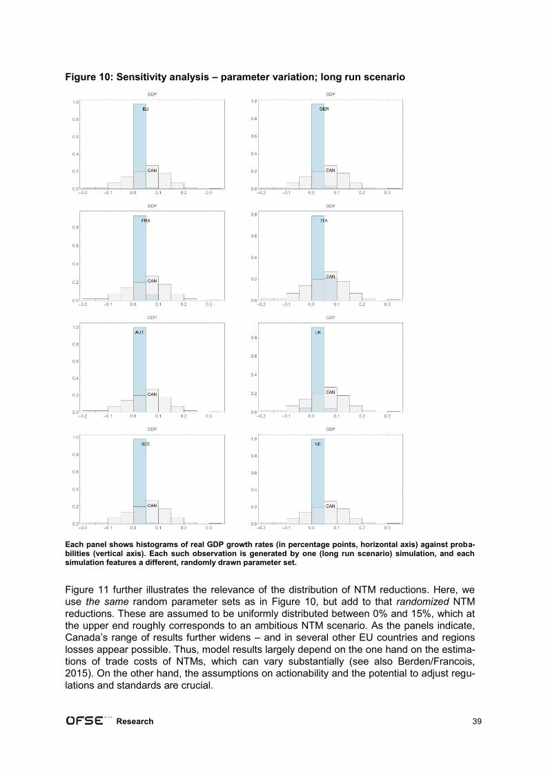
Research 39
Figure 10: Sensitivity analysis – parameter variation; long run scenario
Each panel shows histograms of real GDP growth rates (in percentage points, horizontal axis) against proba-bilities (vertical axis). Each such observation is generated by one (long run scenario) simulation, and each simulation features a different, randomly drawn parameter set.
Figure 11 further illustrates the relevance of the distribution of NTM reductions. Here, we
use the same random parameter sets as in Figure 10, but add to that randomized NTM
reductions. These are assumed to be uniformly distributed between 0% and 15%, which at
the upper end roughly corresponds to an ambitious NTM scenario. As the panels indicate,
Canada’s range of results further widens – and in several other EU countries and regions
losses appear possible. Thus, model results largely depend on the one hand on the estima-
tions of trade costs of NTMs, which can vary substantially (see also Berden/Francois,
2015). On the other hand, the assumptions on actionability and the potential to adjust regu-
lations and standards are crucial.
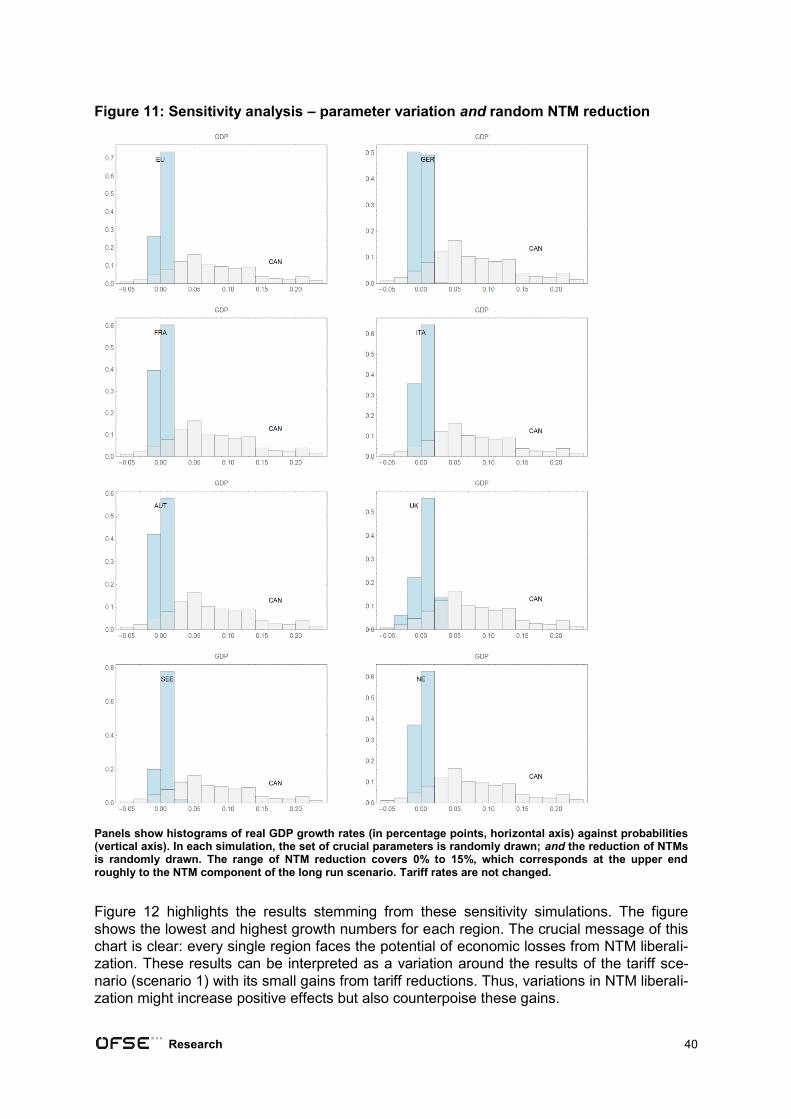
Research 40
Figure 11: Sensitivity analysis – parameter variation and random NTM reduction
Panels show histograms of real GDP growth rates (in percentage points, horizontal axis) against probabilities (vertical axis). In each simulation, the set of crucial parameters is randomly drawn; and the reduction of NTMs is randomly drawn. The range of NTM reduction covers 0% to 15%, which corresponds at the upper end roughly to the NTM component of the long run scenario. Tariff rates are not changed.
Figure 12 highlights the results stemming from these sensitivity simulations. The figure
shows the lowest and highest growth numbers for each region. The crucial message of this
chart is clear: every single region faces the potential of economic losses from NTM liberali-
zation. These results can be interpreted as a variation around the results of the tariff sce-
nario (scenario 1) with its small gains from tariff reductions. Thus, variations in NTM liberali-
zation might increase positive effects but also counterpoise these gains.
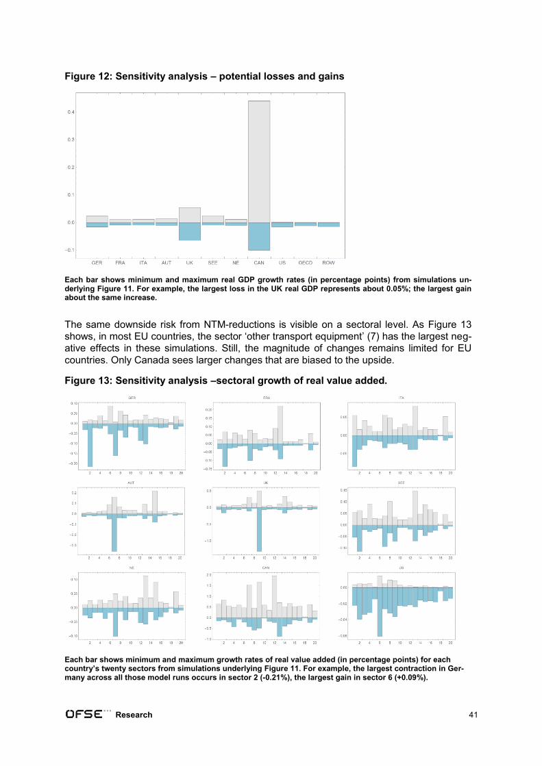
Research 41
Figure 12: Sensitivity analysis – potential losses and gains
Each bar shows minimum and maximum real GDP growth rates (in percentage points) from simulations un-derlying Figure 11. For example, the largest loss in the UK real GDP represents about 0.05%; the largest gain about the same increase.
The same downside risk from NTM-reductions is visible on a sectoral level. As Figure 13
shows, in most EU countries, the sector ‘other transport equipment’ (7) has the largest neg-
ative effects in these simulations. Still, the magnitude of changes remains limited for EU
countries. Only Canada sees larger changes that are biased to the upside.
Figure 13: Sensitivity analysis –sectoral growth of real value added.
Each bar shows minimum and maximum growth rates of real value added (in percentage points) for each country’s twenty sectors from simulations underlying Figure 11. For example, the largest contraction in Ger-many across all those model runs occurs in sector 2 (-0.21%), the largest gain in sector 6 (+0.09%).
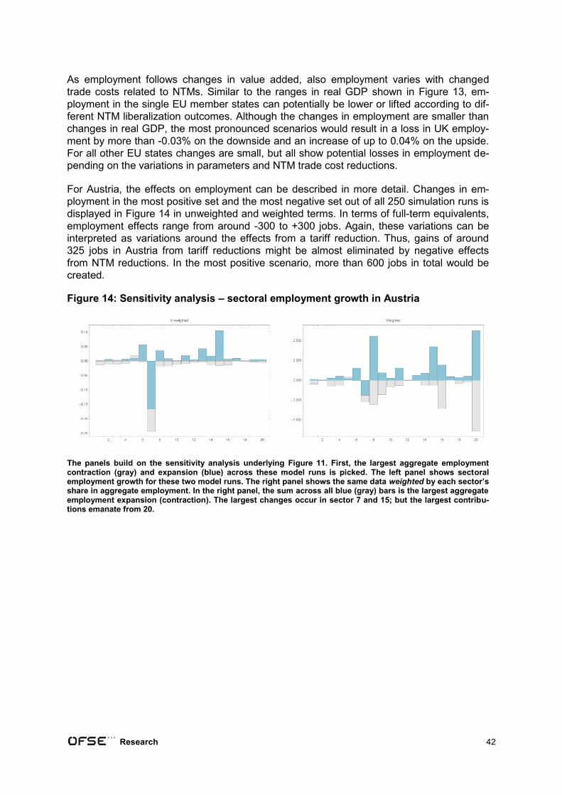
Research 42
As employment follows changes in value added, also employment varies with changed
trade costs related to NTMs. Similar to the ranges in real GDP shown in Figure 13, em-
ployment in the single EU member states can potentially be lower or lifted according to dif-
ferent NTM liberalization outcomes. Although the changes in employment are smaller than
changes in real GDP, the most pronounced scenarios would result in a loss in UK employ-
ment by more than -0.03% on the downside and an increase of up to 0.04% on the upside.
For all other EU states changes are small, but all show potential losses in employment de-
pending on the variations in parameters and NTM trade cost reductions.
For Austria, the effects on employment can be described in more detail. Changes in em-
ployment in the most positive set and the most negative set out of all 250 simulation runs is
displayed in Figure 14 in unweighted and weighted terms. In terms of full-term equivalents,
employment effects range from around -300 to +300 jobs. Again, these variations can be
interpreted as variations around the effects from a tariff reduction. Thus, gains of around
325 jobs in Austria from tariff reductions might be almost eliminated by negative effects
from NTM reductions. In the most positive scenario, more than 600 jobs in total would be
created.
Figure 14: Sensitivity analysis – sectoral employment growth in Austria
The panels build on the sensitivity analysis underlying Figure 11. First, the largest aggregate employment contraction (gray) and expansion (blue) across these model runs is picked. The left panel shows sectoral employment growth for these two model runs. The right panel shows the same data weighted by each sector’s share in aggregate employment. In the right panel, the sum across all blue (gray) bars is the largest aggregate employment expansion (contraction). The largest changes occur in sector 7 and 15; but the largest contribu-tions emanate from 20.
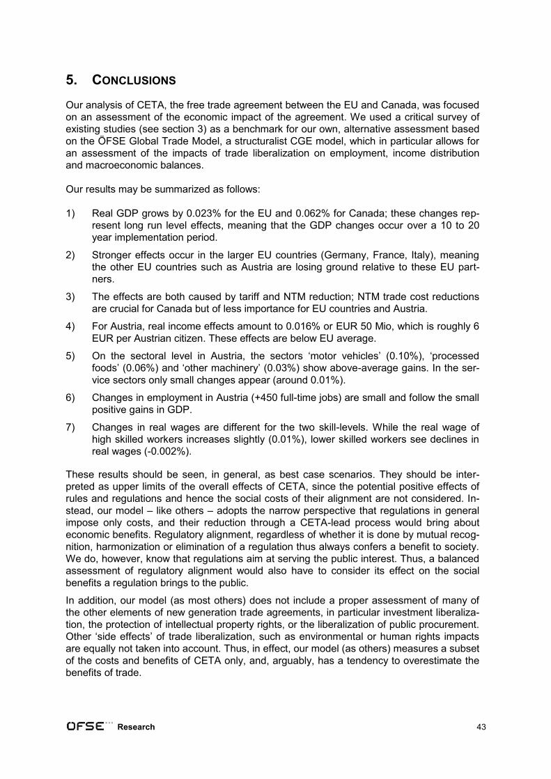
Research 43
5. CONCLUSIONS
Our analysis of CETA, the free trade agreement between the EU and Canada, was focused
on an assessment of the economic impact of the agreement. We used a critical survey of
existing studies (see section 3) as a benchmark for our own, alternative assessment based
on the ÖFSE Global Trade Model, a structuralist CGE model, which in particular allows for
an assessment of the impacts of trade liberalization on employment, income distribution
and macroeconomic balances.
Our results may be summarized as follows:
1) Real GDP grows by 0.023% for the EU and 0.062% for Canada; these changes rep-
resent long run level effects, meaning that the GDP changes occur over a 10 to 20
year implementation period.
2) Stronger effects occur in the larger EU countries (Germany, France, Italy), meaning
the other EU countries such as Austria are losing ground relative to these EU part-
ners.
3) The effects are both caused by tariff and NTM reduction; NTM trade cost reductions
are crucial for Canada but of less importance for EU countries and Austria.
4) For Austria, real income effects amount to 0.016% or EUR 50 Mio, which is roughly 6
EUR per Austrian citizen. These effects are below EU average.
5) On the sectoral level in Austria, the sectors ‘motor vehicles’ (0.10%), ‘processed
foods’ (0.06%) and ‘other machinery’ (0.03%) show above-average gains. In the ser-
vice sectors only small changes appear (around 0.01%).
6) Changes in employment in Austria (+450 full-time jobs) are small and follow the small
positive gains in GDP.
7) Changes in real wages are different for the two skill-levels. While the real wage of
high skilled workers increases slightly (0.01%), lower skilled workers see declines in
real wages (-0.002%).
These results should be seen, in general, as best case scenarios. They should be inter-
preted as upper limits of the overall effects of CETA, since the potential positive effects of
rules and regulations and hence the social costs of their alignment are not considered. In-
stead, our model – like others – adopts the narrow perspective that regulations in general
impose only costs, and their reduction through a CETA-lead process would bring about
economic benefits. Regulatory alignment, regardless of whether it is done by mutual recog-
nition, harmonization or elimination of a regulation thus always confers a benefit to society.
We do, however, know that regulations aim at serving the public interest. Thus, a balanced
assessment of regulatory alignment would also have to consider its effect on the social
benefits a regulation brings to the public.
In addition, our model (as most others) does not include a proper assessment of many of
the other elements of new generation trade agreements, in particular investment liberaliza-
tion, the protection of intellectual property rights, or the liberalization of public procurement.
Other ‘side effects’ of trade liberalization, such as environmental or human rights impacts
are equally not taken into account. Thus, in effect, our model (as others) measures a subset
of the costs and benefits of CETA only, and, arguably, has a tendency to overestimate the
benefits of trade.
Research 44
REFERENCES
Beghin, J./Disdier, A. C./Marette, S./Van Tongeren, F. (2012): Welfare costs and benefits of non-tariff measures in trade: a conceptual framework and application. In: World Trade Re-view, 11(03), pp. 356-375.
Berden, K./Francois, J. (2015): Quantifying Non-Tariff Measures for TTIP. Paper No. 12 in CEPTS-CTR project ,TTIP in the Balance‘ and CEPS Special Report No. 116 / July 2015.
Berden, K./Francois, J./Thelle, M./Wymenga, P./Tamminen, S. (2009): Non-tariff measures in EU-US trade and investment – An economic analysis. In: ECORYS, Study for the Euro-pean Commission, Directorate-General for Trade. See: trade.ec.europa.eu/doclib/docs/2009/december/tradoc_145613.pdf (11/25/2015).
Blanchard, O. J./Fischer, S. (1989): Lectures on macroeconomics. MIT press.
Bratt, M. (2014). “Estimating the bilateral impact of non-tariff measures (NTMs)”, Working Paper WPS 14-01-1, Université de Genève
Dean, J.M./Signoret, J./ Feinberg,R.M./Ludema, R.D./Ferrantino, M.J. (2009): Estimating the Price Effects of Non-Tariff Barriers. The B.E. In: Journal of Economic Analysis & Policy, 9(1), Art. 12
Dee, P./Francois, J./Manchin, M./Norberg, H./Nordås, H./van Tongeren F. (2011): The Im-pact of Trade Liberalisation on Jobs and Growth. OECD Trade Policy Working Papers No. 107, OECD: Paris.
European Commission (2016): CETA – Summary of the final negotiating results. See: http://trade.ec.europa.eu/doclib/docs/2014/december/tradoc_152982.pdf (09/06/2016)
European Commission and Government of Canada (2008): Assessing the Costs and Bene-fits of a Closer EU-Canada Economic Partnership. See: http://trade.ec.europa.eu/doclib/html/141032.htm (05/11/2016)
Francois, J.F./McDonald, B./Nordstrom, H. (1996): Liberalisation and the capital accumula-tion in the GTAP model. GTAP Technical Paper No. 7. See: http://docs.lib.purdue.edu/gtaptp/8/ (20/05/2016)
Francois, J./Manchin, M./Norberg, H./Pindyuk, O./Tomberger, P. (2013): Reducing Transat-lantic Barriers to Trade and Investment – An Economic Assessment. In: CEPR, Study for the European Commission, Final Project Report.
Francois, J./Pindyuk, O (2013): Modeling the Effects of Free Trade Agreements between the EU and Canada, USA and Moldova/Georgia/Armenia on the Austrian Economy: Model Simulations for Trade Policy Analysis, FIW Research Report 2012/13 N° 03, Vienna. See: http://www.fiw.ac.at/fileadmin/Documents/Publikationen/Studien_2012_13/03-ResearchReport-FrancoisPindyuk.pdf (04/11/2016)
Hertel, T./McDougall, R./Narayanan, B./Aguiar A. (2014): GTAP 8 Data Base Documenta-tion – Chapter 14 Behavioural Parameters. See: https://www.gtap.agecon.purdue.edu/resources/download/7047.pdf (04/11/2016)
Kirkpatrick, C. et al. (2011): A Trade SIA Relating to the Negotiation of a Comprehensive Economic and Trade Agreement (CETA) Between the EU and Canada. Trade 10/B3/B06. See: http://ec.europa.eu/trade/policy/policy-making/analysis/sustainability-impact-assessments/assessments/#study-geo-14 (04/11/2016)
Raza, W./Tröster, B./von Arnim, R. (2016a): The blind spots of trade impact assessment: macroeconomic adjustment costs and the social costs of regulatory change. In: European Journal of Economics and Economic Policies: Intervention. 13(1), pp. 87-102.

Research 45
Raza, W./Taylor, L./Tröster, B./ von Arnim, R. (2016b): Modelling the impacts of trade on employment and development: A structuralist CGE-model for the analysis of TTIP and other trade agreements. ÖFSE Working Paper No. 57.
Raza, W./Grumiller, J./Taylor,L./Tröster, B./von Arnim, R.(2014): ASSESS TTIP: Assessing the claimed benefits of the Transatlantic Trade and Investment Partnership. See: http://guengl.eu/uploads/plenary-focus-pdf/ASSESS_TTIP.pdf (11/25/2015).
Rodrik, D. (2015): The War of Trade Models. See: http://rodrik.typepad.com/dani_rodriks_weblog/2015/05/the-war-of-trade-models.html (05/31/2015)
Shoven, J. B./Whalley, J. (1984): Applied general-equilibrium models of taxation and inter-national trade: an introduction and survey. In: Journal of Economic Literature, 22(3), pp. 1007-1051.
Taylor, L. (2004): Reconstructing Macroeconomics: Structuralist Proposals and Critiques of the Mainstream Harvard University Press.
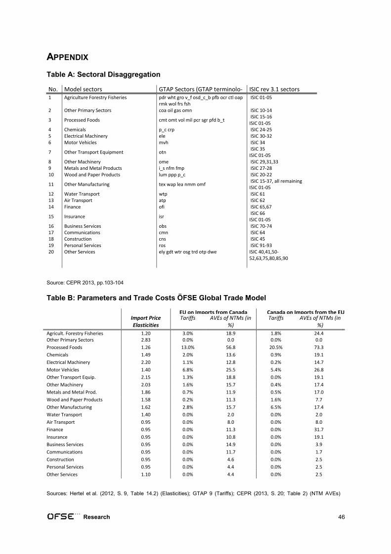
Research 46
APPENDIX
Table A: Sectoral Disaggregation
No. Model sectors GTAP Sectors (GTAP terminolo-gy)
ISIC rev 3.1 sectors 1 Agriculture Forestry Fisheries pdr wht gro v_f osd_c_b pfb ocr ctl oap
rmk wol frs fsh ISIC 01-05
2 Other Primary Sectors coa oil gas omn ISIC 10-14
3 Processed Foods cmt omt vol mil pcr sgr pfd b_t ISIC 15-16 ISIC 01-05
4 Chemicals p_c crp ISIC 24-25 5 Electrical Machinery ele ISIC 30-32 6 Motor Vehicles mvh ISIC 34
7 Other Transport Equipment otn ISIC 35 ISIC 01-05
8 Other Machinery ome ISIC 29,31,33 9 Metals and Metal Products i_s nfm fmp ISIC 27-28 10 Wood and Paper Products lum ppp p_c ISIC 20-22
11 Other Manufacturing tex wap lea nmm omf ISIC 15-37, all remaining ISIC 01-05
12 Water Transport wtp ISIC 61 13 Air Transport atp ISIC 62 14 Finance ofi ISIC 65,67
15 Insurance isr ISIC 66 ISIC 01-05
16 Business Services obs ISIC 70-74 17 Communications cmn ISIC 64 18 Construction cns ISIC 45 19 Personal Services ros ISIC 91-93 20 Other Services ely gdt wtr osg trd otp dwe ISIC 40,41,50-
52,63,75,80,85,90
Source: CEPR 2013, pp.103-104
Table B: Parameters and Trade Costs ÖFSE Global Trade Model
EU on Imports from Canada Canada on Imports from the EU
Import Price Elasticities
Tariffs AVEs of NTMs (in
%) Tariffs AVEs of NTMs (in
%)
Agricult. Forestry Fisheries 1.20 3.0% 18.9 1.8% 24.4 Other Primary Sectors 2.83 0.0% 0.0 0.0% 0.0
Processed Foods 1.26 13.0% 56.8 20.5% 73.3
Chemicals 1.49 2.0% 13.6 0.9% 19.1
Electrical Machinery 2.20 1.1% 12.8 0.2% 14.7
Motor Vehicles 1.40 6.8% 25.5 5.4% 26.8
Other Transport Equip. 2.15 1.3% 18.8 0.0% 19.1
Other Machinery 2.03 1.6% 15.7 0.4% 17.4
Metals and Metal Prod. 1.86 0.7% 11.9 0.5% 17.0
Wood and Paper Products 1.58 0.2% 11.3 1.6% 7.7
Other Manufacturing 1.62 2.8% 15.7 6.5% 17.4
Water Transport 1.40 0.0% 2.0 0.0% 2.0
Air Transport 0.95 0.0% 8.0 0.0% 8.0
Finance 0.95 0.0% 11.3 0.0% 31.7
Insurance 0.95 0.0% 10.8 0.0% 19.1
Business Services 0.95 0.0% 14.9 0.0% 3.9
Communications 0.95 0.0% 11.7 0.0% 1.7
Construction 0.95 0.0% 4.6 0.0% 2.5
Personal Services 0.95 0.0% 4.4 0.0% 2.5
Other Services 1.10 0.0% 4.4 0.0% 2.5
Sources: Hertel et al. (2012, S. 9, Table 14.2) (Elasticities); GTAP 9 (Tariffs); CEPR (2013, S. 20; Table 2) (NTM AVEs)
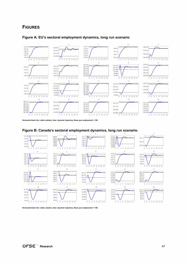
Research 47
FIGURES
Figure A: EU’s sectoral employment dynamics, long run scenario
Horizontal black line: static solution, blue: dynamic trajectory; Base year employment = 100.
Figure B: Canada’s sectoral employment dynamics, long run scenario.
Horizontal black line: static solution, blue: dynamic trajectory; Base year employment = 100.
Research 48
ABOUT THE AUTHORS
Werner Raza is Director at ÖFSE – Austrian Foundation for Development Research in Vi-enna. He holds ad PhD in Economics from the University of Economics and Business in Vienna. His areas of work include International Trade and Development Economics.
Bernhard Tröster is researcher at ÖFSE. He holds a diploma in Economics from the Uni-
versity of Regensburg and a M.A. in International and Development Economics from HTW
Berlin. His areas of works are Development Economics, International Trade and Commodi-
ty Markets.
Rudi von Arnim is Assistant Professor at the Department of Economics, University of
Utah, USA. He holds a PhD in Economics from The New School for Social Research. His
areas of specialization are Macroeconomics and International Economics.

wien.arbeiterkammer.at
ISB
N: 9
78-3
-706
3-06
20-1


![EXTRACTION AND QUANTITATIVE DETERMINATION OF … · claimed to prevent anemia, regulate blood pressure, prevent constipation, cure heartburns and prevent stroke [8]. Even the leaves](https://img.pdfslide.org/doc/110x75/5f1a32d339da2f0c9e3e0560/extraction-and-quantitative-determination-of-claimed-to-prevent-anemia-regulate.jpg)