The Benefits of Adult Learning: Work- Related Training

UniversitätZürichIBW–InstitutfürBetriebswirtschaftslehre

Working Paper No. 167 The Benefits of Adult Learning: Work-Related Training, Social Capital, and Earnings Jens Ruhose, Stephan L. Thomsen and Insa Weilage

April 2019

Die Discussion Papers dienen einer möglichst schnellen Verbreitung von neueren Forschungsarbeiten des Leading Houses und seiner Konferenzen und Workshops. Die Beiträge liegen in alleiniger Verantwortung der

Autoren und stellen nicht notwendigerweise die Meinung des Leading House dar.

Disussion Papers are intended to make results of the Leading House research or its conferences and workshops promptly available to other economists in order to encourage discussion and suggestions for revisions. The

authors are solely responsible for the contents which do not necessarily represent the opinion of the Leading House.

The Swiss Leading House on Economics of Education, Firm Behavior and Training Policies is a Research Program of the Swiss State Secretariat for Education, Research, and Innovation (SERI).

www.economics-of-education.ch

Working Paper No. 167 The Benefits of Adult Learning: Work-Related Training, Social Capital, and Earnings Jens Ruhose, Stephan L. Thomsen and Insa Weilage

Published as: “The benefits of adult learning: Work-related training, social capital, and earnings.“ Economics of Education Review, 72(2019): 166-186. By Jens Ruhose, Stephan L. Thomsen and Insa Weilage. DOI: https://doi.org/10.1016/j.econedurev.2019.05.010

The Benefits of Adult Learning:Work-Related Training, Social Capital, and Earnings⇤

Jens Ruhose† Stephan L. Thomsen‡ Insa Weilage§

April 29, 2019

Abstract

We propose a regression-adjusted matched difference-in-differences framework toestimate pecuniary and non-pecuniary returns to adult education. This approach combineskernel matching with entropy balancing to account for selection bias and sorting on gains.Using data from the German SOEP, we evaluate the effect of work-related training, whichrepresents the largest portion of adult education in OECD countries, on individual socialcapital and earnings. As the related literature, we estimate positive monetary returns towork-related training. In addition, training participation increases participation in civic,political, and cultural activities while not crowding out social participation. Results arerobust against a variety of potentially confounding explanations. These findings implypositive externalities from work-related training over and above the well-documented labormarket effects.JEL Codes: J24, I21, M53Keywords: social capital, earnings, work-related training, matched difference-in-differences approach, entropy balancing

⇤Previous versions of this paper have been circulated under the title “Wider Benefits from Continuous Work-Related Training" and “The Wider Benefits of Adult Learning: Work-Related Training and Social Capital." Weare grateful to Guido Heineck, Sandra McNally, Jens Mohrenweiser, Ina Rüber, Josef Schrader, Nicole Tieben,Simon Wiederhold, Ludger Woessmann, Oleksandr Zhylyevskyy, and seminar and conference participants at theannual meetings of the EEA (Cologne), MEA/SOLE (Evanston), Verein für Socialpolitik (Vienna), standing fieldcommittee on the economics of education of the Verein für Socialpolitik (Bern), the conference of the Centre forVocational Education Research (London), Society for Empirical Educational Research (Basel), the IZA researchseminar (Bonn), Goethe University Frankfurt, Leibniz Universität Hannover, and Leuphana Universität Lüneburgfor their most helpful comments and discussions. Insa Weilage is grateful for participation in and helpful inputsfrom the Doctoral Course Programme of the Swiss Leading House on Economics of Education, Firm Behaviourand Training Policies. Financial support by the German Federal Ministry of Education and Research (BMBF)through the project “Nicht-monetäre Erträge der Weiterbildung: zivilgesellschaftliche Partizipation (NEWz)" isgratefully acknowledged.

†Leibniz Universität Hannover, Königsworther Platz 1, 30167 Hannover, CESifo, and IZA; E-mail:[email protected]

‡Leibniz Universität Hannover, Königsworther Platz 1, 30167 Hannover, ZEW, and IZA; E-mail:[email protected]

§Leibniz Universität Hannover, Königsworther Platz 1, 30167 Hannover; E-mail: [email protected]

1 Introduction

Updating skills and abilities over the life cycle is crucial for workers, firms, and entireeconomies seeking to prevent human capital depreciation and to remain competitive in aglobalized and ever-changing work environment (??). Particularly in industrialized countries,participation in continuing education and training (CET) has become widespread. Forexample, according to the Survey of Adult Skills (PIAAC) 2015, approximately half ofadults aged between 25 and 64 years took part in some CET activity (including open ordistance-learning courses, private lessons, organized sessions for on-the-job training, andworkshops or seminars—some of which might be of short duration) in OECD countries ina given year (?, p. 327). The majority of these activities are nonformal (approximately 92%),meaning that they are organized but are less institutionalized and structured than formal learningactivities (which usually lead to the granting of credentials and certificates).1

While there are numerous studies showing that work-related training affects individual labormarket outcomes and benefits the performance of the firm, there is rarely any causal evidence onthe extent of further non-pecuniary benefits from CET (?).2 Focusing on the case of Germany,where participation rates are close to the OECD average,3 this paper provides an update on themonetary returns to CET and makes two key contributions to the literature on adult education.First, we address empirical challenges in the evaluation of wider benefits from training bytransferring an extended flexible econometric framework from the labor economics literatureinto the literature that evaluates wider benefits of adult education. Second, we apply thisframework to identify the effects of work-related training, which constitutes the majority (82%)of nonformal CET in Germany and elsewhere (??),4 on measures of civic/political, cultural,and social participation—measures that are related to social capital at the individual level (?).Social capital outcomes are high on the political agenda because social capital is considered tofacilitate collaboration and cooperation within a society, yielding positive economic and socialexternalities (see Section ?? for a discussion).

We use rich longitudinal panel data from the German Socio-Economic Panel Study (SOEP)from 1992 to 2014. These data offer detailed information on pecuniary and non-pecuniary

1The PIAAC survey shows that 39% of adults participate in nonformal education only, 4% participate informal education only, 7% participate in both formal and nonformal education, and 50% do not participate inCET. Formal education is defined as “planned education provided in the system of schools, colleges, universitiesand other formal educational institutions" (?, p. 325) and nonformal learning activities are “sustained educationalactivity that does not correspond exactly to the definition of formal education."

2For example, ? and ? provide overview studies on individual labor market outcomes. ??, ??, and ? providestudies on firm performance. ? provide an overview of further non-pecuniary effects of formal education. Inparticular, there is some evidence that formal education can contribute to more civic engagement and politicalparticipation (???).

3In Germany, participation in CET in 2015 is equal to 53%, with 94% of participation taking place in the formof nonformal learning activities (?).

4Work-related training is also an important topic for firms because they allocate substantial resources to traintheir employees. For example, ? estimate that the total costs for German firms amount to 33.5 billion euro for theyear 2016.

1

outcomes, participation in work-related training activities, and a rich set of socio-economicbackground variables. In empirical studies, social capital often constitutes an aggregate of twodimensions: personal involvement in social activities and trust in people generally (?). Whilesocial capital is a multidimensional concept (??) with no consensus about the exact definition(?),5 one can relate the first measure to a structural dimension of social capital (i.e., thechannels and opportunities through which interaction can take place) and the second measureto a relational dimension (i.e., the level of trust, group identification, and the quality of socialties and networks) (?). We use eight non-pecuniary outcome variables to capture the structuraldimension of social capital, which include interest in politics; participating in local politics;volunteering in clubs, organizations, and community services; attending artistic and musicalevents; being active in artistic/musical activities; and meeting with and assisting neighbors,friends, and relatives. To avoid ad-hoc definitions of how to combine the eight variables, we usea principal component analysis (PCA) that reveals and quantifies the underlying data structure.We also discuss the effects on trust in others and the number of close friends to capture therelational dimension of social capital. To measure participation in work-related training, theSOEP provides special survey modules in the years 2000, 2004, and 2008 that specifically askthe respondents about training activities in the last three years prior to the survey. Using thisinformation, we define three periods before, one period during, and three periods after trainingparticipation for each of the modules.

Evaluating the effects of CET requires the construction of the counterfactual situationof what would have happened to training participants if they had not taken part in thetraining. Social experiments provide the gold standard for a causal evaluation because thetreatment status is randomly assigned. However, data from randomized controlled trials andquasi-experiments are not available for many research questions that are interesting from apolicy perspective. Moreover, (quasi-)experimental variation sometimes identifies a specificparameter that is hardly transferable to other interventions and population groups. Our approachtherefore relies on methodological insights from the literature that studies the effects of trainingon labor market outcomes in a real world setting, considering the entire population that maybe affected by the treatment. At the center of the framework is a regression-adjusted matcheddifference-in-differences approach (???), which requires panel data to model the decision toparticipate in training. Using information from two periods before the training, the methodaccounts for selection into the training based on the levels and the trends of a large set ofobservable characteristics. Moreover, our econometric framework incorporates the use ofentropy balancing to refine conventional matching weights (?). By calibrating unit weights

5The most appropriate definition of social capital for this study refers to the view that social capital representssocial connections and interactions, which have (productive) value (?). In the economy, those connections andinteractions lead to social networks, norms of reciprocity, and mutual trust, which have the potential to improvethe efficiency of society by facilitating coordination, collaboration, and cooperation (???). There also exist otherdefinitions of social capital. For example, ? uses his concept of social capital to explain class inequalities, and ?argues that social capital is important for human capital formation because social capital facilitates collective aims.

2

in the non-participation group such that average covariates of the reweighted comparison groupsatisfy prespecified balancing conditions, the approach ensures exact balancing between theparticipant and non-participant groups not only on the mean but also on higher moments suchas the variance of the covariates. This approach is meaningful because we show that theparticipant group is a more homogenous selection of the population than the non-participantgroup. The regression adjustment uses individual fixed effects to control for further selectionon time-invariant unobserved heterogeneity. Although our results are not very sensitive to thechoice of the econometric model, we carefully assess the robustness of each step and discusshow changes in the empirical specification affect the estimates.

We find that participation in work-related training yields positive non-pecuniary returnsin the form of higher civic/political and cultural participation. Those increases do not crowdout social participation. We do not find that trust or the number of close friends increaseafter participation in work-related training. To establish the econometric model, we estimateearnings returns to work-related training of approximately 5% on average, which confirmsprevious findings in the literature (???). A series of robustness checks show that the resultsare not driven by selective sample attrition or functional form assumptions. While work-relatedtraining should primarily increase individual productive skills and abilities, thus leading tojob promotions and earnings increases (?), further results suggest that these improvementsin skills and labor market outcomes are unlikely to explain our findings. By contrast, weprovide suggestive evidence that work-related training opens up opportunities for networking,social interactions, and information exchange, which then lead to higher participation in civic,political, and cultural activities. Supporting this view, we do not find effects for distancelearning courses where people rarely meet and interact with each other. In that sense, thesebenefits come as a by-product of activities engaged in for other purposes (?). Because socialparticipation, trust in others, and the number of close friends do not seem to be relatedto the participation in work-related training, we conclude that participation is characterizedby low-intensity social interactions that do not foster relational dimensions of social capitalimmediately. Being aware that non-experimental data may still conceal correlations ofunobserved factors with the treatment and outcome variables that may violate the identifyingassumption of common trends in the participant and non-participant groups, we provide anextensive discussion to show that the results are unlikely to be driven by endogeneity bias.

Our paper is related to the literature that studies the returns to adult education. Supportingthe widespread belief among researchers (e.g., ????) and policy makers (e.g., ????) that thereare wider benefits of adult education, some studies relate participation in CET to well-being,health, job satisfaction, and worries (??????), social and political attitudes (????), andmeasures of social capital such as membership in civic groups, political interest, voting, socialnetworks, and trust (?????). However, this evidence is almost entirely based on descriptive andqualitative studies, covering only specific questions (????). Many of these studies also do not

3

differentiate by the type of learner, which limits the possibility of identifying causal mechanisms(?).

The paper proceeds as follows. Section ?? discusses the conceptual framework of thisstudy by introducing the concept of social capital and how work-related training may contributeto social capital. Section ?? introduces the data, explains the basic structure of the dataset,develops our measures of social capital, and discusses the construction of the treatment andcomparison groups. That section also sets out the conditioning variables for the matchingprocedure. Section ?? describes the empirical setup and the implementation of the estimator.Section ?? presents the results, discusses the identification assumption, and performs aseries of robustness checks. Section ?? discusses potential mechanisms by looking at effectheterogeneity along individual and training characteristics. Section ?? concludes.

2 Conceptual Framework

2.1 Social Capital: Concept and Measurement

By studying the relationship between local social interactions and networks to explain economicdevelopment differences across Italian regions, ? formulates the concept of social capital. Hedescribes it broadly as features of social organizations, such as networks, norms, and trust,which can improve the efficiency of society by facilitating coordination, collaboration, andcooperation. Subsequently, this work has inspired a large literature that uses measures of socialinteraction, such as the frequency of socialization with others and trust in others, to explaineconomic performance.6 However, social capital may provide further social externalities forsociety (e.g., ?). For example, it has been noted that a democracy relies on individuals whoengage with each other to organize the economy, actively take part in the political process bybeing interested in politics, voting, directly participating, and being willing to volunteer in clubs,organizations, and charities (??).7

However, measuring the level of social capital is demanding because social capital is amultidimensional concept (??). At the individual level, social capital is often seen as anaggregate of two dimensions: trust in people generally and personal involvement in socialactivities (?). The first measure is more associated with the relational dimension of socialcapital (i.e., the level of trust, group identification, and the quality of social ties and networks),whereas the second measure is more related to the structural dimension of social capital (i.e.,the channels and opportunities through which interaction can take place) (?). While especiallyrelational social capital is used to explain economic outcomes (e.g., ????), it is believed that

6See, for example, ???????. ?????? provide overviews.7The European Union and the OECD promote active citizenship as the foundation of an open, democratic, and

well-functioning society (????). Moreover, social capital and active citizenship may also contribute to socialcohesion by reducing the social distance within a society (??). Social cohesion may also provide economicexternalities because the absence of a common culture within a population undermines the efficiency of productionand exchange (e.g., ???).

4

structural social capital is an important prerequisite and foundation for the deployment of othersocial capital dimensions (??) and that the evolution of trust and norms are long-run outcomesof social interactions and networks (?). Moreover, recent research shows that employers oftenuse personal networks and referrals to hire new employees (e.g., ???.8 The literature argues thatstructural social capital can be improved by interacting with others, for example, through activeparticipation in civic-minded groups (e.g., political parties, sports clubs, and neighborhoodassociations) by individuals of equivalent status, which, in turn, has the potential to fosterrelational social capital dimensions (????).

This study focuses on structural social capital by examining participation behavior in socialactivities in three domains: civic/political participation (i.e., interest in politics, participationin local politics, and volunteering), cultural participation (i.e., attending classical and modernevents and being active in musical and artistic activities), and social participation (i.e.,socializing with and assisting friends, neighbors, and relatives). We also study trust and thenumber of close friends as measures of relational dimensions of social capital.

2.2 Social Capital and Work-Related Training

Broadly following the theoretical framework by ? who examine the association between adulteducation and social capital, we argue that work-related training may affect social capital viaat least three channels: (1) economic reasons and positional effects, (2) the development ofabilities and cognitive/non-cognitive skills, and (3) peer effects.

Economic reasons and positional effects. The primary motive for firms to offer work-relatedtraining and for employees to participate in training is to increase productivity (??). Thoseproductivity increases may lead to increasing wages and job promotions (??) and reducesunemployment threats (?). The resulting higher monetary resources may enable civic/political,cultural, and social activities directly (e.g., by being able to spend more money to go to thecinema, purchase books, meet friends, etc.) or indirectly (e.g., by having more freedom tospend time with others instead of working). Higher income levels and job promotions also havethe potential to change both one’s network and the recognition that one receives from familymembers, relatives, friends, and neighbors, thereby affecting an individual’s (perceived andactual) social status (??). However, because leisure is getting more expensive with increasingmonetary returns and because jobs with more responsibility could require more overtime work,we may also observe decreasing participation behavior. Promotions into higher positions canalso be associated with social isolation if the individual is not able to adapt to the new socialenvironment.

Development of abilities and cognitive/non-cognitive skills. ? emphasize that adulteducation fosters generic cognitive (e.g., better cognitive skills facilitating self-management

8Using self-reported sociability and measures of participation in clubs in high school to assess individual socialcapital, ? shows that social capital endowments are perceived to have growing importance for the performance ofhigh-paying jobs because of an increasing demand to coordinate and collaborate efficiently.

5

and reflection) and personal development (e.g., the development of resilience and grit throughlearning experiences). Participating in training about how to organize and manage informationat the workplace may also reduce the costs of gathering and processing information for otherpurposes (?). Personal development could also increase the awareness of political and societalissues. Moreover, successful participation in work-related training may increase self-confidenceand self-esteem (??), which can be helpful for other activities as well.

Peer effects. Participation in training intensifies contact with other colleagues and creates anopportunity to connect with individuals who one would not otherwise have seen or interactedwith (??). This contact creates opportunities for social networking with similar-mindedand engaged persons, potentially leading to higher activity levels. Those new or existingrelationships may also easily spill over into private life (?) because peers may provide usefulinformation and learning opportunities on various topics. For example, breaks during thetraining session can be used to talk about volunteering opportunities, political and social issues,and the latest movie appearing at the cinema. Of course, gains from these interactions dependon the quality of the surrounding peers and how likely an interaction is.

In sum, while a comprehensive formal model of how work-related training affects socialcapital does not yet exist, theoretical considerations make a clear case for such a relationship.This is true even though it is more likely that workers participate in training because they wantto develop skills to increase their occupational standing, keep up with new requirements of theworkplace, and improve their income situation, rather than to foster their social capital.9 It isalso unlikely that employers who initiate most work-related training (?) are primarily concernedabout the social capital of the majority of their employees.10 This is in line with the conjecturethat the creation of social capital is often unconscious and that the individual develops socialcapital as a by-product of activities engaged in for other purposes (?, p. 312).

3 Data

3.1 Basic Data Setup

We use data from the German Socio-Economic Panel Study (SOEP), one of the world’s largestand longest panel studies (??). In the years 2000, 2004, and 2008, the SOEP contained specialsurvey modules with questions about participation in work-related training in the last three

9For example, the Adult Education Survey (AES) reports for the year 2014 that workers took work-relatedtraining courses mainly to update their knowledge about economic issues and issues related to their workenvironment (38%), courses in science, IT, and technology (23%), followed by courses in the area of health andsports (19%). Only 9% of respondents reported that they took work-related training courses to foster social skills.

10In fact, the continuing vocational training survey (CVTS), which is a firm-level survey that is carried out byEUROSTAT, for the year 2015 shows that firms provide work-related training to foster mainly technical, practical,and workplace-related skills (64% of firms). With some difference, the firms report that they want to enhancecustomer-oriented behavior (27%) and IT skills (20%). Skills that are arguably more related to social capital followwith lower percentages: management skills (18%), problem-solving skills (17%), and teamwork skills (16%).

6

years.11 To allow for the identification of a group of participants and non-participants at eachpoint in time in the most comprehensible way, we set up each of the modules as a separateevaluation. Figure ?? illustrates the evaluation periods, marking the survey years that containquestions about work-related training in red. To maximize statistical power, the final datasetstacks all evaluation periods.

Insert Figure ?? here

The three years prior to the survey with the work-related training information (includingthe survey year) form the treatment period. Within this period, we assume that participation inwork-related training can happen at any point in time.12 We expect that training may alreadyaffect outcomes during this period because some people may participate in training at thebeginning of the period. Because information about outcome variables is not equally distributedacross the years, we assign two years to each pre- and posttreatment period. Whenever possible,we average the available information within each treatment period, which should reducemeasurement error.13 Pretreatment periods t � 1 and t � 2 are used to compare participantsto non-participants prior to the training activity, which results in dropping all individuals withmissing information in either of the two periods. To ensure a minimal degree of panel stability,we restrict the sample to individuals with at least one observation in either the treatment periodt = 0 or one of the first two posttreatment periods.

The estimation sample consists to individuals who are between 25 and 55 years old and with(potential) labor market entry before pretreatment period t �2 (labor market entry year equalsbirth year plus years of schooling (incl. apprenticeships and possible university education) plussix). We further distinguish between two occupational groups: blue collar worker and non-bluecollar worker (including white collar workers and public servants). The reason is that we expectthe content and the extent of training to differ by occupational status. To be in one of the twosamples, we require that the worker has worked in one year of the pretreatment period t � 1and in one year of the pretreatment period t � 2 in the respective occupational group. In afew cases where the assignment to one of the groups is not unique, we use the most recentoccupational group for the classification. This sample restriction largely excludes apprentices,retired workers, unemployed individuals who are not in the labor force, and self-employedindividuals (from the pretreatment observations).

11In the years 1989 and 1993, there are also modules with information about participation in work-relatedtraining. However, we concentrate on the more recent modules because the questionnaires are identical.

12While we have the start date of each course, we prefer to use this broader setting. The reason is that weobserve a large bunching of start dates for the last three courses in the year prior to the survey (see AppendixFigure ??). Because this reporting behavior may indicate recall bias, we do not use variation about the timing ofthe course start.

13Averaging takes place only in seven treatment periods because we average only when we have informationon non-pecuniary outcomes (see Figure ??).

7

3.2 Measures of Social Capital

Our measures of structural social capital rely on eight variables that are related to personalinvolvement in social activities and civic-minded groups and are frequently and coherentlyasked about throughout the study period. The first three variables are related to civic/politicalparticipation. Interest in politics asks whether the person has an interest in politics (seeTable ?? for response categories). Participate in politics asks whether the person participatesin local politics. The next variable, volunteer, is concerned with civic participation moregenerally. The question asks the person how often he/she volunteers in clubs, organizations,and community services. The second set of variables is related to cultural participation. Activein artistic/musical activities asks the person how often he/she actively participates in artistic(e.g., painting, photography, acting, and dance) or musical activities. Attend classic events asksthe person how often he/she attends opera, classic concerts, theater, and exhibitions. Attendmodern events asks the person how often he/she attends cinema, pop concerts, disco, andsporting events. Finally, a third set of variables proxies social participation. Socialize askswhether the person meets friends, neighbors, and relatives and assist asks whether the personassists friends, neighbors, and relatives when they need a helping hand.

We construct three non-pecuniary outcome scores for each individual by using a principalcomponent analysis (PCA) on the eight non-pecuniary outcome variables. This approachidentifies underlying concepts because the outcome variables are related to each other (seecorrelation matrix in Appendix Table ??), avoids ad-hoc definitions of how to aggregate theinformation and to increase the statistical discrimination between the outcome dimensions.14

To facilitate the interpretation of the scores, we standardize each non-pecuniary outcome scoresuch that the group of non-participants has a mean of 500 and a standard deviation of 100 in thepretreatment periods (t �2 and t �1) for each evaluation period.15

Constructing outcome scores based on the PCA requires that the individual has answeredall eight questions within the same survey. However, in some years, the survey does not askquestions on socialize, assist, and active in artistic/musical activities (see Figure ??). Forthe missing years, we therefore impute the values on these three variables from the surveythat is closest to the year with the missing information (Appendix Section ?? provides moredetails). For posttreatment years, we use information that is closest to the treatment period(t = 0). Given that we expect positive treatment effects, this imputation procedure providesa conservative approximation for the true values. In the regression analysis, we use dummy

14Factor loadings are based on the group of non-participants who answered all eight questions in pretreatmentperiods t � 1 and t � 2. We follow the criterion to retain components until the eigenvalue of the component issmaller than one to identify the optimal number of components that should be extracted. Appendix Table ?? showsthe factor loadings of the PCA.

15Appendix Figures ?? and ?? plot average scores by educational degree and along the distribution of earnings.Both figures reiterate evidence from PIAAC, the OECD survey of adult skills, which shows a positive associationbetween literacy skills and non-pecuniary outcomes such as volunteering and political efficacy (?). However,the reverse is true for social participation, which may indicate different time-use behaviors of high-skilled versuslow-skilled individuals.

8

variables indicating imputed values for each outcome variable. The final non-pecuniaryoutcome scores are constructed by taking averages for each treatment period. According toFigure ??, this is the case for the years 1994-95, 1996-97, and 1998-99 in the evaluation period2000, years 1996-97, 1998-99, and 2007-08 in the evaluation period 2004, and years 2007-08in the evaluation period 2008.

3.3 Work-Related Training

To define the treatment, we use information on whether the individual has participated inwork-related training courses during the three years prior to the qualification surveys in theyears 2000, 2004, and 2008 (including those that are currently running). According to thisquestion, 34% of the sample reports participating in some form of work-related training (33%in the evaluation period 2000, 32% in 2004, 35% in 2008). These average numbers concealsubstantial heterogeneity. For example, the incidence of training is unequally distributedbetween occupational groups. While blue-collar workers have a participation rate of only16%, non-blue-collar workers (including white collar workers and public servants) have aparticipation rate of 44%.

The survey modules provide more detailed information about the last three courses theindividual has taken.16 For each course, we know the course duration, the costs of the course,who organized the course, and whether it took place during work-time. To construct a morehomogenous treatment group, we concentrate on participants with more than ten hours oftraining. This restriction eliminates approximately 28% of the treated sample and reduces theincidence of training to 27% (28% in 2000, 25% in 2004, 27% in 2008).17 Training participantscompleted an average of 208 course hours (median: 33 course hours). The comparison groupconsists of individuals who have not participated in any training activity in a given evaluationperiod. Pooling all evaluation periods, the baseline sample consists of a total of 49,100person-year observations (6,492 unique persons) with valid information on all control variables.This number splits into 13,862 person-year observations (2,104 unique persons) in the treatmentgroup and 35,238 person-year observations (4,987 unique persons) in the (potential) comparisongroup (before matching).

Because training motivation and outcomes may differ depending on who initiates the course,we try to distinguish between courses that are initiated by the employer (i.e., courses that tookplace during work-time, were financed by the employer, or were organized and hosted by theemployer) and those that are due to the motivation of the employee. This distinction shows that

16The total number of courses could be larger. Appendix Figures ??(a) and (b) show the distribution of thenumber of courses. The distribution shows that about one-third of the individuals having taken part in more thanthree courses.

17The density plot of the cumulative duration of the three training courses in Appendix Figure ?? indicates abunching of short courses with fewer than ten hours of training. Appendix Figure ??(c) shows the distribution ofthe sum of reported course hours for the restricted sample, and Appendix Figure ??(d) provides the CDF for theunrestricted sample.

9

84% report employer-induced courses and only a minority of 16% mainly report having takenwork-related courses entirely on their own.18 Blue-collar workers are less likely to participatein employer-induced training (78%) than non-blue-collar workers (86%). Employer-inducedcourses are on average much shorter than non-employer-induced courses (mean: 144 hoursversus 572 hours; median: 31 hours versus 171 hours) (see Appendix Figure ?? for thedistribution of training hours). Participants in employer-induced courses also report (slightly)less often that they can transfer the new knowledge learned in the course to other workenvironments that are not related to their current job (63% versus 70%).

3.4 Conditioning Variables

Conditioning variables are important in order to find a comparison group that is, on average,very similar to the treated group prior to the training. Therefore, the set of conditioningvariables should contain covariates that affect participation in training and may also have animpact on the change in the outcome variables. We select the variables according to theliterature that investigates the determinants of training participation,19 according to our ownreasoning, and according to data availability. Important for our work is that previous papershave established that more educated workers are more likely to engage in training (????).Moreover, the literature has identified differences in training participation according to age;that is, younger workers are more likely to participate (??). More recently, ? have found thatpersonality characteristics, such as locus of control, can explain training participation as well.Furthermore, the probability of receiving training is higher in larger firms (???).

Table ?? provides an overview of the conditioning variables in this study. They arebroadly classified into demographic characteristics, education, labor market characteristics,satisfaction and worries, and outcomes before treatment. Specifically, conditioning onpretreatment outcome variables is vital to find a valid comparison group. We therefore conditionon the three composite scores as well as on each of the eight underlying variables of the scores.20

Insert Table ?? here

We again use simple averages of variables when there are treatment periods with more thanone survey year. For indicator variables, we always use the information from the survey year

18To distinguish between training participants who take employer-induced versus non-employer-inducedcourses, we first define a course-level indicator that equals one if the course took place during work-time, wasfinanced by the employer, or was organized and hosted by the employer, and zero otherwise. Using the traininghours of each course as weights, we then take a weighted average of the course-level indicator for each individualto characterize the most prevalent nature of the individual training activities. Individuals have taken mainlyemployer-induced training if more than 50% of their course hours are employer-induced. The data show that76% of the individuals took only employer-induced training, 12% took only non-employer-induced training, andthe remaining 12% took both types of courses.

19See, e.g., ???? for overviews.20To make the variable scales comparable, we z-standardize variables according to ?. We do so by subtracting

the mean of each variable and divide the difference by the standard deviation. Means and standard deviations arecalculated from the comparison group in pretreatment periods t �1 and t �2.

10

within a treatment period that is closest to the treatment period t = 0. We use information fromthe other year of the same treatment period to impute missing categorical variables.

4 Empirical Approach

4.1 Setup and Identification

Since the early papers by ?, ? and ?, economists have been interested in the labor market effectsof training programs.21 They acknowledge that selection into training is non-random and leadsto biased conclusions about the effectiveness of a program. Over time, several papers haveoffered different approaches to solve the evaluation problem. ?? and ? proposed matchingestimators to construct counterfactual comparison groups. ? show that matching is not thesilver bullet to approach all evaluation problems, but they conclude that a matching difference-in-differences approach works best among the group of non-experimental estimators.

To identify non-pecuniary effects of work-related training, we adopt the empirical strategyfrom the literature mentioned before and employ a regression-adjusted difference-in-differences(DiD) matching approach (???). The estimator is described in Equation (??). In this setting, n1

is the number of treated individuals, and group membership is indicated by I1 (treated) and I0

(comparison), respectively. SP describes the group of individuals who share common support.The counterfactual comparison group is a weighted average of the change in outcome variables,with weights equal to w(i, j). The estimator is similar to the traditional DiD estimator in that itpartials out selection on unobservables that is time-invariant. In addition, however, it reweightseach observation according to weights w(i, j) that are obtained from matching.

baDiD =1n1

Âi2I1\SP

"(Y a f ter

1i �Y be f ore0i )� Â

j2I0\SP

w(i, j)(Y a f ter0 j �Y be f ore

0 j )

#(1)

Equation (??) gives the identifying assumption for the matched DiD estimator. Y is theoutcome of interest measured before and after the treatment, indicated by D. P = P(D = 1|X)

is the propensity score and gives the conditional probability of participating in work-relatedtraining conditional on a vector of background variables X .

E(Y a f ter0 �Y be f ore

0 |P,D = 1) = E(Y a f ter0 �Y be f ore

0 |P,D = 0) (2)

The condition states that the expected change in the outcome of the treatment group mustbe equal to the expected change in the outcome of the comparison group in the absence oftreatment (indicated by subscript 0). Hence, the estimator identifies a causal effect if there are

21There are at least three strands of literature: The first strand of the literature studies the effects of work-relatedtraining (?????????) and adult learning activities (???). The second strand of the literature focuses on adults whoreturn to upper-secondary schooling or college (???), often after displacement (??). And the third strand of theliterature looks at the effects of training for unemployed individuals, including the effectiveness of active labormarket policies (????). See ? and ? for overviews and ? for a current overview of the main takeaways from theliterature.

11

no unobserved factors that determine participation in work-related training and simultaneouslyinfluence a change in the outcome variable of interest. This is the common trend assumption thatrequires that treated individuals would be on the same trend as individuals in the comparisongroup in the absence of treatment. Using the matched comparison group makes it more plausiblethat this assumption holds. The regression adjustment, including covariates that vary overtime and explicitly take care of the level of the outcome variable prior to the treatment, hasthe advantage that it partials out remaining pretreatment differences that have remained aftermatching (?).

4.2 Implementation

We implement the estimator in five major steps.First step: propensity score estimation. We estimate a logit model to predict participation

in work-related training before treatment. Based on a large number of observable covariates, weconstruct for each individual the propensity to participate in work-related training, P = P(D =

1|X). Table ?? provides an overview of the variables that we use in the matching function,including demographic characteristics, education, labor market characteristics, satisfaction andworries, and, most importantly, a series of outcome variables prior to the treatment. We includeall conditioning variables for pretreatment period t � 1. To control flexibly for differences inindividual time trends, we also include labor market characteristics, health, satisfaction andworries, and outcomes before treatment for pretreatment period t � 2.22 Pooling observationsover all evaluation periods, we have 9,555 observations (6,492 unique persons) in this step. Themodel contains 40 covariates and 208 conditioning variables.

Second step: trimming and re-estimation. In propensity score matching, identificationdepends on matching individuals with similar propensity scores (or the corresponding oddsratios). If the propensity score is close to one or close to zero, it is hard to argue that participation(if the score is close to one) or non-participation (if the score is close to zero) can be random.Therefore, ? and ? recommend trimming observations with propensity scores below 0.1 orabove 0.9. This practice also ensures common support and yields more robust results. Wetherefore follow their recommendation and drop those observations. Appendix Table ?? showsthe pretreatment sample size before and after trimming. Trimming drops 25% of the sample inthe pretreatment period. As a result of the strong self-selection into training, almost everyonewho is dropped come from the comparison group and has a very low probability participating intraining.23 The model does not predict propensity scores that are above 0.9, suggesting that themodel is not overfitted. After trimming the propensity scores, we rerun the same logit model

22Because other demographic characteristics and the educational background do not show substantial variationwithin the four years of the pretreatment periods t �1 and t �2, we only include them in period t �1. We do notweight individuals by sampling weights because the matching function produces a propensity score that acts as abalancing score of the covariates and should not yield inference about the underlying population (??).

23For the treatment group, Appendix Figures ?? and ?? show that trimming causes mainly a parallel shift in theoutcome profile, which has no consequences for the subsequent analysis that eliminates level differences entirely.

12

described before on the trimmed sample and compute propensity scores and odds ratios forfurther analysis.

Third step: matching on odds ratios. We construct kernel matching weights, w(i, j),for the comparison group based on the odds ratios of participating in work-related training.Equation (??) describes these weights, with OR being the odds ratio of individuals i and j, G(·)equal to a kernel function and an equal to a bandwidth parameter. We use the Epanechnikovkernel with a bandwidth of an = 0.06, also applied in ?.24

w(i, j) =G[(OR j �ORi)/an]

Âk2I0 G[(ORk �ORi)/an](3)

There is no consensus about how to incorporate sampling weights into propensity scorematching (?). However, sampling weights are usually important in longitudinal surveys tocorrect for panel mortality and (non-random) sample attrition. With incorrect or unknownsampling weights, ? and ? recommend matching on the odds ratios (P/(1�P)) (or on thelog odds ratios) because they show that the odds ratios obtained from an estimation with theseincorrect or unknown sampling weights is a scalar multiple of the true odds ratios.25 We followthis recommendation in this study and favor matching on the odds ratios over matching on thepropensity score.26

We scale the odds ratios to allow for exact matching on evaluation periods, occupationsample (blue-collar worker versus non-blue-collar worker), previous work-related training, andearnings tertiles. This choice acknowledges, first, that individuals should only be compared withindividuals from the same year. This is important because time-specific shocks, e.g., businesscycle movements, can affect the probability of participation in work-related training as wellas pecuniary and non-pecuniary outcomes. Second, different occupations lead to participationin different types of work-related training. Moreover, because individuals choose occupationsbased on various observable and unobservable characteristics, we suspect that occupationalbackground is a potentially important confounding variable. Third, because 66% (26%) ofindividuals in the treatment (comparison) group have participated in work-related trainingbefore, we match exactly on treatment status in previous evaluation periods.27 This large gapin the probability of participating in training conditional on previous training participation alsosuggests other (observed and unobserved) individual characteristics that are different betweenthese two groups. Fourth, we match exactly on the tertile position in the earnings distribution28

because there is a strong presumption that many workers take up training to improve their24Matching is implemented by using the psmatch2 command in Stata (?).25Sampling weights do not affect single-nearest-neighbor matching (in contrast to kernel matching and local

linear matching) because the weights do not affect the ranking of the potential neighbors, and thus the same set ofpairs is selected regardless of being matched on the odds ratios or the propensity scores (??).

26Matching on the propensity score does not change the results (not shown).27For training in the first evaluation period 2000, we assess participation in previous training by referring to the

qualification survey in the year 1993.28Tertiles are computed for log monthly gross earnings in 2010 euros averaged over t�1 and t�2. Calculations

are based on the sample before matching.

13

income situation. Thus, it is likely that training participation and the type of training chosendepend on the initial earnings position. We also assume that earnings represent a summarymeasure of all sorts of (observed and unobserved) input factors (such as noncognitive skills,school and family environment, peers, and occupational choices) that may also determinetraining participation and outcomes.

Fourth step: entropy balancing. We use entropy balancing to overhaul the conventionalmatching weights (??).29 Entropy balancing is a nonparametric data preprocessing methodfor observational studies that ensures exact balancing between prespecified covariates of thetreatment and comparison group. Weights are adjusted for the comparison group to matchsample moments (i.e., mean, variance, and potentially also higher moments) of the treatmentgroup covariate distribution. The method calculates these weights by minimizing a lossfunction, which accounts for the sample moment restrictions (Appendix Section ?? providesmore details on the method.). However, with many covariates and a limited number ofobservations, it could be difficult for the method to converge on a set of weights that satisfies allmoment restrictions. Therefore, ? also shows that the method can refine matching weights fromconventional matching procedures where the matching weights already try to make the samplescomparable. Entropy balancing then keeps the weights as close as possible to the conventionalmatching weights to prevent loss of information, but at the same time ensures exact balancingon important covariates.

Because it is important for identification that we achieve pretreatment balancing on outcomevariables, we require that entropy balancing overhauls the matching weights for the comparisongroup such that they have the same mean and variance as the treatment group on the threenon-pecuniary outcome scores, log monthly earnings, and log hours worked per week. Weimpose separate restrictions for periods t � 1 and t � 2 and for each of the three evaluationperiods. The main advantage of this approach is that the weights now also take into accountdifferences in the variances of the outcome variables between the two groups. This seems tobe important because the treatment group is a more homogenous group of individuals than thecomparison group. For example, the standard deviation in log monthly earnings is equal to1.43 in the treatment group versus 1.59 in the comparison group in the pretreatment periods.Lower standard deviations in the treatment group than in the comparison group can also beobserved for civic/political (97 vs. 115), cultural (92 vs. 97), and social participation (92 vs.98). Another advantage of entropy balancing is that we do not have to check pretreatmentbalancing for included variables because weights are constructed such that mean and variancedifferences are exactly zero.

Fifth step: regression analysis. Including only individuals with common support and byweighting observations by their matching weights, we finally apply a regression analysis to

29We implement entropy balancing by using the ebalance command in Stata (?).

14

estimate the following model:

Yiet = g +at�2�Trainingie ⇥pret�2

�+at=0 (Trainingie ⇥ treatt=0)+ (4)

J=3

Âj=1

at+ j�Trainingie ⇥postt+ j

�+X0

ietb +(µi ⇥µe)+(µt ⇥µe)+ eiet

In our main analysis, Yiet is one of the three non-pecuniary outcome scores of individual iin evaluation period e at treatment period t. Trainingie is equal to one if individual i hasparticipated in work-related training in evaluation period e and zero otherwise. Pret�2 is a leaddummy variable indicating pretreatment period t �2. Treatt=0 is a dummy variable indicatingthe treatment period. Postt+ j is a dummy variable indicating j’s period after treatment. Xiet is avector of time-variant control variables. As control variables, we use German citizen (dummy),marital status (dummy), homeowner (dummy), children (dummy), vocational degree (dummy),university degree (dummy), school degree (four categories), state of residence (14 categories),and election year to the national parliament (dummy). Including these basic variables shouldincrease the precision of the estimates. µt ⇥µe are treatment-by-evaluation period fixed effectsand purge out all variation that is common to each individual within the same treatment andevaluation period. µi ⇥ µe are individual-by-evaluation period fixed effects and eliminate allindividual-specific time-invariant variation within each evaluation period. We weight individualobservations according to the matching weights that are provided by the matching algorithmoutlined above. Standard errors eiet are clustered at the individual level.

Because standard errors should take into account the uncertainty that arises due to theestimation and refinement of propensity scores (??), we also provide bootstrapped standarderrors (see Appendix Table ??). The bootstrap comprises 3,000 replications of steps one tofive on bootstrap samples of equal size and work-related training status, evaluation period,tertile position, previous training status, and occupation sample (blue-collar worker versusnon-blue-collar worker) as strata. The comparison of clustered and bootstrapped standard errorsshows that our conclusion about the significance of the results does not change by taking intoaccount the uncertainty of the estimates. Because of computational advantages, we thereforereport clustered standard errors throughout.

5 Results

5.1 Covariate Balancing

In line with the literature, Table ?? confirms that there is strong selection into the treatment. Forexample, comparing treated individuals in Column (1) with the non-matched comparison groupin Column (2), we find that training participants are younger, more likely to be male, muchbetter educated, more likely to be full-time employed, more likely to work in large firms, workmore hours per week, and therefore earn more on a monthly and hourly basis. Consideringthe non-pecuniary outcome scores, we find that treated individuals have a civic/political

15

participation score that is 31% of a standard deviation larger compared to the comparison group.For cultural participation, we find an even larger gap of 47% of a standard deviation. However,both groups show no differences with respect to social participation. Looking at the eightunderlying variables, we also find a very similar pattern of strong positive self-selection. Thus,the overall picture shows that treated individuals are highly selected along several pecuniary andnon-pecuniary dimensions. Comparing them to the average individual who has not participatedin any type of training may therefore lead to biased conclusions about the effectiveness ofwork-related training.


While we do not have to check balancing for variables included in entropy balancing, weneed to assess the balancing quality for the remaining variables. We use two indicators: First,according to Equation (??), we calculate normalized differences in average covariates (DX ,k)

for the element Xk of the covariate vector X of the treated (Xt,k) and comparison groups (Xc,k)

(non-matched and matched) as a percentage of the square root of the average of the samplevariances in both groups (S2

X ,t,k and S2X ,c,k) (??). ? suggest that one should regard matching as

unsuccessful when the normalized difference in means exceeds 5%. Columns (3) and (7) ofTable ?? show the results.

DX ,k =Xt,k �Xc,kr

0.5⇣

S2X ,t,k +S2

X ,c,k

⌘ (5)

Second, we use t�tests to test the equality of means in the treated and the comparison samples(?). The tests are based on a regression of the specific variable on the treatment, usingevaluation-period fixed effects. We report the coefficient of that regression in Columns (4)and (8) with the corresponding p-values of the t-test in Columns (5) and (9).

Overall, the balancing table reveals that matching was successful in eliminating the largepretreatment gaps. Almost all p-values are well above conventional levels, which wouldindicate statistical significance. The average and median standardized differences across all96 covariates are greatly reduced. Before reweighting, 70% of covariates yield standardizeddifferences larger than 5%. After reweighting, this is the case for only 2% of variables. Wedo not expect these very small differences to affect our results significantly because remainingpretreatment differences are taken care of explicitly by the regression adjustment (???).

5.2 Pecuniary Benefits of Work-Related Training: Earnings and LaborSupply

In this section, we establish the empirical model by studying the pecuniary returns toparticipation in work-related training and comparing them with the extensive literature onpecuniary returns to work-related training. Then, we proceed by discussing the wider benefitsof work-related training in the next section.

16

By plotting coefficient estimates and 90% confidence intervals, Figure ?? shows the resultsfrom the regression analysis using log monthly earnings.30 The top left panel in Figure ??already shows large treatment gaps before treatment. The DiD estimator on the non-matchedsample (top right panel) reveals that treated individuals are not only ahead in terms of higheraverage earnings but also exhibit higher earnings growth prior to the treatment. Thus, selectionon earnings growth is very likely (??). The bottom two panels show the results using thematched comparison group. There, we cannot find significant pretreatment differences in thecross-sectional setup (bottom left panel). Finally, applying the DiD estimator on the matchedsample (bottom right panel), we find similar results with smaller confidence bands. In terms ofeffect sizes, we find that the effect of work-related training increases gradually from 3.9% inthe treatment period to 7.2% three periods (approximately five years) later (Appendix Table ??,Column (6)). On average, we find earnings gains of 5.1% after participation in training(regression not shown). This effect seems to confirm the existing literature that uses the samedata source (i.e., training information from the qualification modules in the SOEP) and similaridentification strategies (i.e., fixed effects, matching, DiD, and matched DiD estimators).31


Further analysis reveals that introducing control variables (such as German citizenship,martial status, homeownership status, presence of children, educational degrees, and state ofresidence) slightly reduces standard errors (Appendix Table ??, Column (5)). In addition, wetest how much of the earnings gain can be attributed to (endogenous) changes in labor-marketcharacteristics (such as weekly hours worked, unemployment experience, tenure with thecurrent firm, employment position, occupational position, industry, and firm size). The resultshows a substantial decrease in the average effect from 5.1% to 3.5%, indicating that highermonthly earnings are partly driven by changes in labor-market characteristics. For example,Appendix Tables ?? and ?? show that training participation increases both log weekly hoursworked by 3.3% (significant at the 1% level) on average and log hourly earnings by 1.7%(significant at the 10% level) on average.

The extent to which these estimates can be interpreted as causal are highly debated in theliterature. The main reason is that studies exploiting situations with random non-participation(??) and using randomly distributed training vouchers (???) usually do not find strongeffects of training participation on earnings and employment. However, these studies userather specific variation to identify training effects, particularly by evaluating adult learningactivities in general and by relying on specific random variation in training assignment. While

30Appendix Table ?? shows the corresponding regression results. Appendix Figure ?? plots average logmonthly earnings by treatment period.

31See ??????. Appendix Table ?? provides an overview. Most of these studies also use a fixed effectsdifference-in-differences (DiD) strategy, controlling for selection into the treatment based on the earnings leveland prior earnings growth. However, none of them combine the regression-adjusted difference-in-differences(DiD) matching approach with entropy balancing in a multiple event study setting.

17

these limitations question the generalizability of the results to other forms of training, wehave to acknowledge that our results may still partly be driven by unobserved time-varyingheterogeneity.

5.3 Wider Benefits of Work-Related Training: Social Capital

We now turn to the effects of participating in work-related training on our measures of socialcapital. In Figure ??, we plot coefficients and 90% confidence intervals for the same empiricalmodels as in the earnings analysis.32 Turning directly to our preferred specification in thebottom right panel, we find that civic/political and cultural participation gradually increase afterparticipation in training. We do not find any substantial treatment effects for social participationeven though there is a small (insignificant) increase in treatment period t = 0.


For effect sizes, we look at the regression results in Table ??. For civic/politicalparticipation, Column (1) of Panel A shows that participation in training increases theparticipation score by 8.6% of a standard deviation in the treatment period. That decreasesslightly to 4.5% in t + 1 and increases again to 12.2% in t + 2 and 10.6% in t + 3. Wefind similar increases in the cultural participation score by 6.5%, 10.8%, and 11.0% in theposttreatment periods (Column (3) of Panel A) and a small insignificant effect of 3.6% int = 0. Note, however, that the effects in period t = 0 are difficult to interpret because theseeffects are a mixture of effects for treated and not-yet-treated individuals and could be crowdedout by the participation in work-related training. Again, for social participation, we do notsee any noteworthy changes in the participation score. In Panel B of Table ??, we calculatetreatment effects by comparing the averaged effect of the three posttreatment periods to theaveraged effect in the two pretreatment periods. The coefficients show that civic/politicalparticipation and cultural participation increase on average by 8.6% and 8.8%, respectively(Columns (1) and (3) of Panel B). To get an idea about the size of the effect, we can comparethe coefficients to the average difference in civic/political and cultural participation betweenindividuals with an university degree (those most engaged) and those with no educational degree(those least engaged) (see Appendix Figure ??). The comparison reveals a rather modest effect,which amounts to 13% (= 8.6/(545� 477)) and 9% (= 8.8/(566� 464)) of the differencesin civic/political participation and cultural participation, respectively. The effect on socialparticipation is close to zero (Column (5)). Appendix Section ?? provides extensive evidencethat the results are not due to selective sample attrition and robust to various choices of thematching procedure.

Insert Table ?? here32The detailed regression results can be found in Appendix Tables ?? to ??, Columns (1), (3), (4), and (6).

Appendix Figure ?? plots treatment-period averages of the non-pecuniary outcome scores and Appendix Figure ??depicts the same plots for the eight subdimensions.

18

While the non-effect on social participation seems to be puzzling in the first instance,one should remember that the domain captures social activities with friends, neighbors, andrelatives. If at all, participation in work-related training together with training-induced increasesin other activities should crowd out social activities with neighbors and relatives. To the extentthat the participants of the courses are other colleagues in most instances, any effect on thisdimension therefore depends on whether respondents regard former colleagues as new friendswith whom they interact more because of the training participation and that this effect is largerthan the potential crowding out from having less time for meeting and assisting neighbors andrelatives. Transforming former colleagues into new friends requires high-intensity and repeatedinteractions. Further below we show that at least the number of close friends seems to beunaffected by the training participation, which makes high-intensity interactions due to trainingparticipation unlikely. Therefore, we conclude that other activities do not crowd out socialparticipation.

Appendix Table ?? shows regressions for each subdimension. Effects are positive andsignificant for participating in local politics, being active in artistic/musical activities, andattending classic events. We further find economically meaningful effects on volunteeringin clubs, organizations, and community services and on attending modern events. Treatmenteffects are small for interest in politics, socializing, and assisting.

In further analysis, we provide evidence for the effects on two measures of social capitalthat are more related to the relational dimension of social capital: trust in others and the numberof close friends (Appendix Sections ?? and ??). We show that both concepts are strongly linkedto each of our three participation measures, but we do not find that participation in work-relatedtraining affects trust or the number of close friends, respectively. While the number of closefriends is a very rigid measure of one’s social network (the average (median) number of closefriends reported is 4 (4.4)) and trust in others is a rather long-run outcome that may not changeover the six years we are covering in our analysis, we conclude that work-related training doesnot affect these relational measures of social capital directly. However, data coverage for thesetwo concepts is relatively weak in the SOEP (trust is measured in three years and number offriends is measured in four years only), which prevents us from drawing strong conclusionsfrom this analysis.

5.4 Identification

The most important identifying assumption is the common trend assumption (see Section ??).Because outcome measures from t �1 and t �2 are used in the entropy balancing approach andtherefore forced to be comparable between treatment and comparison group, the coefficient ontrainingie ⇥ pret�2 in Table ?? is not informative about the common trend assumption. Hence,to assess the plausibility of the assumption, we extend the sample to pretreatment period t � 3(which has not been used in the matching procedure) and test whether training participation in

19

t = 0 predicts outcomes relative to the pretreatment periods t�1 and t�2.33 Running the modelin Equation (??), we must be concerned about common trends when we observe significantestimates for g1. Specifically, g1 < 0 is problematic because it implies that individuals in thetreatment group are on different trends than individuals in the comparison group prior to thetreatment.

Yiet = g0 + g1�Trainingie ⇥pret�3

�+(µi ⇥µe)+(µt ⇥µe)+hiet (6)

Table ?? shows the results of the test for log monthly earnings and the three participationscores. For all outcome variables, we run the regression on the full sample (attrition in t+2/t+3:yes) and on a sample that keeps only individuals who are still in the panel in periods t +2 andt +3 (attrition in t+2/t+3: no). Because the results are particularly strong in these latter periods,the worry is that respondents in periods t + 2 and t + 3 are differently selected. Panel A ofTable ?? shows the results for the non-matched sample. Negative and significant coefficients onlog monthly earnings confirm the literature and the results from the previous section that trainingparticipants are positively selected based on monetary gains from training. However, we donot find any economically meaningful or statistically significant coefficients on non-pecuniaryoutcomes (Panel A, Columns (3) to (8)). The results for the matched sample in Panel Bsuggest that the empirical approach successfully addresses the pretreatment trends in earnings(Columns (1) and (2)). Other outcomes are still not affected.34 Specifically, the non-findingsfor non-pecuniary outcomes in the non-matched sample imply that selection into the trainingis not driven by anticipated non-pecuniary gains from participation. In fact, this suggests thatselection into the treatment based on these non-pecuniary outcomes is individual-specific andtime-invariant.


The main selection mechanism in work-related training comes down to monetary gains,which may or may not be anticipated in advance. At the same time, it could also be truethat pursuing higher pecuniary returns correlate with improvements in civic engagement. Forexample, individuals may increase their social activities to find other people who are able toprovide access to higher-paying jobs. It is also possible that training-induced increases inmonetary resources lead to more possibilities for participation (see economic reasons as apotential mechanism in Section ??). In Columns (2), (4), and (6) of Table ??, we thereforeinclude potentially endogenous controls for labor market characteristics such as log monthlyearnings, log hours worked, employment status, occupational status, civil service indicator,unemployment experience, tenure with the current firm, industry indicators, and firm size.

33Alternatively, one could include an interaction for period t�3 into the main model (Appendix Table ??). Thisdoes not change the conclusion.

34The findings are in line with the estimation results from the DiD estimator on the non-matched sample, whichrevealed significant pretreatment trends for log monthly earnings (Figure ??, top right panel) but no pretreatmenttrends for the non-pecuniary outcomes (Figure ??, top right panels).

20

However, controlling for these variables does not affect the coefficients on work-related trainingvery much, which lends additional support to the validity of the identifying assumption.

Nevertheless, one may still worry that anticipated monetary gains correlate with changes inunobservable characteristics, which correlates with non-pecuniary outcomes. Therefore, wetest whether our results are similar when we split the treatment group into one group thathas experienced positive monetary returns after training participation, i.e., the training hadpresumably high monetary value, and one group that has not experienced positive monetaryreturns, i.e., the training had low monetary value. To classify training participants into these twogroups, we compare their log hourly earnings trajectory in posttreatment periods t+1, t+2, andt + 3 to the average performance of the weighted comparison group. Training participants arein the high value group when the average difference over the three periods is positive, and theyare in the low value group otherwise. Interestingly, this splits the treatment sample by almosthalf (53% of participants are in the high-value group and 47% are in the low-value group).35

Reassuringly, Table ?? shows that positive monetary returns arise only for the high-value group(Columns (1) and (2)).36 While there is some heterogeneity for participation in civic/political,cultural, and social participation, the results imply that the monetary value of the treatment doesnot systematically affect the conclusions of positive non-pecuniary returns.


To conclude, the identification checks indicate that the common trend assumption holds.Specifically, the results imply that individuals do not take up training to invest in their civicengagement. We therefore interpret the non-pecuniary returns identified above as a by-productof work-related training (in addition to the effects on labor market outcomes). However, twofurther identification issues deserve some attention. First, our approach partials out selectionon a large set of observables and partials out time-invariant selection on unobservables. Thus,one may worry about selection on unobservables that varies over time and is correlated with thetiming of the treatment. We argue above that this is unlikely to be a concern because the non-pecuniary outcomes we study are not a decisive factor in the decision to take up work-relatedtraining.

Second, our analysis relies on retrospective information about training participation. Onemay worry that individuals only remember and report training activities when those activitieshad positive non-pecuniary returns. Because the survey asks explicitly for work-related trainingthat is more associated with labor market outcomes, we argue that the opposite is more likely.Thus, it is very likely that individuals do not report trainings that are directly related to fostering

35While average training hours in the low-value group are higher (228 hours) than in the high-value group (132hours), median training hours are comparable (33 versus 32 hours). High-value trainings are slightly more ofteninduced by the employer than are low-value trainings (91% versus 83%).

36Matching weights from the baseline model are refined by using entropy balancing within the sample splits.The same procedure as outlined in step four of Section ?? is used. To analyze balancing quality, the bottom ofTable ?? reports average normalized differences for different points in the normalized differences distribution.

21

non-pecuniary outcomes but are pursued during leisure time. In fact, the majority of coursesthat are highly beneficial for civic engagement should be outside the firm. However, ourtreatment does not cover those non-work-related courses such as language courses, courses onpolitical and societal issues, and courses to become an exercise instructor at the local sports club.Participation in those courses would probably deliver larger treatment effects, but identificationwould be more problematic due to a more complicated self-selection mechanism. Therefore,on the one hand, our 0/1 treatment setting almost certainly classifies some individuals to thetreatment group who do not gain strongly in terms of non-pecuniary outcomes. On the otherhand, we also assign some individuals to the comparison group who may have participated intrainings that had been highly beneficial to their participation behavior but did not report thatto the interviewer. This misclassification works against our findings of positive non-pecuniaryreturns from work-related training, leading to a lower bound interpretation of the results.

6 Mechanism

In Section ??, we laid out three mechanisms that may explain a connection betweenparticipation in work-related training and our non-pecuniary outcomes: (i) economic reasonsand positional effects, (ii) development of abilities and cognitive/non-cognitive skills, and (iii)peer effects. While direct evidence on the exact mechanism is impossible to establish due tolimited available information in the survey, we use several sample splits to learn more about theorigins of the average effect. In Figures ?? and ??, we present estimates on different subsamplesalong individual characteristics and different features of the training. For each analysis, werefine the baseline matching weights using entropy balancing that imposes exact matching onthe outcome variables (log monthly earnings, log weekly hours worked, three participationscores), separately for pretreatment periods t �1 and t �2.37

Splitting the sample by individual characteristics (Figure ??) reveals that the effects aremuch stronger for females than for males. For other sample splits, we find that the effect oncivic/political participation is largest for individuals with a university degree, in the upper part ofthe wage distribution (measured prior to the treatment as an average of the log monthly earningsdistribution in periods t � 1 and t � 2), and working in a non-blue-collar job. This suggestsa positive interaction between high levels of civic-mindedness and interests in politics andwork-related training. For individuals without a university degree and especially for blue-collarworkers, training does not increase civic/political participation. In fact, this finding limitsthe expectation that participation in work-related training may be able to contribute to socialcohesion in terms of civic/political participation (see also ??). By contrast, while trainingparticipation seems to affect cultural participation for all subgroups positively, the effects arelargest for blue-collar workers. We also split the sample by family status, expecting that the

37Appendix Tables ?? to ?? provide further information on the subsamples, regression results, and statistics onbalancing properties within each subsample.

22

effect is mainly due to childless singles who have the largest amount of spare time availablewhen compared to married individuals and singles with children. The results strongly supportthis view.


Some interesting effect heterogeneity arises when we split the sample by trainingcharacteristics (Figure ??). In general, the treatment effect tends to be stronger with a longertraining duration,38 more courses taken, and when we split the treatment group by whether theindividual has participated in training before. In further analysis, the results are not differentbetween trainings teaching firm-specific and general skills. We also split the sample by firmsize and find that training has a larger non-pecuniary return on civic/political participation insmaller- and medium-sized firms than in large firms. Interestingly, when we split the treatmentgroup by whether the participant reports that the majority of the last three courses substantiallypaid off in the job versus the respondent did not experience that the training yields a payoffin the job or is not yet sure about the payoff, we do not find substantial differences. Finally,splitting the treatment group by whether the individual has taken at least one distance learningcourse yields the clear picture that the effect is driven by courses where people have to meeteach other in person.


Based on the evidence, we conclude that participation in work-related training affectsstructural social capital mainly by opening up opportunities for social networking andinformation exchange rather than by increasing monetary resources, inducing shifts in jobpositions, or improving skills and abilities. We largely rule out channel (i) because controllingfor endogenous labor market characteristics does not change the results (see Section ??). Usinginsights from mediation analysis (see, e.g., ???), it is likely that the effect of training would bemediated by other factors (such as labor market outcomes) if the coefficient of the treatmentindicator decreases (in absolute size) and the adjusted R-squared substantially increases afterthe inclusion of the additional covariates. This would suggest that some part of the variation inthe effect of training on civic/political and cultural participation is channeled through the effectof the training on labor market outcomes. While there are concerns about endogeneity, omittedvariable bias, and measurement error, which potentially invalidate such an interpretation, we donot observe any effect of adding labor market outcomes on coefficient movements or changesin the adjusted R-squared (Table ??). Hence, we can conclude that the effect is not mediatedvia the labor market by increasing monetary resources, shifts in occupational and employmentstatus, or switches to other (larger) firms and industries. The interpretation of an unlikely strongeffect of monetary resource gains as an effect mediator is supported by similar non-pecuniary

38For the training-duration subsamples, we split the treated sample at median training hours (33 hours).

23

returns to treatments with and without high monetary returns (Table ??). Moreover, results arefairly similar when splitting the treatment group by whether the individual experienced a payoffin the job from the course.

The effects through channel (ii) are more difficult to address because there is no directassessment of acquired skills and abilities in the survey. This channel finds some supportby the fact that the effects on civic/political participation are stronger for more educatedworkers (i.e., non-blue-collar versus blue-collar workers and university-educated versusnon-university-educated workers) who presumably undertake more abstract training courses.However, given that it seems that the effects are not mediated through changes in labor marketcharacteristics, we can rule out a strong mediating effect of training-related changes in abilityand skills—at least as long as they are also associated with changes in earnings and jobpositions. Another indication of a limited role of this channel is that there are very similar resultsby whether individuals attended trainings to foster general or firm-specific skills. Usually, onewould assume that general training should be teaching more abstract skills than trainings thatteach firm-specific skills. Finally, the larger effect for females than for males is not compatiblewith the view that cognitive and non-cognitive abilities are the driving force because it wouldpresume that females seek trainings raising cognitive and non-cognitive abilities more than mendo.

By contrast, there is suggestive evidence supporting channel (iii), which argues that theeffect could be due to opening up opportunities for new contacts and information sharing.First evidence comes again from the fact that the effect is mainly due to females. Thismay be explained by the findings of ? and ? who argue that females seek to be sociallyconnected to a higher degree than men are, which makes it plausible that women take upnetworking opportunities to a larger degree than men do. It may also indicate that womenselect more into trainings that offer more opportunities for social interactions. Second, effectsonly materialize for courses that are not distance learning courses (Figure ??). This impliesthat personal involvement is key to establish non-pecuniary effects from work-related training.Third, splitting the sample by family status (Figure ??) suggests that spare time seems to be thelargest constraint on the effect of training on civic/political and cultural participation. Fourth,given that training-induced economic perceptions and realizations do not strongly interfere withthe effect of training on civic/political and cultural participation, it seems more likely that theeffect comes from who you meet at the training and not from what you learn there. Thisconclusion is in line with the notion of social capital formulated by (?, p. 67) who arguesthat “it’s not what you know, but it’s who you know" that matters.

In conclusion, it seems that work-related training fosters the structural dimension of socialcapital through creating more opportunities to engage in social interactions and to exchangeinformation with colleagues and other course participants. However, these new interactions donot seem to be strong because we do not observe significant changes for the number of closefriends, which is a very rigid measure of one’s social network, the degree of social participation,

24

which should have been affected if colleagues become friends, or trust in others, which weexpect to change only over a long time of high-intensity and repeated social interactions. Thisconclusion also seems most reasonable given the rather short average duration of work-relatedtraining. Nevertheless, there is the potential that these new social interactions lead to economicand social externalities by facilitating coordination, collaboration, and cooperation within thepopulation.

7 Conclusions

This paper contributes to the literature on adult learning by describing the implementationof a five-step econometric framework that uses panel data to evaluate treatment effects. Themain methodological problem in the evaluation is to address selection bias, which wouldconfound any empirical analysis on the effects of work-related training. To mitigate this bias,we use rich longitudinal data from the German Socio-Economic Panel (SOEP) to implementa regression-adjusted matched difference-in-differences approach. The matching procedurecombines propensity score matching with entropy balancing. We match on pretreatmentoutcome variables and various covariates to obtain a comparison group that is similar inobservable characteristics to the treated group. Entropy balancing is used to refine conventionalmatching weights such that the comparison group has not only the same mean but also the samevariance in the outcome variables in the pretreatment period. After calculating the weights,we use a difference-in-differences estimator on the matched sample to eliminate time-invariantfixed effects and remaining pretreatment differences. In addition, we control for labor marketoutcomes pre- and posttreatment to net out selection bias that is based on pecuniary returns.

We illustrate the implementation of this framework by focusing on non-pecuniary outcomessuch as civic/political, cultural, and social participation. Although work-related training andlifelong learning are high on the political agenda in many countries, there is no causal study onthe effect of work-related training on those non-pecuniary outcomes. After documenting strongself-selection into treatment, which is also found in terms of non-pecuniary outcomes, we findsignificant positive effects of participation in work-related training on civic/political and culturalparticipation. Specifically, participating in local politics, volunteering in clubs, organizations,and community services, being active in artistic/musical activities, and attending classic andmodern events show improvements after participation in training. We do not document changesin terms of social participation. This finding indicates that increased activities in other domainsdo not crowd out socializing with and assisting friends, family, and neighbors. Of course, thisdoes not imply that there are no other life and social domains that could be negatively affected.We do not find any effects on trust in others or the number of close friends.

The results are robust to a series of identification and robustness checks. We validateour model with an update on the evidence of pecuniary returns to work-related training. Wefind earnings effects of 4.6% to 7.2% of additional earnings after participation in work-related

25

training. These numbers are comparable to what has been found in the existing literature. Wealso extensively study pretreatment trends and cannot find substantial differences between thetreatment and the comparison group in periods before participation in training. We furthershow that treatment effects are comparable when splitting the sample by whether the traininggenerated pecuniary returns, suggesting that selection into the treatment that is potentially basedon anticipated pecuniary returns does not strongly affect our results.

We conclude that participation in work-related training affects structural social capital,potentially yielding beneficial externalities for societies (over and above direct training effects)in the long run. These effects arise mainly as a by-product of participation in work-relatedtraining because it is more plausible that workers and firms consider the improvement ofindividual productive capacity to be a first-order concern when taking up training. By studyingsubsamples, we document that the results are much stronger for females than for males. Theanalysis further reveals that civic/political participation increases most strongly for an affluentgroup of individuals (highly educated, working in better-paying occupations), which limits theexpectation that participation in work-related training improves the civic/political participationof the disadvantaged. This disparity may contribute to the persistence of social inequalities andtherefore raise concerns about distributional effects.

26

ReferencesAcemoglu, D. and Pischke, J.-S. (1998). Why Do Firms Train? Theory and Evidence. Quarterly

Journal of Economics, 113(1):79–119.

Acemoglu, D. and Pischke, J.-S. (1999). Beyond Becker: Training in Imperfect LabourMarkets. Economic Journal, 109(453):112–142.

Alesina, A., Baqir, R., and Easterly, W. (1999). Public Goods and Ethnic Divisions. QuarterlyJournal of Economics, 114(4):1243–1284.

Arulampalam, W. and Booth, A. L. (1997). Who Gets Over the Training Hurdle? A Studyof the Training Experiences of Young Men and Women in Britain. Journal of PopulationEconomics, 10(2):197–217.

Arulampalam, W., Bryan, M. L., and Booth, A. L. (2004). Training in Europe. Journal of theEuropean Economic Association, 2(2-3):346–360.

Ashenfelter, O. C. (1978). Estimating the Effect of Training Programs on Earnings. Review ofEconomics and Statistics, 60(1):47–57.

Ashenfelter, O. C. and Card, D. (1985). Using Longitudinal Structure of Earnings to Estimatethe Effect of Training Programs. Review of Economics and Statistics, 67(4):648–660.

Ashraf, Q. and Galor, O. (2013). The "Out of Africa" Hypothesis, Human Genetic Diversity,and Comparative Economic Development. American Economic Review, 103(1):1–46.

Balatti, J., Black, S., and Falk, I. (2006). Reframing Adult Literacy and Numeracy CourseOutcomes: A Social Capital Perspective. National Centre for Vocational Education Research(NCVER).

Balatti, J. and Falk, I. (2002). Socioeconomic Contributions of Adult Learning to Community:A Social Capital Perspective. Adult Educaton Quarterly, 52(4):281–298.

Bassanini, A., Booth, A., Brunello, G., De Paola, M., and Leuven, E. (2007). WorkplaceTraining in Europe. In Brunello, G., Pietro Garibaldi, and Wasmer, E., editors, Educationand Training in Europe. Oxford University Press.

Blanden, J., Buscha, F., Sturgis, P., and Urwin, P. (2010). Measuring the Returns to LifelongLearning. Centre for the Economics of Education Discussion Paper No. 110.

Blanden, J., Sturgis, P., Buscha, F., and Urwin, P. (2009). The Effect of Lifelong Learningon Intra-Generational Social Mobility: Evidence from Longitudinal Data in the UnitedKingdom.

Blundell, R., Dearden, L., Meghir, C., and Sianesi, B. (1999). Human Capital Investment: TheReturns from Education and Training to the Individual, the Firm and the Economy. FinancialStudies, 20(1):1–23.

Bourdieu, P. (1977). Cultural Reproduction and Social Reproduction. In Karabel, J. and Halsey,A. H., editors, Power and Ideology in Education, pages 487–511. Oxford University Press.

Brade, R. and Piopiunik, M. (2016). Education and Political Participation. CESifo DICE Report,14(1):70–73.

27

Büchel, F. and Pannenberg, M. (2004). Berufliche Weiterbildung in West- und Ostdeutschland:Teilnehmer, Struktur und individueller Ertrag. Journal for Labour Market Research,37(2):73–126.

Burgard, C. and Görlitz, K. (2014). Continuous Training, Job Satisfaction and Gender: AnEmpirical Analysis using German Panel Data. Evidence-based HRM: a Global Forum forEmpirical Scholarship, 2(2):126–144.

Bynner, J. and Hammond, C. (2004). The Benefits of Adult Learning: Quantitative Insights.In Schuller, T., Preston, J., Hammond, C., and Brassett-Grundy, A., editors, The Benefits ofLearning: The Impact of Education on Health, Family Life and Social Capital, chapter 9,pages 161–178. Routledge Chapman Hall.

Caliendo, M., Cobb-Clark, D. A., Seitz, H., and Uhlendorff, A. (2016). Locus of Control andInvestment in Training. IZA Working Paper No. 10406.

Caliendo, M. and Kopeinig, S. (2008). Some Practical Guidance for the Implementation ofPropensity Score Matching. Journal of Economic Surveys, 22(1):31–72.

Calvó-Armengol, A. and Jackson, M. O. (2004). The Effects of Social Networks onEmployment and Inequality. American Economic Review, 94(3):426–454.

Card, D., Kluve, J., and Weber, A. (2010). Active Labour Market Policy Evaluations: A Meta-Analysis. Economic Journal, 120(1976):452–477.

Coleman, J. S. (1990). Foundations of Social Theory. Harvard University Press.

Council of the European Union/European Commission (2015). 2015 Joint Report of theCouncil and the Commission on the implementation of the strategic framework for Europeancooperation in education and training (ET 2020): New priorities for European cooperationin education and training. http://eur-lex.europa.eu/legal-content/EN/TXT/PDF/?uri=CELEX:52015XG1215(02)&from=EN.

Croll, P. (2004). Families, Social Capital and Educational Outcomes. British Journal ofEducational Studies, 52(4):390–416.

De Grip, A. and Sauermann, J. (2012). The Effects of Training on Own and Co-WorkerProductivity: Evidence from a Field Experiment. Economic Journal, 122(560):376–399.

De Grip, A. and Sauermann, J. (2013). The Effect of Training on Productivity: The Transferof On-the-Job Training from the Perspective of Economics. Educational Research Review,8:28–36.

de Tocqueville, A. ([1835, 1840] 1990). Democracy in America. Reprint. Vintage.

Dee, T. S. (2004). Are There Civic Returns to Education? Journal of Public Economics,88(9-10):1697–1720.

Dehejia, R. H. and Wahba, S. (2002). Propensity Score-Matching Methods for NonexperimentalCausal Studies. Review of Economics and Statistics, 84(1):151–161.

Deming, D. J. (2017). The Growing Importance of Social Skills in the Labor Market. QuarterlyJournal of Economics, 132(4):1593–1640.

Desjardins, R. and Schuller, T. (2011). Wider Benefits of Adult Education. In Rubenson,K., editor, International Encyclopedia of Adult Learning and Education, pages 294–298.Elsevier.

28

Dustmann, C., Glitz, A., Schönberg, U., and Brücker, H. (2016). Referral-Based Job SearchNetworks. Review of Economic Studies, 83(2):514–546.

Education Council (2006). Recommendation of the European Parliament and the Council of18 December 2006 on Key Competencies for Lifelong Learning. Brussels: Official Journalof the European Union, 30.12.2006. http://eur-lex.europa.eu/legal-content/EN/TXT/?uri=celex:32006H0962.

Emler, N. and Frazer, E. (1999). Politics: The Education Effect. Oxford Review of Education,25(1-2):251–273.

Federal Ministry of Education and Research (2015). Weiterbildungsverhalten inDeutschland 2014. Ergebnisse des Adult Education Survey. https://www.bmbf.de/pub/Weiterbildungsverhalten_in_Deutschland_2014.pdf.

Federal Ministry of Education and Research (2017). Weiterbildungsverhalten inDeutschland 2016. Ergebnisse des Adult Education Survey. https://www.bmbf.de/pub/Weiterbildungsverhalten_in_Deutschland_2016.pdf.

Feinstein, L. and Hammond, C. (2004). The Contribution of Adult Learning to Health andSocial Capital. Oxford Review of Education, 30(2):199–221.

Field, J. (2011). Researching the Benefits of Learning: The Persuasive Power of LongitudinalStudies. London Review of Education, 9(3):283–292.

Frazis, H. and Loewenstein, M. A. (2005). Reexamining the Returns to Training: FunctionalForm, Magnitude, and Interpretation. Journal of Human Resources, 40(2):453–476.

Frölich, M. (2007). Propensity Score Matching without Conditional Independence Assumption- With an Application to the Gender Wage Gap in the United Kingdom. EconometricsJournal, 10(2):359–407.

Fujiwara, D. (2012). Valuing the Impact of Adult Learning: An Analysis of the Effect of AdultLearning on Different Domains in Life. National Institute for Adult Continuing Education.

Georgellis, Y. and Lange, T. (2007). Participation in Continuous, On-The-Job Training andthe Impact on Job Satisfaction: Longitudinal Evidence from the German Labour Market.International Journal of Human Resource Management, 18(6):969–985.

Goebel, J., Grabka, M. M., Liebig, S., Kroh, M., Richter, D., SchrÃuder, C., and Schupp, J.(2018). The German Socio-Economic Panel (SOEP). Jahrbücher für NationalÃukonomieund Statistik, doi: https://doi.org/10.1515/jbnst-2018-0022.

Görlitz, K. (2011). Continuous Training and Wages: An Empirical Analysis Using aComparison-Group Approach. Economics of Education Review, 30(4):691–701.

Görlitz, K. and Tamm, M. (2016). The Returns to Voucher-Financed Training on Wages,Employment and Job Tasks. Economics of Education Review, 52:51–62.

Goux, D. and Maurin, E. (2000). Returns to Firm-Provided Training: Evidence from FrenchWorker-Firm Matched Data. Labour Economics, 7(1):1–19.

Gradstein, M. and Justman, M. (2000). Human Capital, Social Capital, and Public Schooling.European Economic Review, 44(4-6):879–890.

Gradstein, M. and Justman, M. (2002). Education, Social Cohesion, and Economic Growth.American Economic Review, 92(4):1192–1204.

29

Gradstein, M. and Justman, M. (2018). Diversity and Growth. IZA Working Paper No. 11553.

Green, A., Preston, J., and Janmaat, J. G. (2006). Education, Equality and Social Cohesion: AComparative Analysis. Palgrave Macmillan.

Grund, C. and Martin, J. (2012). Determinants of Further Training – Evidence for Germany.International Journal of Human Resource Management, 23(17):3536–3558.

Guiso, L., Sapienza, P., and Zingales, L. (2008). Alfred Marshall Lecture: Social Capital asGood Culture. Journal of the European Economic Association, 6(2/3):295–320.

Guiso, L., Sapienza, P., and Zingales, L. (2011). Civic Capital as the Missing Link. In Benhabib,J., Bisin, A., and Jackson, M. O., editors, Handbook of Social Economics, volume 1A,chapter 10, pages 417–480. Elsevier B.V.

Hainmueller, J. (2012). Entropy Balancing for Causal Effects: A Multivariate ReweightingMethod to Produce Balanced Samples in Observational Studies. Political Analysis, 20(1):25–46.

Hainmueller, J. and Xu, Y. (2013). ebalance: A Stata Package for Entropy Balancing. Journalof Statistical Software, 54(7):1–18.

Hazleton, V. and Kennan, W. (2000). Social Capital: Reconceptualizing the Bottom Line.Corporate Communications, 5(2):81–86.

Heckman, J. J., Humphries, J. E., and Veramendi, G. (2018). The Non-Market Benefits ofEducation and Ability. Journal of Human Capital, 12(2):282–304.

Heckman, J. J., Ichimura, H., Smith, J., and Todd, P. (1998). Characterizing Selection BiasUsing Experimental Data. Econometrica, 66(5):1017–1098.

Heckman, J. J., Ichimura, H., and Todd, P. E. (1997). Matching as an Econometric EvaluationEstimator: Evidence from Evaluating a Job Training Programme. Review of EconomicStudies, 64(4):605–654.

Heckman, J. J. and Todd, P. E. (2009). A Note on Adapting Propensity Score Matching andSelection Models to Choice Based Samples. Econometrics Journal, 12(S1):230–234.

Helliwell, J. F. (2001). The Contribution of Human and Social Capital to Sustained EconomicGrowth and Well-Being. OECD and Human Resources Development Canada.

Hidalgo, D., Oosterbeek, H., and Webbink, D. (2014). The Impact of Training Vouchers onLow-Skilled Workers. Labour Economics, 31:117–128.

Hoskins, B. L. and Mascherini, M. (2009). Measuring Active Citizenship through theDevelopment of a Composite Indicator. Social Indicators Research, 90(3):459–488.

Huang, J., Maassen van den Brink, H., and Groot, W. (2009). A Meta-Analysis of the Effect ofEducation on Social Capital. Economics of Education Review, 28(4):454–464.

Hujer, R., Thomsen, S. L., and Zeiss, C. (2006). The Effects of Vocational Training Programmeson the Duration of Unemployment in Eastern Germany. Allgemeines Statistisches Archiv,90(2):299–321.

Imbens, G. W. (2015). Matching Methods in Practice: Three Examples. Journal of HumanResources, 50(2):373–419.

30

Imbens, G. W. and Rubin, D. B. (2015). Causal Inference in Statistics, Social, and BiomedicalSciences. Cambridge University Press.

Jacobson, L. S., LaLonde, R., and Sullivan, D. G. (2005). Estimating the Returns to CommunityCollege Schooling for Displaced Workers. Journal of Econometrics, 125(1-2):271–304.

Janmaat, J. G. and Green, A. (2013). Skills Inequality, Adult Learning and Social Cohesion inthe United Kingdom. British Journal of Educational Studies, 61(1):7–24.

Jenkins, A. (2011). Participation in Learning and Wellbeing among Older Adults. InternationalJournal of Lifelong Education, 30(3):403–420.

Keele, L. (2015). Causal Mediation Analysis: Warning! Assumptions Ahead. American Journalof Evaluation, 36(4):500–513.

Kling, J. R., Liebman, J. B., and Katz, L. F. (2007). Experimental Analysis of NeighborhoodEffects. Econometrica, 75(1):83–119.

Kluve, J. (2010). The Effectiveness of European Active Labor Market Programs. LabourEconomics, 17(6):904–918.

Knack, S. (2001). Trust, Associational Life, and Economic Performance. In Helliwell, J. F.,editor, The Contribution of Human and Social Capital to Sustained Economic Growth andWell-Being, chapter 9, pages 172–202. OECD and Human Resources Development Canada.

Knack, S. and Keefer, P. (1997). Does Social Capital Have an Economic Payoff? A Cross-Country Investigation. Quarterly Journal of Economics, 112(4):1251–1288.

LaLonde, R. J. (1986). Evaluating the Econometric Evaluations of Training Programs withExperimental Data. American Economic Review, 76(4):604–620.

Lazear, E. P. (1999). Culture and Language. Journal of Political Economy, 107(S6):S95–S126.

Lechner, M. (1999a). Earnings and Employment Effects of Continuous Off-the-Job Training inEast Germany after Unification. Journal of Business & Economic Statistics, 17(1):74–90.

Lechner, M. (1999b). The Effects of Enterprise-Related Training in East Germany on IndividualEmployment and Earnings. Annales d’Économie et de Statistique, 55/56:97–128.

Leigh, D. E. and Gill, A. M. (1997). Labor Market Returns to Community Colleges: Evidencefor Returning Adults. Journal of Human Resources, 32(2):334–353.

Leuven, E. (2005). The Economics of Private Sector Training: A Survey of the Literature.Journal of Economic Surveys, 19(1):91–111.

Leuven, E. and Oosterbeek, H. (1999). The Demand and Supply of Work-Related Training:Evidence from Four Countries. Research in Labor Economics, 18:303–330.

Leuven, E. and Oosterbeek, H. (2008). An Alternative Approach to Estimate the Wage Returnsto Private-Sector Training. Journal of Applied Econometrics, 23(4):423–434.

Leuven, E. and Sianesi, B. (2003). psmatch2. STATA Module to Perform Full Mahalanobis andPropensity Score Matching, Common Support Graphing, and Covariate Imbalance Testing.https://ideas.repec.org/c/boc/bocode/s432001.html.

Loewenstein, M. A. and Spletzer, J. R. (1999). General and Specific Training: Evidence andImplications. Journal of Human Resources, 34(4):710–733.

31

Lynch, L. M. (1992). Private-Sector Training and the Earnings of Young Workers. AmericanEconomic Review, 82(1):299–312.

Lynch, L. M. and Black, S. E. (1998). Beyond the Incidence of Employer-Provided Training.Industrial and Labor Relations Review, 52(1):64–81.

McCall, B., Smith, J., and Wunsch, C. (2016). Government-Sponsored Vocational Educationfor Adults. In Hanushek, E. A., Machin, S., and Woessmann, L., editors, Handbook of theEconomics of Education, chapter 9, pages 479–652. Elsevier B.V., 5 edition.

Melero, E. (2010). Training and Promotion: Allocation of Skills or Incentives? IndustrialRelations, 49(4):640–667.

Milligan, K., Moretti, E., and Oreopoulos, P. (2004). Does Education Improve Citizenship?Evidence from the United States and the United Kingdom. Journal of Public Economics,88(9-10):1667–1695.

Moore, G. (1990). Structural Determinants of Men’s and Women’s Personal Networks.American Sociological Review, 55(5):726–735.

Muehler, G., Beckmann, M., and Schauenberg, B. (2007). The Returns to ContinuousTraining in Germany: New Evidence from Propensity Score Matching Estimators. Review ofManagerial Science, 1(3):209–235.

Neira, I., Portela, M., and Vieira, E. (2010). Social Capital and Growth in European Regions.Regional and Sectoral Economic Studies, 10(2):19–28.

OECD (2001). The Well-Being of Nations: The Role of Human and Social Capital. OECDPublishing, http://www.oecd.org/site/worldforum/33703702.pdf.

OECD (2005). Promoting Adult Learning. Education and Training Policy, OECD Publishing,https://doi.org/10.1787/9789264010932-en.

OECD (2010). Improving Health and Social Cohesion through Education. Ed-ucational Research and Innovation, OECD Publishing, https://doi.org/10.1787/9789264086319-en.

OECD (2013). OECD Skills Outlook 2013: First Results from the Survey of Adult Skills.OECD Publishing, http://dx.doi.org/10.1787/9789264204256-en.

OECD (2016). Skills Matter: Further Results from the Survey of Adult Skills. OECDPublishing, http://www.oecd.org/skills/skills-matter-9789264258051-en.htm.

OECD (2017). Education at a Glance 2017: OECD Indicators. OECD Publishing, http://dx.doi.org/10.1787/eag-2017-en.

Oosterbeek, H. (1996). A Decomposition of Training Probabilities. Applied Economics,28(7):799–805.

Oosterbeek, H. (1998). Unravelling Supply and Demand Factors in Work-Related Training.Oxford Economic Papers, 50(2):266–283.

Oreopoulos, P. and Salvanes, K. G. (2011). Priceless: The Nonpecuniary Benefits of Schooling.Journal of Economic Perspectives, 25(1):159–184.

Panitsides, E. (2013). Researching Returns Emanating from Participation in Adult EducationCourses: A Quantitative Approach. International Journal of Lifelong Education, 32(5):600–619.

32

Pannenberg, M. (1997). Financing On-The-Job Training: Shared Investment orPromotion Based System? Evidence from Germany. Zeitschrift für Wirtschafts- undSozialwissenschaften, pages 525–543.

Pannenberg, M. (2008). Individuelle Erträge von Weiterbildung in KMU’s und Großbetrieben:Evidenz für Westdeutschland. Sozialer Fortschritt, 57(2):39–43.

Paxton, P. (2002). Social Capital and Democracy. American Sociological Review, 67(2):254–277.

Pearl, J. (2012). The Mediation Formula: A Guide to the Assessment of Causal Pathwaysin Nonlinear Models. In Berzuini, C., Dawid, P., and Bernardinelli, L., editors, Causality:Statistical Perspectives and Applications, pages 151–179. Wiley Series in Probability andStatistics.

Pergamit, M. R. and Veum, J. R. (1999). What is a Promotion? Industrial and Labor RelationsReview, 52(4):581–601.

Pischke, J.-S. (2001). Continuous Training in Germany. Journal of Population Economics,14(3):523–548.

Portes, A. (1998). Social Capital: Its Origins and Applications in Modern Sociology. AnnualReview of Sociology, 24(1):1–24.

Preston, J. (2004a). A Continuous Effort of Sociability: Learning and Social Capital in AdultLife. In Schuller, T., Preston, J., Hammond, C., and Brassett-Grundy, A., editors, The Benefitsof Learning: The Impact of Education on Health, Family Life and Social Capital, chapter 7,pages 119–136. Routledge Chapman Hall.

Preston, J. (2004b). Lifelong Learning and Civic Participation: Inclusion, Exclusion, andCommunity. In Schuller, T., Preston, J., Hammond, C., and Brassett-Grundy, A., editors, TheBenefits of Learning: The Impact of Education on Health, Family Life and Social Capital,chapter 8, pages 137–158. Routledge Chapman Hall.

Preston, J. and Feinstein, L. (2004). Adult Education and Attitude Change. Wider Benefits ofLearning Research Report No. 11.

Preston, J. and Hammond, C. (2002). The Wider Benefits of Further Education: PractitionerViews [Wider Benefits of Learning Research Report No. 1], volume 1. Centre for Researchon the Wider Benefits of Learning, Institute of Education, University of London.

Putnam, R. D. (1993). Making Democracy Work. Princeton University Press.

Putnam, R. D. (1995). Bowling Alone: America’s Declining Social Capital. Journal ofDemocracy, 6(1):65–78.

Putnam, R. D. (2002). Soziales Kapital in der Bundesrepublik Deutschland und in den USA. InEnquete-Kommission "Zukunft des Bürgerschaftlichen Engagements" Deutscher Bundestag,editor, Bürgerschaftliches Engagement und Zivilgesellschaft, pages 257–271. VS Verlag fürSozialwissenschaften, Wiesbaden.

Rüber, I. E., Rees, S.-L., and Schmidt-Hertha, B. (2018). Lifelong Learning – LifelongReturns? A New Theoretical Framework for the Analysis of Civic Returns on Adult Learning.International Review of Education, 64(5):543–562.

33

Rosenbaum, P. R. and Rubin, D. B. (1985). Constructing a Control Group Using MultivariateMatched Sampling Methods that Incorporate the Propensity Score. The AmericanStatistician, 39(1):33–38.

Ruhose, J., Thomsen, S. L., and Weilage, I. (2019). Work-Related Training and SubjectiveWell-Being: Estimating the Effect of Training Participation on Satisfaction, Worries, andHealth in Germany. Zeitschrift für Erziehungswissenschaft, forthcoming.

Schneider, G., Plümper, T., and Baumann, S. (2000). Bringing Putnam to the European Regions:On the Relevance of Social Capital for Economic Growth. European Urban and RegionalStudies, 7(4):307–317.

Schwerdt, G., Messer, D., Woessmann, L., and Wolter, S. C. (2012). The Impact of an AdultEducation Voucher Program: Evidence from a Randomized Field Experiment. Journal ofPublic Economics, 96(7-8):569–583.

Scrivens, K. and Smith, C. (2013). Four Interpretations of Social Capital: An Agenda forMeasurement. OECD Statistics Working Papers, 2013/06, OECD Publishing, Paris.

Seyda, S. and Placke, B. (2017). Die neunte IW-Weiterbildungserhebung. Vierteljahresschriftzur empirischen Wirtschaftsforschung, 44(4):1–19.

Smith, J. and Todd, P. E. (2005a). Rejoinder. Journal of Econometrics, 125(1-2):365–375.

Smith, J. A. and Todd, P. E. (2005b). Does Matching Overcome LaLonde’s Critique ofNonexperimental Estimators? Journal of Econometrics, 125(1-2):305–353.

SOEP (2015). Socio-economic panel, data for years 1984-2014, version 31, doi: https://doi.org/10.5684/soep.v31.

Stenberg, A. (2011). Using Longitudinal Data to Evaluate Publicly Provided Formal Educationfor Low Skilled. Economics of Education Review, 30(6):1262–1280.

Stenberg, A., de Luna, X., and Westerlund, O. (2012). Can Adult Education Delay Retirementfrom the Labour Market? Journal of Population Economics, 25(2):677–696.

Stenberg, A. and Westerlund, O. (2008). Does Comprehensive Education Work for the Long-Term Unemployed? Labour Economics, 15(1):54–67.

Stuart, E. A. (2010). Matching Methods for Causal Inference: A Review and a Look Forward.Statistical Science, 25(1):1–21.

Temple, J. (2001). Growth Effects of Education and Social Capital in the OECD Countries.OECD Economic Studies, 33(2):57–101.

Tett, L. and Maclachlan, K. (2007). Adult Literacy and Numeracy, Social Capital, LearnerIdentities and Self-Confidence. Studies in the Education of Adults, 39(2):150–167.

Todd, P. E. (2008). Evaluating Social Programs with Endogenous Program Placement andSelection of the Treated. In Schultz, T. P. and Strauss, J. A., editors, Handbook ofDevelopment Economics, chapter 60, pages 3847–3894. Elsevier B.V., 4 edition.

Topa, G. (2011). Labor Markets and Referrals. In Benhabib, J., Bisin, A., and Jackson, M. O.,editors, Handbook of Social Economics, volume 1B, chapter 22, pages 1193–1221. ElsevierB.V.

34

Tsai, W. and Ghoshal, S. (1998). Social Capital and Value Creation: The Role of IntrafirmNetworks. Academy of Management Journal, 41(4):464–476.

Umberson, D., Chen, M. D., House, J. S., Hopkins, K., and Slaten, E. (1996). The Effectof Social Relationships on Psychological Well-Being: Are Men and Women Really soDifferent? American Sociological Review, 61(5):837–857.

van Ingen, E. and van der Meer, T. (2011). Welfare State Expenditure and Inequalities inVoluntary Association Participation. Journal of European Social Policy, 21(4):302–322.

VanderWeele, T. J. (2016). Mediation Analysis: A PractitionerâAZs Guide. Annual Review ofPublic Health, 37:17–32.

Westlund, H. and Adam, F. (2010). Social Capital and Economic Performance: AMeta-Analysis of 65 Studies. European Planning Studies, 18(6):893–919.

Widén-Wulff, G. and Ginman, M. (2004). Explaining Knowledge Sharing in OrganizationsThrough the Dimensions of Social Capital. Journal of Information Science, 30(5):448–458.

Woolcock, M. (2001). The Place of Social Capital in Understanding Social and EconomicOutcomes. In Helliwell, J. F., editor, The Contribution of Human and Social Capital toSustained Economic Growth and Well-Being, chapter 5, pages 65–88. OECD and HumanResources Development Canada.

Yendell, A. (2013). Participation in Continuing Vocational Training in Germany between 1989and 2008. Journal of Applied Social Science Studies, 133(2):169–184.

Zanutto, E. L. (2006). A Comparison of Propensity Score and Linear Regression Analysis ofComplex Survey Data. Journal of Data Science, 4:67–91.

35

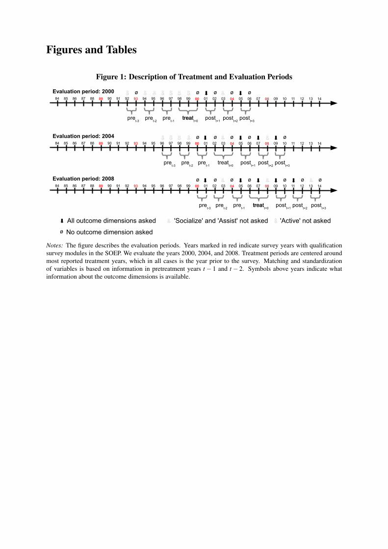
Figures and Tables

Figure 1: Description of Treatment and Evaluation Periods

84 85 86 87 88 89 90 91 92 93 94 95 96 97 98 99 00 01 02 03 04 05 06 07 08 09 10 11 12 13 14

84 85 86 87 88 89 90 91 92 93 94 95 96 97 98 99 00 01 02 03 04 05 06 07 08 09 10 11 12 13 14

84 85 86 87 88 89 90 91 92 93 94 95 96 97 98 99 00 01 02 03 04 05 06 07 08 09 10 11 12 13 14

Evaluation period: 2008

postt+1

treatt=0

pret-1



postt+1

treattreatt=0

pret-1

postt+1

treatpret-1

treatt=0

postt+2

postt+3

postt+3

postt+2

pret-2

pret-2

pret-2

postt+2

postt+3

All outcome dimensions asked 'Active' not asked'Socialize' and 'Assist' not asked

ø ø ø ø

ø øøøø

ø ø ø ø ø

ø No outcome dimension asked

ø

pret-3

ø

pret-3

pret-3

ø

Notes: The figure describes the evaluation periods. Years marked in red indicate survey years with qualificationsurvey modules in the SOEP. We evaluate the years 2000, 2004, and 2008. Treatment periods are centered aroundmost reported treatment years, which in all cases is the year prior to the survey. Matching and standardizationof variables is based on information in pretreatment years t � 1 and t � 2. Symbols above years indicate whatinformation about the outcome dimensions is available.

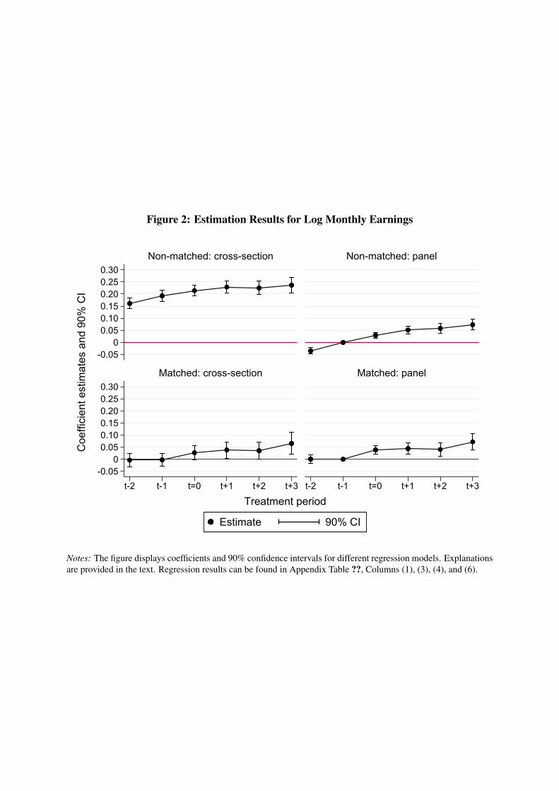
Figure 2: Estimation Results for Log Monthly Earnings

��

��

��

��

W�� W�� W � W�� W�� W�� W�� W�� W � W�� W�� W��

1RQ�PDWFKHG��FURVV�VHFWLRQ 1RQ�PDWFKHG��SDQHO

0DWFKHG��FURVV�VHFWLRQ 0DWFKHG��SDQHO

(VWLPDWH ��&,

&RHIILFLHQW�HVWLPDWHV�DQG��

�&,

7UHDWPHQW�SHULRG

Notes: The figure displays coefficients and 90% confidence intervals for different regression models. Explanationsare provided in the text. Regression results can be found in Appendix Table ??, Columns (1), (3), (4), and (6).

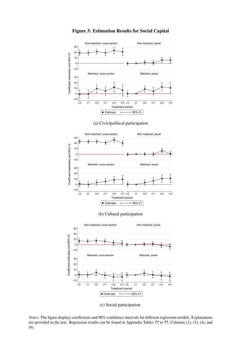
Figure 3: Estimation Results for Social Capital

��

�

��

��

��

��

�

��

��

��

W�� W�� W � W�� W�� W�� W�� W�� W � W�� W�� W��



(VWLPDWH ��&,


�&,

7UHDWPHQW�SHULRG

(a) Civic/political participation

��

�

��

��

��

��

�

��

��

��

W�� W�� W � W�� W�� W�� W�� W�� W � W�� W�� W��



(VWLPDWH ��&,


�&,

7UHDWPHQW�SHULRG

(b) Cultural participation

��

�

��

��

��

��

�

��

��

��

W�� W�� W � W�� W�� W�� W�� W�� W � W�� W�� W��



(VWLPDWH ��&,


�&,

7UHDWPHQW�SHULRG

(c) Social participation

Notes: The figure displays coefficients and 90% confidence intervals for different regression models. Explanationsare provided in the text. Regression results can be found in Appendix Tables ?? to ??, Columns (1), (3), (4), and(6).

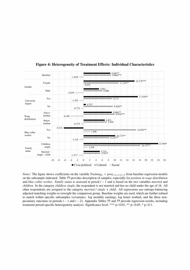
Figure 4: Heterogeneity of Treatment Effects: Individual Characteristics

-1.577

1.298

-1.319

1.999

-0.775

-4.104

-0.772

-1.392

-2.654

0.035

-1.434

5.347*

18.197**

8.232**

16.892**

7.450

9.930***

9.420**

9.113

6.006

11.236**

8.868***

5.235

23.994*

10.172**

-6.321

6.821

9.086**

0.757

17.436**

4.962

16.378***

8.605**

-10 -8 -6 -4 -2 0 2 4 6 8 10 12 14 16 18 20 22 24 26

Married /single + child

Childless single

No

Yes

Below median

Abovemedian

No

Yes

Male

Female

Baseline

Civic/political Cultural Social

Gender

Universitydegree

Wagedistribution

Blue collarworker

Family status

Notes: The figure shows coefficients on the variable Trainingie ⇥ postt+1,t+2,t+3 from baseline regression modelson the subsample indicated. Table ?? provides description of samples; especially for position in wage distributionand blue collar worker. Family status is assessed in period t � 1 and is based on the two variables married andchildren. In the category childless single, the respondent is not married and has no child under the age of 16. Allother respondents are assigned to the category married / single + child. All regressions use entropy-balancingadjusted matching weights to reweight the comparison group. Baseline weights are used, which are further refinedto match within specific subsamples (covariates: log monthly earnings, log hours worked, and the three non-pecuniary outcomes in periods t � 1 and t � 2). Appendix Tables ?? and ?? provide regression results, includingtreatment period-specific heterogeneity analysis. Significance level: *** p<0.01, ** p<0.05, * p<0.1.

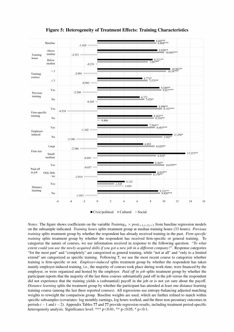
Figure 5: Heterogeneity of Treatment Effects: Training Characteristics

-1.853

3.929

-2.014

-0.657

-0.691

-2.586

-3.190

-1.102

0.406

-4.518

-0.265

-2.260

-0.983

-2.091

-0.231

-2.551

-1.434

9.420***

2.545

8.170**

10.079**

8.836*

8.628**

9.805*

8.683***

8.510**

9.747***

7.076*

9.627***

7.575**

10.347**

7.607**

10.043***

8.868***

9.151**

4.122

8.810**

8.465*

13.233**

6.893

11.296*

7.584**

8.263**

8.998**

6.371

9.349**

6.771*

10.962**

8.321**

9.030**

8.605**

-6 -4 -2 0 2 4 6 8 10 12 14 16

No

Yes

Only little / no

Yes

Small/medium

Large

No

Yes

No

Yes

No

Yes

≤ 3

> 3

Belowmedian

Abovemedian

Baseline

I

I

I


Traininghours

Firm size

Previous training

Training courses

Firm-specific training

Employer-induced

Paid off in job

Distance learning

Notes: The figure shows coefficients on the variable Trainingie ⇥ postt+1,t+2,t+3 from baseline regression modelson the subsample indicated. Training hours splits treatment group at median training hours (33 hours). Previoustraining splits treatment group by whether the respondent has already received training in the past. Firm-specifictraining splits treatment group by whether the respondent has received firm-specific or general training. Tocategorize the nature of courses, we use information received in response to the following question: “To whatextent could you use the newly acquired skills if you got a new job in a different company?". Response categories“for the most part" and “completely" are categorized as general training, while “not at all" and “only to a limitedextend" are categorized as specific training. Following ?, we use the most recent course to categorize whethertraining is firm-specific or not. Employer-induced splits treatment group by whether the respondent has takenmainly employer-induced training, i.e., the majority of courses took place during work-time, were financed by theemployer, or were organized and hosted by the employer. Paid off in job splits treatment group by whether theparticipant reports that the majority of the last three courses substantially paid off in the job versus the respondentdid not experience that the training yields a (substantial) payoff in the job or is not yet sure about the payoff.Distance learning splits the treatment group by whether the participant has attended at least one distance learningtraining course (among the last three reported courses). All regressions use entropy-balancing adjusted matchingweights to reweight the comparison group. Baseline weights are used, which are further refined to match withinspecific subsamples (covariates: log monthly earnings, log hours worked, and the three non-pecuniary outcomes inperiods t �1 and t �2). Appendix Tables ?? and ?? provide regression results, including treatment period-specificheterogeneity analysis. Significance level: *** p<0.01, ** p<0.05, * p<0.1.

Table 1: Overview of Conditioning Variables

Demographic characteristicsAgea 3 categories (25-35, 36-45, 46-55)Female 0 = male, 1 = femaleMigrant 1 = individual or parents moved to Germany, 0 elseGerman citizen 1 = German, 0 foreign citizenMarried 1 = yes, 0 = noHomeowner 1 = home owner, 0 = tenantChildren 1 = children under the age of 16 in household, 0 elseSelf-rated healthb (t �1; t �2) 5 categories (1 bad - 5 very good)Federal stated 14 categoriesEvaluation perioda 3 categories (2000, 2004, 2008)Occupational samplea,e 2 categories (blue collar worker; non-blue collar worker)

EducationVocational 0 = no vocational training, 1 = vocational trainingUniversity 0 = no university degree, 1 = university degreeSchooling 4 categories (no degree/basic school; intermediate/other school; technical school;

academic school track (Abitur))Previous work-related training 1 = participated in work-related training before, 0 else

Labor market characteristicsLog monthly earningsc (t �1; t �2) Log monthly gross earnings in 2010 eurosLog hours worked per weekc (t �1; t �2) Log hours worked per weekEarnings tertilea, f 3 categories (bottom; middle; top)Full-time employed (t �1; t �2) 1 = yes, 0 = noOccupational status (t �1; t �2) 7 categories (blue collar; white collar; public servant; self-employed; unemployed;

non-working; apprentice, retired)Civic service (t �1; t �2) 1 = public service, 0 elseUnemployment experience 3 categories (no experience; 0-2 years; more than two years)Tenure with the current firm 4 categories (0-2 years; 2-8 years; 8-15 years; more than 15 years)Firm size (t �1; t �2) 3 categories (small < 20, medium 20-200, large > 200 employees)Industry (t �1; t �2) 10 categories

Satisfaction and worriesLife satisfactionb (t �1; t �2) 11 categories (0 low - 10 high)Worries: economic situationb (t �1; t �2) 3 categories (1 no worries, 2 some worries, 3 big worries)Worries: own economic situationb (t �1; t �2) 3 categories (1 no worries, 2 some worries, 3 big worries)Worries: job situationb (t �1; t �2) 3 categories (1 no worries, 2 some worries, 3 big worries)

Outcomes before treatmentCivic/political participation scorec,g (t �1; t �2) Score from PCACultural participation scorec,g (t �1; t �2) Score from PCASocial participation scorec,g (t �1; t �2) Score from PCA

Interest in politicsb (t �1; t �2) 4 categories (1 not at all, 2 not so strongly, 3 strongly, 4 very strongly)Participate in politicsb (t �1; t �2) 3 categories (1 never, 2 rarely, 3 often)Volunteerb (t �1; t �2) 4 categories (1 never, 2 rarely, 3 every month, 4 every week)Active in artistic/musical activitiesb (t �1; t �2) 4 categories (1 never, 2 rarely, 3 every month, 4 every week)Attend classic eventsb (t �1; t �2) 4 categories (1 never, 2 rarely, 3 every month, 4 every week)Attend modern eventsb (t �1; t �2) 4 categories (1 never, 2 rarely, 3 every month, 4 every week)Socializeb (t �1; t �2) 4 categories (1 never, 2 rarely, 3 every month, 4 every week)Assistb (t �1; t �2) 4 categories (1 never, 2 rarely, 3 every month, 4 every week)

Notes: All variables are included for period t�1 if not indicated otherwise. aPropensity score matching is exact on these variables. bVariablex is z-standardized by (x�meanx)/sdx (see ?). Mean and SD are based on the comparison group in periods t �1 and t �2. cBalancing onfirst and second moments of these variables in the entropy balancing stage to refine conventional matching weights. dBremen and Hamburgare grouped together with Lower Saxony and Schleswig-Holstein, respectively, due to small samples. eTo belong to the blue-collar workersample, the individual has to report to work in a blue-collar occupation at least in one year during t �1 and at least in one year during t �2.To belong to the non-blue-collar worker sample, the individual has to report to work in a white-collar occupation or as a public servantat least in one year during t � 1 and at least in one year during t � 2. Most recent occupation is assigned in the case of multiple groupmembership assignment options. The variable is only used for exact matching and not included in the matching function (instead: matchingin detailed occupational status). f Tertiles computed for log monthly gross earnings in 2010 euros averaged over t �1 and t �2. Calculationsare based on the sample before matching. gScores are rescaled by evaluation period such that the comparison group has, on average, mean500 and SD 100 in periods t �1 and t �2.

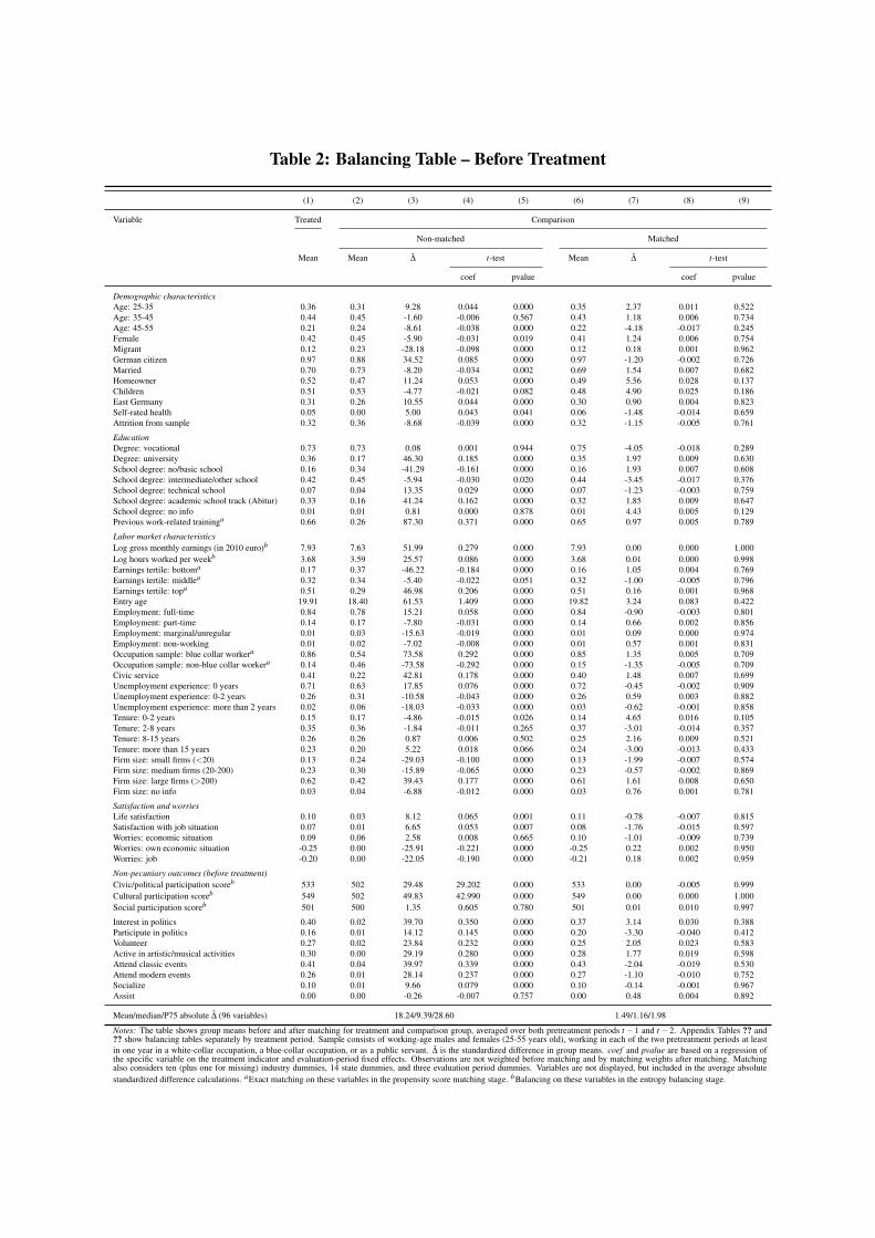
Table 2: Balancing Table – Before Treatment

(1) (2) (3) (4) (5) (6) (7) (8) (9)

Variable Treated Comparison

Non-matched Matched

Mean Mean D t-test Mean D t-test

coef pvalue coef pvalue

Demographic characteristicsAge: 25-35 0.36 0.31 9.28 0.044 0.000 0.35 2.37 0.011 0.522Age: 35-45 0.44 0.45 -1.60 -0.006 0.567 0.43 1.18 0.006 0.734Age: 45-55 0.21 0.24 -8.61 -0.038 0.000 0.22 -4.18 -0.017 0.245Female 0.42 0.45 -5.90 -0.031 0.019 0.41 1.24 0.006 0.754Migrant 0.12 0.23 -28.18 -0.098 0.000 0.12 0.18 0.001 0.962German citizen 0.97 0.88 34.52 0.085 0.000 0.97 -1.20 -0.002 0.726Married 0.70 0.73 -8.20 -0.034 0.002 0.69 1.54 0.007 0.682Homeowner 0.52 0.47 11.24 0.053 0.000 0.49 5.56 0.028 0.137Children 0.51 0.53 -4.77 -0.021 0.082 0.48 4.90 0.025 0.186East Germany 0.31 0.26 10.55 0.044 0.000 0.30 0.90 0.004 0.823Self-rated health 0.05 0.00 5.00 0.043 0.041 0.06 -1.48 -0.014 0.659Attrition from sample 0.32 0.36 -8.68 -0.039 0.000 0.32 -1.15 -0.005 0.761

EducationDegree: vocational 0.73 0.73 0.08 0.001 0.944 0.75 -4.05 -0.018 0.289Degree: university 0.36 0.17 46.30 0.185 0.000 0.35 1.97 0.009 0.630School degree: no/basic school 0.16 0.34 -41.29 -0.161 0.000 0.16 1.93 0.007 0.608School degree: intermediate/other school 0.42 0.45 -5.94 -0.030 0.020 0.44 -3.45 -0.017 0.376School degree: technical school 0.07 0.04 13.35 0.029 0.000 0.07 -1.23 -0.003 0.759School degree: academic school track (Abitur) 0.33 0.16 41.24 0.162 0.000 0.32 1.85 0.009 0.647School degree: no info 0.01 0.01 0.81 0.000 0.878 0.01 4.43 0.005 0.129Previous work-related traininga 0.66 0.26 87.30 0.371 0.000 0.65 0.97 0.005 0.789

Labor market characteristicsLog gross monthly earnings (in 2010 euro)b 7.93 7.63 51.99 0.279 0.000 7.93 0.00 0.000 1.000Log hours worked per weekb 3.68 3.59 25.57 0.086 0.000 3.68 0.01 0.000 0.998Earnings tertile: bottoma 0.17 0.37 -46.22 -0.184 0.000 0.16 1.05 0.004 0.769Earnings tertile: middlea 0.32 0.34 -5.40 -0.022 0.051 0.32 -1.00 -0.005 0.796Earnings tertile: topa 0.51 0.29 46.98 0.206 0.000 0.51 0.16 0.001 0.968Entry age 19.91 18.40 61.53 1.409 0.000 19.82 3.24 0.083 0.422Employment: full-time 0.84 0.78 15.21 0.058 0.000 0.84 -0.90 -0.003 0.801Employment: part-time 0.14 0.17 -7.80 -0.031 0.000 0.14 0.66 0.002 0.856Employment: marginal/unregular 0.01 0.03 -15.63 -0.019 0.000 0.01 0.09 0.000 0.974Employment: non-working 0.01 0.02 -7.02 -0.008 0.000 0.01 0.57 0.001 0.831Occupation sample: blue collar workera 0.86 0.54 73.58 0.292 0.000 0.85 1.35 0.005 0.709Occupation sample: non-blue collar workera 0.14 0.46 -73.58 -0.292 0.000 0.15 -1.35 -0.005 0.709Civic service 0.41 0.22 42.81 0.178 0.000 0.40 1.48 0.007 0.699Unemployment experience: 0 years 0.71 0.63 17.85 0.076 0.000 0.72 -0.45 -0.002 0.909Unemployment experience: 0-2 years 0.26 0.31 -10.58 -0.043 0.000 0.26 0.59 0.003 0.882Unemployment experience: more than 2 years 0.02 0.06 -18.03 -0.033 0.000 0.03 -0.62 -0.001 0.858Tenure: 0-2 years 0.15 0.17 -4.86 -0.015 0.026 0.14 4.65 0.016 0.105Tenure: 2-8 years 0.35 0.36 -1.84 -0.011 0.265 0.37 -3.01 -0.014 0.357Tenure: 8-15 years 0.26 0.26 0.87 0.006 0.502 0.25 2.16 0.009 0.521Tenure: more than 15 years 0.23 0.20 5.22 0.018 0.066 0.24 -3.00 -0.013 0.433Firm size: small firms (<20) 0.13 0.24 -29.03 -0.100 0.000 0.13 -1.99 -0.007 0.574Firm size: medium firms (20-200) 0.23 0.30 -15.89 -0.065 0.000 0.23 -0.57 -0.002 0.869Firm size: large firms (>200) 0.62 0.42 39.43 0.177 0.000 0.61 1.61 0.008 0.650Firm size: no info 0.03 0.04 -6.88 -0.012 0.000 0.03 0.76 0.001 0.781

Satisfaction and worriesLife satisfaction 0.10 0.03 8.12 0.065 0.001 0.11 -0.78 -0.007 0.815Satisfaction with job situation 0.07 0.01 6.65 0.053 0.007 0.08 -1.76 -0.015 0.597Worries: economic situation 0.09 0.06 2.58 0.008 0.665 0.10 -1.01 -0.009 0.739Worries: own economic situation -0.25 0.00 -25.91 -0.221 0.000 -0.25 0.22 0.002 0.950Worries: job -0.20 0.00 -22.05 -0.190 0.000 -0.21 0.18 0.002 0.959

Non-pecuniary outcomes (before treatment)Civic/political participation scoreb 533 502 29.48 29.202 0.000 533 0.00 -0.005 0.999Cultural participation scoreb 549 502 49.83 42.990 0.000 549 0.00 0.000 1.000Social participation scoreb 501 500 1.35 0.605 0.780 501 0.01 0.010 0.997

Interest in politics 0.40 0.02 39.70 0.350 0.000 0.37 3.14 0.030 0.388Participate in politics 0.16 0.01 14.12 0.145 0.000 0.20 -3.30 -0.040 0.412Volunteer 0.27 0.02 23.84 0.232 0.000 0.25 2.05 0.023 0.583Active in artistic/musical activities 0.30 0.00 29.19 0.280 0.000 0.28 1.77 0.019 0.598Attend classic events 0.41 0.04 39.97 0.339 0.000 0.43 -2.04 -0.019 0.530Attend modern events 0.26 0.01 28.14 0.237 0.000 0.27 -1.10 -0.010 0.752Socialize 0.10 0.01 9.66 0.079 0.000 0.10 -0.14 -0.001 0.967Assist 0.00 0.00 -0.26 -0.007 0.757 0.00 0.48 0.004 0.892

Mean/median/P75 absolute D (96 variables) 18.24/9.39/28.60 1.49/1.16/1.98

Notes: The table shows group means before and after matching for treatment and comparison group, averaged over both pretreatment periods t � 1 and t � 2. Appendix Tables ?? and?? show balancing tables separately by treatment period. Sample consists of working-age males and females (25-55 years old), working in each of the two pretreatment periods at leastin one year in a white-collar occupation, a blue-collar occupation, or as a public servant. D is the standardized difference in group means. coef and pvalue are based on a regression ofthe specific variable on the treatment indicator and evaluation-period fixed effects. Observations are not weighted before matching and by matching weights after matching. Matchingalso considers ten (plus one for missing) industry dummies, 14 state dummies, and three evaluation period dummies. Variables are not displayed, but included in the average absolutestandardized difference calculations. aExact matching on these variables in the propensity score matching stage. bBalancing on these variables in the entropy balancing stage.

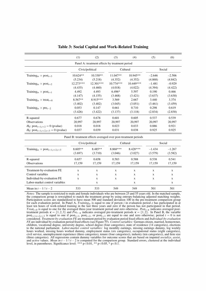
Table 3: Social Capital and Work-Related Training

(1) (2) (3) (4) (5) (6)

Panel A: treatment effects by treatment period


Trainingie ⇥ postt+3 10.624** 10.330** 11.047** 10.945** –2.646 –2.506(5.234) (5.218) (4.352) (4.352) (4.868) (4.842)

Trainingie ⇥ postt+2 12.273*** 12.301*** 10.774*** 10.449*** –1.481 –0.929(4.435) (4.460) (4.018) (4.022) (4.394) (4.422)

Trainingie ⇥ postt+1 4.492 4.493 6.496* 5.597 0.190 0.466(4.147) (4.155) (3.468) (3.421) (3.637) (3.630)

Trainingie ⇥ treatt=0 8.567** 8.915*** 3.569 2.667 3.440 3.374(3.402) (3.402) (3.045) (3.051) (3.461) (3.459)

Trainingie ⇥ pret�2 0.053 0.147 0.661 0.710 0.298 0.619(3.426) (3.422) (3.137) (3.118) (2.834) (2.830)

R-squared 0.677 0.678 0.601 0.605 0.537 0.539Observations 20,997 20,997 20,997 20,997 20,997 20,997H0: postt+1,t+2 = 0 (pvalue) 0.018 0.018 0.023 0.033 0.886 0.921H0: postt+1,t+2,t+3 = 0 (pvalue) 0.037 0.039 0.031 0.038 0.925 0.925

Panel B: treatment effects averaged over post-treatment periods


Trainingie ⇥ postt+1,t+2,t+3 8.605** 8.485** 8.868*** 8.428*** –1.434 –1.267(3.697) (3.710) (3.046) (3.027) (3.579) (3.582)

R-squared 0.657 0.658 0.583 0.588 0.538 0.541Observations 17,159 17,159 17,159 17,159 17,159 17,159

Treatment-by-evaluation FE x x x x x xControl variables x x x x x xIndividual-by-evaluation FE x x x x x xLabor-market control variables x x x

Mean in t �1\ t �2 533 533 549 549 501 501

Notes: The sample is restricted to male and female individuals who are between 25 and 55 years old. In the matched sample,the comparison group is reweighted to match the treatment group by using entropy-balancing adjusted matching weights.Participation scores are standardized to have mean 500 and standard deviation 100 in the pre-treatment comparison groupfor each evaluation period. In Panel A, Trainingie is equal to one if person i in evaluation period e has participated in atleast ten hours of work-related training in the last three years and zero if the person has not participated in that period.Treatt=0 is equal to one for the averaged three-year treatment period and zero otherwise. Postt+k indicates averaged post-treatment periods k = {1,2,3} and Pret�k indicates averaged pre-treatment periods k = {1,2}. In Panel B, the variablepostt+1,t+2,t+3 is equal to one if postt+1, postt+2, or postt+3 are equal to one and zero otherwise; period t = 0 is notconsidered. Treatment-by-evaluation FE are treatment period by evaluation period fixed effects and Individual-by-evaluationFE are individual by evaluation period fixed effects (see Figure ??). Control variables: German citizen, married, homeowner,children, vocational degree, university degree, school degree (four categories), state of residence (14 categories), electionsto the national parliament. Labor-market control variables: log monthly earnings, missing earnings dummy, log weeklyhours worked, missing hours worked dummy, employment status (six categories), occupational status (eight categories),civil service, unemployment experience (three categories), tenure (four categories)), industry (ten categories)), and firm size(three categories). All regressions contain dummy variables for outcome scores that are based on imputed socialize, assist,and active values. Mean in t � 1\ t � 2 is computed for the comparison group. Standard errors, clustered at the individuallevel, in parentheses. Significance level: *** p<0.01, ** p<0.05, * p<0.1.

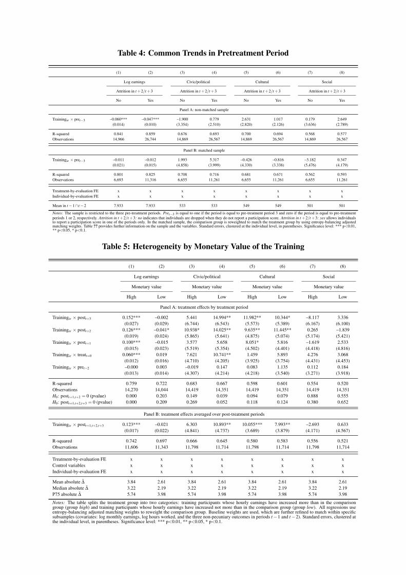
Table 4: Common Trends in Pretreatment Period

(1) (2) (3) (4) (5) (6) (7) (8)

Log earnings Civic/political Cultural Social

Attrition in t +2/t +3 Attrition in t +2/t +3 Attrition in t +2/t +3 Attrition in t +2/t +3

No Yes No Yes No Yes No Yes

Panel A: non-matched sample

Trainingie ⇥ pret�3 –0.060*** –0.047*** –1.900 0.779 2.631 1.017 0.179 2.649(0.014) (0.010) (3.354) (2.510) (2.820) (2.126) (3.636) (2.789)

R-squared 0.841 0.859 0.676 0.693 0.700 0.694 0.568 0.577Observations 14,966 26,744 14,869 26,567 14,869 26,567 14,869 26,567

Panel B: matched sample

Trainingie ⇥ pret�3 –0.011 –0.012 1.993 5.317 –0.426 –0.816 –3.182 0.347(0.021) (0.015) (4.858) (3.999) (4.330) (3.338) (5.476) (4.179)


Treatment-by-evaluation FE x x x x x x x xIndividual-by-evaluation FE x x x x x x x x

Mean in t �1\ t �2 7.933 7.933 533 533 549 549 501 501

Notes: The sample is restricted to the three pre-treatment periods. Pret�3 is equal to one if the period is equal to pre-treatment period 3 and zero if the period is equal to pre-treatmentperiods 1 or 2, respectively. Attrition in t +2/t +3: no indicates that individuals are dropped when they do not report a participation score. Attrition in t +2/t +3: yes allows individualsto report a participation score in one of the periods only. In the matched sample, the comparison group is reweighted to match the treatment group by using entropy-balancing adjustedmatching weights. Table ?? provides further information on the sample and the variables. Standard errors, clustered at the individual level, in parentheses. Significance level: *** p<0.01,** p<0.05, * p<0.1.

Table 5: Heterogeneity by Monetary Value of the Training

(1) (2) (3) (4) (5) (6) (7) (8)

Log earnings Civic/political Cultural Social

Monetary value Monetary value Monetary value Monetary value

High Low High Low High Low High Low


Trainingie ⇥ postt+3 0.152*** –0.002 5.441 14.994** 11.982** 10.344* –8.117 3.336(0.027) (0.029) (6.744) (6.543) (5.573) (5.389) (6.167) (6.100)

Trainingie ⇥ postt+2 0.126*** –0.041* 10.938* 14.025** 9.635** 11.445** 0.265 –1.839(0.019) (0.024) (5.865) (5.641) (4.875) (5.074) (5.174) (5.421)

Trainingie ⇥ postt+1 0.100*** –0.015 3.577 5.658 8.051* 5.816 –1.619 2.533(0.015) (0.023) (5.519) (5.354) (4.502) (4.401) (4.418) (4.816)

Trainingie ⇥ treatt=0 0.060*** 0.019 7.621 10.741** 1.459 5.893 4.276 3.068(0.012) (0.016) (4.710) (4.205) (3.925) (3.754) (4.431) (4.453)

Trainingie ⇥ pret�2 –0.000 0.003 –0.019 0.147 0.083 1.135 0.112 0.184(0.013) (0.014) (4.307) (4.214) (4.218) (3.540) (3.271) (3.918)

R-squared 0.759 0.722 0.683 0.667 0.598 0.601 0.554 0.520Observations 14,270 14,044 14,419 14,351 14,419 14,351 14,419 14,351H0: postt+1,t+2 = 0 (pvalue) 0.000 0.203 0.149 0.039 0.094 0.079 0.888 0.555H0: postt+1,t+2,t+3 = 0 (pvalue) 0.000 0.209 0.269 0.052 0.118 0.124 0.380 0.652


Trainingie ⇥ postt+1,t+2,t+3 0.123*** –0.021 6.303 10.893** 10.055*** 7.993** –2.693 0.633(0.017) (0.022) (4.841) (4.737) (3.689) (3.879) (4.171) (4.567)


Treatment-by-evaluation FE x x x x x x x xControl variables x x x x x x x xIndividual-by-evaluation FE x x x x x x x x

Mean absolute D 3.84 2.61 3.84 2.61 3.84 2.61 3.84 2.61Median absolute D 3.22 2.19 3.22 2.19 3.22 2.19 3.22 2.19P75 absolute D 5.74 3.98 5.74 3.98 5.74 3.98 5.74 3.98

Notes: The table splits the treatment group into two categories: training participants whose hourly earnings have increased more than in the comparisongroup (group high) and training participants whose hourly earnings have increased not more than in the comparison group (group low). All regressions useentropy-balancing adjusted matching weights to reweight the comparison group. Baseline weights are used, which are further refined to match within specificsubsamples (covariates: log monthly earnings, log hours worked, and the three non-pecuniary outcomes in periods t �1 and t �2). Standard errors, clustered atthe individual level, in parentheses. Significance level: *** p<0.01, ** p<0.05, * p<0.1.

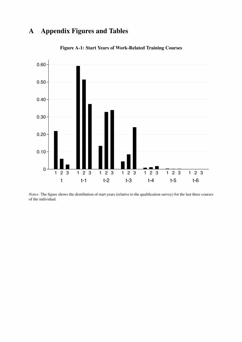
A Appendix Figures and Tables

Figure A-1: Start Years of Work-Related Training Courses

0

0.10

0.20

0.30

0.40

0.50

0.60

t t-1 t-2 t-3 t-4 t-5 t-61 2 3 1 2 3 1 2 3 1 2 3 1 2 3 1 2 3 1 2 3

Notes: The figure shows the distribution of start years (relative to the qualification survey) for the last three coursesof the individual.

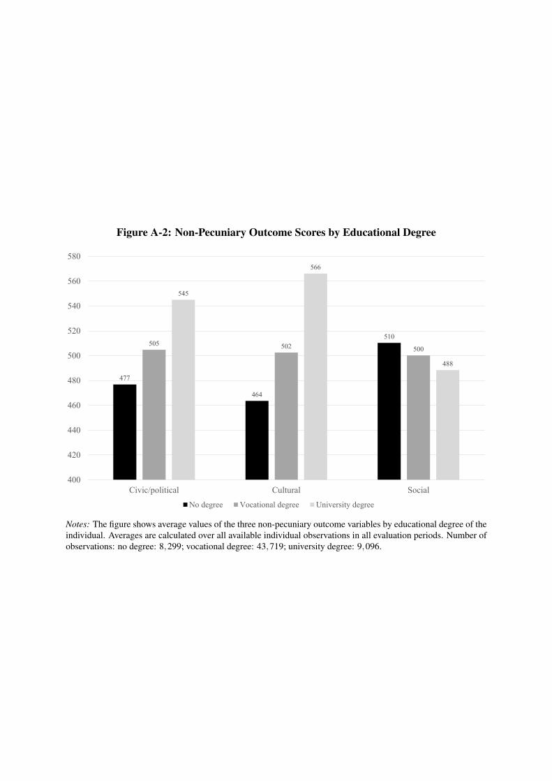
Figure A-2: Non-Pecuniary Outcome Scores by Educational Degree

477

464

510505 502 500

545

566

488

400

420

440

460

480

500

520

540

560

580

Civic/political Cultural SocialNo degree Vocational degree University degree

Notes: The figure shows average values of the three non-pecuniary outcome variables by educational degree of theindividual. Averages are calculated over all available individual observations in all evaluation periods. Number ofobservations: no degree: 8,299; vocational degree: 43,719; university degree: 9,096.

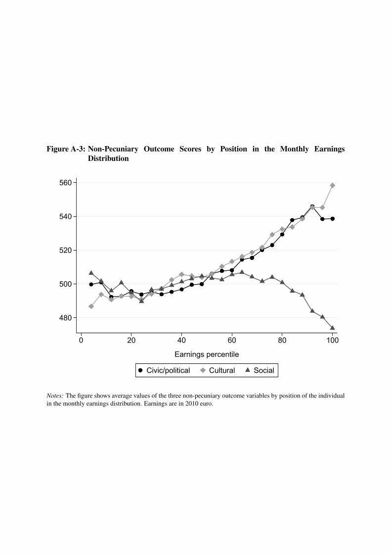
Figure A-3: Non-Pecuniary Outcome Scores by Position in the Monthly EarningsDistribution

��

��

��

��

��

� ��

(DUQLQJV�SHUFHQWLOH

&LYLF�SROLWLFDO &XOWXUDO 6RFLDO

Notes: The figure shows average values of the three non-pecuniary outcome variables by position of the individualin the monthly earnings distribution. Earnings are in 2010 euro.

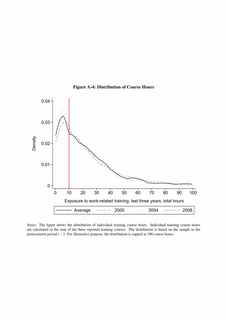
Figure A-4: Distribution of Course Hours

�

��

��

��

��

'HQVLW\

� ��

([SRVXUH�WR�ZRUN�UHODWHG�WUDLQLQJ��ODVW�WKUHH�\HDUV��WRWDO�KRXUV

$YHUDJH ��

Notes: The figure shows the distribution of individual training course hours. Individual training course hoursare calculated as the sum of the three reported training courses. The distribution is based on the sample in thepretreatment period t �1. For illustrative purpose, the distribution is capped at 100 course hours.

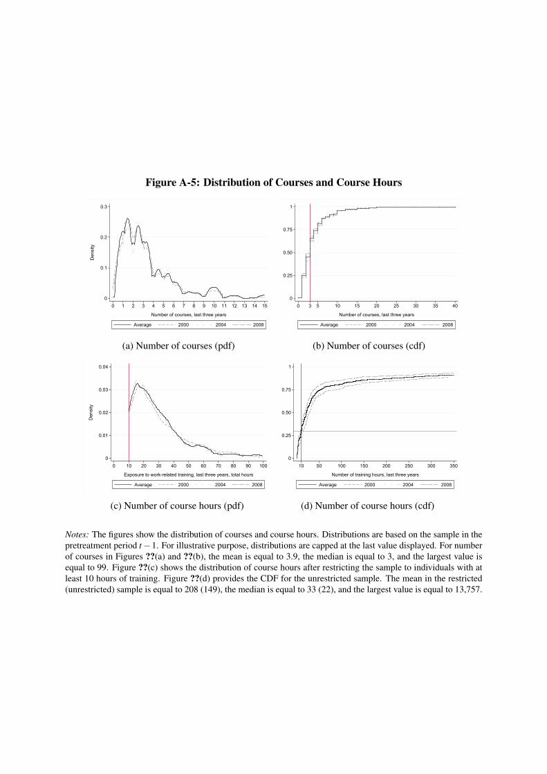
Figure A-5: Distribution of Courses and Course Hours

�

��

��

��

'HQVLW\

� � � � � � � � � � ��

1XPEHU�RI�FRXUVHV��ODVW�WKUHH�\HDUV

$YHUDJH ��

(a) Number of courses (pdf)

�

��

��

��

�

� � � ��

1XPEHU�RI�FRXUVHV��ODVW�WKUHH�\HDUV

$YHUDJH ��

(b) Number of courses (cdf)

�

��

��

��

��

'HQVLW\

� ��


$YHUDJH ��

(c) Number of course hours (pdf)

�

��

��

��

�

��

1XPEHU�RI�WUDLQLQJ�KRXUV��ODVW�WKUHH�\HDUV

$YHUDJH ��

(d) Number of course hours (cdf)

Notes: The figures show the distribution of courses and course hours. Distributions are based on the sample in thepretreatment period t �1. For illustrative purpose, distributions are capped at the last value displayed. For numberof courses in Figures ??(a) and ??(b), the mean is equal to 3.9, the median is equal to 3, and the largest value isequal to 99. Figure ??(c) shows the distribution of course hours after restricting the sample to individuals with atleast 10 hours of training. Figure ??(d) provides the CDF for the unrestricted sample. The mean in the restricted(unrestricted) sample is equal to 208 (149), the median is equal to 33 (22), and the largest value is equal to 13,757.

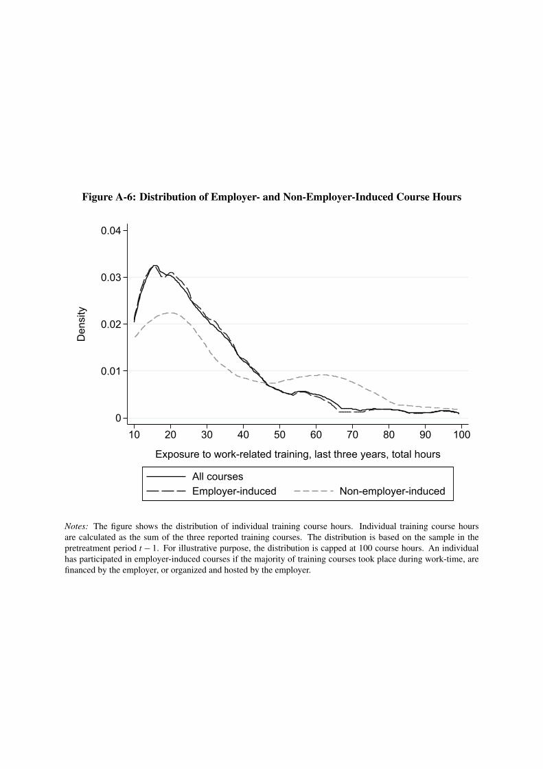
Figure A-6: Distribution of Employer- and Non-Employer-Induced Course Hours

�

��

��

��

��

'HQVLW\

��


$OO�FRXUVHV(PSOR\HU�LQGXFHG 1RQ�HPSOR\HU�LQGXFHG

Notes: The figure shows the distribution of individual training course hours. Individual training course hoursare calculated as the sum of the three reported training courses. The distribution is based on the sample in thepretreatment period t � 1. For illustrative purpose, the distribution is capped at 100 course hours. An individualhas participated in employer-induced courses if the majority of training courses took place during work-time, arefinanced by the employer, or organized and hosted by the employer.

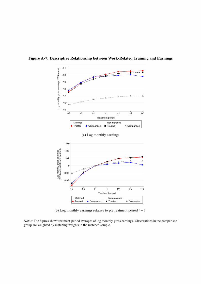
Figure A-7: Descriptive Relationship between Work-Related Training and Earnings

��

��

��

��

��

��

��

/RJ�PRQWKO\�JURVV�HDUQLQJV��HXUR�

W�� W�� W�� W W�� W�� W��

7UHDWPHQW�SHULRG

0DWFKHG 1RQ�PDWFKHG7UHDWHG &RPSDULVRQ 7UHDWHG &RPSDULVRQ

(a) Log monthly earnings

��

��

�

��

��

��

/RJ�PRQWKO\�JURVV�HDUQLQJV

��HXUR��UHODWLYH�WR�SHULRG�W�

W�� W�� W�� W W�� W�� W��

7UHDWPHQW�SHULRG


(b) Log monthly earnings relative to pretreatment period t �1

Notes: The figures show treatment-period averages of log monthly gross earnings. Observations in the comparisongroup are weighted by matching weights in the matched sample.

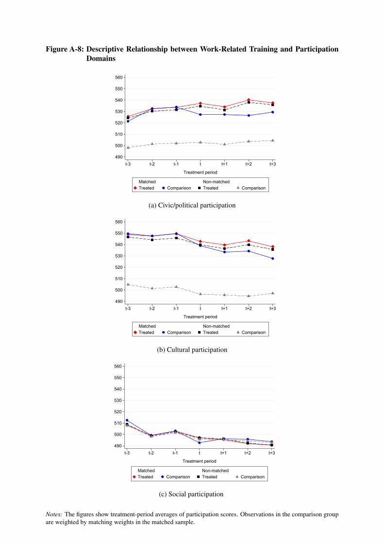
Figure A-8: Descriptive Relationship between Work-Related Training and ParticipationDomains

��

��

��

��

��

��

��

��

W�� W�� W�� W W�� W�� W��

7UHDWPHQW�SHULRG


(a) Civic/political participation

��

��

��

��

��

��

��

��

W�� W�� W�� W W�� W�� W��

7UHDWPHQW�SHULRG


(b) Cultural participation

��

��

��

��

��

��

��

��

W�� W�� W�� W W�� W�� W��

7UHDWPHQW�SHULRG


(c) Social participation

Notes: The figures show treatment-period averages of participation scores. Observations in the comparison groupare weighted by matching weights in the matched sample.

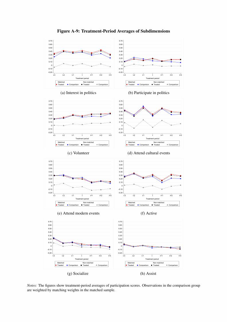
Figure A-9: Treatment-Period Averages of Subdimensions

��

��

�

��

��

��

��

��

��

��

W�� W�� W�� W W�� W�� W��

7UHDWPHQW�SHULRG


(a) Interest in politics

��

��

�

��

��

��

��

��

��

��

W�� W�� W�� W W�� W�� W��

7UHDWPHQW�SHULRG


(b) Participate in politics

��

��

�

��

��

��

��

��

��

��

W�� W�� W�� W W�� W�� W��

7UHDWPHQW�SHULRG


(c) Volunteer

��

��

�

��

��

��

��

��

��

��

W�� W�� W�� W W�� W�� W��

7UHDWPHQW�SHULRG


(d) Attend cultural events

��

��

�

��

��

��

��

��

��

��

W�� W�� W�� W W�� W�� W��

7UHDWPHQW�SHULRG


(e) Attend modern events

��

��

�

��

��

��

��

��

��

��

W�� W�� W�� W W�� W�� W��

7UHDWPHQW�SHULRG


(f) Active

��

��

�

��

��

��

��

��

��

��

W�� W�� W�� W W�� W�� W��

7UHDWPHQW�SHULRG


(g) Socialize

��

��

�

��

��

��

��

��

��

��

W�� W�� W�� W W�� W�� W��

7UHDWPHQW�SHULRG


(h) Assist

Notes: The figures show treatment-period averages of participation scores. Observations in the comparison groupare weighted by matching weights in the matched sample.

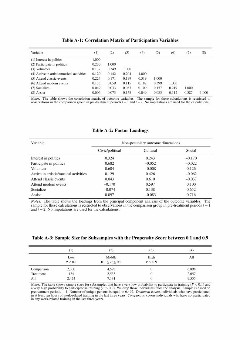
Table A-1: Correlation Matrix of Participation Variables

Variable (1) (2) (3) (4) (5) (6) (7) (8)

(1) Interest in politics 1.000(2) Participate in politics 0.230 1.000(3) Volunteer 0.137 0.349 1.000(4) Active in artistic/musical activities 0.120 0.142 0.204 1.000(5) Attend classic events 0.224 0.171 0.199 0.319 1.000(6) Attend modern events 0.133 0.059 0.115 0.182 0.399 1.000(7) Socialize 0.049 0.033 0.087 0.109 0.157 0.219 1.000(8) Assist 0.006 0.073 0.158 0.049 0.083 0.112 0.387 1.000

Notes: The table shows the correlation matrix of outcome variables. The sample for these calculations is restricted toobservations in the comparison group in pre-treatment periods t �1 and t �2. No imputations are used for the calculations.

Table A-2: Factor Loadings

Variable Non-pecuniary outcome dimensions


Interest in politics 0.324 0.243 –0.170Participate in politics 0.682 –0.052 –0.022Volunteer 0.604 –0.008 0.126Active in artistic/musical activities 0.129 0.426 –0.062Attend classic events 0.043 0.610 –0.037Attend modern events –0.170 0.597 0.100Socialize –0.074 0.138 0.652Assist 0.097 –0.083 0.716

Notes: The table shows the loadings from the principal component analysis of the outcome variables. Thesample for these calculations is restricted to observations in the comparison group in pre-treatment periods t �1and t �2. No imputations are used for the calculations.

Table A-3: Sample Size for Subsamples with the Propensity Score between 0.1 and 0.9

(1) (2) (3) (4)

Low Middle High AllP < 0.1 0.1 P 0.9 P > 0.9

Comparison 2,300 4,598 0 6,898Treatment 124 2,533 0 2,657All 2,424 7,131 0 9,555

Notes: The table shows sample sizes for subsamples that have a very low probability to participate in training (P < 0.1) anda very high probability to participate in training (P > 0.9). We drop those individuals from the analysis. Sample is based onpretreatment period t �1. Number of unique persons is equal to 6,492. Treatment covers individuals who have participatedin at least ten hours of work-related training in the last three years. Comparison covers individuals who have not participatedin any work-related training in the last three years.

Table A-4: Balancing Table – Before Treatment (period t �1)

(1) (2) (3) (4) (5) (6) (7) (8) (9)


Non-matched Matched



Demographic characteristicsAge: 25-35 0.31 0.27 8.75 0.039 0.000 0.31 0.18 0.001 0.962Age: 35-45 0.45 0.45 -0.10 0.002 0.854 0.43 2.93 0.015 0.431Age: 45-55 0.25 0.28 -8.87 -0.041 0.000 0.26 -3.54 -0.015 0.353Female 0.42 0.45 -5.90 -0.031 0.019 0.41 1.24 0.006 0.754Migrant 0.12 0.23 -28.18 -0.098 0.000 0.12 0.18 0.001 0.962German citizen 0.97 0.88 34.00 0.082 0.000 0.97 -1.72 -0.003 0.617Married 0.71 0.74 -8.49 -0.036 0.002 0.71 -1.14 -0.005 0.771Homeowner 0.54 0.48 11.76 0.055 0.000 0.52 4.85 0.024 0.216Children 0.50 0.51 -3.13 -0.013 0.308 0.47 4.84 0.024 0.214East Germany 0.31 0.26 10.39 0.043 0.000 0.31 0.54 0.003 0.893Self-rated health 0.02 -0.04 5.88 0.052 0.026 0.02 -0.96 -0.009 0.798Attrition from sample 0.32 0.36 -8.59 -0.039 0.000 0.32 -1.15 -0.005 0.761

EducationDegree: vocational 0.73 0.73 1.08 0.006 0.621 0.75 -4.32 -0.019 0.274Degree: university 0.37 0.17 46.85 0.187 0.000 0.36 2.07 0.010 0.615School degree: no/basic school 0.16 0.33 -41.90 -0.162 0.000 0.15 1.58 0.006 0.681School degree: intermediate/other school 0.42 0.46 -6.69 -0.034 0.009 0.44 -3.76 -0.019 0.342School degree: technical school 0.08 0.04 14.23 0.031 0.000 0.08 -1.16 -0.003 0.779School degree: academic school track (Abitur) 0.33 0.16 41.74 0.164 0.000 0.32 2.47 0.012 0.542School degree: no info 0.01 0.01 0.67 0.000 0.908 0.01 4.12 0.004 0.170Previous work-related traininga 0.66 0.26 87.29 0.371 0.000 0.65 0.97 0.005 0.789

Labor market characteristicsLog gross monthly earnings (in 2010 euro)b 7.97 7.65 55.97 0.297 0.000 7.97 0.00 0.000 1.000Log hours worked per weekb 3.69 3.59 27.18 0.090 0.000 3.69 0.01 0.000 0.998Earnings tertile: bottoma 0.17 0.37 -46.22 -0.184 0.000 0.16 1.05 0.004 0.769Earnings tertile: middlea 0.32 0.34 -5.40 -0.022 0.051 0.32 -1.00 -0.005 0.796Earnings tertile: topa 0.51 0.29 46.98 0.206 0.000 0.51 0.16 0.001 0.968Entry age 19.91 18.40 61.52 1.409 0.000 19.82 3.24 0.083 0.422Employment: full-time 0.84 0.78 14.80 0.058 0.000 0.84 -0.20 -0.001 0.960Employment: part-time 0.15 0.17 -6.61 -0.027 0.003 0.15 -0.05 0.000 0.990Employment: apprenticeship 0.00 0.00 -2.95 0.000 0.084 0.00 0.000Employment: marginal/unregular 0.01 0.03 -19.52 -0.023 0.000 0.01 -1.55 -0.001 0.632Employment: non-working 0.01 0.02 -5.85 -0.007 0.008 0.01 2.11 0.002 0.546Occupation sample: blue collar worker 0.86 0.54 73.64 0.292 0.000 0.85 1.35 0.005 0.709Occupation sample: non-blue collar worker 0.14 0.46 -73.64 -0.292 0.000 0.15 -1.35 -0.005 0.709Civil service 0.41 0.21 43.95 0.182 0.000 0.41 1.79 0.009 0.654Unemployment experience: 0 years 0.71 0.62 18.35 0.078 0.000 0.71 -0.61 -0.003 0.877Unemployment experience: 0-2 years 0.27 0.32 -10.94 -0.045 0.000 0.26 0.50 0.002 0.900Unemployment experience: more than 2 years 0.03 0.06 -17.94 -0.033 0.000 0.03 0.11 0.000 0.975Tenure: 0-2 years 0.11 0.14 -8.58 -0.024 0.001 0.11 1.00 0.003 0.777Tenure: 2-8 years 0.36 0.36 -0.64 -0.006 0.607 0.36 -0.94 -0.005 0.804Tenure: 8-15 years 0.28 0.28 0.74 0.006 0.580 0.27 2.34 0.010 0.536Tenure: more than 15 years 0.25 0.22 6.24 0.023 0.034 0.26 -2.35 -0.010 0.553Firm size: small firms (<20) 0.12 0.24 -31.47 -0.106 0.000 0.13 -2.94 -0.010 0.435Firm size: medium firms (20-200) 0.24 0.30 -15.30 -0.064 0.000 0.24 -0.67 -0.003 0.859Firm size: large firms (>200) 0.62 0.42 40.54 0.181 0.000 0.61 1.88 0.009 0.625Firm size: no info 0.02 0.04 -6.80 -0.011 0.002 0.02 2.33 0.003 0.483

Satisfaction and worriesLife satisfaction 0.10 0.01 9.69 0.078 0.001 0.09 0.69 0.006 0.852Satisfaction with job situation 0.04 -0.01 5.56 0.046 0.042 0.05 -1.44 -0.013 0.711Worries: economic situation 0.08 0.05 2.89 0.005 0.833 0.11 -2.69 -0.025 0.444Worries: own economic situation -0.27 -0.01 -27.30 -0.241 0.000 -0.28 0.32 0.003 0.935Worries: job -0.19 0.01 -21.41 -0.193 0.000 -0.19 -0.08 -0.001 0.982

Non-pecuniary outcomes (before treatment)Civic/political participation scoreb 534 502 29.26 29.458 0.000 534 -0.01 -0.007 0.999Cultural participation scoreb 550 503 50.29 43.115 0.000 550 0.00 0.000 1.000Social participation scoreb 503 502 1.54 0.462 0.840 503 0.01 0.010 0.998Interest in politics 0.38 -0.01 40.35 0.359 0.000 0.35 3.90 0.038 0.313Participate in politics 0.14 -0.01 14.05 0.144 0.000 0.18 -3.12 -0.038 0.466Volunteer 0.31 0.05 24.74 0.245 0.000 0.30 1.55 0.017 0.697Active in artistic/musical activities 0.24 -0.05 28.48 0.267 0.000 0.22 2.03 0.022 0.581Attend classic events 0.52 0.16 38.30 0.330 0.000 0.55 -3.43 -0.032 0.367Attend modern events 0.22 -0.05 31.25 0.254 0.000 0.22 -0.18 -0.002 0.963Socialize 0.11 0.02 9.70 0.075 0.001 0.11 -0.16 -0.001 0.966Assist 0.02 0.02 -0.35 -0.010 0.661 0.01 0.51 0.005 0.892


Notes: The table shows group means before and after matching for treatment and comparison group for pretreatment period t�1. Sample consists of working-age males and females (25-55years old), working in each of the two pretreatment periods at least in one year in a white collar occupation, a blue collar occupation, or as a public servant. D is the standardized differencein group means. coef and pvalue are based on a regression of the specific variable on the treatment indicator and evaluation-period fixed effects. Observations are not weighted beforematching and by matching weights after matching. Matching also considers ten (plus one for missing) industry dummies, 14 state dummies, and three evaluation period dummies. Variablesare not displayed, but included in the average absolute standardized difference calculations. aExact matching on these variables in the propensity score matching stage. bBalancing onthese variables in the entropy balancing stage.

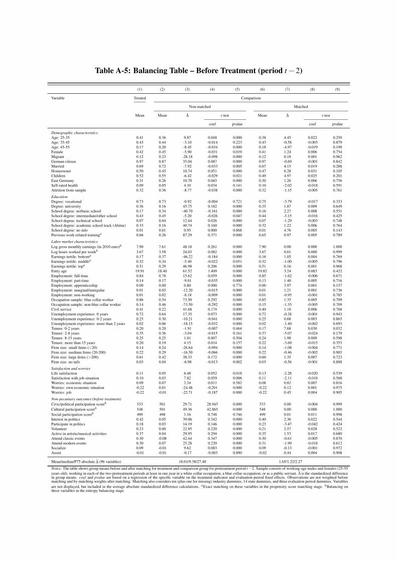
Table A-5: Balancing Table – Before Treatment (period t �2)

(1) (2) (3) (4) (5) (6) (7) (8) (9)


Non-matched Matched



Demographic characteristicsAge: 25-35 0.41 0.36 9.87 0.048 0.000 0.38 4.45 0.022 0.250Age: 35-45 0.43 0.44 -3.10 -0.014 0.223 0.43 -0.58 -0.003 0.879Age: 45-55 0.17 0.20 -8.45 -0.034 0.000 0.18 -4.97 -0.019 0.190Female 0.42 0.45 -5.90 -0.031 0.019 0.41 1.24 0.006 0.754Migrant 0.12 0.23 -28.18 -0.098 0.000 0.12 0.18 0.001 0.962German citizen 0.97 0.87 35.04 0.087 0.000 0.97 -0.69 -0.001 0.842Married 0.69 0.72 -7.92 -0.033 0.005 0.67 4.15 0.019 0.288Homeowner 0.50 0.45 10.74 0.051 0.000 0.47 6.28 0.031 0.105Children 0.52 0.55 -6.42 -0.029 0.021 0.49 4.97 0.025 0.201East Germany 0.31 0.26 10.70 0.045 0.000 0.30 1.26 0.006 0.756Self-rated health 0.09 0.05 4.10 0.034 0.141 0.10 -2.02 -0.018 0.591Attrition from sample 0.32 0.36 -8.77 -0.038 0.000 0.32 -1.15 -0.005 0.761

EducationDegree: vocational 0.73 0.73 -0.92 -0.004 0.721 0.75 -3.79 -0.017 0.333Degree: university 0.36 0.16 45.75 0.182 0.000 0.35 1.87 0.009 0.649School degree: no/basic school 0.17 0.34 -40.70 -0.161 0.000 0.16 2.27 0.008 0.551School degree: intermediate/other school 0.43 0.45 -5.20 -0.026 0.047 0.44 -3.15 -0.016 0.425School degree: technical school 0.07 0.04 12.44 0.026 0.000 0.07 -1.29 -0.003 0.748School degree: academic school track (Abitur) 0.33 0.16 40.74 0.160 0.000 0.32 1.22 0.006 0.764School degree: no info 0.01 0.01 0.95 0.000 0.868 0.01 4.76 0.005 0.143Previous work-related traininga 0.66 0.26 87.29 0.371 0.000 0.65 0.97 0.005 0.789

Labor market characteristicsLog gross monthly earnings (in 2010 euro)b 7.90 7.61 48.18 0.261 0.000 7.90 0.00 0.000 1.000Log hours worked per weekb 3.67 3.58 24.03 0.082 0.000 3.67 0.01 0.000 0.999Earnings tertile: bottoma 0.17 0.37 -46.22 -0.184 0.000 0.16 1.05 0.004 0.769Earnings tertile: middlea 0.32 0.34 -5.40 -0.022 0.051 0.32 -1.00 -0.005 0.796Earnings tertile: topa 0.51 0.29 46.98 0.206 0.000 0.51 0.16 0.001 0.968Entry age 19.91 18.40 61.52 1.409 0.000 19.82 3.24 0.083 0.422Employment: full-time 0.84 0.78 15.62 0.059 0.000 0.85 -1.62 -0.006 0.671Employment: part-time 0.14 0.17 -9.01 -0.035 0.000 0.13 1.40 0.005 0.716Employment: apprenticeship 0.00 0.00 0.80 0.000 0.774 0.00 3.97 0.001 0.157Employment: marginal/unregular 0.01 0.03 -12.20 -0.015 0.000 0.01 1.21 0.001 0.736Employment: non-working 0.01 0.02 -8.18 -0.009 0.000 0.01 -0.95 -0.001 0.785Occupation sample: blue collar worker 0.86 0.54 73.50 0.292 0.000 0.85 1.35 0.005 0.709Occupation sample: non-blue collar worker 0.14 0.46 -73.50 -0.292 0.000 0.15 -1.35 -0.005 0.709Civil service 0.41 0.22 41.68 0.174 0.000 0.40 1.18 0.006 0.768Unemployment experience: 0 years 0.72 0.64 17.35 0.073 0.000 0.72 -0.28 -0.001 0.943Unemployment experience: 0-2 years 0.25 0.30 -10.21 -0.041 0.000 0.25 0.68 0.003 0.865Unemployment experience: more than 2 years 0.02 0.06 -18.15 -0.032 0.000 0.02 -1.40 -0.002 0.693Tenure: 0-2 years 0.20 0.20 -1.91 -0.007 0.464 0.17 7.68 0.030 0.032Tenure: 2-8 years 0.35 0.36 -3.04 -0.015 0.161 0.37 -5.07 -0.024 0.179Tenure: 8-15 years 0.25 0.25 1.01 0.007 0.504 0.24 1.98 0.009 0.598Tenure: more than 15 years 0.20 0.19 4.15 0.014 0.157 0.22 -3.69 -0.015 0.353Firm size: small firms (<20) 0.14 0.24 -26.64 -0.094 0.000 0.14 -1.08 -0.004 0.771Firm size: medium firms (20-200) 0.22 0.29 -16.50 -0.066 0.000 0.22 -0.46 -0.002 0.903Firm size: large firms (>200) 0.61 0.42 38.33 0.172 0.000 0.60 1.35 0.007 0.723Firm size: no info 0.03 0.04 -6.98 -0.013 0.002 0.03 -0.56 -0.001 0.888

Satisfaction and worriesLife satisfaction 0.11 0.05 6.48 0.052 0.018 0.13 -2.28 -0.020 0.539Satisfaction with job situation 0.10 0.03 7.82 0.059 0.006 0.11 -2.11 -0.018 0.568Worries: economic situation 0.09 0.07 2.24 0.011 0.582 0.08 0.82 0.007 0.816Worries: own economic situation -0.22 0.01 -24.48 -0.201 0.000 -0.22 0.12 0.001 0.975Worries: job -0.22 -0.01 -22.71 -0.187 0.000 -0.22 0.45 0.004 0.905

Non-pecuniary outcomes (before treatment)Civic/political participation scoreb 533 501 29.71 28.945 0.000 533 0.00 -0.004 0.999Cultural participation scoreb 548 501 49.36 42.865 0.000 548 0.00 0.000 1.000Social participation scoreb 499 498 1.16 0.748 0.746 499 0.01 0.011 0.998Interest in politics 0.42 0.05 39.06 0.342 0.000 0.40 2.36 0.022 0.544Participate in politics 0.18 0.03 14.19 0.146 0.000 0.23 -3.47 -0.042 0.424Volunteer 0.23 0.00 22.95 0.220 0.000 0.21 2.57 0.028 0.522Active in artistic/musical activities 0.37 0.04 29.95 0.294 0.000 0.35 1.53 0.017 0.680Attend classic events 0.30 -0.08 42.44 0.347 0.000 0.30 -0.61 -0.005 0.870Attend modern events 0.30 0.07 25.28 0.220 0.000 0.31 -1.99 -0.018 0.612Socialize 0.09 -0.01 9.62 0.083 0.000 0.09 -0.13 -0.001 0.972Assist -0.01 -0.01 -0.17 -0.003 0.890 -0.02 0.44 0.004 0.908


Notes: The table shows group means before and after matching for treatment and comparison group for pretreatment period t�2. Sample consists of working-age males and females (25-55years old), working in each of the two pretreatment periods at least in one year in a white collar occupation, a blue collar occupation, or as a public servant. D is the standardized differencein group means. coef and pvalue are based on a regression of the specific variable on the treatment indicator and evaluation-period fixed effects. Observations are not weighted beforematching and by matching weights after matching. Matching also considers ten (plus one for missing) industry dummies, 14 state dummies, and three evaluation period dummies. Variablesare not displayed, but included in the average absolute standardized difference calculations. aExact matching on these variables in the propensity score matching stage. bBalancing onthese variables in the entropy balancing stage.

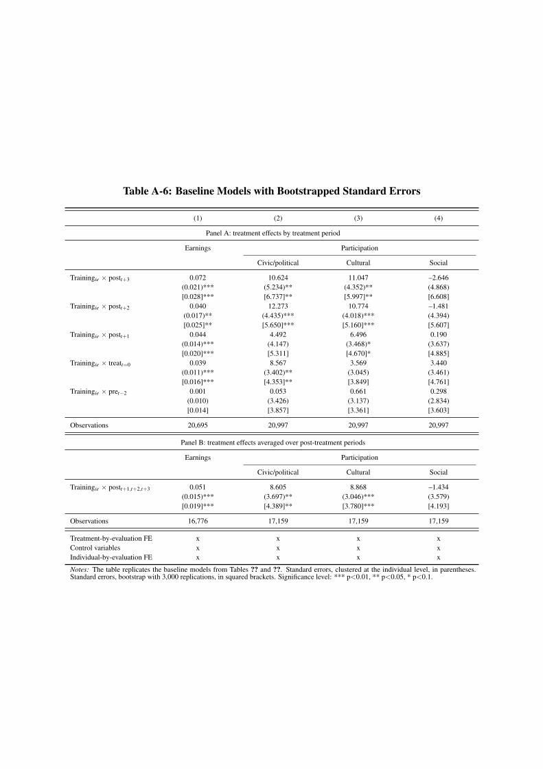
Table A-6: Baseline Models with Bootstrapped Standard Errors

(1) (2) (3) (4)


Earnings Participation


Trainingie ⇥ postt+3 0.072 10.624 11.047 –2.646(0.021)*** (5.234)** (4.352)** (4.868)[0.028]*** [6.737]** [5.997]** [6.608]

Trainingie ⇥ postt+2 0.040 12.273 10.774 –1.481(0.017)** (4.435)*** (4.018)*** (4.394)[0.025]** [5.650]*** [5.160]*** [5.607]

Trainingie ⇥ postt+1 0.044 4.492 6.496 0.190(0.014)*** (4.147) (3.468)* (3.637)[0.020]*** [5.311] [4.670]* [4.885]

Trainingie ⇥ treatt=0 0.039 8.567 3.569 3.440(0.011)*** (3.402)** (3.045) (3.461)[0.016]*** [4.353]** [3.849] [4.761]

Trainingie ⇥ pret�2 0.001 0.053 0.661 0.298(0.010) (3.426) (3.137) (2.834)[0.014] [3.857] [3.361] [3.603]

Observations 20,695 20,997 20,997 20,997


Earnings Participation


Trainingie ⇥ postt+1,t+2,t+3 0.051 8.605 8.868 –1.434(0.015)*** (3.697)** (3.046)*** (3.579)[0.019]*** [4.389]** [3.780]*** [4.193]

Observations 16,776 17,159 17,159 17,159

Treatment-by-evaluation FE x x x xControl variables x x x xIndividual-by-evaluation FE x x x x

Notes: The table replicates the baseline models from Tables ?? and ??. Standard errors, clustered at the individual level, in parentheses.Standard errors, bootstrap with 3,000 replications, in squared brackets. Significance level: *** p<0.01, ** p<0.05, * p<0.1.

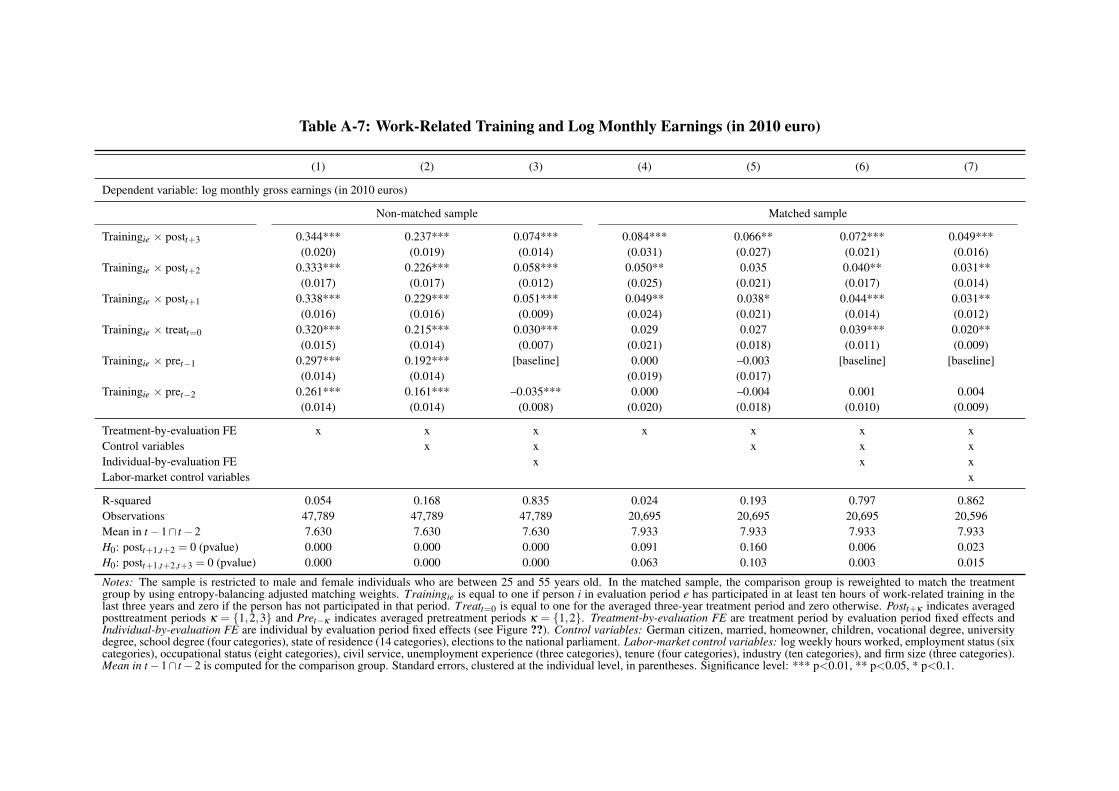
Table A-7: Work-Related Training and Log Monthly Earnings (in 2010 euro)

(1) (2) (3) (4) (5) (6) (7)

Dependent variable: log monthly gross earnings (in 2010 euros)

Non-matched sample Matched sample

Trainingie ⇥ postt+3 0.344*** 0.237*** 0.074*** 0.084*** 0.066** 0.072*** 0.049***(0.020) (0.019) (0.014) (0.031) (0.027) (0.021) (0.016)

Trainingie ⇥ postt+2 0.333*** 0.226*** 0.058*** 0.050** 0.035 0.040** 0.031**(0.017) (0.017) (0.012) (0.025) (0.021) (0.017) (0.014)

Trainingie ⇥ postt+1 0.338*** 0.229*** 0.051*** 0.049** 0.038* 0.044*** 0.031**(0.016) (0.016) (0.009) (0.024) (0.021) (0.014) (0.012)

Trainingie ⇥ treatt=0 0.320*** 0.215*** 0.030*** 0.029 0.027 0.039*** 0.020**(0.015) (0.014) (0.007) (0.021) (0.018) (0.011) (0.009)

Trainingie ⇥ pret�1 0.297*** 0.192*** [baseline] 0.000 –0.003 [baseline] [baseline](0.014) (0.014) (0.019) (0.017)

Trainingie ⇥ pret�2 0.261*** 0.161*** –0.035*** 0.000 –0.004 0.001 0.004(0.014) (0.014) (0.008) (0.020) (0.018) (0.010) (0.009)

Treatment-by-evaluation FE x x x x x x xControl variables x x x x xIndividual-by-evaluation FE x x xLabor-market control variables x

R-squared 0.054 0.168 0.835 0.024 0.193 0.797 0.862Observations 47,789 47,789 47,789 20,695 20,695 20,695 20,596Mean in t �1\ t �2 7.630 7.630 7.630 7.933 7.933 7.933 7.933H0: postt+1,t+2 = 0 (pvalue) 0.000 0.000 0.000 0.091 0.160 0.006 0.023H0: postt+1,t+2,t+3 = 0 (pvalue) 0.000 0.000 0.000 0.063 0.103 0.003 0.015

Notes: The sample is restricted to male and female individuals who are between 25 and 55 years old. In the matched sample, the comparison group is reweighted to match the treatmentgroup by using entropy-balancing adjusted matching weights. Trainingie is equal to one if person i in evaluation period e has participated in at least ten hours of work-related training in thelast three years and zero if the person has not participated in that period. Treatt=0 is equal to one for the averaged three-year treatment period and zero otherwise. Postt+k indicates averagedposttreatment periods k = {1,2,3} and Pret�k indicates averaged pretreatment periods k = {1,2}. Treatment-by-evaluation FE are treatment period by evaluation period fixed effects andIndividual-by-evaluation FE are individual by evaluation period fixed effects (see Figure ??). Control variables: German citizen, married, homeowner, children, vocational degree, universitydegree, school degree (four categories), state of residence (14 categories), elections to the national parliament. Labor-market control variables: log weekly hours worked, employment status (sixcategories), occupational status (eight categories), civil service, unemployment experience (three categories), tenure (four categories), industry (ten categories), and firm size (three categories).Mean in t �1\ t �2 is computed for the comparison group. Standard errors, clustered at the individual level, in parentheses. Significance level: *** p<0.01, ** p<0.05, * p<0.1.

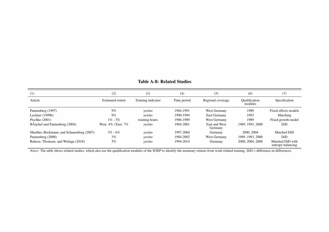
Table A-8: Related Studies

(1) (2) (3) (4) (5) (6) (7)

Article Estimated return Training indicator Time period Regional coverage Qualificationmodules

Specification

Pannenberg (1997) 9% yes/no 1984-1991 West Germany 1989 Fixed effects modelsLechner (1999b) 9% yes/no 1990-1994 East Germany 1993 MatchingPischke (2001) 1% - 3% training hours 1986-1989 West Germany 1989 Fixed growth modelBÃijchel und Pannenberg (2004) West: 4% / East: 7% yes/no 1984-2001 East and West

Germany1989, 1993, 2000 DiD

Muehler, Beckmann, and Schauenberg (2007) 3% - 6% yes/no 1997-2004 Germany 2000, 2004 Matched DiDPannenberg (2008) 3% yes/no 1984-2002 West Germany 1989, 1993, 2000 DiDRuhose, Thomsen, and Weilage (2018) 5% yes/no 1994-2014 Germany 2000, 2004, 2008 Matched DiD with

entropy balancing

Notes: The table shows related studies, which also use the qualification modules of the SOEP to identify the monetary returns from work-related training. DiD = difference-in-differences.

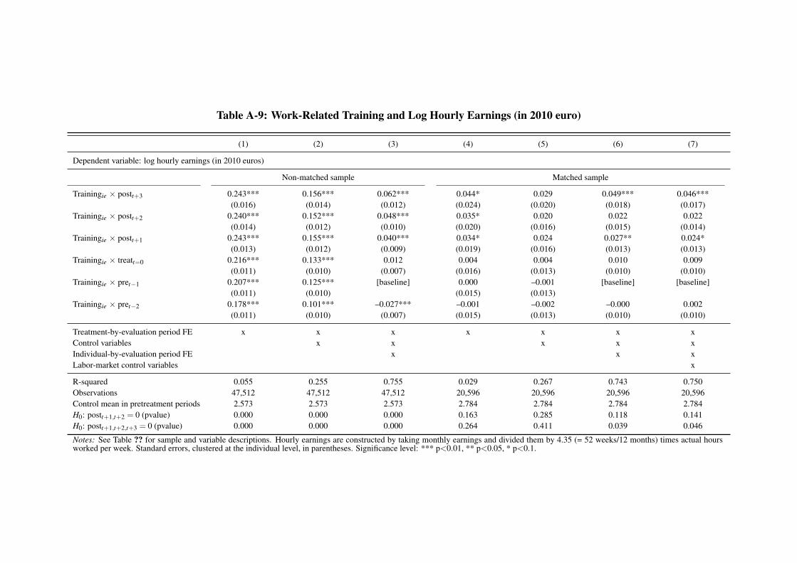
Table A-9: Work-Related Training and Log Hourly Earnings (in 2010 euro)

(1) (2) (3) (4) (5) (6) (7)

Dependent variable: log hourly earnings (in 2010 euros)


Trainingie ⇥ postt+3 0.243*** 0.156*** 0.062*** 0.044* 0.029 0.049*** 0.046***(0.016) (0.014) (0.012) (0.024) (0.020) (0.018) (0.017)

Trainingie ⇥ postt+2 0.240*** 0.152*** 0.048*** 0.035* 0.020 0.022 0.022(0.014) (0.012) (0.010) (0.020) (0.016) (0.015) (0.014)

Trainingie ⇥ postt+1 0.243*** 0.155*** 0.040*** 0.034* 0.024 0.027** 0.024*(0.013) (0.012) (0.009) (0.019) (0.016) (0.013) (0.013)

Trainingie ⇥ treatt=0 0.216*** 0.133*** 0.012 0.004 0.004 0.010 0.009(0.011) (0.010) (0.007) (0.016) (0.013) (0.010) (0.010)


Trainingie ⇥ pret�2 0.178*** 0.101*** –0.027*** –0.001 –0.002 –0.000 0.002(0.011) (0.010) (0.007) (0.015) (0.013) (0.010) (0.010)

Treatment-by-evaluation period FE x x x x x x xControl variables x x x x xIndividual-by-evaluation period FE x x xLabor-market control variables x

R-squared 0.055 0.255 0.755 0.029 0.267 0.743 0.750Observations 47,512 47,512 47,512 20,596 20,596 20,596 20,596Control mean in pretreatment periods 2.573 2.573 2.573 2.784 2.784 2.784 2.784H0: postt+1,t+2 = 0 (pvalue) 0.000 0.000 0.000 0.163 0.285 0.118 0.141H0: postt+1,t+2,t+3 = 0 (pvalue) 0.000 0.000 0.000 0.264 0.411 0.039 0.046

Notes: See Table ?? for sample and variable descriptions. Hourly earnings are constructed by taking monthly earnings and divided them by 4.35 (= 52 weeks/12 months) times actual hoursworked per week. Standard errors, clustered at the individual level, in parentheses. Significance level: *** p<0.01, ** p<0.05, * p<0.1.

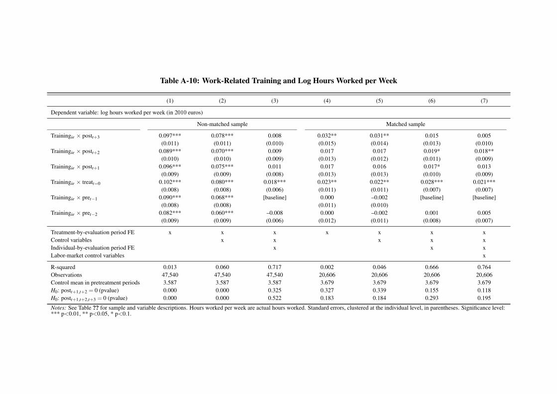
Table A-10: Work-Related Training and Log Hours Worked per Week

(1) (2) (3) (4) (5) (6) (7)

Dependent variable: log hours worked per week (in 2010 euros)


Trainingie ⇥ postt+3 0.097*** 0.078*** 0.008 0.032** 0.031** 0.015 0.005(0.011) (0.011) (0.010) (0.015) (0.014) (0.013) (0.010)

Trainingie ⇥ postt+2 0.089*** 0.070*** 0.009 0.017 0.017 0.019* 0.018**(0.010) (0.010) (0.009) (0.013) (0.012) (0.011) (0.009)

Trainingie ⇥ postt+1 0.096*** 0.075*** 0.011 0.017 0.016 0.017* 0.013(0.009) (0.009) (0.008) (0.013) (0.013) (0.010) (0.009)

Trainingie ⇥ treatt=0 0.102*** 0.080*** 0.018*** 0.023** 0.022** 0.028*** 0.021***(0.008) (0.008) (0.006) (0.011) (0.011) (0.007) (0.007)


Trainingie ⇥ pret�2 0.082*** 0.060*** –0.008 0.000 –0.002 0.001 0.005(0.009) (0.009) (0.006) (0.012) (0.011) (0.008) (0.007)


R-squared 0.013 0.060 0.717 0.002 0.046 0.666 0.764Observations 47,540 47,540 47,540 20,606 20,606 20,606 20,606Control mean in pretreatment periods 3.587 3.587 3.587 3.679 3.679 3.679 3.679H0: postt+1,t+2 = 0 (pvalue) 0.000 0.000 0.325 0.327 0.339 0.155 0.118H0: postt+1,t+2,t+3 = 0 (pvalue) 0.000 0.000 0.522 0.183 0.184 0.293 0.195

Notes: See Table ?? for sample and variable descriptions. Hours worked per week are actual hours worked. Standard errors, clustered at the individual level, in parentheses. Significance level:*** p<0.01, ** p<0.05, * p<0.1.

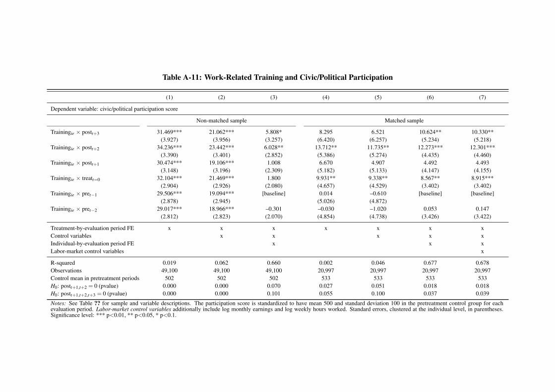
Table A-11: Work-Related Training and Civic/Political Participation

(1) (2) (3) (4) (5) (6) (7)

Dependent variable: civic/political participation score


Trainingie ⇥ postt+3 31.469*** 21.062*** 5.808* 8.295 6.521 10.624** 10.330**(3.927) (3.956) (3.257) (6.420) (6.257) (5.234) (5.218)

Trainingie ⇥ postt+2 34.236*** 23.442*** 6.028** 13.712** 11.735** 12.273*** 12.301***(3.390) (3.401) (2.852) (5.386) (5.274) (4.435) (4.460)

Trainingie ⇥ postt+1 30.474*** 19.106*** 1.008 6.670 4.907 4.492 4.493(3.148) (3.196) (2.309) (5.182) (5.133) (4.147) (4.155)

Trainingie ⇥ treatt=0 32.104*** 21.469*** 1.800 9.931** 9.338** 8.567** 8.915***(2.904) (2.926) (2.080) (4.657) (4.529) (3.402) (3.402)


Trainingie ⇥ pret�2 29.017*** 18.966*** –0.301 –0.030 –1.020 0.053 0.147(2.812) (2.823) (2.070) (4.854) (4.738) (3.426) (3.422)


R-squared 0.019 0.062 0.660 0.002 0.046 0.677 0.678Observations 49,100 49,100 49,100 20,997 20,997 20,997 20,997Control mean in pretreatment periods 502 502 502 533 533 533 533H0: postt+1,t+2 = 0 (pvalue) 0.000 0.000 0.070 0.027 0.051 0.018 0.018H0: postt+1,t+2,t+3 = 0 (pvalue) 0.000 0.000 0.101 0.055 0.100 0.037 0.039

Notes: See Table ?? for sample and variable descriptions. The participation score is standardized to have mean 500 and standard deviation 100 in the pretreatment control group for eachevaluation period. Labor-market control variables additionally include log monthly earnings and log weekly hours worked. Standard errors, clustered at the individual level, in parentheses.Significance level: *** p<0.01, ** p<0.05, * p<0.1.

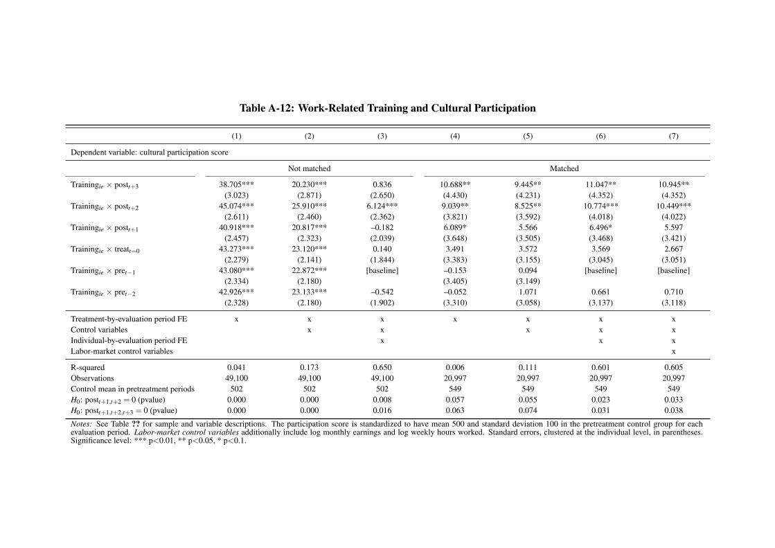
Table A-12: Work-Related Training and Cultural Participation

(1) (2) (3) (4) (5) (6) (7)

Dependent variable: cultural participation score

Not matched Matched

Trainingie ⇥ postt+3 38.705*** 20.230*** 0.836 10.688** 9.445** 11.047** 10.945**(3.023) (2.871) (2.650) (4.430) (4.231) (4.352) (4.352)

Trainingie ⇥ postt+2 45.074*** 25.910*** 6.124*** 9.039** 8.525** 10.774*** 10.449***(2.611) (2.460) (2.362) (3.821) (3.592) (4.018) (4.022)

Trainingie ⇥ postt+1 40.918*** 20.817*** –0.182 6.089* 5.566 6.496* 5.597(2.457) (2.323) (2.039) (3.648) (3.505) (3.468) (3.421)

Trainingie ⇥ treatt=0 43.273*** 23.120*** 0.140 3.491 3.572 3.569 2.667(2.279) (2.141) (1.844) (3.383) (3.155) (3.045) (3.051)

Trainingie ⇥ pret�1 43.080*** 22.872*** [baseline] –0.153 0.094 [baseline] [baseline](2.334) (2.180) (3.405) (3.149)

Trainingie ⇥ pret�2 42.926*** 23.133*** –0.542 –0.052 1.071 0.661 0.710(2.328) (2.180) (1.902) (3.310) (3.058) (3.137) (3.118)




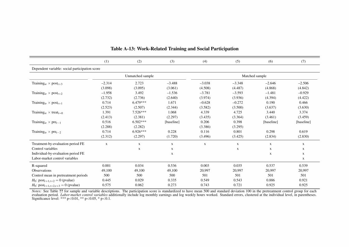
Table A-13: Work-Related Training and Social Participation

(1) (2) (3) (4) (5) (6) (7)

Dependent variable: social participation score

Unmatched sample Matched sample

Trainingie ⇥ postt+3 –2.314 2.723 –3.488 –3.038 –3.348 –2.646 –2.506(3.098) (3.095) (3.061) (4.508) (4.487) (4.868) (4.842)

Trainingie ⇥ postt+2 –1.958 3.492 –1.536 –3.781 –3.593 –1.481 –0.929(2.732) (2.736) (2.640) (3.974) (3.936) (4.394) (4.422)

Trainingie ⇥ postt+1 0.714 6.479*** 1.671 –0.628 –0.272 0.190 0.466(2.523) (2.507) (2.344) (3.582) (3.500) (3.637) (3.630)

Trainingie ⇥ treatt=0 1.391 7.526*** 1.068 4.339 4.725 3.440 3.374(2.413) (2.381) (2.297) (3.435) (3.364) (3.461) (3.459)

Trainingie ⇥ pret�1 0.516 6.502*** [baseline] 0.206 0.398 [baseline] [baseline](2.288) (2.282) (3.386) (3.295)

Trainingie ⇥ pret�2 0.714 6.926*** 0.228 0.116 0.801 0.298 0.619(2.312) (2.297) (1.720) (3.496) (3.425) (2.834) (2.830)




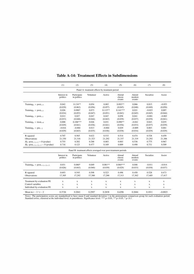
Table A-14: Treatment Effects in Subdimensions

(1) (2) (3) (4) (5) (6) (7) (8)


Interest inpolitics

Participatein politics

Volunteer Active Attendclassicevents

Attendmodernevents

Socialize Assist

Trainingie ⇥ postt+3 0.042 0.134** 0.054 0.083 0.093** 0.066 0.015 –0.053(0.039) (0.062) (0.056) (0.057) (0.045) (0.048) (0.049) (0.050)

Trainingie ⇥ postt+2 0.026 0.090* 0.073 0.115** 0.141*** 0.021 –0.023 0.007(0.034) (0.052) (0.047) (0.051) (0.042) (0.045) (0.045) (0.044)

Trainingie ⇥ postt+1 0.012 0.027 0.047 0.047 0.058 0.041 –0.001 –0.003(0.033) (0.048) (0.044) (0.043) (0.039) (0.037) (0.039) (0.041)

Trainingie ⇥ treatt=0 0.008 0.106*** 0.026 0.031 0.090** –0.041 0.043 0.035(0.029) (0.041) (0.036) (0.041) (0.036) (0.033) (0.037) (0.039)

Trainingie ⇥ pret�2 –0.016 –0.004 0.013 –0.004 0.029 –0.009 0.003 0.001(0.029) (0.043) (0.035) (0.036) (0.038) (0.034) (0.029) (0.029)

R-squared 0.707 0.565 0.622 0.533 0.514 0.474 0.528 0.459Observations 21,330 21,316 21,323 21,292 21,337 21,319 21,292 21,306H0: postt+1,t+2 = 0 (pvalue) 0.755 0.202 0.288 0.083 0.003 0.536 0.775 0.967H0: postt+1,t+2,t+3 = 0 (pvalue) 0.716 0.123 0.477 0.169 0.009 0.490 0.751 0.509


Interest inpolitics

Participatein politics

Volunteer Active Attendclassicevents

Attendmodernevents

Socialize Assist

Trainingie ⇥ postt+1,t+2,t+3 0.031 0.080* 0.049 0.081** 0.084*** 0.046 –0.011 –0.014(0.026) (0.043) (0.040) (0.039) (0.029) (0.033) (0.038) (0.037)


Treatment-by-evaluation FE x x x x x x x xControl variables x x x x x x x xIndividual-by-evaluation FE x x x x x x x x

Mean in t �1\ t �2 0.3726 0.2041 0.2507 0.2838 0.4296 0.2684 0.1011 –0.0023

Notes: The participation scores are standardized to have mean 0 and standard deviation 1 in the pretreatment comparison group for each evaluation period.Standard errors, clustered at the individual level, in parentheses. Significance level: *** p<0.01, ** p<0.05, * p<0.1.

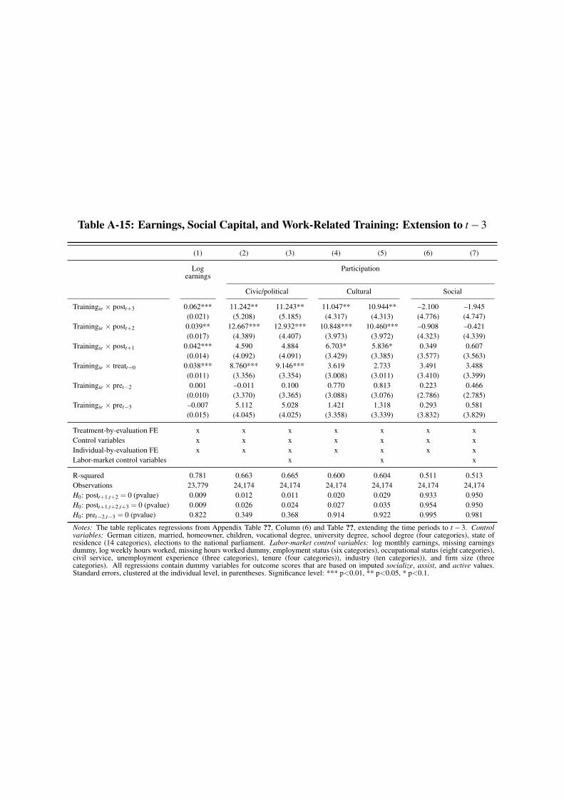
Table A-15: Earnings, Social Capital, and Work-Related Training: Extension to t �3

(1) (2) (3) (4) (5) (6) (7)

Logearnings

Participation


Trainingie ⇥ postt+3 0.062*** 11.242** 11.243** 11.047** 10.944** –2.100 –1.945(0.021) (5.208) (5.185) (4.317) (4.313) (4.776) (4.747)

Trainingie ⇥ postt+2 0.039** 12.667*** 12.932*** 10.848*** 10.460*** –0.908 –0.421(0.017) (4.389) (4.407) (3.973) (3.972) (4.323) (4.339)

Trainingie ⇥ postt+1 0.042*** 4.590 4.884 6.703* 5.836* 0.349 0.607(0.014) (4.092) (4.091) (3.429) (3.385) (3.577) (3.563)

Trainingie ⇥ treatt=0 0.038*** 8.760*** 9.146*** 3.619 2.733 3.491 3.488(0.011) (3.356) (3.354) (3.008) (3.011) (3.410) (3.399)

Trainingie ⇥ pret�2 0.001 –0.011 0.100 0.770 0.813 0.223 0.466(0.010) (3.370) (3.365) (3.088) (3.076) (2.786) (2.785)

Trainingie ⇥ pret�3 –0.007 5.112 5.028 1.421 1.318 0.293 0.581(0.015) (4.045) (4.025) (3.358) (3.339) (3.832) (3.829)

Treatment-by-evaluation FE x x x x x x xControl variables x x x x x x xIndividual-by-evaluation FE x x x x x x xLabor-market control variables x x x

R-squared 0.781 0.663 0.665 0.600 0.604 0.511 0.513Observations 23,779 24,174 24,174 24,174 24,174 24,174 24,174H0: postt+1,t+2 = 0 (pvalue) 0.009 0.012 0.011 0.020 0.029 0.933 0.950H0: postt+1,t+2,t+3 = 0 (pvalue) 0.009 0.026 0.024 0.027 0.035 0.954 0.950H0: pret�2,t�3 = 0 (pvalue) 0.822 0.349 0.368 0.914 0.922 0.995 0.981

Notes: The table replicates regressions from Appendix Table ??, Column (6) and Table ??, extending the time periods to t � 3. Controlvariables: German citizen, married, homeowner, children, vocational degree, university degree, school degree (four categories), state ofresidence (14 categories), elections to the national parliament. Labor-market control variables: log monthly earnings, missing earningsdummy, log weekly hours worked, missing hours worked dummy, employment status (six categories), occupational status (eight categories),civil service, unemployment experience (three categories), tenure (four categories)), industry (ten categories)), and firm size (threecategories). All regressions contain dummy variables for outcome scores that are based on imputed socialize, assist, and active values.Standard errors, clustered at the individual level, in parentheses. Significance level: *** p<0.01, ** p<0.05, * p<0.1.

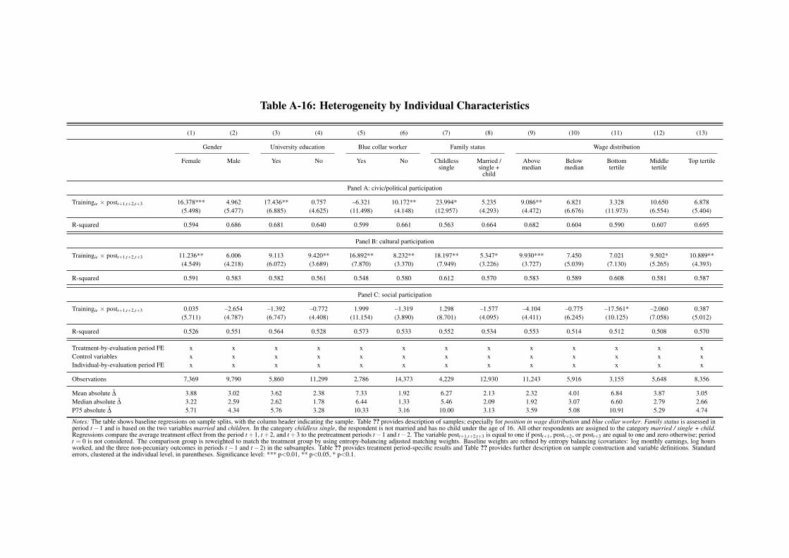
Table A-16: Heterogeneity by Individual Characteristics

(1) (2) (3) (4) (5) (6) (7) (8) (9) (10) (11) (12) (13)

Gender University education Blue collar worker Family status Wage distribution

Female Male Yes No Yes No Childlesssingle

Married /single +

child

Abovemedian

Belowmedian

Bottomtertile

Middletertile

Top tertile

Panel A: civic/political participation

Trainingie ⇥ postt+1,t+2,t+3 16.378*** 4.962 17.436** 0.757 –6.321 10.172** 23.994* 5.235 9.086** 6.821 3.328 10.650 6.878(5.498) (5.477) (6.885) (4.625) (11.498) (4.148) (12.957) (4.293) (4.472) (6.676) (11.973) (6.554) (5.404)

R-squared 0.594 0.686 0.681 0.640 0.599 0.661 0.563 0.664 0.682 0.604 0.590 0.607 0.695

Panel B: cultural participation

Trainingie ⇥ postt+1,t+2,t+3 11.236** 6.006 9.113 9.420** 16.892** 8.232** 18.197** 5.347* 9.930*** 7.450 7.021 9.502* 10.889**(4.549) (4.218) (6.072) (3.689) (7.870) (3.370) (7.949) (3.226) (3.727) (5.039) (7.130) (5.265) (4.393)

R-squared 0.591 0.583 0.582 0.561 0.548 0.580 0.612 0.570 0.583 0.589 0.608 0.581 0.587

Panel C: social participation

Trainingie ⇥ postt+1,t+2,t+3 0.035 –2.654 –1.392 –0.772 1.999 –1.319 1.298 –1.577 –4.104 –0.775 –17.561* –2.060 0.387(5.711) (4.787) (6.747) (4.408) (11.154) (3.890) (8.701) (4.095) (4.411) (6.245) (10.125) (7.058) (5.012)

R-squared 0.526 0.551 0.564 0.528 0.573 0.533 0.552 0.534 0.553 0.514 0.512 0.508 0.570

Treatment-by-evaluation period FE x x x x x x x x x x x x xControl variables x x x x x x x x x x x x xIndividual-by-evaluation period FE x x x x x x x x x x x x x

Observations 7,369 9,790 5,860 11,299 2,786 14,373 4,229 12,930 11,243 5,916 3,155 5,648 8,356

Mean absolute D 3.88 3.02 3.62 2.38 7.33 1.92 6.27 2.13 2.32 4.01 6.84 3.87 3.05Median absolute D 3.22 2.59 2.62 1.78 6.44 1.33 5.46 2.09 1.92 3.07 6.60 2.79 2.66P75 absolute D 5.71 4.34 5.76 3.28 10.33 3.16 10.00 3.13 3.59 5.08 10.91 5.29 4.74

Notes: The table shows baseline regressions on sample splits, with the column header indicating the sample. Table ?? provides description of samples; especially for position in wage distribution and blue collar worker. Family status is assessed inperiod t �1 and is based on the two variables married and children. In the category childless single, the respondent is not married and has no child under the age of 16. All other respondents are assigned to the category married / single + child.Regressions compare the average treatment effect from the period t +1, t +2, and t +3 to the pretreatment periods t �1 and t �2. The variable postt+1,t+2,t+3 is equal to one if postt+1, postt+2, or postt+3 are equal to one and zero otherwise; periodt = 0 is not considered. The comparison group is reweighted to match the treatment group by using entropy-balancing adjusted matching weights. Baseline weights are refined by entropy balancing (covariates: log monthly earnings, log hoursworked, and the three non-pecuniary outcomes in periods t �1 and t �2) in the subsamples. Table ?? provides treatment period-specific results and Table ?? provides further description on sample construction and variable definitions. Standarderrors, clustered at the individual level, in parentheses. Significance level: *** p<0.01, ** p<0.05, * p<0.1.

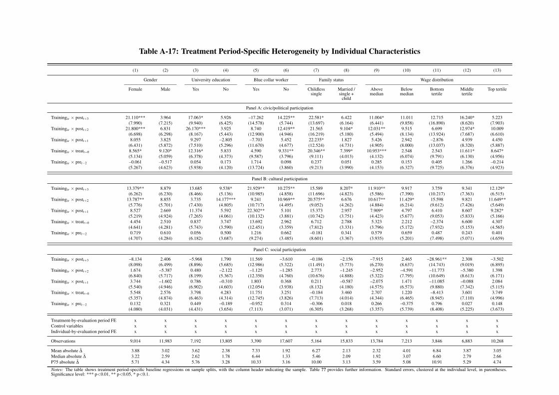
Table A-17: Treatment Period-Specific Heterogeneity by Individual Characteristics

(1) (2) (3) (4) (5) (6) (7) (8) (9) (10) (11) (12) (13)

Gender University education Blue collar worker Family status Wage distribution

Female Male Yes No Yes No Childlesssingle

Married /single +

child

Abovemedian

Belowmedian

Bottomtertile

Middletertile

Top tertile


Trainingie ⇥ postt+3 21.110*** 3.964 17.063* 5.926 –17.262 14.225** 22.581* 6.422 11.004* 11.011 12.715 16.240* 5.223(7.990) (7.215) (9.940) (6.425) (14.578) (5.744) (13.697) (6.164) (6.441) (9.858) (16.890) (8.620) (7.903)

Trainingie ⇥ postt+2 21.800*** 6.831 26.170*** 3.925 8.740 12.419** 21.565 9.104* 12.031** 9.515 6.699 12.974* 10.009(6.698) (6.298) (8.167) (5.443) (12.900) (4.946) (16.219) (5.180) (5.494) (8.134) (13.924) (7.687) (6.610)

Trainingie ⇥ postt+1 8.055 3.825 9.297 –2.805 –7.703 5.452 22.235* 1.827 5.426 2.942 –2.876 4.939 4.450(6.431) (5.872) (7.510) (5.296) (11.670) (4.677) (12.524) (4.731) (4.905) (8.000) (13.037) (8.320) (5.887)

Trainingie ⇥ treatt=0 8.565* 9.120* 12.316* 5.833 4.590 9.331** 20.346** 7.399* 10.953*** 2.548 2.543 11.611* 8.647*(5.134) (5.059) (6.378) (4.373) (9.587) (3.796) (9.111) (4.013) (4.132) (6.074) (9.791) (6.130) (4.956)

Trainingie ⇥ pret�2 –0.061 –0.517 0.054 0.173 1.714 0.098 0.237 0.051 0.285 0.153 0.405 1.266 –0.214(5.267) (4.623) (5.938) (4.120) (13.724) (3.860) (9.213) (3.990) (4.153) (6.327) (9.725) (6.376) (4.923)


Trainingie ⇥ postt+3 13.379** 8.879 13.685 9.538* 21.929** 10.275** 15.589 8.207* 11.910** 9.917 3.759 9.341 12.129*(6.262) (6.230) (8.466) (5.136) (10.985) (4.858) (11.696) (4.823) (5.586) (7.390) (10.217) (7.363) (6.515)

Trainingie ⇥ postt+2 13.787** 8.855 3.735 14.177*** 9.241 10.969** 20.575** 6.676 10.617** 11.429* 15.598 9.821 11.649**(5.776) (5.701) (7.430) (4.805) (10.717) (4.495) (9.052) (4.262) (4.884) (6.214) (9.612) (7.426) (5.649)

Trainingie ⇥ postt+1 8.527 2.669 11.374 5.592 22.302** 5.101 15.373 2.957 7.909* 4.797 6.410 8.607 9.282*(5.219) (4.924) (7.265) (4.061) (10.132) (3.881) (10.742) (3.751) (4.423) (5.677) (9.053) (5.833) (5.166)

Trainingie ⇥ treatt=0 4.454 2.510 0.837 3.747 13.692 2.962 6.712 2.788 5.323 2.212 –2.374 6.600 4.307(4.641) (4.281) (5.743) (3.590) (12.451) (3.359) (7.812) (3.331) (3.796) (5.172) (7.932) (5.153) (4.565)

Trainingie ⇥ pret�2 0.719 0.610 0.056 0.500 1.216 0.662 –0.181 0.341 0.579 0.659 0.487 0.243 0.401(4.707) (4.284) (6.182) (3.687) (9.274) (3.485) (8.601) (3.367) (3.935) (5.201) (7.498) (5.071) (4.659)


Trainingie ⇥ postt+3 –8.134 2.406 –5.968 1.790 11.569 –3.610 –0.186 –2.156 –7.915 2.465 –28.961** 2.308 –3.502(8.098) (6.499) (8.896) (5.685) (12.986) (5.322) (11.491) (5.773) (6.270) (8.637) (14.743) (9.019) (6.895)

Trainingie ⇥ postt+2 1.674 –5.387 0.480 –2.122 –1.125 –1.285 2.773 –1.245 –2.952 –4.591 –11.773 –5.380 1.398(6.840) (5.717) (8.199) (5.367) (12.350) (4.760) (10.676) (4.888) (5.322) (7.795) (10.649) (8.613) (6.171)

Trainingie ⇥ postt+1 3.744 –1.602 0.786 –0.310 1.803 0.368 0.211 –0.587 –2.075 1.471 –11.085 –0.088 2.084(5.540) (4.946) (6.902) (4.603) (12.054) (3.938) (8.132) (4.180) (4.575) (6.573) (9.880) (7.342) (5.115)

Trainingie ⇥ treatt=0 5.548 2.576 3.798 4.283 11.751 3.251 –0.184 3.460 2.707 1.220 –8.413 3.601 3.749(5.357) (4.874) (6.463) (4.314) (12.745) (3.826) (7.713) (4.014) (4.344) (6.465) (8.945) (7.110) (4.996)

Trainingie ⇥ pret�2 0.132 0.321 0.449 –0.189 –0.952 0.314 –0.306 0.018 0.266 –0.375 0.796 0.027 0.148(4.080) (4.031) (4.431) (3.654) (7.113) (3.071) (6.305) (3.268) (3.357) (5.739) (8.408) (5.225) (3.673)

Treatment-by-evaluation period FE x x x x x x x x x x x x xControl variables x x x x x x x x x x x x xIndividual-by-evaluation period FE x x x x x x x x x x x x x

Observations 9,014 11,983 7,192 13,805 3,390 17,607 5,164 15,833 13,784 7,213 3,846 6,883 10,268

Mean absolute D 3.88 3.02 3.62 2.38 7.33 1.92 6.27 2.13 2.32 4.01 6.84 3.87 3.05Median absolute D 3.22 2.59 2.62 1.78 6.44 1.33 5.46 2.09 1.92 3.07 6.60 2.79 2.66P75 absolute D 5.71 4.34 5.76 3.28 10.33 3.16 10.00 3.13 3.59 5.08 10.91 5.29 4.74

Notes: The table shows treatment period-specific baseline regressions on sample splits, with the column header indicating the sample. Table ?? provides further information. Standard errors, clustered at the individual level, in parentheses.Significance level: *** p<0.01, ** p<0.05, * p<0.1.

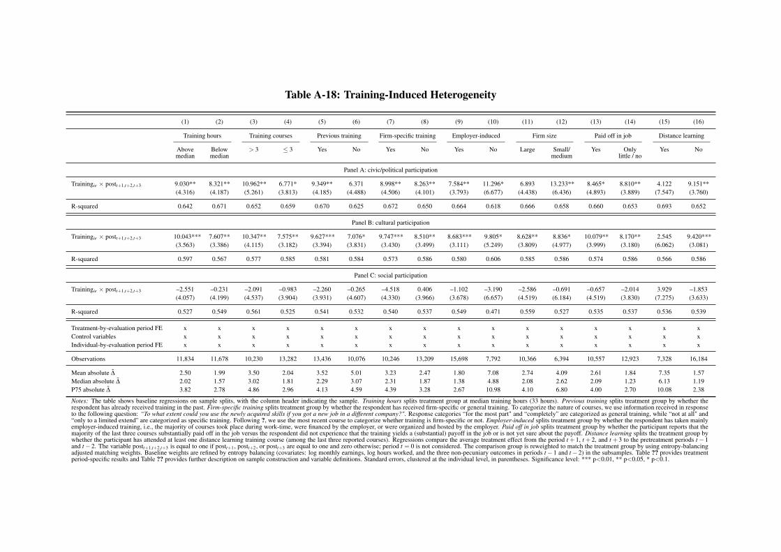
Table A-18: Training-Induced Heterogeneity

(1) (2) (3) (4) (5) (6) (7) (8) (9) (10) (11) (12) (13) (14) (15) (16)

Training hours Training courses Previous training Firm-specific training Employer-induced Firm size Paid off in job Distance learning

Abovemedian

Belowmedian

> 3 3 Yes No Yes No Yes No Large Small/medium

Yes Onlylittle / no

Yes No


Trainingie ⇥ postt+1,t+2,t+3 9.030** 8.321** 10.962** 6.771* 9.349** 6.371 8.998** 8.263** 7.584** 11.296* 6.893 13.233** 8.465* 8.810** 4.122 9.151**(4.316) (4.187) (5.261) (3.813) (4.185) (4.488) (4.506) (4.101) (3.793) (6.677) (4.438) (6.436) (4.893) (3.889) (7.547) (3.760)

R-squared 0.642 0.671 0.652 0.659 0.670 0.625 0.672 0.650 0.664 0.618 0.666 0.658 0.660 0.653 0.693 0.652


Trainingie ⇥ postt+1,t+2,t+3 10.043*** 7.607** 10.347** 7.575** 9.627*** 7.076* 9.747*** 8.510** 8.683*** 9.805* 8.628** 8.836* 10.079** 8.170** 2.545 9.420***(3.563) (3.386) (4.115) (3.182) (3.394) (3.831) (3.430) (3.499) (3.111) (5.249) (3.809) (4.977) (3.999) (3.180) (6.062) (3.081)

R-squared 0.597 0.567 0.577 0.585 0.581 0.584 0.573 0.586 0.580 0.606 0.585 0.586 0.574 0.586 0.566 0.586


Trainingie ⇥ postt+1,t+2,t+3 –2.551 –0.231 –2.091 –0.983 –2.260 –0.265 –4.518 0.406 –1.102 –3.190 –2.586 –0.691 –0.657 –2.014 3.929 –1.853(4.057) (4.199) (4.537) (3.904) (3.931) (4.607) (4.330) (3.966) (3.678) (6.657) (4.519) (6.184) (4.519) (3.830) (7.275) (3.633)

R-squared 0.527 0.549 0.561 0.525 0.541 0.532 0.540 0.537 0.549 0.471 0.559 0.527 0.535 0.537 0.536 0.539

Treatment-by-evaluation period FE x x x x x x x x x x x x x x x xControl variables x x x x x x x x x x x x x x x xIndividual-by-evaluation period FE x x x x x x x x x x x x x x x x

Observations 11,834 11,678 10,230 13,282 13,436 10,076 10,246 13,209 15,698 7,792 10,366 6,394 10,557 12,923 7,328 16,184

Mean absolute D 2.50 1.99 3.50 2.04 3.52 5.01 3.23 2.47 1.80 7.08 2.74 4.09 2.61 1.84 7.35 1.57Median absolute D 2.02 1.57 3.02 1.81 2.29 3.07 2.31 1.87 1.38 4.88 2.08 2.62 2.09 1.23 6.13 1.19P75 absolute D 3.82 2.78 4.86 2.96 4.13 4.59 4.39 3.28 2.67 10.98 4.10 6.80 4.00 2.70 10.08 2.38

Notes: The table shows baseline regressions on sample splits, with the column header indicating the sample. Training hours splits treatment group at median training hours (33 hours). Previous training splits treatment group by whether therespondent has already received training in the past. Firm-specific training splits treatment group by whether the respondent has received firm-specific or general training. To categorize the nature of courses, we use information received in responseto the following question: “To what extent could you use the newly acquired skills if you got a new job in a different company?". Response categories “for the most part" and “completely" are categorized as general training, while “not at all" and“only to a limited extend" are categorized as specific training. Following ?, we use the most recent course to categorize whether training is firm-specific or not. Employer-induced splits treatment group by whether the respondent has taken mainlyemployer-induced training, i.e., the majority of courses took place during work-time, were financed by the employer, or were organized and hosted by the employer. Paid off in job splits treatment group by whether the participant reports that themajority of the last three courses substantially paid off in the job versus the respondent did not experience that the training yields a (substantial) payoff in the job or is not yet sure about the payoff. Distance learning splits the treatment group bywhether the participant has attended at least one distance learning training course (among the last three reported courses). Regressions compare the average treatment effect from the period t + 1, t + 2, and t + 3 to the pretreatment periods t � 1and t �2. The variable postt+1,t+2,t+3 is equal to one if postt+1, postt+2, or postt+3 are equal to one and zero otherwise; period t = 0 is not considered. The comparison group is reweighted to match the treatment group by using entropy-balancingadjusted matching weights. Baseline weights are refined by entropy balancing (covariates: log monthly earnings, log hours worked, and the three non-pecuniary outcomes in periods t �1 and t �2) in the subsamples. Table ?? provides treatmentperiod-specific results and Table ?? provides further description on sample construction and variable definitions. Standard errors, clustered at the individual level, in parentheses. Significance level: *** p<0.01, ** p<0.05, * p<0.1.

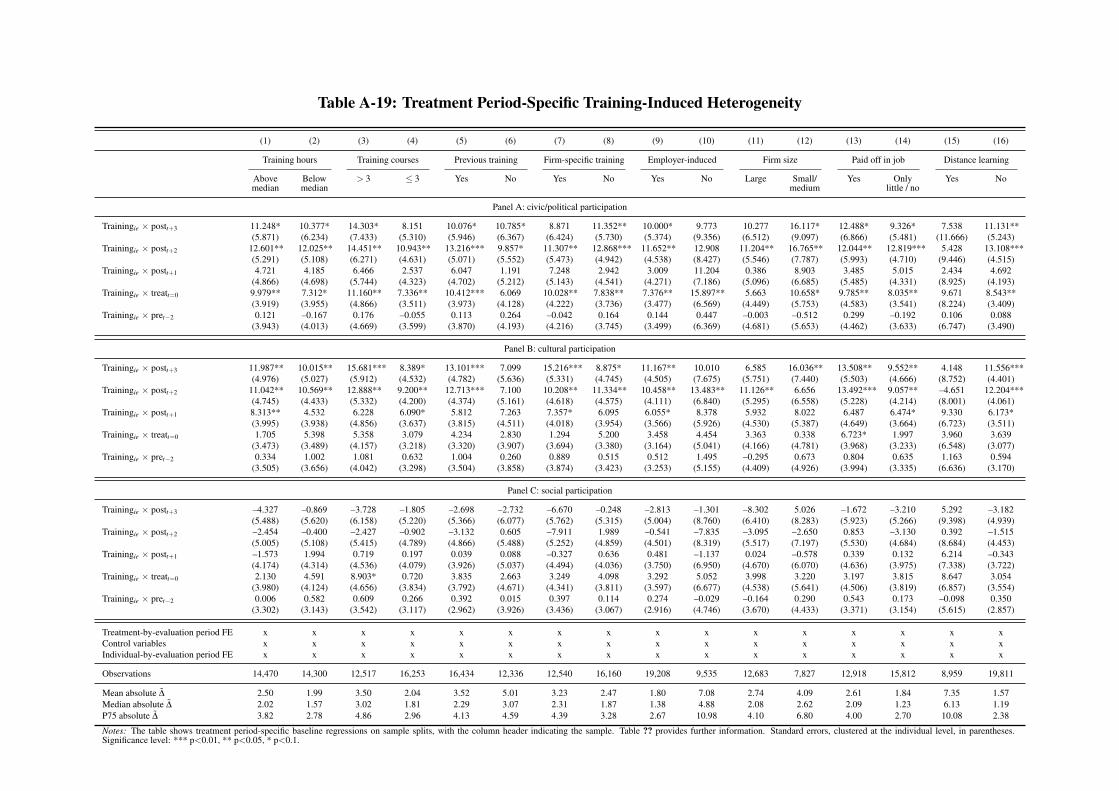
Table A-19: Treatment Period-Specific Training-Induced Heterogeneity

(1) (2) (3) (4) (5) (6) (7) (8) (9) (10) (11) (12) (13) (14) (15) (16)

Training hours Training courses Previous training Firm-specific training Employer-induced Firm size Paid off in job Distance learning

Abovemedian

Belowmedian

> 3 3 Yes No Yes No Yes No Large Small/medium

Yes Onlylittle / no

Yes No


Trainingie ⇥ postt+3 11.248* 10.377* 14.303* 8.151 10.076* 10.785* 8.871 11.352** 10.000* 9.773 10.277 16.117* 12.488* 9.326* 7.538 11.131**(5.871) (6.234) (7.433) (5.310) (5.946) (6.367) (6.424) (5.730) (5.374) (9.356) (6.512) (9.097) (6.866) (5.481) (11.666) (5.243)

Trainingie ⇥ postt+2 12.601** 12.025** 14.451** 10.943** 13.216*** 9.857* 11.307** 12.868*** 11.652** 12.908 11.204** 16.765** 12.044** 12.819*** 5.428 13.108***(5.291) (5.108) (6.271) (4.631) (5.071) (5.552) (5.473) (4.942) (4.538) (8.427) (5.546) (7.787) (5.993) (4.710) (9.446) (4.515)

Trainingie ⇥ postt+1 4.721 4.185 6.466 2.537 6.047 1.191 7.248 2.942 3.009 11.204 0.386 8.903 3.485 5.015 2.434 4.692(4.866) (4.698) (5.744) (4.323) (4.702) (5.212) (5.143) (4.541) (4.271) (7.186) (5.096) (6.685) (5.485) (4.331) (8.925) (4.193)

Trainingie ⇥ treatt=0 9.979** 7.312* 11.160** 7.336** 10.412*** 6.069 10.028** 7.838** 7.376** 15.897** 5.663 10.658* 9.785** 8.035** 9.671 8.543**(3.919) (3.955) (4.866) (3.511) (3.973) (4.128) (4.222) (3.736) (3.477) (6.569) (4.449) (5.753) (4.583) (3.541) (8.224) (3.409)

Trainingie ⇥ pret�2 0.121 –0.167 0.176 –0.055 0.113 0.264 –0.042 0.164 0.144 0.447 –0.003 –0.512 0.299 –0.192 0.106 0.088(3.943) (4.013) (4.669) (3.599) (3.870) (4.193) (4.216) (3.745) (3.499) (6.369) (4.681) (5.653) (4.462) (3.633) (6.747) (3.490)


Trainingie ⇥ postt+3 11.987** 10.015** 15.681*** 8.389* 13.101*** 7.099 15.216*** 8.875* 11.167** 10.010 6.585 16.036** 13.508** 9.552** 4.148 11.556***(4.976) (5.027) (5.912) (4.532) (4.782) (5.636) (5.331) (4.745) (4.505) (7.675) (5.751) (7.440) (5.503) (4.666) (8.752) (4.401)

Trainingie ⇥ postt+2 11.042** 10.569** 12.888** 9.200** 12.713*** 7.100 10.208** 11.334** 10.458** 13.483** 11.126** 6.656 13.492*** 9.057** –4.651 12.204***(4.745) (4.433) (5.332) (4.200) (4.374) (5.161) (4.618) (4.575) (4.111) (6.840) (5.295) (6.558) (5.228) (4.214) (8.001) (4.061)

Trainingie ⇥ postt+1 8.313** 4.532 6.228 6.090* 5.812 7.263 7.357* 6.095 6.055* 8.378 5.932 8.022 6.487 6.474* 9.330 6.173*(3.995) (3.938) (4.856) (3.637) (3.815) (4.511) (4.018) (3.954) (3.566) (5.926) (4.530) (5.387) (4.649) (3.664) (6.723) (3.511)

Trainingie ⇥ treatt=0 1.705 5.398 5.358 3.079 4.234 2.830 1.294 5.200 3.458 4.454 3.363 0.338 6.723* 1.997 3.960 3.639(3.473) (3.489) (4.157) (3.218) (3.320) (3.907) (3.694) (3.380) (3.164) (5.041) (4.166) (4.781) (3.968) (3.233) (6.548) (3.077)

Trainingie ⇥ pret�2 0.334 1.002 1.081 0.632 1.004 0.260 0.889 0.515 0.512 1.495 –0.295 0.673 0.804 0.635 1.163 0.594(3.505) (3.656) (4.042) (3.298) (3.504) (3.858) (3.874) (3.423) (3.253) (5.155) (4.409) (4.926) (3.994) (3.335) (6.636) (3.170)


Trainingie ⇥ postt+3 –4.327 –0.869 –3.728 –1.805 –2.698 –2.732 –6.670 –0.248 –2.813 –1.301 –8.302 5.026 –1.672 –3.210 5.292 –3.182(5.488) (5.620) (6.158) (5.220) (5.366) (6.077) (5.762) (5.315) (5.004) (8.760) (6.410) (8.283) (5.923) (5.266) (9.398) (4.939)

Trainingie ⇥ postt+2 –2.454 –0.400 –2.427 –0.902 –3.132 0.605 –7.911 1.989 –0.541 –7.835 –3.095 –2.650 0.853 –3.130 0.392 –1.515(5.005) (5.108) (5.415) (4.789) (4.866) (5.488) (5.252) (4.859) (4.501) (8.319) (5.517) (7.197) (5.530) (4.684) (8.684) (4.453)

Trainingie ⇥ postt+1 –1.573 1.994 0.719 0.197 0.039 0.088 –0.327 0.636 0.481 –1.137 0.024 –0.578 0.339 0.132 6.214 –0.343(4.174) (4.314) (4.536) (4.079) (3.926) (5.037) (4.494) (4.036) (3.750) (6.950) (4.670) (6.070) (4.636) (3.975) (7.338) (3.722)

Trainingie ⇥ treatt=0 2.130 4.591 8.903* 0.720 3.835 2.663 3.249 4.098 3.292 5.052 3.998 3.220 3.197 3.815 8.647 3.054(3.980) (4.124) (4.656) (3.834) (3.792) (4.671) (4.341) (3.811) (3.597) (6.677) (4.538) (5.641) (4.506) (3.819) (6.857) (3.554)

Trainingie ⇥ pret�2 0.006 0.582 0.609 0.266 0.392 0.015 0.397 0.114 0.274 –0.029 –0.164 0.290 0.543 0.173 –0.098 0.350(3.302) (3.143) (3.542) (3.117) (2.962) (3.926) (3.436) (3.067) (2.916) (4.746) (3.670) (4.433) (3.371) (3.154) (5.615) (2.857)

Treatment-by-evaluation period FE x x x x x x x x x x x x x x x xControl variables x x x x x x x x x x x x x x x xIndividual-by-evaluation period FE x x x x x x x x x x x x x x x x

Observations 14,470 14,300 12,517 16,253 16,434 12,336 12,540 16,160 19,208 9,535 12,683 7,827 12,918 15,812 8,959 19,811

Mean absolute D 2.50 1.99 3.50 2.04 3.52 5.01 3.23 2.47 1.80 7.08 2.74 4.09 2.61 1.84 7.35 1.57Median absolute D 2.02 1.57 3.02 1.81 2.29 3.07 2.31 1.87 1.38 4.88 2.08 2.62 2.09 1.23 6.13 1.19P75 absolute D 3.82 2.78 4.86 2.96 4.13 4.59 4.39 3.28 2.67 10.98 4.10 6.80 4.00 2.70 10.08 2.38

Notes: The table shows treatment period-specific baseline regressions on sample splits, with the column header indicating the sample. Table ?? provides further information. Standard errors, clustered at the individual level, in parentheses.Significance level: *** p<0.01, ** p<0.05, * p<0.1.

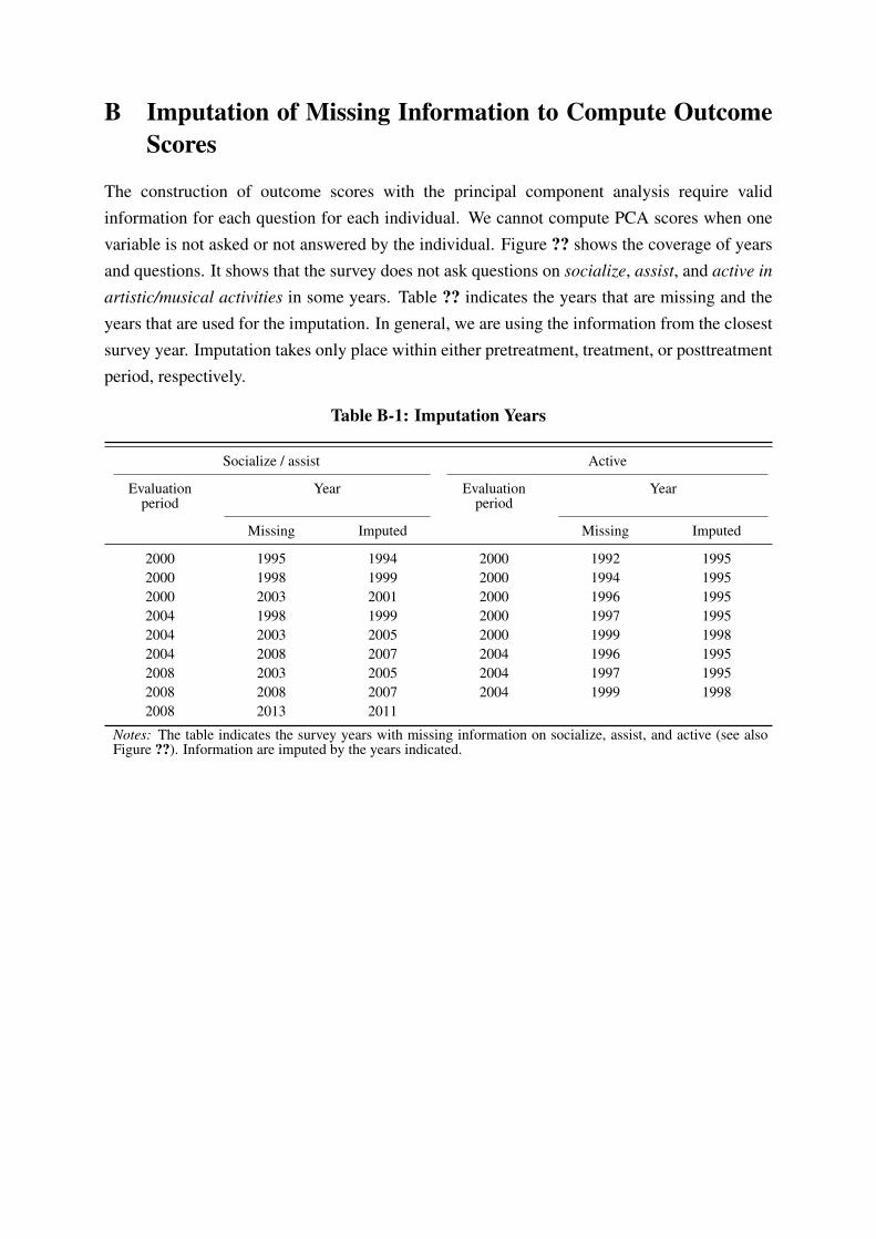
B Imputation of Missing Information to Compute OutcomeScores

The construction of outcome scores with the principal component analysis require validinformation for each question for each individual. We cannot compute PCA scores when onevariable is not asked or not answered by the individual. Figure ?? shows the coverage of yearsand questions. It shows that the survey does not ask questions on socialize, assist, and active inartistic/musical activities in some years. Table ?? indicates the years that are missing and theyears that are used for the imputation. In general, we are using the information from the closestsurvey year. Imputation takes only place within either pretreatment, treatment, or posttreatmentperiod, respectively.

Table B-1: Imputation Years

Socialize / assist Active

Evaluationperiod

Year Evaluationperiod

Year

Missing Imputed Missing Imputed

2000 1995 1994 2000 1992 19952000 1998 1999 2000 1994 19952000 2003 2001 2000 1996 19952004 1998 1999 2000 1997 19952004 2003 2005 2000 1999 19982004 2008 2007 2004 1996 19952008 2003 2005 2004 1997 19952008 2008 2007 2004 1999 19982008 2013 2011

Notes: The table indicates the survey years with missing information on socialize, assist, and active (see alsoFigure ??). Information are imputed by the years indicated.

C Entropy Balancing

In this section, we describe briefly the main points of the entropy balancing method formulatedby ?. Please note that this exposition is only to inform the interested reader about the mostimportant features. The overview is likely to be incomplete and captures only the very basicidea. We refer the reader to ? for a much better and more extensive treatment of the matter.

Entropy balancing can be considered a generalization of the conventional propensity scorematching. The conventional matching approach is to estimate a logit or probit regressionto predict the treatment assignment and then use the propensity scores from that regressionto compute unit weights such that the estimated weights equalizes the covariate distributionsbetween treatment and comparison group. Balancing checks are required to check whether theweights successfully achieve this goal. By contrast, entropy balancing tackles this equalizationproblem from the reverse and estimates the weights directly from the imposed balancingconstraints. The method also allows us to impose restrictions on higher moments of thecovariate distribution and not only on the mean as it is usually the case with conventionalmatching. With entropy balancing, there is no further need for balancing checks because theweights equalize the differences in the prespecified covariate distributions by construction.

In most applications, we are interested in estimating the average treatment effect on thetreated (ATT), which can be expressed as t = E[Y (1)|D = 1]�E[Y (0)|D = 1]. In the simplestpossible case, the counterfactual mean for a population may be estimated by

E \[Y (0)|D = 1] =Â{i|D=0}Yi wi

Â{i|D=0}wi, (7)

where wi is an individual-specific weight chosen by the following reweighting scheme:

minwi

H(w) = Â{i|D=0}

h(wi) (8)

subject to balance and normalizing constraints

Â{i|D=0}

wi cri(Xi) = mr with r 2 1, ...,R and (9)

Â{i|D=0}

wi = 1 and (10)

wi � 0 for all i such that D = 0, (11)

where h(·) is a distance metric (discussed in detail in ?, p. 31) and cri(Xi) = mr describes a setof R balance constraints imposed by the researcher on the covariate moments of the reweightedcomparison group. We further impose that all weights add up to one (Eq. (??)) and that allweights are nonnegative (Eq. (??)).

To fit the entropy balancing weights in practice, we need to minimize the loss function H(w)

subject to the balance and normalization constraints given in equations (??) to (??). Using theLagrange multiplier, we obtain the primal optimization problem:

minW,l0,Z

Lp = Â{i|D=0}

wi log✓

wi

qi

◆+

R

Âr=1

lr

Â{i|D=0}

wicri(Xi)�mr

!

+(l0 �1)

Â{i|D=0}

wi �1

!,

(12)

where Z = {l1, . . . ,lR}0 is a vector of Lagrange multipliers for the balance constraints andl0 �1 is the Lagrange multiplier for the normalization constraints. Given that the loss functionis (strictly) convex and duality holds (see ?, p. 32 for details), the first order condition for eachweight is attained by

w⇤i =

qi exp��ÂR

r=1 lrcri(Xi)�

Â{i|D=0} qi exp��ÂR

r=1 lrcri(Xi)� . (13)

The expression makes clear that the weights can be estimated as a log-linear function ofthe covariates specified in the moment conditions.39 Plugging this expression back into Lp

eliminates the constraints and leads to an unrestricted dual problem given by

minZ

Ld = log

Â{i|D=0}

qi exp⇣�

R

Âr=1

lrcri(Xi)⌘!

+R

Âr=1

lrmr. (14)

The solution to the dual problem Z⇤ solves the primal problem and the weights W ⇤ canbe recovered via equation (??). This dual problem is much more tractable because it isunconstrained and the dimensionality is reduced to a system of nonlinear equations in the RLagrange multipliers. Moreover, if a solution exists, it will be unique since Ld is strictly convex.? applies a Levenberg-Marquardt scheme to find a solution to this optimization problem. Theresulting iterative algorithm is globally convergent if the problem is feasible and the solution isusually obtained within seconds even in moderately large data sets.

39Evidently, the inequality bounds wi � 0 are inactive and can be safely ignored.

D Attrition and Robustness

D.1 Attrition

Because non-pecuniary returns increase over time, one may worry that selective sample attritionis responsible for this finding. For example, assuming that the treatment had no effect, wewould observe the same pattern of results if either the worse-performing individuals in thetreatment group or the better-performing individuals in the comparison group were to drop outover time. In general, attrition in period t +1 is only approximately 4% on average (Table ??).However, attrition increases up to 40% in the non-matched comparison group in period t + 3.Attrition in the treatment group is 5.4 percentage-points lower (significant difference at the onepercent level). However, attrition in the matched comparison group (32% in t + 3) was notsignificantly different from attrition in the treatment group. We also measure to what extentindividuals who drop out of the sample are different compared to individuals who remain inthe sample measured in pretreatment (periods t � 1 and t � 2) outcomes. The results from aregression of the outcome variable on the training indicator interacted with an indicator that isone if the individual drops out from the sample in later periods and zero otherwise indicates thattreated individuals who drop out are relatively more positively selected compared to drop-outsin the comparison group (see Table ??). However, after weighting with matching weights, theinteraction is small and statistically not significant. Finally, estimating the baseline model ona balanced sample (balanced for non-pecuniary outcomes) does not imply that compositionalchanges in either group affect the results (Table ??).

D.2 Robustness Checks

Table ?? shows that the results are qualitatively and quantitatively robust to a variety of changesin the empirical model specification. To keep the results tractable, we concentrate on changesin averaged treatment effects when we change model assumptions (Table ?? shows treatmentperiod-specific robustness results). In Columns (2) to (4), we vary different steps of thebaseline matching approach. Column (2) reports regression results when we further refine thebaseline matching weights by adjusting them for differential trends in the outcome variables(log monthly earnings, log hours worked per week, three non-pecuniary outcomes) by previouswork-related training, university degree, vocational degree, gender, and occupation sample.We again use entropy balancing to overhaul the baseline matching weights. This specificationchange addresses differential pretreatment trends in those groups. As expected, the change hasno effect on the estimates because we have already seen that individuals are not self-selected onthe average pretreatment trend. Trimming the propensity scores may lead to an overestimationof the training effects because we mainly drop individuals in the comparison group with lowpropensity scores. Thus, in Column (3), we report results from specification without trimmingthe sample in the data processing stage. The estimates indicate that trimming does not strongly

affect the results. The choice of the matching procedure may also affect the construction ofthe comparison group. While ? and ? argue for the use of kernel matching, we also apply5-to-1 nearest-neighbor matching and report results in Column (4).40 While coefficients areslightly smaller, we still find statistically and economically significant effects from participationin work-related training.

In the remaining columns of Table ??, we evaluate the performance of using the differentmatching procedures separately. In Column (5), we use conventional kernel matching weightswithout refinement by entropy balancing. Using these weights to construct the comparisongroup also performs well in eliminating pretreatment normalized differences between thetreatment and comparison groups (see last three rows in Column (5)). In Columns (6)and (7), we use entropy balancing without previous adjustment through the propensity scorematching stage. We use all conditioning variables from Table ?? for the construction of thebalancing weights (Column (6)) and with additional refinement of these weights by takingdifferential trends in the outcome variables (log monthly earnings, log hours worked per week,three non-pecuniary outcomes) by previous work-related training, university degree, vocationaldegree, gender, and occupation sample into account (Column (7)). This procedure has theadvantage of allowing us to retain all individuals for the analysis, which increases statisticalprecision. The results show significant positive non-pecuniary returns to work-related trainingwith effect sizes closer to the non-trimmed sample in Column (3). However, this specificationalso means that we keep individuals with very low participation probabilities for identification(even though they enter with low weights). Specifically, in the evaluation of work-relatedtraining, this is a questionable specification choice because individuals with low participationprobabilities are not very likely to ever participate in work-related training.

40Using 1-to-1 nearest-neighbor matching yields very similar results (not shown).

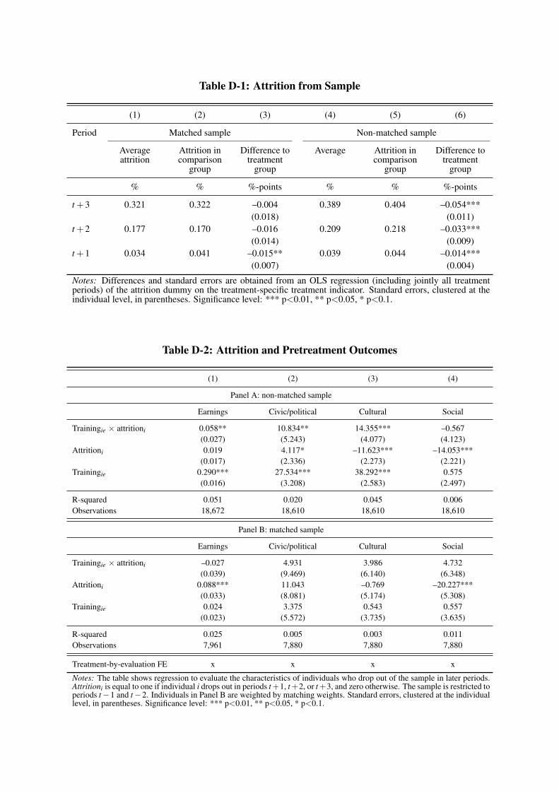
Table D-1: Attrition from Sample

(1) (2) (3) (4) (5) (6)

Period Matched sample Non-matched sample

Averageattrition

Attrition incomparison

group

Difference totreatment

group

Average Attrition incomparison

group

Difference totreatment

group

% % %-points % % %-points

t +3 0.321 0.322 –0.004 0.389 0.404 –0.054***(0.018) (0.011)

t +2 0.177 0.170 –0.016 0.209 0.218 –0.033***(0.014) (0.009)

t +1 0.034 0.041 –0.015** 0.039 0.044 –0.014***(0.007) (0.004)

Notes: Differences and standard errors are obtained from an OLS regression (including jointly all treatmentperiods) of the attrition dummy on the treatment-specific treatment indicator. Standard errors, clustered at theindividual level, in parentheses. Significance level: *** p<0.01, ** p<0.05, * p<0.1.

Table D-2: Attrition and Pretreatment Outcomes

(1) (2) (3) (4)

Panel A: non-matched sample

Earnings Civic/political Cultural Social

Trainingie ⇥ attritioni 0.058** 10.834** 14.355*** –0.567(0.027) (5.243) (4.077) (4.123)

Attritioni 0.019 4.117* –11.623*** –14.053***(0.017) (2.336) (2.273) (2.221)

Trainingie 0.290*** 27.534*** 38.292*** 0.575(0.016) (3.208) (2.583) (2.497)

R-squared 0.051 0.020 0.045 0.006Observations 18,672 18,610 18,610 18,610

Panel B: matched sample


Trainingie ⇥ attritioni –0.027 4.931 3.986 4.732(0.039) (9.469) (6.140) (6.348)

Attritioni 0.088*** 11.043 –0.769 –20.227***(0.033) (8.081) (5.174) (5.308)

Trainingie 0.024 3.375 0.543 0.557(0.023) (5.572) (3.735) (3.635)


Treatment-by-evaluation FE x x x x

Notes: The table shows regression to evaluate the characteristics of individuals who drop out of the sample in later periods.Attritioni is equal to one if individual i drops out in periods t+1, t+2, or t+3, and zero otherwise. The sample is restricted toperiods t �1 and t �2. Individuals in Panel B are weighted by matching weights. Standard errors, clustered at the individuallevel, in parentheses. Significance level: *** p<0.01, ** p<0.05, * p<0.1.

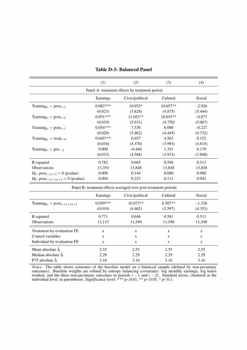
Table D-3: Balanced Panel

(1) (2) (3) (4)



Trainingie ⇥ postt+3 0.082*** 10.952* 10.657** –2.926(0.023) (5.828) (4.875) (5.444)

Trainingie ⇥ postt+2 0.051*** 11.052** 10.653** –0.877(0.019) (5.631) (4.750) (5.067)

Trainingie ⇥ postt+1 0.054*** 7.530 6.088 –0.227(0.020) (5.462) (4.445) (4.732)

Trainingie ⇥ treatt=0 0.045*** 6.657 4.563 0.152(0.016) (4.370) (3.993) (4.615)

Trainingie ⇥ pret�2 0.000 –0.440 1.351 0.179(0.015) (4.588) (3.933) (3.840)

R-squared 0.782 0.665 0.596 0.513Observations 13,354 13,848 13,848 13,848H0: postt+1,t+2 = 0 (pvalue) 0.009 0.144 0.080 0.980H0: postt+1,t+2,t+3 = 0 (pvalue) 0.004 0.223 0.111 0.942



Trainingie ⇥ postt+1,t+2,t+3 0.059*** 10.073** 8.507** –1.328(0.019) (4.462) (3.597) (4.353)


Treatment-by-evaluation FE x x x xControl variables x x x xIndividual-by-evaluation FE x x x x

Mean absolute D 2.55 2.55 2.55 2.55Median absolute D 2.29 2.29 2.29 2.29P75 absolute D 3.16 3.16 3.16 3.16

Notes: The table shows estimates of the baseline model on a balanced sample (defined by non-pecuniaryoutcomes). Baseline weights are refined by entropy balancing (covariates: log monthly earnings, log hoursworked, and the three non-pecuniary outcomes in periods t � 1 and t � 2). Standard errors, clustered at theindividual level, in parentheses. Significance level: *** p<0.01, ** p<0.05, * p<0.1.

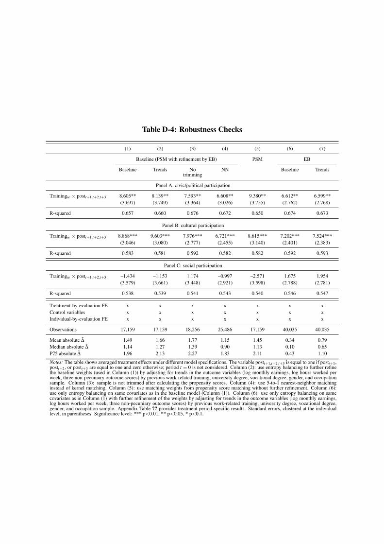
Table D-4: Robustness Checks

(1) (2) (3) (4) (5) (6) (7)

Baseline (PSM with refinement by EB) PSM EB

Baseline Trends Notrimming

NN Baseline Trends


Trainingie ⇥ postt+1,t+2,t+3 8.605** 8.139** 7.593** 6.608** 9.380** 6.612** 6.599**(3.697) (3.749) (3.364) (3.026) (3.755) (2.762) (2.768)

R-squared 0.657 0.660 0.676 0.672 0.650 0.674 0.673


Trainingie ⇥ postt+1,t+2,t+3 8.868*** 9.603*** 7.976*** 6.721*** 8.615*** 7.202*** 7.524***(3.046) (3.080) (2.777) (2.455) (3.140) (2.401) (2.383)

R-squared 0.583 0.581 0.592 0.582 0.582 0.592 0.593


Trainingie ⇥ postt+1,t+2,t+3 –1.434 –1.153 1.174 –0.997 –2.571 1.675 1.954(3.579) (3.661) (3.448) (2.921) (3.598) (2.788) (2.781)

R-squared 0.538 0.539 0.541 0.543 0.540 0.546 0.547

Treatment-by-evaluation FE x x x x x x xControl variables x x x x x x xIndividual-by-evaluation FE x x x x x x x

Observations 17,159 17,159 18,256 25,486 17,159 40,035 40,035

Mean absolute D 1.49 1.66 1.77 1.15 1.45 0.34 0.79Median absolute D 1.14 1.27 1.39 0.90 1.13 0.10 0.65P75 absolute D 1.96 2.13 2.27 1.83 2.11 0.43 1.10

Notes: The table shows averaged treatment effects under different model specifications. The variable postt+1,t+2,t+3 is equal to one if postt+1,postt+2, or postt+3 are equal to one and zero otherwise; period t = 0 is not considered. Column (2): use entropy balancing to further refinethe baseline weights (used in Column (1)) by adjusting for trends in the outcome variables (log monthly earnings, log hours worked perweek, three non-pecuniary outcome scores) by previous work-related training, university degree, vocational degree, gender, and occupationsample. Column (3): sample is not trimmed after calculating the propensity scores. Column (4): use 5-to-1 nearest-neighbor matchinginstead of kernel matching. Column (5): use matching weights from propensity score matching without further refinement. Column (6):use only entropy balancing on same covariates as in the baseline model (Column (1)). Column (6): use only entropy balancing on samecovariates as in Column (1) with further refinement of the weights by adjusting for trends in the outcome variables (log monthly earnings,log hours worked per week, three non-pecuniary outcome scores) by previous work-related training, university degree, vocational degree,gender, and occupation sample. Appendix Table ?? provides treatment period-specific results. Standard errors, clustered at the individuallevel, in parentheses. Significance level: *** p<0.01, ** p<0.05, * p<0.1.

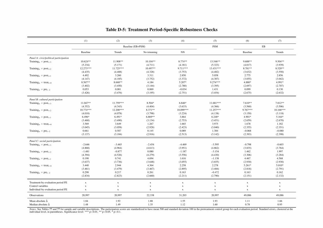
Table D-5: Treatment Period-Specific Robustness Checks

(1) (2) (3) (4) (5) (6) (7)

Baseline (EB+PSM) PSM EB

Baseline Trends No trimming NN Baseline Trends

Panel A: civic/political participationTrainingie ⇥ postt+3 10.624** 11.908** 10.104** 8.774** 13.546** 9.688** 9.504**

(5.234) (5.171) (4.711) (4.181) (5.323) (4.017) (3.939)Trainingie ⇥ postt+2 12.273*** 11.725*** 10.497** 9.711*** 13.431*** 8.781** 8.520**

(4.435) (4.488) (4.328) (3.753) (4.482) (3.632) (3.550)Trainingie ⇥ postt+1 4.492 3.260 3.311 2.850 5.058 2.775 2.856

(4.147) (4.185) (3.752) (3.372) (4.307) (3.055) (3.042)Trainingie ⇥ treatt=0 8.567** 8.668** 4.184 5.207* 9.274*** 4.880* 4.991*

(3.402) (3.450) (3.144) (2.780) (3.395) (2.697) (2.707)Trainingie ⇥ pret�2 0.053 0.081 0.069 –0.034 1.431 0.099 0.130

(3.426) (3.476) (3.195) (2.751) (3.454) (2.675) (2.632)

Panel B: cultural participationTrainingie ⇥ postt+3 11.047** 11.759*** 8.504* 6.846* 11.681*** 7.610** 7.812**

(4.352) (4.343) (4.404) (3.633) (4.366) (3.560) (3.506)Trainingie ⇥ postt+2 10.774*** 12.200*** 8.371** 10.099*** 11.257*** 9.767*** 10.168***

(4.018) (4.078) (3.798) (3.224) (4.138) (3.150) (3.118)Trainingie ⇥ postt+1 6.496* 6.491* 6.869** 3.864 6.248* 4.901* 5.164*

(3.468) (3.490) (3.134) (2.753) (3.451) (2.659) (2.670)Trainingie ⇥ treatt=0 3.569 3.649 1.267 1.665 3.975 1.678 1.182

(3.045) (3.058) (2.928) (2.423) (3.040) (2.355) (2.351)Trainingie ⇥ pret�2 0.661 0.587 0.145 0.089 1.384 –0.068 –0.080

(3.137) (3.184) (2.916) (2.513) (3.142) (2.393) (2.398)

Panel C: social participationTrainingie ⇥ postt+3 –2.646 –3.465 –2.454 –4.469 –3.595 –0.798 –0.603

(4.868) (4.964) (4.613) (3.951) (4.862) (3.835) (3.764)Trainingie ⇥ postt+2 –1.481 –0.877 0.080 –1.187 –3.154 1.462 1.997

(4.394) (4.526) (4.279) (3.556) (4.430) (3.306) (3.284)Trainingie ⇥ postt+1 0.190 0.741 4.694 1.616 –1.138 4.467 4.568

(3.637) (3.736) (3.648) (3.055) (3.655) (2.930) (2.930)Trainingie ⇥ treatt=0 3.440 2.944 4.364 2.258 2.278 5.261* 5.010*

(3.461) (3.479) (3.467) (2.895) (3.484) (2.818) (2.791)Trainingie ⇥ pret�2 0.298 0.217 0.261 0.163 –0.472 0.163 0.162

(2.834) (2.823) (2.660) (2.211) (2.790) (2.151) (2.132)

Treatment-by-evaluation period FE x x x x x x xControl variables x x x x x x xIndividual-by-evaluation period FE x x x x x x x

Observations 20,997 20,997 22,338 31,203 20,997 49,086 49,086

Mean absolute D 1.84 1.92 1.88 1.55 1.93 1.11 1.66Median absolute D 1.48 1.49 1.35 1.12 1.60 0.78 0.95

Notes: See Tables ?? and ?? for sample and variable descriptions. The participation scores are standardized to have mean 500 and standard deviation 100 in the pretreatment control group for each evaluation period. Standard errors, clustered at theindividual level, in parentheses. Significance level: *** p<0.01, ** p<0.05, * p<0.1.

E Trust and Non-Pecuniary Outcomes

In many applications, trust is an important dimension of social capital. The SOEP providesinformation on trust in the years 2003, 2008, and 2013. The question asks to what extent peoplecan agree or disagree with the statement that people can be trusted. The variable is measuredon a 4-point scale from 1 [disagree completely], 2 [disagree], 3 [agree slightly], to 4 [agreecompletely].

Figure ?? shows average participation scores by level of trust. The measures are averagedover all available years (2003, 2008, and 2013). In Figure ??(a), the plot shows the rawcorrelation in the data. Correlation coefficients are equal to r = 0.13 between trust andcivic/political participation, r = 0.18 between trust and cultural participation, and r = 0.05between trust and social participation. In Figure ??(b), the plot shows the same correlation afteradjusting participation scores for gender, age, migrant status, log monthly earnings, universitydegree, vocational degree, and evaluation period-by-survey year fixed effects. Correlationcoefficients are equal to r = 0.11 between trust and conditional civic/political participation,r = 0.14 between trust and conditional cultural participation, and r = 0.07 between trust andconditional social participation. All correlation coefficients are significantly different from zeroat the one percent level.

Table ?? shows linear probability regressions of trust on non-pecuniary outcomes. Thedependent variable is a dummy that is one if the individual agrees or strongly agrees that generalpeople can be trusted and zero if the individual disagrees or strongly disagrees. The dummy isused because the majority of individuals choose either agree and disagree (92%) instead ofstrongly agree and strongly disagree. The results show that there is a strong positive correlationbetween all participation domains and trust. This relationship holds after controlling for a setof covariates.

Finally, Table ?? shows the effect of participating in work-related training on trust. Whilewe do find positive coefficients in the cross-sectional regression on the non-matched sample(Column (1)), this effect disappears completely in either the individual fixed effects regressionsor on the matched sample.

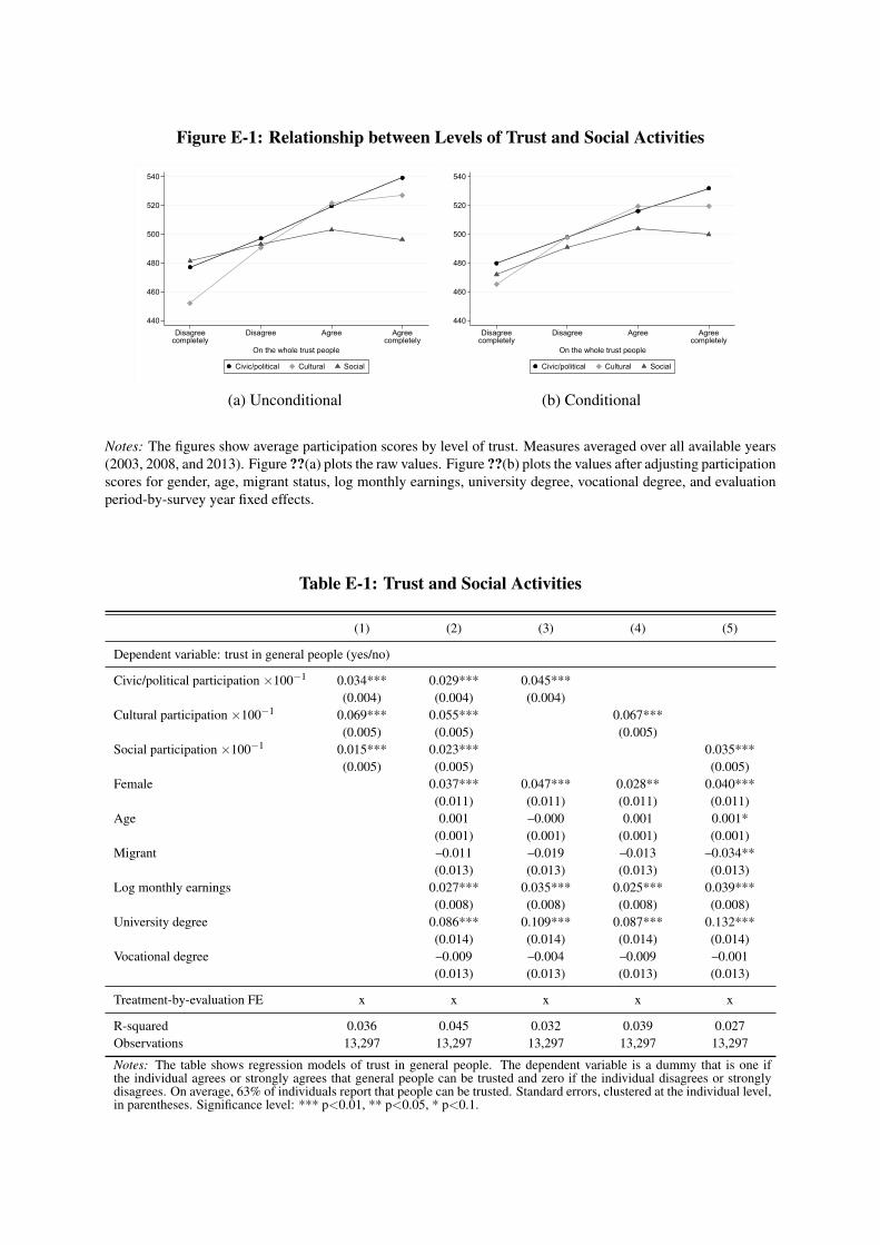
Figure E-1: Relationship between Levels of Trust and Social Activities

��

��

��

��

��

��

'LVDJUHH

FRPSOHWHO\

'LVDJUHH $JUHH $JUHH

FRPSOHWHO\

2Q�WKH�ZKROH�WUXVW�SHRSOH


(a) Unconditional

��

��

��

��

��

��

'LVDJUHH

FRPSOHWHO\

'LVDJUHH $JUHH $JUHH

FRPSOHWHO\

2Q�WKH�ZKROH�WUXVW�SHRSOH


(b) Conditional

Notes: The figures show average participation scores by level of trust. Measures averaged over all available years(2003, 2008, and 2013). Figure ??(a) plots the raw values. Figure ??(b) plots the values after adjusting participationscores for gender, age, migrant status, log monthly earnings, university degree, vocational degree, and evaluationperiod-by-survey year fixed effects.

Table E-1: Trust and Social Activities

(1) (2) (3) (4) (5)

Dependent variable: trust in general people (yes/no)

Civic/political participation ⇥100�1 0.034*** 0.029*** 0.045***(0.004) (0.004) (0.004)

Cultural participation ⇥100�1 0.069*** 0.055*** 0.067***(0.005) (0.005) (0.005)

Social participation ⇥100�1 0.015*** 0.023*** 0.035***(0.005) (0.005) (0.005)

Female 0.037*** 0.047*** 0.028** 0.040***(0.011) (0.011) (0.011) (0.011)

Age 0.001 –0.000 0.001 0.001*(0.001) (0.001) (0.001) (0.001)

Migrant –0.011 –0.019 –0.013 –0.034**(0.013) (0.013) (0.013) (0.013)

Log monthly earnings 0.027*** 0.035*** 0.025*** 0.039***(0.008) (0.008) (0.008) (0.008)

University degree 0.086*** 0.109*** 0.087*** 0.132***(0.014) (0.014) (0.014) (0.014)

Vocational degree –0.009 –0.004 –0.009 –0.001(0.013) (0.013) (0.013) (0.013)

Treatment-by-evaluation FE x x x x x

R-squared 0.036 0.045 0.032 0.039 0.027Observations 13,297 13,297 13,297 13,297 13,297

Notes: The table shows regression models of trust in general people. The dependent variable is a dummy that is one ifthe individual agrees or strongly agrees that general people can be trusted and zero if the individual disagrees or stronglydisagrees. On average, 63% of individuals report that people can be trusted. Standard errors, clustered at the individual level,in parentheses. Significance level: *** p<0.01, ** p<0.05, * p<0.1.

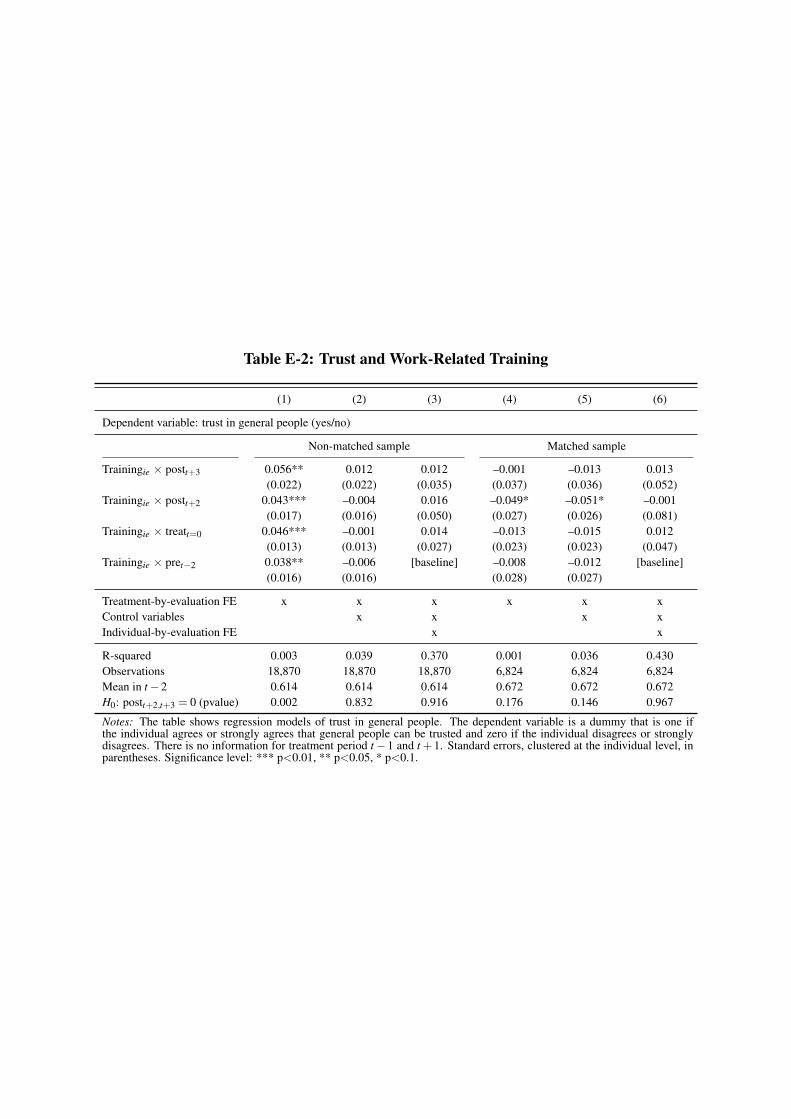
Table E-2: Trust and Work-Related Training

(1) (2) (3) (4) (5) (6)

Dependent variable: trust in general people (yes/no)


Trainingie ⇥ postt+3 0.056** 0.012 0.012 –0.001 –0.013 0.013(0.022) (0.022) (0.035) (0.037) (0.036) (0.052)

Trainingie ⇥ postt+2 0.043*** –0.004 0.016 –0.049* –0.051* –0.001(0.017) (0.016) (0.050) (0.027) (0.026) (0.081)

Trainingie ⇥ treatt=0 0.046*** –0.001 0.014 –0.013 –0.015 0.012(0.013) (0.013) (0.027) (0.023) (0.023) (0.047)

Trainingie ⇥ pret�2 0.038** –0.006 [baseline] –0.008 –0.012 [baseline](0.016) (0.016) (0.028) (0.027)

Treatment-by-evaluation FE x x x x x xControl variables x x x xIndividual-by-evaluation FE x x

R-squared 0.003 0.039 0.370 0.001 0.036 0.430Observations 18,870 18,870 18,870 6,824 6,824 6,824Mean in t �2 0.614 0.614 0.614 0.672 0.672 0.672H0: postt+2,t+3 = 0 (pvalue) 0.002 0.832 0.916 0.176 0.146 0.967

Notes: The table shows regression models of trust in general people. The dependent variable is a dummy that is one ifthe individual agrees or strongly agrees that general people can be trusted and zero if the individual disagrees or stronglydisagrees. There is no information for treatment period t �1 and t +1. Standard errors, clustered at the individual level, inparentheses. Significance level: *** p<0.01, ** p<0.05, * p<0.1.

F Number of Close Friends and Non-Pecuniary Outcomes

In this section, we study the number of close friends as a proxy for the quality indicator of socialties. The SOEP provides information on the number of close friends in the years 2003, 2008,2011, and 2013. The question asks the respondent to report the number of close friends. Theaverage (median) number of friends in our sample is equal to 4.4 (4), which indicates that thequestion is not about the size of the network, but more about a specific aspect of the quality ofthe network.

Figure ?? shows average participation scores by the number of friends. The measures areaveraged over all available years (2003, 2008, 2011, and 2013). In Figure ??(a), the plotshows the raw correlation in the data. Correlation coefficients are equal to r = 0.07 betweennumber of friends and civic/political participation, r = 0.12 between number of friends andcultural participation, and r = 0.17 between number of friends and social participation. InFigure ??(b), the plot shows the same correlation after adjusting participation scores for gender,age, migrant status, log monthly earnings, university degree, vocational degree, and evaluationperiod-by-survey year fixed effects. Correlation coefficients are equal to r = 0.07 betweennumber of friends and conditional civic/political participation, r = 0.11 between number offriends and conditional cultural participation, and r = 0.17 between number of friends andconditional social participation. All correlation coefficients are significantly different from zeroat the one percent level.

Table ?? shows the results of linear probability models of the log number of close friends onnon-pecuniary outcomes. The results show that there is a strong positive correlation between allparticipation domains and the number of close friends. This relationship holds after controllingfor a set of covariates.

Finally, Table ?? shows the effect of participating in work-related training on the log numberof close friends. While we do find positive coefficients in the cross-sectional regression on thenon-matched sample (Column (1)), this effect disappears completely in either the individualfixed effects regressions or on the matched sample.

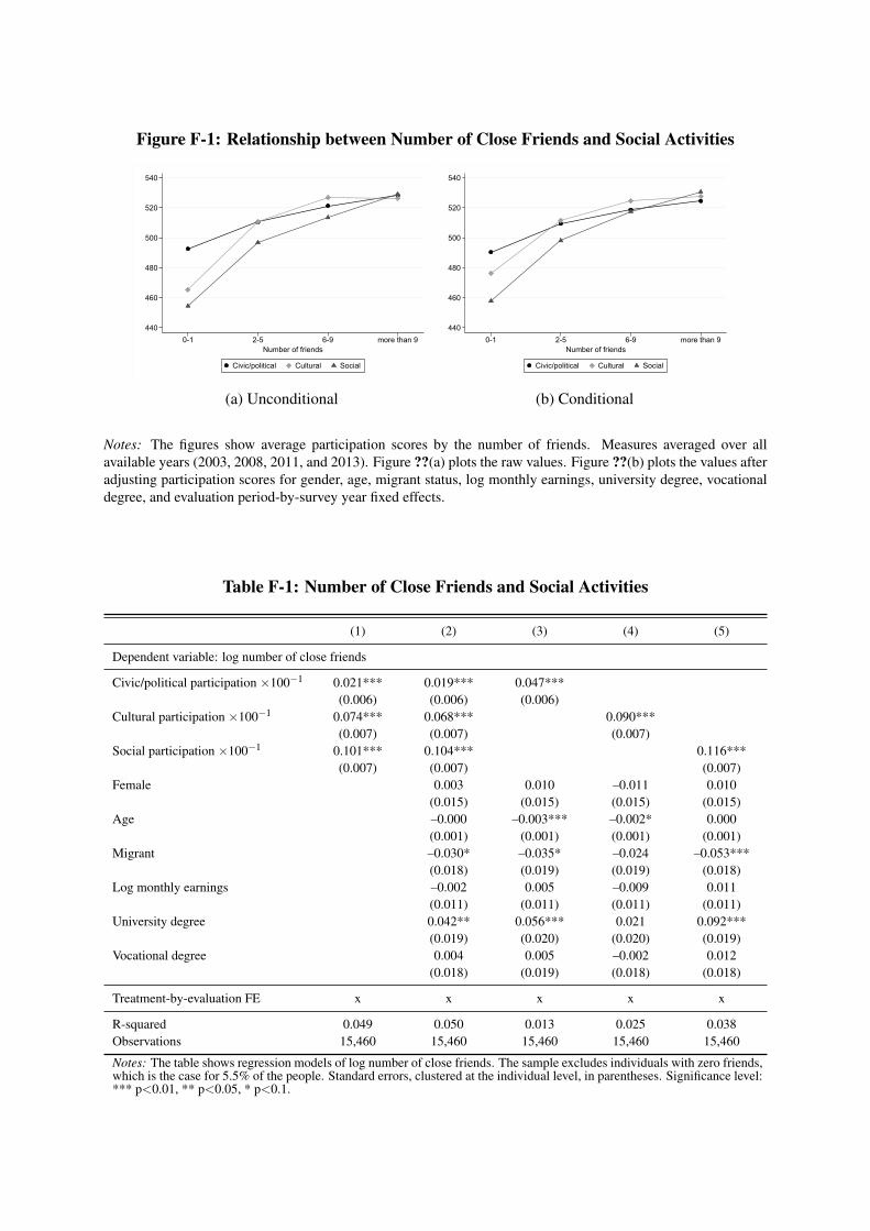
Figure F-1: Relationship between Number of Close Friends and Social Activities

��

��

��

��

��

��

�� PRUH�WKDQ��1XPEHU�RI�IULHQGV


(a) Unconditional

��

��

��

��

��

��

�� PRUH�WKDQ��1XPEHU�RI�IULHQGV


(b) Conditional

Notes: The figures show average participation scores by the number of friends. Measures averaged over allavailable years (2003, 2008, 2011, and 2013). Figure ??(a) plots the raw values. Figure ??(b) plots the values afteradjusting participation scores for gender, age, migrant status, log monthly earnings, university degree, vocationaldegree, and evaluation period-by-survey year fixed effects.

Table F-1: Number of Close Friends and Social Activities

(1) (2) (3) (4) (5)

Dependent variable: log number of close friends

Civic/political participation ⇥100�1 0.021*** 0.019*** 0.047***(0.006) (0.006) (0.006)

Cultural participation ⇥100�1 0.074*** 0.068*** 0.090***(0.007) (0.007) (0.007)

Social participation ⇥100�1 0.101*** 0.104*** 0.116***(0.007) (0.007) (0.007)

Female 0.003 0.010 –0.011 0.010(0.015) (0.015) (0.015) (0.015)

Age –0.000 –0.003*** –0.002* 0.000(0.001) (0.001) (0.001) (0.001)

Migrant –0.030* –0.035* –0.024 –0.053***(0.018) (0.019) (0.019) (0.018)

Log monthly earnings –0.002 0.005 –0.009 0.011(0.011) (0.011) (0.011) (0.011)

University degree 0.042** 0.056*** 0.021 0.092***(0.019) (0.020) (0.020) (0.019)

Vocational degree 0.004 0.005 –0.002 0.012(0.018) (0.019) (0.018) (0.018)

Treatment-by-evaluation FE x x x x x

R-squared 0.049 0.050 0.013 0.025 0.038Observations 15,460 15,460 15,460 15,460 15,460

Notes: The table shows regression models of log number of close friends. The sample excludes individuals with zero friends,which is the case for 5.5% of the people. Standard errors, clustered at the individual level, in parentheses. Significance level:*** p<0.01, ** p<0.05, * p<0.1.

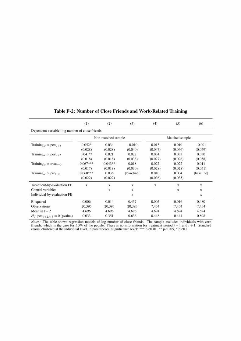
Table F-2: Number of Close Friends and Work-Related Training

(1) (2) (3) (4) (5) (6)

Dependent variable: log number of close friends


Trainingie ⇥ postt+3 0.052* 0.034 –0.010 0.013 0.010 –0.001(0.028) (0.028) (0.040) (0.047) (0.046) (0.059)

Trainingie ⇥ postt+2 0.041** 0.021 0.022 0.034 0.033 0.030(0.018) (0.018) (0.038) (0.027) (0.026) (0.058)

Trainingie ⇥ treatt=0 0.067*** 0.043** 0.018 0.027 0.022 0.011(0.017) (0.018) (0.030) (0.028) (0.028) (0.051)

Trainingie ⇥ pret�2 0.060*** 0.036 [baseline] 0.010 0.004 [baseline](0.022) (0.022) (0.036) (0.035)

Treatment-by-evaluation FE x x x x x xControl variables x x x xIndividual-by-evaluation FE x x

R-squared 0.006 0.014 0.457 0.005 0.016 0.480Observations 20,395 20,395 20,395 7,454 7,454 7,454Mean in t �2 4.696 4.696 4.696 4.694 4.694 4.694H0: postt+2,t+3 = 0 (pvalue) 0.033 0.351 0.636 0.448 0.444 0.808

Notes: The table shows regression models of log number of close friends. The sample excludes individuals with zerofriends, which is the case for 5.5% of the people. There is no information for treatment period t � 1 and t + 1. Standarderrors, clustered at the individual level, in parentheses. Significance level: *** p<0.01, ** p<0.05, * p<0.1.

Documents

The Benefits of Adult Learning: Work- Related Training