INSTITUT FUR INFORMATIKDER LUDWIG–MAXIMILIANS–UNIVERSITAT MUNCHEN

Bachelor Thesis

Spacecraft Operator Schedulingwith Grover’s Algorithm

Antonius Benedikt Anani Scherer

INSTITUT FUR INFORMATIKDER LUDWIG–MAXIMILIANS–UNIVERSITAT MUNCHEN

Spacecraft Operator Schedulingwith Grover’s Algorithm

Antonius Benedikt Anani Scherer

Aufgabensteller: Prof. Dr. Dieter Kranzlmuller

Betreuer: Sophia Grundner-CulemannTobias GuggemosDr. Andreas Spoerl (DLR)Sven Pruefer (DLR)

Abgabetermin: 19. Januar 2021

Hiermit versichere ich, dass ich die vorliegende Bachelorarbeit selbstandig verfasst undkeine anderen als die angegebenen Quellen und Hilfsmittel verwendet habe.

Berlin, den 19. Januar 2021

. . . . . . . . . . . . . . . . . . . . . . . . . . . . . . . . . . . . . . . . . . .(Unterschrift des Kandidaten)

Abstract

The application of quantum algorithms on some problems in NP promises a significantreduction of time complexity. This thesis uses Grover’s Algorithm, originally designed tosearch an unstructured database with quadratic speedup, to find valid solution bit-stringsto the NP-hard personnel scheduling problem. Under consideration of various hard andsoft constraints, we implement this by using the IBMQ backend and Qiskit to optimizethe German Aerospace Center’s spacecraft on-call operator scheduling. We seek an optimalassignment for 52 operators to 17 positions over a period of 180 days under constraintson schedule and personnel. Further, we evaluate the solution quality and compare theperformance with classical and quantum alternatives. While still restricted by intermediate-scale quantum devices in the near term, we explore new approaches in encoding and batchingthe problem to reduce the required number of qubits. In the end, a feasible near-term solutionthat scales well with the quantum devices of the upcoming years is presented.

vii

Contents

1 Introduction 1

2 Background 32.1 Qubit . . . . . . . . . . . . . . . . . . . . . . . . . . . . . . . . . . . . . . . . 32.2 Multi Qubits . . . . . . . . . . . . . . . . . . . . . . . . . . . . . . . . . . . . 42.3 Quantum Gates . . . . . . . . . . . . . . . . . . . . . . . . . . . . . . . . . . . 5

2.3.1 Single Qubit Gates . . . . . . . . . . . . . . . . . . . . . . . . . . . . . 52.3.2 Multi Qubit Gates . . . . . . . . . . . . . . . . . . . . . . . . . . . . . 72.3.3 Quantum Circuits . . . . . . . . . . . . . . . . . . . . . . . . . . . . . 82.3.4 Quantum Algorithms . . . . . . . . . . . . . . . . . . . . . . . . . . . 9

2.4 Grover’s Algorithm . . . . . . . . . . . . . . . . . . . . . . . . . . . . . . . . . 92.4.1 Procedure . . . . . . . . . . . . . . . . . . . . . . . . . . . . . . . . . . 102.4.2 Quantum Arithmetic Operations . . . . . . . . . . . . . . . . . . . . . 152.4.3 Quantum Computational Complexity . . . . . . . . . . . . . . . . . . 152.4.4 Scheduling Problems . . . . . . . . . . . . . . . . . . . . . . . . . . . . 17

3 Problem Description and Requirement Analysis 193.1 OnCall Operator Scheduling . . . . . . . . . . . . . . . . . . . . . . . . . . . . 193.2 Requirement Analysis . . . . . . . . . . . . . . . . . . . . . . . . . . . . . . . 19

3.2.1 Functional Requirements . . . . . . . . . . . . . . . . . . . . . . . . . 193.2.2 Non-functional Requirements . . . . . . . . . . . . . . . . . . . . . . . 20

4 Related Work 214.1 Classical Algorithms . . . . . . . . . . . . . . . . . . . . . . . . . . . . . . . . 214.2 Quantum Algorithms . . . . . . . . . . . . . . . . . . . . . . . . . . . . . . . . 224.3 Quantum Algorithms to Solve Optimization Problems . . . . . . . . . . . . . 23

5 Methods 255.1 Encoding . . . . . . . . . . . . . . . . . . . . . . . . . . . . . . . . . . . . . . 255.2 Automatic Oracle Generation . . . . . . . . . . . . . . . . . . . . . . . . . . . 27

6 Implementation 316.1 Circuit Preparation . . . . . . . . . . . . . . . . . . . . . . . . . . . . . . . . . 316.2 State preparation . . . . . . . . . . . . . . . . . . . . . . . . . . . . . . . . . . 326.3 Grover iteration . . . . . . . . . . . . . . . . . . . . . . . . . . . . . . . . . . . 336.4 Results . . . . . . . . . . . . . . . . . . . . . . . . . . . . . . . . . . . . . . . . 376.5 Evaluation . . . . . . . . . . . . . . . . . . . . . . . . . . . . . . . . . . . . . . 40

7 Conclusion 45

List of Figures 47

ix

Contents

Bibliography 49

x

1 Introduction

In 1982, both Richard Feynman [Fey82] and Paul Benioff [Ben82] independently pointed outthat quantum systems could be used to perform computation. While Benioff’s motivationwas founded on the idea to prove the existence of a reversible Turing Machine, Feynmanrealized that due to its complexity, a quantum system could only be efficiently simulated byanother quantum system. This sparked the idea of a new field known as quantum computing.Even though classical computers improved rapidly over the last decades and as Moore’s lawseems to hold, there are known limitations on what classical programs can solve efficiently.Theoretical computer scientists classified problems that are neither solvable in polynomialtime or space, independent from further development of classical computers. Due to theircomplexity, classical algorithms do often not find an optimal solution in a feasible time oruse metaheuristic methods that only find approximate solutions. Extending Benioff’s andFeynman’s ideas, quantum computing offers a potential solution to these restrictions. Inthe last three decades, researchers developed quantum algorithms that theoretically providepolynomial or even exponential speedups in comparison to their classical counterparts. Apromising application of quantum algorithms are optimizations, especially complex combi-natorial optimization problems. However, current quantum devices are very limited in theirsize and computational power. Even though those NISQ1 era devices are not yet capable ofhaving a deep impact on industry size problems, we use them to develop and study scalablequantum algorithms that will unfold their potential with improving quantum hardware.

Scope of the Thesis

Like many employers, the German Aerospace Centre (DLR) 2 faces difficulties while creatingthe personnel schedule for their employees. This thesis investigates the ability of Grover’ssearch algorithm to solve a specific instance of DLR’s personnel scheduling problem, theon-call spacecraft operator scheduling. While handling a variety of spacecraft missions fromDLR’s mission control center, the OnCall spacecraft operator schedule ensures the constantpresence of capable operators on their dedicated missions. Here, an efficient assignment iscrucial to ensure a frictionless performance as well as a reduction in personnel cost. Thereforewe develop a method that ensures an efficient translation of the underlying optimizationproblem to quantum hardware using IBM’s quantum developer kit Qiskit. Knowing thatNISQ era devices are not yet capable of providing enough computational power to solve thewhole problem instance, we ensure that the method is scalable and able to use the full powerof future quantum hardware.

1Noisy Intermediate-Scale Quantum, or NISQ, is a term coined by John Preskill. It describes the erawhere quantum computers surpass the abilities of classical computers, but won’t be big enough to providefault-tolerant implementations of those underlying quantum algorithms. [Pre18]

2Deutsches Zentrum fur Luft- und Raumfahrt

1

1 Introduction

Structure of the thesis

The thesis consists of five parts: In Chapter 2 we give an introduction to quantum com-puting and explain Grover’s search algorithms, quantum complexity theory, and pin downthe scheduling problem. Chapter 3 describes the on-call operator scheduling problem andperforms a requirement analysis for the method we develop for the DLR. In Chapter 4 wegive an overview of related work that solves scheduling problems classically and uses quan-tum algorithms to solve optimization problems. Further, Chapter 5 describes the two coremethods we develop to efficiently map our problem to a quantum device. Lastly, Chapter6 shows the implementation of the methods in Chapter 5 with IBM’s Qiskit and evaluatesthe results.

2

2 Background

At its core, quantum computing manipulates quantum systems. A quantum system has astate that is represented by a complex vector space and a quantum algorithm is composedof linear transformations acting on that vector space. There are several ways a quantumcomputer can be designed on the hardware side, but the basic axioms of quantum mechanicsdo not vary across the different platforms. The following section gives a brief introductionto the basic concepts and terminology of quantum computing.1

We start by explaining what qubits and multi-qubit systems are, how they are manipulatedthrough quantum gates and how a quantum circuit is composed. Further, an introductionto a basic quantum algorithm is given with an in-depth explanation of Grover’s algorithm,followed by the basic concept of quantum arithmetic operations. The chapter finishes withan overview of quantum computational complexity.

2.1 Qubit

In classical computation and information theory, the bit represents the smallest, indivisibleunit of information. The quantum information counterpart is called ’quantum bit’ or qubit.The classical bit has two possible states, {0, 1}, while the simplest possible states in aquantum system is described through the basis vectors {|0〉 , |1〉} ∈ C2. So the state of aqubit |ψ〉 is a vector in a complex Hilbert space H = C2 described by a linear combinationof its basis vectors |0〉 and |1〉:

|ψ〉 = α |0〉+ β |1〉 (2.1)

with {α, β} ∈ C and normalized as

|α|2 + |β|2 = 1. (2.2)

In quantum mechanics, the Bra-Ket or Dirac notation is often used to describe a quantum

state. While the Ket notation denotes a column vector so that |0〉 =

[10

]and |1〉 =

[01

], the

Bra notation is its entry-wise complex conjugated transpose and therefore a row vector. Thelinear combination in Equation 2.1 is also called a superposition and reflects an arbitrarydirection in which the state vector points within the Hilbert space. To make this idea moreaccessible, we can create a three dimensional geometric representation of such a state φ byrewriting Equation 2.1 as

|ψ〉 = eiγ(

cosθ

2|0〉+ eiϕ sin

θ

2|1〉). (2.3)

1See [NC02] for a detailed introduction to quantum computing and quantum information theory

3

2 Background

eiγ is called the global phase, but since it has no observable effects, we can simply write:

|ψ〉 = cosθ

2|0〉+ eiϕ sin

θ

2|1〉 . (2.4)

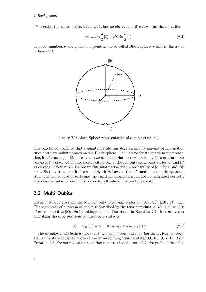
The real numbers θ and ϕ define a point in the so called Bloch sphere, which is illustratedin figure 2.1.

|ψ〉

x

y

z |0〉

|1〉

Figure 2.1: Bloch Sphere representation of a qubit state |ψ〉.

One conclusion could be that a quantum state can store an infinite amount of informationsince there are infinite points on the Bloch sphere. This is true for its quantum representa-tion, but for us to get this information we need to perform a measurement. This measurementcollapses the state |ψ〉 and we receive either one of the computational basis states |0〉 and |1〉as classical information. We obtain this information with a probability of |α|2 for 0 and |β|2for 1. So the actual amplitudes α and β, which have all the information about the quantumstate, can not be read directly and the quantum information can not be translated perfectlyinto classical information. This is true for all values for α and β except 0.

2.2 Multi Qubits

Given a two qubit system, the four computational basis states are |00〉 , |01〉 , |10〉 , |01〉 , |11〉.The joint state of a system of qubits is described by the tensor product ⊗, while |0〉 ⊗ |0〉 isoften shortened to |00〉. So by taking the definition stated in Equation 2.1, the state vectordescribing the superpositions of theses four states is

|ψ〉 = α00 |00〉+ α01 |01〉+ α10 |10〉+ α11 |11〉 . (2.5)

The complex coefficients αi are the state’s amplitudes and squaring them gives the prob-ability the state collapses in one of the corresponding classical states 00, 01, 10, or 11. As inEquation 2.2, the normalization condition requires that the sum of all the probabilities of all

4

2.3 Quantum Gates

possible states is 1. One can say that the mathematical structure of a single qubit generalizesto any higher-dimensional quantum system. It is important to note that the dimension ofthe state space 2n grows exponentially in the number of qubits n. So one can say that anyquantum state can be written as a linear combination of its basis states. However, thereare multi-qubit states, that cannot be written as the tensor product of their single qubitsubsystems. For two-qubit states, one of the most famous examples are the Bell states orEPR2 pairs, of which

|Φ+〉 =|00〉+ |11〉√

2. (2.6)

is one of them. It demonstrates a part of quantum mechanics that does not exist in theclassical world. Both qubits are entangled. So measuring one qubit determines the stateof the other. In the Bell state |Φ+〉 this is either |00〉 or |11〉, with equal probability of( 1√

2)2 = 1

2 . Entanglement is the essential part of quantum computing, since it creates a 2n

dimensional complex vector space out of n qubits, also called superposition, to perform ourcomputations in.

2.3 Quantum Gates

So far, we showed how the quantum state of a qubit is defined. But in order to performquantum computation, we need to be able to manipulate quantum information and thereforethe state of a qubit. This is done through so-called quantum logic gates, whose functionalityis analogous to classical gates. As in classical computation, a quantum circuit is composed ofquantum wires, that carry the information and given quantum logic gates, that manipulatea certain input to get the desired output.

2.3.1 Single Qubit Gates

In the following section, a summary of the most important quantum gates is provided.Quantum gates acting on a single qubit state can always be described by 2x2 matrices.Following our normalization condition in Equation 2.2, which must be true before and afterthe application of a quantum gate, those matrices must be unitary. So for all quantum logicgates U , U †U = I, where U † is the adjoint of U. Generally speaking, every unitary 2x2matrix can be a quantum gate on a single qubit state. And since the state of a qubit isrepresented as a vector in a complex Hilbert space, a quantum logic gate can be seen as arotation of this vector. Let’s start with the simple NOT gate. As expected, the quantumNOT gate, called X-gate in quantum computation, acts on the computational basis state inthe following way:

X |0〉 = |1〉X |1〉 = |0〉

Further it acts linearly on the general superposition state as seen in (2.1):

X(α |0〉+ β |1〉) = α |1〉+ β |0〉 (2.7)

2Named after a paradox described in a paper published by Einstein, Podolsky and Rosen (EPR) in 1935[EPR35]

5

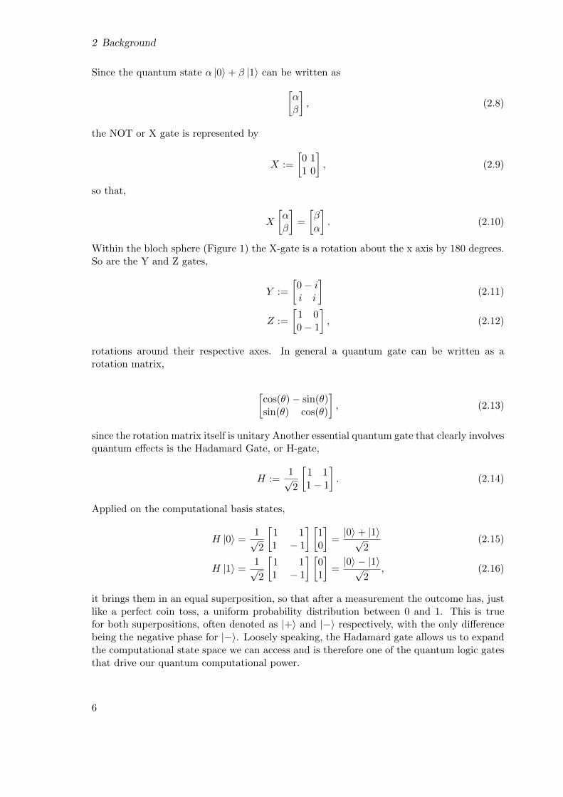
2 Background

Since the quantum state α |0〉+ β |1〉 can be written as[αβ

], (2.8)

the NOT or X gate is represented by

X :=

[0 11 0

], (2.9)

so that,

X

[αβ

]=

[βα

]. (2.10)

Within the bloch sphere (Figure 1) the X-gate is a rotation about the x axis by 180 degrees.So are the Y and Z gates,

Y :=

[0− ii i

](2.11)

Z :=

[1 00− 1

], (2.12)

rotations around their respective axes. In general a quantum gate can be written as arotation matrix,

[cos(θ)− sin(θ)sin(θ) cos(θ)

], (2.13)

since the rotation matrix itself is unitary Another essential quantum gate that clearly involvesquantum effects is the Hadamard Gate, or H-gate,

H :=1√2

[1 11− 1

]. (2.14)

Applied on the computational basis states,

H |0〉 =1√2

[1 11 − 1

] [10

]=|0〉+ |1〉√

2(2.15)

H |1〉 =1√2

[1 11 − 1

] [01

]=|0〉 − |1〉√

2, (2.16)

it brings them in an equal superposition, so that after a measurement the outcome has, justlike a perfect coin toss, a uniform probability distribution between 0 and 1. This is truefor both superpositions, often denoted as |+〉 and |−〉 respectively, with the only differencebeing the negative phase for |−〉. Loosely speaking, the Hadamard gate allows us to expandthe computational state space we can access and is therefore one of the quantum logic gatesthat drive our quantum computational power.

6

2.3 Quantum Gates

2.3.2 Multi Qubit Gates

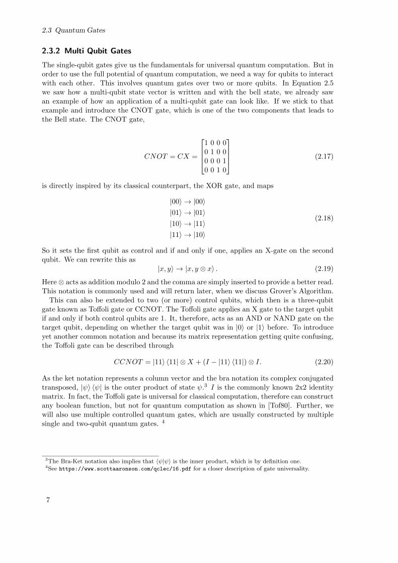
The single-qubit gates give us the fundamentals for universal quantum computation. But inorder to use the full potential of quantum computation, we need a way for qubits to interactwith each other. This involves quantum gates over two or more qubits. In Equation 2.5we saw how a multi-qubit state vector is written and with the bell state, we already sawan example of how an application of a multi-qubit gate can look like. If we stick to thatexample and introduce the CNOT gate, which is one of the two components that leads tothe Bell state. The CNOT gate,

CNOT = CX =

1 0 0 00 1 0 00 0 0 10 0 1 0

(2.17)

is directly inspired by its classical counterpart, the XOR gate, and maps

|00〉 → |00〉|01〉 → |01〉|10〉 → |11〉|11〉 → |10〉

(2.18)

So it sets the first qubit as control and if and only if one, applies an X-gate on the secondqubit. We can rewrite this as

|x, y〉 → |x, y ⊗ x〉 . (2.19)

Here ⊗ acts as addition modulo 2 and the comma are simply inserted to provide a better read.This notation is commonly used and will return later, when we discuss Grover’s Algorithm.

This can also be extended to two (or more) control qubits, which then is a three-qubitgate known as Toffoli gate or CCNOT. The Toffoli gate applies an X gate to the target qubitif and only if both control qubits are 1. It, therefore, acts as an AND or NAND gate on thetarget qubit, depending on whether the target qubit was in |0〉 or |1〉 before. To introduceyet another common notation and because its matrix representation getting quite confusing,the Toffoli gate can be described through

CCNOT = |11〉 〈11| ⊗X + (I − |11〉 〈11|)⊗ I. (2.20)

As the ket notation represents a column vector and the bra notation its complex conjugatedtransposed, |ψ〉 〈ψ| is the outer product of state ψ.3 I is the commonly known 2x2 identitymatrix. In fact, the Toffoli gate is universal for classical computation, therefore can constructany boolean function, but not for quantum computation as shown in [Tof80]. Further, wewill also use multiple controlled quantum gates, which are usually constructed by multiplesingle and two-qubit quantum gates. 4

3The Bra-Ket notation also implies that 〈ψ|ψ〉 is the inner product, which is by definition one.4See https://www.scottaaronson.com/qclec/16.pdf for a closer description of gate universality.

7

2 Background

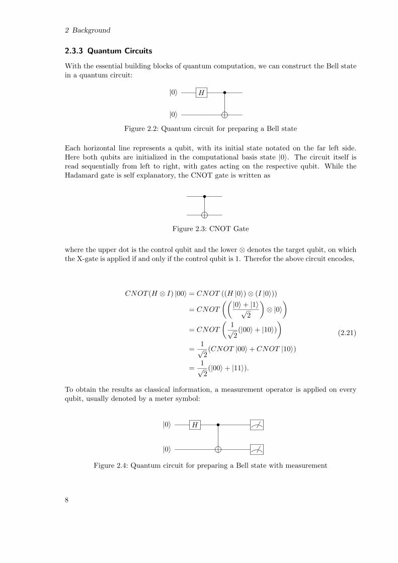
2.3.3 Quantum Circuits

With the essential building blocks of quantum computation, we can construct the Bell statein a quantum circuit:

|0〉 H •

|0〉

Figure 2.2: Quantum circuit for preparing a Bell state

Each horizontal line represents a qubit, with its initial state notated on the far left side.Here both qubits are initialized in the computational basis state |0〉. The circuit itself isread sequentially from left to right, with gates acting on the respective qubit. While theHadamard gate is self explanatory, the CNOT gate is written as

•

Figure 2.3: CNOT Gate

where the upper dot is the control qubit and the lower ⊗ denotes the target qubit, on whichthe X-gate is applied if and only if the control qubit is 1. Therefor the above circuit encodes,

CNOT (H ⊗ I) |00〉 = CNOT ((H |0〉)⊗ (I |0〉))

= CNOT

((|0〉+ |1〉√

2

)⊗ |0〉

)= CNOT

(1√2

(|00〉+ |10〉))

=1√2

(CNOT |00〉+ CNOT |10〉)

=1√2

(|00〉+ |11〉).

(2.21)

To obtain the results as classical information, a measurement operator is applied on everyqubit, usually denoted by a meter symbol:

|0〉 H •

|0〉

Figure 2.4: Quantum circuit for preparing a Bell state with measurement

8

2.4 Grover’s Algorithm

As a result we receive the maximal entangled two-qubit state and as stated above, thequbits will always be in the same state after measurement. The qubit itself is measured inthe computational basis.

2.3.4 Quantum Algorithms

Given the quantum logic gates and the quantum circuit, we can construct any quantumalgorithm following these steps:

Algorithm 1 Construct Quantum Algorithm

Input: Input register of |ψ〉⊗n1: Encode data into the state of the input register qubits2: Apply a sequence of quantum gates on the set of input qubits3: Obtain classical information by measuring one or more qubits at the end or any other

point in time

The central algorithm we will use throughout this thesis is Grover’s quantum search algo-rithm. The next section is dedicated to a deep introduction.

2.4 Grover’s Algorithm

Grover’s Algorithm [Gro96] was discovered shortly after Shor’s algorithm [Sho99] in 1995.Even though it has a quadratic speed up, rather than an exponential one compared to Shor’salgorithm, it is applicable to a wider range of problems. One application is the speedup ofproblems for which a polynomial-time algorithm exists. Its original task was to find anelement in an unordered database. A classical computer algorithm would need a linearnumber of queries, O(n), to find the element. That is because the rules for the O - Notationrequires looking at the worst-case scenario, where the desired object is located at the n-thindex. But even if one would take the more realistic approach to look at the average numberof queries, it would still take a linear in n number of queries ∼ n

2 . Grover’s algorithm onthe other hand requires a maximum of O(

√n) ’quantum’ queries. In its standard version it

achieves this by using a relatively low number of qubits, O(log(N)), and gates, O(√n log(n)).

To understand the functionality of Grovers search algorithm, it is important to understandthat the scenario of searching for an element in an unstructured database might be intuitive,but not quite right. In fact, Grover’s algorithm does not search through a list of elements,it searches through a list of possible inputs x for the function f that returns true or false.So the function f(x) is defined as

f(x) =

{1 if x = x∗

0 if x 6= x(2.22)

where x are bit-strings and x∗ are the solution bit-strings we are looking for. Given f(x) = 1,the circuit will flip an ancilla qubit that is prepared in |−〉 and therefore ’mark’ the correctsolutions by flipping their amplitude.5 This routine is called an oracle. It is important to

5Ancilla qubits are additional qubits in a quantum circuit that are either necessary for a certain algorithmor are implemented to reduce the complexity and depth of a circuit. Initialized to |0〉 they are usuallybrought back to that state through either reversed application of the precious gates or through a reset,depending on the requirements of the circuit. They do not affect the output directly and are often reused.

9

2 Background

note that the oracle does not need to know the exact solution, but it must recognize it.The oracle is also often called a black box since its internal construction is very specific tothe problem one needs to solve and is not required in order to understand the concept ofthe overall algorithm6. For now, it is enough to assume that it is constructed efficiently, itrecognizes the correct solutions, and will flip their amplitude. So given the function fromabove, an oracle O, which in turn is a unitary operator, has |x〉 as the input register and |q〉as the ancilla or oracle qubit:

|x〉 |q〉 O−→ |x〉 |q ⊗ f(x)〉 . (2.23)

As mentioned, the oracle qubit |q〉 is prepared in the state |−〉 = (|0〉 − |1〉)/√

2. So theapplication of the oracle can be written as:

|x〉(|0〉 − |1〉√

2

)O−→ (−1)f(x) |x〉

(|0〉 − |1〉√

2

). (2.24)

Meaning, if the oracle is applied to a non-solution state, it does not change the state. Butif applied to a correct solution state, it will shift its phase.

2.4.1 Procedure

Grover’s search algorithms consists of three main parts:

• State Preparation

• Oracle

• Grover Diffusion

The oracle and the Grover diffusion form the Grover operator or iteration (the actual deno-tation varies across the literature). The overall algorithm is:

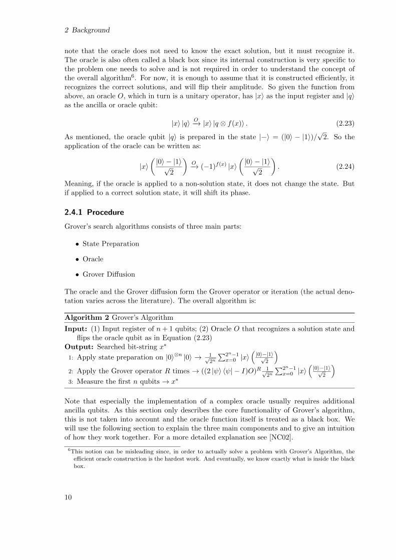
Algorithm 2 Grover’s Algorithm

Input: (1) Input register of n+ 1 qubits; (2) Oracle O that recognizes a solution state andflips the oracle qubit as in Equation (2.23)

Output: Searched bit-string x∗

1: Apply state preparation on |0〉⊗n |0〉 → 1√2n

∑2n−1x=0 |x〉

(|0〉−|1〉√

2

)2: Apply the Grover operator R times → ((2 |ψ〉 〈ψ| − I)O)R 1√

2n

∑2n−1x=0 |x〉

(|0〉−|1〉√

2

)3: Measure the first n qubits → x∗

Note that especially the implementation of a complex oracle usually requires additionalancilla qubits. As this section only describes the core functionality of Grover’s algorithm,this is not taken into account and the oracle function itself is treated as a black box. Wewill use the following section to explain the three main components and to give an intuitionof how they work together. For a more detailed explanation see [NC02].

6This notion can be misleading since, in order to actually solve a problem with Grover’s Algorithm, theefficient oracle construction is the hardest work. And eventually, we know exactly what is inside the blackbox.

10

2.4 Grover’s Algorithm

State Preparation

An important part when finding the right implementation of Grover’s algorithm is an efficientencoding of the problem (or search space) into the input register. We will discuss this moredeeply in section 5, since it is specific to a problem or even an instance of it. It will definewhat the single qubits actually stand for. After an encoding is found, the input state itselfis always prepared in the same way.7 From n input qubits combined in the state |ψ〉, theoverall search space is spanned by putting |ψ〉 in a uniform superposition. Here for we simplyapply a Hadamard on every qubit in |ψ〉 such that:

|ψ〉 = H⊗n |0〉n =1√N

N−1∑x=0

|x〉 , (2.25)

with N = 2n. So far we only prepared the input register encoding our problem space, nextwe need to prepare grover qubit |q〉. As mentioned above, |q〉 need to be in |−〉. Startingfrom |0〉, we achieve this by:

|q〉 = HX |0〉 = H |1〉 =1√2

(|0〉 − |1〉) (2.26)

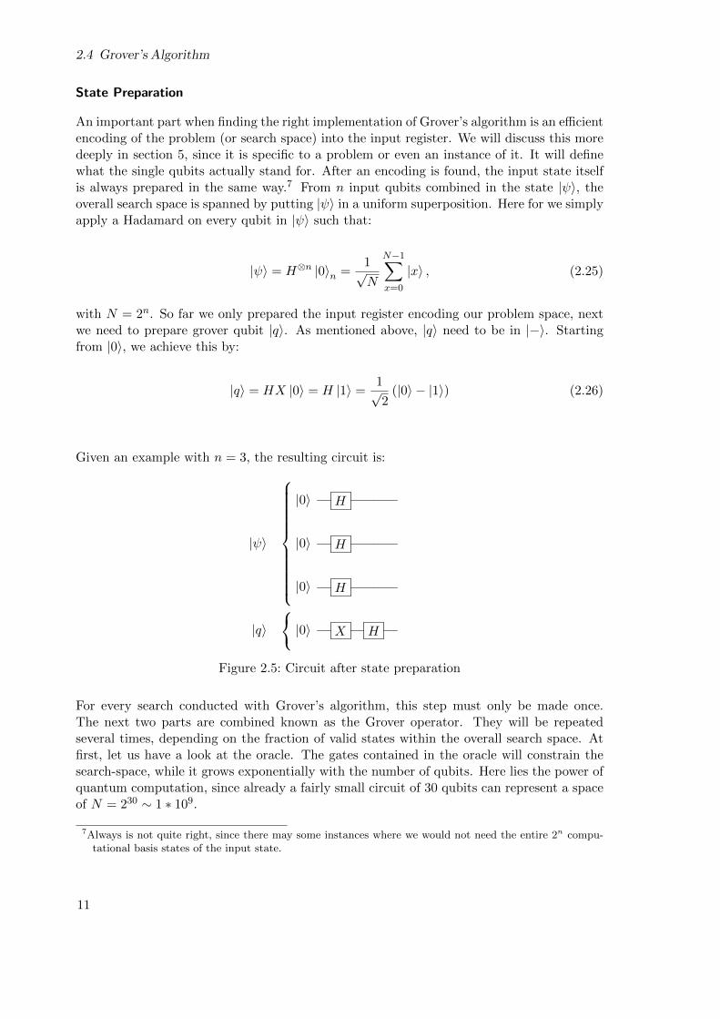
Given an example with n = 3, the resulting circuit is:

|0〉 H

|ψ〉 |0〉 H

|0〉 H

|q〉 |0〉 X H

Figure 2.5: Circuit after state preparation

For every search conducted with Grover’s algorithm, this step must only be made once.The next two parts are combined known as the Grover operator. They will be repeatedseveral times, depending on the fraction of valid states within the overall search space. Atfirst, let us have a look at the oracle. The gates contained in the oracle will constrain thesearch-space, while it grows exponentially with the number of qubits. Here lies the power ofquantum computation, since already a fairly small circuit of 30 qubits can represent a spaceof N = 230 ∼ 1 ∗ 109.

7Always is not quite right, since there may some instances where we would not need the entire 2n compu-tational basis states of the input state.

11

2 Background

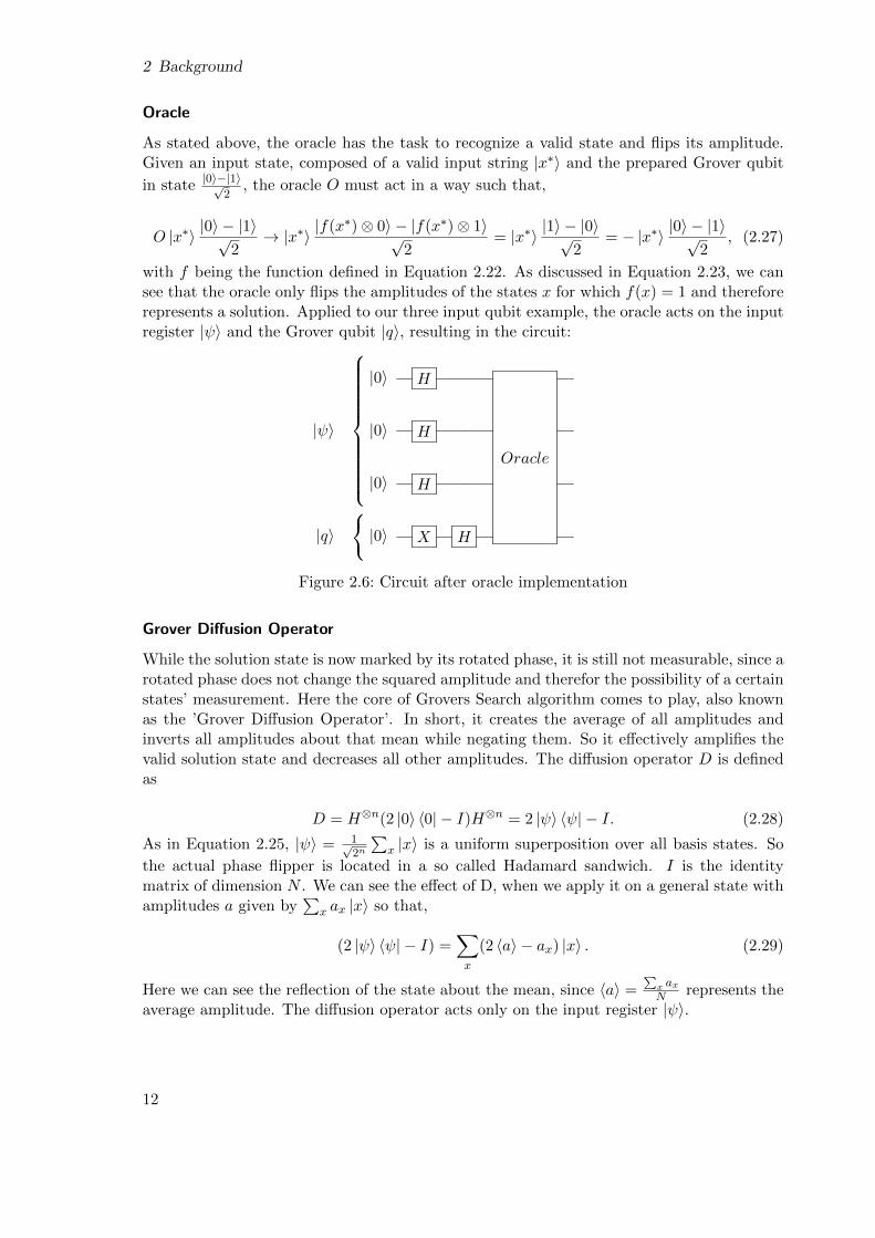
Oracle

As stated above, the oracle has the task to recognize a valid state and flips its amplitude.Given an input state, composed of a valid input string |x∗〉 and the prepared Grover qubit

in state |0〉−|1〉√2

, the oracle O must act in a way such that,

O |x∗〉 |0〉 − |1〉√2→ |x∗〉 |f(x∗)⊗ 0〉 − |f(x∗)⊗ 1〉√

2= |x∗〉 |1〉 − |0〉√

2= − |x∗〉 |0〉 − |1〉√

2, (2.27)

with f being the function defined in Equation 2.22. As discussed in Equation 2.23, we cansee that the oracle only flips the amplitudes of the states x for which f(x) = 1 and thereforerepresents a solution. Applied to our three input qubit example, the oracle acts on the inputregister |ψ〉 and the Grover qubit |q〉, resulting in the circuit:

|0〉 H

Oracle

|ψ〉 |0〉 H

|0〉 H

|q〉 |0〉 X H

Figure 2.6: Circuit after oracle implementation

Grover Diffusion Operator

While the solution state is now marked by its rotated phase, it is still not measurable, since arotated phase does not change the squared amplitude and therefor the possibility of a certainstates’ measurement. Here the core of Grovers Search algorithm comes to play, also knownas the ’Grover Diffusion Operator’. In short, it creates the average of all amplitudes andinverts all amplitudes about that mean while negating them. So it effectively amplifies thevalid solution state and decreases all other amplitudes. The diffusion operator D is definedas

D = H⊗n(2 |0〉 〈0| − I)H⊗n = 2 |ψ〉 〈ψ| − I. (2.28)

As in Equation 2.25, |ψ〉 = 1√2n

∑x |x〉 is a uniform superposition over all basis states. So

the actual phase flipper is located in a so called Hadamard sandwich. I is the identitymatrix of dimension N . We can see the effect of D, when we apply it on a general state withamplitudes a given by

∑x ax |x〉 so that,

(2 |ψ〉 〈ψ| − I) =∑x

(2 〈a〉 − ax) |x〉 . (2.29)

Here we can see the reflection of the state about the mean, since 〈a〉 =∑

x axN represents the

average amplitude. The diffusion operator acts only on the input register |ψ〉.

12

2.4 Grover’s Algorithm

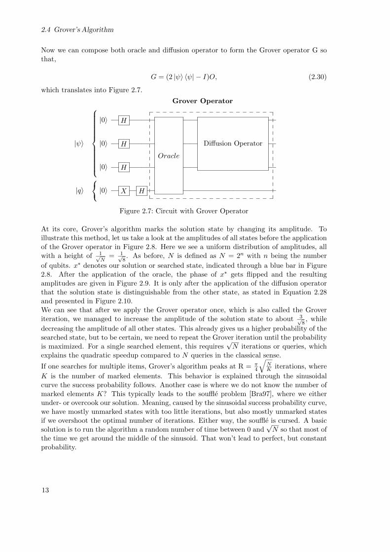
Now we can compose both oracle and diffusion operator to form the Grover operator G sothat,

G = (2 |ψ〉 〈ψ| − I)O, (2.30)

which translates into Figure 2.7.

Grover Operator

|0〉 H

Oracle

Diffusion Operator|ψ〉 |0〉 H

|0〉 H

|q〉 |0〉 X H

Figure 2.7: Circuit with Grover Operator

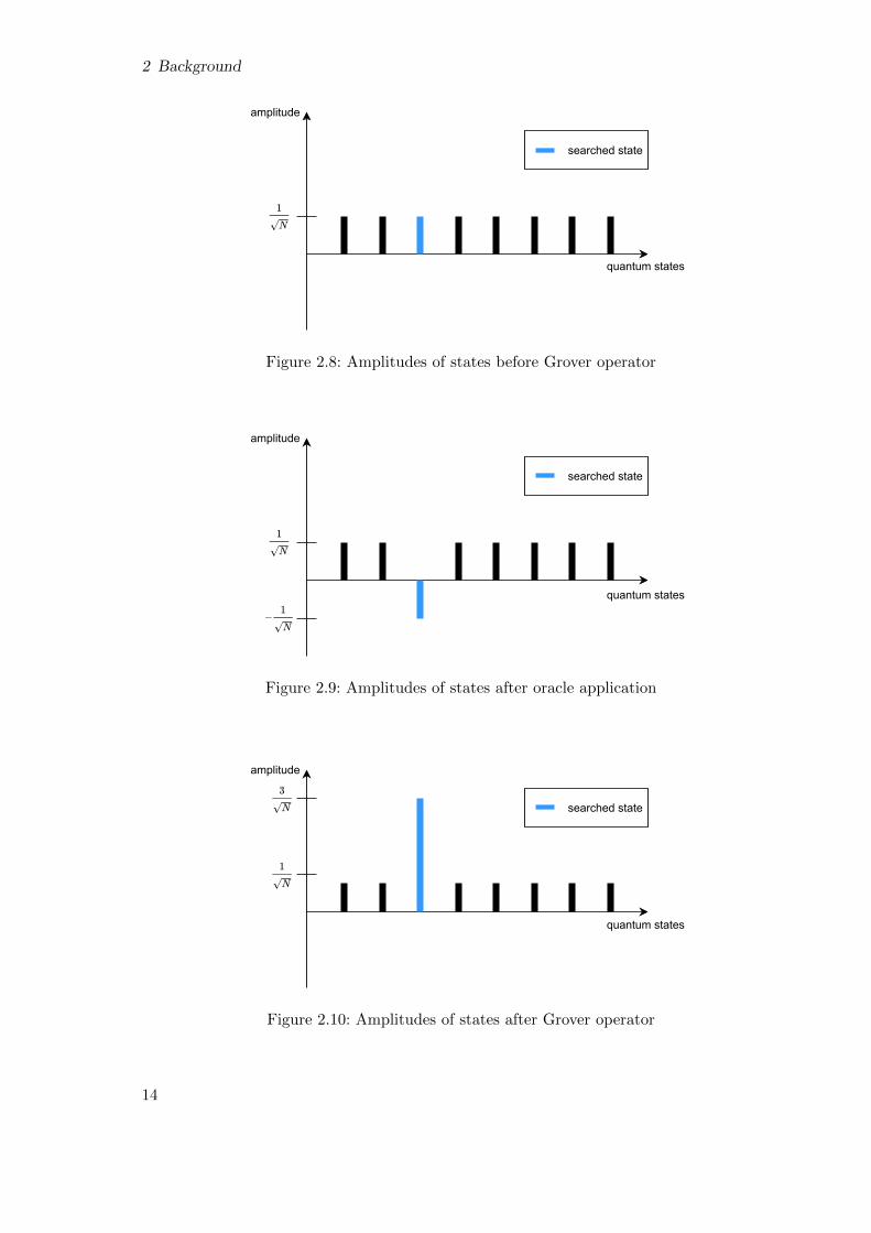
At its core, Grover’s algorithm marks the solution state by changing its amplitude. Toillustrate this method, let us take a look at the amplitudes of all states before the applicationof the Grover operator in Figure 2.8. Here we see a uniform distribution of amplitudes, allwith a height of 1√

N= 1√

8. As before, N is defined as N = 2n with n being the number

of qubits. x∗ denotes our solution or searched state, indicated through a blue bar in Figure2.8. After the application of the oracle, the phase of x∗ gets flipped and the resultingamplitudes are given in Figure 2.9. It is only after the application of the diffusion operatorthat the solution state is distinguishable from the other state, as stated in Equation 2.28and presented in Figure 2.10.We can see that after we apply the Grover operator once, which is also called the Groveriteration, we managed to increase the amplitude of the solution state to about 3√

8, while

decreasing the amplitude of all other states. This already gives us a higher probability of thesearched state, but to be certain, we need to repeat the Grover iteration until the probabilityis maximized. For a single searched element, this requires

√N iterations or queries, which

explains the quadratic speedup compared to N queries in the classical sense.

If one searches for multiple items, Grover’s algorithm peaks at R = π4

√NK iterations, where

K is the number of marked elements. This behavior is explained through the sinusoidalcurve the success probability follows. Another case is where we do not know the number ofmarked elements K? This typically leads to the souffle problem [Bra97], where we eitherunder- or overcook our solution. Meaning, caused by the sinusoidal success probability curve,we have mostly unmarked states with too little iterations, but also mostly unmarked statesif we overshoot the optimal number of iterations. Either way, the souffle is cursed. A basicsolution is to run the algorithm a random number of time between 0 and

√N so that most of

the time we get around the middle of the sinusoid. That won’t lead to perfect, but constantprobability.

13

2 Background

amplitude

quantum states

searched state

Figure 2.8: Amplitudes of states before Grover operator

amplitude

quantum states

searched state

Figure 2.9: Amplitudes of states after oracle application

searched state

quantum states

amplitude

Figure 2.10: Amplitudes of states after Grover operator

14

2.4 Grover’s Algorithm

2.4.2 Quantum Arithmetic Operations

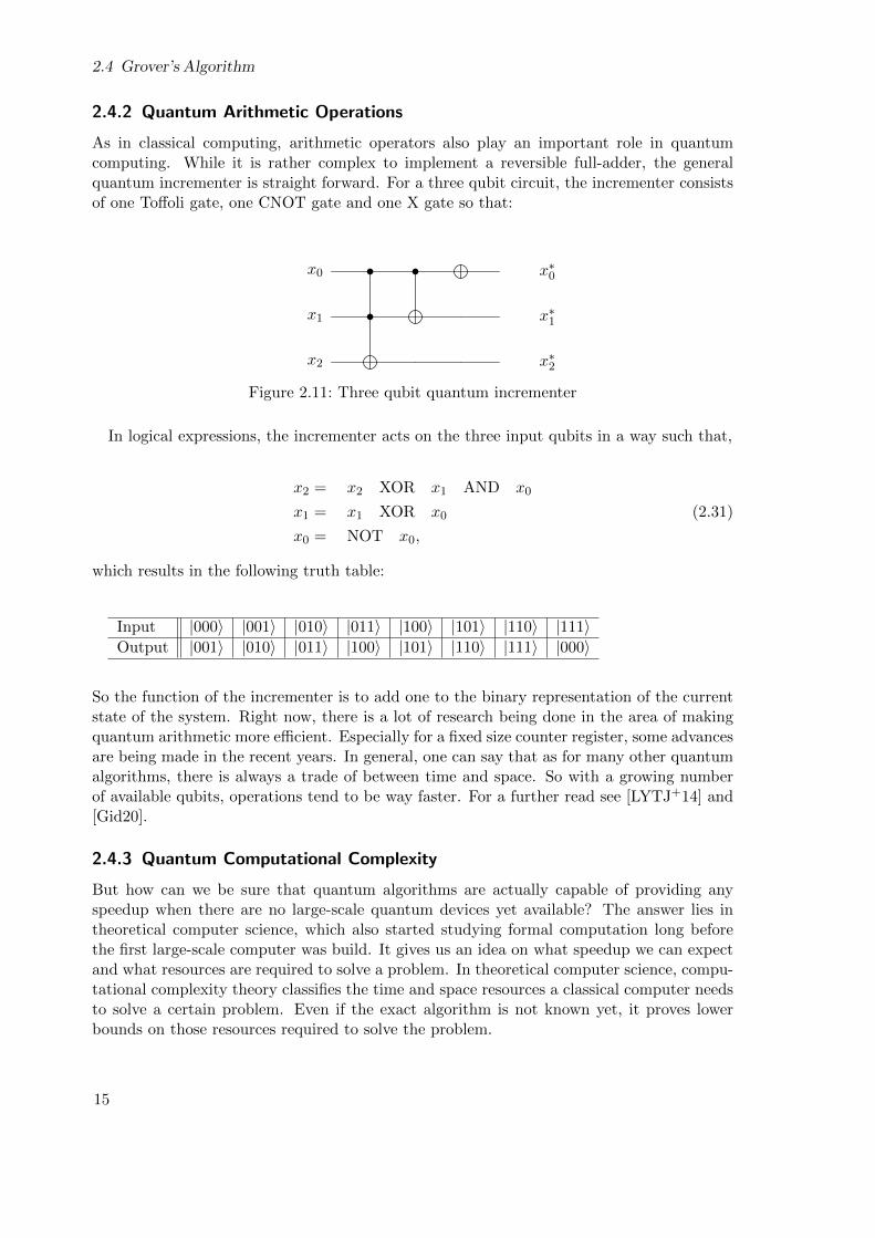
As in classical computing, arithmetic operators also play an important role in quantumcomputing. While it is rather complex to implement a reversible full-adder, the generalquantum incrementer is straight forward. For a three qubit circuit, the incrementer consistsof one Toffoli gate, one CNOT gate and one X gate so that:

x0 • • x∗0

x1 • x∗1

x2 x∗2

Figure 2.11: Three qubit quantum incrementer

In logical expressions, the incrementer acts on the three input qubits in a way such that,

x2 = x2 XOR x1 AND x0

x1 = x1 XOR x0

x0 = NOT x0,

(2.31)

which results in the following truth table:

Input |000〉 |001〉 |010〉 |011〉 |100〉 |101〉 |110〉 |111〉Output |001〉 |010〉 |011〉 |100〉 |101〉 |110〉 |111〉 |000〉

So the function of the incrementer is to add one to the binary representation of the currentstate of the system. Right now, there is a lot of research being done in the area of makingquantum arithmetic more efficient. Especially for a fixed size counter register, some advancesare being made in the recent years. In general, one can say that as for many other quantumalgorithms, there is always a trade of between time and space. So with a growing numberof available qubits, operations tend to be way faster. For a further read see [LYTJ+14] and[Gid20].

2.4.3 Quantum Computational Complexity

But how can we be sure that quantum algorithms are actually capable of providing anyspeedup when there are no large-scale quantum devices yet available? The answer lies intheoretical computer science, which also started studying formal computation long beforethe first large-scale computer was build. It gives us an idea on what speedup we can expectand what resources are required to solve a problem. In theoretical computer science, compu-tational complexity theory classifies the time and space resources a classical computer needsto solve a certain problem. Even if the exact algorithm is not known yet, it proves lowerbounds on those resources required to solve the problem.

15

2 Background

The problems itself are part of complexity classes such as:

• P Problems that are solvable in polynomial time.

• NP Problems that are verified through a deterministic polynomial-time algorithm.

• NP-hard Problems to which every NP problem can be reduced to in polynomial time.

• NP-complete Both in NP and NP-hard.

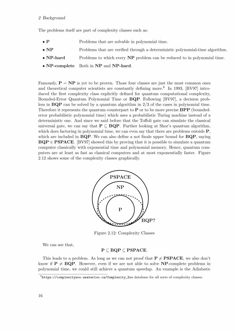
Famously, P = NP is yet to be proven. Those four classes are just the most common onesand theoretical computer scientists are constantly defining more.8 In 1993, [BV97] intro-duced the first complexity class explicitly defined for quantum computational complexity,Bounded-Error Quantum Polynomial Time or BQP. Following [BV97], a decision prob-lem in BQP can be solved by a quantum algorithm in 2/3 of the cases in polynomial time.Therefore it represents the quantum counterpart to P or to be more precise BPP (bounded-error probabilistic polynomial time) which uses a probabilistic Turing machine instead of adeterministic one. And since we said before that the Toffoli gate can simulate the classicaluniversal gate, we can say that P ⊆ BQP. Further looking at Shor’s quantum algorithm,which does factoring in polynomial time, we can even say that there are problems outside P,which are included in BQP. We can also define a not finale upper bound for BQP, sayingBQP ∈ PSPACE. [BV97] showed this by proving that it is possible to simulate a quantumcomputer classically with exponential time and polynomial memory. Hence, quantum com-puters are at least as fast as classical computers and at most exponentially faster. Figure2.12 shows some of the complexity classes graphically.

P

NP

PSPACE

BQP?

Figure 2.12: Complexity Classes

We can see that,

P ⊆ BQP ⊆ PSPACE.

This leads to a problem. As long as we can not proof that P 6= PSPACE, we also don’tknow if P 6= BQP. However, even if we are not able to solve NP-complete problems inpolynomial time, we could still achieve a quantum speedup. An example is the Adiabatic

8https://complexityzoo.uwaterloo.ca/Complexity_Zoo database for all sorts of complexity classes.

16

2.4 Grover’s Algorithm

Algorithm by [FGGS00]. It achieves a strong (potentially up-to exponential) speedup forNP-complete problems by exploiting their structure. The problem is that its performancevaries over different structures. This makes it still very valuable for real use cases but doesnot satisfy theoretical computer scientists. But the same is true for non-quantum algorithms.For NP-complete problems, like the CircuitSAT, it is obvious that the speedup provided byGrover is a real advantage since there is no known classical algorithm that is faster thanbrute force. But for example, 3SAT, a more structured NP-complete problem, is solvablein O(1.3n). Here the focus would be more on combining existing algorithms with Grover’ssearch algorithm, than applying it alone. An overview of such algorithms will be given insection 4. In terms of optimization problems, like the scheduling problem we try to solve,even a relatively small advantage in computational speed might already lead to significantbenefits.

2.4.4 Scheduling Problems

The root of scheduling problems goes back as far as 1954, when [Edi54] and [Dan54] tackledthe problem of traffic delays caused by badly assigned toll booths operators. They introducedthe first scheduling problem, which, constraint by minimizing the cost of personnel, aimed toreduce the average delay for each car. Since then, a variety of such scheduling problems hasbeen identified and researched, such as personnel scheduling problems. And with increasingcomputational power and algorithmic development over the years, its popularity is growing.This increase could be motivated by the economic factor of decreasing labor costs, which is amajor fixed cost for many companies. A good overview of this scheduling problem subset isgiven in [BBDB+13]. Our scheduling problem is closely related to the known nurse schedul-ing/rostering problem, in turn, an especially complex version of the personnel schedulingproblem. Nurse rostering is known to be NP-hard and intends to optimize a schedule con-sisting of multiple shifts and nurses while considering a variety of soft and hard constraints.

So far, we have discussed the principles of quantum computation, Grover’s algorithm, andquantum computational complexity. This will give us the necessary background knowledgeto proceed with the rest of the thesis. Before we explain the actual methods and theirimplementation, we will describe the actual problem and perform a requirement analysis inthe next chapter.

17

3 Problem Description and RequirementAnalysis

In the following chapter, we describe the on-call operator scheduling problem, perform arequirement analysis and conclude with the problem formulation.

3.1 OnCall Operator Scheduling

The German Aerospace Center (DLR) operates a variety of spacecraft missions from itsmission control center, which requires the constant presence of one or more operators persubsystem for each mission. Those operators are organized through an on-call spacecraftoperator scheduling which is created multiple times per year. At the moment, this scheduleis either created manually or through a classical solver tool that uses a brute-force approachto find an optimal assignment. Due to the nature of combinatorial optimization problems,the complexity grows exponentially with their size. So, beginning from fairly small probleminstances, this leads to infeasible computation times. To by-pass this problem, schedulerseither rely in their own intuition or use heuristics, both are very unlikely to find the optimalsolution. Thus, the DLR decided to explore the application of quantum computation inorder to potentially find an optimal solution in feasible time.

3.2 Requirement Analysis

To be applicable to the actual use case, such a software or algorithm must fulfill functionaland non-functional requirements. The functional requirements will describe what the solu-tion must do, while the non-functional requirements indicate how the solution must solvethe problem.

3.2.1 Functional Requirements

The schedule must allocate 52 operators on 17 positions over a period of 180 days and beupdated if certain positions can not be filled as planned. An on-call shift has a durationof 24 hours, so per day, which we use as our time interval, there is at most one operatorassigned to each position. Further, every operator must have a set of subsystems he is ableto operate depending on their background. To be valid, the computed schedule must alsofulfill the following hard constraints:

• Per time-position only one operator can be assigned

• Out of three time units, an operator is only allowed to work two

• An operator can be assigned to at most one position a day

19

3 Problem Description and Requirement Analysis

The general aim is to find an optimal assignment of the operators to their respective positionswhile not violating those constraints. Since the core idea is to solve the problem throughquantum computation, IBM’s quantum systems and its developer tool Qiskit must be usedto implement the quantum algorithms. Those algorithms must contain:

• Method to define the underlying quantum circuit

• Methods that implement the above mentioned constraints within the Grover oracle

• Method that implements the actual Grover circuit into the quantum circuit

• Method that runs the overall circuit and interprets the results

All the methods must be written within a Jupyter notebook, which builds the overall schedul-ing tool. The tool must be able to take an existing schedule or scheduling problem in formof a JSON/YAML data format as an input and return a data format which is readable bythe generic planning tool PINTA.

3.2.2 Non-functional Requirements

In addition, there are four non-functional requirements the tool must meet:

Scalability

The tool should be scalable. Since it is expected that the current quantum hardware limitsthe solvable problem size, all methods should be written in a way that they can dynami-cally adapt to future, more powerful quantum hardware. So while as of today a circuit islimited to roughly 30 qubits, it should also run on devices with more, while fully using theircomputational power.

Performance

Even though it is not required for the present hardware, the performance should surpass thebenchmark given by classical solutions.

Expandability

The tool must be expandable, so that future changes to the constraints can be implemented.It must also be possible to add and subtract constraints without limiting the functionalityof the tool.

Maintainability

In order to ensure a comfortable usage, the tool must be maintainable. Methods should bedefined in a clear manner and reused to avert duplications.

In this section, we defined the on-call scheduling problem and the requirements to a solutiongiven by the DLR. The next chapter discusses the related work.

20

4 Related Work

The following section discusses research conducted in the area of solving optimization prob-lems, both in classical and quantum computing. After providing an overview of state-of-the-art classical approaches, which a quantum solution will eventually face as a benchmarkto break, the quantum section starts with a historical overview of important quantum al-gorithms. Further, recent research in the area of enhancing and applying Grover’s searchalgorithm will be presented, followed by a short survey of alternative quantum optimiza-tion methods. For further information on basic quantum algorithm, [YM08] and [NC02] isrecommended.

4.1 Classical Algorithms

As discussed earlier, our operator scheduling problem maps perfectly on the well-studiednurse scheduling/roastering problem. As a reference, it helps to have a look at classicalsolutions to solve this problem. They mainly fall into three categories: mathematical exact,metaheuristic and hybrid approaches.

Mathematical exact solutions

Exact solutions are given by [ABHW73] and [JSV98], which approach the problem throughlinear programming. Even though they find optimal solutions, their lack of constraintsmakes their approach not feasible for real-world applications. [GDT09] on the other handproposed a model working with GRASP and Knapsack, that actually provides a significantimprovement over existing solutions.

Metaheuristics

Metaheuristic approaches produce not optimal, but reasonably good solution within a limitedrunning time. Popular approaches uses either simulated annealing [AZD13] [CLPR10], tabusearch [BW06] [BBK+10] or genetic algorithms [ABL08] [ABL06].

Hybrid approaches

Another interesting solution is presented by [QH08]. They use hybrid constraint program-ming while decomposing the nurse rostering problem into weekly sub-problems which inturn model a constraint satisfaction problem. Followed by a forward search to generate acomplete solution, they use a variable neighborhood search to further improve the solutions.Studying the current landscape of classical solutions, hybrid solutions tend to be the bestperforming algorithms for scheduling problems.

21

4 RelatedWork

4.2 Quantum Algorithms

The following section will show research conducted in the field of quantum algorithm relatedto Grover’s search algorithm.

Amplitude Amplification

Originally, Grover’s Algorithm was designed to find a single item in an unstructured searchspace. [BHMT02] further developed the algorithm by generalizing its core idea of amplitudeamplification. Their algorithm requires no knowledge of the exact solution and can alsosearch for multiple solutions. Further, they introduce amplitude amplification, which usesShor’s phase estimation to estimate the success probability of a quantum algorithm. Sincethere are some polynomial-time heuristic search algorithms, they show that the combinationof classical heuristic and amplitude amplification would still lead to a quadratic speedup inthe estimated time a solution is found.

Fix-point quantum search

Grover’s algorithm and the generalized amplitude amplification both are hard to use if thefraction of valid states within the overall search space is unknown. A solution is the so-calledfix-point search as proposed in [Gro05] which only needs a lower bound on this fraction andalways amplifies marked states. Through running the algorithm long enough, it improvesits success probability asymptotically. But the price is high, because the initial quadraticspeedup is lost. However, [YLC14] recently presented a fixed-point search that achieves boththrough, as a way to brief summary, adjusting the phases of Grover’s reflection operator.It can be used as a subroutine for every amplitude amplification application and eliminatesthe need to run the algorithm multiple times as suggested in section 2.

Grover Adaptive Search

A promising work regarding its application on combinatorial optimization problems is doneby [GWG19] with the use of Grover Adaptive Search. Grover Adaptive Search is based onthe work of [DH96], which uses amplitude amplification from [Bra97] to solve the minimumsearching problem with Grover’s quadratic speedup. [BBW03] then introduced a way toimplement pure adaptive search with the generalized version of Grover’s Search Algorithmand coined the method Grover Adaptive Search. It searches for the optimum value of a func-tion by iteratively applying Grover’s Search Algorithm while defining thresholds and usingthem to further optimize the solution. In other words, it samples randomly from all the bet-ter solutions and subsequently acts similar to classical sequential approximation methods.[GWG19] uses this method and in its core provides a framework for an efficient automatedoracle construction. This framework is especially efficient for constraint polynomial binaryoptimization and especially for quadratic unconstraint binary optimization. Both are com-mon to model combinatorial optimization problems. This method was also implemented inQiskit and explored as a potential method to solve our scheduling problem. However, therequired ancilla qubit overhead is too big for current simulators, so while it still remains anefficient method further down the road, it will not be further considered in this thesis.

22

4.3 Quantum Algorithms to Solve Optimization Problems

4.3 Quantum Algorithms to Solve Optimization Problems

Due to their complexity, combinatorial optimization problems are also the focus of variousother quantum algorithms. A broad overview is given in [ZZ17] and a more focused one onNISQ era devices is given in [SBC+20].In the following section, I focus on the three most popular ones. All of them use a Hamilto-nian matrix H to represent the respective optimization problem. A Hamiltonian is usuallyused to describe the energy of a system and if it encodes an optimization problem, its lowestenergy state is the optimal solution of the problem.

Variational Quantum Eigensolver

The Variational Quantum Eigensolver (VQE) was introduced by [P+13] to find the eigen-vectors and eigenvalues of the corresponding Hamiltonian. It is declared as a hybrid clas-sical/quantum that uses a parameterized circuit in a fixed form, in which parameters areconstantly updated with intermediate solutions, to find the smallest eigenvalue. This is inturn the ground state of the Hamiltonian and therefore the solution of the optimizationproblem.

Quantum Approximate Optimization Algorithm

Another algorithm to solve combinatorial optimization problems is the Quantum Approxi-mate Optimization Algorithm (QAOA) proposed by [FGG14]. Similar to the VQE it createsa variational circuit and optimizes its parameters starting from a cost and mixer Hamilto-nian. In the end, it samples from the circuit to receive an approximate ground state andtherefore solution to the optimization problem. Even though it is specifically designed tosolve combinatorial optimization problems, it does not have an equal speed up over all ofthem. However, as suggested in [FH16] it might be a strong candidate to achieve quantumsupremacy on NISQ era devices.

Quantum Annealing

Quantum Annealing is another algorithm focused on solving an optimization problem byfinding the ground state of a Hamiltonian. Introduced by [KN98] it displays the quantumalternative to simulated annealing and is therefore a metaheuristic method to solve combi-natorial optimization problems. It evolves an initial Hamiltonian to its final form which isits ground state and therefore the solution. When the dynamics are strictly adiabatic andthe Hamiltonian complex enough, it is equal to adiabatic quantum computing as shown in[AVDK+08]. In contrast to universal gate quantum computers, quantum annealer, devicesthat are specifically designed to perform quantum annealing, are much simpler to build andtherefore obtain more qubits than state-of-the-art universal quantum computers. This makesquantum annealing appealing to early adopters since the size of the solvable problems is suf-ficiently large. Two examples are its application on the nurse scheduling problem in [INH19]and the personnel scheduling problem in [exa20], both closely linked to our scheduling prob-lem. However, it still remains an open question if quantum annealer actually provides acomputational speed up.

23

4 RelatedWork

We began this section by giving an overview of different classical approaches in order tosolve the scheduling problem. Next, we presented research that extended Grover’s algorithmto either make it applicable to more problems or boost its performance. We concludedwith a general overview of other quantum algorithms that were specially developed to solveoptimization problems. Now, we can go on to describe the methods we use to solve ourstated problem.

24

5 Methods

The following section will describe the core methods we developed to map and solve theon-call scheduling problem on a quantum computer. First, we will explain our encodingprocess followed by the automated oracle construction to implement the constraints.

5.1 Encoding

Especially in the NISQ era, qubit encoding is a low hanging fruit in order to decreasethe number of qubits needed to represent the data. As mentioned before, Grover’s searchalgorithm usually takes n qubits as input and applies Hadamard gates, so that

|ψ〉 = H⊗n |0〉n =1√N

N−1∑x=0

|x〉 (5.1)

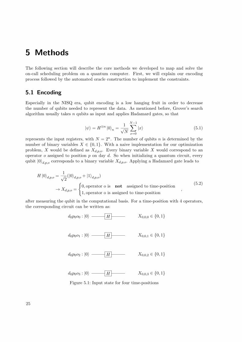
represents the input registers, with N = 2n. The number of qubits n is determined by thenumber of binary variables X ∈ {0, 1}. With a naive implementation for our optimizationproblem, X would be defined as Xd,p,o. Every binary variable X would correspond to anoperator o assigned to position p on day d. So when initializing a quantum circuit, everyqubit |0〉d,p,o corresponds to a binary variable Xd,p,o. Applying a Hadamard gate leads to

H |0〉d,p,o =1√2

(|0〉d,p,o + |1〉d,p,o)

→ Xd,p,o =

{0, operator o is not assigned to time-position

1, operator o is assigned to time-position,

(5.2)

after measuring the qubit in the computational basis. For a time-position with 4 operators,the corresponding circuit can be written as:

d0p0o0 : |0〉 H X0,0,0 ∈ {0, 1}

d0p0o1 : |0〉 H X0,0,1 ∈ {0, 1}

d0p0o2 : |0〉 H X0,0,2 ∈ {0, 1}

d0p0o3 : |0〉 H X0,0,3 ∈ {0, 1}

Figure 5.1: Input state for four time-positions

25

5 Methods

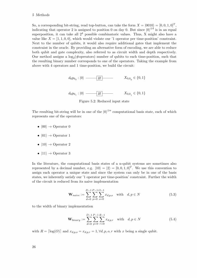
So, a corresponding bit-string, read top-button, can take the form X = |0010〉 = [0, 0, 1, 0]T ,indicating that operator 2 is assigned to position 0 on day 0. But since |0〉⊗4 is in an equalsuperposition, it can take all 24 possible combinatoric values. Thus, X might also have avalue like X = [1, 1, 0, 0], which would violate our ’1 operator per time-position’ constraint.Next to the number of qubits, it would also require additional gates that implement theconstraint in the oracle. By providing an alternative form of encoding, we are able to reduceboth qubit and gate complexity, also referred to as circuit width and depth respectively.Our method assigns a log2(#operators) number of qubits to each time-position, such thatthe resulting binary number corresponds to one of the operators. Taking the example fromabove with 4 operators and 1 time-position, we build the circuit:

d0p00 : |0〉 H X0,00∈ {0, 1}

d0p01 : |0〉 H X0,01∈ {0, 1}

Figure 5.2: Reduced input state

The resulting bit-string will be in one of the |0〉⊗n computational basis state, each of whichrepresents one of the operators:

• |00〉 → Operator 0

• |01〉 → Operator 1

• |10〉 → Operator 2

• |11〉 → Operator 3

In the literature, the computational basis states of a n-qubit systems are sometimes alsorepresented by a decimal number, e.g. |10〉 = |2〉 = [0, 0, 1, 0]T . We use this convention toassign each operator a unique state and since the system can only be in one of the basisstates, we inherently satisfy our ’1 operator per time-position’ constraint. Further the widthof the circuit is reduced from its naive implementation

Wnaive :=

D−1∑d=0

P−1∑p=0

O−1∑o=0

xd,p,o with d, p ∈ N (5.3)

to the width of binary implementation

Wbinary :=D−1∑d=0

P−1∑p=0

R−1∑r=0

xd,p,r with d, p ∈ N (5.4)

with R = dlog(O)e and xd,p,o = xd,p,r = 1,∀d, p, o, r with x being a single qubit.

26

5.2 Automatic Oracle Generation

5.2 Automatic Oracle Generation

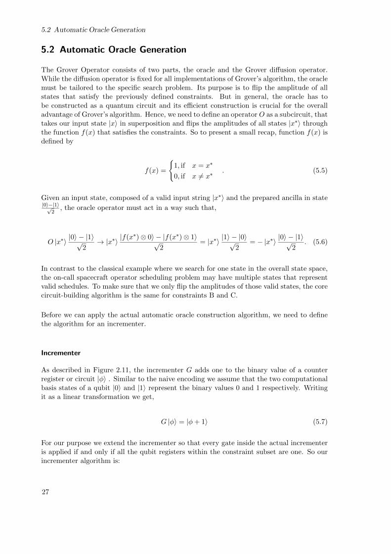
The Grover Operator consists of two parts, the oracle and the Grover diffusion operator.While the diffusion operator is fixed for all implementations of Grover’s algorithm, the oraclemust be tailored to the specific search problem. Its purpose is to flip the amplitude of allstates that satisfy the previously defined constraints. But in general, the oracle has tobe constructed as a quantum circuit and its efficient construction is crucial for the overalladvantage of Grover’s algorithm. Hence, we need to define an operator O as a subcircuit, thattakes our input state |x〉 in superposition and flips the amplitudes of all states |x∗〉 throughthe function f(x) that satisfies the constraints. So to present a small recap, function f(x) isdefined by

f(x) =

{1, if x = x∗

0, if x 6= x∗. (5.5)

Given an input state, composed of a valid input string |x∗〉 and the prepared ancilla in state|0〉−|1〉√

2, the oracle operator must act in a way such that,

O |x∗〉 |0〉 − |1〉√2→ |x∗〉 |f(x∗)⊗ 0〉 − |f(x∗)⊗ 1〉√

2= |x∗〉 |1〉 − |0〉√

2= − |x∗〉 |0〉 − |1〉√

2. (5.6)

In contrast to the classical example where we search for one state in the overall state space,the on-call spacecraft operator scheduling problem may have multiple states that representvalid schedules. To make sure that we only flip the amplitudes of those valid states, the corecircuit-building algorithm is the same for constraints B and C.

Before we can apply the actual automatic oracle construction algorithm, we need to definethe algorithm for an incrementer.

Incrementer

As described in Figure 2.11, the incrementer G adds one to the binary value of a counterregister or circuit |φ〉 . Similar to the naive encoding we assume that the two computationalbasis states of a qubit |0〉 and |1〉 represent the binary values 0 and 1 respectively. Writingit as a linear transformation we get,

G |φ〉 = |φ+ 1〉 (5.7)

For our purpose we extend the incrementer so that every gate inside the actual incrementeris applied if and only if all the qubit registers within the constraint subset are one. So ourincrementer algorithm is:

27

5 Methods

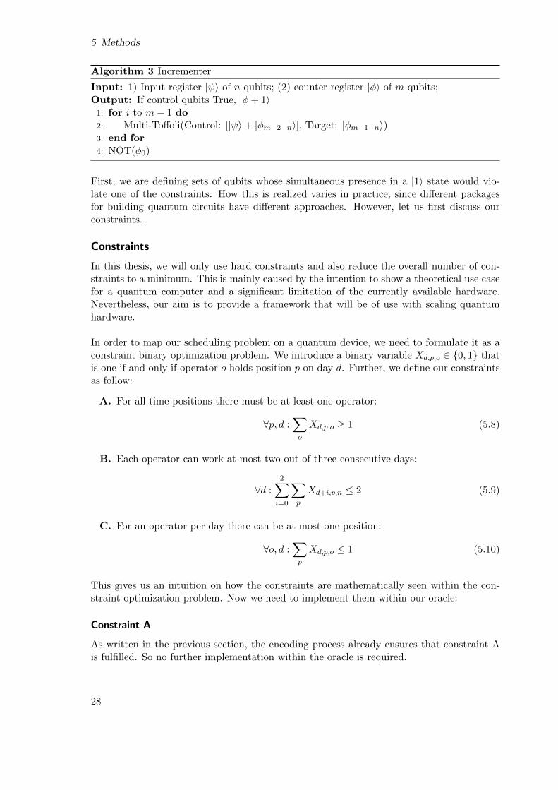
Algorithm 3 Incrementer

Input: 1) Input register |ψ〉 of n qubits; (2) counter register |φ〉 of m qubits;Output: If control qubits True, |φ+ 1〉

1: for i to m− 1 do2: Multi-Toffoli(Control: [|ψ〉+ |φm−2−n〉], Target: |φm−1−n〉)3: end for4: NOT(φ0)

First, we are defining sets of qubits whose simultaneous presence in a |1〉 state would vio-late one of the constraints. How this is realized varies in practice, since different packagesfor building quantum circuits have different approaches. However, let us first discuss ourconstraints.

Constraints

In this thesis, we will only use hard constraints and also reduce the overall number of con-straints to a minimum. This is mainly caused by the intention to show a theoretical use casefor a quantum computer and a significant limitation of the currently available hardware.Nevertheless, our aim is to provide a framework that will be of use with scaling quantumhardware.

In order to map our scheduling problem on a quantum device, we need to formulate it as aconstraint binary optimization problem. We introduce a binary variable Xd,p,o ∈ {0, 1} thatis one if and only if operator o holds position p on day d. Further, we define our constraintsas follow:

A. For all time-positions there must be at least one operator:

∀p, d :∑o

Xd,p,o ≥ 1 (5.8)

B. Each operator can work at most two out of three consecutive days:

∀d :2∑i=0

∑p

Xd+i,p,n ≤ 2 (5.9)

C. For an operator per day there can be at most one position:

∀o, d :∑p

Xd,p,o ≤ 1 (5.10)

This gives us an intuition on how the constraints are mathematically seen within the con-straint optimization problem. Now we need to implement them within our oracle:

Constraint A

As written in the previous section, the encoding process already ensures that constraint Ais fulfilled. So no further implementation within the oracle is required.

28

5.2 Automatic Oracle Generation

Constraint B

The first constraints states that on each day d an operator o can only be assigned to oneposition p. Since our operators are encoded as a binary number in a register for each positionon each day, we store the indices of all equal binary numbers within all positions for eachday.

Constraint C

The second constraint states that an operator is allowed to work at most two out of threedays. For that we store the indices of all equal binary numbers that appear on any positionover more than two days.

Now as we defined our constraints and stored the indices of the respective qubits, we applyour incrementer defined in Algorithm 3 iteratively on those sets. It takes the indices of eachconstraint subset and connects them through logical AND gates, so that the counter registeris only incremented if and only if all qubits, referred to by the indices within the constraintsubset, are |1〉. After the incrementer is implemented for every constraint, the counter reg-ister is checked for its value. If and only if the value of the counter register is 0, an X gateis applied on the Grover qubit, flipping all phases of the corresponding states according toEquation 5.6. Since the amplitude flipping is only possible through the entanglement ofthe input qubits and the whole Grover Operator must be applied multiple times, we needto de-entangle the states again after the phase flip. As the gates within incrementer areunitary, we just apply them in reversed order again for every constraint subset.1

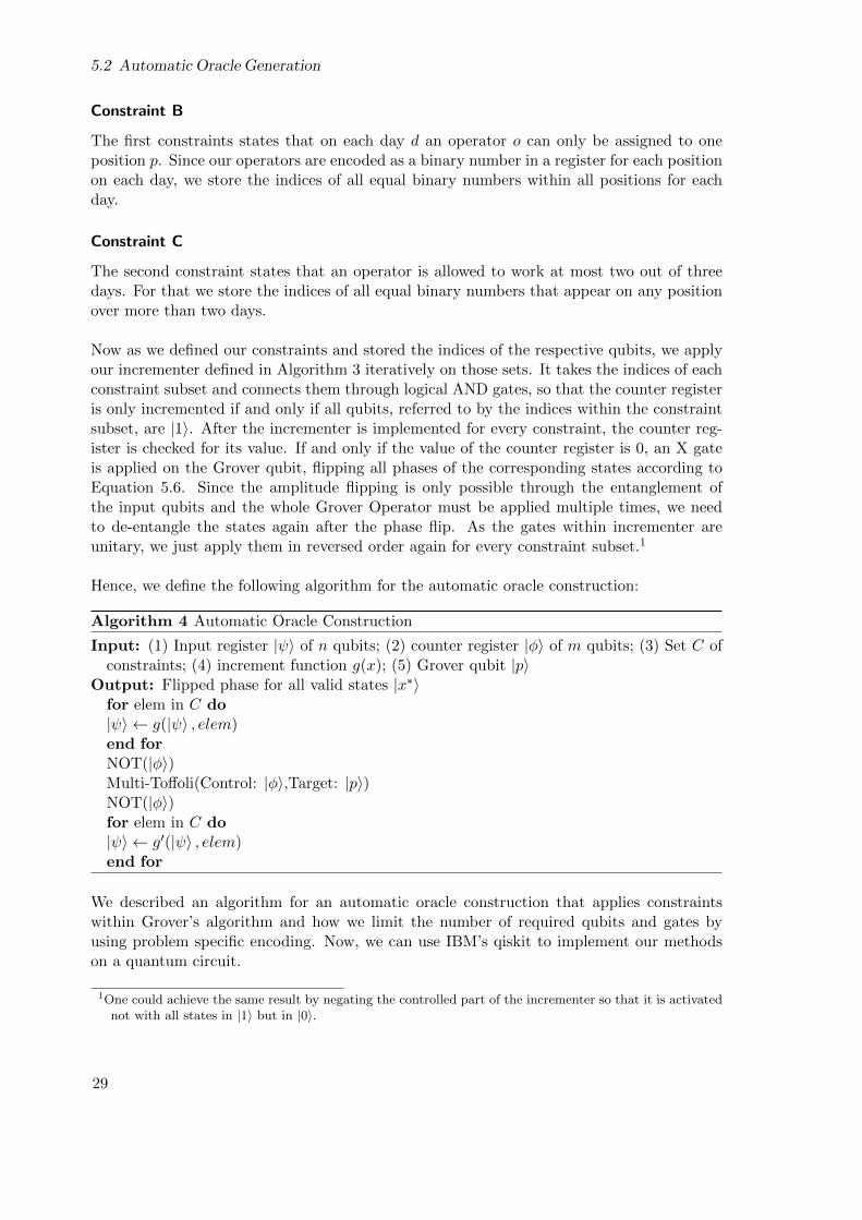
Hence, we define the following algorithm for the automatic oracle construction:

Algorithm 4 Automatic Oracle Construction

Input: (1) Input register |ψ〉 of n qubits; (2) counter register |φ〉 of m qubits; (3) Set C ofconstraints; (4) increment function g(x); (5) Grover qubit |p〉

Output: Flipped phase for all valid states |x∗〉for elem in C do|ψ〉 ← g(|ψ〉 , elem)end forNOT(|φ〉)Multi-Toffoli(Control: |φ〉,Target: |p〉)NOT(|φ〉)for elem in C do|ψ〉 ← g′(|ψ〉 , elem)end for

We described an algorithm for an automatic oracle construction that applies constraintswithin Grover’s algorithm and how we limit the number of required qubits and gates byusing problem specific encoding. Now, we can use IBM’s qiskit to implement our methodson a quantum circuit.

1One could achieve the same result by negating the controlled part of the incrementer so that it is activatednot with all states in |1〉 but in |0〉.

29

6 Implementation

In this section, we will use the previously stated methods and implement them using IBM’sQiskit. Snippets of the actual code and the underlying circuits will be shown and an evalua-tion of the results will be presented. We will also discuss how different numbers of iterationsand sizes of the counter register influence the results. All code is open source and can beaccessed on GitHub1.

Qiskit is an open-source quantum development tool created by IBM [Bib20]. It is writtenin Python and offers a variety of tools to create and manipulate quantum programs, whichthen can be either simulated on a local device or run on the IBM Q backend. Even thoughthere are a variety of pre-written quantum algorithms and optimization tools, we mainly useits Terra and Aer package to create quantum circuits at the machine code level and simulatethem respectively. The implementation itself follows three steps:

1. Circuit preparation

2. State preparation

3. Grover iteration

6.1 Circuit Preparation

Before we can apply quantum gates, we need to define an initial quantum circuit. In Qiskit,quantum circuits are composed of quantum registers, which in turn are composed of singlequbits. This has the advantage, that we can use the registers to clearly define the componentsof our circuit and also apply gates to registers instead of single qubits.

Encoding

Following Section 5.1, we define every time position as a binary number that we implementas a quantum register. The length of those registers, e.g. the number of required qubits, isgiven by log(operators) with operators being the number of operators:

1 # Defines the number of qubits needed to represent the operators as a binary

number

2 log2_operators = math.ceil(math.log2(operators))

The quantum registers are created and stored in a dictionary. This is not only handy forfuture access, but also required by Qiskit to generate quantum circuits on the fly. The vari-able operators, days, positions are defined as the number of their respective entities:

1https://github.com/schererant/operator-scheduling

31

6 Implementation

1 # QuantumRegisters with time positions are created in a dictionary

2 time_positions = {’p%id%i’%(position ,day): QuantumRegister(log2_operators ,

’p%id%i’%(position ,day)) for day in range(days) for position in range(

positions)}

Input Register

Since there is one time-position for each position on every day, the overall input register size

1 # Calculate number of input register qubits

2 var_size = positions * days * log2_operators

For our batch size, the overall number of input qubits is 12 separated in 6 quantum registersa two qubits.

Counter Register

To implement the constraints as in Algorithm 4, a counter register is required, which needsto be incremented for every forbidden state. Additional working qubits are often calledancilla qubits and as we reverse our incrementer, the counter register is reusable for everyGrover iteration. The size of the counter register is approximately growing with O(log(n))with n being the input register size.

1 anc = QuantumRegister(counter_size , ’counter ’)

Oracle Qubit

The oracle qubit will be initialized in |−〉 and is required to flip the amplitude of the validstates. Like the counter register, it is reusable, so its size is fixed to one. Even though itonly has one qubit, for consistency we assign it its own register:

1 f = QuantumRegister (1, ’oracle_qubit ’)

Initial Circuit

Now, we compose all the registers from above in one quantum circuit:

1 # Quantum Circuit gets assembled from the time_position dictionary

2 qc = QuantumCircuit (*[ qubit for qubit in time_positions.values ()], anc ,

measure , f)

To ensure a lucid layout, the circuit is reduced to 2 time-positions and 2 counter qubits.

6.2 State preparation

As mentioned above, two main preparations are required: The oracle qubit register in |−〉and the input registers containing the time-position must be brought in a superposition overall input registers. Please note that Qiskit always initializes a qubit in |0〉.

32

6.3 Grover iteration

Oracle Qubit preparation

By applying the X gate we flip to |1〉 and the Hadamard gate will bring us to |−〉. With qcbeing the initial quantum circuit, we apply both gates through:

1 # Output register gets prepared in |->

2 qc.x(f[0])

3 qc.h(f[0])

Input register preparation

To prepare the input register, we apply a Hadamard gate on every qubit. So with n beingthe size of the input register, we get:

H⊗n |0〉⊗n =1√2n

2n∑x=0

|x〉 (6.1)

The implementation with Qiskit is fairly easy and follows the stated logic:

1 # Input register initialized with hadamard gates

2 for i in range(n):

3 qc.h(i)

Of course it is also possible to apply the Hadamard gate on a whole register, but since ourinput register consists of multiple smaller registers, it is easier to loop through the length ofthe input register.

6.3 Grover iteration

After we prepared the input state, we now implement the Grover operator or iteration,consisting of the oracle and Grover’s diffusion operator.

Oracle Construction

We construct the oracle according to Algorithm 4. The following will present the implemen-tation of both constraints in Figure 2.5. We go into detail for constraint B and just givean outlook for constraint C. This has two reasons: 1. our example circuit has just one dayand therefore fulfills constraint C a priori and 2. the underlying structure is similar in bothcases. Before we start, we need to define how the incrementer is implemented since it is acrucial part of the oracle. For a more in-depth explanation of the incrementer algorithm seeAlgorithm 3.

Incrementer

There is a lot of discussion on how to potentially implement an efficient quantum adder. Forfurther literature see [NC02] and [Gid20]. In our case, we do not need a reversible quantumadder per se. We just build an incrementer consisting of n multi-Toffoli gates, with n beingthe number of counter register qubits. We build two gate groups, one to increment and oneto decrement, given in Figure 6.1.

33

6 Implementation

|ψ〉 : |0〉 • •

counter0 : |0〉

counter1 : |0〉

f0 : |−〉(a) Increment

|ψ〉 : |0〉 • •

counter0 : |0〉

counter1 : |0〉

f0 : |−〉(b) Decrement

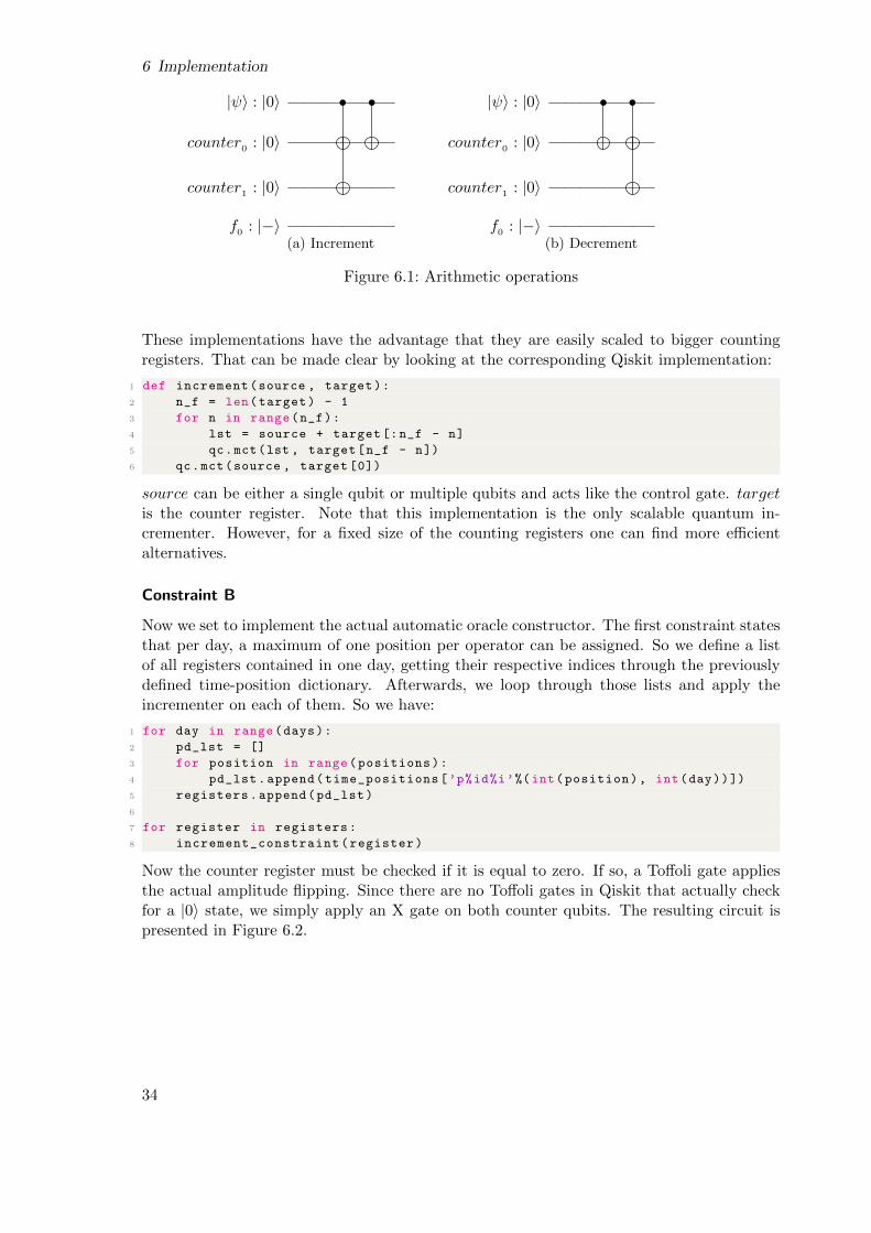
Figure 6.1: Arithmetic operations

These implementations have the advantage that they are easily scaled to bigger countingregisters. That can be made clear by looking at the corresponding Qiskit implementation:

1 def increment(source , target):

2 n_f = len(target) - 1

3 for n in range(n_f):

4 lst = source + target [:n_f - n]

5 qc.mct(lst , target[n_f - n])

6 qc.mct(source , target [0])

source can be either a single qubit or multiple qubits and acts like the control gate. targetis the counter register. Note that this implementation is the only scalable quantum in-crementer. However, for a fixed size of the counting registers one can find more efficientalternatives.

Constraint B

Now we set to implement the actual automatic oracle constructor. The first constraint statesthat per day, a maximum of one position per operator can be assigned. So we define a listof all registers contained in one day, getting their respective indices through the previouslydefined time-position dictionary. Afterwards, we loop through those lists and apply theincrementer on each of them. So we have:

1 for day in range(days):

2 pd_lst = []

3 for position in range(positions):

4 pd_lst.append(time_positions[’p%id%i’%(int(position), int(day))])

5 registers.append(pd_lst)

6

7 for register in registers:

8 increment_constraint(register)

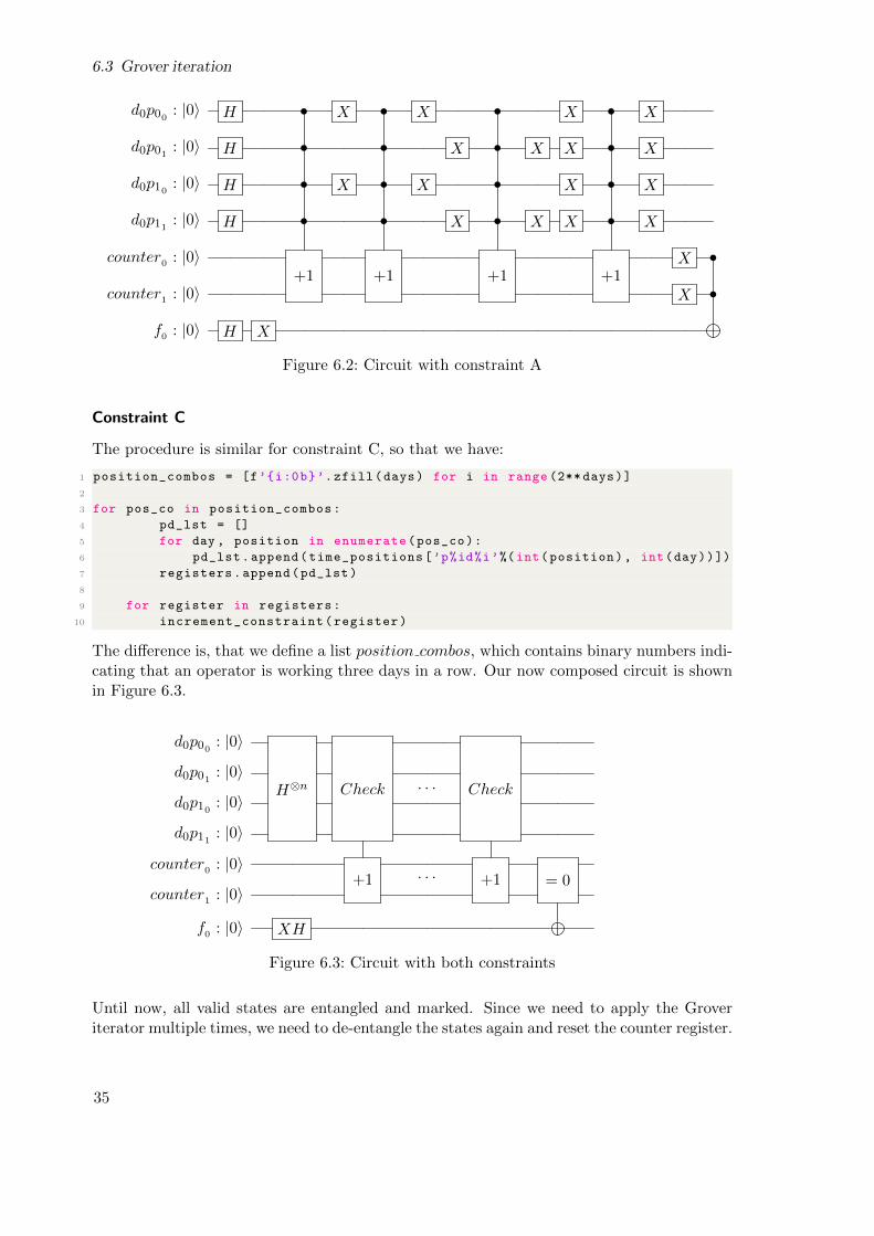
Now the counter register must be checked if it is equal to zero. If so, a Toffoli gate appliesthe actual amplitude flipping. Since there are no Toffoli gates in Qiskit that actually checkfor a |0〉 state, we simply apply an X gate on both counter qubits. The resulting circuit ispresented in Figure 6.2.

34

6.3 Grover iteration

d0p00 : |0〉 H • X • X • X • X

d0p01 : |0〉 H • • X • X X • X

d0p10 : |0〉 H • X • X • X • X

d0p11 : |0〉 H • • X • X X • X

counter0 : |0〉+1 +1 +1 +1

X •

counter1 : |0〉 X •

f0 : |0〉 H X

Figure 6.2: Circuit with constraint A

Constraint C

The procedure is similar for constraint C, so that we have:

1 position_combos = [f’{i:0b}’.zfill(days) for i in range (2** days)]

2

3 for pos_co in position_combos:

4 pd_lst = []

5 for day , position in enumerate(pos_co):

6 pd_lst.append(time_positions[’p%id%i’%(int(position), int(day))])

7 registers.append(pd_lst)

8

9 for register in registers:

10 increment_constraint(register)

The difference is, that we define a list position combos, which contains binary numbers indi-cating that an operator is working three days in a row. Our now composed circuit is shownin Figure 6.3.

d0p00: |0〉

H⊗n Check · · · Checkd0p01

: |0〉

d0p10: |0〉

d0p11: |0〉

· · ·counter0 : |0〉

+1 +1 = 0counter1 : |0〉

f0 : |0〉 XH

Figure 6.3: Circuit with both constraints

Until now, all valid states are entangled and marked. Since we need to apply the Groveriterator multiple times, we need to de-entangle the states again and reset the counter register.

35

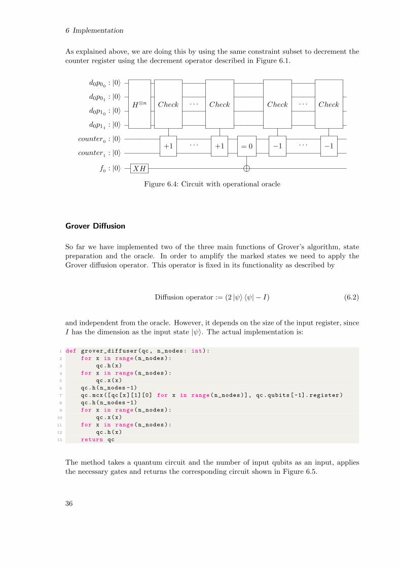
6 Implementation

As explained above, we are doing this by using the same constraint subset to decrement thecounter register using the decrement operator described in Figure 6.1.

d0p00 : |0〉

H⊗n Check · · · Check Check · · · Checkd0p01 : |0〉

d0p10 : |0〉

d0p11 : |0〉

· · · · · ·counter0 : |0〉

+1 +1 = 0 −1 −1counter1 : |0〉

f0 : |0〉 XH

Figure 6.4: Circuit with operational oracle

Grover Diffusion

So far we have implemented two of the three main functions of Grover’s algorithm, statepreparation and the oracle. In order to amplify the marked states we need to apply theGrover diffusion operator. This operator is fixed in its functionality as described by

Diffusion operator := (2 |ψ〉 〈ψ| − I) (6.2)

and independent from the oracle. However, it depends on the size of the input register, sinceI has the dimension as the input state |ψ〉. The actual implementation is:

1 def grover_diffuser(qc , n_nodes: int):

2 for x in range(n_nodes):

3 qc.h(x)

4 for x in range(n_nodes):

5 qc.x(x)

6 qc.h(n_nodes -1)

7 qc.mcx([qc[x][1][0] for x in range(n_nodes)], qc.qubits [-1]. register)

8 qc.h(n_nodes -1)

9 for x in range(n_nodes):

10 qc.x(x)

11 for x in range(n_nodes):

12 qc.h(x)

13 return qc

The method takes a quantum circuit and the number of input qubits as an input, appliesthe necessary gates and returns the corresponding circuit shown in Figure 6.5.

36

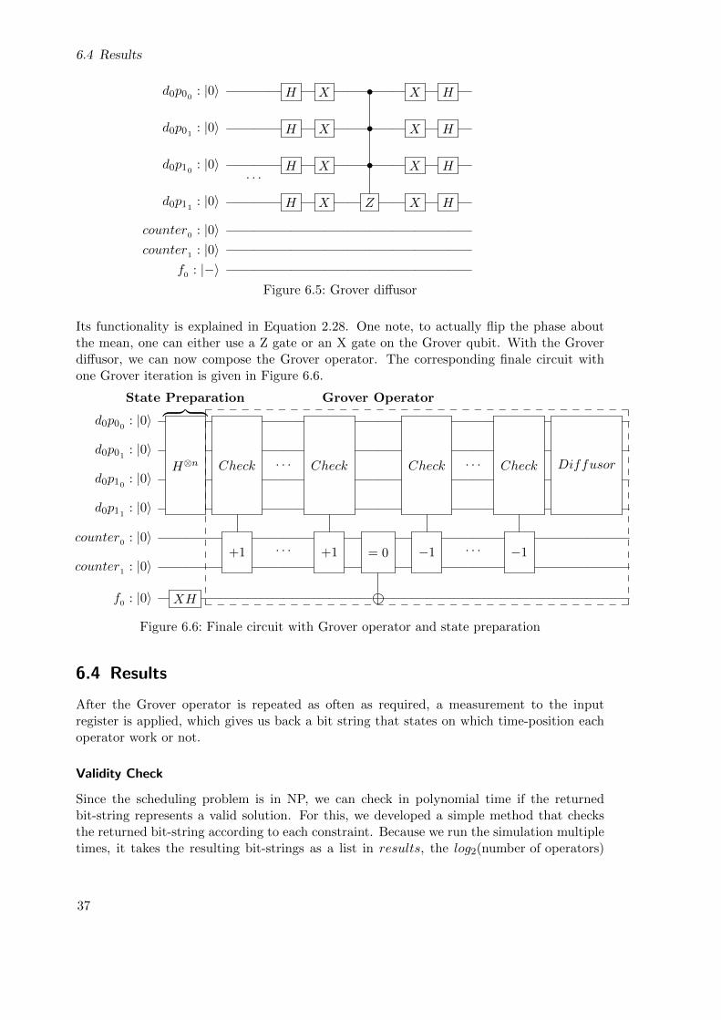
6.4 Results

d0p00: |0〉

· · ·

H X • X H

d0p01: |0〉 H X • X H

d0p10: |0〉 H X • X H

d0p11: |0〉 H X Z X H

counter0 : |0〉counter1 : |0〉

f0 : |−〉Figure 6.5: Grover diffusor

Its functionality is explained in Equation 2.28. One note, to actually flip the phase aboutthe mean, one can either use a Z gate or an X gate on the Grover qubit. With the Groverdiffusor, we can now compose the Grover operator. The corresponding finale circuit withone Grover iteration is given in Figure 6.6.

State Preparation Grover Operator

d0p00: |0〉

H⊗n Check · · · Check Check · · · Check Diffusord0p01

: |0〉

d0p10: |0〉

d0p11: |0〉

· · · · · ·counter0 : |0〉

+1 +1 = 0 −1 −1counter1 : |0〉

f0 : |0〉 XH

︷ ︸︸ ︷

Figure 6.6: Finale circuit with Grover operator and state preparation

6.4 Results

After the Grover operator is repeated as often as required, a measurement to the inputregister is applied, which gives us back a bit string that states on which time-position eachoperator work or not.

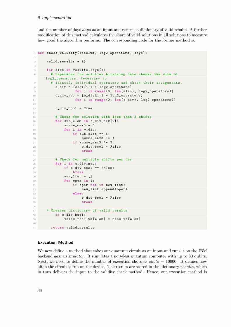
Validity Check

Since the scheduling problem is in NP, we can check in polynomial time if the returnedbit-string represents a valid solution. For this, we developed a simple method that checksthe returned bit-string according to each constraint. Because we run the simulation multipletimes, it takes the resulting bit-strings as a list in results, the log2(number of operators)

37

6 Implementation

and the number of days days as an input and returns a dictionary of valid results. A furthermodification of this method calculates the share of valid solutions in all solutions to measurehow good the algorithm performs. The corresponding code for the former method is:

1 def check_validity(results , log2_operators , days):

2

3 valid_results = {}

4

5 for elem in results.keys():

6 # Separates the solution bitstring into chunks the size of

log2_operators. Necessary to

7 # identify individual operators and check their assignments.

8 o_div = [elem[i:i + log2_operators]

9 for i in range(0, len(elem), log2_operators)]

10 o_div_new = [o_div[i:i + log2_operators]

11 for i in range(0, len(o_div), log2_operators)]

12

13 o_div_bool = True

14

15 # Check for solution with less than 3 shifts

16 for sub_elem in o_div_new [0]:

17 summe_max3 = 0

18 for i in o_div:

19 if sub_elem == i:

20 summe_max3 += 1

21 if summe_max3 >= 3:

22 o_div_bool = False

23 break

24

25 # Check for multiple shifts per day

26 for i in o_div_new:

27 if o_div_bool == False:

28 break

29 new_list = []

30 for oper in i:

31 if oper not in new_list:

32 new_list.append(oper)

33 else:

34 o_div_bool = False

35 break

36

37 # Creates dictionary of valid results

38 if o_div_bool:

39 valid_results[elem] = results[elem]

40

41 return valid_results

Execution Method

We now define a method that takes our quantum circuit as an input and runs it on the IBMbackend qasm simulator. It simulates a noiseless quantum computer with up to 30 qubits.Next, we need to define the number of execution shots as shots = 10000. It defines howoften the circuit is run on the device. The results are stored in the dictionary results, whichin turn delivers the input to the validity check method. Hence, our execution method is

38

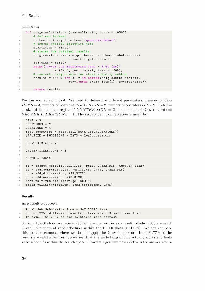
6.4 Results

defined as:

1 def run_simulator(qc: QuantumCircuit , shots = 10000):

2 # defines backend

3 backend = Aer.get_backend(’qasm_simulator ’)

4 # tracks overall execution time

5 start_time = time()

6 # stores the original results

7 orig_counts = execute(qc, backend=backend , shots=shots)

8 .result ().get_counts ()

9 end_time = time()

10 print("Total Job Submission Time - %.5f (ms)"

11 % (( end_time - start_time) * 1000))

12 # converts orig_counts for check_validity method

13 results = {k: v for k, v in sorted(orig_counts.items (),

14 key=lambda item: item[1], reverse=True)}

15

16 return results

We can now run our tool. We need to define five different parameters: number of daysDAY S = 3, number of positions POSITIONS = 2, number of operators OPERATORS =4, size of the counter register COUNTER SIZE = 2 and number of Grover iterationsGROV ER ITERATIONS = 1. The respective implementation is given by:

1 DAYS = 3

2 POSITIONS = 2

3 OPERATORS = 4

4 log2_operators = math.ceil(math.log2(OPERATORS))

5 VAR_SIZE = POSITIONS * DAYS * log2_operators

6

7 COUNTER_SIZE = 2

8

9 GROVER_ITERATIONS = 1

10

11 SHOTS = 10000

12

13 qc = create_circuit(POSITIONS , DAYS , OPERATORS , COUNTER_SIZE)

14 qc = add_constraint(qc, POSITIONS , DAYS , OPERATORS)

15 qc = add_diffuser(qc, VAR_SIZE)

16 qc = add_measure(qc, VAR_SIZE)

17 results = run_simulator(qc , SHOTS)

18 check_validity(results , log2_operators , DAYS)

Results

As a result we receive:

1 Total Job Submission Time - 547.50896 (ms)

2 Out of 2357 different results , there are 863 valid results.

3 In total , 61.05 % of the solutions were correct.

So from 10.000 shots, we receive 2357 different schedules as a result, of which 863 are valid.Overall, the share of valid schedules within the 10.000 shots is 61.05%. We can comparethis to a benchmark, where we do not apply the Grover operator. Here 21.77% of theresults are valid schedules. So we see, that the underlying circuit actually works and findsvalid schedules within the search space. Grover’s algorithm never delivers the answer with a

39

6 Implementation

probability of one, that is why we need to run the circuit multiple times. If we can increasethe share of valid schedules will be the subject of further studies.

To return a solution, we simply pick the state with the highest occurrence. In this case, thecorresponding schedule is:

OnCall Operator Schedule

Days Day 0 Day 1 Day 2

Operator 0 Position 0 — —Operator 1 Position 1 — Position 0Operator 2 — Position 1 Position 1Operator 3 — Position 0 —

6.5 Evaluation

The following section will further evaluate the results and show how our model would performon a real quantum device. It will end with an outlook on how in general methods based onGrover’s algorithm perform in the NISQ era.

Optimal number of iterations and size of the counter register

To check whether we found the optimal number of Grover iterations, we can run the circuitmultiple times with different iterations. Starting from zero iterations, our above-mentionedbenchmark, we expect a sinusoidal change in correct solutions with a growing number ofiterations. As we can see in Figure 6.7, the share of correct solutions is indeed at its peakwith one Grover iteration. Further, we can check how different sizes of the counter registeraffect the share of correct solutions. As Figure 6.8 indicates, a counter register of two qubitsis necessary to identify all the constraints. It is important to keep the size of the counterregister low, since additional qubits are either rare with real quantum devices or increase ourcomputational time significantly as shown in Figure 6.9. So our choice of a counter registerconsisting of two qubits is optimal.

Width and depth of our circuit

After we determined the optimal number of iterations and counter qubits, we can definethe gate complexity and the width and depth of the circuit. With a problem size of fouroperators, three days and two positions, as well as a counter register of two qubits and oneGrover iteration, the overall width of the circuit is 27. Included are 15 qubits and 12 classicalmeasurement bits. Its depth is 320, with a gate complexity of 738 consisting of 509 X-gates,177 multi-Toffoli gates and 39 Hadamard gates. 2

2Since real quantum devices can not implement multi-Toffoli gates directly, we would need to further tran-spile the circuit so that it only consists of rotation gates, here denoted as u3, and CX gates. This wouldlead to a circuit depth of 86749 and a gate complexity of 104906, consisting of 52988 u3 gates and 51906CX gates.

40

6.5 Evaluation

Run on real quantum device

So far, we used IBM’s Aer package with the qasm simulator to simulate a perfect quantumcomputer, since current, publicly available devices do either not have enough qubits to runour circuit or the calculation time of our circuits exceeds the time limit on the devices. How-ever, there is a way to test its performance on a quantum computer. We can use artificialnoise that imitates the error rates of a NISQ era device.Qiskit offers a variety of options to introduce noise while executing on the qasm simulator.One can either manually assign different error rates to certain gates or use the error rates of anexisting quantum device. In our example, we use the noise of the backend ’ibmq 16 melbourne’,which is available through the IBMQ cloud. It has 15 super-conducting qubits with a quan-tum volume of 8. 3 So executing the same circuit as above leads to:

1 Total Job Submission Time - 5493257.68423 (ms)

2 Out of 4096 different results , there are 912 valid results.

3 In total , 29.287000000000003 % of the solutions were correct.

We see that the result is similar to our benchmark, a near uniform distribution of all possiblestates. As an effect, the solution states are no longer distinguishable from the other states,which means that our method no longer returns a solution to the scheduling problem. Thoseresults are mainly explained through the high error rates of current quantum devices likethe ’ibmq 16 melbourne’. While the error rate could be reduced by the application of quan-tum error correction, this would in turn require more qubits and gates that would furthershrink our executable problem sizes. The relatively long submission time is caused by thetranspilation of the circuit and by simulating the error for each gate.

This leads to the general question, whether it makes sense to implement our method on NISQera devices. We showed that even small problem sizes require a circuit length or depth thatare not implementable on current quantum computers. But there is even a further discussionon whether a quadratic speed up, as provided maximally by Grover’s algorithm, is enoughto provide a quantum advantage in a time where expensive error correction must be applied.

Quadratic speedups on NISQ era devises

[BMG+20] addresses this question by investigating which conditions must be satisfied suchthat a polynomial speedup realizes an actual quantum advantage in a fault-tolerant quantumdevice. Especially algorithms that use amplitude amplification, such as Grover’s algorithm,are highly parallelizable on classical devices, which can lead to speedups up to an order of103. Unfortunately, this does not shine a good light on the use of quantum algorithms thatprovide a quadratic speedup on NISQ era devices, since the ’break-even’ point of quantumadvantage in runtime lies at up to 880 years if the classical solution is parallelized. But thereis some hope since only a quartic polynomial speedup would reduce this ’break-even’ point to29 minutes for the same parallelism speedup. Such query reduction algorithms were proposedby [ABB+17] and [ABDKT20], but are still short of a practical use case and implementation.

In this chapter we showed the implementation of our method using Qiskit. We executedthe method on its qasm simulator, presented and evaluated the results and showed what

3Quantum Volume is a measurement of quantum computational performance introduced by IBM. For moreinformation see [CBS+19]

41

6 Implementation

an execution on a noisy current quantum device would return. In the end we discussed thegeneral question whether it makes sense to implement our method on a NISQ era quantumdevice.

42

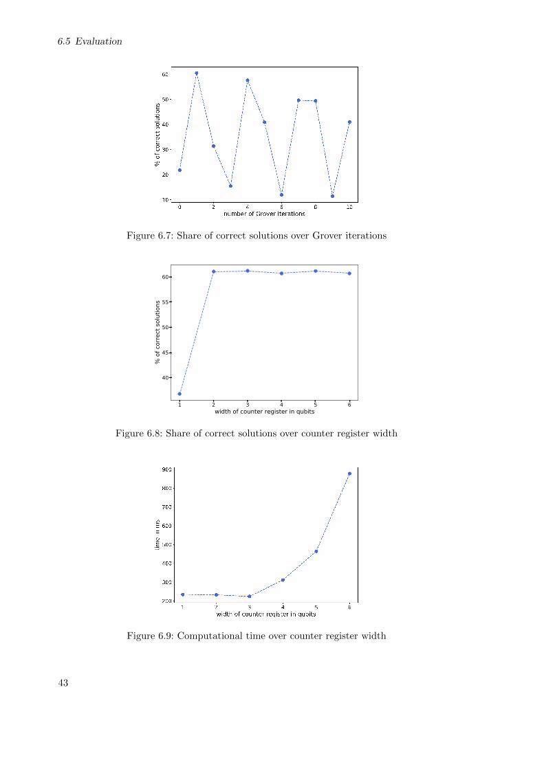
6.5 Evaluation

Figure 6.7: Share of correct solutions over Grover iterations

1 2 3 4 5 6width of counter register in qubits

40

45

50

55

60

% o

f cor

rect

solu

tions

Figure 6.8: Share of correct solutions over counter register width

Figure 6.9: Computational time over counter register width

43

7 Conclusion

This thesis provides a scalable method to solve a scheduling problem with Grover’s searchalgorithm. As an example, we use the on-call spacecraft operator scheduling problem facedby the German Aerospace Center, which seeks for an optimal assignment of 52 operators to17 positions over a period of 180 days, under constraints on schedule and personnel. Witha quadratic computational speed up, Grover’s algorithm promises to find an optimal solu-tion for the underlying combinatorial optimization problem. As NISQ era quantum devicesare scarce in available qubits, we developed a new way of mapping the problem onto therespective qubits. In contrast to the usual one-to-one mapping of each combinatorial binaryvariable to a qubit, we represent every operator through a binary number in a quantumregister for every time-position. This graph coloring inspired encoding process reduces thenumber of required qubits significantly and simultaneously implements one of our three con-straints. The remaining two constraints are implemented in the oracle, for which we createdan automatic construction method that scales with different problem sizes. This is necessary,since the available number of qubits do not allow the encoding and solving of the whole prob-lem size. To test the functionality of our implementation, we reduced the problem size to abatch consisting of 4 operators, 2 positions and 3 days. For this instance, we executed ourcircuit on Qiskit’s qasm simulator which imitates a noiseless quantum computer. The resultsshow that our implementation finds a solution to our problem within the search space. Forour reduced batch size, we further evaluated the optimal number of Grover iterations andthe required number of counting qubits for our automatic oracle construction method. Dueto the length of our circuit, we were not able to test our implementation on a real quantumdevice, but a simulation of the expected level of noise on the qasm simulator showed that theerror rate is too high to produce valid results. Even though it became clear that solving theon-call operator scheduling problem on real quantum devices is not feasible at the moment,our scalable implementation can be used to assess the performance of Grover’s algorithm onfuture quantum devices. For that, the presented code is publicly available on GitHub1.

Future work

While Grover’s algorithm provides at most a quadratic speedup, the actually achievedspeedup varies with the respective implementation. Therefore, the lower and upper boundsof our implementation should be defined and compared to the performance of state-of-the-artclassical algorithms. Further, it should be investigated whether the share of correct solutionscan be improved and how it changes with a growing number of implemented constraints.To improve performance, it might also be necessary to optimize the oracle by eliminatingredundant gates and to study the potential use of methods like autoencoders to furtherenhance the encoding process. Another direction of future work would be to expand theconstraint space and consider the optimziation of soft constraints, which would also allow afull integration of the method within the German Aerospace Center’s scheduling tool.

1https://github.com/schererant/operator-scheduling

45

List of Figures

2.1 The Bloch Sphere . . . . . . . . . . . . . . . . . . . . . . . . . . . . . . . . . . 42.2 Bell State Circuit . . . . . . . . . . . . . . . . . . . . . . . . . . . . . . . . . . 82.3 CNOT Gate . . . . . . . . . . . . . . . . . . . . . . . . . . . . . . . . . . . . . 82.4 Bell State Circuit with Measurement . . . . . . . . . . . . . . . . . . . . . . . 82.5 Prepared Circuit . . . . . . . . . . . . . . . . . . . . . . . . . . . . . . . . . . 112.6 Oracle Circuit . . . . . . . . . . . . . . . . . . . . . . . . . . . . . . . . . . . . 122.7 Grover Operator Circuit . . . . . . . . . . . . . . . . . . . . . . . . . . . . . . 132.8 Amplitudes of states before Grover operator . . . . . . . . . . . . . . . . . . . 142.9 Amplitudes of states after oracle application . . . . . . . . . . . . . . . . . . . 142.10 Amplitudes of states after Grover operator . . . . . . . . . . . . . . . . . . . . 142.11 Quantum Incrementer . . . . . . . . . . . . . . . . . . . . . . . . . . . . . . . 152.12 Complexity Classes . . . . . . . . . . . . . . . . . . . . . . . . . . . . . . . . . 16

5.1 Input State . . . . . . . . . . . . . . . . . . . . . . . . . . . . . . . . . . . . . 255.2 Encoded Input State . . . . . . . . . . . . . . . . . . . . . . . . . . . . . . . . 26

6.1 Arithmetic Operations . . . . . . . . . . . . . . . . . . . . . . . . . . . . . . . 346.2 Circuit with constraint B . . . . . . . . . . . . . . . . . . . . . . . . . . . . . 356.3 Circuit with both constraints . . . . . . . . . . . . . . . . . . . . . . . . . . . 356.4 Circuit with operational oracle . . . . . . . . . . . . . . . . . . . . . . . . . . 366.5 Grover Diffusor circuit . . . . . . . . . . . . . . . . . . . . . . . . . . . . . . . 376.6 Finale circuit with Grover operator and state preparation . . . . . . . . . . . 376.7 Share of correct solutions over Grover iterations . . . . . . . . . . . . . . . . . 436.8 Share of correct solutions over counter register width . . . . . . . . . . . . . . 436.9 Computational time over counter register width . . . . . . . . . . . . . . . . . 43

47

Bibliography

[ABB+17] Ambainis, Andris ; Balodis, Kaspars ; Belovs, Aleksandrs ; Lee, Troy ;Santha, Miklos ; Smotrovs, Juris: Separations in query complexity based onpointer functions. In: Journal of the ACM (JACM) 64 (2017), Nr. 5, S. 1–24

[ABDKT20] Aaronson, Scott ; Ben-David, Shalev ; Kothari, Robin ; Tal, Avishay:Quantum Implications of Huang’s Sensitivity Theorem. In: arXiv preprintarXiv:2004.13231 (2020)

[ABHW73] Abernathy, William J. ; Baloff, Nicholas ; Hershey, John C. ; Wandel,Sten: A three-stage manpower planning and scheduling model—a service-sectorexample. In: Operations Research 21 (1973), Nr. 3, S. 693–711

[ABL06] Aickelin, Uwe ; Burke, Edmund K. ; Li, Jingpeng: Improved squeaky wheeloptimisation for driver scheduling. In: Parallel Problem Solving from Nature-PPSN IX. Springer, 2006, S. 182–191

[ABL08] Aickelin, Uwe ; Burke, Edmund K. ; Li, Jingpeng: An evolutionary squeakywheel optimization approach to personnel scheduling. In: IEEE Transactionson evolutionary computation 13 (2008), Nr. 2, S. 433–443

[AVDK+08] Aharonov, Dorit ; Van Dam, Wim ; Kempe, Julia ; Landau, Zeph ; Lloyd,Seth ; Regev, Oded: Adiabatic quantum computation is equivalent to standardquantum computation. In: SIAM review 50 (2008), Nr. 4, S. 755–787

[AZD13] Akbari, Mohammad ; Zandieh, M ; Dorri, Behrouz: Scheduling part-timeand mixed-skilled workers to maximize employee satisfaction. In: The Inter-national Journal of Advanced Manufacturing Technology 64 (2013), Nr. 5-8, S.1017–1027

[BBDB+13] Bergh, Jorne Van d. ; Belien, Jeroen ; De Bruecker, Philippe ; Demeule-meester, Erik ; De Boeck, Liesje: Personnel scheduling: A literature review.In: European journal of operational research 226 (2013), Nr. 3, S. 367–385

[BBK+10] Bai, Ruibin ; Burke, Edmund K. ; Kendall, Graham ; Li, Jingpeng ; Mc-Collum, Barry: A hybrid evolutionary approach to the nurse rostering prob-lem. In: IEEE Transactions on Evolutionary Computation 14 (2010), Nr. 4, S.580–590

[BBW03] Bulger, David ; Baritompa, William P. ; Wood, Graham R.: Implement-ing pure adaptive search with Grover’s quantum algorithm. In: Journal ofoptimization theory and applications 116 (2003), Nr. 3, S. 517–529

49

Bibliography

[Ben82] Benioff, Paul: Quantum mechanical hamiltonian models of turing machines.29 (1982), Nov, Nr. 3, S. 515–546. http://dx.doi.org/10.1007/BF01342185.– DOI 10.1007/BF01342185. – ISSN 1572–9613

[BHMT02] Brassard, Gilles ; Hoyer, Peter ; Mosca, Michele ; Tapp, Alain: Quantumamplitude amplification and estimation. In: Contemporary Mathematics 305(2002), S. 53–74

[Bib20] Qiskit. https://qiskit.org. Version: Dec 2020. – [Online; accessed 12. Dec.2020]

[BMG+20] Babbush, Ryan ; McClean, Jarrod ; Gidney, Craig ; Boixo, Sergio ; Neven,Hartmut: Focus beyond quadratic speedups for error-corrected quantum ad-vantage. In: arXiv preprint arXiv:2011.04149 (2020)

[Bra97] Brassard, Gilles: Searching a quantum phone book. In: Science 275 (1997),Nr. 5300, S. 627–628

[BV97] Bernstein, Ethan ; Vazirani, Umesh: Quantum complexity theory. In:SIAM Journal on computing 26 (1997), Nr. 5, S. 1411–1473

[BW06] Bard, Jonathan F. ; Wan, Lin: The task assignment problem for unrestrictedmovement between workstation groups. In: Journal of Scheduling 9 (2006), Nr.4, S. 315–341

[CBS+19] Cross, Andrew W. ; Bishop, Lev S. ; Sheldon, Sarah ; Nation, Paul D. ;Gambetta, Jay M.: Validating quantum computers using randomized modelcircuits. In: Physical Review A 100 (2019), Nr. 3, S. 032328

[CLPR10] Cordeau, Jean-Francois ; Laporte, Gilbert ; Pasin, Federico ; Ropke, Ste-fan: Scheduling technicians and tasks in a telecommunications company. In:Journal of Scheduling 13 (2010), Nr. 4, S. 393–409

[Dan54] Dantzig, George B.: Letter to the editor—A comment on Edie’s “Traffic delaysat toll booths”. In: Journal of the Operations Research Society of America 2(1954), Nr. 3, S. 339–341

[DH96] Durr, Christoph ; Hoyer, Peter: A quantum algorithm for finding the mini-mum. In: arXiv preprint quant-ph/9607014 (1996)

[Edi54] Edie, Leslie C.: Traffic delays at toll booths. In: Journal of the operationsresearch society of America 2 (1954), Nr. 2, S. 107–138

[EPR35] Einstein, Albert ; Podolsky, Boris ; Rosen, Nathan: Can quantum-mechanical description of physical reality be considered complete? In: Physicalreview 47 (1935), Nr. 10, S. 777

[exa20] examples dwave: employee-scheduling. https://github.com/

dwave-examples/employee-scheduling. Version: Dec 2020. – [Online;accessed 13. Dec. 2020]

50

Bibliography

[Fey82] Feynman, Richard P.: Simulating physics with computers. 21 (1982),Jun, Nr. 6, S. 467–488. http://dx.doi.org/10.1007/BF02650179. – DOI10.1007/BF02650179. – ISSN 1572–9575

[FGG14] Farhi, Edward ; Goldstone, Jeffrey ; Gutmann, Sam: A quantum approx-imate optimization algorithm. In: arXiv preprint arXiv:1411.4028 (2014)

[FGGS00] Farhi, Edward ; Goldstone, Jeffrey ; Gutmann, Sam ; Sipser, Michael:Quantum computation by adiabatic evolution. In: arXiv preprint quant-ph/0001106 (2000)

[FH16] Farhi, Edward ; Harrow, Aram W.: Quantum supremacy through the quan-tum approximate optimization algorithm. In: arXiv preprint arXiv:1602.07674(2016)

[GDT09] Goodman, Melissa D. ; Dowsland, Kathryn A. ; Thompson, Jonathan M.: Agrasp-knapsack hybrid for a nurse-scheduling problem. In: Journal of Heuristics15 (2009), Nr. 4, S. 351–379

[Gid20] Gidney, Craig: Quantum block lookahead adders and the wait for magic states.In: arXiv preprint arXiv:2012.01624 (2020)

[Gro96] Grover, Lov K.: A fast quantum mechanical algorithm for database search.In: Proceedings of the twenty-eighth annual ACM symposium on Theory ofcomputing, 1996, S. 212–219

[Gro05] Grover, Lov K.: Fixed-point quantum search. In: Physical Review Letters 95(2005), Nr. 15, S. 150501

[GWG19] Gilliam, Austin ; Woerner, Stefan ; Gonciulea, Constantin: Grover Adap-tive Search for Constrained Polynomial Binary Optimization. In: arXiv preprintarXiv:1912.04088 (2019)

[INH19] Ikeda, Kazuki ; Nakamura, Yuma ; Humble, Travis S.: Application of Quan-tum Annealing to nurse Scheduling problem. In: Scientific reports 9 (2019),Nr. 1, S. 1–10

[JSV98] Jaumard, Brigitte ; Semet, Frederic ; Vovor, Tsevi: A generalized linearprogramming model for nurse scheduling. In: European journal of operationalresearch 107 (1998), Nr. 1, S. 1–18

[KN98] Kadowaki, Tadashi ; Nishimori, Hidetoshi: Quantum annealing in the trans-verse Ising model. In: Physical Review E 58 (1998), Nr. 5, S. 5355

[LYTJ+14] Li, Xiaoyu ; Yang, Guowu ; Torres Jr, Carlos M. ; Zheng, Desheng ; Wang,Kang L.: a Class of Efficient Quantum Incrementer Gates for Quantum CircuitSynthesis. In: International Journal of Modern Physics B 28 (2014), Nr. 01, S.1350191

[NC02] Nielsen, Michael A. ; Chuang, Isaac: Quantum computation and quantuminformation. 2002

51

Bibliography

[P+13] Peruzzo, A u. a.: A variational eigenvalue solver on a quantum processor.eprint. In: arXiv preprint arXiv:1304.3061 (2013)

[Pre18] Preskill, John: Quantum Computing in the NISQ era and beyond. In: Quan-tum 2 (2018), Aug, 79. http://dx.doi.org/10.22331/q-2018-08-06-79. –DOI 10.22331/q–2018–08–06–79. – ISSN 2521–327X

[QH08] Qu, Rong ; He, Fang: A hybrid constraint programming approach for nurserostering problems. In: International Conference on Innovative Techniques andApplications of Artificial Intelligence Springer, 2008, S. 211–224

[SBC+20] Sanders, Yuval R. ; Berry, Dominic W. ; Costa, Pedro C. ; Tessler,Louis W. ; Wiebe, Nathan ; Gidney, Craig ; Neven, Hartmut ; Babbush,Ryan: Compilation of fault-tolerant quantum heuristics for combinatorial op-timization. In: PRX Quantum 1 (2020), Nr. 2, S. 020312

[Sho99] Shor, Peter W.: Polynomial-time algorithms for prime factorization and dis-crete logarithms on a quantum computer. In: SIAM review 41 (1999), Nr. 2,S. 303–332

[Tof80] Toffoli, Tommaso: Reversible computing. In: International Colloquium onAutomata, Languages, and Programming Springer, 1980, S. 632–644

[YLC14] Yoder, Theodore J. ; Low, Guang H. ; Chuang, Isaac L.: Fixed-pointquantum search with an optimal number of queries. In: Physical review letters113 (2014), Nr. 21, S. 210501

[YM08] Yanofsky, Noson S. ; Mannucci, Mirco A.: Quantum computing for com-puter scientists. Cambridge University Press, 2008

[ZZ17] Zahedinejad, Ehsan ; Zaribafiyan, Arman: Combinatorial optimization ongate model quantum computers: A survey. In: arXiv preprint arXiv:1708.05294(2017)

52