Bayesian inference for hedge funds with stable distribution of returns

Bayesian inference for hedge funds with stable distribution of returns

by Biliana Güner�, Svetlozar� T. Rachev, Daniel Edelman, Fr�ank J. Fabozzi

No. 1 | AUGUST 2010

WORKING PAPER SERIES IN ECONOMICS

KIT – University of the State of Baden-Wuerttemberg andNational Laboratory of the Helmholtz Association econpapers.wiwi.kit.edu

Impressum

Kar�lsr�uher� Institut für� Technologie (KIT)

Fakultät für� Wir�tschaftswissenschaften

Institut für� Wir�tschaftspolitik und Wir�tschaftsfor�schung (IWW)

Institut für� Wir�tschaftstheor�ie und Statistik (ETS)

Schlossbezir�k 12

76131 Kar�lsr�uhe

KIT – Univer�sität des Landes Baden-Wür�ttember�g und

nationales For�schungszentr�um in der� Helmholtz-Gemeinschaft

Wor�king Paper� Ser�ies in Economics

No. 1, August 2010

ISSN 2190-9806

econpaper�s.wiwi.kit.edu

Bayesian inference for hedge funds with stabledistribution of returns

Biliana Guner∗, Svetlozar T. Rachev†,Daniel Edelman‡, and Frank J. Fabozzi§

Abstract

Recently, a body of academic literature has focused on the area of stable dis-tributions and their application potential for improving our understanding of therisk of hedge funds. At the same time, research has sprung up that applies stan-dard Bayesian methods to hedge fund evaluation. Little or no academic attentionhas been paid to the combination of these two topics. In this paper, we considerBayesian inference for alpha-stable distributions with particular regard to hedgefund performance and risk assessment. After constructing Bayesian estimators foralpha-stable distributions in the context of an ARMA-GARCH time series modelwith stable innovations, we compare our risk evaluation and prediction results tothe predictions of several competing conditional and unconditional models that areestimated in both the frequentist and Bayesian setting. We find that the conditionalBayesian model with stable innovations has superior risk prediction capabilitiescompared with other approaches and, in particular, produced better risk forecastsof the abnormally large losses that some hedge funds sustained in the months ofSeptember and October 2008.

IntroductionThe financial crisis of 2008 had a devastating effect on the hedge fund industry andreshaped the way investors, risk personnel, and portfolio managers think about risk.According to Hedge Fund Research, total industry assets contracted by $461 billionin 2008 and nearly 1,000 hedge funds were liquidated. Hundreds of otherwise attrac-tive, ”safe” hedge funds found themselves unable to pay panicked investors in a timelyfashion. Many were compelled to throw up gates, suspend redemptions, discontinue netasset value calculations, reorganize into illiquid side-pocket tranches, make payments-in-kind rather than cash or otherwise tamper with their ordinary terms and liquidity. Forthe investor, whether individual high net-worth, institution, or fund-of-funds, 2008 led

∗Faculty of Commerce, Yeditepe University, Turkey. Email: [email protected]†School of Economics and Business Engineering, Karlsruhe Institute of Technology, Germany, Univer-

sity of California, Santa Barbara, USA, and FinAnalytica, USA. Email: [email protected]‡Alternative Investment Solutions, UBS Alternative and Quantitative Investments LLC, USA. Email:

[email protected]§Yale School of Management, USA. Email: [email protected]

1

2

to a sober reassessment of the tools and techniques for evaluating hedge fund risk. Theentire spectrum of risk forecasting—from market and credit risk to liquidity analysis,operational due diligence and fraud mitigation to diversification—saw major upheavalsand rethinking over the past year.

This chapter offers a new approach to forecasting the tail risk of hedge funds. Whilesome researchers have studied the topic of Bayesian inference for stable distributions,no researchers to our knowledge have applied this analysis to the hedge fund industry.Furthermore, although numerous authors have applied Bayesian techniques to hedgefund performance, all have assumed normally distributed returns, ignoring the fat-tailedbehavior described by the family of stable distributions. Finally, while researchers havetouched on the topic of stable distributions and hedge funds, to our knowledge nobodyhas considered the analysis within a Bayesian framework.

One of the problems in evaluating the true tail risk of hedge funds is the lack ofaccurate performance data. Hedge funds often drop out of commercially availabledatabases prior to revealing large losses. Many large, institutional-quality hedge fundschoose not to report to public vendors whatsoever. To mitigate such concerns, we ob-tained proprietary data from a leading hedge fund-of-funds, whose database is severaltimes larger than that of the public vendors. As such, we are able to investigate thecomplete and accurate performance histories of many active and dead hedge funds thatare unavailable to any other researchers. We analyze the returns of a large collection offunds through the tumultuous market meltdown surrounding the Lehman bankruptcyin 2008, as well as the dramatic rebound of many survivors through December, 2009.Consequently, our conclusions regarding the fat-tailed behavior of hedge funds may beconsiderably more telling than the findings of most studies written prior to 2008-09.

The goal of the chapter is threefold. The first is illustrative: we discuss the stabledensity that, thanks to its heavy-tailedness and skewness, lends itself well to modelinghedge fund performance. Beginning with a frequentist overview, we proceed to de-scribe a means of estimation of the parameters of the distribution in a Bayesian setting,in both unconditional and ARMA-GARCH contexts. This is followed by an exampleusing simulated data. The second goal is to contrast the results of our risk evaluationmethods with others in a broad, general context. We focus on the performance of theoverall hedge fund industry as represented by a popular index, as well as the trackrecord of an actual hedge fund with a long performance history. This comparison ismore qualitative, and is meant to guide the typical hedge fund practitioner. The thirdgoal also involves evaluating our models against alternatives, but in a more specific,rigorous vein. We assess how each model performs in forecasting value-at-risk (VaR)and conditional value-at-risk (CVaR) during the extreme market turmoil of 2008, withparticular emphasis on the months of September and October of that year. We performa battery of tests to determine whether the various approaches are properly specified,and also the degree of accuracy of each measure. Knowing now that 2008 was for mosthedge funds the worst year ever experienced, we seek to determine whether our meth-ods would have given superior forecasts well enough in advance for a risk or portfoliomanager to have made meaningful preparation for the worst.

3

Literature ReviewUntil the mid 1990s, there was a dearth of research on Bayesian inference on sta-ble distribution parameter estimation. Buckle (1995) is one of the earliest to imple-ment a Markov Chain Monte Carlo (MCMC) algorithm (specifically, the Gibbs sam-pler), to make parametric and predictive Bayesian inference for stable distributions,and to generate Bayesian posterior samples from the parameters of a stable distribu-tion with any prior distribution. The work by Buckle was followed by a slew of ar-ticles across disparate fields—computational statistics, finance/economics, signal pro-cessing, acoustics/speech, astronomy/astrophysics, pattern recognition, pharmacology,and genetics/biostatistics (gene expression profiling), among others. Qiou (1996) andQiou and Ravishanker (1997, 1999) develop a sampling-based conditional Bayesianapproach that simultaneously estimates the stable-law parameters and the parametersof a linear ARMA model, thus extending Buckle’s approach to time series and mul-tivariate sub-Gaussian ARMA problems. Ravishanker and Qiou (1998) further refinethis research using Monte Carlo Expectation Maximization (MCEM). Godsill and Ku-ruoglu (1999) employ a hybrid rejection sampling and importance sampling schemeto implement MCMC and MCEM using a general framework involving scale mixturesof normals (SMiN). They claim their approach improves upon straightforward rejec-tion sampling and Metropolis-Hastings approaches for symmetric stable models, andfind use for this technique in the field of audio signal noise reduction. Tsionas (1999)likewise uses a SMiN representation limited to symmetric stable distributions with ap-plications to econometric time series. Casarin (2004) generalized existing techniquesto include Bayesian inference for mixtures of stable distributions, arguing that in somecases financial data exhibit not only heavy tails and skewness but also multimodality.Salas-Gonzalez, Kuruoglu, and Ruiz (2006a,b) employ a reversible-jump MCMC algo-rithm for parameter estimation of stable distributions involving impulsive, asymmetric,and multimodal data from the field of digital signal processing. Lombardi (2007) devel-ops a random walk Metropolis sampler using a Fast Fourier Transform of the stable-lawcharacteristic function to approximate the likelihood function, as explained in Rachevand Mittnik (2000).

Little has been written on stable distribution modeling of hedge fund returns. Ol-szewski (2005) fits a stable distribution to Hedge Fund Research (HFR) indices andruns simulations to generate returns; he then optimizes a fund-of-funds portfolio ofthese assets using a mean-CVaR objective function. The result is shown to be more ef-ficient than other naive combinations. Literature on Bayesian inference for hedge fundreturns is also scarce, and generally limited to the normal distribution case. Avramov,Kosowski, Naik and Teo (2007) and Kosowski, Naik, and Teo (2007) both use Bayesianapproaches to determine that hedge funds do indeed produce alphas and exhibit returnpersistence. These studies, however, offer limited insight into the dynamics of hedgefund return distributions, and are merely extensions of research done on mutual funds.Agarwal, Bakshi, and Huij (2008) use a Bayesian approach to estimate alphas andfactor sensitivities of hedge funds. Gibson and Wang (2009) improve upon Avramovet.al.’s Bayesian research by incorporating liquidity risk into the assessment of hedgefund returns.

4

Data DescriptionHedge fund performance data was taken from a proprietary database of AlternativeInvestment Solutions (AIS), a large fund-of-funds group that is part of UBS’s Alterna-tive and Quantitative Investments platform. This database is several times larger thanany commercial vendor platform and in fact is a superset of most all publicly availablesystems. As of this writing, the AIS database stores qualitative and quantitative infor-mation on over 20,000 programs and 45,000 share classes of these funds; the typicalvendor lists only about 10,000 classes of 5,000 funds.1 Moreover, the database con-tains the histories of thousands of funds long since liquidated; among these are entitiesdating back over four decades. Having access to a database used by the world’s largestinvestor in hedge funds2 allows for industry analysis that heretofore has been unattain-able by academic researchers. For example, over 30% of the collection of funds in theAIS database are unknown to any vendor. This includes a substantial collection of themost desirable, successful, institutional-quality managers who typically do not reporttheir results publicly. Such data have been obtained directly from primary sources in-cluding the hedge fund managers themselves, fund administrators, and prime brokers.A second benefit is that the data are thoroughly cleaned. By contrast, public providersoften include numerous errors in their performance histories. Quite often, reports bydifferent vendors on the performance of the same fund share class are inconsistent. Athird benefit is that the track records of funds are far more complete than those pro-vided to commercial vendors. AIS captures the complete track record of many fundsthat have ceased reporting to public databases. This includes both successful funds aswell as those that suffered dramatic losses. As commercially available databases paintonly a partial, and potentially inaccurate, picture of the hedge fund landscape, it be-comes evident that quite possibly much academic research heretofore has biases moreserious than previously thought.

The analysis is performed on a range of hedge fund strategies. Here too, we believewe make valuable improvements over previously published studies. Quite a numberof hedge funds are misclassified into incorrect strategies by the hedge fund vendors,who in turn rely on the self-description coming from a manager or marketing agent.Extensive work by a team of practitioners has helped reclassify funds into more mean-ingful categories. The purpose of this classification is to determine whether any of thetechniques we employ in this chapter prove more valuable for certain strategies overothers.

To conduct the analysis, we initially draw a random sample of a bit over a hun-

1The convention used by many hedge fund vendors is to label each entity in their database collectiona “fund.” This is misleading as many of the vehicles reported by such suppliers are actually pari-passutranches of larger programs; such tranches differ only by currency, fees, terms, leverage, hot issue eligibility,or domicile. The practice of AIS’s database is to consider these items “share classes,” of a common “fund”program. A “fund” is thus a unique trading approach or strategy taken by a manager; funds differ based oninvestment criteria, not accounting, financial or legal criteria. In this chapter, we select one share class pereach fund as the representative class for statistical purposes. Typically this class is the one with the longestrecord, and whose fees and terms are most indicative of a USD-based day-one continuing investor.

2Institutional Investor lists UBS Alternative and Quantitative Investments’s multi-manager platform asthe world’s largest hedge fund-of-funds with $32.286 billion in assets under management, as of January 1,2010.

5

dred hedge funds with eight years of monthly in-sample performance data spanningJanuary 2000 to December 2007. Using these 96 observations, we compute the ex-pected VaR and CVaR for the following out-of-sample month, and compare it withactual performance. We repeat this process by rolling forward a month for a total of 24out-of-sample months through December 2009. (Not all funds survived to the end.)

Unlike individual equities, equity indices, mutual funds, and other traded assetswhere researchers can take comfort in long histories of daily observations, hedge fundsprove to be highly difficult vehicles to study due to the infrequency of their perfor-mance reporting (monthly) and lack of history (many funds live short lives, and manyof today’s managers started only recently). While our approach afforded us a relativelythorough sample size of numerous funds with nearly 100 observations, we note severaldata issues. First, funds chosen for this analysis have lengthy histories and are thus notindicative of the totality of all funds (alive and defunct). Second, the object of our anal-ysis is to test critically different risk methodologies over one of the most tumultuousyears in hedge fund history, namely 2008, and the dramatic recovery experienced bymany managers who survived into 2009. However, the efficacy of VaR and CVaR mod-els is better tested over longer business cycles. Third, we are limited in our assessmentof the various risk models by the lack of out-of-sample observations. For a given fund,24 data points are rather restrictive (compared with 250 daily observations in a year fora mutual fund or stock). Tests used in VaR backtesting may thus be lacking in power.

MethodologyA desirable characteristic of the return distribution is that it is flexible enough to ac-commodate varying degrees of tail thickness and asymmetry. Stable distributions aredistributions with very flexible features, which nests as a special case the normal (Gaus-sian) distribution.3 The criticism of stable distributions that has prevented them frombecoming a mainstream distributional choice is the lack of a closed-form density func-tion (with the exception of the three special cases mentioned below). While this crit-icism was valid at one time, the advances in computer power make their applicationincreasingly accessible today. Rachev and Mittnik (2000) is a comprehensive sourceof information on alpha-stable distributions, their estimation, and numerous applica-tions in finance. See also Stoyanov and Racheva-Iotova (2004) for a comparison of theefficiency of various numerical stable density approximation algorithms.

In this chapter, we employ two risk models based on the stable distribution inthe Bayesian setting—an unconditional one and a conditional one—to model hedgefund returns. The conditional stable model has an ARMA(1,1)-GARCH(1,1) formu-lation and we propose its estimation as a two-stage process. First, we estimate anARMA(1,1)-GARCH(1,1) process with Student’s t-distributed innovations and thenwe fit an alpha-stable distribution to the standardized residuals, before computing the

3Stable distributions (both Gaussian and non-Gaussian) possess the property of stability (sums of stablerandom variables are themselves stable), which is clearly a desirable property for modeling returns. More-over, a version of the Central Limit Theorem governs the asymptotic behavior of sums of stable randomvariables. Therefore, the financial modeling framework built around the normal distribution can be extendedto the more general class of stable distributions.

6

expected risk measures. As part of our MCMC computational algorithm for estimationof the stable distribution, we employ the Fast Fourier Transform approach to stabledensity approximation of Rachev and Mittnik (2000).

Bayesian Estimation of the Parameters of the Alpha-Stable Distri-bution in the Unconditional SettingStable distributions are characterized by four parameters: tail parameter, α, skew-ness parameter, β, scale parameter, σ, and location parameter, µ, and are denoted bySα(β, σ, µ). We make the following prior assumptions for the parameters of the stabledistribution in the unconditional setting: α and β have uniform distributions on theintervals (1, 2) and [−1, 1], respectively4; σ is modeled with a gamma distribution, andµ with a stable distribution.5

Since (the stable likelihood function and, therefore,) the log-posterior density is notavailable in closed form, we employ MCMC methods to simulate it. In particular, amodification of the Gibbs sampler, called the griddy Gibbs sampler, is used.6 Devel-oped by Ritter and Tanner (1992), the griddy Gibbs sampler is a combination of anordinary Gibbs sampler and a numerical routine. Each parameter’s conditional poste-rior density is evaluated numerically, on a grid of equally-spaced nodes spanning theeffective support of the respective parameter. The supports of the stable parameters,α and β, are determined by the theoretical and empirical considerations that led to thechoice of priors. The situation is less straightforward in the cases of σ and µ, as thedefinition of “effective support” changes, together with the sampler exploring the pa-rameters’ sampling space.7 Since the number of grid nodes is fixed a priori, the largerthe range of the grid selected, the more sparsely the grid spans that range. Then, itis possible that at a certain iteration of the sampler the value of the posterior densitycomputed at the grid nodes is virtually zero, since most of the probability mass fallsbetween two grid points (or outside of the grid range altogether). On the other hand,constructing a grid with a large number of grid nodes can make the numerical compu-tations prohibitively expensive from a computational standpoint. The reason is that ina given iteration of the griddy Gibbs sampler, to compute the full conditional posteriordensity of a single parameter, the relatively computationally intensive FFT has to beperformed (for each data point and each grid node) for a total of nm times, where n isthe number of data points (hedge fund returns) and m is the number of grid nodes. Weused 26-node grids for each of the four stable distribution parameters, while the length

4For the purposes of modeling returns, it is reasonable to assume that the tail parameter, α, takes valuesbetween 1 and 2. The characteristic function of the stable distribution is discontinuous for α = 1. In orderto avoid this problematic case and disregarding the trivial case of α = 2 (corresponding to the normaldistribution), the support of α is the open interval (1, 2). The support of β is its theoretical support.

5The stable parameters are assumed to be independently distributed, although the independence assump-tion may be contended in the case of α and β. The skewness and the tail parameters are not independent:β becomes unidentified for α = 2. The evidence in Rachev, Stoyanov, Biglova, and Fabozzi (2005) cor-roborates this. Specifying an appropriate joint distribution, though, is indeed a challenge. Lombardi (2004)provides a possible approach to the joint modeling of α and β.

6More information about computational Bayesian methods and MCMC can be found in the chapter byRobert and Marin in this volume.

7The only obvious constraint is that σ’s support is the positive part of the real line.

7

of the sample used for calibration is 96 months.If no prior intuition exists about what the likely parameter values are, a solution

is to employ a variable instead of a fixed grid. Then, at each iteration of the samplingalgorithm, one analyzes the distribution of the posterior mass of a parameter and adjustsspacing (equivalently, range) of the grid, so that the majority of the grid nodes falls intothe interval of the greatest posterior mass (that is, into the effective parameter support).Extensive fine-tuning and sometimes multiple evaluations of the posterior density arerequired in the process.

Once the posterior density has been evaluated numerically, one needs to obtainthe empirical cumulative distribution function (CDF) and draw from the parameter’sposterior distribution using the CDF inversion method.

Bayesian Estimation of ARMA-GARCH Processes with Stable Dis-turbancesOur conditional modeling of hedge fund returns is based on the assumption that returnsare linear functions of two components: a time-varying mean, µt, and an error termwith a time-varying scale parameter, σt. Our model formulation is an ARMA(1,1)-GARCH(1,1) process, which specifies the conditional mean and variance equationsas8

µt = ϕ0 + ϕ1rt−1 + ϕ2ϵt−1 (1)σ2t = ω + ασ2

t−1 + βϵ2t−1,

respectively, where ϵt = σtut is a zero-mean random noise and ut are zero-mean,unit-scale independently and identically distributed (i.i.d.) random variables.

We develop our ARMA-GARCH process with stable innovations in a two-stagemodeling procedure. In the first stage, we assume that the innovations, ϵt, are dis-tributed with the Student’s t distribution with ν degrees of freedom and scale σt andwe estimate the ARMA-GARCH process in (1). This stage accounts for the volatility-clustering feature of hedge-fund returns and, to some degree, for their heavy-tailedness.Nevertheless, the standardized residuals of the ARMA-GARCH process still exhibitleptokurtosis and, moreover, are skewed. Therefore, in the second stage, we fit a stabledistribution to the standardized residuals from stage 1, where the residuals are com-puted using the posterior means of the ARMA-GARCH process parameters.

In our empirical investigation, we consider the risk prediction capabilities of threeconditional models, based on (1). The first one is an ARMA(1,1)-GARCH(1,1) modelwith Student’s t innovations, estimated with the method of maximum likelihood. Thesecond one is an ARMA(1,1)-GARCH(1,1) model with Student’s t innovations, esti-mated in the Bayesian setting, using only step 1 of the procedure above. The thirdone is an ARMA(1,1)-GARCH(1,1) model with stable innovations, estimated in theBayesian setting, using the complete two-stage procedure. In other words, the lattertwo models have a common Bayesian ARMA-GARCH estimation procedure. In thesection on empirical results, we will label these models as Model 6, Model 7, and

8See any standard textbook on time series analysis for detailed definitions of conditional mean and volatil-ity models, as well as their properties and stationarity, invertibility, and other constraints.

8

Model 8, respectively. Below, we outline in some more detail the two estimation stagesof the ARMA-GARCH stable process (i.e., Model 8).

Stage 1: Bayesian Estimation of the ARMA(1,1)-GARCH(1,1) process with Stu-dent’s t-distributed innovations

Uninformative prior distributions are asserted for the ARMA and GARCH parame-ters in (1). For the degrees-of-freedom parameter, ν, we assert an exponential priordistribution.9 During the sampling process, we impose the stationarity, invertibility,and positivity constraints of the ARMA-GARCH process. The (covariance) stationar-ity constraint which, in a GARCH(1,1) model with Student’s t-distributed innovations,takes the form α+βν/(ν−2) < 1,10 is not enforced. Instead, one can observe whetherthat constraint is violated by examining the posterior distribution of the left-hand-sidequantity.

The likelihood function for the ARMA(1,1)-GARCH(1,1) model with Student’s tinnovations is

L(θ | r,ℑ0

)∝

T∏t=1

(σ2t|t−1)

−1

(1 +

1

ν

(rt − (ϕ0 + ϕ1rt−1 + ϕ2ϵt−1)

)2σ2t|t−1

)− ν+12

,

(2)where ℑ0 is the information set at the start of the process (t = 0). For simplicity, allinformation at t = 0 is assumed known; that is, ϵ0 and σ2

0 are known.11

The posterior density of the parameter vector, θ = (ν, ϕ0, ϕ1, ϕ2, ω, α, β), is then

p(θ | r,ℑ0) ∝ L(θ | r,ℑ0

)π(ν)IARMAIGARCH, (3)

where IARMA and IGARCH are the constraints on the ARMA and GARCH parameters,respectively.

When an estimation problem involving the Student’s t distribution is cast in theBayesian setting, it is convenient, from a computational point of view, to employ thescale-mixture of normals representation of the Student’s t distribution, and we adoptthat approach too. The conditional distribution of the additional T parameters, withwhich the parameter space is augmented, is simulated in the MCMC procedure, to-gether with the posterior densities of the remaining parameters. For details on theforms of the likelihood function of the Student’s t distribution, the scale-mixture rep-resentation of the Student’s t distribution, and the forms of the posterior densities of

9Bauwens and Lubrano (1998) contend that if a diffuse prior on the interval [0,∞] is chosen for ν, thenthe posterior distribution is not proper (its right tail does not decay fast enough). One prior distribution optionis a uniform distribution on the interval [0,K], where K is some finite number. Our choice of prior followsGeweke (1993) who advocates the use of the exponential distribution, π(ν) = λ exp(−νλ). Prior intuitioncan be used to determine exponential mean, 1/λ.

10See, for example, Bauwens, Lubrano, and Richard (2000).11It is also possible to treat ϵ0 (and, therefore, σ2

0) as an unknown parameter in the ARMA-GARCHprocess and simulate it together with the remaining parameters in the MCMC algorithm. See, for example,Chib and Greenberg (1994), among others.

9

the model parameters, see Chapters 10 and 11 of Rachev, Hsu, Bagasheva, and Fabozzi(2008).12

Two general approaches are available for the simulation of the posterior densities ofARMA and GARCH parameters: simulation parameter-by-parameter and simulationen bloc. We found that the parameter-by-parameter simulation results in a posteriorsample of the ARMA parameters characterized by very high degree of autocorrelationand cross-correlation. Therefore, for both groups of parameters, we adopt the secondapproach and generate multivariate samples from the posterior distributions of the 3×1vectors of ARMA and GARCH parameters. As proposal distributions, we use multi-variate normal distributions with means given by the modes of the posterior kernelsand covariance matrices given by the negative inverse Hessian matrices evaluated atthe posterior modes.13

Stage 2: Fitting Stable Distribution to the Standardized ARMA(1,1)-GARCH(1,1)Residuals from Stage 1

Stage 2 is the step “upgrading” Model 7 (the conditional Student’s t Bayesian model)to Model 8 (the conditional stable Bayesian model). Since we assume that the innova-tions, ϵt, of the ARMA(1,1)-GARCH(1,1) process are distributed with the Student’s tdistribution, the standardized residuals are given by

ϵt =rt − µt√ν

ν−2 σt|t−1

, (4)

where µt is the vector of conditional means computed at the posterior means of theARMA parameters, σt|t−1 is the vector of conditional scales, computed at the poste-rior means of the GARCH parameters, and ν is the posterior mean of the degrees-of-freedom parameter of the Student’s t distribution. The term ν/(ν − 2) in the denom-inator is due to the variance of the Student’s t distribution. We fit a stable distributionto the standardized residuals above, using the maximum-likelihood FFT approach ofRachev and Mittnik (2000).

Illustration with Simulated DataWe illustrate our Bayesian approaches to unconditional and conditional estimation bysimulating samples of observations from an i.i.d. variable with the stable distributionand from the ARMA(1,1)-GARCH(1,1) with Student’s t innovations (given in (1)) andthen comparing the true parameters to their estimated counterparts.

Unconditional Stable Case

We generate a sample of 500 observations from a stable distribution and estimate itsparameters using our MCMC procedure. The Markov chain is run for 10,000 itera-

12See also the contribution of Ardia and Hoogerheid in the current volume.13The parameters of the proposal density are due to an asymptotic result from maximum-likelihood theory

concerning the distribution of the maximum-likelihood estimator of the mean of the normal distribution. SeeRachev, Hsu, Bagasheva, and Fabozzi (2008) for additional details.

10

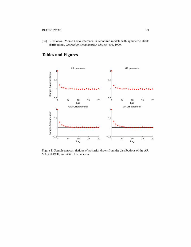
tions. The first 2,000 of the simulations are discarded as burn-in. Table 1 presentsthe comparison among the Bayesian and frequentist estimates and the true parameters.The sample autocorrelations of the stable parameter simulations decay at a comfortablerate. Therefore, a procedure whereby the posterior parameter simulations are sampledperiodically from the generated Markov chain is deemed unnecessary.

Conditional Student’s t Case

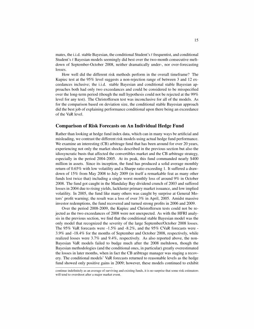
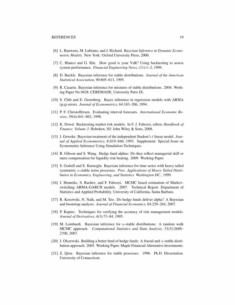
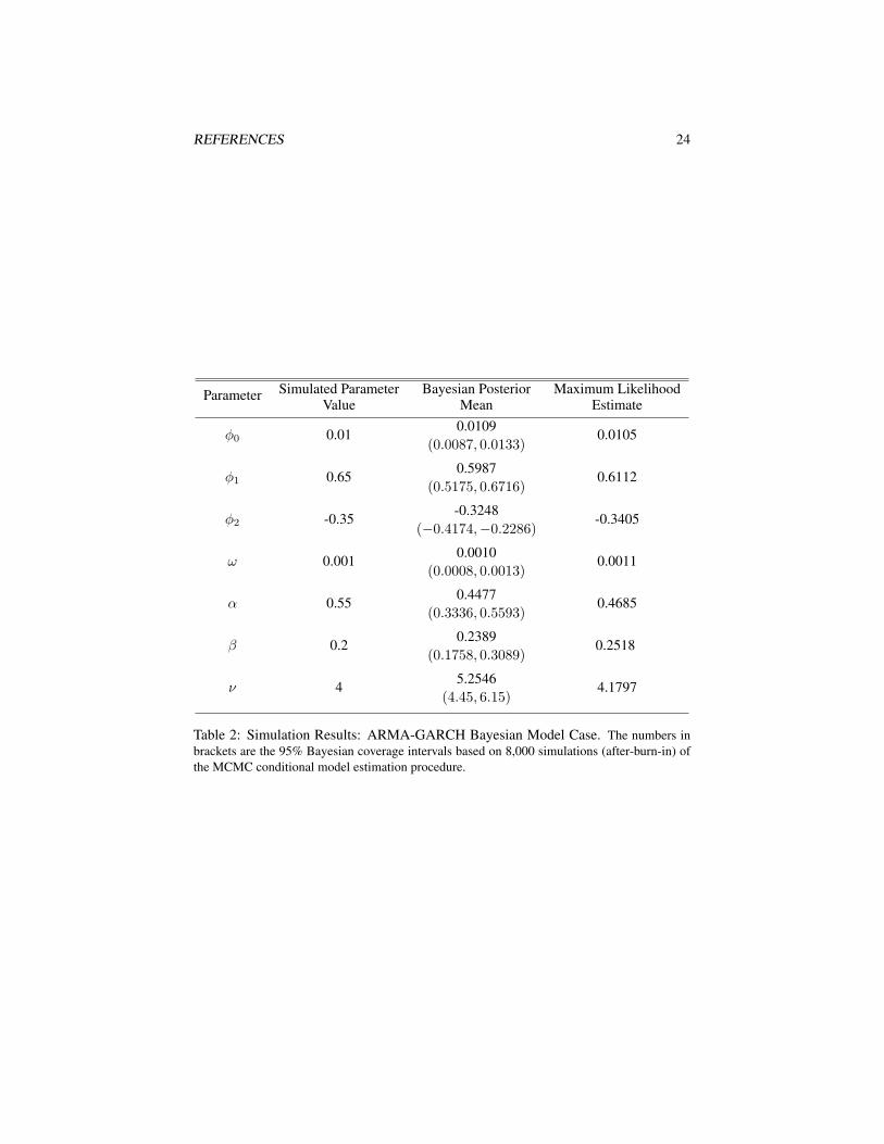
We consider the ARMA(1,1)-GARCH(1,1) model in (1) with Student’s t-distributedinnovations. The generated sample consists of 3,000 observations. We estimate theconditional model using our MCMC approach, running the Markov chain for 10,000iterations, and discarding as burn-in the first 2,000 of them. The comparison amongthe true and estimated parameters, together with the maximum-likelihood estimates,is shown in Table 2. The true parameter values fall into the 95% Bayesian credibleintervals for all parameters, save for the degrees of freedom. Figure 1 presents thesample autocorrelations estimated using the after-burn-in posterior simulations of theAR, MA, GARCH, and ARCH parameters; all sample autocorrelation functions exhibita fast decay.

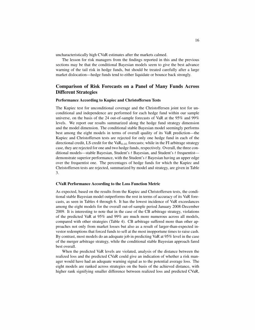
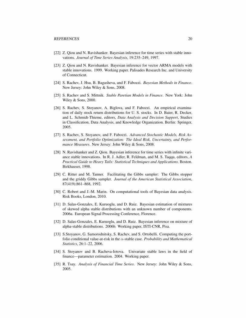
Finally, we observe whether the GARCH(1,1) model stationarity constraint is vio-lated by estimating the posterior probability of the persistence quantity, α+βν/(ν−2),in the GARCH (covariance) stationarity constraint. The posterior mean of this persis-tence quantity is 0.8334 which is below 1 and signifies a conditional process with finitevariance (for comparison, the true value of the quantity is 0.95). The histogram of itsposterior draws is seen in Figure 2. The greater part of the posterior mass is indeedbelow 1, as expected.

Value-at-Risk and Conditional Value-at-Risk PredictionIn our empirical investigation, we estimate VaR and CVaR for a number of risk-

model formulations, the first two of which are very basic standard methodologies, stillused by many banks; we include them for benchmarking purposes. We label theseformulations as Model 1 through Model 8, as follows:14

Model 1: Unconditional (i.i.d.) normal model, estimated in a frequentist (maximum-likelihood) setting

Model 2: Historical VaR/CVaR methodology

Model 3: Unconditional (i.i.d.) stable model, estimated in a frequentist setting

Model 4: Unconditional (i.i.d.) stable model, estimated in a Bayesian setting

Model 5: Unconditional (i.i.d.) Student’s t model, estimated in a frequentistsetting

14For the definitions and properties of various risk measures, in particular VaR and CVaR, as well as theirapplications in risk and portfolio management, see, for example, Rachev, Stoyanov, and Fabozzi (2008).

11

Model 6: Conditional (ARMA(1,1)-GARCH(1,1)) Student’s t model, estimatedin a frequentist setting

Model 7: Conditional (ARMA(1,1)-GARCH(1,1)) Student’s t model, estimatedin a Bayesian setting

Model 8: Conditional (ARMA(1,1)-GARCH(1,1)) stable model, estimated in aBayesian setting.

Recall that Models 7 and 8 have a common Bayesian ARMA-GARCH estimation step(described as Stage 1 in the section on methodology), while Model 8 is obtained via anadditional step of fitting the stable distribution to the standardized residuals from thecommon step (described as Stage 2 in the section on methodology).

In all models, VaR and CVaR estimation is based on the linear-form decompositionof returns, Rt = µt + σtut, where ut is a noise term with the respective distribution(normal—in Model 1, stable—in Models 3, 4, and 8, and Student’s t—in Models 6 and7). Based on the available information up to time t, and using their translation invari-ance and positive homogeneity properties, the VaR and CVaR estimates are expressed,respectively, as

V aRκ,t = σtV aRκ(u)− µt (5)

CV aRκ,t = σtCκ(u)− µt, (6)

where V aRκ(u) is the value-at-risk (the κ quantile) of the innovation’s (ut’s) distri-bution, and Cκ(u) is a constant which depends only on the tail probability, κ.15 (Inour discussion below, we omit the “hats” on VaR and CVaR for notational simplicity.)In the unconditional model approaches (Models 1 through 5), µt and σt are constantsrepresented by the sample estimates and hedge fund returns are assumed independentand identically distributed with the respective distributions. In the conditional model-ing approaches (Models 6 through 8), µt and σt are the forecasts of the conditionalmean and conditional scale from the ARMA(1,1)-GARCH(1,1) model in (1).16

We now outline the explicit and semi-explicit expressions used to compute CVaRfor the normal, Student’s t, and stable distributions.

The Normal Distribution

For a normal distribution with standard deviation σ and expected value µ, the CVaR isexpressed as

CV aRκ(R) =σ

κ√2π

exp

(− (V aRκ(Z))2

2

)− µ, (7)

where Z is a standard normal random variable.15The VaR and CVaR estimates above are computed at a time horizon of one month in our empirical

investigation.16For more details on VaR/CVaR prediction using a time-series model, see, for example, Tsay (2005).

12

The location-scale Student’s t Distribution

In the case of a location-scale Student’s t distribution with degrees of freedom ν, scaleσ, and location µ, CVaR is computed from the following explicit expression:17

CV aRκ(R) =

σΓ( ν+1

2 )

κΓ( ν2 )

√ν−2

(ν−1)√π

(1 +

(t−1ν (κ))2

ν−2

)− ν−12

− µ , ν > 1

∞ , ν = 1,

(8)

where Γ(x) is the gamma function and tν(κ) is the κ-quantile of a standardized (zeromean and variance equal to 1) Student’s t-distributed random variable with ν degreesof freedom.18

The Stable Distribution

Stoyanov et.al. (2006) derived the semi-analytical expression for the CVaR for stabledistributions. The CV aRκ is represented as

CV aRκ(R) = σAκ,α,β − µ. (9)

The term Aκ,α,β is given by

Aκ,α,β =α

1− α

|V aRκ(R)|πκ

∫ π/2

−θ0

g(θ) exp(−|V aRκ(R)|

αα−1 υ(θ)

)dθ,

where

g(θ) =sin (α(θ0 + θ)− 2θ)

sin (α(θ0 + θ))− α cos2 θ

sin2(α(θ0 + θ)),

υ(θ) = (cosαθ0)1

α−1

(cos θ

sin(α(θ0 + θ))

) αα−1 cos(αθ0 + (α− 1)θ)

cos θ,

and θ0 = 1α arctan(β tan πα

2 ), β = −sign(V aRκ(R))β, V aRκ(R) is the VaR ofthe stable distribution at tail probability κ, and β is the stable skewness parameter.The parameters of the stable distribution are estimated either in the frequentist or theBayesian setting.

Backtesting VaR and CVaRWe backtest the risk models using the Kupiec (1995) frequency of failures test andthe Christoffersen (1998) test of independence of the VaR violations. For backtest-ing CVaR, we use a loss function-based procedure.19 Our general backtesting process

17See, for example, Alexander and Sheedy (2008).18For ν = 1, CVaR explodes because the Student’s t distribution with one degree of freedom—known

as the Cauchy distribution—has an infinite expectation. In this case, one can use the median of the lossdistribution, when the loss exceeds V aRκ(R), as a robust alternative to CVaR. See Rachev, Stoyanov, andFabozzi (2008) for more details.

19Backtesting CVaR is a challenging task. See Rachev, Stoyanov, and Fabozzi (2008) for a discussion.

13

consists of repeatedly estimating VaR and CVaR based on a moving estimation win-dow and comparing the predicted risk values to the out-of-sample realization of returnsone-step-ahead. That is, the sequences of VaR and CVaR estimates are based on the up-dated (revised) parameter estimates using the latest estimation window. An exceedanceof the VaR occurs when the realized loss is greater than the predicted VaR for the one-step-ahead horizon. Next, we describe the CVaR backtesting procedure.

CVaR Backtesting Procedure

Our CVaR backtesting procedure relies on a loss function, developed in the spirit ofBlanco and Ihle (1999)’s loss function for ranking models based on their VaR predictivecapacity.20 Denote the loss at time t by Lt. The loss function is defined as

LFt =

{Lt−CV aRκ,t

Lt, if Lt > V aRκ,t

0, if Lt ≤ V aRκ,t

. (10)

Then, the statistic

S =

√√√√ 1

T

T∑t=1

LF 2t , (11)

where T is the sampling horizon, provides a summary metric for the average distanceof the forecast CVaR from the realized loss, in the case of VaR exceedance. In ourempirical analysis, we compute this statistic for each model and each hedge fund inour sample universe.

Empirical AnalysisOur empirical analysis consists of four parts. First, we analyze and compare the mod-els’ risk forecasts using hedge fund index data. Second, we focus on the performance ofa particular convertible arbitrage hedge fund that experienced a large loss in 2008 andstaged a strong recovery in the following year. Third, we perform a general compari-son among models’ VaR and CVaR predictions across six hedge fund strategies mostdeeply impacted by the recent financial crisis: merger arbitrage, convertible bond (CB)arbitrage, directional credit (distressed debt and high-yield), long/short (LS) credit,fixed income (FI) arbitrage, and mortgage-backed security (MBS) arbitrage. Finally,we focus our attention on the momentous months of September and October 2008, withthe aim of comparative evaluation of models across the hedge fund strategies. In allfour investigations, we use eight years of monthly data in-sample (starting in January1990 for the hedge fund index data and in January 2000 for the individual hedge funddata) and compare methodologies on a rolling month-by-month out-of-sample basis(spanning 12 years for the hedge fund index and two years for the remaining data).Our sample universe consists of 27 funds in the merger arbitrage strategy, 17 funds in

20Dowd (2008) provides an overview of backtesting market risk models. For a suggestion on a morerigorous approach to CVaR backtesting, see Rachev, Stoyanov, and Fabozzi (2008).

14

the CB arbitrage strategy, 40 funds in the directional credit strategy, 17 funds in the LScredit strategy, 16 funds in the FI arbitrage strategy, and 10 funds in the MBS arbitragestrategy.

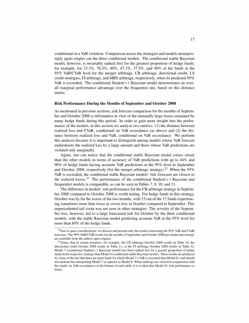
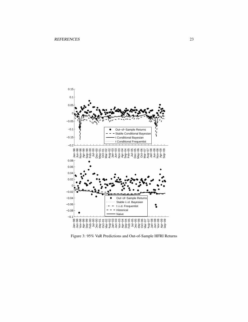
Comparisons of Risk Forecasts on Hedge Fund Index DataThe HFRI Fund Weighted Composite Index is widely used as an indicator of the per-formance of the overall hedge fund industry. Comprised of over 2,000 funds listed inthe internal HFR database, the index is an equally weighted average of monthly returnsnet of fees starting in January 1990. As such, the index records hedge fund trends overa lengthy business cycle of busts and booms. This evaluation includes a number of ma-jor crisis periods ranging from the Long Term Capital/Russian default of August 1998,the terrorist attack of September 2001, the credit crunch of Summer 2002, the creditcorrelation crisis of Spring 2005, the market meltdown of May 2006, the quant deba-cle of August 2007, the subprime jitters of November 2007, the market corrections ofJanuary and March 2008, and, ultimately, the Lehman bankruptcy/market collapse ofSeptember-October 2008. In all, there were 14 monthly events in 12 years (just aboutone in 10 times) where performance, as measured by total return, was less than -2%,yet the overall average return during this period was a positive 0.66%.

As seen in Figure 3, the -8.7% drop in August 1998 and the back-to-back lossesof 6.13% and 6.84% in September and October 2008 sent hedge fund investors into astate of panic. We observe that traditional risk models—naive, historical, and Student’st—did poor jobs not only in forecasting the severity of these downturns but also in ad-justing properly afterwards. For example, after the massive LTCM shock, simple andhistorical models did not adjust their risk prediction much at all, and continued to fore-cast inadequately a VaR at the 95% level of around -2%. Worse, CVaR forecasts forAugust, 1998 were in the -2% range for the non-Bayesian approaches at the 95% leveland only -3% at the 99% level. These results are very difficult to accept for risk man-agers, portfolio decision-makers, and investors, all of whom demand models that makemeaningful forecasts when crises hit, not merely during normal market conditions!

Our first observation is that the stable models tended to do a much better job antic-ipating these large tail events than the non-stable approaches and that the Bayesianmethodologies proved superior to the frequentist forecasts. The conditional stableBayesian model anticipated the losses of August 1998 and September 1998 with pre-dictions of -6.50% and -5.77% of the 99% VaR, while the CVaR forecasts were quiteclose at -12.04% and -6.58%, respectively. However, our second observation is thatthe conditional models—and the conditional stable Bayesian solution, in particular—substantially overshot (in terms of both VaR and CVaR) the actual performance inmonths subsequent to the large market dislocations and the CVaR forecasts of thesemodels took considerable time to re-adjust to more rational levels. While the Bayesianand stable methods were suggesting the potential for worsening conditions, marketsrebounded and hedge funds shook off these isolated losses.21 Of all the CVaR risk esti-

21That the conditional stable Bayesian model suggested considerable losses subsequent to the major mar-ket events of August 1998 and September/October 2008 was not lost on many individual hedge funds whichdid in fact lose almost all their value and liquidate. The analysis herein involves an industry index which hassome biases in that it often fails to include the performance of funds that are terminating. Since the index will

15

mates, the i.i.d. stable Bayesian, the conditional Student’s t frequentist, and conditionalStudent’s t Bayesian models seemingly did best over the two-month consecutive melt-down of September-October 2008, neither dramatically under-, nor over-forecastinglosses.

How well did the different risk methods perform in the overall timeframe? TheKupiec test at the 95% level suggests a non-rejection range of between 3 and 12 ex-ceedances inclusive; the i.i.d. stable Bayesian and conditional stable Bayesian ap-proaches both had only two exceedances and could be considered to be misspecifiedover the long-term period (though the null hypothesis could not be rejected at the 99%level for any test). The Christoffersen test was inconclusive for all of the models. Asfor the comparison based on deviation size, the conditional stable Bayesian approachdid the best job of explaining performance conditional upon there being an exceedanceof the VaR level.

Comparison of Risk Forecasts on An Individual Hedge FundRather than looking at hedge fund index data, which can in many ways be artificial andmisleading, we contrast the different risk models using actual hedge fund performance.We examine an interesting (CB) arbitrage fund that has been around for over 20 years,experiencing not only the market shocks described in the previous section but also theidiosyncratic busts that affected the convertibles market and the CB arbitrage strategy,especially in the period 2004-2005. At its peak, this fund commanded nearly $400million in assets. Since its inception, the fund has produced a solid average monthlyreturn of 0.65% with low volatility and a Sharpe ratio exceeding 1. It suffered a draw-down of 15% from May 2008 to July 2009 (in itself a remarkable feat as many otherfunds lost twice that) including a single worst monthly loss of around 9% in October2008. The fund got caught in the Mandalay Bay dividend crunch of 2003 and sufferedlosses in 2004 due to rising yields, lackluster primary market issuance, and low impliedvolatility. In 2005, the fund like many others was caught by surprise at General Mo-tors’ profit warning; the result was a loss of over 3% in April, 2005. Amidst massiveinvestor redemptions, the fund recovered and turned strong profits in 2006 and 2009.

Over the period 2008-2009, the Kupiec and Christoffersen tests could not be re-jected as the two exceedances of 2008 were not unexpected. As with the HFRI analy-sis in the previous section, we find that the conditional stable Bayesian model was theonly model that recognized the severity of the large September/October 2008 losses.The 95% VaR forecasts were -1.5% and -8.2%, and the 95% CVaR forecasts were -3.9% and -18.4% for the months of September and October 2008, respectively, whilerealized losses were 3.7% and 9.4%, respectively. As also reported above, the non-Bayesian VaR models failed to budge much after the 2008 meltdown, though theBayesian methodologies (and the conditional ones, in particular) greatly overestimatedthe losses in later months, when in fact the CB aribtrage manager was staging a recov-ery. The conditional models’ VaR forecasts returned to reasonable levels as the hedgefund showed only positive gains in 2009; however, these models continued to exhibit

continue indefinitely as an average of surviving and existing funds, it is no surprise that some risk estimatorswill tend to overshoot after a major market event.

16

uncharacteristically high CVaR estimates after the markets calmed.The lesson for risk managers from the findings reported in this and the previous

sections may be that the conditional Bayesian models seem to give the best advancewarning of the tail risk in hedge funds, but should be treated carefully after a largemarket dislocation—hedge funds tend to either liquidate or bounce back strongly.

Comparison of Risk Forecasts on a Panel of Many Funds AcrossDifferent StrategiesPerformance According to Kupiec and Christoffersen Tests

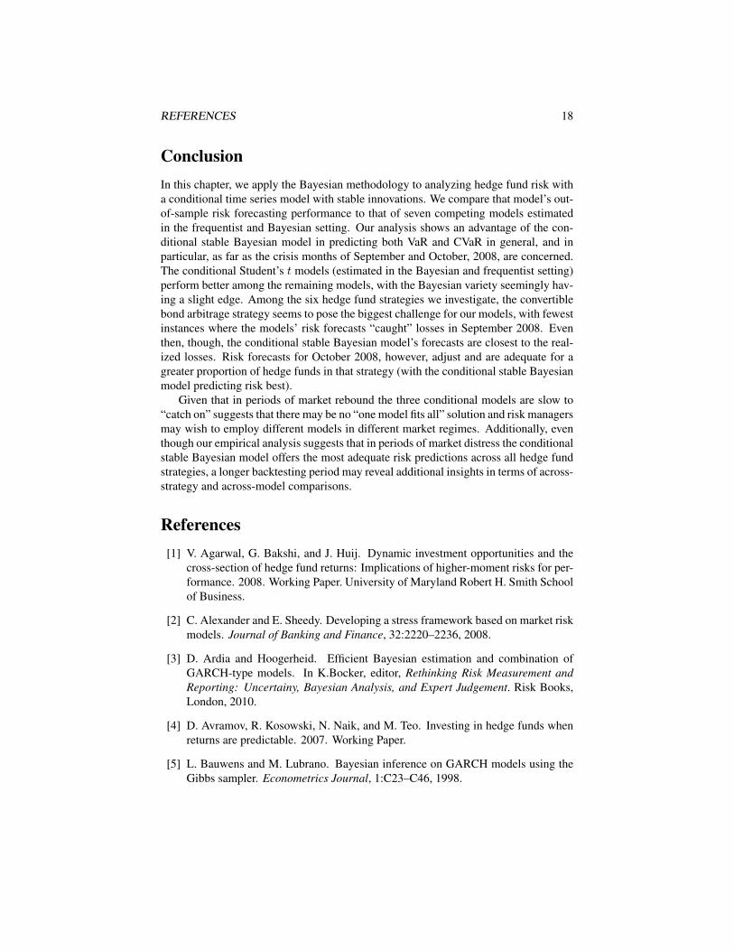
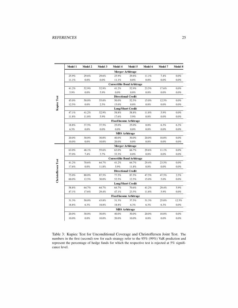
The Kupiec test for unconditional coverage and the Christoffersen joint test for un-conditional and independence are performed for each hedge fund within our sampleuniverse, on the basis of the 24 out-of-sample forecasts of VaR at the 95% and 99%levels. We report our results summarized along the hedge fund strategy dimensionand the model dimension. The conditional stable Bayesian model seemingly performsbest among the eight models in terms of overall quality of its VaR prediction—theKupiec and Christoffersen tests are rejected for only one hedge fund in each of thedirectional credit, LS credit for the VaR0.05 forecasts; while in the FI arbitrage strategycase, they are rejected for one and two hedge funds, respectively. Overall, the three con-ditional models—stable Bayesian, Student’s t Bayesian, and Student’s t frequentist—demonstrate superior performance, with the Student’s t Bayesian having an upper edgeover the frequentist one. The percentages of hedge funds for which the Kupiec andChristoffersen tests are rejected, summarized by model and strategy, are given in Table3.

CVaR Performance According to the Loss Function Metric

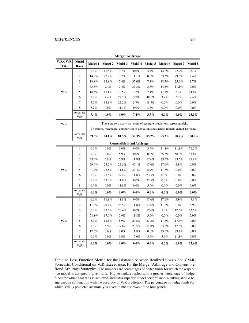
As expected, based on the results from the Kupiec and Christoffersen tests, the condi-tional stable Bayesian model outperforms the rest in terms of accuracy of its VaR fore-casts, as seen in Tables 4 through 6. It has the lowest incidence of VaR exceedancesamong the eight models for the overall out-of-sample period January 2008-December2009. It is interesting to note that in the case of the CB arbitrage strategy, violationsof the predicted VaR at 95% and 99% are much more numerous across all models,compared with other strategies (Table 4). CB arbitrage suffered more than other ap-proaches not only from market losses but also as a result of larger-than-expected in-vestor redemptions that forced funds to sell at the most inopportune times to raise cash.By contrast, most models do an adequate job in predicting VaR at 95% level in the caseof the merger arbitrage strategy, while the conditional stable Bayesian approach faredbest overall.

When the predicted VaR levels are violated, analysis of the distance between therealized loss and the predicted CVaR could give an indication of whether a risk man-ager would have had an adequate warning signal as to the potential average loss. Theeight models are ranked across strategies on the basis of the achieved distance, withhigher rank signifying smaller difference between realized loss and predicted CVaR,

17

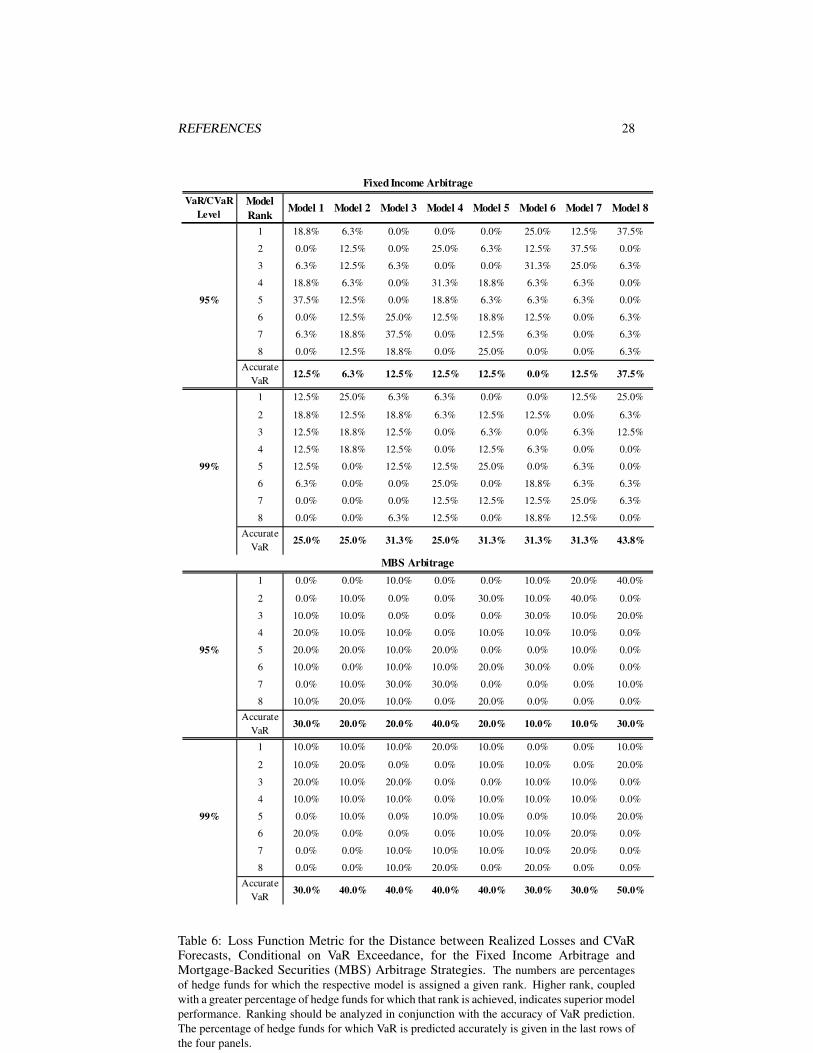
conditional on a VaR violation. Comparison across the strategies and models unsurpris-ingly again singles out the three conditional models. The conditional stable Bayesianmodel, however, is invariably ranked first for the greatest proportion of hedge funds;for example, for 33.3%, 76.5%, 40%, 47.1%, 37.5%, and 40% of the funds at the95% VaR/CVaR level for the merger arbitrage, CB arbitrage, directional credit, LScredit strategies, FI arbitrage, and MBS arbitrage, respectively, when its predicted 95%VaR is exceeded. The conditional Student’s t Bayesian model demonstrates an over-all marginal performance advantage over the frequentist one, based on this distancemetric.

Risk Performance During the Months of September and October 2008

As mentioned in previous sections, risk forecast comparison for the months of Septem-ber and October 2008 is informative in view of the unusually large losses sustained bymany hedge funds during this period. In order to gain more insight into the perfor-mance of the models, in this section we analyze two metrics: (1) the distance betweenrealized loss and CVaR, conditional on VaR exceedance (as above) and (2) the dis-tance between realized loss and VaR, conditional on VaR exceedance. We performthis analysis because it is important to distinguish among models whose VaR forecastundershoots the realized loss by a large amount and those whose VaR predictions areviolated only marginally.

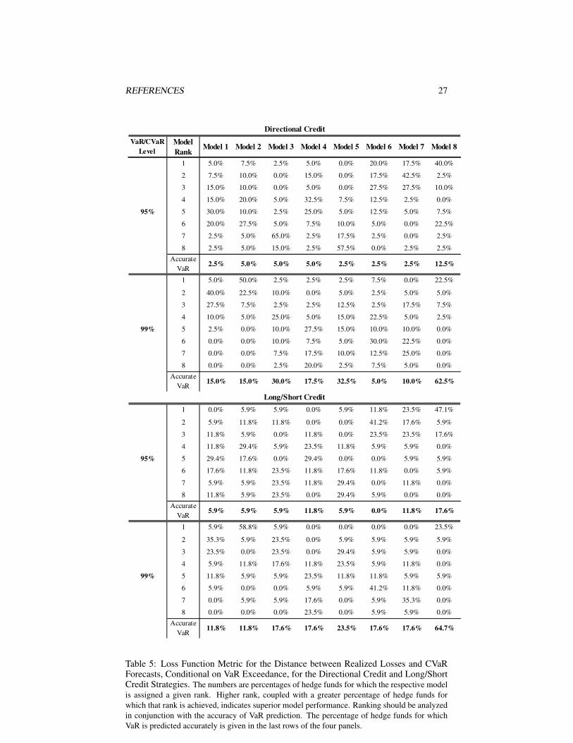
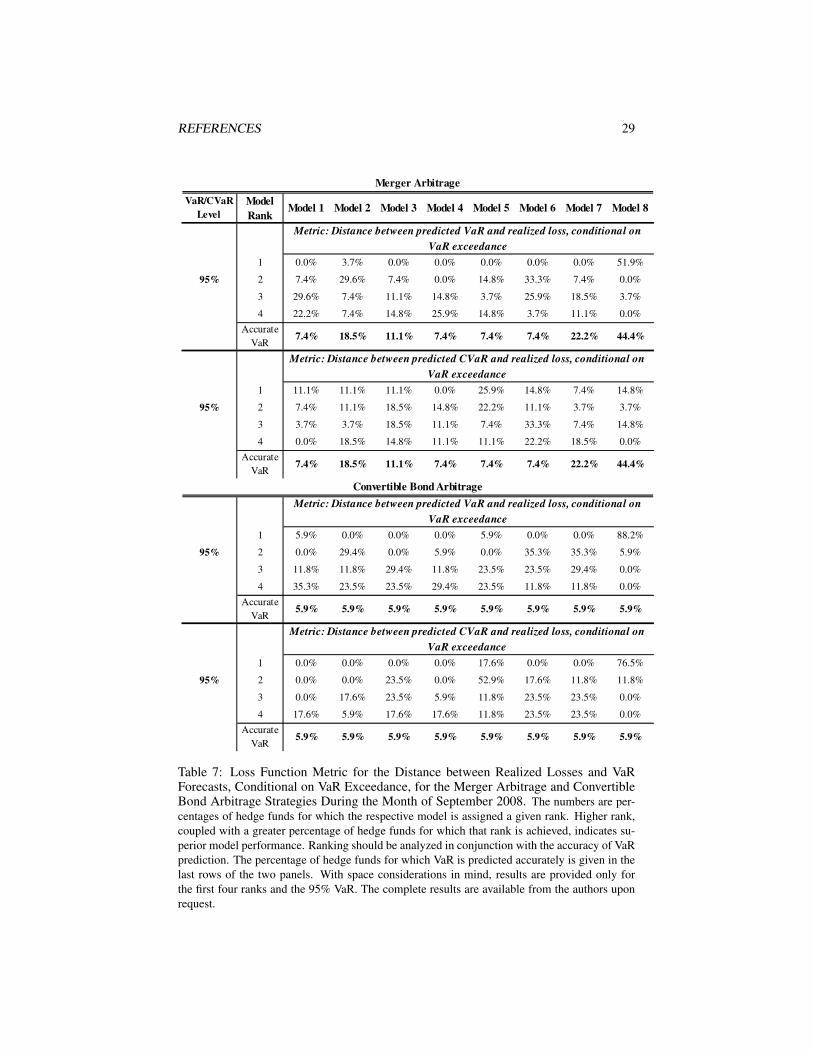
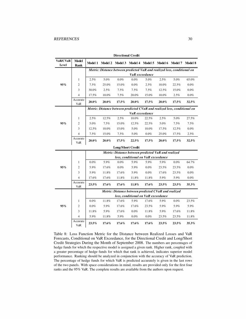
Again, one can notice that the conditional stable Bayesian model comes closerthan the other models in terms of accuracy of VaR predictions with up to 44% and96% of hedge funds having accurate VaR predictions at the 95% level in Septemberand October 2008, respectively (for the merger arbitrage strategy).22 When the 95%VaR is exceeded, the conditional stable Bayesian models’ risk forecasts are closest tothe realized losses.23 The performance of the conditional Student’s t Bayesian andfrequentist models is comparable, as can be seen in Tables 7, 8, 10, and 11.

The difference in models’ risk performance for the CB arbitrage strategy in Septem-ber 2008 compared to October 2008 is worth noting. For hedge funds in this strategy,October was by far the worse of the two months, with 15 out of the 17 funds experienc-ing sometimes more than twice as severe loss in October compared to September. Thisunprecedented tail event was not seen in other strategies. The severity of the Septem-ber loss, however, led to a large forecasted risk for October by the three conditionalmodels, with the stable Bayesian model predicting accurate VaR at the 95% level formore than 60% of the hedge funds.

22Due to space considerations, we discuss and present only the results concerning the 95% VaR and CVaRforecasts. The 99% VaR/CVaR results for the months of September and October 2008 per model and strategyare available from the authors upon request.

23Notice that in certain instances, for example, the CB arbitrage October 2008 results in Table 10, thedirectional credit October 2008 results in Table 11, or the FI arbitrage October 2008 results in Table 12,Model 7 (conditional Student’s t Bayesian model) has been ranked first for a greater proportion of hedgefunds in the respective strategy than Model 8 (conditional stable Bayesian model). These results are producedby virtue of the fact that there are more funds for which Model 7’s VaR is exceeded than Model 8’s and shouldnot mislead into interpreting Model 7 as superior to Model 8. When rankings are viewed in conjunction withthe results on VaR exceedances at the bottom of each table, it is evident that Model 8’s risk performance isbetter.

REFERENCES 18

ConclusionIn this chapter, we apply the Bayesian methodology to analyzing hedge fund risk witha conditional time series model with stable innovations. We compare that model’s out-of-sample risk forecasting performance to that of seven competing models estimatedin the frequentist and Bayesian setting. Our analysis shows an advantage of the con-ditional stable Bayesian model in predicting both VaR and CVaR in general, and inparticular, as far as the crisis months of September and October, 2008, are concerned.The conditional Student’s t models (estimated in the Bayesian and frequentist setting)perform better among the remaining models, with the Bayesian variety seemingly hav-ing a slight edge. Among the six hedge fund strategies we investigate, the convertiblebond arbitrage strategy seems to pose the biggest challenge for our models, with fewestinstances where the models’ risk forecasts “caught” losses in September 2008. Eventhen, though, the conditional stable Bayesian model’s forecasts are closest to the real-ized losses. Risk forecasts for October 2008, however, adjust and are adequate for agreater proportion of hedge funds in that strategy (with the conditional stable Bayesianmodel predicting risk best).

Given that in periods of market rebound the three conditional models are slow to“catch on” suggests that there may be no “one model fits all” solution and risk managersmay wish to employ different models in different market regimes. Additionally, eventhough our empirical analysis suggests that in periods of market distress the conditionalstable Bayesian model offers the most adequate risk predictions across all hedge fundstrategies, a longer backtesting period may reveal additional insights in terms of across-strategy and across-model comparisons.

References[1] V. Agarwal, G. Bakshi, and J. Huij. Dynamic investment opportunities and the

cross-section of hedge fund returns: Implications of higher-moment risks for per-formance. 2008. Working Paper. University of Maryland Robert H. Smith Schoolof Business.

[2] C. Alexander and E. Sheedy. Developing a stress framework based on market riskmodels. Journal of Banking and Finance, 32:2220–2236, 2008.

[3] D. Ardia and Hoogerheid. Efficient Bayesian estimation and combination ofGARCH-type models. In K.Bocker, editor, Rethinking Risk Measurement andReporting: Uncertainy, Bayesian Analysis, and Expert Judgement. Risk Books,London, 2010.

[4] D. Avramov, R. Kosowski, N. Naik, and M. Teo. Investing in hedge funds whenreturns are predictable. 2007. Working Paper.

[5] L. Bauwens and M. Lubrano. Bayesian inference on GARCH models using theGibbs sampler. Econometrics Journal, 1:C23–C46, 1998.

REFERENCES 19

[6] L. Bauwens, M. Lubrano, and J. Richard. Bayesian Inference in Dynamic Econo-metric Models. New York: Oxford University Press, 2000.

[7] C. Blanco and G. Ihle. How good is your VaR? Using backtesting to assesssystem performance. Financial Engineering News, (11):1–2, 1999.

[8] D. Buckle. Bayesian inference for stable distributions. Journal of the AmericanStatistical Association, 90:605–613, 1995.

[9] R. Casarin. Bayesian inference for mixtures of stable distributions. 2004. Work-ing Paper No 0428. CEREMADE, University Paris IX.

[10] S. Chib and E. Greenberg. Bayes inference in regression models with ARMA(p,q) errors. Journal of Econometrics, 64:183–206, 1994.

[11] P. F. Christoffersen. Evaluating interval forecasts. International Economic Re-view, 39(4):841–862, 1998.

[12] K. Dowd. Backtesting market risk models. In F. J. Fabozzi, editor, Handbook ofFinance: Volume 3. Hoboken, NJ: John Wiley & Sons, 2008.

[13] J. Geweke. Bayesian treatment of the independent Student’s t linear model. Jour-nal of Applied Econometrics, 8:S19–S40, 1993. Supplement: Special Issue onEconometric Inference Using Simulation Techniques.

[14] R. Gibson and S. Wang. Hedge fund alphas: Do they reflect managerial skill ormere compensation for liquidity risk bearing. 2009. Working Paper.

[15] S. Godsill and E. Kuruoglu. Bayesian inference for time series with heavy tailedsymmetric α-stable noise processes. Proc. Applications of Heavy Tailed Distri-butios in Economics, Engineering, and Statistics. Washington DC., 1999.

[16] J. Henneke, S. Rachev, and F. Fabozzi. MCMC based estimation of Markov-switching ARMA-GARCH models. 2007. Technical Report. Department ofStatistics and Applied Probability. University of California, Santa Barbara.

[17] R. Kosowski, N. Naik, and M. Teo. Do hedge funds deliver alpha? A Bayesianand bootstrap analysis. Journal of Financial Economics, 84:229–264, 2007.

[18] P. Kupiec. Techniques for verifying the accuracy of risk management models.Journal of Derivatives, 4(3):73–84, 1995.

[19] M. Lombardi. Bayesian inference for α-stable distributions: A random walkMCMC approach. Computational Statistics and Data Analysis, 51(5):2688–2700, 2007.

[20] J. Olszewski. Building a better fund of hedge funds: A fractal and α-stable distri-bution approach. 2005. Working Paper. Maple Financial Alternative Investments.

[21] Z. Qiou. Bayesian inference for stable processes. 1996. Ph.D. Dissertation.University of Connecticut.

REFERENCES 20

[22] Z. Qiou and N. Ravishanker. Bayesian inference for time series with stable inno-vations. Journal of Time Series Analysis, 19:235–249, 1997.

[23] Z. Qiou and N. Ravishanker. Bayesian inference for vector ARMA models withstable innovations. 1999. Working paper. Palisades Research Inc. and Universityof Connecticut.

[24] S. Rachev, J. Hsu, B. Bagasheva, and F. Fabozzi. Bayesian Methods in Finance.New Jersey: John Wiley & Sons, 2008.

[25] S. Rachev and S. Mittnik. Stable Paretian Models in Finance. New York: JohnWiley & Sons, 2000.

[26] S. Rachev, S. Stoyanov, A. Biglova, and F. Fabozzi. An empirical examina-tion of daily stock return distributions for U. S. stocks. In D. Baier, R. Decker,and L. Schmidt-Thieme, editors, Data Analysis and Decision Support, Studiesin Classification, Data Analysis, and Knowledge Organization. Berlin: Springer,2005.

[27] S. Rachev, S. Stoyanov, and F. Fabozzi. Advanced Stochastic Models, Risk As-sessment, and Portfolio Optimization: The Ideal Risk, Uncertainty, and Perfor-mance Measures. New Jersey: John Wiley & Sons, 2008.

[28] N. Ravishanker and Z. Qiou. Bayesian inference for time series with infinite vari-ance stable innovations. In R. J. Adler, R. Feldman, and M. S. Taqqu, editors, APractical Guide to Heavy Tails: Statistical Techniques and Applications. Boston.Birkhauser, 1998.

[29] C. Ritter and M. Tanner. Facilitating the Gibbs sampler: The Gibbs stopperand the griddy Gibbs sampler. Journal of the American Statistical Association,87(419):861–868, 1992.

[30] C. Robert and J.-M. Marin. On computational tools of Bayesian data analysis.Risk Books, London, 2010.

[31] D. Salas-Gonzales, E. Kuruoglu, and D. Ruiz. Bayesian estimation of mixturesof skewed alpha stable distributions with an unknown number of components.2006a. European Signal Processing Conference, Florence.

[32] D. Salas-Gonzales, E. Kuruoglu, and D. Ruiz. Bayesian inference on mixture ofalpha-stable distributions. 2006b. Working paper, ISTI-CNR, Pisa.

[33] S.Stoyanov, G. Samorodnitsky, S. Rachev, and S. Ortobelli. Computing the port-folio conditional value-at-risk in the α-stable case. Probability and MathematicalStatistics, 26:1–22, 2006.

[34] S. Stoyanov and B. Racheva-Iotova. Univariate stable laws in the field offinance—parameter estimation. 2004. Working paper.

[35] R. Tsay. Analysis of Financial Time Series. New Jersey: John Wiley & Sons,2005.

REFERENCES 21

[36] E. Tsionas. Monte Carlo inference in economic models with symmetric stabledistributions. Journal of Econometrics, 88:365–401, 1999.

Tables and Figures

0 5 10 15 20−0.5

0

0.5

1

Lag

Sam

ple

Aut

ocor

rela

tion

AR parameter

0 5 10 15 20−0.5

0

0.5

1

Lag

MA parameter

0 5 10 15 20−0.5

0

0.5

1

Lag

ARCH parameter

0 5 10 15 20−0.5

0

0.5

1

Lag

Sam

ple

Aut

ocor

rela

tion

GARCH parameter

Figure 1: Sample autocorrelations of posterior draws from the distributions of the AR,MA, GARCH, and ARCH parameters

REFERENCES 22

0.65 0.7 0.75 0.8 0.85 0.9 0.95 1 1.05 1.10

100

200

300

400

500

600

700

800

Figure 2: Histogram of draws from the posterior distribution of the GARCH(1,1) sta-tionarity quantity

Simulated Parameter Bayesian Posterior Maximum LikelihoodParameterValue Mean Estimate

1.2464α 1.7

(1.1300, 1.3662)1.7471

0.2733β 0.2

(0.1219, 0.4183)-0.1626

0.1653σ 0.3

(0.1497, 0.1813)0.2786

-0.0210µ 0.05

(−0.0530, 0.0110)0.0429

Table 1: Simulation Results: Stable i.i.d. Bayesian Model Case. The numbers in brack-ets are the 95% Bayesian coverage intervals based on 8,000 simulations (after-burn-in) of theMCMC Stable i.i.d. model estimation procedure.

REFERENCES 23

−0.1

−0.08

−0.06

−0.04

−0.02

0

0.02

0.04

0.06

0.08

Jan−

98Ju

n−98

Nov

−98

Apr

−99

Sep

−99

Feb

−00

Jul−

00D

ec−

00M

ay−

01O

ct−

01M

ar−

02A

ug−

02Ja

n−03

Jun−

03N

ov−

03A

pr−

04S

ep−

04F

eb−

05Ju

l−05

Dec

−05

May

−06

Oct

−06

Mar

−07

Aug

−07

Jan−

08Ju

n−08

Nov

−08

Apr

−09

Sep

−09

Out−of−Sample ReturnsStable i.i.d. Bayesiant i.i.d. FrequentistHistoricalNaive

−0.2

−0.15

−0.1

−0.05

0

0.05

0.1

0.15

Jan−

98Ju

n−98

Nov

−98

Apr

−99

Sep

−99

Feb

−00

Jul−

00D

ec−

00M

ay−

01O

ct−

01M

ar−

02A

ug−

02Ja

n−03

Jun−

03N

ov−

03A

pr−

04S

ep−

04F

eb−

05Ju

l−05

Dec

−05

May

−06

Oct

−06

Mar

−07

Aug

−07

Jan−

08Ju

n−08

Nov

−08

Apr

−09

Sep

−09

Out−of−Sample ReturnsStable Conditional Bayesiant Conditional Bayesiant Conditional Frequentist

Figure 3: 95% VaR Predictions and Out-of-Sample HFRI Returns

REFERENCES 24

Simulated Parameter Bayesian Posterior Maximum LikelihoodParameterValue Mean Estimate

0.0109ϕ0 0.01

(0.0087, 0.0133)0.0105

0.5987ϕ1 0.65

(0.5175, 0.6716)0.6112

-0.3248ϕ2 -0.35

(−0.4174,−0.2286)-0.3405

0.0010ω 0.001

(0.0008, 0.0013)0.0011

0.4477α 0.55

(0.3336, 0.5593)0.4685

0.2389β 0.2

(0.1758, 0.3089)0.2518

5.2546ν 4

(4.45, 6.15)4.1797

Table 2: Simulation Results: ARMA-GARCH Bayesian Model Case. The numbers inbrackets are the 95% Bayesian coverage intervals based on 8,000 simulations (after-burn-in) ofthe MCMC conditional model estimation procedure.

REFERENCES 25

�

Model 1 Model 2 Model 3 Model 4 Model 5 Model 6 Model 7 Model 8

25.9% 29.6% 29.6% 25.9% 29.6% 11.1% 7.4% 0.0%

11.1% 0.0% 0.0% 11.1% 0.0% 0.0% 0.0% 0.0%

41.2% 52.9% 52.9% 41.2% 52.9% 23.5% 17.6% 0.0%

5.9% 0.0% 5.9% 0.0% 0.0% 0.0% 0.0% 0.0%

45.0% 50.0% 55.0% 50.0% 52.5% 15.0% 12.5% 0.0%

12.5% 0.0% 2.5% 15.0% 0.0% 0.0% 0.0% 0.0%

47.1% 41.2% 52.9% 58.8% 58.8% 11.8% 5.9% 0.0%

11.8% 11.8% 5.9% 17.6% 5.9% 0.0% 0.0% 0.0%

18.8% 37.5% 37.5% 25.0% 25.0% 0.0% 6.3% 6.3%

6.3% 0.0% 0.0% 0.0% 0.0% 0.0% 0.0% 0.0%

20.0% 30.0% 30.0% 40.0% 30.0% 20.0% 10.0% 0.0%

10.0% 0.0% 10.0% 20.0% 0.0% 0.0% 0.0% 0.0%

63.0% 48.1% 55.6% 63.0% 66.7% 29.6% 11.1% 0.0%

37.0% 7.4% 3.7% 33.3% 0.0% 0.0% 0.0% 0.0%

41.2% 70.6% 64.7% 41.2% 64.7% 29.4% 23.5% 0.0%

17.6% 0.0% 11.8% 5.9% 11.8% 0.0% 0.0% 0.0%

75.0% 80.0% 87.5% 77.5% 87.5% 47.5% 47.5% 2.5%

60.0% 12.5% 30.0% 52.5% 12.5% 15.0% 5.0% 0.0%

58.8% 64.7% 64.7% 64.7% 70.6% 41.2% 29.4% 5.9%

47.1% 17.6% 29.4% 47.1% 23.5% 11.8% 5.9% 0.0%

31.3% 50.0% 43.8% 31.3% 37.5% 31.3% 25.0% 12.5%

18.8% 6.3% 18.8% 18.8% 6.3% 6.3% 6.3% 0.0%

20.0% 30.0% 30.0% 40.0% 30.0% 20.0% 10.0% 0.0%

10.0% 0.0% 10.0% 20.0% 10.0% 0.0% 0.0% 0.0%

MBS Arbitrage

Convertible Bond Arbitrage

Directional Credit

Long/Short Credit

Ku

pie

c T

est

Ch

ris

toff

erse

n T

est

Merger Arbitrage


Directional Credit

Long/Short Credit

Merger Arbitrage

Fixed Income Arbitrage

MBS Arbitrage


Table 3: Kupiec Test for Unconditional Coverage and Christoffersen Joint Test. Thenumbers in the first (second) row for each strategy refer to the 95% (99%) VaR prediction andrepresent the percentage of hedge funds for which the respective test is rejected at 5% signifi-cance level.

REFERENCES 26

�

VaR/CVaR

Level

Model

RankModel 1 Model 2 Model 3 Model 4 Model 5 Model 6 Model 7 Model 8

1 0.0% 18.5% 3.7% 0.0% 3.7% 14.8% 22.2% 33.3%

2 14.8% 22.2% 3.7% 11.1% 0.0% 33.3% 29.6% 7.4%

3 14.8% 14.8% 7.4% 37.0% 7.4% 18.5% 25.9% 3.7%

4 33.3% 7.4% 7.4% 33.3% 3.7% 14.8% 11.1% 0.0%

95% 5 18.5% 11.1% 18.5% 3.7% 7.4% 11.1% 3.7% 14.8%

6 3.7% 7.4% 22.2% 3.7% 48.1% 3.7% 3.7% 7.4%

7 3.7% 14.8% 22.2% 3.7% 18.5% 0.0% 0.0% 0.0%

8 3.7% 0.0% 11.1% 0.0% 3.7% 0.0% 0.0% 0.0%

Accurate

VaR7.4% 0.0% 0.0% 7.4% 3.7% 0.0% 0.0% 33.3%

99% There are two many instances of accurate predictions across models.

Accurate

VaR59.3% 74.1% 81.5% 59.3% 85.2% 85.2% 88.9% 100.0%

1 0.0% 0.0% 0.0% 0.0% 5.9% 11.8% 11.8% 76.5%

2 0.0% 0.0% 5.9% 0.0% 0.0% 35.3% 58.8% 11.8%

3 23.5% 5.9% 5.9% 11.8% 17.6% 23.5% 23.5% 11.8%

4 29.4% 23.5% 23.5% 47.1% 17.6% 17.6% 5.9% 0.0%

95% 5 41.2% 23.5% 11.8% 29.4% 5.9% 11.8% 0.0% 0.0%

6 5.9% 23.5% 29.4% 11.8% 23.5% 0.0% 0.0% 0.0%

7 0.0% 23.5% 11.8% 0.0% 23.5% 0.0% 0.0% 0.0%

8 0.0% 0.0% 11.8% 0.0% 5.9% 0.0% 0.0% 0.0%

Accurate

VaR0.0% 0.0% 0.0% 0.0% 0.0% 0.0% 0.0% 0.0%

1 0.0% 11.8% 11.8% 0.0% 17.6% 17.6% 5.9% 47.1%

2 11.8% 29.4% 23.5% 11.8% 17.6% 11.8% 0.0% 5.9%

3 0.0% 23.5% 29.4% 0.0% 17.6% 5.9% 17.6% 23.5%

4 58.8% 17.6% 5.9% 11.8% 5.9% 0.0% 0.0% 5.9%

99% 5 5.9% 11.8% 5.9% 23.5% 23.5% 11.8% 17.6% 0.0%

6 5.9% 5.9% 17.6% 23.5% 11.8% 23.5% 17.6% 0.0%

7 17.6% 0.0% 0.0% 11.8% 0.0% 23.5% 29.4% 0.0%

8 0.0% 0.0% 5.9% 17.6% 5.9% 5.9% 11.8% 0.0%

Accurate

VaR0.0% 0.0% 0.0% 0.0% 0.0% 0.0% 0.0% 17.6%

Merger Aribtrage

Therefore, meaningful comparison of deviation sizes across models cannot be made.

Convertible Bond Arbirage

Table 4: Loss Function Metric for the Distance between Realized Losses and CVaRForecasts, Conditional on VaR Exceedance, for the Merger Arbitrage and ConvertibleBond Arbitrage Strategies. The numbers are percentages of hedge funds for which the respec-tive model is assigned a given rank. Higher rank, coupled with a greater percentage of hedgefunds for which that rank is achieved, indicates superior model performance. Ranking should beanalyzed in conjunction with the accuracy of VaR prediction. The percentage of hedge funds forwhich VaR is predicted accurately is given in the last rows of the four panels.

REFERENCES 27

�

VaR/CVaR

Level

Model


1 5.0% 7.5% 2.5% 5.0% 0.0% 20.0% 17.5% 40.0%

2 7.5% 10.0% 0.0% 15.0% 0.0% 17.5% 42.5% 2.5%

3 15.0% 10.0% 0.0% 5.0% 0.0% 27.5% 27.5% 10.0%

4 15.0% 20.0% 5.0% 32.5% 7.5% 12.5% 2.5% 0.0%

95% 5 30.0% 10.0% 2.5% 25.0% 5.0% 12.5% 5.0% 7.5%

6 20.0% 27.5% 5.0% 7.5% 10.0% 5.0% 0.0% 22.5%

7 2.5% 5.0% 65.0% 2.5% 17.5% 2.5% 0.0% 2.5%

8 2.5% 5.0% 15.0% 2.5% 57.5% 0.0% 2.5% 2.5%

Accurate

VaR2.5% 5.0% 5.0% 5.0% 2.5% 2.5% 2.5% 12.5%

1 5.0% 50.0% 2.5% 2.5% 2.5% 7.5% 0.0% 22.5%

2 40.0% 22.5% 10.0% 0.0% 5.0% 2.5% 5.0% 5.0%

3 27.5% 7.5% 2.5% 2.5% 12.5% 2.5% 17.5% 7.5%

4 10.0% 5.0% 25.0% 5.0% 15.0% 22.5% 5.0% 2.5%

99% 5 2.5% 0.0% 10.0% 27.5% 15.0% 10.0% 10.0% 0.0%

6 0.0% 0.0% 10.0% 7.5% 5.0% 30.0% 22.5% 0.0%

7 0.0% 0.0% 7.5% 17.5% 10.0% 12.5% 25.0% 0.0%

8 0.0% 0.0% 2.5% 20.0% 2.5% 7.5% 5.0% 0.0%

Accurate

VaR15.0% 15.0% 30.0% 17.5% 32.5% 5.0% 10.0% 62.5%

1 0.0% 5.9% 5.9% 0.0% 5.9% 11.8% 23.5% 47.1%

2 5.9% 11.8% 11.8% 0.0% 0.0% 41.2% 17.6% 5.9%

3 11.8% 5.9% 0.0% 11.8% 0.0% 23.5% 23.5% 17.6%

4 11.8% 29.4% 5.9% 23.5% 11.8% 5.9% 5.9% 0.0%

95% 5 29.4% 17.6% 0.0% 29.4% 0.0% 0.0% 5.9% 5.9%

6 17.6% 11.8% 23.5% 11.8% 17.6% 11.8% 0.0% 5.9%

7 5.9% 5.9% 23.5% 11.8% 29.4% 0.0% 11.8% 0.0%

8 11.8% 5.9% 23.5% 0.0% 29.4% 5.9% 0.0% 0.0%

Accurate

VaR5.9% 5.9% 5.9% 11.8% 5.9% 0.0% 11.8% 17.6%

1 5.9% 58.8% 5.9% 0.0% 0.0% 0.0% 0.0% 23.5%

2 35.3% 5.9% 23.5% 0.0% 5.9% 5.9% 5.9% 5.9%

3 23.5% 0.0% 23.5% 0.0% 29.4% 5.9% 5.9% 0.0%

4 5.9% 11.8% 17.6% 11.8% 23.5% 5.9% 11.8% 0.0%

99% 5 11.8% 5.9% 5.9% 23.5% 11.8% 11.8% 5.9% 5.9%

6 5.9% 0.0% 0.0% 5.9% 5.9% 41.2% 11.8% 0.0%

7 0.0% 5.9% 5.9% 17.6% 0.0% 5.9% 35.3% 0.0%

8 0.0% 0.0% 0.0% 23.5% 0.0% 5.9% 5.9% 0.0%

Accurate

VaR11.8% 11.8% 17.6% 17.6% 23.5% 17.6% 17.6% 64.7%

Directional Credit

Long/Short Credit

Table 5: Loss Function Metric for the Distance between Realized Losses and CVaRForecasts, Conditional on VaR Exceedance, for the Directional Credit and Long/ShortCredit Strategies. The numbers are percentages of hedge funds for which the respective modelis assigned a given rank. Higher rank, coupled with a greater percentage of hedge funds forwhich that rank is achieved, indicates superior model performance. Ranking should be analyzedin conjunction with the accuracy of VaR prediction. The percentage of hedge funds for whichVaR is predicted accurately is given in the last rows of the four panels.

REFERENCES 28

�

VaR/CVaR

Level

Model


1 18.8% 6.3% 0.0% 0.0% 0.0% 25.0% 12.5% 37.5%

2 0.0% 12.5% 0.0% 25.0% 6.3% 12.5% 37.5% 0.0%

3 6.3% 12.5% 6.3% 0.0% 0.0% 31.3% 25.0% 6.3%

4 18.8% 6.3% 0.0% 31.3% 18.8% 6.3% 6.3% 0.0%

95% 5 37.5% 12.5% 0.0% 18.8% 6.3% 6.3% 6.3% 0.0%

6 0.0% 12.5% 25.0% 12.5% 18.8% 12.5% 0.0% 6.3%

7 6.3% 18.8% 37.5% 0.0% 12.5% 6.3% 0.0% 6.3%

8 0.0% 12.5% 18.8% 0.0% 25.0% 0.0% 0.0% 6.3%

Accurate

VaR12.5% 6.3% 12.5% 12.5% 12.5% 0.0% 12.5% 37.5%

1 12.5% 25.0% 6.3% 6.3% 0.0% 0.0% 12.5% 25.0%

2 18.8% 12.5% 18.8% 6.3% 12.5% 12.5% 0.0% 6.3%

3 12.5% 18.8% 12.5% 0.0% 6.3% 0.0% 6.3% 12.5%

4 12.5% 18.8% 12.5% 0.0% 12.5% 6.3% 0.0% 0.0%

99% 5 12.5% 0.0% 12.5% 12.5% 25.0% 0.0% 6.3% 0.0%

6 6.3% 0.0% 0.0% 25.0% 0.0% 18.8% 6.3% 6.3%

7 0.0% 0.0% 0.0% 12.5% 12.5% 12.5% 25.0% 6.3%

8 0.0% 0.0% 6.3% 12.5% 0.0% 18.8% 12.5% 0.0%

Accurate

VaR25.0% 25.0% 31.3% 25.0% 31.3% 31.3% 31.3% 43.8%

1 0.0% 0.0% 10.0% 0.0% 0.0% 10.0% 20.0% 40.0%

2 0.0% 10.0% 0.0% 0.0% 30.0% 10.0% 40.0% 0.0%

3 10.0% 10.0% 0.0% 0.0% 0.0% 30.0% 10.0% 20.0%

4 20.0% 10.0% 10.0% 0.0% 10.0% 10.0% 10.0% 0.0%

95% 5 20.0% 20.0% 10.0% 20.0% 0.0% 0.0% 10.0% 0.0%

6 10.0% 0.0% 10.0% 10.0% 20.0% 30.0% 0.0% 0.0%

7 0.0% 10.0% 30.0% 30.0% 0.0% 0.0% 0.0% 10.0%

8 10.0% 20.0% 10.0% 0.0% 20.0% 0.0% 0.0% 0.0%

Accurate

VaR30.0% 20.0% 20.0% 40.0% 20.0% 10.0% 10.0% 30.0%

1 10.0% 10.0% 10.0% 20.0% 10.0% 0.0% 0.0% 10.0%

2 10.0% 20.0% 0.0% 0.0% 10.0% 10.0% 0.0% 20.0%

3 20.0% 10.0% 20.0% 0.0% 0.0% 10.0% 10.0% 0.0%

4 10.0% 10.0% 10.0% 0.0% 10.0% 10.0% 10.0% 0.0%

99% 5 0.0% 10.0% 0.0% 10.0% 10.0% 0.0% 10.0% 20.0%

6 20.0% 0.0% 0.0% 0.0% 10.0% 10.0% 20.0% 0.0%

7 0.0% 0.0% 10.0% 10.0% 10.0% 10.0% 20.0% 0.0%

8 0.0% 0.0% 10.0% 20.0% 0.0% 20.0% 0.0% 0.0%

Accurate

VaR30.0% 40.0% 40.0% 40.0% 40.0% 30.0% 30.0% 50.0%


MBS Arbitrage

Table 6: Loss Function Metric for the Distance between Realized Losses and CVaRForecasts, Conditional on VaR Exceedance, for the Fixed Income Arbitrage andMortgage-Backed Securities (MBS) Arbitrage Strategies. The numbers are percentagesof hedge funds for which the respective model is assigned a given rank. Higher rank, coupledwith a greater percentage of hedge funds for which that rank is achieved, indicates superior modelperformance. Ranking should be analyzed in conjunction with the accuracy of VaR prediction.The percentage of hedge funds for which VaR is predicted accurately is given in the last rows ofthe four panels.

REFERENCES 29

�

VaR/CVaR

Level

Model


1 0.0% 3.7% 0.0% 0.0% 0.0% 0.0% 0.0% 51.9%

95% 2 7.4% 29.6% 7.4% 0.0% 14.8% 33.3% 7.4% 0.0%

3 29.6% 7.4% 11.1% 14.8% 3.7% 25.9% 18.5% 3.7%

4 22.2% 7.4% 14.8% 25.9% 14.8% 3.7% 11.1% 0.0%

Accurate

VaR7.4% 18.5% 11.1% 7.4% 7.4% 7.4% 22.2% 44.4%

1 11.1% 11.1% 11.1% 0.0% 25.9% 14.8% 7.4% 14.8%

95% 2 7.4% 11.1% 18.5% 14.8% 22.2% 11.1% 3.7% 3.7%

3 3.7% 3.7% 18.5% 11.1% 7.4% 33.3% 7.4% 14.8%

4 0.0% 18.5% 14.8% 11.1% 11.1% 22.2% 18.5% 0.0%

Accurate

VaR7.4% 18.5% 11.1% 7.4% 7.4% 7.4% 22.2% 44.4%

1 5.9% 0.0% 0.0% 0.0% 5.9% 0.0% 0.0% 88.2%

95% 2 0.0% 29.4% 0.0% 5.9% 0.0% 35.3% 35.3% 5.9%

3 11.8% 11.8% 29.4% 11.8% 23.5% 23.5% 29.4% 0.0%

4 35.3% 23.5% 23.5% 29.4% 23.5% 11.8% 11.8% 0.0%

Accurate

VaR5.9% 5.9% 5.9% 5.9% 5.9% 5.9% 5.9% 5.9%

1 0.0% 0.0% 0.0% 0.0% 17.6% 0.0% 0.0% 76.5%

95% 2 0.0% 0.0% 23.5% 0.0% 52.9% 17.6% 11.8% 11.8%

3 0.0% 17.6% 23.5% 5.9% 11.8% 23.5% 23.5% 0.0%

4 17.6% 5.9% 17.6% 17.6% 11.8% 23.5% 23.5% 0.0%

Accurate

VaR5.9% 5.9% 5.9% 5.9% 5.9% 5.9% 5.9% 5.9%

Merger Arbitrage


Metric: Distance between predicted VaR and realized loss, conditional on

VaR exceedance

Metric: Distance between predicted CVaR and realized loss, conditional on

VaR exceedance


VaR exceedance


VaR exceedance

Table 7: Loss Function Metric for the Distance between Realized Losses and VaRForecasts, Conditional on VaR Exceedance, for the Merger Arbitrage and ConvertibleBond Arbitrage Strategies During the Month of September 2008. The numbers are per-centages of hedge funds for which the respective model is assigned a given rank. Higher rank,coupled with a greater percentage of hedge funds for which that rank is achieved, indicates su-perior model performance. Ranking should be analyzed in conjunction with the accuracy of VaRprediction. The percentage of hedge funds for which VaR is predicted accurately is given in thelast rows of the two panels. With space considerations in mind, results are provided only forthe first four ranks and the 95% VaR. The complete results are available from the authors uponrequest.

REFERENCES 30

�

VaR/CVaR

Level

Model


1 2.5% 5.0% 0.0% 0.0% 5.0% 2.5% 5.0% 65.0%

95% 2 7.5% 25.0% 15.0% 0.0% 2.5% 10.0% 22.5% 0.0%

3 30.0% 2.5% 7.5% 7.5% 7.5% 12.5% 15.0% 0.0%

4 17.5% 10.0% 7.5% 20.0% 15.0% 10.0% 2.5% 0.0%

Accurate

VaR20.0% 20.0% 17.5% 20.0% 17.5% 20.0% 17.5% 32.5%

1 2.5% 12.5% 2.5% 10.0% 22.5% 2.5% 5.0% 27.5%

95% 2 5.0% 7.5% 15.0% 12.5% 22.5% 5.0% 7.5% 7.5%

3 12.5% 10.0% 15.0% 5.0% 10.0% 17.5% 12.5% 0.0%

4 7.5% 15.0% 7.5% 5.0% 0.0% 25.0% 17.5% 2.5%

Accurate

VaR20.0% 20.0% 17.5% 22.5% 17.5% 20.0% 17.5% 32.5%

1 0.0% 5.9% 0.0% 5.9% 5.9% 5.9% 0.0% 64.7%

95% 2 5.9% 17.6% 0.0% 5.9% 0.0% 23.5% 23.5% 0.0%

3 5.9% 11.8% 17.6% 5.9% 0.0% 17.6% 23.5% 0.0%

4 17.6% 17.6% 11.8% 11.8% 11.8% 5.9% 5.9% 0.0%

Accurate

VaR23.5% 17.6% 17.6% 11.8% 17.6% 23.5% 23.5% 35.3%

1 0.0% 11.8% 17.6% 5.9% 17.6% 5.9% 0.0% 23.5%

95% 2 0.0% 5.9% 17.6% 17.6% 23.5% 5.9% 5.9% 5.9%

3 11.8% 5.9% 17.6% 0.0% 11.8% 5.9% 17.6% 11.8%

4 5.9% 11.8% 5.9% 0.0% 0.0% 23.5% 23.5% 11.8%

Accurate

VaR23.5% 17.6% 17.6% 17.6% 17.6% 23.5% 23.5% 35.3%

Directional Credit

Long/Short Credit

Metric: Distance between predicted CVaR and realized

loss, conditional on VaR exceedance


VaR exceedance


VaR exceedance

Metric: Distance between predicted VaR and realized


Table 8: Loss Function Metric for the Distance between Realized Losses and VaRForecasts, Conditional on VaR Exceedance, for the Directional Credit and Long/ShortCredit Strategies During the Month of September 2008. The numbers are percentages ofhedge funds for which the respective model is assigned a given rank. Higher rank, coupled witha greater percentage of hedge funds for which that rank is achieved, indicates superior modelperformance. Ranking should be analyzed in conjunction with the accuracy of VaR prediction.The percentage of hedge funds for which VaR is predicted accurately is given in the last rowsof the two panels. With space considerations in mind, results are provided only for the first fourranks and the 95% VaR. The complete results are available from the authors upon request.

REFERENCES 31

�

VaR/CVaR

Level

Model


1 0.0% 0.0% 0.0% 0.0% 6.3% 6.3% 12.5% 43.8%

95% 2 6.3% 0.0% 6.3% 6.3% 12.5% 31.3% 12.5% 0.0%

3 12.5% 18.8% 0.0% 6.3% 6.3% 0.0% 31.3% 0.0%

4 31.3% 12.5% 6.3% 6.3% 12.5% 0.0% 0.0% 0.0%

Accurate

VaR31.3% 25.0% 25.0% 31.3% 25.0% 31.3% 25.0% 56.3%

1 12.5% 0.0% 0.0% 0.0% 18.8% 0.0% 18.8% 25.0%

95% 2 6.3% 0.0% 6.3% 12.5% 18.8% 25.0% 0.0% 6.3%

3 0.0% 12.5% 18.8% 6.3% 12.5% 6.3% 18.8% 0.0%

4 0.0% 12.5% 18.8% 12.5% 6.3% 6.3% 12.5% 6.3%

Accurate

VaR31.3% 25.0% 25.0% 31.3% 25.0% 31.3% 25.0% 56.3%

1 0.0% 0.0% 10.0% 0.0% 0.0% 0.0% 0.0% 40.0%

95% 2 10.0% 10.0% 0.0% 10.0% 0.0% 10.0% 10.0% 0.0%

3 10.0% 0.0% 0.0% 10.0% 0.0% 10.0% 10.0% 0.0%

4 20.0% 0.0% 0.0% 10.0% 10.0% 0.0% 0.0% 0.0%

Accurate

VaR60.0% 60.0% 50.0% 50.0% 60.0% 60.0% 60.0% 60.0%

1 0.0% 0.0% 20.0% 0.0% 0.0% 0.0% 0.0% 30.0%

95% 2 0.0% 10.0% 0.0% 0.0% 20.0% 0.0% 10.0% 0.0%

3 0.0% 0.0% 10.0% 0.0% 20.0% 10.0% 0.0% 0.0%

4 0.0% 10.0% 0.0% 10.0% 0.0% 10.0% 10.0% 0.0%

Accurate

VaR60.0% 60.0% 50.0% 60.0% 60.0% 60.0% 60.0% 60.0%



Fixed Income Aribtrage

MBS Arbitrage


VaR exceedance


VaR exceedance



Table 9: Loss Function Metric for the Distance between Realized Losses and VaR Fore-casts, Conditional on VaR Exceedance, for the Fixed Income Arbitrage and Mortgage-Backed Securities (MBS) Arbitrage During the Month of September 2008. The numbersare percentages of hedge funds for which the respective model is assigned a given rank. Higherrank, coupled with a greater percentage of hedge funds for which that rank is achieved, indicatessuperior model performance. Ranking should be analyzed in conjunction with the accuracy ofVaR prediction. The percentage of hedge funds for which VaR is predicted accurately is given inthe last rows of the two panels. With space considerations in mind, results are provided only forthe first four ranks and the 95% VaR. The complete results are available from the authors uponrequest.

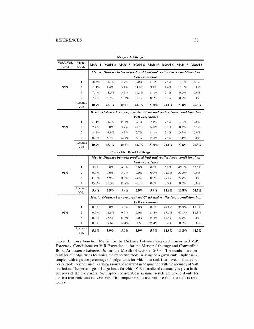
REFERENCES 32

�

VaR/CVaR

Level

Model


1 18.5% 11.1% 3.7% 0.0% 11.1% 7.4% 11.1% 3.7%

95% 2 11.1% 7.4% 3.7% 14.8% 3.7% 7.4% 11.1% 0.0%

3 7.4% 18.5% 3.7% 11.1% 11.1% 7.4% 0.0% 0.0%

4 7.4% 3.7% 33.3% 11.1% 0.0% 3.7% 0.0% 0.0%

Accurate

VaR40.7% 48.1% 40.7% 40.7% 37.0% 74.1% 77.8% 96.3%

1 11.1% 11.1% 14.8% 3.7% 7.4% 7.4% 11.1% 0.0%

95% 2 7.4% 0.0% 3.7% 25.9% 14.8% 3.7% 0.0% 3.7%

3 14.8% 14.8% 3.7% 3.7% 11.1% 7.4% 3.7% 0.0%

4 0.0% 3.7% 22.2% 3.7% 14.8% 7.4% 7.4% 0.0%

Accurate

VaR40.7% 48.1% 40.7% 40.7% 37.0% 74.1% 77.8% 96.3%

1 5.9% 0.0% 0.0% 0.0% 0.0% 5.9% 47.1% 35.3%

95% 2 0.0% 0.0% 5.9% 0.0% 0.0% 52.9% 35.3% 0.0%

3 41.2% 5.9% 0.0% 29.4% 0.0% 29.4% 5.9% 0.0%

4 35.3% 35.3% 11.8% 41.2% 0.0% 0.0% 0.0% 0.0%

Accurate

VaR5.9% 5.9% 5.9% 5.9% 5.9% 11.8% 11.8% 64.7%

1 0.0% 0.0% 5.9% 0.0% 0.0% 47.1% 35.3% 11.8%

95% 2 0.0% 11.8% 0.0% 0.0% 11.8% 17.6% 47.1% 11.8%

3 0.0% 23.5% 11.8% 0.0% 35.3% 17.6% 5.9% 0.0%

4 0.0% 17.6% 29.4% 17.6% 29.4% 5.9% 0.0% 0.0%

Accurate

VaR5.9% 5.9% 5.9% 5.9% 5.9% 11.8% 11.8% 64.7%


Merger Arbitrage


VaR exceedance


VaR exceedance


VaR exceedance


VaR exceedance

Table 10: Loss Function Metric for the Distance between Realized Losses and VaRForecasts, Conditional on VaR Exceedance, for the Merger Arbitrage and ConvertibleBond Arbitrage Strategies During the Month of October 2008. The numbers are per-centages of hedge funds for which the respective model is assigned a given rank. Higher rank,coupled with a greater percentage of hedge funds for which that rank is achieved, indicates su-perior model performance. Ranking should be analyzed in conjunction with the accuracy of VaRprediction. The percentage of hedge funds for which VaR is predicted accurately is given in thelast rows of the two panels. With space considerations in mind, results are provided only forthe first four ranks and the 95% VaR. The complete results are available from the authors uponrequest.

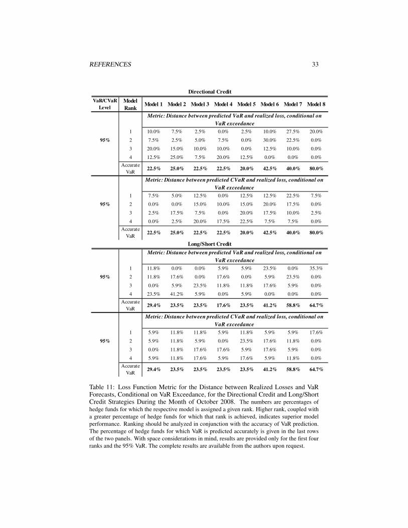
REFERENCES 33

�

VaR/CVaR

Level

Model


1 10.0% 7.5% 2.5% 0.0% 2.5% 10.0% 27.5% 20.0%

95% 2 7.5% 2.5% 5.0% 7.5% 0.0% 30.0% 22.5% 0.0%

3 20.0% 15.0% 10.0% 10.0% 0.0% 12.5% 10.0% 0.0%

4 12.5% 25.0% 7.5% 20.0% 12.5% 0.0% 0.0% 0.0%

Accurate

VaR22.5% 25.0% 22.5% 22.5% 20.0% 42.5% 40.0% 80.0%

1 7.5% 5.0% 12.5% 0.0% 12.5% 12.5% 22.5% 7.5%

95% 2 0.0% 0.0% 15.0% 10.0% 15.0% 20.0% 17.5% 0.0%

3 2.5% 17.5% 7.5% 0.0% 20.0% 17.5% 10.0% 2.5%

4 0.0% 2.5% 20.0% 17.5% 22.5% 7.5% 7.5% 0.0%

Accurate

VaR22.5% 25.0% 22.5% 22.5% 20.0% 42.5% 40.0% 80.0%

1 11.8% 0.0% 0.0% 5.9% 5.9% 23.5% 0.0% 35.3%

95% 2 11.8% 17.6% 0.0% 17.6% 0.0% 5.9% 23.5% 0.0%

3 0.0% 5.9% 23.5% 11.8% 11.8% 17.6% 5.9% 0.0%

4 23.5% 41.2% 5.9% 0.0% 5.9% 0.0% 0.0% 0.0%

Accurate

VaR29.4% 23.5% 23.5% 17.6% 23.5% 41.2% 58.8% 64.7%

1 5.9% 11.8% 11.8% 5.9% 11.8% 5.9% 5.9% 17.6%

95% 2 5.9% 11.8% 5.9% 0.0% 23.5% 17.6% 11.8% 0.0%

3 0.0% 11.8% 17.6% 17.6% 5.9% 17.6% 5.9% 0.0%

4 5.9% 11.8% 17.6% 5.9% 17.6% 5.9% 11.8% 0.0%

Accurate

VaR29.4% 23.5% 23.5% 23.5% 23.5% 41.2% 58.8% 64.7%

Long/Short Credit

Directional Credit


VaR exceedance


VaR exceedance


VaR exceedance


VaR exceedance

Table 11: Loss Function Metric for the Distance between Realized Losses and VaRForecasts, Conditional on VaR Exceedance, for the Directional Credit and Long/ShortCredit Strategies During the Month of October 2008. The numbers are percentages ofhedge funds for which the respective model is assigned a given rank. Higher rank, coupled witha greater percentage of hedge funds for which that rank is achieved, indicates superior modelperformance. Ranking should be analyzed in conjunction with the accuracy of VaR prediction.The percentage of hedge funds for which VaR is predicted accurately is given in the last rowsof the two panels. With space considerations in mind, results are provided only for the first fourranks and the 95% VaR. The complete results are available from the authors upon request.

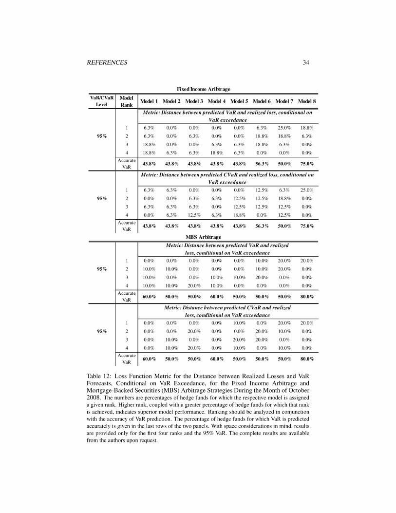
REFERENCES 34

�

VaR/CVaR

Level

Model


1 6.3% 0.0% 0.0% 0.0% 0.0% 6.3% 25.0% 18.8%

95% 2 6.3% 0.0% 6.3% 0.0% 0.0% 18.8% 18.8% 6.3%

3 18.8% 0.0% 0.0% 6.3% 6.3% 18.8% 6.3% 0.0%

4 18.8% 6.3% 6.3% 18.8% 6.3% 0.0% 0.0% 0.0%

Accurate

VaR43.8% 43.8% 43.8% 43.8% 43.8% 56.3% 50.0% 75.0%

1 6.3% 6.3% 0.0% 0.0% 0.0% 12.5% 6.3% 25.0%

95% 2 0.0% 0.0% 6.3% 6.3% 12.5% 12.5% 18.8% 0.0%

3 6.3% 6.3% 6.3% 0.0% 12.5% 12.5% 12.5% 0.0%

4 0.0% 6.3% 12.5% 6.3% 18.8% 0.0% 12.5% 0.0%

Accurate

VaR43.8% 43.8% 43.8% 43.8% 43.8% 56.3% 50.0% 75.0%

1 0.0% 0.0% 0.0% 0.0% 0.0% 10.0% 20.0% 20.0%

95% 2 10.0% 10.0% 0.0% 0.0% 0.0% 10.0% 20.0% 0.0%

3 10.0% 0.0% 0.0% 10.0% 10.0% 20.0% 0.0% 0.0%

4 10.0% 10.0% 20.0% 10.0% 0.0% 0.0% 0.0% 0.0%

Accurate

VaR60.0% 50.0% 50.0% 60.0% 50.0% 50.0% 50.0% 80.0%

1 0.0% 0.0% 0.0% 0.0% 10.0% 0.0% 20.0% 20.0%

95% 2 0.0% 0.0% 20.0% 0.0% 0.0% 20.0% 10.0% 0.0%

3 0.0% 10.0% 0.0% 0.0% 20.0% 20.0% 0.0% 0.0%

4 0.0% 10.0% 20.0% 0.0% 10.0% 0.0% 10.0% 0.0%

Accurate

VaR60.0% 50.0% 50.0% 60.0% 50.0% 50.0% 50.0% 80.0%



Fixed Income Aribtrage


VaR exceedance


VaR exceedance

MBS Arbitrage



Table 12: Loss Function Metric for the Distance between Realized Losses and VaRForecasts, Conditional on VaR Exceedance, for the Fixed Income Arbitrage andMortgage-Backed Securities (MBS) Arbitrage Strategies During the Month of October2008. The numbers are percentages of hedge funds for which the respective model is assigneda given rank. Higher rank, coupled with a greater percentage of hedge funds for which that rankis achieved, indicates superior model performance. Ranking should be analyzed in conjunctionwith the accuracy of VaR prediction. The percentage of hedge funds for which VaR is predictedaccurately is given in the last rows of the two panels. With space considerations in mind, resultsare provided only for the first four ranks and the 95% VaR. The complete results are availablefrom the authors upon request.

No. 1 Biliana Güner, Svetlozar T. Rachev, Daniel Edelman, Frank J. Fabozzi:

Bayesian inference for hedge funds with stable distribution of returns,

August 2010

recent issues

Working Paper Series in Economics

The responsibility for the contents of the working papers rests with the author, not the Institute. Since working papers

are of a preliminary nature, it may be useful to contact the author of a particular working paper about results or ca-

veats before referring to, or quoting, a paper. Any comments on working papers should be sent directly to the author.

Documents

Bayesian inference for hedge funds with stable distribution of returns