econstor www.econstor.eu

Der Open-Access-Publikationsserver der ZBW – Leibniz-Informationszentrum WirtschaftThe Open Access Publication Server of the ZBW – Leibniz Information Centre for Economics

Standard-Nutzungsbedingungen:

Die Dokumente auf EconStor dürfen zu eigenen wissenschaftlichenZwecken und zum Privatgebrauch gespeichert und kopiert werden.

Sie dürfen die Dokumente nicht für öffentliche oder kommerzielleZwecke vervielfältigen, öffentlich ausstellen, öffentlich zugänglichmachen, vertreiben oder anderweitig nutzen.

Sofern die Verfasser die Dokumente unter Open-Content-Lizenzen(insbesondere CC-Lizenzen) zur Verfügung gestellt haben sollten,gelten abweichend von diesen Nutzungsbedingungen die in der dortgenannten Lizenz gewährten Nutzungsrechte.

Terms of use:

Documents in EconStor may be saved and copied for yourpersonal and scholarly purposes.

You are not to copy documents for public or commercialpurposes, to exhibit the documents publicly, to make thempublicly available on the internet, or to distribute or otherwiseuse the documents in public.

If the documents have been made available under an OpenContent Licence (especially Creative Commons Licences), youmay exercise further usage rights as specified in the indicatedlicence.

zbw Leibniz-Informationszentrum WirtschaftLeibniz Information Centre for Economics

Bellora, Cecilia; Bourgeon, Jean-Marc

Working Paper

Agricultural Trade, Biodiversity Effects and FoodPrice Volatility

CESifo Working Paper, No. 5417

Provided in Cooperation with:Ifo Institute – Leibniz Institute for Economic Research at the University ofMunich

Suggested Citation: Bellora, Cecilia; Bourgeon, Jean-Marc (2015) : Agricultural Trade,Biodiversity Effects and Food Price Volatility, CESifo Working Paper, No. 5417

This Version is available at:http://hdl.handle.net/10419/113741

Agricultural Trade, Biodiversity Effects and Food Price Volatility

Cecilia Bellora Jean-Marc Bourgeon

CESIFO WORKING PAPER NO. 5417 CATEGORY 9: RESOURCE AND ENVIRONMENT ECONOMICS

JUNE 2015

Presented at CESifo Area Conference on Applied Microeconomics, March 2015

An electronic version of the paper may be downloaded • from the SSRN website: www.SSRN.com • from the RePEc website: www.RePEc.org

• from the CESifo website: Twww.CESifo-group.org/wp T

ISSN 2364-1428

CESifo Working Paper No. 5417

Agricultural Trade, Biodiversity Effects and Food Price Volatility

Abstract Biotic factors such as pests create biodiversity effects that increase production risks and decrease land productivity when agriculture becomes more specialized. We show in a Ricardian two-country trade setup that production specialization is incomplete under free trade because of the decrease in land productivity. Pesticides allow farmers to reduce these biodiversity effects, but they are damaging for the environment and for human health. When regulating farming practices under free trade, governments face a trade-off: they are tempted to restrict pesticide use compared to under autarky because domestic consumption partly relies on imports and thus depends less on them, but they also want to preserve the competitiveness of their agricultural sector on international markets. We show that at the symmetric equilibrium under free trade, restrictions on pesticides are generally more stringent than under autarky. As a result, trade increases the price volatility of crops produced by both countries, and of some or all of the crops that are country-specific, depending on the intensity of the biodiversity effects.

JEL-Code: F180, Q170.

Keywords: agricultural trade, food prices, agrobiodiversity, pesticides.

Cecilia Bellora CEPII

113 rue de Grenelle France – 75007 Paris

cecilia.bellora@cepii.fr

Jean-Marc Bourgeon UMR Économie publique

AgroParisTech–Paris 16, rue Claude Bernard

France - 75231 Paris Cedex 05 bourgeon@agroparistech.fr

June, 2015 The authors are grateful to Brian Copeland for his comments and suggestions. They also thank seminar participants at Ecole Polytechnique, at the 2014 BioEcon conference, at the 2014 conference of the French Association of Environmental and Resource Economists, and at the 2015 CESifo Area Conference on applied microeconomics. The research leading to these results has received funding from the European Union’s Seventh Framework Programme FP7/2007-2001 under Grant Agreement 290693 FOODSECURE. The authors only are responsible for any omissions or deficiencies. Neither the FOODSECURE project and any of its partner organizations, nor any organization of the European Union are accountable for the content of this paper. Much of this work was done while Cecilia Bellora was a PhD student at Université de Cergy-Pontoise and INRA.

1 Introduction

Agricultural prices are historically more volatile than manufacture prices (Jacks et al.,

2011). Perhaps because this stochasticity is considered to be due to factors beyond hu-

man control, such as weather conditions, economic studies analyzing agricultural price

volatility focus mainly on factors related to market organization, such as demand vari-

ability and the role played by stocks.1 However, in addition to abiotic factors, such

as water stress, temperature, irradiance and nutrient supply, which are often related to

weather conditions, production stochasticity is also caused by biotic factors, also known

as “pests”—including animal pests (such as insects, rodents, birds, etc.), pathogens (such

as viruses, bacteria, fungi, etc.), or weeds—which are harmful organisms that can cause

critical harvest losses.2 The impact of pests on yields is linked to the degree of special-

ization of the agricultural sector, which depends on the country’s openness to trade. The

more cultivation is concentrated on a few high-yielding crops, the more pests specialize

on these crops and the greater their virulence. Yields become more variable with special-

ization and the probability of low harvests rises. This variability is very much reduced

by the use of agrochemicals (pesticides, fungicides, herbicides and the like).3 But these

chemicals generate negative externalities, on human health, biodiversity, water and air

quality.4 Trade questions the necessity of using pesticides because of NIMBY (Not in

My Back Yard) considerations: some of the food consumed locally is produced abroad,

therefore eliminating the amount of pesticide that would have been needed to grow it

at home. Moreover, the portion of the food grown locally that is sold abroad exposes

1See Gilbert & Morgan (2010) and Wright (2011) for overviews on food price volatility and examina-tions of the causes of recent price spikes.

2According to Oerke (2006), potential losses due to pests (i.e. without crop protection of any kind)between 2001 and 2003 were 50% for wheat, 77% for rice and 80% for cotton, among others. Savaryet al. (2000) also find significant losses: the combined average level of injuries led to a decrease of 37.2%in rice yield (if injuries were considered individually, the cumulative yield loss would have been 63.4%).Fernandez-Cornejo et al. (1998) compile similar data on previous periods and find that expected lossesfrom insects and diseases relative to current or potential yield range between 2 to 26% and that lossesfrom weeds range between 0% and 50%.

3In the case of wheat, they reduce potential losses of 50% to average actual losses of about 29% (from14% in Northwest Europe up to 35% and more in Central Africa and Southeast Asia). Actual losses forsoybean average around 26%. The order of magnitude of losses for maize and rice is greater, with actuallosses of respectively 40% and 37% (Oerke, 2006).

4Pimentel (2005) reports more than 26 million cases worldwide of non-fatal pesticide poisoning andapproximately 220, 000 fatalities. He estimates that the effects of pesticides on human health cost about1.2 billion US$ per year in the United States. Mammals and birds are also affected. Farmland birdpopulation decreased by 25% in France between 1989 and 2009 (Jiguet et al., 2012), and a sharp declinewas also observed in the whole EU during the same period (EEA, 2010). Pesticides also contaminatewater and soils and significantly affect water species both locally and regionally (Beketov et al., 2013).Many countries have adopted regulations that forbid the most harmful molecules, have set provisions onthe use and storage of pesticides, and promote their sustainable use. For example, only a fourth of thepreviously marketed molecules passed the safety assessment made within the European review processended in 2009 (EC, 2009). The use of pesticides seems to follow a decreasing trend: in Europe, quantitiessold decreased by 24% between 2001 and 2010 (ECP, 2013).

2

the local population to pesticide externalities without benefitting them personally. The

government regulating farming practices under free trade is then faced with a trade-off:

if it reduces pesticide use compared to the rate under autarky it can satisfy NIMBY con-

cerns, but doing so will reduce the trade competitiveness of its agricultural sector, which

depends on the intensive use of pesticides.

The aim of this paper is to formally analyze how crop biodiversity and environmental

policies interact with trade, and to derive the role of biotic factors on price volatility.

We develop a simple model of farm production affected by biotic factors that vary with

specialization to represent the impacts of crop biodiversity on agricultural productivity

and on the pattern of trade in a Ricardian two-country setup. We isolate these impacts by

assuming that pesticide use is regulated by an environmental tax with no distributional

effects, and we abstract from risk aversion by assuming that farmers and consumers are

risk neutral.5

Our analysis provides three main findings. First, while countries have differing com-

parative advantage under autarky, biodiversity effects lead to incomplete specialization

under free trade. Indeed, because specialization reduces the expected yield of crops, some

of them are produced by both countries because their agricultural sectors end up with the

same productivity given the intensity of cultivation at equilibrium. Second, the trade-off

in the design of environmental policies results in restrictions on pesticides more stringent

under free trade than under autarky: NIMBY considerations are prevalent over the mar-

ket share rivalry that opposes the two countries. Third, agricultural price distributions

depend on the pattern of trade. Trade increases the production volatility of crops pro-

duced by both countries. Country-specific crops for which comparative advantages are

large could see a reduction in their volatility, but that supposes very small biodiversity

effects. The expected market price of country-specific crops is increased for domestic con-

sumers of the producing country compared to under autarky. This is becaused of more

restrictive environmental policies and the intensification of production. For crops pro-

duced by both countries, the change in expected prices depends on the share of farmland

devoted to these crops compared to under autarky.

Our work is related to different strains of literature. The link between crop biodiversity,

yield and revenue variability is empirically investigated in Smale et al. (1998); Di Falco

& Perrings (2005); Di Falco & Chavas (2006). These studies find sometimes contrasting

results but generally tend to show that increasing agricultural biodiversity is associated

with higher production and lower risk exposure (Di Falco, 2012). We add to this literature

an economic foundation of the mechanisms at stake.6 We build on Weitzman (2000) to

5Risk aversion would lead the government to reduce specialisation under trade to diversify productionrisks among countries, as demonstrated by Gaisford & Ivus (2014).

6For more details on the biological mechanisms involved, see Tilman et al. (2005), who use simpleecological models to describe the positive influence of diversity in the biomass produced and corroboratetheir findings with empirical results detailed in Tilman & Downing (1994) and Tilman et al. (1996).

3

model farm production with biodiversity effects: the larger the share of farmland dedicated

to a crop, the more its parasitic species proliferates and thus the more fields of that crop are

at risk of being wiped out.7 Weitzman (2000) uses this model to solve the trade-off between

the private and social optima, the former tending to specializing on a few varieties while

the latter aims at preserving biodiversity. We depart from his work by considering a trade

context, incorporating the use of pesticides, and investigating the impact of biodiversity

effects on production and price distributions. Our setup is a Ricardian trade model

with two countries and many goods, a la Dornbusch et al. (1977). The incorporation

of uncertainty in trade models dates back to Turnovsky (1974), who analyzes how the

pattern of trade and the gains from trade are affected by uncertainty. Newbery & Stiglitz

(1984) analyze how the production choices of risk-averse farmers are affected under free

trade when production is uncertain and show that free trade may be Pareto inferior to no

trade. Then, a whole range of literature looks at the optimal trade policy in presence of

risk aversion, one of the recent contributions being Gaisford & Ivus (2014), who consider

the link between protection and the size of the country. In these models, as well as

in the recent Ricardian models involving more than two countries (Eaton & Kortum,

2002; Costinot & Donaldson, 2012), the stochastic component that affects production

and determines the pattern of trade is not related to the production process itself. In

that sense, it is “exogenous.” We instead consider a stochastic component embedded in

the production process and endogenously determined by the country’s openness to trade:

biotic and abiotic factors affect production stochastically, which generates price volatility,

and also causes productivity losses that prevent complete specialization.

The rest of the paper is organized as follows: the next section details the relationship

between crop biodiversity and the stochastic distribution of the agricultural production.

We determine the profit-maximizing equilibrium of the agricultural sector and show that

biodiversity effects result in an incomplete specialization under free trade. Section 3 is

devoted to the environmental policy. Optimal environmental tax policies are derived with

and without crop biodiversity effects, and in two situations: when governments ignore the

terms of trade effects of the tax and when they take them into account. This allows us

to disentangle the consequences of the different concerns that define the tax policy under

trade, i.e. the NIMBY considerations and the market share rivalry. The implication of the

interaction between biodiversity effects and environmental policies on agricultural price

volatility is exposed in section 4.

7Weitzman (2000) makes an analogy between parasite-host relationships and the species-area curvethat originally applies to islands: the bigger the size of an island, the more species will be located there.He compares the total biomass of a uniform crop to an island in a sea of other biomass. A large literaturein ecology uses the species-area curve which is empirically robust not only for islands but, more generally,for uniform regions (May, 2000; Garcia Martin & Goldenfeld, 2006; Drakare et al., 2006; Plotkin et al.,2000; Storch et al., 2012).

4

2 The model

To investigate the importance of biodiversity effects on the pattern of trade and on price

volatility, we re-examine the standard Ricardian model of trade as developed by Dorn-

busch et al. (1977). Here, we consider two-sector economies, with an industrial/service

sector which produces a homogeneous good (with equal productivities in the two countries

and used as the numeraire) and an agricultural sector producing a range of goods with

different potential yields. The effective yields depend on this potential yield but also on

biotic and abiotic stochastic factors. They also depend on the use of pesticides, which

is regulated by governments. The first part of this section details the farms’ stochastic

production setup and the resulting supply functions. Demands are derived in the second

subsection. Then, we derive the autarky equilibrium. Although by assumption poten-

tial yields are different, in our simplified framework consumer preferences and the other

characteristics of the two economies are such that the autarky case displays symmetric

situations: the agricultural revenue, land rent and environmental tax are at the same

levels in the two countries. Only crop prices differ since yields are different in the two

countries.

2.1 Production

Consider two countries (Home and Foreign) whose economies are composed of two sectors;

industry and agriculture. Our focus being on agriculture, the industrial/service sector is

summarized by a constant return to scale production technology that allows to produce

one item with one unit of labor. The industrial good serves as the numeraire which

implies that the wage in these economies is equal to 1. The agricultural sector produces a

continuum of crops indexed by z ∈ [0, 1] using three factors: land, labor and agrochemicals

(pesticides, herbicides, fungicides and the like) directed to control pests and dubbed

“pesticides” in the following.8 Home is endowed with L units of labor and N land plots,

and Foreign with L∗ and N∗ (asterisks are used throughout the paper to refer to the

foreign country). As farming one plot requires one unit of labor, industry employs L−Nworkers.

Technical coefficients in agriculture differ from one crop to the other, and from one

country to the other. More precisely, absent production externality and adverse meteo-

rological or biological events, this mere combination of one unit of labor with one unit

of land produces a(z) crop z in Home and a∗(z) in Foreign. Crops are ranked in order

of diminishing Home’s absolute yield: the relative crop yield A(z) ≡ a∗(z)/a(z) satisfies

A′(z) > 0, A(0) < 1 and A(1) > 1. Hence, on the basis of these differences in potential

8In order to streamline the analysis, we don’t consider fertilizers. We discuss the way to incorporatethem in our model in Appendix I.

5

yield, Home is more efficient producing goods belonging to [0, zs) and Foreign over (zs, 1]

where zs = A−1(1).

However, production of crops is affected by various factors resulting in an actual yield

that is stochastic and lower than the potential one. Factors impacting production are both

abiotic and biotic, the impact of the latter depending on the way crops are produced: the

more land that is dedicated to the same crop, the more pests specialize on this crop, the

higher the frequency of their attacks and the lower the survival probability of that crop

(Pianka, 2011). To counteract the impact of external events on her plot, a farmer can avail

herself of a large range of chemicals, but because of the externality due to pesticides (on

human health and the environment) governments restrict their use. To ease the exposition

and simplify the following derivations, we model the governmental policy as a tax which

results in a pesticide’s price τ , and we suppose that the governments complement this tax

policy with a subsidy that allows farmers to cope with the environmental regulation: at

equilibrium, it is financially neutral for farmers. We assume that farmers are risk-neutral

and may farm only one crop (the one they want) on one unit plot. Given her crop choice,

farmer i chooses the intensity of the chemical treatment πi of her field in order to reach

expected income

ri(z) ≡ maxπi

E[p(z)yi(z)]− τπi + T (z)− c,

where p(z) is the stochastic crop z price, yi(z) her stochastic production level, T (z) the

subsidy for crop z, which is considered as a lump sum payment to farmer i, and c the

other input costs, i.e. the sum of the wage (one unit of labor is necessary to farm a plot

of land) and rental price of land, which is the same whatever crop is farmed. In the

following, we assume that a unit plot is affected by one or several adverse conditions with

probability 1− ψ, independently of the fate of the other plots. If affected, its production

is totally destroyed. Otherwise, with probability ψ, the plot survives and produces a(z).9

The survival probability of a given crop z depends on the quantity of pesticides used by

farmer i, πi, the average quantity of pesticides used by the other farmers of crop z in

the country, π(z), and the share of land devoted nationally to the crop, B(z) ≡ N(z)/N

where N(z) is the number of crop z plots.10 With atomistic individuals (N is so large that

the yield of a single plot has a negligible effect on the market price), the crop z farmer’s

program can be rewritten as

r(z) = maxπi

a(z)ψ(πi; z, π(z), B(z))p(z)− τπi + T (z)− c,

9Pests and/or meteorological events do not necessarily totally destroy a plot, but rather affect thequantity of biomass produced. Our assumption allows for tractability, our random variable being thenumber of harvested plots rather than the share of harvested biomass.

10Pesticides have a cross-external positive impact on plots surrounding the area treated because theydiminish the overall level of pests. Hence, for a given individual treatment πi(z), the larger π(z), thelower the probability that the plot of farmer i is infected.

6

where p(z) is the per unit average price of crop z, defined as (denoting by y(z) the total

production level of crop z)

p(z) ≡ E[p(z)y(z)]

E[y(z)]= p(z) +

cov(p(z), y(z))

E[y(z)]. (1)

As cov(p(z), y(z)) < 0, the reference price p(z) is lower than the expected market price

due to the correlation between total production y(z) and market price p(z). Solving the

farmer’s program, we obtain that the optimal level of pesticides at the symmetric Nash

equilibrium between crop z farmers, π(z), satisfies

ψ′(π(z); z, π(z), B(z)) =τ

a(z)p(z). (2)

As the subsidy allows farmers to break even, we have T (z) = τπ(z).11 Competition in

the economy leads to r(z) = 0 for all z, hence

a(z)ψ(z)p(z) = c, (3)

where ψ(z) ≡ ψ(π(z); z, π(z), B(z)) is the survival probability of a plot of crop z at

equilibrium. As plots are identically and independently affected, we obtain that

E[p(z)y(z)] = p(z)a(z)ψ(z)NB(z) = cNB(z), (4)

i.e., the expected value of the crop z domestic production is equal to the sum of the wages

and the land value involved in its farming.

The survival probability that allows us to derive our results in the following is given

by

ψ (πi; z, π, B(z)) =µ0 exp[πi(θ(z)− πi/2)]

1 + exp[(θ(z)− π)2/2]κ(z)B(z),

where the impact of abiotic factors on the production of crop z is captured by µ0.12 The

impact of farmer i’s pesticide use on the resilience of her plot is given by exp[πi(θ(z) −πi/2)], where θ(z) corresponds to the level of pesticides that maximizes the expected

yield of crop z. Biodiversity and cross-externality effects appear on the denominator: the

expected resilience of individual plots decreases with B(z), the intensity of the crop culti-

vation, but increases with the average level of pesticides used π, and reaches a maximum

at π = θ(z). Here, κ(z) ≡ κ0 exp[−θ(z)2/2] is the lowest crossexternality factor for crop

11For the sake of simplicity, we consider neither the production nor the market of agrochemicals in thefollowing. Implicitly, farmers thus are “endowed” with a large stock of agrochemicals that farming doesnot exhaust, leading to prices equal to 0.

12This functional form is derived from a probabilistic model that relies on a beta-binomial probabilitydistribution and represents very robust stylized facts in ecology concerning the parasite-host relationship.For more details, see Bellora et al. (2015).

7

z, when all crop z farmers use pesticide level θ(z), and exp[(θ(z)− π)2/2] is the negative

effect on the crop’s resilience induced by an average use of pesticides π ≤ θ(z). We assume

that µ0, κ0 and θ(z) are the same in both countries and such that ψ(·) ≤ 1.13

Using (2) and (3) we obtain that pesticide use for crop z is given by

π(z) = θ(z)− τ/c, (5)

and that the survival probability of a plot at equilibrium is given by

ψ(z) =µ0 exp [θ(z)2/2]

t[1 + tκ(z)B(z)], (6)

where t ≡ exp[(τ/c)2/2] = exp[(θ(z)− π(z))2/2] is the tax index that measures the nega-

tive effect of the restricted use of pesticides on the crop’s resilience. This index diminishes

with π(z) over [0, θ(z)] and reaches a minimum equal to 1 when π(z) = θ(z) (which corre-

sponds to an absence of regulation, i.e. τ = 0). Denoting the crop z maximum expected

yield as a(z) ≡ a(z)µ0 exp[θ(z)2/2], the crop z reference price is given by

p(z) = ct[1 + tκ(z)B(z)]/a(z), (7)

and the expected domestic production level for crop z by

y(z) ≡ E[y(z)] =a(z)NB(z)

t[1 + tκ(z)B(z)]. (8)

Production of crop z decreases with t because of two effects: the corresponding reduc-

tion in the use of pesticides has a direct negative impact on the productivity of each plot

but also an indirect negative cross-externality effect between plots.

2.2 Demand

The representative individuals of the two countries share the same preferences over goods.

Their preferences are given by the following Cobb-Douglas utility function

U = b lnxI + (1− b)∫ 1

0

α(z) ln x(z)dz − hZ,

where∫ 1

0α(z)dz = 1 and h > 0. The first two terms correspond to the utility derived

from the consumption of industrial and agricultural goods respectively, while the last term

13Parameter µ0 may be considered as resulting from factors beyond the control of the collective actionof farmers, such as meteorological events, which may differ from one crop to the other and from onecountry to the other; i.e. we may rather have two functions µ(z) and µ∗(z) taking different values.

However, because competitive advantages are assessed by comparing a(z) = µ0a(z) exp[θ(z)2/2] to its

foreign counterpart, assuming that it is a parameter is innocuous.

8

corresponds to the disutility of the environmental damages caused by a domestic use of

Z = N

∫ 1

0

B(z)π(z)dz

pesticides by farmers. The demand for the industrial good is xI = bR where R is the

revenue per capita. The rest of the revenue, (1− b)R, is spent on agricultural goods with

individual demand for crop z given by

x(z) = α(z)(1− b)R/p(z) (9)

where p(z) depends on the realized production level y(z) and α(z) is the share of the food

spending devoted to crop z. We assume that consumers are risk-neutral and thus evaluate

their ex ante welfare at the average consumption level of crop z, x(z) ≡ E[x(z)]. Using (9),

the corresponding reference price is E[1/p(z)]−1. At market equilibrium under autarky

(the same reasoning applies under free trade), as Lx = y, we obtain from definition (1)

and the fact that Lxp = α(z)(1− b)LR that p(z) = E[1/p(z)]−1, i.e. the consumers’ and

producers’ reference prices are the same. The representative consumer’s indirect utility

function can be written as14

V (R,Z) = ln(R)− (1− b)∫ 1

0

α(z) ln p(z)dz − hZ. (10)

where R = (L−N + cN)/L since there is no profit at equilibrium.

The government determines the optimal policy by maximizing this utility, taking ac-

count of the relationship between pesticides and the value of land.

2.3 Equilibrium under autarky

The autarky equilibrium is derived as follows. The market clearing condition for industrial

goods allows us to derive the cost of agricultural production cA (the sum of the rental

price of the agricultural land and of the wage).15 For a given environmental tax level,

equilibrium on each crop market gives the sharing of land between crops. These levels

allow us to derive the optimal tax policy under autarky.

Due to the constant returns to scale in the industrial sector, the total spending on

industrial products must be equal to the total production cost at equilibrium, i.e.,

bLR = b(NcA + L−N) = L−N

which gives cA = (` − 1)(1 − b)/b where ` ≡ L/N > 1. Consequently, the value of land

14Up to a constant given by b ln(b) + (1− b)∫ 1

0α(z) lnα(z)dz.

15Subscript “A” indexes equilibrium values under autarky.

9

is positive if N < (1 − b)L, a condition assumed to hold in the following. Observe that

this value depends neither on the use of pesticides nor on the crops’ prices and is the

same in both countries in spite of their differences in terms of crop yields. This is due to

the Cobb-Douglas preferences (in addition to the constant productivity in the industrial

sector).

Market equilibrium on the crop z market implies that total expenses are equal to total

production cost, i.e.

α(z)(1− b)LR = NB(z)cA

where the total domestic revenue is given by

LR = NcA + L−N = N(`− 1)/b

for both countries. Combining these expressions gives that the share of land devoted

to crop z satisfies B(z) = α(z). Using (5) and τ/c =√

2 ln t, the disutility of the

environmental damages caused by the use of pesticides is given by

Z = N

∫ 1

0

α(z)θ(z)dz −N√

2 ln t.

The optimal pesticides tax index is determined by maximizing the utility of the represen-

tative consumer (10) which reduces to

mint

(1− b)∫ 1

0

α(z) ln{t[1 + tκ(z)α(z)]}dz + hZ,

a program that applies to both countries. We obtain that the optimal tax index under

autarky, tA, solves

√2 ln tA

[1 +

∫ 1

0

tAκ(z)α(z)2

1 + tAκ(z)α(z)dz

]=

Nh

1− b. (11)

As κ(z) = κ0 exp [−θ(z)2/2], the optimal tax decreases when κ0 increases, with a maxi-

mum given by τA = (L−N)h/b.

While acreage and pesticide levels are the same in both countries, the average pro-

duction of each is different because of the differences in crop yields. The revenue being

the same in both countries, crop demands are identical but because average production

levels are different, break-even prices are also different.

2.4 Free trade equilibrium

We show in this section that when Home and Foreign engage in free trade, biodiver-

sity effects result in an incomplete specialisation. Without these effects, productions are

10

country-specific as described in Dornbusch et al. (1977), a threshold crop delimiting the

production range specific to each country. With biodiversity effects, this clear-cut situa-

tion can no longer exist, because specialisation, i.e. the increase in the acreage devoted

to a crop, reduces the expected yield. As a result, the two countries share the production

of a whole range of crops delimited by two threshold crops.16 We detail these results in

the next paragraphs.

The free trade equilibrium is derived from the equilibrium on industrial good market

which allows us to determine the worldwide agricultural and total revenues. The condition

of equalization of total spending with the total production cost on the industrial market

is given by

b(Nc+ L−N +N∗c∗ + L∗ −N∗) = L−N + L∗ −N∗

where L = L∗ and N = N∗. We obtain c + c∗ = 2(` − 1)(1 − b)/b, hence that the

worldwide agricultural revenue is the same as under autarky. This is also the case for the

total revenue, given by

LR + L∗R∗ = N [c+ c∗ + 2(`− 1)] = 2N(`− 1)/b.

As under autarky, the share of the agricultural sector of this revenue is unchanged,

given by 1− b. For Home, it results in a per-individual revenue given by

R =(`− 1)

`

[1 + 2q

1− bb

], (12)

which depends on the fraction q ≡ c/(c+ c∗) obtained at equilibrium. This share depends

on crop yields and on the environmental tax policies implemented in each country.

However, competitive advantages depend not only on environmental taxes but also

on biodiversity effects, i.e. on the way land is farmed. Indeed, for a given tax level, the

higher the intensity of the farming of a crop, i.e. the more land is devoted to that crop, the

lower the average productivity of the land, because of the production externality effect.

In other words, intensification undermines the competitive advantages apparent under

autarky. More precisely, if crop z is produced by Home only, the market equilibrium

condition implies that worldwide expenses on crop z are equal to total production cost,

i.e.,

2α(z)(`− 1)N(1− b)/b = NB(z)c

which can be written as α(z)/q = B(z). Opening to trade could thus correspond to a large

increase of the acreage devoted to that crop: for example, if q = 1/2, the total farmland

16Incomplete specialisation is obtained in Dornbusch et al. (1977) considering exogenous trade costs,the so-called Samuelson’s iceberg costs. In our setup, it is due to stochastic factors that are directlylinked to the production process and evolve with the openness to trade.

11

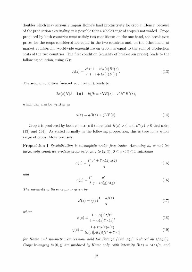
doubles which may seriously impair Home’s land productivity for crop z. Hence, because

of the production externality, it is possible that a whole range of crops is not traded. Crops

produced by both countries must satisfy two conditions: on the one hand, the break-even

prices for the crops considered are equal in the two countries and, on the other hand, at

market equilibrium, worldwide expenditure on crop z is equal to the sum of production

costs of the two countries. The first condition (equality of break-even prices), leads to the

following equation, using (7):

A(z) =c∗

c

t∗

t

1 + t∗κ(z)B∗(z)

1 + tκ(z)B(z). (13)

The second condition (market equilibrium), leads to

2α(z)N(`− 1)(1− b)/b = cNB(z) + c∗N∗B∗(z),

which can also be written as

α(z) = qB(z) + q∗B∗(z). (14)

Crop z is produced by both countries if there exist B(z) > 0 and B∗(z) > 0 that solve

(13) and (14). As stated formally in the following proposition, this is true for a whole

range of crops. More precisely,

Proposition 1 Specialization is incomplete under free trade: Assuming κ0 is not too

large, both countries produce crops belonging to (z, z), 0 ≤ z < z ≤ 1 satisfying

A(z) =t∗

t

q∗ + t∗κ(z)α(z)

q(15)

and

A(z) =t∗

t

q∗

q + tκ(z)α(z). (16)

The intensity of these crops is given by

B(z) = χ(z)1− qφ(z)

q(17)

where

φ(z) ≡ 1 + A(z)t/t∗

1 + α(z)t∗κ(z), (18)

χ(z) ≡ 1 + t∗α(z)κ(z)

tκ(z)[A(z)t/t∗ + t∗/t](19)

for Home and symmetric expressions hold for Foreign (with A(z) replaced by 1/A(z)).

Crops belonging to [0, z] are produced by Home only, with intensity B(z) = α(z)/q, and

12

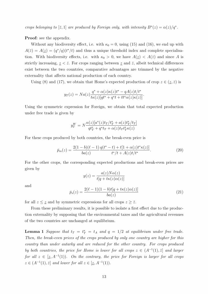
crops belonging to [z, 1] are produced by Foreign only, with intensity B∗(z) = α(z)/q∗.

Proof: see the appendix.

Without any biodiversity effect, i.e. with κ0 = 0, using (15) and (16), we end up with

A(z) = A(z) = (q∗/q)(t∗/t) and thus a unique threshold index and complete specialisa-

tion. With biodiversity effects, i.e. with κ0 > 0, we have A(z) < A(z) and since A is

strictly increasing, z < z. For crops ranging between z and z, albeit technical differences

exist between the two countries, comparative advantages are trimmed by the negative

externality that affects national production of each country.

Using (8) and (17), we obtain that Home’s expected production of crop z ∈ (z, z) is

yT (z) = Na(z)q∗ + α(z)κ(z)t∗ − qA(z)t/t∗

tκ(z)[qt∗ + q∗t+ tt∗α(z)κ(z)].

Using the symmetric expression for Foreign, we obtain that total expected production

under free trade is given by

yWT = Nα(z)[a∗(z)tT/t

∗T + a(z)t∗T/tT ]

qt∗T + q∗tT + α(z)tT t∗Tκ(z)

For these crops produced by both countries, the break-even price is

pm(z) =2(1− b)(`− 1)

ba(z)

q(t∗ − t) + t[1 + α(z)t∗κ(z)]

t∗/t+ A(z)t/t∗. (20)

For the other crops, the corresponding expected productions and break-even prices are

given by

y(z) =a(z)Nα(z)

t[q + tκ(z)α(z)]

and

ps(z) =2(`− 1)(1− b)t[q + tκ(z)α(z)]

ba(z)(21)

for all z ≤ z and by symmetric expressions for all crops z ≥ z.

From these preliminary results, it is possible to isolate a first effect due to the produc-

tion externality by supposing that the environmental taxes and the agricultural revenues

of the two countries are unchanged at equilibrium.

Lemma 1 Suppose that tT = t∗T = tA and q = 1/2 at equilibrium under free trade.

Then, the break-even prices of the crops produced by only one country are higher for this

country than under autarky and are reduced for the other country. For crops produced

by both countries, the price for Home is lower for all crops z ∈ (A−1(1), z] and larger

for all z ∈ [z, A−1(1)). On the contrary, the price for Foreign is larger for all crops

z ∈ (A−1(1), z] and lower for all z ∈ [z, A−1(1)).

13

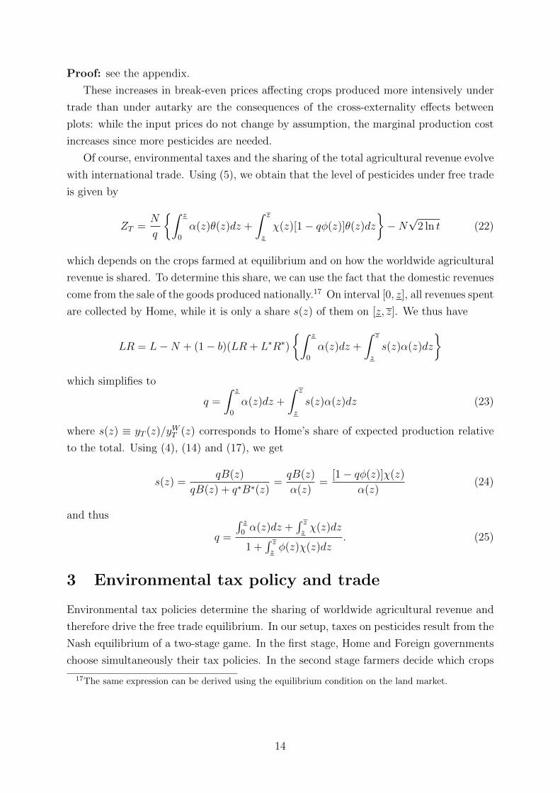
Proof: see the appendix.

These increases in break-even prices affecting crops produced more intensively under

trade than under autarky are the consequences of the cross-externality effects between

plots: while the input prices do not change by assumption, the marginal production cost

increases since more pesticides are needed.

Of course, environmental taxes and the sharing of the total agricultural revenue evolve

with international trade. Using (5), we obtain that the level of pesticides under free trade

is given by

ZT =N

q

{∫ z

0

α(z)θ(z)dz +

∫ z

z

χ(z)[1− qφ(z)]θ(z)dz

}−N√

2 ln t (22)

which depends on the crops farmed at equilibrium and on how the worldwide agricultural

revenue is shared. To determine this share, we can use the fact that the domestic revenues

come from the sale of the goods produced nationally.17 On interval [0, z], all revenues spent

are collected by Home, while it is only a share s(z) of them on [z, z]. We thus have

LR = L−N + (1− b)(LR + L∗R∗)

{∫ z

0

α(z)dz +

∫ z

z

s(z)α(z)dz

}which simplifies to

q =

∫ z

0

α(z)dz +

∫ z

z

s(z)α(z)dz (23)

where s(z) ≡ yT (z)/yWT (z) corresponds to Home’s share of expected production relative

to the total. Using (4), (14) and (17), we get

s(z) =qB(z)

qB(z) + q∗B∗(z)=qB(z)

α(z)=

[1− qφ(z)]χ(z)

α(z)(24)

and thus

q =

∫ z0α(z)dz +

∫ zzχ(z)dz

1 +∫ zzφ(z)χ(z)dz

. (25)

3 Environmental tax policy and trade

Environmental tax policies determine the sharing of worldwide agricultural revenue and

therefore drive the free trade equilibrium. In our setup, taxes on pesticides result from the

Nash equilibrium of a two-stage game. In the first stage, Home and Foreign governments

choose simultaneously their tax policies. In the second stage farmers decide which crops

17The same expression can be derived using the equilibrium condition on the land market.

14

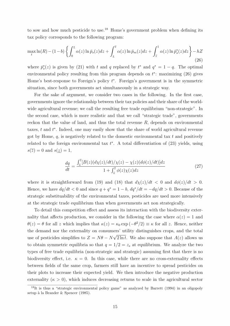
to sow and how much pesticide to use.18 Home’s government problem when defining its

tax policy corresponds to the following program:

maxt

ln(R)− (1−b){∫ z

0

α(z) ln ps(z)dz +

∫ z

z

α(z) ln pm(z)dz +

∫ 1

z

α(z) ln p∗s(z)dz

}−hZ

(26)

where p∗s(z) is given by (21) with t and q replaced by t∗ and q∗ = 1 − q. The optimal

environmental policy resulting from this program depends on t∗: maximizing (26) gives

Home’s best-response to Foreign’s policy t∗. Foreign’s government is in the symmetric

situation, since both governments act simultaneously in a strategic way.

For the sake of argument, we consider two cases in the following. In the first case,

governments ignore the relationship between their tax policies and their share of the world-

wide agricultural revenue; we call the resulting free trade equilibrium “non-strategic”. In

the second case, which is more realistic and that we call “strategic trade”, governments

reckon that the value of land, and thus the total revenue R, depends on environmental

taxes, t and t∗. Indeed, one may easily show that the share of world agricultural revenue

got by Home, q, is negatively related to the domestic environmental tax t and positively

related to the foreign environmental tax t∗. A total differentiation of (23) yields, using

s(z) = 0 and s(z) = 1,

dq

dt=

∫ zz

[B(z)(dχ(z)/dt)/χ(z)− χ(z)(dφ(z)/dt)]dz

1 +∫ zzφ(z)χ(z)dz

(27)

where it is straightforward from (19) and (18) that dχ(z)/dt < 0 and dφ(z)/dt > 0.

Hence, we have dq/dt < 0 and since q + q∗ = 1− b, dq∗/dt = −dq/dt > 0. Because of the

strategic substituability of the environmental taxes, pesticides are used more intensively

at the strategic trade equilibrium than when governments act non strategically.

To detail this competition effect and assess its interaction with the biodiversity exter-

nality that affects production, we consider in the following the case where α(z) = 1 and

θ(z) = θ for all z which implies that κ(z) = κ0 exp (−θ2/2) ≡ κ for all z. Hence, neither

the demand nor the externality on consumers’ utility distinguishes crops, and the total

use of pesticides simplifies to Z = Nθ − N√

2 ln t. We also suppose that A(z) allows us

to obtain symmetric equilibria so that q = 1/2 = zs at equilibrium. We analyze the two

types of free trade equilibria (non-strategic and strategic) assuming first that there is no

biodiversity effect, i.e. κ = 0. In this case, while there are no cross-externality effects

between fields of the same crop, farmers still have an incentive to spread pesticides on

their plots to increase their expected yield. We then introduce the negative production

externality (κ > 0), which induces decreasing returns to scale in the agricultural sector

18It is thus a “strategic environmental policy game” as analyzed by Barrett (1994) in an oligopolysetup a la Brander & Spencer (1985).

15

at the national level.

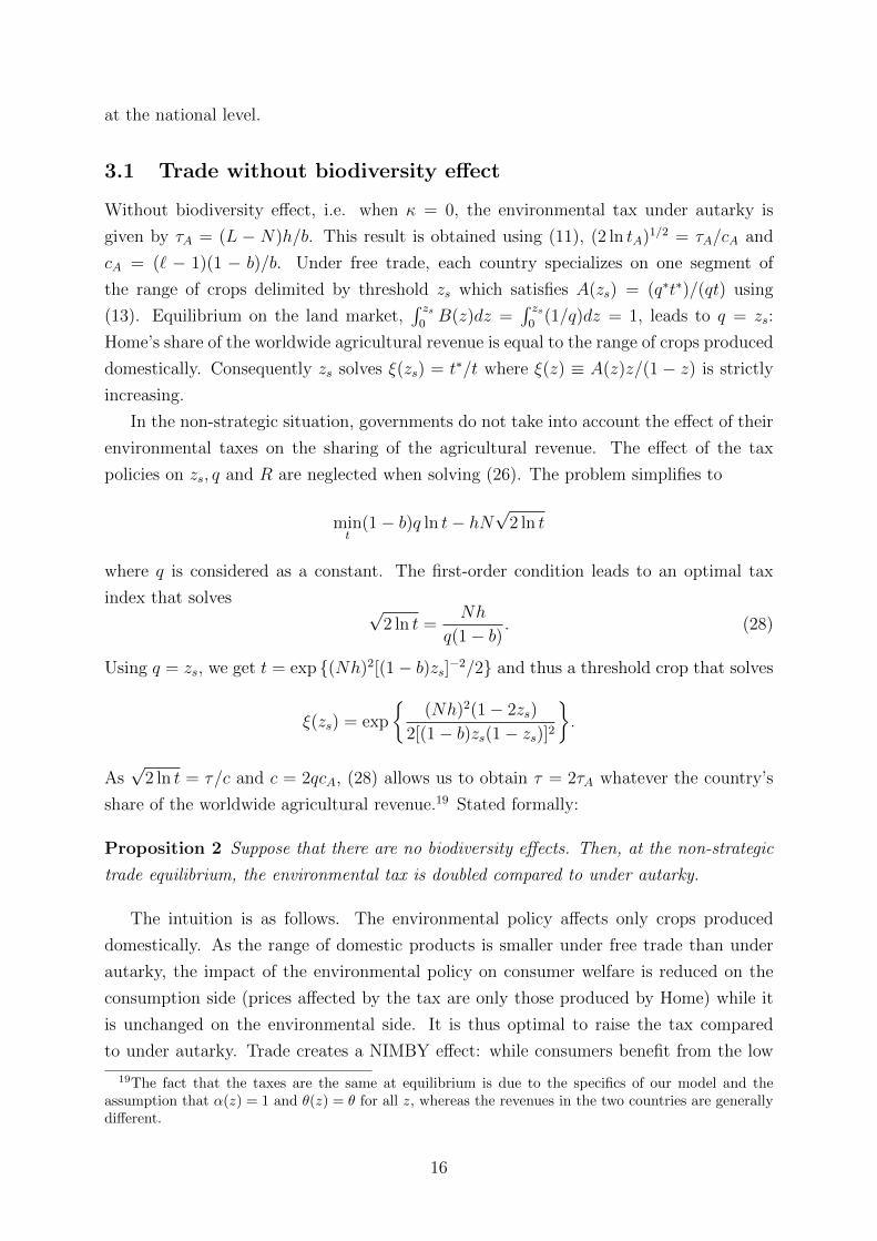
3.1 Trade without biodiversity effect

Without biodiversity effect, i.e. when κ = 0, the environmental tax under autarky is

given by τA = (L − N)h/b. This result is obtained using (11), (2 ln tA)1/2 = τA/cA and

cA = (` − 1)(1 − b)/b. Under free trade, each country specializes on one segment of

the range of crops delimited by threshold zs which satisfies A(zs) = (q∗t∗)/(qt) using

(13). Equilibrium on the land market,∫ zs

0B(z)dz =

∫ zs0

(1/q)dz = 1, leads to q = zs:

Home’s share of the worldwide agricultural revenue is equal to the range of crops produced

domestically. Consequently zs solves ξ(zs) = t∗/t where ξ(z) ≡ A(z)z/(1 − z) is strictly

increasing.

In the non-strategic situation, governments do not take into account the effect of their

environmental taxes on the sharing of the agricultural revenue. The effect of the tax

policies on zs, q and R are neglected when solving (26). The problem simplifies to

mint

(1− b)q ln t− hN√

2 ln t

where q is considered as a constant. The first-order condition leads to an optimal tax

index that solves √2 ln t =

Nh

q(1− b). (28)

Using q = zs, we get t = exp {(Nh)2[(1− b)zs]−2/2} and thus a threshold crop that solves

ξ(zs) = exp

{(Nh)2(1− 2zs)

2[(1− b)zs(1− zs)]2

}.

As√

2 ln t = τ/c and c = 2qcA, (28) allows us to obtain τ = 2τA whatever the country’s

share of the worldwide agricultural revenue.19 Stated formally:

Proposition 2 Suppose that there are no biodiversity effects. Then, at the non-strategic

trade equilibrium, the environmental tax is doubled compared to under autarky.

The intuition is as follows. The environmental policy affects only crops produced

domestically. As the range of domestic products is smaller under free trade than under

autarky, the impact of the environmental policy on consumer welfare is reduced on the

consumption side (prices affected by the tax are only those produced by Home) while it

is unchanged on the environmental side. It is thus optimal to raise the tax compared

to under autarky. Trade creates a NIMBY effect: while consumers benefit from the low

19The fact that the taxes are the same at equilibrium is due to the specifics of our model and theassumption that α(z) = 1 and θ(z) = θ for all z, whereas the revenues in the two countries are generallydifferent.

16

prices allowed by pesticides used abroad, they want pesticide use restricted domestically

to reduce pollution.20 Observe that the resulting situation is not Pareto optimal: indeed,

if the two countries could agree on tax levels, each would have to account for the price

effect of its tax on the other country’s consumers. In our setup, the resulting Pareto

optimal tax level is the autarky one.21

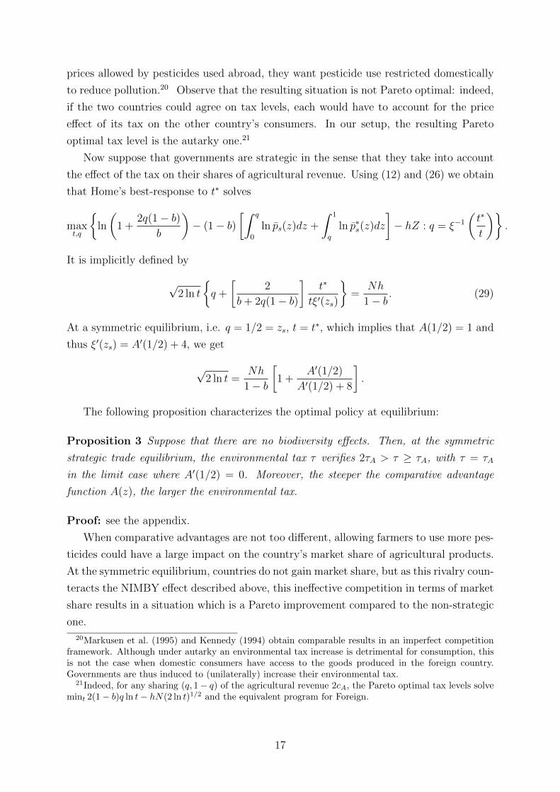
Now suppose that governments are strategic in the sense that they take into account

the effect of the tax on their shares of agricultural revenue. Using (12) and (26) we obtain

that Home’s best-response to t∗ solves

maxt,q

{ln

(1 +

2q(1− b)b

)− (1− b)

[∫ q

0

ln ps(z)dz +

∫ 1

q

ln p∗s(z)dz

]− hZ : q = ξ−1

(t∗

t

)}.

It is implicitly defined by

√2 ln t

{q +

[2

b+ 2q(1− b)

]t∗

tξ′(zs)

}=

Nh

1− b. (29)

At a symmetric equilibrium, i.e. q = 1/2 = zs, t = t∗, which implies that A(1/2) = 1 and

thus ξ′(zs) = A′(1/2) + 4, we get

√2 ln t =

Nh

1− b

[1 +

A′(1/2)

A′(1/2) + 8

].

The following proposition characterizes the optimal policy at equilibrium:

Proposition 3 Suppose that there are no biodiversity effects. Then, at the symmetric

strategic trade equilibrium, the environmental tax τ verifies 2τA > τ ≥ τA, with τ = τA

in the limit case where A′(1/2) = 0. Moreover, the steeper the comparative advantage

function A(z), the larger the environmental tax.

Proof: see the appendix.

When comparative advantages are not too different, allowing farmers to use more pes-

ticides could have a large impact on the country’s market share of agricultural products.

At the symmetric equilibrium, countries do not gain market share, but as this rivalry coun-

teracts the NIMBY effect described above, this ineffective competition in terms of market

share results in a situation which is a Pareto improvement compared to the non-strategic

one.

20Markusen et al. (1995) and Kennedy (1994) obtain comparable results in an imperfect competitionframework. Although under autarky an environmental tax increase is detrimental for consumption, thisis not the case when domestic consumers have access to the goods produced in the foreign country.Governments are thus induced to (unilaterally) increase their environmental tax.

21Indeed, for any sharing (q, 1− q) of the agricultural revenue 2cA, the Pareto optimal tax levels solvemint 2(1− b)q ln t− hN(2 ln t)1/2 and the equivalent program for Foreign.

17

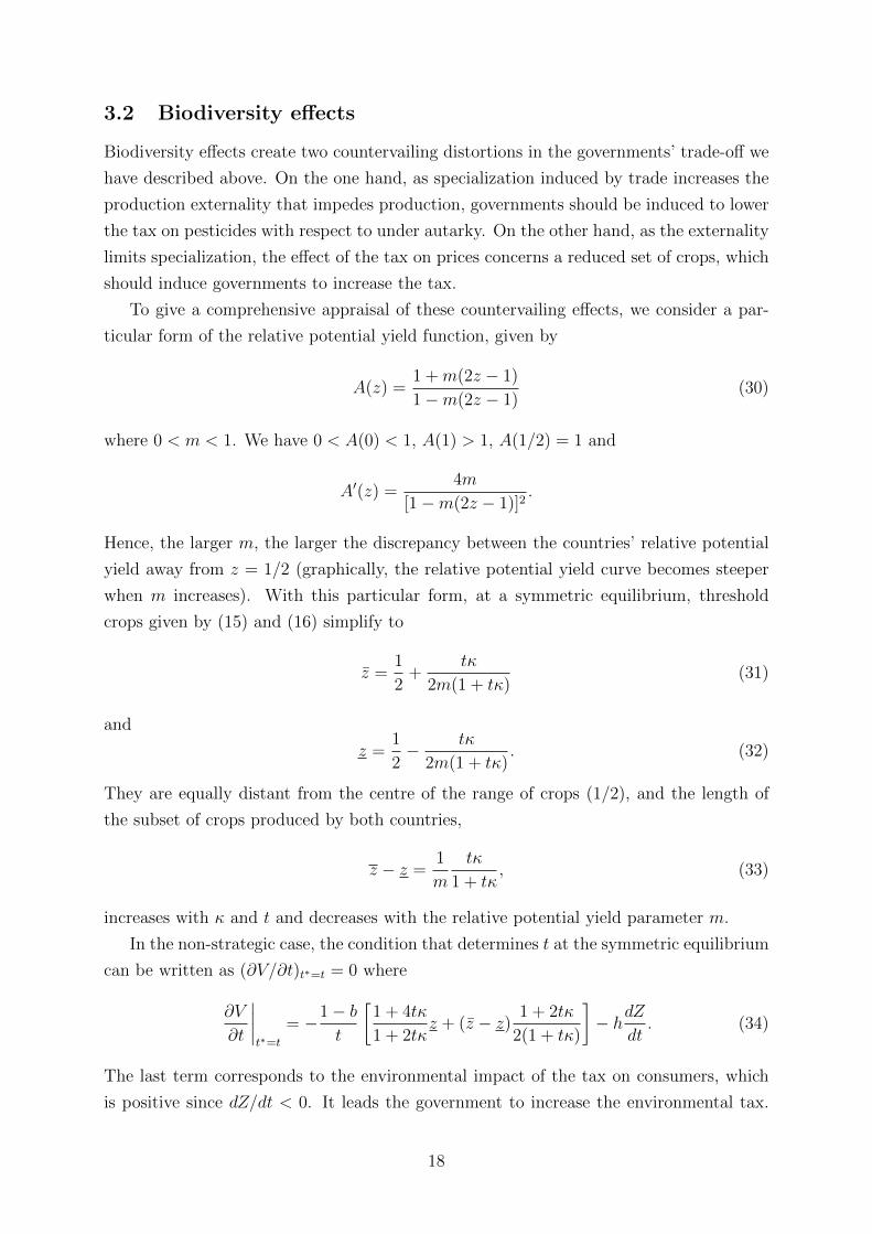
3.2 Biodiversity effects

Biodiversity effects create two countervailing distortions in the governments’ trade-off we

have described above. On the one hand, as specialization induced by trade increases the

production externality that impedes production, governments should be induced to lower

the tax on pesticides with respect to under autarky. On the other hand, as the externality

limits specialization, the effect of the tax on prices concerns a reduced set of crops, which

should induce governments to increase the tax.

To give a comprehensive appraisal of these countervailing effects, we consider a par-

ticular form of the relative potential yield function, given by

A(z) =1 +m(2z − 1)

1−m(2z − 1)(30)

where 0 < m < 1. We have 0 < A(0) < 1, A(1) > 1, A(1/2) = 1 and

A′(z) =4m

[1−m(2z − 1)]2.

Hence, the larger m, the larger the discrepancy between the countries’ relative potential

yield away from z = 1/2 (graphically, the relative potential yield curve becomes steeper

when m increases). With this particular form, at a symmetric equilibrium, threshold

crops given by (15) and (16) simplify to

z =1

2+

tκ

2m(1 + tκ)(31)

and

z =1

2− tκ

2m(1 + tκ). (32)

They are equally distant from the centre of the range of crops (1/2), and the length of

the subset of crops produced by both countries,

z − z =1

m

tκ

1 + tκ, (33)

increases with κ and t and decreases with the relative potential yield parameter m.

In the non-strategic case, the condition that determines t at the symmetric equilibrium

can be written as (∂V/∂t)t∗=t = 0 where

∂V

∂t

∣∣∣∣t∗=t

= −1− bt

[1 + 4tκ

1 + 2tκz + (z − z)

1 + 2tκ

2(1 + tκ)

]− hdZ

dt. (34)

The last term corresponds to the environmental impact of the tax on consumers, which

is positive since dZ/dt < 0. It leads the government to increase the environmental tax.

18

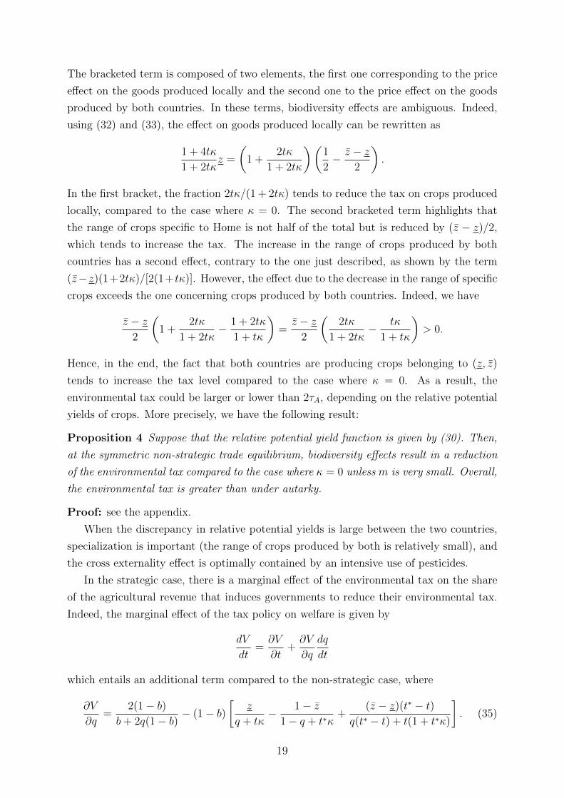
The bracketed term is composed of two elements, the first one corresponding to the price

effect on the goods produced locally and the second one to the price effect on the goods

produced by both countries. In these terms, biodiversity effects are ambiguous. Indeed,

using (32) and (33), the effect on goods produced locally can be rewritten as

1 + 4tκ

1 + 2tκz =

(1 +

2tκ

1 + 2tκ

)(1

2− z − z

2

).

In the first bracket, the fraction 2tκ/(1 + 2tκ) tends to reduce the tax on crops produced

locally, compared to the case where κ = 0. The second bracketed term highlights that

the range of crops specific to Home is not half of the total but is reduced by (z − z)/2,

which tends to increase the tax. The increase in the range of crops produced by both

countries has a second effect, contrary to the one just described, as shown by the term

(z−z)(1+2tκ)/[2(1+ tκ)]. However, the effect due to the decrease in the range of specific

crops exceeds the one concerning crops produced by both countries. Indeed, we have

z − z2

(1 +

2tκ

1 + 2tκ− 1 + 2tκ

1 + tκ

)=z − z

2

(2tκ

1 + 2tκ− tκ

1 + tκ

)> 0.

Hence, in the end, the fact that both countries are producing crops belonging to (z, z)

tends to increase the tax level compared to the case where κ = 0. As a result, the

environmental tax could be larger or lower than 2τA, depending on the relative potential

yields of crops. More precisely, we have the following result:

Proposition 4 Suppose that the relative potential yield function is given by (30). Then,

at the symmetric non-strategic trade equilibrium, biodiversity effects result in a reduction

of the environmental tax compared to the case where κ = 0 unless m is very small. Overall,

the environmental tax is greater than under autarky.

Proof: see the appendix.

When the discrepancy in relative potential yields is large between the two countries,

specialization is important (the range of crops produced by both is relatively small), and

the cross externality effect is optimally contained by an intensive use of pesticides.

In the strategic case, there is a marginal effect of the environmental tax on the share

of the agricultural revenue that induces governments to reduce their environmental tax.

Indeed, the marginal effect of the tax policy on welfare is given by

dV

dt=∂V

∂t+∂V

∂q

dq

dt

which entails an additional term compared to the non-strategic case, where

∂V

∂q=

2(1− b)b+ 2q(1− b)

− (1− b)[

z

q + tκ− 1− z

1− q + t∗κ+

(z − z)(t∗ − t)q(t∗ − t) + t(1 + t∗κ)

]. (35)

19

The first term corresponds to the direct effect on welfare due to the increase in revenue

while the remaining terms concern the effects on the price of crops produced domestically,

abroad and by both countries respectively. At a symmetric equilibrium, the price effects

cancel out, leading to (∂V/∂q)t∗=t,q=1/2 = 2(1 − b). Using (30), we obtain that (27) is

expressed asdq

dt

∣∣∣∣t∗=t,q=1/2

= − 3 + 9tκ+ 4(tκ)2

12t(1 + tκ)[m(1 + tκ) + 1](36)

which decreases with κ. The greater the biodiversity effects, the stronger the negative

impact of the environmental tax on the share of the agricultural revenue. However,

notwithstanding the marginal effect of the tax on the revenue, we show in the appendix

the following result

Proposition 5 Suppose that the relative potential yield function is given by (30). Then,

at the symmetric strategic trade equilibrium the environmental tax is generally greater

than under autarky.

Proof: see the appendix.

To sum up, the main effects linking trade and the pesticide policy are the following:

when governments neglect the impact of the tax on the terms of trade (i.e. under non

strategic trade) and without biodiversity effects, the NIMBY effects described in section

3.1 drive the increase in taxes. Still under non strategic trade but with biodiversity

effects, the production externality leads to a decrease in the taxes, counteracting the

NIMBY effect. However, the tax remains higher than under autarky. In the strategic

case, the marginal effect of the environmental tax on the market share leads governments

to soften their environmental policy. Nevertheless, the environmental policy remains more

stringent under free trade than under autarky.

4 Trade and volatility

Agricultural production is affected both by the way land is farmed, which depends on the

specialization induced by trade, and by the public regulation on pesticides. This section

is devoted to the impacts of these elements on the volatility of the productions and of the

prices.

4.1 Production volatility

We compare the volatility of crop production between the autarky and the free trade

situations using the variation coefficient (VC), defined for random variable X as v(X) ≡

20

σ(X)/E(X). As plots are independently affected by pests, the variance of crop z domes-

tic production is given by Var(y(z)) = a(z)2NB(z)ψ(z)[1 − ψ(z)].22 Denoting µ(z) ≡µ0 exp (θ(z)2/2) and using (6) and (8), the variation coefficient for the production by

Home of a crop z is given by

v(y(z)) =

{t[1 + tκ(z)B(z)]− µ(z)

µ(z)NB(z)

}1/2

. (37)

This coefficient increases with the tax index t and the intensity of biodiversity effects κ,

while it decreases with the total number of plots N and the share of the agricultural area

dedicated to the considered crop, B. Due to independence, both the variance and the

mean increase linearly with N , which results in a negative “scale” effect on volatility: the

larger the agricultural area of the country, the lower the variation coefficient. There is also

a scale effect associated to intensification (an increase in B) that dominates biodiversity

effects. The variation coefficients of the worldwide production of crop z under autarky

are given by

v(yWA (z)) =[Var(yA(z)) + Var(y∗A(z))]1/2

yA(z) + y∗A(z)={[a(z)2 + a∗(z)2]Nα(z)ψ(z)[1− ψ(z)]}1/2

[a(z) + a∗(z)]Nα(z)ψ(z).

Using (6), we get

v(yWA (z)) =

{1− 2A(z)

[1 + A(z)]2

}1/2{tA[1 + tAκ(z)α(z)]− µ(z)

µ(z)Nα(z)

}1/2

. (38)

While the second bracketed term in (38) is similar to (37), the first term reveals a yield

effect on production volatility when the same crops are produced by both countries: as

A(z)/[1 +A(z)]2 is cap-shaped with a maximum at A(z) = 1, this effect is decreasing for

z < 1/2 and increasing for z > 1/2. Hence, the yield effect on volatility is higher the

larger the difference between the crop yields of the two countries.23

Assuming symmetry, α(z) = 1 and θ(z) = θ (which implies µ(z) = µ and κ(z) = κ

for all z), the volatility of domestic production is the same for all crops under autarky

and for all crops produced by one country only under free trade. Indeed, in these two

cases, the intensification effects are constant, since, under autarky, B(z) = 1 for all z and,

under free trade, B(z) = 2 for all crops in the range [0; z[ and B∗(z) = 2 for all crops

in the range ]z; 1]. But the effects of intensification on volatility vary from one crop to

22This variance is obtained considering that plots survive to pests following a binomial distribution ofparameters NB(z), the number of plots growing crop z, and ψ(z), the survival probability of each ofthese plots. Denoting this variable X(z), we have y(z) = a(z)X(z) and thus Var(y(z)) = a(z)2Var(X(z)),with Var(X(z)) = NB(z)ψ(z)[1− ψ(z)].

23With identical yields, i.e. A(z) = 1, this term is equal to√

2/2, the scale effect of a doubling offarmland.

21

the other when we consider crops produced by both countries (z ∈ [z; z]) since farmland

intensities vary. The total share of land devoted to crops at the symmetric equilibrium

is the same (B(z) + B∗(z) = 2 in any case), but the relative importance of Home is

decreasing with z (from B(z) = 2 to B(z) = 0), whereas it is constant under autarky. To

compute the volatility of the world production of crops produced by both countries we use

Var(yW (z)) = Var(yT (z)) + Var(y∗T (z)) and v(yW (z))2 = s(z)2v(y(z))2 + s∗(z)2v(y∗(z))2,

which lead to

v(yW (z)) =

{(1 + tκ)(1 + 2tκ)− µκ

2µNκ− 2(1 + tκ)2

µNκ

A(z)

[1 + A(z)]2

}1/2

. (39)

As under autarky, there is a yield effect at work: the volatility index is decreasing over

[z, 1/2), increasing over (1/2, z], and thus reaches a minimum at z = 1/2. Comparing the

VCs under autarky and trade, we obtain the following result:

Proposition 6 Without biodiversity effects, trade could potentially reduce the production

volatility of all crops. However, because of a higher environmental tax than under autarky

only the volatility of crops for which countries have large comparative advantages is re-

duced (if any). With biodiversity effects, trade increases the production volatility of crops

produced by both countries and of the specialized crops with moderate competitive advan-

tage. The volatility of large comparative advantage crops is reduced only if biodiversity

effects are small and the environmental tax not too different from its autarky level.

Proof: see the appendix.

4.2 Price volatility

Some characteristics of the prices distributions can be derived from the properties of the

production distributions. We take advantage from the fact that the survival probability

of a given plot, ψ, does not depend on the total number of plots N , and thus that the

distribution of the number of plots that survive converges to a normal distribution when

N is large. This implies that the distribution of crop z production converges to the normal

distribution N (y(z), σ(y(z))). First, observe that the break-even price p(z) corresponds

to crop z median price: we have Pr[p(z) ≤ p(z)] = Pr[y(z) ≥ y(z)] = 1/2 since the

normal distribution is symmetric. Consequently, as p(z) is lower than the average market

price p(z) due to the correlation between prices and quantities, the price distribution is

asymmetric.

This asymmetry is also revealed by the upper and lower bounds of the confidence

intervals of crop prices, which are implied by the distribution of crop production. Denoting

by yγd (z) and yγu(z) the lower and upper bounds of the confidence interval of the production

of crop z at confidence level 1 − γ, the corresponding price bounds are derived from

22

Lx = y and (9), which give Pr[yγd (z) ≤ y(z) ≤ yγu(z)] = Pr[pγd(z) ≤ p(z) ≤ pγu(z)] where

pγu(z) ≡ α(z)(1 − b)LR/yγd (z) and pγd(z) ≡ α(z)(1 − b)LR/yγu(z). Because production

distributions are symmetric, yγd (z) and yγu(z) are equally distant from y(z). However,

since prices and quantities are inversely related, this is not the case for pγd(z) and pγu(z).

The following proposition completes these general features of the price distributions with

some useful approximations.

Proposition 7 The expected value and the standard deviation of crop prices are approx-

imated by

p(z) ≈ p(z)[1 + v(y(z))2] (40)

and

σ(p(z)) ≈ p(z)v(y(z))√

1− v(y(z))2.

Confidence intervals at confidence level 1 − γ are delimited by pγu(z) = p(z) + sγuσ(p(z))

and pγd(z) = p(z) + sγdσ(p(z)) with

sγu ≈v(y(z)) + sγ

[1− sγv(y(z))][1− v(y(z))2]1/2(41)

and

sγd ≈v(y(z))− sγ

[1 + sγv(y(z))][1− v(y(z))2]1/2(42)

where sγ ≡ Φ−1(1 − γ/2), Φ being the cumulative distribution function of the standard

normal distribution. Bounds of the confidence interval of the price of crop z are approxi-

mately equal to

pγu(z) ≈ p(z)

[1 + v(y(z))2 + v(y(z))

v(y(z)) + sγ1− sγv(y(z))

](43)

and

pγd(z) ≈ p(z)

[1 + v(y(z))2 + v(y(z))

v(y(z))− sγ1 + sγv(y(z))

]. (44)

Proof: see the appendix.

Because prices and quantities are inversely related, we have sd < su, i.e the price

distribution is skewed to the right: its right tail is longer and fatter than its left tail. The

consequences on volatility are that the chances that a crop price is very low compared to

the expected price, i.e., p(z) ≤ p(z) < p(z), are larger than the chances of a high price, i.e.

p(z) > p(z), since 1/2 = Pr[p(z) ≥ p(z)] > Pr[p(z) > p(z)]. However, the possible range of

high prices is wider than the range of low prices: pu(z)−p(z) > p(z)−pd(z) > p(z)−pd(z).

Note nevertheless that this result depends on the convexity of the demand function.24

24The condition pu(z) − p(z) > p(z) − pd(z) is equivalently written p(z) < [pu(z) + pd(z)]/2, with

23

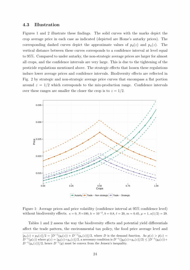
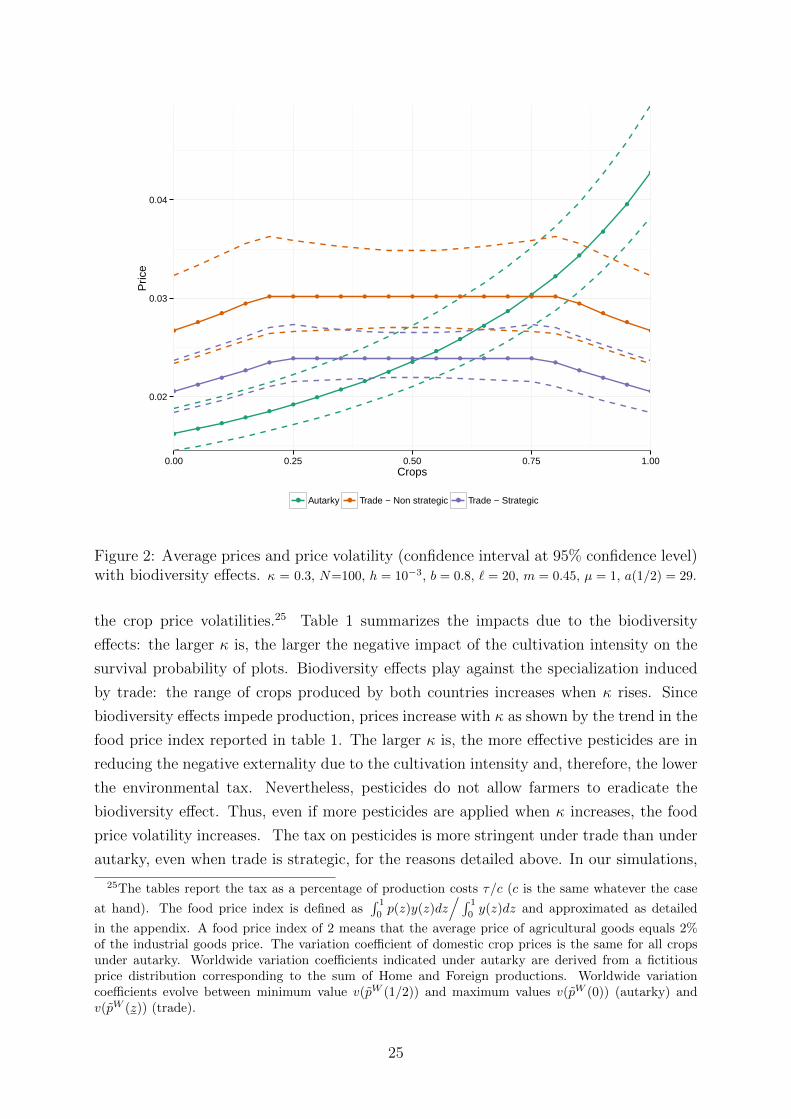
4.3 Illustration

Figures 1 and 2 illustrate these findings. The solid curves with the marks depict the

crop average price in each case as indicated (depicted are Home’s autarky prices). The

corresponding dashed curves depict the approximate values of pd(z) and pu(z). The

vertical distance between these curves corresponds to a confidence interval at level equal

to 95%. Compared to under autarky, the non-strategic average prices are larger for almost

all crops, and the confidence intervals are very large. This is due to the tightening of the

pesticide regulations mentioned above. The strategic effects that loosen these regulations

induce lower average prices and confidence intervals. Biodiversity effects are reflected in

Fig. 2 by strategic and non-strategic average price curves that encompass a flat portion

around z = 1/2 which corresponds to the mix-production range. Confidence intervals

over these ranges are smaller the closer the crop is to z = 1/2.

●

●

●

●

●

●

●

●

●

●

●

●

●

●

●

●

●

●

●

●

●

●

●

●

●

●

●

●

●

●

●

●

●

●

●

●

●

●

●

●

●

●

●

●

●

●

●

●

●

●

●

●

●

●

●

●

●

●

●

●

●

●

●

0.015

0.020

0.025

0.030

0.035

0.00 0.25 0.50 0.75 1.00Crops

Pric

e

● ● ●Autarky Trade − Non strategic Trade − Strategic

Figure 1: Average prices and price volatility (confidence interval at 95% confidence level)without biodiversity effects. κ = 0, N=100, h = 10−3, b = 0.8, ` = 20, m = 0.45, µ = 1, a(1/2) = 29.

Tables 1 and 2 assess the way the biodiversity effects and potential yield differentials

affect the trade pattern, the environmental tax policy, the food price average level and

[pu(z) + pd(z)]/2 = [D−1(yd(z)) + D−1(yu(z))]/2, where D is the demand function. As p(z) > p(z) =D−1(y(z)) where y(z) = [yd(z)+yu(z)]/2, a necessary condition is D−1([yd(z)+yu(z)]/2) ≤ [D−1(yd(z))+D−1(yu(z))]/2, hence D−1(y) must be convex from the Jensen’s inequality.

24

●

●

●

●

●

●

●

●

●

●

●

●

●

●

●

●

●

●

●

●

●

●

●

●

●

● ● ● ● ● ● ● ● ● ● ● ● ●

●

●

●

●

●

●

●

●

●● ● ● ● ● ● ● ● ● ● ●

●

●

●

●

●

0.02

0.03

0.04

0.00 0.25 0.50 0.75 1.00Crops

Pric

e

● ● ●Autarky Trade − Non strategic Trade − Strategic

Figure 2: Average prices and price volatility (confidence interval at 95% confidence level)with biodiversity effects. κ = 0.3, N=100, h = 10−3, b = 0.8, ` = 20, m = 0.45, µ = 1, a(1/2) = 29.

the crop price volatilities.25 Table 1 summarizes the impacts due to the biodiversity

effects: the larger κ is, the larger the negative impact of the cultivation intensity on the

survival probability of plots. Biodiversity effects play against the specialization induced

by trade: the range of crops produced by both countries increases when κ rises. Since

biodiversity effects impede production, prices increase with κ as shown by the trend in the

food price index reported in table 1. The larger κ is, the more effective pesticides are in

reducing the negative externality due to the cultivation intensity and, therefore, the lower

the environmental tax. Nevertheless, pesticides do not allow farmers to eradicate the

biodiversity effect. Thus, even if more pesticides are applied when κ increases, the food

price volatility increases. The tax on pesticides is more stringent under trade than under

autarky, even when trade is strategic, for the reasons detailed above. In our simulations,

25The tables report the tax as a percentage of production costs τ/c (c is the same whatever the case

at hand). The food price index is defined as∫ 1

0p(z)y(z)dz

/∫ 1

0y(z)dz and approximated as detailed

in the appendix. A food price index of 2 means that the average price of agricultural goods equals 2%of the industrial goods price. The variation coefficient of domestic crop prices is the same for all cropsunder autarky. Worldwide variation coefficients indicated under autarky are derived from a fictitiousprice distribution corresponding to the sum of Home and Foreign productions. Worldwide variationcoefficients evolve between minimum value v(pW (1/2)) and maximum values v(pW (0)) (autarky) andv(pW (z)) (trade).

25

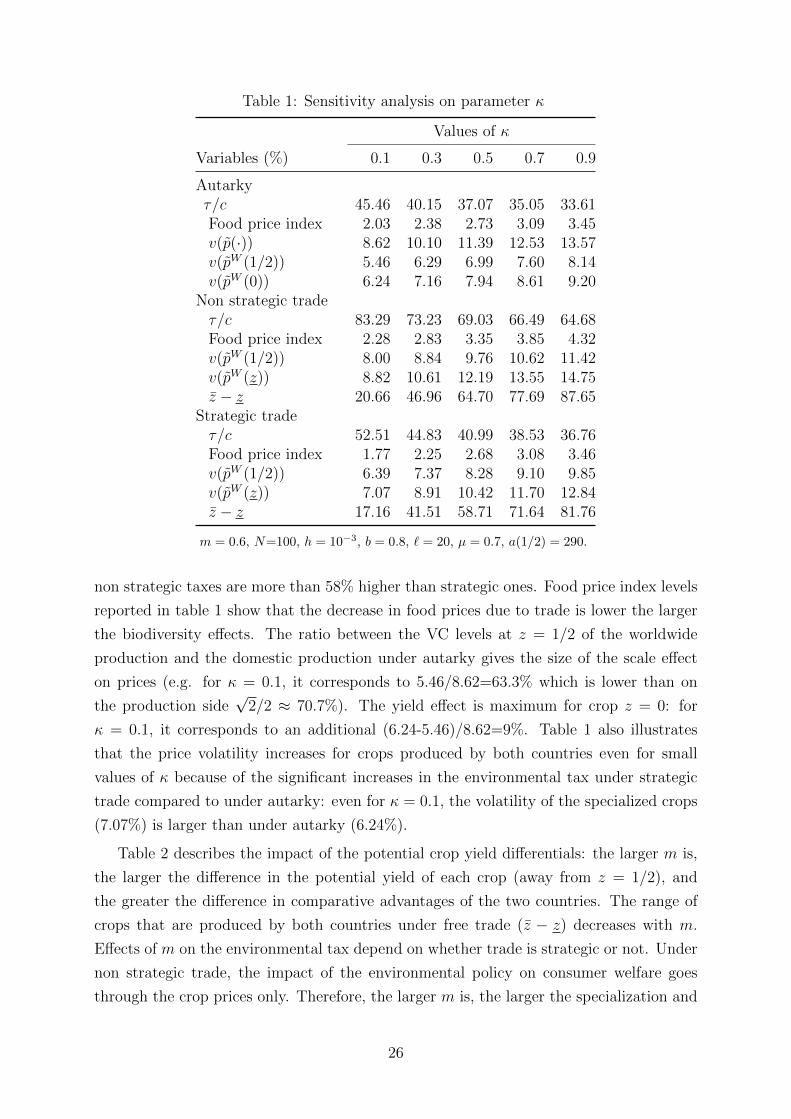
Table 1: Sensitivity analysis on parameter κ

Values of κ

Variables (%) 0.1 0.3 0.5 0.7 0.9

Autarkyτ/c 45.46 40.15 37.07 35.05 33.61Food price index 2.03 2.38 2.73 3.09 3.45v(p(·)) 8.62 10.10 11.39 12.53 13.57v(pW (1/2)) 5.46 6.29 6.99 7.60 8.14v(pW (0)) 6.24 7.16 7.94 8.61 9.20

Non strategic tradeτ/c 83.29 73.23 69.03 66.49 64.68Food price index 2.28 2.83 3.35 3.85 4.32v(pW (1/2)) 8.00 8.84 9.76 10.62 11.42v(pW (z)) 8.82 10.61 12.19 13.55 14.75z − z 20.66 46.96 64.70 77.69 87.65

Strategic tradeτ/c 52.51 44.83 40.99 38.53 36.76Food price index 1.77 2.25 2.68 3.08 3.46v(pW (1/2)) 6.39 7.37 8.28 9.10 9.85v(pW (z)) 7.07 8.91 10.42 11.70 12.84z − z 17.16 41.51 58.71 71.64 81.76

m = 0.6, N=100, h = 10−3, b = 0.8, ` = 20, µ = 0.7, a(1/2) = 290.

non strategic taxes are more than 58% higher than strategic ones. Food price index levels

reported in table 1 show that the decrease in food prices due to trade is lower the larger

the biodiversity effects. The ratio between the VC levels at z = 1/2 of the worldwide

production and the domestic production under autarky gives the size of the scale effect

on prices (e.g. for κ = 0.1, it corresponds to 5.46/8.62=63.3% which is lower than on

the production side√

2/2 ≈ 70.7%). The yield effect is maximum for crop z = 0: for

κ = 0.1, it corresponds to an additional (6.24-5.46)/8.62=9%. Table 1 also illustrates

that the price volatility increases for crops produced by both countries even for small

values of κ because of the significant increases in the environmental tax under strategic

trade compared to under autarky: even for κ = 0.1, the volatility of the specialized crops

(7.07%) is larger than under autarky (6.24%).

Table 2 describes the impact of the potential crop yield differentials: the larger m is,

the larger the difference in the potential yield of each crop (away from z = 1/2), and

the greater the difference in comparative advantages of the two countries. The range of

crops that are produced by both countries under free trade (z − z) decreases with m.

Effects of m on the environmental tax depend on whether trade is strategic or not. Under

non strategic trade, the impact of the environmental policy on consumer welfare goes

through the crop prices only. Therefore, the larger m is, the larger the specialization and

26

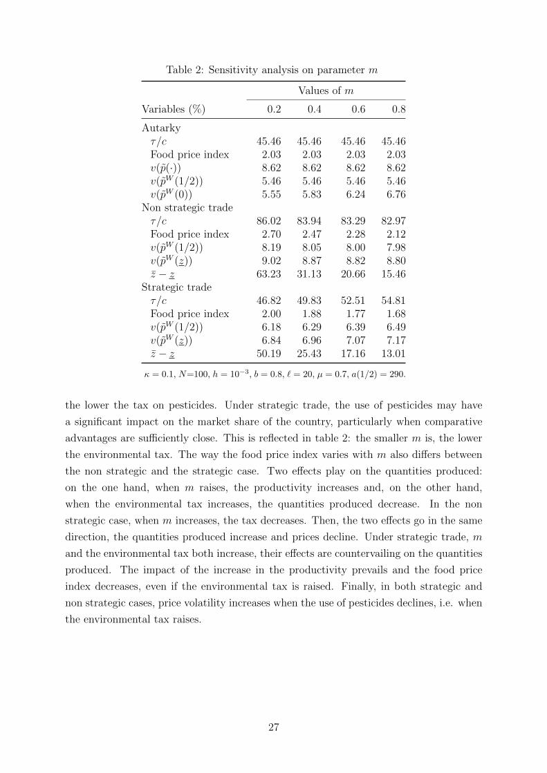
Table 2: Sensitivity analysis on parameter m

Values of m

Variables (%) 0.2 0.4 0.6 0.8

Autarkyτ/c 45.46 45.46 45.46 45.46Food price index 2.03 2.03 2.03 2.03v(p(·)) 8.62 8.62 8.62 8.62v(pW (1/2)) 5.46 5.46 5.46 5.46v(pW (0)) 5.55 5.83 6.24 6.76

Non strategic tradeτ/c 86.02 83.94 83.29 82.97Food price index 2.70 2.47 2.28 2.12v(pW (1/2)) 8.19 8.05 8.00 7.98v(pW (z)) 9.02 8.87 8.82 8.80z − z 63.23 31.13 20.66 15.46

Strategic tradeτ/c 46.82 49.83 52.51 54.81Food price index 2.00 1.88 1.77 1.68v(pW (1/2)) 6.18 6.29 6.39 6.49v(pW (z)) 6.84 6.96 7.07 7.17z − z 50.19 25.43 17.16 13.01

κ = 0.1, N=100, h = 10−3, b = 0.8, ` = 20, µ = 0.7, a(1/2) = 290.

the lower the tax on pesticides. Under strategic trade, the use of pesticides may have

a significant impact on the market share of the country, particularly when comparative

advantages are sufficiently close. This is reflected in table 2: the smaller m is, the lower

the environmental tax. The way the food price index varies with m also differs between

the non strategic and the strategic case. Two effects play on the quantities produced:

on the one hand, when m raises, the productivity increases and, on the other hand,

when the environmental tax increases, the quantities produced decrease. In the non

strategic case, when m increases, the tax decreases. Then, the two effects go in the same

direction, the quantities produced increase and prices decline. Under strategic trade, m

and the environmental tax both increase, their effects are countervailing on the quantities

produced. The impact of the increase in the productivity prevails and the food price

index decreases, even if the environmental tax is raised. Finally, in both strategic and

non strategic cases, price volatility increases when the use of pesticides declines, i.e. when

the environmental tax raises.

27

5 Conclusion

We have shown that biotic risk factors such as pests that affect the productivity of farm-

ing create biodiversity effects that modify standard results of trade models. An explicit

account of their effects on production allows us to clarify the distribution of idiosyncratic

risks affecting farming which depends on the countries’ openness to trade. These pro-

duction shocks translate into the price distribution and are impacted by environmental

policies. Of course, these productive shocks are not the only ones affecting food prices,

but they are an additional factor in their distributions that may explain their greater

volatility compared to manufacture prices.

While these effects are analytically apparent within the standard two-country Ricar-

dian model, an extension to a more encompassing setup involving a larger number of

countries as permitted by Eaton & Kortum (2002) and applied to agricultural trade by

Costinot & Donaldson (2012) and Costinot et al. (2012) is necessary to investigate their

scope statistically. These studies incorporate a stochastic component to determine the

pattern of trade but it is not related to the production process and somehow arbitrary.

Our analysis offers an interesting route to ground these approaches at least in the case

of agricultural products. Introducing these biodiversity effects should allow for a better

assessment of the importance of trade costs in determining the pattern of trade.

28

References

Barrett, S. (1994). Strategic environmental policy and intrenational trade. Journal ofPublic Economics, 54(3), 325 – 338.

Beketov, M. A., Kefford, B. J., Schafer, R. B., & Liess, M. (2013). Pesticides reduceregional biodiversity of stream invertebrates. Proceedings of the National Academy ofSciences, 110(27), 11039–11043.

Bellora, C., Blanc, E., Bourgeon, J.-M., & Strob, E. (2015). Estimating the impact ofcrop diversity on agricultural productivity in South Africa. Working paper.

Brander, J. A. & Spencer, B. J. (1985). Export subsidies and international market sharerivalry. Journal of International Economics, 18(1-2), 83–100.

Costinot, A. & Donaldson, D. (2012). Ricardo’s theory of comparative advantage: Oldidea, new evidence. American Economic Review, 102(3), 453–58.

Costinot, A., Donaldson, D., & Komunjer, I. (2012). What goods do countries trade?a quantitative exploration of ricardo’s ideas. The Review of Economic Studies, 79(2),581–608.

Di Falco, S. (2012). On the value of agricultural biodiversity. Annual Review of ResourceEconomics, 4(1), 207 – 223.

Di Falco, S. & Chavas, J. (2006). Crop genetic diversity, farm productivity and the man-agement of environmental risk in rainfed agriculture. European Review of AgriculturalEconomics, 33(3), 289–314.

Di Falco, S. & Perrings, C. (2005). Crop biodiversity, risk management and the implica-tions of agricultural assistance. Ecological Economics, 55(4), 459–466.

Dornbusch, R., Fischer, S., & Samuelson, P. A. (1977). Comparative advantage, trade,and payments in a ricardian model with a continuum of goods. The American EconomicReview, 67(5), pp. 823–839.

Drakare, S., Lennon, J. J., & Hillebrand, H. (2006). The imprint of the geographical,evolutionary and ecological context on species-area relationships. Ecology Letters, 9(2),215–227.

Eaton, J. & Kortum, S. (2002). Technology, geography, and trade. Econometrica, 70(5),1741–1779.

EC (2009). EU Action on pesticides ”Our food has become greener”. Technical report,European Commission.

ECP (2013). Industry statistics. Technical report, European Crop Protection.

EEA (2010). 10 messages for 2010 – Agricultural ecosystems. Technical report, EuropeanEnvironment Agency.

29

Fernandez-Cornejo, J., Jans, S., & Smith, M. (1998). Issues in the economics of pesticideuse in agriculture: a review of the empirical evidence. Review of Agricultural Economics,20(2), 462–488.

Gaisford, J. & Ivus, O. (2014). Should smaller countries be more protectionist ? thediversification motive for tariffs. Review of International Economics, 22(4), 845–862.

Garcia Martin, H. & Goldenfeld, N. (2006). On the origin and robustness of power-lawspecies-area relationships in ecology. Proceedings of the National Academy of Sciences,103(27), 10310–10315.

Gilbert, C. L. & Morgan, C. W. (2010). Food price volatility. Philosophical Transactionsof the Royal Society B: Biological Sciences, 365(1554), 3023–3034.

Jacks, D. S., O’Rourke, K. H., & Williamson, J. G. (2011). Commodity price volatilityand world market integration since 1700. Review of Economics and Statistics, 93(3),800–813.

Jiguet, F., Devictor, V., Julliard, R., & Couvet, D. (2012). French citizens monitoringordinary birds provide tools for conservation and ecological sciences. Acta Oecologica,44(0), 58–66.

Kennedy, P. W. (1994). Equilibrium pollution taxes in open economies with imperfectcompetition. Journal of Environmental Economics and Management, 27(1), 49 – 63.

Markusen, J. R., Morey, E. R., & Olewiler, N. (1995). Competition in regional environ-mental policies when plant locations are endogenous. Journal of Public Economics,56(1), 55 – 77.

May, R. M. (2000). Species-area relations in tropical forests. Science, 290(5499), 2084–2086.

Newbery, D. M. G. & Stiglitz, J. E. (1984). Pareto inferior trade. The Review of EconomicStudies, 51(1), pp. 1–12.

Oerke, E. (2006). Crop losses to pests. Journal of Agricultural Science, 144(1), 31.

Pianka, E. R. (2011). Evolutionary Ecology. E-book.

Pimentel, D. (2005). Environmental and economic costs of the application of pesticidesprimarily in the United States. Environment, Development and Sustainability.

Plotkin, J. B., Potts, M. D., Yu, D. W., Bunyavejchewin, S., Condit, R., Foster, R.,Hubbell, S., LaFrankie, J., Manokaran, N., Lee, H.-S., & et al. (2000). Predictingspecies diversity in tropical forests. Proceedings of the National Academy of Sciences,97(20), 10850–10854.

Savary, S., Willocquet, L., Elazegui, F. A., Castilla, N. P., & Teng, P. S. (2000). Rice pestconstraints in tropical asia: Quantification of yield losses due to rice pests in a rangeof production situations. Plant Disease, 84(3), 357–369.

30

Smale, M., Hartell, J., Heisey, P. W., & Senauer, B. (1998). The contribution of geneticresources and diversity to wheat production in the Punjab of Pakistan. AmericanJournal of Agricultural Economics, 80(3), 482–493.

Stewart, W. M., Dibb, D. W., Johnston, A. E., & Smyth, T. J. (2005). The contributionof commercial fertilizer nutrients to food production. Agronomy Journal, 97(1), 1.

Storch, D., Keil, P., & Jetz, W. (2012). Universal species – area and endemics – arearelationships at continental scales. Nature, 488(7409), 78–81.

Sutton, M., Howard, C., Erisman, J., Billen, G., Bleeker, A., Grennfelt, P., Grinsven,v. H., & Grizzetti, B., Eds. (2011a). The European Nitrogen Assessment: Sources,Effects and Policy Perspectives. Cambridge University Press.

Sutton, M. A., Oenema, O., Erisman, J. W., Leip, A., van Grinsven, H., & Winiwarter,W. (2011b). Too much of a good thing. Nature, 472(7342), 159–161.

Tilman, D. & Downing, J. A. (1994). Biodiversity and stability in grasslands. Nature,367(6461), 363–365.

Tilman, D., Polasky, S., & Lehman, C. (2005). Diversity, productivity and temporalstability in the economies of humans and nature. Journal of Environmental Economicsand Management, 49(3), 405–426.

Tilman, D., Wedin, D., & Knops, J. (1996). Productivity and sustainability influencedby biodiversity in grassland ecosystems. Nature, 379(6567), 718–720.

Turnovsky, S. J. (1974). Technological and price uncertainty in a ricardian model ofinternational trade. The Review of Economic Studies, 41(2), 201.

Weitzman, M. L. (2000). Economic profitability versus ecological entropy. The QuarterlyJournal of Economics, 115(1), pp. 237–263.

Wright, B. D. (2011). The economics of grain price volatility. Applied Economic Perspec-tives and Policy, 33(1), 32–58.

31

Appendix

A Proof of Proposition 1

For given t, t∗, c, c∗, (13) and (14) define a system of two linear equations with two un-

knowns. Solving this system gives (17). By definition of threshold crops z and z, we must

have B(z) = 0 for all z ≥ z and B∗(z) = 0 for all z ≤ z. This implies that we must

have φ(z) ≥ 1/q or all z ≥ z and φ∗(z) ≥ 1/q∗ for all z ≤ z. Differentiating (18) and its

counterpart for Foreign, we get

φ(z) ≡ φ′(z)

φ(z)=

A′(z)

t∗/t+ A(z)− t∗κ0e

−θ(z)2/2α′(z)− θ′(z)α(z)

1 + t∗α(z)κ(z)

and

φ∗(z) = −A(z) +A′(z)

t∗/t+ A(z)− tκ0e

−θ(z)2/2α′(z)− θ′(z)α(z)

1 + t∗α(z)κ(z).

Suppose κ0 = 0: As A(z) > 0, we have φ(z) = A′(z)/[t∗/t + A(z)] > 0 and φ∗(z) =

−A(z)(t∗/t)/[t∗/t+A(z)] < 0. Both conditions are thus satisfied if κ0 is sufficiently small.

They are also satisfied whatever the value of κ0 if α(z) and θ(z) are constant as supposed

in the symmetric case considered in section 3. Eq. (15) and (16) are derived from

φ(z) = 1/q and φ∗(z) = 1/q∗ respectively. Using these equations, we obtain A(z)/A(z) =

[q∗ + t∗κ(z)α(z)][q + tκ(z)α(z)]/(qq∗) > 1. As A(z) is increasing, we thus have z > z.

B Proof of Lemma 1

Consider the crops produced more intensively by Home (symmetric results hold for For-

eign). For all z < z, it is obvious by setting t = tA and q = 1/2 in (21) that p(z) > pA(z)

given by (7) where c = (`−1)(1−b)/b and B(z) = α(z). For Foreign, we have p(z) < p∗A(z)

iff1 + tAκ(z)α(z)

1 + 2tAκ(z)α(z)> A(z).

As φ∗(z) > 1/q∗ for all z < z, we obtain by setting t = tA and q∗ = 1/2 that

1 + 1/A(z)

1 + tAκ(z)α(z)> 2

for all z < z, which gives, re-arranging terms

A(z) <1

1 + 2tAκ(z)α(z)<

1 + tAκ(z)α(z)

1 + 2tAκ(z)α(z)

hence p(z) < p∗A(z) for all z < z. For crops z in [z, z], we obtain using (20) that p(z) <

32

pA(z) iff 2/[1 + A(z)] < 1, hence the result.

C Proof of Proposition 3

Using (21) which simplifies to

ps(z) =2(`− 1)(1− b)tq

ba(z)

and denoting by $ the Lagrange multiplier associated with the constraint, the first-order

condition with respect to t gives

−(1− b)q +Nh√2 ln t

−$ 1

ξ′(zs)

t∗

t= 0

and the one with respect to q

$ =2(1− b)

b+ 2q(1− b).

Plugging the latter expression into the former and rearranging terms gives (29). At a

symmetric equilibrium, using ξ′(zs) = A′(1/2) + 4 and τA/cA = Nh/(1− b), we get

τ

c=τAcA

[1 +

A′(1/2)

A′(1/2) + 8

]where c = cA. We thus have

τ = τA

[1 +

A′(1/2)

A′(1/2) + 8

].

Denoting M ≡ A′(1/2), we get limM→0 τ = τA, limM→+∞ τ = 2τA and

dτ

dM=

8τA(M + 8)2

> 0.

D Proof of Proposition 4

Differentiating (26) with respect to t, we obtain the following FOC

∂V

∂t= −(1− b)

[zq + 2tκ

t(q + tκ)+

(z − z)(q∗ + t∗κ)

q(t∗ − t) + t(1 + t∗κ)−∫ z

z

A(z)/t∗ − t∗/t2

A(z)t/t∗ + t∗/tdz

]− hdZ

dt.

33

At a symmetric equilibrium, using (A(z) − 1)/(A(z) + 1) = m(2z − 1) and integrating

gives (34). Using (33) in (34) and collecting terms, we arrive at

∂V

∂t=

Nh

t√

2 ln t− (1− b)

[1

2t+ κ

2m(1 + tκ)2 − tκ2m(1 + 2tκ)(1 + tκ)2

].

Denote by t0 the optimal tax when there is no cross-externality effects, i.e. κ = 0. It

verifies (28) where q = 1/2. We have

∂V

∂t

∣∣∣∣t=t0

= −(1− b)κ 2m(1 + t0κ)2 − t0κ2m(1 + 2t0κ)(1 + t0κ)2

which is positive if

m ≤ t0κ

2(1 + t0κ)2≤ 1/8.

We also have

1

1− b∂V

∂t

∣∣∣∣t=tA

=1

2tA+

κ

1 + tAκ− κ 2m(1 + tAκ)2 − tAκ

2m(1 + 2tAκ)(1 + tAκ)2

=1

2tA+

tAκ2

1 + tAκ

2m(1 + tAκ) + 1

2m(1 + 2tAκ)(1 + tAκ)> 0 (45)

hence t > tA at the optimum.

E Proof of Proposition 5

At a symmetric equilibrium (35) simplifies to

∂V

∂q= 2(1− b) + 2(1− b)1− (z + z)

1 + 2tκ

where z + z = 1, hence ∂V/∂q = 2(1− b). We also obtain using (27) that at a symmetric

equilibrium

dq

dt= −

2(1+tκ)t

∫ zz

A(z)[A(z)+1]2

dz − 12t

∫ zz

A(z)A(z)+1

dz

tκ+ z − z.

Denoting m0 = (m+ 1)/2, using∫ z

z

A(z)

[A(z) + 1]2dz =

∫ z

z

[m0 −mz − (m0 −mz)2]dz

= (z − z)(m0 −m/2) +(m0 −mz)3 − (m0 −mz)3

3m

=tκ

2m(1 + tκ)

2(1 + tκ)2 + 1 + 2tκ

6(1 + tκ)2

34

and ∫ z

z

A(z)

A(z) + 1dz =

∫ z

z

(1−m0 +mz)dz = (z − z)(1−m0 +m/2) =tκ

2m(1 + tκ)

yields (36). Differentiating, we get

dq2

dtdκ= −(4−m)(1 + tκ)2 + 4m(1 + tκ) + 2

12(1 + tκ)2[m(1 + tκ) + 1]2< 0.

Using (45) we obtain

1

1− bdV

dt

∣∣∣∣t=tA

=1

2tA+

tAκ2[2m(1 + tAκ) + 1]

2m(1 + 2tAκ)(1 + tAκ)2− 3 + 9tAκ+ 4(tAκ)2

6tA(1 + tAκ)[m(1 + tAκ) + 1](46)

where the second term diverges when m tends to 0 and decreases with m while the last

term increases with m (decreases in absolute value). Assuming that m is large enough

and κ ≈ 0, we have

1

1− bdV

dt

∣∣∣∣t=tA

=1

2tA− 1 + 3tAκ

2tA[m(1 + 2tAκ) + 1 + tAκ]+ o(κ)

=1

2tA

[m(1 + 2tAκ)− 2tAκ

m(1 + 2tAκ) + (1 + tAκ)

]+ o(κ)

where the bracketed term is negative if

m < m ≡ 2tAκ

1 + 2tAκ.

However, as the second term of (46) diverges when m approaches 0, we cannot neglect

this term unless m is above some threshold m > tAκ/(1 + tAκ). Indeed, in the case where

m = tAκ/(1 + tAκ), we have

1

1− bdV

dt

∣∣∣∣t=tA

=1

2tA+

κ

2(1 + tAκ)− 3 + 9tAκ+ 4(tAκ)2

6tA(1 + tAκ)2

=(tAκ)2

3tA(1 + tAκ)2> 0.

Hence, assuming κ is small enough, cases where the environmental tax at equilibrium

is lower than under autarky correspond to m ∈ [m, m] where

m−m <2tAκ

1 + 2tAκ− tAκ

1 + tAκ=

tAκ

(1 + tAκ)(1 + 2tAκ)≤

√2

4 + 3√

2≈ 0.17.

35

F Proof of Proposition 6

Without biodiversity effects, using (37) and (38) with κ = 0, we obtain that v(yWA (z)) ≥v(yW (z)) iff

1− 4A(z)

[1 + A(z)]2≥ t− tAtA − µ

.

As A(z)/[1 + A(z)]2 is cap-shaped with a maximum equal to 1/4 at z = 1/2, this

condition is satisfied for all z only if t = tA. With t > tA, it could be satisfied for z

belonging only to one of the extremes of the crops’ range, i.e. for z either close to 0 or

close to 1, if t − tA is small enough. With biodiversity effects, for z ∈ [z, z], using (39)

and assuming that t ≥ tA, we obtain that v(yWA (z)) ≥ v(yW (z)) iff

4A(z)

[1 + A(z)]2− 1 ≥ tκ(1 + tκ)− κtA(1 + tAκ)

(1 + tκ)2 − κtA(1 + tAκ) + µκ

which is impossible unless t = tA and z = 1/2 since the last term is positive. For all

z ∈ [0, z] ∪ [z, 1], using (37), we have v(yWA (z)) ≥ v(yW (z)) iff

2− 4A(z)

[1 + A(z)]2≥ t(1 + 2tκ)− µtA(1 + tAκ)− µ

.

A necessary condition is given by 2 > [t(1+2tκ)−µ]/[tA(1+ tAκ)−µ], or re-arranging

terms tA−µ > (t− tA)[1 + 2κ(t+ tA)] which is satisfied only if t− tA is not too large and

κ sufficiently small.

G Proof of Proposition 7

A second-order approximation gives

p(z) =α(z)(1− b)LR

y(z)≈ α(z)(1− b)LR

y(z)

[1− y(z)− y(z)

y(z)+

(y(z)− y(z)

y(z)

)2]

= p(z)

[2− y(z)

y(z)+

(y(z)− y(z)

y(z)

)2]

and thus

p(z) ≈ p(z)

[1 + E

(y(z)− y(z)

y(z)

)2]

= p(z)[1 + v(y(z))2].

A first order approximation yields

E[(p(z)− p(z))2]1/2

p(z)≈ E

[(1− y(z)

y(z)

)2]1/2

= v(y(z)),

36

which gives

σ(p(z)) ≈ E[p(z)− p(z)− p(z)v(y(z))2

]1/2=(E[(p(z)− p(z))2

]− p(z)2v(y(z))4

)1/2

= p(z)v(y(z))(1− v(y(z))2)1/2.

From pγu(z) = p(z) + sγuσ(p(z)) we get

sγu ≈1

σ(p(z))

(α(z)(1− b)LRy(z)− sγσ(y(z))

− p(z)(1 + v(y(z))2)

)=

p(z)

σ(p(z))

y(z)(1 + v(y(z))2)− y(z) + sγσ(y(z))

y(z)− sγσ(y(z))

≈ y(z)v(y(z))2 + sγσ(y(z))

v(y(z))(1− v(y(z))2)1/2(y(z)− sγσ(y(z)))

=v(y(z)) + sγ

(1− v(y(z))2)1/2(1− sγv(y(z)))

which gives (43). Similar derivations for pγd(z) = E[p(z)]− sγdσ(p(z)) yield (42) and (44).

H Food Price Index

The food price index is defined as

F =

∫ 1

0

y(z)p(z)dz

/∫ 1

0

y(z)dz

where p(z) is approximated by (40). As we also have p(z)y(z) = cNB(z), we get

p(z)y(z) ≈ cNB(z)[1 + v(y(z))2]. In autarky, c = (` − 1)(1 − b)/b. Using B(z) = 1,

θ(z) = θ, which implies µ(z) = µ, and y(z) = a(z)N/[t(1 + tκ)] gives∫ 1

0

p(z)y(z)dz =N(`− 1)(1− b)

b

[1 +

t(1 + tκ)− µNµ

].

Using a(z) = µ0eθ2/2[1−m(2z − 1)] yields∫ 1

0

y(z)dz =N

t(1 + tκ)

∫ 1

0

µ0eθ2/2[1−m(2z − 1)]dz =

Nµ0eθ2/2

t(1 + tκ)

and thus

FA =(`− 1)(1− b)t(1 + tκ)

bµ0eθ2/2

[1 +

t(1 + tκ)− µNµ

].

Under free trade, we have p(z)y(z) = 2N(l− 1)(1− b)/b. B(z) = 2 for crops produced

37

by only one country and we get, using z + z = 1,∫ z

0

ps(z)y(z)dz +

∫ 1

z

ps(z)y∗(z)dz =4zN(l − 1)(1− b)

b

[1 +

t(1 + 2tκ)− µ2µN

].

For crops produced by both countries we obtain

∫ z

z

pm(z)yW (z)dz =

∫ z

z

2N(`− 1)(1− b)b

[1 +

(1 + tκ)(1 + 2tκ)− µκ2µNκ

− 2(1 + tκ)2

µNκ

A(z)

[1 + A(z)]2

]dz

=2N(`− 1)(1− b)

b

{[1 +

(1 + tκ)(1 + 2tκ)− µκ2µNκ

](z − z)− t[2(1 + tκ)2 + 1 + 2tκ]

µNm6(1 + tκ)

}.

The corresponding quantities are given by∫ z

0

y(z)dz +

∫ 1

z

y(z)dz =2N

t(1 + 2tκ)

{∫ z

0

a(z)dz +

∫ 1

z

a∗(z)dz

}=

2Nµ0eθ2/2

t(1 + 2tκ)[z(m+ 1−mz) + 1− z(1 +mz −m)]

and ∫ z

z

yW (z)dz =N

t(1 + tκ)

∫ z

z

[a∗(z) + a(z)]dz =2Nµ0e

θ2/2(z − z)

t(1 + tκ)=

2Nµ0eθ2/2κ

m(1 + tκ)2.

I Fertilizers

Our focus being on biodiversity effects in agricultural production, we have so far not

discussed the impact of trade on the use of fertilizers. However, because they have con-

siderable effects on both crop yields and on the environment (and human health), changes

in the openness of countries to trade are likely to impact the way their use is regulated.26

We may thus expect that crop price volatility is also affected through this channel. It

is possible to analyze these changes by considering that crop z’s potential yield a(z) is

the result of the intrinsic quality of land and the quantity of fertilizers spread on the

field, g(z). Denoting by a0(z) the potential crop z yield absent any treatment, we have

a(z) = a0(z)f(g(z)) with f(0) = 1, f ′(g) > 0 and f ′′(g) < 0. Total use of fertilizers,

given by G = N∫ 1

0B(z)g(z)dz, has a negative impact on consumer welfare due to envi-

ronmental damages. As pesticides, fertilizers have a direct positive impact on crop yields,

26Commercial fertilizers are responsible for 30% to 50% of crop yields (Stewart et al., 2005). Suttonet al. (2011a,b) find that half of the nitrogen added to farm fields ends up polluting water or air. Excessof nitrogen and phosphorus in freshwater increases cancer risk and creates aquatic and marine dead zonesthrough eutrophication. In the air, nitrates contribute to ozone generation which causes respiratoryand cardiovascular diseases. Sutton et al. (2011a) estimates that in the European Union the benefits ofnitrogen for agriculture through the increase in yields amount to 25 to 130 billion euros per year and thatthey cause between 70 and 320 billion euros per year in damage.

38

but unlike pesticides, their productive impact is limited to the field they are spread on.

Hence, the trade-off that defines the fertilizer policy is similar to the one of the pesticide

regulation without biodiversity effects. While under autarky domestic consumers bear all

the costs and reap all the benefits of the fertilizers used by their fellow farmers, this is no

longer the case in free trade: they benefit from the crops produced abroad and share the

advantages of a productive national sector with foreign consumers. As a result, restric-

tions on fertilizers are tighter under free trade than under autarky, with the same caveat

as for pesticides: governments may use the fertilizer policy strategically. How lenient

they are depends on the impact of fertilizers on relative yields: the more responsive is the

relative yields function, i.e. the larger f ′(g), the lower the restrictions.

39