Embed Size (px)
Citation preview
Community dynamics and development of soft bottom macrozoobenthos in the German Bight (North Sea)
1969 - 2000
Dynamik und Entwicklung makrozoobenthischer Weichbodengemeinschaften
in der Deutschen Bucht (Nordsee) 1969 - 2000
55°
54°
6° 7° 8° 9°
Dissertation zur Erlangung des Grades eines Doktors der Naturwissenschaften (Dr. rer. nat.)
vorgelegt dem Fachbereich 2 (Biologie & Chemie)
der Universität Bremen
Alexander Schroeder
Bremen 2003


Aus dem
Alfred-Wegener-Institut für Polar- und Meeresforschung
Bremerhaven
1. Gutachter: Prof. Dr. W.E. Arntz
2. Gutachter: Dr. R. Knust


Contents
Zusammenfassung ................................................................................................................ I
Summary.................................................................................................................................. III
1. Introduction...................................................................................................................... 1
2. The German Bight (North Sea)................................................................................. 5 2.1 Topography ..................................................................................................................... 5 2.2 Climate............................................................................................................................. 5 2.3 Hydrography ................................................................................................................... 6 2.4 Sediments........................................................................................................................ 7 2.5 Benthic fauna .................................................................................................................. 8
3. Methods ........................................................................................................................... 11 3.1 Long term stations ....................................................................................................... 11 3.2 Benthos data................................................................................................................. 12 3.2.1 Sampling methodology................................................................................................ 12 3.2.2 Sample processing...................................................................................................... 13 3.2.3 Data sources ............................................................................................................... 14 3.2.4 Data quality control...................................................................................................... 15 3.2.5 Data selection for the long-term study......................................................................... 15 3.2.6 Spatial sampling .......................................................................................................... 16 3.3 Environmental data ...................................................................................................... 17 3.4 Analytical methods....................................................................................................... 18 3.4.1 Indices ......................................................................................................................... 18 3.4.1.1 Spatial distribution & variability ............................................................................... 18 3.4.1.2 Diversity .................................................................................................................. 20 3.4.1.3 Multivariate similarity............................................................................................... 23 3.4.2 Multivariate analytical procedures ............................................................................... 24 3.4.2.1 MDS ........................................................................................................................ 24 3.4.2.2 Cluster Analysis ...................................................................................................... 25 3.4.3 Statistical tests............................................................................................................. 26 3.4.3.1 Comparison of univariate measures ....................................................................... 26 3.4.3.2 Correlations............................................................................................................. 26 3.4.3.3 Smoothing of time series ........................................................................................ 26 3.4.3.4 Multivariate differences........................................................................................... 27 3.4.3.5 Comparing multivariate pattern between stations .................................................. 27 3.4.3.6 Multivariate Mantel correlograms............................................................................ 27 3.4.3.7 Multiple statistical test ............................................................................................. 28 3.4.4 Analysis of spatial variability........................................................................................ 29 3.4.5 Samples size dependence .......................................................................................... 30 3.4.6 Temporal community development ............................................................................. 31 3.4.7 Environmental influences ............................................................................................ 32
4. Results ............................................................................................................................. 33 4.1 Precision of sampling position ................................................................................... 33 4.2 Spatial variability .......................................................................................................... 34 4.2.1 Spatial structuring........................................................................................................ 34 4.2.1.1 Gradients................................................................................................................. 35 4.2.1.1.1 Community composition ................................................................................................. 35 4.2.1.1.2 Sum parameter............................................................................................................... 36 4.2.2 Benthic community composition.................................................................................. 37 4.2.2.1 SSd ......................................................................................................................... 37 4.2.2.2 WB .......................................................................................................................... 38 4.2.2.3 Slt ............................................................................................................................ 40 4.2.2.4 FSd.......................................................................................................................... 41 4.2.3 Precision of quantitative sum parameters ................................................................... 42 4.2.3.1 Sample size influence on density............................................................................ 43 4.2.3.2 Sample size influence on biomass ......................................................................... 44 4.2.4 Community structure and sample size influences....................................................... 45 4.2.4.1 Sample size influence on species number ............................................................. 47 4.2.4.2 Sample size influence on evenness ....................................................................... 51 4.2.4.3 Sample size influence on heterogeneity diversity................................................... 52 4.2.5 Multivariate community similarity................................................................................. 53 4.2.5.2 Sample size influence on multivariate similarity ..................................................... 55 4.2.6 Temporal changes in spatial variability ....................................................................... 56 4.3 Methodological changes.............................................................................................. 58 4.3.1 Penetration depth & grab type..................................................................................... 58 4.3.2 Combination of different grabs .................................................................................... 59 4.3.2.1 Univariate measures ............................................................................................... 59 4.3.2.2 Inter-sample similarity ............................................................................................. 61 4.3.3 Sampling time.............................................................................................................. 62 4.4 Benthos time series...................................................................................................... 63 4.4.1 Similarity between benthic communities ..................................................................... 63 4.4.2 Similarity of temporal development ............................................................................. 65 4.4.3 Community development at single stations................................................................. 66 4.4.3.1 SSd ......................................................................................................................... 66 4.4.3.2 WB .......................................................................................................................... 76 4.4.3.3 Slt ............................................................................................................................ 85 4.3.3.4 FSd.......................................................................................................................... 93 4.4.4 Temporal autocorrelation ...................................................................................... 101 4.5 Abiotic environmental time series ............................................................................ 102 4.5.1 Climate: The North Atlantic Oscillation index (NAOI) ................................................ 102 4.5.2 Water temperature..................................................................................................... 103 4.5.3 Wind........................................................................................................................... 105 4.5.4 Salinity ....................................................................................................................... 107 4.5.5 Nutrients .................................................................................................................... 108 4.5.5.1 Phosphate ............................................................................................................. 108 4.5.5.2 Nitrogen................................................................................................................. 109 4.5.5.3 Silicate................................................................................................................... 109 4.5.6 Correlations between abiotic environmental data ..................................................... 110 4.6 Correlation between benthos and abiotic environment ......................................... 112 4.6.1 Sum parameters ........................................................................................................ 112 4.6.1.1 SSd ....................................................................................................................... 113 4.6.1.2 WB ........................................................................................................................ 114 4.6.1.3 Slt .......................................................................................................................... 115 4.6.1.4 FSd........................................................................................................................ 116 4.6.2 Community composition ............................................................................................ 117 4.6.2.1 SSd ....................................................................................................................... 117 4.6.2.2 WB ........................................................................................................................ 119 4.6.2.3 Slt .......................................................................................................................... 121 4.6.2.4 FSd........................................................................................................................ 123
5. Discussion.................................................................................................................... 125 5.1 Sampling gear and penetration depth...................................................................... 125 5.2 Spatial variability of benthic communities at the sampling stations................... 127 5.2.1 Spatial patterns.......................................................................................................... 128 5.2.2 Medium-scale spatial variability and the precision of estimates ............................... 130 5.2.2.1 Organism densities and biomass.......................................................................... 130 5.2.2.2 Community structure............................................................................................. 133 5.2.2.3 Community composition ....................................................................................... 135 5.2.2.4 Temporal changes in spatial variability................................................................. 138 5.2.2.5 Sample size needed for statistical inferences ...................................................... 139 5.2.3 Systematic sample size influence on measures of community structure.................. 140 5.2.3.1 Species number .................................................................................................... 140 5.2.3.2 Evenness .............................................................................................................. 143 5.2.3.3 Heterogeneity diversity ......................................................................................... 144 5.2.4 An optimal sample size ? .......................................................................................... 144 5.3 Temporal development of benthic communities..................................................... 146 5.4 Internal dynamics and external forcing ................................................................... 149 5.4.1 Environmental forcing................................................................................................ 149 5.4.1.1 Correlations between environmental factors ........................................................ 149 5.4.1.2 Effects of environmental variation on benthic communities.................................. 150 5.4.2 Anthropogenic influences .......................................................................................... 152 5.4.2.1 Fisheries ............................................................................................................... 152 5.4.2.2 Pollution ................................................................................................................ 154 5.4.2.3 Eutrophication ....................................................................................................... 156 5.4.3 Biological interactions................................................................................................ 158 5.4.4 Disturbances.............................................................................................................. 160 5.4.4.1 Spatial heterogeneity as symptom of stress......................................................... 162 5.5 Local vs. regional community development............................................................ 164 5.6 Implications for offshore monitoring of soft-bottom benthos............................... 167 5.7 Open questions and further analyses ...................................................................... 170
References ............................................................................................................................. 172 References II: Taxonomic identification keys............................................................................ 189
Annex .......................................................................................................................................A.1 A.1 Species list .................................................................................................................A.2 A.2 Benthos data available in the database ...................................................................A.18 A.3 Database structure and contents .............................................................................A.22 A.4 Species database.....................................................................................................A.23 A.5 Statistical tables........................................................................................................A.30 A.6 Supplementary figures..............................................................................................A.36 A.7 Single species temporal development plots.............................................................A.40 A.8 Glossary ...................................................................................................................A.62
Acknowledgements

Zusammenfassung
Zusammenfassung
Um die Langzeitentwicklung und die interannuelle Variabilität sublittoraler makrozoo-benthischer Weichbodengemeinschaften der Deutschen Bucht zu untersuchen, wurden vier Dauerstationen fortlaufend während der letzten 35 Jahre beprobt. Interannuelle Variabilität und mögliche Langzeittrends wurden anhand von Frühjahrsproben analysiert. Die Umgebung der Stationen wurde 1998 intensiv beprobt, um die räumliche Variabilität der benthischen Gemeinschaften dieser Gebiete beurteilen zu können. Diese Daten wurden außerdem genutzt, um die nötige Probenzahl für eine angemessene Erfassung der benthischen Gemeinschaften abzuschätzen. Gleichzeitig wurde die Abhängigkeit der Gemeinschaftsparameter (Artendichte, Äquität, Ähnlichkeit etc.) von der Probengröße untersucht, da diese bei Felddaten von theoretischen Voraussagen abweicht.
Eine ausreichende Charakterisierung der lokalen Gemeinschaften kleiner homogener Gebiete für Langzeituntersuchungen kann bei einer Standartprobengröße von fünf 0.1 m² van Veen Greifern angenommen werden. Da die größte Zunahme der Genauigkeit der Erfassung der Fauna durch die ersten fünf Greifer erreicht wird, wird diese Probengröße als praktischer Kompromiss akzeptiert, um die wichtigsten Gemeinschaftstrends zu dokumentieren. Für eine Analyse der Populationsdichte einzelner Arten sollten zehn oder mehr Greifer genommen werden. Die vorliegenden Ergebnissen dienen als Grundlage für Empfehlungen für ein Monitoring von Weichboden-Makrozoobenthos der Nordsee.
Die benthischen Gemeinschaften an den Dauerstationen zeigen eine große interannuelle Variabilität sowie Veränderungen auf einer annähernd dekadischen Skala. In Überein-stimmung mit für die Nordsee dokumentierten großräumigen Systemveränderungen, änderten sich auch die Zusammensetzung der benthischen Gemeinschaften zwischen den 70er, 80er und 90iger Jahren. Die Übergänge der Perioden sind nicht durch deutliche Veränderungen gekennzeichnet, sondern spiegeln eher graduelle Veränderungen von Artenzusammensetzung und Dominanzstruktur wider.
Die zeitliche Entwicklung benthischer Gemeinschaften verläuft in verschiedenen Gebieten der Nordsee ähnlich, und scheint eine Folge klimatischer und ozeanographischer Einflüsse zu sein. Die lokale Entwicklung ist allerdings ein Ergebnis lokaler Umwelt-variabilität und biologischer Interaktionen, die sich zwischen verschiedenen Gebieten unterscheiden. Da jede Station eine deutlich andere Bodenfauna aufweist, unterscheidet sich auch die Entwicklung der Gemeinschaften.
Um mögliche klimatische, ozeanographische und anthropogene Einflüsse abzuschätzen, wurde die Entwicklung der benthischen Gemeinschaften mit verschiedenen Umweltdaten korreliert (NAO Index; Wassertemperatur, Wind, Salinität und Nährstoffkonzentrationen bei Helgoland; Elbabflussmengen). Die deutlichste Veränderung von Umweltfaktoren ist die zunehmende Tendenz des NAOI mit den damit verbundenen höheren Winter-temperaturen und der zunehmenden Frequenz von Stürmen in der Deutschen Bucht. Die während der 70er Jahre zunehmende Phosphatkonzentration nahm in den späten
I

Zusammenfassung
80ern wieder ab, während die Stickstoffkonzentration zumindest bis in die mittleren 90er Jahre weiterhin zunahm.
Die Entwicklung der benthischen Gemeinschaften zeigt an allen Stationen eine deutliche Korrelation mit dem NAOI. Die dramatischsten Veränderungen folgten den strengen Wintern von 1970, 1979, 1986 und 1996, mit einer Abnahme der Artenzahlen und Organismendichte an allen Stationen. Die flacheren Feinsand- (FSd) und Schlick- (Slt) Stationen sind durch starke interannuelle Schwankungen charakterisiert, und die Situation nach strengen Wintern unterscheidet sich hier nicht so deutlich von anderen Jahren, wie an den tieferen Schlicksand- (SSd) und "Weiße Bank"- (WB) Stationen.
Ein Einfluss von Eutrophierung lässt sich aus den Korrelationen ableiten, die zwischen Nährstoffkonzentrationen und der Entwicklung der benthischen Gemeinschaften an den Stationen der inneren Deutschen Bucht (SSd und Slt) gefunden wurden. Diese deuten auf eine enge bentho-pelagische Kopplung hin. In Verbindung mit ungünstigen hydrogra-phischen Verhältnissen begünstigt Eutrophierung auch das Auftreten von bodennahem Sauerstoffmangel, der zu einer Reduzierung oder einem Absterben des Makrozoobenthos führen kann. Auswirkungen eines einzelnen Sauerstoffmangelereignisses wurden an der Station WB beobachtet. Die relativ arme benthische Gemeinschaft an der Schlick-Station kann als ein Ergebnis häufigerer Sauerstoffmangelereignisse angesehen werden.
Die Entwicklung der Gemeinschaften von Slt und FSd ist auch mit der Häufigkeit von Stürmen korreliert, die durch starke Wellenbewegungen eine Störung der Sedimente verursachen können. Das Vorherrschen kleiner opportunistischer Arten an der Feinsand-Station mag in den instabilen Sedimenten begründet sein. Die ehemalige Verklappung von Dünnsäure an der Feinsand-Station und von Klärschlamm östlich der Schlick-Station zeigte keine deutlichen Auswirkungen auf die benthischen Gemeinschaften. Auswir-kungen der Bodenfischerei auf die Bodenfauna wurden in zahlreichen Studien nach-gewiesen, wegen fehlender detaillierter Informationen zur lokalen Fischereiintensität an den Dauerstationen sind diese allerdings anhand der vorliegenden Daten nicht belegbar.
Die Hauptfaktoren, die die Entwicklung der benthischen Gemeinschaften beeinflussen, sind biologische Interaktionen sowie Klima, Nahrungsangebot und das Störungsregime. Die häufigsten Störungen sind extrem kalte Winter, Sauerstoffmangel und Störungen der Sedimente während starker Stürme oder durch Bodenfischereigeräte. Besonders an den flacheren Stationen sind die Bodengemeinschaften an häufige Störungen angepasst und eine Erholung nach lokalen Störungen kann sehr schnell erfolgen. Die "normale" Gemeinschaftszusammensetzung spiegelt in diesem Fall eher das Störungsregime wider (bezüglich Art, Intensität und Häufigkeit), als eine "reife" Gemeinschaft.
Eine klare Unterscheidung der Auswirkungen von Klima, Eutrophierung, Verschmutzung oder Bodenfischerei ist kaum möglich, nicht nur da für verschiedene Faktoren ähnliche Auswirkungen vorausgesagt werden, sondern auch weil die beobachteten Veränderungen ein Ergebnis der synergistischen Effekte aller Faktoren darstellen.
II
Summary
Summary
In order to examine the long-term development and the interannual variation of offshore macrozoobenthic soft-bottom communities of the German Bight, four stations have been sampled continuously over the last 35 years. Interannual variability and possible long-term trends were analysed based on spring-time samples. The vicinities of the stations were extensively sampled in 1998 to evaluate the spatial variability of the benthic communities around the stations. These data were also used to estimate the number of grabs needed for an appropriate description of the benthic communities and to investigate the sample-size-dependencies of community descriptors (species density, evenness, similarity, etc.) based on real data, which differ from theoretical predictions.
A sufficient characterisation of a local community of small homogeneous areas for long-term studies may be assumed with a standard number of five replicate 0.1 m² van Veen grabs. Because the largest increase of the precision of estimates is reached by the first five grabs, this sample size is used as a practical compromise to detect the main trends. However, ten or more grabs are desirable for an analysis of single species population densities. Based on the present results, some recommendations are derived for offshore monitoring of North Sea soft-bottom makrozoobenthos.
Benthic communities at the sampling stations show a large interannual variability combined with a variation on a roughly decadal scale. In accordance with large-scale system shifts reported for the North Sea, benthic community transitions occurred between roughly the 1970ies, 80ies and 90ies. The transitions between periods are not distinctly marked by strong changes but rather reflected in gradual changes of the species composition and dominance structure.
The timing of changes in communities is similar between different parts of the North Sea and seems to be a result of climate and oceanographical features. However, the local community development is mainly a product of local environmental variation and biotic interactions, and both differ between areas. As each station represents a clearly distinct benthic fauna, the nature of the community changes differs.
To evaluate possible climatic, oceanographic and anthropogenic influences, the benthic community development was correlated to various environmental data sets (NAO index; water temperature, wind, salinity and nutrient concentrations at Helgoland; Elbe river runoff). Most notable changes of environmental factors are the increasing tendency of the NAOI with its consequences on higher winter temperature and the increasing frequency of storms observed in the German Bight. An increasing concentration of phosphate during the 1970ies was reversed in the late 80ies, while nitrogen concentrations continued to increase at least until the mid-1990ies.
III
Summary
The development of the benthic communities at all stations shows clear correlations to the NAOI. The most dramatic changes of the communities followed the severe winters of 1970, 1979, 1986 and 1996, when reductions in species number and abundance were discernible at all stations. The shallower "Fine Sand" (FSd) and "Silt" (Slt) stations are characterised by larger interannual changes, and the situation following severe winters is not as clearly different from other years as it is the case at the deeper "Silty Sand" (SSd) and "White Bank" (WB) stations.
An influence of eutrophication can be inferred from a high number of correlations found between nutrient concentrations and the benthic community development at the stations in the inner German Bight (SSd and Slt). These hint towards a coupling of the benthic and planktonic system. However, in combination with unfavourable hydrographic conditions, eutrophication also favours the occurrence of benthic hypoxia, leading to a reduction or elimination of macrobenthos. Only at WB an indication of effects of a distinct hypoxic event was observed on a single occasion. The relatively poor benthic community at Slt can be seen as a result of frequent hypoxic episodes.
The community development especially at Slt and FSd is also correlated to the frequency of storms, which may create a physical disturbance of the sediment by wave erosion. The dominance of small opportunistic and mostly mobile worms at FSd may result from unstable sediments. No obvious effects of the former dumping of acid-iron wastes at the FSd station and of sewage sludge east of the Slt station were evident for the benthic communities. Bottom trawling has been shown to have strong impacts on benthic organisms, but, because of the lack of detailed information about the local fishing intensity at the stations, trawling effects can not be proven from the present data.
The main factors affecting benthic community development are biotic interactions as well as climatic conditions, food supply and the disturbance regime. The most common forms of disturbances are extremely cold winters, hypoxia following algal blooms in stratified waters, and physical disturbance of the sediment by turbulent wave erosion during strong storms or by demersal fishing gear. Especially at the shallower stations, the communities are adapted to frequent disturbances, and a recovery following localised disturbances can be very quick. The "normal" community composition in this case reflects the general disturbance regime (in terms of type, intensity and frequency) rather than a "mature" community.
A clear distinction between the effects of climate, eutrophication, pollution or bottom trawling is hardly possible, not only because various factors are predicted to produce similar effects, but also because the observed changes are a result of the synergistic effects of all factors.
IV
1. Introduction
1. Introduction
Because of its mostly sessile character and its ability to "integrate" environmental
influences over longer time scales, the macrozoobenthos is commonly regarded as a
good indicator for environmental impacts (Underwood 1996) as well as for long-term
changes in the ecosystem (Kröncke 1995). It is - especially in shallow shelf seas - an
integral part of the system with major importance in the remineralisation and
transformation of deposited organic matter (Josefson et al. 2002) and as the main food
resource of demersal fishes (Reid 1987).
Soft bottom macrozoobenthic communities of the North Sea have been studied since the
beginning of the 20th century. Several types of communities have been defined, their
distribution being mainly determined by sediment type and water depth (Petersen 1914;
Hagmeier 1925; Stripp 1969; Glemarec 1973; Salzwedel et al. 1985; Eleftheriou &
Basford 1989; Kuenitzer et al. 1992; Craeymeersch et al. 1997; Rachor & Nehmer 2003).
Comparisons of the results from these large-scale investigations revealed that the spatial
distribution of these communities has remained relatively constant, while major
differences in community composition occurred (Salzwedel et al. 1985; Kröncke 1992;
1995; Rumohr et al. 1998; Kaiser & Spence 2002). Over the 20th century, benthic
communities in large parts of the North Sea generally show an increase in biomass and a
change in community structure with a dominance of opportunistic short-lived species and
a decrease of long-living sessile organisms (Duineveld et al. 1987; Rachor 1990; Kröncke
1992; 1995; Witbaard & Klein 1993; Rumohr et al. 1998).
An interpretation of the observed differences between temporally separated studies as
long-term changes is problematic because marine ecological systems are subject to large
variability on various time scales. Seasonal, interannual and multidecadal temporal
patterns are commonly observed not only on local scales but even for whole ocean
basins. Probably the most famous and drastic example of climate-induced changes of
ecosystems is the El Niño Southern Oscillation (ENSO) in the Pacific Ocean. Alterations
of the atmospheric circulation result in changes of the trophic system with dramatic
implications on all trophic levels on an ocean-wide scale (Arntz & Fahrbach 1991). These
fluctuations with periodicities of 3-10 years are embedded in multidecadal regime shifts at
a period of approximately 50 years (Chavez et al. 2003). Although with less extreme
biological effects, similar temporal pattern have also been observed in the North Atlantic
and the North Sea. Water temperature and salinity of the North Atlantic were found to
fluctuate with periods of 3-4, 6-7, 10-11, 18-20 and 100 years, which could be related to
astronomical periodicities (Gray & Christie 1983). The dominant signal of the interannual
1
1. Introduction
variability in the atmospheric circulation over the North Atlantic is the North Atlantic
Oscillation (NAO; Hurrell 1995). It has a cyclical component of 7.9 years and influences
the temperature but also the current regime of the North Atlantic and the North Sea
(Tunberg & Nelson 1998). These climatological variations have far-reaching
repercussions on the ecosystem of the North Sea.
Parallel fluctuations to those of climate were found across several trophic levels from
phytoplankton over zooplankton and fish up to seabirds (Aebisher et al. 1990). Recruit
numbers of different fish species in the North Sea are strongly correlated to the NAO
index (Philippart et al. 1996; Dippner 1997) with some indications for long-term
fluctuations with a period of up to 50 years, paralleled by fluctuations of zooplankton
(Russell 1973). Major shifts of the North Sea system have also been attributed to inflows
of Atlantic waters that also depend on the current regime in the North Atlantic and finally
atmospheric circulation (Lindeboom et al. 1994; Edwards et al. 2002). Changes in
sublitoral benthic communities have also been related to the NAO, mediated by changes
in water temperature and altered hydrodynamics (Tunberg & Nelson 1998; Kröncke et al.
2001; Carpentier et al. 1997; Tunberg & Nelson 1998).
Part of the climatic influences on benthic communities is explained by indirect effects via
alterations of phytoplanktonic primary production (Buchanan 1993; Josefson et al. 1993;
Frid et al. 1996; Pearson & Mannvik 1998; Tunberg & Nelson 1998; Kröncke et al. 2001).
Changes in the phytoplankton community composition may change the trophic structure of
an ecosystem and result in a different amount and quality of organic material arriving at
the sea floor (Sommer et al. 2003). Changes in benthic communities may in turn alter
zooplankton communities especially via the influence of meroplanktonic larvae on the
planktonic food web (Lindley et al. 1995). Besides indirect effects on the food web,
extreme climatic conditions also affect benthic communities of shallower areas directly
and may even appear as "natural disturbances" such as cold winters (Ziegelmeier 1964;
1970; Dörjes et al. 1986; Kröncke et al. 1998; Armonies et al. 2001) or sediment transport
by strong gales (Rachor & Gerlach 1978).
Apart from climatic factors, anthropogenic influences like eutrophication and pollution or
demersal trawling have been made responsible for major changes in the North Sea
ecosystem.
Nutrient concentrations in the German Bight have increased during the 20th century, with a
significant increase in the N:P-ratio especially in the last two decades (Hickel et al. 1997).
Eutrophication has caused major changes in the planktonic communities (Reid et al.
1990) and has consequently been made responsible for changes in benthic communities
2
1. Introduction
caused by the increased supply of organic matter (Pearson et al. 1985; Rachor 1990;
Buchanan 1993).
In combination with warm, calm weather periods, eutrophication increases the risk of
oxygen deficiencies in bottom waters with strong and sometimes catastrophic effects for
benthic communities (Rachor 1977; Arntz 1981; Arntz & Rumohr 1986; Niermann et al.
1990; Heip 1995). Depending on its physical conditions, almost every local system
responds differently to eutrophication (de Jonge et al. 2002).
Bottom trawling has been held responsible for persistent alterations of benthic
communities with a decrease of large, long-lived species and an increase of small
opportunists (Kröncke 1995; Rumohr et al. 1998; Frid et al. 1999). These effects are,
however, similar to those attributed to eutrophication. Changes in eutrophication are also
often coupled to climatological trends (Richardson & Cedhagen 2001). A distinction
between the consequences of eutrophication, demersal fishery and climate changes is
therefore very difficult at present (Rachor & Schröder 2003).
Although similar trends in selected aspects of benthic community dynamics have been
observed at different locations, local conditions determine the actual community
composition of smaller areas and may lead to asynchronous fluctuations of local
population densities (Gray & Christie 1983; Remmert 1991). These local differences
complicate an interpretation of correlations between fauna and large-scale environmental
factors but may in the long run be useful for a distinction of causal relationships. A
comparison of various localities with similar faunal communities but slightly different
environmental conditions may allow inferences on the relative importance of, and possible
interactions between factors.
In order to examine the long-term development and the inter annual variation of the main
offshore macrozoobenthic soft bottom communities of the German Bight, four stations
have been sampled continuously over the last 35 years (Rachor & Salzwedel 1975;
Rachor & Gerlach 1978; Rachor 1980). The vicinities of these stations were extensively
sampled in 1998 to evaluate the spatial variability of the benthic communities around the
stations and to test for possible large-scale spatial patterns in the areas. These data are
also used to estimate the number of grabs needed for an appropriate description of the
benthic communities and to investigate the sample-size-dependency of community
descriptors based on real data, which may differ from theoretical predictions.
3

1. Introduction
The objective of this study is to describe the development of benthic communities at the
permanent sampling stations during the last 30 years and to relate it to climatic,
oceanographic and anthropogenic influences. An analysis of the temporal and spatial
variability of the benthic communities at these stations forms the basis for an evaluation of
the current sampling regime.
Against the background of previously published correlations between environmental
variables and benthic communities, the following hypotheses shall be addressed by the
analysis of the data at hand:
• Benthic communities in the German Bight have undergone distinct changes during the last 30 years of the 20th century.
• Environmental parameters, both natural and anthropogenic, have also changed during this period.
• If large-scale factors like climatic fluctuations are the main influencing factors, the temporal development of the benthic communities at the four stations should run in parallel.
• Direct climatic influences should be more pronounced in shallow habitats. Deeper waters of the North Sea have a more constant temperature regime, and wind induced sediment transports are less common than in shallow areas.
• Eutrophication and pollution effects should be most pronounced in the inner German Bight, while being less important in the outer reaches.
• Extreme environmental conditions (temperature, storms, oxygen deficiencies) may act as disturbances with profound effects on the temporal development of benthic communities.
• Organisms and communities of shallower habitats adapted to high short-term variability should be less influenced by long-term variations.
4
2. The German Bight (North Sea)
2. The German Bight (North Sea) A short description of the abiotic conditions may serve as background information to
understand the living conditions of the benthic fauna in the German Bight. More details on
the whole North Sea as a large marine ecosystem can be found in Lozan et al. (Lozán et
al. 1990; 2003) and Ducrotoy et al. (2000) or the "Quality Status Report 2000 – Region II
Greater North Sea" (OSPAR Commission 2000) and references cited therein.
2.1 Topography The North Sea is a semi-enclosed shallow sea on the north-western European continental
shelf. With a mean depth of only 90 m, it covers an area of 750 000 km² (Ducrotoy et al.
2000; OSPAR Commission 2000). Surrounded by land on three sides, it is open towards
the North Atlantic Ocean in the northwest. In the southwest the English Channel forms
another connection to the Atlantic Ocean and in the east the Skagerrak a connection to
the Baltic Sea. In its present form, the North Sea is a geologically very young sea. During
the last glaciation 15 000 years ago, the main part of today's sea bottom was land. Many
of its main topographic features are remnants from this time (Becker et al. 1992). The river
Elbe cut a deep valley in the older sediments and created the presently still recognisable
Pleistocene Elbe valley. It runs from the modern river mouth of the Elbe in north-westerly
direction and still represents the deepest part of the German Bight (Figge 1981). The
stony and gravely areas east of it represent end-moraines from the ice-age (Pratje 1951).
After the regression of the glaciation about 10 000 years ago, the sea level rose and
reached roughly its present level about 2 000 years ago (Becker 1990). The water depth
of the North Sea increases from South to North. In most of the area of the German Bight,
i.e. the south-eastern part of the North Sea enclosed by the East- and North-Friesian
coasts, the water depth is less than 40 m. Only in the "Helgoländer Tiefe Rinne" and in the
outer reaches of the Pleistocene Elbe valley the water depth reaches up to 60 m.
2.2 Climate The climate of the North Sea region is strongly influenced by the North Atlantic Oscillation
(NAO), a periodic change in the large-scale pressure system measured by the sea
surface pressure difference between Lisbon, Portugal and Reykjavik, Iceland. It
determines the strength of prevailing westerlies and ocean surface currents, leading to
alternations of strong continental influences and generally milder oceanic influences
(Hurrell 1995). During the past two decades, exceptional climatic conditions have been
recorded in the North Sea area. A series of exceptionally cold winters followed by
particularly mild winters were accompanied by high salinities and an increased storminess
(Becker et al. 1997). The recently higher wind speeds have affected water circulation
(Ducrotoy et al. 2000).
5
2. The German Bight (North Sea)
2.3 Hydrography The North Sea is an extremely dynamic system subjected to many different influences
causing a high regional and seasonal variability (Niermann et al. 1990). The main import
of Atlantic water occurs in the North between the Shetlands and Norway as well as
between the Orkneys and the Shetlands and less than 10 % in the South through the
English Channel (Becker 1990). The main water export runs through the Norwegian
trench along the Norwegian coast. This results in a long-term main water transport in an
anti-clockwise gyre. The mean flushing time for the whole North Sea has been estimated
at 1-1.5 years (Otto et al. 1990). The actual dynamic conditions are mainly the result of
wind-induced and tidal currents (Lee 1980). Fresh water enters the North Sea via the
various rivers, from the Baltic Sea and by atmospheric precipitation. About half of the
fresh water input is compensated by evaporation. These proportions are, however, not
constant, and years with stronger Atlantic influences are followed by years with stronger
continental influences (Becker 1990). The oceanographic conditions of the North Sea –
temperature, salinity and circulation – are strongly coupled to the NAO (Becker 2003).
The German Bight is mainly influenced by two water bodies: The outer reaches, especially
the bottom waters in the Pleistocene Elbe valley, are mostly under the influence of the
"central southern North Sea water" (NSW). It originates from Atlantic water and is
characterised by a high salinity of more than 34 PSU and a low concentration of pollutants
(Becker et al. 1992). The water masses of the areas closer to the coast and of the inner
German Bight are named "continental coastal water" (CCW). The CCW is a mixture of
Atlantic water from the English Channel with the river discharges from Rhine, Meuse, Ems
and, in the eastern and northern parts of the German Bight, also from Elbe and Weser.
This mixed water is much more variable in its temperature (annual surface temperature
variation up to 24 °C) and is characterised by a much lower and more variable salinity (30
± 1-3 PSU) than the NSW (Becker et al. 1992).
With the fresh water, the rivers also transport large amounts of fine sediments and of
nutrients and pollutants, either in dissolved form and adsorbed to sediment particles, to
the North Sea. A large proportion of the particulate input from Elbe and Weser is
deposited in the inner German Bight south of Helgoland, but especially the very fine
fractions can also be transported over larger distances. The high input of nutrients allows
in the coastal area and the inner German Bight especially in spring a very high primary
production leading to an increased deposition of organic matter (Bauerfeind et al. 1990;
Colijn et al. 1990). A large proportion is deposited directly in the inner German Bight or
imported into the Wadden Sea (Van Beusekom & de Jonge 2002), but fine material is also
transported in mainly northern direction and deposited in areas with lower current speeds.
6
2. The German Bight (North Sea)
Especially the discharges of Elbe and Weser create a relatively regular haline stratification
in the inner German Bight, because the lighter fresh water from the rivers floats on the
more saline and therefore denser North Sea water. In conjunction with a warming of the
surface waters a pronounced thermo-haline stratification often develops in summer that
extends from the river mouths in north-westerly direction up to the outer reaches of the
German Bight (Goedecke 1968; Becker et al. 1992). Under normal conditions the water
masses in the relatively shallow area of the German Bight are well mixed by wind induced
and tidal currents and the thermo-haline stratification does not persist long. In periods of
calm and warm weather it may, however, persist for longer periods and prevent an
exchange of oxygen between surface and bottom waters. In combination with a high input
of organic matter and its decomposition, this situation may lead to a marked decrease of
the oxygen content of the bottom waters. Low oxygen concentrations of less than 4 mg/l
have been recorded in the German Bight in 1981, '82, '83, '89 and '94 (Rachor & Albrecht
1983; Westernhagen et al. 1986; Frey 1990; Niermann et al. 1990; Van Beusekom et al.
2003). First indications of oxygen deficiencies were reported by Rachor in 1977 (Rachor
1977).
The mean tidal range in the inner German Bight amounts to about 2.4 m and tidal currents
in open waters reach 60 – 100 cm/s and more (Reineck et al. 1968; Becker 2003). The
residual current runs in an anti-clockwise direction and transports the water masses of the
inner German Bight in northern direction with a long term mean of 5 cm/s (Becker et al.
1992). Water bodies entering the North Sea at the Orkneys reaches the German Bight
after about 1.2 years and the time needed for a total local replacement of the water in the
southern North Sea amounts to about 0.2 years (Becker 1990). The mean flushing time of
the German Bight is about 33 days (10 – 56 days) (Lenhart & Pohlmann 1997).
More detailed descriptions about the oceanographic conditions of the North Sea can be
found in Becker (1990; 2003) and Otto et al. (1990).
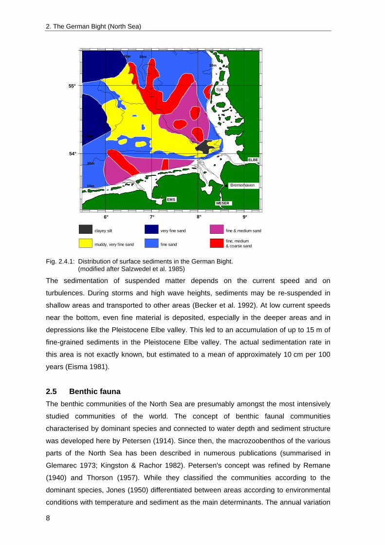
2.4 Sediments Surface sediments of the sea bottom are mostly Holocene fluvio-glacial sands mixed with
silt and coarser sediments (Caston 1979). Detailed sediment maps of the German Bight
have been presented by Gadow & Schäfer (1973) and Figge (1981). A map of the
sediment distribution in the German Bight compiled from several sources by Salzwedel et
al. (1985) is shown in Fig. 2.4.1.
7
2. The German Bight (North Sea)
Bremerhaven
Sylt 55°
54°
6° 7° 8° 9°
ELBE
EMS WESER
clayey silt
muddy, very fine sand
very fine sand
fine sand
fine & medium sand
fine, medium & coarse sand
10m
30m 40m
10m
30m
40m
Fig. 2.4.1: Distribution of surface sediments in the German Bight.
(modified after Salzwedel et al. 1985)
The sedimentation of suspended matter depends on the current speed and on
turbulences. During storms and high wave heights, sediments may be re-suspended in
shallow areas and transported to other areas (Becker et al. 1992). At low current speeds
near the bottom, even fine material is deposited, especially in the deeper areas and in
depressions like the Pleistocene Elbe valley. This led to an accumulation of up to 15 m of
fine-grained sediments in the Pleistocene Elbe valley. The actual sedimentation rate in
this area is not exactly known, but estimated to a mean of approximately 10 cm per 100
years (Eisma 1981).
2.5 Benthic fauna The benthic communities of the North Sea are presumably amongst the most intensively
studied communities of the world. The concept of benthic faunal communities
characterised by dominant species and connected to water depth and sediment structure
was developed here by Petersen (1914). Since then, the macrozoobenthos of the various
parts of the North Sea has been described in numerous publications (summarised in
Glemarec 1973; Kingston & Rachor 1982). Petersen's concept was refined by Remane
(1940) and Thorson (1957). While they classified the communities according to the
dominant species, Jones (1950) differentiated between areas according to environmental
conditions with temperature and sediment as the main determinants. The annual variation
8
2. The German Bight (North Sea)
in bottom water temperature was used by Glémarec (1973) to divide the North Sea area
into three "étages" within which the distribution of benthic fauna was determined by
sediment composition. The southern North Sea including the German Bight belongs to the
"infralittoral étage" with a water depth of less than 60 m and temperature variations of
more then 10 °C. This division has been mainly supported by the international "ICES
North Sea Benthos Survey" in 1986 (Duineveld et al. 1991; Kuenitzer et al. 1992; Heip et
al. 1992), although the differentiation was shifted to slightly different depth contours (100,
70, 50 and 30 m instead of 100 and 60 m by Glémarec). Temperature and food supply
have been identified as main factors influencing the distribution and structure of the faunal
communities (Kuenitzer et al. 1992). The spatial distribution of these factors results from
water depth and coastal distance, current regime and the different water masses. The
latter two factors are decisive for the distribution of the bottom sediments. Therefore the
distribution of bottom fauna communities of the North Sea can be delineated according to
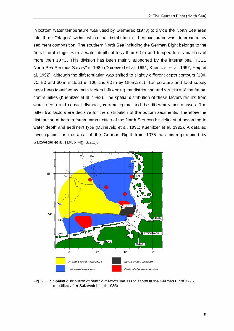
water depth and sediment type (Duineveld et al. 1991; Kuenitzer et al. 1992). A detailed
investigation for the area of the German Bight from 1975 has been produced by
Salzwedel et al. (1985 Fig. 3.2.1).
Bremerhaven
Sylt 55°
54°
6° 7° 8° 9°
ELBE
EMS WESER
Amphiura-filiformis-association
Tellina-fabula-association
Nucula-nitidosa-association
Goniadella-Spisula-association
10m
30m 40m
10m
30m
40m Helgoland
Fig. 2.5.1: Spatial distribution of benthic macrofauna associations in the German Bight 1975. (modified after Salzwedel et al. 1985)
9
2. The German Bight (North Sea)
The distribution of the benthic associations described by Salzwedel et al. (1985) agrees
largely with the results of earlier investigations of smaller parts of the German Bight
(Hagmeier 1925; Stripp 1969; Dörjes 1977). Based on the more detailed investigation of
the whole German Bight and new analytical methods, the borders between the
communities were altered slightly, and the associations were renamed. Results from more
recent studies agree mostly with the associations delineated by Salzwedel et al.
(Duineveld et al. 1991; Kuenitzer et al. 1992; Rumohr et al. 1998; Rachor & Nehmer
2003). Four main associations are generally distinguished:
- The Nucula-nitidosa-association of silty sediments and silty sands between 13 and
35 m depth. It is characterised by the bivalve Nucula nitidosa and the cumacean
Diastylis rathkei (Abra-alba-community sensu Hagmeier 1925).
- The Amphiura-filiformis-association of very fine to silty sands in 34 – 45 m depth. It is
characterised by the brittle star Amphiura filiformis, the polychaetes Pectinaria
auricoma and the gastropod Cylichna cylindracea (Echinocardium-filiformis-community
sensu Hagmeier 1925). This association is similar to the Nucula-nitidosa-association
and was joint with the latter by Jones (1950) while all other authors separated them
(Hagmeier 1925; Remane 1940; Thorson 1957).
- The Tellina-fabula-association of fine and medium sands in 13 – 31 m depth. It is
characterised by the polychaete Magelona papillicornis (M. mirabilis, M. johnstoni), the
bivalve Tellina fabula (Fabulina f.) and the amphipod Urothoë grimaldii (U. poseidonis)
(Venus-gallina-community sensu Hagmeier 1925).
- The Goniadella-Spisula-association of coarse sands to gravel in 14 – 29 m depth. The
characteristic species are the polychaetes Goniadella bobretzkii, the archiannelid
Polygordius appendiculatus and bivalves of the genus Spisula (parts of the Venus-
gallina-community sensu Hagmeier 1925).
The borders between the benthic associations are strongly correlated to the distribution of
sediment types. The exact borders as delineated in Fig. 2.5.1 should however rather be
seen as approximate and deliberate lines. Especially the delineation between the Nucula-
nitidosa-ass. and the Amphiura-filiformis-ass. may be influenced by temporal changes in
the communities and therefore differ between authors (Salzwedel et al. 1985; Rachor &
Nehmer 2003). In reality the transition between the associations is normally represented
by a gradient rather than an abrupt change.
The extensive literature on North Sea benthos, related ecological processes, long-term
changes from various sub-regions and possible influences was reviewed by Kröncke
(1995) and Kröncke & Bergfeld (2001).
10
3. Methods
3. Methods
3.1 Long term stations
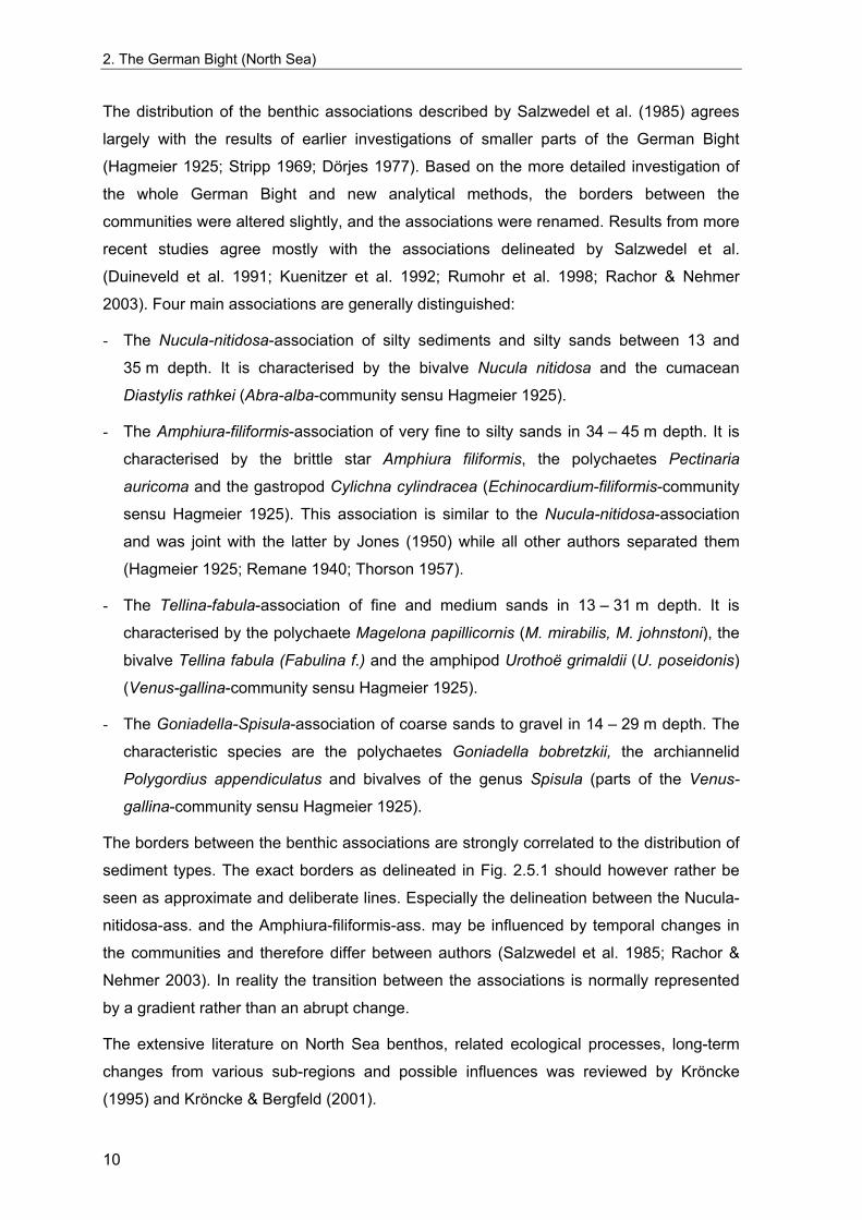
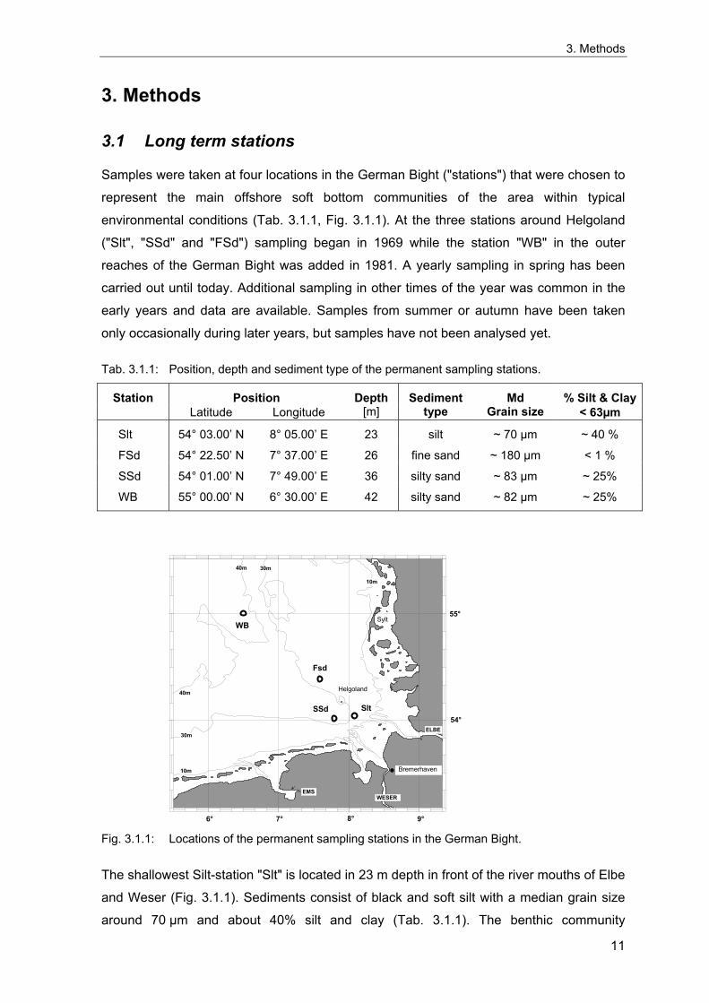
Samples were taken at four locations in the German Bight ("stations") that were chosen to
represent the main offshore soft bottom communities of the area within typical
environmental conditions (Tab. 3.1.1, Fig. 3.1.1). At the three stations around Helgoland
("Slt", "SSd" and "FSd") sampling began in 1969 while the station "WB" in the outer
reaches of the German Bight was added in 1981. A yearly sampling in spring has been
carried out until today. Additional sampling in other times of the year was common in the
early years and data are available. Samples from summer or autumn have been taken
only occasionally during later years, but samples have not been analysed yet.
Tab. 3.1.1: Position, depth and sediment type of the permanent sampling stations.
Station Position Depth Sediment Md % Silt & Clay Latitude Longitude [m] type Grain size < 63µm
Slt 54° 03.00’ N 8° 05.00’ E 23 silt ~ 70 µm ~ 40 %
FSd 54° 22.50’ N 7° 37.00’ E 26 fine sand ~ 180 µm < 1 %
SSd 54° 01.00’ N 7° 49.00’ E 36 silty sand ~ 83 µm ~ 25%
WB 55° 00.00’ N 6° 30.00’ E 42 silty sand ~ 82 µm ~ 25%
Sylt 55°
54°
6° 7° 8° 9°
ELBE
EMS WESER
10m
30m 40m
10m
30m
40m
WB
Fsd
SSd Slt
Helgoland
Bremerhaven
Fig. 3.1.1: Locations of the permanent sampling stations in the German Bight.
The shallowest Silt-station "Slt" is located in 23 m depth in front of the river mouths of Elbe
and Weser (Fig. 3.1.1). Sediments consist of black and soft silt with a median grain size
around 70 µm and about 40% silt and clay (Tab. 3.1.1). The benthic community
11
3. Methods
represents a typical Nucula-nitidosa-association sensu Salzwedel et al. (1985). Until 1980,
sewage sludge from Hamburg had been disposed about 4.5 nm east of this station
(Rachor 1982).
The "FSd"-station is located at the centre of a former dumping area about 15 nm north-
west of Helgoland (Fig. 3.1.1) where acid-iron wastes from TiO2-production had been
discharged from 1969 to 1989 (Rachor & Dethlefsen 1976; Rachor 1972; Rachor &
Gerlach 1978). It is named after its typical sediment of homogeneous fine sand with a
median grain size of 180 µm and a silt and clay content of less than 1 % (Tab. 3.1.1). The
water depth is 26 m and the benthic community is a typical example of the Tellina-fabula-
association sensu Salzwedel et al. (1985).
The Silty-Sand-station "SSd" is situated south of Helgoland in the old Pleistocene Elbe
River valley at 36 m depth (Fig. 3.1.1). Sediments consist of silty fine sands with a median
grain size of about 83 µm and a silt and clay content of about 25 % (Tab. 3.1.1). The
benthic community here is a shallow type of the Amphiura-filiformis-association found in
the German Bight at more than 30 m depth (Salzwedel et al. 1985). Located at the
western boundary of the muddy area in the inner German Bight, it contains also elements
of the Nucula-nitidosa-association of silty sediments.
The deepest station "WB" lies about 60 nm west of the island of Sylt and about 20 nm
east of the White Bank (Fig. 3.1.1), which is also responsible for the station's name. It is
located near the eastern slope of the old Pleistocene Elbe River valley in 42 m water
depth. Sediments are similar to those found at SSd and consist of silty fine sands with a
median grain size of about 82 µm and a silt and clay content of about 25 % (Tab. 3.1.1).
The benthic community at WB is a deeper and more characteristic variant of the
Amphiura-filiformis-community (Salzwedel et al. 1985) than that at SSd.
3.2 Benthos data
Quantitative data on the macrozoobenthic communities are based on samples taken by
bottom grabs.
3.2.1 Sampling methodology
For the long-term series, the most often used sample size consisted of five 0.1m² van-
Veen grabs (vV) per station, resulting in a total sampled area of 0.5 m². The sampling
protocol was not always constant over the whole time span at all stations. During the early
years until 1985, a lighter standard van-Veen grab was used. As this gear showed a low
penetration depth especially in sandy sediments, occasionally larger van-Veen grabs of
12
3. Methods
0.2, 0.4 or 0.5 m² were employed. At FSd and SSd the light vV was complemented by a
0.017 m² Reineck box corer (RBC) that had a much deeper penetration depth, usually in a
combination of two vV's plus six RBC's from 1976 to '89. On a few occasions, some other
sampling gears were employed e.g. van-Veen grabs of 0.05 or 0.4 m² area or a large
0.056 m² Box-corer. From 1986 onwards, a new modified warp-rigged van-Veen grab with
sieve-covered windows on the upper side and a larger weight (Dybern et al. 1976;
Rumohr 1999) was used, resulting in a reduced bow-wave when approaching the bottom
and a deeper penetration depth especially in sandy sediments. Details on the available
data and the gear type used can be found in the annex A.2.
Either data from five 0.1 m² van-Veen grabs or from a combination of two vV's with six
Reineck box corers are available for most years.
In July 1976, a large number of samples were taken at the FSd-station while the ship was
anchored. Data from a total of 16 vV plus 25 RBC were used to evaluate the effect of a
combination of vV's and RBC's on the results regarding species number, diversity,
organism density and inter-samples similarity. Monte-Carlo simulations were based on
10000 permutated samples consisting of random combinations of five vV's or of
combinations of two vV's plus six RBC's.
The variable methodologies require careful consideration of the quality of data extracted
from the database for any analytical question. Details on sampling dates, the respective
sampling gear, the number of replicates and the quality (see paragraph 3.2.3) of the
available data are listed in the table in the annex A.2.
3.2.2 Sample processing
Samples were sieved on board on 0.5 mm round-hole sieves and fixed (and stored) in
buffered 4% formalin. In the laboratory, samples were stained with rose bengal to facilitate
sorting.
Organisms were identified to species level as far as possible, counted and weighted (wet
weight). Methods in general followed the ICES and HELCOM recommendations for
sampling benthos and treatment of samples (Rumohr 1999). Taxonomic groups not
adequately sampled by these methods (Nematoda, Foraminifera), colonial (Hydrozoa)
and mostly pelagic (Calanoida, Chaetognatha) organisms were excluded from the data
analysis. Juvenile and damaged specimens were classified to the lowest level where
confident identification was possible. Nemertines, Plathelminthes, Oligochaetes were not
identified further. A few rare species with difficult identification were combined at genus or
family levels. All densities are reported as organisms per 0.1 m² (one grab sample) unless
specified otherwise.
13
3. Methods
Identification of organisms for newly analysed samples was based on the following
literature:
Crustacea: Lincoln 1979; Dauvin & Bellan-Santini 1988; Myers & McGrath 1991;
Stephensen 1940; Jones 1976; Holdich & Jones 1983; Isaak & Moyse
1990; Isaak et al. 1990; Moyse & Smaldon 1990; King 1974; Mauchline
1984; Naylor 1972; Sars 1894; Sars 1900
Polychaeta: Hartmann-Schröder 1996; Petersen 1998; Fauvel 1923; Fauvel 1927;
Hilbig & Dittmer 1979
Echinodermata: Moyse & Tyler 1990; Webb & Tyler 1985; Lieberkind 1928
Mollusca: Tebble 1966; Jones & Baxter 1987; von Cosel et al. 1982; Graham
1988; Thompson & Brown 1976; Hayward 1990; Hayward et al. 1990;
Poppe & Goto 1991; Poppe & Goto 1993; Ziegelmeier 1957; Ziegelmeier
1966; Luczak & Dewarumez 1992
Others groups: Broch 1928; Ryland 1990; Manuel 1988; Pax 1928; Cornelius et al.
1990; Gibbs 1977
(References are listed separately under "References II"). During earlier years not all of
these in part new releases were available and in some cases older editions were used.
Biomass data were not recorded in most of the previously existing records.
3.2.3 Data sources
For the three stations Slt, SSd and FSd data from 1969 until 1987 were with few
exceptions available from the original laboratory protocols. For the FSd station, spring
data were available until 1991. Parts of these data were published before (Rachor 1977;
1980; 1982; 1990; Rachor & Salzwedel 1975; Rachor & Gerlach 1978; Rachor & Bartel
1981; Rachor et al. 1982; Heuers 1993). Data for later years until 2000 were obtained by
analysis of stored samples as far as available and by continuation of the sampling. All
data for station WB, starting from 1981, were obtained by analysis of stored and newly
taken samples. Before 1974 only one value per sampling date is available in most cases,
as grab samples were pooled either on board or in the laboratory and data were only
reported for the pooled sample. Since 1975, raw data as abundances per sample are
mostly available. Biomass data are available for WB since 1981 and from 1988 for all
stations (newly analysed samples).
All data were entered in a specially developed database (Annex A.3) and checked for
quality and consistency over time (see following paragraph).
14
3. Methods
3.2.4 Data quality control
All data entered into the database were checked by comparing printed reports with
original data sheets. Data were checked for inconsistencies in identification over time and
doubtful identifications re-identified from stored samples as far as available. Original
identification and comments were kept in the "remark" field of the respective database
entry.
A serious source of error for long term analyses as well as for comparisons of data from
different sources are taxonomic difficulties. The simplest possible error source are
synonyms of scientific names, resulting from the use of different identification literature or
from changes of the scientific nomenclature. Over the course of the last 30 years, several
species were renamed, some of them even several times. The problem of synonyms was
overcome by the construction of a specific taxonomic database ("DB99_Species"), linking
all synonyms to one single valid scientific name. This species database contains all
species recorded in the German Bight during the long-term investigations, from large
spatial studies covering the whole area and from selected literature (a detailed description
can be found in annex A.4).
Using this table during the extraction of the data from the database, the result will be free
from synonyms. It can also be used to extract data at a higher systematic level such as
genus, family, order or the like. Less simple is the case of taxa that were determined with
differing precision (species, genus or family) as well as of species that were newly
described, lumped or split. For specific data sets containing such problems, the respective
species were combined at the next higher reliable systematic level, which can be
assumed to be consistent within the respective data set. These cases are not treated
automatically, as other subsets with e.g. a restricted time span may not contain dubious
cases and do not require species lumping with its associated loss of information.
For a large number of samples, only certain taxonomic groups had been identified. Other
samples consist only of one or two grabs (Annex A.2). The status of the data is recorded
for each sample separately, stating whether the analysis of the sample was complete or if
only some major groups had been analysed. Additionally the data status is recorded for
each station, allowing an easier identification of those sampling occasion with a sufficient
number of adequately analysed samples.
3.2.5 Data selection for the long-term study
The analysis of temporal changes in the benthic communities is based on a reduced set of
data. Just like the number of species, similarity calculations are influenced by the sample
15
3. Methods
size (see chapter 4.2.5). Analyses based on any kind of similarity calculations should
therefore be based on samples of the same size wherever possible.
From each year one sampling date from spring (preferably early April) was selected where
the most reliable data were available. As far as possible, samples of five 0.1m² van-Veen
grabs were preferred, but alternative samples (e.g. two vV plus six RBC) had to be
accepted especially for SSd and FSd-stations for certain years.
Whenever appropriate data from April were not available, the date closest to April with
appropriate data was chosen (selected data are marked in annex A.2). All data were
standardized to abundances per m². In cases were different grab types were combined, a
weighted arithmetic mean density was calculated.
3.2.6 Spatial sampling
The sampling for the long term series was intended always to take place at the same
location. Bad weather conditions and less accurate positioning systems in earlier times
(e.g. DECCA) probably often only allowed much less precise positioning than today. If
some kind of spatial structure or gradient was present in the area, a deviation from the
exact position could result in different results for benthic communities. An minimum
accuracy of ± 0.5 nm can be assumed at all times.
To asses the possible effect of deviations from the exact sampling position, 21 van-Veen
grabs were taken in the vicinity of the centre position of all four permanent stations in April
1998 (Tab. 3.2.1). The area covered by the spatial sampling was chosen to cover all
possible deviations from the centre position even under unfavourable conditions. Samples
at 1 nm from the centre were included to asses further spatial variation in the area.
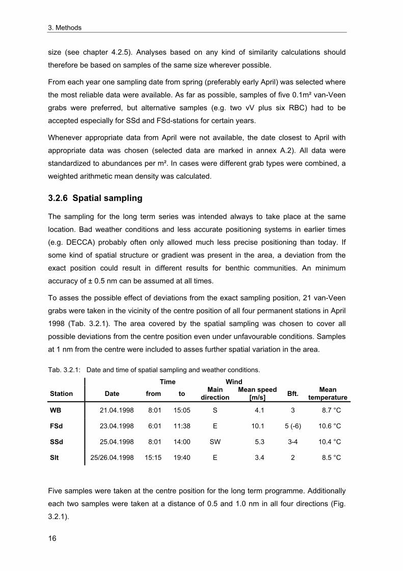
Tab. 3.2.1: Date and time of spatial sampling and weather conditions.
Time Wind Station Date from to Main
direction Mean speed
[m/s] Bft. Mean temperature
WB 21.04.1998 8:01 15:05 S 4.1 3 8.7 °C
FSd 23.04.1998 6:01 11:38 E 10.1 5 (-6) 10.6 °C
SSd 25.04.1998 8:01 14:00 SW 5.3 3-4 10.4 °C
Slt 25/26.04.1998 15:15 19:40 E 3.4 2 8.5 °C
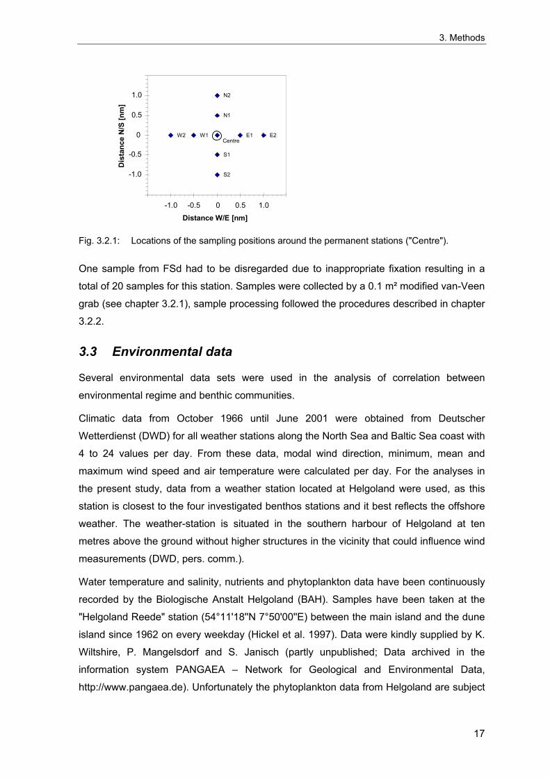
Five samples were taken at the centre position for the long term programme. Additionally
each two samples were taken at a distance of 0.5 and 1.0 nm in all four directions (Fig.
3.2.1).
16
3. Methods
S1
E1
N1
N2
W2 W1 Centre
E2
S2-1.0
-0.5
0
0.5
1.0
-1.0 -0.5 0 0.5 1.0
Distance W/E [nm]
Dis
tanc
e N
/S [n
m]
Fig. 3.2.1: Locations of the sampling positions around the permanent stations ("Centre").
One sample from FSd had to be disregarded due to inappropriate fixation resulting in a
total of 20 samples for this station. Samples were collected by a 0.1 m² modified van-Veen
grab (see chapter 3.2.1), sample processing followed the procedures described in chapter
3.2.2.
3.3 Environmental data
Several environmental data sets were used in the analysis of correlation between
environmental regime and benthic communities.
Climatic data from October 1966 until June 2001 were obtained from Deutscher
Wetterdienst (DWD) for all weather stations along the North Sea and Baltic Sea coast with
4 to 24 values per day. From these data, modal wind direction, minimum, mean and
maximum wind speed and air temperature were calculated per day. For the analyses in
the present study, data from a weather station located at Helgoland were used, as this
station is closest to the four investigated benthos stations and it best reflects the offshore
weather. The weather-station is situated in the southern harbour of Helgoland at ten
metres above the ground without higher structures in the vicinity that could influence wind
measurements (DWD, pers. comm.).
Water temperature and salinity, nutrients and phytoplankton data have been continuously
recorded by the Biologische Anstalt Helgoland (BAH). Samples have been taken at the
"Helgoland Reede" station (54°11'18''N 7°50'00''E) between the main island and the dune
island since 1962 on every weekday (Hickel et al. 1997). Data were kindly supplied by K.
Wiltshire, P. Mangelsdorf and S. Janisch (partly unpublished; Data archived in the
information system PANGAEA – Network for Geological and Environmental Data,
http://www.pangaea.de). Unfortunately the phytoplankton data from Helgoland are subject
17
3. Methods
to several methodological errors and thus are currently not yet usable for an analysis of
the phytoplankton development in the German Bight (K. Wiltshire, pers. comm.).
The water discharge of the river Elbe at km 537 is recorded daily from 1960 to 2000, was
kindly provided by Eggert (2002) (http://www.dgj.de/servlet/IbMenu).
The "North Atlantic Oscillation Index" (NAOI) summarizing the main climatic features over
Northern Europe was provided by the Climate Analysis Section, NCAR, Boulder, USA,
Hurrell (1995) (http://www.cgd.ucar.edu/~jhurrell/nao.html). It is available on a monthly,
seasonal or annual basis from 1865 until 2000 and as winter-index (Dec – Mar) from1864
until 2002.
3.4 Analytical methods
The community structure, spatial distribution and temporal development of the benthic
organisms is summarised and compared by various univariate and multivariate indices
and statistics:
3.4.1 Indices
All diversity and similarity indices are calculated from formulas as stated in Krebs (1998)
and Legendre & Legendre (1998) unless specified otherwise.
Univariate statistics were calculated using STATISTICA vers. 5.5 (StatSoft Inc. 2000),
multivariate analyses based on PRIMER 5 software vers. 5.2.2 (Primer-e 2000). Indices
and p-value adjustment were calculated by custom written Excel Visual-Basic-modules.
3.4.1.1 Spatial distribution & variability
3.4.1.1.1 Univariate statistics
The variability of any measure can be expressed by the ratio between the standard
deviation (SD) and the mean ( x ), which is called coefficient of variation (CV = xSD )
(Elliott 1977). It is independent of the sample size and invariant to linear extrapolations. It
can however not be used to classify the type of spatial distribution of organisms.
One of the oldest and simplest measures of dispersion is the ratio between variance and
mean ( xs² ) of local organism densities. It ranges from 0 for uniform distribution over 1
for random distribution to its maximum which equals the total number of organisms in the
sample (Krebs 1998). Values larger than 1 indicate an aggregated distribution. The
variance-to-mean ratio is however problematic, as any data transformations may change
this ratio. When a simple multiplication with a fixed factor is applied, the square of this
factor will affect the variance, while the mean is only affected by the simple factor. An
18
3. Methods
extrapolation to densities per m² may often result in an interpretation of aggregated
distribution for nearly all species. The variance-to-mean ratio should thus only be applied
to raw data. Another serious concern was raised by Hurlbert (1990) who showed that
several non-random pattern can lead to a variance-to-mean ratio of 1. Other measure of
dispersion may be used to overcome these problems.
The spatial distribution of the organisms can be tested by Morisita's index of dispersion Id
(Morisita 1962).
( )
−
−=
∑∑∑∑xx
xxnI d 2
2
(eq. 3.1)
where n = number of samples Σx = sum of organisms
It has the advantage of having a known sampling distribution and the statistical
significance of non-randomness can be tested (Krebs 1998). This procedure is simplified
by the standardisation of this index to a range of –1 to 1 by Smith-Gill (1975). After the
calculation of Id, two critical values Mu and Mc are calculated:
1)(
2975.
−ΣΣ+−
=x
xnMu
χ and
1)(
2025.
−ΣΣ+−
=x
xnc
χM (eq. 3.2 & 3.3)
where = value of Chi-square distribution with (n-1) d.f. with 97.5% of the area to the right n = number of samples Σx = sum of organisms
2975.χ
Then the standardised Morisita index Ip is calculated by one of the following formulas:
If Id ≥ Mc > 1:
−−
∗+=c
cdp Mn
MII 5.05.0 (eq. 3.4)
If Mc > Id ≥ 1:
−−
∗=11
5.0c
dp M
II (eq. 3.5)
(The term "Mu" given in Krebs (1998) is a mistake, and must read "Mc" (Smith-Gill 1975) )
If 1 > Id > Mu:
−−
∗−=11
5.0u
dp M
II (eq. 3.6)
If 1 > Mu ≥ Id:
−∗+−=
u
udp M
MII 5.05.0 (eq. 3.7)
In this standardised form, Ip-values larger than 0.5 indicate a significantly clumped
distribution, values around 0 a random distribution and values lower than –0.5 a
significantly more even distribution (Krebs 1998).
19
3. Methods
3.4.1.1.2 Multivariate statistics
The multivariate variance is measured by the average similarity between all pairs of
samples and its coefficient of variation (CV). The higher the similarity between two
samples from an area, the lower the multivariate spatial variability within the community.
Similarities however are not independent random variables (Clarke & Warwick 1994), thus
usual statistical procedures can not be applied to test the significance of differences. The
mean and CV can however be used for purely descriptive purposes.
Comparisons of the variability of two samples is only valid if both samples have the same
mean or, in case both samples have different means, if it is known that the variability does
not systematically depend on the mean (Krebs 1998). The same applies to similarity
measures. The exact relation between mean similarity and its variance is an inherent
property of the chosen similarity index and is at present unknown. Comparisons of the
variability of similarities of several groups are strictly only valid if all groups have the same
mean similarity. Comparisons of the CV across groups of different mean similarity are
likely to be valid if the similarity measure changes linearly. The Bray-Curtis-similarity is
one of the few similarity indices that show this linear behaviour (Bloom 1981). This should
allow a comparison of the variability of similarities even between groups of differing mean
similarity.
3.4.1.2 Diversity
Besides purely quantitative descriptions in terms of organism density and biomass,
several measures of diversity in the wider sense are the most common attributes used to
describe biological communities. These include the simple species number, evenness or
dominance indices and various "diversity" indices combining aspects of species richness
and evenness. A combination of these measures is meant to summarise the main
information about the numerical community structure. Most of these measures are
affected by sample size. This dependency is investigated as a background information for
the long-term study and to estimate the minimum sample size necessary for a reliable
value without excessive variability.
Species number
The simplest aspect of diversity is the number of species present (S). The total number of
species in a benthic community is however mostly not possible to determine. The number
of species found is strongly dependent on the sampling effort. The species number should
thus always be related to the respective sample size, and comparisons should only be
made between samples of the same size. For quantitative investigations, this sample size
20
3. Methods
relates to a standard sampling effort (e.g. sampled area, resp. number of grabs) and is
termed species density.
The number of species per unit area is termed species density. The number of species
relative to the number of organisms is called species richness (Gotelli & Colwell 2001).
The total number of species found in an area is termed species spectrum.
Noting the strong dependence between sample size and species number, Sanders (1968)
proposed to calculate the expected number of species for a given (smaller) number of
organisms drawn randomly from the existing sample (E(Sn)). The corrected formula for
this "rarefaction" given by Hurlbert (1971) is:
( ) ∑
−
−=i
i
n
nNnNN
SE 1 (eq. 3.8)
where N = total number of organisms in the collection Ni = number of organisms in species i n = number of organisms chosen for standardisation (n ≤ N)
In this case the species number is related to the number of organisms and called species
richness (Gotelli & Colwell 2001). Rarefaction assumes a random distribution of the
organisms in space. This includes a random distribution within each species and
independence between the species. In practise, most species' distributions are clumped
and there may be positive as well as negative associations between the species. The
larger these violations of the assumption of randomness, the larger will be the
overestimation of the number of species by the rarefaction method (Krebs 1998).
When a sufficient number of samples is available, sample-based species accumulation
curves can be constructed by Monte-Carlo computer simulations of the number of species
in relation to the number of samples (Gotelli & Colwell 2001). These represent an
unbiased presentation of the expected (=mean) number of species for a given sample size
and with an empirical confidence interval around this mean. The sample size can be
interpreted not only in terms of number of samples or the respectively sampled area (sp.
density), but also in terms of mean number of organisms (sp. richness).
21
3. Methods
Evenness
Evenness indices summarise the dominance structure of the community. Maximum
evenness is reached when all species are present in equal densities. The higher the
numerical dominance of a few species, the lower the evenness. Probably the most
common measure of evenness is Pielou's J' (Pielou 1966):
)(log'''
2max SH
HHJ == (eq. 3.9)
It relates the observed heterogeneity to the maximum possible diversity (heterogeneity),
which is reached when all species are equally abundant (H'max=log2(S)).
Although theoretical studies have suggested other indices as preferable (Smith & Wilson
1996), a comparison of sample size dependence and variability of various evenness
indices using real data from the spatial sampling identified J' as the least variable
measure. Results on the sample size dependence of J' and its variability are presented in
the results chapter, details on the results from other indices and their comparison go
beyond the scope of the present study and shall be presented in a forthcoming
publication.
Heterogeneity
The concept of heterogeneity combines the aspects of species richness and evenness
into a single measure.
Based on information theory, the Shannon-Wiener index (Shannon & Weaver 1963) was
first applied in ecology by Margalef (1958).
∑−=i
ii ppH )(log' 2 (eq. 3.10)
where pi = ni / N ni = abundance of species i N = total number of organisms
It measures the uncertainty about the species identity if one more organisms were to be
collected from the respective community (in bits per organism). In theory it can reach very
high values, but for biological communities H' does not seem to exceed 5.0 (Krebs 1998).
As its unit (bit) is a rather hard to interpret, Hurlbert (1971) and Hill (1983) recommended
the use of its exponential form N1=2H' instead. This index has the more readily
understandable unit of species (Santos & Bloom 1983). The exponential transformation
does expand the range and may pronounce especially differences between highly diverse
communities (Gray 2000). As this is a simple monotone transformation of H', it does not
affect the outcome of comparisons or nonparametric statistical tests. In practise, H' is still
22
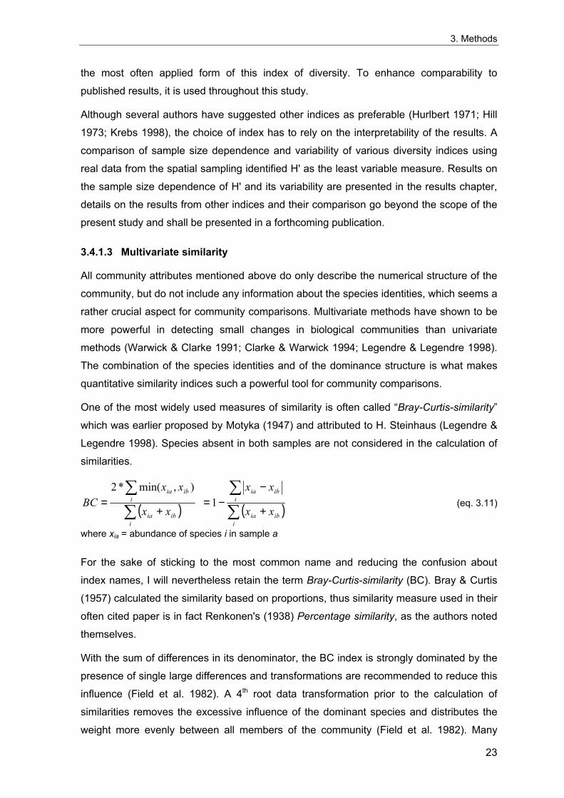
3. Methods
the most often applied form of this index of diversity. To enhance comparability to
published results, it is used throughout this study.
Although several authors have suggested other indices as preferable (Hurlbert 1971; Hill
1973; Krebs 1998), the choice of index has to rely on the interpretability of the results. A
comparison of sample size dependence and variability of various diversity indices using
real data from the spatial sampling identified H' as the least variable measure. Results on
the sample size dependence of H' and its variability are presented in the results chapter,
details on the results from other indices and their comparison go beyond the scope of the
present study and shall be presented in a forthcoming publication.
3.4.1.3 Multivariate similarity
All community attributes mentioned above do only describe the numerical structure of the
community, but do not include any information about the species identities, which seems a
rather crucial aspect for community comparisons. Multivariate methods have shown to be
more powerful in detecting small changes in biological communities than univariate
methods (Warwick & Clarke 1991; Clarke & Warwick 1994; Legendre & Legendre 1998).
The combination of the species identities and of the dominance structure is what makes
quantitative similarity indices such a powerful tool for community comparisons.
One of the most widely used measures of similarity is often called “Bray-Curtis-similarity”
which was earlier proposed by Motyka (1947) and attributed to H. Steinhaus (Legendre &
Legendre 1998). Species absent in both samples are not considered in the calculation of
similarities.
( )∑∑
+=
iibia
iibia
xx
xxBC
),min(*2 ( )∑
∑+
−−=
iibia
iibia
xx
xx1 (eq. 3.11)
where xia = abundance of species i in sample a
For the sake of sticking to the most common name and reducing the confusion about
index names, I will nevertheless retain the term Bray-Curtis-similarity (BC). Bray & Curtis
(1957) calculated the similarity based on proportions, thus similarity measure used in their
often cited paper is in fact Renkonen's (1938) Percentage similarity, as the authors noted
themselves.
With the sum of differences in its denominator, the BC index is strongly dominated by the
presence of single large differences and transformations are recommended to reduce this
influence (Field et al. 1982). A 4th root data transformation prior to the calculation of
similarities removes the excessive influence of the dominant species and distributes the
weight more evenly between all members of the community (Field et al. 1982). Many
23
3. Methods
similarity indices like e.g. the Bray-Curtis-index are invariant to linear scaling of the data
like e.g. calculations of densities per m². This property is maintained if square root or
fourth root transformations are applied (Field et al. 1982), but it is lost if logarithmic
transformations are applied.
In a comparison of the properties of various (dis-) similarity indices, the Bray-Curtis-
similarity with a fourth root transformation was chosen for the further analyses of the
present study as it produced the least variable and most consistent results. Results of the
sample size dependence of the BC are presented here, details on the results from other
indices, transformations and their comparison go beyond the scope of the present study
and shall be presented in a forthcoming publication.
3.4.2 Multivariate analytical procedures
In analyses of ecological communities, the assumption of independent variables (species
or environmental factors) is not realistic. Organism densities are often influenced by
biological interactions and environmental factors are often correlated amongst
themselves. Studying multidimensional data sets using univariate statistics however
assumes this independence. Only multivariate methods taking the dependence of the
variables into account can properly analyse the whole story when dependencies exist
(Legendre & Legendre 1998). This may be one of the main reasons why multivariate
analyses have proven to be more powerful in detecting changes in ecological
communities than various univariate methods (Clarke & Warwick 1994).
3.4.2.1 MDS
Nonmetric Multidimensional Scaling (MDS) (Kruskal 1964) is used to represent the
multivariate similarities between samples in a reduced number of dimensions. It is based
on an association matrix containing the (dis-) similarities between all pairs of samples. A
MDS-plot represents as much of the information contained in the underlying association
matrix in the specified number of dimensions as possible. The quality of this
representation is measured by the "stress"-value (Kruskal 1964). The lower this value, the
better the presentation. A high stress-value indicates a higher dimensionality of the data
(Clarke & Warwick 1994) and is typical for samples which do not contain a clear structure
(Rumohr et al. 2001).
Consecutive MDS-plots based on the same association matrix and with the same stress-
value may differ, because of problems with the placement of samples which are not
closely related to the other samples in the plot. Such point will be located at the periphery
of the plot, more or less at random and probably at different borders in consecutive
iterations of the same analysis (Bob Clarke cited as pers. comm. by Gamito & Raffaelli
24
3. Methods
1992). With other ordination methods such a principal component analysis (PCA) or
correspondence analysis (CA or DCA), such points may be positioned in the first two axes
amongst the other points with which they have no affinity, while being separated on higher
axes. The variation seen in the MDS plots may as such be more informative with regard to
the affinities of such samples (Gamito & Raffaelli 1992).
In order to avoid misinterpretation of the position of single years relative to the whole time-
series, a minimum of ten 2D plots based on the same similarity matrix with the same
minimal stress were compared amongst each other and to 3D solutions. Only those
results were interpreted that were consistent with all 2D and 3D solutions. In doubtful
cases the results were confirmed by inspection of the similarity matrix.
3.4.2.2 Cluster Analysis
Like MDS, this analysis works with any type of similarity measure. Hierarchical cluster
procedures join samples consecutively to produce groups that maximise the similarity
within the groups and at the same time the distinction of the groups. The result is usually
presented as dendrogram. The appearance of this plot is strongly influenced by the
clustering procedure applied. As the similarity between single samples remains
untouched, the pairs with the highest similarity are usually the same for all procedures.
The way these are joined can however differ largely. Out of the large number of
procedures described (Clifford & Stephenson 1975; Legendre & Legendre 1998) the
"Group average" clustering is the preferred standard procedure. It joins two groups by
evaluating the mean similarity between the samples from both groups. It is not as much
prone to the "chaining"-effect as the "Single linkage" procedure nor to an artificial
formation of distinct clusters (as possible with "Complete linkage") (Field et al. 1982 & own
unpublished results). In cases where several groups are rather similar or even
overlapping, "Complete linkage" may provide additional (and possibly clearer) information
to facilitate the decision of where to draw the line between the groups.
25
3. Methods
3.4.3 Statistical tests
3.4.3.1 Comparison of univariate measures Statistical significance of differences between two means of univariate measures were
tested using the U-test (Mann & Whitney 1947). This rank sum test does not rely on
assumptions of normality and homogeneity of variances. It only assumes an ordinal scale.
It is known to be one of, if not the most powerful nonparametric alternative to a two-
sample t-test. In some cases with few observations, it may even be more powerful (Zar
1996). With n > 20, U quickly approaches a normal distribution, while for small n the actual
value of U is compared to all possible values with the given number of observations in
both samples by a permutation test.
Box & Wisker plots are used for a graphical presentation of differences between groups of
samples (Tukey 1977). In the form used here, it displays the median, the 25th and 75th
percentiles and the range of values excluding extremes. Extreme are values that are more
than 1.5 times the interquartile range larger than the 75th percentile or smaller than the
25th percentile (displayed as separate dots). A "notch" around the median indicates the
95% confidence interval of the median (McGill et al. 1978).
3.4.3.2 Correlations Throughout this study, regressions are used for graphical representation of trends in data,
while associated statistics are only used as indications of uncertainty without using them
for statistical inference. Linear regression is strictly speaking only valid under the
assumptions of normality of residuals and homogeneity of variance over the range of the
independent variable. This is often not the case in ecological data sets and confidence
intervals and coefficients of determination are not statistically valid. Statistical inference is
therefore accomplished by the robust nonparametric Spearman's rank-correlation
coefficient ρ (rho). It does not rely on assumptions about the distribution of the data or
linearity of the correlation. It tests for monotonic correlations and is based on ranks and
thus only requires ordinal data.
3.4.3.3 Smoothing of time series
Most time series presented here are shown without smoothing methods, because these
would suppress any short-term effects caused by disturbance. However, for the
development of benthic communities, these disturbances are considered one of the most
important factor. The only exception is the presentation of the long-term (1864 – 2002)
development of the NAOI, which is presented with a low-pass filter, analogue to the
presentation from Hurrel (1995). This low-pass filter represents a weighted running mean
over seven years with weights of 1, 3, 5, 6, 5, 3 and 1.
26
3. Methods
3.4.3.4 Multivariate differences
The statistical significance of multivariate differences between two groups is tested by the
ANOSIM procedure, a permutation test based on Clarke's R statistic (Clarke & Warwick
1994). Clarke's R measures the relation between the mean rank similarities within each
group Wr and the mean rank similarity between both groups Br :
2Mrr
R wB −= (eq. 3.12)
where 2
)1( −= nnM the total number of similarity-ranks in the test
Wr = mean rank similarities within each group
Br = mean rank similarity between both groups
When R equals 1, all similarities within the groups are larger than those between samples
from different groups. R = 0 indicates no differences while negative values indicate the
need to verify the homogeneity of the samples. Large negative values of R do occur when
either or both groups contain outliers, or when two different states are found in both
groups (Chapman & Underwood 1999). As R may be small but still significantly different
from zero, the probability of falsely rejecting the null-hypothesis of R = 0 is calculated by a
permutation test (Clarke & Warwick 1994).
3.4.3.5 Comparing multivariate pattern between stations
To test for a similar multivariate pattern in two sets of samples, a rank correlation is
calculated between the two similarity matrices based on either data set. In case of a
similar temporal development of the communities, there will be a significant correlation
between the similarity matrices. The calculated correlation is compared to results from
randomly permutated samples to test for statistical significance (Clarke & Warwick 1994;
Primer routine RELATE). This correlation can only be calculated for years when data from
both stations are available. A correlation indicates a similar temporal development, e.g.
similar periods of relative stability and similar points of change, but does not imply a
parallel population development for species present at both stations.
3.4.3.6 Multivariate Mantel correlograms
Multivariate Mantel correlograms are used to describe the temporal and the spatial
autocorrelation of species assemblages. Multivariate temporal autocorrelation describes
the similarity of samples in dependence on the time span between the sampling dates
(Legendre & Legendre 1998), in this case for the long term series in years. In the
presence of temporal autocorrelation, samples from consecutive years or separated by
27
3. Methods
only a few years are more similar than samples separated by longer periods. Temporal
correlograms are used to identify cyclical developments as well as long term trends.
Multivariate spatial autocorrelation describes the similarity of samples in dependence on
the spatial distance between the sampling sites (Somerfield & Gage 2000). In the
presence of spatial autocorrelation, samples from sites located closer together are more
similar than samples separated by longer distances. Spatial correlograms can be used to
identify geographical patterns in community composition as well as large scale gradients.
Multivariate Mantel correlograms are based on an association matrix containing the pair-
wise (dis-)similarities between the samples and a second corresponding matrix of
temporal or geographical distances. The latter one is used to construct several model
matrices. The distances are split into classes and one matrix is constructed for each class,
each containing code 1 for those distances that belong to the respective distance class
and zeroes in the remaining fields. A Spearman's rank correlation is calculated between
the association matrix and each of these model matrices and the statistical significance
tested by a permutation test (Mantel-test (Mantel 1967), Primer routine RELATE). As this
involves as many statistical tests as there are distance classes, the p-values are adjusted
for multiple testing by a sequential adjustment procedure for multiple testing (Legendre &
Legendre 1998). The correlations are plotted against distance classes and significant
correlations are marked. Correlations for the largest class(es) commonly involve very few
values and should be disregarded.
3.4.3.7 Multiple statistical test
Statistical test procedures generally results in an error probability "p" indicating the
probability that a null-hypothesis is falsely rejected. When several test are computed
simultaneously, the overall error probability becomes much larger than the nominal error
probability α accepted for the single test. The simplest way to account for this effect is to
adjust the calculated p-values by the number of tests carried out (k) by the Bonferroni-
correction p' = k*p. As this procedure is overly conservative, a much more powerful
procedure is Holm's adjustment (Holm 1979): After ordering the p-values to an increasing
series pi with i running from 1 to k, each pi-value is replaced by pi' = (k - i + 1)*pi. When
proceeding from i = 1 to k, every value which is smaller than its predecessor is augmented
to the larger value, resulting in a monotonously increasing series (Legendre & Legendre
1998). This procedure is also valid for non-independent tests (Wright 1992). An even
more powerful procedure only applicable to independent tests was proposed by Hochberg
(1988). Only the last step differs from Holm's procedure: proceeding this time from i = k to
1, if an adjusted value is larger than its predecessor, it is diminished to the lower value.
With this method, no adjusted p-values can be larger than the largest unadjusted p-value
28
3. Methods
or exceed 1 (Legendre & Legendre 1998). By using either of these adjustments, the
overall error probability is preserved.
3.4.4 Analysis of spatial variability
Spatial variability in organism density between samples taken in any one area may be of
two different types: systematic and random variability. Systematic variability includes
spatial autocorrelation up to larger scale gradients across the whole area. Random
variability results from natural random variance, a patchy distribution of the organisms at a
scale smaller than the distance between sampling positions.
Systematic variability
Total organism density, species density, diversity and evenness were tested for possible
gradients in either N/S or W/E direction by Spearman’s rank correlation to the
geographical position. Probabilities were adjusted for each station separately for testing
two axes by Hochberg's procedure to preserve the 5% error-level for each parameter.
To test for multivariate spatial autocorrelation or a possible gradient in the community,
multivariate Mantel correlograms were constructed. As gradients only present in a single
direction may pass unnoticed in all-directional correlograms (Legendre & Legendre 1998),
unidirectional correlograms were computed separately for the North-South axis and the
West-East axis. Similarities were calculated using Bray-Curtis index and fourth root
transformed data. Geographical distances were split into 5 classes corresponding to the
main distances implied by the sampling scheme (Tab. 4.6.2):
Tab. 3.4.1: Distance class for Mantel-correlograms.
Class [nm] [m] Class centre
1 0 – 0.25 0 – 463 0 nm 2 0.25 – 0.75 463 – 1389 0.5 nm 3 0.75 – 1.25 1389 – 2315 1.0 nm 4 1.25 – 1.75 2315 – 3241 1.5 nm 5 1.75 – 2.25 3241 – 4167 2.0 nm
Random variability
The spatial variability of univariate variables is measured by the coefficient of variation
[CV] (McArdle et al. 1990). The spatial distribution of the organisms is evaluated by the
variance-to-mean ratio and tested by the standardised Morisita index of dispersion Ip
(chapter 3.4.1.1.1). The average Bray-Curtis similarity between all pairs of samples (fourth
root transformed organism densities) and its CV is used as measure of multivariate
variability.
29
3. Methods
3.4.5 Samples size dependence
Even if gradients or spatial autocorrelation were detectable in the benthic community, all
samples taken within the assumed area of sampling are replicate samples from the
respective community including its natural spatial variability. To asses the number of
grabs necessary to adequately describe the benthic community, the statistics used for the
community description are plotted against the sample size.
The variability of the mean number of organisms and biomass per m² is estimated for a
cumulative number of pooled samples by a bootstrap procedure using re-sampling with
replacement to preserve a correct estimate of variance (Manly 1997). Error bars indicate
the standard deviation of the values calculated from different samples sizes. For single
grabs this is the ordinary standard deviation (SD). For larger samples it represents the
standard deviation of the mean density per m² calculated from two, three or more grabs
and is thus equivalent to the standard error of the mean (SE). As most measures are not
normally distributed, these statistics can not be used to construct a confidence interval
(C.I.). An empirical C.I. around the mean is determined that includes 95% of all
permutation values. The precision of the estimated mean is expressed as the ratio
between the size of the empirical C.I. and the mean.
The species density, diversity (H') and evenness (J') (see chapter 3.4.1.2) are compared
regarding their sample size dependence. Values for cumulative number of pooled grabs
are calculated by re-sampling without replacement. Variance estimates are thus slightly
negatively biased (Manly 1997). For samples containing more than half the total number
of samples the decrease in variance is influenced by the decreasing number of possible
permutations and should be interpreted with caution. This drawback has to be accepted
because the number of species in a pooled sample is a function of the number of distinct
samples contained. Selecting e.g. 20 samples with replacement will result in a pooled
sample containing almost always less than 20 distinct samples. Therefore the resulting
number of species should be attributed to the actual number of distinct grabs contained.
For this reason all diversity calculations are done by re-sampling without replacement as
all of them are influenced by the species richness to a certain extend.
30
3. Methods
An adequate sampling can be assumed at the point where the average similarity between
two samples of the same size does not increase remarkably with a further increase in
sample size. This can be graphically presented in a self-similarity or similarity area curve
(Weinberg 1978; Kronberg 1987; Streever & Bloom 1993). If a community is adequately
reflected by a certain sample size, the similarity between samples will be high and the
variability of the similarities will be low. The smaller this variability, the smaller the
differences that can be detected between communities (or their temporal changes).
Similarity matrices were calculated for increasing numbers of pooled randomly chosen
samples without replacement. This procedure assures that no similarities were computed
between pooled samples containing the same grab in both samples and that all grabs
were included in the matrices to an equal extend. For each pooling level, random pooling
and calculation of the similarity matrix was repeated until 10 000 similarity values were
obtained.
Because of the unknown frequency distribution of similarity indices, an empirical
confidence interval around the mean is determined that includes 95% of all permutation
values. This interval represents the range where 95% of all values for the respective
sample size are to be expected.
All permutation and bootstrap procedures were calculated using 10000 replications as far
as possible. Calculations are carried out by custom written Excel Visual-Basic-modules.
3.4.6 Temporal community development
Similarities between years were calculated as Bray-Curtis-Similarity of fourth root
transformed densities per m². Based on this similarity matrix, cluster analysis using group
average clustering was applied to identify major groups. Temporal development was
represented on two dimensional nonmetric MDS plots with consecutive years connected
by lines. This implies that the position of every year is interpreted in relation to the
remaining years. Data points that are very different from the rest are positioned in a
somewhat arbitrary position on the edge of the plot by the MDS (Gamito & Raffaelli 1992).
In order to avoid misinterpretation of the position of single years, a minimum of ten 2D
plots based on the same similarity matrix with the same minimal stress were compared
amongst each other and to 3D solutions. Only those results were interpreted that were
consistent with all 2D and 3D solutions.
31
3. Methods
3.4.7 Environmental influences The relation between the community development and environmental conditions was
investigated by correlating the similarity matrix based on the benthos data to distance
matrices based on combinations of environmental factors:
- The North Atlantic Oscillation index (NAOI) as Winter-NAOI and annual NAOI.
- Mean and minimum water temperature during Winter (Dec. – Mar.) and mean and maximum water temperature during summer (Jul. – Sep.).
- The frequency of strong winds with ≥ 7 Bft (≥ 28 kn) separated for westerly (NW,W,SW) and easterly directions (NE,E,SE) and summed over all directions. The number of days with a mean wind speed of 7 Bft. or more were summed over the windy season from September until March preceding the benthos sampling.
- Mean salinity and concentrations of PO4, DIN and SiO4 at Helgoland as well as Elbe total river runoff were calculated per year (from April of the preceding year to March before the benthic sampling).
A Spearman's rank correlation was calculated between the similarity matrix based on the
faunal data (4th root transformed, Bray-Curtis similarity) and the similarity matrix calculated
from the set of environmental data (untransformed data, Normalised Euclidian distance).
To identify the best explaining variables from the whole set of environmental data, the
calculation of this correlation was repeated for all combinations of up to three variables
including a time lag of up to three years (Primer BIOENV-routine: Clarke & Warwick
1994). The largest correlations are selected and tested by a permutation test. Only
combinations of two factors are listed that yield a higher correlation than the best single
factor. Combinations of three factors are only considered if they result in a higher
correlation than the best two factors.
A selection of the highest observed correlations increases the risk of erroneously
accepting accidental correlations. Most of the highest correlations are statistically
significant if tested singly by permutation tests, but these tests are not formally valid as the
presented correlations are the highest of a great number of possible (combinations of)
factors. A formally valid Bonferroni-correction of the error level may be too conservative as
this reduces the significance of possibly influential factors simply because of the number
of additional and possibly irrelevant factors tested. As an alternative, a series of 1000
variables of random numbers was created and the observed R for real factors compared
to the highest values obtained from a correlation between these random variables and the
benthos data. The percentage of random variables that yield higher correlations than the
tested factor is indicative of the error probability. All correlations larger than the largest
correlation of any random factor can be assumed significant at an error level of < 0.1%.
32
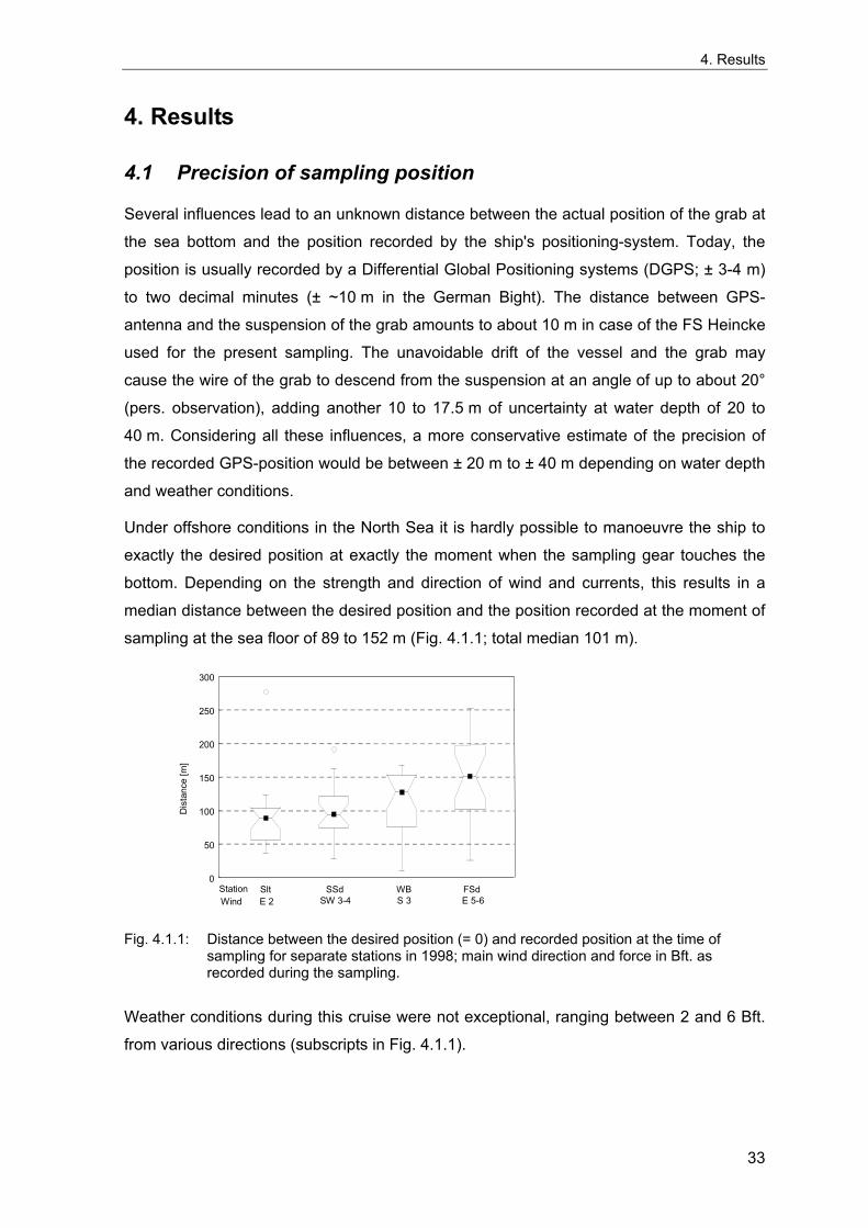
4. Results
4. Results
4.1 Precision of sampling position
Several influences lead to an unknown distance between the actual position of the grab at
the sea bottom and the position recorded by the ship's positioning-system. Today, the
position is usually recorded by a Differential Global Positioning systems (DGPS; ± 3-4 m)
to two decimal minutes (± ~10 m in the German Bight). The distance between GPS-
antenna and the suspension of the grab amounts to about 10 m in case of the FS Heincke
used for the present sampling. The unavoidable drift of the vessel and the grab may
cause the wire of the grab to descend from the suspension at an angle of up to about 20°
(pers. observation), adding another 10 to 17.5 m of uncertainty at water depth of 20 to
40 m. Considering all these influences, a more conservative estimate of the precision of
the recorded GPS-position would be between ± 20 m to ± 40 m depending on water depth
and weather conditions.
Under offshore conditions in the North Sea it is hardly possible to manoeuvre the ship to
exactly the desired position at exactly the moment when the sampling gear touches the
bottom. Depending on the strength and direction of wind and currents, this results in a
median distance between the desired position and the position recorded at the moment of
sampling at the sea floor of 89 to 152 m (Fig. 4.1.1; total median 101 m).
Dis
tanc
e [m
]
0
50
100
150
200
250
300
Slt SSd WB FSdE 2 E 5-6S 3SW 3-4 Wind
Station
Fig. 4.1.1: Distance between the desired position (= 0) and recorded position at the time of
sampling for separate stations in 1998; main wind direction and force in Bft. as recorded during the sampling.
Weather conditions during this cruise were not exceptional, ranging between 2 and 6 Bft.
from various directions (subscripts in Fig. 4.1.1).
33
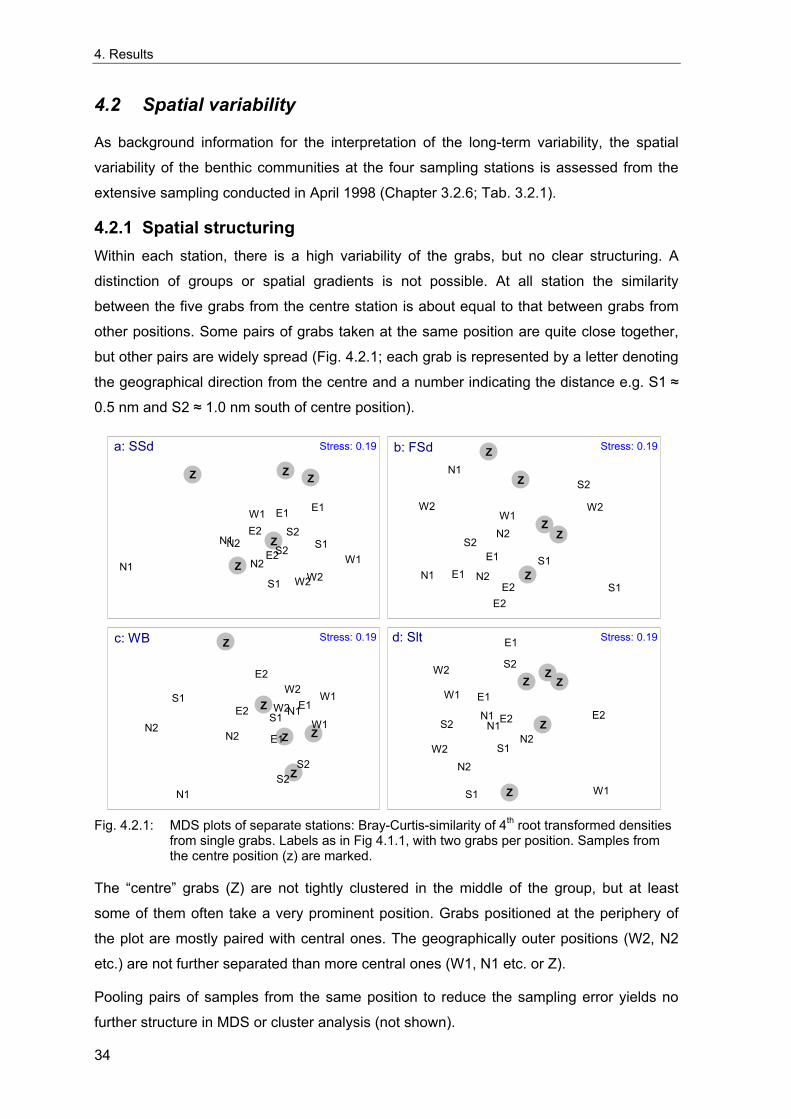
4. Results
4.2 Spatial variability
As background information for the interpretation of the long-term variability, the spatial
variability of the benthic communities at the four sampling stations is assessed from the
extensive sampling conducted in April 1998 (Chapter 3.2.6; Tab. 3.2.1).
4.2.1 Spatial structuring Within each station, there is a high variability of the grabs, but no clear structuring. A
distinction of groups or spatial gradients is not possible. At all station the similarity
between the five grabs from the centre station is about equal to that between grabs from
other positions. Some pairs of grabs taken at the same position are quite close together,
but other pairs are widely spread (Fig. 4.2.1; each grab is represented by a letter denoting
the geographical direction from the centre and a number indicating the distance e.g. S1 ≈
0.5 nm and S2 ≈ 1.0 nm south of centre position).
a: SSd
Z
Z
Z
Z
Z
N1
N1 N2 N2
E1 E1
E2
E2
S1
S1S2
S2
W1
W1
W2 W2
Stress: 0.19 b: FSd
Z
Z
Z
Z
Z
N1
N1 N2
N2
E1E1
E2E2 S1
S1
S2
S2
W1W2 W2
Stress: 0.19
c: WB
Z
Z
Z
Z
Z
N1
N1
N2N2
E1
E1
E2
E2 S1 S1
S2 S2
W1
W1W2 W2
Stress: 0.19 d: Slt
Z Z Z
Z
Z
N1N1
N2
N2
E1
E1
E2
S1
S1
S2
S2
E2
W1
W1
W2
W2
Stress: 0.19
Fig. 4.2.1: MDS plots of separate stations: Bray-Curtis-similarity of 4th root transformed densities
from single grabs. Labels as in Fig 4.1.1, with two grabs per position. Samples from the centre position (z) are marked.
The “centre” grabs (Z) are not tightly clustered in the middle of the group, but at least
some of them often take a very prominent position. Grabs positioned at the periphery of
the plot are mostly paired with central ones. The geographically outer positions (W2, N2
etc.) are not further separated than more central ones (W1, N1 etc. or Z).
Pooling pairs of samples from the same position to reduce the sampling error yields no
further structure in MDS or cluster analysis (not shown).
34
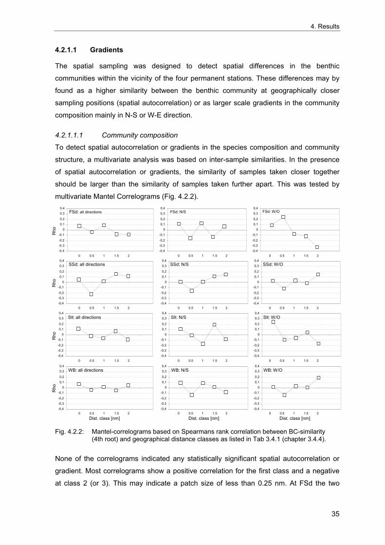
4. Results
4.2.1.1 Gradients
The spatial sampling was designed to detect spatial differences in the benthic
communities within the vicinity of the four permanent stations. These differences may by
found as a higher similarity between the benthic community at geographically closer
sampling positions (spatial autocorrelation) or as larger scale gradients in the community
composition mainly in N-S or W-E direction.
4.2.1.1.1 Community composition
To detect spatial autocorrelation or gradients in the species composition and community
structure, a multivariate analysis was based on inter-sample similarities. In the presence
of spatial autocorrelation or gradients, the similarity of samples taken closer together
should be larger than the similarity of samples taken further apart. This was tested by
multivariate Mantel Correlograms (Fig. 4.2.2).
FSd: all directions
-0.4 -0.3 -0.2 -0.1
0 0.1 0.2 0.3 0.4
FSd: N/S
-0,4-0,3-0,2
-0,10
0,10,2
0,30,4
FSd: W/O
-0,4-0,3-0,2
-0,10
0,10,2
0,30,4
0 0.5 1 1.5 2 0 0.5 1 1.5 2 0 0.5 1 1.5 2
Rho
SSd: all directions
-0,4 -0,3 -0,2 -0,1
0 0,1 0,2 0,3 0,4
SSd: N/S
-0,4-0,3-0,2
-0,10
0,10,2
0,30,4
-0,4-0,3-0,2
-0,10
0,10,2
0,30,4
SSd: W/O
0 0.5 1 1.5 2 0 0.5 1 1.5 2 0 0.5 1 1.5 2
Rho
Di l [ ] Di l [ ] Di l [ ] Slt: all directions
-0,4 -0,3 -0,2 -0,1
0 0,1 0,2 0,3 0,4
-0,4-0,3-0,2
-0,10
0,10,2
0,30,4
Slt: N/S
-0,4-0,3-0,2
-0,10
0,10,2
0,30,4
Slt: W/O
0 0.5 1 1.5 2 0 0.5 1 1.5 2 0 0.5 1 1.5 2
Rho
WB: all directions
-0,4 -0,3 -0,2 -0,1
0 0,1 0,2 0,3 0,4
-0,4-0,3-0,2
-0,10
0,10,2
0,30,4
WB: N/S
-0,4-0,3-0,2
-0,10
0,10,2
0,30,4
WB: W/O
0 0.5 1 1.5 2 0 0.5 1 1.5 2 0 0.5 1 1.5 2
Rho
Dist. class [nm] Dist. class [nm] Dist. class [nm] Fig. 4.2.2: Mantel-correlograms based on Spearmans rank correlation between BC-similarity
(4th root) and geographical distance classes as listed in Tab 3.4.1 (chapter 3.4.4).
None of the correlograms indicated any statistically significant spatial autocorrelation or
gradient. Most correlograms show a positive correlation for the first class and a negative
at class 2 (or 3). This may indicate a patch size of less than 0.25 nm. At FSd the two
35
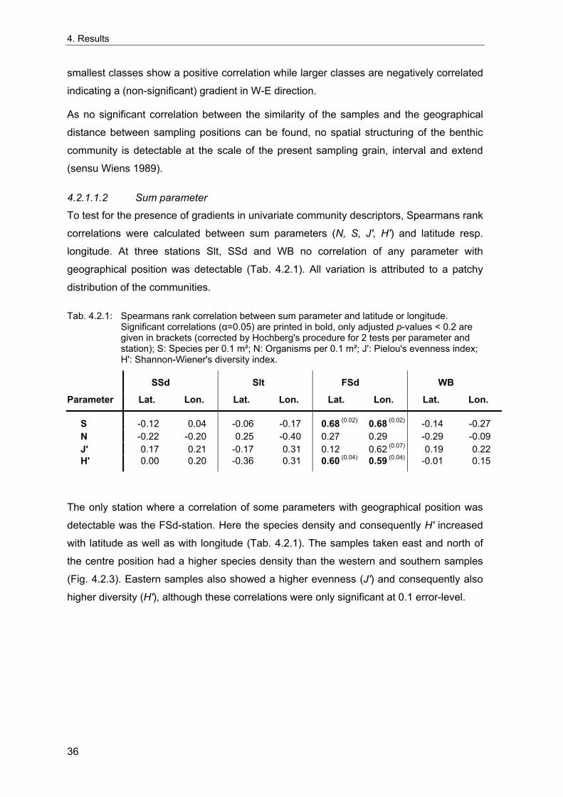
4. Results
smallest classes show a positive correlation while larger classes are negatively correlated
indicating a (non-significant) gradient in W-E direction.
As no significant correlation between the similarity of the samples and the geographical
distance between sampling positions can be found, no spatial structuring of the benthic
community is detectable at the scale of the present sampling grain, interval and extend
(sensu Wiens 1989).
4.2.1.1.2 Sum parameter
To test for the presence of gradients in univariate community descriptors, Spearmans rank
correlations were calculated between sum parameters (N, S, J', H') and latitude resp.
longitude. At three stations Slt, SSd and WB no correlation of any parameter with
geographical position was detectable (Tab. 4.2.1). All variation is attributed to a patchy
distribution of the communities.
Tab. 4.2.1: Spearmans rank correlation between sum parameter and latitude or longitude. Significant correlations (α=0.05) are printed in bold, only adjusted p-values < 0.2 are given in brackets (corrected by Hochberg's procedure for 2 tests per parameter and station); S: Species per 0.1 m²; N: Organisms per 0.1 m²; J': Pielou's evenness index; H': Shannon-Wiener's diversity index.
SSd Slt FSd WB
Parameter Lat. Lon. Lat. Lon. Lat. Lon. Lat. Lon.
S -0.12 0.04 -0.06 -0.17 0.68 (0.02) 0.68 (0.02) -0.14 -0.27 N -0.22 -0.20 0.25 -0.40 0.27 0.29 -0.29 -0.09 J' 0.17 0.21 -0.17 0.31 0.12 0.62 (0.07) 0.19 0.22 H' 0.00 0.20 -0.36 0.31 0.60 (0.04) 0.59 (0.04) -0.01 0.15
The only station where a correlation of some parameters with geographical position was
detectable was the FSd-station. Here the species density and consequently H' increased
with latitude as well as with longitude (Tab. 4.2.1). The samples taken east and north of
the centre position had a higher species density than the western and southern samples
(Fig. 4.2.3). Eastern samples also showed a higher evenness (J') and consequently also
higher diversity (H'), although these correlations were only significant at 0.1 error-level.
36
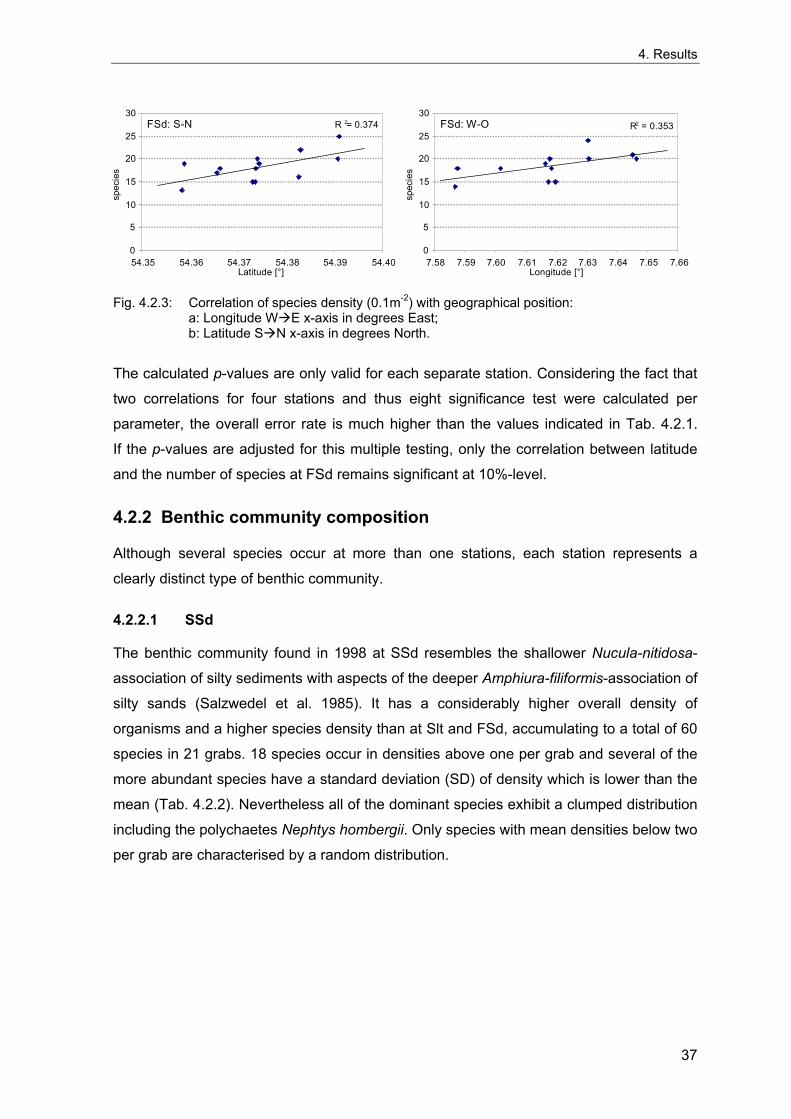
4. Results
R 2 = 0.374
0 5
10 15 20 25 30
54.35 54.36 54.37 54.38 54.39 54.40Latitude [°]
spec
ies
FSd: S-N
R 2 = 0.353
0
5
10
15
20
25
30
7.58 7.59 7.60 7.61 7.62 7.63 7.64 7.65 7.66Longitude [°]
spec
ies
FSd: W-O
Fig. 4.2.3: Correlation of species density (0.1m-2) with geographical position:
a: Longitude W E x-axis in degrees East; b: Latitude S N x-axis in degrees North.
The calculated p-values are only valid for each separate station. Considering the fact that
two correlations for four stations and thus eight significance test were calculated per
parameter, the overall error rate is much higher than the values indicated in Tab. 4.2.1.
If the p-values are adjusted for this multiple testing, only the correlation between latitude
and the number of species at FSd remains significant at 10%-level.
4.2.2 Benthic community composition
Although several species occur at more than one stations, each station represents a
clearly distinct type of benthic community.
4.2.2.1 SSd
The benthic community found in 1998 at SSd resembles the shallower Nucula-nitidosa-
association of silty sediments with aspects of the deeper Amphiura-filiformis-association of
silty sands (Salzwedel et al. 1985). It has a considerably higher overall density of
organisms and a higher species density than at Slt and FSd, accumulating to a total of 60
species in 21 grabs. 18 species occur in densities above one per grab and several of the
more abundant species have a standard deviation (SD) of density which is lower than the
mean (Tab. 4.2.2). Nevertheless all of the dominant species exhibit a clumped distribution
including the polychaetes Nephtys hombergii. Only species with mean densities below two
per grab are characterised by a random distribution.
37
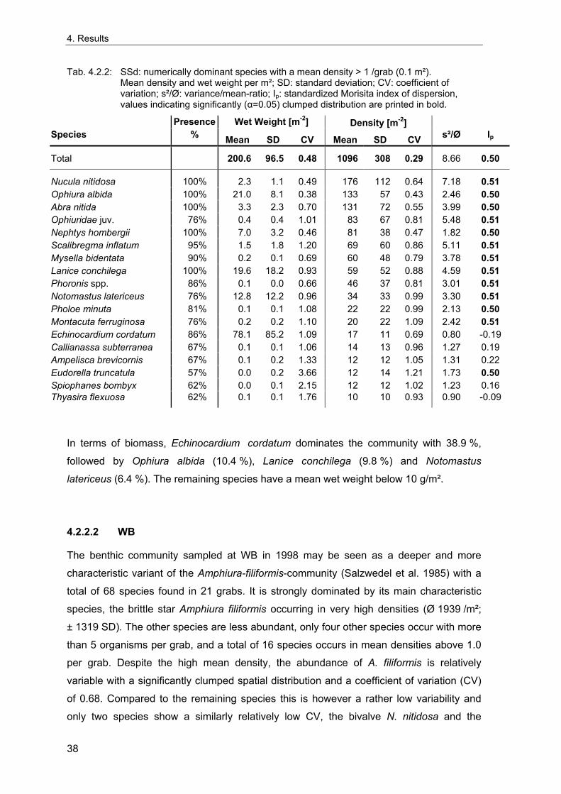
4. Results
Tab. 4.2.2: SSd: numerically dominant species with a mean density > 1 /grab (0.1 m²). Mean density and wet weight per m²; SD: standard deviation; CV: coefficient of variation; s²/Ø: variance/mean-ratio; Ip: standardized Morisita index of dispersion, values indicating significantly (α=0.05) clumped distribution are printed in bold.
Presence Wet Weight [m-2] Density [m-2] Species % Mean SD CV Mean SD CV s²/Ø Ip
Total 200.6 96.5 0.48 1096 308 0.29 8.66 0.50
Nucula nitidosa 100% 2.3 1.1 0.49 176 112 0.64 7.18 0.51 Ophiura albida 100% 21.0 8.1 0.38 133 57 0.43 2.46 0.50 Abra nitida 100% 3.3 2.3 0.70 131 72 0.55 3.99 0.50 Ophiuridae juv. 76% 0.4 0.4 1.01 83 67 0.81 5.48 0.51 Nephtys hombergii 100% 7.0 3.2 0.46 81 38 0.47 1.82 0.50 Scalibregma inflatum 95% 1.5 1.8 1.20 69 60 0.86 5.11 0.51 Mysella bidentata 90% 0.2 0.1 0.69 60 48 0.79 3.78 0.51 Lanice conchilega 100% 19.6 18.2 0.93 59 52 0.88 4.59 0.51 Phoronis spp. 86% 0.1 0.0 0.66 46 37 0.81 3.01 0.51 Notomastus latericeus 76% 12.8 12.2 0.96 34 33 0.99 3.30 0.51 Pholoe minuta 81% 0.1 0.1 1.08 22 22 0.99 2.13 0.50 Montacuta ferruginosa 76% 0.2 0.2 1.10 20 22 1.09 2.42 0.51 Echinocardium cordatum 86% 78.1 85.2 1.09 17 11 0.69 0.80 -0.19 Callianassa subterranea 67% 0.1 0.1 1.06 14 13 0.96 1.27 0.19 Ampelisca brevicornis 67% 0.1 0.2 1.33 12 12 1.05 1.31 0.22 Eudorella truncatula 57% 0.0 0.2 3.66 12 14 1.21 1.73 0.50 Spiophanes bombyx 62% 0.0 0.1 2.15 12 12 1.02 1.23 0.16 Thyasira flexuosa 62% 0.1 0.1 1.76 10 10 0.93 0.90 -0.09
In terms of biomass, Echinocardium cordatum dominates the community with 38.9 %,
followed by Ophiura albida (10.4 %), Lanice conchilega (9.8 %) and Notomastus
latericeus (6.4 %). The remaining species have a mean wet weight below 10 g/m².
4.2.2.2 WB
The benthic community sampled at WB in 1998 may be seen as a deeper and more
characteristic variant of the Amphiura-filiformis-community (Salzwedel et al. 1985) with a
total of 68 species found in 21 grabs. It is strongly dominated by its main characteristic
species, the brittle star Amphiura filiformis occurring in very high densities (Ø 1939 /m²;
± 1319 SD). The other species are less abundant, only four other species occur with more
than 5 organisms per grab, and a total of 16 species occurs in mean densities above 1.0
per grab. Despite the high mean density, the abundance of A. filiformis is relatively
variable with a significantly clumped spatial distribution and a coefficient of variation (CV)
of 0.68. Compared to the remaining species this is however a rather low variability and
only two species show a similarly relatively low CV, the bivalve N. nitidosa and the
38
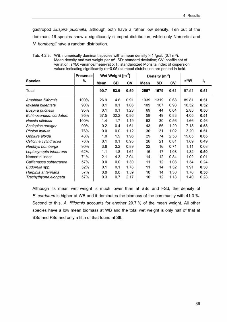
4. Results
gastropod Euspira pulchella, although both have a rather low density. Ten out of the
dominant 16 species show a significantly clumped distribution, while only Nemertini and
N. hombergii have a random distribution.
Tab. 4.2.3: WB: numerically dominant species with a mean density > 1 /grab (0.1 m²). Mean density and wet weight per m²; SD: standard deviation; CV: coefficient of variation; s²/Ø: variance/mean-ratio; Ip: standardized Morisita index of dispersion, values indicating significantly (α=0.05) clumped distribution are printed in bold.
Presence Wet Weight [m-2] Density [m-2] Species % Mean SD CV Mean SD CV s²/Ø Ip
Total 90.7 53.9 0.59 2557 1579 0.61 97.51 0.51
Amphiura filiformis 100% 26.9 4.6 0.91 1939 1319 0.68 89.81 0.51 Mysella bidentata 90% 0.1 0.1 1.06 109 107 0.98 10.52 0.52 Euspira puchella 95% 0.1 0.1 1.23 69 44 0.64 2.85 0.50 Echinocardium cordatum 95% 37.5 32.2 0.86 59 49 0.83 4.05 0.51 Nucula nitidosa 100% 1.4 1.7 1.19 53 30 0.56 1.66 0.46 Scoloplos armiger 90% 0.2 0.4 1.61 43 56 1.29 7.18 0.53 Pholoe minuta 76% 0.0 0.0 1.12 30 31 1.02 3.20 0.51 Ophiura albida 43% 1.0 1.9 1.96 29 74 2.58 19.05 0.65 Cylichna cylindracea 76% 0.1 0.1 0.95 26 21 0.81 1.69 0.49 Nephtys hombergii 90% 3.6 3.2 0.89 22 16 0.71 1.11 0.08 Leptosynapta inhaerens 62% 1.1 1.8 1.61 16 17 1.08 1.82 0.50 Nemertini indet. 71% 2.1 4.3 2.04 14 12 0.84 1.02 0.01 Callianassa subterranea 57% 0.0 0.0 1.30 11 12 1.08 1.34 0.24 Eudorella spp. 52% 0.1 0.1 1.76 11 14 1.32 1.91 0.50 Harpinia antennaria 57% 0.0 0.0 1.59 10 14 1.30 1.76 0.50 Trachythyone elongata 57% 0.3 0.7 2.17 10 12 1.18 1.40 0.28
Although its mean wet weight is much lower than at SSd and FSd, the density of
E. cordatum is higher at WB and it dominates the biomass of the community with 41.3 %.
Second to this, A. filiformis accounts for another 29.7 % of the mean weight. All other
species have a low mean biomass at WB and the total wet weight is only half of that at
SSd and FSd and only a fifth of that found at Slt.
39
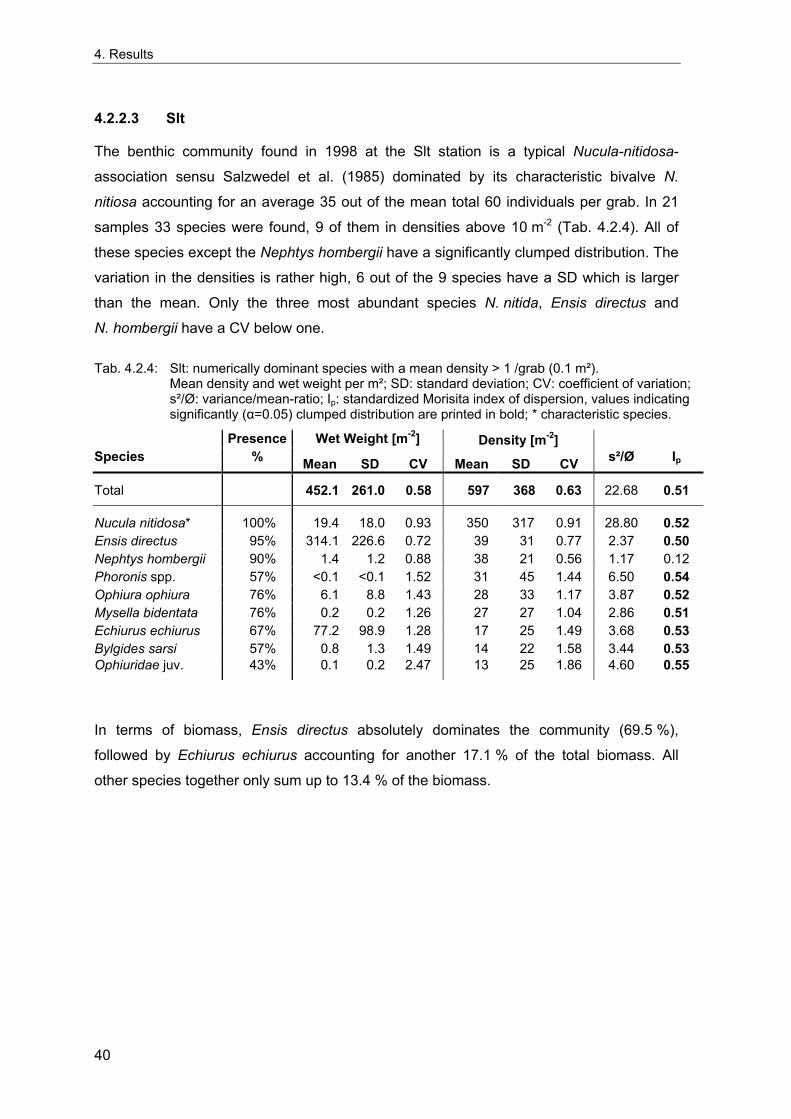
4. Results
4.2.2.3 Slt
The benthic community found in 1998 at the Slt station is a typical Nucula-nitidosa-
association sensu Salzwedel et al. (1985) dominated by its characteristic bivalve N.
nitiosa accounting for an average 35 out of the mean total 60 individuals per grab. In 21
samples 33 species were found, 9 of them in densities above 10 m-2 (Tab. 4.2.4). All of
these species except the Nephtys hombergii have a significantly clumped distribution. The
variation in the densities is rather high, 6 out of the 9 species have a SD which is larger
than the mean. Only the three most abundant species N. nitida, Ensis directus and
N. hombergii have a CV below one.
Tab. 4.2.4: Slt: numerically dominant species with a mean density > 1 /grab (0.1 m²). Mean density and wet weight per m²; SD: standard deviation; CV: coefficient of variation; s²/Ø: variance/mean-ratio; Ip: standardized Morisita index of dispersion, values indicating significantly (α=0.05) clumped distribution are printed in bold; * characteristic species.
Presence Wet Weight [m-2] Density [m-2] Species % Mean SD CV Mean SD CV s²/Ø Ip
Total 452.1 261.0 0.58 597 368 0.63 22.68 0.51
Nucula nitidosa* 100% 19.4 18.0 0.93 350 317 0.91 28.80 0.52 Ensis directus 95% 314.1 226.6 0.72 39 31 0.77 2.37 0.50 Nephtys hombergii 90% 1.4 1.2 0.88 38 21 0.56 1.17 0.12 Phoronis spp. 57% <0.1 <0.1 1.52 31 45 1.44 6.50 0.54 Ophiura ophiura 76% 6.1 8.8 1.43 28 33 1.17 3.87 0.52 Mysella bidentata 76% 0.2 0.2 1.26 27 27 1.04 2.86 0.51 Echiurus echiurus 67% 77.2 98.9 1.28 17 25 1.49 3.68 0.53 Bylgides sarsi 57% 0.8 1.3 1.49 14 22 1.58 3.44 0.53 Ophiuridae juv. 43% 0.1 0.2 2.47 13 25 1.86 4.60 0.55
In terms of biomass, Ensis directus absolutely dominates the community (69.5 %),
followed by Echiurus echiurus accounting for another 17.1 % of the total biomass. All
other species together only sum up to 13.4 % of the biomass.
40
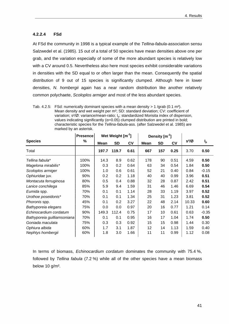
4. Results
4.2.2.4 FSd
At FSd the community in 1998 is a typical example of the Tellina-fabula-association sensu
Salzwedel et al. (1985). 15 out of a total of 50 species have mean densities above one per
grab, and the variation especially of some of the more abundant species is relatively low
with a CV around 0.5. Nevertheless also here most species exhibit considerable variations
in densities with the SD equal to or often larger than the mean. Consequently the spatial
distribution of 9 out of 15 species is significantly clumped. Although here in lower
densities, N. hombergii again has a near random distribution like another relatively
common polychaete, Scoloplos armiger and most of the less abundant species.
Tab. 4.2.5: FSd: numerically dominant species with a mean density > 1 /grab (0.1 m²). Mean density and wet weight per m²; SD: standard deviation; CV: coefficient of variation; s²/Ø: variance/mean-ratio; Ip: standardized Morisita index of dispersion, values indicating significantly (α=0.05) clumped distribution are printed in bold; characteristic species for the Tellina-fabula-ass. (after Salzwedel et al. 1985) are marked by an asterisk.
Presence Wet Weight [m-2] Density [m-2] Species % Mean SD CV Mean SD CV s²/Ø Ip
Total 197.7 119.7 0.61 667 157 0.25 3.70 0.50
Tellina fabula* 100% 14.3 8.9 0.62 178 90 0.51 4.59 0.50 Magelona mirabilis* 100% 0.3 0.2 0.64 63 34 0.54 1.84 0.50 Scoloplos armiger 100% 1.0 0.6 0.61 52 21 0.40 0.84 -0.15 Ophiuridae juv. 90% 0.2 0.2 1.18 40 40 0.99 3.96 0.51 Montacuta ferruginosa 80% 0.5 0.4 0.88 32 28 0.87 2.42 0.51 Lanice conchilega 85% 5.9 9.4 1.59 31 46 1.46 6.69 0.54 Eumida spp. 70% 0.1 0.1 1.14 28 33 1.19 3.97 0.52 Urothoe poseidonis* 70% 0.1 0.1 1.34 25 31 1.23 3.81 0.52 Phoronis spp. 45% 0.1 0.2 3.27 22 48 2.14 10.33 0.60 Bathyporeia elegans 75% 0.0 0.0 0.97 20 16 0.77 1.21 0.14 Echinocardium cordatum 90% 149.3 112.4 0.75 17 10 0.61 0.63 -0.35 Bathyporeia guilliamsoniana 70% 0.1 0.1 0.95 16 17 1.04 1.74 0.50 Goniada maculata 75% 0.3 0.3 0.92 15 15 0.98 1.44 0.30 Ophiura albida 60% 1.7 3.1 1.87 12 14 1.13 1.59 0.40 Nephtys hombergii 60% 1.8 3.0 1.66 11 11 0.99 1.12 0.08
In terms of biomass, Echinocardium cordatum dominates the community with 75.4 %,
followed by Tellina fabula (7.2 %) while all of the other species have a mean biomass
below 10 g/m².
41
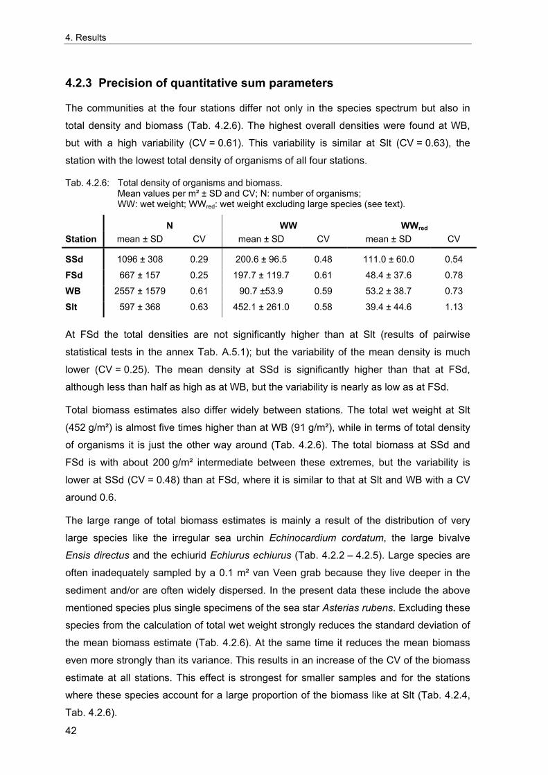
4. Results
4.2.3 Precision of quantitative sum parameters
The communities at the four stations differ not only in the species spectrum but also in
total density and biomass (Tab. 4.2.6). The highest overall densities were found at WB,
but with a high variability (CV = 0.61). This variability is similar at Slt (CV = 0.63), the
station with the lowest total density of organisms of all four stations.
Tab. 4.2.6: Total density of organisms and biomass. Mean values per m² ± SD and CV; N: number of organisms; WW: wet weight; WWred: wet weight excluding large species (see text).
N WW WWred Station mean ± SD CV mean ± SD CV mean ± SD CV
SSd 1096 ± 308 0.29 200.6 ± 96.5 0.48 111.0 ± 60.0 0.54
FSd 667 ± 157 0.25 197.7 ± 119.7 0.61 48.4 ± 37.6 0.78
WB 2557 ± 1579 0.61 90.7 ±53.9 0.59 53.2 ± 38.7 0.73
Slt 597 ± 368 0.63 452.1 ± 261.0 0.58 39.4 ± 44.6 1.13
At FSd the total densities are not significantly higher than at Slt (results of pairwise
statistical tests in the annex Tab. A.5.1); but the variability of the mean density is much
lower (CV = 0.25). The mean density at SSd is significantly higher than that at FSd,
although less than half as high as at WB, but the variability is nearly as low as at FSd.
Total biomass estimates also differ widely between stations. The total wet weight at Slt
(452 g/m²) is almost five times higher than at WB (91 g/m²), while in terms of total density
of organisms it is just the other way around (Tab. 4.2.6). The total biomass at SSd and
FSd is with about 200 g/m² intermediate between these extremes, but the variability is
lower at SSd (CV = 0.48) than at FSd, where it is similar to that at Slt and WB with a CV
around 0.6.
The large range of total biomass estimates is mainly a result of the distribution of very
large species like the irregular sea urchin Echinocardium cordatum, the large bivalve
Ensis directus and the echiurid Echiurus echiurus (Tab. 4.2.2 – 4.2.5). Large species are
often inadequately sampled by a 0.1 m² van Veen grab because they live deeper in the
sediment and/or are often widely dispersed. In the present data these include the above
mentioned species plus single specimens of the sea star Asterias rubens. Excluding these
species from the calculation of total wet weight strongly reduces the standard deviation of
the mean biomass estimate (Tab. 4.2.6). At the same time it reduces the mean biomass
even more strongly than its variance. This results in an increase of the CV of the biomass
estimate at all stations. This effect is strongest for smaller samples and for the stations
where these species account for a large proportion of the biomass like at Slt (Tab. 4.2.4,
Tab. 4.2.6).
42
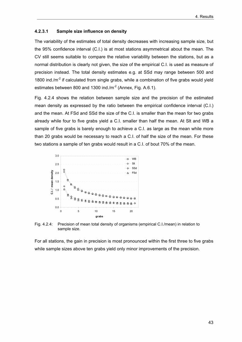
4. Results
4.2.3.1 Sample size influence on density
The variability of the estimates of total density decreases with increasing sample size, but
the 95% confidence interval (C.I.) is at most stations asymmetrical about the mean. The
CV still seems suitable to compare the relative variability between the stations, but as a
normal distribution is clearly not given, the size of the empirical C.I. is used as measure of
precision instead. The total density estimates e.g. at SSd may range between 500 and
1800 ind./m-2 if calculated from single grabs, while a combination of five grabs would yield
estimates between 800 and 1300 ind./m-2 (Annex, Fig. A.6.1).
Fig. 4.2.4 shows the relation between sample size and the precision of the estimated
mean density as expressed by the ratio between the empirical confidence interval (C.I.)
and the mean. At FSd and SSd the size of the C.I. is smaller than the mean for two grabs
already while four to five grabs yield a C.I. smaller than half the mean. At Slt and WB a
sample of five grabs is barely enough to achieve a C.I. as large as the mean while more
than 20 grabs would be necessary to reach a C.I. of half the size of the mean. For these
two stations a sample of ten grabs would result in a C.I. of bout 70% of the mean.
0.0
0.5
1.0
1.5
2.0
2.5
3.0
0 5 10 15 20
grabs
C.I.
/ m
ean
dens
ity
WB
Slt
SSd
FSd
Fig. 4.2.4: Precision of mean total density of organisms (empirical C.I./mean) in relation to
sample size.
For all stations, the gain in precision is most pronounced within the first three to five grabs
while sample sizes above ten grabs yield only minor improvements of the precision.
43
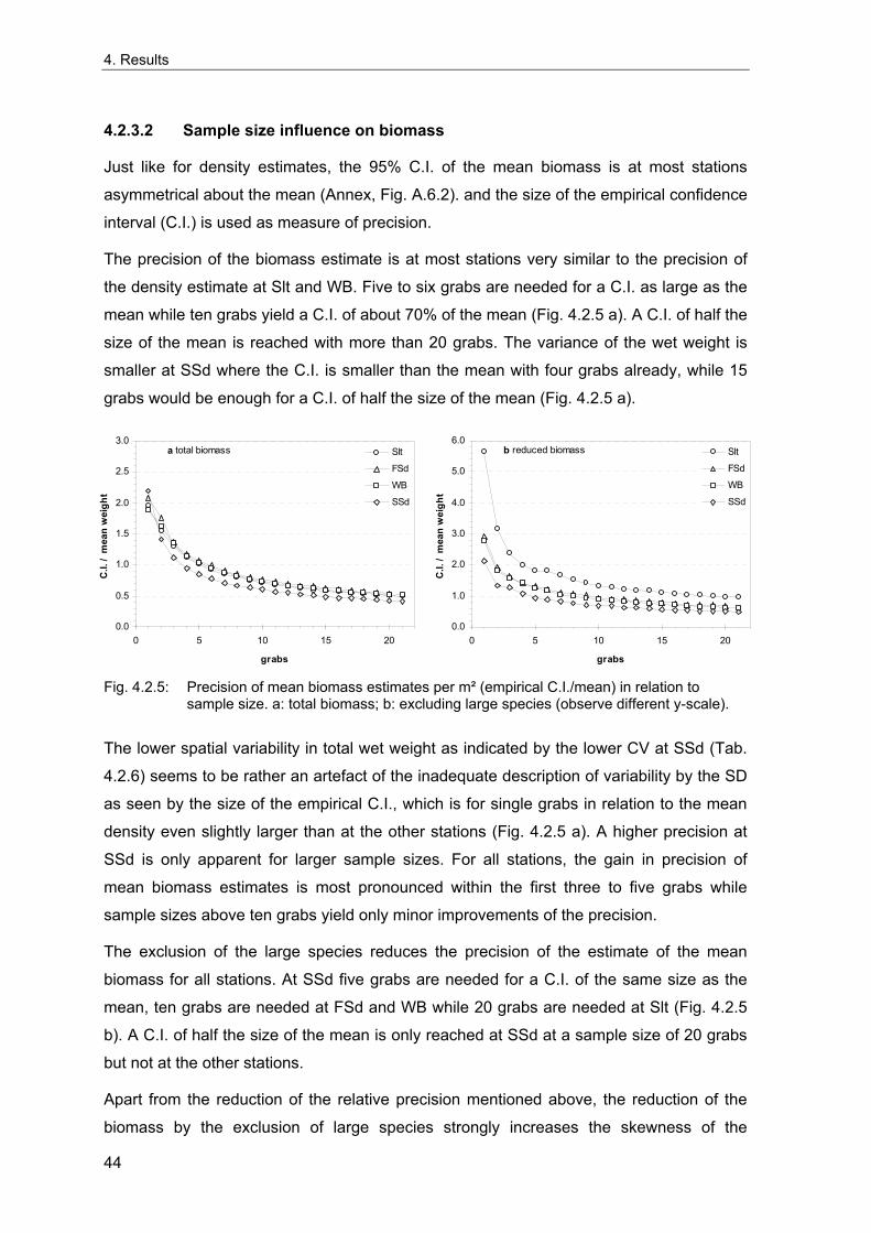
4. Results
4.2.3.2 Sample size influence on biomass
Just like for density estimates, the 95% C.I. of the mean biomass is at most stations
asymmetrical about the mean (Annex, Fig. A.6.2). and the size of the empirical confidence
interval (C.I.) is used as measure of precision.
The precision of the biomass estimate is at most stations very similar to the precision of
the density estimate at Slt and WB. Five to six grabs are needed for a C.I. as large as the
mean while ten grabs yield a C.I. of about 70% of the mean (Fig. 4.2.5 a). A C.I. of half the
size of the mean is reached with more than 20 grabs. The variance of the wet weight is
smaller at SSd where the C.I. is smaller than the mean with four grabs already, while 15
grabs would be enough for a C.I. of half the size of the mean (Fig. 4.2.5 a).
0.0
0.5
1.0
1.5
2.0
2.5
3.0
0 5 10 15 20
grabs
C.I.
/ m
ean
wei
ght
Slt
FSd
WB
SSd
a total biomass
0.0
1.0
2.0
3.0
4.0
5.0
6.0
0 5 10 15 20
grabs
C.I.
/ m
ean
wei
ght
Slt
FSd
WB
SSd
b reduced biomass
Fig. 4.2.5: Precision of mean biomass estimates per m² (empirical C.I./mean) in relation to
sample size. a: total biomass; b: excluding large species (observe different y-scale).
The lower spatial variability in total wet weight as indicated by the lower CV at SSd (Tab.
4.2.6) seems to be rather an artefact of the inadequate description of variability by the SD
as seen by the size of the empirical C.I., which is for single grabs in relation to the mean
density even slightly larger than at the other stations (Fig. 4.2.5 a). A higher precision at
SSd is only apparent for larger sample sizes. For all stations, the gain in precision of
mean biomass estimates is most pronounced within the first three to five grabs while
sample sizes above ten grabs yield only minor improvements of the precision.
The exclusion of the large species reduces the precision of the estimate of the mean
biomass for all stations. At SSd five grabs are needed for a C.I. of the same size as the
mean, ten grabs are needed at FSd and WB while 20 grabs are needed at Slt (Fig. 4.2.5
b). A C.I. of half the size of the mean is only reached at SSd at a sample size of 20 grabs
but not at the other stations.
Apart from the reduction of the relative precision mentioned above, the reduction of the
biomass by the exclusion of large species strongly increases the skewness of the
44
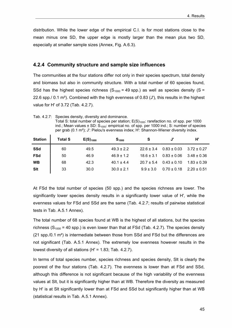
4. Results
distribution. While the lower edge of the empirical C.I. is for most stations close to the
mean minus one SD, the upper edge is mostly larger than the mean plus two SD,
especially at smaller sample sizes (Annex, Fig. A.6.3).
4.2.4 Community structure and sample size influences
The communities at the four stations differ not only in their species spectrum, total density
and biomass but also in community structure. With a total number of 60 species found,
SSd has the highest species richness (S1000 = 49 spp.) as well as species density (S =
22.6 spp./ 0.1 m²). Combined with the high evenness of 0.83 (J'), this results in the highest
value for H' of 3.72 (Tab. 4.2.7).
Tab. 4.2.7: Species density, diversity and dominance. Total S: total number of species per station; E(S)1000: rarefaction no. of spp. per 1000 ind.; Mean values ± SD: S1000: empirical no. of spp. per 1000 ind.; S: number of species per grab (0.1 m²); J': Pielou's evenness index; H': Shannon-Wiener diversity index.
Station Total S E(S)1000 S1000 S J' H'
SSd 60 49.5 49.3 ± 2.2 22.6 ± 3.4 0.83 ± 0.03 3.72 ± 0.27
FSd 50 46.9 46.9 ± 1.2 18.6 ± 3.1 0.83 ± 0.06 3.48 ± 0.36
WB 68 42.3 40.1 ± 4.4 20.7 ± 5.4 0.43 ± 0.10 1.83 ± 0.39
Slt 33 30.0 30.0 ± 2.1 9.9 ± 3.0 0.70 ± 0.18 2.20 ± 0.51
At FSd the total number of species (50 spp.) and the species richness are lower. The
significantly lower species density results in a significantly lower value of H', while the
evenness values for FSd and SSd are the same (Tab. 4.2.7; results of pairwise statistical
tests in Tab. A.5.1 Annex).
The total number of 68 species found at WB is the highest of all stations, but the species
richness (S1000 = 40 spp.) is even lower than that at FSd (Tab. 4.2.7). The species density
(21 spp./0.1 m²) is intermediate between those from SSd and FSd but the differences are
not significant (Tab. A.5.1 Annex). The extremely low evenness however results in the
lowest diversity of all stations (H' = 1.83; Tab. 4.2.7).
In terms of total species number, species richness and species density, Slt is clearly the
poorest of the four stations (Tab. 4.2.7). The evenness is lower than at FSd and SSd,
although this difference is not significant because of the high variability of the evenness
values at Slt, but it is significantly higher than at WB. Therefore the diversity as measured
by H' is at Slt significantly lower than at FSd and SSd but significantly higher than at WB
(statistical results in Tab. A.5.1 Annex).
45
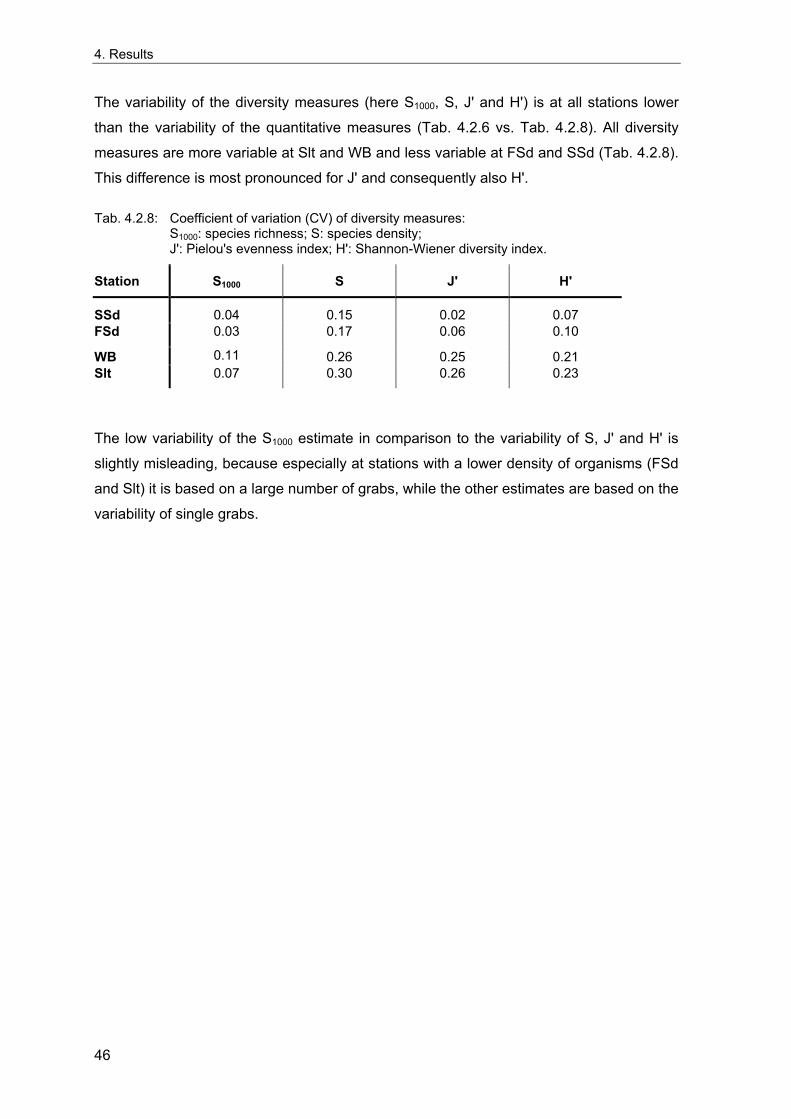
4. Results
The variability of the diversity measures (here S1000, S, J' and H') is at all stations lower
than the variability of the quantitative measures (Tab. 4.2.6 vs. Tab. 4.2.8). All diversity
measures are more variable at Slt and WB and less variable at FSd and SSd (Tab. 4.2.8).
This difference is most pronounced for J' and consequently also H'.
Tab. 4.2.8: Coefficient of variation (CV) of diversity measures: S1000: species richness; S: species density; J': Pielou's evenness index; H': Shannon-Wiener diversity index.
Station S1000 S J' H'
SSd 0.04 0.15 0.02 0.07 FSd 0.03 0.17 0.06 0.10
WB 0.11 0.26 0.25 0.21 Slt 0.07 0.30 0.26 0.23
The low variability of the S1000 estimate in comparison to the variability of S, J' and H' is
slightly misleading, because especially at stations with a lower density of organisms (FSd
and Slt) it is based on a large number of grabs, while the other estimates are based on the
variability of single grabs.
46
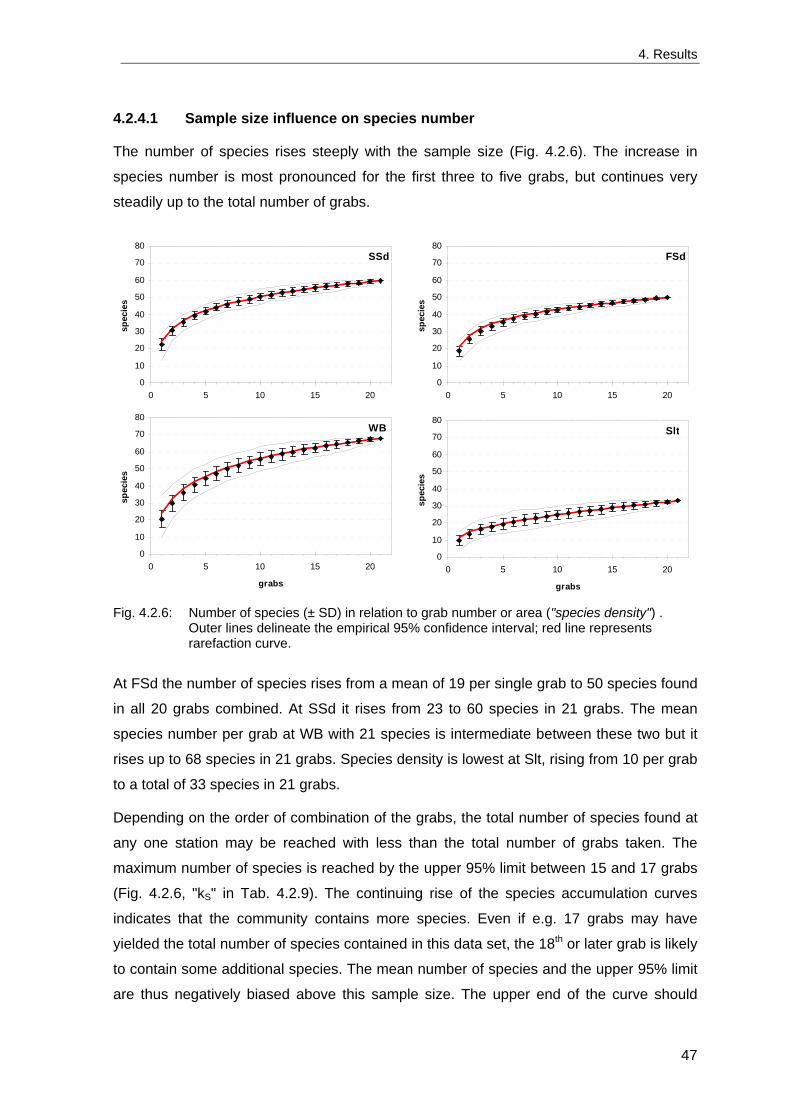
4. Results
4.2.4.1 Sample size influence on species number
The number of species rises steeply with the sample size (Fig. 4.2.6). The increase in
species number is most pronounced for the first three to five grabs, but continues very
steadily up to the total number of grabs.
0
10
20
30
40
50
60
70
80
0 5 10 15 20
spec
ies
SSd
0
10
20
30
40
50
60
70
80
0 5 10 15 20
spec
ies
FSd
0
10
20
30
40
50
60
70
80
0 5 10 15 20
grabs
spec
ies
WB
0
10
20
30
40
50
60
70
80
0 5 10 15 20
grabs
spec
ies
Slt
Fig. 4.2.6: Number of species (± SD) in relation to grab number or area ("species density") .
Outer lines delineate the empirical 95% confidence interval; red line represents rarefaction curve.
At FSd the number of species rises from a mean of 19 per single grab to 50 species found
in all 20 grabs combined. At SSd it rises from 23 to 60 species in 21 grabs. The mean
species number per grab at WB with 21 species is intermediate between these two but it
rises up to 68 species in 21 grabs. Species density is lowest at Slt, rising from 10 per grab
to a total of 33 species in 21 grabs.
Depending on the order of combination of the grabs, the total number of species found at
any one station may be reached with less than the total number of grabs taken. The
maximum number of species is reached by the upper 95% limit between 15 and 17 grabs
(Fig. 4.2.6, "kS" in Tab. 4.2.9). The continuing rise of the species accumulation curves
indicates that the community contains more species. Even if e.g. 17 grabs may have
yielded the total number of species contained in this data set, the 18th or later grab is likely
to contain some additional species. The mean number of species and the upper 95% limit
are thus negatively biased above this sample size. The upper end of the curve should
47
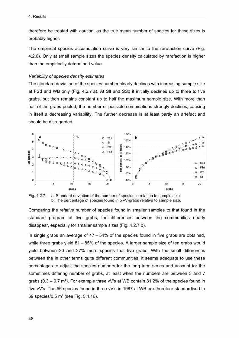
4. Results
therefore be treated with caution, as the true mean number of species for these sizes is
probably higher.
The empirical species accumulation curve is very similar to the rarefaction curve (Fig.
4.2.6). Only at small sample sizes the species density calculated by rarefaction is higher
than the empirically determined value.
Variability of species density estimates
The standard deviation of the species number clearly declines with increasing sample size
at FSd and WB only (Fig. 4.2.7 a). At Slt and SSd it initially declines up to three to five
grabs, but then remains constant up to half the maximum sample size. With more than
half of the grabs pooled, the number of possible combinations strongly declines, causing
in itself a decreasing variability. The further decrease is at least partly an artefact and
should be disregarded.
0
1
2
3
4
5
6
0 5 10 15 20
grabs
SD s
peci
es
WB
Slt
SSd
FSd
n/2a
40%
60%
80%
100%
120%
140%
160%
180%
0 5 10 15 20
grabs
spec
ies
rel.
to 5
gra
bs
SSd
FSd
WB
Slt
b
Fig. 4.2.7: a: Standard deviation of the number of species in relation to sample size;
b: The percentage of species found in 5 vV-grabs relative to sample size.
Comparing the relative number of species found in smaller samples to that found in the
standard program of five grabs, the differences between the communities nearly
disappear, especially for smaller sample sizes (Fig. 4.2.7 b).
In single grabs an average of 47 – 54% of the species found in five grabs are obtained,
while three grabs yield 81 – 85% of the species. A larger sample size of ten grabs would
yield between 20 and 27% more species that five grabs. With the small differences
between the in other terms quite different communities, it seems adequate to use these
percentages to adjust the species numbers for the long term series and account for the
sometimes differing number of grabs, at least when the numbers are between 3 and 7
grabs (0.3 – 0.7 m²). For example three vV's at WB contain 81.2% of the species found in
five vV's. The 56 species found in three vV's in 1987 at WB are therefore standardised to
69 species/0.5 m² (see Fig. 5.4.16).
48
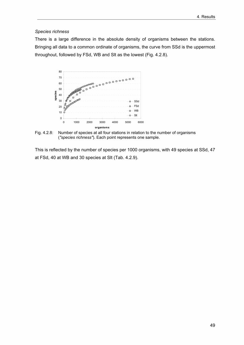
4. Results
Species richness
There is a large difference in the absolute density of organisms between the stations.
Bringing all data to a common ordinate of organisms, the curve from SSd is the uppermost
throughout, followed by FSd, WB and Slt as the lowest (Fig. 4.2.8).
0
10
20
30
40
50
60
70
80
0 1000 2000 3000 4000 5000 6000
organisms
spec
ies
SSd
FSd
WB
Slt
Fig. 4.2.8: Number of species at all four stations in relation to the number of organisms
("species richness"). Each point represents one sample.
This is reflected by the number of species per 1000 organisms, with 49 species at SSd, 47
at FSd, 40 at WB and 30 species at Slt (Tab. 4.2.9).
49
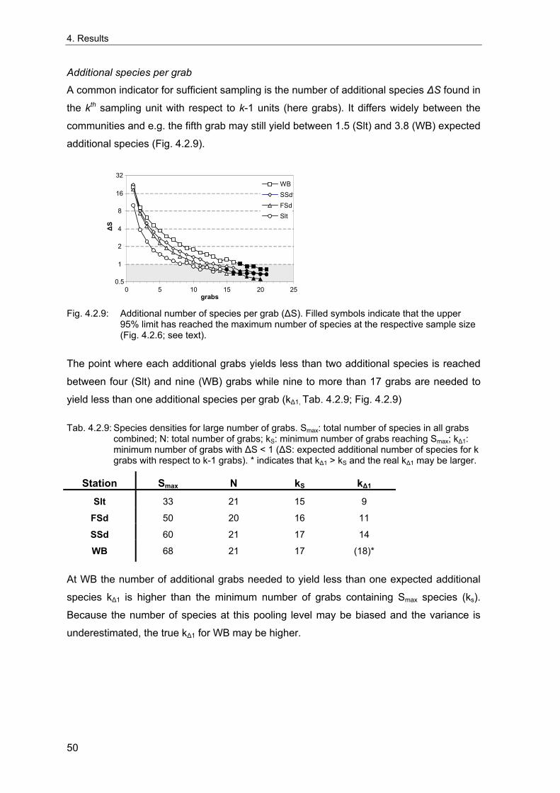
4. Results
Additional species per grab
A common indicator for sufficient sampling is the number of additional species ∆S found in
the kth sampling unit with respect to k-1 units (here grabs). It differs widely between the
communities and e.g. the fifth grab may still yield between 1.5 (Slt) and 3.8 (WB) expected
additional species (Fig. 4.2.9).
0.5 1
2 4
8 16
32
0 5 10 15 20 25grabs
∆S
WBSSdFSdSlt
Fig. 4.2.9: Additional number of species per grab (∆S). Filled symbols indicate that the upper
95% limit has reached the maximum number of species at the respective sample size (Fig. 4.2.6; see text).
The point where each additional grabs yields less than two additional species is reached
between four (Slt) and nine (WB) grabs while nine to more than 17 grabs are needed to
yield less than one additional species per grab (k∆1, Tab. 4.2.9; Fig. 4.2.9)
Tab. 4.2.9: Species densities for large number of grabs. Smax: total number of species in all grabs combined; N: total number of grabs; kS: minimum number of grabs reaching Smax; k∆1: minimum number of grabs with ∆S < 1 (∆S: expected additional number of species for k grabs with respect to k-1 grabs). * indicates that k∆1 > kS and the real k∆1 may be larger.
Station Smax N kS k∆1 Slt 33 21 15 9
FSd 50 20 16 11
SSd 60 21 17 14
WB 68 21 17 (18)*
At WB the number of additional grabs needed to yield less than one expected additional
species k∆1 is higher than the minimum number of grabs containing Smax species (ks).
Because the number of species at this pooling level may be biased and the variance is
underestimated, the true k∆1 for WB may be higher.
50
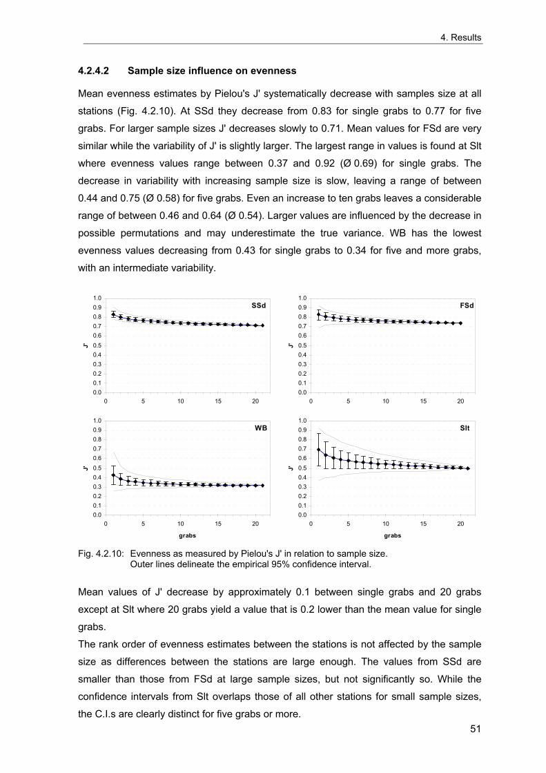
4. Results
4.2.4.2 Sample size influence on evenness
Mean evenness estimates by Pielou's J' systematically decrease with samples size at all
stations (Fig. 4.2.10). At SSd they decrease from 0.83 for single grabs to 0.77 for five
grabs. For larger sample sizes J' decreases slowly to 0.71. Mean values for FSd are very
similar while the variability of J' is slightly larger. The largest range in values is found at Slt
where evenness values range between 0.37 and 0.92 (Ø 0.69) for single grabs. The
decrease in variability with increasing sample size is slow, leaving a range of between
0.44 and 0.75 (Ø 0.58) for five grabs. Even an increase to ten grabs leaves a considerable
range of between 0.46 and 0.64 (Ø 0.54). Larger values are influenced by the decrease in
possible permutations and may underestimate the true variance. WB has the lowest
evenness values decreasing from 0.43 for single grabs to 0.34 for five and more grabs,
with an intermediate variability.
0.00.10.20.30.40.50.60.70.80.91.0
0 5 10 15 20
J'
SSd
0.00.10.20.30.40.50.60.70.80.91.0
0 5 10 15 20
J'
FSd
0.00.10.20.30.40.50.60.70.80.91.0
0 5 10 15 20
grabs
J'
WB
0.00.10.20.30.40.50.60.70.80.91.0
0 5 10 15 20
grabs
J'
Slt
Fig. 4.2.10: Evenness as measured by Pielou's J' in relation to sample size.
Outer lines delineate the empirical 95% confidence interval.
Mean values of J' decrease by approximately 0.1 between single grabs and 20 grabs
except at Slt where 20 grabs yield a value that is 0.2 lower than the mean value for single
grabs.
The rank order of evenness estimates between the stations is not affected by the sample
size as differences between the stations are large enough. The values from SSd are
smaller than those from FSd at large sample sizes, but not significantly so. While the
confidence intervals from Slt overlaps those of all other stations for small sample sizes,
the C.I.s are clearly distinct for five grabs or more. 51
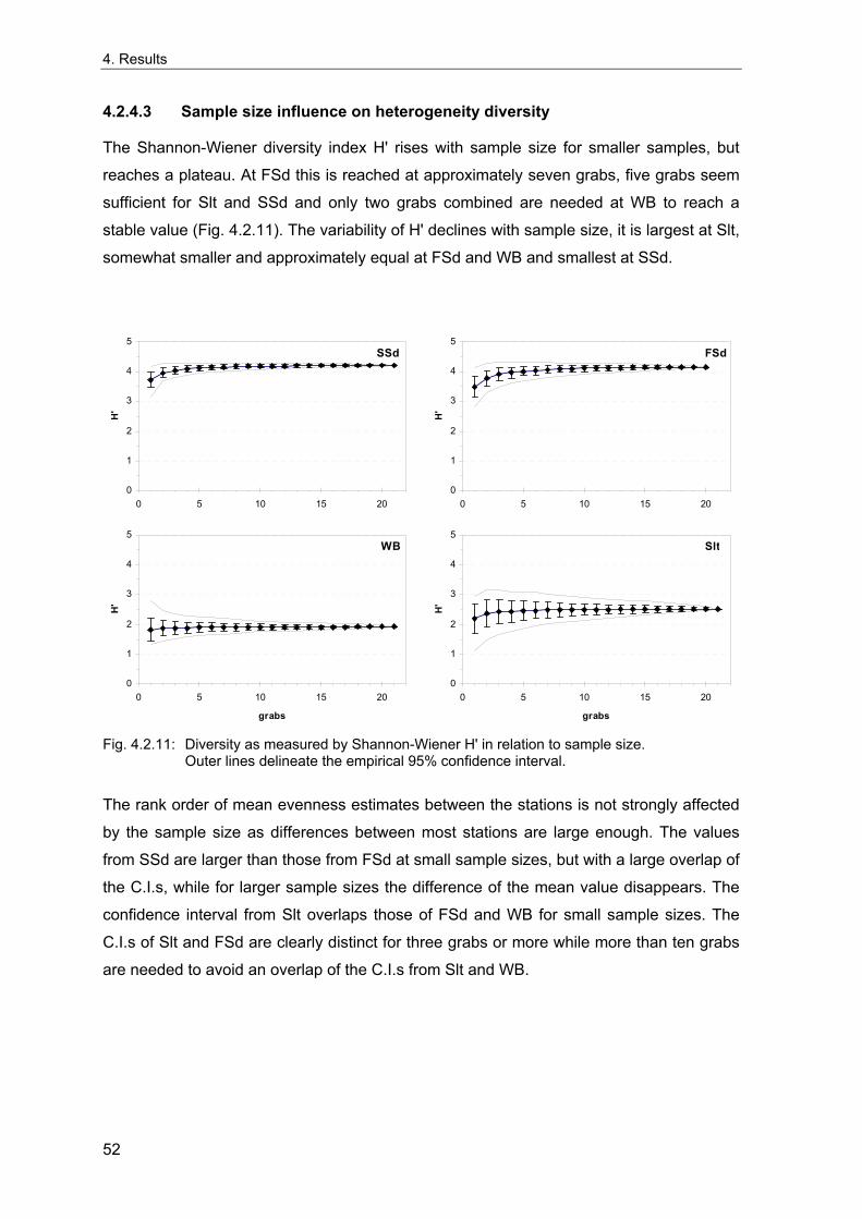
4. Results
4.2.4.3 Sample size influence on heterogeneity diversity
The Shannon-Wiener diversity index H' rises with sample size for smaller samples, but
reaches a plateau. At FSd this is reached at approximately seven grabs, five grabs seem
sufficient for Slt and SSd and only two grabs combined are needed at WB to reach a
stable value (Fig. 4.2.11). The variability of H' declines with sample size, it is largest at Slt,
somewhat smaller and approximately equal at FSd and WB and smallest at SSd.
0
1
2
3
4
5
0 5 10 15 20
H'
SSd
0
1
2
3
4
5
0 5 10 15 20
H'
FSd
0
1
2
3
4
5
0 5 10 15 20
grabs
H'
WB
0
1
2
3
4
5
0 5 10 15 20
grabs
H'
Slt
Fig. 4.2.11: Diversity as measured by Shannon-Wiener H' in relation to sample size.
Outer lines delineate the empirical 95% confidence interval.
The rank order of mean evenness estimates between the stations is not strongly affected
by the sample size as differences between most stations are large enough. The values
from SSd are larger than those from FSd at small sample sizes, but with a large overlap of
the C.I.s, while for larger sample sizes the difference of the mean value disappears. The
confidence interval from Slt overlaps those of FSd and WB for small sample sizes. The
C.I.s of Slt and FSd are clearly distinct for three grabs or more while more than ten grabs
are needed to avoid an overlap of the C.I.s from Slt and WB.
52
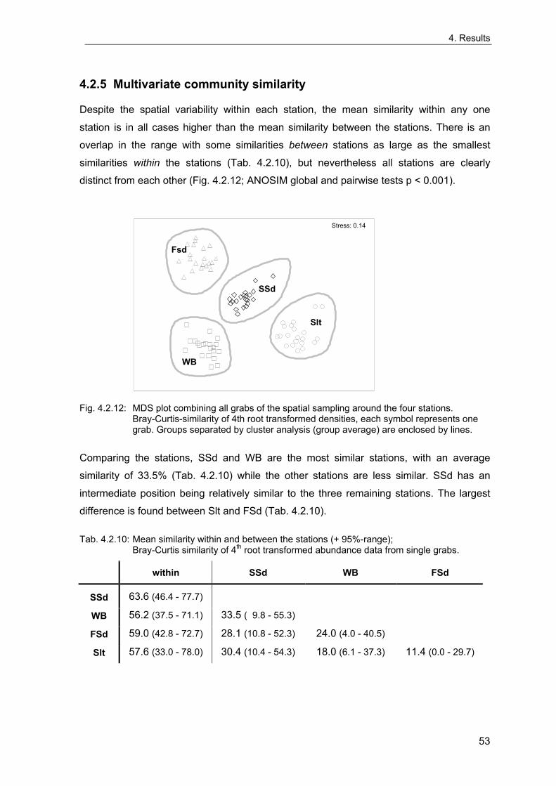
4. Results
4.2.5 Multivariate community similarity
Despite the spatial variability within each station, the mean similarity within any one
station is in all cases higher than the mean similarity between the stations. There is an
overlap in the range with some similarities between stations as large as the smallest
similarities within the stations (Tab. 4.2.10), but nevertheless all stations are clearly
distinct from each other (Fig. 4.2.12; ANOSIM global and pairwise tests p < 0.001).
Stress: 0.14
WB
SSd
Fsd
Slt
Fig. 4.2.12: MDS plot combining all grabs of the spatial sampling around the four stations.
Bray-Curtis-similarity of 4th root transformed densities, each symbol represents one grab. Groups separated by cluster analysis (group average) are enclosed by lines.
Comparing the stations, SSd and WB are the most similar stations, with an average
similarity of 33.5% (Tab. 4.2.10) while the other stations are less similar. SSd has an
intermediate position being relatively similar to the three remaining stations. The largest
difference is found between Slt and FSd (Tab. 4.2.10).
Tab. 4.2.10: Mean similarity within and between the stations (+ 95%-range); Bray-Curtis similarity of 4th root transformed abundance data from single grabs.
within SSd WB FSd
SSd 63.6 (46.4 - 77.7)
WB 56.2 (37.5 - 71.1) 33.5 ( 9.8 - 55.3)
FSd 59.0 (42.8 - 72.7) 28.1 (10.8 - 52.3) 24.0 (4.0 - 40.5)
Slt 57.6 (33.0 - 78.0) 30.4 (10.4 - 54.3) 18.0 (6.1 - 37.3) 11.4 (0.0 - 29.7)
53
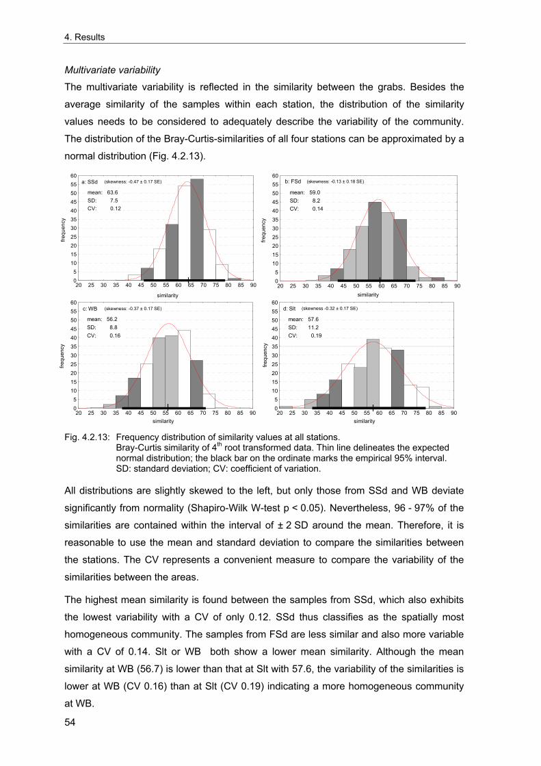
4. Results
Multivariate variability
The multivariate variability is reflected in the similarity between the grabs. Besides the
average similarity of the samples within each station, the distribution of the similarity
values needs to be considered to adequately describe the variability of the community.
The distribution of the Bray-Curtis-similarities of all four stations can be approximated by a
normal distribution (Fig. 4.2.13).
similarity
frequ
ency
0 5
10 15 20 25 30 35 40 45 50 55 60
20 25 30 35 40 45 50 55 60 65 70 75 80 85 90
a: SSd (skewness: -0.47 ± 0.17 SE)
mean: 63.6 SD: 7.5 CV: 0.12
similarity
frequ
ency
05
1015202530354045505560
20 25 30 35 40 45 50 55 60 65 70 75 80 85 90
b: FSd (skewness: -0.13 ± 0.18 SE)
mean: 59.0 SD: 8.2 CV: 0.14
similarity
frequ
ency
0 5
10 15 20 25 30 35 40 45 50 55 60
20 25 30 35 40 45 50 55 60 65 70 75 80 85 90
c: WB (skewness: -0.37 ± 0.17 SE)
mean: 56.2 SD: 8.8 CV: 0.16
similarity
frequ
ency
05
1015202530354045505560
20 25 30 35 40 45 50 55 60 65 70 75 80 85 90
d: Slt (skewness -0.32 ± 0.17 SE)
mean: 57.6 SD: 11.2 CV: 0.19
Fig. 4.2.13: Frequency distribution of similarity values at all stations.
Bray-Curtis similarity of 4th root transformed data. Thin line delineates the expected normal distribution; the black bar on the ordinate marks the empirical 95% interval. SD: standard deviation; CV: coefficient of variation.
All distributions are slightly skewed to the left, but only those from SSd and WB deviate
significantly from normality (Shapiro-Wilk W-test p < 0.05). Nevertheless, 96 - 97% of the
similarities are contained within the interval of ± 2 SD around the mean. Therefore, it is
reasonable to use the mean and standard deviation to compare the similarities between
the stations. The CV represents a convenient measure to compare the variability of the
similarities between the areas.
The highest mean similarity is found between the samples from SSd, which also exhibits
the lowest variability with a CV of only 0.12. SSd thus classifies as the spatially most
homogeneous community. The samples from FSd are less similar and also more variable
with a CV of 0.14. Slt or WB both show a lower mean similarity. Although the mean
similarity at WB (56.7) is lower than that at Slt with 57.6, the variability of the similarities is
lower at WB (CV 0.16) than at Slt (CV 0.19) indicating a more homogeneous community
at WB.
54
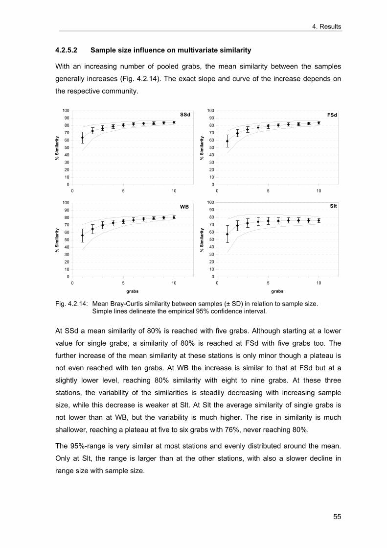
4. Results
4.2.5.2 Sample size influence on multivariate similarity
With an increasing number of pooled grabs, the mean similarity between the samples
generally increases (Fig. 4.2.14). The exact slope and curve of the increase depends on
the respective community.
0
10
20
30
40
50
60
70
80
90
100
0 5
% S
imila
rity
SSd
100
10
20
30
40
50
60
70
80
90
100
0 5
% S
imila
rity
FSd
10
0
10
20
30
40
50
60
70
80
90
100
0 5
grabs
% S
imila
rity
WB
100
10
20
30
40
50
60
70
80
90
100
0 5
grabs
% S
imila
rity
Sl
10
t
Fig. 4.2.14: Mean Bray-Curtis similarity between samples (± SD) in relation to sample size.
Simple lines delineate the empirical 95% confidence interval.
At SSd a mean similarity of 80% is reached with five grabs. Although starting at a lower
value for single grabs, a similarity of 80% is reached at FSd with five grabs too. The
further increase of the mean similarity at these stations is only minor though a plateau is
not even reached with ten grabs. At WB the increase is similar to that at FSd but at a
slightly lower level, reaching 80% similarity with eight to nine grabs. At these three
stations, the variability of the similarities is steadily decreasing with increasing sample
size, while this decrease is weaker at Slt. At Slt the average similarity of single grabs is
not lower than at WB, but the variability is much higher. The rise in similarity is much
shallower, reaching a plateau at five to six grabs with 76%, never reaching 80%.
The 95%-range is very similar at most stations and evenly distributed around the mean.
Only at Slt, the range is larger than at the other stations, with also a slower decline in
range size with sample size.
55
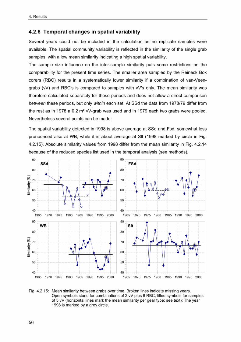
4. Results
4.2.6 Temporal changes in spatial variability
Several years could not be included in the calculation as no replicate samples were
available. The spatial community variability is reflected in the similarity of the single grab
samples, with a low mean similarity indicating a high spatial variability.
The sample size influence on the inter-sample similarity puts some restrictions on the
comparability for the present time series. The smaller area sampled by the Reineck Box
corers (RBC) results in a systematically lower similarity if a combination of van-Veen-
grabs (vV) and RBC's is compared to samples with vV's only. The mean similarity was
therefore calculated separately for these periods and does not allow a direct comparison
between these periods, but only within each set. At SSd the data from 1978/79 differ from
the rest as in 1978 a 0.2 m² vV-grab was used and in 1979 each two grabs were pooled.
Nevertheless several points can be made:
The spatial variability detected in 1998 is above average at SSd and Fsd, somewhat less
pronounced also at WB, while it is about average at Slt (1998 marked by circle in Fig.
4.2.15). Absolute similarity values from 1998 differ from the mean similarity in Fig. 4.2.14
because of the reduced species list used in the temporal analysis (see methods).
40
50
60
70
80
90
1965 1970 1975 1980 1985 1990 1995 2000
Sim
ilarit
y [%
]
SSd
40
50
60
70
80
90
1965 1970 1975 1980 1985 1990 1995 2000
FSd
40
50
60
70
80
90
1965 1970 1975 1980 1985 1990 1995 2000
Sim
ilarit
y [%
]
WB
40
50
60
70
80
90
1965 1970 1975 1980 1985 1990 1995 2000
Slt
Fig. 4.2.15: Mean similarity between grabs over time. Broken lines indicate missing years. Open symbols stand for combinations of 2 vV plus 6 RBC, filled symbols for samples of 5 vV (horizontal lines mark the mean similarity per gear type; see text); The year 1998 is marked by a grey circle.
56
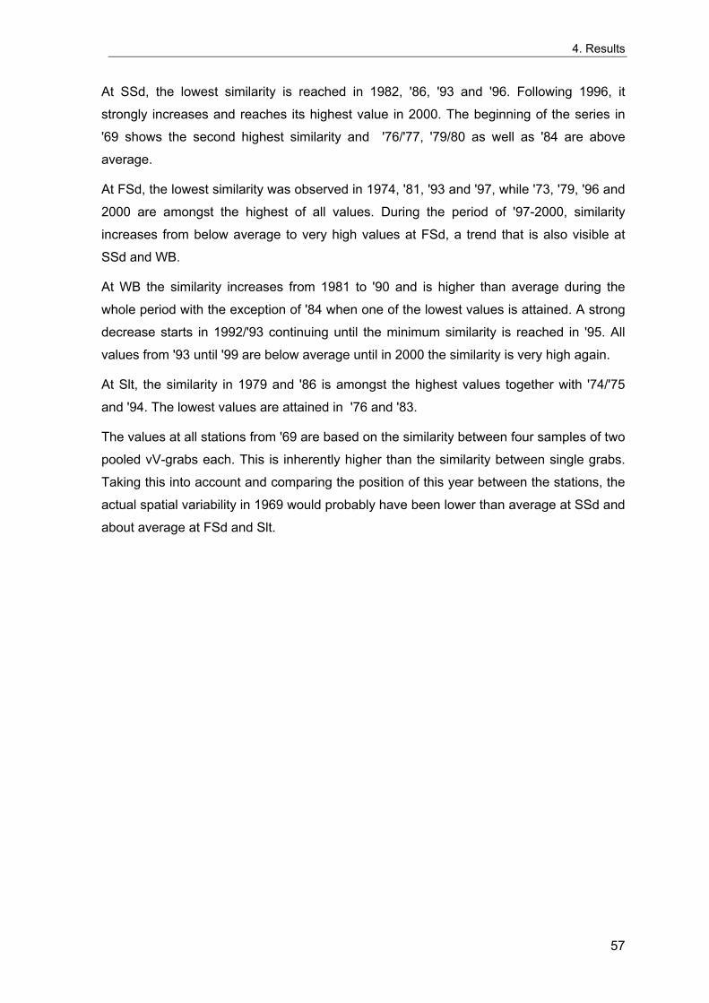
4. Results
At SSd, the lowest similarity is reached in 1982, '86, '93 and '96. Following 1996, it
strongly increases and reaches its highest value in 2000. The beginning of the series in
'69 shows the second highest similarity and '76/'77, '79/80 as well as '84 are above
average.
At FSd, the lowest similarity was observed in 1974, '81, '93 and '97, while '73, '79, '96 and
2000 are amongst the highest of all values. During the period of '97-2000, similarity
increases from below average to very high values at FSd, a trend that is also visible at
SSd and WB.
At WB the similarity increases from 1981 to '90 and is higher than average during the
whole period with the exception of '84 when one of the lowest values is attained. A strong
decrease starts in 1992/'93 continuing until the minimum similarity is reached in '95. All
values from '93 until '99 are below average until in 2000 the similarity is very high again.
At Slt, the similarity in 1979 and '86 is amongst the highest values together with '74/'75
and '94. The lowest values are attained in '76 and '83.
The values at all stations from '69 are based on the similarity between four samples of two
pooled vV-grabs each. This is inherently higher than the similarity between single grabs.
Taking this into account and comparing the position of this year between the stations, the
actual spatial variability in 1969 would probably have been lower than average at SSd and
about average at FSd and Slt.
57
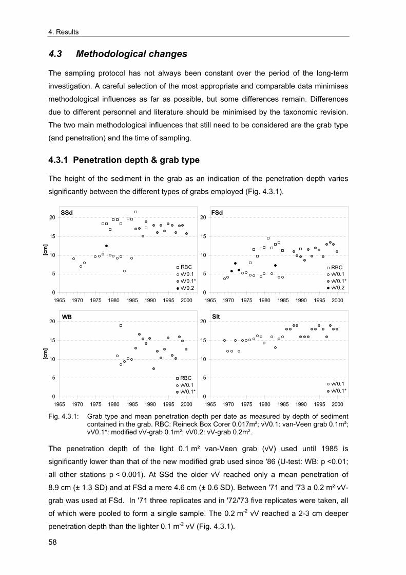
4. Results
4.3 Methodological changes
The sampling protocol has not always been constant over the period of the long-term
investigation. A careful selection of the most appropriate and comparable data minimises
methodological influences as far as possible, but some differences remain. Differences
due to different personnel and literature should be minimised by the taxonomic revision.
The two main methodological influences that still need to be considered are the grab type
(and penetration) and the time of sampling.
4.3.1 Penetration depth & grab type
The height of the sediment in the grab as an indication of the penetration depth varies
significantly between the different types of grabs employed (Fig. 4.3.1).
SSd
0
5
10
15
20
1965 1970 1975 1980 1985 1990 1995 2000
[cm
]
RBCvV0.1vV0.1*vV0.2
FSd
0
5
10
15
20
1965 1970 1975 1980 1985 1990 1995 2000
RBCvV0.1vV0.1*vV0.2
WB
0
5
10
15
20
1965 1970 1975 1980 1985 1990 1995 2000
[cm
]
RBCvV0.1vV0.1*
Slt
0
5
10
15
20
1965 1970 1975 1980 1985 1990 1995 2000
vV0.1vV0.1*
Fig. 4.3.1: Grab type and mean penetration depth per date as measured by depth of sediment
contained in the grab. RBC: Reineck Box Corer 0.017m²; vV0.1: van-Veen grab 0.1m²; vV0.1*: modified vV-grab 0.1m²; vV0.2: vV-grab 0.2m².
The penetration depth of the light 0.1 m² van-Veen grab (vV) used until 1985 is
significantly lower than that of the new modified grab used since '86 (U-test: WB: p <0.01;
all other stations p < 0.001). At SSd the older vV reached only a mean penetration of
8.9 cm (± 1.3 SD) and at FSd a mere 4.6 cm (± 0.6 SD). Between '71 and '73 a 0.2 m² vV-
grab was used at FSd. In '71 three replicates and in '72/'73 five replicates were taken, all
of which were pooled to form a single sample. The 0.2 m-2 vV reached a 2-3 cm deeper
penetration depth than the lighter 0.1 m-2 vV (Fig. 4.3.1).
58
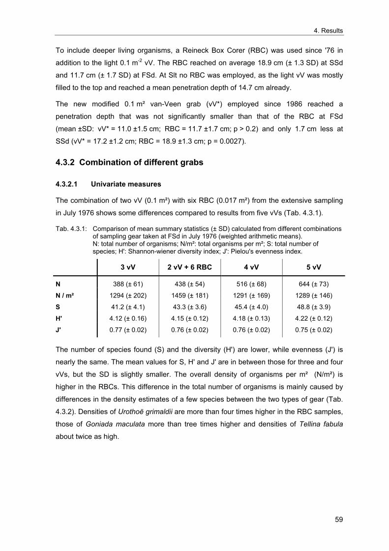
4. Results
To include deeper living organisms, a Reineck Box Corer (RBC) was used since '76 in
addition to the light 0.1 m-2 vV. The RBC reached on average 18.9 cm (± 1.3 SD) at SSd
and 11.7 cm (± 1.7 SD) at FSd. At Slt no RBC was employed, as the light vV was mostly
filled to the top and reached a mean penetration depth of 14.7 cm already.
The new modified 0.1 m² van-Veen grab (vV*) employed since 1986 reached a
penetration depth that was not significantly smaller than that of the RBC at FSd
(mean ±SD: vV* = 11.0 ±1.5 cm; RBC = 11.7 ±1.7 cm; p > 0.2) and only 1.7 cm less at
SSd (vV* = 17.2 ±1.2 cm; RBC = 18.9 ±1.3 cm; p = 0.0027).
4.3.2 Combination of different grabs
4.3.2.1 Univariate measures
The combination of two vV (0.1 m²) with six RBC (0.017 m²) from the extensive sampling
in July 1976 shows some differences compared to results from five vVs (Tab. 4.3.1).
Tab. 4.3.1: Comparison of mean summary statistics (± SD) calculated from different combinations of sampling gear taken at FSd in July 1976 (weighted arithmetic means). N: total number of organisms; N/m²: total organisms per m²; S: total number of species; H': Shannon-wiener diversity index; J': Pielou's evenness index.
3 vV 2 vV + 6 RBC 4 vV 5 vV
N 388 (± 61) 438 (± 54) 516 (± 68) 644 (± 73)
N / m² 1294 (± 202) 1459 (± 181) 1291 (± 169) 1289 (± 146)
S 41.2 (± 4.1) 43.3 (± 3.6) 45.4 (± 4.0) 48.8 (± 3.9)
H' 4.12 (± 0.16) 4.15 (± 0.12) 4.18 (± 0.13) 4.22 (± 0.12)
J' 0.77 (± 0.02) 0.76 (± 0.02) 0.76 (± 0.02) 0.75 (± 0.02)
The number of species found (S) and the diversity (H') are lower, while evenness (J') is
nearly the same. The mean values for S, H' and J' are in between those for three and four
vVs, but the SD is slightly smaller. The overall density of organisms per m² (N/m²) is
higher in the RBCs. This difference in the total number of organisms is mainly caused by
differences in the density estimates of a few species between the two types of gear (Tab.
4.3.2). Densities of Urothoë grimaldii are more than four times higher in the RBC samples,
those of Goniada maculata more than tree times higher and densities of Tellina fabula
about twice as high.
59
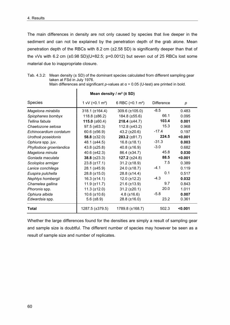
4. Results
The main differences in density are not only caused by species that live deeper in the
sediment and can not be explained by the penetration depth of the grab alone. Mean
penetration depth of the RBCs with 8.2 cm (±2.58 SD) is significantly deeper than that of
the vVs with 6.2 cm (±0.98 SD)(U=82.5; p=0.0012) but seven out of 25 RBCs lost some
material due to inappropriate closure.
Tab. 4.3.2: Mean density (± SD) of the dominant species calculated from different sampling gear taken at FSd in July 1976. Main differences and significant p-values at α = 0.05 (U-test) are printed in bold.
Mean density / m² (± SD)
Species 1 vV (=0.1 m²) 6 RBC (=0.1 m²) Difference p
Magelona mirabilis 318.1 (±164.4) 309.6 (±105.0) -8.5 0.483 Spiophanes bombyx 118.8 (±86.2) 184.8 (±55.6) 66.1 0.095 Tellina fabula 115.0 (±60.4) 218.4 (±44.7) 103.4 0.001 Chaetozone setosa 97.5 (±63.3) 112.8 (±43.2) 15.3 0.968 Echinocardium cordatum 60.6 (±56.9) 43.2 (±20.6) -17.4 0.197 Urothoë poseidonis 58.8 (±32.0) 283.2 (±81.7) 224.5 <0.001 Ophiura spp. juv. 48.1 (±44.5) 16.8 (±18.1) -31.3 0.003 Phyllodoce groenlandica 43.8 (±25.8) 40.8 (±16.9) -3.0 0.682 Magelona minuta 40.6 (±42.3) 86.4 (±34.7) 45.8 0.030 Goniada maculata 38.8 (±23.3) 127.2 (±24.8) 88.5 <0.001 Scoloplos armiger 23.8 (±17.1) 31.2 (±18.9) 7.5 0.389 Lanice conchilega 28.1 (±45.9) 24.0 (±18.7) -4.1 0.119 Euspira pulchella 28.8 (±15.0) 28.8 (±14.4) 0.1 0.517 Nephtys hombergii 16.3 (±14.1) 12.0 (±12.2) -4.3 0.032 Chamelea gallina 11.9 (±11.7) 21.6 (±13.9) 9.7 0.843 Phoronis spp. 11.3 (±12.0) 31.2 (±20.1) 20.0 1.011 Ophiura albida 10.6 (±10.6) 4.8 (±16.6) -5.8 0.007 Edwardsia spp. 5.6 (±8.9) 28.8 (±16.0) 23.2 0.361
Total 1287.5 (±379.5) 1789.8 (±168.7) 502.3 <0.001
Whether the large differences found for the densities are simply a result of sampling gear
and sample size is doubtful. The different number of species may however be seen as a
result of sample size and number of replicates.
60
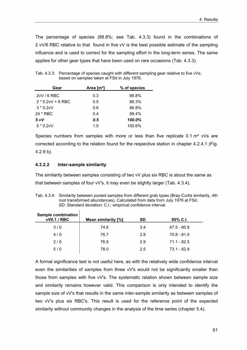
4. Results
The percentage of species (88.8%; see Tab. 4.3.3) found in the combinations of
2 vV/6 RBC relative to that found in five vV is the best possible estimate of the sampling
influence and is used to correct for the sampling effort in the long-term series. The same
applies for other gear types that have been used on rare occasions (Tab. 4.3.3).
Tab. 4.3.3: Percentage of species caught with different sampling gear relative to five vVs; based on samples taken at FSd in July 1976.
Gear Area [m²] % of species
2vV / 6 RBC 0.3 88.8% 2 * 0.2vV + 6 RBC 0.5 88.3% 3 * 0.2vV 0.6 86.8% 24 * RBC 0.4 99.4% 5 vV 0.5 100.0% 5 * 0.2vV 1.0 100.6%
Species numbers from samples with more or less than five replicate 0.1 m² vVs are
corrected according to the relation found for the respective station in chapter 4.2.4.1 (Fig.
4.2.9 b).
4.3.2.2 Inter-sample similarity
The similarity between samples consisting of two vV plus six RBC is about the same as
that between samples of four vV's, it may even be slightly larger (Tab. 4.3.4).
Tab. 4.3.4: Similarity between pooled samples from different grab types (Bray-Curtis similarity, 4th root transformed abundances). Calculated from data from July 1976 at FSd. SD: Standard deviation; C.I.: empirical confidence interval.
Sample combination vV0.1 / RBC Mean similarity [%] SD 95% C.I.
3 / 0 74.6 3.4 67.5 - 80.8
4 / 0 76.7 2.8 70.8 - 81.9
2 / 6 76.9 2.9 71.1 - 82.5
5 / 0 78.0 2.5 73.1 - 82.8
A formal significance test is not useful here, as with the relatively wide confidence interval
even the similarities of samples from three vV's would not be significantly smaller than
those from samples with five vV's. The systematic relation shown between sample size
and similarity remains however valid. This comparison is only intended to identify the
sample size of vV's that results in the same inter-sample similarity as between samples of
two vV's plus six RBC's. This result is used for the reference point of the expected
similarity without community changes in the analysis of the time series (chapter 5.4).
61
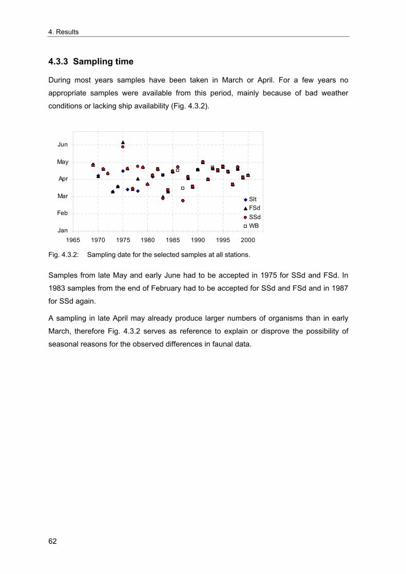
4. Results
4.3.3 Sampling time
During most years samples have been taken in March or April. For a few years no
appropriate samples were available from this period, mainly because of bad weather
conditions or lacking ship availability (Fig. 4.3.2).
Jan
Feb
Mar
Apr
May
Jun
1965 1970 1975 1980 1985 1990 1995 2000
SltFSdSSdWB
Fig. 4.3.2: Sampling date for the selected samples at all stations.
Samples from late May and early June had to be accepted in 1975 for SSd and FSd. In
1983 samples from the end of February had to be accepted for SSd and FSd and in 1987
for SSd again.
A sampling in late April may already produce larger numbers of organisms than in early
March, therefore Fig. 4.3.2 serves as reference to explain or disprove the possibility of
seasonal reasons for the observed differences in faunal data.
62
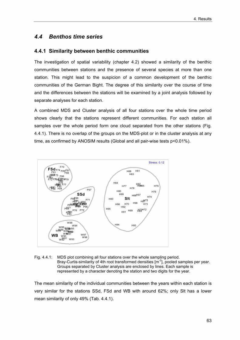
4. Results
4.4 Benthos time series
4.4.1 Similarity between benthic communities
The investigation of spatial variability (chapter 4.2) showed a similarity of the benthic
communities between stations and the presence of several species at more than one
station. This might lead to the suspicion of a common development of the benthic
communities of the German Bight. The degree of this similarity over the course of time
and the differences between the stations will be examined by a joint analysis followed by
separate analyses for each station.
A combined MDS and Cluster analysis of all four stations over the whole time period
shows clearly that the stations represent different communities. For each station all
samples over the whole period form one cloud separated from the other stations (Fig.
4.4.1). There is no overlap of the groups on the MDS-plot or in the cluster analysis at any
time, as confirmed by ANOSIM results (Global and all pair-wise tests p<0.01%).
F00 F69
F70
F71 F72
F73
F74 F75
F76 F77
F78 F79 F80
F81 F82
F83 F84
F85 F88
F89 F90 F91
F92
F93
F94
F95 F96
F97 F98 F99
H00
H69
H70
H71H72
H73
H74H75
H76
H77H78
H79
H80
H81
H82
H83
H84H85
H86
H87
H88
H89
H90
H91
H92
H93H94
H95
H96
H97
H98
H99
P00P69 P71
P72 P75
P76 P77
P78
P79 P80 P81 P82 P83 P84
P85 P86 P87 P88 P89
P91 P92
P93
P94 P95
P96
P97
P98 P99
W00
W81
W82W83
W84 W85
W86 W87
W88 W89 W90
W92 W93
W94 W95 W96
W97
W98
W99
WB
SSd
FSd
Slt
Stress: 0.12
Fig. 4.4.1: MDS plot combining all four stations over the whole sampling period.
Bray-Curtis-similarity of 4th root transformed densities [m-2], pooled samples per year. Groups separated by Cluster analysis are enclosed by lines. Each sample is represented by a character denoting the station and two digits for the year.
The mean similarity of the individual communities between the years within each station is
very similar for the stations SSd, FSd and WB with around 62%; only Slt has a lower
mean similarity of only 49% (Tab. 4.4.1).
63
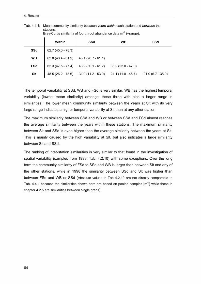
4. Results
Tab. 4.4.1: Mean community similarity between years within each station and between the stations. Bray-Curtis similarity of fourth root abundance data m-2 (+range).
Within SSd WB FSd
SSd 62.7 (45.0 - 78.3)
WB 62.0 (43.4 - 81.2) 45.1 (28.7 - 61.1)
FSd 62.3 (47.5 - 77.4) 43.9 (30.1 - 61.2) 33.2 (22.0 - 47.0)
Slt 48.5 (26.2 - 73.6) 31.0 (11.2 - 53.9) 24.1 (11.0 - 45.7) 21.9 (6.7 - 38.9)
The temporal variability at SSd, WB and FSd is very similar. WB has the highest temporal
variability (lowest mean similarity) amongst these three with also a larger range in
similarities. The lower mean community similarity between the years at Slt with its very
large range indicates a higher temporal variability at Slt than at any other station.
The maximum similarity between SSd and WB or between SSd and FSd almost reaches
the average similarity between the years within these stations. The maximum similarity
between Slt and SSd is even higher than the average similarity between the years at Slt.
This is mainly caused by the high variability at Slt, but also indicates a large similarity
between Slt and SSd.
The ranking of inter-station similarities is very similar to that found in the investigation of
spatial variability (samples from 1998; Tab. 4.2.10) with some exceptions. Over the long
term the community similarity of FSd to SSd and WB is larger than between Slt and any of
the other stations, while in 1998 the similarity between SSd and Slt was higher than
between FSd and WB or SSd (Absolute values in Tab 4.2.10 are not directly comparable to
Tab. 4.4.1 because the similarities shown here are based on pooled samples [m-2] while those in
chapter 4.2.5 are similarities between single grabs).
64
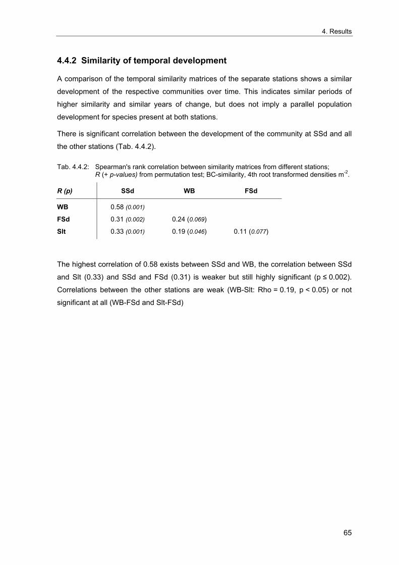
4. Results
4.4.2 Similarity of temporal development
A comparison of the temporal similarity matrices of the separate stations shows a similar
development of the respective communities over time. This indicates similar periods of
higher similarity and similar years of change, but does not imply a parallel population
development for species present at both stations.
There is significant correlation between the development of the community at SSd and all
the other stations (Tab. 4.4.2).
Tab. 4.4.2: Spearman's rank correlation between similarity matrices from different stations; R (+ p-values) from permutation test; BC-similarity, 4th root transformed densities m-2.
R (p) SSd WB FSd
WB 0.58 (0.001)
FSd 0.31 (0.002) 0.24 (0.069)
Slt 0.33 (0.001) 0.19 (0.046) 0.11 (0.077)
The highest correlation of 0.58 exists between SSd and WB, the correlation between SSd
and Slt (0.33) and SSd and FSd (0.31) is weaker but still highly significant (p ≤ 0.002).
Correlations between the other stations are weak (WB-Slt: Rho = 0.19, p < 0.05) or not
significant at all (WB-FSd and Slt-FSd)
65
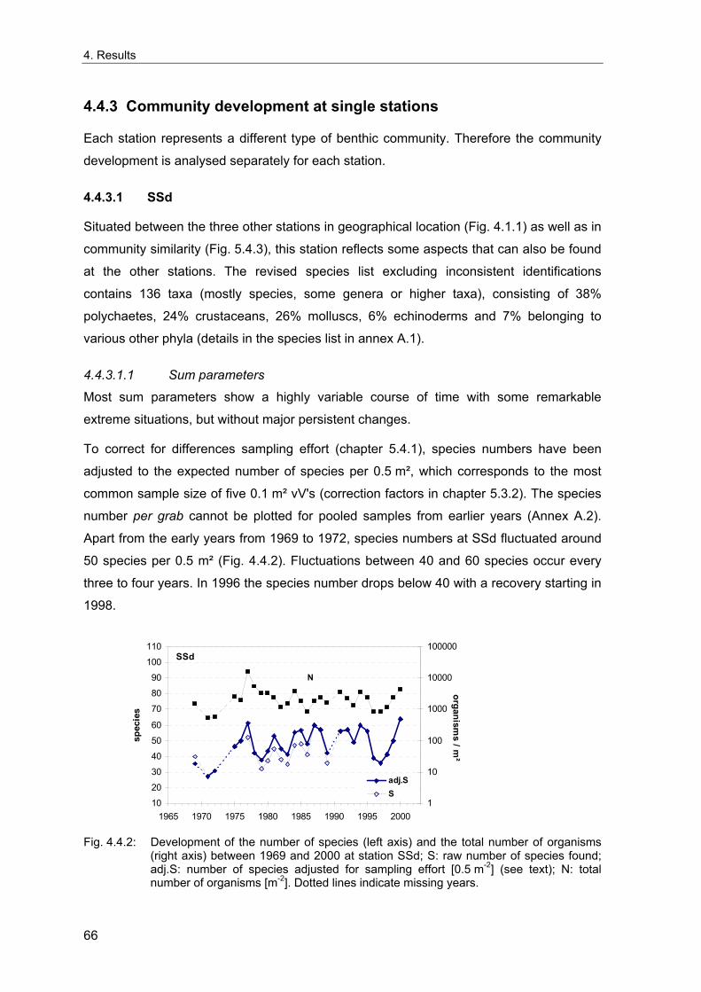
4. Results
4.4.3 Community development at single stations
Each station represents a different type of benthic community. Therefore the community
development is analysed separately for each station.
4.4.3.1 SSd
Situated between the three other stations in geographical location (Fig. 4.1.1) as well as in
community similarity (Fig. 5.4.3), this station reflects some aspects that can also be found
at the other stations. The revised species list excluding inconsistent identifications
contains 136 taxa (mostly species, some genera or higher taxa), consisting of 38%
polychaetes, 24% crustaceans, 26% molluscs, 6% echinoderms and 7% belonging to
various other phyla (details in the species list in annex A.1).
4.4.3.1.1 Sum parameters
Most sum parameters show a highly variable course of time with some remarkable
extreme situations, but without major persistent changes.
To correct for differences sampling effort (chapter 5.4.1), species numbers have been
adjusted to the expected number of species per 0.5 m², which corresponds to the most
common sample size of five 0.1 m² vV's (correction factors in chapter 5.3.2). The species
number per grab cannot be plotted for pooled samples from earlier years (Annex A.2).
Apart from the early years from 1969 to 1972, species numbers at SSd fluctuated around
50 species per 0.5 m² (Fig. 4.4.2). Fluctuations between 40 and 60 species occur every
three to four years. In 1996 the species number drops below 40 with a recovery starting in
1998.
102030405060
708090
100110
1965 1970 1975 1980 1985 1990 1995 2000
spec
ies
1
10
100
1000
10000
100000
organisms / m
²
adj.SS
SSd
N
Fig. 4.4.2: Development of the number of species (left axis) and the total number of organisms
(right axis) between 1969 and 2000 at station SSd; S: raw number of species found; adj.S: number of species adjusted for sampling effort [0.5 m-2] (see text); N: total number of organisms [m-2]. Dotted lines indicate missing years.
66
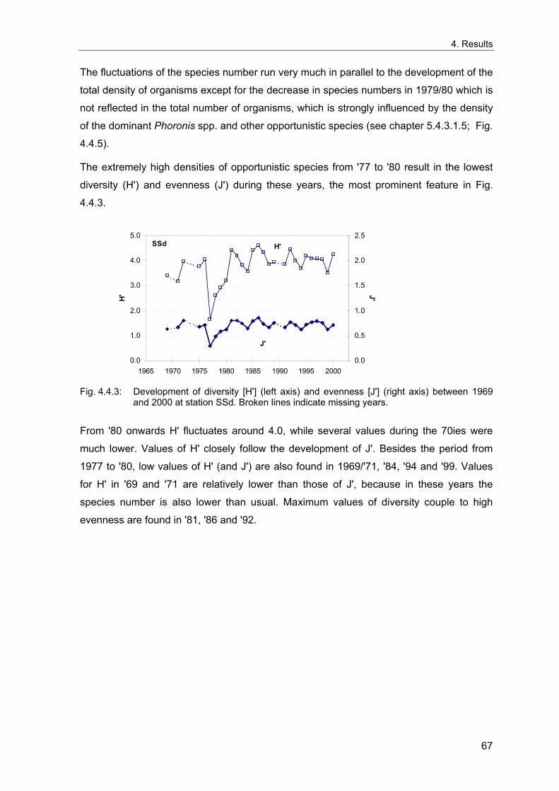
4. Results
The fluctuations of the species number run very much in parallel to the development of the
total density of organisms except for the decrease in species numbers in 1979/80 which is
not reflected in the total number of organisms, which is strongly influenced by the density
of the dominant Phoronis spp. and other opportunistic species (see chapter 5.4.3.1.5; Fig.
4.4.5).
The extremely high densities of opportunistic species from '77 to '80 result in the lowest
diversity (H') and evenness (J') during these years, the most prominent feature in Fig.
4.4.3.
0.0
1.0
2.0
3.0
4.0
5.0
1965 1970 1975 1980 1985 1990 1995 2000
H'
0.0
0.5
1.0
1.5
2.0
2.5
J'
SSd
J'
H'
Fig. 4.4.3: Development of diversity [H'] (left axis) and evenness [J'] (right axis) between 1969
and 2000 at station SSd. Broken lines indicate missing years.
From '80 onwards H' fluctuates around 4.0, while several values during the 70ies were
much lower. Values of H' closely follow the development of J'. Besides the period from
1977 to '80, low values of H' (and J') are also found in 1969/'71, '84, '94 and '99. Values
for H' in '69 and '71 are relatively lower than those of J', because in these years the
species number is also lower than usual. Maximum values of diversity couple to high
evenness are found in '81, '86 and '92.
67
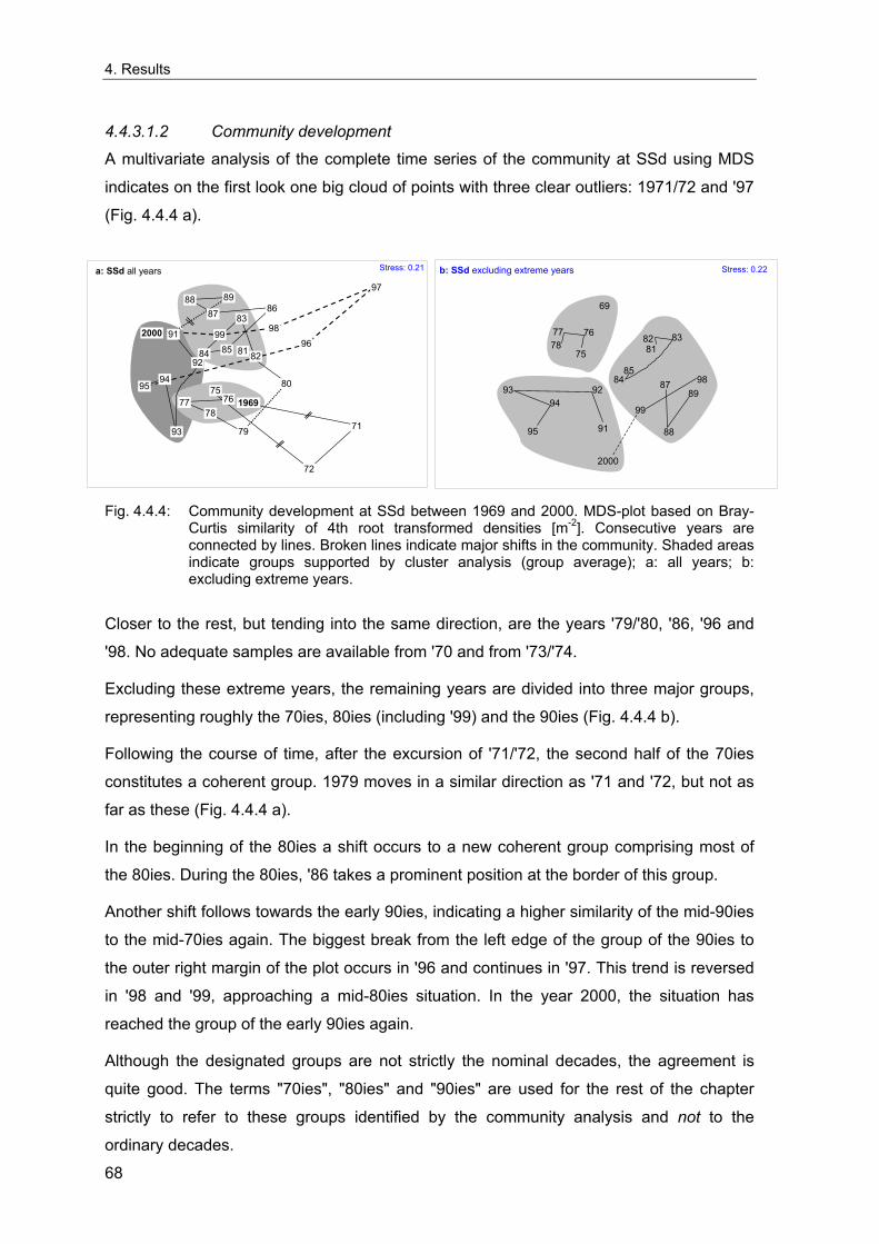
4. Results
4.4.3.1.2 Community development
A multivariate analysis of the complete time series of the community at SSd using MDS
indicates on the first look one big cloud of points with three clear outliers: 1971/72 and '97
(Fig. 4.4.4 a).
1969
71
72
75 76 77
78
79
80
81 82
83
84 85
86 87 88 89
91
92
93
94 95
96
97
98 99 2000
Stress: 0.21 a: SSd all years
69
75
767778 81
82 83
84 85
87
88
89
91
929394
95
98
99
2000
Stress: 0.22 b: SSd excluding extreme years
Fig. 4.4.4: Community development at SSd between 1969 and 2000. MDS-plot based on Bray-
Curtis similarity of 4th root transformed densities [m-2]. Consecutive years are connected by lines. Broken lines indicate major shifts in the community. Shaded areas indicate groups supported by cluster analysis (group average); a: all years; b: excluding extreme years.
Closer to the rest, but tending into the same direction, are the years '79/'80, '86, '96 and
'98. No adequate samples are available from '70 and from '73/'74.
Excluding these extreme years, the remaining years are divided into three major groups,
representing roughly the 70ies, 80ies (including '99) and the 90ies (Fig. 4.4.4 b).
Following the course of time, after the excursion of '71/'72, the second half of the 70ies
constitutes a coherent group. 1979 moves in a similar direction as '71 and '72, but not as
far as these (Fig. 4.4.4 a).
In the beginning of the 80ies a shift occurs to a new coherent group comprising most of
the 80ies. During the 80ies, '86 takes a prominent position at the border of this group.
Another shift follows towards the early 90ies, indicating a higher similarity of the mid-90ies
to the mid-70ies again. The biggest break from the left edge of the group of the 90ies to
the outer right margin of the plot occurs in '96 and continues in '97. This trend is reversed
in '98 and '99, approaching a mid-80ies situation. In the year 2000, the situation has
reached the group of the early 90ies again.
Although the designated groups are not strictly the nominal decades, the agreement is
quite good. The terms "70ies", "80ies" and "90ies" are used for the rest of the chapter
strictly to refer to these groups identified by the community analysis and not to the
ordinary decades.
68
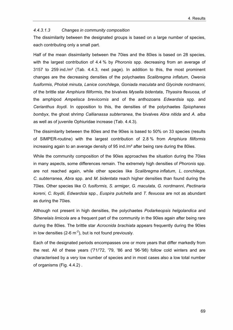
4. Results
4.4.3.1.3 Changes in community composition
The dissimilarity between the designated groups is based on a large number of species,
each contributing only a small part.
Half of the mean dissimilarity between the 70ies and the 80ies is based on 28 species,
with the largest contribution of 4.4 % by Phoronis spp. decreasing from an average of
3157 to 259 ind./m² (Tab. 4.4.3, next page). In addition to this, the most prominent
changes are the decreasing densities of the polychaetes Scalibregma inflatum, Owenia
fusiformis, Pholoë minuta, Lanice conchilega, Goniada maculata and Glycinde nordmanni,
of the brittle star Amphiura filiformis, the bivalves Mysella bidentata, Thyasira flexuosa, of
the amphipod Ampelisca brevicornis and of the anthozoans Edwardsia spp. and
Cerianthus lloydi. In opposition to this, the densities of the polychaetes Spiophanes
bombyx, the ghost shrimp Callianassa subterranea, the bivalves Abra nitida and A. alba
as well as of juvenile Ophiuridae increase (Tab. 4.4.3).
The dissimilarity between the 80ies and the 90ies is based to 50% on 33 species (results
of SIMPER-routine) with the largest contribution of 2.8 % from Amphiura filiformis
increasing again to an average density of 95 ind./m² after being rare during the 80ies.
While the community composition of the 90ies approaches the situation during the 70ies
in many aspects, some differences remain. The extremely high densities of Phoronis spp.
are not reached again, while other species like Scalibregma inflatum, L. conchilega,
C. subterranea, Abra spp. and M. bidentata reach higher densities than found during the
70ies. Other species like O. fusiformis, S. armiger, G. maculata, G. nordmanni, Pectinaria
koreni, C. lloydii, Edwardsia spp., Euspira pulchella and T. flexuosa are not as abundant
as during the 70ies.
Although not present in high densities, the polychaetes Podarkeopsis helgolandica and
Sthenelais limicola are a frequent part of the community in the 90ies again after being rare
during the 80ies. The brittle star Acrocnida brachiata appears frequently during the 90ies
in low densities (2-6 m-2), but is not found previously.
Each of the designated periods encompasses one or more years that differ markedly from
the rest. All of these years ('71/'72, '79, '86 and '96-'98) follow cold winters and are
characterised by a very low number of species and in most cases also a low total number
of organisms (Fig. 4.4.2) .
69
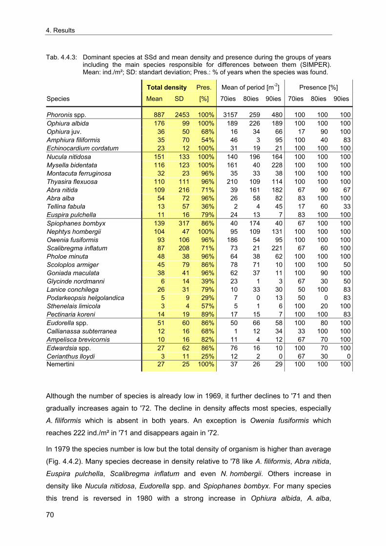
4. Results
Tab. 4.4.3: Dominant species at SSd and mean density and presence during the groups of years including the main species responsible for differences between them (SIMPER). Mean: ind./m²; SD: standart deviation; Pres.: % of years when the species was found.
Total density Pres. Mean of period [m-2] Presence [%]
Species Mean SD [%] 70ies 80ies 90ies 70ies 80ies 90ies
Phoronis spp. 887 2453 100% 3157 259 480 100 100 100Ophiura albida 176 99 100% 189 226 189 100 100 100Ophiura juv. 36 50 68% 16 34 66 17 90 100Amphiura filiformis 35 70 54% 46 3 95 100 40 83Echinocardium cordatum 23 12 100% 31 19 21 100 100 100Nucula nitidosa 151 133 100% 140 196 164 100 100 100Mysella bidentata 116 123 100% 161 40 228 100 100 100Montacuta ferruginosa 32 23 96% 35 33 38 100 100 100Thyasira flexuosa 110 111 96% 210 109 114 100 100 100Abra nitida 109 216 71% 39 161 182 67 90 67Abra alba 54 72 96% 26 58 82 83 100 100Tellina fabula 13 57 36% 2 4 45 17 60 33Euspira pulchella 11 16 79% 24 13 7 83 100 100Spiophanes bombyx 139 317 86% 40 174 40 67 100 100Nephtys hombergii 104 47 100% 95 109 131 100 100 100Owenia fusiformis 93 106 96% 186 54 95 100 100 100Scalibregma inflatum 87 208 71% 73 21 221 67 60 100Pholoe minuta 48 38 96% 64 38 62 100 100 100Scoloplos armiger 45 79 86% 78 71 10 100 100 50Goniada maculata 38 41 96% 62 37 11 100 90 100Glycinde nordmanni 6 14 39% 23 1 3 67 30 50Lanice conchilega 26 31 79% 10 33 30 50 100 83Podarkeopsis helgolandica 5 9 29% 7 0 13 50 0 83Sthenelais limicola 3 4 57% 5 1 6 100 20 100Pectinaria koreni 14 19 89% 17 15 7 100 100 83Eudorella spp. 51 60 86% 50 66 58 100 80 100Callianassa subterranea 12 16 68% 1 12 34 33 100 100Ampelisca brevicornis 10 16 82% 11 4 12 67 70 100Edwardsia spp. 27 62 86% 76 16 10 100 70 100Cerianthus lloydi 3 11 25% 12 2 0 67 30 0Nemertini 27 25 100% 37 26 29 100 100 100
Although the number of species is already low in 1969, it further declines to '71 and then
gradually increases again to '72. The decline in density affects most species, especially
A. filiformis which is absent in both years. An exception is Owenia fusiformis which
reaches 222 ind./m² in '71 and disappears again in '72.
In 1979 the species number is low but the total density of organism is higher than average
(Fig. 4.4.2). Many species decrease in density relative to '78 like A. filiformis, Abra nitida,
Euspira pulchella, Scalibregma inflatum and even N. hombergii. Others increase in
density like Nucula nitidosa, Eudorella spp. and Spiophanes bombyx. For many species
this trend is reversed in 1980 with a strong increase in Ophiura albida, A. alba,
70
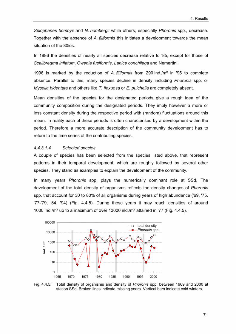
4. Results
Spiophanes bombyx and N. hombergii while others, especially Phoronis spp., decrease.
Together with the absence of A. filiformis this initiates a development towards the mean
situation of the 80ies.
In 1986 the densities of nearly all species decrease relative to '85, except for those of
Scalibregma inflatum, Owenia fusiformis, Lanice conchilega and Nemertini.
1996 is marked by the reduction of A. filiformis from 290 ind./m² in '95 to complete
absence. Parallel to this, many species decline in density including Phoronis spp. or
Mysella bidentata and others like T. flexuosa or E. pulchella are completely absent.
Mean densities of the species for the designated periods give a rough idea of the
community composition during the designated periods. They imply however a more or
less constant density during the respective period with (random) fluctuations around this
mean. In reality each of these periods is often characterised by a development within the
period. Therefore a more accurate description of the community development has to
return to the time series of the contributing species.
4.4.3.1.4 Selected species
A couple of species has been selected from the species listed above, that represent
patterns in their temporal development, which are roughly followed by several other
species. They stand as examples to explain the development of the community.
In many years Phoronis spp. plays the numerically dominant role at SSd. The
development of the total density of organisms reflects the density changes of Phoronis
spp. that account for 30 to 80% of all organisms during years of high abundance ('69, '75,
'77-'79, '84, '94) (Fig. 4.4.5). During these years it may reach densities of around
1000 ind./m² up to a maximum of over 13000 ind./m² attained in '77 (Fig. 4.4.5).
1
10
100
1000
10000
100000
1965 1970 1975 1980 1985 1990 1995 2000
total densityPhoronis spp.
ind.
/ m
²
Fig. 4.4.5: Total density of organisms and density of Phoronis spp. between 1969 and 2000 at
station SSd. Broken lines indicate missing years. Vertical bars indicate cold winters.
71
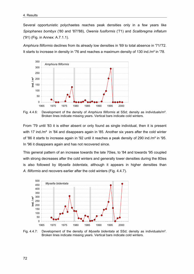
4. Results
Several opportunistic polychaetes reaches peak densities only in a few years like
Spiophanes bombyx ('80 and '87/'88), Owenia fusiformis ('71) and Scalibregma inflatum
('91) (Fig. in Annex: A.7.1.1).
Amphiura filiformis declines from its already low densities in '69 to total absence in '71/'72.
It starts to increase in density in '76 and reaches a maximum density of 130 ind./m² in '78.
Amphiura filiformis
0 50
100 150 200 250 300 350
1965 1970 1975 1980 1985 1990 1995 2000
ind.
/ m
²
Fig. 4.4.6: Development of the density of Amphiura filiformis at SSd; density as individuals/m².
Broken lines indicate missing years. Vertical bars indicate cold winters.
From '79 until '83 it is either absent or only found as single individual, then it is present
with 17 ind./m² in '84 and disappears again in '85. Another six years after the cold winter
of '86 it starts to increase again in '92 until it reaches a peak density of 290 ind./m² in '95.
In '96 it disappears again and has not recovered since.
This general pattern of an increase towards the late 70ies, to '84 and towards '95 coupled
with strong decreases after the cold winters and generally lower densities during the 80ies
is also followed by Mysella bidentata, although it appears in higher densities than
A. filiformis and recovers earlier after the cold winters (Fig. 4.4.7).
ind.
/ m
²
Mysella bidentata
0 50
100 150 200 250 300 350 400 450 500
1965 1970 1975 1980 1985 1990 1995 2000 Fig. 4.4.7: Development of the density of Mysella bidentata at SSd; density as individuals/m².
Broken lines indicate missing years. Vertical bars indicate cold winters.
72
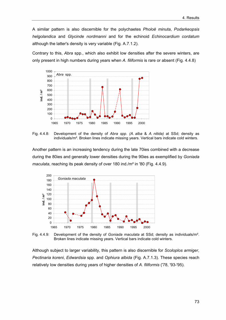
4. Results
A similar pattern is also discernible for the polychaetes Pholoë minuta, Podarkeopsis
helgolandica and Glycinde nordmanni and for the echinoid Echinocardium cordatum
although the latter's density is very variable (Fig. A.7.1.2).
Contrary to this, Abra spp., which also exhibit low densities after the severe winters, are
only present in high numbers during years when A. filiformis is rare or absent (Fig. 4.4.8)
Abra spp.
0 100 200 300 400 500 600 700 800 900
1000
1965 1970 1975 1980 1985 1990 1995 2000
ind.
/ m
²
Fig. 4.4.8: Development of the density of Abra spp. (A. alba & A. nitida) at SSd; density as
individuals/m². Broken lines indicate missing years. Vertical bars indicate cold winters.
Another pattern is an increasing tendency during the late 70ies combined with a decrease
during the 80ies and generally lower densities during the 90ies as exemplified by Goniada
maculata, reaching its peak density of over 180 ind./m² in '80 (Fig. 4.4.9).
ind.
/ m
²
Goniada maculata
0 20 40 60 80
100 120 140 160 180 200
1965 1970 1975 1980 1985 1990 1995 2000 Fig. 4.4.9: Development of the density of Goniada maculata at SSd; density as individuals/m².
Broken lines indicate missing years. Vertical bars indicate cold winters.
Although subject to larger variability, this pattern is also discernible for Scoloplos armiger,
Pectinaria koreni, Edwardsia spp. and Ophiura albida (Fig. A.7.1.3). These species reach
relatively low densities during years of higher densities of A. filiformis ('78, '93-'95).
73
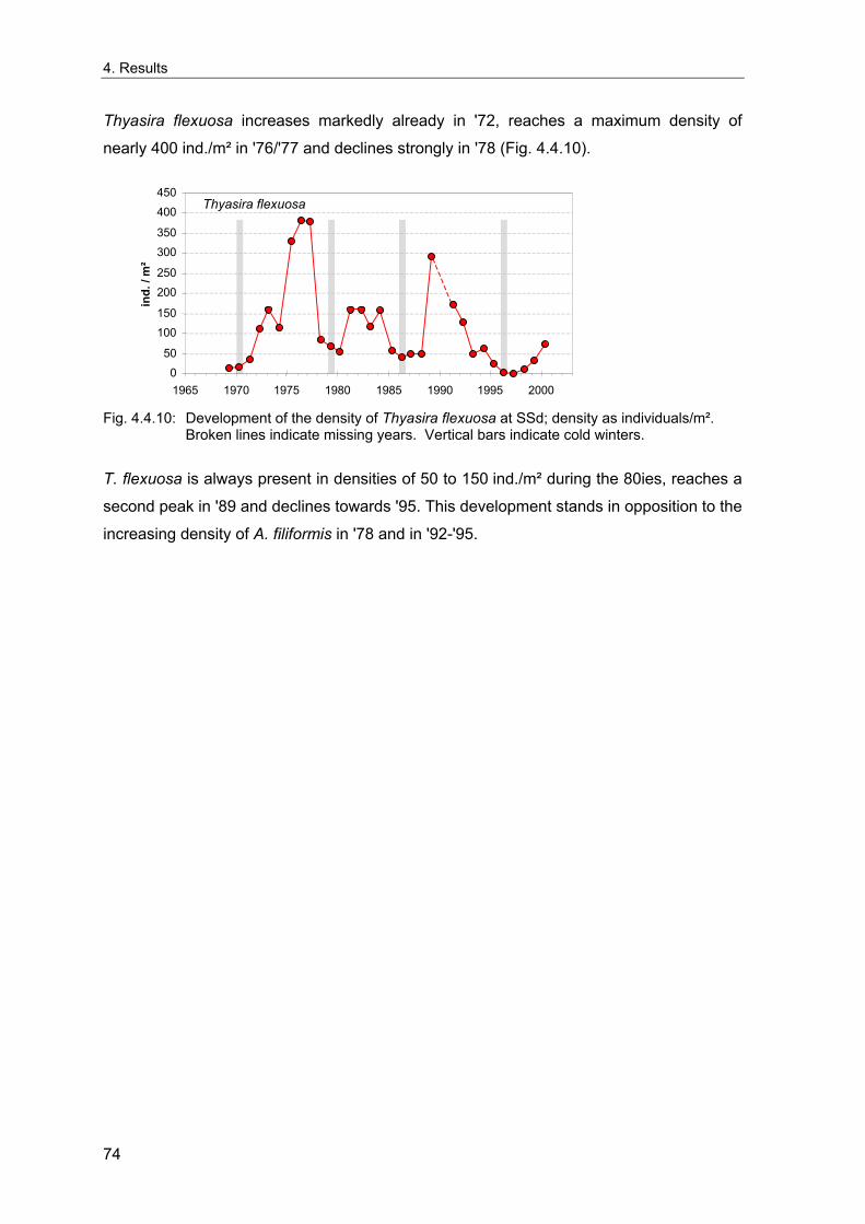
4. Results
Thyasira flexuosa increases markedly already in '72, reaches a maximum density of
nearly 400 ind./m² in '76/'77 and declines strongly in '78 (Fig. 4.4.10).
ind.
/ m
²
Thyasira flexuosa
0 50
100 150 200 250 300 350 400 450
1965 1970 1975 1980 1985 1990 1995 2000 Fig. 4.4.10: Development of the density of Thyasira flexuosa at SSd; density as individuals/m².
Broken lines indicate missing years. Vertical bars indicate cold winters.
T. flexuosa is always present in densities of 50 to 150 ind./m² during the 80ies, reaches a
second peak in '89 and declines towards '95. This development stands in opposition to the
increasing density of A. filiformis in '78 and in '92-'95.
74
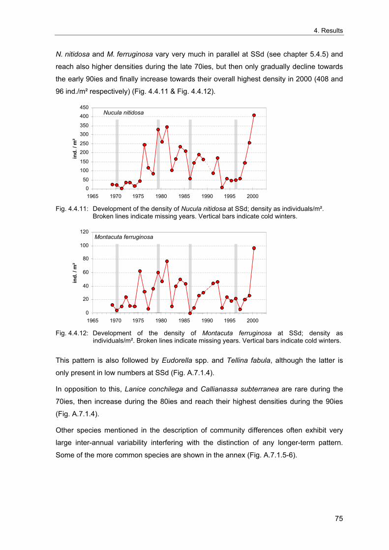
4. Results
N. nitidosa and M. ferruginosa vary very much in parallel at SSd (see chapter 5.4.5) and
reach also higher densities during the late 70ies, but then only gradually decline towards
the early 90ies and finally increase towards their overall highest density in 2000 (408 and
96 ind./m² respectively) (Fig. 4.4.11 & Fig. 4.4.12).
ind.
/ m
²
Nucula nitidosa
0 50
100 150 200 250 300 350 400 450
1965 1970 1975 1980 1985 1990 1995 2000 Fig. 4.4.11: Development of the density of Nucula nitidosa at SSd; density as individuals/m².
Broken lines indicate missing years. Vertical bars indicate cold winters.
ind.
/ m
²
Montacuta ferruginosa
0
20
40
60
80
100
120
1965 1970 1975 1980 1985 1990 1995 2000 Fig. 4.4.12: Development of the density of Montacuta ferruginosa at SSd; density as
individuals/m². Broken lines indicate missing years. Vertical bars indicate cold winters.
This pattern is also followed by Eudorella spp. and Tellina fabula, although the latter is
only present in low numbers at SSd (Fig. A.7.1.4).
In opposition to this, Lanice conchilega and Callianassa subterranea are rare during the
70ies, then increase during the 80ies and reach their highest densities during the 90ies
(Fig. A.7.1.4).
Other species mentioned in the description of community differences often exhibit very
large inter-annual variability interfering with the distinction of any longer-term pattern.
Some of the more common species are shown in the annex (Fig. A.7.1.5-6).
75
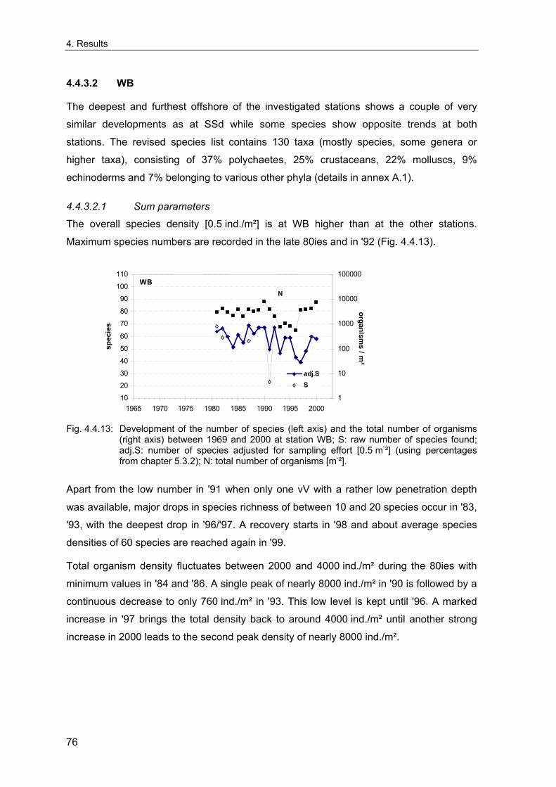
4. Results
4.4.3.2 WB
The deepest and furthest offshore of the investigated stations shows a couple of very
similar developments as at SSd while some species show opposite trends at both
stations. The revised species list contains 130 taxa (mostly species, some genera or
higher taxa), consisting of 37% polychaetes, 25% crustaceans, 22% molluscs, 9%
echinoderms and 7% belonging to various other phyla (details in annex A.1).
4.4.3.2.1 Sum parameters
The overall species density [0.5 ind./m²] is at WB higher than at the other stations.
Maximum species numbers are recorded in the late 80ies and in '92 (Fig. 4.4.13).
102030405060
708090
100110
1965 1970 1975 1980 1985 1990 1995 2000
spec
ies
1
10
100
1000
10000
100000
organisms / m
²
adj.SS
WBN
Fig. 4.4.13: Development of the number of species (left axis) and the total number of organisms
(right axis) between 1969 and 2000 at station WB; S: raw number of species found; adj.S: number of species adjusted for sampling effort [0.5 m-²] (using percentages from chapter 5.3.2); N: total number of organisms [m-²].
Apart from the low number in '91 when only one vV with a rather low penetration depth
was available, major drops in species richness of between 10 and 20 species occur in '83,
'93, with the deepest drop in '96/'97. A recovery starts in '98 and about average species
densities of 60 species are reached again in '99.
Total organism density fluctuates between 2000 and 4000 ind./m² during the 80ies with
minimum values in '84 and '86. A single peak of nearly 8000 ind./m² in '90 is followed by a
continuous decrease to only 760 ind./m² in '93. This low level is kept until '96. A marked
increase in '97 brings the total density back to around 4000 ind./m² until another strong
increase in 2000 leads to the second peak density of nearly 8000 ind./m².
76
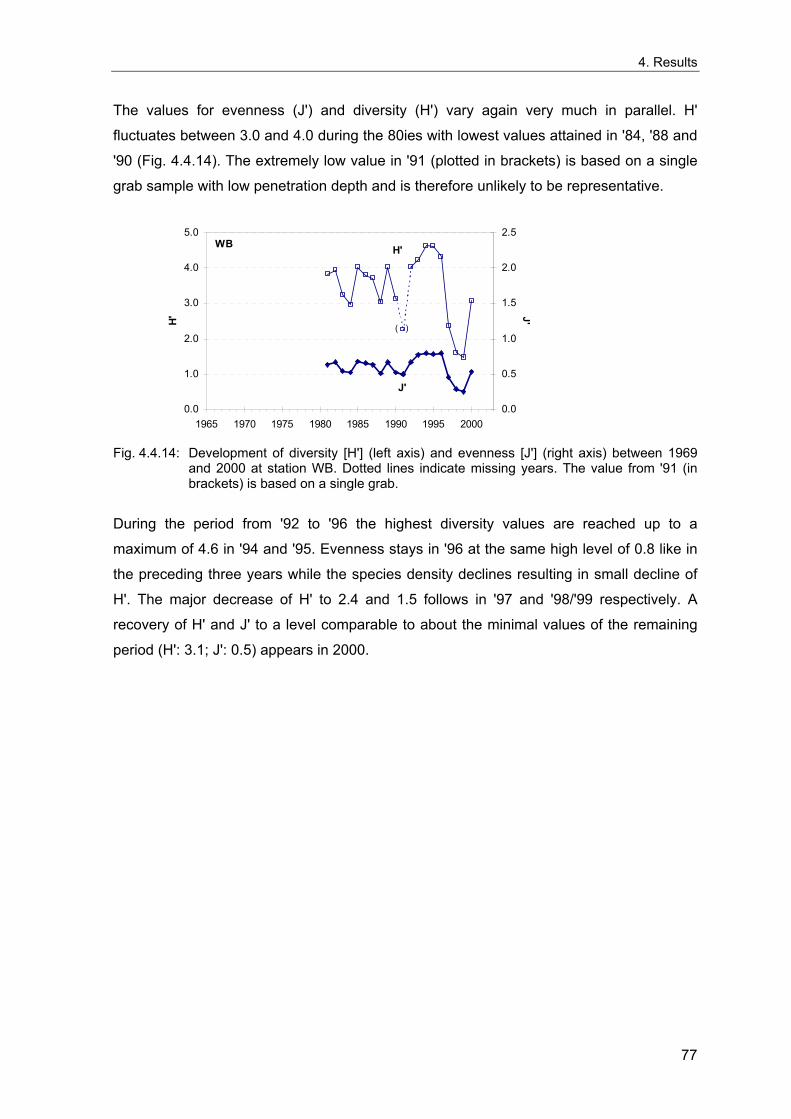
4. Results
The values for evenness (J') and diversity (H') vary again very much in parallel. H'
fluctuates between 3.0 and 4.0 during the 80ies with lowest values attained in '84, '88 and
'90 (Fig. 4.4.14). The extremely low value in '91 (plotted in brackets) is based on a single
grab sample with low penetration depth and is therefore unlikely to be representative.
0.0
1.0
2.0
3.0
4.0
5.0
1965 1970 1975 1980 1985 1990 1995 2000
H'
0.0
0.5
1.0
1.5
2.0
2.5
J'
WB
J'
H'
( )
Fig. 4.4.14: Development of diversity [H'] (left axis) and evenness [J'] (right axis) between 1969
and 2000 at station WB. Dotted lines indicate missing years. The value from '91 (in brackets) is based on a single grab.
During the period from '92 to '96 the highest diversity values are reached up to a
maximum of 4.6 in '94 and '95. Evenness stays in '96 at the same high level of 0.8 like in
the preceding three years while the species density declines resulting in small decline of
H'. The major decrease of H' to 2.4 and 1.5 follows in '97 and '98/'99 respectively. A
recovery of H' and J' to a level comparable to about the minimal values of the remaining
period (H': 3.1; J': 0.5) appears in 2000.
77
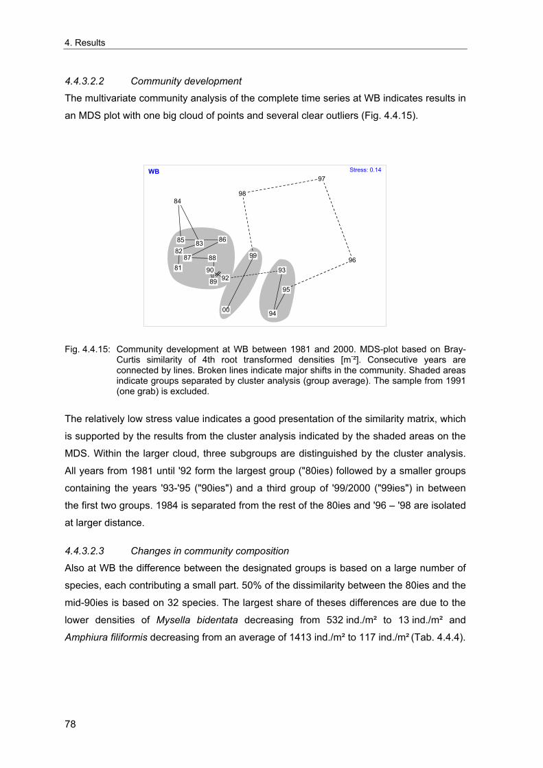
4. Results
4.4.3.2.2 Community development
The multivariate community analysis of the complete time series at WB indicates results in
an MDS plot with one big cloud of points and several clear outliers (Fig. 4.4.15).
81
82 83
84
85 86
87 88
89
90 92
93
94
95
96
97
98
99
00
Stress: 0.14WB
Fig. 4.4.15: Community development at WB between 1981 and 2000. MDS-plot based on Bray-
Curtis similarity of 4th root transformed densities [m-²]. Consecutive years are connected by lines. Broken lines indicate major shifts in the community. Shaded areas indicate groups separated by cluster analysis (group average). The sample from 1991 (one grab) is excluded.
The relatively low stress value indicates a good presentation of the similarity matrix, which
is supported by the results from the cluster analysis indicated by the shaded areas on the
MDS. Within the larger cloud, three subgroups are distinguished by the cluster analysis.
All years from 1981 until '92 form the largest group ("80ies) followed by a smaller groups
containing the years '93-'95 ("90ies") and a third group of '99/2000 ("99ies") in between
the first two groups. 1984 is separated from the rest of the 80ies and '96 – '98 are isolated
at larger distance.
4.4.3.2.3 Changes in community composition
Also at WB the difference between the designated groups is based on a large number of
species, each contributing a small part. 50% of the dissimilarity between the 80ies and the
mid-90ies is based on 32 species. The largest share of theses differences are due to the
lower densities of Mysella bidentata decreasing from 532 ind./m² to 13 ind./m² and
Amphiura filiformis decreasing from an average of 1413 ind./m² to 117 ind./m² (Tab. 4.4.4).
78
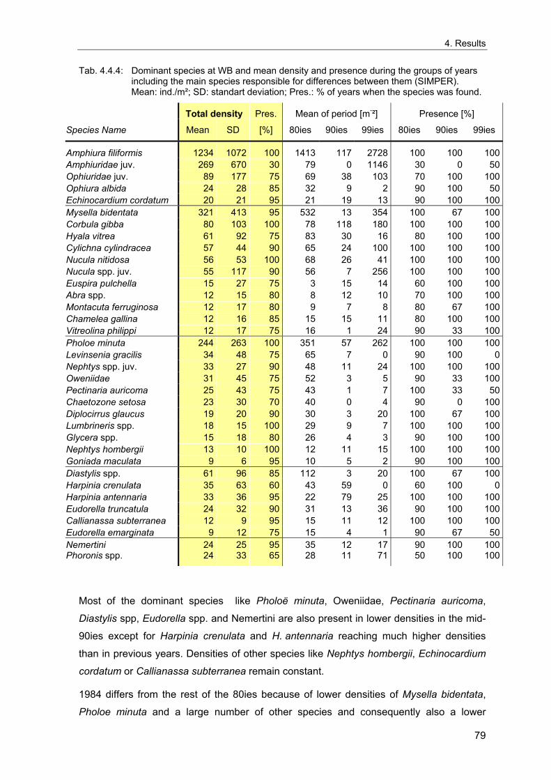
4. Results
Tab. 4.4.4: Dominant species at WB and mean density and presence during the groups of years including the main species responsible for differences between them (SIMPER). Mean: ind./m²; SD: standart deviation; Pres.: % of years when the species was found.
Total density Pres. Mean of period [m-²] Presence [%]
Species Name Mean SD [%] 80ies 90ies 99ies 80ies 90ies 99ies
Amphiura filiformis 1234 1072 100 1413 117 2728 100 100 100Amphiuridae juv. 269 670 30 79 0 1146 30 0 50Ophiuridae juv. 89 177 75 69 38 103 70 100 100Ophiura albida 24 28 85 32 9 2 90 100 50Echinocardium cordatum 20 21 95 21 19 13 90 100 100Mysella bidentata 321 413 95 532 13 354 100 67 100Corbula gibba 80 103 100 78 118 180 100 100 100Hyala vitrea 61 92 75 83 30 16 80 100 100Cylichna cylindracea 57 44 90 65 24 100 100 100 100Nucula nitidosa 56 53 100 68 26 41 100 100 100Nucula spp. juv. 55 117 90 56 7 256 100 100 100Euspira pulchella 15 27 75 3 15 14 60 100 100Abra spp. 12 15 80 8 12 10 70 100 100Montacuta ferruginosa 12 17 80 9 7 8 80 67 100Chamelea gallina 12 16 85 15 15 11 80 100 100Vitreolina philippi 12 17 75 16 1 24 90 33 100Pholoe minuta 244 263 100 351 57 262 100 100 100Levinsenia gracilis 34 48 75 65 7 0 90 100 0Nephtys spp. juv. 33 27 90 48 11 24 100 100 100Oweniidae 31 45 75 52 3 5 90 33 100Pectinaria auricoma 25 43 75 43 1 7 100 33 50Chaetozone setosa 23 30 70 40 0 4 90 0 100Diplocirrus glaucus 19 20 90 30 3 20 100 67 100Lumbrineris spp. 18 15 100 29 9 7 100 100 100Glycera spp. 15 18 80 26 4 3 90 100 100Nephtys hombergii 13 10 100 12 11 15 100 100 100Goniada maculata 9 6 95 10 5 2 90 100 100Diastylis spp. 61 96 85 112 3 20 100 67 100Harpinia crenulata 35 63 60 43 59 0 60 100 0Harpinia antennaria 33 36 95 22 79 25 100 100 100Eudorella truncatula 24 32 90 31 13 36 90 100 100Callianassa subterranea 12 9 95 15 11 12 100 100 100Eudorella emarginata 9 12 75 15 4 1 90 67 50Nemertini 24 25 95 35 12 17 90 100 100Phoronis spp. 24 33 65 28 11 71 50 100 100
Most of the dominant species like Pholoë minuta, Oweniidae, Pectinaria auricoma,
Diastylis spp, Eudorella spp. and Nemertini are also present in lower densities in the mid-
90ies except for Harpinia crenulata and H. antennaria reaching much higher densities
than in previous years. Densities of other species like Nephtys hombergii, Echinocardium
cordatum or Callianassa subterranea remain constant.
1984 differs from the rest of the 80ies because of lower densities of Mysella bidentata,
Pholoe minuta and a large number of other species and consequently also a lower
79
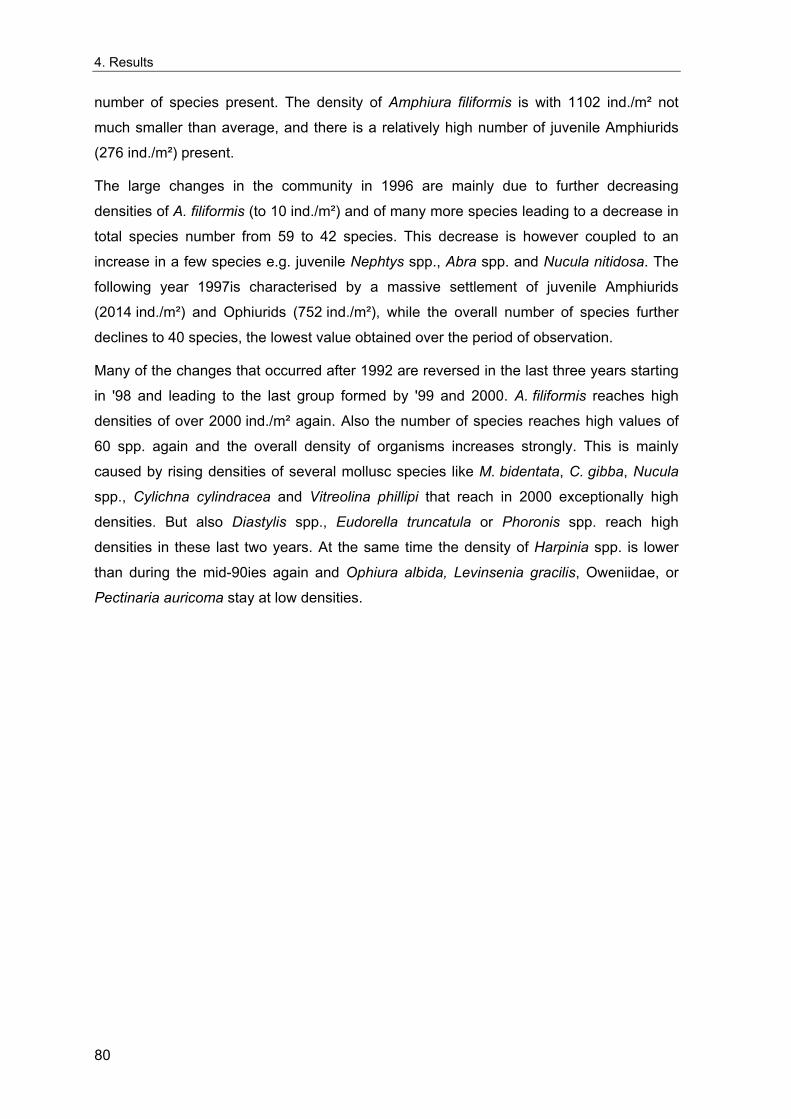
4. Results
number of species present. The density of Amphiura filiformis is with 1102 ind./m² not
much smaller than average, and there is a relatively high number of juvenile Amphiurids
(276 ind./m²) present.
The large changes in the community in 1996 are mainly due to further decreasing
densities of A. filiformis (to 10 ind./m²) and of many more species leading to a decrease in
total species number from 59 to 42 species. This decrease is however coupled to an
increase in a few species e.g. juvenile Nephtys spp., Abra spp. and Nucula nitidosa. The
following year 1997is characterised by a massive settlement of juvenile Amphiurids
(2014 ind./m²) and Ophiurids (752 ind./m²), while the overall number of species further
declines to 40 species, the lowest value obtained over the period of observation.
Many of the changes that occurred after 1992 are reversed in the last three years starting
in '98 and leading to the last group formed by '99 and 2000. A. filiformis reaches high
densities of over 2000 ind./m² again. Also the number of species reaches high values of
60 spp. again and the overall density of organisms increases strongly. This is mainly
caused by rising densities of several mollusc species like M. bidentata, C. gibba, Nucula
spp., Cylichna cylindracea and Vitreolina phillipi that reach in 2000 exceptionally high
densities. But also Diastylis spp., Eudorella truncatula or Phoronis spp. reach high
densities in these last two years. At the same time the density of Harpinia spp. is lower
than during the mid-90ies again and Ophiura albida, Levinsenia gracilis, Oweniidae, or
Pectinaria auricoma stay at low densities.
80
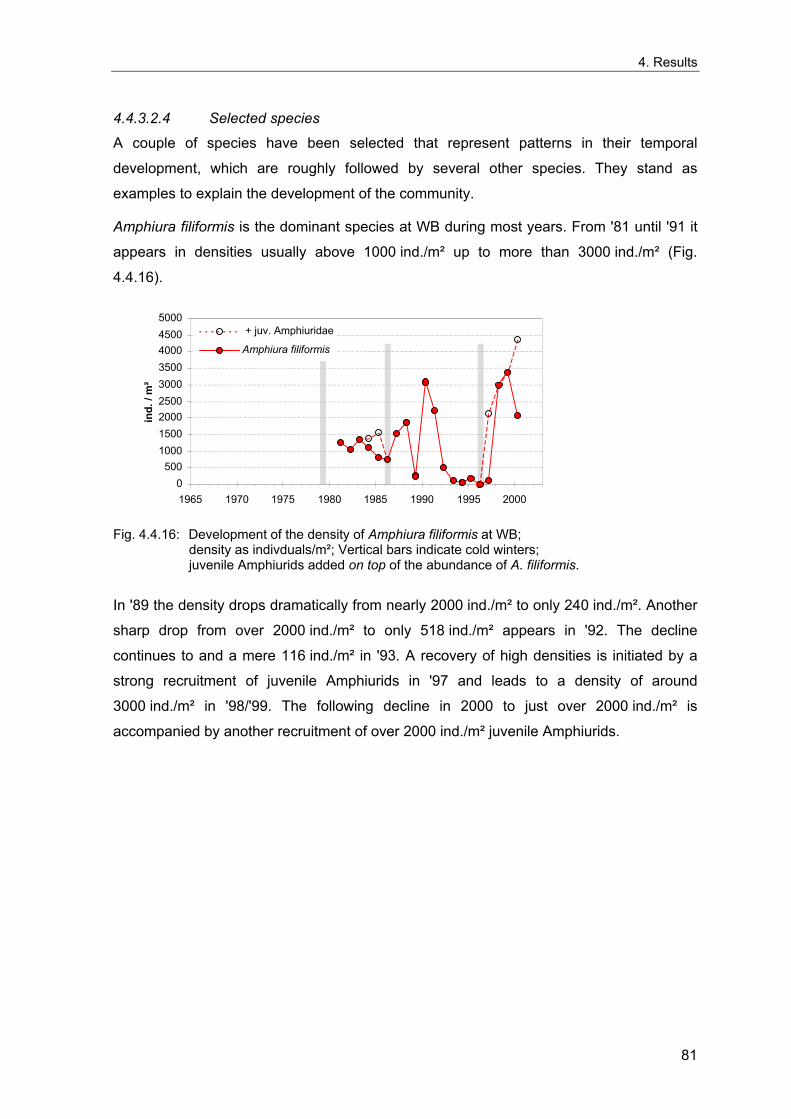
4. Results
4.4.3.2.4 Selected species
A couple of species have been selected that represent patterns in their temporal
development, which are roughly followed by several other species. They stand as
examples to explain the development of the community.
Amphiura filiformis is the dominant species at WB during most years. From '81 until '91 it
appears in densities usually above 1000 ind./m² up to more than 3000 ind./m² (Fig.
4.4.16).
ind.
/ m
²
0 500
1000 1500 2000 2500 3000 3500 4000 4500 5000
1965 1970 1975 1980 1985 1990 1995 2000
+ juv. Amphiuridae
Amphiura filiformis
Fig. 4.4.16: Development of the density of Amphiura filiformis at WB;
density as indivduals/m²; Vertical bars indicate cold winters; juvenile Amphiurids added on top of the abundance of A. filiformis.
In '89 the density drops dramatically from nearly 2000 ind./m² to only 240 ind./m². Another
sharp drop from over 2000 ind./m² to only 518 ind./m² appears in '92. The decline
continues to and a mere 116 ind./m² in '93. A recovery of high densities is initiated by a
strong recruitment of juvenile Amphiurids in '97 and leads to a density of around
3000 ind./m² in '98/'99. The following decline in 2000 to just over 2000 ind./m² is
accompanied by another recruitment of over 2000 ind./m² juvenile Amphiurids.
81
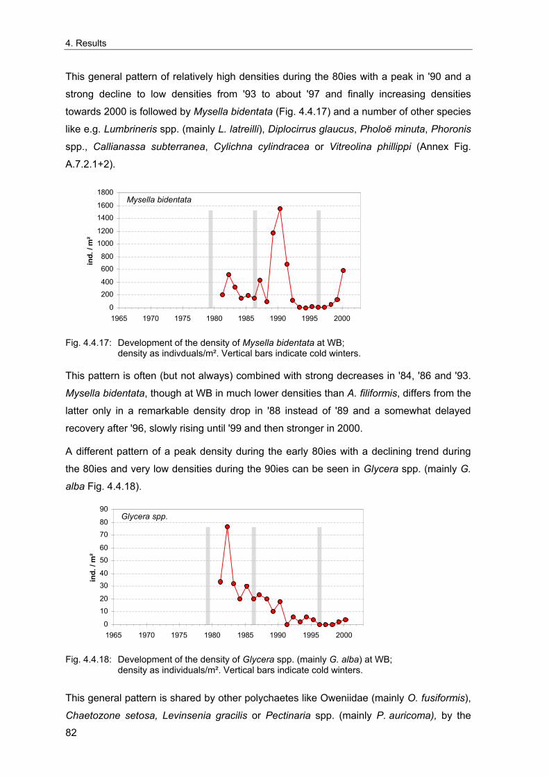
4. Results
This general pattern of relatively high densities during the 80ies with a peak in '90 and a
strong decline to low densities from '93 to about '97 and finally increasing densities
towards 2000 is followed by Mysella bidentata (Fig. 4.4.17) and a number of other species
like e.g. Lumbrineris spp. (mainly L. latreilli), Diplocirrus glaucus, Pholoë minuta, Phoronis
spp., Callianassa subterranea, Cylichna cylindracea or Vitreolina phillippi (Annex Fig.
A.7.2.1+2).
ind.
/ m
²
Mysella bidentata
0 200 400 600 800
1000 1200 1400 1600 1800
1965 1970 1975 1980 1985 1990 1995 2000
Fig. 4.4.17: Development of the density of Mysella bidentata at WB; density as indivduals/m². Vertical bars indicate cold winters.
This pattern is often (but not always) combined with strong decreases in '84, '86 and '93.
Mysella bidentata, though at WB in much lower densities than A. filiformis, differs from the
latter only in a remarkable density drop in '88 instead of '89 and a somewhat delayed
recovery after '96, slowly rising until '99 and then stronger in 2000.
A different pattern of a peak density during the early 80ies with a declining trend during
the 80ies and very low densities during the 90ies can be seen in Glycera spp. (mainly G.
alba Fig. 4.4.18).
ind.
/ m
²
Glycera spp.
0 10 20 30 40 50 60 70 80 90
1965 1970 1975 1980 1985 1990 1995 2000
Fig. 4.4.18: Development of the density of Glycera spp. (mainly G. alba) at WB; density as individuals/m². Vertical bars indicate cold winters.
This general pattern is shared by other polychaetes like Oweniidae (mainly O. fusiformis),
Chaetozone setosa, Levinsenia gracilis or Pectinaria spp. (mainly P. auricoma), by the 82
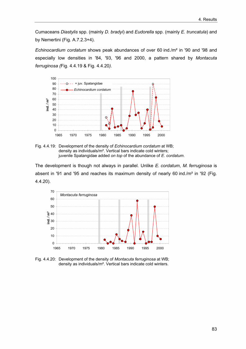
4. Results
Cumaceans Diastylis spp. (mainly D. bradyi) and Eudorella spp. (mainly E. truncatula) and
by Nemertini (Fig. A.7.2.3+4).
Echinocardium cordatum shows peak abundances of over 60 ind./m² in '90 and '98 and
especially low densities in '84, '93, '96 and 2000, a pattern shared by Montacuta
ferruginosa (Fig. 4.4.19 & Fig. 4.4.20).
ind.
/ m
²
0 10 20 30 40 50 60 70 80 90
100
1965 1970 1975 1980 1985 1990 1995 2000
+ juv. Spatangidae
Echinocardium cordatum
Fig. 4.4.19: Development of the density of Echinocardium cordatum at WB;
density as individuals/m². Vertical bars indicate cold winters; juvenile Spatangidae added on top of the abundance of E. cordatum.
The development is though not always in parallel. Unlike E. cordatum, M. ferruginosa is
absent in '91 and '95 and reaches its maximum density of nearly 60 ind./m² in '92 (Fig.
4.4.20).
Montacuta ferruginosa
0 10 20 30 40 50 60 70
1965 1970 1975 1980 1985 1990 1995 2000
ind.
/ m
²
Fig. 4.4.20: Development of the density of Montacuta ferruginosa at WB;
density as individuals/m². Vertical bars indicate cold winters.
83
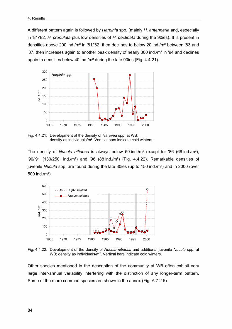
4. Results
A different pattern again is followed by Harpinia spp. (mainly H. antennaria and, especially
in '81/'82, H. crenulata plus low densities of H. pectinata during the 90ies). It is present in
densities above 200 ind./m² in '81/'82, then declines to below 20 ind./m² between '83 and
'87, then increases again to another peak density of nearly 300 ind./m² in '94 and declines
again to densities below 40 ind./m² during the late 90ies (Fig. 4.4.21).
ind.
/ m
²
Harpinia spp.
0
50
100
150
200
250
300
1965 1970 1975 1980 1985 1990 1995 2000
Fig. 4.4.21: Development of the density of Harpinia spp. at WB; density as individuals/m². Vertical bars indicate cold winters.
The density of Nucula nitidosa is always below 50 ind./m² except for '86 (66 ind./m²),
'90/'91 (130/250 ind./m²) and '96 (88 ind./m²) (Fig. 4.4.22). Remarkable densities of
juvenile Nucula spp. are found during the late 80ies (up to 150 ind./m²) and in 2000 (over
500 ind./m²).
ind.
/ m
²
0
100
200
300
400
500
600
1965 1970 1975 1980 1985 1990 1995 2000
+ juv. Nucula Nucula nitidosa
Fig. 4.4.22: Development of the density of Nucula nitidosa and additional juvenile Nucula spp. at
WB; density as individuals/m². Vertical bars indicate cold winters.
Other species mentioned in the description of the community at WB often exhibit very
large inter-annual variability interfering with the distinction of any longer-term pattern.
Some of the more common species are shown in the annex (Fig. A.7.2.5).
84
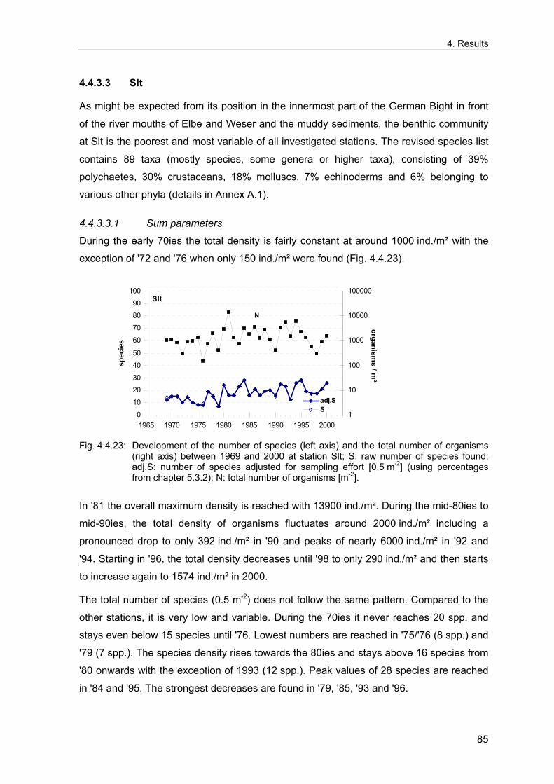
4. Results
4.4.3.3 Slt
As might be expected from its position in the innermost part of the German Bight in front
of the river mouths of Elbe and Weser and the muddy sediments, the benthic community
at Slt is the poorest and most variable of all investigated stations. The revised species list
contains 89 taxa (mostly species, some genera or higher taxa), consisting of 39%
polychaetes, 30% crustaceans, 18% molluscs, 7% echinoderms and 6% belonging to
various other phyla (details in Annex A.1).
4.4.3.3.1 Sum parameters
During the early 70ies the total density is fairly constant at around 1000 ind./m² with the
exception of '72 and '76 when only 150 ind./m² were found (Fig. 4.4.23).
01020304050
60708090
100
1965 1970 1975 1980 1985 1990 1995 2000
spec
ies
1
10
100
1000
10000
100000
organisms / m
²
adj.SS
Slt
N
Fig. 4.4.23: Development of the number of species (left axis) and the total number of organisms
(right axis) between 1969 and 2000 at station Slt; S: raw number of species found; adj.S: number of species adjusted for sampling effort [0.5 m-2] (using percentages from chapter 5.3.2); N: total number of organisms [m-2].
In '81 the overall maximum density is reached with 13900 ind./m². During the mid-80ies to
mid-90ies, the total density of organisms fluctuates around 2000 ind./m² including a
pronounced drop to only 392 ind./m² in '90 and peaks of nearly 6000 ind./m² in '92 and
'94. Starting in '96, the total density decreases until '98 to only 290 ind./m² and then starts
to increase again to 1574 ind./m² in 2000.
The total number of species (0.5 m-2) does not follow the same pattern. Compared to the
other stations, it is very low and variable. During the 70ies it never reaches 20 spp. and
stays even below 15 species until '76. Lowest numbers are reached in '75/'76 (8 spp.) and
'79 (7 spp.). The species density rises towards the 80ies and stays above 16 species from
'80 onwards with the exception of 1993 (12 spp.). Peak values of 28 species are reached
in '84 and '95. The strongest decreases are found in '79, '85, '93 and '96.
85
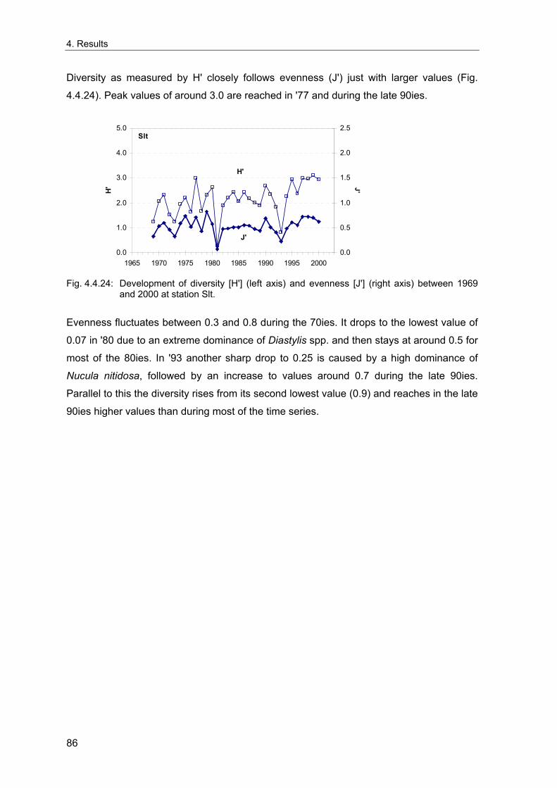
4. Results
Diversity as measured by H' closely follows evenness (J') just with larger values (Fig.
4.4.24). Peak values of around 3.0 are reached in '77 and during the late 90ies.
0.0
1.0
2.0
3.0
4.0
5.0
1965 1970 1975 1980 1985 1990 1995 2000
H'
0.0
0.5
1.0
1.5
2.0
2.5
J'
Slt
J'
H'
Fig. 4.4.24: Development of diversity [H'] (left axis) and evenness [J'] (right axis) between 1969
and 2000 at station Slt.
Evenness fluctuates between 0.3 and 0.8 during the 70ies. It drops to the lowest value of
0.07 in '80 due to an extreme dominance of Diastylis spp. and then stays at around 0.5 for
most of the 80ies. In '93 another sharp drop to 0.25 is caused by a high dominance of
Nucula nitidosa, followed by an increase to values around 0.7 during the late 90ies.
Parallel to this the diversity rises from its second lowest value (0.9) and reaches in the late
90ies higher values than during most of the time series.
86
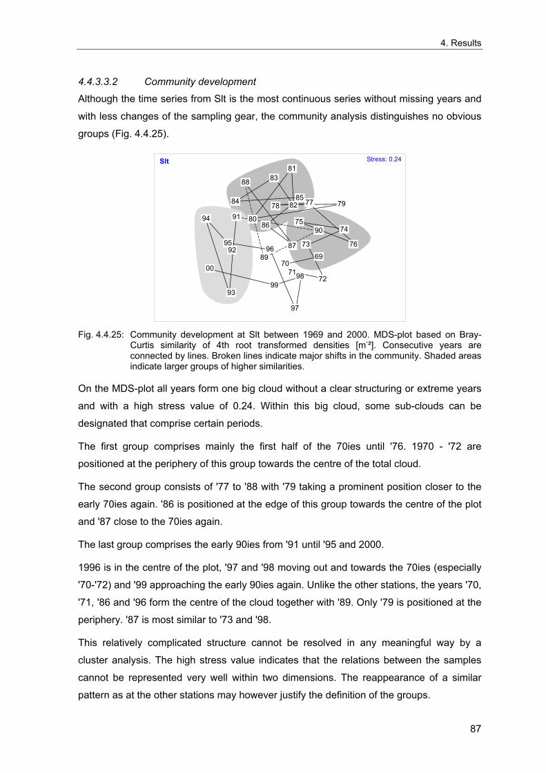
4. Results
4.4.3.3.2 Community development
Although the time series from Slt is the most continuous series without missing years and
with less changes of the sampling gear, the community analysis distinguishes no obvious
groups (Fig. 4.4.25).
6970
7172
73
7475
76
7778 79
80
81
82
83
84 85
86
87
88
89
90
91
92
93
94
9596
97
9899
00
Stress: 0.24 Slt
Fig. 4.4.25: Community development at Slt between 1969 and 2000. MDS-plot based on Bray-
Curtis similarity of 4th root transformed densities [m-²]. Consecutive years are connected by lines. Broken lines indicate major shifts in the community. Shaded areas indicate larger groups of higher similarities.
On the MDS-plot all years form one big cloud without a clear structuring or extreme years
and with a high stress value of 0.24. Within this big cloud, some sub-clouds can be
designated that comprise certain periods.
The first group comprises mainly the first half of the 70ies until '76. 1970 - '72 are
positioned at the periphery of this group towards the centre of the total cloud.
The second group consists of '77 to '88 with '79 taking a prominent position closer to the
early 70ies again. '86 is positioned at the edge of this group towards the centre of the plot
and '87 close to the 70ies again.
The last group comprises the early 90ies from '91 until '95 and 2000.
1996 is in the centre of the plot, '97 and '98 moving out and towards the 70ies (especially
'70-'72) and '99 approaching the early 90ies again. Unlike the other stations, the years '70,
'71, '86 and '96 form the centre of the cloud together with '89. Only '79 is positioned at the
periphery. '87 is most similar to '73 and '98.
This relatively complicated structure cannot be resolved in any meaningful way by a
cluster analysis. The high stress value indicates that the relations between the samples
cannot be represented very well within two dimensions. The reappearance of a similar
pattern as at the other stations may however justify the definition of the groups.
87
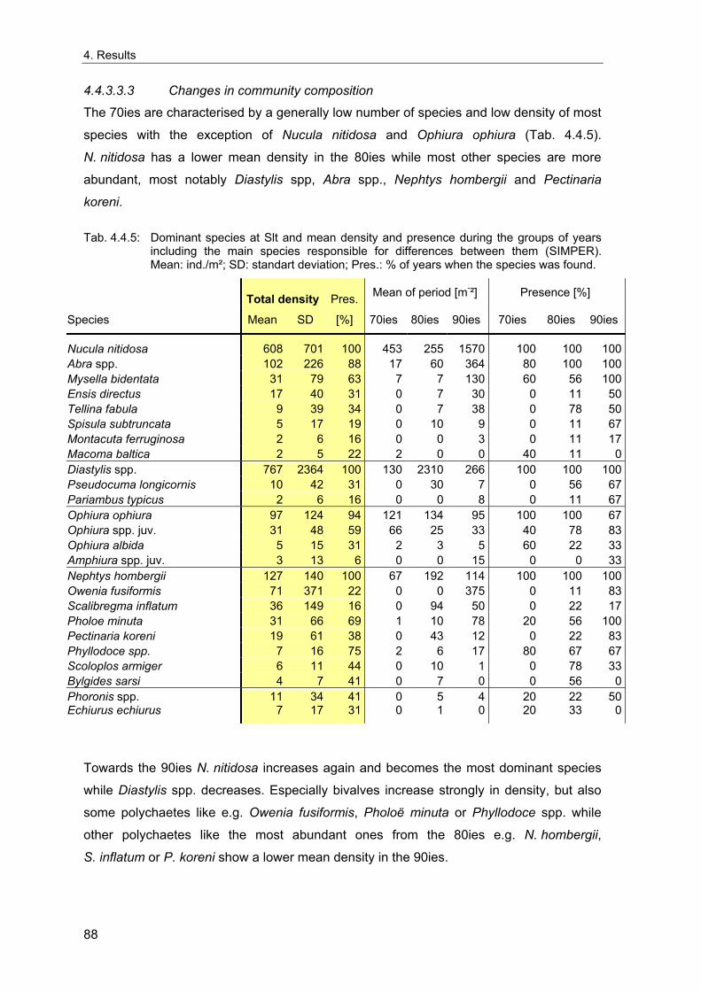
4. Results
4.4.3.3.3 Changes in community composition
The 70ies are characterised by a generally low number of species and low density of most
species with the exception of Nucula nitidosa and Ophiura ophiura (Tab. 4.4.5).
N. nitidosa has a lower mean density in the 80ies while most other species are more
abundant, most notably Diastylis spp, Abra spp., Nephtys hombergii and Pectinaria
koreni.
Tab. 4.4.5: Dominant species at Slt and mean density and presence during the groups of years including the main species responsible for differences between them (SIMPER). Mean: ind./m²; SD: standart deviation; Pres.: % of years when the species was found.
Total density Pres. Mean of period [m-²] Presence [%]
Species Mean SD [%] 70ies 80ies 90ies 70ies 80ies 90ies
Nucula nitidosa 608 701 100 453 255 1570 100 100 100Abra spp. 102 226 88 17 60 364 80 100 100Mysella bidentata 31 79 63 7 7 130 60 56 100Ensis directus 17 40 31 0 7 30 0 11 50Tellina fabula 9 39 34 0 7 38 0 78 50Spisula subtruncata 5 17 19 0 10 9 0 11 67Montacuta ferruginosa 2 6 16 0 0 3 0 11 17Macoma baltica 2 5 22 2 0 0 40 11 0Diastylis spp. 767 2364 100 130 2310 266 100 100 100Pseudocuma longicornis 10 42 31 0 30 7 0 56 67Pariambus typicus 2 6 16 0 0 8 0 11 67Ophiura ophiura 97 124 94 121 134 95 100 100 67Ophiura spp. juv. 31 48 59 66 25 33 40 78 83Ophiura albida 5 15 31 2 3 5 60 22 33Amphiura spp. juv. 3 13 6 0 0 15 0 0 33Nephtys hombergii 127 140 100 67 192 114 100 100 100Owenia fusiformis 71 371 22 0 0 375 0 11 83Scalibregma inflatum 36 149 16 0 94 50 0 22 17Pholoe minuta 31 66 69 1 10 78 20 56 100Pectinaria koreni 19 61 38 0 43 12 0 22 83Phyllodoce spp. 7 16 75 2 6 17 80 67 67Scoloplos armiger 6 11 44 0 10 1 0 78 33Bylgides sarsi 4 7 41 0 7 0 0 56 0Phoronis spp. 11 34 41 0 5 4 20 22 50Echiurus echiurus 7 17 31 0 1 0 20 33 0
Towards the 90ies N. nitidosa increases again and becomes the most dominant species
while Diastylis spp. decreases. Especially bivalves increase strongly in density, but also
some polychaetes like e.g. Owenia fusiformis, Pholoë minuta or Phyllodoce spp. while
other polychaetes like the most abundant ones from the 80ies e.g. N. hombergii,
S. inflatum or P. koreni show a lower mean density in the 90ies.
88
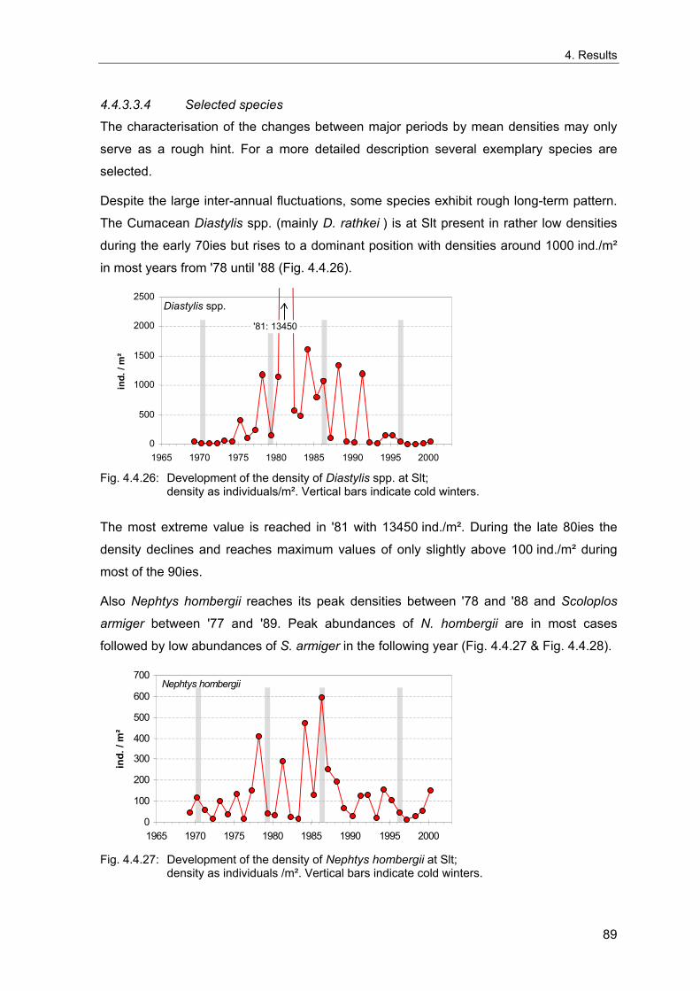
4. Results
4.4.3.3.4 Selected species
The characterisation of the changes between major periods by mean densities may only
serve as a rough hint. For a more detailed description several exemplary species are
selected.
Despite the large inter-annual fluctuations, some species exhibit rough long-term pattern.
The Cumacean Diastylis spp. (mainly D. rathkei ) is at Slt present in rather low densities
during the early 70ies but rises to a dominant position with densities around 1000 ind./m²
in most years from '78 until '88 (Fig. 4.4.26).
Diastylis spp.
0
500
1000
1500
2000
2500
1965 1970 1975 1980 1985 1990 1995 2000
'81: 13450
ind.
/ m
²
Fig. 4.4.26: Development of the density of Diastylis spp. at Slt;
density as individuals/m². Vertical bars indicate cold winters.
The most extreme value is reached in '81 with 13450 ind./m². During the late 80ies the
density declines and reaches maximum values of only slightly above 100 ind./m² during
most of the 90ies.
Also Nephtys hombergii reaches its peak densities between '78 and '88 and Scoloplos
armiger between '77 and '89. Peak abundances of N. hombergii are in most cases
followed by low abundances of S. armiger in the following year (Fig. 4.4.27 & Fig. 4.4.28).
Nephtys hombergii
0 100 200 300 400 500 600 700
1965 1970 1975 1980 1985 1990 1995 2000
ind.
/ m
²
Fig. 4.4.27: Development of the density of Nephtys hombergii at Slt;
density as individuals /m². Vertical bars indicate cold winters.
89
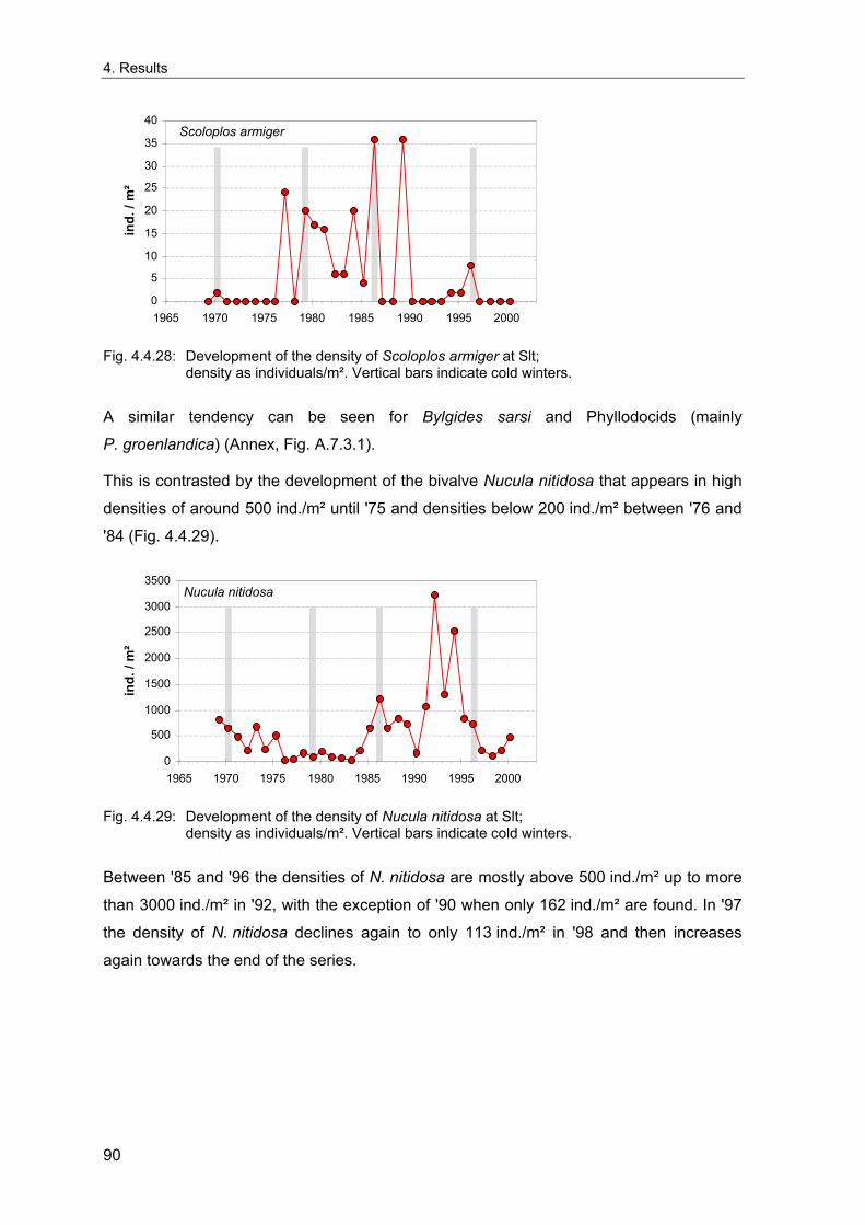
4. Results
Scoloplos armiger
0 5
10 15 20 25 30 35 40
1965 1970 1975 1980 1985 1990 1995 2000
ind.
/ m
²
Fig. 4.4.28: Development of the density of Scoloplos armiger at Slt;
density as individuals/m². Vertical bars indicate cold winters.
A similar tendency can be seen for Bylgides sarsi and Phyllodocids (mainly
P. groenlandica) (Annex, Fig. A.7.3.1).
This is contrasted by the development of the bivalve Nucula nitidosa that appears in high
densities of around 500 ind./m² until '75 and densities below 200 ind./m² between '76 and
'84 (Fig. 4.4.29).
Nucula nitidosa
0 500
1000 1500 2000 2500 3000 3500
1965 1970 1975 1980 1985 1990 1995 2000
ind.
/ m
²
Fig. 4.4.29: Development of the density of Nucula nitidosa at Slt;
density as individuals/m². Vertical bars indicate cold winters.
Between '85 and '96 the densities of N. nitidosa are mostly above 500 ind./m² up to more
than 3000 ind./m² in '92, with the exception of '90 when only 162 ind./m² are found. In '97
the density of N. nitidosa declines again to only 113 ind./m² in '98 and then increases
again towards the end of the series.
90
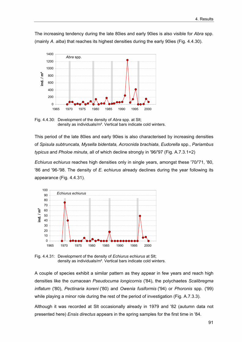
4. Results
The increasing tendency during the late 80ies and early 90ies is also visible for Abra spp.
(mainly A. alba) that reaches its highest densities during the early 90ies (Fig. 4.4.30).
Abra spp.
0 200 400 600 800
1000 1200 1400
1965 1970 1975 1980 1985 1990 1995 2000
ind.
/ m
²
Fig. 4.4.30: Development of the density of Abra spp. at Slt;
density as individuals/m². Vertical bars indicate cold winters.
This period of the late 80ies and early 90ies is also characterised by increasing densities
of Spisula subtruncata, Mysella bidentata, Acrocnida brachiata, Eudorella spp., Pariambus
typicus and Pholoe minuta, all of which decline strongly in '96/'97 (Fig. A.7.3.1+2)
Echiurus echiurus reaches high densities only in single years, amongst these '70/'71, '80,
'86 and '96-'98. The density of E. echiurus already declines during the year following its
appearance (Fig. 4.4.31).
Echiurus echiurus
0 10 20 30 40 50 60 70 80 90
100
1965 1970 1975 1980 1985 1990 1995 2000
ind.
/ m
²
Fig. 4.4.31: Development of the density of Echiurus echiurus at Slt;
density as individuals/m². Vertical bars indicate cold winters.
A couple of species exhibit a similar pattern as they appear in few years and reach high
densities like the cumacean Pseudocuma longicornis ('84), the polychaetes Scalibregma
inflatum ('80), Pectinaria koreni ('80) and Owenia fusiformis ('94) or Phoronis spp. ('99)
while playing a minor role during the rest of the period of investigation (Fig. A.7.3.3).
Although it was recorded at Slt occasionally already in 1979 and '82 (autumn data not
presented here) Ensis directus appears in the spring samples for the first time in '84.
91
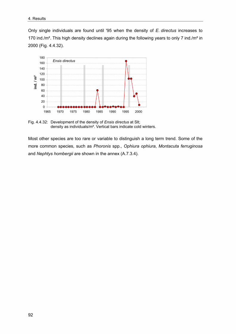
4. Results
Only single individuals are found until '95 when the density of E. directus increases to
170 ind./m². This high density declines again during the following years to only 7 ind./m² in
2000 (Fig. 4.4.32).
Ensis directus
0 20 40 60 80
100 120 140 160 180
1965 1970 1975 1980 1985 1990 1995 2000
ind.
/ m
²
Fig. 4.4.32: Development of the density of Ensis directus at Slt;
density as individuals/m². Vertical bars indicate cold winters.
Most other species are too rare or variable to distinguish a long term trend. Some of the
more common species, such as Phoronis spp., Ophiura ophiura, Montacuta ferruginosa
and Nephtys hombergii are shown in the annex (A.7.3.4).
92
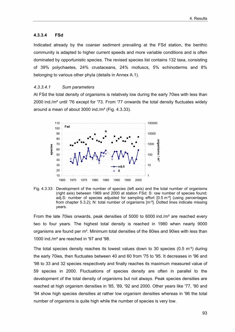
4. Results
4.3.3.4 FSd
Indicated already by the coarser sediment prevailing at the FSd station, the benthic
community is adapted to higher current speeds and more variable conditions and is often
dominated by opportunistic species. The revised species list contains 132 taxa, consisting
of 39% polychaetes, 24% crustaceans, 24% molluscs, 5% echinoderms and 8%
belonging to various other phyla (details in Annex A.1).
4.3.3.4.1 Sum parameters
At FSd the total density of organisms is relatively low during the early 70ies with less than
2000 ind./m² until '76 except for '73. From '77 onwards the total density fluctuates widely
around a mean of about 3000 ind./m² (Fig. 4.3.33).
102030405060
708090
100110
1965 1970 1975 1980 1985 1990 1995 2000
spec
ies
1
10
100
1000
10000
100000
organisms / m
²
adj.SS
FsdN
Fig. 4.3.33: Development of the number of species (left axis) and the total number of organisms
(right axis) between 1969 and 2000 at station FSd; S: raw number of species found; adj.S: number of species adjusted for sampling effort [0.5 m-²] (using percentages from chapter 5.3.2); N: total number of organisms [m-²]. Dotted lines indicate missing years.
From the late 70ies onwards, peak densities of 5000 to 6000 ind./m² are reached every
two to four years. The highest total density is reached in 1980 when nearly 9000
organisms are found per m². Minimum total densities of the 80ies and 90ies with less than
1000 ind./m² are reached in '97 and '98.
The total species density reaches its lowest values down to 30 species (0.5 m-²) during
the early 70ies, then fluctuates between 40 and 60 from '75 to '95. It decreases in '96 and
'98 to 33 and 32 species respectively and finally reaches its maximum measured value of
59 species in 2000. Fluctuations of species density are often in parallel to the
development of the total density of organisms but not always. Peak species densities are
reached at high organism densities in '85, '89, '92 and 2000. Other years like '77, '90 and
'94 show high species densities at rather low organism densities whereas in '96 the total
number of organisms is quite high while the number of species is very low.
93
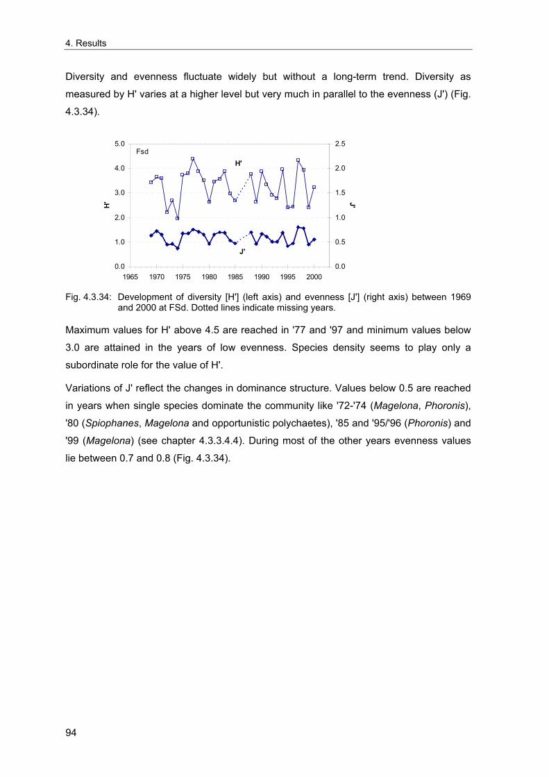
4. Results
Diversity and evenness fluctuate widely but without a long-term trend. Diversity as
measured by H' varies at a higher level but very much in parallel to the evenness (J') (Fig.
4.3.34).
0.0
1.0
2.0
3.0
4.0
5.0
1965 1970 1975 1980 1985 1990 1995 2000
H'
0.0
0.5
1.0
1.5
2.0
2.5
J'
Fsd
J'
H'
Fig. 4.3.34: Development of diversity [H'] (left axis) and evenness [J'] (right axis) between 1969
and 2000 at FSd. Dotted lines indicate missing years.
Maximum values for H' above 4.5 are reached in '77 and '97 and minimum values below
3.0 are attained in the years of low evenness. Species density seems to play only a
subordinate role for the value of H'.
Variations of J' reflect the changes in dominance structure. Values below 0.5 are reached
in years when single species dominate the community like '72-'74 (Magelona, Phoronis),
'80 (Spiophanes, Magelona and opportunistic polychaetes), '85 and '95/'96 (Phoronis) and
'99 (Magelona) (see chapter 4.3.3.4.4). During most of the other years evenness values
lie between 0.7 and 0.8 (Fig. 4.3.34).
94
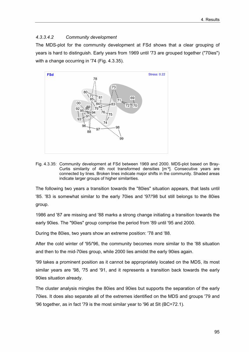
4. Results
4.3.3.4.2 Community development
The MDS-plot for the community development at FSd shows that a clear grouping of
years is hard to distinguish. Early years from 1969 until '73 are grouped together ("70ies")
with a change occurring in '74 (Fig. 4.3.35).
69
7071
72
73
74
7576
77
78
79
80 81
82 8384
85
88
89 90
91
92
93
94 95
96 97 98
Stress: 0.22 FSd
00
99
Fig. 4.3.35: Community development at FSd between 1969 and 2000. MDS-plot based on Bray-
Curtis similarity of 4th root transformed densities [m-²]. Consecutive years are connected by lines. Broken lines indicate major shifts in the community. Shaded areas indicate larger groups of higher similarities.
The following two years a transition towards the "80ies" situation appears, that lasts until
'85. '83 is somewhat similar to the early 70ies and '97/'98 but still belongs to the 80ies
group.
1986 and '87 are missing and '88 marks a strong change initiating a transition towards the
early 90ies. The "90ies" group comprise the period from '89 until '95 and 2000.
During the 80ies, two years show an extreme position: '78 and '88.
After the cold winter of '95/'96, the community becomes more similar to the '88 situation
and then to the mid-70ies group, while 2000 lies amidst the early 90ies again.
'99 takes a prominent position as it cannot be appropriately located on the MDS, its most
similar years are '98, '75 and '91, and it represents a transition back towards the early
90ies situation already.
The cluster analysis mingles the 80ies and 90ies but supports the separation of the early
70ies. It does also separate all of the extremes identified on the MDS and groups '79 and
'96 together, as in fact '79 is the most similar year to '96 at Slt (BC=72.1).
95
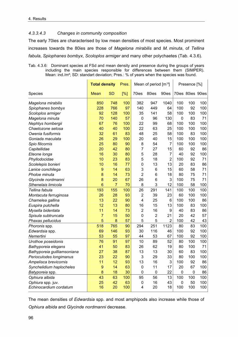
4. Results
4.3.3.4.3 Changes in community composition
The early 70ies are characterised by low mean densities of most species. Most prominent
increases towards the 80ies are those of Magelona mirabilis and M. minuta, of Tellina
fabula, Spiophanes bombyx, Scoloplos armiger and many other polychaetes (Tab. 4.3.6).
Tab. 4.3.6: Dominant species at FSd and mean density and presence during the groups of years including the main species responsible for differences between them (SIMPER). Mean: ind./m²; SD: standart deviation; Pres.: % of years when the species was found.
Total density Pres. Mean of period [m-²] Presence [%]
Species Mean SD [%] 70ies 80ies 90ies 70ies 80ies 90ies
Magelona mirabilis 850 748 100 382 947 1040 100 100 100Spiophanes bombyx 228 766 97 140 449 64 100 92 100Scoloplos armiger 92 128 100 35 141 58 100 100 100Magelona minuta 70 140 57 0 96 130 0 83 71Nephtys hombergii 67 76 100 22 99 68 100 100 100Chaetozone setosa 40 40 100 22 63 25 100 100 100Owenia fusiformis 32 61 83 48 25 58 100 83 100Goniada maculata 26 29 100 20 40 15 100 100 100Spio filicornis 25 80 90 8 54 7 100 100 100Capitellidae 20 42 80 7 27 15 60 92 86Eteone longa 16 30 80 5 28 7 40 92 100Phyllodocidae 10 23 83 5 18 2 100 92 71Scolelepis bonieri 10 16 77 0 13 13 20 83 86Lanice conchilega 9 14 63 3 6 15 60 58 71Pholoe minuta 8 14 73 2 6 18 80 75 71Glycinde nordmanni 8 20 67 26 6 3 100 75 71Sthenelais limicola 6 7 70 8 3 12 100 58 100Tellina fabula 193 155 100 26 291 141 100 100 100Montacuta ferruginosa 26 28 93 2 39 23 60 100 100Chamelea gallina 13 22 90 4 25 6 100 100 86Euspira pulchella 12 13 80 16 15 13 100 83 100Mysella bidentata 11 14 73 2 16 9 40 83 86Spisula subtruncata 7 15 50 0 2 21 20 42 57Phaxas pellucidus 5 8 57 5 5 2 100 42 43Phoronis spp. 518 765 90 294 251 1123 80 83 100Edwardsia spp. 69 146 93 30 116 46 100 92 100Nemertini 53 55 97 44 53 67 100 92 100Urothoe poseidonis 76 91 97 10 89 52 80 100 100Bathyporeia elegans 41 50 83 26 62 19 80 100 71Bathyporeia guilliamsoniana 27 38 87 13 13 30 60 83 100Perioculodes longimanus 23 22 90 3 29 33 80 100 100Ampelisca brevicornis 11 12 93 13 16 3 100 92 86Synchelidium haplocheles 9 14 63 0 11 17 20 67 100Batyporeia spp. 8 18 30 0 0 22 0 0 86Ophiura albida 43 63 100 95 56 13 100 100 100Ophiura spp. juv. 25 42 63 0 16 43 0 50 100Echinocardium cordatum 16 20 100 4 20 18 100 100 100
The mean densities of Edwardsia spp. and most amphipods also increase while those of
Ophiura albida and Glycinde nordmanni decrease.
96
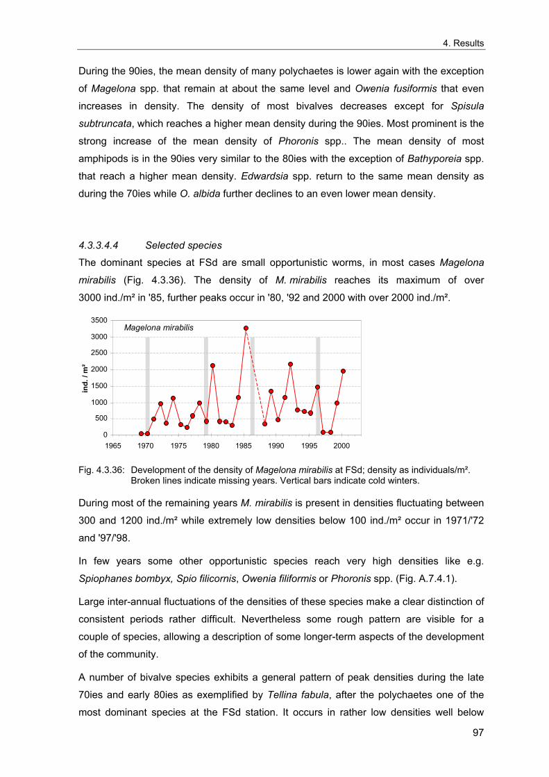
4. Results
During the 90ies, the mean density of many polychaetes is lower again with the exception
of Magelona spp. that remain at about the same level and Owenia fusiformis that even
increases in density. The density of most bivalves decreases except for Spisula
subtruncata, which reaches a higher mean density during the 90ies. Most prominent is the
strong increase of the mean density of Phoronis spp.. The mean density of most
amphipods is in the 90ies very similar to the 80ies with the exception of Bathyporeia spp.
that reach a higher mean density. Edwardsia spp. return to the same mean density as
during the 70ies while O. albida further declines to an even lower mean density.
4.3.3.4.4 Selected species
The dominant species at FSd are small opportunistic worms, in most cases Magelona
mirabilis (Fig. 4.3.36). The density of M. mirabilis reaches its maximum of over
3000 ind./m² in '85, further peaks occur in '80, '92 and 2000 with over 2000 ind./m².
Magelona mirabilis
0 500
1000 1500 2000 2500 3000 3500
1965 1970 1975 1980 1985 1990 1995 2000
ind.
/ m
²
Fig. 4.3.36: Development of the density of Magelona mirabilis at FSd; density as individuals/m².
Broken lines indicate missing years. Vertical bars indicate cold winters.
During most of the remaining years M. mirabilis is present in densities fluctuating between
300 and 1200 ind./m² while extremely low densities below 100 ind./m² occur in 1971/'72
and '97/'98.
In few years some other opportunistic species reach very high densities like e.g.
Spiophanes bombyx, Spio filicornis, Owenia filiformis or Phoronis spp. (Fig. A.7.4.1).
Large inter-annual fluctuations of the densities of these species make a clear distinction of
consistent periods rather difficult. Nevertheless some rough pattern are visible for a
couple of species, allowing a description of some longer-term aspects of the development
of the community.
A number of bivalve species exhibits a general pattern of peak densities during the late
70ies and early 80ies as exemplified by Tellina fabula, after the polychaetes one of the
most dominant species at the FSd station. It occurs in rather low densities well below
97
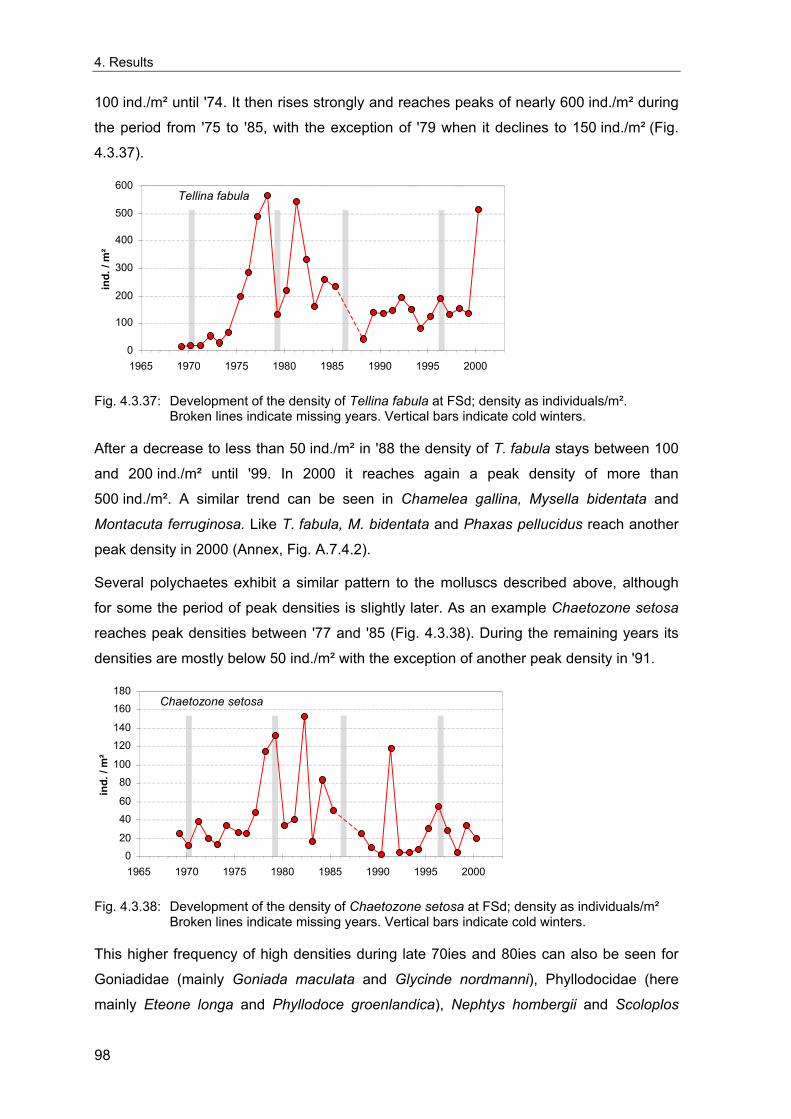
4. Results
100 ind./m² until '74. It then rises strongly and reaches peaks of nearly 600 ind./m² during
the period from '75 to '85, with the exception of '79 when it declines to 150 ind./m² (Fig.
4.3.37).
Tellina fabula
0
100
200
300
400
500
600
1965 1970 1975 1980 1985 1990 1995 2000
ind.
/ m
²
Fig. 4.3.37: Development of the density of Tellina fabula at FSd; density as individuals/m².
Broken lines indicate missing years. Vertical bars indicate cold winters.
After a decrease to less than 50 ind./m² in '88 the density of T. fabula stays between 100
and 200 ind./m² until '99. In 2000 it reaches again a peak density of more than
500 ind./m². A similar trend can be seen in Chamelea gallina, Mysella bidentata and
Montacuta ferruginosa. Like T. fabula, M. bidentata and Phaxas pellucidus reach another
peak density in 2000 (Annex, Fig. A.7.4.2).
Several polychaetes exhibit a similar pattern to the molluscs described above, although
for some the period of peak densities is slightly later. As an example Chaetozone setosa
reaches peak densities between '77 and '85 (Fig. 4.3.38). During the remaining years its
densities are mostly below 50 ind./m² with the exception of another peak density in '91.
Chaetozone setosa
0 20 40 60 80
100 120 140 160 180
1965 1970 1975 1980 1985 1990 1995 2000
ind.
/ m
²
Fig. 4.3.38: Development of the density of Chaetozone setosa at FSd; density as individuals/m²
Broken lines indicate missing years. Vertical bars indicate cold winters.
This higher frequency of high densities during late 70ies and 80ies can also be seen for
Goniadidae (mainly Goniada maculata and Glycinde nordmanni), Phyllodocidae (here
mainly Eteone longa and Phyllodoce groenlandica), Nephtys hombergii and Scoloplos
98
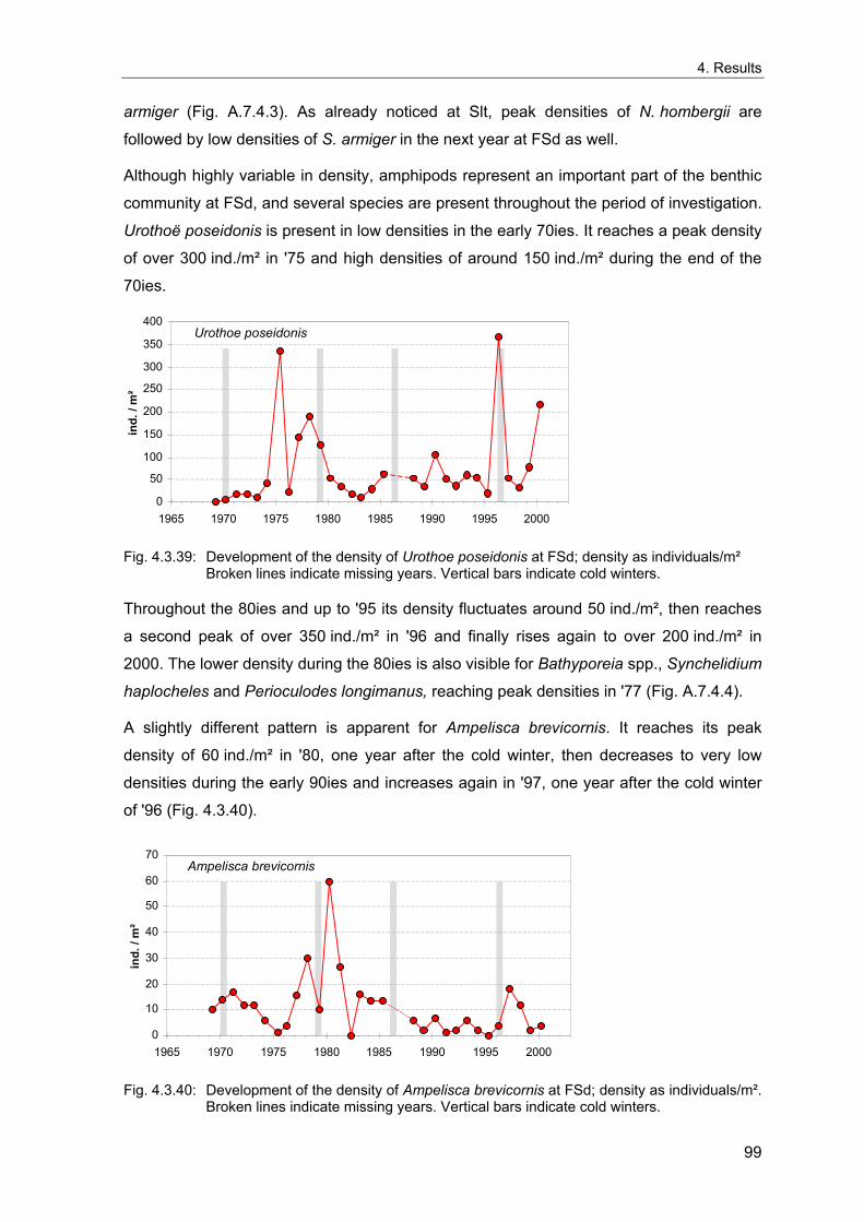
4. Results
armiger (Fig. A.7.4.3). As already noticed at Slt, peak densities of N. hombergii are
followed by low densities of S. armiger in the next year at FSd as well.
Although highly variable in density, amphipods represent an important part of the benthic
community at FSd, and several species are present throughout the period of investigation.
Urothoë poseidonis is present in low densities in the early 70ies. It reaches a peak density
of over 300 ind./m² in '75 and high densities of around 150 ind./m² during the end of the
70ies.
Urothoe poseidonis
0 50
100 150 200 250 300 350 400
1965 1970 1975 1980 1985 1990 1995 2000
ind.
/ m
²
Fig. 4.3.39: Development of the density of Urothoe poseidonis at FSd; density as individuals/m²
Broken lines indicate missing years. Vertical bars indicate cold winters.
Throughout the 80ies and up to '95 its density fluctuates around 50 ind./m², then reaches
a second peak of over 350 ind./m² in '96 and finally rises again to over 200 ind./m² in
2000. The lower density during the 80ies is also visible for Bathyporeia spp., Synchelidium
haplocheles and Perioculodes longimanus, reaching peak densities in '77 (Fig. A.7.4.4).
A slightly different pattern is apparent for Ampelisca brevicornis. It reaches its peak
density of 60 ind./m² in '80, one year after the cold winter, then decreases to very low
densities during the early 90ies and increases again in '97, one year after the cold winter
of '96 (Fig. 4.3.40).
Ampelisca brevicornis
0 10 20 30 40 50 60 70
1965 1970 1975 1980 1985 1990 1995 2000
ind.
/ m
²
Fig. 4.3.40: Development of the density of Ampelisca brevicornis at FSd; density as individuals/m².
Broken lines indicate missing years. Vertical bars indicate cold winters.
99
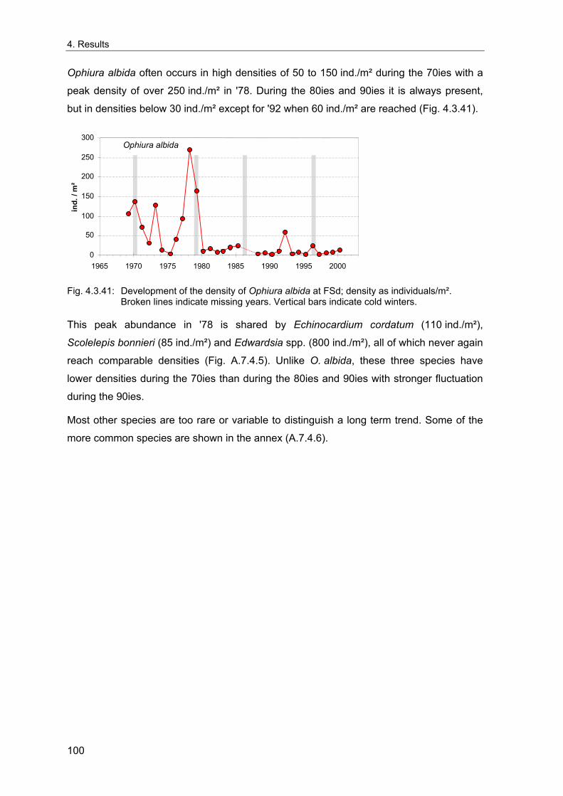
4. Results
Ophiura albida often occurs in high densities of 50 to 150 ind./m² during the 70ies with a
peak density of over 250 ind./m² in '78. During the 80ies and 90ies it is always present,
but in densities below 30 ind./m² except for '92 when 60 ind./m² are reached (Fig. 4.3.41).
Ophiura albida
0
50
100
150
200
250
300
1965 1970 1975 1980 1985 1990 1995 2000
ind.
/ m
²
Fig. 4.3.41: Development of the density of Ophiura albida at FSd; density as individuals/m².
Broken lines indicate missing years. Vertical bars indicate cold winters.
This peak abundance in '78 is shared by Echinocardium cordatum (110 ind./m²),
Scolelepis bonnieri (85 ind./m²) and Edwardsia spp. (800 ind./m²), all of which never again
reach comparable densities (Fig. A.7.4.5). Unlike O. albida, these three species have
lower densities during the 70ies than during the 80ies and 90ies with stronger fluctuation
during the 90ies.
Most other species are too rare or variable to distinguish a long term trend. Some of the
more common species are shown in the annex (A.7.4.6).
100
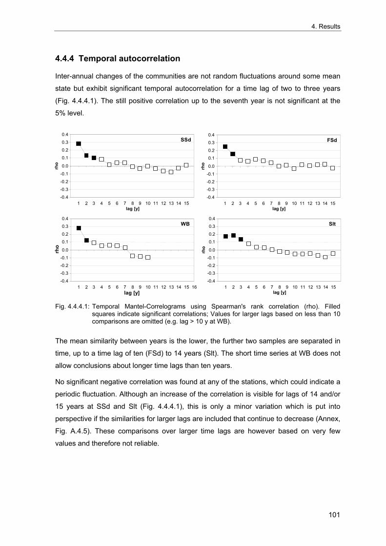
4. Results
4.4.4 Temporal autocorrelation
Inter-annual changes of the communities are not random fluctuations around some mean
state but exhibit significant temporal autocorrelation for a time lag of two to three years
(Fig. 4.4.4.1). The still positive correlation up to the seventh year is not significant at the
5% level.
SSd
-0.4 -0.3 -0.2 -0.1 0.0 0.1 0.2 0.3 0.4
1 2 3 4 5 6 7 8 9 10 11 12 13 14 15lag [y]
rho
FSd
-0.4
-0.3
-0.2-0.1
0.0
0.1
0.2
0.3
0.4
1 2 3 4 5 6 7 8 9 10 11 12 13 14 15lag [y]
rho
WB
-0.4 -0.3 -0.2 -0.1 0.0 0.1 0.2 0.3
1 2 3 4 5 6 7 8 9 10 11 12 13 14 15 16lag [y]
rho
0.4 Slt
-0.4
-0.3
-0.2-0.1
0.0
0.1
0.2
0.3
1 2 3 4 5 6 7 8 9 10 11 12 13 14 15lag [y]
rho
0.4
Fig. 4.4.4.1: Temporal Mantel-Correlograms using Spearman's rank correlation (rho). Filled
squares indicate significant correlations; Values for larger lags based on less than 10 comparisons are omitted (e.g. lag > 10 y at WB).
The mean similarity between years is the lower, the further two samples are separated in
time, up to a time lag of ten (FSd) to 14 years (Slt). The short time series at WB does not
allow conclusions about longer time lags than ten years.
No significant negative correlation was found at any of the stations, which could indicate a
periodic fluctuation. Although an increase of the correlation is visible for lags of 14 and/or
15 years at SSd and Slt (Fig. 4.4.4.1), this is only a minor variation which is put into
perspective if the similarities for larger lags are included that continue to decrease (Annex,
Fig. A.4.5). These comparisons over larger time lags are however based on very few
values and therefore not reliable.
101
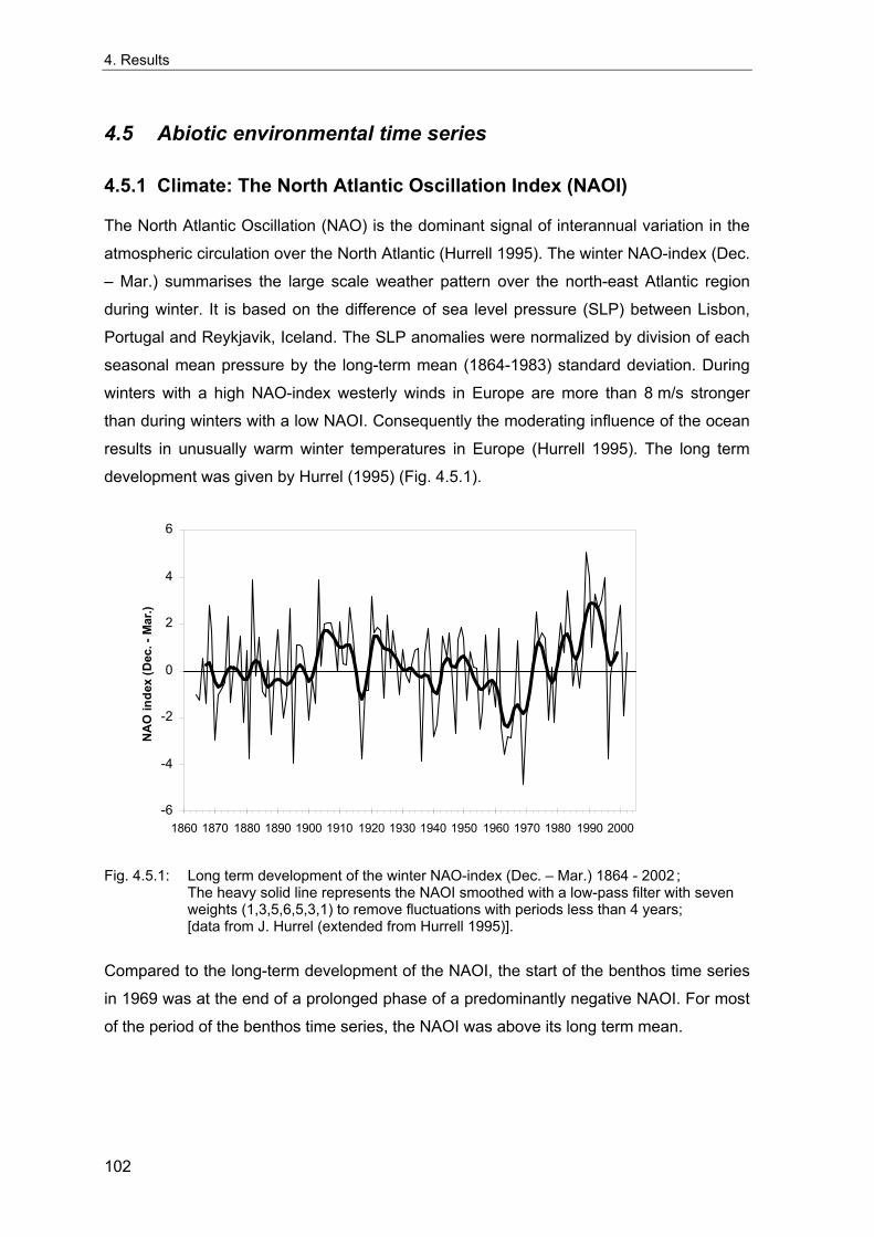
4. Results
4.5 Abiotic environmental time series
4.5.1 Climate: The North Atlantic Oscillation Index (NAOI)
The North Atlantic Oscillation (NAO) is the dominant signal of interannual variation in the
atmospheric circulation over the North Atlantic (Hurrell 1995). The winter NAO-index (Dec.
– Mar.) summarises the large scale weather pattern over the north-east Atlantic region
during winter. It is based on the difference of sea level pressure (SLP) between Lisbon,
Portugal and Reykjavik, Iceland. The SLP anomalies were normalized by division of each
seasonal mean pressure by the long-term mean (1864-1983) standard deviation. During
winters with a high NAO-index westerly winds in Europe are more than 8 m/s stronger
than during winters with a low NAOI. Consequently the moderating influence of the ocean
results in unusually warm winter temperatures in Europe (Hurrell 1995). The long term
development was given by Hurrel (1995) (Fig. 4.5.1).
-6
-4
-2
0
2
4
6
1860 1870 1880 1890 1900 1910 1920 1930 1940 1950 1960 1970 1980 1990 2000
NA
O in
dex
(Dec
. - M
ar.)
Fig. 4.5.1: Long term development of the winter NAO-index (Dec. – Mar.) 1864 - 2002 ;
The heavy solid line represents the NAOI smoothed with a low-pass filter with seven weights (1,3,5,6,5,3,1) to remove fluctuations with periods less than 4 years; [data from J. Hurrel (extended from Hurrell 1995)].
Compared to the long-term development of the NAOI, the start of the benthos time series
in 1969 was at the end of a prolonged phase of a predominantly negative NAOI. For most
of the period of the benthos time series, the NAOI was above its long term mean.
102
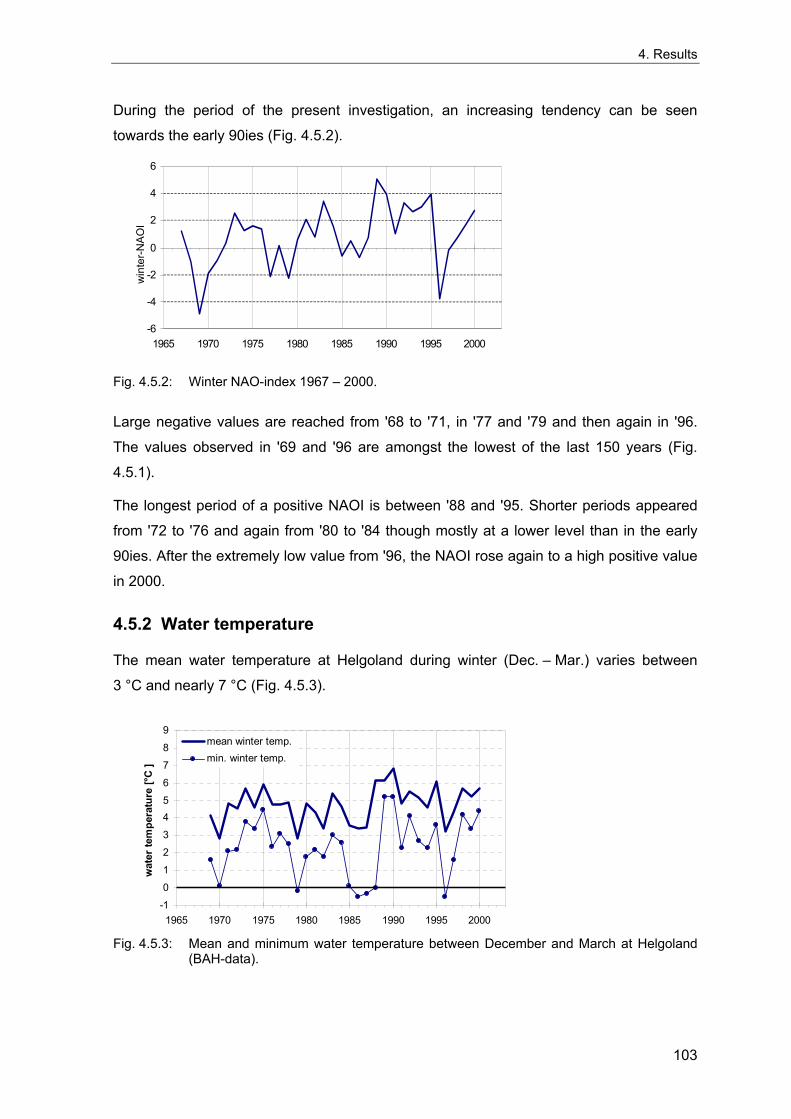
4. Results
During the period of the present investigation, an increasing tendency can be seen
towards the early 90ies (Fig. 4.5.2).
win
ter-N
AOI
-6
-4
-2
0
2
4
6
1965 1970 1975 1980 1985 1990 1995 2000
Fig. 4.5.2: Winter NAO-index 1967 – 2000.
Large negative values are reached from '68 to '71, in '77 and '79 and then again in '96.
The values observed in '69 and '96 are amongst the lowest of the last 150 years (Fig.
4.5.1).
The longest period of a positive NAOI is between '88 and '95. Shorter periods appeared
from '72 to '76 and again from '80 to '84 though mostly at a lower level than in the early
90ies. After the extremely low value from '96, the NAOI rose again to a high positive value
in 2000.
4.5.2 Water temperature
The mean water temperature at Helgoland during winter (Dec. – Mar.) varies between
3 °C and nearly 7 °C (Fig. 4.5.3).
-10123456789
1965 1970 1975 1980 1985 1990 1995 2000
wat
er te
mpe
ratu
re [°
C ]
mean winter temp.min. winter temp.
Fig. 4.5.3: Mean and minimum water temperature between December and March at Helgoland
(BAH-data).
103
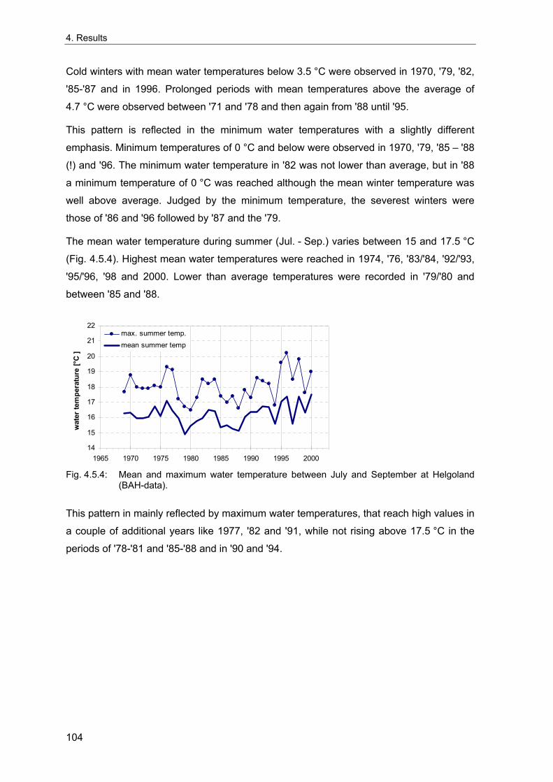
4. Results
Cold winters with mean water temperatures below 3.5 °C were observed in 1970, '79, '82,
'85-'87 and in 1996. Prolonged periods with mean temperatures above the average of
4.7 °C were observed between '71 and '78 and then again from '88 until '95.
This pattern is reflected in the minimum water temperatures with a slightly different
emphasis. Minimum temperatures of 0 °C and below were observed in 1970, '79, '85 – '88
(!) and '96. The minimum water temperature in '82 was not lower than average, but in '88
a minimum temperature of 0 °C was reached although the mean winter temperature was
well above average. Judged by the minimum temperature, the severest winters were
those of '86 and '96 followed by '87 and the '79.
The mean water temperature during summer (Jul. - Sep.) varies between 15 and 17.5 °C
(Fig. 4.5.4). Highest mean water temperatures were reached in 1974, '76, '83/'84, '92/'93,
'95/'96, '98 and 2000. Lower than average temperatures were recorded in '79/'80 and
between '85 and '88.
14
15
16
17
18
19
20
21
22
1965 1970 1975 1980 1985 1990 1995 2000
wat
er te
mpe
ratu
re [°
C ]
max. summer temp.mean summer temp
Fig. 4.5.4: Mean and maximum water temperature between July and September at Helgoland
(BAH-data).
This pattern in mainly reflected by maximum water temperatures, that reach high values in
a couple of additional years like 1977, '82 and '91, while not rising above 17.5 °C in the
periods of '78-'81 and '85-'88 and in '90 and '94.
104
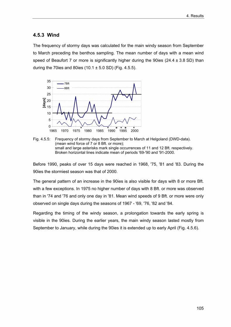
4. Results
4.5.3 Wind
The frequency of stormy days was calculated for the main windy season from September
to March preceding the benthos sampling. The mean number of days with a mean wind
speed of Beaufort 7 or more is significantly higher during the 90ies (24.4 ± 3.8 SD) than
during the 70ies and 80ies (10.1 ± 5.0 SD) (Fig. 4.5.5).
0
5
10
15
20
25
30
35
1965 1970 1975 1980 1985 1990 1995 2000
[day
s]
7Bft8Bft
* * * * * *
Fig. 4.5.5: Frequency of stormy days from September to March at Helgoland (DWD-data). (mean wind force of 7 or 8 Bft. or more); small and large asterisks mark single occurrences of 11 and 12 Bft. respectively. Broken horizontal lines indicate mean of periods '69-'90 and '91-2000.
Before 1990, peaks of over 15 days were reached in 1968, '75, '81 and '83. During the
90ies the stormiest season was that of 2000.
The general pattern of an increase in the 90ies is also visible for days with 8 or more Bft.
with a few exceptions. In 1975 no higher number of days with 8 Bft. or more was observed
than in '74 and '76 and only one day in '81. Mean wind speeds of 9 Bft. or more were only
observed on single days during the seasons of 1967 - '69, '76, '82 and '84.
Regarding the timing of the windy season, a prolongation towards the early spring is
visible in the 90ies. During the earlier years, the main windy season lasted mostly from
September to January, while during the 90ies it is extended up to early April (Fig. 4.5.6).
105
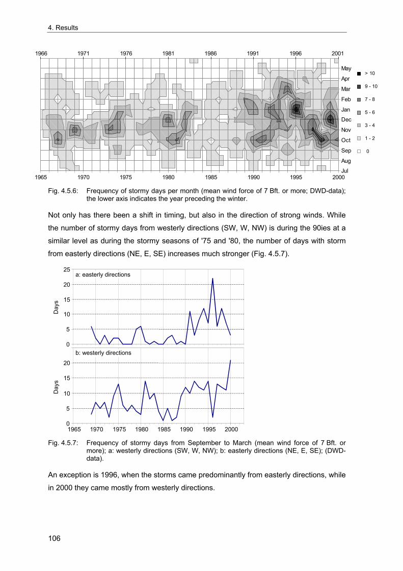
4. Results
1965 1970 1975 1980 1985 1990 1995 2000Jul
Aug
Sep
Oct
Nov
Dec
Jan
Feb
Mar
Apr
May10.5-12
8.5-10.5
6.5-8.5
4.5-6.5
2.5-4.5
0.5-2.5
-1.5-0.5 0
1966 1971 1976 1981 1986 1991 1996 2001
0
1 - 2
3 - 4
5 - 6
7 - 8
9 - 10
> 10
Fig. 4.5.6: Frequency of stormy days per month (mean wind force of 7 Bft. or more; DWD-data);
the lower axis indicates the year preceding the winter.
Not only has there been a shift in timing, but also in the direction of strong winds. While
the number of stormy days from westerly directions (SW, W, NW) is during the 90ies at a
similar level as during the stormy seasons of '75 and '80, the number of days with storm
from easterly directions (NE, E, SE) increases much stronger (Fig. 4.5.7).
a: easterly directions
0
5
10
15
20
25
1965 1970 1975 1980 1985 1990 1995 20000
5
10
15
20
b: westerly directions
Day
s D
ays
Fig. 4.5.7: Frequency of stormy days from September to March (mean wind force of 7 Bft. or
more); a: westerly directions (SW, W, NW); b: easterly directions (NE, E, SE); (DWD-data).
An exception is 1996, when the storms came predominantly from easterly directions, while
in 2000 they came mostly from westerly directions.
106
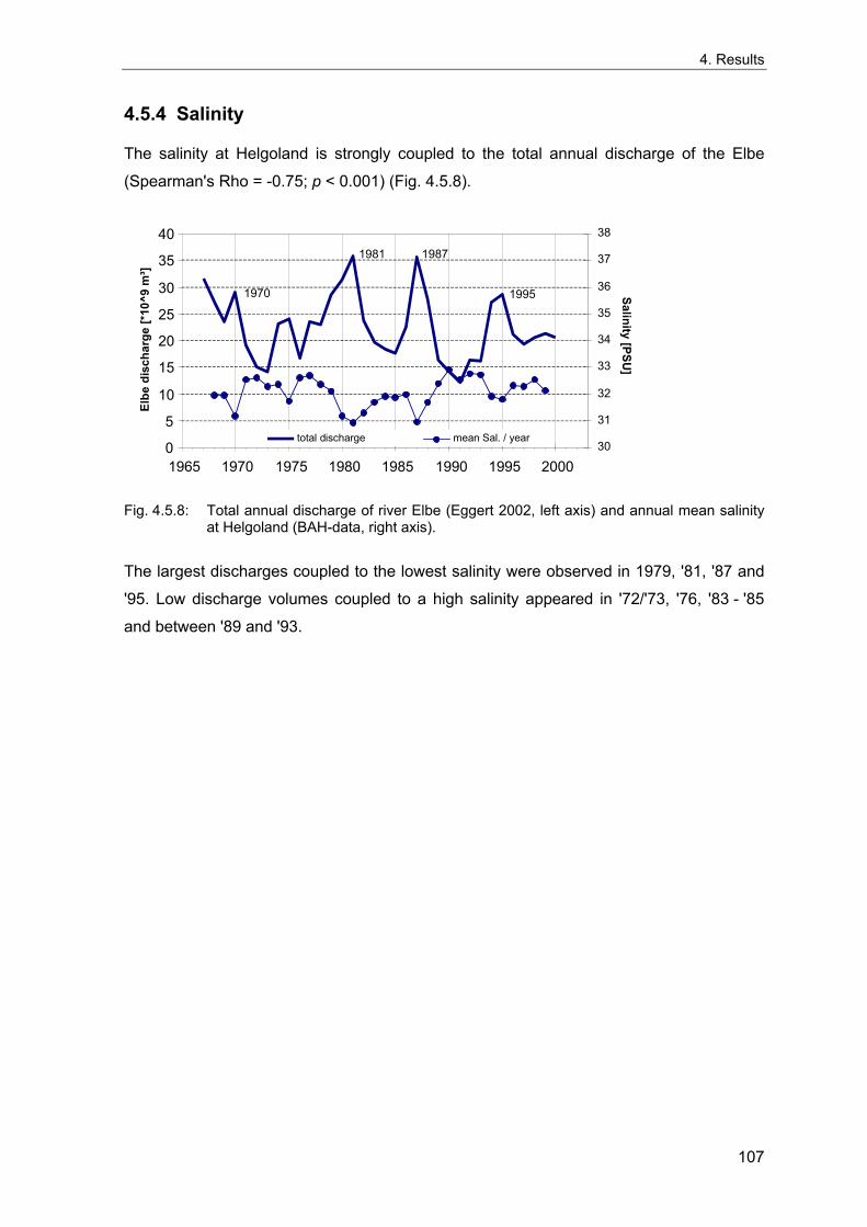
4. Results
4.5.4 Salinity
The salinity at Helgoland is strongly coupled to the total annual discharge of the Elbe
(Spearman's Rho = -0.75; p < 0.001) (Fig. 4.5.8).
1970 1995
1981 1987
0
5
10
15
20
25
30
35
40
1965 1970 1975 1980 1985 1990 1995 2000
Elbe
dis
char
ge [*
10^9
m³]
30
31
32
33
34
35
36
37
38Salinity [PSU
]
total discharge mean Sal. / year
Fig. 4.5.8: Total annual discharge of river Elbe (Eggert 2002, left axis) and annual mean salinity
at Helgoland (BAH-data, right axis).
The largest discharges coupled to the lowest salinity were observed in 1979, '81, '87 and
'95. Low discharge volumes coupled to a high salinity appeared in '72/'73, '76, '83 - '85
and between '89 and '93.
107
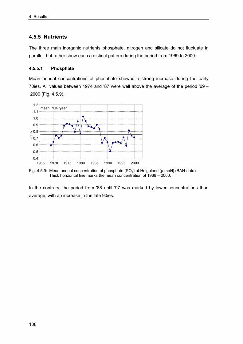
4. Results
4.5.5 Nutrients
The three main inorganic nutrients phosphate, nitrogen and silicate do not fluctuate in
parallel, but rather show each a distinct pattern during the period from 1969 to 2000.
4.5.5.1 Phosphate
Mean annual concentrations of phosphate showed a strong increase during the early
70ies. All values between 1974 and '87 were well above the average of the period '69 –
2000 (Fig. 4.5.9).
mean PO4 /year
0.4
0.5
0.6
0.7
0.8
0.9
1.0
1.1
1.2
1965 1970 1975 1980 1985 1990 1995 2000
µmol
/l
Fig. 4.5.9: Mean annual concentration of phosphate (PO4) at Helgoland [µ mol/l] (BAH-data).
Thick horizontal line marks the mean concentration of 1969 – 2000.
In the contrary, the period from '88 until '97 was marked by lower concentrations than
average, with an increase in the late 90ies.
108
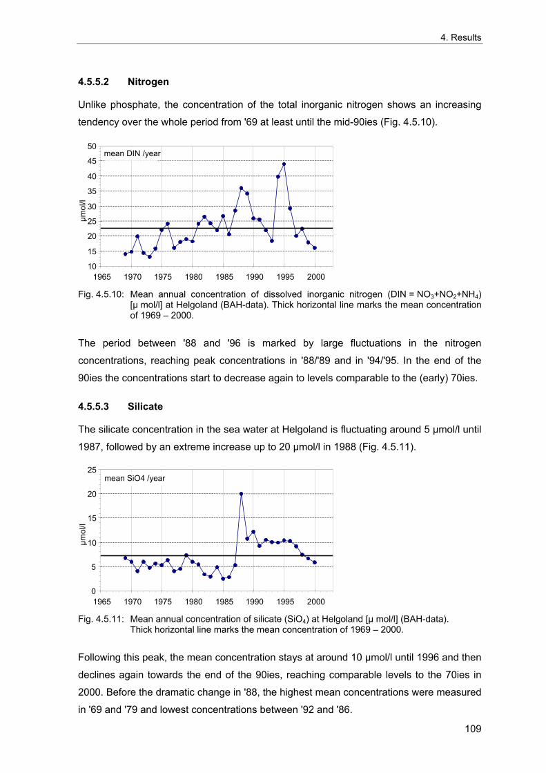
4. Results
4.5.5.2 Nitrogen
Unlike phosphate, the concentration of the total inorganic nitrogen shows an increasing
tendency over the whole period from '69 at least until the mid-90ies (Fig. 4.5.10).
mean DIN /year
10
15
20
25
30
35
40
45
50
1965 1970 1975 1980 1985 1990 1995 2000
µmol
/l
Fig. 4.5.10: Mean annual concentration of dissolved inorganic nitrogen (DIN = NO3+NO2+NH4)
[µ mol/l] at Helgoland (BAH-data). Thick horizontal line marks the mean concentration of 1969 – 2000.
The period between '88 and '96 is marked by large fluctuations in the nitrogen
concentrations, reaching peak concentrations in '88/'89 and in '94/'95. In the end of the
90ies the concentrations start to decrease again to levels comparable to the (early) 70ies.
4.5.5.3 Silicate
The silicate concentration in the sea water at Helgoland is fluctuating around 5 µmol/l until
1987, followed by an extreme increase up to 20 µmol/l in 1988 (Fig. 4.5.11).
mean SiO4 /year
0
5
10
15
20
25
1965 1970 1975 1980 1985 1990 1995 2000
µmol
/l
Fig. 4.5.11: Mean annual concentration of silicate (SiO4) at Helgoland [µ mol/l] (BAH-data).
Thick horizontal line marks the mean concentration of 1969 – 2000.
Following this peak, the mean concentration stays at around 10 µmol/l until 1996 and then
declines again towards the end of the 90ies, reaching comparable levels to the 70ies in
2000. Before the dramatic change in '88, the highest mean concentrations were measured
in '69 and '79 and lowest concentrations between '92 and '86.
109
4. Results
4.4.6 Correlations between abiotic environmental data
Several of the environmental time series described in the previous chapter are correlated
with each other.
The NAO as large-scale climatic pattern influences the European weather. The Winter-
NAOI is highly significantly correlated to the frequency of strong westerly winds (Bft.7W)
and to the mean winter temperature (Tw), consequently the latter two are also positively
correlated (Tab. 4.5.1). The correlation to the overall frequency of strong winds (Bft.7) is
lower but still significant. Winter- and the preceding annual NAOI (ANAOI) and
consequently also winter and preceding summer temperature (Ts) are also correlated. The
annual NAOI is not as strongly correlated to the frequency of windy days and to the winter
temperature, but it shows a higher correlation to the summer temperature and the annual
salinity (Sal.) and a negative correlation to the total river runoff of the Elbe. The salinity is
highly correlated to the river runoff of the Elbe, but also to the frequency of easterly winds
(Bft.7E). Both westerly and easterly winds are not significantly correlated with each other.
Phosphate (PO4) concentrations are negatively correlated to easterly winds while silicate
(SiO4) concentrations are positively correlated to easterly winds. Consequently there is a
strong negative correlation between both nutrients. The silicate concentration is also
positively correlated to the overall wind frequency and to the winter temperature. The
concentrations of both phosphate and dissolved inorganic nitrogen (DIN) are negatively
correlated to the salinity, although only the latter correlation is significant (Tab. 4.5.1).
110
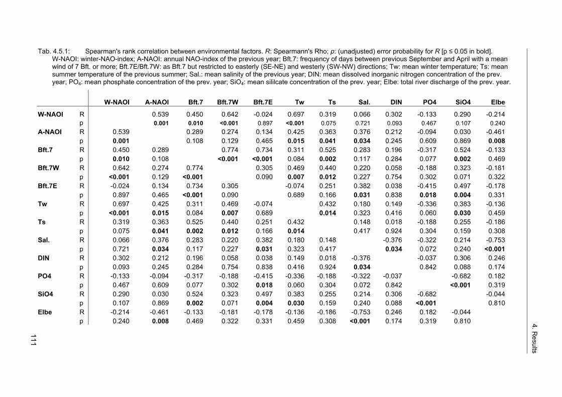
Tab. 4.5.1: Spearman's rank correlation between environmental factors. R: Spearmann's Rho; p: (unadjusted) error probability for R [p ≤ 0.05 in bold]. W-NAOI: winter-NAO-index; A-NAOI: annual NAO-index of the previous year; Bft.7: frequency of days between previous September and April with a mean wind of 7 Bft. or more; Bft.7E/Bft.7W: as Bft.7 but restricted to easterly (SE-NE) and westerly (SW-NW) directions; Tw: mean winter temperature; Ts: mean summer temperature of the previous summer; Sal.: mean salinity of the previous year; DIN: mean dissolved inorganic nitrogen concentration of the prev. year; PO4: mean phosphate concentration of the prev. year; SiO4: mean sililcate concentration of the prev. year; Elbe: total river discharge of the prev. year.
W-NAOI A-NAOI Bft.7 Bft.7W Bft.7E Tw Ts Sal. DIN PO4 SiO4 Elbe
W-NAOI R 0.539 0.450 0.642 -0.024 0.697 0.319 0.066 0.302 -0.133 0.290 -0.214 p 0.001 0.010 <0.001 0.897 <0.001 0.075 0.721 0.093 0.467 0.107 0.240 A-NAOI R 0.539 0.289 0.274 0.134 0.425 0.363 0.376 0.212 -0.094 0.030 -0.461 p 0.001 0.108 0.129 0.465 0.015 0.041 0.034 0.245 0.609 0.869 0.008 Bft.7 R 0.450 0.289 0.774 0.734 0.311 0.525 0.283 0.196 -0.317 0.524 -0.133 p 0.010 0.108 <0.001 <0.001 0.084 0.002 0.117 0.284 0.077 0.002 0.469 Bft.7W R 0.642 0.274 0.774 0.305 0.469 0.440 0.220 0.058 -0.188 0.323 -0.181 p <0.001 0.129 <0.001 0.090 0.007 0.012 0.227 0.754 0.302 0.071 0.322 Bft.7E R -0.024 0.134 0.734 0.305 -0.074 0.251 0.382 0.038 -0.415 0.497 -0.178 p 0.897 0.465 <0.001 0.090 0.689 0.166 0.031 0.838 0.018 0.004 0.331 Tw R 0.697 0.425 0.311 0.469 -0.074 0.432 0.180 0.149 -0.336 0.383 -0.136 p <0.001 0.015 0.084 0.007 0.689 0.014 0.323 0.416 0.060 0.030 0.459 Ts R 0.319 0.363 0.525 0.440 0.251 0.432 0.148 0.018 -0.188 0.255 -0.186 p 0.075 0.041 0.002 0.012 0.166 0.014 0.417 0.924 0.304 0.159 0.308Sal. R 0.066 0.376 0.283 0.220 0.382 0.180 0.148 -0.376 -0.322 0.214 -0.753 p 0.721 0.034 0.117 0.227 0.031 0.323 0.417 0.034 0.072 0.240 <0.001 DIN R 0.302 0.212 0.196 0.058 0.038 0.149 0.018 -0.376 -0.037 0.306 0.246 p 0.093 0.245 0.284 0.754 0.838 0.416 0.924 0.034 0.842 0.088 0.174PO4 R -0.133 -0.094 -0.317 -0.188 -0.415 -0.336 -0.188 -0.322 -0.037 -0.682 0.182 p 0.467 0.609 0.077 0.302 0.018 0.060 0.304 0.072 0.842 <0.001 0.319 SiO4 R 0.290 0.030 0.524 0.323 0.497 0.383 0.255 0.214 0.306 -0.682 -0.044 p 0.107 0.869 0.002 0.071 0.004 0.030 0.159 0.240 0.088 <0.001 0.810Elbe R -0.214 -0.461 -0.133 -0.181 -0.178 -0.136 -0.186 -0.753 0.246 0.182 -0.044 p 0.240 0.008 0.469 0.322 0.331 0.459 0.308 <0.001 0.174 0.319 0.810 4. R
esults
111
4. Results
4.6 Correlation between benthos and abiotic environment
Correlations between environmental factors and the benthic communities can be seen for
sum parameters of the community as well as for the multivariate community composition.
Correlations of single species to environmental factors are weak and differ widely between
stations. An analysis of the correlation of single species densities to environmental factors
would imply the assumption of an influence of the respective factor on the population size
of the species. For a reasonable estimate of the development of the population size of
benthic organisms it would be necessary to sample the main area of their distribution.
Single stations are not representative for the population size. An analysis of the
environmental influence on single species' populations needs to consider a larger spatial
scale and is therefore beyond the scope of the present study.
Local densities are likely to be strongly influenced by interactions between species and by
local environmental influences. A detailed analysis of these factors and interactions
responsible for the local densities requires more sophisticated models than simple
correlations. The development of such models goes beyond the scope of the present
study.
4.6.1 Sum parameters
The various environmental factors described in chapter 4.5 were correlated to sum
parameters of the benthic communities such as species density (S), total organism
density (N), Pielou's evenness index (J') and Shannon-Wiener diversity index (H').
Calculations were done with a time lag of up to three years for the environmental variables
(denoted by an appended "_Lx" to the factor name with x the lag in years).
Several correlations were detected that are statistically significant if tested for themselves.
However the large number of combinations tested (38 for each parameter) strongly
increases the probability of detecting accidental correlations. If the error probability is
adjusted for this multiple testing, a single correlation remains significant: Between the
frequency of strong winds two years before and the species density at WB (chapter
4.6.1.2). Nevertheless the highest detected correlations can be seen as the 'most
probable correlations' at the respective stations.
112
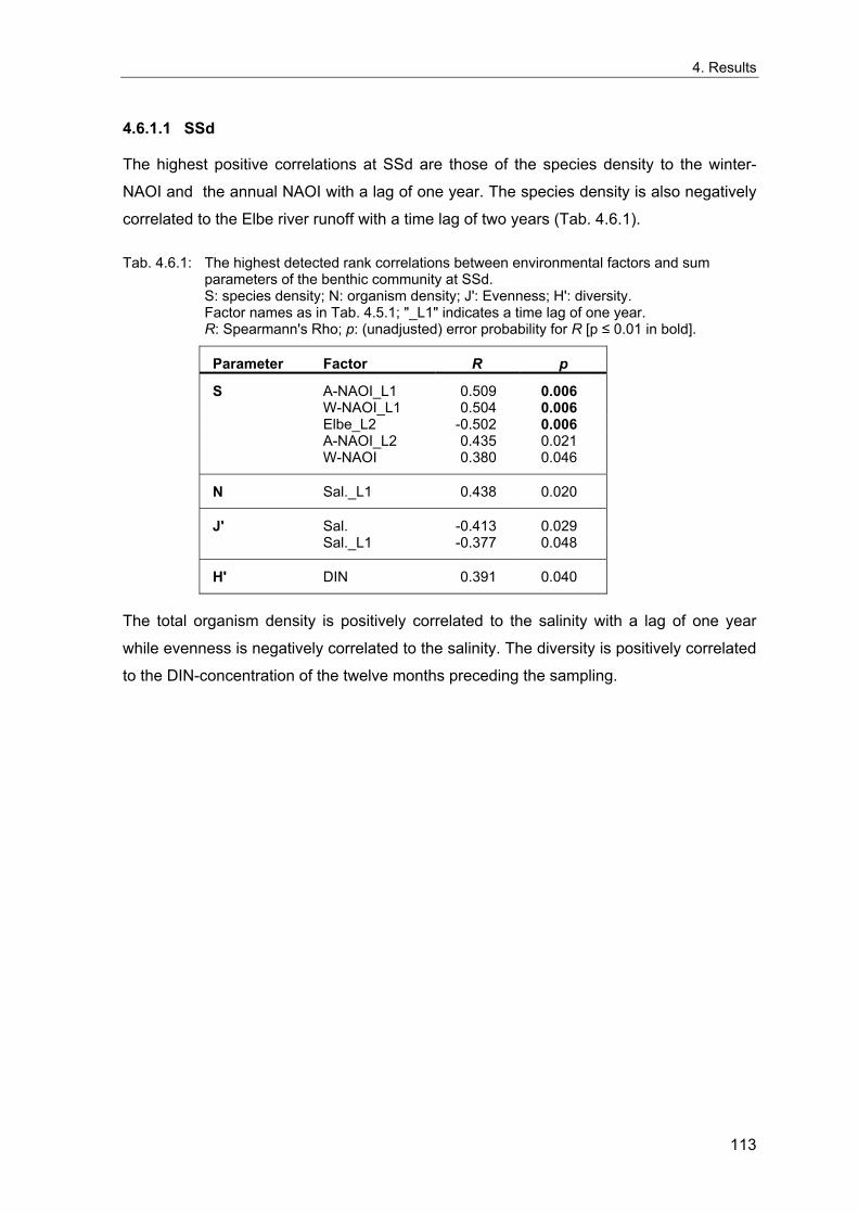
4. Results
4.6.1.1 SSd
The highest positive correlations at SSd are those of the species density to the winter-
NAOI and the annual NAOI with a lag of one year. The species density is also negatively
correlated to the Elbe river runoff with a time lag of two years (Tab. 4.6.1).
Tab. 4.6.1: The highest detected rank correlations between environmental factors and sum parameters of the benthic community at SSd. S: species density; N: organism density; J': Evenness; H': diversity. Factor names as in Tab. 4.5.1; "_L1" indicates a time lag of one year. R: Spearmann's Rho; p: (unadjusted) error probability for R [p ≤ 0.01 in bold].
Parameter Factor R p
S A-NAOI_L1 0.509 0.006 W-NAOI_L1 0.504 0.006 Elbe_L2 -0.502 0.006 A-NAOI_L2 0.435 0.021 W-NAOI 0.380 0.046
N Sal._L1 0.438 0.020
J' Sal. -0.413 0.029 Sal._L1 -0.377 0.048
H' DIN 0.391 0.040
The total organism density is positively correlated to the salinity with a lag of one year
while evenness is negatively correlated to the salinity. The diversity is positively correlated
to the DIN-concentration of the twelve months preceding the sampling.
113
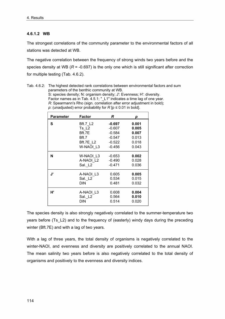
4. Results
4.6.1.2 WB
The strongest correlations of the community parameter to the environmental factors of all
stations was detected at WB.
The negative correlation between the frequency of strong winds two years before and the
species density at WB (R = -0.697) is the only one which is still significant after correction
for multiple testing (Tab. 4.6.2).
Tab. 4.6.2: The highest detected rank correlations between environmental factors and sum parameters of the benthic community at WB. S: species density; N: organism density; J': Evenness; H': diversity. Factor names as in Tab. 4.5.1; "_L1" indicates a time lag of one year. R: Spearmann's Rho (sign. correlation after error adjustment in bold); p: (unadjusted) error probability for R [p ≤ 0.01 in bold].
Parameter Factor R p
S Bft.7_L2 -0.697 0.001 Ts_L2 -0.607 0.005 Bft.7E -0.584 0.007 Bft.7 -0.547 0.013 Bft.7E_L2 -0.522 0.018 W-NAOI_L3 -0.456 0.043
N W-NAOI_L3 -0.653 0.002 A-NAOI_L2 -0.490 0.028 Sal._L2 -0.471 0.036
J' A-NAOI_L3 0.605 0.005 Sal._L2 0.534 0.015 DIN 0.481 0.032
H' A-NAOI_L3 0.608 0.004 Sal._L2 0.564 0.010 DIN 0.514 0.020
The species density is also strongly negatively correlated to the summer-temperature two
years before (Ts_L2) and to the frequency of (easterly) windy days during the preceding
winter (Bft.7E) and with a lag of two years.
With a lag of three years, the total density of organisms is negatively correlated to the
winter-NAOI, and evenness and diversity are positively correlated to the annual NAOI.
The mean salinity two years before is also negatively correlated to the total density of
organisms and positively to the evenness and diversity indices.
114
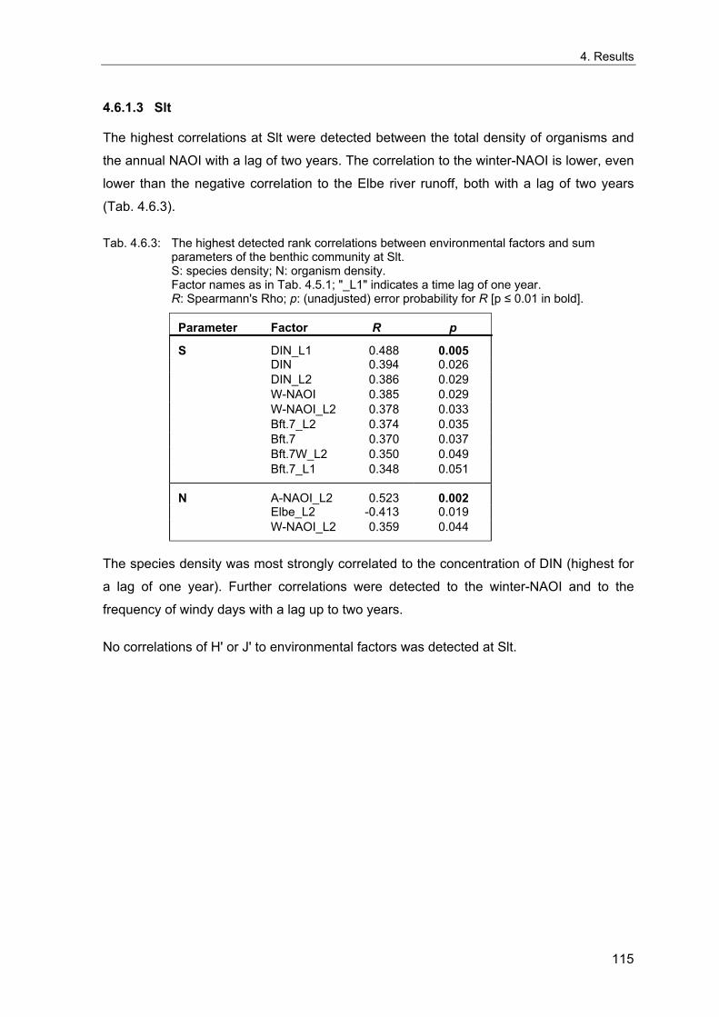
4. Results
4.6.1.3 Slt
The highest correlations at Slt were detected between the total density of organisms and
the annual NAOI with a lag of two years. The correlation to the winter-NAOI is lower, even
lower than the negative correlation to the Elbe river runoff, both with a lag of two years
(Tab. 4.6.3).
Tab. 4.6.3: The highest detected rank correlations between environmental factors and sum parameters of the benthic community at Slt. S: species density; N: organism density. Factor names as in Tab. 4.5.1; "_L1" indicates a time lag of one year. R: Spearmann's Rho; p: (unadjusted) error probability for R [p ≤ 0.01 in bold].
Parameter Factor R p
S DIN_L1 0.488 0.005 DIN 0.394 0.026 DIN_L2 0.386 0.029 W-NAOI 0.385 0.029 W-NAOI_L2 0.378 0.033 Bft.7_L2 0.374 0.035 Bft.7 0.370 0.037 Bft.7W_L2 0.350 0.049 Bft.7_L1 0.348 0.051
N A-NAOI_L2 0.523 0.002 Elbe_L2 -0.413 0.019 W-NAOI_L2 0.359 0.044
The species density was most strongly correlated to the concentration of DIN (highest for
a lag of one year). Further correlations were detected to the winter-NAOI and to the
frequency of windy days with a lag up to two years.
No correlations of H' or J' to environmental factors was detected at Slt.
115
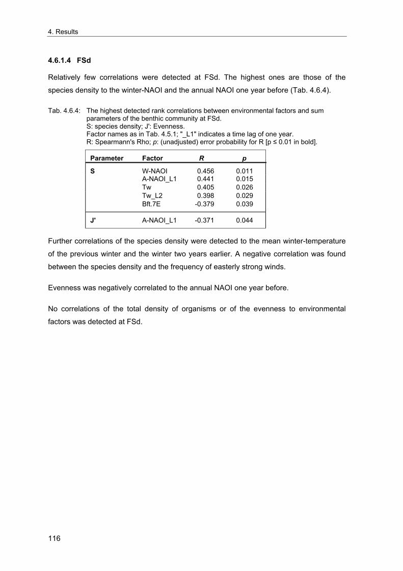
4. Results
4.6.1.4 FSd
Relatively few correlations were detected at FSd. The highest ones are those of the
species density to the winter-NAOI and the annual NAOI one year before (Tab. 4.6.4).
Tab. 4.6.4: The highest detected rank correlations between environmental factors and sum parameters of the benthic community at FSd. S: species density; J': Evenness. Factor names as in Tab. 4.5.1; "_L1" indicates a time lag of one year. R: Spearmann's Rho; p: (unadjusted) error probability for R [p ≤ 0.01 in bold].
Parameter Factor R p
S W-NAOI 0.456 0.011 A-NAOI_L1 0.441 0.015 Tw 0.405 0.026 Tw_L2 0.398 0.029 Bft.7E -0.379 0.039
J' A-NAOI_L1 -0.371 0.044
Further correlations of the species density were detected to the mean winter-temperature
of the previous winter and the winter two years earlier. A negative correlation was found
between the species density and the frequency of easterly strong winds.
Evenness was negatively correlated to the annual NAOI one year before.
No correlations of the total density of organisms or of the evenness to environmental
factors was detected at FSd.
116
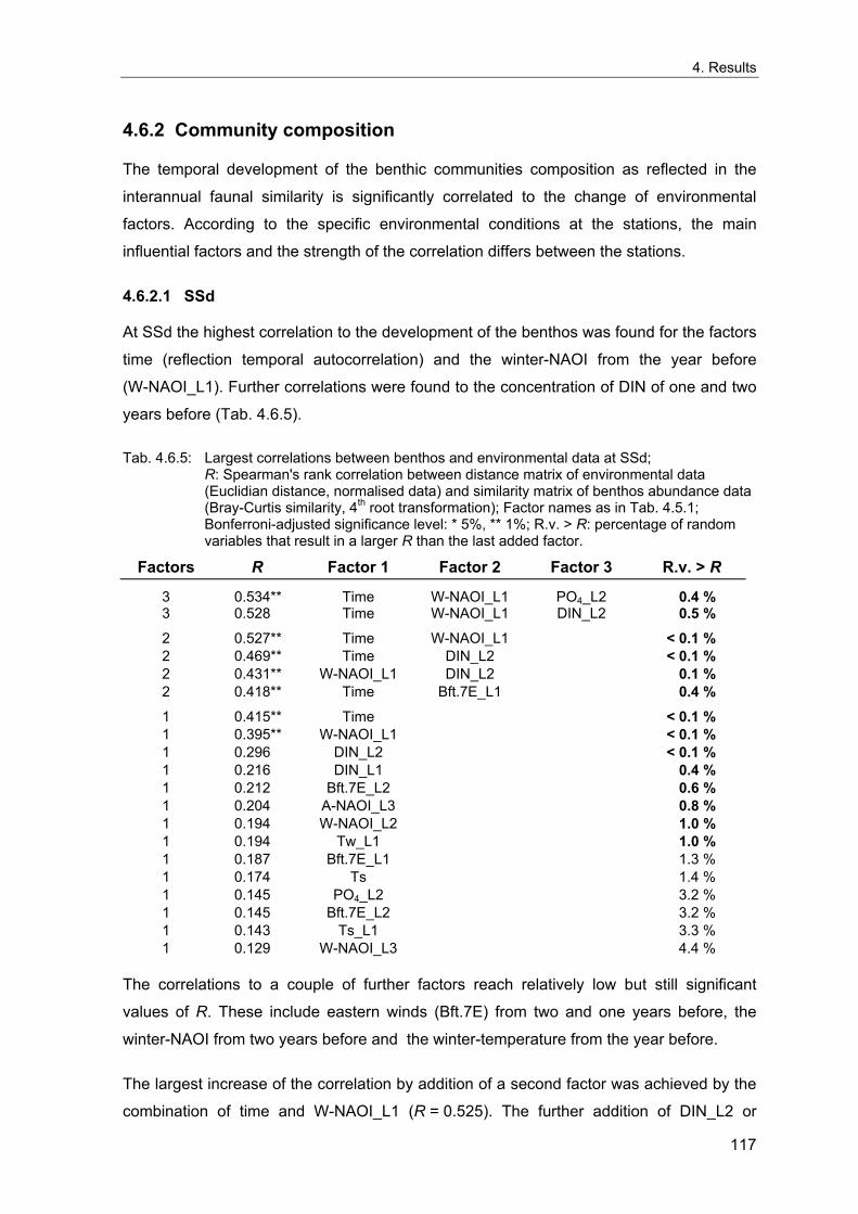
4. Results
4.6.2 Community composition
The temporal development of the benthic communities composition as reflected in the
interannual faunal similarity is significantly correlated to the change of environmental
factors. According to the specific environmental conditions at the stations, the main
influential factors and the strength of the correlation differs between the stations.
4.6.2.1 SSd
At SSd the highest correlation to the development of the benthos was found for the factors
time (reflection temporal autocorrelation) and the winter-NAOI from the year before
(W-NAOI_L1). Further correlations were found to the concentration of DIN of one and two
years before (Tab. 4.6.5).
Tab. 4.6.5: Largest correlations between benthos and environmental data at SSd; R: Spearman's rank correlation between distance matrix of environmental data (Euclidian distance, normalised data) and similarity matrix of benthos abundance data (Bray-Curtis similarity, 4th root transformation); Factor names as in Tab. 4.5.1; Bonferroni-adjusted significance level: * 5%, ** 1%; R.v. > R: percentage of random variables that result in a larger R than the last added factor.
Factors R Factor 1 Factor 2 Factor 3 R.v. > R
3 0.534** Time W-NAOI_L1 PO4_L2 0.4 % 3 0.528 Time W-NAOI_L1 DIN_L2 0.5 % 2 0.527** Time W-NAOI_L1 < 0.1 % 2 0.469** Time DIN_L2 < 0.1 % 2 0.431** W-NAOI_L1 DIN_L2 0.1 % 2 0.418** Time Bft.7E_L1 0.4 % 1 0.415** Time < 0.1 % 1 0.395** W-NAOI_L1 < 0.1 % 1 0.296 DIN_L2 < 0.1 % 1 0.216 DIN_L1 0.4 % 1 0.212 Bft.7E_L2 0.6 % 1 0.204 A-NAOI_L3 0.8 % 1 0.194 W-NAOI_L2 1.0 % 1 0.194 Tw_L1 1.0 % 1 0.187 Bft.7E_L1 1.3 % 1 0.174 Ts 1.4 % 1 0.145 PO4_L2 3.2 % 1 0.145 Bft.7E_L2 3.2 % 1 0.143 Ts_L1 3.3 % 1 0.129 W-NAOI_L3 4.4 %
The correlations to a couple of further factors reach relatively low but still significant
values of R. These include eastern winds (Bft.7E) from two and one years before, the
winter-NAOI from two years before and the winter-temperature from the year before.
The largest increase of the correlation by addition of a second factor was achieved by the
combination of time and W-NAOI_L1 (R = 0.525). The further addition of DIN_L2 or
117
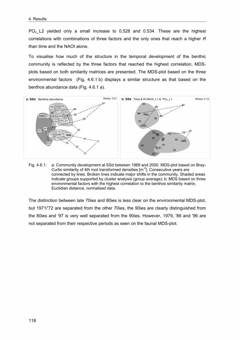
4. Results
PO4_L2 yielded only a small increase to 0.528 and 0.534. These are the highest
correlations with combinations of three factors and the only ones that reach a higher R
than time and the NAOI alone.
To visualise how much of the structure in the temporal development of the benthic
community is reflected by the three factors that reached the highest correlation, MDS-
plots based on both similarity matrices are presented. The MDS-plot based on the three
environmental factors (Fig. 4.6.1 b) displays a similar structure as that based on the
benthos abundance data (Fig. 4.6.1 a).
1969
71
72
75 76 77
78
79
80
81 82
83
84 85
86 87 88 89
91
92
93
94 95
96
97
98 99 2000
Stress: 0.21a: SSd Benthos abundance b: SSd Time & W-NAOI_L1 & PO4_L1
1969
71 72 75
7677 78
79
80
81
82
83
84
85 8687
88
89
9192
93
949596
97
98
99
2000
Stress: 0.12
Fig. 4.6.1: a: Community development at SSd between 1969 and 2000. MDS-plot based on Bray-
Curtis similarity of 4th root transformed densities [m-2]. Consecutive years are connected by lines. Broken lines indicate major shifts in the community. Shaded areas indicate groups supported by cluster analysis (group average); b: MDS based on three environmental factors with the highest correlation to the benthos similarity matrix; Euclidian distance, normalised data.
The distinction between late 70ies and 80ies is less clear on the environmental MDS-plot,
but 1971/'72 are separated from the other 70ies, the 90ies are clearly distinguished from
the 80ies and '97 is very well separated from the 90ies. However, 1979, '86 and '96 are
not separated from their respective periods as seen on the faunal MDS-plot.
118
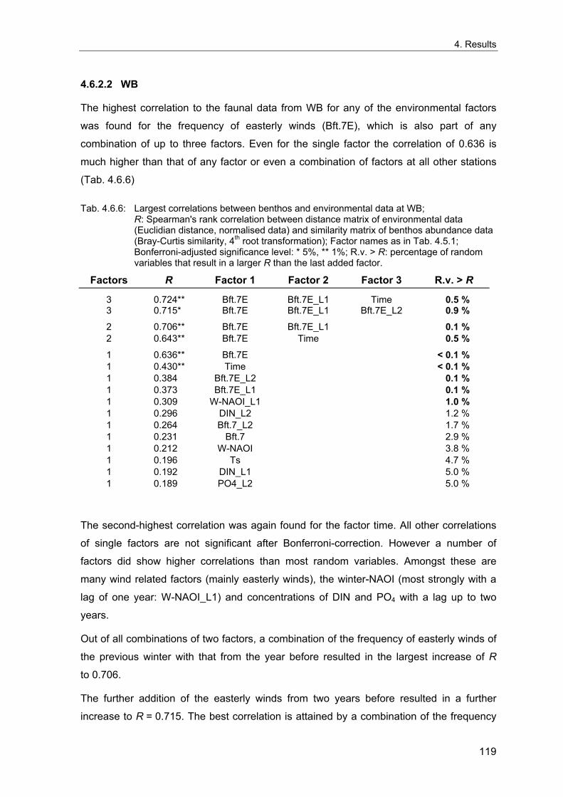
4. Results
4.6.2.2 WB
The highest correlation to the faunal data from WB for any of the environmental factors
was found for the frequency of easterly winds (Bft.7E), which is also part of any
combination of up to three factors. Even for the single factor the correlation of 0.636 is
much higher than that of any factor or even a combination of factors at all other stations
(Tab. 4.6.6)
Tab. 4.6.6: Largest correlations between benthos and environmental data at WB; R: Spearman's rank correlation between distance matrix of environmental data (Euclidian distance, normalised data) and similarity matrix of benthos abundance data (Bray-Curtis similarity, 4th root transformation); Factor names as in Tab. 4.5.1; Bonferroni-adjusted significance level: * 5%, ** 1%; R.v. > R: percentage of random variables that result in a larger R than the last added factor.
Factors R Factor 1 Factor 2 Factor 3 R.v. > R
3 0.724** Bft.7E Bft.7E_L1 Time 0.5 % 3 0.715* Bft.7E Bft.7E_L1 Bft.7E_L2 0.9 % 2 0.706** Bft.7E Bft.7E_L1 0.1 % 2 0.643** Bft.7E Time 0.5 % 1 0.636** Bft.7E < 0.1 % 1 0.430** Time < 0.1 % 1 0.384 Bft.7E_L2 0.1 % 1 0.373 Bft.7E_L1 0.1 % 1 0.309 W-NAOI_L1 1.0 % 1 0.296 DIN_L2 1.2 % 1 0.264 Bft.7_L2 1.7 % 1 0.231 Bft.7 2.9 % 1 0.212 W-NAOI 3.8 % 1 0.196 Ts 4.7 % 1 0.192 DIN_L1 5.0 % 1 0.189 PO4_L2 5.0 %
The second-highest correlation was again found for the factor time. All other correlations
of single factors are not significant after Bonferroni-correction. However a number of
factors did show higher correlations than most random variables. Amongst these are
many wind related factors (mainly easterly winds), the winter-NAOI (most strongly with a
lag of one year: W-NAOI_L1) and concentrations of DIN and PO4 with a lag up to two
years.
Out of all combinations of two factors, a combination of the frequency of easterly winds of
the previous winter with that from the year before resulted in the largest increase of R
to 0.706.
The further addition of the easterly winds from two years before resulted in a further
increase to R = 0.715. The best correlation is attained by a combination of the frequency
119
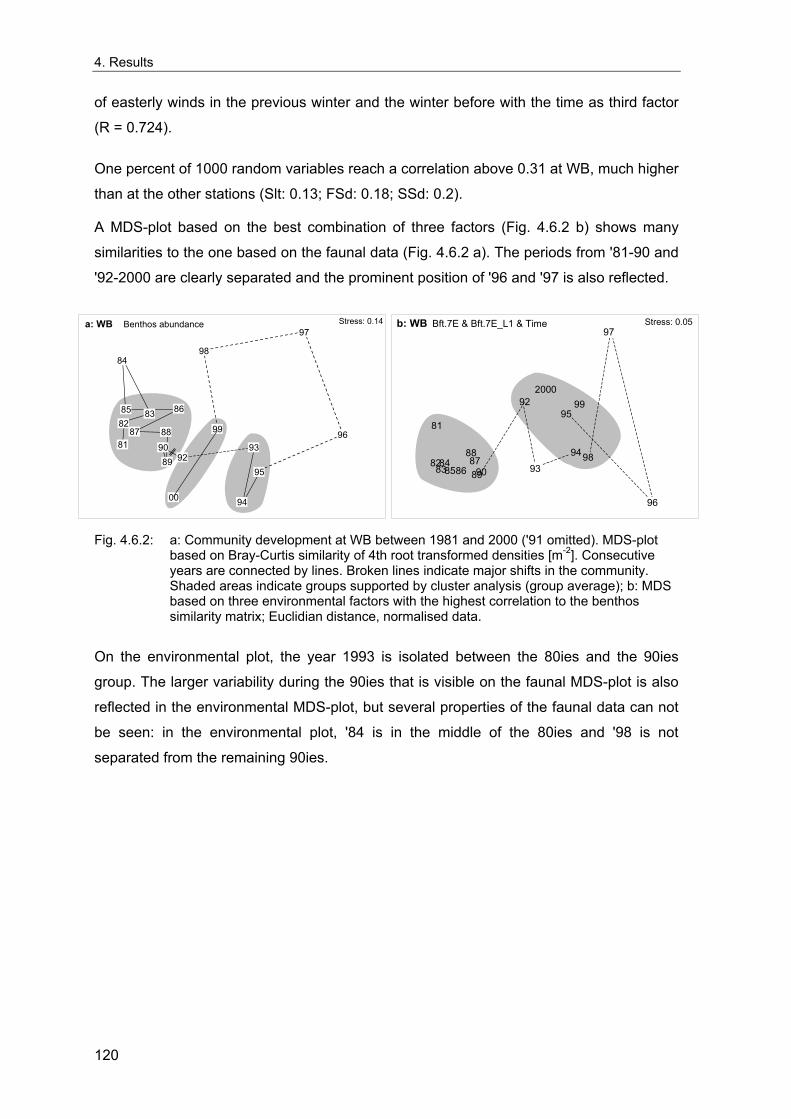
4. Results
of easterly winds in the previous winter and the winter before with the time as third factor
(R = 0.724).
One percent of 1000 random variables reach a correlation above 0.31 at WB, much higher
than at the other stations (Slt: 0.13; FSd: 0.18; SSd: 0.2).
A MDS-plot based on the best combination of three factors (Fig. 4.6.2 b) shows many
similarities to the one based on the faunal data (Fig. 4.6.2 a). The periods from '81-90 and
'92-2000 are clearly separated and the prominent position of '96 and '97 is also reflected.
81
82 83
84
85 86
87 88
89 90
92 93
94
95
96
97
98
99
00
Stress: 0.14a: WB Benthos abundance b: WB Bft.7E & Bft.7E_L1 & Time
81
8283848586
8788
8990
92
9394
95
98
99 2000
Stress: 0.05
96
97
Fig. 4.6.2: a: Community development at WB between 1981 and 2000 ('91 omitted). MDS-plot
based on Bray-Curtis similarity of 4th root transformed densities [m-2]. Consecutive years are connected by lines. Broken lines indicate major shifts in the community. Shaded areas indicate groups supported by cluster analysis (group average); b: MDS based on three environmental factors with the highest correlation to the benthos similarity matrix; Euclidian distance, normalised data.
On the environmental plot, the year 1993 is isolated between the 80ies and the 90ies
group. The larger variability during the 90ies that is visible on the faunal MDS-plot is also
reflected in the environmental MDS-plot, but several properties of the faunal data can not
be seen: in the environmental plot, '84 is in the middle of the 80ies and '98 is not
separated from the remaining 90ies.
120
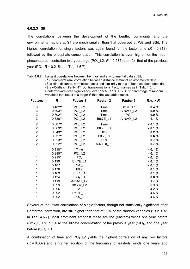
4. Results
4.6.2.3 Slt
The correlations between the development of the benthic community and the
environmental factors at Slt are much smaller than that observed at WB and SSd. The
highest correlation for single factors was again found for the factor time (R = 0.318),
followed by the phosphate-concentration. This correlation is even higher for the mean
phosphate concentration two years ago (PO4_L2; R = 0.285) than for that of the previous
year (PO4, R = 0.215; see Tab. 4.6.7).
Tab. 4.6.7: Largest correlations between benthos and environmental data at Slt; R: Spearman's rank correlation between distance matrix of environmental data (Euclidian distance, normalised data) and similarity matrix of benthos abundance data (Bray-Curtis similarity, 4th root transformation); Factor names as in Tab. 4.5.1; Bonferroni-adjusted significance level: * 5%, ** 1%; R.v. > R: percentage of random variables that result in a larger R than the last added factor.
Factors R Factor 1 Factor 2 Factor 3 R.v. > R
3 0.402** PO4_L2 Time Bft.7E_L1 0.4 % 3 0.393** PO4_L2 Time A-NAOI_L2 0.9 % 3 0.392** PO4_L2 Time PO4 0.9 % 3 0.388** PO4_L2 Bft.7E_L1 A-NAOI_L2 1.1 %
2 0.387** PO4_L2 Time < 0.1 % 2 0.363** PO4_L2 Bft.7E_L1 < 0.1 % 2 0.343** PO4_L2 Bft.7 0.2 % 2 0.337** PO4_L2 Bft.7_L1 0.6 % 2 0.323** PO4_L2 DIN 0.7 % 2 0.322** PO4_L2 A-NAOI_L2 0.7 % 1 0.318** Time < 0.1 % 1 0.285** PO4_L2 < 0.1 % 1 0.215* PO4 < 0.1 % 1 0.199 Bft.7E_L1 < 0.1 % 1 0.187 SiO4 < 0.1 % 1 0.176 Bft.7 0.1 % 1 0.169 Bft.7_L1 0.1 % 1 0.134 SiO4_L1 0.8 % 1 0.119 A-NAOI_L2 1.7 % 1 0.099 Bft.7W_L2 3.9 % 1 0.096 Sal. 4.2 % 1 0.092 Bft.7E_L2 4.6 % 1 0.092 SiO4_L2 4.6 %
Several of the lower correlations of single factors, though not statistically significant after
Bonferroni-correction, are still higher than that of 99% of the random variables ("R.v. > R"
in Tab. 4.6.7). Most prominent amongst these are the (eastern) winds one year before
(Bft.7(E)_L1) but also the silicate concentration of the previous year (SiO4) and one year
before (SiO4_L1).
A combination of time and PO4_L2 yields the highest correlation of any two factors
(R = 0.387) and a further addition of the frequency of easterly winds one years ago
121
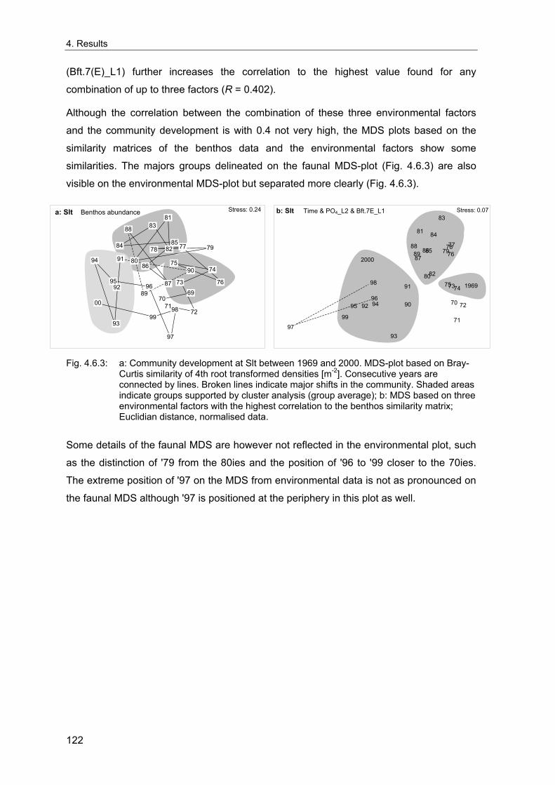
4. Results
(Bft.7(E)_L1) further increases the correlation to the highest value found for any
combination of up to three factors (R = 0.402).
Although the correlation between the combination of these three environmental factors
and the community development is with 0.4 not very high, the MDS plots based on the
similarity matrices of the benthos data and the environmental factors show some
similarities. The majors groups delineated on the faunal MDS-plot (Fig. 4.6.3) are also
visible on the environmental MDS-plot but separated more clearly (Fig. 4.6.3).
69 70
7172
73
74 75
76
77 78 79
80
81
82
83
84 85
86
87
88
89
90
91
92
93
94
95 96
97
98 99
00
Stress: 0.24a: Slt Benthos abundance
b: Slt Time & PO4_L2 & Bft.7E_L1
1969
70
71
72
73 7475
76 77 78
79
80
81
82
83
84
85 86 87
88 89
90
91
92
93
949596
97
98
99
2000
Stress: 0.07
Fig. 4.6.3: a: Community development at Slt between 1969 and 2000. MDS-plot based on Bray-
Curtis similarity of 4th root transformed densities [m-2]. Consecutive years are connected by lines. Broken lines indicate major shifts in the community. Shaded areas indicate groups supported by cluster analysis (group average); b: MDS based on three environmental factors with the highest correlation to the benthos similarity matrix; Euclidian distance, normalised data.
Some details of the faunal MDS are however not reflected in the environmental plot, such
as the distinction of '79 from the 80ies and the position of '96 to '99 closer to the 70ies.
The extreme position of '97 on the MDS from environmental data is not as pronounced on
the faunal MDS although '97 is positioned at the periphery in this plot as well.
122
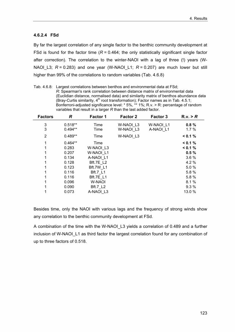
4. Results
4.6.2.4 FSd
By far the largest correlation of any single factor to the benthic community development at
FSd is found for the factor time (R = 0.464; the only statistically significant single factor
after correction). The correlation to the winter-NAOI with a lag of three (!) years (W-
NAOI_L3; R = 0.283) and one year (W-NAOI_L1; R = 0.207) are much lower but still
higher than 99% of the correlations to random variables (Tab. 4.6.8)
Tab. 4.6.8: Largest correlations between benthos and environmental data at FSd; R: Spearman's rank correlation between distance matrix of environmental data (Euclidian distance, normalised data) and similarity matrix of benthos abundance data (Bray-Curtis similarity, 4th root transformation); Factor names as in Tab. 4.5.1; Bonferroni-adjusted significance level: * 5%, ** 1%; R.v. > R: percentage of random variables that result in a larger R than the last added factor.
Factors R Factor 1 Factor 2 Factor 3 R.v. > R
3 0.518** Time W-NAOI_L3 W-NAOI_L1 0.8 % 3 0.494** Time W-NAOI_L3 A-NAOI_L1 1.7 % 2 0.489** Time W-NAOI_L3 < 0.1 % 1 0.464** Time < 0.1 % 1 0.283 W-NAOI_L3 < 0.1 % 1 0.207 W-NAOI_L1 0.5 % 1 0.134 A-NAOI_L1 3.6 % 1 0.128 Bft.7E_L2 4.2 % 1 0.123 Bft.7W_L1 5.0 % 1 0.116 Bft.7_L1 5.8 % 1 0.116 Bft.7E_L1 5.8 % 1 0.096 W-NAOI 8.1 % 1 0.090 Bft.7_L2 9.3 % 1 0.073 A-NAOI_L3 13.0 %
Besides time, only the NAOI with various lags and the frequency of strong winds show
any correlation to the benthic community development at FSd.
A combination of the time with the W-NAOI_L3 yields a correlation of 0.489 and a further
inclusion of W-NAOI_L1 as third factor the largest correlation found for any combination of
up to three factors of 0.518.
123
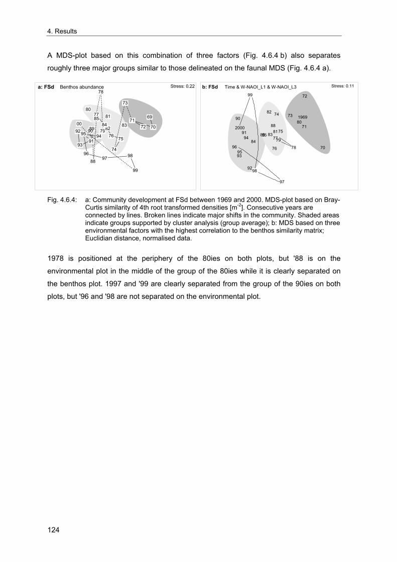
4. Results
A MDS-plot based on this combination of three factors (Fig. 4.6.4 b) also separates
roughly three major groups similar to those delineated on the faunal MDS (Fig. 4.6.4 a).
69
70 71
72
73
74
75 76
77
78
79
80 81
82 83 84
85
88
89 90
91
92
93
94 95
96 97 98
Stress: 0.22 a: FSd Benthos abundance
00
99
b: FSd Time & W-NAOI_L1 & W-NAOI_L3
1969
70
71
72
73 74
75
76
7779
80
81
82
8384
85
88
89
90
91
92
93
94
9596
97
98
99
2000
Stress: 0.11
78
Fig. 4.6.4: a: Community development at FSd between 1969 and 2000. MDS-plot based on Bray-
Curtis similarity of 4th root transformed densities [m-2]. Consecutive years are connected by lines. Broken lines indicate major shifts in the community. Shaded areas indicate groups supported by cluster analysis (group average); b: MDS based on three environmental factors with the highest correlation to the benthos similarity matrix; Euclidian distance, normalised data.
1978 is positioned at the periphery of the 80ies on both plots, but '88 is on the
environmental plot in the middle of the group of the 80ies while it is clearly separated on
the benthos plot. 1997 and '99 are clearly separated from the group of the 90ies on both
plots, but '96 and '98 are not separated on the environmental plot.
124
5. Discussion
5. Discussion
5.1 Sampling gear and penetration depth For long-term studies, the sampling methodology and especially the sampling gear should
ideally be kept constant over the whole period of investigation (e.g. Dybern et al. 1976;
Van der Meer 1997). If changes are necessary, the previous methodology should at least
be continued for a certain period in parallel to the new methodology, to allow an
estimation of the bias introduced by the change (Rumohr 1999). Unfortunately, this has
not been carried out constantly during the sampling of the time series presented here. A
rough comparison of the effects of different sampling gears can be achieved by the
analysis of the extensive sampling with various gear types carried out in July 1976 at the
FSd-station (see chapter 4.3.2).
A combination of two van Veen grabs (vV) with six Reineck box corers (RBC) resulted in a
lower number of species and a lower diversity index, while evenness estimates were
about the same as calculated from five vVs. The lower total area sampled by this gear
combination (2 vVs + 6 RBCs = 0.3 m²) explains the lower species number compared to
that of five vVs (0.5 m²). However, the wider spatial spread of the cores increases the
species number to values comparable to that found in four vVs.
In contrast to the species number, the estimate of overall density of organisms was higher
in the gear combination. Several species were found in significantly different numbers in
the RBCs and the vVs (Tab. 4.3.2). Some of these differences can be explained by the
higher penetration depth of the RBCs, like the higher densities of Goniada maculata or
Tellina fabula, larger individuals of which may live deeper in the sediment than the mean
penetration of the vV of only 6 cm, although T. fabula inhabits the upper 5 - 7 cm, like
most small bivalve species (Birkett 1958). The larger numbers of e.g. Urothoë poseidonis
could also be related to the bow wave of the vV that may push away small organisms on
the surface (Andersin & Sandler 1981). The lower density in the RBCs of Ophiura albida
and juvenile ophiuroids living on the sediment surface, as well as of Nephtys hombergii
and Echinocardium cordatum, which are often found deep in the sediment (Beukema
1974) cannot be explained by these differences in the performance of the gear, but must
be attributed to real spatial differences in the area sampled for the comparison.
The type and magnitude of bias introduced by the change of gear types will vary between
the stations, as each one is characterised by a different sediment type and
macrozoobenthic community. The penetration depth of the gear is influenced by sediment
granulometry (Beukema 1974; Christie 1975; Ankar 1977; Eleftheriou & Holme 1984) as
well as by differences in compactness associated with biogenic structuring of the
125
5. Discussion
sediments (Buchanan 1984). Because of the low penetration depth of the light vV
especially at the FSd- and SSd-station (Fig. 4.3.1), a combination of vVs and RBCs was
used at these stations to benefit from the significantly higher penetration depth of the RBC
and of the higher number of smaller samples, which was expected to improve the spatial
spread and the precision of population density estimates.
Under the assumption that the difference in species numbers is mainly a function of the
sampled area, a correction of the species number was tentatively applied for the long-term
comparison.
The bias in density estimates differs widely between species and will therefore vary
strongly with changes in the community structure. A correction for the different sampling
efficiency does therefore not make sense for other community parameters and is
impossible for multivariate methods.
The largest proportion of the infaunal organisms inhabits the upper 5 – 10 cm of the
sediment (Molander 1928; Holme 1964; Kaplan et al. 1974). These species should for
most of the time at most stations have been appropriately collected. Only in samples from
the early years at FSd their density estimates may be negatively biased because of the
low penetration depth of the old vV. Especially larger organisms often live deeper in the
sediment. Species like the mudshrimps Callianassa subterranea or Upogebia deltaura,
larger polychaetes such as Nereis spp., Nephtys spp. or Lanice conchilega, and echinoids
like Echinocardium cordatum commonly appear in 15 – 20 cm depth and some have been
recorded to more than 50 cm depth (Kaplan et al. 1974; Beukema 1974; Thayer et al.
1975; Santbrink & Bergman 1994). As larger organism mostly occur in small numbers per
sample, their influence should be less pronounced for community analyses based on
density estimates. Their large size would more strongly affect analyses of biomass (Lie &
Patamat 1965; Thayer et al. 1975), which are not covered in the present study because of
the relatively few available biomass data from the present time series (see chapter 3.2.3).
The lighter vV-grabs used until 1985 were not warp rigged and most of them did not have
a sieve covered upper lid. Compared to the new vV introduced in 1986, this resulted in a
lower penetration depth and in a greater bow wave when approaching the bottom, leading
to a loss of deeper living species as well as small surface dwelling species (Ankar 1977;
Bhaud & Duchene 1977; Andersin & Sandler 1981). The new modified and heavier vV
achieved a penetration depth comparable to that of the RBC and the bow wave has been
reduced significantly using the sieve-covered lid (Andersin & Sandler 1981).
126
5. Discussion
The gear type and penetration depth surely have an influence on the community analyses,
which can not be exactly estimated, but seem to be less pronounced than the common
interannual variations of the benthic communities.
Sampling gear changes were not accompanied by larger changes in the faunal data than
the common interannual community changes between other years. The observed
changes are in all cases the result of increasing densities of some species as well as of
decreasing densities of other species and therefore reflect real changes in the
communities beyond sampling influences.
The low densities of several deeper dwelling species and of small species living on the
sediment surface found in the early 1970ies may partly be due to the less efficient
sampling, especially at FSd and SSd.
The changes in sampling gear need always to be considered when interpreting increasing
abundances of deep living or surface dwelling species in the present time series.
5.2 Spatial variability of the benthic communities at the sampling stations
When investigating temporal changes of macrozoobenthic communities, it is essential to
have a good estimate of the spatial sampling variability (Thrush et al. 1994; Underwood
1994). The precision of estimates of community attributes is determined by the size of the
sampling units and the number of replicates as well as by the spatial distribution pattern of
the respective community (Krebs 1998). Spatial patterns in the distribution of the benthic
community around the sampling stations at a larger scale than the actually sampled area
can confound temporal comparisons (Thrush et al. 1994). Small-scale patterns may
reduce the power of the comparisons but will not cause errors (Morrisey et al. 1992;
Stewart-Oaten et al. 1995), as long as several grab samples are combined to adequately
reflect the benthic communities with their inherent variation (Gray 2000).
In addition to this, descriptors of community structure such as the species number or
diversity and evenness indices are generally a function of sample size (Hill 1973; Colwell
& Coddington 1994; Gray 2002). Theoretical studies have so far only investigated the
systematic dependency in simulated samples (Wolda 1981; Smith & Wilson 1996). This
systematic relation is superimposed on the effects of an aggregated distribution of
organisms. The sample size dependency of diversity measures found in real samples can
therefore differ from the predictions of theoretical simulations.
127
5. Discussion
The main intention of the analysis of the spatial variability is threefold:
• To detect any spatial structuring of the community in the sampling area that might confound long-term results.
• To assess the small-scale distribution of the benthic organisms and the resulting variability of the sampling units. Based on this variability we can estimate the sample size (number of replicates) needed to adequately describe the local benthic community with its natural spatial variability.
• To evaluate the sample-size-dependency of community descriptors based on real data and the consequences on the interpretation of these measures.
5.2.1 Spatial patterns If large scale patterns in the spatial distribution of the benthic community were present in
the sampling area, i.e. sub-areas with slightly different types of communities, a deviation
from the exact sampling location might result in a sampling of a different community
(Morrisey et al. 1992). Such patterns should be discernible as spatial autocorrelation or as
large-scale gradients across the area.
Neither a clear spatial pattern, nor a significant spatial autocorrelation or a gradient was
found in the multivariate analysis of the benthic communities.
A hint towards a large-scale pattern or gradient was indicated by a (non-significant)
decreasing spatial autocorrelation at the FSd-station with longitude (Fig. 4.2.2). The
significant correlation of the species density with latitude as well as with longitude may
support the idea of such a gradient (Fig. 4.2.3). Considering the low number of grabs and
the fact that this supposed gradient is not reflected in the normally very sensitive MDS, it
may also be an accidental result of a small-scale variability. On rare occasions, coarse
sediments with pebbles or small stones have been found at FSd (unpublished data from
other sampling occasions, not included in the present analysis) and even large stones
were recorded on photographs of the sea bottom in the area (Fig. 5.1). With the present
data no clear statement about the size and distribution of stones or coarse sediment
"islands" is possible.
128
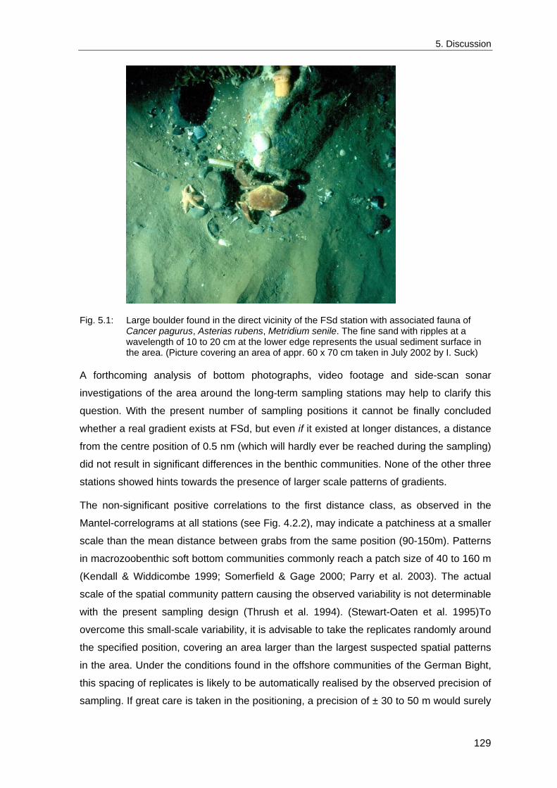
5. Discussion
Fig. 5.1: Large boulder found in the direct vicinity of the FSd station with associated fauna of Cancer pagurus, Asterias rubens, Metridium senile. The fine sand with ripples at a wavelength of 10 to 20 cm at the lower edge represents the usual sediment surface in the area. (Picture covering an area of appr. 60 x 70 cm taken in July 2002 by I. Suck)
A forthcoming analysis of bottom photographs, video footage and side-scan sonar
investigations of the area around the long-term sampling stations may help to clarify this
question. With the present number of sampling positions it cannot be finally concluded
whether a real gradient exists at FSd, but even if it existed at longer distances, a distance
from the centre position of 0.5 nm (which will hardly ever be reached during the sampling)
did not result in significant differences in the benthic communities. None of the other three
stations showed hints towards the presence of larger scale patterns of gradients.
The non-significant positive correlations to the first distance class, as observed in the
Mantel-correlograms at all stations (see Fig. 4.2.2), may indicate a patchiness at a smaller
scale than the mean distance between grabs from the same position (90-150m). Patterns
in macrozoobenthic soft bottom communities commonly reach a patch size of 40 to 160 m
(Kendall & Widdicombe 1999; Somerfield & Gage 2000; Parry et al. 2003). The actual
scale of the spatial community pattern causing the observed variability is not determinable
with the present sampling design (Thrush et al. 1994). (Stewart-Oaten et al. 1995)To
overcome this small-scale variability, it is advisable to take the replicates randomly around
the specified position, covering an area larger than the largest suspected spatial patterns
in the area. Under the conditions found in the offshore communities of the German Bight,
this spacing of replicates is likely to be automatically realised by the observed precision of
sampling. If great care is taken in the positioning, a precision of ± 30 to 50 m would surely
129
5. Discussion
be possible, but this is not desirable to avoid the confounding effects of spatial
autocorrelation.
The combination of the estimated accuracy of the recorded position, and the distance
observed between desired and actual sampling position show that even with today’s
technical possibilities the expected precision under standard offshore conditions will be
about ± 100 m while some samples may be taken more than 200 m from the desired
position. This spatial spread is large enough to overcome any suspected confounding
effects of spatial autocorrelation for the present sampling stations.
As no clear distribution patterns of the benthic communities were detected, the observed
variability is taken as the medium scale local variability of the communities. Samples can
be assumed as random samples of a patchily distributed benthic community.
5.2.2 Medium-scale spatial variability and the precision of estimates Most macrozoobenthos organisms are spatially aggregated and often associated with
other species (Wiens 1989; Gray 2002). This leads to a high variability of samples, and
single sampling units are not sufficient to characterise a benthic community. With an
increasing number of replicates, the precision of most estimates increases. This is the
most important aspect for a determination of an appropriate sample size. The decreasing
variance of the pooled samples is an indication of the amount of local spatial variability
included between the replicates.
5.2.2.1 Organism densities and biomass
The mean density and biomass estimates as well as their variances differ largely between
the stations. The mean density of organisms is five times higher at WB than at Slt. In
opposition to this, the mean biomass at WB is only a fifth of the biomass recorded at Slt.
The variability of the mean density is much higher at these two stations compared to the
other two stations FSd and SSd, which have an intermediate biomass and organism
density. The total organism density at Fsd is not significantly higher than at Slt, but the
variability of this estimate at FSd is the lowest of all stations. Obviously the variability is
not dependent on the mean, but rather related to either external factors or to the
community structure.
The communities at the more variable stations are characterised by a strong numerical
dominance of a single species, Amphiura filiformis at WB (76%) and Nucula nitidosa at Slt
(59%), which is also reflected in the lower evenness at these stations. The dominance of
the most abundant species at the other two stations is much lower (Tellina fabula 27% at
130
5. Discussion
FSd; Nucula nitidosa 16% at SSd), and consequently both stations have a high evenness
value.
The larger variability of total abundance estimates at WB and Slt could be explained by
the numerical dominance of a single species. The variability in the population density of
this species dominates the variance of the total abundance.
This is not to say that the dominant species are the most variable, quite the contrary, the
more abundant species have generally the lower CV. With a larger evenness, however,
high densities of one species in a grab are often levelled out by lower densities of other
species, leading to a lower variability of total organism density. The same mechanism
could also explain the lower variability of biomass estimates at SSd compared to the other
three stations, which are stronger dominated by one or two species in terms of biomass.
It is common practice to exclude the largest species from biomass analyses because they
are poorly represented when taking only a few grab samples, since they are often widely
dispersed and/or live deeper in the sediment than the usual penetration depth of the grab.
This procedure reduces the differences in mean biomass between the stations and leaves
only SSd with a significantly higher biomass, while the reduced biomass of the other three
stations is not significantly different. The exclusion of these large species does not
increase the precision of the biomass estimate but rather decreases it. It does in fact
decrease the standard deviation of the biomass estimate, but as the mean value
decreases even more, the result is a loss of precision as measured by the ratio between
SD and mean (CV). The stronger the reduction of the mean, the stronger is the loss of
precision. This procedure can therefore not be recommended as such. Even if the real
population density and biomass of these species may not be accurately reflected by the
sampling, those specimens that are found in the samples are an integral part of the local
community. Most sublittoral benthic communities of the North Sea are generally regarded
as food-limited (Kuenitzer et al. 1992; Heip & Craeymeersch 1995; Rosenberg 1995). The
area covered by one grab sample (0.1 m²) is small enough to allow direct interaction
between the species present. Apart from direct negative impacts of large predatory
species or of active bioturbation, a few large specimens in the area covered by one grab
sample are likely to reduce the available food (and space) for the remaining species. This
would lead to a lower biomass of the smaller species compared to adjacent areas without
large specimens. This effect might also be reflected in the increased skewness of the
biomass distribution after reduction (Annex: Fig. A.6.3), indicating a more clumped
distribution. Single large specimens, that are regarded as outliers, should therefore only
be disregarded after careful consideration.
131
5. Discussion
Sample size effects
The increase of the precision of the mean biomass and organism density with increasing
sample size is very similar at all stations. The precision at a certain sample size is in the
first place a reflection of the variability of single grabs.
The largest reduction of variability in mean density of organisms and biomass estimates is
reached by the first three to five grabs. With five grabs the size of the empirical confidence
interval of the mean is reduced by more than 50% compared to single grabs.
Nevertheless, even with five grabs, the precision of the mean density estimate at WB and
Slt is rather low and the empirical confidence interval (C.I.) is as large as the mean itself
Fig. 4.2.4). At the two less variable stations SSd and FSd, the precision is much better
and the confidence interval with five replicates is only half as large as the mean. This level
of precision could only be reached with more than 20 grabs at WB or Slt. An increase to
10 replicates results in a 30% gain of precision relative to five replicates. A further
increase of replicate number results only in a small improvement of the precision.
These relative improvements of precision are similar for the mean biomass estimates, but
the precision is lower than for total density estimates at FSd and SSd (Fig. 4.2.5). Five
replicates result in a C.I. as large as the mean at all stations but SSd, where it is only
about 80% of the mean. The variability of the total biomass estimates at WB and Slt is
similar to that of total organism density.
Most species are significantly spatially aggregated. The spatial variability (reflected in the
CV of the mean density) of most species is even higher than that of the sum parameters.
Only species with a low density are characterised as randomly distributed (chapter 4.2.2),
but especially for these species a much higher number of replicates would be necessary
(i.e. 50 to 200 replicates) to achieve a reliable estimate of their spatial distribution (Andrew
& Mapstone 1987; Krebs 1998).
As the investigation of single species populations is not the aim of this study, explicit
calculations on the precision of density or biomass estimates in dependence of sample
size are not presented here. As each species has its own spatial distribution, these
calculations have to be done for each species separately. Many species also show
seasonal changes in their spatial variability, while other species show the same spatial
pattern throughout the year (Dittmer 1977). A large proportion of these differences in
spatial variability can be explained by the increasing variance (s²) with the mean
described by a power function s²=a*meanb known as "Taylors power law" (Taylor 1961;
McArdle et al. 1990; Legendre & Legendre 1998). Some species that are present at
several stations show a different variability at each station, therefore the results may even
132
5. Discussion
differ between stations. Suffice it to say that for most species five grab samples would
result in an asymmetric confidence interval (C.I.) that is considerably larger than the
mean. Under the assumption of a random distribution of organisms, a (symmetric) C.I. is
calculated as
( ) CVn
tx n 1, −± α
where x is the mean density, n the sample size, t(α,n-1) the value of Student's t-distribution
for error probability α and n-1 degrees of freedom and CV the coefficient of variation.
Especially for small sample sizes, this estimate is smaller than the C.I. for aggregated
distributions (Krebs 1998). Nevertheless even this (underestimated) C.I. is larger than the
mean (for n = 5) as long as the CV is larger than 0.4 ( ( ) 54,05.0t = 1.24). Only a single
species reaches such a small CV at a single station (Scoloplos armiger at FSd) while the
CV of most species is considerably larger. A larger number of ten or more replicates is
therefore recommended for studies of population density and spatial variability of single
species (see also Rachor 1976; Dittmer 1977). Such an effort is often not possible
because of practical limits in sample processing time.
A sample size of five replicate 0.1 vVs may be regarded as acceptable for an analysis of
the community development but not for an appropriate description of single species
population densities.
5.2.2.2 Community structure
Besides the sum parameters, the community structure is summarised by the species
number per area (species density [for a definition of terms see methods chapter 3.4.1.2])
and the "evenness" reflecting the dominance structure. Diversity indices, such as H',
combine aspects of species density and dominance structure.
The species density is at all stations much less variable than e.g. estimates of total
organism density or biomass. The variability of the evenness and diversity indices J' and
H' is generally even lower, but this depends on the dominance structure. At SSd and FSd,
the two stations with the highest evenness (0.83), the variability of the evenness is much
lower than that of the species density. The variability of H' is consequently intermediate
between the two. At WB and Slt the evenness is much lower and has a much higher
variability, similar to the variability of the species density. As H' is a product of J' and the
logarithm of the species density, which has an inherently lower SD, the variability of H' is
at WB and Slt lower than that of J' but still much higher than at the other two stations. The
high dominance of single species at WB and Slt increases the variability also of the
133
5. Discussion
community structure. Fluctuations in the abundance of this species directly influence the
value of J' and consequently H'.
The spatial variability seems to be linked closer to the community structure than to the
total organism density and species density. It is not the station with the largest species
density and the highest organism density (WB), that has the lowest spatial variability, but
rather those stations with the highest evenness in the species distribution (SSd & Fsd).
Slt, the station with the lowest organism density and the poorest species spectrum is also
the most spatially variable station. This could be seen as a result of a temporally variable
environment (see chapter 5.4.4), as spatial variability is commonly seen as an indication
of disturbance (Warwick & Clarke 1993). The second highest spatial variability was found
at WB, the station with the highest organism density and the largest species spectrum.
This station, the furthest offshore and deepest of all four stations, would, however,
normally be seen as the most environmentally stable station. However, it is the only
station which is outside the area of the "plaice box", which is partially protected from
bottom trawling. Therefore WB is presumably subjected to the highest intensity of
demersal trawling, which is also known to be patchily distributed in the area (Rijnsdorp et
al. 1998; see chapter 5.4.2.1). Although both communities are not dominated by typically
opportunistic species, the spatial variability could be caused by a higher frequency of
disturbance. Without detailed information on the small-scale spatial distribution of
disturbances at the stations, it is difficult to distinguish between the contributions of biotic
interactions and community structure and those of environmental conditions to the
development of the spatial variability of the community (see also chapter 5.4.4.1).
Sample size effects
Even though species densities and organism densities differ widely between the stations,
there is one point in which all species accumulation curves (Fig. 4.2.6) are similar:
At all stations the number of species continues to rise even for 20 samples or more and
there is no sign of it reaching an upper level within the range of samples at hand.
The total number of species found does not appear to be a good indication for an
appropriate sample size. If the main aim of a study is the species spectrum of the local
community, a deliberate limit has to be set for the expected number of additional species
per additional replicate. In the species-poor community at Slt, nine replicates would have
been enough to reach a point where each additional sample would yield less than one
additional species, while in the species-richer community at WB more than 17 grabs
would have been necessary. Because this measure is highly dependent on the number of
134
5. Discussion
rare species, it is not an appropriate limit when the temporal development of the
community is the focus of the analysis.
The variability of the number of species for a certain sample size seems more informative
for a decision of an appropriate reflection of the species spectrum of the community. At
SSd and Slt, this curve stayed rather constant after an initial decrease up to a sample size
of three to five grabs. The decrease in variability at a sample size larger than half the total
replicate number is biased because of the decreasing number of possible combinations
and cannot be interpreted (Bros & Cowell 1987). This variability in species number is a
result of the spatial distribution especially of the rare species in the community.
Beyond the initial decrease for very small samples the variability in species number does
not seem an appropriate measure either to determine sufficient sampling, but rather one
of spatial heterogeneity in the local species composition of the community.
For analyses of community development an appropriate reflection of the community
structure seems more important.
For single grabs the variability of J' and consequently H' is rather large. The decrease of
the variability is most pronounced for the first three to five grabs.
Nevertheless the remaining variability differs between the stations. The large variability at
Slt especially for J' indicates that a larger sample size of 10 to 15 grabs would be
necessary to achieve a precision in the estimates of diversity at this station that is
comparable to the level of precision reached at the three other stations with a much
smaller sample size. However, such an effort is not realistically feasible in most cases,
taking into account the costs of ship-time and personnel. A fixed level of precision may
also not be necessary, as the variability also reflects the spatial heterogeneity, which is an
attribute of the local community and as such a useful characteristic itself.
5.2.2.3 Community composition
Beyond the variability of sum parameters, spatial community variability is reflected in the
similarity between samples, which includes the species identities and their densities. The
frequency distribution of similarities (Fig. 4.2.13) gives a good impression of the
homogeneity of the community.
The mean similarities between samples reflect the natural spatial variability of the
communities. Consequently the community at SSd with the highest mean similarity
exhibits the lowest community variability, followed by FSd, Slt and finally WB with the
highest variability of the four stations.
135
5. Discussion
The coefficient of variation (CV) of these similarities goes one step further and indicates
how evenly the similarity values are distributed. This could be interpreted in terms of the
spatial distribution of the community. Following this hypothesis, in an area with a patchy
distribution of the benthic community, some pairs of samples should be found with an
especially high similarity and others with extremely low similarities. The resulting CV of the
mean similarity will be larger than in areas where the observed similarities result simply
from random variability. It may therefore serve as a multivariate indicator of patchiness.
This hypothesis should be further investigated by simulation studies. According to this
hypothesis, the patchiness is also lowest at SSd, followed by Fsd. The communities at
WB and Slt exhibit not only a higher spatial variability but also a higher patchiness.
However, while the mean similarity at Slt is higher than at WB, the larger CV indicates a
more patchy distribution of the community at Slt compared to WB.
Multivariate methods have shown to be more powerful for the detection of environmental
impacts on benthos (Clarke & Warwick 1994) and to detect subtle changes in the
community (Legendre & Legendre 1998). They are more powerful means of describing
the community but still require replicate samples to distinguish between local spatial
variability and temporal changes. In each area one to two exceptional samples occurred
amongst the total of 20-21 samples per station, with a low similarity to the remaining
samples (Annex: Fig. A.6.5), which must be expected in any sampling. Single samples
may thus well be misleading. Not only for the possibility of statistical inference, but also for
the recognition of community differences, replicates are clearly needed.
The spatial variability of the community at any single station is significantly lower than the
difference between the benthic communities. The temporal variability of the benthic
community at each station is also in all cases lower than the community differences
between the stations. Each station represents a clearly distinct benthic community.
In both the spatial and the temporal MDS ordinations, SSd is positioned between the three
other stations. The axis between the Slt and FSd can be interpreted in terms of increasing
sediment grain size while the perpendicular axis is related to an increasing distance from
shore. Correspondingly the largest differences in the benthic community are found
between Slt and FSd (finest and largest grain size) and between Slt and WB (in- vs.
offshore). The community at SSd shows aspects of all other stations, but is in all cases
clearly distinct.
136
5. Discussion
Sample size effects
As the precision of mean density estimates of all species rises with sample size, the
differences between the abundance in the samples decrease and the similarity of the
samples increases. For the same reason the variance of the similarities is also related to
the sample size. The smaller the samples, the larger is the variance not only of univariate
measures but also of the similarity between samples. A low variability and high similarity is
indicative of an appropriate reflection of the benthic community by the respective sample
size. Most (dis-) similarity indices are influenced by sample size (Wolda 1981; Streever &
Bloom 1993; Schleier & van Bernem 1998; Kohn & Riggs 1982; Walsh 1997; Cao Yong et
al. 1997; Kobayashi 1987). The systematic influence has been investigated in simulation
studies (e.g. Wolda 1981) based on a theoretical community with a species composition
according to a log-series and an independent random distribution of all species. Under
these assumptions, the expected similarity must be higher than in reality, which is
characterised by spatially clumped distributions and interspecific correlations. The
expected similarity, its sample size dependence and variability for real communities can
therefore only be realistically estimated using real data.
A similarity of 100% for the Bray-Curtis (BC) index can only be reached if the compared
samples contain exactly the same species in exactly the same abundance. With the
natural variability in species composition and organism density, the mean similarity
between replicates from the same community is usually lower (Bray & Curtis 1957).
Values of 70% to 80% BC similarity have been proposed as an indication of a sufficient
sample size (Weinberg 1978; Kronberg 1987). With the present data, a level of 70%
would be achieved with only two grabs at most stations, which seems an unrealistically
small sample considering the observed variability of sum parameters. A level of 80%,
however, is in 1998 not reached at Slt even with a sample size of ten grabs. Nevertheless,
in certain years the mean similarity even between single grabs at Slt can be as high as
80% or even 90%, as visible in the comparison of spatial variability over time (Fig. 5.2.15).
An absolute similarity level for all communities seems not realistic as indication of a
sufficient sample size, as the mean similarity is also a measure of spatial variability of the
community. Instead, an adequate sampling can be assumed at the point where the
average similarity does not increase remarkably with a further increase in sample size.
The very shallow slope of the similarity-area curves above five grabs indicates that only
minor improvements can be achieved by increasing the number of replicates above five.
For a remarkable increase in similarity and reduction in variability, the sample size would
have to be doubled to ten replicates (Fig. 4.2.14). The influence of sample size on the
137
5. Discussion
mean inter-sample similarity results from two effects: The increase in species number and
the increase in precision of mean abundance estimates with increasing sample size.
Some authors claim that similarity indices should be independent of sample size, which is
in this context generally expressed as the number of organisms per sample (Wolda 1981).
Because the number of species in the samples influences most indices, only similarity
measures that are based mainly on the comparison of the dominant species can be
relatively free from sample size influences (Krebs 1998). Beyond the variability for small
samples, a sensitivity for changes in organism density in general is also a desirable
property. Comparing standard samples of equal areas, density differences of the present
populations do reflect something going on. Differences in the abundance of the species
between samples will lead to a lower Bray-Curtis similarity even if the number of species
and the proportional composition remain the same.
5.2.2.4 Temporal changes in spatial variability
The main intention of the spatial sampling was to examine the spatial variation at these
permanent stations as a background for the analysis of the temporal development of the
benthic communities. However, the spatial variability of communities does also vary over
time. The small number of usually five replicates taken for the long-term series does not
allow good estimates of the spatial distribution of single species or the spatial variability of
community parameters. The multivariate similarity between five replicates results in ten
similarity values per sampling occasion. The mean similarity between replicates is the
most inclusive measure for a comparison of the spatial community variability between
years, combining changes in species composition and abundance.
The large differences in mean similarity observed over the years show that the spatial
variability at any station is not constant over time. In a study of the spatial distributions of
polychaetes near the FSd-station, Dittmer (1977) found that the spatial distribution of
many species varied also seasonally. The values calculated from the samples taken in
1998 can therefore not be generalised, although the observed community variability in
1998 is close to the mean variability over time (Fig. 4.2.15). Just like the species number
and dominance structure vary between years, so does the spatial variability. Therefore the
temporal differences between years can only be compared to the spatial variability
estimates of the respective years (ANOSIM results: Annex Tab. A.5.2 - A.5.5).
The community differences between years are in all cases significantly larger than the
respective spatial variability at the station.
Replicate samples are necessary at any sampling time to get an estimate of the spatial
variability. The actual precision of community parameters cannot be exactly predicted
138
5. Discussion
from the analysis of the data from 1998. The relative changes of the respective measures
in relation to sample size and their decreasing variance should however be valid also for
other years.
5.2.2.5 Sample size needed for statistical inferences
As power analysis for nonparametric and multivariate methods is not available, the
desirable sample size for various measures is defined by a compromise between the
increasing effort and the achieved improvement of the precision of the estimate.
If any statistical inference is intended, replicates are needed to assess the within-sample
variability and compare it to the between-sample differences. Because frequency
distributions of sample parameters are hard to estimate from small samples and are
unknown for most diversity and similarity indices, nonparametric methods are more
appropriate and with small sample sizes often even more powerful than parametric
methods (Zar 1996). For small sample sizes the error probability of nonparametric tests is
calculated by a permutation procedure comparing the observed value to all possible
values for the given sample size. In multivariate analyses, difference of the "between" and
"within" group (rank) similarities is also tested for statistical significance by permutation
(Moore et al. 1984; Clarke & Warwick 1994). The number of replicates restricts the
number of possible permutations and thus the maximum possible significance level for
these tests (Clarke & Warwick 1994).
For statistical inferences about community changes, a minimum of four, five or seven
replicates is needed to allow for a significance level of 5%, 1% or 0.1%, respectively.
An exact calculation of the sample size needed for the detection of a certain effect size
based on the observed variability of samples is possible for parametric tests (Zar 1996;
Thomas 1997; Sheppard 1999; Underwood 2000) and specialised software is readily
available (Thomas & Krebs 1997). Statistical power analysis for nonparametric tests,
however, is a very new field of research and can only be realised by simulation (Mumby
2002). Although nothing is known about the formal relationship between power and
sample size for multivariate methods (Clarke & Green 1988), it clearly depends on the
variability of the data and on the effect size that needs to be detected. A quantifiable
measure of power to detect a community change of a certain size would need a detailed
simulation study using artificially created and exactly defined levels of difference between
samples, which would be an interesting topic, but is beyond the scope of the present
study.
139
5. Discussion
5.2.3 Systematic sample size influence on measures of community structure
All measures that are related to the number of species or the community structure also
show a systematic dependency on sample size. The systematic dependency implies that
these measures should only be compared between samples of the same size, but it also
contains information about the spatial homogeneity of the sampled community.
The species number, diversity and evenness indices as well as most similarity indices are
strongly influenced by the sample size (Hill 1973; Colwell & Coddington 1994; Krebs
1998; Gray 2002). However, the sample size dependency found in this study differs in
several aspects from the predictions of theoretical simulations (Wolda 1981; Smith &
Wilson 1996). These differences allow some interesting conclusions about the properties
of the respective measures as well as about the studied communities.
The term "diversity" has been used in so many different ways that Hurlbert (1971) even
declared it a non-concept. Unless one is willing to describe the whole community
structure, a combination of indices may still be useful for comparisons, provided that their
specific information content and focus are borne in mind. Diversity includes two
components, the number of species present and their frequency distribution (Legendre &
Legendre 1998). Diversity indices such as Shannon-Wiener's H' are heterogeneity
measures incorporating both aspects of species number and evenness (Hill 1973).
5.2.3.1 Species number
The species accumulation curves of all four stations do not approach a constant value but
rather continue to rise even for large samples (Fig. 4.2.6). For marine communities, this
seems to be the general rule even for much larger samples (Rumohr & Karakassis 1999;
Gotelli & Colwell 2001; Gray 2002). It is in most cases impossible to determine or even
estimate an absolute number of species for these open communities delimited by
gradients rather than borders. Various methods have been developed to estimate the total
number of species in a community (see e.g. Colwell 2000), but all estimates increase for
marine benthic communities almost as much with sample size as the species number
itself (Ellingsen 2001; Melo & Froehlich 2001; Rumohr et al. 2001; Gotelli & Colwell 2001)
and therefore seem not very helpful.
Just like abundance or biomass values, which are always related to a certain area, the
species number should be related to the sampled area and rather be referred to as
"species density".
Comparing species density between the stations, WB has with 56 species the highest
number of species per m², followed by SSd (50) and FSd (43) and Slt has the lowest
140
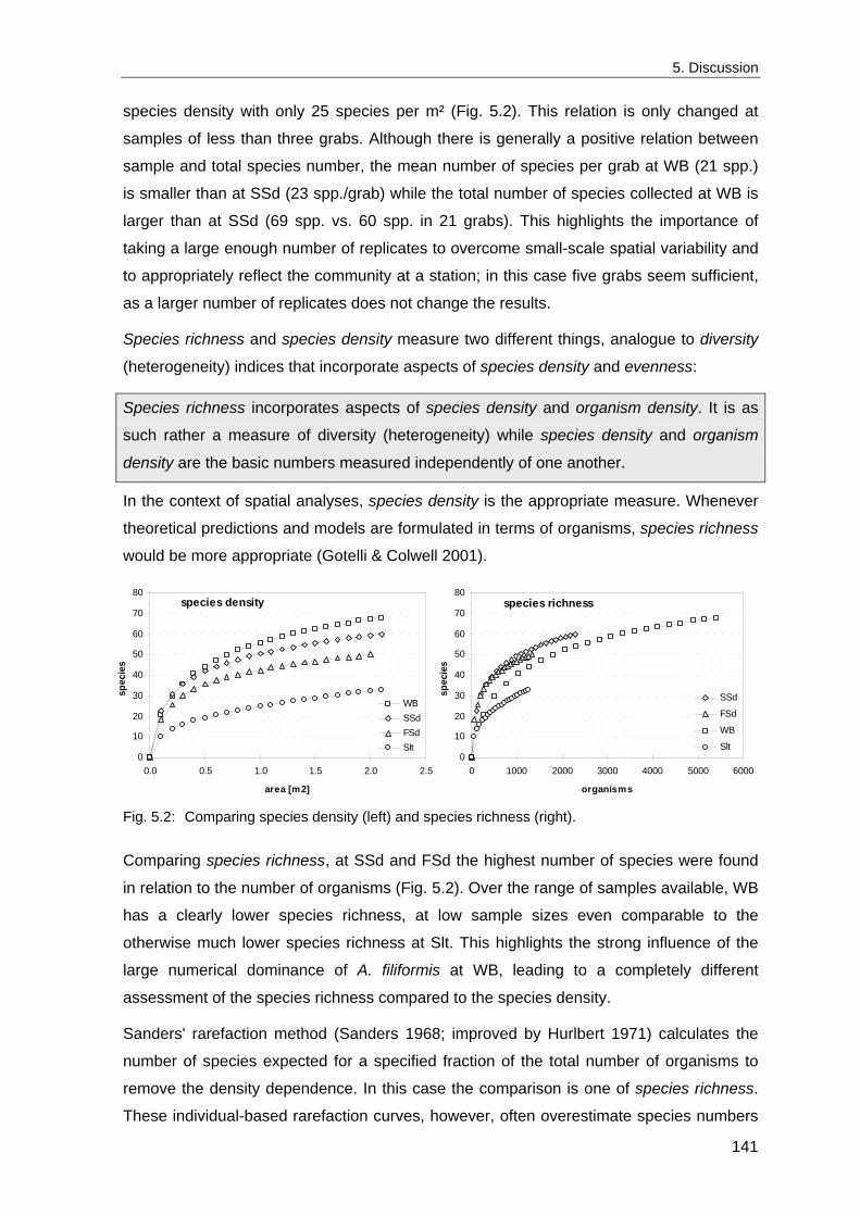
5. Discussion
species density with only 25 species per m² (Fig. 5.2). This relation is only changed at
samples of less than three grabs. Although there is generally a positive relation between
sample and total species number, the mean number of species per grab at WB (21 spp.)
is smaller than at SSd (23 spp./grab) while the total number of species collected at WB is
larger than at SSd (69 spp. vs. 60 spp. in 21 grabs). This highlights the importance of
taking a large enough number of replicates to overcome small-scale spatial variability and
to appropriately reflect the community at a station; in this case five grabs seem sufficient,
as a larger number of replicates does not change the results.
Species richness and species density measure two different things, analogue to diversity
(heterogeneity) indices that incorporate aspects of species density and evenness:
Species richness incorporates aspects of species density and organism density. It is as
such rather a measure of diversity (heterogeneity) while species density and organism
density are the basic numbers measured independently of one another.
In the context of spatial analyses, species density is the appropriate measure. Whenever
theoretical predictions and models are formulated in terms of organisms, species richness
would be more appropriate (Gotelli & Colwell 2001).
0
10
20
30
40
50
60
70
80
0.0 0.5 1.0 1.5 2.0 2.5
area [m2]
spec
ies
WBSSdFSdSlt
species density
0
10
20
30
40
50
60
70
80
0 1000 2000 3000 4000 5000 6000
organisms
spec
ies
SSd
FSd
WB
Slt
species richness
Fig. 5.2: Comparing species density (left) and species richness (right).
Comparing species richness, at SSd and FSd the highest number of species were found
in relation to the number of organisms (Fig. 5.2). Over the range of samples available, WB
has a clearly lower species richness, at low sample sizes even comparable to the
otherwise much lower species richness at Slt. This highlights the strong influence of the
large numerical dominance of A. filiformis at WB, leading to a completely different
assessment of the species richness compared to the species density.
Sanders' rarefaction method (Sanders 1968; improved by Hurlbert 1971) calculates the
number of species expected for a specified fraction of the total number of organisms to
remove the density dependence. In this case the comparison is one of species richness.
These individual-based rarefaction curves, however, often overestimate species numbers
141
5. Discussion
(Simberloff 1972). They rely on the assumption of randomly distributed organisms, and
that dominance does not vary with sample size. The fact that almost all benthic species
are spatially aggregated and dominance usually decreases with sample size has been
made responsible for the reported overestimation for rarefied samples (Gray 2002).
In contrast, sample-based species accumulation curves incorporate the actual spatial
variability of the community and allow more precise estimates and comparisons between
communities (Loehle 1990; Kronberg 1987; Gotelli & Colwell 2001). The sample-based
curve depends on the spatial distribution of the organisms and of the size and placement
of samples (Hurlbert 1990) and can therefore not be theoretically derived.
The difference between individual-based and sample-based species accumulation curves
is seen as an indication of the patchiness in the distribution of the organisms (Colwell &
Coddington 1994; Gotelli & Colwell 2001). Following this interpretation, the very small
difference between these curves observed in this study would be seen as an indication of
nearly randomly distributed organisms. This is, however, not the case, as most species
showed a significantly aggregated distribution at all stations studied here.
A high dominance of a few species may lead to an underestimation of the species number
by rarefaction (Gray 2000). This influence is not apparent for the present samples, as the
rarefaction curve for WB overestimates the species number although the community is
strongly dominated by a single species. The deviation between the rarefaction curve and
the empirical species accumulation curve is even smaller at other stations with a lower
dominance.
A possible explanation for this phenomenon could be a question of species associations.
The difference between the curves could reflect a possibly scale-associated spatial
heterogeneity of the community (Wiens 1989) but not in terms of independently clumped
distributions of the species but rather in terms of spatial correlation between species. In
larger and/or heterogeneous areas species will tend to occur together leading to an over-
estimation of the species density for smaller samples because not all species have the
same probability of being found in any sample. In smaller and/or homogeneous areas the
overall probability is the same for any sample. The question in how far spatial distribution
or species associations are responsible should be analysed in simulation studies that go
beyond the scope of the present study.
142
5. Discussion
5.2.3.2 Evenness
The evenness of the species' frequency distribution is summarized by Pielou's J' relating
the observed diversity to the maximum value obtained when all species are present in
equal abundances (Pielou 1966). Like several other evenness indices it has been
criticised for its sample size dependence (e.g. Krebs 1998).
The systematic dependence between evenness and sample size is an increase with
sample size found in theoretical simulation studies (Smith & Wilson 1996). The behaviour
observed in this study is just the opposite: Evenness decreases with sample size at all
stations. This effect is strongest at small sample sizes, whereas the mean evenness value
for larger sample sizes is almost constant.
Dominance is commonly measured by (1-J') and is the opposite of evenness. Most
studies of larger spatial scales found that dominance decreases with sample size and
increasing species number (Fager 1972; Gage & May 1993; Gray et al. 1997). A possible
positive relation between dominance and species density was proposed by Birch (1981).
This apparent contradiction may not be a question of the relation between dominance and
species number itself, as the above-mentioned authors implied, but rather a question of
sample size and sampling scale or homogeneity of the sampled area:
A possible explanation for the systematic increase in dominance observed in this study
may be found in the distribution of rare species. Especially at smaller sample sizes, the
number of species that are present as single individuals usually increases with sample
size (Rumohr et al. 2001; Gray 2002). A doubling of the sample size will result in a mean
doubling of the abundance of all species except for the rare species. A number of the
latter will still be present with a single individual while other rare species are added. This
results in a (small) decrease of evenness respectively an increase in dominance. This
effect will only be observed if all samples are taken at random from a generally
homogeneous community. It is most pronounced in species poor communities and at
small sample sizes when the increase in species number is largest. The higher the
proportion of rare species, the stronger will be the decrease of evenness with sample size.
A different mechanism can be proposed to cause the decrease in dominance if samples
are taken on a larger spatial scale. The larger the scale, the more slightly different habitat
types will be included. Each of these will have a slightly different dominance structure, i.e.
a different species may be dominant. A combination of two systematically different
samples will not result in a doubling of the abundance of the dominant species in the first
sample but rather in a larger increase in a subdominant species, which is dominant in the
143
5. Discussion
second sample. The larger the differences between the samples, the stronger will be the
increase in evenness respectively the decrease in dominance.
Following this hypothesis, a decreasing evenness with increasing sample size can be
seen as an indication of a homogeneous area and thus, community. An increasing
evenness with increasing number of pooled sampling units can be interpreted as an
indication of a heterogeneous area including several differing types of benthic community.
5.2.3.3 Heterogeneity diversity
The Shannon-Wiener diversity index H' has a low variability of estimates and reaches
quite a constant value at rather low sample sizes. The systematic increase of H' with
sample size is pronounced only for less than five grabs. The sample size influence is
much lower than for the species number (S) or even for the evenness (J'). While the
number of species strongly rises with sample size, evenness declines. Because H' is a
combination of both aspects [H' = J' * log(S)], the opposing trends of species density and
evenness cancel each other out and lead to rather constant values of H' for larger sample
sizes.
Despite the highest total species number found at WB, the strong numerical dominance of
Amphiura filiformis, reflected in the low evenness value, is the reason for the lowest
"diversity" of all stations. The influence of the evenness on H' seems stronger than that of
the species number. The combination of both aspects of diversity is intended to combine
statements on the diversity of faunal communities into one value. As a higher species
number can be cancelled out by a lower evenness (or vice versa), the result of
comparisons of only heterogeneity indices between samples may be misleading. An
additional comparison of the species number and evenness is advisable in any case.
In practise, a presentation of S and J' is the most informative way to summarise the
diversity of faunal communities. Because of the systematic dependency of both measures
on the sample size, they should only be stated in relation to the sample size (area).
5.2.4 An optimal sample size ? As the variability of all measures is the result of the local spatial variability, which is an
inherent property of the examined community, changes in the community will also cause
changes in the precision of the estimates. A fixed limit of precision cannot be reached
without adjusting the number of replicates depending on the respective situation, which is
not feasible in most instances. The relative change and increase in precision in relation to
144
5. Discussion
sample size of the here-examined measures may still be assumed similar. If this is the
case, some general assumptions can be derived.
There is no absolute sample size that is appropriate for all studies. Depending on the aims
of the study, a sample size has to be found that achieves a sufficient precision of the
studied measures. For specific types of analyses and an a priori fixed effect size, the
required sample size can be calculated by power analysis using the observed variance of
representative samples. However, the precision achieved by a certain replicate number
differs not only for the different parameters and between the stations, but varies also in
time. Therefore to be sure to achieve a certain power, the maximum variability observed in
time would have to be assumed.
In practise a compromise has to be found between feasibility and power. Although power
analysis has not been developed yet for multivariate methods, these methods have
proven to be very powerful in detecting even small changes in benthic communities. For
such analyses even a definition of an effect size is very difficult and simulation studies
based on null-models would be necessary. The practical choice of sample size for
community studies will mostly rely on an evaluation of the improvement achievable by an
increase in sample size, compared to the expended effort (Bros & Cowell 1987).
As often the number of replicates goes at the expense of the number of stations, two to
three replicate 0.1 m² vVs may be a compromise for studies of large-scale spatial
distribution of communities. If spatial or temporal comparisons are intended, a larger
number of replicates per area are required, depending on the spatial variability of the
area. A sufficient characterisation of a local community of small homogeneous areas (like
those around the long-term stations) for long-term studies may be assumed with a
standard number of five replicates as a practical compromise to detect the main trends.
This is, however, still a rather crude measure and a sample size of ten or more grabs
would be desirable for an analysis of the local densities of the dominant species.
145
5. Discussion
5.3 Temporal development of benthic communities
At all stations, a large interannual variability of the benthic communities was combined
with a variation on a roughly decadal scale and a couple of unusual years presumably
following disturbances. A general description of the temporal development will be followed
by a more detailed discussion of the effects of influential factors in subsequent chapters.
The multivariate community analysis identified several groups of years with a similar
community composition at all stations and a couple of exceptional years. The groups
represent roughly the 70ies, 80ies and 90ies, but they are not distinctly separated by
strong changes. Exceptional community compositions were recorded in most cases
following extremely cold winters (see e.g. Fig. 4.3.4a).
The transitions between the periods are rather gradual changes in species composition
and dominance structure, and each period is itself subject to large interannual community
fluctuations.
The periods correspond roughly to the observed shifts in various compartments of the
biological system of the North Sea in the late 70ies and the late 80ies (Lindeboom et al.
1994; Reid et al. 2001). Major transitions in benthic communities were recorded in various
parts of the North Sea around 1979-81 and 1986-89 (Austen et al. 1991; Kröncke et al.
2001; Warwick et al. 2002). While some indications of changes as early as 1987 may also
be seen at WB and SSd, large changes followed between 1989 and 1990 and again
1992/93 and make a clear identification of a "point of change" in the German Bight
difficult. Apart from the poor communities found at all stations during the early 70ies,
which are suspected to be at least partly due to methodological changes, the above-
mentioned periods do not differ significantly in total density of organisms, species number
or community structure. Major changes of these parameters are reflections of short-term
fluctuations often related to disturbances rather than persistent changes over longer
periods. The largest changes in the benthic communities follow severe winters, which
strongly influence macrofaunal communities in coastal areas (Ziegelmeier 1964; 1970;
Gerdes 1977; Buhr 1981; Dörjes et al. 1986; Arntz & Rumohr 1986; Beukema 1989;
Kröncke et al. 1998; Armonies et al. 2001).
The clearest development can be seen at the two deeper stations, the Silty-Sand-station
(SSd) and the station east of the White Bank (WB).
The most prominent feature of the community development at SSd are the changes
following the severe winters of 1970, '79, '86 and '96 (Fig. 4.4.4). Following all of these
winters, the densities of many species decline markedly and a few opportunistic species,
146
5. Discussion
mostly small polychaetes, increase, as already found in earlier years by Ziegelmeier
(1964; 1970). While the community during 1993-95 approached a similar composition as
already found during the 70ies, the change initiated in 1996 is followed by a recovery from
1997 to '99 that results in a similar community composition as found during the 80ies. In
2000, the community approaches the situation of the early 90ies again, although A.
filiformis has not regained its former densities, while several small bivalve species
(Nucula nitidosa, Mysella bidentata, Montacuta ferruginosa, Tellina fabula, Abra spp.)
reach extremely high densities.
A similar temporal development is visible in the shorter series from WB. Here, most of the
80ies represent a rather persistent community dominated by Amphiura filiformis, only
interrupted by 1984 with a low species number and lower density of many species
indicating a possible influence of the hypoxic bottom waters recorded in the area in 1983
(Niermann et al. 1990; 1997). Similar low oxygen contents recorded in the area already in
1981 and '82 (Rachor & Albrecht 1983) are, however, not reflected in the benthic
communities. A low density of A. filiformis in 1989 may be seen as a beginning of a
gradual change in the community over the following years, but a major change in the
community occurs in 1992/93. Strong decreases of the dominant species, especially A.
filiformis, lead to a more even community structure, which persists until 1995. The severe
winter of 1995/96 initiates the largest changes observed at this station, with a strong
decrease of most species. This is followed by a massive recruitment mainly of the species
that were dominant during the 80ies, and by 1999 the community has reached a similar
composition as during the early 90ies.
Although a roughly similar temporal development is discernible at the shallower Silt-
station (Slt) and Fine-Sand-station (FSd), large interannual fluctuations render the picture
less clear.
The community at Slt is characterised by the lowest interannual similarity of all stations,
with very large fluctuations of most species. The community composition following the
cold winters is not as clearly different from other years, although most of these years are
to some extent separated from the respective periods, with generally low species numbers
and abundances. The community development following 1996 is similar to the
development after 1970, and the community approaches in the 90ies the situation of the
70ies again. Both periods are characterised by a dominance of Nucula nitidosa, which
was less abundant during the 80ies, when Diastylis rathkei dominated the community.
Although interannual similarity is higher at FSd, the community is dominated by
opportunistic species like Magelona mirabilis and other small polychaetes during most
years. Therefore, the years following most severe winters are not as clearly separated
147
5. Discussion
from the remaining years. However, marked changes are visible following 1996, and a
situation similar to the early 90ies is only reached again by the year 2000.
The separation of roughly decadal periods should not be interpreted as periods of relative
stability separated by major transition.
Each of these periods is characterised by strong fluctuations and often a development
within the period. Periods without major changes are the exception, and significant inter-
annual changes are the rule.
Whenever enough replicates are available, nearly all years are significantly different in
community composition from all other years (Annex Tab. A.5.2 – A.5.5).
Large inter-annual changes and interruptions by "exceptional" years make a statistical
detection of temporal trends difficult. An application of regression analysis or smoothing
methods or filters to extract long-term development against interannual ("random?")
variability would also ignore the occurrences of distinct disturbances, which are a
characteristic feature of these shallow-water systems. Therefore, the simple visual
inspection and description of the development of the communities and nonparametric
correlation analyses with environmental factors are probably the best way to interpret the
present data.
As each station represents a clearly distinct type of community, the nature of the
community changes differs. Fluctuations in total abundance or species density are not in
parallel between the stations, except for a few common features. Lower total abundance
and species number found at most stations during the early 70ies may in part by related to
low penetration depth of the grab especially at FSd and SSd. As the increasing species
number in the late 70ies was also observed at Slt, where it is not correlated to
methodological changes, it should be based on real increases in species density. From
then until 1995, no major trends in the species number are observed. The development
during the 90ies is remarkably similar between the stations, with a relatively high species
number until '95 (with the exception of a low species number in '93). At all stations,
species number drops after the severe winter of 1995/96 with a recovery after two to three
years.
Beyond these similar development of the species density, the temporal development of
the benthic communities at the different stations does not run very much in parallel and a
couple of species do even exhibit opposing trends at different stations. While large inter-
annual fluctuation make a detection of long-term trends difficult, a number of significant
correlations to environmental variables was detected at all stations.
148
5. Discussion
5.4 Internal dynamics and external forcing
Temporal fluctuations of shallow water benthic communities are mainly the result of
environmental fluctuations including abiotic factors as well as a variable food supply from
pelagic production, while the nature of the response of the community depends on the
type of community present and on interactions between species.
5.4.1 Environmental forcing A persistent community structure can only develop under stable environmental conditions.
However, the environmental factors examined here exhibit large inter-annual variations
and some decadal changes.
Most notable are the increasing tendency of the NAOI (Fig. 4.5.1 & 4.5.2), with its
consequences on higher winter temperature (Fig. 4.5.3) and the increasing frequency of
strong winds observed in the German Bight (Fig. 4.5.5). An increasing concentration of
phosphate during the 70ies was reversed in the late 80ies (Fig. 4.5.9), while nitrogen
concentrations continued to increase (Fig. 4.5.10).
Several of these variables were correlated to changes in the benthic communities.
Correlations cannot be used to infer direct functional relations, but if known mechanisms
(e.g. from experimental studies) are tested on the long-term data, correlations can give
evidence for the relevance of these mechanisms for community ecology.
5.4.1.1 Correlations between environmental factors
The NAO index (NAOI) reflects the main weather pattern over the northeast Atlantic and
therefore summarises several climatic factors, but also all other environmental variables
presented here are correlated to several others (see Tab. 4.6.1):
The North Atlantic Oscillation (NAO) strongly influences the weather in northern Europe
especially in winter. Positive values of the winter-NAOI are associated with westerly
weather and thus a stronger oceanic influence and mild winters (Hurrell 1995). This is
reflected very well in the strong, positive correlation between the NAOI and the frequency
of strong westerly winds as well as the winter water temperature at Helgoland. Negative
NAOI values are associated with easterly weather, which results in a continental influence
on northern Europe and, consequently, often cold winters (Hurrell 1995). Cold winters are
however not always connected to a very low NAOI. The very cold winter of 1979 has a low
but not exceptional NAOI. The winters between 1985 and '87 were amongst the coldest of
the last thirty years, and water temperatures at Helgoland declined even below 0°C (Fig.
4.5.3), while the NAOI was around zero. The frequency of stormy days is also correlated
to the NAOI, especially for westerly directions, but the frequency of easterly winds shows
149
5. Discussion
a development that is not reflected in the NAOI. Local water temperatures and storms are
those factors that may directly influence benthic communities whereas the NAOI is a
summarising factor for the large-scale weather development. It may therefore incorporate
signals from larger scale processes that are not necessarily reflected in local abiotic
factors.
The main windy season in the German Bight is between September and April. The annual
NAOI is therefore not so closely correlated to the frequency of strong winds, but it shows a
significantly negative correlation to the river runoff of the Elbe and consequently a positive
correlation to the salinity at Helgoland. A positive annual NAOI is associated with lower
precipitation and river runoff (Hurrell 1995). The large rivers entering the North Sea are
the main sources of inorganic nutrients such as phosphate and nitrogen (OSPAR
Commission 2000), which are important factors for the primary production by
phytoplankton. While nitrate concentrations in river waters increase during phases of
higher precipitation and associated leaching from agricultural areas, concentrations of
phosphate, originating mainly from waste water discharges, are generally rather diluted
(Hickel et al. 1997). Nevertheless, the total amount of nutrients entering the German Bight
increases with higher river runoff (OSPAR Commission 2000). The actual concentrations
of these nutrients at Helgoland are negatively correlated to the salinity, but this correlation
is not very high, as the nutrient concentrations are also influenced by the actual uptake by
phytoplankton and by the relation between the amount of nutrients that is recycled in the
pelagic system or exported to the benthos. The correlation between nutrients and Elbe
river runoff is even lower, as variable hydrographic conditions may alter the amount of
riverine waters reaching Helgoland (Hickel et al. 1997).
The concentration of silicate is only correlated to the frequency of strong winds, especially
from easterly directions and to the mean winter temperature. Strong winds mix the water
and bring nutrients from deeper layers to the euphotic zone. In the German Bight,
especially easterly winds result in an offshore transport of surface waters, which is
replaced by an onshore transport of deeper waters through the Pleistocene Elbe valley.
This and/or an export from the Wadden Sea may explain an increasing supply of silicate.
5.4.1.2 Effects of environmental variation on benthic communities
Even if the temporal development of the benthic communities shows similar features for
all stations, the environmental factors that show the highest correlation to the benthos
differ between the stations (see chapter 4.7). The winter-NAOI shows a correlation to the
development of the benthic communities at all stations.
Except for the deepest and most offshore station WB, a positive correlation of the species
number to the winter NAOI was found at all other stations. This is a common
150
5. Discussion
phenomenon, which has also been found in other studies and is presumably mostly
mediated by the water temperature (Kröncke et al. 1998). The fact that nearly no direct
correlation to the mean winter temperature or the possibly even more important minimum
winter temperature has been found at any of the stations does not question the strong
influence of severe winters on the benthic communities. Clear changes have been found
at all stations following these cold winters. A correlation between the benthic community
and the water temperature may not be detected because it is not a monotonic one, but
rather a form of disturbance that only happens when a certain threshold has been
surpassed. In these severe winters the survival of less cold-adapted species is low,
leading to a decreasing species number (Kröncke et al. 1998). Especially when some of
the dominant species are affected, such as A. filiformis at SSd and WB, major changes in
the community structure may result, which are only reversed after several years.
The effects of the severe winter 1995/96 were clearly visible at WB and correlations of the
abundance and community structure to the NAO were also observed at WB (Tab. 4.7.2 &
4.7.6). The strong correlation of the benthos development at WB to the frequency of
easterly winds is mainly caused by the strong increase of the latter seen in 1991 and from
'93 onwards. During the years '92/'93 the most pronounced changes occurred in the
benthic community at WB including a dramatic decrease of Amphiura filiformis and
several related species. These started to recover, however, already in 1998, while eastern
storms still occurred frequently with a decrease in frequency only visible in 2000. This
indicates that the observed correlation cannot be seen as a direct influence, but might
rather hint at some indirect mechanisms like changes in hydrographic conditions.
A conspicuous feature of the benthos-environment correlations at SSd is - besides the
influence of the NAOI - the prevalence of factors related to nutrient concentrations and the
lag of two years (Tab. 4.7.1 & 4.7.5). This indicates a possible influence via the planktonic
system (see below). The fact that neither salinity nor the river discharge of the Elbe shows
any correlation to the benthic community development makes a direct influence of the
river water unlikely.
The species density at Slt is most closely correlated to the concentration of nitrogen. The
correlation of the benthic community development to the phosphate concentration also
indicates a connection to the phytoplankton development. Besides the correlations to the
NAO and the frequency of storms, the community at Slt is correlated to all nutrient
concentrations in some way (Tab. 4.7.3 & 4.7.7).
At FSd, the total abundance is not correlated to any of the environmental variables.
However, the species density is significantly correlated to the NAOI, the winter
temperature and the frequency of easterly storms (Tab. 4.7.4). A low NAOI and winter
151
5. Discussion
temperature as well as a high frequency of easterly storms result in a reduction of the
species density. Also the community development at FSd is significantly correlated mainly
to the winter NAOI and to the frequency of storms (Tab. 4.7.8). Winter temperature and
storms seem to be the main influential factors for the community development at FSd,
although the correlations with lags up to three years and the factor time indicate the
importance of biotic interactions (see chapter 5.4.3).
The development of the benthic communities at all stations shows correlations to the
winter-NAOI and exhibits clear changes following severe winters.
In addition to this, the local communities are also influenced by differing factors:
• at WB by easterly storms, which may hint at some indirect mechanisms like changes
in hydrographic conditions;
• at FSd and Slt by storms;
• at SSd and Slt a correlation to nutrient concentrations indicates influences of the
planktonic system.
While some of the detected correlations and large time lags are difficult to interpret with
the present data, they may be seen as indications of indirect effects and biological
processes producing a delayed perception in the benthic community. In many cases,
these are presumably related to changes in the planktonic system, which may in turn be
driven by nutrient supply. These connections are further discussed in the context of
eutrophication (chapter 5.4.2.3).
5.4.2 Anthropogenic influences
5.4.2.1 Fisheries
Relating the observed long-term changes in benthic communities over the last century
(Rachor 1990; Kröncke 1990; 1992; 1995; Rumohr et al. 1998; Reid & Edwards 2001) to
the direct effects of demersal fisheries (Bergman & van Santbrink 1994; Bergman & Hup
1992; Bergman et al. 1990) and to the differences found between fished and unfished
areas (Tuck et al. 1998) has led to the conclusion that demersal fishery has become a key
factor causing or at least affecting the detected changes of the benthic fauna of the North
Sea (Groot & Lindeboom 1994; Kröncke 1995; Lindeboom & de Groot 1998; Jennings &
Kaiser 1998; Frid et al. 1999; 2000; Piet et al. 2000; Kaiser & de Groot 2000). However, a
clear identification of the contribution of bottom trawling to the observed changes is still
difficult. On the one hand this is due to the relatively high natural variability of the
communities of the North Sea and their elasticity against short-term and localised
disturbances (Rachor & Gerlach 1978; Niermann et al. 1990; Rachor 1990). On the other
152
5. Discussion
hand it is often not possible to distinguish the influence of fisheries from the multiple
influences of pollution and eutrophication (Rachor 1990; Duineveld et al. 1991; Rachor &
Schröder 2003).
In 1989, a partially closed area in the coastal waters of the southeastern North Sea, the
"plaice box", was established, to reduce the trawling effort of large beam trawlers
(>300 hp) and thereby to protect the main nursery areas of plaice (Pleuronectes platessa).
The beam trawl effort has decreased in two phases. During 1989–1993, when the "plaice
box" was closed only during the second and third quarter, effort was reduced to around
40% of the original level. When the box was also closed in the fourth (1994) and first
quarter (1995 onwards), effort decreased to around 6% (Pastoors et al. 2000). Following
the establishment of the "plaice box", the effort in the adjacent areas increased.
The station WB is situated outside the "plaice box" in one of the most intensively fished
areas in the southern North Sea with an annual trawling frequency of four to eight times
per year by the Dutch fleet alone, although a rather patchy distribution of effort (Rijnsdorp
et al. 1998). Detailed information on other fleets is not available. The strong decline of
Amphiura filiformis at WB in 1989 and from 1992 until 1995 could be related to an
increased fishing effort in the area. The fact that the low density in 1989 is followed by a
high density in the next year may indicate some localised influence at this station, followed
by an immigration of adult individuals from the vicinity, as A. filiformis is a relatively mobile
species (47m/h) (Rosenberg et al. 1997). However, community changes between 1992
and 1993 are also evident at the other stations, suggesting an influence of other, large-
scale factors.
The three other stations are situated within the area of the "plaice box" and should
therefore have experienced a decreasing effort since 1989. An intensive eel fishery in the
inner German Bight was also cancelled in July 1988 when the catches were not worth the
effort any more (15-20kg / 12h) (Lozán 1990). This may have contributed to the changes
observed at the stations in the inner German Bight during the 90ies such as the increasing
density of Lanice conchilega or Callianassa subterranea, but these could also be related
to changes in climatological factors or the planktonic system. However, smaller vessels
are still fishing in the area and as detailed information on the spatial distribution of fishing
effort is not available, any inferences about the influence on the communities at the
sampling stations remains speculative.
Frequent disturbances favour the establishment of small, opportunistic species, while the
densities of larger long lived species are reduced (Rachor & Gerlach 1978; Riesen &
Reise 1982; Kröncke & Rachor 1992). Apart from the influence of eutrophication, which
generally induces a similar effect, this may be seen as an indication for an increase in the
153
5. Discussion
frequency of disturbance from the increased fishing pressure. This may contribute to the
explanation of the frequently observed extremely high numbers of Phoronis spp.,
Magelona spp., Owenia fusiformis, Spiophanes bombyx and other opportunistic species.
These species can colonise disturbed areas very quickly, and they are not very dependent
on a specific type of sediment, leading to a wide spread dominance of this group. Mostly,
the increased eutrophication had been used to explain this trend (Pearson & Rosenberg
1978; Rachor 1990), but a general increase in the supply of organic matter within certain
limits should also result in better conditions for filter and suspension feeders such as most
bivalves and several echinoderms. However, the numbers and especially the biomass of
these species declined, while that of the above mentioned opportunistic species
increased. This provides evidence for an increased frequency of disturbance (see chapter
5.4.4), affecting longer-lived species more strongly and putting the faunal communities
back to an earlier successional stage.
Bottom trawling has been shown to have strong impacts on benthic organisms. However,
from the benthic community data analysed here, a distinction of the trawling effects from
the often similar effects of various other factors is not possible. Inferences about the
fishing effects on the benthic communities without detailed information on the
development of the local trawling intensity at the sampling stations remain speculative.
5.4.2.2 Pollution
Changes in benthic communities due to pollution have been shown for estuarine and
coastal regions and in the vicinity of oil or gas platforms (Rees & Eleftheriou 1989; Davies
et al. 1984; Kingston 1992; Kröncke et al. 1992; Tapp et al. 1993; Olsgard & Gray 1995).
Also in the open North Sea, elevated levels of many heavy metals and other contaminants
have been found in sediments as well as in the fauna (OSPAR Commission 2000;
Kröncke & Bergfeld 2001). The physiological effects of several contaminants like e.g.
Tributyltin (TBT) on gastropods are well documented, leading to "imposex" with
subsequent reductions of the populations (Spence et al. 1990; Cadée et al. 1995).
Organic toxicants and TBT may also negatively affect zooplankton grazing and thereby
contribute to larger phytoplankton blooms (OSPAR Commission 2000) and enhancing
several effects of eutrophication. Nevertheless, it is still difficult to prove a correlation
between contaminant levels and benthic community changes in open waters (Kröncke
1995).
The most probable pollution effects on the communities of the long-term stations in the
German Bight should be expected from the former dumping of wastes at the FSd station
and east of the Slt station.
154
5. Discussion
About 4.5 nm east of the Slt station sewage sludge from Hamburg was disposed until
1980 (Rachor 1982). A trend of impoverishment of the fauna at Slt in the 70ies with a
decrease of the dominant bivalve Nucula nitidosa has been attributed to the development
of anaerobic conditions, favoured by thermohaline stratifications of the water during
summer in combination with the sewage sludge disposal (Rachor 1977; 1980). The
dumping ceased in 1980 and species numbers have since been higher, although the
densities of several bivalves remained low until the mid- to late 80ies. However, the
dominant bivalve N. nitidosa is able to tolerate anaerobic conditions for several days and
its mobility allows unburying itself if covered by sediments during stormy weather.
N. nitidosa was also abundant in the direct area of the sewage sludge disposal (Rachor
1976). Although some changes of the local community in the dumping area have been
attributed to the disposal, a lasting effect could not be proven due to the frequent
occurrence of mass developments of several species and population breakdowns, which
reflect the natural variability of the community structure (Muehlenhardt-Siegel 1981;
Muehlenhardt-Siegel 1988; Muehlenhardt-Siegel 1990). The effects of dumping are
difficult to distinguish from eutrophication and pollution effects and presumably cannot be
separated, as the observed effects are the result of the combination of all factors.
The FSd-station is situated in the centre of a former disposal area of acid-iron wastes from
titanium dioxide production, which had been used from 1969 to 1989 (Rachor 1972;
Rachor & Gerlach 1978). However, no reduction in species number or in abundance was
detected during the dumping phase (Fig. 4.3.32). Instead, an increase in species number
and in the abundance of many species, not only of opportunistic nature but also including
bivalves like Tellina fabula, has been observed at Fsd during the 80ies, which is most
likely an effect of increased food supply due to eutrophication. Despite the harmful effects
shown in experimental studies, no ecological effects on the macrozoobenthos were
detectable (Rachor 1972; Rachor & Dethlefsen 1976). In the water, the iron is oxidised
and sinks to the bottom (together with other heavy metals), where it was observed floating
above the sediment as ferric hydroxide flakes (Rachor 1972). The fact that no biological
effects were detectable in the benthos has been attributed to rapid dilution and
hydrographic conditions in the area that result in a wide dispersion (Rachor 1972; Rachor
& Dethlefsen 1976). High natural fluctuations of the community and the effects of wave
erosion during heavy storms (Rachor & Gerlach 1978) further complicate the distinction of
possible effects.
A considerable input of environmental chemicals (notably DDT) at the end of 1995 and the
beginning of 1996 (ARGE Elbe 1997) was made responsible for dramatic effects on the
health of the whole ecosystem in the German Bight (Schmolke et al. 1999). This may
have contributed to the drastic changes observed for the benthic communities in 1996/97,
155
5. Discussion
which have so far been mostly explained mainly by the severe winter of 1995/96,
highlighting again the problems of attributing observed changes to a specific factor.
No effects of the former dumping of wastes at the FSd station and east of the Slt station
were obvious for the benthic communities. High natural fluctuations and the simultaneous
(and possibly synergistic) effects of eutrophication or other factors complicate the
distinction of possible pollution effects.
5.4.2.3 Eutrophication
An influence of eutrophication on the benthic communities of the German Bight can be
inferred from the high number of correlations found between nutrient concentrations and
the benthic communities at Slt, SSd and Fsd.
Nutrient concentrations do not directly influence benthic organisms, but they are the most
important factor limiting primary production (Van Beusekom & de Jonge 2002),
determining the amount of organic material reaching the sea bottom as primary source of
energy for the benthic system. Food availability is a major structuring factor for sublittoral
benthic communities, which are generally regarded as food limited (Pearson & Rosenberg
1987; Rosenberg 1995). An increasing food supply may result in an increased biomass
(Josefson 1998) or in communities of small individuals (Pearson et al. 1985). However,
large phytoplankton blooms in combination with unfavourable hydrographic conditions
may also lead to oxygen deficiency resulting in a reduction or elimination of macrobenthos
(Rachor 1977; 1980; Rachor & Albrecht 1983; Niermann et al. 1990; Heip 1995; Gray et
al. 2002). New production in coastal waters may have increased by about 25% in recent
decades (Richardson & Pedersen 1998), and hypoxia in stratified waters is becoming a
widespread phenomenon of growing concern (Diaz et al. 1995).
The benthic community at Slt receives large amounts of high quality organic matter
resulting in often high numbers of organisms inhabiting mainly the upper sediment layers
(Dauwe et al. 1998). The high input of organic matter also leads to hypoxic conditions in
the sediment and occasionally in near-bottom water, sometimes accompanied by
enrichment of hydrogen sulphide, and may result in sudden breakdowns of population
density, mainly during late summer (Rachor 1977; 1980). The period from the late 70ies
until the early 90ies is characterised by mass occurrences of the highly mobile cumacean
Diastylis rathkei and several polychaetes with strong interannual fluctuations. N. nitidosa
starts to increase again in abundance during the mid 80ies and regains a dominant role in
the community in the 90ies accompanied by Abra alba and several other species that
were rare during the 80ies, which might indicate an amelioration of the local conditions.
The impoverishment of the fauna at Slt in the 70ies has been attributed to frequent
156
5. Discussion
anaerobic conditions (Rachor 1977; 1980). These result in large interannual changes in
the community and in the prevalence of opportunistic species and species that are able to
tolerate or actively avoid hypoxic conditions (Arntz & Rumohr 1986).
During warm, calm weather periods with a stable thermocline, hypoxic conditions may
also develop in large parts of the outer German Bight. Low oxygen concentrations of less
than 4 mg/l have been recorded in the north-eastern part of the German Bight in 1981,
'82, '83, '89 and '94 (Rachor & Albrecht 1983; Niermann et al. 1990; Heip 1995; Van
Beusekom et al. 2003). While no effects on the macrofauna were observed in 1981
(Rachor & Albrecht 1983), a widespread mass mortality of macrozoobenthos was
documented in 1982 and 1983 (Dyer et al. 1983; Dethlefsen & Westernhagen 1983;
Niermann et al. 1990). Although many populations were extinguished at single stations, a
very quick recovery of the community composition by next spring at most stations was
facilitated by their survival at other stations (Niermann et al. 1990).
The decline of several species at WB in 1984 could be related to the low oxygen
concentrations observed in 1983 in the area, although these effects were not very severe
as the community returned to a similar composition as in the previous years already after
one year. Many species such as A. filiformis or N. nitidosa, which are able to tolerate
moderate hypoxic conditions, were not affected. An influence of hypoxic conditions on the
community at FSd or SSd was not discernible. These stations lie west of the main areas
where hypoxic conditions were recorded. Especially the community at FSd that is adapted
to frequent disturbances may also allow a rapid recovery after the hypoxic conditions in
summer, such that minor community alterations may not persist until the following spring.
The impoverishment of the fauna at Slt may be a result of frequent hypoxic conditions.
Only at WB an indication of effects of low oxygen conditions was observed on a single
occasion. These shallow-water communities with large interannual changes and the
prevalence of opportunistic species are presumably adapted to frequent disturbances and
may rapidly recover after hypoxic conditions.
However, the "pelagic-benthic coupling" is not simply a one-way interaction, but benthic
communities influence pelagic processes in many ways (Arntz et al. 1999). Benthic
suspension feeders may directly influence primary and secondary pelagic production of
shallow areas (Officer et al. 1982; Loo & Rosenberg 1989; Hily 1991). In addition, most
benthic organisms have pelagic larvae that live for a certain period as meroplankton.
During this phase larvae are dependent on the type and amount of food supplied by
phytoplankton, but the larvae themselves may also change the planktonic food web and
alter the species composition of the plankton (Lindley et al. 1995). The relative
composition of nutrients may also strongly influence the species composition of the
157
5. Discussion
phytoplankton (Sommer et al. 2003). Species composition and density as well of
phytoplankton as of planktonic predators may thus severely affect the larval supply of the
benthic communities. In the absence of a comprehensive analysis of the phytoplankton
and (mero-) zooplankton development, nutrient concentrations may be used as proxies for
shifts in the planktonic system even though functional relations remain as yet obscure.
From the development of temperature, salinity, nutrients and phytoplankton observed at
Helgoland (Hickel et al. 1997), Radach (1998) suggested that "the states of the ecosystem
in the inner German Bight in the 70ies and 80ies have abandoned the situation of the
60ies, but are possibly returning in the 90ies to the situation of the 70ies". This is
supported by the development of the benthic communities, which in the early 90ies,
especially at SSd and Slt, show a tendency towards the situation in the 70ies as indicated
by the MDS-results. The hypotheses about connection between benthic and pelagic
systems in the German Bight can only be analysed further in combination with the time-
series of phyto-, zoo- and meroplankton e.g. from the "Helgoland Reede" data when these
are ready for a combined analysis, which is beyond the scope of the present study.
5.4.3 Biological interactions
The influence of biological interactions on population development of the community is not
necessarily reflected in simple correlations between species. More knowledge about
indirect effects and complex models are needed to describe the population development
in the presence of density dependence, interspecific interactions and external forcing (Van
der Meer et al. 2000). Interactions may only become obvious in certain situations or
especially high densities.
An example is the relation between the deposit feeding polychaete Scoloplos armiger with
benthic larval development and the generalist predator Nephtys hombergii with pelagic
larvae (Schubert & Reise 1986; Hartmann-Schröder 1996). In the Wadden Sea, a
negative influence of N. hombergii on the population density of S. armiger was found
without a direct feedback on the population development of N. hombergii (Van der Meer et
al. 2000). In accordance with this, the density of S. armiger declined following peak
densities of N. hombergii at Slt and Fsd. At the other two stations, where S. armiger
occurs in lower abundances, no such relation was observed. The absence of a direct
feedback on the density of N. hombergii can be explained by the wide prey spectrum of
N. hombergii and its reproduction via pelagic larvae, which reduces the dependency of its
abundance fluctuations on the local prey abundance.
The invasion of Ensis directus in an "Abra-alba-community" in the southern bight of the
North Sea coincided with a remarkable change in the community (Carpentier et al. 1997).
158
5. Discussion
The first appearance of E. directus in the inner German Bight in 1979 may have
contributed to the changing community at Slt between 70ies and 80ies. However, local
populations of E. directus fluctuate interannually and mostly only develop for one year
reaching a size of only 10 cm (Dörjes 1992). Because of the very variable community in
the area, an influence of E. directus is not obvious and hardly separable from effects of
other factors.
At SSd, Abra spp. and Amphiura filiformis both are common species and no clear
correlation between their densities is visible during most years. However, a high density of
Abra spp. only occurred in years when Amphiura filiformis was rare or absent. At high
densities, both species inhibit the settlement of pelagic larvae (Eagle 1975; Crowe et al.
1987). A less stringent but still negative effect can be expected also at lower densities,
especially considering the presence of numerous other additional species, many of which
may exert additional negative effects. This may contribute to the lower settlement of Abra
when Amphiura was present, but also possibly to the delayed recovery of the Amphiura
population after the severe winters observed at SSd. At WB, Abra occurred only in low
densities, and juvenile Amphiura were found in the first year following the severe winter of
1995/96. However, the delayed recovery of the Amphiura population at SSd may also be
related to hydrographic conditions in the German Bight and their effects on the advection
of pelagic larvae of A. filiformis (Gerdes 1977).
Parallel fluctuations of Amphiura filiformis and Mysella bidentata at SSd and WB reflect
the known commensalism between these species (Ockelmann & Muus 1978), but this
association is only facultative, and high densities of M. bidentata occur at SSd during
many years when A. filiformis is absent. A similar commensalism has been described for
Montacuta ferruginosa and Echinocardium cordatum (Gage 1966), which is more clearly
visible at WB than at SSd, while at SSd M. ferruginosa varies very much in parallel to
Nucula nitidosa. Such an association can however not be seen at WB and may just be a
parallel response to a common factor.
These cases may serve as a few examples for known interaction between pairs of
species. Density-dependent inhibition of recruitment by adult deposit-feeders or predators
is a common regulatory mechanism and post-larval settlement processes may have a
much more critical influence on benthic community structure than any variability in larval
recruitment levels (Crowe et al. 1987; Olafsson et al. 1994; Osman & Whitlatch 1998).
However, complex interactions between species within a developed community often lead
to more positive than negative correlations between species on a small scale (Woodin
1978; Josefson 1986; Schaffner 1990). Large and deep-burrowing species create a three-
dimensional sediment structure of tubes, burrows etc. providing a variety of microhabitats
159
5. Discussion
for other, small species (Pearson 2001). Several species like A. filiformis or tube-building
polychaetes are able to rapidly collect food supplied on the sediment and to subduct it
several cm into the sediments (Rosenberg et al. 1997),(Levin et al. 1997) where it
becomes available also for other deep-burrowing species. Beyond the enlargement of
oxygenated sediment surface, the increased habitat complexity itself often leads to a
higher diversity of benthic communities (Johnson et al. 2003). Bioturbation and irrigation
of the sediment increase the depth of the oxygenated sediment layer and modify fluxes of
particles as well as dissolved substances across the sediment-water interface (Graf &
Rosenberg 1997; Pearson 2001; Rosenberg 2001). Bioturbation can reduce sediment
stability by feeding movements or the accumulation of loose material in fecal mounds with
negative effects on other species. Other species, especially tube builders (e.g. Lanice)
may stabilise the sediment and provide additional structures that lead to a diversification
of the community (Rhoads & Young 1970; Posey et al. 1991; Hall 1994; Widdicombe &
Austen 1999; Berkenbusch et al. 2000; Solan & Kennedy 2002).
It is evident from these examples that biotic interactions are amongst the most important
determinants for benthic community composition. In most cases, they will tend to stabilise
the community, which is reflected in the temporal autocorrelation found at all stations. The
major antagonistic factor are disturbances that tend to destabilise the web of biotic
interactions.
5.4.4 Disturbances
The most dramatic changes in the benthic communities are related to "disturbances"
resulting from "extreme" conditions of environmental factors or from anthropogenic
inferences and can lead to "catastrophic" reductions of benthic communities. For the
communities in the German Bight, the most common forms of disturbances are extremely
cold winters, hypoxia following algal blooms in stratified waters, feeding of large predators
and physical disturbance of the sediment by wave erosion during strong storms or by
demersal fishing gear.
With the exception of WB, the three stations in the inner German Bight are dominated by
short-lived species and recovery of the community composition following localised
disturbances is very quick. The effects of the severe winters were most clearly notable at
the two deeper stations SSd and WB.
Nevertheless, the largest changes of the benthic communities are observed following
severe winters, especially that of 1995/96, possibly aggravated by a pollution event (see
chapter 5.4.2.2). While the direct effects of the severe winter of 1979 were discernible for
160
5. Discussion
less than two years, those following the cold winter of 1996 lasted at least until 1999 and
some species like A. filiformis at SSd did not even reach the previous densities by 2000.
In shallow waters, most bivalve species are affected by cold temperatures (Ziegelmeier
1964), but this effect was not observed for N. nitidosa at Slt, while other species like Abra
alba declined markedly. Other especially larger, long-lived species may permanently
remain rare because of the increased frequency of various disturbances. However, most
long-lived species (except for e.g. ophiuroids) are too rare to be adequately sampled by
five 0.1 m² vV-grabs, and inferences about their long-term development can therefore not
be drawn from the present data.
Although the effects may differ in severity and spatial extent, the main result of any
disturbance is mostly a reduction of species number, abundance and biomass.
Subsequently, a process of succession will develop towards "mature ecosystems"
(Margalef 1968) with a pattern of species numbers, abundance and biomass changing in
a predictable way (Pearson & Rosenberg 1978), which is similar for many kinds of
disturbances (Arntz & Rumohr 1986). A general scheme for succession from azoic
sediments to a diverse benthic community has been proposed by Pearson & Rosenberg
(1978) and Rhoads & Germano (1986). The pioneer species, usually small opportunistic
worms, may quickly dominate a community. Lack of intraspecific interference competition
and the subsequent depletion of food often cause sudden outbreaks followed by sudden
breakdowns in these populations (Chesney 1985). Dominant species are often
represented by mainly a single year class, adding to the instability of the community
(Eagle 1975). As gradually larger and deep-burrowing species establish, a three-
dimensional structure of tubes, burrows etc. provides a variety of microhabitats for other
species, finally leading to a "mature" community.
For many communities, the frequent occurrence of disturbance events is an inherent
feature of the "normal" environmental regime and leads to the "typical" appearance of the
respective community.
At FSd, the dominance of small opportunistic and mostly mobile worms results from the
unstable sediments. The relatively poor community at Slt can be seen as a result of
frequent hypoxic conditions. The "normal" community composition in this case reflects the
general disturbance regime (in terms of type, intensity and frequency) rather than a
mature community.
Parallels can be found in many areas (e.g. Baltic Sea, Peruvian Coast etc. see Diaz et al.
1995), where frequent or even persistent hypoxic conditions are characteristics of the
environmental regime (comp. e.g. Arntz 1981; Arntz & Rumohr 1986; Tarazona et al.
161
5. Discussion
1996). Changes in the community are therefore likely to occur when the disturbance
regime changes. The quality of the disturbance by e.g. a beam trawl is different from that
of wave-induced erosion, cold water temperature affects other species than hypoxic
conditions. Different species are susceptible to other factors. Not only the type of
disturbance will affect different species in a different way, but also the timing of a
disturbance may have a significant effect on succession (Zajac & Whitlatch 1982a;
1982b).
Hypoxia has become one of the most severe disturbances for benthic communities in the
German Bight (as already discussed in the context of eutrophication; chapter 5.4.2.3).
Depending on the severity of hypoxia, the recovery may reach an almost identical
community structure within less than two years (Nilsson & Rosenberg 2000) or even
quicker in areas where hypoxia is a common phenomenon and benthic communities are
suggested to be pre-adapted and mainly composed of opportunistic species (Arntz 1981).
In more severely affected areas, with long-lived species and where biogenic sediment
structuring is important for the development of the community, recovery may take five
years or longer (Rosenberg 1976).
Although there are natural factors of disturbance like oxygen deficiency situations, strong
storms causing sediment movements or extremely cold temperatures, fishery has become
a very important disturbing factor since several decades. Mechanical disturbances caused
by natural events (sediment movements) may expose or bury organisms, but will rarely
result in mechanical damage or destruction of animals. None of the naturally occurring
events produces the same effects as bottom fisheries, physically crushing or damaging
many benthic animals (Arntz & Weber 1970; Rumohr & Krost 1991; Bergman & van
Santbrink 1994; 2000; Bergman & Hup 1992; Kaiser & Spencer 1995; Bergman et al.
1998). Thus, the additional disturbance caused by bottom fishery not only increases the
frequency of disturbances but also adds a different quality of disturbance.
5.4.4.1 Spatial heterogeneity as symptom of stress
Changes in the benthic community do not only affect the abundance of organisms and the
dominance structure, but also their spatial distribution and therefore the spatial
heterogeneity of the community. Increased spatial variability is interpreted as a symptom
of stress in benthic communities (Warwick & Clarke 1993).
Spatial variability caused by biotic interactions within the benthic community (Schaffner
1990; Posey et al. 1991; Berkenbusch et al. 2000; Bergstrom et al. 2002) or from other
organisms in the ecosystem (Arntz 1980; 1986; Hall et al. 1991) will change with
variations in the dominance structure and possibly more drastically with changes in the
162
5. Discussion
species composition. Within the community, predation and competition create a spatial
structuring (Ambrose 1991). In addition to this, especially those species that alter their
environment by creating hard structures or reworking the sediment have pronounced
effects on the community structure of their immediate vicinity (Brenchley 1981; Schaffner
1990; Graf & Rosenberg 1997; Widdicombe & Austen 1999; Pearson 2001; Solan &
Kennedy 2002). These biologically caused spatial variability may also be destroyed by
disturbances. Especially severe disturbances that lead to more or less defaunated
sediments may subsequently be recovered by mass settlements of planktonic larvae and
thus lead to lower spatial variability.
An evaluation of the question whether spatial variability increases after disturbances at the
investigated stations would imply an a priori knowledge when these disturbances were
present at the respective stations. While many years with presumably disturbed situations
from e.g. cold winters exhibit increased spatial variability, at some stations just the
opposite phenomenon arises, like at FSd, where the spatial variability in 1996 was the
lowest of all years (Fig. 4.2.15). Also in 1979 the spatial variability was low at all stations.
In 2000, the spatial variability of all stations was one of the lowest values except at Slt.
No clear correlation between stress and dispersion is visible. However, this may also point
to the fact that we do not really know when disturbances occurred at a specific station.
Especially physical disturbances from fishing gear or from natural sediment movements
create a spatial variability that cannot be detected by the present explanatory data.
The spatial variability in 1993 is amongst the highest at all stations, which seems to
represent a disturbed situation, supported by a low total number of organisms and low
species densities. This effect is most pronounced at Slt, where also the evenness and the
diversity are extremely low during this year. At Slt, this results from the fact that the
dominant Nucula nitidosa is the only species that is still abundant. At WB, 1993
represents the beginning of a phase of high spatial variability with low densities of the
otherwise dominant Amphiura filiformis but also several other species. This phase ended
after the severe winter of 1995/96, when many species, including A. filiformis, decreased
further in abundance. Subsequent recovery led to a similar community as that found in the
beginning of the 90ies. The responsible factors for the change observed in 1993 remain
as yet obscure, as no extreme environmental conditions are visible in the present
explanatory data.
163
5. Discussion
5.5 Local vs. regional community development
Local densities of single species are a product of local conditions, and are not
representative for the population development of the respective species. If observed
population densities and changes from single stations are referred to a large area, the
estimate of the mean for the whole area is biased and the variance is underestimated
(Van der Meer 1997). For a serious description of populations in the German Bight,
sampling would be necessary on a wider spatial scale to encompass the major habitat
patches that may fluctuate out of phase (Reise 1991; Thrush et al. 1997; Armonies 2000;
2001).
Beyond the small-scale spatial variability within the area of a sampling station, each
benthic community includes a large-scale variability between parts of the total area. The
Dutch sector of the North Sea contains similar communities as those found in the German
Bight (Craeymeersch et al. 1997; Heip & Craeymeersch 1995). The temporal
development of single species in the Dutch area (Holtmann et al. 1999), however, is very
different. No similar development in species density, total abundance or H' is visible
between SSd or WB and the Oyster Ground that have a generally very similar community
composition or between the Dutch "offshore area" and FSd (Holtmann et al. 1999). The
only obvious similarity between the Dutch area and the stations in the German Bight is the
drop in species number and abundance after the severe winter of 1995/96, which is
apparent in most areas.
But even within the relatively small area of the German Bight, remarkable differences in
community development can be observed. Almost none of the pattern found for single
species by Kröncke et al. (2002) is seen at the FSd station, although the species
composition is very similar. The general pattern observed on the MDS for the second
quarter of the year in their paper (Fig. 10 in Kröncke et al. 2002) is, however, very similar
to the pattern observed during the present study especially at SSd and WB.
164
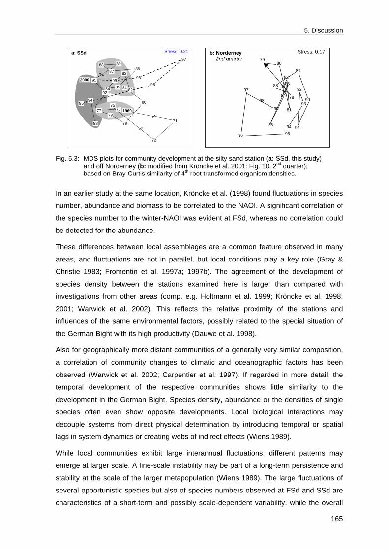
5. Discussion
1969
71
72
7576 77
78
79
80
81 82
83
84 85
86 87 88 89
91
92
93
94 95
96
97
98 992000
Stress: 0.21 a: SSd 2nd quarter
78
79 80
81
82
83
84
85
86
87
88
89
90
91
92
93
94 95 96
97
98
99
Stress: 0.17 b: Norderney
Fig. 5.3: MDS plots for community development at the silty sand station (a: SSd, this study)
and off Norderney (b: modified from Kröncke et al. 2001: Fig. 10, 2nd quarter); based on Bray-Curtis similarity of 4th root transformed organism densities.
In an earlier study at the same location, Kröncke et al. (1998) found fluctuations in species
number, abundance and biomass to be correlated to the NAOI. A significant correlation of
the species number to the winter-NAOI was evident at FSd, whereas no correlation could
be detected for the abundance.
These differences between local assemblages are a common feature observed in many
areas, and fluctuations are not in parallel, but local conditions play a key role (Gray &
Christie 1983; Fromentin et al. 1997a; 1997b). The agreement of the development of
species density between the stations examined here is larger than compared with
investigations from other areas (comp. e.g. Holtmann et al. 1999; Kröncke et al. 1998;
2001; Warwick et al. 2002). This reflects the relative proximity of the stations and
influences of the same environmental factors, possibly related to the special situation of
the German Bight with its high productivity (Dauwe et al. 1998).
Also for geographically more distant communities of a generally very similar composition,
a correlation of community changes to climatic and oceanographic factors has been
observed (Warwick et al. 2002; Carpentier et al. 1997). If regarded in more detail, the
temporal development of the respective communities shows little similarity to the
development in the German Bight. Species density, abundance or the densities of single
species often even show opposite developments. Local biological interactions may
decouple systems from direct physical determination by introducing temporal or spatial
lags in system dynamics or creating webs of indirect effects (Wiens 1989).
While local communities exhibit large interannual fluctuations, different patterns may
emerge at larger scale. A fine-scale instability may be part of a long-term persistence and
stability at the scale of the larger metapopulation (Wiens 1989). The large fluctuations of
several opportunistic species but also of species numbers observed at FSd and SSd are
characteristics of a short-term and possibly scale-dependent variability, while the overall
165
5. Discussion
species composition remains relatively stable. This is only possible within a larger mosaic
of habitat elements, where a regional species pool persists, which contains all species
that could eventually colonise a location if competitive exclusion was unimportant (Gray
2002). Benthic soft-bottom communities are characterised as a mosaic of patches at
various spatial scales that may exhibit differing temporal development following the
mosaic-cycle concept (Aubreville 1936; see also Remmert 1991). This may lead to an
overall stability of loosely coupled elements, dispersed over habitat patches, and local
stability is no longer relevant. Instead, temporal and spatial scaling of the cycling
communities and processes driving the cycles come into focus (Reise 1991).
Within benthic communities biological interactions (predation, spatial interference,
bioturbation etc.) cause a small-scale patchiness and a mosaic-cycle on a scale of a few
centimetres to a few metres (Reise 1991). In addition, on a larger scale of several
kilometres not only the community composition changes, but also the spatial patterns shift
seasonally and between years (Eagle 1975). The observed changes in local densities at
the stations in the German Bight may also reflect spatial shifts of populations. While the
local population density of Nucula nitidosa at Slt was lower during the 80ies and then
increased again, N. nitidosa was more abundant at SSd during the 80ies and then
declined again. Following cold winters, the local populations of Amphiura filiformis in the
inner German Bight collapse and may take several years before reaching higher densities
again (like at SSd), which was explained by hydrographic conditions by Gerdes (1977). In
deeper parts of the area, recovery can be much faster, and high densities are reached
already after two years, as observed at WB. A slow return to the inner parts, whether
caused by hydrography or biotic interactions, leads to the perceived outward shift of the
limit between the Amphiura-filiformis-association and the Nucula-nitidosa-association in
the Pleistocene Elbe valley (Rachor & Nehmer 2003). In several parts of the Oyster
Grounds west of the German Bight, A. filiformis was present in high densities during the
90ies (Holtmann et al. 1999). According to the main easterly direction of the residual
current, this should allow a supply of larvae to the German Bight. The actual current
conditions are, however, depending on the wind and conditions during the larval phase
and may not have allowed an advection of the larvae into the inner German Bight. Effects
related to this question can only be solved in combination with meroplankton and
hydrographic data.
The spatial distribution of benthic organisms on a regional scale within the southern North
Sea is different between studies (Duineveld et al. 1987; Craeymeersch et al. 1997).
Meroplanktonic larvae of many benthic species allow a dispersal over wide areas and the
use of habitat mosaics at very large spatial scales. So they can shift to other geographic
166
5. Discussion
regions when confronted with an adverse phase of a long-term environmental periodicity
(Reise 1991)
The highly significant correlation between the similarity matrices of the temporal
development of the communities at several stations indicates a parallel development of
the communities. This applies to similar periods and similar "unusual" years indicating a
possible dependence on the same factors acting on a large scale. The lower correlation
between stations separated by the furthest geographical distance (WB/Slt), or with the
most different sediment composition (FSd/Slt) respectively, indicates the importance of
local conditions and/or of the community composition for the temporal community
development.
The timing of changes in communities is similar between different parts of the North Sea
and may be a result of climate and oceanographic features. However, the local community
development is a product of local environmental variation and biotic interactions, and both
differ between areas.
Therefore, a direct correlation between large-scale environmental factors and population
changes in the wider area may not lead to consistent results. However, the local
development, influenced by interactions and in relation to local abiotic conditions, could
possibly be further analysed using advanced mathematical models if local environmental
conditions can be adequately quantified.
5.6 Implications for offshore monitoring of soft-bottom benthos
The power to detect trends in community composition depends on the sample size, the
magnitude of the trend, and the magnitude of random variation, just as it does with
univariate analyses (Philippi et al. 1998). The present design with five replicate van-Veen
grabs at four selected stations seems sufficient to follow the local community
development. However, as discussed in the previous chapter, single stations do only allow
inferences about the local development, which may be only one element in a large scale
mosaic cycle. To differentiate between the natural fluctuations of mosaic elements and
long term trends, a repeated mapping of the area would be needed (Reise 1991).
For studies of the development of the benthic communities in larger heterogeneous areas,
a stratified random sampling is presumably the most powerful design (Krebs 1998). Under
the assumption that each stratum represents a homogeneous area (which can adequately
be represented by e.g. a mean density per species), randomly selected stations with only
a single replicate per station provide the largest power to detect community differences
(Cuff & Coleman 1979; Van der Meer 1997). These strata should not include
heterogeneous communities and borders between strata should be avoided, because this
167
5. Discussion
would greatly reduce the power to detect changes (Philippi et al. 1998). For marine
community studies, formal random selection of sites is less important since the spatially
stochastic distribution of populations will probably generate an appropriate randomness
from evenly spaced sites (Milne 1959; Clarke & Green 1988). Random selection may
sometimes even lead to an uneven distribution of effort across an area and an appropriate
spatial dispersion of sites across the area needs to ascertained (Hurlbert 1984).
Once the stations are selected, the same stations should be revisited in succeeding years
to reduce the confounding effects of spatial variation and increase the power to detect
temporal changes (Thrush et al. 1994; Stewart-Oaten et al. 1995; Van der Meer 1997).
The appropriate number of stations depends on the size of the area and its spatial
variability. A larger extent will incorporate greater spatial heterogeneity (Wiens 1989;
Philippi et al. 1998).
Such a large-scale stratified random sampling is realised in the Dutch offshore monitoring
program BIOMON (Van der Meer 1997; Holtmann et al. 1999). This approach includes all
spatial variation on all scales within the designated strata and therefore leads to very large
variability of the data especially with small-sized sampling gear (e.g. Holtmann et al. 1999;
Armonies 2000). Apart from this, it precludes comparisons among stations, and changes
in the spatial distribution within the stratum are likely to pass unnoticed. The variability of
single grab samples is too high to detect differences between sub-areas except for the
most extreme ones as, e.g., between different communities. If any comparison between
sampling sites is intended, replicates are needed to assess the within-site similarity
between replicates (Clarke & Green 1988; Philippi et al. 1998). Two replicates are the
minimum, but more replicates allow a more precise description of the local community and
greatly enhance the power of comparisons by increasing the possible number of
permutations in randomisation tests (see chapter 5.2.2).
A nested design over different spatial scales allows a distinction of the variability and
relevant processes at different scales (Morrisey et al. 1992; Thrush et al. 1997; Kendall &
Widdicombe 1999; Paiva 2001; Hewitt et al. 2002). In nested designs, it is important to
allocate the effort across the levels efficiently to maximise the power for the most
important questions of the study. The optimal balance can be calculated when the
variability at the respective scales is known (Clarke & Green 1988). A selection of sites for
the German Bight could be realised by analysing the spatial distribution of benthic
communities within the designated communities from large scale surveys (Salzwedel et al.
1985; Rachor & Nehmer 2003) and comparing it to the local variability analysed here.
Time series of benthic communities are mostly characterised by a considerable seasonal
variation (Arntz & Rumohr 1982; 1986; Muehlenhardt-Siegel 1988; Frid et al. 1996;
168
5. Discussion
Kröncke et al. 1998). For long-term observations of benthic communities, the late-winter
or early spring situation is preferred as the communities are reduced to those species that
are able to survive in the area over longer periods. In summer many species settle in the
area, sometimes in very large numbers, but may not be able to survive until the next year.
When interspecific interactions control the community development, the establishment of
large densities often of opportunistic species may be impaired or even inhibited (Crowe et
al. 1987; Olafsson et al. 1994) and the development may mainly be characterised by
density increases of the species already present (Weigelt 1991). While this general
pattern occurs in most years, the identity of the successful species varies and is not
predictable. It may be a question of which species happens to be in the area at the right
time (Reise 1991). This seasonal variation adds to the spatial variation and complicates
the identification of long-term trends. While single sampling occasions in early spring are
appropriate to document long-term changes in benthic communities, each change
observed to the previous year's situation is a result of various processes including
recruitment and mortality over the whole year. If inferences about processes were
intended, biannual sampling in spring and autumn would be necessary (Alden et al. 1997).
Beyond the description of community variability, inferences about responsible factors can
only be made if appropriate data of possibly influential variables are available. As several
of these factors also vary on various spatial and temporal scales, measurements should
ideally be directly connected to the sampling of the benthic communities. Values for all
relevant variables should be determined from each replicate sample (on the appropriate
scale for the respective variable), thus matching the biological, physical and chemical data
as closely as possible (Clarke & Green 1988).
A general statement about the regional community development beyond the local
conditions would require a larger extent of sampling within each community. Any
conclusions about changes in the spatial distribution would require several stations with
replicate samples. A more functional analysis would only be possible with a higher
frequency of sampling to identify the exact timing of changes in benthic communities in
relation to fluctuations of environmental variables and a continuous recording of the
relevant environmental factors locally at the benthos sampling stations.
If annual sampling of numerous stations is not feasible, information on the long-term
development of benthic communities beyond local conditions could be derived by a
combination of annual sampling at selected stations with extensive large-scale surveys at
longer intervals (e.g. every ten years). A combined analysis of the large-scale spatial and
local temporal variability may be seen as a compromise to investigate the spatial
distribution of the communities and their long-term development.
169
5. Discussion
5.7 Open questions and further analyses
Spatio-temporal definition of benthic communities
The definition of benthic communities from spatial surveys can identify the spatial extent
of relatively similar associations. Consecutive surveys covering the same area have often
found other species to be characteristic of a certain area. This depends partly on the
sampling grain and extent of the survey, but also on the temporal variability of the benthic
communities, which should be incorporated, leading to a spatio-temporal definition of the
community. At the same time, the temporal variability could be compared to the spatial
variability on a larger scale to evaluate the local fluctuations in relation to the large-scale
spatial variability.
Combined analyses of benthic and planktonic time series
Information on planktonic primary production in combination with hydrodynamic models
might allow an estimate of the interannual variations in food supply at the stations. A more
comprehensive study of the connections between nutrients, primary production, the
planktonic food web and the benthos is a very challenging problem, which needs
expertise from specialists. It could be tackled in a scientific cooperation using e.g. the data
presented here in combination with nutrient and phyto- and (mero-)zooplankton
community time series from Helgoland, when these are available for analysis.
Predictive models
The correlations between multivariate community structure and several environmental
factors weight each factor equally. A more differentiated weighting may further increase
the fit. Rank correlations detected in this study can only be used for qualitative predictions.
A further investigation using more quantitative models and advanced techniques (e.g.
distance-based redundancy analysis (Legendre & Anderson 1999)) may lead to predictive
models. Such models do not necessarily have to incorporate the exact knowledge about
functional relationships, but may on the basis of empirical correlations allow predictions
about changes in the ecological system under various scenarios of environmental change.
Sample size sensitivity of diversity and dominance indices based on real samples
The analysis of the sample size dependency of the Shannon-Wiener diversity (H') and
Pielou's evenness (J') indices has shown that the dependency found in real samples can
differ from predictions of theoretical simulations. Each index has a slightly different focus
and its own properties regarding sample size sensitivity and variability (Hurlbert 1971; Hill
1973; Smith & Wilson 1996; Krebs 1998). The choice of index may have profound effects
on the interpretation of the results. The sample size dependence and variability of indices
170
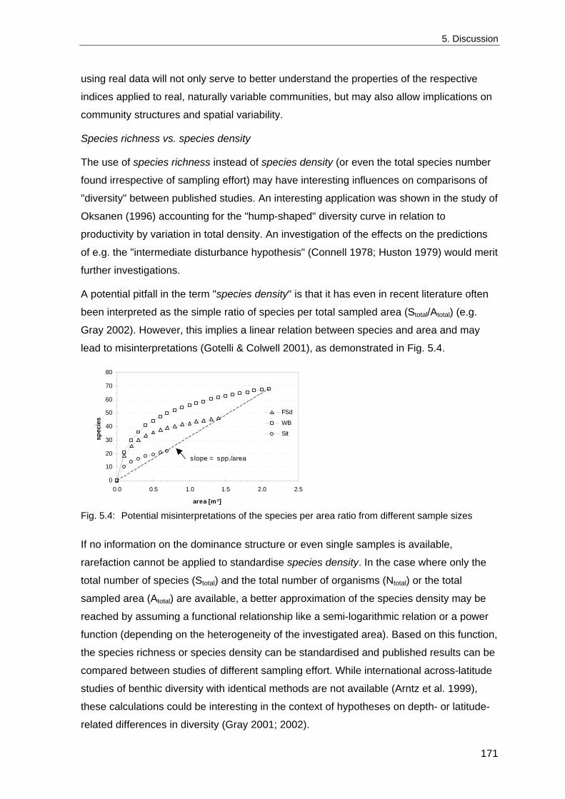
5. Discussion
using real data will not only serve to better understand the properties of the respective
indices applied to real, naturally variable communities, but may also allow implications on
community structures and spatial variability.
Species richness vs. species density
The use of species richness instead of species density (or even the total species number
found irrespective of sampling effort) may have interesting influences on comparisons of
"diversity" between published studies. An interesting application was shown in the study of
Oksanen (1996) accounting for the "hump-shaped" diversity curve in relation to
productivity by variation in total density. An investigation of the effects on the predictions
of e.g. the "intermediate disturbance hypothesis" (Connell 1978; Huston 1979) would merit
further investigations.
A potential pitfall in the term "species density" is that it has even in recent literature often
been interpreted as the simple ratio of species per total sampled area (Stotal/Atotal) (e.g.
Gray 2002). However, this implies a linear relation between species and area and may
lead to misinterpretations (Gotelli & Colwell 2001), as demonstrated in Fig. 5.4.
0
10
20
30
40
50
60
70
80
0.0 0.5 1.0 1.5 2.0 2.5
area [m²]
spec
ies
FSd
WB
Slt
slope = spp./area
Fig. 5.4: Potential misinterpretations of the species per area ratio from different sample sizes
If no information on the dominance structure or even single samples is available,
rarefaction cannot be applied to standardise species density. In the case where only the
total number of species (Stotal) and the total number of organisms (Ntotal) or the total
sampled area (Atotal) are available, a better approximation of the species density may be
reached by assuming a functional relationship like a semi-logarithmic relation or a power
function (depending on the heterogeneity of the investigated area). Based on this function,
the species richness or species density can be standardised and published results can be
compared between studies of different sampling effort. While international across-latitude
studies of benthic diversity with identical methods are not available (Arntz et al. 1999),
these calculations could be interesting in the context of hypotheses on depth- or latitude-
related differences in diversity (Gray 2001; 2002).
171
References
References
Aebisher, N.J.; Coulsen, J.C. & Colebrook, J.M. (1990): Parallel long-term trends across four marine trophic levels and weather. Nature 347: 753-755.
Alden, R.W.; Weisberg, S.B.; Ranasinghe, J.A. & Dauer, D.M. (1997): Optimizing Temporal Sampling Strategies for Benthic Environmental Monitoring Programs. Mar. Pollut. Bull. 34(11): 913-922.
Ambrose, W.G. Jr (1991): Are infaunal predators important in structuring marine soft-bottom communities?. Am. Zool. 31(6): 849-860.
Andersin, A.B. & Sandler, H. (1981): Comparison of the sampling efficiency of two van Veen Grabs. Fin. Mar. Res. 248: 137-142.
Andrew, N.L. & Mapstone, B.D. (1987): Sampling and the description of spatial pattern in marine ecology. Oceanogr. Mar. Biol. Annu. Rev. 25: 39-90.
Ankar, S. (1977): Digging profile and penetration of the van Veen grab in different sediment types. Contributions From the Askö Lab. Univ. of Stockholm, Sweden 16: 22pp.
ARGE Elbe (1997): 20 Jahre Arbeitsgemeinschaft für die Reinerhaltung der Elbe.; Wassergütestelle Elbe, Hamburg. 34 pp.
Armonies, W. (2000): On the spatial scale needed for benthos community monitoring in the coastal North Sea. J. Sea Res. 43(2): 121-133.
Armonies, W. (2001): What an introduced species can tell us about the spatial extension of benthic populations. Mar. Ecol. Prog. Ser. 209: 289-294.
Armonies, W.; Herre, E. & Sturm, M. (2001): Effects of the severe winter 1995/96 on the benthic macrofauna of the Wadden Sea and the coastal North Sea near the island of Sylt. Helgol. Mar. Res. 55(3): 170-175.
Arntz, W. E. (1980): Predation by demersal fish and its impact on the dynamics of macrobenthos. In: Tenore, K. R. & Coul, B. C. (eds.): Marine benthic dynamics. University of South Carolina Press, Columbia: pp. 121-149.
Arntz, W. E. (1981): Zonation and dynamics of macrozoobenthos biomass in an area stressed by oxygen defficiency. In: Barret, G. W. & Rosenberg, R. (eds.): Stress effects on natural ecosystems. John Wiley & Sons, Chichester: pp. 215-225.
Arntz, W. E. & Fahrbach, E. (1991): El Nińo - Klimaexperiment der Natur. Physikalische Ursachen und biologische Folgen .; Birkhäuser, Basel. 264 pp.
Arntz, W. E.; Gili, J. M. & Reise, K. (1999): Unjustifiably ignored: Reflections on the role of benthos in marine ecosystems. In: Gray, J. S.; Ambrose, W. G. & Szaniawska, A. (eds.): Biogeochemical Cycling and Sediment Ecology. Kluwer Academic Publishers, the Netherlands: pp. 105-124.
Arntz, W.E. & Rumohr, H. (1982): An experimental study of macrobenthic colonization and succession, and the importance of seasonal variation in temperate latitudes. J. Exp. Mar. Biol. Ecol. 64(1): 17-46.
Arntz, W.E. & Rumohr, H. (1986): Fluctuations of benthic macrofauna during succession and in an established community. Meeresforschung Rep. Mar. Res. 31(2): 97-114.
Arntz, W.E. & Weber, W. (1970): Cyprina islandica L. (Mollusca, Bivalvia) als Nahrung von Dorsch und Kliesche in der Kieler Bucht. Ber. Dt. Wiss. Komm. Meeresforsch. 21: 193-209.
Aubreville, A. (1936): La foret coloniale: Les forets de L' Afrique occidentale francaise. Ann. Acad. Sci. Colon. Paris 9: 1-245.
172
References
Austen, M.C.; Buchanan, J.B.; Hunt, H.G.; Josefson, A.B. & Kendall, M.A. (1991): Comparison of long-term trends in benthic and pelagic communities of the North Sea. J. Mar. Biol. Ass. U.K. 71(1): 179-190.
Bauerfeind , E.; Hickel, W.; Niermann, U. & Westernhagen, H.von (1990): Phytoplankton Biomass and potential nutrient limitation of phytoplankton development in the southeastern North Sea in Spring 1985 and 1986. Neth. J. Sea Res. 25(1/2): 131-142.
Becker, G. (2003): Physikalische Beschreibung der Nordsee. In: Lozán, J. L.; Rachor, E.; Reise, K.; Sündermann, J. & H. v. Westernhagen (eds.): Warnsignale aus Nordsee & Wattenmeer. Eine aktuelle Umweltbilanz. Verlag Wissenschaftliche Auswertungen, Hamburg: pp. 34-39.
Becker, G. A. (1990): Die Nordsee als physikalisches System. In: Lozan, J. L.; Lenz, W.; Rachor, E.; Watermann, B. & von Westernhagen, H.: Warnsignale aus der Nordsee. P. Parey, Berlin: pp. 11-27.
Becker, G.A.; Dick, S. & Dippner, J.W. (1992): Hydrography of the German Bight. Mar. Ecol. Prog. Ser. 91: 9-18.
Becker, G.A.; Frohse, A. & Damm, P. (1997): The North Western European shelf temperature and salinity variability. Dtsch. Hydrogr. Z. 49(2-3): 145-161.
Bergman, M. J. N.; Ball, B.; Bijleveld, C.; Craeymeersch, J. A.; Munday, B. W.; Rumohr, H. & van Santbrink, J. W. (1998): Direct mortality due to trawling. In: Lindeboom, H. J. & de Groot, S. J. (eds.): IMPACT II: The effects of different types of fisheries on the North Sea and Irish Sea benthic ecosystem. NIOZ-rapport 1998-1: pp. 28-33.
Bergman, M.J.N.; Fonds, M.; Hup, M.; Lewis, P.; van der Puyl, P.; Stam, A. & den Uyl, D. (1990): Direct effects of beamtrawl fishing on benthic fauna in the North Sea. BEON Report 8: 33-57.
Bergman, M.J.N. & Hup, M. (1992): Direct effects of beamtrawling on macrofauna in a sandy sediment in the southern North Sea. ICES J. Mar. Sci 49: 5-11.
Bergman, M. J. N. & van Santbrink, J. W. (1994): Direct effects of beam trawling on macrofauna in sandy areas off the Dutch coast. In: de Groot, S. J. & Lindeboom, H. J. (eds.): Environmental impact of bottom gears on benthic fauna in relation to natural resources management and protection of the North Sea. NIOZ-Rapport 1994/11: pp. 179-208.
Bergman, M. J. N. & van Santbrink, J. W. (2000): Fishing mortality of populations of megafauna in sandy sediments. In: Kaiser, M. J. & de Groot, S. J. (eds.): Effects of fishing on non-target species and habitats . Blackwell Science, Oxford: pp. 49-68.
Bergstrom, U.; Englund, G. & Bonsdorff, E. (2002): Small-scale spatial structure of Baltic Sea zoobenthos-inferring processes from patterns. J. Exp. Mar. Biol. Ecol. 281 (1-2): 123-136.
Berkenbusch, K.; Rowden, A.A. & Keith Probert, P.K. (2000): Temporal and spatial variation in macrofauna community composition imposed by ghost shrimp Callianassa filholi bioturbation. Mar. Ecol. Prog. Ser. 192: 249-257.
Beukema, J.J. (1974): The efficiency of the Van Veen grab compared with the Reineck box sampler. J. Cons. Int. Explor. Mer 35(3): 319-327.
Beukema, J.J. (1989): Long-term changes in macrozoobenthic abundance on the tidal flats of the western part of the Dutch Wadden Sea. Helgol. Meeresunters. 43(3-4): 405-415.
Bhaud, M. & Duchene, J.C. (1977): Observations sur l'efficacitée comparée de deux bennes. Vie Et Milieu, Ser. A 27(1): 35-53.
Birch, D.W. (1981): Dominance in marine ecosystems. Am. Nat. 118: 262-274.
173
References
Birkett, L. (1958): A basis for comparing grabs. J. Cons. Int. Explor. Mer. 23: 202-207.
Bloom, S.A. (1981): Similarity indices in community studies: potential pitfalls. Mar. Ecol. Prog. Ser. 5: 125-128.
Bray, J.R. & Curtis, J.T. (1957): An ordination of the upland forest of Southern Wisconsin. Ecol. Monogr. 27: 225-349.
Brenchley, G.A. (1981): Disturbance and Community Structure: An Experimental Study of Bioturbation in Marine Soft-Bottom Environments. J. Mar. Res. 39(4): 767-790.
Bros, W.E. & Cowell, B.C. (1987): A technique for optimizing sample size (replication). J. Exp. Mar. Biol. Ecol. 114(1): 63-71.
Buchanan, J. B. (1984): Sediment analysis. In: Holme, N. A. & McIntyre, A. D. (eds.): Methods for the study of marine benthos. IBP Handbook 16. ed. Blackwell, Oxford: pp. 41-65.
Buchanan, J.B. (1993): Evidence of benthic pelagic coupling at a station off the Northumberland coast. J. Exp. Mar. Biol. Ecol. 172(1-2): 1-10.
Buhr, K.J. (1981): Auswirkungen des kalten Winters 1978/79 auf das Makrobenthos der Lanice-Siedlung im Weser-ästuar. Veröff. Inst. Meeresforsch. Bremerh. 19: 115-131.
Cadée, G.C.; Boon, J.P.; Fischer, C.V.; Mensink, B.P. & Ten-Hallers-Tjabbes, C.C. (1995): Why the whelk (Buccinum undatum) has become extinct in the Dutch Wadden Sea. Neth. J. Sea Res. 34(4): 337-339.
Callaway, R.; Alsvåg, J.; de Boois, I.; Cotter, J.; Ford, A.; Hinz, H.; Jennings, S.; Kröncke, I.; Lancaster, J.; Piet, G.; Prince, P. & Ehrich, S. (2002): Diversity and community structure of epibenthic invertebrates and fish in the North Sea. ICES J. Mar. Sci. 59: 1199-1214.
Cao Yong; Williams, W.P. & Bark, A.W. (1997): Effects of sample size (replicate number) on similarity measures in river benthic Aufwuchs community analysis. Water Environ. Res. 69(1): 107-114.
Carpentier, P.; Dewarumez, J.M. & Lepretre, A. (1997): Long-term variability of the Abra alba community in the Southern Bight of the North Sea. Oceanol. Acta 20(1): 283-290.
Caston, V. N. D. (1979): The quaternary sediments of the North Sea. In: Banner, F. T.; Collins, M. S. & Massie, K. S. (eds.): The north west European shelf seas: The sea bed and the sea in motion: I. Geology and Sedimentology. Elsevier, Oxford: pp. 195-270.
Chapman, M.G. & Underwood, A.J. (1999): Ecological patterns in multivariate assemblages: Information and interpretation of negative values in ANOSIM tests. Mar. Ecol. Prog. Ser. 180: 257-265.
Chavez, F.P.; Ryan, J.; Lluch-Cota, S.E. & Niquen C., M. (2003): From Anchovies to Sardines and Back: Multidecadal Change in the Pacific Ocean. Science 299(5604): 217-221.
Chesney, E. J. (1985): Succession in soft-bottom benthic environments: are pioneering species really outcompeted? In: Gibbs, P. E., (ed.): Proceedings of the 19th Marine Biology Symposium . Cambridge: Cambridge University Press: pp. 277-286.
Christie, N.D. (1975): Relationship between sediment texture, species richness and volume of sediment sampled by a grab. Mar. Biol. 30: 89-96.
Clarke, K.R. & Green, R.H. (1988): Statistical design and analysis for a "biological effects" study. Mar. Ecol. Prog. Ser. 46(1-3): 213-226.
Clarke, K. R. & Warwick, R. M. (1994): Change in marine communities: an approach to statistical analysis and interpretation.; Natural Environment Research Council, UK. 144 pp.
174
References
Clifford, H. T. & Stephenson, W. (1975): An introduction to numerical calssification.; Academic Press, New York. xii + 229 pp.
Colijn, F.; Villerius, L.; Rademaker, M.; Hammer, K.D. & Eberlein, K. (1990): Changes in spatial distribution of primary production, photosynthetic pigments and phytoplankton species composition during two surveys in the German Bight. Neth. J. Sea Res. 25(1/2): 155-164.
Colwell, R.K. (2000): EstimateS: Statistical Estimation of Species Richness and Shared Species from Samples, User's Guide and Application Vers. 6.0b1. Published at: http://viceroy.eeb.uconn.edu/estimates .
Colwell, R.K. & Coddington, J.A. (1994): Estimating terrestrial biodiversity through extrapolation. Philos. Trans. R. Soc. Lond. B Biol. Sci. 345: 101-118.
Connell, J.H. (1978): Diversity in tropical rain forests and coral reefs. Science 199: 1302-1310.
Craeymeersch, J. A.; Heip, C. H. R. & Buijs, J. (1997): Atlas of North Sea benthic infauna. Based on the 1986 North Sea Benthos Survey. ICES Coop. Res. Rep. 1997/218: 86 pp.
Crowe, W.A.; Josefson, A.B. & Svane, I. (1987): Influence of adult density on recruitment into soft sediments: A short-term in situ sublittoral experiment. Mar. Ecol. Prog. Ser. 41(1): 61-69.
Cuff, W. & Coleman, N. (1979): Optimal survey design: Lessons from a stratified random Sample of Macrobenthos. J. Fish. Res. Board Can. 36: 351-361.
Dauwe, B.; Herman, P.M.J. & Heip, C.H.R. (1998): Community structure and bioturbation potential of macrofauna at four North Sea stations with contrasting food supply. Mar. Ecol. Prog. Ser. 173: 67-83.
Davies, J.M.; Addy, J.M.; Blackman, R.; Blanchard, J.R.; Moore, D.C.; Sommerville, H.J.; Whitehead, A. & Wilkinson, T. (1984): Environmental effects of oil based mud cuttings. Mar. Pollut. Bull. 15: 363-370.
de Jonge, V.N.; Elliott, M. & Orive, E. (2002): Causes, historical development, effects and future challenges of a common environmental problem: eutrophication . Hydrobiologia 475/476: 1-19.
Dethlefsen, V. & Westernhagen, H.von (1983): Oxygen deficiency and effects on bottom fauna in the eastern German Bight 1982. Meeresforschung Rep. Mar. Res. 30(1): 42-53.
Diaz, R.J.; Rosenberg, R.; Ansell, A.D.; Gibson, R.N. & Barnes, M., eds. (1995): Marine benthic hypoxia: A review of its ecological effects and the behavioural responses of benthic macrofauna. Oceanogr. Mar. Biol. Annu. Rev. 33: 245-03.
Dippner, J.W. (1997): Recruitment success of different fish stocks in the North Sea in relation to climate variability. Dt. Hydrogr. Z. 49(2/3): 277-293.
Dittmer, J.-D. (1977): Zur Dynamik der kleinräumigen Verteilung von Polychaeten (Annelida) auf Sandböden im Sublitoral der Deutschen Bucht. Univ. Kiel Diploma Thesis.
Ducrotoy, J.P.; Elliott, M. & De Jonge, V.N. (2000): The North Sea. Mar. Pollut. Bull. 41(1-6): 5-23.
Duineveld, G.C.A.; Kuenitzer, A. & Heyman, R.P. (1987): Amphiura filiformis (Ophiuroidea: Echinodermata) in the North Sea. Distribution, present and former abundance and size composition. Neth. J. Sea Res. 21(4): 317-329.
Duineveld, G.C.A.; Kuenitzer, A.; Niermann, U.; De Wilde, P.A.W.J. & Gray, J.S. (1991): The macrobenthos of the North Sea. Neth. J. Sea Res. 28(1-2): 53-65.
Dybern, B.I.; Ackefors, H. & Elmgren, R. (1976): Recommendations on methods for marine biological studies in the Baltic Sea. Baltic Marine Biologist 1: 98pp.
175
References
Dyer, M.F.; Fry, W.G.; Fry, P.D. & Cranmer, G.J. (1983): Benthic regions within the North Sea. J. Mar. Biol. Ass. U.K. 63: 683-693.
Dörjes, J. (1977): Über die Bodenfauna des Borkum Riffgrundes (Nordsee). Senckenb. Marit. 9(1/2): 1-17.
Dörjes, J. (1992): Die amerikanische Schwertmuschel Ensis directus (Conrad) in der Deutschen Bucht. III. Langzeitentwicklung nach 10 Jahren. Senckenb. Marit. 22(1-2): 29-35.
Dörjes, J.; Michaelis, H. & Rhode, B. (1986): Long-term studies of macro-zoobenthos in the intertidal and shallow subtidal habitats near the island of Norderney (East Frisian coast, Germany). Hydrobiologia 142: 217-232.
Eagle, R.A. (1975): Natural Fluctuations in a Soft Bottom Benthic Community. J. Mar. Biol. Ass. U.K. 55: 865-878.
Edwards, M.; Beaugrand, G.; Reid, P.C.; Rowden, A.A. & Jones, M.B. (2002): Ocean climate anomalies and the ecology of the North Sea. Mar. Ecol. Prog. Ser. 239: 1-10.
Eggert (2002): Deutsches Gewässerkundliches Jahrbuch, Elbegebiet, Teil III.; Freie und Hansestadt Hamburg, Wirtschaftsbehörde, Strom- und Hafenbau, http://www.dgj.de/servlet/IbMenu.
Eisma, D. (1981): Supply and deposition of suspended matter in the North Sea. Publ. Int. Ass. Sediment 5: 415-428.
Eleftheriou, A. & Basford, D. (1989): The macrobenthic infauna of the offshore northern North Sea. J. Mar. Biol. Ass. U.K. 69: 123-143.
Eleftheriou, A. & Holme, N. A. (1984): Macrofauna techniques. In: Holme, N. A. & McIntyre, A. D. (eds.): Methods for the study of marine benthos. pp. 140-216.
Ellingsen, K.E. (2001): Biodiversity of a continental shelf soft-sediment macrobenthos community. Mar. Ecol. Prog. Ser. 218: 1-15.
Elliott, J. M. (1977): Some methods for the statistical analysis of samples of benthic invertebrates. 2 ed. Freshwater Biological Association Sci. Publ. No. 25.
Fager, E.W. (1972): Diversity: a sampling study. Am. Nat. 106: 293-310.
Field, J.G.; Clarke, K.R. & Warwick, R.M. (1982): A practical strategy for analysing multispecies distribution patterns. Mar. Ecol. Prog. Ser. 8(1): 37-52.
Figge, K. (1981): Sedimentverteilung in der Deutschen Bucht. 1:250 000.; Dt. Hydrogr. Inst., Hamburg. Karte Nr. 2900 pp.
Frey, H. (1990): Stratification during periods of oxygen deficiency in the German Bight during the summer from 1981 to 1983: a comparison with the long-term variation in stratification. Meeresforsch. 32: 306-328.
Frid, C.L.J.; Buchanan, J.B. & Garwood, P.R. (1996): Short Communication: Variability and stability in benthos: twenty-two years of monitoring off Northumberland. ICES J. Mar. Sci. 53(6): 978-980.
Frid, C.L.J.; Clark, R.A. & Hall, J.A. (1999): Long-term changes in the benthos on a heavily fished ground off the NE coast of England. Mar. Ecol. Prog. Ser. 188: 13-20.
Frid, C.L.J.; Harwood, K.G.; Hall, S.J. & Hall, J.A. (2000): Long-term changes in the benthic communities on North Sea fishing grounds. ICES J. Mar. Sci. 57(5): 1303-1309.
Fromentin, J.M.; Dauvin, J.C.; Ibanez, F.; Dewarumez, J.M. & Elkaim, B. (1997a): Long-term variations of four macrobenthic community structures. Oceanol. Acta 20(1): 43-54.
176
References
Fromentin, J.M.; Ibanez, F.; Dauvin, J.C.; Dewarumez, J.-M. & Elkaim, B. (1997b): Long term changes of four macrobenthic assemblages from 1978 to 1992. J. Mar. Biol. Ass. U.K. 77(1): 287-310.
Gadow, S. & Schäfer, A. (1973): Die Sedimente der Deutschen Bucht: Korngröβen, Tonmineralien und Schwermetalle. Senckenb. Marit. 5: 165-178.
Gage, J.D. (1966): Observations on the bivalves Montacuta substriata and M. ferruginosa, 'commensals' with spatangoids. J. Mar. Biol. Ass. U.K. 46: 49-70.
Gage, J.D. & May, R.M. (1993): A dip into the deep seas. Nature 365: 609-610.
Gamito, S. & Raffaelli, D. (1992): The sensitivity of several ordination methods to sample replication in benthic surveys. J. Exp. Mar. Biol. Ecol. 164(2): 221-232.
Gerdes, D. (1977): The re-establishment of an Amphiura filiformis (O.F. Muller) population in the inner part of the German Bight.Biology of benthic organisms. 11. European Symposium on Marine Biology; Galway. Oxford (UK): Pergamon Press: pp. 277-284.
Glemarec, M. (1973): The benthic communities of the European North Atlantic shelf. Oceanogr. Mar. Biol. Annu. Rev. 11: 263-289.
Goedecke, E. (1968): Über die hydrographische Struktur der Deutschen Bucht im Hinblick auf die Verschmutzung der Konvergenzzone. Helgol. Wiss. Meeresunters. 17: 108-125.
Gotelli, N.J. & Colwell, R.K. (2001): Quantifying biodiversity: procedures and pitfalls in the measurement and comparison of species richness. Ecol. Lett. 4: 379-391.
Graf, G. & Rosenberg, R. (1997): Bioresuspension and biodeposition: A review. J. Mar. Syst. 11(3-4): 269-278.
Gray, J.S. (2000): The measurement of marine species diversity, with an application to the benthic fauna of the Norwegian continental shelf. J. Exp. Mar. Biol. Ecol. 250(1-2): 23-49.
Gray, J.S. (2001): Marine diversity: the paradigms in patterns of species richness examined. Sci. Mar. 65(Suppl. 2): 41-56.
Gray, J.S. (2002): Species richness of marine soft sediments. Mar. Ecol. Prog. Ser. 244: 285-297.
Gray, J.S. & Christie, H. (1983): Predicting long-term changes in marine benthic communities. Mar. Ecol. Prog. Ser. 13(1): 87-94.
Gray, J.S.; Poore G.C.B.; Ugland, K.I.; Wilson, R.S.; Olsgard, F. & Johanessen, Ø. (1997): Coastal and deep-sea benthic diversities compared. Mar. Ecol. Prog. Ser. 159: 97-103.
Gray, J.S.; Wu, R.S. & Or, Y.Y. (2002): Effects of hypoxia and organic enrichment on the coastal marine environment. Mar. Ecol. Prog. Ser. 238: 249-279.
Groot, S.J.d. & Lindeboom, H.J., eds (1994): Environmental impact of bottom gears on benthic fauna in relation to natural resources management and protection of the North Sea. Netherlands Institute for Sea Research. NIOZ-Rapport 1994-11, RIVO-DLO Report CO26/94.
Hagmeier, A. (1925): Vorläufiger Bericht über die vorbereitenden Untersuchungen der Bodenfauna der Deutschen Bucht mit dem Petsersen-Bodengreifer. Ber. Dt. Wiss. Komm. Meeresforsch. 1: 249-272.
Hall, S.J. (1994): Physical disturbance and marine benthic communities: Life in unconsolidated sediments. Oceanogr. Mar. Biol. Annu. Rev. 32: 179-239.
Hall, S.J.; Basford, D.J.; Robertson, M.R.; Raffaelli, D.G. & Tuck, I. (1991): Patterns of recolonisation and the importance of pit-digging by the crab Cancer pagurus in a subtidal sand habitat. Mar. Ecol. Prog. Ser. 72(1-2): 93-102.
177
References
Hartmann-Schröder, G. ( 1996): Annelida, Borstenwürmer, Polychaeta. 2. ed. (Dahl, F.: Die Tierwelt Deutschlands und der angrenzenden Meeresteile: 58); Gustav Fischer, Jena.
Heip, C. (1995): Eutrophication and zoobenthos dynamics. Ophelia 41: 113-136.
Heip, C.; Basford, D.; Craeymeersch, J.A.; Dewarumez, J.M.; Dörjes, J.; DeWilde, P.; Duineveld, G.; Eleftheriou, A.; Herman, P.M.J.; Niermann, U.; Kingston, P.; Kuenitzer, A.; Rachor, E.; Rumohr, H. & Soetaert, K. (1992): Trends in biomass, density and diversity of North Sea macrofauna. ICES J. Mar. Sci. 49(1): 13-22.
Heip, C. & Craeymeersch, J. A. (1995): Benthic community structures in the North Sea. In: Franke, H. D. and Luening, K.The Challenge to Marine Biology in a Changing World ; Helgoland (FRG). Hamburg (FRG): Biologische Anstalt Helgoland: pp. 313-328. Helgoländer Meeresuntersuchungen
Heuers, J. (1993): Entwicklung des Makrozoobenthos in einem Sandgebiet in der Deutschen Bucht 1967 - 1992. Diplomarbeit Univ. Bremen.
Hewitt, J.E.; Thrush, S.F.; Legendre, P.; Cummings, V.J. & Norkko, A. (2002): Integrating heterogeneity across spatial scales: interactions between Atrina zelandica and benthic macrofauna. Mar. Ecol. Prog. Ser. 239: 115-128.
Hickel, W.; Eickhoff, M.; Spindler, M.; Berg, J.; Raabe, T. & Müller, R. (1997): Auswertungen von Langzeit-Untersuchungen von Nährstoffen und Phytoplankton in der Deutschen Bucht. Umweltbundesamt, Texte 23/97: 215 pp.
Hill, M.O. (1973): Diversity and eveness: A unifying notation and it's consequences. Ecology 54(2): 427-432.
Hily, C. (1991): Is the activity of benthic suspension feeders a factor controlling water quality in the Bay of Brest? Mar. Ecol. Prog. Ser. 69: 179-188.
Hochberg, Y. (1988): A sharper Bonferroni procedure for multiple tests of significance . Biometrika 75: 800-802.
Holm, S. (1979): A simple sequentially rejective multiple test procedure. Scand.J. Stat. 6: 65-70.
Holme, N.A. (1964): Methods of sampling the benthos. Adv. Mar. Biol. 2: 171-260.
Holtmann, S. E.; Duineveld, G. C. A. & Mulder, M. (1999): The macrobenthic fauna in the Dutch sector of the North Sea in 1998 and a comparison with previous data. NIOZ-report 1999-5: 105 pp.
Hurlbert, S.H. (1971): The non-concept of species diversity: a critique and alternative parameters. Ecology 52(4): 577-586.
Hurlbert, S.H. (1984): Pseudoreplication and the design of ecological field experiments. Ecol. Monogr. 54(2): 187-211.
Hurlbert, S.H. (1990): Spatial distribution of the mountain unicorn. Oikos 58: 257-271.
Hurrell, J.W. (1995): Decadal trends in North Atlantic Oscillation: regional temperatures and precipitation. Science 269: 676-679.
Huston, M. (1979): A general hypothesis on species diversity. Am. Nat. 113: 81-101.
Jennings, S. & Kaiser, M.J. (1998): The effects of fishing on marine ecosystems. Adv. Mar. Biol. 34: 201-352.
Johnson, M.P.; Frost, N.J.; Mosley, M.W.J.; Roberts, M.F. & Hawkins, S.J. (2003): The area-independent effects of habitat complexity on biodiversity vary between regions. Ecol. Lett. 6(2): 126-132.
Jones, N.S. (1950): Marine bottom communities. Biol. Rev. 25: 283-313.
178
References
Josefson, A.B. (1986): Temporal heterogeneity in deep-water soft-sediment benthos - an attempt to reveal temporal structure. Estuar. Coast. Shelf Sci. 23(2): 147-169.
Josefson, A.B. (1998): Resource limitation in marine soft sediments - Differential effects of food and space in the association between the brittle-star Amphiura filiformis and the bivalve Mysella bidentata? Hydrobiologia 375-376(1-3): 297-305.
Josefson, A.B.; Forbes, T.L. & Rosenberg, R. (2002): Fate of phytodetritus in marine sediments: functional importance of macrofaunal community. Mar. Ecol. Prog. Ser. 230: 71-85.
Josefson, A.B.; Jensen, J.N. & Aertebjerg, G. (1993): The benthos community structure anomaly in the late 1970s and early 1980s -- a result of a major food pulse? J. Exp. Mar. Biol. Ecol. 172(1-2): 31-45.
Kaiser, M. J. & de Groot, S. J. (2000): Effects of fishing on non-target species and habitats: biological, conservation and socio-economic issues.; Blackwell, Oxford.
Kaiser, M.J. & Spence, F.E. (2002): Inconsistent temporal changes in the megabenthos of the English Channel. Mar. Biol. 141: 321-331.
Kaiser, M.J. & Spencer, B.E. (1995): Survival of by-catch from a beam trawl. Mar. Ecol. Prog. Ser. 126(1-3): 31-38.
Kaplan, E.H.; Welker, J.R. & Krause, M.G. (1974): A shallow water system for sampling macrobenthic infauna. Limnol. Oceanogr. 19: 346-350.
Kendall, M.A. & Widdicombe, S. (1999): Small scale patterns in the structure of macrofaunal assemblages of shallow soft sediments. J. Exp. Mar. Biol. Ecol. 237(1): 127-140.
Kingston, P.F. (1992): Impact of offshore oil installations on the benthos of the North Sea. ICES J. Mar. Sci. 49: 45-53.
Kingston, P. F. & Rachor, E. (1982): North Sea level bottom communities. ICES C.M. 1982/L:41 : 20 pp.
Kobayashi, S. (1987): Heterogeneity ratio: a measure of beta-diversity and its use in community classification. Ecol. Res. 2: 101-111.
Kohn, A.J. & Riggs, A.C. (1982): Sample Size Dependence in Measures of Proportional Similarity. Mar. Ecol. Prog. Ser. 9(2): 147-151.
Krebs, C. J. (1998): Ecological Methodology. 2nd ed. Harper Collins, New York.
Kronberg, I. (1987): Accuracy of species and abundance minimal areas determined by similarity area curves. Mar. Biol. 96: 555-561.
Kruskal, J.B. (1964): Multidimensional scaling by optimising goodness of fit to a non-metric hypothesis. Psychometrica 29: 1-27.
Kröncke, I. (1990): Macrofauna standing stock of the Dogger Bank. A comparison: II. 1951-1952 versus 1985-1987--Are changes in the community of the northeastern part of the Dogger Bank due to environmental changes?. Neth. J. Sea Res. 25(1-2): 189-198.
Kröncke, I. (1992): Macrofauna standing stock of the Dogger Bank. A comparison: 3. 1950-54 Versus 1985-87. A final summary. Helgol. Meeresunters. 46(2): 137-169.
Kröncke, I. (1995): Long-term changes in North Sea benthos. Senckenb. Marit. 26(1-2): 73-80.
Kröncke, I. & Bergfeld, C. (2001): Review of the current knowledge on North Sea benthos. Ber. Zentr. Meeres- Klimaforsch. Z 12: 112 pp.
Kröncke, I.; Dippner, J.W.; Heyen, H. & Zeiss, B. (1998): Long-term changes in macrofaunal communities off Norderney (East Frisia, Germany) in relation to climate variability. Mar. Ecol. Prog. Ser. 167: 25-36.
179
References
Kröncke, I.; Duineveld, G.C.A.; Raak, S.; Rachor, E. & Daan, N. (1992): Effects of a former discharge of drill cuttings on the macrofauna community. Mar. Ecol. Prog. Ser. 91: 277-287.
Kröncke, I. & Rachor, E. (1992): Macrofauna investigations along a transect from the inner German Bight towards the Dogger Bank. Mar. Ecol. Prog. Ser. 91(1-3 ): 269-276.
Kröncke, I.; Zeiss, B. & Rensing, C. (2001): Long-term variability in macrofauna species composition off the island of Norderney (East Frisia, Germany) in relation to changes in climatic and environmental conditions. Senckenb. Marit. 31(1): 65-82.
Kuenitzer, A.; Basford, D.; Craeymeersch, J.A.; Dewarumez, J.M.; Dörjes, J.; Duineveld, G.C.A.; Eleftheriou, A.; Heip, C. & Herman, P. (1992): The benthic infauna of the North Sea: Species distribution and assemblages. ICES J. Mar. Sci. 49(2): 127-143.
Lee, A. J. (1980): North Sea: Physical Oceanography. In: Banner, F. T.; Collins, M. B. & Massie, K. S. (eds.): The North West European shelf seas: the sea bed and the sea in motion. 2. Physical and chemical oceanography and physical resources. Elsevier, Amsterdam: pp. 467-493.
Legendre, L. & Legendre, P. (1998): Numerical ecology. 2nd ed. Elsevier, Amsterdam. xv + 853 pp.
Legendre, P. & Anderson, M.J. (1999): Distance-based Redundancy Analysis: Testing multispecies responses in multifactorial ecological experiments. Ecol. Monogr. 69(1): 1-24.
Lenhart, H.J. & Pohlmann, T. (1997): The ICES-boxes approach in relation to results of a North Sea Circulation model. Tellus 49A: 139-160.
Levin, L.; Blair, N.; DeMaster, D.; Plaia, G.; Fornes, W.; Martin, C. & Thomas, C. (1997): Rapid subduction of organic matter by maldanid polychaetes on the North Carolina slope. J. Mar. Res. 55: 595-611.
Lie, U. & Patamat, M. (1965): Digging characteristics and sampling efficiency of the 0.1 m² van Veen grab. Limnol. Oceanogr. 10: 379-384.
Lindeboom, H. J. & de Groot, S. J. eds. (1998): IMPACT II: The effects of different types of fisheries on the North Sea and Irish Sea benthic ecosystem.; NIOZ-rapport 1998-1.
Lindeboom, H. J.; Raaphorst, W.van; Beukema, J. J.; Cadée, G. C. & Swennen, C. (1994): (Sudden) changes in the biota of the North Sea: Oceanic influences underestimated? ICES C.M. 1994/L:27: 16 pp.
Lindley, J.A.; Gamble, J.C. & Hunt, H.G. (1995): A change in the zooplankton of the central North Sea (55° to 58° N): A possible consequence of changes in the benthos. Mar. Ecol. Prog. Ser. 119(1-3): 299-303.
Loehle, C. (1990): Proper statistical treatment of species-area data. Oikos 57(1): 143-145.
Loo, L.O. & Rosenberg, R. (1989): Bivalve suspension-feeding dynamics and benthic-pelagic coupling an an eutrophicated marine bay. J. Exp. Mar. Biol. Ecol. 130: 253-276.
Lozán, J. L. (1990): Zur Gefährdung der Fischfauna - Das Beispiel der diadromen Fischarten und Bemerkungen über andere Spezies. In: Lozán, J. L.; Lenz, W.; Rachor, E.; Watermann, B. & Westernhagen, H. von: Warnsignale aus der Nordsee. P. Parey, Berlin: pp. 231-249.
Lozán, J. L.; Lenz, W.; Rachor, E.; Watermann, B. & Westernhagen, H. von (eds.) (1990): Warnsignale aus der Nordsee.; P. Parey, Berlin. 428 pp.
Lozán, J. L.; Rachor, E.; Reise, K.; Sündermann, J. & Westernhagen, H. von (eds.) (2003): Warnsignale aus Nordsee & Wattenmeer. Eine aktuelle Umweltbilanz.; Verlag Wissenschaftliche Auswertungen, Hamburg. 448 pp.
180
References
Manly, B. J. F. (1997): Randomization, bootstrap and Monte Carlo methods in biology. 2 ed. Chapman & Hall, London. xix + 339 pp.
Mann, H.B. & Whitney, D.R. (1947): On a test of wether one of two random variables is stochistically larger than the other. Ann. Math. Statist. 18: 50-60.
Mantel, N. (1967): The detection of desease clustering in a generalized regression approach. Canc. Res. 27: 209-220.
Margalef, R. (1958): Information theory in ecology. General Systems 3: 36-71.
Margalef, R. (1968): Perspectives in Ecological Theory.; Univ. Chicago Press, Chicago. 111 pp.
McArdle, B.H. & Gaston, K.J. (1992): Comparing population variability. Oikos 64(3): 610-612.
McArdle, B.H.; Gaston, K.J. & Lawton, J.H. (1990): Variation in the size of animal populations. J. Anim. Ecol. 59: 439-454.
McGill, R.; Tukey, J.W. & Larsen, W.A. (1978): Variations of box plots. Am. Stat. 32(1): 12-16.
Melo, A.S. & Froehlich, C.G. (2001): Evaluation of methods for estimating macroinvertebrate species richness using individual stones in tropical streams. Freshwat. Biol. 46(6): 711-721.
Milne, A. (1959): The centric systematic area-sample treated as random sample. Biometrics 15: 270-297.
Molander, A.R. (1928): Investigations into the vertical distribution of the fauna of the bottom deposits in the Gullmar Fjord. Svensk. Hydr. Biol. Komm. Skr., N.S. Hydr. 6: 1-5.
Moore, W.E.C.; Holdeman , L.V.; Cato, E.P.; Good, I.J.; Smith, E.P.; Ranney, R.R. & Palcanis, K.G. (1984): Variation in periodontal flora. Infect. Immun. 46(3): 720-726.
Morisita, M. (1962): Id-index, a measure of dispersion of individuals. Res. Pop. Ecol. 4: 1-7.
Morrisey, D.J.; Howitt, L.; Underwood, A.J. & Stark, J.S. (1992): Spatial variation in soft-sediment benthos. Mar. Ecol. Prog. Ser. 81(2): 197-204.
Motyka, J. (1947): O zadaniach i metodach badan geobodanicznych. Sur les buts et les méthodes des recherches géobotaniques. Ann. Univ. Mariae Curie-Sklodowska, Sec. C Suppl. I: viii + 168.
Muehlenhardt-Siegel, U. (1981): Die Biomasse mariner Makrobenthos-Gesellschaften im Einflussbereich der Klaerschlammverklappung vor der Elbemuendung. Helgol. Meeresunters. 34(4): 427-437.
Muehlenhardt-Siegel, U. (1988): Die Weichbodenfauna vor der Elbemuendung unter dem Einfluss der Klaerschlammverklappung. 1. Die saisonale Veraenderung von Arten- und Individuenzahl sowie Biomasse unter Beruecksichtigung der Sedimentstruktur. Helgol. Meeresunters. 42(1): 37-65.
Muehlenhardt-Siegel, U. (1990): Die Weichbodengemeinschaft vor der Elbemuendung unter dem Einfluss der Klaerschlammverklappung. 2. Die Gemeinschaftsstruktur im saisonalen Wechsel. Helgol. Meeresunters. 44(2): 189-217.
Mumby, P.J. (2002): Statistical power of non-parametric tests: A quick guide for designing sampling strategies. Mar. Pollut. Bull. 44(1): 85-87.
Niermann, U. (1997): Macrobenthos of the south-eastern North Sea during 1983-1988. Ber. Biol. Anst. Helgol. (13): 144 pp.
Niermann, U.; Bauerfeind, E.; Hickel, W. & Westernhagen, H.von (1990): The recovery of benthos following the impact of low oxygen content in the German Bight. Neth. J. Sea Res. 25(1-2): 215-226.
181
References
Nilsson, H.C. & Rosenberg, R. (2000): Succession in marine benthic habitats and fauna in response to oxygen deficiency: analysed by sediment profile-imaging and by grab samples. Mar. Ecol. Prog. Ser. 197: 139-149.
Ockelmann, K.W. & Muus, K. (1978): The Biology, Ecology and Behaviour of the Bivalve Mysella bidentata (Montagu). Ophelia 17(1): 1-93.
Officer, C.B.; Smayda, T.J. & Mann, R. (1982): Benthic Filter Feeding: A Natural Eutrophication Control. Mar. Ecol. Prog. Ser. 9(2): 203-210.
Oksanen, J. (1996): Is the humped relationship between species richness and biomass an artifact due to plot size? J. Ecol. 84: 293-295.
Olafsson, E.B.; Peterson, C.H. & Ambrose, W.G. Jr (1994): Does recruitment limitation structure populations and communities of macro-invertebrates in marine soft sediments: The relative significance of pre- and post-settlement processes. Oceanogr. Mar. Biol. Annu. Rev. 32: 65-109.
Olsgard, F. & Gray, J.S. (1995): A comprehensive analysis of the effects of offshore oil and gas exploration and production on the benthic communities of the Norwegian continental shelf. Mar. Ecol. Prog. Ser. 122: 277-306.
Osman, R.W. & Whitlatch, R.B. (1998): Local control of recruitment in an epifaunal community and the consequences to colonization processes. Hydrobiologia 375-376(1-3): 113-123.
OSPAR Commission (2000): Quality Status Report 2000, Region II - Greater North Sea.; OSPAR Commission, London. 136 + xiii pp.
Otto, L.; Zimmerman, J.T.F.; Furnes, G.K.; Mork, M.; Saetre, R. & Becker, G. (1990): Review of the physical oceanography of the North Sea. Neth. J. Sea Res. 26(2-4): 161-238.
Paiva, P.C. (2001): Spatial and Temporal Variation of a Nearshore Benthic Community in Southern Brazil: Implications for the Design of Monitoring Programs. Estuar. Coast. Shelf Sci. 52(4): 423-433.
Parry, D.M.; Kendall, M.A.; Pilgrim, D.A. & Jones, M.B. (2003): Identification of patch structure within marine benthic landscapes using a remotely operated vehicle. J. Exp. Mar. Biol. Ecol. 285-286: 497-511.
Pastoors, M.A.; Rijnsdorp, A.D. & van Beek, F.A. (2000): Effects of a partially closed area in the North Sea ("plaice box") on stock development of plaice. ICES J. Mar. Sci. 57(4): 1014-1022.
Pearson, T.H. (2001): Functional group ecology in soft-sediment marine benthos: The role of bioturbation. Oceanogr. Mar. Biol. Annu. Rev. 39: 233-267.
Pearson, T.H.; Josefson, A.B. & Rosenberg, R. (1985): Peterssen's benthic stations revisited.1. Is the Kattegatt becoming eutrophic ? J. Exp. Mar. Biol. Ecol. 92: 157-206.
Pearson, T.H. & Mannvik, H.P. (1998): Long-term changes in the diversity and faunal structure of benthic communities in the northern North Sea: Natural variability or induced instability? Hydrobiologia 375-376(1-3): 317-329.
Pearson, T.H. & Rosenberg, R. (1978): Macrobenthic succession in relation to organic enrichment and pollution of the marine environment. Oceanogr. Mar. Biol. Annu. Rev. 16: 229-311.
Pearson, T. H. & Rosenberg, R. (1987): Feast and Famine: Structuring factors in marine benthic communities. In: Gee, J. H. R. and Giller, P. S., (eds.): The 27th Symposium of The British Ecological Society, Aberystwyth 1986. Oxford: Blackwell Scientific Publications: pp. 373-395.
182
References
Petersen, C.G.J. (1914): Valuation of the sea II. The animal communities on the sea-bottom and their importance for marine zoogeography. Rep. Dan. Biol. Stn. 21: 1-44.
Philippart, C.J.M.; Lindeboom, H.J.; Van der Meer, J.; van der Veer, H.W. & Witte, J.IJ. (1996): Long-term fluctuations in fish recruit abundance in the western Wadden Sea in relation to variation in the marine environment. ICES J. Mar. Sci. 53(6): 1120-1129.
Philippi, T.E.; Dixon, P.M. & Taylor, B.M. (1998): Detecting trends in species composition. Ecol. Appl. 8(2): 300-308.
Pielou, E.C. (1966): The measurement of diversity in different types of biological collections. J. Theor. Biol. 13: 131-144.
Piet, G.J.; Rijnsdorp, A.D.; Bergman, M.J.N.; van Santbrink, J.W.; Craeymeersch, J.A. & Buijs, J. (2000): A quantitative evaluation of the impact of beam trawling on benthic fauna in the southern North Sea. ICES J. Mar. Sci. 57: 1332-1339.
Posey, M.H.; Dumbauld, B.R. & Armstrong, D.A. (1991): Effects of a burrowing mud shrimp, Upogebia pugettensis (Dana), on abundances of macro-infauna. J. Exp. Mar. Biol. Ecol. 148(2): 283-294.
Pratje, O. (1951): Die Deutung der Steingründe in der Nordsee als Endmoränen. Dtsch. Hydrogr. Z. 4(3): 106-114.
Primer-e (2000): PRIMER 5 for Windows: Plymouth routines in multivariate ecological research. Plymouth, UK .
Rachor, E. (1972): On the influence of industrial waste containing H2SO4 and FeSO4 on the bottom fauna off Helgoland (German Bight). Ruivo, M.: Marine pollution and sea life. Fishing News Ltd., London: pp. 390-392.
Rachor, E. (1976): Structure, dynamics and productivity of a population of Nucula nitidosa (Bivalvia, Protobranchiata) in the German Bight. Ber. Dt. Wiss. Komm. Meeresforsch. 24: 296-331.
Rachor, E. (1977): Faunenverarmung in einem Schlickgebiet in der Nähe Helgolands. Helgol. Wiss. Meeresunters. 30: 633-651.
Rachor, E. (1980): The inner German Bight - an ecologically sensitive area as indicated by the bottom fauna. Helgol. Meeresunters. 33: 522-530.
Rachor, E. (1982): Indikatorarten fuer Umweltbelastungen im Meer . Decheniana Beih. 26: 128-137.
Rachor, E. (1990): Changes in sublittoral zoobenthos in the German Bight with regard to eutrophication. Neth. J. Sea Res. 25(1-2): 209-214.
Rachor, E. & Albrecht, H. (1983): Sauerstoff-Mangel im Bodenwasser der Deutschen Bucht. Veröff. Inst. Meeresforsch. Bremerh. 19(2): 209-227.
Rachor, E.; Arntz, W.E.; Rumohr, H. & Mantau, K.H. (1982): Seasonal and long-term population fluctuations in Diastylis rathkei (Crustacea: Cumacea) of Kiel Bay and German Bight. Neth. J. Sea Res. 16: 141-150.
Rachor, E. & Bartel, S. (1981): Occurrence and Ecological Significance of the Spoon-Worm Echiurus echiurus in the German Bight. Veröff. Inst. Meeresforsch. Bremerh. 19(1): 71-88.
Rachor, E. & Dethlefsen, V. (1976): Review on the effects os sea disposal of acid-iron wastesTiews, K., (ed.): Proceedings of the International Seminar on Fisheries Resources and their Management in Southeast Asia. Bonn: German Foundation for International Development: pp. 381-390.
183
References
Rachor, E. & Gerlach, S.A. (1978): Changes of macrobethos in a sublittoral sand area of the German Bight 1967 to 1975. Rapp. P. V. Réun. Cons. Int. Explor. Mer. 172: 418-431.
Rachor, E. & Nehmer, P. (2003): Erfassung und Bewertung ökologisch wertvoller Lebensräume in der Nordsee. BfN-Projekt-Bericht : in prep.
Rachor, E. & Salzwedel, H. (1975): Studies on population dynamics and productuctivity of some bivalves in the German Bight10th European Symposium on Marine Biology; Ostend, Belgium. pp. 575-588.
Rachor, E. & Schröder, A. (2003): Auswirkungen auf das Makrozoobenthos - Nutznießer und Geschädigte der Eutrophierung. In: Lozán, J. L.; Rachor, E.; Reise, K.; Sündermann, J. & H. v. Westernhagen (eds.): Warnsignale aus Nordsee & Wattenmeer. Eine aktuelle Umweltbilanz. Verlag Wissenschaftliche Auswertungen, Hamburg: pp. 201-203.
Radach, G. (1998): Quantification of long-term changes in the German Bight using an ecological development index. ICES J. Mar. Sci. 55: 587-599.
Rees, H.L. & Eleftheriou, A. (1989): North Sea benthos: A review of field investigations into the biological effects of man's activities. J. Cons. Int. Explor. Mer 45(3 ): 284-305.
Reid, P.C. (1987): The importance of the planktonic ecosystem of the North Sea in the context of oil and gas development. Philos. Trans. R. Soc. Lond. Ser. B 316B(1181): 587-602.
Reid, P.C.; De Borges, M.F. & Svendsen, E. (2001): A regime shift in the North Sea circa 1988 linked to changes in the North Sea horse mackerel fishery. Fish. Res. 50(1/2): 163-171.
Reid, P.C. & Edwards, M. (2001): Long-term changes in the Fishery, pelagos and benthos of the North Sea. Senckenb. Marit. 31(2): 107-116.
Reid, P.C.; Lancelot, C.; Gieskes, W.W.C.; Hagmeier, E. & Weichart, G. (1990): Phytoplankton of the North Sea and its dynamics: A review. Neth. J. Sea Res. 26(2-4): 295-331.
Reineck, H.E.; Dörjes, J.; Gadow, S. & Hertweck, G. (1968): Sedimentologie, Faunenzonierung und Faziesabfolge vor der Ostküste der inneren Deutschen Bucht. Senckenb. Lethaea 49(4): 261-309.
Reise, K. (1991): Mosaic cycles in the marine benthos. In: Remmert, H. ((ed)): The Mosaic-cycle concept of ecosystems. Springer Verlag Ecological Studies, Berlin: pp. 61-82.
Remane, A. (1940): Einführung in die zoologische Ökologie der Nord- und Ostsee. (Tierwelt der Nord- und Ostsee: Ia); Grimpe & Wagler, Leipzig. 238 pp.
Remmert, H. (1991): The Mosaic-Cycle concept of ecosystems - An overview. In: Remmert, H. ((ed)): The Mosaic-cycle concept of ecosystems. Springer Verlag Ecological Studies, Berlin: pp. 1-21.
Renkonen, O. (1938): Statistisch.Ökkologische Untersuchungen über die terrestrische Käferwelt der finnischen Bruchmoore. Ann. Zool. Soc. Bot. Fenn. Vanamo 6: 1-231.
Rhoads, D.C. & Germano, J.D. (1986): Interpreting long-term changes in benthic community structure: a new protocol. Hydrobiologia 142: 291-308.
Rhoads, D.C. & Young, D.K. (1970): The influence of deposit-feeding organisms on sediment stability and community trophic structure. J. Mar. Res. 28: 150-178.
Richardson, K. & Cedhagen, T. (2001): Quantifying pelagic-benthic coupling in the North-Sea: Are we asking the right questions? Senckenb. Marit. 31(2): 215-224.
Richardson, K. & Pedersen, F.B. (1998): Estimation of new production in the North Sea: consequences for temporal and spatial variability of phytoplankton. ICES J. Mar. Sci. 55: 574-580.
184
References
Riesen, W. & Reise, K. (1982): Macrobenthos of the subtidal Wadden Sea: revisited after 55 years. Helgol. Wiss. Meeresunters. 35: 409-423.
Rijnsdorp, A.D.; Buys, A.M.; Storbeck, F. & Visser, E.G. (1998): Micro-scale distributon of beam trawl effort in the southern North Sea between 1993 and 1996 in relation to trawling frequency of the sea bed and the impact an benthic organisms. ICES J. Mar. Sci. 55(3): 403-419.
Rosenberg, R. (1976): Benthic faunal dynamics during succession following pollution abatement in a Swedish estuary. Oikos 27: 414-427.
Rosenberg, R. (1995): Benthic marine fauna structured by hydrodynamic processes and food availability. Neth. J. Sea Res. 34: 303-317.
Rosenberg, R. (2001): Marine benthic faunal successional stages and related sedimentary activity. Sci. Mar. 65(Suppl. 2): 107-119.
Rosenberg, R.; Nilsson, H.C.; Hollertz, K. & Hellman, B. (1997): Density-dependent migration in an Amphiura filiformis (Amphiuridae, Echinodermata) infaunal population. Mar. Ecol. Prog. Ser. 159: 121-131.
Rumohr, H. (1999): Soft bottom macrofauna: collection, treatment, and quality assurance of samples. ICES Tech. Mar. Environ. Sci. 27: 1-19.
Rumohr, H.; Ehrich, S.; Knust, R.; Kujawski, T.; Phillipart, C. J. M. & Schröder, A. (1998): Long term trends in demersal fish and benthic invertebrates. (Chapter 2.8 + 3.8). In: Lindeboom, H. J. & de Groot, S. J. (eds.): IMPACT II: The effects of different types of fisheries on the North Sea and Irish Sea benthic ecosystem. NIOZ-rapport 1998-1: pp. 280-352.
Rumohr, H. & Karakassis, I. (1999): Comparison of multivariate patterns: different taxonomic levels in macrofaunal analysis versus sediment profiling imagery (SPI). Mar. Ecol. Prog. Ser. 190: 125-132.
Rumohr, H.; Karakassis, I. & Nørrevang Jensen, J. (2001): Estimating species richness, abundance and diversity with 70 macrobenthic replicates in the Western Baltic Sea. Mar. Ecol. Prog. Ser. 214: 103-110.
Rumohr, H. & Krost, P. (1991): Experimental evidence of damage to benthos by bottom trawling with special reference to Arctica islandica. Meeresforsch. 33: 340-345.
Russell, F.S. (1973): A summary of the observations on the occurence of planktonic stages of fish off Plymouth 1924-1972. J. Mar. Biol. Assoc. U.K. 53: 347-355.
Salzwedel, H.; Rachor, E. & Gerdes, D. (1985): Benthic macrofauna communities in the German Bight. Veröff. Inst. Meeresforsch. Bremerh. 20(2): 199-267 .
Sanders, H.L. (1968): Marine Benthic Diversity: A Comparative Study. Am. Nat. 102: 243-282.
Santbrink, J. W. V. & Bergman, M. J. N. (1994): Direct effects of beam trawling on macrofauna in a soft bottom area in the southern North Sea. In: de Groot, S. J. & Lindeboom, H. J. (eds.): Environmental impact of bottom gears on benthic fauna in relation to natural resources management and protection of the North Sea. NIOZ-Rapport 1994/11: pp. 147-179.
Santos, S.L. & Bloom, S.A. (1983): Evalutation of succession in an estuarine macrobenthic soft-bottom community near Tampa, Florida. Int. Rev. Gesamt. Hydrobiol. 68(5): 617-632.
Schaffner, L.C. (1990): Small-scale organism distributions and patterns of species diversity: Evidence for positive interactions in an estuarine benthic community. Mar. Ecol. Prog. Ser. 61(1-2): 107-117.
185
References
Schleier, U. & van Bernem, K.H. (1998): Statistical methods to determine sample size for the estimation of species richness and species' abundances in benthic communities. Arch. Fish. Mar. Res. 46(3): 205-223.
Schmolke, S.R.; Broeg, K.; Zander, S.; Bissinger, V.; Hansen, P.D.; Kress, N.; Herut, B.; Jantzen, E.; Krüner, G.; Sturm, A.; Körting, W. & Westernhagen, H.v. (1999): Multivariate statistical approach to the temporal and spatial patterns of selected bioindicators observed in the North Sea during the years 1995-1997. Helgol. Mar. Res. 53(3/4): 257-266.
Schubert, A. & Reise, K. (1986): Predatory effects of Nephtys hombergii on other polychaetes in tidal flat sediments. Mar. Ecol. Prog. Ser. 34: 117-124.
Shannon, C. E. & Weaver, W. (1963): The mathematical theory of communication.; Univ. of Illinois Press, Urbana, Illinois.
Sheppard, C.R.C. (1999): How Large should my Sample be? Some Quick Guides to Sample Size and the Power of Tests. Mar. Pollut. Bull. 38(6): 439-447.
Simberloff, D. (1972): Properties of the rarefaction diversity measurement. Am. Nat. 106: 414-418.
Smith, B. & Wilson, J.B. (1996): A consumer's guide to evenness indices. Oikos 76: 70-82.
Smith-Gill, S.J. (1975): Cytophysiological basis of disruptive pigmentary patterns in the leopard frog Rana pipiens. II. Wild type and mutant cell specific patterns. J. Morphol. 146: 35-54.
Solan, M. & Kennedy, R. (2002): Observation and quantification of in situ animal-sediment relations using time-lapse sediment profile imagery (t-SPI). Mar. Ecol. Prog. Ser. 228: 179-191.
Somerfield, P.J. & Gage, J.D. (2000): Community structure of the benthos in Scottish Sea-lochs. IV. Multivariate spatial pattern . Mar. Biol. 136(6): 1133-1145.
Sommer, U.; Stibor, H.; Katechakis, A.; Sommer, F. & Hansen, T. (2003): Pelagic food web configurations at different levels of nutrient richness and their implications for the ratio fish production:primary production. Hydrobiologia in press: 1-10.
Spence, S.K.; Bryan, G.W.; Gibbs, P.E.; Masters, D.; Morris, L. & Hawkins, S.J. (1990): Effects of TBT contamination on Nucella populations. Funct. Ecol. 4(3): 425-432.
StatSoft Inc. (2000): STATISTICA for Windows [Computer-program]. Tulsa, OK .
Stewart-Oaten, A.; Murdoch, W.W. & Walde, S.J. (1995): Estimation of temporal variability in populations. Am. Nat. 146: 519-535.
Streever, W.J. & Bloom, S.A. (1993): The self-similarity curve: A new method of determining the sampling effort required to characterize communities. J. Freshwat. Ecol. 8(4): 401-403.
Stripp, K. (1969): Die Assoziationen des Benthos in der Helgoländer Bucht. Veröff. Inst. Meeresforsch. Bremerh. 12: 95-142.
Tapp, J.F.; Shillabeer, N. & Ashman, C.M. (1993): Continued observations of the benthic fauna of the industrialised Tees Estuary, 1979-1990. J. Exp. Mar. Biol. Ecol. 172(1-2): 67-80.
Tarazona, J.; Arntz, W.E. & Canahuire, E. (1996): Impact in two "El Nino" events of different intensity on the hypoxic soft bottom macrobenthos off the central Peruvian coast. Mar. Ecol. 17(1-3): 425-446.
Taylor, L.R. (1961): Aggregation, variance and the mean. Nature 189: 732-735.
Thayer, G.W.; Williams, R.B.; Price, T.J. & Colby, D.R. (1975): A large corer for quantitatively sampling benthos in shallow water. Limnol. Oceanogr. 20: 474-480.
Thomas, L. (1997): Retrospective power analysis. Conserv. Biol. 11 (1): 276-280.
Thomas, L. & Krebs, C.J. (1997): A review of statistical power analysis software. Bull. Ecol. Soc. Am. 78(2): 126-139.
186

References
Thorson, G.E. (1957): Bottom communities (Sublittoral or shallow shelf). Mem. Geol. Soc. America 67(1): 461-534.
Thrush, S.F.; Pridmore, R.D. & Hewitt, J.E. (1994): Impacts on soft-sediment macrofauna: The effects of spatial variation on temporal trends. Ecol. Appl. 4(1): 31-41.
Thrush, S.F.; Schneider, D.C.; Legendre, P.; Whitlatch, R.B.; Dayton, P.K.; Hewitt, J.E.; Hines, A.H.; Cummings, V.J.; Lawrie, S.M.; Grant, J.; Pridmore, R.D.; Turner, S.J. & McArdle, B.H. (1997): Scaling-up from experiments to complex ecological systems: Where to next? J. Exp. Mar. Biol. Ecol. 216(1-2): 243-254.
Tuck, I.; Ball, B. & Schröder, A. (1998): Comparison of undisturbed and disturbed areas. In: Lindeboom, H. J. & de Groot, S. J. (eds.): IMPACT II: The effects of different types of fisheries on the North Sea and Irish Sea benthic ecosystem. NIOZ-rapport 1998-1: pp. 245-279.
Tukey, W. (1977): Exploratory data analysis. 1rst ed. Addison Westey Publishing Co., Reading, Mass.
Tunberg, B.G. & Nelson, W.G. (1998): Do climatic oscillations influence cyclical patterns of soft bottom macrobenthic communities on the Swedish west coast? Mar. Ecol. Prog. Ser. 170: 85-94.
Underwood, A. J. (1994): Spatial and temporal problems with monitoring. Calow, P. & Petts, G. E. (eds): Rivers Handbook. Blackwell, London: pp. 101-123.
Underwood, A.J. (1996): Detection, interpretation, prediction and management of environmental disturbances: Some roles for experimental marine ecology. J. Exp. Mar. Biol. Ecol. 200(1-2): 1-27.
Underwood, A.J. (2000): Importance of experimental design in detecting and measuring stresses in marine populations. J. Aquat. Ecosyst. Stress Recovery 7(1): 3-24.
Van Beusekom, J. E. E.; Brockmann, U.; Elbrächter, M.; Paetsch, J. & Wiltshire, K. (2003): Die Bedeutung und die Gefahr von Algenblüten in Wattenmeer und Nordsee. In: Lozán, J. L.; Rachor, E.; Reise, K.; Sündermann, J. & H. v. Westernhagen (eds.): Warnsignale aus Nordsee & Wattenmeer. Eine aktuelle Umweltbilanz. Verlag Wissenschaftliche Auswertungen, Hamburg: pp. 182-192.
Van Beusekom, J.E.E. & de Jonge, V.N. (2002): Long-term changes inWadden Sea nutrient cycles: importance of organic matter import from the North Sea. Hydrobiologia 475/456: 185-194.
Van der Meer, J. (1997): Sampling design of monitoring programmes for marine benthos: a comparison between the use of fixed versus randomly selected stations. J. Sea Res. 37: 167-179.
Van der Meer, J.; Beukema, J.J. & Dekker, R. (2000): Population dynamics of two marine polychaetes: the relative role of density dependence, predation, and winter conditions. ICES J. Mar. Sci. 57: 1488-1494.
Walsh, C.J. (1997): A multivariate method for determining optimal subsample size in the analysis of macroinvertebrate samples. Mar. Freshwat. Res. 47(3): 241-248.
Warwick, R.M.; Ashman, C.M.; Brown, A.R.; Clarke, K.R.; Dowell, B.; Hart, B.; Lewis, R.E.; Shillabeer, N.; Somerfield, P.J. & Tapp, J.F. (2002): Inter-annual changes in the biodiversity and community structure of the macrobenthos in Tees Bay and the Tees estuary, UK, associated with local and regional environmental events. Mar. Ecol. Prog. Ser. 234: 1-13.
Warwick, R.M. & Clarke, K.R. (1991): A comparison of some methods for analysing changes in benthic community structure. J. Mar. Biol. Ass. U.K. 71(1): 225-244.
187
References
Warwick, R.M. & Clarke, K.R. (1993): Increased variability as a symptom of stress in marine communities. J. Exp. Mar. Biol. Ecol. 172(1-2): 215-226.
Weigelt, M. (1991): Short- and long-term changes in the benthic community of the deeper parts of Kiel Bay (western Baltic) due to oxygen depletion and eutrophication. Meeresforsch. 33(2-3): 197-224.
Weinberg, S. (1978): The minimal area problem in invertebrate communities of mediterranean rocky substrata. Mar. Biol. 49: 33-40.
Westernhagen, H.v.; Hickel, W.; Bauerfeind, E.; Niermann, U. & Kröncke, I. (1986): Sources and effects of oxygen deficiencies in the south-eastern North Sea. Ophelia 26: 457-473.
Widdicombe, S. & Austen, M.C. (1999): Mesocosm investigation into the effects of bioturbation on the diversity and structure of a subtidal macrobenthic community. Mar. Ecol. Prog. Ser. 189: 181-193.
Wiens, J.A. (1989): Spatial scaling in ecology. Funct. Ecol. 3: 385-397.
Witbaard, R. & Klein, R. (1993): A method to estimate the bottom trawl intensity independently from fisheries itself by using internal molluscan growth lines. COPENHAGEN DENMARK ICES : 10 pp.
Wolda, H. (1981): Similarity indices, sample size and diversity. Oecologia 50: 296-302.
Woodin, S.A. (1978): Refuges, disturbance, and comunity structure: a marine soft-bottom example. Ecology 59(2): 274-284.
Wright, S.P. (1992): Adjusted P-values for simultaneous inference. Biometrics 48: 1005-1013.
Zajac, R.N. & Whitlatch, R.B. (1982a): Responses of estuarine infauna to disturbance. 1. Spatial and temporal variation of initial recolonization. Mar. Ecol. Prog. Ser. 10(1): 1-14.
Zajac, R.N. & Whitlatch, R.B. (1982b): Responses of estuarine infauna to disturbance. 2. Spatial and temporal variation of succession. Mar. Ecol. Prog. Ser. 10(1): 15-27.
Zar, J. H. (1996): Biostatistical analysis. 3rd ed. Prentice Hall, London. 662 pp.
Ziegelmeier, E. (1964): Einwirkungen des kalten Winters 1962/63 auf das Makrobenthos im Ostteil der Deutschen Bucht. Helgol. Wiss. Meeresunters. 10: 276-282.
Ziegelmeier, E. (1970): Über Massenvorkommen verschiedener makrobenthaler Wirbelloser während der Wiederbesiedlungsphase nach Schädigung durch "katastrophale" Umwelteinflüsse. Helgol. Wiss. Meeresunters. 21: 9-20.
188
References
References II: Taxonomic identification keys
Broch, H. (1928): Hydrozoa. (Tierwelt der Nord und Ostsee: II. Teil); Grimpe & Wagler, Leipzig.
Cornelius, P. F. S.; Manuel, R. L. & Ryland, J. S. (1990): Cnidaria. In: Hayward, P. J. & Ryland, J. S. (eds.): The Marine Fauna of the British Isles and North West Europe. Oxford University Press, New York: pp. 101-180.
Dauvin, J.-C. & Bellan-Santini, D. (1988): Illustrated key to Ampelisca species from the north-eastern Atlantic. J. Mar. Biol. Ass. U.K. 68(4): 659-676.
Fauvel, P. (1923): Polychaetes errantes.; Faune de France, Paris.
Fauvel, P. (1927): Polychaetes sédentaires. Addenda aux Errantes, Archannelides, Myzostomaires.; Faune de France, Paris.
Gibbs, P. E. (1977): British Sipunculans - Keys and Notes for the Identification of the Species. (Synopses of the British Fauna: 12); Academic Press, London, for the Linnean Society of London.
Graham, A. (1988): Molluscs: Prosobranch and Pyramidellid Gastropods. (Synopses of the British Fauna (New Series): 2); Brill & Backhuys, Leiden, for the Linnean Society of London.
Hartmann-Schröder, G. ( 1996): Annelida, Borstenwürmer, Polychaeta. 2. ed. (Dahl, F.: Die Tierwelt Deutschlands und der angrenzenden Meeresteile: 58); Gustav Fischer, Jena.
Hayward, P. J. (1990): Mollusca II : Bivalvia and Cephalopoda. In: Hayward, P. J. & Ryland, J. S.: The Marine Fauna of the British Isles and North West Europe. Oxford University Press, New York: pp. 731-793.
Hayward, P. J.; Wigham, G. D. & Yonow, N. (1990): Mollusca I : Polyplacophora, Scaphopoda and Gastropoda. In: Hayward, P. J. & Ryland, J. S. (eds.): The Marine Fauna of the British Isles and North West Europe. Oxford University Press, New York: pp. 628-730.
Hilbig, B. & Dittmer, D. (1979): Gyptis helgolandica sp.n. (Hesionidae, Annelidae), eine neue Polychaetenart aus dem Sublitoral der Deutschen Bucht. Veröff. Inst. Meeresforsch. Bremerh. 18: 101-110.
Holdich, D. M. & Jones, J. A. (1983): Tanaids. (Synopses of the British Fauna (New Series): 27); Cambridge University Press, Cambridge, for the Linnean Society of London.
Isaak, M. J.; Makings, P.; Naylor, E.; Smaldon, G. & Withers, R. G. (1990): Crustacea II : Malacostraca Peracarida. In: Hayward, P. J. & Ryland, J. S. (eds.): The Marine Fauna of the British Isles and North West Europe. Oxford University Press, New York: pp. 362-488.
Isaak, M. J. & Moyse, J. (1990): Crustacea I : Entomostraca. In: Hayward, P. J. & Ryland, J. S. (eds.): The Marine Fauna of the British Isles and North West Europe. Oxford University Press, New York: pp. 322-361.
Jones, A. M. & Baxter, J. M. (1987): Molluscs: Caudofoveata, Solenogastres, Polyplacophora and Scaphopoda. (Synopses of the British Fauna (New Series): 37); Brill & Backhuys, Leiden, for the Linnean Society of London.
Jones, N. S. (1976): British Cumaceans. (Synopses of the British Fauna (New Series): 7); Academic Press, London, for the Linnean Society of London.
King, P. E. (1974): British Sea Spiders (Arthropoda, Pycnogonida). (Synopses of the British Fauna (New Series): 5); Academic Press, London, for the Linnean Society of London.
Lieberkind, I. (1928): Echinodermata. (Dahl, F: Die Tierwelt Deutschlands und der angrenzenden Meeresteile: 4. Teil); Gustav Fischer, Jena.
Lincoln, R. J. (1979): British Gammaridean Amphipods.; British Museum (Natural History), London.
189
References
Luczak, C. & Dewarumez, J.-M. (1992): Note on the identification of Ensis directus (Conrad, 1843). Cah. Biol. Mar. 33: 515-518.
Manuel, R. L. (1988): British Anthozoa. (Synopses of the British Fauna (New Series): 18); Brill & Backhuys, Leiden, for the Linnean Society of London.
Mauchline, J. (1984): Euphausiid, Stomatopod and Leptostracan Crustaceans - Keys and notes for the identification of the species . (Kermack, D. M. and Barnes, R. S. K.: Synopses of the British Fauna (New Series): 30); Brill & Backhuys, London.
Moyse, J. & Smaldon, G. (1990): Crustacea III : Malacostraca Eucarida. In: Hayward, P. J. & Ryland, J. S. (eds.): The Marine Fauna of the British Isles and North West Europe. Oxford University Press, New York: pp. 489-552.
Moyse, J. & Tyler, P. A. (1990): Echinodermata. In: Hayward, P. J. & Ryland, J. S.: The Marine Fauna of the British Isles and North West Europe. Oxford University Press, New York: pp. 839-872.
Myers, A.A. & McGrath, D. (1991): The Ampelisca diadema group of species (Amphipoda: Gammaridea) in British and Irish waters. J. Mar. Biol. Ass. U.K. 71(2): 265-279.
Naylor, E. (1972): British Marine Isopods. (Synopses of the British Fauna (New Series): 3); Academic Press, London, for the Linnean Society of London.
Pax, F. (1928): Anthozoa. (Dahl, F.: Die Tierwelt Deutschlands und der angrenzenden Meeresteile: 4. Teil); Gustav Fischer, Jena.
Petersen, M.E. (1998): Pholoe (Polychaeta: Pholoidae) from northern Europe: a key and notes on the nearshore species. J. Mar. Biol. Assoc. U.K. 78(4): 1373-1376.
Poppe, G. T. & Goto, Y. (1991): European Seashells. Vol. I : Polyplacophora, Caudofoveata, Solenogastra, Gastropoda.; Hemmen, Wiesbaden.
Poppe, G. T. & Goto, Y. (1993): European Seashells. Vol. II : Scaphopoda, Bivalvia, Cephalopoda.; Hemmen, Wiesbaden.
Ryland, J. S. (1990): Cephalocordata and Euchordata. In: Hayward, P. J. & Ryland, J. S.: The Marine Fauna of the British Isles and North West Europe. Oxford University Press, New York: pp. 905-952.
Sars, G. O. (1894): An Account of the Crustacea of Norway, I, Amphipoda parts 1 and 2.; Bergen.
Sars, G. O. (1900): An Account of the Crustacea of Norway, I, Amphipoda part 3 .; Bergen .
Stephensen, K. (1940): Amphipoda. (Tierwelt der Nord und Ostsee: 10); Grimpe & Wagler , Leipzig.
Tebble, N. (1966): British Bivalve Seashells.; British Museum (Natural History) Publications, London.
Thompson, T. E. & Brown, G. H. (1976): British Opisthobranch Molluscs. (Synopses of the British Fauna (New Series): 8); Academic Press, London, for the Linnean Society of London.
von Cosel, R.; Dörjes, J. & Muehlenhardt-Siegel, U. (1982): Die amerikanische Schwertmuschel Ensis directus (Conrad) in der Deutschen Bucht. I. Zoogeographie und Taxonomie in Vergleich mit den einheimischen Schwertmuschel-Arten. Senckenb. Marit. 14(3/4): 147-173.
Webb, C.M. & Tyler, P.A. (1985): Post-larval development of the common North-West European brittle stars Ophiura ophiura, O. albida and Acrocnida brachiata (Echinodermata: Ophiuroidea). Mar. Biol. 89(3 ): 281-292.
Ziegelmeier, E. (1957): Die Muscheln (Bivalvia) der deutschen Meeresgebiete. Helgol. Wiss. Meeresunters. 6: 1-64.
Ziegelmeier, E. (1966): Die Schnecken (Gastropoda, Prosobranchia) der deutschen Meeresgebiete und brackigen Küstengewässer. Helgol. Wiss. Meeresunters 13: 1-61.
190
Annex
Annex
A.1 Species list ....................................................................................................... A.2
A.2 Benthos data available in the database....................................................... A.18
A.3 Database structure and contents................................................................. A.22
A.4 Species database........................................................................................... A.23 A.4.1 Contents and structure .............................................................................................. A.24 A.4.2 Code generation principles........................................................................................ A.28
A.5 Statistical tables ............................................................................................ A.30 A.5.1 Results from pair-wise U-tests for differences between stations .............................. A.31 A.5.2 ANOSIM results SSd ................................................................................................. A.32 A.5.3 ANOSIM results WB .................................................................................................. A.33 A.5.4 ANOSIM results Slt.................................................................................................... A.34 A.5.5 ANOSIM results FSd ................................................................................................. A.35
A.6 Supplementary figures.................................................................................. A.36 A.6.1 Mean density of organisms in relation to sample size............................................... A.37 A.6.2 Mean total biomass in relation to sample size .......................................................... A.38 A.6.3 Mean total biomass excluding large species in relation to sample size.................... A.38 A.6.4 Frequency distribution of mean similarity .................................................................. A.39 A.6.5 Community similarity and time lag............................................................................. A.39
A.7 Single species temporal development plots............................................... A.40 A.7.1 SSd ............................................................................................................................ A.41 A.7.2 WB ............................................................................................................................. A.47 A.7.3 Slt............................................................................................................................... A.52 A.7.4 FSd ............................................................................................................................ A.56
A.8 Glossary ......................................................................................................... A.62
A.1

Annex A.1
A.1 Species list
For each station the mean densities ([m-2] ± SD) from the data selected for the long-term analysis are given for all species found.
Species found only outside the selected data sets as well as outdated synonyms that appear in the database are marked by an "x".
A.2
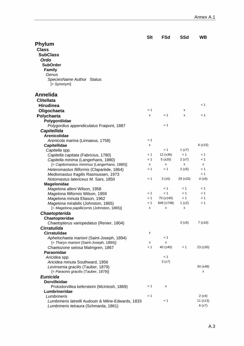
Annex A.1
Slt FSd SSd WB
Phylum
Class
SubClass
Ordo
SubOrder
Family
Genus
SpeciesName Author Status [= Synonym]
Annelida
Clitellata
Hirudinea < 1
Oligochaeta < 1 x
Polychaeta x < 1 x < 1
Polygordiidae
Polygordius appendiculatus Fraipont, 1887 < 1
Capitellida
Arenicolidae
Arenicola marina (Linnaeus, 1758) < 1
Capitellidae x 6 (±15)
Capitella spp. < 1 1 (±7)
Capitella capitata (Fabricius, 1780) < 1 12 (±36) < 1 < 1
Capitella minima (Langerhans, 1880) < 1 5 (±20) 2 (±7) < 1 [= Capitomastus minimus (Langerhans, 1880)] x x x x
Heteromastus filiformis (Claparède, 1864) < 1 < 1 2 (±5) < 1
Mediomastus fragilis Rasmussen, 1973 < 1
Notomastus latericeus M. Sars, 1850 < 1 3 (±5) 29 (±33) 4 (±6)
Magelonidae
Magelona alleni Wilson, 1958 < 1 < 1 < 1
Magelona filiformis Wilson, 1959 < 1 < 1 < 1 < 1
Magelona minuta Eliason, 1962 < 1 70 (±140) < 1 < 1
Magelona mirabilis (Johnston, 1865) < 1 849 (±748) 1 (±2) < 1 [= Magelona papillicornis (Johnston, 1865)] x x x
Chaetopterida
Chaetopteridae
Chaetopterus variopedatus (Renier, 1804) 3 (±5) 7 (±10)
Cirratulida
Cirratulidae x
Aphelochaeta marioni (Saint-Joseph, 1894) < 1 [= Tharyx marioni (Saint-Joseph, 1894)] x x
Chaetozone setosa Malmgren, 1867 < 1 40 (±40) < 1 23 (±30)
Paraonidae
Aricidea spp. < 1
Aricidea minuta Southward, 1956 3 (±7)
Levinsenia gracilis (Tauber, 1879) 34 (±48) [= Paraonis gracilis (Tauber, 1879)] x
Eunicida
Dorvilleidae
Protodorvillea kefersteini (McIntosh, 1869) < 1 x
Lumbrineridae
Lumbrineris < 1 2 (±4)
Lumbrineris latreilli Audouin & Milne-Edwards, 1833 < 1 11 (±13)
Lumbrineris tetraura (Schmarda, 1861) 6 (±7)
A.3
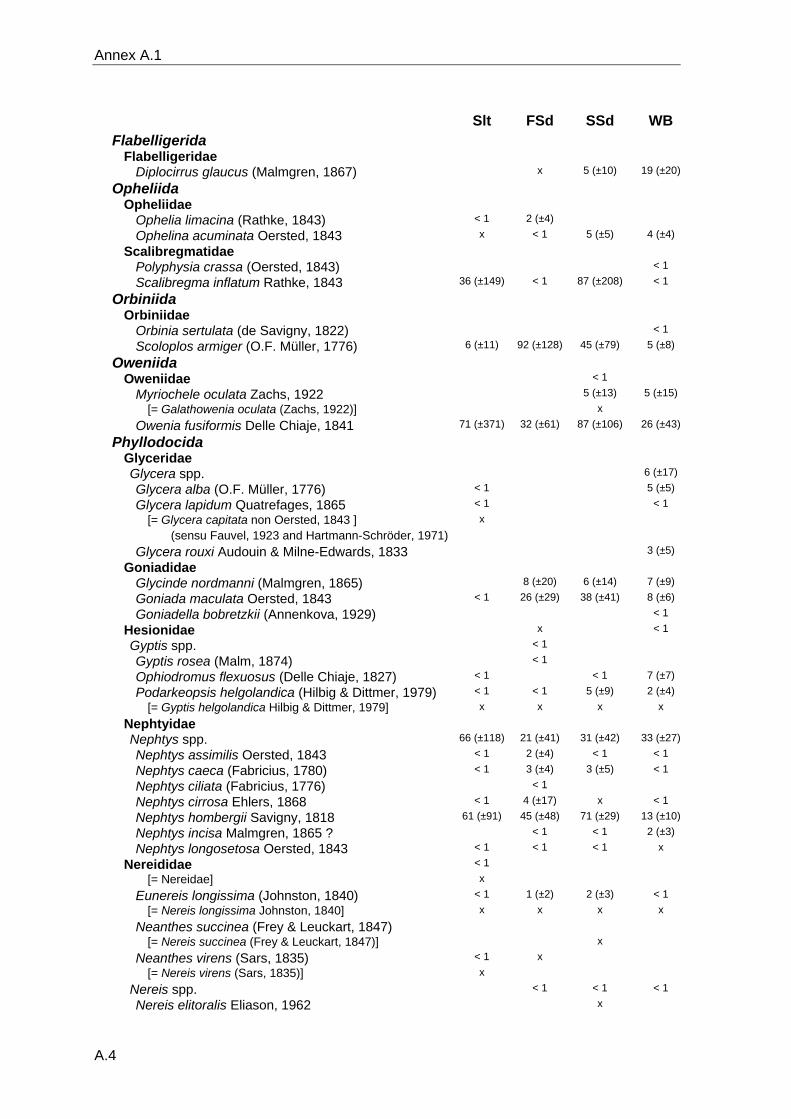
Annex A.1
Slt FSd SSd WB
Flabelligerida
Flabelligeridae
Diplocirrus glaucus (Malmgren, 1867) x 5 (±10) 19 (±20)
Opheliida
Opheliidae
Ophelia limacina (Rathke, 1843) < 1 2 (±4)
Ophelina acuminata Oersted, 1843 x < 1 5 (±5) 4 (±4)
Scalibregmatidae
Polyphysia crassa (Oersted, 1843) < 1
Scalibregma inflatum Rathke, 1843 36 (±149) < 1 87 (±208) < 1
Orbiniida
Orbiniidae
Orbinia sertulata (de Savigny, 1822) < 1
Scoloplos armiger (O.F. Müller, 1776) 6 (±11) 92 (±128) 45 (±79) 5 (±8)
Oweniida
Oweniidae < 1
Myriochele oculata Zachs, 1922 5 (±13) 5 (±15) [= Galathowenia oculata (Zachs, 1922)] x
Owenia fusiformis Delle Chiaje, 1841 71 (±371) 32 (±61) 87 (±106) 26 (±43)
Phyllodocida
Glyceridae
Glycera spp. 6 (±17)
Glycera alba (O.F. Müller, 1776) < 1 5 (±5)
Glycera lapidum Quatrefages, 1865 < 1 < 1 [= Glycera capitata non Oersted, 1843 ] x (sensu Fauvel, 1923 and Hartmann-Schröder, 1971)
Glycera rouxi Audouin & Milne-Edwards, 1833 3 (±5)
Goniadidae
Glycinde nordmanni (Malmgren, 1865) 8 (±20) 6 (±14) 7 (±9)
Goniada maculata Oersted, 1843 < 1 26 (±29) 38 (±41) 8 (±6)
Goniadella bobretzkii (Annenkova, 1929) < 1
Hesionidae x < 1
Gyptis spp. < 1
Gyptis rosea (Malm, 1874) < 1
Ophiodromus flexuosus (Delle Chiaje, 1827) < 1 < 1 7 (±7)
Podarkeopsis helgolandica (Hilbig & Dittmer, 1979) < 1 < 1 5 (±9) 2 (±4) [= Gyptis helgolandica Hilbig & Dittmer, 1979] x x x x
Nephtyidae
Nephtys spp. 66 (±118) 21 (±41) 31 (±42) 33 (±27)
Nephtys assimilis Oersted, 1843 < 1 2 (±4) < 1 < 1
Nephtys caeca (Fabricius, 1780) < 1 3 (±4) 3 (±5) < 1
Nephtys ciliata (Fabricius, 1776) < 1
Nephtys cirrosa Ehlers, 1868 < 1 4 (±17) x < 1
Nephtys hombergii Savigny, 1818 61 (±91) 45 (±48) 71 (±29) 13 (±10)
Nephtys incisa Malmgren, 1865 ? < 1 < 1 2 (±3)
Nephtys longosetosa Oersted, 1843 < 1 < 1 < 1 x
Nereididae < 1 [= Nereidae] x
Eunereis longissima (Johnston, 1840) < 1 1 (±2) 2 (±3) < 1 [= Nereis longissima Johnston, 1840] x x x x
Neanthes succinea (Frey & Leuckart, 1847) [= Nereis succinea (Frey & Leuckart, 1847)] x
Neanthes virens (Sars, 1835) < 1 x [= Nereis virens (Sars, 1835)] x
Nereis spp. < 1 < 1 < 1
Nereis elitoralis Eliason, 1962 x
A.4
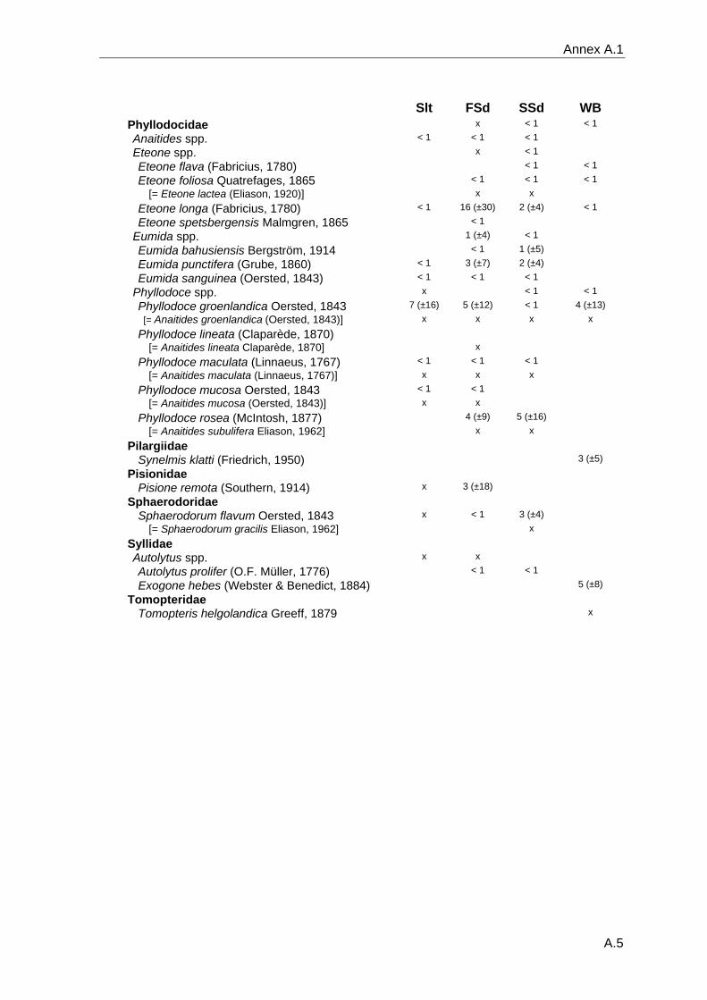
Annex A.1
Slt FSd SSd WB
Phyllodocidae x < 1 < 1
Anaitides spp. < 1 < 1 < 1
Eteone spp. x < 1
Eteone flava (Fabricius, 1780) < 1 < 1
Eteone foliosa Quatrefages, 1865 < 1 < 1 < 1 [= Eteone lactea (Eliason, 1920)] x x
Eteone longa (Fabricius, 1780) < 1 16 (±30) 2 (±4) < 1
Eteone spetsbergensis Malmgren, 1865 < 1
Eumida spp. 1 (±4) < 1
Eumida bahusiensis Bergström, 1914 < 1 1 (±5)
Eumida punctifera (Grube, 1860) < 1 3 (±7) 2 (±4)
Eumida sanguinea (Oersted, 1843) < 1 < 1 < 1
Phyllodoce spp. x < 1 < 1
Phyllodoce groenlandica Oersted, 1843 7 (±16) 5 (±12) < 1 4 (±13) [= Anaitides groenlandica (Oersted, 1843)] x x x x
Phyllodoce lineata (Claparède, 1870) [= Anaitides lineata Claparède, 1870] x
Phyllodoce maculata (Linnaeus, 1767) < 1 < 1 < 1 [= Anaitides maculata (Linnaeus, 1767)] x x x
Phyllodoce mucosa Oersted, 1843 < 1 < 1 [= Anaitides mucosa (Oersted, 1843)] x x
Phyllodoce rosea (McIntosh, 1877) 4 (±9) 5 (±16) [= Anaitides subulifera Eliason, 1962] x x
Pilargiidae
Synelmis klatti (Friedrich, 1950) 3 (±5)
Pisionidae
Pisione remota (Southern, 1914) x 3 (±18)
Sphaerodoridae
Sphaerodorum flavum Oersted, 1843 x < 1 3 (±4) [= Sphaerodorum gracilis Eliason, 1962] x
Syllidae
Autolytus spp. x x
Autolytus prolifer (O.F. Müller, 1776) < 1 < 1
Exogone hebes (Webster & Benedict, 1884) 5 (±8)
Tomopteridae
Tomopteris helgolandica Greeff, 1879 x
A.5

Annex A.1
Slt FSd SSd WB
Aphroditoidea
Aphroditidae
Aphrodita aculeata Linnaeus, 1761 < 1 x 2 (±2) 2 (±3)
Pholoidae
Pholoe minuta (Fabricius, 1780) 31 (±66) 8 (±14) 48 (±38) 244 (±263)
Polynoidae < 1
Bylgides sarsi (Kinberg, 1856) 4 (±7) < 1 < 1 < 1 [= Harmothoe sarsi (Kinberg, 1856)] x x x x [= Harmothoe sarsi sarsi (Kinberg, 1856)] x x
Enipo kinbergi Malmgren, 1865 < 1 < 1 [= Polynoe kinbergi (Malmgren, 1865)] x x
Eunoe nodosa (M. Sars, 1861) < 1 < 1 3 (±7) [= Harmothoe nodosa (M. Sars, 1861)] x x x
Gattyana cirrosa (Pallas, 1766) < 1 < 1 4 (±7) 3 (±5)
Harmothoe spp. < 1 < 1 < 1 < 1
Harmothoe glabra (Malmgren, 1865) < 1 < 1 1 (±2) 2 (±3) [= Harmothoe longisetis (Malmgren, 1865)] x x x x
Harmothoe imbricata (Linnaeus, 1767) < 1
Harmothoe impar (Johnston, 1839) < 1 x < 1 < 1
Harmothoe ljungmani (Malmgren, 1867) < 1
Lagisca extenuata (Grube, 1840) x
Malmgrenia spp. [= Malmgreniella] x x
Malmgrenia andreapolis McIntosh, 1874 < 1 [= Malmgreniella andreapolis (McIntosh, 1874)] x
Malmgrenia castanea (McIntosh, 1876) < 1 < 1 < 1 [= Malmgreniella castanea (McIntosh, 1876)] x x x
Malmgrenia lunulata (Delle Chiaje, 1830) < 1 2 (±3) < 1 [= Harmothoe lunulata (Delle Chiaje, 1830)] x x x [= Malmgreniella lunulata (Delle Chiaje, 1830)] x x x
Sigalionidae
Sigalion mathildae Audouin & Milne-Edwards, 1830 1 (±3)
Sthenelais spp. < 1
Sthenelais boa (Johnston, 1833) < 1
Sthenelais limicola (Ehlers, 1864) x 6 (±7) 3 (±4) 4 (±4)
Sabellida
Sabellidae
Chone spp. x
Chone duneri Malmgren, 1867 < 1 < 1
Chone infundibuliformis Krøyer, 1856 < 1 x
A.6
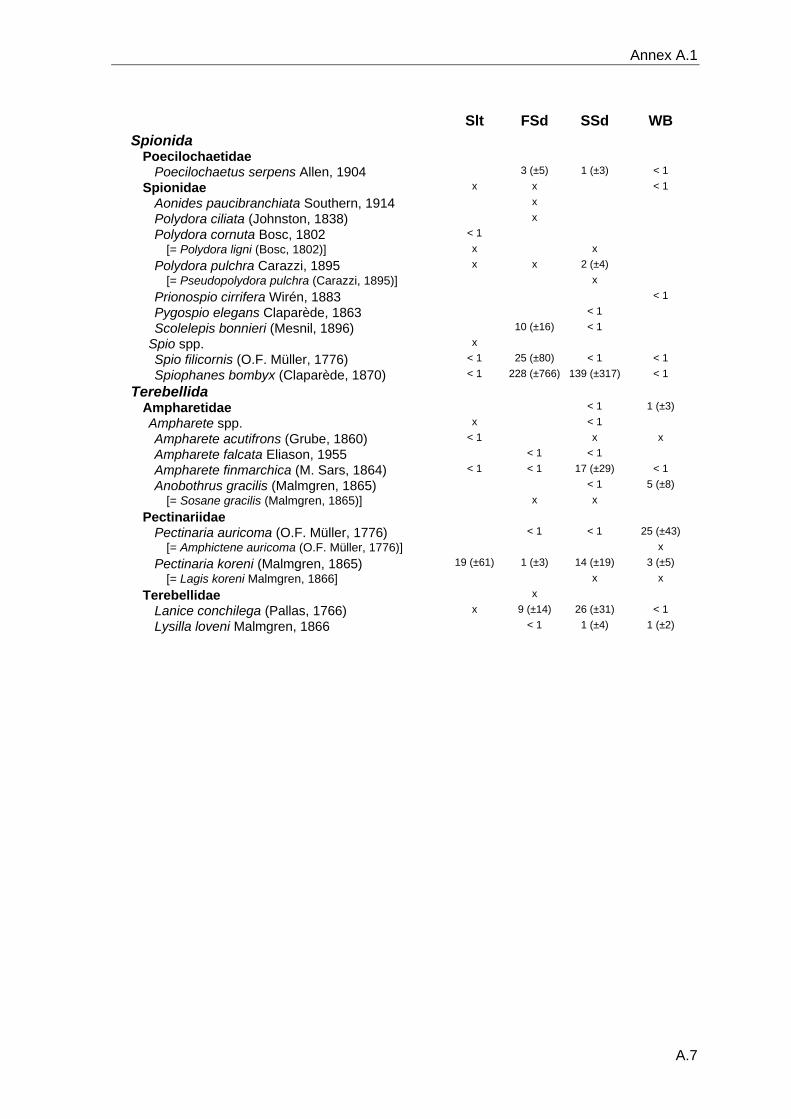
Annex A.1
Slt FSd SSd WB
Spionida
Poecilochaetidae
Poecilochaetus serpens Allen, 1904 3 (±5) 1 (±3) < 1
Spionidae x x < 1
Aonides paucibranchiata Southern, 1914 x
Polydora ciliata (Johnston, 1838) x
Polydora cornuta Bosc, 1802 < 1 [= Polydora ligni (Bosc, 1802)] x x
Polydora pulchra Carazzi, 1895 x x 2 (±4) [= Pseudopolydora pulchra (Carazzi, 1895)] x
Prionospio cirrifera Wirén, 1883 < 1
Pygospio elegans Claparède, 1863 < 1
Scolelepis bonnieri (Mesnil, 1896) 10 (±16) < 1
Spio spp. x
Spio filicornis (O.F. Müller, 1776) < 1 25 (±80) < 1 < 1
Spiophanes bombyx (Claparède, 1870) < 1 228 (±766) 139 (±317) < 1
Terebellida
Ampharetidae < 1 1 (±3)
Ampharete spp. x < 1
Ampharete acutifrons (Grube, 1860) < 1 x x
Ampharete falcata Eliason, 1955 < 1 < 1
Ampharete finmarchica (M. Sars, 1864) < 1 < 1 17 (±29) < 1
Anobothrus gracilis (Malmgren, 1865) < 1 5 (±8) [= Sosane gracilis (Malmgren, 1865)] x x
Pectinariidae
Pectinaria auricoma (O.F. Müller, 1776) < 1 < 1 25 (±43) [= Amphictene auricoma (O.F. Müller, 1776)] x
Pectinaria koreni (Malmgren, 1865) 19 (±61) 1 (±3) 14 (±19) 3 (±5) [= Lagis koreni Malmgren, 1866] x x
Terebellidae x
Lanice conchilega (Pallas, 1766) x 9 (±14) 26 (±31) < 1
Lysilla loveni Malmgren, 1866 < 1 1 (±4) 1 (±2)
A.7
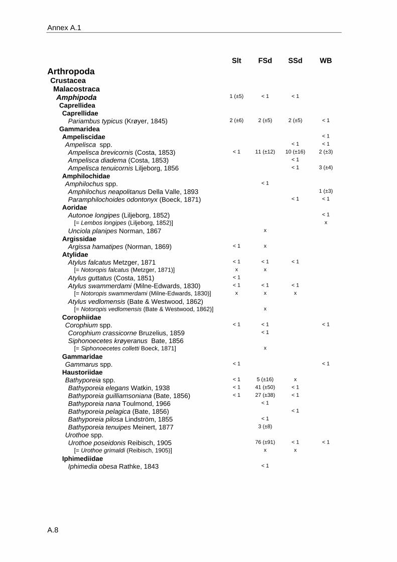
Annex A.1
Slt FSd SSd WB
Arthropoda
Crustacea
Malacostraca
Amphipoda 1 (±5) < 1 < 1
Caprellidea
Caprellidae
Pariambus typicus (Krøyer, 1845) 2 (±6) 2 (±5) 2 (±5) < 1
Gammaridea
Ampeliscidae < 1
Ampelisca spp. < 1 < 1
Ampelisca brevicornis (Costa, 1853) < 1 11 (±12) 10 (±16) 2 (±3)
Ampelisca diadema (Costa, 1853) < 1
Ampelisca tenuicornis Liljeborg, 1856 < 1 3 (±4)
Amphilochidae
Amphilochus spp. < 1
Amphilochus neapolitanus Della Valle, 1893 1 (±3)
Paramphilochoides odontonyx (Boeck, 1871) < 1 < 1
Aoridae
Autonoe longipes (Liljeborg, 1852) < 1 [= Lembos longipes (Liljeborg, 1852)] x
Unciola planipes Norman, 1867 x
Argissidae
Argissa hamatipes (Norman, 1869) < 1 x
Atylidae
Atylus falcatus Metzger, 1871 < 1 < 1 < 1 [= Notoropis falcatus (Metzger, 1871)] x x
Atylus guttatus (Costa, 1851) < 1
Atylus swammerdami (Milne-Edwards, 1830) < 1 < 1 < 1 [= Notoropis swammerdami (Milne-Edwards, 1830)] x x x
Atylus vedlomensis (Bate & Westwood, 1862) [= Notoropis vedlomensis (Bate & Westwood, 1862)] x
Corophiidae
Corophium spp. < 1 < 1 < 1
Corophium crassicorne Bruzelius, 1859 < 1
Siphonoecetes krøyeranus Bate, 1856 [= Siphonoecetes colletti Boeck, 1871] x
Gammaridae
Gammarus spp. < 1 < 1
Haustoriidae
Bathyporeia spp. < 1 5 (±16) x
Bathyporeia elegans Watkin, 1938 < 1 41 (±50) < 1
Bathyporeia guilliamsoniana (Bate, 1856) < 1 27 (±38) < 1
Bathyporeia nana Toulmond, 1966 < 1
Bathyporeia pelagica (Bate, 1856) < 1
Bathyporeia pilosa Lindström, 1855 < 1
Bathyporeia tenuipes Meinert, 1877 3 (±8)
Urothoe spp.
Urothoe poseidonis Reibisch, 1905 76 (±91) < 1 < 1 [= Urothoe grimaldi (Reibisch, 1905)] x x
Iphimediidae
Iphimedia obesa Rathke, 1843 < 1
A.8
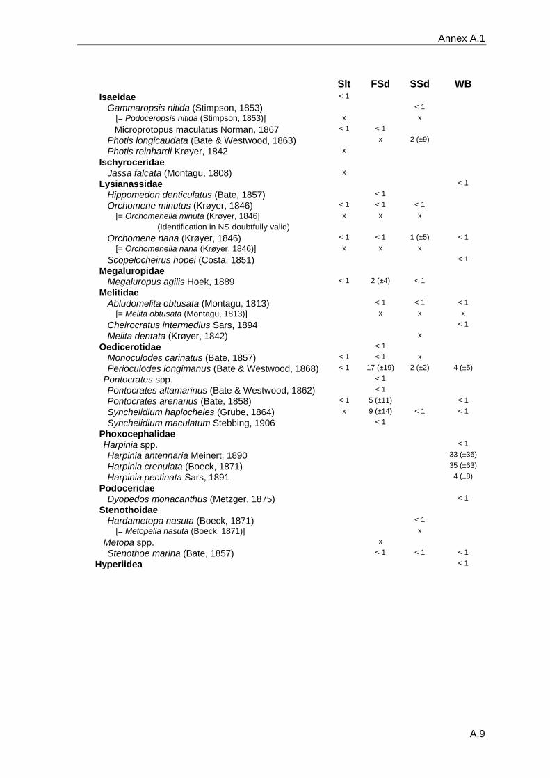
Annex A.1
Slt FSd SSd WB
Isaeidae < 1
Gammaropsis nitida (Stimpson, 1853) < 1 [= Podoceropsis nitida (Stimpson, 1853)] x x
Microprotopus maculatus Norman, 1867 < 1 < 1
Photis longicaudata (Bate & Westwood, 1863) x 2 (±9)
Photis reinhardi Krøyer, 1842 x
Ischyroceridae
Jassa falcata (Montagu, 1808) x
Lysianassidae < 1
Hippomedon denticulatus (Bate, 1857) < 1
Orchomene minutus (Krøyer, 1846) < 1 < 1 < 1 [= Orchomenella minuta (Krøyer, 1846] x x x (Identification in NS doubtfully valid)
Orchomene nana (Krøyer, 1846) < 1 < 1 1 (±5) < 1 [= Orchomenella nana (Krøyer, 1846)] x x x
Scopelocheirus hopei (Costa, 1851) < 1
Megaluropidae
Megaluropus agilis Hoek, 1889 < 1 2 (±4) < 1
Melitidae
Abludomelita obtusata (Montagu, 1813) < 1 < 1 < 1 [= Melita obtusata (Montagu, 1813)] x x x
Cheirocratus intermedius Sars, 1894 < 1
Melita dentata (Krøyer, 1842) x
Oedicerotidae < 1
Monoculodes carinatus (Bate, 1857) < 1 < 1 x
Perioculodes longimanus (Bate & Westwood, 1868) < 1 17 (±19) 2 (±2) 4 (±5)
Pontocrates spp. < 1
Pontocrates altamarinus (Bate & Westwood, 1862) < 1
Pontocrates arenarius (Bate, 1858) < 1 5 (±11) < 1
Synchelidium haplocheles (Grube, 1864) x 9 (±14) < 1 < 1
Synchelidium maculatum Stebbing, 1906 < 1
Phoxocephalidae
Harpinia spp. < 1
Harpinia antennaria Meinert, 1890 33 (±36)
Harpinia crenulata (Boeck, 1871) 35 (±63)
Harpinia pectinata Sars, 1891 4 (±8)
Podoceridae
Dyopedos monacanthus (Metzger, 1875) < 1
Stenothoidae
Hardametopa nasuta (Boeck, 1871) < 1 [= Metopella nasuta (Boeck, 1871)] x
Metopa spp. x
Stenothoe marina (Bate, 1857) < 1 < 1 < 1
Hyperiidea < 1
A.9

Annex A.1
Slt FSd SSd WB
Cumacea x 3 (±16)
Bodotriidae
Bodotria scorpioides (Montagu, 1804) < 1 < 1 < 1
Cumopsis goodsiri (van Beneden, 1861) < 1 x
Iphinoe trispinosa (Goodsir, 1843) < 1 4 (±7) < 1 < 1
Diastylidae
Diastylis spp. 173 (±378) < 1 < 1 23 (±57)
Diastylis bradyi Norman, 1879 6 (±17) 2 (±4) 2 (±5) 5 (±5)
Diastylis laevis Norman, 1869 7 (±35) < 1 < 1 5 (±10)
Diastylis lucifera (Krøyer, 1841) x x 25 (±38)
Diastylis rathkei (Krøyer, 1841) 582 (±2373) < 1 3 (±8) 3 (±5)
Lampropidae
Lamprops fasciata Sars, 1863 < 1 < 1 x
Leuconidae
Eudorella spp. < 1
Eudorella emarginata (Krøyer, 1846) < 1 19 (±37) 9 (±12)
Eudorella truncatula (Bate, 1856) 1 (±4) 29 (±48) 24 (±32)
Nannastacidae
Campylaspis costata G.O. Sars, 1865 x
Pseudocumatidae
Pseudocuma spp. < 1
Pseudocuma longicornis (Bate, 1858) 10 (±42) 2 (±4) < 1 2 (±3)
Pseudocuma similis Sars, 1900 x 1 (±5) x
Decapoda
Pleocyemata
Callianassidae
Callianassa spp. < 1
Callianassa subterranea (Montagu, 1808) < 1 12 (±16) 12 (±9)
Corystidae
Corystes cassivelaunus (Pennant, 1777) < 1 x < 1
Crangonidae
Crangon spp. < 1 < 1 < 1
Crangon allmani Kinahan, 1857 < 1 x < 1 < 1
Crangon crangon (Linnaeus, 1758) < 1 < 1 < 1
Philocheras bispinosus (Hailstone, 1835) x
Galatheidae
Galathea intermedia Liljeborg, 1851 x
Leucosiidae
Ebalia cranchii Leach, 1817 < 1 < 1
Paguridae x
Pagurus spp. [= Eupagurus spp.] x
Pagurus bernhardus (Linnaeus, 1758) < 1 < 1 < 1 < 1 [= Eupagurus bernhardus (Linnaeus, 1758)] x x x x
Pinnotheridae
Pinnotheres pisum (Linnaeus, 1767) < 1
Portunidae < 1
Liocarcinus holsatus (Fabricius, 1798) < 1 < 1 < 1 [= Macropipus holsatus (Fabricius, 1798)] x x x [= Portunus holsatus (Fabricius, 1798)] x x x
Processidae
Processa canaliculata Leach, 1815 x x
Processa nouveli holthuisi Al-Adhub & Williamson, 1975 < 1 < 1
Upogebiidae
Upogebia deltaura (Leach, 1815) x < 1
A.10
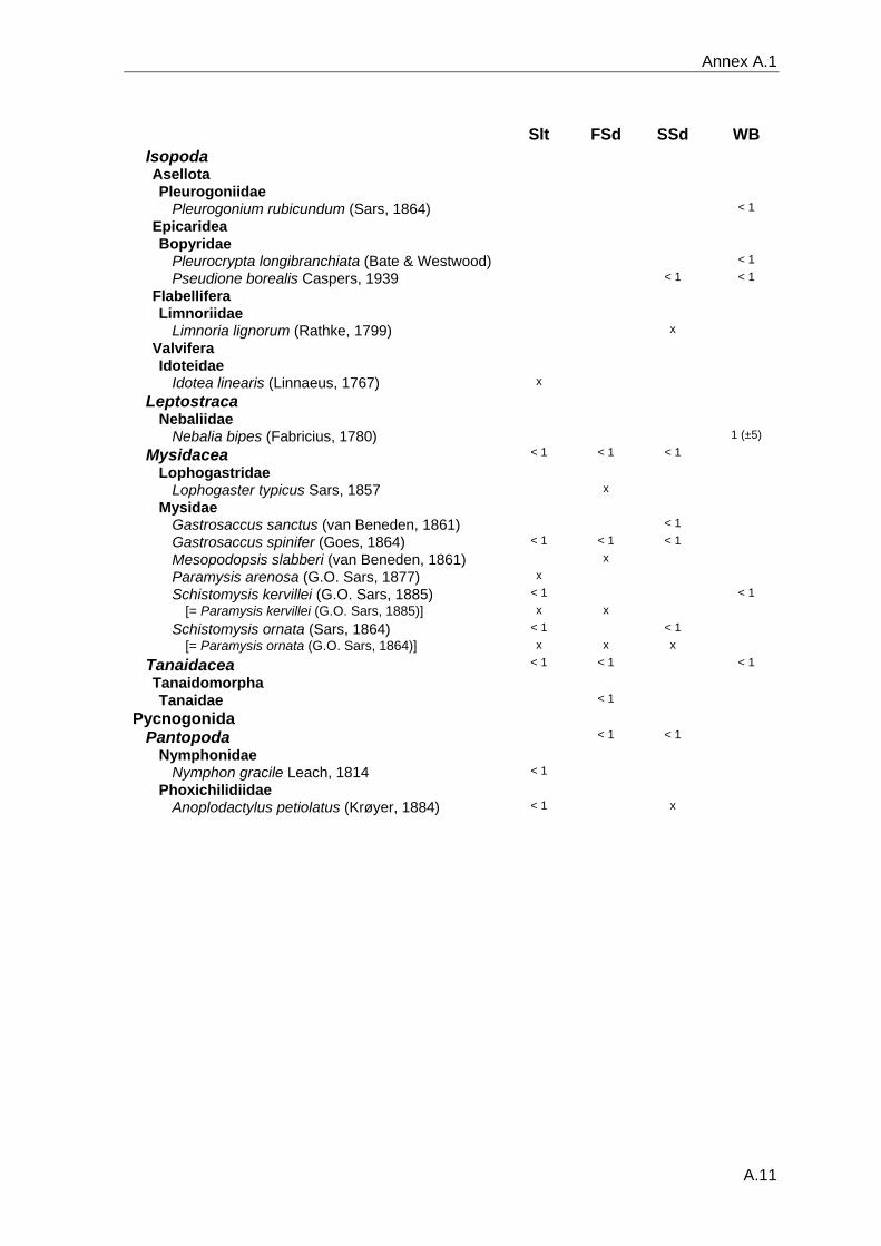
Annex A.1
Slt FSd SSd WB
Isopoda
Asellota
Pleurogoniidae
Pleurogonium rubicundum (Sars, 1864) < 1
Epicaridea
Bopyridae
Pleurocrypta longibranchiata (Bate & Westwood) < 1
Pseudione borealis Caspers, 1939 < 1 < 1
Flabellifera
Limnoriidae
Limnoria lignorum (Rathke, 1799) x
Valvifera
Idoteidae
Idotea linearis (Linnaeus, 1767) x
Leptostraca
Nebaliidae
Nebalia bipes (Fabricius, 1780) 1 (±5)
Mysidacea < 1 < 1 < 1
Lophogastridae
Lophogaster typicus Sars, 1857 x
Mysidae
Gastrosaccus sanctus (van Beneden, 1861) < 1
Gastrosaccus spinifer (Goes, 1864) < 1 < 1 < 1
Mesopodopsis slabberi (van Beneden, 1861) x
Paramysis arenosa (G.O. Sars, 1877) x
Schistomysis kervillei (G.O. Sars, 1885) < 1 < 1 [= Paramysis kervillei (G.O. Sars, 1885)] x x
Schistomysis ornata (Sars, 1864) < 1 < 1 [= Paramysis ornata (G.O. Sars, 1864)] x x x
Tanaidacea < 1 < 1 < 1
Tanaidomorpha
Tanaidae < 1
Pycnogonida
Pantopoda < 1 < 1
Nymphonidae
Nymphon gracile Leach, 1814 < 1
Phoxichilidiidae
Anoplodactylus petiolatus (Krøyer, 1884) < 1 x
A.11
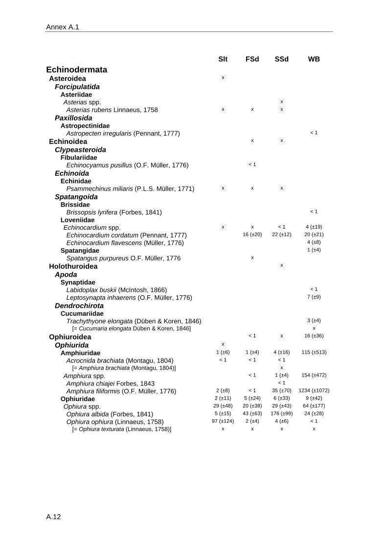
Annex A.1
Slt FSd SSd WB
Echinodermata
Asteroidea x
Forcipulatida
Asteriidae
Asterias spp. x
Asterias rubens Linnaeus, 1758 x x x
Paxillosida
Astropectinidae
Astropecten irregularis (Pennant, 1777) < 1
Echinoidea x x
Clypeasteroida
Fibulariidae
Echinocyamus pusillus (O.F. Müller, 1776) < 1
Echinoida
Echinidae
Psammechinus miliaris (P.L.S. Müller, 1771) x x x
Spatangoida
Brissidae
Brissopsis lyrifera (Forbes, 1841) < 1
Loveniidae
Echinocardium spp. x x < 1 4 (±19)
Echinocardium cordatum (Pennant, 1777) 16 (±20) 22 (±12) 20 (±21)
Echinocardium flavescens (Müller, 1776) 4 (±8)
Spatangidae 1 (±4)
Spatangus purpureus O.F. Müller, 1776 x
Holothuroidea x
Apoda
Synaptidae
Labidoplax buskii (McIntosh, 1866) < 1
Leptosynapta inhaerens (O.F. Müller, 1776) 7 (±9)
Dendrochirota
Cucumariidae
Trachythyone elongata (Düben & Koren, 1846) 3 (±4) [= Cucumaria elongata Düben & Koren, 1846] x
Ophiuroidea < 1 x 16 (±36)
Ophiurida x
Amphiuridae 1 (±6) 1 (±4) 4 (±16) 115 (±513)
Acrocnida brachiata (Montagu, 1804) < 1 < 1 < 1 [= Amphiura brachiata (Montagu, 1804)] x
Amphiura spp. < 1 1 (±4) 154 (±472)
Amphiura chiajei Forbes, 1843 < 1
Amphiura filiformis (O.F. Müller, 1776) 2 (±8) < 1 35 (±70) 1234 (±1072)
Ophiuridae 2 (±11) 5 (±24) 6 (±33) 9 (±42)
Ophiura spp. 29 (±48) 20 (±38) 29 (±43) 64 (±177)
Ophiura albida (Forbes, 1841) 5 (±15) 43 (±63) 176 (±99) 24 (±28)
Ophiura ophiura (Linnaeus, 1758) 97 (±124) 2 (±4) 4 (±6) < 1 [= Ophiura texturata (Linnaeus, 1758)] x x x x
A.12
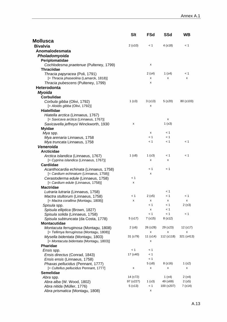
Annex A.1
Slt FSd SSd WB
Mollusca
Bivalvia 2 (±10) < 1 4 (±18) < 1
Anomalodesmata
Pholadomyoida
Periplomatidae
Cochlodesma praetenue (Pulteney, 1799) x
Thraciidae
Thracia papyracea (Poli, 1791) 2 (±4) 1 (±4) < 1 [= Thracia phaseolina (Lamarck, 1818)] x x x
Thracia pubescens (Pulteney, 1799) x
Heterodonta
Myoida
Corbulidae
Corbula gibba (Olivi, 1792) 1 (±3) 3 (±13) 5 (±20) 80 (±103) [= Aloidis gibba (Olivi, 1792)] x
Hiatellidae
Hiatella arctica (Linnaeus, 1767) [= Saxicava arctica (Linnaeus, 1767)] x
Saxicavella jeffreysi Winckworth, 1930 x 1 (±3)
Myidae
Mya spp. x < 1
Mya arenaria Linnaeus, 1758 < 1 < 1
Mya truncata Linnaeus, 1758 < 1 < 1 < 1
Veneroida
Arcticidae
Arctica islandica (Linnaeus, 1767) 1 (±8) 1 (±3) < 1 < 1 [= Cyprina islandica (Linnaeus, 1767)] x x
Cardiidae
Acanthocardia echinata (Linnaeus, 1758) < 1 < 1 [= Cardium echinatum (Linnaeus, 1758)] x
Cerastoderma edule (Linnaeus, 1758) < 1 [= Cardium edule (Linnaeus, 1758)] x
Mactridae
Lutraria lutraria (Linnaeus, 1758) < 1
Mactra stultorum (Linnaeus, 1758) < 1 2 (±5) < 1 < 1 [= Mactra corallina (Montagu, 1808)] x x x x
Spisula spp. < 1 < 1 2 (±3)
Spisula elliptica (Brown, 1827) x < 1
Spisula solida (Linnaeus, 1758) < 1 < 1 < 1
Spisula subtruncata (da Costa, 1778) 5 (±17) 7 (±15) 8 (±12)
Montacutidae
Montacuta ferruginosa (Montagu, 1808) 2 (±6) 26 (±28) 29 (±23) 12 (±17) [= Tellimya ferruginosa (Montagu, 1808)] x x x
Mysella bidentata (Montagu, 1803) 31 (±79) 11 (±14) 112 (±118) 321 (±413) [= Montacuta bidentata (Montagu, 1803)] x
Pharidae
Ensis spp. < 1 < 1
Ensis directus (Conrad, 1843) 17 (±40) < 1
Ensis ensis (Linnaeus, 1758) < 1
Phaxas pellucidus (Pennant, 1777) 5 (±8) 8 (±16) 1 (±2) [= Cultellus pellucidus Pennant, 1777] x x x x
Semelidae
Abra spp. 14 (±72) 1 (±4) 2 (±4)
Abra alba (W. Wood, 1802) 97 (±227) 1 (±3) 49 (±69) 2 (±5)
Abra nitida (Müller, 1776) 5 (±13) < 1 100 (±207) 7 (±14)
Abra prismatica (Montagu, 1808) x
A.13
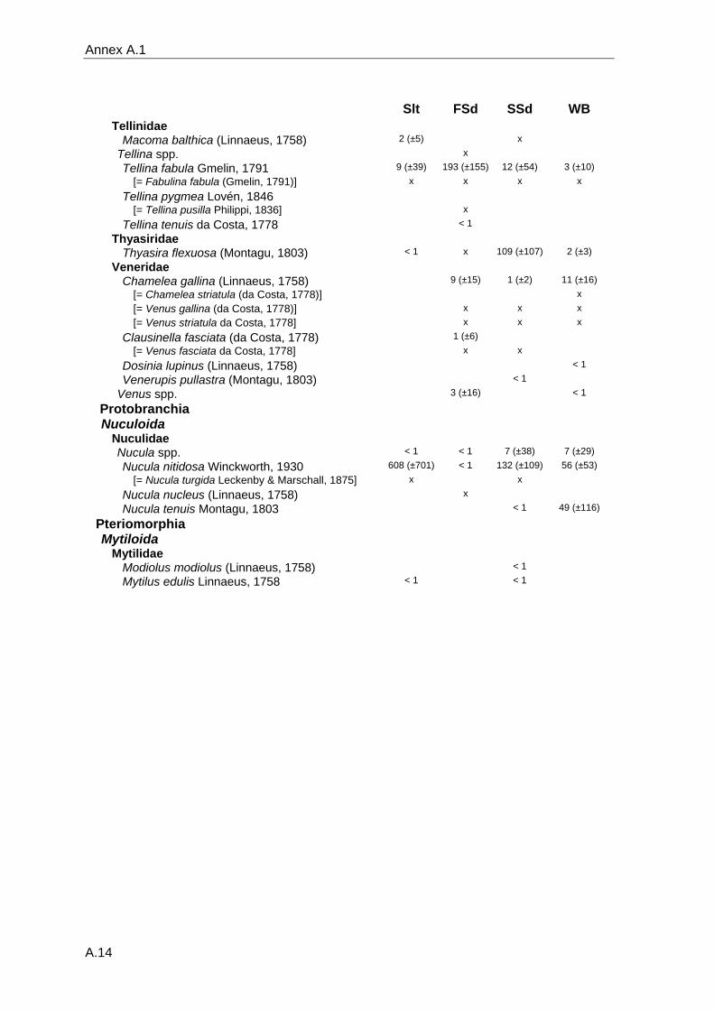
Annex A.1
Slt FSd SSd WB
Tellinidae
Macoma balthica (Linnaeus, 1758) 2 (±5) x
Tellina spp. x
Tellina fabula Gmelin, 1791 9 (±39) 193 (±155) 12 (±54) 3 (±10) [= Fabulina fabula (Gmelin, 1791)] x x x x
Tellina pygmea Lovén, 1846 [= Tellina pusilla Philippi, 1836] x
Tellina tenuis da Costa, 1778 < 1
Thyasiridae
Thyasira flexuosa (Montagu, 1803) < 1 x 10⁹ (±107) 2 (±3)
Veneridae
Chamelea gallina (Linnaeus, 1758) 9 (±15) 1 (±2) 11 (±16) [= Chamelea striatula (da Costa, 1778)] x [= Venus gallina (da Costa, 1778)] x x x [= Venus striatula da Costa, 1778] x x x
Clausinella fasciata (da Costa, 1778) 1 (±6) [= Venus fasciata da Costa, 1778] x x
Dosinia lupinus (Linnaeus, 1758) < 1
Venerupis pullastra (Montagu, 1803) < 1
Venus spp. 3 (±16) < 1
Protobranchia
Nuculoida
Nuculidae
Nucula spp. < 1 < 1 7 (±38) 7 (±29)
Nucula nitidosa Winckworth, 1930 608 (±701) < 1 132 (±109) 56 (±53) [= Nucula turgida Leckenby & Marschall, 1875] x x
Nucula nucleus (Linnaeus, 1758) x
Nucula tenuis Montagu, 1803 < 1 49 (±116)
Pteriomorphia
Mytiloida
Mytilidae
Modiolus modiolus (Linnaeus, 1758) < 1
Mytilus edulis Linnaeus, 1758 < 1 < 1
A.14
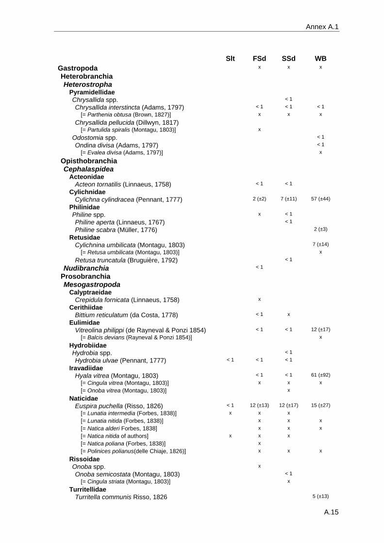
Annex A.1
Slt FSd SSd WB
Gastropoda x x x
Heterobranchia
Heterostropha
Pyramidellidae
Chrysallida spp. < 1
Chrysallida interstincta (Adams, 1797) < 1 < 1 < 1 [= Parthenia obtusa (Brown, 1827)] x x x
Chrysallida pellucida (Dillwyn, 1817) [= Partulida spiralis (Montagu, 1803)] x
Odostomia spp. < 1
Ondina divisa (Adams, 1797) < 1 [= Evalea divisa (Adams, 1797)] x
Opisthobranchia
Cephalaspidea
Acteonidae
Acteon tornatilis (Linnaeus, 1758) < 1 < 1
Cylichnidae
Cylichna cylindracea (Pennant, 1777) 2 (±2) 7 (±11) 57 (±44)
Philinidae
Philine spp. x < 1
Philine aperta (Linnaeus, 1767) < 1
Philine scabra (Müller, 1776) 2 (±3)
Retusidae
Cylichnina umbilicata (Montagu, 1803) 7 (±14) [= Retusa umbilicata (Montagu, 1803)] x
Retusa truncatula (Bruguière, 1792) < 1
Nudibranchia < 1
Prosobranchia
Mesogastropoda
Calyptraeidae
Crepidula fornicata (Linnaeus, 1758) x
Cerithiidae
Bittium reticulatum (da Costa, 1778) < 1 x
Eulimidae
Vitreolina philippi (de Rayneval & Ponzi 1854) < 1 < 1 12 (±17) [= Balcis devians (Rayneval & Ponzi 1854)] x
Hydrobiidae
Hydrobia spp. < 1
Hydrobia ulvae (Pennant, 1777) < 1 < 1 < 1
Iravadiidae
Hyala vitrea (Montagu, 1803) < 1 < 1 61 (±92) [= Cingula vitrea (Montagu, 1803)] x x x [= Onoba vitrea (Montagu, 1803)] x
Naticidae
Euspira puchella (Risso, 1826) < 1 12 (±13) 12 (±17) 15 (±27) [= Lunatia intermedia (Forbes, 1838)] x x x [= Lunatia nitida (Forbes, 1838)] x x x [= Natica alderi Forbes, 1838] x x x [= Natica nitida of authors] x x x [= Natica poliana (Forbes, 1838)] x [= Polinices polianus(delle Chiaje, 1826)] x x x
Rissoidae
Onoba spp. x
Onoba semicostata (Montagu, 1803) < 1 [= Cingula striata (Montagu, 1803)] x
Turritellidae
Turritella communis Risso, 1826 5 (±13)
A.15
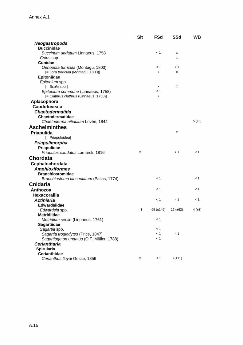
Annex A.1
Slt FSd SSd WB
Neogastropoda
Buccinidae
Buccinum undatum Linnaeus, 1758 < 1 x
Colus spp. x
Conidae
Oenopota turricula (Montagu, 1803) < 1 < 1 [= Lora turricula (Montagu, 1803)] x x
Epitoniidae
Epitonium spp. [= Scala spp.] x x
Epitonium commune (Linnaeus, 1758) < 1 [= Clathrus clathrus (Linnaeus, 1758)] x
Aplacophora
Caudofoveata
Chaetodermatida
Chaetodermatidae
Chaetoderma nitidulum Lovén, 1844 5 (±6)
Aschelminthes
Priapulida x
[= Priapuloidea]
Priapulimorpha
Priapulidae
Priapulus caudatus Lamarck, 1816 x < 1 < 1
Chordata
Cephalochordata
Amphioxiformes
Branchiostomidae
Branchiostoma lanceolatum (Pallas, 1774) < 1 < 1
Cnidaria
Anthozoa < 1 < 1
Hexacorallia
Actiniaria < 1 < 1 < 1
Edwardsiidae
Edwardsia spp. < 1 69 (±146) 27 (±62) 4 (±3)
Metridiidae
Metridium senile (Linnaeus, 1761) < 1
Sagartiidae
Sagartia spp. < 1
Sagartia troglodytes (Price, 1847) < 1 < 1
Sagartiogeton undatus (O.F. Müller, 1788) < 1
Ceriantharia
Spirularia
Cerianthidae
Cerianthus lloydi Gosse, 1859 x < 1 3 (±11)
A.16
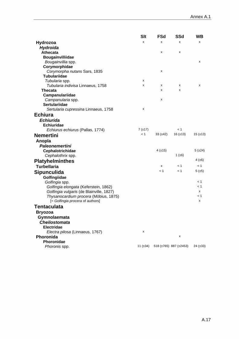
Annex A.1
Slt FSd SSd WB
Hydrozoa x x x x
Hydroida
Athecata x x
Bougainvilliidae
Bougainvillia spp. x
Corymorphidae
Corymorpha nutans Sars, 1835 x
Tubulariidae
Tubularia spp. x
Tubularia indivisa Linnaeus, 1758 x x x x
Thecata x x
Campanulariidae
Campanularia spp. x
Sertulariidae
Sertularia cupressina Linnaeus, 1758 x
Echiura
Echiurida
Echiuridae
Echiurus echiurus (Pallas, 1774) 7 (±17) < 1
Nemertini < 1 33 (±42) 16 (±13) 15 (±13)
Anopla
Paleonemertini
Cephalotrichidae 4 (±15) 5 (±24)
Cephalothrix spp. 1 (±6)
Platyhelminthes 4 (±6)
Turbellaria x < 1 < 1
Sipunculida < 1 < 1 5 (±5)
Golfingiidae
Golfingia spp. < 1
Golfingia elongata (Keferstein, 1862) < 1
Golfingia vulgaris (de Blainville, 1827) x
Thysanocardium procera (Möbius, 1875) < 1 [= Golfingia procera of authors] x
Tentaculata
Bryozoa
Gymnolaemata
Cheilostomata
Electridae
Electra pilosa (Linnaeus, 1767) x
Phoronida x
Phoronidae
Phoronis spp. 11 (±34) 518 (±765) 887 (±2453) 24 (±33)
A.17

Annex A.2
A.18
A.2 Benthos data available in the database
This list contains: - the cruise-code as listed in the database, - the dates of the cruise, - the type of gear employed and the number of replicates taken
o vV: 0.1 m² van Veen grab if not indicated otherwise o 0.05 vV: 0.05 m² van Veen grab o 0.2 vV: 0.2 m² van Veen grab o 0.5 vV: 0.5 m² van Veen grab o RBC: 0.017 m² Reineck box corer o 0.1 BC: 0.1 m² box corer
- information on the data quality: o samples where only some taxonomic groups have been analysed:
M: Mollusca P: Polychaeta E: Echinodermata C: Crustacea O: other taxa
o for pooled samples the number of replicates is given in brackets behind the number of separate data sets available in the database.
- comments Data from existing protocols are printed in normal typeface, data obtained by new analysis of stored samples are printed in boldface. The data selected for the long-term analysis are shaded.

Annex A.2
A.19
Available data sets in DB99 Comments Date H1 P12 FSD WB
Cruise from to vV RBC vV RBC vV RBC vV RBC HE130 10.04 14.04.2000 5 5 5 5 HE118 06.04 30.04.1999 5 5 5 5 HE 102 20.04 26.04.1998 21 21 20 21 VH0197 24.03 25.03.1997 5 5 5 5 VH0796 16.04 17.04.1996 5 5 5 5 LI0695 25.04 27.04.1995 5 5 5 5 VH0894 19.04 22.04.1994 5 5 5 5 VH0693 23.04 24.04.1993 5 5 5 5 VH0492 22.04 24.04.1992 5 +24 vV in surrounding of station; Heuers 1992; 1000µ VH0192 31.03 03.04.1992 5 5 5 5 VH4491 12.12 12.12.1991 5 +22 vV in surrounding of station; Heuers 1992; 1000µ VH3391 15.08 16.08.1991 5P 5P VH1391 04.05 05.05.1991 5 5 1(7) 1 WB: only 1 vV! SExx90 25.10 26.10.1990 5PM VH1290 19.04 21.04.1990 5 5 6 5 Crustacean data missing. Newly identified. VH4389 07.11 08.11.1989 2P VH4089 23.10 25.10.1989 2P VH1089 21.04 21.04.1989 1 1 VH0489 20.03 23.03.1989 5 2 6 5 5 VH3788 19.10 20.10.1988 5P VH2888 01.08 04.08.1988 5P VH0688 05.04 08.04.1988 5 5 1(2) (6) 5 VH3287 31.08 03.09.1987 5CM 5PM VH1987 15.06 17.06.1987 5 VH0687 17.03 22.03.1987 5PE 3 VH0287 23.02 25.02.1987 5 5 VH5086 11.11 14.11.1986 5 2PC VH1486 18.04 27.04.1986 5 1+1* 6 5 *0.1 BC VHxx85 13.11 5 6 VH4085 05.08 07.08.1985 5 VH3385 25.06 28.06.1985 2 VH2785 12.06 13.06.1985 5 5 VH1585 16.04 18.04.1985 5 2 6 2 6 5 VH0985 18.03 21.03.1985 5 VH5284 06.11 08.11.1984 5 5 5 2 VH3884 03.09 06.09.1984 5 VH3684 06.08 08.08.1984 5 2 6 2 6 VH3184 09.07 10.07.1984 5 VH1584 09.04 13.04.1984 2 VH0984 12.03 15.03.1984 5 2 6 2 6 5 VH5383 03.11 03.11.1983 5 2 6 GAxx83 02.10 03.10.1983 2 VH3783 15.08 18.08.1983 5 VH3183 18.07 22.07.1983 5 2 6 2 6 VH2883 21.06 24.06.1983 4(5) 6 VH1483 11.04 15.04.1983 5 5 VH0783 28.02 04.03.1983 5 2 6 2* 6 *0.2 vV VH6582 25.10 27.10.1982 2 6 GA3082 23.10 24.10.1982 2 2 VH5582 06.09 08.09.1982 5 2 6 VH4882 11.08 12.08.1982 2 VH4582 02.08 04.08.1982 5 VH4382 19.07 20.07.1982 5 2 VH3582 14.06 16.06.1982 5 2 6 2 20 VH2682 21.04 23.04.1982 5 2 6 2 6 2/6 VH3082 14.03 15.03.1982 5 6 VH0282 27.01 30.01.1982 5 GAxx81 14.10 17.10.1981 5 2 6 VH5981 25.08 26.08.1981 2 2 6 6 VH5781 18.08 19.08.1981 5 VH5581 27.07 29.07.1981 2 2 6 2 6 VH5381 20.07 21.07.1981 5 VH4181 19.06 20.06.1981 2 6 VH3x81 25.05 27.05.1981 5 GA1681 08.04 10.04.1981 5 2 6 2 6 6 WB: 3 stations x 2 vV each VH1581 23.03 23.03.1981 5 VH0581 24.02 25.02.1981 5 VH0181 27.01 29.01.1981 5 5 6 5 6 SExx80 22.12 23.12.1980 5 2 VH3480 09.09 10.09.1980 5 2 VH3280 28.08 28.08.1980 5 2 2 VH2980 31.07 31.07.1980 5 VH2280 25.06 26.06.1980 5 6 2 6 2 6 VH1280 24.04 25.04.1980 5 VH0980 25.03 26.03.1980 5 2 2 6 2 6 H1: Biomass per groups

Annex A.2
A.20
Available data sets in DB99 Comments Date H1 P12 FSD WB
Cruise from to vV RBC vV RBC vV RBC vV RBC VH5179 14.11 15.11.1979 5 5 FHxx79 09.10 11.10.1979 5 6 2 6 2 12 Fsd: MEC only VH4179 29.08 29.08.1979 5 VH3779 06.08 06.08.1979 5 VH3279 09.07 10.07.1979 5 2 6 VH2879 20.06 20.06.1979 5 VH2679 14.06 14.06.1979 2 6 6 VH1779 23.04 26.04.1979 5 1(2) 3(6) 1(2) 6(12) VH1379 22.03 23.03.1979 5 12 VH1079 20.02 21.02.1979 5 2 VH8278 19.12 20.12.1978 6* 6 *H1: each 2 RBC N,O,S,W from centre position VH7578 02.11 03.11.1978 5 6 2 6 2 6 VH6478 02.10 03.10.1978 3 VH5678 30.08 31.08.1978 2 7 VH5278 03.08 03.08.1978 2 6 2 6 VH4878 19.07 20.07.1978 2* 6 *0.2vV VH4078 14.06 14.06.1978 6 VH3478 22.05 25.05.1978 2 6 6 VH2578 25.04 01.05.1978 3+2* 2* 6 12 *0.2vV VH1778 14.03 16.03.1978 5 VH0878 13.02 14.02.1978 6 2 6 12 Fsd: 24 RBC (with April data combined: 0.4m²) VH8177 14.12 15.12.1977 6 2 6 VH7077 20.10 21.10.1977 6 2 6 2 12 VH5977 21.09 21.09.1977 5 3 VH4977 24.08 26.08.1977 5 6 12 VH4277 12.07 13.07.1977 2 VH3777 22.06 23.06.1977 5 2 12 2 12 VH2077 28.04 29.04.1977 3* 2* *0.2vV VH1077 16.03 18.03.1977 5 2 6 2 7 VH9476 15.12 6 VH8976 25.11 26.11.1976 5 2 12 VH8176 27.10 28.10.1976 6 3 5 6 5 12 VH7576 26.09 28.09.1976 4 12 VH7076 09.09 09.09.1976 8 5 VH6376 16.08 17.08.1976 5 12 2 8 VH5476 12.07 13.07.1976 6 9 **** Fsd: 4x 0.4vV+8x 0.2vV+16x 0.1vV+17x 0.05vV
+25x RBC VH5276 06.07 07.07.1976 5 2 6 VH4876 22.06 26.06.1976 5 5 5* 9 *0.2vV VH4376 03.06 03.06.1976 5 VH4176 17.05 18.05.1976 2(5+2*) 3* 3** 3 9** *0.2vV **0.1 BC VH3476 22.04 23.04.1976 5 5 8 1 VH2476 16.03 17.03.1976 8 3 12 3+2* 6 *0.2vV VH1676 17.02 18.02.1976 5 6 12 VH0376 14.01 14.01.1976 12 6 2* *0.1 BC VH5175 16.12 17.12.1975 12 5MC VH4775 24.11 25.11.1975 5 5 5 VH4275 28.10 30.10.1975 12 VH3775 03.10 03.10.1975 11 12MC VH3275 08.09 09.09.1975 12 11 12MC VH2375 11.08 14.08.1975 12 VH1775 15.07 16.07.1975 2MC 10MC VH1075 26.06 26.06.1975 7MC VH0775 03.06 10.06.1975 6 2 12 5 24 R77/75 28.05 31.05.1975 5 R75/75 18.04 18.04.1975 5 1 5 R74/75 24.03 25.03.1975 5*M 12 *0.2vV R73/75 04.03 04.03.1975 3*M *0.2vV R72/75 31.01 31.01.1975 3+5° 2(5)M 2(5) °0.05vV R71/74 17.10 17.10.1974 1M 2M 1 13 R70/74 19.09 20.09.1974 5 3M 3 R69/74 01.07 01.07.1974 5M R68/74 30.05 30.05.1974 5 R67/74 30.05 30.05.1974 1(3*) *0.2vV R66/74 21.03 22.03.1974 2(5) 2(5)MP 5 R65/74 04.01 04.01.1974 6 3(5*)M 2(5*) *0.2vV R64/73 23.08 23.08.1973 8° °0.05vV R63/73 21.08 21.08.1973 5+5° 5*M 5* *0.2vV; °0.05vV R62/73 22.05 23.05.1973 [24] 2(1+5)M 10 [24] 4 stations each 1x 0.2vV; 2x 0.1vV; 3x 0.05vV R61/73 12.03 12.03.1973 2(5) +1(15°) 1(5*)M 2(5*) °0.05vV; *0.2vV

Annex A.2
A.21
Available data sets in DB99 Comments Date H1 P12 FSD WB
Cruise from to vV RBC vV RBC vV RBC vV RBC R60/72 15.12 15.12.1972 3*+5° 5*M 5* *0.2vV; °0.05vV R59/72 05.10 06.10.1972 5 5*M *0.2vV R58/72 12.09 12.09.1972 5* 5*M 5* *0.2vV R57/72 19.07 19.07.1972 3 R56/72 14.06 14.06.1972 1(5) R55/72 08.05 10.05.1972 1(5)+25° 1(5)M °0.05vV R54/72 13.04 14.04.1972 1(5) 1(5) 1(5*) *0.2vV R53/72 02.03 03.03.1972 R52/72 28.02 28.02.1972 R51/72 31.01 02.02.1972 1(5*) 1(5*)M 1(5*) *0.2vV R50/72 07.01 07.01.1972 1**M **0.5vV R49/71 29.11 30.11.1971 5 5M R48/71 12.10 15.10.1971 5* 5*M 5* *0.2vV R47/71 20.09 20.09.1971 1**M **0.5vV R46/71 13.09 15.09.1971 5+5° 5M °0.05vV R45/71 17.08 17.08.1971 5 R44/71 11.08 12.08.1971 1**M 1**M **0.5vV R43/71 27.07 29.07.1971 5 5M 5* *0.2vV R42/71 07.07 08.07.1971 15 5M 5 R41/71 22.06 23.06.1971 5M R40/71 18.05 26.05.1971 1(3*) 1(3*)M 1(3*)PEC *0.2vV R39/71 19.04 22.04.1971 1(5) 1(5) 1(3*) *0.2vV R38/71 01.04 01.04.1971 1** **0.5vV R37/71 23.03 24.03.1971 1(5) 1(5)M R36b71 16.03 16.03.1971 1(2)M R36a71 03.03 03.03.1971 1(2) R36/71 19.02 19.02.1971 1** **0.5vV R35/71 11.02 12.02.1971 1(5) 1(5)M R34/71 27.01 29.01.1971 1(2*) 1(2*)M 1(3*) *0.2vV R33/70 15.12 18.12.1970 5 5 R31/70 27.11 27.11.1970 2* *0.2vV R30/70 23.11 24.11.1970 5 5M 5 R28/70 05.10 06.10.1970 5 5M 5 R27/70 23.09 23.09.1970 1**ME **0.5vV R26/70 02.09 08.09.1970 5 R25/70 26.08 27.08.1970 5 5M 5 R24/70 13.08 14.08.1970 5 5M 5 R23/70 23.07 23.07.1970 1* 1*M *0.2vV R22/70 29.06 30.06.1970 1(5) 1(5)M 1(5) R21/70 18.06 19.06.1970 1(5) 1(5)M 1(5) R20/70 28.05 28.05.1970 1(5) 1(5)M R19/70 09.05 14.05.1970 1** 1**M+2*M 1*+1** *0.2vV; **0.5vV R18/70 09.04 10.04.1970 4(5) 4(5)EM 4(5) R16/70 10.03 12.03.1970 4 R15/70 12.02 13.02.1970 2(3*) 1(3*)EM *0.2vV; H1: 2 grabs only "qualitative" R14/70 11.02 11.02.1970 1** **0.5vV R13/69 17.12 18.12.1969 4M R12/69 04.12 04.12.1969 1**M **0.5vV R10/69 06.10 06.10.1969 1**M **0.5vV R09/69 08.09 12.09.1969 5 5MP R08/69 07.08 08.08.1969 5 5M 5 R07/69 22.07 22.07.1969 1**M **0.5vV R05/69 23.06 23.06.1969 1(4) R04/69 11.06 12.06.1969 1ME** **0.5vV R03/69 20.05 22.05.1969 1(4) 4EM 4(8) R02/69 08.05 08.05.1969 4 R01/69 28.04 30.04.1969 4(8) 4(8) 4(8) ST0667 05.06 05.06.1967 1(2) 1(2) 1(2) from Stripp 1969a/b
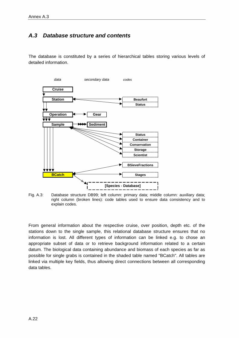
Annex A.3
A.22
A.3 Database structure and contents
The database is constituted by a series of hierarchical tables storing various levels of detailed information.
data secondary data codes
Cruise
Station BeaufortStatus
BSieveFractions
BCatch Stages
[Species - Database]
Operation Gear
Sample Sediment
StatusContainer
ConservationStorageScientist
Fig. A.3: Database structure DB99; left column: primary data; middle column: auxiliary data;
right column (broken lines): code tables used to ensure data consistency and to explain codes.
From general information about the respective cruise, over position, depth etc. of the stations down to the single sample, this relational database structure ensures that no information is lost. All different types of information can be linked e.g. to chose an appropriate subset of data or to retrieve background information related to a certain datum. The biological data containing abundance and biomass of each species as far as possible for single grabs is contained in the shaded table named "BCatch". All tables are linked via multiple key fields, thus allowing direct connections between all corresponding data tables.
Annex A.4
A.23
A.4 Species Database
A.4.1 Contents and structure
A.4.2 Code generation principles
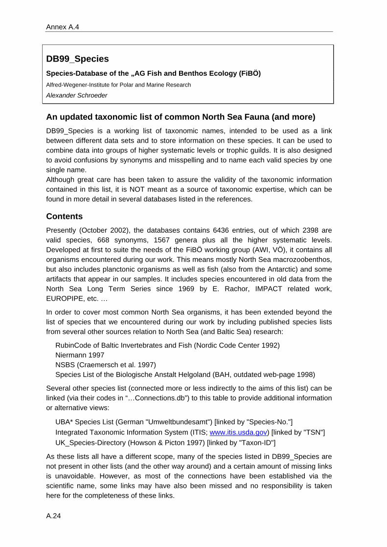
Annex A.4
A.24
DB99_Species Species-Database of the „AG Fish and Benthos Ecology (FiBÖ) Alfred-Wegener-Institute for Polar and Marine Research
Alexander Schroeder
An updated taxonomic list of common North Sea Fauna (and more) DB99_Species is a working list of taxonomic names, intended to be used as a link between different data sets and to store information on these species. It can be used to combine data into groups of higher systematic levels or trophic guilds. It is also designed to avoid confusions by synonyms and misspelling and to name each valid species by one single name. Although great care has been taken to assure the validity of the taxonomic information contained in this list, it is NOT meant as a source of taxonomic expertise, which can be found in more detail in several databases listed in the references.
Contents Presently (October 2002), the databases contains 6436 entries, out of which 2398 are valid species, 668 synonyms, 1567 genera plus all the higher systematic levels. Developed at first to suite the needs of the FiBÖ working group (AWI, VÖ), it contains all organisms encountered during our work. This means mostly North Sea macrozoobenthos, but also includes planctonic organisms as well as fish (also from the Antarctic) and some artifacts that appear in our samples. It includes species encountered in old data from the North Sea Long Term Series since 1969 by E. Rachor, IMPACT related work, EUROPIPE, etc. …
In order to cover most common North Sea organisms, it has been extended beyond the list of species that we encountered during our work by including published species lists from several other sources relation to North Sea (and Baltic Sea) research:
RubinCode of Baltic Invertebrates and Fish (Nordic Code Center 1992) Niermann 1997 NSBS (Craemersch et al. 1997) Species List of the Biologische Anstalt Helgoland (BAH, outdated web-page 1998)
Several other species list (connected more or less indirectly to the aims of this list) can be linked (via their codes in “…Connections.db”) to this table to provide additional information or alternative views:
UBA* Species List (German "Umweltbundesamt") [linked by "Species-No."] Integrated Taxonomic Information System (ITIS; www.itis.usda.gov) [linked by "TSN"] UK_Species-Directory (Howson & Picton 1997) [linked by "Taxon-ID"]
As these lists all have a different scope, many of the species listed in DB99_Species are not present in other lists (and the other way around) and a certain amount of missing links is unavoidable. However, as most of the connections have been established via the scientific name, some links may have also been missed and no responsibility is taken here for the completeness of these links.
Annex A.4
A.25
Taxonomic status Taxonomic status and systematic system have been revised and controlled intensively, nevertheless some error may still remain.
Besides the scientific names identified as the actually “valid” ones, the list also contains (old) “synonyms” encountered during the compilation of the list. This list of synonyms is quite extensive but by no means exhaustive and mostly several additional names can be found in more specialized taxonomic databases. Within this list, synonyms are intended to be able to extract data from several different sources, combining them under one scientific name. The opinion as to what name is actually “valid” differs depending on the source used and is subjected to more or less frequent changes. Although a great effort was made during the compilation of this list to identify the actually correct name, this list is NOT meant as a source of taxonomic expertise, but solely to avoid confusions by synonyms and misspelling and to name each valid species by one single name. To achieve this goal, some old or “misspelled” species names have been kept in the database in addition to the correct spelling in order to grant compatibility with other data if they are linked via the species name. The classification of each entry is visible from the “TaxStatus”, also identifying “artifacts” appearing in the samples, entries with alternative (misspelled) Codes (“CODE-error”), old taxonomic units that are no longer used (“not valid”), questionable (“?”) entries and those not found in recent literature during the last revision of the list (“unknown”) [as listed in “TaxStatus_lkp”].
A comprehensive list of this kind can only improve with the help of all users. Any changes made in the accompanied form “Fauna 5.8” are marked with date and user to allow tracking of changes made by different users. Therefore if any changes are made not through this form, this has to be documented manually.
Structure The complete species list consists of several tables, connected via the “Code”:
“DB99_Species”, the main table, contains the codes for each name (“Rubin”), the scientific name and author, the “Code” to connect to the assumed correct species name and the systematic hierarchy.
“DB99_CommonNames” contains common names in several languages.
”DB99_Feeding” contains feeding types.
”DB99_Connections” contains connection codes to other databases.
(Codes used in these tables are connected to explaining tables “…_lkp.db”)
The taxonomic level is indicated by the “Tax_Level” (as explained in “..TaxLevel_lkp”). Grouping at higher taxonomic levels can be achieved via the corresponding fields. As there are in several groups more systematic levels than fields in this table, these fields do not necessarily contain all possible levels (whose detail differ between major groups). The fields “Genus”, Family”, “Ordo”, “Class” and “Phylum” always contain exactly these groups, while intermediate levels like “SubOrder” and “SubClass” can also contain e.g. SuperFamilies or SuperOrders (and the like) respectively. The exact systematic hierarchy can be constructed via the “Parent” field. For each entry it contains the code of the next higher combining level.
Annex A.4
A.26
Technical note:
The complete database consists of several tables. A couple of forms were added that simplify the handling of the tables. In order to allow all links to be established correctly between all tables and within the forms, all files should be placed in one directory. The alias “TaxNet” has to be created, pointing to this directory, as this is used in all references to other tables.
Code The code has been created following the principles of the “Rubin Code”. It has been adjusted to fulfill some specific needs of this database (see: “Code Principles DB99_Species.doc”).
Sources Systematic hierarchy follows the following sources: Algae: Lüning (1985) Annelida: Polychaeta: Hartmann-Schröder (1996) Clitellata: Kästner (1984) {still valid see ERMS} Arthropoda: Kästner (1993) {still valid see ERMS} Brachiopoda: NEAT Bryozoa: Hayward P. J. (1985); Hayward, P.J., & Ryland, J.S. (1985, 1998, 1999) Chaetognatha: NEAT Chordata: Pisces: Fishbase (Eschmeyer), Tunicata: Hayward & Ryland (1998b) Mammalia: NEAT Cnidaria/Ctenophora: Kästner (1984) {still valid see ERMS} Echinodermata: NEAT Mollusca: ERMS Nemathelminthes: Kästner (1984) {still valid see ERMS} Nemertini: Kästner (1984) {still valid see ERMS} Plathelminthes: Kästner (1984) {still valid see ERMS} Porifera: Kästner (1980) {still valid see ERMS} Sipunculida: ERMS
WWW-Links …used in the preparation of this list, containing further details and additional information: European Register of Marine Species (ERMS) (Costello et al. 2001): http://erms.biol.soton.ac.uk Check List of European Marine Mollusca (CLEMAM): www.mnhn.fr/mnhn/bimm/clemam/page.htm North East Atlantic Taxa (NEAT): www.tmbl.gu.se/libdb/taxon/taxa.html Species 2000 Annual Checklist: www.sp2000.org/AnnualChecklist.html Integrated Taxonomic Information System (ITIS): www.itis.usda.gov FishBase: http://filaman.uni-kiel.de/search.cfm
Annex A.4
A.27
References
Costello, M.J.; Emblow, C.S. & White, R.e. (2001): European Register of Marine Species. A check-list of the marine species in Europe and a bibliography of guides to their identification. Patrimoines Naturels 50: 463 pp.
Craeymeersch, J. A.; Heip, C. H. R. & Buijs, J. (1997): Atlas of North Sea benthic infauna. Based on the 1986 North Sea Benthos Survey. ICES Coop. Res. Rep. 1997/218: pp. 86
Hartmann-Schröder (1996): Annelida, Borstenwürmer, Polychaeta. 2. ed. Gustav Fischer, Jena.
Hayward P. J. (1985): Ctenostome bryozoans. Synopses of the British Fauna (New Series). No. 33
Hayward, P.J., & Ryland, J.S. (1985): Cyclostome bryozoans. Synopses of the British Fauna (New Series). No. 34
Hayward, P.J., & Ryland, J.S. (1998): Cheilostomatous Bryozoa. Part 1. Aeteoidea - Cribrilinoidea. Synopses of the British Fauna (new series), No. 10
Hayward, P.J., & Ryland, J.S. (1999): Cheilostomatous Bryozoa. Part 2. Hippothoidea - Celleporoidea. Synopses of the British Fauna (New Series), No. 14
Hayward & Ryland (eds.) (1998b): Handbook of the Marine Fauna of North West Europe. Oxford University Press.
Howson, C.M. & Picton, B.E. (1997): The Species Directory of the Marine Fauna and Flora of the British Isles and surrounding seas. Pub. The Ulster Museum and The Marine Conservation Society, Belfast and Ross-on-Wye : 508 pp.
Kästner (1980): Lehrbuch der speziellen Zoologie Bd I, Teil 1, Fischer, Stuttgart Kästner (1984): Lehrbuch der speziellen Zoologie Bd. I Teil 2, Fischer, Stuttgart Kästner (1984): Lehrbuch der speziellen Zoologie Bd. I Teil 3, Fischer, Stuttgart. Kästner (1993): Lehrbuch der speziellen Zoologie Bd. I Teil 4, Fischer, Stuttgart. Lüning (1985): Meeresbotanik, Thieme, Stuttgart. Niermann, U. (1997): Macrobenthos of the south-eastern North Sea during 1983-1988.
Ber. Biol. Anst. Helgol. (13): 144 pp. Nordic Code Centre (1992): Species lists on Baltic Invertebrates, Mollusca, Crustacea,
Fish. The Museum of Natural History, Documentation Center; PoB 50007, S-104 05 Stockholm.
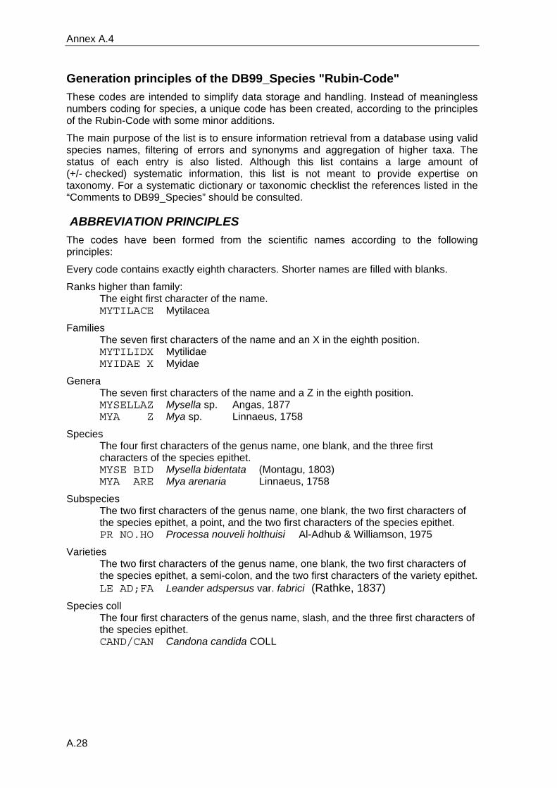
Annex A.4
A.28
Generation principles of the DB99_Species "Rubin-Code" These codes are intended to simplify data storage and handling. Instead of meaningless numbers coding for species, a unique code has been created, according to the principles of the Rubin-Code with some minor additions.
The main purpose of the list is to ensure information retrieval from a database using valid species names, filtering of errors and synonyms and aggregation of higher taxa. The status of each entry is also listed. Although this list contains a large amount of (+/- checked) systematic information, this list is not meant to provide expertise on taxonomy. For a systematic dictionary or taxonomic checklist the references listed in the “Comments to DB99_Species” should be consulted.
ABBREVIATION PRINCIPLES The codes have been formed from the scientific names according to the following principles:
Every code contains exactly eighth characters. Shorter names are filled with blanks.
Ranks higher than family: The eight first character of the name. MYTILACE Mytilacea
Families The seven first characters of the name and an X in the eighth position. MYTILIDX Mytilidae MYIDAE X Myidae
Genera The seven first characters of the name and a Z in the eighth position. MYSELLAZ Mysella sp. Angas, 1877 MYA Z Mya sp. Linnaeus, 1758
Species The four first characters of the genus name, one blank, and the three first characters of the species epithet. MYSE BID Mysella bidentata (Montagu, 1803) MYA ARE Mya arenaria Linnaeus, 1758
Subspecies The two first characters of the genus name, one blank, the two first characters of the species epithet, a point, and the two first characters of the species epithet. PR NO.HO Processa nouveli holthuisi Al-Adhub & Williamson, 1975
Varieties The two first characters of the genus name, one blank, the two first characters of the species epithet, a semi-colon, and the two first characters of the variety epithet. LE AD;FA Leander adspersus var. fabrici (Rathke, 1837)
Species coll The four first characters of the genus name, slash, and the three first characters of the species epithet. CAND/CAN Candona candida COLL
Annex A.4
A.29
Misspelled names The same principle as for normal entries, except if it would be the same code as for the properly spelled name. In the latter case a number replaces the eighth position (in all cases but for genera and families, where it replaces the seventh position). TRIG GU1 Triglia gurnardus = TRIG GUR Trigla gurnardus Linnaeus, 1758 TRIGLI1Z Triglia sp. = TRIGLA Z Trigla sp. Linnaeus, 1758
DEVIATING CODES Misspelled species names are kept in the list to allow a link via this field, even if the compared list contains typing errors. These have been assigned the status “misspelled” and are linked to the actual code.
Alternative codes have been incorporated, where earlier lists contained deviating codes, to ensure backwards compatibility. These have been assigned the status “CODE-error” and are linked to the actual code.
When standard codes would become equal for two or more taxa, one of these codes is manually altered into a unique one.
All “Rubin”-codes are unambiguous within the list. There might, however, be similar codes in other lists. A combination of this list with other lists containing a “Rubin-Code” may thus lead to inconsistencies.
REFERENCES
Code List Baltic Invertebrates, 81195-SYST, SNV PM 1557, 1982.

Annex A.5
A.30
A.5 Statistical tables
A.5.1 Results from pair-wise U-tests for differences between stations
A.5.2 ANOSIM results SSd
A.5.3 ANOSIM results WB
A.5.4 ANOSIM results Slt
A.5.5 ANOSIM results FSd
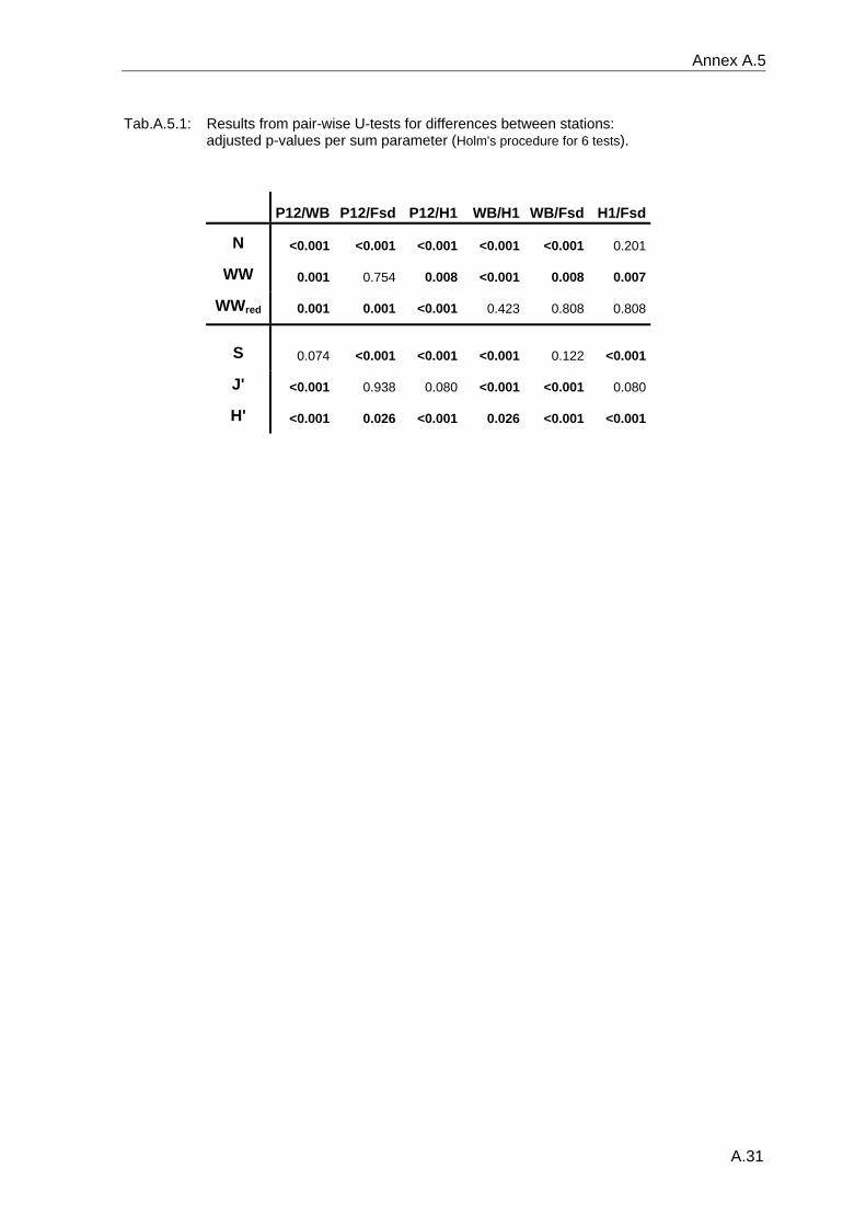
Annex A.5
A.31
Tab.A.5.1: Results from pair-wise U-tests for differences between stations: adjusted p-values per sum parameter (Holm's procedure for 6 tests).
P12/WB P12/Fsd P12/H1 WB/H1 WB/Fsd H1/Fsd
N <0.001 <0.001 <0.001 <0.001 <0.001 0.201
WW 0.001 0.754 0.008 <0.001 0.008 0.007
WWred 0.001 0.001 <0.001 0.423 0.808 0.808
S 0.074 <0.001 <0.001 <0.001 0.122 <0.001
J' <0.001 0.938 0.080 <0.001 <0.001 0.080
H' <0.001 0.026 <0.001 0.026 <0.001 <0.001
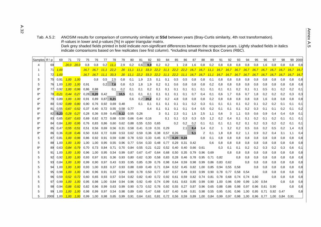
Sam \ p 69 71 72 75 76 77 78 79 80 81 82 83 84 85 86 87 88 89 91 92 93 94 95 96 97 98 99 2000
4 69 20,0 20,0 0,8 0,8 0,2 11,1 2,9 0,2 0,6 9,9 0,2 0,2 1 2,8 1,6 0,8 0,2 0,8 0,8 0,8 0,8 0,8 1,6 0,8 0,8 0,8 0,81 71 1,00 16,7 16,7 11,1 22,2 20 11,1 11,1 33,3 22,2 11,1 22,2 22,2 16,7 16,7 11,1 16,7 16,7 16,7 16,7 16,7 16,7 16,7 16,7 16,7 16,71 72 1,00 16,7 16,7 11,1 33,3 20 11,1 22,2 33,3 22,2 11,1 22,2 11,1 16,7 16,7 11,1 16,7 16,7 16,7 16,7 16,7 16,7 16,7 16,7 16,7 16,75 75 0,91 1,00 1,00 0,8 0,5 2,5 0,8 0,1 1,9 2,5 0,1 0,1 0,5 0,5 0,8 0,8 0,1 0,8 0,8 0,8 0,8 0,8 0,8 0,8 0,8 0,8 0,85 76 1,00 1,00 1,00 0,91 0,2 7,6 0,8 0,3 1,8 1,9 0,2 0,1 0,6 0,8 0,8 0,8 0,2 0,8 0,8 0,8 0,8 0,8 0,8 0,8 0,8 0,8 0,88 77 0,92 1,00 0,96 0,86 0,88 0,1 0,2 0,1 0,1 0,2 0,1 0,1 0,1 0,1 0,1 0,1 0,1 0,1 0,1 0,2 0,1 0,1 0,5 0,1 0,2 0,2 0,18 78 0,21 0,44 0,27 0,28 0,20 0,42 10,5 0,1 0,1 0,1 0,1 0,1 0,1 0,1 0,7 0,4 0,1 0,6 1,7 0,6 0,7 1,8 0,2 0,2 0,2 0,3 0,34 79 0,89 1,00 1,00 0,91 0,89 0,87 0,21 0,6 0,2 20,2 0,2 0,2 4,8 0,8 0,8 0,8 0,2 0,8 0,8 0,8 0,8 0,8 1,6 0,8 0,8 0,8 0,88 80 0,92 0,89 0,80 0,90 0,76 0,92 0,69 0,48 0,1 0,1 0,1 0,1 0,1 0,1 0,2 0,3 0,1 0,1 0,1 0,1 0,2 0,1 0,2 0,2 0,1 0,1 0,18 81 0,55 0,67 0,52 0,37 0,40 0,72 0,55 0,58 0,77 0,4 0,1 0,1 0,1 0,1 0,4 0,5 0,2 0,1 0,1 0,1 0,2 0,3 0,1 0,1 0,2 0,1 0,28 82 0,23 0,28 0,27 0,28 0,36 0,59 0,45 0,12 0,55 0,26 3 0,1 2,3 0,1 1,5 2,5 1,1 0,6 3 1,1 0,5 0,6 0,9 0,4 0,4 0,9 0,18 83 0,65 0,67 0,63 0,69 0,62 0,72 0,68 0,50 0,66 0,44 0,16 0,1 0,1 0,3 0,3 0,5 1,2 0,2 0,4 0,1 0,1 0,2 0,1 0,2 0,1 0,1 0,18 84 0,84 1,00 0,95 0,76 0,83 0,86 0,60 0,62 0,88 0,55 0,53 0,65 0,2 0,2 0,2 0,1 0,1 0,1 0,1 0,2 0,1 0,2 0,3 0,2 0,2 0,1 0,18 85 0,47 0,55 0,51 0,51 0,56 0,69 0,56 0,31 0,58 0,41 0,19 0,31 0,29 2,1 8,4 3,4 0,2 1 3,2 0,2 0,5 0,6 0,2 0,5 0,2 1,4 0,38 86 0,36 0,18 0,46 0,50 0,63 0,72 0,69 0,53 0,62 0,59 0,36 0,38 0,57 0,26 5,1 2 0,1 1,8 0,8 0,2 1,1 0,9 0,2 0,4 3,1 1,1 0,45 87 0,81 1,00 0,96 0,86 0,92 0,91 0,59 0,88 0,78 0,53 0,33 0,45 0,77 0,20 0,24 0,8 0,1 0,8 0,8 0,8 0,8 0,8 0,8 0,8 0,8 0,8 0,85 88 1,00 1,00 1,00 1,00 1,00 0,95 0,55 0,96 0,77 0,54 0,33 0,48 0,77 0,29 0,31 0,42 0,6 0,8 0,8 0,8 0,8 0,8 0,8 0,8 0,8 0,8 0,88 89 0,63 0,84 0,79 0,70 0,73 0,84 0,71 0,70 0,84 0,55 0,21 0,22 0,52 0,40 0,40 0,66 0,61 0,3 0,1 0,1 0,2 0,2 0,3 0,2 0,3 0,6 0,15 91 1,00 1,00 1,00 0,96 1,00 0,95 0,54 0,99 0,87 0,67 0,47 0,64 0,68 0,50 0,35 0,79 0,96 0,69 0,8 0,8 0,8 0,8 0,8 0,8 0,8 0,8 0,85 92 0,92 1,00 1,00 0,93 0,97 0,91 0,36 0,93 0,80 0,62 0,30 0,58 0,83 0,28 0,46 0,78 0,95 0,71 0,82 0,8 0,8 0,8 0,8 0,8 0,8 0,8 0,85 93 0,84 1,00 1,00 0,99 0,90 0,97 0,43 0,93 0,95 0,85 0,39 0,76 0,98 0,64 0,59 0,98 0,99 0,86 0,83 0,62 0,8 0,8 0,8 0,8 0,8 0,8 0,85 94 1,00 1,00 1,00 0,93 1,00 0,83 0,37 0,93 0,88 0,69 0,49 0,71 0,84 0,52 0,45 0,82 1,00 0,85 0,94 0,55 0,58 0,8 0,8 0,8 0,8 0,8 0,85 95 0,98 1,00 1,00 0,90 0,96 0,91 0,33 0,94 0,89 0,78 0,50 0,77 0,87 0,57 0,49 0,93 0,99 0,90 0,78 0,77 0,58 0,54 0,8 0,8 0,8 0,8 0,85 96 0,59 0,52 0,72 0,60 0,65 0,93 0,57 0,54 0,82 0,82 0,40 0,72 0,92 0,61 0,59 0,82 0,74 0,81 0,78 0,68 0,74 0,74 0,60 0,8 0,8 0,8 0,85 97 0,99 1,00 1,00 0,95 0,98 1,00 0,84 0,94 0,96 0,92 0,49 0,74 0,99 0,61 0,63 0,85 0,99 0,90 1,00 0,96 0,99 0,99 1,00 0,54 0,8 0,8 0,85 98 0,94 0,88 0,92 0,82 0,96 0,99 0,63 0,99 0,90 0,73 0,52 0,76 0,92 0,55 0,27 0,87 0,96 0,65 0,88 0,86 0,98 0,97 0,96 0,61 0,90 0,8 0,85 99 1,00 1,00 1,00 0,98 0,99 0,97 0,54 0,98 0,89 0,60 0,47 0,68 0,67 0,40 0,46 0,81 0,98 0,55 0,95 0,91 0,96 1,00 0,95 0,71 0,92 0,47 0,85 2000 1,00 1,00 1,00 0,99 1,00 0,98 0,65 0,99 0,91 0,64 0,61 0,81 0,72 0,56 0,59 0,89 1,00 0,84 0,99 0,97 0,98 1,00 0,96 0,77 1,00 0,84 0,91
Annex A
.5
A.32
T .5.2: ANOSIM results for comparison of community similarity at SSd between years (Bray-Curtis similarity, 4th root transformation). R-values in lower and p-values [%] in upper triangular matrix. Dark grey shaded fields printed in bold indicate non-significant differences between the respective years. Lightly shaded fields in italics indicate comparisons based on few replicates (see first column). *including small Reineck Box Corers (RBC).
ples R * * * * * * * * * * *
ab. A
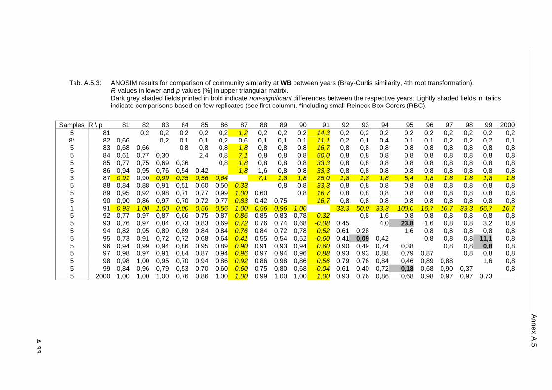
Samples R \ p 81 82 83 84 85 86 87 88 89 90 91 92 93 94 95 96 97 98 99 2000
5 81 0,2 0,2 0,2 0,2 0,2 1,2 0,2 0,2 0,2 14,3 0,2 0,2 0,2 0,2 0,2 0,2 0,2 0,2 0,28* 82 0,66 0,2 0,1 0,1 0,2 0,6 0,1 0,1 0,1 11,1 0,2 0,1 0,4 0,1 0,1 0,2 0,2 0,2 0,15 83 0,68 0,66 0,8 0,8 0,8 1,8 0,8 0,8 0,8 16,7 0,8 0,8 0,8 0,8 0,8 0,8 0,8 0,8 0,85 84 0,61 0,77 0,30 2,4 0,8 7,1 0,8 0,8 0,8 50,0 0,8 0,8 0,8 0,8 0,8 0,8 0,8 0,8 0,85 85 0,77 0,75 0,69 0,36 0,8 1,8 0,8 0,8 0,8 33,3 0,8 0,8 0,8 0,8 0,8 0,8 0,8 0,8 0,85 86 0,94 0,95 0,76 0,54 0,42 1,8 1,6 0,8 0,8 33,3 0,8 0,8 0,8 0,8 0,8 0,8 0,8 0,8 0,83 87 0,91 0,90 0,99 0,35 0,56 0,64 7,1 1,8 1,8 25,0 1,8 1,8 1,8 5,4 1,8 1,8 1,8 1,8 1,85 88 0,84 0,88 0,91 0,51 0,60 0,50 0,33 0,8 0,8 33,3 0,8 0,8 0,8 0,8 0,8 0,8 0,8 0,8 0,85 89 0,95 0,92 0,98 0,71 0,77 0,99 1,00 0,60 0,8 16,7 0,8 0,8 0,8 0,8 0,8 0,8 0,8 0,8 0,85 90 0,90 0,86 0,97 0,70 0,72 0,77 0,83 0,42 0,75 16,7 0,8 0,8 0,8 0,8 0,8 0,8 0,8 0,8 0,81 91 0,93 1,00 1,00 0,00 0,56 0,56 1,00 0,56 0,96 1,00 33,3 50,0 33,3 100,0 16,7 16,7 33,3 66,7 16,75 92 0,77 0,97 0,87 0,66 0,75 0,87 0,86 0,85 0,83 0,78 0,32 0,8 1,6 0,8 0,8 0,8 0,8 0,8 0,85 93 0,76 0,97 0,84 0,73 0,83 0,69 0,72 0,76 0,74 0,68 -0,08 0,45 4,0 23,8 1,6 0,8 0,8 3,2 0,85 94 0,82 0,95 0,89 0,89 0,84 0,84 0,76 0,84 0,72 0,78 0,52 0,61 0,28 1,6 0,8 0,8 0,8 0,8 0,85 95 0,73 0,91 0,72 0,72 0,68 0,64 0,41 0,55 0,54 0,52 -0,60 0,41 0,09 0,42 0,8 0,8 0,8 11,1 0,85 96 0,94 0,99 0,94 0,86 0,95 0,89 0,90 0,91 0,93 0,94 0,60 0,90 0,49 0,74 0,38 0,8 0,8 0,8 0,85 97 0,98 0,97 0,91 0,84 0,87 0,94 0,96 0,97 0,94 0,96 0,88 0,93 0,93 0,88 0,79 0,87 0,8 0,8 0,85 98 0,98 1,00 0,95 0,70 0,94 0,86 0,92 0,86 0,98 0,86 0,56 0,79 0,76 0,84 0,46 0,89 0,88 1,6 0,85 99 0,84 0,96 0,79 0,53 0,70 0,60 0,60 0,75 0,80 0,68 -0,04 0,61 0,40 0,72 0,18 0,68 0,90 0,37 0,85 2000 1,00 1,00 1,00 0,76 0,86 1,00 1,00 0,99 1,00 1,00 1,00 0,93 0,76 0,86 0,68 0,98 0,97 0,97 0,73
Annex A
.5A.33
Tab. A.5.3: ANOSIM results for comparison of community similarity at WB between years (Bray-Curtis similarity, 4th root transformation). R-values in lower and p-values [%] in upper triangular matrix. Dark grey shaded fields printed in bold indicate non-significant differences between the respective years. Lightly shaded fields in italics indicate comparisons based on few replicates (see first column). *including small Reineck Box Corers (RBC).
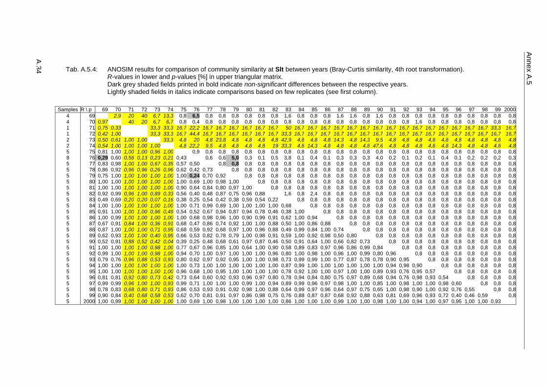
Samples R \ p 69 70 71 72 73 74 75 76 77 78 79 80 81 82 83 84 85 86 87 88 89 90 91 92 93 94 95 96 97 98 99 2000
4 69 2,9 20 40 6,7 13,3 0,8 6,5 0,8 0,8 0,8 0,8 0,8 0,8 1,6 0,8 0,8 0,8 1,6 1,6 0,8 1,6 0,8 0,8 0,8 0,8 0,8 0,8 0,8 0,8 0,8 0,84 70 0,97 40 20 6,7 6,7 0,8 0,4 0,8 0,8 0,8 0,8 0,8 0,8 0,8 0,8 0,8 0,8 0,8 0,8 0,8 0,8 0,8 0,8 1,6 0,8 0,8 0,8 0,8 0,8 0,8 0,81 71 0,75 0,33 33,3 33,3 16,7 22,2 16,7 16,7 16,7 16,7 16,7 16,7 50 16,7 16,7 16,7 16,7 16,7 16,7 16,7 16,7 16,7 16,7 16,7 16,7 16,7 16,7 16,7 33,3 16,71 72 0,42 1,00 33,3 33,3 16,7 44,4 16,7 16,7 16,7 16,7 16,7 16,7 33,3 16,7 16,7 16,7 16,7 16,7 16,7 16,7 16,7 16,7 16,7 16,7 16,7 16,7 16,7 16,7 16,7 16,72 73 0,50 0,61 1,00 1,00 33,3 4,8 20 4,8 23,8 4,8 4,8 4,8 4,8 42,9 4,8 4,8 4,8 14,3 4,8 14,3 9,5 4,8 4,8 4,8 4,8 4,8 4,8 4,8 4,8 4,8 4,82 74 0,54 1,00 1,00 1,00 1,00 4,8 22,2 9,5 4,8 4,8 4,8 4,8 19 33,3 4,8 14,3 4,8 4,8 4,8 4,8 47,6 4,8 4,8 4,8 4,8 4,8 14,3 4,8 4,8 4,8 4,85 75 0,81 1,00 1,00 1,00 0,96 1,00 0,9 0,8 0,8 0,8 0,8 0,8 0,8 0,8 0,8 0,8 0,8 0,8 0,8 0,8 0,8 0,8 0,8 0,8 0,8 0,8 0,8 0,8 0,8 0,8 0,88 76 0,29 0,60 0,56 0,13 0,23 0,21 0,43 0,6 0,6 5,0 0,3 0,1 0,5 3,8 0,1 0,4 0,1 0,3 0,3 0,3 4,0 0,2 0,1 0,2 0,1 0,4 0,1 0,2 0,2 0,2 0,35 77 0,83 0,98 1,00 1,00 0,67 0,35 0,57 0,50 0,8 0,8 0,8 0,8 0,8 0,8 0,8 0,8 0,8 0,8 0,8 0,8 0,8 0,8 0,8 0,8 0,8 0,8 0,8 0,8 0,8 0,8 0,85 78 0,86 0,92 0,96 0,96 0,26 0,96 0,62 0,42 0,73 0,8 0,8 0,8 0,8 0,8 0,8 0,8 0,8 0,8 0,8 0,8 0,8 0,8 0,8 0,8 0,8 0,8 0,8 0,8 0,8 0,8 0,85 79 0,75 1,00 1,00 1,00 1,00 1,00 1,00 0,24 0,70 0,92 0,8 0,8 0,8 0,8 0,8 0,8 0,8 0,8 0,8 0,8 0,8 0,8 0,8 0,8 0,8 0,8 0,8 0,8 0,8 0,8 0,85 80 1,00 1,00 1,00 1,00 1,00 1,00 1,00 0,69 1,00 0,98 1,00 0,8 0,8 0,8 0,8 0,8 0,8 0,8 0,8 0,8 0,8 0,8 0,8 0,8 0,8 0,8 0,8 0,8 0,8 0,8 0,85 81 1,00 1,00 1,00 1,00 1,00 1,00 0,90 0,64 0,84 0,80 0,97 1,00 0,8 0,8 0,8 0,8 0,8 0,8 0,8 0,8 0,8 0,8 0,8 0,8 0,8 0,8 0,8 0,8 0,8 0,8 0,85 82 0,92 0,99 0,96 1,00 0,89 0,33 0,56 0,40 0,48 0,87 0,75 0,96 0,88 1,6 0,8 2,4 0,8 0,8 0,8 0,8 0,8 0,8 0,8 0,8 0,8 0,8 0,8 0,8 0,8 0,8 0,85 83 0,49 0,69 0,20 0,20 0,07 0,16 0,38 0,25 0,54 0,42 0,38 0,59 0,54 0,22 0,8 0,8 0,8 0,8 0,8 0,8 0,8 0,8 0,8 0,8 0,8 0,8 0,8 0,8 0,8 0,8 0,85 84 1,00 1,00 1,00 1,00 1,00 1,00 1,00 0,71 0,99 0,89 1,00 1,00 1,00 1,00 0,68 0,8 0,8 0,8 0,8 0,8 0,8 0,8 0,8 0,8 0,8 0,8 0,8 0,8 0,8 0,8 0,85 85 0,91 1,00 1,00 1,00 0,96 0,49 0,54 0,52 0,67 0,94 0,87 0,94 0,78 0,46 0,38 1,00 0,8 0,8 0,8 0,8 0,8 0,8 0,8 0,8 0,8 0,8 0,8 0,8 0,8 0,8 0,85 86 1,00 0,99 1,00 1,00 1,00 1,00 1,00 0,68 0,98 0,96 1,00 0,90 0,99 0,91 0,62 1,00 0,94 0,8 0,8 0,8 0,8 0,8 0,8 0,8 0,8 0,8 0,8 0,8 0,8 0,8 0,85 87 0,67 0,91 0,84 1,00 0,36 0,91 0,68 0,47 0,86 0,74 0,92 1,00 1,00 0,88 0,50 1,00 0,86 0,88 0,8 0,8 0,8 0,8 0,8 0,8 0,8 0,8 0,8 0,8 0,8 0,8 0,85 88 0,87 1,00 1,00 1,00 0,71 0,95 0,68 0,59 0,92 0,68 0,97 1,00 0,96 0,88 0,49 0,99 0,84 1,00 0,74 0,8 0,8 0,8 0,8 0,8 0,8 0,8 0,8 0,8 0,8 0,8 0,85 89 0,62 0,93 1,00 1,00 0,40 0,95 0,66 0,53 0,82 0,78 0,79 1,00 0,98 0,91 0,59 1,00 0,92 0,98 0,50 0,80 0,8 0,8 0,8 0,8 0,8 0,8 0,8 0,8 0,8 0,8 0,85 90 0,52 0,91 0,88 0,52 0,42 0,04 0,39 0,25 0,48 0,68 0,61 0,97 0,87 0,46 0,50 0,91 0,64 1,00 0,66 0,82 0,73 0,8 0,8 0,8 0,8 0,8 0,8 0,8 0,8 0,8 0,85 91 1,00 1,00 1,00 1,00 0,98 1,00 0,77 0,67 0,96 0,85 1,00 0,64 1,00 0,90 0,58 0,89 0,83 0,97 0,96 0,86 0,99 0,84 0,8 0,8 0,8 0,8 0,8 0,8 0,8 0,8 0,85 92 0,99 1,00 1,00 1,00 0,98 1,00 0,94 0,70 1,00 0,97 1,00 1,00 1,00 0,96 0,80 1,00 0,98 1,00 0,96 1,00 0,99 0,80 0,96 0,8 0,8 0,8 0,8 0,8 0,8 0,8 0,85 93 0,79 0,76 0,96 0,88 0,53 0,93 0,80 0,62 0,97 0,92 0,95 1,00 1,00 0,98 0,73 0,99 0,99 1,00 0,77 0,87 0,78 0,78 0,90 0,95 0,8 0,8 0,8 0,8 0,8 0,8 0,85 94 1,00 1,00 1,00 1,00 1,00 1,00 1,00 0,73 1,00 1,00 1,00 1,00 1,00 1,00 0,87 0,99 1,00 1,00 1,00 1,00 1,00 1,00 0,94 0,98 0,90 0,8 0,8 0,8 0,8 0,8 0,85 95 1,00 1,00 1,00 1,00 1,00 1,00 0,96 0,68 1,00 0,95 1,00 1,00 1,00 1,00 0,78 0,92 1,00 1,00 0,97 1,00 1,00 0,89 0,93 0,76 0,95 0,57 0,8 0,8 0,8 0,8 0,85 96 0,81 0,81 0,92 0,80 0,73 0,42 0,73 0,64 0,60 0,92 0,93 0,96 0,97 0,80 0,78 0,94 0,84 0,80 0,75 0,97 0,89 0,68 0,94 0,76 0,98 0,93 0,54 0,8 0,8 0,8 0,85 97 0,99 0,99 0,96 1,00 1,00 0,93 0,99 0,71 1,00 1,00 1,00 0,99 1,00 0,94 0,89 0,99 0,96 0,97 0,98 1,00 1,00 0,85 1,00 0,98 1,00 1,00 0,98 0,60 0,8 0,8 0,85 98 0,78 0,83 0,68 0,80 0,71 0,93 0,86 0,53 0,93 0,91 0,92 0,98 1,00 0,88 0,64 0,99 0,97 0,96 0,64 0,97 0,75 0,65 1,00 0,98 0,90 1,00 0,92 0,76 0,55 0,8 0,85 99 0,90 0,84 0,40 0,68 0,58 0,53 0,62 0,70 0,81 0,91 0,97 0,86 0,98 0,75 0,76 0,88 0,87 0,87 0,68 0,92 0,88 0,63 0,81 0,69 0,96 0,93 0,72 0,40 0,46 0,59 0,85 2000 1,00 0,99 1,00 1,00 1,00 1,00 1,00 0,69 1,00 0,98 1,00 1,00 1,00 1,00 0,86 1,00 1,00 1,00 0,99 1,00 1,00 0,98 1,00 1,00 0,94 1,00 0,97 0,95 1,00 1,00 0,93
Annex A
.5
A.34 Tab. A.5.4: ANOSIM results for comparison of community similarity at Slt between years (Bray-Curtis similarity, 4th root transformation).
R-values in lower and p-values [%] in upper triangular matrix. Dark grey shaded fields printed in bold indicate non-significant differences between the respective years. Lightly shaded fields in italics indicate comparisons based on few replicates (see first column).
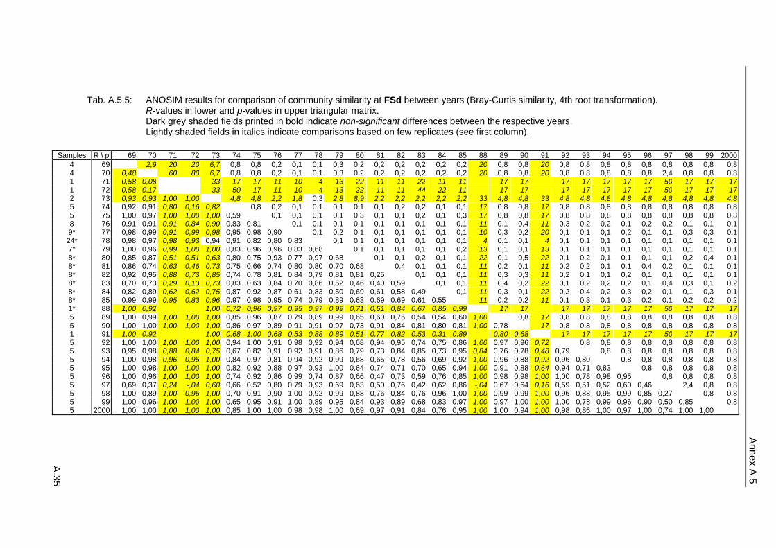
Samples R \ p 69 70 71 72 73 74 75 76 77 78 79 80 81 82 83 84 85 88 89 90 91 92 93 94 95 96 97 98 99 2000
4 69 2,9 20 20 6,7 0,8 0,8 0,2 0,1 0,1 0,3 0,2 0,2 0,2 0,2 0,2 0,2 20 0,8 0,8 20 0,8 0,8 0,8 0,8 0,8 0,8 0,8 0,8 0,84 70 0,48 60 80 6,7 0,8 0,8 0,2 0,1 0,1 0,3 0,2 0,2 0,2 0,2 0,2 0,2 20 0,8 0,8 20 0,8 0,8 0,8 0,8 0,8 2,4 0,8 0,8 0,81 71 0,58 0,08 33 17 17 11 10 4 13 22 11 11 22 11 11 17 17 17 17 17 17 17 50 17 17 17 1 72 0,58 0,17 33 50 17 11 10 4 13 22 11 11 44 22 11 17 17 17 17 17 17 17 50 17 17 17 2 73 0,93 0,93 1,00 1,00 4,8 4,8 2,2 1,8 0,3 2,8 8,9 2,2 2,2 2,2 2,2 2,2 33 4,8 4,8 33 4,8 4,8 4,8 4,8 4,8 4,8 4,8 4,8 4,8 5 74 0,92 0,91 0,80 0,16 0,82 0,8 0,2 0,1 0,1 0,1 0,1 0,1 0,2 0,2 0,1 0,1 17 0,8 0,8 17 0,8 0,8 0,8 0,8 0,8 0,8 0,8 0,8 0,85 75 1,00 0,97 1,00 1,00 1,00 0,59 0,1 0,1 0,1 0,1 0,3 0,1 0,1 0,2 0,1 0,3 17 0,8 0,8 17 0,8 0,8 0,8 0,8 0,8 0,8 0,8 0,8 0,88 76 0,91 0,91 0,91 0,84 0,90 0,83 0,81 0,1 0,1 0,1 0,1 0,1 0,1 0,1 0,1 0,1 11 0,1 0,4 11 0,3 0,2 0,2 0,1 0,2 0,2 0,1 0,1 0,19* 77 0,98 0,99 0,91 0,99 0,98 0,95 0,98 0,90 0,1 0,2 0,1 0,1 0,1 0,1 0,1 0,1 10 0,3 0,2 20 0,1 0,1 0,1 0,2 0,1 0,1 0,3 0,3 0,1
24* 78 0,98 0,97 0,98 0,93 0,94 0,91 0,82 0,80 0,83 0,1 0,1 0,1 0,1 0,1 0,1 0,1 4 0,1 0,1 4 0,1 0,1 0,1 0,1 0,1 0,1 0,1 0,1 0,17* 79 1,00 0,96 0,99 1,00 1,00 0,83 0,96 0,96 0,83 0,68 0,1 0,1 0,1 0,1 0,1 0,2 13 0,1 0,1 13 0,1 0,1 0,1 0,1 0,1 0,1 0,1 0,1 0,18* 80 0,85 0,87 0,51 0,51 0,63 0,80 0,75 0,93 0,77 0,97 0,68 0,1 0,1 0,2 0,1 0,1 22 0,1 0,5 22 0,1 0,2 0,1 0,1 0,1 0,1 0,2 0,4 0,18* 81 0,86 0,74 0,63 0,46 0,73 0,75 0,66 0,74 0,80 0,80 0,70 0,68 0,4 0,1 0,1 0,1 11 0,2 0,1 11 0,2 0,2 0,1 0,1 0,4 0,2 0,1 0,1 0,18* 82 0,92 0,95 0,88 0,73 0,85 0,74 0,78 0,81 0,84 0,79 0,81 0,81 0,25 0,1 0,1 0,1 11 0,3 0,3 11 0,2 0,1 0,1 0,2 0,1 0,1 0,1 0,1 0,18* 83 0,70 0,73 0,29 0,13 0,73 0,83 0,63 0,84 0,70 0,86 0,52 0,46 0,40 0,59 0,1 0,1 11 0,4 0,2 22 0,1 0,2 0,2 0,2 0,1 0,4 0,3 0,1 0,28* 84 0,82 0,89 0,62 0,62 0,75 0,87 0,92 0,87 0,61 0,83 0,50 0,69 0,61 0,58 0,49 0,1 11 0,3 0,1 22 0,2 0,4 0,2 0,3 0,2 0,1 0,1 0,3 0,18* 85 0,99 0,99 0,95 0,83 0,96 0,97 0,98 0,95 0,74 0,79 0,89 0,63 0,69 0,69 0,61 0,55 11 0,2 0,2 11 0,1 0,3 0,1 0,3 0,2 0,1 0,2 0,2 0,21* 88 1,00 0,92 1,00 0,72 0,96 0,97 0,95 0,97 0,99 0,71 0,51 0,84 0,67 0,85 0,99 17 17 17 17 17 17 17 50 17 17 17 5 89 1,00 0,99 1,00 1,00 1,00 0,85 0,96 0,87 0,79 0,89 0,99 0,65 0,60 0,75 0,54 0,54 0,60 1,00 0,8 17 0,8 0,8 0,8 0,8 0,8 0,8 0,8 0,8 0,85 90 1,00 1,00 1,00 1,00 1,00 0,86 0,97 0,89 0,91 0,91 0,97 0,73 0,91 0,84 0,81 0,80 0,81 1,00 0,78 17 0,8 0,8 0,8 0,8 0,8 0,8 0,8 0,8 0,81 91 1,00 0,92 1,00 0,68 1,00 0,68 0,53 0,88 0,89 0,51 0,77 0,82 0,53 0,31 0,89 0,80 0,68 17 17 17 17 17 50 17 17 17 5 92 1,00 1,00 1,00 1,00 1,00 0,94 1,00 0,91 0,98 0,92 0,94 0,68 0,94 0,95 0,74 0,75 0,86 1,00 0,97 0,96 0,72 0,8 0,8 0,8 0,8 0,8 0,8 0,8 0,85 93 0,95 0,98 0,88 0,84 0,75 0,67 0,82 0,91 0,92 0,91 0,86 0,79 0,73 0,84 0,85 0,73 0,95 0,84 0,76 0,78 0,48 0,79 0,8 0,8 0,8 0,8 0,8 0,8 0,85 94 1,00 0,98 0,96 0,96 1,00 0,84 0,97 0,81 0,94 0,92 0,99 0,68 0,65 0,78 0,56 0,69 0,92 1,00 0,96 0,88 0,92 0,96 0,80 0,8 0,8 0,8 0,8 0,8 0,85 95 1,00 0,98 1,00 1,00 1,00 0,82 0,92 0,88 0,97 0,93 1,00 0,64 0,74 0,71 0,70 0,65 0,94 1,00 0,91 0,88 0,64 0,94 0,71 0,83 0,8 0,8 0,8 0,8 0,85 96 1,00 0,96 1,00 1,00 1,00 0,74 0,92 0,86 0,99 0,74 0,87 0,66 0,47 0,73 0,59 0,76 0,85 1,00 0,98 0,98 1,00 1,00 0,78 0,98 0,95 0,8 0,8 0,8 0,85 97 0,69 0,37 0,24 -,04 0,60 0,66 0,52 0,80 0,79 0,93 0,69 0,63 0,50 0,76 0,42 0,62 0,86 -,04 0,67 0,64 0,16 0,59 0,51 0,52 0,60 0,46 2,4 0,8 0,85 98 1,00 0,89 1,00 0,96 1,00 0,70 0,91 0,90 1,00 0,92 0,99 0,88 0,76 0,84 0,76 0,96 1,00 1,00 0,99 0,99 1,00 0,96 0,88 0,95 0,99 0,85 0,27 0,8 0,85 99 1,00 0,96 1,00 1,00 1,00 0,65 0,95 0,91 1,00 0,89 0,95 0,84 0,93 0,89 0,68 0,83 0,97 1,00 0,97 1,00 1,00 1,00 0,78 0,99 0,96 0,90 0,50 0,85 0,8 5 2000 1,00 1,00 1,00 1,00 1,00 0,85 1,00 1,00 0,98 0,98 1,00 0,69 0,97 0,91 0,84 0,76 0,95 1,00 1,00 0,94 1,00 0,98 0,86 1,00 0,97 1,00 0,74 1,00 1,00
Annex A
.5
A.35
Tab. A.5.5: ANOSIM results for comparison of community similarity at FSd between years (Bray-Curtis similarity, 4th root transformation). R-values in lower and p-values in upper triangular matrix. Dark grey shaded fields printed in bold indicate non-significant differences between the respective years. Lightly shaded fields in italics indicate comparisons based on few replicates (see first column).
Annex A.6
A.36
A.6 Supplementary figures
A.6.1 Mean density of organisms in relation to sample size
A.6.2 Mean total biomass in relation to sample size
A.6.3 Mean total biomass excluding large species in relation to sample size
A.6.4 Frequency distribution of mean similarity
A.6.5 Community similarity and time lag
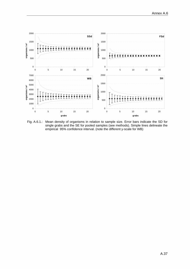
Annex A.6
A.37
SSd
0
500
1000
1500
2000
0 5 10 15 20
orga
nism
s / m
²
FSd
0
500
1000
1500
2000
0 5 10 15 20
orga
nism
s / m
²
WB
0
1000
2000
3000
4000
5000
6000
7000
0 5 10 15 20
grabs
orga
nism
s / m
²
Slt
0
500
1000
1500
2000
0 5 10 15 20
grabs
orga
nism
s / m
²
Fig. A.6.1.: Mean density of organisms in relation to sample size. Error bars indicate the SD for
single grabs and the SE for pooled samples (see methods). Simple lines delineate the empirical 95% confidence interval. (note the different y-scale for WB)
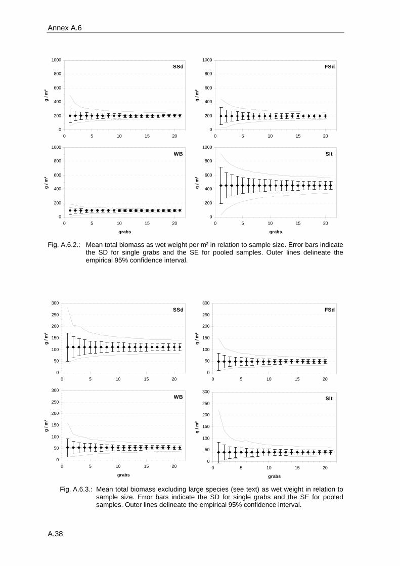
Annex A.6
A.38
SSd
0
200
400
600
800
1000
0 5 10 15 20
g / m
²
FSd
0
200
400
600
800
1000
0 5 10 15 20
g / m
²
WB
0
200
400
600
800
1000
0 5 10 15 20
grabs
g / m
²
Slt
0
200
400
600
800
1000
0 5 10 15 20
grabs
g / m
²
Fig. A.6.2.: Mean total biomass as wet weight per m² in relation to sample size. Error bars indicate
the SD for single grabs and the SE for pooled samples. Outer lines delineate the empirical 95% confidence interval.
SSd
0
50
100
150
200
250
300
0 5 10 15 20
g / m
²
FSd
0
50
100
150
200
250
300
0 5 10 15 20
g / m
²
WB
0
50
100
150
200
250
300
0 5 10 15 20
grabs
g / m
²
Slt
0
50
100
150
200
250
300
0 5 10 15 20
grabs
g / m
²
Fig. A.6.3.: Mean total biomass excluding large species (see text) as wet weight in relation to
sample size. Error bars indicate the SD for single grabs and the SE for pooled samples. Outer lines delineate the empirical 95% confidence interval.
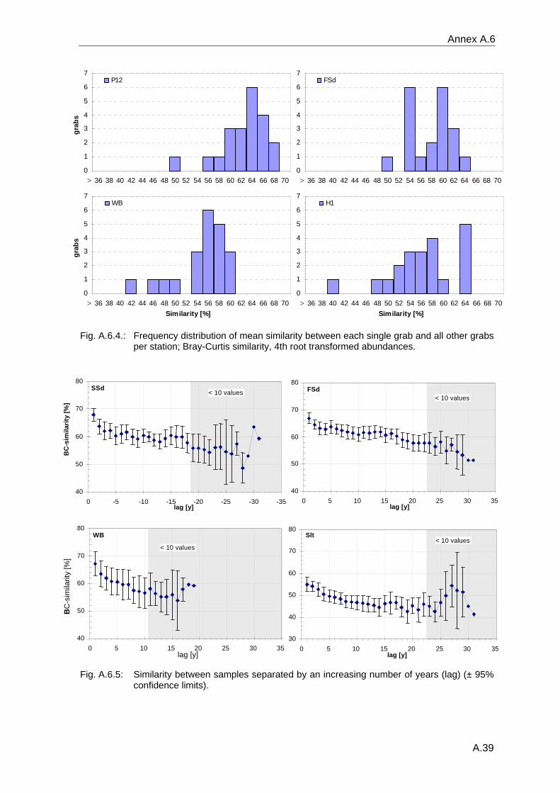
Annex A.6
A.39
0
1
2
3
4
5
6
7
36 38 40 42 44 46 48 50 52 54 56 58 60 62 64 66 68 70
grab
sP12
>0
1
2
3
4
5
6
7
36 38 40 42 44 46 48 50 52 54 56 58 60 62 64 66 68 70
FSd
>
0
1
2
3
4
5
6
7
36 38 40 42 44 46 48 50 52 54 56 58 60 62 64 66 68 70Similarity [%]
grab
s
WB
>0
1
2
3
4
5
6
7
36 38 40 42 44 46 48 50 52 54 56 58 60 62 64 66 68 70Similarity [%]
H1
>
Fig. A.6.4.: Frequency distribution of mean similarity between each single grab and all other grabs
per station; Bray-Curtis similarity, 4th root transformed abundances.
40
50
60
70
80
-35-30-25 -20 -15 -10 -5 0 lag [y]
BC
-sim
ilarit
y [%
]
< 10 valuesSSd
< 10 values
40
50
60
70
80
353025 20 151050lag [y]
FSd
40
50
60
70
80
353025 20 15 10 5 0 lag [y]
BC
-sim
ilarit
y [%
]
< 10 values WB
< 10 values
30
40
50
60
70
80
353025 20 151050lag [y]
Slt
Fig. A.6.5: Similarity between samples separated by an increasing number of years (lag) (± 95%
confidence limits).
Annex A.7
A.40
A.7 Single species temporal development plots
A.7.1 SSd
A.7.2 WB
A.7.3 Slt
A.7.4 FSd
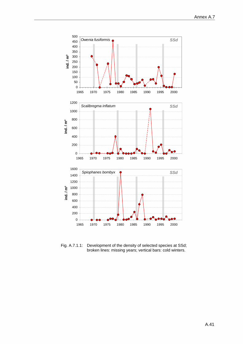
Annex A.7
A.41
Owenia fusiformis
0 50
100 150 200 250 300 350 400 450 500
1965 1970 1975 1980 1985 1990 1995 2000
ind.
/ m
²
SSd
Scalibregma inflatum
0
200
400
600
800
1000
1200
1965 1970 1975 1980 1985 1990 1995 2000
ind.
/ m
²
SSd
Spiophanes bombyx
0 200 400 600 800
1000 1200 1400 1600
1965 1970 1975 1980 1985 1990 1995 2000
ind.
/ m
²
SSd
Fig. A.7.1.1: Development of the density of selected species at SSd;
broken lines: missing years; vertical bars: cold winters.
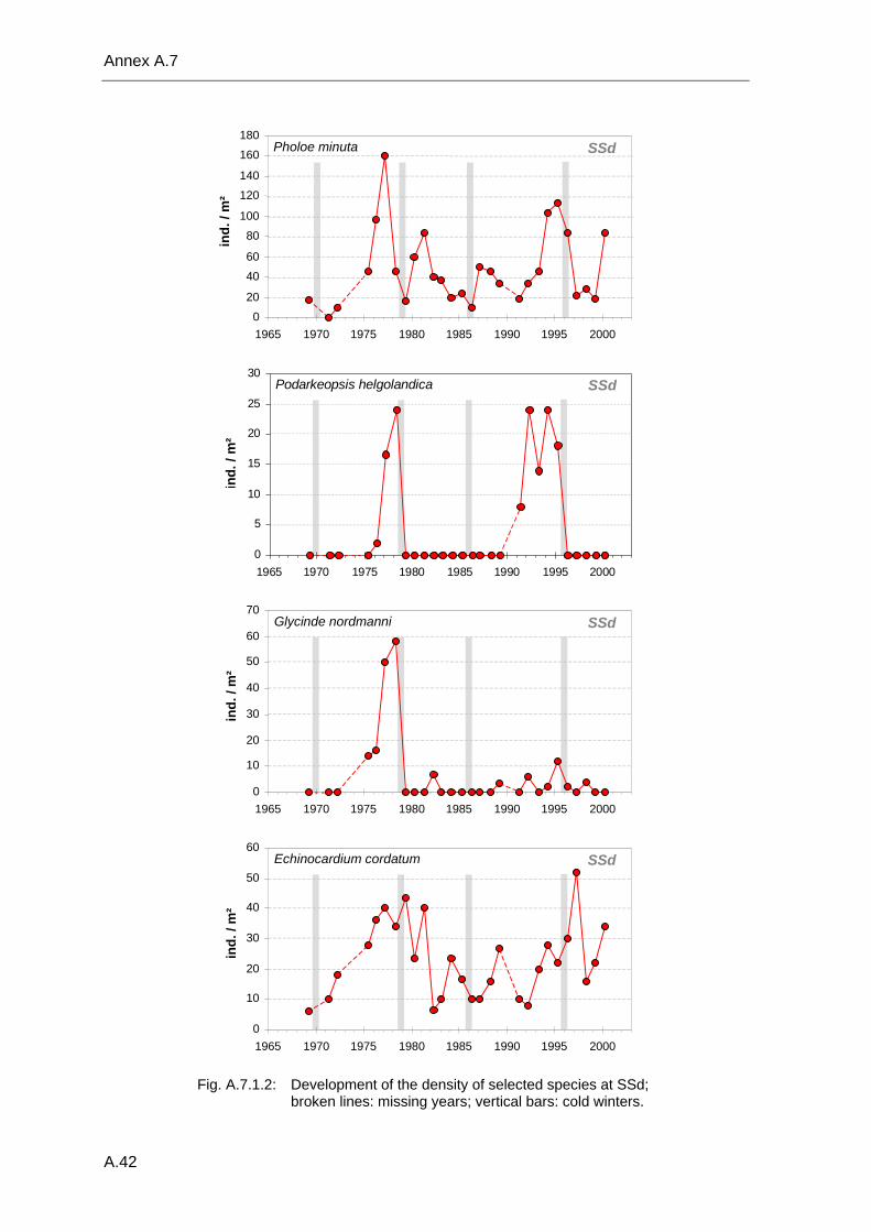
Annex A.7
A.42
Pholoe minuta
0
20
40
60
80
100
120
140
160
180
1965 1970 1975 1980 1985 1990 1995 2000
ind.
/ m
²
SSd
Podarkeopsis helgolandica
0
5
10
15
20
25
30
1965 1970 1975 1980 1985 1990 1995 2000
ind.
/ m
²
SSd
Glycinde nordmanni
0
10
20
30
40
50
60
70
1965 1970 1975 1980 1985 1990 1995 2000
ind.
/ m
²
SSd
Echinocardium cordatum
0
10
20
30
40
50
60
1965 1970 1975 1980 1985 1990 1995 2000
ind.
/ m
²
SSd
Fig. A.7.1.2: Development of the density of selected species at SSd;
broken lines: missing years; vertical bars: cold winters.
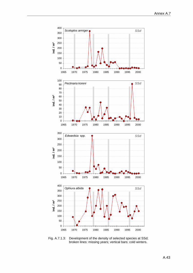
Annex A.7
A.43
Scoloplos armiger
0 50
100 150 200 250 300 350 400
1965 1970 1975 1980 1985 1990 1995 2000
ind.
/ m
²
SSd
Pectinaria koreni
0 10 20 30 40 50 60 70 80 90
100
1965 1970 1975 1980 1985 1990 1995 2000
ind.
/ m
²
SSd
Edwardsia spp.
0 50
100 150 200 250 300 350
1965 1970 1975 1980 1985 1990 1995 2000
i nd.
/ m
²
SSd
Ophiura albida
0 50
100 150 200 250 300 350 400
1965 1970 1975 1980 1985 1990 1995 2000
i nd.
/ m
²
SSd
Fig. A.7.1.3: Development of the density of selected species at SSd;
broken lines: missing years; vertical bars: cold winters.
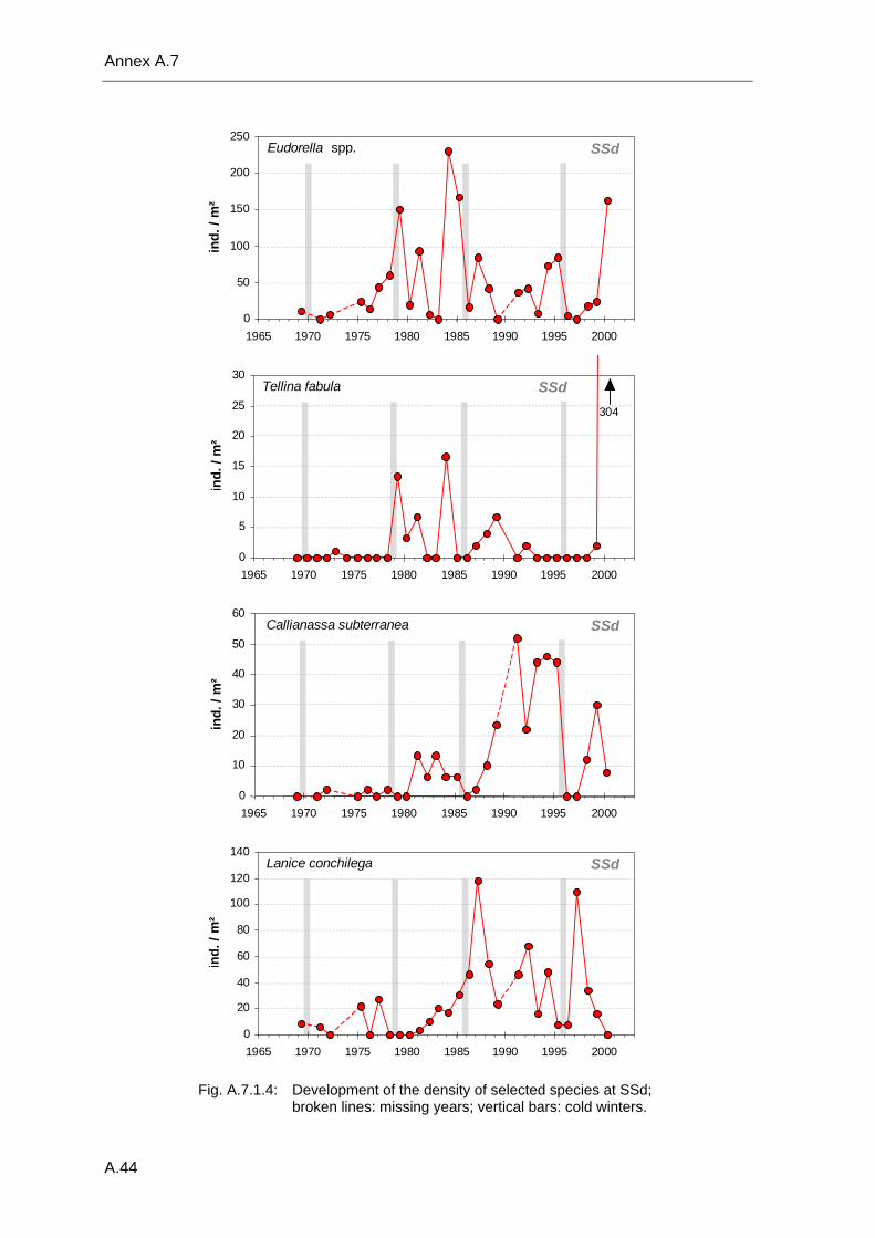
Annex A.7
A.44
Eudorella spp.
0
50
100
150
200
250
1965 1970 1975 1980 1985 1990 1995 2000
ind.
/ m
²
SSd
Tellina fabula
0
5
10
15
20
25
30
1965 1970 1975 1980 1985 1990 1995 2000
ind.
/ m
²
304
SSd
Callianassa subterranea
0
10
20
30
40
50
60
1965 1970 1975 1980 1985 1990 1995 2000
i nd.
/ m
²
SSd
Lanice conchilega
0 20 40 60 80
100 120 140
1965 1970 1975 1980 1985 1990 1995 2000
i nd.
/ m
²
SSd
Fig. A.7.1.4: Development of the density of selected species at SSd;
broken lines: missing years; vertical bars: cold winters.
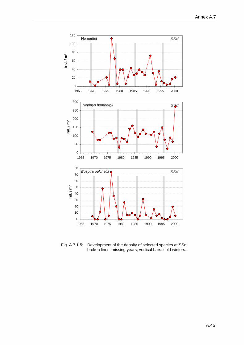
Annex A.7
A.45
Nemertini
0
20
40
60
80
100
120
1965 1970 1975 1980 1985 1990 1995 2000
ind.
/ m
²
SSd
SSd Nephtys hombergii
0
50
100
150
200
250
300
1965 1970 1975 1980 1985 1990 1995 2000
ind.
/ m
²
Euspira pulchella
0 10 20 30 40 50 60 70 80
1965 1970 1975 1980 1985 1990 1995 2000
ind.
/ m
²
SSd
Fig. A.7.1.5: Development of the density of selected species at SSd;
broken lines: missing years; vertical bars: cold winters.
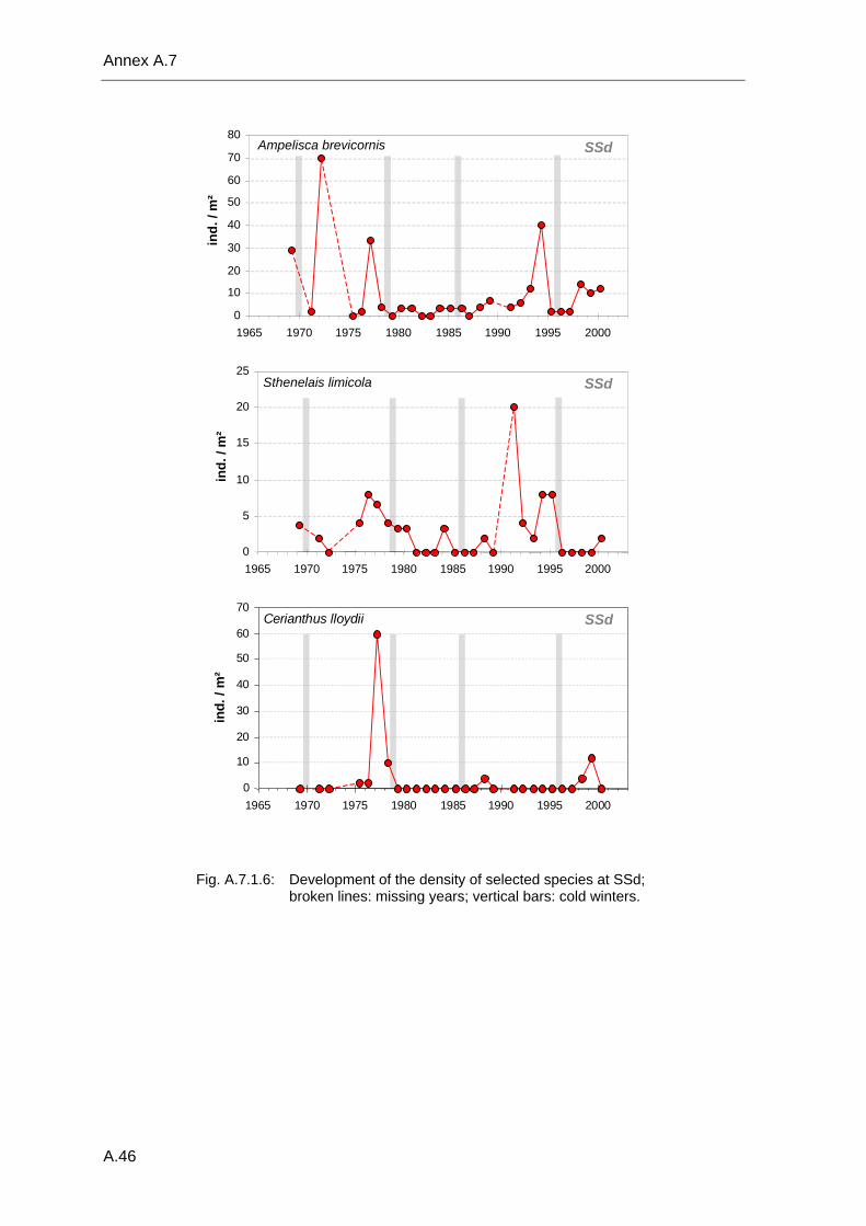
Annex A.7
A.46
Ampelisca brevicornis
0 10 20 30 40 50 60 70 80
1965 1970 1975 1980 1985 1990 1995 2000
ind.
/ m
²
SSd
Sthenelais limicola
0
5
10
15
20
25
1965 1970 1975 1980 1985 1990 1995 2000
ind.
/ m
²
SSd
Cerianthus lloydii
0 10 20 30 40 50 60 70
1965 1970 1975 1980 1985 1990 1995 2000
ind.
/ m
²
SSd
Fig. A.7.1.6: Development of the density of selected species at SSd;
broken lines: missing years; vertical bars: cold winters.
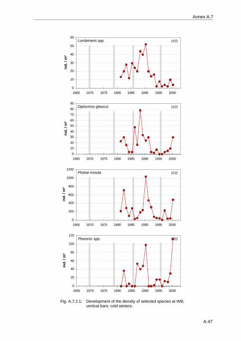
Annex A.7
A.47
Lumbrineris spp.
0
10
20
30
40
50
60
1965 1970 1975 1980 1985 1990 1995 2000
ind.
/ m
²
WB
Diplocirrus glaucus
0
10
20
3040
5060
70
80
90
1965 1970 1975 1980 1985 1990 1995 2000
ind.
/ m
²
WB
Pholoe minuta
0
200
400
600
800
1000
1200
1965 1970 1975 1980 1985 1990 1995 2000
ind.
/ m
²
WB
WB Phoronis spp.
0
20
40
60
80
100
120
1965 1970 1975 1980 1985 1990 1995 2000
ind.
/ m
²
Fig. A.7.2.1: Development of the density of selected species at WB;
vertical bars: cold winters.
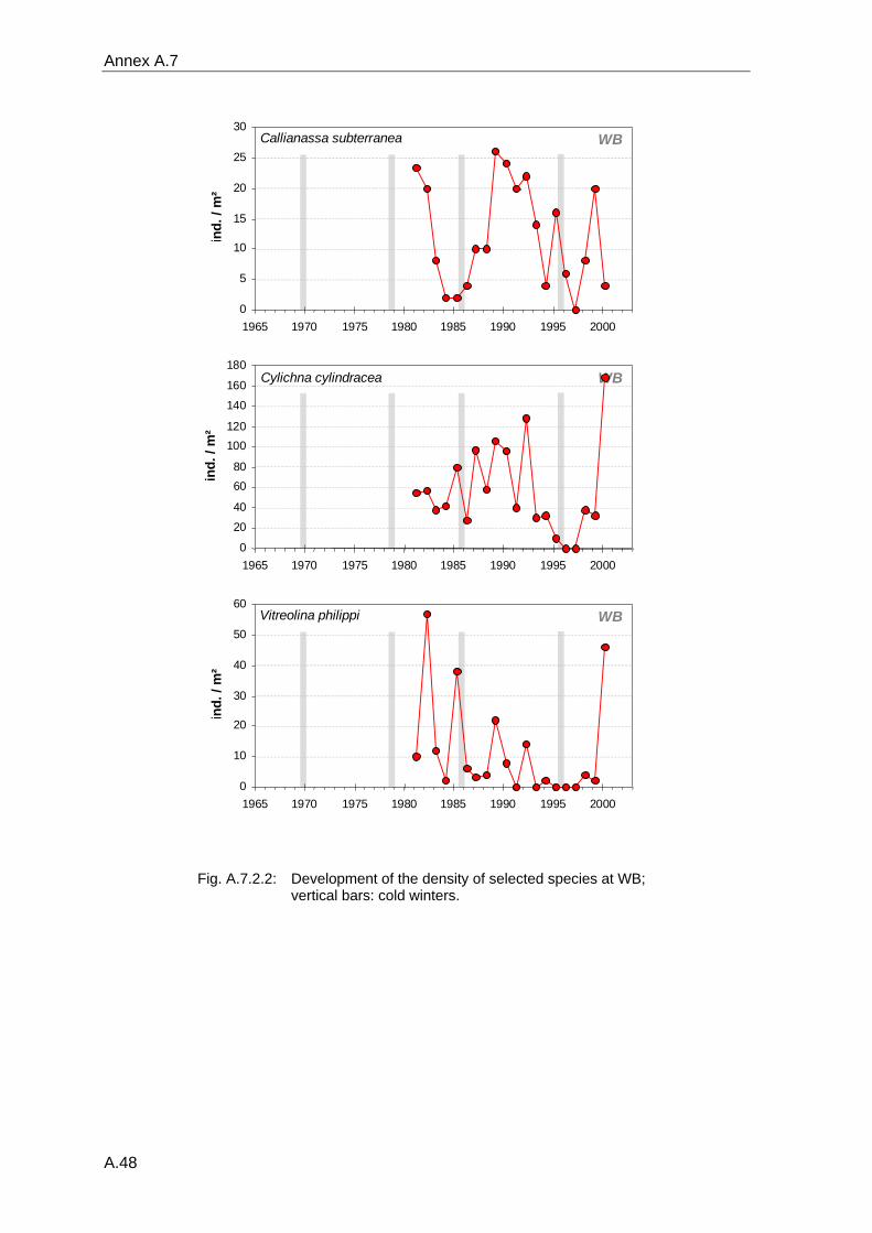
Annex A.7
A.48
Callianassa subterranea
0
5
10
15
20
25
30
1965 1970 1975 1980 1985 1990 1995 2000
ind.
/ m
²
WB
WB Cylichna cylindracea
0 20 40 60 80
100 120 140 160 180
1965 1970 1975 1980 1985 1990 1995 2000
ind.
/ m
²
Vitreolina philippi
0
10
20
30
40
50
60
1965 1970 1975 1980 1985 1990 1995 2000
ind.
/ m
²
WB
Fig. A.7.2.2: Development of the density of selected species at WB;
vertical bars: cold winters.
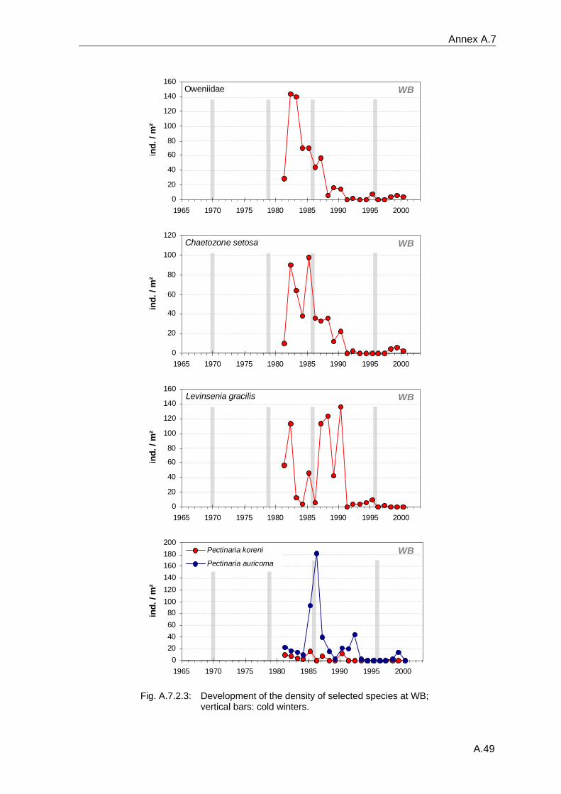
Annex A.7
A.49
Oweniidae
0 20 40 60 80
100 120 140 160
1965 1970 1975 1980 1985 1990 1995 2000
ind.
/ m
²
WB
Chaetozone setosa
0
20
40
60
80
100
120
1965 1970 1975 1980 1985 1990 1995 2000
ind.
/ m
²
WB
Levinsenia gracilis
0 20 40 60 80
100 120 140 160
1965 1970 1975 1980 1985 1990 1995 2000
ind.
/ m
²
WB
0 20 40 60 80
100 120 140 160 180 200
1965 1970 1975 1980 1985 1990 1995 2000
ind.
/ m
²
Pectinaria koreni
Pectinaria auricomaWB
Fig. A.7.2.3: Development of the density of selected species at WB;
vertical bars: cold winters.
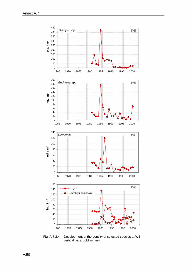
Annex A.7
A.50
Diastylis spp.
0 50
100 150 200 250 300 350 400 450
1965 1970 1975 1980 1985 1990 1995 2000
ind.
/ m
²
WB
0 20 40 60 80
100 120 140 160 180 200
1965 1970 1975 1980 1985 1990 1995 2000
ind.
/ m
²
Eudorella spp. WB
Nemertini
0 20 40 60 80
100 120 140
1965 1970 1975 1980 1985 1990 1995 2000
ind.
/ m
²
WB
0 20 40 60 80
100 120 140 160
1965 1970 1975 1980 1985 1990 1995 2000
ind.
/ m
²
+ juv. Nephtys hombergii
WB
Fig. A.7.2.4: Development of the density of selected species at WB;
vertical bars: cold winters.
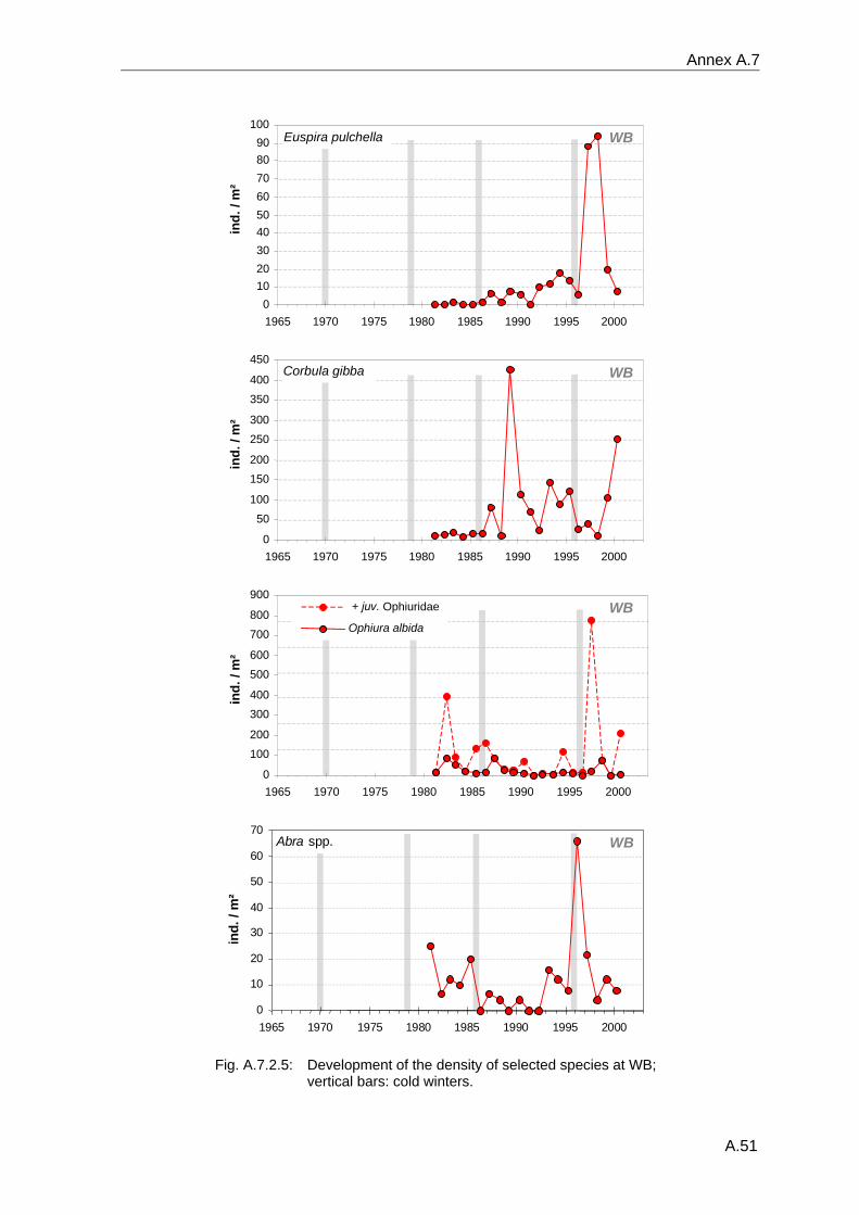
Annex A.7
A.51
0 10 20 30 40 50 60 70 80 90
100
1965 1970 1975 1980 1985 1990 1995 2000
ind.
/ m
²
Euspira pulchella WB
0 50
100 150 200 250 300 350 400 450
1965 1970 1975 1980 1985 1990 1995 2000
ind.
/ m
²
Corbula gibba WB
0 100 200 300 400 500 600 700 800 900
1965 1970 1975 1980 1985 1990 1995 2000
ind.
/ m
²
+ juv. Ophiuridae
Ophiura albidaWB
Abra spp.
0
10
20
30
40
50
60
70
1965 1970 1975 1980 1985 1990 1995 2000
ind.
/ m
²
WB
Fig. A.7.2.5: Development of the density of selected species at WB;
vertical bars: cold winters.
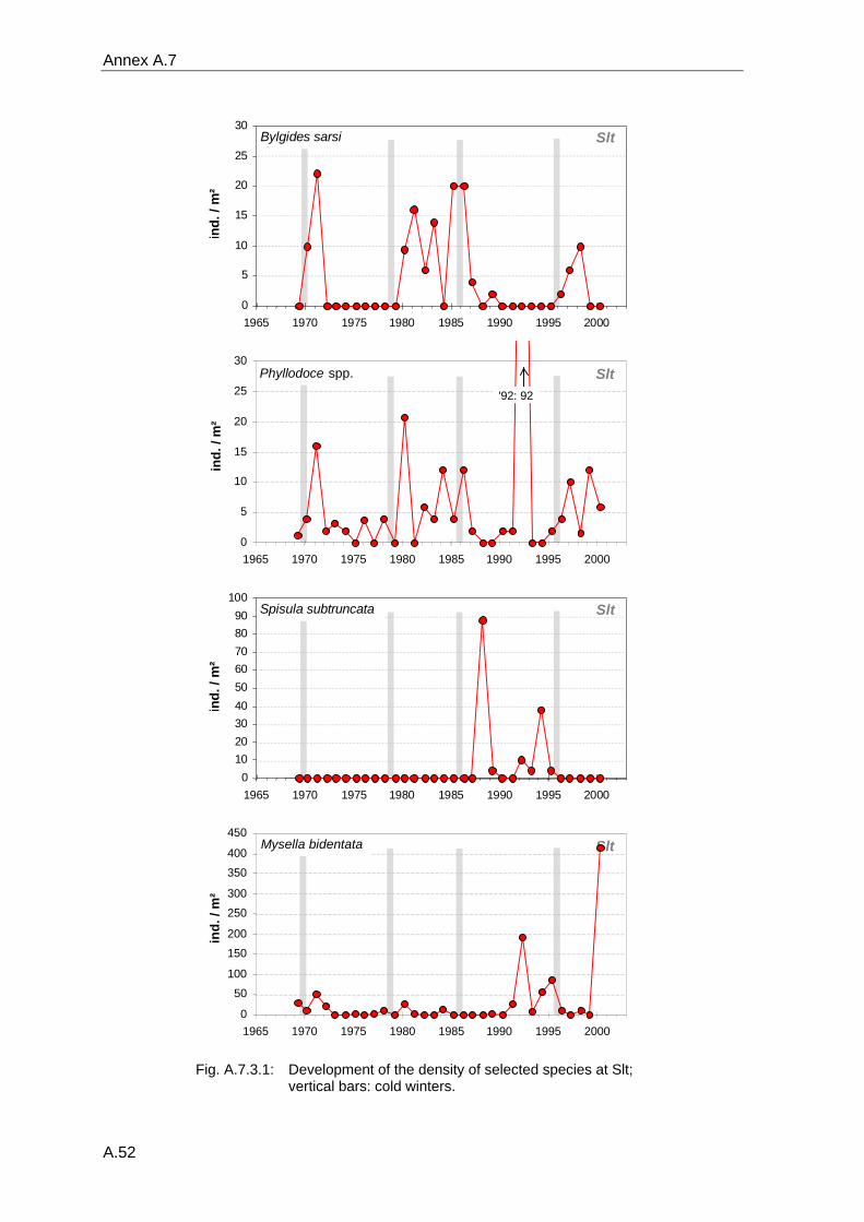
Annex A.7
A.52
Bylgides sarsi
0
5
10
15
20
25
30
1965 1970 1975 1980 1985 1990 1995 2000
ind.
/ m
²
Slt
Phyllodoce spp.
0
5
10
15
20
25
30
1965 1970 1975 1980 1985 1990 1995 2000
ind.
/ m
²
Slt '92: 92
Spisula subtruncata
0 10 20 30 40 50 60 70 80 90
100
1965 1970 1975 1980 1985 1990 1995 2000
ind.
/ m
²
Slt
Slt Mysella bidentata
0 50
100 150 200 250 300 350 400 450
1965 1970 1975 1980 1985 1990 1995 2000
ind.
/ m
²
Fig. A.7.3.1: Development of the density of selected species at Slt;
vertical bars: cold winters.
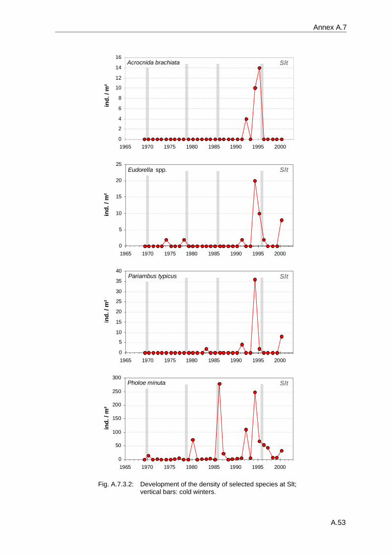
Annex A.7
A.53
Acrocnida brachiata
0
2
4
6
8
10
12
14
16
1965 1970 1975 1980 1985 1990 1995 2000
ind.
/ m
²
Slt
Eudorella spp.
0
5
10
15
20
25
1965 1970 1975 1980 1985 1990 1995 2000
ind.
/ m
²
Slt
Pariambus typicus
0 5
10
15
20
25
30
35
40
1965 1970 1975 1980 1985 1990 1995 2000
ind.
/ m
²
Slt
Pholoe minuta
0
50
100
150
200
250
300
1965 1970 1975 1980 1985 1990 1995 2000
ind.
/ m
²
Slt
Fig. A.7.3.2: Development of the density of selected species at Slt;
vertical bars: cold winters.
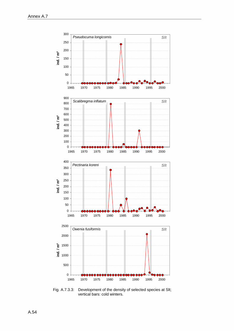
Annex A.7
A.54
Pseudocuma longicornis
0
50
100
150
200
250
300
1965 1970 1975 1980 1985 1990 1995 2000
ind.
/ m
²
Slt
Scalibregma inflatum
0100
200
300
400
500
600
700
800900
1965 1970 1975 1980 1985 1990 1995 2000
ind.
/ m
²
Slt
Pectinaria koreni
0 50
100 150 200 250 300 350 400
1965 1970 1975 1980 1985 1990 1995 2000
ind.
/ m
²
Slt
Owenia fusiformis
0
500
1000
1500
2000
2500
1965 1970 1975 1980 1985 1990 1995 2000
ind.
/ m
²
Slt
Fig. A.7.3.3: Development of the density of selected species at Slt;
vertical bars: cold winters.
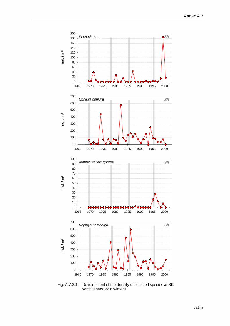
Annex A.7
A.55
0 20 40 60 80
100 120 140 160 180 200
1965 1970 1975 1980 1985 1990 1995 2000
ind.
/ m
²
Phoronis spp. Slt
Ophiura ophiura
0 100 200 300 400 500 600 700
1965 1970 1975 1980 1985 1990 1995 2000
ind.
/ m
²
Slt
0 10 20 30 40 50 60 70 80 90
100
1965 1970 1975 1980 1985 1990 1995 2000
i nd.
/ m
²
Montacuta ferruginosa Slt
Nephtys hombergii
0 100 200 300 400 500 600 700
1965 1970 1975 1980 1985 1990 1995 2000
ind.
/ m
²
Slt
Fig. A.7.3.4: Development of the density of selected species at Slt;
vertical bars: cold winters.
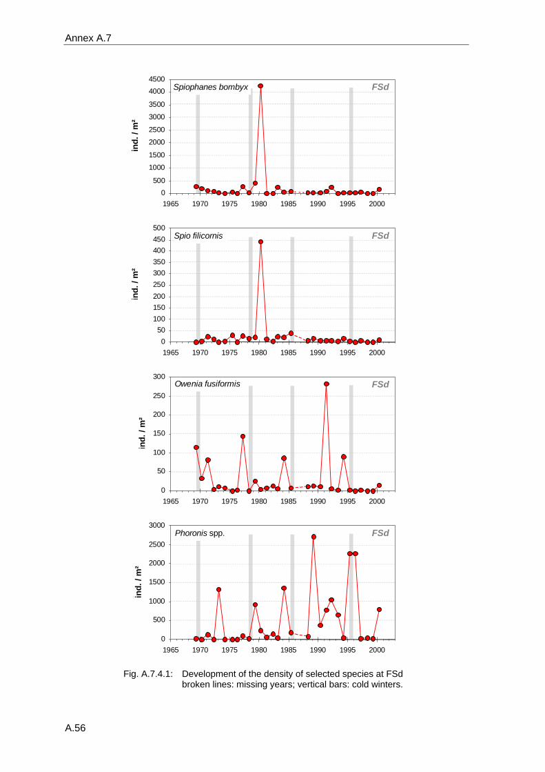
Annex A.7
A.56
Spiophanes bombyx
0500
1000
1500
2000
2500
3000
3500
40004500
1965 1970 1975 1980 1985 1990 1995 2000
ind.
/ m
²
FSd
050
100150200250300350400450500
1965 1970 1975 1980 1985 1990 1995 2000
ind.
/ m
²
Spio filicornis FSd
0
50
100
150
200
250
300
1965 1970 1975 1980 1985 1990 1995 2000
i nd.
/ m
²
Owenia fusiformis FSd
0
500
1000
1500
2000
2500
3000
1965 1970 1975 1980 1985 1990 1995 2000
i nd.
/ m
²
Phoronis spp. FSd
Fig. A.7.4.1: Development of the density of selected species at FSd
broken lines: missing years; vertical bars: cold winters.
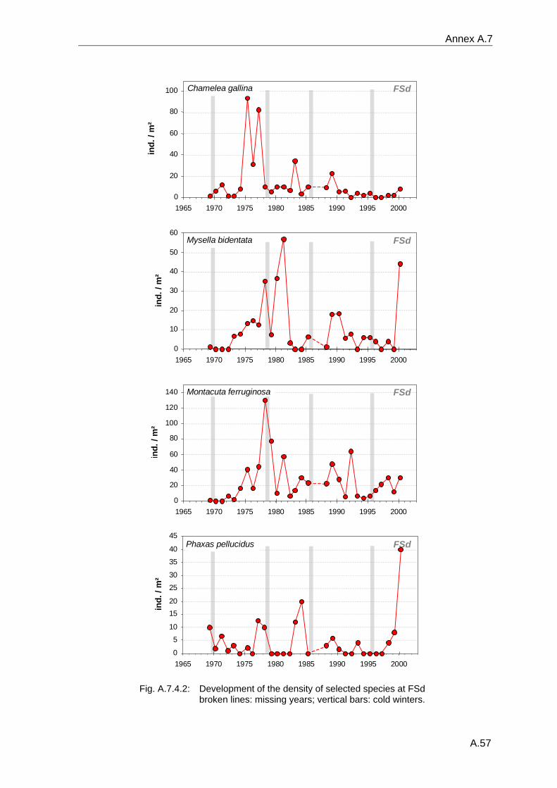
Annex A.7
A.57
Chamelea gallina
0
20
40
60
80
100
1965 1970 1975 1980 1985 1990 1995 2000
ind.
/ m
²
FSd
Mysella bidentata
0
10
20
30
40
50
60
1965 1970 1975 1980 1985 1990 1995 2000
ind.
/ m
²
FSd
Montacuta ferruginosa
0 20 40 60 80
100 120 140
1965 1970 1975 1980 1985 1990 1995 2000
ind.
/ m
²
FSd
FSd Phaxas pellucidus
0 5
10 15 20 25 30 35 40 45
1965 1970 1975 1980 1985 1990 1995 2000
i nd.
/ m
²
Fig. A.7.4.2: Development of the density of selected species at FSd
broken lines: missing years; vertical bars: cold winters.
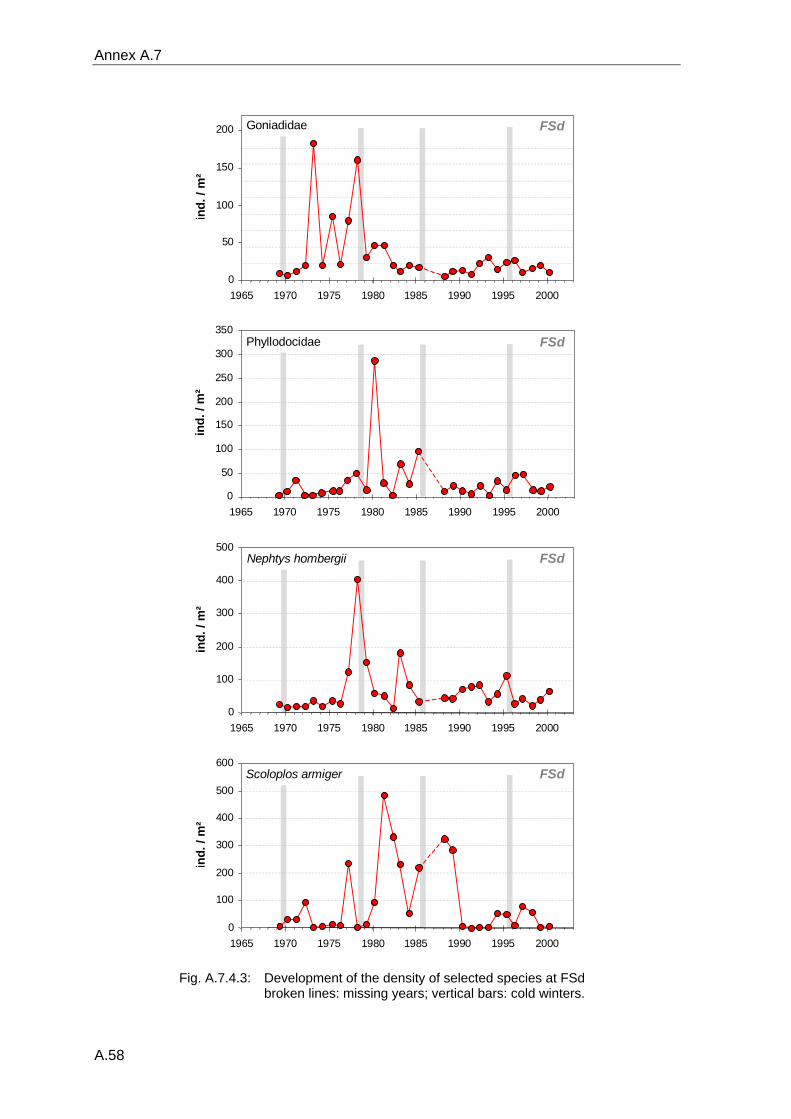
Annex A.7
A.58
Goniadidae
0
50
100
150
200
1965 1970 1975 1980 1985 1990 1995 2000
ind.
/ m
²
FSd
Phyllodocidae
0
50
100
150
200
250
300
350
1965 1970 1975 1980 1985 1990 1995 2000
ind.
/ m
²
FSd
Nephtys hombergii
0
100
200
300
400
500
1965 1970 1975 1980 1985 1990 1995 2000
ind.
/ m
²
FSd
Scoloplos armiger
0
100
200
300
400
500
600
1965 1970 1975 1980 1985 1990 1995 2000
i nd.
/ m
²
FSd
Fig. A.7.4.3: Development of the density of selected species at FSd
broken lines: missing years; vertical bars: cold winters.
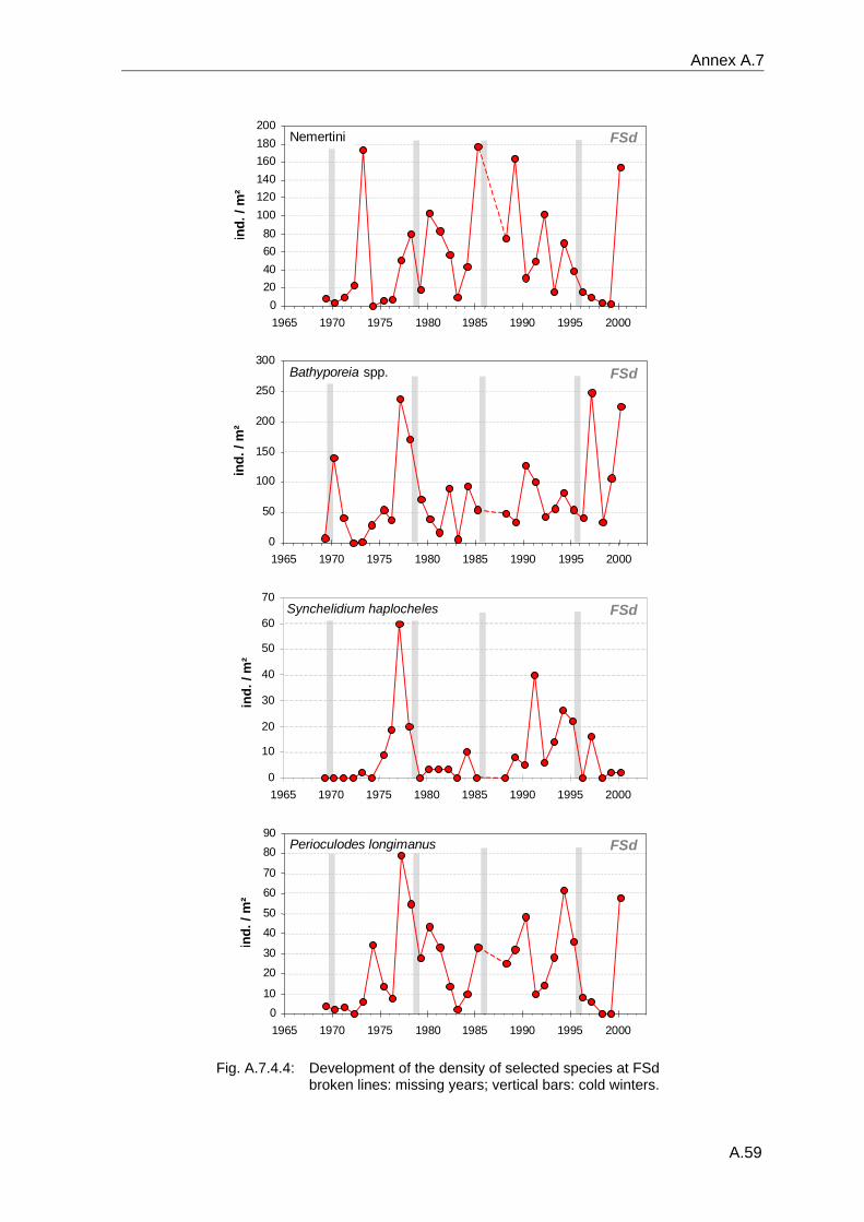
Annex A.7
A.59
Nemertini
0 20 40 60 80
100 120 140 160 180 200
1965 1970 1975 1980 1985 1990 1995 2000
ind.
/ m
²
FSd
Bathyporeia spp.
0
50
100
150
200
250
300
1965 1970 1975 1980 1985 1990 1995 2000
ind.
/ m
²
FSd
Synchelidium haplocheles
0 10 20 30 40 50 60 70
1965 1970 1975 1980 1985 1990 1995 2000
ind.
/ m
²
FSd
Perioculodes longimanus
0 10 20 30 40 50 60 70 80 90
1965 1970 1975 1980 1985 1990 1995 2000
ind.
/ m
²
FSd
Fig. A.7.4.4: Development of the density of selected species at FSd
broken lines: missing years; vertical bars: cold winters.
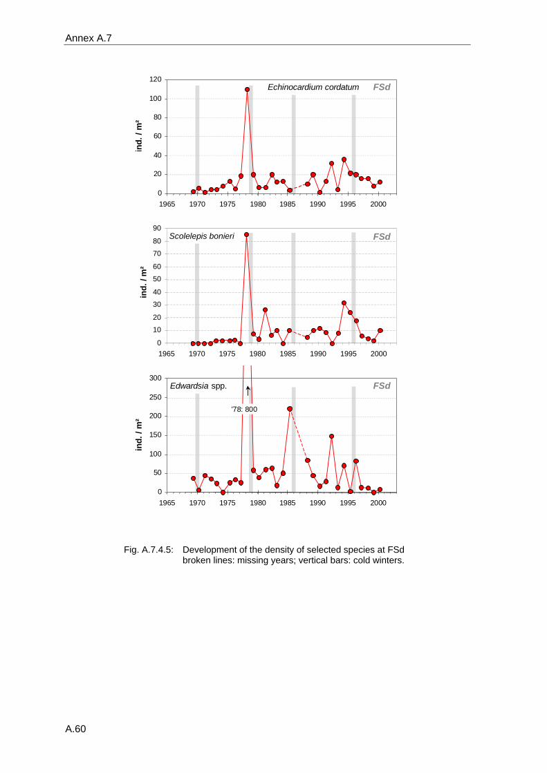
Annex A.7
A.60
Echinocardium cordatum
0
20
40
60
80
100
120
1965 1970 1975 1980 1985 1990 1995 2000
ind.
/ m
²
FSd
Scolelepis bonieri
0
10
20
30
40
50
60
70
80
90
1965 1970 1975 1980 1985 1990 1995 2000
ind.
/ m
²
FSd
Edwardsia spp.
0
50
100
150
200
250
300
1965 1970 1975 1980 1985 1990 1995 2000
ind.
/ m
²
'78: 800
FSd
Fig. A.7.4.5: Development of the density of selected species at FSd
broken lines: missing years; vertical bars: cold winters.
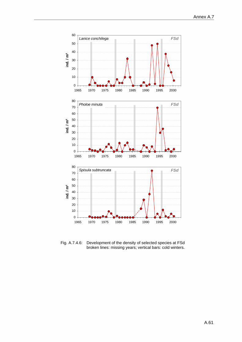
Annex A.7
A.61
Lanice conchilega
0
10
20
30
40
50
60
1965 1970 1975 1980 1985 1990 1995 2000
ind.
/ m
²
FSd
Pholoe minuta
0 10 20 30 40 50 60 70 80
1965 1970 1975 1980 1985 1990 1995 2000
ind.
/ m
²
FSd
Spisula subtruncata
0 10 20 30 40 50 60 70 80
1965 1970 1975 1980 1985 1990 1995 2000
i nd.
/ m
²
FSd
Fig. A.7.4.6: Development of the density of selected species at FSd
broken lines: missing years; vertical bars: cold winters.
Annex A.8
A.62
A.8 Glossary
FSd: "Fine Sand" station SSd: "Silty Sand" station Slt: "Silt" station WB: "White Bank" station
station: permanent sampling station of long-term study position: sampling location within station sample: composed of several replicates (sampling units) sampling unit: grab vV: van Veen grab (0.1 m² if not stated otherwise) RBC: Reineck box corer (0.017 m²) S: number of species N: total number of organisms ni: number of organisms in species i SD: standard deviation SE: standard error (of the mean) CV: coefficient of variation C.I.: confidence interval s²: variance ø: mean s²/ø: variance to mean ratio Id: Morisita's index of dispersion Ip: standardisation of Morisita's index of dispersion H’: Shannon-Wiener index of diversity J’: Pielou's index of evenness BC: Bray-Curtis index of similarity MDS: nonmetric multidimensional scaling NAO: North Atlantic oscillation NAOI: North Atlantic oscillation index W-NAOI: winter- (December – March) NAOI A-NAOI: annual NAOI Bft.: Beaufort wind-speed PO4: phosphate DIN: dissolved inorganic nitrogen SiO4: silicate PSU: SI-unit for salinity: "Practical Salinity Units" ≈ ‰
Acknowledgements
Acknowledgements
Last but not least, I would like to thank all those without whom this work would not have
been possible:
Prof. Dr. Wolf Arntz for supervising this work and constructive comments and discussion
of an earlier version of the manuscript;
Dr. Rainer Knust for his support with whatever problems arose during the preparation of
this work over the years and for his comments on the manuscript;
Dr. Eicke Rachor for supplying the largest part of the benthic community data and
samples and for helpful comments on the manuscript;
The crew of FS "Victor Hensen" and FS "Heincke" and all those people that helped during
the sampling at sea, sorting of the samples or entering the data into the database;
Various people that made accessory data available for the interpretation of the faunal
data: Dr. Karen Wiltshire and Peter Mangelsdorf (AWI/BAH) supplied the "Helgoland
Reede" data on water temperature, salinity and nutrients; the Deutscher Wetterdienst
(DWD) provided weather data from over 30 years; Dr. Eggert (BfG) supplied water
discharge data of the river Elbe; Dr. James Hurrel (Climate Analysis Section, NCAR,
Boulder, USA) provided the "North Atlantic Oscillation Index" (NAOI) data;
Inken for a choice of sea bottom photographs, Jan for honest comments on an earlier
draft and all the other colleagues at the institute, especially the members of the FiBÖ
working group, for help, discussions, conversations etc.;
… and (l.b.n.l. again) Pitty for good times, never-ending support, fruitful discussions and
helpful hands and words whenever I needed some.
This work was supported by the bilateral cooperation program between The Netherlands
and the city of Bremen NEBROC (NEtherlands BRemen OCeanography) as part of sub-
project 2.3: "Decadal and centennial variations and long term changes of the North Sea
and Wadden Sea ecosystems".