Embed Size (px)
Citation preview
Prof. Dr. Barbara Wohlmuth
Lehrstuhl fur Numerische Mathematik
III. Iterative Loser
III.1 Direkte Loser und ihre Nachteile
III.2 Klassische Iterationsverfahren
Kapitel III (0) 1
Prof. Dr. Barbara Wohlmuth
Lehrstuhl fur Numerische Mathematik
Erinnerung: Lineares Gleichungssystem bei FDM
Diskretisierung einer linearen PDGL 2. Ordnung mit Finiten Differenzen/FEMfuhrt zu einem linearen Gleichungssystem Ax = b, welches
• groß ist (typischerweise: Dimension = O(h−d)),
• dunn besetzt ist (O(h−d) nicht-Null Eintrage)
• schlecht konditioniert ist (κ(A) = O(h−2)),
• haufig symmetrisch, positiv definit ist, und
• bei geeigneter Nummerierung eine Bandstruktur besitzt.
Kapitel III (numalg65) 2
Prof. Dr. Barbara Wohlmuth
Lehrstuhl fur Numerische Mathematik
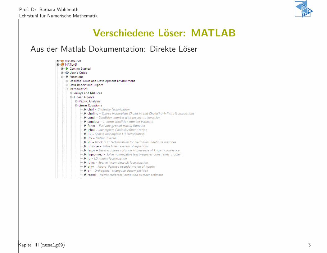
Verschiedene Loser: MATLAB
Aus der Matlab Dokumentation: Direkte Loser
Kapitel III (numalg69) 3
Prof. Dr. Barbara Wohlmuth
Lehrstuhl fur Numerische Mathematik
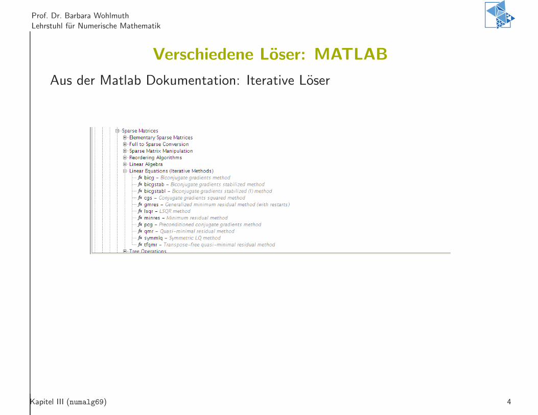
Verschiedene Loser: MATLAB
Aus der Matlab Dokumentation: Iterative Loser
Kapitel III (numalg69) 4
Prof. Dr. Barbara Wohlmuth
Lehrstuhl fur Numerische Mathematik
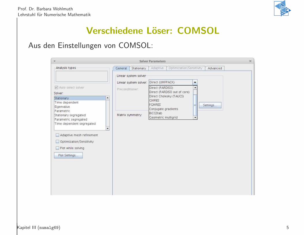
Verschiedene Loser: COMSOL
Aus den Einstellungen von COMSOL:
Kapitel III (numalg69) 5
Prof. Dr. Barbara Wohlmuth
Lehrstuhl fur Numerische Mathematik
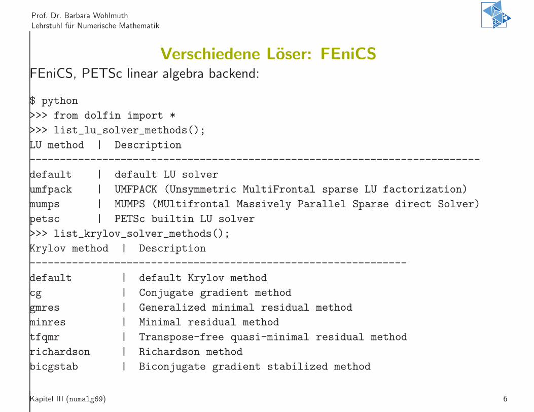
Verschiedene Loser: FEniCSFEniCS, PETSc linear algebra backend:
$ python
>>> from dolfin import *
>>> list_lu_solver_methods();
LU method | Description
--------------------------------------------------------------------------
default | default LU solver
umfpack | UMFPACK (Unsymmetric MultiFrontal sparse LU factorization)
mumps | MUMPS (MUltifrontal Massively Parallel Sparse direct Solver)
petsc | PETSc builtin LU solver
>>> list_krylov_solver_methods();
Krylov method | Description
--------------------------------------------------------------
default | default Krylov method
cg | Conjugate gradient method
gmres | Generalized minimal residual method
minres | Minimal residual method
tfqmr | Transpose-free quasi-minimal residual method
richardson | Richardson method
bicgstab | Biconjugate gradient stabilized method
Kapitel III (numalg69) 6
Prof. Dr. Barbara Wohlmuth
Lehrstuhl fur Numerische Mathematik
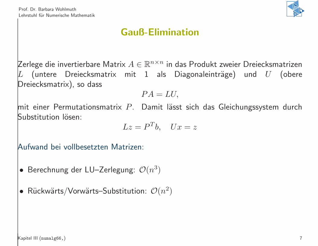
Gauß-Elimination
Zerlege die invertierbare Matrix A ∈ Rn×n in das Produkt zweier Dreiecksmatrizen
L (untere Dreiecksmatrix mit 1 als Diagonaleintrage) und U (obereDreiecksmatrix), so dass
PA = LU,
mit einer Permutationsmatrix P . Damit lasst sich das Gleichungssystem durchSubstitution losen:
Lz = P T b, Ux = z
Aufwand bei vollbesetzten Matrizen:
• Berechnung der LU–Zerlegung: O(n3)
• Ruckwarts/Vorwarts–Substitution: O(n2)
Kapitel III (numalg66,) 7
Prof. Dr. Barbara Wohlmuth
Lehrstuhl fur Numerische Mathematik
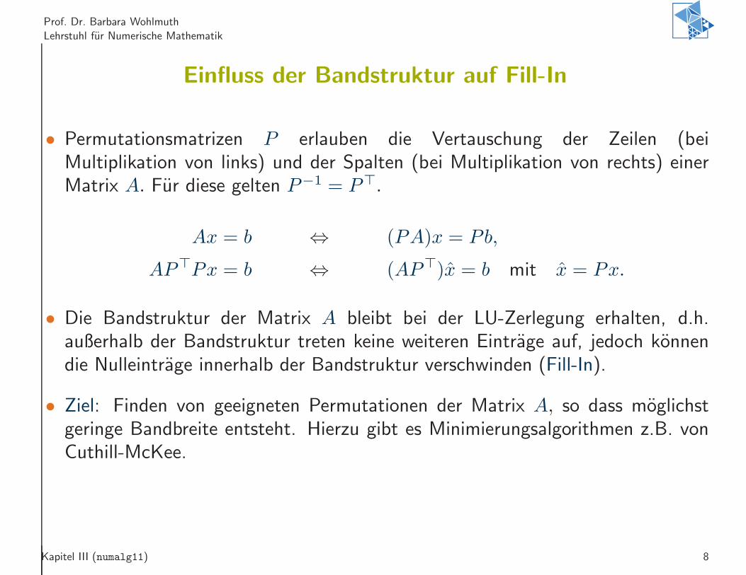
Einfluss der Bandstruktur auf Fill-In
• Permutationsmatrizen P erlauben die Vertauschung der Zeilen (beiMultiplikation von links) und der Spalten (bei Multiplikation von rechts) einerMatrix A. Fur diese gelten P−1 = P⊤.
Ax = b ⇔ (PA)x = Pb,
AP⊤Px = b ⇔ (AP⊤)x = b mit x = Px.
• Die Bandstruktur der Matrix A bleibt bei der LU-Zerlegung erhalten, d.h.außerhalb der Bandstruktur treten keine weiteren Eintrage auf, jedoch konnendie Nulleintrage innerhalb der Bandstruktur verschwinden (Fill-In).
• Ziel: Finden von geeigneten Permutationen der Matrix A, so dass moglichstgeringe Bandbreite entsteht. Hierzu gibt es Minimierungsalgorithmen z.B. vonCuthill-McKee.
Kapitel III (numalg11) 8
Prof. Dr. Barbara Wohlmuth
Lehrstuhl fur Numerische Mathematik
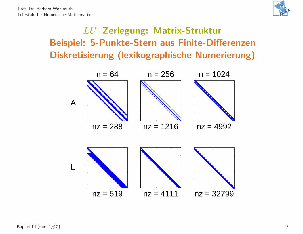
LU–Zerlegung: Matrix-Struktur
Beispiel: 5-Punkte-Stern aus Finite-Differenzen
Diskretisierung (lexikographische Numerierung)
nz = 288
n = 64
nz = 519
nz = 1216
n = 256
nz = 4111
nz = 4992
n = 1024
nz = 32799
A
L
Kapitel III (numalg12) 9
Prof. Dr. Barbara Wohlmuth
Lehrstuhl fur Numerische Mathematik
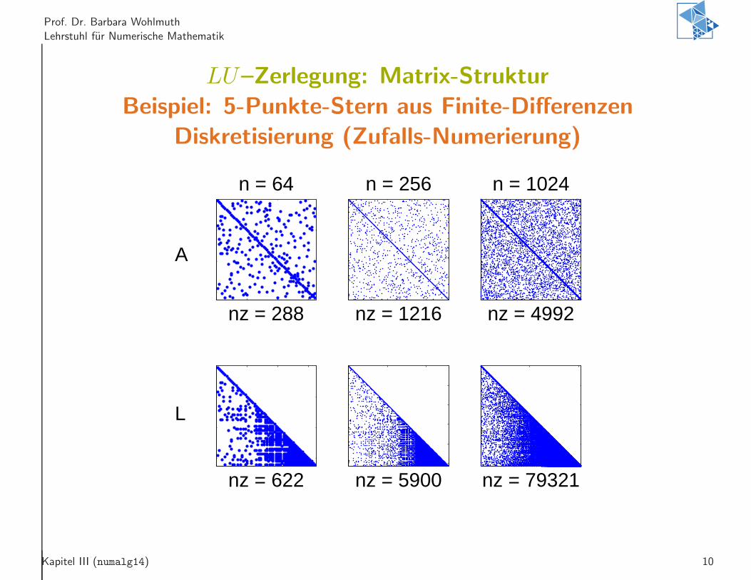
LU–Zerlegung: Matrix-Struktur
Beispiel: 5-Punkte-Stern aus Finite-Differenzen
Diskretisierung (Zufalls-Numerierung)
nz = 288
n = 64
nz = 622
nz = 1216
n = 256
nz = 5900
nz = 4992
n = 1024
nz = 79321
A
L
Kapitel III (numalg14) 10
Prof. Dr. Barbara Wohlmuth
Lehrstuhl fur Numerische Mathematik
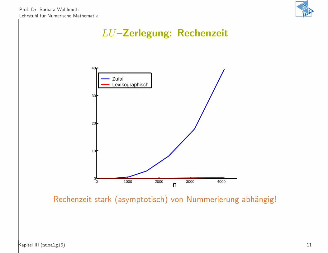
LU–Zerlegung: Rechenzeit
n0 1000 2000 3000 4000
0
10
20
30
40
ZufallLexikographisch
Rechenzeit stark (asymptotisch) von Nummerierung abhangig!
Kapitel III (numalg15) 11
Prof. Dr. Barbara Wohlmuth
Lehrstuhl fur Numerische Mathematik
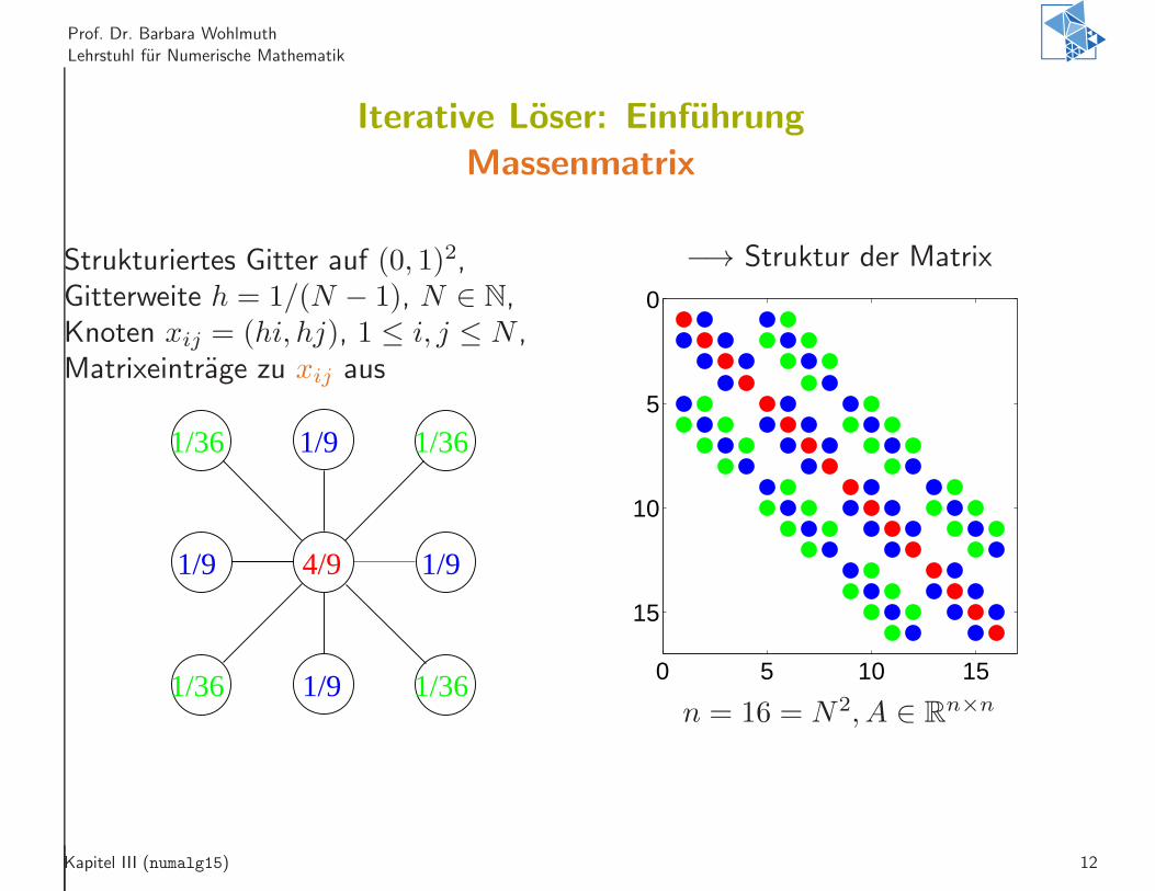
Iterative Loser: Einfuhrung
Massenmatrix
Strukturiertes Gitter auf (0, 1)2,Gitterweite h = 1/(N − 1), N ∈ N,Knoten xij = (hi, hj), 1 ≤ i, j ≤ N ,Matrixeintrage zu xij aus
1/9
1/9 1/9
1/9
4/9
1/36 1/36
1/361/36
−→ Struktur der Matrix
0 5 10 15
0
5
10
15
n = 16 = N2, A ∈ Rn×n
Kapitel III (numalg15) 12
Prof. Dr. Barbara Wohlmuth
Lehrstuhl fur Numerische Mathematik
Iterative Loser: Einfuhrung
Aufwandsabschatzung fur die Massenmatrix
• Bandbreite: ω = O(N)
• Die Anzahl der Nicht-Nulleintrage wachst mit O(n)
• Anwendung von z.B. LU-Zerlegung erfordert Aufwand von O(n2)
• Matrix-Vektor-Multiplikation hat Aufwand von O(n)
Kapitel III (numalg15) 13
Prof. Dr. Barbara Wohlmuth
Lehrstuhl fur Numerische Mathematik
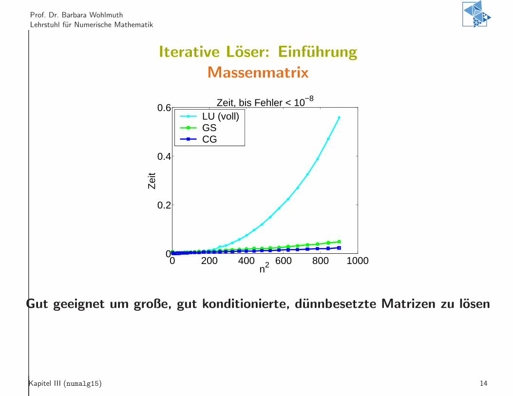
Iterative Loser: Einfuhrung
Massenmatrix
0 200 400 600 800 10000
0.2
0.4
0.6 Zeit, bis Fehler < 10−8
n2
Zei
t
LU (voll)GSCG
Gut geeignet um große, gut konditionierte, dunnbesetzte Matrizen zu losen
Kapitel III (numalg15) 14
Prof. Dr. Barbara Wohlmuth
Lehrstuhl fur Numerische Mathematik
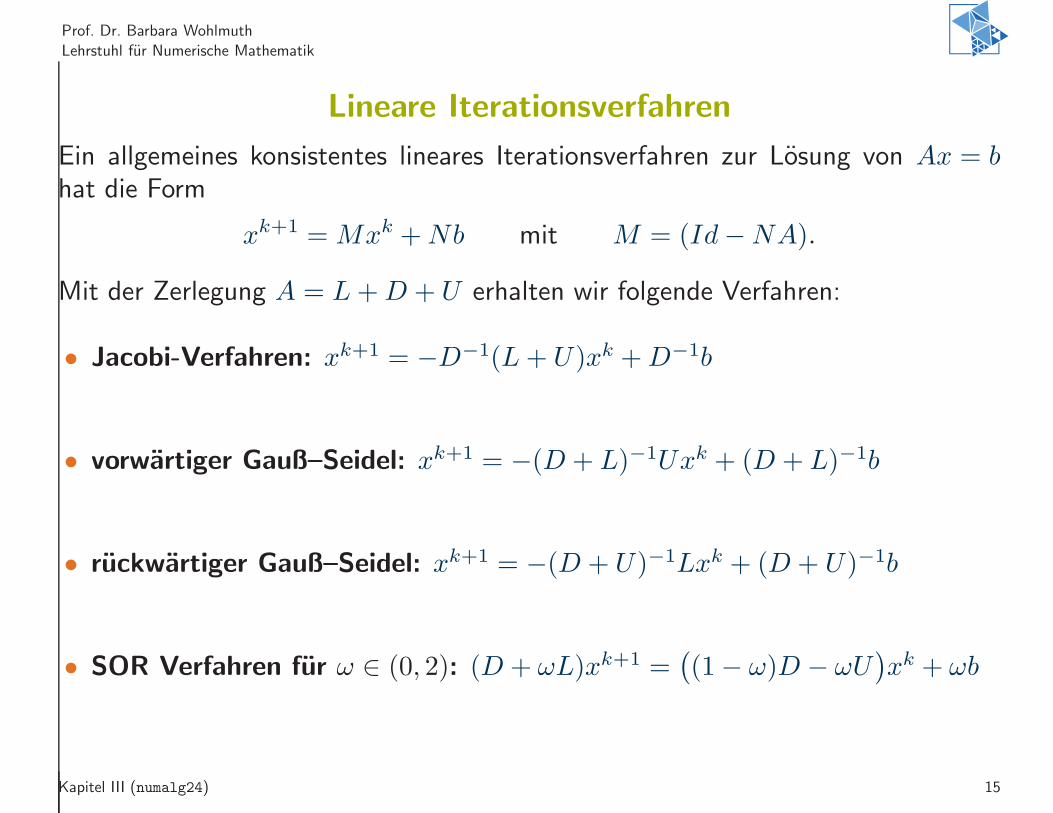
Lineare Iterationsverfahren
Ein allgemeines konsistentes lineares Iterationsverfahren zur Losung von Ax = bhat die Form
xk+1 = Mxk +Nb mit M = (Id−NA).
Mit der Zerlegung A = L+D + U erhalten wir folgende Verfahren:
• Jacobi-Verfahren: xk+1 = −D−1(L+ U)xk +D−1b
• vorwartiger Gauß–Seidel: xk+1 = −(D + L)−1Uxk + (D + L)−1b
• ruckwartiger Gauß–Seidel: xk+1 = −(D + U)−1Lxk + (D + U)−1b
• SOR Verfahren fur ω ∈ (0, 2): (D + ωL)xk+1 =(
(1− ω)D − ωU)
xk + ωb
Kapitel III (numalg24) 15
Prof. Dr. Barbara Wohlmuth
Lehrstuhl fur Numerische Mathematik
Historische Bemerkungen
C.F. Gauß in einem Brief vom 26.12.1823 an Gerling:Ich empfehle Ihnen diesen Modus zur Nachahmung. Schwerlich werden Sie jewieder direct eliminieren, wenigstens nicht, wenn Sie mehr als 2 Unbekanntehaben. Das indirecte Verfahren lasst sich halb im Schlafe ausfuhren, oder mankann wahrend desselben an andere Dinge denken.
[C.F. Gauß: Werke Bd. 9, S. 280f, Gottingen 1903]
Block Gauß–Seidel Verfahren: (1819-1822)Supplementum theoriae combinationis observationum erroribus minime obnoxiae
C.G. Jacobi: 1845Uber eine neue Auflosungsart der bei der Methode der kleinsten Quadratevorkommenden linearen Gleichungen
Kapitel III (numalg25) 16
Prof. Dr. Barbara Wohlmuth
Lehrstuhl fur Numerische Mathematik
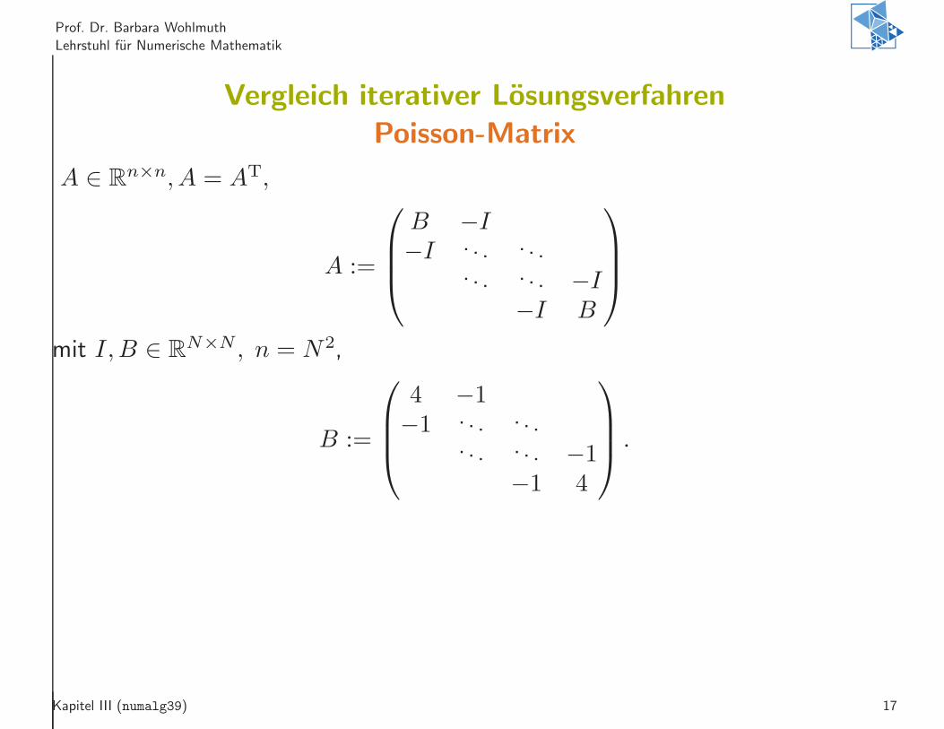
Vergleich iterativer Losungsverfahren
Poisson-Matrix
A ∈ Rn×n, A = AT,
A :=
B −I−I . . . . . .
. . . . . . −I−I B
mit I,B ∈ RN×N , n = N2,
B :=
4 −1−1 . . . . . .
. . . . . . −1−1 4
.
Kapitel III (numalg39) 17
Prof. Dr. Barbara Wohlmuth
Lehrstuhl fur Numerische Mathematik
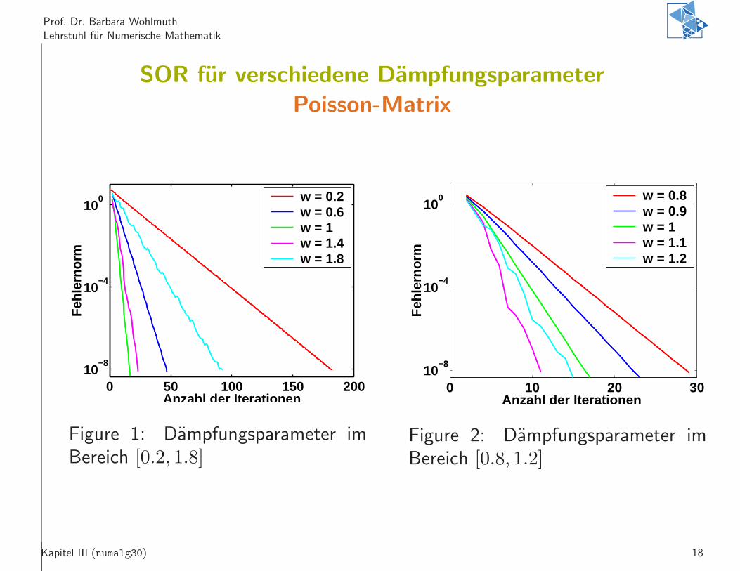
SOR fur verschiedene Dampfungsparameter
Poisson-Matrix
0 50 100 150 20010
−8
10−4
100
Anzahl der Iterationen
Feh
lern
orm
w = 0.2w = 0.6w = 1w = 1.4w = 1.8
Figure 1: Dampfungsparameter imBereich [0.2, 1.8]
0 10 20 3010
−8
10−4
100
Anzahl der Iterationen F
ehle
rnor
m
w = 0.8w = 0.9w = 1w = 1.1w = 1.2
Figure 2: Dampfungsparameter imBereich [0.8, 1.2]
Kapitel III (numalg30) 18
Prof. Dr. Barbara Wohlmuth
Lehrstuhl fur Numerische Mathematik
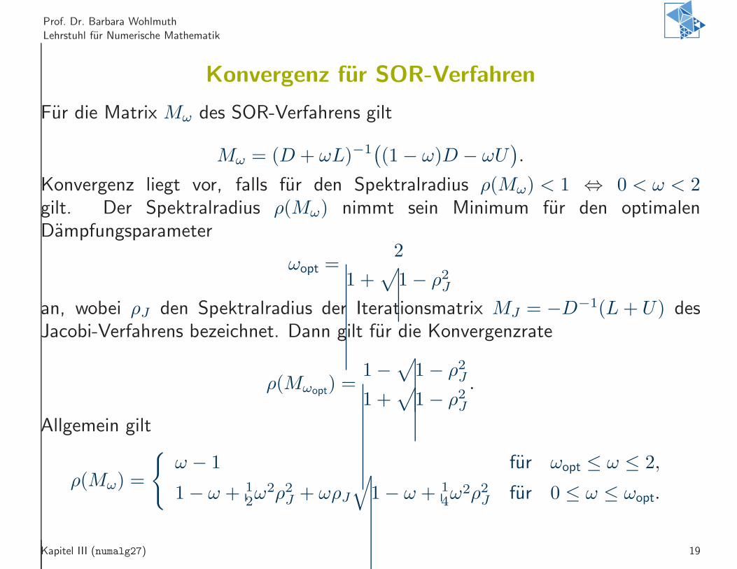
Konvergenz fur SOR-Verfahren
Fur die Matrix Mω des SOR-Verfahrens gilt
Mω = (D + ωL)−1(
(1− ω)D − ωU)
.
Konvergenz liegt vor, falls fur den Spektralradius ρ(Mω) < 1 ⇔ 0 < ω < 2gilt. Der Spektralradius ρ(Mω) nimmt sein Minimum fur den optimalenDampfungsparameter
ωopt =2
1 +√
1− ρ2Jan, wobei ρJ den Spektralradius der Iterationsmatrix MJ = −D−1(L+ U) desJacobi-Verfahrens bezeichnet. Dann gilt fur die Konvergenzrate
ρ(Mωopt) =1−
√
1− ρ2J1 +
√
1− ρ2J.
Allgemein gilt
ρ(Mω) =
{
ω − 1 fur ωopt ≤ ω ≤ 2,
1− ω + 1
2ω2ρ2J + ωρJ
√
1− ω + 1
4ω2ρ2J fur 0 ≤ ω ≤ ωopt.
Kapitel III (numalg27) 19
Prof. Dr. Barbara Wohlmuth
Lehrstuhl fur Numerische Mathematik
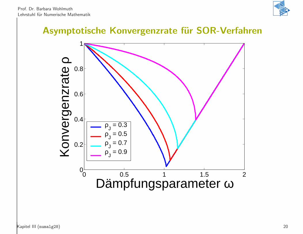
Asymptotische Konvergenzrate fur SOR-Verfahren
0 0.5 1 1.5 20
0.2
0.4
0.6
0.8
1
Dämpfungsparameter ω
Kon
verg
enzr
ate
ρ
ρJ = 0.3
ρJ = 0.5
ρJ = 0.7
ρJ = 0.9
Kapitel III (numalg28) 20
Prof. Dr. Barbara Wohlmuth
Lehrstuhl fur Numerische Mathematik
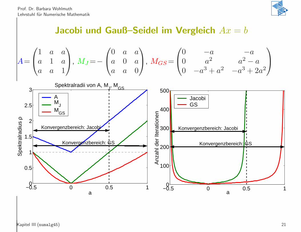
Jacobi und Gauß–Seidel im Vergleich Ax = b
A=
1 a aa 1 aa a 1
, MJ=−
0 a aa 0 aa a 0
, MGS=
0 −a −a0 a2 a2 − a0 −a3 + a2 −a3 + 2a2
−0.5 0 0.5 10
0.5
1
1.5
2
2.5
3Spektralradii von A, M
J, M
GS
a
Spe
ktra
lradi
us ρ
AM
JM
GS
Konvergenzbereich: Jacobi
Konvergenzbereich: GS
−0.5 0 0.5 10
100
200
300
400
500
a
Anz
ahl d
er It
erat
ione
n
JacobiGS
Konvergenzbereich: Jacobi
Konvergenzbereich: GS
Kapitel III (numalg45) 21
Prof. Dr. Barbara Wohlmuth
Lehrstuhl fur Numerische Mathematik
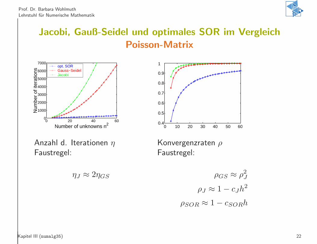
Jacobi, Gauß-Seidel und optimales SOR im Vergleich
Poisson-Matrix
0 20 40 600
1000
2000
3000
4000
5000
6000
7000
Number of unknowns n2
Num
ber
of it
erat
ions
opt. SOR Gauss−SeidelJacobi
0 10 20 30 40 50 600.4
0.5
0.6
0.7
0.8
0.9
1
Anzahl d. Iterationen ηFaustregel:
ηJ ≈ 2ηGS
Konvergenzraten ρFaustregel:
ρGS ≈ ρ2J
ρJ ≈ 1− cJh2
ρSOR ≈ 1− cSORh
Kapitel III (numalg35) 22
Prof. Dr. Barbara Wohlmuth
Lehrstuhl fur Numerische Mathematik
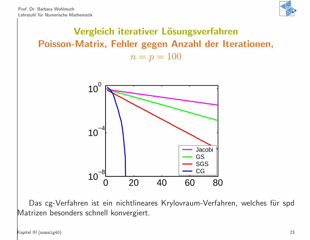
Vergleich iterativer Losungsverfahren
Poisson-Matrix, Fehler gegen Anzahl der Iterationen,
n = p = 100
0 20 40 60 8010
−8
10−4
100
JacobiGSSGSCG
Das cg-Verfahren ist ein nichtlineares Krylovraum-Verfahren, welches fur spdMatrizen besonders schnell konvergiert.
Kapitel III (numalg40) 23


![Kapitel 2: MerkmalsräumeKapitel 2: Merkmalsräume · Eigenvalue Model [Kriegel, Kröger, Mashael, Pfeifle, Pötke , Seidl 03 ] – Volumen-Diskretisierung durch Voxel (3dimensionale](https://img.pdfslide.org/doc/110x75/5d527f0188c9939c1b8b567e/kapitel-2-merkmalsraeumekapitel-2-merkmalsrae-eigenvalue-model-kriegel-kroeger.jpg)