Embed Size (px)
Citation preview
DISSERTATION
A Topographie Mars Information System
Concepts for Management, Analysis and Visualization of Planet-Wide Data
ausgeführt zum Zwecke der Erlangung des akademischen Grades eines Doktors der
technischen Wissenschaften unter der Leitung von
Ao.Univ.Prof. Dipl.-Ing. Dr.techn. Josef Jansa
Institut für Photogrammetrie und Fernerkundung (E122)
eingereicht an der Technischen Universität Wien
Fakultät für Mathematik und Geoinformation
von
Dipl.-Ing. Peter Dominger
Matr. Nr. 9425300
Emil Kögler-Gasse 13
2511 Pfaffstätten
Wien, am 3. Juni 2004
Die approbierte Originalversion dieser Dissertation ist an der Hauptbibliothek der Technischen Universität Wien aufgestellt (http://www.ub.tuwien.ac.at). The approved original version of this thesis is available at the main library of the Vienna University of Technology (http://www.ub.tuwien.ac.at/englweb/).

The participation of the Institute of Photogrammetry and Remote Sensing (I.P.F.) in the Mars Express
project was supported by the Federal Ministry of Technology (BMVIT) under project number GZ
190.174/2-V/B/10/2000. The following thesis is based on investigations in this project. Further on the
author received a two years scholarship by the Neumaier Foundation from March 2001 to March 2003.
Die Beteiligung des Institutes für Photogrammetrie und Fernerkundung (I.P.F.) am Mars Express
Projekt wurde durch das Bundesministerium für Verkehr, Innovation und Technologie (BMVIT) unter
der GZ 190.174/2-V/B/10/2000 finanziert. Die vorliegende Arbeit basiert auf wissenschaftlichen
Ergebnissen dieses Projektes. Außerdem erhielt der Autor ein zweijähriges Stipendium, finanziert
durch die Neumaier Stiftung.
Acknowledgements
Acknowledgements
I would like to thank all those who have contributed their time and effort to realize this research thesis.
First of all, I would like to thank Josef Jansa, my Supervisor, for his untiring encouragement and
support of my study. Further, I am especially grateful to Georg Gärtner for constructive discussions
and Jörg Albertz for reviewing this thesis.
I am much obliged to Laszio Molnar; without his encouragement this work probably would not have
been finished. I further wish to thank Christian Briese and Gottfried Mandelburger for their assistance
and for proof-reading and all my colleagues at the I.P.F. for supporting me whenever necessary. A
Special thank goes to Hans Thüminger for his Professional assistance in Computer related problems.
I would also like to thank Thomas Roatsch, Marita Wählisch and Frank Schölten as representatives of
the Institute for Planetary Research, DLR, Berlin for their cooperation concerning the realization of
TMIS and their assistance in Mars related matters.
Finally, I would like to express my utmost appreciation to my parents, my wife Angela and my son
Christoph for their unwavering support and encouragement.
Abstract
Abstract
The Institute of Photogrammetry and Remote Sensing (I.P.F.) is participating at the project Mars
Express which is supported by the European Space Agency (ESA). Task of the I.P.F. is the
development of a Topographie Mars Information System (TMIS) for efficient management and
distribution of the high amount of image data provided by the High Resolution Stereo Camera (HRSC)
on board the spacecraft, and also of surface point data as derived from these images using feature-
based image matching methods, as well as subsequently derived digital terrain modeis (DTMs). Thus,
the TMIS acts as the main interface for data exchange among the Co-Investigators of the HRSC on
Mars Express project group.
The first part of this thesis deals with coneepts of spatial data modeling and management and with
data formats and data exchange with respect to available Standards, mostly based on the Extensible
Markup Language (XML). Special attention is paid to the Geography Markup Language (GML) for data
representation and exchange and to Scalable Vector Graphics (SVG) for web presentation of spatial
data. Web presentation formats based on static images provided by a Web Map Service (WMS) are
compared to objeet-based presentation formats. Further on, shortcomings as well as possible
improvements and extensions to enhance the capability for efficient application of XML and related
technologies in the area of geodata management are presented. Finally, the realization of the TMIS
framework is described.
In the second part, methods for topographic data manipulation and analysis are investigated. For
testing purposes, image and topographic data acquired by the NASA probe Mars Global Surveyor
(MGS) has been used. Since the original surface point cloud contained gross errors due to incorrect
referencing of the sensor platform, a method to detect and eliminate the erroneous points became
essential. The computation of DTMs for further analysis is described afterwards. Ever since the
surface of Mars is investigated in detail, scientists are discussing if liquid surface water was involved in
the surface forming process in former times. To help answering this question, raster-based
hydrological analysis methods were applied to regions which were possibly formed by water. The
results are prepared for Visual presentation. Finally, 3D visualizations of these results, e.g. for web
presentation, are provided.
Kurzfassung
Kurzfassung
Das Institut für Photogrammetrie und Fernerkundung (I.P.F.) ist am Mars Express Projekt der
Europäischen Raumfahrtsbehörde ESA beteiligt. Die Aufgabe des I.P.F. ist die Entwicklung eines
Topographischen Mars Informationssystems (TMIS). Dieses soll die enormen Mengen an Bilddaten,
welche vom hochauflösenden Kamerasystem High Resolution Stereo Camera (HRSC) erfasst
werden, effizient verwalten. Die Verwaltung topographischer Daten als Originalpunktewolken sowie
auch davon abgeleiteter digitaler Geländemodelle (DGMe) soll ebenfalls möglich sein. TMIS stellt
somit die zentrale Datendrehscheibe innerhalb der Projektgruppe HRSC on Mars Express dar.
Im ersten Teil der Arbeit werden Konzepte zur Modellierung und Verwaltung räumlicher Daten unter
Berücksichtigung vorhandener Standards und Normen beschrieben. Die Möglichkeiten auf Extensible
Markup Language (XML) basierten Formaten für Datenhaltung und Datenaustausch raumbezogener
Daten sowie für deren kartographische Aufbereitung zur Darstellung im Internet werden im Detail
untersucht. Derzeitig verfügbare Implementierungen von Web Map Services (WMS) liefern meist
statische Kartendarstellungen, obwohl seitens der Spezifikation von WMS auch objekt-basierte
Ausgabeformate wie z.B. Scalable Vector Graphics (SVG) unterstützt werden. Im Rahmen der
Entwicklung einer kartenbasierten Benutzerschnittstelle für TMIS wurden die Möglichkeiten von SVG
eingehend untersucht. Basierend auf den resultierenden Erkenntnissen werden mögliche
Erweiterungen zur Verbesserung der Anwendbarkeit vorhandener XML basierter Formate im Bereich
der Geodatenmodellierung und -Verwaltung präsentiert. Abschließend wird der gegenwärtige
Implementierungsstand von TMIS als Anwendungsbeispiel der beschriebenen Methoden gezeigt.
Im zweiten Teil der Arbeit werden Methoden zur Bearbeitung und Analyse topographischer Marsdaten
untersucht. Als Testdatensatz dienten Bild- und Topographiedaten welche im Rahmen der NASA
Mission Mars Global Surveyor (MGS) erfasst wurden. Zunächst wird eine Methode zur Detektion und
anschließenden Elimination grober Datenfehler, welche in den Originalpunkten enthalten sind,
vorgestellt. Die Ableitung homogener und von zufälligen Fehlern bereinigter DGMe als Grundlage für
weiterführende Analysen wir ebenfalls näher beschrieben. Seit die Oberfläche des Mars erkundet wird
drängt sich die Frage auf, ob es in früheren Zeiten Oberflächenwasser gab. Um der Beantwortung
dieser Frage näher zu kommen, wurden rasterbasierte, hydrologische Analysemethoden an
ausgewählten, möglicherweise durch Oberflächenwasser geformten Bereichen des Mars angewandt
und die Ergebnisse visuell aufbereitet. Als Abschluss der Arbeit werden dreidimensionale
Visualisierungen dieser Resultate, unter anderem zur Darstellung im Internet, präsentiert.
Contents
Contents
1 INTRODUCTION 1
1.1 MOTIVATION 1
1.2 OBJECTIVES 2
1.3 OVERVIEW 3
2 MARS EXPRESS 2003 - THE SEARCH FOR WATER 5
2.1 THE PLANET MARS 5
2.2 SCIENTIFIC GOALS 6
2.3 HRSC ON MARS EXPRESS 7
3 CONCEPTS FOR SPATIAL DATA MANAGEMENT 9
3.1 INITIAL SITUATION 9
3.1.1 Topographie Information Systems 9
3.1.2 RelatedWork 9
3.2 SPATIAL DATA MODELING 10
3.2.1 Database Management Systems 10
3.2.2 Database Models 11
3.2.3 Modeling Spatial Data Structures 13
3.2.4 Realizations of Spatial Data Modeling using Extended Relational Models 15
3.3 EXTENSIBLE MARKUP LANGUAGE FOR SPATIAL DATA REPRESENTATION 20
3.3.1 Introduction to XML 20
3.3.2 Geography Markup Language 21
3.3.3 Scalable Vector Graphics 22
3.3.4 Improving XML Performance 27
3.3.5 XML and Topographie Data 29
3.3.6 Integration of XML Documents in Databases 32
3.3.7 XPath Performance Considerations 33
3.4 CONCEPTS FOR W E B APPLICATIONS 34
3.4.1 Web Services 34
3.4.2 Web Services and Spatial Data 35
3.4.3 Spatial Data Presentation using Web Map Services 36
Contents vii
4 REALIZING THE TOPOGRAPHIC MARS INFORMATION SYSTEM 38
4.1 SYSTEM ARCHITECTURE 38
4.2 DATA MANAGEMENT 39
4.2.1 Meta Data Catalogue 39
4.2.2 Topographie Data Server 41
4.3 DATA ACCESS AND MANIPULATION 42
4.3.1 Requesting Footprint Maps 43
4.3.2 Requesting HRSC Images 45
4.3.3 Requesting Topographie Data 45
4.3.4 Integration of DTM Analysis and Visualization Tools 46
4.4 DATA PRESENTATION 47
4.4.1 Object-Based Visualization Methods 48
4.4.2 Image-Based Visualization Methods 49
4.4.3 Object- vs. Image-Based Visualization Methods 51
5 MODELING THE TOPOGRAPHY OF MARS 52
5.1 INITIAL SITUATION 53
5.1.1 Topographie and Image Datafrom the Mars Surface 54
5.1.2 Referencing Considerations 55
5.2 -DTM COMPUTATION FROM ORIGINAL MARS SURFACE POINTS 57
5.2.1 Method for DTM Interpolation 57
5.2.2 Error Elimination 58
5.2.3 Comparison of Error Elimination Methods 66
5.2.4 DTM Computation 67
5.2.5 Results 70
6 HYDROLOGICAL ANALYSIS OF THE MARS SURFACE 72
6.1 HYDROLOGICAL ANALYSIS 73
6.1.1 Hydrological Map of Tharsis Region and Valles Marineris 73
6.1.2 Outflow Channel Detection in the Elysium Region 76
6.1.3 Simulated Outflow Behavior in Ma'adim Vallis and Gusev Crater 80
6.2 DERIVING STRUCTURE LINES FROM POINT CLOUDS 84
6.3 VlSUALIZATIONS 85
6.3.1 Perspective Views 86
6.3.2 Virtual 3D Modeling 87
6.3.3 3D Hardcopy of Olympus Mons 89
Contents viii
7 CONCLUSIONS 91
7.1 SUMMARYANDACHIEVEMENTS 91
7.2 FURTHER INVESTIGATIONS 92
APPENDIX 94
A MARS FACT SHEET 94
B CHRONOLOGY OF MARS EXPLORATION 97
C MARS EXPRESS FACT SHEET 99
D SCIENTIFIC OBJECTIVES OF THE I.P.F. AS HRSC CO-lNVESTIGATOR 100
E HRSC PERFORMANCE 101
F SCIENTIFIC PUBLICATIONS AND PUBLIC RELATIONS 102
ACRONYMS AND ABBREVIATIONS 103
REFERENCES 106
CURRICULUM VITAE 114
Chapter 1: Introduction
1 Introduction
"The exploration of other worlds underscores our responsibility to deal more kindly and
compassionately with one another and to preserve and cherish that pale blue dot, the only home
we've ever known." (Carl Sagan 1934-1996)
On 14"1 of July 1965, the NASA probe Mariner 4 passed the Mars and transmitted 21 images, covering
about 1 % of the Mars surface. The era of Mars photogrammetry has begun. Since then, almost 30
Mars missions were accomplished and about half of them were successful. From a topographic point
of view, the most important one is Mars Global Surveyor (MGS), supported by the NASA as well
(NASA-MGS, 2004)1. Among other results, it provided 112.000 coloured, high-resolution images (1.4
m/pixel at 400 km altitude) covering about 3 % of the surface and images covering almost the whole
planet at a resolution of 280 m/pixel from 400 km altitude, using a wide-angle camera (NASA-MOC,
2004). Further on, more than 600 million individually measured surface points were determined, using
a laser profiling altimeter. This point cloud describes the topography of the planet's surface. It allows to
derive a digital terrain model (DTM) with a resolution of 1/128° grid width. This is equivalent to 463 m
at the Martian equator (NASA-MOLA, 2004).
Mars Express (MEX), the first European Mars mission, was successfully launched on 2nd of June,
2003. Since 25th of December 2003, it is in an orbit around Mars and on 10m of January 2004, the
operational phase has started. The mission is supported by the European Space Agency (ESA).
Among other instruments on board the spacecraft, the High Resolution Stereo Camera (HRSC) is the
instrument for photogrammetric surveying. Its scientific aim is high-resolution mapping of the whole
Martian surface at a resolution of down to 10 m/pixel in color and stereo and about 1 % of the Martian
surface in grayscale at a resolution of down to 2.5 m/pixel. The stereo images are to be used for
deriving highly accurate surface points which will lead to an improvement of the currently available
topographic modeis.
1.1 Motivation
As this work was started in 2001, most web-based image archives of Mars related data were based on
file archives, available via FTP (e.g. Planetary Data System archives, MGS archives at the web
Servers of the related institutions,...). Other approaches provided static image maps at the client-side.
Furthermore, most of these Solutions were implemented for a specific purpose and it turned out, they
will not be applicable to solve the given task without major modifications and adaptations.
1 Results of the current NASA orbiter Mars Odyssey are not considered within this thesis, as data for improving the topographic
description of the Mars surface is not provided. The THEMIS (Thermal Emission Imaging System) acquires promising high
resolution daylight image data from sampled areas and thermal images from almost the whole surface; potentially, they will
allow to improve the current geological model (NASA-ODYSSEY, 2004).
Chapter 1: Introduction
In order to provide the best capabilities for managing and distributing the expected huge amount of
HRSC topographic and image data - as well as of derived higher level products such as map
projected images or DTMs - in an efficient manner, building up of a Topographic Mars Information
System (TMIS) has been included into the project preparations.
The conceptual design and following realization of an information System for management and
distribution of image and topographic data from the project group HRSC on Mars Express constitutes
the central theme of this thesis. The original task of this research can be outlined as finding answers to
the following two questions:
"Which realizable and, if possible, standardized methods for management and for
presentation of planet-wide image and topographic data do exist? How can they be applied
to implement a web portal as central data provider for the project group "HRSC on Mars
Express" in order to increase the efficiency ofthe HRSC experiment?"
The first part of the thesis focuses on this task. Different modeis for data management and their
historical development are described with a Special view on the object-relational model. Furthermore,
current trends are introduced such as object-oriented modeis or XML based data management.
Afterwards, the concept for the realization of the web-based TMIS framework is described. In
particular, vector and raster-based methods for the representation of spatial information using
common web browsers are compared.
It was intended to integrate analysis and visualization functionality in the TMIS. Hence, the following
question arose:
"Are raster-based hydrological analysis methods (rain Simulation) appropriate to improve the
Interpretation of available and Mure DTMs of the Mars surface in order to determine
hydrologically originated surface structures?"
Consequently, the second part of this thesis describes the development of new and the adaptation of
already available methods and algorithms for hydrological analysis and following visualization of Mars
DTMs and their integration into the TMIS environment. As the surface point cloud used for testing
purposes contained gross errors due to incorrect referencing of the sensor platform, a method to
detect and eliminate the erroneous points was investigated.
1.2 Objectives
Starting from a single-user, single-machine topographic database application based on a relational
database enhanced by topological data types and access methods, a concept for a multi-user, web
application had to be developed for efficient management and distribution of the data provided by the
HRSC experiment. The interoperability between implemented modules and the new methods had to
be guaranteed. As a matter of course, a graphical user interface based on both, parameter selection
forms and interactive maps had to be provided.
Chapter 1: Introduction
An important matter of research was the Integration and application of available and future Standards,
mostly based on the Extensible Markup Language (XML) for data transport (e.g. Geographie Markup
Language - GML) and visualization (e.g. Scalable Vector Graphics - SVG). The capabilities of web
presentation formats based on static images provided by a Web Map Service (WMS) aecording to the
OpenGIS Consortium (OGC) implementation speeifications are compared to objeet-based
presentation formats.
This thesis describes the conceptual design and the realization of the TMIS. The advantages and
shortcomings of the Standards and methods used in relation to commercially used and already
available other Solutions are discussed. Possible improvements and extensions to enhance the
capability for efficient application of XML and related technologies in the area of geodata management
are presented.
A current focus of research at the I.P.F. concerns interpolation, management, application and
visualization of nation-wide terrain data. Many scientific results were implemented in the commercially
available Software package SCOP++ (IPF-SCOP, 2004). The partieipation in the Mars Express Team
was the first attempt to investigate the capabilities of these methods as applied to extraterrestrial data
in a planet-wide context and to improve the already existing methods, technologies and applications in
order to be able to apply them to Mars and, later on, reeeive a feedback for further Earth related
Problems.
For about ten years, Airborne Laser Scanning has become an effective method for topographic data
acquisition with a high degree of automation. In 2001, when the research for this thesis began, the
Mars-wide surface point cloud, acquired by the MGS, represented a new dimension of amount of
laser-scanner points. On the one hand, by then it was one of the largest laser Scanner projeets in
terms of measurements (more than 600 Mio. points) and on the other hand, this point cloud covers a
whole planet. Besides being able to manage data on a complete sphere, organizing data describing
the extensive surface area of Mars, which is equivalent to 1/3 of the Earth's surface or the total area of
our continents, has become a challenging task.
Therefore, new methods for data management and access had to be found. As the original points
contained gross errors due to incorrect referencing of the spacecraft, a method for detecting and
eliminating those erroneous points was necessary. And last but not least, the application of methods
for analysis and visualization of the derived DTMs were investigated, as they might facilitate finding
some answers concerning the evolution of the Mars surface, possibly influenced by the appearance of
liquid surface water.
1.3 Overview
The following chapter 2 introduces the reader to Mars-related research from ancient times until today.
The scientific goals of the Mars Express mission are described and the contributions of the HRSC
experiment to them discussed.
Chapter 1: Introduction
Chapter 3 presents concepts for spatial data modeling and results of investigating the Extensible
Markup Language (XML) for spatial data representation and visualization. A closer look is taken on
Geography Markup Language (GML) for data exchange and on Scalable Vector Graphics (SVG) for
data representation and web visualization. As Web Services are emerging as the basic concepts for
web applications, they are discussed finally.
The Topographie Mars Information System (TMIS) is a multi-user web application for management,
distribution, analysis and visualization of planet-wide topographic data in combination with image
datasets. The provided functionality has been separated into two different groups:
• data management and distribution and
• analysis and visualization.
Data management and distribution are provided by a web application, based on a database
management System (DBMS). This System represents the kernel of TMIS and thus, it is referred to as
TMIS in the following. The concepts of the system's realization are presented in chapter 4. Special
attention is paid to the visualization of planet-wide shape Information (polygonal boundahes of regions
as used for footprints of images) within a web browser environment using standardized vector- and
raster-based methods. Furthermore, planet-wide topographic data is management by TMIS and the
way of distribution via the Internet is presented.
The analysis and visualization functionality is provided by a package named TMIS-Extended
Functionality (TMIS-EF). The investigation of new algorithms and methods for deriving homogeneous,
"error-free" digital terrain modeis (DTMs) and subsequently their analysis and visualization are
described in the chapters 5 (topographic data processing) and 6 (application and results).
The final chapter 7 summarizes the results and gives outlook to further investigations.
Chapter 2: Mars Express 2003 - The Search for Water
2 Mars Express 2003 - The Search for Water
"Mars Express is the first fully European mission to any planet. It is an exciting challenge for European
technology." (Rudolf Schmidt, Mars Express Project Manager, ESA).
This chapter concentrates on general issues concerning Mars and the mission Mars Express. After a
brief introduction to the historical knowledge of the planet, the mission Mars Express and its scientific
goals, in particular the project objectives of HRSC on Mars Express, are described. Additionally
information such as a Mars Fact Sheet, a Chronology of Mars Exploration Missions and a Summary of
Mars Express as well as facts about HRSC on Mars Express may be found in the Appendix.
2.1 The Planet Mars
Mars is our immediate neighbor out from the Sun and the outermost of the hard, rocky terrestrial
planets before the asteroid belt and the gas giants, such as Jupiter and Saturn (Battrick, Talevi, 2001).
Since he can be observed by the naked eye, he was always known as one of the seven "planets"
(Mercury, Venus, Mars, Jupiter, Saturn, Moon and Sun) which seemed to be moving around the fixed
Earth, which was considered as center of the universe in former times. Inspired by its red color, which
was already known 4000 years AD, he was associated with war. Within the Greek mythology he was
named Ares, the god of war, always accompanied by Phobos (fear) and Deimos (panic). The name
Mars was introduced by the Romans.
From these first observations to our present knowledge, a very long process of technological progress
took place. During the Dark Ages, this progress was nearby stopped, due to the fact that the Church
was not prepared to accept that the Sun, rather than the Earth, is the center of gravitation within our
solar System, and billions of such Systems are existing within the universe. They referred to Aristoteles
who did not believe in the plurality of worlds. The astronomer Carl Sagan said once: "Without
Aristoteles, maybe Greek spacecrafts would travel between Mars and Earth nowadays" (Puttkamer,
1997, p. 42).
Nevertheless, the fundamentals of current space science were established at that time. Nikolaus
Kopernikus (1473 - 1543) defined the Sun as the center of gravitation, Tycho Brahe (1546 - 1601)
observed the Mars with the naked eye and defined an empirical basis for Johannes Kepler (1571 -
1630), who derived his three laws about the moving of the planets using this information. Galileo
Galilei (1564 - 1642) was the first who observed the Moons of Jupiter using a telescope. Based on
observations of planets using telescopes, Isaak Newton (1643 - 1727) was able to define the law of
gravity and to improve Kepler's third law considering the mass of the planets.
The first "albedo map" of Mars was drawn by Christian Huygens (1629 - 1695), who discovered Syrtis
Major, a large, dark highland at the equatorial region of the planet. 1877 became a Special year
concerning Mars observations, as an advantageous Opposition did occur. During this approach
Giovanni Schiaparelli (1835 - 1910) produced the first detailed Mars map and named numerous
Chapter 2: Mars Express 2003 - The Search for Water
features. These names are still used nowadays. Furthermore, he was convinced to see rifts and
Channels (ital. canali) of natural origin. This experience was misinterpreted, and the story of large,
artificial water Channels and Vegetation along them was born! Many well-known scientists (even
Wernher von Braun, one of the most famous and important Mars scientists ever, who was involved
into NASA's Mars exploration program until the 1970s) believed into this misinterpretation, until
Mariner 4 took the first dose ränge images of the Mars surface during its fly-by in 1965. The reality
was disillusioning. David Knight said: "After the publication of the images, the scientific world was
shocked. They found out, that the red planet - the only one in our solar system which allowed for the
speculation for any kind of extraterrestrial life - has a Moon-like surface füll ofcraters; a dead world as
itseemed."(Eisfeld, Jeschke, 2003, p. 171).
During the 1970s the scientific image of Mars changed again. Orbiting spacecrafts - first Mahner 9
(1971) an then the two Viking missions (1975) - showed there was much more to the Martian surface
than craters. Mariner 9 saw volcanoes twice as tall as on Earth. There were canyons as deep as the
Earth's deepest ocean trenches. There were what appeared to be desiccated river Systems. There
were plains scoured by floods large enough to drain the Mediterranean in a month (Morton, 2004, p.
14).
After the following almost two decades without successful Mars missions, a new era of Mars
investigation started with NASA's Mars Global Surveyor (MGS), launched in 1996. This mission
captured data with a degree of detail not available until then. Followed by the results of Mars Odyssey,
scientists were able to discover surface features which seem to be of rather young age. Some of them
appeared to be evidence that liquid water could have flowed on the surface in the recent past (Morton,
2004). This led to confusion by the Mars scientists, as they thought so far, that most of the surface
forming processes took place in the planet's distant past.
In order to answer the upcoming questions raised by the new information, further missions are
intended to observe the planet. As the year 2003 provided a very dose up Opposition of Earth and
Mars (55,4 Mio km), three missions were launched: Mars Express (MEX), the first European Mars
mission and two similar so-called Mars Exploration Rovers (MER) sent by the NASA (NASA-MER,
2004). Whereas the primary aim of MEX is the search for current water as well as for signs of past or
current life, the task of the rovers is to determine, if liquid water persisted long enough to make Mars
hospitable for life. Unfortunately the lander of MEX, Beagle2 was lost after its insertion into the Martian
atmosphere, and the Japanese Nozomi spacecraft, which was on its way to Mars since 1998 in order
to observe the Martian atmosphere, was lost in December 2003 as well.
2.2 Scientific Goals
Mars Express was launched on 2nd of June, 2003 in Baikunur, Kasachstan. It consists of an orbiter
which reached its operating orbit in January 2004 and the above mentioned lander, Beagle2. Most of
the instruments were taken over with some modifications from the unsuccessful Russian mission
Mars96. An operational phase of one Martian year (687 Earth days) is funded. The spacecraft is
designed for a further Martian year's Operation.
Chapter 2: Mars Express 2003 - The Search for Water
The scientific goals of Mars Express are global high-resolution photogeology and mineralogical
mapping, the search for subsurface water and the analysis of atmospheric composition and circulation.
The following list describes them in more detail:
• Global high-resolution photogeology (including topography, morphology,
paleoclimatology, etc..) at10m resolution
• Super-resolution photogeology of selected areas of the planet (2 m/pixel)
• Global high spatial resolution mineralogical mapping of the Martian surface at kilometer
scale down to several 100 m resolution
• Global atmospheric circulation characterization, and high-resolution mapping of the
atmospheric composition
• Subsurface structure characterization at kilometer scale down to the permafrost (a few
kilometers)
• Surface-atmosphere interaction; interaction of the atmosphere with the interplanetary
medium (solar wind)
• Structure ofthe interior, atmosphere and environment via radio science measurements
• Surface geochemistry and exobiology
(from: ESA, 2004)
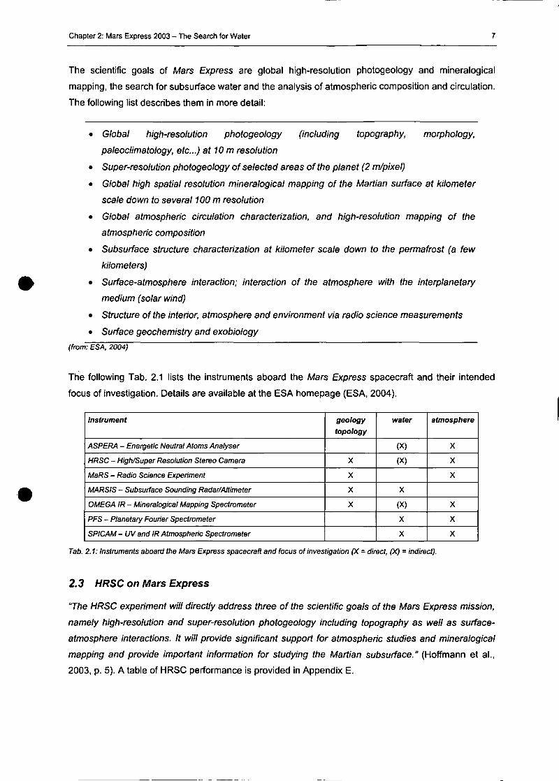
The following Tab. 2.1 lists the instruments aboard the Mars Express spacecraft and their intended
focus of investigation. Details are available at the ESA homepage (ESA, 2004).
Instrument
ASPERA - Energetic Neutral Atoms Analyser
HRSC - High/Super Resolution Stereo Camera
MaRS - Radio Science Experiment
MARSIS - Subsurface Sounding Radar/Altimeter
OMEGA IR - Mineralogical Mapping Spectrometer
PFS - Planetary Fourier Spectrometer
SPICAM - UV and IR Atmospheric Spectrometer
geology
topology
X
X
X
X
water
(X)
(X)
X
(X)
X
X
atmosphere
X
X
X
X
X
X
Tab. 2.1: Instruments aboard the Mars Express spacecraft and focus of investigation (X = direct, (X) = indirect).
2.3 HRSC on Mars Express
"The HRSC experiment will directly address three of the scientific goals of the Mars Express mission,
namely high-resolution and super-resolution photogeology including topography as well as surface-
atmosphere interactions. It will provide significant support for atmospheric studies and mineralogical
mapping and provide important Information for studying the Martian subsurface." (Hoffmann et al.,
2003, p. 5). A table of HRSC Performance is provided in Appendix E.
Chapter 2: Mars Express 2003 - The Search for Water
The scientific objectives and measurement goals of the HRSC experiment on Mars Express have
been formulated by the international team of 43 Co-Investigators from 10 countries under the
leadership of the Principal Investigator Prof. G. Neukum. The major scientific objectives are:
• Evolution of the Martian surface morphology through time and geologic processes
involved
Climate and the rote of water throughout the Martian history
Evolution of volcanism on Mars
Evolution oftectonism and the structure ofthe crust
Atmosphere / surface interactions and Eolian processes
• Atmospheric characteristics and dynamic atmospheric phenomena,
• Characteristics ofpast, present, and future landing Sites
• Potential resources on Mars
• Support for exobiological studies
• Observation of Phobos and Deimos
(Hoffmann and Neukum, 2003, p. 9)
By comparing the already existing Martian imagery and the expected Performance of cameras and
altimeters aboard ongoing or planned missions, the imaging data to be acquired by the HRSC
experiment should dose the existing gap between medium- to Iow-resolution coverage and the very
high-resolution images of the Mars Observer Camera on Mars Global Surveyor as well as the in-situ
observations and measurements by landers.
The following imaging data and surface coverage will be achieved during the nominal mission lifetime
of one Martian year:
• Medium to high-resolution imaging at 10-20 m/pixel: ~ 50% of the Martian surface,
targeted observations
• "Super" resolution imaging at 2-5 m/pixel: > 1% of the Martian surface, targeted
observations
• Medium resolution imaging at 20-40 m/pixel: 70 % of the Martian surface, global and
multiple coverage
• "Low" resolution at < 100 m/pixel: 100 % of the Martian surface, global and multiple
coverage
• Limb sounding (resolution variable) 2to3 times per month
• "Spot Pointing" (EPFL) observations for atmospheric and photometric studies
• In-flight calibration and commissioning
• Phobos imaging at high-resolution = <30 m/pixel ~ 50% of Phobos surface
• Phobos imaging at ulow"-resolution = <100 m/pixel ~ 100% of Phobos surface
• Deimos imaging as feasible
(Hoffmann, Neukum, 2003, p. 11)
Chapter 3: Concepts for Spatial Data Management
3 Concepts for Spatial Data Management
In this chapter, different concepts for spatial data modeling are introduced. Afterwards, the capabilities
of the Extensible Markup Language (XML) for spatial data representation and visualization are
discussed. A closer look is taken on two already standardized XML applications: Geography Markup
Language (GML) for data exchange and Scalable Vector Graphics (SVG) for data representation and
web presentation. Current shortcomings of XML related technologies are outlined. As Web Map
Services (WMS) are widely used for cartographic web presentation, this technology is investigated as
well. The chapter concludes with general concepts for the realization of web applications.
3.1 Initial Situation
3.1.1 Topographie Information Systems
For more than 10 years, one of the I.P.F.'s focus of research has been in the area of Topographie
Information Systems (TIS), a category of spatial information Systems concentrating on digital data and
modeis of natural and artificial topography at a scale of 1:2,500 to 1:100,000 (Kraus, 2000, pp. 1f.).
TopDB is a realization of such a System, first presented by Loitsch and Molnar (1991). It is a relational
database with additional data types and operations enabling topological relations. Loitsch and Molnar
(1991) named this coneept "Topology in terms of relationality", thus, TopDB is a topologic-relational
database. Hochstöger (1996) introduced and implemented the database application TopDM
(Topographie Data Management) in order to manage data, stored in TopDB, in a consistent State.
Therefore, TopDM represents a Database Management System (DBMS) for consistent and efficient
management of country-wide topographic data upon TopDB. Although this System would, from the
conceptual pointof view, enable coneurrent user management, itwas never implemented.
The Topographic Mars Information System (TMIS) is a multi-user web application for management,
distribution, analysis and visualization of planet-wide available topographic data in combination with
image datasets. It has been developed to increase the efficiency of the HRSC experiment working
group of Mars Express. When setting up the TMIS coneept, the main intention was the extension of
the single-user, single-machine database application of TopDM to a distributed storage, multi-user
web application, based on the commercial database kernel Oracle (Oracle, 2004). Furthermore, the
realization should take into aecount XML related Standards.
3.12 Related Work
When this work started in 2001, most web-based image archives of Mars-related data were based on
file archives, available via FTP from the investigating institutes. As an example the Planetary Data
System (PDS, 2004; should be mentioned, which archives and distributes scientific data from NASA
planetary missions (e.g. MGS), astronomical observations, and laboratory measurements. Other
approaches provided static image maps at the client-side. The Arizona State University (ASU)
operates the THEMIS archives in such a way (ASU, 2004). Furthermore, most of these Solutions were
Chapter 3: Concepts for Spatial Data Management 10
implemented for a distinct purpose and it turned out, that they will not be applicable to fulfill the given
task without major modifications and adaptations. Therefore, the Data Processing Working Group of
the HRSC project group decided to develop a web-based information system.
An approach, similar to the TMIS concept is provided by Gilbert (2002). The Centre for Topographie
Information in Sherbrooke (CTI), Canada, distributes digital topographic data using a web application
entirely implemented in Java. The user interface is realized using HTML pages and the map-based
data access is provided through a WMS serving static image presentations. But this System is
restricted to the management of country-wide datasets.
Another interesting realization of a so-called spatial data infrastrueture describe Fitzke et al. (2004).
The Free Software project degree started as a framework for integrating Software produets of different
vendors on base of OpenGIS (OGC, 2004) and ISO Standards (ISO, 2004).
In 2001, fat Clients were not yet used for security reasons. Therefore, although providing a high degree
of functionality, Java-Applets were not considered for TMIS. Most of the Co-Is were not willing to
permit Java functionality in their browsing environment then. Nevertheless, new web-based database
interfaces are realized using the Applet technology (e.g. EOLI-Web Envisat Catalogue, 2004).
Therefore, another method to include client-side functionality, the Scaleable Vector Graphics (SVG), is
investigated in this thesis. Obviously the best reference for SVG examples is carto:net (CARTONET,
2004).
3.2 Spatial Data Modeling
3.2.1 Database Management Systems
According to Reinhart (1995, p. 32) a database System (DBS) consists of two parts:
• a Database (DB) representing a struetured collection of data and
• a Database Management System (DBMS), an application for handling the data.
A list of advantages of a centralized data management using a DBMS as compared to decentralized
file storage gives Date (1990, pp. 15 ff.):
• Due to the fact, that the data can be provided to different applications, data redundancy can
be decreased to a necessary extent and hence the amount of secondary storage capacity is
reduced.
• Control and maintenance of remaining (intended) redundancy is simplified and the danger of
inconsistent content is reduced.
• The preservation of the integrity (content correetness) of the data is supported.
• Unified data security and data backup concepts are realizable in a more simple way.
• Standards, conceming data representation such as naming or type Conventions, can be
realized easier.
Chapter 3: Concepts for Spatial Data Management 11
According to the "ANSI/X3/SPARC Study Group on Database Management Systems (1970)°, a DBMS
has to support two aspects of data independence:
• Implementation independence - physical data independence: The conceptual view on the
data is independent from the internal (physical) data storage.
• Application independence = logical data independence: Separation from DB and application
interface.
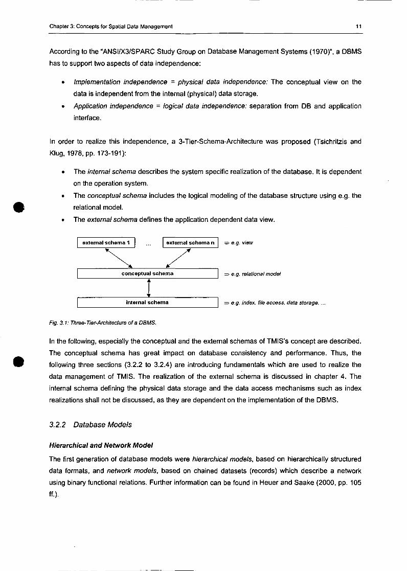
In order to realize this independence, a 3-Tier-Schema-Architecture was proposed (Tsichritzis and
Klug, 1978, pp. 173-191):
• The internal Schema describes the System specific realization of the database. It is dependent
on the Operation System.
• The conceptual Schema includes the logical modeling of the database structure using e.g. the
relational model.
• The external schema defines the application dependent data view.
external Schema 1 ... external schema n =• e.g. view
conceptual schema
internal schema
Fig. 3.1: Three-Tier-Architecture ofa DBMS.
• e.g. relational model
• e.g. index. iile access, data storage, ...
In the following, especially the conceptual and the external Schemas of TMIS's concept are described.
The conceptual schema has great impact on database consistency and Performance. Thus, the
following three sections (3.2.2 to 3.2.4) are introducing fundamentals which are used to realize the
data management of TMIS. The realization of the external schema is discussed in chapter 4. The
internal schema defining the physical data storage and the data access mechanisms such as index
realizations shall not be discussed, as they are dependent on the implementation of the DBMS.
3.2.2 Database Models
Hierarchical and Network Model
The first generation of database modeis were hierarchical modeis, based on hierarchically structured
data formats, and network modeis, based on chained datasets (records) which describe a network
using binary functional relations. Further information can be found in Heuer and Saake (2000, pp. 105
ff.).
Chapter 3: Concepts for Spatial Data Management 12
Relational Model
In 1970, Edgar F. Codd (1970) invented the relational database model as the first abstract model for
database management. This model describes real world object types (often named entities) using
relation Schemata R={A,, A2, ..., An} with the attributes A; representing common properties of an
object. Domains (value ranges) are associated with the attributes, mostly using Standard data types
such as i n t ege r , s t r i n g , r e a l or boolean (dom(A)). A database Schema consists of a set of
relation Schemata. A relation (r) represents a subset of the Cartesian product over the domain of the
attributes of the relation schema. Hence, it represents the current data of a relation schema being an
instance of this schema. A relation according to a relation schema is named r(R). One element of a
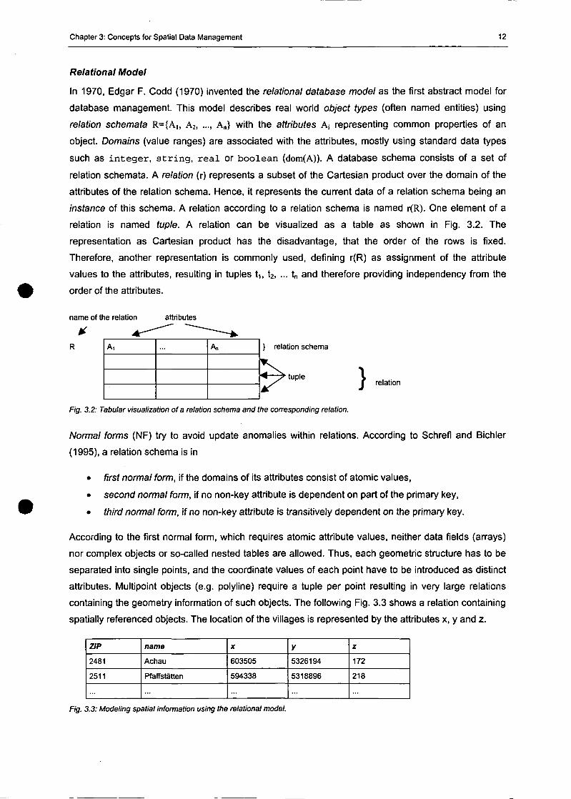
relation is named tuple. A relation can be visualized as a table as shown in Fig. 3.2. The
representation as Cartesian product has the disadvantage, that the order of the rows is fixed.
Therefore, another representation is commonly used, defining r(R) as assignment of the attribute
values to the attributes, resulting in tuples t i , t2, ... t„ and therefore providing independency from the
order of the attributes.
name of the relation attributes
A, A„ } relation schema
< > tuple^ S I relation
Fig. 3.2: Tabular visualization ofa relation schema and the corresponding relation.
Normal forms (NF) try to avoid update anomalies within relations. According to Schrefl and Bichler
(1995), a relation schema is in
• First normal form, if the domains of its attributes consist of atomic values,
• second normal form, if no non-key attribute is dependent on part of the primary key,
• third normal form, if no non-key attribute is transitively dependent on the primary key.
According to the first normal form, which requires atomic attribute values, neither data fields (arrays)
nor complex objects or so-called nested tables are allowed. Thus, each geometric structure has to be
separated into Single points, and the coordinate values of each point have to be introduced as distinct
attributes. Multipoint objects (e.g. polyline) require a tuple per point resulting in very large relations
containing the geometry Information of such objects. The following Fig. 3.3 shows a relation containing
spatially referenced objects. The location of the villages is represented by the attributes x, y and z.
ZIP
2481
2511
name
Achau
Pfaffstätten
X
603505
594338
y
5326194
5318896
z
172
218
Fig. 3.3: Modeling spatial Information using the relational model.
Chapter 3: Concepts for Spatial Data Management 13
The following section introduces alternative modeis as well as "extensions" to the relational model for
more efficient modeling of complex structures.
3.2.3 Modeling Spatial Data Structures
J\lmost everything that happens, happens somewhere. Knowing where something happens is
chtically important." (Longley et al. 2001). About 80 % of available data can be associated to a spatial
context. This can be the position of data acquisition defined by coordinates, or neighborhood
relationships, referred to as topology as well. As shown in section 3.2.2, the core relational model is
not appropriate to störe spatial structures.
NP Model
The 1st normal form (NF) is important in order to avoid database anomalies, but it prevents the
definition of complex objects. An attempt to overcome this problem is the NF2 model. NF2 Stands for
Non First Normal Form, and allows to define non-atomic attribute data types. A relation Schema
R={Ai, A2,..., An} may be defined using dom(Aj)eD of Standard data types or Ai={Au, ..., A im}, being
recursively a set of attributes. On the one hand, this enables the definition of nested relations using
constructors such as se t o f and t u p l e o f and on the other hand, of array data types using the
constructor a r r a y of . A realization of spatial data management using an array data type is
presented in section 3.2.4.
Semantic Data Model
Semantic data modeis support further concepts of abstraction. According to Heuer and Saake (2000,
pp. 125 ff.), currently no commercial database system realizes a semantic data model. A
representative is the Enhanced Entity Relationship Model (EER), defined by Engels et al. (1992, pp.
157-204). The semantic data modeis are not further discussed in this work.
Object-Oriented Model
The object-oriented (OO) database model is the consequent enhancement of semantic and nested
relational modeis. Thus, it extends the concept of modeling complex structures by
• complex data type constructors enabling to model complex real world entities as one abstract
object,
• object-identity enabling the distinction of objects and their values,
• inhehtance of attributes and methods between objects
and it provides concepts to realize object specific operations such as
• access methods.
The first commercial object-oriented database Systems (OODBS) were released in 1987. Beeri (1989)
published a theoretical description for OO database modeis. There are three different directions of
development
Chapter 3: Concepts for Spatial Data Management 14
• extensions to object-oriented programming languages (e.g. C++, Java),
• extensions to relational database Systems (PostGreSQL (POSTGRESQL, 2004), Oracle
Spatial (ORACLE, 2004), IBM DB2 (IBMDB2, 2004),...),
• new developments (O2 (Bancilhon et al., 1992),...) using OO database modeis.
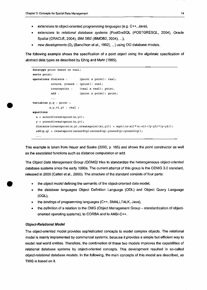
The following example shows the specification of a point object using the algebraic specification of
abstract data types as described by Ehrig and Mahr (1985).
datatype point based on real;
sorts point;
operations distance : (point x point): real;
xcoord, ycoord : (point): real;
createpoint : (real x real): point;
add : (point x point): point;
variables p,q : point ;
x,y,xl,yl : real ;
equations
x = xcoord (createpoint (x,y) ),-
y = ycoord(createpoint(x,y));
distance(createpoint(x,y),createpoint(xl,yl)) = sqrt((x-xl)*(x-xl)+(y-yl)*(y-yl));
add(p.q) = createpoint(xcoord(p)+xcoord(q),ycoord(p)+ycoord(q));
This example is taken from Heuer and Saake (2000, p. 185) and shows the point constructor as well
as the associated functions such as distance computation or add.
The Object Data Management Group (ODMG) tries to standardize the heterogeneous object-oriented
database Systems since the early 1990s. The current attempt of this group is the ODMG 3.0 Standard,
released in 2000 (Cattell et al., 2000). The structure of the Standard consists of four parts:
• the object model defining the semantic of the object-oriented data model,
• the database languages Object Definition Language (ODL) and Object Query Language
(OQL),
• the bindings of programming languages (C++, SMALLTALK, Java),
• the definition of a relation to the OMG (Object Management Group - standardization of object-
oriented operating Systems), to CORBA and to ANSI-C++.
Object-Relational Model
The object-oriented model provides sophisticated concepts to model complex objects. The relational
model is mainly implemented by commercial Systems, because it provides a simple but efficient way to
model real world entities. Therefore, the combination of these two modeis improves the capabilities of
relational database Systems by object-oriented concepts. This development resulted in so-called
object-relational database modeis. In the following, the main concepts of this model are described, as
TMIS is based on it.
Chapter 3: Concepts for Spatial Data Management 15
The relational model is strongly associated with the SQL (Structured Query Language) Standard. SQL
is a relational database language. It may be separated into different groups of languages according to
their functionality: e.g. the Interactive Query Language (IQL) to formalize database queries, the Data
Definition Language (DDL) to define the conceptual database Schema and the Data Manipulation
Language (DML) to insert and manipulate managed data. It was first standardized in 1989 as SQL89-
standard and enhanced in 1992 as SQL2, which was then accepted and implemented by the majority
of the commercial vendors of relational databases. A new version, SQL3, is in progress, but has not
been released yet. SQL99 realizes parts of SQL3, enhancing SQL's capabilities, for example, by
object-oriented concepts, hence supporting
• abstract data types (ADT),
• object identifiers,
• ADT hierarchies,
• table hierarchies,
• definition of methods and functions on ADTs,
• overriding of functions and
• definition of complex data types.
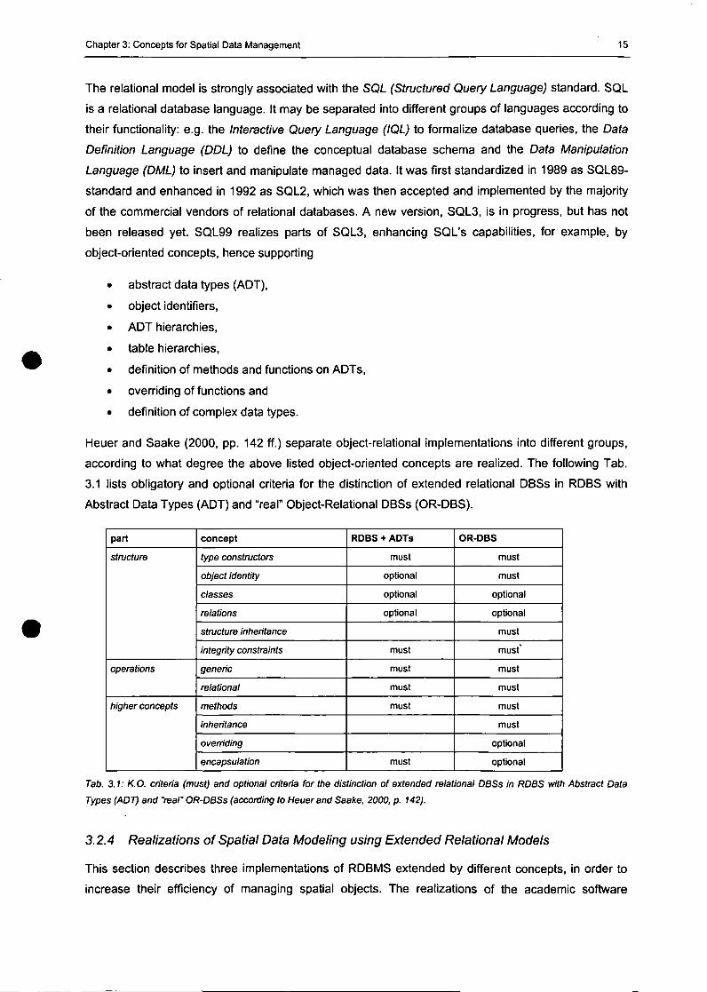
Heuer and Saake (2000, pp. 142 ff.) separate object-relational implementations into different groups,
according to what degree the above listed object-oriented concepts are realized. The following Tab.
3.1 lists obligatory and optional criteria for the distinction of extended relational DBSs in RDBS with
Abstract Data Types (ADT) and "real" Object-Relational DBSs (OR-DBS).
part
strvcture
operations
higher concepts
concept
type constructors
object identity
classes
relations
structure inheritance
integrity constraints
generic
relational
methods
inheritance
overriding
encapsulation
RDBS + ADTs
must
optional
optional
optional
must
must
must
must
must
OR-DBS
must
must
optional
optional
must
must*
must
must
must
must
optional
optional
Tab. 3.1: K.O. criteria (must) and optional criteria for the distinction of extended relational DBSs in RDBS with Abstract Data
Types (ADT) and "real" OR-DBSs (according to Heuerand Saake, 2000, p. 142).
3.2.4 Realizations of Spatial Data Modeling using Extended Relational Models
This section describes three implementations of RDBMS extended by different concepts, in order to
increase their efficiency of managing spatial objects. The realizations of the academic Software
Chapter 3: Concepts for Spatial Data Management 16
package TopDM, the commercial System Oracle and the open source System PostGreSQL are
introduced and discussed.
Topographie Data Management - TopDM:
TopDM is a topographic database application, intended for long time storage and archiving in a
consistent way. It provides a GUI (graphical user interface) based access to topographic data
managed by an RDBMS. To increase the quality of the managed data, the coneept of TopDM supports
the storage of a wide ränge of meta data such as aecuraey, compilation method, authorized data
users, and so forth (Hochstöger, 1996). Currently, two DBSs are supported through an abstract
interface: TopDB and Oracle Spatial. It is not visible to the user, which database system is used. All
necessary settings are defined during the initialization of the application. Thus, this System supports
the distinetion of logical and physical schema aecording to the ANSI/X3/SPARC model.
TopDB is an RDBS, extended by geometric/topologic elements (objeets) and geometric/topologic
Operators in order to handle those elements. Topological data types include AREA (closed polyline),
L I N E (open polyline), P O I N T (Single point) and WINDOW (rectangle parallel to coordinate system axis).
Additional Operators (.X. , .<. , .> ) enable the intersection and selection of geometric/topological
datasets.
The communication between TopDB and the application TopDM is realized by a database language
called "TOPSQL". Its current functionality is on the one hand a subset of ANSI-SQL but on the other
hand an extension regarding the geometric/topological data types and Operators. A typical data
selection could be to extract all data from a speeified table, which are at least partially inside a given
area, where the height aecuraey is better than 30 cm and have been compiled later than 2004-05-03.
This query can be formulated by using TOPSQL as follows:
SELECT * FROM DHMDATA
WHERE (COORDINATES .X. AREA (10000 50000
15000 60000
20000 40000)
AND (ZACCURACY < 0.30)
AND (COMPILEDATE > 03.05.2004);
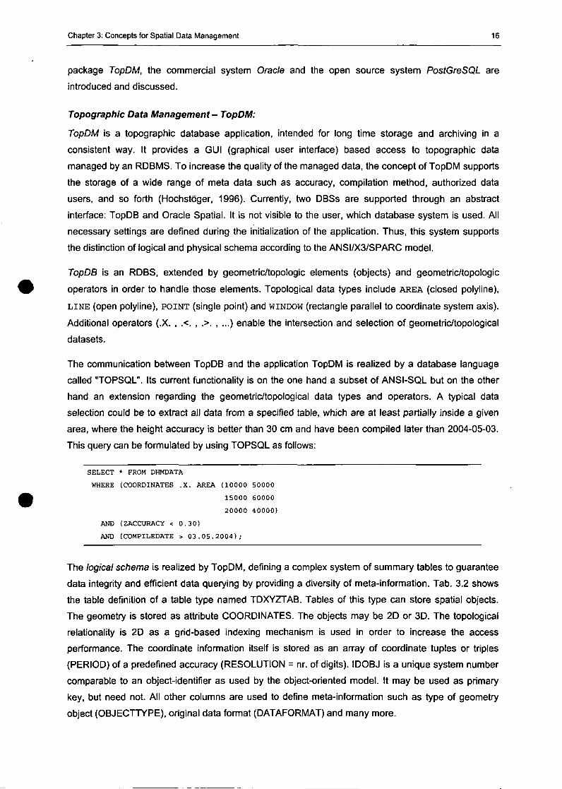
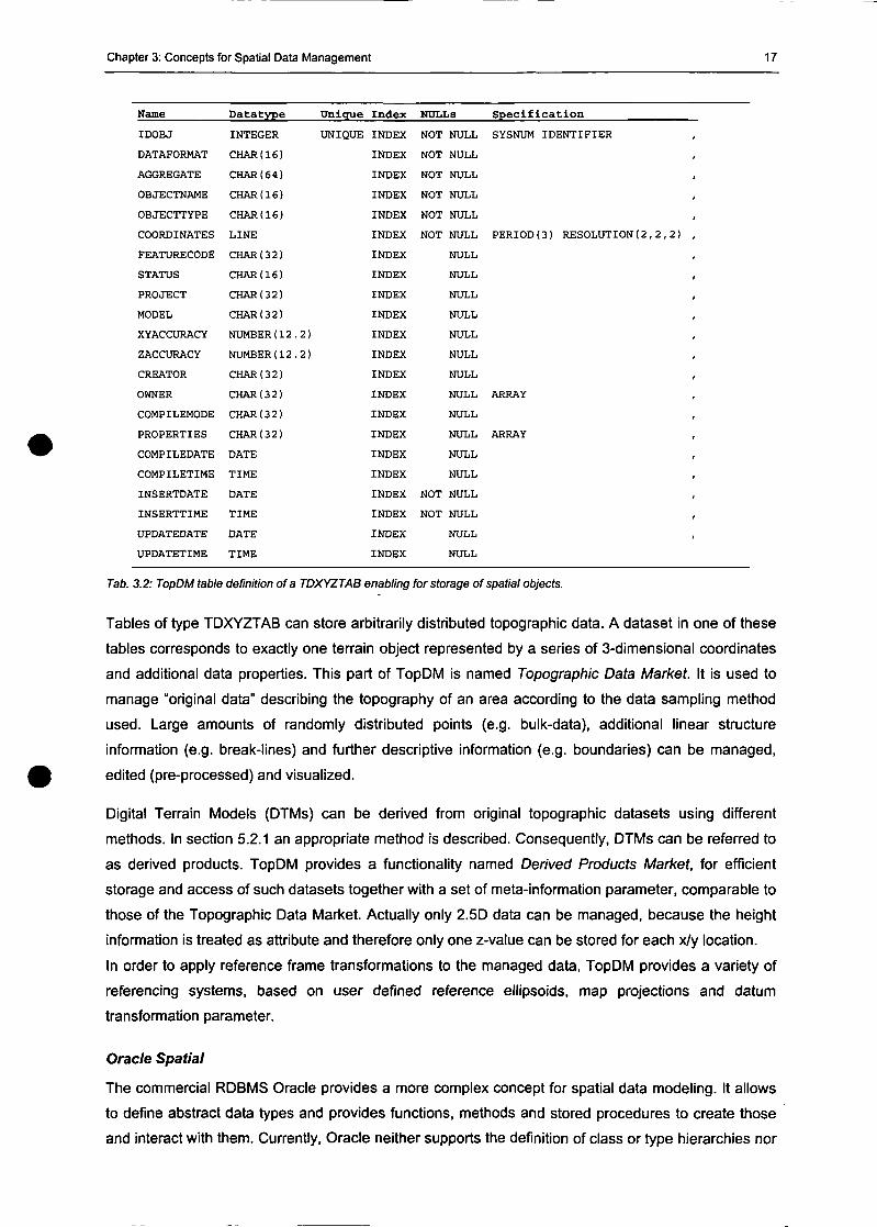
The logical schema is realized by TopDM, defining a complex system of summary tables to guarantee
data integrity and efficient data querying by providing a diversity of meta-information. Tab. 3.2 shows
the table definition of a table type named TDXYZTAB. Tables of this type can störe spatial objeets.
The geometry is stored as attribute COORDINATES. The objeets may be 2D or 3D. The topological
relationality is 2D as a grid-based indexing mechanism is used in order to increase the access
Performance. The coordinate information itself is stored as an array of coordinate tuples or triples
(PERIOD) of a predefined aecuraey (RESOLUTION = nr. of digits). IDOBJ is a unique system number
comparable to an objeet-identifier as used by the objeet-oriented model. It may be used as primary
key, but need not. All other columns are used to define meta-information such as type of geometry
objeet (OBJECTTYPE), original data format (DATAFORMAT) and many more.
Chapter 3: Concepts for Spatial Data Management 17
Name Datatype Unique Index NULL3 Specification
UNIQUE INDEX NOT NULL SYSNUM IDENTIFIER
INDEX NOT NULL
INDEX NOT NULL
INDEX NOT NULL
INDEX NOT NULL
INDEX NOT NULL PERIOD(3) RESOLUTION(2,2,2)
IDOBJ
DATAFORMAT
AGGREGATE
OBJECTNAME
OBJECTTYPE
COORDINATES
FEATURECODE
STATUS
PROJECT
MODEL
XYACCURACY
ZACCURACY
CREATOR
OWNER
COMPILEMODE
PROPERTIES
COMPILEDATE
COMPILETIME
INSERTDATE
INSERTTIME
UPDATEDATE
UPDATETIME
INTEGER
CHAR(16)
CHAR(64)
CHAR(16)
CHAR(16)
LINE
CHARO2)
CHAR(16)
CHAR(32)
CHAR(32)
NUMBER(12.2)
NUMBER(12.2)
CHAR(32)
CHAR(32)
CHAR(32)
CHAR(32)
DATE
TIME
DATE
TIME
DATE
TIME
INDEX
INDEX
INDEX
INDEX
INDEX
INDEX
INDEX
INDEX
INDEX
INDEX
INDEX
INDEX
INDEX
INDEX
INDEX
INDEX
NULL
NULL
NULL
NULL
NULL
NULL
NULL
NULL ARRAY
NULL
NULL ARRAY
NULL
NULL
NOT NULL
NOT NULL
NULL
NULL
Tab. 3.2: TopDM table definition ofa TDXYZTAB enabling for storage of spatial objects.
Tables of type TDXYZTAB can störe arbitrarily distributed topographic data. A dataset in one of these
tables corresponds to exactiy one terrain object represented by a series of 3-dimensional coordinates
and additional data properties. This part of TopDM is named Topographic Data Market. It is used to
manage "original data" describing the topography of an area according to the data sampling method
used. Large amounts of randomly distributed points (e.g. bulk-data), additional linear structure
information (e.g. break-lines) and further descriptive Information (e.g. boundaries) can be managed,
edited (pre-processed) and visualized.
Digital Terrain Models (DTMs) can be derived from original topographic datasets using different
methods. In section 5.2.1 an appropriate method is described. Consequently, DTMs can be referred to
as derived products. TopDM provides a functionality named Derived Products Market, for efficient
storage and access of such datasets together with a set of meta-information parameter, comparable to
those of the Topographic Data Market. Actually only 2.5D data can be managed, because the height
information is treated as attribute and therefore only one z-value can be stored for each x/y location.
In order to apply reference frame transformations to the managed data, TopDM provides a variety of
referencing Systems, based on user defined reference ellipsoids, map projections and datum
transformation parameter.
Oracle Spatial
The commercial RDBMS Oracle provides a more complex concept for spatial data modeling. It allows
to define abstract data types and provides functions, methods and stored procedures to create those
and interact with them. Currently, Oracle neither Supports the definition of class or type hierarchies nor
Chapter 3: Concepts for Spatial Data Management 18
inheritance. As already mentioned, Heuer and Saake (2000) call such Systems 'Database System with
Abstract Data Types' and not object-relational as they define those object-oriented characteristics as
essential (see section 3.2.3). For reasons of simplicity and because the vendor himself defines his
System as OR-DBS, it will be named an OR-DBS in the following.
TMIS is based on Oracle 9i. The following considerations are related to this version of Oracle,
although currently Oracle 10g is released. But this does not matter as it is not intended to give an
introduction into this commercial System; only the concepts for spatial data management using this
Software are discussed.
The 'Oracle Spatial Users's Guide and Reference' (Oracle Spatial, 2003) defines Oracle Spatial as
follows:
Oracle Spatial is an integrated set of functions and procedures that enables spatial data to
be stored, accessed, and analyzed quickly and efficiently in an Oracle9i database. Spatial
data represents the essential location characteristics of real or conceptual objects as those
objects relate to the real or conceptual space in which they exist.
Oracle Spatial, often referred to as Spatial, provides an SQL schema and functions that
facilitate the storage, retrieval, Update, and query of collections of spatial features in an
Oracle9i database. Spatial consists ofthe following components:
- A schema (MDSYS) that prescribes the storage, syntax, and semantics of
supported geometric data types
- A spatial indexing mechanism
- A set of Operators and functions for performing area-of-interest queries, spatial join
queries, and other spatial analysis operations
- Administrative Utilities
The spatial component of a spatial feature is the geometric representation of its shape in
some coordinate space. This is referred to as its geometry
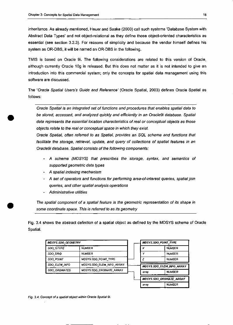
Fig. 3.4 shows the abstract definition of a spatial object as defined by the MDSYS schema of Oracle
Spatial.
imSYS.SDO_GE<W£TRY
SDO_GTYP£
SDO_SRID
SDO_POINT
SDO ELEM INFO
SDO ORDINATES
NUMBER
NUMBER
MDSYS. SDO_PO INT_TYPE
MDSYS.SDO ELEM INFO ARRAY
MDSYS.SDO ORDINATE ARRAY
IWSYS.SDO POINT TYPE
X
Y
Z
NUMBER
NUMBER
NUMBER
imSYS.SDO ELEM (NFO ARRAY
array NUMBER
MDSYS.SDO ORDINATE ARRAY
array NUMBER
Fig. 3.4: Concept ofa spatial object within Oracle Spatial 9i.
Chapter 3: Concepts for Spatial Data Management 19
The geometry object represents a nested object with five attributes, from which three are non atomic
data types. The access to the values of a spatial object is realized in an object-oriented manner. The
following SQL code shows an INSERT command invoking the insertion of a spatial object:
INSERT INTO "TMIS"."SPATIALJTAB" VALUES(
"MDSYS"."SDO_GEOMETRY"(
2003, -- 2-dimensional polygon
NULL, -- no spatial reference System (SRS) defined
NULL, --
MDSYS.SDO_ELEM_INFO_ARRAY(1,1003,1), -- one polygon (exterior polygon ring)
MDSYS.SDO_ORDINATE_ARRAY(12.23,23.45,34.56,45.56,56.67,67.78,12.23,23.45)
The first attribute, SDO_GTYPE, indicates the type of the geometry according to the "Geometry Object
Model for the OGC Simple Features for SQL specifications" (OGC, 2004). The presented example
defines a 2D polyline. The S D O _ S R I D attribute can be used to identify a spatial reference System
(SRS). If no SRS is associated to the geometry, the value is set to NULL. Either the third attribute
SDO_POINT or the following two, SDO_ELEM_INFO and SDOJDRDINATES, have to be NULL. The
SDO_POINT attribute is used to define a simple point using the SDO_POINT_TYPE. This geometry
type is recommended by Oracle for randomly distributed points; but it is not applicable to a large
amount of Single points as discussed in section 4.2.2. The other two attributes allow to define more
complex geometries. SDO_ELEM_INFO is of type ELEM_INFO_ARRAY and defines the geometry type.
S D O O R D I N A T E S stores the geometry Information using an array type.
To enable spatial queries on attributes of spatial data type, a spatial index has to be created. Oracle
Supports two different implementations: R-Tree and Quadtree (Oracle, 2003, pp. 4-1 pp.). The spatial
query Operator is realized as a two-step process. The first step performs a selection according to the
index Information only. The second step realizes a selection according to the geometry Information of
the set of results determined by step one. R-Tree-indexed attributes can be queried in 3D.
Unfortunately, only the first filter step is implemented for 3D queries.
In order to create a spatial index, metadata, defining the dimension, extension and resolution of the
geometry types to be managed within an attribute, has to be stored within a global metadata table.
This has to be realized by the application and is not performed by the index creation method.
Oracle Spatial is used as DBMS for the metadata catalogue of the TMIS. The realization of the
conceptual Schema as well as the data access is described in chapter 4.
PostgreSQL
According to its documentation, PostgreSQL, currently available as Version 7.4.2, is an OR-DBMS,
(POSTGRESQL, 2004). According to the definitions presented in section 3.2.3, it is an RDBMS
enabling ADTs, as no object or nested data types are supported. The realization of spatial data
modeling is based on array data types. The fundamental building block for all geometry types is
Chapter 3: Concepts for Spatial Data Management 20
Point . Supported geometry types are LineSegment, Box, Path, Polygon, C i r c l e . Several index
types (R-Tree, B-Tree) and geometric functions and operations on geometric objects are provided
(intersection, area, isopen, ...)• Core PostgreSQL Supports only 2D geometries. PostGIS, developed
by Refractions Research (POSTGIS, 2004), adds Support for 2.5D geometries to the PostgreSQL
Server. Both Systems are open source projects, distributed under the GNU General Public License
(GNU, 2004). Therefore, it may be an interesting, possibly cheap, opportunity compared to
commercially distributed Systems.
3.3 Extensible Markup Language for Spatial Data Representation
This section gives an introduction to data management, exchange and visualization Standards based
on the Extensible Markup Language (XML). Their main characteristics and capabilities are described.
3.3.1 Introduction to XML
XML as data exchange format for the Internet tries to overcome the shortcomings of HTML (Hypertext
Markup Language). These are syntax limitation (the HTML Document Type Definition (DTD) is fixed
without the possibility of extension) and mixture of formatting information and data (XML allows to
separate them). Furthermore, XML is especially built for reusability and it Supports the Unicode
character set, increasing its capability for internationalization.
An XML document consists of three different logical structures: Tags, Attributes and Data. A simple
document might look like the following:
<person gender="male">
<firstname>Peter</firstname>
<lastname>Dorninger</lastname>
</person>
Tag names are enclosed with angle brackets '<' and '>'. They either occur in pairs as start and end tag
or, for empty elements, as an empty element tag closed by a slash '/'• Start tags may include
attributes. Attribute values have to be bounded by quotes. Data can be stored as attribute values.
However, normally attributes are used to hold some meta-information which is used for several
purposes (e.g.: language information) by the parser when interpreting the document.
XML documents represent their content as semi-structured data. Semi-structured data have one or
several of the following characteristics:
• the Schema definition is not stored in a central data dictionary. It is included into each
document
• the data structure might change (different attributes, left attributes, different order)
• data itself has no further structure
• data types are not part of integrity constraints
• large number of attributes
• no strict distinction between data and Schema
Chapter 3: Concepts for Spatial Data Management 21
The valid structure of an XML document can be defined using two different mechanisms: Document
Type Definitions (DTD) and XML Schema Definition Language (XSD). The XSD is generally used to
define XML applications, as it is standardized by the W3C, it is defined in XML and it provides more
flexibility than DTDs.
The following list gives an overview of furtherXML related technologies (from: W3C-XML, 2004).
namespaces restrict the scope of validity of XML objects
XSD XML Schema Definition Language - defines valid structures and data types of an
XML document
XLink allows for linking of documents (extended HTML hyperlink functionality)
XPath object selection language
XQuery query language for XML documents (interface to databases)
XSL Extensible Stylesheet Language - describes how to display / render documents;
it consists of two parts:
XSLT defines the transformation from one XML format into another
XSL:FO formatting objects - allow to format an XML document
The acceptance and application of XML-based formats in the commercial market is growing.
Unfortunately, there are still shortcomings within the available XML-based Software Solutions. For
example, the current implementations of XPath have great Performance shortcomings. As Gottlob
(2002) shows in his tests, the evaluation time grows exponentially with the complexity of a query. This
problem will be discussed in particular in section 3.3.7.
Currently several promising XML Standards concerning geodata exist. In the following sections, an
introduction to two already standardized XML applications for geodata is given:
• Geography Markup Language (GML) for data storage, management and distribution and
• Scalable Vector Graphics (SVG) for data visualization.
3.3.2 Geography Markup Language
The OpenGIS Consortium (OGC) was founded in 1994 in order to define Standards for inter-vendor
exchange of geodata. The OpenGIS Interface Specifications have become a successful foundation for
interoperable geodata processing (e.g.: OpenGIS Simple Feature Specification). The increasing
importance of the World Wide Web (WWW) as data exchange medium and the development of XML
as a framework for the definition of proprietary data exchange formats lead to the development of the
Geography Markup Language (GML). GML can be characterized as follows:
Geography Markup Language (GML) is an XML extension for encoding the transport and
storage of geographic Information, which includes geometry and properties of geographic
features (Reichardt, 2001).
This definition uses the expression "XML extension' as a synonym for 'XML application'. The GML
Standard modeis the world according to the OGC Abstract Specifications, which define a geographic
Chapter 3: Concepts for Spatial Data Management 22
feature as "an abstraction of a real worid phenomenon; it is a geographic feature, if it is associated
with a location relative to the Earth." (Cox et al., 2004). The GML 2 specifications (latest version: 2.12)
are concerned with the OGC Simple Features, features whose geometry properties are restricted to
'simple'. Point, line, linestring or are are good examples for such objeets. The current version, GML 3
(version 3.0 was released in January 2003 and version 3.1 is available as committee draft) overcomes
many of the former restrictions. Thus, GML 3 allows to represent non-linear geometries (e.g. eubie,
spline, bspline, bezier, clothoid, ...), 3D objeets (e.g. building modeis), features with 2D topology,
features with temporal properties, dynamic features, coverages and observations. GML 3 tries to fulfill
the guidelines defined by the ISO 19100 Standards (ISO, 2004). On the one hand, this important
extension of the GML Standard provides more flexibility in its application. On the other hand, the
schema definitions became twenty times longer, making them much more difficult to be applied.
As one of the main characteristics of XML applications, GML supports füll extensibility. Therefore,
individual types can be defined. Another benefit of XML is the Separation of content and presentation,
and, as described in the previous section, there are several concepts to transform GML documents
into appropriate formats for visualization such as SVG (to be discussed in the following section) or
X3D, an XML application that can easily be transformed into VRML (Virtual Reality Modeling
Language is the commonly used visualization Standard for web presentation of 3D data. Further
considerations relating to VRML are given in section 6.3.2).
GML is currently not integrated in the TMIS framework for several reasons: Most data to managed by
TM IS can be characterized as structured according to the definitions for semi-structured data given in
section 3.3.1. Thus, the Integration of the strueture information into TMIS relevant documents causes a
large overhead of meta-information stored together with the data. Concerning topographic data which
consists of numerous individual geometry objeets with identical meta-information (e.g. objeet type,
acquisition method, Standard deviation, ...), the amount of metadata to be handled is very high.
Nevertheless, section 3.3.5 describes an approach to map two different data formats for topographic
data representation onto GML.
3.3.3 Scalable Vector Graphics
Scalable Vector Graphics (SVG), standardized by the W3C since September 2001 is an XML
application for storage, exchange and especially for web presentation of geodata. The currently
released version 1.1 can be found on the web (Ferraiolo et al., 2003). Since May 2004, a working draft
version of SVG 1.2 is available.
The term Scalable Vector Graphics is misleading: SVG is in no way limited to vector graphics; on the
contrary, it is surprisingly universal. SVG supports interactivity and animation and it is compatible to
other XML Standards such as DOM (Document Objeet Model - supports access of the objeets
entities), XSL (XML Stylesheet Language), SMIL (Synchronized Multimedia Integration Language) and
many others. Therefore, a GML document, for example the result of a database request, can easily be
transformed into an SVG document using XSLT.
There are three different groups of objeet types which can be represented using SVG:
Chapter 3: Concepts for Spatial Data Management 23
• Vector Data
• Raster Images
• Text
The following basic vector geometry types are defined: rectangle, circle, ellipse, line, polyline, polygon,
symbol and path. Path is the most complex one, because it has the capability to represent line
Segments, Square and cubic Bezier curves and arc Segments. Various style attributes may be defined
such as line-style, weight, color and so on. Using raster overlays, raster images can be combinded
with vector data. They can be treated like any other geometry object using the same methods. Text
objects have the same Status as any other basic geometry type and the same attributes may be
assigned to them.
SVG provides numerous methods to visualize and render spatial objects. Besides line-style and color
definitions, sophisticated filter methods are realized which can be applied to raster overlays as well as
to vector type elements. Another important feature is the capability of SVG to störe georeferencing
information and to define transformations between different reference frames. Mathematically, all
transformations can be represented as 3x3 transformation matrices. Nesting of transformations is
allowed.
SVG and 3D data
A major shortcoming SVG is its sole Support of 2D geometry. The SVG Schema might be extended,
but the additional properties can only be used for internal data representation, because the
commercially available Software Solutions do not support non standardized properties. For example,
the coordinates of linear objects are stored as a stream of separated x and y coordinates. Thus, there
is no possibility to define a stream consisting of x, y and z coordinates, because no rendering engine
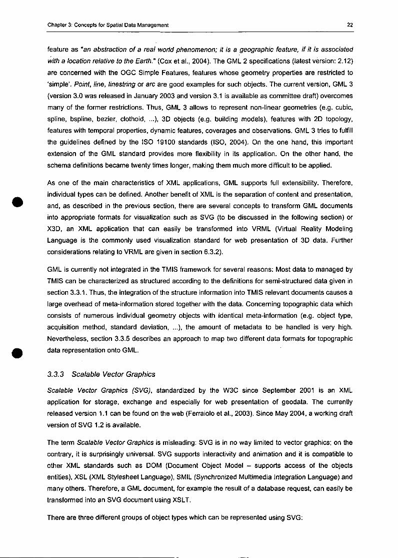
will support such a geometry. The following example of a simple DTM analysis tool based on three
vector and two raster layers, shows an effort to support 2.5D geometries using SVG. The five data
layers are shown in Fig. 3.5.
Fig. 3.5: Three vector and two raster layers used to create an SVG-based DTM analysis tool.
Chapter 3: Concepts for Spatial Data Management 24
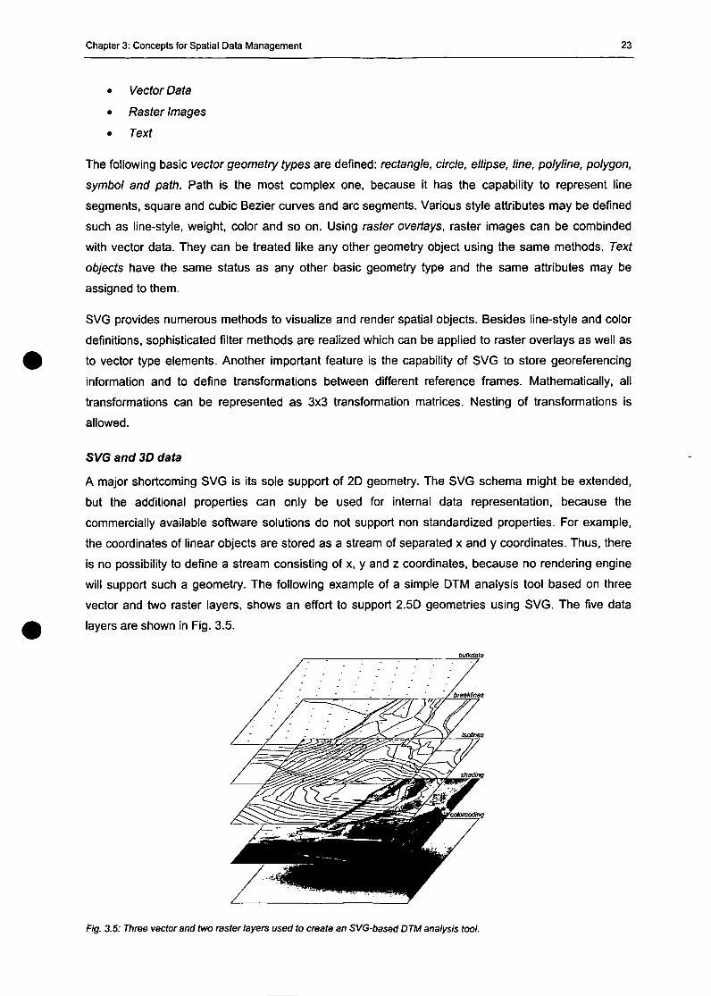
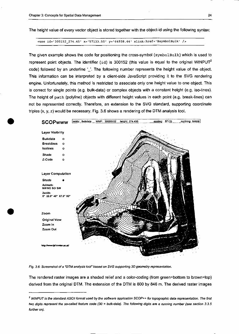
The height value of every vector object is stored together with the object-id using the following syntax:
<use id='300152_274.45' x='57133.50' y='64938.44' xlink:href='ttsymbolBulk1 />
The given example shows the code for positioning the cross-symbol (symbolBulk) which is used to
represent point objects. The identifier ( id ) is 300152 (this value is equal to the original WINPUT2
code) followed by an underline '_'. The following number represents the height value of the object.
This Information can be interpreted by a client-side JavaScript providing it to the SVG rendering
engine. Unfortunately, this method is restricted to associate only one height value to one object. This
is correct for Single points (e.g. bulk-data) or complex objects with a constant height (e.g. iso-lines).
The height of pa th (polyline) objects with different height values in each point (e.g. break-lines) can
not be represented correctly. Therefore, an extension to the SVG Standard, supporting coordinate
triples (x, y, z) would be necessary. Fig. 3.6 shows a rendering of the DTM analysis tool.
S C O P W W W ^enlity: Bul l" la 'a VMP: 30000152 height: 274.450 eastinp: 57133 northing: 64938]
LayerVisibility
Bulkdata o
Breaklines o
Isolines o
Shade
Z-Codeo
o
Layer Computation
Shade •
Azimuth:NW NO SO SW
Zenith:0* 22.5» 45° 67.5* 90*
Zoom
Original View
Zoom In
Zoom Out
http:Jhmmr.tpf.anMtti.iot/
Fig. 3.6: Screenshot of a "DTM analysis tool" based on SVG supporting 3D geometry representation.
The rendered raster images are a shaded relief and a color-coding (from green=bottom to brown=top)
derived from the original DTM. The extension of the DTM is 800 by 846 m. The derived raster images
2 WINPUT is the Standard ASCII format used by the Software application SCOP++ for topographic data represent ation. The first
two digits represent the so-called feature code (30 = bulk-data). The following digits are a running number (see section 3.3.5
further on).
Chapter 3: Concepts for Spatial Data Management 25
are provided in PNG format with a resolution of 1 m/pixel. For Performance reasons, the whole region
was divided into three by three tiles. The color-coding as well as the shaded relief can be rendered
individually, or they can be combined, using SVG's filter options. f eComposite, a predefined filter
rule, can be used to combine two source images in the following way:
result - kx • ix • i2 + k2 • /, + k3 • i2 + k4
/i is the intensity of image 1 and i2 the intensity of image 2. The parameters k{ can be defined
individually. The following SVG code snippet shows the application of the feComposite filter to
combine two images:
<filter id="filter" filterUnits="objectBoundingBox" x="0" y="0" width="100%"
height="100%">
<felmage xlink:href="shd.png" result="shd" />
<feComposite in="SourceGraphic" in2="shd" operator="arithmetic" kl="O.O" k2="0.75"
k3="0.75" k4="0.0" result=ncompIMG"/>
</filter>
On the fly Generation ofSVG
There are different methods for efficient access and manipulation of SVG documents. In the following,
several Java technologies which can be used for on-the-fly (OTF) generation of SVG are introduced.
JavaServerPages (JSP) allow to create dynamic and interactive HTML pages. Conventional HTML
pages are static. Some rather restricted methods to apply interactivity and dynamic processes to a
web page are supported by Scripting languages like JavaScript which is a subset of core Java. For
example, it can be used to define simple functions, to evaluate input parameters or for visualization
purposes. JSP allow to include pure Java code with all its capabilities into a conventional HTML
source. To compile and interpret this functionality, a JSP and Servlet Container is necessary. For
example, the Tomcat Servlet Container, which is part of Apaches Jakarta Project, is an open source
Java implementation of such a tool (JAKARTA, 2004). Servlets are Java classes which can be
requested by an HTTP request. The given input parameters can be processed and the result is
provided as HTML document which can be displayed using Standard web browsers. In the same way,
SVG documents can be created dynamically. Every JSP is translated and subsequently compiled into
a Servlet at the first request. From then on, every request is directly sent to the corresponding Servlet
class. Servlets provide füll Java functionality and therefore, can call native methods of other classes,
thus supporting reuse of already implemented methods that have been used and tested within other
applications so far.
There are two shortcomings concerning the dynamical creation of SVG using JSP:
• Embedding into another JSP is not supported by all web browsers, and
• the resulting document cannot be compressed.
Chapter 3: Concepts for Spatial Data Management 26
A possible solution is the embedding of static SVG into JSP, which are generated and subsequently
compressed on demand. Several tests and considerations conceming SVG compression are given in
section 3.3.4.
Java Database Connectivity (JDBC) is an API (Application Programming Interface) that allows to
access tabular data sources such as relational databases. It is based on a driver management
enabling the integration of core SQL commands into the Java code. Most vendors of relational
database Systems provide an JDBC-API.
Current Status ofSVG Development
In the early conceptual phase of the TMIS, in 2001, SVG seemed to become the Standard for geodata
representation and visualization on the web. They provide many useful features to handle vector data
and to render them together with raster images. But the acceptance of SVG did not develop as
expected. Microsoft left the SVG standardization group. Adobe, Corel and other members do support
import and export interfaces which are not completely compatible to the Standard. Exporting a
document using an Adobe Software application is rendered slightly different within an Corel
environment. Especially formatting information is interpreted in different ways. Besides, the
automatically generated SVG code is quite unstructured and therefore hard to read. But, the main
bottleneck for web presentation is the missing of a Standard, platform-independent rendering Container
for web browsers. A plug-in Version provided by Adobe (current Version 3.01, ADOBE, 2004) does
exist for MS Internet Explorer. It was implemented in 2001. The Mozilla foundation (MOZILLA, 2004)
provides a native implementation of the SVG specification for the open Source browser Mozilla.
Although this implementation is currently improved, it still does not implement the whole SVG Standard
and it is not integrated in the browser's kernel. This causes two major problems:
• As long as SVG rendering engines are not integrated into the kernel of web browsers, there
will emerge Performance shortcomings due to the interaction of plug-in or native
implementations with the browser Software.
• SVG is not available to everyone, considering the problems of installing an additional Software
on a Computer without administrator's Privileges.
A plug-in solution can be successful as well. For example, the Macromedia Flash (MACROMEDIA,
2004) plug-in is provided by a commercial vendor and available in current versions for almost any
platform. Thus, it is widely accepted and available to a broad Community. In Maren 2004, NPD
Research condueted a study to determine the percentage of Web browsers with Macromedia Flash
preinstalled. The result shows, that 98 % of Web users can experience Macromedia Flash content
without having to download and install a player, whereas only 17 % have access to an SVG rendering
engine (from MACROMEDIA, 2004).
Within the Community of web cartographers, there is a large acceptance for the SVG Standard.
Especially the Swiss Federal Institute of Technology in Zürich, Switzerland, forces its development
and application. They established a yearly Conference, the SVGOpen (SVGOPEN, 2004), which had
about 150 partieipants for the first time in 2002, and the audience is increasing from year to year. But
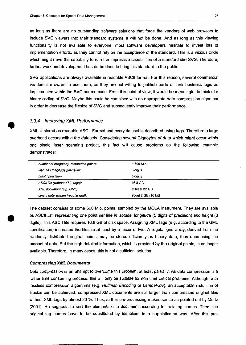
Chapter 3: Concepts for Spatial Data Management 27
as long as there are no outstanding Software Solutions that force the vendors of web browsers to
include SVG Viewers into their Standard Systems, it will not be done. And as long as this viewing
functionality is not available to everyone, most Software developers hesitate to invest lots of
implementation efforts, as they cannot rely on the acceptance of the Standard. This is a vicious circle
which might have the capability to ruin the impressive capabilities of a Standard like SVG. Therefore,
further work and development has do be done to bring this Standard to the public.
SVG applications are always available in readable ASCII format. For this reason, several commercial
vendors are aware to use them, as they are not willing to publish parts of their business logic as
implemented within the SVG source code. From this point of view, it would be meaningfui to think of a
binary coding of SVG. Maybe this could be combined with an appropriate data compression algorithm
in order to decrease the filesize of SVG and subsequently improve their Performance.
3.3.4 Improving XML Performance
XML is stored as readable ASCII-Format and every dataset is described using tags. Therefore a large
overhead occurs within the datasets. Considering several Gigabytes of data which might occur within
one Single laser scanning project, this fact will cause problems as the following example
demonstrates:
number of irregularty distributed points:
latitude / longitude precision:
height precision:
ASCII list (without XML tags):
XML document (e.g. GML):
binary data stream (regulär grid):
- 600 Mio.
5 digits
3 digits
16.8 GB
at least 32 GB
about2GB(16bit)
The dataset consists of some 600 Mio. points, sampled by the MOLA instrument. They are available
as ASCII list, representing one point per line in latitude, longitude (5 digits of precision) and height (3
digits). This ASCII file requires 16.8 GB of disk space. Assigning XML tags (e.g. according to the GML
specification) increases the filesize at least by a factor of two. A regulär grid array, derived from the
randomly distributed original points, may be stored efficiently as binary data, thus decreasing the
amount of data. But the high detailed information, which is provided by the original points, is no longer
available. Therefore, in many cases, this is not a sufficient solution.
Compressing XML Documents
Data compression is an attempt to overcome this problem, at least partially. As data compression is a
rather time consuming process, this will only be suitable for non time critical problems. Although, with
lossless compression algorithms (e.g. Huffman Encoding or Lempel-Ziv), an acceptable reduction of
filesize can be achieved, compressed XML documents are still larger than compressed original files
without XML tags by almost 20 %. Thus, further pre-processing makes sense as pointed out by Mertz
(2001). He suggests to sort the elements of a document according to their tag names. Then, the
original tag names have to be substituted by identifiers in a sophisticated way. After this pre-
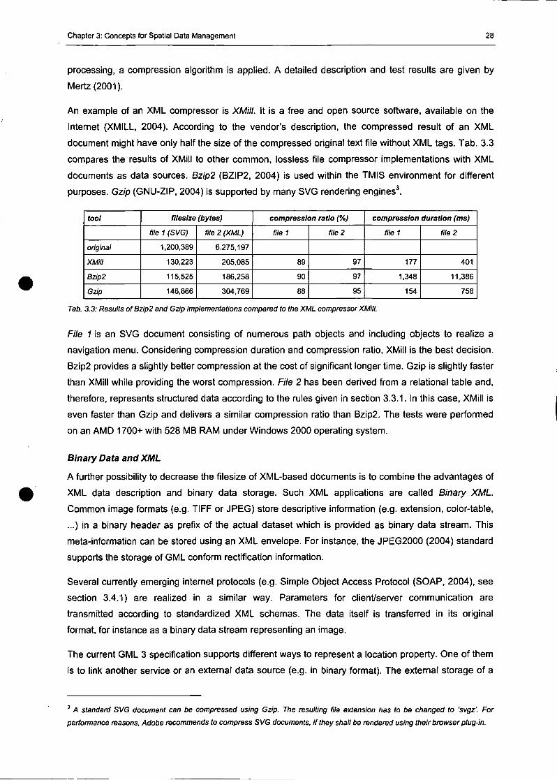
Chapter 3: Concepts for Spatial Data Management 28
processing, a compression algorithm is applied. A detailed description and test results are given by
Mertz(2001).
An example of an XML compressor is XMill. It is a free and open source Software, available on the
Internet (XMILL, 2004). According to the vendor's description, the compressed result of an XML
document might have only half the size of the compressed original text file without XML tags. Tab. 3.3
compares the results of XMill to other common, lossless file compressor implementations with XML
documents as data sources. Bzip2 (BZIP2, 2004) is used within the TMIS environment for different
purposes. Gzip (GNU-ZIP, 2004) is supported by many SVG rendering engines3.
tool
original
XMill
Bzip2
Gzip
filesize (bytes)
file 1 (SVG)
1,200,389
130,223
115,525
146,866
file 2 (XML)
6.275,197
205,085
186,258
304,769
compression ratio (%)
file 1
89
90
88
file 2
97
97
95
compression duration (ms)
filei
177
1,348
154
file 2
401
11,386
758
Tab. 3.3: Results ofBzip2 and Gzip implementations compared to the XML compressor XMill.
File 1 is an SVG document consisting of numerous path objects and including objects to realize a
navigation menu. Considering compression duration and compression ratio, XMill is the best decision.
Bzip2 provides a slightly better compression at the cost of significant longer time. Gzip is slightly faster
than XMill while providing the worst compression. File 2 has been derived from a relational table and,
therefore, represents structured data according to the rules given in section 3.3.1. In this case, XMill is
even faster than Gzip and delivers a similar compression ratio than Bzip2. The tests were performed
on an AMD 1700+ with 528 MB RAM under Windows 2000 operating System.
Binary Data and XML
A further possibility to decrease the filesize of XML-based documents is to combine the advantages of
XML data description and binary data storage. Such XML applications are called Binary XML.
Common image formats (e.g. TIFF or JPEG) störe descriptive information (e.g. extension, color-table,
...) in a binary header as prefix of the actual dataset which is provided as binary data stream. This
meta-information can be stored using an XML envelope. For instance, the JPEG2000 (2004) Standard
Supports the storage of GML conform rectification information.
Several currently emerging internet protocols (e.g. Simple Object Access Protocol (SOAP, 2004), see
section 3.4.1) are realized in a similar way. Parameters for client/server communication are
transmitted according to standardized XML Schemas. The data itself is transferred in its original
format, for instance as a binary data stream representing an image.
The current GML 3 specification supports different ways to represent a location property. One of them
is to link another Service or an external data source (e.g. in binary format). The extemal storage of a
3 A Standard SVG document can be compressed using Gzip. The resulting file extension has to be changed to 'svgz'. For
Performance reasons, Adobe recommends to compress SVG documents, if they shall be rendered using their browser plug-in.
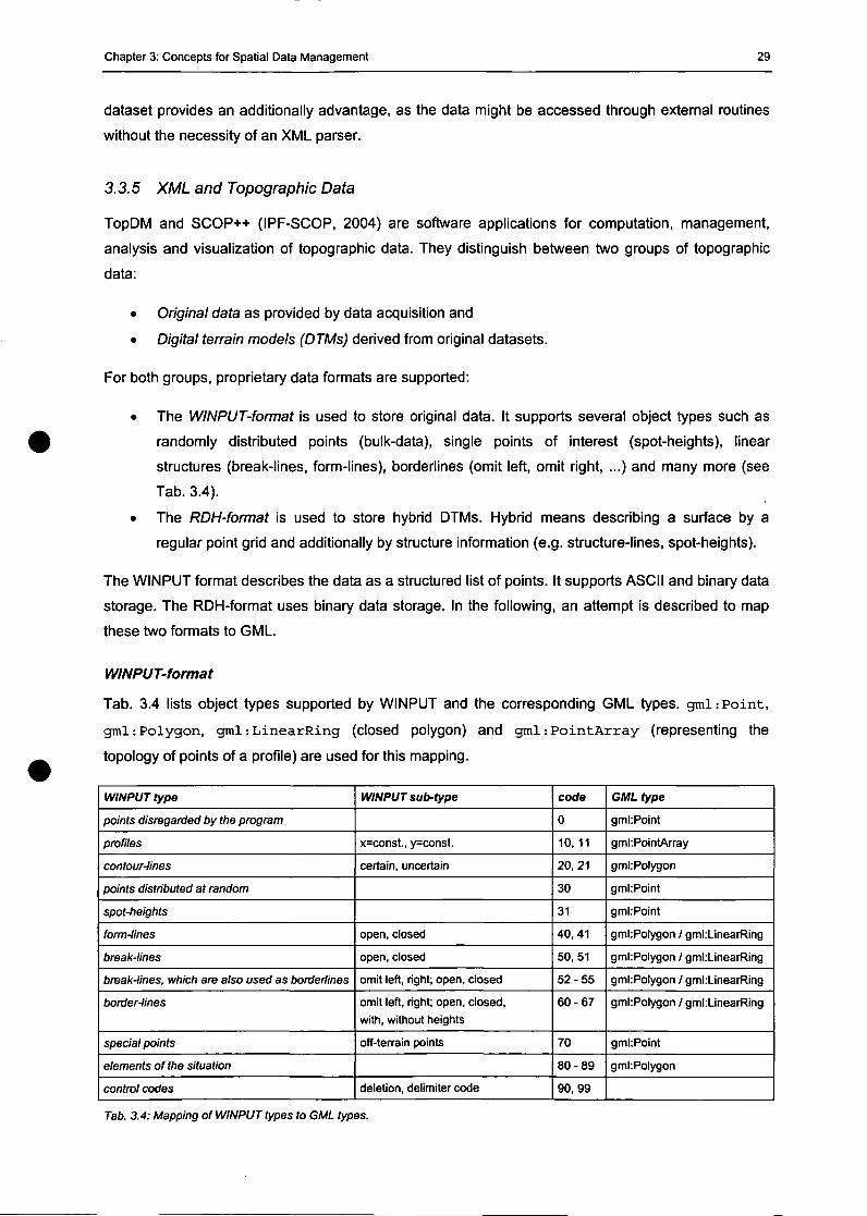
Chapter 3: Concepts for Spatial Data Management 29
dataset provides an additionally advantage, as the data might be accessed through extemal routines
without the necessity of an XML parser.
3.3.5 XML and Topographie Data
TopDM and SCOP++ (IPF-SCOP, 2004) are Software applications for computation, management,
analysis and visualization of topographic data. They distinguish between two groups of topographic
data:
• Original data as provided by data acquisition and
• Digital terrain modeis (DTMs) derived from original datasets.
For both groups, proprietary data formats are supported:
• The WINPUT-format is used to störe original data. It supports several objeet types such as
randomly distributed points (bulk-data), Single points of interest (spot-heights), linear
struetures (break-lines, form-lines), borderlines (omit left, omit right, ...) and many more (see
Tab. 3.4).
• The RDH-format is used to störe hybrid DTMs. Hybrid means describing a surface by a
regulär point grid and additionally by strueture information (e.g. structure-lines, spot-heights).
The WINPUT format describes the data as a struetured list of points. It supports ASCII and binary data
storage. The RDH-format uses binary data storage. In the following, an attempt is described to map
these two formats to GML.
WINPUT-format
Tab. 3.4 lists objeet types supported by WINPUT and the corresponding GML types. gml : Po in t ,
gml : Polygon, gml : L inearR ing (closed polygon) and gml : Po in tA r ray (representing the
topology of points of a profile) are used for this mapping.
WINPUT type
points disregarded by the program
profiles
contour-lines
points distributed at random
spot-heights
form-lines
break-lines
break-lines, which are also used as borderiines
border-lines
Special points
elements of the Situation
control codes
WINPUT sub-type
x=const., y=const.
certain, uncertain
open, closed
open, closed
omit left, right; open, closed
omit left, right; open, closed,
with, without heights
off-terrain points
deletion, delimiter code
code
0
10, 11
20,21
30
31
40,41
50,51
52-55
60-67
70
80-89
90,99
GML type
gml:Point
gmkPointArray
gml:Polygon
gml:Point
gmhPoint
gml:Polygon / gmkLinearRing
gml:Polygon / gml:LinearRing
gmkPolygon / gml:ünearRing
gmhPolygon / gml:LinearRing
gmhPoint
gml:Polygon
Tab. 3.4: Mapping of WINPUT types to GML types.
Chapter 3: Concepts for Spatial Data Management 30
In the following example, these mapping constraints were applied to a dataset consisting of 55,801
points acquired by analytical photogrammetry. 16,140 points belong to compound topological objects
such as form-, break- or borderlines. The others are randomly distributed points (mean point distance
of some 50 m) and spot-heights. Tab. 3.5 compares the filesize of the original ASCII file in WINPUT-
format to that of the GML mapping. The files were compressed using Bzip2 and XMill (see section
3.3.4).
format
WINPUT
GML
filesize (bytes)
ASCI)
2,567,260
4,744,025
Bzip2-compressed
346,363
335,141
XMill-compressed
440,327
Tab. 3.5: Comparison of WINPUT and GML documents.
As expected, the XML tags increase the filesize by a factor of two. Similar results were achieved with
other datasets. Compressing the WINPUT and the GML document results in almost similar filesizes.
This can be explained, as some redundancy of the WINPUT format (e.g. the WINPUT code is stored
together with every point of a compound element) is no longer stored within the GML document.
Further on, the XML-tags, of the GML document have a high degree of similarity, and allow a high
compression rate. Similar to the results of section 3.3.4, the Performance of XMill is much better than
those of Bzip2 (500 ms vs. 6,800 ms) while providing slightly less compression ratio. The following
conclusions can be drawn:
• Due to the significantly greater filesize of GML documents compared to WINPUT files (both in
ASCII format), a GML application may suffer from storage problems.
• Although a GML document contains additional Information, it can be compressed almost as
highly as a WINPUT file. Therefore, GML might be a good choice for non-time-critical
applications (e.g. data archiving).
RDH-format
The base structure within the RDH-format is a regulär grid of points, derived from the original data. If
the original data is provided in WINPUT-format, the groups of objects described in Tab. 3.4 are treated
as follows: points, contour-lines and points distributed at random (referred to as bulk or "raster-type"
data) are replaced by an interpolated regulär grid of points within the RDH structure, carrying just the
height values. On the contrary, spot-heights, form-lines, break-lines and border-lines (referred to as
"vector-type" data) are integrated in the RDH structure. Every spot-height and the vertices of Segments
of linear structures are stored as 2.5D points (x, y, z-values). Also the height values of the points
obtained by intersecting the linear structures with the Virtual mesh-lines of the grid are stored. For
addressing the integrated "vector-type" data, an optimized System of assignments is stored with them.
For Performance reasons, the RDH-format is organized in Computing units (CU). Fig. 3.7 shows a
schematic example of the RDH-data-structure.
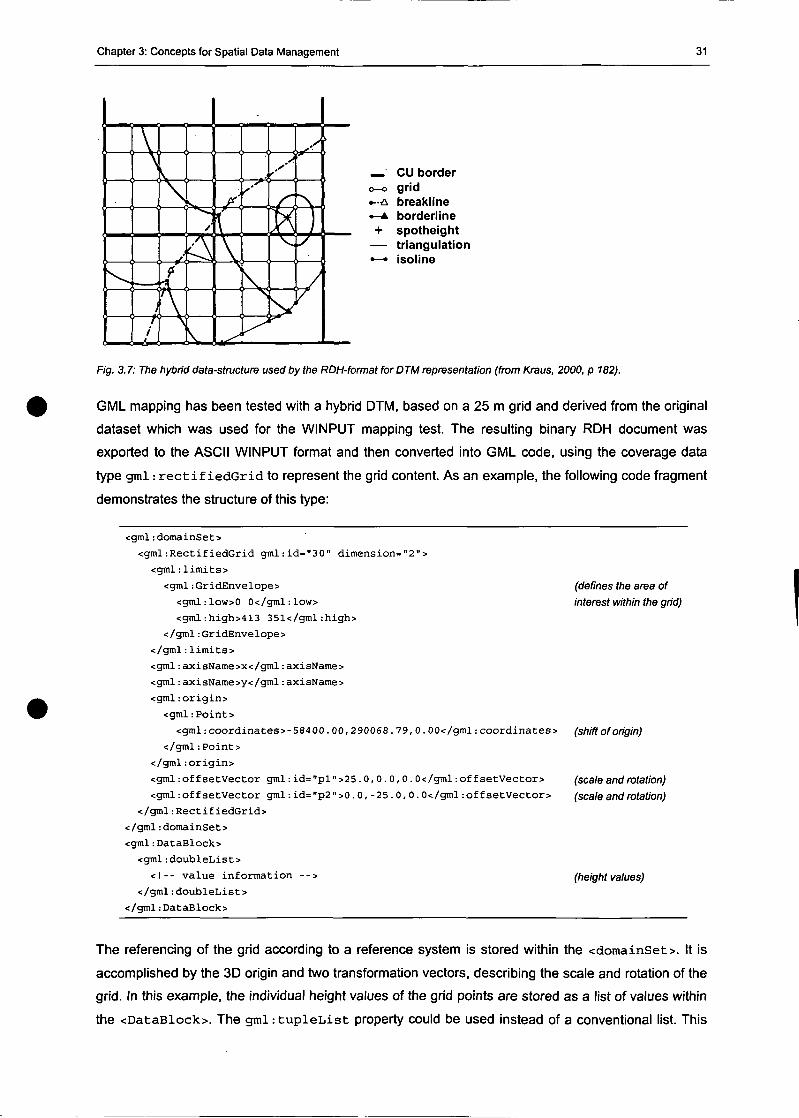
Chapter 3: Concepts for Spatial Data Management 31
_ CU bordero-o grid• -A breakline•—A borderline+ spotheight
— triangulation•—• isoline
Fig. 3.7: The hybrid data-structure used by the RDH-format forDTM representation (from Kraus, 2000, p 182).
GML mapping has been tested with a hybrid DTM, based on a 25 m grid and derived from the original
dataset which was used for the WINPUT mapping test. The resulting binary RDH document was
exported to the ASCII WINPUT format and then converted into GML code, using the coverage data
type gml : r e c t i f i e d G r i d to represent the grid content. As an example, the following code fragment
demonstrates the structure of this type:
(defines the area of
interest within the grid)
<gml:domainSet>
<gml:RectifiedGrid gml:id="30" dimension="2">
<gml:limits>
<gml:GridEnvelope>
<gml:low>0 0</gml:low>
<gml:high>413 351</gml:high>
</gml:GridEnvelope>
</gml:limits>
<gml:axisName>x</gml:axisName>
<gml:axisName>y</gml:axisName>
<gml:origin>
<gml:Point>
<gml :coordinates>-584 00.00,290068. 79, 0. 00</gtnl :coordinates>
</gml:Point>
</gml:origin>
<gral:offsetVector gml:id="pl">25.0,0.0,0.0</gml:offsetVector>
<gml:offsetVector gml:id="p2">0.0, -25.0, 0. 0</gml:offsetVector>
</gml:RectifiedGrid>
</gml:domainSet>
<gml:DataBlock>
<gml:doubleList>
<!-- value information -->
</gml:doubleList>
</gml:DataBlock>
(shift oforigin)
(scale and rotation)
(scale and rotation)
(height values)
The referencing of the grid according to a reference System is stored within the <domainSet>. It is
accomplished by the 3D origin and two transformation vectors, describing the scale and rotation of the
grid. In this example, the individual height values of the grid points are stored as a list of values within
the <DataBlock>. The gml : t u p l e L i s t property could be used instead of a conventional list. This
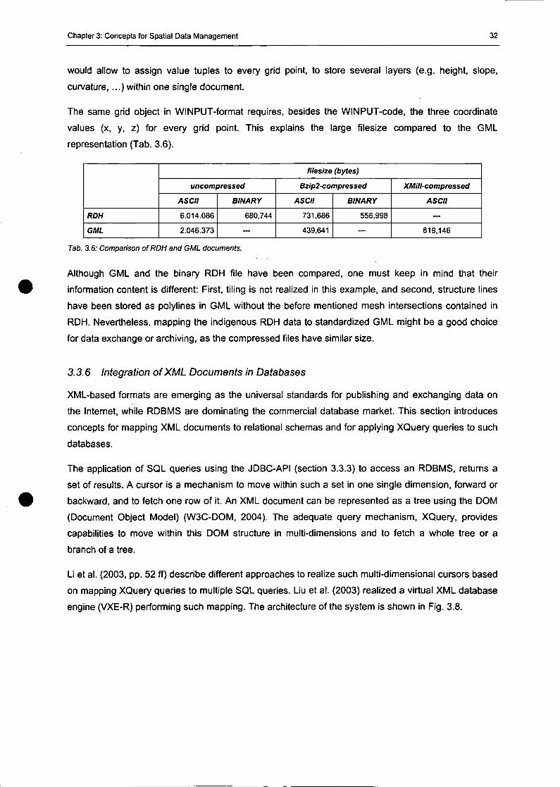
Chapter 3: Concepts for Spatial Data Management 32
would allow to assign value tuples to every grid point, to störe several layers (e.g. height, slope,
curvature,...) within one Single document.
The same grid object in WINPUT-format requires, besides the WINPUT-code, the three coordinate
values (x, y, z) for every grid point. This explains the large filesize compared to the GML
representation (Tab. 3.6).
RDH
GML
filesize (bytes)
uncompressed
ASCII
6.014.086
2.046.373
BINARY
680,744
—
Bzip2-compressed
ASCII
731,686
439,641
BINARY
556,998
—
XMill-compressed
ASCII
—
619,146
Tab. 3.6: Comparison ofRDH and GML documents.
Although GML and the binary RDH file have been compared, one must keep in mind that their
Information Content is different: First, tiling is not realized in this example, and second, structure lines
have been stored as polylines in GML without the before mentioned mesh intersections contained in
RDH. Nevertheless, mapping the indigenous RDH data to standardized GML might be a good choice
for data exchange or archiving, as the compressed files have similar size.
3.3.6 Integration ofXML Documents in Databases
XML-based formats are emerging as the universal Standards for Publishing and exchanging data on
the Internet, while RDBMS are dominating the commercial database market. This section introduces
concepts for mapping XML documents to relational Schemas and for applying XQuery queries to such
databases.
The application of SQL queries using the JDBC-API (section 3.3.3) to access an RDBMS, returns a
set of results. A Cursor is a mechanism to move within such a set in one Single dimension, forward or
backward, and to fetch one row of it. An XML document can be represented as a tree using the DOM
(Document Object Model) (W3C-DOM, 2004). The adequate query mechanism, XQuery, provides
capabilities to move within this DOM structure in multi-dimensions and to fetch a whole tree or a
branch of a tree.
Li et al. (2003, pp. 52 ff) describe different approaches to realize such multi-dimensional Cursors based
on mapping XQuery queries to multiple SQL queries. Liu et al. (2003) realized a Virtual XML database
engine (VXE-R) performing such mapping. The architecture of the System is shown in Fig. 3.8.
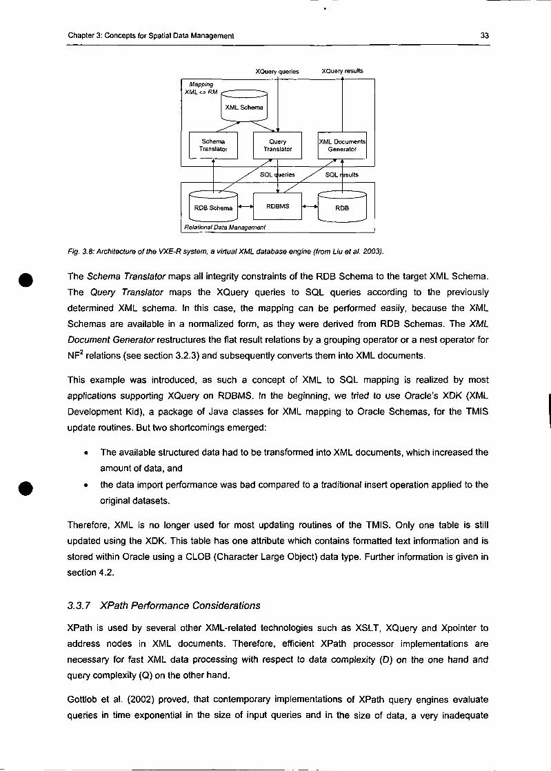
Chapter 3: Concepts for Spatial Data Management 33
XQuery queries XQuery results
Fig. 3.8: Architecture ofthe VXE-R System, a Virtual XML database engine (from Liu et al. 2003).
The Schema Translator maps all integrity constraints of the RDB Schema to the target XML Schema.
The Query Translator maps the XQuery queries to SQL queries according to the previously
determined XML Schema. In this case, the mapping can be performed easily, because the XML
Schemas are available in a normalized form, as they were derived from RDB Schemas. The XML
Document Generator restructures the flat result relations by a grouping Operator or a nest Operator for
NF2 relations (see section 3.2.3) and subsequently converts them into XML documents.
This example was introduced, as such a concept of XML to SQL mapping is realized by most
applications supporting XQuery on RDBMS. In the beginning, we tried to use Oracle's XDK (XML
Development Kid), a package of Java classes for XML mapping to Oracle Schemas, for the TMIS
update routines. But two shortcomings emerged:
• The available structured data had to be transformed into XML documents, which increased the
amount of data, and
• the data import Performance was bad compared to a traditional insert Operation applied to the
original datasets.
Therefore, XML is no longer used for most updating routines of the TMIS. Only one table is still
updated using the XDK. This table has one attribute which contains formatted text information and is
stored within Oracle using a CLOB (Character Large Object) data type. Further information is given in
section 4.2.
3.3.7 XPath Performance Considerations
XPath is used by several other XML-related technologies such as XSLT, XQuery and Xpointer to
address nodes in XML documents. Therefore, efficient XPath processor implementations are
necessary for fast XML data processing with respect to data complexity (D) on the one hand and
query complexity (Q) on the other hand.
Gottlob et al. (2002) proved, that contemporary implementations of XPath query engines evaluate
queries in time exponential in the size of input queries and in the size of data, a very inadequate
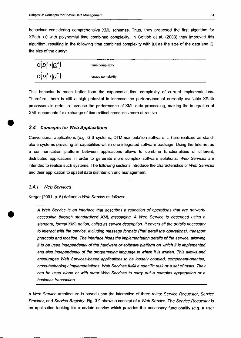
Chapter 3: Concepts for Spatial Data Management 34
behaviour considering comprehensive XML Schemas. Thus, they proposed the first algorithm for
XPath 1.0 with polynomial time combined complexity. In Gottlob et al. (2003) they improved this
algorithm, resulting in the following time combined complexity with |D| as the size of the data and |Q|
the size of the query:
time complexity
OlLD * \Q\ J space complexity
This behavior is much better than the exponential time complexity of current implementations.
Therefore, there is still a high potential to increase the Performance of currently available XPath
processors in order to increase the Performance of XML data processing, making the Integration of
XML documents for exchange of time critical processes more attractive.
3.4 Concepts for Web Applications
Conventional applications (e.g. GIS Systems, DTM manipulation Software, ...) are realized as stand-
alone Systems providing all capabilities within one integrated Software package. Using the Internet as
a communication platform between applications allows to combine functionalities of different,
distributed applications in order to generate more complex Software Solutions. Web Services are
intended to realize such Systems. The following sections introduce the characteristics of Web Services
and their application to spatial data distribution and management.
3.4.1 Web Services
Kreger (2001, p. 6) defines a Web Service as follows:
A Web Service is an interface that describes a collection of operations that are network-
accessible through standardized XML messaging. A Web Service is described using a
Standard, formal XML notion, called its service description. It Covers all the details necessary
to interact with the service, including message formats (that detail the operations), transport
protocols and location. The interface hides the Implementation details ofthe service, allowing
it to be used independently of the hardware or Software platform on which it is implemented
and also independently of the programming language in which it is written. This allows and
encourages Web Services-based applications to be loosely coupled, component-ohented,
cross-technology implementations. Web Services fulfill a specific task or a set oftasks. They
can be used alone or with other Web Services to carry out a complex aggregation or a
business transaction.
A Web Service architecture is based upon the interaction of three roles: Service Requestor, Service
Provider, and Service Registry. Fig. 3.9 shows a concept of a Web Service. The Service Requestor is
an application looking for a certain service which provides the necessary functionality (e.g. a user
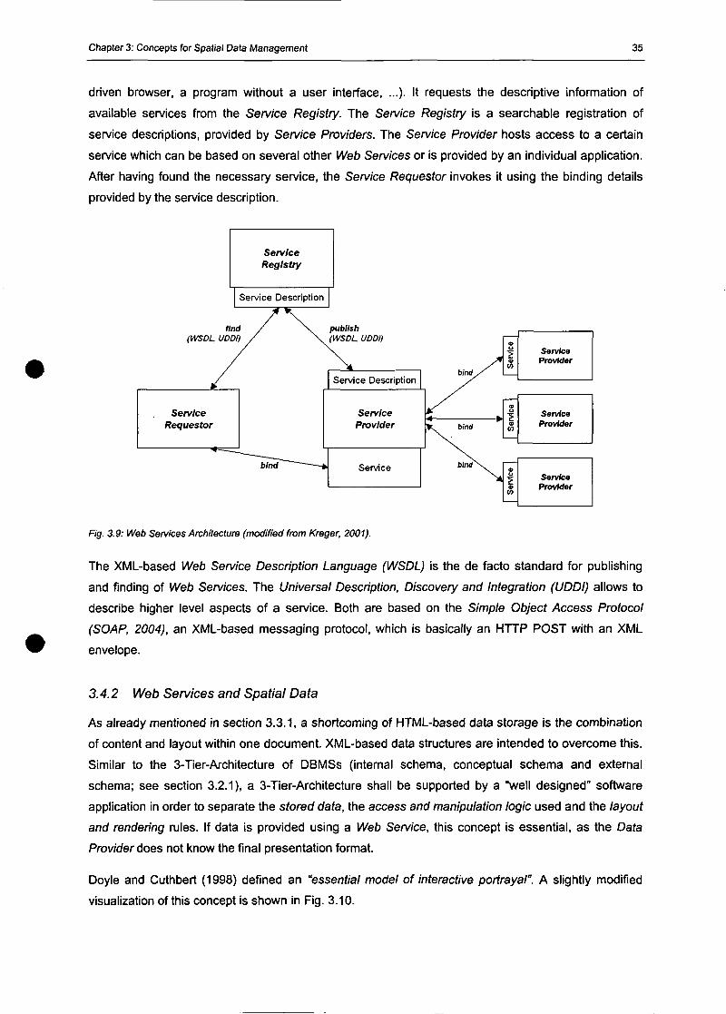
Chapter 3: Concepts for Spatial Data Management 35
driven browser, a program without a user interface, ...)• It requests the descriptive information of
available Services from the Service Registry. The Service Registry is a searchable registration of
service descriptions, provided by Service Providers. The Service Provider hosts access to a certain
service which can be based on several other Web Services or is provided by an individual application.
After having found the necessary service, the Service Requestor invokes it using the binding details
provided by the service description.
(WSDL.
ServiceRequestor
ServiceRegistry
Service Description
find / N.UDDI) / \
bind " *
publlsh(WSDL. UDDI)
\
Service Description
ServiceProvider
Service
sb/nd/
bind
bind\
Ser
vice
1
<P
1 S
er
N
\ S
ervi
ce
|
ServiceProvider
ServiceProvider
ServiceProvider
Fig. 3.9: Web Services Architecture (modified from Kreger, 2001).
The XML-based Web Service Description Language (WSDL) is the de facto Standard for Publishing
and finding of Web Services. The Universal Description, Discovery and Integration (UDDI) allows to
describe higher level aspects of a service. Both are based on the Simple Object Access Protocol
(SOAP, 2004), an XML-based messaging protocol, which is basically an HTTP POST with an XML
envelope.
3.4.2 Web Services and Spatial Data
As already mentioned in section 3.3.1, a shortcoming of HTML-based data storage is the combination
of content and layout within one document. XML-based data structures are intended to overcome this.
Similar to the 3-Tier-Architecture of DBMSs (internal schema, conceptual Schema and external
Schema; see section 3.2.1), a 3-Tier-Architecture shall be supported by a "well designed" Software
application in order to separate the stored data, the access and manipulation logic used and the layout
and rendering rules. If data is provided using a Web Service, this concept is essential, as the Dafa
Provider does not know the final presentation format.
Doyle and Cuthbert (1998) defined an "essential model of interactive portrayal". A slightly modified
visualization of this concept is shown in Fig. 3.10.
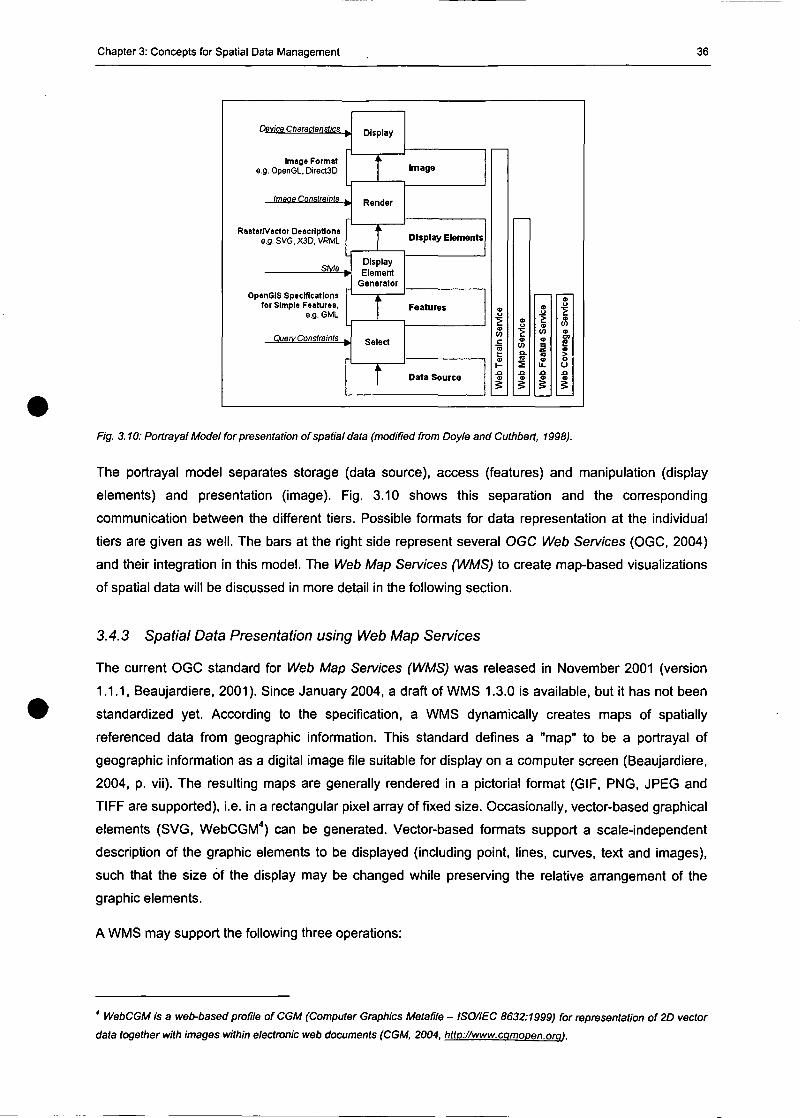
Chapter 3: Concepts for Spatial Data Management 36
Device Characteristics ..
Image Formate.g. OpenGL, Direct3D
imaQR Cnnstraints ^
Raster/Vector Descripttonse.g. SVG. X3D, VRML
SMS .
OpenGIS Speciflcatlons |for Simple Features,
e.g. GML
QuervConslreints ^
1
Display
Render
i
DisplayElement
Generator
L
Select
t
knage
Display Elements
Features
Data Source
1s
iu.o
u
Ser
vl
<D
29A0
O
I
F/g. 3.10: Portrayal Model for presentation of spatial data (modified from Doyle and Cuthbert, 1998).
The portrayal model separates storage (data source), access (features) and manipulation (display
elements) and presentation (image). Fig. 3.10 shows this Separation and the corresponding
communication between the different tiers. Possible formats for data representation at the individual
tiers are given as well. The bars at the right side represent several OGC Web Services (OGC, 2004)
and their Integration in this model. The Web Map Services (WMS) to create map-based visualizations
of spatial data will be discussed in more detail in the following section.
3.4.3 Spatial Data Presentation using Web Map Services
The current OGC Standard for Web Map Services (WMS) was released in November 2001 (version
1.1.1, Beaujardiere, 2001). Since January 2004, a draft of WMS 1.3.0 is available, but it has not been
standardized yet. According to the specification, a WMS dynamically creates maps of spatially
referenced data from geographic information. This Standard defines a "map" to be a portrayal of
geographic information as a digital image file suitable for display on a Computer screen (Beaujardiere,
2004, p. vii). The resulting maps are generally rendered in a pictorial format (GIF, PNG, JPEG and
TIFF are supported), i.e. in a rectangular pixel array of fixed size. Occasionally, vector-based graphical
elements (SVG, WebCGM4) can be generated. Vector-based formats support a scale-independent
description of the graphic elements to be displayed (including point, lines, curves, text and images),
such that the size of the display may be changed while preserving the relative arrangement of the
graphic elements.
A WMS may support the following three operations:
4 WebCGM is a web-based profile of CGM (Computer Graphics Metafile - ISO/IEC 8632:1999) for representation of 2D vector
data together with images within electronic web documents (CGM, 2004, htto://www.camooen arg).

Chapter 3: Concepts for Spatial Data Management 37
• GetCapabilities (mandatory): Returns metadata on the Service using a standardized XML
Schema.
• GetMap (mandatory): Returns a map (or a Service exception) according to the given
Parameters.
• GetFeaturelnfo (optional): Returns further Information on a selected feature.
The GefCapaö/W/es-operation provides the service description according to the Web Service
definition. The GeWWap-operation Supports the binding of the service. The implementation of a WMS is
presented in section 4.3.
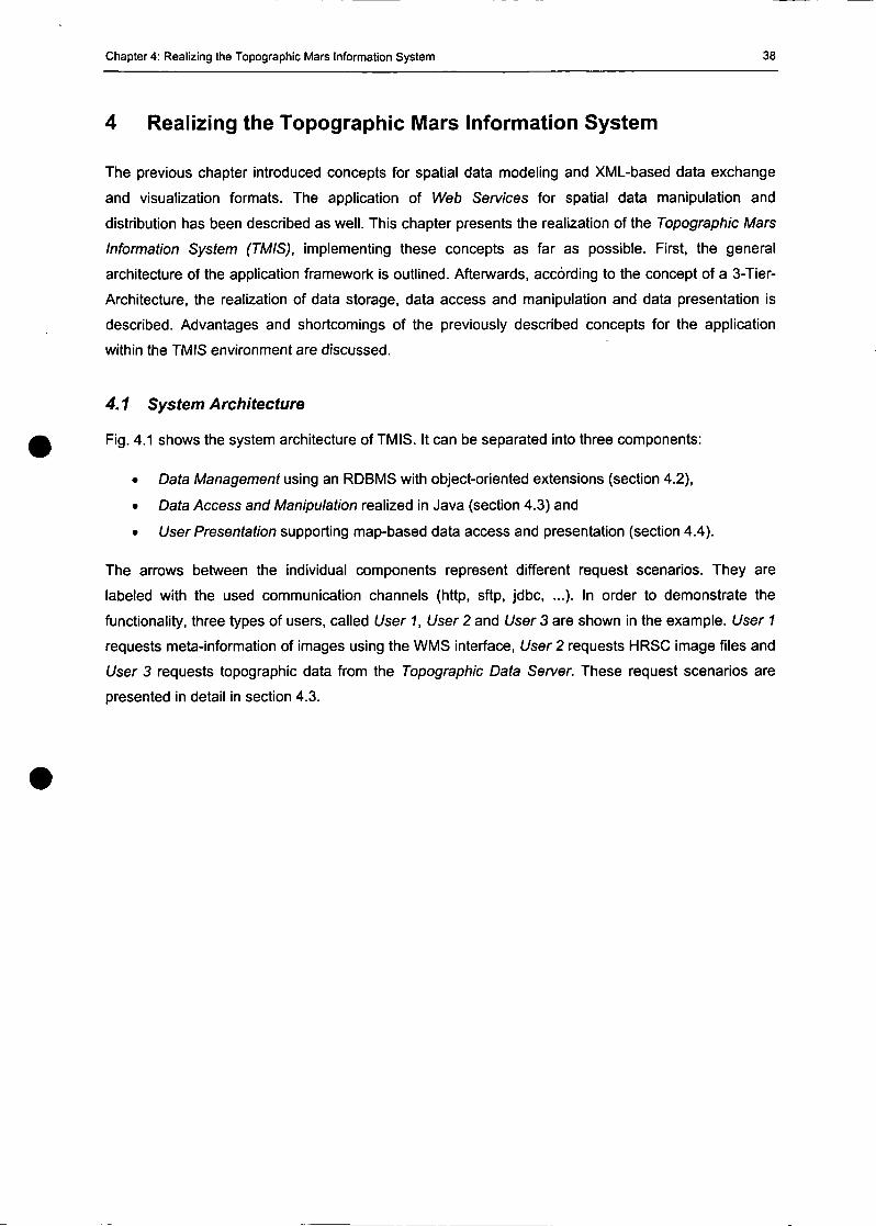
Chapter 4: Realizing the Topographie Mars Information System 38
4 Realizing the Topographie Mars Information System
The previous chapter introduced coneepts for spatial data modeling and XML-based data exchange
and visualization formats. The application of Web Services for spatial data manipulation and
distribution has been described as well. This chapter presents the realization of the Topographie Mars
Information System (TMIS), implementing these coneepts as far as possible. First, the general
architecture of the application framework is outlined. Afterwards, accörding to the coneept of a 3-Tier-
Architecture, the realization of data storage, data access and manipulation and data presentation is
described. Advantages and shortcomings of the previously described coneepts for the application
within the TMIS environment are discussed.
4.1 System Architecture
Fig. 4.1 shows the system architecture of TMIS. It can be separated into three components:
• Data Management using an RDBMS with objeet-oriented extensions (section 4.2),
• Data Access and Manipulation realized in Java (section 4.3) and
• User Presentation supporting map-based data access and presentation (section 4.4).
The arrows between the individual components represent different request scenarios. They are
labeled with the used communication Channels (http, sftp, jdbc, ...). In order to demonstrate the
functionality, three types of users, called User 1, User 2 and User 3 are shown in the example. User 1
requests meta-information of images using the WMS interface, User 2 requests HRSC image files and
User 3 requests topographic data from the Topographie Data Server. These request scenarios are
presented in detail in section 4.3.
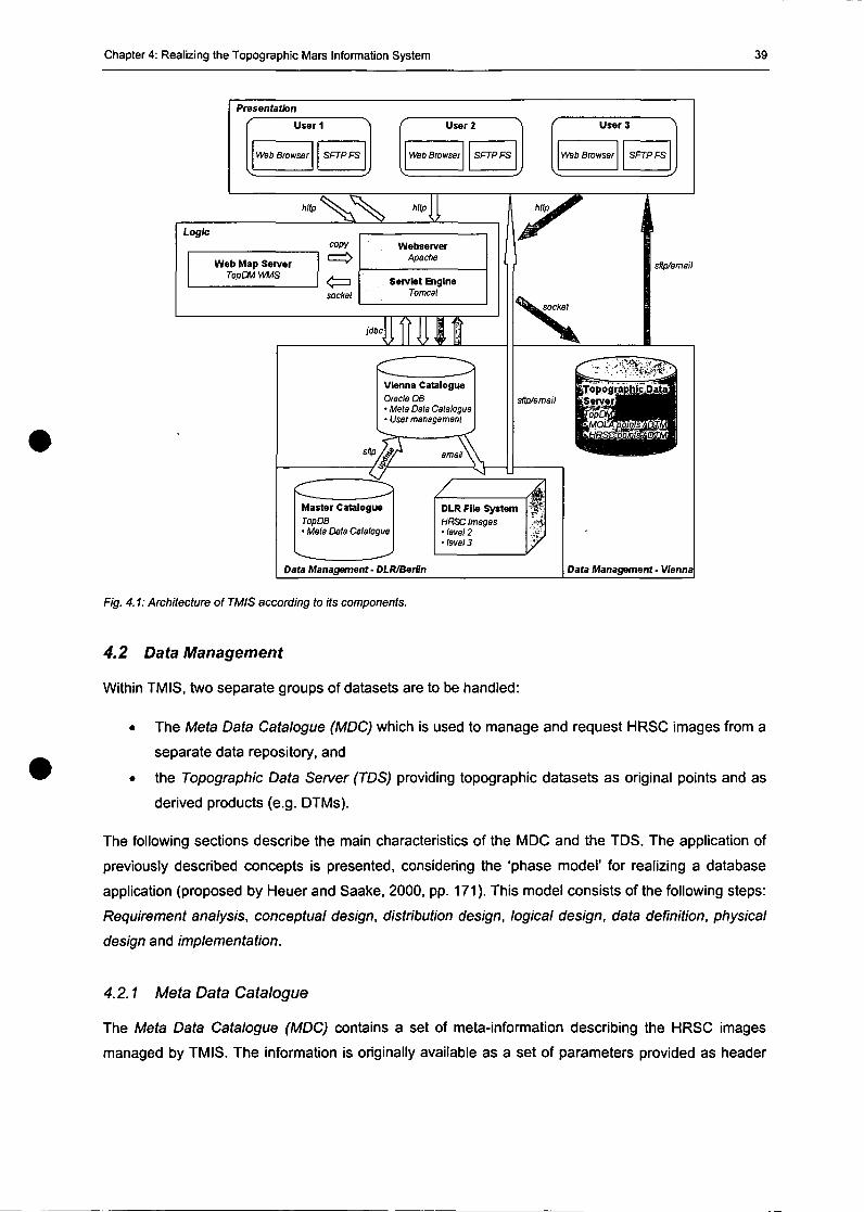
Chapter 4: Realizing the Topographic Mars Information System 39
Präsentation
User!
Web Browser SFTPFS
User 2
Wab Browser SFTPFS
User 3
Web Browser SFTPFS
http X X -IILogic
copy
Web Map ServerTopDMWMS
sockel
WebserverApache
Servlet EngineTomcat
jdbc\
sflp
Vienna Catalogue
Oracle DB• Meta Data Calalogue• User management
emaity
sockel
sUp/email
süp/emeil
Master Catalogue
TopDB• Mete Data Catalogue
Data Management - DLR/BerBn
DLR File System
HRSC Images•Ievel2•Ievel3
Data Management- Vienna
Fig. 4.1: Architecture of TMIS according to its components.
4.2 Data Management
Within TMIS, two separate groups of datasets are to be handled:
• The Meta Data Catalogue (MDC) which is used to manage and request HRSC images from a
separate data repository, and
• the Topographic Data Server (TDS) providing topographic datasets as original points and as
derived products (e.g. DTMs).
The foilowing sections describe the main characteristics of the MDC and the TDS. The application of
previously described concepts is presented, considering the 'phase model' for realizing a database
application (proposed by Heuer and Saake, 2000, pp. 171). This model consists of the foilowing Steps:
Requirement analysis, conceptual design, distribution design, logical design, data definition, physical
design and implementation.
4.2.1 Meta Data Catalogue
The Meta Data Catalogue (MDC) contains a set of meta-information describing the HRSC images
managed by TMIS. The information is originally available as a set of Parameters provided as header
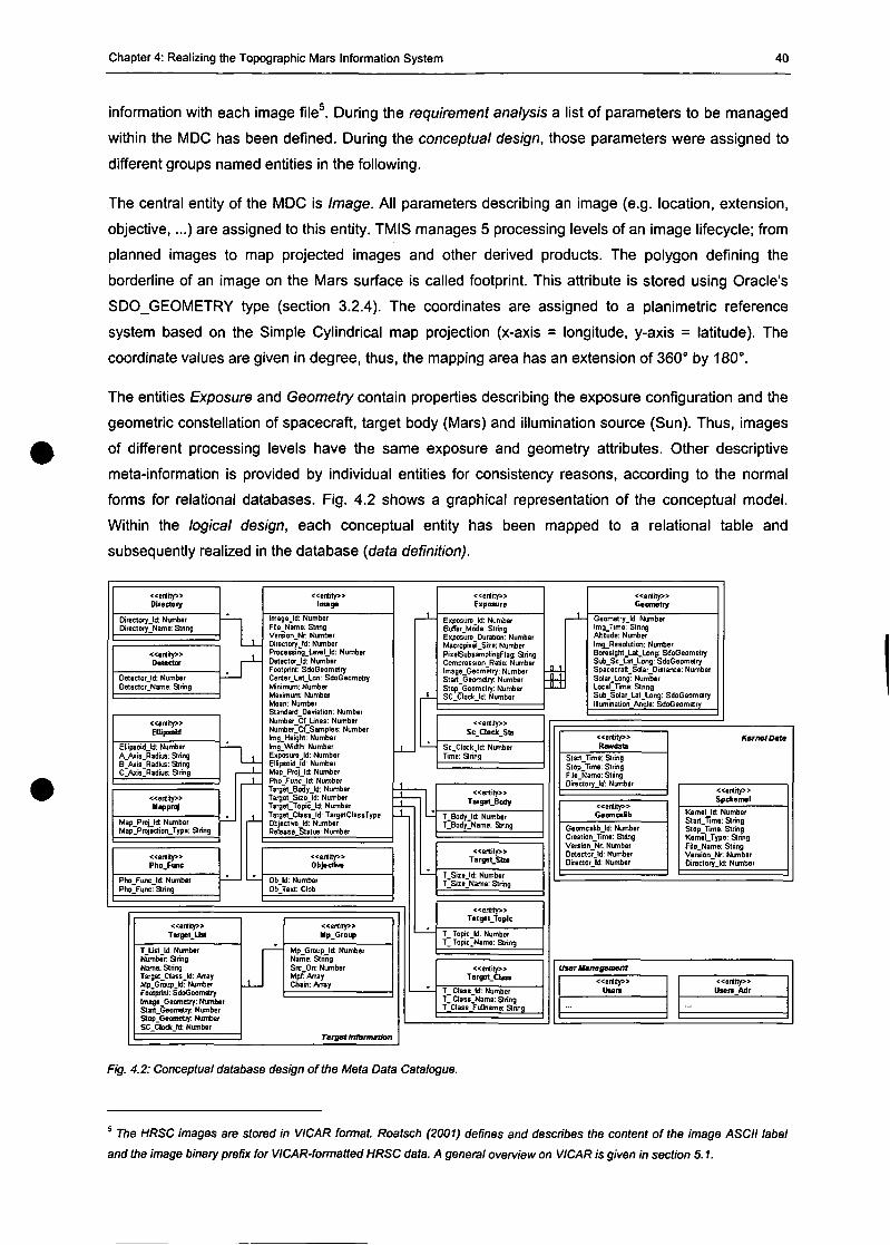
Chapter 4: Realizing the Topographie Mars Information System 40
information with each image file5. During the requirement analysis a list of Parameters to be managed
within the MDC has been defined. During the conceptual design, those parameters were assigned to
different groups named entities in the following.
The central entity of the MDC is Image. All parameters describing an image (e.g. location, extension,
objeetive,...) are assigned to this entity. TMIS manages 5 processing levels of an image lifecycle; from
planned images to map projeeted images and other derived produets. The polygon defining the
borderline of an image on the Mars surface is called footprint. This attribute is stored using Oracle's
SDO_GEOMETRY type (section 3.2.4). The coordinates are assigned to a planimetric reference
System based on the Simple Cylindrical map projeetion (x-axis = longitude, y-axis = latitude). The
coordinate values are given in degree, thus, the mapping area has an extension of 360° by 180°.
The entities Exposure and Geometry contain properties describing the exposure configuration and the
geometric constellation of spacecraft, target body (Mars) and illumination source (Sun). Thus, images
of different processing levels have the same exposure and geometry attributes. Other descriptive
meta-information is provided by individual entities for consistency reasons, aecording to the normal
forms for relational databases. Fig. 4.2 shows a graphical representation of the conceptual model.
Within the logical design, each conceptual entity has been mapped to a relational table and
subsequently realized in the database (data definition).
«ert i ty»Dlrectoiy
Dtrectoryjd: NumberDirectory_Name: String
«ert i ty»Dstector
Detectorjd: NumberDetector_Name: Sring
«ert i ty»EMpsold
Ellipsoidjd: NumberA Avis Radius: SlringBlAiislRadius: StringC Axe Radius Slring
«ert i ty»Mapp'4
Map_PrcjJd: NumberMap~Projection_Typ»; Slring
«ert i ty»Pho Func
Pho_Func_ld: NumberPho_Func: String
«er t i ty»Image
Imagejd: NumberFile Name: StringVersion_Nr NumberDirectoryJd: NumberProcessing_Level_ld: NumberDetBCtorJd: NumberFootprint: SdoGeometryCerrter_Lat_lon: SdoGeometryMinimum: NumberMaxrnum: NumberMean: NumberStandard_Deviation: NumberNumber_OfJJnes: NumberNumber~oTSamples: Numberlmg_Height: Numberlmg_Widtrt NumberExposure Id: NumberEllipsoidjd: NumberMap_ProjJd: NumberPho_Func_ld: NumberTarget_BodyJd: NumberTarget_Size_ld: NumberTarget_TopicJd: NumberTarget_ClassJd: TargetClassTypeObjectrvejd: NumberRelease Status: Number
«er t i ty»Objectiv«
Objd: NumberOb Text: Clob
«ert i ty»Tafgel.Ua
T List Id: NumberNumber! 3 ringName: StringTarget Class Id: ArrayMp Group U: Number
Image Geometry: NumberStart Geometry: NumberStop Geometry: NumbsfSC.CIodcJd: Number
1
«ert i ty»Mp_Group
Mp Group Id: NumberName: StringSrc On: NumberMpf. ArrayChain: Array
Target Information
«ert i ty»Exposure
Exposurejd: NumberBufferJrtöde: StringExposure_Duration: NumberMacropixel_Size; NumberPixeEubsampfingFlag: StringCompression_Ratio: Numberlmage_Geometry: NumberStart_Geometry: NumberSlop Geometry: NumberSC Clockjd: Number
«ert i ty»Sc_dod( Sta
Sc_ClockJd: NumberTime: String
«ert i ty»Targei_Body
T_Bo<Jy_ld: NumberT~Body~Name: Slring
«ert i ty»TargrtSIra
T_Size_ld: NumberT_SJ2e_Name: String
«ert i ty»Target_Toplc
T_ Topicjd: NumberT_ Topit_Name: String
«ert i ty»Targot_CJas»
T_ Ctass Jd: NumberT_ Ctass_NamB: StringT_Class_FuHname: String
«er t i ty»Geometty
Geometryjd: Numberlmg_Timfl: StringAttitüde: Numbertmg_Resolution: NumberBoresight Lat Long: SdoGeometrySub_Sc_Lat_Long: SdoGeometrySpacecraft_Sotar_Di8tance: NumberSolar_Long: NumberLocal_Time: StringSub_Solar_Lat_Long: SdoGeometrylllumination_Angle: SdoGeometry
User Management
«ert i ty»Rawvdata
Start_Tim9: SringStop_Time: StringFile_Name: StringDirectoryjd: Number
«ert i ty»GeomcBlb
Geomcalibjd: NumberCreation_Time: StringVereion_Nr. NumberDetector Id: NumberDiredor Id: Number
KerneJDato
Spckemel
Kemeljd: NumberStart_Üme: StringStop_Time: StringKernel Type: SringFile Name: StringVersion_Nr NunberDirectoryjd: Number
«er t i ly»Ussn
«er t i ty»Ussn Adr
Fig. 4.2: Conceptual database design ofthe Meta Data Catalogue.
5 77JO HRSC images are stored in VICAR formal Roatsch (2001) defines and describes the content of the image ASCII label
and the image binary prefix for VICAR-formatted HRSC data. A general overview on VICAR is given in section 5.1.
Chapter 4: Realizing the Topographie Mars Information System 41
For security and responsibility reasons, the MDC is managed in two, locally separated, catalogues,
physically located on different machines. The so-called Master Catalogue, based on TopDB, is
situated at the Institute for Planetary Research (Data Processing Working Group) at the German
Aerospace Center (DLR) in Berlin, Germany. This catalogue is used for data input of planned and real
image metadata. The filling Software application is implemented in IDL (Interactive Data Language,
2004). Therefore, an interface between the filling Software and TopDB has been realized. The Master
Catalogue is only available for members of the Data Processing Working Group.
The Vienna Catalogue, based on an Oracle Spatial database kernel, is available to all TMIS users and
accessible through the Internet. This catalogue is automatically updated using data unloads from the
Master Catalogue. The regularly updated tables are Image, Exposure, Geometry, SC_Clock_Sta,
Objective, Kernel and Target_List. Unfortunately, not only insert operations oeeur; Updates of existing
datasets are necessary as well (e.g. planning has been changed, new versions of already existing
images have been derived and released, ...). Therefore, it would be complicated to compare the
current Status of the Vienna Catalogue with that of the data, unloaded from the Master Catalogue, in
order to select the modified datasets. Thus, it is simpler to delete the whole Vienna Catalogue and fill it
again within every update process. In order to provide System availability during and data consistency
after this process, extensive update routines have been implemented. First, an XML-based exchange
format was tested. As the data has a struetured nature (compare section 3.3.1), the XML overhead
tumed out to be not necessary (increasing filesize, decreasing Performance, ...). Therefore, a simple,
ordered ASCII list is used. Only the OBJECTIVE table is still updated using an XML exchange format,
as it contains an attribute containing formatted text which is mapped to a Character Large Object
(CLOB) type within the database.
The HRSC image flies are stored in a filesystem at the DLR for two reasons: On the one hand, the
Terabytes of available images would increase the size of physical database storage to a great extend,
if they were managed within the DBMS (e.g. as Binary Large Objects - BLOBs); on the other hand,
many TMIS users employed at the DLR in Berlin and the Principal Investigator have direct access to
this filesystem.
4.2.2 Topographie Data Server
Besides the MDC, TMIS provides planet-wide topographic datasets as original data and as derived
DTMs, sampled by MOLA or derived from HRSC images. Requests for these datasets are time and
CPU intensive transactions. Therefore, the Topographic Data Server (TDS) is a physically separate
machine. TopDB is used for data management. Since data access is provided by TopDM, reference
System transformation and resampling capabilities are supported.
First tests were performed using the planet-wide MOLA dataset. Two different versions of MOLA
surface points are available: The randomly distributed original measurements and derived grid DTMs
with a resolution of 1/128°. The following Tab. 4.1 shows the amount of data if these datasets are
managed using TopDB and Oracle Spatial.
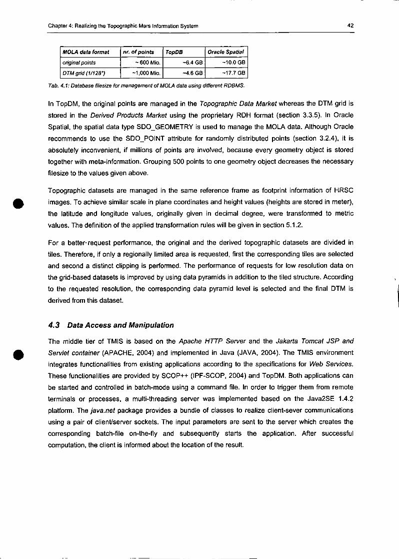
Chapter 4: Realizing the Topographie Mars Information System 42
MOLA data format
original points
DTMgrid (1/128°)
nr. of points
- 600 Mio.
-1,000 Mio.
TopDB
-6.4 GB
-4.6 GB
Oracle Spatial
-10.0 GB
-17.7 GB
Tab. 4.1: Database filesize for management of MOLA data using different RDBMS.
In TopDM, the original points are managed in the Topographie Data Market whereas the DTM grid is
stored in the Derived Products Market using the proprietary RDH format (section 3.3.5). In Oracle
Spatial, the spatial data type SDO_GEOMETRY is used to manage the MOLA data. Although Oracle
recommends to use the SDO_POINT attribute for randomly distributed points (section 3.2.4), it is
absolutely inconvenient, if millions of points are involved, because every geometry objeet is stored
together with meta-information. Grouping 500 points to one geometry objeet decreases the necessary
filesize to the values given above.
Topographie datasets are managed in the same reference frame as footprint information of HRSC
images. To achieve similar scale in plane coordinates and height values (heights are stored in meter),
the latitude and longitude values, originally given in decimal degree, were transformed to metric
values. The definition of the applied transformation rules will be given in section 5.1.2.
For a better-request Performance, the original and the derived topographic datasets are divided in
tiles. Therefore, if only a regionally limited area is requested, first the corresponding tiles are selected
and second a distinet clipping is performed. The Performance of requests for Iow resolution data on
the grid-based datasets is improved by using data pyramids in addition to the tiled strueture. According
to the requested resolution, the corresponding data pyramid level is selected and the final DTM is
derived from this dataset.
4.3 Data Access and Manipulation
The middle tier of TMIS is based on the Apache HTTP Server and the Jakarta Tomcat JSP and
Servlet Container (APACHE, 2004) and implemented in Java (JAVA, 2004). The TMIS environment
integrates functionalities from existing applications according to the speeifications for Web Services.
These functionalities are provided by SCOP++ (IPF-SCOP, 2004) and TopDM. Both applications can
be started and controlled in batch-mode using a command file. In order to trigger them from remote
terminals or processes, a multi-threading Server was implemented based on the Java2SE 1.4.2
platform. The java.net package provides a bündle of classes to realize client-sever Communications
using a pair of client/server sockets. The input parameters are sent to the Server which creates the
corresponding batch-file on-the-fly and subsequently Starts the application. After successful
computation, the dient is informed about the location of the result.
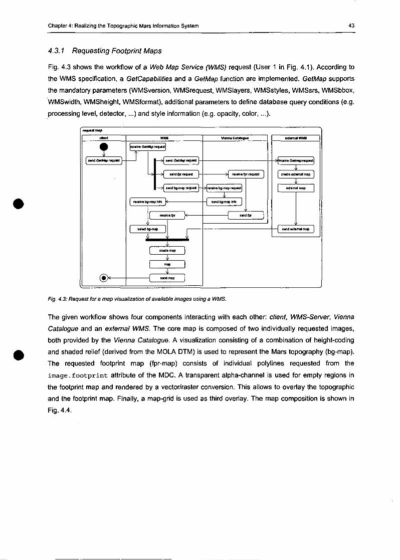
Chapter 4: Realizing the Topographie Mars Information System 43
4.3.1 Requesting Footprint Maps
Fig. 4.3 shows the Workflow of a Web Map Service (WMS) request (User 1 in Fig. 4.1). According to
the WMS speeification, a GetCapabilities and a GetMap funetion are implemented. GetMap supports
the mandatory parameters (WMSversion, WMSrequest, WMSlayers, WMSstyles, WMSsrs, WMSbbox,
WMSwidth, WMSheight, WMSformat), additional parameters to define database query conditions (e.g.
processing level, detector,...) and style information (e.g. opacity, color,...).
nquestmap
»hwGrfftfepraquH.
und GtfMap rtquast [
send fpr rat^Md
sartd bg-map r*qu«st
recalv« bg-map Wo te-
racalvafpr
salad bg-map
craatamap
sind map
Manna Catatogua
racalva fpr request
Mr*c*iv« bg-map raquast
ssnd bg-map bift
itndfpr
Fig. 4.3: Request fora map visualization ofavailable images using a WMS.
The given Workflow shows four components interacting with each other: dient, WMS-Server, Vienna
Catalogue and an external WMS. The core map is composed of two individually requested images,
both provided by the Vienna Catalogue. A visualization consisting of a combination of height-coding
and shaded relief (derived from the MOLA DTM) is used to represent the Mars topography (bg-map).
The requested footprint map (fpr-map) consists of individual polylines requested from the
image. f o o t p r i n t attribute of the MDC. A transparent alpha-channel is used for empty regions in
the footprint map and rendered by a vector/raster conversion. This allows to overlay the topographic
and the footprint map. Finally, a map-grid is used as third overlay. The map composition is shown in
Fig. 4.4.
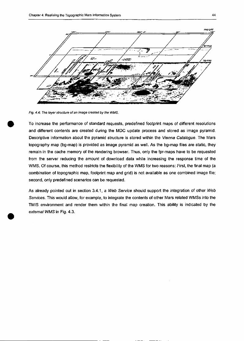
Chapter 4: Realizing the Topographie Mars Information System 44
map grid
Fig. 4.4: The layer structure ofan image created by the WMS.
To increase the Performance of Standard requests, predefined footprint maps of different resolutions
and different contents are created during the MDC update process and stored as image pyramid.
Descriptive information about the pyramid structure is stored within the Vienna Catalogue. The Mars
topography map (bg-map) is provided as image pyramid as well. As the bg-map files are static, they
remain in the cache memory of the rendering browser. Thus, only the fpr-maps have to be requested
from the Server reducing the amount of download data while increasing the response time of the
WMS. Of course, this method restricts the flexibility of the WMS for two reasons: First, the final map (a
combination of topographic map, footprint map and grid) is not available as one combined image file;
second, only predefined scenarios can be requested.
As already pointed out in section 3.4.1, a Web Service should support the integration of other Web
Services. This would allow, for example, to integrate the contents of other Mars related WMSs into the
TMIS environment and render them within the final map creation. This ability is indicated by the
external WMS in Fig. 4.3.
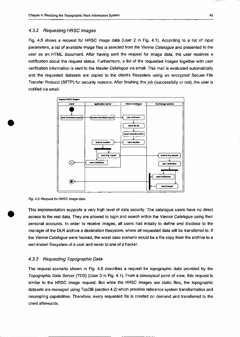
Chapter 4: Realizing the Topographie Mars Information System 45
4.3.2 Requesting HRSC Images
Fig. 4.5 shows a request for HRSC image data (User 2 in Fig. 4.1). According to a list of input
Parameters, a list of available image files is selected from the Vienna Catalogue and presented to the
user as an HTML document. After having sent the request for image data, the user reeeives a
notification about the request Status. Furthermore, a list of the requested images together with user
verification information is sent to the Master Catalogue via email. This mail is evaluated automatically
and the requested datasets are copied to the dient's filesystem using an encrypted Secure File
Transfer Protocol (SFTP) for security reasons. After finishing this job (successfully or not), the user is
notified via email.
reguast HRSC tneges
Isend Download request] ^racalva Download request j * l
appllcaUon
recalve rasuBset
sand bng request
Vtaina Catalogua
usar veriflcBUon
talad metaliformallon
DLR Image archive
recetve bng requast
user veriflceSon
liisend notfflcatJonfl < [ send tmaaes
Fig. 4.5: Request for HRSC image data.
This implementation supports a very high level of data security. The catalogue users have no direct
access to the real data. They are allowed to login and search within the Vienna Catalague using their
personal aecounts. In order to reeeive images, all users had initially to define and disclose to the
manager of the DLR archive a destination filesystem, where all requested data will be transferred to. If
the Vienna Catalogue were hacked, the worst case scenario would be a file copy from the archive to a
well-known filesystem of a user and never to one of a hacker.
4.3.3 Requesting Topographie Data
The request scenario shown in Fig. 4.6 describes a request for topographic data provided by the
Topographie Data Server (TDS) (User 3 in Fig. 4.1). From a conceptual point of view, this request is
similar to the HRSC image request. But while the HRSC images are static files, the topographic
datasets are managed using TopDB (section 4.2) which provides reference System transformation and
resampling capabilities. Therefore, every requested file is created on demand and transferred to the
dient afterwards.
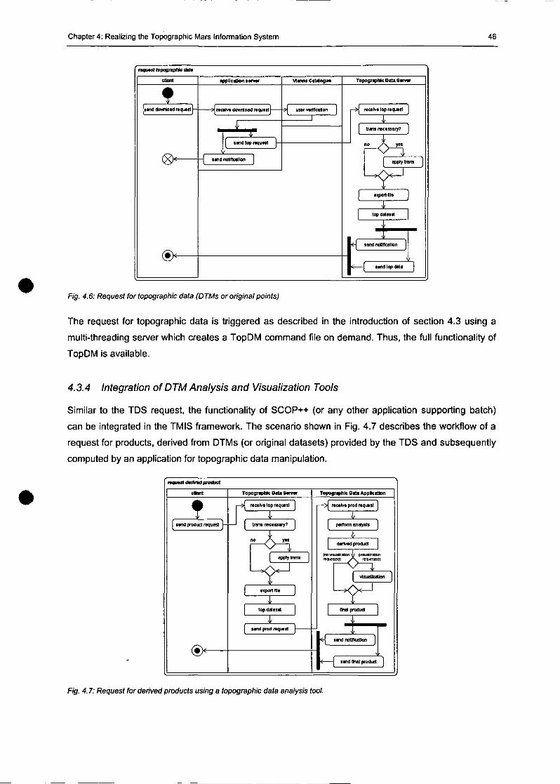
Chapter 4: Realizing the Topographic Mars Information System 46
request CopograpMo deta
send download request t
< § > -
appUcatf on sei
recelve dowriodd requsst
sind top request
send nouftcation
Viaina CataJogue
usar vwfflcaUon
Topographie Data Sarvar
->( recelve top raquast
itrans necessary?
apply trans
txponflla
top dataset
k T sand top dala
Fig. 4.6: Request for topographic data (DTMs or original points)
The request for topographic data is triggered as described in the introduction of section 4.3 using a
multi-threading Server which creates a TopDM command file on demand. Thus, the füll functionality of
TopDM is available.
4.3.4 Integration of DTM Analysis and Visualization Tools
Similar to the TDS request, the functionality of SCOP++ (or any other application supporting batch)
can be integrated in the TMIS framework. The scenario shown in Fig. 4.7 describes the Workflow of a
request for products, derived from DTMs (or original datasets) provided by the TDS and subsequentiy
computed by an application for topographic data manipulation.
requast derfmtf produet
sand produd request
Topographic Data Server
rocelve top request
trans neeexsary?
appty Irans
exportffle
top dfllaset
send prod raquist
Topographie Data Applcstton
recelve prod request
perform anatysts
denved produd
|no vrauacaoon \ l / (vttuatttaoon
flnflJ pi oduet
LJ —
B^i sand nouncfitJon
k 1 und (hol prod
Fig. 4.7: Request for derived products using a topographic data analysis tool.
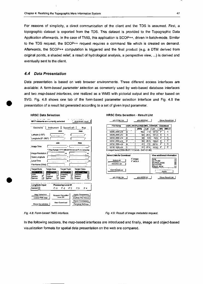
Chapter 4: Realizing the Topographie Mars Information System 47
For reasons of simplicity, a direct communication of the dient and the TDS is assumed. First, a
topographic dataset is exported from the TDS. This dataset is provided to the Topographie Data
Application afterwards. In the case of TMIS, this application is SCOP++, driven in batch-mode. Similar
to the TDS request, the SCOP++ request requires a command file which is created on demand.
Afterwards, the SCOP++ computation is triggered and the final produet (e.g. a DTM derived from
original points, a shaded relief, a result of hydrological analysis, a perspective view, ...) is derived and
eventually sent to the dient.
4.4 Data Presentation
Data presentation is based on web browser environments. Three different access interfaces are
available: A form-based parameter selection as commonly used by web-based database interfaces
and two map-based interfaces, one realized as a WMS with pictorial Output and the other based on
SVG. Fig. 4.8 shows one tab of the form-based parameter selection interface and Fig. 4.9 the
presentation of a result list generated according to a set of given input parameter.
HRSC Data Selection
18817 dataset» are currently selected ; deactivate com
Geometry Instrument | SpaceCraft
min
Map
max
Latitude (± 90'):
! Longitude (0*-360*):
min
Image Time | J- LZ
| Image Resolution f Z I Z T
j Solar Longitude |
J Local Time |
• Tim»Formet YVYY-UllDDTbli:rrm:a3.m tu • Kibstring
m I _ ' m
• |
h |
I File Name (Orbit) [ |
Target Body Target Size Target Topic Target Class
global ,Vj |color i£J |jnipact__ __^J
Longitude Input
leastemM
Processing Level ID
C-3 C-2 C2 rj3 r,4
Mop Selection | R p m i M t R p B 1 „ I t i R t
create FPR map | *""" DB
. Start DownloadQose this Window |
Appry Parameters
min/max Par Values
Reset Parameters
Personal Setiin gs
Fig. 4.8: Form-based TMIS interface.
HRSC Data Selection - Result List
p/s HTML list | p/s ASCII list Ctose Result List |
File Name ;VER_NR
. 1h0205_aaao.s23 ;|3
h0228_OO0D.s23 ||5
h0232_OQ00.s23 :[5
FILESIZE ;IMG_CENTER[MB] j
162
60
38
h0241_0000.s23 j|7 j 56
h0243_0000.s23 !|4
h0248_0000.s23 |J1
41j
31|
Lat
-7 2,
-30.^
8.5
-30.7j
-7.3,
-37.4
Lon
187.9
157.2
74.5;
156.4
297.6
102.8'
Download 'IMGr
r -
•=r :r: •
MOLA
n iC !
n jn 1n i
6 images found (2004-06-07 /17:0<!:48 - GMT+01:00)
Select Data for Download
' Seled all |
I Oeselect all |
{ Start Download |
rimageTMOLA
View addltional Information
noneALTTTUDEBUFFER.MODEDETECTOREVEMT_NOTE
I Appry
äUli
|p/s HTML list | p/8 ASCII lisl dose Result List |
Fig. 4.9: Result of image metadata request.
In the following sections, the map-based interfaces are introduced and finally, image and object-based
visualization formats for spatial data presentation on the web are compared.
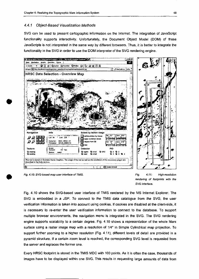
Chapter 4: Realizing the Topographie Mars Information System 48
4.4.1 Object-Based Visualization Methods
SVG can be used to present cartographic Information on the Internet. The Integration of JavaScript
functionality Supports interactivity. Unfortunately, the Document Object Model (DOM) of these
JavaScripts is not interpreted in the same way by different browsers. Thus, it is better to integrate the
functionality in the SVG in order to use the DOM interpreter of the SVG rendering engine.
B*el Gearteten anskrt favorten Egtros l
-•ZuOck | ^Suchen gJFavorten gj ffi S] &j » j (»Wethselnzu |
HRSC Data Selection - Overview Map
Navigation Info
Detector: MEX_HRSC_S1Filename: h0143_0009s13
ToxturoOstiadingOzcoOjng
Seals: 1Textur«: IM TpixStatus: ready!
Select by lat/lon ränge^ J defme Window by mouse
^ J apply numerical values
PBp request from DB
Qhdp
Detector| Or/g/bm O»l/s2 O SRC
O nadir 9 P"P2
I lat: -32 • I llon: 352*1L V " . Jl. . T J-SO -45 0 4S M 1S02700 SO 18
llat: 19' llon: 316"
• « -45 Q 45 90 ISO 270 0 SO 180
PIDO-3 O-20 2 O 3 9 4
This tool is based on Scalable Vector Graphics. The usage of the tool as well as Ihe Installation of the neccessary plug-in aredescribed in the help section.
___../«
Fig. 4.10: SVG-based map user interface of TMIS. Fig. 4.11: High-resolution
rendering of footprints with the
SVG interface.
Fig. 4.10 shows the SVG-based user interface of TMIS rendered by the MS Internet Explorer. The
SVG is embedded in a JSP. To connect to the TMIS data catalogue from the SVG, the user
verification Information is taken into aecount using Cookies. If Cookies are disabled at the client-side, it
is necessary to re-enter the user verification Information to connect to the database. To support
multiple browser environments, the navigation menu is integrated in the SVG. The SVG rendering
engine Supports scalability to a certain degree. Fig. 4.10 shows a representation of the whole Mars
surface using a raster image map with a resolution of 1/4° in Simple Cylindrical map projeetion. To
support further zooming to a higher resolution (Fig. 4.11), different levels of detail are provided in a
pyramid strueture. If a certain zoom level is reached, the corresponding SVG level is requested from
the server and replaces the former one.
Every HRSC footprint is stored in the TMIS MDC with 100 points. As it is often the case, thousands of
images have to be displayed within one SVG. This results in requesting large amounts of data from
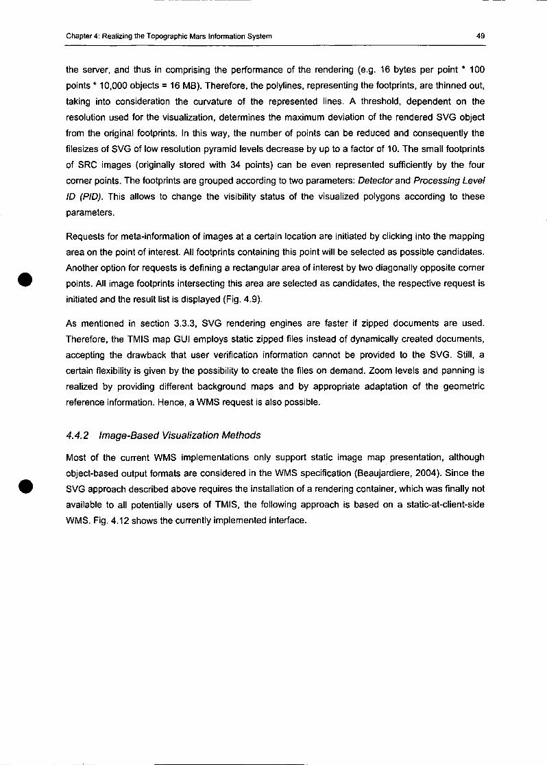
Chapter 4: Realizing the Topographie Mars Information System 49
the Server, and thus in comprising the Performance of the rendering (e.g. 16 bytes per point * 100
points * 10,000 objeets = 16 MB). Therefore, the polylines, representing the footprints, are thinned out,
taking into consideration the curvature of the represented lines. A threshold, dependent on the
resolution used for the visualization, determines the maximum deviation of the rendered SVG objeet
from the original footprints. In this way, the number of points can be reduced and consequently the
filesizes of SVG of Iow resolution pyramid levels decrease by up to a factor of 10. The small footprints
of SRC images (originally stored with 34 points) can be even represented sufficiently by the four
corner points. The footprints are grouped aecording to two parameters: Detector and Processing Level
ID (PID). This allows to change the visibility Status of the visualized polygons aecording to these
Parameters.
Requests for meta-information of images at a certain location are initiated by clicking into the mapping
area on the point of interest. All footprints containing this point will be selected as possible candidates.
Another Option for requests is defining a reetangular area of interest by two diagonally opposite corner
points. All image footprints intersecting this area are selected as candidates, the respective request is
initiated and the result list is displayed (Fig. 4.9).
As mentioned in section 3.3.3, SVG rendering engines are faster if zipped documents are used.
Therefore, the TMIS map GUI employs static zipped files instead of dynamically created documents,
aeeepting the drawback that user verification information cannot be provided to the SVG. Still, a
certain flexibility is given by the possibility to create the files on demand. Zoom levels and panning is
realized by providing different background maps and by appropriate adaptation of the geometric
reference information. Hence, a WMS request is also possible.
4.4.2 Image-Based Visualization Methods
Most of the current WMS implementations only support static image map presentation, although
objeet-based Output formats are considered in the WMS speeification (Beaujardiere, 2004). Since the
SVG approach described above requires the installation of a rendering Container, which was finally not
available to all potentially users of TMIS, the following approach is based on a static-at-client-side
WMS. Fig. 4.12 shows the currently implemented interface.
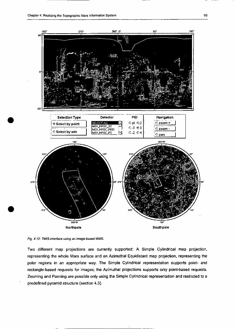
Chapter 4: Realizing the Topographie Mars Information System 50
180* 270' 360* 0'
Selection Type
f? Select by point
C Select by win
Detector
MEX_HRSC_S2MEX_HRSC_REDMEX_HRSC_P2
PID
Gall O2O-3 ©3Q-2 CM
Navigation
C zoom +
I C zoom -
I O pan
315-
360*10* HO'
Northpole Southpole
Fig. 4.12: TMIS-interface using an image-based WMS.
Two different map projections are currently supported: A Simple Cylindrical map projection,
representing the whole Mars surface and an Azimuthai Equidistant map projection, representing the
polar regions in an appropriate way. The Simple Cylindrical representation supports point- and
rectangle-based requests for images; the Azimuthai projections supports only point-based requests.
Zooming and Panning are possible only using the Simple Cylindrical representation and restricted to a
predefined pyramid strueture (section 4.3).
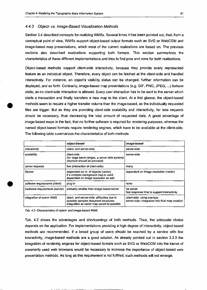
Chapter 4: Realizing the Topographie Mars Information System 51
4.4.3 Object- vs. Image-Based Visualization Methods
Section 3.4 described coneepts for realizing WMSs. Several times it has been pointed out, that, from a
conceptual point of view, WMSs support objeet-based output formats such as SVG or WebCGM and
image-based map presentations, which most of the current realizations are based on. The previous
sections also described realizations supporting both formats. This section summarizes the
characteristics of these different implementations and tries to find pros and cons for both realizations.
Object-based methods support client-side interactivity, because they provide every represented
feature as an individual object. Therefore, every object can be fetched at the client-side and handled
interactively. For instance, an object's visibility Status can be changed, further information can be
displayed, and so forth. Contrarily, image-based map presentations (e.g. GIF, PNG, JPEG, ...) behave
static, as no client-side interaction is allowed. Every user interaction has to be sent to the Server which
Starts a transaction and finally transfers a new map to the dient. At a first glance, the object-based
methods seem to require a higher transfer volume than the image-based, as the individually requested
files are bigger. But as they are providing client-side scalability and interactivity, far less requests
should be necessary, thus decreasing the total amount of requested data. A great advantage of
image-based maps is the fact, that no further Software is required for rendering purposes, whereas the
named object-based formats require rendering engines, which have to be available at the client-side.
The following table summarizes the characteristics of both methods.
interactivity
scalability
Server requests
filesize
Software requirements (dient)
hardware requirements (Server)
Integration of extern WMS
object-based
dient- and server-side
client-side(for large zoom ranges, a server-side pyramidstrueture should be provided)
few (interaction at client-side)
dependent on nr. of objeets (vector)if a complex background map is used:dependent on image resolution as well
plug-in
probably smaller than image-based Server
dient- and server-side: difficulties due topossibly complex document struetures;Integration as raster map would be possible
image-based
server-side
server-side
many
dependent on image resolution (raster)
none
fat serverfast response time to support interactivity
client-side: using overlaysserver-side: Integration into final map creation
Tab. 4.2: Characteristics of object- and image-based WMS.
Tab. 4.2 shows the advantages and shortcomings of both methods. Thus, the adequate choiee
depends on the application. For implementations providing a high degree of interactivity, object-based
methods are recommended. If a broad group of users should be reached by a Service with few
interactivity, image-based methods are a good solution. As already pointed out in section 3.3.3 the
integration of rendering engines for object-based formats such as SVG or WebCGM into the kernel of
commonly used web browsers would be necessary to increase the importance of object-based web
presentation methods. As long as this requirement is not fulfilled, such methods will not emerge.
Chapter 5: Modeling the Topography 52
5 Modeling the Topography of Mars
Information Systems dealing with spatial data are often named Geographie Information Systems (GIS).
Per definition, a GIS is a Computer based System, consisting of hardware, Software, data and
applications. It is dedicated to acquisition, editing, storage, and reorganization, to modeling and
analysis and to alphanumeric and graphical presentation of spatial data. Although TMIS fulfills those
requirements, it cannot be compared to commercial GIS Systems such as Arclnfo (ESRI, 2004) or to
the open source projeet GRASS (GRASS, 2004), as the provided functionality has been separated
into two different groups:
• data management and distribution and
• analysis and visualization.
Chapter 3 presented coneepts and methods for data management and distribution and chapter 4 their
application to realize the TMIS. The Integration of topographic data processing and analysis tools into
the TMIS environment is discussed in this chapter (topographic data processing) and chapter 6
(application and results). The tools and methods providing these capabilities are named TMIS
Extended Functionality (TMIS-EF). Most of these tools are directly integrated into the TMIS and
available through the TMIS-Col-Interface. Some are part of the Software application SCOP++ (IPF-
SCOP, 2004), which is - as part of the TMIS usage contract - available to the entire HRSC Co-
Investigator projeet group.
The following sections describe the initial State of the available methods (most of them originally
developed for application on Earth) and the necessary modifications and extensions for application to
Mars DTMs. The investigation and implementation of methods and algorithms for manipulation,
analysis and visualization of topographic data is of general interest. But in order to evaluate their
usability, it is essential to apply them within an appropriate context and to modify them if necessary.
Therefore, topographic and image datasets from the NASA mission Mars Global Surveyor (MGS) were
investigated in detail.
This chapter and the following chapter 6 deals present whole Workflow as applied to the available data
- from data pre-processing to the computation of DTMs - and the analysis and appropriate
visualizations of both, the data and the results. After an overview of the initial Situation, chapter 5 deals
with the task of deriving a homogeneous DTM from the available MOLA original points which contain
erroneous measurements. Thus, the data pre-processing consists of error elimination and data
homogenization. An automated method for error detection and subsequent elimination of erroneous
points from the original MOLA point cloud is described in detail and different possibilities to derive a
grid-based DTM from the inhomogeneously distributed original points are discussed.
In chapter 6, the application of raster-based methods for analyzing those DTMs is described.
Especially hydrological analysis seems to have a high potential to derive modeis to reconstruet the
behavior of possible former surface water on Mars in a plausible manner. The results of the analysis of
Chapter 5: Modeling the Topography 53
three selected regions on Mars, which are very likely to have been formed by surface water, are
discussed in detail:
• hydrological mapping of the Tharsis Highlands and Valles Mahneris (section 6.1.1);
• outflow Channel detection in the Elysium Region (section 6.1.2);
• simulated outflow behavior in Ma'adim Vallis and Gusev Crater (section 6.1.3).
Finally different methods for 3D visualization of DTMs and corresponding raster image overlays are
described and exemplary results are presented.
5.1 Initial Situation
Most of the widely used methods and applications for DTM analysis and visualization are based on a
raster data structure. A discrete quadratic area, often named pixel, is associated to one Single value
containing the mean height of the area to be represented. A regulär raster of adjacent cells covers the
whole area of interest (Kraus, 2000, p. 181). A commonly used Software application applied to
topographic Mars data is VICAR. It is a set of Computer programs and procedures designed to
facilitate the acquisition, processing and handling of digital image data. The VICAR image processing
language was defined and implemented in 1966 at the Jet Propulsion Laboratory (JPL) to process
image data produced by the planetary exploration program (Duxbury and Jensen, 1994). Since then, it
has been continuously improved.
A raster-based DTM is a simple matrix structure, organized in lines and samples and stored as a
binary stream of values, e.g. representing the heights. The meta-information (extension, geo-
referencing, data acquisition, ...) can be provided by a so-called header included in the dataset. The
VICAR format may include two separate parts of meta-information: A piain text label provided as a
header containing general information on the dataset (e.g. number of lines, number of samples,
referencing, origin, purpose, ...) and an optional label information for each individual line, containing
descriptive information on this line (e.g. erroneous pixel,...). Such formats are simple to read and write
and thus provide a high Performance as no redundant information is necessary. Contrary to randomly
distributed points, in a regulär raster it is not necessary to störe the individual coordinates of the
points. The location can be derived from the associated line and sample number using the header
information. The great advantage of the possibility to use fast raster-based operations is combined
with the disadvantage that derived products depend on the given raster width. Thus, data manipulation
involving resampling (e.g. a datum transformation) can cause a loss of information.
The data format used in the following considerations describes the terrain using a hybrid DTM
structure (section 3.3.5). As a matter of principle, it is also based on the storage of regulär, grid-wise
distributed points, derived from the original measured points. But the data access algorithm Supports
the computation of any point within this grid using a high level function to interpolate the area between
the given points. This allows to derive products (iso-lines, shaded relief, ...) at a higher resolution as
provided by the given grid.
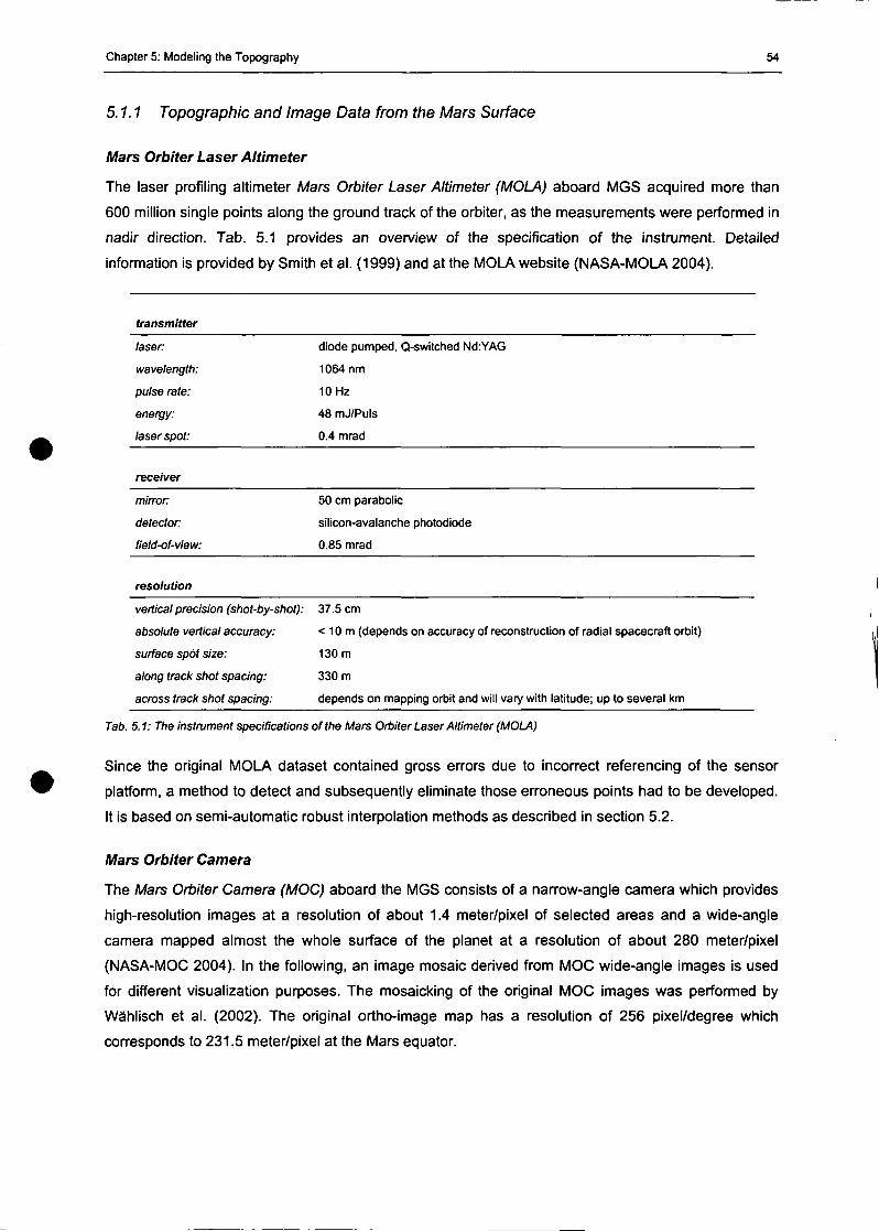
Chapter 5: Modeling the Topography 54
5.1.1 Topographie and Image Data from the Mars Surface
Mars Orbiter Laser Altimeter
The laser profiling altimeter Mars Orbiter Laser Altimeter (MOLA) aboard MGS acquired more than
600 million Single points along the ground track of the orbiter, as the measurements were performed in
nadir direction. Tab. 5.1 provides an overview of the speeification of the instrument. Detailed
information is provided by Smith et al. (1999) and at the MOLA Website (NASA-MOLA 2004).
transmitter
laser: diode pumped, Q-switched Nd:YAG
wavelength: 1064 nm
pulse rate: 10 Hz
energy: 48 mJ/Puls
laser spot: 0.4 mrad
reeeiver
mirror: 50 cm parabolic
detecton silicon-avalanche photodiode
field-of-view: 0.85 mrad
resolution
vertical precision (shot-by-shot): 37.5 cm
absolute vertical aecuraey: < 10 m (depends on aecuraey of reconstruetion of radial spacecraft orbit)
surface spot size: 130 m
along track shot spacing: 330 m
across track shot spacing: depends on mapping orbit and will vary with latitude; up to several km
Tab. 5.1: The instrument speeifications ofthe Mars Orbiter Laser Altimeter (MOLA)
Since the original MOLA dataset contained gross errors due to incorrect referencing of the sensor
platform, a method to detect and subsequently eliminate those erroneous points had to be developed.
It is based on semi-automatic robust interpolation methods as described in section 5.2.
Mars Orbiter Camera
The Mars Orbiter Camera (MOC) aboard the MGS consists of a narrow-angle camera which provides
high-resolution images at a resolution of about 1.4 meter/pixel of selected areas and a wide-angle
camera mapped almost the whole surface of the planet at a resolution of about 280 meter/pixel
(NASA-MOC 2004). In the following, an image mosaic derived from MOC wide-angle images is used
for different visualization purposes. The mosaicking of the original MOC images was performed by
Wählisch et al. (2002). The original ortho-image map has a resolution of 256 pixel/degree which
corresponds to 231.5 meter/pixel at the Mars equator.
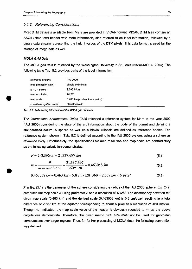
Chapter 5: Modeling the Topography 55
5.1.2 Referencing Considerations
Most DTM datasets available from Mars are provided in VICAR format. VICAR DTM files contain an
ASCII (piain text) header with meta-information, also referred to as label Information, followed by a
binary data stream representing the height values of the DTM pixels. This data format is used for the
storage of image data as well.
MOLA Grid Data
The MOLA grid data is released by the Washington University in St. Louis (NASA-MOLA, 2004). The
following table Tab. 5.2 provides parts of the label information:
reference System: IAU 2000
map projection type: simple cylindrical
a = b = c-axis: 3,396.0 km
map resolution: 1/128°
map scale: 0.463 km/pixel (at the equator)
coordinate System name: planetocentric
Tab. 5.2: Referencing information ofthe MOLA grid datasets.
The International Astronomical Union (IAU) released a reference System for Mars in the year 2000
(IAU 2000) considering the State of the art information about the body of the planet and defining a
standardized datum. A sphere as well as a biaxial ellipsoid are defined as reference bodies. The
reference System shown in Tab. 5.2 is defined according to the IAU 2000 System, using a sphere as
reference body. Unfortunately, the specifications for map resolution and map scale are contradictory
as the following calculation demonstrates:
P = 2-3,396-;r = 21,337.697 km (5.1)
P 21,337.697 _ . „ . . . ,m = = — = 0.463058 km (5.2)
map resolution 3 60 * 12 80.463058 km - 0.463 km = 5.8 cm • 128 • 360 = 2.657 km « 6 pixel (5.3)
P in Eq. (5.1) is the perimeter of the sphere considering the radius of the IAU 2000 sphere. Eq. (5.2)
computes the map scale m using perimeter P and a resolution of 1/128°. The discrepancy between the
given map scale (0.463 km) and the derived scale (0.463058 km) is 5.8 cm/pixel resulting in a total
difference of 2.657 km at the equator corresponding to about 6 pixel at a resolution of 463 m/pixel.
Though not indicated, the map scale value of the header is obviously rounded to m, as the above
calculations demonstrate. Therefore, the given metric pixel size must not be used for geometric
computations over larger regions. Thus, for further processing of MOLA data, the following Convention
was defined:
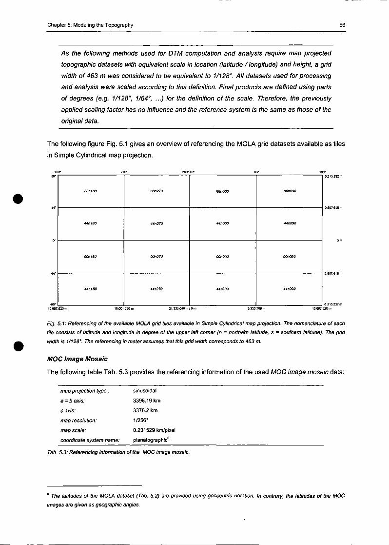
Chapter 5: Modeling the Topography 56
As the following methods used for DTM computation and analysis require map projected
topographic datasets with equivalent scale in location (latitude / longitude) and height, a grid
width of463 m was considered to be equivalent to 1/128°. All datasets used for processing
and analysis were scaled according to this definition. Final products are defined using parts
of degrees (e.g. 1/128", 1/64", ...) for the definition of the scale. Therefore, the previously
applied scaling factor has no influence and the reference System is the same as those of the
original data.
The following figure Fig. 5.1 gives an overview of referencing the MOLA grid datasets available as tiles
in Simple Cylindrical map projection.
88M80
44M80
00n180
«ST 80
eenno
44n!70
OOn27O
44S270
BSnOOO
44n000
OOnOOO
44S00Q
88n090
AAnOiO
OOnOSO
44SO90
10.667.520m 16.001.280m 21.S35.040m/0m 5.333760m 10667.520m
Fig. 5.1: Referencing of the available MOLA grid tiles available in Simple Cylindrical map projection. The nomenclature of each
tile consists of latitude and longitude in degree of the upper left comer (n = northe'm latitude, s = southern latitude). The grid
width is 1/128°. The referencing in meter assumes that this grid width corresponds to 463 m.
MOC Image Mosaic
The following table Tab. 5.3 provides the referencing information of the used MOC image mosaic data:
map projection type:
a = b axis:
c axis:
map resolution:
map scale:
sinusoidal
3396.19 km
3376.2 km
1/256°
0.231529 km/pixel
coordinate System name: planetographic
Tab. 5.3: Referencing Information ofthe MOC image mosaic.
6 7776 latitudes of the MOLA dataset (Tab. 5.2) are provided using geocentric notation. In contrary, the latitudes ofthe MOC
images are given as geographic angles.
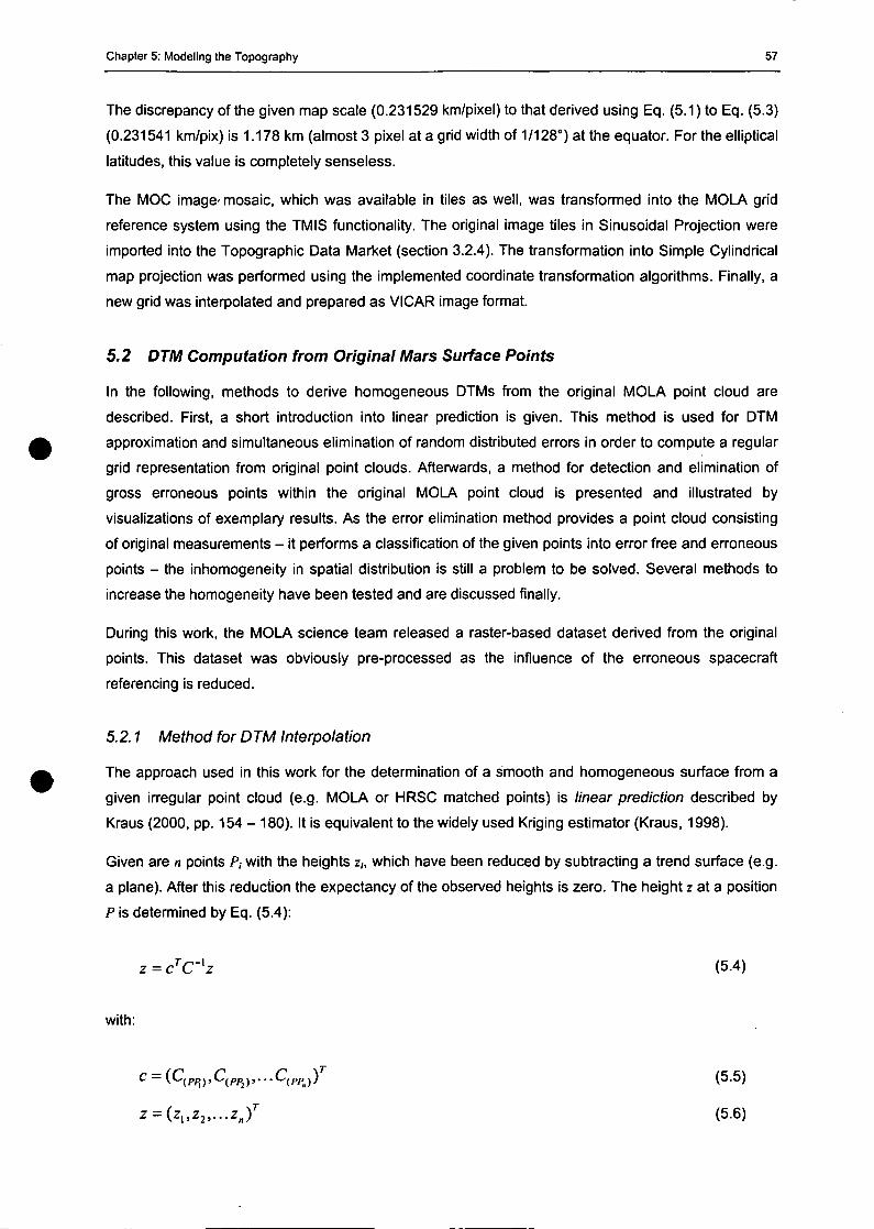
Chapter 5: Modeling the Topography 57
The discrepancy of the given map scale (0.231529 km/pixel) to that derived using Eq. (5.1) to Eq. (5.3)
(0.231541 km/pix) is 1.178 km (almost 3 pixel at a grid width of 1/128°) at the equator. For the elliptical
latitudes, this value is completely senseless.
The MOC image- mosaic, which was available in tiles as well, was transformed into the MOLA grid
reference System using the TM IS functionality. The original image tiles in Sinusoidal Projection were
imported into the Topographie Data Market (section 3.2.4). The transformation into Simple Cylindrical
map projection was performed using the implemented coordinate transformation algorithms. Finally, a
new grid was interpolated and prepared as VICAR image format.
5.2 DTM Computation from Original Mars Surface Points
In the following, methods to derive homogeneous DTMs from the original MOLA point cloud are
described. First, a Short introduetion into linear prediction is given. This method is used for DTM
approximation and simultaneous elimination of random distributed errors in order to compute a regulär
grid representation from original point clouds. Afterwards, a method for detection and elimination of
gross erroneous points within the original MOLA point cloud is presented and illustrated by
visualizations of exemplary results. As the error elimination method provides a point cloud consisting
of original measurements - it performs a classification of the given points into error free and erroneous
points - the inhomogeneity in spatial distribution is still a problem to be solved. Several methods to
increase the homogeneity have been tested and are discussed finally.
During this work, the MOLA science team released a raster-based dataset derived from the original
points. This dataset was obviously pre-processed as the influence of the erroneous spacecraft
referencing is reduced.
5.2.1 Method for D TM Interpolation
The approach used in this work for the determination of a smooth and homogeneous surface from a
given irregulär point cloud (e.g. MOLA or HRSC matched points) is linear prediction described by
Kraus (2000, pp. 154 - 180). It is equivalent to the widely used Kriging estimator (Kraus, 1998).
Given are n points />, with the heights z„ which have been reduced by subtracting a trend surface (e.g.
a plane). After this reduetion the expeetancy of the observed heights is zero. The height z at a position
P is determined by Eq. (5.4):
z = cTC'lz (5.4)
with:
c — C^(p/>)j^(p/>2)>---^-(ppn)) (5.5)
z = (2„z2,...z„)r (5.6)
Chapter 5: Modeling the Topography 58
c =
c(V.
(5.7)
The values C(ppk) describe the covariance between two points on the surface in the following way
(Gaussian model):
(5.8)
with:
Cm = covariance for a distance of zero,
PjPk = horizontal Euclidian distance between the two surface points />, and Pk,
c = factor (estimated from the given points) for Controlling the steepness of the
covariance function.
V in Matrix C of Eq. (5.7) is the variance of the given points, which is the sum of C(0) and the
variance of the measurements of. The points are considered to have the same <J02 (a priori accuracy),
but different weights/?,. The accuracy a? of a point P, is obtained from:
er, =•Pi
(5.9)
The variance of each point P, can be computed by:
(5.10)
(Kraus, 2000). It can be proved, that a high point density (high redundancy) allows for the computation
of a DTM with a better inner accuracy of the interpolated points than those of the individual given
points. Furthermore, it should be mentioned, that Eq. (5.4) can be derived in another way by
minimizing the sum of the Squares of the interpolation errors. So the linear prediction approach is also
known as least Squares interpolation as described by Moritz and Sünkel (1978).
5.2.2 Error Elimination
A prerequisite for deriving high-quality DTMs is a correct and aecurate dataset of measurements.
Initially, the free available dataset of MOLA original points, released by the MOLA science team and
Chapter 5: Modeling the Topography 59
distributed on the web (NASA-MOLA, 2004), contained errors due to incorrect referencing of the
spacecraft, as already mentioned. Since October 2002, an improved dataset is available. The
predefined grid spacing of this dataset is 1/128° which corresponds to about 463 m at the Mars
equator (see section 5.1.2). The original points have been released in October 2003 using an
improved reference System. Within this "final" release, several erroneous tracks have been removed,
while some are still remaining within the dataset. Publications about the applied error elimination
methods are not available.
The following approach is an automated method for detection and subsequent elimination of
erroneous points, based on robust interpolation methods. It allows to do this without having
information about the orbit data and thus, without the possibility to correct them. This approach,
therefore, would work within other similarly deteriorated data as well as it does not require detailed a
priori knowledge about the dataset and about reasons for incorrectness of the data.
Because of the inhomogeneous distribution of the given points, the use of a hierarchical robust
interpolation seemed to be appropriate. This method was originally developed to classify airborne
laser Scanner (ALS) data in Earth applications into terrain points for DTM interpolation, and off-terrain
points, such as Vegetation or buildings. A detailed description of this method and its capabilities is
provided by Briese et al. (2002a, pp. 55 - 61). Unexpectedly, when applied tö the MOLA points, the
results were not satisfying. Due to the roughness of the Mars surface, points in regions without scan
errors were eliminated as well. The rugged terrain did not fit the functional model of linear prediction,
which was originally designed to generate very smooth surfaces as they usually occur in Earth
applications. Several tests of applying the hierarchical robust interpolation for classification of ALS
data in mountain regions at the Earth show similar effects in rocky alpine areas with their peaks, rims,
ridges and other rough structures. In that cases, a smoothing effect eliminates the typical roughness of
the terrain.
Currently no satisfying solution is available for the application of ALS data. In order to improve the
results on MOLA points, the approach was modified as follows. Instead of analyzing each individual
point, scan line segments were investigated, assuming that the errors to be detected are always
effecting a series of successive points rather than Single points. The average filter value of a segment,
the RMS (root mean Square error of the residuals of the points belonging to this segment), turned out
to provide an appropriate measure for detecting segments with gross errors. The Separation in
segments was enabled due to the fact that the original points are available track-wise in the order of
measurement. This circumstance allowed for considering a series of points (e.g. 500) as one segment.
Unfortunately, erroneous segments cause a deformation of the interpolated DTM and increase the
RMS of correct line segments in their neighborhood with respect to the (incorrect) DTM. The profile of
a DTM as shown in Fig. 5.2 Sketches the behavior of a predicted surface (a horizontal plane) near to a
gross error. The light gray band represents the threshold for acceptance of points. This threshold
would obviously eliminate correct line segments due to the strong deformation of the model in that
area caused by one gross erroneous track. In order to solve this problem, the method has to be
applied iteratively, starting with a large threshold value and reducing it from one iteration to the next.
This procedure corresponds to a robust interpolation using a box weight function to yield decreasing
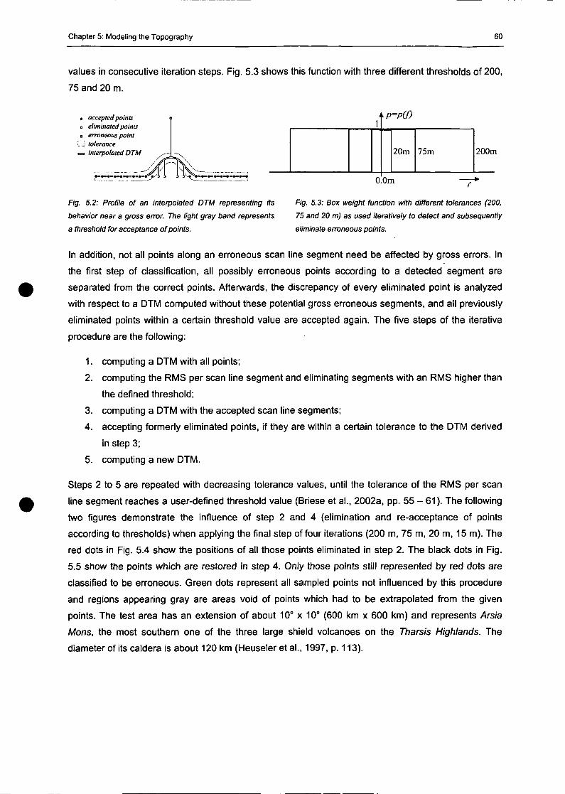
Chapter 5: Modeling the Topography 60
values in consecutive iteration Steps. Fig. 5.3 shows this function with three different thresholds of 200,
75 and 20 m.
• accepted pointso eliminated pointso erroneous point
l j tolerance= interpolated DTM ^- ^ 20m 75m 200m
Fig. 5.2: Profile of an interpolated DTM representing its
behavior near a gross error. The light gray band represents
a threshold for acceptance of points.
0.0m —j*
Fig. 5.3: Box weight function with different tolerances (200,
75 and 20 m) as used iteratively to detect and subsequently
eliminate erroneous points.
In addition, not all points along an erroneous scan line segment need be affected by gross errors. In
the first step of classification, all possibly erroneous points according to a detected segment are
separated from the correct points. Afterwards, the discrepancy of every eliminated point is analyzed
with respect to a DTM computed without these potential gross erroneous segments, and all previously
eliminated points within a certain threshold value are accepted again. The five Steps of the iterative
procedure are the following:
1. Computing a DTM with all points;
2. Computing the RMS per scan line segment and eliminating segments with an RMS higher than
the defined threshold;
3. Computing a DTM with the accepted scan line segments;
4. accepting formerly eliminated points, if they are within a certain tolerance to the DTM derived
in step 3;
5. Computing a new DTM.
Steps 2 to 5 are repeated with decreasing tolerance values, until the tolerance of the RMS per scan
line segment reaches a user-defined threshold value (Briese et al., 2002a, pp. 55 - 61). The following
two figures demonstrate the influence of step 2 and 4 (elimination and re-acceptance of points
according to thresholds) when applying the final step of four iterations (200 m, 75 m, 20 m, 15 m). The
red dots in Fig. 5.4 show the positions of all those points eliminated in step 2. The black dots in Fig.
5.5 show the points which are restored in step 4. Only those points still represented by red dots are
classified to be erroneous. Green dots represent all sampled points not influenced by this procedure
and regions appearing gray are areas void of points which had to be extrapolated from the given
points. The test area has an extension of about 10° x 10° (600 km x 600 km) and represents Arsia
Mons, the most southern one of the three large shield volcanoes on the Tharsis Highlands. The
diameter of its caldera is about 120 km (Heuseier et al., 1997, p. 113).
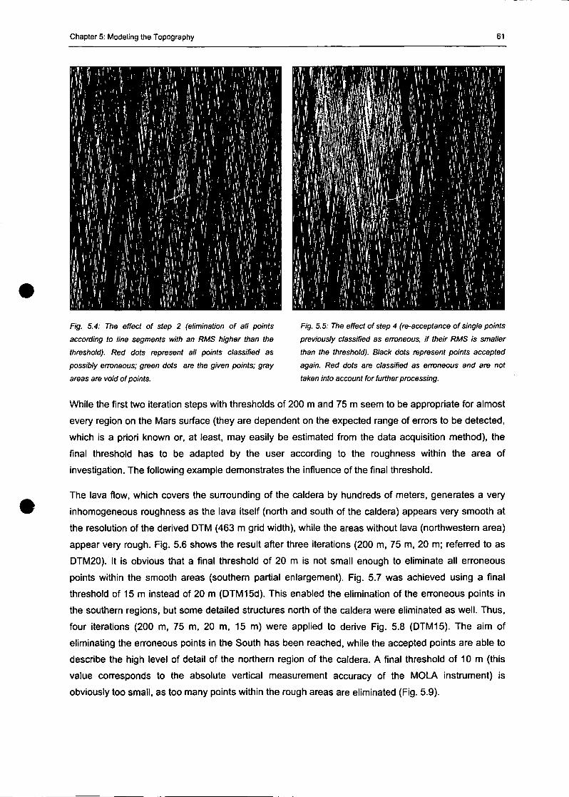
Chapter 5: Modeling the Topography 61
Fig. 5.4: The effect of step 2 (elimination of all points
according to line Segments with an RMS higher than the
threshold). Red dots represent all points classified as
possibly enroneous; green dots are the given points; gray
areas are void of points.
Fig. 5.5: The effect of step 4 (re-acceptance of Single points
previously classified as envneous, if their RMS is smaller
than the threshold). Black dots represent points accepted
again. Red dots are classified as erroneous and are not
taken into account for further processing.
While the first two iteration steps with thresholds of 200 m and 75 m seem to be appropriate for almost
every region on the Mars surface (they are dependent on the expected ränge of errors to be detected,
which is a priori known or, at least, may easily be estimated from the data acquisition method), the
final threshold has to be adapted by the user according to the roughness within the area of
investigation. The following example demonstrates the influence of the final threshold.
The lava flow, which covers the surrounding of the caldera by hundreds of meters, generates a very
inhomogeneous roughness as the lava itself (north and south of the caldera) appears very smooth at
the resolution of the derived DTM (463 m grid width), while the areas without lava (northwestem area)
appear very rough. Fig. 5.6 shows the result after three iterations (200 m, 75 m, 20 m; referred to as
DTM20). It is obvious that a final threshold of 20 m is not small enough to eliminate all erroneous
points within the smooth areas (southern partial enlargement). Fig. 5.7 was achieved using a final
threshold of 15 m instead of 20 m (DTM15d). This enabled the elimination of the erroneous points in
the southern regions, but some detailed structures north of the caldera were eliminated as well. Thus,
four iterations (200 m, 75 m, 20 m, 15 m) were applied to derive Fig. 5.8 (DTM15). The aim of
eliminating the erroneous points in the South has been reached, while the accepted points are able to
describe the high level of detail of the northern region of the caldera. A final threshold of 10 m (this
value corresponds to the absolute vertical measurement accuracy of the MOLA instrument) is
obviously too small, as too many points within the rough areas are eliminated (Fig. 5.9).
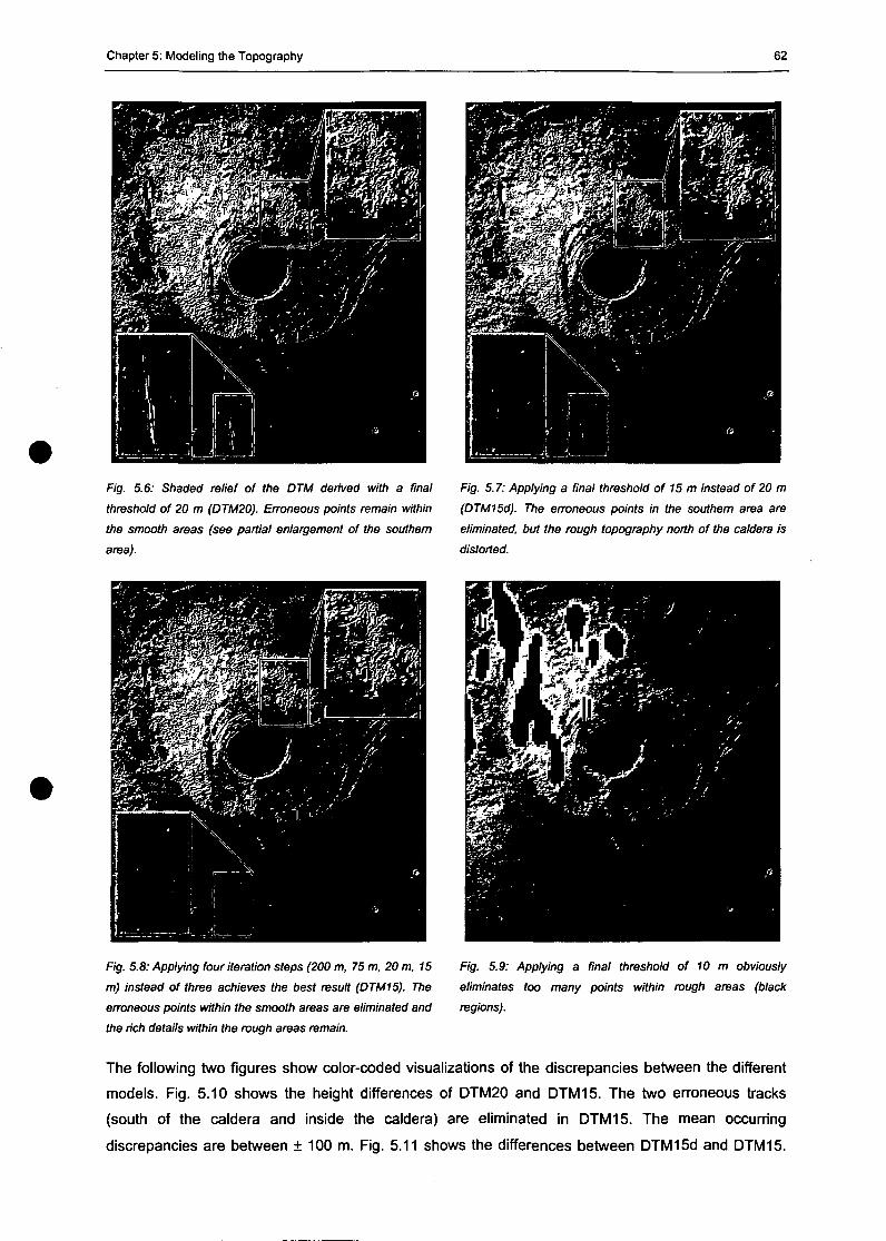
Chapter 5: Modeling the Topography 62
Fig. 5.6: Shaded relief of the DTM derived with a final
threshold of 20 m (DTM20). Erroneous points remain within
the smooth areas (see partial enlargement of the southem
area).
Fig. 5.7: Applying a final threshold of 15 m instead of 20 m
(DTM15d). The erroneous points in the southern area are
eliminated, but the rough topography north of the caldera is
distorted.
Fig. 5.8: Applying four Iteration Steps (200 m, 75 m, 20 m, 15
m) instead of three achieves the best result (DTM15). The
erroneous points wtthin the smooth areas are eliminated and
the rieh details wtthin the rough areas remain.
Fig. 5.9: Applying a final threshold of 10 m obviously
eliminates too many points within rough areas (black
regions).
The following two figures show color-coded visualizations of the discrepancies between the different
modeis. Fig. 5.10 shows the height differences of DTM20 and DTM15. The two erroneous tracks
(south of the caldera and inside the caldera) are eliminated in DTM15. The mean oecurring
discrepancies are between ± 100 m. Fig. 5.11 shows the differences between DTM15d and DTM15.
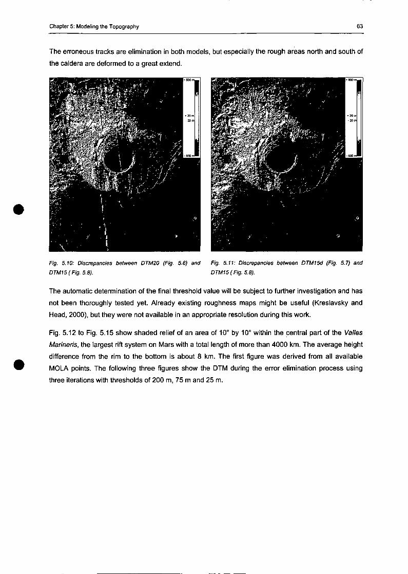
Chapter 5: Modeling the Topography 63
The erroneous tracks are elimination in both modeis, but especially the rough areas north and south of
the caldera are deformed to a great extend.
Fig. 5.10: Discrepancies between DTM20 (Fig. 5.6) and
DTM15(Fig.5.8).
Fig. 5.11: Discrepancies between DTM15d (Fig. 5.7) and
DTM15(Fig.5.8).
The automatic determination of the final threshold value will be subject to further investigation and has
not been thoroughly tested yet. Already existing roughness maps might be useful (Kreslavsky and
Head, 2000), but they were not available in an appropriate resolution during this work.
Fig. 5.12 to Fig. 5.15 show shaded relief of an area of 10° by 10° within the central part of the Valles
Marineris, the largest rift System on Mars with a total length of more than 4000 km. The average height
difference from the rim to the bottom is about 8 km. The first figure was derived from all available
MOLA points. The following three figures show the DTM during the error elimination process using
three iterations with thresholds of 200 m, 75 m and 25 m.
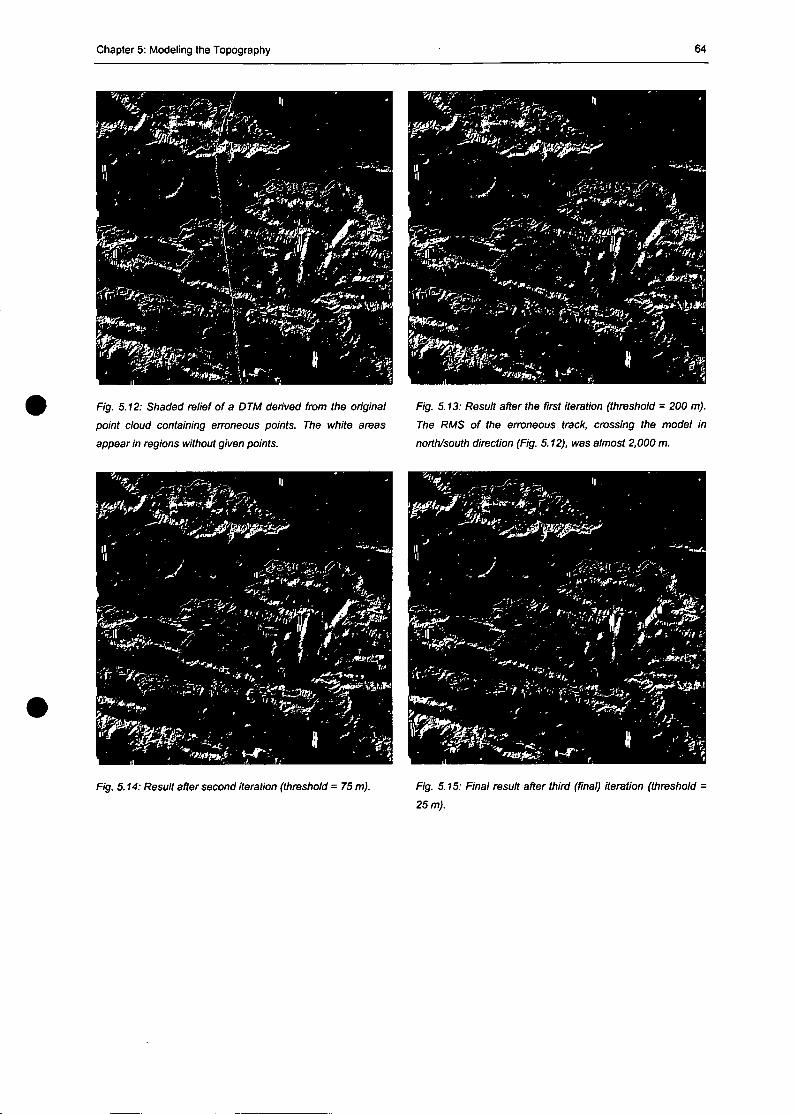
Chapter 5: Modeling the Topography 64
Fig. 5.12: Shaded relief of a DTM derived from the original
point cloud containing erroneous points. The white areas
appear in regions without given points.
Fig. 5.13: Result after the first iteration (threshold = 200 m).
The RMS of the erroneous track, crossing the model in
north/south direction (Fig. 5.12), was almost 2,000 m.
Fig. 5.14: Result after second iteration (threshold = 75 m). Fig. 5.15: Final result after third (final) iteration (threshold •
25 m).
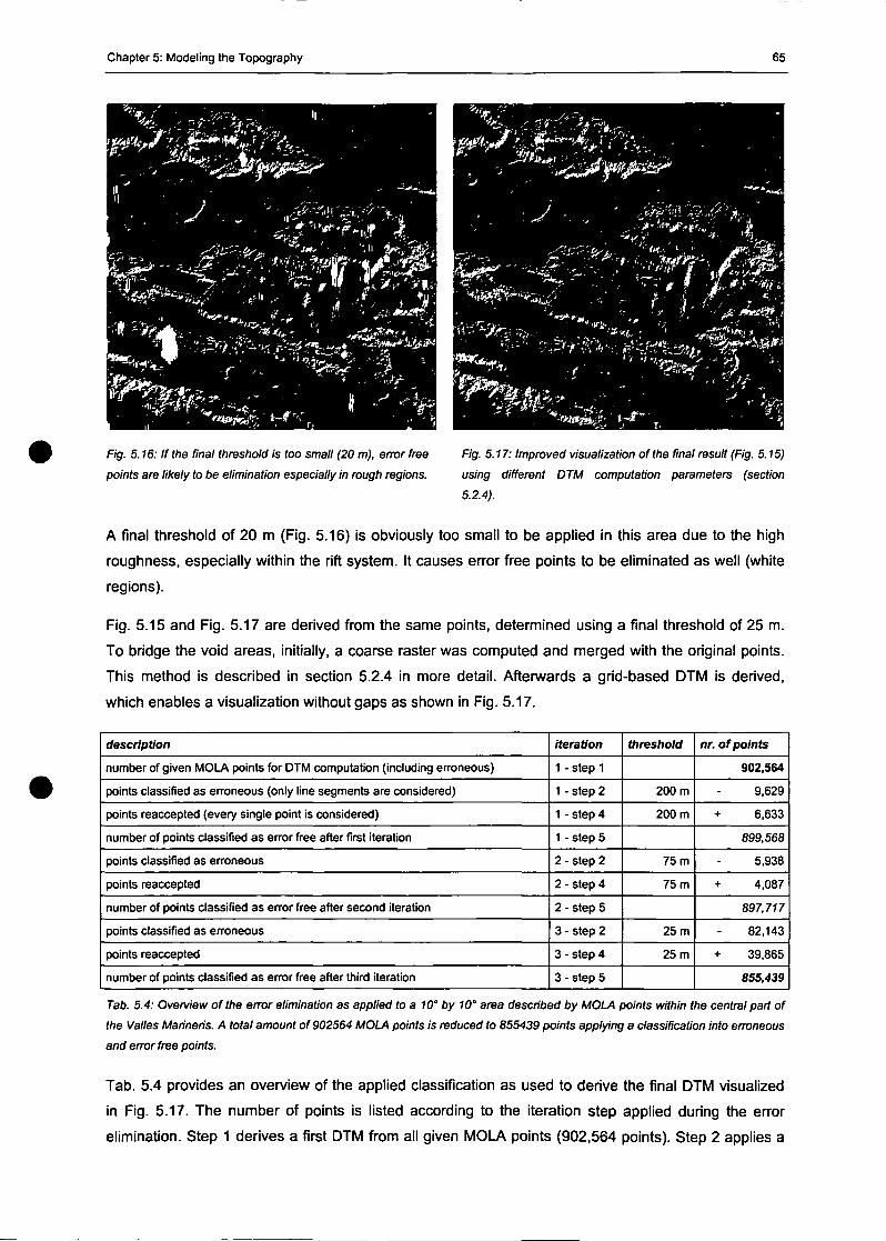
Chapter 5: Modeling the Topography 65
F/g. 5. t6: /f the final threshold is too small (20 m), error free
points are likely to be elimination especially in rough regions.
Fig. 5.17: Improved visualization ofthe final result (Fig. 5.15)
using different DTM computation parameters (section
5.2.4).
A final threshold of 20 m (Fig. 5.16) is obviously too small to be applied in this area due to the high
roughness, especially within the rift System. It causes error free points to be eliminated as well (white
regions).
Fig. 5.15 and Fig. 5.17 are derived from the same points, determined using a final threshold of 25 m.
To bridge the void areas, initially, a coarse raster was computed and merged with the original points.
This method is described in section 5.2.4 in more detail. Afterwards a grid-based DTM is derived,
which enables a visualization without gaps as shown in Fig. 5.17.
description
number of given MOLA points for DTM computation (including erroneous)
points classified as erroneous (only line Segments are considered)
points reaccepted (every Single point is considered)
number of points classified as error free after first iteration
points classified as erroneous
points reaccepted
number of points classified as error free after second iteration
points classified as erroneous
points reaccepted
number of points classified as error free after third iteration
iteration
1 - step 1
1 - step 2
1 - step 4
1 - step 5
2 - step 2
2 - step 4
2 - step 5
3 - step 2
3 - step 4
3 - step 5
threshold
200 m
200 m
75 m
75 m
25 m
25 m
nr. of points
902,564
9,629
+ 6,633
899,568
5,938
+ 4,087
897,717
82,143
+ 39,865
855,439
Tab. 5.4: Overview of the error elimination as applied to a 10° by 10° area described by MOLA points wtthin the central part of
the Valles Marineris. A total amount of 902564 MOLA points is reduced to 855439 points applying a classification into erroneous
and error free points.
Tab. 5.4 provides an overview of the applied classification as used to derive the final DTM visualized
in Fig. 5.17. The number of points is listed according to the iteration step applied during the error
elimination. Step 1 derives a first DTM from all given MOLA points (902,564 points). Step 2 applies a
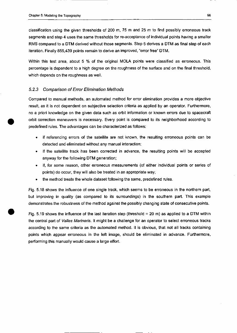
Chapter 5: Modeling the Topography 66
classification using the given thresholds of 200 m, 75 m and 25 m to find possibly erroneous track
segments and step 4 uses the same thresholds for re-acceptance of individual points having a smaller
RMS compared to a DTM derived without those segments. Step 5 derives a DTM as final step of each
iteration. Finally 855,439 points remain to derive an improved, "errorfree" DTM.
Within this test area, about 5 % of the original MOLA points were classified as erroneous. This
percentage is dependent to a high degree on the roughness of the surface and on the final threshold,
which depends on the roughness as well.
5.2.3 Comparison of Error Elimination Methods
Compared to manual methods, an automated method for error elimination provides a more objective
result, as it is not dependent on subjective selection criteria as applied by an Operator. Furthermore,
no a priori knowledge on the given data such as orbit Information or known errors due to spacecraft
orbit correction maneuvers is necessary. Every point is compared to its neighborhood according to
predefined rules. The advantages can be characterized as follows:
• if referencing errors of the satellite are not known, the resulting erroneous points can be
detected and eliminated without any manual interaction;
• if the satellite track has been corrected in advance, the resulting points will be accepted
anyway for the following DTM generation;
• if, for some reason, other erroneous measurements (of either individual points or series of
points) do occur, they will also be treated in an appropriate way;
• the method treats the whole dataset following the same, predefined rules.
Fig. 5.18 shows the influence of one Single track, which seems to be erroneous in the northern part,
but improving in quality (as compared to its surroundings) in the southern part. This example
demonstrates the robustness of the method against the possibly changing State of consecutive points.
Fig. 5.19 shows the influence of the last iteration step (threshold = 20 m) as applied to a DTM within
the central part of Valles Marineris. It might be a challenge for an Operator to select erroneous tracks
according to the same criteria as the automated method. It is obvious, that not all tracks containing
points which appear erroneous in the left image, should be eliminated in advance. Furthermore,
performing this manually would cause a large effort.
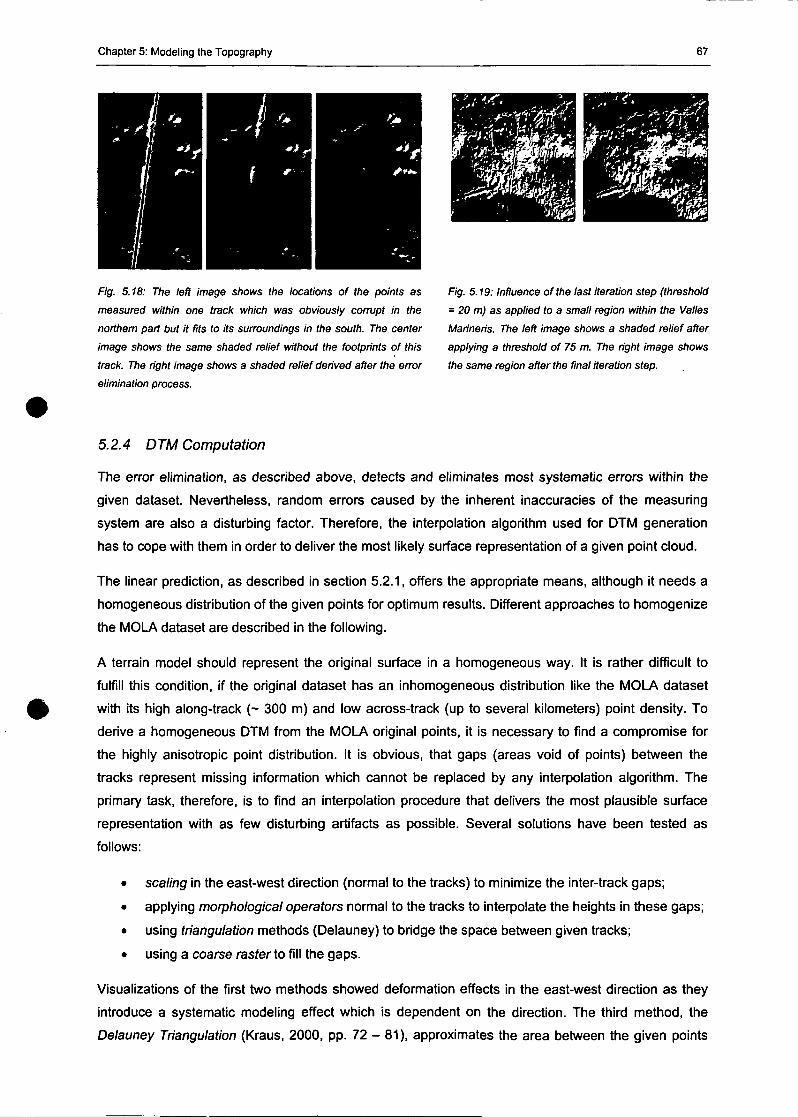
Chapter 5: Modeling the Topography 67
Fig. 5.18: The left image shows the locations of the points as
measured within one track which was obviously comipt in the
northern pari but it fits to its sunvundings in the south. The center
image shows the same shaded relief without the footprints of this
track. The right image shows a shaded relief derived after the error
elimination process.
Fig. 5.19: Influence of the last iteration step (threshold
= 20 m) as applied to a small region within the Valles
Marineris. The left image shows a shaded relief after
applying a threshold of 75 m. The right image shows
the same region after the final iteration step.
5.2.4 DTM Computation
The error elimination, as described above, detects and eliminates most systematic errors within the
given dataset. Nevertheless, random errors caused by the inherent inaccuracies of the measuring
System are also a disturbing factor. Therefore, the interpoiation algorithm used for DTM generation
has to cope with them in order to deliver the most likely surface representation of a given point cloud.
The linear prediction, as described in section 5.2.1, offers the appropriate means, although it needs a
homogeneous distribution of the given points for Optimum results. Different approaches to homogenize
the MOLA dataset are described in the following.
A terrain model should represent the original surface in a homogeneous way. It is rather difficult to
fulfill this condition, if the original dataset has an inhomogeneous distribution like the MOLA dataset
with its high along-track (- 300 m) and Iow across-track (up to several kilometers) point density. To
derive a homogeneous DTM from the MOLA original points, it is necessary to find a compromise for
the highly anisotropic point distribution. It is obvious, that gaps (areas void of points) between the
tracks represent missing information which cannot be replaced by any interpoiation algorithm. The
primary task, therefore, is to find an interpoiation procedure that delivers the most plausible surface
representation with as few disturbing artifacts as possible. Several Solutions have been tested as
follows:
• scaling in the east-west direction (normal to the tracks) to minimize the inter-track gaps;
• applying morphological Operators normal to the tracks to interpolate the heights in these gaps;
• using thangulation methods (Delauney) to bridge the space between given tracks;
• using a coarse raster to fill the gaps.
Visualizations of the first two methods showed deformation effects in the east-west direction as they
introduce a systematic modeling effect which is dependent on the direction. The third method, the
Delauney Triangulation (Kraus, 2000, pp. 72 - 81), approximates the area between the given points
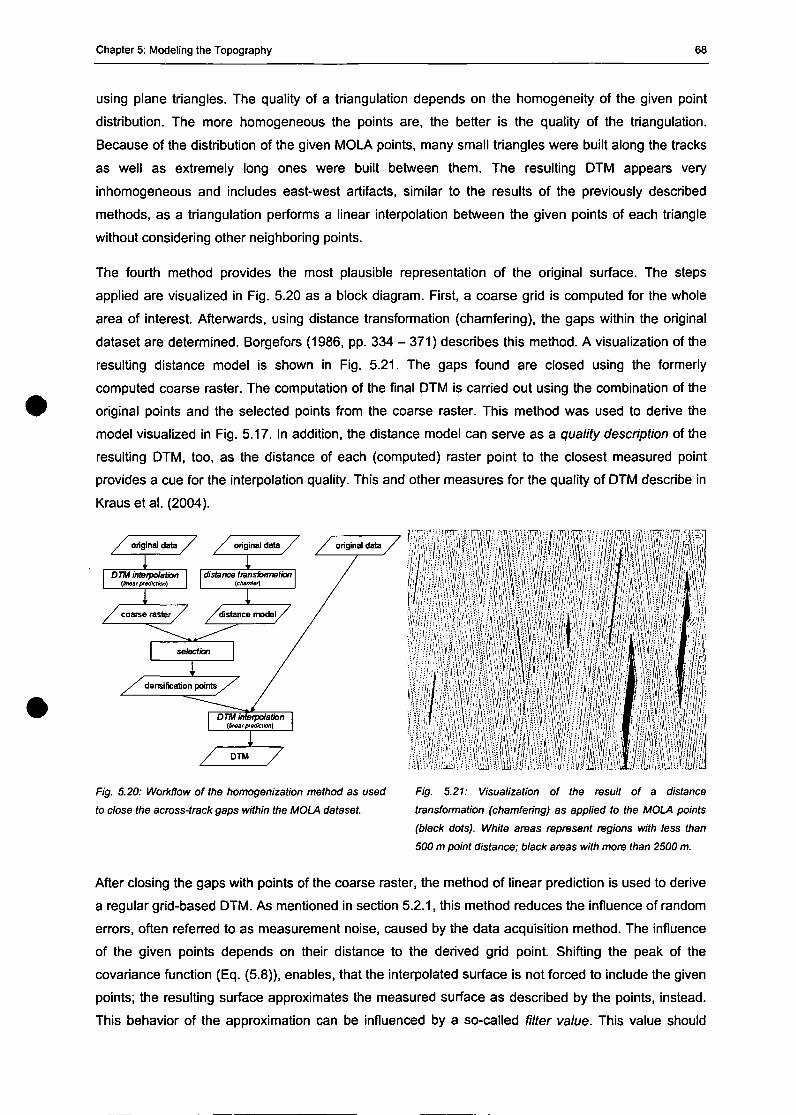
Chapter 5: Modeling the Topography 68
using plane triangles. The quality of a triangulation depends on the homogeneity of the given point
distribution. The more homogeneous the points are, the better is the quality of the triangulation.
Because of the distribution of the given MOLA points, many small triangles were built along the tracks
as well as extremely long ones were built between them. The resulting DTM appears very
inhomogeneous and includes east-west artifacts, similar to the results of the previously described
methods, as a triangulation performs a linear interpolation between the given points of each triangle
without considering other neighboring points.
The fourth method provides the most plausible representation of the original surface. The steps
applied are visualized in Fig. 5.20 as a block diagram. First, a coarse grid is computed for the whole
area of interest. Afterwards, using distance transformation (chamfering), the gaps within the original
dataset are determined. Borgefors (1986, pp. 334 - 371) describes this method. A visualization of the
resulting distance model is shown in Fig. 5.21. The gaps found are closed using the formerly
computed coarse raster. The computation of the final DTM is carried out using the combination of the
original points and the selected points from the coarse raster. This method was used to derive the
model visualized in Fig. 5.17. In addition, the distance model can serve as a quality description of the
resulting DTM, too, as the distance of each (computed) raster point to the dosest measured point
provides a cue for the interpolation quality. This and other measures for the quality of DTM describe in
Kraus et al. (2004).
/ original data .
1D TM interpolation
(fi»ir (Wrtclwi)
/ z original data /
1distancQ transfotwotion
(chamfor)
i/ coarse raster /
1/distance model/
setecfjon
1/ densification points /
//
' /
DTM
DTM Interpolationtbnear prediction)
Fig. 5.20: Workflow of the homogenization method as used
to dose the across-track gaps within the MOLA dataset.
Fig. 5.21: Visualization of the result of a distance
transfonvation (chamfering) as applied to the MOLA points
(black dots). White areas represent regions with less than
500 m point distance; black areas with more than 2500 m.
After closing the gaps with points of the coarse raster, the method of linear prediction is used to derive
a regulär grid-based DTM. As mentioned in section 5.2.1, this method reduces the influence of random
errors, often referred to as measurement noise, caused by the data acquisition method. The influence
of the given points depends on their distance to the derived grid point. Shifting the peak of the
covariance function (Eq. (5.8)), enables, that the interpolated surface is not forced to include the given
points; the resulting surface approximates the measured surface as described by the points, instead.
This behavior of the approximation can be influenced by a so-called filter value. This value should
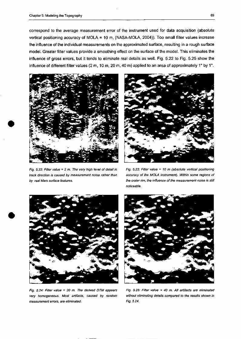
Chapter 5: Modeling the Topography 69
correspond to the average measurement error of the instrument used for data acquisition (absolute
vertical positioning accuracy of MOLA = 10 m, (NASA-MOLA, 2004)). Too small filter values increase
the influence of the individual measurements on the approximated surface, resulting in a rough surface
model. Greater filter values provide a smoothing effect on the surface of the model. This eliminates the
influence of gross errors, but it tends to eliminate real details as well. Fig. 5.22 to Fig. 5.25 show the
influence of different filter values (2 m, 10 m, 20 m, 40 m) applied to an area of approximately 1° by 1°.
Fig. 5.22: Filter value = 2 m. The very high level of detail in
track direction is caused by measurement noise rather than
by real Mars surface features.
Fig. 5.23: Filter value = 10 m (absolute vertical positioning
accuracy of the MOLA instrument). Within some regions of
the crater rim, the influence of the measurement noise is still
noticeable.
Fig. 5.24: Filter value = 20 m. The derived DTM appears
very homogeneous. Most artifacts, caused by random
measurement errors, are eliminated.
Fig. 5.25: Filter value = 40 m. All artifacts are eliminated
without eliminating details compared to the results shown in
Fig. 5.24.
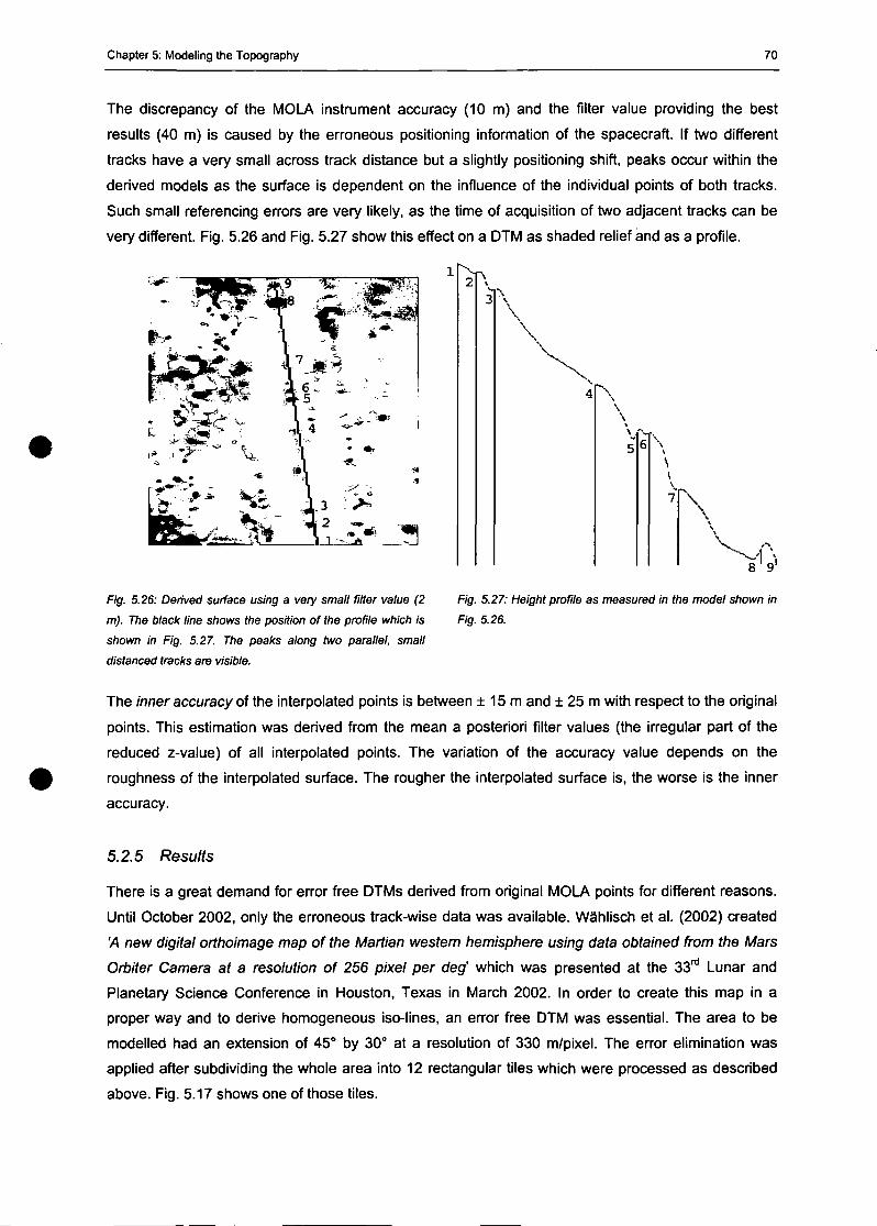
Chapter 5: Modeling the Topography 70
The discrepancy of the MOLA instrument accuracy (10 m) and the filter value providing the best
results (40 m) is caused by the erroneous positioning information of the spacecraft. If two different
tracks have a very small across track distance but a slightly positioning shift, peaks occur within the
derived modeis as the surface is dependent on the influence of the individual points of both tracks.
Such small referencing errors are very likely, as the time of acquisition of two adjacent tracks can be
very different. Fig. 5.26 and Fig. 5.27 show this effect on a DTM as shaded relief and as a profile.
r\
|*\
[\
Fig. 5.26: Derived surface using a very small filter value (2
m). The black line shows the position of the profile which is
shown in Fig. 5.27. The peaks along two parallel, small
distanced tracks are visible.
8 ' 9 '
Fig. 5.27: Height profile as measured in the model shown in
Fig. 5.26.
The inner accuracy of the interpolated points is between ± 15 m and ± 25 m with respect to the original
points. This estimation was derived from the mean a posteriori filter values (the irregulär part of the
reduced z-value) of all interpolated points. The Variation of the accuracy value depends on the
roughness of the interpolated surface. The rougher the interpolated surface is, the worse is the inner
accuracy.
5.2.5 Results
There is a great demand for error free DTMs derived from original MOLA points for different reasons.
Until October 2002, only the erroneous track-wise data was available. Wählisch et al. (2002) created
'A new digital orthoimage map of the Martian western hemisphere using data obtained from the Mars
Orbiter Camera at a resolution of 256 pixel per deg' which was presented at the 33"* Lunar and
Planetary Science Conference in Houston, Texas in March 2002. In Order to create this map in a
proper way and to derive homogeneous iso-lines, an error free DTM was essential. The area to be
modelled had an extension of 45° by 30° at a resolution of 330 m/pixel. The error elimination was
applied after subdividing the whole area into 12 rectangular tiles which were processed as described
above. Fig. 5.17 shows one of those tiles.
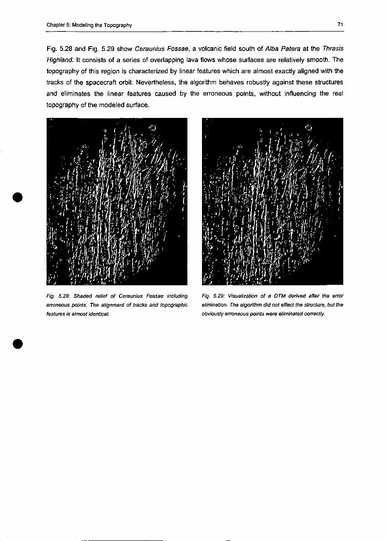
Chapter 5: Modeling the Topography 71
Fig. 5.28 and Fig. 5.29 show Ceraunius Fossae, a volcanic field south of Alba Patera at the Thrasis
Highland. It consists of a series of overlapping lava flows whose surfaces are relatively smooth. The
topography of this region is characterized by linear features which are almost exactiy aligned with the
tracks of the spacecraft orbit. Nevertheless, the algorithm behaves robustly against these structures
and eliminates the linear features caused by the erroneous points, without influencing the real
topography of the modeled surface.
Fig. 5.28: Shaded relief of Ceraunius Fossae including
erroneous points. The alignment of tracks and topographic
features is almost identical.
Fig. 5.29: Visualization of a DTM derived after the error
elimination. The algorithm did not effect the structure, but the
obviously erroneous points were eliminated correctly.
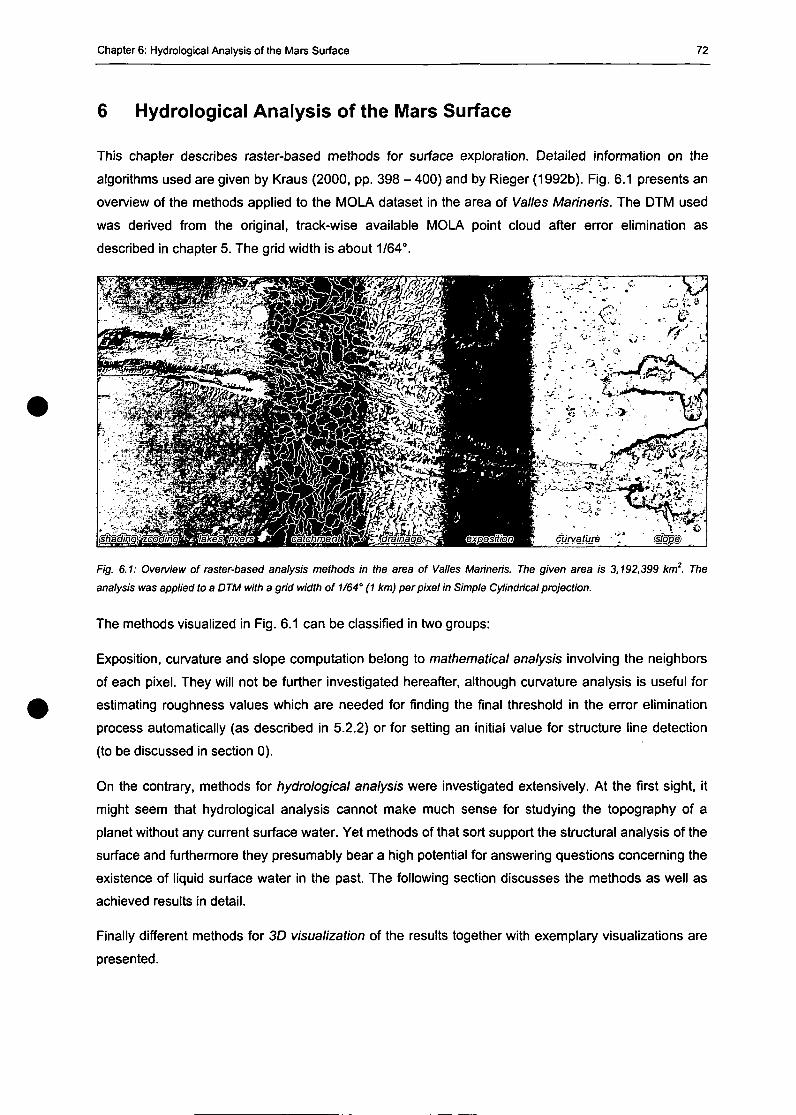
Chapter 6: Hydrological Analysis of the Mars Surface 72
6 Hydrological Analysis of the Mars Surface
This chapter describes raster-based methods for surface exploration. Detailed information on the
algorithms used are given by Kraus (2000, pp. 398 - 400) and by Rieger (1992b). Fig. 6.1 presents an
overview of the methods applied to the MOLA dataset in the area of Valles Marineris. The DTM used
was derived from the original, track-wise available MOLA point cloud after error elimination as
described in chapter 5. The grid width is about 1/64°.
- . i •
Cifiyature •
F/g. 6.f: Overv/ew of raster-based analysis methods in the area of Valles Marineris. The given area is 3,192,399 km2. The
analysis was applied to a DTM with a grid width of 1/64° (1 km) perpixel in Simple Cylindrical projection.
The methods visualized in Fig. 6.1 can be classified in two groups:
Exposition, curvature and slope computation belong to mathematical analysis involving the neighbors
of each pixel. They will not be further investigated hereafter, although curvature analysis is useful for
estimating roughness values which are needed for finding the final threshold in the error elimination
process automatically (as described in 5.2.2) or for setting an initial value for structure line detection
(to be discussed in section 0).
On the contrary, methods for hydrological analysis were investigated extensively. At the first sight, it
might seem that hydrological analysis cannot make much sense for studying the topography of a
planet without any current surface water. Yet methods of that sort support the structural analysis of the
surface and furthermore they presumably bear a high potential for answering questions concerning the
existence of liquid surface water in the past. The following section discusses the methods as well as
achieved results in detail.
Finally different methods for 3D visualization of the results together with exemplary visualizations are
presented.
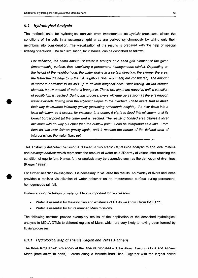
Chapter 6: Hydrological Analysis of the Mars Surface 73
6.1 Hydrological Analysis
The methods used for hydrological analysis were implemented as systolic processes, where the
conditions of the cells in a rectangular grid array are derived synchronously by taking only their
neighbors into consideration. The visualization of the results is prepared with the help of Special
filtering operations. The rain Simulation, for instance, can be described as follows:
Per definition, the same amount of water is brought onto each grid element of the given
(impermeable) surface, thus simulating a permanent, homogeneous rainfall. Depending on
the height of the neighborhood, the water drains in a certain direction; the steeper the area,
the faster the drainage (only the füll neighbors (4-environment) are considered). The amount
of water is permitted to be split up to several neighbor cells. After having left the surface
element, a new amount of water is brought in. These two Steps are repeated until a condition
of equilibrium is reached. During this process, rivers will emerge as soon as there is enough
water available flowing from the adjacent slopes to the riverbed. These rivers Start to make
their way downwards following gravity (assuming orthometric heights). If a river flows into a
local minimum, as it occurs, for instance, in a crater, it Starts to flood this minimum, until its
Iowest border point (at the crater hm) is reached. The resulting flooded area defines a local
minimum with no way out other than the outflow point. It can be interpreted as a lake. From
then on, the river follows gravity again, until it reaches the border of the defmed area of
interest where the water flows out.
This abstractly described behavior is realized in two Steps: Depression analysis to find local minima
and drainage analysis which represents the amount of water as a 2D array of values after reaching the
condition of equilibrium. Hence, further analysis may be appended such as the derivation of river lines
(Rieger 1992a).
For further scientific investigation, it is necessary to visualize the results. An overlay of rivers and lakes
provides a realistic visualization of water behavior on an impermeable surface during permanent,
homogeneous rainfall.
Understanding the history of water on Mars is important for two reasons:
• Water is essential for the evolution and existence of life as we know it from the Earth.
• Water is essential for future manned Mars missions.
The following sections provide exemplary results of the application of the described hydrological
analysis to MOLA DTMs to different regions of Mars, which are very likely to having been formed by
fluvial processes.
6.1.1 Hydrological Map of Tharsis Region and Valles Marineris
The three large shield volcanoes at the Tharsis Highland - Arsia Mons, Pavonis Mons and Ascäus
Mons (from south to north) - arose along a tectonic break line. Together with the largest shield
Chapter 6: Hydrological Analysis of the Mars Surface 74
volcano Olympus Mons, situated northwest of them, they are the largest and longest active volcanoes
(billions of years) within our solar System (Heuseier et al., 1997, p. 110). The Valles Marineris are
situated east of the Tharsis Region, just below the equator. Their longitudinal extension in east/west
direction is about 4,000 km. Geographically they can be separated into three areas: The Noctis
Labyhnthus in the West, the central rims and the beginning of the drainage Valleys in the east
(Heuseier et al., 1997, p. 90). The regions east of the Valles Marineris are characterized by so called
chaotic regions. These areas are 2 - 5 km below the surrounding, undisturbed terrain and mostly
covered with large jumbled blocks of material from the former surface. This indicates that the chaotic
terrain have formed by collapse rather than by removal of material from the above, indicating the
involvement of groundwater in the Channel formation process. They merge westwards with the canyon
System and northwards with outflow Channels. However, particularly to the north of the Valles
Marineris, Channels tend to emanate from completely enclosed canyons containing chaotic terrain like
Echus, Hebes, Juventas and Ganges Chasma (Jaumann et al. 2001, p. 91).
The most reliable hypothesis about the evolution of the large outflow Channels, starting in these
chaotic areas and draining into Chryse Planitia (a former 'ocean' northeast of Valles Marineris), are
catastrophic releases of ground water or drainage of surface lakes. Several processes are discussed
that may cause large floods on Mars. For instance, groundwater under high artesian pressure confined
below a permafrost zone may break out, triggered by events, which disrupt the permafrost seal, such
as impacts or Mars-quakes, either by breaking the surface or sending a large pressure pulse through
the aquifer. The dimensions of the outflow Channels indicate discharges in the order of 107-109 mV 1
(Jaumann etal. 2001, p. 101, Carr 1996).
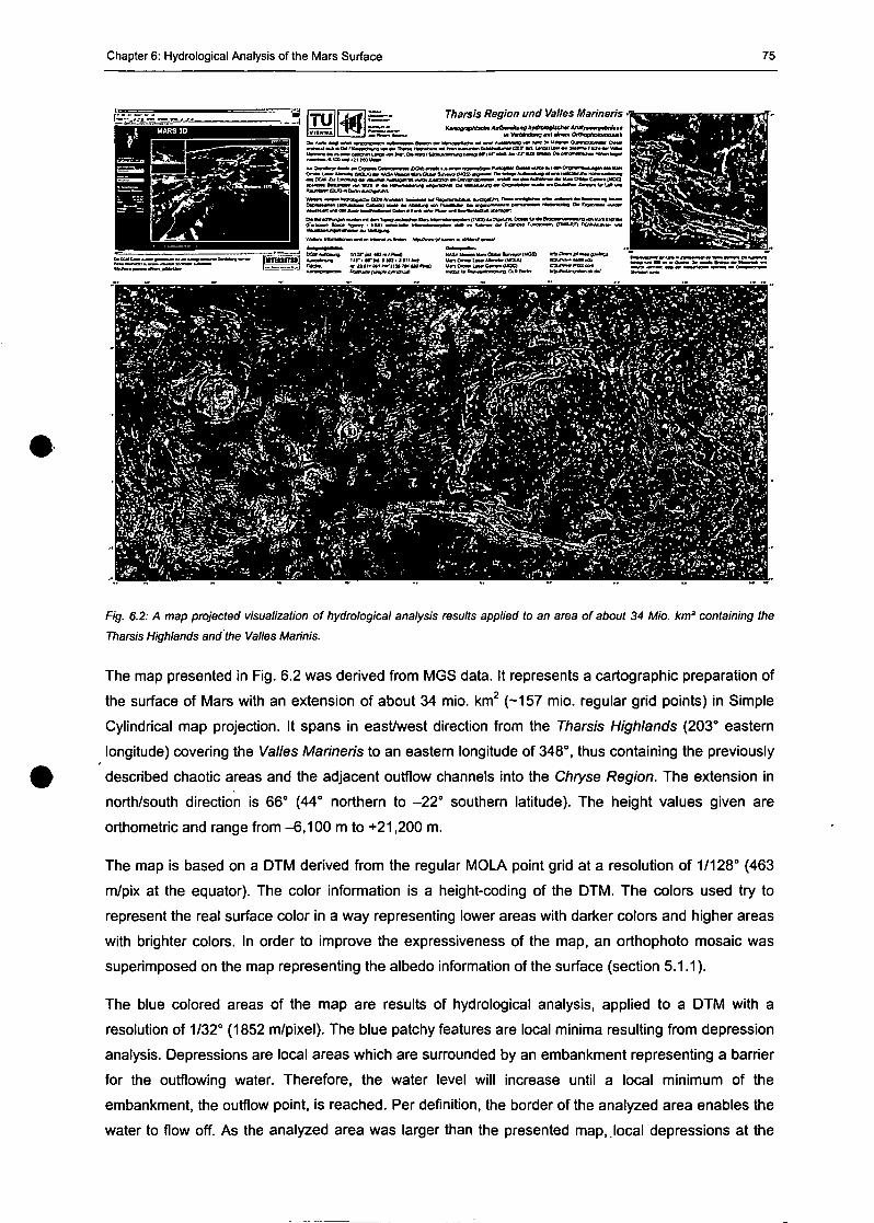
Chapter 6: Hydrological Analysis of the Mars Surface 75
l-'vCS5=-=-- Tharsis Region und Valles MarinerisKarttgnv>f>fecfw Aufbmibmg hy&ohgiKltw
Rg. 6.2: d map projected visualization of hydrological analysis results applied to an area of about 34 Mio. km2 containing the
Tharsis Highlands and the Valles Marinis.
The map presented in Fig. 6.2 was derived from MGS data. It represents a cartographic preparation of
the surface of Mars with an extension of about 34 mio. km2 (-157 mio. regulär grid points) in Simple
Cylindrical map projection. It spans in east/west direction from the Tharsis Highlands (203° eastern
longitude) covering the Valles Marineris to an eastern longitude of 348°, thus containing the previously
described chaotic areas and the adjacent outflow Channels into the Chryse Region. The extension in
north/south direction is 66° (44° northern to -22° southem latitude). The height values given are
orthometric and ränge from -6,100 m to +21,200 m.
The map is based on a DTM derived from the regulär MOLA point grid at a resolution of 1/128° (463
m/pix at the equator). The color information is a height-coding of the DTM. The colors used try to
represent the real surface color in a way representing Iower areas with darker colors and higher areas
with brighter colors. In order to improve the expressiveness of the map, an orthophoto mosaic was
superimposed on the map representing the albedo information of the surface (section 5.1.1).
The blue colored areas of the map are results of hydrological analysis, applied to a DTM with a
resolution of 1/32° (1852 m/pixel). The blue patchy features are local minima resulting from depression
analysis. Depressions are local areas which are surrounded by an embankment representing a barrier
for the outflowing water. Therefore, the water level will increase until a local minimum of the
embankment, the outflow point, is reached. Per definition, the border of the analyzed area enables the
water to flow off. As the analyzed area was larger than the presented map,.local depressions at the
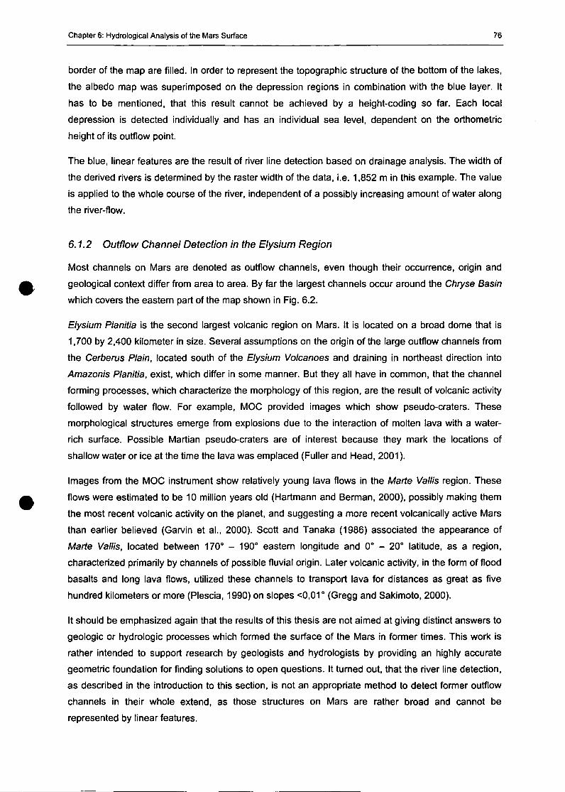
Chapter 6: Hydrological Analysis of the Mars Surface 76
border of the map are filled. In order to represent the topographic structure of the bottom of the lakes,
the albedo map was superimposed on the depression regions in combination with the blue layer. It
has to be mentioned, that this result cannot be achieved by a height-coding so far. Each local
depression is detected individually and has an individual sea level, dependent on the orthometric
height of its outflow point.
The blue, linear features are the result of river line detection based on drainage analysis. The width of
the derived rivers is determined by the raster width of the data, i.e. 1,852 m in this example. The value
is applied to the whole course of the river, independent of a possibly increasing amount of water along
the river-flow.
6.1.2 Outflow Channel Detection in the Elysium Region
Most Channels on Mars are denoted as outflow Channels, even though their occurrence, origin and
geological context differ from area to area. By far the largest Channels occur around the Chryse Basin
which Covers the eastern part of the map shown in Fig. 6.2.
Elysium Planitia is the second largest volcanic region on Mars. It is located on a broad dorne that is
1,700 by 2,400 kilometer in size. Several assumptions on the origin of the large outflow Channels from
the Cerberus Piain, located south of the Elysium Volcanoes and draining in northeast direction into
Amazonis Planitia, exist, which differ in some manner. But they all have in common, that the Channel
forming processes, which characterize the morphology of this region, are the result of volcanic activity
followed by water flow. For example, MOC provided images which show pseudo-craters. These
morphological structures emerge from explosions due to the interaction of molten lava with a water-
rich surface. Possible Martian pseudo-craters are of interest because they mark the locations of
shallow water or ice at the time the lava was emplaced (Füller and Head, 2001).
Images from the MOC instrument show relatively young lava flows in the Marie Vallis region. These
flows were estimated to be 10 million years old (Hartmann and Berman, 2000), possibly making them
the most recent volcanic activity on the planet, and suggesting a more recent volcanically active Mars
than earlier believed (Garvin et al., 2000). Scott and Tanaka (1986) associated the appearance of
Marie Vallis, located between 170° - 190° eastern longitude and 0° - 20° latitude, as a region,
characterized primarily by Channels of possible fluvial origin. Later volcanic activity, in the form of flood
basalts and long lava flows, utilized these Channels to transport lava for distances as great as five
hundred kilometers or more (Plescia, 1990) on slopes <0,01° (Gregg and Sakimoto, 2000).
It should be emphasized again that the results of this thesis are not aimed at giving distinct answers to
geologic or hydrologic processes which formed the surface of the Mars in former times. This work is
rather intended to support research by geologists and hydrologists by providing an highly accurate
geometric foundation for fmding Solutions to open questions. It turned out, that the river line detection,
as described in the introduction to this section, is not an appropriate method to detect former outflow
Channels in their whole extend, as those structures on Mars are rather broad and cannot be
represented by linear features.
Chapter 6: Hydrological Analysis of the Mars Surface 77
Depression analysis of the area south of the Elysium Planitia containing the Cerberus Piain and the
Marte Vallis, delivers numerous small, direction dependent local depressions. Fig. 6.3 shows a shaded
relief of this area with an extension of about 35° by 24°. The light blue areas represent the result of the
depression analysis. A morphological closing (i.e. a sequence of blowing and shrinking) combines
adjacent depressions to continuous areas. The large continuous river area in Marie Vallis is
superimposed in dark blue. Morphologie features with a high degree of similarity to Earth-like fluvial
topography with meanders, islands and well defined river banks can be recognized. The presented
results were achieved by analyzing a grid-based DTM of this area derived from MOLA grid data at a
resolution of 1/64° (926 m) per pixel.
Fig. 6.3: Shaded relief derived from the MOLA grid DTM data representing the area of Cerberus Piain and Marie Vallis. The light
blue areas represent the result of a depression analysis. The dark blue area has been obtained byjoining adjacent depressions
with the help ofa pixel-based closing Operation.
Fig. 6.4 to Fig. 6.7 show the Marte Vallis region at a higher resolution. The different steps of the semi-
automatic boundary extraction of the fluvial area are the following:
• depression analysis (Fig. 6.4);
• morphological blowing to combine the numerous, adjacent depressions;
• morphological shrinking to derive the original outer extend of the river (Fig. 6.5);
• selection of the continuous river area of Marte Vallis
• boundary extraction (Fig. 6.6).
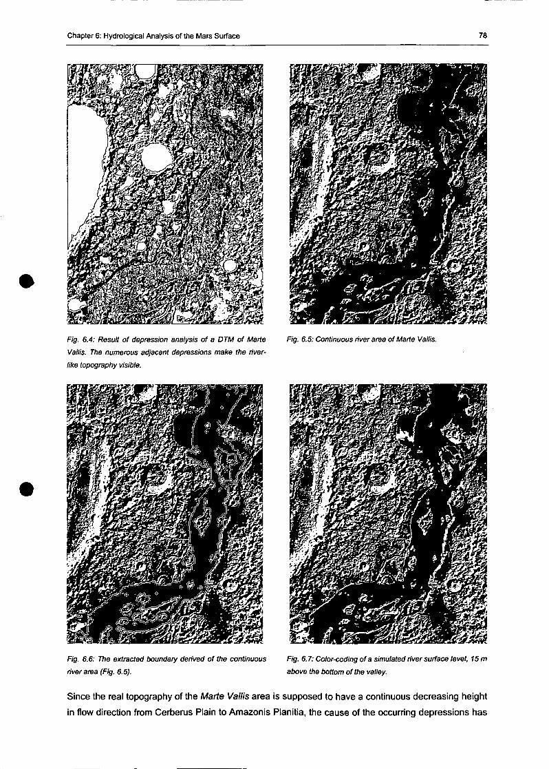
Chapter 6: Hydrological Analysis of the Mars Surface 78
Fig. 6.4: Result of depression analysis of a DTM of Maris
Vallis. The numerous adjacent depressions make the river-
like topography visible.
Fig. 6.6: The extracted boundary derived of the continuous
riverarea (Fig. 6.5).
Fig. 6.5: Continuous riverarea ofMarte Vallis.
Fig. 6.7: Color-coding of a simulated river surface level, 15 m
above the bottom ofthe valley.
Since the real topography of the Marie Vallis area is supposed to have a continuous decreasing height
in flow direction from Cerberus Piain to Amazonis Planitia, the cause of the occurring depressions has
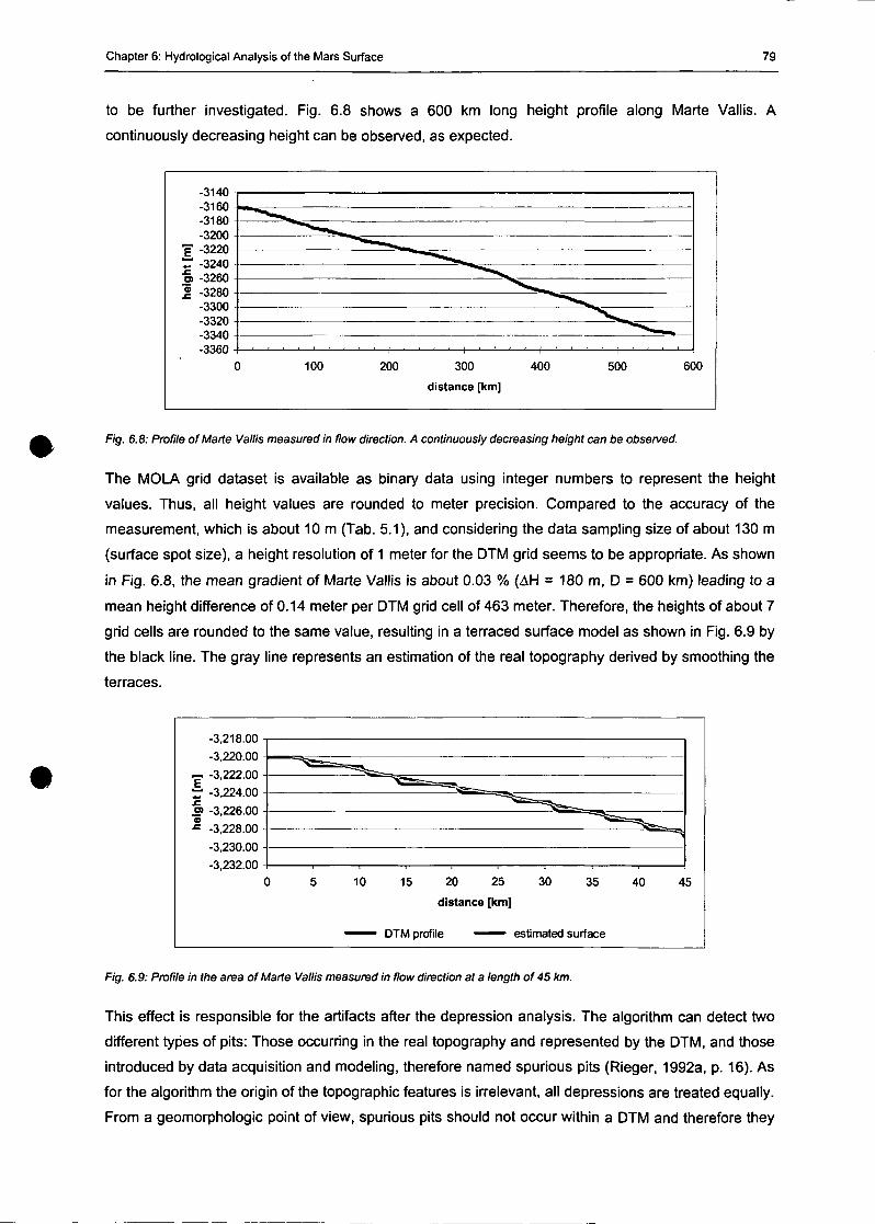
Chapter 6: Hydrological Analysis of the Mars Surface 79
to be further investigated. Fig. 6.8 shows a 600 km long height profile along Marte Vallis. A
continuously decreasing height can be observed, as expected.
-3140-3160-3180-3200
1" -3220r -3240 •o) -3260
-3300-3320-3340-3360
100 200 300
distance [km]
400 500 600
Fig. 6.8: Profile of Marte Vallis measured in flow direction. A continuously decreasing height can be observed.
The MOLA grid dataset is available as binary data using integer numbers to represent the height
values. Thus, all height values are rounded to meter precision. Compared to the accuracy of the
measurement, which is about 10 m (Tab. 5.1), and considering the data sampling size of about 130 m
(surface spot size), a height resolution of 1 meter for the DTM grid seems to be appropriate. As shown
in Fig. 6.8, the mean gradient of Marte Vallis is about 0.03 % (AH = 180 m, D = 600 km) leading to a
mean height difference of 0.14 meter per DTM grid cell of 463 meter. Therefore, the heights of about 7
grid cells are rounded to the same value, resulting in a terraced surface model as shown in Fig. 6.9 by
the black line. The gray line represents an estimation of the real topography derived by smoothing the
terraces.
-3,218.00
-3,220.00
~ -3,222.00
— -3,224.00
w -3,226.00•= -3,228.00
-3,230.00
-3,232.00
10 15 20 25
distance [km]
30 35 40 45
DTM profile estimated surface
Fig. 6.9: Profile in the area of Marte Vallis measured in flow direction at a length of45 km.
This effect is responsible for the artifacts after the depression analysis. The algorithm can detect two
different types of pits: Those occurring in the real topography and represented by the DTM, and those
introduced by data acquisition and modeling, therefore named spurious pits (Rieger, 1992a, p. 16). As
for the algorithm the origin of the topographic features is irrelevant, all depressions are treated equally.
From a geomorphologic point of view, spurious pits should not occur within a DTM and therefore they
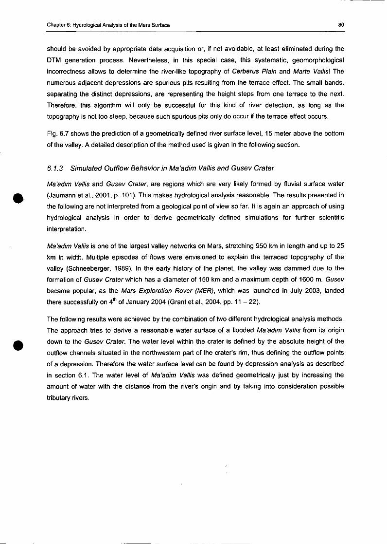
Chapter 6: Hydrological Analysis of the Mars Surface 80
should be avoided by appropriate data acquisition or, if not avoidable, at least eliminated during the
DTM generation process. Nevertheless, in this Special case, this systematic, geomorphological
incorrectness allows to determine the river-like topography of Cerberus Piain and Marie Vallisl The
numerous adjacent depressions are spurious pits resulting from the terrace effect. The small bands,
separating the distinct depressions, are representing the height steps from one terrace to the next.
Therefore, this algorithm will only be successful for this kind of river detection, as long as the
topography is not too steep, because such spurious pits only do occur if the terrace effect occurs.
Fig. 6.7 shows the prediction of a geometrically defined river surface level, 15 meter above the bottom
of the valley. A detailed description of the method used is given in the following section.
6.1.3 Simulated Outflow Behavior in Ma'adim Vallis and Gusev Crater
Ma'adim Vallis and Gusev Crater, are regions which are very likely formed by fluvial surface water
(Jaumann et al., 2001, p. 101). This makes hydrological analysis reasonable. The results presented in
the following are not interpreted from a geological point of view so far. It is again an approach of using
hydrological analysis in order to derive geometrically defined simulations for further scientific
Interpretation.
Ma'adim Vallis is one of the largest valley networks on Mars, stretching 950 km in length and up to 25
km in width. Multiple episodes of flows were envisioned to explain the terraced topography of the
valley (Schneeberger, 1989). In the early history of the planet, the valley was dammed due to the
formation of Gusev Crater which has a diameter of 150 km and a maximum depth of 1600 m. Gusev
became populär, as the Mars Exploration Rover (MER), which was launched in July 2003, landed
there successfully on 4 * of January 2004 (Grant et al., 2004, pp. 11 - 22).
The following results were achieved by the combination of two different hydrological analysis methods.
The approach tries to derive a reasonable water surface of a flooded Ma'adim Vallis from its origin
down to the Gusev Crater. The water level within the crater is defined by the absolute height of the
outflow Channels situated in the northwestern part of the crater's hm, thus defining the outflow points
of a depression. Therefore the water surface level can be found by depression analysis as described
in section 6.1. The water level of Ma'adim Vallis was defined geometrically just by increasing the
amount of water with the distance from the river's origin and by taking into consideration possible
tributary rivers.
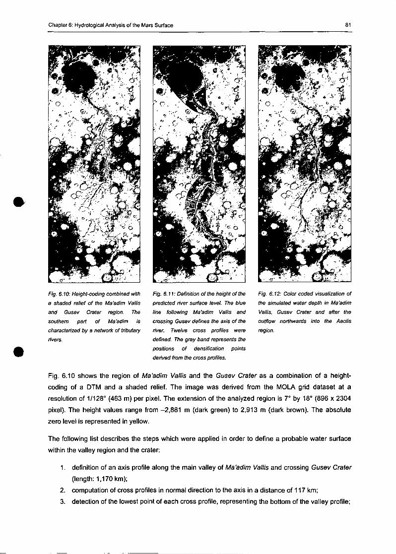
Chapter 6: Hydrological Analysis of the Mars Surface 81
Fig. 6.10: Height<oding combined with
a shaded relief of the Ma'adim Vallis
and Gusev Crater region. The
southern pari of Ma'adim is
charactehzed by a network of tributary
rivers.
Fig. 6.11: Definition of the height of the
predicted river surface level. The blue
line following Ma'adim Vallis and
crossing Gusev defines the axis of the
river. Twelve cross profiles were
defmed. The gray band represents the
positions of densification points
derived from the cross profiles.
Fig. 6.12: Color coded visualization of
the simulated water depth in Ma'adim
Vallis, Gusev Crater and after the
outflow northwards into the Aeolis
region.
Fig. 6.10 shows the region of Ma'adim Vallis and the Gusev Crater as a combination of a height-
coding of a DTM and a shaded relief. The image was derived from the MOLA grid dataset at a
resolution of 1/128° (463 m) per pixel. The extension of the analyzed region is 7° by 18° (896 x 2304
pixel). The height values ränge from -2,881 m (dark green) to 2,913 m (dark brown). The absolute
zero level is represented in yellow.
The following list describes the Steps which were applied in order to define a probable water surface
within the valley region and the crater:
1. defmition of an axis profile along the main valley of Ma'adim Vallis and crossing Gusev Crater
(length: 1,170 km);
2. computation of cross profiles in normal direction to the axis in a distance of 117 km;
3. detection of the Iowest point of each cross profile, representing the bottom of the valley profile;
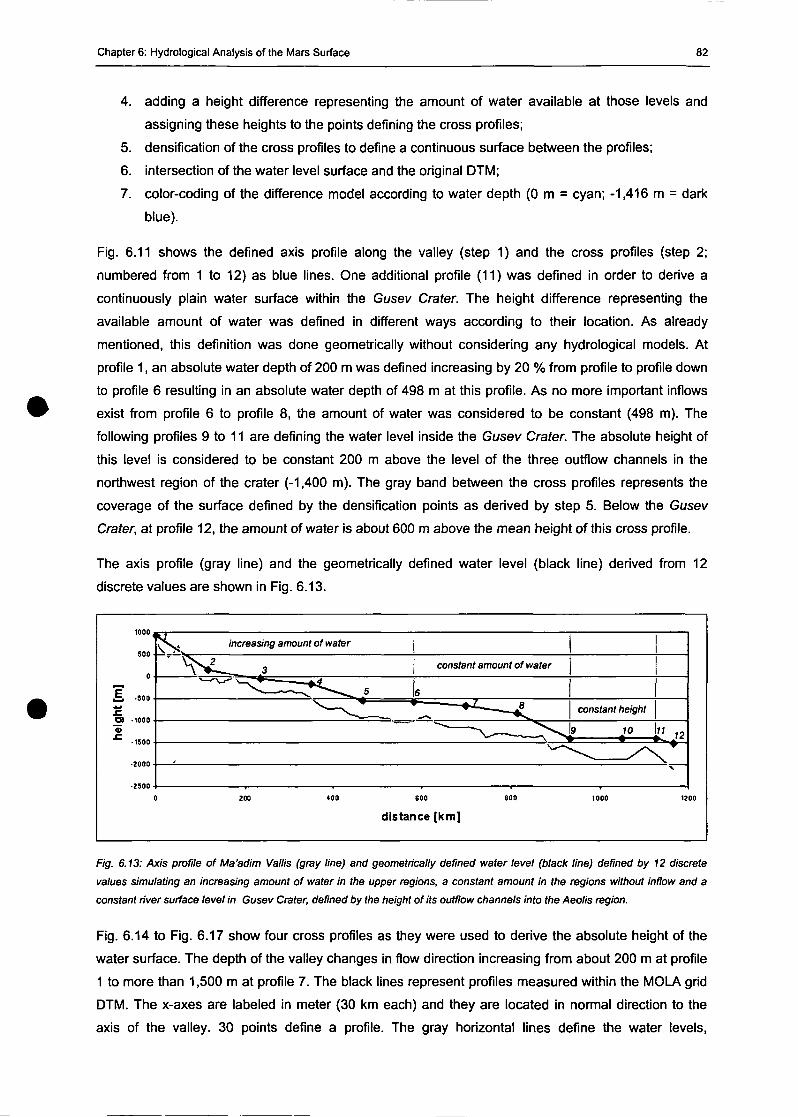
Chapter 6: Hydrological Analysis of the Mars Surface 82
4. adding a height difference representing the amount of water available at those levels and
assigning these heights to the points defining the cross profiles;
5. densification of the cross profiles to define a continuous surface between the profiles;
6. intersection of the water level surface and the original DTM;
7. color-coding of the difference model according to water depth (0 m = cyan; -1,416 m = dark
blue).
Fig. 6.11 shows the defined axis profile along the valley (step 1) and the cross profiles (step 2;
numbered from 1 to 12) as blue lines. One additional profile (11) was defined in order to derive a
continuously piain water surface within the Gusev Crater. The height difference representing the
available amount of water was defined in different ways according to their location. As already
mentioned, this definition was done geometrically without considering any hydrological modeis. At
profile 1, an absolute water depth of 200 m was defined increasing by 20 % from profile to profile down
to profile 6 resulting in an absolute water depth of 498 m at this profile. As no more important inflows
exist from profile 6 to profile 8, the amount of water was considered to be constant (498 m). The
following profiles 9 to 11 are defining the water level inside the Gusev Crater. The absolute height of
this level is considered to be constant 200 m above the level of the three outflow Channels in the
northwest region of the crater (-1,400 m). The gray band between the cross profiles represents the
coverage of the surface defined by the densification points as derived by step 5. Below the Gusev
Crater, at profile 12, the amount of water is about 600 m above the mean height of this cross profile.
The axis profile (gray line) and the geometrically defined water level (black line) derived from 12
discrete values are shown in Fig. 6.13.
increasing amount of water
constant amount of water
constant height
400 600
distance [km]
Fig. 6.13: Axis profile of Ma'adim Vallis (gray line) and geometrically defined water level (black line) defined by 12 discrete
values simulating an increasing amount of water in the upper regions, a constant amount in the regions without inflow and a
constant river surface level in Gusev Crater, defined by the height of its outflow Channels into the Aeolis region.
Fig. 6.14 to Fig. 6.17 show four cross profiles as they were used to derive the absolute height of the
water surface. The depth of the valley changes in flow direction increasing from about 200 m at profile
1 to more than 1,500 m at profile 7. The black lines represent profiles measured within the MOLA grid
DTM. The x-axes are labeled in meter (30 km each) and they are located in normal direction to the
axis of the valley. 30 points define a profile. The gray horizontal lines define the water levels,
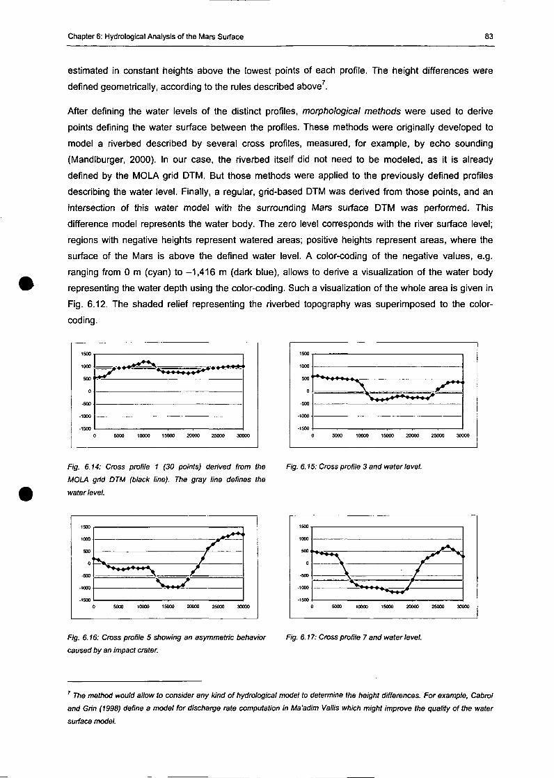
Chapter 6: Hydrological Analysis of the Mars Surface 83
estimated in constant heights above the Iowest points of each profile. The height differences were
defined geometrically, according to the rules described above7.
After defining the water levels of the distinct profiles, morphological methods were used to derive
points defining the water surface between the profiles. These methods were originally developed to
model a riverbed described by several cross profiles, measured, for example, by echo sounding
(Mandlburger, 2000). In our case, the riverbed itself did not need to be modeled, as it is already
defined by the MOLA grid DTM. But those methods were applied to the previously defined profiles
describing the water level. Finally, a regulär, grid-based DTM was derived from those points, and an
intersection of this water model with the surrounding Mars surface DTM was performed. This
difference model represents the water body. The zero level corresponds with the river surface level;
regions with negative heights represent watered areas; positive heights represent areas, where the
surface of the Mars is above the defined water level. A color-coding of the negative values, e.g.
ranging from 0 m (cyan) to -1,416 m (dark blue), allows to derive a visualization of the water body
representing the water depth using the color-coding. Such a visualization of the whole area is given in
Fig. 6.12. The shaded relief representing the riverbed topography was superimposed to the color-
coding.
Fig. 6.14: Cross profile 1 (30 points) derived from the
MOLA grid DTM (black line). The gray line defmes the
water level.
0 5000 10000 15000 20000 25000 30000
Fig. 6.15: Cross profile 3 and water level.
5000 10000 15000 20000 25000 30000 5000 10000 15000 20000 25000 30000
Fig. 6.16: Cross profile 5 showing an asymmetric behavior Fig. 6.17: Cross profile 7 and water level.
caused by an impact crater.
7 The method would allow to consider any kind of hydrological model to determine the height differences. For example, Cabrol
and Grin (1998) define a model for discharge rate computation in Ma'adim Vallis which might improve the quality of the water
surface model.
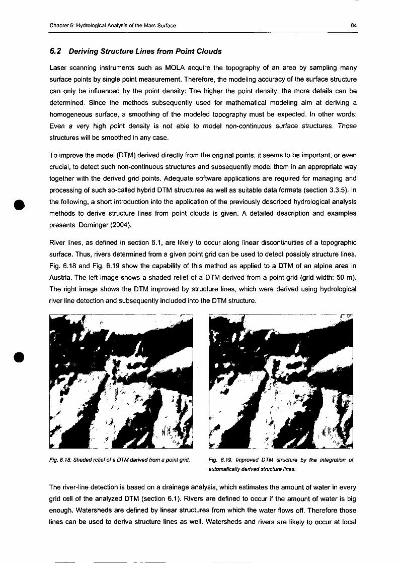
Chapter 6: Hydrological Analysis of the Mars Surface 84
6.2 Deriving Structure Lines from Point Clouds
Laser scanning instruments such as MOLA acquire the topography of an area by sampling many
surface points by Single point measurement. Therefore, the modeling accuracy of the surface structure
can only be influenced by the point density: The higher the point density, the more details can be
determined. Since the methods subsequently used for mathematical modeling aim at deriving a
homogeneous surface, a smoothing of the modeled topography must be expected. In other words:
Even a very high point density is not able to model non-continuous surface structures. Those
structures will be smoothed in any case.
To improve the model (DTM) derived directly from the original points, it seems to be important, or even
crucial, to detect such non-continuous structures and subsequently model them in an appropriate way
together with the derived grid points. Adequate Software applications are required for managing and
processing of such so-called hybrid DTM structures as well as suitable data formats (section 3.3.5). In
the following, a Short introduction into the application of the previously described hydrological analysis
methods to derive structure lines from point clouds is given. A detailed description and examples
presents Dorninger (2004).
River lines, as defined in section 6.1, are likely to occur along linear discontinuities of a topographic
surface. Thus, rivers determined from a given point grid can be used to detect possibly structure lines.
Fig. 6.18 and Fig. 6.19 show the capability of this method as applied to a DTM of an alpine area in
Austria. The left image shows a shaded relief of a DTM derived from a point grid (grid width: 50 m).
The right image shows the DTM improved by structure lines, which were derived using hydrological
river line detection and subsequently included into the DTM structure.
Fig. 6.18: Shaded relief of a DTM derived from a point grid. Fig. 6.19: Improved DTM structure by the Integration of
automatically derived structure lines.
The river-line detection is based on a drainage analysis, which estimates the amount of water in every
grid cell of the analyzed DTM (section 6.1). Rivers are defined to occur if the amount of water is big
enough. Watersheds are defined by linear structures from which the water flows off. Therefore those
lines can be used to derive structure lines as well. Watersheds and rivers are likely to occur at local
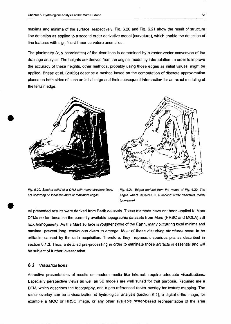
Chapter 6: Hydrological Analysis of the Mars Surface 85
maxima and minima of the surface, respectively. Fig. 6.20 and Fig. 6.21 show the result of structure
line detection as applied to a second order derivative model (curvature), which enable the detection of
line features with significant linear curvature anomalies.
The planimetry (x, y coordinates) of the river-lines is determined by a raster-vector conversion of the
drainage analysis. The heights are derived from the original model by interpolation. In order to improve
the accuracy of these heights, other methods, probably using those edges as initial values, might be
applied. Briese et al. (2002b) describe a method based on the computation of discrete approximation
planes on both sides of such an initial edge and their subsequent intersection for an exact modeling of
the terrain edge.
Fig. 6.20: Shaded relief of a DTM with many structure lines,
not occurring on local minimum or maximum edges.
Fig. 6.21: Edges derived from the model of Fig. 6.20. The
edges where detected in a second order derivative model
(curvature).
All presented results were derived from Earth datasets. These methods have not been applied to Mars
DTMs so far, because the currently available topographic datasets from Mars (HRSC and MOLA) still
lack homogeneity. As the Mars surface is rougher those of the Earth, many occurring local minima and
maxima, prevent long, continuous rivers to emerge. Most of these disturbing structures seem to be
artifacts, caused by the data acquisition. Therefore, they represent spurious pits as described in
section 6.1.3. Thus, a detailed pre-processing in order to eliminate those artifacts is essential and will
be subject of further investigation.
6.3 Visualizations
Attractive presentations of results on modern media like Internet, require adequate visualizations.
Especially perspective views as well as 3D modeis are well suited for that purpose. Required are a
DTM, which describes the topography, and a geo-referenced raster overlay for texture mapping. The
raster overlay can be a visualization of hydrological analysis (section 6.1), a digital ortho-image, for
example a MOC or HRSC image, or any other available raster-based representation of the area
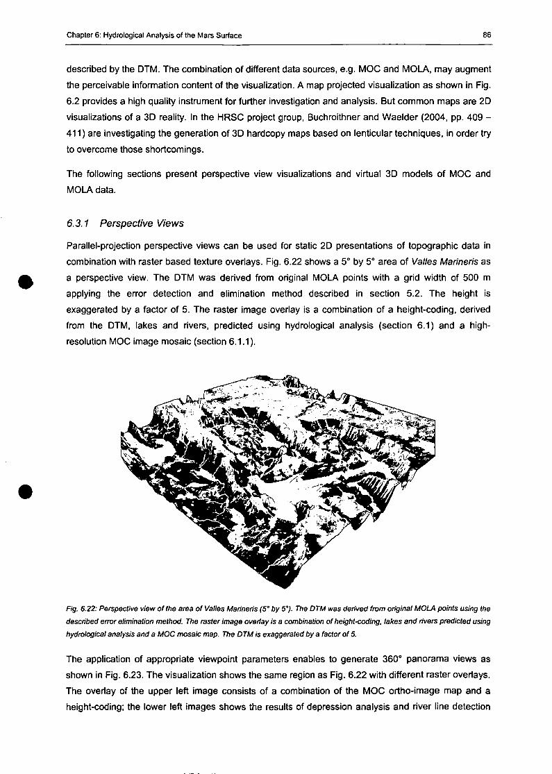
Chapter 6: Hydrological Analysis of the Mars Surface 86
deschbed by the DTM. The combination of different data sources, e.g. MOC and MOLA, may augment
the perceivable Information content of the visualization. A map projected visualization as shown in Fig.
6.2 provides a high quality instrument for further investigation and analysis. But common maps are 2D
visualizations of a 3D reality. In the HRSC project group, Buchroithner and Waelder (2004, pp. 409 -
411) are investigating the generation of 3D hardcopy maps based on lenticular techniques, in order try
to overcome those shortcomings.
The following sections present perspective view visualizations and Virtual 3D modeis of MOC and
MOLA data.
6.3.1 Perspective Views
Parallel-projection perspective views can be used for static 2D presentations of topographic data in
combination with raster based texture overlays. Fig. 6.22 shows a 5° by 5° area of Valles Marineris as
a perspective view. The DTM was derived from original MOLA points with a grid width of 500 m
applying the error detection and elimination method described in section 5.2. The height is
exaggerated by a factor of 5. The raster image overlay is a combination of a height-coding, derived
from the DTM, lakes and rivers, predicted using hydrological analysis (section 6.1) and a high-
resolution MOC image mosaic (section 6.1.1).
Fig. 6.22: Perspective view ofthe area of Valles Marineris (5° by 5°). The DTM was derived from original MOLA points using the
described error elimination method. The raster image overiay is a combination of height-coding, lakes and rivers predicted using
hydrological analysis and a MOC mosaic map. The DTM is exaggerated by a factor of 5.
The application of appropriate viewpoint parameters enables to generate 360° panorama views as
shown in Fig. 6.23. The visualization shows the same region as Fig. 6.22 with different raster overlays.
The overlay of the upper left image consists of a combination of the MOC ortho-image map and a
height-coding; the Iower left images shows the results of depression analysis and river line detection
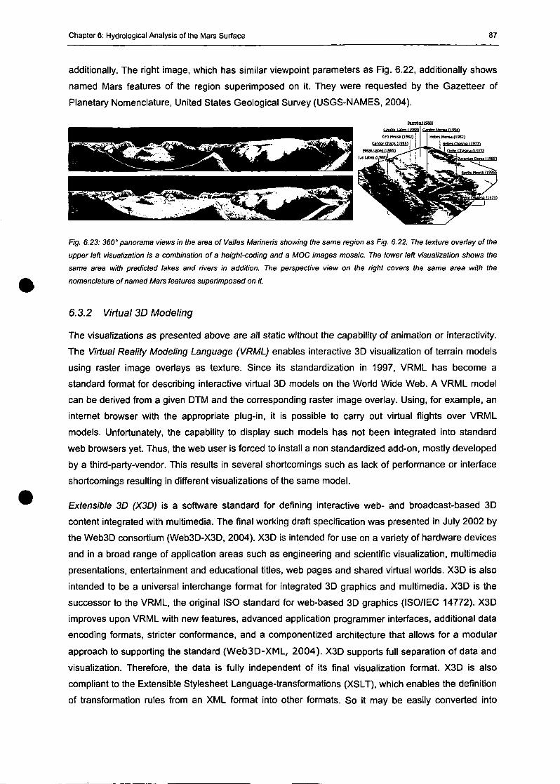
Chapter 6: Hydrological Analysis of the Mars Surface 87
additionally. The right image, which has similar viewpoint parameters as Fig. 6.22, additionally shows
named Mars features of the region superimposed on it. They were requested by the Gazetteer of
Planetary Nomenclature, United States Geological Survey (USGS-NAMES, 2004).
Fig. 6.23:360° panorama views in the area of Valles Marineris showing the same region as Fig. 6.22. The texture overiay of the
upper left visualization is a combination of a height-coding and a MOC images mosaic. The Iower left visualization shows the
same area with predicted lakes and rivers in addition. The perspective view on the right Covers the same area with the
nomenclature of named Mars features superimposed on it.
6.3.2 Virtual 3D Modeling
The visualizations as presented above are all static without the capability of animation or interactivity.
The Virtual Reality Modeling Language (VRML) enables interactive 3D visualization of terrain modeis
using raster image overlays as texture. Since its standardization in 1997, VRML has become a
Standard format for describing interactive Virtual 3D modeis on the World Wide Web. A VRML model
can be derived from a given DTM and the corresponding raster image overiay. Using, for example, an
internet browser with the appropriate plug-in, it is possible to carry out Virtual flights over VRML
modeis. Unfortunately, the capability to display such modeis has not been integrated into Standard
web browsers yet. Thus, the web user is forced to install a non standardized add-on, mostly developed
by a third-party-vendor. This results in several shortcomings such as lack of Performance or interface
shortcomings resulting in different visualizations of the same model.
Extensible 3D (X3D) is a Software Standard for defining interactive web- and broadcast-based 3D
content integrated with multimedia. The final working draft specification was presented in July 2002 by
the Web3D consortium (Web3D-X3D, 2004). X3D is intended for use on a variety of hardware devices
and in a broad ränge of application areas such as engineering and scientific visualization, multimedia
presentations, entertainment and educational titles, web pages and shared Virtual worlds. X3D is also
intended to be a universal interchange format for integrated 3D graphics and multimedia. X3D is the
successor to the VRML, the original ISO Standard for web-based 3D graphics (ISO/IEC 14772). X3D
improves upon VRML with new features, advanced application programmer interfaces, additional data
encoding formats, stricter conformance, and a componentized architecture that allows for a modular
approach to supporting the Standard (Web3D-XML, 2004). X3D Supports füll Separation of data and
visualization. Therefore, the data is fully independent of its final visualization format. X3D is also
compliant to the Extensible Stylesheet Language-transformations (XSLT), which enables the definition
of transformation rules from an XML format into other formats. So it may be easily converted into
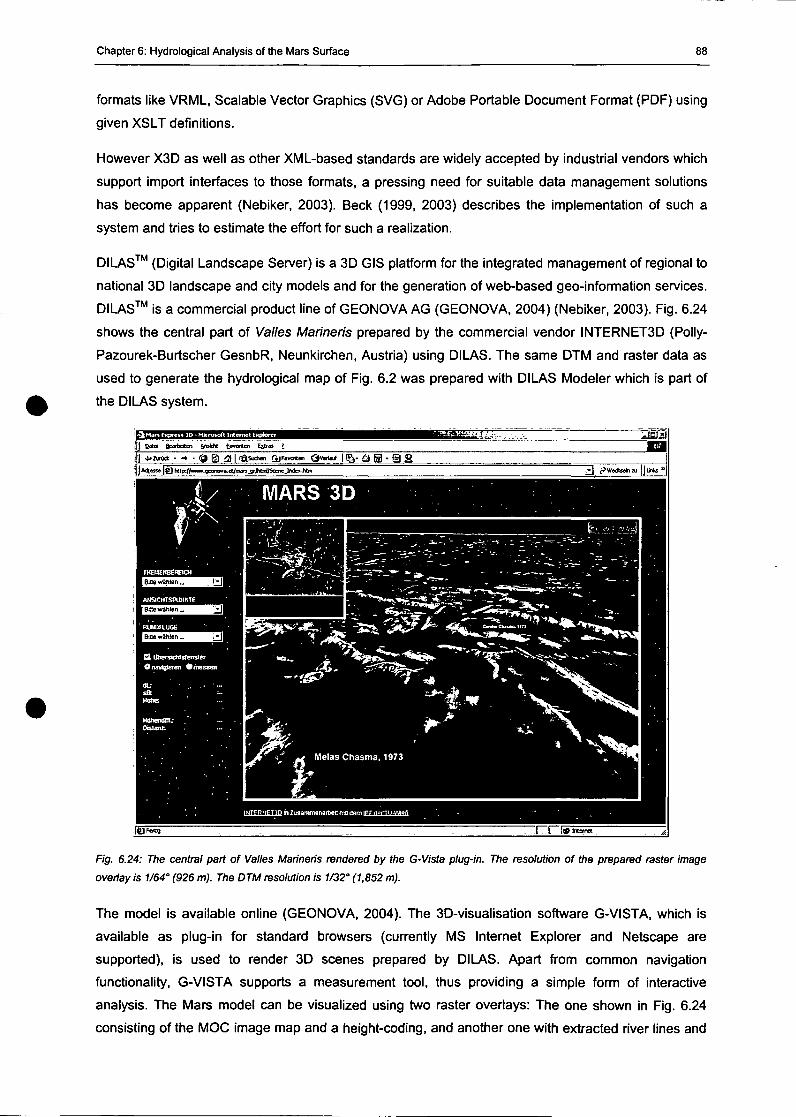
Chapter 6: Hydrological Analysis of the Mars Surface 88
formats like VRML, Scalable Vector Graphics (SVG) or Adobe Portable Document Format (PDF) using
given XSLT definitions.
However X3D as well as other XML-based Standards are widely accepted by industrial vendors which
support import interfaces to those formats, a pressing need for suitable data management Solutions
has become apparent (Nebiker, 2003). Beck (1999, 2003) describes the implementation of such a
System and tries to estimate the effort for such a realization.
DILAS™ (Digital Landscape Server) is a 3D GIS platform for the integrated management of regional to
national 3D landscape and city modeis and for the generation of web-based geo-information Services.
DILAS™ is a commercial product line of GEONOVA AG (GEONOVA, 2004) (Nebiker, 2003). Fig. 6.24
shows the central part of Valles Marineris prepared by the commercial vendor INTERNET3D (Polly-
Pazourek-Burtscher GesnbR, Neunkirchen, Austria) using DILAS. The same DTM and raster data as
used to generate the hydrological map of Fig. 6.2 was prepared with DILAS Modeler which is part of
the DILAS System.
Bold
*fces»|
Statrfm JrekM Covcrten Es»« >
k . 4 - f l | f l | S«t», SJF,»«., O»»"Ü WtK/>-»..g»nw**»».j»/h(»US«r«Jnite.J«»
1 !ä- £» ® • Sl fi
Fig. 6.24: The central part of Valles Marineris rendered by the G-Vista plug-in. The resolution of the prepared raster image
overiay is 1/64° (926 m). The DTM resolution is 1/32" (1,852 m).
The model is available online (GEONOVA, 2004). The 3D-visualisation Software G-VISTA, which is
available as plug-in for Standard browsers (currently MS Internet Explorer and Netscape are
supported), is used to render 3D scenes prepared by DILAS. Apart from common navigation
functionality, G-VISTA Supports a measurement tool, thus providing a simple form of interactive
analysis. The Mars model can be visualized using two raster overlays: The one shown in Fig. 6.24
consisting of the MOC image map and a height-coding, and another one with extracted river lines and
Chapter 6: Hydrological Analysis of the Mars Surface 89
results of depression analysis superimposed on it. The model was presented at the Intergeo 2003 in
Hamburg, Germany.
6.3.3 3D Hardcopy of Olympus Mons
The above described methods were applied to derive Virtual 3D modeis. An appropriate Virtual reality
environment is necessary to visualize such modeis, for instance, on a monitor. This finally described
task aims to create a three-dimensional hardcopy of the caldera region of Olympus Mons.
The Output device used was a Dimension 3D plotter (DIMENSION, 2004). This plotter generates 3D
plastics hardcopies of any three-dimensional digital model. The plastics used for modeling is melted
and brought onto a platform slice by slice. Every slice has a thickness of 0.25 mm. The digital input
model has to be a closed (water proof) surface provided in Stereo Lithography (STL) format. STL
describes a surface by the means of triangulation. The closed model of Olympus Mons consisted of a
bottom piain, the topographical model and four vertical plains connecting the topographic surface with
the bottom.
The topography was derived from HRSC stereo images by the DLR applying feature-based image
matching. The regulär grid DTM describing the caldera region had an extension of 100 km by 80 km.
The maximum workspace of the plotter is 20 cm by 20 cm by 30 cm (height). The model grid width
was assigned to 0.25 mm, according to the height resolution of the plotter (thickness of the individual
slices). Thus, the hardcopy had a planimetric extension of 20 cm by 16 cm representing a scale of
1:500,000. The height values were exaggerated by a factor of 5, resulting in an absolute model height
of about6 cm.
First attempts to derive a triangulation from the grid-based DTM were made using the Software
package Geomagic Studio by Raindrop Geomagic (GEOMAGIC, 2004). This Software provides two
different implementations of a füll 3D triangulation algorithm. They are named Surface and Volume.
Unfortunately, the Surface method showed a direction dependent behavior, as the triangulation was
not performed properly in almost vertical areas. Fig. 6.25 shows a quarter of the caldera to be
modeled with missing triangulation surfaces at the steep rim of the crater.
The second implementation, Volume, seemed to be more appropriate to model the given body in a
correct way. First attempts on a simplified model were promising. But as applied to the füll detailed
object, the used machine was not able to perform the computation (528 MB RAM).
Therefore a simple 2D triangulation was implemented, thus deriving the edges of the triangles from a
regulär planimetric grid. The height values of the given points were assigned to the nodes of the
triangles afterwards, and the result was converted to STL format. This simple triangulation was only
possible because of the 2.5D behavior of the given dataset. A rendered visualization of this object is
shown in Fig. 6.26. The plotting process lasted about 16 hours.
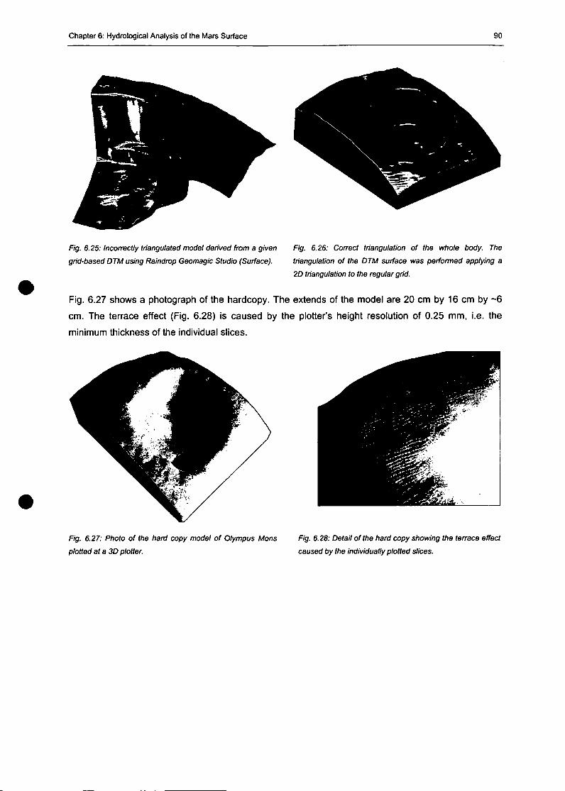
Chapter 6: Hydrological Analysis of the Mars Surface 90
Fig. 6.25: Incorrectly triangulated model derived from a given
grid-based DTM using Raindmp Geomagic Studio (Surface).
Fig. 6.26: Correct triangulation of the whole body. The
triangulation of the DTM surface was performed applying a
2D triangulation to the regulär grid.
Fig. 6.27 shows a photograph of the hardcopy. The extends of the model are 20 cm by 16 cm by ~6
cm. The terrace effect (Fig. 6.28) is caused by the plotter's height resolution of 0.25 mm, i.e. the
minimum thickness of the individual slices.
Fig. 6.27: Photo of the hard copy model of Olympus Mons
plotted at a 3D plotter.
Fig. 6.28: Detail ofthe hard copy showing the terrace effect
caused by the individually plotted slices.
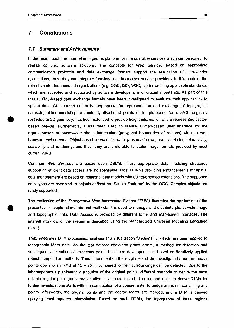
Chapter 7: Conclusions 91
7 Conclusions
7.1 Summary and Achievements
In the recent past, the Internet emerged as platform for interoperable Services which can be joined to
realize complex Software Solutions. The concepts for Web Services based on appropriate
communication protocols and data exchange formats support the realization of inter-vendor
applications, thus, they can integrate functionalities from other service Providers. In this context, the
role of vendor-independent organizations (e.g. OGC, ISO, W3C, ...) for defining applicable Standards,
which are accepted and supported by Software developers, is of crucial importance. As part of this
thesis, XML-based data exchange formats have been investigated to evaluate their applicability to
spatial data. GML turned out to be appropriate for representation and exchange of topographic
datasets, either consisting of randomly distributed points or in grid-based form. SVG, originally
restricted to 2D geometry, has been extended to provide height information of the represented vector-
based objects. Furthermore, it has been used to realize a map-based user interface for the
representation of planet-wide shape information (polygonal boundaries of regions) within a web
browser environment. Object-based formats for data presentation support client-side interactivity,
scalability and rendering, and thus, they are preferable to static image formats provided by most
current WMS.
Common Web Services are based upon DBMS. Thus, appropriate data modeling structures
supporting efficient data access are indispensable. Most DBMSs providing enhancements for spatial
data management are based on relational data modeis with object-oriented extensions. The supported
data types are restricted to objects defined as "Simple Features" by the OGC. Complex objects are
rarely supported.
The realization of the Topographic Mars Information System (TMIS) illustrates the application of the
presented concepts, Standards and methods. It is used to manage and distribute planet-wide image
and topographic data. Data Access is provided by different form- and map-based interfaces. The
internal Workflow of the System is described using the standardized Universal Modeling Language
(UML).
TMIS integrates DTM processing, analysis and visualization functionality, which has been applied to
topographic Mars data. As the test dataset contained gross errors, a method for detection and
subsequent elimination of erroneous points has been developed. It is based on iteratively applied
robust interpolation methods. Thus, dependent on the roughness of the investigated area, erroneous
points down to an RMS of 15 - 20 m compared to their surroundings can be detected. Due to the
inhomogeneous planimetric distribution of the original points, different methods to derive the most
reliable regulär point grid representation have been tested. The method used to derive DTMs for
further investigations Starts with the computation of a coarse raster to bridge areas not containing any
points. Afterwards, the original points and the coarse raster are merged, and a DTM is derived
applying least Squares interpolation. Based on such DTMs, the topography of three regions
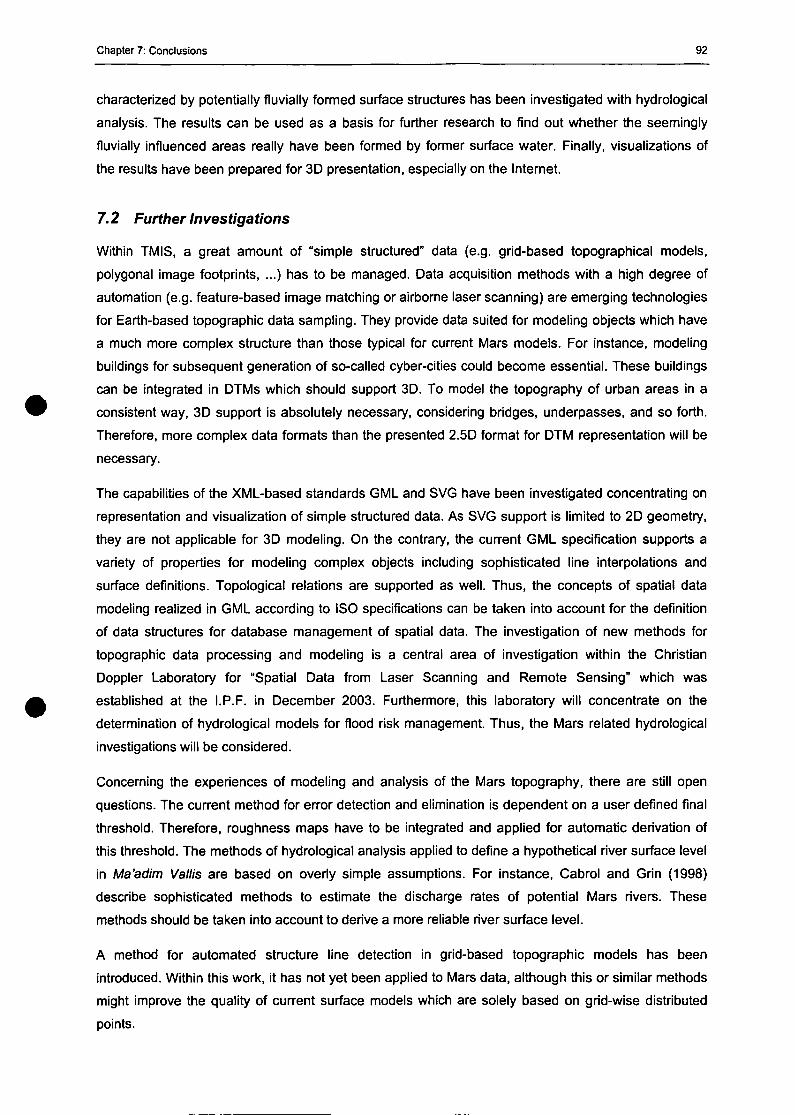
Chapter 7: Conclusions 92
characterized by potentially fluvially formed surface structures has been investigated with hydrological
analysis. The results can be used as a basis for further research to find out whether the seemingly
fluvially influenced areas really have been formed by former surface water. Finally, visualizations of
the results have been prepared for 3D presentation, especially on the Internet.
7.2 Further Investigations
Within TMIS, a great amount of "simple structured" data (e.g. grid-based topographical modeis,
polygonal Image footprints, ...) has to be managed. Data acquisition methods with a high degree of
automation (e.g. feature-based image matching or airborne laser scanning) are emerging technologies
for Earth-based topographic data sampling. They provide data suited for modeling objects which have
a much more complex structure than those typical for current Mars modeis. For instance, modeling
buildings for subsequent generation of so-called cyber-cities could become essential. These buildings
can be integrated in DTMs which should support 3D. To model the topography of urban areas in a
consistent way, 3D support is absolutely necessary, considering bridges, underpasses, and so forth.
Therefore, more complex data formats than the presented 2.5D format for DTM representation will be
necessary.
The capabilities of the XML-based Standards GML and SVG have been investigated concentrating on
representation and visualization of simple structured data. As SVG support is limited to 2D geometry,
they are not applicable for 3D modeling. On the contrary, the current GML specification supports a
variety of properties for modeling complex objects including sophisticated line interpolations and
surface definitions. Topological relations are supported as well. Thus, the concepts of spatial data
modeling realized in GML according to ISO specifications can be taken into account for the definition
of data structures for database management of spatial data. The investigation of new methods for
topographic data processing and modeling is a central area of investigation within the Christian
Doppier Laboratory for "Spatial Data from Laser Scanning and Remote Sensing" which was
established at the I.P.F. in December 2003. Furthermore, this laboratory will concentrate on the
determination of hydrological modeis for flood risk management. Thus, the Mars related hydrological
investigations will be considered.
Concerning the experiences of modeling and analysis of the Mars topography, there are still open
questions. The current method for error detection and elimination is dependent on a user defined final
threshold. Therefore, roughness maps have to be integrated and applied for automatic derivation of
this threshold. The methods of hydrological analysis applied to define a hypothetical river surface level
in Ma'adim Vallis are based on overly simple assumptions. For instance, Cabrol and Grin (1998)
describe sophisticated methods to estimate the discharge rates of potential Mars rivers. These
methods should be taken into account to derive a more reliable river surface level.
A method for automated structure line detection in grid-based topographic modeis has been
introduced. Within this work, it has not yet been applied to Mars data, although this or similar methods
might improve the quality of current surface modeis which are solely based on grid-wise distributed
points.

Chapter 7: Conclusions 93
Finally it has to be stated, that none of the described methods had ever been applied to DTMs derived
from HRSC image data, although the HRSC project has been the framework for this thesis. First
attempts to derive reliable DTMs from currently available point clouds which have been acquired by
feature-based image matching methods, have not been satisfying. It will be a great challenge to
perform the described hydrological analysis to the high-resolution topographic modeis of Mars
provided by the HRSC in order to to evaluate the presented results using the more detailed
information.
The main task of TMIS is management and distribution of planet-wide image and topographic data.
Since January 2004 the Mars Express spacecraft is in operational mode and it has already delivered
almost 100 Gigabytes of image data which is available to all related scientists via TMIS. The
application of the investigated methods for topographic data processing and analysis to HRSC data
will be a future challenge!
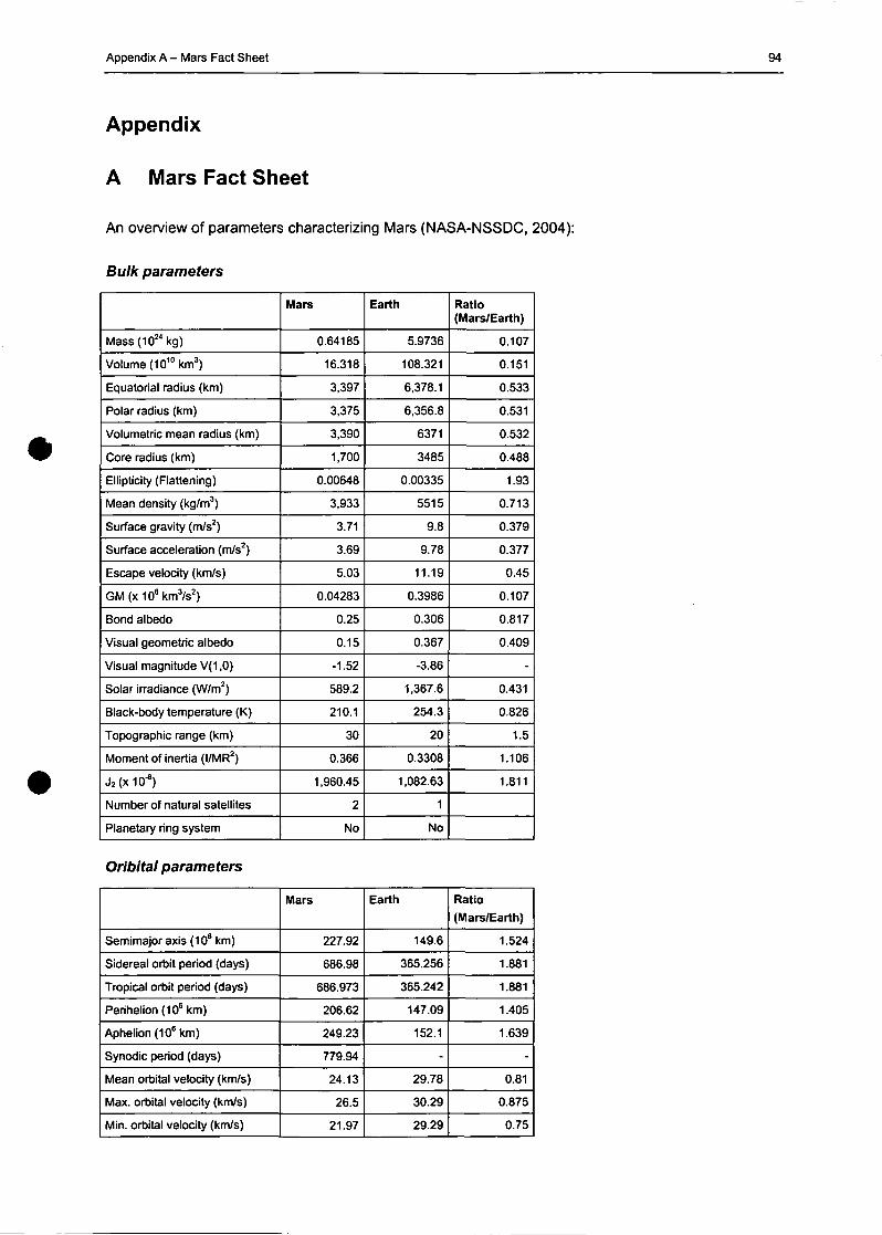
Appendix A - Mars Fact Sheet 94
Appendix
A Mars Fact Sheet
An overview of parameters characterizing Mars (NASA-NSSDC, 2004):
Bulk parameters
Mass(1024kg)
Volume (1010 km3)
Equatorial radius (km)
Polar radius (km)
Volumetrie mean radius (km)
Core radius (km)
Ellipticity (Flattening)
Mean density (kg/m3)
Surface gravity (m/s2)
Surface acceleration (m/s2)
Escape velocity (km/s)
GM(x106km3/s2)
Bond albedo
Visual geometric albedo
Visual magnitude V(1,0)
Solar irradiance (W/m2)
Black-body temperature (K)
Topographie ränge (km)
Moment of inertia (I/MR2)
J2(x10-6)
Number of natural satellites
Planetary ring System
Mars
0.64185
16.318
3,397
3,375
3,390
1,700
0.00648
3,933
3.71
3.69
5.03
0.04283
0.25
0.15
-1.52
589.2
210.1
30
0.366
1,960.45
2
No
Earth
5.9736
108.321
6,378.1
6,356.8
6371
3485
0.00335
5515
9.8
9.78
11.19
0.3986
0.306
0.367
-3.86
1,367.6
254.3
20
0.3308
1,082.63
1
No
Ratio(Mars/Earth)
0.107
0.151
0.533
0.531
0.532
0.488
1.93
0.713
0.379
0.377
0.45
0.107
0.817
0.409
-
0.431
0.826
1.5
1.106
1.811
Oribital parameters
Semimajor axis (106 km)
Sidereal orbit period (days)
Tropical orbit period (days)
Perihelion(106km)
Aphelion(106km)
Synodic period (days)
Mean orbital velocity (km/s)
Max. orbital velocity (km/s)
Min. orbital velocity (km/s)
Mars
227.92
686.98
686.973
206.62
249.23
779.94
24.13
26.5
21.97
Earth
149.6
365.256
365.242
147.09
152.1
-
29.78
30.29
29.29
Ratio
(Mars/Earth)
1.524
1.881
1.881
1.405
1.639
-
0.81
0.875
0.75
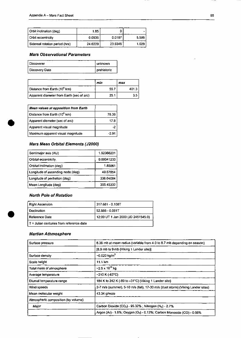
Appendix A - Mars Fact Sheet 95
Orbit inclination (deg)
Orbit eccentricity
Sidereal rotation period (hrs)
1.85
0.0935
24.6229
0
0.0167
23.9345
-
5.599
1.029
Mars Observational Parameters
Discoverer
Discovery Date
unknown
prehistoric
Distance from Earth (106 km)
Apparent diameter from Earth (sec of arc)
min
55.7
25.1
max
401.3
3.5
Mean values at Opposition from Earth
Distance from Earth (106 km)
Apparent diameter (sec of arc)
Apparent Visual magnitude
Maximum apparent Visual magnitude
78.39
17.9
-2
-2.91
Mars Mean Orbital Elements (J2000)
Semimajor axis (AU)
Orbital eccentricity.
Orbital inclination (deg)
Longitude of ascending node (deg)
Longitude of perihelion (deg)
Mean Longitude (deg)
1.52366231
0.09341233
1.85061
49.57854
336.04084
355.45332
North Pole of Rotation
Right Ascension
Declination
Reference Date
317.681-0.108T
52.886- 0.061 T
12:00 UT 1 Jan 2000 (JD 2451545.0)
T = Julian centuries from reference date
Martian Athmosphere
Surface pressure
Surface density
Scale height
Total mass of atmosphere
Average temperature
Diumal temperature ränge
Wind speeds
Mean molecular weight
Atmospheric composition (by volume)
Major
6.36 mb at mean radius (variable from 4.0 to 8.7 mb depending on season)
[6.9 mb to 9 mb (Viking 1 Lander site)]
-0.020 kg/m3
11.1 km
-2.5x101 6kg
-210K(-63°C)
184 K to 242 K (-89 to -31 °C) (Viking 1 Lander site)
2-7 m/s (summer), 5-10 m/s (fall), 17-30 m/s (dust storm) (Viking Lander Sites)
43.34 g/mole
Carbon Dioxide (CO2) - 95.32% ; Nitrogen (N2) - 2.7%
Argon (Ar) -1.6%; Oxygen (O2) - 0.13%; Carbon Monoxide (CO) - 0.08%
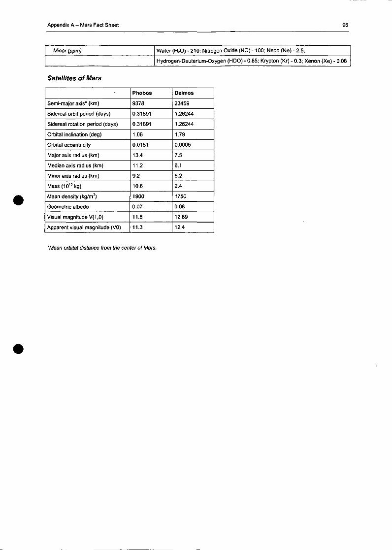
Appendix A - Mars Fact Sheet 96
Minor (ppm) Water (H20) - 210; Nitrogen Oxide (NO) -100; Neon (Ne) - 2.5;
Hydrogen-Deuterium-Oxygen (HDO) - 0.85; Krypton (Kr) - 0.3; Xenon (Xe) - 0.08
Satellites of Mars
Semi-major axis* (km)
Sidereal orbit period (days)
Sidereal rotation period (days)
Orbital inclination (deg)
Orbital eccentricity
Major axis radius (km)
Mediän axis radius (km)
Minor axis radius (km)
Mass(1015kg)
Mean density (kg/m3)
Geometrie albedo
Visual magnitude V(1,0)
Apparent Visual magnitude (V0)
Phobos
9378
0.31891
0.31891
1.08
0.0151
13.4
11.2
9.2
10.6
1900
0.07
11.8
11.3
Deimos
23459
1.26244
1.26244
1.79
0.0005
7.5
6.1
5.2
2.4
1750
0.08
12.89
12.4
'Mean orbital distance from the center of Mars.
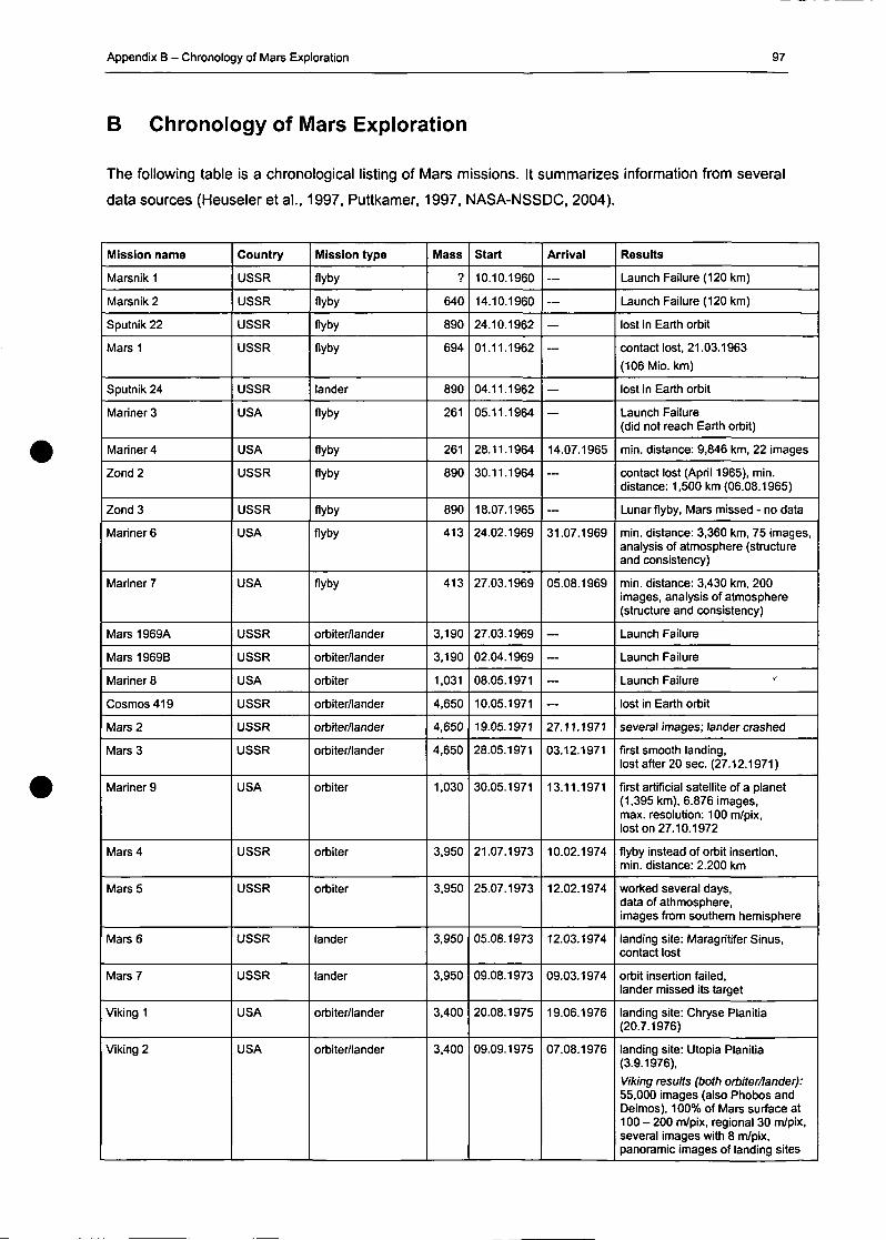
Appendix B - Chronology of Mars Exploration 97
B Chronology of Mars Exploration
The following table is a chronological listing of Mars missions. It summarizes information from several
data sources (Heuseier et al., 1997, Puttkamer, 1997, NASA-NSSDC, 2004).
Mission name
Marsnik 1
Marsnik 2
Sputnik 22
Mars 1
Sputnik 24
Mariner 3
Mariner 4
Zond2
Zond 3
Mariner 6
Mariner 7
Mars1969A
Mars1969B
Mariner 8
Cosmos419
Mars 2
Mars 3
Mariner 9
Mars 4
Mars 5
Mars 6
Mars 7
Viking 1
Viking 2
Country
USSR
USSR
USSR
USSR
USSR
USA
USA
USSR
USSR
USA
USA
USSR
USSR
USA
USSR
USSR
USSR
USA
USSR
USSR
USSR
USSR
USA
USA
Mission type
flyby
flyby
flyby
flyby
lander
flyby
flyby
flyby
flyby
flyby
flyby
orbiter/lander
orbiter/lander
orbiter
orbiter/lander
orbiter/lander
orbiter/lander
orbiter
orbiter
orbiter
lander
lander
orbiter/lander
orbiter/lander
Mass
?
640
890
694
890
261
261
890
890
413
413
3,190
3,190
1,031
4,650
4,650
4,650
1,030
3,950
3,950
3,950
3,950
3,400
3,400
Start
10.10.1960
14.10.1960
24.10.1962
01.11.1962
04.11.1962
05.11.1964
28.11.1964
30.11.1964
18.07.1965
24.02.1969
27.03.1969
27.03.1969
02.04.1969
08.05.1971
10.05.1971
19.05.1971
28.05.1971
30.05.1971
21.07.1973
25.07.1973
05.08.1973
09.08.1973
20.08.1975
09.09.1975
Arrival
—
—
—
—
—
—
14.07.1965
—
—
31.07.1969
05.08.1969
—
—
—
—
27.11.1971
03.12.1971
13.11.1971
10.02.1974
12.02.1974
12.03.1974
09.03.1974
19.06.1976
07.08.1976
Results
Launen Failure (120 km)
Launch Failure (120 km)
lost in Earth orbit
contact lost, 21.03.1963
(106 Mio. km)
lost in Earth orbit
Launch Failure(did not reach Earth orbit)
min. distance: 9,846 km, 22 images
contact lost (April 1965), min.distance: 1,500 km (06.08.1965)
Lunar flyby, Mars missed - no data
min. distance: 3,360 km, 75 images,analysis of atmosphere (struetureand consistency)
min. distance: 3,430 km, 200images, analysis of atmosphere(strueture and consistency)
Launch Failure
Launch Failure
Launch Failure
lost in Earth orbit
several images; lander crashed
first smooth landing,lost after 20 sec. (27.12.1971)
first artificial satellite of a planet(1,395 km), 6.876 images,max. resolution: 100 m/pix,loston 27.10.1972
flyby instead of orbit insertion,min. distance: 2.200 km
worked several days,data of athmosphere,images from southem hemisphere
landing Site: Maragritifer Sinus,contact lost
orbit insertion failed,lander missed its target
landing Site: Chryse Planitia(20.7.1976)
landing Site: Utopia Planitia(3.9.1976),
Viking results (both orbiter/lander):55,000 images (also Phobos andDeimos), 100% of Mars surface at100 - 200 m/pix, regional 30 m/pix,several images with 8 m/pix,panoramic images of landing Sites
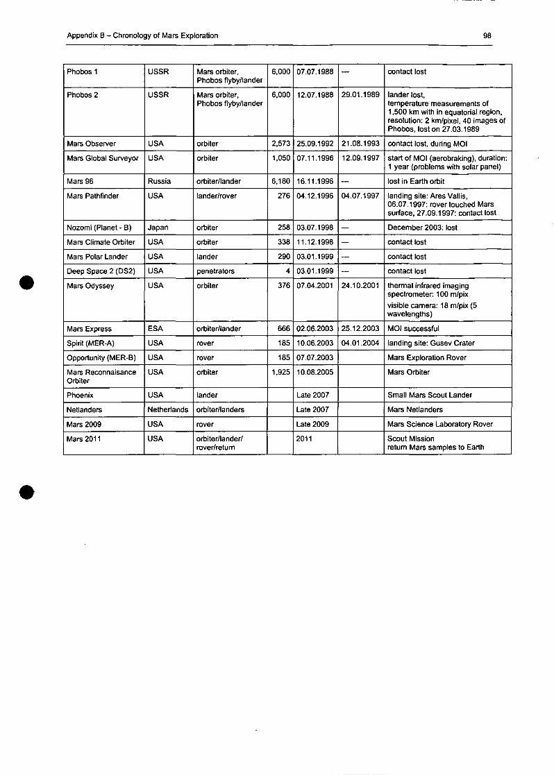
Appendix B - Chronology of Mars Exploration 98
Phobos 1
Phobos 2
Mars Observer
Mars Global Surveyor
Mars 96
Mars Pathfinder
Nozomi (Planet - B)
Mars Climate Orbiter
Mars Polar Lander
Deep Space 2 (DS2)
Mars Odyssey
Mars Express
Spirit (MER-A)
Opportunity (MER-B)
Mars ReconnaisanceOrbiter
Phoenix
Netlanders
Mars 2009
Mars 2011
USSR
USSR
USA
USA
Russia
USA
Japan
USA
USA
USA
USA
ESA
USA
USA
USA
USA
Netherlands
USA
USA
Mars orbiter,Phobos flyby/lander
Mars orbiter,Phobos flyby/lander
orbiter
orbiter
orbiter/lander
lander/rover
orbiter
orbiter
lander
penetrators
orbiter
orbiter/lander
rover
rover
orbiter
lander
orbiter/landers
rover
orbiter/lander/rover/return
6,000
6,000
2,573
1,050
6,180
276
258
338
290
4
376
666
185
185
1,925
07.07.1988
12.07.1988
25.09.1992
07.11.1996
16.11.1996
04.12.1996
03.07.1998
11.12.1998
03.01.1999
03.01.1999
07.04.2001
02.06.2003
10.06.2003
07.07.2003
10.08.2005
Late 2007
Late 2007
Late 2009
2011
—
29.01.1989
21.08.1993
12.09.1997
—
04.07.1997
—
—
24.10.2001
25.12.2003
04.01.2004
contact lost
lander lost,temperature measurements of1,500 km with in equatorial region,resolution: 2 km/pixel, 40 images ofPhobos, lost on 27.03.1989
contact lost, during MOI
Start of MOI (aerobraking), duration:1 year (problems with solar panel)
lost in Earth orbit
landing site: Ares Vallis,06.07.1997: rover touched Marssurface, 27.09.1997: contact lost
December 2003: lost
contact lost
contact lost
contact lost
triermal infrared imagingspectrometer: 100 m/pix
visible camera: 18 m/pix (5wavelengths)
MOI successful
landing site: Gusev Crater
Mars Exploration Rover
Mars Orbiter
Small Mars Scout Lander
Mars Netlanders
Mars Science Laboratory Rover
Scout Missionreturn Mars samples to Earth
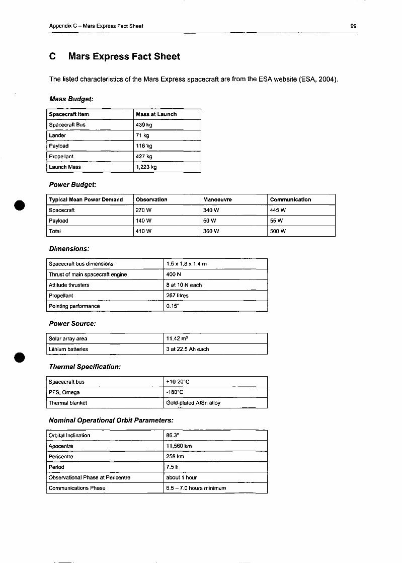
Appendix C - Mars Express Fact Sheet 99
C Mars Express Fact Sheet
The listed characteristics of the Mars Express spacecraft are from the ESA Website (ESA, 2004).
Mass Budget:
Spacecraft Item
Spacecraft Bus
Lander
Payload
Propellant
Launch Mass
Mass at Launch
439 kg
71 kg
116kg
427 kg
1,223 kg
Power Budget:
Typical Mean Power Demand
Spacecraft
Payload
Total
Observation
270 W
140 W
410W
Manoeuvre
340 W
50 W
360 W
Communication
445 W
55 W
500 W
Dimensions:
Spacecraft bus dimensions
Thrust of main spacecraft engine
Attitüde thrusters
Propellant
Pointing Performance
1.5 x 1.8 x 1.4 m
400 N
8at10Neach
267 litres
0.15°
Power Source:
Solar array area
Lithium batteries
11.42 m2
3 at 22.5 Ah each
Thermal Specification:
Spacecraft bus
PFS, Omega
Thermal blanket
+10-20°C
-180X
Gold-plated AlSn alloy
Nominal Operational Orbit Parameters:
Orbital Inclination
Apocentre
Pericentre
Period
Observational Phase at Pericentre
Communications Phase
86.3°
11,560 km
258 km
7.5 h
about 1 hour
6.5 - 7.0 hours minimum
Appendix D - Scientific Objectives of the I.P.F. as HRSC Co-Investigator 100
D Scientific Objectives of the I.P.F. as HRSC Co-Investigator
The TMIS (Topographie Mars Information System) should be a package of methods and Software that
is a further development and augmentation of an already existing system for topographic data
management on Earth. The Institute of Photogrammetry and Remote Sensing at the Vienna University
of Technology has got great expertise in that field for years. The strueture of the TMIS uses TopDM as
kernel, were various spatially related datasets can be stored. The system is extended by additional
functionality, for instance by a tool for geodetic transformations from one reference system and datum
to another and from one map projeetion to another. Most importantly, the TMIS will also be open to
external users who do not want to have an additional implementation of a stand-alone System. Library
routines will be available for access from separately working programs or even from remote Sites via
communication networks. In addition to the central Software, further Software will be included as
peripheral modules, such as ortho-photo generation, map composition, radiometric correction due to
topographic influences, DTM interpolation and other features. Extensive import and export filters will
provide off-line access to the contents of the database (Hoffmann and Neukum, 2003, p. 18).
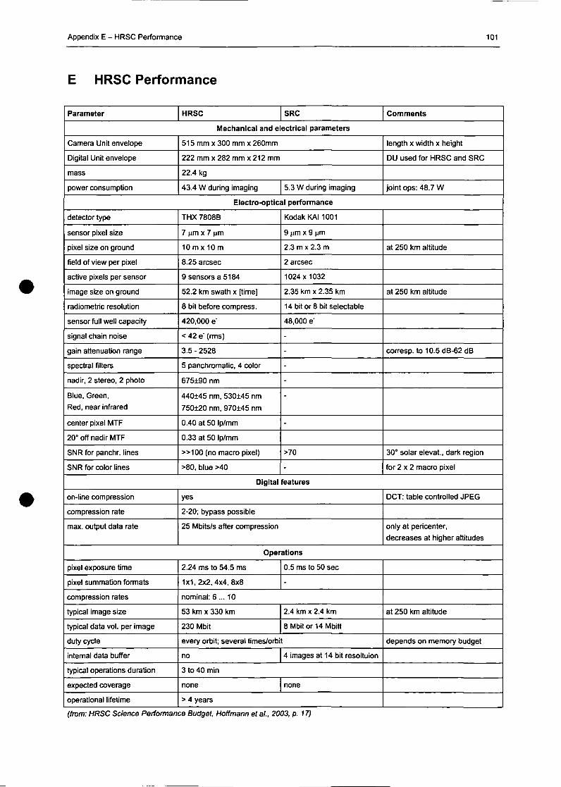
Appendix E - HRSC Performance 101
E HRSC Performance
Parameter HRSC SRC Comments
Mechanical and electrical Parameters
Camera Unit envelope
Digital Unit envelope
mass
power consumption
515 mm x 300 mm x 260mm
222 mm x 282 mm x 212 mm
22.4 kg
43.4 W during imaging 5.3 W during imaging
length x width x height
DU used for HRSC and SRC
Joint ops: 48.7 W
Electro-optical Performance
detector type
sensor pixel size
pixel size on ground
field of view per pixel
active pixels per sensor
image size on ground
radiometric resolution
sensor füll well capacity
Signal chain noise
gain attenuation ränge
spectral filters
nadir, 2 Stereo, 2 photo
Blue, Green,
Red, near infrared
center pixel MTF
20° off nadir MTF
SNR for panchr. lines
SNR for color lines
THX 7808B
7 um x 7 um
10mx 10 m
8.25 arcsec
9 sensors a 5184
52.2 km swath x [time]
8 bit before compress.
420,000 e"
< 42 e' (rms)
3.5 - 2528
5 panchromatic, 4 color
675±90 nm
440+45 nm, 530±45 nm
750±20 nm, 970±45 nm
0.40 at 50 Ip/mm
0.33 at 50 Ip/mm
» 1 0 0 (nomacro pixel)
>80, blue >40
Kodak KA11001
9 (im x 9 um
2.3 mx 2.3 m
2 arcsec
1024x1032
2.35 km x 2.35 km
14bitor8bitselectable
48,000 e"
-
-
-
-
-
-
>70
-
at 250 km altitude
at 250 km altitude
corresp. to 10.5 dB-62 dB
30° solar elevat., dark region
for 2 x 2 macro pixel
Digital features
on-line compression
compression rate
max. Output data rate
yes
2-20; bypass possible
25 Mbits/s after compression
DCT: table controlled JPEG
only at pericenter,
decreases at higher altitudes
Operations
pixel exposure time
pixel summation formats
compression rates
typical image size
typical data vol. per image
duty cycle
intemal data buffer
typical operations duration
expected coverage
operational lifetime
2.24 ms to 54.5 ms
1x1,2x2,4x4,8x8
0.5 ms to 50 sec
-
nominal: 6... 10
53 km x 330 km
230 Mbit
2.4 km x 2.4 km
8 Mbit or 14 Mbitt
every orbit; several times/orbit
no 4 images at 14 bit resoltuion
3 to 40 min
none none
> 4 years
at 250 km altitude
depends on memory budget
(from: HRSC Science Performance Budget, Hoffmann et al., 2003, p. 17)
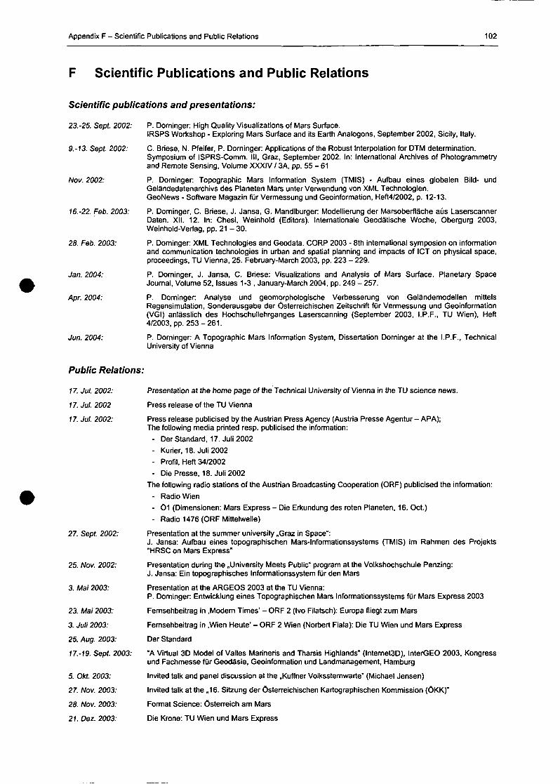
Appendix F - Scientific Publications and Public Relations 102
F Scientific Publications and Public Relations
Scientific publications and presentations:
23.-25. Sept. 2002:
9.-13. Sept. 2002:
Nov. 2002:
16.-22. Feb. 2003:
28. Feb. 2003:
Jan. 2004:
Apr. 2004:
Jun. 2004:
P. Dorninger: High Quality Visualizations of Mars Surface.IRSPS Workshop - Exploring Mars Surface and its Earth Analogons, September 2002, Sicily, Italy.
C. Briese, N. Pfeifer, P. Dorninger: Applications of the Robust Interpolation for DTM determination.Symposium of ISPRS-Comm. III, Graz, September 2002. In: International Archives of Photogrammetryand Remote Sensing, Volume XXXIV / 3A, pp. 55 - 61
P. Dominger: Topographie Mars Information System (TMIS) - Aufbau eines globalen Bild- undGeländedatenarchivs des Planeten Mars unter Verwendung von XML Technologien.GeoNews - Software Magazin für Vermessung und Geoinformation, Heft4/2002, p. 12-13.
P. Dorninger, C. Briese, J. Jansa, G. Mandlburger: Modellierung der Marsoberfläche aus LaserscannerDaten. XII. 12. In: Chesi, Weinhold (Editors). Internationale Geodätische Woche, Obergurg 2003,Weinhold-Verlag, pp. 21 - 30.
P. Dorninger: XML Technologies and Geodata. CORP 2003 - 8th international Symposion on informationand communication technologies in urban and spatial planning and impacts of ICT on physical space,proeeedings, TU Vienna, 25. February-March 2003, pp. 223 - 229.
P. Dorninger, J. Jansa, C. Briese: Visualizations and Analysis of Mars Surface. Planetary SpaceJournal, Volume 52, Issues 1-3 , January-March 2004, pp. 249 - 257.
P. Dorninger: Analyse und geomorphologische Verbesserung von Geländemodellen mittelsRegensimulation, Sonderausgabe der österreichischen Zeitschrift für Vermessung und Geoinformation(VGI) anlässlich des Hochschullehrganges Laserscanning (September 2003, I.P.F., TU Wien), Heft4/2003, pp. 2 5 3 - 2 6 1 .
P. Dorninger: A Topographie Mars Information System, Dissertation Dominger at the I.P.F., TechnicalUniversity of Vienna
Public Relations:
17. Jul. 2002:
17.Jul.2002
17. Jul. 2002:
27. Sept. 2002:
25. Nov. 2002:
3. Mai 2003:
23. Mai 2003:
3. Juli 2003:
25. Aug. 2003:
17.-19. Sept. 2003:
5. Okt. 2003:
27. Nov. 2003:
28. Nov. 2003:
21. Dez. 2003:
Presentation at the home page of the Technical University of Vienna in the TU science news.
Press release of the TU Vienna
Press release publicised by the Austrian Press Agency (Austria Presse Agentur - APA);The following media printed resp. publicised the information:
- Der Standard, 17. Juli 2002
- Kurier, 18. Juli 2002
- Profil, Heft 34/2002
- Die Presse, 18. Juli 2002
The following radio stations of the Austrian Braadcasting Cooperation (ORF) publicised the information:
- Radio Wien
- 01 (Dimensionen: Mars Express - Die Erkundung des roten Planeten, 16. Oct.)
- Radio 1476 (ORF Mittelwelle)
Presentation at the summer university „Graz in Space":J. Jansa: Aufbau eines topographischen Mars-Informationssystems (TMIS) im Rahmen des Projekts"HRSC on Mars Express"
Presentation during the „University Meets Public" program at the Volkshochschule Penzing:J. Jansa: Ein topographisches Informationssystem für den Mars
Presentation at the ARGEOS 2003 at the TU Vienna:
P. Dorninger: Entwicklung eines Topographischen Mars Informationssystems für Mars Express 2003
Fernsehbeitrag in .Modem Times' - ORF 2 (Ivo Filatsch): Europa fliegt zum Mars
Fernsehbeitrag in .Wien Heute" - ORF 2 Wien (Norbert Fiala): Die TU Wien und Mars Express
Der Standard"A Virtual 3D Model of Valles Marineris and Tharsis Highlands" (lntemet3D), InterGEO 2003, Kongressund Fachmesse für Geodäsie, Geoinformation und Landmanagement, Hamburg
Invited talk and panel discussion at the „Kuffner Volkssternwarte" (Michael Jensen)
Invited talk at the „16. Sitzung der österreichischen Kartographischen Kommission (ÖKK)"
Format Science: Österreich am Mars
Die Krone: TU Wien und Mars Express
Acronyms and Abbreviations 103
Acronyms and Abbreviations
ADT Abstract Data Types
ALS Airborn Laser Scanning
API Application Programming Interface
ASCII American Standard Code for Information Interchange
BLOß Binary Large Object
CLOB Character Large Object
Co-I Co-Investigator
CU Computing Unit
DB Database
DBMS Database Management System
DBS Database System
DDL Data Definition Language
DLR German Aerospace Center
DML Data Manipulation Language
DOM Document Object Model
DTD Document Type Definition
DTM Digital Terrain Model
EER Enhanced Entity Relationship Model
ER Entity Relationship Model
ESA European Space Agency
FTP File Transfer Protocol
GIF Graphics Interchange Format
GIS Geographie Information System
GML Geography Markup Language
GUI Graphical User Interface
HRSC High Resolution Stereo Camera
HTML Hypertext Markup Language
HTTP Hypertext Transfer Protocol
I.P.F. Institute of Photogrammetry and Remote Sensing
IAU International Astronomical Union
IDL Interactive Data Language
IQL Interactive Query Language
ISO International Organization for Standardization
JDBC Java Database Connectivity
JPEG Joint Photographic Expert Group
JPL Jet Propulsion Laboratory
JSP JavaServerPages
MDC Metadata Catalogue

Acronyms and Abbreviations 104
MER Mars Exploration Rover
MEX Mars Express
MGS Mars Global Surveyor
MOC Mars Orbiter Camera
MOLA Mars Orbiter Laser Altimeter
MS Microsoft
NASA National Aeronautics and Space Administration
NF Normal Form
NF2 Non First Normal Form Model
ODL Object Definition Language
ODMG Object Data Management Group
OGC OpenGIS Consortium
OMG Object Management Group
0 0 Object-Oriented
OODBS Object-Oriented Database System
OQL Object Query Language
OR-DBS Object-Relational Database System
OTF on-the-fly
PDF Adobe Portable Document Format
PDS Planetary Data System
Pl Principal Investigator
PNG Portable Network Graphic
RDBMS Relational Database Management System
RDBS Relational Database System
RDH Random Digital Heights
RMS Root Mean Square Error
SCOP++ Stuttgart Contour Program
SFTP Secure File Transfer Protocol
SOAP Simple Object Access Protocol
SQL Structured Query Language
SRS Spatial Reference Frame
SVG Scalable Vector Graphics
TDS Topographie Data Server
THEMIS Thermal Emission Imaging System
TIFF Tagged Image File Format
TIS Topographie Information System
TMIS Topographie Mars Information System
TMIS-EF Topographie Mars Information System - Extended Functionality
TopDB Topographie Database
TopDM Topographie Data Management
TOPSQL Topographie SQL
Acronyms and Abbreviations 105
UDDI Universal Description, Discovery and Integration
USGS United States Geological Service
VICAR Video Image Communication and Retrieval
VRML Virtual Reality Modeling Language
WebCGM Web-based Computer Graphics Metafiie
WINPUT Wiener Input Format
WMS Web Map Services
WSDL Web Service Description Language
X3D Extensible 3D
XDK XML Development Kid
XML Extensible Markup Language
XSD XML Schema Definition Language
XSL Extensible Stylesheet Language
XSL:FO Extensible Stylesheet Language: Formatting Objects
XSLT Extensible Stylesheet Language - Transformations
References 106
References
Bancilhon, F., Delobel, C , Kanellakis, P. (Editors), 2004. Building an Object-Oriented Database
System - The Story of O2. Morgan Kaufmann Publishers, San Mateo, CA, 1992.
Battrick, B., Talevi, M., 2001. Mars Express - Europe goes to Mars!, ESA Publications Division, ESA
BR-174, Noordwijk, The Netherlands, July 2001.
Beaujardiere, J. (Editor), 2001. Web Map Service (WMS) 1.1.1, OpenGIS® Implementation
Specification, OpenGIS Consortium Inc., 27 November 2001, OGC 01-068r2.
Beaujardiere, J. (Editor), 2004. Web Map Service (WMS) 1.3.0, OpenGIS® Implementation
Specification, OpenGIS Consortium Inc., 20 January 2004, OGC 03-109M.
Beck, M., 1999. World-View - Ein generisches Virtual Reality Framework für die interaktive
Visualisierung grosser geographischer Datenmengen, Dissertation in Informatics at the University
of Zürich. 1999.
Beck, M., 2003. Real-time Visualization of big 3D City Models. International Workshop on
"Visualization and Animation of Reality-based 3D Models", ISPRS Com. V, WG 6, 24. - 28.2.2003,
Switzerland. International Archives of Photogrammetry and Remote Sensing, Vol. XXXIV-5/W10.
Beeri, C : Formal Models for Object-Oriented Databases. In: Kim, W., Nicolas, J., Nishio, S. (Editors).
Proceedings of the 1st International Conference on Deductive and Object-Oriented Databases
(DOOD'89), Kyoto, Japan. Elsevier Science Publishers, December 1989.
Borgefors, G., 1986. Distance transformation in digital images. Computer Vision Graphics Image
Processing 34 (3), pp. 344 - 371.
Buchroithner, M., Waelder, O., 2002. Development of Methods for true 3D-Presentations of Mars
Surface. Proceedings of InterCarto 8, GIS for Sustainable Development of Territories, 28.5.-
1.6.2002, Helsinki - St. Petersburg, pp. 409 - 4 1 1 .
Briese, Ch., Pfeifer, N., Dorninger, P., 2002a. Applications of the Robust Interpolation for DTM
Determination. Symposium of ISPRS Com. IM, Graz, September 2002. International Archives of
Photogrammetry and Remote Sensing, Graz, Austria, Vol. XXXIV/3A, pp. 5 5 - 6 1 .
Briese, Ch., Kraus, K., Pfeifer, N., 2002b. Modellierung von dreidimensionalen Geländemodellen in
Laser-Scanner-Daten. Festschrift anlässlich des 65. Geburtstages von Herrn Prof. Dr.-Ing. habil.
Siegfried Meier, TU Dresden, Inst, für Planetare Geodäsie, pp. 47 - 52.
Cabrol, N., A., Grin, A., E., 1998. Ma'adim Vallis Evolution: Geometry and Models of Discharge Rate.
International Journal of Solar System Studies (Icarus), Vol. 132, pp. 362 - 377.
Carr, M.H. (Editor.), 1996. Wateron Mars, Oxford University Press, New York, 1996.
Cattell, R., G., G., Barry, D., K., Berler, M., Eastman, J., Jordan, D., Russell, C , Schadow, O.,
Stanienda, T., Velez, F., 2000. The Object Data Standard: ODMG 3.0. Morgan Kaufmann
Publishers.
Codd, E., F., 1970. A Relational Model of Data for Large Shared Data Banks. Communications of the
ACM, Vol. 13, No. 6, June 1970, pp. 377 - 387
References 107
Cox, S., Daisey, P., Lake, R., Portele, C , Whiteside, A. (Editors), 2004. Geography Markup Language
(GML) 3.1, OpenGIS® Implementation Specification, committee draft, OpenGIS Consortium, 7
February 2004, ISO/TC 211/WG 4/PT 19136.
Date, C , J., 1990. An Introduction to Database Systems, Vol I, Fill. Ed., Reading, Massachusets et. al,
1990.
Dorninger, P., 2004. Analyse und geomorphologische Verbesserung von Geländemodellen mittels
Regensimulation. Hochschullehrgang Laserscanning, Vienna 2003, österreichische Zeitschrift für
Vermessung und Geoinformation (VGI), Heft 4/2003, pp. 253-261.
Doyle, A., Cuthbert, A., 1998. Essential Model of Interactive Portrayal. OpenGIS Project Document 98-
061.
Duxbury, E., Jensen, D., 1994. VICAR User's Guide, Version 3, Jet Propulsion Laboratory, California
Institute of Technology, Pasadena, California, 1994.Eisfeld, R., Jeschke, W., 2003. Marsfieber.
Aufbruch zum Roten Planten, Phantasie und Wirklichkeit, Droemer Verlag, München.
Ehrig, H., Mahr, B., 1985. Fundamentals of Algebraic Specification 1. Equations and Initial Semantics.
Springer-Verlag, Berlin.
Eisfeld, R., Jeschke, W., 2003. Marsfieber. Aufbruch zum Roten Planten, Phantasie und Wirklichkeit,
Droemer Verlag, München.
Engels, G., Gogolla, M., Hohenstein, U., Hülsmann, K., Löhr-Richter, P., Saake, G., Ehrich, H., 1992.
Conceptual Modelling of Database Applications using an Extended ER Model. Data & Knowledge
Engineering, North-Holland, Vol. 9, Nr. 2, pp. 157 - 204.
Fitzke, J., Greve, K., Müller, M., Poth, A., 2004. Building SDIs with Free Software - the deegree
project. In: CORP 2004, Proceedings of 9m Symposion on Info- & Communication Technology in
Urban- and Spatial Planning and Impacts of ICT on Physical Space, Vienna, 2004, pp. 97 - 103.
Ferraiolo, J., Fujisawa, J., Jackson, D., (Editors), 2003. Scalable Vector Graphics (SVG) 1.1
Specification, W3C Recommendation 14 January 2003.
Füller, E., R., Head, J., W., 2001. Volcanism and Sedimentation: Origins of the Smoothest Plains on
Mars. GSA Annual Meeting, Paper No. 178-0, November 5 - 8 , 2001.
Garvin, J., B., Sakimotom, S., E., H., Frawley, J., J., Schnetzler, C , C , Wright, H., M., 2000.
Topographie Evidence for Geologically Recent Near-Polar Volcanism on Mars. International
Journal of Solar System Studies (learus), volume 145, pp. 648 - 652.
Gilbert, M., 2002. On-Line Distribution of Digital Topographie Data. In: International Archives of
Photogrammetry, Remote Sensing and Spatial Information Sciences, ISPRS, Vol. XXXIV, Part 4,
Com. IV, Ottawa, Juli 2002, pp. 185 - 189.
Gottlob, G., Koch, Ch., Reinhard, P., 2002. Efficient Algorithms for Processing XPath Queries,
Proceedings of 28th International Conference on Very Large Data Bases (VLDB), Hong Kong,
China, August 2002.
Gottlob, G., Koch, Ch., Pichler, R., 2003. Xpath query evalutation: Improving tima and space
efficiency. In Proc. IEEE Conference on Data Engineering.
References 108
Grant, J., A., Golombek, M., P., Parker, T., J., Crips, A., J., Squyres, S., W., Weitz, C , M., 2004.
Selecting landing Sites for the 2003 Mars Exploration Rovers. Planetary and Space Science.
Volume 52, Issues 1 - 3, January - March 2004. pp. 21 - 21.
Gregg, T., K., P., Sakimoto, S., E., H., 2000. Marte Valles Lava Channel Flow Rates and Rheology
from MOC and MOLA Data. Lunar and Planetary Space Science Conference XXI, No. 1758.
Hartmann, W. K., Berman, D. C , 2000. Elysium Planitia lava flows: Crater count chronology and
geological implications, J. Geophys. Res. 105,15011-15026, 2000.
Heuer, A., Saake, G., 2000. Datenbanken: Konzepte und Sprachen. 2. aktualisierte und erweiterte
Auflage, mitp-Verlag, Landsberg, 2000.
Heuseier, H., Jaumann, R., Neukum, G., 1997. Die Mars Mission. Pathfinder, Sojourner und die
Eroberung des Roten Planeten, BLV Verlag, München.
Hochstöger, F., 1996. Software for Managing Country-Wide Digital Elevation Data. International
Archives for Photogrammetry and Remote Sensing, XXXI, Part B2, Vienna 1996, pp. 160 - 163.
Hoffmann, H., Behnke, Th., Hauber, E., Flohrer, J., Matz, K.-D., Pischel, R., Jaumann, R,. Neukum,
G., 2003. Science Performance Budget for the HRSC on Mars Express.
Hoffmann, H., Neukum, G., 2003. HRSC on Mars Express Co-Investigator Team: Experiment
Implementation and Internat Management Plan
Jaumann, R., Hauber, E., Lanz, J., Hoffmann, H., Neukum, G., 2001. Geomorphological Record of
Water-Related Erosion on Mars, in Horneck, G., Baumstark-Khan, Ch. (Editors): Astrobiology: The
Quest for the Conditions of Life, Springer Verlag, Köln, 2001, pp. 89 - 110.
Kraus, K., 1998. Interpolation nach kleinsten Quadraten versus Krige-Schätzer. österreichische
Zeitschrift für Vermessung & Geoinformation. 86. Jahrg., Heft 1, pp. 45 - 48.
Kraus, K., 2000. Photogrammetrie Band 3. Topographische Informationssysteme, 1s t edition. Dümmler
Verlag, Köln.
Kraus, K., Briese, Ch., Attwenger, M., Pfeifer, N., 2004. Quality Measures for Digital Terrain Models.
In: Proceedings of 20m Congress of the International Society for Photogrammetry and Remote
Sensing, ISPRS, Istanbul, July 2004, in press.
Kreger, H., 2001. Web Services Conceptual Architecture (WSCA 1.0). IBM Software Group, May
2001.
Kreslavsky, M., A., Head, J., W., 2000. Kilometer-scale roughness of Mars: Results from MOLA data
analysis, J. Geophys. Res., 101, 26,695-26,711, 2000.
Li, N., Hui, J., Hsiao, H., Tijare, P., 2003. Cursor Management for XML Data, in Database and XML
Technologies (Bellahsene et al. Eds.), Database and XML Technologies, Proceedings of First
International XML Database Symposium, XSym 2003, Berlin, Germany, September 2003
Liu, C , Vincent, M., Liu, J., Guo, M., 2003. A Virtual XML Database Engine for Relational Databases.
In: Proceedings of Spatial Data 2000, Department of Photogrammetry and Surveying, University
College London, pp. 260-269.
References 109
Loitsch, J., Molnar, L, 1991. A Relational Database Management System with Topological Elements
and Topological Operators. In: Proceedings of Spatial Data 2000, Department of Photogrammetry
and Surveying, University College London, pp. 260-269.
Longley, P., Goodchild, M., Maguirem, D., Rhind, D., 2001. Geographie Information Systems and
Science. Chichester, John Wiley & Sons, Ltd, 2001.
Mandlburger, G., 2000. Verdichtung von Echolot Querprofilen unter Berücksichtigung der
Flussmorphologie, österreichische Zeitschrift für Vermessung & Geoinformation, 88. Jahrgang,
Heft 4, 2000, pp. 211-214.
Mertz, D., 2001. XML and Compression, Exploring the entropy of documents, Gnosis Software, Ine,
September 2001
Moritz, H., Sünkel, H., 1978. Approximation Methods in Geodesy. Sammlung Wichmann, Neue Folge,
Band 10. Wichmann-Verlag, Karlsruhe.
Morton, O., 2004. Mars Revisited. National Geographie. Official Journal of the National Geographie
Society. January 2004. p2 - 31.
Nebiker, S., 2003. Support for Visualisation and Animation in a Scalable 3D GIS Environment -
Motivation, Concepts and Implementation. ", ISPRS Com. V, WG 6, February 2003, Switzerland.
International Archives of Photogrammetry and Remote Sensing, Vol. XXXIV-5/W10.
Oracle Spatial, 2003. Oracle Spatial - Users's Guide and Reference, Release 9.2, Part No. A96630-
01, March 2002
Plescia, J., B., 1990. Recent flood lavas in the Elysium region of Mars, learus, 88, pp. 465 - 490,
1990.
Puttkamer, J., 1997. Jahrtausendprojekt Mars. Chance und Schicksal der Menschheit, Droemer Knaur
Verlag, München
Reichardt, M., 2001. OGC's GML 2.0 - A New Wave of Open Geoprocessing on the Web,
Geolnformtics, Magazine for Geo-IT Professionals, Issue July/August 2001, pp. 18 - 21.
Reinhart, M., 1995. Relationales Datenbankdesign, Verlag Franz Vahlen GmbH, München.
Rieger, W., 1992a. Hydrologische Anwendungen des digitalen Geländemodelles. Dissertation at the
Vienna University of Technology. 1992.
Rieger, W., 1992b. Automated River Line and Catchment Area Extraction from DEM Data.
International Archives of Photogrammetry and Remote Sensing, Washington, USA, Vol. XXIX/B4,
pp. 642 - 649.
Roatsch, T. (Editor), 2001. HRSC VICAR Label Description Document. HRSC-DLR-TN-4200-002,
June 2001.
Schneeberger, D., M., 1989. Episodic Channel activity at Ma'adim Vallis [abstract]. In Lunar Planetary
Science Conference, Vol. XX, pp. 964 - 965.
Schrefl, M., Bichler, P., 1995. Modeling Reality in an Information System, in Frank, A., U. (Ed.):
Geographie Information Systems, Vol. 1, Spatial Information,
References 110
Scott, D. H., Tanaka, K. L, 1986. Geologie map of the western equatorial region of Mars, U.S. Geol.
Surv. Misc. Invest. Map, 1-1802-A.
Smith, D.E., Zuber, M.T., Solomon, S.C., Phillips, R.J., Head, J.W., Garvin, J.B., Banerdt, W.B.,
Muhleman, D.O., Pettengill, G.H., Neumann, G.A., Lemoine, F.G., Abshire, J.B., Aharonson, O.,
Brown, CD., Hauck, S.A., Ivanov, A.B., McGovern, P.J., Zwally, HJ. , Duxbury, T.C., 1999. The
global Topography of Mars and Implications for Surface Evolution, Science, 284 1495-1503,1999.
Tsichritzis, D., Klug, A., 1978. The ANSI/X3/SPARC DBMS Framework Report of the Study Group on
Database Management Systems. Information Systems, Vol. 3, Nr. 3, pp. 173-191
Wählisch, M., Niedermaier, G., van Gasselt, S., Schölten, F., Wewel, F., Roatsch, T., Matz, K-D.,
Jaumann, R., 2002. A new digital orthoimage map of the Martian western hemisphere using data
obtained from the Mars Orbiter Camera at a resolution of 256 pixel/deg. 33"1 Lunar and Planetary
Science Conference, Houston, TX, March 2002.

References 111
Web Links
(Portal Site)
(THEMIS image archive)
ADOBE, 2004. The Adobe SVG Zone.
http://www. adobe.com/svp/
APACHE, 2004. The Apache Software Foundation.
http://www. apache. orq/
ASU, 2004. Arizona State University.
http://www. asu. edu/
http://themis-data. asu. edu/
BZIP2, 2004. The Bzip2 Official Homepage.
http://sources. redhat. com/bzip2/
CARTONET, 2004. carto:net.
http://www. carto. net
CGM, 2004. CGM Open, an OASIS Community.
http://www. cQmopen.org
DIMENSION, 2004. Dimension, Stratasys Inc.
http://www. dimensionprintinp. com
EOLI, 2004. EOLI-Web Envisat Catalogue.
http://muis-env.esrin.esa.it/peteolisa/index.html
ESA, 2004. European Space Agency, Science Programme Portal.
http://sci.esa.int
ESRI, 2004. Environmental Systems Research Institute.
http://www. esri. com
GEOMAGIC, 2004. Raindrop Geomagic GmbH, Cologne, Germany,
http://www. peomagic. com
GEONOVA, 2004. lnternet3D, powered by GEONOVA, Geoinformation Solutions.
http://www. peonova. at (Portal Site)
http://www. peonova.at/mars pr/start. htm (Virtual Model of Valles Marinehs)
GNU, 2004. GNU General Public License. Free Software Foundation, Inc., Boston, USA, June 1991.
http://www.pnu.orp/copyleft/ppl.html
GNU-ZIP, 2004. The Gzip Homepage.
http://www.pzip.orp/
GRASS, 2004. Geographie Resources Analysis Support System.
http://prass. itc. it/
IBMDB2, 2004. IBM DB2 Product Family.
www, ibm. com/software/data/db2/
IDL, 2004. Research Systems Inc., The Interactive Data Language.
http://www.rsinc.com/
References 112
IPF-SCOP, 2004. Product info Site of the I.P.F.
http://www.ipf. tuwien. ac.at/products/products. html
ISO, 2004. International Organization for Standardization, Geographie Information/Geomatics.
http://www. iso. orp
http://www. isotc211.orp
JAKARTA, 2004. The Apache Jakarta Project.
http.V/jakarta.apache. org/tomeat/
JAVA, 2004. Java Products and Technology.
http://java.sun. com/
JPEG2000, 2004.
http://www. jpeg. ora/ipea2000/
MACROMEDIA, 2004. Macromedia, Inc.
http://www. macromedia.com/
MOZILLA, 2004. The Mozilla Project.
http://www. mozilla. orq
NASA-MER, 2004. Mars Exploration Rover (MER), Jet Propulsion Laboratory, California Institute of
Technology, USA.
http://marsrovers.ipl.nasa.pov/home/
NASA-MGS, 2004. Mars Global Surveyor (MGS), Jet Propulsion Laboratory, California Institute of
Technology, USA.
http://mars.ipl.nasa.QOv/mas
NASA-MOC, 2004. Mars Orbiter Camera (MOC), Malin Space Science Systems, San Diego,
California, USA.
http://www. msss. com/
NASA-MOLA, 2004. Mars Orbiter Laser Altimeter (MOLA) Science Investigation Site, NASA's
Goddard Space Flight Center, USA.
httpJ/ltpwww. asfe. nasa.Qov/tharsis/mola.html
http://www. wustl. edu/
NASA-NSSDC, 2004. National Space Science Data Center, NASA Goddard Space Flight Center,
Greenbelt, USA.
httpJ/nssdc. Qsfc. nasa.gov/
httpJ/nssdc. qsfe. nasa.Qov/planetary/factsheet/marsfact.html (Mars Fact Sheet)
httpJ/nssdc.Qsfc.nasa.QQv/planetary/chronoloQv mars.html (Mars Express Fact Sheet)
NASA-ODYSSEY, 2004. Mars Odyssey Mission, Jet Propulsion Laboratory, California Institute of
Technology, USA.
http://marsproQram.ipl.nasa.Qov/odvssey/
OGC, 2004. OpenGIS Consortium.
http://www.openQis.orQ
References 113
ORACLE, 2004. Oracle Corporation.
http://www. oracle. com
PDS, 2004. The Planetary Data System, NASA.
http://pds. jpl. nasa.gov
POSTGIS, 2004. Refractions Research, PostGIS, Geographie Objects for PostGreSQL.
httpJ/postgis. refractions. net/
POSTGRESQL, 2004. PostGreSQL.
http://www.postgresal.org/
SOAP, 2004. Simple Object Access Protocol.
http://www. w3. org/TR/soap/
SVGOPEN, 2004. SVG Open, Conference and Exhibition.
http://www. svgopen.org
USGS-NAMES, 2004. Gazetteer of Planetary Nomenclature, United States Geological Survey,
Flagstaff, USA.
http://planetarynames. wr. usgs.gov/
W3C-DOM, 2004. W3C Architecture Domain, Document Object Model.
http://www. w3. org/DOM/
W3C-XML, 2004. World Wide Web Consortium. Extensible Markup Language.
http://www. w3. org/XMU
Web3D-X3D, 2004. Information Technology, Computer Graphics and Image Processing, Extensible
3D (X3D). ISO/IEC 19775:200x, Extensible 3D (X3D). Web3D Consortium.
http://www. web3d. org/
XMILL, 2004. XMill, An Efficient Compressor for XML.
http://www. research.att. com/sw/tools/xmill/

Curriculum Vitae 114
Curriculum Vitae
Name:
Date and Place ofBirth:
Marital Status:
Dipl.-Ing. Peter Dorninger
March 18, 1976 in Vienna
married with Dr. Angela Dorninger
1982- 1986 Elementary School, Biedermannsdorf
1986- 1994 BG/BRG Franz Keimgasse, Mödling (Grammar School)
1994 - 1997 Surveying (Vermessungswesen), Vienna University of Technology (TU Vienna)
1997-2000 Surveying and Geoinformation, TU Vienna
1998 - 2000 Tutor at the TU Vienna
1999 - 2000 Research assistant at the Institute of Photogrammetry and Remote Sensing (I.P.F.)
16/05/2000 Dipl.-Ing. degree (M. Sc.) with honors from the Vienna University of Technology
2000 - 2001 Military Services
since 2001 Research associate at the I.P.F. (TU Vienna) and
Doctoral program in the frame of Mars Express
i