Essays on Bargaining

Disstertation

zur Erlangung des akademischen Grades eines

Doktors der Wirtschaftswissenschaft

(Dr. rer. pol.)

durch die Fakultat fur Wirtschaftswissenschaften

der Universitat Duisburg-Essen

Campus Essen

vorgelegt von

Name: Nadine Leonhardt

Geburtsort: Plauen

Essen 2015

Tag der mundlichen Prufung: 7. Juli 2015

Erstgutachter: Prof. Dr. Erwin Amann

Zweitgutachterin: Prof. Dr. Jeannette Brosig-Koch

I thank Erwin Amann.

For being a cool guy, great boss, and the best advisor I could have wished for.

Contents

Introduction 1

1 Commitment Problems in International Bargaining 9

1.1 Introduction . . . . . . . . . . . . . . . . . . . . . . . . . . . . . . . . . . . . . 10

1.2 The Basic Model . . . . . . . . . . . . . . . . . . . . . . . . . . . . . . . . . . 10

1.3 Commitment Problems . . . . . . . . . . . . . . . . . . . . . . . . . . . . . . . 15

1.3.1 Shift in military power . . . . . . . . . . . . . . . . . . . . . . . . . . . 16

1.3.2 Increase in A’s costs of war . . . . . . . . . . . . . . . . . . . . . . . . 18

1.3.3 Decrease in B’s costs of war . . . . . . . . . . . . . . . . . . . . . . . . 19

1.3.4 Shift in proposal power . . . . . . . . . . . . . . . . . . . . . . . . . . 20

1.4 Conclusion . . . . . . . . . . . . . . . . . . . . . . . . . . . . . . . . . . . . . 20

2 Note on the Equilibrium in a Rubinstein-type Bargaining Game with Ran-

dom Proposers and Two-Sided Outside Options 22

2.1 Introduction . . . . . . . . . . . . . . . . . . . . . . . . . . . . . . . . . . . . . 23

2.2 The Model . . . . . . . . . . . . . . . . . . . . . . . . . . . . . . . . . . . . . 23

2.3 Conclusion . . . . . . . . . . . . . . . . . . . . . . . . . . . . . . . . . . . . . 28

3 Crisis Bargaining, Democracy and the Transparency Argument 29

3.1 Introduction . . . . . . . . . . . . . . . . . . . . . . . . . . . . . . . . . . . . . 30

3.2 The Classical Crisis Bargaining Approach . . . . . . . . . . . . . . . . . . . . 33

3.3 Extension of the Classical Approach . . . . . . . . . . . . . . . . . . . . . . . 35

3.4 The Model . . . . . . . . . . . . . . . . . . . . . . . . . . . . . . . . . . . . . 37

i

3.5 Equilibrium Analysis . . . . . . . . . . . . . . . . . . . . . . . . . . . . . . . . 39

3.5.1 Open-door bargaining . . . . . . . . . . . . . . . . . . . . . . . . . . . 40

3.5.2 Closed-door bargaining . . . . . . . . . . . . . . . . . . . . . . . . . . 48

3.6 Conclusion . . . . . . . . . . . . . . . . . . . . . . . . . . . . . . . . . . . . . 55

4 Dynamic Pricing in Lemons Markets 56

4.1 Introduction . . . . . . . . . . . . . . . . . . . . . . . . . . . . . . . . . . . . . 57

4.2 The Model . . . . . . . . . . . . . . . . . . . . . . . . . . . . . . . . . . . . . 60

4.3 Uniform Pricing . . . . . . . . . . . . . . . . . . . . . . . . . . . . . . . . . . . 62

4.4 Dynamic Pricing . . . . . . . . . . . . . . . . . . . . . . . . . . . . . . . . . . 69

4.5 Conclusion . . . . . . . . . . . . . . . . . . . . . . . . . . . . . . . . . . . . . 74

Conclusion 76

Bibliography 78

ii

Introduction

Most of human interaction can be considered as negotiations of some form. As a consequence,

literature on bargaining, be it theory or applications, is ubiquitous and, when it comes to

applications, very diverse. Research topics range from marital bargaining, acknowledging

the fact that married couples are almost constantly negotiating over a variety of matters to

international relations concerned with negotiations among national governments on economic,

environmental or territorial issues. Of course, also commodity prices are often the outcome

of negotiations and analyzed by the means of bargaining theory. Quite generally, in this

dissertation, I am interested in the variables that determine the outcome of negotiations and

especially the factors that lead to their breakdown.

With respect to bargaining theory, basically all research can be traced back to the seminal

works of Nash (1950) and Rubinstein (1982). I will give a brief overview of bargaining

theory and anchor the theoretic concepts used in this dissertation in the section Bargaining

Theory. I will then provide an outline of the specific problems and situations to which I

apply bargaining theory in the section Bargaining Applications.

Bargaining Theory

In any bargaining situation, individuals see the possibility of reaching a mutually beneficial

agreement but are not consent about how this agreement should look like. There is an inherent

conflict of interest about how the gains from bargaining should be distributed among the

involved parties. It is the aim of bargaining theory to identify solutions to these distributional

problems.

Real world bargaining is usually tied to a bargaining process, and the outcome of bargain-

1

ing very much depends on the specific procedural features of this process, such as who can

make offers and when. Nash (1950) abstracts away from such procedural features and consid-

ers only the set of agreements that satisfy “reasonable” properties, that are conditions that

any outcome arrived at by rational decision makers should satisfy a priori. These conditions

are treated as axioms, from which the outcome is deduced. The resulting Nash bargaining

solution is pinned down only by the axioms of underlying expected utility, in addition to

symmetry and independence of irrelevant alternatives. It has the remarkable property that

the outcome is implemented cooperatively and uniquely by maximizing the players’ utilities.

Nash’s axiomatic approach to solve the two-person bargaining problem has become the

foundation of modern bargaining theory. Still, even Nash felt the need to provide a non-

cooperative foundation of his very abstract cooperative solution concept and came up with

an explicitly modeled strategic game in Nash (1953). In the Nash demand game, two players

make simultaneous demands and agreement is only reached if the combined demands are

feasible. As is the problem with most non-cooperative models, the Nash demand game

has multiple equilibria since any split constitutes a Nash equilibrium. Nash (1953) solves

the problem by introducing uncertainty in the payoff function and obtains that the Nash

bargaining solution is the unique limiting outcome of the demand game when uncertainty

vanishes. Ever since, game theorists have set out to construct non-cooperative bargaining

games with the purpose to validate the axiomatic solution concept and broaden the scope of

its applicability.1

The most famous non-cooperative approach in this vein, is the two-person bargaining

game analyzed in Rubinstein (1982) in which players make alternating offers over the division

of a pie that shrinks over time because of costs of delay. Rubinstein is able to show that the

game has a unique solution, depending on who makes the first offer. Further, it is shown in

Binmore (1987) that the non-cooperative equilibria of the Rubinstein game converge to the

Nash bargaining solution when delay between offers goes to zero. Nevertheless, the Rubinstein

outcome can only approximate Nash’s solution because the costs of delay can never become

completely insignificant as they constitute the driving force behind the bargaining process.2

1This endeavor is commonly referred to as the “Nash program”.2Without costs of delay, the bargaining process is indeterminate. The bargaining could go on

indefinitely because the players have no incentive to strike a deal today rather than tomorrow.

2

The axiomatic approach has the advantage that it determines a unique outcome by a

fairly simple formula and is therefore very attractive to applied economics with a focus not

especially on the bargaining process. It has the disadvantage that its application is limited

to bargaining situation that fit the underlying axioms. Strategic models on the other hand

can be tailored to the particular specifications of any bargaining situation. On the downside,

this makes them very sensitive to procedural changes: even small changes in the rules of the

bargaining process can have a decisive impact on the bargaining outcome.

In light of the different virtues and shortcomings of the cooperative and non-cooperative

approach, it is now the prevalent view in bargaining literature that axiomatic and strategic

models are complementary (see Sutton 1986). The reason for choosing an exclusively non-

cooperative perspective in this thesis was to stay as close as possible to related literature.

Chapter 1 is based on a bargaining game with outside options and an infinite horizon

in which a player is randomly chosen in every period to make a take-it-or-leave-it offer. In

this game, reject and counteroffer is not a possible move but rejection of an offer immediately

results in the breakdown of bargaining and the players taking up their respective outside

options. In case of agreement, bargaining continues in the next period. The main ingredients

in this set-up are the outside options and repeated interaction. Outside options are relevant

because I focus on a crisis bargaining application in which outside options are usually mod-

eled as the states payoffs from going to war.3 Repeated interaction is crucial because I study

the effect of commitment problems on the bargaining outcome. Commitment problems only

arise when a party involved cannot credibly commit to an agreement because it can demand

revisions later in time. The inability to commit is only relevant in repeated interaction.

The game is an extension of the bargaining model used in Fearon (1995) and Powell (2006)

in the context of crisis bargaining with commitment problems and has not been analyzed

before. In their models only one player has the power to make a take-it-or-leave-it offer

in every period which means that this player has the entire bargaining power. I relax this

assumption by introducing random proposal power which gives both players some bargaining

power.

3see for example Powell (2006)

3

As a variation of this bargaining set-up, in Chapter 2 I analyze a one-time bargain-

ing game with the possibility of counteroffers and a possibly infinite horizon that is close to

the Rubinstein game only that there are random proposers instead of alternating offers and

two-sided outside options. I find that both bargaining models, the models in Chapter 1 and

2 have an equilibrium which generates identical subgame perfect equilibrium payoffs. The

proof draws on Binmore, Shaked and Sutton (1989) who first studied the effect of outside

options on the bargaining outcome and introduced the notion of ‘outside option principle’

by identifying the unique subgame-perfect equilibrium of a Rubinstein bargaining game with

outside options.

In Chapter 3, I considerably reduce complexity with regard to the bargaining game in

order to concentrate on the principal-agent relationship which is the driving force in this

model. Since I am no longer interested in a temporal dimension, I skip repeated interaction

so that the bargaining game boils down to a one-time take-it-or-leave-it offer game with out-

side options and random proposers. This has the advantage that the game is considerably

simpler and easier to solve. Still, the important features of the crisis bargaining process

are retained: both sides have bargaining power and the possibility to opt out and go to

war. In addition, I introduce asymmetric information: the players outside options are now

private information. The impact of such private information on the crisis bargaining out-

come has first been analyzed in Powell (1996). Ever since, asymmetric information about the

opponent’s outside option is considered a potential rational reason for the breakdown of inter-

national negotiations and the onset of war (see Fearon 1995). By showing that democracies

can overcome such information asymmetries, I provide a rational reason for the ‘democratic

peace’, that is, the empirical observation that democracies rarely fight wars with one another.

Chapter 4 retains information asymmetries as a potential source of breakdown but ap-

plies the bargaining set-up to a simple market structure. The market structure is a version

of Akerlof’s (1970) market for lemons in which trade is decentralized and buyers and sellers

are randomly matched. As an extension of Akerlofs model, the buyer side is not completely

uninformed about quality but a share of buyers is equally informed as the sellers. Once

4

matched, a seller makes a take-it-or-leave-it offer to the buyer who can either accept the offer

or reject it. This is the most rudimentary version of a bargaining situation but it captures

the common praxis in many markets, for example most retail markets, that prices are simply

posted by sellers, without the buyer having much influence on the price.4 This set-up al-

lows the analysis of the price formation process because, unlike Akerlof’s centralized market

version, equilibrium need not be exclusively defined by a single price equating supply and

demand but may be characterized by different prices (see Wilson 1980).

Bargaining Applications

Chapters 1-3 of this dissertation apply bargaining theory to international relations and aim

to shed light on rational reasons for war and peace. The idea to analyze war arguments on

the basis of bargaining models has been initiated by Fearon (1995). In his seminal work on

rationalist explanations for war, Fearon (1995) provides a coherent theory about the occur-

rence of war by introducing a formalization of the bargaining problem faced by two states

in conflict and on these grounds establishes two main rational causes of war: information

asymmetries and commitment problems. While commitment problems play the central role

in Chapters 1 and 2, asymmetric information is explored in Chapter 3.

Commitment problems are present in many bargaining situations that are characterized by

a temporal dimension. The parties involved in these interactions must be confident that

agreements made in the present will be binding in future periods or else they might prefer

to abstain from an agreement altogether. A commitment is not credible if one party has

the incentive to renege on an earlier agreement. In the context of international relations,

an increasingly powerful state may be unable to credibly commit to a current settlement

because it can demand revisions later in time. Anticipating this, a declining state may have

reason to fight in the present in order to guarantee itself a minimum of the stakes. It is

Fearon (1995) who first connects commitment problems to the idea of preventive wars by

4Of course there are also markets in which prices are the outcome of actual bilateral negotiationswith offers and counteroffers, for example bazaars, and there is a line of literature investigating thepros and cons of the two pricing institutions also in the context of asymmetric quality information.See for example Bester (1993) and Arnold and Lippman (1998).

5

showing that anticipated future shifts in power are a rational reason for a declining state to

start war. Later Powell (2006) expands on Fearon’s analysis by showing that this mechanism

also explains related phenomena like preemptive attacks and bargaining over issues that, by

themselves, are sources of bargaining power.

While formalizing the argument that adverse shifts in power between states in conflict can

lead to preventive war is an important step in understanding the reasons for war, there are

still historic examples that contradict this prediction and one question remains: why do states

not always respond to the anticipation of substantial negative power shifts with a strategy of

preventive war and sometimes do fight preventively even though a shift in (military) power

has not occurred? Chapters 1-2 aim to solve this puzzle by breaking down the concept of

power and identifying the kind of power that can trigger preventive war.

Bargaining power can be defined as a measure of a player’s relative power to extract a

share from the opponent during negotiation with respect to the opponent’s power to do the

same. In this sense, a party’s bargaining power is captured by its share of the surplus. In war

bargaining models, bargaining power is usually determined by the power to make proposals

and the outside option payoff, which is the expected payoff, a country receives by going to

war. This war payoff, in turn, is determined by a party’s probability to win the war and

the pie it will receive in case of winning, decimated by the party’s costs of fighting. In the

literature, so far, only a shift in military power has been analyzed. An increase in military

power directly translates into increased bargaining power since it alters both parties’ outside

option payoffs through the winning probability. But as pointed out above, there are other

means to increase bargaining leverage than military power, namely changes in the parties’

respective costs of war and changes in the level of proposal power.

The models in Chapters 1-2 explicitly investigate these other means and find that war is

only an equilibrium outcome if a state expects a reduction in its war payoff. On the other

hand, war does not occur if the declining state’s outside option is unaffected by the rising

state’s enhanced bargaining position.

Chapter 3 also draws on Fearon’s bargaining approach to war, in the attempt to pro-

vide a rational explanation of the “democratic peace”, that is, the empirical observation that

6

democracies tend not to fight wars with one another. I argue that democracies can overcome

information asymmetries so that this rational reason for war dissolves when democracies are

involved. The means by which democracies achieve this result, is successful signaling of their

type due to general transparency within democracies. The model’s theoretic underpinning is

the principal-agent nature of democratic political systems and the fact that the actual bar-

gaining with a third party is delegated to an elected representative (agent), a practice which

is common when one side involved in the bargaining process consists of a group of people

(principal). There are other examples of delegated bargaining, like elected labor union leaders

representing their union members when bargaining with management, politicians bargaining

for their constituencies in domestic politics, and boards of directors bargaining on behalf of

company shareholders. The model applies the idea of delegated bargaining to the literature

on war initiation and analyzes how transparency within democracies and accountability of

political representatives help overcome information asymmetries. The results of this analysis

are then used to find out what degree of agency transparency is preferable in an international

bargaining setting, comparing two scenarios, open-door bargaining in which the democratic

public can observe the bargaining process between its representative and a third party and

closed-door bargaining, in which the agent’s actions are partly hidden.

Chapter 4 is also concerned with bargaining in the presence of asymmetric information

but shifts the focus to a competitive market situation in which the quality of the good is

the sellers’ private information. Following Akerlof (1970), the prediction for such markets is

that, when the average quality of the good held by sellers is low and buyers cannot distin-

guish quality, bad products drive out good products and only low-quality units trade in the

competitive equilibrium. This dynamic is termed adverse selection and has been investigated

in the context of various settings, such as health insurance and labor markets.

The model relaxes the general assumption that the buyer side is completely uninformed

and integrates informed buyers into the lemons market. I investigate how the presence of

informed buyers affects adverse selection and welfare by comparing two different market

structures: one in which sellers cannot distinguish between informed and uninformed buyers

and one in which sellers can learn whether a buyer is informed or not and price-discriminate

7

on an individual level. I find that the presence of informed buyers reduces adverse selection

and a sufficiently high share of informed buyers even induces an efficient fully-separating

equilibrium. This is the reason why in most cases individual price discrimination leads to a

welfare reduction.

8

Chapter 1

Commitment Problems in

International Bargaining1

Abstract

When contracts are not enforceable, bargaining can break down because of commitment

problems. In the international context, standard models predict that a shift in military

power can cause preventive war because it changes the relative bargaining position between

states. We find that shifts in military power are not the only cause of war under commitment

problems and that commitment problems per se are not necessarily a cause of war even if

the relative bargaining position changes substantially.

1see Amann, Erwin and Nadine Leonhardt (2013): Commitment Problems in International Bar-gaining, Ruhr Economic Papers 403

9

1.1 Introduction

Commitment problems arise if the relative bargaining position between states changes and

an increasingly powerful state is unable to credibly commit to a current settlement because

it can demand revisions later in time. Anticipating this, a declining state may have reason

to fight now in order to still guarantee itself a minimum of the stakes.

Fearon (1995) and Powell (2006) formalize this argument in a bargaining model in which

war constitutes the parties’ outside option. We describe the war payoff as the result of a

costly lottery that is determined by a party’s military power and her costs of fighting. In

the literature, so far, only shifts in military power have been analyzed and associated with

commitment problems and the risk of war.2 The implications of changes in the parties’

respective costs of war have not been studied yet. Also, previous works have not explicitly

modeled bargaining power so that the effects of changes in bargaining power are still unclear.3

The present paper introduces variable proposal power which facilitates the analysis of

situations in which both parties have some bargaining power. We show that a shift in bar-

gaining power affects the distribution of the bargaining surplus, but does not lead to war.

Also, an isolated decrease in one party’s costs of war can have an impact on the realative

bargaining position but never causes war. On the other hand, war can occur in equilibrium

if a party’s costs of war increase even though military power does not change.

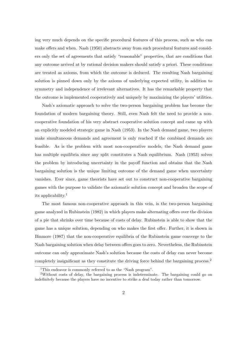
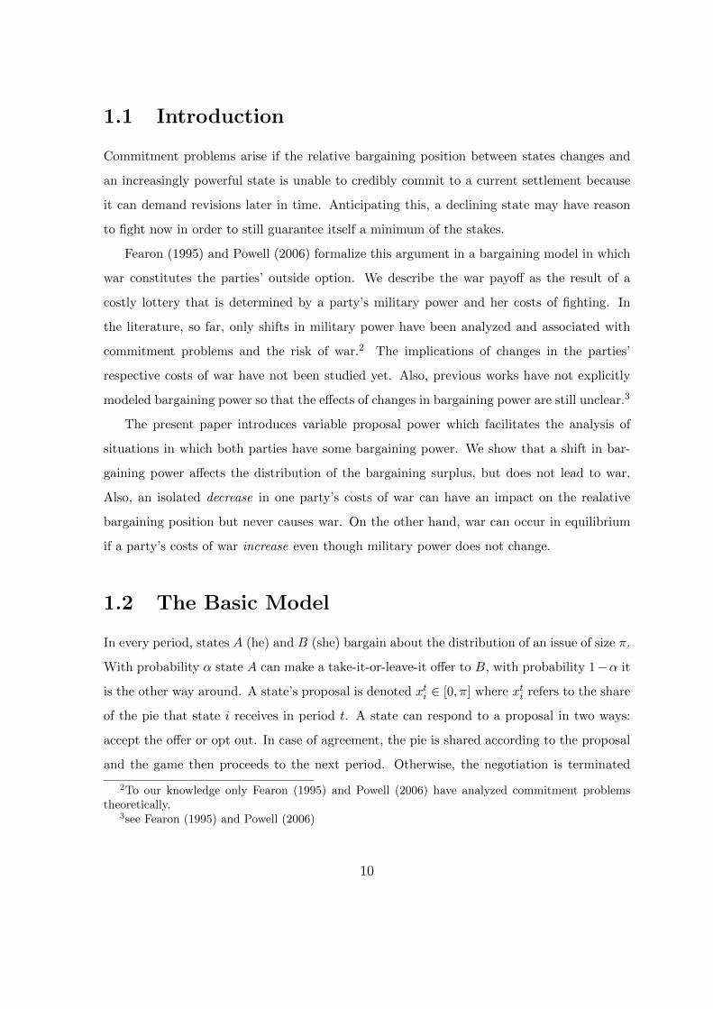
1.2 The Basic Model

In every period, states A (he) and B (she) bargain about the distribution of an issue of size π.

With probability α state A can make a take-it-or-leave-it offer to B, with probability 1−α it

is the other way around. A state’s proposal is denoted xti ∈ [0, π] where xti refers to the share

of the pie that state i receives in period t. A state can respond to a proposal in two ways:

accept the offer or opt out. In case of agreement, the pie is shared according to the proposal

and the game then proceeds to the next period. Otherwise, the negotiation is terminated

2To our knowledge only Fearon (1995) and Powell (2006) have analyzed commitment problemstheoretically.

3see Fearon (1995) and Powell (2006)

10

and the states fight. In case of war, state A wins with probability p ∈ [0, 1] and state B with

probability 1−p, leading to future payoffs per period (π− cA, 0) when A wins and (0, π− cB)

when B wins, where ci represent the irreversible costs of war. Consequently, the expected

values of the outside options are wA1−δ = p(π−cA)

1−δ and wB1−δ = (1−p)(π−cB)

1−δ with δ ∈ [0, 1] being

the states’ common discount factor. Obviously, the two states have an incentive to reach an

agreement if cA + cB ≥ 0. Figure 1.1 below illustrates the game tree:

11

Lemma 1 In any subgame perfect equilibrium of the basic model, agreement is always reached

and the equilibrium outcome is therefore Pareto efficient.

Proof. Let (MA,MB) be the expected payoffs to A and B in a subgame perfect equilibrium

of the game, or correspondingly any subgame starting with a move of nature. Let MminA ≤

MA ≤ MmaxA and Mmin

B ≤ MB ≤ MmaxB be the corresponding interval for a specific set of

SPE outcomes of this game. Then wA+wB1−δ ≤MA +MB ≤ π

1−δ . Since the aggregate payoff in

case of agreement in period t is always bigger than the war payoff, wA+wB1−δ ≤ π+δ(MA+MB),

war can occur only if the whole pie π (xi = 0) is too small to meet the expectations of the

opponent,

π + δM−i <w−i

1− δ. (1.1)

However, Mmin−i ≥ αw−i

1−δ + (1 − α)w−i

1−δ = w−i

1−δ since the opponent can always respond by

choosing the outside option, and if he gets to make an offer, additionally extract potential

efficiency gains in the current period and therefore expects to get at least his own outside

option payoff. This, however, is in contradiction to Equation (1.1)

π + δw−i

1− δ≤ π + δM−i <

w−i1− δ

as long as π ≥ w−i.

Thus, in any subgame perfect equilibrium the equilibrium offer is always accepted and

either makes the respondend indifferent between acceptance and war or provides the respon-

dend with the minimal value (x∗i = π) in which case the outside option is not binding.

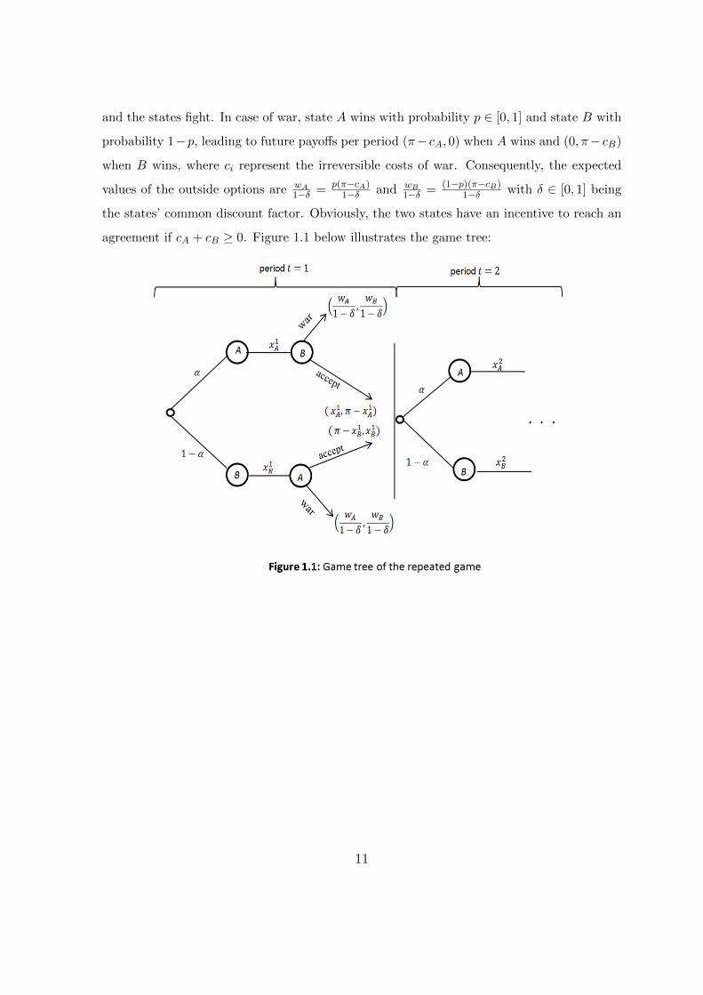
Figure 1.2 below depicts different regions of the player’s proposals depending on whether or

not the outside options are binding. Theorem 1 caracterizes all subgame perfect equilibria.

12

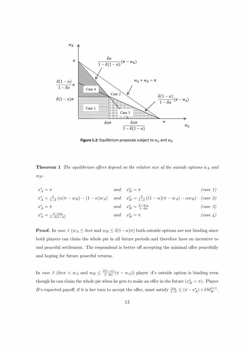
Theorem 1 The equilibrium offers depend on the relative size of the outside options wA and

wB:

x∗A = π and x∗B = π (case 1)

x∗A = δ1−δ (α(π − wB)− (1− α)wA) and x∗B = δ

1−δ ((1− α)(π − wA)− αwB) (case 2)

x∗A = π and x∗B = π−wA1−δα (case 3)

x∗A = π−wB1−δ(1−α) and x∗B = π (case 4)

Proof. In case 1 (wA ≤ δαπ and wB ≤ δ(1−α)π) both outside options are not binding since

both players can claim the whole pie in all future periods and therefore have no incentive to

end peaceful settlement. The respondend is better off accepting the minimal offer peacefully

and hoping for future peaceful returns.

In case 3 (δαπ < wA and wB ≤ δ(1−α)1−δα (π − wA)) player A’s outside option is binding even

though he can claim the whole pie when he gets to make an offer in the future (x∗B < π). Player

B’s expected payoff, if it is her turn to accept the offer, must satisfy wB1−δ ≤ (π−x∗A)+δM t+1

B .

13

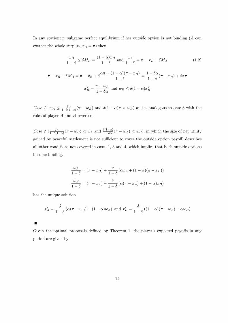
In any stationary subgame perfect equilibrium if her outside option is not binding (A can

extract the whole surplus, xA = π) then

wB1− δ

≤ δMB =(1− α)xB

1− δand

wA1− δ

= π − xB + δMA. (1.2)

π − xB + δMA = π − xB + δαπ + (1− α)(π − xB)

1− δ=

1− δα1− δ

(π − xB) + δαπ

x∗B =π − wA1− δα

and wB ≤ δ(1− α)x∗B

Case 4 ( wA ≤ δα1−δ(1−α)(π − wB) and δ(1 − α)π < wB) and is analogous to case 3 with the

roles of player A and B reversed.

Case 2 ( δα1−δ(1−α)(π − wB) < wA and δ(1−α)

1−δα (π − wA) < wB), in which the size of net utility

gained by peaceful settlement is not sufficient to cover the outside option payoff, describes

all other conditions not covered in cases 1, 3 and 4, which implies that both outside options

become binding.

wA1− δ

= (π − xB) +δ

1− δ(αxA + (1− α)(π − xB))

wB1− δ

= (π − xA) +δ

1− δ(α(π − xA) + (1− α)xB)

has the unique solution

x∗A =δ

1− δ(α(π − wB)− (1− α)wA) and x∗B =

δ

1− δ((1− α)(π − wA)− αwB)

Given the optimal proposals defined by Theorem 1, the player’s expected payoffs in any

period are given by:

14

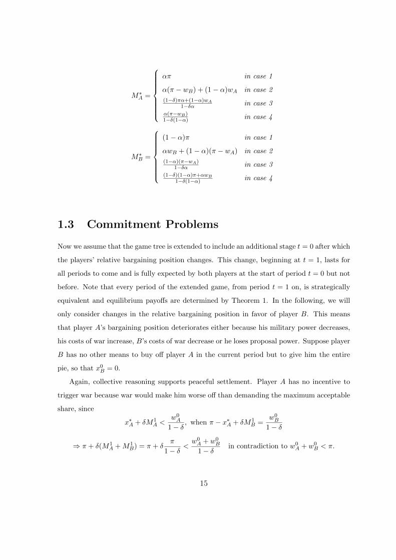
M∗A =

απ in case 1

α(π − wB) + (1− α)wA in case 2

(1−δ)πα+(1−α)wA

1−δα in case 3

α(π−wB)1−δ(1−α) in case 4

M∗B =

(1− α)π in case 1

αwB + (1− α)(π − wA) in case 2

(1−α)(π−wA)1−δα in case 3

(1−δ)(1−α)π+αwB

1−δ(1−α) in case 4

1.3 Commitment Problems

Now we assume that the game tree is extended to include an additional stage t = 0 after which

the players’ relative bargaining position changes. This change, beginning at t = 1, lasts for

all periods to come and is fully expected by both players at the start of period t = 0 but not

before. Note that every period of the extended game, from period t = 1 on, is strategically

equivalent and equilibrium payoffs are determined by Theorem 1. In the following, we will

only consider changes in the relative bargaining position in favor of player B. This means

that player A’s bargaining position deteriorates either because his military power decreases,

his costs of war increase, B’s costs of war decrease or he loses proposal power. Suppose player

B has no other means to buy off player A in the current period but to give him the entire

pie, so that x0B = 0.

Again, collective reasoning supports peaceful settlement. Player A has no incentive to

trigger war because war would make him worse off than demanding the maximum acceptable

share, since

x∗A + δM1A <

w0A

1− δ, when π − x∗A + δM1

B =w0B

1− δ

⇒ π + δ(M1A +M1

B) = π + δπ

1− δ<w0A + w0

B

1− δin contradiction to w0

A + w0B < π.

15

The same argument applies to player B who also prefers bargaining over fighting.

A commitment problem can arise in this situation if player player B cannot credibly

commit in t = 0 to not exploit her improved bargaining position in future periods.

1.3.1 Shift in military power

A shift in military power changes the states’ respective probabilities of winning war p and

1−p. When military power shifts in favor of B, A’s outside option decreases and B’s outside

option increases, since wA1−δ = p(π−cA)

1−δ increases in p and wB1−δ = (1−p)(π−cB)

1−δ decreases in p. This

change in the players’ outside options can create a shift in the relative bargaining position

if it alters the future distribution of the bargaining surplus. It can lead to preventive war

if player A’s current outside option exceeds his expected future gains from bargaining. The

war condition determines the critical value of w0A from which player A prefers going to war

to bargaining. That is,w0A

1− δ> π +

δ

1− δM1A (1.3)

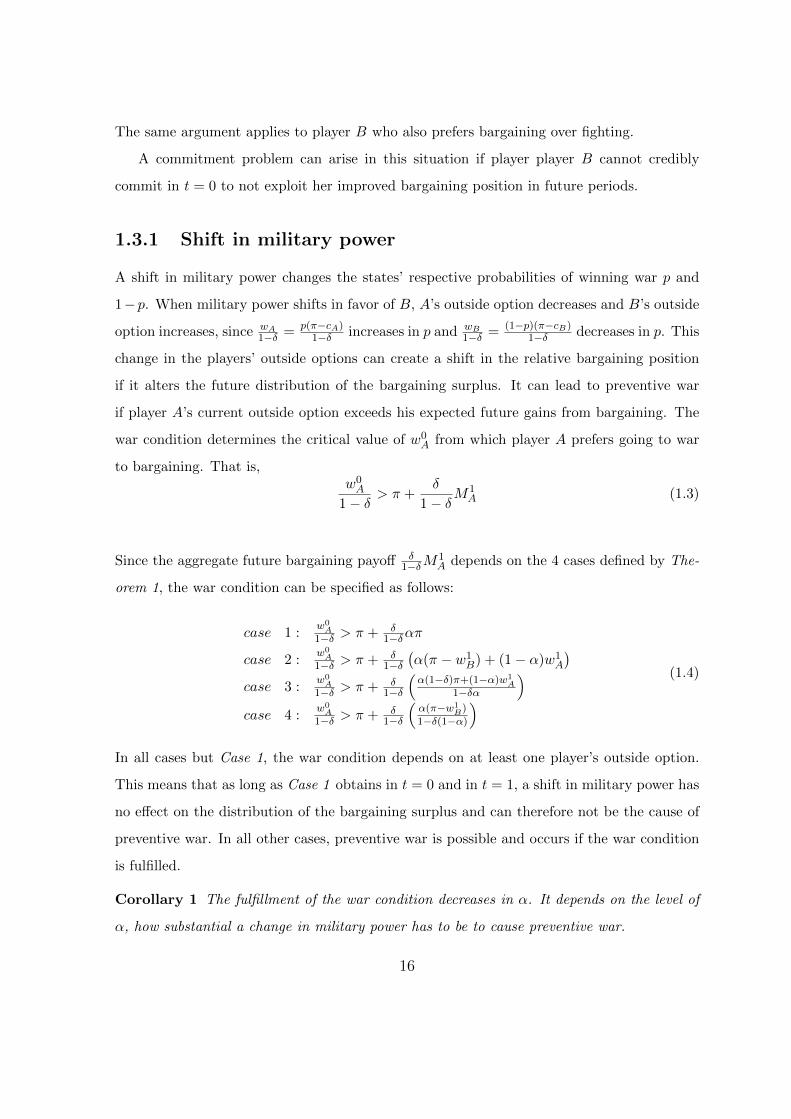
Since the aggregate future bargaining payoff δ1−δM

1A depends on the 4 cases defined by The-

orem 1, the war condition can be specified as follows:

case 1 :w0

A1−δ > π + δ

1−δαπ

case 2 :w0

A1−δ > π + δ

1−δ(α(π − w1

B) + (1− α)w1A

)case 3 :

w0A

1−δ > π + δ1−δ

(α(1−δ)π+(1−α)w1

A1−δα

)case 4 :

w0A

1−δ > π + δ1−δ

(α(π−w1

B)

1−δ(1−α)

) (1.4)

In all cases but Case 1, the war condition depends on at least one player’s outside option.

This means that as long as Case 1 obtains in t = 0 and in t = 1, a shift in military power has

no effect on the distribution of the bargaining surplus and can therefore not be the cause of

preventive war. In all other cases, preventive war is possible and occurs if the war condition

is fulfilled.

Corollary 1 The fulfillment of the war condition decreases in α. It depends on the level of

α, how substantial a change in military power has to be to cause preventive war.

16

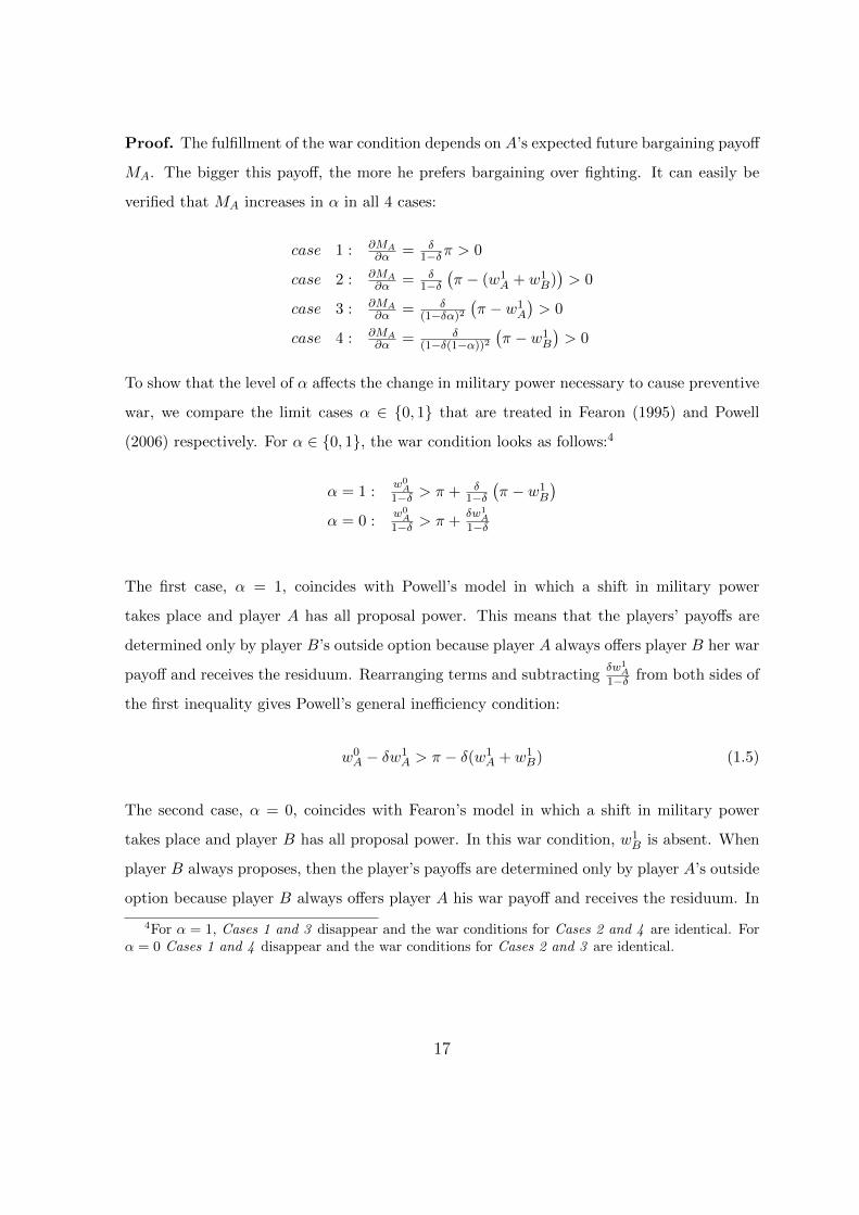
Proof. The fulfillment of the war condition depends on A’s expected future bargaining payoff

MA. The bigger this payoff, the more he prefers bargaining over fighting. It can easily be

verified that MA increases in α in all 4 cases:

case 1 : ∂MA∂α = δ

1−δπ > 0

case 2 : ∂MA∂α = δ

1−δ(π − (w1

A + w1B))> 0

case 3 : ∂MA∂α = δ

(1−δα)2(π − w1

A

)> 0

case 4 : ∂MA∂α = δ

(1−δ(1−α))2(π − w1

B

)> 0

To show that the level of α affects the change in military power necessary to cause preventive

war, we compare the limit cases α ∈ {0, 1} that are treated in Fearon (1995) and Powell

(2006) respectively. For α ∈ {0, 1}, the war condition looks as follows:4

α = 1 :w0

A1−δ > π + δ

1−δ(π − w1

B

)α = 0 :

w0A

1−δ > π +δw1

A1−δ

The first case, α = 1, coincides with Powell’s model in which a shift in military power

takes place and player A has all proposal power. This means that the players’ payoffs are

determined only by player B’s outside option because player A always offers player B her war

payoff and receives the residuum. Rearranging terms and subtractingδw1

A1−δ from both sides of

the first inequality gives Powell’s general inefficiency condition:

w0A − δw1

A > π − δ(w1A + w1

B) (1.5)

The second case, α = 0, coincides with Fearon’s model in which a shift in military power

takes place and player B has all proposal power. In this war condition, w1B is absent. When

player B always proposes, then the player’s payoffs are determined only by player A’s outside

option because player B always offers player A his war payoff and receives the residuum. In

4For α = 1, Cases 1 and 3 disappear and the war conditions for Cases 2 and 4 are identical. Forα = 0 Cases 1 and 4 disappear and the war conditions for Cases 2 and 3 are identical.

17

this case, the war condition can be written as:

w0A − δw1

A > π − δπ (1.6)

Comparing Condition 1.5 with Condition 1.6, it follows that the shift in military power

necessary to trigger war, (left hand side of the conditions) is smaller for α = 0 than for α = 1

since π > w1B.

The findings confirm the standard argument that a shift in military power can change the

relative bargaining position which can cause preventive war. But in contrast to Powell (2006)

who concludes that the shift in military power necessary to cause preventive war needs to be

“large and rapid”, we can show that the necessary shift depends on the parties’ respective

bargaining power. When the declining party has little bargaining power and can only extract

a small share of the bargaining surplus, then a smaller shift in military power is necessary to

trigger war. When α = 0, the necessary shift even goes to zero for δ → 1, as can be seen in

Condition 1.6.

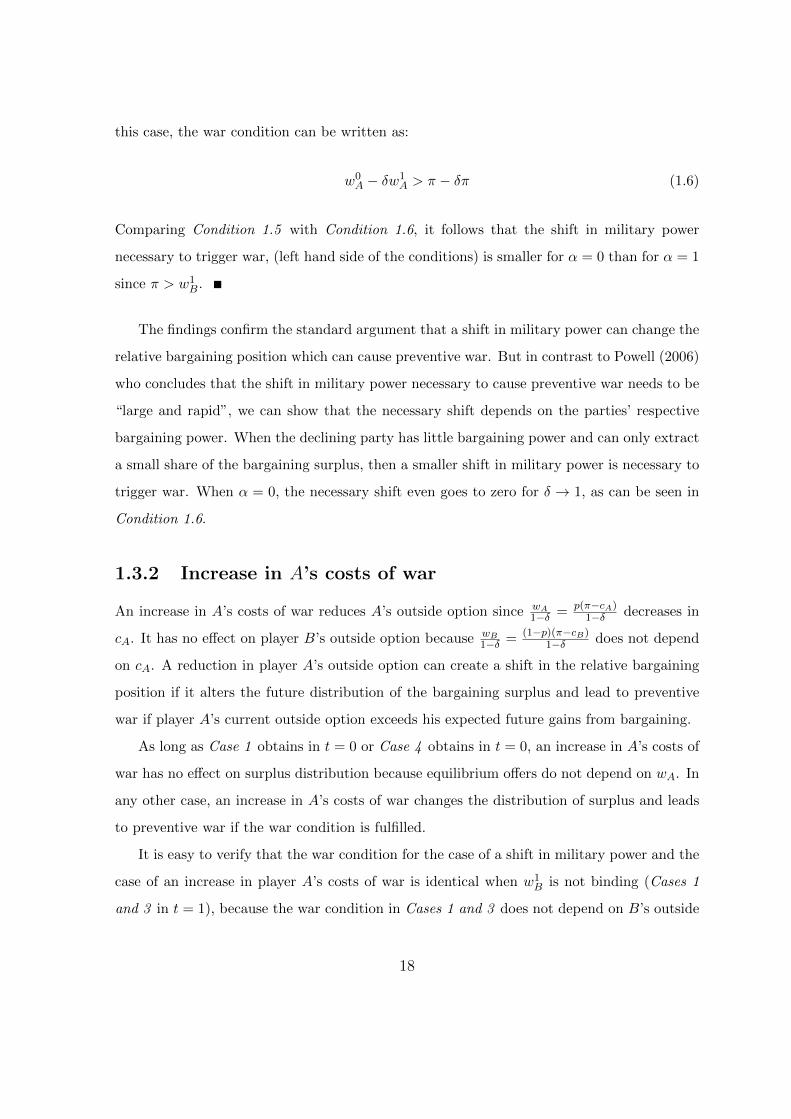
1.3.2 Increase in A’s costs of war

An increase in A’s costs of war reduces A’s outside option since wA1−δ = p(π−cA)

1−δ decreases in

cA. It has no effect on player B’s outside option because wB1−δ = (1−p)(π−cB)

1−δ does not depend

on cA. A reduction in player A’s outside option can create a shift in the relative bargaining

position if it alters the future distribution of the bargaining surplus and lead to preventive

war if player A’s current outside option exceeds his expected future gains from bargaining.

As long as Case 1 obtains in t = 0 or Case 4 obtains in t = 0, an increase in A’s costs of

war has no effect on surplus distribution because equilibrium offers do not depend on wA. In

any other case, an increase in A’s costs of war changes the distribution of surplus and leads

to preventive war if the war condition is fulfilled.

It is easy to verify that the war condition for the case of a shift in military power and the

case of an increase in player A’s costs of war is identical when w1B is not binding (Cases 1

and 3 in t = 1), because the war condition in Cases 1 and 3 does not depend on B’s outside

18

option w1B.

In Cases 2 and 4, the war condition depends on w1B. In these cases, it makes a difference

whether a change in military power causes A’s decline or an increase in his costs of war. A

cost increase only affects A’s outside option while a shift in military power not only reduces

A’s outside option but at the same time increases B’s outside option which further reduces

A’s expected future gains from bargaining.

The finding that bargaining can break down not only because of a change in military

power but also because of an isolated increase in one state’s costs of war is novel and has

not yet been acknowledged in the formal literature on war initiation. Increased costs of war

can result if, for example, one state intends to take measures to direct the blame of potential

war to the adversary and secure diplomatic support. If this were the case, a shift in military

power would not take place but still the adversary would expect to sustain a reduction in his

outside option and possibly go to war in order to prevent this.

Next, we will present two cases of shifts in the relative bargaining position which, in

contrast to military power shifts and costs increases, do not result in the breakdown of

bargaining.

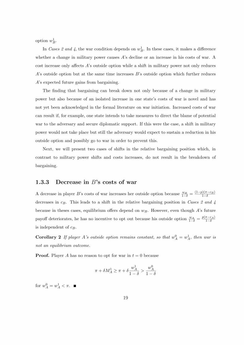
1.3.3 Decrease in B’s costs of war

A decrease in player B’s costs of war increases her outside option because wB1−δ = (1−p)(π−cB)

1−δ

decreases in cB. This leads to a shift in the relative bargaining position in Cases 2 and 4

because in theses cases, equilibrium offers depend on wB. However, even though A’s future

payoff deteriorates, he has no incentive to opt out because his outside option wA1−δ = p(π−cA)

1−δ

is independent of cB.

Corollary 2 If player A’s outside option remains constant, so that w0A = w1

A, then war is

not an equilibrium outcome.

Proof. Player A has no reason to opt for war in t = 0 because

π + δM1A ≥ π + δ

w1A

1− δ>

w0A

1− δ

for w0A = w1

A < π.

19

Notice that this result contradicts the standard argument that a shift in the player’s

respective bargaining position can by itself be enough to make war a rational possibility.

Here, the relative bargaining position of player B can improve at the cost of diminished

expected gains for player A, without involving inefficient outcomes.

The analysis concludes with the verification that changes in proposal power can also not

be the cause of bargaining breakdowns.

1.3.4 Shift in proposal power

A shift in proposal power changes the players’ relative bargaining position in all cases because

equilibrium offers always depend on α. A negative shift in proposal power reduces player A’s

expected future bargaining payoff MA and thus also positively affects the fulfillment of the

war condition as shown in corollary 2. However, a negative shift in proposal power alone

cannot cause preventive war because player A’s outside option does not decrease. This

follows immediately from Corollary 2.

Corollary 3 A reduction in player A’s proposal power does not lead to war.

1.4 Conclusion

Our model specifies the concept of commitment problems in international bargaining. We

provide two main results. First, we show that a negative shift in the relative bargaining

position problems does not necessarily lead to preventive war under commitment. Both, a

decrease in one party’s costs of war and a loss of proposal power affect the parties’ relative

bargaining position, and can diminish a party’s gains, but interestingly, cannot lead to pre-

ventive war. Second, we find that in addition to shifts in military power, increased costs of

war can also result in preventive war under commitment problems.

This analysis builds the formal groundwork for preventive war arguments. It also allows

conjectures about the role of third party intervention in international conflicts because it

clarifies what kinds of power shifts between nations can actually induce preventive war. The

model predicts that both economic (reduced costs of war) and military (higher probability

20

of winning war) support can improve a party’s bargaining position, while only military in-

tervention can cause preventive war if it triggers a shift in the winning probabilities and/or

increases the opponent’s costs of war.

21

Chapter 2

Note on the Equilibrium in a

Rubinstein-type Bargaining Game

with Random Proposers and

Two-Sided Outside Options

Abstract

This note characterizes equilibrium behavior in a Rubinstein-type bargaining game with the

possibility of counteroffers, random proposers and outside options and compares its unique

SPE with the stationary SPE of the repeated bargaining game with take-it-or-leave-it offers

presented in Chapter 1. It is shown that both games generate identical SPE payoffs. Since

the war condition in Chapter 1 critically depends on the declining state’s future payoff, all

results carry over to the one-time bargaining case discussed here.

22

2.1 Introduction

If a player’s bargaining power is captured by her share of the surplus, then beginning with

the seminal work by Rubinstein (1982), bargaining literature has identified three independent

key sources of bargaining power: the ability to propose an allocation, the ability to wait

for agreement and the ability to quit the negotiation. The ability to wait, represented by

the discount factor is an important element in the original model, indicating “shrinking

cakes”. It also has the appealing feature of conveying bargaining power through the players’

respective valuation of time. The bargaining power resulting from the possibility of leaving

the negotiation table permanently has first been analyzed by Shaked and Sutton (1984) and

further explored in the works of Binmore, Shaked and Sutton (1989) and Ponsatı and Sakovics

(1998). Proposal power on the other hand has long been considered the less attractive feature

of the alternating offer protocol which conveys an undesired advantage to moving first.

The one-time bargaining model studied here is a variation of the Rubinstein alternating

offer game with two-sided outside options. The alternating offer protocol is substituted with

random determination of the proposer in each negotiation round. This constitutes a game

in which all three sources of bargaining power - proposal power, discount factor and outside

option - are variables. I find that this game has a unique equilibium and that the players’

expected payoffs in this equilibrium coincide with the expected per period payoffs of the game

in Chapter 1 which features infinitely repeated interaction but no counter offers. Because the

expected payoffs are the same in both games and the analysis of changes in bargaining power

depends on expected payoffs, all the results presented in Section 1.4 carry over to this game.

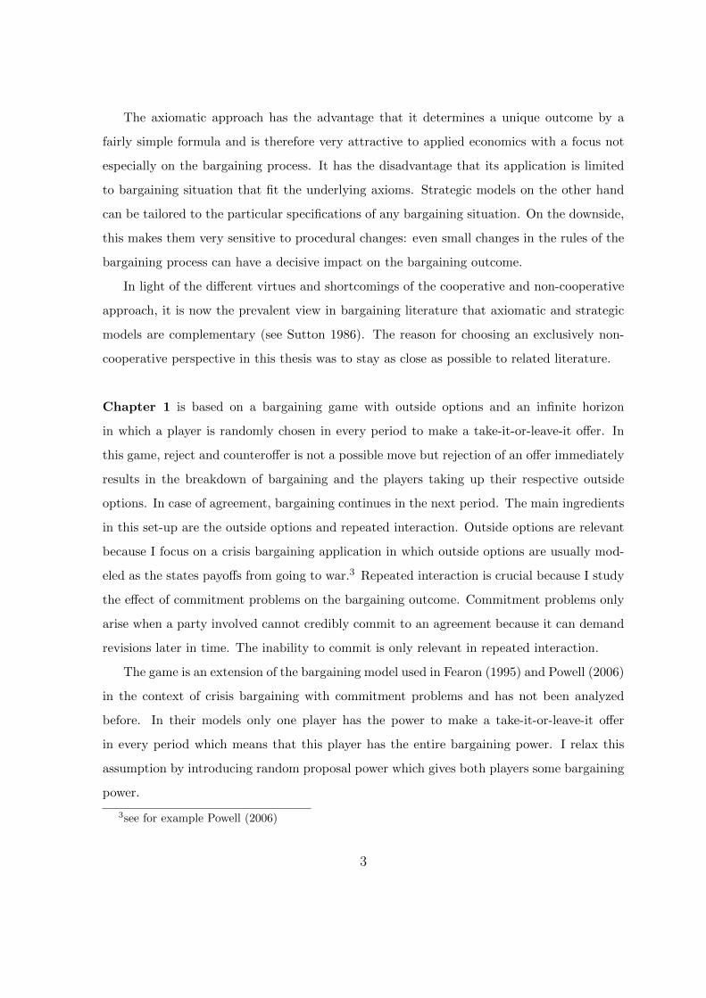
2.2 The Model

Negotiators A (he) and B (she) bargain about the distribution of an issue of size π > 0. Be-

fore the negotiation starts, each player’s proposal power is determined exogenously. Proposal

power is measured by a fixed variable α ∈ (0, 1). More specifically, α determines the proba-

bility that player A can make a proposal on the distribution in the current period. Players A

and B discount future payoffs with a common discount factor 0 < δ < 1. A player’s proposal

23

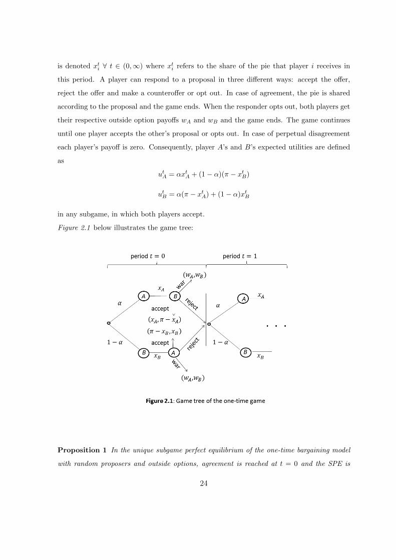
is denoted xti ∀ t ∈ (0,∞) where xti refers to the share of the pie that player i receives in

this period. A player can respond to a proposal in three different ways: accept the offer,

reject the offer and make a counteroffer or opt out. In case of agreement, the pie is shared

according to the proposal and the game ends. When the responder opts out, both players get

their respective outside option payoffs wA and wB and the game ends. The game continues

until one player accepts the other’s proposal or opts out. In case of perpetual disagreement

each player’s payoff is zero. Consequently, player A’s and B’s expected utilities are defined

as

utA = αxtA + (1− α)(π − xtB)

utB = α(π − xtA) + (1− α)xtB

in any subgame, in which both players accept.

Figure 2.1 below illustrates the game tree:

Proposition 1 In the unique subgame perfect equilibrium of the one-time bargaining model

with random proposers and outside options, agreement is reached at t = 0 and the SPE is

24

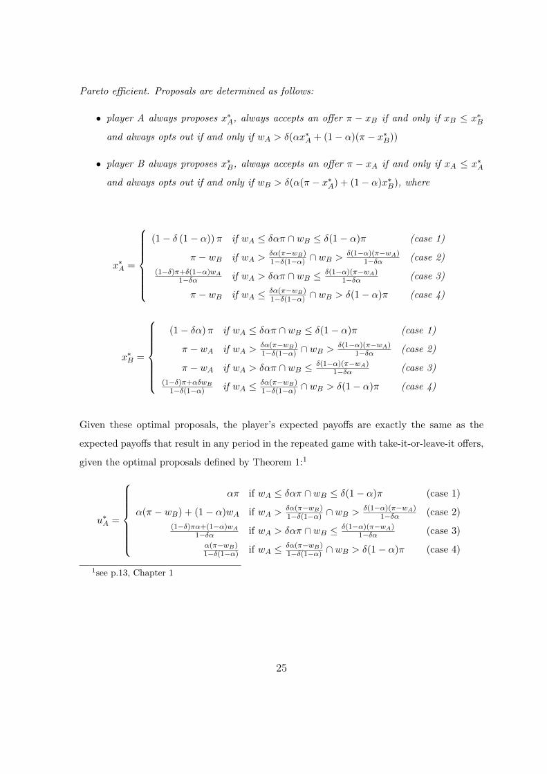
Pareto efficient. Proposals are determined as follows:

• player A always proposes x∗A, always accepts an offer π − xB if and only if xB ≤ x∗B

and always opts out if and only if wA > δ(αx∗A + (1− α)(π − x∗B))

• player B always proposes x∗B, always accepts an offer π − xA if and only if xA ≤ x∗A

and always opts out if and only if wB > δ(α(π − x∗A) + (1− α)x∗B), where

x∗A =

(1− δ (1− α))π if wA ≤ δαπ ∩ wB ≤ δ(1− α)π (case 1)

π − wB if wA >δα(π−wB)1−δ(1−α) ∩ wB > δ(1−α)(π−wA)

1−δα (case 2)

(1−δ)π+δ(1−α)wA

1−δα if wA > δαπ ∩ wB ≤ δ(1−α)(π−wA)1−δα (case 3)

π − wB if wA ≤ δα(π−wB)1−δ(1−α) ∩ wB > δ(1− α)π (case 4)

x∗B =

(1− δα)π if wA ≤ δαπ ∩ wB ≤ δ(1− α)π (case 1)

π − wA if wA >δα(π−wB)1−δ(1−α) ∩ wB > δ(1−α)(π−wA)

1−δα (case 2)

π − wA if wA > δαπ ∩ wB ≤ δ(1−α)(π−wA)1−δα (case 3)

(1−δ)π+αδwB

1−δ(1−α) if wA ≤ δα(π−wB)1−δ(1−α) ∩ wB > δ(1− α)π (case 4)

Given these optimal proposals, the player’s expected payoffs are exactly the same as the

expected payoffs that result in any period in the repeated game with take-it-or-leave-it offers,

given the optimal proposals defined by Theorem 1:1

u∗A =

απ if wA ≤ δαπ ∩ wB ≤ δ(1− α)π (case 1)

α(π − wB) + (1− α)wA if wA >δα(π−wB)1−δ(1−α) ∩ wB > δ(1−α)(π−wA)

1−δα (case 2)

(1−δ)πα+(1−α)wA

1−δα if wA > δαπ ∩ wB ≤ δ(1−α)(π−wA)1−δα (case 3)

α(π−wB)1−δ(1−α) if wA ≤ δα(π−wB)

1−δ(1−α) ∩ wB > δ(1− α)π (case 4)

1see p.13, Chapter 1

25

u∗B =

(1− α)π if wA ≤ δαπ ∩ wB ≤ δ(1− α)π (case 1)

αwB + (1− α)(π − wA) if wA >δα(π−wB)1−δ(1−α) ∩ wB > δ(1−α)(π−wA)

1−δα (case 2)

(1−α)(π−wA)1−δα if wA > δαπ ∩ wB ≤ δ(1−α)(π−wA)

1−δα (case 3)

(1−δ)(1−α)π+αwB

1−δ(1−α) if wA ≤ δα(π−wB)1−δ(1−α) ∩ wB > δ(1− α)π (case 4)

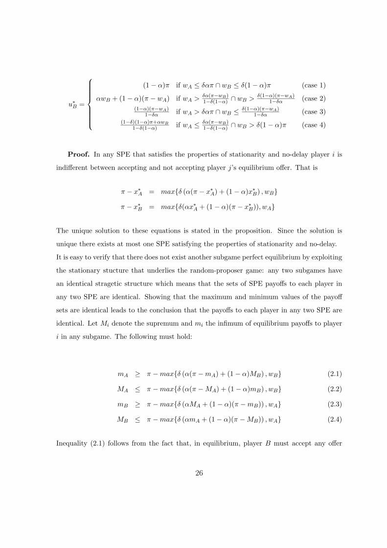
Proof. In any SPE that satisfies the properties of stationarity and no-delay player i is

indifferent between accepting and not accepting player j’s equilibrium offer. That is

π − x∗A = max{δ (α(π − x∗A) + (1− α)x∗B) , wB}

π − x∗B = max{δ(αx∗A + (1− α)(π − x∗B)), wA}

The unique solution to these equations is stated in the proposition. Since the solution is

unique there exists at most one SPE satisfying the properties of stationarity and no-delay.

It is easy to verify that there does not exist another subgame perfect equilibrium by exploiting

the stationary stucture that underlies the random-proposer game: any two subgames have

an identical stragetic structure which means that the sets of SPE payoffs to each player in

any two SPE are identical. Showing that the maximum and minimum values of the payoff

sets are identical leads to the conclusion that the payoffs to each player in any two SPE are

identical. Let Mi denote the supremum and mi the infimum of equilibrium payoffs to player

i in any subgame. The following must hold:

mA ≥ π −max{δ (α(π −mA) + (1− α)MB) , wB} (2.1)

MA ≤ π −max{δ (α(π −MA) + (1− α)mB) , wB} (2.2)

mB ≥ π −max{δ (αMA + (1− α)(π −mB)) , wA} (2.3)

MB ≤ π −max{δ (αmA + (1− α)(π −MB)) , wA} (2.4)

Inequality (2.1) follows from the fact that, in equilibrium, player B must accept any offer

26

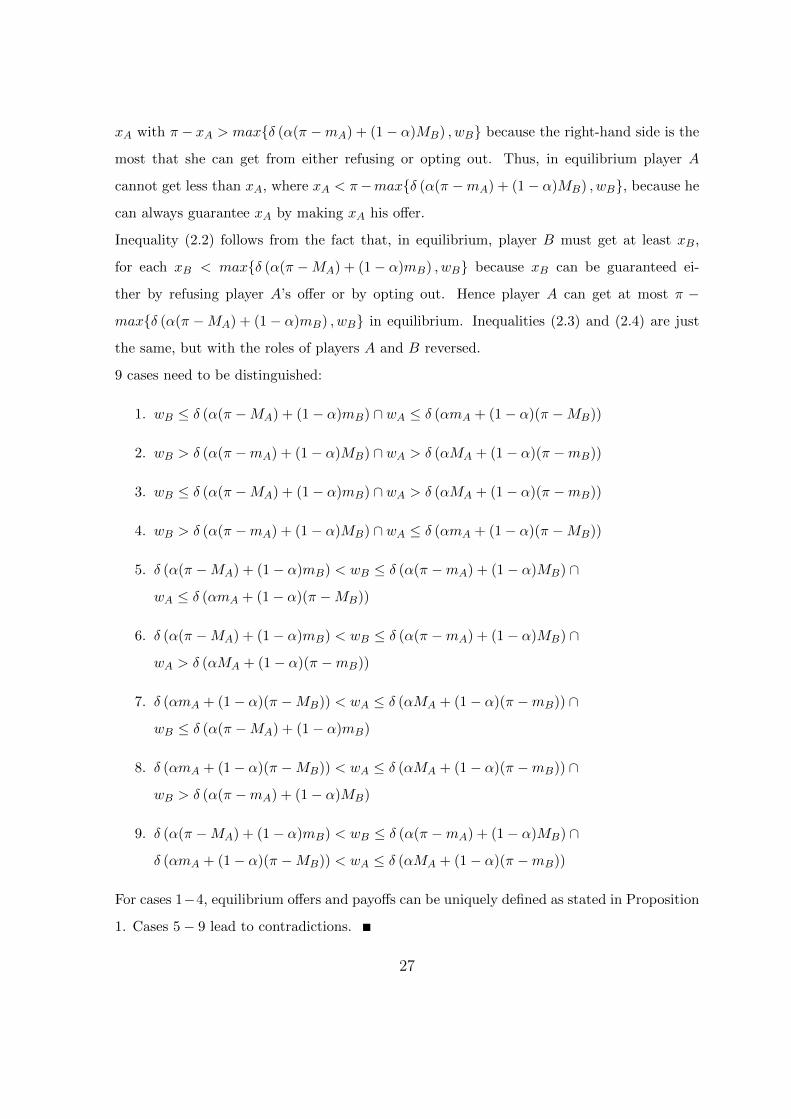
xA with π − xA > max{δ (α(π −mA) + (1− α)MB) , wB} because the right-hand side is the

most that she can get from either refusing or opting out. Thus, in equilibrium player A

cannot get less than xA, where xA < π−max{δ (α(π −mA) + (1− α)MB) , wB}, because he

can always guarantee xA by making xA his offer.

Inequality (2.2) follows from the fact that, in equilibrium, player B must get at least xB,

for each xB < max{δ (α(π −MA) + (1− α)mB) , wB} because xB can be guaranteed ei-

ther by refusing player A’s offer or by opting out. Hence player A can get at most π −

max{δ (α(π −MA) + (1− α)mB) , wB} in equilibrium. Inequalities (2.3) and (2.4) are just

the same, but with the roles of players A and B reversed.

9 cases need to be distinguished:

1. wB ≤ δ (α(π −MA) + (1− α)mB) ∩ wA ≤ δ (αmA + (1− α)(π −MB))

2. wB > δ (α(π −mA) + (1− α)MB) ∩ wA > δ (αMA + (1− α)(π −mB))

3. wB ≤ δ (α(π −MA) + (1− α)mB) ∩ wA > δ (αMA + (1− α)(π −mB))

4. wB > δ (α(π −mA) + (1− α)MB) ∩ wA ≤ δ (αmA + (1− α)(π −MB))

5. δ (α(π −MA) + (1− α)mB) < wB ≤ δ (α(π −mA) + (1− α)MB) ∩

wA ≤ δ (αmA + (1− α)(π −MB))

6. δ (α(π −MA) + (1− α)mB) < wB ≤ δ (α(π −mA) + (1− α)MB) ∩

wA > δ (αMA + (1− α)(π −mB))

7. δ (αmA + (1− α)(π −MB)) < wA ≤ δ (αMA + (1− α)(π −mB)) ∩

wB ≤ δ (α(π −MA) + (1− α)mB)

8. δ (αmA + (1− α)(π −MB)) < wA ≤ δ (αMA + (1− α)(π −mB)) ∩

wB > δ (α(π −mA) + (1− α)MB)

9. δ (α(π −MA) + (1− α)mB) < wB ≤ δ (α(π −mA) + (1− α)MB) ∩

δ (αmA + (1− α)(π −MB)) < wA ≤ δ (αMA + (1− α)(π −mB))

For cases 1−4, equilibrium offers and payoffs can be uniquely defined as stated in Proposition

1. Cases 5− 9 lead to contradictions.

27

2.3 Conclusion

The note defines the unique equilibrium in a Rubinstein-type bargaining game with the

possibility of counteroffers, random proposers and two-sided outside options. It shows that

the equilibrium payoffs are the same as in the structurally different game in Chapter 1 in

which the base game is infinitely repeated, counteroffers are excluded and the players only

have the choice between acceptance and opting out.

28

Chapter 3

Crisis Bargaining, Democracy and

the Transparency Argument

Abstract

Transparency, along with accountability of democratic representatives, has long been iden-

tified as a key component of democratic peace. The paper shows how these two arguments

interact and facilitate democratic peace in a simple game-theoretic model. Based on this

analysis, I investigate how the level of transparency within the principal-agent relationship of

a democratic public and its elected leader affects the crisis bargaining outcome and whether

more transparency and accountability always translates into better results for the democratic

public.

29

3.1 Introduction

Democratic peace refers to the very stable empirical observation that democracies rarely go

to war with one another, but are not immune from fighting wars with non-democracies.1

The present paper is a contribution to the game-theoretic literature which aims to explain

democratic peace with informational advantages of democracies.2 This strand of literature

originated in Fearon’s (1994) famous paper on audience costs and highlights the importance

of successful signaling in eliminating miscommunications between democracies that may oth-

erwise lead states to miscalculate the willingness of the opponent to fight over an issue.

Audience costs theory claims that democracies are better able to signal their intentions

because democratic leaders incur audience costs if they make threats that they later fail to

follow through. In contrast, statements of politically unaccountable dictators are considered

to lack that source of credibility because they are able to bluff without facing domestic costs.

Despite the prominence of audience costs theory (Snyder and Borghard (2011) count over

400 references in scholarly journals), the actual relevance of audience costs in real world crisis

bargaining could not be verified in empirical studies.3 Also, Snyder and Borghard point out

that, in historic cases, public threats are rarely unambiguous which prevents leaders to be

held fully accountable for failed threats and the audience costs argument to unfold. Weeks

(2008), on the other hand, argues that democracies need not be unique in their ability to

raise audience costs. She identifies various sources of audience costs in autocracies and, on

these grounds, concludes that a signaling advantage for democratic leaders based on audience

costs does not exist.

Numerous scholars have since followed the signaling approach and added new arguments

to the pool of reasons why democracies are able to signal successfully. Smith (1998) and

Guisinger and Smith (2002) include democratic politics and endogenize the credibility of a

threat to the leadership selection process, in the attempt to provide a rational underpinning as

to why domestic audiences punish leaders who back down from a threat. Schultz (1998) takes

the public behavior of an informed opposition into account, assuming that the opposition’s

1see for example Oneal and Russett (1997) and Maoz and Abdolali (1989)2for a critical appreciation of democratic peace theory see Rosato (2003)3for an overview of empirical studies on audience costs see Gartzke and Lupu (2012)

30

rhetoric qualifies as a credible signaling device. Ramsay (2004) elaborates the domestic

opposition angle showing that the opposition’s endorsement of the leader can work as a

costly signal in crisis bargaining and eliminate information asymmetries.

In this study, I take one step back and show that democracies do not require a costly sig-

naling device to credibly convey their intentions but that transparency (within democracies)

and accountability (of democratic representatives) is sufficient. More specifically, when politi-

cal leaders care sufficiently about reelection, they are ready to align their private interest with

that of the public, and because public interests are in fact quite public in democracies, the

opponent knows what to expect from a democracy, leading to the phenomenon of democratic

peace in the dyadic case.

This approach simplifies the analysis because it is not build around a signaling device and

thus creates room to address another important question that has usually been investigated

in separate articles and separate models but is essentially related: The question of what level

of transparency is optimal within the agency relationship between the political leader and the

voters. Especially, why is crisis bargaining sometimes completely public while other times

happening behind closed doors, and how does that affect the crisis bargaining outcome.

With that respect, I distinguish between two kinds of transparency: First, a general

kind of transparency, including freedom of speech, free press and media, is the reason why

all parties involved in crisis bargaining share the same information about the democratic

majority’s preferences. Second, by agency transparency, I mean the ability of the principal

to observe the agent’s behavior and its consequences.

The paper has two objectives: First, it is to provide a simple game-theoretic foundation

of the most prevalent arguments for democratic peace: transparency and accountability.4

Second, it is to analyze what degree of agency transparency is preferable in an international

bargaining setting by comparing two scenarios, open-door bargaining in which the democratic

public can observe the bargaining process between its representative and a third party and

closed-door bargaining, in which the agent’s actions are partly hidden.

I find that imperfect information can have two effects. Firstly and predictably, it can

worsen the agent’s accountability and increase his incentive to follow his own preferences

4see Schultz (1999)

31

instead of the principal’s which reduces the predictability of democracies and can increase

the probability of a bargaining breakdown. But secondly and interestingly, less information

and less accountability can also increase the opponent’s offer and lead to better outcomes for

the democratic public.

The idea that revealing more information may not always be beneficial is fairly new and

departs from earlier research proclaiming that agency relationships should be as transparent

as possible because transparency improves accountability.5 Recent studies on career concern

models suggest that in some circumstances, transparency may have detrimental effects if it

leads to inefficient posturing. Prat (2005) employs a quite general model of career concerns for

experts in which the agent’s type determines his ability to understand the state of the world

and finds that more transparency has a negative effect if it induces the agent to disregard

useful private signals and to act according to how an able agent is expected to act a priori.

The present paper is closer related to Stasavage (2004) who assumes that the public is

uncertain about a representative’s preferences instead of his ability. He also finds that more

transparency and less difficulty in inferring a representative’s type has the negative effect

that unbiased representatives have more incentive to ignore their private signal (about the

opponent’s minimum acceptable offer) and posture. Stasavage concludes that because pos-

turing is the unique equilibrium under open-door bargaining as long as reputational concerns

are sufficiently strong, “one should expect to see more uncompromising positions taken dur-

ing open-door bargaining, greater polarization of debate, and more frequent breakdowns in

bargaining than would otherwise be the case.”(Stasavage 2004)

In the present paper, however, a negative effect from posturing cannot arise because

there is no private signal (about the opponent’s minimal offer) that could be neglected and

posturing is never beneficial for unbiased agents. But even with the negative posturing

effect under open-door bargaining missing, I find that closed-door bargaining can generate

comparatively better results for the democratic public if it induces the opponent to increase

his offer. This is why democracies may sometimes prefer closed-door bargaining even though

it includes a higher risk of bargaining breakdown.

5see Holmstrom (1999)

32

3.2 The Classical Crisis Bargaining Approach

Two parties, A and B, bargain about the distribution of an issue of size 1. Each player has

an individual outside option wi, which is private information. For simplification, I assume

that one of the bargainers is selected at random to make a take-it-or-leave-it offer, which the

opponent accepts if and only if this offer meets at least her outside option wi. Otherwise, she

opts out and both parties receive their respective outside option payoffs.

This modeling correlates to the literature on war bargaining that often treats war as

a costly lottery which is won by party A with probability φA ∈ [0, 1] and party B with

probability φB = 1 − φA. The expected gains from this lottery can be interpreted as the

parties’ respective outside options wi = φi− ci of the bargining game, where ci represent the

costs of war. Note that, in this formulation, the term ci captures the relative net value that

a party places on winning or losing the war. That is, ci reflects party i’s costs of war relative

to any possible benefits. In practice, low costs of war translate into a high outside option or

high resolve, which means that the issue at stake is highly valued and going to war a viable

option at relatively small costs. On the other hand, if a party sees little to gain from winning

war, then ci would be large even if the actual costs, incurred by war, were small.6

War can occur when there is asymmetric information about the opponent’s resolve. When

the opponent can either have a high outside option (high resolve) or a low outside option

(low resolve), a state may have an incentive to screen the opponent’s type and make an offer

which is only acceptable to the weak type, leading to war whenever the opponent is strong.

Asymmetric information about the opponent’s outside option either means that the par-

ties have private information about the probability to win a war, which basically refers to

military ressources, or private information about the costs of war, which will be applied here.

As stated above, high costs of war immediately result in a low outside option and low costs

of war in a high outside option.

The asymmetry in information is modeled as follows: From A’s point of view, player B’s

outside option is low (wlB) with probability 0 < β < 1 and high (whB ) with probability 1−β,

with wlB < whB. Equally, player B believes that A’s outside option is low (weak type) with

6see Fearon (1995)

33

probability 0 < α < 1 and high (strong type) with probability 1− α. In contrast to the case

of asymmetric information about military resources, in the case of asymmetric information

about costs, a mutually beneficial bargaining outcome always exists, even when two strong

types negotiate, whA + whB ≤ 1.

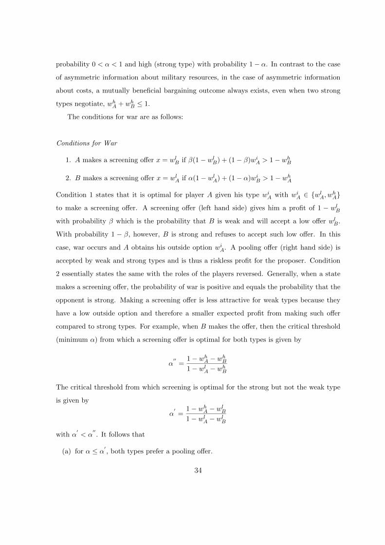
The conditions for war are as follows:

Conditions for War

1. A makes a screening offer x = wlB if β(1− wlB) + (1− β)wiA > 1− whB

2. B makes a screening offer x = wlA if α(1− wlA) + (1− α)wiB > 1− whA

Condition 1 states that it is optimal for player A given his type wiA with wiA ∈ {wlA, whA}

to make a screening offer. A screening offer (left hand side) gives him a profit of 1 − wlBwith probability β which is the probability that B is weak and will accept a low offer wlB.

With probability 1 − β, however, B is strong and refuses to accept such low offer. In this

case, war occurs and A obtains his outside option wiA. A pooling offer (right hand side) is

accepted by weak and strong types and is thus a riskless profit for the proposer. Condition

2 essentially states the same with the roles of the players reversed. Generally, when a state

makes a screening offer, the probability of war is positive and equals the probability that the

opponent is strong. Making a screening offer is less attractive for weak types because they

have a low outside option and therefore a smaller expected profit from making such offer

compared to strong types. For example, when B makes the offer, then the critical threshold

(minimum α) from which a screening offer is optimal for both types is given by

α′′

=1− whA − whB1− wlA − whB

The critical threshold from which screening is optimal for the strong but not the weak type

is given by

α′

=1− whA − wlB1− wlA − wlB

with α′< α

′′. It follows that

(a) for α ≤ α′ , both types prefer a pooling offer.

34

(b) for α′< α ≤ α′′ , the weak type prefers a pooling and the strong type a screening offer.

(c) for α′′< α, both types prefer a screening offer.

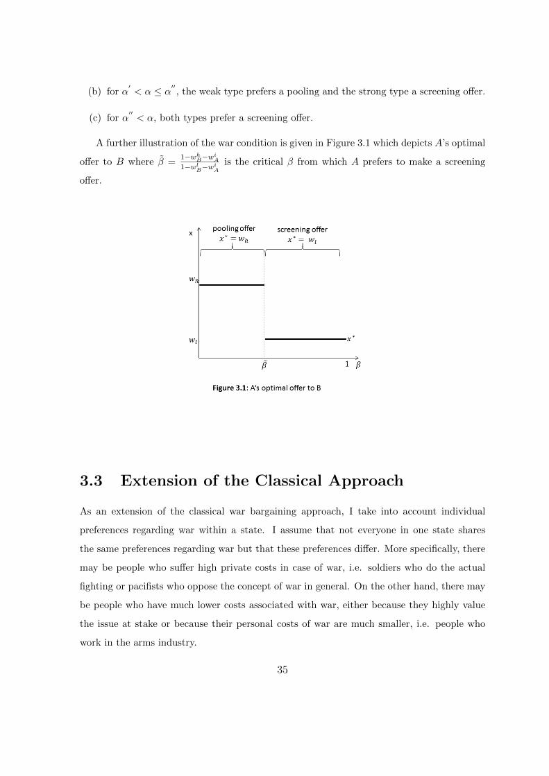
A further illustration of the war condition is given in Figure 3.1 which depicts A’s optimal

offer to B where β =1−wh

B−wiA

1−wlB−wi

A

is the critical β from which A prefers to make a screening

offer.

3.3 Extension of the Classical Approach

As an extension of the classical war bargaining approach, I take into account individual

preferences regarding war within a state. I assume that not everyone in one state shares

the same preferences regarding war but that these preferences differ. More specifically, there

may be people who suffer high private costs in case of war, i.e. soldiers who do the actual

fighting or pacifists who oppose the concept of war in general. On the other hand, there may

be people who have much lower costs associated with war, either because they highly value

the issue at stake or because their personal costs of war are much smaller, i.e. people who

work in the arms industry.

35

Additionally, I follow in the steps of Fearon (1994), Jackson and Morelli (2007) and many

others by assuming that states feature a principal-agent relationship with the agent being

the political leader who engages in a crisis bargaining game with a third party on behalf of

his principal, the people. While both regime types share this characteristic, the difference

between democracy and autocracy is that the revelation of the principal’s preferences is

private in autocracies but public in democracies.7 It is this general transparency within

democracies that facilitates signaling to the opponent.

However, within the framework of this model, this transparency does not necessarily

translate into efficient signaling if the agent’s preferences (regarding resolve for war) differ

from majority’s preferences. Since, as opposed to classical principal-agent literature, in the

context of political institutions, the principal cannot make a specific incentive compatible

contract to induce the right behavior in the agent but can only elect and dismiss, the agent

may still not be completely deterred from following his own and not majority’s preferences

even under perfect information. The problem intensifies when information is imperfect and

the agent’s action cannot be fully observed by the principal.

What is also interesting to note is that even though revealing weak resolve to the oppo-

nent through signaling cannot be in the principal’s best interest, otherwise there would be

no reason to conceal the type and no grounds for miscommunications in the first place, the

conclusion that successful signaling provides democracies with more peaceful yet disadvan-

tageous bargaining outcomes turns out to be wrong. Although there are situations in which

revealing a weak type through signaling has negative effects on the bargaining share, I will

show that there are also situations in which democracies are offered comparably higher shares

than autocracies in a similar position despite the public signal revealing a weak type.

The reason for this lies within the principal-agent relationship. Although the signal

about majority’s preferences is public, the opponent does not know from the outset how a

democratic leader will react in the bargaining game because the leader’s type is still private

information. Since the public’s control over the agent is limited to removing him from office,

7In accordance with Bueno de Mesquita et al. (1999), I suppose that one decisive difference betweendemocracy and autocracy is the size of the winning coalition, where the winning coalition subsumesall “people whose support is required to keep the incumbent in office” and is typically large in ademocracy, while small in autocracies. Because the winning coalition is small in autocracies, I arguethat the political leader can learn the principal’s preferences privately while in a democracy he cannot.

36

and agents may be more interested in obtaining their preferable bargaining outcome than

being reelected, agents may still defect from majority’s preferences even if their actions can

be monitored. In order to satisfy such biased agents, the opponent may be ready to offer more

than he would to an autocracy. This will be discussed in Section 3.5.1 Open-door bargaining

and used as a reference case for Section 3.5.2 Closed-door bargaining. Under closed-door

bargaining, the public can monitor the agent’s choice of action imperfectly. But even though

imperfect information worsens the agent’s accountability and increases his incentive to follow

his own preferences, which counteracts successful signaling, there are situations in which less

information and less accountability leads to better outcomes for the democratic public.

3.4 The Model

Suppose there is a democratic state involved in crisis bargaining with another state, denoted

O (opponent, which can either be a democratic or an autocratic state). Let A denote the

leader (agent) of a democracy and P the democratic majority (principal). In the bargaining

game, A decides what offer to make to the opponent and what offer to accept, and majority

decides if the leader will remain in office afterwards.

The leader cares about the bargaining outcome as well as getting reelected. In the bar-

gaining game he decides whether to act in the principal’s interest (unbiased) or his own

interest (biased). The principal has two types, w ∈ {wl, wh} depending on the democratic

majority’s preferences, where majority is weak (wl) with probability β and strong (wh) with

probability 1 − β. Majority’s type becomes known immediately to the agent and the oppo-

nent through a public signal. As any other individual in the democracy, the agent has two

types that differ in their preferences, he is either wl with probability β or wh with probability

1− β, which is private information. I assume that the public is not interested in the agent’s

type but in his action. In the election that follows crisis bargaining, the voter’s concern is

to reelect an agent that acted unbiased and replace an agent that acted biased. The reason

for this assumption is that the bargaining issue is not a constant but subject to change so

that in the next bargaining case the leader’s preferences may be unaligned with majority’s

preferences. With this in mind, the voter is better off making his reelection decision based

37

on the leader’s action and not dismiss leaders who act in the public’s interest.

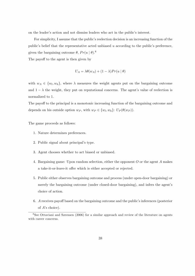
For simplicity, I assume that the public’s reelection decision is an increasing function of the

public’s belief that the representative acted unbiased u according to the public’s preference,

given the bargaining outcome θ, Pr(u | θ).8

The payoff to the agent is then given by

UA = λθ(wA) + (1− λ)Pr(u | θ)

with wA ∈ {wl, wh}, where λ measures the weight agents put on the bargaining outcome

and 1 − λ the weight, they put on reputational concerns. The agent’s value of reelection is

normalized to 1.

The payoff to the principal is a monotonic increasing function of the bargaining outcome and

depends on his outside option wP , with wP ∈ {wl, wh}: UP (θ(wP )).

The game proceeds as follows:

1. Nature determines preferences.

2. Public signal about principal’s type.

3. Agent chooses whether to act biased or unbiased.

4. Bargaining game: Upon random selection, either the opponent O or the agent A makes

a take-it-or-leave-it offer which is either accepted or rejected.

5. Public either observes bargaining outcome and process (under open-door bargaining) or

merely the bargaining outcome (under closed-door bargaining), and infers the agent’s

choice of action.

6. A receives payoff based on the bargaining outcome and the public’s inferences (posterior

of A’s choice).

8See Ottaviani and Sørensen (2006) for a similar approach and review of the literature on agentswith career concerns.

38

Because the signal about the principal’s type is private in autocracies, signaling is not

possible for an autocracy within the framework of this model. The propensity of war in the

Autocracy/Autocracy case therefore coincides with that predicted by classical crisis bargain-

ing models as presented in Section 3.2. In the following equilibrium analysis I will distinguish

between the Democracy/Autocracy case in which the opponent is an autocracy and the

Democracy/Democracy case in which the opponent is also a democracy.

3.5 Equilibrium Analysis

Note that agents whose preferences are aligned with the principal’s preferences have every

incentive to act in the principal’s interest because otherwise they would incur a payoff loss

in terms of bargaining outcome and in terms of reputation. The following conditions ensure

that agents whose preferences differ from the principal’s act in the principal’s interest when

democracy responds to an offer:

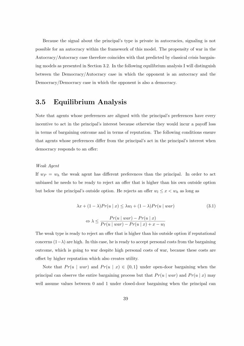
Weak Agent

If wP = wh the weak agent has different preferences than the principal. In order to act

unbiased he needs to be ready to reject an offer that is higher than his own outside option

but below the principal’s outside option. He rejects an offer wl ≤ x < wh as long as

λx+ (1− λ)Pr(u | x) ≤ λwl + (1− λ)Pr(u | war) (3.1)

⇔ λ ≤ Pr(u | war)− Pr(u | x)

Pr(u | war)− Pr(u | x) + x− wl

The weak type is ready to reject an offer that is higher than his outside option if reputational

concerns (1−λ) are high. In this case, he is ready to accept personal costs from the bargaining

outcome, which is going to war despite high personal costs of war, because these costs are

offset by higher reputation which also creates utility.

Note that Pr(u | war) and Pr(u | x) ∈ {0, 1} under open-door bargaining when the

principal can observe the entire bargaining process but that Pr(u | war) and Pr(u | x) may

well assume values between 0 and 1 under closed-door bargaining when the principal can

39

merely observe the bargaining outcome.

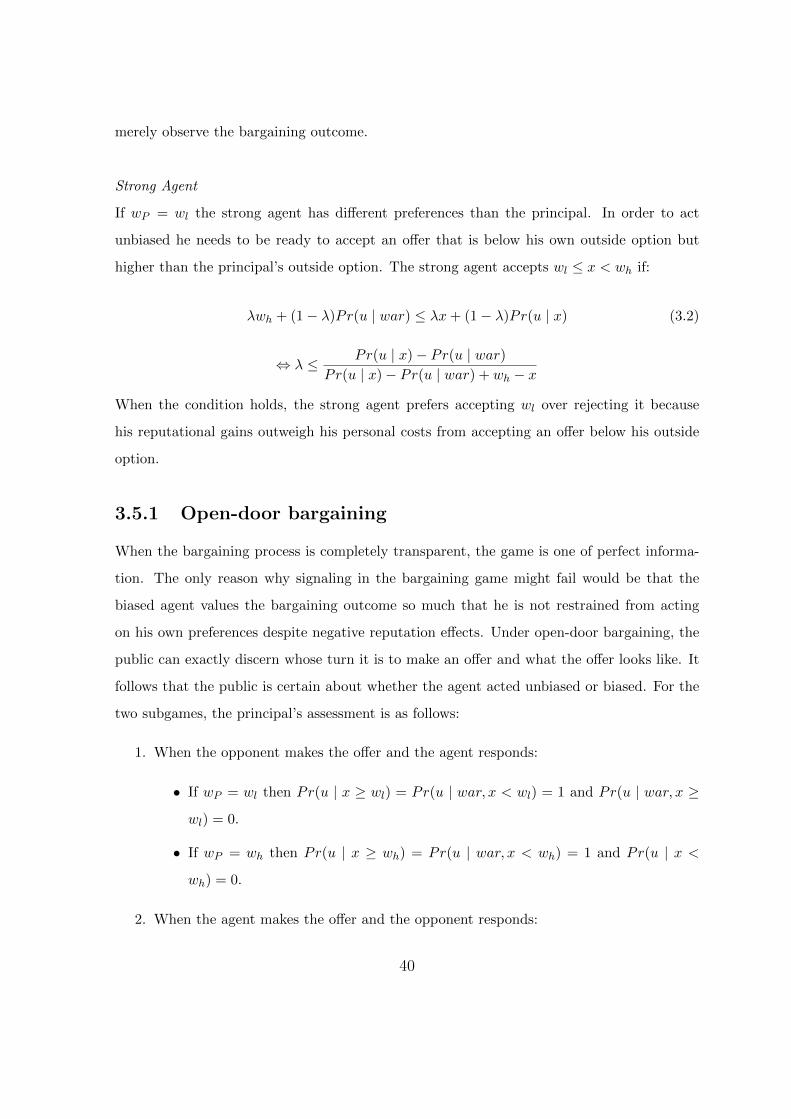
Strong Agent

If wP = wl the strong agent has different preferences than the principal. In order to act

unbiased he needs to be ready to accept an offer that is below his own outside option but

higher than the principal’s outside option. The strong agent accepts wl ≤ x < wh if:

λwh + (1− λ)Pr(u | war) ≤ λx+ (1− λ)Pr(u | x) (3.2)

⇔ λ ≤ Pr(u | x)− Pr(u | war)Pr(u | x)− Pr(u | war) + wh − x

When the condition holds, the strong agent prefers accepting wl over rejecting it because

his reputational gains outweigh his personal costs from accepting an offer below his outside

option.

3.5.1 Open-door bargaining

When the bargaining process is completely transparent, the game is one of perfect informa-

tion. The only reason why signaling in the bargaining game might fail would be that the

biased agent values the bargaining outcome so much that he is not restrained from acting

on his own preferences despite negative reputation effects. Under open-door bargaining, the

public can exactly discern whose turn it is to make an offer and what the offer looks like. It

follows that the public is certain about whether the agent acted unbiased or biased. For the

two subgames, the principal’s assessment is as follows:

1. When the opponent makes the offer and the agent responds:

• If wP = wl then Pr(u | x ≥ wl) = Pr(u | war, x < wl) = 1 and Pr(u | war, x ≥

wl) = 0.

• If wP = wh then Pr(u | x ≥ wh) = Pr(u | war, x < wh) = 1 and Pr(u | x <

wh) = 0.

2. When the agent makes the offer and the opponent responds:

40

• If the principal prefers a pooling offer xp then Pr(u | x = 1 − xp) = 1 and

Pr(u | x 6= 1− xp) = 0.

• If the principal prefers a screening offer xs then Pr(u | x = 1 − xs) = 1 and

Pr(u | x 6= 1− xs) = 0.

Democracy/Autocracy

I will first look at the case, that the opponent is an autocracy, meaning a single actor with

an outside option wO ∈ {wl, wh}.

Democracy makes the offer

The democratic agent’s offer to the autocracy does not differ from the offer that an autoc-

racy would make in this position as long as democratic agents are sufficiently interested in

reelection. To see this, rememeber that the democratic principal is considered a unitary actor

with preferences wP ∈ {wl, wh}. Just as an autocracy, he prefers to make a screening offer

if the probability that the opponent is weak, α, is sufficiently high. The critical values for α

are the same as in the Autocracy/Autocracy case presented in Section 3.2. Note that when

α ≤ α′ , a pooling offer is optimal for both types and when α′′< α both types prefer to make

a screening offer, so that there is no conflict of interest between the principal and the agent

independent of their types. However, when α′< α ≤ α′′ strong types prefer a screening offer

while weak types prefer a pooling offer which may create a conflict of interest.

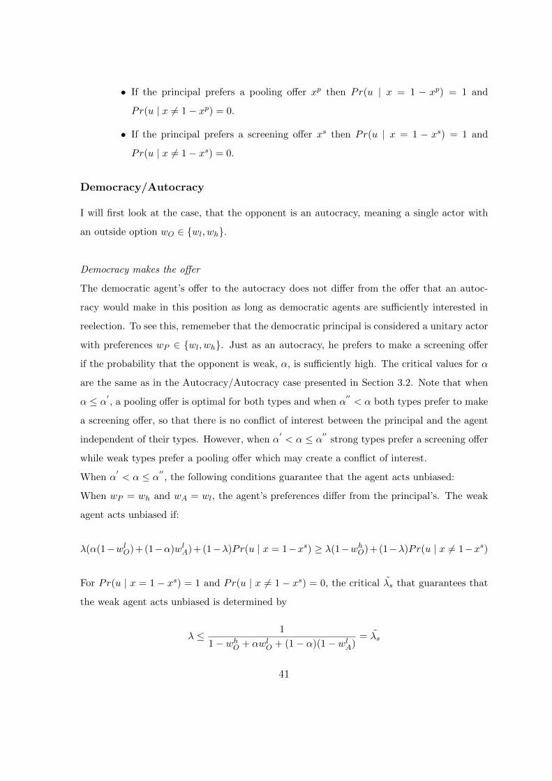
When α′< α ≤ α′′ , the following conditions guarantee that the agent acts unbiased:

When wP = wh and wA = wl, the agent’s preferences differ from the principal’s. The weak

agent acts unbiased if:

λ(α(1−wlO)+(1−α)wlA)+(1−λ)Pr(u | x = 1−xs) ≥ λ(1−whO)+(1−λ)Pr(u | x 6= 1−xs)

For Pr(u | x = 1− xs) = 1 and Pr(u | x 6= 1− xs) = 0, the critical λs that guarantees that

the weak agent acts unbiased is determined by

λ ≤ 1

1− whO + αwlO + (1− α)(1− wlA)= λs

41

When wP = wl and wA = wh, the agent’s preferences differ from the principal’s. The strong

agent acts unbiased if:

λ(1−whO)+(1−λ)Pr(u | x = 1−xp) ≥ λ(α(1−wlO)+(1−α)whA)+(1−λ)Pr(u | x 6= 1−xp)

For Pr(u | x = 1− xp) = 1 and Pr(u | x 6= 1− xp) = 0, the critical λp that guarantees that

the strong agent acts unbiased is determined by

λ ≤ 1

α(1− wlO) + (1− α)whA + whO= λp

Corollary 4 When bargaining is open-door and reputation is sufficiently important to biased

agents, so that λ ≤ min{λs, λp}, the optimal offer to an autocracy is independent of regime

type.

Because screening offers are made as frequently as in the Autocracy/Autocracy case, given

that reelection is important, the probability of war is also the same. That is why the fol-

lowing analysis concentrates on the offer that is accepted by the democracy because here the

equilibrium offer changes with regime type when reputation is important.

Democracy responds to an offer

When wP = wh, the unbiased agent will accept no offer x < wh. The opponent makes a

pooling offer x = wh, if he has no incentive to deviate to a screening offer acceptable only to

the weak agent. The following condition must hold:

1− wh ≥ β(1− x) + (1− β)wO (3.3)

The left hand side is the opponent’s payoff from making a high offer accepted by both

types and the right hand side is his payoff from making an offer x < wh that is accepted

with probability β (by the weak type) and rejected with probability 1 − β (by the strong

type) in which case war results leaving the opponent with his outside option wO. An offer

x < wh is acceptable to the weak agent if his incentive constraint, Condition 3.1, fails. For

42

Pr(u | war, x < wh) = 1 and Pr(u | x < wh) = 0, that is if

x >1

λ+ wl − 1 = xh (3.4)

So xh defines the weak agent’s minimum acceptable offer. Let x′h define the maximum

screening offer the opponent is ready to make to the weak agent. It is determined by failure

of Condition 3.3:

x < 1− wO −1− wO − wh

β= x

′h (3.5)

It follows from Conditions 3.4 and 3.5 that there is a screening equilibrium for xh < x′h in

which the opponent makes a screening offer x = max{wl, xh} that is accepted by the weak

type and rejected by the strong type, and there is a pooling equilibrium for xh ≥ x′h in which

the offer x = wh is accepted by both types of agent.

Let λh define the maximum λ for which a pooling equilibrium exists. Then λh is determined

by:

xh ≥ x′h

⇔ 1

λ+ wl − 1 ≥ 1− wO −

1− wO − whβ

⇔ λ ≤ β

(1− wl)β − (1− β)(1− wO) + wh= λh (3.6)

For λ > λh a screening equilibrium results.

If wP = wl, the opponent makes a pooling offer x ≥ wl acceptable to both types if his

payoff from making such an offer (right hand side of Condition 3.7 below) exceeds his payoff

from making a screening offer x = wl that is only accepted by the weak type (left hand side

of Condition 3.7):

β(1− wl) + (1− β)wO ≤ 1− x (3.7)

An offer wl ≤ x < wh is acceptable to both types of agent if the strong type’s incentive

constraint, Condition 3.2, holds. For Pr(u | war, x ≥ wl) = 0 and Pr(u | x ≥ wl) = 1, that

is if

x ≥ 1 + wh −1

λ= xl (3.8)

43

So xl defines the strong agent’s minimum acceptable offer. Let x′l define the maximum pooling

offer the opponent is ready to make, which results from Condition 3.7:

x ≤ 1− β(1− wl)− (1− β)wO = x′l (3.9)

It follows from Conditions 3.8 and 3.9 that there is a screening equilibrium for xl > x′l in

which the opponent makes a screening offer x = wl that is accepted by the weak unbiased

type and rejected by the strong biased type, and there is a pooling equilibrium for xl ≤ x′l in

which the offer x = max{xl, wl} is accepted by both types of agent.

Let λl define the maximum λ for which a pooling equilibrium exists. Then λl is determined

by:

x′l ≥ xl

⇔ 1− β(1− wl)− (1− β)wO ≥ 1 + wh −1

λ

⇔ λ ≤ 1

(1− wl)β + (1− β)wO + wh= λl (3.10)

For λ > λl a screening equilibrium results.

Corollary 5 When bargaining is open-door and reputation is sufficiently important to biased

agents, so that λ ≤ min{λl, λh}, the opponent makes a pooling offer x = wh if wP = wh and

x = max{wl, xl} if wP = wl and democracy always accepts this offer in equilibrium. When

λ > λh and wP = wh, the opponent makes a screening offer x = max{wl, xh} that is rejected

with probability 1− β, by the strong unbiased type. When λ > λl and wP = wl, the opponent

makes a screening offer x = wl that is rejected with probability 1 − β, by the strong biased

type.

Figures 3.2 and 3.3 below show the equilibrium offer in the two cases wP = wh and

wP = wl. We can see that as long as reelection concerns are sufficiently important (λ ≤

min{λl, λh}), the opponent makes a pooling offer that is peacefully accepted.

In the following, I will analyze whether democratic transparency, that is, revealing the

democratic public’s type to the opponent in international bargaining leads to disadvantageous

bargaining outcomes for democracies. To do so, I compare the equilibrium offer that the

44

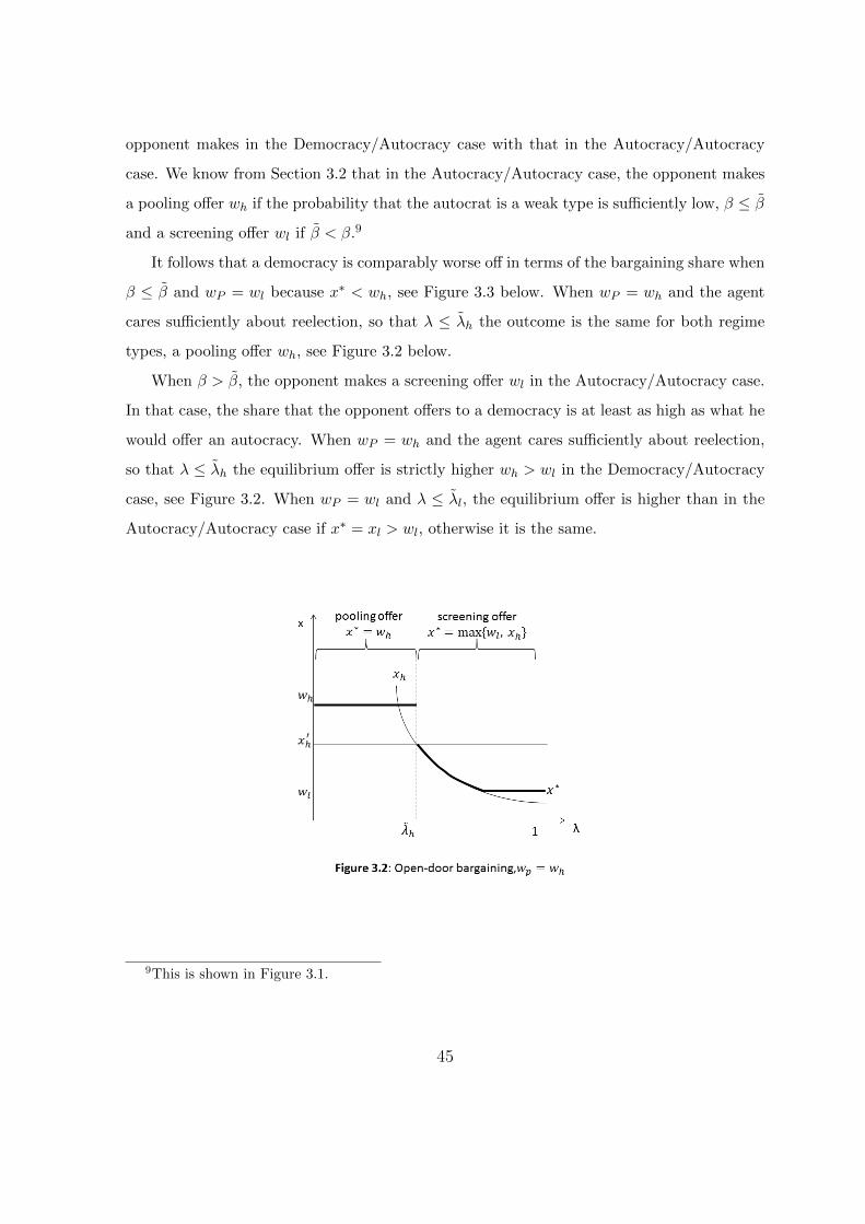
opponent makes in the Democracy/Autocracy case with that in the Autocracy/Autocracy

case. We know from Section 3.2 that in the Autocracy/Autocracy case, the opponent makes

a pooling offer wh if the probability that the autocrat is a weak type is sufficiently low, β ≤ β

and a screening offer wl if β < β.9

It follows that a democracy is comparably worse off in terms of the bargaining share when

β ≤ β and wP = wl because x∗ < wh, see Figure 3.3 below. When wP = wh and the agent

cares sufficiently about reelection, so that λ ≤ λh the outcome is the same for both regime

types, a pooling offer wh, see Figure 3.2 below.

When β > β, the opponent makes a screening offer wl in the Autocracy/Autocracy case.

In that case, the share that the opponent offers to a democracy is at least as high as what he

would offer an autocracy. When wP = wh and the agent cares sufficiently about reelection,

so that λ ≤ λh the equilibrium offer is strictly higher wh > wl in the Democracy/Autocracy

case, see Figure 3.2. When wP = wl and λ ≤ λl, the equilibrium offer is higher than in the

Autocracy/Autocracy case if x∗ = xl > wl, otherwise it is the same.

9This is shown in Figure 3.1.

45

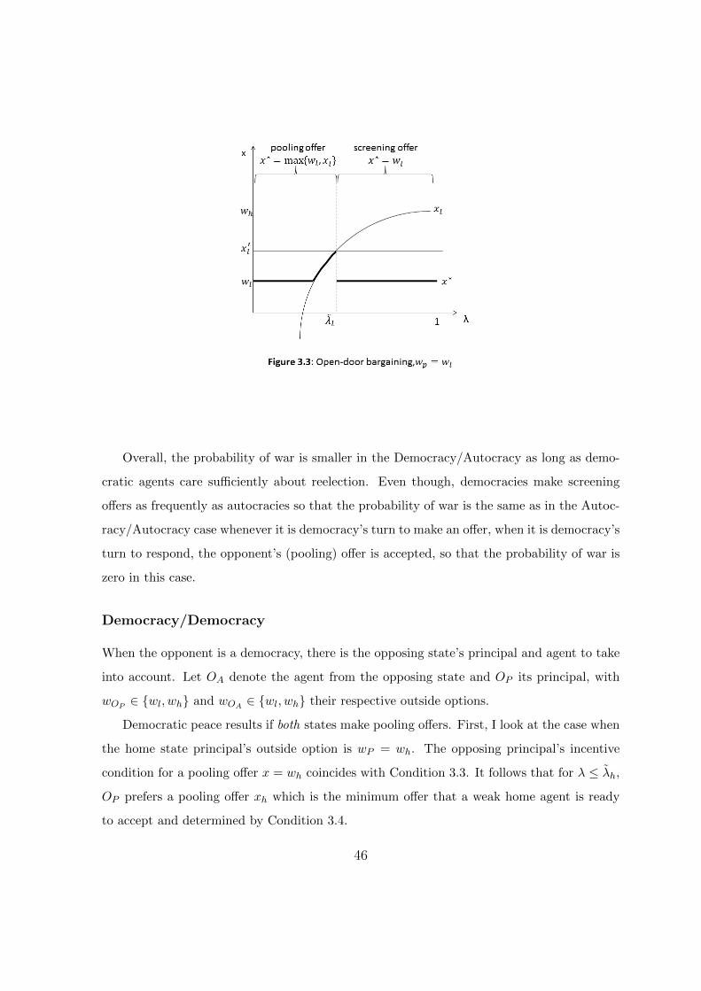
Overall, the probability of war is smaller in the Democracy/Autocracy as long as demo-

cratic agents care sufficiently about reelection. Even though, democracies make screening

offers as frequently as autocracies so that the probability of war is the same as in the Autoc-

racy/Autocracy case whenever it is democracy’s turn to make an offer, when it is democracy’s

turn to respond, the opponent’s (pooling) offer is accepted, so that the probability of war is

zero in this case.

Democracy/Democracy

When the opponent is a democracy, there is the opposing state’s principal and agent to take

into account. Let OA denote the agent from the opposing state and OP its principal, with

wOP∈ {wl, wh} and wOA

∈ {wl, wh} their respective outside options.

Democratic peace results if both states make pooling offers. First, I look at the case when

the home state principal’s outside option is wP = wh. The opposing principal’s incentive

condition for a pooling offer x = wh coincides with Condition 3.3. It follows that for λ ≤ λh,

OP prefers a pooling offer xh which is the minimum offer that a weak home agent is ready

to accept and determined by Condition 3.4.

46

When wOP= wh, then a pooling offer is always optimal independent of λ because if

a pooling offer is optimal for the strong type, it is also optimal for the weak type. When

wOP= wl and wOA

= wh, the opposing state’s agent OA might have an incentive to make a

screening offer. He is ready to make the pooling offer if

λ(1−wh)+(1−λ)Pr(u | x = 1−xp) ≥ λ(β(1−xh)+(1−β)wOA)+(1−λ)Pr(u | x 6= 1−xp)

Let λOhdenote the maximum λ at which OA is ready to make the pooling offer. For Pr(u |

x = 1− xp) = 1 and Pr(u | x 6= 1− xp) = 0, λOhis determined by

λ ≤ 1

β(1− xh) + (1− β)wOA+ wh

= λOh(3.11)

When the home state principal’s outside option is wP = wl, the opposing principal’s incentive

condition for a pooling offer x ≥ wl coincides with Condition 3.7. It follows that for λ ≤ λl,

OP prefers the pooling offer xl which is the minimum offer that is acceptable to both types

of the home agent and determined by Condition 3.8. Again, when wOP= wh, a pooling offer

is always optimal independent of λ. When wOP= wl and wOA

= wh, OA might have an

incentive to make a screening offer. He is ready to make the pooling offer if

λ(1−x) + (1−λ)Pr(u | x = 1−xp) ≥ λ(β(1−wl) + (1−β)wOA) + (1−λ)Pr(u | x 6= 1−xp)

Let λOldenote the maximum λ at which OA is ready to make the pooling offer. For Pr(u |

x = 1− xp) = 1 and Pr(u | x 6= 1− xp) = 0, λOlis determined by

λ ≤ 1

β(1− wl) + (1− β)wOA+ xl

= λOl(3.12)

Corollary 6 When reputation is sufficiently important to democratic agents, pooling offers

are made and accepted both ways, which constitutes the democratic peace.

47

3.5.2 Closed-door bargaining

When bargaining takes place behind closed doors, there is informational asymmetry. The

principal cannot observe who makes the offer, what the offer looks like and which offer has

been rejected by whom.

Under closed-door bargaining, the agent’s payoff can change because Pr(u | war) is no

longer certain. When an offer is accepted, the principal can still infer who made the offer

and whether the agent acted in a biased manner.10 However, when it comes to the rejection

of an offer and war occurs, the principal can no longer identify the reason, because war can

result either if the agent rejects an offer or if the agent’s offer is rejected.

Democracy/Autocracy

Under closed-door bargaining, the principal cannot distinguish between responder and pro-

poser which means that there are no longer two subgames that can be analyzed independently.

The principal’s optimal offer to the opponent depends on the principal’s type and the prob-

ability that the opposing autocrat is weak, as explained in Section 3.2:

(a) α ≤ α′ , both types prefer a pooling offer.

(b) α′< α ≤ α′′ , the weak type prefers a pooling and the strong type a screening offer.

(c) α′′< α, both types prefer a screening offer.

When wP = wh, the agent acts according to the principal’s preferences if he rejects x < wh

and, in Cases (b) and (c), makes a screening offer. It follows that in Cases (b) and (c)

Pr(u | war) = 1, independent of the opponent’s offer because acting biased either means

accepting an offer x < wh or making a pooling offer to the opponent, both actions which do

not lead to war. For Pr(u | war) = 1 (and Pr(u | x < wh) = 0) the weak type’s incentive

constraint is the same as under open-door bargaining and equilibrium is determined as stated

in Corollary 5.

In Case (a), it is optimal for both types to make a pooling offer to the opponent. In this case,

10In case of agreement, the principal’s share is 1−whO when the agent made a pooling offer, 1−wl

O

when the agent made a screening offer, and wl ≤ x ≤ wh < 1−wlO when the opponent made a pooling

offer.

48

Pr(u | war) is an off-equilibrium belief if the opponent’s best response is also a pooling offer.

Otherwise, when the opponent makes a screening offer, Pr(u | war) = 0 which is the same as

under open-door bargaining so that the results are the same. Only when the off-equilibrium

belief Pr(u | war) > 0, the weak type’s incentive constraint, Condition 3.4 changes:

xh,c =1− λλ

Pr(u | war) + wl (3.13)

where xh,c < xh for Pr(u | war) < 1. In terms of λ, a screening equilibrium results if:

xh,c ≥ x′h

⇔ 1− λλ

Pr(u | war) + wl ≥ 1− wO −1− wO − wh

β

so that the critical λ from which screening is optimal is determined by

λ ≤ βPr(u | war)(Pr(u | war)− wl)β − (1− β)(1− wO) + wh

= λh,c (3.14)

Since λh,c < λh for Pr(u | war) < 1, the critical threshold for a screening equilibrium is lower

compared to open-door bargaining for Pr(u | war) < 1.

However, Pr(u | war) < 1 is not a plausible off-equilibrium belief because it would mean

that the principal believes that the agent did not act in his interest in case of war but

somehow acted more aggressive. This is not possible since the principal is a strong type and

the agent can either be equally strong or weaker. The only plausible off-equilibrium belief

is Pr(u | war) = 1 for which the results do not differ from the results under open-door

bargaining.

Corollary 7 When wP = wh, the results are the same as under open-door bargaining in

Cases (b) and (c). In Case (a), the threshold for a pooling equilibrium may be below the

threshold under open-door bargaining, however only for implausible off-equilibrium beliefs. For

the only plausible off-equilibrium belief the results are the same as under open-door bargaining.

When wP = wl and Case (c), Pr(u | war) = 1 if the opponent makes a pooling offer x ≤ whand the strong agent’s incentive constraint holds. But when Pr(u | war) = Pr(u | x ≥ wl) =

49

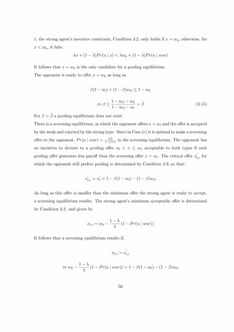
1, the strong agent’s incentive constraint, Condition 3.2, only holds if x = wh, otherwise, for

x < wh, it fails:

λx+ (1− λ)Pr(u | x) < λwh + (1− λ)Pr(u | war)

It follows that x = wh is the only candidate for a pooling equilibrium.

The opponent is ready to offer x = wh as long as

β(1− wl) + (1− β)wO ≤ 1− wh

⇔ β ≤ 1− wO − wh1− wO − wl

= β (3.15)

For β > β a pooling equilibrium does not exist.

There is a screening equilibrium, in which the opponent offers x = wl and the offer is accepted

by the weak and rejected by the strong type. Since in Case (c) it is optimal to make a screening

offer to the opponent, Pr(u | war) = αβ1−β+α in the screening equilibrium. The opponent has

no incentive to deviate to a pooling offer wl < x ≤ wh acceptable to both types if such

pooling offer generates less payoff than the screening offer x = wl. The critical offer x′l,c for

which the opponent still prefers pooling is determined by Condition 3.9, so that:

x′l,c = x

′l = 1− β(1− wl)− (1− β)wO

As long as this offer is smaller than the minimum offer the strong agent is ready to accept,

a screening equilibrium results. The strong agent’s minimum acceptable offer is determined

by Condition 3.2. and given by

xl,c = wh −1− λλ

(1− Pr(u | war))

It follows that a screening equilibrium results if,

xl,c > x′l,c

⇔ wh −1− λλ

(1− Pr(u | war)) > 1− β(1− wl)− (1− β)wO

50

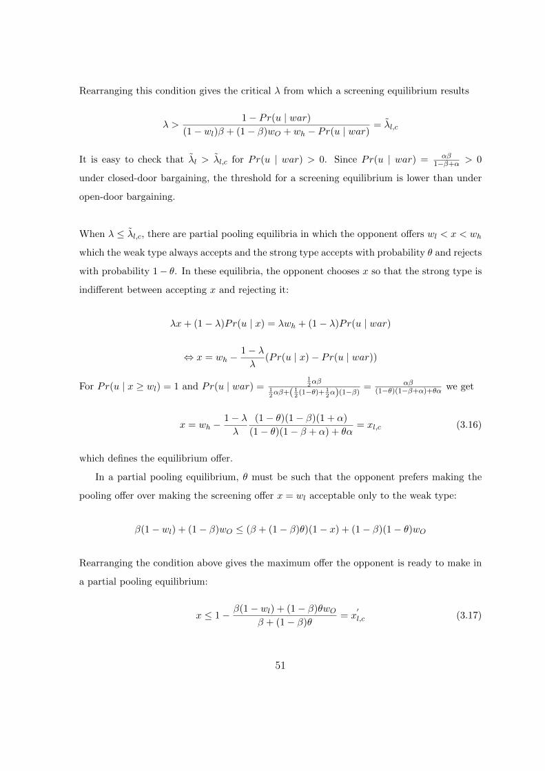
Rearranging this condition gives the critical λ from which a screening equilibrium results

λ >1− Pr(u | war)

(1− wl)β + (1− β)wO + wh − Pr(u | war)= λl,c

It is easy to check that λl > λl,c for Pr(u | war) > 0. Since Pr(u | war) = αβ1−β+α > 0

under closed-door bargaining, the threshold for a screening equilibrium is lower than under

open-door bargaining.

When λ ≤ λl,c, there are partial pooling equilibria in which the opponent offers wl < x < wh

which the weak type always accepts and the strong type accepts with probability θ and rejects

with probability 1− θ. In these equilibria, the opponent chooses x so that the strong type is

indifferent between accepting x and rejecting it:

λx+ (1− λ)Pr(u | x) = λwh + (1− λ)Pr(u | war)

⇔ x = wh −1− λλ

(Pr(u | x)− Pr(u | war))

For Pr(u | x ≥ wl) = 1 and Pr(u | war) =12αβ

12αβ+( 1

2(1−θ)+ 1

2α)(1−β)

= αβ(1−θ)(1−β+α)+θα we get

x = wh −1− λλ

(1− θ)(1− β)(1 + α)

(1− θ)(1− β + α) + θα= xl,c (3.16)

which defines the equilibrium offer.

In a partial pooling equilibrium, θ must be such that the opponent prefers making the

pooling offer over making the screening offer x = wl acceptable only to the weak type:

β(1− wl) + (1− β)wO ≤ (β + (1− β)θ)(1− x) + (1− β)(1− θ)wO

Rearranging the condition above gives the maximum offer the opponent is ready to make in

a partial pooling equilibrium:

x ≤ 1− β(1− wl) + (1− β)θwOβ + (1− β)θ

= x′l,c (3.17)

51

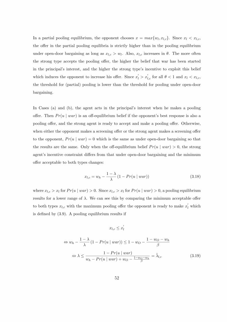
In a partial pooling equilibrium, the opponent chooses x = max{wl, xl,c}. Since xl < xl,c,

the offer in the partial pooling equilibria is strictly higher than in the pooling equilibrium

under open-door bargaining as long as xl,c > wl. Also, xl,c increases in θ. The more often

the strong type accepts the pooling offer, the higher the belief that war has been started

in the principal’s interest, and the higher the strong type’s incentive to exploit this belief

which induces the opponent to increase his offer. Since x′l > x

′l,c for all θ < 1 and xl < xl,c,

the threshold for (partial) pooling is lower than the threshold for pooling under open-door

bargaining.

In Cases (a) and (b), the agent acts in the principal’s interest when he makes a pooling

offer. Then Pr(u | war) is an off-equilibrium belief if the opponent’s best response is also a

pooling offer, and the strong agent is ready to accept and make a pooling offer. Otherwise,

when either the opponent makes a screening offer or the strong agent makes a screening offer

to the opponent, Pr(u | war) = 0 which is the same as under open-door bargaining so that

the results are the same. Only when the off-equilibrium belief Pr(u | war) > 0, the strong

agent’s incentive constraint differs from that under open-door bargaining and the minimum

offer acceptable to both types changes:

xl,c = wh −1− λλ

(1− Pr(u | war)) (3.18)

where xl,c > xl for Pr(u | war) > 0. Since xl,c > xl for Pr(u | war) > 0, a pooling equilibrium

results for a lower range of λ. We can see this by comparing the minimum acceptable offer

to both types xl,c with the maximum pooling offer the opponent is ready to make x′l which

is defined by (3.9). A pooling equilibrium results if

xl,c ≤ x′l

⇔ wh −1− λλ

(1− Pr(u | war)) ≤ 1− wO −1− wO − wh

β

⇔ λ ≤ 1− Pr(u | war)wh − Pr(u | war) + wO − 1−wO−wh

β

= λl,c (3.19)

52

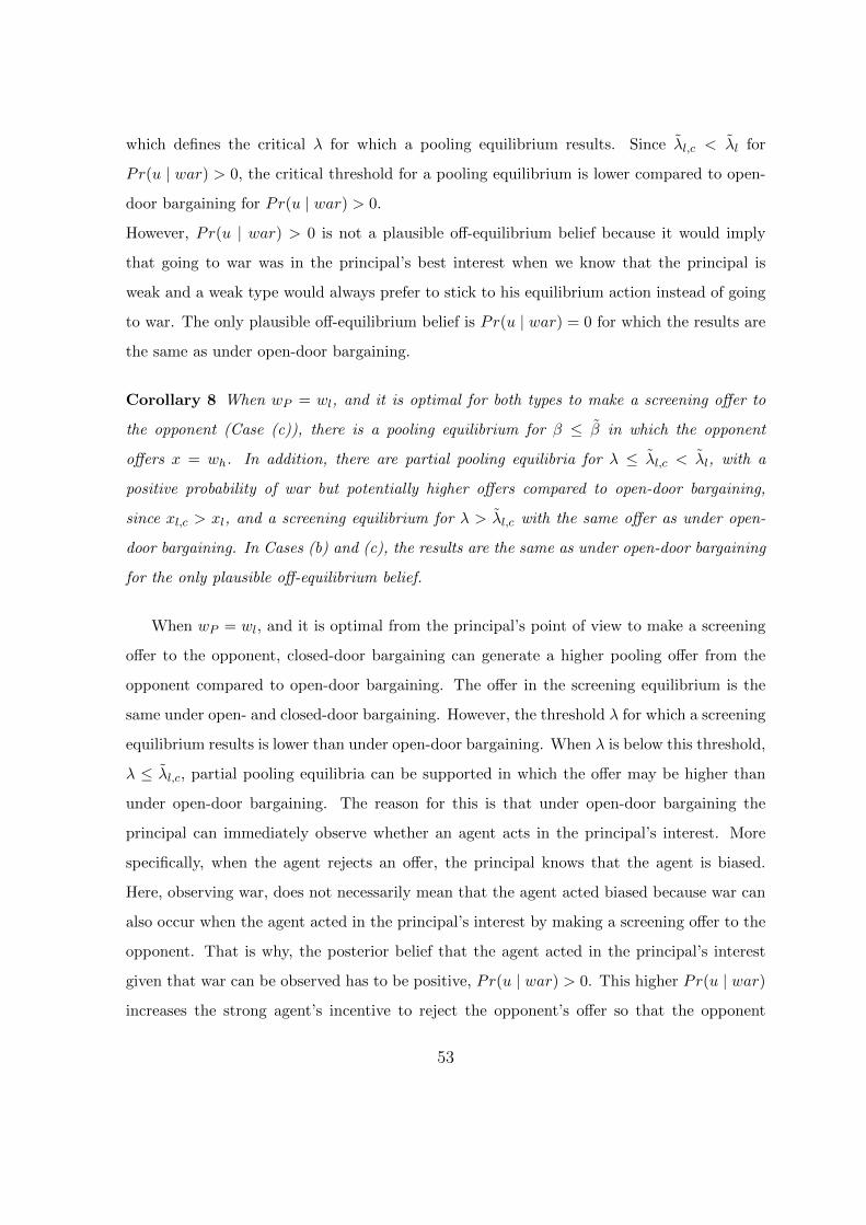
which defines the critical λ for which a pooling equilibrium results. Since λl,c < λl for

Pr(u | war) > 0, the critical threshold for a pooling equilibrium is lower compared to open-

door bargaining for Pr(u | war) > 0.

However, Pr(u | war) > 0 is not a plausible off-equilibrium belief because it would imply

that going to war was in the principal’s best interest when we know that the principal is

weak and a weak type would always prefer to stick to his equilibrium action instead of going

to war. The only plausible off-equilibrium belief is Pr(u | war) = 0 for which the results are

the same as under open-door bargaining.

Corollary 8 When wP = wl, and it is optimal for both types to make a screening offer to

the opponent (Case (c)), there is a pooling equilibrium for β ≤ β in which the opponent

offers x = wh. In addition, there are partial pooling equilibria for λ ≤ λl,c < λl, with a

positive probability of war but potentially higher offers compared to open-door bargaining,

since xl,c > xl, and a screening equilibrium for λ > λl,c with the same offer as under open-

door bargaining. In Cases (b) and (c), the results are the same as under open-door bargaining

for the only plausible off-equilibrium belief.

When wP = wl, and it is optimal from the principal’s point of view to make a screening

offer to the opponent, closed-door bargaining can generate a higher pooling offer from the

opponent compared to open-door bargaining. The offer in the screening equilibrium is the

same under open- and closed-door bargaining. However, the threshold λ for which a screening

equilibrium results is lower than under open-door bargaining. When λ is below this threshold,

λ ≤ λl,c, partial pooling equilibria can be supported in which the offer may be higher than

under open-door bargaining. The reason for this is that under open-door bargaining the

principal can immediately observe whether an agent acts in the principal’s interest. More

specifically, when the agent rejects an offer, the principal knows that the agent is biased.

Here, observing war, does not necessarily mean that the agent acted biased because war can

also occur when the agent acted in the principal’s interest by making a screening offer to the

opponent. That is why, the posterior belief that the agent acted in the principal’s interest

given that war can be observed has to be positive, Pr(u | war) > 0. This higher Pr(u | war)

increases the strong agent’s incentive to reject the opponent’s offer so that the opponent

53

needs to make a higher offer in order to keep the strong agent satisfied under closed-door

bargaining.

Besides these two equilibria types, there is a pooling equilibrium for β ≤ β that only

exists under closed-door bargaining in which the opponent offers x = wh even though the

public signal is low. This equilibrium coincides with the pooling equilibrium in the Autoc-

racy/Autocracy case.

The results from Corollary 7 and 8 suggest that a democracy bargaining with an autocracy

prefers closed-door bargaining whenever the democratic public has a weak resolve for war and

is indifferent between open- and closed door bargaining when the democratic public is highly

resolved.

Democracy/Democracy

Section 3.5.1 shows that when reelection is sufficiently important to democratic agents, pool-

ing offers are made and accepted in equilibrium when the bargaining process is public. Under

closed-door bargaining, this equilibrium also exists with Pr(u | war) as an off-equilibrium

belief.

54

3.6 Conclusion

The paper develops a simple game-theoretic model based on the bargaining approach to

war. The analysis shows that general transparency within democracies and accountability

of democratic leaders enables democracies to signal their resolve for war successfully, so

that war can be avoided when two democracies interact, constituting the phenomenon of

democratic peace. Further, I show that this revealing of preferences need not necessarily

be to the democracy’s disadvantage, but that under some circumstances, democracies can

capture higher shares in the bargaining game than an autocrat would in the same position.

Another contribution of the paper is to analyze how the level of agency transparency

affects the outcome of crisis bargaining. In this regard, I analyze under which circumstances

democracies prefer open- or closed-door bargaining.

55

Chapter 4

Dynamic Pricing in Lemons

Markets

Abstract

In this paper, I study markets with two-sided asymmetric information: quality uncertainty

on part of some buyers and uncertainty about the buyer’s knowledge of quality on part of

the sellers. It will be shown that resolving one source of uncertainty, by giving sellers the

opportunity to learn the buyer’s type and price discriminate, can lead to increased adverse

selection and a decrease in overall welfare. The reason for this is that informed buyers can

act as a deterrent for low quality sellers to mimic good quality when sellers can only quote

one price to all buyers.

56

4.1 Introduction

Ever since Akerlof’s (1970) seminal paper, adverse selection has been widely investigated

in different market models and under different assumptions. One assumption, that is sur-

prisingly robust in the literature, is the idea that all buyers are equally uninformed about

quality.

The present paper seeks to relax this assumption. Its starting point is motivated by

previous research on customer-specific price discrimination which supports the idea that

buyers are not homogenous in their knowledge of quality and that sellers use certain cues to

identify informed buyers. There is evidence to this effect from traditional on-site transactions,

and even more so from online transactions.

For example, Ayres and Siegelman (1995) study race and gender discrimination in on-site

bargaining for a new car and find that black and female test buyers are quoted significantly

higher prices than their male counterparts using identical, scripted bargaining strategies. As

a possible explanation for this result, Ayres and Siegelman suggest that car dealers believe

white males to be more knowledgeable of quality. They observe that “dealers were somewhat

more likely to volunteer information about the cost of the car to white males than to the

other testers, possibly because they believed that white males already had such information.”

(Ayres and Siegelman 1995) The study suggests that there are important cues that salespeo-

ple can use in on-site transactions to gauge a customer’s information status and infer his

willingness to pay.

Even though transactions over the internet obfuscate some of these consumer characteris-

tics, the increasing development of information technologies and web-browser cookies allows

firms to collect, keep, and process even more and possibly more precise information about

consumers. Information about consumers’ previous buying or search behavior may be used to

charge customer-specific prices, a pricing practice known in the literature as behavior-based

price discrimination.1

It is only a small step from there to conjecture that firms can use a consumer’s browser

history to infer the consumer’s knowledge of quality and identify him as an informed or

1See for example Fudenberg and Villas-Boas (2006) for a survey on behavior-based price discrimi-nation.

57

uninformed buyer.

In this paper, I am interested in the question, if sellers can obtain information about

the buyer’s knowledge of the product’s quality, how does that affect adverse selection, and

efficiency in lemons markets in general. The purpose of the paper is twofold: First, it is to

establish equilibria in markets susceptible to the lemons problem, in which some buyers also

have knowledge of quality. Second, it is to clear what welfare effects customer-specific price

discrimination has in such markets.

To that end, two settings are investigated, a uniform pricing regime in which sellers do

not price discriminate and a dynamic pricing regime in which sellers can acquire consumer

data, identify the buyer’s type and price discriminate on an individual level based on the

buyer’s knowledge of quality.

In order to account for differences in buyer information, I employ a lemons market model

in which sellers set individual prices and are matched randomly with buyers, a market model

that has first been analyzed in Wilson (1980). In contrast to the centralized market approach

in Akerlof (1970), buyers and sellers can be modeled heterogenously and there may be different

prices in the market instead of only one price.

I find that, under uniform pricing, the existence of informed buyers can reduce adverse

selection. Since informed buyers do not buy low quality at a high price, the low quality

seller’s incentive to offer at a high price is diminished because he can only quote one price to

all consumers and needs to take into account the informed buyers resistance to buy overpriced

low quality goods. Anticipating the low quality seller’s reduced incentive to cheat, uninformed

buyers are ready to buy at a high price more frequently which reduces adverse selection.

When dynamic pricing becomes possible (through browser histories or other methods),

the market gets segmented based on consumer types. First, there is an informed buyers

market in which trade can always be concluded. Second, there is an uninformed buyers

market in which adverse selection may be more severe than under uniform pricing due to

the absence of informed buyers. Only if average quality is sufficiently high and there is a

pooling equilibrium in the uninformed buyer’s market, dynamic pricing leads to a welfare

improvement. Whenever the sellers separate in their prices and quote different prices to

uninformed buyers, adverse selection is more severe than in the unsegmented market because

58

low quality sellers no longer need to factor in informed buyers’ resistance to buy at a high

price. In these cases, dynamic pricing leads to a welfare loss.

Releated Literature

There is extensive literature on markets with quality uncertainty, which, following Akerlof

(1970), are termed lemons markets. Only few papers have so far considered lemons mar-

kets with a partially informed buyer side. Bester and Ritzberger (2001) give consumers the

possibility to buy a perfect quality signal and investigate how this affects equilibrium with

a monopolistic seller. In Voorneveld and Weibull (2011) all buyers receive a costless but

noisy private signal about quality in a competitive market with quality uncertainty. In both

models, buyers are homogenous in the beginning because they face the same cost of acquiring

information about quality.

In the present paper, buyers are heterogenous in their quality information from the be-

ginning. Some buyers are informed about quality and some are not. With this respect, the

paper is related to a range of signaling models showing that monopolistic sellers can signal

high quality by charging high prices, in particular so when some informed consumers are

present. Milgrom and Roberts (1986) and Bagwell and Riordan (1991) predict upward price

distortion for signaling purposes. Most recently, Mahenc (2004) develops a signaling model,

in which informed buyers are necessary for a monopolist to use prices as signals of product

quality.

In contrast to this literature, the pricing side of the present model is not a monopoly

but competitive. Most pertinent in this regard is Kessler (2001) who, like the present paper,

stays within a competitive framework. Kessler (2001) can be considered as the theoretic

counterpart to the present paper as she also extends Akerlof’s model by relaxing the strict

assumptions to the information status of the players and compares market performance under

two different informational structures. The crucial difference is that where I assume some

buyers to be equally informed as the sellers, Kessler looks at the case in which some sellers

are equally uninformed as the buyers.

The paper is also related to the literature on dynamic pricing, focussing mostly on its

effect on profit and consumer surplus in different market structures. The diversity of topics

59

that is investigated in this context, includes: dynamic pricing in dynamic settings (Fudenberg

and Tirole, 2000), the impact of dynamic pricing on consumer perceptions of price fairness

(Haws and Bearden, 2006), the effect of dynamic pricing when consumers are strategic and

avail themselves for the low price (Chen and Zhang, 2009) or avoid revealing information

that will hurt them (Taylor, 2004).

There is no literature investigating the effect of price discrimination on adverse selection

in markets with two-sided asymmetric information. In such markets, buyers have different

knowledge of quality and sellers can learn the buyer’s type and tailor special prices on an

individual level. The present article closes this gap, as it particularly addresses the impact

of dynamic pricing on adverse selection.

The paper proceeds as follows: Section 2 lays down the market model with informed

buyers, section 3 defines equilibria in this market with uniform prices based on the share of

informed buyers. Section 4 defines equilibria with information acquisition and price discrim-

ination. Section 5 concludes.

4.2 The Model

Consider the following market: There are potential sellers of an indivisible object and poten-

tial buyers. Each seller owns and each buyer wishes to purchase only one unit of the object.

The market operates for only one period. All agents enter the market at the beginning of

this period and each seller posts a fixed price. Agents are matched randomly. Sellers differ in

the quality of the object they want to sell. A seller owns good quality qh with probability λ

and bad quality ql with probability 1− λ. Buyers can also be sorted into different, privately

known types because their information on quality varies. A buyer is either perfectly informed

about quality with probability θ or completely uninformed with probability 1− θ. I consider

the most simple model in which types are all binary. The seller’s and buyer’s expected payoffs

vs and vb are given by

vs = σp+ (1− σ)εqi (4.1)

and

vb = σ(qi − p) (4.2)

60

where ε ∈ (0, 1) is a fixed valuation parameter, p is the price for quality q and σ is a binary

variable with σ = 1 if the object is sold and σ = 0 otherwise.

If quality were publicly observable to all buyers, all objects would be sold at pi = qi

∀i ∈ {l, h}, that is the buyer’s reservation value. The seller can capture the entire surplus

from trade because he can make a take-it-or-leave-it offer (post a price) and the buyer’s outside

option is zero.2 Throughout the paper, it will be assumed that εqh > ql, so that ε > qlqh

which

implies that a high quality seller will not sell at a low price because his reservation price εqh

exceeds the maximum price that buyers are willing to pay for low quality ql.

When quality is observable only to informed buyers, buyers differ in the maximum amount

they are willing to pay. Informed buyers are ready to buy as long as p ≤ q and uninformed

buyers form expectations about quality and upon these expectations they decide to buy

or not. In the presence of informed buyers, the outcome depends on the seller’s ability to

differentiate between the two buyer types. In the following, I will analyze the welfare effects

of the two respective market environments of uniform pricing in which sellers are unaware of

the buyers’ types and of dynamic pricing in which sellers learn the buyers’ types.

Independent of the market environment, in equilibrium, the price of a low quality object

cannot be below the buyer’s maximum willingness to pay for low quality because a low quality

seller offering for less than ql could always increase his price to ql and still sell for sure. It

follows that, in equilibria with different prices, the price for low quality will be equal to the

buyer’s maximum willingness to pay for low quality: p∗l = ql. On the other hand, a buyer

will not buy if the seller asks a price above the buyer’s maximum willingness to pay for high

quality. Since a seller of high quality only sells above εqh, in equilibrium it must be that

p∗h ∈ [εqh, qh].

2Here, the buyer’s outside option is zero because the market only operates for one period whichleaves him without an opportunity to find an alternative seller. The fact that the seller captures theentire surplus from trade does not change even if we assume that the market operates for more thanone period and the buyer can search for another seller. Following Diamond (1971), each seller cancharge the monopoly price in this setting as long as search costs are posititve.

61

4.3 Uniform Pricing

Under uniform pricing, each seller quotes one price to the buyer that he is matched with,

independent of the buyer’s type. Quite generally, when quality is private information, low

quality sellers have two options. They can either imitate high quality sellers and hope to be

mistaken for high quality or they post a low price and make a sale for sure.

Due to the presence of informed buyers, low quality sellers face an additional restraint

from offering at a high price because informed buyers do not buy low quality at a high price.3

When there are sufficiently many informed buyers, low quality sellers can even be deterred

completely from mimicking high quality because the sale probability at the high price is too

low for the low quality sellers who therefore prefer posting a low price which definitely results

in trade. In this case, efficient fully separating equilibria can be obtained.

Otherwise, there are 3 different possible but inefficient types of equilibria: fully separating

equilibria, semi-separating equilibria and, under some conditions, also a pooling equilibrium.

For a start, I investigate the existence of efficient fully separating equilibria. Such equi-

libria exist if all goods are traded, all high quality sellers post a high price ph and all low

quality sellers post a low price pl.

Efficient-Fully Separating Equilibria

When the share of informed buyers θ is sufficiently high, then low quality sellers prefer posting

a low price which definitely results in sale (left hand side of the condition below) over posting

a high price which deters informed buyers (right hand side of the condition below):

ql − εql ≥ (1− θ)(ph − εql)

⇔ θ ≥ ph − qlph − εql

(4.3)

Proposition 2 There is an efficient separating equilibrium for θ ≥ θ = qh−qlqh−εql . Low quality

sellers post a low price p∗l = ql and high quality sellers post a high price p∗h = qh. All buyers

buy at the posted price so that all goods are traded and the market is efficient.

3Since εqh > ql, the minimum price acceptable to high quality sellers is higher than the buyer’smaximum willingness to pay for low quality.

62

Proof. It is obvious that the high quality seller has no incentive to deviate from the

proposed strategy because he captures the entire surplus from trade and trades for sure. Given

Condition 4.3, low quality sellers have no incentive to deviate from the proposed strategy.

The buyers have no incentive to deviate because they are indifferent between buying and not.

The following results apply to situations in which θ < θ and the share of informed buyers

is below the critical threshold that guarantees the efficient separating equilibrium as stated

in Proposition 3.

First of all, it is important to note that there are efficient separating equilibria even for

θ < θ. Since a lower share θ < θ can be substituted to some extent with a lower price, the

high price needs to be smaller than in the efficient equilibrium shown above, ph < qh, in

order to reduce the low quality seller’s incentive to mimic high quality in these equilibria.

Rearranging Condition 4.3 gives an upper constraint on ph that guarantees that low quality

sellers have no incentive to deviate to the high price:

ph ≤ql − θεql

1− θ< qh (4.4)

We also need to make sure that the high price is not too small in order to prevent high

quality sellers from posting the maximum high price qh and selling only to informed buyers.

The following condition guarantees that:

ph − εqh ≥ θ(qh − εqh)

⇔ ph ≥ θqh + (1− θ)εqh (4.5)

Proposition 3 For θ > θ ≥ θ∗, there are efficient fully-separating equilibria in which the

low quality seller posts p∗l = ql and the high quality seller posts p∗h = ql−θεql1−θ < qh. All buyers

buy at the posted price so that all goods are traded and the outcome is efficient.

Proof. Buyers have no incentive to deviate because they are indifferent between buying

and not buying when matched with low quality sellers and get positive utility when matched

63

with high quality sellers since p∗h < qh. In equilibrium, Condition 4.4, the low quality seller’s

incentive constraint is binding because at any price p ∈[θqh+(1−θ)εqh, ql−θεql1−θ

), high quality

sellers have an incentive to deviate to p∗h = ql−θεql1−θ in order to get a higher profit.

In equilibrium, the high quality seller’s incentive constraint (Condition 4.5) must hold at p∗h:

ql − θεql1− θ

≥ θqh + (1− θ)εqh

which gives the minimum θ for which these equilibria exist:

θ =

(qh(1− 2ε)− qlε

)+√(

qh(1− 2ε)− qlε)2 − 4

(qh(1− ε)

)(ql − εqh)

2(qh − εqh)= θ∗

Inefficient Fully-Separating Equilibria

For θ < θ there are also inefficient fully-separating equilibria with prices p∗h = qh and p∗l = ql.

Given these prices, uninformed buyers are indifferent between buying and not buying (in both

cases the expected payoff is zero). They can therefore also use any mixed strategy. With

this in mind, equilibria can be constructed in which uninformed buyers put sufficient weight

on not buying at a high price, so that the low quality seller is deterred from posting a high

price. The low quality seller is deterred as long as his expected profit selling at a low price to

all buyers weakly exceeds his expected profit selling at a high price only to those uninformed

buyers who are ready to buy at a high price. Let β be the probability with which uninformed

buyers buy at a high price. The following must hold:

ql − εql ≥ (1− θ)β(qh − εql)

⇔ β ≤ ql − εql(qh − εql)(1− θ)

= β (4.6)

Proposition 4 For θ > θ ≥ 0, there is a range of inefficient fully-separating equilibria in

which the high quality seller posts p∗h = qh and the low quality seller posts p∗l = ql. Uninformed

64

buyers mix between “accept p∗l and p∗h” and “accept only p∗l ”, choosing “accept p∗l and p∗h”

with probability 0 ≤ β ≤ β.

Proof. Condition 4.6 together with the assumption that the uninformed buyer’s off-equilibrium

belief that quality is low equals 1, assures that neither seller type has an incentive to post

any other price. Buyers have no incentive to deviate because they are indifferent between

buying at p∗l or p∗h and not buying.

It is easy to see that there are no other inefficient fully-separating equilibria because at

any other high price ph < p∗h (at ph > p∗h no one will buy), uninformed buyers would strictly

prefer to buy at ph and no longer be indifferent between buying and not buying. But if

uninformed buyers always buy at ph, then low quality sellers have an incentive to post ph

instead of p∗l which would prevent full separation.

In the worst of these equilibria, β = 0 and uninformed buyers do not buy at a high price

at all. Still, high quality goods are sold with probability θ to informed buyers. In the best

of these equilibria, uninformed buyers buy at a high price with probability β so that the sale

probability of high quality goods equals θ + β(1− θ).

Infficient Semi-Separating Equilibria

In addition to the efficient and inefficient fully-separating equilibria, there is also a range of

semi-separating equilibria for θ < θ in which low quality sellers mix between posting a high

and a low price and uninformed buyers mix between buying at both prices and buying only

at the low price.

For a mixed equilibrium to exist, players need to be indifferent between the pure strategies

that are used in the mix. Suppose the low quality seller, that occurs with probability 1 −

λ, chooses ph with probability α and pl with probability 1 − α. The uninformed buyer

chooses “accept pl and ph” with probability β and “accept only pl” with probability 1 − β.

Consequently, the low quality seller is indifferent between ph and pl if:

(ph − εql)(1− θ)β = pl − εql

65

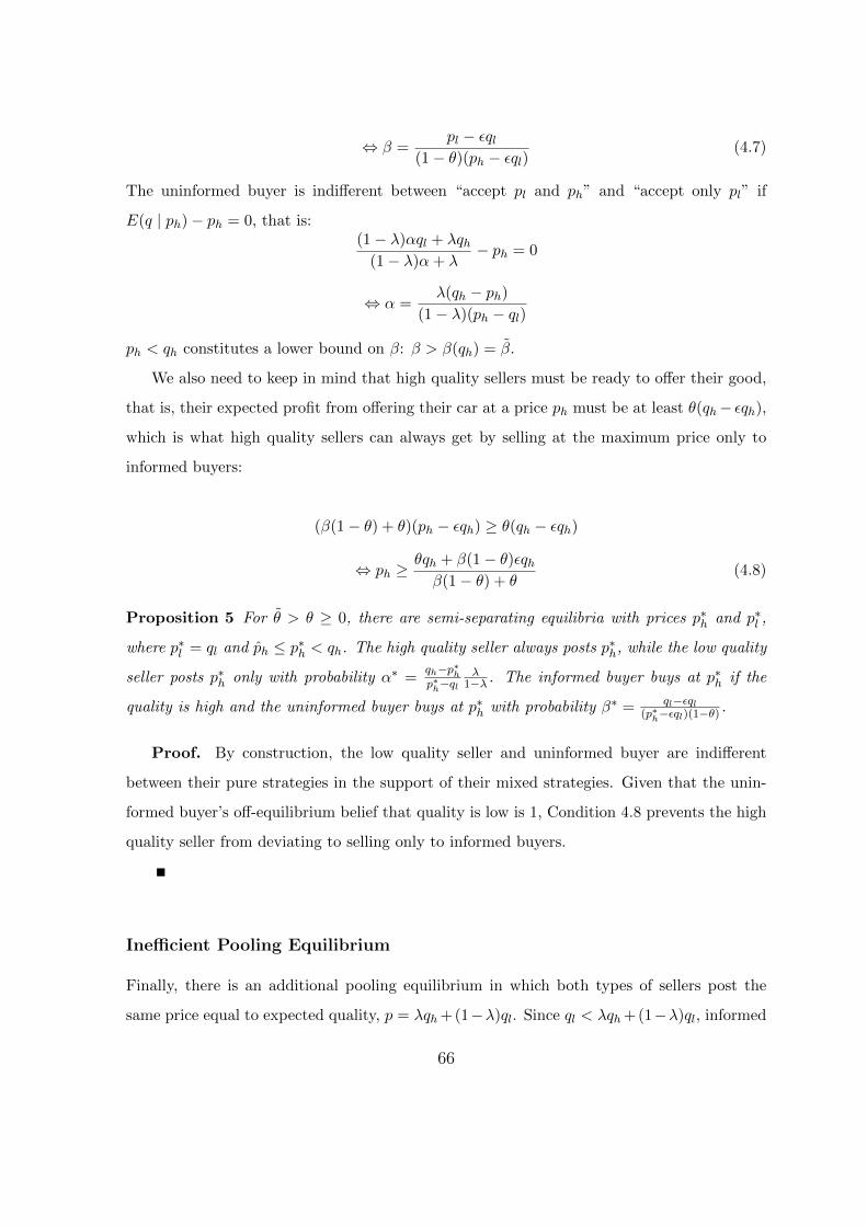
⇔ β =pl − εql

(1− θ)(ph − εql)(4.7)

The uninformed buyer is indifferent between “accept pl and ph” and “accept only pl” if

E(q | ph)− ph = 0, that is:(1− λ)αql + λqh

(1− λ)α+ λ− ph = 0

⇔ α =λ(qh − ph)

(1− λ)(ph − ql)

ph < qh constitutes a lower bound on β: β > β(qh) = β.

We also need to keep in mind that high quality sellers must be ready to offer their good,

that is, their expected profit from offering their car at a price ph must be at least θ(qh− εqh),

which is what high quality sellers can always get by selling at the maximum price only to

informed buyers:

(β(1− θ) + θ)(ph − εqh) ≥ θ(qh − εqh)

⇔ ph ≥θqh + β(1− θ)εqhβ(1− θ) + θ

(4.8)

Proposition 5 For θ > θ ≥ 0, there are semi-separating equilibria with prices p∗h and p∗l ,

where p∗l = ql and ph ≤ p∗h < qh. The high quality seller always posts p∗h, while the low quality

seller posts p∗h only with probability α∗ =qh−p∗hp∗h−ql

λ1−λ . The informed buyer buys at p∗h if the

quality is high and the uninformed buyer buys at p∗h with probability β∗ = ql−εql(p∗h−εql)(1−θ)

.

Proof. By construction, the low quality seller and uninformed buyer are indifferent

between their pure strategies in the support of their mixed strategies. Given that the unin-

formed buyer’s off-equilibrium belief that quality is low is 1, Condition 4.8 prevents the high

quality seller from deviating to selling only to informed buyers.

Inefficient Pooling Equilibrium

Finally, there is an additional pooling equilibrium in which both types of sellers post the

same price equal to expected quality, p = λqh+(1−λ)ql. Since ql < λqh+(1−λ)ql, informed

66

buyers do not buy from low quality sellers at p. Therefore, we need to make sure that low

quality sellers are ready to post p instead of posting ql and selling also to informed buyers.

The following condition guarantees that the low quality seller’s expected profit from selling

at p only to uninformed buyers weakly exceeds the profit from selling at ql to all buyers:

(p− εql)(1− θ) ≥ ql − εql

⇔ (λqh + (1− λ)ql − εql)(1− θ) ≥ ql − εql

⇔ θ ≤ λ(qh − ql)λ(qh − ql) + ql − εql

(4.9)

But also high quality sellers must be ready to offer their good at p. Since high quality sellers

always have the option to sell at the maximum price only to informed buyers, we need to

make sure that their expected profit from offering at p must be at least θ(qh − εqh), their

profit from selling only to informed buyers:

p− εqh ≥ θ(qh − εqh)

⇔ λqh + (1− λ)ql − εqh ≥ θ(qh − εqh)

⇔ θ ≤ λ(qh − ql) + ql − εqhqh − εqh

(4.10)

Both high and low quality sellers only sell their good if the pooling price p is sufficiently

high. p increases in the share of high quality goods λ. The higher the share of informed buyers

θ, the higher must be λ for the sellers’ incentive constraints to still be fulfilled. Rearranging

conditions 4.8 and 4.9, we get the following constraints on λ:

λ ≥ θ(ql − εql)(1− θ)(qh − ql)

(4.11)

for the low quality seller and

λ ≥ θ(qh − εqh) + εqh − qlqh − ql

(4.12)

67

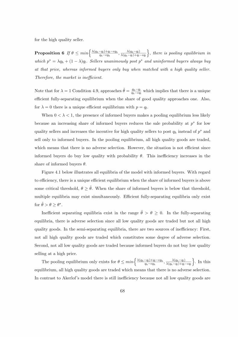
for the high quality seller.

Proposition 6 If θ ≤ min{λ(qh−ql)+ql−εqh

qh−εqh , λ(qh−ql)λ(qh−ql)+ql−εql

}, there is pooling equilibrium in

which p∗ = λqh + (1 − λ)ql. Sellers unanimously post p∗ and uninformed buyers always buy

at that price, whereas informed buyers only buy when matched with a high quality seller.

Therefore, the market is inefficient.

Note that for λ = 1 Condition 4.9, approaches θ = qh−qlqh−εql which implies that there is a unique

efficient fully-separating equilibrium when the share of good quality approaches one. Also,

for λ = 0 there is a unique efficient equilibrium with p = ql.

When 0 < λ < 1, the presence of informed buyers makes a pooling equilibrium less likely

because an increasing share of informed buyers reduces the sale probability at p∗ for low

quality sellers and increases the incentive for high quality sellers to post qh instead of p∗ and

sell only to informed buyers. In the pooling equilibrium, all high quality goods are traded,

which means that there is no adverse selection. However, the situation is not efficient since

informed buyers do buy low quality with probability θ. This inefficiency increases in the

share of informed buyers θ.

Figure 4.1 below illustrates all equilibria of the model with informed buyers. With regard

to efficiency, there is a unique efficient equilibrium when the share of informed buyers is above

some critical threshold, θ ≥ θ. When the share of informed buyers is below that threshold,

multiple equilibria may exist simultaneously. Efficient fully-separating equilibria only exist

for θ > θ ≥ θ∗.

Inefficient separating equilibria exist in the range θ > θ ≥ 0. In the fully-separating

equilibria, there is adverse selection since all low quality goods are traded but not all high

quality goods. In the semi-separating equilibria, there are two sources of inefficiency: First,

not all high quality goods are traded which constitutes some degree of adverse selection.

Second, not all low quality goods are traded because informed buyers do not buy low quality

selling at a high price.

The pooling equilibrium only exists for θ ≤ min{λ(qh−ql)+ql−εqh

qh−εqh , λ(qh−ql)λ(qh−ql)+ql−εql

}. In this

equilibrium, all high quality goods are traded which means that there is no adverse selection.

In contrast to Akerlof’s model there is still inefficiency because not all low quality goods are

68

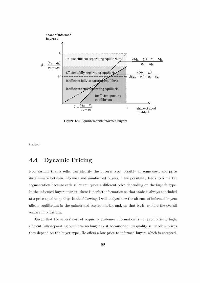
traded.

4.4 Dynamic Pricing

Now assume that a seller can identify the buyer’s type, possibly at some cost, and price

discriminate between informed and uninformed buyers. This possibility leads to a market

segmentation because each seller can quote a different price depending on the buyer’s type.

In the informed buyers market, there is perfect information so that trade is always concluded

at a price equal to quality. In the following, I will analyze how the absence of informed buyers

affects equilibrium in the uninformed buyers market and, on that basis, explore the overall

welfare implications.

Given that the sellers’ cost of acquiring customer information is not prohibitively high,

efficient fully-separating equilibria no longer exist because the low quality seller offers prices

that depend on the buyer type. He offers a low price to informed buyers which is accepted.

69

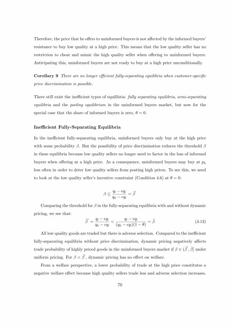
Therefore, the price that he offers to uninformed buyers is not affected by the informed buyers’

resistance to buy low quality at a high price. This means that the low quality seller has no

restriction to cheat and mimic the high quality seller when offering to uninformed buyers.

Anticipating this, uninformed buyers are not ready to buy at a high price unconditionally.

Corollary 9 There are no longer efficient fully-separating equilibria when customer-specific

price discrimination is possible.

There still exist the inefficient types of equilibria: fully separating equilibria, semi-separating

equilibria and the pooling equilibrium in the uninformed buyers market, but now for the

special case that the share of informed buyers is zero, θ = 0.

Inefficient Fully-Separating Equilibria

In the inefficient fully-separating equilibria, uninformed buyers only buy at the high price

with some probability β. But the possibility of price discrimination reduces the threshold β

in these equilibria because low quality sellers no longer need to factor in the loss of informed

buyers when offering at a high price. As a consequence, uninformed buyers may buy at ph

less often in order to deter low quality sellers from posting high prices. To see this, we need

to look at the low quality seller’s incentive constraint (Condition 4.6) at θ = 0:

β ≤ ql − εqlqh − εql

= β′

Comparing the threshold for β in the fully-separating equilibria with and without dynamic

pricing, we see that:

β′

=ql − εqlqh − εql

<ql − εql

(qh − εql)(1− θ)= β (4.13)

All low quality goods are traded but there is adverse selection. Compared to the inefficient

fully-separating equilibria without price discrimination, dynamic pricing negatively affects

trade probability of highly priced goods in the uninformed buyers market if β ∈ (β′, β] under

uniform pricing. For β < β′, dynamic pricing has no effect on welfare.

From a welfare perspective, a lower probability of trade at the high price constitutes a

negative welfare effect because high quality sellers trade less and adverse selection increases.

70

Since all other market participants are indifferent between the two regimes, we can say that

overall welfare is negatively affected by price discrimination at least for β ∈ (β′, β].4

Corollary 10 Under dynamic pricing, in the inefficient fully separating equilibria, unin-

formed buyers accept a high price p∗h = qh with probability β, where 0 ≤ β < β′< β.

Compared to uniform pricing, welfare is worse in these equilibria for β ∈ (β′, β] because of

higher adverse selection.

Next, I analyze how the semi-separating equilibria are affected by the absence of informed

buyers.

Inefficient Semi-Separating Equilibria

When the share of informed buyers is zero, θ = 0, the low quality seller’s indifference condition

(Condition 4.7) becomes:

β′

=ql − εqlph − εql

(4.14)

Comparing β′, the probability with which uninformed buyers buy at a high price in the

semi-separating equilibria under dynamic pricing with β∗, the respective probability under

uniform pricing (defined by Propostition 6), it follows that

β′

=ql − εqlph − εql

<ql − εql

(1− θ)(ph − εql)= β∗ (4.15)

Since β′< β∗, uninformed buyers buy at the high price less often in the semi-separating

equilibria when price discrimination is possible. Again, low quality sellers do not need to

factor in the loss of informed buyers when offering a high price to uninformed buyers. The

low quality sellers’ reduced incentive to post a low price is anticipated by uninformed buyers

who buy at a high price less often. This, in turn, negatively affects the high quality sellers’

probability of trade.

Comparing the semi-separating equilibria with and without price discrimination, the fol-

lowing can be stated: The expected payoff from trading is ql − εql for low quality sellers and

4Both buyer types are indifferent between the two regimes because equilibrium prices are such thattheir expected payoff from trade is zero. Low quality sellers gain ql − εql under both regimes.

71

0 for uninformed buyers with and without price discrimination.5 Informed buyers gain under

uniform pricing when buying from high quality sellers because ph < qh compared to ph = qh

under dynamic pricing. But this payoff gain on part of informed buyers translates into a

payoff loss on part of high quality sellers, so that welfare is unaffected. What negatively af-

fects welfare though, is the increased reluctance to buy at a high price on part of uninformed

buyers under dynamic pricing which results in a decrease in the trade of highly priced goods

and thus an increase in adverse selection.

Corollary 11 Under dynamic pricing, in the semi-separating equilibria, uninformed buyers

accept a high price p∗h < qh with probability β′, where β

′< β∗. Compared to uniform pricing,

welfare is worse in these equilibria because of higher adverse selection.

Efficient Pooling Equilibrium

In the pooling equilibrium, sellers post a price equal to expected quality at that price, p =

λqh+(1−λ)ql, to uninformed buyers. High quality sellers are ready to offer the pooling price

to uninformed buyers as long as this price exceeds their reservation value:

εqh ≥ λqh + (1− λ)ql

⇔ λ ≥ εqh − qlqh − ql

When sellers quote the pooling price to uninformed buyers and pi = qi to informed

buyers, then all goods are traded. The surplus from trade is captured entirely by the sellers,

where low quality sellers benefit disproportionately high compared to high quality sellers

in the uninformed buyers market because of the pooling price. Compared to the pooling

equilibrium without price discrimination, this equilibrium generates a better result in terms

of welfare because all low quality goods are traded while in the pooling equilibrium without

price discrimination, low quality goods do not always trade.

5When price discrimination is possible, low quality sellers trade with informed buyers at pl = ql,so that the sellers’ payoff is ql − εql. Their expected payoff from trade with uninformed buyers is alsoql − εql because uninformed buyers buy less often at high prices (β

′< β∗) in order to offset the low

quality sellers’ increased incentive to offer at a high price.

72

Corollary 12 If λ ≥ εqh−qlqh−ql , there is an efficient pooling equilibrium in the uninformed

buyers’ market in which sellers offer p∗ = λqh + (1 − λ)ql to uninformed buyers. Compared

to uniform pricing, welfare is better in this equilibrium because all goods are traded.

With respect to consumer welfare, dynamic pricing and market segmentation is not beneficial

for informed buyers because sellers can easily identify informed buyers and push them to

their reservation value.6 In the case of uniform pricing, uninformed consumers can impart

a benefit on informed buyers because prices may be below the informed buyer’s reservation

value so to still address uninformed buyers with a higher reservation value due to their lack

of information.

The overall welfare effects of price discrimination can be subsumed as follows:

Corollary 13 Price discrimination generates an efficient equilibrium only if the average

quality is high and both types of sellers make a pooling offer to uninformed buyers. When the

average quality is low or sellers separate in their offer to uninformed buyers, price discrimi-

nation can have a negative welfare effect because it increases adverse selection.

Figure 4.2 below depicts all equilibria in the uninformed buyers market when sellers can

price discriminate. Because the market is segmented, equilibria in the uninformed buyers

market are independent of the share of informed buyers.

6Uninformed buyers are indifferent between both pricing regimes because their expected payoff iszero in both cases.

73

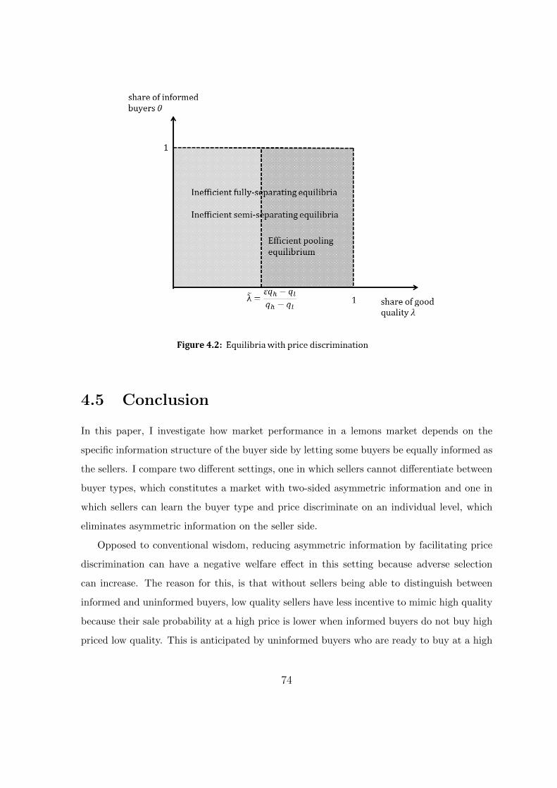
4.5 Conclusion

In this paper, I investigate how market performance in a lemons market depends on the

specific information structure of the buyer side by letting some buyers be equally informed as

the sellers. I compare two different settings, one in which sellers cannot differentiate between

buyer types, which constitutes a market with two-sided asymmetric information and one in

which sellers can learn the buyer type and price discriminate on an individual level, which

eliminates asymmetric information on the seller side.

Opposed to conventional wisdom, reducing asymmetric information by facilitating price

discrimination can have a negative welfare effect in this setting because adverse selection

can increase. The reason for this, is that without sellers being able to distinguish between

informed and uninformed buyers, low quality sellers have less incentive to mimic high quality

because their sale probability at a high price is lower when informed buyers do not buy high

priced low quality. This is anticipated by uninformed buyers who are ready to buy at a high

74

price more often when the market is unsegmented.

The results presented in this paper shed some light on the often neglected issue of inter-

mediate degrees of informational asymmetry and reveal the connection between the level of

market information and the level of adverse selection in a simple and intuitive manner which

may be useful in applications.

75

Conclusion

The studies in this Dissertation show that bargaining theory is applicable to a wide range

of problems because many, even seemingly unrelated ‘non-economic’ interactions have a bar-

gaining problem at heart.

From a scientific point of view, the motivation for bargaining is not especially exciting

because bargaining is mutually beneficial to all parties involved. The interesting part is to

identify reasons why bargaining sometimes breaks down in spite of the potential gains.

Two different reasons for a breakdown of bargaining are explored in this Dissertation:

commitment problems and asymmetric information. While Chapters 1 and 2 concentrate on

commitment problems as a possible reason for the inability to reach an agreement in repeated

interaction, Chapters 3 and 4 focus on asymmetric information in one-time bargaining.

Commitment Problems are a source of inefficiency when binding contracts are not enforce-

able because a powerful authority capable of guaranteeing agreements is absent. It follows

that commitment problems are less prevalent in bargaining activities within the rule of law

and more relevant with regard to illegal activities and negotiations on an international level.

The basic trouble with bargaining under commitment problems is the bargainers’ incentive

to break up the negotiation before it even started when there is no guarantee that the other

party sticks to the agreement. A good way to illustrate this dilemma is by thinking of the

reason why crime witnesses are in danger of being ‘silenced forever’. Because a witness cannot

credibly commit to not go to the police and report the crime, the criminal has no rational

choice other than kill the witness, even though he would prefer the witness to live and not

tell. Chapter 1 investigates this logic within the framework of crisis bargaining between

autonomous states and preventive war as the result of bargaining breakdown.

76

Compared to commitment problems, the role of asymmetric information has been exten-

sively analyzed in the bargaining literature and identified as a viable source of bargaining

inefficiencies such as strikes, wars and costly delay. Despite the very different set-ups and

fields of application, the bargaining problems in Chapters 3 and 4 boil down to a simple

negotiation between two bargainers with privately known reservation prices. In this case, an

agreement may not be struck because a bargainer with a low reservation price (low outside

option in Chapter 3 or low quality good in Chapter 4) has the incentive to pretend to be a

type with a high reservation price (high outside option in Chapter 3 or high quality good in

Chapter 4).

The inability of one negotiator to distinguish between different types of his negotiating

partner and the incentive to cheat on part of weak types can be the reason for a breakdown

in bargaining. Of course, bargaining need not necessarily break down and in bargaining

models with multiple rounds in which players have the option to reject offers and make

counteroffers, agreement can usually be reached, albeit not without cost of delay. In such

settings, inefficiencies are often the means by which bargainers become able to identify the

other party’s type and finally conclude an agreement.

Since the models presented in Chapters 3 and 4 preclude the possibility of counteroffers,

an agreement that can not be struck at once, immediately results in the worst possible

outcome, the termination of bargaining. In Chapter 3, terminating negotiations means war,

in Chapter 4, it means some buyer/seller matches do not result in trade even though trading

generates surplus.

77

Bibliography

[1] Akerlof, George (1970), “The Market for “Lemons”: Qualitative Uncertainty and the

Market Mechanism”, Quarterly Journal of Economics, 84 (3), p 488-500.

[2] Arnold, Michael A. and Steven A. Lippman (1998), “Posted Prices versus Bargaining in

Markets with Asymmetric Information”, Economic Inquiry, 36 (3), p 450-457.

[3] Ayres, Ian and Peter Siegelman (1995), “Race and Gender Discrimination in Bargaining

for a New Car”, American Economic Review, 85 (3), p 304-321.

[4] Bagwell, Kyle and Michael H. Riordan (1991), “High and Declining Prices Signal Product

Quality”, American Economic Review, 81 (1), p 224-239.

[5] Bester, Helmut (1993), “Bargaining versus Price Competition in Markets with Quality

Uncertainty”, American Economic Review, 83 (1), p 278-288.

[6] Bester, Helmut and Klaus Ritzberger (2001), “Strategic Pricing, Signalling, and Costly

Information Acquisition”, International Journal of Industrial Organization, 19 (9), p

1347-1361.

[7] Binmore, Ken (1987), “Perfect Equilibria in Bargaining Models”, in The Economics of

Bargaining (K. G. Binmore and P. S. Dasgupta, Eds.) Oxford: Blackwell, p 76-105.

[8] Binmore, Ken, Avner Shaked and John Sutton (1989), “An Outside Option Experiment”,

The Quarterly Journal of Economics, 104 (4), p 753-770.

[9] Bueno de Mesquita, Bruce, James D. Morrow, Randolph M. Siverson and Alastair Smith

(1999), “An Institutional Explanation of the Democratic Peace”, American Political

Science Review, 93 (4), p 791-812.

78

[10] Chen, Yuxina and Z. John Zhang (2009), “Dynamic Targeted Pricing with Strategic

Consumers”, International Journal of Industrial Organization, 27 (1), p 43-50.

[11] Diamond, Peter A. (1971), “A Model of Price Adjustment”, Journal of Economic

Theory, 3 (2), p 156-168.

[12] Fearon, James D. (1994), “Domestic Political Audiences and the Escalation of Interna-

tional Disputes”, American Political Science Review, 88 (3), p 577-592.

[13] Fearon, James D. (1995), “Rationalist Explanations for War”, International Organiza-

tion, 49 (3), p 379-414.

[14] Fudenberg, Drew and Jean Tirole (2000), “Customer Poaching and Brand Switching”,

The RAND Journal of Economics, 31 (4), p 634-657.

[15] Fudenberg, Drew and J. M. Villas-Boas (2006), “Behavior-Based Price Discrimination

and Customer Recognition”, in Hendershott, T. J. (ed.), Handbook on Economics and

Information Systems, Elsevier, Amsterdam, The Netherlands

[16] Gartzke, Erik and Yonatan Lupu (2012), “Still Looking for Audience Costs”, Security

Studies, 21 (3), p 391-397.

[17] Guisinger, Alexandra, and Alastair Smith. (2002), “Honest Threats: The Interaction

of Reputation and Political Institutions in International Crises”, Journal of Conflict

Resolution, 46 (2), p 175-200.

[18] Haws, Kelly L. and William O. Bearden (2006), “Dynamic Pricing and Consumer

Fairness Perceptions”, Journal of Consumer Research, 33 (3), p 304-311.

[19] Holmstrom, Bengt (1999), “Managerial Incentive Problems: A Dynamic Perspective”,

Review of Economic Studies, 66 (1), p 169-182.

[20] Jackson, Matthew O. and Massimo Morelli (2007), “Political Bias and War”, The

American Economic Review, 97 (4), p 1353-1373.

[21] Kessler, Anke S. (2001), “Revisiting the Lemons Market”, International Economic

Review, 42 (1), p 25-41.

79

[22] Mahenc, Philippe (2004), “Influence of Informed Buyers in Markets Susceptible to the

Lemons Problem”, American Journal of Agricultural Economics, 86 (3), p 649-659.

[23] Maoz, Zeev, and Nazrin Abdolali (1989), “Regime Types and International Conflict,

1816-1976”, Journal of Conflict Resolution , 33 (1), p 3-35.

[24] Milgrom, Paul and John Roberts (1986), “Price and Advertising Signals of Product

Quality”, Journal of Political Economy, 94 (4), p 796-821.

[25] Nash, John F. (1950), “The Bargaining Problem”, Econometrica, 18 (2), p 155-162.

[26] Nash, John F. (1953), “Two-Person Cooperative Games”, Econometrica, 21 (1), p

128-140.

[27] Oneal, John R. and Bruce M. Russett (1997), “The Classical Liberals Were Right:

Democracy, Interdependence, and Conflict, 1950-1985”, International Studies Quarterly,

41 (2), p 267-293. Reputational Cheap Talk

[28] Ottaviani, Marco and Peter Norman Sørensen (2006), “Reputational Cheap Talk”, The

RAND Journal of Economics, 37 (1), p 155-175.

[29] Ponsatı, Clara and Jozsef Sakovics (1998), “Rubinstein Bargaining with Two-sided

Outside Options”, Economic Theory, 11 (3), p 667-672.

[30] Powell, Robert (1996), “Bargaining in the Shadow of Power”, Games and Economic

Behavior, 15 (2), p 255-289.

[31] Powell, Robert (2006), “War as a Commitment Problem”, International Organization,

60 (1), p 169-203.

[32] Prat, Andrea (2005), “The Wrong Kind of Transparency”, The American Economic

Review, 95 (3), p 862-877.

[33] Ramsay, Kristopher W. (2004), “Politics at the Water’s Edge: Crisis Bargaining and

Electoral Competition”, Journal of Conflict Resolution, 48 (4), p 459486.

80

[34] Rosato, Sebastian (2003), “The Flawed Logic of Democratic Peace Theory”, American

Political Science Review, 97 (4), p 585-602.

[35] Rubinstein, Ariel (1982), “Perfect Equilibrium in a Bargaining Model”, Econometrica,

50 (1), p 97-109.

[36] Schultz, Kenneth A. (1998), “Domestic Opposition and Signaling in International

Crises”, The American Political Science Review, 92 (4), p 829-844.

[37] Schultz, Kenneth A. (1999), “Do Democratic Institutions Constrain or Inform? Con-

trasting Two Institutional Perspectives on Democracy and War”, International Organi-

zation, 53 (2), p 233-266.

[38] Shaked, Avner and John Sutton (1984), “Involuntary Unemployment as a Perfect Equi-

librium in a Bargaining Model”, Econometrica, 52 (6), p 1351-1364.

[39] Smith, Alastair (1998), “International Crises and Domestic Politics”, The American

Political Science Review, 92 (3), p 623-638.

[40] Snyder, Jack and Erica D. Borghard (2011), “The Cost of Empty Threats: A Penny,

Not a Pound”, American Political Science Review , 105 (3), p 437-456.

[41] Stasavage, David (2004), “Open-Door or Closed-Door? Transparency in Domestic and

International Bargaining”, International Organization , 58 (4), p 667-703.

[42] Sutton, John (1986), “Non-cooperative Bargaining Theory: An Introduction”, Review

of Economic Studies, 53 (5), p 709-724.

[43] Taylor, Curtis R. (2004), “Consumer Privacy and the Market for Customer Information”,

The RAND Journal of Economics, 35 (4), p 631-650.

[44] Weeks, Jessica L. (2008), “Autocratic Audience Costs: Regime Type and Signaling

Resolve”, International Organization , 62 (1), p 35-64.

[45] Wilson, Charles (1980), “The Nature of Equilibrium in Markets with Asymmetric In-

formation”, The Bell Journal of Economics, 11 (1), p 108-130.

81

[46] Voorneveld, Mark and Jorgen W. Weibull (2011), “A Scent of Lemon - Seller Meets

Buyer with a Noisy Quality Observation”, Games, 2 (1), p 163-186.

82