Embed Size (px)
Citation preview

Essays on Portfolio- andBank-Management
Wissenschaftliche Arbeit zur Erlangung des Grades
Doktor der Wirtschaftswissenschaften (Dr. rer. pol.)
im Fachbereich Wirtschaftswissenschaften
der Universitat Konstanz
Verfasser: Ferdinand GrafAn der Alten Gießerei 1160388 Frankfurt/Main
Datum der mundlichen Prufung: 25.11.2011
1. Gutachter: Prof. Dr. Dr. h.c. Gunter Franke2. Gutachter: Prof. Dr. Jens C. Jackwerth
Frankfurt/Main, den 29.11.2011

Vorwort
Es gibt viele Menschen, denen ich zum Dank verpflichtet bin. Die sich anschließende
Liste erhebt nicht den Anspruch auf Vollstandigkeit.
Zuerst mochte ich meinem Betreuer und Koautor, Prof. Dr. Dr. h.c. Gunter Franke,
fur die Betreuung meiner Dissertation danken. In zahlreichen Diskussionen hat er
mir immer wertvolle Kommentare gegeben und neue Sichtweisen aufgezeigt. Prof.
Dr. Jens Jackwerth, der sich freundlicherweise als Zweitgutachter bereiterklart hat,
und Prof. Dr. h.c. Harris Schlesinger, Ph.D., danke ich ebenso fur konstruktive
Kritik und Unterstutzung.
Ich mochte auch meinen Kollegen und Freunden an der Universitat Konstanz, ins-
besondere am Lehrstuhl von Prof. Franke, fur deren Unterstutzung und das an-
genehme, produktive Arbeitsklima danken.
Mein Dank gilt meinen Eltern, die mir nicht nur das Studium und die Promotion
in Konstanz ermoglicht haben, und meinem Bruder, auf den ich mich immer ver-
lassen kann. Besonders mochte ich meiner Frau Julia fur ihre Geduld und liebevolle
Unterstutzung danken.
1

Contents
Non-technical Summary 8
Nichttechnische Zusammenfassung 11
1 Does Portfolio Optimization Pay? 14
1.1 Introduction . . . . . . . . . . . . . . . . . . . . . . . . . . . . . . . . 14
1.2 Literature Review . . . . . . . . . . . . . . . . . . . . . . . . . . . . . 17
1.3 The Approximation Approach . . . . . . . . . . . . . . . . . . . . . . 18
1.4 The Approximation Quality . . . . . . . . . . . . . . . . . . . . . . . 20
1.4.1 The General Argument . . . . . . . . . . . . . . . . . . . . . . 20
1.4.2 The Approximation Loss . . . . . . . . . . . . . . . . . . . . . 22
1.5 Approximation in a Continuous State Space . . . . . . . . . . . . . . 24
1.5.1 Demand Functions for State-Contingent Claims . . . . . . . . 24
1.5.2 Simulation Results for γ ≥ φ = θ . . . . . . . . . . . . . . . . 28
1.5.3 Simulation Results for γ ≥ φ 6= θ . . . . . . . . . . . . . . . . 32
1.5.4 Non-Constant Elasticity of the Pricing Kernel . . . . . . . . . 33
1.5.5 Incomplete Markets . . . . . . . . . . . . . . . . . . . . . . . . 35
1.5.6 Extension to Parameter Uncertainty . . . . . . . . . . . . . . 35
1.6 Approximation in a Discrete State Space . . . . . . . . . . . . . . . . 37
1.6.1 One Risky Asset . . . . . . . . . . . . . . . . . . . . . . . . . 38
2

CONTENTS 3
1.6.2 Two Risky Assets with Dependent Returns . . . . . . . . . . . 40
1.6.3 The 1/n Policy . . . . . . . . . . . . . . . . . . . . . . . . . . 42
1.7 Conclusion . . . . . . . . . . . . . . . . . . . . . . . . . . . . . . . . . 44
1.8 Appendix . . . . . . . . . . . . . . . . . . . . . . . . . . . . . . . . . 45
1.8.1 Alternative Approximation Approach . . . . . . . . . . . . . . 45
1.8.2 Proof of Lemma 3 . . . . . . . . . . . . . . . . . . . . . . . . . 46
1.9 Bibliography . . . . . . . . . . . . . . . . . . . . . . . . . . . . . . . . 47
2 Mechanically Evaluated Company News 50
2.1 Introduction . . . . . . . . . . . . . . . . . . . . . . . . . . . . . . . . 50
2.2 Related Literature . . . . . . . . . . . . . . . . . . . . . . . . . . . . 53
2.3 Market Reactions . . . . . . . . . . . . . . . . . . . . . . . . . . . . . 55
2.3.1 Hypotheses . . . . . . . . . . . . . . . . . . . . . . . . . . . . 55
2.3.2 Measures of Market Reactions . . . . . . . . . . . . . . . . . . 57
2.4 Company News . . . . . . . . . . . . . . . . . . . . . . . . . . . . . . 59
2.5 Content Analysis . . . . . . . . . . . . . . . . . . . . . . . . . . . . . 63
2.5.1 Variable Construction . . . . . . . . . . . . . . . . . . . . . . 63
2.5.2 Descriptive Statistics . . . . . . . . . . . . . . . . . . . . . . . 66
2.6 Regression Results . . . . . . . . . . . . . . . . . . . . . . . . . . . . 69
2.6.1 Contemporaneous Analysis . . . . . . . . . . . . . . . . . . . . 69
2.6.2 Predicting Market Activity . . . . . . . . . . . . . . . . . . . . 76
2.6.3 Robustness . . . . . . . . . . . . . . . . . . . . . . . . . . . . 79
2.7 Trading Strategies . . . . . . . . . . . . . . . . . . . . . . . . . . . . 81
2.8 Conclusion . . . . . . . . . . . . . . . . . . . . . . . . . . . . . . . . . 87
2.9 Appendix . . . . . . . . . . . . . . . . . . . . . . . . . . . . . . . . . 88
2.9.1 News Coverage . . . . . . . . . . . . . . . . . . . . . . . . . . 88
2.9.2 RICs - Company Names . . . . . . . . . . . . . . . . . . . . . 89

CONTENTS 4
2.10 Bibliography . . . . . . . . . . . . . . . . . . . . . . . . . . . . . . . . 91
3 Leverage, Profitability and Risk of Banks 95
3.1 Introduction . . . . . . . . . . . . . . . . . . . . . . . . . . . . . . . . 95
3.2 Literature Review . . . . . . . . . . . . . . . . . . . . . . . . . . . . . 99
3.3 Hypotheses and Data Description . . . . . . . . . . . . . . . . . . . . 102
3.3.1 Hypotheses . . . . . . . . . . . . . . . . . . . . . . . . . . . . 102
3.3.2 Profitability and Risk-Adjusted Profitability . . . . . . . . . . 103
3.3.3 Controls . . . . . . . . . . . . . . . . . . . . . . . . . . . . . . 104
3.3.4 Descriptive Statistics . . . . . . . . . . . . . . . . . . . . . . . 106
3.4 Empirical Analysis . . . . . . . . . . . . . . . . . . . . . . . . . . . . 109
3.4.1 Active Capital Structure Management . . . . . . . . . . . . . 109
3.4.2 Performance Maximizing Leverage Ratio . . . . . . . . . . . . 113
3.4.3 Robustness . . . . . . . . . . . . . . . . . . . . . . . . . . . . 120
3.4.4 Default Costs and Leverage Ratio . . . . . . . . . . . . . . . . 126
3.5 Conclusion . . . . . . . . . . . . . . . . . . . . . . . . . . . . . . . . . 129
3.6 Appendix . . . . . . . . . . . . . . . . . . . . . . . . . . . . . . . . . 131
3.7 Bibliography . . . . . . . . . . . . . . . . . . . . . . . . . . . . . . . . 131
Complete Bibliography 135

List of Tables
1.1 Optimal Investment - Market with One Risky Asset . . . . . . . . . . 38
2.1 Descriptive Statistics of Reuters Company News . . . . . . . . . . . . 61
2.2 Descriptive Statistics of Sentiment and Disagreement . . . . . . . . . 68
2.3 Company Individual Regression Estimates for Sentiment and Dis-
agreement . . . . . . . . . . . . . . . . . . . . . . . . . . . . . . . . . 71
2.4 Pooled Regression Estimates - Contemporaneous Relationship be-
tween the Market and News . . . . . . . . . . . . . . . . . . . . . . . 75
2.5 Pooled Regression Estimates - Relationship between the Market and
lagged News . . . . . . . . . . . . . . . . . . . . . . . . . . . . . . . . 78
2.6 Risk and Return of Trading Strategies based on Company News . . . 85
2.7 Determinants of News Coverage . . . . . . . . . . . . . . . . . . . . . 89
2.8 Names and Reuters Instrument Codes of Analyzed Companies . . . . 90
3.1 Descriptive Statistics of Bank Performance, Leverage Ratio and Con-
trol Variables . . . . . . . . . . . . . . . . . . . . . . . . . . . . . . . 108
3.2 Regression Estimates - Partial Adjustments in the Leverage Ratio . . 111
3.3 Regression Estimates - Determents of Performance for U.S. Banks . . 115
3.4 Regression Estimates - Determents of Performance for European Banks116
3.5 Robustness Check - Lagged Independent Variables . . . . . . . . . . . 121
3.6 Robustness Check for U.S. Banks - Linear Polynomial in Leverage
Ratio . . . . . . . . . . . . . . . . . . . . . . . . . . . . . . . . . . . . 122
5

LIST OF TABLES 6
3.7 Robustness Check for European Banks - Linear Polynomial in Lever-
age Ratio . . . . . . . . . . . . . . . . . . . . . . . . . . . . . . . . . 123
3.8 Robustness Check - Alternative Bank Size and Loan Portfolio Quality 127
3.9 Regression Estimates - Relationship between CDS spread and the
Leverage Ratio . . . . . . . . . . . . . . . . . . . . . . . . . . . . . . 128
3.10 Names of Listed Banks . . . . . . . . . . . . . . . . . . . . . . . . . . 131

List of Figures
1.1 Absolute Risk Aversion as a Function of Excess Return . . . . . . . . 21
1.2 Optimal Demand Function in a Complete Market . . . . . . . . . . . 26
1.3 Approximation Loss in a Complete Market with log-normally Dis-
tributed Market Return . . . . . . . . . . . . . . . . . . . . . . . . . 29
1.4 Approximation Loss in a Complete Market with Fat-Tailed and Skewed
Market Return Distribution . . . . . . . . . . . . . . . . . . . . . . . 31
1.5 Approximation Loss as a Function of the Pricing Kernel Elasticity . . 34
1.6 A-Posteriori Approximation Loss in a Market with Parameter Uncer-
tainty . . . . . . . . . . . . . . . . . . . . . . . . . . . . . . . . . . . 37
1.7 Approximation Loss in a Market with two Binomially Distributed
Assets . . . . . . . . . . . . . . . . . . . . . . . . . . . . . . . . . . . 41
1.8 Volume Effect and Structure Effect in a Market with two Binomially
Distributed Assets . . . . . . . . . . . . . . . . . . . . . . . . . . . . 42
1.9 Approximation Loss of the 1/n Policy . . . . . . . . . . . . . . . . . . 43
2.1 Time Series of News Releases with ‘Bankruptcy’ and for ‘Bank of
America’ . . . . . . . . . . . . . . . . . . . . . . . . . . . . . . . . . . 62
2.2 Arbitrage Profit of Trading Strategies based on Company News . . . 86
3.1 Residual Plots for European and U.S. banks . . . . . . . . . . . . . . 118
7

Non-technical Summary
This cumulative dissertation is a collection of three independent research papers, all
of which have been presented on conferences with refereed programs, and are under
review of international journals. The papers were written during October 2007 to
September 2011 at the University of Konstanz. Two papers are on trading strategies
and portfolio optimization, respectively. The paper Does Portfolio Optimization
Pay? analyzes static portfolio policies and demonstrates by simulations that a
simple approximation of the optimal portfolio performs very well compared to the
optimal portfolio. The paper Mechanically Evaluated Company News analyses the
impact of company news on the financial market and the profitability of dynamic
portfolio strategies based on company news. The third paper, Leverage, Profitability
and Risk of Banks, is motivated by the regulatory reforms in the aftermath of the
financial crisis. It relates risk and profitability of banks to the leverage ratio. In
the following three paragraphs, I briefly describe the methodologies and the main
results of each paper.
Chapter 1, Does Portfolio Optimization Pay?, is joint work with Gunter Franke.
The structure of the optimal, risky portfolio of a rational investor with hyperbolic
absolute risk aversion is entirely governed by the exponent in her utility function.
Hence, the optimal portfolio is described by two decisions, the structure of the risky
portfolio and the wealth allocated to the risky portfolio and to the risk-free asset,
respectively. This is known as two-fund-separation. We show that a simple approxi-
mation of the optimal portfolio reduces the certainty equivalent only to a very small
extent, if there are no approximate arbitrage opportunities in the market. With-
out loss of generality, let us consider constant relative risk aversion. All investors
have the same initial endowment. Then, we use the structure of the optimal risky
portfolio of an investor with low relative risk aversion φ as an approximation for
the structure of the optimal risky portfolio of investors with higher relative risk
aversion γ, γ ≥ φ. Therefore, the structure of the approximate risky portfolio is
8

Non-technical Summary 9
the same for all investors, even though the exponents in the utility functions might
differ. To approximate the optimal allocation of capital to the risky portfolio, we
scale the risky portfolio of the φ-investor by the ratio of relative risk aversions, i.e.
φ/γ. Overall, the certainty equivalent is almost insensitive if we replace the optimal
portfolio by the approximation. Hence, we extend the two-fund-separation heuris-
tically. Furthermore, the approximation portfolio might be more robust to changes
in the return distribution and to parameter uncertainty than the optimal portfolio.
These results have important implications for the fund and asset management in-
dustry. Even though the customers of an asset management company might differ
with respect to their exponent in the utility function, it might be sufficient for the
asset management company to offer only one risky fund. This might reduce costs
significantly. Also in markets with strong parameter uncertainty, exact portfolio
optimization does not appear to pay.
In Chapter 2, Mechanically Evaluated Company News, I shed light on the question
how investors respond to information on corporations. I consider 62 companies
listed in the S&P500 with liquid stock option and credit derivative markets. The
information flow about these companies is measured by Reuters company news.
This hand-collected dataset is mechanically analyzed with the ‘General Inquirer’
dictionary considering the word categories ‘positive’, ‘negative’, ‘strong’ and ‘weak’.
Given a company, a news story is reduced to a numerical value, called sentiment.
The variation in the sentiment among company news within one trading day is
called disagreement. I estimate a vector autoregressive model to relate sentiment
and disagreement to the financial market, i.e. stock return, option implied volatil-
ity, stock and option trading volume and the CDS spread. The model is estimated
company-specifically and also jointly for all companies. In both settings, the es-
timated relationships between news and the financial market are consistent with
market microstructure models where investors observe public signals and interpret
them individually, i.e. strong positive and negative sentiment and high disagreement
are associated with high trading volume. I further find that stock returns and CDS
spreads are correlated with sentiment and disagreement. Moreover, stock markets
appear to be not fully efficient with respect to information in news articles. Sen-
timent and disagreement predict stock returns at the following day. The economic
relevance of this pattern is tested with trading strategies. Simple, dynamic trading
strategies that invest in a stock given ‘good’ company news, and short-sell the stock
given ‘bad’ news are comparable to approximate arbitrage opportunities even in the
presence of realistic transaction costs.
Non-technical Summary 10
In Chapter 3, Leverage, Profitability and Risk of Banks, I analyze market prices
and balance sheets of European and U.S. banks. This analysis is motivated by the
financial crisis and the ensuing regulatory reforms, especially the implementation of
an upper limit on the non-risk weighted leverage ratio in Europe. Since the non-risk
weighted capital structure of U.S. banks was already capped, different relationships
between profitability, risk and the leverage ratio for U.S. and European banks might
allow predicting effects of an upper limit on the leverage ratio for European banks.
First, I investigate the speed of adjustment in the leverage ratio and find that it
is faster for U.S. banks than for European banks. Compared to the literature on
industrial corporations, U.S. banks have a significantly higher speed of adjustment.
The adjustment speed of European banks is similar to that of industrial corpora-
tions. The restriction on the capital structure might force U.S. banks to adjust
their capital structure faster. Second, I find that profitability and risk-adjusted
profitability of banks is, on average, maximized for some interior leverage ratio,
i.e. profitability and risk-adjusted profitability increase with the leverage ratio up
to critical thresholds and then declines. This finding is robust and, for European
banks, the decrease in profitability appears to be very strong if the leverage ratio
exceeds the threshold. CDS spreads of European banks indicate that the decrease
in profitability and risk-adjusted profitability is predominantly caused by a strong
increase in expected default frequencies. However, the CDS spreads of U.S. banks
appear to be not related to leverage. This might be due to the upper cap on the
leverage ratio in the United States. The findings of this analysis are important for
bank owners and the regulator. If the owners of a bank maximize profitability, high
and low leverage ratios might not be optimal. Also, since CDS spreads might be
positively correlated with systemic risk, an upper limit on the non-risk weighted
leverage ratio might be an efficient tool for the regulator to restrict systemic risk.

Nichttechnische Zusammenfassung
Die vorliegende Dissertation besteht aus drei unabhangigen Forschungsarbeiten,
die alle auf begutachteten Konferenzen vorgetragen wurden, und die sich im Be-
gutachtungsprozess bei internationalen Fachzeitschriften befinden. Die Arbeiten
entstanden zwischen Oktober 2007 und September 2011 an der Universitat Kon-
stanz. Das erste Papier, Does Portfolio Optimization Pay?, untersucht anhand von
Simulationen eine einfache Approximation des optimalen Portfolios eines Investors
mit hyperbolischer absoluter Risikoaversion, das zweite Papier, Mechanically Eval-
uated Company News, testet unter anderem dynamische Handelsstrategien, die auf
der Analyse von Unternehmensnachrichten basieren. Im dritten Papier, Leverage,
Profitability and Risk of Banks, untersuche ich den Zusammenhang von Risiko, Prof-
itabilitat und dem Verschuldungsgrad bei amerikanischen und europaischen Banken.
Im Folgenden beschreibe ich kurz das Vorgehen in den Papieren und deren wichtig-
sten Ergebnisse.
Kapitel 1, Does Portfolio Optimization Pay?, ist gemeinsam mit Gunter Franke ver-
fasst. Die Struktur des optimalen, riskanten Portfolios eines rationalen Investors
mit hyperbolischer absoluter Risikoaversion wird vom Exponenten in der Nutzen-
funktion bestimmt. Das optimale Portfolio kann folglich durch zwei Entscheidungen
beschrieben werden, der Struktur des riskanten Portfolios und der Aufteilung des
Vermogens zwischen dem riskanten Portfolio und der risikofreien Anlage. Dieses
Prinzip wird Zwei-Fonds-Separation genannt. Fur Markte ohne approximative Arbi-
trage entwickeln wir eine einfache Approximation fur das optimale Portfolio, die nur
einen unbedeutenden Ruckgang im Sicherheitsaquivalent des Investors verursacht.
Ohne Beschrankung der Allgemeinheit betrachten wir den Fall konstanter relativer
Risikoaversion. Alle Investoren haben die gleiche Anfangsausstattung. Wir nehmen
die Struktur des optimalen Portfolios eines Investors mit niedriger konstanter rela-
tiver Risikoaversion, φ, als Approximation fur die Struktur des optimalen, riskanten
Portfolios von Investoren mit hoherer relativer Risikoaversion, γ, γ ≥ φ. Die Ap-
11

Nichttechnische Zusammenfassung 12
proximation der optimalen Struktur ist somit unabhangig von der Nutzenfunktion
des Investors. Um die Große des optimalen, riskanten Portfolio zu approximieren,
skalieren wir das optimale riskante Portfolio des φ-Investors mit dem Quotienten
der relativen Risikoaversionen, d.h. φ/γ. Das Sicherheitsaquivalent des γ-Investors
bleibt fast unverandert, falls das optimale Portfolio durch die Approximation ersetzt
wird. Dieses Resultat erweitert die Zwei-Fonds-Separation heuristisch. Ferner ist
die Approximation robust gegen Anderungen der Wahrscheinlichkeitsverteilung der
Renditen und gegen Parameterunsicherheit. Diese Resultate haben weitreichende
Implikationen fur das praktische Portfolio- und Fondsmanagement. Ein Fondsman-
ager mit Kunden, die sich bezuglich ihrer Risikoaversion unterscheiden, benotigt
keinen individuellen riskanten Fonds fur jeden Investor. Dies kann die Kosten fur
das Fondsmanagement signifikant reduzieren. Des Weiteren lohnt sich in Markten
mit hoher Unsicherheit bezuglich der Verteilung der Renditen eine exakte Portfolio
Optimierung oft nicht.
In Kapitel 2, Mechanically Evaluated Company News, untersuche ich den Einfluss
von Unternehmensnachrichten auf den Finanzmarkt. Ich betrachte 62 Unternehmen
aus dem S&P500, die einen liquiden Options- und CDS Markt haben. Meine selbst
erstellte Datenbank mit Unternehmensnachrichten von Reuters wird mit dem ‘Gen-
eral Inquirer’ Lexikon ausgewertet. Die Wortkategorien ‘positiv’, ‘negativ’, ‘stark’
und ‘schwach’ werden benutzt, um durch Nachrichten das Sentiment fur ein Un-
ternehmen zu messen. Die Variation des Sentiments von Unternehmensnachrichten
an einem Handelstag bezeichne ich als Disagreement. Der Einfluss von Sentiment
und Disagreement auf den Finanzmarkt wird mittels eines vektor-autoregressiven
Modells ermittelt. Dieses Modell wird sowohl fur jedes Unternehmen einzeln, als
auch fur alle Unternehmen gemeinsam geschatzt. Beide Vorgehensweisen zeigen,
dass Sentiment und Disagreement stark mit Aktienrenditen, der Volatilitat, Han-
delsvolumen in Aktien und Optionen, und dem CDS Spread, korreliert sind. Die
Ergebnisse bestatigen Modelle zur Marktstruktur und zur Informationsverarbeitung
von Investoren, in welchen Investoren offentliche Signale beobachten und diese in-
dividuell interpretieren. Eine weitere Beobachtung ist, dass die Finanzmarkte nicht
vollstandig effizient erscheinen. Sentiment und Disagreement prognostizieren Ak-
tienrenditen am folgenden Handelstag. Die okonomische Relevanz dieser Beobach-
tung wird mit einfachen, dynamischen Handelsstrategien getestet. Aktien werden
gekauft, nachdem positive Nachrichten publiziert wurden, und werden leerverkauft,
wenn negative Nachrichten publiziert wurden. Die Renditen solcher Strategien sind
vergleichbar zu denen bei approximativer Arbitrage, selbst unter Berucksichtigung

Nichttechnische Zusammenfassung 13
von Transaktionskosten.
In Kapitel 3, Leverage, Profitability and Risk of Banks, analysiere ich Markt- und Bi-
lanzdaten von amerikanischen und europaischen Banken. Die Untersuchung ist unter
anderem durch die Finanzmarktkrise und die angekundigten Anderungen in der
Bankregulierung in Europa, speziell der Beschrankung des nicht risiko-gewichteten
Verschuldungsgrads, motiviert. Da der Verschuldungsgrad von U.S. Banken bereits
einer Obergrenze unterliegt, ermoglicht ein Vergleich der Ergebnisse fur U.S. und eu-
ropaische Banken mogliche Konsequenzen einer Obergrenze fur europaische Banken
abzuschatzen. Als erstes bestimme ich die Anpassungsgeschwindigkeit des Verschul-
dungsgrads. Europaische Banken adjustieren den Verschuldungsgrad langsamer als
amerikanische Banken. Verglichen mit Ergebnissen aus der Literatur uber Industrie-
unternehmen ist die Geschwindigkeit der Adjustierung von amerikanischen Banken
deutlich hoher, die von europaischen Banken ist auf ahnlichem Niveau. Des Weit-
eren steigt die (risikoangepasste) Profitabilitat zunachst mit dem Verschuldungs-
grad bis zu einem kritischen Wert und fallt danach. Dieser Zusammenhang ist ro-
bust und fur europaische Banken stark ausgepragt. Eine Analyse der CDS Spreads
belegt, dass europaische Banken mit hohem Verschuldungsgrad auch einen hohen
CDS Spread haben. Dies deutet an, dass der schnelle Ruckgang der Profitabilitat,
falls der Verschuldungsgrad eine gewisse Grenze uberschreitet, aus steigenden Aus-
fallwahrscheinlichkeiten resultiert, die nicht durch Steuervorteile kompensiert wer-
den. Dieser Zusammenhang wird nicht fur amerikanische Banken gefunden und
kann mit den Unterschieden in der Regulierung begrundet werden. Die Resultate
der Studie sind wichtig fur die Gesellschafter einer Bank und fur den Regulator. Falls
die Gesellschafter die Rendite maximieren, ist der Verschuldungsgrad eine wichtige
Determinante, und ein hoher und niedriger Verschuldungsgrad nicht optimal. Da
CDS Spreads positiv mit systemischem Risiko korrelieren, kann eine Obergrenze fur
den Verschuldungsgrad das systemische Risiko senken.

Chapter 1
Does Portfolio Optimization Pay?1
Abstract: All HARA-utility investors with the same exponent invest in
a single risky fund and the risk-free asset. In a continuous time-model
stock proportions are proportional to the inverse local relative risk aver-
sion of the investor (1/γ-rule). This paper analyzes the conditions under
which the optimal buy and hold-portfolio of a HARA-investor can be ap-
proximated by the optimal portfolio of an investor with some low level of
constant relative risk aversion using the 1/γ-rule. It turns out that the
approximation works very well in markets without approximate arbitrage
opportunities. In markets with high equity premiums this approximation
may be of low quality.
1.1 Introduction
Over the last decades a sophisticated theory of decision making under risk, based on
the expected utility paradigm, has been developed. Following the seminal papers by
Arrow (1974), Pratt (1964), Rothschild and Stiglitz (1970), Diamond and Stiglitz
(1974), many papers showed how optimal decisions depend on the utility function.
In finance, portfolio choice is perhaps the most important application of expected
utility theory.
This paper argues that portfolio optimization often does not pay. It shows that in
a large variety of market settings an investor with a HARA (hyperbolic absolute
1joint work with Gunter Franke
14
CHAPTER 1. DOES PORTFOLIO OPTIMIZATION PAY? 15
risk aversion) - utility function may simply buy a given risky fund and the risk-free
asset without noticeable effects on her expected utility. Our approach builds on
two seminal papers. Cass and Stiglitz (1970) proved two fund-separation for any
HARA-function given the exponent φ. We argue that, in the absence of approximate
arbitrage opportunities, the same risky fund may be used by investors with higher
exponents. To determine the proportion of wealth invested in the risky fund we
build on Merton (1971). He showed that in a continuous-time model with i.i.d. asset
returns the optimal instantaneous stock proportions of an investor are proportional
to 1/γ with γ being the local relative risk aversion of the agent. We use the 1/γ-
rule as a rule of thumb for portfolio choice in our finite period setting. Instead of
continuously adjusting the investment in the risky fund we assume a buy and hold-
policy to restrain transaction costs. To analyze the quality of this simple portfolio
policy, we derive the optimal portfolio for some HARA-investor with exponent φ
and for another HARA-investor with a higher exponent γ and check how well the
γ-optimal portfolio is approximated by the φ-optimal portfolio.
We measure the approximation quality by the approximation loss. This is defined as
the relative increase in initial endowment required for the approximation portfolio to
generate the same certainty equivalent as the optimal portfolio. If, for example, an
initial endowment of 100 $ is invested in the optimal portfolio and the approximation
loss is 5%, then the investor needs to invest 105 $ in the approximation portfolio to
equalize the certainty equivalents of both portfolios.
The main findings of the paper can be summarized as follows. For a given market
setting the approximation loss depends not only on γ and φ, but also on the elasticity
of the pricing kernel, θ. To illustrate, assume a stock market such that the elasticity
of the pricing kernel with respect to the market return is a constant θ. Investors
buy/sell stocks and borrow/lend at the risk-free rate. According to the 1/γ-rule,
the γ-investor buys the optimal stock portfolio of the φ-investor, multiplied by γ/φ,
without changing its structure. If γ < φ, then the γ-investor invests more in stocks
than the φ-investor. Hence the γ-investor may have to borrow at the risk-free rate.
But then she may end up with negative terminal wealth which is infeasible. Hence,
we require γ ≥ φ. We find a very small approximation loss for γ ≥ φ ≥ θ. Then
the 1/γ -rule works very well. But we find possibly high approximation losses for
θ ≥ γ ≥ φ and for γ ≥ θ ≥ φ. Whenever the elasticity of the pricing kernel, θ,
is much higher than φ, the φ-investor will be very aggressive in her risk taking.
Her portfolio implies a high approximation loss for an investor whose relative risk
aversion γ is clearly higher than φ. The γ-investor would be more conservative in

CHAPTER 1. DOES PORTFOLIO OPTIMIZATION PAY? 16
her risk taking than the 1/γ-rule suggests. Therefore this rule does a poor job. A
market setting with a high pricing kernel elasticity implies a high equity premium,
it also provides approximate arbitrage opportunities as defined by Bernardo and
Ledoit (2000). If, however, γ is very large, then the γ-investor takes a very small
risk anyway so that the approximation loss is rather small. Hence, the 1/γ-rule
works quite well when the equity premium is rather small, but it may be seriously
misleading in case of a high equity premium.
Fortunately the problem of a high equity premium can be resolved by replacing
the market return by a transformed market return with a low pricing kernel elas-
ticity. Also, if the pricing kernel elasticity of the market return is not constant, a
transformed market return with low constant pricing kernel elasticity can easily be
derived. This transformed market return can be viewed as the payoff of a special
exchange traded fund (ETF). Then the approximation portfolio invests in this ETF
and the risk-free asset. The approximation loss is quite small then for a wide range
of HARA-investors. This result also holds under parameter uncertainty. Thus, the
approximation may be viewed as a generalization of the two-fund separation of Cass
and Stiglitz (1970).
The practical relevance of our findings is easily illustrated. A portfolio manager has
many different customers investing in different risky funds and the risk-free asset.
Their preferences may be characterized by increasing, constant or declining relative
risk aversion (RRA) and can be approximated by a HARA-function. The portfolio
manager proceeds as follows. First, she derives the optimal portfolio for some low
constant RRA φ. Second, she allocates the customer’s initial endowment to the
same portfolio and the risk-free asset, using the 1/γ-rule for the risky investment and
putting the rest in the risk-free asset. Hence, the allocations for different customers
only differ by the amount invested in that risky portfolio and the amount invested
risk-free. Also, if an investor manages her portfolio herself, she might not bother
about the precise optimization of the risky fund, but use the same fund as other
HARA-investors.
Our analysis refers to static portfolio choice. We do not address dynamic portfolio
strategies, which may try to exploit predictability of asset returns. As a caveat, our
results should not be applied to risk management, which focuses on tail risks. Our
results are based on the certainty equivalent of portfolio payoffs covering the full
distribution of payoffs.
The rest of the paper is organized as follows. Section 2 gives a literature review.

CHAPTER 1. DOES PORTFOLIO OPTIMIZATION PAY? 17
Section 3 and 4 describe the general approximation approach and the measurement
of the approximation quality. Section 5 analyzes the approximation quality in a
perfect market with a continuous state space and long investment horizons. In
section 6, we consider a market with very few states. Section 7 concludes.
1.2 Literature Review
There is an extensive literature on portfolio choice. Hakansson (1970) derives the
optimal portfolio for a HARA-investor in a complete market. Regarding dynamic
strategies, Merton (1971) was one of the first to look into these strategies in a contin-
uous time model. Later on, Karatzas et al. (1986) provide a rigorous mathematical
treatment of these strategies. They pay attention, in particular, to non-negativity
constraints for consumption. Viceira (2001) discusses dynamic strategies in the
presence of uncertain labor income. He uses an approximation approach to derive
a simplified strategy which, however, deviates very little in terms of the certainty
equivalent from the optimal strategy. Other papers, for example, Balduzzi and
Lynch (1999), Brandt et al. (2005), look for optimal strategies in the case of asset
return predictability, Chacko and Viceira (2005) analyze the impact of stochastic
volatility in incomplete markets. Brandt et al. (2009) derive optimal portfolios
using stock characteristics like the firm’s capitalization and book-to-market ratio.
Black and Littermann (1992) show that the optimal portfolio for a (µ, σ)-investor
reacts very sensitively to changes in asset return parameters. Yet, the Sharpe-ratio
may vary only little. Then an intensive discussion on shrinkage-models started. Re-
cently, DeMiguel, Garlappi and Uppal (2009) compare several portfolio strategies
to the simple 1/n strategy that gives equal weight to all risky investments. Using
the certainty equivalent return for an investor with a quadratic utility function, the
Sharpe-ratio and the turnover volume of each strategy, they find that no strategy
consistently outperforms the 1/n strategy. In a related paper, DeMiguel, Garlappi,
Nogales and Uppal (2009) solve for minimum-variance-portfolios under additional
constraints. They find that a partial minimum-variance portfolio calibrated by op-
timizing the portfolio return in the previous period performs best out-of-sample.
Jacobs, Muller and Weber (2009) compare various asset allocation strategies includ-
ing stocks, bonds and commodities and find that a broad class of asset allocation
strategies with fixed weights for the asset classes performs out-of-sample equally well
in terms of the Sharpe-ratio as long as strong diversification is maintained. Hod-

CHAPTER 1. DOES PORTFOLIO OPTIMIZATION PAY? 18
der, Jackwerth and Kolokolova (2009) find that portfolios based on second order
stochastic dominance perform best out-of-sample. Our approximation results will
be shown to hold also under parameter uncertainty.
1.3 The Approximation Approach
To explain our approximation approach, first derive the optimal portfolio of a
HARA-investor. We consider a market with n risky assets and one risk-free as-
set. The gross return of asset i is denoted Ri for i ∈ {1, . . . , n}. We denote the
vector (R1, . . . , Rn)′ by R. The gross risk-free rate is Rf . An investor with initial
endowment W0 maximizes her expected utility of payoff V , given by
V := V (α,W0) = (W0 − α′1)Rf + αR = W0Rf + αr,
where αi denotes the dollar-amount invested in asset i, α = (α1, . . . , αn), and 1 is
the n-dimensional vector consisting only of ones. ri = Ri −Rf denotes the random
excess return of asset i and r = (r1, . . . , rn)′. The investor has a utility function
with hyperbolic absolute risk aversion
u(V ) =γ
1− γ
(η + V
γ
)1−γ
, (1.1)
where the parameters η and γ assure that u is increasing and concave in V . More-
over, 0 < γ < ∞ indicates decreasing absolute risk aversion. For γ = 1, we obtain
log-utility. The well-known first order condition for this optimization problem is
E
[ri
(η +W0Rf + α+r
γ
)−γ]= 0, ∀i ∈ {1, . . . , n}. (1.2)
The optimal solution is denoted α+.
Our approximation approach consists of the following three steps. First, we trans-
form the decision problem to an equivalent problem under constant RRA. Define
W0 = ηRf
+ W0 as the enlarged initial endowment. Then after substituting W0 in
(1.2), this condition remains the same, but the investor is constant relative risk
averse. Second, we restrict the enlarged initial endowment to the artificial initial
endowment γ/Rf . This leaves the structure of the optimal portfolio unchanged.
Without loss of generality, we multiply the first order condition (1.2) by (W0Rf/γ)γ.
This gives
E
[ri
(1 +
α+r
γ
)−γ]= 0, ∀i ∈ {1, . . . , n}. (1.3)

CHAPTER 1. DOES PORTFOLIO OPTIMIZATION PAY? 19
The terminal wealth implied by (1.3) is
V + = V
(α+,
γ
Rf
)= γ + α+r > 0. (1.4)
Positivity follows from u′(V +)→∞ for V + → 0.
The solution of the optimization problem for an investor with enlarged initial endow-
ment W0 is proportional to that with artificial endowment γRf
: V + = V +W0Rf/γ
with α+ = α+ W0Rfγ
= α+ η+W0Rfγ
.
Third, we define some low level of constant relative aversion φ to approximate the
optimal portfolio. We approximate the solution of equation (1.3), α+, by α−, the
solution of
E
[ri
(1 +
α−r
φ
)−φ]= 0, ∀i ∈ {1, . . . , n}. (1.5)
The terminal wealth implied by (1.5) is φ+ α−r > 0, given the artificial endowment
φ/Rf . To make up for the difference in artificial initial endowment in our approxi-
mation, the difference, γ/Rf −φ/Rf , is simply invested in the risk-free asset adding
γ − φ to the terminal wealth φ+ α−r,
V − = φ+ α−r + (γ − φ) = γ + α−r. (1.6)
Since φ+ α−r > 0, V − is also positive for γ ≥ φ.
Comparing α+ and α− reveals two effects, a structure effect and a volume effect.
The structure of α is defined by α1 : α2 : α3 : . . . : αn. This structure changes
with the level of RRA used for optimization. This structure change is denoted the
structure effect. The volume is defined as the amount of money invested in all risky
assets together. Hence the volume equals∑n
i=1 αi. This volume also changes when
RRA φ replaces RRA γ. The volume change is denoted the volume effect.
The 1/γ-rule suggests that the stock proportions are inversely proportional to the
investor’s local relative risk aversion.
α+
γRf
∼ 1
γor α+ ∼ 1
Rf
.
Similarly,α−
φRf
∼ 1
φor α− ∼ 1
Rf
.

CHAPTER 1. DOES PORTFOLIO OPTIMIZATION PAY? 20
Hence if the 1/γ-rule is absolutely correct, α+ = α−. As a consequence, the volume
and the structure effect would disappear. Doubling γ doubles the artificial initial
endowment and the relative risk aversion so that the 1/γ-rule implies unchanged
risky investments. Therefore, one benchmark for evaluating the quality of our ap-
proximation approach is a zero volume effect and a zero structure effect.
The approximation (1.6) assures V − > 0 for γ ≥ φ. For γ < φ, the investor would
borrow (φ−γ)/Rf at the risk-free rate. Then, V − might turn negative since φ+ α−r
can be very close to zero. V − < 0 would be infeasible and is ruled out if γ ≥ φ.
Therefore our approximation requires γ ≥ φ. This will be assumed in the following.2
1.4 The Approximation Quality
1.4.1 The General Argument
Whether portfolio optimization pays depends on the approximation quality. First,
we present some arguments which support our conjecture of a strong approximation
quality. Comparing (1.4) and (1.6) gives the difference between the optimal and the
approximation portfolio payoff, V + − V − = (α+ − α−) r. Hence we expect a good
approximation if the vectors α+ and α− are similar. Essential for this is that both
utility functions display similar patterns of absolute risk aversion in the range of
relevant terminal wealth. The utility functions
γ
1− γ
(γ + αr
γ
)1−γ
andφ
1− φ
(φ+ αr
φ
)1−φ
give absolute risk aversion functions
1
1 + αr/γand
1
1 + αr/φ.
Hence, if the portfolio excess return αr is zero, both utility functions display absolute
risk aversion of 1. As long as the portfolio excess return does not differ much from 0,
absolute risk aversion is similar for both functions implying similar portfolio choice.
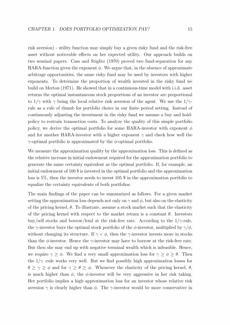
Figure 1.1 illustrates the absolute risk aversion functions for different levels of γ. The
smaller is γ, the steeper the curve is. For exponential utility, the curve is horizontal
at a level of 1. The similarity of the absolute risk aversion patterns suggests small
volume and structure effects.
2In the appendix, we briefly describe an alternative approximation based on the exponentialutility function.
CHAPTER 1. DOES PORTFOLIO OPTIMIZATION PAY? 21
−0.5 0 0.50.8
0.9
1
1.1
1.2
1.3
1.4
1.5
Excess Return
Abs
olut
e R
isk
Ave
rsio
n
gamma = 2gamma = 3gamma = 4gamma = 5gamma = 15
Figure 1.1: The absolute risk aversion of the HARA-function with endowment γ/Rf
declines in the portfolio excess return. For increasing γ the difference between the
absolute risk aversion of the HARA-function and that of the exponential utility
function, being 1 everywhere, decreases.
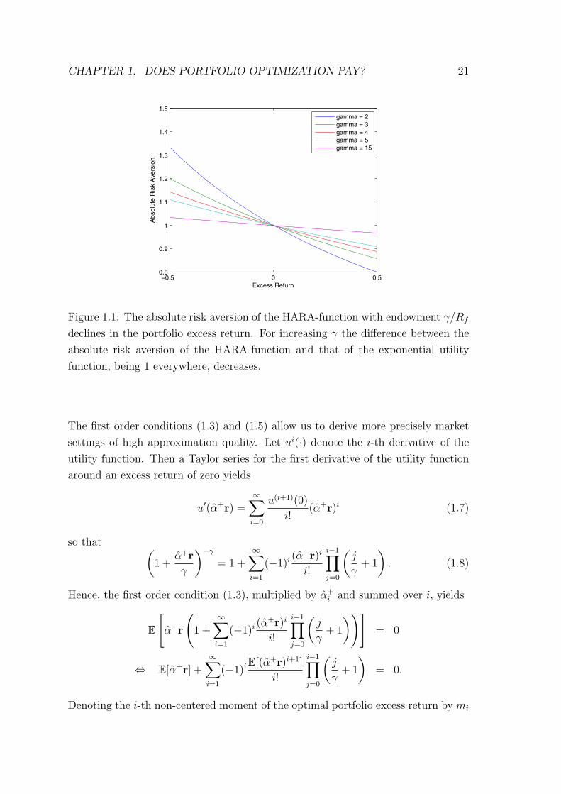
The first order conditions (1.3) and (1.5) allow us to derive more precisely market
settings of high approximation quality. Let ui(·) denote the i-th derivative of the
utility function. Then a Taylor series for the first derivative of the utility function
around an excess return of zero yields
u′(α+r) =∞∑i=0
u(i+1)(0)
i!(α+r)i (1.7)
so that (1 +
α+r
γ
)−γ= 1 +
∞∑i=1
(−1)i(α+r)i
i!
i−1∏j=0
(j
γ+ 1
). (1.8)
Hence, the first order condition (1.3), multiplied by α+i and summed over i, yields
E
[α+r
(1 +
∞∑i=1
(−1)i(α+r)i
i!
i−1∏j=0
(j
γ+ 1
))]= 0
⇔ E[α+r] +∞∑i=1
(−1)iE[(α+r)i+1]
i!
i−1∏j=0
(j
γ+ 1
)= 0.
Denoting the i-th non-centered moment of the optimal portfolio excess return by mi

CHAPTER 1. DOES PORTFOLIO OPTIMIZATION PAY? 22
and rearranging the last equation, the previous equation can be rewritten as
m1
m2
+1
2
m3
m2
(1
γ+ 1
)− 1
6
m4
m2
(2
γ+ 1
)(1
γ+ 1
)+ . . . = 1. (1.9)
From the first order condition (1.5) we have
n1
n2
+1
2
n3
n2
(1
φ+ 1
)− 1
6
n4
n2
(2
φ+ 1
)(1
φ+ 1
)+ . . . = 1, (1.10)
where ni is the i-th non-centered moment of α−r. Absolute portfolio excess re-
turns below 1 imply |αr|i+1 < |αr|i. Then it follows for the non-centered moments:
|mi+2| � |mi|, i ≥ 2. Also, |m3| � m2. Therefore, we may neglect the terms
mi, i ≥ 5, in the Taylor series and focus on the first four moments. The same is
true for ni.
Whenever the excess return distributions of the optimal and the approximation
portfolio have non-centered third and fourth moments close to zero, both first order
conditions are very similar implying a very good approximation quality3. Otherwise,
equations (1.9) and (1.10) indicate that the approximated return distribution derived
from (1.10) attaches too much weight to the skewness and the kurtosis relative to
(1.9) for γ > φ. Hence, we expect the approximated return distribution to have fatter
tails, but less skewness than the optimal return distribution. This follows because
a HARA-investor with declining absolute risk aversion likes positive skewness, but
dislikes kurtosis.
We summarize our findings in the following lemma:
Lemma 1 Let γ ≥ φ. The approximation is of high quality even for large differences
between φ and γ if the non-centered moments of the optimal and of the approximation
portfolio excess return decline fast, i.e. if mi+2 � mi, i ≥ 2, m3 � m2 and
ni+2 � ni, i ≥ 2, n3 � n2.
1.4.2 The Approximation Loss
We measure the economic impact of the approximation by the approximation loss.
Compare the certainty equivalent of the optimal portfolio α+ and that of the ap-
proximation portfolio α−. In both cases, the certainty equivalent is based on the
3For small portfolio risk, mi → 0 for i > 2. Then the optimal portfolio satisfies m1/m2 → 1rendering γ irrelevant. This is the case in a continuous time model with i.i.d. returns. Then thevolume and the structure effect disappear.

CHAPTER 1. DOES PORTFOLIO OPTIMIZATION PAY? 23
investor’s HARA-function (1.1). For that utility function, given a portfolio α, the
certainty equivalent, CE, is defined by(η + CE
γ
)1−γ
= E[
(η/Rf +W0)Rf + αr
γ
]1−γ
=
(W0
Rf
γ
)1−γ
E[1 +
αr
γ
]1−γ
=
(ce
γ
)1−γ
. (1.11)
Expected utility is the same for an investor with utility function (1.1) and endow-
ment W0 and an investor with constant relative risk aversion and enlarged initial
endowment W0 = η/Rf +W0. Therefore, we consider the enlarged certainty equiva-
lent ce = η +CE. Define ε as the ratio of the enlarged certainty equivalent, ce+, of
the optimal portfolio α+ = α+W0Rf/γ, and the enlarged certainty equivalent, ce−,
of the approximated optimal portfolio α− = α−W0Rf/γ. Then
ε =ce+
ce−=
E[(
(η/Rf+W0)Rf+α+r
γ
)1−γ]
E[(
(η/Rf+W0)Rf+α−r
γ
)1−γ]
1/(1−γ)
=
E[(
1 + α+rγ
)1−γ]
E[(
1 + α−rγ
)1−γ]
1/(1−γ)
.
(1.12)
Hence, ε is the same for the enlarged initial endowment η/Rf +W0 and the artificial
initial endowment γ/Rf . This is stated in:
Lemma 2 For a given market setting, the certainty equivalent ratio ε depends on
the exponent γ, but not on the initial endowment nor on the parameter η.
The lower boundary of ε is one, since the optimal portfolio α+ yields the highest
possible certainty equivalent. For a HARA-investor there exists a second interpreta-
tion of ε. k = (ε− 1) ≥ 0 is the relative increase in the enlarged initial endowment
W0, that is required for the approximation portfolio to generate the same expected
utility as the optimal portfolio generates with initial endowment W0. To see that
ε = 1 + k, note(W0Rf
γ
)1−γ
E
[(1 +
α+r
γ
)1−γ]
=
((1 + k)W0Rf
γ
)1−γ
E
[(1 +
α−r
γ
)1−γ].
Rearranging yields
1 + k =
E[(
1 + α+rγ
)1−γ]
E[(
1 + α−rγ
)1−γ]
1/(1−γ)
=ce+
ce−= ε.

CHAPTER 1. DOES PORTFOLIO OPTIMIZATION PAY? 24
We call k the approximation loss. If k = 0.02, for example, then the investor needs
to invest additionally 2% of his enlarged initial endowment in the approximation
portfolio to achieve the same expected utility as her optimal portfolio does.
For γ = φ, the approximation loss is 0, by definition. If we increase γ, the approx-
imation loss will be positive. But it does not increase monotonically. Instead, for
γ → ∞, k → 0 again. For γ → ∞, the investor’s utility is exponential and the
artificial initial endowment tends to infinity. The exponential utility investor buys
a risky portfolio independently of her initial endowment. Given an infinite artificial
initial endowment, this risky portfolio turns out to be irrelevant for the optimal
payoff V +. The same is true for the approximated payoff V −. Hence, both certainty
equivalents converge for γ →∞ so that k → 0.
In the following, we illustrate the approximation loss k by looking, first, at a complete
market with a continuous state space and different distributions of the market return.
Thereafter, we consider a discrete state space with few states only.
1.5 Approximation in a Continuous State Space
1.5.1 Demand Functions for State-Contingent Claims
Characterization of Demand Functions
We start from a perfect market with a continuous state space. First, assume a
complete market. Then state-contingent claims for all possible states s ∈ S exist.
Hakansson (1970) was the first to investigate investment and consumption strategies
of HARA investors in a complete market. Consider an investor with constant relative
risk aversion γ and artificial initial endowment γ/Rf . The investor’s demand for
state-contingent claims, α = (αs)s∈S , is optimized
maxα
E
[γ
1− γ
(γ + α
γ
)1−γ]s.t. E[πV ] = γ/Rf , (1.13)
where π = (πs)s∈S denotes the pricing kernel and αs is the demand for claims
with payoff one in state s and zero otherwise. Differentiating the corresponding
Lagrangian with respect to αs gives the well-known optimality condition for each
state (γ + αsγ
)−γ= λπs, s ∈ S. (1.14)

CHAPTER 1. DOES PORTFOLIO OPTIMIZATION PAY? 25
First, we assume that the pricing kernel is a power function of the market portfolio
return
πs =1
Rf
R−θM,s
E[R−θM ], (1.15)
where RM,s denotes the gross market return in state s and θ is the constant relative
risk aversion of the market, i.e. the constant elasticity of the pricing kernel. Hence,
we assume a pricing kernel as implied by the Black-Scholes setting.
Replacing πs by (1.15) and solving (1.14) for V +s = γ + αs yields for finite γ
V +s = R
θ/γM,s exp{a(γ)}. (1.16)
a(γ) depends on the investor’s relative risk aversion and is determined by the budget
constraint: E[Rθ/γM exp{a(γ)}π] = γ
Rf. We have
exp{a(γ)} = γE[R−θM ]
E[R−θ+θ/γM
] =γ
EQ[Rθ/γM
] , (1.17)
with EQ[·] being the expectation operator under the risk neutral probability measure
using the pricing kernel π(RM).
The optimal terminal wealth, V +, is approximated by V −. For γ ≥ φ, V − is the
optimal terminal wealth of an investor with CRRA φ and artificial endowment φ/Rf ,
supplemented by the risk-free payoff (γ − φ),
V −s = Rθ/φM,s exp{a(φ)}+ (γ − φ). (1.18)
How does (V +s − V −s ) depend on (γ − φ) for γ > φ? The functions V +(RM) and
V −(RM) intersect twice, given a sufficiently large domain of RM . Both functions
have to intersect at least once to rule out arbitrage opportunities. For RM → 0,
V − → γ−φ > V + → 0. Also V − > V + for RM →∞ (this follows from θ/γ < θ/φ).
Since V +(RM) is more concave than V −(RM), both functions intersect twice. The
demand for state contingent claims is overestimated by the approximation in the
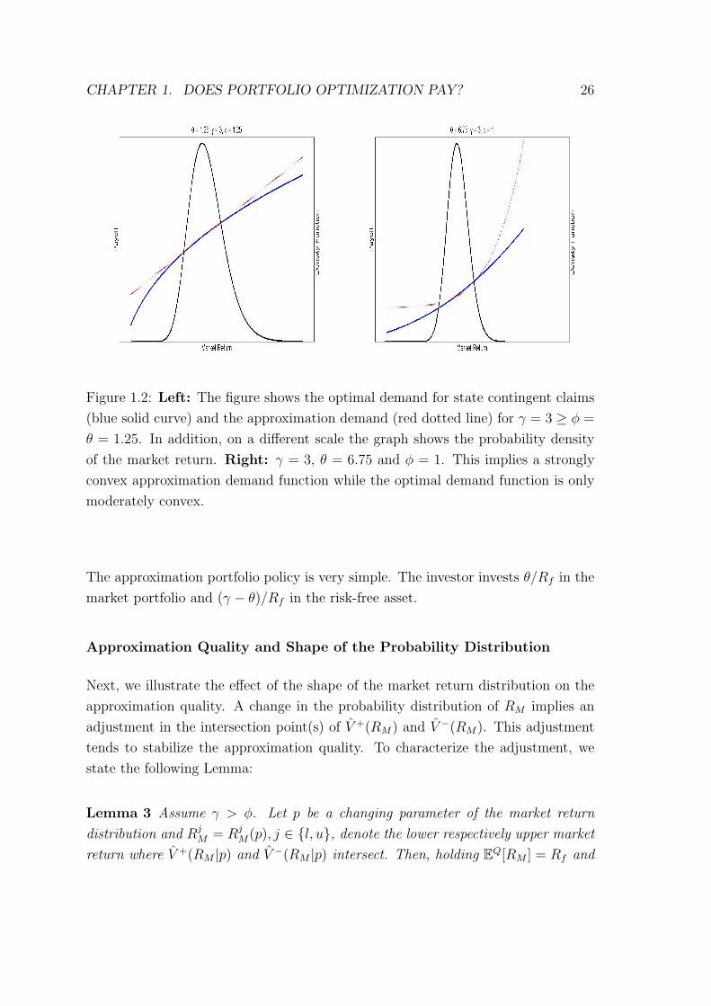
bad states and in the good states and underestimated in between, as Figure 1.2
illustrates. This range-dependent over-/underestimation of the optimal demand
characterizes the structure effect.
Consider the special case φ = θ. This implies that V − is linear in RM and, hence,
exp{a(θ)} = θ/EQ[RM ] = θ/Rf . Then (1.18) yields
V −s =θ
Rf
RM,s + γ − θ, γ ≥ θ. (1.19)
CHAPTER 1. DOES PORTFOLIO OPTIMIZATION PAY? 26
Figure 1.2: Left: The figure shows the optimal demand for state contingent claims
(blue solid curve) and the approximation demand (red dotted line) for γ = 3 ≥ φ =
θ = 1.25. In addition, on a different scale the graph shows the probability density
of the market return. Right: γ = 3, θ = 6.75 and φ = 1. This implies a strongly
convex approximation demand function while the optimal demand function is only
moderately convex.
The approximation portfolio policy is very simple. The investor invests θ/Rf in the
market portfolio and (γ − θ)/Rf in the risk-free asset.
Approximation Quality and Shape of the Probability Distribution
Next, we illustrate the effect of the shape of the market return distribution on the
approximation quality. A change in the probability distribution of RM implies an
adjustment in the intersection point(s) of V +(RM) and V −(RM). This adjustment
tends to stabilize the approximation quality. To characterize the adjustment, we
state the following Lemma:
Lemma 3 Assume γ > φ. Let p be a changing parameter of the market return
distribution and RjM = Rj
M(p), j ∈ {l, u}, denote the lower respectively upper market
return where V +(RM |p) and V −(RM |p) intersect. Then, holding EQ[RM ] = Rf and

CHAPTER 1. DOES PORTFOLIO OPTIMIZATION PAY? 27
θ constant,∂ lnRjM∂p
is given by
∂ lnRjM
∂p
θ
φ
1
γ
[V +(Rj
M)− γ]
=
[∂a(γ)
∂p− ∂a(φ)
∂p
]V +(Rj
M)
(γ − φ)+∂a(φ)
∂p, (1.20)
with
γ∂a(γ)
∂p= −
∫ ∞0
V +(RM)∂FQ(RM)
∂p(1.21)
and
φ∂a(φ)
∂p= −
∫ ∞0
V −(RM)∂FQ(RM)
∂p. (1.22)
FQ(RM) is the cumulative probability distribution of RM under the risk-neutral mea-
sure.
The proof of this lemma is given in the appendix. The lemma relates changes
in the risk-neutral probability distribution of the market return to changes in the
intersection points of V +(RM) and V −(RM). For simplicity, assume θ = φ. Then
exp{a(φ)} = φ/Rf so that ∂a(φ)/∂p = 0. Then, by (1.20), since V + > 0 and
V +(RlM)−γ < 0, V +(Ru
M)−γ > 0, a marginal change in the underlying probability
distribution function of RM (1) either lowers RlM and raises Ru
M or (2) raises RlM
and lowers RuM , or (3) leaves both unchanged.
For illustration, consider a mean preserving spread in the market return, such that
EQ[RM ] = Rf stays the same. Lemma 1 suggests that the approximation loss
increases. However, Lemma 3 implies that an increase in the volatility lowers Rl
and increases Ru. To see this, subtract φ∂a(φ)∂p
= 0 from equation (1.21),
γ∂a(γ)
∂p=
∫ ∞0
[V −(RM)− V +(RM)
] ∂FQ(RM)
∂p.
Increasing the volatility reallocates probability mass from the center to the tails, so
that the integral is positive. Then, by (1.20),lnRlM∂p
< 0 andlnRuM∂p
> 0. This reduces
the claim difference (V + − V −) in the tails and raises it in the center so that the
approximation quality is stabilized.
Alternatively, consider a reduction in the skewness of the market return distribution.
It is not clear whether the intersection points are spreading. Relocating probability
mass from the right to the left tail of the market return distribution would lower
EQ[RM ] and, therefore, is infeasible. In order to keep EQ[RM ] = Rf unchanged, the
probability mass needs to go up in some range of RM with RM > Rf . Therefore,
a(γ) can change in either direction, stabilizing the approximation quality.

CHAPTER 1. DOES PORTFOLIO OPTIMIZATION PAY? 28
1.5.2 Simulation Results for γ ≥ φ = θ
Normal Distribution
Now we illustrate the approximation loss numerically for various probability dis-
tributions of RM and various time horizons. The investor buys state-contingent
claims due at the time horizon. She does not readjust the portfolio over time. First
assume that lnRM is normally distributed with mean µ and variance σ2. Then
ln E[RM ] = µ+ σ2
2so that the annual Sharpe-ratio is
E[RM ]−Rf
σ(RM)=
[1− exp
{rf −
(µ+
σ2
2
)}] (exp{σ2} − 1
)−1/2.
The elasticity of the pricing kernel is θ =µ+σ2/2−rf
σ2 , the certainty equivalent of V +
has a closed form representation
ce(V +) = γ exp
{1
2
σ2θ2
γ
}.
For γ ≥ φ, the approximation portfolio is given by (1.19). To compute its certainty
equivalent, we have to rely on numerical integration techniques.
Consider the case φ = θ. To calibrate our analysis to observable market returns, we
first use an annual expected logarithmic market return µ = 6%, an annual market
volatility σ = 25% and an instantaneous risk-free rate rf = 3%. This implies a
pricing kernel elasticity of θ = 0.98, an annual equity premium of 6.51% and an
annual Sharpe-ratio of 23.4%. We consider investors with constant relative risk
aversion in the range [0.98; 8], an investment horizon between three month and 5
years and assume an i.i.d. market return. Hence, the expected logarithmic market
return for t years is µt = tµ and the standard deviation of the t-year logarithmic
market return is σt =√tσ.
Figure 1.3 shows the approximation loss. For γ = 0.98, the approximation portfolio
equals the optimal portfolio so that there is no approximation loss. For γ > φ = θ,
the approximation loss increases with a longer investment horizon because the mar-
ket return distribution becomes wider implying higher risk. Yet, the approximation
quality still remains very good. The highest approximation loss in Figure 1.3, left,
is about 0.3% for an investor with γ about 3 and an investment horizon of 5 years,
or, about 0.06% per year. In other words, the investor would need to raise her ini-
tial endowment by 0.3% to make up for the approximation loss. This suggests that
portfolio optimization does not pay.
CHAPTER 1. DOES PORTFOLIO OPTIMIZATION PAY? 29
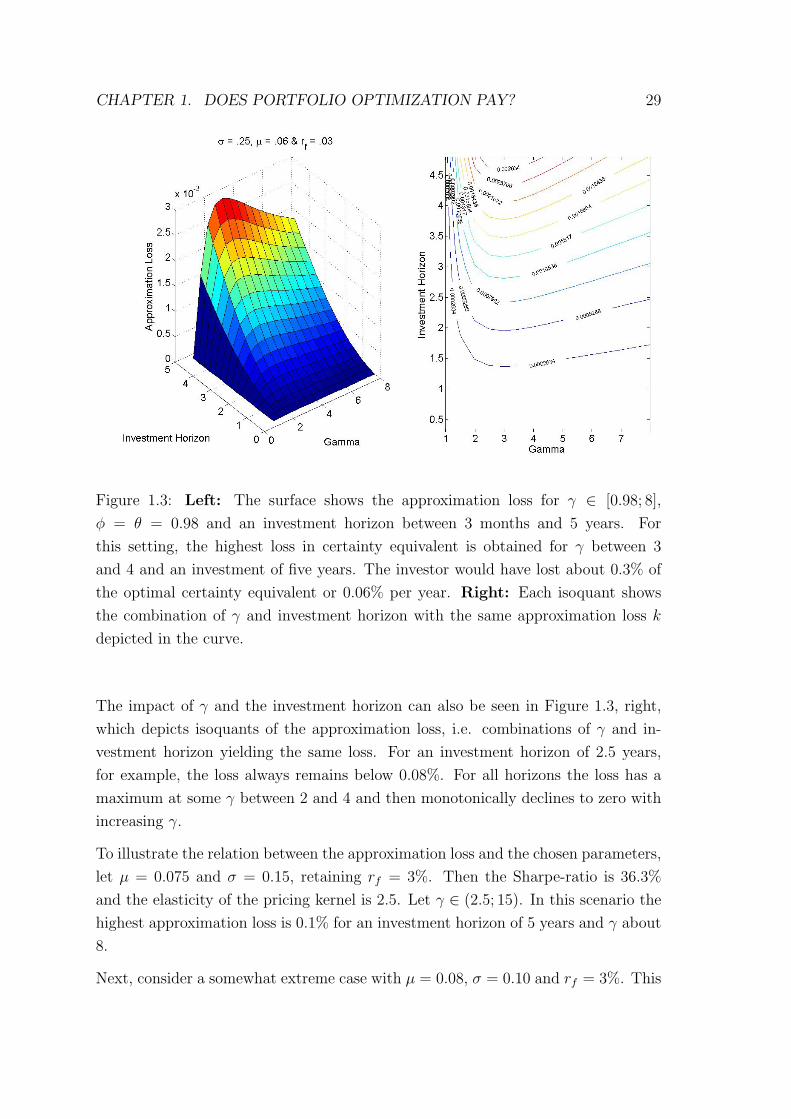
Figure 1.3: Left: The surface shows the approximation loss for γ ∈ [0.98; 8],
φ = θ = 0.98 and an investment horizon between 3 months and 5 years. For
this setting, the highest loss in certainty equivalent is obtained for γ between 3
and 4 and an investment of five years. The investor would have lost about 0.3% of
the optimal certainty equivalent or 0.06% per year. Right: Each isoquant shows
the combination of γ and investment horizon with the same approximation loss k
depicted in the curve.
The impact of γ and the investment horizon can also be seen in Figure 1.3, right,
which depicts isoquants of the approximation loss, i.e. combinations of γ and in-
vestment horizon yielding the same loss. For an investment horizon of 2.5 years,
for example, the loss always remains below 0.08%. For all horizons the loss has a
maximum at some γ between 2 and 4 and then monotonically declines to zero with
increasing γ.
To illustrate the relation between the approximation loss and the chosen parameters,
let µ = 0.075 and σ = 0.15, retaining rf = 3%. Then the Sharpe-ratio is 36.3%
and the elasticity of the pricing kernel is 2.5. Let γ ∈ (2.5; 15). In this scenario the
highest approximation loss is 0.1% for an investment horizon of 5 years and γ about
8.
Next, consider a somewhat extreme case with µ = 0.08, σ = 0.10 and rf = 3%. This
CHAPTER 1. DOES PORTFOLIO OPTIMIZATION PAY? 30
yields a Sharpe-ratio of 53.4% and a pricing kernel elasticity of 5.5. Let γ ∈ (5.5; 20).
Then the highest approximation loss is 0.04% for an investment horizon of 5 years
and γ about 17.
The results indicate that the highest approximation loss is inversely related to the
pricing kernel elasticity respectively the Sharpe-ratio, provided γ ≥ φ = θ. This is
not surprising because a higher pricing kernel elasticity has only small effects on the
shape of the V +(RM)- and V −(RM)-curves, but is associated with a strong decline
in σ(RM) so that the moments mj and nj, j > 1, of the portfolio excess return
decline (Lemma 1). Thus, the approximation works quite well.
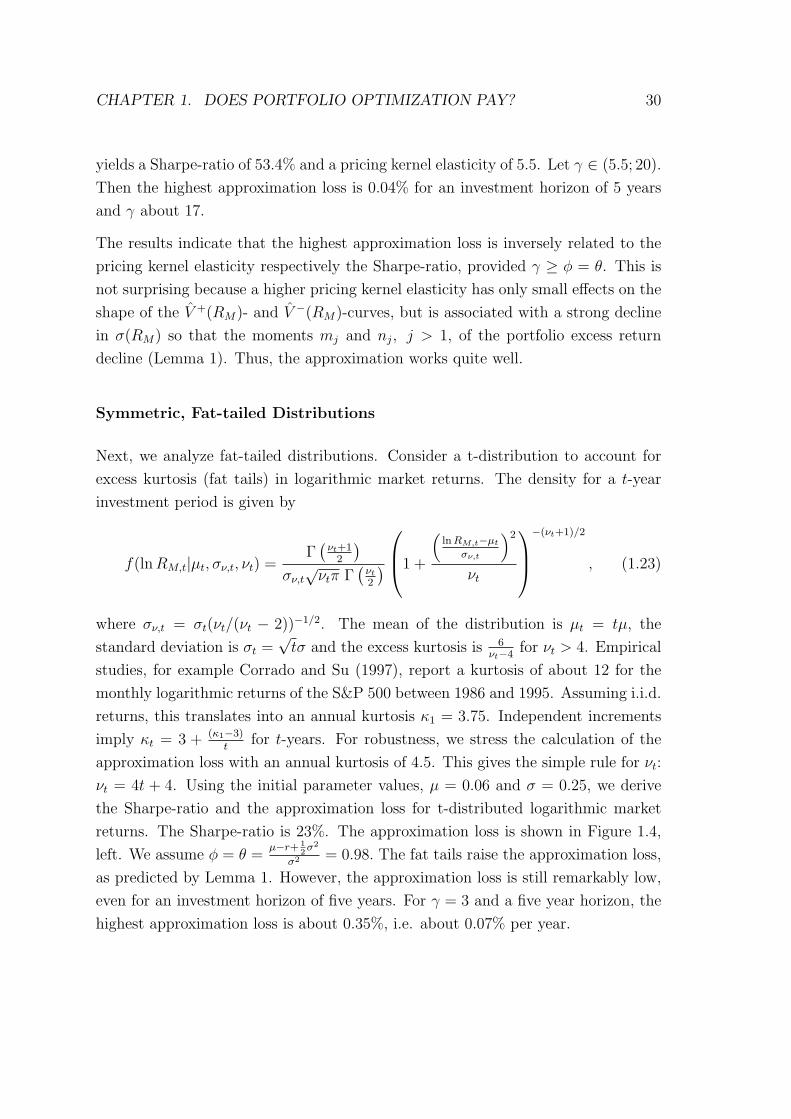
Symmetric, Fat-tailed Distributions
Next, we analyze fat-tailed distributions. Consider a t-distribution to account for
excess kurtosis (fat tails) in logarithmic market returns. The density for a t-year
investment period is given by
f(lnRM,t|µt, σν,t, νt) =Γ(νt+1
2
)σν,t√νtπ Γ
(νt2
)1 +
(lnRM,t−µt
σν,t
)2
νt
−(νt+1)/2
, (1.23)
where σν,t = σt(νt/(νt − 2))−1/2. The mean of the distribution is µt = tµ, the
standard deviation is σt =√tσ and the excess kurtosis is 6
νt−4for νt > 4. Empirical
studies, for example Corrado and Su (1997), report a kurtosis of about 12 for the
monthly logarithmic returns of the S&P 500 between 1986 and 1995. Assuming i.i.d.
returns, this translates into an annual kurtosis κ1 = 3.75. Independent increments
imply κt = 3 + (κ1−3)t
for t-years. For robustness, we stress the calculation of the
approximation loss with an annual kurtosis of 4.5. This gives the simple rule for νt:
νt = 4t + 4. Using the initial parameter values, µ = 0.06 and σ = 0.25, we derive
the Sharpe-ratio and the approximation loss for t-distributed logarithmic market
returns. The Sharpe-ratio is 23%. The approximation loss is shown in Figure 1.4,
left. We assume φ = θ =µ−r+ 1
2σ2
σ2 = 0.98. The fat tails raise the approximation loss,
as predicted by Lemma 1. However, the approximation loss is still remarkably low,
even for an investment horizon of five years. For γ = 3 and a five year horizon, the
highest approximation loss is about 0.35%, i.e. about 0.07% per year.

CHAPTER 1. DOES PORTFOLIO OPTIMIZATION PAY? 31
Figure 1.4: The surface shows the approximation loss for γ ∈ [0.98; 8], φ = θ = 0.98
and an investment horizon between 3 months and 5 years. Left: The logarithmic
market return is t-distributed. We assume independent and identically distributed
increments, hence, µt = 0.06t, σt = 0.25√t and νt = 4t + 4. For γ ≈ 3 and
an investment horizon of five years, the highest approximation loss is about 0.4%.
Right: The logarithmic market return is left-skewed, fat tailed distributed with
independent and identically distributed increments.
Left-skewed, Fat-tailed Distributions
As a final example of a complete market we consider a distribution with fat tails
and negative skewness. Since 1987 stock returns up to one year are mostly skewed
to the left. This is also true for stock index returns. For the simulation we use the
skewed, fat tailed normal distribution to model the logarithmic market return. The
density function is given by
f(lnRM,t|λt, ωt, ξt) =
(2
σt
)n
(lnRM,t − λt
ωt
)N(ξt
(lnRM,t − λt
ωt
)), (1.24)
where n(·) is the density of the standard normal distribution andN (·) is the standard
normal distribution function. The mean is given by µt = λt+ωtδt√
2/π, the standard
deviation is σt = ωt√
1− 2δ2t /π, where δt = ξt/
√1 + ξ2
t4. Corrado and Su (1997)
find that the monthly logarithmic stock returns of the S&P 500 are skewed to the
4The skewness is skt = 4−π2
“δt
√2/π
”3
(1−2δ2t /π)3/2 and the excess kurtosis is 2(π − 3)
“δt
√2/π
”4
(1−2δ2t /π)2.

CHAPTER 1. DOES PORTFOLIO OPTIMIZATION PAY? 32
left at -1.67. Assuming i.i.d. returns, this translates to an annual skewness of about
-0.55. We stress this number and use an annual skewness of -0.6 together with
an annual excess kurtosis of 0.4426. For each investment horizon, we choose the
parameters λt, ωt and ξt such that µt = 0.06t, σt = 0.25√t, skt = −0.6/
√t and
the excess kurtosis over t years is (3.4426 − 3)/t . This yields a somewhat higher
annual Sharpe-ratio of 24.6%. The approximation loss is shown in Figure 1.4, right,
for γ ≥ φ = θ, and t ∈ [0.3; 5]. The highest loss is about 0.36% for γ = 3 and
5 years. Figure 1.4, left, and Figure 1.4, right, indicate very similar loss levels.
Skewness and excess kurtosis do not affect the approximation loss substantially.
This is driven also by the adjustment of the intersection points of the optimal and
the approximate demand functions to the shape of the probability distribution.
Hence the approximation works well also for skewed, leptokurtic distributions, given
γ ≥ φ = θ. The costs of a sophisticated portfolio optimization are likely to exceed
its benefits.
1.5.3 Simulation Results for γ ≥ φ 6= θ
So far the simulations were based on γ ≥ φ = θ. If the pricing kernel elasticity is
lowered, then the smaller equity premium induces investors to take less risk. This
is true for the optimal and for the approximation portfolio. Hence the approxi-
mation loss should decline with a smaller θ. Since the last section shows that the
approximation loss is rather insensitive to skewness and leptokurtosis, we use again
the lognormal distribution with σ = 0.25 and µ + σ2
2− rf = θσ2 to simulate the
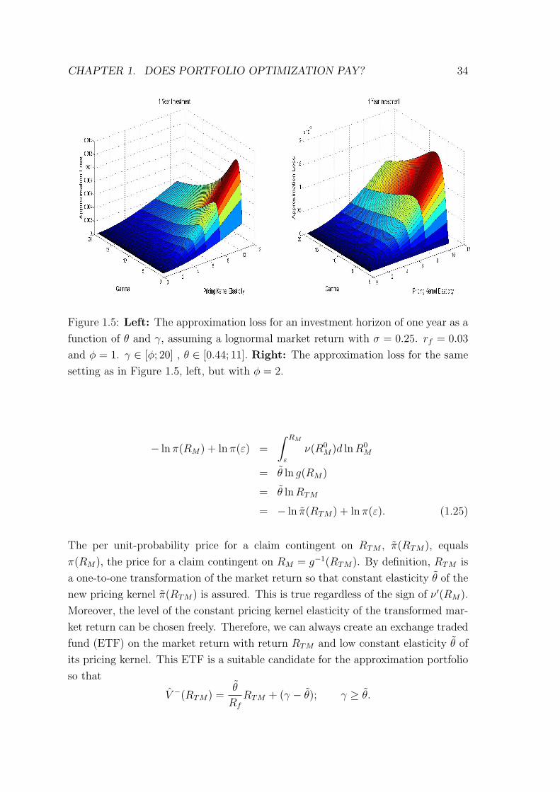
impact of θ on the approximation loss. Figure 1.5 shows the approximation loss for
an investment horizon of one year and different combinations of γ and θ. In Figure
1.5, left, φ = 1, in Figure 1.5, right, φ = 2. Both figures clearly show that the
approximation loss monotonically grows with θ, holding γ and φ constant. Hence,
if θ < φ, the approximation loss is smaller than that for θ = φ. Therefore, the
approximation works even better for θ < φ, as expected.
Conversely, the approximation loss strongly increases with the pricing kernel elas-
ticity, given θ � φ. For φ = 1, the highest approximation loss in Figure 1.5, left, is
about 1.1% for the highest θ = 11 and γ ≈ 5. For φ = 2 (Figure 1.5, right), it is
about 0.16% for θ = 11 and γ ≈ 6.5. These findings nicely illustrate the approxi-
5Independent increments imply skt = sk1/√t, where sk1 denotes the skewness for one year and
skt is the skewness for t-years.
CHAPTER 1. DOES PORTFOLIO OPTIMIZATION PAY? 33
mate arbitrage-story of Bernado and Ledoit (2000). They show that a market with
very high pricing kernel elasticity offers approximate arbitrage opportunities. An
investor with low relative risk aversion would then take very much risk through a
strongly convex demand function for state-contingent claims, see Figure 1.2, right.
Claims in states of high market returns are very cheap, they almost offer a free
lunch to investors with low relative risk aversion. Therefore these investors buy a
large number of these claims. Investors with γ ≥ θ benefit much less from this
effect because they buy a linear or a concave demand function. This implies a high
approximation loss as long as γ is not very high.
Clearly, the approximation loss is smaller for a higher φ. This is due to the fact
that an investor with higher φ would take less risk and, thus, benefit less from the
approximate arbitrage opportunity. The effect on the approximation loss can be
seen by comparing Figures 1.5, left, and 1.5, right.
Summarizing, the approximation does a very good job when the approximation is
based on a linear or concave demand function (φ ≥ θ). But it does a poor job when
the approximation is based (1) on a strongly convex demand function (θ � φ), (2)
the investor’s optimal demand function is much less convex (γ � φ) and (3) γ is
not so high that risk taking becomes negligible.
1.5.4 Non-Constant Elasticity of the Pricing Kernel
So far we assumed constant elasticity of the pricing kernel for the market return.
Ait-Sahalia and Lo (2000), Jackwerth (2000), Rosenberg and Engle (2002), Bliss
and Panigirtzoglou (2004), Barone-Adesi, Engle and Mancini (2008) estimate the
elasticity of the pricing kernel using prices of options on the S&P 500 and the FTSE
100. They conclude that the pricing kernel elasticity is declining, perhaps with a
local maximum in between.
If the pricing kernel of the market portfolio does not have constant elasticity, we de-
rive a transformed market portfolio such that its pricing kernel has low constant elas-
ticity. Then, instead of the market portfolio, we use this transformed market portfo-
lio for the approximation. Assume that the elasticity ν(RM) = −∂ lnπ(RM)/∂ lnRM
is positive and non-constant. Let RTM := g(RM) := exp{
1θ
∫ RMε
ν(R0M)d lnR0
M
},
where θ is a small, positive constant. ε is a positive lower bound of RM . g is invert-
ible and yields a pricing kernel π of constant elasticity θ with respect to RTM . This
follows since
CHAPTER 1. DOES PORTFOLIO OPTIMIZATION PAY? 34
Figure 1.5: Left: The approximation loss for an investment horizon of one year as a
function of θ and γ, assuming a lognormal market return with σ = 0.25. rf = 0.03
and φ = 1. γ ∈ [φ; 20] , θ ∈ [0.44; 11]. Right: The approximation loss for the same
setting as in Figure 1.5, left, but with φ = 2.
− lnπ(RM) + ln π(ε) =
∫ RM
ε
ν(R0M)d lnR0
M
= θ ln g(RM)
= θ lnRTM
= − ln π(RTM) + ln π(ε). (1.25)
The per unit-probability price for a claim contingent on RTM , π(RTM), equals
π(RM), the price for a claim contingent on RM = g−1(RTM). By definition, RTM is
a one-to-one transformation of the market return so that constant elasticity θ of the
new pricing kernel π(RTM) is assured. This is true regardless of the sign of ν ′(RM).
Moreover, the level of the constant pricing kernel elasticity of the transformed mar-
ket return can be chosen freely. Therefore, we can always create an exchange traded
fund (ETF) on the market return with return RTM and low constant elasticity θ of
its pricing kernel. This ETF is a suitable candidate for the approximation portfolio
so that
V −(RTM) =θ
Rf
RTM + (γ − θ); γ ≥ θ.

CHAPTER 1. DOES PORTFOLIO OPTIMIZATION PAY? 35
This approximation assures a low approximation loss.
1.5.5 Incomplete Markets
So far we considered complete markets. In an incomplete market, the pricing ker-
nel is no longer unique. Suppose, first, that a pricing kernel on the market with
low constant elasticity is feasible. For this case the preceding analysis has shown
that buying the market portfolio and the risk-free asset provides a very good ap-
proximation to the optimal portfolio for a large variety of settings. Actually, in an
incomplete market the approximation quality is even better. This follows because
incompleteness does not affect the availability of the market portfolio and, hence,
the approximation portfolio, but the optimal portfolio in a complete market may
not be available. This reduces the approximation loss.
Second, suppose that a pricing kernel with low constant elasticity is not feasible.
Then we can use an ETF. If both, the ETF and the portfolio which would be optimal
in a complete market, cannot be replicated exactly in an incomplete market, then
the approximation loss might go up or down. But, given a large number of available
risky assets, the difference between a complete and an incomplete market should be
small.
1.5.6 Extension to Parameter Uncertainty
So far all parameters are assumed to be known precisely. The discussion on param-
eter uncertainty focuses on the probability with which one portfolio is preferable to
another one in the presence of parameter uncertainty. As discussed before, several
papers conclude that, given a set of well-diversified portfolio strategies, no strategy
significantly outperforms the other strategies. To address this issue, consider the
following setting. Initially the investor buys a portfolio of state-contingent claims
based on the a priori probability distribution of the market return. The pricing
kernel is consistent with the a priori distribution. In the spirit of the papers on pa-
rameter uncertainty, we derive the a priori probability that ex post, i.e. given the a
posteriori distribution, the ex ante optimal portfolio is still preferred to the approxi-
mation portfolio. Let I denote the parameter vector of the a posteriori distribution
of the market return. Hence, we check
P = Prob[I∣∣∣ ce(V +|I) ≥ ce(V −|I)
], (1.26)
CHAPTER 1. DOES PORTFOLIO OPTIMIZATION PAY? 36
where ce(V |I) is the certainty equivalent of portfolio payoff V , given the a posteriori
distribution I.
To illustrate, assume that each a posteriori distribution of the market return is
log normal, n(lnRM |I). Then the a priori probability density of RM is given by∫n(lnRM |I)dF (I), with F (I) being the cumulative probability distribution of I.
We use a symmetric truncated normal distribution for I = [E[RM ], σ(RM)] with
bounds [0.8955; 1.2955] for E[RM ] and [0.1782; 0.3782] for σ(RM). We assume that
E[RM ] and σ(RM) are uncorrelated and that the standard deviation of both param-
eters is 0.1. This yields an a priori probability distribution of RM with simulated
expected market return of 1.0974 and standard deviation of 0.2942. This distri-
bution is not log normal. Given the a priori distribution, we derive exp{a(γ)} by
simulation and obtain the optimal demand V +(RM). The linear demand function
V −(RM) is based on φ = θ = 1 and is independent of the distribution. Figure 1.6
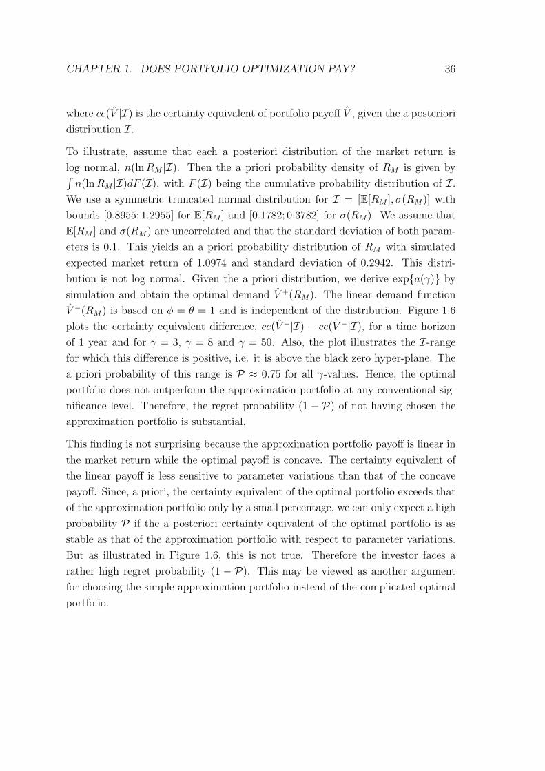
plots the certainty equivalent difference, ce(V +|I) − ce(V −|I), for a time horizon
of 1 year and for γ = 3, γ = 8 and γ = 50. Also, the plot illustrates the I-range
for which this difference is positive, i.e. it is above the black zero hyper-plane. The
a priori probability of this range is P ≈ 0.75 for all γ-values. Hence, the optimal
portfolio does not outperform the approximation portfolio at any conventional sig-
nificance level. Therefore, the regret probability (1 − P) of not having chosen the
approximation portfolio is substantial.
This finding is not surprising because the approximation portfolio payoff is linear in
the market return while the optimal payoff is concave. The certainty equivalent of
the linear payoff is less sensitive to parameter variations than that of the concave
payoff. Since, a priori, the certainty equivalent of the optimal portfolio exceeds that
of the approximation portfolio only by a small percentage, we can only expect a high
probability P if the a posteriori certainty equivalent of the optimal portfolio is as
stable as that of the approximation portfolio with respect to parameter variations.
But as illustrated in Figure 1.6, this is not true. Therefore the investor faces a
rather high regret probability (1 − P). This may be viewed as another argument
for choosing the simple approximation portfolio instead of the complicated optimal
portfolio.

CHAPTER 1. DOES PORTFOLIO OPTIMIZATION PAY? 37
Figure 1.6: The plot shows the a posteriori-approximation loss assuming parameter
uncertainty. The expected market return and the market volatility are a posteriori-
realizations of truncated, normally distributed random variables. The blue (red)
[green] surface shows the loss assuming γ = 3 (γ = 8) [γ = 50], the black hyper-
plane marks zero everywhere.
1.6 Approximation in a Discrete State Space
In a continuous state space the probability mass of the optimal and the approxi-
mation portfolio payoff may be concentrated around the zero excess payoff inducing
a strong approximation quality. This quality might be weaker for portfolio returns
with more probability mass in the tails. Lemma 1, however, suggests that the ap-
proximation loss is similar in a continuous and a discrete state space whenever the
non-central moments are similar. To find out about these effects, we now analyze
the approximation quality in a discrete state space with few states.
As an example, consider a bank which only invests in loans. The loan market is
arbitrage free. Loans either are fully paid or go into default paying a non-random
recovery amount. If the bank can invest in many different loans, it can achieve
strong portfolio diversification. Then the loan portfolio payoff can be approximated
quite well by a continuous unimodal probability distribution. This suggests again a
high approximation quality in the absence of approximate arbitrage opportunities.

CHAPTER 1. DOES PORTFOLIO OPTIMIZATION PAY? 38
γ = 2 γ = 3 γ = 10Distribution R L R L R L
α+ 4.7813 1.8519 4.3083 1.8830 3.7183 1.9187(α+ − α−) −1.6290 0.1158 −2.1020 0.1469 −2.6920 0.1826
k 0.0038 0.0002 0.0048 0.0002 0.0028 0.0001
Table 1.1: It shows the optimal investment in the risky asset for γ = 2, 3 and 10and the volume effect (α+ − α−). The approximated investment based on φ = 1is α− = 6.4103 for R and α− = 1.9677 for L. k is the approximation loss. R (L)denotes the probability distribution skewed to the right (left).
Critical might be cases in which the number of loans is small. In the following, we
present examples with one and two loans.
1.6.1 One Risky Asset
In the case of only one risky asset, there is no structure effect. Yet, the volume effect
(α+ − α−) remains and determines the approximation loss. A volume effect would
not exist if the 1/γ-rule would work perfectly. α+ = α(γ) and α− = α(φ) denote
the optimal and the approximate amount invested in the single risky asset, derived
from the first order conditions (1.3) respectively (1.5).
We analyze a negatively and a positively skewed binomial distribution. Both distri-
butions have the same expected return of 10.5% and standard deviation of 30%, so
that the Sharpe-ratio is the same. The risk-free rate is 3%. Let u (d) be the gross
return in the up-state (down-state). p is the up-state probability for the distribu-
tion R skewed to the right and also the down-state probability for the distribution
L skewed to the left. For example, let p = 0.25, uR = 1.42 and dR = 1, uL = 1.21
and dL = 0.79. Hence the distribution R has a skewness of 0.191, while distribution
L has a skewness of −0.165. The approximated investment in the risky asset is the
optimal investment using φ = 1. The optimal investment, the volume effect and the
approximation loss are shown in Table 1.1 for an investor with constant relative risk
aversion γ = 2, γ = 3 and γ = 10.
The volume effect is negative (positive) for the positively (negatively) skewed return
distribution. The volume effect relative to the optimal investment in the risky asset
is rather large (small) for the positively (negatively) skewed distribution. Yet, the

CHAPTER 1. DOES PORTFOLIO OPTIMIZATION PAY? 39
approximation loss is rather small in all cases. It is larger for the positively skewed
distribution, and declines with increasing γ for high values of γ.
The intuition for the sign of the volume effect can be derived from Figure 1.1. The
optimal volume depends on the absolute risk aversion levels in the down-state and
the up-state. Given γ > φ, the absolute risk aversion is higher [smaller] for the
utility function with parameter φ than for that with parameter γ in the down-state
[up-state].
For the positively skewed distribution the absolute difference in risk aversion is
much higher in the up-state than in the down-state. Therefore we expect a negative
volume effect, α+ < α−. For a negatively skewed distribution we expect a positive
volume effect. This is confirmed in Table 1.1. For a symmetric distribution, the
absolute difference in risk aversion is about the same in the down- and in the up-
state. Therefore α+(γ) ≈ α−(φ) implying a very small volume effect.
There is an easy way to understand the strong volume effect for the positively skewed
distribution. For a binomial distribution, the first order condition yields
puru
(1 +
α+ruγ
)−γ= (1− pu)|rd|
(1 +
α+rdγ
)−γ
⇔ puru(1− pu)|rd|
=
(γ + α+ruγ + α+rd
)γ. (1.27)
The left hand side of (1.27) denotes the gain/loss- ratio of Bernado and Ledoit
(2000). The higher it is, the closer is an approximate arbitrage opportunity. For
the positively (negatively) skewed distribution the gain/loss- ratio is 4.33 (2.25).
Hence, the positively skewed distribution is much closer to approximate arbitrage.
An investor with low relative risk aversion benefits more from approximate arbitrage
than an investor with higher risk aversion by choosing a more aggressive portfolio.
This explains for φ = 1 the high value of α− = 6.41, the strong negative volume
effect and the relatively high approximation loss.
As argued by Bernado and Ledoit, a high elasticity of the pricing kernel indicates
an approximate arbitrage opportunity6. The pricing kernel elasticity is 4.18 (1.90)
6Consider the Arrow-Debreu prices in this complete market setting. For a binomial return therealways exists a pricing kernel with constant elasticity. The two Arrow-Debreu prices are
πu =1Rf
puR−θu
E[R−θ]and πd =
1Rf
(1− pu)R−θd
E[R−θ].
CHAPTER 1. DOES PORTFOLIO OPTIMIZATION PAY? 40
for the positively (negatively) skewed distribution. Hence, the higher elasticity for
the positively skewed distribution also motivates a higher approximation loss.
1.6.2 Two Risky Assets with Dependent Returns
Next, consider two risky loans with correlated binomial returns. In this case there ex-
ist only 4 states of nature. If there are two loans with different expected returns and
perfectly negatively correlated returns, then there exists an arbitrage opportunity.
If the returns are strongly negatively correlated, then there exists an approximate
arbitrage opportunity. Hence, investors with low relative risk aversion will take very
large positions in the risky assets which should raise the approximation loss.
For illustration, let the marginal distribution of each risky asset have a binomial
distribution with equal probability for both outcomes, the up-state and the down-
state. The gross return of asset 1 is R1 = (1.2; 0.925) and of asset 2 is R2 =
(1.3; 0.85), respectively. The risk-free rate is 3%. This implies an expected excess
return of 3.25% for asset 1 and 4.5% for asset 2. The standard deviation is 13.75%
for the first asset and 22.5% for the second asset. Holding the marginal distributions
for both asset returns constant, we change the return correlation by the following
procedure. Let Ps,t := Prob(R1 = s, R2 = t) denote the probability that asset 1
is in the s-state and asset 2 is in the t-state, s, t ∈ {up, down}. Then, the joint
probability is
[Ps,t]s,t∈{up, down} =
(0.5− x x
x 0.5− x
),
with x ∈ [0; 0.5]. Reducing Pup, up and Pdown, down by x and adding x to Pdown, upand Pup, down, decreases the correlation without affecting the marginal distributions.
The approximation portfolio is based on φ = 0.98. For relative risk aversion γ ∈[0.98; 8] and for a return correlation between -0.8 and 0.8, Figure 1.7, left, shows the
approximation loss. It is very low for correlations above -0.5, but increases strongly
for lower correlations. Given negatively correlated assets, the investor can buy a
The ratio πu
πdcan be used to solve for the pricing kernel elasticity θ,
θ =ln(
gain-loss-ratio)
ln(Ru
Rd
) .
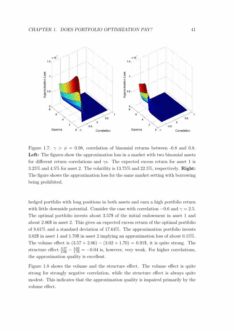
CHAPTER 1. DOES PORTFOLIO OPTIMIZATION PAY? 41
Figure 1.7: γ > φ = 0.98, correlation of binomial returns between -0.8 and 0.8.
Left: The figures show the approximation loss in a market with two binomial assets
for different return correlations and γs. The expected excess return for asset 1 is
3.25% and 4.5% for asset 2. The volatility is 13.75% and 22.5%, respectively. Right:
The figure shows the approximation loss for the same market setting with borrowing
being prohibited.
hedged portfolio with long positions in both assets and earn a high portfolio return
with little downside potential. Consider the case with correlation −0.6 and γ = 2.5.
The optimal portfolio invests about 3.57$ of the initial endowment in asset 1 and
about 2.06$ in asset 2. This gives an expected excess return of the optimal portfolio
of 8.61% and a standard deviation of 17.64%. The approximation portfolio invests
3.02$ in asset 1 and 1.70$ in asset 2 implying an approximation loss of about 0.15%.
The volume effect is (3.57 + 2.06) − (3.02 + 1.70) = 0.91$, it is quite strong. The
structure effect 3.572.06− 3.02
1.70= −0.04 is, however, very weak. For higher correlations,
the approximation quality is excellent.
Figure 1.8 shows the volume and the structure effect. The volume effect is quite
strong for strongly negative correlation, while the structure effect is always quite
modest. This indicates that the approximation quality is impaired primarily by the
volume effect.
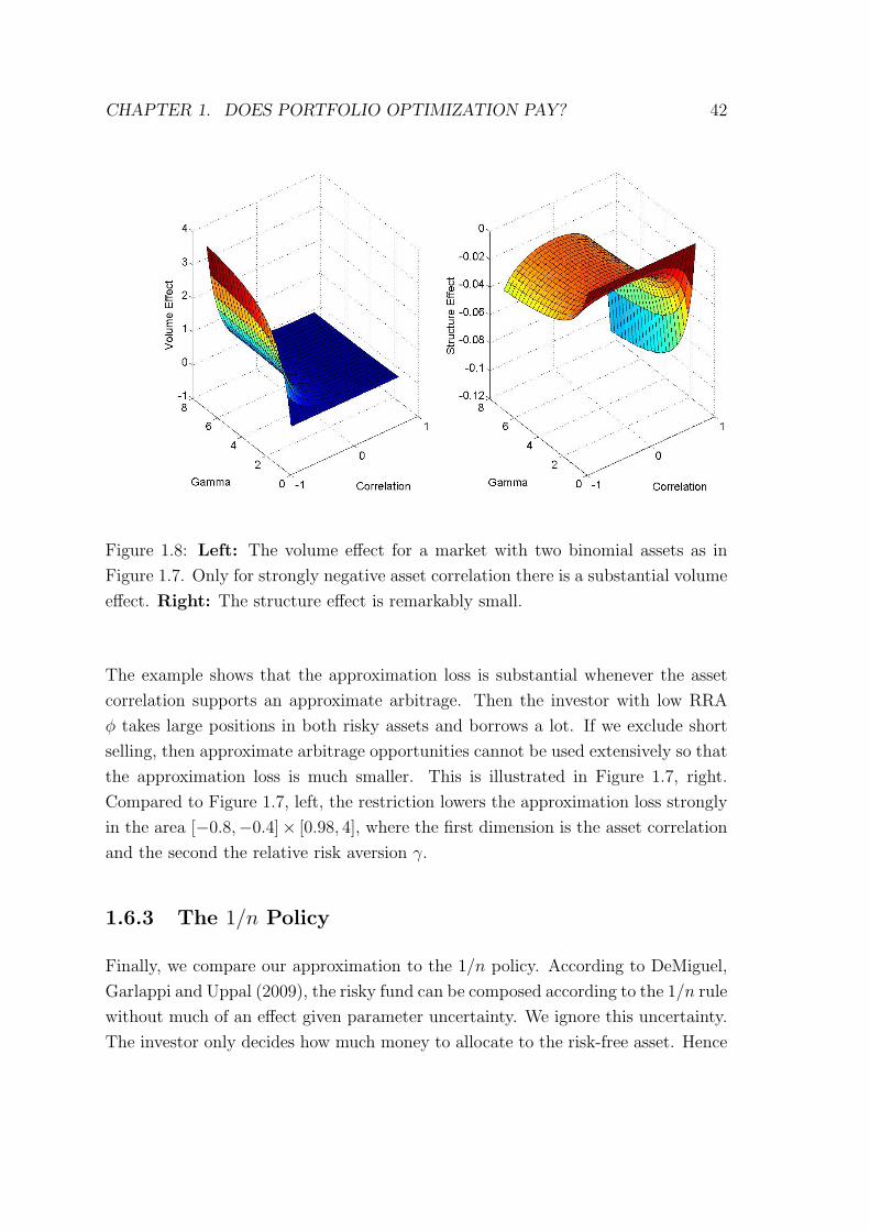
CHAPTER 1. DOES PORTFOLIO OPTIMIZATION PAY? 42
Figure 1.8: Left: The volume effect for a market with two binomial assets as in
Figure 1.7. Only for strongly negative asset correlation there is a substantial volume
effect. Right: The structure effect is remarkably small.
The example shows that the approximation loss is substantial whenever the asset
correlation supports an approximate arbitrage. Then the investor with low RRA
φ takes large positions in both risky assets and borrows a lot. If we exclude short
selling, then approximate arbitrage opportunities cannot be used extensively so that
the approximation loss is much smaller. This is illustrated in Figure 1.7, right.
Compared to Figure 1.7, left, the restriction lowers the approximation loss strongly
in the area [−0.8,−0.4]× [0.98, 4], where the first dimension is the asset correlation
and the second the relative risk aversion γ.
1.6.3 The 1/n Policy
Finally, we compare our approximation to the 1/n policy. According to DeMiguel,
Garlappi and Uppal (2009), the risky fund can be composed according to the 1/n rule
without much of an effect given parameter uncertainty. We ignore this uncertainty.
The investor only decides how much money to allocate to the risk-free asset. Hence
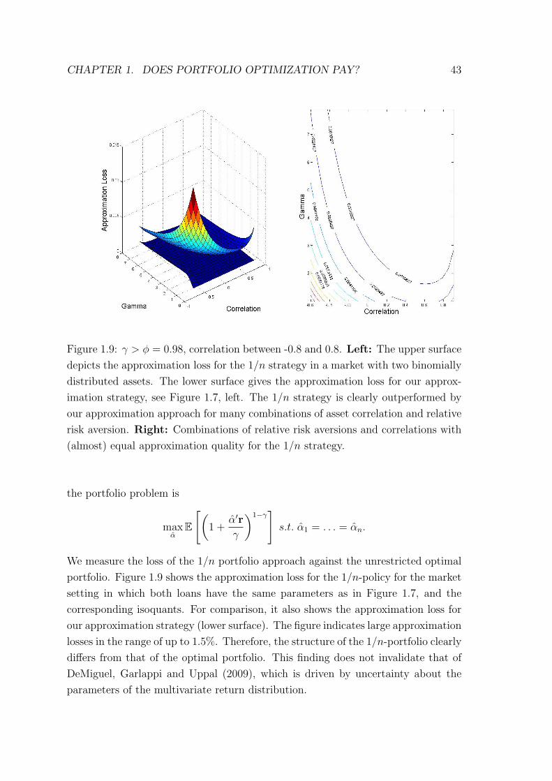
CHAPTER 1. DOES PORTFOLIO OPTIMIZATION PAY? 43
Figure 1.9: γ > φ = 0.98, correlation between -0.8 and 0.8. Left: The upper surface
depicts the approximation loss for the 1/n strategy in a market with two binomially
distributed assets. The lower surface gives the approximation loss for our approx-
imation strategy, see Figure 1.7, left. The 1/n strategy is clearly outperformed by
our approximation approach for many combinations of asset correlation and relative
risk aversion. Right: Combinations of relative risk aversions and correlations with
(almost) equal approximation quality for the 1/n strategy.
the portfolio problem is
maxα
E
[(1 +
α′r
γ
)1−γ]s.t. α1 = . . . = αn.
We measure the loss of the 1/n portfolio approach against the unrestricted optimal
portfolio. Figure 1.9 shows the approximation loss for the 1/n-policy for the market
setting in which both loans have the same parameters as in Figure 1.7, and the
corresponding isoquants. For comparison, it also shows the approximation loss for
our approximation strategy (lower surface). The figure indicates large approximation
losses in the range of up to 1.5%. Therefore, the structure of the 1/n-portfolio clearly
differs from that of the optimal portfolio. This finding does not invalidate that of
DeMiguel, Garlappi and Uppal (2009), which is driven by uncertainty about the
parameters of the multivariate return distribution.

CHAPTER 1. DOES PORTFOLIO OPTIMIZATION PAY? 44
1.7 Conclusion
Sophisticated portfolio optimization is unlikely to pay in a large variety of settings.
We constrain our analysis to HARA-investors with declining absolute risk aversion
and ask whether the parameters of the utility function really matter for optimal in-
vestment decisions. The paper shows that the optimal portfolio can be approximated
without noticeable harm by the portfolio which is optimal for some HARA-investor
with lower relative risk aversion, if approximate arbitrage opportunities do not exist.
If these opportunities exist and the approximation portfolio takes high risk while
the optimal portfolio does not, then the approximation leads to high approximation
losses. Whenever the pricing kernel of the market return displays constant elasticity,
an investor with higher relative risk aversion may simply buy the market portfolio
and the risk-free asset without noticeable harm. Otherwise, the investor may buy
a transformed market portfolio with low constant elasticity of the pricing kernel.
Critical for a strong approximation quality is that the investor’s relative risk aver-
sion is higher than that used for the approximation and that approximate arbitrage
opportunities do not exist.
Our findings generalize the two fund-separation of Cass and Stiglitz such that dif-
ferences in the structures of optimal risky funds, driven by different levels of relative
risk aversion, matter little in the absence of approximate arbitrage opportunities.
If there exists uncertainty about the parameters of the asset returns, then our ex-
amples demonstrate that the approximation portfolio turns out to be better than
the optimal portfolio with a substantial probability. This also supports the use of
a simple approximation portfolio. Further research might analyze the approxima-
tion quality in market settings in which investors use dynamic trading strategies to
benefit from stock return predictability. Also the set of utility functions should be
widened beyond HARA.

CHAPTER 1. DOES PORTFOLIO OPTIMIZATION PAY? 45
1.8 Appendix
1.8.1 Alternative Approximation Approach
An alternative approximation approach is based on the optimal portfolio of an in-
vestor with constant absolute risk aversion of 1 and artificial initial endowment
γ/Rf . For this investor, the first order condition is
E [ri exp{−α′r}] = 0, ∀i ∈ {1, . . . , n}, (1.28)
irrespective of her initial endowment. We make use of (1 + x/p)p → exp{x} for
p→∞ to connect the first order condition (1.3) of an investor with artificial initial
endowment γ/Rf and constant relative risk aversion to the first order condition of
an investor with constant absolute risk aversion of 1, i.e.
E
[ri
(1 +
α′r
γ
)−γ]γ→∞−→ E[ri exp{−α′r}], ∀i ∈ {1, . . . , n}. (1.29)
Hence, the solution of (1.28) might be used as an alternative approximation for α+,
the solution of (1.3). However, this approach does not rule out negative terminal
values of the approximate optimal portfolio, which is infeasible for HARA utility
functions. To see this, consider a complete market with market return RM and a
pricing kernel with constant elasticity θ. In general, the optimal portfolio payoff is
implicitly given by∂ lnV
∂ lnRM
=θ
RRA(V ),
where RRA(V ) denotes the relative risk aversion. For the exponential utility in-
vestor, this yields the demand function V −s = θ lnRM,s + b, where b is determined
by the budget constraint E[V −π] = γ/Rf , hence b = γ− θE[R−θM lnRM ]
E[R−θM ]. Now consider
normally distributed logarithmic market returns, i.e. lnRM ∼ N (µ, σ2). This yields
the explicit demand function
V −s = γ + θ lnRM,s − θ(µ− θσ2),
which is not positive for all market returns. More precisely, the probability that the
portfolio payoff is negative is N (−θσ− γ/(θσ)), with N being the standard normal
distribution function. Therefore, this approach is not discussed.

CHAPTER 1. DOES PORTFOLIO OPTIMIZATION PAY? 46
1.8.2 Proof of Lemma 3
At an intersection point, V +(RjM) = V −(Rj
M). Then, we have at an intersection
with R = RjM ,
∂V +(R)
∂p=∂V −(R)
∂p
⇔ θ
γexp{a(γ)}R(θ/γ)−1∂R
∂p+∂a(γ)
∂pV +(R)
=θ
φexp{a(φ)}R(θ/φ−1)∂R
∂p+∂a(φ)
∂p
[V −(R)− (γ − φ)
]Since V +(R) = V −(R), we have
θ
γV +(R)
∂ lnR
∂p+∂a(γ)
∂pV +(R) =
[ θφ
∂ lnR
∂p+∂a(φ)
∂p
][V +(R)− (γ − φ)]
⇔ ∂ lnR
∂p
θ
φ
1
γ(γ − φ)[V +(R)− γ] =
[∂a(γ)
∂p− ∂a(φ)
∂p
]V +(R) +
∂a(φ)
∂p(γ − φ).
Dividing by (γ − φ) yields equation (1.20). Equations (1.21) and (1.22) follow from
differentiating the budget constraint with respect to p.

Bibliography
[1] Ait-Sahalia, Y. and A. W. Lo, 2000, ”Nonparametric Risk Management and
Implied Risk Aversion”, Journal of Econometrics 94, 9-51.
[2] Arrow, K. J., 1974, ”Essays in the Theory of Risk-Bearing”, Markham Publishing
Co.
[3] Balduzzi, P. and A. Lynch, 1999, ”Transaction Costs and Predictability: Some
Utility Cost Calculations”, Journal of Financial Economics 52, 47-78.
[4] Barone-Adesi G., R. F. Engle and L. Mancini, 2008, ”A GARCH Option Pricing
Model with Filtered Historical Simulation”, Review of Financial Studies 21,
1223-1258.
[5] Bernado, A. and O. Ledoit, 2000, ”Gain, Loss and Asset Pricing”, Journal of
Political Economy 108, 144-172.
[6] Black, F., R. Littermann, 1992, ”Global Portfolio Optimization”, Financial An-
alysts Journal, Sept/Oct. 28-43.
[7] Bliss, R. R. and N. Panigirtzoglou, 2004, ”Option-Implied Risk Aversion Esti-
mates”, Journal of Finance 59, 407-446.
[8] Brandt, M., A. Goyal, P. Santa-Clara and J. Stroud, 2005, ”A Simulation Ap-
proach to Dynamic Portfolio Choice with an Application to Learning About
Return Predictability”, Review of Financial Studies 18, 831-873.
[9] Brandt, M., P. Santa-Clara and R. Valkanov, 2009, ”Parametric Portfolio Poli-
cies: Exploiting Characteristics in the Cross Section of Equity Returns”, Review
of Financial Studies 22, 3411-3447.
47
CHAPTER 1. DOES PORTFOLIO OPTIMIZATION PAY? 48
[10] Cass, D., and J. E. Stiglitz, 1970, ”The Structure of Investor Preferences and
Asset Returns, and Separability in Portfolio Allocation: A Contribution to the
Pure Theory of Mutual Funds”, Journal of Economic Theory 2, 122-160.
[11] Chacko, G. and L. Viceira, 2005, ”Dynamic Consumption and Portfolio Choice
with Stochastic Volatility in Incomplete Markets”, Review of Financial Studies,
18, 1369-1402.
[12] Corrado, C. J. and T. Su, 1997 ”Implied Volatility Skews and Stock Index
Skewness and Kurtosis in S&P 500 Index Option Prices.”, Journal of Derivatives,
4, 8-19.
[13] DeMiguel, V., L. Garlappi and R. Uppal, 2009, ”Optimal versus Naive Diver-
sification: How Inefficient is the 1/N Portfolio Strategy?”, Review of Financial
Studies 22, 1915-1953.
[14] DeMiguel, V., L. Garlappi, J. Nogales and R. Uppal, 2009, ”A Generalized
Approach to Portfolio Optimization: Improving Performance By Constraining
Portfolio Norms”, Management Science 55, 798-812.
[15] Diamond, P. A. and J. E. Stiglitz, 1974, ”Increase in Risk and Risk Aversion”,
Journal of Economic Theory 66, 522-535.
[16] Hakansson, N. H. 1970, ”Optimal Investment and Consumption Strategies Un-
der Risk for a Class of Utility Functions”, Econometrica, 38, 587-607.
[17] Hodder, J., J. Jackwerth and O. Kokolova, 2009, ”Improved Portfolio Choice
Using Second Order Stochastic Dominance”, Working paper, University Kon-
stanz.
[18] Jackwerth, J., 2000, ”Recovering Risk Aversion from Option Prices and Real-
ized Returns”, Review of Financial Studies 13, 433-451.
[19] Jacobs, H., S. Mueller and M. Weber, 2009, ”How Should Private Investors
Diversify? An Empirical Evaluation of Alternative Asset Allocation Policies to
Construct a ’World Market Portfolio”, Working paper, University of Mannheim.
[20] Karatzas, I., J. Lehoczky, S. Sethi, S. Shreve, 1986, ”Explicit Solution of a Gen-
eral Consumption/Investment Problem”, Mathematics of Operations Research
11, 261-294.

CHAPTER 1. DOES PORTFOLIO OPTIMIZATION PAY? 49
[21] Merton, R. C. 1971, ”Optimal Consumption and Investment Rules in a Con-
tinuous Time Model”, Journal of Economic Theory 3, 373-413.
[22] Pratt, J. W., 1964, ”Risk Aversion in the Small and in the Large”, Econometrica
32, 122-136.
[23] Rosenberg, J. V. and R. F. Engle, 2002, ”Option Hedging Using Empirical
Pricing Kernels”, Journal of Financial Economics 64, 341-372.
[24] Rothschild, M. and J. E. Stiglitz, 1970, ”Increasing Risk I: A Definition”, Jour-
nal of Economic Theory 2, 225-243.
[25] Viceira, L. (2001), ”Optimal Portfolio Choice for Lang-Horizon Investors with
Non-tradable Labor Income”, Journal of Finance 61,433-470.

Chapter 2
Mechanically Evaluated Company
News and their Impact on Stock
and Credit Markets
Abstract: I analyze company news from Reuters with the ‘General In-
quirer’ and relate measures of positive sentiment, negative sentiment and
disagreement to abnormal stock returns, stock and option trading vol-
ume, the volatility spread and the CDS spread. I test hypotheses derived
from market microstructure models. Consistent with these models, sen-
timent and disagreement are strongly related to trading volume. More-
over, sentiment and disagreement might be used to predict stock returns,
trading volume and volatility. Trading strategies based on positive and
negative sentiment are profitable if the transaction costs are moderate,
indicating that stock markets are not fully efficient.
2.1 Introduction
Investors read daily newspapers, internet articles, watch TV news and listen to the
radio. The information obtained might affect their trading decision and, hence, mar-
ket prices, trading volume and volatility. Barber and Odean (2008) show that the
number of news releases by Dow Jones News Service is related to the trading behav-
ior of individual investors. Engelberg and Parsons (2011) find a causal relationship
between financial news articles in local newspapers and the trading volume of local
50
CHAPTER 2. MECHANICALLY EVALUATED COMPANY NEWS 51
retail investors. However, news have many dimensions. The number of relevant
news articles for a company is a very restrictive measure and ignores much infor-
mation that might be important for financial markets, e.g. the sentiment. Tetlock
(2007) and Groß-Klußmann and Hautsch (2011) find that the sentiment of news
articles predicts daily index returns, and intraday liquidity and volatility, respec-
tively. The sentiment of chat-room postings, which could contain news as well, may
have predictive power for financial markets too, see Antweiler and Frank (2004),
Das, Matinez-Jeres and Tufano (2005) and Das and Chen (2007). I build on these
studies and construct a flexible content analysis algorithm to measure sentiment and
disagreement, analyzing company news from Reuters.
Reuters company news usually describe and interpret a wide range of facts and
events which might be relevant for companies. The author’s interpretation and her
word choice may provide valuable information for financial markets. The author’s
view might account for the economic environment, the firm’s industry position, the
management quality and much more aspects which are rather hard to measure quan-
titatively. If the author concludes that some fact is positive news for a company, she
will use friendly and positive words to write the news story. If the facts are consid-
ered as negative, alarmed and sad words will probably characterize the news story.
Of course, the quality of the author’s comments depends on her background. This
makes the analysis of chat-room postings and their impact on the market difficult,
since everybody can post her opinion, rumors or lies without reputation damage.
Reuters company news are more credible, which makes their analysis interesting.
Another advantage of Reuters company news is that they allow studying the im-
pact of heterogeneous events (e.g. earnings and dividends announcements, analyst
recommendations, et cetera) on financial markets simultaneously.
I use the ‘General Inquirer’ to measure the sentiment of a news story with respect to a
company and disagreement among news stories mechanically. The ‘General Inquirer’
assigns words to word categories. The word categories ‘positive’ and ‘negative’ are
used to measure positive and negative sentiment of news stories. Also, I use the
word categories ‘strong’ and ‘weak’ to measure the uncertainty of a news story. I
test whether positive sentiment, negative sentiment and disagreement of Reuters
company news articles impact financial markets. My dataset consists of information
on 62 large U.S. companies listed at the NYSE or the Nasdaq with liquid stock
option and CDS markets for the time period June 01, 2007 to December 31, 2010.
First, I investigate the co-movement of sentiment and disagreement with abnormal

CHAPTER 2. MECHANICALLY EVALUATED COMPANY NEWS 52
stock return derived from the three factor Fama-French model, stock and option
trading volume, the volatility spread and the CDS spread using daily data. This
analysis allows to test implications given by market microstructure models where
investors interpret public signals individually. Sentiment approximates the intensity
of public signals and disagreement approximates the degree of difference of opinion.
My results are consistent with these models.
Second, I show that sentiment and disagreement have predictive power for (abnor-
mal) stock returns, stock trading volume and the volatility spread. Positive senti-
ment is frequently followed by positive (abnormal) returns and disagreement tends
to lower (abnormal) returns on the following day. The volatility spread increases
after negative sentiment and disagreement. Stock trading volume is significantly
higher after news with positive sentiment, but disagreement tends to reduce stock
trading volume at the following day. The latter finding is surprising and might be
due to an immediate execution of orders scheduled to the following day, given in-
consistent news articles. Then, trading volume might be low during the subsequent
day.
Finally, I test the economic relevance of positive and negative sentiment by analyzing
trading strategies based on sentiment. Even though I consider realistic transaction
costs of 10 bps per round-trip, the trading strategies are comparable to approximate
arbitrage opportunities, indicating that the stock market is not fully efficient. For
transaction costs of 20 bps, the trading strategies are, on average, still profitable, but
bear a substantial loss potential. The strategies cannot compensate for transaction
costs of 30 bps and more.
The contribution of this paper is manyfold. (1) I consider a large number of compa-
nies with liquid stock and derivative markets and analyze the relationship between
news articles and (abnormal) stock returns, stock and option trading volume, the
volatility spread and the CDS spread company individually. Hence, I do not ag-
gregate returns, etc., at the same day across companies. This distinguishes this
study from Tetlock (2007), who considers index returns, and from Das et al. (2005),
who analyze four representative companies individually. (2) I analyze a compre-
hensive and hand-collected dataset of news stories, downloaded from the homepage
of Reuters with a flexible procedure. I extend Groß-Klußman and Hautsch (2011),
who relate pre-calculated dummy variables for positive and negative sentiment to
the stock market, by introducing a continuous sentiment score. (3) Reuters company
news are highly credible. This distinguishes this analysis from Antweiler and Frank

CHAPTER 2. MECHANICALLY EVALUATED COMPANY NEWS 53
(2004) and Das and Chen (2007), who study chat-room postings. Das et al. (2005)
analyze chat-room postings, too, claiming that these postings disseminate public
information. My analysis might contribute to those study, since it analyzes news
articles which might be closer to public information and, hence, less noisy. (4) To
my best knowledge, this study is the first that analyzes the relationship between the
CDS spread and sentiment and disagreement, respectively, of general news articles.
The rest of the paper is organized as follows. Section 2 gives a literature review.
Section 3 derives testable hypotheses from market microstructure models. There-
after, I explain how market activity is measured. I describe my hand-collected news
database in section 4. Section 5 describes the content analysis and defines measures
for sentiment and disagreement. Thereafter, I relate these measures to the market
variables and develop trading strategies based on sentiment. Section 8 concludes
and gives an outlook for further research.
2.2 Related Literature
Several papers investigate the relationship between a company’s publicity and the
stock market. Publicity often refers to the number of newspaper articles on the
company. In an early study, Mitchell and Mulherin (1994) relate the number of
news releases by Dow Jones & Company to the absolute value of the market return,
the absolute value of firm-specific return and the trading volume. By controlling
for macroeconomic announcements and weekday effects, the study documents a sig-
nificant relationship between news activity and market activity. Barber and Odean
(2008) define attention-grabbing stocks as stocks with high abnormal trading vol-
ume, extreme returns or news coverage. They show that individual investors are
more likely to purchase attention-grabbing stocks than other stocks. Engelberg and
Parsons (2011) address the causality between news articles and investors’ behav-
ior. They identify articles on earnings announcement in local newspapers. Local
news coverage predicts trading volume of local investors and gives strong support
to a causal relationship from news coverage to trading. Fang and Peress (2009)
study the cross-section of stock returns. They find that stocks with media cover-
age, measured by the number of articles on the company in the four major U.S.
newspapers (New York Times, USA Today, Wall Street Journal, Washington Post),
underperform stocks without media coverage.
Of course, the number of news per day ignores the content of the news article.
CHAPTER 2. MECHANICALLY EVALUATED COMPANY NEWS 54
Tetlock (2007) identifies weak or negative words in the daily article ‘Abreast of the
Market’ in the Wall Street Journal with a content analysis algorithm, the ‘General
Inquirer’. He finds that the number of negative or weak words predicts the return
of the Dow Jones Industrial Average on the following day. This effect is offset
within the subsequent five days and disappears after one week. Groß-Klußmann
and Hautsch (2011) show that the sentiment of news articles and their relevance for
companies listed at the LSE predict high frequency returns, volatility and liquidity.
The sentiment of a news article is calculated by Reuters and can take on only the
values +1, 0 and -1. The relevance of the news story determines the sensitivity
of the market with respect to the news article. Tetlock et al. (2008) show that
print news can predict fundamental value as well as market value. However, trading
strategies based on these forecasts generate profits only if transaction costs are
excluded. Carretta et al. (2010) study the Italian stock market and its reaction to
corporate governance news. News stories are analyzed with respect to content and
tone, revealing that the content of news on profitable corporations is important to
explain stock returns.
Several studies use a more general definition of news and consider chat-room post-
ings as news. However, this kind of information is presumably more noisy and,
hence, less credible than regular news articles. Antweiler and Frank (2004) relate
measures for bullishness and disagreement in chat-room postings and chat-room
activity to market activity. Their main finding is that chat-room postings predict
realized volatility and trading volume, given high frequency data. Das et al. (2005)
analyze chat-room postings for four representative companies with different size and
find a contemporaneous relationship between the sentiment of investors’ conversa-
tions and market returns, but no predictive power. This motivates their conclusion
that investors first trade and then talk. Das and Chen (2007) apply a wide spec-
trum of text analysis algorithms to chat-rooms postings and develop measures for
sentiment and disagreement. Relating these measures to the stock market return of
the corresponding company also shows that investors’ sentiment is related to market
activity. Tumarkin and Whitelaw (2001) analyze chat-room postings, too. However,
their findings on the interdependence between market observations and posted news
are inconclusive.
By using a narrow definition of news, the number of articles might reduce signifi-
cantly and a mechanical content analysis might not be necessary. Brooks, Patel and
Su (2003) analyze stock responses to rare, negative surprises like the Exxon Valdes
catastrophe, plane crashes or the sudden death of a CEO. They find that stocks

CHAPTER 2. MECHANICALLY EVALUATED COMPANY NEWS 55
respond with a delay to fully unanticipated news, but overreact, see also Brounen
and Derwall (2010), who study the impact of terrorist attacks and earthquakes,
respectively. Yu (2011) uses the dispersion in analyst forecasts to measure disagree-
ment. A portfolio of stocks with high disagreement underperforms compared to a
portfolio with low disagreement. Boyd, Hu and Jagannathan (2005) do not focus on
firm specific news, they analyze unemployment reports and find that stock markets
respond to unemployment news conditional on the state of the economy.
Not only stock prices seem to respond to textual information, there is evidence that
the prices of credit derivatives and fixed income securities do so as well. Norden
(2008) studies the relationship between credit default swap spreads and rating an-
nouncements, see also Hull, Predrescu and White (2004), finding that the market
anticipates rating reviews and downgrades. The number of bank lenders determines
the degree of anticipation, indicating that information spills over from the major
lenders to the market. Hess et al. (2008) study the impact of macroeconomic news
on commodity future price indices. The index return responds to news about the
inflation rate or real activity only in a recession. Hautsch and Hess (2002) analyze
the U.S. employment report’s impact on T-bond futures returns. Besides of liquidity
patterns, the study documents asymmetries in the T-bond future price reaction to
positive and negative news. Coval and Shumway (2001) propose a very remarkable
measure of information arrival, the ambient noise in the CBOT trading pit. This
measure predicts returns, liquidity and the customer order flow of the 30 year U.S.
treasury bond for several minutes.
2.3 Market Reactions
2.3.1 Hypotheses
The efficient market hypothesis says that market prices adjust immediately to public
information. I test this hypothesis. Hence
Hypothesis 1: Market prices adjust immediately to public information
(i.e. sentiment and disagreement) leaving no predictive power for public
company news.
The next hypotheses relate stock and option trading volume and volatility to news.
Assuming homogeneous beliefs, the absence of private information and homogeneous
CHAPTER 2. MECHANICALLY EVALUATED COMPANY NEWS 56
preferences, investors do not trade if new information becomes public, starting at an
equilibrium, see Milgrom and Stokey (1982). However, this is inconsistent with the
empirical studies cited before. Harris and Raviv (1993) and Kandel and Pearson
(1995) drop the assumption of homogeneous beliefs. They assume that investors
observe noisy, public signals and update their beliefs consistently with their indi-
vidual interpretation. Different levels of confidence with respect to the noisy, public
signal across investors (difference of opinion) might cause heterogeneous changes in
the demand for risky assets and, hence, trading. Furthermore, Cao and Ou-Yang
(2009) extend this framework and show that public signals and heterogeneous priors
may also cause trading in stock options. Banerjee and Kremer (2010) relate a time-
varying magnitude of difference of opinion to trading volume and price volatility
and find that “[...] periods of major disagreement are periods of higher volume and
also of higher absolute price changes” (Journal of Finance 65, p. 1271). The latter
might be a measure of return volatility.
Company news might be closely related to public signals. They are usually unsched-
uled and fundamental. Therefore, I approximate the intensity of public company
signals by the sentiment of relevant news article. The degree of differences of opinion
is approximated by the variation in the sentiment of relevant news articles within a
trading day, hereafter called disagreement. Hence
Hypothesis 2: Trading volume of stocks and options increases with
positive sentiment and negative sentiment.
Hypothesis 3: An increase in disagreement raises trading volume of
stocks and options.
Hypothesis 4: The stock return volatility increases with disagreement.
According to Hong and Stone (2007), heterogeneous priors of investors are one
explanation why disagreement affects the stock market. Others are limited attention
and gradual information flow. These explanations have similar implications on the
relationship between the stock market and disagreement.
Another strand of literature explains trading by information asymmetries across
investors. Tetlock (2010) analyzes market data around company announcements
and finds pattern which are consistent with information asymmetries. Blume, Easley
and O’Hara (1994) show theoretically that trading volume might contain valuable
information to determine the precision of noisy, private information and might be
CHAPTER 2. MECHANICALLY EVALUATED COMPANY NEWS 57
useful for stock pricing, see also Suominen (2001). Sarwar (2005) and Kyriacou
and Sarno (1999) study option trading volume and market volatility. Both studies
find a strong predictive power of option trading volume for volatility and vice versa.
Adjusting hedged portfolios to changes in volatility might explain why volatility
predicts option trading volume. Also, investors with private information might
exploit their informational advantage aggressively with options and use the leverage
effect or bet on volatility via derivatives. Hence, option trading volume might predict
volatility. By analyzing the ratio of traded put and call options, Pan and Poteshman
(2006) find that stocks with low ratios significantly outperform stocks with high
ratios. Again, this indicates that informed traders use derivates to realize their
informational advantage. These studies show that one has to control for the implicit
information such as historical returns, volatility and trading volume, to measure the
role of news accurately.
Besides of returns, stock and option trading volume and volatility, I include the CDS
spread of a company in the analysis for two reasons: (1) Structure models for credit
derivatives, such as Merton (1974), imply that the equity market and the credit
market are closely linked. Cremers et al. (2006) and Zhang, Zhou and Zhu (2009)
document a close relationship between credit markets and equity markets. Hence, I
control for information spillovers from debt to equity markets and vice versa. (2) I
test if the CDS spread is related to the degree of difference of opinion and to public
signals. Since equity volatility and the unobservable asset volatility in structure
models are positively related, the CDS spread might also respond to a change in
difference of opinion, given that the equity volatility reacts and that markets are
efficient. Therefore
Hypothesis 5: The CDS spread increases with disagreement.
Furthermore, the volatility spread and the CDS spread represent market prices of
traded derivatives. Predictability might indicate low market efficiency and would
contradict Hypothesis 1.
2.3.2 Measures of Market Reactions
The daily close-to-close excess stock return of company i at day t, denoted ri,t,
might be used as a measure for the stock market’s response to news releases. More

CHAPTER 2. MECHANICALLY EVALUATED COMPANY NEWS 58
appropriate and in line with many other studies is the abnormal stock return, mea-
sured by the residuum in the three factor Fama-French model (hereafter FF model
/ factors / residuum), see Fama and French (1993). The residual measures the
stock price movements that are not due to common market risk factors, but might
be due to firm-specific risk factors and news, respectively. The FF factors and the
risk-free interest rate are downloaded from the homepage of Kenneth French see
http://mba.tuck.dartmouth.edu/pages/faculty/ken.french/index.html, the
dividend adjusted stock prices are downloaded from Thomson Reuters Datastream.
I estimate
ri,t = αi + βi,MarketXMarket,t + βSMB,iXSMB,t + βHML,iXHML,t + εi,t, (2.1)
where βi,· denotes the factor loading of the corresponding factor X·,t (Market, Small
Minus Big market capitalization, High Minus Low book to market ratio). The
estimated residuum is defined by εi,t := ri,t − ri,t, where ri,t is the explained stock
return.1
I measure the stock trading volume by the daily turnover volume, divided by the
average turnover volume in the preceding 3 months. This measure is denoted Ti,t.
To address the study of Sarwar (2005) and Kyriacou and Sarno (1999), and to
test the model of Cao and Ou-Yang (2009), I also include the cumulated option
trading volume of all outstanding options on stock i at day t, divided by its 3-
month moving average. This measure is denoted Oi,t. The time series of trading
volumes are provided by Thomson Reuters Datastream. I use the 3-month volatility
spread, defined by
Vi,t = IVi,t −RVi,t,
to measure the investors expectations on volatility relative to realized volatility.
IVi,t is the at-the-money implied volatility of 3-month constant maturity options,
calculated by Thomson Reuters Datastream. According to Martens and van Dijk
(2007), the 3-month realized volatility is well approximated by
RVi,t =
√√√√1
2
t∑s=t−60
[(lnHi,s − lnLi,s)2 − (2 ln 2− 1)(lnRi,s)2],
where Hi,s is the highest intraday stock price within day s and Li,s is the lowest
1ε is estimated in-sample. εi,t is not adjusted for momentum since momentum might be usefulto explain trading volume or volatility in the regression analysis. Furthermore, the regressionmodels account for autocorrelation in returns.
CHAPTER 2. MECHANICALLY EVALUATED COMPANY NEWS 59
intraday stock price. Ri,s is the close-to-close gross stock return of day s.2 Finally, I
use the 5-year CDS spread on senior debt as an indicator for the company’s default
risk. The CDS spreads is denoted Ci,t, the data are provided by CMA.
2.4 Company News
Given a date (mmddyyyy) and a company, identified with its RIC (= Reuters instru-
ment code), the domain Reuters.com returns a list of news articles for the uniform
resource locator (url) www.reuters.com/finance/stocks/companyNews?symbol=
RIC&date=mmddyyyy. I download all news stories for companies in the S&P500,
FTSE100 or EuroStoxx50 for the time period June 01, 2007 to December 31, 2010
mechanically. Long news stories might span over more than one internet page.
However, the download routine recognizes this and controls for it.
A news story consists of a headline, the full text or body, a time stamp (date
and time), keywords and a list of companies, that indicates for which companies
the news story might be important. In the following, this list is called ’related
RICs’. The assignment of keywords and related RICs to a news story is done by
Reuters. Keywords provide a rough, standardized categorization of the news story
(e.g. Major Breaking News, Debt ratings news, Corporate Results, Mergers and
Acquisitions). In a nutshell, company news inform about rating adjustments, analyst
reports and changes for the stock price target, give summarizing statements on
quarterly and annual reports, ad-hoc news and general news (e.g. macro-economic
indicators, political events, articles in the Washington Post, New York Times, Wall
Street Journal, etc.). Corrected or updated news are not excluded to capture the
information flow correctly. For the observation period June 01, 2007 to December
31, 2010, there are more than 350,000 unique news stories with respect to the url.
The average news article consists of 301.29 words (including numerical expressions
and symbols) with a standard deviation of 239.64 words. The median of words per
news article is 272 and indicates that the distribution of words per article is skewed
to the right. The 99% quantile is 961 words. On average, a news article consists
of 14.02 sentences with a standard deviation of 33.20. The median is 11, again,
2Even though the implied volatility is supplemented for the realized volatility, the time series Vis found to be non-stationary for many companies and is, hence, differentiated. Since the realizedvolatility moves very slowly, it has only little impact on the first difference of V , such that theresults do not depend on the realized volatility and its calculation.
CHAPTER 2. MECHANICALLY EVALUATED COMPANY NEWS 60
indicating that the distribution of sentences per news story is skewed to the right,
and the 99% quantile is 44.
Table 2.1 provides descriptive statistics for the number of news articles per day for all
S&P500 companies jointly, for the components of the Dow Jones Industrial Average
by January 01, 2011 and for some frequently used keywords. I have 210,495 news
articles for all S&P500 companies on 1311 days. Hence, the daily, average number
of news articles for all S&P500 companies is 160.56 with a standard deviation of
94.01. Ignoring Saturdays and Sundays, the average number of news releases per
day increases to 212.63 with standard deviation 52.94. On October 22, 2009, 354
news stories were published, this is the maximum number of news stories per day
in the observation period. There are 17,525 news stories labeled with the keywords
‘Corporate Result’, ‘Result Forecast’ or ‘Warnings’, this gives a daily average of
13.36 with a standard deviation of 20.13. The total number of news stories having
the keywords ‘Broker research and recommendation’ is 1,867, the daily average is,
hence, 1.42 and the standard deviation is 2.26. News stories on e.g. Bank of America
(BAC.N), identified by searching for ‘BAC.N’ in ‘related RICs’, sum up to 11,974,
with a mean of 9.13 news stories per day and standard deviation of 8.23.
Figure 2.1, upper plot, shows the time series of the daily number of news stories with
the keywords ‘Bankruptcy’ or ‘Insolvency’ (blue curve) and its 3 day moving average
(red curve). For some reason, there are no such news stories prior to November 23,
2007. Therefore, the plot starts at November 23, 2007. The large number of news
stories in the middle of September 2008 marks the bankruptcy of Lehman Brothers
and the peaks in 2009 and 2010 are mainly due to the sovereign debt crisis in
Europe. The lower plot shows the time series of the daily number of news stories
for Bank of America and the corresponding 3-day moving average. This time series
starts at June 1, 2007. The time series displays a weekly cyclicality caused by the
low number of news articles during the weekend. Again, the default of Lehman
Brothers at September 15, 2008 can be identified clearly. The peak in January 2009
is caused by the arranged acquisition of Merrill Lynch by Bank of America.
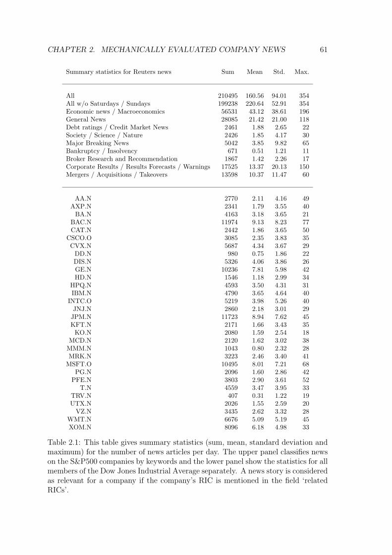
CHAPTER 2. MECHANICALLY EVALUATED COMPANY NEWS 61
Summary statistics for Reuters news Sum Mean Std. Max.
All 210495 160.56 94.01 354All w/o Saturdays / Sundays 199238 220.64 52.91 354Economic news / Macroeconomics 56531 43.12 38.61 196General News 28085 21.42 21.00 118Debt ratings / Credit Market News 2461 1.88 2.65 22Society / Science / Nature 2426 1.85 4.17 30Major Breaking News 5042 3.85 9.82 65Bankruptcy / Insolvency 671 0.51 1.21 11Broker Research and Recommendation 1867 1.42 2.26 17Corporate Results / Results Forecasts / Warnings 17525 13.37 20.13 150Mergers / Acquisitions / Takeovers 13598 10.37 11.47 60
AA.N 2770 2.11 4.16 49AXP.N 2341 1.79 3.55 40
BA.N 4163 3.18 3.65 21BAC.N 11974 9.13 8.23 77CAT.N 2442 1.86 3.65 50
CSCO.O 3085 2.35 3.83 35CVX.N 5687 4.34 3.67 29
DD.N 980 0.75 1.86 22DIS.N 5326 4.06 3.86 26GE.N 10236 7.81 5.98 42HD.N 1546 1.18 2.99 34
HPQ.N 4593 3.50 4.31 31IBM.N 4790 3.65 4.64 40
INTC.O 5219 3.98 5.26 40JNJ.N 2860 2.18 3.01 29
JPM.N 11723 8.94 7.62 45KFT.N 2171 1.66 3.43 35
KO.N 2080 1.59 2.54 18MCD.N 2120 1.62 3.02 38
MMM.N 1043 0.80 2.32 28MRK.N 3223 2.46 3.40 41
MSFT.O 10495 8.01 7.21 68PG.N 2096 1.60 2.86 42
PFE.N 3803 2.90 3.61 52T.N 4559 3.47 3.95 33
TRV.N 407 0.31 1.22 19UTX.N 2026 1.55 2.59 20
VZ.N 3435 2.62 3.32 28WMT.N 6676 5.09 5.19 45XOM.N 8096 6.18 4.98 33
Table 2.1: This table gives summary statistics (sum, mean, standard deviation andmaximum) for the number of news articles per day. The upper panel classifies newson the S&P500 companies by keywords and the lower panel show the statistics for allmembers of the Dow Jones Industrial Average separately. A news story is consideredas relevant for a company if the company’s RIC is mentioned in the field ‘relatedRICs’.
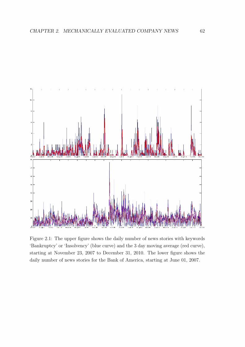
CHAPTER 2. MECHANICALLY EVALUATED COMPANY NEWS 62
Figure 2.1: The upper figure shows the daily number of news stories with keywords
‘Bankruptcy’ or ‘Insolvency’ (blue curve) and the 3 day moving average (red curve),
starting at November 23, 2007 to December 31, 2010. The lower figure shows the
daily number of news stories for the Bank of America, starting at June 01, 2007.

CHAPTER 2. MECHANICALLY EVALUATED COMPANY NEWS 63
2.5 Content Analysis
2.5.1 Variable Construction
According to Groß-Klußmann and Hautsch (2011), the relevance of a news article
for a company determines the strength of the relationship between the sentiment of
the news article and the market. Hence, I start with a narrow definition of relevant
news:
A news article is relevant for a company, if it mentions the company
name or its nickname in the headline and has the company’s RIC in the
field ‘related RICs’.
A broader definition is used for robustness checks. In the following, the term com-
pany name refers to the shortest fraction of the full company name that clearly
identifies the company, e.g. ‘Disney’ instead of ‘Walt Disney Co’ or ‘Conoco’ instead
of ‘ConocoPhillips’. For most companies, I am also able to identify the company’s
nickname very accurately. For example, Bank of America is frequently called BofA,
Johnson & Johnson is called J&J and American Express is AmEx. Texas Instru-
ments, often called TI, and General Electrics, shortened GE, can only be identified
with a small error rate. Synonyms for the company name are not recognized. The
restriction on ‘related RICs’ in the above definition ensures that a news story with
a headline such as ’BofA cuts Google price target ’ is assigned to Google, but not to
Bank of America.
Even though a news article is relevant for a company, it is unlikely that all words in
the full text are important for the company as well. Hence, I define which passages
in the full text of a relevant news story have to be analyzed. I define the relevant
text by:
All words in a sentence are relevant if the company name or nickname
is mentioned within the same sentence.
I test an alternative definition of relevant test in the robustness section.
Given a company, I analyze the content of the relevant text of a relevant news story
and assign a numerical value to it. The approach relies on the ‘General Inquirer’, see
http://www.webuse.umd.edu:9090/. The ‘General Inquirer’ is a dictionary based

CHAPTER 2. MECHANICALLY EVALUATED COMPANY NEWS 64
content analysis algorithm. It assigns words to word categories and reports the
number of hits in each cluster, relative to all analyzed words. There are about 80
word categories. However, I restrict myself to the categories ‘positive’, ‘negative’,
‘strong’ and ‘weak’. Even though being very popular, the ‘General Inquirer’ is
not perfect. Many words have more than one meaning and might be incorrectly
assigned to a word category, see for example Loughran and McDonald (2011), who
test the performance of the ‘General Inquirer’ by analyzing annual and 10-K reports,
and find that a substantial fraction of negative words (about 60%) is misinterpreted.
However, the content of the Reuters news articles is more general than 10-K reports,
hence I expect a low error rate. Moreover, I use the word lists suggested by Loughran
and McDonald for a robustness analysis.
Alternative content analysis algorithms are e.g. Bayesian classifier, vector-distance
classifier and support vector machines, see Das and Chen (2007). However, these
classifiers require a pre-classified training set, which determines the quality of the
classification. Therefore, those classifiers might be subjective and are not consider
here.
Consider, for example, the following news stories:
Feb. 29, 2008, Northrop-EADS beats Boeing to built U.S. tanker
WASHINGTON (Reuters) - The U.S. Air Force said on Friday it had pickeda transatlantic team led by Northrop Grumman, instead of Boeing, to startbuilding a new aerial refueling fleet in a surprise choice worth about $35 bil-lion. Northrop Grumman Corp (NOC.N) and its European partner, Airbusparent EADS (EAD.PA), ”clearly provided the best value to the government,”Sue Payton, the Air Force’s chief weapons buyer, told reporters at a briefing.The contract is to supply up to 179 tanker aircraft in a deal valued at about$35 billion over the next 15 years, the Air Force said in a statement. Theaircraft will replace [...]
Apr. 29, 2009, IBM Q1 rev disappoints, Texas Instruments solid
NEW YORK/BOSTON (Reuters) - IBM disappointed investors on Mon-day with lackluster quarterly revenue, but Texas Instruments afforded themarket some cheer with a solid sales performance. IBM reported a bigger-than-expected 11 percent fall in quarterly sales, showing that even one of thehealthier U.S. technology companies is getting hurt by a slowdown in corpo-rate spending. [...]

CHAPTER 2. MECHANICALLY EVALUATED COMPANY NEWS 65
Clearly, the first news story is rather positive for Northrop and negative for Boeing,
and the second is positive for Texas Instruments and negative for IBM. According
to the ’General Inquirer’ dictionary, the first sentence of the first news article is
neutral. There are several positive words in the second sentence of the first news
story (‘clearly’, ‘provide’, ‘best’). There, Northrop (and EADS, respectively) is men-
tioned, but not Boeing. Hence, the overall sentiment of the (fraction of the) news
article is consistent with our expectations. Now, let us consider the second news
article. Texas Instruments and IBM are both mentioned in the first sentence of the
second news story. Since positive words (e.g. ‘cheer’) are also associated with IBM
and negative words (e.g. ‘disappoint’) with Texas Instruments, the sentiment of the
(fraction of the) news article is the same for both companies, which is counterintu-
itive. In this case, the definition of relevant text might lead to wrong conclusions.
However, the procedure performs very well for simple or well-structured news.
To homogenize market data and news stories, I assign news stories that were released
after 4 p.m. New York time to the following trading day. News stories published
between Friday, 4 p.m. and Monday, 4 p.m. are assigned to Monday. Assume there
are Qi,t ∈ N relevant news stories for company i on day t. Given the relevant text,
let Posi,t,j [Negi,t,j] denote the number of positive [negative] words relative to the
total number of words in the relevant text of news story j = 1, . . . , Qi,t. Then,
the average, relative number of positive words and the average, relative number of
negative words are used to measure positive sentiment, Pi,t, and negative sentiment,
Ni,t, at t and for company i, i.e.
Pi,t = max
1
Qi,t
Qi,t∑j=1
(Pos i,t,j − Neg i,t,j), 0
,
Ni,t = max
1
Qi,t
Qi,t∑j=1
(Neg i,t,j − Pos i,t,j), 0
. (2.2)
Pi,t and Ni,t might be also interpreted as positive and negative public signals in the
style of Harris and Raviv (1993). High values of Pi,t or Ni,t indicate strong signals.
It is likely that there is a monotone relationship between the average net sentiment
of day t, i.e. 1Qi,t
∑Qi,tj=1(Pos i,t,j−Neg i,t,j), and the abnormal stock returns or the CDS
spread, but trading volume and volatility are presumably not monotonically related
to the net sentiment. Therefore, positive and negative sentiment are disentangled.
I do not exclude days without news releases since these days are important as well
and might indicate ‘neutral’ or ‘calm’ days. The sentiment for these days is set to
CHAPTER 2. MECHANICALLY EVALUATED COMPANY NEWS 66
zero.
Furthermore, I define two disagreement scores. If news stories disagree heavily, it
is likely that investors disagree as well. Hence, the degree of difference of opinion
among investors might be well approximated by the variation in the sentiment of
news stories at the same day. I define
Dstdi,t = σ
((Posi,t,j − Negi,t,j)j∈Qi,t
), (2.3)
where σ(·) is the standard deviation. I set Dstdi,t = 0 if Qi,t ≤ 1.
Inspired by Das and Chen (2007), I construct a second measure for disagreement.
Define the auxiliary variable Ai,t,j := 1(Negi,t,j < Posi,t,j) − 1(Negi,t,j > Posi,t,j).
1(·) is the indicator function. It is one if and only if the argument is true. Hence,
Ai,t,j = 1 if the net sentiment of news j is positive, it is zero if Posi,t,j = Negi,t,j and
−1 otherwise. Ai,t,l might be interpreted as buy- or sell-signal. Then, disagreement
is alternatively measured by
Dpoli,t =
max{∑Qi,t
j=1 |Ai,t,j|, 1}
max{∣∣∣∑Qi,t
j=1 Ai,t,j
∣∣∣, 1} . (2.4)
Dpol measures the polarity of (Ai,t,j)j∈Qi,t . If all news stories on day t and for
company i have a positive sentiment or all have a negative sentiment, Dpoli,t = 1.
For days with less than two news stories, I set Dpoli,t = 1, too, which indicates no
disagreement. For all other days, Dpoli,t > 1. D
poli,t is high if there are many news
stories with positive or negative sentiment (numerator is large) and the number
of positive and negative news stories is balanced (denominator is small). These
days might be associated with high disagreement across investors. Whereas Dpoli,t
considers only the variation of the sign of net sentiment within a trading day and
ignores variations the magnitude completely, Dstd is sensitive to variations in the
net sentiment even though the sign of the net sentiment might be the same for all
news stories.
2.5.2 Descriptive Statistics
Table 2.2 shows company-individually the number of days with positive and negative
sentiment and disagreement (#(· > 0)), the conditional means (m(·|· > 0)) and the
conditional standard deviations (σ(·|· > 0)). The cross-sectional mean and standard

CHAPTER 2. MECHANICALLY EVALUATED COMPANY NEWS 67
deviation is given at the bottom of Table 2.2. Disagreement is measured by Dstd.
The companies listed in Table 2.2 are chosen because they have a liquid option and
CDS market. Table 2.8 lists the company names and the RICs. Option data is
available for most companies since June 2008 and determine the beginning of the
joint observation period of market data and news, whereas the CDS spreads are
available until October 2010 and determine the end. With the exception of Intel
Technology (INTC.O) and Travelers Companies (TRV.N), I have 597 days without
missing observations for each company. There are 479 observations for Intel and 660
observations for Travelers.
On average, news stories have a positive tenor. The cross-sectional average number
of days with positive sentiment is 92 and the average number of days with negative
sentiment is 41. The cross-sectional conditional mean of positive sentiment is 3.3174
and of negative sentiment is 2.4194. This gives an average net sentiment of 1.5489
per day with news. Compared to the cross-sectional average sentiment, American
Express Co (AXP.N), American International Group Inc (AIG.N) and Travelers
Companies Inc (TRV.N) have very low average net sentiment. One reason might
be that these companies were hit hard by the financial crisis. For some reasons,
The Boeing Company (BA.N), The Dow Chemical Co (DOW.N) and Fedex Corp
(FDX.N) have low average net sentiment, too. On average, positive and negative
sentiment are correlated by -0.0725, positive sentiment and Dstd are correlated by
0.2613 and negative sentiment and Dstd by 0.1727. The average correlation between
Dpol and P respectively N are almost the same.
Regarding the market variables, the augmented Dicky-Fuller test cannot reject the
unit-root hypothesis for the CDS spread and for the volatility spread for many
companies. Hence, I replace these time series by the corresponding first differences
for all companies to prevent spurious regressions, see Sarwar (2005). ∆V and ∆C
denote the first difference of the volatility spread and the CDS spread, respectively.
εi,t, Ti,t andOi,t are always stationary. The average correlation between the abnormal
return and the change in the volatility spread across all companies is -0.2859. Stock
and option trading volume are on average correlated by 0.3201 and the change in
the volatility spread and the CDS spread are on average correlated by 0.2219. All
other correlations between the market variables are close to zero.

CHAPTER 2. MECHANICALLY EVALUATED COMPANY NEWS 68
RIC #(P
>0)
m(P|P
>0)
σ(P|P
>0)
#(N
>0)
m(N|N
>0)
σ(N|N
>0)
#(D
>0)
m(D|D
>0)
σ(D|D
>0)
AA.N 79 3.2504 2.4254 48 2.7442 2.0826 54 2.4188 2.2592ABT .N 64 2.9495 1.9430 20 2.3062 1.1289 31 1.6257 1.6121AIG.N 173 3.6032 2.3316 136 3.9970 3.0133 209 3.2710 2.1547
AMGN .O 60 2.4562 1.4674 27 1.9520 1.8325 33 1.7816 1.6824APC.N 56 4.2889 2.6812 25 3.7985 2.7814 32 1.8993 1.7249AXP .N 64 3.8703 4.7347 65 3.1979 2.4588 54 2.7427 2.8239BA.N 172 2.3197 1.7603 138 2.4733 2.0844 202 2.0917 1.7702
BAC.N 229 2.6885 2.0884 107 2.4113 2.1768 216 2.2327 1.9952BAX.N 27 3.1350 2.3361 6 1.3261 1.0626 13 2.8396 2.5411BMY .N 68 3.5177 2.1955 20 2.0438 1.6211 43 1.7008 1.7800BSX.N 28 2.4508 1.9893 17 1.3504 0.9238 19 1.9882 2.4059
C.N 302 3.1279 2.0583 99 1.9581 1.6824 276 2.2967 1.6895CAT .N 52 3.0266 1.8953 16 1.7822 1.3524 27 2.1223 2.3512COP .N 130 2.9440 1.5714 84 2.8550 2.0177 103 2.3616 1.5052CSC.N 7 5.2307 3.1978 2 2.8250 2.5809 2 1.8420 0.9650
CSCO.O 120 3.6380 2.6329 19 2.0095 1.6628 73 1.7396 2.1665CVX.N 136 2.7571 2.0611 94 3.0215 1.9161 133 2.1836 1.8328DD.N 42 3.4745 2.2462 23 2.8427 1.9362 21 1.1783 1.1597
DELL.O 99 2.7777 2.1504 42 1.8228 1.7795 78 1.3372 1.3688DIS.N 123 3.1999 2.1781 31 1.9420 1.3118 86 1.3702 1.4605
DOW .N 28 4.2514 2.3947 31 3.9294 2.7804 29 3.1736 2.5388DVN .N 32 3.4291 2.1876 8 1.8642 1.5859 20 2.4095 2.5574
F .N 198 3.0296 2.2643 88 2.4773 2.0080 177 1.6024 1.5340FDX.N 40 2.7887 2.2183 30 3.2106 3.6588 31 2.4819 2.4811GE.N 59 3.8617 2.7574 37 3.0648 1.9041 42 2.3322 1.9647
GLW .N 19 5.2515 3.9589 15 2.6617 3.9609 17 3.2953 3.3540GR.N 20 4.7729 5.7485 2 1.4533 0.5704 8 1.8870 1.7545GS.N 235 2.9275 2.1619 116 2.3064 1.9284 207 2.1838 1.7548HD.N 172 2.1888 4.2864 21 0.1210 0.8923 94 0.6554 2.0871
HON .N 45 3.3022 2.1268 9 2.5706 1.5175 27 1.2727 1.2025HPQ.N 119 3.0873 2.2698 52 2.1668 1.8391 88 2.1268 1.8925IBM .N 138 3.6778 2.9647 37 2.7328 2.5395 111 1.6985 2.2262INTC.O 112 2.9896 2.2001 48 2.2750 1.5690 94 1.8811 1.9041JNJ.N 102 3.1333 2.6229 46 2.8465 2.7153 72 2.1668 1.9909JPM .N 183 2.7744 2.2258 106 2.9178 2.6319 162 2.4532 2.5032KFT .N 94 2.6039 1.6123 14 2.4609 1.9463 82 1.3556 1.1954KO.N 50 3.3672 2.3124 20 5.2119 4.8020 23 3.1491 2.7196LLY .N 56 2.9219 1.7841 25 3.2295 2.9857 33 2.3060 1.8998LMT .N 105 3.5112 2.4568 44 2.1761 1.8434 55 1.6729 1.3771MCD.N 70 3.4556 2.3593 31 2.0148 1.5340 53 1.8974 1.3850MDT .N 38 3.5020 2.7540 21 1.6765 1.1224 32 1.7002 1.7557MO.N 27 2.9978 2.6200 6 1.0153 1.2205 13 1.7484 0.9833
MON .N 65 3.9448 3.6470 30 2.3710 2.2904 35 2.3683 3.0473MMM .N 27 3.5051 2.1892 5 2.2973 0.9381 12 1.4302 1.3572MRK.N 99 3.4270 2.6114 48 2.3156 1.9083 69 2.2193 1.8914MS.N 201 2.8148 2.1083 75 2.4378 1.9433 151 2.1024 1.8497
MSFT .O 226 2.6009 1.6957 72 1.8498 1.4563 212 1.8450 1.5528ORCL.O 70 2.8478 2.2948 51 2.9248 2.5158 65 2.2632 2.4857OXY .N 23 4.5061 3.3075 2 1.3525 0.6824 7 2.1770 1.7105PFE.N 122 3.0920 2.3710 62 2.3397 1.5395 87 1.9404 1.7370PG.N 52 2.5772 1.7435 48 2.2890 1.4934 49 1.8380 1.7458SLB.N 34 3.2163 2.5419 12 2.5346 1.9957 22 1.7485 1.7624
T .N 102 3.0401 1.8108 36 2.0412 1.8221 77 1.2798 1.3578TRV .N 9 1.8596 0.9999 8 3.3083 2.2270 8 2.2566 2.0838TWX.N 75 3.0055 2.1811 21 1.8660 2.7775 59 1.1914 1.5567TXN .N 21 5.6115 4.4692 5 2.4740 1.1307 15 2.6765 1.2774UTX.N 8 5.0200 3.0939 7 3.9548 0.7271 3 1.4775 1.5095V Z.N 121 2.8905 2.0383 26 1.5650 0.8817 76 1.4279 1.4429
WFC.N 84 3.4648 2.4066 54 2.3091 1.6347 62 1.6387 1.5371WMT .N 180 2.7180 2.0239 62 2.6808 2.1770 137 1.7030 1.5085WLP .N 36 3.7594 2.3134 9 1.3725 1.2788 18 1.7603 1.6106XOM .N 160 3.2283 2.1963 89 2.6779 1.9955 149 2.0730 1.6049
Mean 92.0000 3.3174 2.4561 41.0000 2.4194 1.9093 72.0000 1.9982 1.8539Std. 66.7503 0.7475 0.8025 34.5148 0.8016 0.7851 64.6547 0.5301 0.4964
Table 2.2: The table shows the number of days with positive sentiment (first col-umn), negative sentiment (fourth column) and disagreement (seventh column) com-pany individually. Moreover, it gives the conditional mean of positive and negativesentiment and disagreement and the standard deviations. Disagreement is measuredby Dstd. The last two rows show the cross-sectional mean and standard deviation.
CHAPTER 2. MECHANICALLY EVALUATED COMPANY NEWS 69
2.6 Regression Results
2.6.1 Contemporaneous Analysis
I analyze the contemporaneous relationship between the financial market and sen-
timent, respectively disagreement. This analysis is motivated by the literature on
difference of opinion and extends Das et al. (2005). It allows testing Hypotheses 2
to 5 on the co-movement of market variables and public signals and the degree of
difference of opinion, respectively. The analysis does not allow to conclude on mar-
ket efficiency and the predictability of market returns. Even though the news stories
are unscheduled, a significant relationship between sentiment or disagreement and
market returns on a daily frequency might be consistent with efficient markets if the
market anticipates the news.
Company Individual Analysis
As shown in Blume, Easley and O’Hara (1994), volatility and historical stock prices
might be valuable information for future stock returns. Pan and Poteshman (2006)
document that option trading contains relevant information for stock returns, too,
and according to Sarwar (2006) and Kyriacou and Sarno (1999), option trading
volume and volatility interact. Cremers et al. (2008) report a significant relationship
between equity markets and credit markets. Chordia, Sarkar and Subrahmanyam
(2005) study the intertemporal association between liquidity, volatility and returns
by applying a vector autoregressive model. Also, the difference of opinion literature
implies positive autocorrelation in trading volume and negative autocorrelation in
returns. To control for these associations and to determine the relationship between
the financial market and sentiment and disagreement, respectively, accurately, I
choose the most parsimonious regression model that allows for the aforementioned
patterns, a vector autoregressive process with one lag. I estimate[εi,t Ti,t ∆Vi,t Oi,t ∆Ci,t
]′(2.5)
= Λi
[εi,t−1 Ti,t−1 ∆Vi,t−1 Oi,t−1 ∆Ci,t−1
]′+ βi[Pi,t Ni,t Di,t]
′ +KiUt + ηi,t.
D stands for the disagreement score and refers to Dstd or Dpol. Λi is a 5× 5 matrix
and captures possible inter-temporal associations between the abnormal returns,
trading volume in the stock and stock options, and the change in the volatility
CHAPTER 2. MECHANICALLY EVALUATED COMPANY NEWS 70
spread and the CDS spread, respectively. βi is a 5 × 3 matrix and measures the
associations between the market and sentiment and disagreement, respectively. Ut
is 5 × 1 vector with weekday dummies and Ki’s dimension is 5 × 5. ηi,t is a white
noise vector.
Tables 2.3 show the - at the 10% confidence level - significant estimates for βi.
The first entry in a filed gives the impact of positive sentiment, the second entry
corresponds to the impact of negative sentiment and the third to disagreement
(Dstd). Insignificant coefficients are replaced by the symbol ‘/’. Single underlined
coefficients are significant at the 5% level and double underlined coefficients at the
1% confidence level. The lower panel of Table 2.3 gives the number of significant,
positive and significant, negative regression coefficients and the number of companies
for which positive and negative sentiment and disagreement are jointly insignificant.
I do not show the regression estimates for Λi and Ki.
Positive sentiment and negative sentiment are frequently significant for the FF
residuum. Often, the coefficient of positive sentiment is significant, positive (for
14 companies out of 62) and the coefficient of negative sentiment is significant, neg-
ative (for 14 companies), indicating that positive news are associated with positive
abnormal returns and negative news with negative abnormal returns. This suggests
that the General Inquirer and the relevant text identification procedure approxi-
mate the ‘true’ sentiment or the public company signal accurately. Disagreement
is frequently significant, but the sign of the significant coefficients varies among
companies. There are 9 significant, positive coefficients and 10 significant, negative
coefficients. Hence, the dominant effect of disagreement in the cross section is am-
biguous. The average R2 of model (2.5) across all companies with respect to the
abnormal return is 4.57%. Compared to an average R2 of 2.99% in regression model
(2.5) and omitting βi[Pi,tNi,tDi,t], positive and negative sentiment and disagreement
account on average for 1.58 percentage points in R2. This significant increase by
more than 50% is exclusively due to the content analysis and highlights its accuracy.
The average R2 of regression model (2.5) with respect to stock trading volume is
38.48% and the average R2 of (2.5) and without the regressors [Pi,tNi,tDi,t] is 34.92%,
indicating that the content analysis adds about 4 percentage points. Regarding
option trading volume, the average R2 increases from 15.43% without the content
analysis to 16.46%. To test Hypothesis 2, I use positive sentiment and negative
sentiment to approximate the public signal’s intensity and study its co-movement
with the trading volume on the same day. The coefficient of positive sentiment

CHAPTER 2. MECHANICALLY EVALUATED COMPANY NEWS 71
ε T ∆V O ∆C
AA.N 0.0017;−0.0035;/ /;−0.0356;0.1077 /;0.0088;/ 0.0343;−0.0501;0.0469 /;2.9180;/
ABT .N /;/;−0.0022 0.0249;/;0.0682 /;/;/ /;/;/ /;/;/AIG.N /;/;/ /;−0.0327;0.0653 /;/;/ /;/;0.0437 /;/;/
AMGN .O /;/;0.0085 /;0.1162;0.2571 /;0.0048;−0.0051 0.0773;0.1479;0.1350 /;0.3611;−0.6805
APC.N /;−0.0030;/ /;/;0.1083 /;0.0050;/ /;0.0395;/ /;3.0280;/
AXP .N /;/;/ /;/;0.0749 /;/;/ 0.0285;/;0.0277 /;2.1222;/
BA.N /;/;−0.0018 /;/;0.0514 /;/;0.0013 /;/;/ /;/;/
BAC.N /;/;/ /;/;0.0628 /;/;/ /;/;0.0367 /;/;/
BAX.N /;−0.0240;−0.0024 /;1.2724;0.3327 /;0.0108;/ /;/;0.2572 /;/;/
BMY .N 0.0010;/;/ 0.0273;/;/ /;−0.0025;/ /;/;/ −0.0914;/;/BSX.N /;/;−0.0124 /;0.7366;0.3925 /;/;0.0169 /;/;/ /;/;3.3971
C.N /;/;/ /;/;0.0515 −0.0038;/;/ /;/;0.0234 /;/;/CAT .N 0.0031;/;/ 0.0587;/;0.1059 /;/;/ /;/;/ −0.6997;/;/
COP .N /;/;/ /;/;0.0207 /;/;/ /;/;/ /;−0.1752;0.2143CSC.N /;0.0091;0.0128 /;0.1801;0.3420 /;−0.0080;0.0217 /;/;/ /;/;7.2457
CSCO.O /;/;−0.0013 /;0.0783;0.0349 /;/;/ /;0.0588;/ −0.1287;/;/
CVX.N −0.0006;/;0.0008 /;/;/ /;/;/ /;/;/ /;/;/DD.N /;/;/ /;0.0323;0.1190 /;/;/ /;/;/ /;1.8261;/
DELL.O /;−0.0045;/ /;0.0706;0.0898 /;/;/ 0.0468;/;0.1456 /;0.5376;/
DIS.N /;−0.0024;0.0017 /;/;0.0797 /;/;/ /;/;/ /;/;−0.3150
DOW .N /;/;/ /;/;0.2729 /;/;/ /;/;0.1078 /;/;/
DVN .N /;−0.0088;0.0061 /;/;0.0848 /;0.0220;/ /;/;0.1263 /;/;/
F .N /;/;/ 0.0268;/;0.0440 /;/;/ /;/;0.0411 /;/;/
FDX.N 0.0040;/;−0.0029 0.0758;/;0.2532 /;/;/ 0.1048;/;0.0986 −0.5887;/;0.9380
GE.N /;/;0.0021 0.0266;0.0529;/ 0.0033;/;−0.0058 /;/;/ /;/;/
GLW .N 0.0018;−0.0073;/ 0.0226;0.2269;0.0610 /;/;/ 0.0625;/;/ /;/;/
GR.N −0.0015;0.0159;0.0096 0.1334;/;0.3587 /;/;/ 0.0872;1.4221;0.4344 −0.2023;/;/
GS.N /;−0.0019;/ /;0.0480;/ /;0.0034;/ /;0.0338;/ /;/;1.0095HD.N 0.0004;/;/ 0.0007;0.0291;0.0395 /;/;/ 0.0130;/;0.0425 /;/;/
HON .N /;/;/ 0.0282;/;0.0832 /;/;−0.0046 /;/;/ /;/;/HPQ.N 0.0010;−0.0022;/ /;0.0652;0.0813 0.0012;/;−0.0025 /;0.0419;0.0591 0.2170;0.3178;/
IBM .N /;/;/ /;/;0.0592 /;0.0014;/ /;/;0.0982 /;/;/
INTC.O /;/;/ /;/;0.0745 /;/;/ /;/;0.0864 /;−0.7197;0.2383
JNJ.N /;/;/ 0.0196;/;0.0272 0.0009;/;/ /;/;/ /;/;/JPM .N 0.0010;/;−0.0010 /;/;/ /;0.0032;/ /;/;/ /;/;/KFT .N /;−0.0019;/ /;/;/ /;/;/ /;/;/ /;/;/KO.N 0.0009;/;/ 0.0328;/;0.0599 /;/;−0.0022 /;/;/ /;/;/
LLY .N −0.0013;/;/ /;/;0.0413 /;/;/ /;/;/ /;/;0.2304
LMT .N /;/;/ /;/;0.0861 −0.0008;/;/ 0.0413;/;/ /;/;/
MCD.N 0.0010;/;/ 0.0310;/;0.0846 /;/;/ /;/;/ /;/;/
MDT .N /;/;−0.0045 /;0.1235;0.2090 /;0.0051;/ /;/;/ /;/;/
MO.N /;/;−0.0033 /;/;0.1571 −0.0022;/;/ /;/;/ /;/;/
MON .N 0.0010;/;/ /;/;0.0819 /;/;/ /;/;0.0666 /;/;/
MMM .N 0.0022;/;/ 0.0532;/;0.1856 /;/;/ /;/;0.3179 /;/;0.6947
MRK.N /;−0.0023;/ 0.0282;/;0.0479 /;/;0.0019 /;/;/ /;/;/
MS.N /;−0.0028;/ /;/;/ −0.0036;/;/ 0.0259;/;/ /;/;/MSFT .O /;/;/ /;/;0.0423 /;/;/ /;−0.0615;/ /;/;/
ORCL.O /;/;/ 0.0599;/;/ /;/;/ 0.0971;/;/ /;/;/
OXY .N /;/;/ /;/;/ /;/;/ 0.0324;/;0.1249 0.2416;/;/PFE.N /;/;/ /;/;0.0358 /;/;/ /;/;/ /;/;0.3807
PG.N /;/;/ 0.0289;/;0.0588 /;−0.0023;/ /;−0.1008;0.1997 /;/;/
SLB.N −0.0018;/;0.0064 /;/;0.0920 /;0.0084;−0.0071 /;/;0.0708 /;0.5508;−0.8166
T .N /;/;/ /;/;0.0526 /;/;/ /;/;/ /;/;0.5071
TRV .N 0.0105;0.0075;−0.0081 0.1612;/;/ −0.0140;/;/ /;/;/ /;/;/
TWX.N /;/;/ /;/;/ /;/;/ /;/;/ /;/;/TXN .N /;/;/ /;/;0.2319 /;/;/ /;/;0.2729 /;4.5247;/
UTX.N 0.0021;/;/ /;/;/ /;/;/ /;/;/ /;/;/
V Z.N /;/;0.0019 /;/;0.0550 /;/;/ /;/;/ /;/;/
WFC.N /;−0.0033;/ 0.0387;0.0730;0.1155 −0.0066;/;/ /;/;0.0590 /;/;/
WMT .N /;−0.0012;/ /;/;0.0763 /;0.0016;−0.0014 /;/;0.3018 /;/;/
WLP .N /;/;/ 0.0387;/;0.1351 /;/;/ /;/;/ 0.4564;/;1.1201
XOM .N /;/;/ /;/;/ /;/;/ /;/;/ /;/;/
+ & sig. 14;3;9 20;13;50 3;11;4 12;6;24 3;9;11− & sig. 4;14;10 0;2;0 6;3;7 0;2;0 5;2;3All insig. 23 8 34 29 36
Table 2.3: The table shows the - at the 10% confidence level significant - company-individual regression coefficients for positive sentiment (first entry), negative sen-timent (second entry) and disagreement, measured by Dstd, (third entry) on themarket variables. Single [double] underlined coefficients are significant at the 5%[10%] confidence level. The last three rows show the number of significant, positiveand significant, negative regression coefficients and the number of companies wherepositive and negative sentiment and disagreement are jointly insignificant.

CHAPTER 2. MECHANICALLY EVALUATED COMPANY NEWS 72
is significant, positive for stock trading volume for 20 out of 62 companies. The
coefficient of negative sentiment is significant, positive for 13 companies. Option
trading volume shows similar patterns. Therefore, the signal’s intensity seems to be
positively related to trading volume, as stated in Hypothesis 2.
Hypothesis 3 relates stock and option trading volume to disagreement. High dis-
agreement is associated with significantly higher stock trading volume for 50 compa-
nies out of 62. There is no company with a significant, negative regression coefficient.
Regarding the relationship between option trading volume and disagreement, I find
23 positive and significant relationships out of 62 companies. Hence, I have very
strong support for Hypotheses 3. Investors seem to trade on public signals and
disagreement accelerates trading volume.
The relationship between the volatility spread and disagreement is ambiguous. The
number of significant regression coefficients is small, and the number of significant,
negative and significant, positive regression coefficients is almost balanced. Hence,
it is infeasible to draw robust conclusions on the relationship between volatility and
disagreement. However, Table 2.3 indicates that the volatility spread widens at days
with negative sentiment (11 positive and significant coefficients). This finding is con-
sistent with evidence on negative correlation between index returns and volatility,
since days with negative sentiment are also associated with negative abnormal re-
turns. The average R2 of the full regression model with respect to the change in the
volatility spread is 6.80% and the contribution of the content analysis in terms of
average R2 is 1.13 percentage points. Nevertheless, Hypothesis 4 is not supported.
The change in the CDS spread is often significantly negatively correlated with pos-
itive sentiment and positively correlated with negative sentiment. This is econom-
ically reasonable and consistent with the relationship between abnormal stock re-
turns and sentiment, and with the relationship between the volatility spread and
sentiment. The coefficient of disagreement is often significant and positive, which
is consistent with Hypothesis 5, even though Hypothesis 4 is not supported. The
content analysis increases the average R2 of the change in the CDS spread from
5.91% to 7.11%.
Most results remain qualitatively unchanged if I consider Dpol as a measure of dis-
agreement instead of Dstd. Therefore, the results are not shown. A change worth
mentioning is that the relationship between disagreement and abnormal stock re-
turns is more often significant, negative. This is consistent with Yu (2011), who
shows that stocks with high analyst forecast dispersion, which might be another
CHAPTER 2. MECHANICALLY EVALUATED COMPANY NEWS 73
measure of disagreement, underperform relative to stocks with low forecast disper-
sion. Perhaps as a consequence, the CDS spread increases with Dpol for many
companies even though the volatility might not go up.
Pooled Analysis
Next, I analyze all companies jointly. The purpose of this analysis is to investi-
gate the dominant relationship between the financial market and sentiment and
disagreement, respectively, for all companies. It also simplifies the interpretation of
the regression coefficients. I estimate[sεi,t sTi,t s∆Vi,t sOi,t s∆Ci,t
]′(2.6)
= Λ[sεi,t−1 sTi,t−1 s∆Vi,t−1 sOi,t−1 s∆Ci,t−1
]′+ β[sPi,t sNi,t sDi,t]
′ +KUt + ηi,t.
The prefix s denotes standardized time series. The regression coefficients Λ, β and K
are now independent of the company index i. Hence, I make the strong assumption
that the relationships between the (standardized) market variables, measured by
Λ, and between the market variables and the information extracted from company
news, measured by β, are described by the same coefficients for all companies. Λ, β
and K are estimated by
{Λ, β, K} = argminΛ,β,K
{11×G
([sε sT s∆V sO s∆C] (2.7)
− [sε−1 sT−1 s∆V−1 sO−1 s∆C−1] Λ− [sP sN sD] β − UK)2
15×1
},
where, as an example, the vectors sT and sT−1 are given by
sT−1 =
[[T1,t −m(T1,·)
σ(T1,·)
]t=1,...,G1−1
, . . . ,
[TL,t −m(TL,·)
σ(TL,·)
]t=1,...,GL−1
]′and
sT =
[[T1,t −m(T1,·)
σ(T1,·)
]t=2,...,G1
, . . . ,
[TL,t −m(TL,·)
σ(TL,·)
]t=2,...,GL
]′.
m(·) denotes the mean, σ(·) is the standard deviation, L is the number of companies
and Gi is the number of observations for company i. G =∑L
i=1(Gi − 1), 1a×b is
a matrix of dimension a × b with 1s everywhere and U is the pooled matrix of
weekday dummies. The square symbol in (2.7) refers to each component in the
vector of residuals.

CHAPTER 2. MECHANICALLY EVALUATED COMPANY NEWS 74
Pooling all observations gives in total 36,229 company-day observations. Table 2.4
shows Λ, β and K. In the upper panel, disagreement is measured by Dstd and
in the lower panel by Dpol. The regression estimates of Λ and K are similar for
both approaches. Stock trading volume displays positive autocorrelation, which is
consistent with the models of Harris and Raviv (1993) and Banerjee and Kremer
(2010). Furthermore, there are several patterns, which are consistent with informa-
tion asymmetry. Trading volume predicts abnormal stock returns, as discussed in
Blume, Easley and O’Hara (1994). Also option trading volume predicts abnormal
returns, which might be related to the result of Pan and Poteshman (2006), even
though I do not study the ratio of traded put and call options, but the sum.
Large abnormal stock returns, strong increases in the volatility spread or the CDS
spread and high option trading volume predict high stock trading volume. These
findings are consistent with Barber and Odean (2008), who study attention-grabbing
stocks, amongst others defined by stocks with large stock price movements, and find
that these stocks have a higher turnover volume than stocks that do not attract
attention. However, attention might also be gained by strong increases in the CDS
spread or in the volatility spread. Consistent with structure models on credit deriva-
tives, the CDS spread increases given an increase in volatility. Surprisingly, it also
tends to increase given a positive abnormal return. The weekday dummies are fre-
quently significant, indicating the presence of weekday effects.
Positive and negative sentiment are highly significant for abnormal returns. Consis-
tent with the results in the previous section, positive sentiment is positively related
to abnormal returns and negative sentiment negatively. The coefficient of Dstd is
insignificant, see upper panel. This does not necessarily mean that disagreement
is not relevant for the abnormal return. The insignificance might be rather due
to the heterogeneous relationship between stock returns and disagreement among
news articles, e.g. Table 2.3 shows 9 significant, positive and 10 significant, negative
relationships. Hence, both effects are likely to cancel out in the pooled regression.
Furthermore, the alternative disagreement score Dpol detects a significant, negative
relationship between abnormal returns and disagreement, see Table 2.4, lower panel.
This is consistent with Yu (2011).
The R2s in Table 2.4 with respect to the abnormal return are lower than the average
R2 of the firm individual regression analysis. So, the R2 of sε is 0.4% and 0.51%,
respectively, whereas the average R2 of εi in (2.5) is 4.57%. This decrease might be
due to the restrictive assumption of identical regression coefficients for all compa-

CHAPTER 2. MECHANICALLY EVALUATED COMPANY NEWS 75
Pooled Analysis -Contemporaneous sε sT s∆V sO s∆C
sε−1 −0.0010 0.0088b −0.0034 0.0063 0.0151a
sT−1 0.0221a 0.5380a −0.0528a 0.0854a −0.0049s∆V−1 0.0349a 0.0734a −0.1591a 0.0184a 0.1232a
sO−1 −0.0190a 0.0262a 0.0037 0.2701a −0.0163a
s∆C−1 −0.0082 0.0274a 0.0035 −0.0018 0.0876a
sP 0.0273a 0.0455a −0.0111a 0.0237a −0.0069sN −0.0321a 0.0374a 0.0128a 0.0088c 0.0194a
sDstd 0.0008 0.1187a −0.0058 0.0599a 0.0142a
Monday 0.0493a −0.2202a 0.1149a −0.0089 −0.1259a
Tuesday 0.0349b 0.0616a −0.0621a 0.0489a −0.1059a
Wednesday −0.0085 −0.0541a 0.0538a −0.0091 −0.0880a
Thursday 0.0203 0.0095 0.1196a 0.0184 −0.0408b
Constant −0.0199 0.0387a −0.0445a −0.0097 0.0713a
R2 0.0041 0.3499 0.0340 0.1067 0.0297
sε−1 −0.0017 0.0103b −0.0033 0.0063 0.0159a
sT−1 0.0237a 0.5345a −0.0522a 0.0849a −0.0043s∆V−1 0.0353a 0.0731a −0.1605a 0.0175a 0.1220a
sO−1 −0.0169a 0.0228a 0.0044 0.2683a −0.0159a
s∆C−1 −0.0077 0.0250a 0.0046 −0.0034 0.0870a
sP 0.0429a 0.0124a −0.0075 0.0016 −0.0125b
sN −0.0146b −0.0137a 0.0176a −0.0230a 0.0115b
sDpol −0.0388a 0.1650a −0.0131b 0.0969a 0.0237a
Monday 0.0472a −0.2201a 0.1138a −0.0120 −0.1259a
Tuesday 0.0359b 0.0568a −0.0616a 0.0454a −0.1043a
Wednesday −0.0058 −0.0561a 0.0528a −0.0119 −0.0893a
Thursday 0.0206 0.0091 0.1199a 0.0170 −0.0416b
Constant −0.0194 0.0402a −0.0443a −0.0076 0.0716a
R2 0.0051 0.3552 0.0341 0.1097 0.0299
#Obs. 36229 36229 36229 36229 36229
Table 2.4: The table shows the regression estimates for Λ, β and K in the pooledregression model, allowing for a contemporaneous relationships between the marketvariables and sentiment and disagreement, respectively, i.e. regression model (2.6).The upper panel measures disagreement with sDstd and the lower panel with sDpol.a denotes significance at the 1% confidence level, b at the 5% confidence level and cat the 10% level.
CHAPTER 2. MECHANICALLY EVALUATED COMPANY NEWS 76
nies. However, the contribution of the content analysis to the R2 of sε is about 0.2
percentage point and doubles the explained variation in abnormal returns.
The average R2 of stock trading volume and allowing for company individual re-
gression coefficients is 38.48% and reduces in the pooled analysis to 34.99% and
35.52%, respectively. The R2 of standardized option trading volume is 10.67% and
10.97%, respectively, whereas the average R2 of the company individual analysis
about 16.46%. These rather moderate decreases in the R2s indicate that the as-
sumption of identical regression coefficients is not too restrictive for trading volume.
The contribution of the text analysis to the R2 is about 3 percentage points for stock
trading volume and about 0.65 percentage points for option trading volume.
In the upper panel, standardized stock and option trading volume increase with
positive and negative sentiment and disagreement. The relationships are highly
significant and consistent with the company individual analysis and Hypotheses 2
and 3. Surprisingly, the coefficient of negative sentiment turns significant, negative
for trading volume if disagreement is measured by Dpol, see the lower panel of Table
2.4. As argued by Barber and Odean (2008), investment restrictions, or liquidity
dry-ups subsequent to negative news during the financial crisis, might explain the
fragile relationship between negative sentiment and trading volume.
The volatility spread narrows with positive sentiment and it increases with negative
sentiment. However, the estimated relationship between the volatility spread and
disagreement is still inconclusive. Whereas the coefficient of Dstd is insignificant in
the upper panel of Table 2.4, the coefficient of Dpol is weakly significant and nega-
tive. Both results are inconsistent with Hypothesis 4. Nevertheless, and consistent
with Hypothesis 5, the CDS spread increases with disagreement. As argued before,
this increase is presumably due to the decrease in the market value, given high dis-
agreement, and not due to an increase in the equity volatility and asset volatility,
respectively. Moreover, the CDS spread increases with negative sentiment and, at
least in the lower panel of Table 2.4, decreases with positive sentiment.
2.6.2 Predicting Market Activity
Now, I use the pooled regression model to study the predictive power of senti-
ment and disagreement. Hence, I do not analyze the contemporaneous relationship
between market activity and sentiment and disagreement, respectively, but the re-
lationship between the market and sentiment and disagreement from the previous
CHAPTER 2. MECHANICALLY EVALUATED COMPANY NEWS 77
trading day. Hence, the regression model changes to[sεi,t sTi,t s∆Vi,t sOi,t s∆Ci,t
]′= Λ
[sεi,t−1 sTi,t−1 s∆Vi,t−1 sOi,t−1 s∆Ci,t−1
]′+ β[sPi,t−1 sNi,t−1 sDi,t−1]′ +KUt + ηi,t. (2.8)
Now, the residual in the objective function (2.7) is[sε sT s∆V sO s∆C
]−[sε−1 sT−1 s∆V−1 sO−1 s∆C−1
]Λ
−[sP−1 sN−1 sD−1
]β − UK. (2.9)
Table 2.5 shows the regression estimates for Λ, β and K. Again, the results in the
upper panel are based on the disagreement measure Dstd and the results in the lower
panel are based on Dpol. The estimates for Λ and for K are very similar compared
to the contemporaneous analysis. However, the R2s decrease. Positive sentiment is
still highly significant and predicts positive abnormal returns on the following day.
Both disagreement measures predict negative abnormal returns on the following
trading day. Negative sentiment is insignificant. However, the relationship between
abnormal stock returns and positive sentiment and disagreement, respectively, are
still unexpected and might be inconsistent with Hypothesis 1. Assuming efficient
markets, prices should respond to new information immediately. However, the sig-
nificance of lagged positive sentiment and lagged disagreement - even on a daily
frequency - hints towards market inefficiencies. These results become even stronger
if I consider excess stock returns instead of abnormal stock returns. Then, positive
sentiment is significant, positive and negative sentiment is significant, negative. Dis-
agreement is almost significant at the 10% confidence level.3 The R2 of the excess
return in (2.8) increases to 1.16%. The others estimates do not change significantly.
The volatility spread increases significantly after negative sentiment and after dis-
agreement, measured by Dstd. Dpol is insignificant. Compared to the contem-
poraneous relationship between disagreement and the volatility spread, which is
inconclusive, the result for the one-day lagged Dstd is more consistent with Hypoth-
esis 4. The delayed response of the volatility spread could be due to a rather slow
information processing and might also hint towards market inefficiencies.
I find no significant relationship between the change in the CDS spread and the
one-day lagged sentiment. In the lower panel, the p-value of disagreement with
3Consider that disagreement is measured by Dstd. Then, the estimates of β in regression model(2.8) and using excess stock returns instead of abnormal stock returns is (0.0135,−0.0133,−0.0085)with p-values (0.0139, 0.0127, 0.1292). If disagreement is measured by Dpol, the estimate is(0.0145,−0.0112,−0.0085) with p-values (0.0132, 0.0613, 0.1972).

CHAPTER 2. MECHANICALLY EVALUATED COMPANY NEWS 78
Pooled Analysis -Predictive sε sT s∆V sO s∆C
sε−1 −0.0005 0.0079c −0.0028 0.0054 0.0155a
sT−1 0.0239a 0.5475a −0.0548a 0.0910a −0.0044s∆V−1 0.0347a 0.0751a −0.1605a 0.0187a 0.1224a
sO−1 −0.0182a 0.0350a 0.0033 0.2749a −0.0147a
s∆C−1 −0.0081 0.0272a 0.0041 −0.0022 0.0871a
sP−1 0.0105a 0.0093b −0.0058 0.0043 −0.0011sN−1 −0.0042 −0.0027 0.0149a 0.0070 0.0074sDstd
−1 −0.0163a −0.0248a 0.0097c −0.0104a 0.0071
Monday 0.0501a −0.2338a 0.1152a −0.0190 −0.1275a
Tuesday 0.0342b 0.0687a −0.0615a 0.0524a −0.1021a
Wednesday −0.0064 −0.0366a 0.0513a −0.0013 −0.0874a
Thursday 0.0200 0.0248c 0.1189a 0.0252 −0.0401b
Constant −0.0196 0.0331a −0.0440a −0.0116 0.0707a
R2 0.0025 0.3291 0.0340 0.1018 0.0291
sε−1 −0.0010 0.0069 −0.0026 0.0052 0.0154a
sT−1 0.0242a 0.5487a −0.0544a 0.0906a −0.0033s∆V−1 0.0345a 0.0746a −0.1605a 0.0187a 0.1222a
sO−1 −0.0179a 0.0356a 0.0033 0.2749a −0.0144a
s∆C−1 −0.0080 0.0275a 0.0041 −0.0022 0.0872a
sP−1 0.0131b 0.0151a −0.0055 0.0042 0.0015sN−1 0.0007 0.0067 0.0142b 0.0082 0.0096sDpol
−1 −0.0179a −0.0319a 0.0058 −0.0069 −0.0020
Monday 0.0500 −0.2342a 0.1150a −0.0188 −0.1279a
Tuesday 0.0337b 0.0676a −0.0616a 0.0524 −0.1026a
Wednesday −0.0064 −0.0367a 0.0513a −0.0012 −0.0874a
Thursday 0.0201 0.0251b 0.1189a 0.0252 −0.0399a
Constant −0.0193 0.0334a −0.0440a −0.0116 0.0708a
R2 0.0025 0.3292 0.0340 0.1017 0.0291
#Obs. 36229 36229 36229 36229 36229
Table 2.5: The table shows the regression estimates for Λ, β and K in the pooledregression model without contemporaneous relationships, i.e. (2.8). Hence, all ex-planatory variables are lagged by one day. The upper panel measures disagreementwith sDstd and the lower panel with sDpol. a denotes significance at the 1% confi-dence level, b at the 5% confidence level and c at the 10% level.

CHAPTER 2. MECHANICALLY EVALUATED COMPANY NEWS 79
respect to ∆C is 0.1066, indicating - at best - a weak, positive relationship between
disagreement and CDS spreads. Hence, the credit market seems to be efficient
with respect to the information extracted from Reuters company news and in this
framework. However, the company individual analysis (the results are not shown)
indicates that negative sentiment and disagreement predict the change in the CDS
spread for several companies.
Furthermore, positive sentiment predicts stock trading volume on the following day,
indicating that positive signals have a long-lasting impact on trading volume. How-
ever, negative sentiment is insignificant. This heterogeneity might be due to in-
vestment restrictions, see Barber and Odean (2008). Surprisingly, the regression
coefficients of both disagreement measures are significantly negative. One explana-
tion might be that investors execute orders, which are scheduled to the following
day, immediately, given disagreement. Then, the stock trading volume might be
lower after days with disagreement.
2.6.3 Robustness
As a robustness check, I weight sentiment with uncertainty. Uncertainty is measured
with two approaches. (1) Uncertainty in news articles might be measured with
the ‘General Inquirer’ word categories ‘strong’ and ‘weak’. However, there is a
substantial overlap between the categories ‘positive’ and ‘strong’, and ‘negative’
and ‘weak’. This might bias the results. Nevertheless, I measure the uncertainty of
a news article by
H(1)i,t,j =
Zi,t,j + ϑ
Wi,t,j + Zi,t,j + 2ϑ,
where Zi,t,j denotes the number of strong words and Wi,t,j is the number of weak
words in the relevant text of news article j. ϑ is a small, positive constant that
ensures the existence of Hi,t,j even though there are neither strong nor weak words.
Then, Hi,t,j = 0.5. If there are only strong words, Hi,t,j ≈ 1 and if there are only
weak words Hi,t,j is close to zero. (2) Alternatively, if the author of a news article
uses many positive and negative words in the relevant text of a company, she might
discuss positive and negative scenarios, which indicates that she is unsure about the
final consequences. Therefore, uncertainty is measured by
H(2)i,t,j =
|Pos i,t,j − Neg i,t,j|max{Pos i,t,j + Neg i,t,j, ϑ}
.

CHAPTER 2. MECHANICALLY EVALUATED COMPANY NEWS 80
If positive and negative words are almost balanced, H(2)i,t,j is close to zero. If either
positive words clearly dominate negative words or negative words clearly dominate
positive words, H(2)i,t,j is close to 1. ϑ is again a small, positive constant.
Now, by multiplying the net sentiment, i.e. Posi,t,j −Negi,t,j, in (2.2) with H(1)i,t,j or
H(2)i,t,j, the uncertainty that is related to a news article might be taken into account.
All previously discussed results are robust against the uncertainty adjustment and
remain qualitatively the same. For the sake of brevity, the results are not shown.
Moreover, I use a broader definition to identify relevant news stories for a company,
i.e. I consider all news stories as relevant if the company’s RIC appears in the
field ‘related RICs’. Hence, the company name or nickname is not required to
be mentioned in the headline. As before, all sentences that mention the company
name, the nickname or ticker symbol are analyzed. The results are consistent with
the previously discussed findings and are not shown.
To investigate the robustness of the results with respect to the definition of relevant
text, I consider all words with a distance of at most 5 words to the company name,
nickname or ticker symbol as relevant. Words that contain numerical expressions
(e.g. ‘B330-200’, ‘$35’) are not counted for the word distance. This approach is sen-
sitive to changes in the sentiment within a sentence. Most results stay quantitatively
the same.
I use the financial word lists suggested by Loughran and McDonald (2011), see http:
//www.nd.edu/~mcdonald/Word_Lists.html, and the Porter word stemmer algo-
rithm, see http://tartarus.org/~martin/PorterStemmer/index.html, to mea-
sure positive and negative sentiment and disagreement with an alternative classifier.
These lists might account for specialties of financial text more accurately than the
General Inquirer. Pi,t, Ni,t, Dstd and Dpol are calculated according to equations
(2.2), (2.3) and (2.4), but Posi,t, and Negi,t,j are now the number of hits in the
positive and the negative word list of Loughran and McDonald. The results for
regression model (2.6) are comparable to the estimates in Table 2.4 and indicate a
strong contemporaneous relationship between company news and the financial mar-
ket. However, the one-day lagged sentiment in regression model (2.8) is insignificant
with respect to all market variables. This puzzling result might indicate that the
financial word lists are too restrictive to analyze general company news.

CHAPTER 2. MECHANICALLY EVALUATED COMPANY NEWS 81
2.7 Trading Strategies
According to the previous sections, positive sentiment and disagreement are statis-
tically significant to predict abnormal stock returns and excess returns. However,
this does not allow to conclude on the economic significance of sentiment and on
market efficiency. Therefore, I study trading strategies based on positive and neg-
ative sentiment to gain insights on the economic relevance of news articles for the
stock market.
Assume that an investor trades the previously considered 62 stocks simultaneously.
The investor has no initial endowment. She observes the signals
Xi,t = 1(Pi,t > Ni,t)− 1(Pi,t < Ni,t).
Xi,t can take on the value +1, 0 and −1. Xi,t = 1 might be interpreted as a long-
signal and Xi,t = −1 as a short-signal. Xi,t = 0 might indicate a neutral position.4
I assume that Xi,t is observed at 4 p.m. New York time, even though news stories
might be published much earlier, which might give insights on the value of Xi,t.
This conservative assumption implies a delayed investment decision as a response
to news stories, and rules out intraday trading, such as algorithmic trading.
Whenever Xi,t = 1, the investor borrows one USD at the risk-free rate and purchases
(a fraction of) stock i at the closing price at day t. At the following day, the stock
is sold at the closing price of day t+ 1 and the loan is repaid, if the signal changes
to neutral or to sell. Otherwise, the position is not closed until the long-signal
disappears. If Xi,t changes to −1, the investor short-sells one USD in stock i,
invests this one USD at the risk-free rate Rf and holds the position until the signal
disappears. Profits and losses, due to trading, are collected in her money account,
which is grossed up with the risk-free rate. Furthermore, the investor has to pay
transaction costs for each round-trip. For simplicity, I assume that the risk-free rate
for lending and borrowing is the same and that the transaction costs are paid when
the position is closed.5
More precisely, let Mt denote the value of the money account at day t, Si,t is the
closing price of stock i at day t and Rft is the gross risk-free interest rate for one
4The variables X and A, as used in equation (2.4), differ since A is defined for each news story,but X refers to the average net sentiment of a trading day, and not to an individual news article.
5The transaction costs might also cover the bid-ask spread and different rates for borrowingand lending.
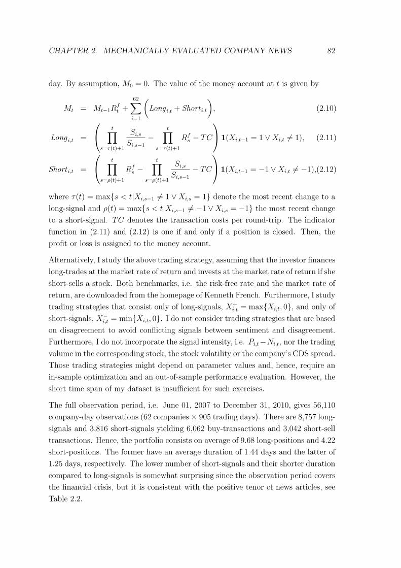
CHAPTER 2. MECHANICALLY EVALUATED COMPANY NEWS 82
day. By assumption, M0 = 0. The value of the money account at t is given by
Mt = Mt−1Rft +
62∑i=1
(Long i,t + Short i,t
), (2.10)
Long i,t =
t∏s=τ(t)+1
Si,sSi,s−1
−t∏
s=τ(t)+1
Rfs − TC
1(Xi,t−1 = 1 ∨Xi,t 6= 1), (2.11)
Short i,t =
t∏s=ρ(t)+1
Rfs −
t∏s=ρ(t)+1
Si,sSi,s−1
− TC
1(Xi,t−1 = −1 ∨Xi,t 6= −1),(2.12)
where τ(t) = max{s < t|Xi,s−1 6= 1 ∨Xi,s = 1} denote the most recent change to a
long-signal and ρ(t) = max{s < t|Xi,s−1 6= −1 ∨Xi,s = −1} the most recent change
to a short-signal. TC denotes the transaction costs per round-trip. The indicator
function in (2.11) and (2.12) is one if and only if a position is closed. Then, the
profit or loss is assigned to the money account.
Alternatively, I study the above trading strategy, assuming that the investor finances
long-trades at the market rate of return and invests at the market rate of return if she
short-sells a stock. Both benchmarks, i.e. the risk-free rate and the market rate of
return, are downloaded from the homepage of Kenneth French. Furthermore, I study
trading strategies that consist only of long-signals, X+i,t = max{Xi,t, 0}, and only of
short-signals, X−i,t = min{Xi,t, 0}. I do not consider trading strategies that are based
on disagreement to avoid conflicting signals between sentiment and disagreement.
Furthermore, I do not incorporate the signal intensity, i.e. Pi,t−Ni,t, nor the trading
volume in the corresponding stock, the stock volatility or the company’s CDS spread.
Those trading strategies might depend on parameter values and, hence, require an
in-sample optimization and an out-of-sample performance evaluation. However, the
short time span of my dataset is insufficient for such exercises.
The full observation period, i.e. June 01, 2007 to December 31, 2010, gives 56,110
company-day observations (62 companies × 905 trading days). There are 8,757 long-
signals and 3,816 short-signals yielding 6,062 buy-transactions and 3,042 short-sell
transactions. Hence, the portfolio consists on average of 9.68 long-positions and 4.22
short-positions. The former have an average duration of 1.44 days and the latter of
1.25 days, respectively. The lower number of short-signals and their shorter duration
compared to long-signals is somewhat surprising since the observation period covers
the financial crisis, but it is consistent with the positive tenor of news articles, see
Table 2.2.
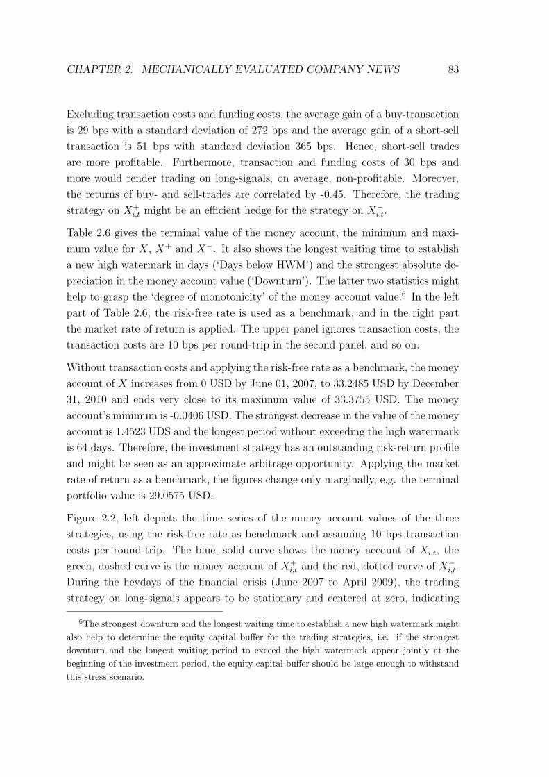
CHAPTER 2. MECHANICALLY EVALUATED COMPANY NEWS 83
Excluding transaction costs and funding costs, the average gain of a buy-transaction
is 29 bps with a standard deviation of 272 bps and the average gain of a short-sell
transaction is 51 bps with standard deviation 365 bps. Hence, short-sell trades
are more profitable. Furthermore, transaction and funding costs of 30 bps and
more would render trading on long-signals, on average, non-profitable. Moreover,
the returns of buy- and sell-trades are correlated by -0.45. Therefore, the trading
strategy on X+i,t might be an efficient hedge for the strategy on X−i,t.
Table 2.6 gives the terminal value of the money account, the minimum and maxi-
mum value for X, X+ and X−. It also shows the longest waiting time to establish
a new high watermark in days (‘Days below HWM’) and the strongest absolute de-
preciation in the money account value (‘Downturn’). The latter two statistics might
help to grasp the ‘degree of monotonicity’ of the money account value.6 In the left
part of Table 2.6, the risk-free rate is used as a benchmark, and in the right part
the market rate of return is applied. The upper panel ignores transaction costs, the
transaction costs are 10 bps per round-trip in the second panel, and so on.
Without transaction costs and applying the risk-free rate as a benchmark, the money
account of X increases from 0 USD by June 01, 2007, to 33.2485 USD by December
31, 2010 and ends very close to its maximum value of 33.3755 USD. The money
account’s minimum is -0.0406 USD. The strongest decrease in the value of the money
account is 1.4523 UDS and the longest period without exceeding the high watermark
is 64 days. Therefore, the investment strategy has an outstanding risk-return profile
and might be seen as an approximate arbitrage opportunity. Applying the market
rate of return as a benchmark, the figures change only marginally, e.g. the terminal
portfolio value is 29.0575 USD.
Figure 2.2, left depicts the time series of the money account values of the three
strategies, using the risk-free rate as benchmark and assuming 10 bps transaction
costs per round-trip. The blue, solid curve shows the money account of Xi,t, the
green, dashed curve is the money account of X+i,t and the red, dotted curve of X−i,t.
During the heydays of the financial crisis (June 2007 to April 2009), the trading
strategy on long-signals appears to be stationary and centered at zero, indicating
6The strongest downturn and the longest waiting time to establish a new high watermark mightalso help to determine the equity capital buffer for the trading strategies, i.e. if the strongestdownturn and the longest waiting period to exceed the high watermark appear jointly at thebeginning of the investment period, the equity capital buffer should be large enough to withstandthis stress scenario.

CHAPTER 2. MECHANICALLY EVALUATED COMPANY NEWS 84
no arbitrage profits, but the performance of trades on short-signals is excellent and
the value of the money account increases almost monotonically. However, in spring
2009, governments and central banks successfully calmed down the financial markets
and the stock market recovered. In the aftermath, the trading strategy on short-
signals fails to generate profits and the money account stays constant or decreases
slightly. At the same time, trading on long-signals works very well. This example
also nicely highlights the good hedging quality of trading on long-signals against
trading on short-signals and vice versa. Combining both trading strategies give an
almost globally, monotonically increasing money account value, that increases to
24.0594 USD and has a maximum of 24.2044 UDS and minimum of -0.1286 USD.
Figure 2.2, left also shows the strongest decrease in the value of the money account
of Xi,t (black line, -1.81 USD in May and June 2009) and the longest waiting period
to exceed the watermark (light blue line, 112 days during Spring and Summer 2010).
Both figures appear to be moderate.
The assumption of 20 bps transaction costs per round-trip reduces the terminal
values of the money accounts, the terminal value of trading on long- and short-
signals jointly is now 14.8703 USD and 10.6793 USD, depending on the benchmark.
The minimum portfolio value is -1.5261 USD and -1.6210 USD, respectively, and
the maximum value is 15.3437 USD and 14.0891 USD, respectively. The trading
strategies might still be attractive, profitable investment opportunities, but they
now bears a higher shortfall risk. Transaction costs of 30 bps imply that the investor
realizes, on average, losses on every buy-transaction and on many sell-transactions.
Hence, the terminal value of the money account of X+i,t is negative. However, X−i,t
might still be profitable. X−i,t cannot compensate transaction costs of 50 bps or more.
Other approaches, which rely on the General Inquirer dictionary, such as using only
the five words in the neighborhood of the company name to calculate the sentiment,
give similar results. I also test the trading strategies on the sentiment calculated
with the financial word lists of Loughran and McDonald. Figure 2.2, right shows the
corresponding values of the money accounts of Xi,t, X+i,t and X−i,t assuming 10 bps
transaction costs and using the risk-free interest rate as a benchmark. As already
indicated by the regression analysis in the robustness section, the results weaken
significantly. Trading on short-signals performs well during the financial crisis and
attains a maximum of about 15 USD in February 2009, which is very similar to the
trading strategy of short-signal based on the General Inquirer dictionary. However,
it generates significant losses in the subsequent period. Also the performance of long-
signals is reduced, even though the money account does not turn negative during
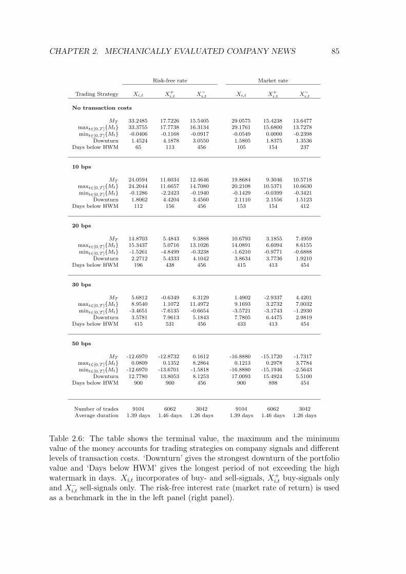
CHAPTER 2. MECHANICALLY EVALUATED COMPANY NEWS 85
Risk-free rate Market rate
Trading Strategy Xi,t X+i,t X−i,t Xi,t X+
i,t X−i,t
No transaction costs
MT 33.2485 17.7226 15.5405 29.0575 15.4238 13.6477maxt∈[0,T ]{Mt} 33.3755 17.7738 16.3134 29.1761 15.6800 13.7278mint∈[0,T ]{Mt} -0.0406 -0.1168 -0.0917 -0.0549 0.0000 -0.2398
Downturn 1.4524 4.1878 3.0550 1.5805 1.8375 1.3536Days below HWM 65 113 456 105 154 237
10 bps
MT 24.0594 11.6034 12.4646 19.8684 9.3046 10.5718maxt∈[0,T ]{Mt} 24.2044 11.6657 14.7080 20.2108 10.5371 10.6630mint∈[0,T ]{Mt} -0.1286 -2.2423 -0.1940 -0.1429 -0.0399 -0.3421
Downturn 1.8062 4.4204 3.4560 2.1110 2.1556 1.5123Days below HWM 112 156 456 153 154 412
20 bps
MT 14.8703 5.4843 9.3888 10.6793 3.1855 7.4959maxt∈[0,T ]{Mt} 15.3437 5.0716 13.1026 14.0891 6.6094 8.6155mint∈[0,T ]{Mt} -1.5261 -4.8499 -0.3238 -1.6210 -0.9771 -0.6888
Downturn 2.2712 5.4333 4.1042 3.8634 3.7736 1.9210Days below HWM 196 438 456 415 413 454
30 bps
MT 5.6812 -0.6349 6.3129 1.4902 -2.9337 4.4201maxt∈[0,T ]{Mt} 8.9540 1.1072 11.4972 9.1693 3.2732 7.0032mint∈[0,T ]{Mt} -3.4651 -7.6135 -0.6654 -3.5721 -3.1743 -1.2930
Downturn 3.5781 7.9613 5.1843 7.7805 6.4475 2.9819Days below HWM 415 531 456 433 413 454
50 bps
MT -12.6970 -12.8732 0.1612 -16.8880 -15.1720 -1.7317maxt∈[0,T ]{Mt} 0.0809 0.1352 8.2864 0.1213 0.2978 3.7784mint∈[0,T ]{Mt} -12.6970 -13.6701 -1.5818 -16.8880 -15.1946 -2.5643
Downturn 12.7780 13.8053 8.1253 17.0093 15.4924 5.5100Days below HWM 900 900 456 900 898 454
Number of trades 9104 6062 3042 9104 6062 3042Average duration 1.39 days 1.46 days 1.26 days 1.39 days 1.46 days 1.26 days
Table 2.6: The table shows the terminal value, the maximum and the minimumvalue of the money accounts for trading strategies on company signals and differentlevels of transaction costs. ‘Downturn’ gives the strongest downturn of the portfoliovalue and ‘Days below HWM’ gives the longest period of not exceeding the highwatermark in days. Xi,t incorporates of buy- and sell-signals, X+
i,t buy-signals onlyand X−i,t sell-signals only. The risk-free interest rate (market rate of return) is usedas a benchmark in the in the left panel (right panel).
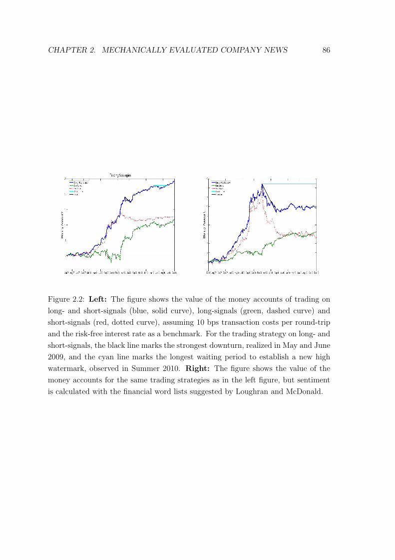
CHAPTER 2. MECHANICALLY EVALUATED COMPANY NEWS 86
Figure 2.2: Left: The figure shows the value of the money accounts of trading on
long- and short-signals (blue, solid curve), long-signals (green, dashed curve) and
short-signals (red, dotted curve), assuming 10 bps transaction costs per round-trip
and the risk-free interest rate as a benchmark. For the trading strategy on long- and
short-signals, the black line marks the strongest downturn, realized in May and June
2009, and the cyan line marks the longest waiting period to establish a new high
watermark, observed in Summer 2010. Right: The figure shows the value of the
money accounts for the same trading strategies as in the left figure, but sentiment
is calculated with the financial word lists suggested by Loughran and McDonald.
CHAPTER 2. MECHANICALLY EVALUATED COMPANY NEWS 87
September 2009 to March 2010. The money account value of the trading strategy
on long- and short-signals at December 31, 2010, is 11.6224 USD with a maximum
downturn of 6.2212 USD (black line) and being far away from the high watermark of
16.8852 USD (cyan line). The lower performance of the trading strategies based the
financial word lists indicates that non-financial expressions are important as well to
measure the sentiment of rather general company news articles.
2.8 Conclusion
Das et al. (2005) analyzed chat-room postings and conclude that “people trade
first and talk later” (Financial Management 34, p.135). I analyze company news
of Reuters. These news are more reliable than chat room postings, which - at
best - disseminate public information. Simple, dictionary based content analysis
algorithms with rather general word lists might be applied to measure sentiment and
disagreement of news articles. Both, sentiment and disagreement contain valuable
information for financial markets.
My results are mostly consistent with the difference of opinion literature, i.e. in-
vestors are more likely to trade stocks and options when public signals occur. Dis-
agreement across news articles, which might measure the degree of difference of
opinion, is also positively correlated with stock and option trading volume and re-
turn volatility. Moreover, sentiment and disagreement are statistically significant
to predict returns, volatility and trading volume. With moderate transaction costs,
it might be possible to exploit market inefficiencies by trading on long- and short-
signals based on mechanically evaluated company news. However, transaction costs
of 30 bps and more render these trading strategies non-profitable. Therefore, only
institutional investors might be able to take advantage of this inefficiency.
CHAPTER 2. MECHANICALLY EVALUATED COMPANY NEWS 88
2.9 Appendix
2.9.1 News Coverage
I investigate the company characteristics that expose a company to news coverage. I
consider the 61 large companies in the S&P500 with liquid option and CDS market,
listed in Table 2.8.7 The news coverage of a company is measured by its average
number of news articles per day, identified by searching for the company’s RIC
in ‘related RICs’. This measure is denoted Qi. Alternatively, news coverage is
measured by the number of days with at least one news story. This measure is
denoted Yi. Companies are characterized by the average market capitalization in
the observation period, CAPi, the average price-to-book ratio, P2Bi, the stock
return during the observation period, Reti, and the corresponding return volatility,
σ(Reti).
The average company has an average market capitalization during June 01, 2007
to December 31, 2010 of 8,3223 millions USD and an average price-to-book ratio of
2.67. The average stock market performance in this period and across companies
is -9.41% and the average stock return volatility is 42.63%. I estimate an ordinary
linear regression model, i.e.
Qi = α + β1P2Bi + β2 ln(CAPi) + β3Reti + β4σ(Reti) + ηi. (2.13)
Table 2.7 shows the regression estimates for (2.13) and for some straightforward
modifications of the regression model. a indicates significance at the 1% confidence
level, b at the 5% level and c at the 10% level. Even though this analysis excludes
small and mid-sized companies, the company size is still a significant, positive de-
terminant of the news coverage. The price-to-book ratio is significant and negative
in all regressions. This indicates that companies with high ratios are less often in
the news compared to companies with low ratios. One reason for this pattern might
be that the latter companies have a higher potential for stock price increases. The
stock return is weakly significant and negative. The stock return volatility is sig-
nificant, too, and positive. Both indicate that troubled companies are frequently in
the media. However, this result might also be due to the financial crisis.
All results are qualitatively the same if Yi is considered instead of Qi. Hence, large
companies with low price-to-book ratios and volatile stock returns have a high media
7Time Warner (TWX.N) is excluded since I found no information on the price-to-book ratio.

CHAPTER 2. MECHANICALLY EVALUATED COMPANY NEWS 89
Qi Yi
constant −20.8872a −23.0588a −2.0450a −2.0569a
P2B −0.3051a −0.2101a −0.0251a −0.0225a
ln(CAP ) 2.2701a 2.3374a 0.2481a 0.2501a
Ret - −1.9734b - −0.1547b
σ(Ret) - 6.9538a - 0.2916b
R2 38.73% 68.26% 54.58% 65.89%# Obs. 61 61 61 61
Table 2.7: The table shows the regression estimates for model (2.13). The subscripta, b and c indicate significance at the 1%, 5% and 10% confidence level. Qi denotesthe average number of news per day of company i, and Yi is the average numberof days with at least one news story. A news story is relevant for a company if thecompany’s RIC is mentioned in the field ‘related RICs’.
coverage, or conversely, companies with a high media coverage are large, have a low
price-to-book ratio and their stock price is rather volatile.
2.9.2 RICs - Company Names

CHAPTER 2. MECHANICALLY EVALUATED COMPANY NEWS 90
RIC Company Name
AA.N Alcoa IncorporatedABT .N Abbott LaboratoriesAIG.N American International Group Inc
AMGN .O Amgen IncAPC.N Anadarko Petroleum CorpAXP .N American Express CoBA.N The Boeing Company
BAC.N Bank of America CorpBAX.N Baxter International IncBMY .N Bristol Myers Squibb Co
BSX.N Boston Scientific CorpC.N Citigroup Inc
CAT .N Caterpillar IncCOP .N ConocoPhillipsCSC.N Computer Sciences Corp
CSCO.O Cisco Systems IncCVX.N Chevron CorpDD.N E I Du Pont De Nemours And Company
DELL.O Dell IncDIS.N Walt Disney Co
DOW .N The Dow Chemical CoDVN .N Devon Energy Corp
F .N Ford Motor CoFDX.N Fedex CorpGE.N General Electric Co
GLW .N Corning IncGR.N Goodrich CorpGS.N The Goldman Sachs Group IncHD.N The Home Depot Inc
HON .N Honeywell International Inc
HPQ.N Hewlett Packard CoIBM .N International Business Machines CorpINTC.O Intel CorpJNJ.N Johnson & JohnsonJPM .N Jpmorgan Chase & CoKFT .N Kraft Foods IncKO.N The Coca Cola Co
MCD.N McDonald’s CorpMDT .N Medtronic IncMO.N Altria Group Inc
MON .N Monsanto CoMMM .N 3m CoMRK.N Merck and Co IncMS.N Morgan Stanley
MSFT .O Microsoft CorpLLY .N Eli Lilly And CoLMT .N Lockheed Martin CorpORCL.O Oracle CorpOXY .N Occidental Petroleum CorpPFE.N Pfizer Inc
PG.N Procter & Gamble CoSLB.N Schlumberger NV
T .N AT&T IncTRV .N Travelers Companies IncTWX.N Time Warner IncTXN .N Texas Instruments IncUTX.N United Technologies CorpV Z.N Verizon Communications Inc
WFC.N Wells Fargo and CoWMT .N Wal Mart Stores Inc
WLP .N WellPoint IncXOM .N Exxon Mobil Corp
Table 2.8: The table gives the list of companies that are included in the analysesand matches the company name with the company’s RIC (= Reuters instrumentcode)

Bibliography
[1] Antweiler, Werner and Murry Z. Frank, 2004, ”Is all that just Noise? The
Information Content of internet Stock Message Boards”, Journal of Finance 59,
1259-1294.
[2] Banerjee, Snehal and Ilan Kremer, 2010, ”Disagreement and Learning: Dynamic
Pattern of Trading Volume”, Journal of Finance 65, 1269-1302.
[3] Barber, Brad M. and Terrance Odean, 2008, ”All That Glitters: The Effect
of Attention and News on the Buying Behavior of Individual and Institutional
Investors”, Review of Financial Studies 21, 785-818.
[4] Blume, Lawrence, David Easley, Maureen O’Hara, 1994, ”Market Statistics and
Technical Analysis: The Role of Volume”, Journal of Finance 49, 153-181.
[5] Boyd, John H., Jian Hu and Ravi Jagannathan, 2005, ”The Stock Market’s
Reaction to Unemployment News: Why Bad News Is Usually Good for Stocks”
Journal of Finance 60, 649-672.
[6] Brooks, Raymond M., Ajay Patel and Tie Su, 2003, ”How the Equity Market
Responds to Unanticipated Events”, Journal of Business 76, 109-133.
[7] Brounen, Dirk and Jeroen Derwall, 2010, ”The Impact of Terrorist Attacks on
International Stock Markets”, European Financial Management 16, 585-598.
[8] Cao, H. Henry and Hui Ou-Yang, 2009, ”Differences of Opinion of Public In-
formation and Speculative Trading in Stocks and Options”, Review of Financial
Studies 22, 299-335.
[9] Carretta, Alessandro, Vincenzo Farina, Duccio Martelli, Franco Fiordelisi and
Paola Schwizer, 2010, ”The Impact of Corporate Governance Press News on
Stock Market Return”, European Financial Management 17, 100-119.
91

CHAPTER 2. MECHANICALLY EVALUATED COMPANY NEWS 92
[10] Chordia, Tarum, Asani Sarkar and Avanidhar Subrahmanyam, 2005, ”An Em-
pirical Analysis of Stock and Bond Market Liquidity”, Review of Financial Stud-
ies 18, 85-129.
[11] Coval, Joshua D. and Tyler Shumway, 2001, ”Is Sound Just Noise?”, Journal
of Finance 56, 1887-1910.
[12] Cremers, Martijn, Joost Driessen, Pascal Maenhout and David Weinbaum,
2008, ”Individual Stock-Option Prices and Credit Spreads”, Journal of Banking
and Finance 32, 2706-2715.
[13] Das, Sanjiv R. and Mike Y. Chen, 2007, ”Yahoo! for Amazon; Sentiment
Extraction form Small Talk on the Web”, Management Science 53, 1375-1388.
[14] Das, Sanjiv R., Asis Martinez-Jerez and Peter Tufano, 2005, ”e-Information:
A Clinical Study of Investor Discussion and Sentiment”, Financial Management
34, 103-137.
[15] Engelberg, Joseph E. and Christopher A. Parsons, 2011, ”The Causal Impact
of Media in Financial Markets”, Journal of Finance 66, 67-98.
[16] Fama, Eugene F. and Kenneth French, 1993, ”Common Risk Factors in the
Returns on Stocks and Bonds”, Journal of Financial Economics 33, 3-56.
[17] Fang, Lily and Joel Peress, 2009, ”Media Coverage and the Cross-section of
Stock Returns”, Journal of Finance 64, 2023-2052.
[18] Groß-Klußmann, Axel and Nikolas Hautsch, 2011, ”When Machines Read the
News: Using Automated Text Analysis to Quantify High Frequency News-
Implied Market Reactions”, Journal of Empirical Finance 18, 321-340.
[19] Harris, Milton and Artur Raviv, 1993, ”Differences of Opinion Make a Horse
Race”, Review of Financial Studies 6, 473-506.
[20] Hautsch, Nikolaus and Dieter Hess, 2002, ”The Processing of Non-Anticipated
Information in Financial Markets: Analyzing the Impact of Surprises in the
Employment Report”, European Financial Review 6, 133-161.
[21] Hess, Dieter, 2008, ”How Do Commodity Futures Respond to Macroeconomic
News?”, Financial Markets and Portfolio Management 22, 127-146.

CHAPTER 2. MECHANICALLY EVALUATED COMPANY NEWS 93
[22] Hong, Harrison and Jeremy C. Stein, 2007, ”Disagreement and the Stock Mar-
ket”, Journal of Economic Perspectives 21, 109-128.
[23] Hull, John, Mirela Predescu and Alan White, 2004, ”The Relationship between
Credit Default Swap Spreads, Bond Yields, and Credit Rating Announcements”,
Journal of Banking and Finance 28, 2789-2811.
[24] Kandel, Eugene and Neil D. Pearson, 1995, ”Interpretation of Public Signals
and Trade in Speculative Makets, Journal of Political Economy 103, 831-872.
[25] Kyriacou, Kyriaos and Lucio Sarno, 1999, ”The Temporal Relationship between
Derivatives Trading and Spot Market Volatility in the U.K.: Empirical Analysis
and Monte Carlo Evidence”, Journal of Futures Markets 19, 245-270.
[26] Loughran, Tim and Bill McDonald, 2011, ”When Is a Liability Not a Liability?
Textual Analysis, Dictionaries, and 10-Ks”, Journal of Finance 66, 35-66.
[27] Milgrom, Paul and Nancy Stokey, 1982, ”Information, Trade and Common
Knowledge”, Journal of Economic Theory 26, 17-27.
[28] Mitchell, Mark L. and J. Harold Mulherin, 1994, ”The Impact of Public Infor-
mation on the Stock Market”, Journal of Finance 49, 923-950.
[29] Merton, Robert C., 1974, ”On the Pricing of Corporate Debt: The Risk Struc-
ture of Interest Rates”, Journal of Finance 29, 449-70
[30] Norden, Lars, 2009, ”Credit Derivatives, Corporate News, and Credit Ratings”,
working paper.
[31] Pan, Jun and Allen M. Poteshman, 2006, ”The Information in Option Volume
for Future Stock Prices”, Review of Financial Studies 19, 871-908.
[32] Sarwar, Ghulam, 2005, ”The Informational Role of Option Trading Volume in
Equity Index Options Markets”, Review of Quantitative Finance and Accounting
24, 159-176.
[33] Suominen, Matti, (2001), ”Trading Volume and Information Revelation in
Stock Markets”, Journal of Financial and Quantitative Analysis 36, 545-565.
[34] Tetlock, Paul C., 2007, ”Giving Content to Investor Sentiment: The Role of
Media in the Stock Market”, Journal of Finance 62, 1139-1167.

CHAPTER 2. MECHANICALLY EVALUATED COMPANY NEWS 94
[35] Tetlock, Paul C., 2010, ”Does Public Financial News Resolve Asymmetric In-
formation?”, Review of Financial Studies 23, 3520-3557.
[36] Tetlock, Paul C., Maytal Saar-Tsechansky and Sofus Macskassy, 2008, ”More
than Words: Quantifying Language to Measure Firms’ Fundamentals”, Journal
of Finance 63, 1437-1467.
[37] Tumarkin, Robert and Robert F. Whitelaw, 2001, ”News or Noise? Internet
Posting and Stock Prices”, Financial Analysts Journal 57, 41-51.
[38] Yu, Jialin, 2011, ”Disagreement and Return Predictability of Stock Portfolios”,
Journal of Financial Economics 99, 162-183.
[39] Zhang, Benjamin Yibin, Hou Zhou and Haibin Zhu, 2009, ”Explaining Credit
Default Swap Spreads with the Equity Volatility and Jump Risks of Individual
Firms”, Review of Financial Studies 22, 5099-5131.
Chapter 3
Leverage, Profitability and Risk of
Banks - An Empirical Analysis
Abstract: This paper studies the relationship between the leverage
ratio and profitability and risk-adjusted profitability, respectively, for
European and U.S. banks. Risk-adjusted profitability is measured by
accounting figures and, alternatively, by stock prices. Applying a dy-
namic panel regression and controlling for several bank characteristics
(e.g. loan portfolio quality, liquidity endowment, size), I find that banks
adjust their leverage ratio (defined as total assets over book equity) fast
compared to industrial companies. Moreover, bank performance is non-
monotonically, inversely ’u’-shaped related to the leverage ratio. When
the leverage ratio of a European bank is high, CDS spreads tend to be
high, too, indicating that expected default costs dominate benefits of
the tax shield. For U.S. banks, I find no significant relation between the
leverage ratio and the CDS spread. This puzzling result might be due
to a restriction on the non-risk weighted capital structure of U.S. banks.
3.1 Introduction
Given various market imperfections, many papers investigate the optimal capital
structure of corporations. Especially during the ongoing financial crisis, the capital
structure of banks is discussed not only in academia, but also in public. The failure
of Lehman Brothers caused financial distress for many poorly capitalized banks.
95
CHAPTER 3. LEVERAGE, PROFITABILITY AND RISK OF BANKS 96
Strong support by governments and central banks helped to avoid the collapse of
major financial institutions. There is an ongoing debate how to prevent such events
in the future. Adjusting incentive systems for bank managers and raising risk-
weighted equity capital requirements of banks are prominent suggestions. Also an
upper limit for the non risk-weighted leverage ratio (defined as total book assets over
book equity) of banks is imposed.1 This raises the following questions: (1) How are
bank profits related to the capital structure and how do they react if some maximum
leverage ratio is implemented? (2) How is the default probability of a bank related
to its capital structure? (3) What is an adequate limit for the leverage ratio? This
paper tries to answer these questions by analyzing the relationship between the non
risk-weighted leverage ratio and profitability, risk-adjusted profitability and expected
default costs, respectively.
In a perfect market, the market value of a firm is independent of its capital structure,
see Modigliani and Miller (1958). In reality, tax effects, bankruptcy costs and infor-
mation asymmetry might affect profits and the firm value. According to the trade-off
theory, the optimal capital structure balances the tax shield and bankruptcy costs.
Alternatively, the pecking-order theory relates the costs of different funding sources
to asymmetric information between the owners and external investors. This implies
a preferred order of funding sources. Many empirical papers test these theories for
industrial corporations. The results are mixed.
Compared to industrial corporations, financial institutions are different with respect
to the capital structure and the flexibility of funding in liquid markets. Industrial
firms have a fairly low leverage ratio and use long-term bonds and loans for fund-
ing, whereas financial institutions are more leveraged and use short-term loans to
a large extent. Moreover, the capital structure of financial institutions must satisfy
regulatory requirements. These issues might imply more active capital structure
management and a different relationship between the capital structure and prof-
itability for financial institutions than for industrial corporations. Hence, results for
industrial corporations should not be transferred to banks.
Theoretical papers such as Diamond and Rajan (2000), Inderst and Mueller (2008)
and Koziol and Lawrenz (2009) prove the existence of an optimal leverage ratio for
profit maximizing banks under certain assumptions. The major determinants are
1See, for example, Report of the Financial Stability Board to G20 Leaders, ”Improving FinancialRegulation”, September 2009 or Basel Committee on Banking Supervision ”Strengthening theResilience of the Banking Sector”, December 2009
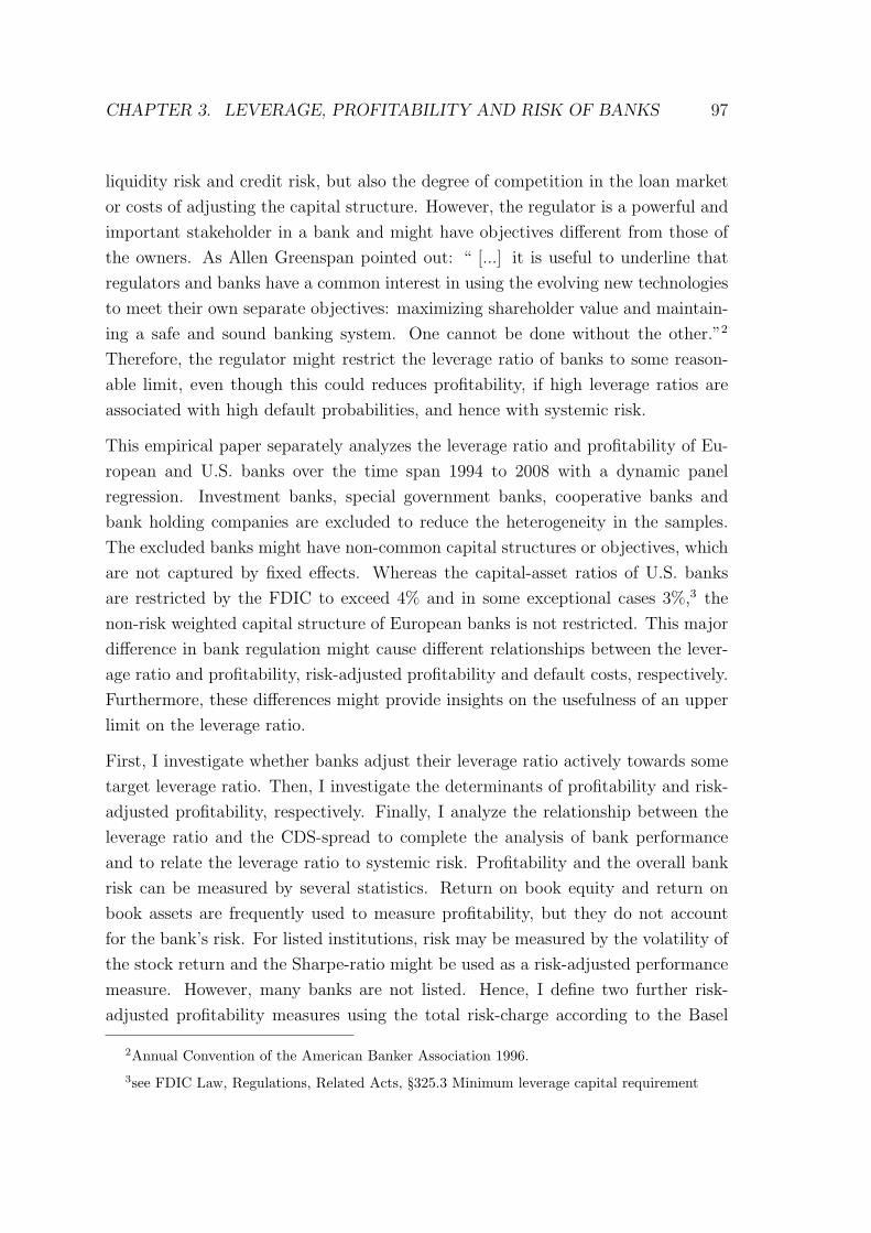
CHAPTER 3. LEVERAGE, PROFITABILITY AND RISK OF BANKS 97
liquidity risk and credit risk, but also the degree of competition in the loan market
or costs of adjusting the capital structure. However, the regulator is a powerful and
important stakeholder in a bank and might have objectives different from those of
the owners. As Allen Greenspan pointed out: “ [...] it is useful to underline that
regulators and banks have a common interest in using the evolving new technologies
to meet their own separate objectives: maximizing shareholder value and maintain-
ing a safe and sound banking system. One cannot be done without the other.”2
Therefore, the regulator might restrict the leverage ratio of banks to some reason-
able limit, even though this could reduces profitability, if high leverage ratios are
associated with high default probabilities, and hence with systemic risk.
This empirical paper separately analyzes the leverage ratio and profitability of Eu-
ropean and U.S. banks over the time span 1994 to 2008 with a dynamic panel
regression. Investment banks, special government banks, cooperative banks and
bank holding companies are excluded to reduce the heterogeneity in the samples.
The excluded banks might have non-common capital structures or objectives, which
are not captured by fixed effects. Whereas the capital-asset ratios of U.S. banks
are restricted by the FDIC to exceed 4% and in some exceptional cases 3%,3 the
non-risk weighted capital structure of European banks is not restricted. This major
difference in bank regulation might cause different relationships between the lever-
age ratio and profitability, risk-adjusted profitability and default costs, respectively.
Furthermore, these differences might provide insights on the usefulness of an upper
limit on the leverage ratio.
First, I investigate whether banks adjust their leverage ratio actively towards some
target leverage ratio. Then, I investigate the determinants of profitability and risk-
adjusted profitability, respectively. Finally, I analyze the relationship between the
leverage ratio and the CDS-spread to complete the analysis of bank performance
and to relate the leverage ratio to systemic risk. Profitability and the overall bank
risk can be measured by several statistics. Return on book equity and return on
book assets are frequently used to measure profitability, but they do not account
for the bank’s risk. For listed institutions, risk may be measured by the volatility of
the stock return and the Sharpe-ratio might be used as a risk-adjusted performance
measure. However, many banks are not listed. Hence, I define two further risk-
adjusted profitability measures using the total risk-charge according to the Basel
2Annual Convention of the American Banker Association 1996.3see FDIC Law, Regulations, Related Acts, §325.3 Minimum leverage capital requirement
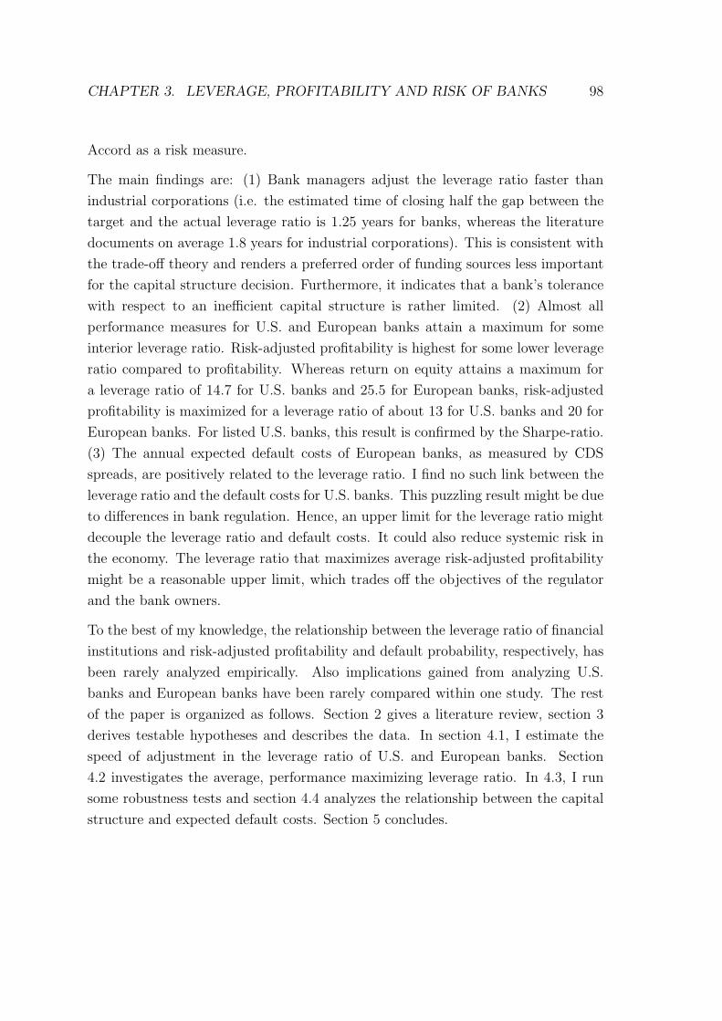
CHAPTER 3. LEVERAGE, PROFITABILITY AND RISK OF BANKS 98
Accord as a risk measure.
The main findings are: (1) Bank managers adjust the leverage ratio faster than
industrial corporations (i.e. the estimated time of closing half the gap between the
target and the actual leverage ratio is 1.25 years for banks, whereas the literature
documents on average 1.8 years for industrial corporations). This is consistent with
the trade-off theory and renders a preferred order of funding sources less important
for the capital structure decision. Furthermore, it indicates that a bank’s tolerance
with respect to an inefficient capital structure is rather limited. (2) Almost all
performance measures for U.S. and European banks attain a maximum for some
interior leverage ratio. Risk-adjusted profitability is highest for some lower leverage
ratio compared to profitability. Whereas return on equity attains a maximum for
a leverage ratio of 14.7 for U.S. banks and 25.5 for European banks, risk-adjusted
profitability is maximized for a leverage ratio of about 13 for U.S. banks and 20 for
European banks. For listed U.S. banks, this result is confirmed by the Sharpe-ratio.
(3) The annual expected default costs of European banks, as measured by CDS
spreads, are positively related to the leverage ratio. I find no such link between the
leverage ratio and the default costs for U.S. banks. This puzzling result might be due
to differences in bank regulation. Hence, an upper limit for the leverage ratio might
decouple the leverage ratio and default costs. It could also reduce systemic risk in
the economy. The leverage ratio that maximizes average risk-adjusted profitability
might be a reasonable upper limit, which trades off the objectives of the regulator
and the bank owners.
To the best of my knowledge, the relationship between the leverage ratio of financial
institutions and risk-adjusted profitability and default probability, respectively, has
been rarely analyzed empirically. Also implications gained from analyzing U.S.
banks and European banks have been rarely compared within one study. The rest
of the paper is organized as follows. Section 2 gives a literature review, section 3
derives testable hypotheses and describes the data. In section 4.1, I estimate the
speed of adjustment in the leverage ratio of U.S. and European banks. Section
4.2 investigates the average, performance maximizing leverage ratio. In 4.3, I run
some robustness tests and section 4.4 analyzes the relationship between the capital
structure and expected default costs. Section 5 concludes.
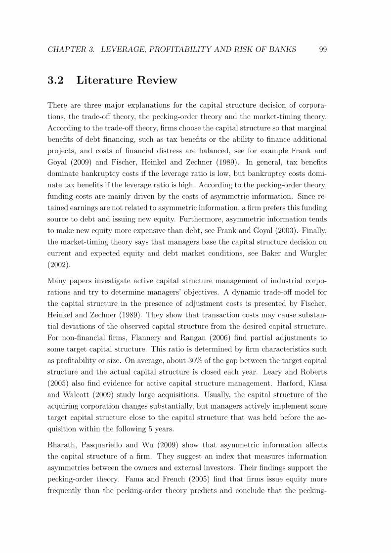
CHAPTER 3. LEVERAGE, PROFITABILITY AND RISK OF BANKS 99
3.2 Literature Review
There are three major explanations for the capital structure decision of corpora-
tions, the trade-off theory, the pecking-order theory and the market-timing theory.
According to the trade-off theory, firms choose the capital structure so that marginal
benefits of debt financing, such as tax benefits or the ability to finance additional
projects, and costs of financial distress are balanced, see for example Frank and
Goyal (2009) and Fischer, Heinkel and Zechner (1989). In general, tax benefits
dominate bankruptcy costs if the leverage ratio is low, but bankruptcy costs domi-
nate tax benefits if the leverage ratio is high. According to the pecking-order theory,
funding costs are mainly driven by the costs of asymmetric information. Since re-
tained earnings are not related to asymmetric information, a firm prefers this funding
source to debt and issuing new equity. Furthermore, asymmetric information tends
to make new equity more expensive than debt, see Frank and Goyal (2003). Finally,
the market-timing theory says that managers base the capital structure decision on
current and expected equity and debt market conditions, see Baker and Wurgler
(2002).
Many papers investigate active capital structure management of industrial corpo-
rations and try to determine managers’ objectives. A dynamic trade-off model for
the capital structure in the presence of adjustment costs is presented by Fischer,
Heinkel and Zechner (1989). They show that transaction costs may cause substan-
tial deviations of the observed capital structure from the desired capital structure.
For non-financial firms, Flannery and Rangan (2006) find partial adjustments to
some target capital structure. This ratio is determined by firm characteristics such
as profitability or size. On average, about 30% of the gap between the target capital
structure and the actual capital structure is closed each year. Leary and Roberts
(2005) also find evidence for active capital structure management. Harford, Klasa
and Walcott (2009) study large acquisitions. Usually, the capital structure of the
acquiring corporation changes substantially, but managers actively implement some
target capital structure close to the capital structure that was held before the ac-
quisition within the following 5 years.
Bharath, Pasquariello and Wu (2009) show that asymmetric information affects
the capital structure of a firm. They suggest an index that measures information
asymmetries between the owners and external investors. Their findings support the
pecking-order theory. Fama and French (2005) find that firms issue equity more
frequently than the pecking-order theory predicts and conclude that the pecking-
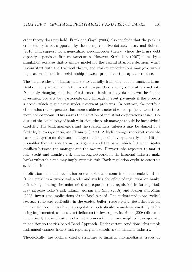
CHAPTER 3. LEVERAGE, PROFITABILITY AND RISK OF BANKS 100
order theory does not hold. Frank and Goyal (2003) also conclude that the pecking
order theory is not supported by their comprehensive dataset. Leary and Roberts
(2010) find support for a generalized pecking-order theory, where the firm’s debt
capacity depends on firm characteristics. However, Strebulaev (2007) shows by a
simulation exercise that a simple model for the capital structure decision, which
is consistent with the trade-off theory, and market imperfections may give wrong
implications for the true relationship between profits and the capital structure.
The balance sheet of banks differs substantially from that of non-financial firms.
Banks hold dynamic loan portfolios with frequently changing compositions and with
frequently changing qualities. Furthermore, banks usually do not own the funded
investment projects but participate only through interest payments if the projects
succeed, which might cause underinvestment problems. In contrast, the portfolio
of an industrial corporation has more stable characteristics and projects tend to be
more homogeneous. This makes the valuation of industrial corporations easier. Be-
cause of the complexity of bank valuation, the bank manager should be incentivized
carefully. The bank manager’s and the shareholders’ interests may be aligned by a
fairly high leverage ratio, see Flannery (1994). A high leverage ratio motivates the
bank manager to monitor and manage the loan portfolio very carefully. In addition,
it enables the manager to own a large share of the bank, which further mitigates
conflicts between the manager and the owners. However, the exposure to market
risk, credit and liquidity risk and strong networks in the financial industry make
banks vulnerable and may imply systemic risk. Bank regulation ought to constrain
systemic risk.
Implications of bank regulation are complex and sometimes unintended. Blum
(1999) presents a two-period model and studies the effect of regulation on banks’
risk taking, finding the unintended consequence that regulation in later periods
may increase today’s risk taking. Adrian and Shin (2008) and Jokipii and Milne
(2008) investigate implications of the Basel Accord. The authors find a pro-cyclical
leverage ratio and cyclicality in the capital buffer, respectively. Both findings are
unintended, too. Therefore, new regulation tools should be analyzed carefully before
being implemented, such as a restriction on the leverage ratio. Blum (2008) discusses
theoretically the implications of a restriction on the non risk-weighted leverage ratio
in addition to the risk-based Basel Approach. Under certain conditions, this simple
instrument ensures honest risk reporting and stabilizes the financial industry.
Theoretically, the optimal capital structure of financial intermediaries trades off
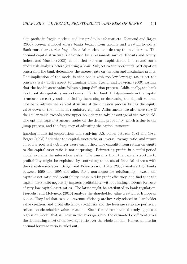
CHAPTER 3. LEVERAGE, PROFITABILITY AND RISK OF BANKS 101
high profits in fragile markets and low profits in safe markets. Diamond and Rajan
(2000) present a model where banks benefit from lending and creating liquidity.
Bank runs characterize fragile financial markets and destroy the bank’s rent. The
optimal capital structure is described by a reasonable mix of deposits and equity.
Inderst and Mueller (2008) assume that banks are sophisticated lenders and run a
credit risk analysis before granting a loan. Subject to the borrower’s participation
constraint, the bank determines the interest rate on the loan and maximizes profits.
One implication of the model is that banks with too low leverage ratios act too
conservatively with respect to granting loans. Koziol and Lawrenz (2009) assume
that the bank’s asset value follows a jump-diffusion process. Additionally, the bank
has to satisfy regulatory restrictions similar to Basel II. Adjustments in the capital
structure are costly and modeled by increasing or decreasing the deposit volume.
The bank adjusts the capital structure if the diffusion process brings the equity
value down to the minimum regulatory capital. Adjustments are also necessary if
the equity value exceeds some upper boundary to take advantage of the tax shield.
The optimal capital structure trades off the default probability, which is due to the
jump process, and the frequency of adjusting the capital structure.
Ignoring industrial corporations and studying U.S. banks between 1983 and 1989,
Berger (1995) finds that the capital-asset-ratio, or inverse leverage ratio, and return
on equity positively Granger-cause each other. The causality from return on equity
to the capital-asset-ratio is not surprising. Reinvesting profits in a multi-period
model explains the interaction easily. The causality from the capital structure to
profitability might be explained by controlling the costs of financial distress with
the capital-asset-ratio. Berger and Bonaccorsi di Patti (2006) analyze U.S. banks
between 1990 and 1995 and allow for a non-monotone relationship between the
capital-asset ratio and profitability, measured by profit efficiency, and find that the
capital-asset ratio negatively impacts profitability, without finding evidence for costs
of very low capital-asset ratios. The latter might be attributed to bank regulation.
Fiordelisi and Molyneux (2010) analyze the shareholder value creation of European
banks. They find that cost and revenue efficiency are inversely related to shareholder
value creation, and profit efficiency, credit risk and the leverage ratio are positively
related to shareholder value creation. Since the aforementioned study applies a
regression model that is linear in the leverage ratio, the estimated coefficient gives
the dominating effect of the leverage ratio over the whole domain. Hence, an interior
optimal leverage ratio is ruled out.
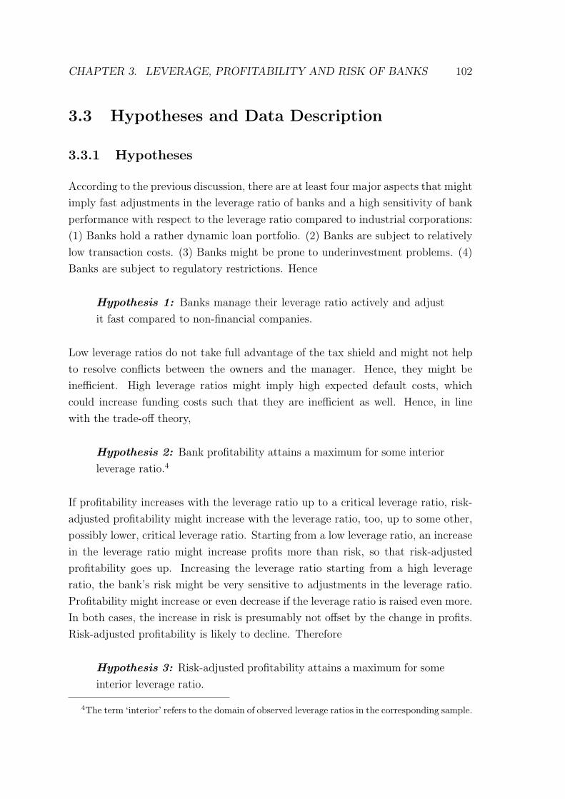
CHAPTER 3. LEVERAGE, PROFITABILITY AND RISK OF BANKS 102
3.3 Hypotheses and Data Description
3.3.1 Hypotheses
According to the previous discussion, there are at least four major aspects that might
imply fast adjustments in the leverage ratio of banks and a high sensitivity of bank
performance with respect to the leverage ratio compared to industrial corporations:
(1) Banks hold a rather dynamic loan portfolio. (2) Banks are subject to relatively
low transaction costs. (3) Banks might be prone to underinvestment problems. (4)
Banks are subject to regulatory restrictions. Hence
Hypothesis 1: Banks manage their leverage ratio actively and adjust
it fast compared to non-financial companies.
Low leverage ratios do not take full advantage of the tax shield and might not help
to resolve conflicts between the owners and the manager. Hence, they might be
inefficient. High leverage ratios might imply high expected default costs, which
could increase funding costs such that they are inefficient as well. Hence, in line
with the trade-off theory,
Hypothesis 2: Bank profitability attains a maximum for some interior
leverage ratio.4
If profitability increases with the leverage ratio up to a critical leverage ratio, risk-
adjusted profitability might increase with the leverage ratio, too, up to some other,
possibly lower, critical leverage ratio. Starting from a low leverage ratio, an increase
in the leverage ratio might increase profits more than risk, so that risk-adjusted
profitability goes up. Increasing the leverage ratio starting from a high leverage
ratio, the bank’s risk might be very sensitive to adjustments in the leverage ratio.
Profitability might increase or even decrease if the leverage ratio is raised even more.
In both cases, the increase in risk is presumably not offset by the change in profits.
Risk-adjusted profitability is likely to decline. Therefore
Hypothesis 3: Risk-adjusted profitability attains a maximum for some
interior leverage ratio.
4The term ‘interior’ refers to the domain of observed leverage ratios in the corresponding sample.
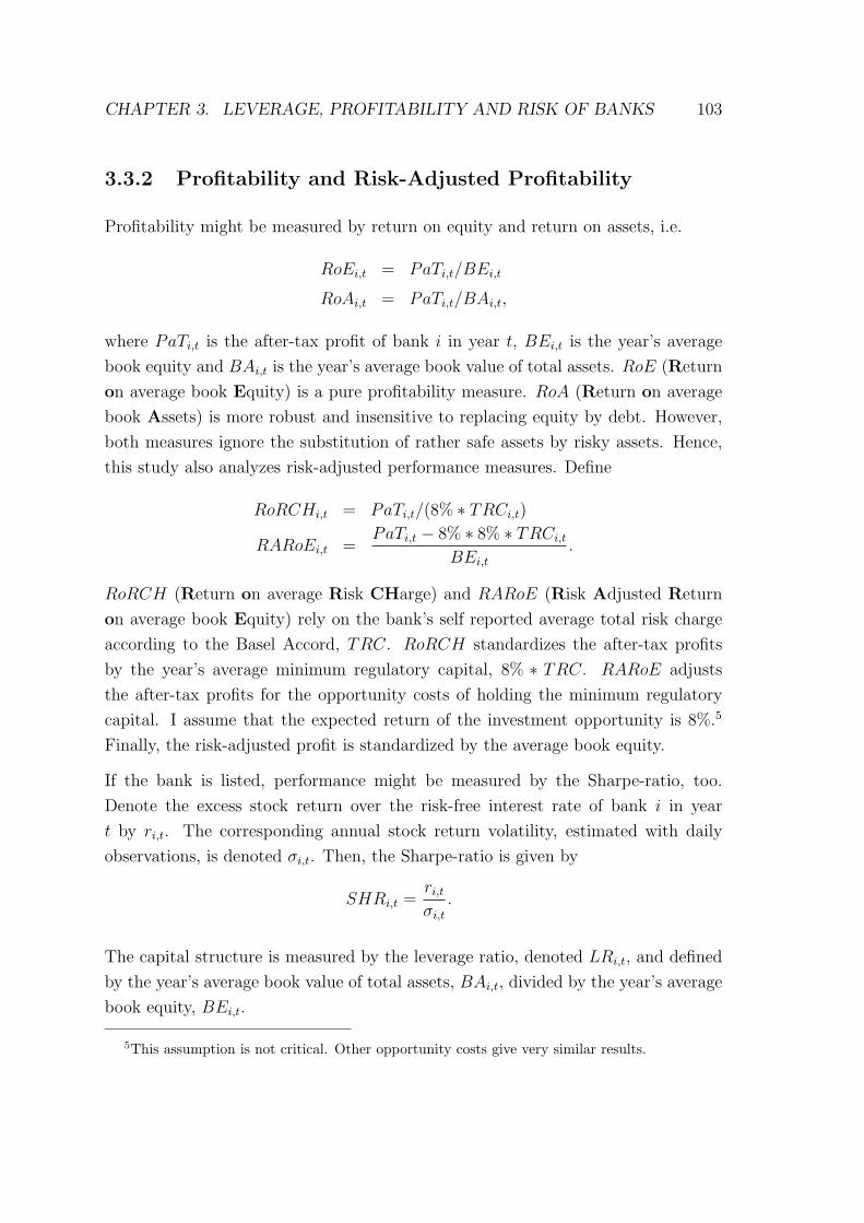
CHAPTER 3. LEVERAGE, PROFITABILITY AND RISK OF BANKS 103
3.3.2 Profitability and Risk-Adjusted Profitability
Profitability might be measured by return on equity and return on assets, i.e.
RoEi,t = PaTi,t/BEi,t
RoAi,t = PaTi,t/BAi,t,
where PaTi,t is the after-tax profit of bank i in year t, BEi,t is the year’s average
book equity and BAi,t is the year’s average book value of total assets. RoE (Return
on average book Equity) is a pure profitability measure. RoA (Return on average
book Assets) is more robust and insensitive to replacing equity by debt. However,
both measures ignore the substitution of rather safe assets by risky assets. Hence,
this study also analyzes risk-adjusted performance measures. Define
RoRCHi,t = PaTi,t/(8% ∗ TRCi,t)
RARoEi,t =PaTi,t − 8% ∗ 8% ∗ TRCi,t
BEi,t.
RoRCH (Return on average Risk CHarge) and RARoE (Risk Adjusted Return
on average book Equity) rely on the bank’s self reported average total risk charge
according to the Basel Accord, TRC. RoRCH standardizes the after-tax profits
by the year’s average minimum regulatory capital, 8% ∗ TRC. RARoE adjusts
the after-tax profits for the opportunity costs of holding the minimum regulatory
capital. I assume that the expected return of the investment opportunity is 8%.5
Finally, the risk-adjusted profit is standardized by the average book equity.
If the bank is listed, performance might be measured by the Sharpe-ratio, too.
Denote the excess stock return over the risk-free interest rate of bank i in year
t by ri,t. The corresponding annual stock return volatility, estimated with daily
observations, is denoted σi,t. Then, the Sharpe-ratio is given by
SHRi,t =ri,tσi,t
.
The capital structure is measured by the leverage ratio, denoted LRi,t, and defined
by the year’s average book value of total assets, BAi,t, divided by the year’s average
book equity, BEi,t.
5This assumption is not critical. Other opportunity costs give very similar results.
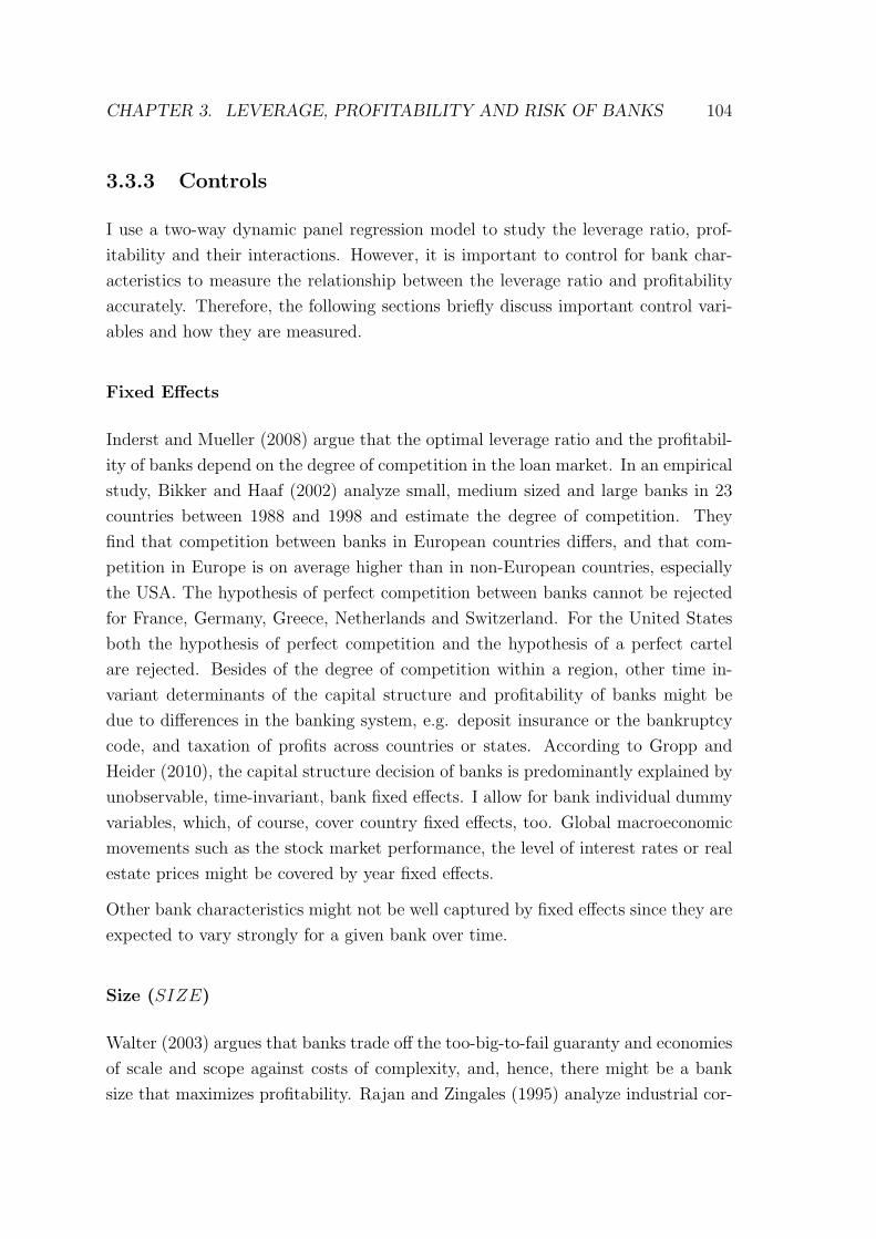
CHAPTER 3. LEVERAGE, PROFITABILITY AND RISK OF BANKS 104
3.3.3 Controls
I use a two-way dynamic panel regression model to study the leverage ratio, prof-
itability and their interactions. However, it is important to control for bank char-
acteristics to measure the relationship between the leverage ratio and profitability
accurately. Therefore, the following sections briefly discuss important control vari-
ables and how they are measured.
Fixed Effects
Inderst and Mueller (2008) argue that the optimal leverage ratio and the profitabil-
ity of banks depend on the degree of competition in the loan market. In an empirical
study, Bikker and Haaf (2002) analyze small, medium sized and large banks in 23
countries between 1988 and 1998 and estimate the degree of competition. They
find that competition between banks in European countries differs, and that com-
petition in Europe is on average higher than in non-European countries, especially
the USA. The hypothesis of perfect competition between banks cannot be rejected
for France, Germany, Greece, Netherlands and Switzerland. For the United States
both the hypothesis of perfect competition and the hypothesis of a perfect cartel
are rejected. Besides of the degree of competition within a region, other time in-
variant determinants of the capital structure and profitability of banks might be
due to differences in the banking system, e.g. deposit insurance or the bankruptcy
code, and taxation of profits across countries or states. According to Gropp and
Heider (2010), the capital structure decision of banks is predominantly explained by
unobservable, time-invariant, bank fixed effects. I allow for bank individual dummy
variables, which, of course, cover country fixed effects, too. Global macroeconomic
movements such as the stock market performance, the level of interest rates or real
estate prices might be covered by year fixed effects.
Other bank characteristics might not be well captured by fixed effects since they are
expected to vary strongly for a given bank over time.
Size (SIZE)
Walter (2003) argues that banks trade off the too-big-to-fail guaranty and economies
of scale and scope against costs of complexity, and, hence, there might be a bank
size that maximizes profitability. Rajan and Zingales (1995) analyze industrial cor-
CHAPTER 3. LEVERAGE, PROFITABILITY AND RISK OF BANKS 105
porations and find that size affects the capital structure decision. The same might
be true for banks, too. The size of an industrial corporation is often measured by
the logarithm of the book value of total assets. For financial institutions, this mea-
sure might be very noisy. Banks assets are hardly related to economic goods, hence,
total assets might not measure the sustainable bank size. A more resilient bank size
measure might be the logarithm of the (annual, average of) number of employees.
However, the logarithm of total assets is used for robustness checks.
Regulatory Pressure (REGP )
Banks with a total risk-weighted capital ratio below 10% operate close to the min-
imum regulatory requirements, and might be subject to regulatory pressure. As a
consequence, they might be restricted in their policy. Moreover, the bank’s creditors
and regulatory authorities might be alarmed, and, in efficient markets, funding costs
are likely to be high. This might cause a decline in profitability. Also, the bank
might be forced to adjust the balance sheet, which could affect the leverage ratio.
Hence, regulatory pressure might be a determinant of profitability and the leverage
ratio. I follow Flannery and Rangan (2008) and measure regulatory pressure by a
dummy variable, denoted REGP , that is one if a banks (annual, average of) total
risk-weighted capital ratio is below 10%.
Asset Structure (LPQ and LIQ)
The asset structure of a bank is measured by two variables, the loan portfolio quality
(LPQ) and the liquidity endowment (LIQ). This is, among others, motivated by
Diamond and Rajan (2000), who argue that credit risk and the liquidity endowment
determine the capital structure of banks. Angbazo (1997) and Berger (1995) show
that the loan portfolio quality, measured by the inverse of risk-weighted assets, of
non-performing assets or the net charge-off, is positively related to profitability, i.e.
the net interest margin and return on equity, respectively. Goddard et al. (2004)
and Molyneux and Thornton (1992) analyze the relationship between profits and
the liquidity endowment, but their results are ambiguous.
In this study, the loan portfolio quality is measured by the loan loss reserve relative
to the average total value of the loan portfolio. Given that a bank has a constant
charge-off policy, low values indicate high-quality loan portfolios and vice versa.
Alternative measures of the loan portfolio quality are discussed in the robustness
CHAPTER 3. LEVERAGE, PROFITABILITY AND RISK OF BANKS 106
section. The liquidity endowment is approximated by liquid assets over the sum of
customer deposits and short term funding.
Diversification (DIV )
Besides of interest income, commercial banks’ major income sources are fees and
commissions. Income from proprietary trading and off-balance sheet activity also
contribute to the overall bank income. To account for the income structure of a
bank, I measure the bank’s income diversification by the ratio of other operational
income - this is income others than interest, fee or commission income - divided
by total operational income. A value close to zero indicates that a bank’s business
is focused on ‘traditional’ income sources such as the loan business. A high ratio
indicates that the bank is heavily involved in e.g. proprietary trading or off-balance
sheet activities.
Angbazo (1997) and Lepetit et al. (2008) study off-balance sheet activity and bank-
income diversification, respectively, in detail, see also in Goddard et al. (2004).
However, the effect of income diversification on bank profitability and bank risk
are mixed. Diversification benefits might disappear fast since trading income and
off-balance sheet activities are normally more volatile than interest income.
Education / R&D (EDU)
Flannery and Rangan (2006) find that R&D expenses of industrial companies are
useful to explain the capital structures. R&D expenses are not available for banks.
However, the logarithm of personnel expenses per employee of banks might approx-
imate R&D expenses, since it also measures investments to develop and educate the
existing staff and to hire new, talented employees.
3.3.4 Descriptive Statistics
I analyze the balance sheets and income statements between 1994 and 2008 of Eu-
ropean and U.S. commercial banks, obtained from the Bankscope database. Due
to their special business models, investment banks, cooperative banks, special gov-
ernment banks and bank holding companies are not considered. Acquired or closed
banks are not excluded to mitigate the survivorship bias. The following European
CHAPTER 3. LEVERAGE, PROFITABILITY AND RISK OF BANKS 107
countries are included: Austria, Belgium, France, Germany, Great Britain, Italy,
Ireland, Luxembourg, Netherlands, Portugal, Spain and Switzerland. Small banks
are excluded. Therefore, I choose a minimum threshold for the book value of total
assets of 5 billion USD for U.S. banks and of 1 billion USD for European banks.
European savings banks are included, too. This measure and the lower threshold for
total assets for European banks raise the number of observations for the European
sample and allow to calculate robust estimates, even though they might increase
heterogeneity. Removing obvious data mistakes, e.g. banks with negative equity,
yields up to 1200 complete observations for about 175 U.S. banks and about 1000
observations for 205 European banks. The observations are almost equally spread
across years, however, for some reasons there are slightly fewer observations for the
years 2005 and 2006 than for the other years.
Table 3.10 in the appendix provides names of all listed banks in my sample. For
these banks, I download daily stock prices, adjusted for dividend payments and
stock splits, from Datastream. The LIBOR rate is used to approximate the risk-free
rate. I calculate the annual Sharpe-ratio for the time span 1994 to 2007 and exclude
the year 2008, since 2008 is characterized by extreme market turmoil for financial
institutions. Those market prices presumably were not the fundamental values and
are likely to bias the results. Even though the number of listed European banks is
larger than the number of listed U.S. banks (36 vs. 22), there are 178 bank-year
observations for the U.S. sample but only 132 observations for European banks.
This is due to the relatively low number of missing accounting figure for U.S. banks.
Table 3.1 shows descriptive statistics for all variables for U.S. banks and for European
banks. The upper panel gives the mean and the standard deviation across banks and
over time, the lower panel shows the correlation matrix for both samples separately.
Since the selection rule for European banks is less restrictive than for U.S. banks,
the column ‘EU Banks Cmp’ in the upper panel provides the mean and standard
deviation for European banks, applying the same selection rule as for U.S. banks,
i.e. a minimum threshold for the book value of total assets of 5 billion USD and
commercial banks only.
On average, U.S. banks are more profitable than European banks. The average RoE
of U.S. banks is 14.7 whereas the average RoE of European banks with comparable
size is 10.2. The differences in RoA are even more severe, 1.3 for U.S. banks and 0.56
for European banks. RoRCH and RARoE give similar results. The large differences
between RoA of U.S. and European banks might be due to the - on average - lower

CHAPTER 3. LEVERAGE, PROFITABILITY AND RISK OF BANKS 108
U.S. Banks EU Banks EU Banks Cmp
Mean Std. Dev. Mean Std. Dev. Mean Std. Dev.Variable
LR 11.7999 3.3748 21.1021 9.0802 23.5038 10.4958REGP 0.0042 0.0646 0.0568 0.2314 0.1101 0.3131LPQ 1.7023 1.1348 2.9940 3.0658 2.8041 2.5520LIQ 15.3627 20.3590 30.0273 21.6237 28.6799 21.4030DIV 0.3475 0.3175 0.1027 0.6959 0.1754 1.2880SIZE 8.2377 1.5900 6.5806 1.4078 7.6185 1.7174EDU 4.0897 0.5750 4.2280 0.5300 4.4612 0.6103
RoE 14.7089 11.0919 8.1574 13.3700 10.2052 14.5427RoA 1.3144 1.1532 0.5029 1.0259 0.5573 0.7781RoRCH 1.8886 1.5233 1.1557 3.0795 1.1561 4.6706RARoE 15.6323 11.5320 9.4067 11.9490 9.2052 14.7734SHR 0.2837 1.1018 0.2717 1.0698 0.2717 1.0698
U.S
.B
anks
RoE
RoA
RoRCH
RARoE
LR
REGP
LPQ
LIQ
DIV
SIZE
EDU
RoE
1.0
000
RoA
0.8
820
1.0
000
RoRCH
0.7
779
0.8
327
1.0
000
RARoE
0.9
585
0.8
545
0.8
312
1.0
000
LR
0.1
549
−0.2
150
−0.1
003
0.1
097
1.0
000
REGP
−0.1
502
−0.1
071
−0.1
223
−0.1
932
−0.0
575
1.0
000
LPQ
0.1
816
0.3
627
0.1
269
0.1
461
−0.2
931
−0.0
258
1.0
000
LIQ
−0.0
840
−0.0
791
0.0
178
−0.0
789
0.0
462
−0.0
138
−0.0
033
1.0
000
DIV
0.1
232
0.1
785
0.1
272
0.1
026
−0.0
181
0.0
592
0.1
969
−0.0
223
1.0
000
SIZE
−0.0
167
−0.0
182
−0.0
775
−0.0
081
−0.0
147
−0.0
412
−0.0
030
0.1
256
0.2
350
1.0
000
EDU
−0.2
163
−0.2
729
−0.1
060
−0.1
634
0.1
131
0.0
177
−0.2
580
0.2
880
−0.0
503
−0.0
996
1.0
000
Euro
pean
Banks
RoE
RoA
RoRCH
RARoE
LR
REGP
LPQ
LIQ
DIV
SIZE
EDU
RoE
1.0
000
RoA
0.7
221
1.0
000
RoRCH
0.3
630
0.2
419
1.0
000
RAROE
0.9
380
0.6
667
0.4
253
1.0
000
LR
−0.1
838
−0.5
816
0.0
040
−0.1
782
1.0
000
REGP
0.0
122
−0.0
733
−0.0
410
0.0
481
0.0
992
1.0
000
LPQ
−0.1
021
−0.0
767
−0.1
186
−0.1
276
−0.0
758
0.0
511
1.0
000
LIQ
0.0
152
0.0
047
0.2
500
−0.0
060
−0.0
660
−0.1
108
0.2
139
1.0
000
DIV
0.3
030
0.2
374
0.0
492
0.3
040
−0.0
697
0.0
049
−0.1
375
0.0
066
1.0
000
SIZE
−0.0
169
−0.2
272
−0.0
773
−0.0
177
0.2
934
0.0
580
−0.1
375
−0.2
275
0.0
948
1.0
000
EDU
−0.0
556
−0.2
144
0.2
218
−0.0
002
0.0
490
−0.0
319
−0.0
375
−0.1
583
0.0
551
−0.1
844
1.0
000
Table 3.1: The upper panel shows the mean and standard deviation of bank char-acteristics, the lower panel gives the correlation matrices. RoE= return on equity,RoA= return on assets, RoRCH,RARoE= risk-adjusted profitability, LR= lever-age ratio, LPQ= loan portfolio quality, LIQ= liquidity endowment, DIV = incomediversification, SIZE= ln # employees, EDU= ln personnel expenses per employee.
CHAPTER 3. LEVERAGE, PROFITABILITY AND RISK OF BANKS 109
profitability (see RoE) and the higher leverage ratio of European banks, 23.5 versus
11.8. This is consistent with Inderst and Mueller (2008), who argue that the optimal
leverage ratio increases with the degree of competition in the loan market, and Bikker
and Haaf (2002), who show that the competition in the loan market is stronger in
Europe than in the USA. However, there is no significant difference between the
Sharpe-ratios of European banks and U.S. banks. The average Sharpe-ratio of U.S.
banks is 28.37% and 27.17% for European banks. The corresponding standard
deviations are similar, too. The highest Sharpe-ratio of a U.S. bank [European
banks] is 3.47 in 1997 [4.39 in 1997] and the lowest Sharpe-ratio is -2.46 in 2007
[-2.24 in 1999].
Consistent with Flannery and Rangan (2008), the total risk-weighted capital ratio
of U.S. banks is mostly not binding. Only 0.5% of the bank-year observations (or
5 observations) undershoot the 10% total risk-weighted capital ratio. The total
risk-weighted capital ratio of European banks is below 10% for about 50 bank-year
observations. The liquidity endowment of U.S. banks is significantly lower compared
to European banks. While U.S. banks hold on average about 15% of customer
deposits and short term funding in liquid assets, European banks hold almost twice
as much in liquid assets. Also, European banks have a higher loan loss reserve
relative to the total loan portfolio. The income structure of U.S. banks seems to be
more diversified than the income structure of European banks. Whereas U.S. banks
generate on average about 35% of their total income through income sources other
than interest income and commissions and fees, European banks seem to be more
focused on these traditional income sources.
The lower panel of Table 3.1 gives the estimated correlation matrix of the bank
characteristics. By construction, the profitability measures are highly correlated.
The absolute values of the other correlation coefficients are almost always below
0.3, indicating that collinearity is not present.
3.4 Empirical Analysis
3.4.1 Active Capital Structure Management
I follow Flannery and Rangan (2006) to find out whether bank mangers actively
implement some target leverage ratio and to estimate the speed of adjustment of
the leverage ratio. The existence of a target leverage ratio and a high speed of
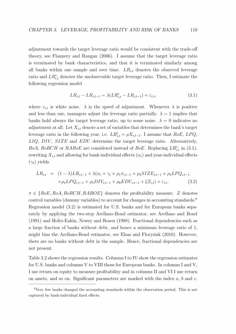
CHAPTER 3. LEVERAGE, PROFITABILITY AND RISK OF BANKS 110
adjustment towards the target leverage ratio would be consistent with the trade-off
theory, see Flannery and Rangan (2006). I assume that the target leverage ratio
is terminated by bank characteristics, and that it is terminated similarly among
all banks within one sample and over time. LRi,t denotes the observed leverage
ratio and LR∗i,t denotes the unobservable target leverage ratio. Then, I estimate the
following regression model
LRi,t − LRi,t−1 = λ(LR∗i,t − LRi,t−1) + εi,t, (3.1)
where εi,t is white noise. λ is the speed of adjustment. Whenever λ is positive
and less than one, managers adjust the leverage ratio partially. λ = 1 implies that
banks hold always the target leverage ratio, up to some noise. λ = 0 indicates no
adjustment at all. Let Xi,t denote a set of variables that determines the bank’s target
leverage ratio in the following year, i.e. LR∗i,t = ρXi,t−1. I assume that RoE, LPQ,
LIQ, DIV , SIZE and EDU determine the target leverage ratio. Alternatively,
RoA, RoRCH or RARoE are considered instead of RoE. Replacing LR∗i,t in (3.1),
rewriting Xi,t and allowing for bank-individual effects (αi) and year-individual effects
(γt) yields
LRi,t = (1− λ)LRi,t−1 + λ(αi + γt + ρ1πi,t−1 + ρ2SIZEi,t−1 + ρ3LPQi,t−1
+ρ4LPQi,t−1 + ρ5DIVi,t−1 + ρ6EDUi,t−1 + ξZi,t) + εi,t. (3.2)
π ∈ {RoE,RoA,RoRCH,RAROE} denotes the profitability measure. Z denotes
control variables (dummy variables) to account for changes in accounting standards.6
Regression model (3.2) is estimated for U.S. banks and for European banks sepa-
rately by applying the two-step Arellano-Bond estimator, see Arellano and Bond
(1991) and Holtz-Eakin, Newey and Rosen (1988). Fractional dependencies such as
a large fraction of banks without debt, and hence a minimum leverage ratio of 1,
might bias the Arellano-Bond estimator, see Elsas and Florysiak (2010). However,
there are no banks without debt in the sample. Hence, fractional dependencies are
not present.
Table 3.2 shows the regression results. Columns I to IV show the regression estimates
for U.S. banks and columns V to VIII those for European banks. In columns I and V,
I use return on equity to measure profitability and in columns II and VI I use return
on assets, and so on. Significant parameters are marked with the index a, b and c.
6Very few banks changed the accounting standards within the observation period. This is notcaptured by bank-individual fixed effects.
CHAPTER 3. LEVERAGE, PROFITABILITY AND RISK OF BANKS 111
U.S
.B
anks
EU
Ban
ks
Reg
ress
ion
Num
ber
III
III
IVV
VI
VII
VII
I
LRi,t−
10.
4598a
0.43
08a
0.39
51a
0.40
84a
0.65
86a
0.66
03a
0.69
10a
0.69
13a
RoE
i,t−
1−
0.01
55a
--
-−
0.00
51-
--
RoA
i,t−
1-
−0.
0926a
--
-−
0.20
81b
--
RoRCHi,t−
1-
-−
0.00
67-
--
0.67
28a
-RARoE
i,t−
1-
--
−0.
0128a
--
-0.
0659a
SIZEi,t−
1−
0.08
40−
0.10
97−
0.06
69−
0.04
881.
8641a
1.75
33a
4.83
41a
5.11
69a
REGPi,t−
10.
2876
0.27
260.
1416
0.14
19−
0.04
51−
0.11
46−
1.12
19a−
1.00
31a
LPQi,t−
10.
0394
0.02
990.
0271
0.02
740.
0630
−0.
0716
0.07
37−
0.21
18c
LIQi,t−
10.
0019
0.00
280.
0009
0.00
15−
0.01
49a−
0.01
86a−
0.00
730.
0011
DIVi,t−
10.
0696
0.04
410.
0088
0.05
441.
6748b
1.70
96b
18.6
304a
21.5
772a
EDUi,t−
1−
0.01
32−
0.04
971−
0.03
350.
0346
1.60
371.
5307a
4.32
38a
4.80
93a
#O
bs74
274
273
673
665
465
420
020
0#
Ban
ks15
115
115
115
118
518
565
65
Sarg
ante
stof
over
-ide
ntify
ing
rest
rict
ions
pva
lue
0.26
480.
2438
0.25
380.
3194
0.66
750.
6851
0.99
500.
9987
Are
llano
-Bon
dte
stth
atav
erag
eau
toco
vari
ance
inre
sidu
als
is...
...of
orde
r1
is0:
H0:
noau
toco
rrel
atio
np
valu
e0.
7586
0.74
420.
3582
0.22
300.
3112
0.33
030.
2520
0.23
60
Tab
le3.
2:T
he
table
show
sth
ere
gres
sion
esti
mat
esfo
rpar
tial
adju
stm
ents
inth
ele
vera
gera
tio
tow
ards
ata
rget
leve
rage
rati
ofo
rU
.S.
ban
ks
(lef
tpan
el)
and
Euro
pea
nban
ks
(rig
ht
pan
el),
i.e.
regr
essi
onm
odel
(3.1
).a
den
otes
sign
ifica
nce
atth
e1%
confiden
cele
vel,b
atth
e5%
confiden
cele
vel
andc
atth
e10
%le
vel.
CHAPTER 3. LEVERAGE, PROFITABILITY AND RISK OF BANKS 112
a denotes significance at the 1% confidence level, b at the 5% confidence level and c
at the 10% level. The Sagran test fails to reject the hypothesis of correctly specified
instrumental variables7 and the Arellano-Bond test fails to reject the hypothesis of
no autocorrelations in the residuals. The estimated speed of adjustments of U.S.
banks is in the range 55% to 60% (1− 0.4598 to 1− 0.3951). This means that the
average bank closes half of the gap between the target leverage ratio and the actual
leverage ratio within 14 to 15 months, or equivalently, about 40% to 44% of the
gap each year.8 The estimated speed of adjustment for U.S. banks is significantly
higher than the estimated speed of adjustment of industrial corporations, which are
analyzed by Flannery and Rangan (2006). They find that the average company
closes half of the gap between the current and the target capital structure in about
two years. For European banks, the estimated speed of adjustment is about 35%
and of similar magnitude as in Flannery and Rangan (2006). The results are also
consistent with Gropp and Heider (2010), who study European and U.S. banks
jointly, and report a speed of adjustment of about 45%, which is within the interval
given by the estimates for European and U.S. banks presented here.
The rather high estimate of λ for U.S. banks is consistent with the trade-off theory
and with the hypothesis that financial institutions have a lower tolerance for holding
an undesired capital structure than non-financial corporations. The estimated speed
of adjustment of European banks is lower compared to U.S. banks, but might still
be consistent with the trade-off theory, as argued by Flannery and Rangan (2006).
This low adjustment speed might have two reasons: (1) European banks manage
their capital structure less actively than U.S. banks. This might be due to the
less restrictive bank regulation in Europe, i.e. no floor on the capital-asset ratio.
(2) The higher degree of heterogeneity in the European sample, caused by the less
restrictive minimum bank size, the joint analysis of commercial bank and savings
banks, and the pooling across European countries, might bias the estimates towards
a low adjustment speed.
Even though I apply other selection criteria and consider a different observation
period, the estimates of the determinants of the target leverage ratio are generally
consistent with Gropp and Heider (2010), i.e. profitability seems to be the most
7The instrumental variables are implicitly defined in the two step Arellano-Bond estimator.8Consider the estimate for λ in regression I. The half-life time is calculated by ln 2/λ ≈ 1.26,
which is about 15 months. Hence, the bank closes 11.26 ∗50% ≈ 40% of the gap between the leverage
ratios each year.
CHAPTER 3. LEVERAGE, PROFITABILITY AND RISK OF BANKS 113
important determinant. Moreover, since profitability is interacted with risk in re-
gressions III, IV, VII and VIII, new insights arise. For U.S. banks, all determinants
of the target leverage ratio are insignificant with the exception for return on equity,
return on assets and risk-adjusted return on equity, which have a significant, negative
coefficient. The impact of return on assets is negative and significant for European
banks, too. Hence, banks seem to use profits as a funding source and reduce the
leverage ratio after realizing high profits. However, risk adjusted profitability is sig-
nificant and positive for European banks. Therefore, at least in Europe, banks with
a sound risk-return profile are - ceteris paribus - likely to leverage up in the following
year. One reason might be to take advantage of the tax shield without suffering too
much from high default costs. Since U.S. banks can leverage up only to some limit,
this relationship might be mitigated and could explain the insignificant regression
coefficient for RoRCH and the significant, negative coefficient for RARoE.
For European banks, size turns out as a significant determinant of the leverage ratio,
as hypothesized by Rajan and Zingales (1995). This result does not change if total
book assets are used to measure size. The results are not shown. Furthermore, in
regressions VII and VIII, banks that are confronted with regulatory pressure tend
to reduce their leverage ratio. This finding is not robust and might depend on the
sample, since regulatory pressure is insignificant in regressions V and VI, which are
based on a larger number of observations.
3.4.2 Performance Maximizing Leverage Ratio
Given the evidence that banks manage their leverage ratio towards a target lever-
age ratio, I now investigate whether there is a performance maximizing leverage
ratio. This leverage ratio might be important not only for the bank owners and the
bank manager, but also for the regulator. Therefore, I assume that the bank man-
ager maximizes profitability or risk-adjusted profitability. This assumption seems
plausible since profitability and risk-adjusted profitability are the only consistently
significant variables in the previous analysis.
Again, I use a two-way panel regression model to relate bank performance to the
leverage ratio and the control variables. According to Berger et al. (2000), bank
profits are highly persistent. To account for this, the regression model allows for
autoregression of order 1 in profitability. Furthermore, and consistent with the trade-
off theory and with Berger and Bonaccorsi di Patti (2006) and Korteweg (2010), I
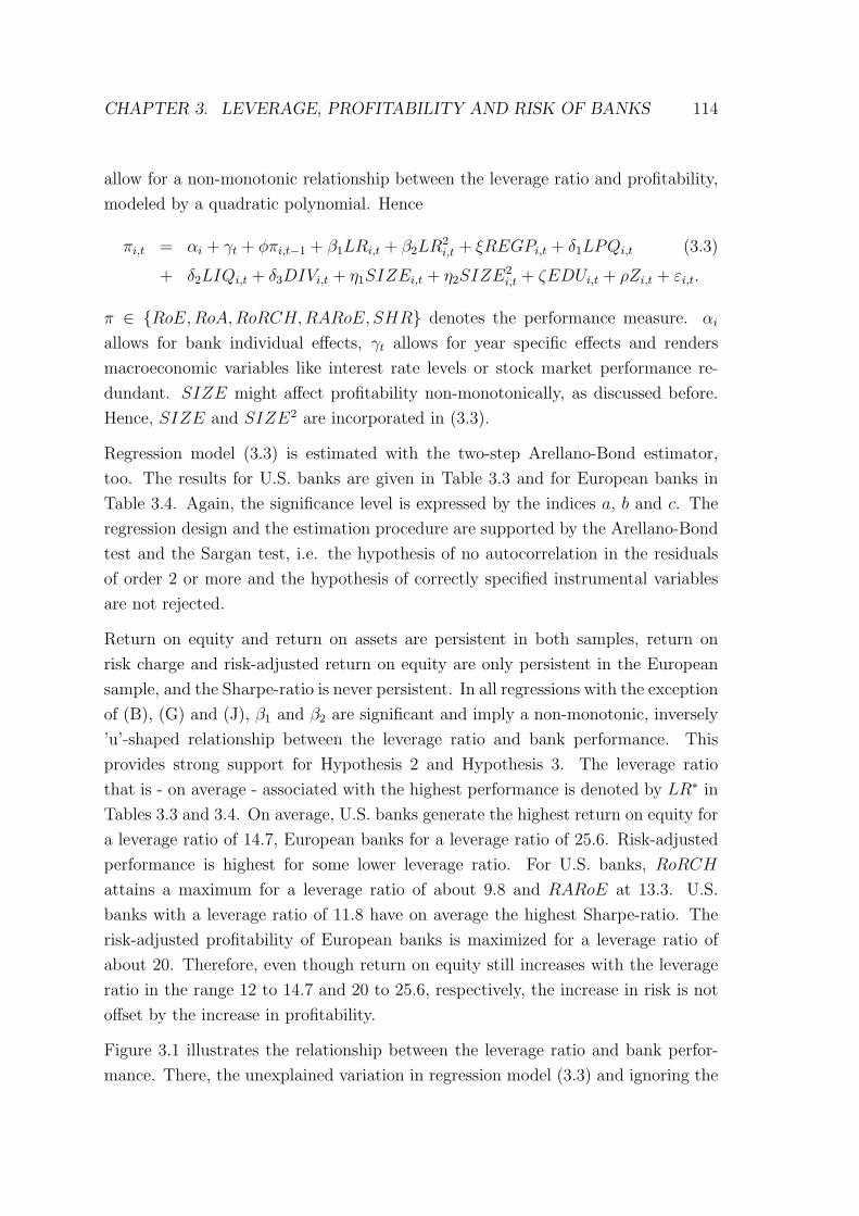
CHAPTER 3. LEVERAGE, PROFITABILITY AND RISK OF BANKS 114
allow for a non-monotonic relationship between the leverage ratio and profitability,
modeled by a quadratic polynomial. Hence
πi,t = αi + γt + φπi,t−1 + β1LRi,t + β2LR2i,t + ξREGPi,t + δ1LPQi,t (3.3)
+ δ2LIQi,t + δ3DIVi,t + η1SIZEi,t + η2SIZE2i,t + ζEDUi,t + ρZi,t + εi,t.
π ∈ {RoE,RoA,RoRCH,RARoE, SHR} denotes the performance measure. αi
allows for bank individual effects, γt allows for year specific effects and renders
macroeconomic variables like interest rate levels or stock market performance re-
dundant. SIZE might affect profitability non-monotonically, as discussed before.
Hence, SIZE and SIZE2 are incorporated in (3.3).
Regression model (3.3) is estimated with the two-step Arellano-Bond estimator,
too. The results for U.S. banks are given in Table 3.3 and for European banks in
Table 3.4. Again, the significance level is expressed by the indices a, b and c. The
regression design and the estimation procedure are supported by the Arellano-Bond
test and the Sargan test, i.e. the hypothesis of no autocorrelation in the residuals
of order 2 or more and the hypothesis of correctly specified instrumental variables
are not rejected.
Return on equity and return on assets are persistent in both samples, return on
risk charge and risk-adjusted return on equity are only persistent in the European
sample, and the Sharpe-ratio is never persistent. In all regressions with the exception
of (B), (G) and (J), β1 and β2 are significant and imply a non-monotonic, inversely
’u’-shaped relationship between the leverage ratio and bank performance. This
provides strong support for Hypothesis 2 and Hypothesis 3. The leverage ratio
that is - on average - associated with the highest performance is denoted by LR∗ in
Tables 3.3 and 3.4. On average, U.S. banks generate the highest return on equity for
a leverage ratio of 14.7, European banks for a leverage ratio of 25.6. Risk-adjusted
performance is highest for some lower leverage ratio. For U.S. banks, RoRCH
attains a maximum for a leverage ratio of about 9.8 and RARoE at 13.3. U.S.
banks with a leverage ratio of 11.8 have on average the highest Sharpe-ratio. The
risk-adjusted profitability of European banks is maximized for a leverage ratio of
about 20. Therefore, even though return on equity still increases with the leverage
ratio in the range 12 to 14.7 and 20 to 25.6, respectively, the increase in risk is not
offset by the increase in profitability.
Figure 3.1 illustrates the relationship between the leverage ratio and bank perfor-
mance. There, the unexplained variation in regression model (3.3) and ignoring the
CHAPTER 3. LEVERAGE, PROFITABILITY AND RISK OF BANKS 115
U.S. Banks
Dependent Variable RoE RoA RoRCH RARoE SHRRegression Number (A) (B) (C) (D) (E)
φ (LAG π) 0.2413a 0.1684a −0.0064 0.0248 −0.2060β1 (LR) 2.5827a 0.0417 0.1686b 4.8405a 13.0200c
β2 (LR2) −0.0881a −0.0040c −0.0086a −0.1822a −0.5508c
ξ (REGP ) −14.9639 −1.3448 −2.3540 −32.4769 -δ1 (LPQ) −1.3385a −0.1864a −0.5062a −2.3825a 1.7776δ2 (LIQ) −0.0777a −0.0075a −0.0018 −0.0915a 0.2082δ3 (DIV ) −0.2294 0.1423c −0.0343 −2.2790 21.0180η1 (SIZE) 1.3738 0.1426 1.4555a 2.1799 −10.1920η2 (SIZE2) −0.0398 −0.0117 −0.0853a −0.0684 0.5163η3 (EDU) 3.2564a 0.3035a 0.6308a 3.9256a 1.0961
LR∗ 14.7 - 9.8 13.3 11.8
#of Obs / Banks 917 / 175 917 / 175 806 / 156 806 / 156 156 / 20
Sargan test of over-identifying restrictionspvalue 0.1333 0.2372 0.3776 0.1534 1.0000
Arellano-Bond test that average autocovariance in residuals is ...... of order 1 is 0: H0: no autocorrelationpvalue 0.0000 0.0009 0.0014 0.0010 0.2761... of order 2 is 0: H0: no autocorrelationpvalue 0.3300 0.2077 0.1014 0.0924 0.8486
Table 3.3: The table shows the regression results of the determinants of bank per-formance for U.S. banks, i.e. regression model (3.3). Profitability is measured byreturn on equity, return on assets, return on risk-charge, risk-adjusted return onequity and the Sharpe-ratio. a denotes significance at the 1% confidence level, bat the 5% confidence level and c at the 10% level. LR∗ denotes the on average,performance maximizing leverage ratio.

CHAPTER 3. LEVERAGE, PROFITABILITY AND RISK OF BANKS 116
European Banks
Dependent Variable RoE RoA RoRCH RARoE SHRRegression Number (F) (G) (H) (I) (J)
φ (LAG π) 0.3837a 0.3793a 0.7947a 0.4907a −0.2802β1 (LR) 2.0777a 0.0158 0.1157a 1.2538a 0.0413β2 (LR2) −0.0406a −0.0006a −0.0030a −0.0305a −0.0011ξ (REGP ) 1.3152a 0.0944a 0.0309 −1.2128b −0.5301δ1 (LPQ) −1.1957a −0.1403a 0.0021 −0.0026 1.2085δ2 (LIQ) 0.0052 −0.0006 0.0113a 0.1731a 0.0209δ3 (DIV ) −13.8234a −0.4679a −4.2824a −29.1219a 2.3403η1 (SIZE) −5.0860 −0.6635a 0.6445 2.6687 24.8900c
η2 (SIZE2) 0.1327 0.0294b 0.0015 0.5762b −1.2944c
η3 (EDU) −1.1755 −0.1470a 0.7531a 11.9212a 3.1954
LR∗ 25.6 - 19.3 20.6 -
#of Obs / Banks 828 / 208 828 / 208 199 / 61 199 / 61 95 / 24
Sargan test of over-identifying restrictionspvalue 0.8934 0.8792 0.9878 0.9989 1.0000
Arellano-Bond test that average autocovariance in residuals is ...... of order 1 is 0: H0: no autocorrelationpvalue 0.0051 0.0669 0.1695 0.1974 0.3006... of order 2 is 0: H0: no autocorrelationpvalue 0.3012 0.3106 0.2237 0.1616 0.0230
Table 3.4: The table shows the regression results of the determinants of bank per-formance for European banks, i.e. regression model (3.3). Profitability is measuredby return on equity, return on assets, return on risk-charge, risk-adjusted returnon equity and the Sharpe-ratio. a denotes significance at the 1% confidence level,b at the 5% confidence level and c at the 10% level. LR∗ denotes the on average,performance maximizing leverage ratio.
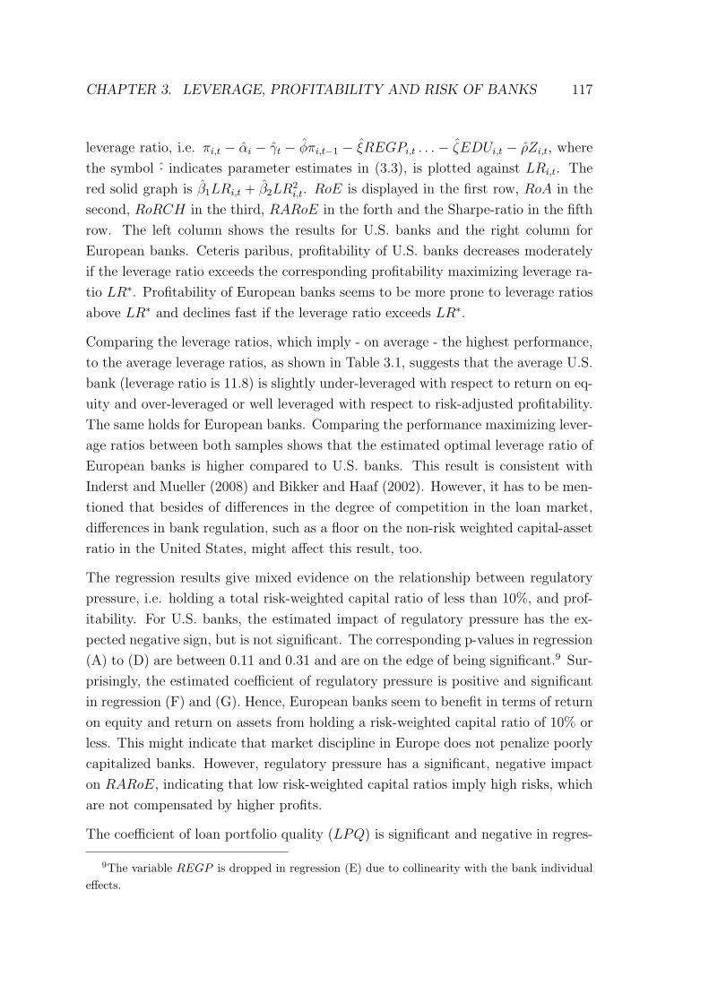
CHAPTER 3. LEVERAGE, PROFITABILITY AND RISK OF BANKS 117
leverage ratio, i.e. πi,t − αi − γt − φπi,t−1 − ξREGPi,t . . . − ζEDUi,t − ρZi,t, where
the symbol · indicates parameter estimates in (3.3), is plotted against LRi,t. The
red solid graph is β1LRi,t + β2LR2i,t. RoE is displayed in the first row, RoA in the
second, RoRCH in the third, RARoE in the forth and the Sharpe-ratio in the fifth
row. The left column shows the results for U.S. banks and the right column for
European banks. Ceteris paribus, profitability of U.S. banks decreases moderately
if the leverage ratio exceeds the corresponding profitability maximizing leverage ra-
tio LR∗. Profitability of European banks seems to be more prone to leverage ratios
above LR∗ and declines fast if the leverage ratio exceeds LR∗.
Comparing the leverage ratios, which imply - on average - the highest performance,
to the average leverage ratios, as shown in Table 3.1, suggests that the average U.S.
bank (leverage ratio is 11.8) is slightly under-leveraged with respect to return on eq-
uity and over-leveraged or well leveraged with respect to risk-adjusted profitability.
The same holds for European banks. Comparing the performance maximizing lever-
age ratios between both samples shows that the estimated optimal leverage ratio of
European banks is higher compared to U.S. banks. This result is consistent with
Inderst and Mueller (2008) and Bikker and Haaf (2002). However, it has to be men-
tioned that besides of differences in the degree of competition in the loan market,
differences in bank regulation, such as a floor on the non-risk weighted capital-asset
ratio in the United States, might affect this result, too.
The regression results give mixed evidence on the relationship between regulatory
pressure, i.e. holding a total risk-weighted capital ratio of less than 10%, and prof-
itability. For U.S. banks, the estimated impact of regulatory pressure has the ex-
pected negative sign, but is not significant. The corresponding p-values in regression
(A) to (D) are between 0.11 and 0.31 and are on the edge of being significant.9 Sur-
prisingly, the estimated coefficient of regulatory pressure is positive and significant
in regression (F) and (G). Hence, European banks seem to benefit in terms of return
on equity and return on assets from holding a risk-weighted capital ratio of 10% or
less. This might indicate that market discipline in Europe does not penalize poorly
capitalized banks. However, regulatory pressure has a significant, negative impact
on RARoE, indicating that low risk-weighted capital ratios imply high risks, which
are not compensated by higher profits.
The coefficient of loan portfolio quality (LPQ) is significant and negative in regres-
9The variable REGP is dropped in regression (E) due to collinearity with the bank individualeffects.
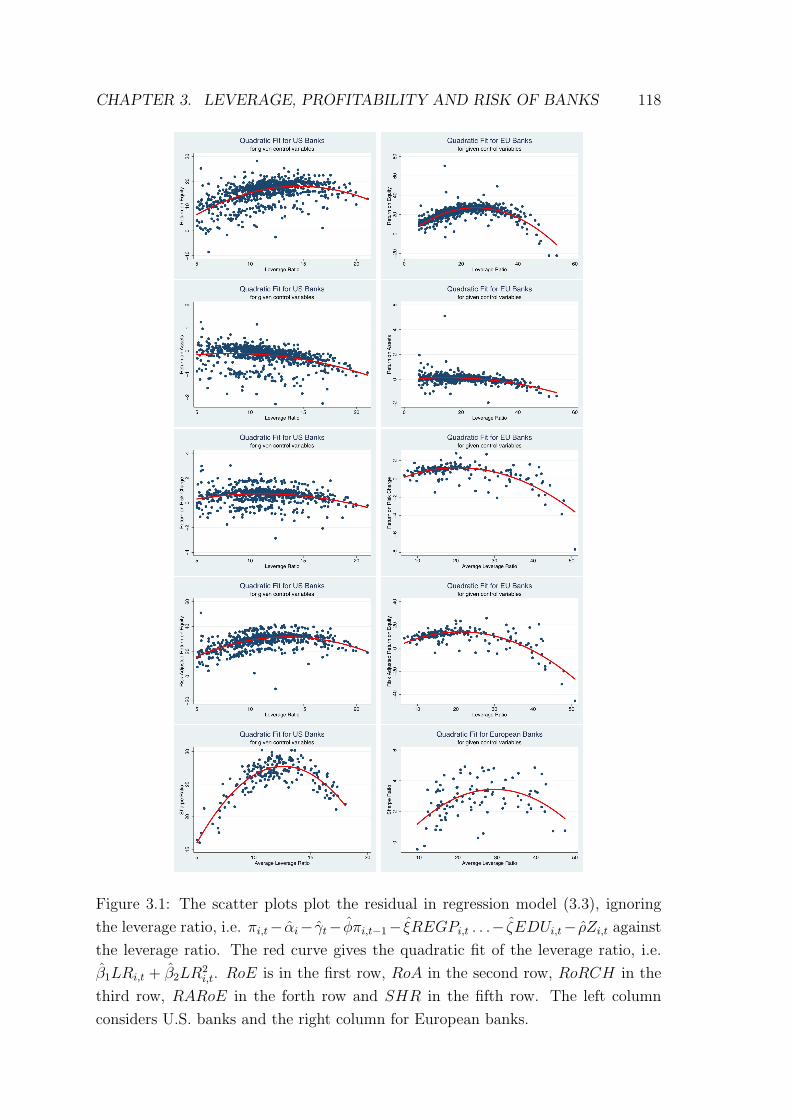
CHAPTER 3. LEVERAGE, PROFITABILITY AND RISK OF BANKS 118
Figure 3.1: The scatter plots plot the residual in regression model (3.3), ignoring
the leverage ratio, i.e. πi,t− αi− γt− φπi,t−1− ξREGPi,t . . .− ζEDUi,t− ρZi,t against
the leverage ratio. The red curve gives the quadratic fit of the leverage ratio, i.e.
β1LRi,t + β2LR2i,t. RoE is in the first row, RoA in the second row, RoRCH in the
third row, RARoE in the forth row and SHR in the fifth row. The left column
considers U.S. banks and the right column for European banks.
CHAPTER 3. LEVERAGE, PROFITABILITY AND RISK OF BANKS 119
sion (A) to (D) and (F) and (G). Since a high value of LPQ indicates a low loan
portfolio quality, the regressions imply that profitability and risk-adjusted profitabil-
ity are high for banks with high-quality loans. This finding is consistent with the
literature, see e.g. Berger (1995). The estimated coefficient of liquidity endowment,
δ2, is negative and significant in (A), (B) and (D) and positive and significant for
(H) and (I). δ2 < 0 in (A) and (B) indicates that liquid assets tend to reduce return
on equity and return on assets. Furthermore, the negative sign of δ2 in (D) indicates
that the decline in profits, caused by holding a high proportion of liquid assets,
is not compensated by risk reduction. Hence, the dominant relationship between
risk-adjusted profitability and liquidity is negative, too. RoE and RoA of European
banks are not sensitive to the liquidity endowment, but RoRCH and RARoE are
positively related to the liquidity endowment. Hence, a high liquidity endowment
tends to reduce the bank’s risk and does not affect profitability. So, risk-adjusted
profitability increases.
Income diversification does not affect RoE, RoRCH and RARoE but is positive
and significant for RoA in the U.S. sample. It is negative and significant for Euro-
pean banks in regressions (F) to (I). Lepetit et al. (2008) argue that non-interest
income is more volatile than interest income. Hence, diversification benefits might
be destroyed fast, such that banks with a high fraction of non-interest income spoil
their risk-return profile. This could explain the negative relationship between risk-
adjusted profitability and income diversification.
The regression estimates for the coefficients of bank size give no evidence for an
optimal bank size. η1 and η2 are jointly significant in (C) and (G). In (G), the
coefficients imply an ’u’-shaped relation between the logarithmic number of em-
ployees and bank performance, which contradicts the existence of an optimal bank
size. Hence, it remains ambiguous whether an optimal bank size exists. The aver-
age personnel expenses per employees are positive and significant for all performance
measures for U.S. banks, indicating that banks with well-trained employees generate
- on average - higher profits and have a sound risk-return profile. η3 is insignificant
in regression (F), negative and significant in (G) and positive and significant in (H)
and (I). Even though profitability of European banks tends to increase if banks
invest less in their employees, presumably due to cost advantages, risk-adjusted
profitability is positively related to EDU .
There might be a lagged relationship between the leverage ratio and profitability,
if benefits of holding the desired leverage ratio, loan-portfolio quality or liquidity
CHAPTER 3. LEVERAGE, PROFITABILITY AND RISK OF BANKS 120
endowment pay off in later periods. Therefore, I estimate regression model (3.3)
with independent variables lagged by one year. Furthermore, this analysis might
be used to predict bank profitability rather than to explain it. Table 3.5 shows
the regression estimates. The Sharpe-ratio is not considered since the number of
observations is insufficient. Due to collinearity between the dummy variable REGP
and the bank- and year-fixed effects, REGP is excluded for U.S. banks. As can be
seen in all regressions, the relationship between the leverage ratio and profitability
and risk-adjusted profitability, respectively, is consistent with the previous estimates.
The profitability maximizing leverage ratio of U.S. bank is about 14.6, see regression
(A.1). However, return on assets is now inversely ’u’-shaped related to the leverage
ratio, too, see (B.1). This gives further support to Hypothesis 2. The leverage ratio
that maximizes average return on assets is about 13.1. Risk-adjusted profitability
is maximized for a leverage ratio of about 12.8. European banks’ return on equity
is maximized for a leverage ratio of 25.4 and risk-adjusted profitability for 20.9 and
23.3, respectively. However, the sign of the loan portfolio quality is now significant,
positive, indicating that the relationship between the loan portfolio quality and
profitability is fragile or more complex.
3.4.3 Robustness
Capital Structure
The regression estimates in Tables 3.3, 3.4 and 3.5 support a non-monotone, in-
versely ’u’-shaped relationship between the leverage ratio and return on equity and
risk-adjusted profitability, respectively. However, this result might be artificial.
A globally increasing and concave relationship might be well approximated by a
quadratic polynomial, which attains a maximum in the interior of the supported
domain, if there are only few observations in the right tail and many observations
in the left tail. Another shortcoming of a quadratic polynomial is that it implies a
symmetric relationship. Furthermore, the control variables might affect profitability
conditionally on high or low leverage ratios.
Therefore, I divide the sample into two subsamples, hereafter the left tail and the
right tail. The tails depend on the performance measure. Since the previous section
indicates that RoE, RoRCH and RARoE are consistently non-monotonically re-
lated to the leverage ratio, I consider only these three performance measures. Banks
with a leverage ratio lower than LR1(π) are considered as moderately leveraged
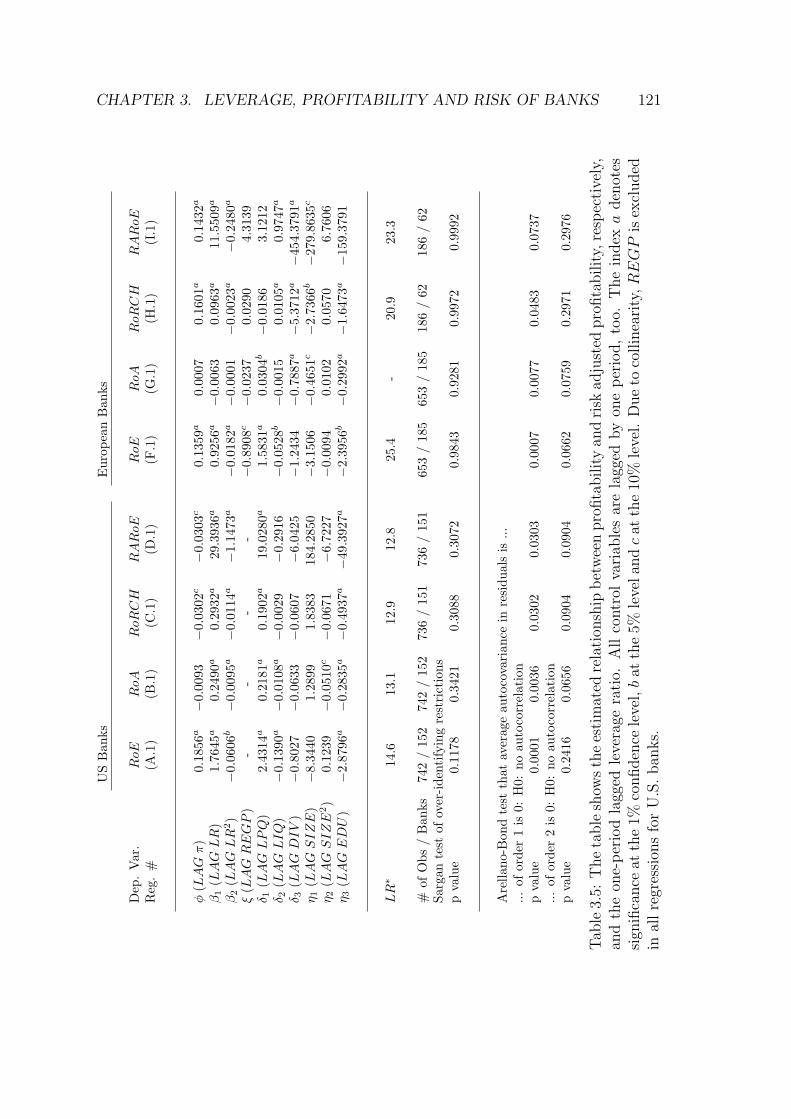
CHAPTER 3. LEVERAGE, PROFITABILITY AND RISK OF BANKS 121U
SB
anks
Eur
opea
nB
anks
Dep
.V
ar.
RoE
RoA
RoRCH
RARoE
RoE
RoA
RoRCH
RARoE
Reg
.#
(A.1
)(B
.1)
(C.1
)(D
.1)
(F.1
)(G
.1)
(H.1
)(I
.1)
φ(LAGπ
)0.
1856a−
0.00
93−
0.03
02c
−0.
0303c
0.13
59a
0.00
070.
1601a
0.14
32a
β1
(LAGLR
)1.
7645a
0.24
90a
0.29
32a
29.3
936a
0.92
56a−
0.00
630.
0963a
11.5
509a
β2
(LAGLR
2)
−0.
0606b−
0.00
95a−
0.01
14a
−1.
1473a
−0.
0182a−
0.00
01−
0.00
23a
−0.
2480a
ξ(LAGREGP
)-
--
-−
0.89
08c−
0.02
370.
0290
4.31
39δ 1
(LAGLPQ
)2.
4314a
0.21
81a
0.19
02a
19.0
280a
1.58
31a
0.03
04b−
0.01
863.
1212
δ 2(LAGLIQ
)−
0.13
90a−
0.01
08a−
0.00
29−
0.29
16−
0.05
28b−
0.00
150.
0105a
0.97
47a
δ 3(LAGDIV
)−
0.80
27−
0.06
33−
0.06
07−
6.04
25−
1.24
34−
0.78
87a−
5.37
12a−
454.
3791a
η 1(LAGSIZE
)−
8.34
401.
2899
1.83
8318
4.28
50−
3.15
06−
0.46
51c−
2.73
66b−
279.
8635c
η 2(LAGSIZE
2)
0.12
39−
0.05
10c−
0.06
71−
6.72
27−
0.00
940.
0102
0.05
706.
7606
η 3(LAGEDU
)−
2.87
96a−
0.28
35a−
0.49
37a−
49.3
927a
−2.
3956b−
0.29
92a−
1.64
73a−
159.
3791
LR∗
14.6
13.1
12.9
12.8
25.4
-20
.923
.3
#of
Obs
/B
anks
742
/15
274
2/
152
736
/15
173
6/
151
653
/18
565
3/
185
186
/62
186
/62
Sarg
ante
stof
over
-ide
ntify
ing
rest
rict
ions
pva
lue
0.11
780.
3421
0.30
880.
3072
0.98
430.
9281
0.99
720.
9992
Are
llano
-Bon
dte
stth
atav
erag
eau
toco
vari
ance
inre
sidu
als
is...
...of
orde
r1
is0:
H0:
noau
toco
rrel
atio
np
valu
e0.
0001
0.00
360.
0302
0.03
030.
0007
0.00
770.
0483
0.07
37...
ofor
der
2is
0:H
0:no
auto
corr
elat
ion
pva
lue
0.24
160.
0656
0.09
040.
0904
0.06
620.
0759
0.29
710.
2976
Tab
le3.
5:T
he
table
show
sth
ees
tim
ated
rela
tion
ship
bet
wee
npro
fita
bilit
yan
dri
skad
just
edpro
fita
bilit
y,re
spec
tive
ly,
and
the
one-
per
iod
lagg
edle
vera
gera
tio.
All
contr
olva
riab
les
are
lagg
edby
one
per
iod,
too.
The
index
aden
otes
sign
ifica
nce
atth
e1%
confiden
cele
vel,b
atth
e5%
leve
lan
dc
atth
e10
%le
vel.
Due
toco
llin
eari
ty,REGP
isex
cluded
inal
lre
gres
sion
sfo
rU
.S.
ban
ks.
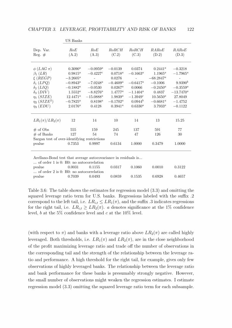
CHAPTER 3. LEVERAGE, PROFITABILITY AND RISK OF BANKS 122
US Banks
Dep. Var. RoE RoE RoRCH RoRCH RARoE RARoEReg. # (A.2) (A.3) (C.2) (C.3) (D.2) (D.3)
φ (LAG π) 0.3090a −0.0959a −0.0139 0.0374 0.2441a −0.3218β1 (LR) 0.9815a −0.4227c 0.0718a −0.1663a 1.1965a −1.7965a
ξ (REGP ) −3.2605a - 0.0276 - −68.2847a -δ1 (LPQ) −0.8943a −7.0248a −0.4609a −0.6417a −0.1006 9.9390b
δ2 (LIQ) −0.1882a −0.0530 0.0267a 0.0066 −0.2450a −0.3559a
δ3 (DIV ) 1.5552a −8.8276a 1.4777a −1.1404a 0.4837 −13.7470a
η1 (SIZE) 12.4471a −15.0888a 1.9839a −1.3949c 10.5650a 27.8049η2 (SIZE2) −0.7825a 0.8198a −0.1702a 0.0944b −0.6681a −1.4752η3 (EDU) 2.0176a 0.4128 0.3941a 0.6330a 3.7933a −0.1122
LR1(π)/LR2(π) 12 14 10 14 13 15.25
# of Obs 555 159 245 137 591 77# of Banks 127 54 74 47 126 30Sargan test of over-identifying restrictionspvalue 0.7353 0.9997 0.6134 1.0000 0.3479 1.0000
Arellano-Bond test that average autocovariance in residuals is...... of order 1 is 0: H0: no autocorrelationpvalue 0.0031 0.1155 0.0317 0.1060 0.0010 0.3122... of order 2 is 0: H0: no autocorrelationpvalue 0.7039 0.0493 0.0859 0.1535 0.6928 0.4657
Table 3.6: The table shows the estimates for regression model (3.3) and omitting thesquared leverage ratio term for U.S. banks. Regressions labeled with the suffix .2correspond to the left tail, i.e. LRi,t ≤ LR1(π), and the suffix .3 indicates regressionsfor the right tail, i.e. LRi,t ≥ LR2(π). a denotes significance at the 1% confidencelevel, b at the 5% confidence level and c at the 10% level.
(with respect to π) and banks with a leverage ratio above LR2(π) are called highly
leveraged. Both thresholds, i.e. LR1(π) and LR2(π), are in the close neighborhood
of the profit maximizing leverage ratio and trade off the number of observations in
the corresponding tail and the strength of the relationship between the leverage ra-
tio and performance. A high threshold for the right tail, for example, gives only few
observations of highly leveraged banks. The relationship between the leverage ratio
and bank performance for these banks is presumably strongly negative. However,
the small number of observations might weaken the regression estimates. I estimate
regression model (3.3) omitting the squared leverage ratio term for each subsample.
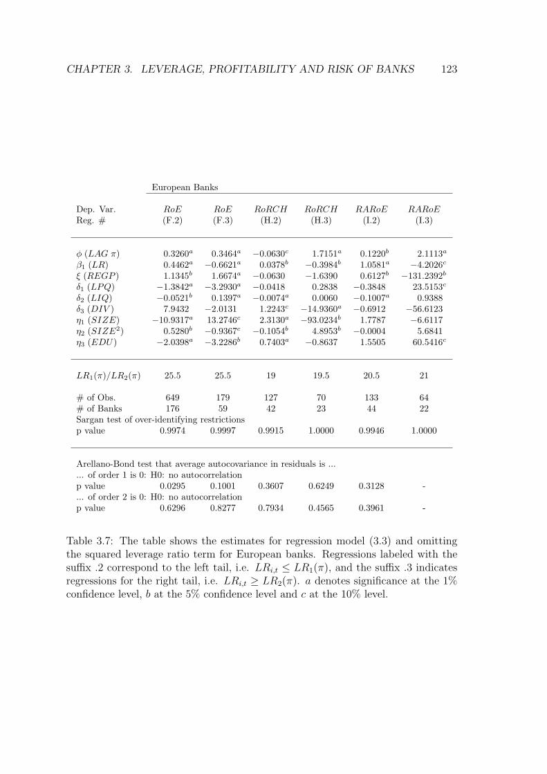
CHAPTER 3. LEVERAGE, PROFITABILITY AND RISK OF BANKS 123
European Banks
Dep. Var. RoE RoE RoRCH RoRCH RARoE RARoEReg. # (F.2) (F.3) (H.2) (H.3) (I.2) (I.3)
φ (LAG π) 0.3260a 0.3464a −0.0630c 1.7151a 0.1220b 2.1113a
β1 (LR) 0.4462a −0.6621a 0.0378b −0.3984b 1.0581a −4.2026c
ξ (REGP ) 1.1345b 1.6674a −0.0630 −1.6390 0.6127b −131.2392b
δ1 (LPQ) −1.3842a −3.2930a −0.0418 0.2838 −0.3848 23.5153c
δ2 (LIQ) −0.0521b 0.1397a −0.0074a 0.0060 −0.1007a 0.9388δ3 (DIV ) 7.9432 −2.0131 1.2243c −14.9360a −0.6912 −56.6123η1 (SIZE) −10.9317a 13.2746c 2.3130a −93.0234b 1.7787 −6.6117η2 (SIZE2) 0.5280b −0.9367c −0.1054b 4.8953b −0.0004 5.6841η3 (EDU) −2.0398a −3.2286b 0.7403a −0.8637 1.5505 60.5416c
LR1(π)/LR2(π) 25.5 25.5 19 19.5 20.5 21
# of Obs. 649 179 127 70 133 64# of Banks 176 59 42 23 44 22Sargan test of over-identifying restrictionsp value 0.9974 0.9997 0.9915 1.0000 0.9946 1.0000
Arellano-Bond test that average autocovariance in residuals is ...... of order 1 is 0: H0: no autocorrelationp value 0.0295 0.1001 0.3607 0.6249 0.3128 -... of order 2 is 0: H0: no autocorrelationp value 0.6296 0.8277 0.7934 0.4565 0.3961 -
Table 3.7: The table shows the estimates for regression model (3.3) and omittingthe squared leverage ratio term for European banks. Regressions labeled with thesuffix .2 correspond to the left tail, i.e. LRi,t ≤ LR1(π), and the suffix .3 indicatesregressions for the right tail, i.e. LRi,t ≥ LR2(π). a denotes significance at the 1%confidence level, b at the 5% confidence level and c at the 10% level.
CHAPTER 3. LEVERAGE, PROFITABILITY AND RISK OF BANKS 124
Table 3.6 gives the regression estimates for U.S. banks and Table 3.7 for European
banks. The regression estimates for the subsamples with LRi,t ≤ LR1(π) are labeled
with the suffix (.2) and estimates for subsamples with LRi,t ≥ LR2(π) are labeled
with (.3). LR1(π) and LR2(π) are given in Tables 3.6 and 3.7, too. For all regressions
the estimated coefficient for the leverage ratio, β1, is significant and positive for the
left tail and significant and negative for the right tail. Hence, I conclude that the
average RoE, RoRCH and RARoE are maximized for some leverage ratio close to
the estimated optimal leverage ratio LR(π)∗ given in Table 3.3 and 3.4. Furthermore,
RoRCH and RARoE are very prone to high leverage ratios and decrease fast if the
leverage ratio exceeds LR2(π). This is consistent with Figure 1 and indicates an
asymmetric relation between the leverage ratio and bank performance. Consider,
for example, RoRCH of European banks. β1 is about 0.04 in regression (H.2) and
about -0.4 in (H.3). Ceteris paribus, the average risk-adjusted profitability tends to
decreases 10 times faster if the leverage ratio exceeds the upper threshold than it
increases up to the lower threshold.
Regulatory pressure is significant and negative in (A.2) and (D.2) and insignificant
in (C.2). The dummy variable REGP is excluded in regressions (A.3), (C.3) and
(D.3) for highly leveraged U.S. banks due to collinearity. The significant, negative
regression coefficients in (A.2) and (D.2) indicate that poorly capitalized banks
generate below average profits. Consistent with regression (F), regulatory pressure
is significant and positive in (F.2) and (F.3), indicating that market discipline is
rather weak for European banks with respect to RoE. Regulatory pressure is also
significant and positive in (I.2), but turns significant and negative in (I.3). Therefore,
moderately leveraged banks may increase RARoE by reducing total risk-weighted
capital ratio even below 10%. This is not true for highly leveraged banks. This
heterogeneous relationship between risk-weighted capital and performance for highly
leveraged banks and moderately leveraged banks indicates that bank lenders monitor
the non risk-weighted leverage ratio and the total risk-weighted capital ratio jointly.
The coefficient of the loan portfolio quality is significant and negative for to RoE
and RoRCH for U.S. banks, see (A.2), (A.3), (C.2) and (C.3) and indicates that
a high loan portfolio quality is associated with high profitability. Comparing the
magnitude of δ1 in (A.2) and (A.3) and in (C.2) and (C.3), respectively, shows that
profitability of highly leveraged banks is more sensitive to the loan portfolio quality
than the profitability of moderately leveraged banks. Hence, market participants
seem to interpret the risk of the loan portfolio conditional on the leverage ratio.
Surprisingly, δ1 is insignificant in (D.2) and turns even positive and significant in
CHAPTER 3. LEVERAGE, PROFITABILITY AND RISK OF BANKS 125
(D.3). One explanation might be the low number of observations in regression (D.3).
As Table 3.4 already reveals, the loan portfolio quality affects return on equity of
European banks, but not RoRCH and RARoE. This result is confirmed in Table
3.7. (F.2) and (F.3) also show that return on equity of European banks is more
prone to the loan portfolio quality if the bank’s leverage ratio is high.
Consistent with regression (A), (A.2) and (A.3) show that high liquidity endowment
is associated with low return on equity, irrespective of the leverage ratio. Regression
(C.2) shows that moderately leveraged banks might improve RoRCH by reducing
the liquidity endowment, whereas the liquidity endowment turns insignificant for
highly leveraged banks, see (C.3). In contrast, I find a significant, negative relation-
ship between RARoE and the liquidity endowment in (D.2) and (D.3), indicating
that low liquidity buffers stimulate RARoE. Therefore, the overall impact of the
liquidity endowment is ambiguous. Income diversification of U.S. banks positively
impact profitability, given a moderate leverage ratio, but has the opposite effect for
high leverage ratios. The estimated impact of the liquidity endowment and income
diversification on profitability of European banks is ambiguous, too.
The relationship between bank size and profitability is still ambiguous. η1 and η2
change the sign frequently and give no clear implications. Whereas the average
personnel expenses per employee are positively related to the return on equity of
U.S. banks, EDU has a significant, negative coefficient in regression (F.2) and (F.3).
Again, this might indicate that cost advantages are more important than benefits
of well educated employees with respect to return on equity. However, this reverses
if risk-adjusted profitability measures are considered.
Loan Portfolio Quality and Size
In this section, I test the robustness of the previous results by applying alternative
measures of bank size and the loan portfolio quality. Even though the logarithm
of the average book value of total assets is stronger correlated with the leverage
ratio than the logarithmic number of employees, I use it in the following to measure
bank size. The loan portfolio quality is measured by the net charge-offs divided by
the annual, average book value of the loan portfolio. This measure does not rely
on a constant charge-off policy. Table 3.8 gives the estimates of regression model
(3.3), but with the alternative measure for the loan portfolio quality, LPQ, and the
alternative size measure, SIZE. The alternative measures reduce the number of
CHAPTER 3. LEVERAGE, PROFITABILITY AND RISK OF BANKS 126
observations for European banks significantly since information about net charge-
offs of European banks is sparse. The Sharpe-ratio is not considered due to an
insufficient number of observations. The coefficients of the leverage ratio change
only little compared to Tables 3.3 and 3.4. However, β1 and β2 are not significant in
regression (H.4), indicating a fragile relationship between RoRCH and the leverage
ratio of European banks. Consistent with the previous results, δ1 is negative and
significant in all regressions. Again, this indicates that banks benefit from a high
loan portfolio quality. For U.S. banks, there is no significant relationship between the
logarithm of total assets and profitability or risk-adjusted profitability, respectively,
confirming the previous results. Size is significant for European banks, but the
coefficients give no implications for an optimal bank size.
3.4.4 Default Costs and Leverage Ratio
Section 4.1 shows that banks adjust their capital structure fast. Section 4.2 and
4.3 show that some interior leverage ratio is on average associated with the high-
est profitability and risk-adjusted profitability, respectively. Both decline fast for
European banks if the leverage ratio exceeds this leverage ratio. According to the
trade-off theory, the decline is due to a strong increase in default costs. In the
following, I analyze the relationship between the expected default costs of banks
and the leverage ratio. A positive relationship might support the implementation
of a maximum leverage ratio in addition to a risk-based restriction on the capital
structure to control systemic risks in the economy.
I use the annual average spread of 3 years credit default swaps on senior debt to
measure the expected default costs of a bank. CDS spreads are taken from Datas-
tream (CMA, respectively) and Credit Trade and are available from 2003 to 2008
for 27 European banks and only 9 U.S. banks. Banks with CDS spreads are marked
with the symbol (*) in Table 3.10.10
Denote the average CDS spread of year t and bank i by CDSi,t. Then, I estimate
the following regression model
CDSi,t = αi + γt + β1LRi,t + ξREGPi,t + δ1LPQi,t + δ2LIQi,t (3.4)
+ δ3DIVi,t + η1SIZEi,t + η2SIZE2i,t + ζEDUi,t + ρZi,t + εi,t,
10European banks with CDS spreads and without traded stocks are Anglo Irish Bank, NorthernRock and Rabobank.

CHAPTER 3. LEVERAGE, PROFITABILITY AND RISK OF BANKS 127U
SB
anks
Eur
opea
nB
anks
Dep
.V
ar.
RoE
RoA
RoRCH
RARoE
RoE
RoA
RoRCH
RARoE
Reg
.#
(A.3
)(B
.3)
(C.3
)(D
.3)
(F.3
)(G
.3)
(H.3
)(I
.3)
φ(LAGπ
)0.
2059a
0.12
34a
0.00
290.
0440b
0.25
03a
0.44
29a−
0.13
20c
0.00
23β
1(LR
)2.
2219a−
0.01
420.
1516b
4.87
58a
2.41
24a−
0.00
400.
0364
1.55
84a
β2
(LR
2)
−0.
0678a−
0.00
11−
0.00
79a
−0.
1778a
−0.
0452a
0.00
00−
0.00
09−
0.03
41a
ξ(REGP
)−
12.3
083
−1.
7343b−
2.32
61−
32.5
543
0.48
650.
0360
−0.
0161
0.16
08δ 1
(LPQ
)−
2.33
06a−
0.22
59a−
0.23
88a
−2.
1122a
−0.
4288a−
0.01
53c−
0.05
11b
−1.
1144a
δ 2(LIQ
)−
0.06
41a−
0.00
57b
0.00
19−
0.10
10a
−0.
0961a−
0.00
74a−
0.00
25−
0.06
21b
δ 3(DIV
)−
0.34
520.
1685c
0.01
94−
1.18
93−
0.12
280.
4706c−
5.21
25a−
35.4
799a
η 1(SIZE
)1.
8632
0.11
72−
0.53
286.
4444
−21
.230
9a−
2.07
73a−
2.11
18a−
27.8
384a
η 2(SIZE
2)
−0.
0500
−0.
0062
0.01
02−
0.21
270.
5984a
0.05
98a
0.06
50a
0.94
29a
η 3(EDU
)4.
2826a
0.42
88a
0.68
42a
4.24
70a
−0.
1083
0.05
96−
0.02
01−
0.66
07
#of
Obs
/B
anks
916
/17
491
6/
174
806
/15
680
6/
156
378
/10
237
8/
102
146
/46
146
/46
Sarg
ante
stof
over
-ide
ntify
ing
rest
rict
ions
pva
lue
0.16
870.
3653
0.37
630.
1066
0.99
230.
9928
0.99
990.
9985
Are
llano
-Bon
dte
stth
atav
erag
eau
toco
vari
ance
inre
sidu
als
is...
...of
orde
r1
is0:
H0:
noau
toco
rrel
atio
np
valu
e0.
0000
0.00
060.
0042
0.00
080.
0159
0.02
630.
1655
0.65
33...
ofor
der
2is
0:H
0:no
auto
corr
elat
ion
pva
lue
0.22
240.
1279
0.17
580.
0889
0.97
650.
4227
0.27
340.
0889
Tab
le3.
8:T
he
table
show
sth
ere
gres
sion
esti
mat
esfo
rm
odel
(3.3
)an
dth
eal
tern
ativ
em
easu
res
for
ban
ksi
zean
dth
elo
anp
ortf
olio
qual
ity.
The
left
par
tof
the
table
show
sth
ees
tim
ates
for
U.S
.ban
ks,
the
righ
tpar
tsh
ows
the
resu
lts
for
Euro
pea
nban
ks.a
den
otes
sign
ifica
nce
atth
e1%
confiden
cele
vel,b
atth
e5%
confiden
cele
vel
andc
atth
e10
%le
vel.
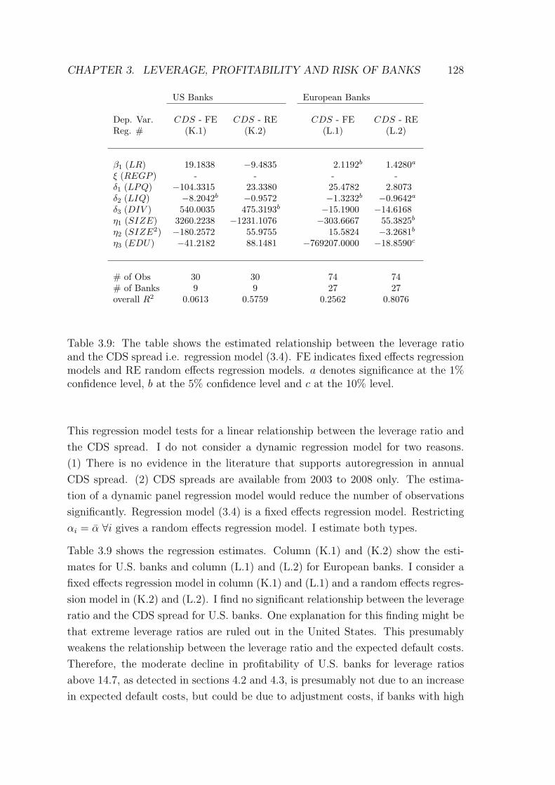
CHAPTER 3. LEVERAGE, PROFITABILITY AND RISK OF BANKS 128
US Banks European Banks
Dep. Var. CDS - FE CDS - RE CDS - FE CDS - REReg. # (K.1) (K.2) (L.1) (L.2)
β1 (LR) 19.1838 −9.4835 2.1192b 1.4280a
ξ (REGP ) - - - -δ1 (LPQ) −104.3315 23.3380 25.4782 2.8073δ2 (LIQ) −8.2042b −0.9572 −1.3232b −0.9642a
δ3 (DIV ) 540.0035 475.3193b −15.1900 −14.6168η1 (SIZE) 3260.2238 −1231.1076 −303.6667 55.3825b
η2 (SIZE2) −180.2572 55.9755 15.5824 −3.2681b
η3 (EDU) −41.2182 88.1481 −769207.0000 −18.8590c
# of Obs 30 30 74 74# of Banks 9 9 27 27overall R2 0.0613 0.5759 0.2562 0.8076
Table 3.9: The table shows the estimated relationship between the leverage ratioand the CDS spread i.e. regression model (3.4). FE indicates fixed effects regressionmodels and RE random effects regression models. a denotes significance at the 1%confidence level, b at the 5% confidence level and c at the 10% level.
This regression model tests for a linear relationship between the leverage ratio and
the CDS spread. I do not consider a dynamic regression model for two reasons.
(1) There is no evidence in the literature that supports autoregression in annual
CDS spread. (2) CDS spreads are available from 2003 to 2008 only. The estima-
tion of a dynamic panel regression model would reduce the number of observations
significantly. Regression model (3.4) is a fixed effects regression model. Restricting
αi = α ∀i gives a random effects regression model. I estimate both types.
Table 3.9 shows the regression estimates. Column (K.1) and (K.2) show the esti-
mates for U.S. banks and column (L.1) and (L.2) for European banks. I consider a
fixed effects regression model in column (K.1) and (L.1) and a random effects regres-
sion model in (K.2) and (L.2). I find no significant relationship between the leverage
ratio and the CDS spread for U.S. banks. One explanation for this finding might be
that extreme leverage ratios are ruled out in the United States. This presumably
weakens the relationship between the leverage ratio and the expected default costs.
Therefore, the moderate decline in profitability of U.S. banks for leverage ratios
above 14.7, as detected in sections 4.2 and 4.3, is presumably not due to an increase
in expected default costs, but could be due to adjustment costs, if banks with high
CHAPTER 3. LEVERAGE, PROFITABILITY AND RISK OF BANKS 129
leverage ratios are forced to adjust their capital structure more often to satisfy the
regulatory requirements than banks with low leverage ratios.
β1 is positive and significant for European banks, see (L.1) and (L.2). This indicates
that high leverage ratios are associated with high default costs and might explain
the sharp decline in profitability and risk-adjusted profitability if the leverage ratio
exceeds 25 and 20, respectively. Furthermore, it seems that a restriction on the
leverage ratio decouples expected default costs and the leverage ratio. It is likely
that expected default costs of banks and systemic risk are positively correlated,
hence, systemic risk might be reduced by an upper limit on the non-risk weighted
leverage ratio.
The coefficients of size, measured by the logarithm of the average number of employ-
ees, are significant in (L.2), and imply that the CDS spreads of banks with at least
2,400 employees are negatively related to the (logarithmic) number of employees.
This result is consistent with the implicit too-big-to-fail guarantee.
3.5 Conclusion
Banks adjust their capital structure fast, compared to industrial corporations. Be-
sides of bank- and year-individual fixed effects, profitability and risk-adjusted prof-
itability are consistently significant determinants of the leverage ratio. Moreover,
profitability and risk-adjusted profitability of banks are non-monotonically, inversely
‘u’-shape related to the leverage ratio. High and low leverage ratios reduce both,
profitability and risk-adjusted profitability. Further determinants of profitability are
the loan portfolio quality and the liquidity endowment. The results of diversifica-
tion, size and personal expenses are ambiguous. I find evidence that default costs
increase significantly with the leverage ratio for European banks. Hence, the decline
in profitability of European banks is presumably due to high default costs. This
result does not hold for U.S. banks. In addition to a restriction on the risk-weighted
capital ratio, U.S. banks are restricted in their non-risk weighted capital structure.
This additional restriction could weaken the relationship between the leverage ratio
and expected default costs.
How should the regulator respond to the new challenges in the financial industry? As
shown by Blum (2008), promoted by the Basel Committee on Banking Supervision,
and applied in the USA, a restriction on the non risk-weighted capital structure
CHAPTER 3. LEVERAGE, PROFITABILITY AND RISK OF BANKS 130
in addition to the risk-based capital approach of Basel II might be appropriate
to control systemic risk. Restricting the leverage ratio of European banks to the
ratio, that is associated with the highest risk-adjusted profitability (≈ 20), might
be a reasonable compromise between the regulators objectives and the bank owners
objectives, as suggested by Allen Greenspan. This restriction reduces the average
return on equity, ceteris paribus, by approximately 1.25 to 2.25 percentage points
compared to the average profitability maximizing leverage ratio of about 25 and
according to the estimates in regressions (F) and (F.2), respectively.
This study does not measure systemic risk explicitly. Further research might analyze
the relationship between the capital structure of banks and other, explicit measures
of systemic risk. Moreover, the regulator might impose further restrictions on banks
(see Basel III), which are not discussed here, but will affect profitability and risk-
adjusted profitability. Further empirical research might focus on those regulatory
tools and evaluate the consequences.

CHAPTER 3. LEVERAGE, PROFITABILITY AND RISK OF BANKS 131
3.6 Appendix
U.S. Banks EU Banks
Bank of America, National Association (*) ABN Amro Holding NV (*)Bank of New York (*) Banca Carige SpABranch Banking and Trust Company Banca Popolare di Milano SCaRL (*)Capital One National Association (*) Banco Bilbao Vizcaya Argentaria SA (*)Charter One Bank, NA Banco de Sabadell SA (*)Chase Bank USA, NA Banco de Valencia SACitibank NA (*) Banco Espanol de Credito SAComerica Bank Banco Espirito Santo SAFifth Third Bank Banco Pastor SA (*)Huntington National Bank Banco Popular Espanol SA (*)JP Morgan Chase Bank, NA (*) Banco Santander SAKey Bank USA, National Association Bank of Ireland (*)Manufacturers and Traders Trust Company Bankinter SA (*)Northern Trust Company (The) Barclays Bank Plc (*)PNC Bank, National Association BNP Paribas (*)Regions Bank Commerzbank AG (*)Sallie Mae-SLM Corporation Deutsche Bank AG (*)State Street Corporation Dexia BankSunTrust Bank EFG Bank European Financial GroupWachovia Bank, National Association (*) Erste Group Bank AGWashington Mutual Bank (*) Gruppo Monte dei Paschi di SienaWells Fargo Bank, NA (*) HSBC Bank plc (*)
ING Bank NV (*)Intesa Sanpaolo (*)KBC Bank NV (*)Lloyds TSB Bank Plc (*)Mediobanca SpAMillennium Banco Comercial Portuguis (*)National Westminster Bank PlcNatixis (*)Raiffeisen International Bank-HoldingRoyal Bank of Scotland Plc (The)SNS Bank N.V. (*)Societe Generale (*)UBS AG (*)UniCredit SpA (*)
22 Banks 36 Banks178 Observations 132 Observations
Table 3.10: The table shows the listed banks for which we calculate the Sharpe-ratio as risk adjusted profitability measure. The symbol (*) marks banks with CDSspreads. Those banks are used in section 4.3. Banks with CDS spreads and withoutlisted stocks are Anglo Irish Bank, Northern Rock and Rabobank.

Bibliography
[1] Adrian, Tobias and Hyun Song Shin, 2010, ”Liquidity and Leverage”, Journal
of Financial Intermediation 19, 418-437.
[2] Angbazo, Lazarus 1997, ”Commercial Bank Net Interest Margins, Default Risk,
Interest-Rate Risk, and Off-Balance Sheet Banking”, Journal of Banking and
Finance 21, 55-87.
[3] Arellano, Manuel and Stephen Bond 1991, ”Some Tests of Specification for Panel
Data: Monte Carlo Evidence and an Application to Employment Equations”,
Review of Economic Studies 58, 277-297.
[4] Baker, Malcolm and Jeffrey Wurgler, 2002, ”Market Timing and Capital Struc-
ture” Journal of Finance 57, 1-32.
[5] Berger, Allen N. 1995, ”The Relationship between Capital and Earnings in Bank-
ing”, Journal of Money, Credit and Banking 27, 432-456.
[6] Berger, Allen N., Seth D. Bonime, Daniel M. Covitz and Dianna Hancock 2000,
”Why are Bank Profits so Persistent? The Roles of Product Market Competi-
tion, Informational Opacity, and Regional / Macroeconomic Shocks”, Journal of
Banking and Finance 24, 1203-1235.
[7] Berger, Allen N. and Emilia Bonaccorsi di Patti, 2006, ”Capital Structure and
Firm Performance: A new Approach to Testing agency Theory and an Applica-
tion to the Banking Industry”, Journal of Banking and Finance 30, 1065-1102.
[8] Bikker, Jacob A. and Katharina Haaf 2002, ”Competition, Concentration and
their Relationship: An Empirical Analysis of the Banking Industry”, Journal of
Banking and Finance 26, 2191-2214.
[9] Blum, Jurg, 1999, ”Do Capital Adequacy Requirements Reduce Risks in Bank-
ing?” Journal of Banking and Finance 23, 755-771.
132

CHAPTER 3. LEVERAGE, PROFITABILITY AND RISK OF BANKS 133
[10] Blum, Jurg, 2008, ”Why ’Basel II’ may need a Leverage Ratio Restriction”,
Journal of Banking and Finance 32, 1699-1707.
[11] Diamond, Douglas W. and Raghuram G. Rajan, 2000, ”A Theory of Bank
Capital”, Journal of Finance 55, 2431-2465.
[12] Fama, Eugene and Kenneth French, 2005, ”Financing Decisions: Who Issues
Stock”, Journal of Financial Economics 76, 549-582.
[13] Fischer, Edwin O., Robert Heinkel and Josef Zechner 1989, ”Dynamic Capital
Structure Choice: Theory and Test”, Journal of Finance 44, 19-40.
[14] Fiordelisi Franco and Phil Molyneux, 2010. ”The Determinant of Shareholder
Value in European Banking”, Journal of Banking and Finance 34, 1189-1200.
[15] Flannery, Mark J., 1994, ”Debt Maturity and the Deadweight Cost of Leverage:
Optimally Financing Banking Firms”, American Economic Review 84, 320-331.
[16] Flannery, Mark J. and Kasturi P. Rangan, 2006, ”Partial Adjustment towards
Target Capital Structures”, Journal of Financial Economics 79, 469-506.
[17] Flannery, Mark J. and Kasturi P. Rangan, 2008, ”What Caused the Bank
Capital Build-Up of the 1990s?”, Review of Finance 12, 391-429.
[18] Frank, Murray Z., and Vidhan K. Goyal, 2003, ”Testing the Pecking Order
Theory of Capital Structure”, Journal of Financial Economics 67, 217-248.
[19] Frank, Murray Z., and Vidhan K. Goyal, 2009, ”Capital Structure Decisions:
Which Factors are Reliably Important?”, Financial Management 38, 1-37.
[20] Goddard, John, Phil Molyneux and John O.S. Wilson, 2004, ”Dynamics of
Growth and Profitability in Banks”, Journal of Money, Credit and Banking 36,
1069-1090.
[21] Gropp, Reint and Florian Heider, 2010, ”The Determinants of Bank Capital
Structure”, Review of Finance 14, 587-622.
[22] Harford, Jarrad, Sandy Klasa and Nathan Walcott 2009, ”Do Firms have Lever-
age Targets? Evidence from Acquisitions”, Journal of Financial Economics 93,
1-14.
[23] Holtz-Eakin, Douglas, Whitney Newey, Harvey S. Rosen, 1988, ”Estimating
Vector Autoregressions with Panel Data”, Econometrica 56, 1371-1395.

CHAPTER 3. LEVERAGE, PROFITABILITY AND RISK OF BANKS 134
[24] Inderst, Roman and Holger M. Mueller, 2008, ”Bank Capital Structure and
Credit Decusions”, Journal of Financial Intermediation 17, 295-314.
[25] Jokipii, Terhi and Alistair Milne, 2008, ”The Cyclical Behaviour of European
Bank Capital Buffers”, Journal of Banking and Finance 23, 1440-1451.
[26] Korteweg, Arthur, 2010, ”The Net Benefits to Leverage”, Journal of Finance
65, 2137-2170.
[27] Koziol, Christian and Jochen Lawrenz, ”What Makes a Bank Risky? - Insights
from the Optimal Capital Structure of Banks”, Journal of Banking and Finance
33, 861-873.
[28] Leary, Mark T. and Michael R. Roberts, 2005, ”Do Firms Rebalance Their
Capital Structures?”, Journal of Finance 60, 2575-2619.
[29] Lepetit, Laetitia, Emmanuelle Nys, Philippe Rous and Amine Tarazi, 2008,
”Bank Income Structure and Risk: An Empirical Analysis of European Banks”,
Journal of Banking and Finance 32, 1452-1467.
[30] Modigliani, Franco and Merton Miller, 1958, ”The Cost of Capital, Corporation
Finance and the Theory of Investment”, American Economic Review 48, 361-
297.
[31] Molyneux, Philip and Thornton, John, 1992, ”Determinants of European Bank
Profitability: A note” Journal of Banking and Finance 16, 1173-1178.
[32] Rajan, Raghuram and Luigi Zingales, 1995, ”What Do We Know about Capital
Structure? Some Evidence from International Data”, Journal of Finance 50,
1421-1460.
[33] Strebulaev, Ilya A., 2007, ”Do Tests of Capital Structure Theory Mean What
They Say?”, Journal of Finance 62, 1747-1787.
[34] Walter, Ingo, 2003, ”Strategies in Financial Services, the Shareholders, and
the System: Is Bigger and Broader Better?” Brookings-Wharton Papers on
Financial Services 1-36.

Complete Bibliography
[1] Adrian, Tobias and Hyun Song Shin, 2010, ”Liquidity and Leverage”, Journal
of Financial Intermediation 19, 418-437.
[2] Ait-Sahalia, Y. and A. W. Lo, 2000, ”Nonparametric Risk Management and
Implied Risk Aversion”, Journal of Econometrics 94, 9-51.
[3] Angbazo, Lazarus 1997, ”Commercial Bank Net Interest Margins, Default Risk,
Interest-Rate Risk, and Off-Balance Sheet Banking”, Journal of Banking and
Finance 21, 55-87.
[4] Antweiler, Werner and Murry Z. Frank, 2004, ”Is all that just Noise? The
Information Content of internet Stock Message Boards”, Journal of Finance 59,
1259-1294.
[5] Arellano, Manuel and Stephen Bond 1991, ”Some Tests of Specification for Panel
Data: Monte Carlo Evidence and an Application to Employment Equations”,
Review of Economic Studies 58, 277-297.
[6] Arrow, K. J., 1974, ”Essays in the Theory of Risk-Bearing”, Markham Publishing
Co.
[7] Baker, Malcolm and Jeffrey Wurgler, 2002, ”Market Timing and Capital Struc-
ture” Journal of Finance 57, 1-32.
[8] Balduzzi, P. and A. Lynch, 1999, ”Transaction Costs and Predictability: Some
Utility Cost Calculations”, Journal of Financial Economics 52, 47-78.
[9] Banerjee, Snehal and Ilan Kremer, 2010, ”Disagreement and Learning: Dynamic
Pattern of Trading Volume”, Journal of Finance 65, 1269-1302.
135

COMPLETE BIBLIOGRAPHY 136
[10] Barber, Brad M. and Terrance Odean, 2008, ”All That Glitters: The Effect
of Attention and News on the Buying Behavior of Individual and Institutional
Investors”, Review of Financial Studies 21, 785-818.
[11] Barone-Adesi G., R. F. Engle and L. Mancini, 2008, ”A GARCH Option Pricing
Model with Filtered Historical Simulation”, Review of Financial Studies 21,
1223-1258.
[12] Berger, Allen N. 1995, ”The Relationship between Capital and Earnings in
Banking”, Journal of Money, Credit and Banking 27, 432-456.
[13] Berger, Allen N., Seth D. Bonime, Daniel M. Covitz and Dianna Hancock 2000,
”Why are Bank Profits so Persistent? The Roles of Product Market Competi-
tion, Informational Opacity, and Regional / Macroeconomic Shocks”, Journal of
Banking and Finance 24, 1203-1235.
[14] Berger, Allen N. and Emilia Bonaccorsi di Patti, 2006, ”Capital Structure and
Firm Performance: A new Approach to Testing agency Theory and an Applica-
tion to the Banking Industry”, Journal of Banking and Finance 30, 1065-1102.
[15] Bernado, A. and O. Ledoit, 2000, ”Gain, Loss and Asset Pricing”, Journal of
Political Economy 108, 144-172.
[16] Bikker, Jacob A. and Katharina Haaf 2002, ”Competition, Concentration and
their Relationship: An Empirical Analysis of the Banking Industry”, Journal of
Banking and Finance 26, 2191-2214.
[17] Black, F., R. Littermann, 1992, ”Global Portfolio Optimization”, Financial
Analysts Journal, Sept/Oct. 28-43.
[18] Bliss, R. R. and N. Panigirtzoglou, 2004, ”Option-Implied Risk Aversion Esti-
mates”, Journal of Finance 59, 407-446.
[19] Blum, Jurg, 1999, ”Do Capital Adequacy Requirements Reduce Risks in Bank-
ing?” Journal of Banking and Finance 23, 755-771.
[20] Blum, Jurg, 2008, ”Why ’Basel II’ may need a Leverage Ratio Restriction”,
Journal of Banking and Finance 32, 1699-1707.
[21] Blume, Lawrence, David Easley, Maureen O’Hara, 1994, ”Market Statistics and
Technical Analysis: The Role of Volume”, Journal of Finance 49, 153-181.
COMPLETE BIBLIOGRAPHY 137
[22] Boyd, John H., Jian Hu and Ravi Jagannathan, 2005, ”The Stock Market’s
Reaction to Unemployment News: Why Bad News Is Usually Good for Stocks”
Journal of Finance 60, 649-672.
[23] Brandt, M., A. Goyal, P. Santa-Clara and J. Stroud, 2005, ”A Simulation
Approach to Dynamic Portfolio Choice with an Application to Learning About
Return Predictability”, Review of Financial Studies 18, 831-873.
[24] Brandt, M., P. Santa-Clara and R. Valkanov, 2009, ”Parametric Portfolio Poli-
cies: Exploiting Characteristics in the Cross Section of Equity Returns”, Review
of Financial Studies 22, 3411-3447.
[25] Brooks, Raymond M., Ajay Patel and Tie Su, 2003, ”How the Equity Market
Responds to Unanticipated Events”, Journal of Business 76, 109-133.
[26] Brounen, Dirk and Jeroen Derwall, 2010, ”The Impact of Terrorist Attacks on
International Stock Markets”, European Financial Management 16, 585-598.
[27] Cao, H. Henry and Hui Ou-Yang, 2009, ”Differences of Opinion of Public In-
formation and Speculative Trading in Stocks and Options”, Review of Financial
Studies 22, 299-335.
[28] Carretta, Alessandro, Vincenzo Farina, Duccio Martelli, Franco Fiordelisi and
Paola Schwizer, 2010, ”The Impact of Corporate Governance Press News on
Stock Market Return”, European Financial Management 17, 100-119.
[29] Cass, D., and J. E. Stiglitz, 1970, ”The Structure of Investor Preferences and
Asset Returns, and Separability in Portfolio Allocation: A Contribution to the
Pure Theory of Mutual Funds”, Journal of Economic Theory 2, 122-160.
[30] Chacko, G. and L. Viceira, 2005, ”Dynamic Consumption and Portfolio Choice
with Stochastic Volatility in Incomplete Markets”, Review of Financial Studies,
18, 1369-1402.
[31] Chordia, Tarum, Asani Sarkar and Avanidhar Subrahmanyam, 2005, ”An Em-
pirical Analysis of Stock and Bond Market Liquidity”, Review of Financial Stud-
ies 18, 85-129.
[32] Corrado, C. J. and T. Su, 1997 ”Implied Volatility Skews and Stock Index
Skewness and Kurtosis in S&P 500 Index Option Prices.”, Journal of Derivatives,
4, 8-19.

COMPLETE BIBLIOGRAPHY 138
[33] Coval, Joshua D. and Tyler Shumway, 2001, ”Is Sound Just Noise?”, Journal
of Finance 56, 1887-1910.
[34] Cremers, Martijn, Joost Driessen, Pascal Maenhout and David Weinbaum,
2008, ”Individual Stock-Option Prices and Credit Spreads”, Journal of Banking
and Finance 32, 2706-2715.
[35] Das, Sanjiv R. and Mike Y. Chen, 2007, ”Yahoo! for Amazon; Sentiment
Extraction form Small Talk on the Web”, Management Science 53, 1375-1388.
[36] Das, Sanjiv R., Asis Martinez-Jerez and Peter Tufano, 2005, ”e-Information:
A Clinical Study of Investor Discussion and Sentiment”, Financial Management
34, 103-137.
[37] DeMiguel, V., L. Garlappi and R. Uppal, 2009, ”Optimal versus Naive Diver-
sification: How Inefficient is the 1/N Portfolio Strategy?”, Review of Financial
Studies 22, 1915-1953.
[38] DeMiguel, V., L. Garlappi, J. Nogales and R. Uppal, 2009, ”A Generalized
Approach to Portfolio Optimization: Improving Performance By Constraining
Portfolio Norms”, Management Science 55, 798-812.
[39] Diamond, Douglas W. and Raghuram G. Rajan, 2000, ”A Theory of Bank
Capital”, Journal of Finance 55, 2431-2465.
[40] Diamond, P. A. and J. E. Stiglitz, 1974, ”Increase in Risk and Risk Aversion”,
Journal of Economic Theory 66, 522-535.
[41] Engelberg, Joseph E. and Christopher A. Parsons, 2011, ”The Causal Impact
of Media in Financial Markets”, Journal of Finance 66, 67-98.
[42] Fama, Eugene F. and Kenneth French, 1993, ”Common Risk Factors in the
Returns on Stocks and Bonds”, Journal of Financial Economics 33, 3-56.
[43] Fama, Eugene and Kenneth French, 2005, ”Financing Decisions: Who Issues
Stock”, Journal of Financial Economics 76, 549-582.
[44] Fang, Lily and Joel Peress, 2009, ”Media Coverage and the Cross-section of
Stock Returns”, Journal of Finance 64, 2023-2052.
[45] Fischer, Edwin O., Robert Heinkel and Josef Zechner 1989, ”Dynamic Capital
Structure Choice: Theory and Test”, Journal of Finance 44, 19-40.

COMPLETE BIBLIOGRAPHY 139
[46] Fiordelisi Franco and Phil Molyneux, 2010. ”The Determinant of Shareholder
Value in European Banking”, Journal of Banking and Finance 34, 1189-1200.
[47] Flannery, Mark J., 1994, ”Debt Maturity and the Deadweight Cost of Leverage:
Optimally Financing Banking Firms”, American Economic Review 84, 320-331.
[48] Flannery, Mark J. and Kasturi P. Rangan, 2006, ”Partial Adjustment towards
Target Capital Structures”, Journal of Financial Economics 79, 469-506.
[49] Flannery, Mark J. and Kasturi P. Rangan, 2008, ”What Caused the Bank
Capital Build-Up of the 1990s?”, Review of Finance 12, 391-429.
[50] Frank, Murray Z., and Vidhan K. Goyal, 2003, ”Testing the Pecking Order
Theory of Capital Structure”, Journal of Financial Economics 67, 217-248.
[51] Frank, Murray Z., and Vidhan K. Goyal, 2009, ”Capital Structure Decisions:
Which Factors are Reliably Important?”, Financial Management 38, 1-37.
[52] Goddard, John, Phil Molyneux and John O.S. Wilson, 2004, ”Dynamics of
Growth and Profitability in Banks”, Journal of Money, Credit and Banking 36,
1069-1090.
[53] Gropp, Reint and Florian Heider, 2010, ”The Determinants of Bank Capital
Structure”, Review of Finance 14, 587-622.
[54] Groß-Klußmann, Axel and Nikolas Hautsch, 2011, ”When Machines Read the
News: Using Automated Text Analysis to Quantify High Frequency News-
Implied Market Reactions”, Journal of Empirical Finance 18, 321-340.
[55] Hakansson, N. H. 1970, ”Optimal Investment and Consumption Strategies Un-
der Risk for a Class of Utility Functions”, Econometrica, 38, 587-607.
[56] Harford, Jarrad, Sandy Klasa and Nathan Walcott 2009, ”Do Firms have Lever-
age Targets? Evidence from Acquisitions”, Journal of Financial Economics 93,
1-14.
[57] Harris, Milton and Artur Raviv, 1993, ”Differences of Opinion Make a Horse
Race”, Review of Financial Studies 6, 473-506.
[58] Hautsch, Nikolaus and Dieter Hess, 2002, ”The Processing of Non-Anticipated
Information in Financial Markets: Analyzing the Impact of Surprises in the
Employment Report”, European Financial Review 6, 133-161.
COMPLETE BIBLIOGRAPHY 140
[59] Hess, Dieter, 2008, ”How Do Commodity Futures Respond to Macroeconomic
News?”, Financial Markets and Portfolio Management 22, 127-146.
[60] Hodder, J., J. Jackwerth and O. Kokolova, 2009, ”Improved Portfolio Choice
Using Second Order Stochastic Dominance”, Working paper, University Kon-
stanz.
[61] Holtz-Eakin, Douglas, Whitney Newey, Harvey S. Rosen, 1988, ”Estimating
Vector Autoregressions with Panel Data”, Econometrica 56, 1371-1395.
[62] Hong, Harrison and Jeremy C. Stein, 2007, ”Disagreement and the Stock Mar-
ket”, Journal of Economic Perspectives 21, 109-128.
[63] Hull, John, Mirela Predescu and Alan White, 2004, ”The Relationship between
Credit Default Swap Spreads, Bond Yields, and Credit Rating Announcements”,
Journal of Banking and Finance 28, 2789-2811.
[64] Inderst, Roman and Holger M. Mueller, 2008, ”Bank Capital Structure and
Credit Decusions”, Journal of Financial Intermediation 17, 295-314.
[65] Jackwerth, J., 2000, ”Recovering Risk Aversion from Option Prices and Real-
ized Returns”, Review of Financial Studies 13, 433-451.
[66] Jacobs, H., S. Mueller and M. Weber, 2009, ”How Should Private Investors
Diversify? An Empirical Evaluation of Alternative Asset Allocation Policies to
Construct a ’World Market Portfolio”, Working paper, University of Mannheim.
[67] Jokipii, Terhi and Alistair Milne, 2008, ”The Cyclical Behaviour of European
Bank Capital Buffers”, Journal of Banking and Finance 23, 1440-1451.
[68] Kandel, Eugene and Neil D. Pearson, 1995, ”Interpretation of Public Signals
and Trade in Speculative Makets, Journal of Political Economy 103, 831-872.
[69] Karatzas, I., J. Lehoczky, S. Sethi, S. Shreve, 1986, ”Explicit Solution of a Gen-
eral Consumption/Investment Problem”, Mathematics of Operations Research
11, 261-294.
[70] Korteweg, Arthur, 2010, ”The Net Benefits to Leverage”, Journal of Finance
65, 2137-2170.
[71] Kyriacou, Kyriaos and Lucio Sarno, 1999, ”The Temporal Relationship between
Derivatives Trading and Spot Market Volatility in the U.K.: Empirical Analysis
and Monte Carlo Evidence”, Journal of Futures Markets 19, 245-270.

COMPLETE BIBLIOGRAPHY 141
[72] Koziol, Christian and Jochen Lawrenz, ”What Makes a Bank Risky? - Insights
from the Optimal Capital Structure of Banks”, Journal of Banking and Finance
33, 861-873.
[73] Leary, Mark T. and Michael R. Roberts, 2005, ”Do Firms Rebalance Their
Capital Structures?”, Journal of Finance 60, 2575-2619.
[74] Lepetit, Laetitia, Emmanuelle Nys, Philippe Rous and Amine Tarazi, 2008,
”Bank Income Structure and Risk: An Empirical Analysis of European Banks”,
Journal of Banking and Finance 32, 1452-1467.
[75] Loughran, Tim and Bill McDonald, 2011, ”When Is a Liability Not a Liability?
Textual Analysis, Dictionaries, and 10-Ks”, Journal of Finance 66, 35-66.
[76] Marcus, Alan J., 1983, ”The Bank Capital Decision: A Time Series-Cross Sec-
tional Analysis”, Journal of Finance 37, 1217-1232.
[77] Merton, R. C. 1971, ”Optimal Consumption and Investment Rules in a Con-
tinuous Time Model”, Journal of Economic Theory 3, 373-413.
[78] Milgrom, Paul and Nancy Stokey, 1982, ”Information, Trade and Common
Knowledge”, Journal of Economic Theory 26, 17-27.
[79] Mitchell, Mark L. and J. Harold Mulherin, 1994, ”The Impact of Public Infor-
mation on the Stock Market”, Journal of Finance 49, 923-950.
[80] Merton, Robert C., 1974, ”On the Pricing of Corporate Debt: The Risk Struc-
ture of Interest Rates”, Journal of Finance 29, 449-70.
[81] Modigliani, Franco and Merton Miller, 1958, ”The Cost of Capital, Corporation
Finance and the Theory of Investment”, American Economic Review 48, 361-
297.
[82] Molyneux, Philip and Thornton, John, 1992, ”Determinants of European Bank
Profitability: A Note” Journal of Banking and Finance 16, 1173-1178.
[83] Norden, Lars, 2009, ”Credit Derivatives, Corporate News, and Credit Ratings”,
working paper.
[84] Pratt, J. W., 1964, ”Risk Aversion in the Small and in the Large”, Econometrica
32, 122-136.

COMPLETE BIBLIOGRAPHY 142
[85] Pan, Jun and Allen M. Poteshman, 2006, ”The Information in Option Volume
for Future Stock Prices”, Review of Financial Studies 19, 871-908.
[86] Rajan, Raghuram and Luigi Zingales, 1995, ”What Do We Know about Capital
Structure? Some Evidence from International Data”, Journal of Finance 50,
1421-1460.
[87] Rosenberg, J. V. and R. F. Engle, 2002, ”Option Hedging Using Empirical
Pricing Kernels”, Journal of Financial Economics 64, 341-372.
[88] Rothschild, M. and J. E. Stiglitz, 1970, ”Increasing Risk I: A Definition”, Jour-
nal of Economic Theory 2, 225-243.
[89] Sarwar, Ghulam, 2005, ”The Informational Role of Option Trading Volume in
Equity Index Options Markets”, Review of Quantitative Finance and Accounting
24, 159-176.
[90] Strebulaev, Ilya A., 2007, ”Do Tests of Capital Structure Theory Mean What
They Say?”, Journal of Finance 62, 1747-1787.
[91] Suominen, Matti, (2001), ”Trading Volume and Information Revelation in
Stock Markets”, Journal of Financial and Quantitative Analysis 36, 545-565.
[92] Tetlock, Paul C., 2007, ”Giving Content to Investor Sentiment: The Role of
Media in the Stock Market”, Journal of Finance 62, 1139-1167.
[93] Tetlock, Paul C., 2010, ”Does Public Financial News Resolve Asymmetric In-
formation?”, Review of Financial Studies 23, 3520-3557.
[94] Tetlock, Paul C., Maytal Saar-Tsechansky and Sofus Macskassy, 2008, ”More
than Words: Quantifying Language to Measure Firms’ Fundamentals”, Journal
of Finance 63, 1437-1467.
[95] Tumarkin, Robert and Robert F. Whitelaw, 2001, ”News or Noise? Internet
Posting and Stock Prices”, Financial Analysts Journal 57, 41-51.
[96] Viceira, L. (2001), ”Optimal Portfolio Choice for Lang-Horizon Investors with
Non-tradable Labor Income”, Journal of Finance 61,433-470.
[97] Walter, Ingo, 2003, ”Strategies in Financial Services, the Shareholders, and
the System: Is Bigger and Broader Better?” Brookings-Wharton Papers on
Financial Services 1-36.

COMPLETE BIBLIOGRAPHY 143
[98] Yu, Jialin, 2011, ”Disagreement and Return Predictability of Stock Portfolios”,
Journal of Financial Economics 99, 162-183.
[99] Zhang, Benjamin Yibin, Hou Zhou and Haibin Zhu, 2009, ”Explaining Credit
Default Swap Spreads with the Equity Volatility and Jump Risks of Individual
Firms”, Review of Financial Studies 22, 5099-5131.

144
Erklarung
Ich versichere hiermit, dass ich die vorliegende Arbeit
Essays on Portfolio- and Bank-Management
ohne unzulassige Hilfe Dritter und ohne Benutzung anderer als der angegebenen Hilf-
smittel angefertigt habe. Die aus anderen Quellen direkt oder indirekt ubernommenen
Daten und Konzepte sind unter Angabe der Quelle gekennzeichnet. Weitere Perso-
nen, insbesondere Promotionsberater, waren an der inhaltlich materiellen Erstellung
dieser Arbeit nicht beteiligt.11 Die Arbeit wurde bisher weder im In- noch im Aus-
land in gleicher oder ahnlicher Form einer anderen Prufungsbehorde vorgelegt.
Konstanz, 29.11.2011 (Ferdinand Graf)
11Siehe hierzu die Abgrenzung auf der folgenden Seite

145
Abgrenzung
Das erste Kapitel der Arbeit, Does Portfolio Optimization Pay?, habe ich zusammen
mit Gunter Franke von der Universitat Konstanz verfasst. Die Idee fur die Approxi-
mation stammt von Gunter Franke, wir haben diese dann gemeinsam weiterentwick-
elt und das Papier gemeinsam geschrieben. Ich habe die Programme geschrieben
und die Simulationen durchgefuhrt.
Kapitel 2, Mechanically Evaluated Company News, und 3, Leverage, Profitability
and Risk of Banks, habe ich allein angefertigt.
Konstanz, 29.11.2011 (Ferdinand Graf)