Embed Size (px)
Citation preview
1
European TWSTFT Calibration Campaign 2014 --- Calibration Report ---
F.J. Galindo1, A. Bauch2, D. Piester2, H. Esteban1, I. Sesia3, J. Achkar4, and K. Jaldehag5
1 Real Instituto y Observatorio de la Armada en San Fernando, 11100 San Fernando, Spain [email protected], [email protected]
2 Physikalisch-Technische Bundesanstalt, 38116 Braunschweig, Germany [email protected], [email protected]
3 Istituto Nazionale Ricerca Metrologica, 10135 Torino, Italy. [email protected] 4 Observatoire de Paris, 75014 Paris, France. [email protected]
5 Technical Research Institute of Sweden, SE-501 15 Boras, Sweden. [email protected] Abstract This report presents part of the results of the 2014 campaign intended for the calibration of the time transfer links established via TWSTFT between the Galileo Precise Timing Facilities PTF1 and PTF2, and five UTC(k) laboratories associated to the Galileo Full Operational Capability Time and Geodetic Validation Facility (hereinafter referred to as UTC(k)_labs). This report is restricted to provide the calibration results for links between these involved UTC(k) laboratories: INRIM, OP, PTB, ROA, SP.
This calibration exercise was performed during the deployment and operations (“FOC”) phase of the Galileo Program, according to the Time Validation Facility (TVF) Statement of Work, issued by the TVF industrial prime GMV, Tres Cantos, Spain. The calibration, involving a travelling TWSTFT station subcontracted to TimeTech, GmbH, Stuttgart, Germany, took place in summer 2014 (June 5th to August 17th).
As a result of the visit of five UTC(k) laboratories (besides the two Galileo Control Centers, and the fixed station at TimeTech), after about 10000 km of distance travelled, and 600 hours of effective measurement, this document includes the calibration results of 10 time links using the site method.
This report also includes the calibration results for links between the laboratories previously mentioned and USNO (in total 4 links). For theses links new CALR values were provided, based on the triangles UTC(k)_labs − PTB and PTB − USNO, respectively.
2
CONTENTS:
List of Tables: 4
List of Figures: 41 Introduction 6
1.1 Scope of the Document 6
1.2 Document Structure 6
1.3 Documents 6
1.3.1 Reference Documents 6
1.3.2 Acronyms and Abbreviations 6
2 Contractual TWSTFT Operation Status 7
2.1 TWSTFT Operation Status 7
2.2 Contractual arrangements for the FOC TVF TWSTFT calibrations 8
3 Organization of the June/August 2014 campaign 8
3.1 Travel Schedule and measurement periods 8
3.1.1 Travel Schedule 8
3.1.2 Effective measurement schedule 8
3.2 TWSTFT Station Information 8
4 Information on TWSTFT 9
4.1 Quantities determined in a TWSTFT Calibration 9
4.2 The REFDELAY issue 10
4.3 The ESDVAR issue 11
5 Operation of MOB 12
5.1 Signal Scheme 12
5.2 TWSTFT Measurement Schedule during the campaign 13
6 Documentation of data collection and results 14
6.1 Data collection and individual results relative to MOB Station 14
6.1.1 MOB at TIM – closure measurement 14
6.1.2 MOB at INRIM 15
6.1.3 MOB at OP 15
6.1.4 MOB at ROA 16
6.1.5 MOB at PTB 16
6.1.6 MOB at SP 17
6.2 TWSTFT link calibration values 17
6.2.1 Links between UTC(k) TWSTFT stations 17
3
6.2.2 Summary and discussion of uncertainty contributions 18
6.3 Triangle Calibrations of links UTC(k) labs against USNO 20
6.3.1 Discussion of uncertainty contributions 23
6.4 Discussion of results 23
7 Application of CALR values in TWSTFT ITU files 24
Acknowledgement 25
4
List of Tables:
Table 1-1 List of Reference Documents 6
Table 1-2 List of Acronyms and Abbreviations 6
Table 3-1 Travel Schedule adhered to by the mobile TWSTFT station (MOB) 8
Table 3-2 Periods of data taking of MOB while installed at the various sites 8
Table 3-3 Designation and location of TWSTFT stations involved 8
Table 4-1 Correction of ITU files provided by MOB and Sagnac Corrections 11
Table 5-1 MOB cable identification 12
Table 5-2 TWSTFT schedule implemented during the campaign, even hour sessions 13
Table 5-3 TWSTFT schedule implemented during the campaign, odd hour sessions 13
Table 6-1 CALR values (in ns) for pairs of UTC(k) stations participating in TWSTFT calibration campaign 18
Table 6-2 CALRinterim values (in ns) for pairs of UTC(k) stations participating in TWSTFT calibration campaign 18
Table 6-3 CALRinterim values (in ns) obtained during the campaign, compared to old values 18
Table 6-4 CALR variation for TWSTFT links, ESDVAR left unchanged 19
Table 6-5 Uncertainty contributions and combined uncertainty U 20
Table 6-6 CALRinterim values (in ns) obtained through triangular calibration for UTC(k) labs; Date indicates when the CALR(old) value was determined 21
Table 6-7 CALR* values (in ns) obtained through triangular calibration 21
Table 6-8 Uncertainty contributions and combined uncertainty U (in ns), in case of CALR calculations based on triangulation 23
List of Figures:
Figure 4-1 Schematics of a TWSTFT set-up, including the designation of the various signal delays [RD03] 9
Figure 5-1 View of the mobile station at ROA (left) and ROA fixed station antenna with mobile station antenna at the bottom (right) 12
Figure 5-2 MOB signal interfaces 12
Figure 6-1 Result of common-clock measurements MOB at TimeTech, circles: data taken at even hours, triangles: data taken at odd hours 15
Figure 6-2 Result of common-clock measurements MOB at INRIM, circles: data taken at even hours, triangles: data taken at odd hours 15
Figure 6-3 Result of common-clock measurements MOB at OP, circles: data taken at even hours, triangles: data taken at odd hours 16
5
Figure 6-4 Result of common-clock measurements MOB at ROA, circles: data taken at even hours, triangles: data taken at odd hours 16
Figure 6-5 Result of common-clock measurements MOB at PTB, circles: data taken at even hours, triangles: data taken at odd hours 17
Figure 6-6 Result of common-clock measurements MOB at SP, circles: data taken at even hours, triangles: data taken at odd hours 17
Figure 6-7 Results of the TWSTFT link UTC(PTB) – UTC(USNO) after applying the new calibration values. 20
Figure 6-8 CALR(INRIM, USNO)new, triangulation via PTB as pivot 21
Figure 6-9 CALR(OP, USNO)new, triangulation via PTB as pivot 22
Figure 6-10 CALR(ROA, USNO)new, triangulation via PTB as pivot 22
Figure 6-11 CALR(SP, USNO)new, triangulation via PTB as pivot 22
6
1 Introduction
1.1 Scope of the Document This document presents part of the results of the 2014 campaign intended for the calibration of the time transfer links established via TWSTFT between the Galileo Precise Timing Facilities PTF1 and PTF2, and five UTC(k) laboratories associated to the Galileo Full Operational Capability Time and Geodetic Validation Facility (hereinafter referred to as UTC(k)_labs). This report is restricted to provide the calibration results for links between these involved UTC(k) laboratories: INRIM, OP, PTB, ROA, SP (see acronyms explained in Table 1-2).
This document also includes the calibration results for links between the laboratories previously mentioned, and USNO. For theses links new CALR values were provided, based on the triangles UTC(k)_labs − PTB and PTB − USNO, respectively.
1.2 Document Structure Section 1 of this document gives the introduction, comprising the scope of the document, document structure and a document baseline (in terms of applicable and reference documents and used acronyms).
Section 2 describes the current contractual relation between UTC(k) laboratories and the provider of the satellite transponder capacity used in the time transfer via TWSTFT.
Section 3 describes the calibration campaign undertaken in June / August 2014 and lists the involved institutes and relevant parameters.
Section 4 presents the theoretical framework for a calibration of TWSTFT links involving a mobile station.
Section 5 illustrates the installation of the mobile station used and contains the measurement schedule adhered to.
Section 6 contains the collection of raw results obtained.
Section 7 explains how the determined CALR value shall be introduced in TWSTFT results reports.
1.3 Documents
1.3.1 Reference Documents
The following documents are used as reference in this document.
Table 1-1 List of Reference Documents
Ref. Title Code Version Issue
RD01 Directive for operational use and data handling in two-way satellite time and frequency transfer (TWSTFT)
Rapport BIPM-2011/01, Bureau International des Poids et Mesures, Sèvres, 25 pp.
2011
RD02 The operational use of two-way satellite time and frequency transfer employing PN codes
ITU Radiocommunication Sector, Recommendation ITU-R TF.1153-3, Geneva, Switzerland.
2010
RD03 Time transfer with nanosecond accuracy for the realization of International Atomic Time
Metrologia, 45, (2008), pp. 185 – 198 2008
RD04 Calibration of the link UTC(USNO) – UTC(PTB) by means of the USNO portable X-band TWSTFT station
Report 2014-06 X-band USNO-PTB 2.0 June 2014
1.3.2 Acronyms and Abbreviations
Table 1-2 List of Acronyms and Abbreviations
Acronym Definition BIPM Bureau International des Poids et Mesures CCTF Consultative Committee for Time and Frequency EPS European Participating Stations (in TWSTFT) FOC Full Operational Capacity GEO Geo-stationary satellite
7
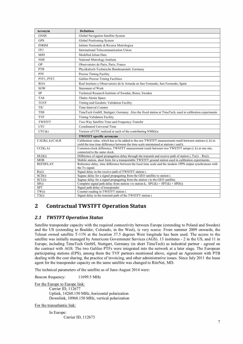
Acronym Definition GNSS Global Navigation Satellite System GPS Global Positioning System INRIM Istituto Nazionale di Ricerca Metrologica ITU International Telecommunication Union MJD Modified Julian Date NMI National Metrology Institute OP Observatoire de Paris, Paris, France PTB Physikalisch-Technische Bundesanstalt, Germany PTF Precise Timing Facility PTF1, PTF2 Galileo Precise Timing Facilities ROA Real Instituto y Observatorio de la Armada en San Fernando, San Fernando, Spain SOW Statement of Work SP Technical Research Institute of Sweden, Boras, Sweden TAS Thales Alenia Space TGVF Timing and Geodetic Validation Facility TIC Time Interval Counter TIM TimeTech GmbH, Stuttgart, Germany. Also the fixed station at TimeTech, used in calibration experiments TVF Timing Validation Facility TWSTFT Two-Way Satellite Time and Frequency Transfer UTC Coordinated Universal Time UTC(k) Version of UTC realized at each of the contributing NMI(k)s TWSTFT specific acronyms
CALR(i, k)/CALR Calibration value, which has to be added to the raw TWSTFT measurement result between stations (i, k) to yield the true time difference between the time scale maintained at stations i and k.
CCD(i, k) Common-clock difference, TWSTFT measurement result between two TWSTFT setups (i, k) at one site, connected to the same clock.
DLD(i) Difference of signal propagation delay through the transmit and receive path of station i, Tx(i) – Rx(i). MOB Mobile station, short form for a transportable TWSTFT ground station used in calibration experiments. REFDELAY Reference delay, time difference between the local time scale and the modem 1PPS output synchronous with
the Tx signal. Rx(i) Signal delay in the receive path of TWSTFT station i. SCD(i) Sagnac delay for a signal propagating from the GEO satellite to station i. SCU(i) Sagnac delay for a signal propagating from the station i to the GEO satellite. SP(i) Complete signal path delay from station i to station k, SPU(k) + SPT(k) + SPD(i) SPT Signal path delay of transponder TW(i) Counter reading in TWSTFT station i. TX(i) Signal delay in the transmit path of the TWSTFT station i.
2 Contractual TWSTFT Operation Status
2.1 TWSTFT Operation Status Satellite transponder capacity with the required connectivity between Europe (extending to Poland and Sweden) and the US (extending to Boulder, Colorado, in the West), is very scarce. From summer 2009 onwards, the Telesat owned satellite T-11N at the location 37.5 degrees West longitude has been used. The access to the satellite was initially managed by Americom Government Services (AGS). 13 institutes - 2 in the US, and 11 in Europe, including TimeTech GmbH, Stuttgart, Germany (in short TimeTech) as industrial partner - agreed on the contract with AGS. The two Galileo PTFs were integrated into the network at a later stage. The European participating stations (EPS), among them the TVF partners mentioned above, signed an Agreement with PTB dealing with the cost sharing, the practice of invoicing, and other administrative issues. Since July 2011 the lease agent for the transponder capacity on the same satellite was changed to RiteNet, MD.
The technical parameters of the satellite as of June-August 2014 were:
Beacon frequency: 11699.5 MHz
Carrier ID, 112677 For the Europe to Europe link:
Uplink, 14260.150 MHz, horizontal polarization Downlink, 10960.150 MHz, vertical polarization
In Europe:
For the transatlantic link:
Carrier ID, 112673
8
Uplink, 14046.5900 MHz, horizontal polarization Downlink, 11489.060 MHz, vertical polarization
In USA: Carrier ID, 112701 Uplink, 14289.060 MHz, horizontal polarization Downlink, 11746.590 MHz, vertical polarization
2.2 Contractual arrangements for the FOC TVF TWSTFT calibrations According to the TVF Statement of Work (TGVF-SOW-05300), a calibration exercise involving a travelling TWSTFT station and comprising PTF1, PTF2, INRIM, OP, PTB, ROA, and SP, should be organized and evaluated by ROA in 2014 and took place in summer 2014 (June 5th to August 17th).
The provision of the mobile TWSTFT station which is designated as MOB in this Report and its operation was directly subcontracted to TimeTech GmbH, Stuttgart, Germany, by GMV.
3 Organization of the June/August 2014 campaign
3.1 Travel Schedule and measurement periods
3.1.1 Travel Schedule
Table 3-1 Travel Schedule adhered to by the mobile TWSTFT station (MOB)
From To Distance Time to travel
Start Date and Time (Local time)
Reach Date and Time (Local time)
Stuttgart Oberpfaffenhofen 226 km 3hrs 15 Jun, 18:00 15 Jun, 21:00 Oberpfaffenhofen Neuchatel 434 km 6 hrs 18 Jun, 16:00 18 Jun, 22:00 Neuchatel Torino 327 km 4 hrs 26 Jun, 17:00 26 Jun, 21:00 Torino Paris 772 km 10 hrs 30 Jun, 11:00 01 Jul, 13:00 Paris San Fernando 1863 km 24 hrs 04 Jul, 13:00 06 Jul, 21:00 San Fernando Ortuccio 2579 km 33 hrs 10 Jul, 12:00 12 Jul, 21:00 Ortuccio Braunschweig 1599 km 20 hrs 16 Jul, 17:00 18 Jul, 13:00 Braunschweig Boras 840 km 10 hrs 24 Jul, 12:00 23 Jul, 15:00 Boras Stuttgart 1300 km 17 hrs 28 Jul, 12:00 30 Jul, 12:00
3.1.2 Effective measurement schedule
Table 3-2 Periods of data taking of MOB while installed at the various sites
MOB at Week# From Date and Time (UTC)
To Date and Time (UTC) MJD
TIM 24 Tue, 10 Jun 2014 00:00 Thu, 12 Jun 2014 08:00 56818 – 56820 INRIM 26/27 Fri, 27 Jun 2014 10:00 Mon, 30 Jun 2014 07:00 56835 – 56838 OP 27 Tue, 01 Jul 2014 14:00 Fri, 04 Jul 2014 09:00 56839 – 56842 ROA 28 Mon, 07 Jul 2014 09:00 Thu, 10 Jul 2014 08:00 56845 – 56848 PTB 29/30 Fri, 18 Jul 2014 14:00 Tue, 22 Jul 2014 08:00 56856 – 56860 SP 30/31 Wed, 23 Jul 2014 16:00 Mon, 28 Jul 2014 09:00 56861 – 56866 TIM 31 Wed, 30 Jul 2014 13:00 Fri, 01Aug 2014 08:00 56868 – 56870
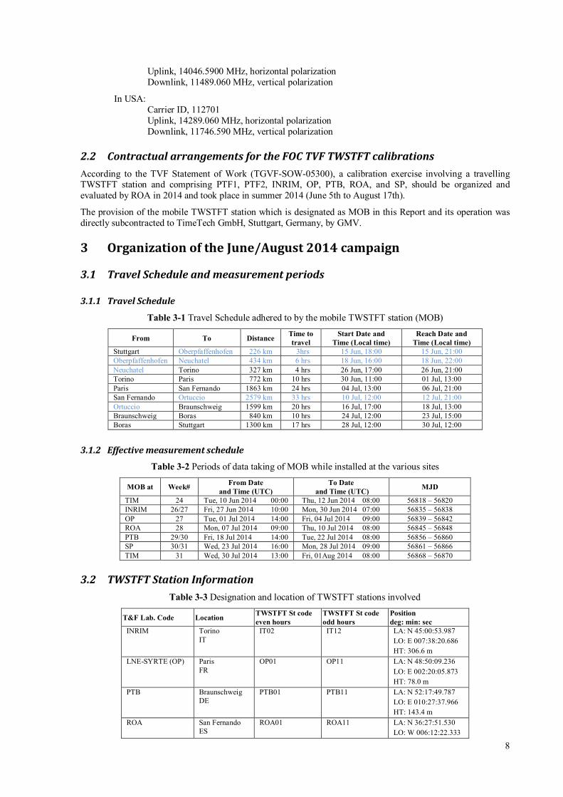
3.2 TWSTFT Station Information Table 3-3 Designation and location of TWSTFT stations involved
T&F Lab. Code Location TWSTFT St code even hours
TWSTFT St code odd hours
Position deg: min: sec
INRIM Torino IT
IT02 IT12 LA: N 45:00:53.987 LO: E 007:38:20.686 HT: 306.6 m
LNE-SYRTE (OP) Paris FR
OP01 OP11 LA: N 48:50:09.236 LO: E 002:20:05.873 HT: 78.0 m
PTB Braunschweig DE
PTB01 PTB11 LA: N 52:17:49.787 LO: E 010:27:37.966 HT: 143.4 m
ROA San Fernando ES
ROA01 ROA11 LA: N 36:27:51.530 LO: W 006:12:22.333
9
T&F Lab. Code Location TWSTFT St code even hours
TWSTFT St code odd hours
Position deg: min: sec HT: 74.7 m
SP Boras SE
SP01 SP11 LA: N 57:42:55.000 LO: E 012:53:27.000 HT: 225.0 m
TIM Stuttgart DE
TIM01 TIM11 LA: N 48:44.16.272 LO: E 009:06:45.106 HT: 529.0 m
MOB Stuttgart DE
MOB02 MOB12 Mobile
Table 3-3 summarizes the TWSTFT stations involved, including MOB which was shipped in sequence between TimeTech (TIM), INRIM, OP, ROA, PTB, and SP. The station code (columns 3 and 4 in Table 3-3) is part of the designation of data lines [RD01, RD02] in which measurement results are reported. According to the usual practice in the TWSTFT community it is changed between regular sessions – during even hours,00:00 to 01:00 ff – and extra sessions – during odd hours, 01:00 to 02:00 ff (in UTC).
4 Information on TWSTFT
4.1 Quantities determined in a TWSTFT Calibration In this section, we recall the theoretical background and derive the equations necessary for the determination of calibration constants. We follow, if possible and expedient, the description and naming of the ITU-R Recommendation TF.1153-3 [RD02] and extend or deviate thereof only if necessary. In particular, we use some of the common abbreviating acronyms in the text and in equations, which are listed in Table 1-2.
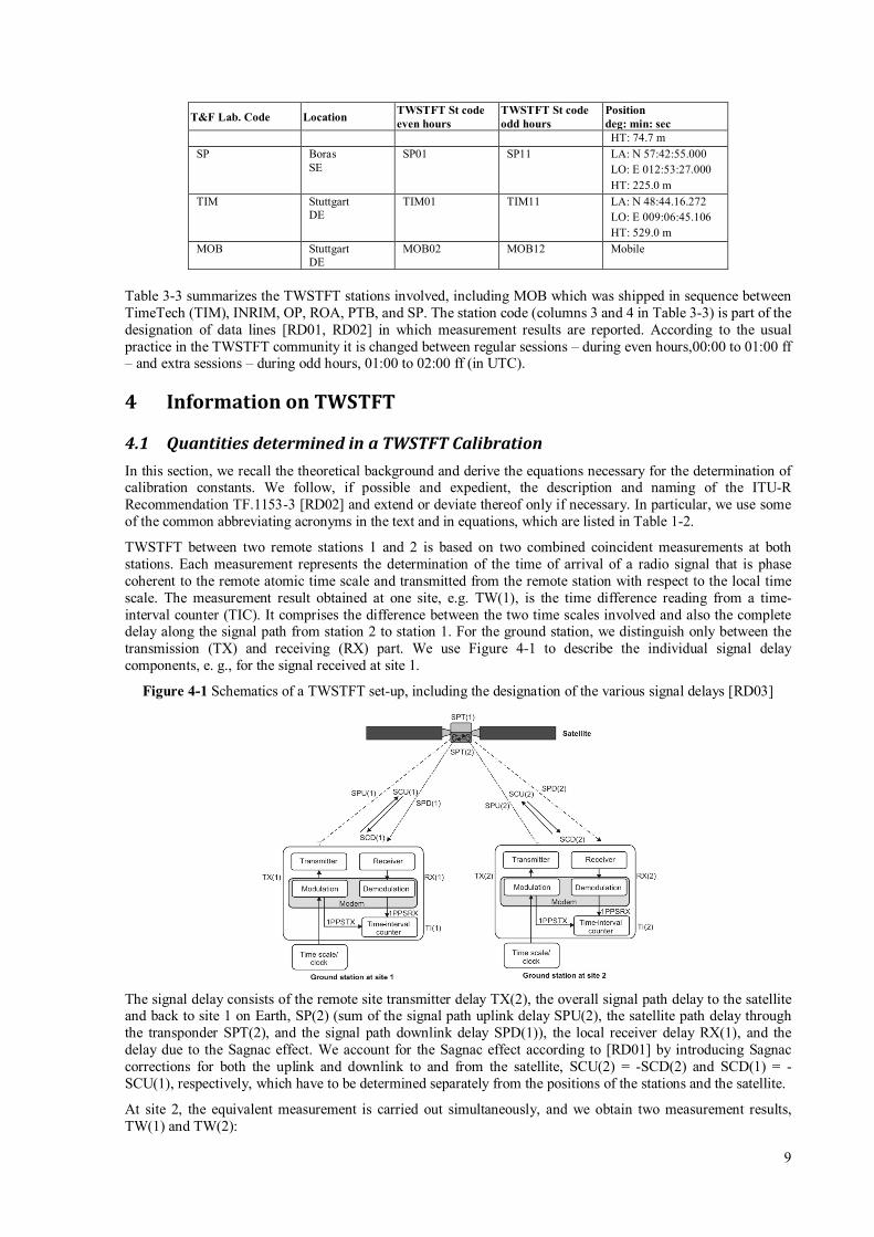
TWSTFT between two remote stations 1 and 2 is based on two combined coincident measurements at both stations. Each measurement represents the determination of the time of arrival of a radio signal that is phase coherent to the remote atomic time scale and transmitted from the remote station with respect to the local time scale. The measurement result obtained at one site, e.g. TW(1), is the time difference reading from a time-interval counter (TIC). It comprises the difference between the two time scales involved and also the complete delay along the signal path from station 2 to station 1. For the ground station, we distinguish only between the transmission (TX) and receiving (RX) part. We use Figure 4-1 to describe the individual signal delay components, e. g., for the signal received at site 1.
Figure 4-1 Schematics of a TWSTFT set-up, including the designation of the various signal delays [RD03]
The signal delay consists of the remote site transmitter delay TX(2), the overall signal path delay to the satellite and back to site 1 on Earth, SP(2) (sum of the signal path uplink delay SPU(2), the satellite path delay through the transponder SPT(2), and the signal path downlink delay SPD(1)), the local receiver delay RX(1), and the delay due to the Sagnac effect. We account for the Sagnac effect according to [RD01] by introducing Sagnac corrections for both the uplink and downlink to and from the satellite, SCU(2) = -SCD(2) and SCD(1) = -SCU(1), respectively, which have to be determined separately from the positions of the stations and the satellite.
At site 2, the equivalent measurement is carried out simultaneously, and we obtain two measurement results, TW(1) and TW(2):
10
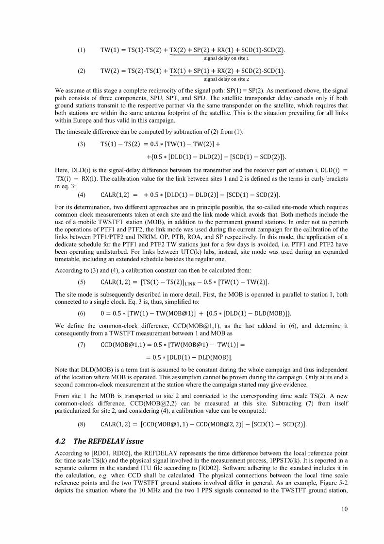
(1) TW(1) = TS(1)-TS(2) + TX(2) + SP(2) + RX(1) + SCD(1)-SCD(2)�����������������������������signal delay on site 1
.
(2) TW(2) = TS(2)-TS(1) + TX(1) + SP(1) + RX(2) + SCD(2)-SCD(1)�����������������������������signal delay on site 2
.
We assume at this stage a complete reciprocity of the signal path: SP(1) = SP(2). As mentioned above, the signal path consists of three components, SPU, SPT, and SPD. The satellite transponder delay cancels only if both ground stations transmit to the respective partner via the same transponder on the satellite, which requires that both stations are within the same antenna footprint of the satellite. This is the situation prevailing for all links within Europe and thus valid in this campaign.
The timescale difference can be computed by subtraction of (2) from (1):
(3) TS(1) − TS(2) = 0.5 ∗ [TW(1)− TW(2)] +
+{0.5 ∗ [DLD(1)− DLD(2)] − [SCD(1)− SCD(2)]}.
Here, DLD(i) is the signal-delay difference between the transmitter and the receiver part of station i, DLD(i) = TX(i) − RX(i). The calibration value for the link between sites 1 and 2 is defined as the terms in curly brackets in eq. 3:
(4) CALR(1,2) = + 0.5 ∗ [DLD(1)− DLD(2)]− [SCD(1)− SCD(2)].
For its determination, two different approaches are in principle possible, the so-called site-mode which requires common clock measurements taken at each site and the link mode which avoids that. Both methods include the use of a mobile TWSTFT station (MOB), in addition to the permanent ground stations. In order not to perturb the operations of PTF1 and PTF2, the link mode was used during the current campaign for the calibration of the links between PTF1/PTF2 and INRIM, OP, PTB, ROA, and SP respectively. In this mode, the application of a dedicate schedule for the PTF1 and PTF2 TW stations just for a few days is avoided, i.e. PTF1 and PTF2 have been operating undisturbed. For links between UTC(k) labs, instead, site mode was used during an expanded timetable, including an extended schedule besides the regular one.
According to (3) and (4), a calibration constant can then be calculated from:
(5) CALR(1, 2) = [TS(1)− TS(2)]LINK − 0.5 ∗ [TW(1)− TW(2)].
The site mode is subsequently described in more detail. First, the MOB is operated in parallel to station 1, both connected to a single clock. Eq. 3 is, thus, simplified to:
(6) 0 = 0.5 ∗ [TW(1)− TW(MOB@1)] + {0.5 ∗ [DLD(1)− DLD(MOB)]}.
We define the common-clock difference, CCD(MOB@1,1), as the last addend in (6), and determine it consequently from a TWSTFT measurement between 1 and MOB as
(7) CCD(MOB@1,1) = 0.5 ∗ [TW(MOB@1)− TW(1)] =
= 0.5 ∗ [DLD(1)− DLD(MOB)].
Note that DLD(MOB) is a term that is assumed to be constant during the whole campaign and thus independent of the location where MOB is operated. This assumption cannot be proven during the campaign. Only at its end a second common-clock measurement at the station where the campaign started may give evidence.
From site 1 the MOB is transported to site 2 and connected to the corresponding time scale TS(2). A new common-clock difference, CCD(MOB@2,2) can be measured at this site. Subtracting (7) from itself particularized for site 2, and considering (4), a calibration value can be computed:
(8) CALR(1, 2) = [CCD(MOB@1, 1) − CCD(MOB@2, 2)] − [SCD(1)− SCD(2)].
4.2 The REFDELAY issue According to [RD01, RD02], the REFDELAY represents the time difference between the local reference point for time scale TS(k) and the physical signal involved in the measurement process, 1PPSTX(k). It is reported in a separate column in the standard ITU file according to [RD02]. Software adhering to the standard includes it in the calculation, e.g. when CCD shall be calculated. The physical connections between the local time scale reference points and the two TWSTFT ground stations involved differ in general. As an example, Figure 5-2 depicts the situation where the 10 MHz and the two 1 PPS signals connected to the TWSTFT ground station,
11
here in particular the MOB, are from the same physical source. In this case, REFDELAY is just a constant that would change only if cable connections are changed.
More specific than (7), one has to consider
(9) CCD(MOB@k, k)true = 0.5 ∗ �TW(MOB@k)– TW(k)� + +REFDELAY(MOB@k)− REFDELAY(k) =
= 0. 5 ∗ �TW(MOB@k)– TW(k)�+ REFDLYdiff(MOB@k, k).
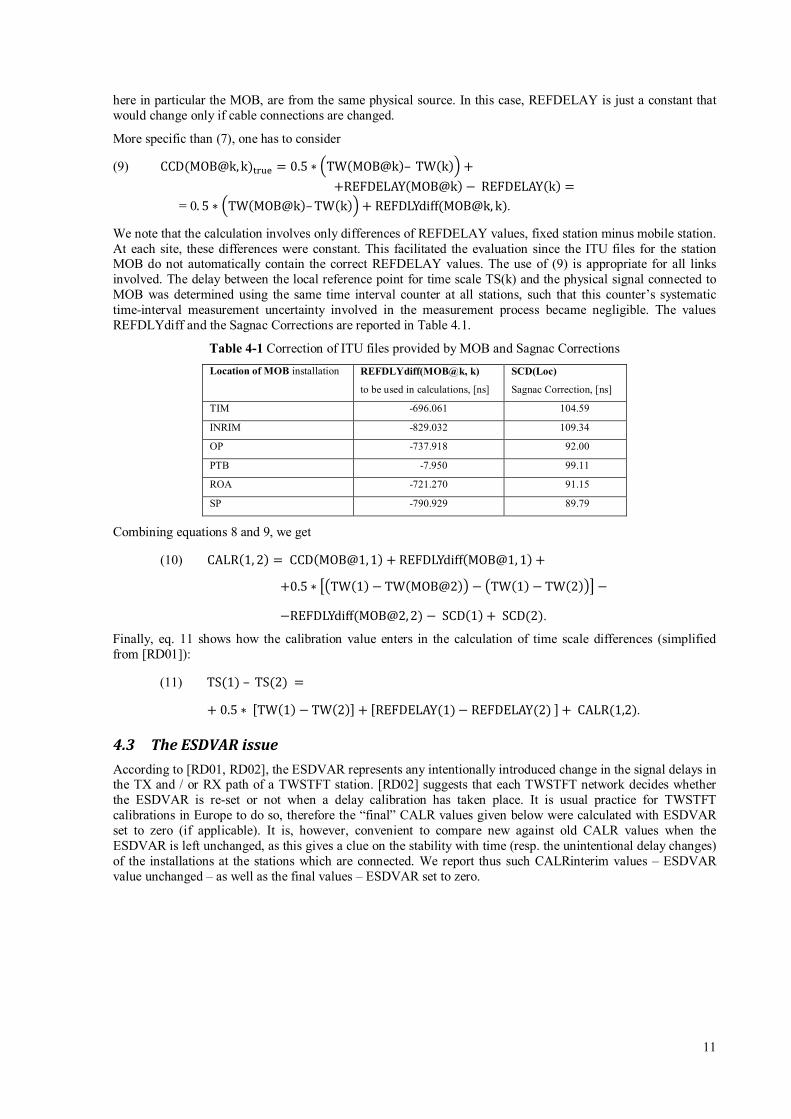
We note that the calculation involves only differences of REFDELAY values, fixed station minus mobile station. At each site, these differences were constant. This facilitated the evaluation since the ITU files for the station MOB do not automatically contain the correct REFDELAY values. The use of (9) is appropriate for all links involved. The delay between the local reference point for time scale TS(k) and the physical signal connected to MOB was determined using the same time interval counter at all stations, such that this counter’s systematic time-interval measurement uncertainty involved in the measurement process became negligible. The values REFDLYdiff and the Sagnac Corrections are reported in Table 4.1.
Table 4-1 Correction of ITU files provided by MOB and Sagnac Corrections Location of MOB installation REFDLYdiff(MOB@k, k)
to be used in calculations, [ns]
SCD(Loc)
Sagnac Correction, [ns]
TIM -696.061 104.59
INRIM -829.032 109.34
OP -737.918 92.00
PTB -7.950 99.11
ROA -721.270 91.15
SP -790.929 89.79
Combining equations 8 and 9, we get
(10) CALR(1, 2) = CCD(MOB@1, 1) + REFDLYdiff(MOB@1, 1) +
+0.5 ∗ ��TW(1)− TW(MOB@2)� − �TW(1)− TW(2)�� −
−REFDLYdiff(MOB@2, 2) − SCD(1) + SCD(2).
Finally, eq. 11 shows how the calibration value enters in the calculation of time scale differences (simplified from [RD01]):
(11) TS(1) – TS(2) =
+ 0.5 ∗ [TW(1)− TW(2)] + [REFDELAY(1)− REFDELAY(2) ] + CALR(1,2).
4.3 The ESDVAR issue According to [RD01, RD02], the ESDVAR represents any intentionally introduced change in the signal delays in the TX and / or RX path of a TWSTFT station. [RD02] suggests that each TWSTFT network decides whether the ESDVAR is re-set or not when a delay calibration has taken place. It is usual practice for TWSTFT calibrations in Europe to do so, therefore the “final” CALR values given below were calculated with ESDVAR set to zero (if applicable). It is, however, convenient to compare new against old CALR values when the ESDVAR is left unchanged, as this gives a clue on the stability with time (resp. the unintentional delay changes) of the installations at the stations which are connected. We report thus such CALRinterim values – ESDVAR value unchanged – as well as the final values – ESDVAR set to zero.
12
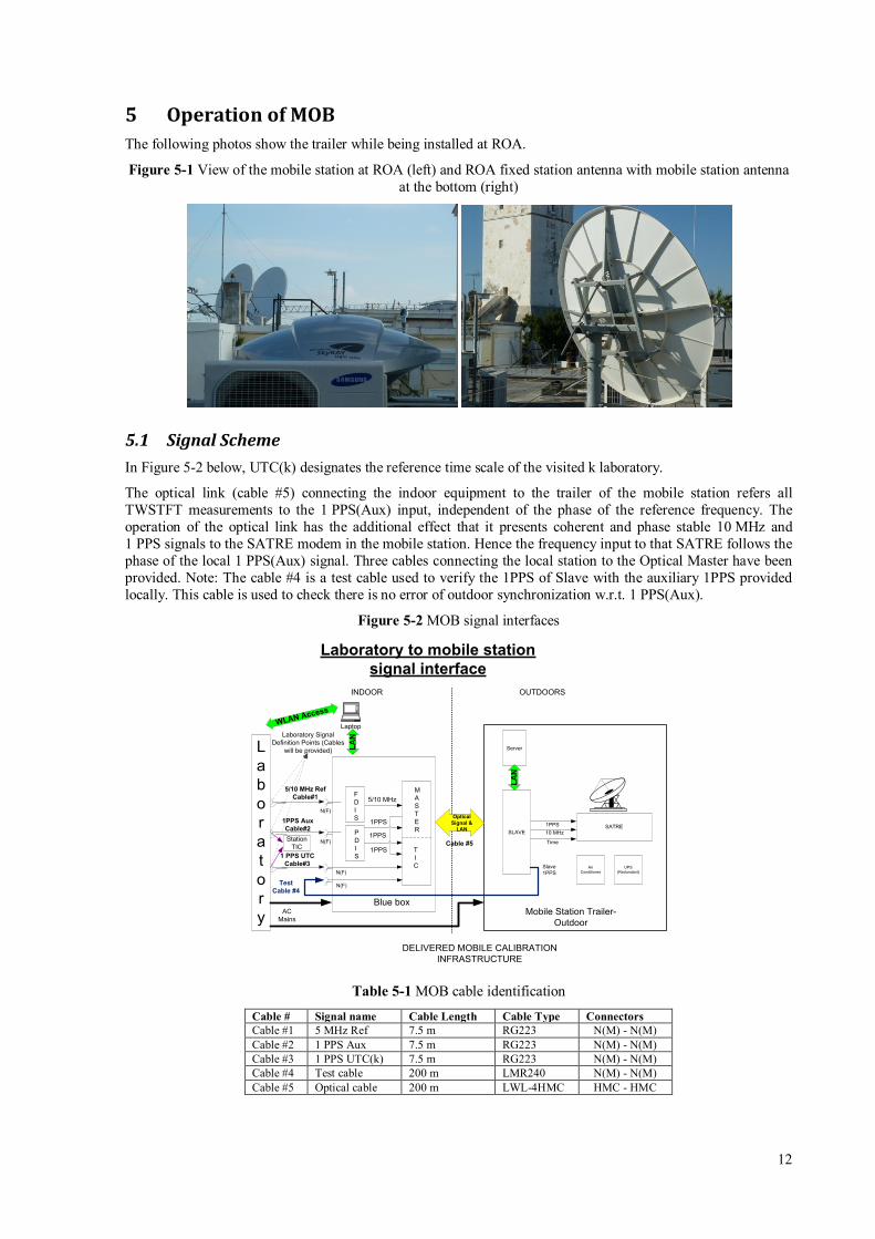
5 Operation of MOB The following photos show the trailer while being installed at ROA.
Figure 5-1 View of the mobile station at ROA (left) and ROA fixed station antenna with mobile station antenna at the bottom (right)
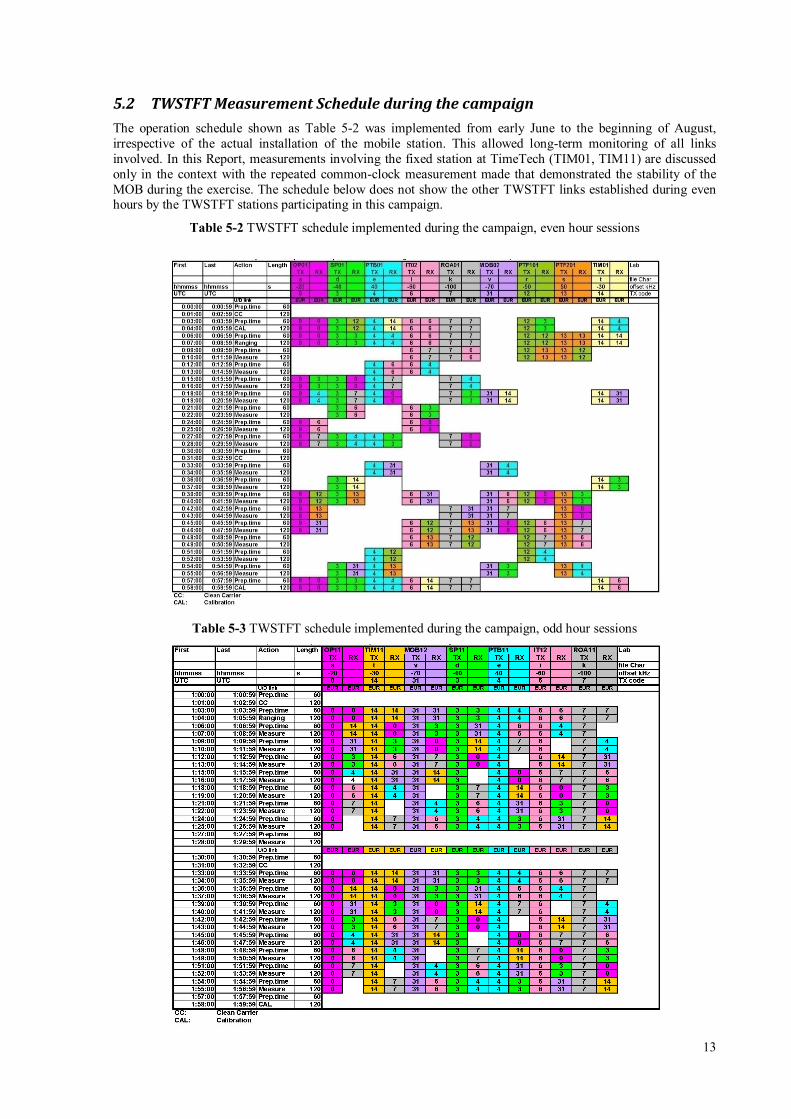
5.1 Signal Scheme In Figure 5-2 below, UTC(k) designates the reference time scale of the visited k laboratory.
The optical link (cable #5) connecting the indoor equipment to the trailer of the mobile station refers all TWSTFT measurements to the 1 PPS(Aux) input, independent of the phase of the reference frequency. The operation of the optical link has the additional effect that it presents coherent and phase stable 10 MHz and 1 PPS signals to the SATRE modem in the mobile station. Hence the frequency input to that SATRE follows the phase of the local 1 PPS(Aux) signal. Three cables connecting the local station to the Optical Master have been provided. Note: The cable #4 is a test cable used to verify the 1PPS of Slave with the auxiliary 1PPS provided locally. This cable is used to check there is no error of outdoor synchronization w.r.t. 1 PPS(Aux).
Figure 5-2 MOB signal interfaces
Table 5-1 MOB cable identification
Cable # Signal name Cable Length Cable Type Connectors Cable #1 5 MHz Ref 7.5 m RG223 N(M) - N(M) Cable #2 1 PPS Aux 7.5 m RG223 N(M) - N(M) Cable #3 1 PPS UTC(k) 7.5 m RG223 N(M) - N(M) Cable #4 Test cable 200 m LMR240 N(M) - N(M) Cable #5 Optical cable 200 m LWL-4HMC HMC - HMC
PDIS
MASTER SLAVE
TIC
5/10 MHz
1PPS
1PPS
1PPS AuxCable#2
1 PPS UTCCable#3
Laboratory to mobile station signal interface
Laboratory
SATRE1PPS10 MHz
Mobile Station Trailer-Outdoor
Time
FDIS 1PPS
Server
Blue box
Air Conditioner
UPS (Redundant)
Laptop
LAN
Optical Signal &
LAN
LAN
DELIVERED MOBILE CALIBRATION INFRASTRUCTURE
AC Mains
Laboratory Signal Definition Points (Cables
will be provided)
WLAN Access
N(F)
N(F)
INDOOR OUTDOORS
N(F)Slave1PPS
5/10 MHz RefCable#1
TestCable #4
N(F)
StationTIC Cable #5
13
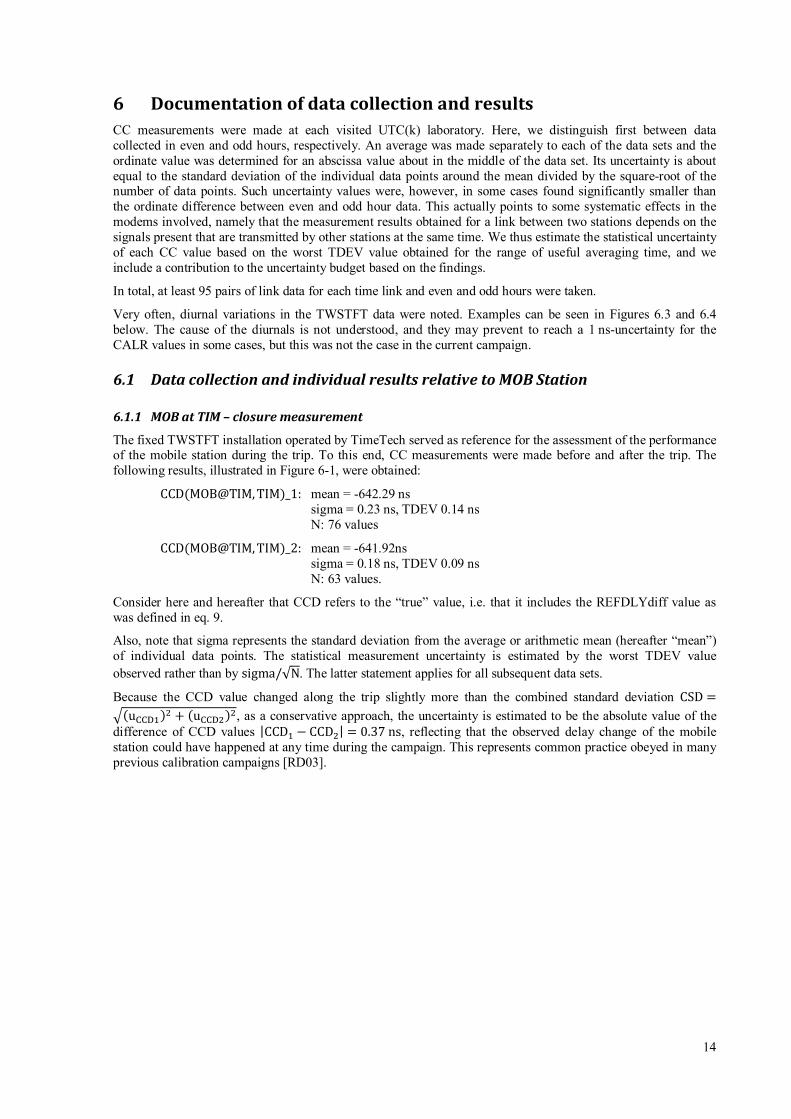
5.2 TWSTFT Measurement Schedule during the campaign The operation schedule shown as Table 5-2 was implemented from early June to the beginning of August, irrespective of the actual installation of the mobile station. This allowed long-term monitoring of all links involved. In this Report, measurements involving the fixed station at TimeTech (TIM01, TIM11) are discussed only in the context with the repeated common-clock measurement made that demonstrated the stability of the MOB during the exercise. The schedule below does not show the other TWSTFT links established during even hours by the TWSTFT stations participating in this campaign.
Table 5-2 TWSTFT schedule implemented during the campaign, even hour sessions
Table 5-3 TWSTFT schedule implemented during the campaign, odd hour sessions
14
6 Documentation of data collection and results CC measurements were made at each visited UTC(k) laboratory. Here, we distinguish first between data collected in even and odd hours, respectively. An average was made separately to each of the data sets and the ordinate value was determined for an abscissa value about in the middle of the data set. Its uncertainty is about equal to the standard deviation of the individual data points around the mean divided by the square-root of the number of data points. Such uncertainty values were, however, in some cases found significantly smaller than the ordinate difference between even and odd hour data. This actually points to some systematic effects in the modems involved, namely that the measurement results obtained for a link between two stations depends on the signals present that are transmitted by other stations at the same time. We thus estimate the statistical uncertainty of each CC value based on the worst TDEV value obtained for the range of useful averaging time, and we include a contribution to the uncertainty budget based on the findings.
In total, at least 95 pairs of link data for each time link and even and odd hours were taken.
Very often, diurnal variations in the TWSTFT data were noted. Examples can be seen in Figures 6.3 and 6.4 below. The cause of the diurnals is not understood, and they may prevent to reach a 1 ns-uncertainty for the CALR values in some cases, but this was not the case in the current campaign.
6.1 Data collection and individual results relative to MOB Station
6.1.1 MOB at TIM – closure measurement
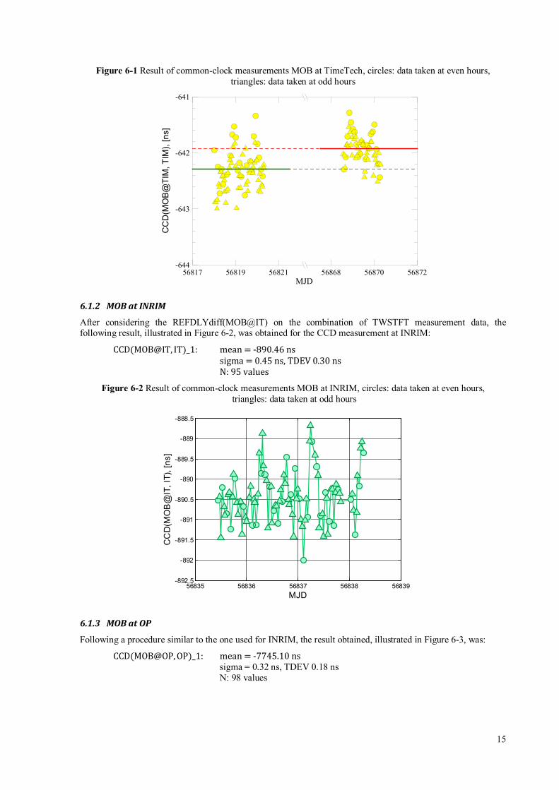
The fixed TWSTFT installation operated by TimeTech served as reference for the assessment of the performance of the mobile station during the trip. To this end, CC measurements were made before and after the trip. The following results, illustrated in Figure 6-1, were obtained:
CCD(MOB@TIM, TIM)_1: mean = -642.29 ns sigma = 0.23 ns, TDEV 0.14 ns N: 76 values
CCD(MOB@TIM, TIM)_2: mean = -641.92ns sigma = 0.18 ns, TDEV 0.09 ns N: 63 values.
Consider here and hereafter that CCD refers to the “true” value, i.e. that it includes the REFDLYdiff value as was defined in eq. 9.
Also, note that sigma represents the standard deviation from the average or arithmetic mean (hereafter “mean”) of individual data points. The statistical measurement uncertainty is estimated by the worst TDEV value observed rather than by sigma/√N. The latter statement applies for all subsequent data sets.
Because the CCD value changed along the trip slightly more than the combined standard deviation CSD =�(uCCD1)2 + (uCCD2)2, as a conservative approach, the uncertainty is estimated to be the absolute value of the difference of CCD values |CCD1 − CCD2| = 0.37 ns, reflecting that the observed delay change of the mobile station could have happened at any time during the campaign. This represents common practice obeyed in many previous calibration campaigns [RD03].
15
Figure 6-1 Result of common-clock measurements MOB at TimeTech, circles: data taken at even hours, triangles: data taken at odd hours
6.1.2 MOB at INRIM
After considering the REFDLYdiff(MOB@IT) on the combination of TWSTFT measurement data, the following result, illustrated in Figure 6-2, was obtained for the CCD measurement at INRIM:
CCD(MOB@IT, IT)_1: mean = -890.46 ns sigma = 0.45 ns, TDEV 0.30 ns N: 95 values
Figure 6-2 Result of common-clock measurements MOB at INRIM, circles: data taken at even hours, triangles: data taken at odd hours
6.1.3 MOB at OP
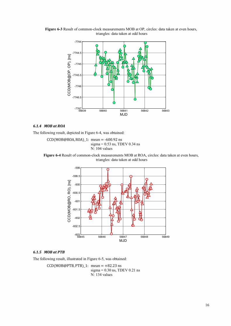
Following a procedure similar to the one used for INRIM, the result obtained, illustrated in Figure 6-3, was:
CCD(MOB@OP, OP)_1: mean = -7745.10 ns sigma = 0.32 ns, TDEV 0.18 ns N: 98 values
56817 56819 56821 56868 56870 56872MJD
-644
-643
-642
-641
CC
D(M
OB
@TI
M, T
IM),
[ns]
56835 56836 56837 56838 56839-892.5
-892
-891.5
-891
-890.5
-890
-889.5
-889
-888.5
MJD
CC
D(M
OB
@IT
, IT)
, [ns
]
16
Figure 6-3 Result of common-clock measurements MOB at OP, circles: data taken at even hours, triangles: data taken at odd hours
6.1.4 MOB at ROA
The following result, depicted in Figure 6-4, was obtained:
CCD(MOB@ROA, ROA)_1: mean = -600.92 ns sigma = 0.53 ns, TDEV 0.34 ns N: 104 values
Figure 6-4 Result of common-clock measurements MOB at ROA, circles: data taken at even hours, triangles: data taken at odd hours
6.1.5 MOB at PTB
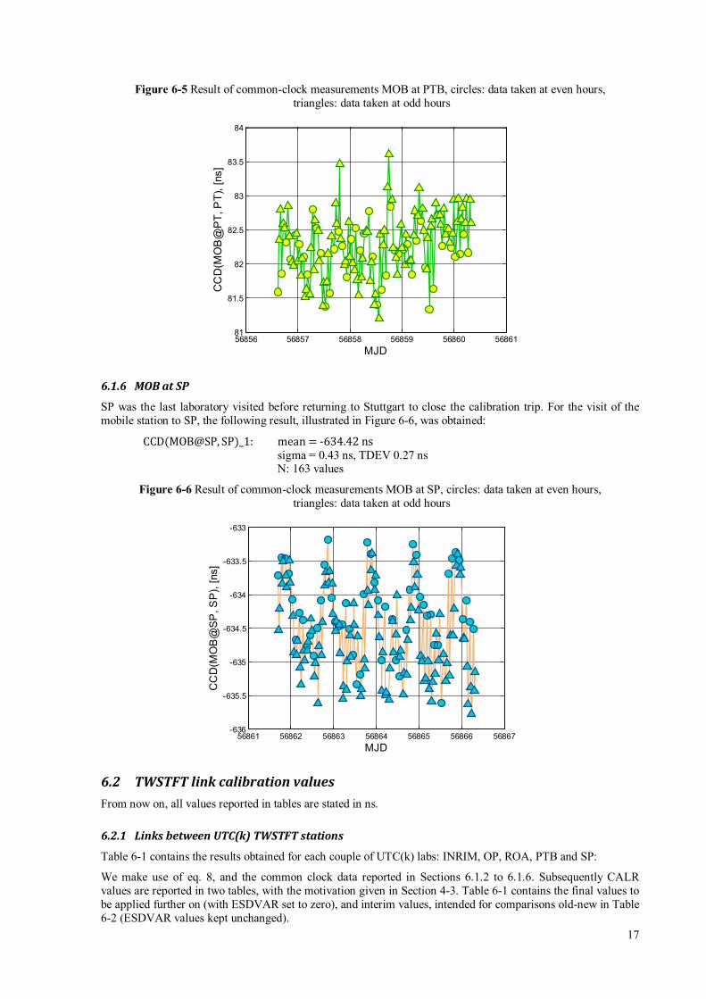
The following result, illustrated in Figure 6-5, was obtained:
CCD(MOB@PTB, PTB)_1: mean = +82.23 ns sigma = 0.30 ns, TDEV 0.21 ns N: 134 values
56839 56840 56841 56842 56843-7747
-7746.5
-7746
-7745.5
-7745
-7744.5
-7744
MJD
CC
D(M
OB
@O
P, O
P),
[ns]
56845 56846 56847 56848 56849-603
-602.5
-602
-601.5
-601
-600.5
-600
-599.5
-599
MJD
CC
D(M
OB
@R
O, R
O),
[ns]
17
Figure 6-5 Result of common-clock measurements MOB at PTB, circles: data taken at even hours, triangles: data taken at odd hours
6.1.6 MOB at SP
SP was the last laboratory visited before returning to Stuttgart to close the calibration trip. For the visit of the mobile station to SP, the following result, illustrated in Figure 6-6, was obtained:
CCD(MOB@SP, SP)_1: mean = -634.42 ns sigma = 0.43 ns, TDEV 0.27 ns N: 163 values
Figure 6-6 Result of common-clock measurements MOB at SP, circles: data taken at even hours, triangles: data taken at odd hours
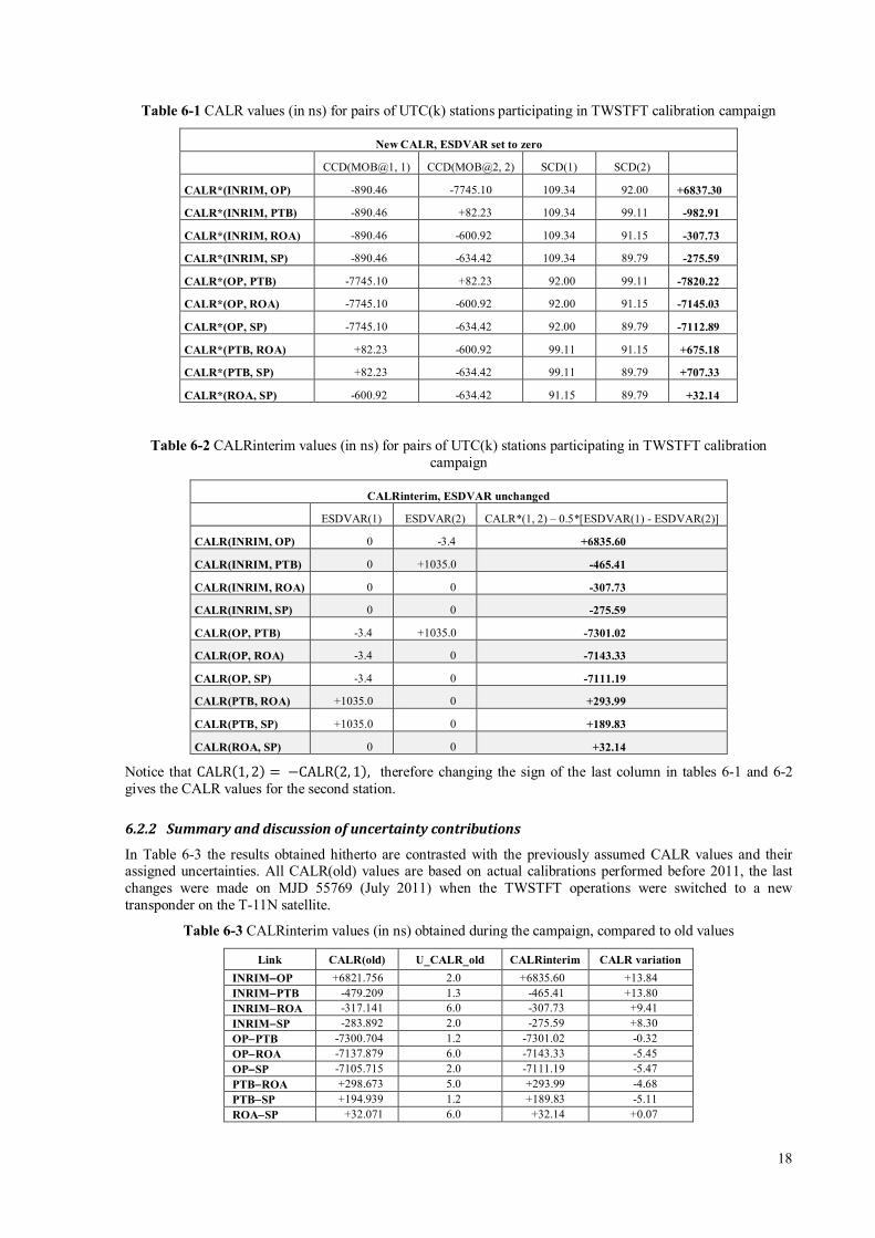
6.2 TWSTFT link calibration values From now on, all values reported in tables are stated in ns.
6.2.1 Links between UTC(k) TWSTFT stations
Table 6-1 contains the results obtained for each couple of UTC(k) labs: INRIM, OP, ROA, PTB and SP:
We make use of eq. 8, and the common clock data reported in Sections 6.1.2 to 6.1.6. Subsequently CALR values are reported in two tables, with the motivation given in Section 4-3. Table 6-1 contains the final values to be applied further on (with ESDVAR set to zero), and interim values, intended for comparisons old-new in Table 6-2 (ESDVAR values kept unchanged).
56856 56857 56858 56859 56860 5686181
81.5
82
82.5
83
83.5
84
MJD
CC
D(M
OB
@P
T, P
T), [
ns]
56861 56862 56863 56864 56865 56866 56867-636
-635.5
-635
-634.5
-634
-633.5
-633
MJD
CC
D(M
OB
@S
P, S
P),
[ns]
18
Table 6-1 CALR values (in ns) for pairs of UTC(k) stations participating in TWSTFT calibration campaign
New CALR, ESDVAR set to zero
CCD(MOB@1, 1) CCD(MOB@2, 2) SCD(1) SCD(2)
CALR*(INRIM, OP) -890.46 -7745.10 109.34 92.00 +6837.30
CALR*(INRIM, PTB) -890.46 +82.23 109.34 99.11 -982.91
CALR*(INRIM, ROA) -890.46 -600.92 109.34 91.15 -307.73
CALR*(INRIM, SP) -890.46 -634.42 109.34 89.79 -275.59
CALR*(OP, PTB) -7745.10 +82.23 92.00 99.11 -7820.22
CALR*(OP, ROA) -7745.10 -600.92 92.00 91.15 -7145.03
CALR*(OP, SP) -7745.10 -634.42 92.00 89.79 -7112.89
CALR*(PTB, ROA) +82.23 -600.92 99.11 91.15 +675.18
CALR*(PTB, SP) +82.23 -634.42 99.11 89.79 +707.33
CALR*(ROA, SP) -600.92 -634.42 91.15 89.79 +32.14
Table 6-2 CALRinterim values (in ns) for pairs of UTC(k) stations participating in TWSTFT calibration campaign
CALRinterim, ESDVAR unchanged
ESDVAR(1) ESDVAR(2) CALR*(1, 2) – 0.5*[ESDVAR(1) - ESDVAR(2)]
CALR(INRIM, OP) 0 -3.4 +6835.60
CALR(INRIM, PTB) 0 +1035.0 -465.41
CALR(INRIM, ROA) 0 0 -307.73
CALR(INRIM, SP) 0 0 -275.59
CALR(OP, PTB) -3.4 +1035.0 -7301.02
CALR(OP, ROA) -3.4 0 -7143.33
CALR(OP, SP) -3.4 0 -7111.19
CALR(PTB, ROA) +1035.0 0 +293.99
CALR(PTB, SP) +1035.0 0 +189.83
CALR(ROA, SP) 0 0 +32.14
Notice that CALR(1, 2) = −CALR(2, 1), therefore changing the sign of the last column in tables 6-1 and 6-2 gives the CALR values for the second station.
6.2.2 Summary and discussion of uncertainty contributions
In Table 6-3 the results obtained hitherto are contrasted with the previously assumed CALR values and their assigned uncertainties. All CALR(old) values are based on actual calibrations performed before 2011, the last changes were made on MJD 55769 (July 2011) when the TWSTFT operations were switched to a new transponder on the T-11N satellite.
Table 6-3 CALRinterim values (in ns) obtained during the campaign, compared to old values
Link CALR(old) U_CALR_old CALRinterim CALR variation INRIM−OP +6821.756 2.0 +6835.60 +13.84 INRIM−PTB -479.209 1.3 -465.41 +13.80 INRIM−ROA -317.141 6.0 -307.73 +9.41 INRIM−SP -283.892 2.0 -275.59 +8.30 OP−PTB -7300.704 1.2 -7301.02 -0.32 OP−ROA -7137.879 6.0 -7143.33 -5.45 OP−SP -7105.715 2.0 -7111.19 -5.47 PTB−ROA +298.673 5.0 +293.99 -4.68 PTB−SP +194.939 1.2 +189.83 -5.11 ROA−SP +32.071 6.0 +32.14 +0.07
19
The current CALR values (column CALR(old) in Table 6-3) involving INRIM are taking into account a constant value of about 10 ns, due to hardware delay changes, which was for some historical reason included in the old CALR instead of being properly reported in REFDELAY of INRIM ITU files. At the time of implementation of the new CALR values, a correction for such constant value in the REFDELAY field of INRIM ITU files is planned. Therefore for links involving INRIM the CALR variation with respect to the previous calibration is given by CALRinterim− (CALR(old) + REFDELAYchange) = CALRinterim− (CALR(old) + 11.7 ns).
With the current calibration campaign INRIM took the opportunity to properly fix this issue, which was well known since many years. Such constant value was then moved to the proper field in which it should be reported according to the Recommendation [RD02], that is, in the REFDELAY field of TWSTFT final ITU-formatted files.
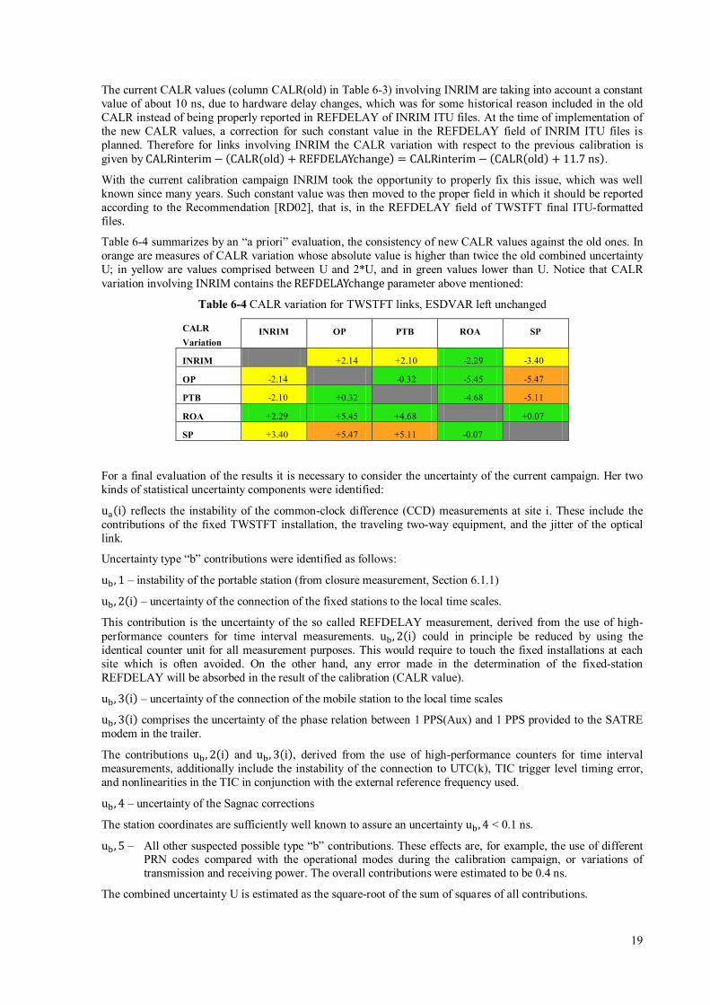
Table 6-4 summarizes by an “a priori” evaluation, the consistency of new CALR values against the old ones. In orange are measures of CALR variation whose absolute value is higher than twice the old combined uncertainty U; in yellow are values comprised between U and 2*U, and in green values lower than U. Notice that CALR variation involving INRIM contains the REFDELAYchange parameter above mentioned:
Table 6-4 CALR variation for TWSTFT links, ESDVAR left unchanged
CALR Variation
INRIM OP PTB ROA SP
INRIM +2.14 +2.10 -2.29 -3.40
OP -2.14 -0.32 -5.45 -5.47
PTB -2.10 +0.32 -4.68 -5.11
ROA +2.29 +5.45 +4.68 +0.07
SP +3.40 +5.47 +5.11 -0.07
For a final evaluation of the results it is necessary to consider the uncertainty of the current campaign. Her two kinds of statistical uncertainty components were identified:
ua(i) reflects the instability of the common-clock difference (CCD) measurements at site i. These include the contributions of the fixed TWSTFT installation, the traveling two-way equipment, and the jitter of the optical link.
Uncertainty type “b” contributions were identified as follows:
ub, 1 – instability of the portable station (from closure measurement, Section 6.1.1)
ub, 2(i) – uncertainty of the connection of the fixed stations to the local time scales.
This contribution is the uncertainty of the so called REFDELAY measurement, derived from the use of high-performance counters for time interval measurements. ub, 2(i) could in principle be reduced by using the identical counter unit for all measurement purposes. This would require to touch the fixed installations at each site which is often avoided. On the other hand, any error made in the determination of the fixed-station REFDELAY will be absorbed in the result of the calibration (CALR value).
ub, 3(i) – uncertainty of the connection of the mobile station to the local time scales
ub, 3(i) comprises the uncertainty of the phase relation between 1 PPS(Aux) and 1 PPS provided to the SATRE modem in the trailer.
The contributions ub, 2(i) and ub, 3(i), derived from the use of high-performance counters for time interval measurements, additionally include the instability of the connection to UTC(k), TIC trigger level timing error, and nonlinearities in the TIC in conjunction with the external reference frequency used.
ub, 4 – uncertainty of the Sagnac corrections
The station coordinates are sufficiently well known to assure an uncertainty ub, 4 < 0.1 ns.
ub, 5 – All other suspected possible type “b” contributions. These effects are, for example, the use of different PRN codes compared with the operational modes during the calibration campaign, or variations of transmission and receiving power. The overall contributions were estimated to be 0.4 ns.
The combined uncertainty U is estimated as the square-root of the sum of squares of all contributions.
20
Table 6-5 summarizes the uncertainty contribution case by case. All values are in ns, U represents the 1-σ uncertainty, rounded to 0.1 ns.
Table 6-5 Uncertainty contributions and combined uncertainty U
Case ua(1) ua(2) ub,1 ub,2(1) ub,2(2) ub,3(1) ub,3(2) ub,4 ub,5 U CALR(INRIM, OP) 0.30 0.18 0.37 0.20 0.20 0.20 0.28 0.10 0.40 0.8 CALR(INRIM, PTB) 0.30 0.21 0.37 0.20 0.20 0.20 0.20 0.10 0.40 0.8 CALR(INRIM, ROA) 0.30 0.34 0.37 0.20 0.21 0.20 0.20 0.10 0.40 0.8 CALR(INRIM, SP) 0.30 0.27 0.37 0.20 0.21 0.20 0.20 0.10 0.40 0.8 CALR(OP, PTB) 0.18 0.21 0.37 0.20 0.20 0.28 0.20 0.10 0.40 0.8 CALR(OP, ROA) 0.18 0.34 0.37 0.20 0.21 0.28 0.20 0.10 0.40 0.8 CALR(OP, SP) 0.18 0.27 0.37 0.20 0.21 0.28 0.20 0.10 0.40 0.8 CALR(PTB, ROA) 0.21 0.34 0.37 0.20 0.21 0.20 0.20 0.10 0.40 0.8 CALR(PTB, SP) 0.21 0.27 0.37 0.20 0.21 0.20 0.20 0.10 0.40 0.8 CALR(ROA, SP) 0.34 0.27 0.37 0.21 0.21 0.20 0.20 0.10 0.40 0.8
6.3 Triangle Calibrations of links UTC(k) labs against USNO At the time of the calibration campaign, TWSTFT was routinely made between the institutes involved in this campaign and USNO.
The method used for the calibration of a third TWSTFT station not participating in the calibration campaign is referred to as Triangle Closure Analysis. This method is based on the triviality that {TS(1)– TS(2)} – {TS(1)– TS(3)} + {TS(2)– TS(3)} is zero. This relation has been used to determine further calibration values, e. g. for the combination 1 = ROA, 2 = PTB, and 3 = USNO. The new calibration value of course build on existing calibrations of the link PTB – USNO (in this example), and the uncertainty of this calibration adds to the uncertainty of CALR(ROA, USNO). Obviously, the triangle calibrations can be done using any other TWSTFT participating station as the pivot, provided that a previous calibration of its link with USNO exists.
We will keep for now the ESDVAR values unchanged, so that the equation is simplified. The values are obtained as follows (e.g., for the triplet ROA, PTB, USNO):
Since in general, TS(1) − TS(2) is defined as in eq. 5, combining this expression applied to each one of the three links, and arranging terms, turns out:
(12) CALR(ROA, USNO)new =
= [ROA – PTB]new + [PTB – USNO]old – [ROA – USNO]old + CALR(ROA, USNO)old
[..]new represents TWSTFT results with the newly determined CALR value, and [..]old represent TWSTFT results with the CALR values as used up to now. The CALR(PTB, USNO) value is taken from the last calibration by means of the USNO portable X-band TWSTFT station in June 2014 [RD04].
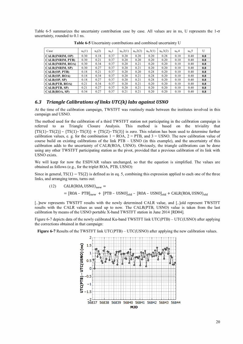
Figure 6-7 depicts data of the newly calibrated Ku-band TWSTFT link UTC(PTB) – UTC(USNO) after applying the corrections obtained in that campaign:
Figure 6-7 Results of the TWSTFT link UTC(PTB) – UTC(USNO) after applying the new calibration values.
21
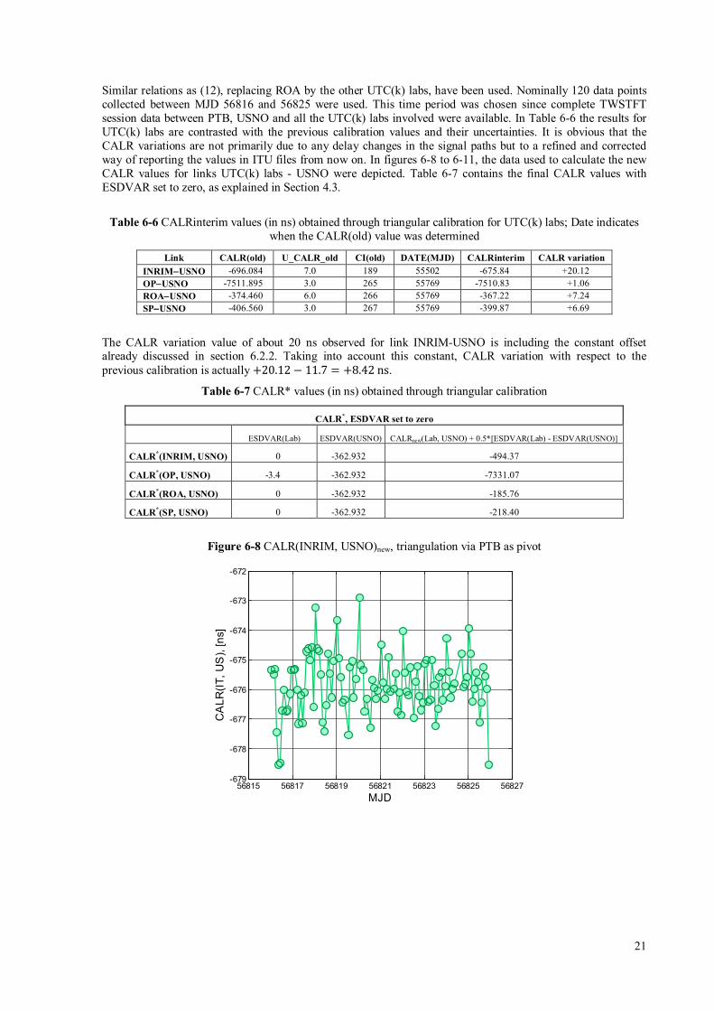
Similar relations as (12), replacing ROA by the other UTC(k) labs, have been used. Nominally 120 data points collected between MJD 56816 and 56825 were used. This time period was chosen since complete TWSTFT session data between PTB, USNO and all the UTC(k) labs involved were available. In Table 6-6 the results for UTC(k) labs are contrasted with the previous calibration values and their uncertainties. It is obvious that the CALR variations are not primarily due to any delay changes in the signal paths but to a refined and corrected way of reporting the values in ITU files from now on. In figures 6-8 to 6-11, the data used to calculate the new CALR values for links UTC(k) labs - USNO were depicted. Table 6-7 contains the final CALR values with ESDVAR set to zero, as explained in Section 4.3.
Table 6-6 CALRinterim values (in ns) obtained through triangular calibration for UTC(k) labs; Date indicates when the CALR(old) value was determined
Link CALR(old) U_CALR_old CI(old) DATE(MJD) CALRinterim CALR variation INRIM−USNO -696.084 7.0 189 55502 -675.84 +20.12 OP−USNO -7511.895 3.0 265 55769 -7510.83 +1.06 ROA−USNO -374.460 6.0 266 55769 -367.22 +7.24 SP−USNO -406.560 3.0 267 55769 -399.87 +6.69
The CALR variation value of about 20 ns observed for link INRIM-USNO is including the constant offset already discussed in section 6.2.2. Taking into account this constant, CALR variation with respect to the previous calibration is actually +20.12− 11.7 = +8.42 ns.
Table 6-7 CALR* values (in ns) obtained through triangular calibration
CALR*, ESDVAR set to zero
ESDVAR(Lab) ESDVAR(USNO) CALRnew(Lab, USNO) + 0.5*[ESDVAR(Lab) - ESDVAR(USNO)]
CALR*(INRIM, USNO) 0 -362.932 -494.37
CALR*(OP, USNO) -3.4 -362.932 -7331.07
CALR*(ROA, USNO) 0 -362.932 -185.76
CALR*(SP, USNO) 0 -362.932 -218.40
Figure 6-8 CALR(INRIM, USNO)new, triangulation via PTB as pivot
56815 56817 56819 56821 56823 56825 56827-679
-678
-677
-676
-675
-674
-673
-672
MJD
CA
LR(IT
, US
), [n
s]
22
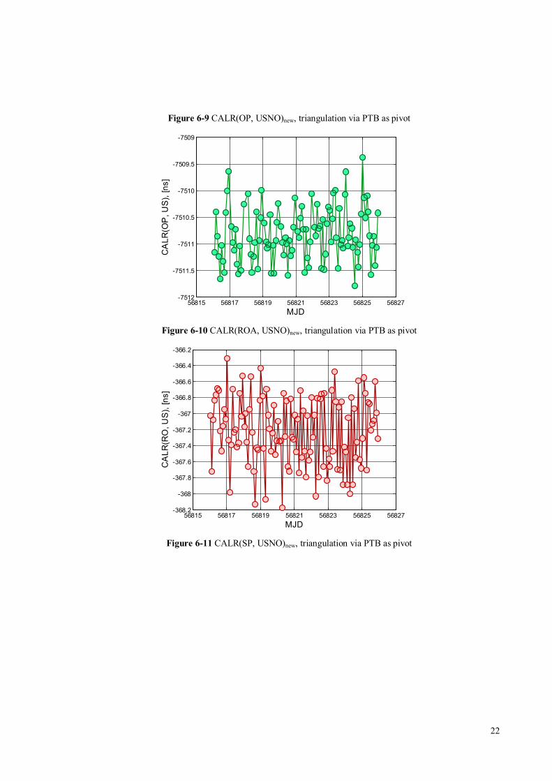
Figure 6-9 CALR(OP, USNO)new, triangulation via PTB as pivot
Figure 6-10 CALR(ROA, USNO)new, triangulation via PTB as pivot
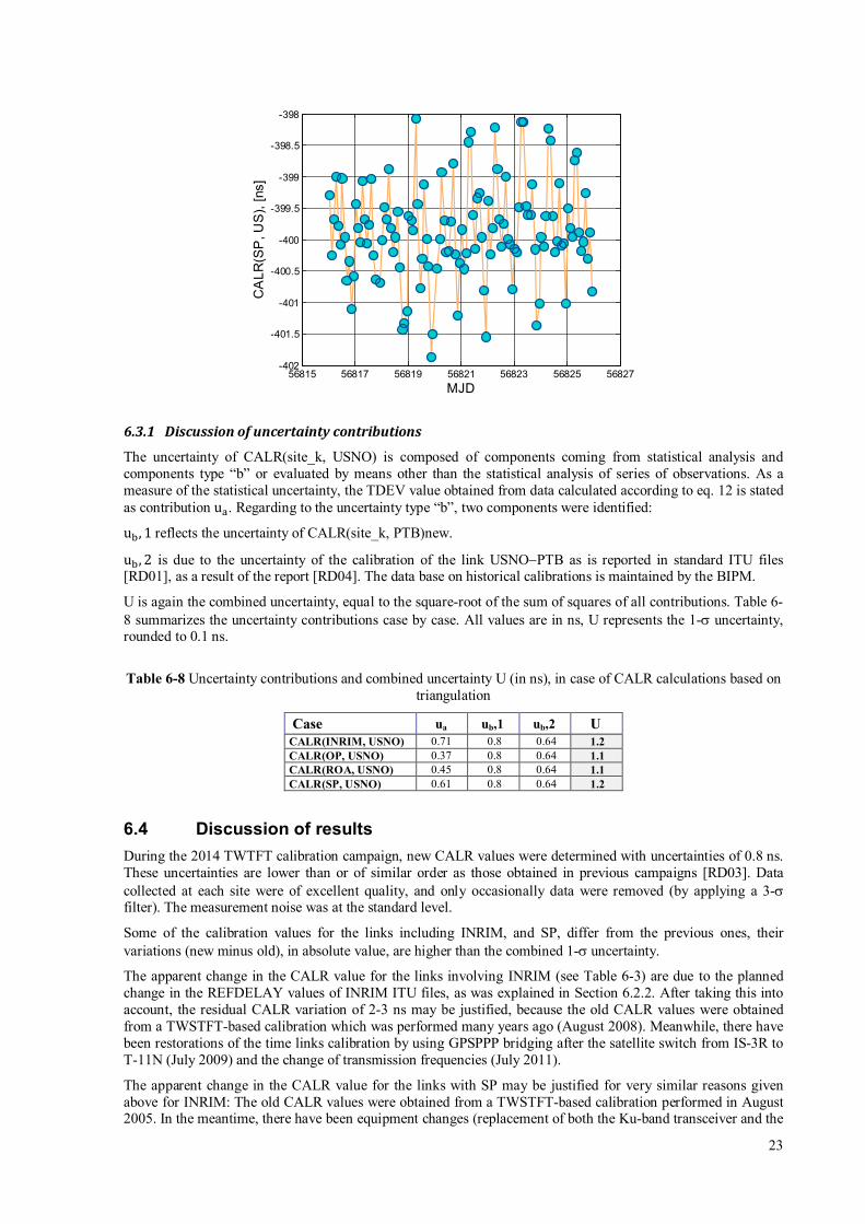
Figure 6-11 CALR(SP, USNO)new, triangulation via PTB as pivot
56815 56817 56819 56821 56823 56825 56827-7512
-7511.5
-7511
-7510.5
-7510
-7509.5
-7509
MJD
CA
LR(O
P, U
S),
[ns]
56815 56817 56819 56821 56823 56825 56827-368.2
-368
-367.8
-367.6
-367.4
-367.2
-367
-366.8
-366.6
-366.4
-366.2
MJD
CA
LR(R
O, U
S),
[ns]
23
6.3.1 Discussion of uncertainty contributions
The uncertainty of CALR(site_k, USNO) is composed of components coming from statistical analysis and components type “b” or evaluated by means other than the statistical analysis of series of observations. As a measure of the statistical uncertainty, the TDEV value obtained from data calculated according to eq. 12 is stated as contribution ua. Regarding to the uncertainty type “b”, two components were identified:
ub, 1 reflects the uncertainty of CALR(site_k, PTB)new.
ub, 2 is due to the uncertainty of the calibration of the link USNO−PTB as is reported in standard ITU files [RD01], as a result of the report [RD04]. The data base on historical calibrations is maintained by the BIPM.
U is again the combined uncertainty, equal to the square-root of the sum of squares of all contributions. Table 6-8 summarizes the uncertainty contributions case by case. All values are in ns, U represents the 1-σ uncertainty, rounded to 0.1 ns.
Table 6-8 Uncertainty contributions and combined uncertainty U (in ns), in case of CALR calculations based on triangulation
Case ua ub,1 ub,2 U CALR(INRIM, USNO) 0.71 0.8 0.64 1.2 CALR(OP, USNO) 0.37 0.8 0.64 1.1 CALR(ROA, USNO) 0.45 0.8 0.64 1.1 CALR(SP, USNO) 0.61 0.8 0.64 1.2
6.4 Discussion of results During the 2014 TWTFT calibration campaign, new CALR values were determined with uncertainties of 0.8 ns. These uncertainties are lower than or of similar order as those obtained in previous campaigns [RD03]. Data collected at each site were of excellent quality, and only occasionally data were removed (by applying a 3-σ filter). The measurement noise was at the standard level.
Some of the calibration values for the links including INRIM, and SP, differ from the previous ones, their variations (new minus old), in absolute value, are higher than the combined 1-σ uncertainty.
The apparent change in the CALR value for the links involving INRIM (see Table 6-3) are due to the planned change in the REFDELAY values of INRIM ITU files, as was explained in Section 6.2.2. After taking this into account, the residual CALR variation of 2-3 ns may be justified, because the old CALR values were obtained from a TWSTFT-based calibration which was performed many years ago (August 2008). Meanwhile, there have been restorations of the time links calibration by using GPSPPP bridging after the satellite switch from IS-3R to T-11N (July 2009) and the change of transmission frequencies (July 2011).
The apparent change in the CALR value for the links with SP may be justified for very similar reasons given above for INRIM: The old CALR values were obtained from a TWSTFT-based calibration performed in August 2005. In the meantime, there have been equipment changes (replacement of both the Ku-band transceiver and the
56815 56817 56819 56821 56823 56825 56827-402
-401.5
-401
-400.5
-400
-399.5
-399
-398.5
-398
MJD
CA
LR(S
P, U
S),
[ns]
24
SSPA) and station reconfiguration (relocation of transceiver, with the necessary cable changes), besides the subsequent restoration of the time links calibration after the satellite change and the frequency change.
The results for the triangular calibration were clearly improved thanks to the small contribution of the uncertainty in the recent calibration of the link USNO−PTB by a portable X-band TWSTFT station. The most significant changes are however due to improved bookkeeping and reporting of values in the ITU files further on.
It is thus proposed to apply the new values of CALR as is explained in the following section.
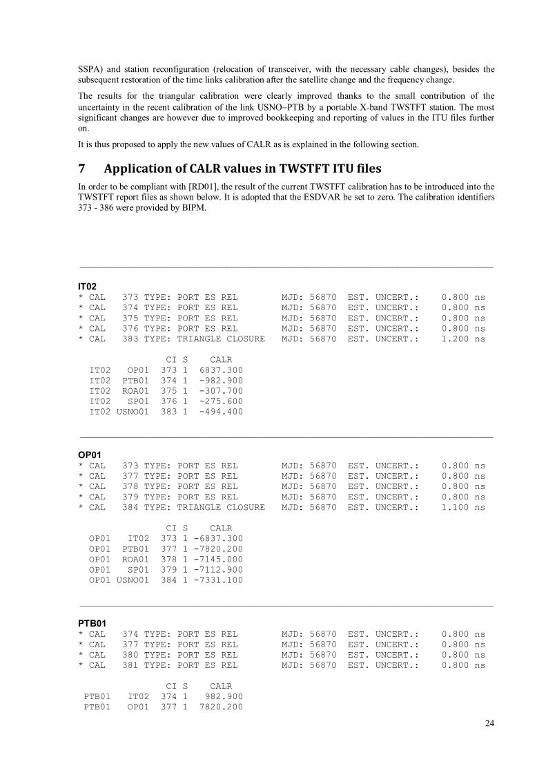
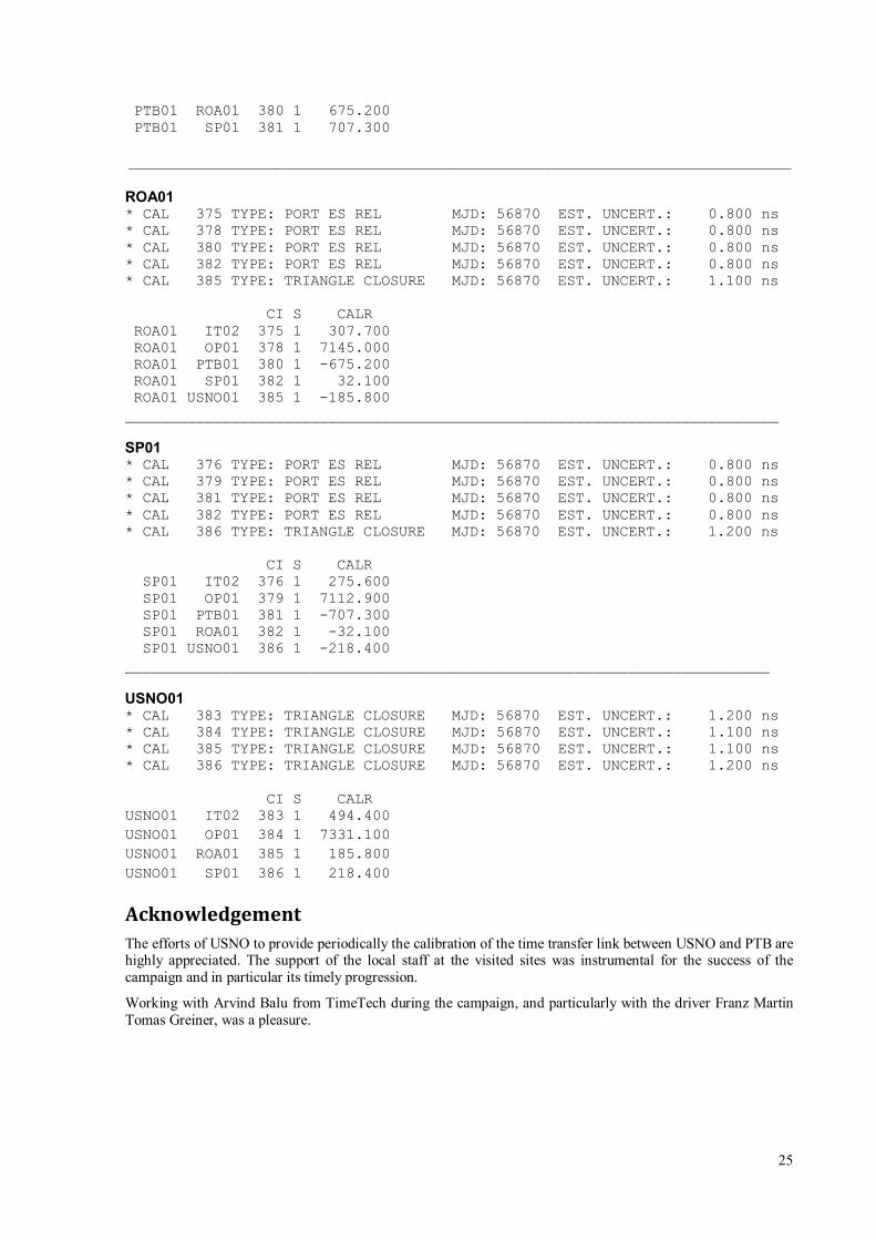
7 Application of CALR values in TWSTFT ITU files In order to be compliant with [RD01], the result of the current TWSTFT calibration has to be introduced into the TWSTFT report files as shown below. It is adopted that the ESDVAR be set to zero. The calibration identifiers 373 - 386 were provided by BIPM.
__________________________________________________________________________________________
IT02 * CAL 373 TYPE: PORT ES REL MJD: 56870 EST. UNCERT.: 0.800 ns * CAL 374 TYPE: PORT ES REL MJD: 56870 EST. UNCERT.: 0.800 ns * CAL 375 TYPE: PORT ES REL MJD: 56870 EST. UNCERT.: 0.800 ns * CAL 376 TYPE: PORT ES REL MJD: 56870 EST. UNCERT.: 0.800 ns * CAL 383 TYPE: TRIANGLE CLOSURE MJD: 56870 EST. UNCERT.: 1.200 ns CI S CALR IT02 OP01 373 1 6837.300 IT02 PTB01 374 1 -982.900 IT02 ROA01 375 1 -307.700 IT02 SP01 376 1 -275.600 IT02 USNO01 383 1 -494.400 __________________________________________________________________________________________ OP01 * CAL 373 TYPE: PORT ES REL MJD: 56870 EST. UNCERT.: 0.800 ns * CAL 377 TYPE: PORT ES REL MJD: 56870 EST. UNCERT.: 0.800 ns * CAL 378 TYPE: PORT ES REL MJD: 56870 EST. UNCERT.: 0.800 ns * CAL 379 TYPE: PORT ES REL MJD: 56870 EST. UNCERT.: 0.800 ns * CAL 384 TYPE: TRIANGLE CLOSURE MJD: 56870 EST. UNCERT.: 1.100 ns CI S CALR OP01 IT02 373 1 -6837.300 OP01 PTB01 377 1 -7820.200 OP01 ROA01 378 1 -7145.000 OP01 SP01 379 1 -7112.900 OP01 USNO01 384 1 -7331.100 __________________________________________________________________________________________ PTB01 * CAL 374 TYPE: PORT ES REL MJD: 56870 EST. UNCERT.: 0.800 ns * CAL 377 TYPE: PORT ES REL MJD: 56870 EST. UNCERT.: 0.800 ns * CAL 380 TYPE: PORT ES REL MJD: 56870 EST. UNCERT.: 0.800 ns * CAL 381 TYPE: PORT ES REL MJD: 56870 EST. UNCERT.: 0.800 ns CI S CALR PTB01 IT02 374 1 982.900 PTB01 OP01 377 1 7820.200
25
PTB01 ROA01 380 1 675.200 PTB01 SP01 381 1 707.300 __________________________________________________________________________________________ ROA01 * CAL 375 TYPE: PORT ES REL MJD: 56870 EST. UNCERT.: 0.800 ns * CAL 378 TYPE: PORT ES REL MJD: 56870 EST. UNCERT.: 0.800 ns * CAL 380 TYPE: PORT ES REL MJD: 56870 EST. UNCERT.: 0.800 ns * CAL 382 TYPE: PORT ES REL MJD: 56870 EST. UNCERT.: 0.800 ns * CAL 385 TYPE: TRIANGLE CLOSURE MJD: 56870 EST. UNCERT.: 1.100 ns CI S CALR ROA01 IT02 375 1 307.700 ROA01 OP01 378 1 7145.000 ROA01 PTB01 380 1 -675.200 ROA01 SP01 382 1 32.100 ROA01 USNO01 385 1 -185.800 __________________________________________________________________________ SP01 * CAL 376 TYPE: PORT ES REL MJD: 56870 EST. UNCERT.: 0.800 ns * CAL 379 TYPE: PORT ES REL MJD: 56870 EST. UNCERT.: 0.800 ns * CAL 381 TYPE: PORT ES REL MJD: 56870 EST. UNCERT.: 0.800 ns * CAL 382 TYPE: PORT ES REL MJD: 56870 EST. UNCERT.: 0.800 ns * CAL 386 TYPE: TRIANGLE CLOSURE MJD: 56870 EST. UNCERT.: 1.200 ns CI S CALR SP01 IT02 376 1 275.600 SP01 OP01 379 1 7112.900 SP01 PTB01 381 1 -707.300 SP01 ROA01 382 1 -32.100 SP01 USNO01 386 1 -218.400 _________________________________________________________________________ USNO01 * CAL 383 TYPE: TRIANGLE CLOSURE MJD: 56870 EST. UNCERT.: 1.200 ns * CAL 384 TYPE: TRIANGLE CLOSURE MJD: 56870 EST. UNCERT.: 1.100 ns * CAL 385 TYPE: TRIANGLE CLOSURE MJD: 56870 EST. UNCERT.: 1.100 ns * CAL 386 TYPE: TRIANGLE CLOSURE MJD: 56870 EST. UNCERT.: 1.200 ns CI S CALR USNO01 IT02 383 1 494.400 USNO01 OP01 384 1 7331.100 USNO01 ROA01 385 1 185.800 USNO01 SP01 386 1 218.400
Acknowledgement The efforts of USNO to provide periodically the calibration of the time transfer link between USNO and PTB are highly appreciated. The support of the local staff at the visited sites was instrumental for the success of the campaign and in particular its timely progression.
Working with Arvind Balu from TimeTech during the campaign, and particularly with the driver Franz Martin Tomas Greiner, was a pleasure.

26
End of Document