FE Simulation of Installation and Loading of a

Tube-Installed Pile

Syawal SATIBI, MSc. Ayman ABED, MSc. Chuang YU, Dr. Martino LEONI, Dr. Pieter A. VERMEER, Prof. Dr.-Ing.

2007 – Institutsbericht 29

des Instituts für Geotechnik

Herausgeber P. A. Vermeer

Der Institutsbericht ist Eigentum des IGS und darf deswegen nur mit dem Einverständnis des IGS ausgeliehen und kopiert (auch auszugsweise) werden.

Table of Content

1. Introduction 1

2. Material Properties and Geometry 3

2.1 Material Model for Soil ................................................................................................3 2.2 The Mohr-Coulomb Interface Model ...........................................................................5 2.3 Finite Element Mesh and Initial Soil Condition...........................................................8

3. K-Pressure Method 10

3.1 Pile Installation with K-pressure Method...................................................................10 3.1.1 Stress-Controlled Cavity Expansion using Elasticity..............................................11 3.1.2 Returning Stresses to Mohr-Coulomb Yield Surface. .............................................12 3.2 Pile Loading after K-pressure Method .......................................................................16

4. Displacement-Controlled Cavity Expansion Method 21

4.1 Pile Installation with Displacement-Controlled Cavity Expansion............................21 4.2 Pile Loading after Displacement-Controlled Cavity Expansion ................................23

5. Increased Ko Method 26

5.1 Pile Installation...........................................................................................................26 5.2 Pile Loading................................................................................................................26

6. Influence of Dilatancy Cut-off 30

6.1 Preliminary Considerations ........................................................................................30 6.2 Parameters for Dilatancy Cut-off in Interface ............................................................31 6.3 Parameters for Dilatancy Cut-off in Surrounding Soil...............................................32 6.4 Pile Load Test Simulation which includes Dilatancy Cut-off....................................33 6.5 Increased Ko with Dilatancy Cut-off...........................................................................34

7. Influence of Small Strain Stiffness 35

7.1 Parameters for HS-Small Model ................................................................................35 7.2 Pile Load Test Simulation with HS-Small Model ......................................................36

8. Sensitivity Analyses (Not yet ready) 38

8.1 Parametric Studies on the Stiffness Parameters of the Hardening Soil Model. .........38 8.1.1 The Influence of on the Load-Settlement Curve..............................................38 refE50

8.1.2 The Influence of on the Load-Settlement Curve.............................................38 refoedE

8.1.3 The Influence of on the Load-Settlement Curve .............................................38 refurE

8.2 Parametric Study on the Small Strain Stiffness Parameters .......................................38 8.3 Influence of mesh .......................................................................................................38

9. Best-fit Parameter Set (Not yet ready) 38

10. Conclusions 39

11. References 40

i

1. Introduction Several pile load tests on small diameter piles (∅ = 18 cm), which are called HSP micropiles with embedment depth of 6.25 m have been supervised by the Institute for Geotechnical Engineering and the Institute for Material Testing of Stuttgart University. The test site was in Wijchen, the Netherlands. The soil at the site consists of well packed fluvial layers of medium fine to coarse sand and gravel, which were deposited during the Pleistocene era (Vermeer and Schad, 2005). The tested piles are installed by jacking a steel tube at constant speed, if necessary supported by vibration. Once the tube has reached the required depth, the tube is withdrawn and high slump concrete is pumped continuously into the cavity. The tube withdrawal can only start when a predetermined minimum concrete pressure has been reached.

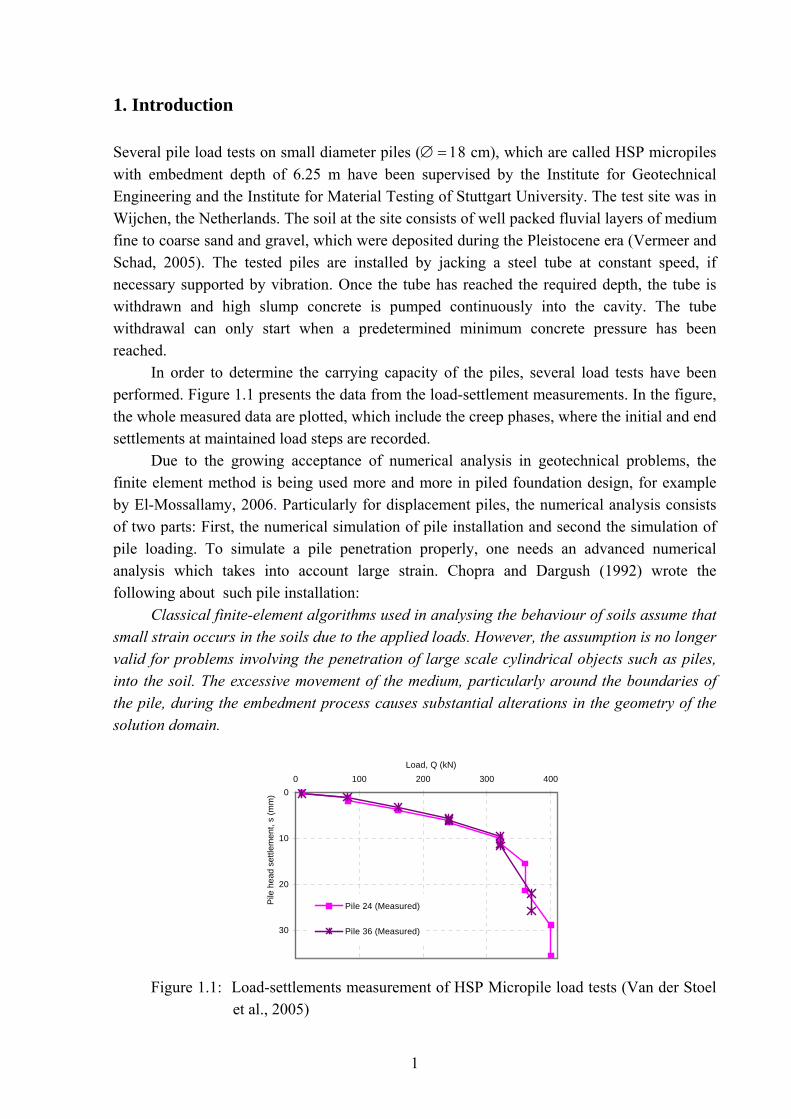
In order to determine the carrying capacity of the piles, several load tests have been performed. Figure 1.1 presents the data from the load-settlement measurements. In the figure, the whole measured data are plotted, which include the creep phases, where the initial and end settlements at maintained load steps are recorded.

Due to the growing acceptance of numerical analysis in geotechnical problems, the finite element method is being used more and more in piled foundation design, for example by El-Mossallamy, 2006. Particularly for displacement piles, the numerical analysis consists of two parts: First, the numerical simulation of pile installation and second the simulation of pile loading. To simulate a pile penetration properly, one needs an advanced numerical analysis which takes into account large strain. Chopra and Dargush (1992) wrote the following about such pile installation:

Classical finite-element algorithms used in analysing the behaviour of soils assume that small strain occurs in the soils due to the applied loads. However, the assumption is no longer valid for problems involving the penetration of large scale cylindrical objects such as piles, into the soil. The excessive movement of the medium, particularly around the boundaries of the pile, during the embedment process causes substantial alterations in the geometry of the solution domain.

0

10

20

30

0 100 200 300 400Load, Q (kN)

Pile

hea

d se

ttlem

ent,

s (m

m)

Pile 24 (Measured)

Pile 36 (Measured)

Figure 1.1: Load-settlements measurement of HSP Micropile load tests (Van der Stoel

et al., 2005)

1

As a result, strains are no longer linearly related to displacement gradients in such regions, and the equilibrium equations must be modified to take into account these changes in geometry. Of course, irreversible plastic deformation is also prevalent.

In addition to that, it might be added that dynamic effects due to pile driving or pile vibration also need to be taken into account. Moreover, it may be added that such a large strain analysis needs a constitutive model that is advanced on the topic of large deformation and density changes. Therefore, large strain numerical analyses have been applied for pile penetration by researchers (Henke and Grabe, 2006; Mabsout et al.,1999; Wieckowsky, 2004). As yet, the results of large strain numerical analyses are still deviating from the experimental data (Dijkstra et al., 2006). Furthermore, due to the lack of availability of the code for large strain numerical algorithm, the complexity of the analysis and excessive computational time-cost, large strain FE-analysis is from the point of view of practical engineers not yet popular.

No doubt that the major effect of a particular pile installation procedure is the resulting stress field around the pile. Indeed, bored piles will hardly disturb the initial geostatic stress field, but the installation of displacement piles create an increase of the radial stress around the pile. One uses the expression of (e.g. Lancellotta, 1995), where is the

initial effective overburden stress and K is a constant which depends on the soil, the diameter of the pile and the installation procedure. If direct empirical data on K is missing, its value will be back-analysed from a pile loading test. Even in times of growing computer power and advanced numerical modelling, pile loading tests remain of utmost importance as even advanced numerical models need field calibration. Hence, it is not believed that numerical models will ever be suited for the analysis of pile foundation without field calibration.

''vor K σσ ⋅= '

voσ

On having field data on the K-value, it is no longer necessary to simulate the precise pile installation process. Instead, the back-analysed K-value can be used to initialise the appropriate stress field around the pile. The simplest procedure would be to use the back-analysed K-value as a Ko-value, i.e. as a coefficient for the at rest lateral pressure all around the soil. However, it will be shown that this gives highly non-realistic stress fields as well as inappropriate load-settlement curves for displacement piles. On the other hand, it will be shown that realistic stress fields can be obtained by cylindrical cavity expansion up to the appropriate K-value. This simplified simulation of pile installation involves a small strain FE-analyses and it is consequently within the realm of practical engineering.

Considering cavity expansion, one has the option of using either a stress-controlled expansion or a displacement-controlled one. Moreover, one has the option of using various different constitutive models in the numerical simulation of a cylindrical cavity expansion. Some such possibilities will be investigated in this study. This study focuses on tube-installed displacement piles. Such piles (or stone columns) are installed by jacking or vibrating a closed-bottom tube into the ground. Upon withdrawal of the tube, the cavity is filled with concrete (or stones), so there is no skin friction due to installation. The aim of this study is to find methods to account for the effects of installation and demonstrate a feasible way of FE-displacement pile analyses for engineering practice.

2

2. Material Properties and Geometry In numerical analysis, material behaviour of the soil and pile are represented by material constitutive models. The material behaviour of the pile is considered to be linear elastic with parameters as given in Table 2.1. The soil behaviour follows the so-called the Hardening Soil model as briefly described in Chapter 2.1.

Table 2.1: Pile Parameters (Linear Elastic)

Parameters Values Unit weight (γ ) [kN/m3] 23.5 Poisson’s ratio (ν ) [ - ] 0 Young’s Modulus (E ) [ MPa ] 15000

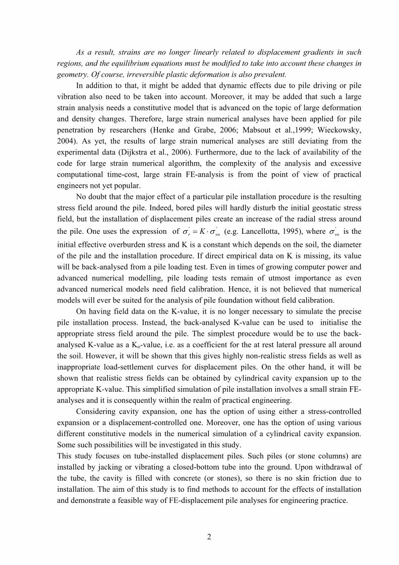
2.1 Material Model for Soil The Hardening-Soil model is an elasto-plastic model for simulating the behaviour of both soft and stiff soils (Schanz and Vermeer, 1998). The model accommodates stress-dependent stiffness of soil, which is according to a power law. Stiffness equations as applied in the model are:

m

refref

pccEE ⎟⎟

⎠

⎞⎜⎜⎝

⎛++

='cot'

''cot' 35050 ϕ

σϕ m

refrefoedoed pc

cEE ⎟⎟⎠

⎞⎜⎜⎝

⎛++

='cot'

''cot' 1

ϕσϕ

m

refrefurur pc

cEE ⎟⎟⎠

⎞⎜⎜⎝

⎛++

='cot'

''cot' 3

ϕσϕ (1)

where:

'1σ is the effective major principal stress is the effective minor principal stress '

3σ

and the following model parameters are being used m is the power law parameter which value is around 1 for clay and 0.5 for sand

refE50 is the reference stiffness modulus corresponding to the reference stress . It

is determined from a triaxial stress-strain-curve for a mobilization of 50% of the maximum shear strength q

refp

f (see Figure 2a) refoedE is the tangent stiffness for primary oedometer loading at reference stress (see

Figure 2b) refurE is the unloading /reloading stiffness at reference stress (see Figure 2a)

pref is a reference pressure is the effective cohesion 'c

'ϕ is the effective internal fiction angle

3

(a) (b)

σ1

ε1

Figure 2.1: Description of stiffness parameters (a) Hyperbolic deviatoric stress-axial

strain relationship for primary loading for a drained triaxial test with constant confining pressure (b) Characteristic curve of an oedometer

test

'3σ

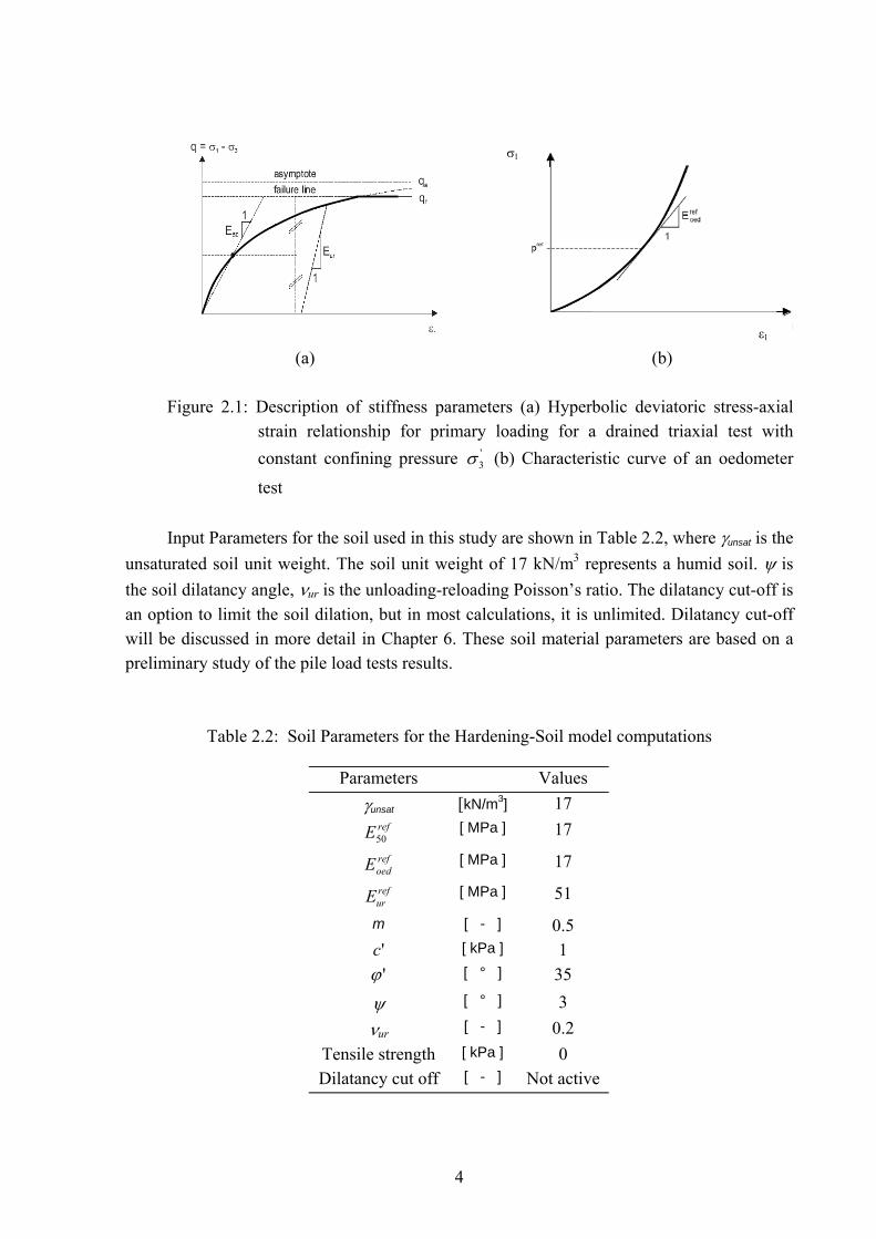
Input Parameters for the soil used in this study are shown in Table 2.2, where γunsat is the

unsaturated soil unit weight. The soil unit weight of 17 kN/m3 represents a humid soil. ψ is the soil dilatancy angle, νur is the unloading-reloading Poisson’s ratio. The dilatancy cut-off is an option to limit the soil dilation, but in most calculations, it is unlimited. Dilatancy cut-off will be discussed in more detail in Chapter 6. These soil material parameters are based on a preliminary study of the pile load tests results.

Table 2.2: Soil Parameters for the Hardening-Soil model computations

Parameters Values γunsat [kN/m3] 17

refE50 [ MPa ] 17 refoedE [ MPa ] 17 refurE [ MPa ] 51

m [ - ] 0.5 'c [ kPa ] 1 'ϕ [ ° ] 35

ψ [ ° ] 3 νur [ - ] 0.2

Tensile strength [ kPa ] 0 Dilatancy cut off [ - ] Not active

4

2.2 The Mohr-Coulomb Interface Model Direct soil-pile interaction is modelled by interface elements. The interface elements follow Mohr-Coulomb constitutive behaviour as described in Figure 2.2a for a constant normal stress. The parameters for the interface Mohr-Coulomb constitutive model are , , ψinc inϕ in, νin

and Ein, which are the interface cohesion, friction angle, dilatancy angle, Poison’s ratio and Elastic stiffness respectively. Another important parameter for the interface element is the virtual interface thickness tin. As for the interface stiffness, it can be specified as a linear elastic stiffness or non-linear elastic stiffness. If a non linear elastic interface stiffness is used, the interface stiffness is stress level dependent following the power law with Ein proportional to the effective normal stress as expressed below: '

inσ

m

refinin

inininrefinin pc

cEE ⎟⎟⎠

⎞⎜⎜⎝

⎛++

=ϕ

σϕcot

'cot (2)

where is an input parameter. The elastic interface incremental strains can be expressed in

terms of incremental interface stresses as follows:

refinE

in

ein

ein C σε && ⋅= (3)

or in matrix form:

(4) ⎥⎦

⎤⎢⎣

⎡⋅⎥

⎦

⎤⎢⎣

⎡=⎥

⎦

⎤⎢⎣

⎡

in

in

in

oedin

ein

ein

GE

τσ

γε

&

&

&

& '

/100/1

where is the elastic interface normal strain, is the elastic interface shear strain and

denotes the elastic compliance matrix expressed in term of interface oedometer (constrained) modulus and interface shear modulus G

einε e

inγ einC

oedinE in. with

)1(2 in

inin

EGν+

= , in

inin

oedin GE

νν21

12−−

= (5)

The elasto-plastic behaviour follows the Mohr-Coulomb yield function with non associated plastic potential as expressed below: , (6) ininininin cf τϕσ −+= tan'

ininining τψσ −= tan'

following the basic equations of elasto-plastic modelling, one can write that:

5

(7) ⎥⎦

⎤⎢⎣

⎡+⎥

⎦

⎤⎢⎣

⎡=⎥

⎦

⎤⎢⎣

⎡p

in

pin

ein

ein

in

in

γε

γε

γε

&

&

&

&

&

&

where is the total interface normal strain, defined as inε in

ninin ttΔ=ε with is the interface

normal displacement and is the total interface shear strain, which is defined as

nintΔ

inγ

ininin ttγγ Δ= with is the interface slip displacement. Figure 2.2b shows the deformation

mechanism of the interface element. The plastic part of the interface strains and can be

expressed in following formulas:

γintΔ

pinε p

inγ

'in

inpin

gσ

ε∂∂

Λ=& , in

inpin

gτ

γ∂∂

Λ=& (8)

where ís a plastic multiplier. Hence, the total incremental stress-strain formulation can be written as follows:

Λ

)()(in

inin

ein

pinin

einin

einin

gDDDσ

εεεεσ∂∂

Λ−=−=⋅= &&&&& (9)

where e

inD is the elastic interface stiffness matrix as follows:

⎥⎦

⎤⎢⎣

⎡=

in

oedine

in GE

D0

0 (10)

In order to solve the plastic multiplier Λ , one needs a consistency equation. For the case of perfect plasticity, it is expressed as below:

0=∂∂

= in

T

in

inin

ff σσ

&& (11)

thus, it yields:

inein

T

in

in Dfd

εσ

&∂∂

=Λ1 with ininin

oedin

in

inein

T

in

in GEgDfd +=∂∂

∂∂

= ψϕσσ

tantan (12)

which gives the final result for the total stress-strain relationship as follows:

ininin M εσ && ⋅= with ein

T

in

in

in

inein

einin DfgD

dDM

σσα

∂∂

∂∂

−= (13)

6

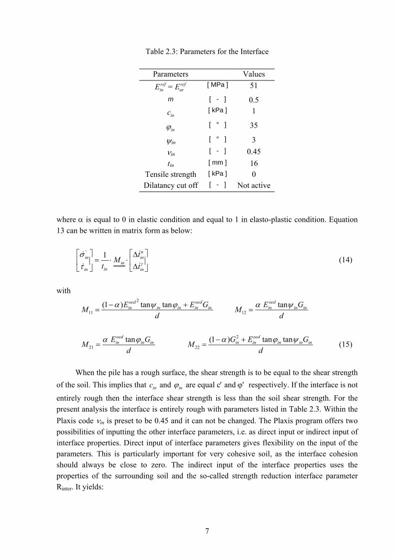
Table 2.3: Parameters for the Interface

Parameters Values refinE = ref

urE [ MPa ] 51

m [ - ] 0.5

inc [ kPa ] 1

inϕ [ ° ] 35

ψin [ ° ] 3 νin [ - ] 0.45 tin [ mm ] 16

Tensile strength [ kPa ] 0 Dilatancy cut off [ - ] Not active

where α is equal to 0 in elastic condition and equal to 1 in elasto-plastic condition. Equation 13 can be written in matrix form as below:

⎥⎦

⎤⎢⎣

⎡

ΔΔ

⋅⋅=⎥⎦

⎤⎢⎣

⎡γτ

σ

in

nin

ininin

in

tt

Mt &

&

&

& 1'

(14)

with

d

GEEM inoedininin

oedin +−

=ϕψα tantan)1( 2

11 d

GEM ininoedin ψα tan

12 =

dGEM inin

oedin ϕα tan

21 = d

GEGM inininoedinin ψϕα tantan)1( 2

22+−

= (15)

When the pile has a rough surface, the shear strength is to be equal to the shear strength

of the soil. This implies that and are equal c′ and ϕ′ respectively. If the interface is not

entirely rough then the interface shear strength is less than the soil shear strength. For the present analysis the interface is entirely rough with parameters listed in Table 2.3. Within the Plaxis code ν

inc inϕ

in is preset to be 0.45 and it can not be changed. The Plaxis program offers two possibilities of inputting the other interface parameters, i.e. as direct input or indirect input of interface properties. Direct input of interface parameters gives flexibility on the input of the parameters. This is particularly important for very cohesive soil, as the interface cohesion should always be close to zero. The indirect input of the interface properties uses the properties of the surrounding soil and the so-called strength reduction interface parameter Rinter. It yields:

7

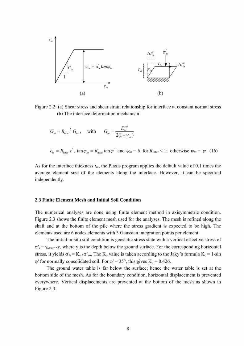
(a) (b)

Figure 2.2: (a) Shear stress and shear strain relationship for interface at constant normal stress (b) The interface deformation mechanism

urin GRG 2inter= , with

)1(2 ur

refur

urEG

ν+=

'

interin cRc = , and ψ'inter tantan ϕϕ Rin = in = 0 for Rinter < 1; otherwise ψin = ψ (16)

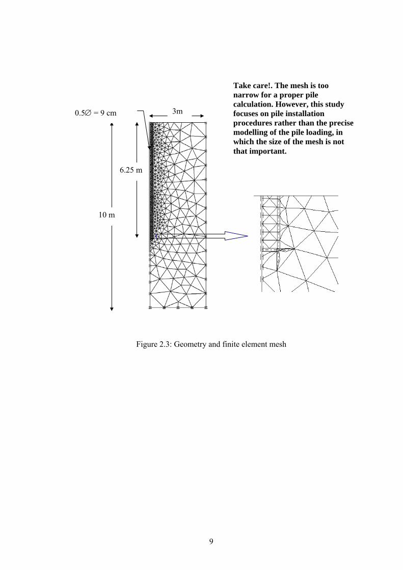
As for the interface thickness tin, the Plaxis program applies the default value of 0.1 times the average element size of the elements along the interface. However, it can be specified independently. 2.3 Finite Element Mesh and Initial Soil Condition The numerical analyses are done using finite element method in axisymmetric condition. Figure 2.3 shows the finite element mesh used for the analyses. The mesh is refined along the shaft and at the bottom of the pile where the stress gradient is expected to be high. The elements used are 6 nodes elements with 3 Gaussian integration points per element.

The initial in-situ soil condition is geostatic stress state with a vertical effective stress of σ'v = γunsat • y, where y is the depth below the ground surface. For the corresponding horizontal stress, it yields σ'h = Ko • σ'vo. The Ko value is taken according to the Jaky’s formula Ko = 1-sin ϕ' for normally consolidated soil. For ϕ' = 35°, this gives Ko = 0.426.

The ground water table is far below the surface; hence the water table is set at the bottom side of the mesh. As for the boundary condition, horizontal displacement is prevented everywhere. Vertical displacements are prevented at the bottom of the mesh as shown in Figure 2.3.

nintΔ

inγ

'inσ

inτ

γintΔ

int

inτ

inanϕtσc 'inin +

1 inG

inγ

8

3m

10 m

0.5∅ = 9 cm

6.25 m

Take care!. The mesh is too narrow for a proper pile calculation. However, this study focuses on pile installation procedures rather than the precise modelling of the pile loading, in which the size of the mesh is not that important.

Figure 2.3: Geometry and finite element mesh

9

3. K-Pressure Method The increase of radial stress due to pile installation is a major concern in the analysis of a displacement pile. One of the assumptions for the radial stress increase due to pile installation is that radial stress σ′r increases according to a constant K-value times the initial vertical stress σ'vo, where K is σ′r/σ'vo. Kulhawy (1984) suggests a range of 0.75≤ K ≤2 for analytical calculation of pile shaft capacity. One of the research findings on numerical analyses of a jacked pile performed by Henke and Grabe (2006) also shows that the radial stress increases almost linearly with depth following a constant K-value after installation. For a particular loose sand and a pile diameter of 30 cm, they obtained a K-value of 1.25. The increase of radial stress due to pile installation can be created by applying horizontal stresses with . This procedure is showed in the following sections. ''

vor K σσ ⋅=

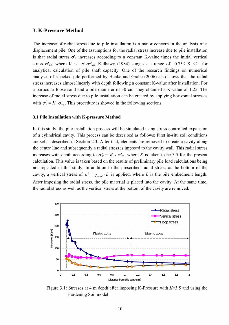
3.1 Pile Installation with K-pressure Method In this study, the pile installation process will be simulated using stress controlled expansion of a cylindrical cavity. This process can be described as follows: First in-situ soil conditions are set as described in Section 2.3. After that, elements are removed to create a cavity along the centre line and subsequently a radial stress is imposed to the cavity wall. This radial stress increases with depth according to σ′r = K • σ'vo, where K is taken to be 3.5 for the present calculation. This value is taken based on the results of preliminary pile load calculations being not repeated in this study. In addition to the prescribed radial stress, at the bottom of the cavity, a vertical stress of Lγσ' unsatv ⋅= is applied, where L is the pile embedment length.

After imposing the radial stress, the pile material is placed into the cavity. At the same time, the radial stress as well as the vertical stress at the bottom of the cavity are removed.

0

50

100

150

200

250

300

0 0,2 0,4 0,6 0,8 1 1,2 1,4 1,6 1,8 2

Distance from pile centre (m)

Stre

sses

(Kpa

)

Radial stressVertical stressHoop stress

Plastic zone Elastic zone

Figure 3.1: Stresses at 4 m depth after imposing K-Pressure with K=3.5 and using the Hardening Soil model

10

In the above process, the Hardening Soil model as described in Section 2.1 might

directly be applied. However, on using the Hardening Soil model, the cavity expansion is significantly non-uniform. Moreover, on using the Hardening Soil model for the installation process, vertical effective stress in the soil would significantly be decreased in the plastic zone around the cavity, as shown in Figure 3.1. However, it is doutbfull that the decrease of vertical stress is realistic.

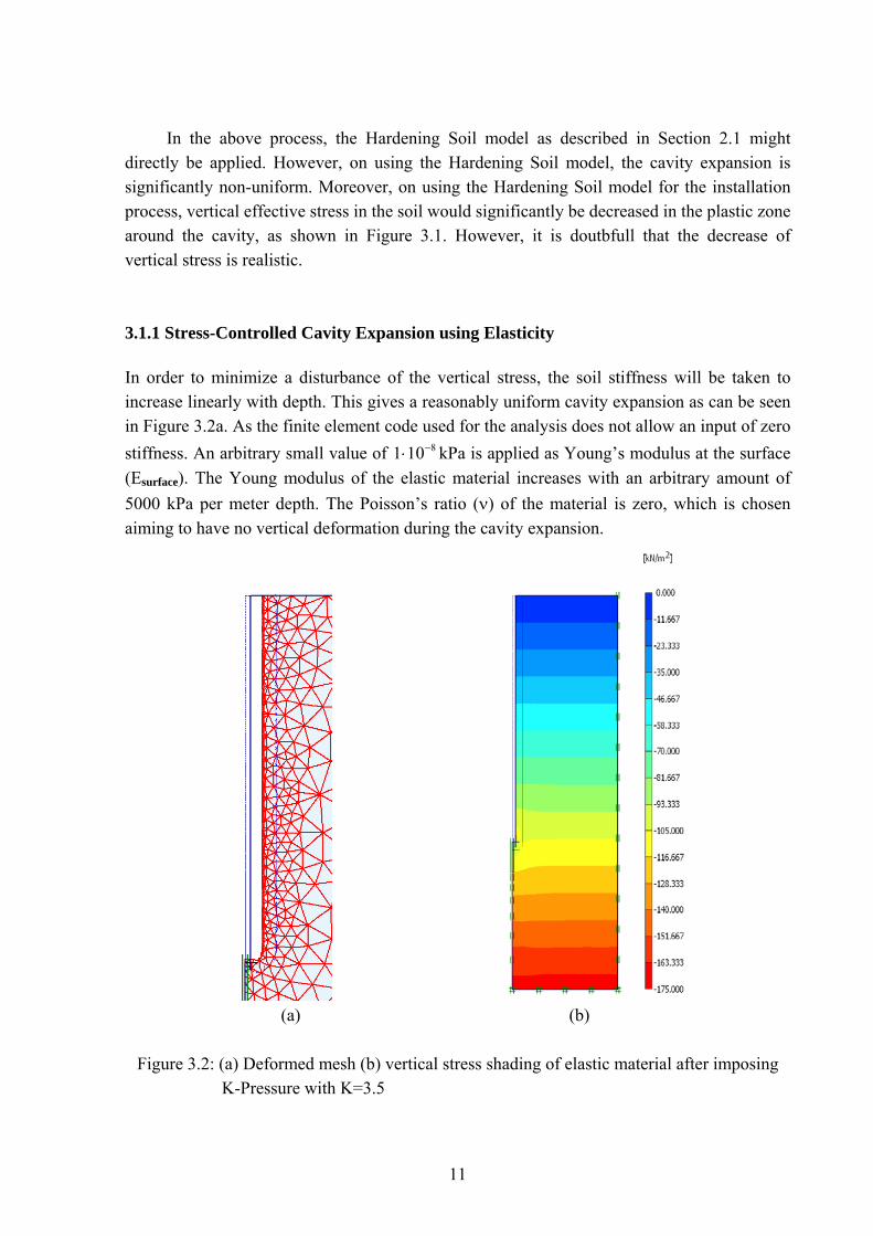
3.1.1 Stress-Controlled Cavity Expansion using Elasticity In order to minimize a disturbance of the vertical stress, the soil stiffness will be taken to increase linearly with depth. This gives a reasonably uniform cavity expansion as can be seen in Figure 3.2a. As the finite element code used for the analysis does not allow an input of zero stiffness. An arbitrary small value of kPa is applied as Young’s modulus at the surface (E

8101 −⋅surface). The Young modulus of the elastic material increases with an arbitrary amount of

5000 kPa per meter depth. The Poisson’s ratio (ν) of the material is zero, which is chosen aiming to have no vertical deformation during the cavity expansion.

(a) (b)

Figure 3.2: (a) Deformed mesh (b) vertical stress shading of elastic material after imposing

K-Pressure with K=3.5

11

-200

-150

-100

-50

0

50

100

150

200

250

0 0,4 0,8 1,2 1,6 2

Distance from pile centre (m)

Stre

sses

(Kpa

)Radial stressVertical stressHoop stress

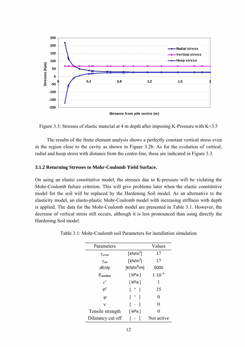
Figure 3.3: Stresses of elastic material at 4 m depth after imposing K-Pressure with K=3.5

The results of the finite element analysis shows a perfectly constant vertical stress even

in the region close to the cavity as shown in Figure 3.2b. As for the evolution of vertical, radial and hoop stress with distance from the centre-line, these are indicated in Figure 3.3.

3.1.2 Returning Stresses to Mohr-Coulomb Yield Surface. On using an elastic constitutive model, the stresses due to K-pressure will be violating the Mohr-Coulomb failure criterion. This will give problems later when the elastic constitutive model for the soil will be replaced by the Hardening Soil model. As an alternative to the elasticity model, an elasto-plastic Mohr-Coulomb model with increasing stiffness with depth is applied. The data for the Mohr-Coulomb model are presented in Table 3.1. However, the decrease of vertical stress still occurs, although it is less pronounced than using directly the Hardening Soil model.

Table 3.1: Mohr-Coulomb soil Parameters for installation simulation

Parameters Values

γunsat [kN/m3] 17 γsat [kN/m3] 17

dE/dy [KN/m2/m] 5000 Esurface [ kPa ] 8101 −⋅

' c [ kPa ] 1 'ϕ [ ° ] 35

ψ [ ° ] 0 ν [ - ] 0

Tensile strength [ kPa ] 0 Dilatancy cut off [ - ] Not active

12

0

50

100

150

200

0 0,2 0,4 0,6 0,8 1 1,2 1,4 1,6 1,8 2

Distance from pile centre (m)

Stre

sses

(kPa

)MC model for entire cavity expansion

elastic expansion with MC-correction

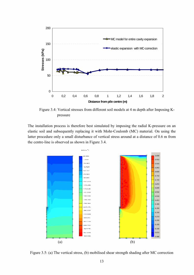
Figure 3.4: Vertical stresses from different soil models at 4 m depth after Imposing K-

pressure The installation process is therefore best simulated by imposing the radial K-pressure on an elastic soil and subsequently replacing it with Mohr-Coulomb (MC) material. On using the latter procedure only a small disturbance of vertical stress around at a distance of 0.6 m from the centre-line is observed as shown in Figure 3.4.

(a) (b)

Figure 3.5: (a) The vertical stress, (b) mobilised shear strength shading after MC correction

13

0

50

100

150

200

250

300

0 0,4 0,8 1,2 1,6 2

Distance from pile centre (m)

Stre

sses

(Kpa

)Radial stressVertical stressHoop stress

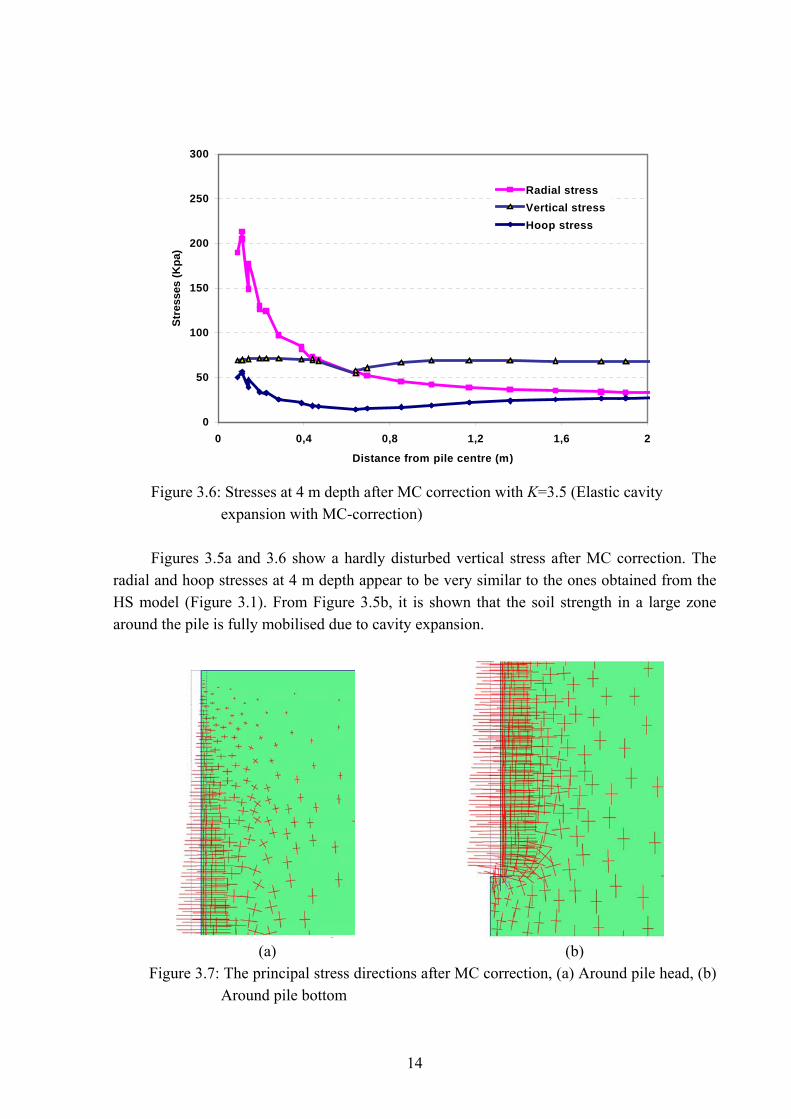
Figure 3.6: Stresses at 4 m depth after MC correction with K=3.5 (Elastic cavity

expansion with MC-correction) Figures 3.5a and 3.6 show a hardly disturbed vertical stress after MC correction. The

radial and hoop stresses at 4 m depth appear to be very similar to the ones obtained from the HS model (Figure 3.1). From Figure 3.5b, it is shown that the soil strength in a large zone around the pile is fully mobilised due to cavity expansion.

(a) (b)

Figure 3.7: The principal stress directions after MC correction, (a) Around pile head, (b) Around pile bottom

14

(a) deformed mesh (b) horizontal displacement

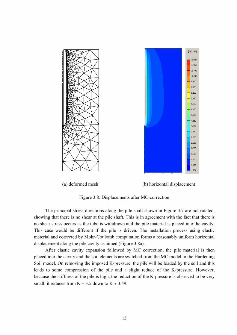
Figure 3.8: Displacements after MC-correction

The principal stress directions along the pile shaft shown in Figure 3.7 are not rotated, showing that there is no shear at the pile shaft. This is in agreement with the fact that there is no shear stress occurs as the tube is withdrawn and the pile material is placed into the cavity. This case would be different if the pile is driven. The installation process using elastic material and corrected by Mohr-Coulomb computation forms a reasonably uniform horizontal displacement along the pile cavity as aimed (Figure 3.8a).

After elastic cavity expansion followed by MC correction, the pile material is then placed into the cavity and the soil elements are switched from the MC model to the Hardening Soil model. On removing the imposed K-pressure, the pile will be loaded by the soil and this leads to some compression of the pile and a slight reduce of the K-pressure. However, because the stiffness of the pile is high, the reduction of the K-pressure is observed to be very small; it reduces from K = 3.5 down to K ≈ 3.49.

15

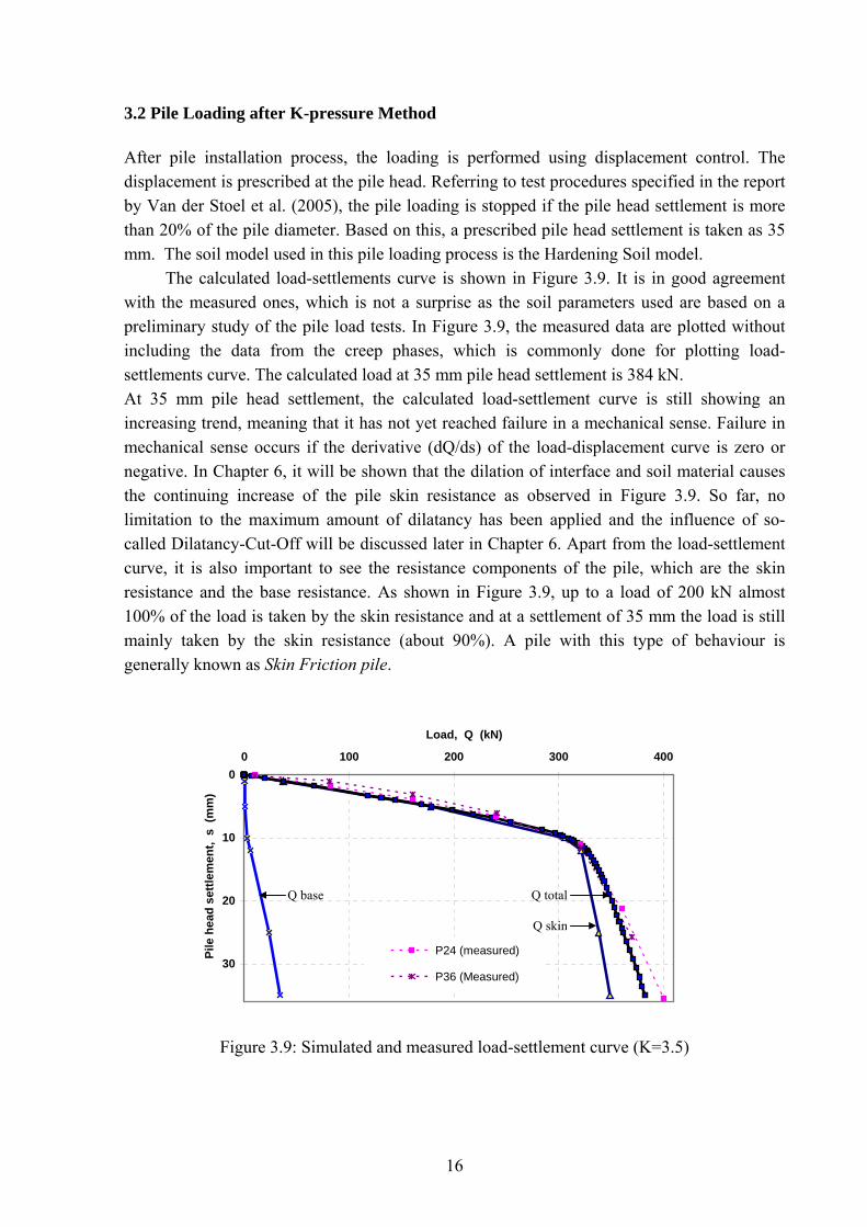
3.2 Pile Loading after K-pressure Method After pile installation process, the loading is performed using displacement control. The displacement is prescribed at the pile head. Referring to test procedures specified in the report by Van der Stoel et al. (2005), the pile loading is stopped if the pile head settlement is more than 20% of the pile diameter. Based on this, a prescribed pile head settlement is taken as 35 mm. The soil model used in this pile loading process is the Hardening Soil model.

The calculated load-settlements curve is shown in Figure 3.9. It is in good agreement with the measured ones, which is not a surprise as the soil parameters used are based on a preliminary study of the pile load tests. In Figure 3.9, the measured data are plotted without including the data from the creep phases, which is commonly done for plotting load-settlements curve. The calculated load at 35 mm pile head settlement is 384 kN. At 35 mm pile head settlement, the calculated load-settlement curve is still showing an increasing trend, meaning that it has not yet reached failure in a mechanical sense. Failure in mechanical sense occurs if the derivative (dQ/ds) of the load-displacement curve is zero or negative. In Chapter 6, it will be shown that the dilation of interface and soil material causes the continuing increase of the pile skin resistance as observed in Figure 3.9. So far, no limitation to the maximum amount of dilatancy has been applied and the influence of so-called Dilatancy-Cut-Off will be discussed later in Chapter 6. Apart from the load-settlement curve, it is also important to see the resistance components of the pile, which are the skin resistance and the base resistance. As shown in Figure 3.9, up to a load of 200 kN almost 100% of the load is taken by the skin resistance and at a settlement of 35 mm the load is still mainly taken by the skin resistance (about 90%). A pile with this type of behaviour is generally known as Skin Friction pile.

0

10

20

30

0 100 200 300 400

Load, Q (kN)

Pile

hea

d se

ttlem

ent,

s (

mm

)

P24 (measured)

P36 (Measured)

Q base Q total

Q skin

Figure 3.9: Simulated and measured load-settlement curve (K=3.5)

16

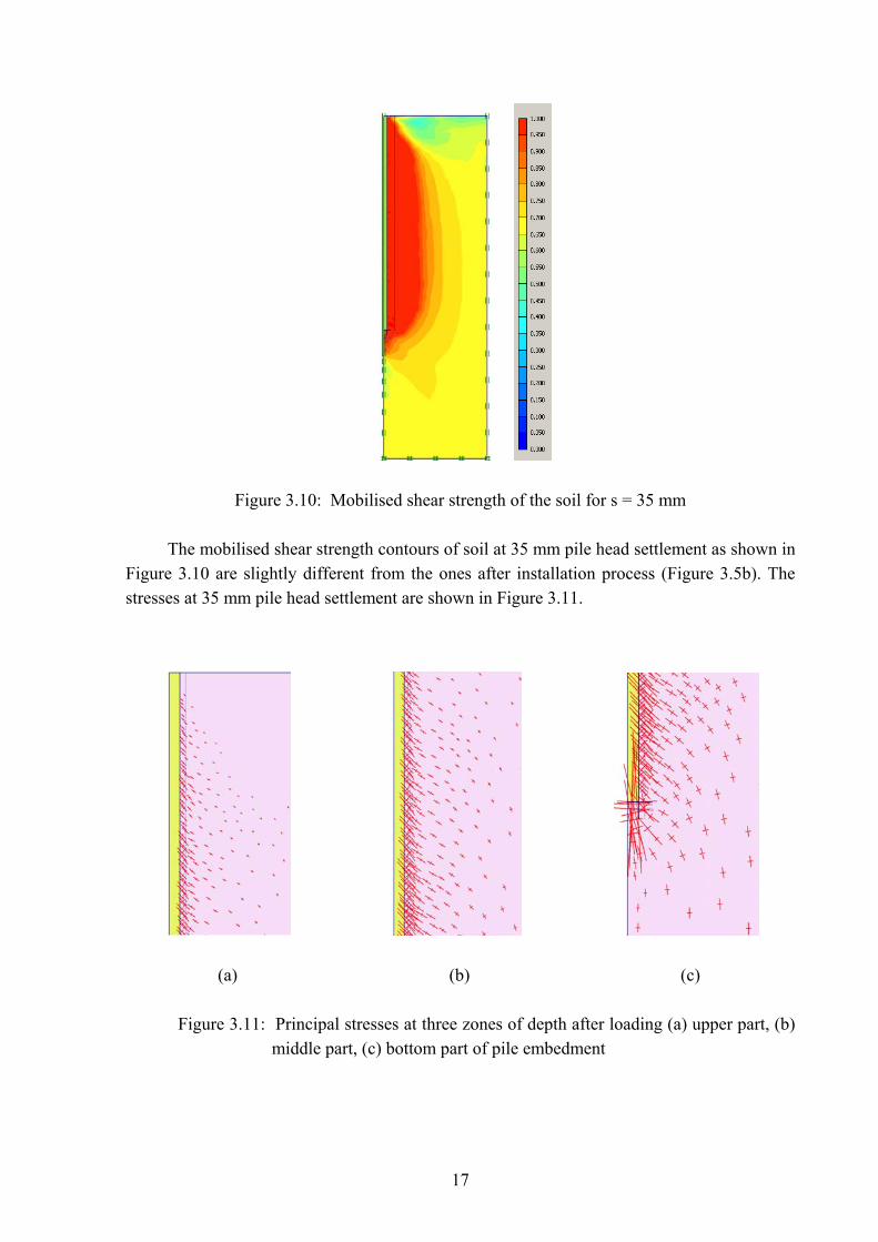
Figure 3.10: Mobilised shear strength of the soil for s = 35 mm

The mobilised shear strength contours of soil at 35 mm pile head settlement as shown in Figure 3.10 are slightly different from the ones after installation process (Figure 3.5b). The stresses at 35 mm pile head settlement are shown in Figure 3.11.

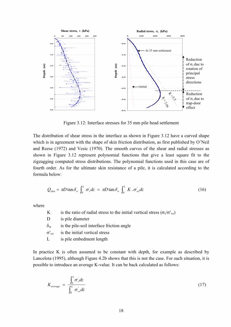
(a) (b) (c)

Figure 3.11: Principal stresses at three zones of depth after loading (a) upper part, (b) middle part, (c) bottom part of pile embedment

17

-6,5

-5,5

-4,5

-3,5

-2,5

-1,5

-0,5

0 50 100 150 200 250

S )hear stress (Kpa

-6,5

-5,5

-4,5

-3,5

-2,5

-1,5

-0,5

0 100 200 300 400

R

Depth

(m)

adial stress σ'xx (Kpa)Shear stress, τ (kPa) Radial stress, σr (kPa)

At 35 mm settlement

Reduction of σr due to rotation of principal stress directions

Depth (

m)D

epth

(m

)

Dep

th (

m)

Initial

Reduction of σr due to trap-door effect

K =3.5K = 2.66

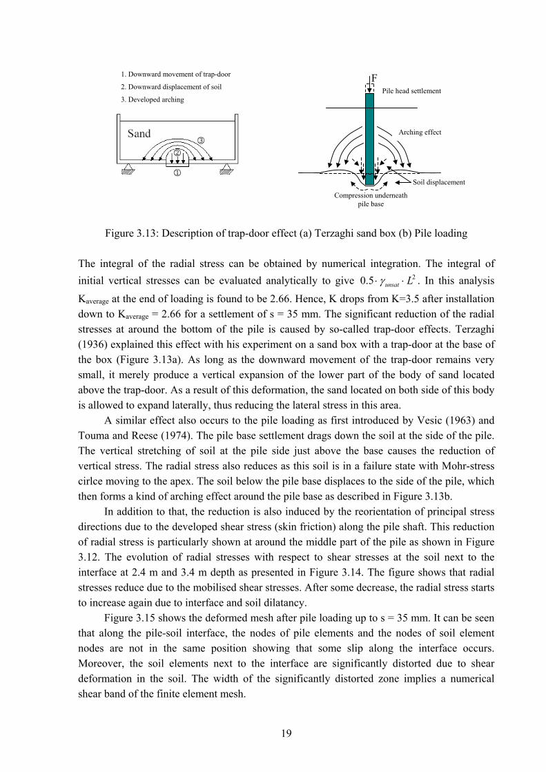
Figure 3.12: Interface stresses for 35 mm pile head settlement

The distribution of shear stress in the interface as shown in Figure 3.12 have a curved shape which is in agreement with the shape of skin friction distribution, as first published by O’Neil and Reese (1972) and Vesic (1970). The smooth curves of the shear and radial stresses as shown in Figure 3.12 represent polynomial functions that give a least square fit to the zigzagging computed stress distributions. The polynomial functions used in this case are of fourth order. As for the ultimate skin resistance of a pile, it is calculated according to the formula below:

dzKDdzDQL

vow

L

rwskin ∫∫ •==0

'

0

' tantan σδπσδπ (16)

where

K is the ratio of radial stress to the initial vertical stress (σr/σ'vo) D is pile diameter δw is the pile-soil interface friction angle σ'vo is the initial vertical stress L is pile embedment length

In practice K is often assumed to be constant with depth, for example as described by Lancelota (1995), although Figure 4.2b shows that this is not the case. For such situation, it is possible to introduce an average K-value. It can be back calculated as follows:

dz

dzK L

vo

L

r

average

∫∫

=

0

'

0

'

σ

σ (17)

18

1. Downward movement of trap-door F Pile head settlement

Arching effect

Compression underneath pile base

Soil displacement

2. Downward displacement of soil

3. Developed arching

Figure 3.13: Description of trap-door effect (a) Terzaghi sand box (b) Pile loading The integral of the radial stress can be obtained by numerical integration. The integral of initial vertical stresses can be evaluated analytically to give . In this analysis

K

25.0 Lunsat ⋅⋅ γ

average at the end of loading is found to be 2.66. Hence, K drops from K=3.5 after installation down to Kaverage = 2.66 for a settlement of s = 35 mm. The significant reduction of the radial stresses at around the bottom of the pile is caused by so-called trap-door effects. Terzaghi (1936) explained this effect with his experiment on a sand box with a trap-door at the base of the box (Figure 3.13a). As long as the downward movement of the trap-door remains very small, it merely produce a vertical expansion of the lower part of the body of sand located above the trap-door. As a result of this deformation, the sand located on both side of this body is allowed to expand laterally, thus reducing the lateral stress in this area.

A similar effect also occurs to the pile loading as first introduced by Vesic (1963) and Touma and Reese (1974). The pile base settlement drags down the soil at the side of the pile. The vertical stretching of soil at the pile side just above the base causes the reduction of vertical stress. The radial stress also reduces as this soil is in a failure state with Mohr-stress cirlce moving to the apex. The soil below the pile base displaces to the side of the pile, which then forms a kind of arching effect around the pile base as described in Figure 3.13b.

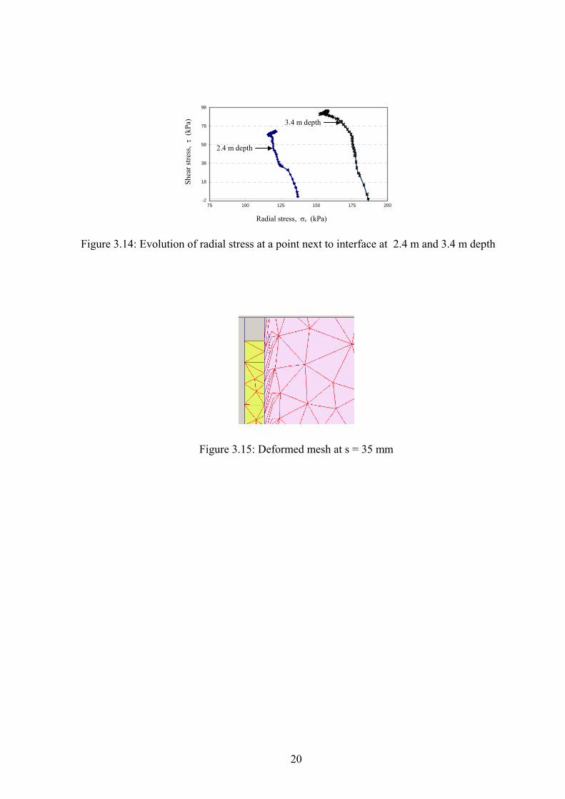
In addition to that, the reduction is also induced by the reorientation of principal stress directions due to the developed shear stress (skin friction) along the pile shaft. This reduction of radial stress is particularly shown at around the middle part of the pile as shown in Figure 3.12. The evolution of radial stresses with respect to shear stresses at the soil next to the interface at 2.4 m and 3.4 m depth as presented in Figure 3.14. The figure shows that radial stresses reduce due to the mobilised shear stresses. After some decrease, the radial stress starts to increase again due to interface and soil dilatancy.

Figure 3.15 shows the deformed mesh after pile loading up to s = 35 mm. It can be seen that along the pile-soil interface, the nodes of pile elements and the nodes of soil element nodes are not in the same position showing that some slip along the interface occurs. Moreover, the soil elements next to the interface are significantly distorted due to shear deformation in the soil. The width of the significantly distorted zone implies a numerical shear band of the finite element mesh.

19

-2

18

38

58

78

98

75 100 125 150 175 200

Radial stress (kPa)

Shea

r str

ess

(kPa

)

2.4 m depth

3.4 m depth

Radial stress, σr (kPa)

Shea

r stre

ss,

τ (k

Pa)

Figure 3.14: Evolution of radial stress at a point next to interface at 2.4 m and 3.4 m depth

Figure 3.15: Deformed mesh at s = 35 mm

20

4. Displacement-Controlled Cavity Expansion Method Another method for simulating pile installation is using displacement-controlled cavity expansion. This is done by prescribing a uniform horizontal displacement on a cavity wall. This method has been used by Debats et al. (2003) for simulating the installation of stone column and by Dijkstra et al (2006) for simulating a driven pile installation. 4.1 Pile Installation with Displacement-Controlled Cavity Expansion This pile installation procedure can be described as follows: the process is started with setting the initial conditions as explained in Section 2.3. After that, pile elements are removed to create a cavity along the centre line and subsequently the cavity wall is expanded uniformly by prescribing a horizontal displacement. In addition to that, a vertical stress ( Lγσ' unsatv ⋅= ) is

applied at the bottom of the cavity, where L is the pile embedment length. After the displacement-controlled cavity expansion process, the pile material is placed

into the cavity. On doing so, the prescribed horizontal displacement as well as the vertical stress at the bottom of the cavity are removed. In this process, the Hardening Soil model is directly applied during the installation process. This is done because this is the simplest installation procedure and the cavity expansion is enforced to be uniform. Furthermore, it is also aimed to compare results from simplest installation procedure with the previous accurate procedure.

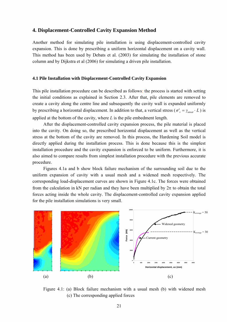
Figures 4.1a and b show block failure mechanism of the surrounding soil due to the uniform expansion of cavity with a usual mesh and a widened mesh respectively. The corresponding load-displacement curves are shown in Figure 4.1c. The forces were obtained from the calculation in kN per radian and they have been multiplied by 2π to obtain the total forces acting inside the whole cavity. The displacement-controlled cavity expansion applied for the pile installation simulations is very small.

0

2000

4000

6000

8000

10000

0 500 1000 1500 2000 2500 3000 3500 4000

Horizontal displacement, ux (mm)

Forc

e (k

N)

Kaverage = 50

Widened geometry

Kaverage = 30

Current geometry

(a) (b) (c) Figure 4.1: (a) Block failure mechanism with a usual mesh (b) with widened mesh

(c) The corresponding applied forces

21

-6 ,5

-5,5

-4 ,5

-3 ,5

-2 ,5

-1,5

-0 ,5

0 5 10 15 2 0

K

-6,5

-5,5

-4,5

-3,5

-2,5

-1,5

-0,5

0 100 200 300 400

adial stre (Kpa)R ss K Radial stress, σr (kPa)

After uniform cavity expansion

Uniform cavity expansion Kaverage = 3.69

Dep

th (

m)

Depth

(m)

Dep

th (

m)

K = 3.69 K-pressure (K= 3.5)

Initial

(a) (b)

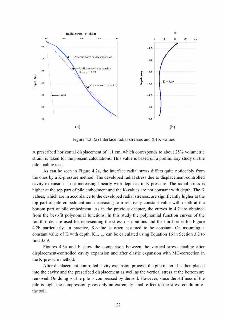
Figure 4.2: (a) Interface radial stresses and (b) K-values

A prescribed horizontal displacement of 1.1 cm, which corresponds to about 25% volumetric strain, is taken for the present calculations. This value is based on a preliminary study on the pile loading tests.

As can be seen in Figure 4.2a, the interface radial stress differs quite noticeably from the ones by a K-pressure method. The developed radial stress due to displacement-controlled cavity expansion is not increasing linearly with depth as in K-pressure. The radial stress is higher at the top part of pile embedment and the K-values are not constant with depth. The K values, which are in accordance to the developed radial stresses, are significantly higher at the top part of pile embedment and decreasing to a relatively constant value with depth at the bottom part of pile embedment. As in the previous chapter, the curves in 4.2 are obtained from the best-fit polynomial functions. In this study the polynomial function curves of the fourth order are used for representing the stress distributions and the third order for Figure 4.2b particularly. In practice, K-value is often assumed to be constant. On assuming a constant value of K with depth, Kaverage can be calculated using Equation 16 in Section 3.2 to find 3.69.

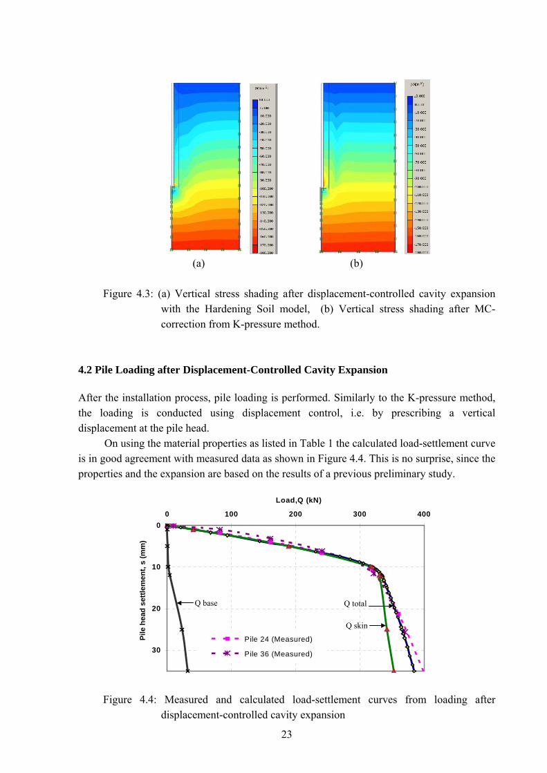
Figures 4.3a and b show the comparison between the vertical stress shading after displacement-controlled cavity expansion and after elastic expansion with MC-correction in the K-pressure method.

After displacement-controlled cavity expansion process, the pile material is then placed into the cavity and the prescribed displacement as well as the vertical stress at the bottom are removed. On doing so, the pile is compressed by the soil. However, since the stiffness of the pile is high, the compression gives only an extremely small effect to the stress condition of the soil.

22

(a) (b)

Figure 4.3: (a) Vertical stress shading after displacement-controlled cavity expansion

with the Hardening Soil model, (b) Vertical stress shading after MC-correction from K-pressure method.

4.2 Pile Loading after Displacement-Controlled Cavity Expansion

After the installation process, pile loading is performed. Similarly to the K-pressure method, the loading is conducted using displacement control, i.e. by prescribing a vertical displacement at the pile head.

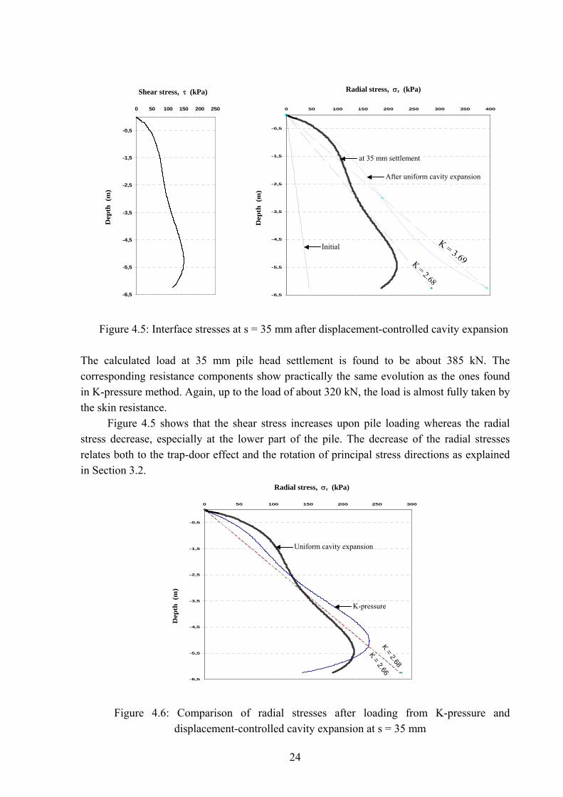
On using the material properties as listed in Table 1 the calculated load-settlement curve is in good agreement with measured data as shown in Figure 4.4. This is no surprise, since the properties and the expansion are based on the results of a previous preliminary study.

0

10

20

30

0 100 200 300 400

Load,Q (kN)

Pile

hea

d se

ttlem

ent,

s (m

m)

Pile 24 (Measured)

Pile 36 (Measured)

Q base Q total

Q skin

Figure 4.4: Measured and calculated load-settlement curves from loading after displacement-controlled cavity expansion

23

-6,5

-5,5

-4,5

-3,5

-2,5

-1,5

-0,5

0 50 100 150 200 250

Shear stress (Kpa)

Dept

h (m

)

-6,5

-5,5

-4,5

-3,5

-2,5

-1,5

-0,5

0 50 100 150 200 250 300 350 400

Radial stress (Kpa)

Depth

(m)

Radial stress, σr (kPa) Shear stress, τ (kPa)

at 35 mm settlement

After uniform cavity expansion

Dep

th (

m)

Dep

th (

m)

K = 3.69K = 2.68

Initial

Figure 4.5: Interface stresses at s = 35 mm after displacement-controlled cavity expansion The calculated load at 35 mm pile head settlement is found to be about 385 kN. The corresponding resistance components show practically the same evolution as the ones found in K-pressure method. Again, up to the load of about 320 kN, the load is almost fully taken by the skin resistance.

Figure 4.5 shows that the shear stress increases upon pile loading whereas the radial stress decrease, especially at the lower part of the pile. The decrease of the radial stresses relates both to the trap-door effect and the rotation of principal stress directions as explained in Section 3.2.

-6,5

-5,5

-4,5

-3,5

-2,5

-1,5

-0,5

0 50 100 150 200 250 300

Radial stress (Kpa)Radial stress, σr (kPa)

Uniform cavity expansion

Depth

(m)D

epth

(m

)

K-pressure

K = 2.66K = 2.68

Figure 4.6: Comparison of radial stresses after loading from K-pressure and displacement-controlled cavity expansion at s = 35 mm

24

Similarly to K-pressure method, K-value can be back calculated and is found in this case to decrease from K = 3.69 to K = 2.68. With K-pressure method the K-value was found to decrease from 3.5 down to 2.66. Similar K-value has also been found by Aboutaha et al. (1993). From their experimental study of a load test on a jacked pile in medium dense sand, K-value of about 2.6 to 2.7 was observed.

As shown is Figure 4.6, the radial stress distribution after loading with displacement-controlled cavity expansion in the installation process is slightly different from the curve with installation process using K-pressure. The radial stress from displacement-controlled cavity expansion is higher around pile top and lower around pile tip. However, the integral of radial stresses at 35 mm settlement after both installation processes give almost the same value. The curves representing the stress distributions in Figures 4.5 and 4.6 are polynomial curves of the fourth order.

25

5. Increased Ko Method The easiest method for simulating the radial stress increase due pile installation is the use of an increased Ko value as for instance used by Russo (2004). However, it should be realized that if Ko is increased, not only the radial stress is increased but also the hoop stress. This does not represent an expansion of a cavity due to pile jacking as obtained the K-pressure method and the displacement controlled cavity expansion. As for the other methods of pile installation, the value of the increased Ko should be taken carefully. In this study, several calculation results for different increased Ko values will be presented.

5.1 Pile Installation The installation process begins with setting the initial conditions of the soil as motioned in Chapter 2 except for the Ko value. The Ko value of the soil down to the depth of pile embedment is increased to a certain value to obtain higher horizontal stress. Below the pile embedment depth, the Ko value of the soil is set according Jaky’s formula, Ko = 1-sin ϕ' for normally consolidated soil. After that, the pile is installed.

Due to increased Ko, the horizontal stresses, which include radial and hoop stresses are increased to the same value. The increase covers the whole area where increased Ko is applied. As mentioned before, this is not the case in the true installation process, which follows cavity expansion behaviour. In a cavity expansion, hoop stress should decrease at the same amount as the radial stress increase in the elastic region and then increases differently with radial stress in the plastic region. Moreover, the stresses change only to some distance surrounding the pile due to the cavity expansion. In spite of those drawbacks in the installation process, it is of beneficial to observe the results of load-settlement behaviour after loading the pile and to compare them to the previous results.

5.2 Pile Loading

The loading is done using displacement control by prescribing a vertical displacement at the pile head. Similarly to the previous methods, a prescribed vertical displacement of 35 mm is applied. In the loading the soil model used is the Hardening Soil model as described in Section 2.1.

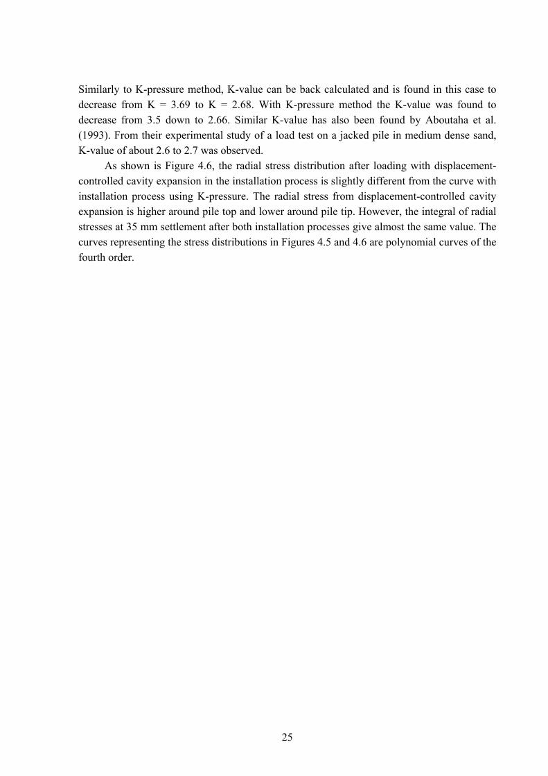
It can be seen from Figure 5.1 that the shapes of the computed load-settlement curves differ significantly from the measured ones. Load-settlement curves from increased Ko equal 1 and 2 match the measured curves in the very beginning, but not further. For the increased Ko = 3, the curve differs from the measured ones by far. The use dilatancy cut-off would improve the computed load-settlement curve significantly as will be shown in Section 6.5.

26

0

10

20

30

0 100 200 300 400 500 600Load, Q (kN)

Pile

Hea

d Se

ttlem

ent,

s (

mm

) Pile 24 (Measured)

Pile 36 (Measured)

Ko = 0.426

Ko = 3

K = 1

K = 2

Figure 5.1: Load-settlement curves for different values of increased Ko

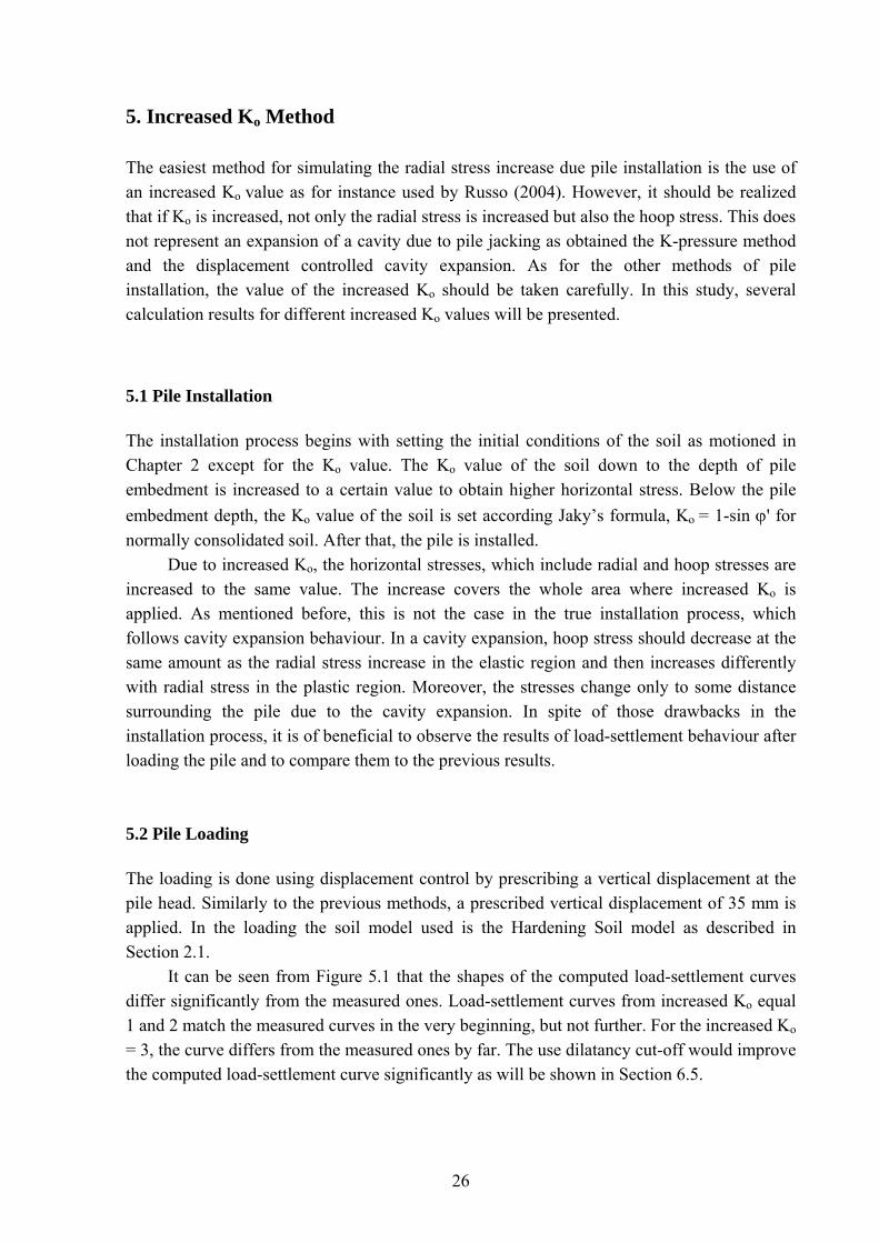
Figure 5.2 shows a load-settlement curve from increased Ko equal 1.5, which gives almost the same load at s = 35 mm as the measured one. However, for smaller settlement, the skin friction is not high enough to fully take the applied load compared to the skin frictions from the previous methods shown in Figure 3.7 and 4.4.

0

10

20

30

0 100 200 300 400

Load, Q (kN)

Pile

hea

d se

ttlem

ent,

s (

mm

)

P 36 measured

P 24 measured

Q-base Q-total

Q-skin

Figure 5.2: Measured and simulated load-settlement curves from Ko = 1.5

27

-6,5

-5,5

-4,5

-3,5

-2,5

-1,5

-0,5

0 100 200

hear stress (Kpa

S )

Dept

h (m

)

-6,5

-5,5

-4,5

-3,5

-2,5

-1,5

-0,5

0 50 100 150 200 250

Radial stress (Kpa)Radial stress, σr (kPa) Shear stress, τ (kPa)

At 35 mm settlement

Dep

th (m

)

K-Pressure

Dep

th (

m)

Dep

th (

m)

Increased Ko = 1.5

Figure 5.3: Interface stresses at 35 mm settlement with increased Ko = 1.5

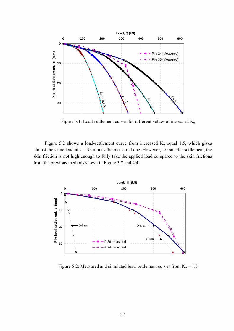
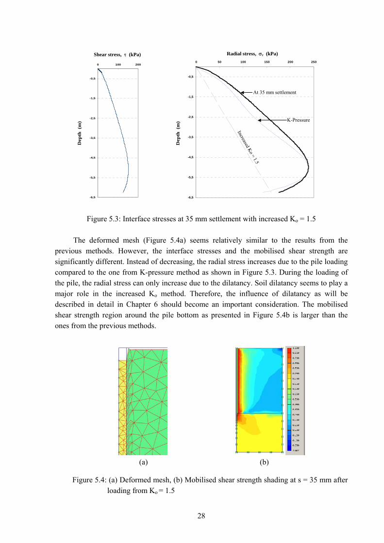
The deformed mesh (Figure 5.4a) seems relatively similar to the results from the previous methods. However, the interface stresses and the mobilised shear strength are significantly different. Instead of decreasing, the radial stress increases due to the pile loading compared to the one from K-pressure method as shown in Figure 5.3. During the loading of the pile, the radial stress can only increase due to the dilatancy. Soil dilatancy seems to play a major role in the increased Ko method. Therefore, the influence of dilatancy as will be described in detail in Chapter 6 should become an important consideration. The mobilised shear strength region around the pile bottom as presented in Figure 5.4b is larger than the ones from the previous methods.

(a) (b)

Figure 5.4: (a) Deformed mesh, (b) Mobilised shear strength shading at s = 35 mm after loading from Ko = 1.5

28

(a) (b)

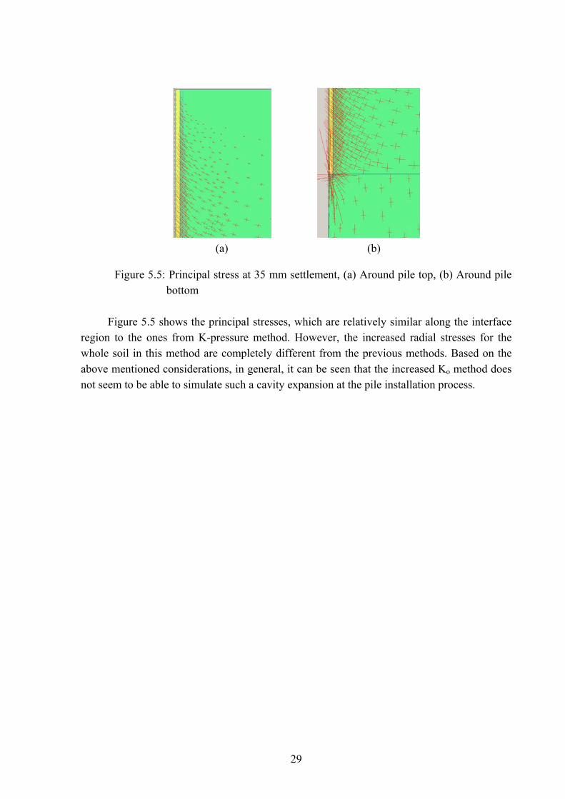
Figure 5.5: Principal stress at 35 mm settlement, (a) Around pile top, (b) Around pile bottom

Figure 5.5 shows the principal stresses, which are relatively similar along the interface

region to the ones from K-pressure method. However, the increased radial stresses for the whole soil in this method are completely different from the previous methods. Based on the above mentioned considerations, in general, it can be seen that the increased Ko method does not seem to be able to simulate such a cavity expansion at the pile installation process.

29

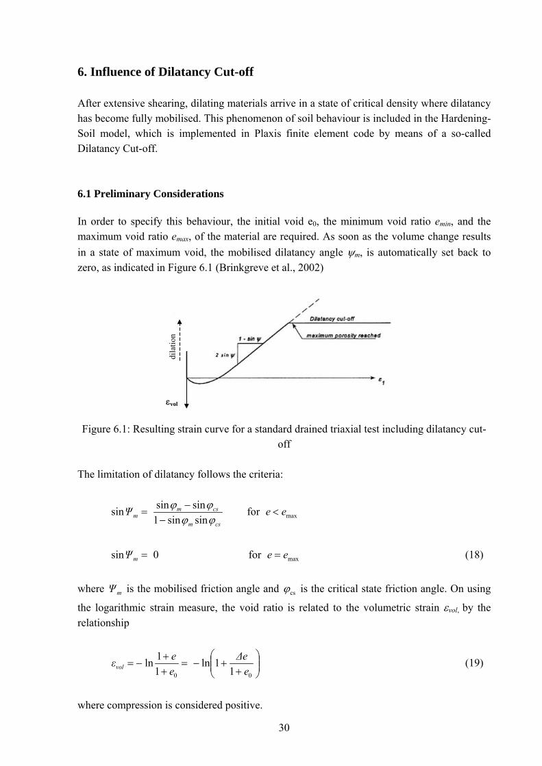
6. Influence of Dilatancy Cut-off After extensive shearing, dilating materials arrive in a state of critical density where dilatancy has become fully mobilised. This phenomenon of soil behaviour is included in the Hardening-Soil model, which is implemented in Plaxis finite element code by means of a so-called Dilatancy Cut-off. 6.1 Preliminary Considerations In order to specify this behaviour, the initial void e0, the minimum void ratio emin, and the maximum void ratio emax, of the material are required. As soon as the volume change results in a state of maximum void, the mobilised dilatancy angle ψm, is automatically set back to zero, as indicated in Figure 6.1 (Brinkgreve et al., 2002)

Figure 6.1: Resulting strain curve for a standard drained triaxial test including dilatancy cut-off

The limitation of dilatancy follows the criteria:

maxforsinsin1sinsinsin eeΨ

csm

csmm <

−−

=ϕϕϕϕ

maxfor0sin eeΨm == (18)

where is the mobilised friction angle and mΨ csϕ is the critical state friction angle. On using

the logarithmic strain measure, the void ratio is related to the volumetric strain εvol, by the relationship

⎟⎟⎠

⎞⎜⎜⎝

⎛+

+−=++

−=00 1

1ln11ln

eΔe

eeεvol (19)

where compression is considered positive.

dila

tion

εvol

30

For small strains, it yields Δe/(1+e0) < 0.1 and one obtains the usual small strain definition,

01 ee

vol +Δ−

≈ε (20)

6.2 Parameters for Dilatancy Cut-off in Interface The piles as considered in this study have a very rough interface with the surrounding soils. This implies the occurrence of a more or less usual shear band around the pile. Soil shear bands have a thickness of about 10-12 times d50, where d50 is the average grain size of the soil. Unfortunately, no grain size distribution is available. However, for a medium fine to coarse sand, it can be assumed that the d50 is around 0.4 mm. Thus, the shear band thickness is found to be about 4 mm. It is further assume that the void ratios of the sand are as follows:

400min .e = , emax = 0.90 , eo = 0.65 This sand can therefore dilate no more than 25065090 ...Δe =−= . For a shear band this implies:

1501

maxmax .e

Δeεo

vol =+

−=

For a shear band thickness of t = 4 mm, this implies that

mm.εtΔt vol 60maxmax =⋅= (21)

The finite element mesh being used involves an interface thickness of tin = 16 mm, which is beyond the real interface thickness of 4 mm. The thick FE-interface may dilate up to

. In order to achieve that, the volumetric interface strain has to be restricted to

the low value of

mm.Δtin 60max =

0375016

60maxmax ..

tΔtε

in

invol ===

In order to realize this dilatancy cut-off, the following emax will be input in the model.

710060650max0max ...Δeee =+=+=

31

Thus, the input parameters for the dilatancy cut-off in the FE-interface are 400min .e = , and .

710max .e = 650.eo =

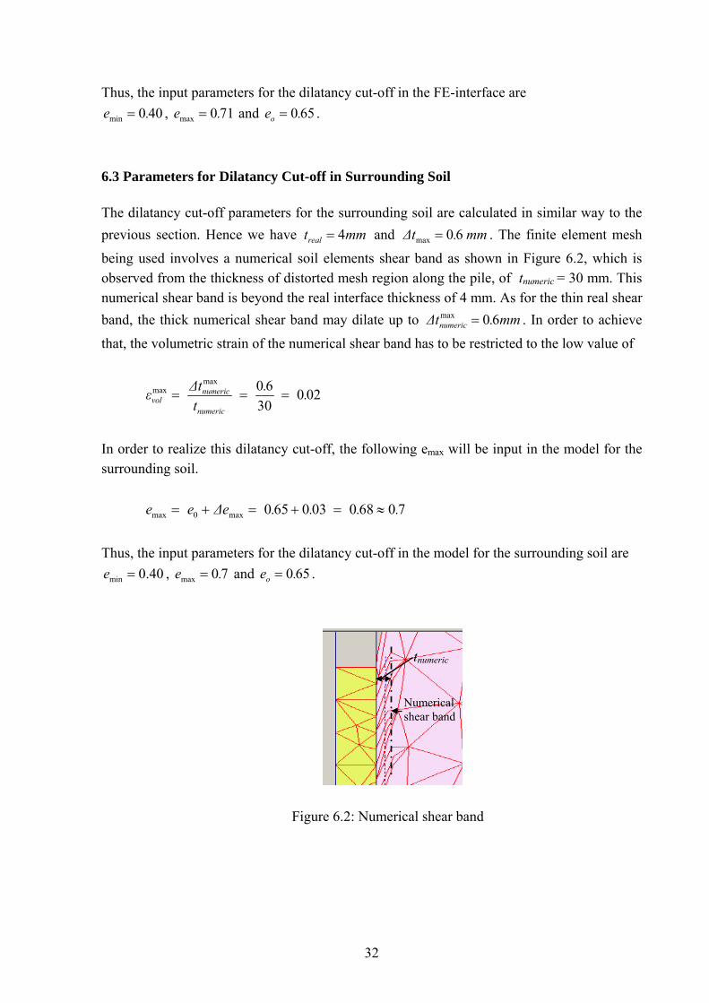
6.3 Parameters for Dilatancy Cut-off in Surrounding Soil The dilatancy cut-off parameters for the surrounding soil are calculated in similar way to the previous section. Hence we have and mmtreal 4= mm.Δt 60max = . The finite element mesh

being used involves a numerical soil elements shear band as shown in Figure 6.2, which is observed from the thickness of distorted mesh region along the pile, of tnumeric = 30 mm. This numerical shear band is beyond the real interface thickness of 4 mm. As for the thin real shear band, the thick numerical shear band may dilate up to . In order to achieve

that, the volumetric strain of the numerical shear band has to be restricted to the low value of

mm.Δtnumeric 60max =

02030

60maxmax ..

tΔtε

numeric

numericvol ===

In order to realize this dilatancy cut-off, the following emax will be input in the model for the surrounding soil.

70680030650max0max ....Δeee ≈=+=+=

Thus, the input parameters for the dilatancy cut-off in the model for the surrounding soil are

, and . 40.0min =e 70max .e = 650.eo =

tnumeric

Numerical shear band

Figure 6.2: Numerical shear band

32

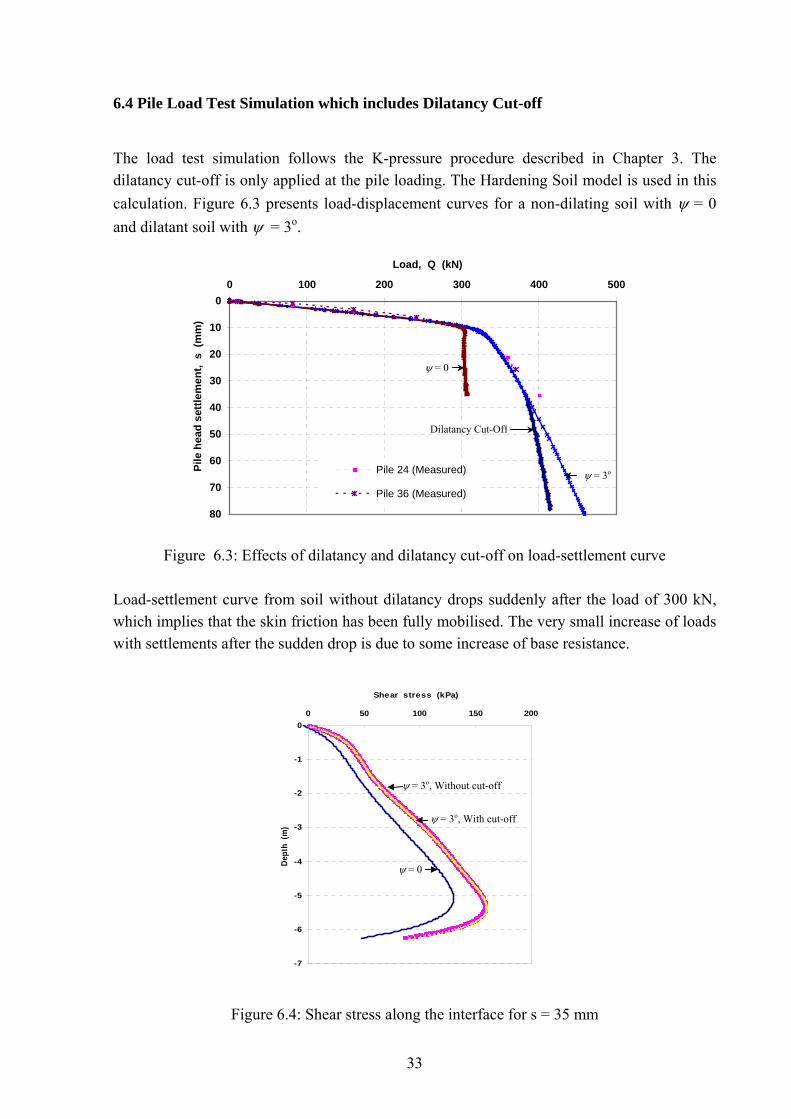
6.4 Pile Load Test Simulation which includes Dilatancy Cut-off The load test simulation follows the K-pressure procedure described in Chapter 3. The dilatancy cut-off is only applied at the pile loading. The Hardening Soil model is used in this calculation. Figure 6.3 presents load-displacement curves for a non-dilating soil with ψ = 0 and dilatant soil with ψ = 3o.

0

10

20

30

40

50

60

70

80

0 100 200 300 400 500

Load, Q (kN)

Pile

hea

d se

ttlem

ent,

s (

mm

)

Pile 24 (Measured)

Pile 36 (Measured)

ψ = 0

Dilatancy Cut-Off

ψ = 3o

Figure 6.3: Effects of dilatancy and dilatancy cut-off on load-settlement curve

Load-settlement curve from soil without dilatancy drops suddenly after the load of 300 kN, which implies that the skin friction has been fully mobilised. The very small increase of loads with settlements after the sudden drop is due to some increase of base resistance.

-7

-6

-5

-4

-3

-2

-1

00 50 100 150 200

Shear stress (kPa)

Dept

h (m

)

ψ = 3o, Without cut-off

ψ = 3o, With cut-off

ψ = 0

Figure 6.4: Shear stress along the interface for s = 35 mm

33

The effect of dilatancy cut-off is also significant as shown in Figure 6.3. If the dilatancy cut-off is applied, the load-settlement curve after the sudden drop at around 320 kN does not continuously increase as without applying the dilatancy cut-off. There is another drop at a load around 380 kN, after that part the soil around the pile is not dilating anymore. The small increase of the load after this part relates to the increase of base resistance.

As shown in Figure 6.4, the shear stress distributions between the soil with and without dilatancy cut-off show only a very small difference at s = 35mm. On the other hand the difference between dilating and non-dilating soils is quite significant showing that dilatancy plays a major role in the resistance of a pile.

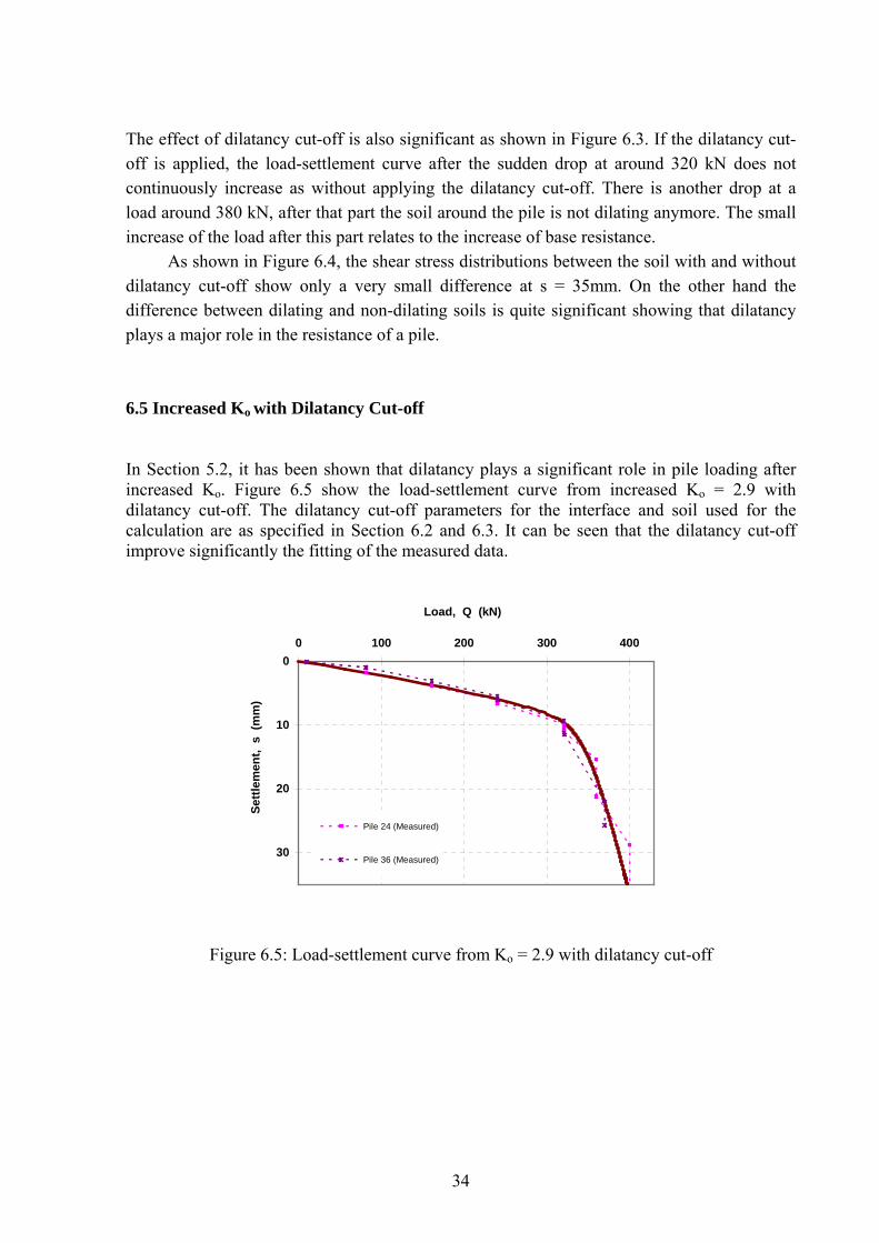
6.5 Increased Ko with Dilatancy Cut-off In Section 5.2, it has been shown that dilatancy plays a significant role in pile loading after increased Ko. Figure 6.5 show the load-settlement curve from increased Ko = 2.9 with dilatancy cut-off. The dilatancy cut-off parameters for the interface and soil used for the calculation are as specified in Section 6.2 and 6.3. It can be seen that the dilatancy cut-off improve significantly the fitting of the measured data.

0

10

20

30

0 100 200 300 400

Load, Q (kN)

Settl

emen

t, s

(m

m)

Pile 24 (Measured)

Pile 36 (Measured)

Figure 6.5: Load-settlement curve from Ko = 2.9 with dilatancy cut-off

34

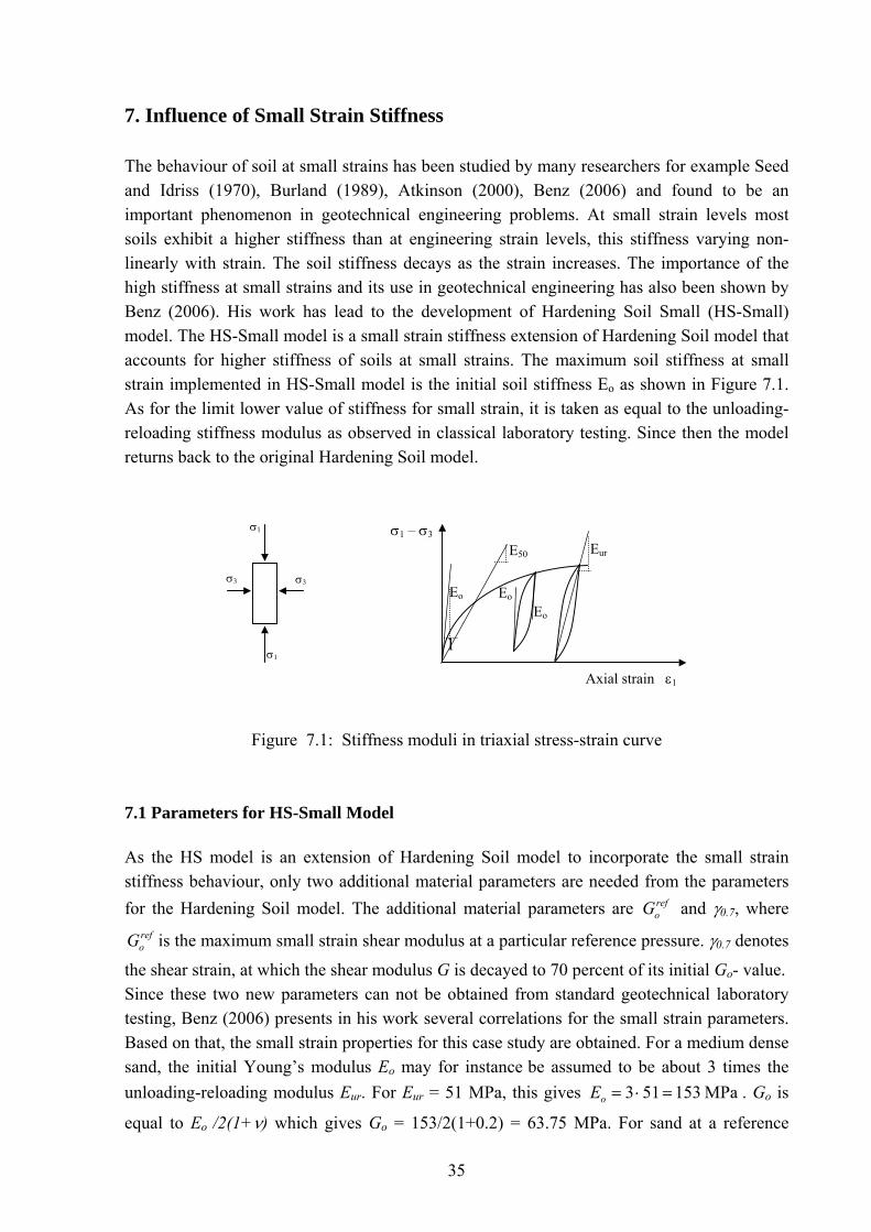
7. Influence of Small Strain Stiffness The behaviour of soil at small strains has been studied by many researchers for example Seed and Idriss (1970), Burland (1989), Atkinson (2000), Benz (2006) and found to be an important phenomenon in geotechnical engineering problems. At small strain levels most soils exhibit a higher stiffness than at engineering strain levels, this stiffness varying non-linearly with strain. The soil stiffness decays as the strain increases. The importance of the high stiffness at small strains and its use in geotechnical engineering has also been shown by Benz (2006). His work has lead to the development of Hardening Soil Small (HS-Small) model. The HS-Small model is a small strain stiffness extension of Hardening Soil model that accounts for higher stiffness of soils at small strains. The maximum soil stiffness at small strain implemented in HS-Small model is the initial soil stiffness Eo as shown in Figure 7.1. As for the limit lower value of stiffness for small strain, it is taken as equal to the unloading-reloading stiffness modulus as observed in classical laboratory testing. Since then the model returns back to the original Hardening Soil model. σ1

σ1

σ3σ3

σ1 – σ3

Axial strain ε1

Eo Eo

Eo

1

EurE50

Figure 7.1: Stiffness moduli in triaxial stress-strain curve

7.1 Parameters for HS-Small Model As the HS model is an extension of Hardening Soil model to incorporate the small strain stiffness behaviour, only two additional material parameters are needed from the parameters for the Hardening Soil model. The additional material parameters are and γref

oG 0.7, where

is the maximum small strain shear modulus at a particular reference pressure. γrefoG 0.7 denotes

the shear strain, at which the shear modulus G is decayed to 70 percent of its initial Go- value. Since these two new parameters can not be obtained from standard geotechnical laboratory testing, Benz (2006) presents in his work several correlations for the small strain parameters. Based on that, the small strain properties for this case study are obtained. For a medium dense sand, the initial Young’s modulus Eo may for instance be assumed to be about 3 times the unloading-reloading modulus Eur. For Eur = 51 MPa, this gives MPa153513 =⋅=oE . Go is

equal to Eo /2(1+ν) which gives Go = 153/2(1+0.2) = 63.75 MPa. For sand at a reference

35

pressure of 100 kPa, γ0.7 tends to be in the range between to . For the present calculation a value of is used which gives better fit load-settlement curve to the

measured data. Therefore, = 63.75 MPa and γ

4101 −⋅ 4102 −⋅4101 −⋅

refoG 0.7 = are used as the additional input

parameters in the HS-Small model.

4101 −⋅

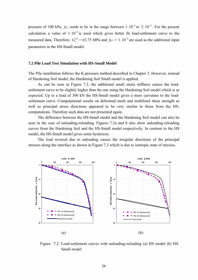
7.2 Pile Load Test Simulation with HS-Small Model The Pile installation follows the K-pressure method described in Chapter 3. However, instead of Hardening Soil model, the Hardening Soil Small model is applied.

As can be seen in Figure 7.2, the additional small strain stiffness causes the load-settlement curve to be slightly higher than the one using the Hardening Soil model which is as expected. Up to a load of 300 kN the HS-Small model gives a more curvature to the load-settlement curve. Computational results on deformed mesh and mobilised shear strength as well as principal stress directions appeared to be very similar to those from the HS-computations. Therefore such data are not presented again.

The difference between the HS-Small model and the Hardening Soil model can also be seen in the case of unloading-reloading. Figures 7.2a and b also show unloading-reloading curves from the Hardening Soil and the HS-Small model respectively. In contrast to the HS model, the HS-Small model gives some hysteresis.

The load reversal due to unloading causes the irregular directions of the principal stresses along the interface as shown in Figure 7.3 which is due to isotropic state of stresses.

0

10

20

30

40

0 100 200 300 400

Load, Q (kN)

Pile

hea

d se

ttlem

ent,

s (

mm

)

Pile 24 (Measured)

Pile 36 (Measured)

Hardening model

0

10

20

30

40

0 100 200 300 400

Load, Q (kN)

Pile

hea

d se

ttlem

ent,

s (

mm

)

Pile 24 (Measured)

Pile 36 (Measured)

HS Small

(a) (b)

Figure 7.2: Load-settlement curves with unloading-reloading (a) HS model (b) HS-

Small model

36

(a) (b) (c)

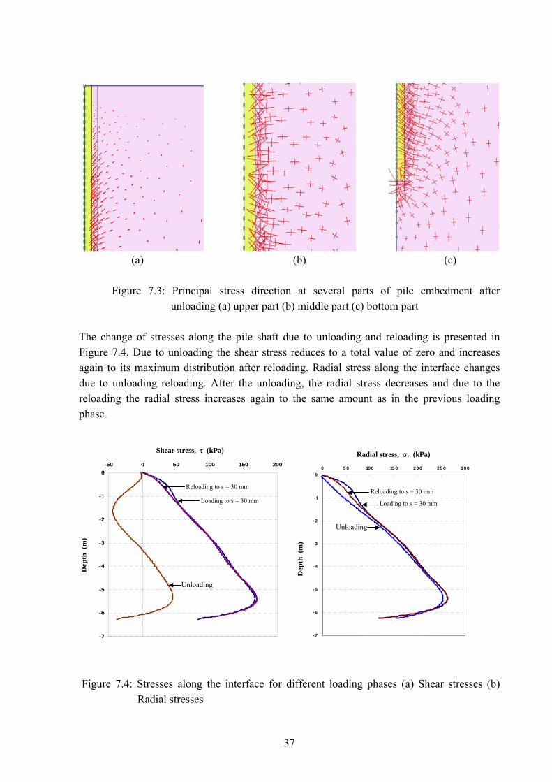
Figure 7.3: Principal stress direction at several parts of pile embedment after

unloading (a) upper part (b) middle part (c) bottom part

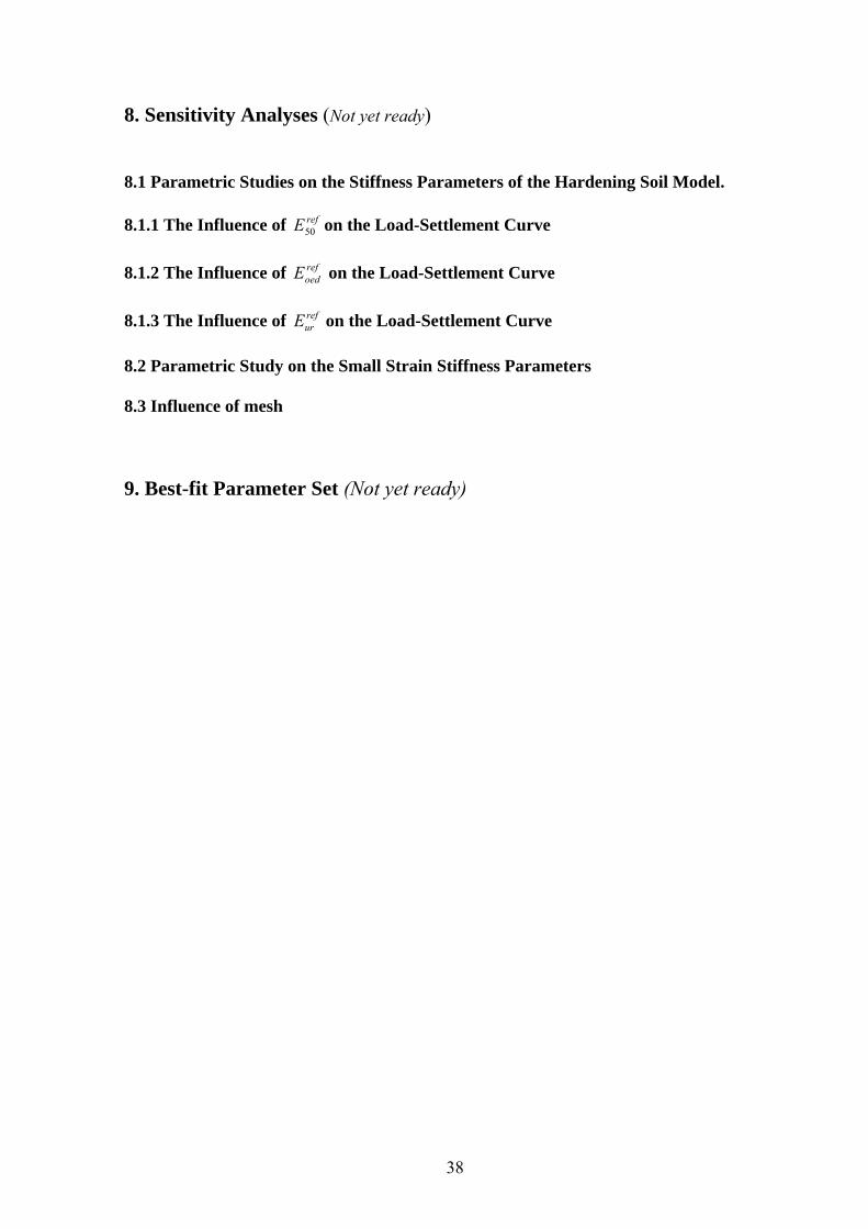
The change of stresses along the pile shaft due to unloading and reloading is presented in Figure 7.4. Due to unloading the shear stress reduces to a total value of zero and increases again to its maximum distribution after reloading. Radial stress along the interface changes due to unloading reloading. After the unloading, the radial stress decreases and due to the reloading the radial stress increases again to the same amount as in the previous loading phase.

-7

-6

-5

-4

-3

-2

-1

0-50 0 50 100 150 200

Shear stress (kPa)

Dept

h (m

)

- 7

-6

-5

-4

-3

-2

-1

00 50 100 150 200 250 300

Radial stress (kPa)

Dept

h (m

)

Shear stress, τ (kPa) Radial stress, r (kσ Pa)

Figure 7.4: Stresses along the interface for different loading phases (a) Shear stresses (b)

Radial stresses

Loading to s = 30 mm

Unloading

Unloading

Loading to s = 30 mm

Reloading to s = 30 mm Reloading to s = 30 mm

Dep

th (

m)

Dep

th (

m)

37

8. Sensitivity Analyses (Not yet ready) 8.1 Parametric Studies on the Stiffness Parameters of the Hardening Soil Model. 8.1.1 The Influence of on the Load-Settlement Curve refE50

8.1.2 The Influence of on the Load-Settlement Curve ref

oedE 8.1.3 The Influence of ref

urE on the Load-Settlement Curve 8.2 Parametric Study on the Small Strain Stiffness Parameters 8.3 Influence of mesh 9. Best-fit Parameter Set (Not yet ready)

38

10. Conclusions The major effect of a displacement pile installation in sand is the increase of the radial stress around the pile, which later increases the pile capacity. This study is aimed to find methods to account for effects of installation process of a tube-installed displacement pile i.e. the increase of radial stress with zero skin friction between the pile and soil after installation.

Three methods of simulating the increase of radial stress in the surrounding soil by FEM have been considered: The K-pressure method, displacement controlled cavity expansion method and increased Ko method. The first two methods would seem to be reasonably appropriate methods for simulating displacement pile installation whereas the increased Ko method was found to be a less appropriate method. Increased Ko method generates a non-realistic stress field around the pile after the installation process.

On using K- pressure method radial stress along the pile side, it yields , where K

is a constant. The K value is back calculated from a the measured load-settlement curves. Hence, a pile load test is needed to calibrate the K-pressure method. This method gives reasonable stress fields.

'voK σ⋅

On using the displacement-controlled cavity expansion, the increase of radial stress is induced by applying a prescribed horizontal displacement on a cavity wall. The horizontal displacement is back-calculated from a measured load-settlement curves. The K value resulting from this method is not constant. However an average K value can be back calculated. Realistic stress fields after cavity expansion and pile loading are obtained, although they are sligthly different from the results of K-pressure method.

Although both methods give reasonable results for a displacement pile analysis the K-pressure method is more favourable. This is because the increase of radial stress with a constant K value, which is often assume in common practice is directly back-calculated from the pile load test measurement.

The interface elements are even more important when the soil is very cohesive as the interface cohesion should be close to zero. Moreover, the interface elements are highly important when considering prefabricated displacement piles.

This study also includes the effect of small strain stiffness to pile loading calculations. For this, the HS-Small model has been used. The HS-Small model which is the extension of the Hardening soil model, requires two extra parameters which are Eo and γ0.7. It was found that small strain stiffness parameters give better curvature of the load-settlement curve. Moreover, hysteresis due to unloading-reloading cycle is more obvious on using the HS-Small model. In addition to that, on using the HS-Small model the sensitivity on chosing the boundary conditions is less when compared to other model without small strain stiffness. Hence, the use of the HS-Small model is recommended.

39

11. References Aboutaha, M., De Roeck, G., Van Impe, W. F. (1993). Bored versus displacement piles in

sand-experimental study. Deep Foundation on Bored and Auger Piles. ed. Van Impe, Balkema, Rotterdam, 157-162.

Atkinson, J. H. (2000). Non-linear soil stiffness in routine design. Géotechnique, 50: 487–

508. Benz, T. (2006). Small strain stiffness of soils and its numerical consequences. PHD Thesis,

Institut for Geotechnical Engineering, University of Stuttgart. Brinkgreve, R. B. J. editor. (2002) PLAXIS, 2D Version 8. AA. Balkema. Burland, J. B. 1989. Ninth Laurits Bjerrum Memorial Lecture: “Small is beautiful” — the

stiffness of soils at small strains. Canadian Geotechnical Journal, 26: 499–516. Chopra, M. B., Dargush, G. F. (1992). Finite-element analysis of time-dependent large-

deformation problems. Int. J. for Numer. Analyt. Meth. Geomech.,16:101-130. Debats, J. M., Guetif, Z., Bouassida, M. (2003). Soft soil improvement due to vibro-

compacted columns installation. Int. workshop on geotechnics of soft soils-theory and practice, Vermeer, Karstunen & Curdy(eds).

Dijkstra, W. J., Broere, van Tol, A. F. (2006). Numerical investigation into stress and strain

development around a displacement pile in sand. In Schweiger (Ed.), Numerical Methods in Geotechnical Engineering (pp. 595-600). London: Taylor & Francis Group.

El-Mossallamy, Y. (2006). Numerical analyses of pile foundation in complex geological

conditions. In Schweiger (Ed.), Numerical Methods in Geotechnical Engineering (pp. 619-625). London: Taylor & Francis Group.

Henke S., Grabe J. (2006): Simulation of pile driving by 3-dimensional Finite-Element

analysis. Proceedings of 17th European Young Geotechnical Engineers' Conference, Zagreb, Crotia, ed. by V.Szavits-Nossan, Croatian Geotechnical Society, 215-233.

Kulhawy, F. H. (1984). Limiting tip and side resistance: Fact or fallacy. Proc., Symp. on

Design and Analysis of Pile Found., ASCE, New York, 80–98. Lancellotta, R.(1995).Geotechnical Engineering. A.A.Balkema, Rotterdam, Brookfield. Mabsout, E. M. et al. (1995). Study of pile driving by finite-element method. Journal of

Geotechnical Engineering,Volume 121, Issue 7, 535-543. Mabsout, E.M. (1999). Pile Driving by Numerical Cavity Expansion. International journal for

numerical and analytical methods in geomechanics, Volume 23, Issue 11, 1121-1140. O’Neil, M. W., Reese, L. C. (1972). Behaviour of bored piles in Beaumont clay. Journal of

the Soil Mechanics and Foundation Division 98, No. SM2, 195-213.

40

Russo, G. (2004). Full-scale load tests on instrumented piles. Proceeding of the Institution of

Civil Engineers, Geotechnical Engineering 157, Issue GE3, 127-135. Seed, H.B., Idriss, I.M., (1970). Soil moduli and damping factors for dynamic response

analyses: Earthquake Engineering Research Center Report No. EERC 70-10, University of California, Berkeley.

Schanz, T., Vermeer, P. A. (1998). On the stiffness of sands. Geotechnique 48,383-387. Terzaghi, K. (1936). Stress distribution in dry and in saturated sand above a yielding trap-

door. Proceeding of the International Conference on Soil Mechanics and Foundation Engineering Bd.1. Cambrigde, 307-311.

Touma, F. T., Reese, L. C. (1974). Behaviour of bored pile in sand. Journal of the

Geotechnical Engineering Devision 100, No. GT7, 749-761. Vermeer, P. A., Schad. H. (2005). HSP pile loading tests in Wijchen. Inspection Report,

Institut for Geotechnical Engineering, University of Stuttgart. Van der Stoel, A. E. C., Klaver, J. M., van Dijk, S. (2005). Test HSP Wijchen. Rapport no

04079a, Voorbij Funderingtechnieken BV, Amsterdam. Vesic, A. S. (1963). Bearing capacity of deep foundation in sand. National Academy of

Sciences, National Research Council, Highway Research Record, No. 39, 112-153. Vesic, A. S. (1970). Test on Instrumented piles, Ogeechee river site. Journal of the Soil

Mechanics and Foundation Devision 96, No. GT2, 561-584. Wehnert, M., Vermeer, P.A. (2004). Numerical analyses of load tests on bored piles.

Proceedings 9th Symposium on Numerical Models in Geomechanics (NUMOG IX), Ottawa, Canada, pp. 505-511, A.A. Balkema Publishers, Leiden, 2004.

Wieckowsky, Z. (2004). The material point method in large strain engineering problems.

Computer methods in applied mechanics and engineering 193, pp. 4417-4438.

41

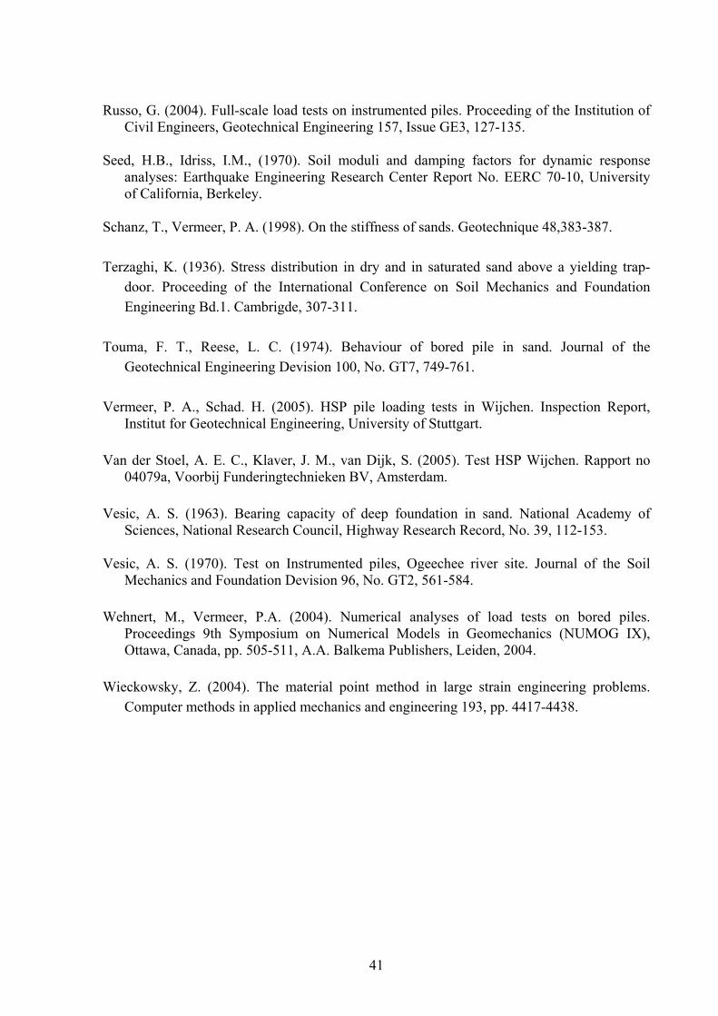
Appendices

(a) Loading to settlement of 30mm (b) Unloading (c) Reloading to settlement of 35mm

Figure i: Shear stress distribution along the interface at different loading phases

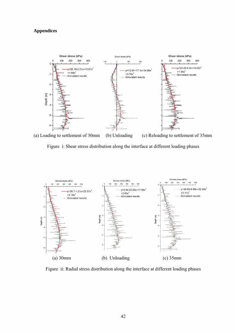
(a) 30mm (b) Unloading (c) 35mm

Figure ii: Radial stress distribution along the interface at different loading phases

42