UNIVERSITAT LINZJOHANNES KEPLER JKU

Technisch-NaturwissenschaftlicheFakultat

Symbolic Regression for Knowledge Discovery –Bloat, Overfitting, and Variable Interaction

Networks

DISSERTATION

zur Erlangung des akademischen Grades

Doktor

im Doktoratsstudium der

Technischen Wissenschaften

Eingereicht von:

Dipl.-Ing. Gabriel Kronberger

Angefertigt am:

Institut fur formale Modelle und Verifikation

Beurteilung:

Priv.-Doz. Dipl.-Ing. Dr. Michael Affenzeller (Betreuung)Assoc.-Prof. Dipl.-Ing. Dr. Ulrich Bodenhofer

Linz, 12, 2010

For Gabi

Acknowledgments

This thesis would not have been possible without the support of a number of people.

First and foremost I want to thank my adviser Dr. Michael Affenzeller, who has notonly become my mentor but also a close friend in the years since I first started my foraysinto the area of evolutionary computation.

Furthermore, I would like to express my gratitude to my second adviser Dr. UlrichBodenhofer for introducing me to the statistical elements of machine learning and en-couraging me to critically scrutinize modeling results.

I am also thankful to Prof. Dr. Witold Jacak, dean of the School of Informatics,Communications and Media in Hagenberg of the Upper Austria University of AppliedSciences, for giving me the opportunity to work at the research center Hagenberg andallowing me to work on this thesis.

I thank all members of the research group for heuristic and evolutionary algorithms(HEAL). Andreas Beham, for implementing standard variants of heuristic algorithmsin HeuristicLab. Michael Kommenda, for discussing extensions and improvements ofsymbolic regression for practical applications, some of which are described in this thesis.Dr. Stefan Wagner, for tirelessly improving HeuristicLab, which has been used as thesoftware environment for all experiments presented in this thesis. Dr. Stephan Winkler,for introducing me to genetic programming and system identification and for proofread-ing a first draft of this thesis to improve its linguistic quality. Ciprian Zavoianu, for theinteresting discussions about aspects of genetic programming.

I also wish to extend my thanks to my colleagues who invested a part of their valuabletime to improve application-specific sections of this thesis. Christoph Feilmayr, foradvice regarding data-based modeling of the blast furnace process and for proofreadingand improving a draft of Chapter 8. Leonhard Schickmair, for his input on variablerelevance metrics and for proofreading and improving a draft of Chapter 8. Dr. StefanFink, for preparing a dataset for economic modeling and for the discussion of economicmodels produced by genetic programming.

Finally, I thank my parents and my family who supported me and my interests incomputer science. I thank all my friends for encouraging me to finish this thesis. Thiswork is dedicated to Gabi for her love and support.

This thesis mainly reflects research work done within the Josef Ressel-center for heuris-tic optimization “Heureka!” at the Upper Austria University of Applied Sciences, Cam-pus Hagenberg. The center “Heureka!” is supported within the program “Josef Ressel-Centers” by the Austrian Research Promotion Agency (FFG) on behalf of the AustrianFederal Ministry of Economy, Family and Youth (BMWFJ).

i

Zusammenfassung

Mit der wachsenden Datenmenge, die in unterschiedlichsten Anwendungsbereichen ge-sammelt und aufgezeichnet wird, wachst auch das Bedurfnis, diese Daten sinnvoll zunutzen. In der Wissenschaft haben Daten schon seit jeher einen hohen Stellenwert. Inden jungeren Jahren gewinnt aber auch das wirtschaftliche Potential von Daten zu-nehmend an Bedeutung. In Kombination mit Verfahren zur Datenanalyse kann diesesPotential ausgeschopft werden, sei es im kommerziellen Bereich zur Optimierung vonAngeboten, oder im industriellen Bereich zur Optimierung von Ressourceneinsatz oderProduktqualitat basierend auf Prozessdaten.

In dieser Arbeit wird ein neuer Ansatz fur die Analyse von Daten vorgestellt, der aufsymbolischer Regression mit genetischer Programmierung basiert und das Ziel verfolgt,einen Gesamtuberblick uber das Zusammenspiel von einzelnen Faktoren eines Systemszu ermoglichen. Dabei sollen moglichst alle potentiell interessanten Zusammenhange,welche in einem Datensatz erkennbar sind, in Form von kompakten und verstandlichenModellen identifiziert werden.

Im ersten Teil der vorliegenden Arbeit wird dieser Ansatz der umfassenden symbo-lischen Regression im Detail beschrieben. Wesentliche Themen, die dabei eine Rollespielen, sind die Vermeidung von Bloat und Uberanpassung, die Vereinfachung von Mo-dellen und die Identifikation von relevanten Einflussgroßen. In diesem Zusammenhangwerden unterschiedliche Verfahren zur Vermeidung von Bloat vorgestellt und verglichen.Insbesondere wird der Einfluss von Nachkommenselektion auf Bloat analysiert. Daruberhinaus wird eine neue Moglichkeit zur Erkennung von Uberanpassung vorgestellt. Im Zu-ge dessen werden darauf basierende Erweiterungen zur Reduktion von Uberanpassungvorgestellt und verglichen. Eine wichtige Rolle spielt dabei das Pruning von Modellen,einerseits um Uberanpassung zu verhindern und andererseits um komplexe Modelle zuvereinfachen.

Ein weiterer wesentlicher Aspekt ist die Analyse und Darstellung der umfangreichenMenge von unterschiedlichen Modellen, die aus dem vorgestellten Ansatz resultiert. Indiesem Zusammenhang werden Moglichkeiten zur Quantifizierung von relevanten Ein-flussgroßen vorgestellt, die in weiterer Folge verwendet werden konnen, um Interaktionenvon Variablen des analysierten Systems zu identifizieren. Durch die Visualisierung die-ser Interaktionen entsteht ein Gesamtuberblick uber das betrachtete System. Dies warealleine durch die Analyse einzelner Modelle, die sich auf spezielle Aspekte konzentrie-ren, nicht moglich. Zusatzlich wird im ersten Teil auch die Prognose von multivariatenZeitserien mit genetischer Programmierung beschrieben.

Im zweiten Teil dieser Arbeit wird gezeigt, wie der vorgestellte Ansatz fur die Analysevon realen Systemen eingesetzt werden kann und dadurch neue Einblicke ermoglichtwerden konnen. Die Daten stammen von einem Hochofen fur die Produktion von Stahlund von einem industriellen chemischen Prozess. Zusatzlich wird gezeigt wie derselbeAnsatz zur Identifikation von makrookonomischen Zusammenhangen eingesetzt werdenkann.

Abstract

With the growing amount of data that are collected and recorded in various applicationareas the need to utilize these data is also growing. In science, data have always playedan important role; in recent years, however, the economic potential of data has alsobecome increasingly important. In combination with methods for data analysis, datacan be utilized to their full potential, whether in the commercial sector to optimize offers,or in the industrial sector to optimize resources and product quality based on processdata.

This work describes a new approach for the analysis of data which is based on sym-bolic regression with genetic programming and aims to generate an overall view of theinteractions of various variables of a system. By this means, all potentially interestingrelationships, which can be detected in a dataset, should be identified and representedas compact and understandable models.

In the first part of this work, this approach of comprehensive symbolic regression isdescribed in detail. Important issues that play a role in the process are the preventionof bloat and over-fitting, the simplification of models, and the identification of relevantinput variables. In this context, different methods for bloat control and prevention arepresented and compared. In particular, the influence of offspring selection on bloat isanalyzed. In addition, a new way to detect over-fitting is presented. On the basis ofthis, extensions for the reduction of over-fitting are presented and compared. Pruningof models is featured prominently, on the one hand to prevent over-fitting and on theother hand to simplify complex models.

An important aspect is the analysis of the vast amount of different models that resultsfrom the proposed approach. In this context, different methods to quantify relevantfactors are proposed. These methods can be used to identify interactions of variablesof the analyzed system. Visualizing such interactions provides a general overview ofthe system in question which would not be possible by analysis of individual modelswhich are concentrated on selected aspects of the problem. Additionally, the prognosisof multivariate time series with genetic programming is described in the first part.

The second part of this work shows how the described approach can be applied tothe analysis of real-world systems, and how the result of this data analysis process canresult in the gain of new knowledge about the investigated system. The analyzed datastem from a blast furnace for the production of steel and an industrial chemical process.In addition the same approach is also applied on a data collection storing economic datain order to identify macro-economic interactions.

Eidesstattliche Erklarung

Ich erklare an Eides statt, dass ich die vorliegende Dissertation selbststandig und ohnefremde Hilfe verfasst, andere als die angegebenen Quellen und Hilfsmittel nicht benutztbzw. die wortlich oder sinngemaß entnommenen Stellen als solche kenntlich gemachthabe.

Linz, December 15, 2010 Dipl.-Ing. Gabriel Kronberger

vii

Contents

1. Introduction 71.1. Thesis Statement . . . . . . . . . . . . . . . . . . . . . . . . . . . . . . . . 101.2. Research Project Background . . . . . . . . . . . . . . . . . . . . . . . . . 11

2. Machine Learning and Data Mining 132.1. Supervised Learning and Unsupervised Learning . . . . . . . . . . . . . . 132.2. Classification, Regression and Clustering . . . . . . . . . . . . . . . . . . . 142.3. Reinforcement Learning . . . . . . . . . . . . . . . . . . . . . . . . . . . . 152.4. Time Series Forecasting . . . . . . . . . . . . . . . . . . . . . . . . . . . . 162.5. Generalization and Overfitting . . . . . . . . . . . . . . . . . . . . . . . . 16

2.5.1. Overfitting . . . . . . . . . . . . . . . . . . . . . . . . . . . . . . . 172.5.2. Bad Generalization because of Incomplete Data . . . . . . . . . . . 182.5.3. Time Series Modeling Pitfalls . . . . . . . . . . . . . . . . . . . . . 18

3. Evolutionary Algorithms and Genetic Programming 213.1. Evolutionary Algorithms . . . . . . . . . . . . . . . . . . . . . . . . . . . . 213.2. Genetic Programming . . . . . . . . . . . . . . . . . . . . . . . . . . . . . 22

3.2.1. Genetic Programming Variants . . . . . . . . . . . . . . . . . . . . 223.3. Bloat . . . . . . . . . . . . . . . . . . . . . . . . . . . . . . . . . . . . . . . 24

3.3.1. Inviable Code and Unoptimized Code . . . . . . . . . . . . . . . . 253.3.2. Bloat Control in Practice . . . . . . . . . . . . . . . . . . . . . . . 253.3.3. Bloat Theory . . . . . . . . . . . . . . . . . . . . . . . . . . . . . . 263.3.4. Theoretically Motivated Bloat Control . . . . . . . . . . . . . . . . 273.3.5. Quantification of Bloat . . . . . . . . . . . . . . . . . . . . . . . . . 28

3.4. Data-based modeling with Genetic Programming . . . . . . . . . . . . . . 293.4.1. Symbolic Regression . . . . . . . . . . . . . . . . . . . . . . . . . . 293.4.2. Overfitting . . . . . . . . . . . . . . . . . . . . . . . . . . . . . . . 30

3.5. Offspring Selection . . . . . . . . . . . . . . . . . . . . . . . . . . . . . . . 313.6. Genetic Programming with HeuristicLab . . . . . . . . . . . . . . . . . . . 32

4. Interpretation and Simplification of Symbolic Regression Solutions 354.1. Bloat Control - Searching for Parsimonious Solutions . . . . . . . . . . . . 35

4.1.1. Static Depth and Length Limits . . . . . . . . . . . . . . . . . . . 364.1.2. Parsimony Pressure . . . . . . . . . . . . . . . . . . . . . . . . . . 364.1.3. Dynamic Depth Limits . . . . . . . . . . . . . . . . . . . . . . . . . 384.1.4. Experiments . . . . . . . . . . . . . . . . . . . . . . . . . . . . . . 414.1.5. Operator Equalization . . . . . . . . . . . . . . . . . . . . . . . . . 42

1

4.1.6. Pruning to Reduce Bloat . . . . . . . . . . . . . . . . . . . . . . . 49

4.1.7. Does Offspring Selection Reduce Bloat? . . . . . . . . . . . . . . . 50

4.1.8. Multi-objective GP . . . . . . . . . . . . . . . . . . . . . . . . . . . 54

4.1.9. Summary of Results of Bloat Experiments . . . . . . . . . . . . . . 54

4.1.10. Effects of Bloat Control on Genetic Diversity . . . . . . . . . . . . 54

4.2. Simplification of Symbolic Regression Solutions . . . . . . . . . . . . . . . 57

4.2.1. Restricted Function Sets . . . . . . . . . . . . . . . . . . . . . . . . 57

4.2.2. Automatic Simplification of Symbolic Expressions . . . . . . . . . 58

4.2.3. Branch Impact Metrics . . . . . . . . . . . . . . . . . . . . . . . . 58

4.2.4. Visual Support for Manual Simplification . . . . . . . . . . . . . . 58

5. Generalization in Genetic Programming 615.1. How to Detect Overfitting in GP . . . . . . . . . . . . . . . . . . . . . . . 62

5.2. Countermeasures Against Overfitting . . . . . . . . . . . . . . . . . . . . . 64

5.2.1. Restarts . . . . . . . . . . . . . . . . . . . . . . . . . . . . . . . . . 64

5.2.2. Parsimony Pressure Against Overfitting . . . . . . . . . . . . . . . 65

5.2.3. Pruning Against Overfitting . . . . . . . . . . . . . . . . . . . . . . 65

5.3. Experiments . . . . . . . . . . . . . . . . . . . . . . . . . . . . . . . . . . . 66

5.4. Results . . . . . . . . . . . . . . . . . . . . . . . . . . . . . . . . . . . . . . 68

5.4.1. Results: Covariant Parsimony Pressure . . . . . . . . . . . . . . . 68

5.4.2. Results: SGP and OSGP . . . . . . . . . . . . . . . . . . . . . . . 70

5.4.3. Results: Adaptive CPP and Overfitting-triggered Pruning . . . . . 71

6. Genetic Programming and Data Mining 776.1. Genetic Programming . . . . . . . . . . . . . . . . . . . . . . . . . . . . . 77

6.1.1. Flexible Model Representation . . . . . . . . . . . . . . . . . . . . 77

6.1.2. Implicit Feature Selection . . . . . . . . . . . . . . . . . . . . . . . 77

6.1.3. Non-Determinism . . . . . . . . . . . . . . . . . . . . . . . . . . . . 78

6.1.4. Training Performance . . . . . . . . . . . . . . . . . . . . . . . . . 79

6.1.5. Predictive Accuracy . . . . . . . . . . . . . . . . . . . . . . . . . . 79

6.2. Analysis of Relevant Variables . . . . . . . . . . . . . . . . . . . . . . . . . 80

6.2.1. Relation to Feature Selection . . . . . . . . . . . . . . . . . . . . . 80

6.2.2. Relative Variable Importance in Linear Models . . . . . . . . . . . 81

6.2.3. Variable Importance in GP . . . . . . . . . . . . . . . . . . . . . . 81

6.2.4. Variable Importance in Random Forests . . . . . . . . . . . . . . . 85

6.2.5. Generalized Variable Importance . . . . . . . . . . . . . . . . . . . 86

6.2.6. Improved Formulations of Variable Importance Metrics for GP . . 87

6.2.7. Validation of Variable Relevance Metrics . . . . . . . . . . . . . . . 89

6.3. Data Mining and Symbolic Regression . . . . . . . . . . . . . . . . . . . . 95

6.4. GP-Based Search for Implicit Equations . . . . . . . . . . . . . . . . . . . 95

6.5. Comprehensive Search for Symbolic Regression Models . . . . . . . . . . . 96

6.5.1. Case Study: Chemical-II Dataset . . . . . . . . . . . . . . . . . . . 96

6.6. Improving GP Performance . . . . . . . . . . . . . . . . . . . . . . . . . . 102

6.6.1. Parallelization . . . . . . . . . . . . . . . . . . . . . . . . . . . . . 103

2

6.6.2. Improving Fitness Evaluation Performance . . . . . . . . . . . . . 103

7. Multi-Variate Symbolic Regression and Time Series Prognosis 1057.1. Evaluation of Multi-Variate Symbolic Regression Models . . . . . . . . . . 106

7.1.1. Curse of Dimensionality . . . . . . . . . . . . . . . . . . . . . . . . 1087.2. Multi-variate Time Series Modeling and Prognosis . . . . . . . . . . . . . 108

7.2.1. Evaluation of Multi-variate Time Series Prognosis Models . . . . . 1107.2.2. Case Study: Financial Time Series Prognosis . . . . . . . . . . . . 111

8. Applications and Case Studies 1198.1. Blast Furnace . . . . . . . . . . . . . . . . . . . . . . . . . . . . . . . . . . 119

8.1.1. Modeling . . . . . . . . . . . . . . . . . . . . . . . . . . . . . . . . 1218.1.2. Results . . . . . . . . . . . . . . . . . . . . . . . . . . . . . . . . . 1218.1.3. Result Details . . . . . . . . . . . . . . . . . . . . . . . . . . . . . . 1248.1.4. Concluding Remarks . . . . . . . . . . . . . . . . . . . . . . . . . . 130

8.2. Econometric Modeling . . . . . . . . . . . . . . . . . . . . . . . . . . . . . 1318.2.1. Macro-Economic Dataset . . . . . . . . . . . . . . . . . . . . . . . 1318.2.2. Modeling . . . . . . . . . . . . . . . . . . . . . . . . . . . . . . . . 1338.2.3. Results . . . . . . . . . . . . . . . . . . . . . . . . . . . . . . . . . 1348.2.4. Concluding Remarks . . . . . . . . . . . . . . . . . . . . . . . . . . 141

8.3. Chemical Process . . . . . . . . . . . . . . . . . . . . . . . . . . . . . . . . 1448.3.1. Modeling . . . . . . . . . . . . . . . . . . . . . . . . . . . . . . . . 1448.3.2. Results . . . . . . . . . . . . . . . . . . . . . . . . . . . . . . . . . 1458.3.3. Detailed Results . . . . . . . . . . . . . . . . . . . . . . . . . . . . 146

9. Concluding Remarks 151

A. Additional Material 155A.1. Model Accuracy Metrics . . . . . . . . . . . . . . . . . . . . . . . . . . . . 155

A.1.1. Regression Models . . . . . . . . . . . . . . . . . . . . . . . . . . . 155A.1.2. Time Series Models . . . . . . . . . . . . . . . . . . . . . . . . . . 158

A.2. Numerical Approximation of Derivatives . . . . . . . . . . . . . . . . . . . 161A.3. Datasets Used in Experiments . . . . . . . . . . . . . . . . . . . . . . . . . 161

A.3.1. Artificial benchmark datasets . . . . . . . . . . . . . . . . . . . . . 162A.3.2. Real World Datasets . . . . . . . . . . . . . . . . . . . . . . . . . . 163

A.4. Colophon . . . . . . . . . . . . . . . . . . . . . . . . . . . . . . . . . . . . 195

Bibliography 195

Curriculum Vitae 195

3

Overview

The main theme of this work is how genetic programming (GP) can be used for knowl-edge discovery. In particular, adaptations of GP to search for accurate, interesting,and understandable models are discussed. Additionally ways to filter and present theinformation gathered through GP runs are presented that aim to improve knowledgediscovery process and lead to a better understanding of the examined system or pro-cess. This work puts strong emphasis on producing comprehensible models with GP, theaccuracy of the output of the models is only secondary.

This work mainly concentrates on the practitioners view of GP and symbolic regres-sion. Thus the majority of this work is about practical aspects, theoretic aspects areonly treated briefly. GP theory has seen a lot of progress in the recent years. Thesecontributions are very relevant for a better understanding of the internal dynamics of GPand provide a solid basis on which to conduct empirical or practically oriented research.

The main advantage of GP compared to other data-analysis methods is that it pro-duces white-box models that might lead to new knowledge about the examined system.The price to pay for this is that GP also requires more computational resources thanother data-analysis methods. The internal dynamics of genetic programming often leadsto final solutions that are relatively complex and hard to understand. In the literaturea large number of possible remedies for this issue have been described and analyzed,however, from a practitioners point of view the results are not satisfactory. In the firstpart the following novel concepts are presented:

• Comprehensive GP-based identification of interesting models or interactions in agiven data-set.

• Data-based methods to quantify and visualize relevant interrelations of variablesof a system.

The following issues relate to the main objectives and are also discussed in the first part:

• Methods to create compact and comprehensible models with GP.

• Methods to detect and avoid overfitting with GP.

• Symbolic vector-regression for the identification of multi-variate models.

• GP-based time series modeling for prognosis.

In the second part the concepts described in the first part are applied to a number ofreal world data mining problems.

5

1. Introduction

Well organized and accurate data have become increasingly important as a potentialsource of profits for businesses. As more and more data are generated and stored inlarge repositories the desire to generate value from the available data grows. Businessintelligence as a discipline is intimately related to the collection, aggregation and analysisof business-relevant data. Decision support systems play an important role in businessintelligence to analyze and summarize relevant data often in form of charts and condensedreports. The main purpose of decision support systems is to support managers to makecorrect profitable decisions. Decision support systems of various complexity are alreadyubiquitously implemented in many areas (politics, finance, health, industries...) andhave an impact on our everyday life.

A large number of data-analysis methods for different applications have been describedranging from very simple methods to mathematically complex and powerful algorithms.The methods can be categorized in one or multiple of the following partially overlappingdisciplines: System theory, statistics, machine learning, and data mining. All these dis-ciplines have in common that they cover the topic of data-based modeling [124, 72, 27].Additional research areas related to these disciplines are artificial neural networks andreinforcement learning [210]. “Artificial neural networks are a development of the Per-ceptron [173] [. . . ] and the area has transformed into a community of its own [...]. Thisis quite remarkable, since the topic is but a flexible way of parameterizing arbitrary hy-persurfaces for regression and classification. The main reason for the interest is thatthese structures have proved to be very effective for solving a large number of nonlinearestimation problems.” [124]. Recently a number of novel contributions have been pub-lished discussing learning for so-called deep networks with very many hidden layers forwhich back-propagation learning algorithms do not work well [85, 60, 132].

Data mining includes a wide range of different techniques to analyze, filter, exploreand visualize data [79, 233]. Fayyad et al. define data mining in the following way: “Datamining is the application of specific algorithms for extracting patterns from data” [61].Another definition is given by Hand et al.: “Data mining is the analysis of (often large)observational data sets to find unsuspected relationships and to summarize the data innovel ways that are both understandable and useful to the data owner.” [79]. Based onthese definitions many data-based modeling approaches can also be called data miningmethods. Data mining also includes exploratory elements like drilling down into inter-esting facts in an interactive cyclic process of model construction and interpretation.Fayyad et al. define data mining as a step in the process of knowledge discovery fromdatabases. The whole process also includes data selection, preprocessing and trans-formation as necessary preparatory steps for data mining and the interpretation andevaluation of the results obtained from data mining as a necessary follow up step to

7

achieve the stated goal of knowledge discovery. An essential requirement for effectivedata mining is that results are presented in a clear and informative way in order to allowa data miner to evaluate and interpret the results easily. Methods and principles forthe visual display of quantitative data [217, 218] are closely related to data mining andknowledge discovery.

This work concentrates on the application of genetic programming for data mining ofdata collections that fit entirely into main memory. In particular, this work does notcover issues and solutions related to very large data collections that must be read sequen-tially from external memory. Genetic programming is a nature inspired meta-heuristicwhich is applicable to a wide range of problems in its general formulation. The idea ofGP is to imitate aspects of biological evolution such as selection, recombination, andmutation for find computer programs that solve a given problem in small evolutionarysteps starting with an initial population of random programs. Genetic programming inits most general formulation can be called an “invention machine” [104, 105]. In mostcases, however, problem-specific variants of GP are used to solve well defined problems.One example for a specific and rather simple GP approach is symbolic regression; inthis application GP is used to search for models that can be represented as symbolicexpressions and approximate the response of a system based on observations of the inputand output behavior of the system. Symbolic regression relies on the power of GP tofind the correct structure for the model in combination with the model parameters. Thisproperty makes GP especially suitable for data-analysis tasks where only little informa-tion about the origin of the data and the examined system is available. Multiple authors[94, 232, 3, 231, 191, 126, 174, 18] have demonstrated that problem-specific GP variantsfor data-analysis can find very good solutions for specialized tasks like regression andclassification. A more general approach is introduced in [154] which uses GP to generateclassification algorithms which can later be executed to produce classifiers based on aspecific data-set.

The general formulation of GP has the drawback that it often takes more computa-tional effort to achieve solutions of comparable accuracy than it would take with othermore specific methods. This disadvantage is often accepted as the time spent for modeltraining is usually not critical. The time spent for training is often only a small partof the total time spent in the knowledge discovery process. A major part of the timeis spent on data preparation and model interpretation and analysis [70]. If genetic pro-gramming is to be used to search for interesting patterns in large datasets it is beneficialif the training time can be reduced as more potentially interesting patterns can be un-covered in the same time frame. The chance to find previously unknown interrelationsin the data grows with the number of good models. In Section 6.6 we describe methodsto increase the training performance of GP that do not have a negative effect on themodel accuracy.

Data analysis methods can be classified based the representation of models producedby the method. The spectrum ranges from comprehensible white-box models on the oneend to complex black-box models on the other end. Often the distinction is not clearand various shades of gray-box models are located in between the two extremes. Modelsproduced by symbolic regression are located near the white-box end of the spectrum.

8

Typically symbolic regression models are mathematical expressions which can be directlyinterpreted in order to gain knowledge about the patterns which were found in thedataset. Support vector machines are an example for an approach that produces black-box models located on the other end of the spectrum. Artificial neural network modelsare usually said to be gray-box models because the network structure can be interpretedbut it is hard to gain a full understanding of the interrelations in the network.

While the fact that GP produces white-box models is often stated as an advantagethis is often not apparent in practice. The models presented as final result is oftenrather complex and difficult to understand. Even though the model is a mathematicalexpression it is often impossible to gain an understanding of the model when it containsdeeply nested functions. This problem is also a major topic in [94] which discusses theapplication of genetic programming for scientific discovery. One cause for this is thatgenetic programming has the tendency to build ever larger and more complex programsover time without a proportional improvement in program fitness. In the GP communitythis phenomenon is called code bloat and a lot of effort has been put into designingcounter-measures that reduce or prevent this behavior. In Chapter 4 this phenomenonand a few selected counter-measures will be described in more detail. Even though anumber of counter-measures has been described in the literature [188] there is not yet aconsensus which methods are effective in practical applications. If symbolic regressionis used for an unguided search for interesting patterns in a dataset then an effectiveanti-bloat strategy is very important because only small and at the same time accurateand generalizable models are interesting as a source for new insights into the nature ofthe dataset.

Another reason why it is important to create compact, comprehensible models is thatthe data miner is more likely to trust a model to be true when it is understandableand and easy to validate. The issue of models which can be trusted should not beunderestimated [99] as it is the first and foremost criterion that a data miner trusts themodel before the model is examined in more detail. Demonstrating that a model canbe trusted is even more important than the accuracy of the model. Models that are tooaccurate to be true might raise concerns that the model might be over trained and thuscannot be trusted (for a more detailed discussion of overfitting see Chapter 5). One wayto increase the chance that a model is trusted is to reduce the complexity of the model,making it easier to validate and analyze the model. Another way is to demonstrateclearly that the model also is accurate on new data, for instance through validation ona hold-out set or through cross-validation. Even though such validation methods arecommon practice in the machine learning community these standards are not yet fullyimplemented in the evolutionary computation community [59]. In a recent contributionO’Neill et al. state that: “[...] this issue in GP has not received the attention it deservesand only few papers dealing with the problem of generalization have appeared [...]” [148].

In the original formulation of symbolic regression with genetic programming a singlevariable must be explicitly declared as the target variable [101]. However, often it is notimmediately clear which variable is the variable of interest or there are multiple variablesthat could be declared as a target variable. So it is often necessary to explore the optionswith multiple symbolic regressions runs with different configurations.

9

Another data mining task that is relevant in practice but has not yet been treatedextensively in the GP literature, is multi-variate symbolic regression. In this approachGP has to find a symbolic multi-variate regression model that approximates all targetvariables. If GP is to be used for unguided data mining without an explicit target variablethe solution representation and the search process of genetic programming have to beextended. In Chapter 6 a simple approach of independent runs to create and collectmodels for all variables of the dataset is described. In Chapter 7 several extensionsof the solution representation for the simultaneous modeling of multiple variables aredescribed.

1.1. Thesis Statement

To summarize the previous paragraphs genetic programming can be used for data min-ing to find potentially interesting patterns or interactions in large datasets when thetraditional symbolic regression approach is extended and adapted appropriately.

• Solution representation: Instead of a single target variable the process shouldidentify the potentially interesting variables automatically. This work describesseveral different ways to extend the solution representation for data mining tasksand introduces ways to manage the potentially large set identified models.

• Model complexity and presentation: In order to facilitate knowledge discovery fromGP models, appropriate and effective methods for reduction of model complexityhave to be integrated into the search process. This work describes different methodsto reduce the model complexity and introduces new ways of visualizing results tosimplify detailed analysis of models.

• Trustable models: Results presented by the process must be clearly validated toenable the data miner to estimate how trustable a model is. This work describes avalidation procedure for GP that is effective in practical applications and describeshow visualizations can be used to improve the trustability of models.

• Performance: In order to make unguided search for interesting patterns in largedata sets feasible it is necessary to reduce the training time of GP. In this workbriefly discusses possible ways to increase GP performance.

Chapter 2 gives a cursory introduction of machine learning and data mining includingcommonly used terms. Chapter 3 discusses relevant previous work in the area of evo-lutionary algorithms in general and genetic programming specifically. Chapter 4 is thefirst core chapter of this thesis and discusses the problem of bloat and countermeasuresto reduce bloat and also describes ways to simplify solutions with pruning. Chapter 5introduces an effective way to detect overfitting and countermeasures against overfittingin GP. Chapter 6 describes unconstrained GP-based search for interesting models andhow the information collected in those experiments can be prepared and visualized toimprove the knowledge acquisition process. In Chapter 6 the topic of variable relevance

10

metrics is discussed as it is necessary for the representation of variable relation networks.Chapter 7 describes an approach to create multi-variate symbolic regression models withGP and how multi-variate auto-regressive time series models can be used for the progno-sis of future values of a multi-variate time series. Finally, Chapter 8 demonstrates howthe methods discussed in the previous chapters can be applied to real world applications.

1.2. Research Project Background

This thesis mainly reflects research work done within the Josef Ressel-center for heuristicoptimization “Heureka!” at the Upper Austria University of Applied Sciences, CampusHagenberg. The center “Heureka!” is supported within the program “Josef Ressel-Centers” by the Austrian Research Promotion Agency (FFG) on behalf of the AustrianFederal Ministry of Economy, Family and Youth (BMWFJ).

11

2. Machine Learning and Data Mining

Essentially, all models are wrong, butsome are useful.

George Box

This chapter gives a brief overview of the disciplines of machine learning and datamining. A number of terms frequently in the machine learning literature that are nec-essary to understand the core of the work are explained in the following sections. Thereader who is already familiar with machine learning can skip this chapter and advanceto the chapter.

Learning is the process of knowledge acquisition from observations. Knowledge is de-fined by the Oxford Dictionary of English as: “(i) facts, information, and skills acquiredthrough experience or education; the theoretical or practical understanding of a subject;(ii) the sum of what is known; (iii) information held on a computer system.” [152]. Oneof the goals of machine learning as a research discipline is to define algorithms whichwhen executed by a computer enable it to learn general facts from examples in sucha way that previously unseen examples can also be recognized and a correct action istriggered.

As such the knowledge learned by the machine learning method should be specific torecognize known examples and general to also recognize slightly different new examples.In statistics the learning or training phase is called model estimation. Model estimationis the process of selecting a specific model from a class of models that fits the availabledata best.

Typically a discrimination is made between the two terms features and variables. Inmachine learning the term variable usually indicates the original variable while a featurecan be a combination of multiple variables. Often kernel functions are used to transforma combination of variables to features. In this work no distinction between the two termsis made and the terms variable and feature are used interchangeably.

2.1. Supervised Learning and Unsupervised Learning

Learning methods can be categorized into two general classes: supervised and unsuper-vised methods. The methods have different goals and are also different by the way howexamples are presented in the training or learning phase.

Supervised learning methods accept pairs of training examples with a correct label asinput. From these training examples the algorithm should learn how to correctly label

13

new examples in a generalizable way and learn from these examples which label fits bestfor future unseen examples.

Unsupervised learning methods accept training examples without labeling future inputexamples are compared to the previously learned training examples and one or multiplesamples, that are most similar to the current example, are produced as output.

The semi-supervised learning hybrid approach is also possible. This is often usefulwhen a large number of examples are available but only a small part of them is labeled.Semi-supervised learning methods determine labels for the unlabeled examples by find-ing similar labeled representatives and then use the unlabeled examples for training.Typical tasks solved by supervised learning methods are classification and regression;unsupervised learning is often used for clustering.

2.2. Classification, Regression and Clustering

The input data for classification, regression and clustering are usually a collection of ntraining examples. Each example in the training data is a row vector of k values. Theset of training examples can be represented as a matrix T(n,k).

For the classification task the training samples have class values from a finite usuallysmall domain. The most common case is binary classification, meaning that the classlabels can have only two values (e.g. 0 or 1, malign or benign). However classificationfor three or more distinct class labels is also possible. It is not necessary that an orderingrelation can be defined on the class labels. The goal of classification algorithms is tolearn from the presented training samples in which class to categorize new and previ-ously unseen data points. The quality of classification algorithms is measured by a lossfunction. Usually the loss function compares the class predicted by the algorithm withthe actual class of the data point and then calculated from the number of correctly andincorrectly classified data points. Examples for classification algorithms are: linear dis-criminant analysis, C4.5 (decision tree learning) [169], support vector machines (SVM)[222, 41], k-nearest-neighbor (kNN) [42, 65], classification and regression trees (CART)[28].

For the regression task the training samples usually in Rn are labeled with values in R.The algorithm should learn the value linked with each data point so that it can generatea predicted value for new and previously unseen data points. Labels can be ordered sothe loss of a regression model is often measured as a distance of the predicted from theactual target values. Examples for regression algorithms are: linear regression, CART[28], SVM regression [221].

The task of binary classification can be reformulated into the regression task of findinga discriminant function g : Rn → R. The classification is achieved by assuming a constantseparator value c so that class = 0 if g < c and class = 1 if g ≥ c. A perfect predictioncan be achieved when a value c exists that separates both classes perfectly.

Regressing and classification are supervised learning tasks. In contrast, clustering isan unsupervised learning task [79, 83]. The goal of clustering is to group examples bysimilarity into a number of representative clusters. Each cluster is a set of examples and

14

a representative example. New examples are assigned to one of the learned clusters intowhich the new examples fits best. Clustering can also be applied to unlabeled examples.

A typical example of clustering is market basket analysis based recommender systems.The system uses a clustering method to find clusters of customers who purchased similarproducts. Based on the clustering the recommender system can suggest related productsbased on the products that other customers in the same cluster frequently purchased.Examples for clustering algorithms are: k-Means [125], expectation-maximization (EM)[49], and methods based on principal component analysis (PCA) [156, 89].

2.3. Reinforcement Learning

Reinforcement learning is a branch of machine learning that does not fit into the cate-gories supervised vs. unsupervised learning. Reinforcement learning is concerned withonline processes in which an agent can take actions and receives rewards for actions[210]. The acquisition of new observations which implicitly cause an unknown loss isintegrated directly in the learning process The objective is to find a policy for the agentthat minimizes the regret, which is the difference of the reward that the agent receivedto the reward that the agent could have received, if it would have executed the optimalactions at all times. The difference to supervised learning is that the correct actions arenever explicitly presented to the agent.

The best example to illustrate reinforcement learning methods is the multi-armedbandit problem that describes the situation of a rigged casino, a bandit gambling machinewith multiple arms with a different rate of winning plays and possibly unequal rewards.The goal for a player is to allocate plays to the machines in such a way, as to maximize theexpected total reward. The probability distribution of rewards for each arm is unknown,so an effective strategy has to be found that balances exploration of new arms andexploitation of the best arm so far. The K-armed bandit problem can be described asK random variables with Xi(0 ≤ i < K), where Xi is the stochastic reward given by thearm with index i. The rewards Xi are independent and the distributions are generallynot identical. The laws of the distributions and the expected value µi for the rewards Xi

are unknown. The goal is to find an allocation strategy that determines the next armto play, based on past plays and received rewards, that maximizes the expected totalreward for the player. Or put in other words: to find a way of playing that minimizesthe regret, which is defined as the expected loss occurred by not playing the optimalarm each time.

Since a player does not know which of the arms is the best he can only make as-sumptions based on previous plays and received rewards and concentrate his efforts onthe arm that gave the highest rewards so far. However it is necessary to strike a goodbalance between exploiting the currently best arm and exploring the other arms to makesure that an arm with a higher expected reward value can be discovered.

15

2.4. Time Series Forecasting

The notable difference of time series forecasting in comparison to regression or classifi-cation is that there is a time-dependent structure in the processed data points. Specialcare has to be taken in the training phase and when using the trained model so thatthe time-dependency or the ordering of the data points is not destroyed. In particularit is not valid to shuffle the data points in the training phase as this would destroy theinternal structure.

The goal of time series forecasting is to predict future values of a variable based onpast values of the variable and optionally other related variables. If the method uses pastvalues of the target variable for the prediction of future values it is an auto-regressivemethod.

Time series forecasting is a traditional application of statistics. Since the very firstformulations of time series models a large corpus of ever refined modeling approaches hasbeen described ranging from simple linear auto-regressive and moving average models[74, 90] to intricate models including trends and seasonal changes and multivariate timeseries [229]. For an extensive discussion of statistic approaches to time series modelingsee [23, 29, 30, 157, 57, 82].

Genetic programming has also been effectively used for time series prognosis tasks[101]. The power of genetic programming to evolve the structure of solution candidatesin combination with the parameters enables the process to automatically adjust themodel structure appropriately for instance to account for seasonal changes, trends orrecurrent events if such elements are detected in the data.

Chapter 7 discusses multi-variate time series modeling with genetic programming.

2.5. Generalization and Overfitting

Any data-based model, regardless of which learning or estimation process is used, mustgeneralize well in order to be useful. Models which generalize well are models that alsowork consistently for new observations. In contrast models that do no generalize wellproduce inaccurate or even largely incorrect estimations for new observations and arethus useless in practice. The generalization ability of a given model can be estimatedby using a hold out dataset which contains samples that are not used in the trainingprocess. The fit on the hold-out is an indicator for the fit on new observations. If themodel performs equally well on the training set and on the hold-out set it can be assumedthat the model generalizes well. This assumption only holds in general when a numberof assumptions about the analyzed system and the selection the training set and thehold-out set are fulfilled. The number of different states of the system must be limitedand the training set and the hold-out set must be a representative sample of the wholepopulation of observable states of the analyzed system. If these assumptions hold newobservations from the same system will be similar to observations in the training- andhold-out set, and the fit on the hold-out set is an accurate estimator for the expected fitfor new observations.

16

2 4 6 8 100

0.2

0.4

0.6

0.8

1

1.2

Complexity

Error

Training error

Expected generalization error

Figure 2.1.: Underfitting and overfitting

First we discuss possible causes for bad generalization behavior in an ideal settingwhere all the assumptions hold. In practice the situation is more difficult as some of theassumptions might not hold. This will be discussed later in more detail.

2.5.1. Overfitting

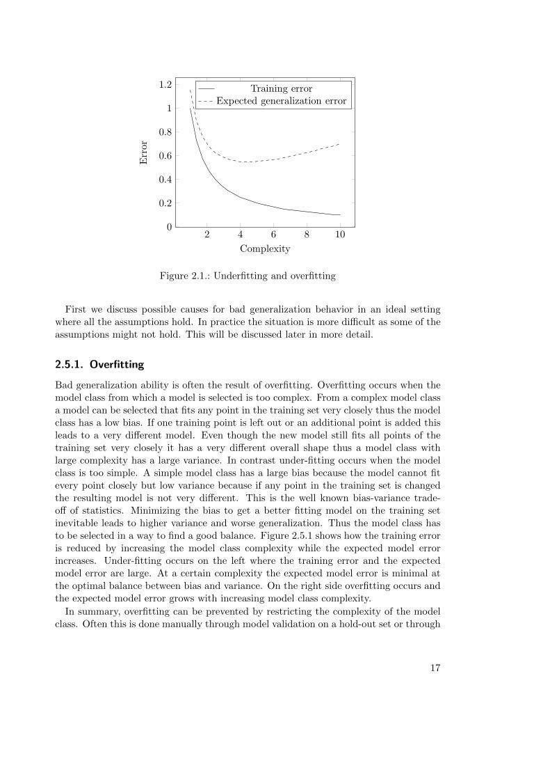
Bad generalization ability is often the result of overfitting. Overfitting occurs when themodel class from which a model is selected is too complex. From a complex model classa model can be selected that fits any point in the training set very closely thus the modelclass has a low bias. If one training point is left out or an additional point is added thisleads to a very different model. Even though the new model still fits all points of thetraining set very closely it has a very different overall shape thus a model class withlarge complexity has a large variance. In contrast under-fitting occurs when the modelclass is too simple. A simple model class has a large bias because the model cannot fitevery point closely but low variance because if any point in the training set is changedthe resulting model is not very different. This is the well known bias-variance trade-off of statistics. Minimizing the bias to get a better fitting model on the training setinevitable leads to higher variance and worse generalization. Thus the model class hasto be selected in a way to find a good balance. Figure 2.5.1 shows how the training erroris reduced by increasing the model class complexity while the expected model errorincreases. Under-fitting occurs on the left where the training error and the expectedmodel error are large. At a certain complexity the expected model error is minimal atthe optimal balance between bias and variance. On the right side overfitting occurs andthe expected model error grows with increasing model class complexity.

In summary, overfitting can be prevented by restricting the complexity of the modelclass. Often this is done manually through model validation on a hold-out set or through

17

cross-validation. Such methods can be used with any kind of data-based modeling algo-rithm. Some algorithms include countermeasures for overfitting into the learning process.Often this is done by adding a complexity term to the objective function so that themodel accuracy is optimized together in combination with the model complexity as forinstance used in SVMs. Another approach is to use an internal validation set to controlthe complexity of models as for instance used in enhanced implementations of ANN.

2.5.2. Bad Generalization because of Incomplete Data

In real world scenarios bad generalization can often be the result of incomplete data.The assumption that the training set is a set of independently sampled observations andrepresentative for the whole population of possible observations does often not hold.

If the training set does not contain examples for all system states that are likely tobe observed, it is not possible to create a model that will generalize well to all newobservations. The learning algorithm can only build a model based on the incompleteinformation in the training set. If the state of the analyzed system or its inputs arechanged the system behavior will also change and the model does not fit anymore. Amodel trained from an incomplete training set will not generalize well if the behaviorof the underlying system changes. It should be noted that this problem is independentof overfitting. Even if the model showed good fit via cross-validation the generalizationerror can be large as cross-validation assumes that the samples in the training set andhold out were sampled independently. Even though the bad generalization is in this casenot caused by overfitting in the original definition but by incomplete data the remediesto improve the generalization are similar. Reduction of complexity to increase the biasand reduce the variance of the model class should lead to better generalization behaviorin both situations. In the remainder of this work we will thus refer to both causes forbad generalization as overfitting.

2.5.3. Time Series Modeling Pitfalls

Time series have an implicit time-dependent structure which must be preserved for mod-eling and estimation. In particular two observations of a time series are not independent.It should be noted that many collections of observations are by definition a time seriesas the observations are usually made over a certain timespan and not simultaneously.Often the original time-dependency is dropped, however, when it can be argued that theobservations are independent. In order to drop the time-dependency it must be shownthat all pairs of observations x(i) and x(j)(i > j) are independent (nothing that effectedobservation x(i) can have an effect on observation x(j)). In particular x(t+ 1) must beindependent from x(t). A simple but non-sufficient criteria to check is if x(t) and x(t+k)are correlated. Alternatively visual examination is also a quick way to determine if thedata has a time-dependent structure.

In many situations the time-dependency must be preserved. Examples are series ofmeasurements of technical systems, financial or economic time series, series of diagnosticvalues of patients over time.

18

As a consequence shuffling of examples is not allowed for time series as it would breakup the time-dependency. Shuffling of examples is often done as preparatory step beforetraining or cross-validation, and is implemented in this way in many algorithm imple-mentations (e.g. libSVM [32]). For time series the examples in the training- and hold-outset must be a set of consecutive observations. Semantically it is more appropriate to usesamples x(0) to x(k) as training set and samples x(k + i)i ∈ [1..n − k] as hold-out set,forecasting from previous observations.

19

3. Evolutionary Algorithms and GeneticProgramming

3.1. Evolutionary Algorithms

Evolutionary algorithms imitate aspects of biological evolution such as selection, recom-bination, and mutation to find a solution to a given problem starting with an initialpopulation of random solution candidates. From the initial population two solutioncandidates are selected as parents and recombined to produce one or two offspring in-dividuals which are then optionally mutated and subsequently added to the population.Parent selection has a higher chance to select solution candidates with an above averagefitness and recombination has the effect to combine the traits of the parent individualsin the offspring individuals. This is related to the principle of “survival of the fittest”in biological evolution. The selective bias and the combination of positive traits in in-dividuals have the effect, that the average fitness of the population increases over manygenerations producing better and better solution candidates over time.

The pioneers of evolutionary algorithms are Fogel who first described evolutionary pro-gramming [67], Rechenberg who first described evolution strategies [171], and Hollandwho first described genetic algorithms [86] at around the same time. The three algo-rithms all imitate aspects of biological evolution, however, each of the authors used aslightly different approach. The first descriptions of genetic algorithms use a binarysolution encoding and emphasize the aspect of parental selection and sexual reproduc-tion and recombination of positive traits. In contrast the first descriptions of evolutionstrategies use a real-valued encoding and emphasize the aspect of mutation and selectionfor survival of excess offspring. Self-adaptive aspects also play a large role in evolutionstrategies and have been integrated to improve the algorithm already very early [185]. Inthe first description of evolutionary programming graphical models in the form of finitestate machines for the prediction of a series of symbols are evolved through a combi-nation of sexual reproduction with crossover and mutation. Evolutionary programmingalso emphasizes the selection of offspring with above average fitness [66] and has thusbeen compared mainly with evolution strategies.

The fundamentally different approaches of genetic algorithms, evolution strategies,and evolutionary programming initially lead to a fragmentation of the research com-munities in separate camps. However, this initial fragmentation became gradually lessdistinct over the years, as the approaches have been further developed and aspects ofgenetic algorithms have also been integrated into evolution strategies, and vice versa.

21

3.2. Genetic Programming

Genetic programming [101] is an evolutionary algorithm to find computer programs thatsolve a given problem when executed. In contrast to genetic algorithms and evolutionstrategies which directly evolve solution candidates for the problem, the individuals inGP are computer programs which can be interpreted or executed to produce a solution tothe original problem. The structure of GP solution candidates is not fixed, in particular,the length of programs evolved in GP is not predetermined. This is a major differenceto other evolutionary algorithms which use fixed-length solution encodings for instancereal-valued vectors, bit-strings, or permutation arrays.

Solution candidates in GP are most often encoded as symbolic expression trees thatrepresent computer programs. The set of allowed symbols in a tree and the evaluationof trees are problem specific, and can be adjusted through algorithm parameters. Theseparameters are the function set, terminal set, and the fitness function. The function setcontains symbols that can be used as internal nodes of the tree and the terminal setcontains symbols which are allowed as terminal nodes.

Generally genetic programming can be used to evolve solutions for a given problem, ifit is possible to define a language describing possible solutions and a fitness function forsuch solutions. Genetic programming has been used to find novel and human competitivesolutions to hard problems and to find re-discover previously patented solutions [103,14, 19, 105, 6, 133, 102].

3.2.1. Genetic Programming Variants

Many different variants of genetic programming have been studied in the literature andthere is no precise definition of a genetic programming algorithm. Instead the termgenetic programming encompasses all the different algorithm variants. As stated by Poliet al., “At the most abstract level GP is a systematic, domain-independent method forgetting computers to solve problems automatically starting from a high-level statementof what needs to be done.”.

The different variants of GP can be differentiated into different classes by the wayhow the programs are represented (solution encoding). Koza-style GP [101], often calledstandard GP, uses a tree-based solution encoding. This representation of programs hasthe advantage that recombination and manipulation operators are relatively easy to im-plement. One problem of Koza-style GP is the requirement that the function set musthave the closure property, which means that the types of all terminals, function results,and function arguments must be compatible. This property is necessary to guaranteethat all possible tree shapes can be evaluated. The only syntactic constraint available instandard GP is the number of sub-trees allowed for each function symbol. This simpleassumptions of standard GP make it possible to define effective and easy to implementrecombination and mutation operators for the evolution of trees. More complex GP vari-ants are often more powerful but also significantly more difficult to implement correctly,especially because the evolutionary operators are often more complex.

In some applications it is necessary that the possible structure and characteristic of GP

22

solutions can be defined more precisely. This issue has been addressed in two differentbut related ways, leading to the definition of grammar-based GP and strongly typed GP.

Grammar-based GP

In grammar-based GP [228, 234] all possible GP solutions are defined through a grammarfor GP solutions. The grammar defines the syntax of the programming language usedby GP to express solutions, in the same way as the grammar of a programming languagedefines the possible programs that can be written in this language. In grammar-based GPit is easy to restrict the structure of GP solutions. This is for instance necessary if GP isused to evolve programs for a given existing programming language. Grammar-based GPhas for instance been used successfully to evolve classification algorithms represented asJava programs [154]. A successful variant using this approach is grammatical evolution[147]. In grammar-based GP the grammar is used only to restrict the possible shapesof solutions. In grammatical evolution the grammar is also used to construct trees andfrom a linear representation. The solution is encoded as a variable-length list of integers.Each element defines which branch in a syntax rule must be taken to construct a validtree. The translation process starts with the first element of the list and the main entrypoint of the grammar.

Strongly-typed GP

In strongly typed GP [136] the types of terminals, functions, and function arguments aredeclared. Each time the GP system produces a new tree for instance through crossover, itmust make sure that the type of the argument is compatible to the type of the parameterof the function. As long as the number of possible types handled by the GP system israther small the type constraints can be handled also through syntactical constructsusing grammar-based GP, however, a strongly-typed GP system is more appropriate ifthe GP system must be capable to handle many different types.

Strongly-typed GP and grammar-based GP define constraints for the construction oftrees, thus in the implementation of such GP systems the operators for initialization,recombination, and mutation must be extended to check all constraints. Both variantsare generalizations of standard GP, which is essentially a strongly typed GP systemwith only one type instance and a very simple grammar that specifies only the numberof arguments of functions.

Linear GP

In linear GP [21] the program code is evolved directly in a variable-length linear repre-sentation instead of a tree-based representation. The solutions represented in linear formare closer to the executing machine than the tree-based programs and thus evaluation ofsolution candidates is usually more efficient in linear GP than in tree-based GP variants.In the most extreme case linear GP directly evolves machine code [145]. Because linearcode lacks the structure available in tree-based representations memory operations to

23

read and write stores or registers are necessary. In a recent contribution a linear GPapproach to evolve Java byte-code is described [150].

PushGP [198] is an especially interesting strongly-typed linear GP system which uses astack-oriented execution model. In the execution of Push expressions a separate evalua-tion stack is used for each occurring type and it is allowed to push quoted code-fragments.Thereby, it is possible to manipulate and transform the program code before execution.It has been suggested that PushGP can be used as an “autoconstructive evolution sys-tem” [198, 197], where the evolutionary operators used to recombine and manipulateoperators are evolved simultaneously with the solutions. This is a very powerful andgeneral approach which allows the GP system to self-adapt to the specific problem thatmust be solved.

Graph-based GP

In graph-based GP solution candidates are represented in form of a graph which isa more general data-structure than a tree. Graph-based programs can potentially beexecuted in parallel fashion [159]. The drawback of the approach is that the implemen-tation of crossover and mutation operators for the evolution of graphs is more complex.Additionally, the interpretation of solutions is difficult.

Cartesian GP [81, 135] is a special form of graph-based GP. The execution model alsouses a graph-based program representation, but in Cartesian GP a level of indirectionis introduced as the graph is encoded in linear form. The evolutionary operators aredefined on the variable-length linear representation which is translated into a graphdata-structure for evaluation. The solutions are encoded as integer tuples each onedescribing the properties of a cell in a two-dimensional grid. The elements in the tuplesdefine the symbol of the node, and the incoming edges from other cells. Cartesian GPwas initially introduced for the evolution of electronic circuits [134]. Recently extensionsto Cartesian GP have been described to allow to allow the definition and execution ofself modifying programs [81]

3.3. Bloat

The term bloat in genetic programming relates to the growth of program length overa run without a proportional improvement in fitness [117]. The effect has also beendescribed as “survival of the fattest” [58]. Genetic programming uses a variable-lengthsolution encoding so average program length of the solution candidates in the popula-tion can grow or shrink over a GP run. The randomly generated programs in the firstgeneration are limited to a certain range of possible sizes. Changes in average programsize are thus a result of the evolutionary operators acting on the population. It hasbeen observed already early that standard GP bloats without special countermeasuresto prevent unlimited growth of programs. Bloat is problematic because of the memoryconsumption and the increased computational effort necessary to evaluate bloated solu-tions. Additionally, bloated solutions produced by GP are difficult to understand andvalidate. Thus the topic has been studied intensively in the literature and a number

24

of different hypotheses for the cause of bloat and methods to control bloat have beendescribed.

3.3.1. Inviable Code and Unoptimized Code

Bloated programs contain a lot of code that has no or only minor effect on the outputof the program. The ineffective code fragments can be differentiated into two classes,namely inviable code and unoptimized code [16, 188, 238]. Inviable code fragments(introns [17]) are not executed at all and so have no effect on the program behavior.Introns can occur when non-sequential execution flow for instance conditional evaluationof code fragments is possible in the GP solutions. Is relatively easy to detect inviablecode through dynamic code analysis. All code fragments that are not visited when theprogram is executed are inviable code and can be removed easily without altering theprogram behavior.

Unoptimized code fragments, in comparison, are executed and have an effect on theprogram output. However, the code fragment is either detrimental to the fitness ofthe program, or its contribution to fitness is not proportional to its length. In generalunoptimized code is executed but can be replaced by more compact code or even re-moved completely in the case of detrimental code fragments. It is rather difficult todetect or replace unoptimized code. One approach that can be used to partially removeunoptimized code fragments for tree-based GP is pruning [232]. Pruning determinesunoptimized branches by calculating for each branch of the original program the fitnessof a transformed program where that branch has been replaced by neutral code. If thefitness of the transformed program is not significantly worse than the fitness of the orig-inal program the branch is unoptimized code and can be removed. In Chapters 4 and 5we discuss pruning in more detail.

It has been suggested that symbolic regression is not prone to the propagation ofinviable code, but very much affected by unoptimized code [186, 187]. This is howeverstill an open question [129].

3.3.2. Bloat Control in Practice

Out of the necessity to control bloat a number of effective methods have been proposedfor practical applications. A straight forward approach is to add static size and depthlimits for trees [101]. The crossover and mutation operators check if newly created treesare within the size limits and invalid trees are discarded. Another approach are size-fairevolutionary operators that produce a new tree that has the same size as the originaltree [112, 165] or mutation operators that actively reduce the program length [96, 15].Alternatively, selection can be adjusted to control bloat. Parsimony pressure increasesthe probability to select smaller individuals by including a weighted penalty term thatdepends on program length into the fitness function [239]. Lexicographic tournamentselection is an extension of tournament selection where the smaller solution is selectedif two solutions have the same fitness value [128].

25

3.3.3. Bloat Theory

Even though the bloating effect of GP has been observed already early, the cause forbloat has long remained an open question. Over the time different theories for the causeof bloat have been formulated often in combination with methods to control bloat. Inthe following a number of frequently cited hypothesis for bloat are discussed, as the topicis also very relevant for this thesis. A good survey of past and current bloat theories isgiven in [188]. The topic will be revisited in Chapter 4.

Defense against crossover

An early theory for bloat was that bloated solutions are more robust against disruptivechanges by crossover [10]. The probability that crossover has a strong negative effect onthe fitness of an individual is smaller for solutions that bloated and contain many intronsrelative to compact solutions. This means bloated individuals are preferred by selectionas they are not destructed by crossover so easily and over time the evolutionary processleads to more bloated individuals in the population. The theory has been disputed [188]and is currently not considered to be a valid theory for the cause of bloat in tree-basedGP.

Removal Bias

The removal bias theory of bloat [195] is closely related to the defense against crossovertheory and also relates the cause for bloat to the fact that a surplus of inviable code makesit easier to add more code without negative effects on fitness. In particular, fitness isnot effected strongly when crossover affects an inviable branch. In such crossover eventsthere is an asymmetry, namely that the sub-branch which is removed from the inviablebranch has a limited size, but the branch that is inserted from the other parent can beof any size and in particular larger than the removed branch. This asymmetry can leadto code growth even when the crossover is protected, producing only offspring that arestrictly better than their parents. The removal bias theory has also been superseded bythe more recent crossover bias theory.

Fitness causes bloat

The fitness causes bloat theory relates the cause for bloat to the nature of the programsearch space [111, 116]. In this theory introns are merely an effect of bloat but not acause, in contrast to removed bias theory or defense against crossover theory. Fitnesscauses bloat theory proceeds from the assumption that bloat does not occur when noselection pressure is applied to the population. It has been shown that bloat does notoccur when a constant or random fitness function is used [20, 116, 110]. If crossover isapplied repeatedly on a number of solutions with only random selection (or with flatfitness) no code growth can be observed.

The theory states that bloat occurs if the program search space has the property thatany solution can be expressed in many alternative but semantically equivalent ways,

26

and that there are more longer than shorter alternative representations. An additionalrequirement for the occurrence of bloat is a static fitness function that assigns the samefitness to all semantically equivalent programs regardless of their size. The length dis-tribution of equivalent programs causes a drift to larger solutions.

The theory is general and is applicable to all iterative search algorithms with a discretevariable-length solution encoding and a static fitness function. In particular, bloat is notspecific to population-based algorithms but can also occur in trajectory-based algorithmsand in algorithms that do not use a crossover operator.

Crossover bias

Crossover bias theory [164, 52] is related to fitness causes bloat theory and is the mostrecent theory for the cause of bloat. It states that bloat occurs because of a bias of thecombination of sub-tree crossover and selection. As stated in the fitness causes bloattheory bloat only occurs in the presence of selection pressure and a program search spacewhere for a given fitness many more larger solutions than small solutions exist.

Crossover bias theory is based on the observation that sub-tree swapping crossoverin tree-based genetic programming produces offspring with a particular size distribution(Lagrange distribution of the second kind). The average size of offspring is not alteredby sub-tree swapping crossover, as the removed branch and the inserted branch have thesame size on average. However, crossover produces more smaller individuals then largeindividuals. It has been shown that the size distribution of individuals produced bycrossover depends on the symbols in the function set and on the number of parametersof the functions [55].

The combined effect of this crossover bias in combination with a fitness landscapewhere smaller individuals are more likely to have lower fitness than larger individualscauses a drift to larger individuals. Actually, any operator that produces a surplus ofsmaller individuals leads to bloat. Thus, it has been suggested recently to rename thetheory to operator length bias theory [55].

3.3.4. Theoretically Motivated Bloat Control

A number of effective bloat control methods are based on crossover bias theory. Asbloat control is a major topic in this thesis theses methods are discussed briefly in thefollowing. In Chapters 4 and 5 bloat control methods are discussed in more detail.

Tarpeian Method

Tarpeian bloat control sets the fitness of individuals with above average length to a verylow value which effectively zeros the chance of selection of this individual. This methodof bloat control is very simple and can be controlled through only one parameter thatdetermines the chance that a given individual is assigned a zero fitness. The effectof Tarpeian bloat control is that the dynamic holes in the fitness landscape reduce thechance of selecting larger individuals and bloat is prevented or at least reduced. Recently,the covariant Tarpeian method for bloat control has been introduced [161], where the

27

probability that a solutions fitness is zeroed, is automatically adapted based on thecovariance of program lengths and fitnesses in the population.

Covariant Parsimony Pressure

The covariant parsimony pressure method to control bloat [163] is based on the sizeevolution equation [162]. The parsimony pressure method adjusts selection probabilityto prefer smaller individuals relative to larger individuals with the same fitness. For thisan adjusted fitness value is calculated that includes not only the raw fitness but adds apenalty term depending on the length of the solution. In covariant parsimony pressurethe penalty term is adjusted dynamically based on the covariance of fitness and lengthover all individuals in the population. It has been shown that the average program lengthcan be controlled tightly using covariant parsimony pressure to completely remove bloat.

Operator Equalization

The operator equalization method to control bloat [54] is also based on crossover biastheory and removes bloat by adjusting the distribution of individuals produced by theevolutionary operators. This is accomplished by an equalization step which filters newlycreated individuals, so that the length distribution of solutions in the next populationmatches a specific target distribution. As soon as the frequency of individuals of a spe-cific size matches the target frequency, newly created individuals of the same size arediscarded. The method continues creating new offspring using the evolutionary opera-tors until the population can be fully filled and the size distribution in the populationmatches the specified target distribution. A self-adaptive variant of operator equaliza-tion has also been described, where the target size distribution is adjusted to follow thefitness distribution while still preventing bloat [189, 190]. In comparison to Tarpeianbloat control which hooks into fitness evaluation to control bloat, operator equalizationremoves the other necessary ingredient for bloat, namely the operator length bias.

3.3.5. Quantification of Bloat

In a recent contribution a measure for bloat has been defined that can be used to comparethe relative amount of bloat in GP runs [220]. Bloat is the disproportional growth ofprogram length relative to fitness improvement, thus the function shown in Equation 3.1measures the amount of bloat at generation g as the relative change of average programlength δ from the initial generation to generation g over the relative change of averagefitness f in the same interval.

bloat(g) =(δ(g)− δ(0))/δ(0)

(f(0)− f(g))/f(0)(3.1)

If no bloat has occurred the function bloat(g) has a value of one, indicating that theaverage program size and the average fitness changed by the same amount. Notably,the function can also become negative if the average program length decreases while theaverage fitness increases.

28

The original definition shown in Equation 3.1 only works for minimization problems,for maximization problems the relative change in fitness can be calculated as (f(g) −f(0))/f(0). A problem occurs when f(0) is close to zero which leads to unstable results.This can happen for instance when the squared correlation coefficient is used as fitnessmeasure. To mitigate such problems the calculation of the relative change in fitnessshould be adjusted accordingly as shown in Equation 3.2.

bloat(g)max =(δ(g)− δ(0))/δ(0)

(f(g)− f(0))/(1 + f(0))(3.2)

In Chapter 4 this function is used to compare the effect of different bloat controlmethods.

3.4. Data-based modeling with Genetic Programming

3.4.1. Symbolic Regression

One possible problem that can be solved by genetic programming is symbolic regression.Symbolic regression [101] is concerned about finding a model f(x) (functional expres-sion), that is a good approximation of the values of the target variable y given a numberof input variables x. The values of the target variable are produced by an unknownresponse function of the studied system f(x). The input for symbolic regression is adataset with n observed values of each variable of the studied system. The result isa functional expression f(x) encoded as a symbolic expression tree. For symbolic re-gression the GP function set usually includes at the arithmetic operators (+,-,*,/), andthe terminal set includes all allowed input variables and constant values. A possibleand frequently used fitness function is the mean of the squared errors (MSE) of theapproximated values calculated by the symbolic regression model f(x) and the actuallyobserved values y.

MSE(fx, y) =1

n

n∑

i=1

(f(x)i − yi)2 (3.3)

The observed values y of the target function f(x) include a certain amount of noise,so the error term to be minimized in symbolic regression is the sum of the error of themodel εmodel and the error of the measurements εnoise. The aim is to approximate theunknown function f(x), however, the implicit measurement error εnoise in y cannot becompletely removed and is the limiting factor for the accuracy of the approximations ofthe model relative to the response function f(x) of the studied system.

f(x) = y + εmodel

y = f(x) + εnoise(3.4)

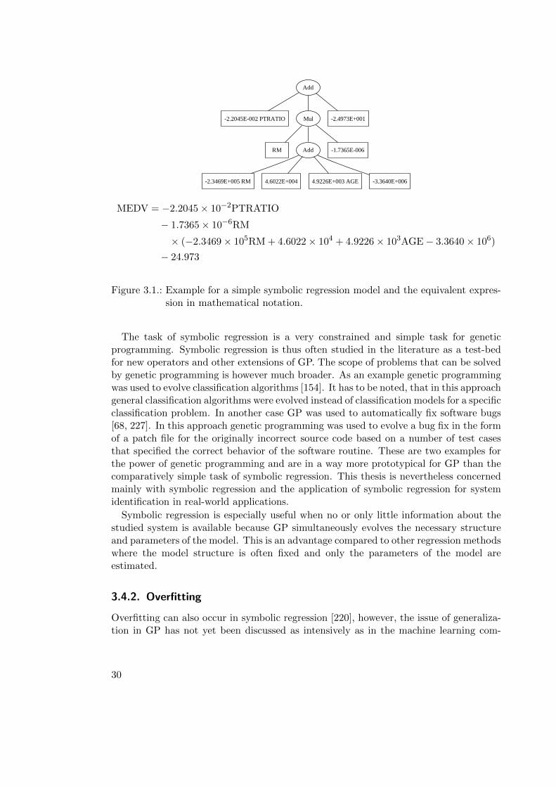
Figure 3.1 shows an example for a symbolic regression model and the equivalent ex-pression in mathematical notation.

29

Add

-2.2045E-002 PTRATIO Mul -2.4973E+001

RM Add -1.7365E-006

-2.3469E+005 RM 4.6022E+004 4.9226E+003 AGE -3.3640E+006

MEDV = −2.2045× 10−2PTRATIO

− 1.7365× 10−6RM

× (−2.3469× 105RM+ 4.6022× 104 + 4.9226× 103AGE− 3.3640× 106)

− 24.973

Figure 3.1.: Example for a simple symbolic regression model and the equivalent expres-sion in mathematical notation.

The task of symbolic regression is a very constrained and simple task for geneticprogramming. Symbolic regression is thus often studied in the literature as a test-bedfor new operators and other extensions of GP. The scope of problems that can be solvedby genetic programming is however much broader. As an example genetic programmingwas used to evolve classification algorithms [154]. It has to be noted, that in this approachgeneral classification algorithms were evolved instead of classification models for a specificclassification problem. In another case GP was used to automatically fix software bugs[68, 227]. In this approach genetic programming was used to evolve a bug fix in the formof a patch file for the originally incorrect source code based on a number of test casesthat specified the correct behavior of the software routine. These are two examples forthe power of genetic programming and are in a way more prototypical for GP than thecomparatively simple task of symbolic regression. This thesis is nevertheless concernedmainly with symbolic regression and the application of symbolic regression for systemidentification in real-world applications.

Symbolic regression is especially useful when no or only little information about thestudied system is available because GP simultaneously evolves the necessary structureand parameters of the model. This is an advantage compared to other regression methodswhere the model structure is often fixed and only the parameters of the model areestimated.

3.4.2. Overfitting

Overfitting can also occur in symbolic regression [220], however, the issue of generaliza-tion in GP has not yet been discussed as intensively as in the machine learning com-

30

munity [59], [148]. Frequently only the training quality of models generated with GPis reported, even though it has been shown repeatedly that this approach methodicallyinvalid and might lead to overfit models that do not generalize well to new observations[83].

It can be argued that compact symbolic regression models that describe a functionalrelation between the input variables and the target variable are unlikely to overfit onthe training. However, it has been shown that this is not true in the general case, verycompact solutions can also be less robust concerning the generalization behavior as hasbeen suggested by [56].

One approach that has been used to reduce overfitting in symbolic regression is touse an internal validation set on which all solutions of the population are evaluated. Asolution that has a comparable accuracy on the training and validation set is returned asthe final result [73, 232, 231]. This approach can been extended to a solution archive inwhich Pareto optimal (quality and size) solutions on the validation set are kept [193, 180].The result of the GP run is the set of solutions in the archive. The advantage of thisapproach is that an appropriate model can be selected a-posteriori.

It is generally assumed that bloat and overfitting are related. However, it has beenrecently observed that overfitting can occur in absence of bloat, and vice versa. Thus, ithas been suggested that overfitting and bloat are two separate phenomenons in geneticprogramming [220], [190].

3.5. Offspring Selection

A nice description of offspring selection comparing it to similar approaches has beengiven by the author in [107]:

Offspring selection [2, 3] is a generic selection concept for evolutionary algo-rithms that aims to reduce the effect of premature convergence often observedwith traditional selection operators by preservation of important alleles [4].The main difference to the usual definition of evolutionary algorithms isthat after parent selection, recombination and optional mutation, offspringselection filters the newly generated solutions. Only solutions that have abetter quality than their best parent are added to the next generation of thepopulation. In this aspect offspring selection is similar to non-destructivecrossover [194], soft brood selection [10], and hill-climbing crossover [149].Non-destructive crossover compares the quality of one child to the qualityof the parent and adds the better one to the next generation, whereas off-spring selection generates new children until a successful offspring is found.Soft brood selection generates n offspring and uses tournament selection todetermine the individual that is added to the next generation, but in compar-ison to offspring selection the children do not compete against the parents.Hill-climbing crossover generates new offspring from the parents as long asbetter solutions can be found. The best solution found by this hill-climbingscheme is added to the next generation. The recently described hereditary

31

selection concept [138, 137] also uses a similar offspring selection scheme incombination with parent selection that is biased to select solutions with fewcommon ancestors.

Offspring selection can be controlled via two parameters, namely the comparison factorand the success ratio. The comparison factor is used in the success criterion and definesa threshold for the fitness of the offspring based on the two fitness values of the parents.The comparison factor is ∈ R, where a value of zero sets the threshold to the minimalfitness of all parents, and value of one sets the threshold to the maximal fitness of allparents. The success ratio is the target ratio of successful offspring in the population andis a value in the range [0 . . . 1]. With offspring selection new individuals are generatedthrough crossover and mutation until the population can be filled with the correct ratioof successful and unsuccessful offspring as defined by the success ratio. A success ratioof one means all offspring must be successful. Strict offspring selection denotes offspringselection with a comparison factor of one and a success ratio of one, which means thatall new offspring must have strictly higher fitness than their parents.

Genetic programming with strict offspring selection has for instance been used toproduce highly accurate classifiers for medical datasets [231].

3.6. Genetic Programming with HeuristicLab

HeuristicLab is a software environment for heuristic optimization. It has been developedby members of the research group “Heuristic and Evolutionary Algorithms Laboratory”(HEAL) in Hagenberg. The chief architect of HeuristicLab is Dr. Stefan Wagner whoalso designed and implemented the core framework [224]. HeuristicLab is open sourcesoftware and can be downloaded from http://dev.heuristiclab.com. The defaultinstallation of HeuristicLab also includes a genetic programming framework which hasbeen implemented mainly by the author of this thesis and Michael Kommenda based onan earlier implementation of Dr. Stephan Winkler [3]. All experiments in this work havebeen prepared and executed with HeuristicLab. The GP implementation in HeuristicLabdeviates in a view aspects from other GP implementations. In the following sections thespecifics of the GP framework of HeuristicLab are described.

HeuristicLab is a generic environment for heuristic optimization in general and notsolely for genetic programming. Two important concepts in HeuristicLab are algorithmsand problems. A given problem can be configured and loaded into an algorithm, whichcan then be used to find a solution for the problem. The framework is designed ina way to make it possible to combine problems and algorithms freely. The defaultinstallation provides a number of different algorithms for heuristic optimization includinggenetic algorithm, evolution strategy, tabu search, simulated annealing, local search.GP problems like symbolic regression are implemented as problems using a symbolicexpression tree encoding for Koza-style (tree-based) genetic programming. A symbolicregression problem can be solved for instance with the predefined genetic algorithm.HeuristicLab does not provide an algorithm specifically for genetic programming.

32

The GP framework in HeuristicLab is not strongly typed. Functions of different typesmust be defined explicitly in the function set, and the compatibility of functions ofdifferent types must be represented through syntactic rules. The set of all syntacticrules defines a context free grammar for symbolic expression trees. This grammar is notused to transform a linear representation to a symbolic expression tree as in grammar-based GP systems. Instead the grammar only defines the possible and valid tree shapes.Operators acting on symbolic expression trees always produce grammatically correctexpressions.

The symbolic regression implementation in HeuristicLab does not support “ephemeralrandom constants” [101] (ERC) as described by Koza. In the original formulation ofsymbolic regression ERC are random constants that are added to the terminal set ad-ditionally to variable symbols for each input variable. The ERC are initialized at thebeginning of the GP run and are not adapted over the GP run. GP can generate ar-bitrarily complex expressions to combine ERCs, so almost all possible constant valuescan be generated through combination of the available ERCs. In HeuristicLab constantvalues are directly embedded in symbolic expressions trees and are adapted over the GPrun through manipulation operators similar to operators described in [183] .

33

4. Interpretation and Simplification ofSymbolic Regression Solutions

Knowledge discovery is hindered by overly complicated models. The bloating effectof genetic programming leads to unnecessarily complex solutions which are difficult tounderstand and validate. Bloat is an important open topic in genetic programming [166]and a number of different theories for the cause of bloat and various methods to controlbloat have been described in the literature [129, 188]. If genetic programming is usedfor data mining and knowledge discovery effective methods to improve parsimony andcomprehensibility of GP solutions are necessary.

This topic should be addressed via multiple paths. Prevention, active reduction, andsupport for interactive exploration.

4.1. Bloat Control - Searching for Parsimonious Solutions

This section describes and compares algorithmic changes to genetic programming whichlead to more compact and comprehensible final solutions. The different approaches aretested on a set of symbolic regression problems and compared regarding the solutionquality on the test set and solution complexity. Initially two algorithms Koza-stylestandard GP and GP with offspring selection [2, 3] both without limits on the solu-tion size or depth are compared. Both algorithms are then extended by the followingapproaches: static size and depth limits, dynamic depth limits, pruning, and dynamicoperator equalization.

In the experiments in this chapter we are mainly concerned about methods to limitthe size of solutions. It is possible that a deterioration in best solution quality is incurredby such methods as the search space is restricted. In this section we also always comparethe best solution quality of each bloat control technique to the solution quality obtainedwith the reference algorithm. Best solution quality is measured on the training data only.The quality of solutions on a hold out set might differ significantly from the trainingquality especially if overfitting occurs. Regardless of overfitting the training quality vs.solution length ratio is an indicator for the complexity of solutions in the populationand as such also relates to the complexity of a solution which is finally selected by avalidation procedure. The validation procedure is necessary in any case regardless of theconstraints applied to the GP process to search for compact solutions. Chapter 5 treatsoverfitting and countermeasures in more detail.

35

4.1.1. Static Depth and Length Limits

The initial generation of the population is filled with randomly created solutions whichfollow a certain size or depth distribution. The distribution depends on the operatorthat is used for initialization. In the following generations the growth of solutions can belimited by setting a static length or depth limit for the crossover and mutation operators.In the crossover operator the newly created trees are checked if they exceed the size ordepth limit and if this is the case, a new offspring is created using the same parents. Ifit is not possible to create a new child which is smaller than the limit, one of the parentsis used after a certain number of tries [101].

Static depth or length limits are a simple way to prevent unlimited growth of GPindividuals. Static depth limits have been used already in [101] to limit the growth ofGP trees. In the same work a rather large depth limit of 17 levels is used for mostproblems suggesting that it is sufficient to solve most problems.

Static limits are problematic when the average size of the population converged nearthe limit in later stages of the run. At that point it becomes increasingly hard for thecrossover operator to produce improved offspring because the number of valid crossoverpoints is highly restricted. A surprising result is that static size limits might even increasebloat as stated by Dignum and Poli: “[...] size limits effectively increase the tendencyto bloat since they induce more sampling of short programs, and, so, in the presenceof non-flat fitness landscapes, GP populations rush towards the limit even more quicklythan in the absence of the size limit!” [53].

4.1.2. Parsimony Pressure

Parsimony Coefficient

One way to apply parsimony pressure to a population of individuals is to select parentsbased on an adjusted fitness value that takes the individuals size into account [101, 239].Formally the adjusted fitness is

fadj(i) = f(i) + c`(i) (4.1)

where f(i) is the raw fitness of the individual i and `(i) is the size of the individual. Theparsimony coefficient c is a constant value that determines the relative importance ofthe size in comparison to the raw fitness. The correct value for c is problem-dependentand it is rather difficult to find a good setting for parsimony coefficient. Intuitively itmight also be beneficial to adjust c dynamically so that at a later stage of a GP runthe value is different from the initial value. Thus a dynamic adjustment strategy for theparsimony coefficient has been introduced through which full control over the programlength in a GP run can be exerted [163].

Covariant Parsimony Pressure

In covariant parsimony pressure [163] the parsimony coefficient is adapted based onthe covariance of the individual fitness with its length. covariant parsimony pressure is

36

theoretically motivated and derived from the size evolution equation [162]

E[µ(t+ 1)] =∑

l

S(Gl)p(Gl, t), (4.2)

which describes the dynamics of expected average program size in GP. It expected meansize of programs µ at generation t + 1 is the sum over all possible program shapes l,where S(Gl) is the size of programs in the set Gl of all programs of with l. p(Gl, t) is theprobability of selecting programs from set Gl from the population at generation t [163].

Rewriting equation 4.2 Poli and McPhee arrive at

E[∆µ] =Cov(`, f)

f(t), (4.3)

which shows that equation 4.2 is related to Price’s theorem [168]

∆Q =Cov(z, q)

z, (4.4)

which describes the dynamics of inheritable traits in biological evolution. This is quite aremarkable result as it connects GP schema theory to a theorem of biological evolutionproving at the same time Price’s theorem [163].

Based on this equation Poli and McPhee derive a number of different control strategiesfor the parsimony coefficient to control the dynamics of the average program size over aGP run. To hold the average size constant from one generation to the next the adjustedfitness function 4.5 should be used.

fadj(x, t) = f(x)− c(t)`(x, t)

c(t) = Cov(`, f)/Var(`)(4.5)

It has been shown that the average length of individuals in the population can betightly controlled through covariant parsimony pressure and that the target averageprogram length can be controlled to follow a given function over the GP run (e.g. sine).

Poli and McPhee have suggested to turn covariant parsimony pressure on and off atspecific generations of a GP run and to let the population grow freely in between phaseswhere parsimony pressure is applied [163]. This suggestion is taken up in this work inChapter 5 where we introduce a novel overfitting prevention mechanism which activatescovariant parsimony pressure only when overfitting is detected in a GP run. The idea isthat in an overfitting phase the average length of programs in the generation should notgrow. At such stages covariant parsimony pressure can be used, to keep the average codelength constant or gradually reduce the average program size. As long as no overfittingoccurs, parsimony pressure is deactivated and the population is allowed to grow freely.

With parsimony pressure there is a risk that selection probability becomes mainlydriven through the parsimony pressure and the fitness of the individual is less relevant.If this happens it is expected that the final solution quality produced by such runs is worsethan the solution quality that would be achieved with hard limits. In [163] it has been

37

shown for simple regression problems (single-variate polynomial of 6th degree and 9thdegree) that solution quality is not negatively effected by covariant parsimony pressure.Such polynomial functions are often used as benchmark problems for symbolic regressionbut they are only very simple test cases. It has not yet been analyzed how covariateparsimony pressure works for real world problems. In this work we also apply covariantparsimony pressure on real word problems; the experimental results are presented laterin this chapter.

The theory behind covariant parsimony pressure is based on fitness proportional se-lection. In [163] it has been demonstrated that for benchmark problems the methodalso works when tournament selection with group size of two is used. We observed thatwith tournament selection the trajectory of average program sizes are not as stable aswith proportional selection. In particular, because the average program size can only becontrolled to assume a given value in expectations there are fluctuations in the actualaverage program size. The fluctuations can have the effect that the whole populationis forced down to the minimal program size in only a few generations in extreme cases.We observed such effects especially when combining covariant parsimony pressure withtournament selection, however, we did not pursue this yet, further experiments are nec-essary. In the experiments presented later in this section we used fitness proportionalselection only in combination with covariant parsimony pressure.

Lexicographic Parsimony Pressure

In [128] a variant of tournament selection has been described which select individuals notonly based on their fitness but also on their size. Lexicographic tournament selectionworks in the same way as tournament selection, only that it prefers individuals withsmaller size if they have the same quality. It has been suggested in [129] that a largenumber of different fitness values are possible in symbolic regression because changesin the lowest parts of the trees cause minor changes in fitness. Two bucketing vari-ants have been proposed for such situations [128]. Individuals are assigned to bucketsbased on their fitness and individuals from the same bucket are treated in lexicographictournament selection as if they have the same fitness value.

In this work lexicographic tournament selection is not analyzed in greater detail. Inmost experiments presented in the following sections, standard tournament selection isused and bloat is controlled by other mechanisms.

4.1.3. Dynamic Depth Limits

Recent work describes how depth-limits can be varied dynamically based on fitness[188]. Initially the dynamic depth limit (DDL) is set to small value. When a new bestsolution is found which exceeds the dynamic depth limit it is set to the depth of thenew best solution. If the best solution is smaller than the dynamic depth limit it can bedecreased again. In this case some individuals in the current population might exceedthe depth limit. Through the application of crossover, however, the individuals of thenext generation are limited to the new reduced depth limit. If no reproduction is used

38

the depth of all individuals of the next generation is within the depth limit, otherwisea few generational steps are necessary until all individuals of the population are withinthe bounds again.

The advantage of dynamic depth limits in comparison to static limits is that the limitis adapted by the algorithm as necessary for the problem. In the case of static limitssolutions exceeding the limit are rejected in all cases even when they improve the bestknown solution. With dynamic depth limits the limit is adapted accordingly when a newbest of run solution is found. Even though program growth is not prohibited becausethe dynamic limit can potentially be extended, the approach still effectively preventsprogram growth which is not matched with a proportional improvement in solutionquality.

Dynamic Depth Limits for Offspring Selection

Dynamic depth limits have been combined with offspring selection [238]. For each newlycreated offspring first the offspring selection success criterion is checked. If the offspringis successful, the dynamic depth limit is adapted based on the quality and the depthof the offspring. The dynamic depth limit is decreased if the offspring has a smallerdepth and is better than the best solution (on the training) so far. All offspring notexceeding the depth limit are accepted. If offspring exceeds the dynamic depth limitthen it is only accepted if it has better quality than the best solution so far. In thiscase the dynamic depth limit is set to the depth of the new offspring and the offspring isaccepted. If the offspring exceeds the depth limit and it is worse than the best solutionso far then the offspring is rejected. In order to prevent fluctuations in the dynamicdepth limit any increase or decrease of the dynamic depth limit must be backed by asignificant improvement in solution quality. This can be controlled via parameters clower

and cRaise. Zavoianu suggests values of 3% and 1.5%, respectively [238].

Algorithm 1 describes how the dynamic depth limit is adapted based on the depthand quality of a newly created offspring. This algorithm is derived from the originalformulation of DDL [186, 188].

In [238] OSGP with dynamic depth limits has been applied to two real world problemsand it has been shown that the dynamic depth limit leads to smaller final solutions withcomparable model quality. In this work we compare the final solutions produced bySGP and OSGP, both extended with dynamic depth limits on benchmark problems andadditional real world problems.

In the original formulation of Silva and Costa [188] an offspring is replaced by oneof its parents, if it is rejected because of the dynamic depth limit. In the adaptionfor offspring selection [238] this is not the case. Instead new parents are selected andcrossover is applied again. The strategy potentially amplifies the effect of crossover bias.It has been suggested that it is better to accept the parents if crossover produces illegaloffspring [188].

39

Algorithm 1: Dynamic depth limits for offspring selection

if SuccessfulOffspring thenif Maximization then

relativeQuality ← (quality / bestQuality) - 1 ;else

relativeQuality ← (bestQuality / quality) - 1;endif treedepth ≤ ddl then

// depth is smaller than dynamic limit => reduce limit if the

quality improvement is large enough

if relativeQuality ≥ cLower(ddl − treedepth) thenddl ← Max(treedepth, InitialDepthLimit);

end

else// depth is larger than dynamic limit => increase limit if

the quality improvement is large enough

if relativeQuality ≥ cRaise(treedepth − ddl) thenddl ← treedepth;

else// depth is larger but no improvement => reject

SuccessfulOffspring ← false;end

end

end

40

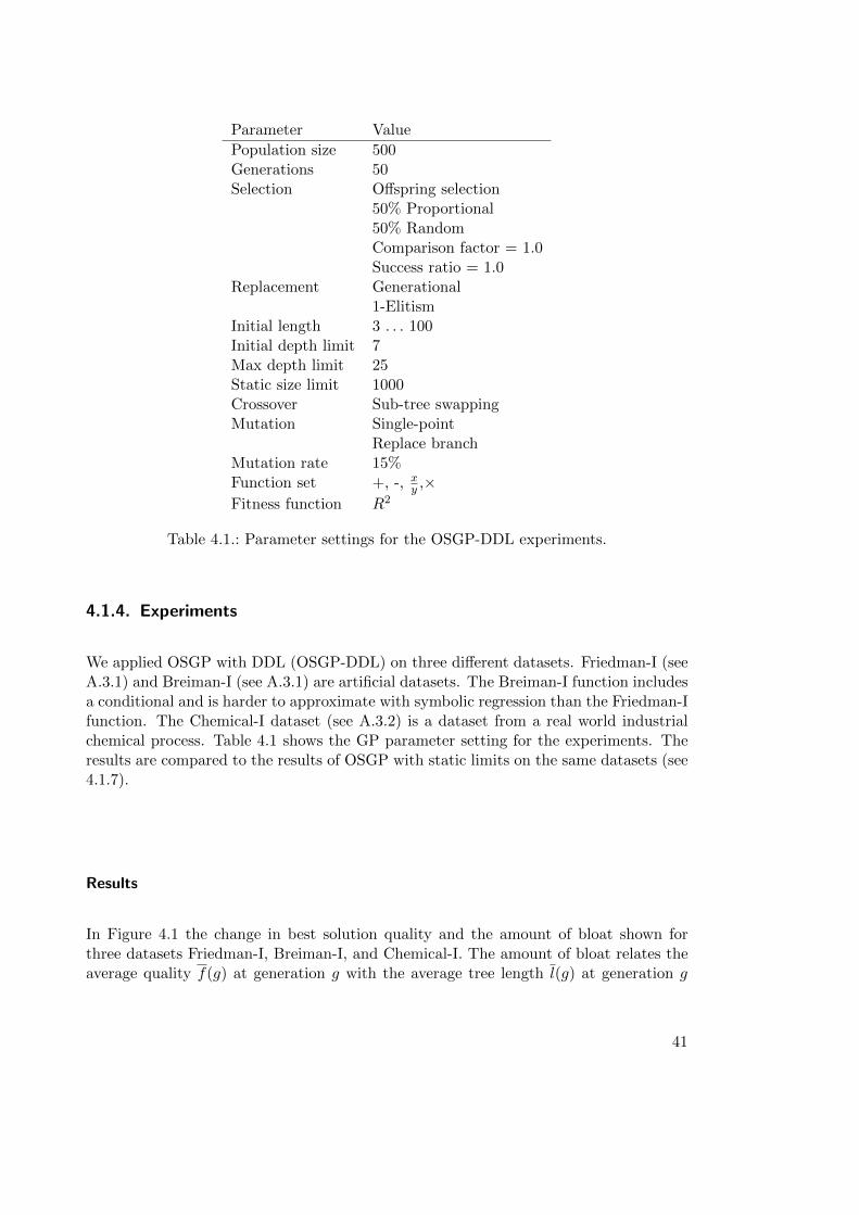
Parameter Value

Population size 500Generations 50Selection Offspring selection

50% Proportional50% RandomComparison factor = 1.0Success ratio = 1.0

Replacement Generational1-Elitism

Initial length 3 . . . 100Initial depth limit 7Max depth limit 25Static size limit 1000Crossover Sub-tree swappingMutation Single-point

Replace branchMutation rate 15%Function set +, -, x

y ,×Fitness function R2

Table 4.1.: Parameter settings for the OSGP-DDL experiments.

4.1.4. Experiments

We applied OSGP with DDL (OSGP-DDL) on three different datasets. Friedman-I (seeA.3.1) and Breiman-I (see A.3.1) are artificial datasets. The Breiman-I function includesa conditional and is harder to approximate with symbolic regression than the Friedman-Ifunction. The Chemical-I dataset (see A.3.2) is a dataset from a real world industrialchemical process. Table 4.1 shows the GP parameter setting for the experiments. Theresults are compared to the results of OSGP with static limits on the same datasets (see4.1.7).

Results

In Figure 4.1 the change in best solution quality and the amount of bloat shown forthree datasets Friedman-I, Breiman-I, and Chemical-I. The amount of bloat relates theaverage quality f(g) at generation g with the average tree length l(g) at generation g

41

and is calculated using equation 4.6 [220] (also see Chapter 3).

bloat(g) =∆l(g)

∆f(g)

∆f(g) =f(g)− f(0)

1 + f(0)

∆l(g) =l(g)− l(0)

l(0)

(4.6)

In all experiments in this chapter we are mainly interested in the fitness on the trainingset. All qualities that are reported in the results are the squared correlation coefficient(R2) on the training set. In Chapter 5 more experiment results are presented that focuson the generalization ability of different GP configurations.

Figure 4.1 shows that because of dynamic depth limits the amount of bloat is greatlyreduced in comparison to OSGP with static limits. The best solution quality is notnegatively effected by the application of dynamic depth limits.

The best solution quality and amount of bloat for the last generation are also givenin Tables 4.4, 4.5, and 4.6 later in this chapter.

4.1.5. Operator Equalization

Operator equalization is an bloat control measure motivated by the crossover bias the-ory of bloat [54]. To counteract the bias of crossover to produce more smaller offspringan equalization step is introduced after crossover. Offspring created from crossover arefiltered before they are accepted into the next generation of the population. Algorithm2 shows the general method of filtering offspring based on an acceptance criterion. Off-spring selection, dynamic depth limits, and operator equalization all plug into the GPprocess in the same way repeatedly creating new offspring until the population is full.

Algorithm 2: Filtering of offspring in the formulation of dynamic depth limitsand operator equalization

while Population is not full doSelect parents;Create offspring;if Accept(offspring) then

Add offspring to next generation of population;end

end

The difference lies in the way how the acceptance criterion is defined. In the case ofoperator equalization the filter effectively controls the length distribution of individualsin the population by limiting the number of individuals of a given size in the population.The basis of operator equalization is a target length distribution histogram. Individuals

42

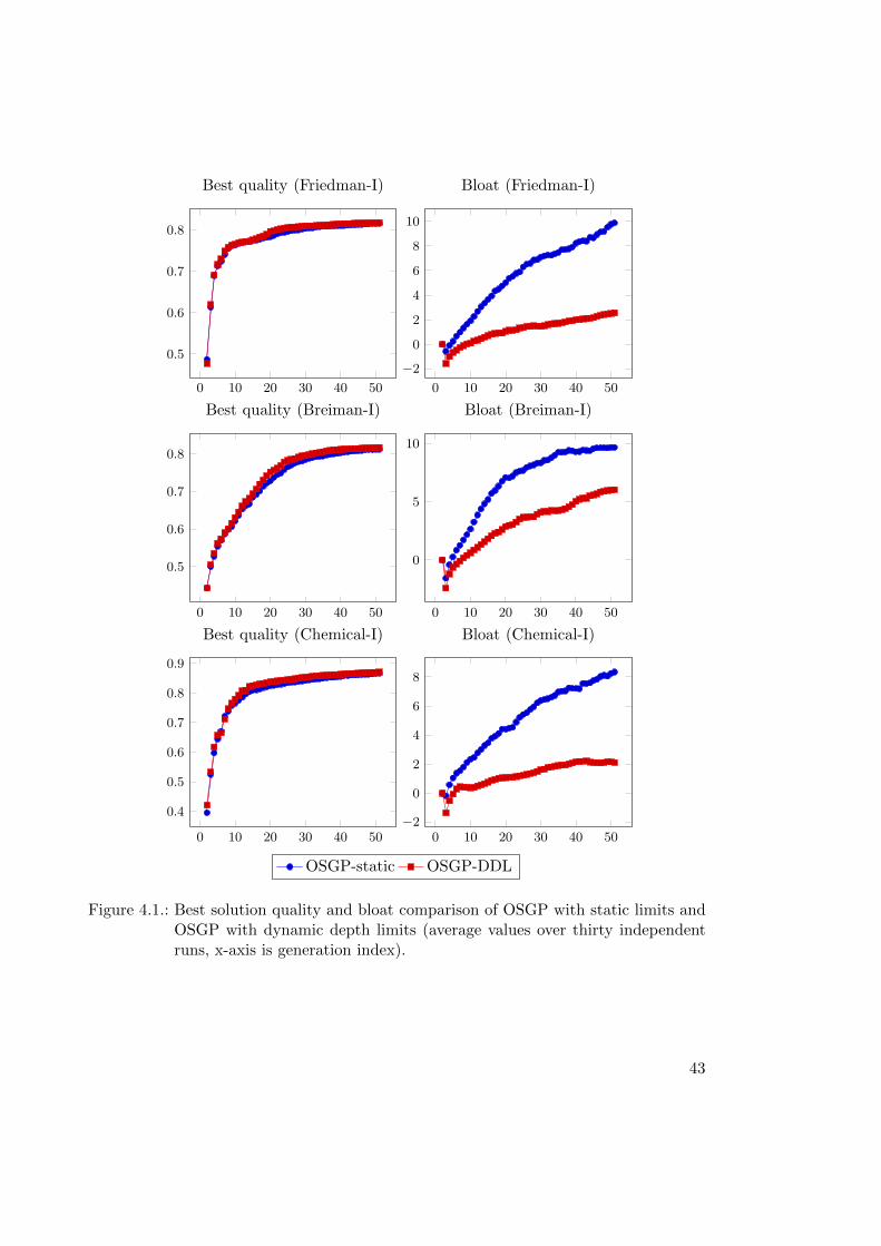
0 10 20 30 40 50

0.5

0.6

0.7

0.8

Best quality (Friedman-I)

0 10 20 30 40 50

−2

0

2

4

6

8

10

Bloat (Friedman-I)

0 10 20 30 40 50

0.5

0.6

0.7

0.8

Best quality (Breiman-I)

0 10 20 30 40 50

0

5

10

Bloat (Breiman-I)

0 10 20 30 40 50

0.4

0.5

0.6

0.7

0.8

0.9

Best quality (Chemical-I)

0 10 20 30 40 50

−2

0

2

4

6

8

Bloat (Chemical-I)

OSGP-static OSGP-DDL

Figure 4.1.: Best solution quality and bloat comparison of OSGP with static limits andOSGP with dynamic depth limits (average values over thirty independentruns, x-axis is generation index).

43

are grouped by length into several bins using equation 4.7. The number of individualsthat can be accepted into each bin is limited by a static bin capacity. The target sizedistribution of solutions in the population can be configured freely through manipulationof the bin capacities.

b ← btreelength − 1

binSizec+ 1 (4.7)

It has been shown empirically that genetic programming with operator equalization isbloat free [54]. This is strong empirical evidence for the crossover bias theory of bloat. Itshould be noted that individuals are evaluated only after they have been accepted intothe population by the equalization filter, otherwise a lot of effort is wasted evaluatingindividuals which are discarded by the equalization filter after fitness evaluation.

Dynamic Operator Equalization

Operator equalization is a method to control the length distribution of individuals inthe population exactly by filtering offspring based on their length. The weakness ofoperator equalization is that the target distribution and the maximal size limit whichis appropriate for a given problem is not known a-priori. Thus the method has beenimproved to adapt the target distribution and the maximal size limit dynamically basedon the fitness and length of individuals in the population [188, 189, 190, 191].

Dynamic operator equalization combines dynamic depth limits and operator equal-ization. Instead of the static target distribution the initial target distribution is createdwith bin capacities to hold all solutions of the initial generation. In the following gener-ations the bin capacity is adapted based on the average fitness of solutions in each bin inrelation to the average fitness over the whole population using equation 4.8. The capac-ity of bins, that hold individuals that are fitter on average than the whole population,is increased while the capacity of bins, that hold individuals that are on average worsethan the population, is accordingly decreased.

binCapacityi = round(PopSize f i/∑

j

f j) (4.8)

The algorithm for acceptance of an offspring is shown in Algorithm 3. For each newoffspring the target bin is determined based on its length. The offspring is acceptedinto the population only when the bin is not yet full. The only exception is if the newoffspring has a better fitness than the best solution in that bin so far. In this case theoffspring is accepted even though the bin is already full and the capacity of the bin isincreased.

The acceptance criterion shown in Algorithm 3 combined with the adaption of bincapacities leads to dynamic adaption of the target distribution based on solution fitness.Similarly to dynamic depth limits dynamic operator equalization an extension of the sizedistribution is possible when a new best of run solution is found for which a bin doesnot yet exist. In this case a new bin of capacity one is created and the solution is addedto the bin. If necessary bins in between the newly created bin and the last existing binare created with a capacity of one.

44

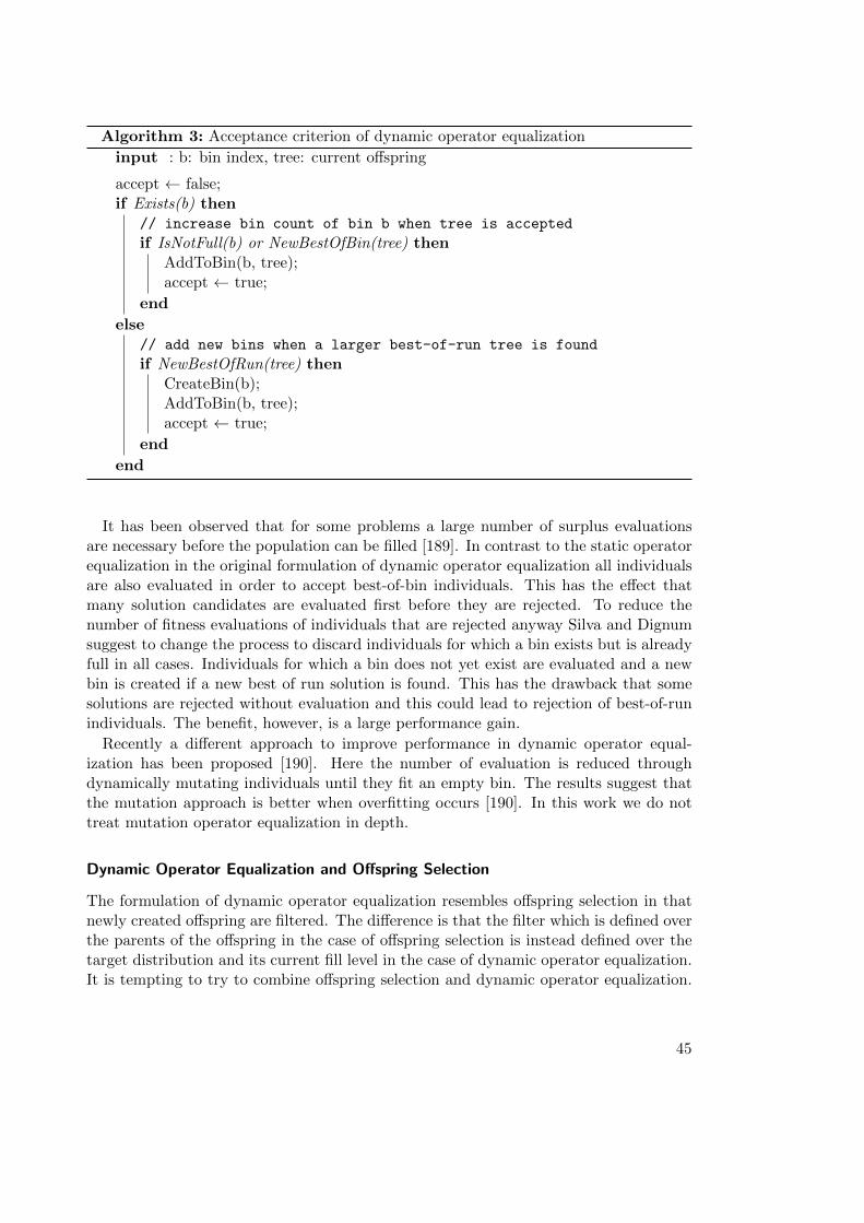
Algorithm 3: Acceptance criterion of dynamic operator equalization

input : b: bin index, tree: current offspring

accept ← false;if Exists(b) then

// increase bin count of bin b when tree is accepted

if IsNotFull(b) or NewBestOfBin(tree) thenAddToBin(b, tree);accept ← true;

end

else// add new bins when a larger best-of-run tree is found

if NewBestOfRun(tree) thenCreateBin(b);AddToBin(b, tree);accept ← true;

end

end

It has been observed that for some problems a large number of surplus evaluationsare necessary before the population can be filled [189]. In contrast to the static operatorequalization in the original formulation of dynamic operator equalization all individualsare also evaluated in order to accept best-of-bin individuals. This has the effect thatmany solution candidates are evaluated first before they are rejected. To reduce thenumber of fitness evaluations of individuals that are rejected anyway Silva and Dignumsuggest to change the process to discard individuals for which a bin exists but is alreadyfull in all cases. Individuals for which a bin does not yet exist are evaluated and a newbin is created if a new best of run solution is found. This has the drawback that somesolutions are rejected without evaluation and this could lead to rejection of best-of-runindividuals. The benefit, however, is a large performance gain.

Recently a different approach to improve performance in dynamic operator equal-ization has been proposed [190]. Here the number of evaluation is reduced throughdynamically mutating individuals until they fit an empty bin. The results suggest thatthe mutation approach is better when overfitting occurs [190]. In this work we do nottreat mutation operator equalization in depth.

Dynamic Operator Equalization and Offspring Selection

The formulation of dynamic operator equalization resembles offspring selection in thatnewly created offspring are filtered. The difference is that the filter which is defined overthe parents of the offspring in the case of offspring selection is instead defined over thetarget distribution and its current fill level in the case of dynamic operator equalization.It is tempting to try to combine offspring selection and dynamic operator equalization.

45

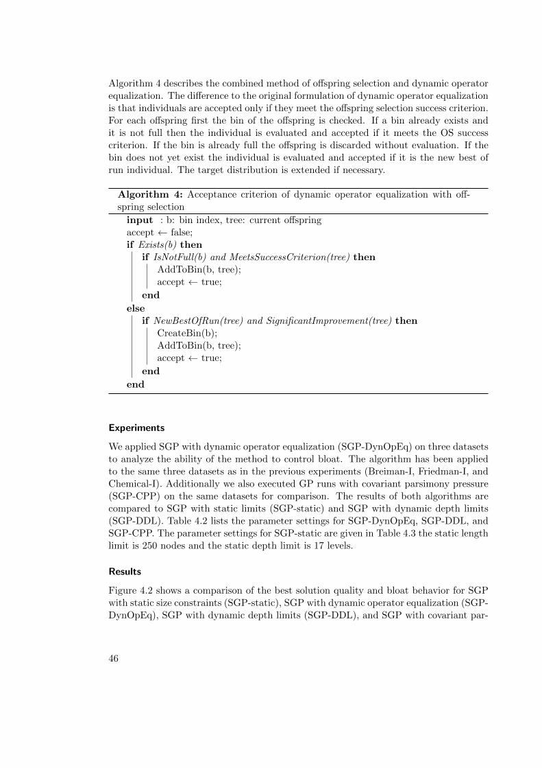
Algorithm 4 describes the combined method of offspring selection and dynamic operatorequalization. The difference to the original formulation of dynamic operator equalizationis that individuals are accepted only if they meet the offspring selection success criterion.For each offspring first the bin of the offspring is checked. If a bin already exists andit is not full then the individual is evaluated and accepted if it meets the OS successcriterion. If the bin is already full the offspring is discarded without evaluation. If thebin does not yet exist the individual is evaluated and accepted if it is the new best ofrun individual. The target distribution is extended if necessary.

Algorithm 4: Acceptance criterion of dynamic operator equalization with off-spring selection

input : b: bin index, tree: current offspringaccept ← false;if Exists(b) then

if IsNotFull(b) and MeetsSuccessCriterion(tree) thenAddToBin(b, tree);accept ← true;

end

elseif NewBestOfRun(tree) and SignificantImprovement(tree) then

CreateBin(b);AddToBin(b, tree);accept ← true;

end

end

Experiments

We applied SGP with dynamic operator equalization (SGP-DynOpEq) on three datasetsto analyze the ability of the method to control bloat. The algorithm has been appliedto the same three datasets as in the previous experiments (Breiman-I, Friedman-I, andChemical-I). Additionally we also executed GP runs with covariant parsimony pressure(SGP-CPP) on the same datasets for comparison. The results of both algorithms arecompared to SGP with static limits (SGP-static) and SGP with dynamic depth limits(SGP-DDL). Table 4.2 lists the parameter settings for SGP-DynOpEq, SGP-DDL, andSGP-CPP. The parameter settings for SGP-static are given in Table 4.3 the static lengthlimit is 250 nodes and the static depth limit is 17 levels.

Results

Figure 4.2 shows a comparison of the best solution quality and bloat behavior for SGPwith static size constraints (SGP-static), SGP with dynamic operator equalization (SGP-DynOpEq), SGP with dynamic depth limits (SGP-DDL), and SGP with covariant par-

46

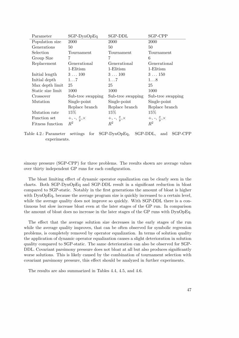
Parameter SGP-DynOpEq SGP-DDL SGP-CPP

Population size 2000 2000 2000Generations 50 50 50Selection Tournament Tournament TournamentGroup Size 7 7 6Replacement Generational Generational Generational

1-Elitism 1-Elitism 1-ElitismInitial length 3 . . . 100 3 . . . 100 3 . . . 150Initial depth 1. . .7 1. . .7 1. . .8Max depth limit 25 25 25Static size limit 1000 1000 1000Crossover Sub-tree swapping Sub-tree swapping Sub-tree swappingMutation Single-point Single-point Single-point

Replace branch Replace branch Replace branchMutation rate 15% 15% 15%Function set +, -, x

y ,× +, -, xy ,× +, -, x

y ,×Fitness function R2 R2 R2

Table 4.2.: Parameter settings for SGP-DynOpEq, SGP-DDL, and SGP-CPPexperiments.

simony pressure (SGP-CPP) for three problems. The results shown are average valuesover thirty independent GP runs for each configuration.

The bloat limiting effect of dynamic operator equalization can be clearly seen in thecharts. Both SGP-DynOpEq and SGP-DDL result in a significant reduction in bloatcompared to SGP-static. Notably in the first generations the amount of bloat is higherwith DynOpEq, because the average program size is quickly increased to a certain level,while the average quality does not improve so quickly. With SGP-DDL there is a con-tinuous but slow increase bloat even at the later stages of the GP run. In comparisonthe amount of bloat does no increase in the later stages of the GP runs with DynOpEq.

The effect that the average solution size decreases in the early stages of the runwhile the average quality improves, that can be often observed for symbolic regressionproblems, is completely removed by operator equalization. In terms of solution qualitythe application of dynamic operator equalization causes a slight deterioration in solutionquality compared to SGP-static. The same deterioration can also be observed for SGP-DDL. Covariant parsimony pressure does not bloat at all but also produces significantlyworse solutions. This is likely caused by the combination of tournament selection withcovariant parsimony pressure, this effect should be analyzed in further experiments.

The results are also summarized in Tables 4.4, 4.5, and 4.6.

47

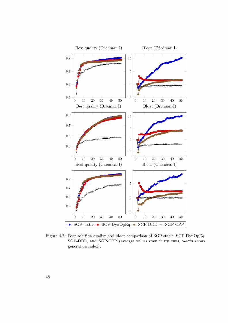
0 10 20 30 40 50

0.5

0.6

0.7

0.8

Best quality (Friedman-I)

0 10 20 30 40 50

−5

0

5

10

Bloat (Friedman-I)

0 10 20 30 40 50

0.5

0.6

0.7

0.8

Best quality (Breiman-I)

0 10 20 30 40 50

−5

0

5

10

Bloat (Breiman-I)

0 10 20 30 40 50

0.5

0.6

0.7

0.8

Best quality (Chemical-I)

0 10 20 30 40 50

−5

0

5

Bloat (Chemical-I)

SGP-static SGP-DynOpEq SGP-DDL SGP-CPP

Figure 4.2.: Best solution quality and bloat comparison of SGP-static, SGP-DynOpEq,SGP-DDL, and SGP-CPP (average values over thirty runs, x-axis showsgeneration index).

48

4.1.6. Pruning to Reduce Bloat

Pruning in tree-based genetic programming means to remove branches from GP solu-tions that have no or only minimal effect on the quality of the solution. Pruning is alsofrequently used in other learning methods with tree-based model representation for in-stance CART [28] and MARS [71], where it is often used to reduce overfitting. Pruningcan be used to reduce bloat by removing inviable code from individuals over the wholepopulation [8, 3, 97]. To make pruning viable it must be possible to determine the effectof removing a branch efficiently. For some GP problems it is possible to determine theeffect of branch-removal statically without fully evaluating the individual. For instancefor the artificial ant problem turning left and in the next operation turning right is unop-timized code which can be removed because through semantic analysis this is obviouslyuseless. Similar patterns can be defined for symbolic regression (e.g. x * 0). However,the impact of static pruning is limited since the number of such patterns is very largeand it is practically impossible to define all patterns which might lead to inviable orunoptimized code. In the case of symbolic regression the relevance of branches can bedetermined by comparing the output of the original tree with a pruned tree. If theoutput of the pruned tree is almost the same then the pruned tree still contains theimportant code.

When pruning is included into the GP process a number of aspects must be considered.Since pruning is applied frequently it should be rather efficient so that the process doesnot become too slow. Also pruning should not remove too much genetic diversity. Weobserved that a certain amount of unoptimized code in the population is necessary forthe evolutionary process. If pruning is applied too vigorously there is a risk of prematureconvergence because of the sudden reduction of genetic diversity.

In practical applications we found a greedy pruning strategy based on branch impactmetrics (see Section 6.2.6) shown in Algorithm 5 to work sufficiently well. The greedymethod evaluates all branch impacts and then removes the branch with smallest impactpreferring larger branches. This is done iteratively until a maximal quality deteriorationis reached or the size of the tree has been reduced by a certain factor. A similar approachfor numerical simplification based on a number of additional metrics for the relevance oftree-branches is proposed in [97, 88].

The disadvantage of the greedy pruning strategy is that certain types of unoptimizedcode cannot be detected or removed. Since the method removes one branch at a timeit is not possible to detect cases of interaction between two separate branches, whereremoving one of them causes a big change in solution quality, even though removingboth simultaneously would not change the quality at all. Such cases are however ratherdifficult to detect and can practically only be removed through exhaustive methods whichcannot be included in the GP process because of performance considerations.

The calculation of the branch impact is rather expensive as the branch has to be eval-uated to calculate a replacement value and then the manipulated tree must be evaluatedto determine the effect on the quality. To make the method more efficient, only a limitednumber of branches is considered for removal in every iteration (tournament size) andthe branch as well as the manipulated tree are not evaluated on the full training set,

49

Algorithm 5: Greedy iterated tournament pruning

Data: t: original tree, iterations, groupSizeResult: prunedTreeprunedTree ← tree;while c ≤ iterations do

B ← SelectRandomBranches(prunedTree, groupSize);prunedBranch ← argminb∈B Impact(b) / RelativeSize(t,b);Inc(c);

end

RelativeSize(t, b) = Size(t)/(Size(t)− Size(b))

but instead only on a limited number of random samples from the training set. This isespecially important if the training set contains a large number of samples.

4.1.7. Does Offspring Selection Reduce Bloat?

Offspring selection with strict parameter settings enforces that newly created offspringmust improve upon its parents quality. Because of this, offspring selection should in-tuitively have a limiting effect on bloat because it has a negative bias against introns(inviable code). In the light of crossover bias theory [164, 52], however, there is noindication that offspring selection should reduce bloat. Instead the effect of crossoverbias could be amplified, because parent selection and crossover are executed repeatedlyuntil the population can be filled with successful offspring. Sub-tree crossover producesmore smaller offspring then larger offspring. Smaller offspring tendentially have lowerfitness. This leads to a bias to accept more larger offspring into the population. Ifsub-tree crossover is repeatedly applied until a successful individual is found the effect ofcrossover bias is amplified. In this work the hypothesis that OS reduces bloat is testedfor the first time and the effect of offspring selection on bloat is analyzed.

In symbolic regression inviable code is unlikely to occur if function sets with onlyarithmetic operators are used [186, 187]. The bloating effect is caused mainly by thegrowth of unoptimized code. If conditional and boolean functions are included in thefunction set, inviable code can be produced by the process much more easily. In light ofthese observations, we also compare the amount of bloat of both SGP and OSGP with asmall function set including only arithmetic operators and with an extended function setalso including conditionals and boolean operators. If the hypothesis holds that offspringselection reduces bloat because of its bias against inviable code, then the difference inbloat between OSGP and SGP should be even larger with the extended function set.The amount of bloat observed with the extended function set should be smaller thanthe amount of bloat observed with the arithmetic function set.

50

Parameter SGP OSGP

Population size 2000 500Generations 50 50Selection Tournament Selection Offspring selection

Group size = 7 50% Proportional50% RandomComparison factor = 1.0Success ratio = 1.0

Replacement Generational Generational1-Elitism 1-Elitism

Initial length 3 . . . 100 3 . . . 100Max. initial depth 12 12Crossover Sub-tree swapping Sub-tree swappingMutation rate 15% 15%Mutation Single-point Single-point

Replace branch Replace branchFitness function R2 R2

Table 4.3.: Genetic programming parameter settings for the analysis of bloat in SGPand OSGP.

Experiment Setup

Two types of experiments are executed. First standard GP (SGP) and GP with offspringselection (OSGP) are applied to a number of test problems without constraints on theprogram size. Then the same experiments are repeated with static size limits for bothalgorithms.

In the experiments without size constraints four different configurations are tested:SGP with arithmetic functions only (SGP), SGP with an extended function set in-cluding conditionals and boolean operators (SGP-full), OSGP with arithmetic functions(OSGP), and OSGP with the extended function set (OSGP-full).

Additionally the four same experiments are also executed using static depth and lengthlimits (SGP-static, SGP-static-full, OSGP-static, and OSGP-static-full). The parametersettings of both algorithms are given in Table 4.3. For the experiments without sizeconstraints the depth and length limits are set to very large values (100, 100000) tomake sure that the limit is not reached over the whole run. For the experiments withstatic constraints the depth limit was set to 17 levels and the length limit was set to 250nodes.

For the experiments we use three different datasets. Friedman-I (see A.3.1) andBreiman-I (see A.3.1) are artificial datasets. The Breiman-I function includes a con-ditional and is harder to approximate with symbolic regression than the Friedman-Ifunction. The Chemical-I dataset (see A.3.2) is a dataset from a real world industrialchemical process.

51

Results

The results presented below show the trajectories of the best solution quality and theamount of bloat (see 3) over the whole run averaged over thirty independent runs.

Results Without Size Limits

Figure 4.3 shows the best quality and amount of bloat for the Friedman-I, Breiman-I,and Chemical-I datasets without limits on the program length or depth.

OSGP produces better solutions than SGP for all problems especially with the ex-tended function set (OSGP-full). Surprisingly OSGP-full also bloats fastest with theFriedman-I and Chemical-I datasets. With the Breiman-I dataset OSGP using onlyarithmetic functions bloats fastest. In general OSGP bloats fastest with all datasets.Even though it produces better solutions, the larger growth in solution length is notmatched by a proportional growth in solution quality.

Another interesting observation is that OSGP bloats faster with the full function setthan with the arithmetic function set. With the full function set inviable code is muchmore likely than with the arithmetic function set. Even though strict OSGP as it is usedin this experiment has a bias against inviable code the bloating effect is stronger. Thiscontradicts the hypothesis that OSGP reduces bloat because of a bias against inviablecode.

The Breiman-I function includes a conditional and is more difficult to approximatewith GP. This can also be observed in the results of the experiments.

The results for the final generation are also given in Tables 4.4, 4.5, and 4.6 that showa comparison of all experiment results in this chapter for all datasets.

Results With Static Size Limits

Figure 4.4 shows the best quality and amount of bloat for the Friedman-I, Breiman-Iand Chemical-I problems with static limits on the program length and depth. The staticlimits for length and depth are 250 nodes and 17 levels, respectively.

The results are similar to the results of the experiments without size limits. OSGPproduces solutions with a higher fitness than SGP especially when using the full func-tion set. OSGP-full also bloats faster than the other configurations with all datasets.Compared to the results without size constraints the amount of bloat is less for all con-figurations because of the size constraints but the relative differences between algorithmsare similar.

For the Breiman-I problem the configurations with the full function set bloat fasterthan the configurations with only arithmetic functions. Notably, SGP-full bloats pro-duces more bloat than OSGP with the small function set for this dataset.

The results for the final generation are also given in Tables 4.4, 4.5, and 4.6.

52

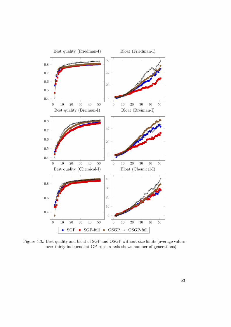
0 10 20 30 40 50

0.4

0.5

0.6

0.7

0.8

Best quality (Friedman-I)

0 10 20 30 40 50

0

20

40

60

Bloat (Friedman-I)

0 10 20 30 40 50

0.4

0.5

0.6

0.7

0.8

Best quality (Breiman-I)

0 10 20 30 40 50

0

20

40

Bloat (Breiman-I)

0 10 20 30 40 50

0.4

0.6

0.8

Best quality (Chemical-I)

0 10 20 30 40 50

0

10

20

30

40

Bloat (Chemical-I)

SGP SGP-full OSGP OSGP-full

Figure 4.3.: Best quality and bloat of SGP and OSGP without size limits (average valuesover thirty independent GP runs, x-axis shows number of generations).

53

Conclusion

Interpreting the results of the experiments shown in Figures 4.3 and 4.4 the intuitiveassumption that offspring selection reduces bloat does not hold. Instead we observedthat average program length grows faster when offspring selection is used, both withand without size constraints. The average quality of solutions is higher when offspringselection applied but this is combined with a disproportional increase in solution size.This has also been suggested already in [238]. The results of these experiments provideadditional evidence for the crossover bias theory of bloat.

4.1.8. Multi-objective GP

Multi-objective optimization approaches have also been used for bloat control [22, 45,44, 153]. Instead of including the solution complexity as an penalization term into thefitness value the multi-objective approach uses a multi-dimensional fitness value whichincludes a component for accuracy and a component for complexity. The aim of thealgorithm is to produce a Pareto-optimal front of solutions for both fitness components.

One of the most well known multi objective optimization algorithm is the non-dom-inated sorting genetic algorithm (NSGA-II) [47, 48]. NSGA-II has for instance beenused for to search for parsimonious symbolic regression models in [94].

In this work we do not treat the topic of multi-objective optimization in full detailand a single-objective GP algorithm is used for all experiments.

4.1.9. Summary of Results of Bloat Experiments

Tables 4.4, 4.5, and 4.6 summarize the results of all experiments with different bloatcontrol methods in this chapter. The results for SGP and OSGP without any constraintson program size are also given for comparison. Size is the average program length in thelast generation. Best solution quality is the squared correlation coefficient (R2) in thelast generation on the training set. The bloat value is the value of the last generationcalculated using equation 4.6. All values are averages over 30 independent GP runs theconfidence interval is given for α = 0.05 and assumes normally distributed values.

4.1.10. Effects of Bloat Control on Genetic Diversity

Bloat control methods can have a strong effect on the dynamic of the GP process andmight interfere with genetic diversity. If the bloat control method causes a suddenreduction of genetic diversity from one population to the next it is possible that thisultimately leads to premature convergence. Issues regarding bloat control and geneticdiversity have been discussed in [239, 45, 44] and more recently also in [9]. If bloatcontrol measures are used it is recommended to also observe the genetic diversity in thepopulation and if necessary counteract loss (e.g. by increasing the mutation rate).

54

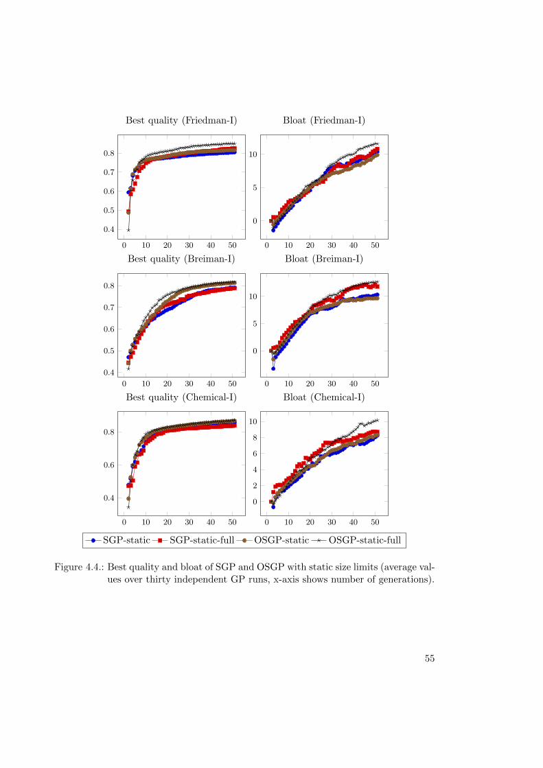
0 10 20 30 40 50

0.4

0.5

0.6

0.7

0.8

Best quality (Friedman-I)

0 10 20 30 40 50

0

5

10

Bloat (Friedman-I)

0 10 20 30 40 50

0.4

0.5

0.6

0.7

0.8

Best quality (Breiman-I)

0 10 20 30 40 50

0

5

10

Bloat (Breiman-I)

0 10 20 30 40 50

0.4

0.6

0.8

Best quality (Chemical-I)

0 10 20 30 40 50

0

2

4

6

8

10

Bloat (Chemical-I)

SGP-static SGP-static-full OSGP-static OSGP-static-full

Figure 4.4.: Best quality and bloat of SGP and OSGP with static size limits (average val-ues over thirty independent GP runs, x-axis shows number of generations).

55

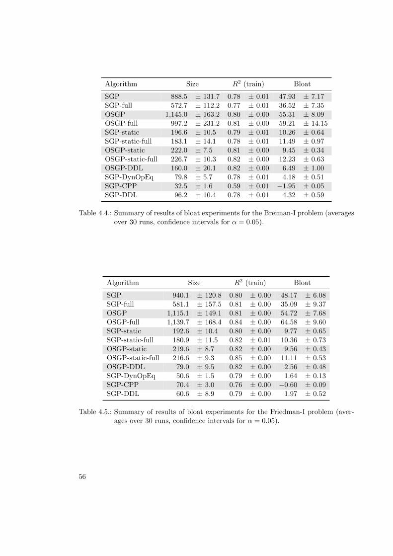
Algorithm Size R2 (train) Bloat

SGP 888.5 ± 131.7 0.78 ± 0.01 47.93 ± 7.17SGP-full 572.7 ± 112.2 0.77 ± 0.01 36.52 ± 7.35OSGP 1,145.0 ± 163.2 0.80 ± 0.00 55.31 ± 8.09OSGP-full 997.2 ± 231.2 0.81 ± 0.00 59.21 ± 14.15SGP-static 196.6 ± 10.5 0.79 ± 0.01 10.26 ± 0.64SGP-static-full 183.1 ± 14.1 0.78 ± 0.01 11.49 ± 0.97OSGP-static 222.0 ± 7.5 0.81 ± 0.00 9.45 ± 0.34OSGP-static-full 226.7 ± 10.3 0.82 ± 0.00 12.23 ± 0.63OSGP-DDL 160.0 ± 20.1 0.82 ± 0.00 6.49 ± 1.00SGP-DynOpEq 79.8 ± 5.7 0.78 ± 0.01 4.18 ± 0.51SGP-CPP 32.5 ± 1.6 0.59 ± 0.01 −1.95 ± 0.05SGP-DDL 96.2 ± 10.4 0.78 ± 0.01 4.32 ± 0.59

Table 4.4.: Summary of results of bloat experiments for the Breiman-I problem (averagesover 30 runs, confidence intervals for α = 0.05).

Algorithm Size R2 (train) Bloat

SGP 940.1 ± 120.8 0.80 ± 0.00 48.17 ± 6.08SGP-full 581.1 ± 157.5 0.81 ± 0.00 35.09 ± 9.37OSGP 1,115.1 ± 149.1 0.81 ± 0.00 54.72 ± 7.68OSGP-full 1,139.7 ± 168.4 0.84 ± 0.00 64.58 ± 9.60SGP-static 192.6 ± 10.4 0.80 ± 0.00 9.77 ± 0.65SGP-static-full 180.9 ± 11.5 0.82 ± 0.01 10.36 ± 0.73OSGP-static 219.6 ± 8.7 0.82 ± 0.00 9.56 ± 0.43OSGP-static-full 216.6 ± 9.3 0.85 ± 0.00 11.11 ± 0.53OSGP-DDL 79.0 ± 9.5 0.82 ± 0.00 2.56 ± 0.48SGP-DynOpEq 50.6 ± 1.5 0.79 ± 0.00 1.64 ± 0.13SGP-CPP 70.4 ± 3.0 0.76 ± 0.00 −0.60 ± 0.09SGP-DDL 60.6 ± 8.9 0.79 ± 0.00 1.97 ± 0.52

Table 4.5.: Summary of results of bloat experiments for the Friedman-I problem (aver-ages over 30 runs, confidence intervals for α = 0.05).

56

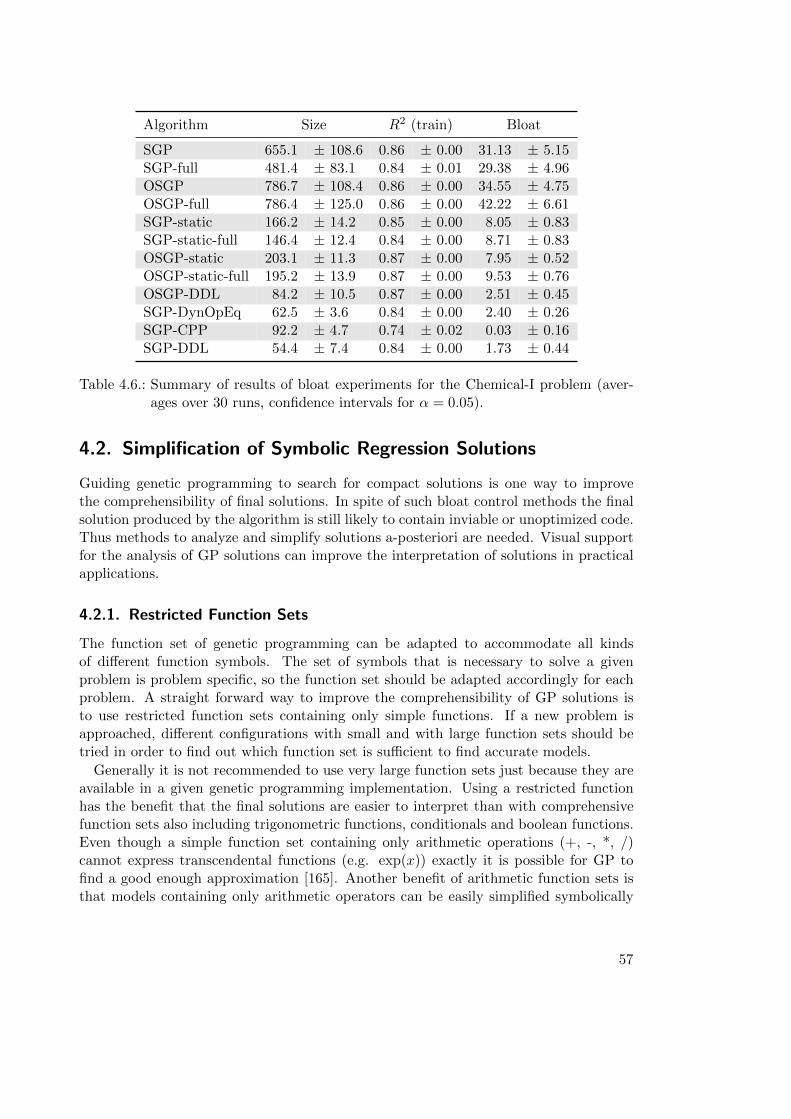
Algorithm Size R2 (train) Bloat

SGP 655.1 ± 108.6 0.86 ± 0.00 31.13 ± 5.15SGP-full 481.4 ± 83.1 0.84 ± 0.01 29.38 ± 4.96OSGP 786.7 ± 108.4 0.86 ± 0.00 34.55 ± 4.75OSGP-full 786.4 ± 125.0 0.86 ± 0.00 42.22 ± 6.61SGP-static 166.2 ± 14.2 0.85 ± 0.00 8.05 ± 0.83SGP-static-full 146.4 ± 12.4 0.84 ± 0.00 8.71 ± 0.83OSGP-static 203.1 ± 11.3 0.87 ± 0.00 7.95 ± 0.52OSGP-static-full 195.2 ± 13.9 0.87 ± 0.00 9.53 ± 0.76OSGP-DDL 84.2 ± 10.5 0.87 ± 0.00 2.51 ± 0.45SGP-DynOpEq 62.5 ± 3.6 0.84 ± 0.00 2.40 ± 0.26SGP-CPP 92.2 ± 4.7 0.74 ± 0.02 0.03 ± 0.16SGP-DDL 54.4 ± 7.4 0.84 ± 0.00 1.73 ± 0.44

Table 4.6.: Summary of results of bloat experiments for the Chemical-I problem (aver-ages over 30 runs, confidence intervals for α = 0.05).

4.2. Simplification of Symbolic Regression Solutions

Guiding genetic programming to search for compact solutions is one way to improvethe comprehensibility of final solutions. In spite of such bloat control methods the finalsolution produced by the algorithm is still likely to contain inviable or unoptimized code.Thus methods to analyze and simplify solutions a-posteriori are needed. Visual supportfor the analysis of GP solutions can improve the interpretation of solutions in practicalapplications.

4.2.1. Restricted Function Sets

The function set of genetic programming can be adapted to accommodate all kindsof different function symbols. The set of symbols that is necessary to solve a givenproblem is problem specific, so the function set should be adapted accordingly for eachproblem. A straight forward way to improve the comprehensibility of GP solutions isto use restricted function sets containing only simple functions. If a new problem isapproached, different configurations with small and with large function sets should betried in order to find out which function set is sufficient to find accurate models.

Generally it is not recommended to use very large function sets just because they areavailable in a given genetic programming implementation. Using a restricted functionhas the benefit that the final solutions are easier to interpret than with comprehensivefunction sets also including trigonometric functions, conditionals and boolean functions.Even though a simple function set containing only arithmetic operations (+, -, *, /)cannot express transcendental functions (e.g. exp(x)) exactly it is possible for GP tofind a good enough approximation [165]. Another benefit of arithmetic function sets isthat models containing only arithmetic operators can be easily simplified symbolically

57

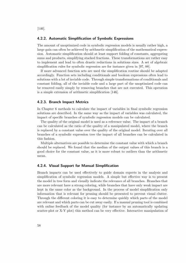
[146].

4.2.2. Automatic Simplification of Symbolic Expressions

The amount of unoptimized code in symbolic regression models is usually rather high, alarge gain can often be achieved by arithmetic simplification of the mathematical expres-sion. Automatic simplification should at least support folding of constants, aggregatingsums and products, simplifying stacked fractions. These transformations are rather easyto implement and lead to often drastic reductions in solutions sizes. A set of algebraicsimplification rules for symbolic regression are for instance given in [97, 88].

If more advanced function sets are used the simplification routine should be adaptedaccordingly. Function sets including conditionals and boolean expressions often lead tosolutions with a lot of inviable code. Through simple transformations of conditionals andconstant folding, all of the inviable code and a large part of the unoptimized code canbe removed easily simply by removing branches that are not executed. This operationis a simple extension of arithmetic simplification [146].

4.2.3. Branch Impact Metrics

In Chapter 6 methods to calculate the impact of variables in final symbolic regressionsolutions are described. In the same way as the impact of variables was calculated, theimpact of specific branches of symbolic regression models can be calculated.

The quality of the original model is used as a reference value. The impact of a branchcan be calculated as the ratio of the quality of a manipulated model, where the branchis replaced by a constant value over the quality of the original model. Iterating over allbranches of a symbolic expression tree the impact of all branches can be calculated inthis fashion.

Multiple alternatives are possible to determine the constant value with which a branchshould be replaced. We found that the median of the output values of this branch is agood choice for the constant value, as it is more robust to outliers than the arithmeticmean.

4.2.4. Visual Support for Manual Simplification

Branch impacts can be used effectively to guide domain experts in the analysis andsimplification of symbolic regression models. A simple but effective way is to presentthe model in tree form and visually indicate the relevance of all branches. Branches thatare more relevant have a strong coloring, while branches that have only weak impact arekept in the same color as the background. In the process of model simplification onlyinformation that is relevant for pruning should be presented to prevent visual clutter.Through the different coloring it is easy to determine quickly which parts of the modelare relevant and which parts can be cut away easily. If a manual pruning tool is combinedwith online feedback of the model quality (for instance by an automatically updatingscatter-plot or X-Y plot) this method can be very effective. Interactive manipulation of

58

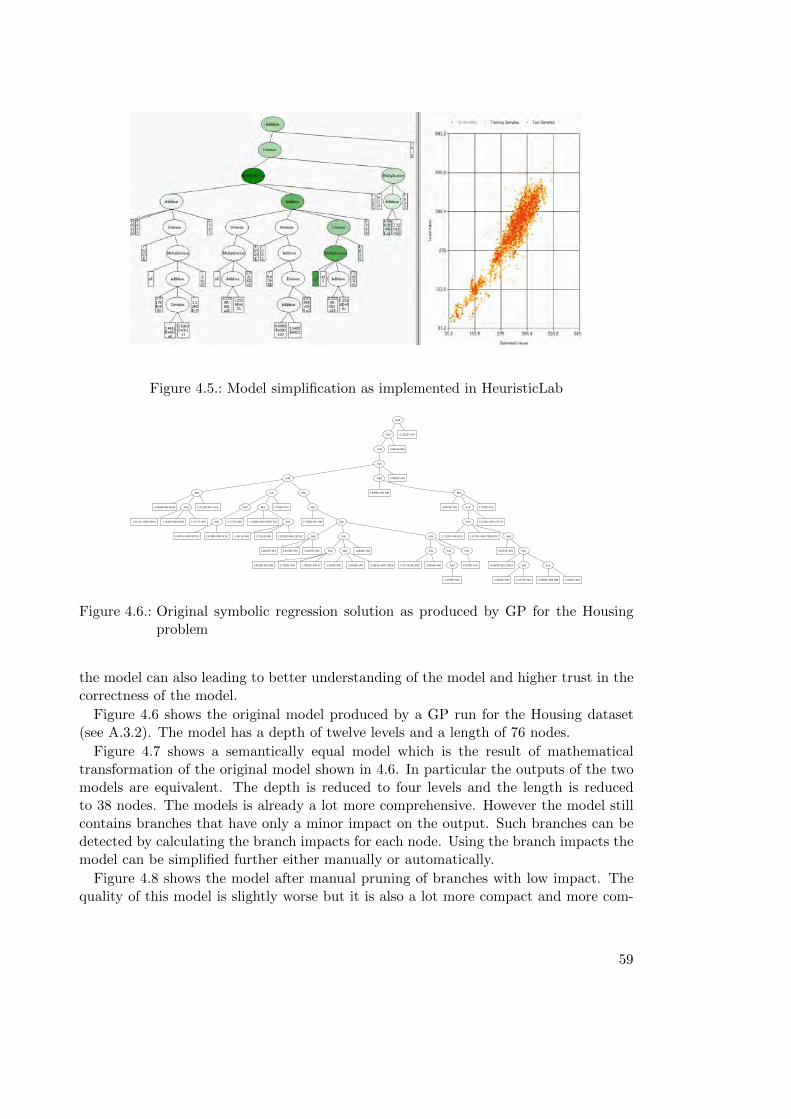
Figure 4.5.: Model simplification as implemented in HeuristicLab

Add

Mul -2.5822E+001

Add 4.4631E-006

Sub

Add Mul 5.9982E+001

Mul Sub Mul

6.9669E-001 NOX Add -2.7213E-002 AGE

1.9252E+000 CRIM 1.1042E+000 RAD 2.2277E+001

Add Mul 3.7502E+001

Mul

1.4907E+000 INDUS 2.4748E+000 NOX

4.1757E+001 1.4598E+000 PTRATIO Add

3.3415E+001 3.7161E+001 1.0239E+000 LSTAT

Mul

2.7506E-001 RM Sub

Mul Sub Add

3.4839E+001 5.8374E+001 5.4597E+001 Sub Mul 3.8446E+001

1.8526E-001 DIS 3.7339E+001 1.7003E+000 B 3.2430E+001 3.3008E+001 2.0425E+000 CHAS

Sub Sub Sub

5.3171E-002 DIS 3.0456E+001 Add

2.2799E+001

3.0350E+001

3.8909E-001 RM Mul

4.8073E+001 Sub 3.7205E+001

Add 1.3534E+000 LSTAT

2.7523E+000 AGE 1.4375E+000 PTRATIO Mul

3.6553E+001 Sub

6.0607E-002 CHAS Add Sub

2.5630E+001 5.1872E+001 3.5898E+000 RM 2.6426E+001

Figure 4.6.: Original symbolic regression solution as produced by GP for the Housingproblem

the model can also leading to better understanding of the model and higher trust in thecorrectness of the model.

Figure 4.6 shows the original model produced by a GP run for the Housing dataset(see A.3.2). The model has a depth of twelve levels and a length of 76 nodes.

Figure 4.7 shows a semantically equal model which is the result of mathematicaltransformation of the original model shown in 4.6. In particular the outputs of the twomodels are equivalent. The depth is reduced to four levels and the length is reducedto 38 nodes. The models is already a lot more comprehensive. However the model stillcontains branches that have only a minor impact on the output. Such branches can bedetected by calculating the branch impacts for each node. Using the branch impacts themodel can be simplified further either manually or automatically.

Figure 4.8 shows the model after manual pruning of branches with low impact. Thequality of this model is slightly worse but it is also a lot more compact and more com-

59

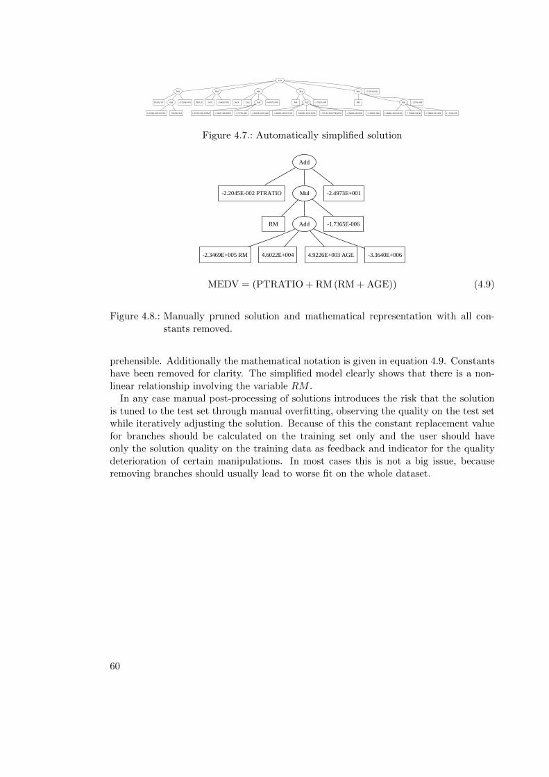
Add

Mul Mul Mul Mul Mul -2.5822E+001

PTRATIO Add -2.7206E-004

1.0239E+000 LSTAT 7.0576E+001

INDUS NOX 1.6465E-005 NOX AGE Add -8.4617E-008

1.9252E+000 CRIM 1.1042E+000 RAD 2.2277E+001

RM Add -1.7365E-006

4.9226E+003 AGE -2.4206E+003 LSTAT 3.9624E+003 CHAS 2.5711E+003 PTRATIO -2.3469E+005 RM -3.3393E+006

RM Add 1.2276E-006

2.1864E+003 CHAS 1.7003E+000 B -2.3843E-001 DIS 1.1119E+005

Figure 4.7.: Automatically simplified solution

Add

-2.2045E-002 PTRATIO Mul -2.4973E+001

RM Add -1.7365E-006

-2.3469E+005 RM 4.6022E+004 4.9226E+003 AGE -3.3640E+006

MEDV = (PTRATIO + RM(RM+AGE)) (4.9)

Figure 4.8.: Manually pruned solution and mathematical representation with all con-stants removed.

prehensible. Additionally the mathematical notation is given in equation 4.9. Constantshave been removed for clarity. The simplified model clearly shows that there is a non-linear relationship involving the variable RM .

In any case manual post-processing of solutions introduces the risk that the solutionis tuned to the test set through manual overfitting, observing the quality on the test setwhile iteratively adjusting the solution. Because of this the constant replacement valuefor branches should be calculated on the training set only and the user should haveonly the solution quality on the training data as feedback and indicator for the qualitydeterioration of certain manipulations. In most cases this is not a big issue, becauseremoving branches should usually lead to worse fit on the whole dataset.

60

5. Generalization in Genetic Programming

Overfitting means to train, estimate or select models which do not generalize well tonew observations. The effect can be observed when a model is applied to a dataset,which was not used in the training process and the fit on the new dataset is considerablyworse, even though the model has a good fit on the training data. Overfitting occurswhen a model is fit too tightly to the observations in the dataset in order to reducethe approximation error by increasing the complexity of the model. Observations in thetraining dataset are usually afflicted with a certain amount of noise. Thus, at a certainpoint the increased complexity is solely used to approximate random fluctuations in thedataset. This is counter-productive because at this point only the approximation erroron the observations in the dataset can be reduced, and the expected error of the model fornew observations increases. The model becomes useless for practical application. Thisleads to the problem of the well-known bias-variance trade-off in data-based modeling[83]

It is generally assumed that bloat and overfitting are related. However, it has beenrecently observed that overfitting can occur in absence of bloat, and vice versa. Thus, ithas been suggested that overfitting and bloat are two separate phenomenons in geneticprogramming [220], [190]. This suggests that overfitting and bloat should be controlledalso by separate mechanisms.

One way to reduce overfitting is to use an internal validation set on which all solutionsof the population are evaluated. A solution that has a comparable accuracy on thetraining and validation set is returned as the final result [73, 232, 231]. This approachcan been extended to a solution archive in which Pareto optimal (quality and size)solutions on the validation set are kept [193, 180]. The result of the GP run is the set ofsolutions in the archive. The advantage of this approach is that an appropriate modelcan be selected a-posteriori because all good solutions on the validation set, discoveredover the whole run, are available at the end. The problem of this approach is thatwithout parsimony pressure the set of good solutions on the validation set is more likelyto be extended at the end where the larger solutions are located. The chance that smallsolutions, which improve solutions which are already in the archive, are found in laterstages of a GP run diminishes through the bloat-effect.

Other approaches to control overfitting and improve generalization that are oftenused in statistical learning methods are based either on the estimation of the expectedgeneralization error or on penalization of overly complex models [83]. The first approachis to tune the algorithm parameters in iterative steps to find parameter settings whichresult in a model that generalizes well using an estimator for the expected generalizationerror of the model. The expected generalization error can be estimated using a hold-outset or through cross-validation. The second approach is to add a penalty term that

61

depends on the model complexity and optionally on the number of training samplesto the objective function that is minimized. This approach integrates directly into thetraining algorithm and produces a model with a good balance of training error andcomplexity.

In practice the approach of using a validation set has turned out to be a workingmethod to reduce the chance of choosing an overfit model [231]. The approach is simpleand practical but not very efficient. If overfitting occurs in the early stages of the GPrun a lot of effort is wasted evaluating solutions which are too complex, and often thesolution found in the initial stages is not improved over the rest of the GP run becausesearch concentrates on uninteresting areas of the search space.

A simple improvement is to introduce an early stopping criterion. If the best solutionon the validation set is not updated for a predetermined number of generations, thatGP run should be stopped. The basic idea is that starting a new GP run is more likelyto produce a better solution on the validation sets than continuing the current GP runwhich is already in an overfitting stage. The value for the number of generations withno improvement after which the run should be stopped must be hand-tuned, based onthe results observed in a few long running test runs. Setting this parameter can often bedifficult, because if new genetic diversity is brought into the population through mutationor migration, the overfitting effect is reduced and a new validation-best solution can befound.

If overfitting can be detected reliably in the process, this information could be usedeffectively to adjust the complexity of the search space. First it is necessary to define areliable measure for overfitting that can be calculated in a GP run. Then an effectivescheme which acts as a complexity reducer, can be used which gradually moves the pop-ulation into a non-overfitting solution space again. Gradual slow changes are preferredbecause a sudden change in complexity reduction for instance through exhaustive prun-ing of the whole population is likely to cause a significant loss in genetic diversity andmight lead to premature convergence of the process.

The general setup should lead the process to search for solutions which perform equallywell on the training and validation set. Contrary to the ambitions followed in 4 in thissetup the maximal complexity of solutions is not constrained and there is generally nobias to search for compact solutions. Instead, as long as no overfitting occurs, the algo-rithm is allowed to generate more and more complex solutions. Most countermeasuresagainst bloat discussed in the previous chapter can be combined with countermeasuresagainst overfitting. Both phenomenons should be treated by specific countermeasures.Bloat can be controlled through size limits or parsimony pressure, and overfitting canbe reduced through validation and complexity reduction.

5.1. How to Detect Overfitting in GP

If an internal validation set is available then the validation set can be used to efficientlydetect overfitting on the training set. Each solution candidate in a population is alsoevaluated on the validation set. So for each solution candidate two fitness values are

62

calculated, namely ftraining and fvalidation. Only the fitness on the training set is used forselection, so the fitness on the validation set can be used to detect when overfitting occurs.An indicator for overfitting is when the average or best validation fitness decreases, whilethe average or best training fitness is increased. A simple boolean function for overfittingat generation g based on this principle is 5.1. This metric returns true if the movingaverage of the average validation fitness MAk(fval, g) over the previous k generations atgeneration g decreases by more than a given ratio p over k generations.

MAk(fval, g) =1

k

k∑

i=1

fval(g − i)

Thresholdk(fval, g, p) = (1− p)fval(g − k)

Overfitting(g)p,k =

{true if MAk(fval, g) < Thresholdk(fval, g, p)

false otherwise

(5.1)

The problem with this overfitting detection function is that there is a rather largedelay between the time when the algorithm actually starts to overfit and the time whenthe decrease in average fitness quality is detected. When overfitting is detected, italready caused a significant decrease in validation fitness, which means that the solutioncandidates in the whole population are already rather overfit. It is however not so easyto recognize overfitting earlier with this detection function as a minimal k is necessaryto make the function robust against minor variations in average validation fitness.

Another issue with this function is that when it is used in combination with a complex-ity reduction method, the point at which overfitting does not occur anymore is difficultto detect, because the average validation quality also is decreased together with theaverage training quality when the complexity reduction mechanism is applied.

An alternative way to detect overfitting that is presented for the first time in thiswork is based on the correlation of training fitness and validation fitness of solutioncandidates in the population at generation g 5.2. Intuitively, if no overfitting occurs,the validation fitness of solution candidates should be strongly correlated to the trainingfitness. Solution candidates with larger training fitness are more likely to be selectedfor recombination, so ideally such solution candidates should also have a high validationfitness. Solution candidates that have low training fitness should also have low validationfitness. If the correlation of training and validation fitness is high, the selection pressureimplicitly leads to solutions that have better training and validation fitness. In contrast,if the correlation of training and validation fitness is low, the selection pressure will leadto solution candidates that are better only in respect to training fitness, and the chanceto create solutions with lower validation fitness increases.

In our experiments we used Spearman’s rank correlation ρ [196] and an alpha valuein the range 0.5 – 0.8.

Overfitting(g)α =

{true if ρ(ftraining(g), fvalidation(g)) < α

false otherwise(5.2)

63

The correlation-based overfitting detection function indicates very early when theprocess starts to overfit. If the correlation value is low in the current generation theselection pressure causes a decrease in validation quality in the next generation. Becauseof this, any countermeasure for overfitting can be applied in early stages when thepopulation does not yet contain a large number of overfit solution candidates.

A drawback of the correlation-based overfitting detection function is, that the fitnesscorrelation is also low when under-fitting occurs, because in this situation the trainingfitness values are rather similar and a high training fitness is not necessarily related toa high validation fitness.

The fitness correlation is also low, if the population is converged to a small set ofsolution candidates with similar fitness values. In this situation the correlation is lowbecause the spread of fitness values is small, thus small deviations in validation qualitystart to have a larger effect on the correlation value. Additionally, if the population isconverged to a small set of solution candidates, the number of different fitness values istoo small for the correlation coefficient to be significant.

The effect of any overfitting countermeasure can be measured with the same overfittingdetection function. An effective countermeasure should lead to an increase in the fitnesscorrelation value. Any overfitting countermeasure should not introduce strong biases orsudden changes in the search process, otherwise there is a risk of premature convergenceor directing the process into under-fitting. If the interference is too strong the processcould jump from an overfitting stage to under-fitting within just one generation and itwould be impossible to detect that there was a state change with the correlation basedoverfitting detection function.

5.2. Countermeasures Against Overfitting

5.2.1. Restarts

If overfitting occurs in a run a pragmatic approach is to stop the current run and startanother run. This assumes that a good solution has already been found and that it isunlikely to improve the current best solution by continuing the run which is already in anoverfitting stage. Finally after a maximum number of restarts one of the final solutionsis selected as the overall result. Selection of the final result should be based on overallfitness on training and validation set and ideally combine with a complexity metric toprefer more compact models.

Instead of starting a new completely independent run with the same algorithm config-uration an adaptive approach could be more effective. Decreasing the maximally allowedprogram size or the maximal size of trees in the initial generation with each run shoulddelay the overfitting stage. Alternatively gradually reducing the selection pressure witheach restart for instance through reduction of the tournament group size should alsodelay the overfitting stage as the evolutionary process improves the training fitness moreslowly.

64

5.2.2. Parsimony Pressure Against Overfitting

Overfitting can be reduced by reducing the complexity of solution candidates in the pop-ulation. Intuitively, the complexity of solution candidates can be removed by reducingthe average program length in the population. Parsimony pressure increases the prob-ability of selection of smaller individuals by adjusting the fitness value of solutions tointegrate the solution complexity. Covariant parsimony pressure [163] (also see previousChapter 4) is an elegant way to dynamically adapt the parsimony pressure coefficient inorder to tightly control the average program length over the GP run.

It has already been suggested by Poli and McPhee in [163] to dynamically turn co-variant parsimony pressure on and off at specific stages of the GP run. This suggestionis taken up in this work to introduce a novel approach to reduce overfitting. If a ro-bust overfitting detection function like the on explained in Section 5.1 is available, itis possible to use covariant parsimony pressure to gradually decrease the average pro-gram length to a point where no overfitting occurs. When the algorithm is back in anon-overfitting stage parsimony pressure can be turned off again. In this way the evo-lutionary process can freely increase the solution complexity to a level that is necessaryto solve the problem and limit the complexity from above as soon as the process startsto overfit.

Again, the parsimony pressure should be configured in such a way to reduce the averageprogram length only slowly. If parsimony pressure is applied too strongly there is therisk that the program length becomes the attribute that determines selection probability.This can happen for instance by forcing the average program size to a certain level whichis a lot smaller than the current average program size. In such cases the adjusted fitnessvalues are strongly correlated to the program length instead of program raw fitness andthe evolutionary process will be mainly driven by the program length.

In the results section the results of the experiments with covariant parsimony pressureto counter overfitting are shown in Figure 5.3.

5.2.3. Pruning Against Overfitting

Pruning of GP solutions has been discussed already in the previous section. Pruning canalso be used against overfitting. The idea is based on the hypothesis that the overfittingbehavior is caused by small code fragments which have only a small positive impacton the training fitness but a large negative impact on the validation set and that thesecode fragments are spatially grouped. Such branches can be removed selectively bepruning operations. Pruning cannot be effective if the overfitting effect is caused bycode fragments which are scattered over the whole program.

The effect of pruning is that code fragments which have no impact or only small impacton the program output are removed. The original intention of pruning is to create morecompact final solutions or when used in the GP process to remove bloated code fromthe population in order to make room for effective code fragments. If overfitting iscaused by small spatially grouped code fragments which only have a small impact onthe program output pruning should remove exactly those code fragments and reduce

65

overfitting. Pruning operations which cause a slight deterioration in fitness should bepossible and removal of smaller branches should be preferred.

If softening the distinction between the training and validation dataset partitions isallowed, the pruning operation can be changed to calculate the fitness deterioration onthe validation fitness instead of the training fitness. This is meaningful for the applicationof pruning against overfitting because the branches responsible for bad validation fitnesscan be easily and robustly identified if the validation fitness is used to evaluate the effectof branch removal. Pruning operations can be applied very selectively only removingbranches which actually decrease validation fitness. The drawback of this is that thevalidation dataset is used not only as an indicator for overfitting. Instead, the validationfitness has a direct impact on solution candidates in the population and so also has anequally strong effect on the evolutionary process as the training fitness. This leads to therisk that the process produces solutions which are overfit on the combination of trainingand validation fitness. This cannot be detected through observation of the trajectory ofthe fitness on the validation set.

Similarly to parsimony pressure, pruning can be integrated into the GP process as astep after evaluation of the current generation. If the overfitting detection function indi-cates that the process is in an overfitting stage all individuals of the current generationare pruned and evaluated. Only after this optional pruning step the next generation ofthe population is generated as usual.

Pruning reduces the genetic diversity in the population and should be applied onlyvery carefully. Many different ways of pruning are possible [232], but in this work we onlyuse a simple greedy pruning variant for symbolic expression tree encoding (see Algorithm5). An effective pruning method should guarantee that the necessary building blocks ofgood solutions are kept unchanged and that code fragments are removed in such a wayto make it possible to create new solution candidates of similar or better fitness.

In the previous section it has been shown that pruning can be used to control bloat.In this situation it often makes sense to prune only a part of the population, excludingthe very best individuals. This is, however, not recommended if pruning is used againstoverfitting, because the best individuals of the population are more likely to be over-fit. The best individuals also should be pruned. Simply pruning all individuals of thepopulation without exceptions worked well in our experiments.

5.3. Experiments

To analyze and compare the effects of different anti-overfitting methods we used twodatasets, on which SGP and OSGP produced overfit solutions. The first dataset is theBoston Housing dataset (see Section A.3.2). The second dataset is the Chemical-I dataset(see Section A.3.2). To show the overfitting behavior we evaluated all individuals of thepopulation also on a test set in each generation. In this set of experiments the datasetshave been partitioned into training-, validation- and hold-out set. Only the training setis used to calculate the fitness. The validation set is used to calculate the correlationof training- and validation fitness. The validation fitness is used by the algorithm only

66

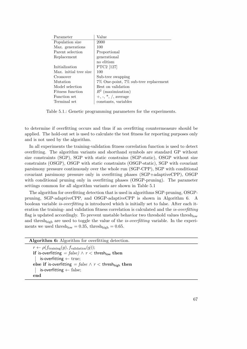
Parameter ValuePopulation size 2000Max. generations 100Parent selection ProportionalReplacement generational

no elitismInitialization PTC2 [127]Max. initial tree size 100Crossover Sub-tree swappingMutation 7% One-point, 7% sub-tree replacementModel selection Best on validationFitness function R2 (maximization)Function set +, -, *, /, averageTerminal set constants, variables

Table 5.1.: Genetic programming parameters for the experiments.

to determine if overfitting occurs and thus if an overfitting countermeasure should beapplied. The hold-out set is used to calculate the test fitness for reporting purposes onlyand is not used by the algorithm.

In all experiments the training-validation fitness correlation function is used to detectoverfitting. The algorithm variants and shorthand symbols are standard GP withoutsize constraints (SGP), SGP with static constrains (SGP-static), OSGP without sizeconstraints (OSGP), OSGP with static constraints (OSGP-static), SGP with covariantparsimony pressure continuously over the whole run (SGP-CPP), SGP with conditionalcovariant parsimony pressure only in overfitting phases (SGP+adaptiveCPP), OSGPwith conditional pruning only in overfitting phases (OSGP-pruning). The parametersettings common for all algorithm variants are shown in Table 5.1

The algorithm for overfitting detection that is used in algorithms SGP-pruning, OSGP-pruning, SGP-adaptiveCPP, and OSGP-adaptiveCPP is shown in Algorithm 6. Aboolean variable is-overfitting is introduced which is initially set to false. After each it-eration the training- and validation fitness correlation is calculated and the is-overfittingflag is updated accordingly. To prevent unstable behavior two threshold values threshlowand threshhigh are used to toggle the value of the is-overfitting variable. In the experi-ments we used threshlow = 0.35, threshhigh = 0.65.

Algorithm 6: Algorithm for overfitting detection.

r ← ρ(ftraining(g), fvalidation(g));if is-overfitting = false) ∧ r < threshlow then

is-overfitting ← true;else if is-overfitting = false ∧ r < threshhigh then

is-overfitting ← false;end

67

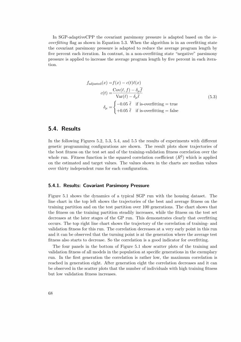
In SGP-adaptiveCPP the covariant parsimony pressure is adapted based on the is-overfitting flag as shown in Equation 5.3. When the algorithm is in an overfitting statethe covariant parsimony pressure is adapted to reduce the average program length byfive percent each iteration. In contrast, in a non-overfitting state “negative” parsimonypressure is applied to increase the average program length by five percent in each itera-tion.

fadjusted(x) =f(x)− c(t)`(x)

c(t) =Cov(`, f)− δµf

Var(`)− δµ`

δµ =

{−0.05 ` if is-overfitting = true

+0.05 ` if is-overfitting = false

(5.3)

5.4. Results

In the following Figures 5.2, 5.3, 5.4, and 5.5 the results of experiments with differentgenetic programming configurations are shown. The result plots show trajectories ofthe best fitness on the test set and of the training-validation fitness correlation over thewhole run. Fitness function is the squared correlation coefficient (R2) which is appliedon the estimated and target values. The values shown in the charts are median valuesover thirty independent runs for each configuration.

5.4.1. Results: Covariant Parsimony Pressure

Figure 5.1 shows the dynamics of a typical SGP run with the housing dataset. Theline chart in the top left shows the trajectories of the best and average fitness on thetraining partition and on the test partition over 100 generations. The chart shows thatthe fitness on the training partition steadily increases, while the fitness on the test setdecreases at the later stages of the GP run. This demonstrates clearly that overfittingoccurs. The top right line chart shows the trajectory of the correlation of training- andvalidation fitness for this run. The correlation decreases at a very early point in this runand it can be observed that the turning point is at the generation where the average testfitness also starts to decrease. So the correlation is a good indicator for overfitting.

The four panels in the bottom of Figure 5.1 show scatter plots of the training andvalidation fitness of all models in the population at specific generations in the exemplaryrun. In the first generation the correlation is rather low, the maximum correlation isreached in generation eight. After generation eight the correlation decreases and it canbe observed in the scatter plots that the number of individuals with high training fitnessbut low validation fitness increases.

68

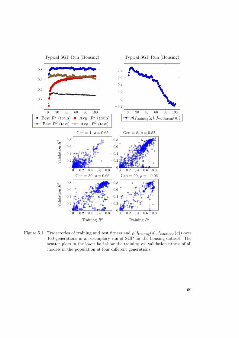
0 20 40 60 80 100

0

0.2

0.4

0.6

0.8

Typical SGP Run (Housing)

Best R2 (train) Avg. R2 (train)

Best R2 (test) Avg. R2 (test)

0 20 40 60 80 100

−0.2

0

0.2

0.4

0.6

0.8

Typical SGP Run (Housing)

ρ(ftraining(g), fvalidation(g))

0 0.2 0.4 0.6 0.80

0.2

0.4

0.6

0.8

ValidationR

2

Gen = 1, ρ = 0.65

0 0.2 0.4 0.6 0.80

0.2

0.4

0.6

0.8

Gen = 8, ρ = 0.82

0 0.2 0.4 0.6 0.80

0.2

0.4

0.6

0.8

Training R

2

ValidationR

2

Gen = 30, ρ = 0.66

0 0.2 0.4 0.6 0.80

0.2

0.4

0.6

0.8

Training R

2

Gen = 90, ρ = −0.06

Figure 5.1.: Trajectories of training and test fitness and ρ(ftraining(g), fvalidation(g)) over100 generations in an exemplary run of SGP for the housing dataset. Thescatter plots in the lower half show the training vs. validation fitness of allmodels in the population at four different generations.

69

0 20 40 60 80 100

0.2

0.3

0.4

0.5

Best Test Quality (Chemical-I)

0 20 40 60 80 100

0.3

0.4

0.5

0.6

0.7

Best Test Quality (Housing)

0 20 40 60 80 100

−0.2

0

0.2

0.4

Correlation (Chemical-I)

0 20 40 60 80 100

−0.2

0

0.2

0.4

0.6

0.8

Correlation (Housing)

SGP OSGP

Figure 5.2.: Overfitting behavior of SGP and OSGP without size limits and withoutoverfitting control.

5.4.2. Results: SGP and OSGP

Figure 5.2 shows the best test quality and the correlation between training and validationquality for standard GP and GP with offspring selection for two different problems. Inthis first set of experiments no limits have been set for either program length or depth.For the Chemical-I dataset SGP does not overfit but with offspring selection overfittingoccurs in the late stage of the run. For the Housing dataset both algorithms overfit.The correlation between training and validation quality is low for both problems and forboth algorithms. OSGP has a lower correlation value in both cases.

Figure 5.3 shows the results of SGP and OSGP with static limits and SGP with co-variant parsimony pressure. For SGP-static and OSGP-static the static limit programlength is 250 nodes and the depth limit is 17 levels. SGP-CPP is configured to keepthe average program length at 100 nodes over the whole run through covariant parsi-mony pressure. OSGP-static overfits for both problems. SGP-static overfits only onthe Housing problem. SGP-CPP works best but still overfits on the Housing problem.

70

0 20 40 60 80 100

0.2

0.3

0.4

0.5

0.6

Best Test Quality (Chemical-I)

0 20 40 60 80 100

0.5

0.6

0.7

Best Test Quality (Housing)

0 20 40 60 80 100

−0.2

0

0.2

0.4

0.6

0.8

Correlation (Chemical-I)

0 20 40 60 80 100

−0.2

0

0.2

0.4

0.6

0.8

Correlation (Housing)

SGP-static OSGP-static SGP-CPP

Figure 5.3.: Overfitting behavior of SGP-static, OSGP-static, and SGP-CPP withoutoverfitting control.

The correlation of training and validation fitness is again very low for OSGP-static butrelatively high for SGP-static and SGP-CPP.

5.4.3. Results: Adaptive CPP and Overfitting-triggered Pruning

Figure 5.4 shows the best test quality and training-validation correlation for SGP withoverfitting detection and adaptive covariant parsimony pressure and SGP with over-fitting-triggered pruning. For comparison the values for SGP without size constraintsare also shown in the same plots. For the Chemical-I problem the target range forthe correlation value was 0.45 – 0.65. For the Housing problem a range of 0.45 – 0.75was used. The plots of the training-validation correlation show that both methods,pruning and adaptive parsimony pressure successfully steered the algorithm to keepthe correlation in the target range. For the Chemical-I problem no overfitting can beobserved and both variants lead to better solution quality on the test set. For theHousing problem minor overfitting can be observed but both variants are better than

71

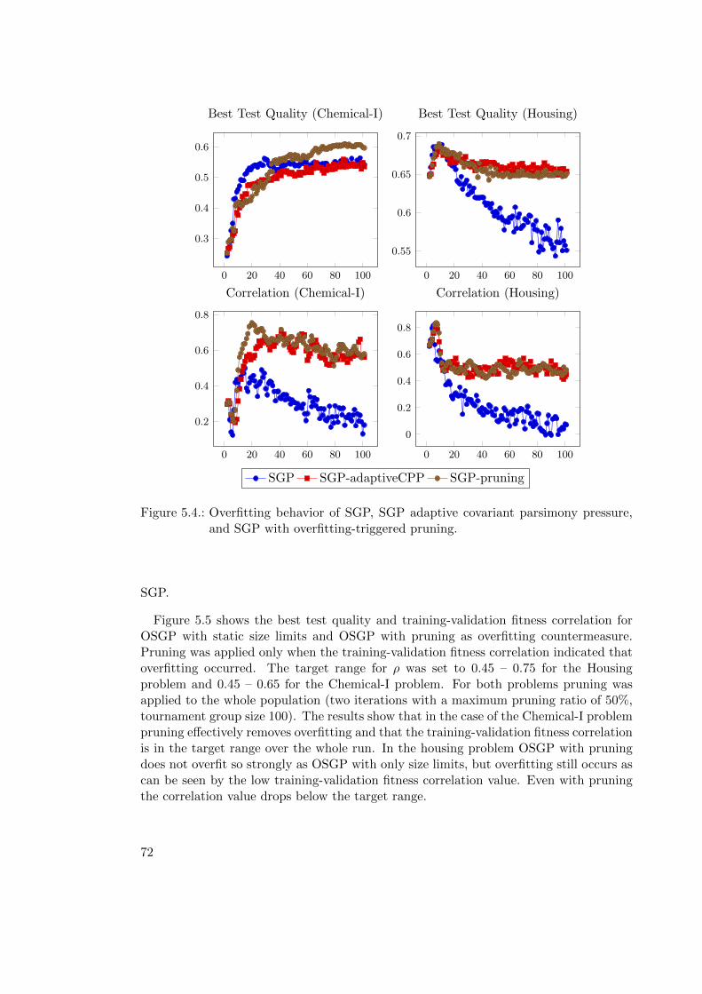
0 20 40 60 80 100

0.3

0.4

0.5

0.6

Best Test Quality (Chemical-I)

0 20 40 60 80 100

0.55

0.6

0.65

0.7

Best Test Quality (Housing)

0 20 40 60 80 100

0.2

0.4

0.6

0.8

Correlation (Chemical-I)

0 20 40 60 80 100

0

0.2

0.4

0.6

0.8

Correlation (Housing)

SGP SGP-adaptiveCPP SGP-pruning

Figure 5.4.: Overfitting behavior of SGP, SGP adaptive covariant parsimony pressure,and SGP with overfitting-triggered pruning.

SGP.

Figure 5.5 shows the best test quality and training-validation fitness correlation forOSGP with static size limits and OSGP with pruning as overfitting countermeasure.Pruning was applied only when the training-validation fitness correlation indicated thatoverfitting occurred. The target range for ρ was set to 0.45 – 0.75 for the Housingproblem and 0.45 – 0.65 for the Chemical-I problem. For both problems pruning wasapplied to the whole population (two iterations with a maximum pruning ratio of 50%,tournament group size 100). The results show that in the case of the Chemical-I problempruning effectively removes overfitting and that the training-validation fitness correlationis in the target range over the whole run. In the housing problem OSGP with pruningdoes not overfit so strongly as OSGP with only size limits, but overfitting still occurs ascan be seen by the low training-validation fitness correlation value. Even with pruningthe correlation value drops below the target range.

72

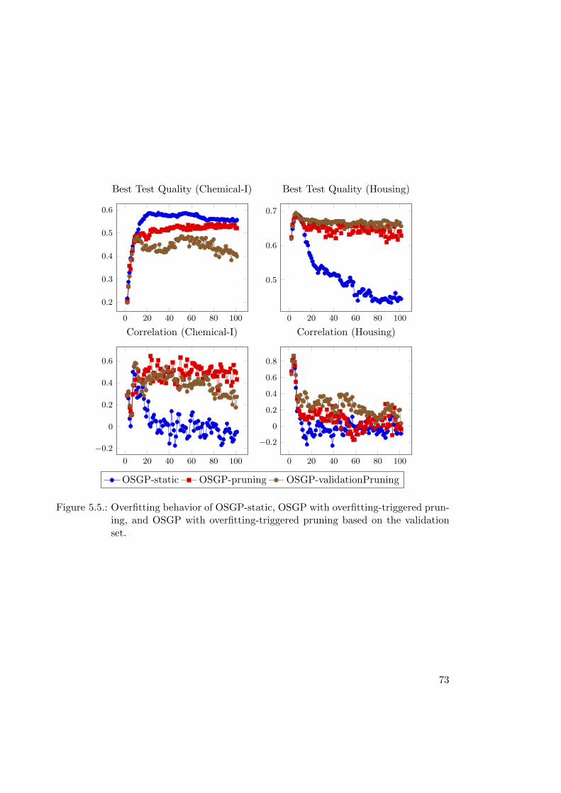
0 20 40 60 80 100

0.2

0.3

0.4

0.5

0.6

Best Test Quality (Chemical-I)

0 20 40 60 80 100

0.5

0.6

0.7

Best Test Quality (Housing)

0 20 40 60 80 100

−0.2

0

0.2

0.4

0.6

Correlation (Chemical-I)

0 20 40 60 80 100

−0.2

0

0.2

0.4

0.6

0.8

Correlation (Housing)

OSGP-static OSGP-pruning OSGP-validationPruning

Figure 5.5.: Overfitting behavior of OSGP-static, OSGP with overfitting-triggered prun-ing, and OSGP with overfitting-triggered pruning based on the validationset.

73

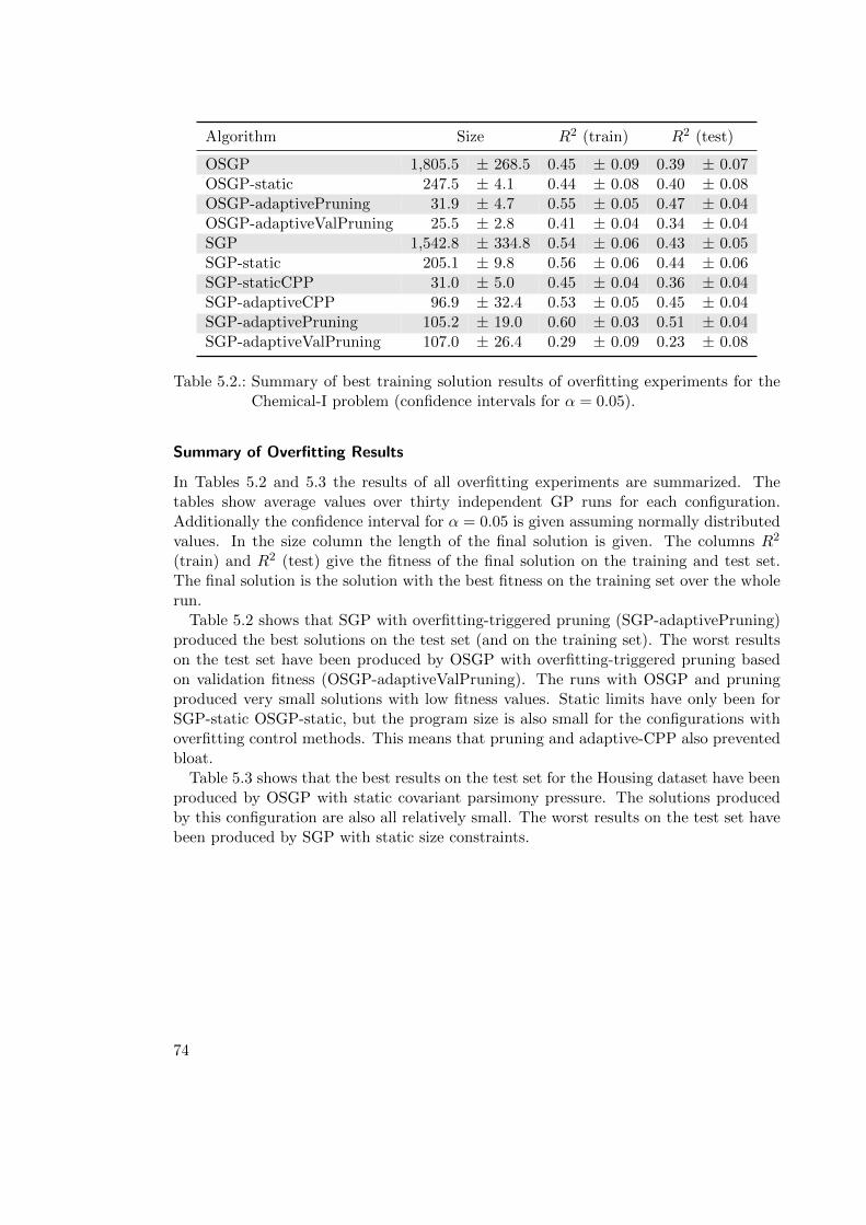
Algorithm Size R2 (train) R2 (test)

OSGP 1,805.5 ± 268.5 0.45 ± 0.09 0.39 ± 0.07OSGP-static 247.5 ± 4.1 0.44 ± 0.08 0.40 ± 0.08OSGP-adaptivePruning 31.9 ± 4.7 0.55 ± 0.05 0.47 ± 0.04OSGP-adaptiveValPruning 25.5 ± 2.8 0.41 ± 0.04 0.34 ± 0.04SGP 1,542.8 ± 334.8 0.54 ± 0.06 0.43 ± 0.05SGP-static 205.1 ± 9.8 0.56 ± 0.06 0.44 ± 0.06SGP-staticCPP 31.0 ± 5.0 0.45 ± 0.04 0.36 ± 0.04SGP-adaptiveCPP 96.9 ± 32.4 0.53 ± 0.05 0.45 ± 0.04SGP-adaptivePruning 105.2 ± 19.0 0.60 ± 0.03 0.51 ± 0.04SGP-adaptiveValPruning 107.0 ± 26.4 0.29 ± 0.09 0.23 ± 0.08

Table 5.2.: Summary of best training solution results of overfitting experiments for theChemical-I problem (confidence intervals for α = 0.05).

Summary of Overfitting Results

In Tables 5.2 and 5.3 the results of all overfitting experiments are summarized. Thetables show average values over thirty independent GP runs for each configuration.Additionally the confidence interval for α = 0.05 is given assuming normally distributedvalues. In the size column the length of the final solution is given. The columns R2

(train) and R2 (test) give the fitness of the final solution on the training and test set.The final solution is the solution with the best fitness on the training set over the wholerun.

Table 5.2 shows that SGP with overfitting-triggered pruning (SGP-adaptivePruning)produced the best solutions on the test set (and on the training set). The worst resultson the test set have been produced by OSGP with overfitting-triggered pruning basedon validation fitness (OSGP-adaptiveValPruning). The runs with OSGP and pruningproduced very small solutions with low fitness values. Static limits have only been forSGP-static OSGP-static, but the program size is also small for the configurations withoverfitting control methods. This means that pruning and adaptive-CPP also preventedbloat.

Table 5.3 shows that the best results on the test set for the Housing dataset have beenproduced by OSGP with static covariant parsimony pressure. The solutions producedby this configuration are also all relatively small. The worst results on the test set havebeen produced by SGP with static size constraints.

74

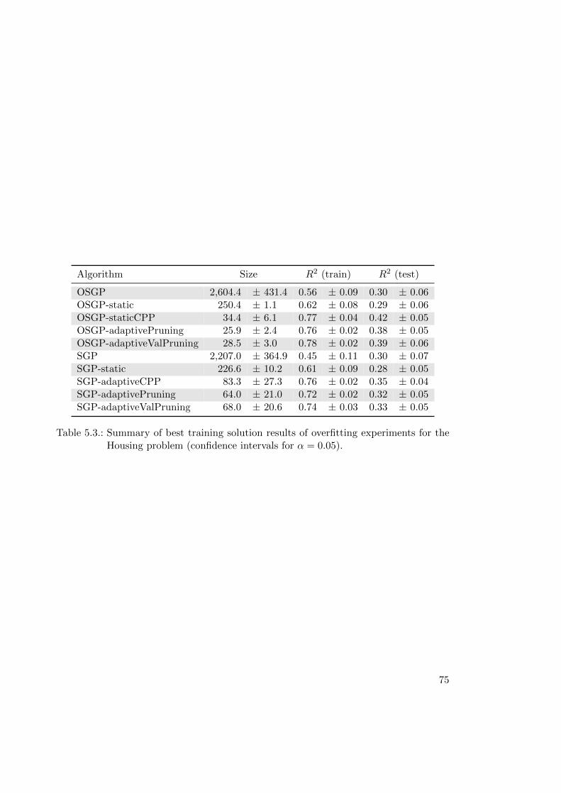
Algorithm Size R2 (train) R2 (test)

OSGP 2,604.4 ± 431.4 0.56 ± 0.09 0.30 ± 0.06OSGP-static 250.4 ± 1.1 0.62 ± 0.08 0.29 ± 0.06OSGP-staticCPP 34.4 ± 6.1 0.77 ± 0.04 0.42 ± 0.05OSGP-adaptivePruning 25.9 ± 2.4 0.76 ± 0.02 0.38 ± 0.05OSGP-adaptiveValPruning 28.5 ± 3.0 0.78 ± 0.02 0.39 ± 0.06SGP 2,207.0 ± 364.9 0.45 ± 0.11 0.30 ± 0.07SGP-static 226.6 ± 10.2 0.61 ± 0.09 0.28 ± 0.05SGP-adaptiveCPP 83.3 ± 27.3 0.76 ± 0.02 0.35 ± 0.04SGP-adaptivePruning 64.0 ± 21.0 0.72 ± 0.02 0.32 ± 0.05SGP-adaptiveValPruning 68.0 ± 20.6 0.74 ± 0.03 0.33 ± 0.05

Table 5.3.: Summary of best training solution results of overfitting experiments for theHousing problem (confidence intervals for α = 0.05).

75

6. Genetic Programming and Data Mining

6.1. Genetic Programming

Genetic programming as a general problem solving meta-heuristic is especially suitablefor data mining tasks. The foremost goal of data mining is to find interesting patterns inlarge datasets which lead to the discovery of knowledge. The most important propertyof GP in the data mining aspect is that it produces interpretable white box models. Thisis an important factor to make knowledge discovery from GP models feasible. Anotheressential property of GP in the data mining aspect is that it simultaneously evolvesthe structure of the model and the parameters of the model. When mining data, thenecessary complexity and structure of models is usually not known a priory. To thecontrary the structure and complexity of the model should be a result of data mining,leading to knowledge about the inherent complexity in the data.

6.1.1. Flexible Model Representation

Genetic programming can be adapted easily to search for different kinds of patterns.This work concentrates mainly on regression and time series forecasting. In these datamining tasks, patterns are usually symbolic functional expressions which relate the inputvariables to the target variable. For binary classification tasks the pattern is often adiscriminant function, which is again just a symbolic functional expression. Class labelsare generated by wrapping the discriminant function into a function which determines theclass label based on the output of the discriminant function and a class separator value.For classification tasks another commonly used pattern structure is a set of conditionalif-then rules. This structure is often preferred because it is more interpretable [70].Enforcing that the structure of the GP solutions is a set of if-then rules is differentthan simply adding conditionals to the function set. Conditional functions can also beuseful in regression models, but usually the models are not restricted to a set of if-thenrules. Genetic programming can be adapted to evolve all kinds of different patterns byconfiguration of the symbol set. In grammar-based GP systems the pattern structurecan be specified more rigidly by defining a grammar for pattern expressions. In strongly-typed GP systems the pattern structure can be restricted by specifying type-constraintson symbols.

6.1.2. Implicit Feature Selection

A frequent task in data mining is the identification of relevant variables or feature se-lection. Usually, a large set of variables is available to describe a given fact, however, it

77

is assumed that only a subset of these variables is actually relevant. Determining thissubset of relevant variables has several advantages. First of all information about therelevant variables is valuable in itself. Although there are no details about the relationof the input variables to the target variable (e.g. positive or negative effect), the set ofimportant variables is easy to understand and can already increase knowledge consid-erably. Additionally, in subsequent modeling steps one can concentrate on explainingeffects of the relevant variables on the target variable in detail, and the resulting modelsare easier to understand and less prone to overfitting.

Determining the subset of relevant variables is usually non-trivial, especially whenthere are non-linear or conditional relations. Implicit dependencies in the variables alsomake this task more difficult, as this ultimately leads to multiple sets of different variableswhich are equally plausible.

Feature selection is absolutely necessary for high-dimensional datasets where the num-ber of variables exceeds the number of observations (p >> N). Such problems have be-come increasingly important lately and frequently occur in bio-informatics. For instancein the analysis of micro-array datasets the number of observations is often small (around50), however, one observation includes measurements of many thousands of variables.In such situations it is often possible to find correlated variables by pure chance, eventhough the variables are actually independent. Thus, overfitting and feature selectionare important topics in such applications. The models are often strongly regularized inorder to avoid overfitting. Additionally, it is necessary to rigorously assert the validity ofmodels and training algorithms through methods like cross-validation and hold-out sets,and by calculating confidence intervals and statistical significance for results. The intri-cacies of high-dimensional problems have spurred the development of various specializeddata-analysis algorithms (cf. [83]). In this work this topic is not further discussed,instead we concentrate on data-analysis problems where the number of observations ex-ceeds the number of variables (N >> p). Such problems frequently occur in the analysisof technical systems.

In genetic programming feature selection is implicit because fitness-based selection hasthe effect, that models, which contain relevant variables, are more likely to be included inthe next generation. Over many generations this causes a genetic drift so that referencesto relevant variables are more frequent than references to irrelevant variables. It has beenshown that GP is even applicable for feature selection problems with many variables butonly few observations [114]. The implicit feature selection of genetic programming alsoremoves variables which are pairwise strongly correlated but irrelevant for the targetvariable. However, if correlated variables also affect the target variable value, GP doesnot recognize that one of the variables can be removed, and it keeps both correlatedvariables.

6.1.3. Non-Determinism

While GP has some advantages that make it an ideal method for data mining there arealso some obvious disadvantages that need to be addressed appropriately. One disad-vantage of GP is that it is a non-deterministic method. Solving the same problem with

78

the same parameter settings multiple times with GP produces multiple different models.Even though GP is a global search method there is no guarantee that a single GP runwill produce a result that is at a global optimum. The final solutions of different runshave a different output response but, which is even more crucial, also often have a dif-ferent structure. The virtually infinite solution space of genetic programming combinedwith the non-deterministic search are the main reasons for this effect. Such effects aremagnified, if the dataset contains variables which are interrelated. If this is the caseGP will produce diverse solutions, using different sets of variables to model the sameresponse of the underlying system. All this leads to the problem that, if the solutionsof multiple GP runs are analyzed they are not only different in accuracy but also instructure, which input variables are used and which input variables have a strong effecton the model output. This reduces the trust in the models and the method, and theknowledge that can be gained from such a set of solutions is rather limited.

The power to find diverse solutions of good quality, if multiple equivalent solutionsare possible, can also be seen as a virtue of genetic programming in comparison todeterministic methods which produce the same model each time even if alternative for-mulations are possible. The problem is rather to extract the interesting information outof a large solution set produced by GP. A method is needed which analyzes the solutionset and extracts which parts are common to many solutions and which parts can be usedinterchangeably because alternative formulations are possible.

6.1.4. Training Performance

Another disadvantage of GP is that it is rather slow compared to other non-linear datamining methods. However, this is often not an issue, as the time spent for data miningis only a small part of the time spent in the whole process of knowledge discovery fromdatabases. The data mining task can easily take a few days; however, the analysis ofresults produced in this step often takes much longer. Genetic programming and all othermethods from the family of evolutionary algorithms additionally have the advantage,that they are embarrassingly easy to parallelize, as the population-based concept allowsindependent and potentially concurrent evaluation of solutions.

In any case, the factor that as many interesting patterns as possible should be un-covered is more important than the time spent to find the patterns. The fact that GPproduces white box models and interpretable results reduces the effort that is necessaryin the result analysis step.

6.1.5. Predictive Accuracy

An advantage of symbolic regression is that the resulting models are simple mathematicalexpressions. Thus, it is possible to analyze the structure of the model and the variableinterrelations expressed in the model in detail. This is often helpful for model validationor to gain knowledge about previously unknown variable interrelations. The drawbackis that simple models usually produce less accurate approximations than more complexmodels, as for instance produced by support vector regression. A good trade-off that

79

balances the predictive accuracy and the comprehensibility of the model is necessary.In practical applications it is recommended to explore the full space of possible models,

including highly accurate but complex models and only slightly accurate but very simplemodels. We observed that SVM models often have a very high predictive accuracy andlinear regression can be used to establish a base line for the accuracy. Symbolic regressionmodels produced with genetic programming often lie in the middle between SVM andLR models. A successful approach should combine the information gathered throughdifferent modeling algorithms. Usually, the symbolic regression model only includes asmall subset of all available variables. Thus, the accuracy of a symbolic regression modelshould also be compared to the accuracy of SVM and LR models using the same subsetof input variables. Such comparisons should also include residual analysis, because itquickly shows if a LR model is not sufficient and non-linear models are necessary. Ideally,a symbolic regression model should have an accuracy comparable to the accuracy of aSVM model using the same set of input variables. If the LR model also has a comparableaccuracy and the residual analysis indicates no problem then the LR model should bepreferred over both the SVM and symbolic regression model.

In this thesis the accuracy of a comparable SVM model for a symbolic regressionmodel is only explicitly stated for one example (see Section 6.5.1). In this example theaccuracy of the SVM model is significantly better than the accuracy achieved by thebest symbolic regression model. However, in this thesis we explicitly do not strive tofind the best possible regression models, instead the major concern is comprehensibility.

6.2. Analysis of Relevant Variables

Knowledge about the minimal set of input variables, that are necessary to describe agiven system response, is often very valuable for domain experts. This information canimprove the overall understanding of the examined system as it is easy to understandand verify.

6.2.1. Relation to Feature Selection

Feature selection methods are a way to determine the subset of relevant variables fora model. Especially when a large number of features are available compared to thenumber of samples it is necessary to reduce the set of features used in the model, inorder make models interpretable and to prevent problems with overfitting. A survey offeature selection methods is given in [78]. Feature selection is often used as a wrapperaround the model building step, where the subset of features is iteratively adapted untila model with acceptable balance between accuracy and complexity is found. Two generalvariants of this kind are forward and backward selection. Forward selection increasesthe size of the feature set starting from an empty set. Backward selection works inthe other direction, reducing the size of the feature set in each step. Usually it isnot feasible to try each possible combination of features because of the large numberof possible combinations. So forward and backward selection are often greedy usingheuristic functions to determine the utility of a given feature. The implication of this is,

80

that feature selection methods are not guaranteed in the general case to find the optimalsubset of features for a given maximal size.

Feature selection methods can help to reduce the set of features to a subset of features,which are apparently relevant to model the unknown response function. Often it is alsointeresting to calculate variable ranks or weights indicating the relative importance ofthe features. Variable ranking is a by-product of iterative feature selection methods, asthe order of adding or removing variables is determined by a heuristic relevance criterion.In general variable ranking and relative variable importance is problematic because ofnon-linear relations between features. See [78] for a discussion of such problems.

6.2.2. Relative Variable Importance in Linear Models

For linear regression the set of necessary variables can be determined through variableselection or via shrinkage methods [83]. Variable selection methods usually wrap linearregression and iteratively create new models adapting the subset of variables at eachstep until a satisfying solution is found. Shrinkage methods integrate variable selectiondirectly into the modeling step by adding penalty terms for the number of variables intothe cost function. Ridge regression and the Lasso method are examples for shrinkagemethods for linear regression [83].

Linear regression models provide a set of necessary variables and also include informa-tion about the relative importance of the variables. The variable coefficient immediatelyindicates if the variable is proportional or indirectly proportional to the target variable.

Even for linear models it is not straight forward to determine the relative importanceof variables. The issue of relative variable importance for linear methods has beendiscussed intensively. Surveys of the main contributions regarding this topic are givenin [87, 64, 109].

Early approaches based on decompositions of different accuracy metrics lead to in-consistent results if the regressors are correlated. This issue has been addressed laterin [122], where an approach based on the average reduction of residual variance overall orderings of regressors has been proposed, which was later also reinvented by [108].The purpose of averaging over all orderings of regressors is to get more robust impor-tance values in situations with correlated regressors. This approach has been extendedin [214, 215] based on information-theoretic error measures.

In a recent contribution [77] the approach of [122, 108] is revisited and analyzedthrough simulation studies. Another recent contribution proposes the proportionalmarginal decomposition method [63] to calculate relative variable importance.

6.2.3. Variable Importance in GP

As stated in the beginning of this chapter genetic programming can be used for theanalysis of relevant variables. Depending on the set of allowed symbols linear, non-linear and conditional impact factors can be identified reliably. This section discusses amethod to gather information about the relevant variables in a system through multipleindependent GP runs.

81

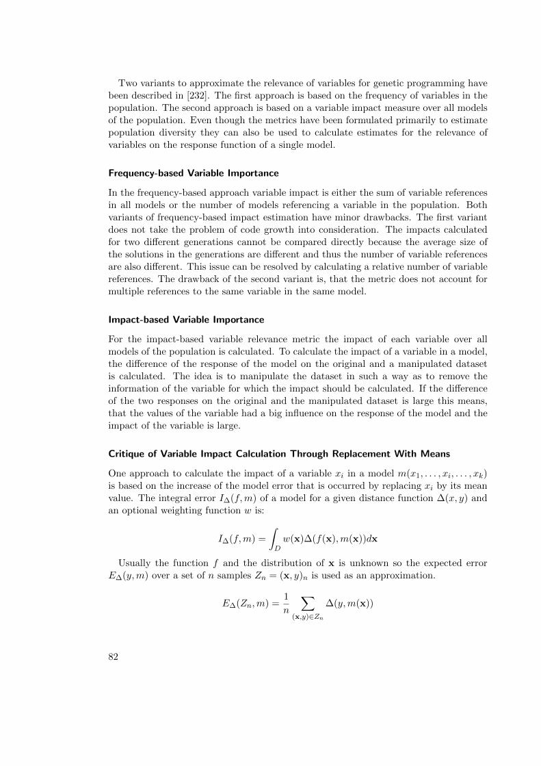
Two variants to approximate the relevance of variables for genetic programming havebeen described in [232]. The first approach is based on the frequency of variables in thepopulation. The second approach is based on a variable impact measure over all modelsof the population. Even though the metrics have been formulated primarily to estimatepopulation diversity they can also be used to calculate estimates for the relevance ofvariables on the response function of a single model.

Frequency-based Variable Importance

In the frequency-based approach variable impact is either the sum of variable referencesin all models or the number of models referencing a variable in the population. Bothvariants of frequency-based impact estimation have minor drawbacks. The first variantdoes not take the problem of code growth into consideration. The impacts calculatedfor two different generations cannot be compared directly because the average size ofthe solutions in the generations are different and thus the number of variable referencesare also different. This issue can be resolved by calculating a relative number of variablereferences. The drawback of the second variant is, that the metric does not account formultiple references to the same variable in the same model.

Impact-based Variable Importance

For the impact-based variable relevance metric the impact of each variable over allmodels of the population is calculated. To calculate the impact of a variable in a model,the difference of the response of the model on the original and a manipulated datasetis calculated. The idea is to manipulate the dataset in such a way as to remove theinformation of the variable for which the impact should be calculated. If the differenceof the two responses on the original and the manipulated dataset is large this means,that the values of the variable had a big influence on the response of the model and theimpact of the variable is large.

Critique of Variable Impact Calculation Through Replacement With Means

One approach to calculate the impact of a variable xi in a model m(x1, . . . , xi, . . . , xk)is based on the increase of the model error that is occurred by replacing xi by its meanvalue. The integral error I∆(f,m) of a model for a given distance function ∆(x, y) andan optional weighting function w is:

I∆(f,m) =

∫

Dw(x)∆(f(x),m(x))dx

Usually the function f and the distribution of x is unknown so the expected errorE∆(y,m) over a set of n samples Zn = (x, y)n is used as an approximation.

E∆(Zn,m) =1

n

∑

(x,y)∈Zn

∆(y,m(x))

82

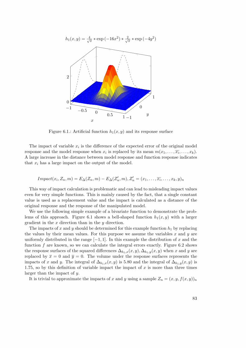
−1−0.5 0

0.5 1−1

0

10

2

x

y

h1(x, y) =4√

π

∗ exp (−16x2) ∗ 2√

π

∗ exp (−4y2)

Figure 6.1.: Artificial function h1(x, y) and its response surface

The impact of variable xi is the difference of the expected error of the original modelresponse and the model response when xi is replaced by its mean m(x1, . . . , xi, . . . , xk).A large increase in the distance between model response and function response indicatesthat xi has a large impact on the output of the model.

Impact(xi, Zn,m) = E∆(Zn,m)− E∆(Z′n,m), Z ′

n = (x1, . . . , xi, . . . , xk, y)n

This way of impact calculation is problematic and can lead to misleading impact valueseven for very simple functions. This is mainly caused by the fact, that a single constantvalue is used as a replacement value and the impact is calculated as a distance of theoriginal response and the response of the manipulated model.

We use the following simple example of a bivariate function to demonstrate the prob-lems of this approach. Figure 6.1 shows a bell-shaped function h1(x, y) with a largergradient in the x direction than in the y direction.

The impacts of x and y should be determined for this example function h1 by replacingthe values by their mean values. For this purpose we assume the variables x and y areuniformly distributed in the range [−1, 1]. In this example the distribution of x and thefunction f are known, so we can calculate the integral errors exactly. Figure 6.2 showsthe response surfaces of the squared differences ∆h1,x(x, y),∆h1,y(x, y) when x and y arereplaced by x = 0 and y = 0. The volume under the response surfaces represents theimpacts of x and y. The integral of ∆h1,x(x, y) is 5.80 and the integral of ∆h1,y(x, y) is1.75, so by this definition of variable impact the impact of x is more than three timeslarger than the impact of y.

It is trivial to approximate the impacts of x and y using a sample Zn = (x, y, f(x, y))n

83

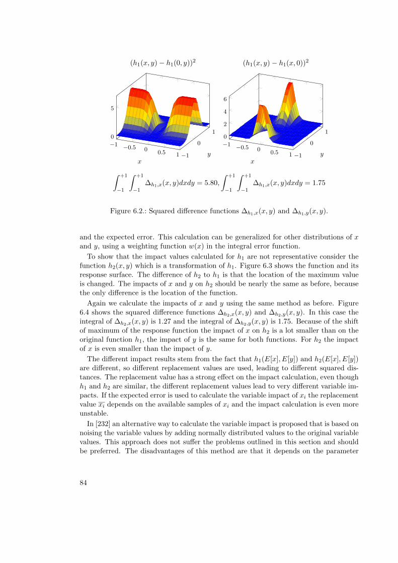
−1−0.5 0

0.51−1

0

10

5

x

y

(h1(x, y)− h1(0, y))2

−1−0.5 0

0.51−1

0

10

2

4

6

x

y

(h1(x, y)− h1(x, 0))2

∫ +1

−1

∫ +1

−1∆h1,x(x, y)dxdy = 5.80,

∫ +1

−1

∫ +1

−1∆h1,x(x, y)dxdy = 1.75

Figure 6.2.: Squared difference functions ∆h1,x(x, y) and ∆h1,y(x, y).

and the expected error. This calculation can be generalized for other distributions of xand y, using a weighting function w(x) in the integral error function.

To show that the impact values calculated for h1 are not representative consider thefunction h2(x, y) which is a transformation of h1. Figure 6.3 shows the function and itsresponse surface. The difference of h2 to h1 is that the location of the maximum valueis changed. The impacts of x and y on h2 should be nearly the same as before, becausethe only difference is the location of the function.

Again we calculate the impacts of x and y using the same method as before. Figure6.4 shows the squared difference functions ∆h2,x(x, y) and ∆h2,y(x, y). In this case theintegral of ∆h2,x(x, y) is 1.27 and the integral of ∆h2,y(x, y) is 1.75. Because of the shiftof maximum of the response function the impact of x on h2 is a lot smaller than on theoriginal function h1, the impact of y is the same for both functions. For h2 the impactof x is even smaller than the impact of y.

The different impact results stem from the fact that h1(E[x], E[y]) and h2(E[x], E[y])are different, so different replacement values are used, leading to different squared dis-tances. The replacement value has a strong effect on the impact calculation, even thoughh1 and h2 are similar, the different replacement values lead to very different variable im-pacts. If the expected error is used to calculate the variable impact of xi the replacementvalue xi depends on the available samples of xi and the impact calculation is even moreunstable.

In [232] an alternative way to calculate the variable impact is proposed that is based onnoising the variable values by adding normally distributed values to the original variablevalues. This approach does not suffer the problems outlined in this section and shouldbe preferred. The disadvantages of this method are that it depends on the parameter

84

−1−0.5 0

0.5 1−1

0

10

2

x

y

h2(x, y) = ( 4√

π

∗ exp (−16(x − 1)2) + 4√

π

∗ exp (−16(x+ 1)2)) ∗ 2√

π

∗ exp (−4y2)

Figure 6.3.: Artificial function h2(x, y) and its response surface

σ which determines the variance of the additive noise term and that the distribution ofthe input values is changed if the original values are not normally distributed.

6.2.4. Variable Importance in Random Forests

Random forests are a supervised learning approach for classification and regression pro-posed by [26]. The approach is based on the observation that ensembles of classificationor regression models can produce better estimations than a single model [25]. The esti-mated value for an ensemble of models is calculated by a voting scheme or by averagingover the estimated values of all models. This has the effect that it is less likely to receiveestimations with a large error because of the averaging effect over many models. Therequirement for this positive effect is, that the models in the ensemble should be struc-turally diverse. Ensemble methods additionally have the nice property that estimates forthe generalization error can often be calculated easily without cross-validation [24, 26]and that confidence intervals for estimated values can be calculated naturally.

Each model in a random forests is a classification and regression tree (CART) [28]trained on a different subset of training samples and deliberately not pruned which isusually necessary for CART to prevent overfitting. Even though the random forest cancontain overfit models the ensemble is not likely to overfit because a few outliers do nothave a large impact on the average prediction value over all models.

The disadvantage of random forests is that the unique property of CART that themodels are very easy to interpret and analyze is lost because of the large number ofstructurally diverse trees in the forest. Thus a non-parametric variable importancescheme for random forests has been proposed in [26, 83] to make it possible to argueabout the effects of input variables on the output value. For the permutation accuracy

85

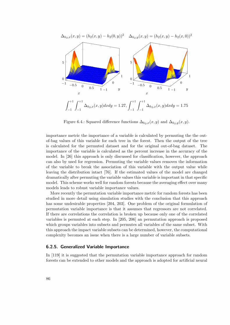
−1−0.5 0

0.51−1

0

10

5

x

y

∆h2,x

(x, y) = (h2(x, y)− h2(0, y))2

−1−0.5 0

0.51−1

0

10

5

x

y

∆h2,y

(x, y) = (h2(x, y) − h2(x, 0))2

∫ +1

−1

∫ +1

−1∆h2,x(x, y)dxdy = 1.27,

∫ +1

−1

∫ +1

−1∆h2,x(x, y)dxdy = 1.75

Figure 6.4.: Squared difference functions ∆h2,x(x, y) and ∆h2,y(x, y).

importance metric the importance of a variable is calculated by permuting the the out-of-bag values of this variable for each tree in the forest. Then the output of the treeis calculated for the permuted dataset and for the original out-of-bag dataset. Theimportance of the variable is calculated as the percent increase in the accuracy of themodel. In [26] this approach is only discussed for classification, however, the approachcan also by used for regression. Permuting the variable values removes the informationof the variable to break the association of this variable with the output value whileleaving the distribution intact [76]. If the estimated values of the model are changeddramatically after permuting the variable values this variable is important in that specificmodel. This scheme works well for random forests because the averaging effect over manymodels leads to robust variable importance values.

More recently the permutation variable importance metric for random forests has beenstudied in more detail using simulation studies with the conclusion that this approachhas some undesirable properties [204, 203]. One problem of the original formulation ofpermutation variable importance is that it assumes that regressors are not correlated.If there are correlations the correlation is broken up because only one of the correlatedvariables is permuted at each step. In [205, 206] an permutation approach is proposedwhich groups variables into subsets and permutes all variables of the same subset. Withthis approach the impact variable subsets can be determined, however, the computationalcomplexity becomes an issue when there is a large number of variable subsets.

6.2.5. Generalized Variable Importance

In [119] it is suggested that the permutation variable importance approach for randomforests can be extended to other models and the approach is adopted for artificial neural

86

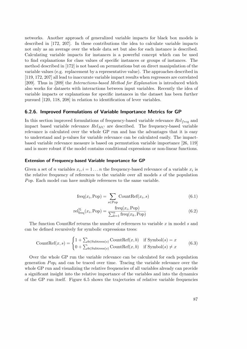
networks. Another approach of generalized variable impacts for black box models isdescribed in [172, 207]. In these contributions the idea to calculate variable impactsnot only as an average over the whole data set but also for each instance is described.Calculating variable impacts for instances is a powerful concept which can be usedto find explanations for class values of specific instances or groups of instances. Themethod described in [172] is not based on permutations but on direct manipulation of thevariable values (e.g. replacement by a representative value). The approaches described in[119, 172, 207] all lead to inaccurate variable impact results when regressors are correlated[209]. Thus in [209] the Interactions-based Method for Explanation is introduced whichalso works for datasets with interactions between input variables. Recently the idea ofvariable impacts or explanations for specific instances in the dataset has been furtherpursued [120, 118, 208] in relation to identification of lever variables.

6.2.6. Improved Formulations of Variable Importance Metrics for GP

In this section improved formulations of frequency-based variable relevance Relfreq andimpact based variable relevance RelMC are described. The frequency-based variablerelevance is calculated over the whole GP run and has the advantages that it is easyto understand and p-values for variable relevance can be calculated easily. The impact-based variable relevance measure is based on permutation variable importance [26, 119]and is more robust if the model contains conditional expressions or non-linear functions.

Extension of Frequency-based Variable Importance for GP

Given a set of n variables xi, i = 1 . . . n the frequency-based relevance of a variable xi isthe relative frequency of references to the variable over all models s of the populationPop. Each model can have multiple references to the same variable.

freq(xi,Pop) =∑

s∈PopCountRef(xi, s) (6.1)

rel%freq(xi,Pop) =freq(xi,Pop)∑n

k=1 freq(xk,Pop)(6.2)

The function CountRef returns the number of references to variable x in model s andcan be defined recursively for symbolic expressions trees:

CountRef(x, s) =

{1 +

∑b∈Subtrees(s)CountRef(x, b) if Symbol(s) = x

0 +∑

b∈Subtrees(s)CountRef(x, b) if Symbol(s) 6= x(6.3)

Over the whole GP run the variable relevance can be calculated for each populationgeneration Popi and can be traced over time. Tracing the variable relevance over thewhole GP run and visualizing the relative frequencies of all variables already can providea significant insight into the relative importance of the variables and into the dynamicsof the GP run itself. Figure 6.5 shows the trajectories of relative variable frequencies

87

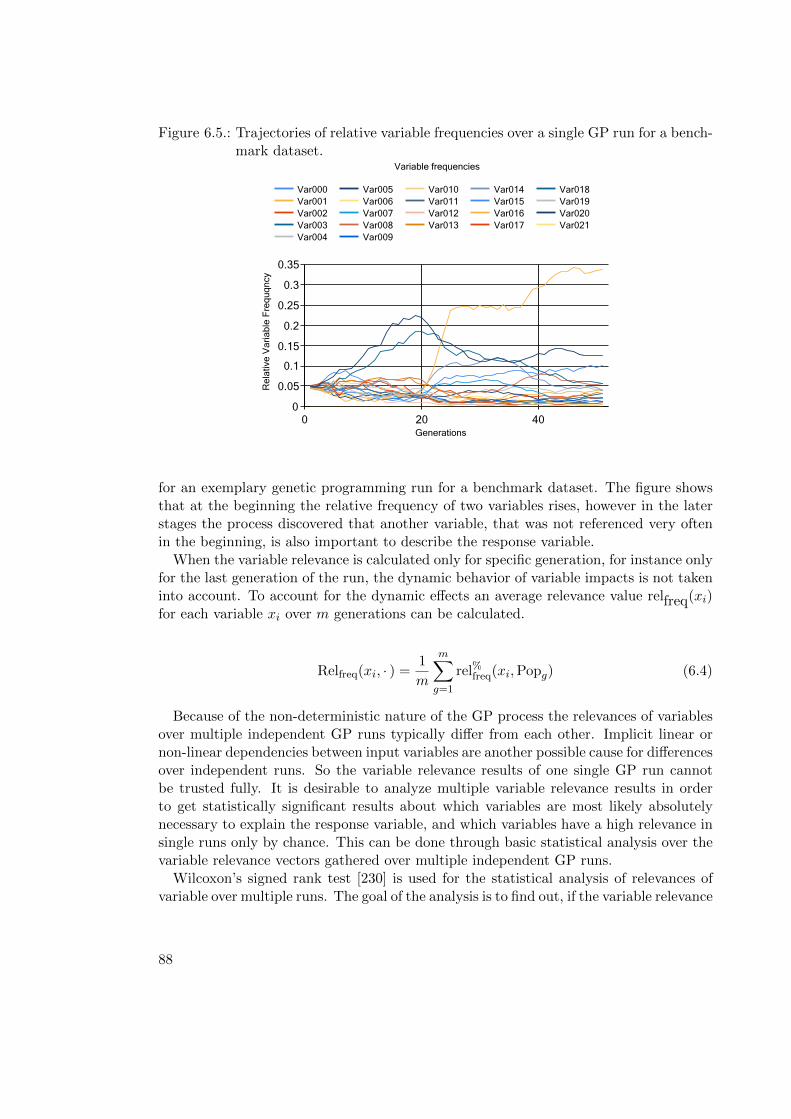
Figure 6.5.: Trajectories of relative variable frequencies over a single GP run for a bench-mark dataset.

0

0.05

0.1

0.15

0.2

0.25

0.3

0.35

0 20 40

Var000

Var001

Var002

Var003

Var004

Var005

Var006

Var007

Var008

Var009

Var010

Var011

Var012

Var013

Var014

Var015

Var016

Var017

Var018

Var019

Var020

Var021

Variable frequencies

Generations

Re

lative

Va

ria

ble

Fre

qu

qn

cy

for an exemplary genetic programming run for a benchmark dataset. The figure showsthat at the beginning the relative frequency of two variables rises, however in the laterstages the process discovered that another variable, that was not referenced very oftenin the beginning, is also important to describe the response variable.

When the variable relevance is calculated only for specific generation, for instance onlyfor the last generation of the run, the dynamic behavior of variable impacts is not takeninto account. To account for the dynamic effects an average relevance value relfreq(xi)for each variable xi over m generations can be calculated.

Relfreq(xi, · ) = 1

m

m∑

g=1

rel%freq(xi,Popg) (6.4)

Because of the non-deterministic nature of the GP process the relevances of variablesover multiple independent GP runs typically differ from each other. Implicit linear ornon-linear dependencies between input variables are another possible cause for differencesover independent runs. So the variable relevance results of one single GP run cannotbe trusted fully. It is desirable to analyze multiple variable relevance results in orderto get statistically significant results about which variables are most likely absolutelynecessary to explain the response variable, and which variables have a high relevance insingle runs only by chance. This can be done through basic statistical analysis over thevariable relevance vectors gathered over multiple independent GP runs.

Wilcoxon’s signed rank test [230] is used for the statistical analysis of relevances ofvariable over multiple runs. The goal of the analysis is to find out, if the variable relevance

88

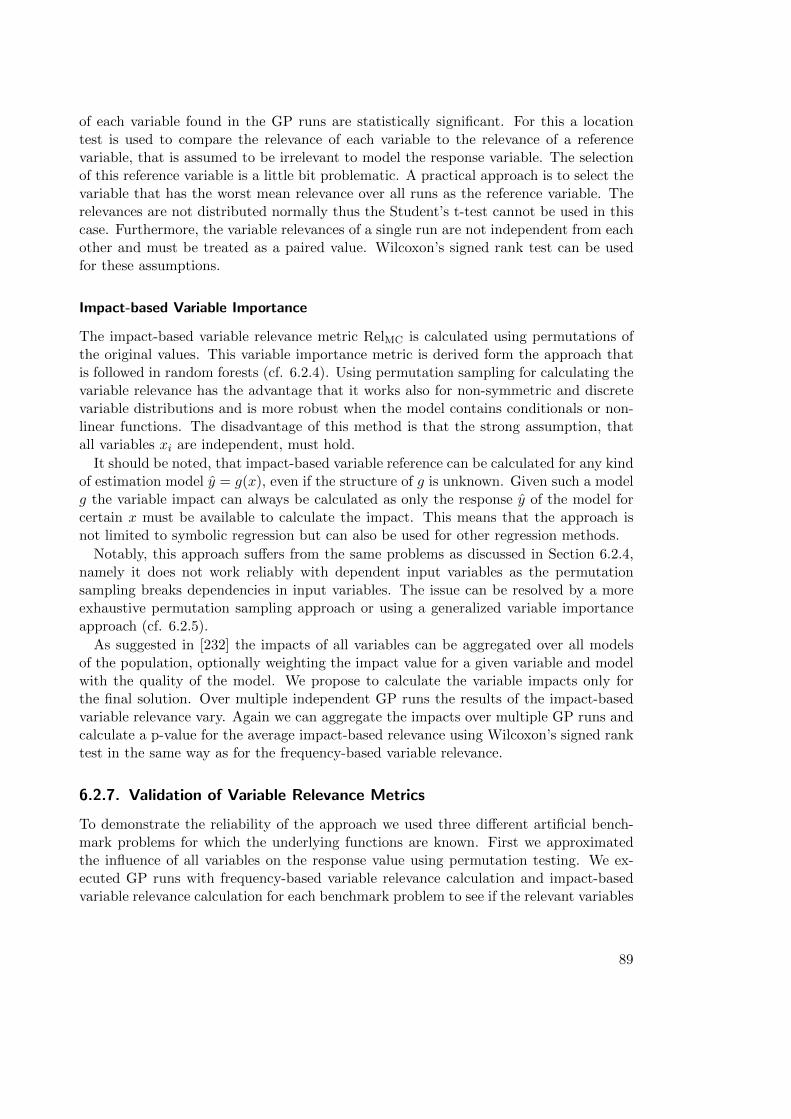
of each variable found in the GP runs are statistically significant. For this a locationtest is used to compare the relevance of each variable to the relevance of a referencevariable, that is assumed to be irrelevant to model the response variable. The selectionof this reference variable is a little bit problematic. A practical approach is to select thevariable that has the worst mean relevance over all runs as the reference variable. Therelevances are not distributed normally thus the Student’s t-test cannot be used in thiscase. Furthermore, the variable relevances of a single run are not independent from eachother and must be treated as a paired value. Wilcoxon’s signed rank test can be usedfor these assumptions.

Impact-based Variable Importance

The impact-based variable relevance metric RelMC is calculated using permutations ofthe original values. This variable importance metric is derived form the approach thatis followed in random forests (cf. 6.2.4). Using permutation sampling for calculating thevariable relevance has the advantage that it works also for non-symmetric and discretevariable distributions and is more robust when the model contains conditionals or non-linear functions. The disadvantage of this method is that the strong assumption, thatall variables xi are independent, must hold.

It should be noted, that impact-based variable reference can be calculated for any kindof estimation model y = g(x), even if the structure of g is unknown. Given such a modelg the variable impact can always be calculated as only the response y of the model forcertain x must be available to calculate the impact. This means that the approach isnot limited to symbolic regression but can also be used for other regression methods.

Notably, this approach suffers from the same problems as discussed in Section 6.2.4,namely it does not work reliably with dependent input variables as the permutationsampling breaks dependencies in input variables. The issue can be resolved by a moreexhaustive permutation sampling approach or using a generalized variable importanceapproach (cf. 6.2.5).

As suggested in [232] the impacts of all variables can be aggregated over all modelsof the population, optionally weighting the impact value for a given variable and modelwith the quality of the model. We propose to calculate the variable impacts only forthe final solution. Over multiple independent GP runs the results of the impact-basedvariable relevance vary. Again we can aggregate the impacts over multiple GP runs andcalculate a p-value for the average impact-based relevance using Wilcoxon’s signed ranktest in the same way as for the frequency-based variable relevance.

6.2.7. Validation of Variable Relevance Metrics

To demonstrate the reliability of the approach we used three different artificial bench-mark problems for which the underlying functions are known. First we approximatedthe influence of all variables on the response value using permutation testing. We ex-ecuted GP runs with frequency-based variable relevance calculation and impact-basedvariable relevance calculation for each benchmark problem to see if the relevant variables

89

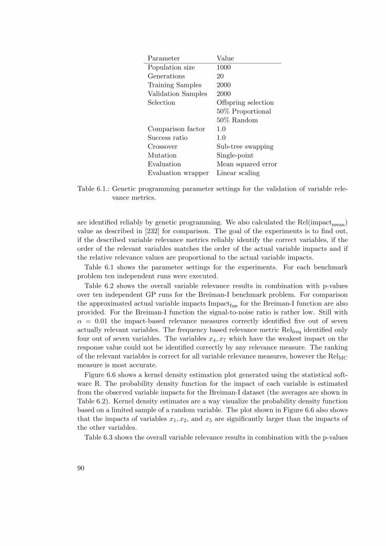
Parameter Value

Population size 1000Generations 20Training Samples 2000Validation Samples 2000Selection Offspring selection

50% Proportional50% Random

Comparison factor 1.0Success ratio 1.0Crossover Sub-tree swappingMutation Single-pointEvaluation Mean squared errorEvaluation wrapper Linear scaling

Table 6.1.: Genetic programming parameter settings for the validation of variable rele-vance metrics.

are identified reliably by genetic programming. We also calculated the Rel(impactmean)value as described in [232] for comparison. The goal of the experiments is to find out,if the described variable relevance metrics reliably identify the correct variables, if theorder of the relevant variables matches the order of the actual variable impacts and ifthe relative relevance values are proportional to the actual variable impacts.

Table 6.1 shows the parameter settings for the experiments. For each benchmarkproblem ten independent runs were executed.

Table 6.2 shows the overall variable relevance results in combination with p-valuesover ten independent GP runs for the Breiman-I benchmark problem. For comparisonthe approximated actual variable impacts Impactfun for the Breiman-I function are alsoprovided. For the Breiman-I function the signal-to-noise ratio is rather low. Still withα = 0.01 the impact-based relevance measures correctly identified five out of sevenactually relevant variables. The frequency based relevance metric Relfreq identified onlyfour out of seven variables. The variables x4, x7 which have the weakest impact on theresponse value could not be identified correctly by any relevance measure. The rankingof the relevant variables is correct for all variable relevance measures, however the RelMC

measure is most accurate.

Figure 6.6 shows a kernel density estimation plot generated using the statistical soft-ware R. The probability density function for the impact of each variable is estimatedfrom the observed variable impacts for the Breiman-I dataset (the averages are shown inTable 6.2). Kernel density estimates are a way visualize the probability density functionbased on a limited sample of a random variable. The plot shown in Figure 6.6 also showsthat the impacts of variables x1, x2, and x5 are significantly larger than the impacts ofthe other variables.

Table 6.3 shows the overall variable relevance results in combination with the p-values

90

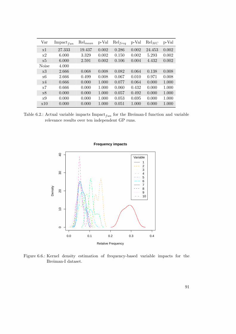
Var Impactfun Relmean p-Val Relfreq p-Val RelMC p-Val

x1 27.333 19.437 0.002 0.286 0.002 24.453 0.002x2 6.000 3.329 0.002 0.150 0.002 5.293 0.002x5 6.000 2.591 0.002 0.106 0.004 4.432 0.002

Noise 4.000x3 2.666 0.068 0.008 0.082 0.064 0.138 0.008x6 2.666 0.499 0.008 0.067 0.010 0.971 0.008x4 0.666 0.000 1.000 0.077 0.064 0.000 1.000x7 0.666 0.000 1.000 0.060 0.432 0.000 1.000x8 0.000 0.000 1.000 0.057 0.492 0.000 1.000x9 0.000 0.000 1.000 0.053 0.695 0.000 1.000x10 0.000 0.000 1.000 0.051 1.000 0.000 1.000

Table 6.2.: Actual variable impacts Impactfun for the Breiman-I function and variable

relevance results over ten independent GP runs.

0.0 0.1 0.2 0.3 0.4

010

2030

40

Relative Frequency

Den

sity

Frequency impacts

Variable

12345678910

Figure 6.6.: Kernel density estimation of frequency-based variable impacts for theBreiman-I dataset.

91

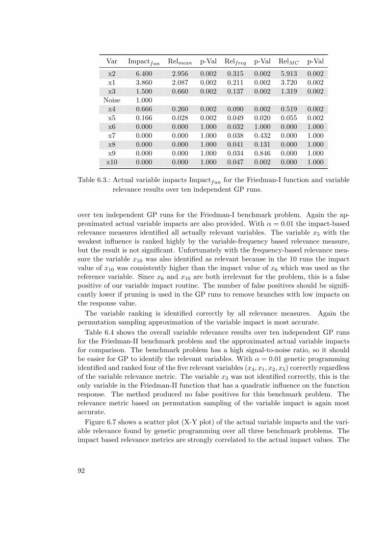
Var Impactfun Relmean p-Val Relfreq p-Val RelMC p-Val

x2 6.400 2.956 0.002 0.315 0.002 5.913 0.002x1 3.860 2.087 0.002 0.211 0.002 3.720 0.002x3 1.500 0.660 0.002 0.137 0.002 1.319 0.002

Noise 1.000x4 0.666 0.260 0.002 0.090 0.002 0.519 0.002x5 0.166 0.028 0.002 0.049 0.020 0.055 0.002x6 0.000 0.000 1.000 0.032 1.000 0.000 1.000x7 0.000 0.000 1.000 0.038 0.432 0.000 1.000x8 0.000 0.000 1.000 0.041 0.131 0.000 1.000x9 0.000 0.000 1.000 0.034 0.846 0.000 1.000x10 0.000 0.000 1.000 0.047 0.002 0.000 1.000

Table 6.3.: Actual variable impacts Impactfun for the Friedman-I function and variable

relevance results over ten independent GP runs.

over ten independent GP runs for the Friedman-I benchmark problem. Again the ap-proximated actual variable impacts are also provided. With α = 0.01 the impact-basedrelevance measures identified all actually relevant variables. The variable x5 with theweakest influence is ranked highly by the variable-frequency based relevance measure,but the result is not significant. Unfortunately with the frequency-based relevance mea-sure the variable x10 was also identified as relevant because in the 10 runs the impactvalue of x10 was consistently higher than the impact value of x6 which was used as thereference variable. Since x6 and x10 are both irrelevant for the problem, this is a falsepositive of our variable impact routine. The number of false positives should be signifi-cantly lower if pruning is used in the GP runs to remove branches with low impacts onthe response value.

The variable ranking is identified correctly by all relevance measures. Again thepermutation sampling approximation of the variable impact is most accurate.

Table 6.4 shows the overall variable relevance results over ten independent GP runsfor the Friedman-II benchmark problem and the approximated actual variable impactsfor comparison. The benchmark problem has a high signal-to-noise ratio, so it shouldbe easier for GP to identify the relevant variables. With α = 0.01 genetic programmingidentified and ranked four of the five relevant variables (x4, x1, x2, x5) correctly regardlessof the variable relevance metric. The variable x3 was not identified correctly, this is theonly variable in the Friedman-II function that has a quadratic influence on the functionresponse. The method produced no false positives for this benchmark problem. Therelevance metric based on permutation sampling of the variable impact is again mostaccurate.

Figure 6.7 shows a scatter plot (X-Y plot) of the actual variable impacts and the vari-able relevance found by genetic programming over all three benchmark problems. Theimpact based relevance metrics are strongly correlated to the actual impact values. The

92

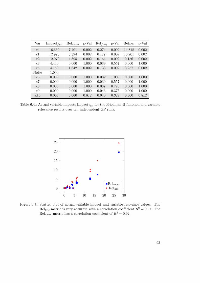
Var Impactfun Relmean p-Val Relfreq p-Val RelMC p-Val

x4 16.660 7.401 0.002 0.274 0.002 14.818 0.002x1 12.970 5.394 0.002 0.177 0.002 10.201 0.002x2 12.970 4.895 0.002 0.164 0.002 9.156 0.002x3 4.440 0.000 1.000 0.039 0.557 0.000 1.000x5 4.160 1.642 0.002 0.133 0.002 3.257 0.002

Noise 1.000x6 0.000 0.000 1.000 0.032 1.000 0.000 1.000x7 0.000 0.000 1.000 0.039 0.557 0.000 1.000x8 0.000 0.000 1.000 0.037 0.770 0.000 1.000x9 0.000 0.000 1.000 0.046 0.375 0.000 1.000x10 0.000 0.000 0.812 0.040 0.322 0.000 0.812

Table 6.4.: Actual variable impacts Impactfun for the Friedman-II function and variable

relevance results over ten independent GP runs.

0 5 10 15 20 25 30

0

5

10

15

20

25

Relmean

RelMC

Figure 6.7.: Scatter plot of actual variable impact and variable relevance values. TheRelMC metric is very accurate with a correlation coefficient R2 = 0.97. TheRelmean metric has a correlation coefficient of R2 = 0.92.

93

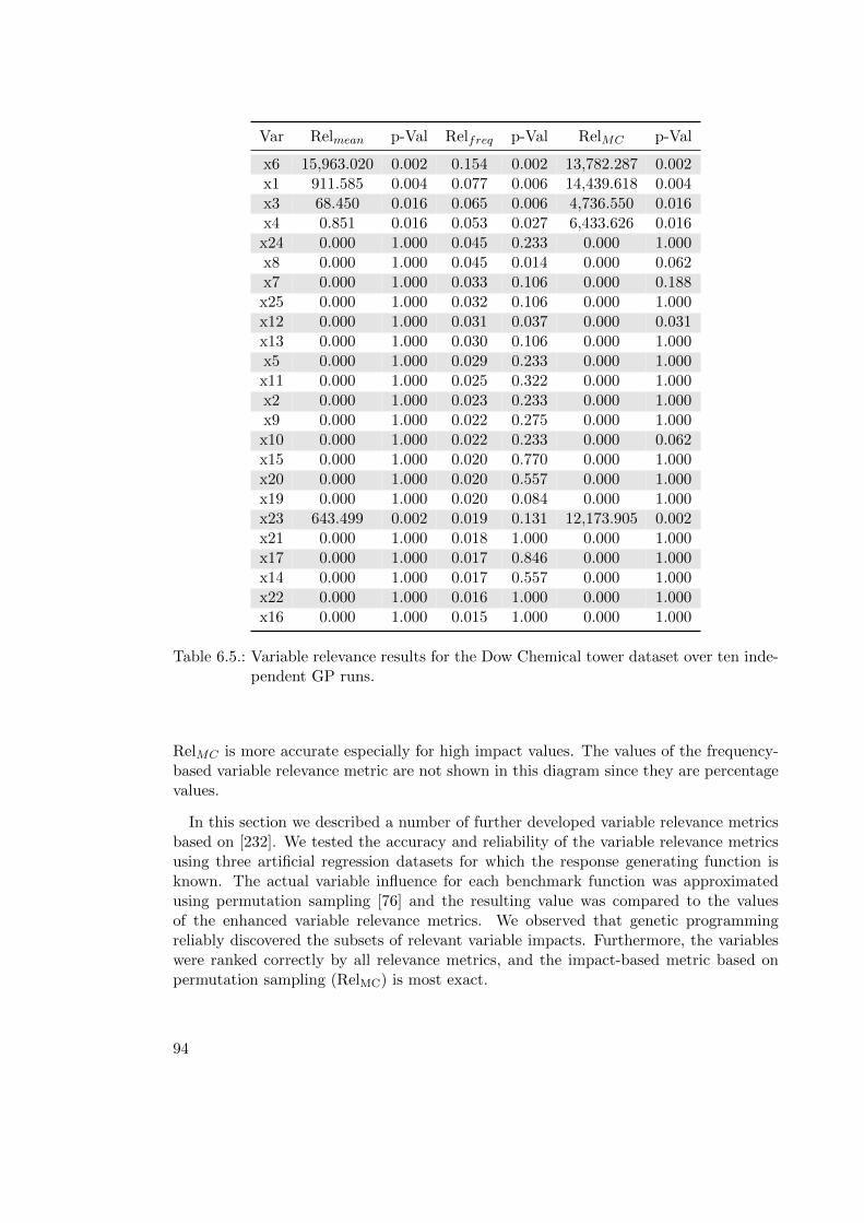
Var Relmean p-Val Relfreq p-Val RelMC p-Val

x6 15,963.020 0.002 0.154 0.002 13,782.287 0.002x1 911.585 0.004 0.077 0.006 14,439.618 0.004x3 68.450 0.016 0.065 0.006 4,736.550 0.016x4 0.851 0.016 0.053 0.027 6,433.626 0.016x24 0.000 1.000 0.045 0.233 0.000 1.000x8 0.000 1.000 0.045 0.014 0.000 0.062x7 0.000 1.000 0.033 0.106 0.000 0.188x25 0.000 1.000 0.032 0.106 0.000 1.000x12 0.000 1.000 0.031 0.037 0.000 0.031x13 0.000 1.000 0.030 0.106 0.000 1.000x5 0.000 1.000 0.029 0.233 0.000 1.000x11 0.000 1.000 0.025 0.322 0.000 1.000x2 0.000 1.000 0.023 0.233 0.000 1.000x9 0.000 1.000 0.022 0.275 0.000 1.000x10 0.000 1.000 0.022 0.233 0.000 0.062x15 0.000 1.000 0.020 0.770 0.000 1.000x20 0.000 1.000 0.020 0.557 0.000 1.000x19 0.000 1.000 0.020 0.084 0.000 1.000x23 643.499 0.002 0.019 0.131 12,173.905 0.002x21 0.000 1.000 0.018 1.000 0.000 1.000x17 0.000 1.000 0.017 0.846 0.000 1.000x14 0.000 1.000 0.017 0.557 0.000 1.000x22 0.000 1.000 0.016 1.000 0.000 1.000x16 0.000 1.000 0.015 1.000 0.000 1.000

Table 6.5.: Variable relevance results for the Dow Chemical tower dataset over ten inde-pendent GP runs.

RelMC is more accurate especially for high impact values. The values of the frequency-based variable relevance metric are not shown in this diagram since they are percentagevalues.

In this section we described a number of further developed variable relevance metricsbased on [232]. We tested the accuracy and reliability of the variable relevance metricsusing three artificial regression datasets for which the response generating function isknown. The actual variable influence for each benchmark function was approximatedusing permutation sampling [76] and the resulting value was compared to the valuesof the enhanced variable relevance metrics. We observed that genetic programmingreliably discovered the subsets of relevant variable impacts. Furthermore, the variableswere ranked correctly by all relevance metrics, and the impact-based metric based onpermutation sampling (RelMC) is most exact.

94

6.3. Data Mining and Symbolic Regression

For data mining tasks a target variable is often not known beforehand. Instead theprocess should identify interesting and relevant relations between variables. Multipleextensions to the simple formulation of symbolic regression have been proposed to allowmultiple target variables or to let the GP process identify interesting target variablesimplicitly.

[101] formulated extensions of symbolic regression for multi-variate targets and demon-strated that GP is able to find solutions to simple multi-variate symbolic regressionproblems. However the GP literature concentrates on the formulation for a single targetvariable. Chapter 7 will treat this topic in more detail.

An alternative evaluation scheme which enables GP to search for implicit equations(e.g., 0 = f(x)) is described in [178]. This approach is remarkable as it is not necessaryto specify target variables, instead the process will find functional expressions whichevaluate to a constant. This approach will be described in more detail in the followingsection.

The most trivial way to approach a data mining task is to try to find independentsymbolic regression models for all variables. Models that accurately match the originalvariable values are potentially more interesting and thus should be presented to the dataminer. However, the large number of unconnected regression models will most likely leadto confusion. Additionally, if there are correlated variables this process will just outputa model, where the single correlated variable is used to explain the target variable. Thisbehavior is most likely unwanted since such relations are most likely already known.Instead the process should be able to recognize such trivial relations and search formodels that are more interesting.

Instead of independent genetic programming runs, resulting in an unconnected set ofsymbolic regression problems for all variables, it is more desirable to combine the resultsin order to allow a data miner to gain a full understanding of the interrelations in thedataset. In Section 6.5 a cooperative process for GP-based data mining is described.

6.4. GP-Based Search for Implicit Equations

Genetic programming has been used to search for implicit equations in the form of0 = f(x, y) [178, 180]. This is essentially a way to search accurate models for multipletarget variables. For example if a function f(x, y) = 0 is to be found, the target variablesare x and y. To make sure that the process does not converge to trivial functionalexpressions (e.g., 1 − 1, 2 ∗ x − x − x) partial differentials of the model for all targetvariables are evaluated and compared to the numeric approximation of the differential.The error measure is defined as the sum of errors over all partial differentials [84, 179].The drawback of this approach is, that differentials of variables must be approximatednumerically. Especially in the presence of noisy data the noise will be further amplified bytrivial numeric differential approximation methods based on finite differences. If the datacontains noise, the problem can be alleviated through smoothing methods (e.g. using

95

the locally weighted scatter-plot smoother [38, 39]) or more sophisticated interpolationmethods. However, it is likely, that relevant information in the data is lost throughsmoothing or interpolation methods. This method has been applied successfully to findequations for well known physical systems (e.g., pendulum, spring pendulum) [180].

6.5. Comprehensive Search for Symbolic Regression Models

Given a dataset that contains observed values from a system, the usual objective is toapproximate one target variable using a subset of the possible input variables. This isoften problematic because of implicit relations in the set of input variables. Pairwisecorrelated variables can be detected easily but the input variables might be related in anon-linear fashion which is difficult to detect. Implicit relations in the input variableshave the effect that it is not possible to produce one unique ideal model for the targetvariables. Instead it is possible to produce equally accurate and correct models usingalternative representations resulting from the implicit relations.

A simple but very powerful way to approach this issue is to search for all accuratemodels over the whole dataset. Instead of a single target variable treat each variable asthe target variable and try to create an approximation model using all other variablesas potential inputs. With this approach it is possible to uncover non-linear implicitrelations which might can be used interchangeably in models for the target variables.This can also lead to a better understanding of the overall system because hierarchicalstructures in approximation models are made explicit and can be studied in detail.

6.5.1. Case Study: Chemical-II Dataset

In this section the unguided approach to generate symbolic regression models is demon-strated on the Chemical-II dataset. This dataset has been has been prepared and pub-lished by Arthur Kordon, research leader at the Dow Chemical company. The datasetcontains 4999 observations of 26 variables of a chemical process and can be downloadedfrom http://vanillamodeling.com/realproblems.html. The following description ofthe Tower dataset also stems from the same source.

The observations in the dataset stem from a chemical process and include tempera-tures, flows, and pressures. The target variable is the propylene concentration and isa gas chromatography measurement at the top of a distillation tower. The propyleneconcentration is measured in regular intervals of 15 minutes. The actual sampling rateof the input variables is one minute, but 15 minutes averages of the inputs are usedto synchronize with the measurements of the target variable. The range of the mea-sured propylene concentration is very broad and covers most of the expected operatingconditions in the distillation tower.

Modeling

A screening of the dataset for correlated variables shows that the dataset contains fourgroups of variables with strong pairwise correlations. For each group one variable is se-

96

Variable cluster

x20, x21x12, x13, x16x3, x7, x11x8, x25

Table 6.6.: Groups of variables with strong pairwise correlations in the Chemical-IIdataset.

lected as the representative and the remaining variables are not considered for modeling.Table 6.6 lists the identified clusters of strongly correlated variables.

For modeling the full dataset is partitioned into a training partition (rows 100–2050)used to calculate model fitness, an internal validation partition (rows 2050–4000) usedto select the final model, and a test partition (rows 4000-4999) used to estimate thegeneralization error of the final model.

Table 6.7 shows GP parameter settings for the experiments. The final model (best onvalidation) is linearly scaled to match the location and scale of the original target values.This is necessary because the squared correlation coefficient, which is invariant to scale,and location is used as fitness function. As shown by [95] maximization of the squaredPearson’s Product Moment Correlation Coefficient is equivalent to minimization of thescaled mean squared error. Static length and depth constraints are used for the models toprevent unlimited code growth. The initialization procedure PTC2 [128] creates randomtrees with a target distribution for the tree length between 3 and 100 nodes.

The same parameter settings are used to create models for each remaining variable ofthe dataset. Ten independent GP runs are executed for each configuration, leading to190 symbolic regression models, produced in the same number of GP runs.

Results

Figure 6.8 shows a box-plot of the R2 of the models produced by GP for each of thevariables over 10 independent runs. From the box-plot it is immediately clear thatthe dataset contains a number of implicit variable relations. GP consistently identifiedalmost perfect models for variables x3, x5, x6, x8, x9, x12 and x20. GP also identified anumber of highly accurate models with squared correlation coefficient larger than 0.9for variables x1, x4, and x22. Models produced by GP for the response variable haveon average R2 = 0.87. For variables x19, x15, and x24 GP also consistently producedrelatively accurate models. For the remaining variables the R2 of the GP models variesstrongly, especially for variable x2 no accurate models are found.

The box-plot can give an indication about the ability to approximate variables whenother variable values are known. The full power of the unguided approach is more appar-ent when the information gathered in all GP runs is combined to produce the variablerelation network shown in Figure 6.9. In the network the most relevant input variablesto approximate a variable are shown where a → b means a is a relevant variable for GPmodels approximating variable b. The network is based on the permutation impact of

97

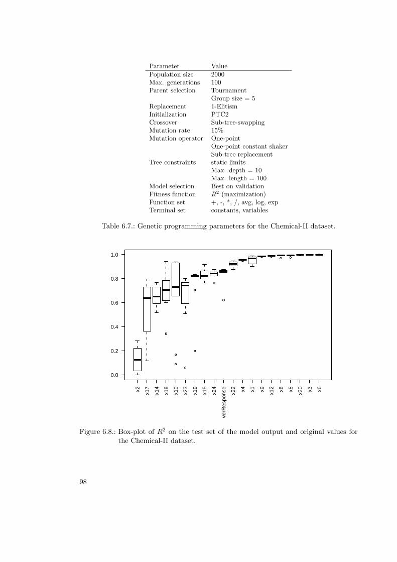
Parameter ValuePopulation size 2000Max. generations 100Parent selection Tournament

Group size = 5Replacement 1-ElitismInitialization PTC2Crossover Sub-tree-swappingMutation rate 15%Mutation operator One-point

One-point constant shakerSub-tree replacement

Tree constraints static limitsMax. depth = 10Max. length = 100

Model selection Best on validationFitness function R2 (maximization)Function set +, -, *, /, avg, log, expTerminal set constants, variables

Table 6.7.: Genetic programming parameters for the Chemical-II dataset.

x2 x17

x14

x18

x10

x23

x19

x15

x24

tow

erR

espo

nse

x22 x4 x1 x9 x12 x8 x5 x20 x3 x6

0.0

0.2

0.4

0.6

0.8

1.0

Figure 6.8.: Box-plot of R2 on the test set of the model output and original values forthe Chemical-II dataset.

98

variables in the final model. For a given variable x the permutation impact of all othervariables is calculated over the 10 models for x. Only significant impacts (p-Value <0.005) are kept and shown in the network diagram. The variable clusters identified inthe preliminary analysis of the dataset are also shown as rectangles containing all vari-ables of the cluster. In depth analysis of the relationships identified by GP showed, thatvariables x1 and x6 and the two clusters with representatives x8 and x3 are all pairwisestrongly connected. So a larger cluster has been manually introduced that encompassesall those variables.

Analyzing the network generated for the Chemical-II dataset in more detail, leads toa better overall insight into the process. An immediate observation is, that the largecluster with representative x1 and the cluster with representative x12 play a central rolein the process. Additional variables with many outgoing arrows are x10 and x19. Thesetwo variables are often used to approximate other variables.

Another fact that is immediately clear is, that there are many double-linked variablepairs and two long double-linked chains of variables. This indicates that the two variablesare strongly related. One chain relates the cluster with representative x20 with x5 whichis in turn strongly connected to x14. Another chain connects variables x17, x22 and x24.Other strongly related variable pairs are x18 and x19, and x10 and x23.

The relevant input variables for models for the response variable are x23 and onevariable in the large central cluster with variable x1.

The network diagram shows the general relations of variables in the dataset. For moredetailed information the models produced for each variable should be analyzed in detail.

Result Details

In this section a number of manually selected and simplified highly accurate modelsproduced for the Chemical-II dataset are presented in detail.

Table 6.8 gives an overview of the presented models including the squared correlationcoefficient (R2) on the test set.

GP identified simple but highly accurate linear models for variables x6 (6.10), x12(6.13), and x20 (6.14). GP also identified a linear model with R2 = 0.87 for the responsevariable using only six input variables (6.16). For comparison we also trained a ν-SVMregression model [222] using the same six input variables with five-fold cross-validationand a grid search for the parameters ν, C, γ using the open source SVM implementationlibSVM [32]. The best SVM model we found has a R2 of 0.97 which is significantly betterthan the linear model. Motivated by the SVM result we also trained a more complexGP model using only the subset of six variables. The GP runs produced a non-linearmodel (6.17) which after some manual simplification has a R2 = 0.90.

It is now possible to deconstruct the model for the response variable further becauseaccurate models for all input variables are available. The original model uses variablesx1, x6 and x12 for which accurate approximations are available. It is possible to replacethe input variables by their approximation models and so get an alternative approxi-mation model for the response. Through this procedure the model does not necessarilybecome more complex because, if the introduced models contain common terms these

99

x8

x25

x3 x7

x11

x1x6

x20

x21

x12

x13

x16

x10

x2

x23

x24

x22

x4x9

towerResponse

x14

x5

x15

x19

x17

x18

Figure 6.9.: Identified variable relations for the Chemical-II dataset.

100

Target Model R2 (test)

x1 (6.5) 0.97x3 (6.6) 0.99x4 (6.8) 0.91x5 (6.9) 0.99x6 (6.10) 0.96x8 (6.11) 0.99x9 (6.12) 0.98x12 (6.13) 0.98x20 (6.14) 0.99x22 (6.15) 0.94Response (6.16) 0.87Response (6.17) 0.90

Table 6.8.: Accuracy of selected and simplified models for the Chemical-II dataset onthe test set.

can be unified. In this case all approximations contain the variable x3 which does notoccur in the original model for the response variable. This hierarchical approach ofmodel analysis leads to a more throughout understanding of the possible impact factorsand implicit relations, that are relevant for the approximation of the response variable.

101

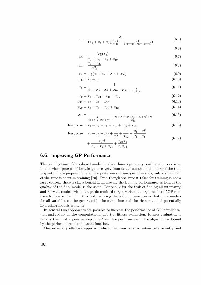
x1 =x6

(x3 + x8 + x10)(x8x10

+ x3(x3+x10)(x3+x4+x6)

)(6.5)

(6.6)

x3 =log(x8)

x1 + x6 + x8 + x10(6.7)

x4 =x3 + x24

x223(6.8)

x5 = log(x3 + x9 + x10 + x20) (6.9)

x6 = x3 + x8 (6.10)

x8 =1

x1 + x3 + x6 + x10 + x24 +1

x3+x6

(6.11)

x9 = x3 + x12 + x15 + x19 (6.12)

x12 = x3 + x9 + x20 (6.13)

x20 = x3 + x5 + x10 + x12 (6.14)

x22 =1

x17x1+x19+x10+c0

+ x9+exp(x17+x4+x24+c1)+c2x217

(6.15)

Response = x1 + x2 + x6 + x12 + x15 + x23 (6.16)

Response = x2 + x6 + x15 +1

x2+

1

x12+

x31 + x21x1 + x6

+x1x

22

x1 + x2 + x23+

x23x6x1x12

(6.17)

6.6. Improving GP Performance

The training time of data-based modeling algorithms is generally considered a non-issue.In the whole process of knowledge discovery from databases the major part of the timeis spent in data preparation and interpretation and analysis of models, only a small partof the time is spent in training [70]. Even though the time it takes for training is not alarge concern there is still a benefit in improving the training performance as long as thequality of the final model is the same. Especially for the task of finding all interestingand relevant models without a predetermined target variable a large number of GP runshave to be executed. For this task reducing the training time means that more modelsfor all variables can be generated in the same time and the chance to find potentiallyinteresting models is higher.

In general two approaches are possible to increase the performance of GP, paralleliza-tion and reduction the computational effort of fitness evaluation. Fitness evaluation isusually the most expensive step in GP and the performance of the algorithm is boundby the performance of the fitness function.

One especially effective approach which has been pursued intensively recently and

102

combines both aspects is genetic programming on GPUs [235, 236, 113, 80, 37, 115].The recent developments in hardware and software have made powerful massively parallelarchitectures accessible for general purposes and facilitated such research.

6.6.1. Parallelization

Evolutionary algorithms in general are embarrassingly easy to parallelize because ofthe concept of independent solutions which are combined to a population. A num-ber of parallel and distributed execution schemes have been described for evolution-ary algorithms in general [7, 139] which can also be applied to genetic programming[13, 151, 160, 91, 201, 46, 34].

6.6.2. Improving Fitness Evaluation Performance

Often a number of preliminary experiments with a reduced training set are carried outto find good parameter values for a algorithm before the final model is trained using thefull training set.

It is also possible to reduce the number of fitness cases dynamically in a single GPrun. The fitness value of an individual is usually only an approximation of the actualfitness of the individual even when all fitness cases are considered. Thus, if an accurateapproximation is also possible when only a small number of fitness cases are evaluatedthe performance of the algorithm can be increased.

Reducing the number of fitness cases has already been discussed by Holland who in-troduced a method for the “optimal allocation of trials” in [86] which is based on asolution of the multi-armed bandit problem. The method tries to find a good approxi-mation for the fitness with a limited amount of fitness cases. Later an extended approachcalled “rational allocation of trials” has been introduced in [212]. In [75] it has beenshown that the number of fitness cases that is needed in the GP fitness function canbe upper-bounded via statistical and information-theoretic considerations. In [98] it hasbeen shown that a very simple scheme that randomly selects a small subset of fitnesscases (e.g. 10% of the training partition) for each evaluation also work well for specificapplications and has a large effect on performance.

Recently an approach for the reduction of fitness cases specifically for symbolic regres-sion has been introduced [223]. The aim of this approach is not primarily to improvethe performance of the algorithm but to produce more robust models by intelligent databalancing. In the case of symbolic regression a data-set often contains a large number ofsimilar data points and the outer regions of the data-space are populated only sparsely.Data balancing weights the fitness cases by relevance metrics based on the distance of adata-point to the remaining data points and removes redundant data-points completelyin order to put more emphasis on the outer regions of the data-space. Effectively thenumber of fitness cases can be removed and the performance of fitness evaluation isincreased.

Another approach to increase fitness evaluation performance is to use fitness predictorswhich can for instance be co-evolved with the actual solution candidates [181].

103

In conclusion it is not necessary to use all fitness cases in symbolic regression and anumber of different approaches for the reduction of fitness cases have been described inthe literature. In our experiments we found that the scheme of randomly sampling asmall subset of fitness cases for each fitness evaluation is simple and effective and doesnot have a negative effect on final solution quality.

104

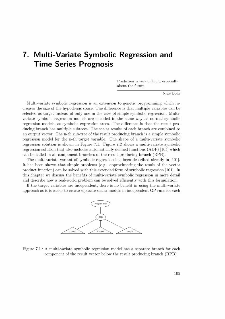
7. Multi-Variate Symbolic Regression andTime Series Prognosis

Prediction is very difficult, especiallyabout the future.

Niels Bohr

Multi-variate symbolic regression is an extension to genetic programming which in-creases the size of the hypothesis space. The difference is that multiple variables can beselected as target instead of only one in the case of simple symbolic regression. Multi-variate symbolic regression models are encoded in the same way as normal symbolicregression models, as symbolic expression trees. The difference is that the result pro-ducing branch has multiple subtrees. The scalar results of each branch are combined toan output vector. The n-th sub-tree of the result producing branch is a simple symbolicregression model for the n-th target variable. The shape of a multi-variate symbolicregression solution is shown in Figure 7.1. Figure 7.2 shows a multi-variate symbolicregression solution that also includes automatically defined functions (ADF) [105] whichcan be called in all component branches of the result producing branch (RPB).

The multi-variate variant of symbolic regression has been described already in [101].It has been shown that simple problems (e.g. approximating the result of the vectorproduct function) can be solved with this extended form of symbolic regression [101]. Inthis chapter we discuss the benefits of multi-variate symbolic regression in more detailand describe how a real-world problem can be solved efficiently with this formulation.

If the target variables are independent, there is no benefit in using the multi-variateapproach as it is easier to create separate scalar models in independent GP runs for each

Program Root

RPB

Comp0 Comp1 CompN

Figure 7.1.: A multi-variate symbolic regression model has a separate branch for eachcomponent of the result vector below the result producing branch (RPB).

105

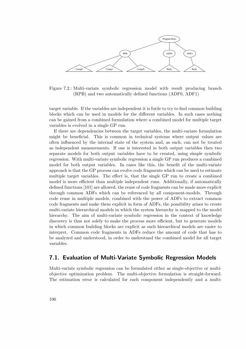
Program Root

RPB ADF0 ADF1

Comp0 Comp1 CompN Body Body

Figure 7.2.: Multi-variate symbolic regression model with result producing branch(RPB) and two automatically defined functions (ADF0, ADF1)

target variable. If the variables are independent it is futile to try to find common buildingblocks which can be used in models for the different variables. In such cases nothingcan be gained from a combined formulation where a combined model for multiple targetvariables is evolved in a single GP run.

If there are dependencies between the target variables, the multi-variate formulationmight be beneficial. This is common in technical systems where output values areoften influenced by the internal state of the system and, as such, can not be treatedas independent measurements. If one is interested in both output variables then twoseparate models for both output variables have to be created, using simple symbolicregression. With multi-variate symbolic regression a single GP run produces a combinedmodel for both output variables. In cases like this, the benefit of the multi-variateapproach is that the GP process can evolve code fragments which can be used to estimatemultiple target variables. The effect is, that the single GP run to create a combinedmodel is more efficient than multiple independent runs. Additionally, if automaticallydefined functions [101] are allowed, the reuse of code fragments can be made more explicitthrough common ADFs which can be referenced by all component-models. Throughcode reuse in multiple models, combined with the power of ADFs to extract commoncode fragments and make them explicit in form of ADFs, the possibility arises to createmulti-variate hierarchical models in which the system hierarchy is mapped to the modelhierarchy. The aim of multi-variate symbolic regression in the context of knowledgediscovery is thus not solely to make the process more efficient, but to generate modelsin which common building blocks are explicit as such hierarchical models are easier tointerpret. Common code fragments in ADFs reduce the amount of code that has tobe analyzed and understood, in order to understand the combined model for all targetvariables.

7.1. Evaluation of Multi-Variate Symbolic Regression Models

Multi-variate symbolic regression can be formulated either as single-objective or multi-objective optimization problem. The multi-objective formulation is straight-forward.The estimation error is calculated for each component independently and a multi-

106

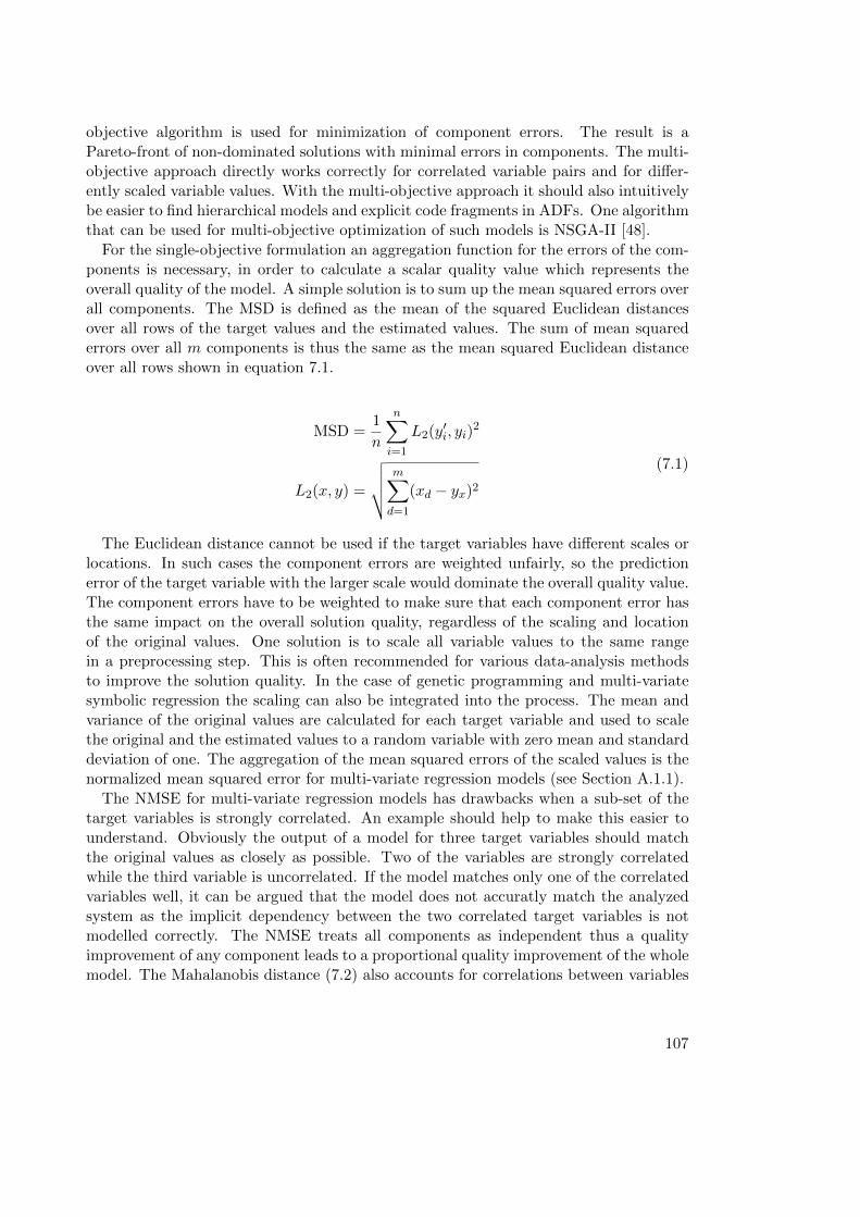
objective algorithm is used for minimization of component errors. The result is aPareto-front of non-dominated solutions with minimal errors in components. The multi-objective approach directly works correctly for correlated variable pairs and for differ-ently scaled variable values. With the multi-objective approach it should also intuitivelybe easier to find hierarchical models and explicit code fragments in ADFs. One algorithmthat can be used for multi-objective optimization of such models is NSGA-II [48].

For the single-objective formulation an aggregation function for the errors of the com-ponents is necessary, in order to calculate a scalar quality value which represents theoverall quality of the model. A simple solution is to sum up the mean squared errors overall components. The MSD is defined as the mean of the squared Euclidean distancesover all rows of the target values and the estimated values. The sum of mean squarederrors over all m components is thus the same as the mean squared Euclidean distanceover all rows shown in equation 7.1.

MSD =1

n

n∑

i=1

L2(y′i, yi)

2

L2(x, y) =

√√√√m∑

d=1

(xd − yx)2

(7.1)

The Euclidean distance cannot be used if the target variables have different scales orlocations. In such cases the component errors are weighted unfairly, so the predictionerror of the target variable with the larger scale would dominate the overall quality value.The component errors have to be weighted to make sure that each component error hasthe same impact on the overall solution quality, regardless of the scaling and locationof the original values. One solution is to scale all variable values to the same rangein a preprocessing step. This is often recommended for various data-analysis methodsto improve the solution quality. In the case of genetic programming and multi-variatesymbolic regression the scaling can also be integrated into the process. The mean andvariance of the original values are calculated for each target variable and used to scalethe original and the estimated values to a random variable with zero mean and standarddeviation of one. The aggregation of the mean squared errors of the scaled values is thenormalized mean squared error for multi-variate regression models (see Section A.1.1).

The NMSE for multi-variate regression models has drawbacks when a sub-set of thetarget variables is strongly correlated. An example should help to make this easier tounderstand. Obviously the output of a model for three target variables should matchthe original values as closely as possible. Two of the variables are strongly correlatedwhile the third variable is uncorrelated. If the model matches only one of the correlatedvariables well, it can be argued that the model does not accuratly match the analyzedsystem as the implicit dependency between the two correlated target variables is notmodelled correctly. The NMSE treats all components as independent thus a qualityimprovement of any component leads to a proportional quality improvement of the wholemodel. The Mahalanobis distance (7.2) also accounts for correlations between variables

107

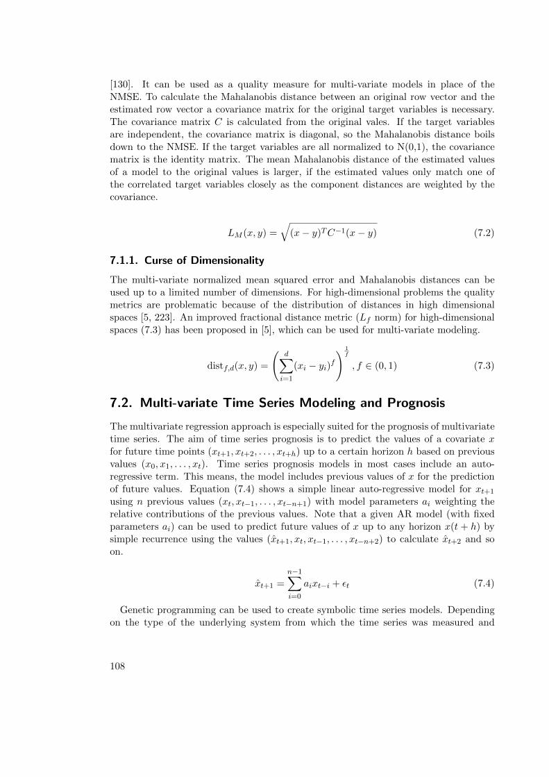
[130]. It can be used as a quality measure for multi-variate models in place of theNMSE. To calculate the Mahalanobis distance between an original row vector and theestimated row vector a covariance matrix for the original target variables is necessary.The covariance matrix C is calculated from the original vales. If the target variablesare independent, the covariance matrix is diagonal, so the Mahalanobis distance boilsdown to the NMSE. If the target variables are all normalized to N(0,1), the covariancematrix is the identity matrix. The mean Mahalanobis distance of the estimated valuesof a model to the original values is larger, if the estimated values only match one ofthe correlated target variables closely as the component distances are weighted by thecovariance.

LM (x, y) =√(x− y)TC−1(x− y) (7.2)

7.1.1. Curse of Dimensionality

The multi-variate normalized mean squared error and Mahalanobis distances can beused up to a limited number of dimensions. For high-dimensional problems the qualitymetrics are problematic because of the distribution of distances in high dimensionalspaces [5, 223]. An improved fractional distance metric (Lf norm) for high-dimensionalspaces (7.3) has been proposed in [5], which can be used for multi-variate modeling.

distf,d(x, y) =

(d∑

i=1

(xi − yi)f

) 1f

, f ∈ (0, 1) (7.3)

7.2. Multi-variate Time Series Modeling and Prognosis

The multivariate regression approach is especially suited for the prognosis of multivariatetime series. The aim of time series prognosis is to predict the values of a covariate xfor future time points (xt+1, xt+2, . . . , xt+h) up to a certain horizon h based on previousvalues (x0, x1, . . . , xt). Time series prognosis models in most cases include an auto-regressive term. This means, the model includes previous values of x for the predictionof future values. Equation (7.4) shows a simple linear auto-regressive model for xt+1

using n previous values (xt, xt−1, . . . , xt−n+1) with model parameters ai weighting therelative contributions of the previous values. Note that a given AR model (with fixedparameters ai) can be used to predict future values of x up to any horizon x(t + h) bysimple recurrence using the values (xt+1, xt, xt−1, . . . , xt−n+2) to calculate xt+2 and soon.

xt+1 =n−1∑

i=0

aixt−i + εt (7.4)

Genetic programming can be used to create symbolic time series models. Dependingon the type of the underlying system from which the time series was measured and

108

the intended application of the model, different modeling approaches are possible. Theapproach discussed here, is useful for the identification or approximation of dynamicsystems. This task is closely related to symbolic regression, however, because of thesystem dynamics the previous values of x can have an influence on y as well, so theinput values of the model have to be extended to include previous values of x up to amaximal lag l. Equation (7.5) shows a model for a dynamic system, in comparison toregression models the time parameter is relevant and previous values of x are includedas model inputs. In order to create dynamic models with genetic programming, theterminal set has to be extended to include terminals for lagged variables up a certainmaximal lag limit. For dynamic models the same fitness functions, which are used forsymbolic regression, can be used (e.g. MSE).

yt = f(xt, xt−1, . . . , xt−l) + εt (7.5)

If the dynamic system includes a feedback loop, the response yt of the system notonly depends on the values xt and previous values of xt−i but also on previous outputvalues yt−i. So the model has to be extended to also include previous values of y up toa maximal lag m and the result is the auto-regressive model 7.6.

yt = f(xt, xt−1, . . . , xt−l, yt−1, . . . , yt−m) + εt (7.6)

To create auto-regressive models with genetic programming the terminal set has to beextended to also include terminal symbols for lagged values of y. This kind of model canbe used to predict the future values of y when the future values of the input / controlvariables are known. The question that the model can answer is: What is the responseof the system for future values of the control variables x and current and previous valuesof x and y. The estimation yt+1 can be feed back as input into the model and incombination with the inputs xt+1 the estimated response yt+2 at time t+2 is produced.

The model cannot be used to predict future values of y when future values of x arenot known yet. In some applications it is sufficient to predict y only up to a limitedhorizon h. In such cases a compromise is possible by using values of x only up to timestep xt−h as input (7.7). With this model it is possible to predict the next h values ofy based on the previous values of x and y. The disadvantage of this approach is thatrecent values of x cannot be included in the approximation, the larger the predictionhorizon the larger the gap between input-values and estimated values.

yt+h = f(xt, xt−1, . . . , xt−l, yt+h−1, . . . , yt−m) + εt (7.7)

For this reason it is sometimes preferable to create fully auto-regressive models withoutexogenous variables 7.8. This model has no explicit target variable, all values are usedas input and produced as output. Similarly to multi-variate regression, we can easilycreate such multi-variate time series models with genetic programming. Note that fora fixed model it is possible to predict future values of x to any finite horizon throughrecurrence (even though the accuracy of the prognosis is expected to deteriorate withincreased time steps (t+ i) because of the accumulation of approximation errors εt+i).

109

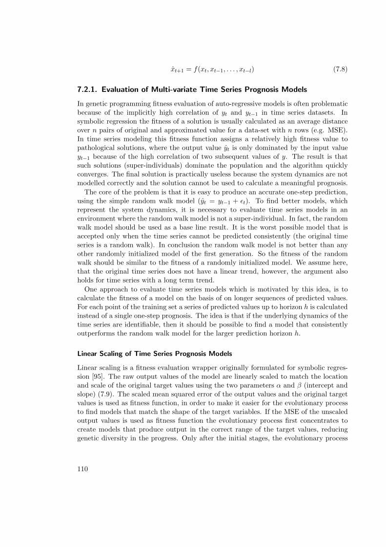
xt+1 = f(xt, xt−1, . . . , xt−l) (7.8)

7.2.1. Evaluation of Multi-variate Time Series Prognosis Models

In genetic programming fitness evaluation of auto-regressive models is often problematicbecause of the implicitly high correlation of yt and yt−1 in time series datasets. Insymbolic regression the fitness of a solution is usually calculated as an average distanceover n pairs of original and approximated value for a data-set with n rows (e.g. MSE).In time series modeling this fitness function assigns a relatively high fitness value topathological solutions, where the output value yt is only dominated by the input valueyt−1 because of the high correlation of two subsequent values of y. The result is thatsuch solutions (super-individuals) dominate the population and the algorithm quicklyconverges. The final solution is practically useless because the system dynamics are notmodelled correctly and the solution cannot be used to calculate a meaningful prognosis.

The core of the problem is that it is easy to produce an accurate one-step prediction,using the simple random walk model (yt = yt−1 + εt). To find better models, whichrepresent the system dynamics, it is necessary to evaluate time series models in anenvironment where the random walk model is not a super-individual. In fact, the randomwalk model should be used as a base line result. It is the worst possible model that isaccepted only when the time series cannot be predicted consistently (the original timeseries is a random walk). In conclusion the random walk model is not better than anyother randomly initialized model of the first generation. So the fitness of the randomwalk should be similar to the fitness of a randomly initialized model. We assume here,that the original time series does not have a linear trend, however, the argument alsoholds for time series with a long term trend.

One approach to evaluate time series models which is motivated by this idea, is tocalculate the fitness of a model on the basis of on longer sequences of predicted values.For each point of the training set a series of predicted values up to horizon h is calculatedinstead of a single one-step prognosis. The idea is that if the underlying dynamics of thetime series are identifiable, then it should be possible to find a model that consistentlyoutperforms the random walk model for the larger prediction horizon h.

Linear Scaling of Time Series Prognosis Models

Linear scaling is a fitness evaluation wrapper originally formulated for symbolic regres-sion [95]. The raw output values of the model are linearly scaled to match the locationand scale of the original target values using the two parameters α and β (intercept andslope) (7.9). The scaled mean squared error of the output values and the original targetvalues is used as fitness function, in order to make it easier for the evolutionary processto find models that match the shape of the target variables. If the MSE of the unscaledoutput values is used as fitness function the evolutionary process first concentrates tocreate models that produce output in the correct range of the target values, reducinggenetic diversity in the progress. Only after the initial stages, the evolutionary process

110

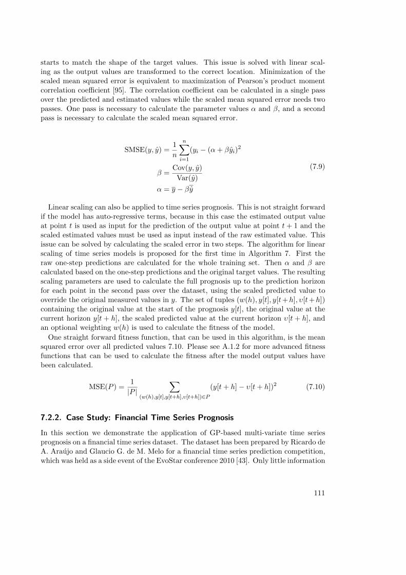
starts to match the shape of the target values. This issue is solved with linear scal-ing as the output values are transformed to the correct location. Minimization of thescaled mean squared error is equivalent to maximization of Pearson’s product momentcorrelation coefficient [95]. The correlation coefficient can be calculated in a single passover the predicted and estimated values while the scaled mean squared error needs twopasses. One pass is necessary to calculate the parameter values α and β, and a secondpass is necessary to calculate the scaled mean squared error.

SMSE(y, y) =1

n

n∑

i=1

(yi − (α+ βyi)2

β =Cov(y, y)

Var(y)

α = y − βy

(7.9)

Linear scaling can also be applied to time series prognosis. This is not straight forwardif the model has auto-regressive terms, because in this case the estimated output valueat point t is used as input for the prediction of the output value at point t+ 1 and thescaled estimated values must be used as input instead of the raw estimated value. Thisissue can be solved by calculating the scaled error in two steps. The algorithm for linearscaling of time series models is proposed for the first time in Algorithm 7. First theraw one-step predictions are calculated for the whole training set. Then α and β arecalculated based on the one-step predictions and the original target values. The resultingscaling parameters are used to calculate the full prognosis up to the prediction horizonfor each point in the second pass over the dataset, using the scaled predicted value tooverride the original measured values in y. The set of tuples (w(h), y[t], y[t+h], υ[t+h])containing the original value at the start of the prognosis y[t], the original value at thecurrent horizon y[t+ h], the scaled predicted value at the current horizon υ[t+ h], andan optional weighting w(h) is used to calculate the fitness of the model.

One straight forward fitness function, that can be used in this algorithm, is the meansquared error over all predicted values 7.10. Please see A.1.2 for more advanced fitnessfunctions that can be used to calculate the fitness after the model output values havebeen calculated.

MSE(P ) =1

|P |∑

(w(h),y[t],y[t+h],υ[t+h])∈P(y[t+ h]− υ[t+ h])2 (7.10)

7.2.2. Case Study: Financial Time Series Prognosis

In this section we demonstrate the application of GP-based multi-variate time seriesprognosis on a financial time series dataset. The dataset has been prepared by Ricardo deA. Araujo and Glaucio G. de M. Melo for a financial time series prediction competition,which was held as a side event of the EvoStar conference 2010 [43]. Only little information

111

Algorithm 7: Linear scaling and fitness evaluation of time series prognosis models

input : Model: m, Fitness function: f , Column vector: yn, Matrix:X = [xi,j ]n×k, Maximal lag: lmax, Horizon: hmax

output: Fitness of m

// subset of yn for which the model can be evaluated

target ← ylmax...n;// calculate one step predictions

y ← (m(yi−lmax...i−1, Xi−lmax...i×k)|i ← lmax . . . n);// calculate linear scaling parameters

β ← Cov(target,y)Var(y) ;

α ← target− βy;P ← ®;for t ← lmaxto n− hmax do

υn ← yn;for h ← 1 to hmax do

υ[t+ h] ← α+ βm(υt+h−lmax...t+h−1, Xt+h−lmax...t+h×k);P ← P ∪ (w(h), y[t], y[t+ h], υ[t+ h]);

endreturn f(P );

end

about the origin of the dataset has been published, except that the dataset stems fromreal financial time series from the Brazilian stock exchange.

The original dataset contains 200 observations of ten financial time series. The originalcompetition objective was to predict the next 10 data-points for each of the 10 time series.Unfortunately the 10 data points, which were originally held back by the organizers toevaluate the entries, have never been published. So we repartitioned the dataset into atraining partition (rows 1–190) and a test partition (rows 190–200).

Modeling

Table 7.1 shows the GP parameter settings for the time series prognosis experiments. Inthis experiment static size and depth limits are used to prevent unlimited code growth.The size limit is rather large (1000 nodes) because a single multi-variate model has tenbranches, one for each component of the multi-variate time series. The random modelsof the initial population are created with the probabilistic tree creator with a uniformtarget distribution of tree sizes between 1 and 1000 nodes. The function set containsarithmetic operators including a special function for the calculation of the arithmeticmean and additionally logarithm, exponential and sine function symbols. The terminalset includes random constants, lagged variables and derivatives with allowed time offsetsbetween (t-27) and (t-1) and additionally terminal symbols to calculate the moving-average and integral of the values of a variable over a given time span within the range

112

Parameter ValuePopulation size 10000Max. generations 100Parent selection Tournament

Group size = 5Replacement 1-ElitismInitialization PTC2Crossover Sub-tree-swappingMutation rate 15%Mutation operator One-point

One-point constant shakerSub-tree replacement

Tree constraints Static limitsMax. depth = 10Max. size = 1000

Model selection Best on validationFitness function scaled NMSE

Prediction horizon = 10Function set +, -, *, /, avg, log, exp, sinTerminal set const, lagged variable, ma, integral, derivative

Time offsets: (t-27)–(t-1)

Table 7.1.: Genetic programming parameter settings for the financial time series prog-nosis experiments.

of allowed time offsets. For instance the expression MA(x1,−10,−5) is the moving-average of the variable x1 in the time span from (t-10) up to (t-5). The derivative valuesof a variable are approximated numerically from the original values without smoothing(see A.2). The model is auto-recursive because all target variables are allowed also asinput variables, and the output values of the model for time t are used as input valuesto calculate the output for time t+1. The maximal prediction horizon is ten time steps.Models which do not reuse output values can be created if the time lags in all terminalsare smaller than -10.

For the GP runs the training partition spanning 190 rows is further partitioned intoa dataset that is used for fitness evaluation (rows 30–130) and an internal validation set(rows 130–180). In total only 150 rows are used for training, because 30 rows have tobe skipped in the beginning to allow for dynamic models including time offsets, and 10rows have to be trimmed at the end because the prediction horizon is 10. Figure 7.3shows the model of evaluation for the 10-step prognosis of the financial time series. Ateach point t of the training partition a prognosis consisting of 10 predicted values for(t+ 1) . . . (t+ 10) is calculated.

The fitness function is the scaled normalized mean squared error for 10-step predictionssummed over the ten time series. Each component-branch of the model is linearly scaledto fit the location and scale of that component of the original multi-variate time series asdescribed in algorithm (7). Scaling of branch output is based on the one-step predictionsof the model. After scaling the 10-step prognosis of the resulting model for each of the

113

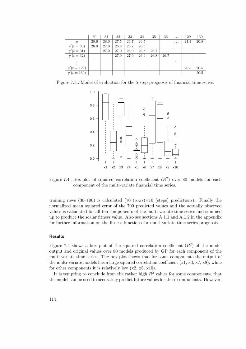
30 31 32 33 34 35 36 . . . 129 130

y 28.6 28.0 27.5 26.7 26.5 . . . 21.1 20.8

y′(t = 30) 26.8 27.0 26.8 26.7 26.6

y′(t = 31) 27.0 27.0 26.9 26.8 26.7

y′(t = 32) 27.0 27.0 26.9 26.8 26.7...

. . .

y′(t = 129) 20.5 20.5

y′(t = 130) 20.5

Figure 7.3.: Model of evaluation for the 5-step prognosis of financial time series.

x1 x2 x3 x4 x5 x6 x7 x8 x9 x10

0.0

0.2

0.4

0.6

0.8

1.0

Figure 7.4.: Box-plot of squared correlation coefficient (R2) over 80 models for eachcomponent of the multi-variate financial time series.

training rows (30–100) is calculated (70 (rows)×10 (steps) predictions). Finally thenormalized mean squared error of the 700 predicted values and the actually observedvalues is calculated for all ten components of the multi-variate time series and summedup to produce the scalar fitness value. Also see sections A.1.1 and A.1.2 in the appendixfor further information on the fitness functions for multi-variate time series prognosis.

Results

Figure 7.4 shows a box plot of the squared correlation coefficient (R2) of the modeloutput and original values over 80 models produced by GP for each component of themulti-variate time series. The box-plot shows that for some components the output ofthe multi-variate models has a large squared correlation coefficient (x1, x3, x7, x8), whilefor other components it is relatively low (x2, x5, x10).

It is tempting to conclude from the rather high R2 values for some components, thatthe model can be used to accurately predict future values for these components. However,

114

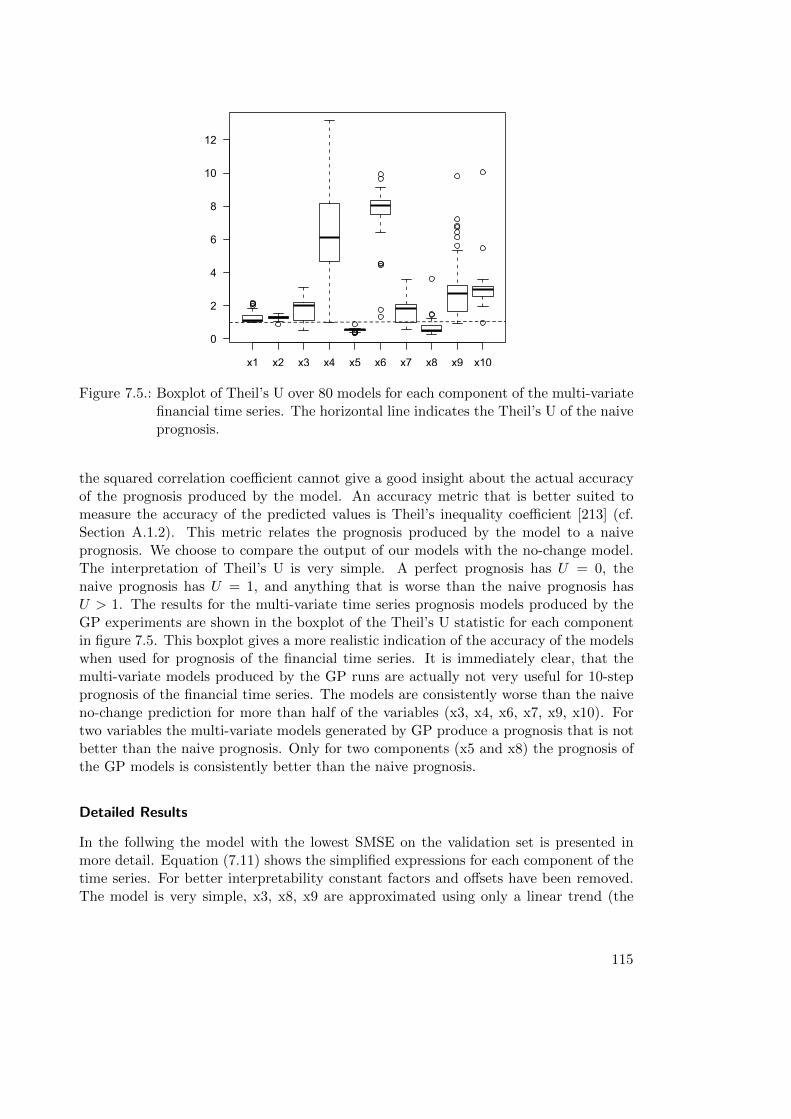
x1 x2 x3 x4 x5 x6 x7 x8 x9 x10

0

2

4

6

8

10

12

Figure 7.5.: Boxplot of Theil’s U over 80 models for each component of the multi-variatefinancial time series. The horizontal line indicates the Theil’s U of the naiveprognosis.

the squared correlation coefficient cannot give a good insight about the actual accuracyof the prognosis produced by the model. An accuracy metric that is better suited tomeasure the accuracy of the predicted values is Theil’s inequality coefficient [213] (cf.Section A.1.2). This metric relates the prognosis produced by the model to a naiveprognosis. We choose to compare the output of our models with the no-change model.The interpretation of Theil’s U is very simple. A perfect prognosis has U = 0, thenaive prognosis has U = 1, and anything that is worse than the naive prognosis hasU > 1. The results for the multi-variate time series prognosis models produced by theGP experiments are shown in the boxplot of the Theil’s U statistic for each componentin figure 7.5. This boxplot gives a more realistic indication of the accuracy of the modelswhen used for prognosis of the financial time series. It is immediately clear, that themulti-variate models produced by the GP runs are actually not very useful for 10-stepprognosis of the financial time series. The models are consistently worse than the naiveno-change prediction for more than half of the variables (x3, x4, x6, x7, x9, x10). Fortwo variables the multi-variate models generated by GP produce a prognosis that is notbetter than the naive prognosis. Only for two components (x5 and x8) the prognosis ofthe GP models is consistently better than the naive prognosis.

Detailed Results

In the follwing the model with the lowest SMSE on the validation set is presented inmore detail. Equation (7.11) shows the simplified expressions for each component of thetime series. For better interpretability constant factors and offsets have been removed.The model is very simple, x3, x8, x9 are approximated using only a linear trend (the

115

variable Date is the row index). Variables x5, x6, x7 and x10 are approximated usingeither the integral symbol or the moving average symbol for smoothing.

Figure 7.6 shows line charts of the original variable values and the 10-step predictionof the model (7.11) for each component over the whole dataset. The model matches thelong term trend of the original values relatively well but fails to predict the short termvariations except for variable x7.

Figure 7.7 shows line charts of the actual continuation of the time series in the testset (rows 190–200) and the continuation predicted by the model at time t = 190. Thisline chart shows that the model is not capable to predict the short-term future valuesof the multi-variate time series very well because the model only approximates the longterm trend. For most variables the predictions of the model are far off the actual valuesand the model produces almost constant predictions for most variables. For variablesx3, x4, and x7 the model predicts the trend in the wrong direction. The prediction hasa positive trend, even though the variable values are actually decreasing.

In conclusion, the time series prognosis approach where GP is used to produce multi-variate models succeeded in predicting the long term trend of the multi-variate timeseries correctly, however, the short term variations are not predicted correctly.

x1(t) = x10(t− 10) + Date

x2(t) = x3(t− 24)

x3(t) = Date

x4(t) = x9(t− 8)× x8(t− 20)

x5(t) = x7(t− 1) + I(x6,−14,−4) + Date

x6(t) = I(x6,−26,−4) +MA(x8,−24,−7)

x7(t) =1

I(x7,−8,−1)

x8(t) = Date

x9(t) = Date

x10(t) = I(x7,−8,−1)

(7.11)

116

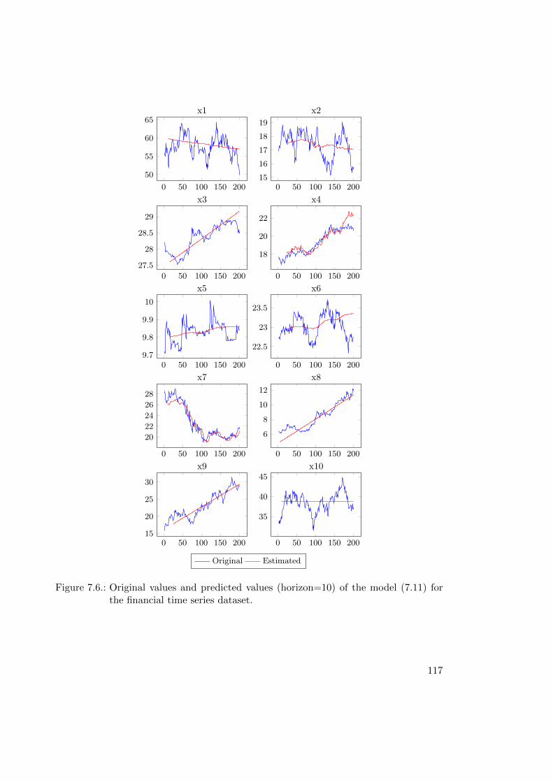
0 50 100 150 200

50

55

60

65

x1

0 50 100 150 200

15

16

17

18

19

x2

0 50 100 150 200

27.5

28

28.5

29

x3

0 50 100 150 200

18

20

22

x4

0 50 100 150 200

9.7

9.8

9.9

10

x5

0 50 100 150 200

22.5

23

23.5

x6

0 50 100 150 200

20

22

24

26

28

x7

0 50 100 150 200

6

8

10

12

x8

0 50 100 150 200

15

20

25

30

x9

0 50 100 150 200

35

40

45

x10

Original Estimated

Figure 7.6.: Original values and predicted values (horizon=10) of the model (7.11) forthe financial time series dataset.

117

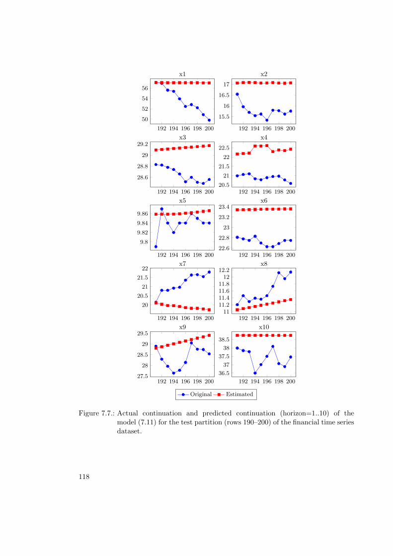
192 194 196 198 200

50

52

54

56

x1

192 194 196 198 200

15.5

16

16.5

17

x2

192 194 196 198 200

28.6

28.8

29

29.2

x3

192 194 196 198 200

20.5

21

21.5

22

22.5

x4

192 194 196 198 200

9.8

9.82

9.84

9.86

x5

192 194 196 198 200

22.6

22.8

23

23.2

23.4

x6

192 194 196 198 200

20

20.5

21

21.5

22x7

192 194 196 198 200

11

11.2

11.4

11.6

11.8

12

12.2

x8

192 194 196 198 200

27.5

28

28.5

29

29.5

x9

192 194 196 198 200

36.5

37

37.5

38

38.5

x10

Original Estimated

Figure 7.7.: Actual continuation and predicted continuation (horizon=1..10) of themodel (7.11) for the test partition (rows 190–200) of the financial time seriesdataset.

118

8. Applications and Case Studies

The best thing about being astatistician is that you get to play ineveryone’s backyard.

John Tukey

Genetic programming with the enhancements discussed in the preceding chapters canbe used effectively to identify interrelations between variables of complex systems. Inthis chapter we apply the methods discussed in the previous chapters to analyze: theblast furnace process for iron production, an industrial chemical process, and interactionsof macro-economic variables.

8.1. Blast Furnace

Parts of this section have been published by the author in [106]. The author thanksChristoph Feilmayr for his expert input about the blast furnace process and for criticallyreviewing draft versions of this section.

The blast furnace is the most common process to produce hot metal globally. Around881 million tons of hot metal and 1240 million tons of steel were produced in 2006 [199].More than 60% of the iron used for steel production is produced in the blast furnaceprocess [182].

The raw materials for the production of hot metal enter the blast furnace via two paths.At the top of the blast furnace ferrous oxides and coke are charged in alternating layers.The ferrous oxides include sinter, pellets and lump ore. Additionally feedstock to adjustthe basicity is also charged at the top of the blast furnace. In the lower area of the blastfurnace the hot blast (air, 1200 ◦C) and reducing agents are injected through tuyeres.Reducing agents include heavy oil, pulverized coal, coke oven or natural gas, and coketar. Sometimes other reducing agents, like waste plastics, are added to substitute coke.The products of the blast furnace are liquid iron (hot metal) and the liquid byproductslag, tapped at the bottom, and blast furnace gas which is collected at the top.

Figure 8.1 shows a schematic diagram of a blast furnace for the production of pig iron(image taken from [106]).

Inside the blast furnace the raw materials undergo a number of physical and chemicalreactions. The ferrous oxides and coke gradually move down into the lower and hotterparts of the furnace. In this process the mechanical properties of ferrous oxides changebecause of pressure, temperature and the reducing gas atmosphere. The oxygen con-tained in ferrous oxides is removed by the reducing agents carbon, carbon monoxide and

119

Figure 8.1.: Schematic diagram of the blast furnace and input and output materials. Atthe top ferrous oxides and coke are charged in alternating layers. Near thebottom the hot blast and reducing agents are injected through the tuyeres.Hot metal and slag are tapped in regular intervals from the hearth of theblast furnace. Blast furnace gas is collected at the top of the blast furnace.

in minor proportion hydrogen. Carbon monoxide is created through partial oxidationof reducing agents and from carbon dioxide and carbon (Boudouard-reaction). In theupper part of the blast furnace the carbon monoxide reduces the ferrous oxides creatingcarbon dioxide. The resulting metallic iron is melted and carburized. For more detailsabout the process see [202, 155, 184].

The general process and the physical and chemical reactions occurring in the blastfurnace are quite well understood. On a detailed level many of the inter-relationshipsof different parameters and the occurrence of fluctuations and unsteady behavior in theblast furnace are not totally understood. An example is the change in the cooling lossesvia the walls of the furnace. Changes in the cooling losses are strongly related to theefficiency of the process. However the causes for the effect are not totally understood.Knowledge about such effects can be used to improve various aspects of the blast furnaceprocess, e.g. the quality of the products, the amount of resources consumed, or thestability of the process.

A number of mathematical and simulation models have been developed for specificprocesses in the blast furnace [11, 12, 192]. A survey of recent progress on mathematicalmodels for the blast furnace is given in [219]. Additionally data-based methods have beenapplied to model certain aspects of the blast furnace process. The data-based approaches

120

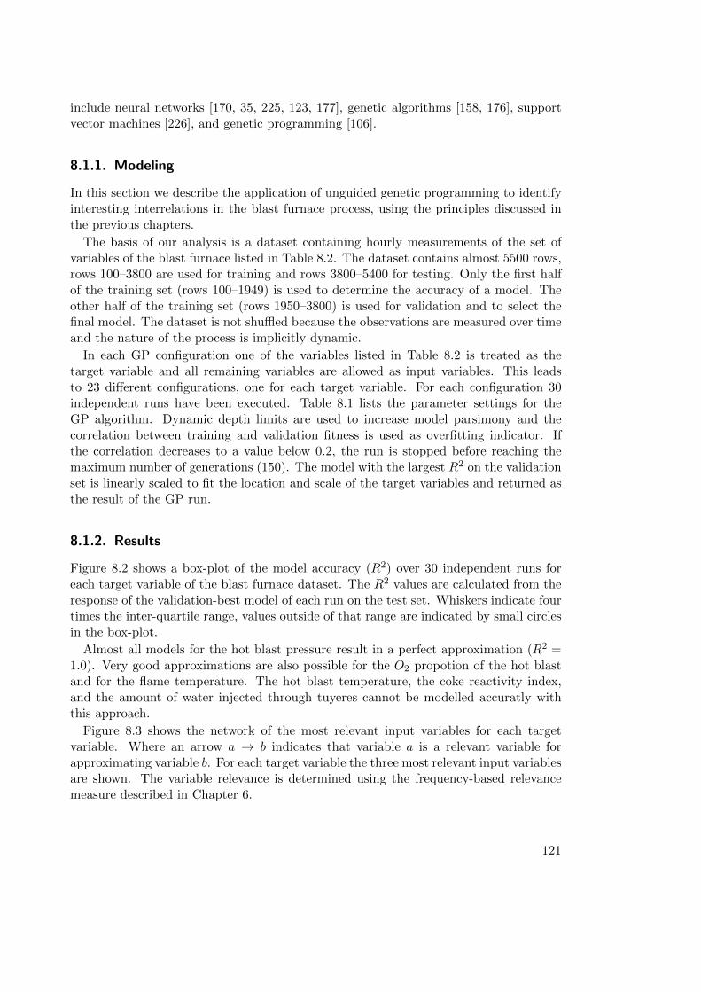
include neural networks [170, 35, 225, 123, 177], genetic algorithms [158, 176], supportvector machines [226], and genetic programming [106].

8.1.1. Modeling

In this section we describe the application of unguided genetic programming to identifyinteresting interrelations in the blast furnace process, using the principles discussed inthe previous chapters.

The basis of our analysis is a dataset containing hourly measurements of the set ofvariables of the blast furnace listed in Table 8.2. The dataset contains almost 5500 rows,rows 100–3800 are used for training and rows 3800–5400 for testing. Only the first halfof the training set (rows 100–1949) is used to determine the accuracy of a model. Theother half of the training set (rows 1950–3800) is used for validation and to select thefinal model. The dataset is not shuffled because the observations are measured over timeand the nature of the process is implicitly dynamic.

In each GP configuration one of the variables listed in Table 8.2 is treated as thetarget variable and all remaining variables are allowed as input variables. This leadsto 23 different configurations, one for each target variable. For each configuration 30independent runs have been executed. Table 8.1 lists the parameter settings for theGP algorithm. Dynamic depth limits are used to increase model parsimony and thecorrelation between training and validation fitness is used as overfitting indicator. Ifthe correlation decreases to a value below 0.2, the run is stopped before reaching themaximum number of generations (150). The model with the largest R2 on the validationset is linearly scaled to fit the location and scale of the target variables and returned asthe result of the GP run.

8.1.2. Results

Figure 8.2 shows a box-plot of the model accuracy (R2) over 30 independent runs foreach target variable of the blast furnace dataset. The R2 values are calculated from theresponse of the validation-best model of each run on the test set. Whiskers indicate fourtimes the inter-quartile range, values outside of that range are indicated by small circlesin the box-plot.

Almost all models for the hot blast pressure result in a perfect approximation (R2 =1.0). Very good approximations are also possible for the O2 propotion of the hot blastand for the flame temperature. The hot blast temperature, the coke reactivity index,and the amount of water injected through tuyeres cannot be modelled accuratly withthis approach.

Figure 8.3 shows the network of the most relevant input variables for each targetvariable. Where an arrow a → b indicates that variable a is a relevant variable forapproximating variable b. For each target variable the three most relevant input variablesare shown. The variable relevance is determined using the frequency-based relevancemeasure described in Chapter 6.

121

Parameter ValuePopulation size 2000Max. generations 150Parent selection Tournament

Group size = 7Replacement 1-ElitismInitialization PTC2Crossover Sub-tree-swappingMutation rate 15%Mutation operator One-point

One-point constant shakerSub-tree replacement

Tree constraints Dynamic depth limitInitial limit = 7

Model selection Best on validationStopping criterion Corr(Fitnesstrain,Fitnessval) < 0.2Fitness function R2 (maximization)Function set +,-,*,/,avg,log,expTerminal set constants, variable

Table 8.1.: Genetic programming parameters for the blast furnace dataset.

Group Variable

Hot blast

pressureO2 proportionspeedamounttemperaturetotal humidity

Tuyere Injectionamount of heavy oilamount of coal taramount of water

Charging

coke charge weightamount of pelletsamount of lump oreamount of sinteramount of cokecoke reactivity indexburden basicity B2

Tappinghot metal temperatureamount of slagamount of alkali

Blast furnace top gastemperaturegas utilization CO

Process parametersmelting ratecooling losses (staves)

Table 8.2.: Variables included in the blast furnace dataset.

122

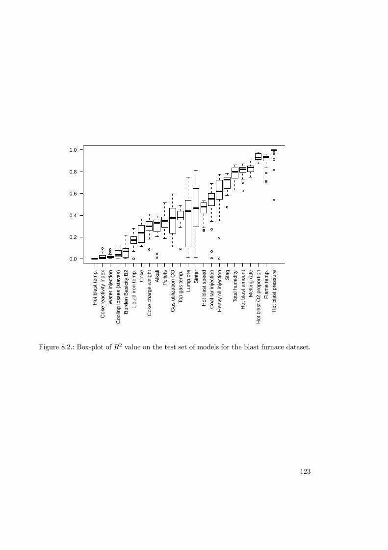
Hot

bla

st te

mp.

Cok

e re

activ

ity in

dex

Wat

er in

ject

ion

Coo

ling

loss

es (

stav

es)

Bur

den

Bas

icity

B2

Liqu

id ir

on te

mp.

Cok

e

Cok

e ch

arge

wei

ght

Alk

ali

Pel

lets

Gas

util

izat

ion

CO

Top

gas

tem

p.

Lum

p or

e

Sin

ter

Hot

bla

st s

peed

Coa

l tar

inje

ctio

n

Hea

vy o

il in

ject

ion

Sla

g

Tota

l hum

idity

Hot

bla

st a

mou

nt

Mel

ting

rate

Hot

bla

st O

2 pr

opor

tion

Fla

me

tem

p.

Hot

bla

st p

ress

ure

0.0

0.2

0.4

0.6

0.8

1.0

Figure 8.2.: Box-plot of R2 value on the test set of models for the blast furnace dataset.

123

Some variables in the network are connected by arrows in both directions. This is anindicator that the pair of variables is strongly related. The value of the first variable canbe approximated, if the value of the second variable is known and vice versa.

Variables that have many outgoing arrows play a central role in the process and can beused to approximate many other variables. In the blast furnace network central variablesare the melting rate, the amount of slag, the amount of injected heavy oil, the amountof pellets, and the hot blast speed and its O2 proportion.

In Figure 8.3 all target variables are displayed to present the full results of the ex-periments. In a data mining scenario it is a good idea to filter the results dynamically,showing only results for target variables for which accurate models are available. Theunfiltered variable relationship network should be interpreted in combination with thebox plot in Figure 8.2, because the significance (not in the statistical sense) of arrowspointing to variables which cannot be approximated accurately, is low. One example arethe cooling losses of the staves. The three most relevant input variables for models forthe cooling losses are: the gas utilization (CO), the amount of alkali, and the amountof heavy oil injected through tuyeres. This result has to be viewed critically because allmodels for the cooling losses, which have been found in the process, are rather inaccurate(R2 value of approximately 0.2). In any case, the knowledge gained by this experimentcan be used to study the effects of these three variables on the cooling losses in moredetail.

8.1.3. Result Details

The relationship network for the blast furnace process presented in Figure 8.3 providesa good overview of the blast furnace process. However, many interesting details arenot shown in the network because this would add visual clutter to the figure and makeit hard to interpret the results. For a more thorough analysis it is necessary to lookat the models in more detail. In this section we present a number of selected modelsfor a subset of target variables for which accurate models have been identified. Themodels presented in this section are simplified versions of the original models producedby GP. The simplification includes manual pruning of branches with minor impact onthe prediction and automatic simplification. Table 8.3 gives an overview of the modelspresented below.

It is important to note that the models presented in Equations 8.1 to 8.12 are the directresult of a data-analysis process and can only show relations of variable values in thedataset in a statistical sense. In particular, the models do not necessarily approximateactual physical or chemical relations or causations in the blast furnace process.

The models show a strong relation of the melting rate with the hot blast parameters.The melting rate is used in models for the hot blast parameters: pressure (8.1), O2-proportion (8.5), the hot blast amount (8.9), and the total humidity (8.8) which is largelydetermined by the hot blast. In return the hot blast parameters play an important role inthe model for the melting rate (8.11). Parameters of the hot blast are directly controlledby the operator who adjusts the amount, the temperature, and the O2 proportion ofthe hot blast [62]. As such the models identified for the hot blast are not interesting for

124

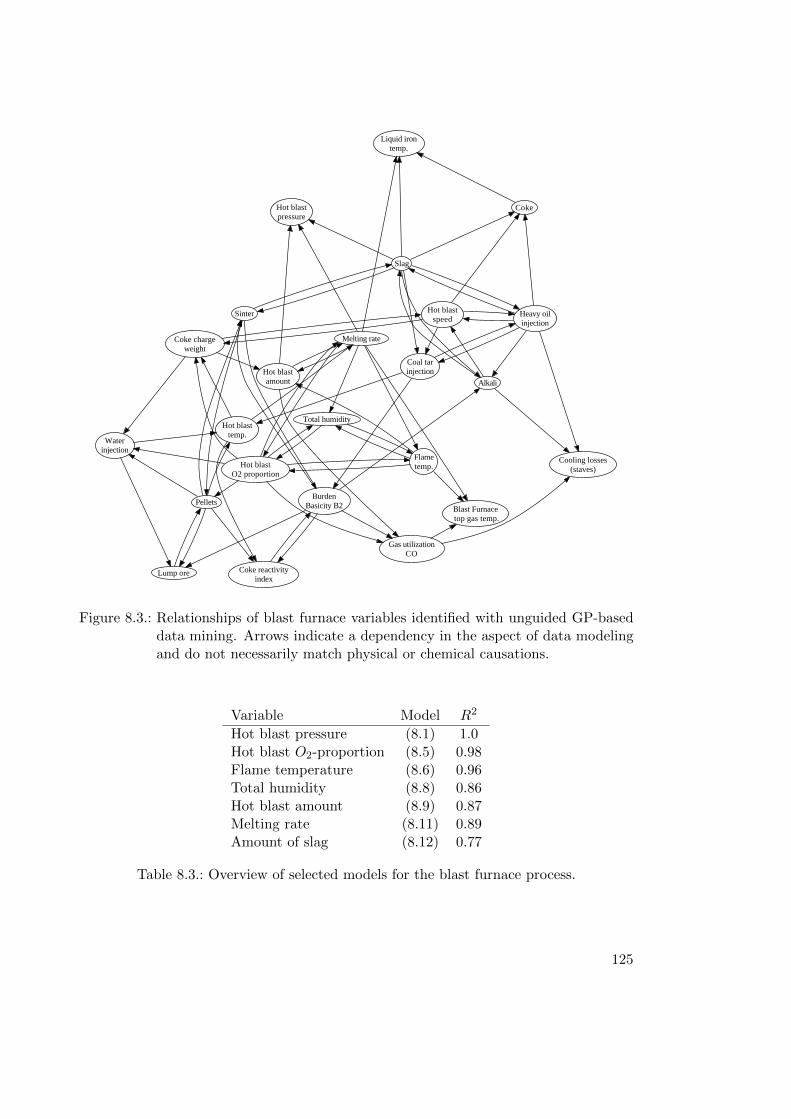
Hot blastpressure

Hot blastO2 proportion

Total humidity

Flametemp.

Melting rate

Gas utilizationCO

Waterinjection

Coke chargeweight

Pellets

Hot blastspeed

Heavy oilinjection

Coal tarinjection

Coke

Hot blastamount

Hot blasttemp.

Coke reactivityindex

Blast Furnace top gas temp.

Liquid irontemp.

Cooling losses(staves)

Slag

Alkali

BurdenBasicity B2

Lump ore

Sinter

Figure 8.3.: Relationships of blast furnace variables identified with unguided GP-baseddata mining. Arrows indicate a dependency in the aspect of data modelingand do not necessarily match physical or chemical causations.

Variable Model R2

Hot blast pressure (8.1) 1.0Hot blast O2-proportion (8.5) 0.98Flame temperature (8.6) 0.96Total humidity (8.8) 0.86Hot blast amount (8.9) 0.87Melting rate (8.11) 0.89Amount of slag (8.12) 0.77

Table 8.3.: Overview of selected models for the blast furnace process.

125

3.6 3.7 3.8 3.9 4 4.13.4

3.6

3.8

4

4.2

Estimated

Original

Y vs. Y’

Training

Test

Figure 8.4.: Scatter plot of the original values of PressureHB and the output of model8.1.

the blast furnace operator [62]. However, they are helpful for the interpretation of othermodels as they represent the implicit relations of different variables which might be usedinterchangeably by GP in models for more interesting variables like the melting rate.

The pressure of the hot blast is a result of the hot blast amount and temperature andpermeability of the burden through which the hot blast is pressed [62]. The model iden-tified using symbolic regression is shown in Equation 8.1. It has a very high correlationwith the original measured values considering only the test partition.

PressureHB = c0 logc1SpeedHB

AmountHB × TempHB

+ c2

c0 = −11.4233

c1 = 0.79701

c2 = −68.9197

(8.1)

The scatter plot of the original values and the output of this model is shown in Figure8.4. As can be seen in the scatter plot the value is approximated correctly for thetest set, however, an additional unknown term which is not included in the model alsoinfluences the pressure of the hot blast. This missing term is the tuyere area whichchanges intermittently every two to six months and stays constant over large time spans[62]. As can be seen in Figure 8.4 the tuyere area is changed five times over the wholeperiod from which the blast furnace data set was collected.

Model 8.1 can be further simplified to the expression shown in Equation 8.2.

PressureHB = α(− log(SpeedHB) + log(AmountHB) + log(TempHB)) + β (8.2)

126

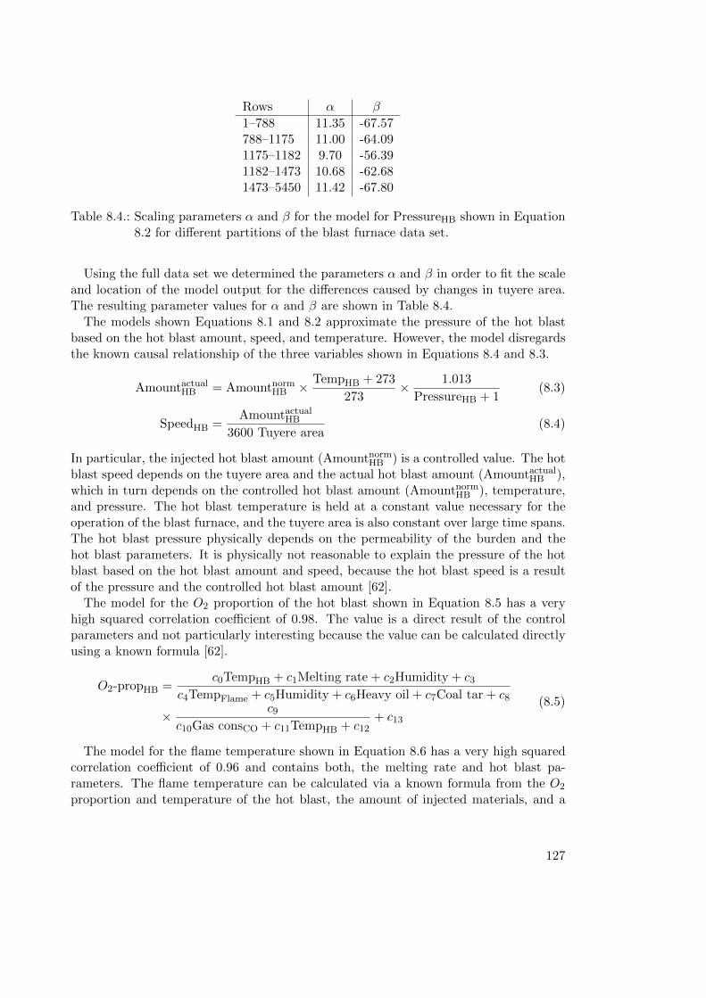
Rows α β

1–788 11.35 -67.57788–1175 11.00 -64.091175–1182 9.70 -56.391182–1473 10.68 -62.681473–5450 11.42 -67.80

Table 8.4.: Scaling parameters α and β for the model for PressureHB shown in Equation8.2 for different partitions of the blast furnace data set.

Using the full data set we determined the parameters α and β in order to fit the scaleand location of the model output for the differences caused by changes in tuyere area.The resulting parameter values for α and β are shown in Table 8.4.

The models shown Equations 8.1 and 8.2 approximate the pressure of the hot blastbased on the hot blast amount, speed, and temperature. However, the model disregardsthe known causal relationship of the three variables shown in Equations 8.4 and 8.3.

AmountactualHB = AmountnormHB × TempHB + 273

273× 1.013

PressureHB + 1(8.3)

SpeedHB =AmountactualHB

3600 Tuyere area(8.4)

In particular, the injected hot blast amount (AmountnormHB ) is a controlled value. The hotblast speed depends on the tuyere area and the actual hot blast amount (AmountactualHB ),which in turn depends on the controlled hot blast amount (AmountnormHB ), temperature,and pressure. The hot blast temperature is held at a constant value necessary for theoperation of the blast furnace, and the tuyere area is also constant over large time spans.The hot blast pressure physically depends on the permeability of the burden and thehot blast parameters. It is physically not reasonable to explain the pressure of the hotblast based on the hot blast amount and speed, because the hot blast speed is a resultof the pressure and the controlled hot blast amount [62].

The model for the O2 proportion of the hot blast shown in Equation 8.5 has a veryhigh squared correlation coefficient of 0.98. The value is a direct result of the controlparameters and not particularly interesting because the value can be calculated directlyusing a known formula [62].

O2-propHB =c0TempHB + c1Melting rate + c2Humidity + c3

c4TempFlame + c5Humidity + c6Heavy oil + c7Coal tar + c8

× c9c10Gas consCO + c11TempHB + c12

+ c13

(8.5)

The model for the flame temperature shown in Equation 8.6 has a very high squaredcorrelation coefficient of 0.96 and contains both, the melting rate and hot blast pa-rameters. The flame temperature can be calculated via a known formula from the O2

proportion and temperature of the hot blast, the amount of injected materials, and a

127

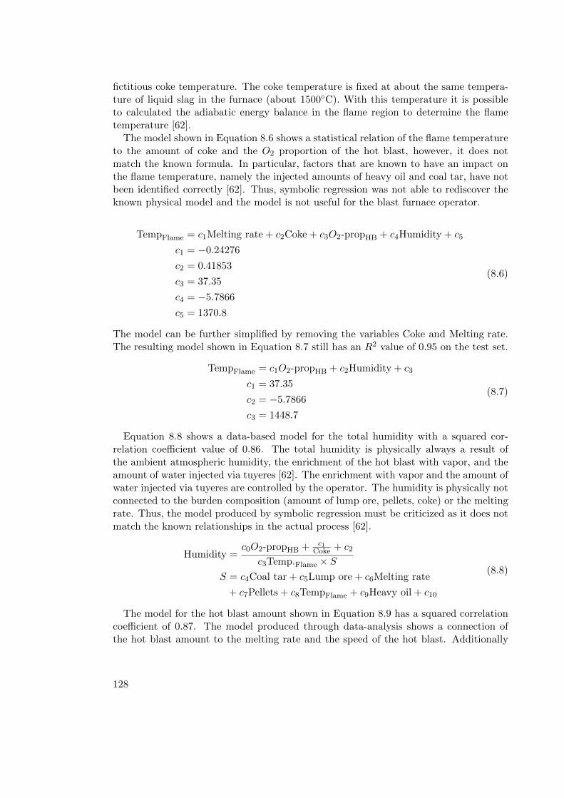
fictitious coke temperature. The coke temperature is fixed at about the same tempera-ture of liquid slag in the furnace (about 1500◦C). With this temperature it is possibleto calculated the adiabatic energy balance in the flame region to determine the flametemperature [62].

The model shown in Equation 8.6 shows a statistical relation of the flame temperatureto the amount of coke and the O2 proportion of the hot blast, however, it does notmatch the known formula. In particular, factors that are known to have an impact onthe flame temperature, namely the injected amounts of heavy oil and coal tar, have notbeen identified correctly [62]. Thus, symbolic regression was not able to rediscover theknown physical model and the model is not useful for the blast furnace operator.

TempFlame = c1Melting rate + c2Coke + c3O2-propHB + c4Humidity + c5

c1 = −0.24276

c2 = 0.41853

c3 = 37.35

c4 = −5.7866

c5 = 1370.8

(8.6)

The model can be further simplified by removing the variables Coke and Melting rate.The resulting model shown in Equation 8.7 still has an R2 value of 0.95 on the test set.

TempFlame = c1O2-propHB + c2Humidity + c3

c1 = 37.35

c2 = −5.7866

c3 = 1448.7

(8.7)

Equation 8.8 shows a data-based model for the total humidity with a squared cor-relation coefficient value of 0.86. The total humidity is physically always a result ofthe ambient atmospheric humidity, the enrichment of the hot blast with vapor, and theamount of water injected via tuyeres [62]. The enrichment with vapor and the amount ofwater injected via tuyeres are controlled by the operator. The humidity is physically notconnected to the burden composition (amount of lump ore, pellets, coke) or the meltingrate. Thus, the model produced by symbolic regression must be criticized as it does notmatch the known relationships in the actual process [62].

Humidity =c0O2-propHB + c1

Coke + c2

c3Temp.Flame × S

S = c4Coal tar + c5Lump ore + c6Melting rate

+ c7Pellets + c8TempFlame + c9Heavy oil + c10

(8.8)

The model for the hot blast amount shown in Equation 8.9 has a squared correlationcoefficient of 0.87. The model produced through data-analysis shows a connection ofthe hot blast amount to the melting rate and the speed of the hot blast. Additionally

128

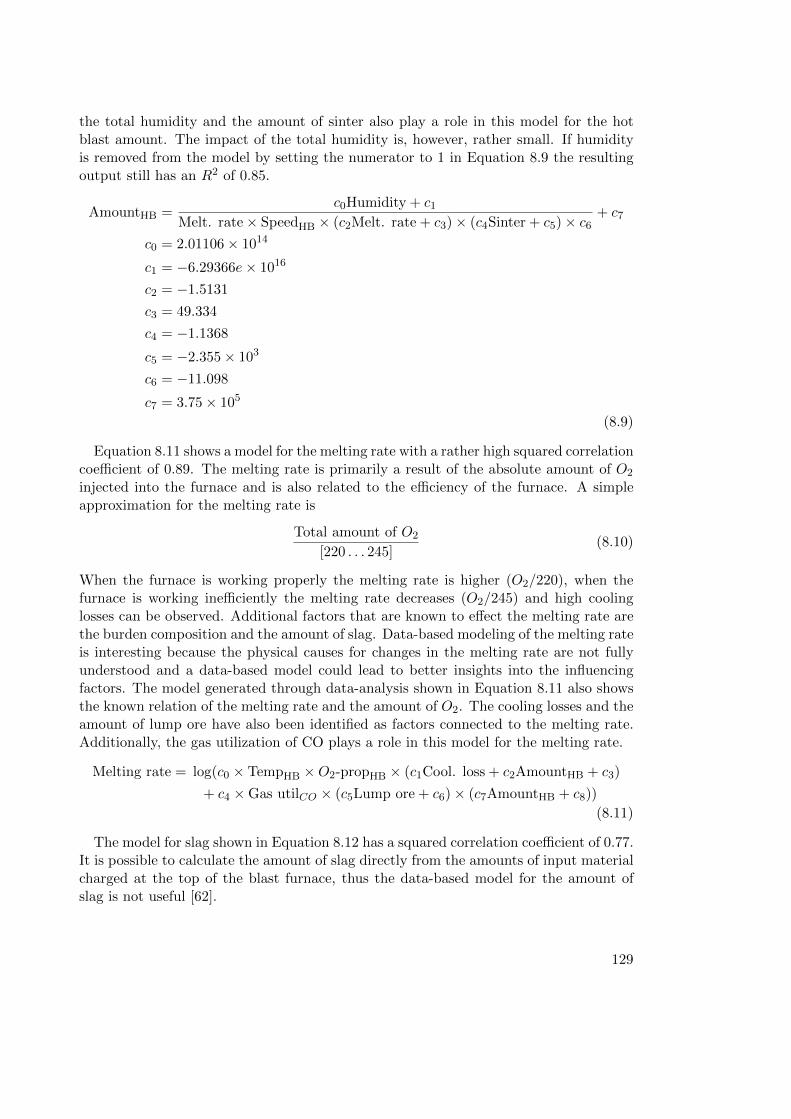
the total humidity and the amount of sinter also play a role in this model for the hotblast amount. The impact of the total humidity is, however, rather small. If humidityis removed from the model by setting the numerator to 1 in Equation 8.9 the resultingoutput still has an R2 of 0.85.

AmountHB =c0Humidity + c1

Melt. rate× SpeedHB × (c2Melt. rate + c3)× (c4Sinter + c5)× c6+ c7

c0 = 2.01106× 1014

c1 = −6.29366e× 1016

c2 = −1.5131

c3 = 49.334

c4 = −1.1368

c5 = −2.355× 103

c6 = −11.098

c7 = 3.75× 105

(8.9)

Equation 8.11 shows a model for the melting rate with a rather high squared correlationcoefficient of 0.89. The melting rate is primarily a result of the absolute amount of O2

injected into the furnace and is also related to the efficiency of the furnace. A simpleapproximation for the melting rate is

Total amount of O2

[220 . . . 245](8.10)

When the furnace is working properly the melting rate is higher (O2/220), when thefurnace is working inefficiently the melting rate decreases (O2/245) and high coolinglosses can be observed. Additional factors that are known to effect the melting rate arethe burden composition and the amount of slag. Data-based modeling of the melting rateis interesting because the physical causes for changes in the melting rate are not fullyunderstood and a data-based model could lead to better insights into the influencingfactors. The model generated through data-analysis shown in Equation 8.11 also showsthe known relation of the melting rate and the amount of O2. The cooling losses and theamount of lump ore have also been identified as factors connected to the melting rate.Additionally, the gas utilization of CO plays a role in this model for the melting rate.

Melting rate = log(c0 × TempHB ×O2-propHB × (c1Cool. loss + c2AmountHB + c3)

+ c4 ×Gas utilCO × (c5Lump ore + c6)× (c7AmountHB + c8))

(8.11)

The model for slag shown in Equation 8.12 has a squared correlation coefficient of 0.77.It is possible to calculate the amount of slag directly from the amounts of input materialcharged at the top of the blast furnace, thus the data-based model for the amount ofslag is not useful [62].

129

Slag = c0Sinter +c1Heavy oil + c2c3 log(Alkali) + c4

+ c5Alkali (8.12)

8.1.4. Concluding Remarks

Using a comprehensive symbolic regression approach a number of data-based modelshave been identified for certain variables in the blast furnace process that approximatethe observed values rather accurately.

In the detailed analysis of the models presented in this section it became clear, thatthe majority of the models are not useful for the blast furnace operator because the realprocess is not described correctly [62]. In particular, the symbolic regression modelsoften contain input variables which are known to be independent from the target vari-able, whereas input variables which do have an influence on the target variable are notidentified correctly.

Additionally, the comprehensive symbolic regression approach produced many modelswhich are not useful for the blast furnace operator because the modeling process isuntargeted. In particular, some variables which are considered as target variables are notrelevant for the analysis of the process because they are directly or indirectly controlledby the blast furnace operator [62]. Also, the value of some variables can be determinedthrough known formulas which are more accurate than the data-based models.

As described in the previous sections, many variables in the blast furnace processare implicitly related, either because of underlying physical relations, or because of theexternal control of blast furnace parameters. This causes problems in the identifica-tion and description of symbolic regression models, because it is possible to express anidentified dependency in multiple different but semantically identical ways via the im-plicit relations. Usually, implicit relations are not known a-priori in data-based modelingmethods, thus a method to identify all implicit dependencies can be useful. However, inthe situation of the blast furnace process many of the implicit dependencies are alreadyknown, thus the untargeted approach is inefficient and misleading. Instead, it is betterto create models for a few carefully selected target variables, where the set of inputvariables is restricted to a few variables. For the definition of the modeling scenarios,as well as for the interpretation of the models, expert knowledge about the process andthe implicit dependencies is necessary.

In retrospect the comprehensive symbolic regression approach is not useful for mod-eling the blast furnace process, where many physical relations are known beforehand.A very interesting extension of that approach, left for future work, would be to includea-priori knowledge into the modeling process. If the control parameters and knowncausal chains are predefined and supplied as input to the modeling approach it would bepossible to restrict the search for actually relevant and potentially interesting models.

130

8.2. Econometric Modeling

Macro-economic models describe the dynamics of economic quantities of countries orregions, as well as their interaction on international markets. Macro-economic variablesthat play a role in such models are for instance the unemployment rate, gross domesticproduct, current account figures and monetary aggregates. Macro-economic models canbe used to estimate the current economic conditions and to forecast economic develop-ments and trends. Therefore macro-economic models play a substantial role in financialand political decisions.

Genetic programming has been used to rediscover well known non-linear econometricmodels from noisy datasets [100, 101]. Numerous papers have been published, describ-ing applications of genetic programming in finance and econometrics, in particular formodeling and prediction of financial time series [36, 121, 92, 216, 144, 93, 31] and thediscovery of effective trading rules [143, 141, 142, 140, 131, 50, 51, 237].

In this contribution we take up the idea of using symbolic regression to generate modelsdescribing macro-economic interactions based on observations of economic quantities.However, contrary to the constrained situation studied in [100], we use a more extensivedataset with observations of many different economic quantities, and aim to identify allpotentially interesting economic interactions that can be derived from the observationsin the dataset. Also, we are not concerned about the prognosis of economic time series,but in the relation of different economic variables over the observed time span.

8.2.1. Macro-Economic Dataset

The dataset we used for the discovery of macro-economic models has been collectedand kindly provided to us by Dr. Stefan Fink. The original dataset contains monthlyobservations of 104 economic variables and indexes from the United States of America,Germany, and the Euro zone in the time span from January 1978 until December 2008.However, not all variables contain values for the full time span so, as preparation formodeling with GP, we reduced the number of rows to cover the time span from January1980 until July 2007 (331 rows). Next we reduced the set of input variables and keptonly those variables, for which values for the whole time span are available. All variablevalues have been scaled to values between 1 and 2. The variable days is a index variablefor the number of days elapsed since 01/01/1980. Using this variable, the GP processcan theoretically identify seasonal changes in the variables. Table 8.5 lists the remainingvariables of the macro-economic dataset.

Preliminary analysis of the dataset showed, that some of the variables are stronglycorrelated. The strongly correlated variables pairs are: the number of housing startsand the number of building permits, the ISM manufacturing purchase managers indexand the Chicago purchase managers index, and the university of Michigan sentimentindex and the university of Michigan conditions index. The three variables correlatedvariables, housing starts, ISM mfg PMI, and U. Mich. sentiment have been removedfrom the dataset.

The following variables have a general rising trend and are pairwise strongly cor-

131

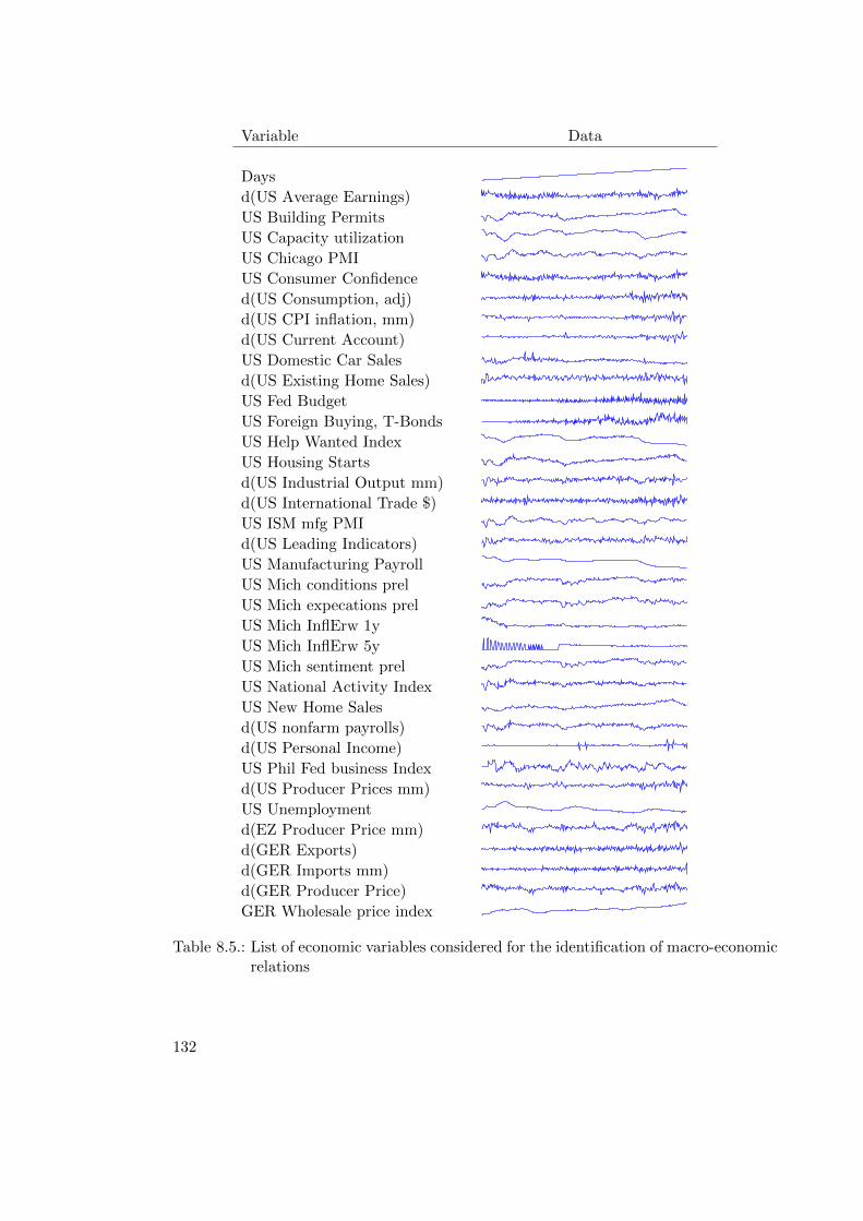
Variable Data

Days

d(US Average Earnings)

US Building Permits

US Capacity utilization

US Chicago PMI

US Consumer Confidence

d(US Consumption, adj)

d(US CPI inflation, mm)

d(US Current Account)

US Domestic Car Sales

d(US Existing Home Sales)

US Fed Budget

US Foreign Buying, T-Bonds

US Help Wanted Index

US Housing Starts

d(US Industrial Output mm)

d(US International Trade $)

US ISM mfg PMI

d(US Leading Indicators)

US Manufacturing Payroll

US Mich conditions prel

US Mich expecations prel

US Mich InflErw 1y

US Mich InflErw 5y

US Mich sentiment prel

US National Activity Index

US New Home Sales

d(US nonfarm payrolls)

d(US Personal Income)

US Phil Fed business Index

d(US Producer Prices mm)

US Unemployment

d(EZ Producer Price mm)

d(GER Exports)

d(GER Imports mm)

d(GER Producer Price)

GER Wholesale price index

Table 8.5.: List of economic variables considered for the identification of macro-economicrelations

132

related: personal income, existing house sales, current account, international trade,consumption, leading indicators, industrial output, average earnings, non-farm payrolls,producer price, CPI inflation, imports (GER), exports (GER), producer price (EZ).These correlations are not particularly useful, so we decided to study the derivatives(monthly changes) of the variables instead of the absolute values to find more interest-ing relations. The derivative variables (d(x)) are calculated using the five point formulafor the numerical approximation of the derivative (see Section A.2). The drawback ofthe numerical approximation of the derivative is, that the noise in the original values isamplified by the calculation of the derivative and it is more difficult to produce accuratemodels for the derivative variable.

8.2.2. Modeling

The dataset is split into training (rows 13–300) and test (rows 300–331). The testingperiod is January 2005 to July 2007. Only rows 13–200 are used for fitness evaluationand rows 100–300 are used as internal validation set for overfitting detection and forthe selection of the final (best on validation) model. Note, that there is an overlappingregion of rows that are used for the fitness calculation and for internal validation. Thedataset is rather small and the overlap is on purpose to increase the number of rows,used for validation. The drawback of the overlap is, that the chance to return overfitmodels is larger.

The goal of the modeling step is to identify the network of relevant variable interactionsin the macro-economic dataset. Thus, several symbolic regression runs were executedto produce approximation models for each variable of the dataset. The same parametersettings were used for all runs. Only the target variable and the list of allowed inputvariables was adapted. The GP parameter settings for our experiments are specified inTable 8.6. We used rather standard GP configuration with tree-based solution encoding,tournament selection, sub-tree swapping crossover, and two mutation operators. Thefitness function is the squared correlation coefficient of the model output and the actualvalues of target variables. Only the final model is linearly scaled to match the locationand scale of the target variable [95].

In the experiments we used two adaptations of the algorithm to reduce bloat andoverfitting described in the previous chapters. Dynamic depth limits [188] with an initialdepth limit of seven are used to reduce the amount of bloat. An internal validation setis used to reduce the chance of overfitting. Each solution candidate is evaluated on thetraining and on the validation set. Selection is based solely on the fitness on the trainingset, the fitness on the validation set is used as an indicator for overfitting. Models thathave a high training fitness but a low validation fitness are likely to be overfit. Thus,after each iteration the correlation of the training- and validation fitness values of allsolution candidates in the population is calculated using Spearman’s rank correlationρ(Fitnesstrain,Fitnessval). If the correlation of training- and validation fitness in thepopulation drops below a certain threshold the algorithm is stopped.

133

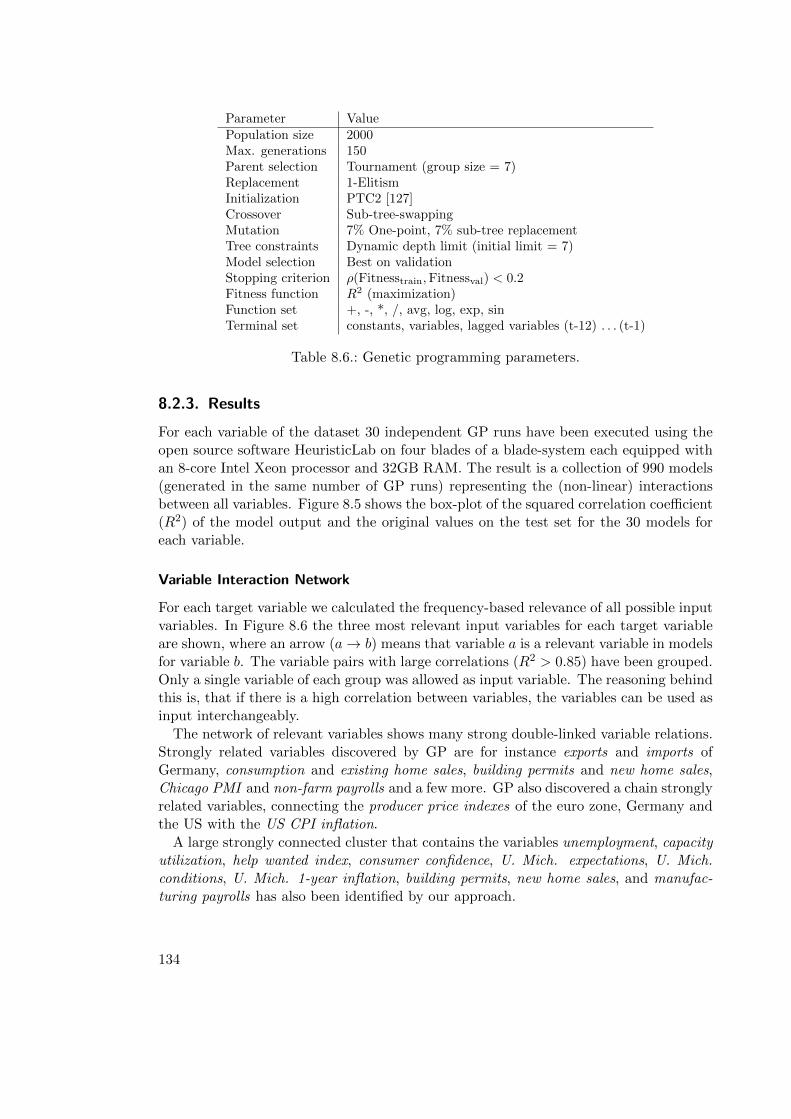
Parameter ValuePopulation size 2000Max. generations 150Parent selection Tournament (group size = 7)Replacement 1-ElitismInitialization PTC2 [127]Crossover Sub-tree-swappingMutation 7% One-point, 7% sub-tree replacementTree constraints Dynamic depth limit (initial limit = 7)Model selection Best on validationStopping criterion ρ(Fitnesstrain,Fitnessval) < 0.2Fitness function R2 (maximization)Function set +, -, *, /, avg, log, exp, sinTerminal set constants, variables, lagged variables (t-12) . . . (t-1)

Table 8.6.: Genetic programming parameters.

8.2.3. Results

For each variable of the dataset 30 independent GP runs have been executed using theopen source software HeuristicLab on four blades of a blade-system each equipped withan 8-core Intel Xeon processor and 32GB RAM. The result is a collection of 990 models(generated in the same number of GP runs) representing the (non-linear) interactionsbetween all variables. Figure 8.5 shows the box-plot of the squared correlation coefficient(R2) of the model output and the original values on the test set for the 30 models foreach variable.

Variable Interaction Network

For each target variable we calculated the frequency-based relevance of all possible inputvariables. In Figure 8.6 the three most relevant input variables for each target variableare shown, where an arrow (a → b) means that variable a is a relevant variable in modelsfor variable b. The variable pairs with large correlations (R2 > 0.85) have been grouped.Only a single variable of each group was allowed as input variable. The reasoning behindthis is, that if there is a high correlation between variables, the variables can be used asinput interchangeably.

The network of relevant variables shows many strong double-linked variable relations.Strongly related variables discovered by GP are for instance exports and imports ofGermany, consumption and existing home sales, building permits and new home sales,Chicago PMI and non-farm payrolls and a few more. GP also discovered a chain stronglyrelated variables, connecting the producer price indexes of the euro zone, Germany andthe US with the US CPI inflation.

A large strongly connected cluster that contains the variables unemployment, capacityutilization, help wanted index, consumer confidence, U. Mich. expectations, U. Mich.conditions, U. Mich. 1-year inflation, building permits, new home sales, and manufac-turing payrolls has also been identified by our approach.

134

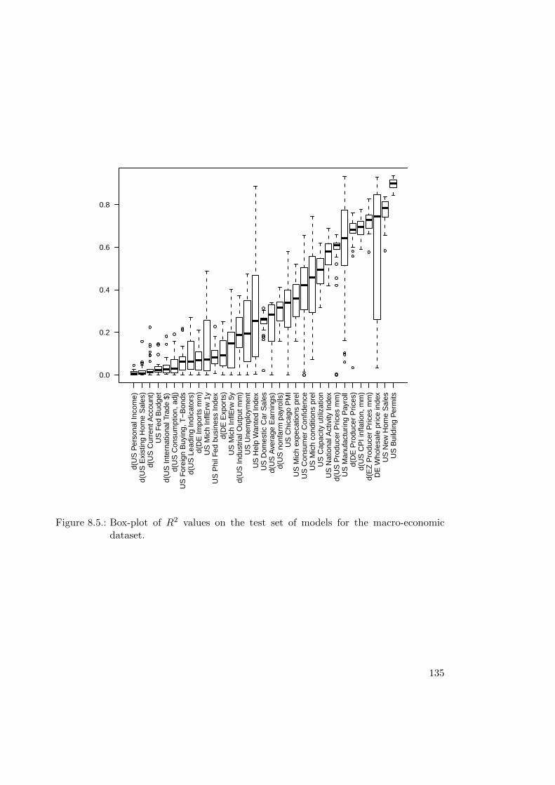
d(U

S P

erso

nal I

ncom

e)d(

US

Exi

stin

g H

ome

Sal

es)

d(U

S C

urre

nt A

ccou

nt)

US

Fed

Bud

get

d(U

S In

tern

atio

nal T

rade

$)

d(U

S C

onsu

mpt

ion,

adj

)U

S F

orei

gn B

uyin

g, T

−B

onds

d(U

S L

eadi

ng In

dica

tors

)d(

DE

Impo

rts

mm

)U

S M

ich

InflE

rw 1

yU

S P

hil F

ed b

usin

ess

Inde

xd(

DE

Exp

orts

)U

S M

ich

InflE

rw 5

yd(

US

Indu

stria

l Out

put m

m)

US

Une

mpl

oym

ent

US

Hel

p W

ante

d In

dex

US

Dom

estic

Car

Sal

esd(

US

Ave

rage

Ear

ning

s)d(

US

non

farm

pay

rolls

)U

S C

hica

go P

MI

US

Mic

h ex

peca

tions

pre

lU

S C

onsu

mer

Con

fiden

ceU

S M

ich

cond

ition

s pr

elU

S C

apac

ity u

tiliz

atio

nU

S N

atio

nal A

ctiv

ity In

dex

d(U

S P

rodu

cer

Pric

es m

m)

US

Man

ufac

turin

g P

ayro

lld(

DE

Pro

duce

r P

rices

)d(

US

CP

I inf

latio

n, m

m)

d(E

Z P

rodu

cer

Pric

es m

m)

DE

Who

lesa

le p

rice

inde

xU

S N

ew H

ome

Sal

esU

S B

uild

ing

Per

mits

0.0

0.2

0.4

0.6

0.8

Figure 8.5.: Box-plot of R2 values on the test set of models for the macro-economicdataset.

135

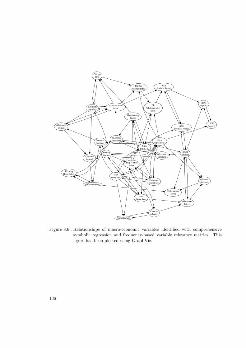
d(CPIinflation)d(Average

Earnings)

d(ProducerPrices)

d(DEProducer Prices)

d(CurrentAccount)

d(InternationalTrade)

d(DEImports)

d(PersonalIncome)

MichInflErw 1y

d(LeadingIndicators)

NewHome Sales

ManufacturingPayroll

Michconditions

National ActivityIndex

d(ExistingHome Sales)

BuildingPermits

Michexpecations

Help WantedIndex

d(nonfarmpayrolls)

DomesticCar Sales

ConsumerConfidence

DEWholesale price

index

Phil Fedbusiness Index

d(DEExports)

Unemployment

Capacityutilization

ChicagoPMI

d(IndustrialOutput)

d(EZProducer Prices)

d(Consumption)

Figure 8.6.: Relationships of macro-economic variables identified with comprehensivesymbolic regression and frequency-based variable relevance metrics. Thisfigure has been plotted using GraphViz.

136

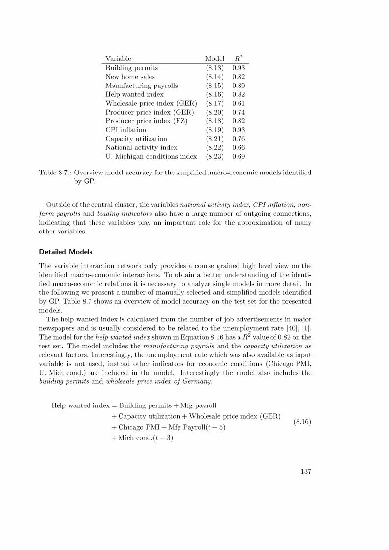
Variable Model R2

Building permits (8.13) 0.93New home sales (8.14) 0.82Manufacturing payrolls (8.15) 0.89Help wanted index (8.16) 0.82Wholesale price index (GER) (8.17) 0.61Producer price index (GER) (8.20) 0.74Producer price index (EZ) (8.18) 0.82CPI inflation (8.19) 0.93Capacity utilization (8.21) 0.76National activity index (8.22) 0.66U. Michigan conditions index (8.23) 0.69

Table 8.7.: Overview model accuracy for the simplified macro-economic models identifiedby GP.

Outside of the central cluster, the variables national activity index, CPI inflation, non-farm payrolls and leading indicators also have a large number of outgoing connections,indicating that these variables play an important role for the approximation of manyother variables.

Detailed Models

The variable interaction network only provides a course grained high level view on theidentified macro-economic interactions. To obtain a better understanding of the identi-fied macro-economic relations it is necessary to analyze single models in more detail. Inthe following we present a number of manually selected and simplified models identifiedby GP. Table 8.7 shows an overview of model accuracy on the test set for the presentedmodels.

The help wanted index is calculated from the number of job advertisements in majornewspapers and is usually considered to be related to the unemployment rate [40], [1].The model for the help wanted index shown in Equation 8.16 has a R2 value of 0.82 on thetest set. The model includes the manufacturing payrolls and the capacity utilization asrelevant factors. Interestingly, the unemployment rate which was also available as inputvariable is not used, instead other indicators for economic conditions (Chicago PMI,U. Mich cond.) are included in the model. Interestingly the model also includes thebuilding permits and wholesale price index of Germany.

Help wanted index = Building permits +Mfg payroll

+ Capacity utilization +Wholesale price index (GER)

+ Chicago PMI +Mfg Payroll(t− 5)

+Mich cond.(t− 3)

(8.16)

137

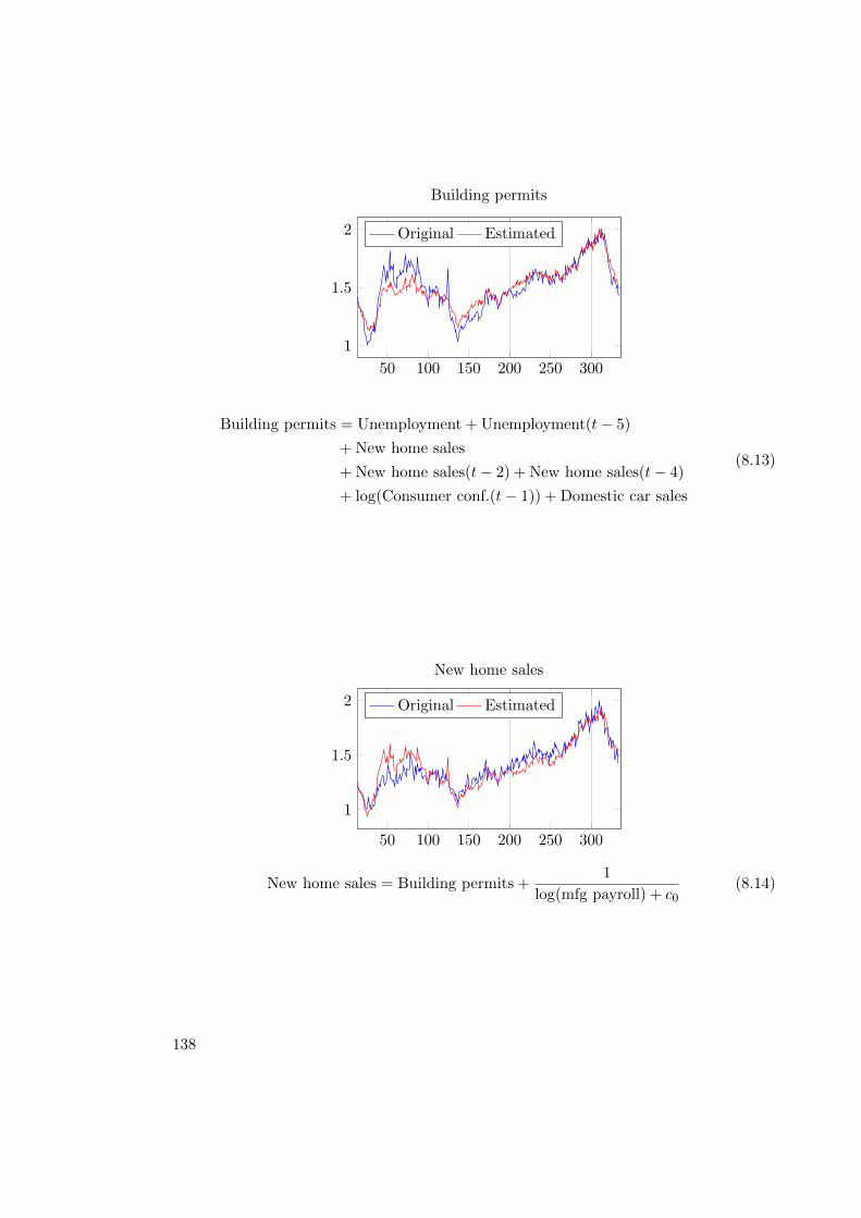
50 100 150 200 250 300

1

1.5

2

Building permits

Original Estimated

Building permits = Unemployment + Unemployment(t− 5)

+ New home sales

+ New home sales(t− 2) + New home sales(t− 4)

+ log(Consumer conf.(t− 1)) + Domestic car sales

(8.13)

50 100 150 200 250 300

1

1.5

2

New home sales

Original Estimated

New home sales = Building permits +1

log(mfg payroll) + c0(8.14)

138

50 100 150 200 250 300

1

1.5

Manufacturing payrolls

Original Estimated

Mfg payrolls =Days + c0

Help wanted index×Help wanted index(t− 6)

+ log(Consumer conf.(t− 1) +Mich 1y infl(t− 6))

(8.15)

50 100 150 200 250 300

1

1.5

2

Help wanted index

Original Estimated

Figure 8.7.: Line chart of the actual value of the US Help wanted index and the estimatedvalues produced by the model (Equation 8.16). Test set starts at index 300.

Figure 8.7 shows a line chart for the actual values of the help wanted index in the USand the estimated values of the model (Equation 8.16) over the whole time span coveredby the dataset.

The consumer price index measures the change in prices paid by customers for acertain market basket containing goods and services, and is measure for the inflation inan economy. The output of the model for the CPI inflation in the US shown in Equation8.19 is very accurate with a squared correlation coefficient of 0.93 on the test set. Themodel approximates the consumer price index based on the unemployment, car sales,New home sales, and the consumer confidence.

CPI inflation = Unemployment + Domestic car sales + New home sales

+ log(New home sales(t− 4) + New home sales(t− 2)

+ Consumer conf.(t− 1) + Unemployment(t− 5))

(8.19)

139

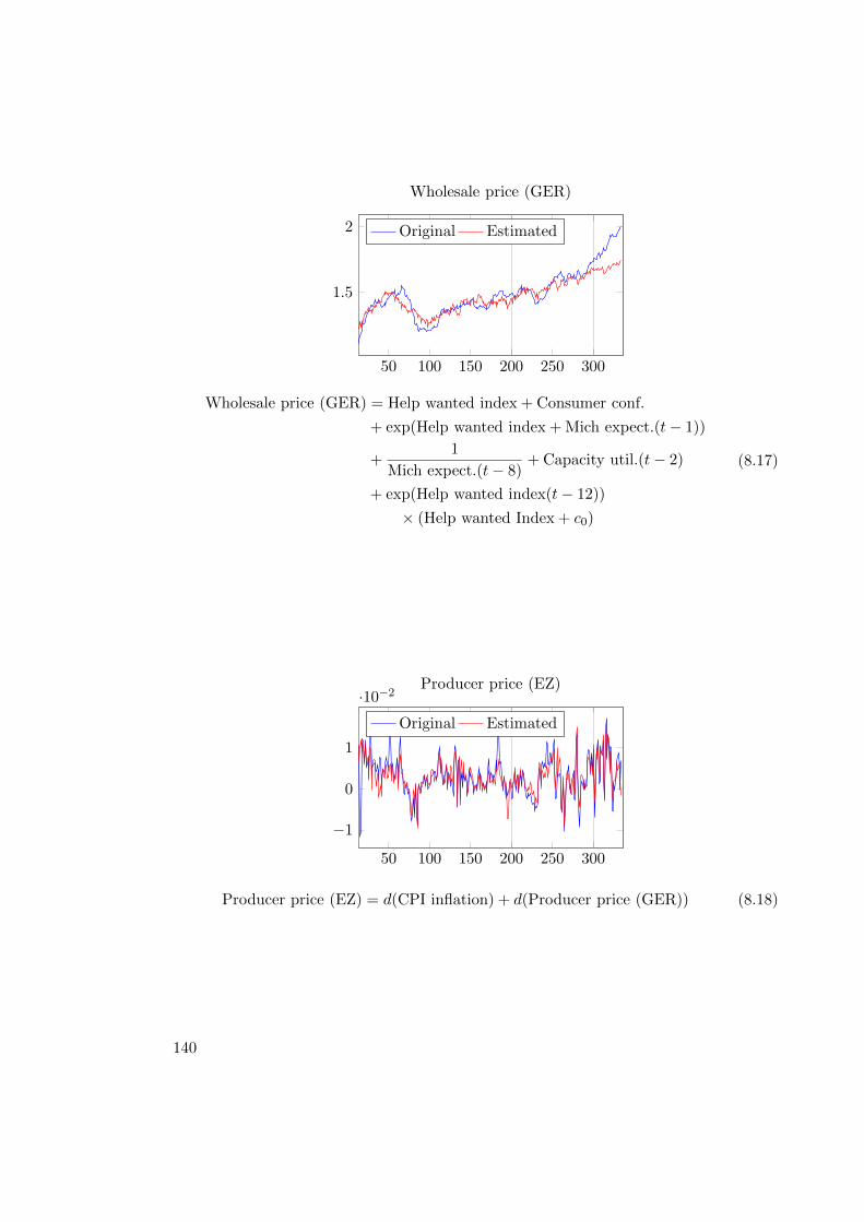
50 100 150 200 250 300

1.5

2

Wholesale price (GER)

Original Estimated

Wholesale price (GER) = Help wanted index + Consumer conf.

+ exp(Help wanted index +Mich expect.(t− 1))

+1

Mich expect.(t− 8)+ Capacity util.(t− 2)

+ exp(Help wanted index(t− 12))

× (Help wanted Index + c0)

(8.17)

50 100 150 200 250 300

−1

0

1

·10−2Producer price (EZ)

Original Estimated

Producer price (EZ) = d(CPI inflation) + d(Producer price (GER)) (8.18)

140

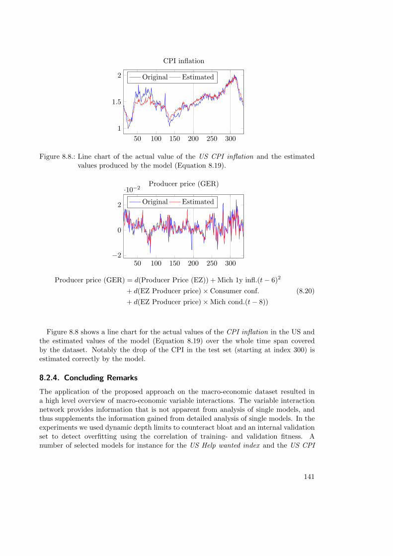
50 100 150 200 250 300

1

1.5

2

CPI inflation

Original Estimated

Figure 8.8.: Line chart of the actual value of the US CPI inflation and the estimatedvalues produced by the model (Equation 8.19).

50 100 150 200 250 300−2

0

2

·10−2Producer price (GER)

Original Estimated

Producer price (GER) = d(Producer Price (EZ)) +Mich 1y infl.(t− 6)2

+ d(EZ Producer price)× Consumer conf.

+ d(EZ Producer price)×Mich cond.(t− 8))

(8.20)

Figure 8.8 shows a line chart for the actual values of the CPI inflation in the US andthe estimated values of the model (Equation 8.19) over the whole time span coveredby the dataset. Notably the drop of the CPI in the test set (starting at index 300) isestimated correctly by the model.

8.2.4. Concluding Remarks

The application of the proposed approach on the macro-economic dataset resulted ina high level overview of macro-economic variable interactions. The variable interactionnetwork provides information that is not apparent from analysis of single models, andthus supplements the information gained from detailed analysis of single models. In theexperiments we used dynamic depth limits to counteract bloat and an internal validationset to detect overfitting using the correlation of training- and validation fitness. Anumber of selected models for instance for the US Help wanted index and the US CPI

141

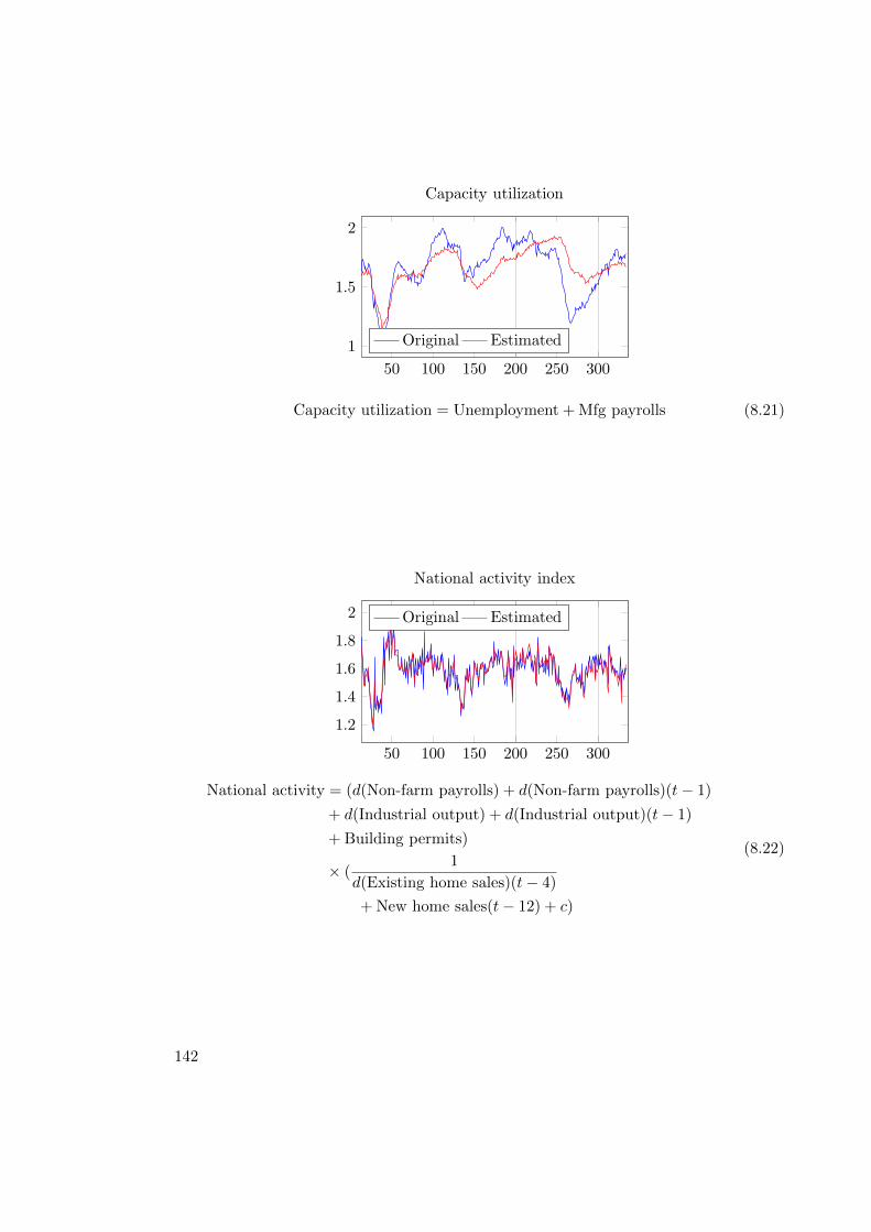
50 100 150 200 250 300

1

1.5

2

Capacity utilization

Original Estimated

Capacity utilization = Unemployment +Mfg payrolls (8.21)

50 100 150 200 250 300

1.2

1.4

1.6

1.8

2

National activity index

Original Estimated

National activity = (d(Non-farm payrolls) + d(Non-farm payrolls)(t− 1)

+ d(Industrial output) + d(Industrial output)(t− 1)

+ Building permits)

× (1

d(Existing home sales)(t− 4)

+ New home sales(t− 12) + c)

(8.22)

142

50 100 150 200 250 3001

1.5

2

U. Mich. conditions index

Original Estimated

Mich. cond. = Mfg payrolls(t− 10)

× Consumer conf.

× (Mich 1-year inflation +Mich expect.

+ Help wanted index(t− 2) + c)

× (c

Consumer conf.× (Mich expect. + c)

+ Help wanted index×Wholesale price (GER)(t− 9) + c)

×(

c

Consumer conf.× (Mich expect. + c)+ c

)

(8.23)

inflation have been presented and discussed in detail. The models are rather accuratealso on the test set and are relatively comprehensible.

143

Correlated variables

x33, x51, x52, x53x35, x37x31, x47x39, x40x1, x7, x10, x38x4, x20, x21x54, x55x9, x16, x17, x18, x19x23, x24, x25, x26, x27, x28

Table 8.8.: Clusters of strongly correlated variables in the chemical dataset. The variableused as representative for the cluster in the modeling process is indicated inbold font.

8.3. Chemical Process

The last application studied in this chapter is the analysis of data from a chemical pro-cess. The dataset analyzed in this section has been prepared and published by ArthurKordon of Dow Chemical for the symbolic regression competition, which has been heldas a side event of the EvoStar conference 2010. Only little information about chemi-cal process, from which the data was collected, is available. The measurements stemfrom a real industrial process. The input variables are process parameters like temper-atures, pressures and material flows (input material). The target variable y describesthe chemical composition of the output of the process. The values of y are measuredin the laboratory and are noisy and rather expensive to measure. The objective is tofind a robust model which accurately approximates the lab value y from the processparameters (virtual sensor). Through interpretation of the model it is possible to gaina better understanding of the impacts of different process parameters on the chemicalcomposition. This knowledge can be used for controlling the process, in order to improveproduct quality.

Some of the input variables are implicitly related so a full search for non-linear relationson the whole dataset is beneficial in order to get a better understanding of the wholeprocess. This is also helpful for the interpretation of model for y as the implicit relationscan be used to generalize over multiple equally accurate models for y.

8.3.1. Modeling

Preliminary analysis shows that a number of variable pairs are strongly correlated leadingto a number of clusters of strongly correlated variables. For each cluster only a singlerepresentative variable is kept in the dataset the remaining variables in the cluster areremoved because they can be expressed through the representative variable of the cluster.Table 8.8 lists the clusters identified by correlation analysis.

The dataset contains 57 input variables x1–x57 and the target variable y. The dataset

144

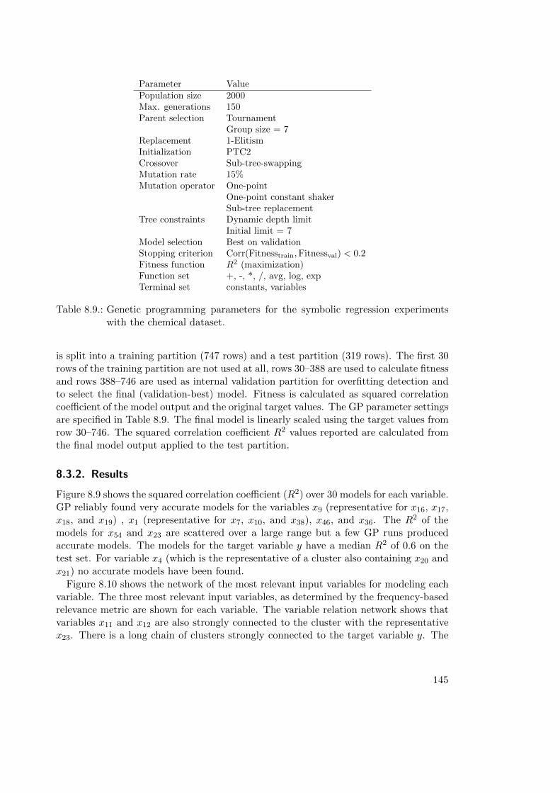
Parameter ValuePopulation size 2000Max. generations 150Parent selection Tournament

Group size = 7Replacement 1-ElitismInitialization PTC2Crossover Sub-tree-swappingMutation rate 15%Mutation operator One-point

One-point constant shakerSub-tree replacement

Tree constraints Dynamic depth limitInitial limit = 7

Model selection Best on validationStopping criterion Corr(Fitnesstrain,Fitnessval) < 0.2Fitness function R2 (maximization)Function set +, -, *, /, avg, log, expTerminal set constants, variables

Table 8.9.: Genetic programming parameters for the symbolic regression experimentswith the chemical dataset.

is split into a training partition (747 rows) and a test partition (319 rows). The first 30rows of the training partition are not used at all, rows 30–388 are used to calculate fitnessand rows 388–746 are used as internal validation partition for overfitting detection andto select the final (validation-best) model. Fitness is calculated as squared correlationcoefficient of the model output and the original target values. The GP parameter settingsare specified in Table 8.9. The final model is linearly scaled using the target values fromrow 30–746. The squared correlation coefficient R2 values reported are calculated fromthe final model output applied to the test partition.

8.3.2. Results

Figure 8.9 shows the squared correlation coefficient (R2) over 30 models for each variable.GP reliably found very accurate models for the variables x9 (representative for x16, x17,x18, and x19) , x1 (representative for x7, x10, and x38), x46, and x36. The R2 of themodels for x54 and x23 are scattered over a large range but a few GP runs producedaccurate models. The models for the target variable y have a median R2 of 0.6 on thetest set. For variable x4 (which is the representative of a cluster also containing x20 andx21) no accurate models have been found.

Figure 8.10 shows the network of the most relevant input variables for modeling eachvariable. The three most relevant input variables, as determined by the frequency-basedrelevance metric are shown for each variable. The variable relation network shows thatvariables x11 and x12 are also strongly connected to the cluster with the representativex23. There is a long chain of clusters strongly connected to the target variable y. The

145

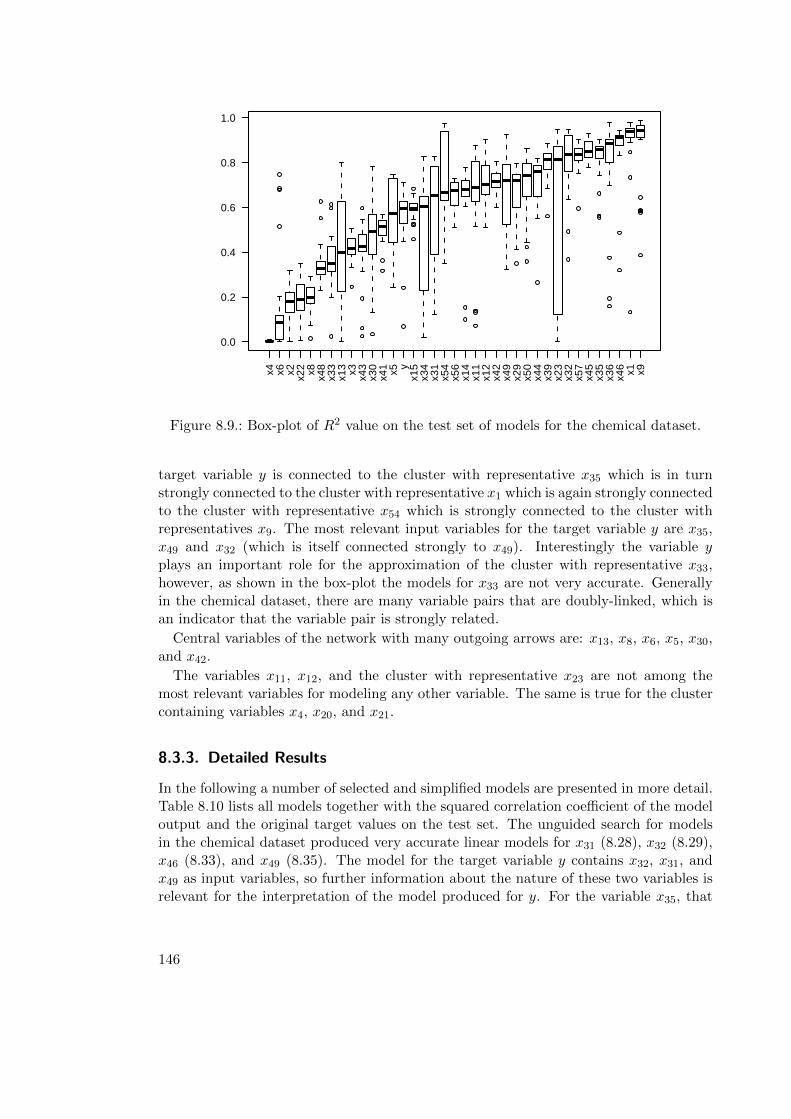
x4 x6 x2 x22 x8 x48

x33

x13 x3 x43

x30

x41 x5 y

x15

x34

x31

x54

x56

x14

x11

x12

x42

x49

x29

x50

x44

x39

x23

x32

x57

x45

x35

x36

x46 x1 x9

0.0

0.2

0.4

0.6

0.8

1.0

Figure 8.9.: Box-plot of R2 value on the test set of models for the chemical dataset.

target variable y is connected to the cluster with representative x35 which is in turnstrongly connected to the cluster with representative x1 which is again strongly connectedto the cluster with representative x54 which is strongly connected to the cluster withrepresentatives x9. The most relevant input variables for the target variable y are x35,x49 and x32 (which is itself connected strongly to x49). Interestingly the variable yplays an important role for the approximation of the cluster with representative x33,however, as shown in the box-plot the models for x33 are not very accurate. Generallyin the chemical dataset, there are many variable pairs that are doubly-linked, which isan indicator that the variable pair is strongly related.

Central variables of the network with many outgoing arrows are: x13, x8, x6, x5, x30,and x42.

The variables x11, x12, and the cluster with representative x23 are not among themost relevant variables for modeling any other variable. The same is true for the clustercontaining variables x4, x20, and x21.

8.3.3. Detailed Results

In the following a number of selected and simplified models are presented in more detail.Table 8.10 lists all models together with the squared correlation coefficient of the modeloutput and the original target values on the test set. The unguided search for modelsin the chemical dataset produced very accurate linear models for x31 (8.28), x32 (8.29),x46 (8.33), and x49 (8.35). The model for the target variable y contains x32, x31, andx49 as input variables, so further information about the nature of these two variables isrelevant for the interpretation of the model produced for y. For the variable x35, that

146

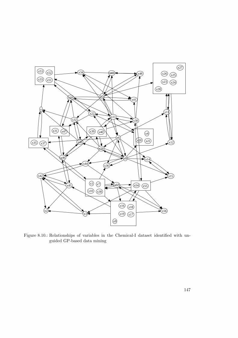
x1 x7

x10 x38

x4

x20 x21

x9

x17

x18

x19

x16

x23 x24

x25x26

x27

x28

x31 x47

x33 x51

x52x53

x35 x37

x39 x40

x54 x55x57

x56

x45

x2

x42

x46

x3

x44

x8

x22

x6

x36

x50

x12

x15

x14

x49

x13

x43

x5

x30

x34 x48

x32

x11

x29x41

y

Figure 8.10.: Relationships of variables in the Chemical-I dataset identified with un-guided GP-based data mining

147

Variable Model R2

x1 (8.24) 0.98x9 (8.25) 0.85x14 (8.26) 0.76x15 (8.27) 0.65x31 (8.28) 0.83x32 (8.29) 0.96x35 (8.30) 0.90x39 (8.31) 0.86x42 (8.32) 0.84x46 (8.33) 0.93x48 (8.34) 0.51x49 (8.35) 0.93x54 (8.36) 0.71y (8.3.3) 0.64

Table 8.10.: Overview of models for the chemical dataset.

also occurs in the model for y, a very accurate non-linear model has been found (8.30)which relates x35 to variables x6, x33, and x57. The only variable occurring in the modelfor y, which cannot be approximated accurately through other variables, is x48 (8.34).

x1 =x8 + x9 + x29 + x15 + x34 + x35 + x45 + y +x9 (x57 + x34 + x49)

x54(8.24)

x9 =1

x35 + x54(8.25)

x14 = x15 + x50 +1

exp(x8)(8.26)

x15 = log

exp(x14)log(y) + c0

log(x5 + c1)× exp(x14 + c2)

(8.27)

x31 = x30 + x32 + x46 + x50 (8.28)

x32 = x5 + x14 + x31 + x33 + x44 + x46 + x49 + x50 (8.29)

148

x35 =1

x33 +x21(x6+c0)x57+c1

+ c2(8.30)

x39 =x30 +

x13

(x50+c0)2 + c

x5 + x29 + x41 + x45 + x46 + x50 + c(8.31)

x42 =1

x34 + x43 + x45(8.32)

x46 = x3 + x5 + x8 + x30 + x31 + x36 + x39 + x44 + x45 + x49 (8.33)

x48 =(x5 + x44 + c) (x30 + x33 + x34 + c) (x33 + c) (x42 + c)

x34 + c(8.34)

x49 = x1 + x8 + x31 + x32 + x44 + x46 + x54 + x50 (8.35)

x54 = exp

(exp

(x9

x22x30

))(8.36)

149

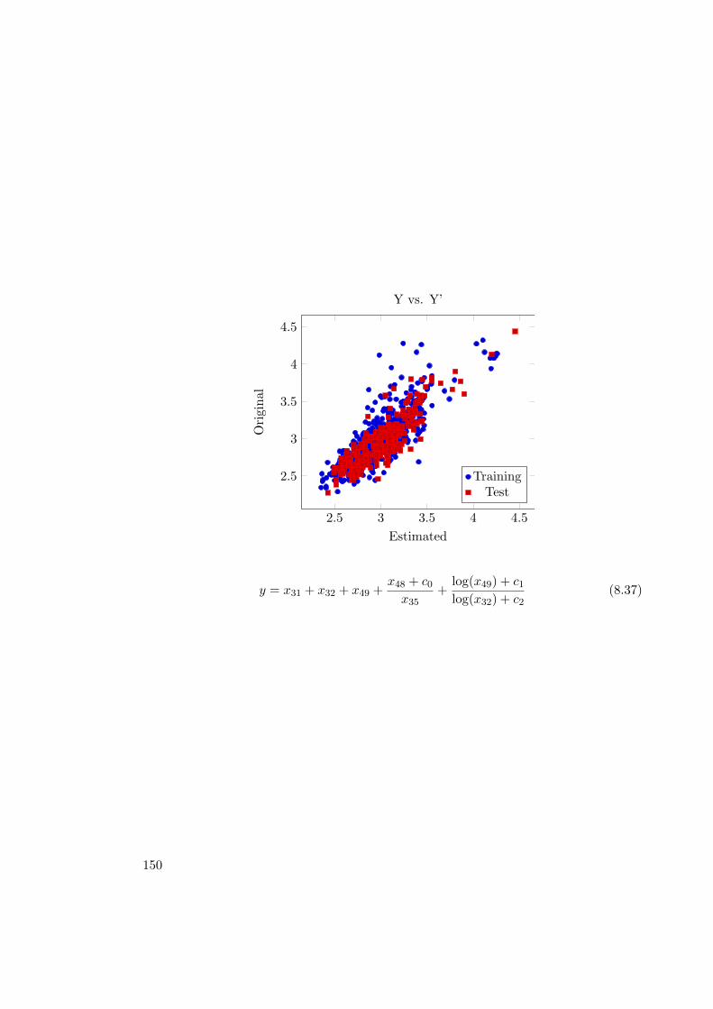
2.5 3 3.5 4 4.5

2.5

3

3.5

4

4.5

Estimated

Original

Y vs. Y’

Training

Test

y = x31 + x32 + x49 +x48 + c0

x35+

log(x49) + c1log(x32) + c2

(8.37)

150

9. Concluding Remarks

The main topic of this work is the application of genetic programming, in particularsymbolic regression, for the identification of comprehensible and accurate models in real-world scenarios. We have focused on aspects of symbolic regression that are relevantfor practical applications. The main contribution is the description of a comprehensivesymbolic regression method for the identification of variable interaction networks. Suchnetworks provide a coarse grained overview of the strongest (non-linear) dependenciesof variables in the studied system. This method is based on a new approach to quantifyrelevant input variables, which is presented for the first time in this thesis.

In practical applications a major concern is the comprehensibility and generality ofmodels. Thus, methods to reduce bloat and overfitting are prominently featured in thisthesis as well. Additionally, we also describe a new method for auto-regressive modelingof multi-variate time series with genetic programming. The methods described in thefirst part of this thesis are applied to a number of real-world problems in the secondpart.

The following topics are covered in this thesis:

• The problem of bloat and a number of bloat control methods are discussed. Inthis thesis the effect of offspring selection on bloat is analyzed for the first time.We have observed that offspring selection does not reduce bloat, instead it has thetendency to increase bloat because of the higher selection pressure.

• Overfitting is an issue in symbolic regression that can occur even in the absence ofbloat . Bloat and overfitting are two related but separate phenomena. We suggestthat an effective symbolic regression approach should include specific countermea-sures for bloat and overfitting. In this thesis a new approach for the detectionof overfitting based on the correlation of training- and validation fitness is de-scribed for the first time. Based on this overfitting criterion, we propose two newapproaches to reduce overfitting. The first approach uses covariant parsimony pres-sure to adaptively control the average program length in the population based onthe overfitting criterion. The second approach uses selective pruning in overfittingphases to remove code fragments that have only a small effect on the fitness of themodel but potentially have a negative effect on the generalization ability of themodel.

The newly proposed overfitting criterion and the two approaches for overfittingreduction are tested on two real world datasets where standard genetic program-ming produces overfit models and based on the results we have observed that theoverfitting criterion reliably indicates overfitting phases and that the two proposedmethods reduce overfitting.

151

In this thesis the effects of offspring selection on overfitting are analyzed for thefirst time. We observe that the overfitting effect is stronger because of the higherselection pressure resulting from offspring selection. Thus, we strongly advise touse an effective method for the validation of symbolic regression models producedin runs with offspring selection.

• Genetic programming has the tendency to build convoluted solutions containingunoptimized code or introns. This effect can be reduced but not completely pre-vented through bloat control methods. Such convoluted solutions are problematicin practical applications, thus we suggest to simplify symbolic regression solutionsin two steps. First the model should be simplified using algebraic transformationsand in a second step the branches which have only a minor effect on the outputshould be removed through either automatic or manual pruning. In this thesis weshow that this simplification approach significantly improves the comprehensibil-ity of symbolic regression solutions while the fitness of the model is only slightlydecreased.

In this context, we also suggest that a small function set including only few simpleoperators should be preferred for practical applications. Arithmetic expressionscan be simplified easily and are easier to comprehend than expressions with deeplynested complex functions.

• Measuring variable importance is a big topic in regression modeling and is con-nected to feature selection. In practical applications the information about therelevant factors that might have an effect on a target variable is often very valu-able.

In this thesis we review different ways to determine relative variable importancein regression modeling and propose two new methods to determine relevant vari-ables in symbolic regression. The first method is specific for symbolic regression,and calculates variable importance as the average relative frequency of variablereferences over the whole symbolic regression run. The second method is derivedfrom the variable importance metric used for random forests and uses permutationsampling to estimate the relative importance of a variable in a regression model.

The different methods are applied to a number of benchmark problems where thevariable importance is known a-priori, and the results show that the permutationsampling approach produces the best approximations for the variable importance.

Additionally, we discuss at length an approach to determine variable importance,where the values of the variable are replaced by the average value. We conclude thatthis approach should not be used as it produces misleading variable importanceresults even for very simple examples.

• Real-world datasets are often characterized by many highly correlated variables andother non-linear variable interactions. In this thesis the approach of comprehensivesymbolic regression is described for the first time. The approach aims to produce acoarse-grained overview of all variable dependencies that are apparent in a dataset

152

and is based on variable relevance metrics. We suggest to apply the method toexplore implicit dependencies in the dataset whenever a new data-analysis problemis approached. The advantage of this method is that the implicit relations, whichmight be known by a domain expert but are often unknown to the data analyst,are made explicit and can be considered in the analysis of a specific aspect of thesystem.

• Time series modeling and prognosis of time series is a topic that is relevant es-pecially in finance and economics. In this work we present for the first time anapproach to generate auto-regressive models for multi-variate time series with ge-netic programming. In this context, a specialized fitness function that extendslinear scaling also to time series prognosis is described. The proposed approachis applied to predict future values of a multi-variate financial time series. Theresulting model approximates the long term of the time series accurately, however,the short term variations are not predicted correctly.

• In the second part the described methods are applied to three real-world data-analysis problems. The comprehensive symbolic regression approach producesinteresting results for the chemical dataset and the economic dataset. In thosetwo application scenarios no prior knowledge about variable interactions is avail-able, thus the comprehensive modeling approach is reasonable to uncover implicitvariable relations. In contrast, for the blast furnace process most of the under-lying physical relations are already known a-priori and the untargeted modelingapproach results in too many models. Additionally, most of the models are eithernot useful for the blast furnace operator or are only crude approximations of al-ready known physical dependencies. Thus, we conclude that the comprehensivesymbolic regression approach is useful when there is only little knowledge aboutthe dataset, however, if many of the implicit relations are known already a moretargeted modeling approach should be preferred.

The models produced by the comprehensive symbolic regression approach usingthe enhancements against bloat and overfitting are relatively accurate and com-prehensible.

Needless to say this thesis does not claim to provide answers to all issues encounteredin symbolic regression. Many new ideas and future research topics arise naturally fromsome results of this work. Four particular noteworthy topics are:

• Generalization of variable relevance metrics to other learning methods. The vari-able relevance measure based on permutation sampling can be used for any re-gression model, and as a matter of fact there have been approaches to apply itto neural networks and support vector machine models. Such approaches are in-teresting as the information gained through variable importance measures is oftenvery insightful.

• Improving the multi-variate modeling approach through distance metrics for high-dimensional spaces. The experimental results show that multi-variate symbolic

153

regression models can be generated with genetic programming, however, the ac-curacies of the models are rather disappointing. It would be interesting to tryif the model accuracy can be improved by using specialized distance metrics forhigh-dimensional spaces to calculate fitness of multi-variate models.

• Analysis of overfitting and model complexity. In this thesis various approaches toreduce overfitting are described, however, all approaches assume that overfittingcan be reduced by reducing the solution length. Essentially program length andmodel complexity are treated as equal. This is slightly questionable, as seman-tically simple models can be represented as very long programs, and vice versa.Thus, it would be interesting to analyze overfitting in relation to model complexityand design methods to reduce overfitting by controlling model complexity insteadof program length.

• Integration of a-priori knowledge for a targeted exploration of datasets. The com-prehensive symbolic regression approach is not effective if a lot of a-priori knowl-edge about the modeled system is available, as for instance in the blast furnaceapplication scenario. In such situations a more targeted modeling approach thattakes a-priori knowledge into consideration is promising.

154

A. Additional Material

A.1. Model Accuracy Metrics

Throughout this work various different statistics are used to estimate the quality ofmodels. The general quality of a prediction model is subjective and depends on thecontext, in which the model should be applied. The most relevant values for the modelquality are its accuracy and its comprehensibility. The accuracy can be quantified moreeasily while the comprehensibility of a model is subjective. The accuracy of the modelcan be calculated from the output values yi of the given model and the actual targetvalues yi. A number of frequently used statistics for the accuracy of model output aredefined in the following sections.

A.1.1. Regression Models

The quality of regression models yi = g(xi) = yi + ε can be determined by comparingthe output values of the model yi with the actual target values yi usually through theanalysis of residuals ri = yi − yi. In the following the symbol p is used instead of y forthe predicted values of a model.

Mean Squared Error

The most well known accuracy metric for regression models is the mean squared error(MSE) function

MSE(p,y) =1

n

n∑

i=1

(pi − yi)2, (A.1)

which is defined as the sum of the squared residuals of two vectors p,y with n elementsover the number of elements n.

For many applications the MSE of the predicted values and the original target valuesis a good indicator for the loss incurred by incorrect predictions of the model. Oneproblem of the MSE function is, that outliers can have strong influence on the result.Another problem is that MSE value depends on the location and scale of the originaland estimated target variable values. Thus, the MSE is not invariant to linear trans-formations of the target variable values and MSE values of different input vectors y arenot comparable. The root mean squared error (RMSE)

RMSE(p,y) =√MSE(p,y) (A.2)

is often reported in practice because it has the same dimension as the original values.

155

Normalized Mean Squared Error

Sometimes it is necessary to compare the accuracy of predictions for different targetvariables with different locations or scales. The MSE has the drawback, that it dependson the scale and the location of the target values, so the MSE of a prediction for onetarget variable cannot be readily compared to the MSE of a prediction for another targetvariable when the target variable values have not been normalized. The normalized meansquared error (NMSE) function

NMSE(p,y) =1

n

n∑

i=1

(pi − y

sy− yi − y

sy

)2

=1

n

1

s2y

n∑

i=1

(pi − yi)2

=MSE(p,y)

s2y

s2y =1

n− 1

n∑

i=1

(yi − y)2

(A.3)

is one possibility to overcome the problem. In the NMSE function the input samplesy and p are standardized using the mean y and population variance s2y of the originaltarget variable. The NMSE value is a coefficient without dimension and the result fordifferent input vectors can be compared easily, even with different locations and scales.The NMSE function is also relevant for the calculation of squared errors of the outputof multi-variate regression models.

Multi-Variate Normalized Mean Squared Error

The extension of the normalized mean squared error to multi-variate inputs P and Y ,

P = (pi,j)i=1...n,j=1...k,

Y = (yi,j)i=1...n,j=1...k,

with n values of dimension k, is the mean of the squared normalized Euclidean distances(A.5) of the actual values yi and the predicted values pi.

MVNMSE(P, Y ) =1

n

n∑

i=1

d(pi,yi)2 (A.4)

d(pi,yi) =

√√√√k∑

d=1

(pi,d − y·,d

syd− yi,d − y·,d

syd

)2

s2y,d =1

n− 1

n∑

i=1

(yi,d − y·,d)2,

(A.5)

where s2y,d is the population variance of the d-th component of the original values of thetarget variable.

156

Mean Absolute Percentage Error

The mean absolute percentage error MAPE or relative error of a regression model is anintuitive and easily understandable accuracy metric. The MAPE of a vector of predictedvalues p and a vector of original values y) is

MAPE(p,y) =1

n

n∑

i=1

∣∣∣∣pi − yi

yi

∣∣∣∣ . (A.6)

The MAPE function gives the average percental error of the predicted values p relativeto the original values y. The result value is not defined if the original values containelements equal to zero.

The MAPE functions is a generalization of the mean relative error (MRE) function

MRE(p,y) =1

n

n∑

i=1

pi − yiyi

, yi > 0, (A.7)

which is not defined for target variables that can take negative or zero values. Fortarget variable that only have strictly positive values, the MAPE and MRE metrics areequivalent.

Pearson’s Product Moment Correlation Coefficient

Pearson’s product moment correlation coefficient ρ (PPMC) is a measure for the cor-relation between two samples, in this case estimated values p and the target valuesy.

ρ(p,y) =Cov(p,y)√

Var(p)√Var(y)

Cov(p,y) =1

n− 1

n∑

i=1

(pi − p)(yi − y)

Var(x) =1

n− 1

n∑

i=1

(xi − x)2,

(A.8)

where Cov(p,y) is the sample covariance of vectors p and y, and Var(x) is the samplevariance of vector x.

ρ can assume a value in the range of [−1 . . . 1], where a value of −1 indicates perfectlyindirectly correlated values, and a value of +1 indicates perfectly positive correlatedvalues. A value of zero means there is no correlation of both variables. Note that ρ = 0does not imply independence of the two samples; this is for instance discussed in [211]which introduces the distance correlation function. Usually the value of ρ2 (R2) is usedas a metric for the accuracy of the model.

The PPMC is only applicable when the values of both samples stem from normallydistributed random variables.

157

A.1.2. Time Series Models

All metrics for regression models can also be calculated for time series forecasts. Fortime series models, however, additional metrics for the accuracy of forecasts and predic-tions are frequently useful. Some of these accuracy metrics for time series forecasts arediscussed in the following sections.

Mean Squared Error for Forecasts

The mean squared prediction error for time series forecasts p with forecast horizon h forthe original time series y with n elements is

MSPE(p,y, h) =1

n− h

n−h∑

t=1

(pt+h − yt+h)2. (A.9)

This function can be generalized to multi-step forecasts P

P = (pt,j)t=1...n,j=1...h, (A.10)

where one forecast pt is a vector of predictions (pt,1, pt,2, . . . , pt,h) for horizons j = 1 . . . hfor the actual values y. The MSPE for multi-step forecasts P is

MSPE(P,y, h) =1

n− h

n−h∑

t=1

1

h

h∑

j=1

(pt,j − yt+j)2w(j). (A.11)

The MSPE function for forecasts is simply the average of the squared errors of thepredicted values pt,j relative to the actual values yt+j over all forecasts t and horizonsj, and thus very similar to the more familiar MSE function. Optionally forecasts for agiven horizon j can be weighted using a weight function w(j) to decrease the influenceof predictions of large horizons relative to short term predictions.

Theil’s U Statistic

Theil’s inequality coefficient U2 [213] is a statistic for the accuracy of forecasts of times.It relates the mean squared prediction error MSPE(P,y, h) of predictions P with theMSPE of a naive no-change forecast. Given a series of pairs of predicted changes Pi andobserved changes Ai, Theil’s inequality coefficient U is:

U2 =

∑(Pi −Ai)

2

∑A2

i

(A.12)

∑(Pi−Ai)

2 in the numerator is the sum over all squared errors of pairs of predicted andrealized changes. The denominator

∑A2

i is the sum of squared observed changes, whichis equivalent to the squared error of a no-change model. Theil’s inequality coefficient Ucan be interpreted as the root mean squared prediction error of the predicted changesover the root mean squared prediction error of naive no-change predictions. Usually the

158

model for the naive predictions is the no-change model pt,h = yt. If the underlying timeseries has a clear linear trend, the linear model pt,h = hdyt + yt should be used instead,where d is the linear trend of the series y calculated as the mean of the percental changesof y.

The inequality coefficient value can be easily interpreted. A perfect prediction hasan inequality coefficient of zero, a prediction with an inequality coefficient between zeroand one is better than a naive no-change prediction, and predictions with an inequalitycoefficient over one are worse than naive predictions.

In [213] relative predicted Pt and relative realized changes At are used for the anal-ysis of economic forecasts because in this application the relative changes of economicvariables over time are more interesting than the levels of the variables.

At =at − at−1

at−1(A.13)

Pt =pt − a∗t−1

a∗t−1

(A.14)

Where at is the actual level of the analyzed variable at time t, at−1 is the actual levelat the previous time step, pt is the implied predicted level of the variable and a∗t−1 is thelevel of the variable at time t−1 as it was estimated at the time when the prediction wasmade. This distinction is made deliberately because, especially for economic forecasts,the value of a variable at a given time might be adjusted over time as more data becomeavailable.

To overcome the problem that relative changes are asymmetric (a 5 percent increasefollowed by a 5 percent decrease does not accumulate to the original value) Theil workedwith the logarithms of (1 + Pt) and (1 + At):

At = log(1 + At) (A.15)

Pt = log(1 + Pt) (A.16)

This approach cannot be used when the variables can take negative or zero values.In such cases alternative definitions of realized or observed changes Ai and predictedchanges Pi must be used.

Given n pairs of one step forecasts yt from any time series prognosis model and ob-served values of the time series yt, the (n−1) pairs of predicted changes Pi and observedchanges Ai can be defined as:

Pi = yt − yt−1 (A.17)

Ai = yt − yt−1 (A.18)

The definition of the inequality coefficient can be extended to multi-step forecastsup to a finite positive horizon h. In this case a forecast at time t is a combination hpredictions yt+1, yt+2, . . . , yt+h which can be paired with the actually observed values

159

yt+1, yt+2, . . . , yt+h for the calculation of the inequality coefficient of the predictions.Given a multi-step forecast at time t for horizons i ∈ [1..h] the set of pairs of predictedchanges Pt,h and realized changes At,h for this forecast is:

Pt,i = yt+i − yt (A.19)

At,i = yt+i − yt (A.20)

Given n observed values of the time series yt we can calculate the inequality coefficientfor (n− h) multi-step forecasts as:

U2 =

∑n−ht=1

∑hi=1(Pt,i −At,i)

2

∑n−ht=1

∑hi=1A

2t,i

(A.21)

Directional Symmetry

The directional symmetry (DS) of time series forecast is a statistic for the accuracyof predictions of directional changes. The directional symmetry is the percentage ofdirectional changes of the target variable that are predicted correctly.

DS = 1001

n− h

n−h∑

t=0

h∑

i=1

dt,i (A.22)

dt,i =

{1, if Pt,iAt,i ≥ 0

0, otherwise(A.23)

Pt,i = yt+i − yt (A.24)

At,i = yt+i − yt (A.25)

Weighted Directional Symmetry

The weighted directional symmetry includes the size of the change into the metric.Because of its discrete definition the directional symmetry metric does not give a goodestimation of the quality of the model. For instance, if the model can forecast smalldirectional changes correctly, but cannot forecast large directional changes, then thequality of the model is actually worse than the directional symmetry indicates. For thisreason the weighted directional symmetry includes the size of the change.

WDS = 1001

n− h

n−h∑

t=0

h∑

i=1

dt,i |(yt+i − yt+i| (A.26)

dt,i =

{1, if Pt,iAt,i ≥ 0

0, otherwise(A.27)

Pt,i = yt+i − yt (A.28)

At,i = yt+i − yt (A.29)

160

The weighted directional symmetry of models which can predict large directionalchanges better might have a better weighted directional symmetry, than models thatpredict more of the total directional changes correctly but fail at predicting large direc-tional changes.

A.2. Numerical Approximation of Derivatives

In some situations it is necessary to calculate derivatives of input variables before, as apreprocessing step for modeling. This is common for time series modeling where dx

dt iseither the target variable or used as an input variable. Because the generating functionof the variable values is generally not known in such situations, the derivative can onlybe approximated numerically using the original data of variable x. The three pointformula A.30 or the slightly more accurate five-point approximation A.31 are centralapproximations and use forward and backward data of the series. Strictly forward A.32 orbackward A.33 approximations are also useful for instance to calculate derivatives at theendpoints of a data series. Also see [167] for more details about numeric approximationsof derivatives and integrals.

f ′(x) =f(x+ h)− f(x− h)

2h(A.30)

f ′(x) =−f(x+ 2h) + 8f(x+ h)− 8f(x− h) + f(x− 2h)

12h(A.31)

f ′(x) =−3f(x) + 4f(x+ h)− f(x+ 2h)

2h(A.32)

f ′(x) =+3f(x)− 4f(x− h) + f(x− 2h)

2h(A.33)

It has to be noted that numeric approximations of derivatives are problematic whenthe original data series contains noisy values, because the noise is amplified when calcu-lating the derivative. Often it is necessary to smooth the original data series before itsderivative can be calculated, for instance using a Savitzky-Golay filter [175, 200, 167].The drawback of smoothing is that relevant information, that is necessary for modeling,might be lost. A recent contribution discussing numeric derivation of noisy data is [33].

A.3. Datasets Used in Experiments

In this section the origin and details about the datasets, used in experiments in thiswork, are given. All data sets can be downloaded from http://dev.heuristiclab.com/

trac/hl/core/wiki/AdditionalMaterial, either in comma-separated values format oras HeuristicLab problem files.

161

A.3.1. Artificial benchmark datasets

Friedman I

This dataset is described in [71] where it is used to benchmark the multi-variate adaptiveregression splines (MARS) algorithm. The signal-to-noise ratio in this dataset is ratherlow, so it is difficult to rediscover the generating function, especially the terms belowthe noise level (x4 and x5).

x1, . . . , x10 are sampled uniformly from the unit hypercube.

f(x) = 0.1e4x1 +4

1 + e−20(x2−0.5)+ 3x3 + 2x4 + x5

yi = f(xi) + εi, 1 ≤ i ≤ N(A.34)

εi is generated from the standard normal distribution.This dataset is used to analyze different variable relevance metrics for GP in Chapter

6, and to study bloat and anti-bloat measures in Chapter 4.

Friedman II

This dataset is also described in [71] and used to benchmark the MARS algorithm. Thesignal-to-noise ratio is high, so it is easier to rediscover the generating function than forthe Friedman-I dataset.

x1, . . . , x10 are sampled uniformly from the unit hypercube.

f(x) = 10 sin(πx1x2) + 20(x3 − 1

2)2 + 10x4 + 5x5 + σ(0, 1) (A.35)

This dataset is used to analyze different variable relevance metrics for GP in Chapter6, and to study bloat and anti-bloat measures in Chapter 4.

Breiman I

This dataset is described in [28] where it is used to benchmark the classification andregression trees (CART) algorithm. The signal-to-noise ratio is rather low and addi-tionally it contains a crisp conditional which makes it rather difficult to rediscover thegenerating function with a symbolic regression approach.

x1, . . . , x10 are randomly sampled attributes following the probability distributions:

P (x1 = −1) = P (x1 = 1) =1

2

P (xm = −1) = P (xm = 0) = P (Xm = 1) =1

3,m = 2, . . . , 10

f(x) =

{x1 = 1, 3 + 3x2 + 2x3 + x4

otherwise −3 + 3x5 + 2x6 + x7

y = f(x) + εi

ε ∼ N(0, 2)

(A.36)

162

This dataset is used to analyze different variable relevance metrics for GP in Chapter6, and to study bloat and anti-bloat measures in Chapter 4.

A.3.2. Real World Datasets

Chemical-I

This dataset has been prepared and published by Arthur Kordon, research leader at theDow Chemical company for the EvoCompetitions side event of the EvoStar conference2010. The dataset stems from a real industrial process and contains 747+319 observa-tions of 58 variables. The values of the target variable are noisy lab measurements of thechemical composition of the product which are expensive to measure. The remaining 57variables are material flows, pressures, temperatures collected from the process whichcan be measured easily.

This dataset is used in Chapter 4 to study bloat and anti-bloat measures, and inChapter 5 to analyze overfitting and anti-overfitting methods for GP. In Chapter 8 thisdataset is studied in full detail.

Chemical-II

This dataset is the “Tower” dataset which has also been prepared and published byArthur Kordon, Dow Chemical. The dataset contains 4999 observations of 26 vari-ables of a chemical process and can be downloaded from http://vanillamodeling.

com/realproblems.html. The following description of the Tower dataset also stemsfrom the same URL.

The observations in the dataset stem from a chemical process and include tempera-tures, flows, and pressures. The target variable is the propylene concentration and isa gas chromatography measurement at the top of a distillation tower. The propyleneconcentration is measured in regular intervals of 15 minutes. The actual sampling rateof the input variables is one minute, but 15 minutes averages of the inputs are usedto synchronize with the measurements of the target variable. The range of the mea-sured propylene concentration is very broad and covers most of the expected operatingconditions in the distillation tower.

The dataset is used in this work to study different variable relevance metrics for GPin Chapter 6.

Blast Furnace Dataset

This dataset contains measurements of a blast furnace for the production of liquid ironat the voestalpine plant in Linz. The dataset contains hourly measurements over a timespan of several years and is treated as a time series. The observations stem from a tightlycontrolled blast furnace process. The data set contains sensitive information and thus isunfortunately not freely available.

This dataset is studied in full detail in Chapter 8.

163

Financial-I

The dataset has been prepared by Ricardo de A. Araujo and Glaucio G. de M. Melofor a financial time series prediction competition which was held as a side event of theEvoStar conference 2010 [43]. Only little information about the origin of the dataset hasbeen published, except that the dataset stems from real financial time series from theBrazilian stock exchange.

The original dataset contains 200 observations of ten financial time series. The originalcompetition objective was to predict the next 10 data-points for each of the 10 time series.Unfortunately the 10 data points, which were originally held back by the organizers toevaluate the entries, have never been published.

The dataset was used to demonstrate GP-based multi-variate time series prognosis inChapter 7

Macro-Economic

This dataset has been prepared and provided to us by Dr. Stefan Fink. The datasetcontains 331 monthly observations of 33 macro economic variables mainly from the USin the time span from January 1980 until July 2007.

The dataset is studied in full detail in Chapter 8

Housing

This dataset is the Boston housing dataset from the UCI machine learning repository [69]and can be downloaded from http://archive.ics.uci.edu/ml/datasets/Housing.The original data source is the StatLib library, which is maintained at Carnegie MellonUniversity. The dataset contains 506 observations of 14 variables concerning the housingvalues in the suburbs around Boston.

The dataset is used in this thesis to study overfitting and anti-overfitting measures forGP in Chapter 5.

164

List of Figures

2.1. Underfitting and overfitting . . . . . . . . . . . . . . . . . . . . . . . . . . 17

3.1. Example for a simple symbolic regression model and the equivalent ex-pression in mathematical notation. . . . . . . . . . . . . . . . . . . . . . . 30

4.1. Best solution quality and bloat comparison of OSGP with static limits andOSGP with dynamic depth limits (average values over thirty independentruns, x-axis is generation index). . . . . . . . . . . . . . . . . . . . . . . . 43

4.2. Best solution quality and bloat comparison of SGP-static, SGP-DynOpEq,SGP-DDL, and SGP-CPP (average values over thirty runs, x-axis showsgeneration index). . . . . . . . . . . . . . . . . . . . . . . . . . . . . . . . 48

4.3. Best quality and bloat of SGP and OSGP without size limits (average val-ues over thirty independent GP runs, x-axis shows number of generations). 53

4.4. Best quality and bloat of SGP and OSGP with static size limits (averagevalues over thirty independent GP runs, x-axis shows number of genera-tions). . . . . . . . . . . . . . . . . . . . . . . . . . . . . . . . . . . . . . . 55

4.5. Model simplification as implemented in HeuristicLab . . . . . . . . . . . . 59

4.6. Original symbolic regression solution as produced by GP for the Housingproblem . . . . . . . . . . . . . . . . . . . . . . . . . . . . . . . . . . . . . 59

4.7. Automatically simplified solution . . . . . . . . . . . . . . . . . . . . . . . 60

4.8. Manually pruned solution and mathematical representation with all con-stants removed. . . . . . . . . . . . . . . . . . . . . . . . . . . . . . . . . . 60

5.1. Trajectories of training and test fitness and ρ(ftraining(g), fvalidation(g))over 100 generations in an exemplary run of SGP for the housing dataset.The scatter plots in the lower half show the training vs. validation fitnessof all models in the population at four different generations. . . . . . . . . 69

5.2. Overfitting behavior of SGP and OSGP without size limits and withoutoverfitting control. . . . . . . . . . . . . . . . . . . . . . . . . . . . . . . . 70

5.3. Overfitting behavior of SGP-static, OSGP-static, and SGP-CPP withoutoverfitting control. . . . . . . . . . . . . . . . . . . . . . . . . . . . . . . . 71

5.4. Overfitting behavior of SGP, SGP adaptive covariant parsimony pressure,and SGP with overfitting-triggered pruning. . . . . . . . . . . . . . . . . . 72

5.5. Overfitting behavior of OSGP-static, OSGP with overfitting-triggeredpruning, and OSGP with overfitting-triggered pruning based on the vali-dation set. . . . . . . . . . . . . . . . . . . . . . . . . . . . . . . . . . . . . 73

165

6.1. Artificial function h1(x, y) and its response surface . . . . . . . . . . . . . 83

6.2. Squared difference functions ∆h1,x(x, y) and ∆h1,y(x, y). . . . . . . . . . . 84

6.3. Artificial function h2(x, y) and its response surface . . . . . . . . . . . . . 85

6.4. Squared difference functions ∆h2,x(x, y) and ∆h2,y(x, y). . . . . . . . . . . 86

6.5. Trajectories of relative variable frequencies over a single GP run for abenchmark dataset. . . . . . . . . . . . . . . . . . . . . . . . . . . . . . . . 88

6.6. Kernel density estimation of frequency-based variable impacts for theBreiman-I dataset. . . . . . . . . . . . . . . . . . . . . . . . . . . . . . . . 91

6.7. Scatter plot of actual variable impact and variable relevance values. TheRelMC metric is very accurate with a correlation coefficient R2 = 0.97.The Relmean metric has a correlation coefficient of R2 = 0.92. . . . . . . . 93

6.8. Box-plot of R2 on the test set of the model output and original values forthe Chemical-II dataset. . . . . . . . . . . . . . . . . . . . . . . . . . . . . 98

6.9. Identified variable relations for the Chemical-II dataset. . . . . . . . . . . 100

7.1. A multi-variate symbolic regression model has a separate branch for eachcomponent of the result vector below the result producing branch (RPB). 105

7.2. Multi-variate symbolic regression model with result producing branch(RPB) and two automatically defined functions (ADF0, ADF1) . . . . . . 106

7.3. Model of evaluation for the 5-step prognosis of financial time series. . . . 114

7.4. Box-plot of squared correlation coefficient (R2) over 80 models for eachcomponent of the multi-variate financial time series. . . . . . . . . . . . . 114

7.5. Boxplot of Theil’s U over 80 models for each component of the multi-variate financial time series. The horizontal line indicates the Theil’s Uof the naive prognosis. . . . . . . . . . . . . . . . . . . . . . . . . . . . . . 115

7.6. Original values and predicted values (horizon=10) of the model (7.11) forthe financial time series dataset. . . . . . . . . . . . . . . . . . . . . . . . 117

7.7. Actual continuation and predicted continuation (horizon=1..10) of themodel (7.11) for the test partition (rows 190–200) of the financial timeseries dataset. . . . . . . . . . . . . . . . . . . . . . . . . . . . . . . . . . . 118

8.1. Schematic diagram of the blast furnace and input and output materials.At the top ferrous oxides and coke are charged in alternating layers. Nearthe bottom the hot blast and reducing agents are injected through thetuyeres. Hot metal and slag are tapped in regular intervals from thehearth of the blast furnace. Blast furnace gas is collected at the top ofthe blast furnace. . . . . . . . . . . . . . . . . . . . . . . . . . . . . . . . . 120

8.2. Box-plot of R2 value on the test set of models for the blast furnace dataset.123

8.3. Relationships of blast furnace variables identified with unguided GP-baseddata mining. Arrows indicate a dependency in the aspect of data modelingand do not necessarily match physical or chemical causations. . . . . . . . 125

8.4. Scatter plot of the original values of PressureHB and the output of model8.1. . . . . . . . . . . . . . . . . . . . . . . . . . . . . . . . . . . . . . . . . 126

166

8.5. Box-plot of R2 values on the test set of models for the macro-economicdataset. . . . . . . . . . . . . . . . . . . . . . . . . . . . . . . . . . . . . . 135

8.6. Relationships of macro-economic variables identified with comprehensivesymbolic regression and frequency-based variable relevance metrics. Thisfigure has been plotted using GraphViz. . . . . . . . . . . . . . . . . . . . 136

8.7. Line chart of the actual value of the US Help wanted index and the esti-mated values produced by the model (Equation 8.16). Test set starts atindex 300. . . . . . . . . . . . . . . . . . . . . . . . . . . . . . . . . . . . . 139

8.8. Line chart of the actual value of the US CPI inflation and the estimatedvalues produced by the model (Equation 8.19). . . . . . . . . . . . . . . . 141

8.9. Box-plot of R2 value on the test set of models for the chemical dataset. . 1468.10. Relationships of variables in the Chemical-I dataset identified with un-

guided GP-based data mining . . . . . . . . . . . . . . . . . . . . . . . . . 147

167

List of Tables

4.1. Parameter settings for the OSGP-DDL experiments. . . . . . . . . . . . . 41

4.2. Parameter settings for SGP-DynOpEq, SGP-DDL, and SGP-CPP exper-iments. . . . . . . . . . . . . . . . . . . . . . . . . . . . . . . . . . . . . . . 47

4.3. Genetic programming parameter settings for the analysis of bloat in SGPand OSGP. . . . . . . . . . . . . . . . . . . . . . . . . . . . . . . . . . . . 51

4.4. Summary of results of bloat experiments for the Breiman-I problem (av-erages over 30 runs, confidence intervals for α = 0.05). . . . . . . . . . . . 56

4.5. Summary of results of bloat experiments for the Friedman-I problem (av-erages over 30 runs, confidence intervals for α = 0.05). . . . . . . . . . . . 56

4.6. Summary of results of bloat experiments for the Chemical-I problem (av-erages over 30 runs, confidence intervals for α = 0.05). . . . . . . . . . . . 57

5.1. Genetic programming parameters for the experiments. . . . . . . . . . . . 67

5.2. Summary of best training solution results of overfitting experiments forthe Chemical-I problem (confidence intervals for α = 0.05). . . . . . . . . 74

5.3. Summary of best training solution results of overfitting experiments forthe Housing problem (confidence intervals for α = 0.05). . . . . . . . . . . 75

6.1. Genetic programming parameter settings for the validation of variablerelevance metrics. . . . . . . . . . . . . . . . . . . . . . . . . . . . . . . . . 90

6.2. Actual variable impacts Impactfun for the Breiman-I function and variablerelevance results over ten independent GP runs. . . . . . . . . . . . . . . . 91

6.3. Actual variable impacts Impactfun for the Friedman-I function and vari-able relevance results over ten independent GP runs. . . . . . . . . . . . . 92

6.4. Actual variable impacts Impactfun for the Friedman-II function and vari-able relevance results over ten independent GP runs. . . . . . . . . . . . . 93

6.5. Variable relevance results for the Dow Chemical tower dataset over tenindependent GP runs. . . . . . . . . . . . . . . . . . . . . . . . . . . . . . 94

6.6. Groups of variables with strong pairwise correlations in the Chemical-IIdataset. . . . . . . . . . . . . . . . . . . . . . . . . . . . . . . . . . . . . . 97

6.7. Genetic programming parameters for the Chemical-II dataset. . . . . . . . 98

6.8. Accuracy of selected and simplified models for the Chemical-II dataset onthe test set. . . . . . . . . . . . . . . . . . . . . . . . . . . . . . . . . . . . 101

7.1. Genetic programming parameter settings for the financial time series prog-nosis experiments. . . . . . . . . . . . . . . . . . . . . . . . . . . . . . . . 113

169

8.1. Genetic programming parameters for the blast furnace dataset. . . . . . . 1228.2. Variables included in the blast furnace dataset. . . . . . . . . . . . . . . . 1228.3. Overview of selected models for the blast furnace process. . . . . . . . . . 1258.4. Scaling parameters α and β for the model for PressureHB shown in Equa-

tion 8.2 for different partitions of the blast furnace data set. . . . . . . . . 1278.5. List of economic variables considered for the identification of macro-

economic relations . . . . . . . . . . . . . . . . . . . . . . . . . . . . . . . 1328.6. Genetic programming parameters. . . . . . . . . . . . . . . . . . . . . . . 1348.7. Overview model accuracy for the simplified macro-economic models iden-

tified by GP. . . . . . . . . . . . . . . . . . . . . . . . . . . . . . . . . . . 1378.8. Clusters of strongly correlated variables in the chemical dataset. The

variable used as representative for the cluster in the modeling process isindicated in bold font. . . . . . . . . . . . . . . . . . . . . . . . . . . . . . 144

8.9. Genetic programming parameters for the symbolic regression experimentswith the chemical dataset. . . . . . . . . . . . . . . . . . . . . . . . . . . . 145

8.10. Overview of models for the chemical dataset. . . . . . . . . . . . . . . . . 148

170

List of Algorithms

1. Dynamic depth limits for offspring selection . . . . . . . . . . . . . . . . . . 402. Filtering of offspring in the formulation of dynamic depth limits and oper-

ator equalization . . . . . . . . . . . . . . . . . . . . . . . . . . . . . . . . . 423. Acceptance criterion of dynamic operator equalization . . . . . . . . . . . . 454. Acceptance criterion of dynamic operator equalization with offspring selection 465. Greedy iterated tournament pruning . . . . . . . . . . . . . . . . . . . . . . 50

6. Algorithm for overfitting detection. . . . . . . . . . . . . . . . . . . . . . . 67

7. Linear scaling and fitness evaluation of time series prognosis models . . . . 112

171

Bibliography

[1] Katharine G. Abraham and Michael Wachter. Help-wanted advertising, job vacan-cies, and unemployment. Brookings Papers on Economic Activity, pages 207–248,1987.

[2] Michael Affenzeller and Stefan Wagner. Offspring selection: A new self-adaptiveselection scheme for genetic algorithms. In B. Ribeiro, R. F. Albrecht, A. Dob-nikar, D. W. Pearson, and N. C. Steele, editors, Adaptive and Natural ComputingAlgorithms, Springer Computer Series, pages 218–221. Springer, 2005.

[3] Michael Affenzeller, Stephan Winkler, Stefan Wagner, and Andreas Beham. Ge-netic Algorithms and Genetic Programming - Modern Concepts and Practical Ap-plications, volume 6 of Numerical Insights. CRC Press, Chapman & Hall, 2009.

[4] Michael Affenzeller, Stephan M. Winkler, and Stefan Wagner. Effective allelepreservation by offspring selection: An empirical study for the TSP. InternationalJournal of Simulation and Process Modelling, 6(1):29–39, 2010.

[5] Charu Aggarwal, Alexander Hinneburg, and Daniel Keim. On the surprising be-havior of distance metrics in high dimensional space. In Jan Van den Busscheand Victor Vianu, editors, Database Theory – ICDT 2001, volume 1973 of LectureNotes in Computer Science, pages 420–434. Springer Berlin / Heidelberg, 2001.

[6] Sameer H. Al-Sakran, John R. Koza, and Lee W. Jones. Automated re-inventionof a previously patented optical lens system using genetic programming. InMaarten Keijzer, Andrea Tettamanzi, Pierre Collet, Jano I. van Hemert, andMarco Tomassini, editors, Proceedings of the 8th European Conference on GeneticProgramming, volume 3447 of Lecture Notes in Computer Science, pages 25–37,Lausanne, Switzerland, 30 March - 1 April 2005. Springer.

[7] Enrique Alba. Parallel metaheuristics: a new class of algorithms. Wiley-Interscience, 2005.

[8] Eva Alfaro-Cid, Anna Esparcia-Alcazar, Ken Sharman, Francisco Fernandez deVega, and J. J. Merelo. Prune and plant: A new bloat control method for geneticprogramming. In Proceedings of the 2008 8th International Conference on HybridIntelligent Systems, pages 31–35, Washington, DC, USA, 2008. IEEE ComputerSociety.

[9] Eva Alfaro-Cid, Juan J. Merelo, Francisco Fernandez de Vega, Anna I. Esparcia-Alcazar, and Ken Sharman. Bloat control operators and diversity in genetic pro-gramming: A comparative study. Evolutionary Computation, 18(2):305–332, 2010.

173

[10] Lee Altenberg. Emergent phenomena in genetic programming. In Anthony V. Se-bald and Lawrence J. Fogel, editors, Evolutionary Programming — Proceedings ofthe Third Annual Conference, pages 233–241, San Diego, CA, USA, 24-26 February1994. World Scientific Publishing.

[11] Dietmar Andahazy, Gerhard Loffler, Franz Winter, Christoph Feilmayr, andThomas Burgler. Theoretical analysis on the injection of H2, CO, CH4 rich gasesinto the blast furnace. ISIJ International, 45(2):166–174, 2005.

[12] Dietmar Andahazy, Sabine Slaby, Gerhard Loffler, Franz Winter, Christoph Feil-mayr, and Thomas Burgler. Governing processes of gas and oil injection into theblast furnace. ISIJ International, 46(4):496–502, 2006.

[13] David Andre and John R. Koza. Parallel genetic programming: A scalable im-plementation using the transputer network architecture. In Peter J. Angeline andK. E. Kinnear, Jr., editors, Advances in Genetic Programming 2, chapter 16, pages317–338. MIT Press, Cambridge, MA, USA, 1996.

[14] David Andre, Forrest H Bennett III, and John R. Koza. Discovery by geneticprogramming of a cellular automata rule that is better than any known rule forthe majority classification problem. In John R. Koza, David E. Goldberg, David B.Fogel, and Rick L. Riolo, editors, Genetic Programming 1996: Proceedings of theFirst Annual Conference, pages 3–11, Stanford University, CA, USA, 28–31 July1996. MIT Press.

[15] Peter J. Angeline. An investigation into the sensitivity of genetic programming tothe frequency of leaf selection during subtree crossover. In John R. Koza, David E.Goldberg, David B. Fogel, and Rick L. Riolo, editors, Genetic Programming 1996:Proceedings of the First Annual Conference, pages 21–29, Stanford University, CA,USA, 28–31 July 1996. MIT Press.

[16] Peter J. Angeline. A historical perspective on the evolution of executable struc-tures. Fundamenta Informaticae, 35(1–4):179–195, August 1998. ISSN 0169-2968.

[17] Peter John Angeline. Evolutionary Algorithms and Emergent Intelligence. PhDthesis, Ohio State University, 1993.

[18] Francesco Archetti, Ilaria Giordani, and Leonardo Vanneschi. Genetic program-ming for anticancer therapeutic response prediction using the NCI-60 dataset.Computers & Operations Research, 37(8):1395–1405, 2010. Operations Researchand Data Mining in Biological Systems.

[19] V. Arkov, C. Evans, P. J. Fleming, D. C. Hill, J. P. Norton, I. Pratt, D. Rees,and K. Rodriguez-Vazquez. System identification strategies applied to aircraft gasturbine engines. Annual Reviews in Control, 24(1):67–81, 2000.

174

[20] W. Banzhaf and W. B. Langdon. Some considerations on the reason for bloat.Genetic Programming and Evolvable Machines, 3(1):81–91, March 2002. ISSN1389-2576.

[21] Wolfgang Banzhaf. Genetic programming for pedestrians. MERL Technical Report93-03, Mitsubishi Electric Research Labs, Cambridge, MA, USA, 1993.

[22] Stefan Bleuler, Martin Brack, Lothar Thiele, and Eckart Zitzler. Multiobjectivegenetic programming: Reducing bloat using SPEA2. In Proceedings of the 2001Congress on Evolutionary Computation CEC2001, pages 536–543, COEX, WorldTrade Center, 159 Samseong-dong, Gangnam-gu, Seoul, Korea, 27-30 May 2001.IEEE Press.

[23] George Box and Gwilym Jenkins. Time series analysis: forecasting and control.Holden-Day, Oakland, California, 1976.

[24] Leo Breiman. Out-of-bag estimation. Technical report, Statistics Department,University of California, 1996.

[25] Leo Breiman. Bagging predictors. Machine Learning, 24:123–140, 1996.

[26] Leo Breiman. Random forest. Machine Learning, 45, 2001.

[27] Leo Breiman. Statistical modeling: The two cultures. Statistical Science, 16(3):199–231, 2001.

[28] Leo Breiman, Jerome H. Friedman, Charles J. Stone, and R.A. Olson. Classifica-tion and Regression Trees. Chapman and Hall/CRC, 1984.

[29] Peter J. Brockwell and Richard A. Davis. Time Series and Forecasting Methods.Springer, New York, second edition, 1991.

[30] Peter J. Brockwell and Richard A. Davis. Introduction to Time Series and Fore-casting. Springer, New York, 1996.

[31] Matthew Butler and Vlado Keselj. Optimizing a pseudo financial factor model withsupport vector machines and genetic programming. In Yong Gao and Nathalie Jap-kowicz, editors, 22nd Canadian Conference on Artificial Intelligence, Canadian AI2009, volume 5549 of Lecture Notes in Computer Science, pages 191–194, Kelowna,Canada, May 25-27 2009. Springer.

[32] Chih-Chung Chang and Chih-Jen Lin. LIBSVM: a library for support vectormachines, 2001. Software available at http://www.csie.ntu.edu.tw/~cjlin/

libsvm.

[33] Rick Chartrand. Numerical differentiation of noisy, nonsmooth data. Submitted,2010.

175

[34] Sin Man Cheang, Kwong Sak Leung, and Kin Hong Lee. Genetic parallel pro-gramming: Design and implementation. Evolutionary Computation, 14(2):129–156, Summer 2006.

[35] Jian Chen. A predictive system for blast furnaces by integrating a neural networkwith qualitative analysis. Engineering Applications of Artificial Intelligence, 14(1):77–85, 2001.

[36] Shu-Heng Chen, Hung-Shuo Wang, and Byoung-Tak Zhang. Forecasting high-frequency financial time series with evolutionary neural trees: The case of hang-seng stock index. In Hamid R. Arabnia, editor, Proceedings of the InternationalConference on Artificial Intelligence, IC-AI ’99, volume 2, pages 437–443, LasVegas, Nevada, USA, 28 June-1 July 1999. CSREA Press.

[37] Darren M. Chitty. A data parallel approach to genetic programming using pro-grammable graphics hardware. In Dirk Thierens, Hans-Georg Beyer, Josh Bon-gard, Jurgen Branke, John Andrew Clark, Dave Cliff, Clare Bates Congdon,Kalyanmoy Deb, Benjamin Doerr, Tim Kovacs, Sanjeev Kumar, Julian F. Miller,Jason Moore, Frank Neumann, Martin Pelikan, Riccardo Poli, Kumara Sastry,Kenneth Owen Stanley, Thomas Stutzle, Richard A Watson, and Ingo Wegener,editors, GECCO ’07: Proceedings of the 9th annual conference on Genetic andevolutionary computation, volume 2, pages 1566–1573, London, 7-11 July 2007.ACM Press.

[38] William S. Cleveland. Robust locally weighted regression and smoothing scatter-plots. Journal of the American Statistical Association, 74:829–836, 1979.

[39] William S. Cleveland and Susan J. Devlin. Locally weighted regression: An ap-proach to regression analysis by local fitting. Journal of the American StatisticalAssociation, 83:596–610, 1988.

[40] Malcolm S. Cohen and Robert M. Solow. The behavior of help-wanted advertising.The Review of Economics and Statistics, 49(1):108–110, Feb. 1967.

[41] Corinna Cortes and Vladimir Vapnik. Support-vector networks. Machine Learning,20:273–297, 1995. ISSN 0885-6125. 10.1007/BF00994018.

[42] Thomas M. Cover and Peter E. Hart. Nearest neighbor pattern classification.IEEE Transactions on Information Theory, 13:21–27, January 1967.

[43] Ricardo de A. Araujo and Glaucio G. de M. Melo. Financial time series competitionin evo*. online: http://www.gm2.com.br/ftspc/, April 2010.

[44] Edwin D. de Jong and Jordan B. Pollack. Multi-objective methods for tree sizecontrol. Genetic Programming and Evolvable Machines, 4(3):211–233, September2003.

176

[45] Edwin D. de Jong, Richard A. Watson, and Jordan B. Pollack. Reducing bloat andpromoting diversity using multi-objective methods. In Lee Spector, Erik D. Good-man, Annie Wu, W. B. Langdon, Hans-Michael Voigt, Mitsuo Gen, Sandip Sen,Marco Dorigo, Shahram Pezeshk, Max H. Garzon, and Edmund Burke, editors,Proceedings of the Genetic and Evolutionary Computation Conference (GECCO-2001), pages 11–18, San Francisco, California, USA, 7-11 July 2001. Morgan Kauf-mann.

[46] Francisco Fernandez de Vega, Juan M. Sanchez, Marco Tomassini, and Juan A.Gomez. A parallel genetic programming tool based on PVM. In J. Dongarra,E. Luque, and T. Margalef, editors, Recent Advances in Parallel Virtual Machineand Message Passing Interface, Proceedings of the 6th European PVM/MPI Users’Group Meeting, volume 1697 of Lecture Notes in Computer Science, pages 241–248,Barcelona, Spain, September 1999. Springer-Verlag.

[47] Kalyanmoy Deb. Multi-Objective Optimization Using Evolutionary Algorithms.Wiley, 1 edition, 2001.

[48] Kalyanmoy Deb, Amrit Pratap, Samir Agarwal, and T. Meyarivan. A fast andelitist multi-objective genetic algorithm: NSGA-II. IEEE Transactions on Evolu-tionary Computation, 6, April 2002.

[49] Arthur P. Dempster, Nan M. Laird, and Donald B. Rubin. Maximum-likelihoodfrom incomplete data via the em algorithm. Journal of the Royal Statistical Society,39:1–38, 1977.

[50] Michael A. H. Dempster and Chris M. Jones. A real-time adaptive trading systemusing genetic programming. Quantitative Finance, 1:397–413, 2000.

[51] Michael A. H. Dempster, Tom W. Payne, Yazann Romahi, and G. W. P. Thomp-son. Computational learning techniques for intraday FX trading using populartechnical indicators. IEEE Transactions on Neural Networks, 12(4):744–754, July2001.

[52] Stephen Dignum and Riccardo Poli. Generalisation of the limiting distribution ofprogram sizes in tree-based genetic programming and analysis of its effects on bloat.In Dirk Thierens, Hans-Georg Beyer, Josh Bongard, Jurgen Branke, John AndrewClark, Dave Cliff, Clare Bates Congdon, Kalyanmoy Deb, Benjamin Doerr, TimKovacs, Sanjeev Kumar, Julian F. Miller, Jason Moore, Frank Neumann, MartinPelikan, Riccardo Poli, Kumara Sastry, Kenneth Owen Stanley, Thomas Stutzle,Richard A Watson, and Ingo Wegener, editors, GECCO ’07: Proceedings of the9th annual conference on Genetic and evolutionary computation, volume 2, pages1588–1595, London, 7-11 July 2007. ACM Press.

[53] Stephen Dignum and Riccardo Poli. Crossover, sampling, bloat and the harmfuleffects of size limits. In Proceedings of the 11th European conference on Genetic pro-gramming, EuroGP’08, pages 158–169, Berlin, Heidelberg, 2008. Springer-Verlag.

177

[54] Stephen Dignum and Riccardo Poli. Operator equalisation and bloat free GP.In Michael O’Neill, Leonardo Vanneschi, Steven Gustafson, Anna Isabel EsparciaAlcazar, Ivanoe De Falco, Antonio Della Cioppa, and Ernesto Tarantino, editors,Proceedings of the 11th European Conference on Genetic Programming, EuroGP2008, volume 4971 of Lecture Notes in Computer Science, pages 110–121, Naples,26-28 March 2008. Springer.

[55] Stephen Dignum and Riccardo Poli. Sub-tree swapping crossover and arity his-togram distributions. In Anna Isabel Esparcia-Alcazar, Aniko Ekart, Sara Silva,Stephen Dignum, and A. Sima Uyar, editors, Proceedings of the 13th EuropeanConference on Genetic Programming, EuroGP 2010, volume 6021 of LNCS, pages38–49, Istanbul, 7-9 April 2010. Springer.

[56] Pedro Domingos. The role of occam’s razor in knowledge discovery. Data Miningand Knowledge Discovery, 3:409–425, 1999. ISSN 1384-5810.

[57] James Durbin and Siem Jan Koopman. Time Series Analysis by State SpaceMethods. Oxford University Press, 2001.

[58] A. E. Eiben and J. E. Smith. Introduction to Evolutionary Computing. Springer,2003. ISBN 3-540-40184-9.

[59] Agoston E. Eiben and Mark Jelasity. A critical note on experimental researchmethodology in EC. In In Congress on Evolutionary Computation (CEC’02),pages 582–587. IEEE Press, 2002.

[60] Dumitru Erhan, Yoshua Bengio, Aaron Courville, Pierre-Antoine Manzagol, Pas-cal Vincent, and Samy Bengio. Why does unsupervised pre-training help deeplearning? Journal of Machine Learning Research, 2010.

[61] Usama Fayyad, Gregory Piatetsky-Shapiro, and Padhraic Smyth. From data min-ing to knowledge discovery in databases. AI Magazin, 17(3):37–54, 1996.

[62] Christoph Feilmayr. personal communication, 2010.

[63] Barry Feldman. Relative importance and value. Manuscript (latest version), down-loadable at http://www.prismanalytics.com/docs/RelativeImportance.pdf, 2005.

[64] David Firth. Relative importance of explanatory variables. Conference onStatistical Issues in the Social Sciences, Stockholm, October 1998. Online athttp://www.nuff.ox.ac.uk/sociology/alcd/relimp.pdf., October 1998.

[65] Evelyn Fix and Joseph L. Hodges. Discriminatory analysis, nonparametric dis-crimination: consistency properties. Technical Report 4, USAF School of AviationMedicine, Randolph Field, Texas, 1951.

[66] David B. Fogel. Evolutionary Computation: Toward a New Philosophy of MachineIntelligence. IEEE Press, Piscataway, NJ, 1995.

178

[67] Lawrence J. Fogel, A.J. Owens, and M.J. Walsh. Artificial Intelligence throughSimulated Evolution. John Wiley, 1966.

[68] Stephanie Forrest, ThanhVu Nguyen, Westley Weimer, and Claire Le Goues. Agenetic programming approach to automated software repair. In Guenther Raidl,Franz Rothlauf, Giovanni Squillero, Rolf Drechsler, Thomas Stuetzle, Mauro Birat-tari, Clare Bates Congdon, Martin Middendorf, Christian Blum, Carlos Cotta, Pe-ter Bosman, Joern Grahl, Joshua Knowles, David Corne, Hans-Georg Beyer, KenStanley, Julian F. Miller, Jano van Hemert, Tom Lenaerts, Marc Ebner, JaumeBacardit, Michael O’Neill, Massimiliano Di Penta, Benjamin Doerr, ThomasJansen, Riccardo Poli, and Enrique Alba, editors, GECCO ’09: Proceedings ofthe 11th Annual conference on Genetic and evolutionary computation, pages 947–954, Montreal, Quebec, Canada, 8-12 July 2009. ACM. ISBN 978-1-60558-325-9.

[69] A. Frank and A. Asuncion. UCI machine learning repository, 2010. URL http:

//archive.ics.uci.edu/ml.

[70] Alex Freitas. Data Mining and Knowledge Discovery with Evolutionary Algo-rightms. Springer-Verlag, August 2002. (264 pages).

[71] Jerome H. Friedman. Multivariate adaptive regression splines. The Annals ofStatistics, 19(1):1–141, 1991.

[72] Jerome H. Friedman. Data mining and statistics: What’s the connection? online,November 1997. http://www-stat.stanford.edu/ jhf/ftp/dm-stat.pdf.

[73] Christian Gagne, Marc Schoenauer, Marc Parizeau, and Marco Tomassini. Geneticprogramming, validation sets, and parsimony pressure. In Genetic Programming,9th European Conference, EuroGP2006, volume 3905 of Lecture Notes in ComputerScience, pages 109–120, Berlin, Heidelberg, New York, 2006. Springer.

[74] G. Gardner, Andrew C. Harvey, and Garry D. A. Phillips. Algorithm AS154.an algorithm for exact maximum likelihood estimation of autoregressive-movingaverage models by means of Kalman filtering. Applied Statistics, 29:311–322, 1980.

[75] M. Giacobini, M. Tomassini, and L. Vanneschi. Limiting the number fitness cases ingenetic programming using statistics. In J.J. Merelo-Guervos, P. Adamidis, H.-G.Beyer, J.-L. Fernandez-Villacanas, and H.-P. Schwefel, editors, Parallel ProblemSolving from Nature - PPSN VII, volume 2439 of Lecture Notes in ComputerScience, pages 371–380. Springer, 2002.

[76] Phillip Good. Permutation, parametric, and bootstrap tests of hypotheses.Springer-Verlag, New York, 2005.

[77] Ulrike Gromping. Estimators of relative importance in linear regression based onvariance decomposition. The American Statistician, 61(2):132–138, May 2007.

179

[78] Isabelle Guyon and Andre Elisseeff. An introduction to variable and feature selec-tion. Journal of Machine Learning Research, 3:1157–1182, March 2003.

[79] David J. Hand, Heikki Mannila, and Padhraic Smyth. Principles of Data Mining.The MIT Press, 2001.

[80] Simon Harding and Wolfgang Banzhaf. Fast genetic programming on GPUs. InMarc Ebner, Michael O’Neill, Aniko Ekart, Leonardo Vanneschi, and Anna IsabelEsparcia-Alcazar, editors, Proceedings of the 10th European Conference on GeneticProgramming, volume 4445 of Lecture Notes in Computer Science, pages 90–101,Valencia, Spain, 11-13 April 2007. Springer.

[81] Simon Harding, Julian F. Miller, and Wolfgang Banzhaf. Developments in carte-sian genetic programming: self-modifying CGP. Genetic Programming and Evolv-able Machines, 11(3/4):397–439, September 2010. ISSN 1389-2576. Tenth An-niversary Issue: Progress in Genetic Programming and Evolvable Machines.

[82] Andrew C. Harvey. Time Series Models. Harvester Wheatsheaf, 2nd edition, 1993.

[83] Trevor Hastie, Robert Tibshirani, and Jerome Friedman. The Elements of Statis-tical Learning - Data Mining, Inference, and Prediction. Springer, 2009. SecondEdition.

[84] Christopher J. Hillar and Friedrich T. Sommer. On the article ”Distilling free-form natural laws from experimental data”. Retrieved Oct. 2010, 2009. URLhttp://www.msri.org/people/members/chillar/files/hs09b.pdf.

[85] Geoffrey E. Hinton and Ruslan R. Salakhutdinov. Reducing the dimensionality ofdata with neural networks. Science, July 2006.

[86] John Holland. Adaptation in Natural and Artificial Systems. MIT Press, 1992.

[87] Jeff W. Johnson and James M. Lebetron. History and use of relative importanceindices in organizational research. Organizational Research Methods, 4:238–257,July 204.

[88] Mark Johnston, Thomas Liddle, and Mengjie Zhang. A relaxed approach to sim-plification in genetic programming. In Anna Esparcia-Alcazar, Aniko Ekart, SaraSilva, Stephen Dignum, and A. Uyar, editors, Genetic Programming, volume 6021of Lecture Notes in Computer Science, pages 110–121. Springer Berlin / Heidel-berg, 2010.

[89] I.T. Jolliffe. Principal Component Analysis. Springer Series in Statistics. Springer,NY, 2nd edition, 2002.

[90] Richard H. Jones. Maximum likelihood fitting of ARMA models to time serieswith missing observations. Technometrics, 20:389–395, 1980.

180

[91] Hugues Juille and Jordan B. Pollack. Massively parallel genetic programming. InPeter J. Angeline and K. E. Kinnear, Jr., editors, Advances in Genetic Program-ming 2, chapter 17, pages 339–358. MIT Press, Cambridge, MA, USA, 1996.

[92] Mak Kaboudan. A measure of time series predictability using genetic programmingapplied to stock returns. Journal of Forecasting, 18:345–357, 1999.

[93] Mak Kaboudan. Extended daily exchange rates forecasts using wavelet temporalresolutions. New Mathematics and Natural Computing, 1:79–107, 2005.

[94] Maarten Keijzer. Scientific Discovery using Genetic Programming. PhD thesis,Lyngby, Denmark, May 2002.

[95] Maarten Keijzer. Scaled symbolic regression. Genetic Programming and EvolvableMachines, 5(3):259–269, September 2004.

[96] Kenneth E. Kinnear, Jr. Alternatives in automatic function definition: A com-parison of performance. In Kenneth E. Kinnear, Jr., editor, Advances in GeneticProgramming, chapter 6, pages 119–141. MIT Press, 1994.

[97] David Kinzett, Mark Johnston, and Mengjie Zhang. Numerical simplification forbloat control and analysis of building blocks in genetic programming. EvolutionaryIntelligence, 2:151–168, 2009. ISSN 1864-5909.

[98] Michael Kommenda, Gabriel K. Kronberger, Michael Affenzeller, Stephan M. Win-kler, Christoph Feilmayr, and Stefan Wagner. Symbolic regression with sampling.In Proc. of the 22nd European Modeling and Simulation Symposium EMSS 2010,pages 13–18, Fes, Marokko, 2010.

[99] Mark Kotanchek, Guido Smits, and Ekaterina Vladislavleva. Trustable symbolicregression models: Using ensembles, interval arithmetic and pareto fronts to de-velop robus and trust-aware models. In Rick Riolo, Terence Soule, and Bill Worzel,editors, Genetic Programming Theory and Practice V, Genetic and EvolutionaryComputation, pages 203–222. Springer, 2008.

[100] John R. Koza. A genetic approach to econometric modeling. In Sixth WorldCongress of the Econometric Society, Barcelona, Spain, 1990.

[101] John R. Koza. Genetic Programming: On the Programming of Computers byMeans of Natural Selection. MIT Press, Cambridge, MA, USA, 1992.

[102] John R. Koza. Human-competitive results produced by genetic programming.Genetic Programming and Evolvable Machines, 11(3–4):251–284, 2010.

[103] John R. Koza, Forrest H Bennett III, David Andre, and Martin A. Keane. Fourproblems for which a computer program evolved by genetic programming is com-petitive with human performance. In Proceedings of the 1996 IEEE InternationalConference on Evolutionary Computation, volume 1, pages 1–10. IEEE Press, 1996.

181

[104] John R. Koza, Forrest H Bennett III, and Oscar Stiffelman. Genetic programmingas a Darwinian invention machine. In Riccardo Poli, Peter Nordin, William B.Langdon, and Terence C. Fogarty, editors, Genetic Programming, Proceedings ofEuroGP’99, volume 1598 of LNCS, pages 93–108, Goteborg, Sweden, 26-27 May1999. Springer-Verlag.

[105] John R. Koza, Martin A. Keane, Matthew J. Streeter, William Mydlowec, JessenYu, and Guido Lanza. Genetic Programming IV: Routine Human-CompetitiveMachine Intelligence. Kluwer Academic Publishers, 2003.

[106] Gabriel Kronberger, Christoph Feilmayr, Michael Kommenda, Stephan Winkler,Michael Affenzeller, and Thomas Burgler. System identification of blast furnaceprocesses with genetic programming. In 2nd International Symposium on Logisticsand Industrial Informatics, LINDI 2009, pages 1–6, Linz, Austria, 10-11 Septem-ber 2009.

[107] Gabriel Kronberger, Stephan Winkler, Michael Affenzeller, Andreas Beham, andStefan Wagner. On the success rate of crossover operators for genetic program-ming with offspring selection. In Roberto Moreno-Dıaz, Franz Pichler, and AlexisQuesada-Arencibia, editors, Computer Aided Systems Theory - EUROCAST 2009,volume 5717 of Lecture Notes in Computer Science, pages 793–800. Springer Berlin/ Heidelberg, 2009.

[108] William Kruskal. Relative importance by averaging over orderings. The AmericanStatistician, 41:6–10, 1987.

[109] William Kruskal and Ruth Majors. Concepts of relative importance in recentscientific literature. The American Statistician, 43:2–6, 1989.

[110] W. B. Langdon and R. Poli. Fitness causes bloat: Mutation. In Chris Clack, KantaVekaria, and Nadav Zin, editors, ET’97 Theory and Application of EvolutionaryComputation, pages 59–77, University College London, UK, 15 December 1997.

[111] William B. Langdon. The evolution of size in variable length representations. In1998 IEEE International Conference on Evolutionary Computation, pages 633–638, Anchorage, Alaska, USA, 5-9 May 1998. IEEE Press.

[112] William B. Langdon. Size fair and homologous tree genetic programmingcrossovers. Genetic Programming and Evolvable Machines, 1(1/2):95–119, April2000.

[113] William B. Langdon. A SIMD interpreter for genetic programming on GPU graph-ics cards. Technical Report CSM-470, Department of Computer Science, Universityof Essex, Colchester, UK, 3 July 2007.

[114] William B. Langdon and Bernard F. Buxton. Genetic programming for mining dnachip data from cancer patients. Genetic Programming and Evolvable Machines, 5(3):251–257, September 2004.

182

[115] William B. Langdon and Andrew P. Harrison. GP on SPMD parallel graphicshardware for mega bioinformatics data mining. Soft Computing, 12(12):1169–1183,October 2008. Special Issue on Distributed Bioinspired Algorithms. Submitted 26Sept 2007.

[116] William B. Langdon and Riccardo Poli. Fitness causes bloat. Technical ReportCSRP-97-09, University of Birmingham, School of Computer Science, Birming-ham, B15 2TT, UK, 24 February 1997.

[117] William B. Langdon and Riccardo Poli. Foundations of Genetic Programming.Springer-Verlag, 2002.

[118] Vincent Lemair, Carine Hue, and Olivier Bernier. Data Mining in Public and Pri-vate Sectors: Organizational and Government Applications, chapter CorrelationAnalysis in Classifiers, pages 204–218. IGI Global, 2010.

[119] Vincent Lemaire and Fabrice Clerot. An input variable importance definitionbased on empirical data probability and its use in variable selection. In IEEEInternational Joint Conference on Neural Networks, 2004, volume 2, pages 1375–1380, July 2004.

[120] Vincent Lemaire, Raphael Feraud, and Nicolas Voisine. Contact personalizationusing a score understaning method. In International Conference On Neural Infor-mation Processing (ICONIP), Hong-Kong, October 2006.

[121] Jin Li and Edward P. K. Tsang. Investment decision making using FGP: A casestudy. In Peter J. Angeline, Zbyszek Michalewicz, Marc Schoenauer, Xin Yao, andAli Zalzala, editors, Proceedings of the Congress on Evolutionary Computation,volume 2, pages 1253–1259, Mayflower Hotel, Washington D.C., USA, 6-9 July1999. IEEE Press.

[122] Richard H. Lindeman, Peter F. Merenda, and Ruth Z. Gold. Introduction toBivariate and Multivariate Analysis. Scott Foresman, Glenview, IL, 1980.

[123] Xueyi Liu, Yikang Wang, and Wenhui Wang. Prediction of silicon content in hotmetal based on bayesian network. International Conference on Natural Computa-tion, 5:446–450, 2007.

[124] Lennart Ljung. Perspectives on system identification. Annual Reviews in Control,34(1):1–12, 2010.

[125] Stuart P. Lloyd. Least squares quantization in pcm. IEEE Transactions on Infor-mation Theory, 28:128–137, 1982. Technical Note, Bell Laboratories.

[126] Marco Lotz and Sara Silva. Application of genetic programming classificationin an industrial process resulting in greenhouse gas emission reductions. In Ce-cilia Di Chio, Anthony Brabazon, Gianni A. Di Caro, Marc Ebner, MuddassarFarooq, Andreas Fink, Jorn Grahl, Gary Greenfield, Penousal Machado, Michael

183

O’Neill, Ernesto Tarantino, and Neil Urquhart, editors, Applications of Evolu-tionary Computation, volume 6025 of Lecture Notes in Computer Science, pages131–140. Springer, 2010.

[127] Sean Luke. Two fast tree-creation algorithms for genetic programming. IEEETransactions on Evolutionary Computation, 4(3):274–283, September 2000.

[128] Sean Luke and Liviu Panait. Lexicographic parsimony pressure. In W. B. Lang-don, E. Cantu-Paz, K. Mathias, R. Roy, D. Davis, R. Poli, K. Balakrishnan,V. Honavar, G. Rudolph, J. Wegener, L. Bull, M. A. Potter, A. C. Schultz, J. F.Miller, E. Burke, and N. Jonoska, editors, GECCO 2002: Proceedings of the Ge-netic and Evolutionary Computation Conference, pages 829–836, New York, 9-13July 2002. Morgan Kaufmann Publishers.

[129] Sean Luke and Liviu Panait. A comparison of bloat control methods for geneticprogramming. Evolutionary Computation, 14(3):309–344, 2006.

[130] Prasanta Chandra Mahalanobis. On the generalised distance in statistics. NationalInstitute of Sciences of India, 2(1), April 1936.

[131] John Paul Marney, D. Miller, Colin Fyfe, and Heather F. E. Tarbert. Risk ad-justed returns to technical trading rules: a genetic programming approach. In7th International Conference of Society of Computational Economics, Yale, 28-29June 2001.

[132] James Martens. Deep learning via hessian-free optimization. In Proc. of the 27thInternational Conference on Machine Learning, Haifa, Isreal, 2010.

[133] Paul Massey, John A. Clark, and Susan Stepney. Evolution of a human-competitivequantum fourier transform algorithm using genetic programming. In Hans-Georg Beyer, Una-May O’Reilly, Dirk V. Arnold, Wolfgang Banzhaf, ChristianBlum, Eric W. Bonabeau, Erick Cantu-Paz, Dipankar Dasgupta, Kalyanmoy Deb,James A. Foster, Edwin D. de Jong, Hod Lipson, Xavier Llora, Spiros Mancoridis,Martin Pelikan, Guenther R. Raidl, Terence Soule, Andy M. Tyrrell, Jean-PaulWatson, and Eckart Zitzler, editors, GECCO 2005: Proceedings of the 2005 con-ference on Genetic and evolutionary computation, volume 2, pages 1657–1663,Washington DC, USA, 25-29 June 2005. ACM Press.

[134] Julian F. Miller. Evolution of digital filters using a gate array model. In Ric-cardo Poli, Hans-Michael Voigt, Stefano Cagnoni, David Corne, George D. Smith,and Terence C. Fogarty, editors, Proceedings of the First European Workshops onEvolutionary Image Analysis, Signal Processing and Telecommunications, volume1596 of LNCS, pages 17–30, Goteborg, Sweden, 26-27 May 1999. Springer-Verlag.ISBN 3-540-65837-8.

[135] Julian F. Miller and Peter Thomson. Cartesian genetic programming. In RiccardoPoli, Wolfgang Banzhaf, William B. Langdon, Julian F. Miller, Peter Nordin, and

184

Terence C. Fogarty, editors, Genetic Programming, Proceedings of EuroGP’2000,volume 1802 of LNCS, pages 121–132, Edinburgh, 15-16 April 2000. Springer-Verlag. ISBN 3-540-67339-3.

[136] David J. Montana. Strongly typed genetic programming. BBN Technical Report#7866, Bolt Beranek and Newman, Inc., 10 Moulton Street, Cambridge, MA02138, USA, 7 May 1993.

[137] Gearoid Murphy and Conor Ryan. A simple powerful constraint for geneticprogramming. In Proceedings of the 11th European Conference on GeneticProgramming, EuroGP 2008, volume 4971 of Lecture Notes in Computer Sci-ence, pages 146–157, Naples, 26-28 March 2008. Springer. doi: doi:10.1007/978-3-540-78671-9 13.

[138] Gearoid Murphy and Conor Ryan. Exploiting the path of least resistance in evo-lution. In GECCO ’08: Proceedings of the 10th annual conference on Genetic andevolutionary computation, pages 1251–1258, Atlanta, GA, USA, 12-16 July 2008.ACM.

[139] Nadia Nedjah, Enrique Alba, and Luiza de Macedo Mourelle, editors. ParallelEvolutionary Computations. Springer, 2006.

[140] Christopher J. Neely. Risk-adjusted, ex ante, optimal technical trading rules inequity markets. International Review of Economics and Finance, 12(1):69–87,Spring 2003.

[141] Christopher J. Neely and Paul A. Weller. Technical trading rules in the europeanmonetary system. Journal of International Money and Finance, 18(3):429–458,1999.

[142] Christopher J. Neely and Paul A. Weller. Technical analysis and central bank in-tervention. Journal of International Money and Finance, 20(7):949–970, December2001.

[143] Christopher J. Neely, Paul A. Weller, and Rob Dittmar. Is technical analysis inthe foreign exchange market profitable? A genetic programming approach. TheJournal of Financial and Quantitative Analysis, 32(4):405–426, December 1997.

[144] Nikolay Y. Nikolaev and Hitoshi Iba. Genetic programming of polynomial modelsfor financial forecasting. In Shu-Heng Chen, editor, Genetic Algorithms and Ge-netic Programming in Computational Finance, chapter 5, pages 103–123. KluwerAcademic Press, 2002.

[145] Peter Nordin. A compiling genetic programming system that directly manipu-lates the machine code. In Kenneth E. Kinnear, Jr., editor, Advances in GeneticProgramming, chapter 14, pages 311–331. MIT Press, 1994.

185

[146] Peter Norvig. Paradigms of artificial intelligence programming: case studies incommon LISP. Morgan Kaufmann, 1992.

[147] Michael O’Neill and Conor Ryan. Grammatical Evolution: Evolutionary AutomaticProgramming in a Arbitrary Language, volume 4 of Genetic programming. KluwerAcademic Publishers, 2003. ISBN 1-4020-7444-1. URL http://www.wkap.nl/

prod/b/1-4020-7444-1.

[148] Michael O’Neill, Leonardo Vanneschi, Steven Gustafson, and Wolfgang Banzhaf.Open issues in genetic programming. Genetic Programming and Evolvable Ma-chines, 11(3–4):339–396, September 2010.

[149] Una-May O’Reilly and Franz Oppacher. Hybridized crossover-based search tech-niques for program discovery. In Proceedings of the 1995 World Conference onEvolutionary Computation, volume 2, pages 573–578, Perth, Australia, 29 Novem-ber - 1 December 1995. IEEE Press. ISBN 0-7803-2759-4.

[150] Michael Orlov and Moshe Sipper. Finch: A system for evolving java (bytecode).In Rick Riolo, Trent McConaghy, and Ekaterina Vladislavleva, editors, GeneticProgramming Theory and Practice VIII, volume 8 of Genetic and EvolutionaryComputation, pages 1–16. Springer New York, 2011. ISBN 978-1-4419-7747-2.

[151] Mouloud Oussaidene, Bastien Chopard, Olivier V. Pictet, and Marco Tomassini.Parallel genetic programming and its application to trading model induction. Par-allel Computing, 23(8):1183–1198, August 1997.

[152] Oxford Dictionary of English. The Oxford Dictionary of English. Oxford UniversityPress, 2nd edition, 2005.

[153] Liviu Panait and Sean Luke. Alternative bloat control methods. In KalyanmoyDeb, Riccardo Poli, Wolfgang Banzhaf, Hans-Georg Beyer, Edmund Burke, PaulDarwen, Dipankar Dasgupta, Dario Floreano, James Foster, Mark Harman, OwenHolland, Pier Luca Lanzi, Lee Spector, Andrea Tettamanzi, Dirk Thierens, andAndy Tyrrell, editors, Genetic and Evolutionary Computation – GECCO-2004,Part II, volume 3103 of Lecture Notes in Computer Science, pages 630–641, Seattle,WA, USA, 26-30 June 2004. Springer-Verlag.

[154] Gisele L. Pappa and Alex. A. Freitas. Automating the Design of Data MiningAlgorithms: an Evolutionary Computation Approach. Springer, 2010. xiii + 187pages.

[155] J. G. Peacey and W. G. Davenport. The Iron Blast Furnace: Theory and Practice.Pergamon Press, 1979.

[156] Karl Pearson. On lines and planes of closest fit to systems of points in space.Philosophical Magazine, 2(6):559–572, 1901.

186

[157] Donald B. Percival and Andrew T. Walden. Spectral Analysis for Physical Appli-cations. Cambridge University Press, 1998.

[158] Frank Pettersson, Henrik Saxen, and Jan Hinnela. A genetic algorithm evolvingcharging programs in the ironmaking blast furnace. Materials and ManufacturingProcesses, 20(3):351–361, 2005.

[159] Riccardo Poli. Parallel distributed genetic programming. Technical Report CSRP-96-15, School of Computer Science, University of Birmingham, B15 2TT, UK,September 1996.

[160] Riccardo Poli. Parallel distributed genetic programming. Technical Report CSRP-96-15, School of Computer Science, University of Birmingham, B15 2TT, UK,September 1996.

[161] Riccardo Poli. Covariant tarpeian method for bloat control in genetic program-ming. In Rick Riolo, Trent McConaghy, and Ekaterina Vladislavleva, editors,Genetic Programming in Theory and Practice VIII, pages 71–89. Springer, 2011.

[162] Riccardo Poli and Nicholas F. McPhee. General schema theory for genetic pro-gramming with subtree-swapping crossover: Part II. Evolutionary Computation,11(2):169–206, June 2003.

[163] Riccardo Poli and Nicholas F. McPhee. Covariant parsimony pressure for geneticprogramming. Technical Report CES-480, Department of Computing and Elec-tronic Systems, University of Essex, UK, 2008.

[164] Riccardo Poli, William B. Langdon, and Stephen Dignum. On the limiting dis-tribution of program sizes in tree-based genetic programming. In Marc Ebner,Michael O’Neill, Aniko Ekart, Leonardo Vanneschi, and Anna Isabel Esparcia-Alcazar, editors, Proceedings of the 10th European Conference on Genetic Pro-gramming, volume 4445 of Lecture Notes in Computer Science, pages 193–204,Valencia, Spain, 11-13 April 2007. Springer.

[165] Riccardo Poli, William B. Langdon, and Nicholas F. McPhee. A field guide togenetic programming. Published via http://lulu.com and freely available athttp://www.gp-field-guide.org.uk, 2008. (With contributions by J. R. Koza).

[166] Riccardo Poli, Leonardo Vanneschi, William B. Langdon, and Nicholas F. McPhee.Theoretical results in genetic programming: the next ten years? Genetic Program-ming and Evolvable Machines, 11(3–4):285–320, 2010.

[167] William H. Press, Saul A. Teukolsky, William T. Vetterling, and Brian P. Flan-nery. Numerical Recipes in C++: The Art of Scientific Computing. CambridgeUniversity Press, 2002.

[168] George R. Price. Selection and covariance. Nature, 227:520–521, August 1970.

187

[169] J. Ross Quinlan. C4.5: programs for machine learning. Morgan Kaufmann Pub-lishers Inc., San Francisco, CA, USA, 1993. ISBN 1-55860-238-0.

[170] V. R. Radhakrishnan and A. R. Mohamed. Neural networks for the identificationand control of blast furnace hot metal quality. Journal of Process Control, 10(6):509 – 524, 2000.

[171] Ingo Rechenberg. Evolutionsstrategie – Optimierung technischer Systeme nachPrinzipien der biologischen Evolution. Fommann-Holzboog, Stuttgart, 1973.

[172] Marko Robnik-Sikonja and Igor Kononenko. Explaining classifications for indi-vidual instances. IEEE Transactions on Knowledge and Data Engineering, 20:589–600, 2008.

[173] Frank Rosenblatt. Principles of neurodynamics: Perceptrons and the theory ofbrain mechanisms. Spartan Books, 1962.

[174] Kumara Sastry. Genetic Algorithms and Genetic Programming for Multiscale Mod-eling: Applications in Materials Science and Chemistry and Advances in Scalabil-ity. PhD thesis, University of Illinois at Urbana-Champaign, Urbana, Illinois,September 2007. IlliGAL Report No. 2007019.

[175] Abraham Savitzky and Marcel J. E. Golay. Smoothing and differentiation of databy simplified least squares procedures. Analytical Chemistry, 36(8):1627–1639,1964.

[176] Henrik Saxen, Frank Pettersson, and Kiran Gunturu. Evolving nonlinear time-series models of the hot metal silicon content in the blast furnace. Materials andManufacturing Processes, 22(5):577–584, 2007. ISSN 1042-6914.

[177] Henrik Saxen, Frank Pettersson, and Matias Waller. Mining data from a metallur-gical process by a novel neural network pruning method. In Bartlomiej Beliczynski,Andrzej Dzielinski, Marcin Iwanowski, and Bernardete Ribeiro, editors, Adaptiveand Natural Computing Algorithms, volume 4432 of Lecture Notes in ComputerScience, pages 115–122. Springer Berlin / Heidelberg, 2007.

[178] Michael Schmidt and Hod Lipson. Distilling free-form natural laws from experi-mental data. Science, 324(5923):81–85, April 2009.

[179] Michael Schmidt and Hod Lipson. A rebuttal to Christopher Hillar and FriedrichSommer’s comment on distilling laws from data. www, July 24 2009.

[180] Michael Schmidt and Hod Lipson. Symbolic regression of implicit equations. InRick Riolo, Una-May O’Reilly, and Trent McConaghy, editors, Genetic Program-ming Theory and Practice VII, Genetic and Evolutionary Computation, pages73–85. Springer US, 2010.

188

[181] Michael D. Schmidt and Hod Lipson. Co-evolving fitness predictors for accelerat-ing and reducing evaluations. In Rick L. Riolo, Terence Soule, and Bill Worzel,editors, Genetic Programming Theory and Practice IV, volume 5 of Genetic andEvolutionary Computation, chapter 17, pages –. Springer, Ann Arbor, 11-13 May2006.

[182] Peter Schmole and Hans Bodo Lungen. Einsatz von vorreduzierten Stoffen im Ho-chofen: metallurgische, okologische und wirtschaftliche Aspekte. Stahl und Eisen,4(127):47–56, 2007.

[183] Marc Schoenauer, Michele Sebag, Francois Jouve, Bertrand Lamy, and HabibouMaitournam. Evolutionary identification of macro-mechanical models. In Peter J.Angeline and K. E. Kinnear, Jr., editors, Advances in Genetic Programming 2,chapter 23, pages 467–488. MIT Press, Cambridge, MA, USA, 1996. ISBN 0-262-01158-1.

[184] Hans Schoppa. Was der Hochofner von seiner Arbeit wissen muss. Stahleisen,Dusseldorf, 4 edition, 1992.

[185] Hans-Paul Schwefel. Numerische Optimierung von Computer-Modellen mittels derEvolutionsstrategie. Birkhauser Verlag, Basel und Stuttgart, 1977.

[186] Sara Silva and Jonas Almeida. Dynamic maximum tree depth. In E. Cantu-Paz,J. A. Foster, K. Deb, D. Davis, R. Roy, U.-M. O’Reilly, H.-G. Beyer, R. Standish,G. Kendall, S. Wilson, M. Harman, J. Wegener, D. Dasgupta, M. A. Potter, A. C.Schultz, K. Dowsland, N. Jonoska, and J. Miller, editors, Genetic and EvolutionaryComputation – GECCO-2003, volume 2724 of LNCS, pages 1776–1787, Chicago,12-16 July 2003. Springer-Verlag.

[187] Sara Silva and Ernesto Costa. Dynamic limits for bloat control: Variations onsize and depth. In Kalyanmoy Deb, Riccardo Poli, Wolfgang Banzhaf, Hans-Georg Beyer, Edmund Burke, Paul Darwen, Dipankar Dasgupta, Dario Floreano,James Foster, Mark Harman, Owen Holland, Pier Luca Lanzi, Lee Spector, AndreaTettamanzi, Dirk Thierens, and Andy Tyrrell, editors, Genetic and EvolutionaryComputation – GECCO-2004, Part II, volume 3103 of Lecture Notes in ComputerScience, pages 666–677, Seattle, WA, USA, 26-30 June 2004. Springer-Verlag.

[188] Sara Silva and Ernesto Costa. Dynamic limits for bloat control in genetic pro-gramming and a review of past and current bloat theories. Genetic Programmingand Evolvable Machines, 10(2):141–179, 2009.

[189] Sara Silva and Stephen Dignum. Extending operator equalisation: Fitness basedself adaptive length distribution for bloat free GP. In Leonardo Vanneschi, StevenGustafson, Alberto Moraglio, Ivanoe De Falco, and Marc Ebner, editors, Proceed-ings of the 12th European Conference on Genetic Programming, EuroGP 2009,volume 5481 of LNCS, pages 159–170, Tuebingen, April 15-17 2009. Springer.

189

[190] Sara Silva and Leonardo Vanneschi. Operator equalisation, bloat and overfitting: astudy on human oral bioavailability prediction. In Guenther Raidl, Franz Rothlauf,Giovanni Squillero, Rolf Drechsler, Thomas Stuetzle, Mauro Birattari, Clare BatesCongdon, Martin Middendorf, Christian Blum, Carlos Cotta, Peter Bosman, JoernGrahl, Joshua Knowles, David Corne, Hans-Georg Beyer, Ken Stanley, Julian F.Miller, Jano van Hemert, Tom Lenaerts, Marc Ebner, Jaume Bacardit, MichaelO’Neill, Massimiliano Di Penta, Benjamin Doerr, Thomas Jansen, Riccardo Poli,and Enrique Alba, editors, GECCO ’09: Proceedings of the 11th Annual conferenceon Genetic and evolutionary computation, pages 1115–1122, Montreal, 8-12 July2009. ACM.

[191] Sara Silva, Maria Vasconcelos, and Joana Melo. Bloat free genetic programmingversus classification trees for identification of burned areas in satellite imagery.In Cecilia Di Chio, Stefano Cagnoni, Carlos Cotta, Marc Ebner, Aniko Ekart,Anna I. Esparcia-Alcazar, Chi-Keong Goh, Juan J. Merelo, Ferrante Neri, MikePreuss, Julian Togelius, and Georgios N. Yannakakis, editors, EvoIASP, volume6024 of LNCS, Istanbul, 7-9 April 2010. Springer.

[192] Sabine Slaby, Dietmar Andahazy, Franz Winter, Christoph Feilmayr, and ThomasBurgler. Reducing ability of CO and H2 of gases formed in the lower part of theblast furnace by gas and oil injection. ISIJ International, 46(7):1006–1013, 2006.

[193] Guido F. Smits and Mark Kotanchek. Pareto-front exploitation in symbolic regres-sion. In Una-May O’Reilly, Tiny Yu, Rick Riolo, and Bill Worzel, editors, GeneticProgramming in Theory and Practice II, pages 283–299. Springer, 2005.

[194] Terence Soule and James A. Foster. Code size and depth flows in genetic pro-gramming. In John R. Koza, Kalyanmoy Deb, Marco Dorigo, David B. Fogel,Max Garzon, Hitoshi Iba, and Rick L. Riolo, editors, Genetic Programming 1997:Proceedings of the Second Annual Conference, pages 313–320, Stanford University,CA, USA, 13-16 July 1997. Morgan Kaufmann.

[195] Terence Soule and James A. Foster. Removal bias: a new cause of code growthin tree based evolutionary programming. In 1998 IEEE International Conferenceon Evolutionary Computation, pages 781–786, Anchorage, Alaska, USA, 5-9 May1998. IEEE Press.

[196] Charles Spearman. The proof and measurement of association between two things.The American Journal of Psychology, 15(1):72–101, 1904.

[197] Lee Spector. Towards practical autoconstructive evolution: Self-evolution ofproblem-solving genetic programming systems. In Rick Riolo, Trent McConaghy,and Ekaterina Vladislavleva, editors, Genetic Programming Theory and PracticeVIII, volume 8 of Genetic and Evolutionary Computation, chapter 2, pages 17–34.Springer, 2011.

190

[198] Lee Spector and Alan Robinson. Genetic programming and autoconstructive evo-lution with the push programming language. Genetic Programming and EvolvableMachines, 3(1):7–40, March 2002. ISSN 1389-2576.

[199] Stahlinstitut VDEh / Wirtschaftsvereinigung Stahl (WV), editor. Jahrbuch Stahl2008, Band 1. Stahleisen, 2007.

[200] Jean Steinier, Yves Termonia, and Jules Deltour. Comments on smoothing anddifferentiation of data by simplified least square procedure. Analytical Chemistry,11(44):1906–1909, 1972.

[201] Thomas Sterling. Beowulf-class clustered computing: Harnessing the power of par-allelism in a pile of PCs. In John R. Koza, Wolfgang Banzhaf, Kumar Chellapilla,Kalyanmoy Deb, Marco Dorigo, David B. Fogel, Max H. Garzon, David E. Gold-berg, Hitoshi Iba, and Rick Riolo, editors, Genetic Programming 1998: Proceedingsof the Third Annual Conference, page 883, University of Wisconsin, Madison, Wis-consin, USA, 22-25 July 1998. Morgan Kaufmann. Invited talk.

[202] Julius H. Strassburger, Dwight C. Brown, Terence E. Dancy, and Robert L.Stephenson, editors. Blast furnace - theory and practice. Gordon and BreachScience Publishers, New York, 1969. Second Printing August 1984.

[203] Carolin Strobl and Achim Zeileis. Danger: High power! - exploring the statisticalproperties of a test for random forest variable importance. In P. Brito, editor,COMPSTAT 2008 - Proccedings in Computational Statistics, volume 2, pages 59–66, Heidelberg, Germany, 2008. Physica Verlag.

[204] Carolin Strobl, Anne-Laure Boulesteix, Achim Zeileis, and Torsten Hothorn. Biasin random forest variable importance measures: Illustrations, sources and a solu-tion. BMC Bioinformatics, 8(25), January 2007.

[205] Carolin Strobl, Anne-Laure Boulesteix, Thomas Kneib, Thomas Augustin, andAchim Zeileis. Conditional variable importance for random forests. TechnicalReport 23, Department of Statistics, University of Munich, 2008.

[206] Carolin Strobl, Torsten Hothorn, and Achim Zeileis. Party on! a new, conditionalvariable importance measure for random forests available in the party package.Technical Report 50, Department of Statistics, University of Munich, 2009.

[207] Erik Strumbelj and Igor Kononenko. Towards a model independent method forexplaining classification for individual instances. In I.-Y. Song, J. Eder, and T.M.Nguyen, editors, DaWaK 2008, number 5182 in LNCS, pages 273–282. Springer-Verlag Berlin Heidelberg, 2008.

[208] Erik Strumbelj and Igor Kononenko. An efficient explanation of individual clas-sifications using game theory. Journal of Machine Learning Research, 11:1–18,January 2010.

191

[209] Erik Strumbelj, Igor Kononenko, and Marko Robnik-Sikonja. Explaining instanceclassifications with interationcs of subsets of feature values. Data & KnowledgeEngineering, 68:886–904, 2009.

[210] Richard S. Sutton, , and Andrew G. Barto. Reinforcement Learning: An Intro-duction. MIT Press, Cambridge, MA, 1998.

[211] G. J. Szekely, M. L. Rizzo, and N. K. Bakirov. Measuring and testing independenceby correlation of distances. Annals of Statistics, 35(6):2769–2794, 2007.

[212] Astro Teller and David Andre. Automatically choosing the number of fitness cases:The rational allocation of trials. In John R. Koza, Kalyanmoy Deb, Marco Dorigo,David B. Fogel, Max Garzon, Hitoshi Iba, and Rick L. Riolo, editors, GeneticProgramming 1997: Proceedings of the Second Annual Conference, pages 321–328,Stanford University, CA, USA, 13-16 July 1997. Morgan Kaufmann.

[213] Henri Theil. Applied Economic Forecasting. North-Holland Publishing Company,Amsterdam, 1966.

[214] Henry Theil. How many bits of information does an independent variable yield inmultiple regression? Statistics and Probability Letters, 6:107–108, 1987.

[215] Henry Theil and C. F. Chung. Information-theoretic measures of fit for univariateand multivariate linear regression. The American Statistician, 42:249–252, 1988.

[216] Edward Tsang, Paul Yung, and Jin Li. EDDIE-automation, a decision supporttool for financial forecasting. Decision Support Systems, 37(4):559–565, 2004. Datamining for financial decision making.

[217] Edward R. Tufte. The Visual Display of Quantitative Information. Graphics Press,Cheshire, Connecticut, second edition, 2001.

[218] Edward R. Tufte. Envisioning Information. Graphics Press LLC, Cheshire, Con-neticut, 2006. Eleventh Printing.

[219] Shigeru Ueda, Shungo Natsui, Hiroshi Nogami, Jun ichiro Yagi, and TatsuroAriyama. Recent progress and future perspective on mathematical modeling ofblast furnace. ISIJ International, 50(7):914–923, 2010.

[220] Leonardo Vanneschi, Mauro Castelli, and Sara Silva. Measuring bloat, overfittingand functional complexity in genetic programming. In Proc. GECCO’10, pages877–884, July 7–11 2010.

[221] Vladimir Vapnik, Steven E. Golowich, and Alex Smola. Support vector method forfunction approximation, regression estimation, and signal processing. In Advancesin Neural Information Processing Systems 9, pages 281–287. MIT Press, 1996.

[222] Vladimir N. Vapnik. The nature of statistical learning theory. Springer-Verlag NewYork, Inc., New York, NY, USA, 1995.

192

[223] Ekaterina Vladislavleva, Guido Smits, and Dick den Hertog. On the importanceof data balancing for symbolic regression. IEEE Transactions on EvolutionaryComputation, 14(7), April 2010.

[224] Stefan Wagner. Heuristic Optimization Software Systems - Modeling of HeuristicOptimization Algorithms in the HeuristicLab Software Environment. PhD thesis,Institute for Formal Models and Verification, Johannes Kepler University, Linz,Austria, 2009.

[225] Wenhui Wang. Application of BP network and principal component analysis toforecasting the silicon content in blast furnace hot metal. Workshop on IntelligentInformation Technology Applications, 2007, 3:42–46, 2008.

[226] Yikang Wang and Xiangguan Liu. Prediction of silicon content in hot metal basedon the combined model of EMD and SVM. Workshop on Intelligent InformationTechnology Applications, 2007, 1:561–565, 2008.

[227] Westley Weimer, ThanhVu Nguyen, Claire Le Goues, and Stephanie Forrest. Au-tomatically finding patches using genetic programming. In Stephen Fickas, editor,International Conference on Software Engineering (ICSE) 2009, pages 364–374,Vancouver, May 16-24 2009. URL http://www.cs.unm.edu/~tnguyen/papers/

genprog.pdf.

[228] P. A. Whigham. Search bias, language bias, and genetic programming. In John R.Koza, David E. Goldberg, David B. Fogel, and Rick L. Riolo, editors, GeneticProgramming 1996: Proceedings of the First Annual Conference, pages 230–237,Stanford University, CA, USA, 28–31 July 1996. MIT Press.

[229] Peter Whittle. On the fitting of multivariate autoregressions and the approximatecanonical factorization of a spectral density matrix. Biometrika, 40:129–134, 1963.

[230] Frank Wilcoxon. Individual comparisons by ranking methods. Biometrics, 1:80–83,1945.

[231] Stephan Winkler, Michael Affenzeller, and Stefan Wagner. Using enhanced geneticprogramming techniques for evolving classifiers in the context of medical diagnosis.Genetic Programming and Evolvable Machines, 10(2):111–140, 2009.

[232] Stephan M. Winkler. Evolutionary System Identification - Modern Concepts andPractical Applications. Number 59 in Reihe C - Technik und Naturwissenschaften.Trauner Verlag, Linz, 2008.

[233] Ian H. Witten and Eibe Frank. Data mining: practical machine learning tools andtechniques. Morgan Kaufman - Elsevier, 2nd edition, 2005.

[234] Man Leung Wong and Kwong Sak Leung. Data Mining Using Grammar BasedGenetic Programming and Applications, volume 3 ofGenetic Programming. KluwerAcademic Publishers, January 2000. ISBN 0-7923-7746-X.

193

[235] Man-Leung Wong, Tien-Tsin Wong, and Ka-Ling Fok. Parallel evolutionary algo-rithms on graphics processing unit. In David Corne, Zbigniew Michalewicz, BobMcKay, Gusz Eiben, David Fogel, Carlos Fonseca, Garrison Greenwood, GuntherRaidl, Kay Chen Tan, and Ali Zalzala, editors, Proceedings of the 2005 IEEECongress on Evolutionary Computation, volume 3, pages 2286–2293, Edinburgh,Scotland, UK, 2-5 September 2005. IEEE Press.

[236] Qizhi Yu, Chongcheng Chen, and Zhigeng Pan. Parallel genetic algorithms onprogrammable graphics hardware. In Lipo Wang, Ke Chen, and Yew-Soon Ong,editors, Advances in Natural Computation, First International Conference, ICNC2005, Proceedings, Part III, volume 3612 of Lecture Notes in Computer Science,pages 1051–1059, Changsha, China, August 27-29 2005. Springer.

[237] Tina Yu and Shu-Heng Chen. Using genetic programming with lambda abstractionto find technical trading rules. In Computing in Economics and Finance, Universityof Amsterdam, 8-10 July 2004.

[238] Alexandru-Ciprian Zavoianu. Towards solution parsimony in an enhanced geneticprogramming process. Master’s thesis, International School Informatics: Engineer-ing & Management, ISI-Hagenberg, Johannes Kepler University, Linz, 2010.

[239] Byoung-Tak Zhang and Heinz Muhlenbein. Balancing accuracy and parsimony ingenetic programming. Evolutionary Computation, 3(1):17–38, 1995.

194

A.4. Colophon

This thesis has been type set with LATEX and BibTEX. The author used primarily emacs

to edit the source files. Subversion has been used as revision control system for allrelated files.

The variable relationship graphs in Chapters 6 and 8 have been generated with theGraphviz graph visualization software. The line-charts, scatter-plots, and 3-d surfaceplots have been generated with the pgfplots package by Christian Feuersanger. Theresult tables have been generated with the pgfplotstable package also by ChristanFeuersanger. Box-plots in Chapters 6 and 8 and the kernel density estimation plothave been created using R, the free software environment for statistical computing andgraphics. Screenshots in Chapters 4 6 show HeuristicLab http://dev.heuristiclab.

com, a software environment for heuristic optimization developed by members of theresearch group HEAL. Bitmap graphics have been edited with Paint.NET and convertedto postscript format with Inkscape.

195

Gabriel KronbergerCurriculum Vitae

Marienstrasse 44020 Linz

H mobile +43 650/7614904B gkronber@heuristiclab.com

Personal Data

Position Research Assistant, Upper Austria University of Applied Sciences, Research CenterHagenberg

Dates of Birth June 29th, 1981 in Kirchdorf, AustriaNationality Austrian

Martial status UnmarriedEducation

1987–1991 Primary School, Volksschule, Micheldorf, Austria.1991–1995 Secondary School, Bundesrealgymnasium, Kirchdorf, Austria.1995–1999 High School, Bundesrealgymnasium, Kirchdorf, Austria.2000–2005 Masters degree in computer science, Johannes Kepler University, Linz, Austria.2005–2010 PhD studies in engineering sciences, Johannes Kepler University, Linz, Austria.

Experience

Vocational2003 Web-developer, Ars Electronica Center, Digital Economy, Linz, Austria.

since 2005 Research Assistant, Upper Austria University of Applied Sciences, Research CenterHagenberg, Austria.

since 2006 External Lecturer, Upper Austria University of Applied Sciences, Hagenberg, Aus-tria, Courses in Software Engineering: Introduction to Programming, Elementary Al-gorithms and Data-structures, Advanced Algorithms and Data-structures, and Dis-tributed and Parallel Software Systems.Courses in Bioinformatics: Numerical Methods in Bioinformatics.

Public Service1999–2000 Military service, Kremstalkaserne, Kirchdorf, Austria.

PublicationsBook Chapters

[1] M. Affenzeller, S. M. Winkler, S. Wagner, A. Beham, G. K. Kronberger, and M. Kofler. Meta-heuristic optimization. In Hagenberg Research, pages 103–156. Springer Verlag, 2009.

Conference Articles[2] M. Affenzeller, G. K. Kronberger, S. M. Winkler, M. Ionescu, and S. Wagner. Heuristic

optimization methods for the tuning of input parameters of simulation models. In Proc. ofInternational Mediterranean Modelling Multiconference I3M2007, pages 278–283, Genoa, Italy,October 2007.

[3] M. Affenzeller, L. Pöllabauer, G. K. Kronberger, E. Pitzer, S. Wagner, S. M. Winkler, A. Beham,and M. Kofler. On-line parameter optimization strategies for metaheuristics. In Proc. of22nd European Modeling and Simulation Symposium EMSS 2010, pages 31–36, Fes, Morocco,October 2010.

[4] A. Beham, M. Affenzeller, S. Wagner, and G. K. Kronberger. Simulation optimization withHeuristicLab. In Proc. of the 20th European Modeling and Simulation Symposium, pages75–80, Campora San Giovanni, Spain, September 2009.

[5] M. Kofler, S. Wagner, A. Beham, G. K. Kronberger, and M. Affenzeller. Priority rule generationwith a genetic algorithm to minimize sequence dependent setup costs. In Roberto Moreno-Diaz, Franz Pichler, and Alexis Quesada-Arencibia, editors, Computer Aided Systems Theory -EUROCAST 2009, 12th International Conference, volume 5717 of Lecture Notes in ComputerScience, pages 817–824. Springer Verlag, October 2009.

[6] M. Kommenda, G. K. Kronberger, M. Affenzeller, S. M. Winkler, C. Feilmayr, and S. Wagner.Symbolic regression with sampling. In Proc. of 22nd European Modeling and SimulationSymposium EMSS 2010, pages 13–18, Fes, Morocco, October 2010.

[7] M. Kommenda, G. K. Kronberger, S. M. Winkler, M. Affenzeller, S. Wagner, L. Schickmair,and B. Lindner. Application of genetic programming on temper mill datasets. In Proc. of theIEEE 2nd International Symposium on Logistics and Industrial Informatics (Lindi 2009), pages58–62, Linz, Austria, September 2009.

[8] G. K. Kronberger and R. Braune. Bandit-based monte-carlo planning for the single-machinetotal weighted tardiness scheduling problem. In Roberto Moreno Diaz, Franz Pichler, andAlexis Quesada Arencibia, editors, Computer Aided Systems Theory - EUROCAST 2007, volume4739 of Lecture Notes in Computer Science, pages 837–844. Springer Verlag, December 2007.

[9] G. K. Kronberger, C. Feilmayr, M. Kommenda, S. M. Winkler, M. Affenzeller, and T. Buergler.System identification of blast furnace processes with genetic programming. In Proc. of theIEEE 2nd International Symposium on Logistics and Industrial Informatics (Lindi 2009), pages63–68, Linz, Austria, September 2009.

[10] G. K. Kronberger and A. Weidenhiller. Automated generation of simulation models from ERPdata - an example. In Proc. FH Science Day 2006, pages 160–165, Hagenberg, Austria, October2006.

[11] G. K. Kronberger, A. Weidenhiller, B. Kerschbaumer, and H. Jodlbauer. Automated simulationmodel generation for scheduler-benchmarking in manufacturing. In Proc. of the InternationalMediterranean Modelling Multiconference (I3M 2006), pages 45–50, Barcelona, Spain, October2006.

[12] G. K. Kronberger, S. M. Winkler, M. Affenzeller, A. Beham, and S. Wagner. On the success rateof crossover operators for genetic programming with offspring selection. In Roberto Moreno-Diaz, Franz Pichler, and Alexis Quesada-Arencibia, editors, Computer Aided Systems Theory -EUROCAST 2009, 12th International Conference, volume 5717 of Lecture Notes in ComputerScience, pages 793–800. Springer Verlag, November 2009.

[13] G. K. Kronberger, S. M. Winkler, M. Affenzeller, M. Kommenda, and S. Wagner. Effects ofmutation before and after offspring selection in genetic programming for symbolic regression. InProc. of 22nd European Modeling and Simulation Symposium EMSS 2010, pages 37–42, Fes,Morocco, October 2010.

[14] G. K. Kronberger, S. M. Winkler, M. Affenzeller, and S. Wagner. Data mining via distributedgenetic programming agents. In Proc. of the 20th European Modeling and Simulation Sympo-sium, pages 95–99, Campora San Giovanni, Spain, September 2009.

[15] G. K. Kronberger, S. M. Winkler, M. Affenzeller, and S. Wagner. On crossover success ratein genetic programming with offspring selection. In Leonardo Vanneschi, Steven Gustoafson,Alberto Moraglio, Ivanoe De Falco, and Marc Ebner, editors, Genetic Programming, volume5481 of Lecture Notes in Computer Science, pages 232–243. Springer Verlag, April 2009.

[16] S. Wagner, M. Affenzeller, A. Beham, G. K. Kronberger, and S. M. Winkler. Mutation effectsin genetic algorithms with offspring selection applied to combinatorial optimization problems.In Proc. of 22nd European Modeling and Simulation Symposium EMSS 2010, pages 43–48,Fes, Morocco, October 2010.

[17] S. Wagner, A. Beham, G. K. Kronberger, M. Kommenda, E. Pitzer, M. Kofler, S. Vonolfen, S. M.Winkler, V. Dorfer, and M. Affenzeller. HeuristicLab 3.3: A unified approach to metaheuristicoptimization. In Proceedings of the 7th Spanish Congress on Metaheuristics, Evolutionary andBioinspired Algorithms (MAEB’10), Valencia, Spain, Spain, September 2010.

[18] S. Wagner, G. K. Kronberger, A. Beham, S. M. Winkler, and M. Affenzeller. Model driven rapidprototyping of heuristic optimization algorithms. In Roberto Moreno-Diaz, Franz Pichler, andAlexis Quesada-Arencibia, editors, Computer Aided Systems Theory - EUROCAST 2009, 12thInternational Conference, volume 5717 of Lecture Notes in Computer Science, pages 729–736.Springer Verlag, December 2009.

[19] S. Wagner, G. K. Kronberger, A. Beham, S. M. Winkler, and M. Affenzeller. Modeling ofheuristic optimization algorithms. In Proc. of the 20th European Modeling and SimulationSymposium, pages 106–111, Campora San Giovanni, Spain, September 2009.

[20] S. Wagner, S. M. Winkler, E. Pitzer, G. K. Kronberger, A. Beham, R. Braune, and M. Affenzeller.Benefits of plugin-based heuristic optimization software systems. In Roberto Moreno Diaz, FranzPichler, and Alexis Quesada Arencibia, editors, Computer Aided Systems Theory - EUROCAST2007, volume 4739 of Lecture Notes in Computer Science, pages 747–754. Springer Verlag,November 2007.

[21] A. Weidenhiller and G. K. Kronberger. New developments in scheduling - improved model andsolver approaches. In Proc. FH Science Day 2006, pages 153–159, Hagenberg, Austria, October2006.

[22] A. Weidenhiller and G. K. Kronberger. Simulation-based comparison of integrated schedulingwith MRP and KANBAN. In Proc. FH Science Day 2007, pages 139–143, Wels, Austria,October 2007.

[23] S. M. Winkler, M. Affenzeller, G. K. Kronberger, M. Kommenda, and S. Wagner. Using geneticprogramming in nonlinear model identification. In Proc. of Workshop on Identification inAutomotive 2010, Linz, Austria, July 2010.

[24] S. M. Winkler, M. Affenzeller, G. K. Kronberger, S. Wagner, W. Jacak, and H. Stekel. Featureselection in the analysis of tumor marker data using evoutionary algorithms. In Proc. of 22ndEuropean Modeling and Simulation Symposium EMSS 2010, pages 1–6, Fes, Morocco, October2010.

[25] S. M. Winkler, M. Affenzeller, S. Wagner, and G. K. Kronberger. Analysis of patient data andevolutionary design of virtual sensors for diseases. In Proc. of the 3rd Symposium of AustrianUniversities of Applied Sciences, pages 56–61, FH Kärnten, Villach, Austria, April 2009.

[26] S. M. Winkler, M. Affenzeller, S. Wagner, G. K. Kronberger, and A. Beham. Evolutionäresdesign von virtuellen sensoren. In Proc. of the Industrial Symposium Mechatronics 2007 onSensorics, pages 166–175, Linz, Austria, October 2007.

[27] S. M. Winkler, M. Affenzeller, S. Wagner, G. K. Kronberger, and M. Kommenda. Analysis ofstructural similarities of mathematical models in the context of genetic programming. In Proc.of the 4th Symposium of Austrian Universities of Applied Sciences, pages 315–320, Pinkafeld,Austria, April 2010.