Embed Size (px)
Citation preview
Fouling layer formation by flocs in inside-out driven capillary ultrafiltration membranes
Von der Fakultät für Ingenieurwissenschaften, Abteilung Maschinenbau der
Universität Duisburg-Essen
zur Erlangung des akademischen Grades
DOKTOR-INGENIEUR
genehmigte Dissertation
von
André Lerch
aus
Düsseldorf
Referent: Prof. Dr.-Ing. habil. Rolf Gimbel
Korreferent: Prof. Dr.-Ing. Wolfgang Uhl
Korreferent: Prof. Dr. Anthony G. Fane
Tag der mündlichen Prüfung: 28.02.2008

i
Abstract
The interest in low pressure membrane filtration, i. e. micro- and ultrafiltration (MF
and UF) increased rapidly in recent years, particularly due to the extremely high
requirements for potable water quality with respect to hygiene aspects. However,
some limiting factors exist, especially when applying MF or UF for the direct
treatment of surface waters without any pretreatment. Particularly dissolved organic
matter (DOM) can be very problematic due to the formation of hardly reversible
and/or irreversible fouling layers and due to its general contribution in formation of
disinfection by-products (DBP). To get these problems under control, different
pretreatment processes are conceivable and available, whereas this work is focused
on the hybrid process coagulation and UF. Coagulation is an established technology
for the removal of DOM and, from an engineering perspective, can easily be
combined with membrane processes.
To achieve an appropriate operation performance of hybrid process with respect to
economic and procedural engineering aspects, it is necessary to understand what
the limiting factors are, when they are of importance and how their effects may be
avoided by design and the chosen operating parameters. The most important point in
this respect is to understand how fouling layers are formed, because these layers will
limit the efficiency of the entire process. Therefore, the objective of this work was to
contribute to the understanding of formation of fouling layers by porous floc
aggregates during filtration of coagulated raw waters in inside-out driven capillary UF
membranes.
A computational fluid dynamics (CFD) model was developed for the description of the
complete fluid flow field in inside-out driven UF capillaries of arbitrary cylindrical
geometry, alignment and physical properties of the membrane and chosen operation
condition. This was done by numerical calculations of the Navier-Stokes and
continuity equations. Based on the fluid flow field, floc velocities and trajectories were
derived by balancing the forces and torques acting on the flocs in the flow field. They
were used to determine places of preferential floc deposition for flocs of different
properties, considering floc volume concentration derived from numerical calculations
of the convection and diffusion equation and the influence of the membrane wall.
Abstract
ii
The models were coupled and eventually used to account for the growing fouling
layer height and its influence on the resulting fluid flow field, floc volume distribution
and floc trajectories, delivering a dynamic fouling layer formation over time. It was
shown that the local resistance of the fouling layer increases at surface areas of
preferential deposition, whereupon the fluid rather flows through uncoated or less
coated areas. Hence, fouling layer formation over time and eventually clogging
behaviour for longer filtration times could be investigated theoretically for different
cylindrical capillary geometries, alignments, operation conditions and physical
properties of the flocs and the membrane.
New aspects could be derived qualitatively to understand the formation of fouling
layers by porous floc aggregates in inside-out driven capillary membranes from which
recommendations for appropriate operation conditions were concluded. Under these
are, e. g. top-down dead-end or cross-flow operation for the filtration of flocs,
ballasted with micro sand.
iii
Acknowledgements
This work was created during my activities as a research assistant at the Universität
Duisburg-Essen, Institute for Energy- and Environmental Engineering, Process
Engineering/Water Technology, at the IWW Rheinisch-Westfälisches Institut für
Wasserforschung gGmbH in Mülheim a. d. Ruhr (IWW Water Center) and at the
Technische Universität Dresden (TU Dresden), Institute of Urban Water
Management, Chair of Water Supply Engineering.
A work such as this cannot be completed without assistance, and I am deeply
indebted to the following people for their help throughout the project. In particular, I
am profoundly indebted to my doctoral advisor Prof. Dr. Rolf Gimbel. He always was
interested in my work, supported my research activities and gave me the necessary
freedom to tap new topics at the university and the IWW Water Center. He has
decisively promoted my work by his critical suggestions and by sharing his
philosophy of plausibility checks of colourful CFD figures.
I am deeply grateful to Prof. Dr. Wolfgang Uhl from the Institute of Urban Water
Management, Chair of Water Supply Engineering at the TU Dresden for not being an
examiner evaluating my dissertation only, but for supporting me and my research
activities during the last years in Dresden. He always was interested in my work and
gave valuable and critical advice and especially free time if necessary to bring this
work to a successful end. I am really looking forward to our future collaboration.
Further, I am very grateful to Prof. Dr. Anthony G. (Tony) Fane from the UNESCO
Centre for Membrane Science and Technology, University of New South Wales,
Australia, for being my second examiner and for his critical contributions and
suggestions when evaluating my dissertation.
Gratitude is expressed to all my former and current research teammates at the
Universität Duisburg-Essen, the IWW water center and the TU Dresden. They let me
participate in a lot of research experience, theoretical knowledge and practical know-
how. Especially, I would like to thank for the invaluable discussions with Dr. Georg
Hagmeyer, Dr. Ralph Hobby, Dr. Achim Mälzer, Dr. Andreas Nahrstedt, Andreas
Palinski and Dr. Stefan Panglisch. Now its my part to support younger researchers

Acknowledgements
iv
and students as well. I hope I can be as good. Furthermore, the excellent working
atmospheres in Duisburg, Mülheim a. d. Ruhr and Dresden could not have been
created without all the other staff members in the laboratory, technical centre and
administration. I could always rely on their support. My sincere thanks to Dr. Markus
Gerlach, who can be made somehow responsible for this thesis too. He awoke my
interest in water treatment processes and research in particular by sharing his
enthusiasm of his own work on the role of humic substances in bank filtration when
supervising me in my first research project.
I would like to gratefully thank all students who have written their research, project or
diploma theses in my group. My deepest gratitude goes to Christina Neuhaus, who
was working as my student assistant in Duisburg. Her support, diligence, correctness
and friendship was highly appreciated all the time. Thank you for this so much! I am
deeply grateful to Kristina Wachholz, who has produced an excellent piece of work in
designing and setting up the test unit for single capillaries in her project thesis. I
regret that, due to time restrictions, it was not possible to do more experiments on it.
Thanks to the staff of COMSOL Multiphysics and the members of the COMSOL_
Users yahoo! group, in particular Roland Martin, Dan Smith, Akos Tota, Dr. Andreas
Wilde and Prof. Dr. Will Zimmerman, for their support and invaluable discussions.
And last, but not least, thanks goes to my immediate family and friends who have
been an important and indispensable source of spiritual support. Special thanks to
my friend Dr. Sandra Rosenberger for discussing and proof-reading the thesis,
providing me with valuable comments and giving it a better structure, which was
certainly not that easy considering my writing style.
Especially, this thesis had not been written without the endless support, great
encouragement, tolerance, patience and understanding of my dearly beloved wife
Alexandra and our son Wesley. They gave me love and inspiration all the time,
especially when I needed it most. Wesley taught me that playing ‘bamm’ with him,
i. e. football, is definitely much more interesting than just modelling the trajectory of
the kicked ball. Thanks for this mate!
v
Content
1 Introduction ................................................................................................. 1
1.1 Problem description and objectives................................................................1
1.2 Description of the work procedure..................................................................3
2 State of the art ............................................................................................. 5
2.1 Membrane processes in potable water treatment...........................................5 2.1.1 Mechanisms ..............................................................................................................5 2.1.2 Classification of membrane processes......................................................................6 2.1.3 Membrane materials, structure and modules ............................................................9 2.1.4 Hydraulic configuration ............................................................................................12 2.1.5 Operation of membrane processes .........................................................................14
2.2 Hybrid membrane processes........................................................................19
2.3 Modelling ......................................................................................................23
3 Theoretical considerations and modelling ............................................. 26
3.1 Velocity and concentration profiles in capillaries with permeable walls ........26 3.1.1 Verification of the flow regime and start-up length ..................................................26 3.1.2 The Navier-Stokes equations for laminar flow.........................................................28 3.1.3 The convection and diffusion equation ....................................................................30
3.2 The flow of porous floc aggregates...............................................................31 3.2.1 Effective floc suspension viscosity ..........................................................................31 3.2.2 Drag coefficient of permeable flocs .........................................................................37
3.3 Forces and torques acting on flocs...............................................................40 3.3.1 General remarks......................................................................................................40 3.3.2 Drag.........................................................................................................................41 3.3.3 Virtual mass.............................................................................................................47 3.3.4 Buoyancy and sedimentation ..................................................................................49 3.3.5 Brownian diffusion ...................................................................................................49 3.3.6 Shear induced diffusion ...........................................................................................51 3.3.7 Lateral migration......................................................................................................52 3.3.8 DLVO interactions ...................................................................................................55 3.3.9 Force balances ........................................................................................................58
Content
vi
3.4 CFD/FEM Modelling .....................................................................................59 3.4.1 Brief introduction into COMSOL ..............................................................................59 3.4.2 Geometry of the model, constants, parameters and mesh......................................61 3.4.3 Determination of the flow field .................................................................................65 3.4.4 Determination of the floc trajectories .......................................................................69 3.4.5 Determination of the concentration distribution .......................................................70 3.4.6 Determination of fouling layer formation..................................................................73
3.5 Results of the theoretical considerations and modelling...............................77 3.5.1 Initial fluid flow field..................................................................................................77 3.5.2 Floc transport...........................................................................................................84 3.5.3 Fouling layer formation and resulting transient flow field.......................................103
4 Experiments............................................................................................. 110
4.1 Used materials ...........................................................................................110 4.1.1 UF capillaries.........................................................................................................110 4.1.2 Primary particles....................................................................................................110
4.2 Coagulation and floc formation...................................................................111
4.3 Setup of the test unit for single capillaries ..................................................113
4.4 Determination of the initial membrane resistance RM .................................115
4.5 Experimental examination of fluid flow and floc deposition and comparison with modelled results ..............................................................117
5 Engineering and scientific relevance .................................................... 128
6 Summary.................................................................................................. 137
References ............................................................................................................ 140
Nomenclature........................................................................................................ 157
Tables .................................................................................................................. 167
Figures .................................................................................................................. 168
Appendix ............................................................................................................... 175
1
1 Introduction
1.1 Problem description and objectives
Potable water treatment of surface waters involves most commonly the removal of
particulate and dissolved matter by combinations of coagulation, flocculation,
sedimentation or flotation and filtration processes along with disinfection prior
distribution of the finished water. Hence, filtration processes for particle removal are
the basic part of the multi barrier principle in potable water treatment, conventionally
in form of granular multi media depths filters.
Even though filtration by granular media filters can produce high quality water, the
process generally represents a probabilistic rather than an absolute barrier and
consequently, pathogens can still pass through the filters and may pose a health risk,
especially if anthropogenic influenced surface waters are to be treated. Disinfection
processes provide an additional measure of public health protection by inactivating
these pathogens. However, some microorganisms like parasites, such as Crypto-
sporidium or Giardia or their resistant dormant bodies oocysts and cysts respectively,
are resistant to common processes of potable water disinfection using chlorine,
chlorine dioxide or ultraviolet (UV) irradiation. These disinfection processes will be
ineffective not only in the control of parasites but also where viral and bacterial
agents are present in particles of faecal origin. Furthermore, potable water
regulations have established maximum contaminant levels for disinfection by-
products (DBP) that may create incentive for water utilities to minimise the
application of some disinfectants. As a result of the concern over chlorine-resistant
microorganisms and DBP formation, the potable water industry is increasingly
utilising alternative treatment technologies in effort to balance the often-competing
objectives of disinfection and DBP control. One such alternative technology that has
gained broad acceptance is membrane filtration.
Although the use of membrane processes has increased rapidly in recent years, the
application of membranes for water treatment extends back several decades.
Reverse osmosis (RO) membranes have been used for desalination of water since
the 1960s, with more widespread use of nanofiltration (NF) for softening and removal
1 - Introduction
2
of total organic carbon (TOC) dating to the late 1980s. The commercialisation of
backwashable capillary microfiltration (MF) and ultrafiltration (UF) processes for the
removal of particulate matter, i. e. turbidity and microorganisms, in the early 1990s
has had the most profound impact on the use, acceptance and regulation of all types
of membrane processes for potable water treatment. MF and UF can be used to
retain particulate matter and are therefore able to retain bacteria and parasites, like
Escherichia coli, Giardia cysts or Cryptosporidium, which have been in discussion
worldwide due to public health issues, accompanied by recent outbreaks of
waterborne diseases as e. g. in Walkerton, Ontario, (HUCK ET AL. (2001)) and North
Battleford, Saskatchewan (STIRLING ET AL. (2001)) in a row with others (CRAUN (1979)
and CRAUN ET AL. (1998)). Since then, membranes in potable and industrial water
production, in recycling and reuse have emerged as a cost competitive and viable
alternative to conventional methods due to a dramatic decrease in membrane
filtration costs as a result of innovations in membrane manufacturing and process
conditions (BOERLAGE (2001), GIMBEL AND HAGMEYER (2003), PANGLISCH ET AL.
(2004)). This is reflected for instance in the exponential increase of the production
capacity of low pressure membranes (MF/UF) plants installed worldwide (LERCH ET
AL. (2005B)). Especially the interest in UF increased due to the extremely high water
quality with respect to hygienically relevant parameters. Compared to conventional
treatment processes, UF provides two main advantages. First, UF is a complete
barrier against all kind of microorganisms and particles, integrity presumed, and
second, the filtrate quality is independent of raw water quality regarding colloidal and
particulate matter. Further advantages are for instance the possibility of fully
automatic operation, compact system design with efficient space utilisation and
flexibility in system enlargements, modernisations and new installations.
However, one limiting factor in membrane filtration is fouling. Generally, fouling can
be defined as the gradual accumulation of water components, i. e. foulants or/and
scalants, on the membrane surface or within the porous membrane structure that
inhibits the passage of water, see chapter 2.1.5. Particularly dissolved organic matter
(DOM) like humic substances can cause severe problems due to formation of hardly
reversible or even irreversible fouling layers on the membrane surface. In order to
target these problems and to utilise the advantages of membrane filtration, hybrid
processes were developed and established, see chapter 2.2. The hybrid process
1.2 - Description of the work procedure
3
considered in this work is the combination of coagulation and membrane filtration. To
achieve an appropriate operation performance of coagulation and MF/UF with
respect to economic and procedural engineering aspects, it is necessary to
understand what the limiting factors are, when they are of importance and how their
effects may be avoided by design and chosen operating parameters. The main factor
limiting performance considered here is the increase of transmembrane pressure
(TMP) necessary to maintain constant flux operation due to fouling layer formation
during filtration of coagulated raw waters with inside-out driven capillary membranes.
Hence, the objective of this work is to answer the following questions:
• How are fouling layers formed by porous floc aggregates?
• What are the main influencing parameters?
• What are the appropriate operation conditions?
The approach is to develop a model based on finite element method (FEM) and
computational fluid dynamics (CFD) models for the description of the flow field in
inside-out driven membrane capillaries and on models for floc transport and
deposition. The developed model will then be used to describe and predict at least
qualitatively the loss in permeability as function of the floc and membrane properties
and the chosen operating conditions.
1.2 Description of the work procedure
PANGLISCH (2001) showed that solid particles with a size smaller than a certain
limiting diameter will settle homogeneously on the surface along the total length of a
capillary driven in dead-end and inside-out mode. Larger particles occupy preferential
places and do not deposit until they are at a certain distance from the inlet. If the
particle is larger than a so called „plug forming diameter“, then it is transported to the
dead-end which may cause complete clogging of the capillary. Thus, while filtering
particle suspensions it comes to the formation of zones of different composition,
porosity and thickness.
In principle, the described fouling layer formation is applicable for the filtration of floc
suspensions too. Flocs are always thought of being aggregates consisting of iron or
1 - Introduction
4
aluminium hydroxide with embedded primary particles and colloids, being rigid and
ideally spherical and of constant shape, but reveal basic floc properties such as inner
porosity, low density and low zeta potential. However, in contrast to the work of
PANGLISCH (2001) the homogeneous distribution on the membrane surface and the
preferential deposition of smaller and mid sized particles will decrease or vanish,
depending on coagulation efficiency of those particles. For smaller and mid sized
primary particles it applies that they are embedded into the formed flocs in significant
number during coagulation. It is hypothesised, depending on operational as on
geometrical boundary conditions, porous flocs formed behave like solid particles of
similar hydraulic size and are transported likewise to the dead-end of the capillary.
The consequence is that smaller and mid size particles are transported also more
deeply into the capillary by the flocs as they would actually do due to their own size
and density. This hypothesis will be confirmed with following work steps:
• Modelling of the complete flow field for inside-out driven membrane capillaries of
arbitrary cylindrical geometries and membrane operation conditions like cross-
flow or dead-end in CFD. This will be done by numerical calculations of the
Navier-Stokes and continuity equations for stationary and transient flows.
• Modelling the floc volume concentration distribution for inside-out driven
membrane capillaries of arbitrary geometries and membrane operation conditions
by numerical calculations of the convection and diffusion equation, based on the
modelled flow field and parallel calculated floc velocities.
• Modelling of floc trajectories and velocities by balancing the forces and torques
acting on the flocs under the previously modelled flow field and parallel modelled
concentration distribution, considering arbitrary floc properties like porosity,
density, size and surface charge etc.
• Derivation and discussion of fouling layer formation under consideration of the
derived transport and deposition behaviour.
• Examination and discussion of the theoretical model results by experimental
investigations.
• Description and discussion of the engineering and scientific relevance.
5
2 State of the art
2.1 Membrane processes in potable water treatment
2.1.1 Mechanisms
Membrane processes have been subject to a considerable strong increased
technical development in recent decades and are nowadays established in different
areas like potable water and wastewater treatment, chemistry -, environmental- and
medical technology. They became irreplaceable for blood cleaning and are nearly
unrivalled for the concentration of proteins, for the production of beverages and
seawater desalination for instance. MULDER (1991) characterised membrane
processes by the use of a membrane to accomplish a particular separation of
components. Herein, the membrane itself can be considered as a permselective
barrier between two phases, transporting one component more readily than others
because of differences in physical and/or chemical properties between the
membrane and the permeating components. This transport through the membrane
takes place due to driving forces, i. e. concentration c, pressure p, temperature T or
electrical potential E (chemical or electro-chemical respectively), acting on the
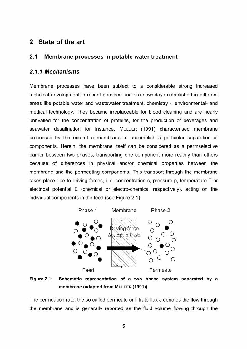
individual components in the feed (see Figure 2.1).
Figure 2.1: Schematic representation of a two phase system separated by a membrane (adapted from MULDER (1991))
The permeation rate, the so called permeate or filtrate flux J denotes the flow through
the membrane and is generally reported as the fluid volume flowing through the
2 - State of the art
6
membrane per unit surface area of the membrane and time. Hence, permeate or
filtrate flux has the dimension of velocity (m/s), often expressed as (L/m²/h).
The proportionality between the flux and the driving force is presented by MULDER
(1991) with the general phenomenological equation
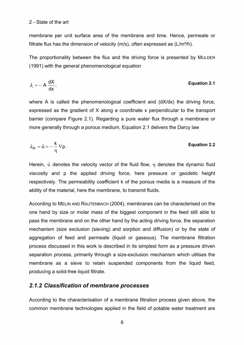
dxdXAJi −= , Equation 2.1
where A is called the phenomenological coefficient and (dX/dx) the driving force,
expressed as the gradient of X along a coordinate x perpendicular to the transport
barrier (compare Figure 2.1). Regarding a pure water flux through a membrane or
more generally through a porous medium, Equation 2.1 delivers the Darcy law
pkuJW ∇η
−== . Equation 2.2
Herein, u denotes the velocity vector of the fluid flow, η denotes the dynamic fluid
viscosity and p the applied driving force, here pressure or geodetic height
respectively. The permeability coefficient k of the porous media is a measure of the
ability of the material, here the membrane, to transmit fluids.
According to MELIN AND RAUTENBACH (2004), membranes can be characterised on the
one hand by size or molar mass of the biggest component in the feed still able to
pass the membrane and on the other hand by the acting driving force, the separation
mechanism (size exclusion (sieving) and sorption and diffusion) or by the state of
aggregation of feed and permeate (liquid or gaseous). The membrane filtration
process discussed in this work is described in its simplest form as a pressure driven
separation process, primarily through a size-exclusion mechanism which utilises the
membrane as a sieve to retain suspended components from the liquid feed,
producing a solid-free liquid filtrate.
2.1.2 Classification of membrane processes
According to the characterisation of a membrane filtration process given above, the
common membrane technologies applied in the field of potable water treatment are
2.1 - Membrane processes in potable water treatment
7
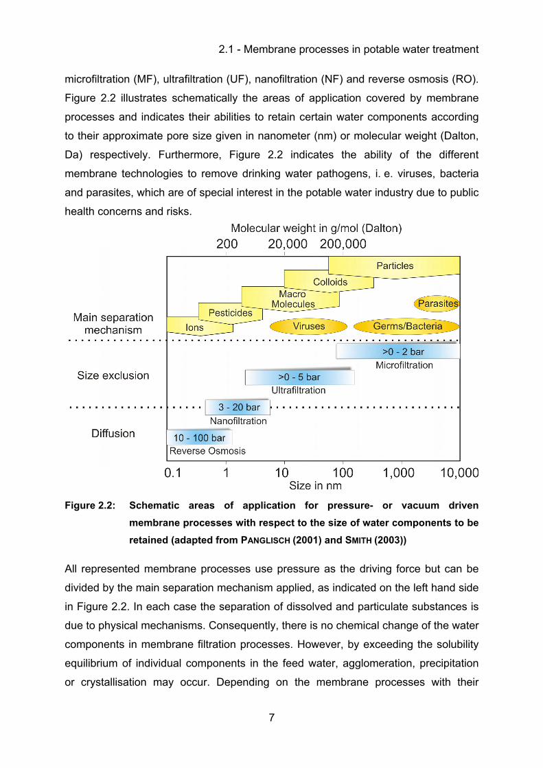
microfiltration (MF), ultrafiltration (UF), nanofiltration (NF) and reverse osmosis (RO).
Figure 2.2 illustrates schematically the areas of application covered by membrane
processes and indicates their abilities to retain certain water components according
to their approximate pore size given in nanometer (nm) or molecular weight (Dalton,
Da) respectively. Furthermore, Figure 2.2 indicates the ability of the different
membrane technologies to remove drinking water pathogens, i. e. viruses, bacteria
and parasites, which are of special interest in the potable water industry due to public
health concerns and risks.
Figure 2.2: Schematic areas of application for pressure- or vacuum driven membrane processes with respect to the size of water components to be retained (adapted from PANGLISCH (2001) and SMITH (2003))
All represented membrane processes use pressure as the driving force but can be
divided by the main separation mechanism applied, as indicated on the left hand side
in Figure 2.2. In each case the separation of dissolved and particulate substances is
due to physical mechanisms. Consequently, there is no chemical change of the water
components in membrane filtration processes. However, by exceeding the solubility
equilibrium of individual components in the feed water, agglomeration, precipitation
or crystallisation may occur. Depending on the membrane processes with their
2 - State of the art
8
different mass transport mechanisms, different resistances opposed by the
membrane, i. e. hydraulic resistance for convective mass transport and/or osmotic
pressure for diffusive mass transport, have to be overcome by the applied
transmembrane pressure (TMP) necessary to operate the membrane process.
Furthermore, operation and raw water condition etc. influence the TMP. Typical
applied TMP are indicated as pressure ranges in Figure 2.2 for each membrane
technology.
The membranes used in UF and MF are exclusively porous membranes. Whether
particulate matter will be retained by the membrane depends particularly on its size
and structure relative to the size and structure of the membrane pores, i. e. the
retention is based on size exclusion. Contrary to the dense membranes of RO a
primarily convective mass transport takes place in the porous membranes of UF and
MF. Pore size and pore size distribution of the membrane used determine the
retention characteristics. Pore size distribution will vary according to the membrane
material and manufacturing process. When a pore size is stated, it can be presented
as either nominal, i. e. the average pore size, or absolute, i. e. the maximum pore
size, usually in terms of microns (µm). MF membranes are generally considered to
have a nominal pore size in the range of 0.1 to 0.2 µm, although there are
exceptions, as MF membranes with pore sizes of up to 10 µm are available on the
market. A typical MF water flux is about 150 L/m²/h or higher with an applied TMP up
to 2 bar. Figure 2.2 indicates that MF can be used to retain particulate matter to great
extent and that it is even able to retain bacteria and parasites. However, UF provides
more reliability and safety when it comes to retention of colloids and viruses to the
greatest possible extent. For UF, pore sizes generally range from 0.1 down to
0.05 µm or less, decreasing to an extent at which the concept of a discernable ‘pore’
becomes inappropriate. Though, in terms of pore size, the lower cut off for UF
membranes is approximately about 5 nm. Because tight UF membranes have the
ability to retain larger organic macromolecules, they have historically been
characterised by the molecular weight cut off (MWCO, expressed in Daltons) rather
than by a particular pore size. MWCO is a measure of the retention characteristic of a
membrane in terms of atomic weight (or mass) rather than size, determined by the
retention of at least 90% of a specific compound with a certain molecular weight.
Thus, UF membranes specified by MWCO are presumed to act as a barrier to
2.1 - Membrane processes in potable water treatment
9
compounds of molecules with a molecular weight exceeding the stated MWCO.
Typical MWCO levels for UF range from 300 to 500,000 Da, with most membranes
used for potable water treatment at approximately 100,000 Da (USEPA (2003)). UF
usually excites fluxes of 40 to 100 L/m²/h at a TMP up to 5 bar.
2.1.3 Membrane materials, structure and modules
2.1.3.1 General remarks
There are a number of different types of membrane materials, modules, and
associated systems that are utilised in pressure driven membrane processes. While
several different types of membrane modules may be employed for any single
membrane filtration technology, each class of membrane technology is typically
associated with only one type of membrane module. This is in general, MF and UF
use mainly tubular and capillary membrane modules, and NF and RO use mainly
spiral-wound membrane modules. This chapter will give a brief overview and
descriptions on MF and UF membranes, as well as the materials from which the
membranes are made and the systems into which they are configured. However,
explanation will mainly be given for capillary, organic UF and MF membranes, driven
in inside-out mode, since these kinds of membranes were used in the experimental
and theoretical part of this thesis. Further detailed descriptions and additional
information about other materials, modules and processes etc. can be found in
CHERYAN (1998), MELIN AND RAUTENBACH (2004) and MULDER (1991)
2.1.3.2 Membrane materials
Only synthetic membranes are employed in water treatment processes. They can be
made from a large number of different materials, which can be divided further into the
groups of organic and inorganic membranes. The material properties of the
membrane may significantly impact the design and operation of the filtration system.
Its selection is crucial in deciding the membranes porosity and pore size distribution,
as it is essentially an intrinsic property of the polymer selected (MULDER (1991)) and
also determines the mechanical and surface properties of the membrane. The
polymers used in MF are not inevitably the same as used in UF due to differences in
the applied production techniques for polymeric membranes. Commonly used
2 - State of the art
10
polymers in MF are polycarbonate (PC), polysulphone (PS), polyvinylidene fluoride
(PVDF), polypropylene (PP) and polytetrafluoroethylene (PTFE). Organic UF
membranes are mainly prepared by a phase inversion process and may also be
constructed from a wide variety of materials, including cellulose acetate (CA), PVDF,
polyacrylonitrile (PAN), PS, polyethersulfone (PES), polyimide (PI) and aliphatic
polyamide (PA). Ceramic MF and UF membranes are based mainly on the materials
alumina (Al2O3), titania (TiO2) and zirconia (ZrO2). Each of these materials used in
MF and UF membrane production has different properties with respect to surface
charge, degree of hydrophobicity, pH and oxidant tolerance, strength and flexibility.
Some properties of membranes used in potable water treatment are shown in the
appendix, Table A.1.
2.1.3.3 Membrane structure
The selection of the membranes, either polymeric or ceramic, in reference to their
structure is closely associated with its separation mechanism and therefore with its
application to be used in. Two types of membranes can be distinguished by the
structure of the cross sectional area of the membrane wall. This structure is used to
describe the level of uniformity throughout this area, i. e. symmetric and asymmetric.
MF and UF membranes usually are either symmetric or integral asymmetric
membranes. Symmetric membranes (porous or homogeneous) are roughly about 10
to 200 µm thick. The resistance to mass transfer is hence determined by the total
membrane thickness. Asymmetric membranes are more or less about the same
thickness but there is a change in density of the membrane material across the cross
sectional area and the resistance to mass transfer is linked to the resistance of the
top or active layer. In some asymmetric membranes the porous structure gradually
increases in porosity from the feed to the permeate side of the membrane. They can
be subdivided further into integral asymmetric, i. e. from a single (polymeric) material
or blend, and composite asymmetric, i. e. composed from different (polymeric)
materials or blends. Figure 2.3 shows exemplarily some scanning electron
microscopy (SEM) pictures of integral asymmetric membrane wall cross sections.
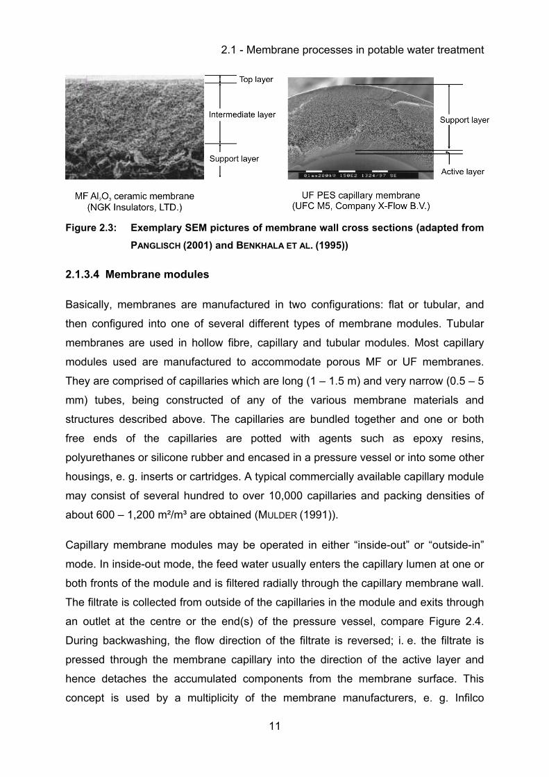
2.1 - Membrane processes in potable water treatment
11
Figure 2.3: Exemplary SEM pictures of membrane wall cross sections (adapted from PANGLISCH (2001) and BENKHALA ET AL. (1995))
2.1.3.4 Membrane modules
Basically, membranes are manufactured in two configurations: flat or tubular, and
then configured into one of several different types of membrane modules. Tubular
membranes are used in hollow fibre, capillary and tubular modules. Most capillary
modules used are manufactured to accommodate porous MF or UF membranes.
They are comprised of capillaries which are long (1 – 1.5 m) and very narrow (0.5 – 5
mm) tubes, being constructed of any of the various membrane materials and
structures described above. The capillaries are bundled together and one or both
free ends of the capillaries are potted with agents such as epoxy resins,
polyurethanes or silicone rubber and encased in a pressure vessel or into some other
housings, e. g. inserts or cartridges. A typical commercially available capillary module
may consist of several hundred to over 10,000 capillaries and packing densities of
about 600 – 1,200 m²/m³ are obtained (MULDER (1991)).
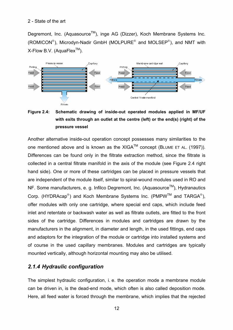
Capillary membrane modules may be operated in either “inside-out” or “outside-in”
mode. In inside-out mode, the feed water usually enters the capillary lumen at one or
both fronts of the module and is filtered radially through the capillary membrane wall.
The filtrate is collected from outside of the capillaries in the module and exits through
an outlet at the centre or the end(s) of the pressure vessel, compare Figure 2.4.
During backwashing, the flow direction of the filtrate is reversed; i. e. the filtrate is
pressed through the membrane capillary into the direction of the active layer and
hence detaches the accumulated components from the membrane surface. This
concept is used by a multiplicity of the membrane manufacturers, e. g. Infilco
2 - State of the art
12
Degremont, Inc. (AquasourceTM), inge AG (Dizzer), Koch Membrane Systems Inc.
(ROMICON®), Microdyn-Nadir GmbH (MOLPURE® and MOLSEP®), and NMT with
X-Flow B.V. (AquaFlexTM).
Figure 2.4: Schematic drawing of inside-out operated modules applied in MF/UF with exits through an outlet at the centre (left) or the end(s) (right) of the pressure vessel
Another alternative inside-out operation concept possesses many similarities to the
one mentioned above and is known as the XIGATM concept (BLUME ET AL. (1997)).
Differences can be found only in the filtrate extraction method, since the filtrate is
collected in a central filtrate manifold in the axis of the module (see Figure 2.4 right
hand side). One or more of these cartridges can be placed in pressure vessels that
are independent of the module itself, similar to spiral-wound modules used in RO and
NF. Some manufacturers, e. g. Infilco Degremont, Inc. (AquasourceTM), Hydranautics
Corp. (HYDRAcap®) and Koch Membrane Systems Inc. (PMPWTM and TARGA®),
offer modules with only one cartridge, where special end caps, which include feed
inlet and retentate or backwash water as well as filtrate outlets, are fitted to the front
sides of the cartridge. Differences in modules and cartridges are drawn by the
manufacturers in the alignment, in diameter and length, in the used fittings, end caps
and adaptors for the integration of the module or cartridge into installed systems and
of course in the used capillary membranes. Modules and cartridges are typically
mounted vertically, although horizontal mounting may also be utilised.
2.1.4 Hydraulic configuration
The simplest hydraulic configuration, i. e. the operation mode a membrane module
can be driven in, is the dead-end mode, which often is also called deposition mode.
Here, all feed water is forced through the membrane, which implies that the rejected
2.1 - Membrane processes in potable water treatment
13
components of the feed are accumulated (deposited) at the membrane surface in a
so called fouling layer along the capillary. Furthermore, dead-end mode implies that
there is one point in the capillary where the longitudinal velocity of the feed water flow
through the capillary becomes zero. If the feed water enters the capillary only from
one side, this point will be on the opposite end of the capillary. If the feed water
enters the capillary from both sides, e. g. in membrane cartridges applied in the
XIGATM concept, this point will be somewhere within the capillary length, depending
on inlet pressure on both sides of the capillary and membrane resistance. However,
even if there is a feed water flow tangential to the membrane surface inside the
capillary, the velocity is much smaller than in cross-flow mode, which will be
described next.
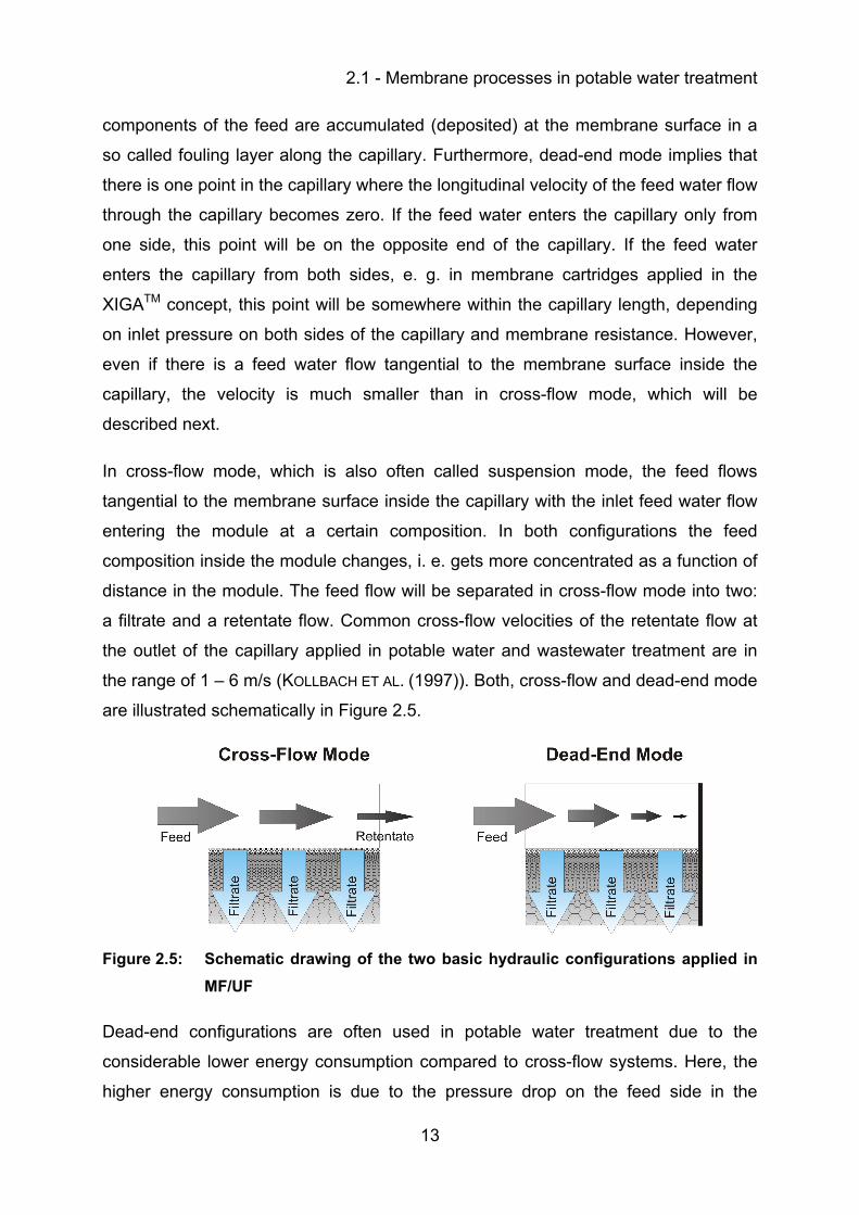
In cross-flow mode, which is also often called suspension mode, the feed flows
tangential to the membrane surface inside the capillary with the inlet feed water flow
entering the module at a certain composition. In both configurations the feed
composition inside the module changes, i. e. gets more concentrated as a function of
distance in the module. The feed flow will be separated in cross-flow mode into two:
a filtrate and a retentate flow. Common cross-flow velocities of the retentate flow at
the outlet of the capillary applied in potable water and wastewater treatment are in
the range of 1 – 6 m/s (KOLLBACH ET AL. (1997)). Both, cross-flow and dead-end mode
are illustrated schematically in Figure 2.5.
Figure 2.5: Schematic drawing of the two basic hydraulic configurations applied in MF/UF
Dead-end configurations are often used in potable water treatment due to the
considerable lower energy consumption compared to cross-flow systems. Here, the
higher energy consumption is due to the pressure drop on the feed side in the
2 - State of the art
14
capillary, aroused by the necessary cross-flow velocity. The energy demand of dead-
end operated processes is in the range of about 0.1 – 0.5 kWh/m³Filtrate (MELIN AND
RAUTENBACH (2004), PANGLISCH ET AL. (1997)), which is much lower than in cross-flow
operated processes with about 1 – 7 kWh/m³Filtrate (MELIN AND RAUTENBACH (2004),
KOLLBACH ET AL. (1997)). However, with increasing content of solids in the feed water,
dead-end operation becomes more and more inappropriate because of the higher
risk to clog the capillaries, or membrane module respectively, and because of the
loss of filtrate due to distinct higher backwashing frequencies, which themselves
consume high amounts of energy.
Capillary membrane filtration systems are designed and constructed in one or more
discrete water production units, also called racks, trains or skids. A unit consists of a
number of membrane modules that share feed and filtrate valving, and the individual
units can usually be isolated from the rest of the system for testing, cleaning or
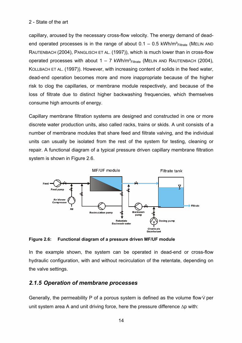
repair. A functional diagram of a typical pressure driven capillary membrane filtration
system is shown in Figure 2.6.
Figure 2.6: Functional diagram of a pressure driven MF/UF module
In the example shown, the system can be operated in dead-end or cross-flow
hydraulic configuration, with and without recirculation of the retentate, depending on
the valve settings.
2.1.5 Operation of membrane processes
Generally, the permeability P of a porous system is defined as the volume flow V per
unit system area A and unit driving force, here the pressure difference Δp with:
2.1 - Membrane processes in potable water treatment
15
pAVPΔ⋅
= Equation 2.3
If the porous system is a UF or MF membrane, then the permeability of the
membrane PM is defined as the fluid flow V per unit membrane surface area AM –
which delivers the filtrate flux J - and transmembrane pressure difference TMP.
Hence, permeability is also often called specific flux and is calculated as shown in
Equation 2.4 with:
TMPAV
TMPJP
MM ⋅
== . Equation 2.4
According to Darcy’s law, compare Equation 2.2, PM is inversely proportional to the
dynamic viscosity of the fluid η and the total resistance RTot acting against the
transport of fluid through the membrane as shown in the following Equation 2.5:
TotM R
1P⋅η
= . Equation 2.5
The TMP can be calculated according to its hydraulic configuration, which, in cross-
flow mode, is the arithmetic mean of the inlet and outlet pressure pin and pout minus
the filtrate pressure, commonly called the backpressure pFiltrate as:
Filtrateoutin p
2ppTMP −
+= . Equation 2.6
In dead-end mode the TMP is generally approximated by use of Equation 2.6. Here,
it is assumed that the outlet pressure pout at the dead-end of the capillary equals the
inlet pressure pin, which is in fact not true, even for clean membranes. This is
because the pressure along the membrane surface and at the dead-end of the
capillary depends significantly on membrane resistance and on length and inner
diameter of the capillary and therefore varies more or less, see also chapter 3.5.1.
The resistance acting in opposition to the driving force, inhibiting the transport of
water across the membrane, can be generally quantified according to the resistance
2 - State of the art
16
in series model. The model divides the total resistance RTot into two components: the
intrinsic resistance of the membrane RM and the resistance attributed to the coating
layer RCL due to fouling. Generally, fouling can be defined as the gradual
accumulation of water components, i. e. foulants and/or scalants, on the membrane
surface or within the porous membrane structure that inhibits the passage of water,
resulting in an increased necessary pressure difference to let the water pass the
membrane. Depending on kind of water components three types of fouling can be
distinguished, i. e. organic fouling, colloidal particulate fouling, scaling due to crystal
growth and biological fouling. Usually all types may occur during membrane filtration
of surface waters and combinations of them are possible and probable.
To account for concentration polarisation, which is the gradual increase in
concentration of accumulated substances at the membrane surface forming a
boundary layer, an additional resistance term RCP can be added to the total
resistance equation as:
CPCLMTot RRRR ++= , Equation 2.7
where RCP is a function of operating parameters and physical properties. At low
pressures, the RCP term will be small compared to RM and RCL. At high pressures, the
resistance of the boundary layer will increase and the RCP term will be relatively
large. RM and RCP should remain constant under constant operating conditions, the
latter one after a given period of time when steady-state conditions are established.
The increase in fouling during operation and the decrease in fouling as a result of
backwashing and chemical cleaning causes RCL to fluctuate. RM can be
experimentally determined by measuring the filtrate flux of pure water at constant
TMP and temperature, hence at constant dynamic viscosity, and applying a known
membrane area. With Equation 2.4 and Equation 2.5 the membrane resistance of the
clean membrane can then be calculated with:
VTMPAR M
M ⋅η⋅
= . Equation 2.8
The pure water flux as a measure of hydraulic permeability of the clean membrane
depends on temperature. This temperature dependency equals the dependency of
2.1 - Membrane processes in potable water treatment
17
the dynamic water viscosity on temperature. Hence, the membrane resistance itself
is not significantly temperature dependent. Generally, the membrane permeability is
normalised on a reference temperature, typically 20°C, for the purpose of monitoring
the system productivity independent of changes in water temperature:
C20MC20
M PP °°
ηη
= . Equation 2.9
The dynamic fluid viscosity η of the filtrate as a function of temperature T can be
approximately expressed by following polynomial Equation 2.10:
0.0001*)T0.000134-T0.01299+T0.6003-(17.9098 32 ⋅⋅⋅=η , Equation 2.10
whereas the dynamic viscosity η of the filtrate at 20°C is approximately ° −η = ⋅20 C 31 10 kg/m/s. The given polynomial Equation 2.10 was derived by regression
of listed values in VEREIN DEUTSCHER INGENIEURE (1988) and PERRY ET AL. (1984). It is
important to note that the normalised permeability or flux does not represent an
actual operating condition. This term simply represents what the flux or permeability
would be at 20°C for a certain TMP and total membrane resistance RTot. Thus,
changes in the value of flux during course of normal operation are indicative of
changes in pressure and/or total resistance due to fouling and not temperature. While
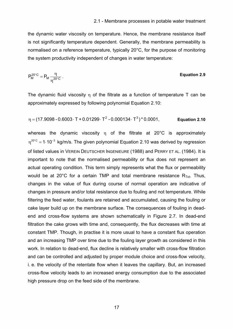
filtering the feed water, foulants are retained and accumulated, causing the fouling or
cake layer build up on the membrane surface. The consequences of fouling in dead-
end and cross-flow systems are shown schematically in Figure 2.7. In dead-end
filtration the cake grows with time and, consequently, the flux decreases with time at
constant TMP. Though, in practise it is more usual to have a constant flux operation
and an increasing TMP over time due to the fouling layer growth as considered in this
work. In relation to dead-end, flux decline is relatively smaller with cross-flow filtration
and can be controlled and adjusted by proper module choice and cross-flow velocity,
i. e. the velocity of the retentate flow when it leaves the capillary. But, an increased
cross-flow velocity leads to an increased energy consumption due to the associated
high pressure drop on the feed side of the membrane.
2 - State of the art
18
Figure 2.7: Flux decline (arbitrary scale) in dead-end (left) and cross-flow (right) operation and cake-layer build-up at constant TMP (arbitrary scale), (adapted from CHERYAN (1998) and MULDER (1991))
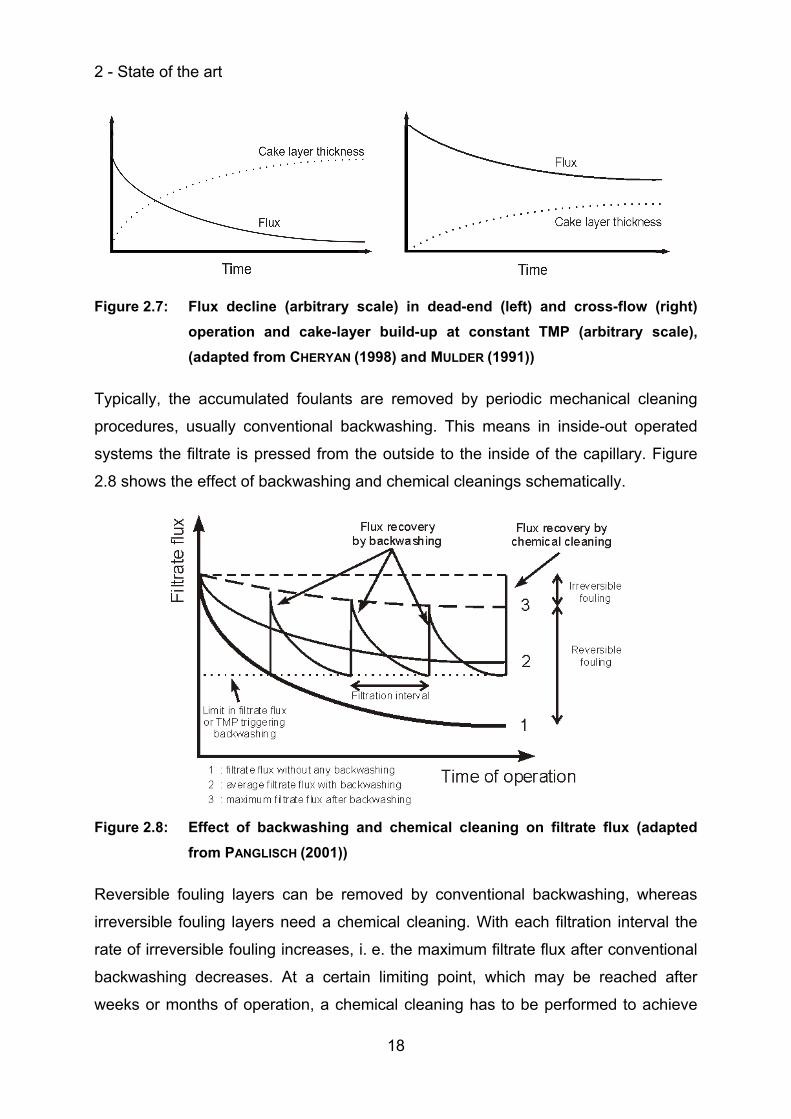
Typically, the accumulated foulants are removed by periodic mechanical cleaning
procedures, usually conventional backwashing. This means in inside-out operated
systems the filtrate is pressed from the outside to the inside of the capillary. Figure
2.8 shows the effect of backwashing and chemical cleanings schematically.
Figure 2.8: Effect of backwashing and chemical cleaning on filtrate flux (adapted from PANGLISCH (2001))
Reversible fouling layers can be removed by conventional backwashing, whereas
irreversible fouling layers need a chemical cleaning. With each filtration interval the
rate of irreversible fouling increases, i. e. the maximum filtrate flux after conventional
backwashing decreases. At a certain limiting point, which may be reached after
weeks or months of operation, a chemical cleaning has to be performed to achieve
2.1 - Membrane processes in potable water treatment
19
the desired filtration flux again. This shows that the rate of irreversible fouling is not
only a function of the feed water quality and operation conditions but also a function
of the quality of the conventional backwashing procedure. A chemical cleaning which
may be performed in-situ, i. e. cleaning in place (CIP) usually recovers the initial state
of the filtration performance of the system completely but can be labour and chemical
intensive and causes longer production downtimes. Chemicals used for chemical
cleanings are often different cleaning solutions, oxidants like sodium hypochlorite,
hydrogen peroxide as well as citric acid, hydrochloric acid, sulphuric acid or sodium
hydroxide. Often, a conventional backwashing procedure is enhanced by dosing
chemicals into the filtrate flow during backwashing, followed by soaking of the
membrane with the chemical-dose water for some minutes before the chemicals are
flushed out by an additional conventional backwashing. This kind of backwashing
procedure is called chemical enhanced backwashing (CEB) and is usually performed
fully automated several times per week of operation. Chemicals used are usually
acids and bases like citric acid, hydrochloric acid, sulphuric acid or sodium hydroxide.
A further improvement of conventional backwashing efficiency may be achieved by
use of a so called forward flush. Here, the capillaries are cleaned by flushing water,
which may be feed water or filtrate, along the membrane surface. For inside-out
operated processes it could be shown that the high shear forces achieved by forward
flushing could be used to increase flux recovery (GIMBEL ET AL. (1996), FUTSELAAR
AND WEIJENBERG (1998), FUTSELAAR ET AL. (1998)). If the modules are mounted
vertically, this effect can be further improved by applying a two phase-flow, i. e.
adding air to the flushing water flow (FUTSELAAR AND WEIJENBERG (1998), FUTSELAAR
ET AL. (1998), POSPÍSIL ET AL. (2004)). But, the efficiency of an air-flush strongly
depends on the diameter of the tubes; hence the air flush is best used in tubular
membrane modules (VERBERK (2005)).
2.2 Hybrid membrane processes
In water, natural organic matter (NOM) is a complex mixture of particulate and
dissolved components of both inorganic and organic origin that varies from one
source to another (HOWE ET AL. (2002), WONG ET AL. (2002) and LEEUWEN ET AL.
(2002)). NOM is a heterogeneous mixture with wide ranges in molecular weight (MW)
2 - State of the art
20
and functional groups (phenolic, hydroxyl, carbonyl groups and carboxylic acid). In
water it is formed by autochthonous input such as algae and allochthonous input
such as terrestrial and vegetative debris (ZULARISAMA ET AL. (2006)). Among these
components, dissolved organic matter (DOM) is found to have the most detrimental
effect on membrane performance as it can result in the formation of hardly reversible
and/or irreversible fouling layers on the membrane surface and/or within the
membrane pores (see chapter 2.1.3.2) due to direct adsorption onto the membrane
material. DOM is a ubiquitous constituent in natural waters and is generally
comprised of humic substances: polysaccharides, amino acids, proteins, fatty acids,
phenols, carboxylic acids, quinines, lignins, carbohydrates, alcohols, resins, and
inorganic compounds such as silica, alumino-silicates, iron, aluminium, suspended
solids and microorganisms (bacteria and fungi) (ZULARISAMA ET AL. (2006)). Retention
of DOM by porous membranes is generally determined by its molecular weight and
structure, charge density and hydrophobicity. Furthermore, specific solution
parameters including pH-value, ionic strength and presence of other solutes such as
calcium and additionally membrane characteristics including hydrophobicity, charge
and surface morphology play a decisive role (SCHÄFER (1999), HOWE (2001)). Hence,
clear statements of retention efficiencies of DOM cannot be found in literature and
published results vary strongly and are mainly given from the quantitative point of
view. For instance, HOWE (2001) and HOWE AND CLARK (2002) showed that the
majority of DOM does not foul MF and UF membranes and identified small colloidal
matter as the primary foulant, as did CARROLL ET AL. (2000) and FAN ET AL. (2001) for
instance. GRAY ET AL. (2004) showed for different raw waters that the hydrophobic
components were the major foulant for the one and the hydrophilics for the other
water. Yet, a good review is presented in the work of HOWE (2001) and AMY (2007),
considering all aspects mentioned above.
As a result of degraded operation performance caused by NOM fouling layers,
membrane processes can not be driven economically caused by a necessary
increase of the backwash frequency and intensity, i. e. duration of backwashing or
use of chemical enhanced backwashes (CEB) for example. Beside the retention of
NOM additional interrelated treatment aims may arise depending on raw water
quality. Those aims might be the reduction of colour, odour and trace organic
compounds and cannot be solved by UF or MF alone. To get those challenging
2.2 - Hybrid membrane processes
21
problems and treatment tasks under control but still being able utilising the
advantages of membrane filtration as treatment step, hybrid processes were
developed and established.
Generally, hybrid processes are combinations of two or more separately and usually
independently working processes like filtration, coagulation, sedimentation or
adsorption. The feature of a hybrid process is that both processes already represent
independent solutions, but develop additional new desired characteristics by their
combination. Nevertheless, the terminology hybrid membrane process is often used
in literature for the combination with different pre-treatment steps too. Depending on
raw water quality, processes integrated with membrane processes in water treatment
are most often such as coagulation/flocculation, sometimes followed by
sedimentation, flotation or rapid sand filtration prior membrane filtration, often
adsorption on powdered activated carbon, on particulate iron oxides or on ion
exchange resins, but also biofiltration, oxidation and softening. The hybrid process
considered in this work consists of the combination of coagulation and membrane
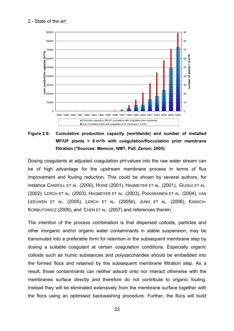
filtration due to the increasing interest as outlined in Figure 2.9, illustrating the
exponential development of production capacity and number of plants applying
coagulation prior membrane filtration for the production of potable water, mainly from
surface waters, until 2005. About 14 % of worldwide installed MF/UF plants are used
in combination with coagulation and produce about 22 % of the total potable water
produced by MF/UF plants, whereas the biggest plant is located in the Chestnut
Avenue Water Works (Chestnut, Singapore) with a production capacity of
11,375 m³/h (JANSON ET AL. (2006)).
2 - State of the art
22
0
10000
20000
30000
40000
50000
60000
70000
80000
90000
1988 1989 1990 1991 1992 1993 1994 1995 1996 1997 1998 1999 2000 2001 2002 2003 2004 2005
cum
. pro
duct
ion
capa
city
[m³/h
]
0
10
20
30
40
50
60
70
80
90
num
ber o
f pla
nts
> 8
m³/h
Production capacity of MF/UF (cumulative) with coagulation prior membraneSum of installed plants with coagulation prior membrane > 8 m³/h
Figure 2.9: Cumulative production capacity (worldwide) and number of installed MF/UF plants > 8 m³/h with coagulation/flocculation prior membrane filtration (*Sources: Memcor, NMT, Pall, Zenon; 2005)
Dosing coagulants at adjusted coagulation pH-values into the raw water stream can
be of high advantage for the upstream membrane process in terms of flux
improvement and fouling reduction. This could be shown by several authors, for
instance CARROLL ET AL. (2000), HOWE (2001), HAGMEYER ET AL. (2001), GUIGUI ET AL.
(2002), LERCH ET AL. (2003), HAGMEYER ET AL. (2003), PIKKARAINEN ET AL. (2004), VAN
LEEUWEN ET AL. (2005), LERCH ET AL. (2005B), JUNG ET AL. (2006), KABSCH-
KORBUTOWICZ (2006), and CHEN ET AL. (2007) and references therein.
The intention of the process combination is that dispersed colloids, particles and
other inorganic and/or organic water contaminants in stable suspension, may be
transmuted into a preferable form for retention in the subsequent membrane step by
dosing a suitable coagulant at certain coagulation conditions. Especially organic
colloids such as humic substances and polysaccharides should be embedded into
the formed flocs and retained by the subsequent membrane filtration step. As a
result, those contaminants can neither adsorb onto nor interact otherwise with the
membranes surface directly and therefore do not contribute to organic fouling.
Instead they will be eliminated extensively from the membrane surface together with
the flocs using an optimised backwashing procedure. Further, the flocs will build
2.3 - Modelling
23
highly permeable fouling layers, giving less resistance to fluid flow than layers build
from smaller particles and colloids (LAHOUSSINE-TURCAUD ET AL. (1992), LEE ET AL.
(2000), HOWE AND CLARK (2002), NGUYEN AND RIPPERGER (2002), KENNEDY ET AL.
(2002), NGUYEN (2004), CHO ET AL. (2006)). Thus, performance will be improved and
an economical process is possible, even if high coagulant dosages are necessary
due to high contaminant loads. Especially for new installations or modernisation of
water works it is a promising and cost-efficient alternative. Moreover, coagulation can
be performed and optimised within the hybrid process as ‘enhanced coagulation’,
whereas the term enhanced coagulation refers to the process of improved removal of
disinfection by-product precursors (USEPA - DBPR (1999)). Hence, beside the
advantage of achieving stable operation conditions, the hybrid process coagulation
and membrane filtration will lead to an increased retention of NOM.
2.3 Modelling
Investigations on colloidal and particulate fouling were performed by several authors,
e. g. PORTER (1972B), PORTER (1972A), GREEN AND BELFORT (1980), ALTENA AND
BELFORT (1984), BELFORT AND NAGATA (1985), DREW ET AL. (1991), considering first
more basic or simplifying models. The main emphasis here was usually set on
calculating particle trajectories based on the thin-film or gel polarisation model, i. e.
balancing filtration drag and a (solute) back-diffusive flow described by the 1st Fickian
law for mass transport, combined with inertia induced lateral migration of matter,
which was first observed by SEGRÉ AND SILBERBERG (1962A), SEGRÉ AND SILBERBERG
(1962B) and investigated theoretically by KARNIS ET AL. (1966), COX AND BRENNER
(1968), HO AND LEAL (1974) and VASSEUR AND COX (1976). The authors assumed that
non-hydrodynamic forces between the particles and the surface are negligible.
Further, the authors considered cross-flow filtration only, but different geometries like
ducts, capillaries, tubes and/or channels with one or two permeable walls, non-
interacting particles in the free solution, i. e. diluted suspensions at some distance
from the membrane wall and filtrate flux being constant and independent of the axial
coordinate. The used description of the velocity profiles for laminar flow in porous
ducts was often based on the work of BERMAN (1953) and YUAN AND FINKELSTEIN
(1956), whereas the used boundary condition at the boundary between the
permeable wall and the free fluid was first presented by BEAVERS AND JOSEPH (1967).
2 - State of the art
24
A good review of research related to steady, single phase, two dimensional,
isothermal, incompressible and internal laminar flow in porous walls, considering
different flow regimes, boundary conditions and geometries was given by CHELLAM ET
AL. (1995). FANE ET AL. (1982) postulated an alternative or additional mechanism for
larger solids, founded on shear-induced transport or scour of the polarised layer by
tangentially flowing feed suspensions. The model based on the analogy between
suspension flow across a filter cake and the motion of a sediment-laden stream over
a layer of settled sediment. DAVIS AND LEIGHTON (1987) introduced the shear-induced
hydrodynamic diffusion mechanism to describe the lateral migration of particles away
from the porous wall as the layer is sheared. At steady state, the effective particle
diffusion within the layer is balanced by the convective flux of particles toward the
porous wall due to the fluid flow into the wall. Though, FANE (1984) could show for
stirred, i. e. cross-flow, and unstirred, i. e. dead-end filtration experiments that if the
mechanisms are considered as simultaneous, a minimum in flux across porous
membranes could be found at some particle diameter. Also WIESNER ET AL. (1989)
and LAHOUSSINE-TURCAUD ET AL. (1990) showed that the minimum in particle transport
with respect to particle size should result in a preferential deposition of particles of a
certain diameter that correspond to this minimum. Their experiments showed further
that the removal of submicron materials, i. e. colloidal organics and inorganics, by
coagulation to form larger flocs may improve the performance of membrane filtration
units. The maximum floc size was found for cross-flow and dead-end batch
experiments when the zeta potential of the flocculated suspension was near zero.
However, interactions between the coagulant and the membrane were not
considered. Later, CHELLAM AND WIESNER (1992) extended the theory developed by
ALTENA AND BELFORT (1984) to include the effects of sedimentation, London-van der
Waals attraction, double layer repulsion and added mass of entrained fluid. However,
these effects were discussed even earlier, e. g. by HUNG AND TIEN (1976), but not
introduced as significant effects into the models, as it was done afterwards by several
authors, e. g. SONG AND ELIMELECH (1995), ALTMANN AND RIPPERGER (1997), HARMANT
AND AIMAR (1996), BACCHIN ET AL. (1995), PANGLISCH (2001) and NGUYEN (2004).
It becomes clear that accurate modelling of flow and particle or floc trajectories
leading to deposition and fouling layer formation in pressure driven membrane
processes is inhibited by the complex couplings in the flow equations along with any
2.3 - Modelling
25
added effect of variable particle, floc and membrane properties. Due to the rapid
computer development in the last decade, accompanied with improved computational
capacity, increasingly more complex computations can be accomplished nowadays.
While models of fluid flow in porous ducts, particle deposition and fouling with varying
degrees of complexity have been developed as described above, reports of the use
of CFD have only recently appeared. For instance, WILEY AND FLETCHER (2002) and
WILEY AND FLETCHER (2003) developed a general CFD model of concentration
polarisation and fluid flow in pressure driven membrane processes, which has been
tested and validated against semi-analytical solutions and shown to perform correctly
from quantitative and qualitative perspective. They stated that one advantage of CFD
models is that they contain specific equations for the cases to be investigated, but
that they can be readily modified to encompass any combination of variations in the
parameters of interest. Another model was published by KROMKAMP ET AL. (2005),
who developed a model for suspension flow and concentration polarisation in cross-
flow MF with shear induced diffusion as back-transport mechanism. Here, a more
realistic approach was found to be especially significant for the calculation of the
fouling layer profile at the beginning and the end of the membrane. A good prediction
of a three-dimensional CFD model for calculating the flux through a cross-flow driven
MF was presented by RAHIMI ET AL. (2005). Even here, the results and validation with
laboratory experiments showed that flux predictions were more accurate in
comparison with simple models. BACCHIN ET AL. (2006B) published the results of a
CFD model accounting for colloidal phase transition leading to the formation of a
deposit from the accumulated concentration polarisation phase in cross-flow MF. The
model was used to determine the critical flux, predicting filtration conditions where
particle accumulation occurs or where it is avoided. The predicted values were about
4 times larger than observed experimentally. This discrepancy was explained by
heterogeneities of the membrane material which effected the local permeate flux and
was not embedded into the CFD code. Even if such reports have only recently
appeared, CFD is arising more and more interest and is increasingly applied also in
other fields in water research (DO-QUANG ET AL. (2000), SCHWINGE ET AL. (2004),
RANADE AND KUMAR (2006), SUBRAMANIA ET AL. (2006), KOUTSOU ET AL. (2007)).
26
3 Theoretical considerations and modelling
3.1 Velocity and concentration profiles in capillaries with permeable walls
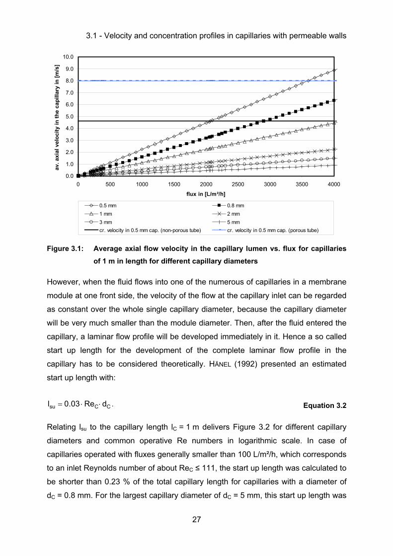
3.1.1 Verification of the flow regime and start-up length
The axial flow regime inside the porous capillary is assumed to be laminar according
to the general accepted transition between laminar and turbulent flow in a non-
porous tube at a critical Reynold number Re ≤ 2300. Additionally, BELFORT AND
NAGATA (1985) found that the onset of turbulence was delayed to critical Reynold
numbers of about Re ≤ 4000 for flows in porous tubes when compared to flows in
non-porous tubes. The capillary Reynold number ReC can be calculated as shown in
Equation 3.1:
ν⋅
= CC
dvRe , Equation 3.1
where v denotes the axial fluid flow velocity, dC denotes the capillary diameter and ν
denotes the kinematic fluid viscosity. For the largest considered capillary diameter of
5 mm the critical Re number will be exceeded at an average axial flow velocity of
about 0.8 m/s and at about 8.0 m/s for the smallest capillary diameter of 0.5 mm.
Figure A.1 in the appendix illustrates calculated capillary Re numbers for porous
tubes for different capillary diameters vs. the average axial flow velocity in the
capillary lumen at a temperature T = 20°C. For example, in dead-end operation mode
driven 1 m long capillaries with a capillary diameter of 0.5 mm could thus theoretically
be operated in laminar flow regime up to a flux of about 3600 L/m²/h in porous
capillaries as shown in Figure 3.1. The shown values are quite far from reality for
dead-end driven UF and even MF membrane systems. Considering a common flux of
up to 100 L/m²/h for a dead-end driven UF capillary of 1 m in length at T = 20°C, an
average axial flow velocity up to 0.25 m/s is achieved depending on the capillary
diameter. Hence, the capillaries will always reveal laminar flow as indicated in Figure
A.2. Therefore, a laminar flow regime inside the capillary lumen will be considered
throughout this work.
3.1 - Velocity and concentration profiles in capillaries with permeable walls
27
0.0
1.0
2.0
3.0
4.0
5.0
6.0
7.0
8.0
9.0
10.0
0 500 1000 1500 2000 2500 3000 3500 4000
flux in [L/m²/h]
av. a
xial
vel
ocity
in th
e ca
pilla
ry in
[m/s
]
0.5 mm 0.8 mm1 mm 2 mm3 mm 5 mmcr. velocity in 0.5 mm cap. (non-porous tube) cr. velocity in 0.5 mm cap. (porous tube)
Figure 3.1: Average axial flow velocity in the capillary lumen vs. flux for capillaries of 1 m in length for different capillary diameters
However, when the fluid flows into one of the numerous of capillaries in a membrane
module at one front side, the velocity of the flow at the capillary inlet can be regarded
as constant over the whole single capillary diameter, because the capillary diameter
will be very much smaller than the module diameter. Then, after the fluid entered the
capillary, a laminar flow profile will be developed immediately in it. Hence a so called
start up length for the development of the complete laminar flow profile in the
capillary has to be considered theoretically. HÄNEL (1992) presented an estimated
start up length with:
CCsu dRe03.0l ⋅⋅= . Equation 3.2
Relating lsu to the capillary length lC = 1 m delivers Figure 3.2 for different capillary
diameters and common operative Re numbers in logarithmic scale. In case of
capillaries operated with fluxes generally smaller than 100 L/m²/h, which corresponds
to an inlet Reynolds number of about ReC ≤ 111, the start up length was calculated to
be shorter than 0.23 % of the total capillary length for capillaries with a diameter of
dC = 0.8 mm. For the largest capillary diameter of dC = 5 mm, this start up length was
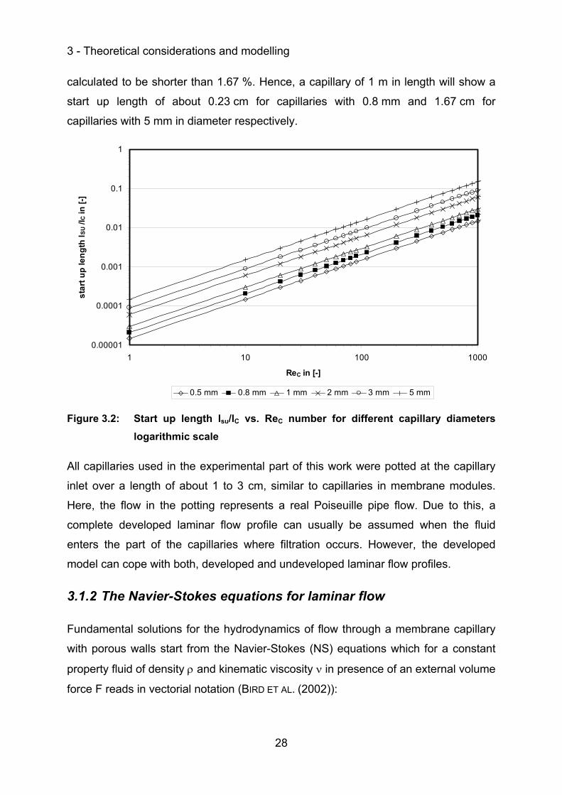
3 - Theoretical considerations and modelling
28
calculated to be shorter than 1.67 %. Hence, a capillary of 1 m in length will show a
start up length of about 0.23 cm for capillaries with 0.8 mm and 1.67 cm for
capillaries with 5 mm in diameter respectively.
0.00001
0.0001
0.001
0.01
0.1
1
1 10 100 1000
ReC in [-]
star
t up
leng
th l S
U /l C
in [-
]
0.5 mm 0.8 mm 1 mm 2 mm 3 mm 5 mm
Figure 3.2: Start up length lsu/lC vs. ReC number for different capillary diameters logarithmic scale
All capillaries used in the experimental part of this work were potted at the capillary
inlet over a length of about 1 to 3 cm, similar to capillaries in membrane modules.
Here, the flow in the potting represents a real Poiseuille pipe flow. Due to this, a
complete developed laminar flow profile can usually be assumed when the fluid
enters the part of the capillaries where filtration occurs. However, the developed
model can cope with both, developed and undeveloped laminar flow profiles.
3.1.2 The Navier-Stokes equations for laminar flow
Fundamental solutions for the hydrodynamics of flow through a membrane capillary
with porous walls start from the Navier-Stokes (NS) equations which for a constant
property fluid of density ρ and kinematic viscosity ν in presence of an external volume
force F reads in vectorial notation (BIRD ET AL. (2002)):
3.1 - Velocity and concentration profiles in capillaries with permeable walls
29
( ) p1uFuutu
∇ρ
−Δν+=∇⋅+∂∂
. Equation 3.3
Here, u denotes the velocity vector, F the external force vector (such as gravity), p
the pressure and t the time. Together with appropriate boundary conditions and the
mass conservation law, also known as the equation of continuity, as:
0u =⋅∇ , Equation 3.4
this leads to a complete description of the isothermal fluid motion in the capillary.
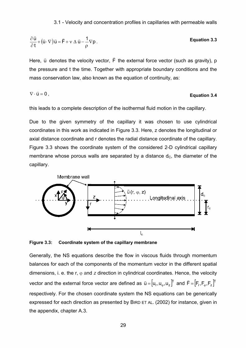
Due to the given symmetry of the capillary it was chosen to use cylindrical
coordinates in this work as indicated in Figure 3.3. Here, z denotes the longitudinal or
axial distance coordinate and r denotes the radial distance coordinate of the capillary.
Figure 3.3 shows the coordinate system of the considered 2-D cylindrical capillary
membrane whose porous walls are separated by a distance dC, the diameter of the
capillary.
Figure 3.3: Coordinate system of the capillary membrane
Generally, the NS equations describe the flow in viscous fluids through momentum
balances for each of the components of the momentum vector in the different spatial
dimensions, i. e. the r, ϕ and z direction in cylindrical coordinates. Hence, the velocity
vector and the external force vector are defined as [ ]Tzr u,u,uu ϕ= and [ ]Tzr F,F,FF ϕ=
respectively. For the chosen coordinate system the NS equations can be generically
expressed for each direction as presented by BIRD ET AL. (2002) for instance, given in
the appendix, chapter A.3.
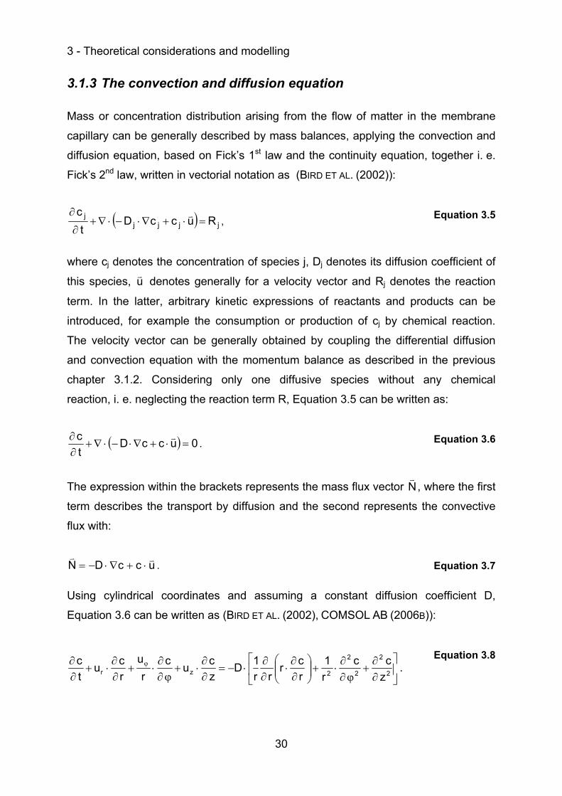
3 - Theoretical considerations and modelling
30
3.1.3 The convection and diffusion equation
Mass or concentration distribution arising from the flow of matter in the membrane
capillary can be generally described by mass balances, applying the convection and
diffusion equation, based on Fick’s 1st law and the continuity equation, together i. e.
Fick’s 2nd law, written in vectorial notation as (BIRD ET AL. (2002)):
( ) jjjjj RuccD
tc
=⋅+∇⋅−⋅∇+∂
∂, Equation 3.5
where cj denotes the concentration of species j, Dj denotes its diffusion coefficient of
this species, u denotes generally for a velocity vector and Rj denotes the reaction
term. In the latter, arbitrary kinetic expressions of reactants and products can be
introduced, for example the consumption or production of cj by chemical reaction.
The velocity vector can be generally obtained by coupling the differential diffusion
and convection equation with the momentum balance as described in the previous
chapter 3.1.2. Considering only one diffusive species without any chemical
reaction, i. e. neglecting the reaction term R, Equation 3.5 can be written as:
( ) 0uccDtc
=⋅+∇⋅−⋅∇+∂∂
. Equation 3.6
The expression within the brackets represents the mass flux vector N, where the first
term describes the transport by diffusion and the second represents the convective
flux with:
uccDN ⋅+∇⋅−= . Equation 3.7
Using cylindrical coordinates and assuming a constant diffusion coefficient D,
Equation 3.6 can be written as (BIRD ET AL. (2002), COMSOL AB (2006B)):
⎥⎦
⎤⎢⎣
⎡
∂∂
+ϕ∂
∂⋅+⎟⎟
⎠
⎞⎜⎜⎝
⎛∂∂
⋅∂∂
⋅−=∂∂
⋅+ϕ∂
∂⋅+
∂∂
⋅+∂∂ ϕ
2
2
2
2
2zr zcc
r1
rcr
rr1D
zcuc
ru
rcu
tc .
Equation 3.8
3.2 - The flow of porous floc aggregates
31
3.2 The flow of porous floc aggregates
While filtering floc suspensions in an inside-out driven capillary membrane,
concentration and therefore effective suspension viscosity will change depending on
the axial and radial coordinates in the capillary. An increased concentration leads to
a change of the fluid velocities in longitudinal and radial direction. Additionally,
hydrodynamic forces, such as drag forces, acting on the flocs in the suspension are
influenced by the fractal structure and inner porosity of the flocs. This is, because the
fluid flow is around and through the porous aggregates. Both points will be briefly
discussed in the following subchapters and correction functions will be derived and
introduced to be used for the calculation of the acting forces and torques on the flocs
in chapter 3.3. However, the flow through the fouling layer formed by deposited flocs
is for the flow of the permeating fluid, i. e. water, through porous media only. Hence,
the viscosity of water will be used without any correction functions within the formed
fouling layers, compare chapter 3.4.6.
3.2.1 Effective floc suspension viscosity
LEIGHTON AND ACRIVOS (1987) presented the ratio of the dynamical or effective
suspension viscosity and dynamical fluid viscosity depending on the particle
concentration in suspension with:
2
max
S
15.11
⎟⎟⎟⎟
⎠
⎞
⎜⎜⎜⎜
⎝
⎛
φφ
−
φ⋅+=
ηη
,
Equation 3.9
where φ denotes the particle volume concentration in the suspension, η the dynamic
fluid viscosity and Sη the dynamic suspension viscosity. maxφ is called the limit or
maximum particle volume concentration in the suspension and was given by
LEIGHTON AND ACRIVOS (1987) with 0.58 for rigid, spherical particles after fitting
empirically for latex particles of diameter 46 µm and a shear velocity gradient of
about G = 24 s-1. A more general relationship was given by LIU AND MASLIYAH (1996),
cited in LIU (1999), which is valid for both diluted and concentrated suspension flows
of mono-sized spherical particles with:
3 - Theoretical considerations and modelling
32
⎥⎥⎦
⎤
⎢⎢⎣
⎡φ⋅⎟
⎟⎠
⎞⎜⎜⎝
⎛
φ−+φ⋅⎟⎟
⎠
⎞⎜⎜⎝
⎛φ
−+⎟⎟⎠
⎞⎜⎜⎝
⎛φ
φ−=
ηη
−2
2max
Hmax
E
2
max
S 6k2k1 . Equation 3.10
Here, kE = 2.5 denotes the Einstein constant and kH the Huggins constant, the latter
one depending on flow strength. At low velocities kH is set to kH = 6.0 and at high
velocities kH is set to kH = 7.1. However, LIU (1999) did not give exact ranges for the
flow velocities to be used. He showed that the experimental results could be best
fitted for values of maxφ = 0.71, which is close to the theoretical maximum particle
volume concentration of spherical particles with maxφ = 0.74, when the suspension
flow was strong. The reason for this was found to be that the particles could fill into
the gaps which were inaccessible in weaker suspension flows where the particle-
particle alignment is more or less at random, leading to 64.0max ≈φ . If the particle
concentration was high, i. e. up to values larger than φ > 0.54, it could be shown that
Equation 3.10 could be simplified to:
2
max
S 1−
⎟⎟⎠
⎞⎜⎜⎝
⎛φ
φ−=
ηη
. Equation 3.11
Considering now the filtration of floc suspensions some assumptions have to be
taken to contribute for the porosity of the floc aggregates and its effect on viscosity of
the bulk flow. It is assumed that the floc concentration in the bulk may vary from low
to high concentrations. The maximum floc volume concentration was chosen to
be max,Fφ = 0.74, independent of flow strength and the Huggins constant was chosen
to be kH = 7.1. However, the maximum floc volume concentration in the concentration
polarised layer and the coating layer at the membrane wall will be probably higher for
real deformable, compressed and overlapping flocs than for spherical rigid particles
(STRENGE (1993), PARK ET AL. (2004)). Further it is assumed that the effective
viscosity in the porous floc is equal to the viscosity of the bulk flow as it is often
assumed by several authors as stated by VEERAPANENI AND WIESNER (1996).
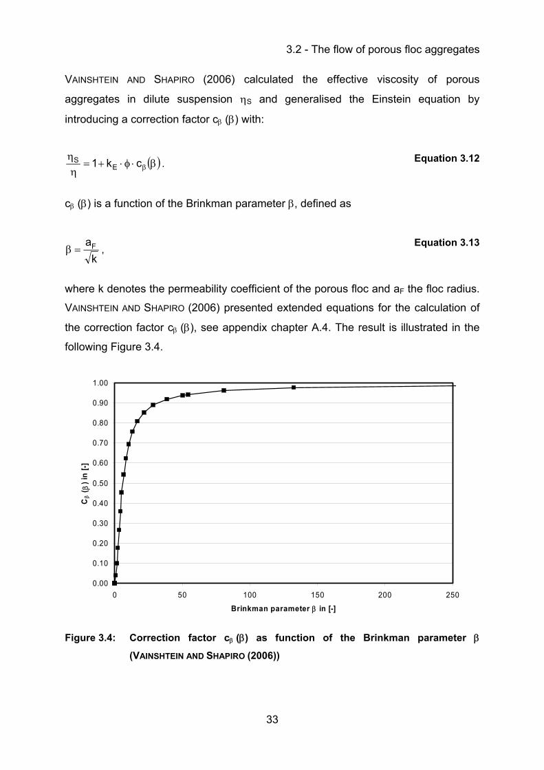
3.2 - The flow of porous floc aggregates
33
VAINSHTEIN AND SHAPIRO (2006) calculated the effective viscosity of porous
aggregates in dilute suspension ηS and generalised the Einstein equation by
introducing a correction factor cβ (β) with:
( )β⋅φ⋅+=η
ηβck1 E
S . Equation 3.12
cβ (β) is a function of the Brinkman parameter β, defined as
kaF=β ,
Equation 3.13
where k denotes the permeability coefficient of the porous floc and aF the floc radius.
VAINSHTEIN AND SHAPIRO (2006) presented extended equations for the calculation of
the correction factor cβ (β), see appendix chapter A.4. The result is illustrated in the
following Figure 3.4.
0.00
0.10
0.20
0.30
0.40
0.50
0.60
0.70
0.80
0.90
1.00
0 50 100 150 200 250
Brinkman parameter β in [-]
Cβ ( β
) in
[-]
Figure 3.4: Correction factor cβ (β) as function of the Brinkman parameter β
(VAINSHTEIN AND SHAPIRO (2006))
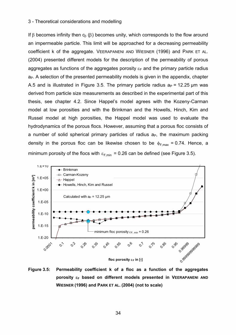
3 - Theoretical considerations and modelling
34
If β becomes infinity then cβ (β) becomes unity, which corresponds to the flow around
an impermeable particle. This limit will be approached for a decreasing permeability
coefficient k of the aggregate. VEERAPANENI AND WIESNER (1996) and PARK ET AL.
(2004) presented different models for the description of the permeability of porous
aggregates as functions of the aggregates porosity εF and the primary particle radius
aP. A selection of the presented permeability models is given in the appendix, chapter
A.5 and is illustrated in Figure 3.5. The primary particle radius aP = 12.25 µm was
derived from particle size measurements as described in the experimental part of this
thesis, see chapter 4.2. Since Happel’s model agrees with the Kozeny-Carman
model at low porosities and with the Brinkman and the Howells, Hinch, Kim and
Russel model at high porosities, the Happel model was used to evaluate the
hydrodynamics of the porous flocs. However, assuming that a porous floc consists of
a number of solid spherical primary particles of radius aP, the maximum packing
density in the porous floc can be likewise chosen to be max,Fφ = 0.74. Hence, a
minimum porosity of the flocs with min,Fε = 0.26 can be defined (see Figure 3.5).
1.E-20
1.E-15
1.E-10
1.E-05
1.E+00
1.E+05
1.E+10
0.000
1 0.1 0.2 0.26
0.35
0.45
0.55 0.6 0.7 0.7
50.8
50.9
5
0.999
99
0.999
9999
9999
9
floc porosity εF in [-]
perm
eabi
lity
coef
ficie
nt k
in [m
²]
BrinkmanCarman-KozenyHappelHowells, Hinch, Kim and Russel
Calculated with aP = 12.25 µm
minimum floc porosity εF, min = 0.26
Figure 3.5: Permeability coefficient k of a floc as a function of the aggregates
porosity εF based on different models presented in VEERAPANENI AND
WIESNER (1996) and PARK ET AL. (2004) (not to scale)
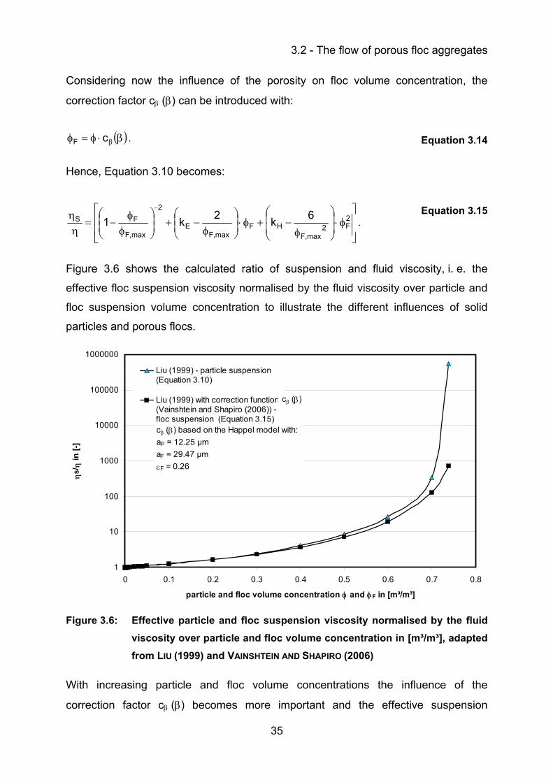
3.2 - The flow of porous floc aggregates
35
Considering now the influence of the porosity on floc volume concentration, the
correction factor cβ (β) can be introduced with:
( )β⋅φ=φ βcF . Equation 3.14
Hence, Equation 3.10 becomes:
⎥⎥
⎦
⎤
⎢⎢
⎣
⎡φ⋅
⎟⎟
⎠
⎞
⎜⎜
⎝
⎛
φ−+φ⋅⎟
⎟⎠
⎞⎜⎜⎝
⎛
φ−+⎟
⎟⎠
⎞⎜⎜⎝
⎛
φφ
−=η
η−
2F2
,maxFHF
,maxFE
2
,maxF
FS 6k2k1 . Equation 3.15
Figure 3.6 shows the calculated ratio of suspension and fluid viscosity, i. e. the
effective floc suspension viscosity normalised by the fluid viscosity over particle and
floc suspension volume concentration to illustrate the different influences of solid
particles and porous flocs.
1
10
100
1000
10000
100000
1000000
0 0.1 0.2 0.3 0.4 0.5 0.6 0.7 0.8
particle and floc volume concentration φ and φ F in [m³/m³]
ηS/
η in
[-]
Liu (1999) - particle suspension(Equation 3.10)
Liu (1999) with correction function(Vainshtein and Shapiro (2006)) -floc suspension (Equation 3.15)
cβ (β)
cβ (β) based on the Happel model with:aP = 12.25 µmaF = 29.47 µmεF = 0.26
Figure 3.6: Effective particle and floc suspension viscosity normalised by the fluid viscosity over particle and floc volume concentration in [m³/m³], adapted from LIU (1999) and VAINSHTEIN AND SHAPIRO (2006)
With increasing particle and floc volume concentrations the influence of the
correction factor cβ (β) becomes more important and the effective suspension
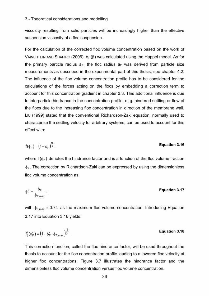
3 - Theoretical considerations and modelling
36
viscosity resulting from solid particles will be increasingly higher than the effective
suspension viscosity of a floc suspension.
For the calculation of the corrected floc volume concentration based on the work of
VAINSHTEIN AND SHAPIRO (2006), cβ (β) was calculated using the Happel model. As for
the primary particle radius aP, the floc radius aF was derived from particle size
measurements as described in the experimental part of this thesis, see chapter 4.2.
The influence of the floc volume concentration profile has to be considered for the
calculations of the forces acting on the flocs by embedding a correction term to
account for this concentration gradient in chapter 3.3. This additional influence is due
to interparticle hindrance in the concentration profile, e. g. hindered settling or flow of
the flocs due to the increasing floc concentration in direction of the membrane wall.
LIU (1999) stated that the conventional Richardson-Zaki equation, normally used to
characterise the settling velocity for arbitrary systems, can be used to account for this
effect with:
( ) 316
FF 1)(f φ−=φ , Equation 3.16
where )(f Fφ denotes the hindrance factor and is a function of the floc volume fraction
Fφ . The correction by Richardson-Zaki can be expressed by using the dimensionless
floc volume concentration as:
,maxF
FF φ
φ=φ∗ , Equation 3.17
with 74.0,maxF ≅φ as the maximum floc volume concentration. Introducing Equation
3.17 into Equation 3.16 yields:
( ) 316
,maxFFFt 1)(f φ⋅φ−=φ ∗∗φ .
Equation 3.18
This correction function, called the floc hindrance factor, will be used throughout the
thesis to account for the floc concentration profile leading to a lowered floc velocity at
higher floc concentrations. Figure 3.7 illustrates the hindrance factor and the
dimensionless floc volume concentration versus floc volume concentration.
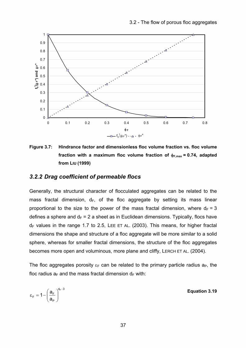
3.2 - The flow of porous floc aggregates
37
0
0.1
0.2
0.3
0.4
0.5
0.6
0.7
0.8
0.9
1
0 0.1 0.2 0.3 0.4 0.5 0.6 0.7 0.8
φ F
f φt ( φF*
) and
φF*
fft(fF*) fft(fF*)φF*fφt(φF*)
Figure 3.7: Hindrance factor and dimensionless floc volume fraction vs. floc volume
fraction with a maximum floc volume fraction of φF,max = 0.74, adapted
from LIU (1999)
3.2.2 Drag coefficient of permeable flocs
Generally, the structural character of flocculated aggregates can be related to the
mass fractal dimension, dF, of the floc aggregate by setting its mass linear
proportional to the size to the power of the mass fractal dimension, where dF = 3
defines a sphere and dF = 2 a sheet as in Euclidean dimensions. Typically, flocs have
dF values in the range 1.7 to 2.5, LEE ET AL. (2003). This means, for higher fractal
dimensions the shape and structure of a floc aggregate will be more similar to a solid
sphere, whereas for smaller fractal dimensions, the structure of the floc aggregates
becomes more open and voluminous, more plane and cliffy, LERCH ET AL. (2004).
The floc aggregates porosity εF can be related to the primary particle radius aP, the
floc radius aF and the mass fractal dimension dF with:
3d
P
FF
F
aa1
−
⎟⎟⎠
⎞⎜⎜⎝
⎛−=ε
Equation 3.19
3 - Theoretical considerations and modelling
38
However, because the mass fractal dimension dF could not be measured throughout
the experimental work of this thesis, the hydrodynamic properties of fractal
aggregates are evaluated by modelling them as porous aggregates governed by the
Happel model as described above. Resistance to the fluid flow through the aggregate
is predicted to increase with increasing fractal dimension, i. e. lower inner porosity.
VEERAPANENI AND WIESNER (1996) showed that a reasonable estimate of the fluid
drag force on a fractal aggregate may be obtained by assigning a constant volume-
averaged porosity to the aggregate and using any of the expressions available in the
literature for aggregates with uniform permeability. Therefore, VEERAPANENI AND
WIESNER (1996) introduced an additional hydrodynamic parameter, the
homogeneous drag coefficient Ω. The drag coefficient is defined as the force exerted
by the fluid on a permeable aggregate of radius a, normalised by the force exerted by
the fluid on an impermeable sphere of radius a. However, even water entering the
inner parts of the floc may be immobilised and trapped within while the rest is flowing
through the interior of the floc (STRENGE (1993)).
Assuming only flocs with homogeneous permeability, Ω can be calculated with:
β⋅⋅
=Ω3
B2h Equation 3.20
where B is a factor used for the calculation of Ωh, as presented by MASLIYAH ET AL.
(1987), cited in VEERAPANENI AND WIESNER (1996) and given in the appendix, chapter
A.6. Figure 3.8 shows the homogeneous drag coefficient Ωh illustrated versus floc
porosity.
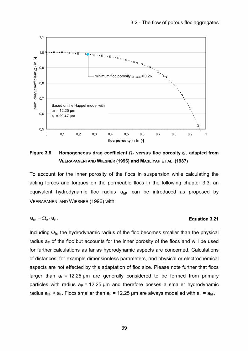
3.2 - The flow of porous floc aggregates
39
0,5
0,6
0,7
0,8
0,9
1,0
1,1
0 0,1 0,2 0,3 0,4 0,5 0,6 0,7 0,8 0,9 1
floc porosity εF in [-]
hom
. dra
g co
effic
ient
Ωh i
n [-]
minimum floc porosity εF, min = 0.26
Based on the Happel model with:aP = 12.25 µmaF = 29.47 µm
Figure 3.8: Homogeneous drag coefficient Ωh versus floc porosity εF, adapted from
VEERAPANENI AND WIESNER (1996) and MASLIYAH ET AL. (1987)
To account for the inner porosity of the flocs in suspension while calculating the
acting forces and torques on the permeable flocs in the following chapter 3.3, an
equivalent hydrodynamic floc radius hFa can be introduced as proposed by
VEERAPANENI AND WIESNER (1996) with:
FhhF aa ⋅Ω= . Equation 3.21
Including Ωh, the hydrodynamic radius of the floc becomes smaller than the physical
radius aF of the floc but accounts for the inner porosity of the flocs and will be used
for further calculations as far as hydrodynamic aspects are concerned. Calculations
of distances, for example dimensionless parameters, and physical or electrochemical
aspects are not effected by this adaptation of floc size. Please note further that flocs
larger than aF = 12.25 µm are generally considered to be formed from primary
particles with radius aP = 12.25 µm and therefore posses a smaller hydrodynamic
radius ahF < aF. Flocs smaller than aF = 12.25 µm are always modelled with aF = ahF.
3 - Theoretical considerations and modelling
40
3.3 Forces and torques acting on flocs
3.3.1 General remarks
At first, some thoughts have to be stated about the chosen notation used in the
following for single particles and flocs and their suspensions in water. The referred
authors usually applied rigid, solid and spherical particles in their experimental setup
and in their theoretical considerations and derived equations. Consequently, the
notations are often ‘particle’ or ‘sphere’ and will be introduced as such. Because this
thesis is about fouling layer formation due to floc transport and deposition, the
behaviour of floc aggregates is discussed in this work. Flocs are always thought of
being aggregates consisting of iron or aluminium hydroxide with embedded particles
and colloids. Particles and colloids are always considered as single primary particles
and colloids, not being embedded in agglomerates. However, flocs are considered to
be rigid and ideally spherical and of constant shape, but reveal basic floc properties
such as porosity, low density and low zeta potential. This approach is reasonable as
a first approximation because of the more macroscopic model investigated in this
work. Hence, the presented equations are used for flocs without further adaptations if
not stated otherwise.
Nevertheless, the coating layer build-up by floc deposition can be described by
trajectory calculations. The floc trajectories can be derived from balances of the
acting forces and torques according to the calculated and CFD modelled
hydrodynamic conditions inside the capillary lumen and to physical properties of the
flocs, usually dominant in the far-field region, and due to electrochemical properties
of the flocs and the membrane, usually dominant in the near-field region. The acting
forces and torques are introduced and discussed in the following. Various forces and
torques act on flocs, which are supposed to be in continuous motion under the
influence of these various forces and torques until they get deposited, or in case of
cross-flow filtration mode until they get out of the system, i. e. the capillary. Figure 3.9
illustrates the acting forces and torques. Please note that the shown modelled floc
and capillary are not illustrated to scale.
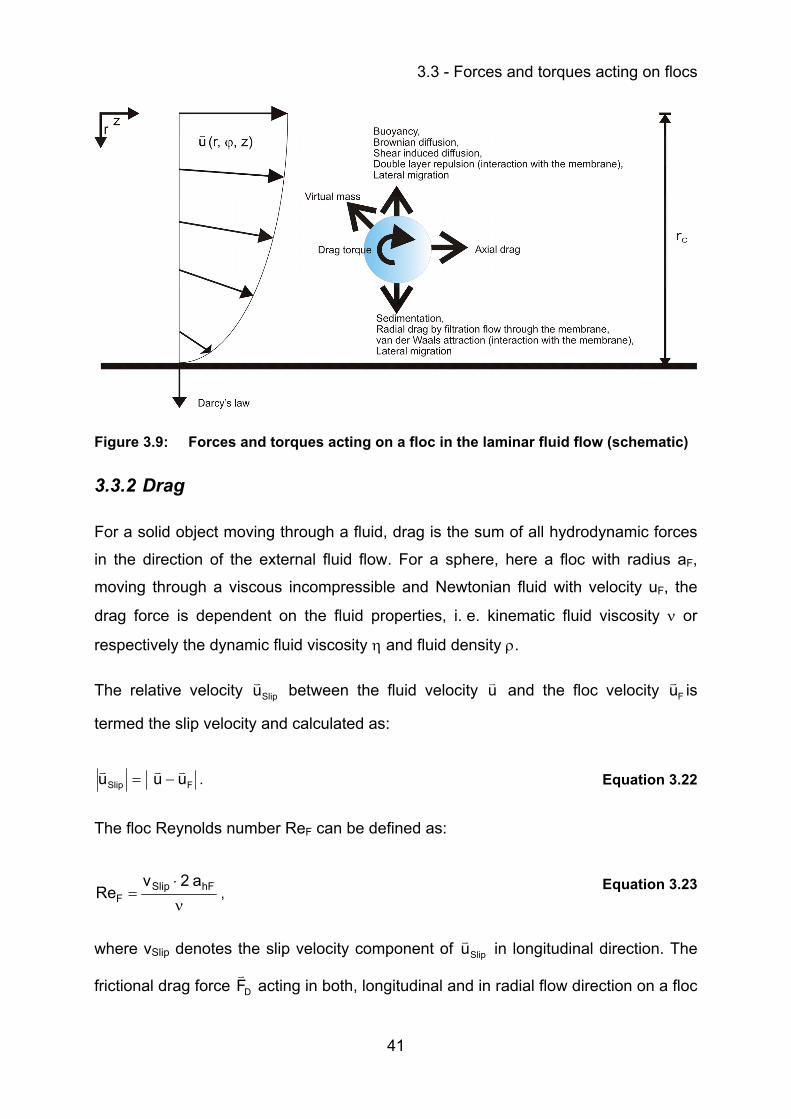
3.3 - Forces and torques acting on flocs
41
Figure 3.9: Forces and torques acting on a floc in the laminar fluid flow (schematic)
3.3.2 Drag
For a solid object moving through a fluid, drag is the sum of all hydrodynamic forces
in the direction of the external fluid flow. For a sphere, here a floc with radius aF,
moving through a viscous incompressible and Newtonian fluid with velocity uF, the
drag force is dependent on the fluid properties, i. e. kinematic fluid viscosity ν or
respectively the dynamic fluid viscosity η and fluid density ρ.
The relative velocity Slipu between the fluid velocity u and the floc velocity Fu is
termed the slip velocity and calculated as:
FSlip uuu −= . Equation 3.22
The floc Reynolds number ReF can be defined as:
ν
⋅= hFSlip
Fa2v
Re , Equation 3.23
where vSlip denotes the slip velocity component of Slipu in longitudinal direction. The
frictional drag force DF acting in both, longitudinal and in radial flow direction on a floc
3 - Theoretical considerations and modelling
42
of hydrodynamic radius hFa , is, at low Reynold numbers, linearly proportional to the
floc velocity relative to the surrounding fluid, Slipu with:
SlipD uF ⋅ξ−= , Equation 3.24
where ξ is the friction coefficient given by:
hFa6 ⋅η⋅π⋅=ξ . Equation 3.25
Since the theoretical treatment of this subject has grown out of the early work of
Stokes, the above equation is often referred to as Stokes' law (ELIMELECH ET AL.
(1995)). Stokes showed that the relation provided good agreement with his
experimental results obtained at low Reynolds numbers, i. e. ReF < 1 representing
creeping flow (see Equation 3.23). This expression can be derived from the so called
Stokes equation. The Stokes equation is a special, steady state case of the NS
equation, given in Equation 3.3, where the inertia of the fluid, i. e. the left-hand side
terms are neglected, assuming further that external forces are absent or negligible.
Hence, the Stokes equation for creeping flow can be written as:
up1Δν=∇
ρ. Equation 3.26
An extension to account for inertia effects at large distances from the obstacle, here
the floc, has been made by OSEEN (1910) (cited in ELIMELECH ET AL. (1995)) which
has been shown to be valid for ReF ≤ 5 (SCHLICHTING (1955) cited in ELIMELECH ET AL.
(1995)). However, both expressions given above apply only to flocs moving in an
undisturbed, i. e. unbounded flow field of the fluid. Because this case is not given in
capillary membrane filtration the presence of the boundary, i. e. the permeable
membrane wall at finite distances, necessitates a modification to Stokes' law. Usually
such modifications are given in the form of a dimensionless correction factor λ so
that the drag force becomes:
sliphFD ua6F ⋅λ⋅⋅η⋅π⋅= . Equation 3.27
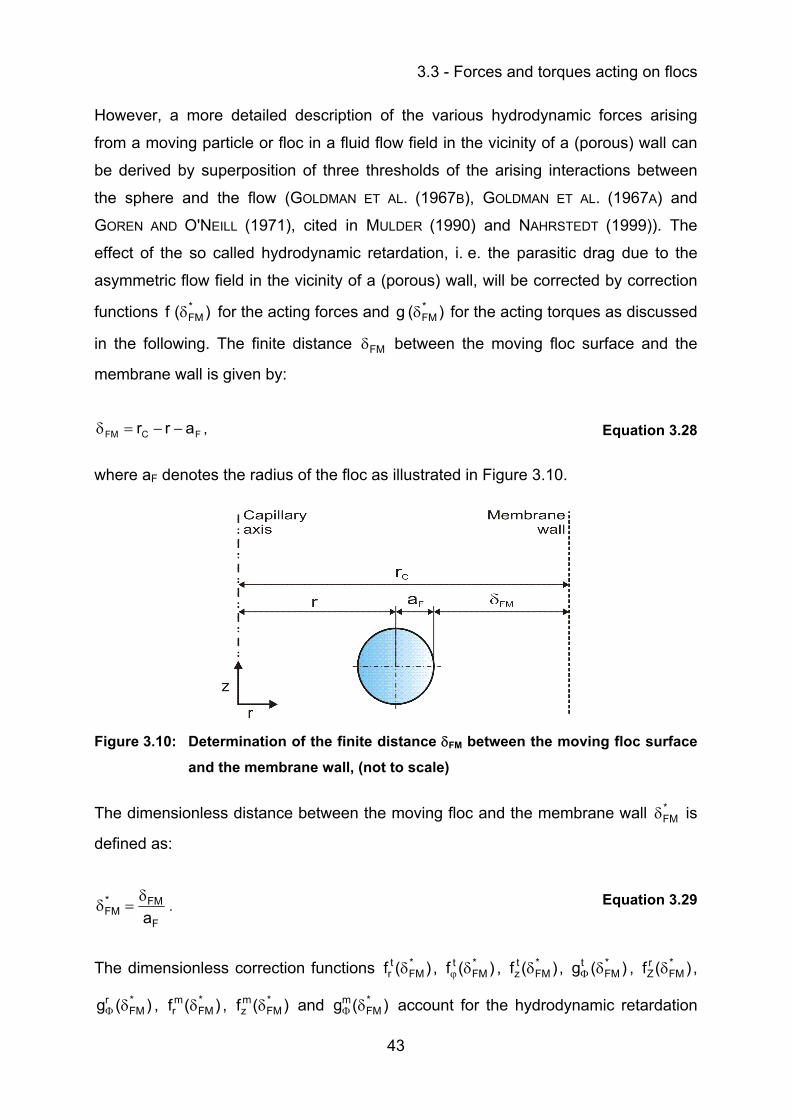
3.3 - Forces and torques acting on flocs
43
However, a more detailed description of the various hydrodynamic forces arising
from a moving particle or floc in a fluid flow field in the vicinity of a (porous) wall can
be derived by superposition of three thresholds of the arising interactions between
the sphere and the flow (GOLDMAN ET AL. (1967B), GOLDMAN ET AL. (1967A) and
GOREN AND O'NEILL (1971), cited in MULDER (1990) and NAHRSTEDT (1999)). The
effect of the so called hydrodynamic retardation, i. e. the parasitic drag due to the
asymmetric flow field in the vicinity of a (porous) wall, will be corrected by correction
functions )(f *FMδ for the acting forces and )(g *
FMδ for the acting torques as discussed
in the following. The finite distance FMδ between the moving floc surface and the
membrane wall is given by:
FCFM arr −−=δ , Equation 3.28
where aF denotes the radius of the floc as illustrated in Figure 3.10.
Figure 3.10: Determination of the finite distance δFM between the moving floc surface
and the membrane wall, (not to scale)
The dimensionless distance between the moving floc and the membrane wall *FMδ is
defined as:
F
FM*FM a
δ=δ . Equation 3.29
The dimensionless correction functions )(f *FM
tr δ , )(f *
FMt δϕ , )(f *
FMtz δ , )(g *
FMt δΦ , )(f *
FMrZ δ ,
)(g *FM
r δΦ , )(f *FM
mr δ , )(f *
FMmz δ and )(g *
FMm δΦ account for the hydrodynamic retardation
3 - Theoretical considerations and modelling
44
excited by the membrane wall. PANGLISCH (2001) mentioned that )(f *FM
tr δ and )(f *
FMt δϕ
describe the same wall effect in a capillary, because the velocities in direction of the
coordinates r and ϕ are perpendicular and both are orientated to the membrane wall.
Hence )(f *FM
tr δ equals )(f *
FMt δϕ and just )(f *
FMtr δ will be used in the following. It has to
be pointed out that the used approximations and interpolations derived by MULDER
(1990) are valid only for the motion of particles in the direct vicinity of just one plane
and not for a two dimensional Poiseuille flow in a capillary. However, PANGLISCH
(2001) showed for the translatory velocities that the dimensionless functions given by
MULDER (1990) could be validated also with correction functions for a two
dimensional Poiseuille flow presented in literature, e. g. HO AND LEAL (1974).
Furthermore, PANGLISCH (2001) stated that these correction functions are valid over
the whole cross section of a capillary, except for )(f *FM
tr δ . GOREN (1979) showed for
particles approaching a permeable wall, that the dimensionless function )(f *FM
tr δ did
not become infinite at the permeable wall as it should for impermeable walls but aims
a finite value depending on size and resistance given by the permeable wall, i. e. the
membrane resistance RM. Hence, )(f *FM
tr δ at the membrane wall becomes:
FMt,maxr
tr aR
32f)0(f ⋅⋅== .
Equation 3.30
The drag force increases as the gap between the approaching floc and the wall is
reduced but the increase becomes significantly less pronounced as the permeability
of the wall increases. For finite wall permeability, a finite hydrodynamic force on the
floc is expected even for the floc coming into contact with the permeable wall. This is
in contrast to the infinitely large drag force predicted for impermeable walls as can be
seen in Figure 3.11. PANGLISCH (2001) introduced an approximation to calculate the
correction function )(f *FM
tr δ . On the one hand, his approximation accounts for the
influence of the permeable wall at short dimensionless distances *FMδ but on the
other hand for the negligible influence of the permeable wall for larger dimensionless
distances *FMδ . Hence, his approximation will be used to calculate the correction
function )(f *FM
tr δ at permeable walls. If impermeable walls have to be considered,
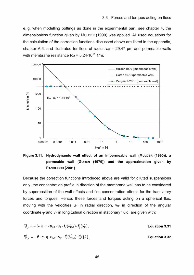
3.3 - Forces and torques acting on flocs
45
e. g. when modelling pottings as done in the experimental part, see chapter 4, the
dimensionless function given by MULDER (1990) was applied. All used equations for
the calculation of the correction functions discussed above are listed in the appendix,
chapter A.6, and illustrated for flocs of radius aF = 29.47 µm and permeable walls
with membrane resistance RM = 5.24·1011 1/m.
1
10
100
1000
10000
100000
0.00001 0.0001 0.001 0.01 0.1 1 10 100 1000
δFM* in [-]
f rt ( δFM
*) in
[-]
Mulder 1990 (impermeable wall)
Goren 1979 (permeable wall)
Panglisch 2001 (permeable wall)
RM · aF = 1.54·107
Figure 3.11: Hydrodynamic wall effect of an impermeable wall (MULDER (1990)), a permeable wall (GOREN (1979)) and the approximation given by PANGLISCH (2001)
Because the correction functions introduced above are valid for diluted suspensions
only, the concentration profile in direction of the membrane wall has to be considered
by superposition of the wall effects and floc concentration effects for the translatory
forces and torques. Hence, these forces and torques acting on a spherical floc,
moving with the velocities uF in radial direction, wF in direction of the angular
coordinate ϕ and vF in longitudinal direction in stationary fluid, are given with:
)(f)(fua6F Ft*
FMtrFhF
tr,D
∗φ φ⋅δ⋅⋅⋅η⋅π⋅−= , Equation 3.31
)(f)(fva6F Ft*
FMtzFhF
tz,D
∗φ φ⋅δ⋅⋅⋅η⋅π⋅−= , Equation 3.32
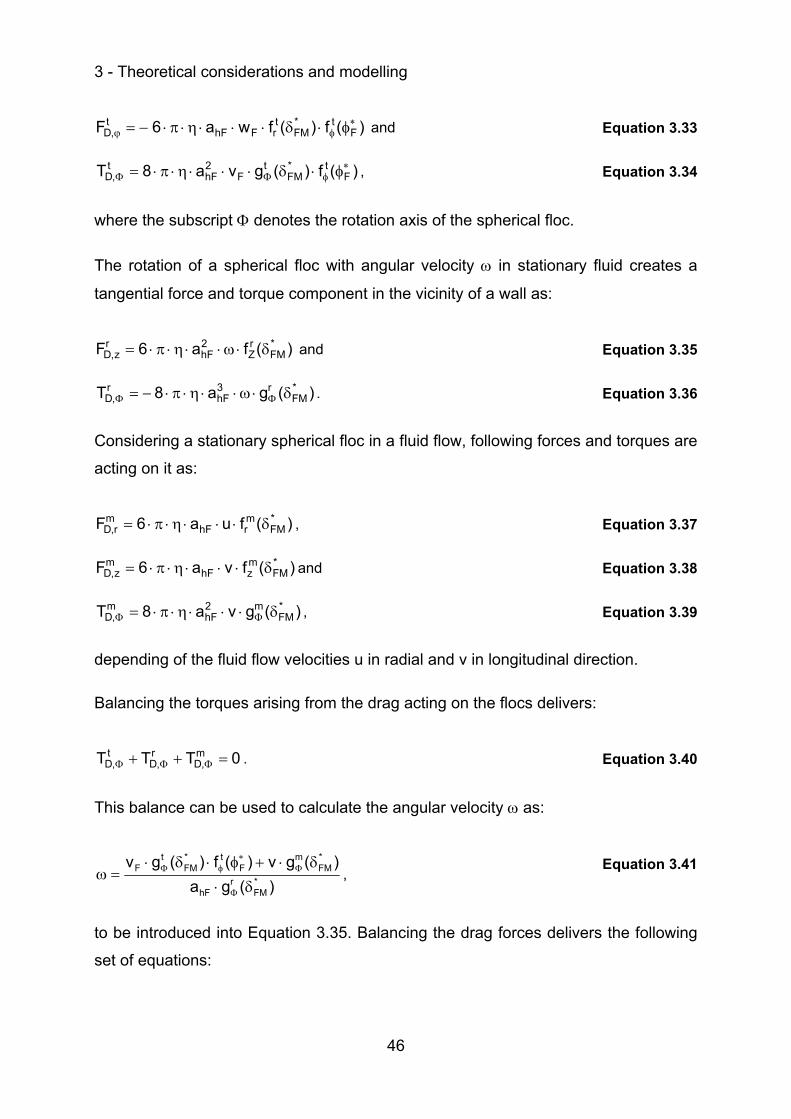
3 - Theoretical considerations and modelling
46
)(f)(fwa6F Ft*
FMtrFhF
t,D
∗φϕ φ⋅δ⋅⋅⋅η⋅π⋅−= and Equation 3.33
)(f)(gva8T Ft*
FMt
F2hF
t,D
∗φΦΦ φ⋅δ⋅⋅⋅η⋅π⋅= , Equation 3.34
where the subscript Φ denotes the rotation axis of the spherical floc.
The rotation of a spherical floc with angular velocity ω in stationary fluid creates a
tangential force and torque component in the vicinity of a wall as:
)(fa6F *FM
rZ
2hF
rz,D δ⋅ω⋅⋅η⋅π⋅= and Equation 3.35
)(ga8T *FM
r3hF
r,D δ⋅ω⋅⋅η⋅π⋅−= ΦΦ . Equation 3.36
Considering a stationary spherical floc in a fluid flow, following forces and torques are
acting on it as:
)(fua6F *FM
mrhF
mr,D δ⋅⋅⋅η⋅π⋅= , Equation 3.37
)(fva6F *FM
mzhF
mz,D δ⋅⋅⋅η⋅π⋅= and Equation 3.38
)(gva8T *FM
m2hF
m,D δ⋅⋅⋅η⋅π⋅= ΦΦ , Equation 3.39
depending of the fluid flow velocities u in radial and v in longitudinal direction.
Balancing the torques arising from the drag acting on the flocs delivers:
0TTT m,D
r,D
t,D =++ ΦΦΦ . Equation 3.40
This balance can be used to calculate the angular velocity ω as:
)(ga)(gv)(f)(gv
*FM
rhF
*FM
mF
t*FM
tF
δ⋅
δ⋅+φ⋅δ⋅=ω
Φ
Φ∗
φΦ , Equation 3.41
to be introduced into Equation 3.35. Balancing the drag forces delivers the following
set of equations:
3.3 - Forces and torques acting on flocs
47
( ))(f)(fu)(fua6FFF Ft*
FMtrF
*FM
mrhF
tr,D
mr,Dr,D
∗φ φ⋅δ⋅−δ⋅⋅⋅η⋅π⋅=+= , Equation 3.42
)(f)(fwa6F Ft*
FMtrFhF,D
∗φϕ φ⋅δ⋅⋅⋅η⋅π⋅−= . Equation 3.43
( ))(fa)(f)(fv)(fva6
FFFF*FM
rZhFF
t*FM
tzF
*FM
mzhF
rz,D
tz,D
mz,Dz,D
δ⋅ω⋅+φ⋅δ⋅−δ⋅⋅⋅η⋅π⋅=
++=∗
φ
Equation 3.44
3.3.3 Virtual mass
The expressions for the viscous drag are valid only for constant slip velocities. If an
unbalanced force exists, the particle or floc mass accelerates and a finite mass of the
fluid immediately surrounding or being within the floc will be accelerated too. Hence,
an extra drag or virtual mass force has to be considered. CHELLAM AND WIESNER
(1992) stated that the extra fluid mass is proportional to the floc volume and the fluid
density. To account for this added mass force, which opposes the motion, the
following force acting on a floc has to be considered in the force balances:
dtuda
34kF F3
hFvmVM ρ⋅⋅π⋅⋅−= . Equation 3.45
Here, kvm is a proportionality constant presented by CHELLAM AND WIESNER (1992) as
a function of the dimensionless distance of the floc to the membrane wall *FMδ with:
...k2563k
163
21k
6
*FM
3
*FM
vm +⎟⎟⎠
⎞⎜⎜⎝
⎛
δ⋅+⎟⎟
⎠
⎞⎜⎜⎝
⎛
δ⋅+=
∗∗
. Equation 3.46
The factor ∗k is called the dimensionless floc radius, i. e. the floc radius aF
normalised with the channel width or capillary diameter dC respectively as:
C
F
C
F
r2a
dak
⋅==∗ . Equation 3.47
Hence, in an unbounded fluid flow kvm becomes 0.5 and for a flow bounded by the
membrane wall kvm increases to infinity when the floc approaches the membrane wall
as illustrated in Figure 3.12.
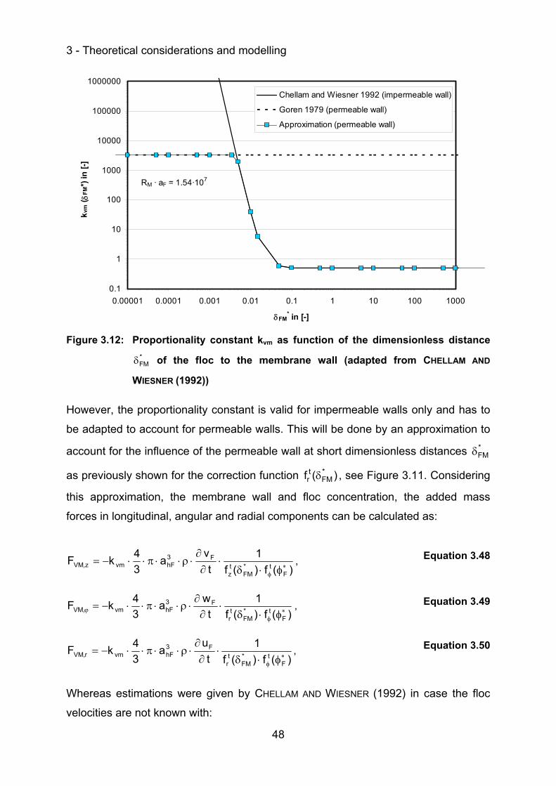
3 - Theoretical considerations and modelling
48
0.1
1
10
100
1000
10000
100000
1000000
0.00001 0.0001 0.001 0.01 0.1 1 10 100 1000
δFM* in [-]
k vm
( δFM
*) in
[-]
Chellam and Wiesner 1992 (impermeable wall)
Goren 1979 (permeable wall)
Approximation (permeable wall)
RM · aF = 1.54·107
Figure 3.12: Proportionality constant kvm as function of the dimensionless distance *FMδ of the floc to the membrane wall (adapted from CHELLAM AND
WIESNER (1992))
However, the proportionality constant is valid for impermeable walls only and has to
be adapted to account for permeable walls. This will be done by an approximation to
account for the influence of the permeable wall at short dimensionless distances *FMδ
as previously shown for the correction function )(f *FM
tr δ , see Figure 3.11. Considering
this approximation, the membrane wall and floc concentration, the added mass
forces in longitudinal, angular and radial components can be calculated as:
)(f)(f1
tv
a34kF
Ft*
FMtz
F3hFvmz,VM ∗
φ φ⋅δ⋅
∂∂
⋅ρ⋅⋅π⋅⋅−= , Equation 3.48
)(f)(f1
twa
34kF
Ft*
FMtr
F3hFvm,VM ∗
φϕ φ⋅δ
⋅∂
∂⋅ρ⋅⋅π⋅⋅−= , Equation 3.49
)(f)(f1
tu
a34kF
Ft*
FMtr
F3hFvmr,VM ∗
φ φ⋅δ⋅
∂∂
⋅ρ⋅⋅π⋅⋅−= , Equation 3.50
Whereas estimations were given by CHELLAM AND WIESNER (1992) in case the floc
velocities are not known with:
3.3 - Forces and torques acting on flocs
49
)(f)(f1
lv
a34kF
Ft*
FMtzC
2max3
hFvmz,VM ∗φ φ⋅δ
⋅⋅ρ⋅⋅π⋅⋅−= , Equation 3.51
)(f)(f1
r2ua
34kF
Ft*
FMtrC
23hFvmr,VM ∗
φ φ⋅δ⋅
⋅⋅ρ⋅⋅π⋅⋅−= . Equation 3.52
Here, vmax denotes the characteristic fluid flow velocity at the flow centre line.
3.3.4 Buoyancy and sedimentation
Balancing buoyancy and gravity as acting forces on a spherical floc, the resulting
force will be the so called sedimentation force. Considering just spherical flocs arising
torques can be neglected. The sedimentation force can be subdivided into acting
components in radial and longitudinal direction r and z respectively, depending on the
direction of the acting gravity force. This force can be calculated as the difference of
buoyancy and gravity as:
( ) z3hFFz,BS ga
34F ⋅⋅π⋅⋅ρ−ρ= , and Equation 3.53
( ) r3hFFr,BS ga
34F ⋅⋅π⋅⋅ρ−ρ= . Equation 3.54
Here, g denotes the gravitational acceleration constant, ρ denotes the fluid and ρF the
floc density respectively. Depending on the direction of the acting gravity, fluid flow in
horizontal and vertically orientated capillaries can be described.
3.3.5 Brownian diffusion
In all cases of diffusion, the net flux J of the transported quantity (atoms, energy, or
electrons) is equal to a physical property (diffusivity, thermal conductivity, electrical
conductivity) multiplied by a gradient (a concentration, a thermal or electric field
gradient). According to the general phenomenological Equation 2.1, the 1st Fickian
law describes the steady state diffusion flux of matter. The diffusive flux JBD is
proportional to the diffusion coefficient DBD and driven by a concentration gradient
rc
∂∂ in the system. It is given by:
3 - Theoretical considerations and modelling
50
rcDJ BDBD ∂
∂⋅−= . Equation 3.55
Diffusion of matter, i. e. submicron or Brownian particles or micro flocs, suspended in
water originates from an incessant, sometimes chaotic movement, whereby it comes
to a constant but coincidental change of position. If no concentration gradient exists,
then the changes of position will be compensated in the statistic mean and no
directed transport occurs. For instance, in thermal diffusion, if the temperature is
constant, thermal energy will move as quickly in one direction as in the other,
producing no heat transport and change in temperature. With presence of a
concentration gradient, the coincidental change of position turns into a directed
movement in opposite direction of the gradient. Hence, a directed diffusion flux will
be developed. A measure for the flexibility of submicron matter was given by the
Stokes-Einstein relationship (EINSTEIN (1905)) for the diffusion coefficient with:
F
BBD a6
TkD⋅η⋅π⋅
⋅= , Equation 3.56
where kB denotes the Boltzmann constant.
The effective lateral velocity due to the action of Brownian diffusion in the presence
of a concentration gradient of suspended flocs can be expressed by (HO AND LEAL
(1974)):
drdDu F
F
BDBD
φ⋅
φ−= . Equation 3.57
For the calculation of uBD neither floc-floc nor floc-wall interactions are considered
(PANGLISCH (2001)). Hence, the acting force in radial direction r,BDF can be calculated
using the Stokes-equation without using correction terms as:
hFF
F
BDr,BD a6
drdDF ⋅η⋅π⋅⋅
φ⋅
φ−= . Equation 3.58
3.3 - Forces and torques acting on flocs
51
3.3.6 Shear induced diffusion
Larger flocs or particles are able to develop a strong, directed motion if they are
present in a sufficiently high concentration and if shearing forces exist (LEIGHTON AND
ACRIVOS (1987)). Hence, a fluid moving across a membrane initiates floc migration
and at a critical point overcomes the advective force of fluid moving through the
membrane. ZYDNEY AND COLTON (1986) proposed that particles in a shear flow are
displaced as the result of complex particle-particle interactions arising from the
rotation of the particles, the resultant drag force exerted on neighbouring particles
and the interception of particles moving along different streamlines. Each
displacement is a product of a random configuration of particles and so the motion of
an individual particle should behave as a random walk and is characterised by an
effective diffusion coefficient DSiD. The frequency or probability of particle-particle
interaction will be greater for higher concentrations of particles. ECKSTEIN ET AL.
(1977) found that the effective diffusivity of particles in shear flow increased with
square of particle diameter and linearly with shear rate. Based on these
observations, DAVIS AND LEIGHTON (1987) and LEIGHTON AND ACRIVOS (1986)
proposed an expression for the approximation of the effective, or ‘shear induced’
diffusivity of particles, here written to denote for flocs as:
⎥⎦⎤
⎢⎣⎡ +φγ= φ⋅ F8.82
F2
FSiD e211a
31D , Equation 3.59
where γ denotes the local shear rate of the Newtonian fluid, considering the limiting
influence of the floc suspension with:
Srdvd
ηη
⋅=γ . Equation 3.60
In contrast to Brownian diffusion, the shear induced diffusion coefficient increases
with increasing floc size. Further, the shear induced diffusion coefficient will increase
with increasing floc concentration until it suddenly decreases strongly for values
larger than φF = 0.58 and smaller than the maximum concentration of φF, max = 0.74,
see also PANGLISCH (2001). However, for the acting force in radial direction FSiD,r due
to shear induced diffusion, the concentration profile in the capillary has to be
3 - Theoretical considerations and modelling
52
recognised and hence, the correction function )(f Ft ∗φ φ will be encountered into the
formula as:
)(fa6dr
dDF Ft
hFF
F
SiDr,SiD
∗φ φ⋅⋅η⋅π⋅⋅
φ⋅
φ−= . Equation 3.61
3.3.7 Lateral migration
Lateral migration, i. e. migration or lift of a free floc perpendicular to the streamlines
in the flow field, is driven by the fluid motion or its shear flow respectively. If there is
no shear, there is no lift. As shown in chapter 3.1, the flow inside the capillaries is
Poiseuille pipe flow. Here, there is not only a shear, but a shear gradient (curvature)
which produces lateral forces acting on the flocs. SEGRÉ AND SILBERBERG (1962A),
SEGRÉ AND SILBERBERG (1962B) were the first who experimentally studied the
behaviour of neutrally buoyant rigid spheres in Poiseuille pipe flow. They observed
that the spherical particles in the flow through a pipe of radius R migrated to an
equilibrium radial position located at r* = 0.63 R. Due to the tube-like shape of the
annular region to which the spheres migrate, this effect was called the 'tubular pinch
effect'. These results were confirmed by several studies, often in the case of neutrally
buoyant spherical particles in vertical Poiseuille pipe flow, e. g. COX AND BRENNER
(1968), KARNIS ET AL. (1966) and VASSEUR AND COX (1976). However, the authors
investigated beside the effect on neutrally buoyant rigid spherical and discoidal
particles further the effect of density differences between the particles and the fluid
on lateral migration, i. e. nonneutrally buoyant spherical particles. They found that the
equilibrium position for those particles may be moved either towards the axis if the
particle lags the flow or towards the wall if the particle leads the flow, depending upon
their relative densities. In case of neutrally buoyant deformable particles such as
elastomer fibres or blood cells, KARNIS ET AL. (1966) and ZHAO AND SHARP (1999)
found in experimental studies that those particles migrated always to the axis. As
stated in MATAS ET AL. (2004), HO AND LEAL (1974) and later VASSEUR AND COX (1976)
eventually predicted most of the experimental observations for neutrally and
nonneutrally buoyant particles in linear and quadratic flow fields. Both studies show
that there will be in general a competition between an inwards and an outwards
directed force, leading to an equilibrium position of about 60 % from the centre to the
3.3 - Forces and torques acting on flocs
53
walls at small Re numbers. VASSEUR AND COX (1976) presented different lateral
migration velocities of spherical particles in Poiseuille flow between two walls,
depending on whether the particle is neutrally buoyant or not, whether it is free to
rotate or not or if it is sedimenting in a quiescent or a very slowly moving fluid. They
presented further cases intermediates among them by superposition. Their
considerations assume that the boundary conditions 1ReF << and 1k <<∗ are
satisfied. Further it is also required that the sphere should not be too close to the
wall, i. e 1/a CFMF <<δ , with C
FMδ as the finite distance between the floc centre and the
membrane wall.
Considering at first separately, i. e. without transition within both cases, neutrally and
nonneutrally buoyant spherical particles, rotating in the fluid flow, the following
equations for the lateral migration velocity were presented by VASSEUR AND COX
(1976). The lateral migration velocity uLM,b of a nonneutrally buoyant spherical particle
can be expressed as:
)(fvvau *CFM2max
ShFb,LM δ⋅⋅⎟
⎠
⎞⎜⎝
⎛ν⋅
−= Equation 3.62
and the lateral migration velocity of a neutrally buoyant spherical floc as:
)(fkvau *CFM3
22maxhF
c,LM δ⋅⋅⎟⎟⎠
⎞⎜⎜⎝
⎛ν⋅
= ∗ . Equation 3.63
Here, vmax denotes the characteristic fluid flow velocity at the flow centre line, vS
denotes the (Stokes) sedimentation velocity of the moving floc in quiescent fluid,
derived from Equation 3.53 or Equation 3.54 respectively and k* is the dimensionless
floc radius as introduced with Equation 3.47. The functions f2 ( *CFMδ ) and f3 ( *C
FMδ ) are
functions of the dimensionless distance of the floc centre from the wall, given by:
C
CFM*C
FM rδ
=δ . Equation 3.64
3 - Theoretical considerations and modelling
54
They can be considered as dimensionless inertia induced velocities. The equations
for the calculation of f2 ( *CFMδ ) and f3 ( *C
FMδ ) are given in the appendix, chapter A.8.
ALTENA AND BELFORT (1984) showed that the considerations of VASSEUR AND COX
(1976) may be adapted for particle behaviour in the flow through a slit with one
porous wall as well. They extended the work of VASSEUR AND COX (1976) to include
the effect of porous boundaries on inertia induced transport for rigid, spherical and
neutrally buoyant particles. When superposing permeation drag forces and lateral
migration forces they found for a very small relative permeation drag force, that the
particle trajectories converge at an equilibrium position reminiscent of flow in a
nonporous pipe as described above. As the relative permeation drag force is
increased, the equilibrium position moves closer to the porous wall and finally
resulting in particle capture. PANGLISCH (2001) mentioned that the dimensionless
inertia induced velocity only has one radial component, being constant for all ϕ in a
capillary or pipe flow respectively and substituted the dimensionless particle distance
with the dimensionless radial particle distance r*. The derived equations and
illustrations of the substituted functions are given in chapter A.8 too.
However, in real world problems, one is unlikely to encounter flocs which are
precisely neutrally buoyant, nor flocs which are much lighter or heavier than the fluid.
For this reason both cases were superposed which delivers a lateral migration
velocity of:
⎟⎠⎞⎜
⎝⎛ ϕ⋅⋅−ϕ⋅⋅⋅⋅⋅⎟
⎠⎞
⎜⎝⎛
ν= ∗ )cosr(fv)cosr(fvkvau *
2S*
3max2
maxhF
LM . Equation 3.65
In case of small density differences, irrespective of whether the floc is lighter or
heavier than the fluid, the theory presented by VASSEUR AND COX (1976) is in good
accordance to those found by FENG ET AL. (1994). FENG ET AL. (1994) and later HUANG
ET AL. (1997) found in case of lighter particles that when the density difference is
large enough (5 % to 15 %), the equilibrium position shifts back again toward the
centreline, i. e. particles being repelled near the wall at an equilibrium stand-away
distance. Especially interestingly, FENG ET AL. (1994) and HUANG ET AL. (1997) found
that the restrictions, which apply to perturbation theories as used by HO AND LEAL
3.3 - Forces and torques acting on flocs
55
(1974) and VASSEUR AND COX (1976) do not apply to direct numerical simulation,
which was used in their studies. Hence, the effects of the wall on hydrodynamic
induced rotations, the lift force, the lateral velocities and equilibrium positions for the
particles, here for the flocs could be obtained from direct numerical simulations
without compromising assumptions. Summarising the above, inertia induced lateral
migration of flocs is caused by the acting inertia force FLM,r. Accounting for the
presence of the membrane walls the correction function )(f *FM
tr δ and for the floc
concentration profile the correction function )(f Ft ∗φ φ have to be included for the
calculation of FLM,r, acting in radial direction, with:
)(f)(fua6 F Ft*
FMtrLMhFr,LM
∗φ φ⋅δ⋅⋅⋅η⋅π⋅= . Equation 3.66
3.3.8 DLVO interactions
Within the framework of the DLVO theory, named after the work of DERJAGUIN,
LANDAU, VERWEY and OVERBEEK, the total colloidal interaction forces acting on the
particles or flocs can be calculated as the sum of the van der Waals and the electrical
double layer interactions operating between charged spherical surfaces, i. e. flocs
and plane surfaces, i. e. membrane wall, at short distances. Both interactions will be
described in the following. Chapter A.9 in the appendix will give a brief overview of
how surface charges are developed in aqueous media and about the resulting
electrical double layer, based on STUMM AND MORGAN (1996) and NAHRSTEDT (1999).
Graphical illustrations of calculated DLVO forces for the investigated systems iron
hydroxide floc/membrane wall and latex particle/membrane wall can be found in the
appendix, chapter A.10.
3.3.8.1 van der Waals attraction
Due to the motion of electrons around their atomic nuclei, temporary asymmetries of
the charge distribution will arise, delivering a fluctuating electromagnetic field around
the atoms. For two closely separated atoms or surfaces, their electromagnetic fields
will interact, leading to a spontaneous electrical and magnetic polarisation resulting in
a synchronised electromagnetic field. The arising force is generally called the van der
Waals force and is typically attractive. Van der Waals forces have only small ranges
3 - Theoretical considerations and modelling
56
but are significant when surfaces are very close to each other, i. e. in the nanometer
range. GREGORY (1981), cited in NAHRSTEDT (1999), expanded the work of Hamaker
and derived the radial acting van der Waals force under consideration of retardation
as:
⎥⎥⎦
⎤
⎢⎢⎣
⎡⎟⎠⎞
⎜⎝⎛
δ⋅λ
+−⋅δ
⋅=−1
c2
effr,vdW 32.5
11a6H F ,
Equation 3.67
where H is the Hamaker constant, δ is the dimensional distance between a floc and a
collector, either floc or membrane wall, and λc is the characteristic wavelength of
interaction and is close to 100 nm for most particles (GREGORY (1989) cited in
CHELLAM AND WIESNER (1992)) and was used to account for flocs too. The effective
radius aeff can be expressed as:
Feff a a = , Equation 3.68
for the system floc / membrane or as:
2F1F
2F1Feff aa
aaa+⋅
= , Equation 3.69
for the system floc / floc or particle / particle as presented by NAHRSTEDT (1999).
The range of Hamaker constants of suspended solids of material 1 (index 1) in water
(index 3) is in between H131 = (0.1 ... 10)*10-20 J (GREGORY (1975), Cited in
NAHRSTEDT (1999)). The lower range represents polymers, the middle range
crystalline solids and the upper one metallic solids and graphite. Elaborate libraries
can be found in VISSER (1972), LYKLEMA (1991) and BERGSTRÖM (1997). However,
depending on the accuracy of the measurements and the used experimental
equipment, the values may vary significantly. PANGLISCH (2001) presented two
Hamaker constants for typical membrane materials with 1.0·10-19 J (polysulfone) and
1.8·10-19 J (cellulose acetate). BEHRENS AND BORKOVEC (1999) used a Hamaker
constant of H131 = 6·10-20 J and VISSER (1972) of about H131 = 2·10-19 J for iron
hydroxides across water and H131 = 1.26·10-19 J for aluminium hydroxides
across water. To account for two different materials (index 1 for material 1 and index
3.3 - Forces and torques acting on flocs
57
2 for material 2) in the system of interest, fitted Hamaker constants, based on the
specific Hamaker constant of each involved material can be calculated using different
correlations as presented by VISSER (1972). For instance, PANGLISCH (2001)
calculated a Hamaker constant of H132 = 1.54·10-20 J for the combination
polystyrol / water / polyethersulfone, representing the system of suspended latex
particles in the vicinity of the membrane. Based on the values mentioned above,
fitted Hamaker constants were calculated for the system iron hydroxide floc and
membrane across water with H132 = 2.63·10-19 J and with H132 = 6.51·10-20 J for
aluminium hydroxide flocs and membrane across water respectively. These values
were used throughout the thesis if not indicated otherwise.
3.3.8.2 Double layer repulsion
Solids like particles, flocs or membranes located in aqueous media may develop an
electric charge at their surface. This electric charge is depending on the pH value of
the aqueous media and is typically negative for the interesting particles or flocs at the
pH range of natural waters. The values obtained in the experimental part of this work
are described in chapter 4.1 and 4.2.
As elucidated by NAHRSTEDT (1999), the theoretical description of the potential
distribution in the diffusive double layer, introduced by GOUY and CHAPMAN, is based
on a combination of the Poiseuille equation for charge densities and the Boltzmann
expression, giving the charge density depending on the local concentration of anions
and cations and these depending on the local potential. A more detailed description
can be found in ELIMELECH ET AL. (1995) for instance. The force arising by
superposition of single potential distributions of two solids may be calculated by using
the so called linear superposition approximation (LSA) method. For two approaching
solids, the LSA method represents a good compromise for the limiting cases of a
constant surface charge on the one hand and the constant potential of the outer
Stern plane on the other hand, compare Figure A.13 in the appendix. Using the LSA
method, following force distribution for small distances between a collector and a floc
or particle in a symmetrical electrolyte is given by GREGORY (1975), cited in
NAHRSTEDT (1999), with:
3 - Theoretical considerations and modelling
58
( ))(expaTkn128F 021effB
r,DL δ−δκ−⋅Γ⋅Γ⋅⋅κ
⋅⋅⋅π⋅−= . Equation 3.70
Here, the number concentration of ions per unit volume n is considered either for
anions or cations. 1Γ and 2Γ can be written as:
⎟⎟⎠
⎞⎜⎜⎝
⎛⋅⋅
Ψ⋅⋅=Γ
Tk4ez
tanhB
1,S1 , and
Equation 3.71
⎟⎟⎠
⎞⎜⎜⎝
⎛⋅⋅
Ψ⋅⋅=Γ
Tk4ez
tanhB
2,S2 .
Equation 3.72
In Equation 3.70 to Equation 3.72 kB denotes the Boltzmann constant, T denotes the
absolute temperature, κ denotes the Debye-Hückel parameter, δ denotes the
distance between the surfaces, δ0 denotes the minimum possible adhesion distance
between two surfaces, ΨS,i denotes the stern potential of the interacting
surfaces i, i. e. 1 and 2 respectively, z denotes the valency of the counterions and n
denotes the number concentration of all counterions (approximately also valid for
asymmetrical electrolytes (GIMBEL (1984), cited in NAHRSTEDT (1999)). The effective
radius aeff can be derived analogous as introduced in chapter 3.3.8.1 with Equation
3.68 and Equation 3.69. The Debye-Hückel parameter is given with:
∑εε=κ
i
2ii
B0r
2)zn(
Tke
, Equation 3.73
where e denotes the electron charge, ε0 denotes the electrical permittivity, εr denotes
the relative dielectric constant, i. e. 78 for water, ni denotes the number concentration
of counterions of species i and zi denotes the valency of the ions of species i.
3.3.9 Force balances
The balances of the forces acting on the moving floc in the capillary membrane
during filtration deliver the following set of equations in r-, ϕ- and z-direction with:
0FFFFFFFF r,BDr,SiDr,DLr,vdWr,LMr,BSr,VMr,D =+++++++ , Equation 3.74
3.3 - Forces and torques acting on flocs
59
0FF ,VM,D =+ ϕϕ , and Equation 3.75
0FFF z,BSz,VMz,D =++ . Equation 3.76
Arranging the equations given above to solve for the resulting floc velocities in r-, ϕ-
and z-direction following expressions were found:
)(f)(fa6F
)(f)(f)(fuu
Ft*
FMtrhF
r
Ft*
FMtr
*FM
mr
F ∗φ
∗φ φ⋅δ⋅⋅η⋅π⋅
+φ⋅δ
δ⋅= ∑ ,
with r,BDr,SiDr,DLr,vdWr,LMr,BSr,VMr FFFFFFFF ++++++=∑
Equation 3.77
)(f)(fa6FF
wF
t*FM
trhF
,BS,VMF ∗
φ
ϕϕ
φ⋅δ⋅⋅η⋅π⋅
+= . Equation 3.78
)(g)(g)(f)(f
)(f)(f
1
a6FF
)(g)(g)(f)(fvv
*FM
r
*FM
tF
t*FM
rz
Ft*
FMtz
hF
z,BSz,VM*FM
r
*FM
m*FM
rZ*
FMmzF
δ⋅δ⋅φ⋅δ
−φ⋅δ⋅
⎥⎦
⎤⎢⎣
⎡
⋅η⋅π⋅+
+⎟⎟⎠
⎞⎜⎜⎝
⎛δ
δ⋅δ+δ⋅=
Φ
Φ∗
φ∗φ
Φ
Φ
Equation 3.79
The forces and velocities will be used to derive the floc concentration distribution
within the capillary and the trajectories of flocs of certain diameter in capillaries of
arbitrary size. The transformation into the model will be shown and discussed in the
following chapters.
3.4 CFD/FEM Modelling
3.4.1 Brief introduction into COMSOL
The physical aspects of any flow are generally governed by the following three
fundamental principles: 1. mass conservation, 2. Newton’s second law amF ⋅= and
3. energy conservation. These fundamental principles can be expressed in terms of
mathematical equations, which in their most general form are usually partial
differential equations (PDE). CFD is, in part, the art of replacing the governing partial
differential equations with numbers, and advancing these numbers in space and/or
time to obtain a final numerical description of the complete flow field of interest
3 - Theoretical considerations and modelling
60
(ANDERSON ET AL. (1992)). The numerical procedures can be used to approximately
solve different equations of a certain flow problem under the compliance of defined
boundary and start conditions without encountering too serious simplifications and
assumptions. Hence, these methods can be normally used for the calculation of
technical flows for complex and arbitrary geometries, e. g. describing the fluid flow in
entire membrane modules or single capillaries. COMSOL Multiphysics is an
advanced software environment for modelling and simulation of physical processes
in scientific and engineering problems based on partial differential equations,
developed and distributed by the company COMSOL AB (Sweden). The software
can be used for linear and nonlinear stationary, transient, i. e. time dependent and
eigenvalue analyses of arbitrary models. The analyses are initially performed for
dimensional systems but can be manually rearranged for dimensionless analyses
too. The software package can handle systems of first and second order partial
differential equations in one, two and three space dimensions, i. e. 1D, 2D and 3D.
They are discretised by FEM using unstructured elements on triangles (in 2D) and
tetrahedrons (in 3D), or structured elements on quadrilateral (in 2D) and hexahedral
(in 3D) elements, respectively. Mapped quadrilateral mesh elements can be used for
geometries fairly regular in shape. A graphical user interface allows for an efficient
graphical design of rather complex geometries in one, two and three dimensions.
COMSOL 3.3a was used to model the fluid flow field, the floc concentration
distribution, the floc trajectories within the capillary, the fouling layer build-up and
resulting pressure drop increase. The flow and the floc concentration distribution
inside the capillary were modelled by using the application modes ‘incompressible
Navier-Stokes’ and ‘convection and diffusion’ of the ‘Chemical Engineering Module’
provided by the COMSOL software. The fouling layer build-up was modelled by a so
called PDE general form, a framework offered by the software to implement and
calculate user defined nonlinear PDE. Here, extrusion coupling variables were
additionally used, which maps values from the source domain, subdomain or
boundary to the destination domain, subdomain or boundary. For additional
information refer to COMSOL AB (2006B).
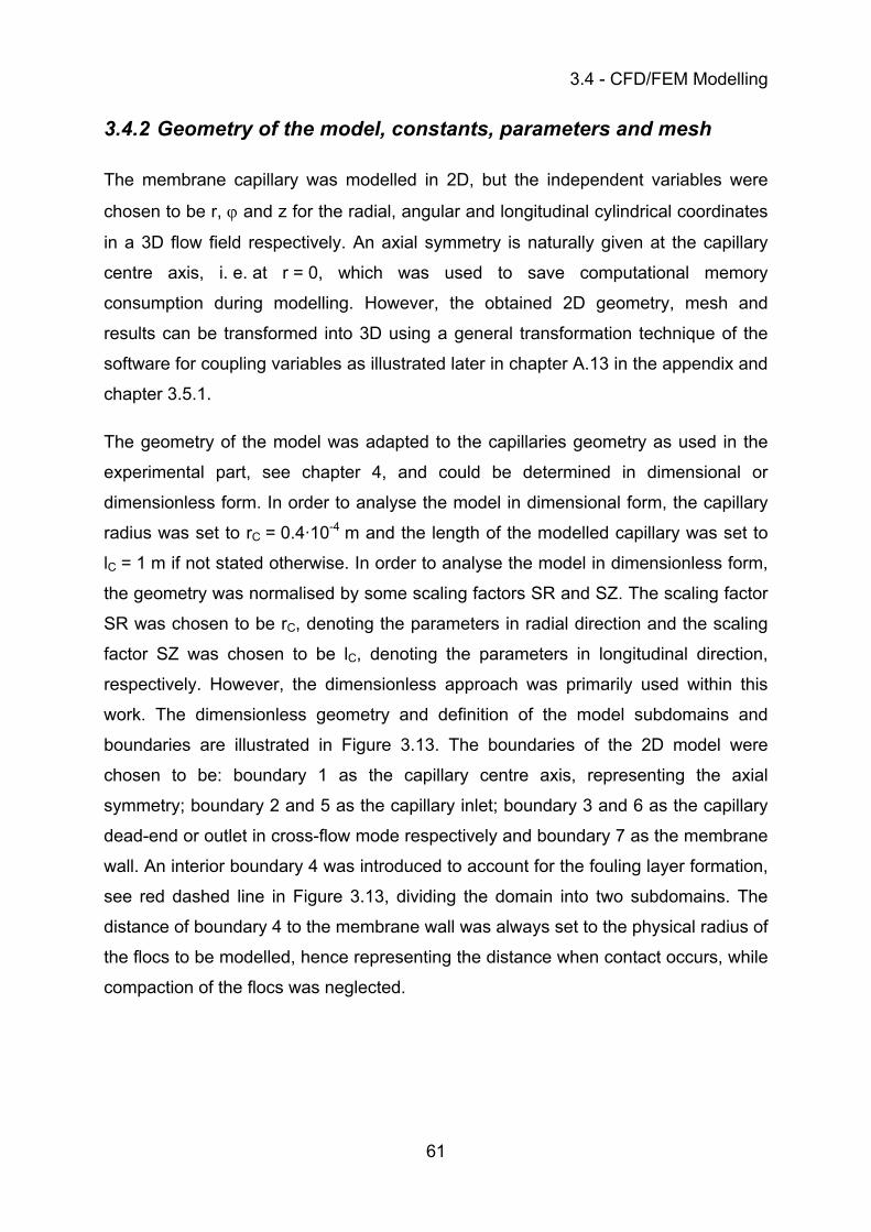
3.4 - CFD/FEM Modelling
61
3.4.2 Geometry of the model, constants, parameters and mesh
The membrane capillary was modelled in 2D, but the independent variables were
chosen to be r, ϕ and z for the radial, angular and longitudinal cylindrical coordinates
in a 3D flow field respectively. An axial symmetry is naturally given at the capillary
centre axis, i. e. at r = 0, which was used to save computational memory
consumption during modelling. However, the obtained 2D geometry, mesh and
results can be transformed into 3D using a general transformation technique of the
software for coupling variables as illustrated later in chapter A.13 in the appendix and
chapter 3.5.1.
The geometry of the model was adapted to the capillaries geometry as used in the
experimental part, see chapter 4, and could be determined in dimensional or
dimensionless form. In order to analyse the model in dimensional form, the capillary
radius was set to rC = 0.4·10-4 m and the length of the modelled capillary was set to
lC = 1 m if not stated otherwise. In order to analyse the model in dimensionless form,
the geometry was normalised by some scaling factors SR and SZ. The scaling factor
SR was chosen to be rC, denoting the parameters in radial direction and the scaling
factor SZ was chosen to be lC, denoting the parameters in longitudinal direction,
respectively. However, the dimensionless approach was primarily used within this
work. The dimensionless geometry and definition of the model subdomains and
boundaries are illustrated in Figure 3.13. The boundaries of the 2D model were
chosen to be: boundary 1 as the capillary centre axis, representing the axial
symmetry; boundary 2 and 5 as the capillary inlet; boundary 3 and 6 as the capillary
dead-end or outlet in cross-flow mode respectively and boundary 7 as the membrane
wall. An interior boundary 4 was introduced to account for the fouling layer formation,
see red dashed line in Figure 3.13, dividing the domain into two subdomains. The
distance of boundary 4 to the membrane wall was always set to the physical radius of
the flocs to be modelled, hence representing the distance when contact occurs, while
compaction of the flocs was neglected.
3 - Theoretical considerations and modelling
62
Figure 3.13: Geometry and definition of the modelled subdomains and boundaries
Constants, for instance membrane resistance RM, capillary diameter rC and length lC,
were used for modelling the flow field and the concentration distribution in the
membrane capillary as given in Table A.3 in the appendix. Additionally, some initial
parameters at time t0 = 0 were defined for the numerical analysis of the Navier-
Stokes equations. As presented by PANGLISCH (2001), the initial inlet pressure p0 and
velocity v0 of the fluid at the capillary entry can be calculated with:
2C
00 r
Vv⋅π
= and Equation 3.80
( ) p4CC
00 p
ralatanhV8p +
⋅π⋅⋅⋅η⋅⋅
= . Equation 3.81
The parameter a was introduced by PANGLISCH (2001) as a parameter depending on
membrane resistance RM and capillary radius rC with:
M3C Rr16a⋅
= . Equation 3.82
3.4 - CFD/FEM Modelling
63
Further, the membrane surface area AM and the inlet volume flow 0V were calculated
with:
CCM lr2A ⋅⋅π⋅= , and Equation 3.83
JAV M0 ⋅= . Equation 3.84
The dynamic fluid viscosity η0 at the capillary inlet could be calculated using a
polynomial approximation as function of temperature, compare Equation 2.10. The
initial fluid density ρ0 can be approximated with following polynomial equation as:
0.0001)T0.000134-T0.01299+T0.6003-(17.9098 320 ⋅⋅⋅⋅=ρ , Equation 3.85
derived by regression of listed values in VEREIN DEUTSCHER INGENIEURE (1988) and
PERRY ET AL. (1984). The determined values for different initial parameters, for
instance fluid inlet velocity in radial and longitudinal direction, u0 and v0, and fluid inlet
pressure p0 at time t0 = 0 are listed in Table A.4. Please note that the gravitational
forces Fr and Fz were defined to account for gravitation in a horizontally orientated
capillary.
As mentioned above, the software is able to work with triangular, quadrilateral,
tetrahedral, brick, and prism meshes using fully automatic and adaptive mesh
generation. However, some general remarks and limitations of quadrilateral elements
are given in chapter A.13 while all conditions were met in the existing case of the
capillary. Especially for numerical calculation of the fluid flow quadrilateral elements
were usually used, because less element numbers were needed to meet the high
convergence criteria, chosen to be 1·10-6. The mesh was always set up to account
for a sufficient high resolution especially at boundary 4 where interacting forces
between fluid flow, moving flocs and membrane wall will be likely highest and where
the fouling layer formation occurs. Nevertheless, the mesh has to be adapted for
each model. For example, one chosen mesh used for modelling the velocity profile
within a capillary consists of 78.750 elements over the whole modelled capillary, with
1.380 elements directly at the boundaries, delivering 1.644.941 degrees of freedom
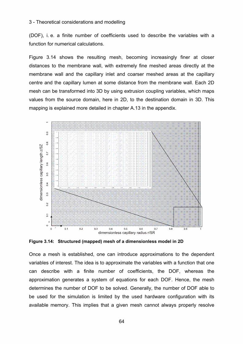
3 - Theoretical considerations and modelling
64
(DOF), i. e. a finite number of coefficients used to describe the variables with a
function for numerical calculations.
Figure 3.14 shows the resulting mesh, becoming increasingly finer at closer
distances to the membrane wall, with extremely fine meshed areas directly at the
membrane wall and the capillary inlet and coarser meshed areas at the capillary
centre and the capillary lumen at some distance from the membrane wall. Each 2D
mesh can be transformed into 3D by using extrusion coupling variables, which maps
values from the source domain, here in 2D, to the destination domain in 3D. This
mapping is explained more detailed in chapter A.13 in the appendix.
Figure 3.14: Structured (mapped) mesh of a dimensionless model in 2D
Once a mesh is established, one can introduce approximations to the dependent
variables of interest. The idea is to approximate the variables with a function that one
can describe with a finite number of coefficients, the DOF, whereas the
approximation generates a system of equations for each DOF. Hence, the mesh
determines the number of DOF to be solved. Generally, the number of DOF able to
be used for the simulation is limited by the used hardware configuration with its
available memory. This implies that a given mesh cannot always properly resolve
3.4 - CFD/FEM Modelling
65
small-scale effects. The used computer was equipped with a Windows XP64 and a
SUSE Linux 10.1 system, two Intel Xeon Dual Core CPUs 5160 with a frequency of
3 GHz and 16 GB RAM plus 30GB virtual memory. The number of DOF usually
solved for was approximately 400,000.
3.4.3 Determination of the flow field
As introduced in chapter 3.1.2 the Navier-Stokes equations are used for the
description of the fluid flow in the capillary lumen. The software uses a generalised
version of the Navier-Stokes equations to allow calculations of variable viscosity too,
i. e. non-Newtonian fluids (COMSOL AB (2006B)). The generalised equations as
used in the incompressible Navier-Stokes application mode, denoted as the total
stress tensor formulation are defined by Equation 3.86 and Equation 3.87 as given
below:
( )( )[ ] ( ) FuuuuIptu T =∇⋅ρ+∇+∇η+⋅−⋅∇−
∂∂
ρ and Equation 3.86
0u =⋅∇ . Equation 3.87
where I is the identity matrix or unit diagonal matrix. The incompressible Navier-
Stokes equations were solved for the pressure p and the velocity vector components
of u in stationary and transient analysis. The solver applied was the so called ‘Direct
(UMFPACK)’ solver for nonlinear, stationary or transient flow problems and the
convergence criteria was chosen to be 1·10-6. For more detailed information about
the numerical analysis refer to COMSOL AB (2006B) and COMSOL AB (2006A).
However, some additional terms and parameters related to the Navier-Stokes
equations used in the software will be introduced in the following. The viscous stress
tensor τ is defined as:
( )( )Tuu ∇+∇η=τ . Equation 3.88
Due to the fluid pressure p, internal stresses can arise in addition to the stress due to
viscous forces. Hence, the total stress tensor σ is introduced and defined as:
3 - Theoretical considerations and modelling
66
( )( )TuuIpIp ∇+∇η+−=τ+−=σ . Equation 3.89
From these stress tensors, one can further define the viscous boundary force K ,
which is per unit area as:
nK τ= , Equation 3.90
and the total boundary force BT , also per unit area as:
nTB σ= , Equation 3.91
where n is the outward normal vector on the boundary.
The equation system form was chosen to be set to ‘General’ in case of dimensional
models, using generally the equations as presented above, and to ‘Weak’ for
analysing dimensionless models. In the latter one, the provided equations of the
software were adapted by normalising the r and z derivates of the fluid velocity vector
u by the scaling factors SR and SZ respectively as introduced in chapter 3.4.2.
Additionally, the radial variable r was adapted by multiplication with the scaling factor
SR too. If internal variables of the software were needed for modelling the fluid flow
and the floc movement, they were treated in the same way as described. All following
model information are valid for both, the dimensional as well as the dimensionless
case. Further, all variables and parameters are always introduced as dimensional
values if not stated otherwise.
3.4.3.1 Model boundaries
The software package offers several predefined boundary conditions, but only those
are discussed here which were applied in the flow field model. For additional
information about the boundary conditions refer to the software users guides, i. e.
COMSOL AB (2006A) and COMSOL AB (2006B), for instance. The governing
equations of the chosen boundary conditions and the chosen calculation of the
expressions are discussed in the following. Boundary 1 represents the axial
symmetry of the capillary. Hence, the radial coordinate was set to:
3.4 - CFD/FEM Modelling
67
0r = . Equation 3.92
For the imposed fluid velocity at boundary 2 and 5, together representing the
capillary inlet, the velocity vector normal to the boundary can be specified by:
0unu =⋅ . Equation 3.93
This boundary condition is called the inflow/outflow boundary condition. For
modelling the fluid flow at the capillary inlet just the longitudinal velocity component
has to be considered. Hence, the radial component u was set to u = 0 m/s and the
longitudinal velocity v was set to v = v0 as introduced in Table A.4.
Boundary 3 and 6 represent the dead-end of a capillary driven in dead-end mode and
the slip or symmetry condition was used. A slip condition means that the normal
component of the velocity equals zero with:
0nu =⋅ Equation 3.94
and that the tangential component of the viscous force vanishes with:
0Kt =⋅ . Equation 3.95
Hence, the chosen condition states that there are no velocity components
perpendiculars to that boundary. However, for a capillary driven in cross-flow mode
operation boundary 3 and 6 have to be set as the so called outflow/pressure
condition to:
npT 0B −= . Equation 3.96
This boundary condition states that the total force on the boundary is a pressure
force defined by p0, where the pressure can be set to the outlet pressure pout of the
capillary, compare Equation 2.6. If the outlet pressure is not known, boundary 3 and
6 can be set to a fixed outflow velocity as given by Equation 3.93. This flow velocity
can be represented by a laminar flow profile too.
3 - Theoretical considerations and modelling
68
The interior boundary 4 is set to neutral. The software treats a neutral boundary as if
there were no boundary, which means that the total or viscous force vanishes, i. e.
0K = , and Equation 3.97
0TB = . Equation 3.98
Boundary 7 represents the membrane wall where the filtrate leaves the modelled
geometry. The so called normal flow/pressure or straight-out boundary condition is
applied to set the velocity components in the tangential direction to zero with:
0ut =⋅ , Equation 3.99
and further, to set the pressure to a specific value with:
0B pTn −=⋅ . Equation 3.100
This boundary condition is usually provided to simulate channels that are long in
length where flow is assumed to have stabilised so that all velocity occurring in the
tangential direction is negligible. The equation used for boundary 7 is given with:
FiltrateM pRup +⋅η⋅= . Equation 3.101
Please note that η is denoted to the local dynamic fluid viscosity. Equation 3.101
could be derived from Darcy’s law as introduced with Equation 2.2 when considering
radial outflow of the filtrate only, i. e. perpendicular to the boundary. Here, the
pressure drop in radial direction through the membrane has to be considered. The
radial pressure drop depends on the active membrane thickness δM, but can be
mathematically cancelled after introducing the permeability coefficient kM with:
M
MM R
k δ= . Equation 3.102
Solving Equation 3.101 within the model will deliver the initial fluid flow field. Please
note, if different membrane resistances were used within one capillary, as it was
done in the experimental part of this work, the actual local membrane resistance was
3.4 - CFD/FEM Modelling
69
used. As it will be described later in chapter 3.4.6, the boundary condition will be
changed to account for the additional resistance of the formed fouling layer when
solving the transient suspension flow problem, i. e. over time, to
FiltrateTot pRup +⋅η⋅= . Equation 3.103
Another boundary condition has to be introduced as the no-slip condition, which is
normally used at walls. For no-slip conditions, all components of the velocity vector
are eliminated by:
0u = . Equation 3.104
This boundary condition will be used in the experimental part of this thesis as
described in chapter 4 when modelling pottings for example.
3.4.4 Determination of the floc trajectories
Generally, the software generates trajectories by solving the fundamental equation of
motion:
⎥⎦
⎤⎢⎣
⎡∂∂
=∂∂
⋅tx,x,tF
txm 2
2
F , Equation 3.105
for x (t) being the trajectory. Here, mF is the flocs mass, F equals the force
component acting on the floc as introduced in chapter 3.3, and t is time. This delivers
a system of ordinary differential equations (ODE) for x , which COMSOL Multiphysics
solves using a pair of Runge-Kutta methods of orders four and five, compare
FINLAYSON (2006), which are iterative numerical methods for the approximation of
solutions of ODE systems. The solver advances the algorithm with the solution of
order five and uses the difference between the order-five and order-four solutions to
obtain the local error estimate. For the used 2D axis-symmetric model all three force
components were used. Hence, the algorithm solves for a trajectory in 3D in
cylindrical coordinates, but only the projection on the axis-symmetry plane is plotted
in 2D. For neutrally buoyant particles, the equation of motion is given by:
3 - Theoretical considerations and modelling
70
[ ]u,tutx
F=∂∂
. Equation 3.106
3.4.5 Determination of the concentration distribution
For modelling mass balances in the convection and diffusion application mode of the
Chemical Engineering Module two mass balance formulations are available: a so
called conservative and non-conservative formulation. The conservative formulation
was given by Equation 3.5 in chapter 3.1.3. The non-conservative formulation
removes the convective term from the divergence operator in Equation 3.5, which
gives more stability to systems coupled to momentum balances. It should only be
applied to systems that contain incompressible or slightly compressible fluids,
because the continuity equation, as introduced with Equation 3.4, is already satisfied
for such coupled systems. However, this validity of the continuity equation is only
given for fluid elements when coupled to the momentum balance and therefore for
dissolved species in the fluid. Considering now the flow of flocs, u has to be chosen
to denote the actual floc velocity vector Fu , as introduced in chapter 3.3.9.
Accordingly, the continuity equation has to be solved again for the velocity
components of flocs to achieve mass conservation. Hence, the conservative form
was used as presented with Equation 3.5. For additional information refer to
COMSOL AB (2006A) and COMSOL AB (2006B), for instance.
Accounting for the floc volume concentration φF, the floc velocity vector Fu as
introduced in chapter 3.3.9 and neglecting any reaction Equation 3.5 becomes:
( ) 0uDt FFFF =⋅φ+φ∇⋅−⋅∇+
∂φ∂
. Equation 3.107
For stationary analysis the term with the time derivative gets dropped. As introduced
in chapter 3.4.3, the equation system form was set to ‘General’ in case of
dimensional models, using generally the equation as presented above, and to ‘Weak’
for analysing dimensionless models. In the latter case, adoption was performed as
described in chapter 3.4.3. The used diffusion coefficient was derived by
superposition of the Brownian diffusion coefficient as introduced in chapter 3.3.5 and
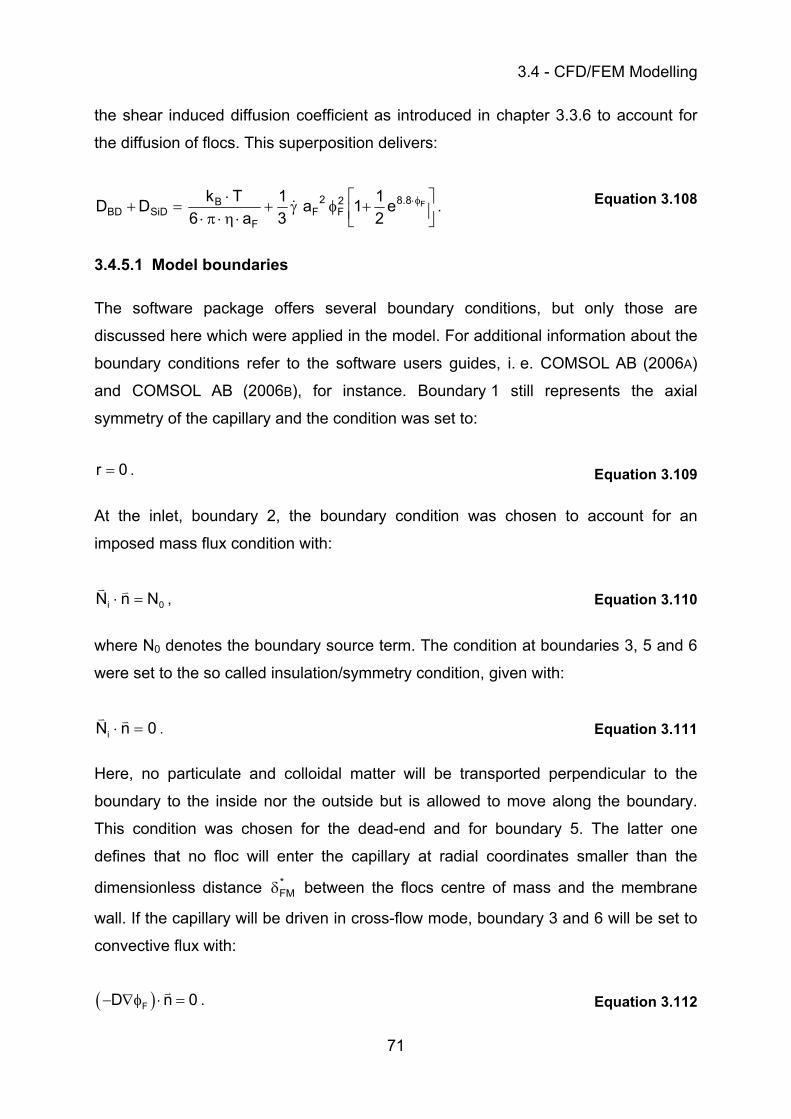
3.4 - CFD/FEM Modelling
71
the shear induced diffusion coefficient as introduced in chapter 3.3.6 to account for
the diffusion of flocs. This superposition delivers:
⎥⎦⎤
⎢⎣⎡ +φγ+
⋅η⋅π⋅⋅
=+ φ⋅ F8.82F
2F
F
BSiDBD e
211a
31
a6TkDD . Equation 3.108
3.4.5.1 Model boundaries
The software package offers several boundary conditions, but only those are
discussed here which were applied in the model. For additional information about the
boundary conditions refer to the software users guides, i. e. COMSOL AB (2006A)
and COMSOL AB (2006B), for instance. Boundary 1 still represents the axial
symmetry of the capillary and the condition was set to:
r 0= . Equation 3.109
At the inlet, boundary 2, the boundary condition was chosen to account for an
imposed mass flux condition with:
0i NnN =⋅ , Equation 3.110
where N0 denotes the boundary source term. The condition at boundaries 3, 5 and 6
were set to the so called insulation/symmetry condition, given with:
0nNi =⋅ . Equation 3.111
Here, no particulate and colloidal matter will be transported perpendicular to the
boundary to the inside nor the outside but is allowed to move along the boundary.
This condition was chosen for the dead-end and for boundary 5. The latter one
defines that no floc will enter the capillary at radial coordinates smaller than the
dimensionless distance *FMδ between the flocs centre of mass and the membrane
wall. If the capillary will be driven in cross-flow mode, boundary 3 and 6 will be set to
convective flux with:
( )FD n 0− ∇φ ⋅ = . Equation 3.112
3 - Theoretical considerations and modelling
72
The condition at boundary 4 was set to continuity, i. e. there is no change in transport
of matter along boundary 4 from subdomain 1 into subdomain 2, compare Figure
3.13. This condition can be expressed as:
( ) 0NNn 2,i1,i =−⋅ , Equation 3.113
whereas 1,iN and 2,iN represent the mass flux vectors of species i in subdomain 1
and subdomain 2 respectively. The condition at boundary 7 was set to convective
flux with:
( )FD n 0− ∇φ ⋅ = . Equation 3.114
This condition was chosen to account for the high Péclet numbers in the modelled
domains. The Péclet number is a dimensionless number, defined as the product of
the Reynold and Schmidt numbers as:
DdvScRePe CF ⋅
=⋅= , Equation 3.115
and describes the ratio of convective to diffusive transport. Due to the high velocities
and the low diffusion coefficients used in the model, convective transport of the flocs
is far more dominant than diffusive transport. Calculated Pe numbers are in the range
of 30,000 to 30,000,000. Initially it was intended to choose the boundary condition at
boundary 7 to be insulating as well to account for a 100 % retention efficiency of the
membrane wall for flocs. However, this could not be realised due to major problems
in using FEM to solve the problem numerically. Here, discretisation of convection-
dominated transport problems can introduce instabilities in the solution. Instabilities
might be detected as oscillations in the studied fields, primarily where steep gradients
are present. These oscillations can even be large enough to prevent the solution
from converging. All of these problems result from the poor (mesh) discretisation of
the continuous equations and are not general properties of the equations
themselves. As long as any diffusion is present in the problem, there is - at least in
theory - a mesh resolution beyond which the discretisation is stable. However, in
most cases the mesh size is determined by available memory in the computer used
3.4 - CFD/FEM Modelling
73
for the simulation, which implies that a given mesh cannot always properly resolve
small-scale effects. As a rule of thumb for sizing the initial mesh in dimensionless grid
scale one should use 1/Pe (email correspondence with Prof. Will Zimmerman).
Inserting the Pe numbers mentioned above, this would result in extremely fine
meshes, not able to be dealt with by the used computer hardware. To address this
problem, COMSOL Multiphysics offers several stabilisation techniques, available to
handle local numerical instabilities without the need for mesh refinement. These
techniques can all be grouped under the name artificial diffusion (artificial viscosity or
numerical diffusion/viscosity are also commonly used terms). However, in this work
stabilisation was usually done where needed by using the build-in function of the so
called compensated Petrov-Galerkin method, which introduces artificial diffusion
along the streamlines. It operates on the test functions of the variables solved for,
and, theoretically, does not change the original problem. This is all true in theory, but
in practice the solutions might be somewhat smeared out along the streamlines. For
more information about stabilisation techniques please refer to the software users
guides, i. e. COMSOL AB (2006A) and COMSOL AB (2006B), for instance. However,
the condition of convective flux was chosen to minimise numerical instability during
the calculations and to find convergence during modelling. Physically, particulate and
colloidal matter will not be modelled to accumulate after being deposited, but to leave
the capillary at the membrane wall. Because the interest is set in describing
accumulation of flocs at the membrane wall, the resulting mass flux will be integrated
along boundary 4 to calculate the accumulated mass of particulate matter through
this boundary. The accumulation can then be used to calculate the height of the
fouling layer, see chapter 3.5.3.
3.4.6 Determination of fouling layer formation
While filtering the feed suspension, foulants are retained and accumulated at the
membrane wall. This causes the formation of a concentration polarisation layer and
of a coating layer as illustrated in Figure 3.15.
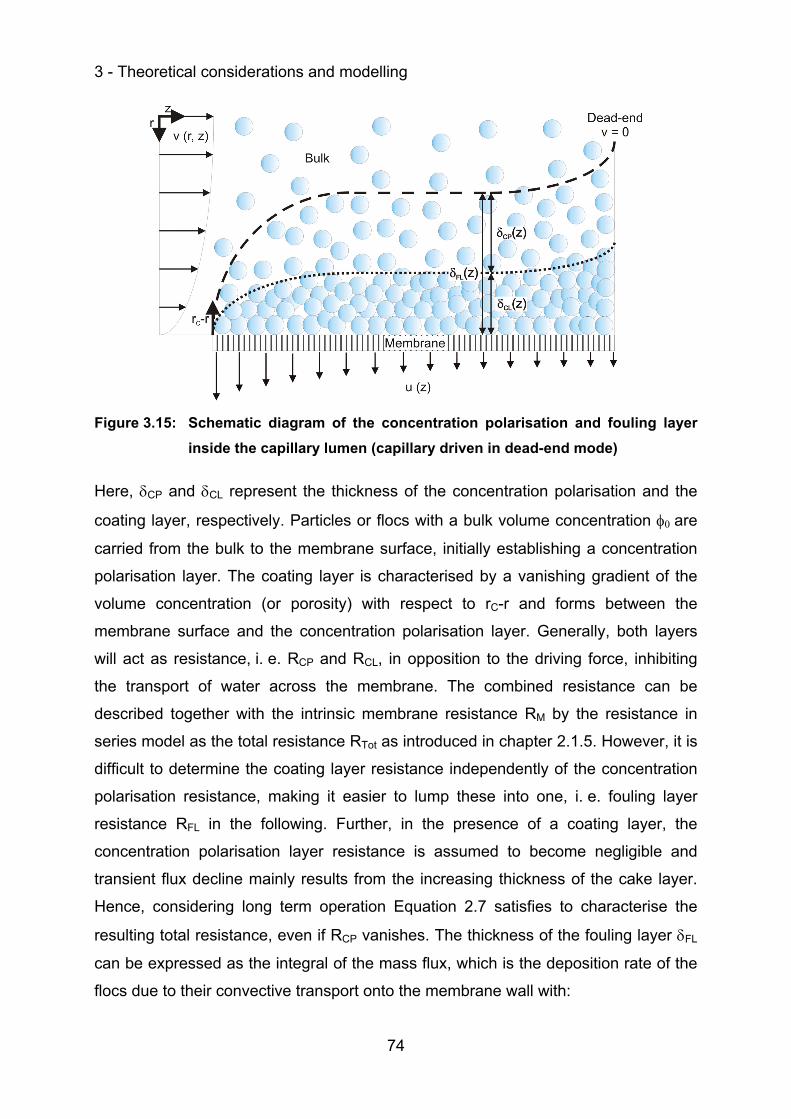
3 - Theoretical considerations and modelling
74
Figure 3.15: Schematic diagram of the concentration polarisation and fouling layer inside the capillary lumen (capillary driven in dead-end mode)
Here, δCP and δCL represent the thickness of the concentration polarisation and the
coating layer, respectively. Particles or flocs with a bulk volume concentration φ0 are
carried from the bulk to the membrane surface, initially establishing a concentration
polarisation layer. The coating layer is characterised by a vanishing gradient of the
volume concentration (or porosity) with respect to rC-r and forms between the
membrane surface and the concentration polarisation layer. Generally, both layers
will act as resistance, i. e. RCP and RCL, in opposition to the driving force, inhibiting
the transport of water across the membrane. The combined resistance can be
described together with the intrinsic membrane resistance RM by the resistance in
series model as the total resistance RTot as introduced in chapter 2.1.5. However, it is
difficult to determine the coating layer resistance independently of the concentration
polarisation resistance, making it easier to lump these into one, i. e. fouling layer
resistance RFL in the following. Further, in the presence of a coating layer, the
concentration polarisation layer resistance is assumed to become negligible and
transient flux decline mainly results from the increasing thickness of the cake layer.
Hence, considering long term operation Equation 2.7 satisfies to characterise the
resulting total resistance, even if RCP vanishes. The thickness of the fouling layer δFL
can be expressed as the integral of the mass flux, which is the deposition rate of the
flocs due to their convective transport onto the membrane wall with:
3.4 - CFD/FEM Modelling
75
( ) ( ) tdzzu F
t
0FFL φ⋅=δ ∫ .
Equation 3.116
Integration of Equation 3.116 over filtration time delivers the fouling layer thickness.
As mentioned in chapter 3.4.5, this will be realised by integrating the convective floc
flux through boundary 4 over time. A user specified PDE was introduced in the model
to account for this additional step by solving numerically Equation 3.116 as
FFFL ut
φ⋅=∂δ∂
. Equation 3.117
The PDE is calculated over the entire domain and linked to boundary 4 by
introducing a so called boundary extrusion coupling variable, see chapter 3.4.1. The
deposited fouling layer will increase with time and therefore, flux will decrease as the
thickness of the layer increases. The resulting resistance RFL of this layer can be
calculated as the ratio of its thickness and permeability coefficient kFL with:
( )FL
FLFL k
tR δ= . Equation 3.118
Assuming a homogeneous fouling layer structure, the fouling layer permeability
coefficient kFL can be calculated based on the Happel model as introduced and
discussed in chapter 3.2.1, using the hydrodynamic floc ahF size as primary particle
size. Other authors, e. g. ALTMANN AND RIPPERGER (1997), SONG (1998), KIM AND
HOEK (2002), HOEK AND ELIMELECH (2003) and LEE ET AL. (2003) often apply the
Carman-Kozeny model to describe the permeability coefficient of the formed fouling
layer. Figure 3.16 shows the difference between both models over the investigated
fouling layer porosity range from 0.26 to 0.74. The results delivered by the Happel
model will be larger than the results delivered from the Carman-Kozeny model up to
a fouling layer porosity of ε = 0.58 and smaller for larger porosities. At the minimum
porosity of ε = 0.26 the difference was calculated to be approximately 11.5 % and at
the maximum porosity of ε = 0.74 approximately 24.6 %.
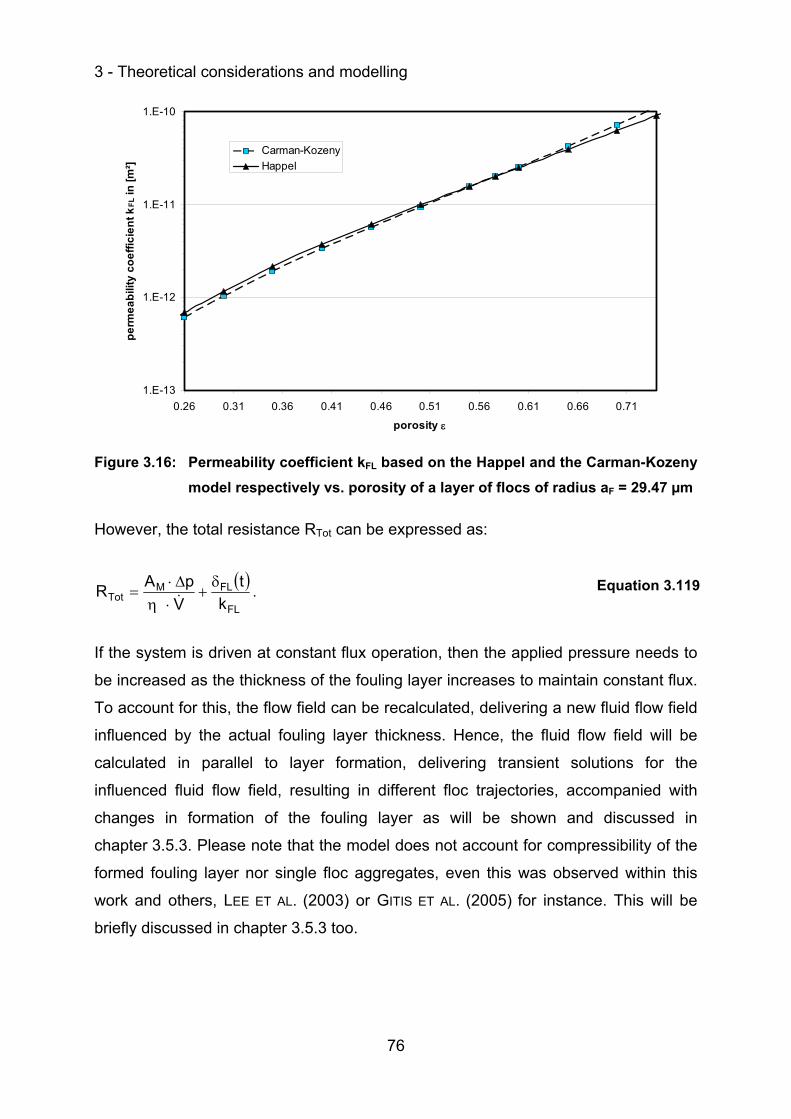
3 - Theoretical considerations and modelling
76
1.E-13
1.E-12
1.E-11
1.E-10
0.26 0.31 0.36 0.41 0.46 0.51 0.56 0.61 0.66 0.71
porosity ε
perm
eabi
lity
coef
ficie
nt k
FL in
[m²]
Carman-KozenyHappel
Figure 3.16: Permeability coefficient kFL based on the Happel and the Carman-Kozeny model respectively vs. porosity of a layer of flocs of radius aF = 29.47 µm
However, the total resistance RTot can be expressed as:
( )FL
FLMTot k
tV
pAR δ+
⋅ηΔ⋅
= . Equation 3.119
If the system is driven at constant flux operation, then the applied pressure needs to
be increased as the thickness of the fouling layer increases to maintain constant flux.
To account for this, the flow field can be recalculated, delivering a new fluid flow field
influenced by the actual fouling layer thickness. Hence, the fluid flow field will be
calculated in parallel to layer formation, delivering transient solutions for the
influenced fluid flow field, resulting in different floc trajectories, accompanied with
changes in formation of the fouling layer as will be shown and discussed in
chapter 3.5.3. Please note that the model does not account for compressibility of the
formed fouling layer nor single floc aggregates, even this was observed within this
work and others, LEE ET AL. (2003) or GITIS ET AL. (2005) for instance. This will be
briefly discussed in chapter 3.5.3 too.
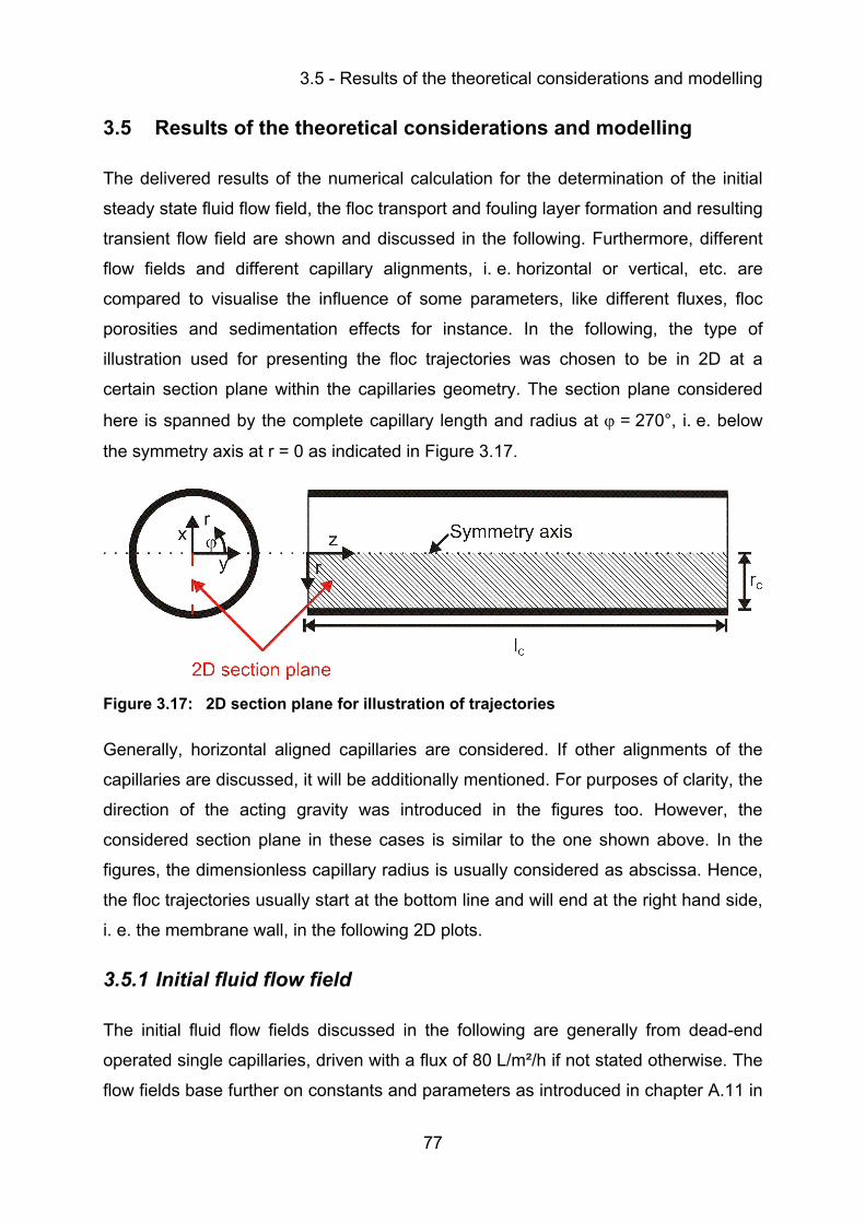
3.5 - Results of the theoretical considerations and modelling
77
3.5 Results of the theoretical considerations and modelling
The delivered results of the numerical calculation for the determination of the initial
steady state fluid flow field, the floc transport and fouling layer formation and resulting
transient flow field are shown and discussed in the following. Furthermore, different
flow fields and different capillary alignments, i. e. horizontal or vertical, etc. are
compared to visualise the influence of some parameters, like different fluxes, floc
porosities and sedimentation effects for instance. In the following, the type of
illustration used for presenting the floc trajectories was chosen to be in 2D at a
certain section plane within the capillaries geometry. The section plane considered
here is spanned by the complete capillary length and radius at ϕ = 270°, i. e. below
the symmetry axis at r = 0 as indicated in Figure 3.17.
Figure 3.17: 2D section plane for illustration of trajectories
Generally, horizontal aligned capillaries are considered. If other alignments of the
capillaries are discussed, it will be additionally mentioned. For purposes of clarity, the
direction of the acting gravity was introduced in the figures too. However, the
considered section plane in these cases is similar to the one shown above. In the
figures, the dimensionless capillary radius is usually considered as abscissa. Hence,
the floc trajectories usually start at the bottom line and will end at the right hand side,
i. e. the membrane wall, in the following 2D plots.
3.5.1 Initial fluid flow field
The initial fluid flow fields discussed in the following are generally from dead-end
operated single capillaries, driven with a flux of 80 L/m²/h if not stated otherwise. The
flow fields base further on constants and parameters as introduced in chapter A.11 in
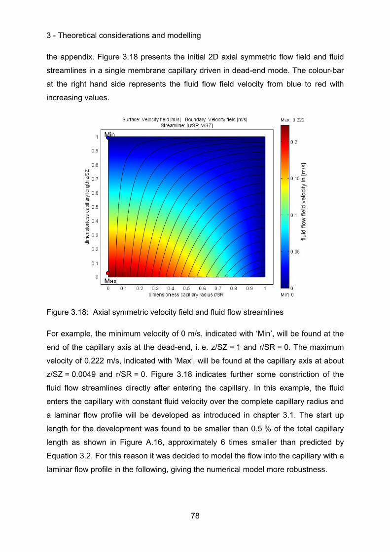
3 - Theoretical considerations and modelling
78
the appendix. Figure 3.18 presents the initial 2D axial symmetric flow field and fluid
streamlines in a single membrane capillary driven in dead-end mode. The colour-bar
at the right hand side represents the fluid flow field velocity from blue to red with
increasing values.
Figure 3.18: Axial symmetric velocity field and fluid flow streamlines
For example, the minimum velocity of 0 m/s, indicated with ‘Min’, will be found at the
end of the capillary axis at the dead-end, i. e. z/SZ = 1 and r/SR = 0. The maximum
velocity of 0.222 m/s, indicated with ‘Max’, will be found at the capillary axis at about
z/SZ = 0.0049 and r/SR = 0. Figure 3.18 indicates further some constriction of the
fluid flow streamlines directly after entering the capillary. In this example, the fluid
enters the capillary with constant fluid velocity over the complete capillary radius and
a laminar flow profile will be developed as introduced in chapter 3.1. The start up
length for the development was found to be smaller than 0.5 % of the total capillary
length as shown in Figure A.16, approximately 6 times smaller than predicted by
Equation 3.2. For this reason it was decided to model the flow into the capillary with a
laminar flow profile in the following, giving the numerical model more robustness.
Min
Max
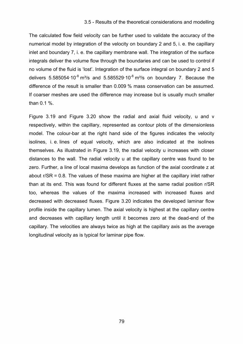
3.5 - Results of the theoretical considerations and modelling
79
The calculated flow field velocity can be further used to validate the accuracy of the
numerical model by integration of the velocity on boundary 2 and 5, i. e. the capillary
inlet and boundary 7, i. e. the capillary membrane wall. The integration of the surface
integrals deliver the volume flow through the boundaries and can be used to control if
no volume of the fluid is ‘lost’. Integration of the surface integral on boundary 2 and 5
delivers 5.585054·10-8 m³/s and 5.585529·10-8 m³/s on boundary 7. Because the
difference of the result is smaller than 0.009 % mass conservation can be assumed.
If coarser meshes are used the difference may increase but is usually much smaller
than 0.1 %.
Figure 3.19 and Figure 3.20 show the radial and axial fluid velocity, u and v
respectively, within the capillary, represented as contour plots of the dimensionless
model. The colour-bar at the right hand side of the figures indicates the velocity
isolines, i. e. lines of equal velocity, which are also indicated at the isolines
themselves. As illustrated in Figure 3.19, the radial velocity u increases with closer
distances to the wall. The radial velocity u at the capillary centre was found to be
zero. Further, a line of local maxima develops as function of the axial coordinate z at
about r/SR = 0.8. The values of these maxima are higher at the capillary inlet rather
than at its end. This was found for different fluxes at the same radial position r/SR
too, whereas the values of the maxima increased with increased fluxes and
decreased with decreased fluxes. Figure 3.20 indicates the developed laminar flow
profile inside the capillary lumen. The axial velocity is highest at the capillary centre
and decreases with capillary length until it becomes zero at the dead-end of the
capillary. The velocities are always twice as high at the capillary axis as the average
longitudinal velocity as is typical for laminar pipe flow.
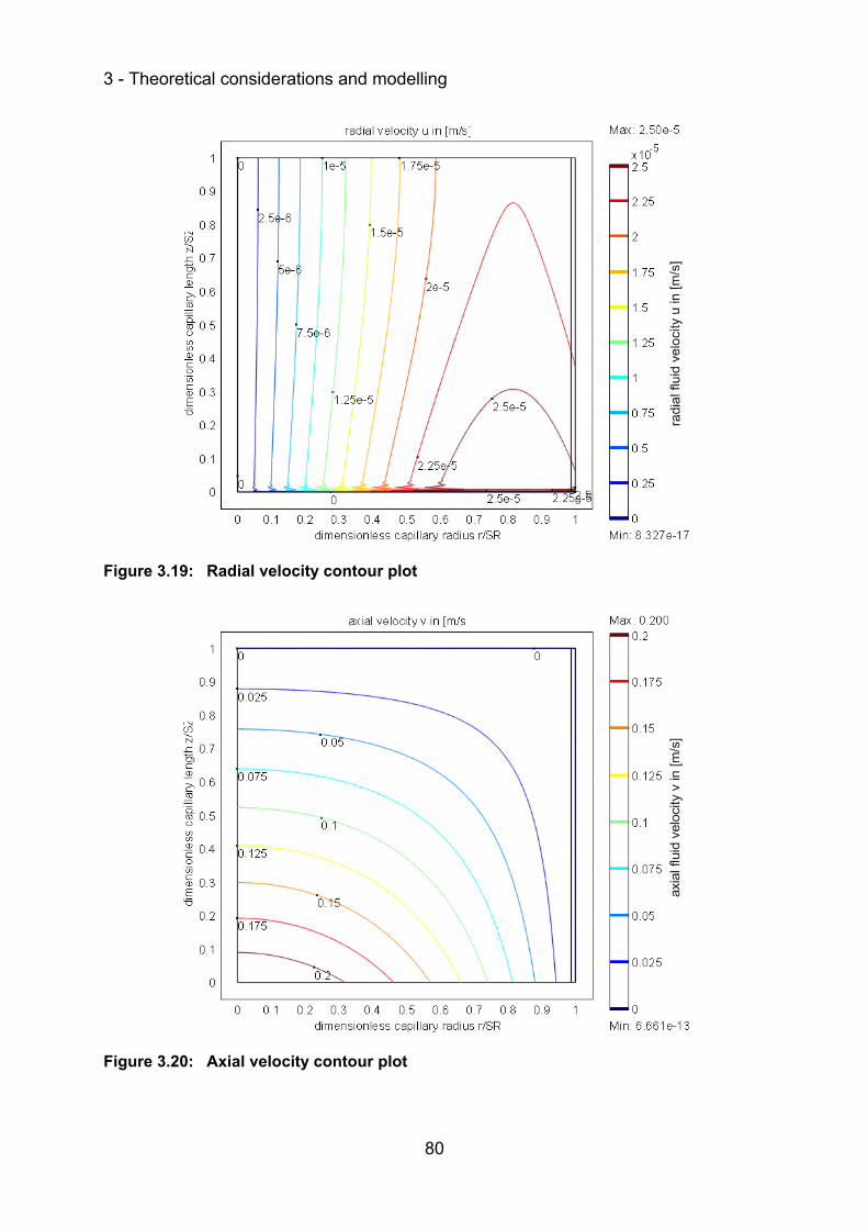
3 - Theoretical considerations and modelling
80
Figure 3.19: Radial velocity contour plot
Figure 3.20: Axial velocity contour plot
axia
l flu
id v
eloc
ity v
in [m
/s]
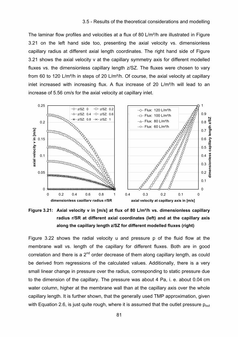
3.5 - Results of the theoretical considerations and modelling
81
The laminar flow profiles and velocities at a flux of 80 L/m²/h are illustrated in Figure
3.21 on the left hand side too, presenting the axial velocity vs. dimensionless
capillary radius at different axial length coordinates. The right hand side of Figure
3.21 shows the axial velocity v at the capillary symmetry axis for different modelled
fluxes vs. the dimensionless capillary length z/SZ. The fluxes were chosen to vary
from 60 to 120 L/m²/h in steps of 20 L/m²/h. Of course, the axial velocity at capillary
inlet increased with increasing flux. A flux increase of 20 L/m²/h will lead to an
increase of 5.56 cm/s for the axial velocity at capillary inlet.
0
0.05
0.1
0.15
0.2
0.25
0 0.2 0.4 0.6 0.8 1
dimensionless capillary radius r/SR
axia
l vel
ocity
v in
[m/s
]
z/SZ: 0 z/SZ: 0.2z/SZ: 0.4 z/SZ: 0.6z/SZ: 0.8 z/SZ: 1
0
0.1
0.2
0.3
0.4
0.5
0.6
0.7
0.8
0.9
1
00.10.20.30.4
axial velocity at capillary axis in [m/s]
dim
ensi
onle
ss c
apill
ary
leng
th z
/SZ
Flux: 120 L/m²/hFlux: 100 L/m²/hFlux: 80 L/m²/hFlux: 60 L/m²/h
Figure 3.21: Axial velocity v in [m/s] at flux of 80 L/m²/h vs. dimensionless capillary radius r/SR at different axial coordinates (left) and at the capillary axis along the capillary length z/SZ for different modelled fluxes (right)
Figure 3.22 shows the radial velocity u and pressure p of the fluid flow at the
membrane wall vs. length of the capillary for different fluxes. Both are in good
correlation and there is a 2nd order decrease of them along capillary length, as could
be derived from regressions of the calculated values. Additionally, there is a very
small linear change in pressure over the radius, corresponding to static pressure due
to the dimension of the capillary. The pressure was about 4 Pa, i. e. about 0.04 cm
water column, higher at the membrane wall than at the capillary axis over the whole
capillary length. It is further shown, that the generally used TMP approximation, given
with Equation 2.6, is just quite rough, where it is assumed that the outlet pressure pout
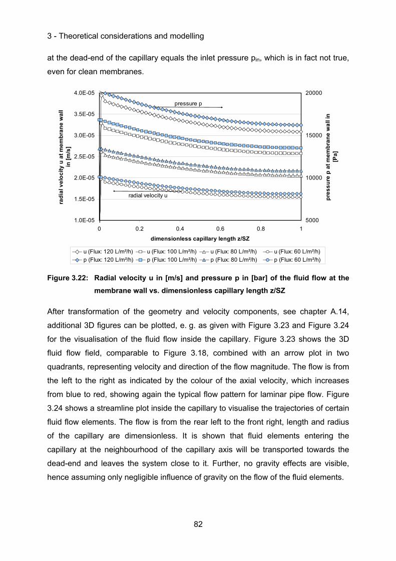
3 - Theoretical considerations and modelling
82
at the dead-end of the capillary equals the inlet pressure pin, which is in fact not true,
even for clean membranes.
1.0E-05
1.5E-05
2.0E-05
2.5E-05
3.0E-05
3.5E-05
4.0E-05
0 0.2 0.4 0.6 0.8 1
dimensionless capillary length z/SZ
radi
al v
eloc
ity u
at m
embr
ane
wal
l in
[m/s
]
5000
10000
15000
20000
pres
sure
p a
t mem
bran
e w
all i
n [P
a]
u (Flux: 120 L/m²/h) u (Flux: 100 L/m²/h) u (Flux: 80 L/m²/h) u (Flux: 60 L/m²/h)p (Flux: 120 L/m²/h) p (Flux: 100 L/m²/h) p (Flux: 80 L/m²/h) p (Flux: 60 L/m²/h)
pressure p
radial velocity u
Figure 3.22: Radial velocity u in [m/s] and pressure p in [bar] of the fluid flow at the membrane wall vs. dimensionless capillary length z/SZ
After transformation of the geometry and velocity components, see chapter A.14,
additional 3D figures can be plotted, e. g. as given with Figure 3.23 and Figure 3.24
for the visualisation of the fluid flow inside the capillary. Figure 3.23 shows the 3D
fluid flow field, comparable to Figure 3.18, combined with an arrow plot in two
quadrants, representing velocity and direction of the flow magnitude. The flow is from
the left to the right as indicated by the colour of the axial velocity, which increases
from blue to red, showing again the typical flow pattern for laminar pipe flow. Figure
3.24 shows a streamline plot inside the capillary to visualise the trajectories of certain
fluid flow elements. The flow is from the rear left to the front right, length and radius
of the capillary are dimensionless. It is shown that fluid elements entering the
capillary at the neighbourhood of the capillary axis will be transported towards the
dead-end and leaves the system close to it. Further, no gravity effects are visible,
hence assuming only negligible influence of gravity on the flow of the fluid elements.
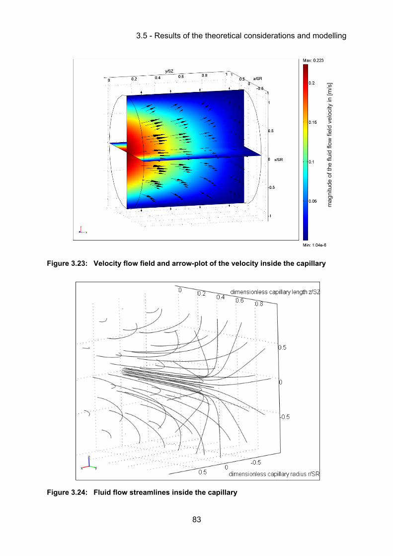
3.5 - Results of the theoretical considerations and modelling
83
Figure 3.23: Velocity flow field and arrow-plot of the velocity inside the capillary
Figure 3.24: Fluid flow streamlines inside the capillary
mag
nitu
de o
f the
flui
d flo
w fi
eld
velo
city
in [m
/s]
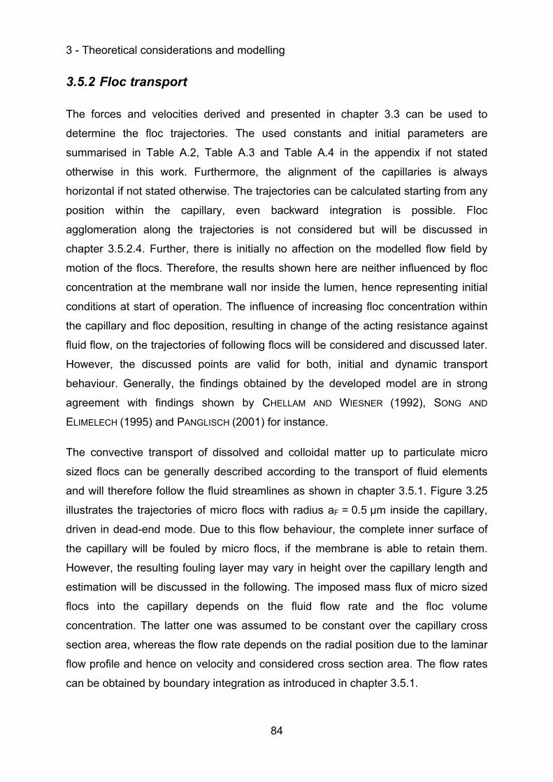
3 - Theoretical considerations and modelling
84
3.5.2 Floc transport
The forces and velocities derived and presented in chapter 3.3 can be used to
determine the floc trajectories. The used constants and initial parameters are
summarised in Table A.2, Table A.3 and Table A.4 in the appendix if not stated
otherwise in this work. Furthermore, the alignment of the capillaries is always
horizontal if not stated otherwise. The trajectories can be calculated starting from any
position within the capillary, even backward integration is possible. Floc
agglomeration along the trajectories is not considered but will be discussed in
chapter 3.5.2.4. Further, there is initially no affection on the modelled flow field by
motion of the flocs. Therefore, the results shown here are neither influenced by floc
concentration at the membrane wall nor inside the lumen, hence representing initial
conditions at start of operation. The influence of increasing floc concentration within
the capillary and floc deposition, resulting in change of the acting resistance against
fluid flow, on the trajectories of following flocs will be considered and discussed later.
However, the discussed points are valid for both, initial and dynamic transport
behaviour. Generally, the findings obtained by the developed model are in strong
agreement with findings shown by CHELLAM AND WIESNER (1992), SONG AND
ELIMELECH (1995) and PANGLISCH (2001) for instance.
The convective transport of dissolved and colloidal matter up to particulate micro
sized flocs can be generally described according to the transport of fluid elements
and will therefore follow the fluid streamlines as shown in chapter 3.5.1. Figure 3.25
illustrates the trajectories of micro flocs with radius aF = 0.5 µm inside the capillary,
driven in dead-end mode. Due to this flow behaviour, the complete inner surface of
the capillary will be fouled by micro flocs, if the membrane is able to retain them.
However, the resulting fouling layer may vary in height over the capillary length and
estimation will be discussed in the following. The imposed mass flux of micro sized
flocs into the capillary depends on the fluid flow rate and the floc volume
concentration. The latter one was assumed to be constant over the capillary cross
section area, whereas the flow rate depends on the radial position due to the laminar
flow profile and hence on velocity and considered cross section area. The flow rates
can be obtained by boundary integration as introduced in chapter 3.5.1.
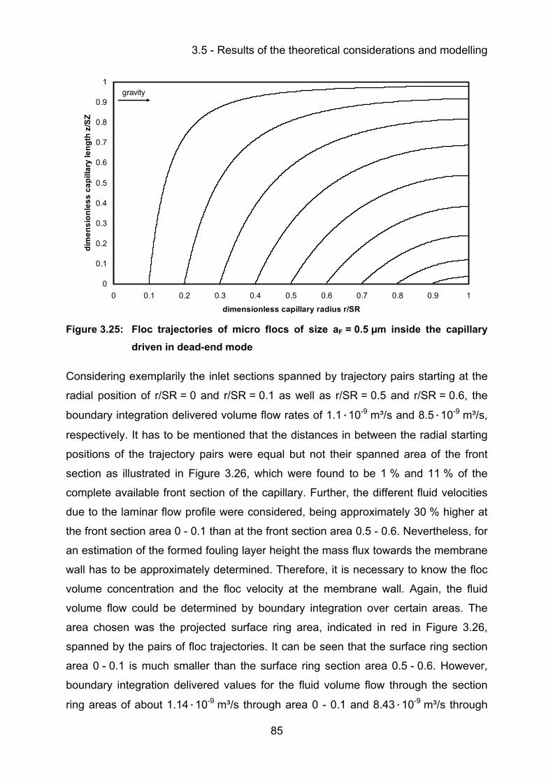
3.5 - Results of the theoretical considerations and modelling
85
0
0.1
0.2
0.3
0.4
0.5
0.6
0.7
0.8
0.9
1
0 0.1 0.2 0.3 0.4 0.5 0.6 0.7 0.8 0.9 1
dimensionless capillary radius r/SR
dim
ensi
onle
ss c
apill
ary
leng
th z
/SZ
gravity
Figure 3.25: Floc trajectories of micro flocs of size aF = 0.5 µm inside the capillary driven in dead-end mode
Considering exemplarily the inlet sections spanned by trajectory pairs starting at the
radial position of r/SR = 0 and r/SR = 0.1 as well as r/SR = 0.5 and r/SR = 0.6, the
boundary integration delivered volume flow rates of 1.1·10-9 m³/s and 8.5·10-9 m³/s,
respectively. It has to be mentioned that the distances in between the radial starting
positions of the trajectory pairs were equal but not their spanned area of the front
section as illustrated in Figure 3.26, which were found to be 1 % and 11 % of the
complete available front section of the capillary. Further, the different fluid velocities
due to the laminar flow profile were considered, being approximately 30 % higher at
the front section area 0 - 0.1 than at the front section area 0.5 - 0.6. Nevertheless, for
an estimation of the formed fouling layer height the mass flux towards the membrane
wall has to be approximately determined. Therefore, it is necessary to know the floc
volume concentration and the floc velocity at the membrane wall. Again, the fluid
volume flow could be determined by boundary integration over certain areas. The
area chosen was the projected surface ring area, indicated in red in Figure 3.26,
spanned by the pairs of floc trajectories. It can be seen that the surface ring section
area 0 - 0.1 is much smaller than the surface ring section area 0.5 - 0.6. However,
boundary integration delivered values for the fluid volume flow through the section
ring areas of about 1.14·10-9 m³/s through area 0 - 0.1 and 8.43·10-9 m³/s through
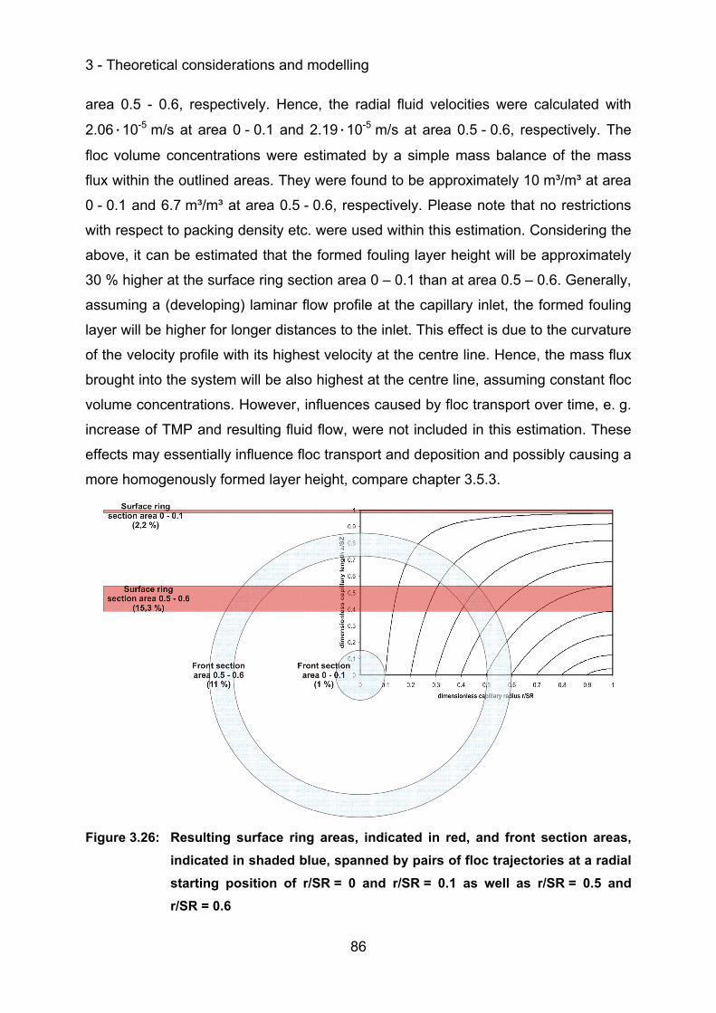
3 - Theoretical considerations and modelling
86
area 0.5 - 0.6, respectively. Hence, the radial fluid velocities were calculated with
2.06·10-5 m/s at area 0 - 0.1 and 2.19·10-5 m/s at area 0.5 - 0.6, respectively. The
floc volume concentrations were estimated by a simple mass balance of the mass
flux within the outlined areas. They were found to be approximately 10 m³/m³ at area
0 - 0.1 and 6.7 m³/m³ at area 0.5 - 0.6, respectively. Please note that no restrictions
with respect to packing density etc. were used within this estimation. Considering the
above, it can be estimated that the formed fouling layer height will be approximately
30 % higher at the surface ring section area 0 – 0.1 than at area 0.5 – 0.6. Generally,
assuming a (developing) laminar flow profile at the capillary inlet, the formed fouling
layer will be higher for longer distances to the inlet. This effect is due to the curvature
of the velocity profile with its highest velocity at the centre line. Hence, the mass flux
brought into the system will be also highest at the centre line, assuming constant floc
volume concentrations. However, influences caused by floc transport over time, e. g.
increase of TMP and resulting fluid flow, were not included in this estimation. These
effects may essentially influence floc transport and deposition and possibly causing a
more homogenously formed layer height, compare chapter 3.5.3.
Figure 3.26: Resulting surface ring areas, indicated in red, and front section areas, indicated in shaded blue, spanned by pairs of floc trajectories at a radial starting position of r/SR = 0 and r/SR = 0.1 as well as r/SR = 0.5 and r/SR = 0.6
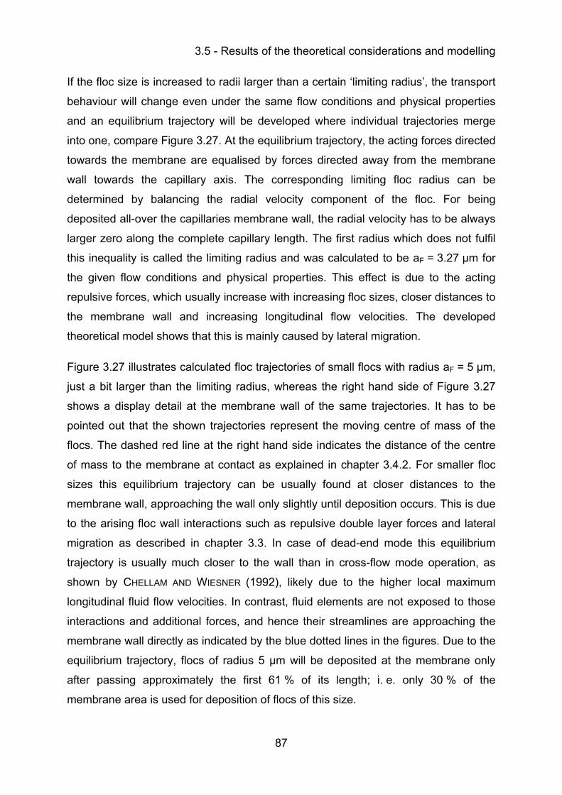
3.5 - Results of the theoretical considerations and modelling
87
If the floc size is increased to radii larger than a certain ‘limiting radius’, the transport
behaviour will change even under the same flow conditions and physical properties
and an equilibrium trajectory will be developed where individual trajectories merge
into one, compare Figure 3.27. At the equilibrium trajectory, the acting forces directed
towards the membrane are equalised by forces directed away from the membrane
wall towards the capillary axis. The corresponding limiting floc radius can be
determined by balancing the radial velocity component of the floc. For being
deposited all-over the capillaries membrane wall, the radial velocity has to be always
larger zero along the complete capillary length. The first radius which does not fulfil
this inequality is called the limiting radius and was calculated to be aF = 3.27 µm for
the given flow conditions and physical properties. This effect is due to the acting
repulsive forces, which usually increase with increasing floc sizes, closer distances to
the membrane wall and increasing longitudinal flow velocities. The developed
theoretical model shows that this is mainly caused by lateral migration.
Figure 3.27 illustrates calculated floc trajectories of small flocs with radius aF = 5 µm,
just a bit larger than the limiting radius, whereas the right hand side of Figure 3.27
shows a display detail at the membrane wall of the same trajectories. It has to be
pointed out that the shown trajectories represent the moving centre of mass of the
flocs. The dashed red line at the right hand side indicates the distance of the centre
of mass to the membrane at contact as explained in chapter 3.4.2. For smaller floc
sizes this equilibrium trajectory can be usually found at closer distances to the
membrane wall, approaching the wall only slightly until deposition occurs. This is due
to the arising floc wall interactions such as repulsive double layer forces and lateral
migration as described in chapter 3.3. In case of dead-end mode this equilibrium
trajectory is usually much closer to the wall than in cross-flow mode operation, as
shown by CHELLAM AND WIESNER (1992), likely due to the higher local maximum
longitudinal fluid flow velocities. In contrast, fluid elements are not exposed to those
interactions and additional forces, and hence their streamlines are approaching the
membrane wall directly as indicated by the blue dotted lines in the figures. Due to the
equilibrium trajectory, flocs of radius 5 µm will be deposited at the membrane only
after passing approximately the first 61 % of its length; i. e. only 30 % of the
membrane area is used for deposition of flocs of this size.
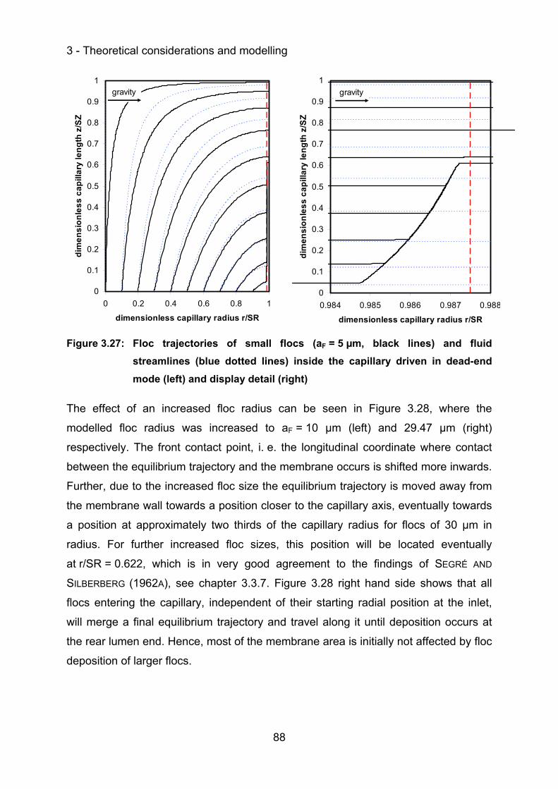
3 - Theoretical considerations and modelling
88
0
0.1
0.2
0.3
0.4
0.5
0.6
0.7
0.8
0.9
1
0 0.2 0.4 0.6 0.8 1
dimensionless capillary radius r/SR
dim
ensi
onle
ss c
apill
ary
leng
th z
/SZ
gravity
0
0.1
0.2
0.3
0.4
0.5
0.6
0.7
0.8
0.9
1
0.984 0.985 0.986 0.987 0.988
dimensionless capillary radius r/SR
dim
ensi
onle
ss c
apill
ary
leng
th z
/SZ
gravity
Figure 3.27: Floc trajectories of small flocs (aF = 5 µm, black lines) and fluid streamlines (blue dotted lines) inside the capillary driven in dead-end mode (left) and display detail (right)
The effect of an increased floc radius can be seen in Figure 3.28, where the
modelled floc radius was increased to aF = 10 µm (left) and 29.47 µm (right)
respectively. The front contact point, i. e. the longitudinal coordinate where contact
between the equilibrium trajectory and the membrane occurs is shifted more inwards.
Further, due to the increased floc size the equilibrium trajectory is moved away from
the membrane wall towards a position closer to the capillary axis, eventually towards
a position at approximately two thirds of the capillary radius for flocs of 30 µm in
radius. For further increased floc sizes, this position will be located eventually
at r/SR = 0.622, which is in very good agreement to the findings of SEGRÉ AND
SILBERBERG (1962A), see chapter 3.3.7. Figure 3.28 right hand side shows that all
flocs entering the capillary, independent of their starting radial position at the inlet,
will merge a final equilibrium trajectory and travel along it until deposition occurs at
the rear lumen end. Hence, most of the membrane area is initially not affected by floc
deposition of larger flocs.
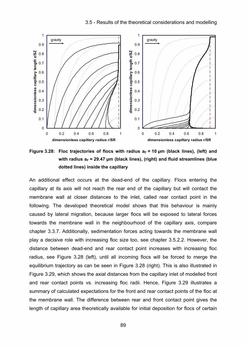
3.5 - Results of the theoretical considerations and modelling
89
0
0.1
0.2
0.3
0.4
0.5
0.6
0.7
0.8
0.9
1
0 0.2 0.4 0.6 0.8 1
dimensionless capillary radius r/SR
dim
ensi
onle
ss c
apill
ary
leng
th z
/SZ
gravity
0
0.1
0.2
0.3
0.4
0.5
0.6
0.7
0.8
0.9
1
0 0.2 0.4 0.6 0.8 1
dimensionless capillary radius r/SR
dim
ensi
onle
ss c
apill
ary
leng
th z
/SZ
gravity
Figure 3.28: Floc trajectories of flocs with radius aF = 10 µm (black lines), (left) and with radius aF = 29.47 µm (black lines), (right) and fluid streamlines (blue dotted lines) inside the capillary
An additional effect occurs at the dead-end of the capillary. Flocs entering the
capillary at its axis will not reach the rear end of the capillary but will contact the
membrane wall at closer distances to the inlet, called rear contact point in the
following. The developed theoretical model shows that this behaviour is mainly
caused by lateral migration, because larger flocs will be exposed to lateral forces
towards the membrane wall in the neighbourhood of the capillary axis, compare
chapter 3.3.7. Additionally, sedimentation forces acting towards the membrane wall
play a decisive role with increasing floc size too, see chapter 3.5.2.2. However, the
distance between dead-end and rear contact point increases with increasing floc
radius, see Figure 3.28 (left), until all incoming flocs will be forced to merge the
equilibrium trajectory as can be seen in Figure 3.28 (right). This is also illustrated in
Figure 3.29, which shows the axial distances from the capillary inlet of modelled front
and rear contact points vs. increasing floc radii. Hence, Figure 3.29 illustrates a
summary of calculated expectations for the front and rear contact points of the floc at
the membrane wall. The difference between rear and front contact point gives the
length of capillary area theoretically available for initial deposition for flocs of certain
3 - Theoretical considerations and modelling
90
size. But, the loss in membrane area available for deposition is mainly governed by
the front contact points. Immediately after exceeding the limiting floc radius of
aF = 3.27 µm the available length for deposition will decrease and the front contact
points will be shifted towards the capillary end.
0
0,1
0,2
0,3
0,4
0,5
0,6
0,7
0,8
0,9
1
0 5 10 15 20 25 30 35 40
floc radius aF in [µm]
dim
ensi
onle
ss a
xial
dis
tanc
e fro
m c
apill
ary
inle
t
front contact pointrear contact point
Selected process parameter(see appendix, chapter A.10 and A.11):
Operation mode: dead-endJ = 80 L/m²/hRM = 5.24·10111/mlC = 1 mrC = 4·10-4 mρF = 1050 kg/m³εF = 0.26Exceeding of limiting floc radius
Merging of front and rear contact point
Figure 3.29: Front and rear contact points at dimensionless axial distance to capillary inlet vs. floc radius aF in [µm]
If the flocs are larger than 10.55 µm in radius, all flocs will be merged together and
only one equilibrium trajectory will come into contact with the membrane wall, of
course under the given flow conditions and properties. This means that all flocs
entering the capillary, independent of their radial starting position at capillary inlet, will
be deposited theoretically at one single point at the membrane wall. This expected
point will be shifted towards the dead-end with increasing floc size.
Considering not only a section plane in 2D but the 3D geometry of the capillary, the
calculated expectations will form a ring at this certain point or area. If gravity acts
perpendicular to the length coordinate, i. e. a horizontal aligned capillary,
sedimentation effects will deform this ring to a ring section as discussed later in
chapter 3.5.2.2
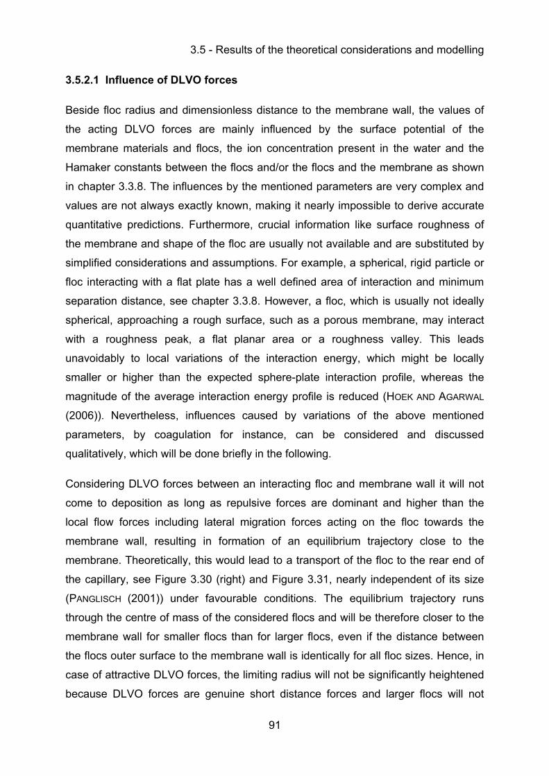
3.5 - Results of the theoretical considerations and modelling
91
3.5.2.1 Influence of DLVO forces
Beside floc radius and dimensionless distance to the membrane wall, the values of
the acting DLVO forces are mainly influenced by the surface potential of the
membrane materials and flocs, the ion concentration present in the water and the
Hamaker constants between the flocs and/or the flocs and the membrane as shown
in chapter 3.3.8. The influences by the mentioned parameters are very complex and
values are not always exactly known, making it nearly impossible to derive accurate
quantitative predictions. Furthermore, crucial information like surface roughness of
the membrane and shape of the floc are usually not available and are substituted by
simplified considerations and assumptions. For example, a spherical, rigid particle or
floc interacting with a flat plate has a well defined area of interaction and minimum
separation distance, see chapter 3.3.8. However, a floc, which is usually not ideally
spherical, approaching a rough surface, such as a porous membrane, may interact
with a roughness peak, a flat planar area or a roughness valley. This leads
unavoidably to local variations of the interaction energy, which might be locally
smaller or higher than the expected sphere-plate interaction profile, whereas the
magnitude of the average interaction energy profile is reduced (HOEK AND AGARWAL
(2006)). Nevertheless, influences caused by variations of the above mentioned
parameters, by coagulation for instance, can be considered and discussed
qualitatively, which will be done briefly in the following.
Considering DLVO forces between an interacting floc and membrane wall it will not
come to deposition as long as repulsive forces are dominant and higher than the
local flow forces including lateral migration forces acting on the floc towards the
membrane wall, resulting in formation of an equilibrium trajectory close to the
membrane. Theoretically, this would lead to a transport of the floc to the rear end of
the capillary, see Figure 3.30 (right) and Figure 3.31, nearly independent of its size
(PANGLISCH (2001)) under favourable conditions. The equilibrium trajectory runs
through the centre of mass of the considered flocs and will be therefore closer to the
membrane wall for smaller flocs than for larger flocs, even if the distance between
the flocs outer surface to the membrane wall is identically for all floc sizes. Hence, in
case of attractive DLVO forces, the limiting radius will not be significantly heightened
because DLVO forces are genuine short distance forces and larger flocs will not
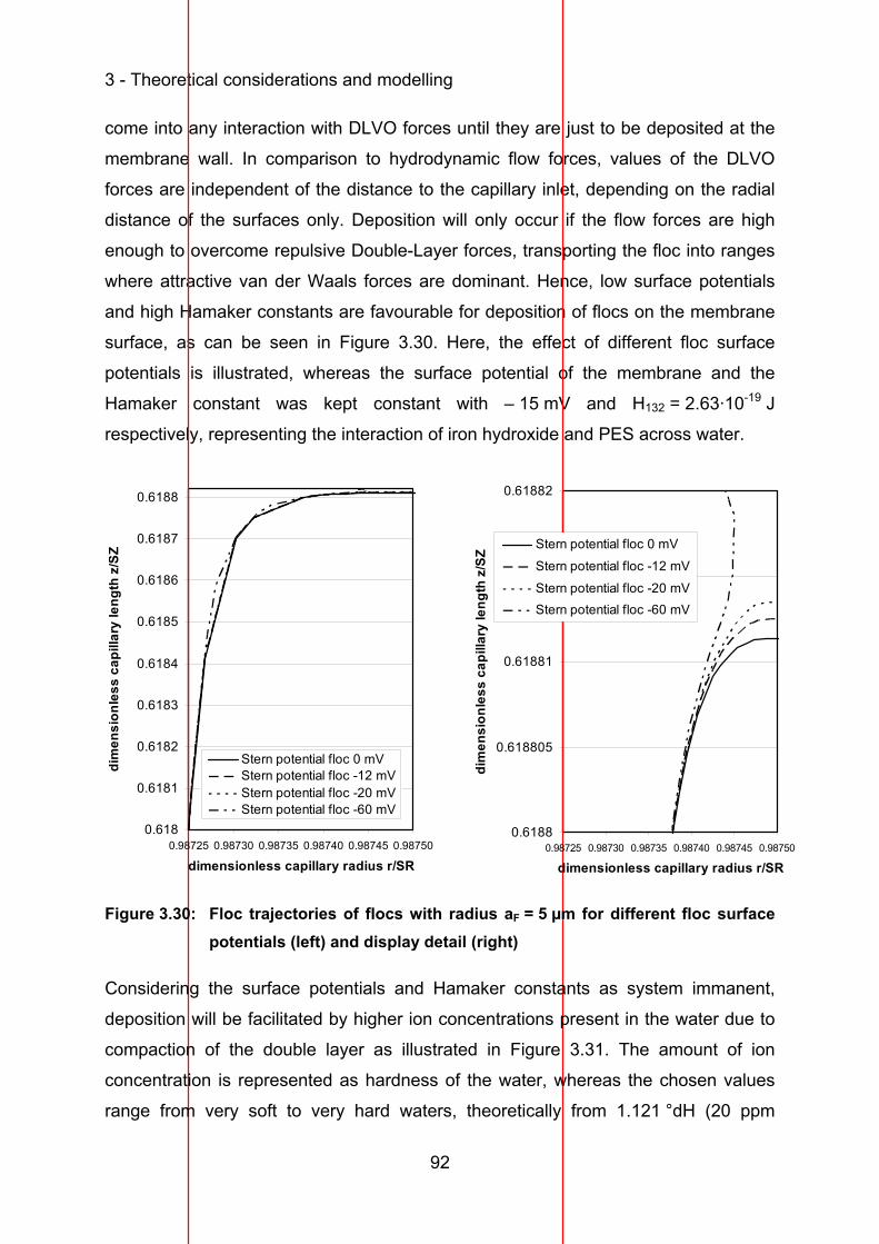
3 - Theoretical considerations and modelling
92
come into any interaction with DLVO forces until they are just to be deposited at the
membrane wall. In comparison to hydrodynamic flow forces, values of the DLVO
forces are independent of the distance to the capillary inlet, depending on the radial
distance of the surfaces only. Deposition will only occur if the flow forces are high
enough to overcome repulsive Double-Layer forces, transporting the floc into ranges
where attractive van der Waals forces are dominant. Hence, low surface potentials
and high Hamaker constants are favourable for deposition of flocs on the membrane
surface, as can be seen in Figure 3.30. Here, the effect of different floc surface
potentials is illustrated, whereas the surface potential of the membrane and the
Hamaker constant was kept constant with – 15 mV and H132 = 2.63·10-19 J
respectively, representing the interaction of iron hydroxide and PES across water.
0.618
0.6181
0.6182
0.6183
0.6184
0.6185
0.6186
0.6187
0.6188
0.98725 0.98730 0.98735 0.98740 0.98745 0.98750
dimensionless capillary radius r/SR
dim
ensi
onle
ss c
apill
ary
leng
th z
/SZ
Stern potential floc 0 mVStern potential floc -12 mVStern potential floc -20 mVStern potential floc -60 mV
0.6188
0.618805
0.61881
0.618815
0.61882
0.98725 0.98730 0.98735 0.98740 0.98745 0.98750
dimensionless capillary radius r/SR
dim
ensi
onle
ss c
apill
ary
leng
th z
/SZ Stern potential floc 0 mV
Stern potential floc -12 mV
Stern potential floc -20 mVStern potential floc -60 mV
Figure 3.30: Floc trajectories of flocs with radius aF = 5 µm for different floc surface potentials (left) and display detail (right)
Considering the surface potentials and Hamaker constants as system immanent,
deposition will be facilitated by higher ion concentrations present in the water due to
compaction of the double layer as illustrated in Figure 3.31. The amount of ion
concentration is represented as hardness of the water, whereas the chosen values
range from very soft to very hard waters, theoretically from 1.121 °dH (20 ppm
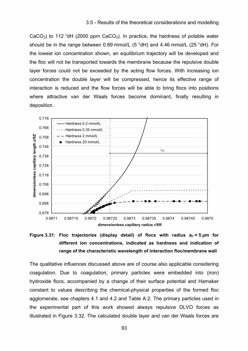
3.5 - Results of the theoretical considerations and modelling
93
CaCO3) to 112 °dH (2000 ppm CaCO3). In practice, the hardness of potable water
should be in the range between 0.89 mmol/L (5 °dH) and 4.46 mmol/L (25 °dH). For
the lowest ion concentration shown, an equilibrium trajectory will be developed and
the floc will not be transported towards the membrane because the repulsive double
layer forces could not be exceeded by the acting flow forces. With increasing ion
concentration the double layer will be compressed, hence its effective range of
interaction is reduced and the flow forces will be able to bring flocs into positions
where attractive van der Waals forces become dominant, finally resulting in
deposition.
0.678
0.688
0.698
0.708
0.718
0.728
0.738
0.748
0.758
0.768
0.778
0.9871 0.98715 0.9872 0.98725 0.9873 0.98735 0.9874 0.98745 0.9875
dimensionless capillary radius r/SR
dim
ensi
onle
ss c
apill
ary
leng
th z
/SZ
Hardness 0.2 mmol/L
Hardness 0.35 mmol/L
Hardness 2 mmol/LHardness 20 mmol/L
λC
Figure 3.31: Floc trajectories (display detail) of flocs with radius aF = 5 µm for different ion concentrations, indicated as hardness and indication of range of the characteristic wavelength of interaction floc/membrane wall
The qualitative influences discussed above are of course also applicable considering
coagulation. Due to coagulation, primary particles were embedded into (iron)
hydroxide flocs, accompanied by a change of their surface potential and Hamaker
constant to values describing the chemical-physical properties of the formed floc
agglomerate, see chapters 4.1 and 4.2 and Table A.2. The primary particles used in
the experimental part of this work showed always repulsive DLVO forces as
illustrated in Figure 3.32. The calculated double layer and van der Waals forces are
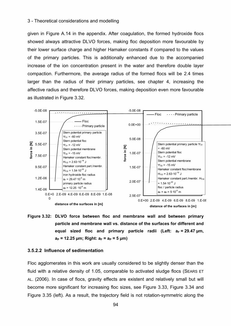
3 - Theoretical considerations and modelling
94
given in Figure A.14 in the appendix. After coagulation, the formed hydroxide flocs
showed always attractive DLVO forces, making floc deposition more favourable by
their lower surface charge and higher Hamaker constants if compared to the values
of the primary particles. This is additionally enhanced due to the accompanied
increase of the ion concentration present in the water and therefore double layer
compaction. Furthermore, the average radius of the formed flocs will be 2.4 times
larger than the radius of their primary particles, see chapter 4, increasing the
affective radius and therefore DLVO forces, making deposition even more favourable
as illustrated in Figure 3.32.
-5.0E-08
1.5E-07
3.5E-07
5.5E-07
7.5E-07
9.5E-07
1.2E-06
1.4E-060.E+0
02.E-09 4.E-09 6.E-09 8.E-09 1.E-08
distance of the surfaces in [m]
forc
e in
[N]
FlocPrimary particle
Stern potential primary particle ΨS1 = -60 mVStern potential flocΨS1 = -12 mVStern potential membraneΨS2 = -15 mVHamaker constant floc/membr. H132 = 2.63·10-19 JHamaker constant part./membr. H132 = 1.54·10-20 Jiron hydroxide floc radiusaF = 29.47·10-6 mprimary particle radiusaP = 12.25 ·10-6 m
-5.0E-08
0.0E+00
5.0E-08
1.0E-07
1.5E-07
2.0E-07
2.5E-070.E+00 2.E-09 4.E-09 6.E-09 8.E-09 1.E-08
distance of the surfaces in [m]
forc
e in
[N]
Floc Primary particle
Stern potential primary particle ΨS1
= -60 mVStern potential flocΨS1 = -12 mVStern potential membraneΨS2 = -15 mVHamaker constant floc/membrane H132 = 2.63·10-19 JHamaker constant part./membr. H132
= 1.54·10-20 Jfloc / particle radiusaF = aP = 5·10-6 m
Figure 3.32: DLVO force between floc and membrane wall and between primary particle and membrane wall vs. distance of the surfaces for different and equal sized floc and primary particle radii (Left: aF = 29.47 µm, aP = 12.25 µm; Right: aF = aP = 5 µm)
3.5.2.2 Influence of sedimentation
Floc agglomerates in this work are usually considered to be slightly denser than the
fluid with a relative density of 1.05, comparable to activated sludge flocs (SEARS ET
AL. (2006). In case of flocs, gravity effects are existent and relatively small but will
become more significant for increasing floc sizes, see Figure 3.33, Figure 3.34 and
Figure 3.35 (left). As a result, the trajectory field is not rotation-symmetric along the
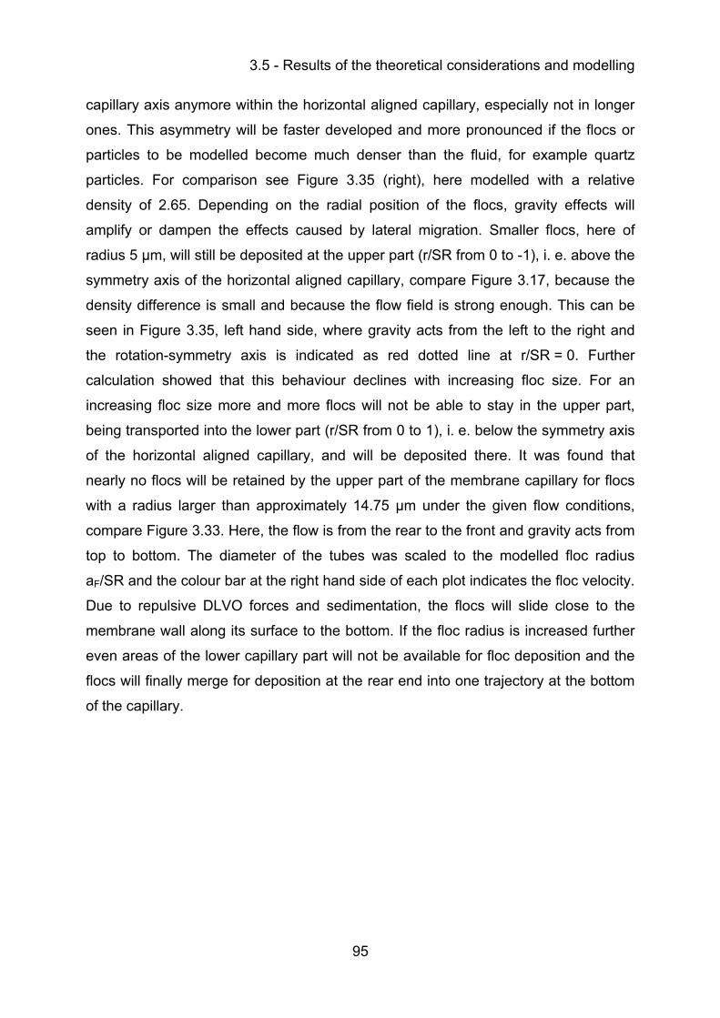
3.5 - Results of the theoretical considerations and modelling
95
capillary axis anymore within the horizontal aligned capillary, especially not in longer
ones. This asymmetry will be faster developed and more pronounced if the flocs or
particles to be modelled become much denser than the fluid, for example quartz
particles. For comparison see Figure 3.35 (right), here modelled with a relative
density of 2.65. Depending on the radial position of the flocs, gravity effects will
amplify or dampen the effects caused by lateral migration. Smaller flocs, here of
radius 5 µm, will still be deposited at the upper part (r/SR from 0 to -1), i. e. above the
symmetry axis of the horizontal aligned capillary, compare Figure 3.17, because the
density difference is small and because the flow field is strong enough. This can be
seen in Figure 3.35, left hand side, where gravity acts from the left to the right and
the rotation-symmetry axis is indicated as red dotted line at r/SR = 0. Further
calculation showed that this behaviour declines with increasing floc size. For an
increasing floc size more and more flocs will not be able to stay in the upper part,
being transported into the lower part (r/SR from 0 to 1), i. e. below the symmetry axis
of the horizontal aligned capillary, and will be deposited there. It was found that
nearly no flocs will be retained by the upper part of the membrane capillary for flocs
with a radius larger than approximately 14.75 µm under the given flow conditions,
compare Figure 3.33. Here, the flow is from the rear to the front and gravity acts from
top to bottom. The diameter of the tubes was scaled to the modelled floc radius
aF/SR and the colour bar at the right hand side of each plot indicates the floc velocity.
Due to repulsive DLVO forces and sedimentation, the flocs will slide close to the
membrane wall along its surface to the bottom. If the floc radius is increased further
even areas of the lower capillary part will not be available for floc deposition and the
flocs will finally merge for deposition at the rear end into one trajectory at the bottom
of the capillary.
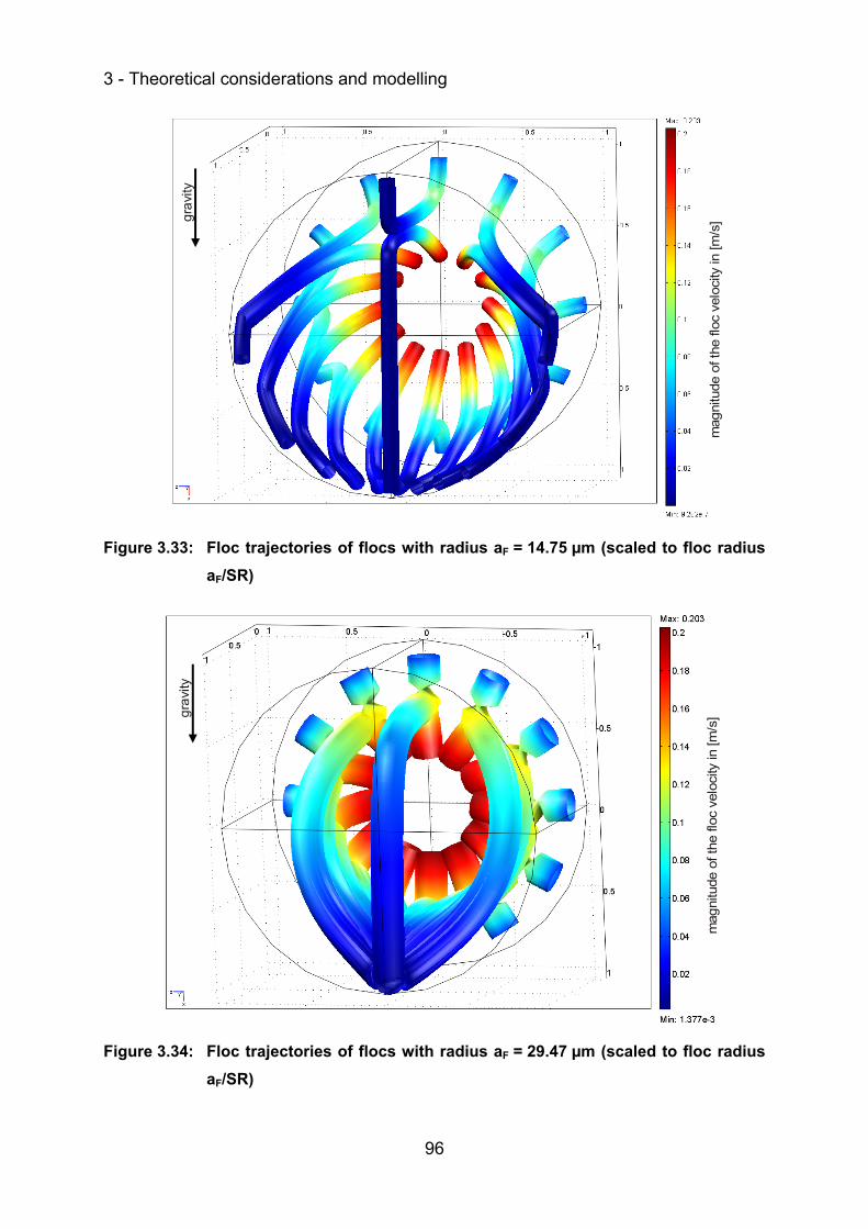
3 - Theoretical considerations and modelling
96
Figure 3.33: Floc trajectories of flocs with radius aF = 14.75 µm (scaled to floc radius aF/SR)
Figure 3.34: Floc trajectories of flocs with radius aF = 29.47 µm (scaled to floc radius aF/SR)
mag
nitu
de o
f the
floc
vel
ocity
in [m
/s]gr
avity
mag
nitu
de o
f the
floc
vel
ocity
in [m
/s]gr
avity
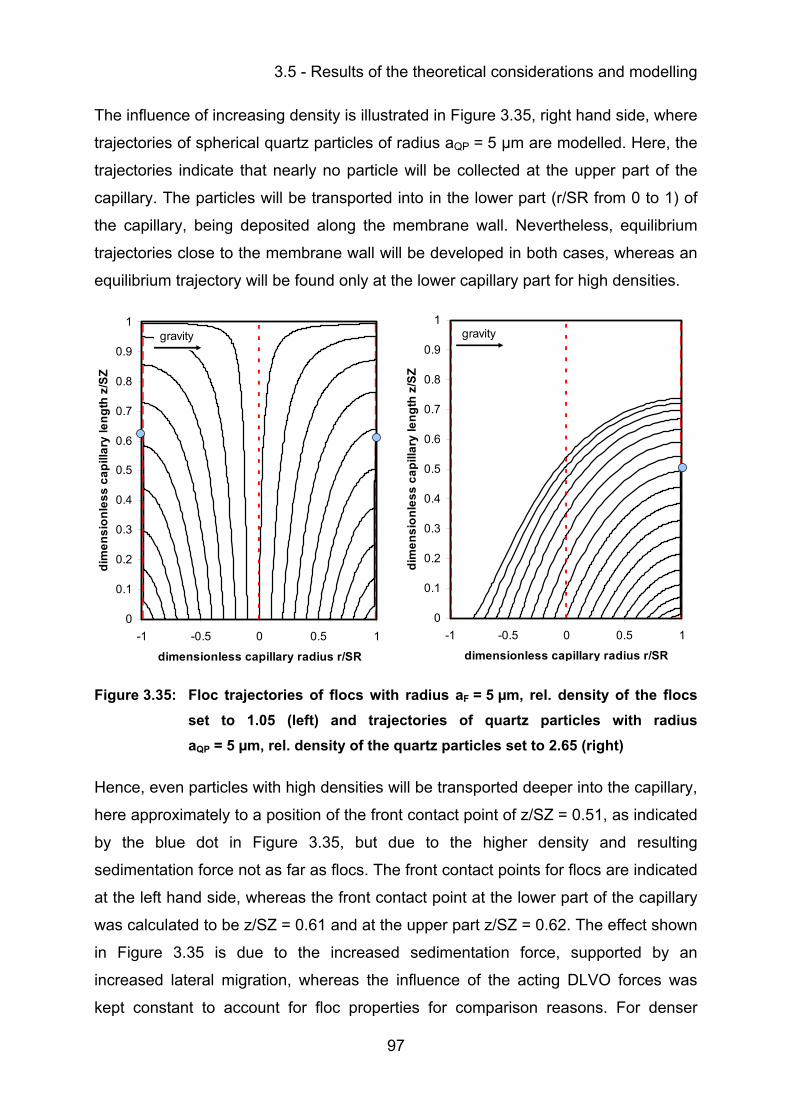
3.5 - Results of the theoretical considerations and modelling
97
The influence of increasing density is illustrated in Figure 3.35, right hand side, where
trajectories of spherical quartz particles of radius aQP = 5 µm are modelled. Here, the
trajectories indicate that nearly no particle will be collected at the upper part of the
capillary. The particles will be transported into in the lower part (r/SR from 0 to 1) of
the capillary, being deposited along the membrane wall. Nevertheless, equilibrium
trajectories close to the membrane wall will be developed in both cases, whereas an
equilibrium trajectory will be found only at the lower capillary part for high densities.
0
0.1
0.2
0.3
0.4
0.5
0.6
0.7
0.8
0.9
1
-1 -0.5 0 0.5 1
dimensionless capillary radius r/SR
dim
ensi
onle
ss c
apill
ary
leng
th z
/SZ
gravity
0
0.1
0.2
0.3
0.4
0.5
0.6
0.7
0.8
0.9
1
-1 -0.5 0 0.5 1
dimensionless capillary radius r/SR
dim
ensi
onle
ss c
apill
ary
leng
th z
/SZ
gravity
Figure 3.35: Floc trajectories of flocs with radius aF = 5 µm, rel. density of the flocs set to 1.05 (left) and trajectories of quartz particles with radius aQP = 5 µm, rel. density of the quartz particles set to 2.65 (right)
Hence, even particles with high densities will be transported deeper into the capillary,
here approximately to a position of the front contact point of z/SZ = 0.51, as indicated
by the blue dot in Figure 3.35, but due to the higher density and resulting
sedimentation force not as far as flocs. The front contact points for flocs are indicated
at the left hand side, whereas the front contact point at the lower part of the capillary
was calculated to be z/SZ = 0.61 and at the upper part z/SZ = 0.62. The effect shown
in Figure 3.35 is due to the increased sedimentation force, supported by an
increased lateral migration, whereas the influence of the acting DLVO forces was
kept constant to account for floc properties for comparison reasons. For denser
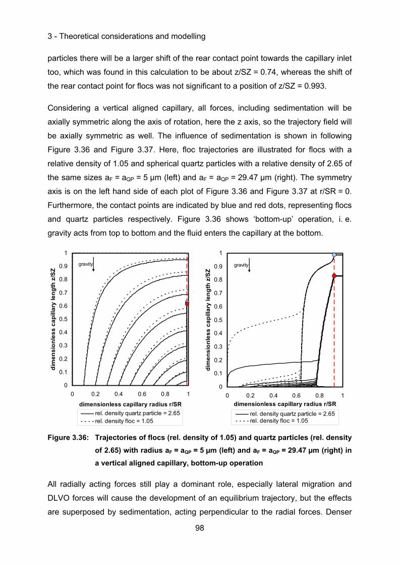
3 - Theoretical considerations and modelling
98
particles there will be a larger shift of the rear contact point towards the capillary inlet
too, which was found in this calculation to be about z/SZ = 0.74, whereas the shift of
the rear contact point for flocs was not significant to a position of z/SZ = 0.993.
Considering a vertical aligned capillary, all forces, including sedimentation will be
axially symmetric along the axis of rotation, here the z axis, so the trajectory field will
be axially symmetric as well. The influence of sedimentation is shown in following
Figure 3.36 and Figure 3.37. Here, floc trajectories are illustrated for flocs with a
relative density of 1.05 and spherical quartz particles with a relative density of 2.65 of
the same sizes aF = aQP = 5 µm (left) and aF = aQP = 29.47 µm (right). The symmetry
axis is on the left hand side of each plot of Figure 3.36 and Figure 3.37 at r/SR = 0.
Furthermore, the contact points are indicated by blue and red dots, representing flocs
and quartz particles respectively. Figure 3.36 shows ‘bottom-up’ operation, i. e.
gravity acts from top to bottom and the fluid enters the capillary at the bottom.
0
0.1
0.2
0.3
0.4
0.5
0.6
0.7
0.8
0.9
1
0 0.2 0.4 0.6 0.8 1
dimensionless capillary radius r/SR
dim
ensi
onle
ss c
apill
ary
leng
th z
/SZ
rel. density quartz particle = 2.65rel. density floc = 1.05
gravity
0
0.1
0.2
0.3
0.4
0.5
0.6
0.7
0.8
0.9
1
0 0.2 0.4 0.6 0.8 1dimensionless capillary radius r/SR
dim
ensi
onle
ss c
apill
ary
leng
th z
/SZ
rel. density quartz particle = 2.65rel. density floc = 1.05
gravity
Figure 3.36: Trajectories of flocs (rel. density of 1.05) and quartz particles (rel. density of 2.65) with radius aF = aQP = 5 µm (left) and aF = aQP = 29.47 µm (right) in a vertical aligned capillary, bottom-up operation
All radially acting forces still play a dominant role, especially lateral migration and
DLVO forces will cause the development of an equilibrium trajectory, but the effects
are superposed by sedimentation, acting perpendicular to the radial forces. Denser
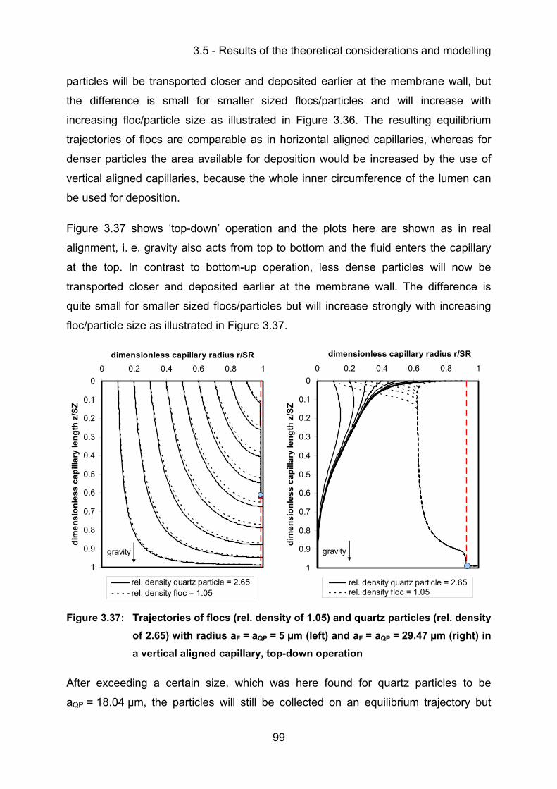
3.5 - Results of the theoretical considerations and modelling
99
particles will be transported closer and deposited earlier at the membrane wall, but
the difference is small for smaller sized flocs/particles and will increase with
increasing floc/particle size as illustrated in Figure 3.36. The resulting equilibrium
trajectories of flocs are comparable as in horizontal aligned capillaries, whereas for
denser particles the area available for deposition would be increased by the use of
vertical aligned capillaries, because the whole inner circumference of the lumen can
be used for deposition.
Figure 3.37 shows ‘top-down’ operation and the plots here are shown as in real
alignment, i. e. gravity also acts from top to bottom and the fluid enters the capillary
at the top. In contrast to bottom-up operation, less dense particles will now be
transported closer and deposited earlier at the membrane wall. The difference is
quite small for smaller sized flocs/particles but will increase strongly with increasing
floc/particle size as illustrated in Figure 3.37.
0
0.1
0.2
0.3
0.4
0.5
0.6
0.7
0.8
0.9
1
0 0.2 0.4 0.6 0.8 1dimensionless capillary radius r/SR
dim
ensi
onle
ss c
apill
ary
leng
th z
/SZ
rel. density quartz particle = 2.65rel. density floc = 1.05
gravity
0
0.1
0.2
0.3
0.4
0.5
0.6
0.7
0.8
0.9
1
0 0.2 0.4 0.6 0.8 1
dimensionless capillary radius r/SR
dim
ensi
onle
ss c
apill
ary
leng
th z
/SZ
rel. density quartz particle = 2.65rel. density floc = 1.05
gravity
Figure 3.37: Trajectories of flocs (rel. density of 1.05) and quartz particles (rel. density of 2.65) with radius aF = aQP = 5 µm (left) and aF = aQP = 29.47 µm (right) in a vertical aligned capillary, top-down operation
After exceeding a certain size, which was here found for quartz particles to be
aQP = 18.04 µm, the particles will still be collected on an equilibrium trajectory but
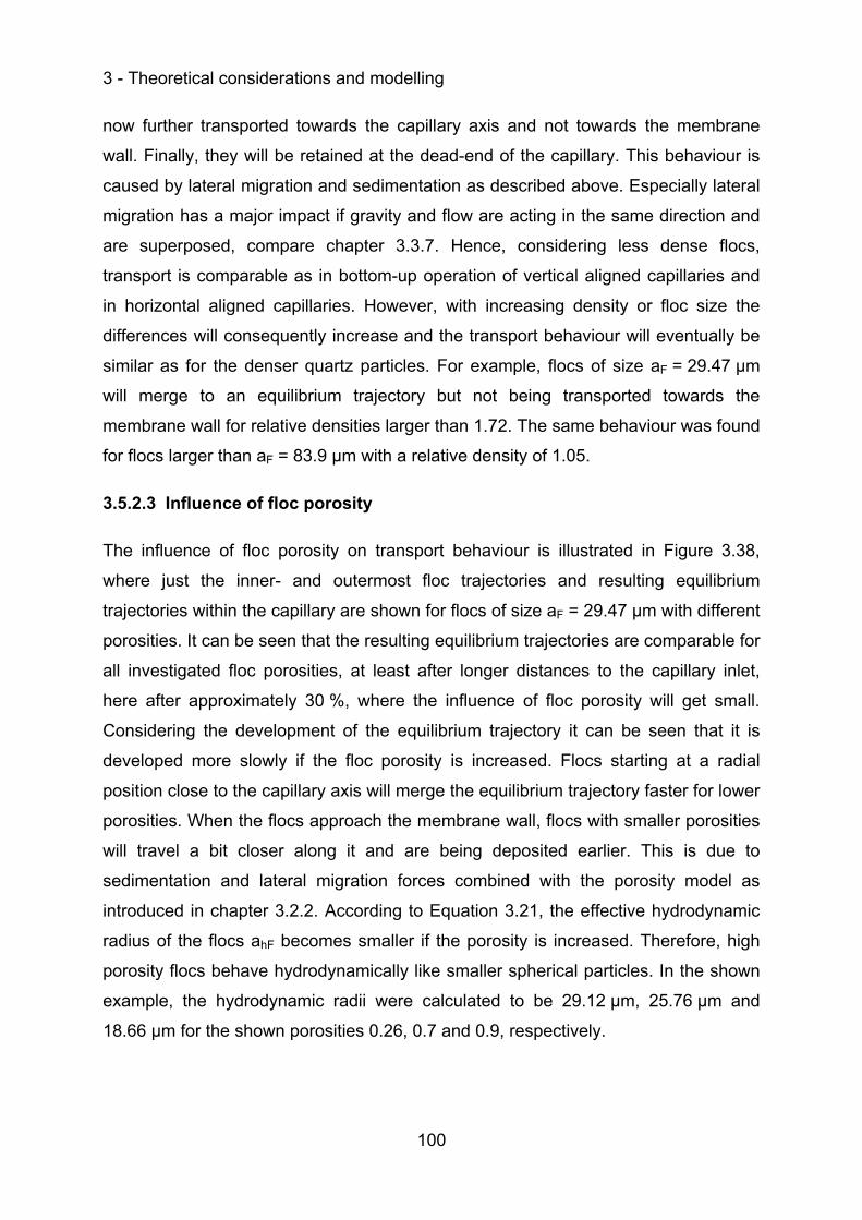
3 - Theoretical considerations and modelling
100
now further transported towards the capillary axis and not towards the membrane
wall. Finally, they will be retained at the dead-end of the capillary. This behaviour is
caused by lateral migration and sedimentation as described above. Especially lateral
migration has a major impact if gravity and flow are acting in the same direction and
are superposed, compare chapter 3.3.7. Hence, considering less dense flocs,
transport is comparable as in bottom-up operation of vertical aligned capillaries and
in horizontal aligned capillaries. However, with increasing density or floc size the
differences will consequently increase and the transport behaviour will eventually be
similar as for the denser quartz particles. For example, flocs of size aF = 29.47 µm
will merge to an equilibrium trajectory but not being transported towards the
membrane wall for relative densities larger than 1.72. The same behaviour was found
for flocs larger than aF = 83.9 µm with a relative density of 1.05.
3.5.2.3 Influence of floc porosity
The influence of floc porosity on transport behaviour is illustrated in Figure 3.38,
where just the inner- and outermost floc trajectories and resulting equilibrium
trajectories within the capillary are shown for flocs of size aF = 29.47 µm with different
porosities. It can be seen that the resulting equilibrium trajectories are comparable for
all investigated floc porosities, at least after longer distances to the capillary inlet,
here after approximately 30 %, where the influence of floc porosity will get small.
Considering the development of the equilibrium trajectory it can be seen that it is
developed more slowly if the floc porosity is increased. Flocs starting at a radial
position close to the capillary axis will merge the equilibrium trajectory faster for lower
porosities. When the flocs approach the membrane wall, flocs with smaller porosities
will travel a bit closer along it and are being deposited earlier. This is due to
sedimentation and lateral migration forces combined with the porosity model as
introduced in chapter 3.2.2. According to Equation 3.21, the effective hydrodynamic
radius of the flocs ahF becomes smaller if the porosity is increased. Therefore, high
porosity flocs behave hydrodynamically like smaller spherical particles. In the shown
example, the hydrodynamic radii were calculated to be 29.12 µm, 25.76 µm and
18.66 µm for the shown porosities 0.26, 0.7 and 0.9, respectively.
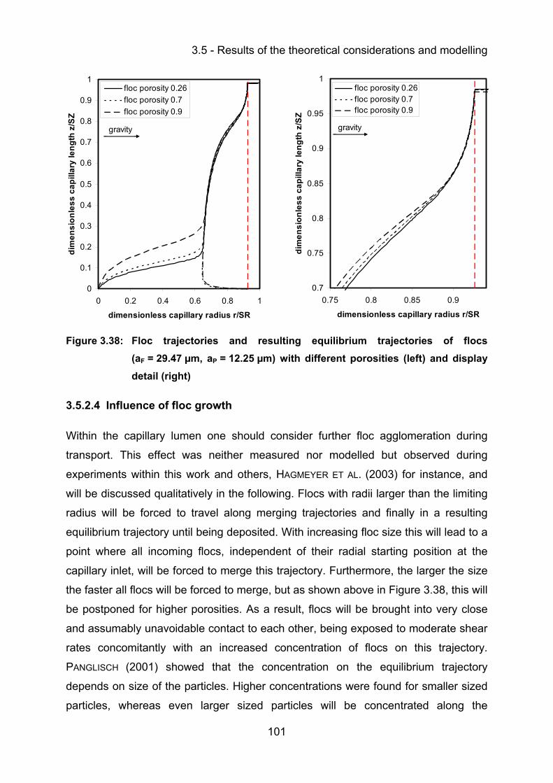
3.5 - Results of the theoretical considerations and modelling
101
0
0.1
0.2
0.3
0.4
0.5
0.6
0.7
0.8
0.9
1
0 0.2 0.4 0.6 0.8 1
dimensionless capillary radius r/SR
dim
ensi
onle
ss c
apill
ary
leng
th z
/SZ
floc porosity 0.26floc porosity 0.7floc porosity 0.9
gravity
0.7
0.75
0.8
0.85
0.9
0.95
1
0.75 0.8 0.85 0.9
dimensionless capillary radius r/SR
dim
ensi
onle
ss c
apill
ary
leng
th z
/SZ
floc porosity 0.26floc porosity 0.7floc porosity 0.9
gravity
Figure 3.38: Floc trajectories and resulting equilibrium trajectories of flocs (aF = 29.47 µm, aP = 12.25 µm) with different porosities (left) and display detail (right)
3.5.2.4 Influence of floc growth
Within the capillary lumen one should consider further floc agglomeration during
transport. This effect was neither measured nor modelled but observed during
experiments within this work and others, HAGMEYER ET AL. (2003) for instance, and
will be discussed qualitatively in the following. Flocs with radii larger than the limiting
radius will be forced to travel along merging trajectories and finally in a resulting
equilibrium trajectory until being deposited. With increasing floc size this will lead to a
point where all incoming flocs, independent of their radial starting position at the
capillary inlet, will be forced to merge this trajectory. Furthermore, the larger the size
the faster all flocs will be forced to merge, but as shown above in Figure 3.38, this will
be postponed for higher porosities. As a result, flocs will be brought into very close
and assumably unavoidable contact to each other, being exposed to moderate shear
rates concomitantly with an increased concentration of flocs on this trajectory.
PANGLISCH (2001) showed that the concentration on the equilibrium trajectory
depends on size of the particles. Higher concentrations were found for smaller sized
particles, whereas even larger sized particles will be concentrated along the
3 - Theoretical considerations and modelling
102
trajectory up to the maximum packing density with increasing bulk concentration. If
contact occurs and larger floc aggregates are formed, they will be immediately
exposed to the same hydrodynamic conditions as before when they have been
individual and smaller, resulting in stronger forces acting on the new and larger
aggregate. This will lead to an additional lateral shift, whereas the direction depends
on the new size and local position in the capillary. Eventually, the floc aggregates will
be moved towards the final position of the equilibrium trajectory at approximately
r/SR = 0.62, resulting in transport downwards towards the dead-end of the capillary
and in an increased floc concentration in the equilibrium trajectory at this limiting
radial position. Furthermore, considering a polydisperse size distribution of flocs
accompanied with their different trajectories during transport, an increase in collisions
rate, i. e. the number of collisions of flocs, can be furthermore assumed due to
crossing and/or constriction of trajectory bundles as shown in Figure 3.39.
0
0.1
0.2
0.3
0.4
0.5
0.6
0.7
0.8
0.9
1
0 0.1 0.2 0.3 0.4 0.5 0.6 0.7 0.8 0.9 1
dimensionless capillary radius r/SR
dim
ensi
onle
ss c
apill
ary
leng
th z
/SZ
aF = 60 µm aF = 29.47 µm aF = 12.25 µm aF = 5 µm
gravity
aFaF aF aF
Figure 3.39: Floc trajectories of different sized flocs within the capillary
According to the conventional coagulation theory and considerations above this
should lead to floc aggregation by some kind of orthokinetic aggregation (IVES (1978),
ELIMELECH ET AL. (1995)). The calculated shear rates are illustrated in Figure 3.40 and
were found to be highest with G = 1100 s-1 at the capillary inlet, directly at the
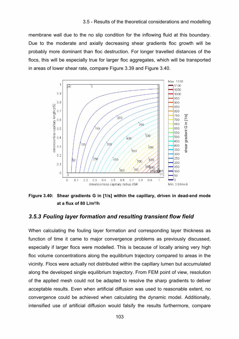
3.5 - Results of the theoretical considerations and modelling
103
membrane wall due to the no slip condition for the inflowing fluid at this boundary.
Due to the moderate and axially decreasing shear gradients floc growth will be
probably more dominant than floc destruction. For longer travelled distances of the
flocs, this will be especially true for larger floc aggregates, which will be transported
in areas of lower shear rate, compare Figure 3.39 and Figure 3.40.
Figure 3.40: Shear gradients G in [1/s] within the capillary, driven in dead-end mode at a flux of 80 L/m²/h
3.5.3 Fouling layer formation and resulting transient flow field
When calculating the fouling layer formation and corresponding layer thickness as
function of time it came to major convergence problems as previously discussed,
especially if larger flocs were modelled. This is because of locally arising very high
floc volume concentrations along the equilibrium trajectory compared to areas in the
vicinity. Flocs were actually not distributed within the capillary lumen but accumulated
along the developed single equilibrium trajectory. From FEM point of view, resolution
of the applied mesh could not be adapted to resolve the sharp gradients to deliver
acceptable results. Even when artificial diffusion was used to reasonable extent, no
convergence could be achieved when calculating the dynamic model. Additionally,
intensified use of artificial diffusion would falsify the results furthermore, compare
shea
r gra
dien
t G in
[1/s
]
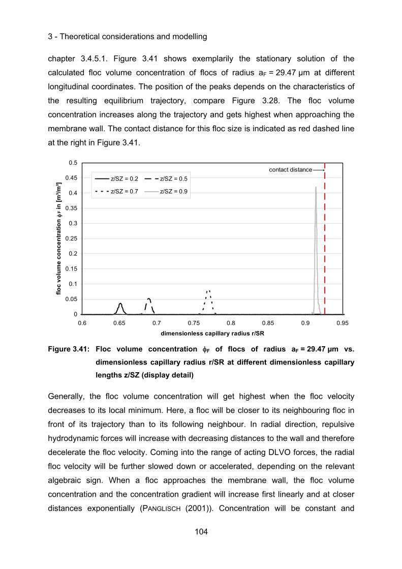
3 - Theoretical considerations and modelling
104
chapter 3.4.5.1. Figure 3.41 shows exemplarily the stationary solution of the
calculated floc volume concentration of flocs of radius aF = 29.47 µm at different
longitudinal coordinates. The position of the peaks depends on the characteristics of
the resulting equilibrium trajectory, compare Figure 3.28. The floc volume
concentration increases along the trajectory and gets highest when approaching the
membrane wall. The contact distance for this floc size is indicated as red dashed line
at the right in Figure 3.41.
0
0.05
0.1
0.15
0.2
0.25
0.3
0.35
0.4
0.45
0.5
0.6 0.65 0.7 0.75 0.8 0.85 0.9 0.95
dimensionless capillary radius r/SR
floc
volu
me
conc
entra
tion
φF i
n [m
³/m³]
z/SZ = 0.2 z/SZ = 0.5
z/SZ = 0.7 z/SZ = 0.9
contact distance
Figure 3.41: Floc volume concentration φF of flocs of radius aF = 29.47 µm vs.
dimensionless capillary radius r/SR at different dimensionless capillary lengths z/SZ (display detail)
Generally, the floc volume concentration will get highest when the floc velocity
decreases to its local minimum. Here, a floc will be closer to its neighbouring floc in
front of its trajectory than to its following neighbour. In radial direction, repulsive
hydrodynamic forces will increase with decreasing distances to the wall and therefore
decelerate the floc velocity. Coming into the range of acting DLVO forces, the radial
floc velocity will be further slowed down or accelerated, depending on the relevant
algebraic sign. When a floc approaches the membrane wall, the floc volume
concentration and the concentration gradient will increase first linearly and at closer
distances exponentially (PANGLISCH (2001)). Concentration will be constant and
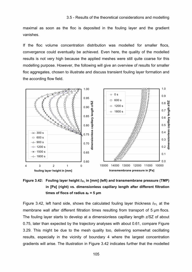
3.5 - Results of the theoretical considerations and modelling
105
maximal as soon as the floc is deposited in the fouling layer and the gradient
vanishes.
If the floc volume concentration distribution was modelled for smaller flocs,
convergence could eventually be achieved. Even here, the quality of the modelled
results is not very high because the applied meshes were still quite coarse for this
modelling purpose. However, the following will give an overview of results for smaller
floc aggregates, chosen to illustrate and discuss transient fouling layer formation and
the according flow field.
0.60
0.65
0.70
0.75
0.80
0.85
0.90
0.95
1.00
01234
fouling layer height in [mm]
dim
ensi
onle
ss c
apill
ary
leng
th z
/SZ
300 s600 s900 s1200 s
1500 s1800 s
0.0
0.1
0.2
0.3
0.4
0.5
0.6
0.7
0.8
0.9
1.0
100001100012000130001400015000
transmembrane pressure in [Pa]di
men
sion
less
cap
illar
y le
ngth
z/S
Z
0 s
600 s
1200 s
1800 s
Figure 3.42: Fouling layer height δFL in [mm] (left) and transmembrane pressure (TMP)
in [Pa] (right) vs. dimensionless capillary length after different filtration times of flocs of radius aF = 5 µm
Figure 3.42, left hand side, shows the calculated fouling layer thickness δFL at the
membrane wall after different filtration times resulting from transport of 5 µm flocs.
The fouling layer starts to develop at a dimensionless capillary length z/SZ of about
0.75, later than expected by the trajectory analyses with about 0.61, compare Figure
3.29. This might be due to the mesh quality too, delivering somewhat oscillating
results, especially in the vicinity of boundary 4 where the largest concentration
gradients will arise. The illustration in Figure 3.42 indicates further that the modelled
3 - Theoretical considerations and modelling
106
maximum height after 30 minutes of filtration was modelled to be δFL = 3.32 mm,
which is 8.3 times higher than the physical radius of the capillary. According to the
shown results, the formed fouling layer would have led to a fast formation of a porous
plug at a dimensionless capillary length z/SZ of about 0.9 after approximately 300
seconds of operation. With ongoing filtration, additional flocs would be transported
towards this plug and finally being captured in it, letting the plug grow and probably
compressing it. Over time, the porosity would therefore decrease and the resistance
to flow would increase. Finally, this would end after potentially long filtration times in
a complete clogging of the membrane at this part of the capillary, making the
membrane area further downstream towards the dead-end unavailable for further floc
deposition (LERCH ET AL. (2005B)). In reality, this clogging may occur close to the
dead-end as expected due to the size of the flocs to be filtered, but may also happen
somewhere else further upstream within the capillary. Both were often experienced in
laboratory experiments. If the plugs were located at the beginning or middle of the
capillary it came to a sudden release of the blocked membrane area in most cases
and it was assumed that the formed plug was pushed towards the dead-end due to
the increasing pressure (GITIS ET AL. (2005)). However, the model was neither
equipped to account for compaction of the flocs nor of the fouling layer and further
not bounded by some geometrical values like the capillary radius. The uncompressed
height of the layer, as can be seen in Figure 3.42, was utilised as an easy to use first
estimation for probably occurring layer compaction, assuming that the uncompressed
layer will offer a comparable resistance to flow than a compressed layer with a
maximum height equal to the capillary radius.
The right hand side of Figure 3.42 shows the corresponding TMP along the
membrane wall, presenting a maximum pressure increase of 0.59 kPa after 30
minutes of operation. Surprisingly, the results obtained for the TMP are indicating an
increase over the complete length of the capillary. However, larger differences
between the initial TMP and the TMP after some filtration time were found to start at
approximately two thirds of the dimensionless capillary length, corresponding to the
outcomes of the trajectory analyses. Hence, the results were used for qualitatively
interpretations.
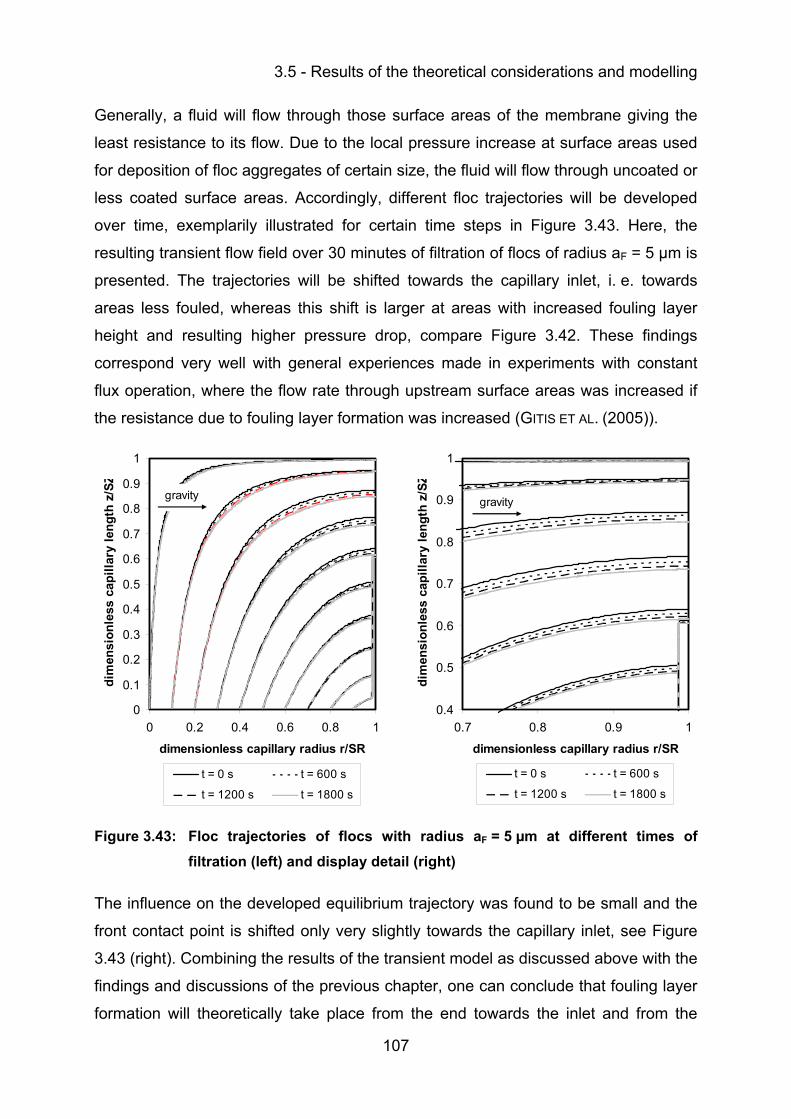
3.5 - Results of the theoretical considerations and modelling
107
Generally, a fluid will flow through those surface areas of the membrane giving the
least resistance to its flow. Due to the local pressure increase at surface areas used
for deposition of floc aggregates of certain size, the fluid will flow through uncoated or
less coated surface areas. Accordingly, different floc trajectories will be developed
over time, exemplarily illustrated for certain time steps in Figure 3.43. Here, the
resulting transient flow field over 30 minutes of filtration of flocs of radius aF = 5 µm is
presented. The trajectories will be shifted towards the capillary inlet, i. e. towards
areas less fouled, whereas this shift is larger at areas with increased fouling layer
height and resulting higher pressure drop, compare Figure 3.42. These findings
correspond very well with general experiences made in experiments with constant
flux operation, where the flow rate through upstream surface areas was increased if
the resistance due to fouling layer formation was increased (GITIS ET AL. (2005)).
0
0.1
0.2
0.3
0.4
0.5
0.6
0.7
0.8
0.9
1
0 0.2 0.4 0.6 0.8 1
dimensionless capillary radius r/SR
dim
ensi
onle
ss c
apill
ary
leng
th z
/SZ
t = 0 s t = 600 s
t = 1200 s t = 1800 s
gravity
0.4
0.5
0.6
0.7
0.8
0.9
1
0.7 0.8 0.9 1
dimensionless capillary radius r/SR
dim
ensi
onle
ss c
apill
ary
leng
th z
/SZ
t = 0 s t = 600 s
t = 1200 s t = 1800 s
gravity
Figure 3.43: Floc trajectories of flocs with radius aF = 5 µm at different times of filtration (left) and display detail (right)
The influence on the developed equilibrium trajectory was found to be small and the
front contact point is shifted only very slightly towards the capillary inlet, see Figure
3.43 (right). Combining the results of the transient model as discussed above with the
findings and discussions of the previous chapter, one can conclude that fouling layer
formation will theoretically take place from the end towards the inlet and from the
3 - Theoretical considerations and modelling
108
bottom to the top of the capillary in a horizontal aligned capillary. However, this will
not lead to immediate clogging of the capillary due to the inner porosity of the formed
fouling layers until this inner porosity is lost due to further added flocs or
compression.
Considering the formation of the fouling layer and its porosity one has to consider the
floc properties such like inner porosity, size and surface charge too, because they will
have an decisive influence on the resulting fouling layer, not only on the place of
deposition but also on its formation and porosity. As described in chapter 3.4.6,
applying the Happel model with Equation A.17 and Equation A.18, the permeability
coefficient kFL of the formed fouling layer will be generally higher for larger flocs of
identical porosity, resulting in lower specific resistance of the formed fouling layer.
This specific resistance will be further reduced for increasing inner floc porosities,
leading to more constant fluid flow field and therefore floc transport conditions over
filtration time.
However, the porosity of the formed fouling layer will be further influenced by near-
field forces between two flocs of equal size approaching each other to form the layer.
Among other forces, the resulting final distance in this layer will be determined by
their interacting DLVO forces too. This effect is much more significant for very small
flocs, such as micro flocs, because all other hydrodynamic forces acting on the flocs
will be of the same magnitude due to the comparatively same position. If repulsive
forces are dominant, then there exists a limiting distance where no additional
approach will be possible, resulting in a porous fouling layer. If the repulsive forces
are overcome and maybe become attractive, then the flocs might be brought into
closer contact and form a denser fouling layer, whereas the final porosity is mainly
influenced by the inner floc porosity. Overcoming repulsive forces is more likely if
larger floc aggregates are involved, because the difference in their local position
might be significant and therefore the difference in hydrodynamically acting forces
might be very large, especially in the neighbourhood of the membrane wall. If the
acting hydrodynamically forces are higher than the maximum repulsive forces
between the flocs within the layer, i. e. for higher flux operation for example, the
distance between the deposited flocs will be minimised and therefore the layers
porosity too. If the repulsive forces cannot be overcome by hydrodynamic flow forces,
3.5 - Results of the theoretical considerations and modelling
109
then the final limiting distance between two flocs will be independent of their size.
The resulting free volume, hence porosity, in the layer is then relatively smaller for
large flocs than for smaller flocs (PANGLISCH (2001)). For instance, PANGLISCH (2001)
stated that the porosity of a fouling layer formed by 0.1 µm sized particles, with a final
distance between the particles surfaces of about 10 nm, will be about 0.36, while the
porosity of a layer formed by 35 µm sized particles and same distance between them
will be about 0.26. However, due to relatively high flow forces repulsive forces are
usually overcome, especially due to the lowered double layer forces after coagulation
and formation of floc aggregates.
If the flow forces are large, compression of the formed fouling layer will be possible
and probable. LEE ET AL. (2003) confirmed with their investigations on dead-end MF
that there is an interaction between floc size and structure and that layers formed of
smaller flocs are more sensitive to floc structure effects than layers of larger flocs.
The compressibility of the formed layer was found to be strongly related to the
applied TMP, particularly for smaller floc sizes. The deposition of porous aggregates
onto the membrane resulted in the formation and maintenance of porous fouling
layers, provided a low TMP (< 10 kPa) was applied. At higher TMP (> 60 kPa) rapid
compression of the layer occurred, indicated by the significantly lower porosity.
Under high TMP conditions, the layer porosity exhibits strong size dependence with
larger floc sizes yielding higher porosities. This result may indicate formation of
relatively impermeable layers with flow around the compressed flocs at higher TMP,
rather than through them at low TMP.
Further, large floc aggregates are usually looser, more open in structure than smaller
flocs, whereas looser flocs are likely to form layers with higher porosities and
therefore lower resistances than layers made of compact flocs of similar size (LEE ET
AL. (2003)). From a practical perspective with respect to highly porous fouling layers,
one can summarise that large, porous flocs, low Hamaker constants, high surface
potentials, low ionic concentrations and filtration at low TMP will be favourable.
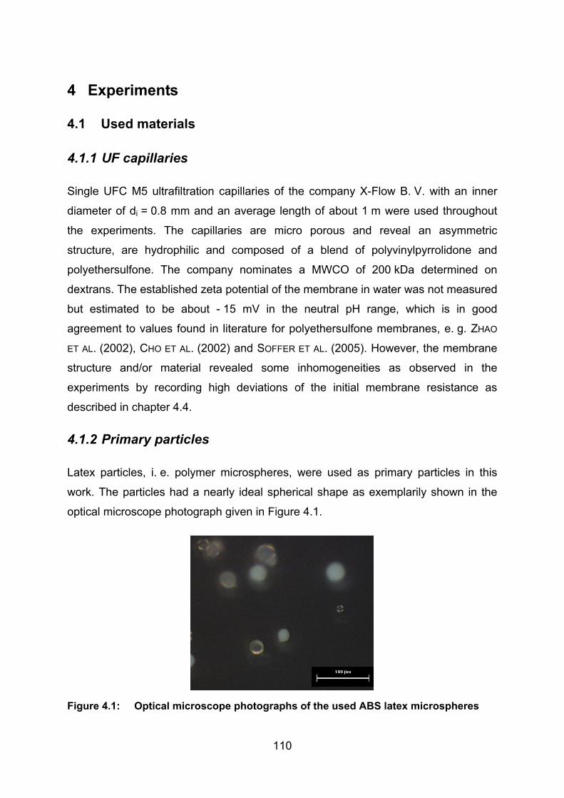
110
4 Experiments
4.1 Used materials
4.1.1 UF capillaries
Single UFC M5 ultrafiltration capillaries of the company X-Flow B. V. with an inner
diameter of di = 0.8 mm and an average length of about 1 m were used throughout
the experiments. The capillaries are micro porous and reveal an asymmetric
structure, are hydrophilic and composed of a blend of polyvinylpyrrolidone and
polyethersulfone. The company nominates a MWCO of 200 kDa determined on
dextrans. The established zeta potential of the membrane in water was not measured
but estimated to be about - 15 mV in the neutral pH range, which is in good
agreement to values found in literature for polyethersulfone membranes, e. g. ZHAO
ET AL. (2002), CHO ET AL. (2002) and SOFFER ET AL. (2005). However, the membrane
structure and/or material revealed some inhomogeneities as observed in the
experiments by recording high deviations of the initial membrane resistance as
described in chapter 4.4.
4.1.2 Primary particles
Latex particles, i. e. polymer microspheres, were used as primary particles in this
work. The particles had a nearly ideal spherical shape as exemplarily shown in the
optical microscope photograph given in Figure 4.1.
Figure 4.1: Optical microscope photographs of the used ABS latex microspheres
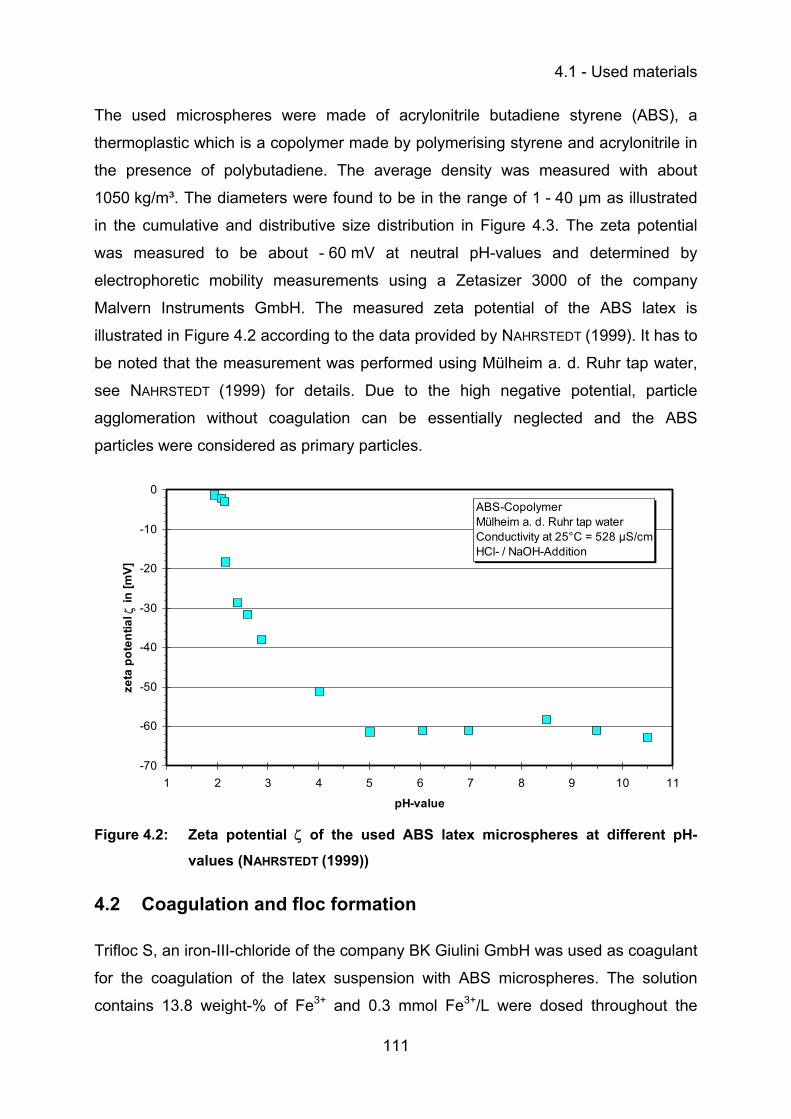
4.1 - Used materials
111
The used microspheres were made of acrylonitrile butadiene styrene (ABS), a
thermoplastic which is a copolymer made by polymerising styrene and acrylonitrile in
the presence of polybutadiene. The average density was measured with about
1050 kg/m³. The diameters were found to be in the range of 1 - 40 µm as illustrated
in the cumulative and distributive size distribution in Figure 4.3. The zeta potential
was measured to be about - 60 mV at neutral pH-values and determined by
electrophoretic mobility measurements using a Zetasizer 3000 of the company
Malvern Instruments GmbH. The measured zeta potential of the ABS latex is
illustrated in Figure 4.2 according to the data provided by NAHRSTEDT (1999). It has to
be noted that the measurement was performed using Mülheim a. d. Ruhr tap water,
see NAHRSTEDT (1999) for details. Due to the high negative potential, particle
agglomeration without coagulation can be essentially neglected and the ABS
particles were considered as primary particles.
-70
-60
-50
-40
-30
-20
-10
0
1 2 3 4 5 6 7 8 9 10 11
pH-value
zeta
pot
entia
l ζ in
[mV]
ABS-CopolymerMülheim a. d. Ruhr tap waterConductivity at 25°C = 528 µS/cmHCl- / NaOH-Addition
Figure 4.2: Zeta potential ζ of the used ABS latex microspheres at different pH-
values (NAHRSTEDT (1999))
4.2 Coagulation and floc formation
Trifloc S, an iron-III-chloride of the company BK Giulini GmbH was used as coagulant
for the coagulation of the latex suspension with ABS microspheres. The solution
contains 13.8 weight-% of Fe3+ and 0.3 mmol Fe3+/L were dosed throughout the
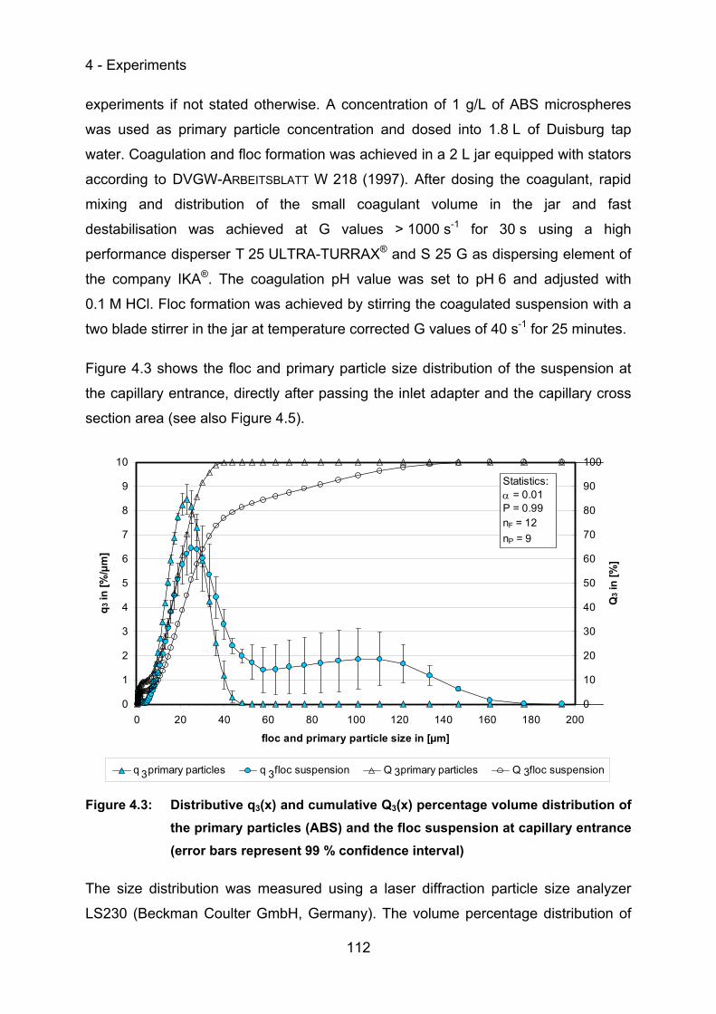
4 - Experiments
112
experiments if not stated otherwise. A concentration of 1 g/L of ABS microspheres
was used as primary particle concentration and dosed into 1.8 L of Duisburg tap
water. Coagulation and floc formation was achieved in a 2 L jar equipped with stators
according to DVGW-ARBEITSBLATT W 218 (1997). After dosing the coagulant, rapid
mixing and distribution of the small coagulant volume in the jar and fast
destabilisation was achieved at G values > 1000 s-1 for 30 s using a high
performance disperser T 25 ULTRA-TURRAX® and S 25 G as dispersing element of
the company IKA®. The coagulation pH value was set to pH 6 and adjusted with
0.1 M HCl. Floc formation was achieved by stirring the coagulated suspension with a
two blade stirrer in the jar at temperature corrected G values of 40 s-1 for 25 minutes.
Figure 4.3 shows the floc and primary particle size distribution of the suspension at
the capillary entrance, directly after passing the inlet adapter and the capillary cross
section area (see also Figure 4.5).
0
1
2
3
4
5
6
7
8
9
10
0 20 40 60 80 100 120 140 160 180 200
floc and primary particle size in [µm]
q3 in
[%/µ
m]
0
10
20
30
40
50
60
70
80
90
100
Q3 i
n [%
]
q primary particles q floc suspension Q primary particles Q floc suspension3 33 3
Statistics:α = 0.01P = 0.99nF = 12nP = 9
Figure 4.3: Distributive q3(x) and cumulative Q3(x) percentage volume distribution of the primary particles (ABS) and the floc suspension at capillary entrance (error bars represent 99 % confidence interval)
The size distribution was measured using a laser diffraction particle size analyzer
LS230 (Beckman Coulter GmbH, Germany). The volume percentage distribution of
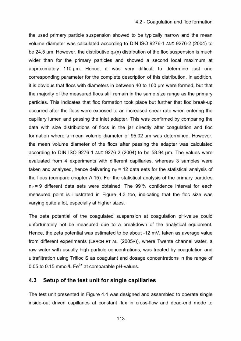
4.2 - Coagulation and floc formation
113
the used primary particle suspension showed to be typically narrow and the mean
volume diameter was calculated according to DIN ISO 9276-1 AND 9276-2 (2004) to
be 24.5 µm. However, the distributive q3(x) distribution of the floc suspension is much
wider than for the primary particles and showed a second local maximum at
approximately 110 µm. Hence, it was very difficult to determine just one
corresponding parameter for the complete description of this distribution. In addition,
it is obvious that flocs with diameters in between 40 to 160 µm were formed, but that
the majority of the measured flocs still remain in the same size range as the primary
particles. This indicates that floc formation took place but further that floc break-up
occurred after the flocs were exposed to an increased shear rate when entering the
capillary lumen and passing the inlet adapter. This was confirmed by comparing the
data with size distributions of flocs in the jar directly after coagulation and floc
formation where a mean volume diameter of 95.02 µm was determined. However,
the mean volume diameter of the flocs after passing the adapter was calculated
according to DIN ISO 9276-1 AND 9276-2 (2004) to be 58.94 µm. The values were
evaluated from 4 experiments with different capillaries, whereas 3 samples were
taken and analysed, hence delivering nF = 12 data sets for the statistical analysis of
the flocs (compare chapter A.15). For the statistical analysis of the primary particles
nP = 9 different data sets were obtained. The 99 % confidence interval for each
measured point is illustrated in Figure 4.3 too, indicating that the floc size was
varying quite a lot, especially at higher sizes.
The zeta potential of the coagulated suspension at coagulation pH-value could
unfortunately not be measured due to a breakdown of the analytical equipment.
Hence, the zeta potential was estimated to be about -12 mV, taken as average value
from different experiments (LERCH ET AL. (2005A)), where Twente channel water, a
raw water with usually high particle concentrations, was treated by coagulation and
ultrafiltration using Trifloc S as coagulant and dosage concentrations in the range of
0.05 to 0.15 mmol/L Fe3+ at comparable pH-values.
4.3 Setup of the test unit for single capillaries
The test unit presented in Figure 4.4 was designed and assembled to operate single
inside-out driven capillaries at constant flux in cross-flow and dead-end mode to
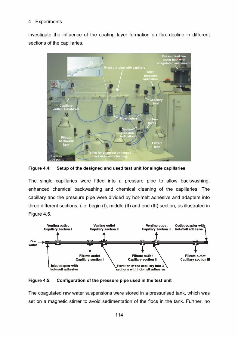
4 - Experiments
114
investigate the influence of the coating layer formation on flux decline in different
sections of the capillaries.
Figure 4.4: Setup of the designed and used test unit for single capillaries
The single capillaries were fitted into a pressure pipe to allow backwashing,
enhanced chemical backwashing and chemical cleaning of the capillaries. The
capillary and the pressure pipe were divided by hot-melt adhesive and adapters into
three different sections, i. e. begin (I), middle (II) and end (III) section, as illustrated in
Figure 4.5.
Figure 4.5: Configuration of the pressure pipe used in the test unit
The coagulated raw water suspensions were stored in a pressurised tank, which was
set on a magnetic stirrer to avoid sedimentation of the flocs in the tank. Further, no
4.3 - Setup of the test unit for single capillaries
115
significant variation in floc size over storage time was observed. The tank was
additionally equipped with a heating system and a resistance thermometer PT 100
TR 101 (WIKA Alexander Wiegand GmbH & Co. KG, Germany) to measure, control
and adjust the temperature of the used suspension. A micro annular gear pump mzr-
4622 (HNP Mikrosysteme GmbH, Germany) was employed as suction pump in the
system and forced the floc suspension or filtrate, respectively, to flow through the
capillary and the membrane wall into the filtrate tank. The total filtrate flow, hence the
overall flux through the capillaries, was kept constant but the flux at the different
sections was allowed to decline. That is, if fouling layer formation occurred and let to
a flux decline at the end of the capillary, then the flux in the upstream sections
increased automatically. The flow rate through each section of the capillary was
measured by LIQUI-FLOW flow meters (Bronkhorst Mättig GmbH, Germany). The
constant overall flow rate was controlled automatically by a closed control loop
between the pump revolution speed as actuating variable and the flow meters signal
as the controlled process variable. The pressure was measured at the capillary inlet
and at the suction side of the pump with standard pressure transducers S10 (WIKA
Alexander Wiegand GmbH & Co. KG, Germany). When the capillaries were driven in
cross-flow mode, the pressure was additionally measured at the capillary outlet.
Conventional and chemical enhanced backwashing as well as chemical cleaning of
the capillaries could be achieved by employing a 4 channel flexible tube pump
REGLO 100 (ISMATEC Laboratoriumstechnik GmbH, Germany), connected to
filtrate, acid and base tanks. The piping of the test unit was equipped with 2-way
electromagnetic valves type A12 - 82 080 (IMI Norgren Buschjost GmbH + Co. KG,
Germany). The setup of the test unit allowed fully automatic control and different
operating conditions. Measurement data acquisition, storage, monitoring and control
were achieved by a data acquisition and control unit TopMessage (Delphin
Technology AG, Germany).
4.4 Determination of the initial membrane resistance RM
The initial membrane resistance RM of each capillary used was determined at the
single capillary test unit as described in chapter 4.3. The capillaries were operated in
filtration mode with ultra pure water for about 45 minutes at a flux of 100 L/m²/h to
rinse out chemicals used for protection of virgin capillaries, i. e. glycerine for pore
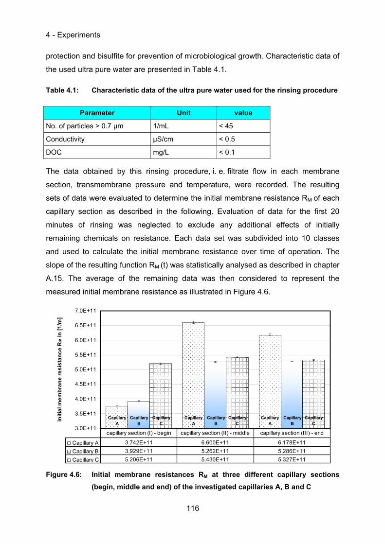
4 - Experiments
116
protection and bisulfite for prevention of microbiological growth. Characteristic data of
the used ultra pure water are presented in Table 4.1.
Table 4.1: Characteristic data of the ultra pure water used for the rinsing procedure
Parameter Unit value
No. of particles > 0.7 µm 1/mL < 45
Conductivity µS/cm < 0.5
DOC mg/L < 0.1
The data obtained by this rinsing procedure, i. e. filtrate flow in each membrane
section, transmembrane pressure and temperature, were recorded. The resulting
sets of data were evaluated to determine the initial membrane resistance RM of each
capillary section as described in the following. Evaluation of data for the first 20
minutes of rinsing was neglected to exclude any additional effects of initially
remaining chemicals on resistance. Each data set was subdivided into 10 classes
and used to calculate the initial membrane resistance over time of operation. The
slope of the resulting function RM (t) was statistically analysed as described in chapter
A.15. The average of the remaining data was then considered to represent the
measured initial membrane resistance as illustrated in Figure 4.6.
3.0E+11
3.5E+11
4.0E+11
4.5E+11
5.0E+11
5.5E+11
6.0E+11
6.5E+11
7.0E+11
initi
al m
embr
ane
resi
stan
ce R
M in
[1/m
]
Capillary A 3.742E+11 6.600E+11 6.178E+11Capillary B 3.929E+11 5.262E+11 5.286E+11Capillary C 5.206E+11 5.430E+11 5.327E+11
capillary section (I) - begin capillary section (II) - middle capillary section (III) - end
CapillaryA
CapillaryA
CapillaryA
CapillaryB
CapillaryB
CapillaryB
CapillaryC
CapillaryC
CapillaryC
Figure 4.6: Initial membrane resistances RM at three different capillary sections (begin, middle and end) of the investigated capillaries A, B and C
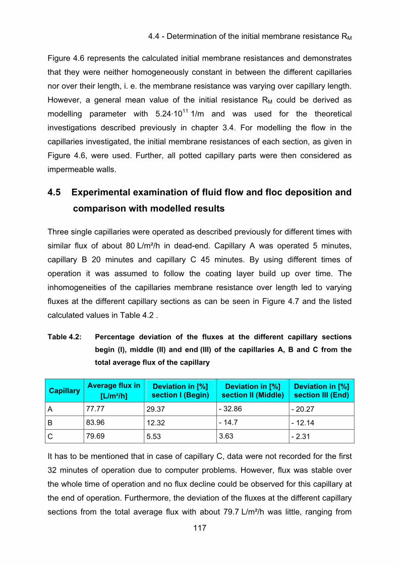
4.4 - Determination of the initial membrane resistance RM
117
Figure 4.6 represents the calculated initial membrane resistances and demonstrates
that they were neither homogeneously constant in between the different capillaries
nor over their length, i. e. the membrane resistance was varying over capillary length.
However, a general mean value of the initial resistance RM could be derived as
modelling parameter with 5.24·1011 1/m and was used for the theoretical
investigations described previously in chapter 3.4. For modelling the flow in the
capillaries investigated, the initial membrane resistances of each section, as given in
Figure 4.6, were used. Further, all potted capillary parts were then considered as
impermeable walls.
4.5 Experimental examination of fluid flow and floc deposition and comparison with modelled results
Three single capillaries were operated as described previously for different times with
similar flux of about 80 L/m²/h in dead-end. Capillary A was operated 5 minutes,
capillary B 20 minutes and capillary C 45 minutes. By using different times of
operation it was assumed to follow the coating layer build up over time. The
inhomogeneities of the capillaries membrane resistance over length led to varying
fluxes at the different capillary sections as can be seen in Figure 4.7 and the listed
calculated values in Table 4.2 .
Table 4.2: Percentage deviation of the fluxes at the different capillary sections begin (I), middle (II) and end (III) of the capillaries A, B and C from the total average flux of the capillary
Capillary Average flux in
[L/m²/h] Deviation in [%] section I (Begin)
Deviation in [%] section II (Middle)
Deviation in [%] section III (End)
A 77.77 29.37 - 32.86 - 20.27
B 83.96 12.32 - 14.7 - 12.14
C 79.69 5.53 3.63 - 2.31
It has to be mentioned that in case of capillary C, data were not recorded for the first
32 minutes of operation due to computer problems. However, flux was stable over
the whole time of operation and no flux decline could be observed for this capillary at
the end of operation. Furthermore, the deviation of the fluxes at the different capillary
sections from the total average flux with about 79.7 L/m²/h was little, ranging from
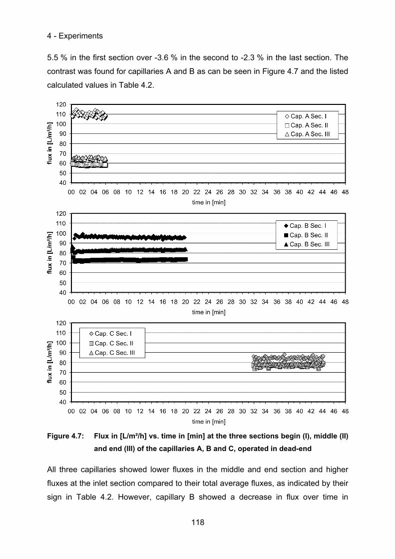
4 - Experiments
118
5.5 % in the first section over -3.6 % in the second to -2.3 % in the last section. The
contrast was found for capillaries A and B as can be seen in Figure 4.7 and the listed
calculated values in Table 4.2.
Figure 4.7: Flux in [L/m²/h] vs. time in [min] at the three sections begin (I), middle (II) and end (III) of the capillaries A, B and C, operated in dead-end
All three capillaries showed lower fluxes in the middle and end section and higher
fluxes at the inlet section compared to their total average fluxes, as indicated by their
sign in Table 4.2. However, capillary B showed a decrease in flux over time in
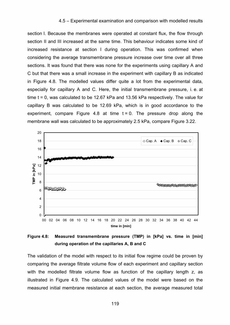
4.5 – Experimental examination and comparison with modelled results
119
section I. Because the membranes were operated at constant flux, the flow through
section II and III increased at the same time. This behaviour indicates some kind of
increased resistance at section I during operation. This was confirmed when
considering the average transmembrane pressure increase over time over all three
sections. It was found that there was none for the experiments using capillary A and
C but that there was a small increase in the experiment with capillary B as indicated
in Figure 4.8. The modelled values differ quite a lot from the experimental data,
especially for capillary A and C. Here, the initial transmembrane pressure, i. e. at
time t = 0, was calculated to be 12.67 kPa and 13.56 kPa respectively. The value for
capillary B was calculated to be 12.69 kPa, which is in good accordance to the
experiment, compare Figure 4.8 at time t = 0. The pressure drop along the
membrane wall was calculated to be approximately 2.5 kPa, compare Figure 3.22.
0
2
4
6
8
10
12
14
16
18
20
00 02 04 06 08 10 12 14 16 18 20 22 24 26 28 30 32 34 36 38 40 42 44
time in [min]
TMP
in [k
Pa]
Cap. A Cap. B Cap. C
Figure 4.8: Measured transmembrane pressure (TMP) in [kPa] vs. time in [min] during operation of the capillaries A, B and C
The validation of the model with respect to its initial flow regime could be proven by
comparing the average filtrate volume flow of each experiment and capillary section
with the modelled filtrate volume flow as function of the capillary length z, as
illustrated in Figure 4.9. The calculated values of the model were based on the
measured initial membrane resistance at each section, the average measured total
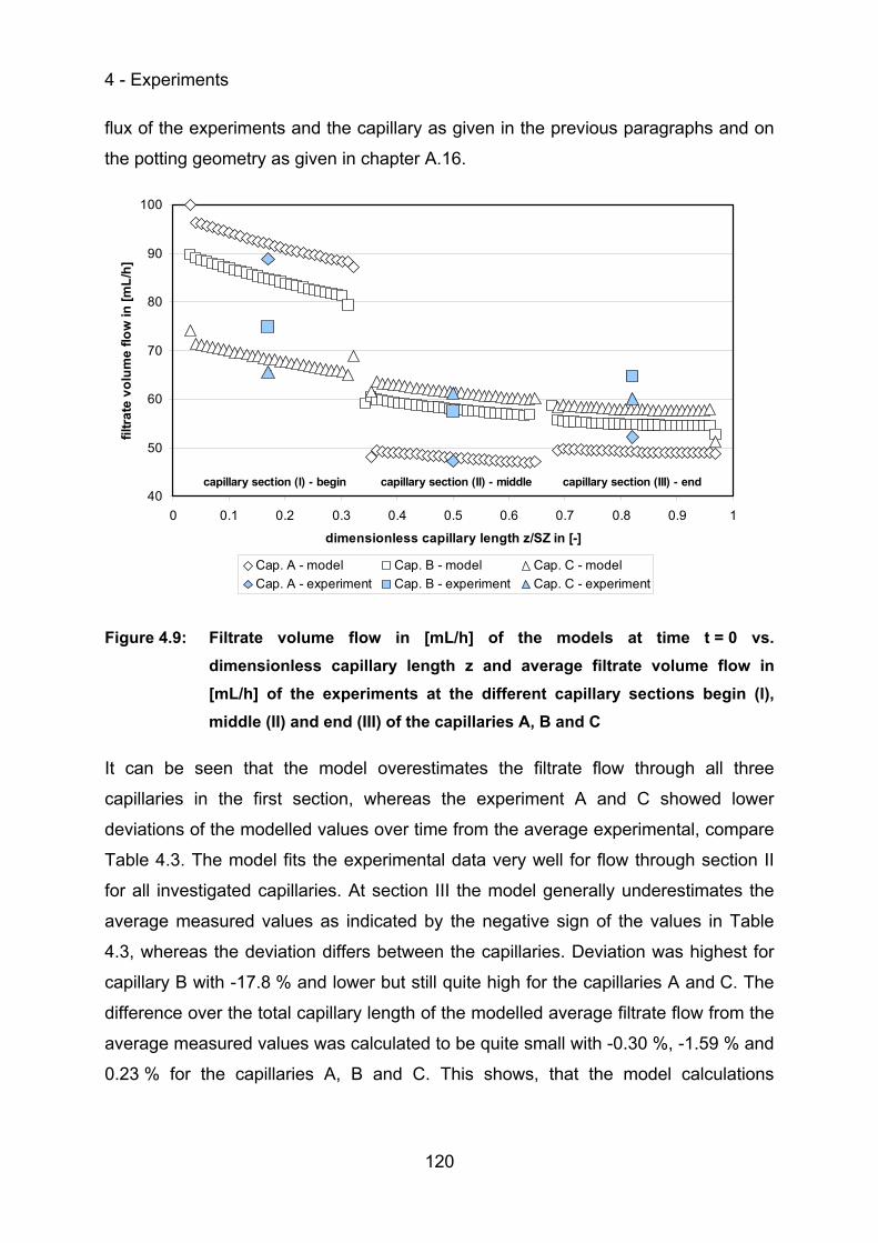
4 - Experiments
120
flux of the experiments and the capillary as given in the previous paragraphs and on
the potting geometry as given in chapter A.16.
40
50
60
70
80
90
100
0 0.1 0.2 0.3 0.4 0.5 0.6 0.7 0.8 0.9 1
dimensionless capillary length z/SZ in [-]
filtra
te v
olum
e flo
w in
[mL/
h]
Cap. A - model Cap. B - model Cap. C - modelCap. A - experiment Cap. B - experiment Cap. C - experiment
capillary section (I) - begin capillary section (II) - middle capillary section (III) - end
Figure 4.9: Filtrate volume flow in [mL/h] of the models at time t = 0 vs. dimensionless capillary length z and average filtrate volume flow in [mL/h] of the experiments at the different capillary sections begin (I), middle (II) and end (III) of the capillaries A, B and C
It can be seen that the model overestimates the filtrate flow through all three
capillaries in the first section, whereas the experiment A and C showed lower
deviations of the modelled values over time from the average experimental, compare
Table 4.3. The model fits the experimental data very well for flow through section II
for all investigated capillaries. At section III the model generally underestimates the
average measured values as indicated by the negative sign of the values in Table
4.3, whereas the deviation differs between the capillaries. Deviation was highest for
capillary B with -17.8 % and lower but still quite high for the capillaries A and C. The
difference over the total capillary length of the modelled average filtrate flow from the
average measured values was calculated to be quite small with -0.30 %, -1.59 % and
0.23 % for the capillaries A, B and C. This shows, that the model calculations
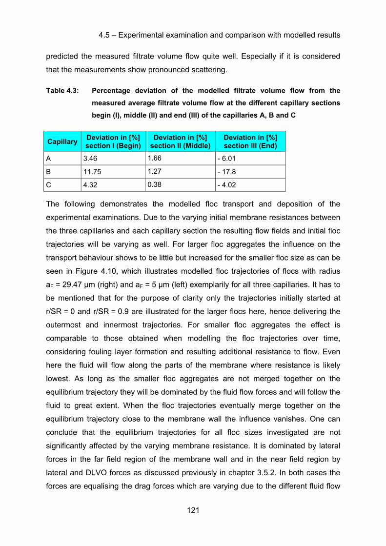
4.5 – Experimental examination and comparison with modelled results
121
predicted the measured filtrate volume flow quite well. Especially if it is considered
that the measurements show pronounced scattering.
Table 4.3: Percentage deviation of the modelled filtrate volume flow from the measured average filtrate volume flow at the different capillary sections begin (I), middle (II) and end (III) of the capillaries A, B and C
Capillary Deviation in [%] section I (Begin)
Deviation in [%] section II (Middle)
Deviation in [%] section III (End)
A 3.46 1.66 - 6.01
B 11.75 1.27 - 17.8
C 4.32 0.38 - 4.02
The following demonstrates the modelled floc transport and deposition of the
experimental examinations. Due to the varying initial membrane resistances between
the three capillaries and each capillary section the resulting flow fields and initial floc
trajectories will be varying as well. For larger floc aggregates the influence on the
transport behaviour shows to be little but increased for the smaller floc size as can be
seen in Figure 4.10, which illustrates modelled floc trajectories of flocs with radius
aF = 29.47 µm (right) and aF = 5 µm (left) exemplarily for all three capillaries. It has to
be mentioned that for the purpose of clarity only the trajectories initially started at
r/SR = 0 and r/SR = 0.9 are illustrated for the larger flocs here, hence delivering the
outermost and innermost trajectories. For smaller floc aggregates the effect is
comparable to those obtained when modelling the floc trajectories over time,
considering fouling layer formation and resulting additional resistance to flow. Even
here the fluid will flow along the parts of the membrane where resistance is likely
lowest. As long as the smaller floc aggregates are not merged together on the
equilibrium trajectory they will be dominated by the fluid flow forces and will follow the
fluid to great extent. When the floc trajectories eventually merge together on the
equilibrium trajectory close to the membrane wall the influence vanishes. One can
conclude that the equilibrium trajectories for all floc sizes investigated are not
significantly affected by the varying membrane resistance. It is dominated by lateral
forces in the far field region of the membrane wall and in the near field region by
lateral and DLVO forces as discussed previously in chapter 3.5.2. In both cases the
forces are equalising the drag forces which are varying due to the different fluid flow
4 - Experiments
122
velocities resulting from the different resistances of the membrane wall against flow,
resulting in a stable position of the trajectory. This can be further seen if the
trajectories were passing the pottings between the different sections in the
experimental setup at dimensionless capillary lengths of about z/SZ = 0.35 and 0.67.
Here, the trajectories are distracted but immediately came back to their stable
equilibrium position. Therefore, the floc contact points in all modelled experiments
were found to be in the range as shown in chapter 3.5.2.
0
0.1
0.2
0.3
0.4
0.5
0.6
0.7
0.8
0.9
1
0 0.2 0.4 0.6 0.8 1
dimensionless capillary radius r/SR
dim
ensi
onle
ss c
apill
ary
leng
th z
/SZ
Cap. A Cap. B Cap. C
0
0.1
0.2
0.3
0.4
0.5
0.6
0.7
0.8
0.9
1
0.5 0.6 0.7 0.8 0.9
dimensionless capillary radius r/SR
dim
ensi
onle
ss c
apill
ary
leng
th z
/SZ
Cap. A Cap. B Cap. C
Figure 4.10: Floc trajectories of flocs with radius aF = 5 µm (left) and aF = 29.47 µm as display detail (right) of the modelled experimental data
After filtration, the capillaries were analysed for iron and primary particles for
validation purposes of the model with respect to the modelled transport and
deposition behaviour of floc aggregates. Therefore, the capillaries were divided into
different pieces according to the sampling point scheme given in Figure 4.11. The
abbreviations used are B, M and E for begin, middle and end of the capillary,
respectively. The subscripts M and P are used for metal and particle analysis and the
numbers indicate the sample taken in each capillary section, hence 1 is closer to the
capillary inlet than 2. The pieces for particle analyses were 10 cm long, whereas the
pieces for iron were 2 cm long. Each piece of sample for particle analysis was stored
gravity
gravity
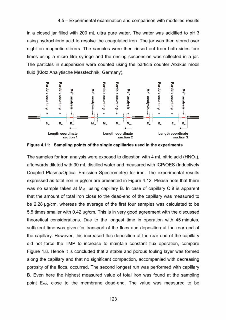
4.5 – Experimental examination and comparison with modelled results
123
in a closed jar filled with 200 mL ultra pure water. The water was acidified to pH 3
using hydrochloric acid to resolve the coagulated iron. The jar was then stored over
night on magnetic stirrers. The samples were then rinsed out from both sides four
times using a micro litre syringe and the rinsing suspension was collected in a jar.
The particles in suspension were counted using the particle counter Abakus mobil
fluid (Klotz Analytische Messtechnik, Germany).
Figure 4.11: Sampling points of the single capillaries used in the experiments
The samples for iron analysis were exposed to digestion with 4 mL nitric acid (HNO3),
afterwards diluted with 30 mL distilled water and measured with ICP/OES (Inductively
Coupled Plasma/Optical Emission Spectrometry) for iron. The experimental results
expressed as total iron in µg/cm are presented in Figure 4.12. Please note that there
was no sample taken at MM1 using capillary B. In case of capillary C it is apparent
that the amount of total iron close to the dead-end of the capillary was measured to
be 2.28 µg/cm, whereas the average of the first four samples was calculated to be
5.5 times smaller with 0.42 µg/cm. This is in very good agreement with the discussed
theoretical considerations. Due to the longest time in operation with 45 minutes,
sufficient time was given for transport of the flocs and deposition at the rear end of
the capillary. However, this increased floc deposition at the rear end of the capillary
did not force the TMP to increase to maintain constant flux operation, compare
Figure 4.8. Hence it is concluded that a stable and porous fouling layer was formed
along the capillary and that no significant compaction, accompanied with decreasing
porosity of the flocs, occurred. The second longest run was performed with capillary
B. Even here the highest measured value of total iron was found at the sampling
point EM2, close to the membrane dead-end. The value was measured to be
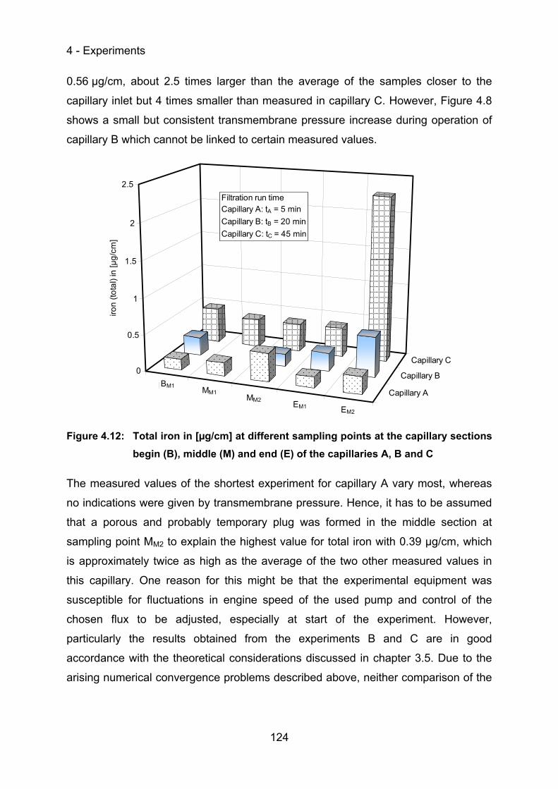
4 - Experiments
124
0.56 µg/cm, about 2.5 times larger than the average of the samples closer to the
capillary inlet but 4 times smaller than measured in capillary C. However, Figure 4.8
shows a small but consistent transmembrane pressure increase during operation of
capillary B which cannot be linked to certain measured values.
BM1MM1
MM2EM1
EM2
Capillary A
Capillary B
Capillary C0
0.5
1
1.5
2
2.5
iron
(tota
l) in
[µg/
cm]
BM1 MM1MM2 EM1 EM2
Filtration run timeCapillary A: tA = 5 minCapillary B: tB = 20 minCapillary C: tC = 45 min
Figure 4.12: Total iron in [µg/cm] at different sampling points at the capillary sections begin (B), middle (M) and end (E) of the capillaries A, B and C
The measured values of the shortest experiment for capillary A vary most, whereas
no indications were given by transmembrane pressure. Hence, it has to be assumed
that a porous and probably temporary plug was formed in the middle section at
sampling point MM2 to explain the highest value for total iron with 0.39 µg/cm, which
is approximately twice as high as the average of the two other measured values in
this capillary. One reason for this might be that the experimental equipment was
susceptible for fluctuations in engine speed of the used pump and control of the
chosen flux to be adjusted, especially at start of the experiment. However,
particularly the results obtained from the experiments B and C are in good
accordance with the theoretical considerations discussed in chapter 3.5. Due to the
arising numerical convergence problems described above, neither comparison of the
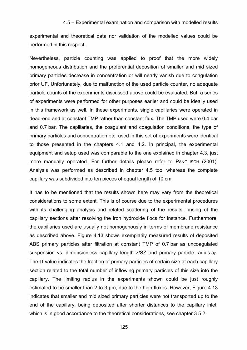
4.5 – Experimental examination and comparison with modelled results
125
experimental and theoretical data nor validation of the modelled values could be
performed in this respect.
Nevertheless, particle counting was applied to proof that the more widely
homogeneous distribution and the preferential deposition of smaller and mid sized
primary particles decrease in concentration or will nearly vanish due to coagulation
prior UF. Unfortunately, due to malfunction of the used particle counter, no adequate
particle counts of the experiments discussed above could be evaluated. But, a series
of experiments were performed for other purposes earlier and could be ideally used
in this framework as well. In these experiments, single capillaries were operated in
dead-end and at constant TMP rather than constant flux. The TMP used were 0.4 bar
and 0.7 bar. The capillaries, the coagulant and coagulation conditions, the type of
primary particles and concentration etc. used in this set of experiments were identical
to those presented in the chapters 4.1 and 4.2. In principal, the experimental
equipment and setup used was comparable to the one explained in chapter 4.3, just
more manually operated. For further details please refer to PANGLISCH (2001).
Analysis was performed as described in chapter 4.5 too, whereas the complete
capillary was subdivided into ten pieces of equal length of 10 cm.
It has to be mentioned that the results shown here may vary from the theoretical
considerations to some extent. This is of course due to the experimental procedures
with its challenging analysis and related scattering of the results, rinsing of the
capillary sections after resolving the iron hydroxide flocs for instance. Furthermore,
the capillaries used are usually not homogenously in terms of membrane resistance
as described above. Figure 4.13 shows exemplarily measured results of deposited
ABS primary particles after filtration at constant TMP of 0.7 bar as uncoagulated
suspension vs. dimensionless capillary length z/SZ and primary particle radius aP.
The Π value indicates the fraction of primary particles of certain size at each capillary
section related to the total number of inflowing primary particles of this size into the
capillary. The limiting radius in the experiments shown could be just roughly
estimated to be smaller than 2 to 3 µm, due to the high fluxes. However, Figure 4.13
indicates that smaller and mid sized primary particles were not transported up to the
end of the capillary, being deposited after shorter distances to the capillary inlet,
which is in good accordance to the theoretical considerations, see chapter 3.5.2.
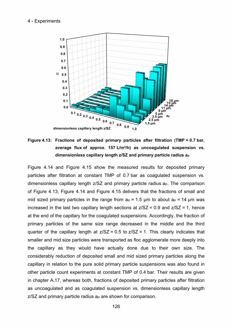
4 - Experiments
126
1.5 µm2.5 µm
3.5 µm5 µm
8 µm11 µm
14 µm15 µm18 µm
0.1 0.2 0.3 0.4 0.5 0.6 0.7 0.8 0.9 1.0
0.0
0.1
0.2
0.3
0.4
0.5
0.6
0.7
0.8
0.9
1.0
Π
dimensionless capillary length z/SZ
aP
Figure 4.13: Fractions of deposited primary particles after filtration (TMP = 0.7 bar, average flux of approx. 157 L/m²/h) as uncoagulated suspension vs. dimensionless capillary length z/SZ and primary particle radius aP
Figure 4.14 and Figure 4.15 show the measured results for deposited primary
particles after filtration at constant TMP of 0.7 bar as coagulated suspension vs.
dimensionless capillary length z/SZ and primary particle radius aP. The comparison
of Figure 4.13, Figure 4.14 and Figure 4.15 delivers that the fractions of small and
mid sized primary particles in the range from aP = 1.5 µm to about aP = 14 µm was
increased in the last two capillary length sections at z/SZ = 0.9 and z/SZ = 1, hence
at the end of the capillary for the coagulated suspensions. Accordingly, the fraction of
primary particles of the same size range decreased in the middle and the third
quarter of the capillary length at z/SZ = 0.5 to z/SZ = 1. This clearly indicates that
smaller and mid size particles were transported as floc agglomerate more deeply into
the capillary as they would have actually done due to their own size. The
considerably reduction of deposited small and mid sized primary particles along the
capillary in relation to the pure solid primary particle suspensions was also found in
other particle count experiments at constant TMP of 0.4 bar. Their results are given
in chapter A.17, whereas both, fractions of deposited primary particles after filtration
as uncoagulated and as coagulated suspension vs. dimensionless capillary length
z/SZ and primary particle radius aP are shown for comparison.
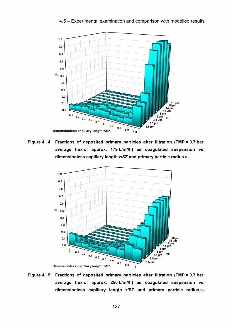
4.5 – Experimental examination and comparison with modelled results
127
1.5 µm2.5 µm
3.5 µm5 µm
8 µm11 µm
14 µm15 µm
18 µm
0.1 0.2 0.3 0.4 0.5 0.6 0.7 0.8 0.91.0
0.0
0.1
0.2
0.3
0.4
0.5
0.6
0.7
0.8
0.9
1.0
Π
dimensionless capillary length z/SZ
aP
Figure 4.14: Fractions of deposited primary particles after filtration (TMP = 0.7 bar, average flux of approx. 179 L/m²/h) as coagulated suspension vs. dimensionless capillary length z/SZ and primary particle radius aP
1.5 µm2.5 µm
3.5 µm5 µm
8 µm11 µm
14 µm15 µm
18 µm
0.1 0.2 0.3 0.4 0.5 0.6 0.7 0.8 0.91
0.0
0.1
0.2
0.3
0.4
0.5
0.6
0.7
0.8
0.9
1.0
Π
dimensionless capillary length z/SZ
aP
Figure 4.15: Fractions of deposited primary particles after filtration (TMP = 0.7 bar, average flux of approx. 250 L/m²/h) as coagulated suspension vs. dimensionless capillary length z/SZ and primary particle radius aP
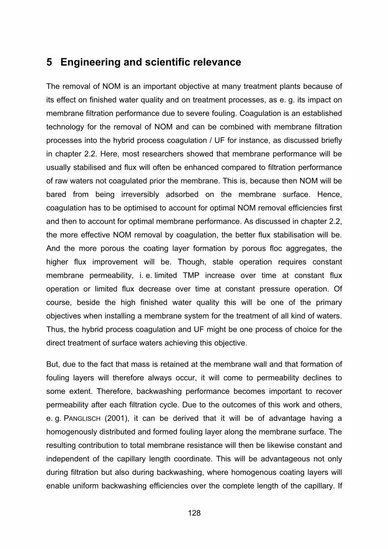
128
5 Engineering and scientific relevance
The removal of NOM is an important objective at many treatment plants because of
its effect on finished water quality and on treatment processes, as e. g. its impact on
membrane filtration performance due to severe fouling. Coagulation is an established
technology for the removal of NOM and can be combined with membrane filtration
processes into the hybrid process coagulation / UF for instance, as discussed briefly
in chapter 2.2. Here, most researchers showed that membrane performance will be
usually stabilised and flux will often be enhanced compared to filtration performance
of raw waters not coagulated prior the membrane. This is, because then NOM will be
bared from being irreversibly adsorbed on the membrane surface. Hence,
coagulation has to be optimised to account for optimal NOM removal efficiencies first
and then to account for optimal membrane performance. As discussed in chapter 2.2,
the more effective NOM removal by coagulation, the better flux stabilisation will be.
And the more porous the coating layer formation by porous floc aggregates, the
higher flux improvement will be. Though, stable operation requires constant
membrane permeability, i. e. limited TMP increase over time at constant flux
operation or limited flux decrease over time at constant pressure operation. Of
course, beside the high finished water quality this will be one of the primary
objectives when installing a membrane system for the treatment of all kind of waters.
Thus, the hybrid process coagulation and UF might be one process of choice for the
direct treatment of surface waters achieving this objective.
But, due to the fact that mass is retained at the membrane wall and that formation of
fouling layers will therefore always occur, it will come to permeability declines to
some extent. Therefore, backwashing performance becomes important to recover
permeability after each filtration cycle. Due to the outcomes of this work and others,
e. g. PANGLISCH (2001), it can be derived that it will be of advantage having a
homogenously distributed and formed fouling layer along the membrane surface. The
resulting contribution to total membrane resistance will then be likewise constant and
independent of the capillary length coordinate. This will be advantageous not only
during filtration but also during backwashing, where homogenous coating layers will
enable uniform backwashing efficiencies over the complete length of the capillary. If
5 - Engineering and scientific relevance
129
the coating layer is not homogeneous and offers different resistances to flow, then
the water will enter the membrane during backwashing at areas of lowest resistance
most. Hence, the fouled membrane surface will be cleaned best where it is initially
least fouled and worst where it is needed most. This can lead to uncleaned areas of
membrane surface if the resistance against backwashing of the fouling layer is high
enough. Furthermore, those areas may hamper the discharge of already detached
parts of the former fouling layer out of the capillary. In addition, if those areas are not
cleaned efficiently during several backwashing cycles this may lead to an increase of
bonding forces between the fouling layer and the membrane surface (GIMBEL (1989)
cited in PANGLISCH (2001)). Generally, only little is presently known about the
detachment characteristics and mechanisms of fouling layers of different composition
during backwashing, which should be suspect of additional research.
Considering the above, one easily finds the contradiction within this process
combination. On the one hand coagulation leads to a significantly decreased number
of colloids and smaller particles by embedding them into larger floc aggregates. On
the other hand, larger floc aggregates themselves will contribute to inhomogeneous
fouling layer formation, caused by their transport behaviour depending on their size,
enhanced by additional floc growth while being transported. This can be reasonably
assumed by the outcomes of this work, see chapters 3.5.2 and 3.5.3. However, it
may contribute to lowered membrane performance, especially if flocs will be
transported to the rear end and clog the capillary, which was found to take place
theoretically from the end towards the inlet and from the bottom to the top in a
horizontal aligned capillary. As a result, membrane surface area available for filtration
can be dramatically reduced over time, especially at high floc volume concentrations
within filtration cycles (LERCH ET AL. (2005B)) and, considering long term operation, by
decreased cleaning efficiency (HEIJMAN ET AL. (2007)). But clogging of the capillary
may also occur somewhere in the beginning or middle of the capillary, especially if
the flocs entering are initially large and grow further while being transported (GITIS ET
AL. (2005). Hence, flocs entering the capillary should not be too large, limiting the risk
of immediate formation of plugs and clogging of the capillary.
If clogging occurs, which may be detected as rapidly increased pressure drop or
decreased flux during operation, filtration cycles should be shortened to avoid
5 - Engineering and scientific relevance
130
compression of the plugged areas and to facilitate backwashing. Further, floc and
fouling layer porosity should be kept preferably high, because then the effect of
inhomogeneous formed layers on resistance to flow and therefore on achievable
performance is low, whereas high porosity will be further supported by larger flocs. If
a porous fouling layer will be compressed, then the resistance to flow will be
increased due to a lowered porosity and the performance will drop during operation,
noticed as pressure drop increase or flux decrease. Hence, large, incompressible
and porous flocs and filtration at low TMP will be favourable as discussed in chapter
3.5, but plugging of the capillaries, which is more likely for larger floc aggregates,
should be avoided. It has to be mentioned that the statements above are restricted to
flocs only; the influence of NOM or other components for instance were not
considered.
As suggested by PANGLISCH (2001) for filtration of uncoagulated raw waters, clogging
might be avoided by introducing a slow cross-flow velocity at the end of the capillary.
The concentrate flow might be further treated in a second membrane stage, adapted
in geometry and operation parameters on the better defined, i. e. more tighten
particle size distribution. Cross-flow operation in this respect would just be used to
transport and push larger flocs out of the capillary which otherwise would be
deposited at the dead-end. The flow profile within the capillary lumen will still be
laminar. Please note that this is different to commonly known cross-flow operation,
where flow along the membrane is often kept turbulent to minimise deposition and
where the extracted water volume is mostly governed by the critical flow concept
(BACCHIN ET AL. (2006A)). In the following, chosen results of models with different
average outlet velocities at boundary 3 and 6 are shown to proof effects of an
introduced slow cross-flow. The average velocities at the capillary outlet were chosen
to be 1 %, 5 % and 20 % of the inlet average velocity, whereas all other previously
used parameters were kept constant. Figure 5.1 shows floc trajectories of different
sized flocs for models with 5 % (left) and 20 % (right) average cross-flow velocity at
the capillary outlet, whereas just the inner- and outermost floc trajectories and
resulting equilibrium trajectories within the capillary for flocs of radius aF = 29.47 µm
and aF = 60 µm are illustrated. It can be seen that in case of slow cross-flow
operation smaller flocs entering the capillary in the neighbouring area of its axis at
the inlet will leave the capillary at the end. The faster the chosen cross-flow velocity

5 - Engineering and scientific relevance
131
the larger this neighbouring area and the more flocs are able to be transported out of
the capillary lumen without being deposited. For flocs of radius aF = 5 µm and 1 %
average cross-flow outlet velocity it was found that all flocs entering between the
capillary axis and a dimensionless capillary radius r/SR = 0.03 will be transported out
of the system. Applying an outlet velocity of 5 % will deliver r/SR = 0.11 and at 20 %
will deliver r/SR = 0.273. Hence, assuming an evenly distributed floc suspension
entering the capillary, about 0.09 %, 1.23 % or 7.67 %, respectively, of all entering
flocs will leave the capillary. This amount will be higher for smaller flocs and lower for
larger flocs. For example, the values for flocs of radius aF = 12.25 µm at 20 % outlet
velocity were calculated to be 0.02 % and for 5 % and slower velocities no floc will
leave the capillary just as well for flocs even larger. For flocs of those sizes, the front
contact point, see chapter 3.5.2, is shifted very slightly towards the inlet for
increasing outlet velocities.
0
0.1
0.2
0.3
0.4
0.5
0.6
0.7
0.8
0.9
1
0 0.2 0.4 0.6 0.8 1
dimensionless capillary radius r/SR
dim
ensi
onle
ss c
apill
ary
leng
th z
/SZ
aF = 60 µm aF = 29.47 µm aF = 5 µm
gravity
aF aF aF
0
0.1
0.2
0.3
0.4
0.5
0.6
0.7
0.8
0.9
1
0 0.2 0.4 0.6 0.8 1
dimensionless capillary radius r/SR
dim
ensi
onle
ss c
apill
ary
leng
th z
/SZ
aF = 60 µm aF = 29.47 µm aF = 5 µm
gravity
aF aF aF
Figure 5.1: Floc trajectories for models with 5 % (left) and 20 % (right) average cross-flow velocity at the capillary outlet
Even at high flux operation, for instance 200 L/m²/h, larger flocs will not be driven out
of the system to great extent as indicated in Figure 5.2. Just flocs from the very upper
part might be able to escape deposition and leave the capillary. Here, the flow is from
the rear to the front and gravity acts from top to bottom. The diameter of the
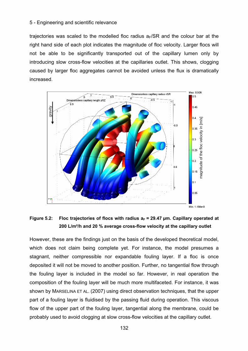
5 - Engineering and scientific relevance
132
trajectories was scaled to the modelled floc radius aF/SR and the colour bar at the
right hand side of each plot indicates the magnitude of floc velocity. Larger flocs will
not be able to be significantly transported out of the capillary lumen only by
introducing slow cross-flow velocities at the capillaries outlet. This shows, clogging
caused by larger floc aggregates cannot be avoided unless the flux is dramatically
increased.
Figure 5.2: Floc trajectories of flocs with radius aF = 29.47 µm. Capillary operated at 200 L/m²/h and 20 % average cross-flow velocity at the capillary outlet
However, these are the findings just on the basis of the developed theoretical model,
which does not claim being complete yet. For instance, the model presumes a
stagnant, neither compressible nor expandable fouling layer. If a floc is once
deposited it will not be moved to another position. Further, no tangential flow through
the fouling layer is included in the model so far. However, in real operation the
composition of the fouling layer will be much more multifaceted. For instance, it was
shown by MARSELINA ET AL. (2007) using direct observation techniques, that the upper
part of a fouling layer is fluidised by the passing fluid during operation. This viscous
flow of the upper part of the fouling layer, tangential along the membrane, could be
probably used to avoid clogging at slow cross-flow velocities at the capillary outlet.
mag
nitu
de o
f the
floc
vel
ocity
in [m
/s]gr
avity
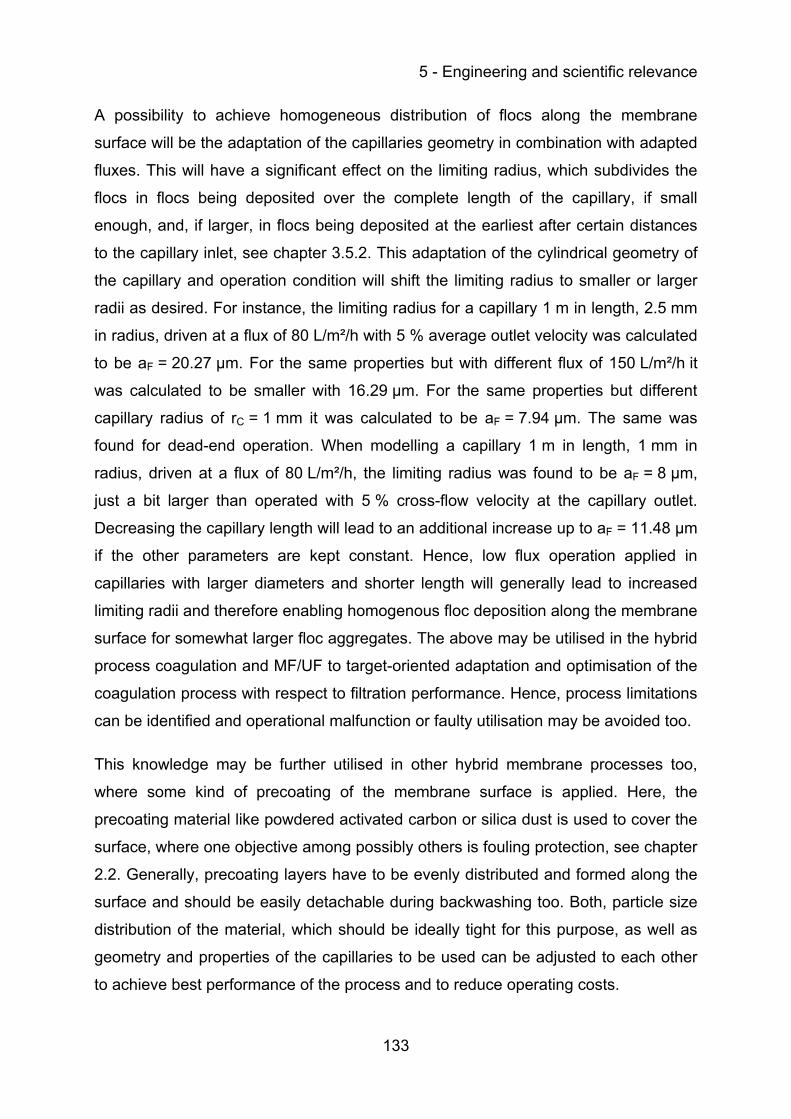
5 - Engineering and scientific relevance
133
A possibility to achieve homogeneous distribution of flocs along the membrane
surface will be the adaptation of the capillaries geometry in combination with adapted
fluxes. This will have a significant effect on the limiting radius, which subdivides the
flocs in flocs being deposited over the complete length of the capillary, if small
enough, and, if larger, in flocs being deposited at the earliest after certain distances
to the capillary inlet, see chapter 3.5.2. This adaptation of the cylindrical geometry of
the capillary and operation condition will shift the limiting radius to smaller or larger
radii as desired. For instance, the limiting radius for a capillary 1 m in length, 2.5 mm
in radius, driven at a flux of 80 L/m²/h with 5 % average outlet velocity was calculated
to be aF = 20.27 µm. For the same properties but with different flux of 150 L/m²/h it
was calculated to be smaller with 16.29 µm. For the same properties but different
capillary radius of rC = 1 mm it was calculated to be aF = 7.94 µm. The same was
found for dead-end operation. When modelling a capillary 1 m in length, 1 mm in
radius, driven at a flux of 80 L/m²/h, the limiting radius was found to be aF = 8 µm,
just a bit larger than operated with 5 % cross-flow velocity at the capillary outlet.
Decreasing the capillary length will lead to an additional increase up to aF = 11.48 µm
if the other parameters are kept constant. Hence, low flux operation applied in
capillaries with larger diameters and shorter length will generally lead to increased
limiting radii and therefore enabling homogenous floc deposition along the membrane
surface for somewhat larger floc aggregates. The above may be utilised in the hybrid
process coagulation and MF/UF to target-oriented adaptation and optimisation of the
coagulation process with respect to filtration performance. Hence, process limitations
can be identified and operational malfunction or faulty utilisation may be avoided too.
This knowledge may be further utilised in other hybrid membrane processes too,
where some kind of precoating of the membrane surface is applied. Here, the
precoating material like powdered activated carbon or silica dust is used to cover the
surface, where one objective among possibly others is fouling protection, see chapter
2.2. Generally, precoating layers have to be evenly distributed and formed along the
surface and should be easily detachable during backwashing too. Both, particle size
distribution of the material, which should be ideally tight for this purpose, as well as
geometry and properties of the capillaries to be used can be adjusted to each other
to achieve best performance of the process and to reduce operating costs.
5 - Engineering and scientific relevance
134
Another interesting and promising approach to enhance operating performance
within the hybrid process coagulation and membrane filtration was found in this work
when discussing the influence of sedimentation on floc transport, see chapter 3.5.2.2.
It was shown that vertical aligned membrane capillaries may be of advantage if the
fluid enters the membrane at the top, i. e. operation is driven in top-down mode. For
smaller flocs, transport is comparable as in bottom-up operation of vertical aligned
capillaries and as in horizontal aligned capillaries. But, after exceeding a certain
limiting size, which was found to be aF = 83.9 µm for flocs with a relative density of
1.05, the flocs will be collected on an equilibrium trajectory and eventually
transported towards the capillary axis and not towards the membrane wall. Finally,
they will be retained at the dead-end of the capillary. Please note, the floc size lies
within the size distribution of the flocs used in the experimental part of this work. The
same behaviour was found for flocs of size aF = 29.47 µm with higher densities as
illustrated in Figure 5.3.
Figure 5.3: Floc trajectories of flocs with radius aF = 29.47 µm, ballasted with micro sand (relative density of 1.72) within a vertical aligned capillary, operated at 80 L/m²/h in top-down dead-end mode
mag
nitu
de o
f the
floc
vel
ocity
in [m
/s]
grav
ity
5 - Engineering and scientific relevance
135
The flocs will merge to equilibrium trajectories but not being transported towards the
membrane wall for relative densities larger than approximately 1.72. An increased
density of the floc aggregates can be achieved within the hybrid process in similar
way as in the ACTIFLO® process (Krüger A/S, Denmark) which utilises micro sand as
a seed for floc formation, providing surface area that enhances coagulation and
acting as ballast in the formed flocs. To avoid clogging of the membrane at the dead-
end, a slight cross-flow of 1 % may be of high advantage. However, this theoretical
approach needs to be further investigated for practical applications in membrane
systems in future research.
Generally, the chosen approach of modelling floc transport and resulting fouling layer
formation in dead-end capillaries with CFD/FEM delivered some advantages. The
model can be easily used as tool to calculate floc, or generally particle transport in
arbitrary cylindrical capillary geometries, due to its scaled dimensionless form, at
arbitrary alignments, due to its universal layout. This may not only be utilised for
modelling the floc transport and fouling layer formation as done in this work, but can
be used for evaluation and optimisation of technical designs and processes in
practical as well as scientific problems. For instance, after some minor adaptations of
the membrane wall boundary for risk analysis in membrane integrity problems too.
Numerical difficulties occurred when modelling the fouling layer formation over time,
especially for larger floc aggregates, as described in chapter 3.5.3. This was because
of locally arising very high floc volume concentrations along the equilibrium trajectory
compared to areas in the vicinity. Resolution of the applied mesh could not be
adapted to resolve the sharp gradients to deliver acceptable results. Additionally, it
was found that the description of floc volume was generally problematic within the
used FEM software modes. This problem is based on the chosen, so called Euler-
Lagrange approach, i. e. one continuous phase (the fluid) related to a fixed
coordinate system and one dispersed phase (the flocs) related to a system moving
with the fluid (compare PASCHEDAG (2004) for instance), used to describe floc
transport and fouling layer formation. The approach considers flocs as single mass
points in the continuous phase only, not as flocs requiring a certain volume. Moving
flocs are therefore numerically calculated along the node points on the mesh. Hence,
calculation and limitation of the floc volume concentration to a fixed value was not
5 - Engineering and scientific relevance
136
directly possible, but might be assessable by additionally codes to be programmed in
future work. Relief may be also found in other commercially available software
products, using finite volume methods (FVM) instead. This enables the direct use of
the so called Euler-Euler approach, i. e. two continuous phases (the fluid and the floc
suspension) related to a fixed coordinate system (compare PASCHEDAG (2004) for
instance). FVM considers a certain volume around its node points on a mesh for
numerical calculation, enabling to consider flocs as spheres rather than points during
numerical calculation.
Future work on the model should also account for size distributions rather than single
sizes and enlarge the model to include additional phases in suspension or solution
respectively, such as dissolved species like dissolved NOM and its components or
salts to include the effect of direct adsorption onto the membrane for instance. To
account for floc agglomeration during transport within the membrane capillary,
population balances might be further implemented into the existing model. This new
approach in numerical modelling accounts for changes of particle or floc properties,
usually size distribution, and simulates the interaction of agglomeration and breakage
of one phase in multi phase flow, SCHÜTZ ET AL. (2007).
Another aspect to be included into future modelling should be the implementation of
the mass fractal dimension dF into the used equations to consider the impact on
transport and deposition behaviour of more realistic floc structures. Considering the
formed fouling layer, it should be done additional modelling work on floc and layer
compressibility as well as the detachment behaviour of deposited flocs.
137
6 Summary
The interest in low pressure membrane filtration, i. e. micro- and ultrafiltration (MF
and UF) increased rapidly in recent years, especially due to the extremely high
requirements for potable water quality with respect to hygiene aspects. With UF, the
filtrate quality is quite independent of the raw water quality with respect to larger
colloidal and particulate water components. Further advantages are the possibility of
fully automatic operation, compact system design, high space utilisation and provided
flexibility in system enlargements, modernisations and new installations. But beside
those advantages some limiting or even adversarial factors exist, especially when
applying MF or UF for the direct treatment of surface. One of these is fouling, another
one the inadequate retention efficiency of disinfection by products (DBP) precursors.
Particularly dissolved organic matter (DOM) can be very problematic due to the
formation of hardly reversible and/or irreversible fouling layers and due to its general
contribution in formation of DBP. To get these problems under control, different
pretreatment processes are conceivable and available, whereas this work is focused
on the hybrid process coagulation and UF. Coagulation is an established technology
for the removal of DOM and, from an engineering perspective, can easily be
combined with membrane processes, still offering the advantages of the membrane
as mentioned above.
Nevertheless, it is necessary to understand what the limiting factors are, when they
are of importance and how their effects may be avoided. The most important point in
this respect is to understand how fouling layers are formed within this process
combination, because these layers will limit the efficiency of the entire process.
Formation of layers of brownian and non-brownian particles and colloids in inside-out
driven capillary membranes is quite well understood but yet the knowledge is not
developed far enough to cope for the formation of larger and porous floc aggregates.
Therefore, the objective of this work was to contribute to the understanding of
formation of fouling layers by porous floc aggregates during filtration of coagulated
raw waters in inside-out driven capillary membranes.
A computational fluid dynamics (CFD) model was developed, using the software
COMSOL Multiphysics (COMSOL AB, Sweden) for the description of the complete

6 - Summary
138
flow field in inside-out driven UF capillaries of arbitrary cylindrical geometry,
alignment, i. e. vertical or horizontal, and operation condition, i. e. cross-flow or dead-
end. This was done by numerical calculations of the Navier-Stokes and continuity
equations first for stationary and second for transient flows, including the effects of
dynamic fouling layer formation. Based on the modelled flow field, floc velocities and
trajectories were derived by balancing the forces and torques acting on the flocs in
the flow field. The forces and torques considered arose from sedimentation, shear
induced and Brownian diffusion, double layer repulsion and van der Waals attraction,
drag by filtration, virtual mass and lateral migration. Floc agglomerates were
considered being ideally spherical, rigid and of constant shape, consisting of primary
particles embedded in iron or aluminium hydroxide, revealing an inner porosity, low
density and low zeta potential. To account for the inner porosity of the flocs an
equivalent hydrodynamic floc radius was introduced. The effect of the porous
aggregates on floc suspension viscosity was considered by introducing a correction
factor. The derived floc velocities were further used to model stationary floc volume
concentration distributions by numerical calculations of the convection and diffusion
equation. In the first step, the models were used to describe initial and stationary floc
transport and deposition behaviour. Deposition of flocs along the membrane surface
will be classed by floc size. Flocs of size smaller than a certain limiting radius will be
deposited widely homogeneous over the total capillary length. Larger flocs occupy
preferential places on the membrane surface and do not deposit until they are at a
certain distance to the capillary inlet. The larger the particle size, the longer this
distance. However, flocs of certain size entering the capillary at its axis or direct
vicinity will not be transported to the rear end of the capillary. They will be deposited
at so called rear contact points, some distance away from the dead-end. The
distance between the dead-end and the rear contact point increases with increasing
floc radius until all incoming flocs are forced to merge an equilibrium trajectory,
independent of their radial starting position at the inlet. All flocs on this trajectory are
deposited theoretically at one single point, ring or ring section at the membrane wall
and will be shifted back towards the dead-end with further increasing floc sizes.
However, in contrast to solid particle suspensions, it could be shown that the more
widely homogeneous distribution and preferential deposition of smaller and mid sized
particles was reduced. Thus, it still comes to the formation of zones with different
6 - Summary
139
composition, porosity and thickness, but the majority of particles embedded in
generally larger flocs will be transported towards the dead-end which may cause
clogging of the capillary. It was further found that this inhomogeneous fouling layer
formation will be enhanced by additional floc growth during transport as can be
reasonably assumed by the outcome of this work.
In a second step the models were coupled and eventually used to account for the
growing layer height and its influence on the flow field, the floc volume distribution
and resulting floc trajectories, predicting fouling layer formation over time. The height
of the layer was calculated by integrating the mass flux of flocs onto the membrane
surface, whereas the porosity of the fouling layer was calculated based on the
Happel model for bulk permeabilities. The increased resistance against the filtrate
flow according to the resistance in series model was then used to derive the new fluid
flow field over time. However, it came to major convergence problems during the
numerical calculation of the floc volume distribution over time, especially if larger
flocs were modelled. But convergence could eventually be achieved for smaller floc
sizes. Though, the results were not satisfying and only imprecise statements could
be made concerning calculability of the permeability decline due to fouling layer
formation, but nevertheless qualitative aspects were concluded. It was shown that
the local resistance increases at surface areas of preferential deposition, whereupon
the fluid rather flows through uncoated or less coated areas. Accordingly, different
floc trajectories are developed over time and transport of flocs is shifted towards the
capillary inlet, i. e. towards areas less fouled. It was further shown that clogging of
the capillaries dead-end takes place over time and theoretically from the end towards
the inlet and from the bottom to the top of a horizontal aligned capillary. Setting the
modelled results in contrast to experimental investigations showed satisfactory
results for both, the modelled flow field and conditionally the fouling layer formation.
New aspects could be derived qualitatively to understand the formation of fouling
layers by porous floc aggregates in inside-out driven capillary membranes on which
recommendations for appropriate operation conditions were concluded. Under these
are e. g. top-down dead-end or cross-flow operation for the filtration of flocs,
ballasted with micro sand.
140
References
ALTENA, F. W.; BELFORT, G.: Lateral migration of spherical particles in porous flow channels: Application to membrane filtration. Chem. Eng. Sci. 39 (1984), Nr. 2, pp. 343-355
ALTMANN, J.; RIPPERGER, S.: Particle deposition and layer formation at the crossflow microfiltration. J. Membr. Sci. 124 (1997), pp. 119-128
AMY, G.: Fundamental understanding of organic matter fouling of membranes In: IWA
SPECIALISED CONFERENCE ON MEMBRANES, Conference Proceedings (Ed.) Bd. CD-ROM. Harrogate: IWA, 2007
ANDERSON, J. D.; DEGREZ, G.; DICK, E.; GRUNDMANN, R.: Computational fluid dynamics; An introduction. In: WENDT, J. F. (Ed.): Computational fluid dynamics; An introduction. Berlin: Springer-Verlag, 1992. - ISBN 3-540-53460-1
BACCHIN, P.; AIMAR, P.; SANCHEZ, V.: Model for colloidal fouling of ultrafiltration membranes. AIChE Journal 41 (1995), Nr. 2, pp. 368-376
BACCHIN, P.; ESPINASSE, B.; BESSIERE, Y.; FLETCHER, D. F.; AIMAR, P.: Numerical simulation of colloidal dispersion filtration: description of critical flux and comparison with experimental results. Desalination 192 (2006), pp. 74-81
BACCHIN, P.; AIMAR, P.; FIELD, R. W.: Critical and sustainable fluxes: Theory, experiments and applications. J. Membr. Sci. 281 (2006), pp. 42-69
BEAVERS, G. S.; JOSEPH, D. D.: Boundary conditions at a naturally permeable wall. J. Fluid Mech. 30 (1967), Nr. 1, pp. 197-207
BEHRENS, S. H.; BORKOVEC, M.: Electrostatic interaction of colloidal surfaces with variable charge. J. Phys. Chem. B 103 (1999), pp. 2918-2928
BELFORT, G.; NAGATA, N.: Fluid mechanics and cross-flow filtration: Some thoughts. Desalination 53 (1985), pp. 57-79
BENKHALA, Y. K.; OULD-DRIS, A.; JAFFRIN, M. Y.; SI-HASSEN, D.: Cake growth mechanism in cross-flow microfiltration of mineral suspensions. J. Membr. Sci. 98 (1995), Nr. 1, pp. 107-117
References
141
BERGSTRÖM, L.: Hamaker constants of inorganic materials. Adv. Coll. Inter. Sci. 70 (1997), pp. 125-169
BERMAN, A. S.: Laminar flow in channels with porous walls. J. Appl. Phys. 24 (1953), Nr. 9, pp. 1232-1235
BIRD, R. B.; STEWART, W. E.; LIGHTFOOT, E. N.: Transport Phenomena. 2. Edition New York: Wiley, 2002. - 0-471-36474-6
BLUME, I.; KOENHEN, D. M.; ROESINK, H. D. W.: The XIGA-Concept; The first full-scale applications using a new module system for ultrafiltration. In: MELIN, T.; RAUTENBACH, R. und DOHMANN, M. (Eds.): Möglichkeiten und Perspektiven der Membrantechnik bei der kommunalen Abwasserbehandlung und Trinkwasseraufbereitung: Begleitbuch zur 1. Aachener Tagung Siedlungswasserwirtschaft und Verfahrenstechnik 30.06.-01.07.97. Aachen, 1997, pp. B7-1 - B7-13
BOERLAGE, S. F. E.: Scaling and particulate fouling in membrane filtration systems. In: WAGENINGEN
UNIVERSITY (Ed.): PhD dissertation at the Wageningen University: Scaling and particulate fouling in membrane filtration systems. Lisse: Swets & Zeitlinger Publishers b.v., 2001. - 90-5809-2429
CARROLL, T.; KING, S.; GRAY, S. R.; BOLTO, B. A.; BOOKER, N. A.: The fouling of microfiltration membranes by NOM after coagulation treatment. Water Res. 34 (2000), Nr. 11, pp. 2861-2868
CHELLAM, S.; WIESNER, M. R.: Particle transport in clean membrane filters in laminar flow. Environ. Sci. Technol. 26 (1992), Nr. 26, pp. 1611-1621
CHELLAM, S.; WIESNER, M. R.; DAWSON, C.: Laminar flow in porous ducts. Reviews in Chemical Engineering 11 (1995), pp. 53-99
CHEN, Y.; DONG, B. Z.; GAO, N. Y.; FAN, J. C.: Effect of coagulation pretreatment on fouling of an ultrafiltration membrane. Desalination 204 (2007), pp. 181-188
CHERYAN, M.: Ultrafiltration and microfiltration handbook. In: CHERYAN, M. (Ed.): Ultrafiltration and microfiltration handbook. Lancaster: Technomic Publishing Company, Inc., 1998
References
142
CHO, J.; SOHN, J.; CHOI, H.; KIM, I. S.; AMY, G.: Effects of molecular weight cutoff, f/k ratio (a hydrodynamic condition), and hydrophobic interactions on natural organic matter rejection and fouling in membranes. J. Water Supp. Res. Technol. - AQUA 51 (2002), Nr. 2, pp. 109-123
CHO, M.-H.; LEE, C.-H.; LEE, S.: Effect of flocculation conditions on membrane permeability in coagulation-microfiltration. Desalination 191 (2006), pp. 386 396
COMSOL AB: In: COMSOL AB (Ed.): Multiphysics User’s Guide. Bd. Version 3.3a. Stockholm: 2006
COMSOL AB: In: COMSOL AB (Ed.): Chemical Engineering Module User’s Guide. Bd. Version 3.3a. Stockholm: 2006
COX, R. G.; BRENNER, H.: The lateral migration of solid particles in Poiseuille flow - I Theory. Chem. Eng. Sci. 23 (1968), pp. 147-173
CRAUN, C. F.; HUBBS, S. A.; FROST, F.; CALDERON, R. L.; VIA, S. H.: Waterborne outbreaks of cryptosporidiosis. AWWA Journal 90 (1998), Nr. 9, pp. 81-91
CRAUN, G. F.: Waterborne outbreaks in Giardiasis. In: JAKUBOWSKI, W. und HOFF, J. C. (Eds.): Waterborne transmission of Giardiasis. Ohio: U.S. Environmental Protection Agency, 1979, pp. 127-149
DAVIS, R. H.; LEIGHTON, D. T.: Shear-induced transport of a particle layer along a porous wall. Chem. Eng. Sci. 42 (1987), Nr. 2, pp. 275-281
DIN ISO 9276-1 AND 9276-2: Darstellung der Ergebnisse von Partikelgrößenanalysen; Teil 1: Grafische Darstellung; Teil 2: Berechnung von mittleren Partikelgrößen/-durchmessern und Momenten aus Partikelgrößenverteilungen. In: DEUTSCHES INSTITUT FÜR NORMUNG E.V (Ed.): DIN ISO 9276-1 und 2. Bd. 9276-1. Berlin: Beuth Verlag, 2004
DO-QUANG, Z.; COCKX, A.; LAINÉ, J.-M.; ROUSTAN, M.: Applying CFD modelling to enhance water treatment. 1st World Water Congress of the International Water Association (IWA) in Paris, Conference Preprint, Drinking Water Treatment. Bd. Book 2. Paris:, 2000, pp. 50-55
References
143
DREW, D. A.; SCHONBERG, J. A.; BELFORT, G.: Lateral inertial migration of small sphere in fast laminar flow through a membrane duct. Chem. Eng. Sci. 46 (1991), Nr. 12, pp. 3219-3224
DVGW-ARBEITSBLATT W 218: Flockung in der Wasseraufbereitung - Flockungstestverfahren. In: DVGW DEUTSCHE
VEREINIGUNG DES GAS- UND WASSERFACHES E.V. (Ed.): DVGW Regelwerk; Technische Mitteilung; Arbeitsblatt W 218. Bd. W 218. Bonn:, 1997. - ISSN 0176 - ISSN 0176-3490
ECKSTEIN, E. C.; BAILEY, D. G.; SHAPIRO, A. H.: Self-diffusion of particles in shear flow of a suspension. J. Fluid Mech. 79 (1977), pp. 191-208
EINSTEIN, A.: Über die von der molekularkinetischen Theorie der Wärme geforderte Bewegung von in ruhenden Flüssigkeiten suspendierten Teilchen. Ann. d. Phys. 323 (1905), Nr. 4 / 18, pp. 549-560
ELIMELECH, M.; GREGORY, J.; JIA, X.; WILLIAMS, R.: Particle Deposition & Aggregation - Measurement, Modelling and Simulation. Particle Deposition & Aggregation. Oxford:, 1995. - 0 7506 0743 2
FACHGRUPPE WASSERCHEMIE IN DER GESELLSCHAFT DEUTSCHER CHEMIKER: Anwendung statistischer Methoden zur Beurteilung von Analysenergebnissen in der Wasseranalytik. In: ARBEITSGRUPPE "STATISTIK IN DER WASSERANALYTIK" IN DER
FACHGRUPPE WASSERCHEMIE, Fachgruppe Wasserchemie in der Gesellschaft Deutscher Chemiker in Gemeinschaft mit dem Normenausschuss Wasserwesen im DIN Deutsches Institut für Normung (Ed.): Deutsche Einheitsverfahren zur Wasser-, Abwasser- und Schlammuntersuchung. Bd. 1. Weinheim: VCH, 1997. - 3-527-28872-4
FAN, L.; HARRIS, J. L.; RODDICK, F.; BOOKER, N. A.: Influence of the characteristics of natural organic matter on the fouling of microfiltration membranes. Water Res. 35 (2001), Nr. 18, pp. 4455-4463
FANE, A. G.: Ultrafiltration of suspensions. J. Membr. Sci. 20 (1984), Nr. 3, pp. 249-259
FANE, A. G.; FELL, C. J. D.; NOR, M. T.: Ultrafiltration of colloidal suspensions and macromolecular solutions in an unstirred batch cell. Ind. Eng. Chem. Fundam. 73 (1982), C1
References
144
FENG, J; HU, H. H.; JOSEPH, D. D.: Direct simulation of initial value problems for the motion of solid bodies in a Newtownian fluid. Part 2. Couette and Poiseuille flows. J. Fluid Mech. 277 (1994), pp. 271-301
FINLAYSON, B. A.: Introduction to chemical engineering computing Hoboken: Wiley, 2006. - 978-0-471-74062-9
FUTSELAAR, H.; WEIJENBERG, D. C.: System design for large-scale ultrafiltration applications. Desalination 119 (1998), pp. 217-224
FUTSELAAR, H.; WILDEBOER, E.; WEIJENBERG, D. C.: The AquaFlex System; New developments in module and system design for water treatment. In: MELIN, T.; RAUTENBACH, R. und DOHMANN, M. (Eds.): Membrantechnik in der öffentlichen Wasseraufbereitung und Abwasserbehandlung - Bemessung, Umsetzung, Kosten; Begleitbuch zur 2. Aachener Tagung Siedlungswasserwirtschaft und Verfahrenstechnik, 15.09.98 - 16.09.98. Melin, T.; Rautenbach, Aachen:, 1998
GIMBEL, R.: Abscheidung von Trübstoffen aus Flüssigkeiten in Tiefenfiltern Habilitationsschrift. In: BEREICH WASSERCHEMIE AM ENGLER-BUNTE-INSTITUT DER
UNIVERSITÄT KARLSRUHE (Ed.): Veröffentlichungen des Bereichs und des Lehrstuhls für Wasserchemie und der DVGW-Forschungsstelle am Engler-Bunte-Institut der Universität Karlsruhe. Bd. 25. Frankfurt: ZfGW-Verlag, 1984. - 3-922671-10-1
GIMBEL, R.: The dynamic particle adhesion process and its effect on particle aggregation. Aqua 38 (1989), pp. 156-164
GIMBEL, R.; HAGMEYER, G.: Anforderungen an die Membrantechnik in der Trinkwasseraufbereitung. In: MELIN, T. und Dohmann, M. (Ed.): Membrantechnik in der Wasseraufbereitung und Abwasserbehandlung -Perspektiven, Neuentwicklungen und Betriebserfahrungen im In- und Ausland- 5. Aachener Tagung Siedlungswasserwirtschaft und Verfahrenstechnik. Bd. 5. Aachen:, 2003. - 3-921955-28-9, pp. Ü3-1 - Ü3-26
GIMBEL, R.; PANGLISCH, S.; HAGMEYER, G.: Abschlußbericht für das Forschungsvorhaben 02WT9411/8 -Ultrafiltration zur Abtrennung von Algen und algenbürtigen Substanzen mit verschiedenen Vorbehandlungen In: GERHARD MERCATOR UNIVERSITÄT -GH DUISBURG (Ed.) Duisburg: Eigenverlag, 1996
GITIS, V.; LERCH, A.; GIMBEL, R.: Retention of humic acid by ultrafiltration with polyaluminium coagulant. J. Water Supp. Res. Technol. - AQUA 54 (2005), Nr. 4, pp. 213-223
References
145
GOLDMAN, A. J.; COX, R. G.; BRENNER, H.: Slow viscous motion of a sphere parallel to a plane wall-II. Couette flow. Chem. Eng. Sci. 22 (1967), pp. 653-660
GOLDMAN, A. J.; COX, R. G.; BRENNER, H.: Slow viscous motion of a sphere parallel to a plane wall-I. Motion through a quiescent fluid. Chem. Eng. Sci. 22 (1967), pp. 637-651
GOREN, S. L.: The hydrodynamic force resisting the approach of a sphere to a plane permeable wall. J. Colloid Interface Sci. 69 (1979), Nr. 1, pp. 78-85
GOREN, S. L.; O'NEILL, M. E.: On the hydrodynamic resistance to a particle of a dilute suspension when in the neighbourhood of a large obstacle. Chem. Eng. Sci. 26 (1971), pp. 325-338
GRAY, S. R.; RITCHIE, C. B.; BOLTO, B. A.: Effect of fractionated NOM on low-pressure membrane flux declines. Water Sci. Technol.: Water Supply 4 (2004), Nr. 4, pp. 189-196
GREEN, G.; BELFORT, G.: Fouling of ultrafiltration membranes: Lateral migration and the particle Trajectory model. Desalination 35 (1980), pp. 129-147
GREGORY, J.: Interfacial Phenomena. In: IVES, K. (Ed.): The Scientific Basis of Filtration. Leyden: Noordhoff, 1975, pp. 53-90
GREGORY, J.: Approximate expressions for retarded van der Waals interaction. J. Colloid Interface Sci. 83 (1981), Nr. 1, pp. 138-145
GREGORY, J.: Fundamentals of flocculation. J. Crit. Rev. Environ. Control 19 (1989), pp. 185 230
GRUBBS, F.; BECK, G.: Extension of Sample Sizes and Percentage Points for Significance Tests of Outlying Observations. Technometrics 14 (1972), Nr. 4, pp. 847-853
GRUBBS, F. E.: Sample criteria for testing outlying observations. Ann. Math. Statist. 21 (1950), Nr. 1, pp. 27-58
References
146
GRUBBS, F. E.: Procedures for detecting outlying observations in samples. Technometrics 11 (1969), Nr. 1, pp. 1-21
GUIGUI, C.; ROUCH, J. C.; DURAND-BOURLIER, L.; BONNELYE, V.; APTEL, P.: Impact of coagulation conditions on the in-line coagulation/UF process for drinking water production. Desalination 147 (2002), pp. 95-100
HAGMEYER, G.; GIMBEL, R.; KIEPKE, O.; DAUTZENBERG, W.: Flocculation/ Ultrafiltration for drinking water treatment of reservoir water. In: AMERICAN WATER WORKS ASSOCIATION (Ed.): Proceedings of the AWWA Membrane Technology Conference, San Antonio. Bd. CD-ROM. San Antonio: Eigenverlag, 2001. - 1-58321-096-2
HAGMEYER, G.; GIMBEL, G.; DAUTZENBERG, W.: Requirements for flocculation followed by ultrafiltration for direct treatment of reservoir water. In: AMERICAN WATER WORKS ASSOCIATION (Ed.): Membrane Technology Conference Proceedings, Atlanta, 02. - 05.03.03. Bd. CD-ROM. Atlanta: Eigenverlag, 2003. - 1-58321-275-2
HÄNEL, D.: In: INSTITUT FÜR VERBRENNUNG UND GASDYNAMIK (Ed.): Strömungslehre I - Eine Einführung in die Mechanik der Fluide. Duisburg: Eigenverlag, 1992
HARMANT, P.; AIMAR, P.: Coagulation of colloids retained by porous walls. AIChE Journal 42 (1996), Nr. 12, pp. 3523-3532
HEIJMAN, S. G. J.; VANTIEGHEM, M.; RAKTOEA, S.; VERBERK, J. Q. J. C.; VAN DIJK, J. C.: Blocking of capillaries as fouling mechanism for dead-end operated ultrafiltration membranes. J. Membr. Sci. 287 (2007), pp. 119-125
HO, B. P.; LEAL, L. G.: Inertial migration of rigid spheres in two-dimensional unidirectional flows. J. Fluid Mech. 65 (1974), Nr. part 2, pp. 365-400
HOEK, E. M. V.; AGARWAL, G. K.: Extended DLVO interactions between spherical particles and rough surfaces. Colloid Interface Sci. 298 (2006), pp. 50-58
HOEK, E. M. V.; ELIMELECH, M.: Cake-enhanced concentration polarization: A new fouling mechanism for salt-rejecting membranes. Environ. Sci. Technol. 37 (2003), pp. 5581-5588
References
147
HOWE, K. J.: Effect of coagulation pretreatment on membrane filtration performance. Dissertation thesis at the university of Illinois at Urbana-Champaign. Urbana:, 2001
HOWE, K. J.; CLARK, M. M.: Fouling of microfiltration and ultrafiltration membranes by natural organic matter. Environ. Sci. Technol. 36 (2002), pp. 3571-3576
HOWE, K. J.; ISHIDA, K. P.; CLARK, M. M.: Use of ATR/FTIR spectrometry to study fouling of microfiltration membranes by natural waters. Desalination 147 (2002), pp. 251-255
HUANG, P. Y; FENG, J; HU, H. H.; JOSEPH, D. D.: Direct simulation of the motion of solid particles in Couette and Poiseuille flows of viscoelastic fluids. J. Fluid Mech. 343 (1997), pp. 73-94
HUCK, P. M.; PAYMENT, P.; HRUDEY, S. E.; ANDERSON, W. B.: A severe waterborne disease outbreak in Walkerton, Ontario: Issues relating to treatment and distribution. In: AMERICAN WATER WORKS ASSOCIATION (Ed.): Conference Proceedings AWWA Water Quality Technology Conference, November 11 - 15, 2001, Nashville, Tennessee. Bd. CD-ROM. Nashville: Eigenverlag, 2001, p. M8-2
HUNG, C.-C.; TIEN, C.: Effect of particle deposition on the reduction of water flux in reverse osmosis. Desalination 18 (1976), pp. 173-187
IVES, K. J.: Rate theories. In: IVES, K.J. (Ed.): The scientific basis of flocculation. Bd. E No. 27. 1. Edition Netherlands: Sijthoff & Noordhoff International Publishers B.V., 1978. - 9028607587, pp. 37-61
JANSON, A.; O’TOOLE, G.; LEE, M.-F.: The 273,000 m3/d immersed membrane system at Chestnut Avenue Water Works: its novel design and first year of operation. J. Water Supp. Res. Technol. - AQUA 6 (2006), Nr. 2, pp. 19-24
JUNG, C.-W.; SON, H.-J.; KANG, L. S.: Effects of membrane material and pretreatment coagulation on membrane fouling: fouling mechanism and NOM removal. Desalination 197 (2006), pp. 154-164
KABSCH-KORBUTOWICZ, M.: Impact of pre-coagulation on ultrafiltration process performance. Desalination 194 (2006), pp. 232-238
References
148
KARNIS, A.; GOLDSMITH, H. L.; MASON, S. G.: The flow of supsensions through tubes V. Inertial effects. Can. J. Chem. Eng. (1966), Nr. August, pp. 181-193
KENNEDY, M. D.; ZHIZHONG, L.; FEBRINA, E.; VAN HOOF, S.; SCHIPPERS, J.: Affects of coagulation on filtration mechanisms in dead-end ultrafiltration. In: IWW
RHEINISCH-WESTFÄLISCHES INSTITUT FÜR WASSERFORSCHUNG GGMBH (Ed.): Berichte aus dem IWW Rheinisch-Westfälisches Institut für Wasserforschung gGmbH. Bd. 37a. Mülheim an der Ruhr: Eigenverlag, 2002. - 0941 - 0961, pp. 185-210
KIM, A. S.; HOEK, E. M. V.: Cake structure in dead-end membrane filtration: Monte Carlo Simulation. Environ. Eng. Sci. 19 (2002), Nr. 6
KOLLBACH, J.-S.; HAESKE, J.; SCHILLING, S.: Planerische Aspekte bei Membrananlagen zur Wasser- und Abwasseraufbereitung. In: MELIN, T.; RAUTENBACH, R. und DOHMANN, M. (Eds.): Möglichkeiten und Perspektiven der Membrantechnik bei der kommunalen Abwasserbehandlung und Trinkwasseraufbereitung; Begleitbuch zur 1. Aachener Tagung Siedlungswasserwirtschaft und Verfahrenstechnik, 30.06.97 - 01.07.97. Aachen:, 1997
KOUTSOU, C. P.; YIANTSIOS, S. G.; KARABELAS, A. J.: Direct numerical simulation of flow in spacer-filled channels: Effect of spacer geometrical characteristics. J. Membr. Sci. 291 (2007), pp. 53-69
KROMKAMP, J.; BASTIAANSE, A.; SWARTS, J.; BRANS G.; VAN DER SMAN, R. G. M.; BOOM, R. M.: A suspension flow model for hydrodynamics and concentration polarisation in crossflow microfiltration. J. Membr. Sci. 253 (2005), pp. 67-79
LAHOUSSINE-TURCAUD, V.; WIESNER, M. R.; BOTTERO, J.-Y.: Fouling in tangential-flow ultrafiltration: The effect of colloid size and coagulation pretreatment. J. Membr. Sci. 52 (1990), pp. 173-190
LAHOUSSINE-TURCAUD, V.; WIESNER, M. R.; BOTTERO, J.-Y.; MALLEVIALLE, J.: Coagulation-Flocculation with aluminium salts: Influence on the filtration efficacy with microporous membranes. Water Res. 26 (1992), Nr. 5, pp. 695-702
LEE, J.-D.; LEE, S.-H.; JO, M.-H.; PARK, P.-K.; LEE, C.-H.; KWAK, J.-W.: Effect of coagulation conditions on membrane filtration characteristics in coagulation-microfiltration process for water treatment. Environ. Sci. Technol. 34 (2000), pp. 3780-3788
References
149
LEE, S. A.; FANE, A. G.; AMAL, R.; WAITE, T. D.: The effect of floc size and structure on specific cake resistance and compressibility in dead-end microfiltration. Sep. Sci. Technol. 38 (2003), Nr. 4, pp. 869-887
LEEUWEN, van, J.; CHOW, C.; FABRIS, R.; WITHERS, N.; PAGE, D.; DRIKAS, M.: Application of a fractionation technique for the better understanding of the removal of NOM by alum coagulation. Water Sci. Technol.: Water Supply 2 (2002), Nr. 5 - 6, pp. 427-433
LEIGHTON, D.; ACRIVOS, A.: Viscous resuspension. Chem. Eng. Sci. 41 (1986), Nr. 6, pp. 1377-1384
LEIGHTON, D.; ACRIVOS, A.: The shear-induced migration of particles in concentrated suspensions . J. Fluid Mech. 181 (1987), pp. 415-439
LERCH, A.; PANGLISCH, S.; HAGMEYER, G.; SCHÖN, M.; FEHN, J.; GIMBEL, R.: Direct Potable Water Treatment of River Waters by Flocculation/Ultrafiltration. In: INTERNATIONAL WATER ASSOCIATION (Ed.): Proceedings of the 3rd IWA World Water Congress, Melbourne, Australia, 7.-12.04.02. Bd. CD-ROM. Melbourne, 2002
LERCH, A.; HAGMEYER, G.; GIMBEL, R.; FEHN, J.: A comparison of laboratory and pilot plant experiments on the combination of flocculation / ultrafiltration for direct potable water treatment of river water. Water Sci. Technol.: Water Supply 3 (2003), Nr. 5-6, pp. 345-352
LERCH, A.; PANGLISCH, S.; NAHRSTEDT, A.; GIMBEL, R.: The influence of temperature on size and structure of flocs in the hybrid process coagulation / ultrafiltration. In: Chemical Water and Wastewater Treatment; Proceedings of the 11th Gothenburg Symposium 2004, Orlando, Florida, USA, H.H. HAHN; E. HOFFMANN; H. ODEGAARD (Eds.), 1. Edition, Vol. 1, London: IWA Publishing, 2004, pp. 265-273 - ISBN/ISSN 1 84339 068 X
LERCH, A.; PANGLISCH, S.; GIMBEL, R.: Research experiences in direct potable water treatment using coagulation/ultrafiltration. Water Sci. Technol. 51 (2005), Nr. 6-7, pp. 221-229
References
150
LERCH, A.; LOI-BRÜGGER, A.; GIMBEL, R.: Teilprojekt C1: Ultra- und Mikrofiltration zur direkten und vorbehandlungsminimierten Aufbereitung von stark belasteten Rohwässern Exportorientierte F&E auf dem Gebiet der Wasserver- und -entsorgung Teil I: Trinkwasser Schlussbericht zum Projektverbund unter Förderung des BMBF 02WT0282. In: DVGW - TECHNOLOGIEZENTRUM WASSER KARLSRUHE (Ed.): Exportorientierte Forschung und Entwicklung auf dem Gebiet der Wasserver- und -entsorgung Teil I: Trinkwasser. Bd. 2 Leitfaden. Karlsruhe: Eigenverlag, 2005. - 3-00-015478-7
LIU, S.: Particle dispersion for suspension flow. Chem. Eng. Sci. 54 (1999), Nr. 7, pp. 873-891
LIU, S.; MASLIYAH, J. H.: Rheology of suspensions. In: SCHRAMM, L. L. (Ed.): Suspensions: fundamentals and applications in the petroleum industry; Advances in chemistry series. Bd. 251. Washington DC : American Chemical Society, 1996. - 0-8412-3136-2, pp. 107-176
LYKLEMA, J.: Fundamentals. Fundamentals of interface and colloid science. Bd. 1. London: Academic Press Ltd., 1991. - 0-12-460525-7
MARSELINA, Y.; LE-CLECH, P.; STUETZ, R. M.; CHEN, V.: Detailed characterization of fouling deposition and removal on hollow fibre membrane by direct observation technique In: IWA SPECIALISED CONFERENCE ON MEMBRANES, Conference Proceedings (Ed.) Bd. CD-ROM. Harrogate: IWA, 2007
MASLIYAH, J. H.; NEALE, G.; MALYSA, K.; VAN DEN VEN, T. G. M.: Creeping flow over a composite sphere: Solid core with porous shell. Chem. Eng. Sci. 42 (1987), Nr. 2, pp. 245-253
MATAS, J. P.; MORRIS, J. F.; GUAZELLI, E.: Lateral forces on a sphere. Oil & Gas Sci. Tech. 59 (2004), Nr. 1, pp. 59-70
MELIN, T.; RAUTENBACH, R.: Membranverfahren: Grundlagen der Modul- und Anlagenauslegung. Membranverfahren: Grundlagen der Modul- und Anlagenauslegung. 2. Edition Berlin Heidelberg: Springer- Verlag, 2004. - 3-540-61573-3
MULDER, M.: Basic principles of membrane technology. Basic principles of membrane technology. Dordrecht: Kluwer Academic Publishers, 1991. - 0-7923-0978-2
References
151
MULDER, T.: Untersuchungen zur Entwicklung permeabler Hohlkörperkollektoren zur Trübstoffabscheidung aus wäßrigen Lösungen in Schüttbettfiltern. Dissertation, Universität - GH - Duisburg. Duisburg:, 1990
NAHRSTEDT, A.: Zum dynamischen Filtrationsverhalten von Schüttschichten aus Permeablen Synthetischen Kollektoren bei der Trübstoffabscheidung aus wäßrigen Suspensionen Dissertation, Universität - GH - Duisburg. In: IWW RHEINISCH-WESTFÄLISCHES INSTITUT
FÜR WASSERFORSCHUNG GEMEINNÜTZIGE GMBH (Ed.): Berichte aus dem IWW Rheinisch-Westfälischen Institut für Wasserforschung gemeinnützige GmbH. Bd. 25. Mülheim a.d.R.: Eigenverlag, 1999. - 0941-0961
NGUYEN, M. T.: Deckschichtbildung in Kapillarmembranen bei der Querstrom-Mikrofiltration und ihre Beeinflussung durch polymere Flockungsmittel. Dissertation an der TU Dresden. Dresden:, 2004
NGUYEN, M.-T.; RIPPERGER, S.: Investigation on the effect of flocculants on the filtration behaviour in microfiltration of fine particles. Desalination 147 (2002), pp. 37-42
OSEEN, C. W.: Über die Stokes'sche Formel und über die verwandte Aufgabe in der Hydrodynamik. Arkiv. Mat. Astron. 6 (1910), pp. 75
OTIS, J. R.; ALTENA, F. W.; MAHAR, J. T.; BELFORT, G.: Measurements of single spherical particle trajectories with lateral migration in a slit with one porous wall under laminar flow conditions. Exp. Fluids 4 (1986), Nr. 1, pp. 1-10
PANGLISCH, S.: Zur Bildung und Vermeidung schwer entfernbarer Partikelablagerungen in Kapillarmembranen bei der Dead-End Filtration Dissertation, Gerhard Mercartor Universität Duisburg. In: IWW RHEINISCH-WESTFÄLISCHES INSTITUT FÜR WASSERFORSCHUNG GGMBH (Ed.): Berichte aus dem IWW Rheinisch-Westfälischen Institut für Wasserforschung gemeinnützige GmbH. Bd. 34. Mülheim an der Ruhr: Eigenverlag, 2001. - 0941-0961
PANGLISCH, S.; KIEPKE, O.; DAUTZENBERG, W.; GIMBEL, R.: Optimisation of operation and cleaning of membranes - Results on ultra- and microfiltration pilot plant investigation to treat reservoir water. Desalination 113 (1997), pp. 247-249
PANGLISCH, S.; BRÜGGER, A.; GIMBEL, R.; LERCH, A.: Entwicklungen im Bereich der Membranfiltration zur Trinkwasserproduktion. Energie Wasser-praxis. 55 (2004), Nr. 10, pp. 36-43
References
152
PARK, P. K.; LEE, S. H.; LEE, C. H.: Permeability of cake layers formed by chemical flocs in coagulation-membrane processes. In: SEOUL NATIONAL UNIVERSITY AND IWA (Ed.): Proceedings of the IWA Specialty Conference; Water Environment - Membrane Technology [WEMT]. Bd. CD-ROM. Seoul: Eigenverlag, 2004
PASCHEDAG, A. R.: In: WILEY-VCH VERLAG GMBH & CO.KGAA (Ed.): CFD in der Verfahrenstechnik - Allgemeine Grundlagen und mehrphasige Anwendungen., 2004. - 3-527-30994-2
PERRY, R. H.; GREEN, D. W.; MALONEY, J. O.: In: PERRY, R. H.; GREEN, D. W. und MALONEY, J. O. (Eds.): Perry's Chemical Engineers' Handbook. 6. Edition New York: McGraw-Hill Companies, Inc., 1984. - 0070494797
PIKKARAINEN, A. T.; JUDD, S. J.; JOKELA, J.; GILLBERG, L.: Pre-coagulation for microfiltration of an upland surface water. Water Res. 38 (2004), pp. 455-465
PORTER, M. C.: Concentration polarization with membrane ultrafiltration. Ind. Eng. Chem. Process Res. Dev. 11 (1972), Nr. 3, pp. 234-248
PORTER, M. C.: Ultrafiltration of colloidal suspensions. AIChE Symposium Series 68 (1972), Nr. 120, pp. 21-30
POSPÍSIL, P.; WAKEMAN, R. J.; HODGSON, I. O. A.; MIKULÁSEK, P.: Shear stress-based modelling of steady state permeate flux in microfiltration enhanced by two-phase flows. Chem. Eng. J. 97 (2004), Nr. 2-3, pp. 257-263
RAHIMI, M.; MADAENI, S. S.; ABBASI, K.: CFD modeling of permeate flux in cross-flow microfiltration membrane. J. Membr. Sci. 255 (2005), pp. 23-31
RANADE, V. V.; KUMAR, A.: Fluid dynamics of spacer filled rectangular and curvilinear channels. J. Membr. Sci. 271 (2006), pp. 1-15
SCHÄFER, A. I.: Natural organics removal using membranes. Dissertation at the UNESCO Centre for Membrane Science and Technology. Sydney: 1999. - 0-7337-0652-1
SCHLICHTING, H.: Boundary layer theory. Boundary layer theory. New York: McGraw-Hill Book Co. Inc., 1955
References
153
SCHÜTZ, S.; PIESCHE, M.; GORBACH, G.; SCHILLING, M.; SEYFERT, C.; KOPF, P.; DEUSCHLE, T.; SAUTTER, N.; POPP E.; WARTH, T.: CFD in der mechanischen Trenntechnik Chem.-Ing.-Tech., 79 (2007), No. 11, pp. 1777-1796
SCHWINGE, J.; NEAL, P. R.; WILEY, D. E.; FLETCHER, D. F.; FANE, A. G.: Spiral wound modules and spacers Review and analysis. J. Membr. Sci. 242 (2004), pp. 129-153
SEARS, K; ALLEMAN, J. E.; BARNARD, J. L.; OLESZKIEWICZ, J. A.: Density and activity characterization of activated sludge flocs. J. Environ. Eng. 132 (2006), Nr. 10, pp. 1235-1242
SEGRÉ, G.; SILBERBERG, A.: Behaviour of macroscopic rigid spheres in Poiseuille flow Part I: Determination of local concentration by statistical analysis of particle passages through crossed light beams . J. Fluid Mech. 14 (1962), pp. 115-135
SEGRÉ, G.; SILBERBERG, A.: Behaviour of macroscopic rigid spheres in Poiseuille flow Part II: Experimental results and interpretation. J. Fluid Mech. 14 (1962), pp. 136-157
SMITH, S. R.: Hydrodynamcis and mass transfer in slug enhanced ultrafiltration using hollow fibre membranes. Dissertation at the Keble College, University of Oxford. Oxford:, 2003
SOFFER, Y.; BEN AIM, R.; ADIN, A.: Membrane fouling and selectivity mechanisms in effluent ultrafiltration coupled with flocculation. Water Sci. Technol. 51 (2005), Nr. 6 - 7, pp. 123-134
SONG, L.: Flux decline in crossflow microfiltration and ultrafiltration: mechanisms and modeling of membrane fouling. J. Membr. Sci. 139 (1998), pp. 183-200
SONG, L.; ELIMELECH, M.: Particle deposition onto a permeable surface in laminar flow. J. Colloid Interface Sci. 173 (1995), pp. 165-180
STIRLING, R.; ARAMINI, J.; ELLIS, A.; LIM, G.; MEYERS, R.; FLEURY, M.; WERKER, D.: Waterborne Cryptosporidiosis Outbreak North Battleford, Saskatchewan, Spring, 2001 In: HEALTH CANADA (Ed.) Eigenverlag, 2001
References
154
STRENGE, K.: Structure formation in disperse systems. In: DOBIÁŠ, Bohuslav (Ed.): Coagulation and Flocculation - Theory and Applications. Bd. 47. New York: Dekker, 1993. - 0-8247-8797-8, pp. 265-320
STUMM, W.; MORGAN, J. J.: In: SCHNOOR, J. L. und ZEHNDER, A. (Eds.): Aquatic chemistry Chemical equilibria and rates in natural waters. 3. Edition New York: John Wiley & Sons, Inc., 1996. - 0-471-51184-6
SUBRAMANIA, A.; KIMB, S.; HOEK, E. M. V.: Pressure, flow and concentration profiles in open and spacer-filled membrane channels. J. Membr. Sci. 277 (2006), pp. 7-17
UHL, W.: Einfluss von Schüttungsmaterial und Prozessparametern auf die Leistung von Bioreaktoren bei der Trinkwasseraufbereitung Dissertation, Gerhard Mercartor Universität Duisburg. In: IWW RHEINISCH-WESTFÄLISCHES INSTITUT FÜR WASSERFORSCHUNG GGMBH (Ed.): Berichte aus dem IWW Rheinisch-Westfälischen Institut für Wasserforschung gemeinnützige GmbH. Bd. 31. Mülheim a.d.R.: Eigenverlag, 2000. - 0941-0961
USEPA: Membrane Filtration Guidance Manual. In: UNITED STATES ENVIRONMENTAL
PROTECTION AGENCY (USEPA) (Ed.): Membrane Filtration Guidance Manual - Proposal Draft -. USA: Eigenverlag, 2003. - EPA 815-D-03-008
USEPA - DBPR: Enhanced coagulation and enhanced precipitative softening guidance manual. In: UNITED STATES ENVIRONMENTAL PROTECTION AGENCY (USEPA) (Ed.): Stage 1 Disinfactants and Disinfection Byorducts rule (DBPR). Eigenverlag, 1999. - EPA 815-R-99-012
VAINSHTEIN, P.; SHAPIRO, M.: Porous agglomerates in the general linear flow field. Colloid Interface Sci. (2006), Nr. 298, pp. 183-191
VAN LEEUWEN, J.; DALY, R.; HOLMES, M.: Modeling the treatment of drinking water to maximize dissolved organic matter removal and minimize disinfection by-product formation. Desalination 176 (2005), pp. 81-89
VASSEUR, P.; COX, R. G.: The lateral migration of a spherical particle in two-dimensional shear flows. J. Fluid Mech. 78 (1976), Nr. 2, pp. 385-413
References
155
VEERAPANENI, S.; WIESNER, M.R.: Hydrodynamics of fractal aggregates with radially varying permeability. J. Colloid Interface Sci. 177 (1996), Nr. 1, pp. 45-57
VERBERK, J. Q. J. C.: Application of air in membrane filtration. Dissertation at the Technical University of Delft. Delft:, 2005. - 90-9019344-8
VEREIN DEUTSCHER INGENIEURE: In: VDI-GESELLSCHAFT VERFAHRENSTECHNIK UND CHEMIEINGENIEURWESEN (GVC) (Ed.): VDI-Wärmeatlas. 5. Edition Berlin: Springer, 1988. - 3184008509
VISSER, J.: On Hamaker constants: A comparison between Hamaker constants and Lifshitz-Van der Waals constants. Adv. Coll. Inter. Sci. 3 (1972), pp. 331-363
WIESNER, M. R.; CLARK, M. M.; MALLEVIALLE, J.: Membrane filtration of coagulated suspensions. J. Environ. Eng. 115 (1989), Nr. 1, pp. 20-40
WILEY, D. E.; FLETCHER, D. F.: Computational fluid dynamics modelling of flow and permeation for pressure-driven membrane processes. Desalination 145 (2002), pp. 183-186
WILEY, D. E.; FLETCHER, D. F.: Techniques for computational fluid dynamics modelling of flow in membrane channels. J. Membr. Sci. 211 (2003), pp. 127-137
WONG, S.; HANNA, J. V.; KING, S.; CARROLL, T.; ELDRIDGE, R. J.; DIXON, D. R.; BOLTO, B. A.; HESSE, S.; ABBT-BRAUN, G.; FRIMMEL, F.H.: Fractionation of natural organic matter in drinking water and characterization by 13C Cross-Polarization Magic-Angle Spinning NMR Spectroscopy and Size Exclusion Chromatography. Environ. Sci. Technol. 36 (2002), Nr. 16, pp. 3497-3503
YUAN, S. W.; FINKELSTEIN, A. B.: Laminar pipe flow with injection and suction through a porous wall. Trans. ASME 78 (1956), pp. 719-724
ZHAO, Y.; SHARP, M. K.: Finite element analysis of the lift on a slightly deformable and freely rotating and translating cylinder in two-dimensional channel flow. J. Biomech. Eng. 121 (1999), Nr. 2, pp. 148-152
References
156
ZHAO, Z.; WANG, Z.; YE, N.; WANG, S.: A novel N, O-carboxymethyl amphoteric chitosan/poly(ethersulfone) composite MF membrane and its charged characteristics. Desalination 144 (2002), pp. 35-39
ZULARISAMA, A. W.; ISMAIL, A. F.; SALIM, R.: Behaviours of natural organic matter in membrane filtration for surface water treatment — a review. Desalination 194 (2006), pp. 211-231
ZYDNEY, A. L.; COLTON, C. K.: A concentration polarization model for the filtrate flux in cross-flow microfiltration of particulate suspensions. Chem. Eng. Commun. 47 (1986), pp. 1-21
157
Nomenclature
Roman symbols
a Panglisch parameter 1/m
aeff effective radius m
aF floc radius m
aF1 radius of floc 1 m
aF2 radius of floc 2 m
ahF hydrodynamic floc radius m
aP primary particle radius m
aQP quartz particle radius m
A phenomenological coefficient -
A system area m²
AM membrane area m²
B calculation parameter -
B0 calculation parameter -
B1 calculation parameter -
c concentration mol/m³
cβ correction function for the effective viscosity of floc suspensions
-
cj concentration of species j mol/m³
cmF mass concentration of a floc kg/m³
D diffusion coefficient m²/s
DBD diffusion coefficient used for Brownian diffusion m²/s
dC capillary diameter m
dF mass fractal dimension -
Dj diffusion coefficient of species j m²/s
Nomenclature
158
DSiD diffusion coefficient used for shear induced diffusion m²/s
dX gradient of the driving force X (c, p, T or E) div.
E chemical or electro-chemical potential J/mol
f correction function for forces -
F external force vector N
FBD,r acting force due to Brownian diffusion N
DF drag force vector N
FDL,r acting force due to electrical double layer forces N
fi calculation function -
f dimensionless inertia induced velocity -
FSiD,r acting force due to shear induced diffusion N
FvdW,r acting force due to London-van der Waals forces N
Fz force component in z-direction N
Fϕ force component in ϕ-direction N
g correction function for torques -
g gravitational acceleration constant m/s²
gr gravitational acceleration constant in radial direction m/s²
gz gravitational acceleration constant in longitudinal direction m/s²
G shear velocity gradient 1/s
H121 Hamaker constant between materials 1 across material 2 J
H123 Hamaker constant between material 1 and material 3 across material 2
J
Hi Hamaker constant of material i J
J flux m³/m²/s
JW water flux m³/m²/s
k* dimensionless floc radius -
Nomenclature
159
kF floc permeability coefficient m²
kFL fouling layer permeability coefficient m²
kM membrane permeability coefficient m²
K viscous boundary force N
lC capillary length m
LP permeability coefficient kg/m²/bar/s
lsu start up length m
n number concentration of ions per unit volume No/m³
n outward normal vector on a boundary -
iN mass concentration flux vector of species i=1, 2 m³/m²/s
N0 imposed mass concentration flux at boundary m³/m²/s
P permeability m³/m²/s/bar
P Safety -
P pressure bar
p0 pressure at boundary bar
pFiltrate filtrate or back pressure bar
pin inlet pressure bar
PM membrane permeability m³/m²/s/bar
pout outlet pressure bar
r radial distance coordinate m
rC capillary radius m
R resistance 1/m
RCP concentration polarisation resistance 1/m
RFL fouling layer resistance 1/m
RM membrane resistance 1/m
Rj reaction term of species j mol/m³/s
Nomenclature
160
RTot total resistance 1/m
t time s
t tangential vector on a boundary -
T temperature °C or K
T Confidence interval div.
TMP transmembrane pressure bar
BT total boundary force N
u fluid velocity component in r-direction m/s
u3D 3D fluid velocity component in x-direction m/s
U3D 3D fluid velocity magnitude m/s
u0 imposed fluid velocity component in r-direction at boundary m/s
u fluid velocity vector m/s
uBD lateral velocity m/s
uF floc velocity component in r-direction m/s
Fu floc velocity vector m/s
uϕ fluid velocity component in ϕ-direction m/s
Pu particle velocity vector m/s
ur fluid velocity component in r-direction m/s
Slipu slip velocity vector m/s
uz fluid velocity component in z-direction m/s
v fluid velocity component in z-direction m/s
v0 imposed fluid velocity component in z-direction at boundary m/s
v3D 3D fluid velocity component in y-direction m/s
V volume flow m³/s
v mean axial fluid velocity at the capillary centre m/s
vF floc velocity component in z-direction m/s
Nomenclature
161
vmax axial fluid velocity at the capillary centre m/s
vS sedimentation velocity m/s
w3D 3D fluid velocity component in z-direction m/s
wF floc velocity component in ϕ-direction m/s
X coordinate perpendicular to the transport barrier m
x value -
z longitudinal distance coordinate m
z valency of ion -
Greek symbols
α calculation parameter -
β Brinkman parameter -
χ Debye-Hückel parameter 1/m
δ finite distance between a floc and a collector m
δFM finite distance between a moving floc (surface) and the membrane wall
m
*FMδ dimensionless distance between a moving floc (surface)
and the membrane wall -
CFMδ finite distance between a moving floc (centre) and the
membrane wall
m
*CFMδ dimensionless distance between a moving floc (centre)
and the membrane wall -
δS Stern layer thickness m
Δ1 calculation parameter -
Δ2 calculation parameter -
Δc calculation parameter -
Δp pressure difference bar
Nomenclature
162
ε0 electrical permittivity As/V/m
εF floc porosity -
φ volume concentration m³/m³
φF floc volume concentration m³/m³
φF, max maximum floc volume concentration m³/m³
φmax maximum volume concentration m³/m³
Φ rotation axis °
γ calculation parameter -
γ local shear velocity 1/s
Γ calculation parameter used for the surface potential m
η dynamic fluid viscosity kg/m/s
η20°C dynamic fluid viscosity at 20°C kg/m/s
ηFC fluid collection efficiency -
ηS dynamic suspension viscosity kg/m/s
Ι identity matrix m
ϕ angular coordinate -
Κ viscous boundary force N
λ dimensionless correction factor -
λC characteristic wavelength of interaction m
μx expected value div.
ν kinematic fluid viscosity m²/s
ρ fluid density kg/m³
ρF floc density kg/m³
σ total stress tensor kg/s²
τ viscous stress tensor kg/s²
Nomenclature
163
ΤB total boundary force N
ω angular velocity 1/s
Ωh homogeneous drag coefficient -
ξ friction coefficient kg/s
Ψ potential V
ΨG Galvani potential V
ΨO surface or Volta potential V
ΨS Stern potential V
ζ Zeta potential V
Superscripts
* dimensionless
C centre
m motion
r rotation
t translation
20°C variable value at T=20°C
Subscripts
0 initial condition at boundary or t = 0
BD Brownian diffusion
BS buoyancy and sedimentation
C capillary
D drag
DL double layer
eff effective
F floc
Nomenclature
164
FL fouling or coating layer
FM floc membrane
hF hydrodynamic floc
i=1, 2, 3 indication of species, material or function i
j=1, 2, 3 indication of species, material or function j
LM lateral migration
M membrane
max maximum value
P primary particle
QP quartz particle
r radial direction
S suspension
SiD shear induced diffusion
vdW van der Waals
VM virtual mass
z longitudinal direction
Φ rotation axis of a spherical floc
ϕ angular direction
Constants
e electron charge -1,6⋅10-19 As
e Euler’s number 2.71828
g gravitational acceleration 9.81 m/s²
kB Boltzman constant 1,3807⋅10-23 J/K
kE Einstein constant 2.5
kH Huggins constant 7.1
NA Avogadro constant 6.0221⋅1023 1/mol
Nomenclature
165
δ0 minimum adhesion distance 1⋅10-9 m
εr permittivity (relative electric constant) 78
π Archimedes constant 3.14159
Dimensionless numbers
ReC capillary Reynolds number -
ReF floc Reynolds number -
Pe Péclet number -
Sc Schmidt number -
Abbreviations
2D Two dimensional
3D Three dimensional
CA Cellulose Acetate
CEB Chemical Enhanced Backwash
CFD Computational Fluid Dynamics
CIP Clean In Place
DBP Disinfection By-Product
DOM Dissolved Organic Matter
FEM Finite Elements Method
FVM Finite Volume Method
MF Microfiltration
NF Nanofiltration
NOM Natural Organic Matter
PA Polyamide
PAN Polyacrylonitrile
PC Polycarbonate
Nomenclature
166
PES Polyethersulfone
PI Polyimide
PP Polypropylene
PS Polysulphone
PTFE Polytetrafluoroethylene
PVDF Polyvinylidene fluoride
RO Reverse Osmosis
TMP Transmembrane Pressure
TOC Total Organic Carbon
UF Ultrafiltration
UV Ultraviolet
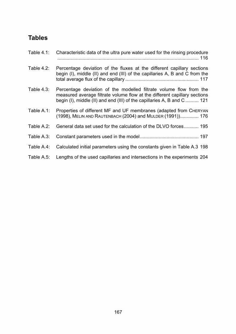
167
Tables
Table 4.1: Characteristic data of the ultra pure water used for the rinsing procedure.......................................................................................................... 116
Table 4.2: Percentage deviation of the fluxes at the different capillary sections begin (I), middle (II) and end (III) of the capillaries A, B and C from the total average flux of the capillary ....................................................... 117
Table 4.3: Percentage deviation of the modelled filtrate volume flow from the measured average filtrate volume flow at the different capillary sections begin (I), middle (II) and end (III) of the capillaries A, B and C .......... 121
Table A.1: Properties of different MF and UF membranes (adapted from CHERYAN (1998), MELIN AND RAUTENBACH (2004) and MULDER (1991)).............. 176
Table A.2: General data set used for the calculation of the DLVO forces........... 195
Table A.3: Constant parameters used in the model............................................ 197
Table A.4: Calculated initial parameters using the constants given in Table A.3 198
Table A.5: Lengths of the used capillaries and intersections in the experiments 204
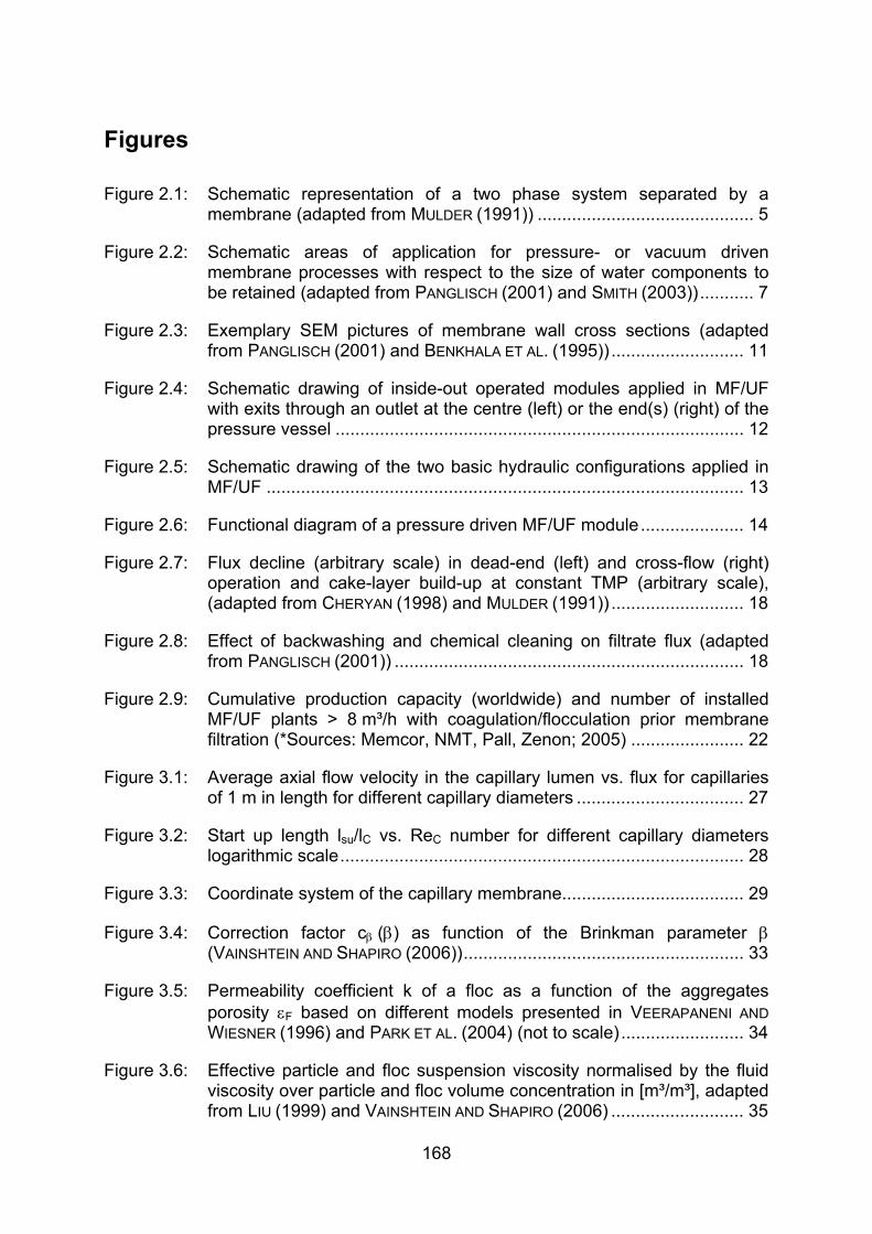
168
Figures
Figure 2.1: Schematic representation of a two phase system separated by a membrane (adapted from MULDER (1991)) ............................................ 5
Figure 2.2: Schematic areas of application for pressure- or vacuum driven membrane processes with respect to the size of water components to be retained (adapted from PANGLISCH (2001) and SMITH (2003))........... 7
Figure 2.3: Exemplary SEM pictures of membrane wall cross sections (adapted from PANGLISCH (2001) and BENKHALA ET AL. (1995)) ........................... 11
Figure 2.4: Schematic drawing of inside-out operated modules applied in MF/UF with exits through an outlet at the centre (left) or the end(s) (right) of the pressure vessel ................................................................................... 12
Figure 2.5: Schematic drawing of the two basic hydraulic configurations applied in MF/UF ................................................................................................. 13
Figure 2.6: Functional diagram of a pressure driven MF/UF module..................... 14
Figure 2.7: Flux decline (arbitrary scale) in dead-end (left) and cross-flow (right) operation and cake-layer build-up at constant TMP (arbitrary scale), (adapted from CHERYAN (1998) and MULDER (1991)) ........................... 18
Figure 2.8: Effect of backwashing and chemical cleaning on filtrate flux (adapted from PANGLISCH (2001)) ....................................................................... 18
Figure 2.9: Cumulative production capacity (worldwide) and number of installed MF/UF plants > 8 m³/h with coagulation/flocculation prior membrane filtration (*Sources: Memcor, NMT, Pall, Zenon; 2005) ....................... 22
Figure 3.1: Average axial flow velocity in the capillary lumen vs. flux for capillaries of 1 m in length for different capillary diameters .................................. 27
Figure 3.2: Start up length lsu/lC vs. ReC number for different capillary diameters logarithmic scale.................................................................................. 28
Figure 3.3: Coordinate system of the capillary membrane..................................... 29
Figure 3.4: Correction factor cβ (β) as function of the Brinkman parameter β (VAINSHTEIN AND SHAPIRO (2006))......................................................... 33
Figure 3.5: Permeability coefficient k of a floc as a function of the aggregates porosity εF based on different models presented in VEERAPANENI AND WIESNER (1996) and PARK ET AL. (2004) (not to scale) ......................... 34
Figure 3.6: Effective particle and floc suspension viscosity normalised by the fluid viscosity over particle and floc volume concentration in [m³/m³], adapted from LIU (1999) and VAINSHTEIN AND SHAPIRO (2006) ........................... 35
Figures
169
Figure 3.7: Hindrance factor and dimensionless floc volume fraction vs. floc volume fraction with a maximum floc volume fraction of φF,max = 0.74, adapted from LIU (1999) .................................................................................... 37
Figure 3.8: Homogeneous drag coefficient Ωh versus floc porosity εF, adapted from VEERAPANENI AND WIESNER (1996) and MASLIYAH ET AL. (1987)............ 39
Figure 3.9: Forces and torques acting on a floc in the laminar fluid flow (schematic)............................................................................................................ 41
Figure 3.10: Determination of the finite distance δFM between the moving floc surface and the membrane wall, (not to scale)................................................. 43
Figure 3.11: Hydrodynamic wall effect of an impermeable wall (MULDER (1990)), a permeable wall (GOREN (1979)) and the approximation given by PANGLISCH (2001) ................................................................................ 45
Figure 3.12: Proportionality constant kvm as function of the dimensionless distance *FMδ of the floc to the membrane wall (adapted from CHELLAM AND
WIESNER (1992)) .................................................................................. 48
Figure 3.13: Geometry and definition of the modelled subdomains and boundaries 62
Figure 3.14: Structured (mapped) mesh of a dimensionless model in 2D ............... 64
Figure 3.15: Schematic diagram of the concentration polarisation and fouling layer inside the capillary lumen (capillary driven in dead-end mode) ........... 74
Figure 3.16: Permeability coefficient kFL based on the Happel and the Carman-Kozeny model respectively vs. porosity of a layer of flocs of radius aF = 29.47 µm...................................................................................... 76
Figure 3.17: 2D section plane for illustration of trajectories ..................................... 77
Figure 3.18: Axial symmetric velocity field and fluid flow streamlines...................... 78
Figure 3.19: Radial velocity contour plot.................................................................. 80
Figure 3.20: Axial velocity contour plot .................................................................... 80
Figure 3.21: Axial velocity v in [m/s] at flux of 80 L/m²/h vs. dimensionless capillary radius r/SR at different axial coordinates (left) and at the capillary axis along the capillary length z/SZ for different modelled fluxes (right) ..... 81
Figure 3.22: Radial velocity u in [m/s] and pressure p in [bar] of the fluid flow at the membrane wall vs. dimensionless capillary length z/SZ...................... 82
Figure 3.23: Velocity flow field and arrow-plot of the velocity inside the capillary .... 83
Figure 3.24: Fluid flow streamlines inside the capillary............................................ 83
Figures
170
Figure 3.25: Floc trajectories of micro flocs of size aF = 0.5 µm inside the capillary driven in dead-end mode..................................................................... 85
Figure 3.26: Resulting surface ring areas, indicated in red, and front section areas, indicated in shaded blue, spanned by pairs of floc trajectories at a radial starting position of r/SR = 0 and r/SR = 0.1 as well as r/SR = 0.5 and r/SR = 0.6 ............................................................................................ 86
Figure 3.27: Floc trajectories of small flocs (aF = 5 µm, black lines) and fluid streamlines (blue dotted lines) inside the capillary driven in dead-end mode (left) and display detail (right) .................................................... 88
Figure 3.28: Floc trajectories of flocs with radius aF = 10 µm (black lines), (left) and with radius aF = 29.47 µm (black lines), (right) and fluid streamlines (blue dotted lines) inside the capillary.................................................. 89
Figure 3.29: Front and rear contact points at dimensionless axial distance to capillary inlet vs. floc radius aF in [µm]............................................................... 90
Figure 3.30: Floc trajectories of flocs with radius aF = 5 µm for different floc surface potentials (left) and display detail (right) .............................................. 92
Figure 3.31: Floc trajectories (display detail) of flocs with radius aF = 5 µm for different ion concentrations, indicated as hardness and indication of range of the characteristic wavelength of interaction floc/membrane wall............................................................................................................ 93
Figure 3.32: DLVO force between floc and membrane wall and between primary particle and membrane wall vs. distance of the surfaces for different and equal sized floc and primary particle radii (Left: aF = 29.47 µm, aP = 12.25 µm; Right: aF = aP = 5 µm) ................................................. 94
Figure 3.33: Floc trajectories of flocs with radius aF = 14.75 µm (scaled to floc radius aF/SR).................................................................................................. 96
Figure 3.34: Floc trajectories of flocs with radius aF = 29.47 µm (scaled to floc radius aF/SR).................................................................................................. 96
Figure 3.35: Floc trajectories of flocs with radius aF = 5 µm, rel. density of the flocs set to 1.05 (left) and trajectories of quartz particles with radius aQP = 5 µm, rel. density of the quartz particles set to 2.65 (right)......... 97
Figure 3.36: Trajectories of flocs (rel. density of 1.05) and quartz particles (rel. density of 2.65) with radius aF = aQP = 5 µm (left) and aF = aQP = 29.47 µm (right) in a vertical aligned capillary, bottom-up operation ............................................................................................. 98
Figure 3.37: Trajectories of flocs (rel. density of 1.05) and quartz particles (rel. density of 2.65) with radius aF = aQP = 5 µm (left) and aF = aQP = 29.47 µm (right) in a vertical aligned capillary, top-down operation............................................................................................................ 99
Figures
171
Figure 3.38: Floc trajectories and resulting equilibrium trajectories of flocs (aF = 29.47 µm, aP = 12.25 µm) with different porosities (left) and display detail (right) ........................................................................... 101
Figure 3.39: Floc trajectories of different sized flocs within the capillary ............... 102
Figure 3.40: Shear gradients G in [1/s] within the capillary, driven in dead-end mode at a flux of 80 L/m²/h.......................................................................... 103
Figure 3.41: Floc volume concentration φF of flocs of radius aF = 29.47 µm vs. dimensionless capillary radius r/SR at different dimensionless capillary lengths z/SZ (display detail)............................................................... 104
Figure 3.42: Fouling layer height δFL in [mm] (left) and transmembrane pressure (TMP) in [Pa] (right) vs. dimensionless capillary length after different filtration times of flocs of radius aF = 5 µm......................................... 105
Figure 3.43: Floc trajectories of flocs with radius aF = 5 µm at different times of filtration (left) and display detail (right)............................................... 107
Figure 4.1: Optical microscope photographs of the used ABS latex microspheres.......................................................................................................... 110
Figure 4.2: Zeta potential ζ of the used ABS latex microspheres at different pH-values (NAHRSTEDT (1999))................................................................ 111
Figure 4.3: Distributive q3(x) and cumulative Q3(x) percentage volume distribution of the primary particles (ABS) and the floc suspension at capillary entrance (error bars represent 99 % confidence interval).................. 112
Figure 4.4: Setup of the designed and used test unit for single capillaries .......... 114
Figure 4.5: Configuration of the pressure pipe used in the test unit..................... 114
Figure 4.6: Initial membrane resistances RM at three different capillary sections (begin, middle and end) of the investigated capillaries A, B and C.... 116
Figure 4.7: Flux in [L/m²/h] vs. time in [min] at the three sections begin (I), middle (II) and end (III) of the capillaries A, B and C, operated in dead-end. 118
Figure 4.8: Measured transmembrane pressure (TMP) in [kPa] vs. time in [min] during operation of the capillaries A, B and C.................................... 119
Figure 4.9: Filtrate volume flow in [mL/h] of the models at time t = 0 vs. dimensionless capillary length z and average filtrate volume flow in [mL/h] of the experiments at the different capillary sections begin (I), middle (II) and end (III) of the capillaries A, B and C ......................... 120
Figure 4.10: Floc trajectories of flocs with radius aF = 5 µm (left) and aF = 29.47 µm as display detail (right) of the modelled experimental data................ 122
Figures
172
Figure 4.11: Sampling points of the single capillaries used in the experiments ..... 123
Figure 4.12: Total iron in [µg/cm] at different sampling points at the capillary sections begin (B), middle (M) and end (E) of the capillaries A, B and C ........ 124
Figure 4.13: Fractions of deposited primary particles after filtration (TMP = 0.7 bar, average flux of approx. 157 L/m²/h) as uncoagulated suspension vs. dimensionless capillary length z/SZ and primary particle radius aP ... 126
Figure 4.14: Fractions of deposited primary particles after filtration (TMP = 0.7 bar, average flux of approx. 179 L/m²/h) as coagulated suspension vs. dimensionless capillary length z/SZ and primary particle radius aP ... 127
Figure 4.15: Fractions of deposited primary particles after filtration (TMP = 0.7 bar, average flux of approx. 250 L/m²/h) as coagulated suspension vs. dimensionless capillary length z/SZ and primary particle radius aP ... 127
Figure 5.1: Floc trajectories for models with 5 % (left) and 20 % (right) average cross-flow velocity at the capillary outlet............................................ 131
Figure 5.2: Floc trajectories of flocs with radius aF = 29.47 µm. Capillary operated at 200 L/m²/h and 20 % average cross-flow velocity at the capillary outlet.................................................................................................. 132
Figure 5.3: Floc trajectories of flocs with radius aF = 29.47 µm, ballasted with micro sand (relative density of 1.72) within a vertical aligned capillary, operated at 80 L/m²/h in top-down dead-end mode........................... 134
Figure A.1: ReC number vs. average axial flow velocity in the capillary lumen at T = 20°C for different capillary diameters and indication of the critical Re for non-porous tube flow and porous tube flow in half logarithmic scale.......................................................................................................... 177
Figure A.2: ReC numbers vs. average axial flow velocity, typical for fluxes up to 100 L/m²/h, for different capillary diameters at T = 20°C and indication of the critical Re for non-porous tube flow and porous tube flow in half logarithmic scale................................................................................ 177
Figure A.3: Approximation of the hydrodynamic wall effect (translation of a spherical rigid floc in r-direction) as a function of the dimensionless floc distance for a floc with radius aF = 29.47 µm and a membrane resistance RM = 5.24·1011 1/m ............................................................................ 182
Figure A.4: Hydrodynamic wall effect (translation of a spherical, rigid floc in z-direction) as a function of the dimensionless floc distance ................ 183
Figure A.5: Hydrodynamic wall effect (translation of a spherical, rigid floc in ϕ-direction) as a function of the dimensionless floc distance ................ 184
Figures
173
Figure A.6: Hydrodynamic wall effect (rotation of a stationary, spherical and rigid floc in stationary fluid in z-direction) as a function of the dimensionless floc distance....................................................................................... 185
Figure A.7: Hydrodynamic wall effect (rotation of a stationary, spherical and rigid floc in stationary fluid in ϕ-direction) as a function of the dimensionless floc distance....................................................................................... 186
Figure A.8: Hydrodynamic wall effect (fluid flow around a stationary, spherical and rigid floc in z-direction) as a function of the dimensionless floc distance.......................................................................................................... 187
Figure A.9: Hydrodynamic wall effect (fluid flow around a stationary, spherical and rigid floc in r-direction) as a function of the dimensionless floc distance.......................................................................................................... 188
Figure A.10: Hydrodynamic wall effect (fluid flow around a stationary, spherical and rigid floc in ϕ-direction) as a function of the dimensionless floc distance.......................................................................................................... 189
Figure A.11: Polynomial fit of the lift velocity experienced by a neutrally buoyant spherical particle or floc in a Poiseuille pipe flow as presented by PANGLISCH (2001) and OTIS ET AL. (1986), cited in CHELLAM AND WIESNER (1992) ................................................................................................ 191
Figure A.12: Polynomial fit of the lift velocity experienced by a nonneutrally buoyant spherical floc in a Poiseuille pipe flow adapted from VASSEUR AND COX (1976) ................................................................................................ 191
Figure A.13: Configuration of the electric double layer at a suspended negatively charged particle and resulting distribution of the charge potential as function of distance (adapted from NAHRSTEDT (1999)) ..................... 193
Figure A.14: DLVO sum, London–van der Waals and electric double layer forces between a primary particle of radius aP = 12.25 µm and the membrane wall .................................................................................................... 196
Figure A.15: DLVO sum, London–van der Waals and electric double layer forces between an iron hydroxide floc of radius aF = 29.47 µm and the membrane wall .................................................................................. 196
Figure A.16: Axial symmetric velocity field and fluid flow streamlines at capillary inlet, display detail of Figure 3.18............................................................... 199
Figure A.17: Unstructured mesh of the dimensionless model in 3D....................... 201
Figure A.18: Fractions of deposited primary particles after filtration (TMP = 0.4 bar, average flux unknown) as uncoagulated suspension vs. dimensionless capillary length z/SZ and primary particle radius aP........................... 205
Figures
174
Figure A.19: Fractions of deposited primary particles after filtration (TMP = 0.4 bar, average flux of approx. 151 L/m²/h) as coagulated suspension vs. dimensionless capillary length z/SZ and primary particle radius aP ... 206
Figure A.20: Fractions of deposited primary particles after filtration (TMP = 0.4 bar, average flux of approx. 186 L/m²/h) as coagulated suspension vs. dimensionless capillary length z/SZ and primary particle radius aP ... 206
Figure A.21: Fractions of deposited primary particles after filtration (TMP = 0.4 bar, average flux of approx. 156 L/m²/h) as coagulated suspension vs. dimensionless capillary length z/SZ and primary particle radius aP ... 207
Figure A.22: Fractions of deposited primary particles after filtration (TMP = 0.4 bar, average flux of approx. 198 L/m²/h) as coagulated suspension vs. dimensionless capillary length z/SZ and primary particle radius aP ... 207
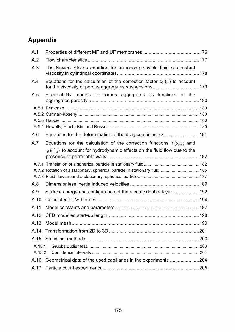
175
Appendix
A.1 Properties of different MF and UF membranes ..........................................176
A.2 Flow characteristics ....................................................................................177
A.3 The Navier- Stokes equation for an incompressible fluid of constant viscosity in cylindrical coordinates..............................................................178
A.4 Equations for the calculation of the correction factor cβ (β) to account for the viscosity of porous aggregates suspensions...................................179
A.5 Permeability models of porous aggregates as functions of the aggregates porosity ε .................................................................................180
A.5.1 Brinkman ...............................................................................................................180 A.5.2 Carman-Kozeny.....................................................................................................180 A.5.3 Happel ...................................................................................................................180 A.5.4 Howells, Hinch, Kim and Russel............................................................................180
A.6 Equations for the determination of the drag coefficient Ω...........................181
A.7 Equations for the calculation of the correction functions )(f *FMδ and
)(g *FMδ to account for hydrodynamic effects on the fluid flow due to the
presence of permeable walls......................................................................182 A.7.1 Translation of a spherical particle in stationary fluid ..............................................182 A.7.2 Rotation of a stationary, spherical particle in stationary fluid.................................185 A.7.3 Fluid flow around a stationary, spherical particle...................................................187
A.8 Dimensionless inertia induced velocities ....................................................189
A.9 Surface charge and configuration of the electric double layer ....................192
A.10 Calculated DLVO forces .............................................................................194
A.11 Model constants and parameters ...............................................................197
A.12 CFD modelled start-up length.....................................................................198
A.13 Model mesh................................................................................................199
A.14 Transformation from 2D to 3D ....................................................................201
A.15 Statistical methods .....................................................................................203 A.15.1 Grubbs outlier test.............................................................................................203 A.15.2 Confidence intervals .........................................................................................204
A.16 Geometrical data of the used capillaries in the experiments ......................204
A.17 Particle count experiments .........................................................................205
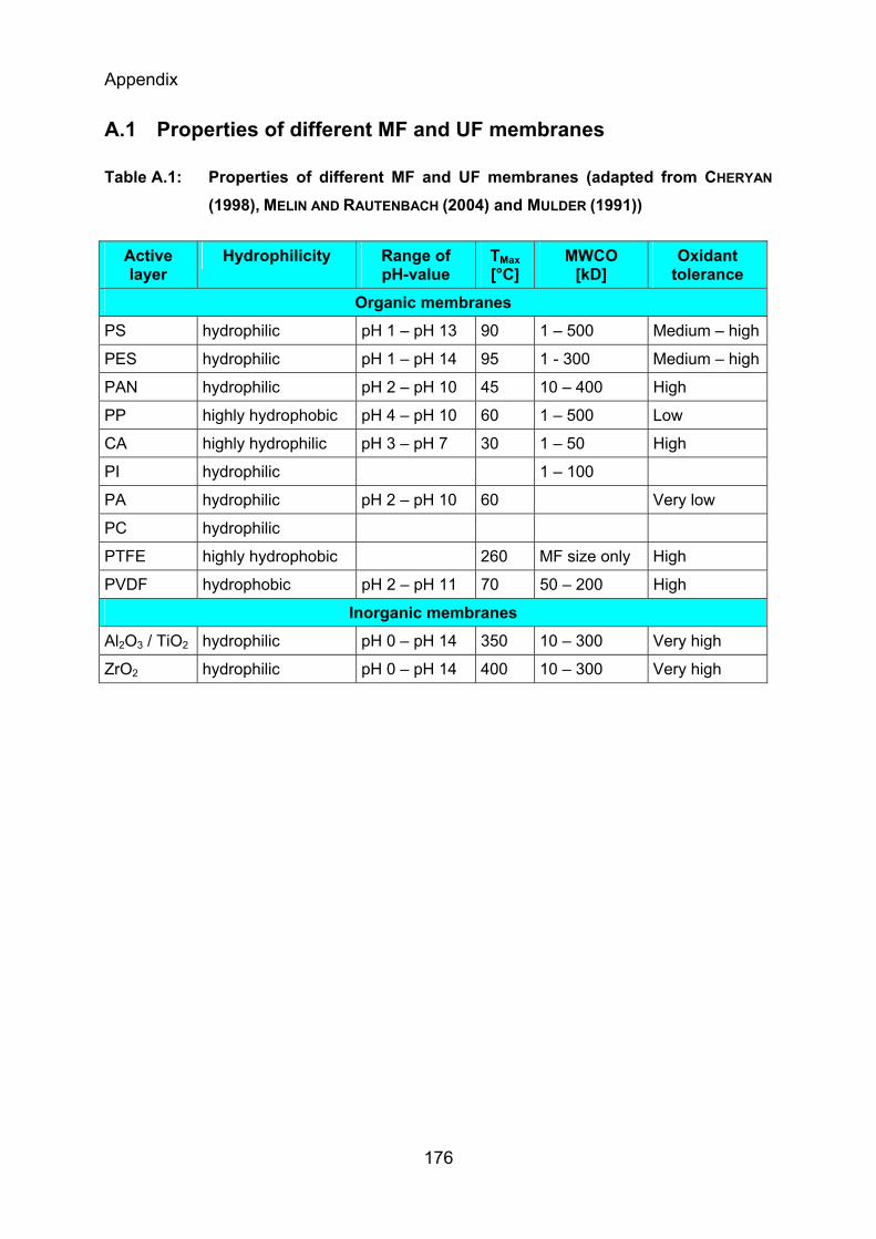
Appendix
176
A.1 Properties of different MF and UF membranes
Table A.1: Properties of different MF and UF membranes (adapted from CHERYAN
(1998), MELIN AND RAUTENBACH (2004) and MULDER (1991))
Active layer
Hydrophilicity Range of pH-value
TMax [°C]
MWCO [kD]
Oxidant tolerance
Organic membranes
PS hydrophilic pH 1 – pH 13 90 1 – 500 Medium – high
PES hydrophilic pH 1 – pH 14 95 1 - 300 Medium – high
PAN hydrophilic pH 2 – pH 10 45 10 – 400 High
PP highly hydrophobic pH 4 – pH 10 60 1 – 500 Low
CA highly hydrophilic pH 3 – pH 7 30 1 – 50 High
PI hydrophilic 1 – 100
PA hydrophilic pH 2 – pH 10 60 Very low
PC hydrophilic
PTFE highly hydrophobic 260 MF size only High
PVDF hydrophobic pH 2 – pH 11 70 50 – 200 High
Inorganic membranes
Al2O3 / TiO2 hydrophilic pH 0 – pH 14 350 10 – 300 Very high
ZrO2 hydrophilic pH 0 – pH 14 400 10 – 300 Very high
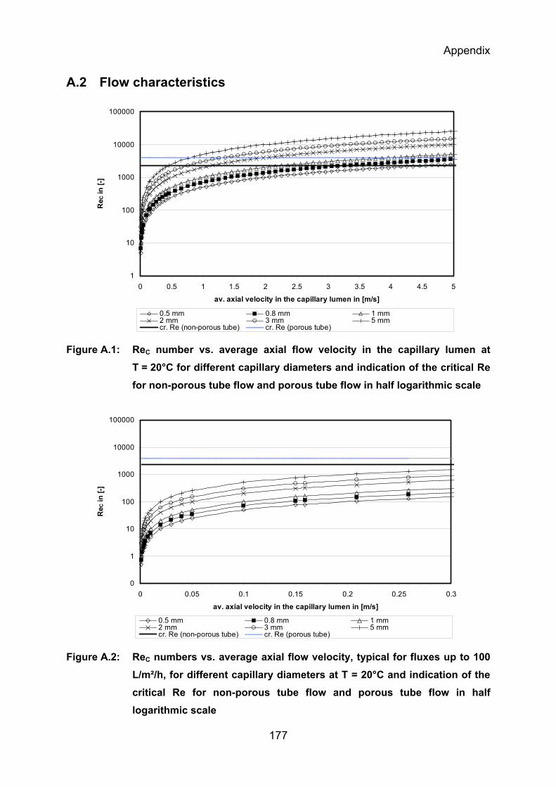
Appendix
177
A.2 Flow characteristics
1
10
100
1000
10000
100000
0 0.5 1 1.5 2 2.5 3 3.5 4 4.5 5
av. axial velocity in the capillary lumen in [m/s]
Re C
in [-
]
0.5 mm 0.8 mm 1 mm2 mm 3 mm 5 mmcr. Re (non-porous tube) cr. Re (porous tube)
Figure A.1: ReC number vs. average axial flow velocity in the capillary lumen at T = 20°C for different capillary diameters and indication of the critical Re for non-porous tube flow and porous tube flow in half logarithmic scale
0
1
10
100
1000
10000
100000
0 0.05 0.1 0.15 0.2 0.25 0.3
av. axial velocity in the capillary lumen in [m/s]
Re C
in [-
]
0.5 mm 0.8 mm 1 mm2 mm 3 mm 5 mmcr. Re (non-porous tube) cr. Re (porous tube)
Figure A.2: ReC numbers vs. average axial flow velocity, typical for fluxes up to 100 L/m²/h, for different capillary diameters at T = 20°C and indication of the critical Re for non-porous tube flow and porous tube flow in half logarithmic scale
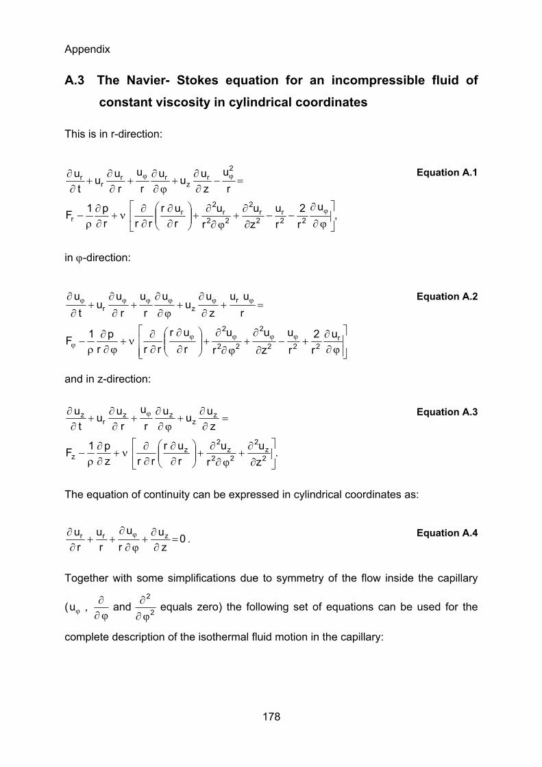
Appendix
178
A.3 The Navier- Stokes equation for an incompressible fluid of constant viscosity in cylindrical coordinates
This is in r-direction:
,u
r2
ru
zu
ru
rur
rrrp1F
ru
zuuu
ru
ruu
tu
22r
2r
2
22r
2r
r
2r
zrr
rr
⎥⎦
⎤⎢⎣
⎡
ϕ∂
∂−−
∂∂
+ϕ∂
∂+⎟⎟
⎠
⎞⎜⎜⎝
⎛∂∂
∂∂
ν+∂∂
ρ−
=−∂∂
+ϕ∂
∂+
∂∂
+∂
∂
ϕ
ϕϕ
Equation A.1
in ϕ-direction:
⎥⎥⎦
⎤
⎢⎢⎣
⎡
ϕ∂∂
+−∂
∂+
ϕ∂
∂+⎟⎟
⎠
⎞⎜⎜⎝
⎛∂
∂
∂∂
ν+ϕ∂
∂ρ
−
=+∂
∂+
ϕ∂
∂+
∂
∂+
∂
∂
ϕϕϕϕϕ
ϕϕϕϕϕϕ
r222
2
22
2
rzr
ur2
ru
zu
ru
rur
rrrp1F
ruu
zu
uu
ru
ru
ut
u
Equation A.2
and in z-direction:
.zu
ru
rur
rrzp1F
zuuu
ru
ruu
tu
2z
2
22z
2z
z
zz
zzr
z
⎥⎦
⎤⎢⎣
⎡
∂∂
+ϕ∂
∂+⎟⎟
⎠
⎞⎜⎜⎝
⎛∂∂
∂∂
ν+∂∂
ρ−
=∂∂
+ϕ∂
∂+
∂∂
+∂
∂ ϕ
Equation A.3
The equation of continuity can be expressed in cylindrical coordinates as:
0z
ur
uru
ru zrr =
∂∂
+ϕ∂
∂++
∂∂ ϕ . Equation A.4
Together with some simplifications due to symmetry of the flow inside the capillary
( 2
2and,u
ϕ∂∂
ϕ∂∂
ϕ equals zero) the following set of equations can be used for the
complete description of the isothermal fluid motion in the capillary:
Appendix
179
,ru
zu
rur
rrrp1F
zuu
ruu
tu
2r
2r
2r
rr
zr
rr ⎥
⎦
⎤⎢⎣
⎡−
∂∂
+⎟⎟⎠
⎞⎜⎜⎝
⎛∂∂
∂∂
ν+∂∂
ρ−=
∂∂
+∂∂
+∂
∂
Equation A.5
,zu
rur
rrzp1F
zuu
ruu
tu
2z
2z
zz
zz
rz ⎥
⎦
⎤⎢⎣
⎡
∂∂
+⎟⎟⎠
⎞⎜⎜⎝
⎛∂∂
∂∂
ν+∂∂
ρ−=
∂∂
+∂
∂+
∂∂
Equation A.6
0z
uru
ru zrr =
∂∂
++∂
∂. Equation A.7
A.4 Equations for the calculation of the correction factor cβ (β) to
account for the viscosity of porous aggregates suspensions
VAINSHTEIN AND SHAPIRO (2006) presented extended equations for the calculation of
the correction function cβ (β) with:
( )15c2c
Δ⋅Δ⋅
=ββ , Equation A.8
kaF=β , Equation A.9
( )( )
( )( ) ⎟⎟
⎠
⎞⎜⎜⎝
⎛
β⋅ββ⋅
+β
+⎟⎟⎠
⎞⎜⎜⎝
⎛
β⋅ββ⋅
−β
⋅⎟⎟⎠
⎞⎜⎜⎝
⎛
β+=Δ
12
33
12
221 f
f10112ff10241 , Equation A.10
( )( )
( )( ) ⎟⎟
⎠
⎞⎜⎜⎝
⎛
β⋅ββ⋅
+β
+⎟⎟⎠
⎞⎜⎜⎝
⎛
β⋅ββ⋅
−β
=Δ1
23
12
2
ff1013
ff102c , Equation A.11
( ) β⎟⎟⎠
⎞⎜⎜⎝
⎛
β+
β+−β⎟⎟
⎠
⎞⎜⎜⎝
⎛+
ββ=β sinh30151cosh165f 4221 , Equation A.12
( ) β⎟⎟⎠
⎞⎜⎜⎝
⎛
β+
β−β⎟⎟
⎠
⎞⎜⎜⎝
⎛+
β=β sinh63cosh16f 322 , and Equation A.13
( ) β⎟⎟⎠
⎞⎜⎜⎝
⎛
β++β
β−=β sinh31cosh3f 23 . Equation A.14
The equations given above show that for the limit ∞→β , ( )ββc will become unity
corresponding to the flow around an impermeable particle or floc. The correction
function ( )ββc is illustrated in Figure 3.4.
Appendix
180
A.5 Permeability models of porous aggregates as functions of the
aggregates porosity ε
The following permeability models of porous aggregates as functions of the
aggregates porosity ε, as presented by VEERAPANENI AND WIESNER (1996) and PARK
ET AL. (2004), were used for the illustration in Figure 3.5. For a more detailed
description of the models please refer to VEERAPANENI AND WIESNER (1996) and PARK
ET AL. (2004) and references therein.
A.5.1 Brinkman
⎟⎟⎠
⎞⎜⎜⎝
⎛−
ε−−
ε−+= 3
183
143
18ak
FF
2P
Brinkmann , Equation A.15
where εF denotes the floc porosity and aP denotes the primary particle radius.
A.5.2 Carman-Kozeny
( )
2 3P F
Carman Kozeny 2F
ak45 1
−
ε=
− ε. Equation A.16
A.5.3 Happel
( )5
65
3
2P
Happel 23
32
92
939
a2
kγ⋅+
⎟⎟⎠
⎞⎜⎜⎝
⎛γ⋅−
γ⋅+
γ⋅−
γ⋅⋅
=
Equation A.17
and
( ) 31
F1 ε−=γ . Equation A.18
A.5.4 Howells, Hinch, Kim and Russel
( )( ) ( ) ( )
( ) ⎟⎟⎟
⎠
⎞
⎜⎜⎜
⎝
⎛
ε−⋅+
ε−⋅ε−⋅+ε−⋅+
ε−⋅⋅
=
F
FFF
F
2P
HHKR
1456.16
1ln164
13512
3119
a2k Equation A.19
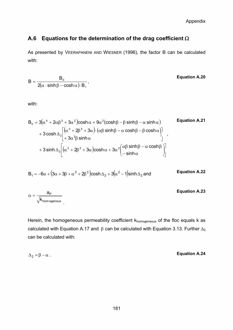
Appendix
181
A.6 Equations for the determination of the drag coefficient Ω
As presented by VEERAPANENI AND WIESNER (1996), the factor B can be calculated
with:
( ) 1
0
Bcoshsinh2B
B⋅α−β⋅α
= , Equation A.20
with:
( ) ( )( ) ( )
( ) ⎥⎦
⎤⎢⎣
⎡⎟⎟⎠
⎞⎜⎜⎝
⎛α−
βα−βαβα+αα+β+αΔ+
⎥⎦
⎤⎢⎣
⎡
αβα+
αβ−βα−βαβ⋅α+β+αΔ+
αα−ββ−βα+αα+αβ+α=
sinhcoshsinh
3cosh32sinh3
sinh3coshcoshsinh32
cosh3
sinhsinhcosh9cosh323B
2332
2
33
2
22340
,
Equation A.21
( ) ( ) 22
233
1 sinh13cosh2336B Δ−α+Δβ+α+β+α+α−= and Equation A.22
ogenoushom
P
ka
=α
.
Equation A.23
Herein, the homogeneous permeability coefficient khomogeneous of the floc equals k as
calculated with Equation A.17 and β can be calculated with Equation 3.13. Further Δ2
can be calculated with:
α−β=Δ2 . Equation A.24
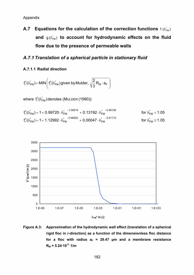
Appendix
182
A.7 Equations for the calculation of the correction functions )(f *FMδ
and )(g *FMδ to account for hydrodynamic effects on the fluid
flow due to the presence of permeable walls
A.7.1 Translation of a spherical particle in stationary fluid
A.7.1.1 Radial direction
⎟⎟⎠
⎞⎜⎜⎝
⎛⋅δ=δ FM
*FM
tr
*FM
tr aR
32,Mulderbygiven)(fMIN)(f
where )(f *FM
tr δ denotes (MULDER (1990)):
05.1for00047.012992.11)(f
05.1for13192.099720.01)(f*FM
01113.0*FM
99252.0*FM
*FM
tr
*FM
46139.0*FM
00014.1*FM
*FM
tr
≥δδ⋅+δ⋅+=δ
<δδ⋅+δ⋅+=δ−−
−−
0
500
1000
1500
2000
2500
3000
3500
1.E-09 1.E-07 1.E-05 1.E-03 1.E-01 1.E+01 1.E+03
δFM* in [-]
f rt ( δFM
*) in
[-]
Figure A.3: Approximation of the hydrodynamic wall effect (translation of a spherical rigid floc in r-direction) as a function of the dimensionless floc distance for a floc with radius aF = 29.47 µm and a membrane resistance RM = 5.24·1011 1/m
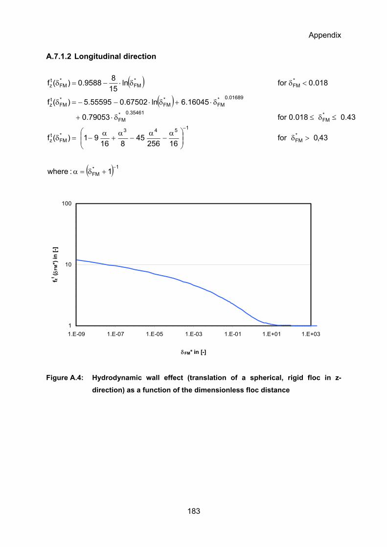
Appendix
183
A.7.1.2 Longitudinal direction
( )( )
( ) 1*FM
*FM
1543*FM
tz
*FM
35461.0*FM
01689.0*FM
*FM
*FM
tz
*FM
*FM
*FM
tz
1:where
43,0for16256
45816
91)(f
43.0018.0for79053.0
16045.6ln67502.055595.5)(f
018.0forln1589588.0)(f
−
−
+δ=α
>δ⎟⎟⎠
⎞⎜⎜⎝
⎛ α−
α−
α+
α−=δ
≤δ≤δ⋅+
δ⋅+δ⋅−−=δ
<δδ⋅−=δ
1
10
100
1.E-09 1.E-07 1.E-05 1.E-03 1.E-01 1.E+01 1.E+03
δFM* in [-]
f zt ( δFM
*) in
[-]
Figure A.4: Hydrodynamic wall effect (translation of a spherical, rigid floc in z-direction) as a function of the dimensionless floc distance
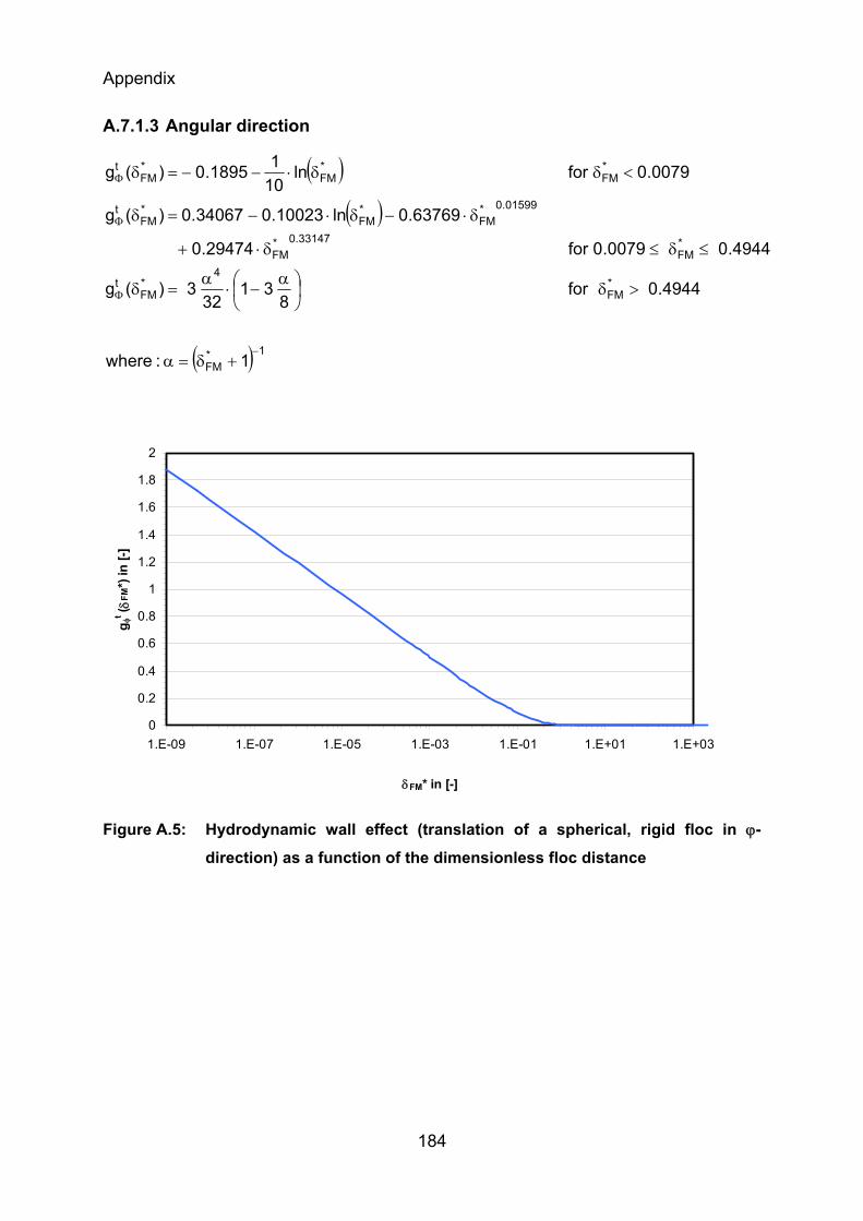
Appendix
184
A.7.1.3 Angular direction
( )( )
( ) 1*FM
*FM
4*FM
t
*FM
33147.0*FM
01599.0*FM
*FM
*FM
t
*FM
*FM
*FM
t
1:where
4944.0for8
3132
3)(g
4944.00079.0for29474.0
63769.0ln10023.034067.0)(g
0079.0forln1011895.0)(g
−
Φ
Φ
Φ
+δ=α
>δ⎟⎠⎞
⎜⎝⎛ α
−⋅α
=δ
≤δ≤δ⋅+
δ⋅−δ⋅−=δ
<δδ⋅−−=δ
0
0.2
0.4
0.6
0.8
1
1.2
1.4
1.6
1.8
2
1.E-09 1.E-07 1.E-05 1.E-03 1.E-01 1.E+01 1.E+03
δFM* in [-]
g φt ( δ
FM*)
in [-
]
Figure A.5: Hydrodynamic wall effect (translation of a spherical, rigid floc in ϕ-
direction) as a function of the dimensionless floc distance
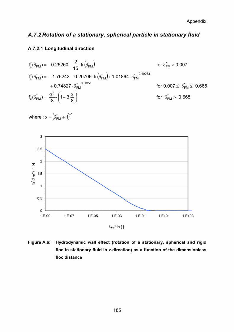
Appendix
185
A.7.2 Rotation of a stationary, spherical particle in stationary fluid
A.7.2.1 Longitudinal direction
( )( )
( ) 1*FM
*FM
4*FM
rz
*FM
00226.0*FM
19263.0*FM
*FM
*FM
rz
*FM
*FM
*FM
rz
1:where
665.0for8
318
)(f
665.0007.0for74827.0
01864.1ln20706.076242.1)(f
007.0forln15225260.0)(f
−+δ=α
>δ⎟⎠⎞
⎜⎝⎛ α
−⋅α
=δ
≤δ≤δ⋅+
δ⋅+δ⋅−−=δ
<δδ⋅−−=δ
0
0.5
1
1.5
2
2.5
3
1.E-09 1.E-07 1.E-05 1.E-03 1.E-01 1.E+01 1.E+03
δFM* in [-]
f zr ( δFM
*) in
[-]
Figure A.6: Hydrodynamic wall effect (rotation of a stationary, spherical and rigid floc in stationary fluid in z-direction) as a function of the dimensionless floc distance
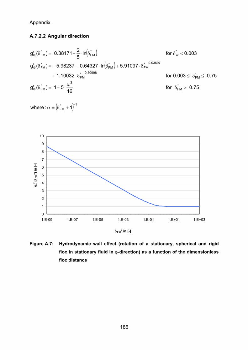
Appendix
186
A.7.2.2 Angular direction
( )( )
( ) 1*FM
*FM
3*FM
r
*FM
30998.0*FM
03697.0*FM
*FM
*FM
r
*w
*FM
*FM
r
1:where
75.0for16
51)(g
75.0003.0for10032.1
91097.5ln64327.098237.5)(g
003.0forln5238171.0)(g
−
Φ
Φ
Φ
+δ=α
>δα
+=δ
≤δ≤δ⋅+
δ⋅+δ⋅−−=δ
<δδ⋅−=δ
0
1
2
3
4
5
6
7
8
9
10
1.E-09 1.E-07 1.E-05 1.E-03 1.E-01 1.E+01 1.E+03
δFM* in [-]
g φr ( δ
FM*)
in [-
]
Figure A.7: Hydrodynamic wall effect (rotation of a stationary, spherical and rigid
floc in stationary fluid in ϕ-direction) as a function of the dimensionless
floc distance
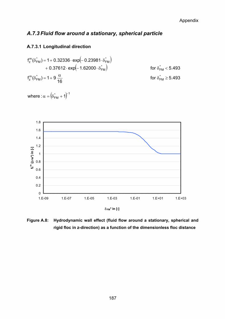
Appendix
187
A.7.3 Fluid flow around a stationary, spherical particle
A.7.3.1 Longitudinal direction
( )( )
( ) 1*FM
*FM
*FM
mz
*FM
*FM
*FM
*FM
mz
1:where
493.5for16
91)(f
493.5for62000.1exp37612.0
23981.0exp32336.01)(f
−+δ=α
≥δα
+=δ
<δδ⋅−⋅+
δ⋅−⋅+=δ
0
0.2
0.4
0.6
0.8
1
1.2
1.4
1.6
1.8
1.E-09 1.E-07 1.E-05 1.E-03 1.E-01 1.E+01 1.E+03
δFM* in [-]
f zm ( δ
FM*)
in [-
]
Figure A.8: Hydrodynamic wall effect (fluid flow around a stationary, spherical and rigid floc in z-direction) as a function of the dimensionless floc distance
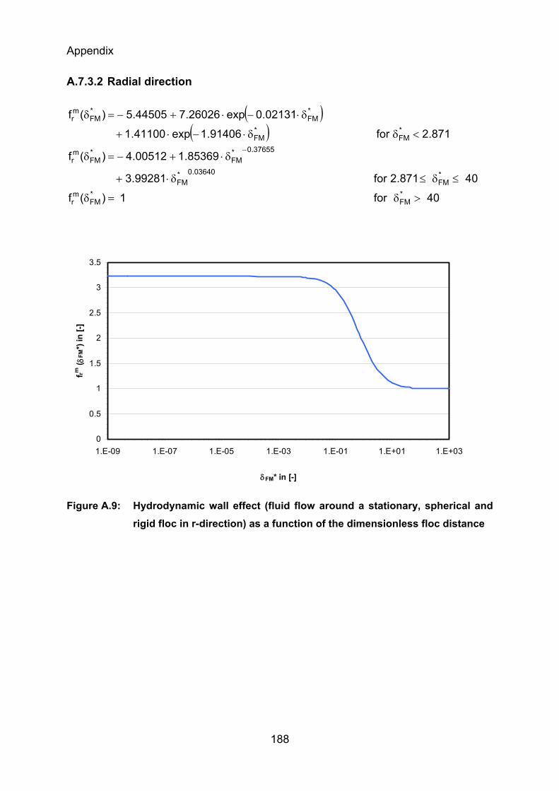
Appendix
188
A.7.3.2 Radial direction
( )( )
40for1)(f
40871.2for99281.3
85369.100512.4)(f
871.2for91406.1exp41100.1
02131.0exp26026.744505.5)(f
*FM
*FM
mr
*FM
03640.0*FM
37655.0*FM
*FM
mr
*FM
*FM
*FM
*FM
mr
>δ=δ
≤δ≤δ⋅+
δ⋅+−=δ
<δδ⋅−⋅+
δ⋅−⋅+−=δ
−
0
0.5
1
1.5
2
2.5
3
3.5
1.E-09 1.E-07 1.E-05 1.E-03 1.E-01 1.E+01 1.E+03
δFM* in [-]
f rm ( δ
FM*)
in [-
]
Figure A.9: Hydrodynamic wall effect (fluid flow around a stationary, spherical and rigid floc in r-direction) as a function of the dimensionless floc distance
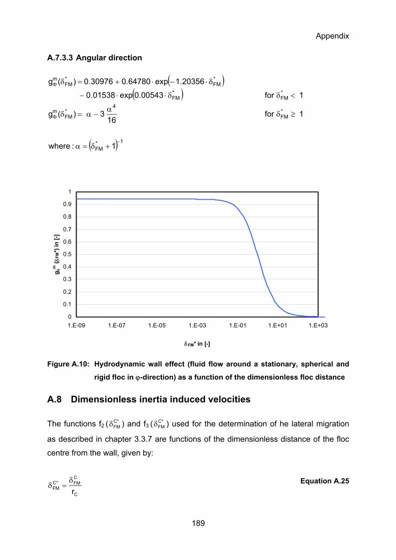
Appendix
189
A.7.3.3 Angular direction
( )( )
( ) 1*FM
*FM
4*FM
m
*FM
*FM
*FM
*FM
m
1:where
1for16
3)(g
1for00543.0exp01538.0
20356.1exp64780.030976.0)(g
−
Φ
Φ
+δ=α
≥δα
−α=δ
<δδ⋅⋅−
δ⋅−⋅+=δ
0
0.1
0.2
0.3
0.4
0.5
0.6
0.7
0.8
0.9
1
1.E-09 1.E-07 1.E-05 1.E-03 1.E-01 1.E+01 1.E+03
δFM* in [-]
g φm
( δFM
*) in
[-]
Figure A.10: Hydrodynamic wall effect (fluid flow around a stationary, spherical and
rigid floc in ϕ-direction) as a function of the dimensionless floc distance
A.8 Dimensionless inertia induced velocities
The functions f2 ( *CFMδ ) and f3 ( *C
FMδ ) used for the determination of he lateral migration
as described in chapter 3.3.7 are functions of the dimensionless distance of the floc
centre from the wall, given by:
C
CFM*C
FM rδ
=δ Equation A.25
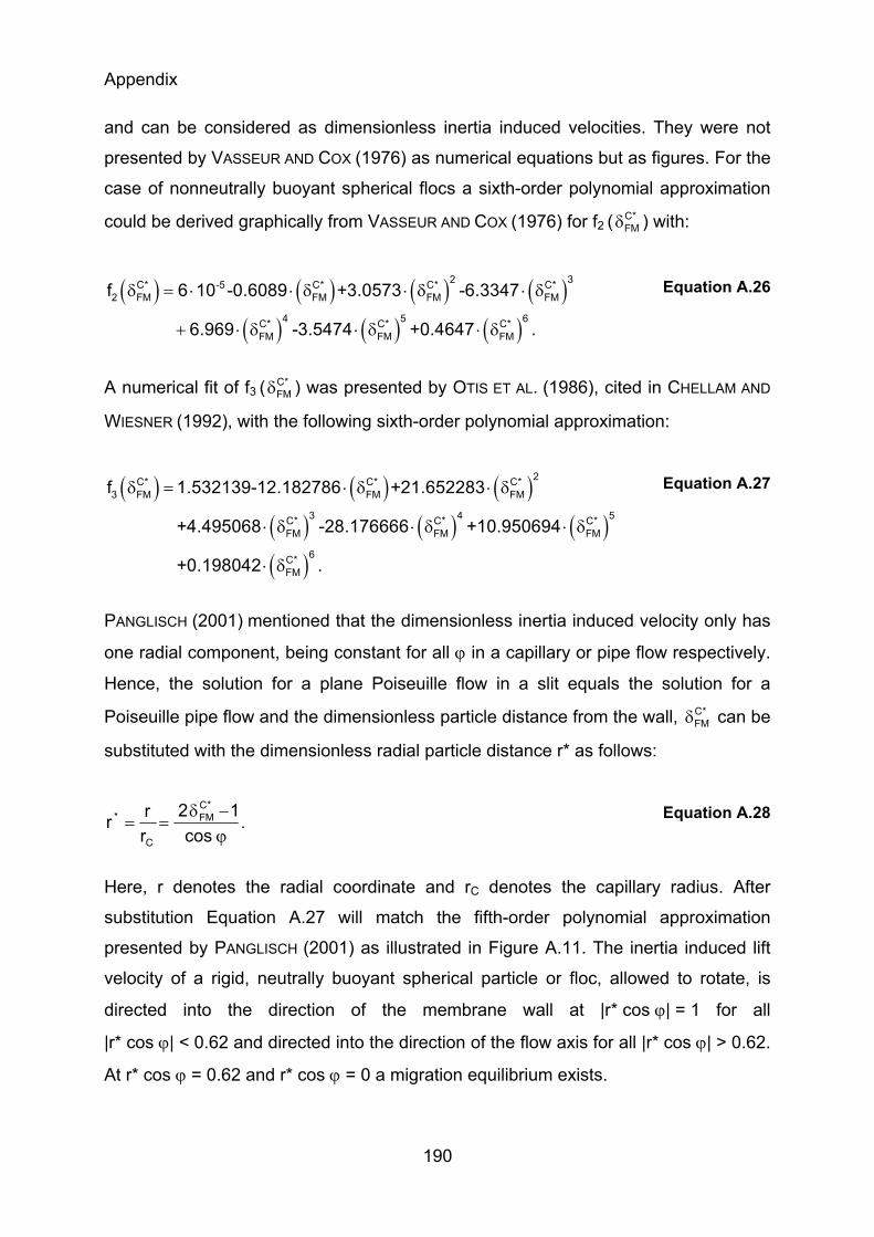
Appendix
190
and can be considered as dimensionless inertia induced velocities. They were not
presented by VASSEUR AND COX (1976) as numerical equations but as figures. For the
case of nonneutrally buoyant spherical flocs a sixth-order polynomial approximation
could be derived graphically from VASSEUR AND COX (1976) for f2 ( *CFMδ ) with:
( ) ( ) ( ) ( )( ) ( ) ( )
2 3C* -5 C* C* C*2 FM FM FM FM
4 5 6C* C* C*FM FM FM
f 6 10 -0.6089 +3.0573 -6.3347
6.969 -3.5474 +0.4647 .
δ = ⋅ ⋅ δ ⋅ δ ⋅ δ
+ ⋅ δ ⋅ δ ⋅ δ
Equation A.26
A numerical fit of f3 ( *CFMδ ) was presented by OTIS ET AL. (1986), cited in CHELLAM AND
WIESNER (1992), with the following sixth-order polynomial approximation:
( ) ( ) ( )( ) ( ) ( )( )
2C* C* C*3 FM FM FM
3 4 5C* C* C*FM FM FM
6C*FM
f 1.532139-12.182786 +21.652283
+4.495068 -28.176666 +10.950694
+0.198042 .
δ = ⋅ δ ⋅ δ
⋅ δ ⋅ δ ⋅ δ
⋅ δ
Equation A.27
PANGLISCH (2001) mentioned that the dimensionless inertia induced velocity only has
one radial component, being constant for all ϕ in a capillary or pipe flow respectively.
Hence, the solution for a plane Poiseuille flow in a slit equals the solution for a
Poiseuille pipe flow and the dimensionless particle distance from the wall, *CFMδ can be
substituted with the dimensionless radial particle distance r* as follows:
ϕ−δ
==cos
12rrr
*CFM
C
* . Equation A.28
Here, r denotes the radial coordinate and rC denotes the capillary radius. After
substitution Equation A.27 will match the fifth-order polynomial approximation
presented by PANGLISCH (2001) as illustrated in Figure A.11. The inertia induced lift
velocity of a rigid, neutrally buoyant spherical particle or floc, allowed to rotate, is
directed into the direction of the membrane wall at |r* cos ϕ| = 1 for all
|r* cos ϕ| < 0.62 and directed into the direction of the flow axis for all |r* cos ϕ| > 0.62.
At r* cos ϕ = 0.62 and r* cos ϕ = 0 a migration equilibrium exists.
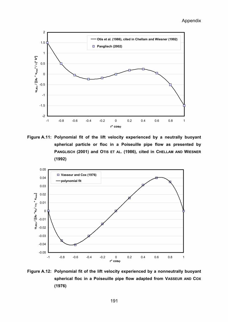
Appendix
191
-2
-1.5
-1
-0.5
0
0.5
1
1.5
2
-1 -0.8 -0.6 -0.4 -0.2 0 0.2 0.4 0.6 0.8 1
r* cosϕ
u LM
,c /
[(aF *
vm
ax² /
ν)*
k²]
Otis et al. (1986), cited in Chellam and Wiesner (1992)
Panglisch (2002)
Figure A.11: Polynomial fit of the lift velocity experienced by a neutrally buoyant spherical particle or floc in a Poiseuille pipe flow as presented by PANGLISCH (2001) and OTIS ET AL. (1986), cited in CHELLAM AND WIESNER
(1992)
-0.05
-0.04
-0.03
-0.02
-0.01
0
0.01
0.02
0.03
0.04
0.05
-1 -0.8 -0.6 -0.4 -0.2 0 0.2 0.4 0.6 0.8 1r* cosϕ
u LM
,b /
[(aF *
v S /
ν F) *
vm
ax]
Vasseur and Cox (1976)
polynomial fit
Figure A.12: Polynomial fit of the lift velocity experienced by a nonneutrally buoyant spherical floc in a Poiseuille pipe flow adapted from VASSEUR AND COX
(1976)
Appendix
192
Compared to Figure A.11, the equilibrium position for nonneutrally buoyant spherical
flocs may be moved either towards the axis if the floc lags the flow, i. e. for flocs
heavier than the fluid, thus going slower, or towards the wall at |r* cos ϕ| = 1 if the
floc leads the flow, i. e. for flocs lighter than the fluid.
A.9 Surface charge and configuration of the electric double layer
The development of an electric charge at the surface of particles can arise in three
principle ways (STUMM AND MORGAN (1996)): Firstly, the charge may arise from
chemical reactions at the surface of solids if the surface contains ionisable groups, i.
e. –OH, –COOH, –OPO3H2 and –SH. The surface charge then depends on the
degree of ionisation, i. e. proton transfer and consequently depending on pH value of
the medium. At low pH values a positively charged surface prevails and at high pH
values a negatively charged surface is formed. At some intermediate pH values, the
so called isoelectric point, the surface charge will be zero. Secondly, the surface
charge at the phase boundary may be caused by latice imperfections at the solid
surface and by isomorphous replacements, i. e. atomic substitution with atoms
having differentially numbers of electrons. This permanent structural charge is
usually for a mineral. Thirdly, a surface charge may be established by adsorption of a
hydrophobic species or a surfactant ion. Ionic species carrying a hydrophobic moiety
may bind inner-spherically or outer spherically depending on whether the surface-
coordinative or the hydrophobic interaction prevails. Thus different types of surface
charge density contribute to the net total particle charge on a particle.
The surface charge of solids suspended in water will be neutralised by contrary
charged ions, the so called counterions, which concentrate in the close vicinity of the
surface. Ions of the same charge as the surface charge of the solids, the so called
co-ions, will be displaced. This leads to a more or less diffusively distribution of the
ions in the liquid in contact with the solid, usually idealised as an electric double layer
as illustrated in Figure A.13. The electric double layer consists of two layers around
the solid surface, the Stern layer and the diffusive double layer. The Stern layer is
directly attached to the negatively charged surface with Galvani potential ΨG and can
be further subdivided into the inner and outer Helmholtz layer, see Figure A.13. The
inner Helmholtz layer is built by specifically adsorbed unhydrated ions and water
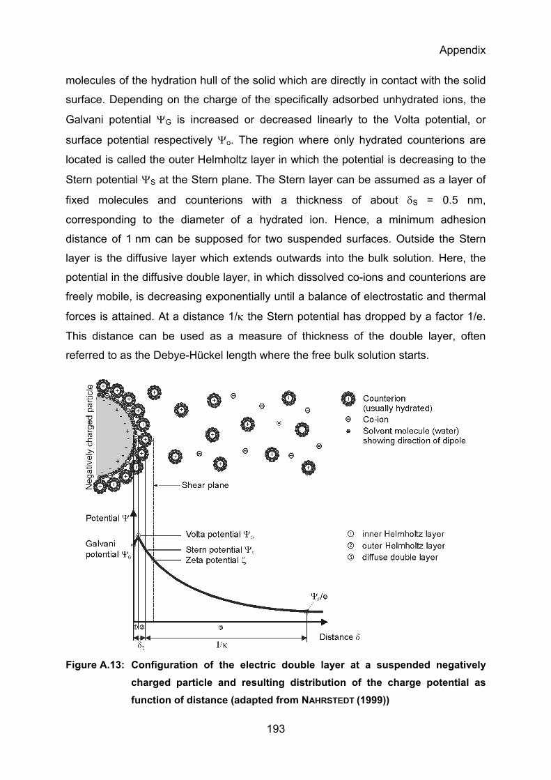
Appendix
193
molecules of the hydration hull of the solid which are directly in contact with the solid
surface. Depending on the charge of the specifically adsorbed unhydrated ions, the
Galvani potential ΨG is increased or decreased linearly to the Volta potential, or
surface potential respectively Ψo. The region where only hydrated counterions are
located is called the outer Helmholtz layer in which the potential is decreasing to the
Stern potential ΨS at the Stern plane. The Stern layer can be assumed as a layer of
fixed molecules and counterions with a thickness of about δS = 0.5 nm,
corresponding to the diameter of a hydrated ion. Hence, a minimum adhesion
distance of 1 nm can be supposed for two suspended surfaces. Outside the Stern
layer is the diffusive layer which extends outwards into the bulk solution. Here, the
potential in the diffusive double layer, in which dissolved co-ions and counterions are
freely mobile, is decreasing exponentially until a balance of electrostatic and thermal
forces is attained. At a distance 1/κ the Stern potential has dropped by a factor 1/e.
This distance can be used as a measure of thickness of the double layer, often
referred to as the Debye-Hückel length where the free bulk solution starts.
Figure A.13: Configuration of the electric double layer at a suspended negatively charged particle and resulting distribution of the charge potential as function of distance (adapted from NAHRSTEDT (1999))
Appendix
194
The shear plane, as illustrated in Figure A.13, separates the ‘fixed’ from the ‘mobile’
parts of the electrical double layer. The electrical potential at the shear plane is the
electrokinetic potential, or the zeta potential, which can be derived with the help of
electrophoretic mobility or streaming potential measurements. It is usually assumed
that the shear plane lies outside but fairly close to the Stern plane, so that essentially
the zeta potential can be used with good agreement as a measure of the real Stern
potential.
A.10 Calculated DLVO forces
According to the DLVO theory, the attractive London-van der Waals and repulsive
double layer forces acting between adjacent surfaces are superposed. The
calculations are based on Equation 3.67 to Equation 3.73 and the general data set
given in Table A.2. The values are those of the experimental setup as introduced in
chapter 4 or taken from literature, i. e. NAHRSTEDT (1999), PANGLISCH (2001), VISSER
(1972), SOFFER ET AL. (2005) and ZHAO ET AL. (2002). The closest calculated distance
was set to 1 nm, representing the minimum adhesion distance δ0 between two
particles/flocs or a particle/floc and the membrane wall respectively.
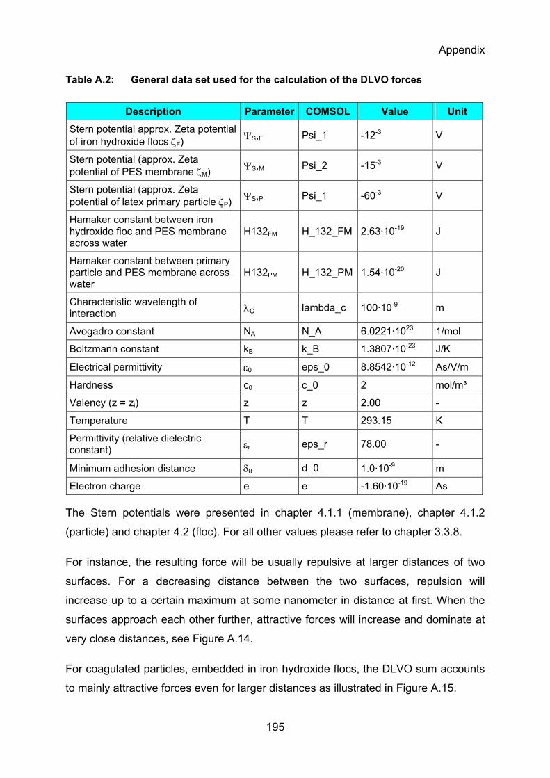
Appendix
195
Table A.2: General data set used for the calculation of the DLVO forces
Description Parameter COMSOL Value Unit
Stern potential approx. Zeta potential of iron hydroxide flocs ζF)
ΨS,F Psi_1 -12-3 V
Stern potential (approx. Zeta potential of PES membrane ζM) ΨS,M Psi_2 -15-3 V
Stern potential (approx. Zeta potential of latex primary particle ζP) ΨS,P Psi_1 -60-3 V
Hamaker constant between iron hydroxide floc and PES membrane across water
H132FM H_132_FM 2.63·10-19 J
Hamaker constant between primary particle and PES membrane across water
H132PM H_132_PM 1.54·10-20 J
Characteristic wavelength of interaction λC lambda_c 100·10-9 m
Avogadro constant NA N_A 6.0221·1023 1/mol
Boltzmann constant kB k_B 1.3807·10-23 J/K
Electrical permittivity ε0 eps_0 8.8542·10-12 As/V/m
Hardness c0 c_0 2 mol/m³
Valency (z = zi) z z 2.00 -
Temperature T T 293.15 K
Permittivity (relative dielectric constant) εr eps_r 78.00 -
Minimum adhesion distance δ0 d_0 1.0·10-9 m
Electron charge e e -1.60·10-19 As
The Stern potentials were presented in chapter 4.1.1 (membrane), chapter 4.1.2
(particle) and chapter 4.2 (floc). For all other values please refer to chapter 3.3.8.
For instance, the resulting force will be usually repulsive at larger distances of two
surfaces. For a decreasing distance between the two surfaces, repulsion will
increase up to a certain maximum at some nanometer in distance at first. When the
surfaces approach each other further, attractive forces will increase and dominate at
very close distances, see Figure A.14.
For coagulated particles, embedded in iron hydroxide flocs, the DLVO sum accounts
to mainly attractive forces even for larger distances as illustrated in Figure A.15.
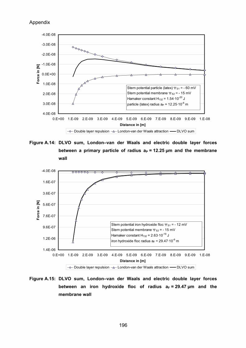
Appendix
196
-4.0E-08
-3.0E-08
-2.0E-08
-1.0E-08
0.0E+00
1.0E-08
2.0E-08
3.0E-08
4.0E-080.E+00 1.E-09 2.E-09 3.E-09 4.E-09 5.E-09 6.E-09 7.E-09 8.E-09 9.E-09 1.E-08
Distance in [m]
Forc
e in
[N]
Double layer repulsion London-van der Waals attraction DLVO sum
Stern potential particle (latex) ΨS1 = - 60 mVStern potential membrane ΨS2 = - 15 mVHamaker constant H132 = 1.54·10-20 Jparticle (latex) radius aP = 12.25·10-6 m
Figure A.14: DLVO sum, London–van der Waals and electric double layer forces between a primary particle of radius aP = 12.25 µm and the membrane wall
-4.0E-08
1.6E-07
3.6E-07
5.6E-07
7.6E-07
9.6E-07
1.2E-06
1.4E-060.E+00 1.E-09 2.E-09 3.E-09 4.E-09 5.E-09 6.E-09 7.E-09 8.E-09 9.E-09 1.E-08
Distance in [m]
Forc
e in
[N]
Double layer repulsion London-van der Waals attraction DLVO sum
Stern potential iron hydroxide floc ΨS1 = - 12 mVStern potential membrane ΨS2 = - 15 mVHamaker constant H132 = 2.63·10-19 Jiron hydroxide floc radius aF = 29.47·10-6 m
Figure A.15: DLVO sum, London–van der Waals and electric double layer forces between an iron hydroxide floc of radius aF = 29.47 µm and the membrane wall
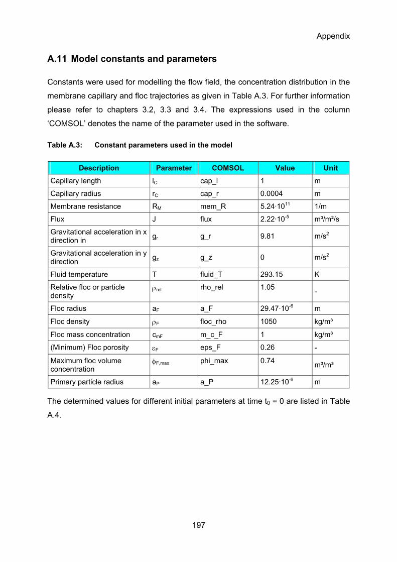
Appendix
197
A.11 Model constants and parameters
Constants were used for modelling the flow field, the concentration distribution in the
membrane capillary and floc trajectories as given in Table A.3. For further information
please refer to chapters 3.2, 3.3 and 3.4. The expressions used in the column
‘COMSOL’ denotes the name of the parameter used in the software.
Table A.3: Constant parameters used in the model
Description Parameter COMSOL Value Unit
Capillary length lC cap_l 1 m
Capillary radius rC cap_r 0.0004 m
Membrane resistance RM mem_R 5.24·1011 1/m
Flux J flux 2.22·10-5 m³/m²/s
Gravitational acceleration in x direction in gr g_r 9.81 m/s2
Gravitational acceleration in y direction gz g_z 0 m/s2
Fluid temperature T fluid_T 293.15 K
Relative floc or particle density
ρrel rho_rel 1.05 -
Floc radius aF a_F 29.47·10-6 m
Floc density ρF floc_rho 1050 kg/m³
Floc mass concentration cmF m_c_F 1 kg/m³
(Minimum) Floc porosity εF eps_F 0.26 -
Maximum floc volume concentration
φF,max phi_max 0.74 m³/m³
Primary particle radius aP a_P 12.25·10-6 m
The determined values for different initial parameters at time t0 = 0 are listed in Table
A.4.
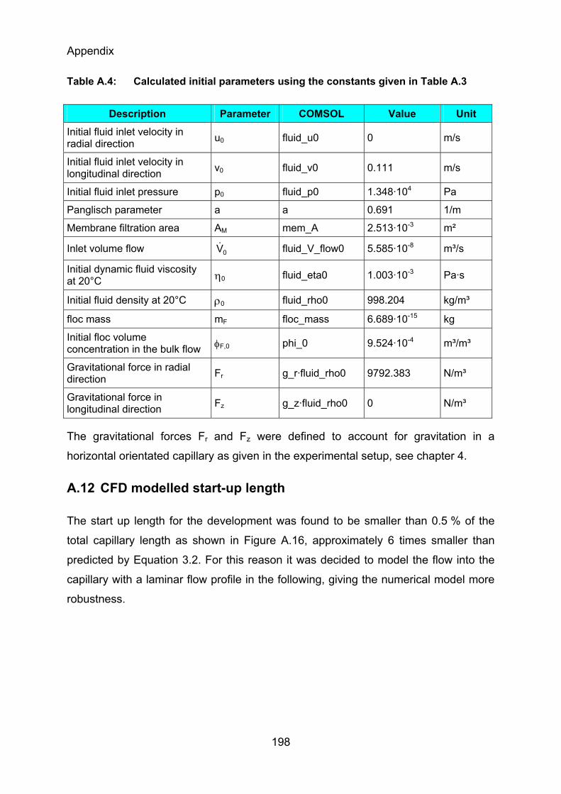
Appendix
198
Table A.4: Calculated initial parameters using the constants given in Table A.3
Description Parameter COMSOL Value Unit
Initial fluid inlet velocity in radial direction u0 fluid_u0 0 m/s
Initial fluid inlet velocity in longitudinal direction v0 fluid_v0 0.111 m/s
Initial fluid inlet pressure p0 fluid_p0 1.348·104 Pa
Panglisch parameter a a 0.691 1/m
Membrane filtration area AM mem_A 2.513·10-3 m²
Inlet volume flow 0V fluid_V_flow0 5.585·10-8 m³/s
Initial dynamic fluid viscosity at 20°C η0 fluid_eta0 1.003·10-3 Pa·s
Initial fluid density at 20°C ρ0 fluid_rho0 998.204 kg/m³
floc mass mF floc_mass 6.689·10-15 kg
Initial floc volume concentration in the bulk flow φF,0 phi_0 9.524·10-4 m³/m³
Gravitational force in radial direction Fr g_r·fluid_rho0 9792.383 N/m³
Gravitational force in longitudinal direction Fz g_z·fluid_rho0 0 N/m³
The gravitational forces Fr and Fz were defined to account for gravitation in a
horizontal orientated capillary as given in the experimental setup, see chapter 4.
A.12 CFD modelled start-up length
The start up length for the development was found to be smaller than 0.5 % of the
total capillary length as shown in Figure A.16, approximately 6 times smaller than
predicted by Equation 3.2. For this reason it was decided to model the flow into the
capillary with a laminar flow profile in the following, giving the numerical model more
robustness.
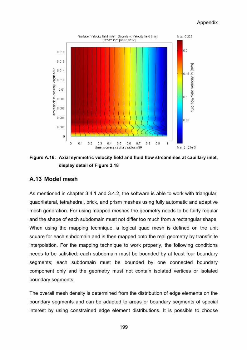
Appendix
199
Figure A.16: Axial symmetric velocity field and fluid flow streamlines at capillary inlet, display detail of Figure 3.18
A.13 Model mesh
As mentioned in chapter 3.4.1 and 3.4.2, the software is able to work with triangular,
quadrilateral, tetrahedral, brick, and prism meshes using fully automatic and adaptive
mesh generation. For using mapped meshes the geometry needs to be fairly regular
and the shape of each subdomain must not differ too much from a rectangular shape.
When using the mapping technique, a logical quad mesh is defined on the unit
square for each subdomain and is then mapped onto the real geometry by transfinite
interpolation. For the mapping technique to work properly, the following conditions
needs to be satisfied: each subdomain must be bounded by at least four boundary
segments; each subdomain must be bounded by one connected boundary
component only and the geometry must not contain isolated vertices or isolated
boundary segments.
The overall mesh density is determined from the distribution of edge elements on the
boundary segments and can be adapted to areas or boundary segments of special
interest by using constrained edge element distributions. It is possible to choose
Appendix
200
between specifying the number of equally distributed edge elements or the
distribution of mesh vertices along the boundary segment. The latter, which gives full
control of the edge element distribution, is specified by vector valued expressions of
strictly increasing values starting with zero, specifying the relative arc length values
of the mesh vertices along the edge. However, for the mapping technique to work,
the opposite sides of each logical unit square need to be discretised by the same
number of edge elements. The vector valued expressions were applied to account for
a sufficient high resolution of the mesh especially at the capillary entrance, where the
laminar flow profile is established and at the membrane wall, where the interacting
forces between fluid flow, moving flocs and membrane wall will be likely highest and
where the cake layer build-up will occur.
The 2D mesh as given in chapter 3.4.2 can be transformed into 3D by using
extrusion coupling variables, which maps values from the source domain, here in 2D,
to the destination domain in 3D. Because the destination domain has higher
dimension than the source domain, the mapping is done by extruding point-wise
values to the higher dimensions. This transformation between the source and
destination is performed by the so called general transformation. Here, the source
transformation is a one-to-one mapping that maps the mesh of the physical source
domain to an intermediate mesh embedded in a space of the same dimension as the
source. The destination transformation is a mapping from the destination domain,
where the value of the variable is defined, to the same space that contains the
intermediate mesh. When the value of the coupling variable is requested somewhere
in the destination domain, the software transforms the destination points using the
destination transformation. It compares the resulting coordinates to the elements in
the intermediate mesh in order to find corresponding locations in the physical source
domain. To avoid the need to solve a nonlinear system of equations for every
destination point, the software assumes that the source transformation is linear on
each element of the intermediate mesh. In practice, the transformation is often trivial
and leaves the coordinates unchanged, but it can also rescale, stretch, bend, or
reflect the mesh. For more detailed information about the applied transformation refer
to COMSOL AB (2006A). While transforming the 2D model into 3D, the applied mesh
is generated automatically with tetrahedral mesh elements. The mesh was always
refined and adjusted to account for a sufficient high resolution at the areas of interest.
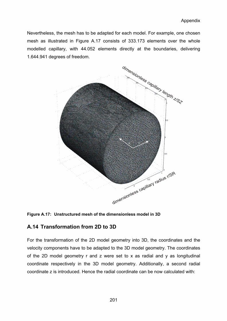
Appendix
201
Nevertheless, the mesh has to be adapted for each model. For example, one chosen
mesh as illustrated in Figure A.17 consists of 333.173 elements over the whole
modelled capillary, with 44.052 elements directly at the boundaries, delivering
1.644.941 degrees of freedom.
Figure A.17: Unstructured mesh of the dimensionless model in 3D
A.14 Transformation from 2D to 3D
For the transformation of the 2D model geometry into 3D, the coordinates and the
velocity components have to be adapted to the 3D model geometry. The coordinates
of the 2D model geometry r and z were set to x as radial and y as longitudinal
coordinate respectively in the 3D model geometry. Additionally, a second radial
coordinate z is introduced. Hence the radial coordinate can be now calculated with:
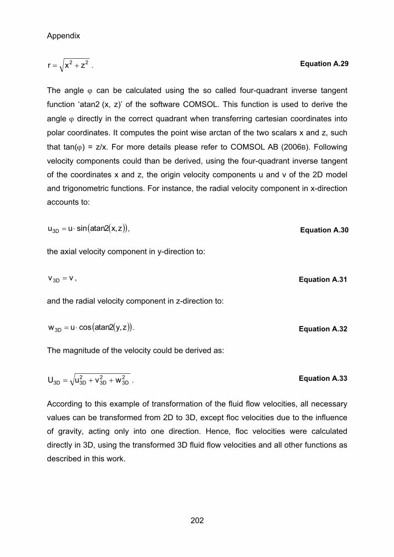
Appendix
202
22 zxr += . Equation A.29
The angle ϕ can be calculated using the so called four-quadrant inverse tangent
function ‘atan2 (x, z)’ of the software COMSOL. This function is used to derive the
angle ϕ directly in the correct quadrant when transferring cartesian coordinates into
polar coordinates. It computes the point wise arctan of the two scalars x and z, such
that tan(ϕ) = z/x. For more details please refer to COMSOL AB (2006B). Following
velocity components could than be derived, using the four-quadrant inverse tangent
of the coordinates x and z, the origin velocity components u and v of the 2D model
and trigonometric functions. For instance, the radial velocity component in x-direction
accounts to:
( )( )z,x2tanasinuu D3 ⋅= , Equation A.30
the axial velocity component in y-direction to:
vv D3 = , Equation A.31
and the radial velocity component in z-direction to:
( )( )z,y2tanacosuw D3 ⋅= . Equation A.32
The magnitude of the velocity could be derived as:
2D3
2D3
2D3D3 wvuU ++= . Equation A.33
According to this example of transformation of the fluid flow velocities, all necessary
values can be transformed from 2D to 3D, except floc velocities due to the influence
of gravity, acting only into one direction. Hence, floc velocities were calculated
directly in 3D, using the transformed 3D fluid flow velocities and all other functions as
described in this work.
Appendix
203
A.15 Statistical methods
6.1.1 Grubbs outlier test
There is a scatter in the results of the measured data due to statistical and
systematic influences. Systematically influenced individual values are considered as
faulty, i. e. as outliers. To assess whether an extreme value is to be designated as an
outlier, test values are calculated by various methods which have to be compared
with tabulated numerical values of different levels of significance. The choice of a
definite level of significance includes the risk to reject an extreme value as outlier
when in fact there is no outlier (type 1 risk). At the same time this choice includes
also a risk of failing to reject an actual outlier (type 2 risk). Since incorrect results may
falsify the result of the measured data, outliers have to be traced and rejected. All
data sets used in this work were tested according to the outlier rm- test as presented
by Grubbs (GRUBBS AND BECK (1972), GRUBBS (1969), GRUBBS (1950) all cited in UHL
(2000)). In statistics, a result is significant if it is unlikely to have occurred by chance,
given that a presumed null hypothesis H0 is true (type 1 risk). The level of
significance was chosen to be highly significant with α = 1 %. The Grubbs rm- test
compares each individual value x* with the mean value x and the standard deviation
s of the measured data set. The null hypothesis H0 is chosen to be that the individual
value x* out of n values is no outlier. This null hypothesis was accepted on the level
of significance if
( )n,rs
xxr̂ mm α≤
−=
∗
Equation A.34
was true, otherwise rejected. If an individual value was tested to be an outlier it was
eliminated and the test repeated for all remaining values of the data set. This was
done for all individual values until all remaining values were accepted and indicated
to be no outlier.
The experimental investigations presented in this work are often time series in which
each individual value has to be evaluated in comparison to the value measured
chronologically before. UHL (2000) presented a method which adapts Grubbs rm- test
to time series. This method is comparable to the moving average method,
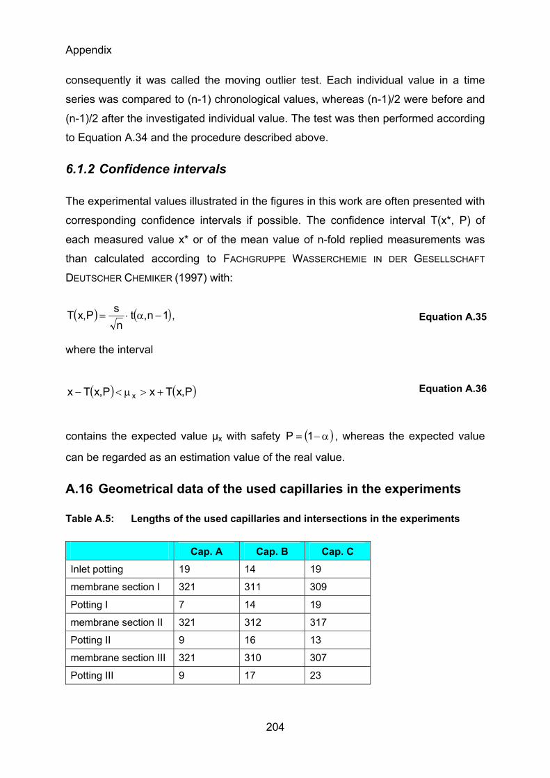
Appendix
204
consequently it was called the moving outlier test. Each individual value in a time
series was compared to (n-1) chronological values, whereas (n-1)/2 were before and
(n-1)/2 after the investigated individual value. The test was then performed according
to Equation A.34 and the procedure described above.
6.1.2 Confidence intervals
The experimental values illustrated in the figures in this work are often presented with
corresponding confidence intervals if possible. The confidence interval T(x*, P) of
each measured value x* or of the mean value of n-fold replied measurements was
than calculated according to FACHGRUPPE WASSERCHEMIE IN DER GESELLSCHAFT
DEUTSCHER CHEMIKER (1997) with:
( ) ( )1n,tnsP,xT −α⋅= , Equation A.35
where the interval
( ) ( )P,xTxP,xTx x +>μ<− Equation A.36
contains the expected value µx with safety ( )α−= 1P , whereas the expected value
can be regarded as an estimation value of the real value.
A.16 Geometrical data of the used capillaries in the experiments
Table A.5: Lengths of the used capillaries and intersections in the experiments
Cap. A Cap. B Cap. C Inlet potting 19 14 19 membrane section I 321 311 309 Potting I 7 14 19 membrane section II 321 312 317 Potting II 9 16 13 membrane section III 321 310 307 Potting III 9 17 23
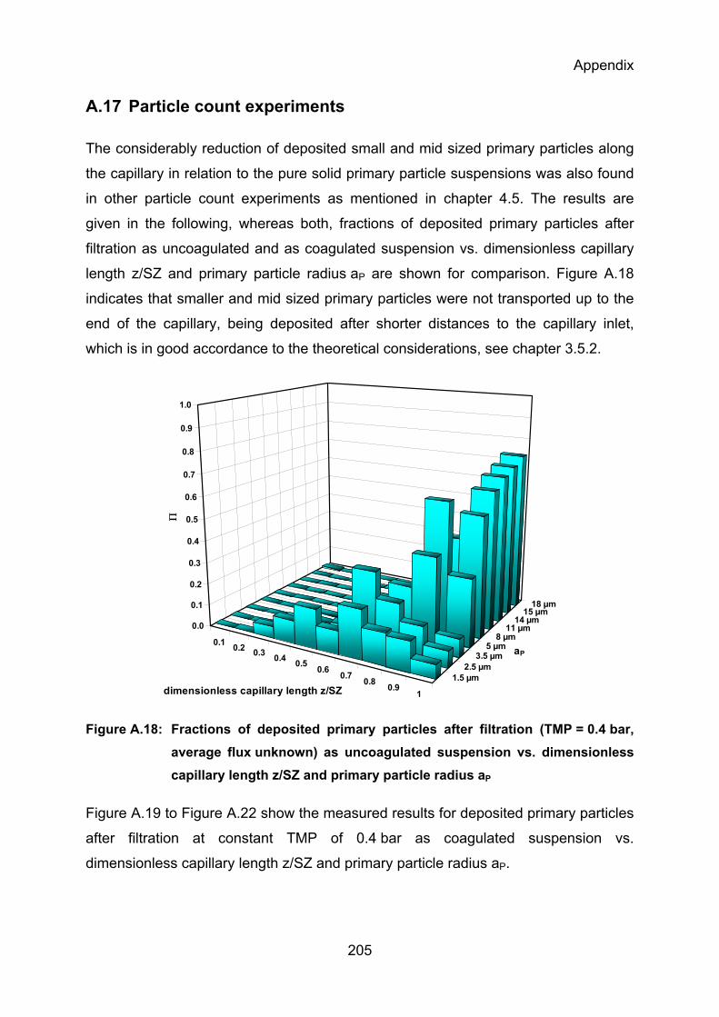
Appendix
205
A.17 Particle count experiments
The considerably reduction of deposited small and mid sized primary particles along
the capillary in relation to the pure solid primary particle suspensions was also found
in other particle count experiments as mentioned in chapter 4.5. The results are
given in the following, whereas both, fractions of deposited primary particles after
filtration as uncoagulated and as coagulated suspension vs. dimensionless capillary
length z/SZ and primary particle radius aP are shown for comparison. Figure A.18
indicates that smaller and mid sized primary particles were not transported up to the
end of the capillary, being deposited after shorter distances to the capillary inlet,
which is in good accordance to the theoretical considerations, see chapter 3.5.2.
1.5 µm2.5 µm
3.5 µm5 µm
8 µm11 µm
14 µm15 µm
18 µm
0.1 0.2 0.3 0.4 0.5 0.6 0.7 0.8 0.91
0.0
0.1
0.2
0.3
0.4
0.5
0.6
0.7
0.8
0.9
1.0
Π
dimensionless capillary length z/SZ
aP
Figure A.18: Fractions of deposited primary particles after filtration (TMP = 0.4 bar, average flux unknown) as uncoagulated suspension vs. dimensionless capillary length z/SZ and primary particle radius aP
Figure A.19 to Figure A.22 show the measured results for deposited primary particles
after filtration at constant TMP of 0.4 bar as coagulated suspension vs.
dimensionless capillary length z/SZ and primary particle radius aP.
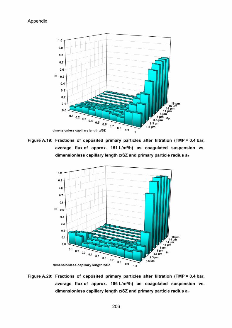
Appendix
206
1.5 µm2.5 µm
3.5 µm5 µm
8 µm11 µm
14 µm15 µm
18 µm
0.1 0.2 0.3 0.4 0.5 0.6 0.7 0.8 0.91
0.0
0.1
0.2
0.3
0.4
0.5
0.6
0.7
0.8
0.9
1.0
Π
dimensionless capillary length z/SZ
aP
Figure A.19: Fractions of deposited primary particles after filtration (TMP = 0.4 bar, average flux of approx. 151 L/m²/h) as coagulated suspension vs. dimensionless capillary length z/SZ and primary particle radius aP
1.5 µm2.5 µm
3.5 µm5 µm
8 µm11 µm
14 µm15 µm
18 µm
0.1 0.2 0.3 0.4 0.5 0.6 0.7 0.8 0.91.0
0.0
0.1
0.2
0.3
0.4
0.5
0.6
0.7
0.8
0.9
1.0
Π
dimensionless capillary length z/SZ
aP
Figure A.20: Fractions of deposited primary particles after filtration (TMP = 0.4 bar, average flux of approx. 186 L/m²/h) as coagulated suspension vs. dimensionless capillary length z/SZ and primary particle radius aP
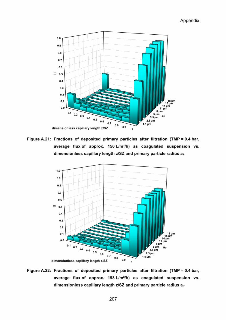
Appendix
207
1.5 µm2.5 µm
3.5 µm5 µm
8 µm11 µm
14 µm15 µm
18 µm
0.1 0.2 0.3 0.4 0.5 0.6 0.7 0.8 0.91
0.0
0.1
0.2
0.3
0.4
0.5
0.6
0.7
0.8
0.9
1.0
Π
dimensionless capillary length z/SZ
aP
Figure A.21: Fractions of deposited primary particles after filtration (TMP = 0.4 bar, average flux of approx. 156 L/m²/h) as coagulated suspension vs. dimensionless capillary length z/SZ and primary particle radius aP
1.5 µm2.5 µm
3.5 µm5 µm
8 µm11 µm
14 µm15 µm
18 µm
0.1 0.2 0.3 0.4 0.5 0.6 0.7 0.8 0.91
0.0
0.1
0.2
0.3
0.4
0.5
0.6
0.7
0.8
0.9
1.0
Π
dimensionless capillary length z/SZ
aP
Figure A.22: Fractions of deposited primary particles after filtration (TMP = 0.4 bar, average flux of approx. 198 L/m²/h) as coagulated suspension vs. dimensionless capillary length z/SZ and primary particle radius aP
Appendix
208
The comparison of Figure A.18 to Figure A.22 delivers similar results as described in
chapter 4.5. The fractions of small and mid sized primary particles in the range from
aP = 1.5 µm to about aP = 14 µm was increased in the last two capillary length
sections at z/SZ = 0.9 and z/SZ = 1, hence at the end of the capillary for the
coagulated suspensions. Accordingly, the fraction of primary particles of the same
size range decreased in the middle and the third quarter of the capillary length at
z/SZ = 0.5 to z/SZ = 1. This clearly indicates that smaller and mid size particles were
transported as floc agglomerate more deeply into the capillary as they would have
actually done due to their own size.
CURRICULUM VITAE
André Paul Lerch
born 10th of April 1969 in Düsseldorf, Germany married, one child
Professional Experience
since 2005 Research Associate at the Institute for Urban Water Management, Water Supply Engineering Group, Technische Universität Dresden, Germany
1999 - 2005 Research Assistant at the Department of Process Engineering / Water Technology, Universität Duisburg-Essen, Germany
Academic Education
1999 M. Sc. (Diplom Hauptprüfung)
1993 B. Sc (Diplom-Vorprüfung)
1990 Enrolment at the Universität – GH- Duisburg , Germany, Studies of Mechanical Engineering
Military service
1989 - 1990 Military service at a technical maintenance company (InstKP 30)
School Education
1989 Abitur (A-level / High School Certificate)
1979 - 1989 städt. Meerbusch Gymnasium (High School) in Meerbusch, Germany
1975 - 1979 St. Martinus Grundschule (Primary School) in Meerbusch, Germany
Dresden, 28th of February 2008