Embed Size (px)
Citation preview
ANGEWANDTE MATHEMATIK
INTEGRALRECHNUNG TEIL 2 Autor: Wolfgang Kugler
Integralrechnung Teil 2 1
Inhaltsverzeichnis
Integralrechnung II.Teil 2
1 Partielle Integration (2.Teil) 2
1.1 Der Trick mit dem Faktor 1 2
1.2 Integrale, die im Laufe der Rechnung wieder auf sich selbst zurückführen 6
2 Rekursive Integrale 22
2.1 Erklärung 22
2.2 Beispiele 22
2.3 Übungsbeispiele 30
3 Integration mittels Partialbruchzerlegung 31
3.1 Übungsbeispiele: 31
4 Numerische Integration 33
4.1 Kepler Formel 33
4.2 Simpson Formel 37 Datum: 27.05.03
WOLFGANG KUGLER TGM ANGEWANDTE MATHEMATIK
Integralrechnung Teil 2 2
INTEGRALRECHNUNG II.TEIL
1 Partielle Integration (2.Teil)
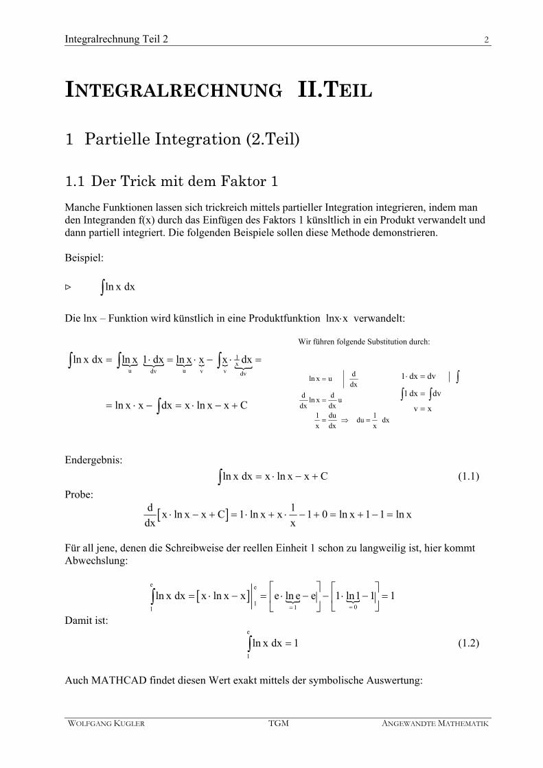
1.1 Der Trick mit dem Faktor 1
Manche Funktionen lassen sich trickreich mittels partieller Integration integrieren, indem man den Integranden f(x) durch das Einfügen des Faktors 1 künsltlich in ein Produkt verwandelt und dann partiell integriert. Die folgenden Beispiele sollen diese Methode demonstrieren. Beispiel:
ln x dx∫ Die lnx – Funktion wird künstlich in eine Produktfunktion lnx⋅x verwandelt:
Wir führen folgende Substitution durch:
1x
u u v vdv dv
ln x dx ln x 1 dx ln x x x dx
ln x x dx x ln x x C
= ⋅ = ⋅ − ⋅
= ⋅ − = ⋅ − +
∫ ∫ ∫
∫
=
dln x u
dxd dln x u
dx dx1 du 1du dxx dx x
=
=
= ⇒ =
1 dx dv
1 dx dv
v x
⋅ =
=
=
∫∫ ∫
Endergebnis: (1.1) ln x dx x ln x x C= ⋅ − +∫Probe:
[ ] 1x ln x x C ln x x 1 0 ln x 1 1 ln xx
d 1dx
⋅ − + ⋅ + ⋅ − + = + − ==
Für all jene, denen die Schreibweise der reellen Einheit 1 schon zu langweilig ist, hier kommt Abwechslung:
[ ]e e
1 011
ln x dx x ln x x e ln e e 1 ln1 1 1==
= ⋅ − = ⋅ − − ⋅ − =
∫
Damit ist:
(1.2) e
1
ln x dx 1=∫ Auch MATHCAD findet diesen Wert exakt mittels der symbolische Auswertung:
WOLFGANG KUGLER TGM ANGEWANDTE MATHEMATIK
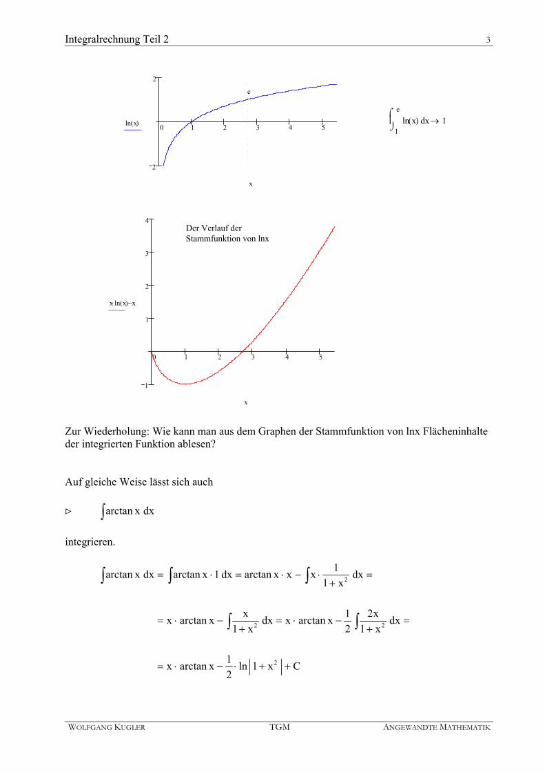
Integralrechnung Teil 2 3
0 1 2 3 4 5
2
2
ln x( )
e
x
1
e
xln x( )⌠⌡
d 1→
0 1 2 3 4 5
1
1
2
3
4
x ln x( )⋅ x−
x
Der Verlauf der Stammfunktion von lnx
Zur Wiederholung: Wie kann man aus dem Graphen der Stammfunktion von lnx Flächeninhalte der integrierten Funktion ablesen? Auf gleiche Weise lässt sich auch
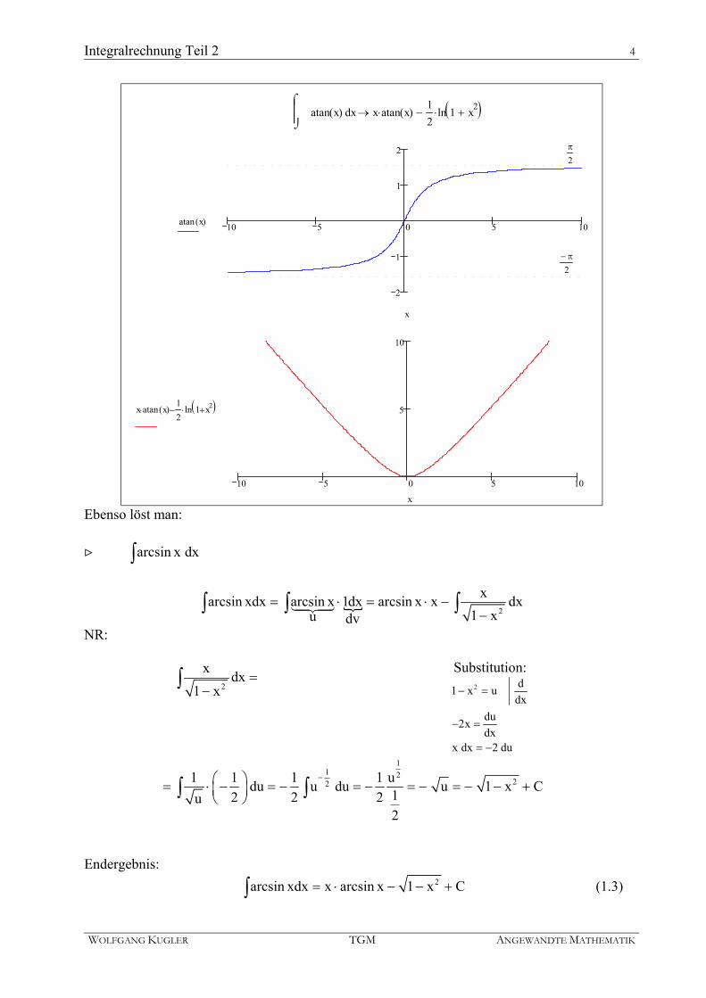
arctan x dx∫ integrieren.
2
2 2
2
1arctan x dx arctan x 1 dx arctan x x x dx1 x
x 1x arctan x dx x arctan x dx1 x 2 1 x
1x arctan x ln 1 x C2
= ⋅ = ⋅ − ⋅ =+
= ⋅ − = ⋅ − =+ +
= ⋅ − ⋅ + +
∫ ∫ ∫
∫ ∫2x
WOLFGANG KUGLER TGM ANGEWANDTE MATHEMATIK
Integralrechnung Teil 2 4
xatan x( )⌠⌡
d x atan x( )⋅12
ln 1 x2+( )⋅−→
10 5 0 5 10
2
1
1
2
π−2
π2
atan x( )
x
10 5 0 5
5
10
10
x atan x( )⋅12
ln 1 x2+( )⋅−
x Ebenso löst man:
arcsin x dx∫
2
xarcsin xdx arcsin x 1dx arcsin x x dx1 xu dv
= ⋅ = ⋅ −−
∫ ∫ ∫
NR:
2
x dx1 x
=−
∫ Substitution:
2 d1 x udx
du2xdx
x dx 2 du
− =
− =
= −
11 2
221 1 1 1 udu u du u 1 x C12 2 2u2
− = ⋅ − = − = − = − = − − + ∫ ∫
Endergebnis: 2arcsin xdx x arcsin x 1 x C= ⋅ − − +∫ (1.3)
WOLFGANG KUGLER TGM ANGEWANDTE MATHEMATIK
Integralrechnung Teil 2 5
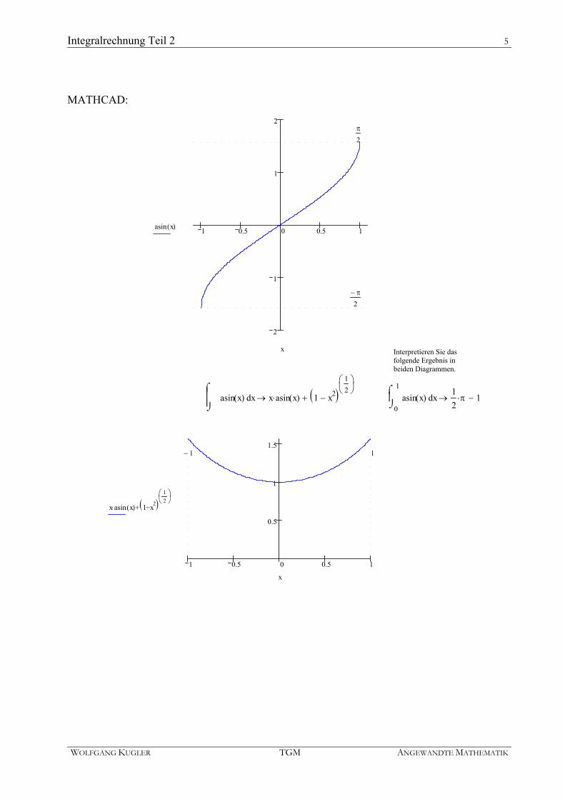
MATHCAD:
1 0.5 0 0.5 1
2
1
1
2
π−
2
π
2
asin x( )
x Interpretieren Sie das folgende Ergebnis in beiden Diagrammen.
xasin x( )⌠⌡
d x asin x( )⋅ 1 x2−( )12
+→0
1
xasin x( )⌠⌡
d12π⋅ 1−→
1 0.5 0 0.5 1
0.5
1
1.5
x asin x( )⋅ 1 x2−( )12
+
1− 1
x
WOLFGANG KUGLER TGM ANGEWANDTE MATHEMATIK
Integralrechnung Teil 2 6
1.2 Integrale, die im Laufe der Rechnung wieder auf sich
selbst zurückführen
1. Beispiel:
Zur Erinnerung: 3xe sin2xdx =∫ udv uv vdu= −∫ ∫
( ) ( )
3x
u dv
3x 3x1 12 2
u duv v
e sin2xdx
e cos 2x cos 2x 3e
= ⋅ =
= ⋅ − − −
∫
∫ dx
3x 3x31
2 2e cos 2x e cos 2x= − + ∫
1.Substitution:
3x
3x
3x
de udx
du3edx
3e dx du
=
=
=
12
12
sin 2xdx dv
sin 2xdx dv
cos 2x vv cos 2x
=
=
− =
= −
∫∫ ∫
Wir müssen hier feststellen, dass das in diesem Ergebnis auftretende Integral
keineswegs einfacher ist. Es hat sich vom Schwierigkeitsgrad eigentlich nichts geändert. Rechnen wir trotzdem weiter. In einer eigenen Nebenrechnung lösen wir das Integral:
nach der gleichen Methode:
3xe cos 2x∫
3xe cos 2x∫
3x 3x
u dv
3x 3x1 12 2
u duv v
3x 3x312 2
e cos 2x e cos 2x dx
e sin 2x sin 2x 3e dx
e sin 2x e sin2xdx
=
= − ⋅
= −
∫ ∫
∫
∫
=
=
2.Substitution:
3x
3x
3x
de udx
dudx
3e dx du
=
=
=
3e 12
12
cos 2xdx dv
cos 2xdx dv
sin 2x vv sin 2x
=
=
==
∫∫ ∫
Dieses Ergebnis wird nun in die oben unterbrochene Rechnung eingesetzt:
3x 3x 3x 3x3 31 12 2 2 2
3x 3x 3x3 912 4 4
e sin2xdx e cos 2x e sin 2x e sin2xdx
e cos 2x e sin 2x e sin2xdx
= = − + −
= − + −
∫ ∫
∫
… =
Hier tritt das Ausgangsintegral wieder auf! Es hat den Anschein, als würde man im Kreis rechnen. Wir können nun jedoch
3x 3x 3x 3x3 912 4 4e sin2xdx e cos 2x e sin 2x e sin2xdx= − + −∫ ∫
WOLFGANG KUGLER TGM ANGEWANDTE MATHEMATIK
Integralrechnung Teil 2 7
als lineare Gleichung für das Ausgangsintegral auffassen. Der Einfachheit halber führen wir kurzzeitig eine Umbenennung ( Substitution ) durch:
3x 3x 3x 3x3 912 4 4
AI I
e sin2xdx e cos 2x e sin 2x e sin2xdx== =
= − + −∫ ∫
Dadurch vereinfacht sich die Gleichung auf:
94I A= − I
Diese lässt sich nun einfach nach I auflösen:
( )
94
94
134
413
I A1 I A
I AI A
= −
+ ⋅ =
=
=
I
Setzen wir nun für I und A wieder ein, so erhalten wir
( )
( )
3x 3x 3x34 113 2 4
3x 3213 2
e sin2xdx e cos 2x e sin 2x
e sin 2x cos 2x
= − +
= −
∫ =
Probe:
( )( ) ( )( )( ) ( )
( )
3x 3x3 32 213 2 13 2
3x 3x3213 2
3x 9213 2
3x 13213 2
3x
e sin 2x cos 2x e sin 2x cos 2x
3e sin 2x cos 2x e 3cos 2x 2sin 2x
e sin 2x 3cos 2x 3cos 2x 2sin 2x
e sin 2x
e sin 2x
′ ′− = − =
= − + + = − + + =
= =
=
=
Bemerkung:
Vielleicht haben Sie sich gefragt, warum gerade die Exponentialfunktion als die zu differenzierende Funktion u und
die Winkelfunktion als die zu integrierende Funktion dv gewählt wurde. Die Antwort ist einfach: Es ist hier völlig
egal, wichtig ist nur, dass man bei der ersten und bei der zweiten partiellen Integration die gleiche Wahl trifft, sonst
rechnet man wirklich "im Kreis" und erhält schließlich nur I = I .
WOLFGANG KUGLER TGM ANGEWANDTE MATHEMATIK
Integralrechnung Teil 2 8
2. Beispiel: Zur Erinnerung: udv uv vdu= −∫ ∫
sin3x cos2x dx∫
u dv
1 12 2
u duv v
312 2
sin3x cos2x dx
sin 3x sin 2x sin2x 3cos3x dx
sin 3x sin 2x cos3x sin2x dx
=
= ⋅ − ⋅
= − ⋅
∫
∫
∫
=
1.Substitution:dsin 3x u
dxdu3cos 3xdx
3cos 3x dx du
=
=
=
12
12
cos 2xdx dv
cos 2xdx dv
sin 2x vv sin 2x
=
=
=
=
∫∫ ∫
Nun wird das Integral in einer Nebenrechnug berechnet: cos3x sin2x dx⋅∫ NR.:
( ) ( ) ( )u dv
1 12 2
uduv v
312 2
cos3x sin2x dx cos3x sin2x dx
cos 3x cos 2x cos 2x 3sin 3x dx
cos 3x cos 2x sin 3x cos 2x dx
⋅ = ⋅ =
= − − − ⋅ −
= −
∫ ∫
∫
∫
=
2.Substitution:
dcos 3x udx
du3sin 3xdx
3sin 3x dx du
=
− =
− =
12
12
sin2xdx dv
sin2xdx dv
cos2x vv cos2x
=
=
− =
= −
∫∫ ∫
In die oben unterbrochene Rechnung eingesetzt erhalten wir:
3 31 12 2 2 2
3 912 4 4
sin3x cos2x dx sin 3x sin 2x cos 3x cos 2x sin 3x cos 2x dx
sin 3x sin 2x cos 3x cos 2x sin 3x cos 2x dx
= = − −
= − +
∫ ∫∫
… =
Es tritt auch hier das Ausgangsintegral wieder auf.
3 912 4 4sin3xcos2x dx sin 3x sin 2x cos 3x cos 2x sin 3x cos 2x dx= + +∫ ∫
Fassen wir diese Identität wieder als Gleichung für unser Ausgangsintegral
auf und führen wir folgende Abkürzungen ein:
I sin3x cos2x dx= ∫
3 91
2 4 4
AI I
sin3xcos2x dx sin 3x sin 2x cos 3x cos 2x sin 3x cos 2x dx= + +∫ ∫
so erhalten wir: 94
54
45
I AI AI A
= +
− =
= −
I
WOLFGANG KUGLER TGM ANGEWANDTE MATHEMATIK
Integralrechnung Teil 2 9
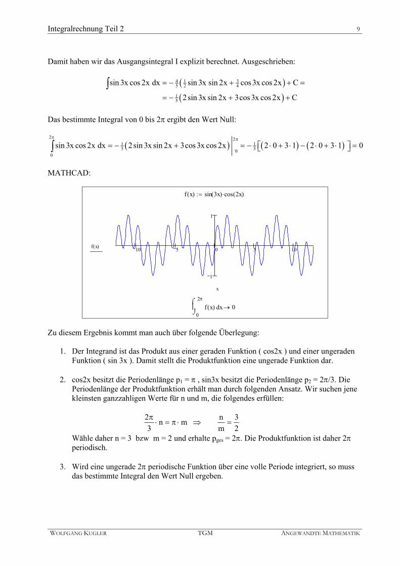
Damit haben wir das Ausgangsintegral I explizit berechnet. Ausgeschrieben:
( )( )
34 15 2 4
15
sin 3x cos 2x dx sin 3x sin 2x cos 3x cos 2x C
2sin 3x sin 2x 3cos 3x cos 2x C
= − + + =
= − + +∫
Das bestimmte Integral von 0 bis 2π ergibt den Wert Null:
( ) ( ) ( )2 2
1 15 5`0
0
sin 3x cos 2x dx 2sin 3x sin 2x 3cos 3x cos 2x 2 0 3 1 2 0 3 1 0π π
= − + = − ⋅ + ⋅ − ⋅ + ⋅ = ∫
MATHCAD:
f x( ) sin 3x( ) cos 2x( )⋅:=
10 5 0 5 10
1
1
f x( )
x
0
2π
xf x( )⌠⌡
d 0→
Zu diesem Ergebnis kommt man auch über folgende Überlegung:
1. Der Integrand ist das Produkt aus einer geraden Funktion ( cos2x ) und einer ungeraden Funktion ( sin 3x ). Damit stellt die Produktfunktion eine ungerade Funktion dar.
2. cos2x besitzt die Periodenlänge p1 = π , sin3x besitzt die Periodenlänge p2 = 2π/3. Die Periodenlänge der Produktfunktion erhält man durch folgenden Ansatz. Wir suchen jene kleinsten ganzzahligen Werte für n und m, die folgendes erfüllen:
2 nn m3 mπ⋅ = π ⋅ ⇒ =
32
Wähle daher n = 3 bzw m = 2 und erhalte pges = 2π. Die Produktfunktion ist daher 2π periodisch.
3. Wird eine ungerade 2π periodische Funktion über eine volle Periode integriert, so muss das bestimmte Integral den Wert Null ergeben.
WOLFGANG KUGLER TGM ANGEWANDTE MATHEMATIK
Integralrechnung Teil 2 10
Bemerkung:
Auch hier stellt sich die Frage, warum bei der ersten partiellen Integration gerade die Winkelfunktion sin3x
als die zu differenzierende Funktion u und die Winkelfunktion cos2x dx als die zu integrierende Funktion dv
gewählt wurde. Die Antwort ist auch hier dieselbe: Es ist hier völlig egal, wichtig ist nur, dass man bei der
ersten und bei der zweiten partiellen Integration die Winkelfunktion mit dem Argument 3x als die zu
differenzierende Funktion und die Winkelfunktion mit dem Argument 2x als die zu integrierende Funktion
wählt. Sonst rechnet man "im Kreis" und erhält schließlich nur I = I. Wenden wir uns nun der Berechnung von allgemeinen Integralen zu: 3. Beispiel:
axe cos bx dx∫
ax ax ax1 1b b
u udv duv v
ax axa1b b
e cos bx dx e sin bx sin bx ae dx
e sin bx e sin bx dx
= −
= −
∫ ∫
∫
=
Substitution:
ax
ax
ax
de udx
duaedx
du ae dx
=
=
=
1b
cos bxdx dv
cos bxdx dv
v sin bx
=
=
=
∫∫ ∫
Nun wird das Integral in einer Nebenrechnug berechnet: axe sin bx dx∫NR.:
( ) ( )ax ax ax1 1b b
u udv duv v
ax axa1b b
e sin bx dx e cos bx cos bx ae dx
e cos bx e cos bx dx
= − − −
= − +
∫ ∫
∫
=
Substitution:ax
ax
ax
de udx
duaedx
du ae dx
=
=
=
1b
sin bxdx dv
sin bxdx dv
v cos bx
=
=
= −
∫∫ ∫
und in die obige Rechnung eingesetzt:
( )
2
2 2
ax ax ax axa a1 1b b b b
ax ax axa a1b b b
e cos bx dx e sin bx e cos bx e cos bx dx
e sin bx e cos bx e cos bx dx
= − − +
= + −
∫ ∫∫
=
Wir erhalten auf der rechten Seite also wieder das Ausgangsintegral. Fassen wir die Gleichung
2
2 2ax ax ax axa a1
b b b
AI I
e cos bx dx e sin bx e cos bx e cos bx dx= + −∫ ∫
als lineare Gleichung für das Ausgangsintegral I auf. Wir substituieren und lösen nach I auf:
WOLFGANG KUGLER TGM ANGEWANDTE MATHEMATIK
Integralrechnung Teil 2 11
( )
2
2
2
2
2
2
ab
ab
ab
I A
I I A
I 1 A
= −
+ =
+ =
I
2a2b
11
2 2b a2b
2
2 2
11
bb a
I A
I A
I A
+
+
+
=
=
=
Rücksubstitution ( Wir setzen für I und A wieder ein ): ( ) ( )2 ax
2 2 2 2 2ax ax axb a e1
bb a b a be cos bx dx e sin bx e cos bx bsin bx a cos bx
+ += + = +∫
Endergebnis:
(ax
ax2 2
ee cos bx dx bsin bx a cos bxa b
= ++∫ ) (1.4)
WOLFGANG KUGLER TGM ANGEWANDTE MATHEMATIK
Integralrechnung Teil 2 12
4. Beispiel: Zur Erinnerung: udv uv vdu= −∫ ∫
sin nx sin mx dx∫
( ) ( )u dv
1 1m m
u duv v
1 nm m
sin nx sin mx dx
sin nx cos mx cos mx n cos nx dx
sin nx cos mx cos nx cos mx dx
=
= ⋅ − − − ⋅
= − + ⋅
∫
∫
∫
=
1.Substitution:
dsin nx udx
dun cos nxdx
du n cos nx dx
=
=
=
1m
1m
sin mxdx dv
sin mxdx dv
cos mx vv sin mx
=
=
− =
= −
∫∫ ∫
In einer eigenen Nebenrechnung lösen wir nun das Integral: nach der
gleichen Methode:
cos nx cos mx dx⋅∫
NR:
( )1 1m m
u v v du
1 nmm
cos nx cos mx dx
cos nx sin mx sin mx n sin nx dx
cos nx sin mx sin nx sin mx dx
⋅ =
= ⋅ − ⋅ −
= +
∫∫
∫
=
2.Substitution:
dcos nx udx
dun sin nxdx
du n sin nx dx
=
− =
= −
1m
1m
cos mxdx dv
cos mxdx dv
sin mx vv sin mx
=
=
==
∫ ∫
Dieses Ergebnis wird nun in die oben unterbrochene Rechnung eingesetzt:
2
2 2
1 n 1 nm m mm
1 n nm m m
sin nx sin mx dx sin nx cos mx cos nx sin mx sin nx sin mx dx
sin nx cos mx cos nx sin mx sin nx sin mx dx
= − + + =
= − + +
∫ ∫∫
Es tritt auch hier das Ausgangsintegral wieder auf. Fassen wir diese Identität als Gleichung für unser Ausgangsintegral auf und führen wir folgende Abkürzungen ein:
2
2 21 n nm m m
I A I
sin nx sin mx dx sin nx cos mx cos nx sin mx sin nx sin mx dx= − + + ∫
so erhalten wir:
( )
2
2
2
2
2 2
2
2
2 2
nm
nm
m nm
mm n
I A
I 1 A
I A
I A
−
−
= +
− =
=
= ⋅
I
Damit haben wir das Ausgangsintegral explizit berechnet. Ausgeschrieben:
WOLFGANG KUGLER TGM ANGEWANDTE MATHEMATIK
Integralrechnung Teil 2 13
( )2
2 2 2m 1 n
mm n msin nx sin mx dx sin nx cos mx cos nx sin mx
−= − +∫
Endergebnis: Für n ≠ m gilt:
( )2 2
1sin nx sin mx dx n cos nx sin mx m sin nx cos mxm n
= ⋅ −−∫ (1.5)
Diese Formel gilt natürlich nur für den Fall n ≠ m. Für den Fall n = m müssen wir anders vorgehen. In (1.5) würden wir durch Null dividieren! Wir können den Integranden bei n = m folgendermaßen umformen:
( )2 1sin nx 1 cos 2nx2
= −
und erhalten ohne partieller Integration:
( ) ( )2 1 1 1 1sin nx dx 1 cos 2nx dx 1 dx cos 2nx dx x sin 2nx2 2 2 2n
= − = − = − ∫ ∫ ∫ ∫
2 1 1sin nx dx x sin 2nx2 2n= − ∫
(1.6)
In dem später vorkommenden Gebiet der Fourierreihen sind diese Integrale als bestimmte Integrale von 0 bis 2π von entscheidender Bedeutung. a) Für den Fall n ≠ m gilt:
( )2
22 2 0
0
1sin nx sin mx dx n cos nx sin mx m sin nx cos mxm n
ππ= ⋅ −
−∫ =
[ ]
2 2
2 2
1 n cos n2 sin m2 m sin n2 cos m2 n cos n0sin m0 m sin n0cos m0m n 00 0 0
1 0 0 0m n
= ⋅ π π − π π − − − == = =
= ⋅ − =−
=
b) Für den Fall n = m gilt:
2 22
00
1 1 1 1 1sin nx dx x sin 2nx 2 sin 2n2 0 sin 02 2n 2 2n 2n 00
1 22
π π = − = π − π − − ==
= ⋅ π = π
∫ =
WOLFGANG KUGLER TGM ANGEWANDTE MATHEMATIK
Integralrechnung Teil 2 14
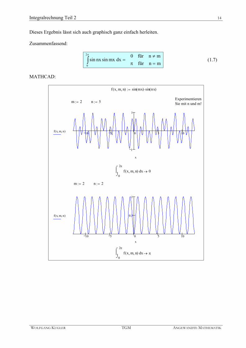
Dieses Ergebnis lässt sich auch graphisch ganz einfach herleiten. Zusammenfassend:
2
0
0 für n msin nx sin mx dx
für n m
π ≠=
π∫ = (1.7)
MATHCAD:
f x m, n,( ) sin mx( ) sin nx( )⋅:=
Experimentieren Sie mit n und m!m 2:= n 5:=
10 5 0 5 10
1
1
f x m, n,( )
x
0
2πxf x m, n,( )
⌠⌡
d 0→
m 2:= n 2:=
10 5 0 5 10
0.5
1
f x m, n,( )
x
0
2πxf x m, n,( )
⌠⌡
d π→
WOLFGANG KUGLER TGM ANGEWANDTE MATHEMATIK
Integralrechnung Teil 2 15
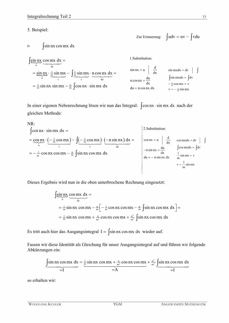
5. Beispiel: Zur Erinnerung: udv uv vdu= −∫ ∫
sin nx cos mx dx∫
u dv
1 1m m
u duv v
1 nm m
sin nx cos mx dx
sin nx sin mx sin mx n cos nx dx
sin nx sin mx cos nx sin mx dx
=
= ⋅ − ⋅
= − ⋅
∫
∫
∫
=
1.Substitution:
dsin nx udx
dun cos nxdx
du n cos nx dx
=
=
=
1m
1m
sin mxdx dv
sin mxdx dv
cos mx vv sin mx
=
=
− =
= −
∫∫ ∫
In einer eigenen Nebenrechnung lösen wir nun das Integral: nach der
gleichen Methode:
cos nx sin mx dx⋅∫
NR:
( ) ( ) ( )1 1m m
u duv v
1 nmm
cos nx sin mx dx
cos nx cos mx cos mx n sin nx dx
cos nx cos mx sin nx cos mx dx
⋅ =
= ⋅ − − − ⋅ −
= − −
∫∫
∫
=
2.Substitution:
dcos nx udx
dun sin nxdx
du n sin nx dx
=
− =
= −
cos mxdx dv
cos mxdx dv
1 sin mx vm
1v sin mxm
=
=
=
=
∫∫ ∫
Dieses Ergebnis wird nun in die oben unterbrochene Rechnung eingesetzt:
2
2 2
u dv
1 n 1 nm m m m
1 n nm m m
sin nx cos mx dx
sin nx cos mx cos nx cos mx sin nx cos mx dx
sin nx cos mx cos nx cos mx sin nx cos mx dx
=
= − − −
= + +
∫
∫∫
=
Es tritt auch hier das Ausgangsintegral wieder auf. I sin nx cos mx dx= ∫ Fassen wir diese Identität als Gleichung für unser Ausgangsintegral auf und führen wir folgende Abkürzungen ein:
2
2 21 n nm m m
sin nx cos mx dx sin nx cos mx cos nx cos mx sin nx cos mx dx
AI I
= + +
== =∫ ∫
so erhalten wir:
WOLFGANG KUGLER TGM ANGEWANDTE MATHEMATIK
Integralrechnung Teil 2 16
( )
2
2
2
2
2 2
2
2
2 2
nm
nm
m nm
mm n
I A
I 1 A
I A
I A
−
−
= +
− =
=
= ⋅
I
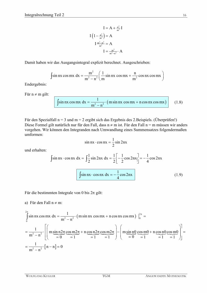
Damit haben wir das Ausgangsintegral explizit berechnet. Ausgeschrieben:
2
2 2 2m 1 nsin nx cos mx dx sin nx cos mx cos nx cos mx
m n m m = + − ∫
Endergebnis: Für n ≠ m gilt:
( )2 2
1sin nx cos mx dx msin nx cos mx n cos nx cos mxm n
= ⋅ +−∫ (1.8)
Für den Spezialfall n = 3 und m = 2 ergibt sich das Ergebnis des 2.Beispiels. (Überprüfen!) Diese Formel gilt natürlich nur für den Fall, dass n ≠ m ist. Für den Fall n = m müssen wir anders vorgehen. Wir können den Integranden nach Umwandlung eines Summensatzes folgendermaßen umformen:
1sin nx cos nx sin 2nx2
⋅ =
und erhalten: 1 1 1 1sin nx cos nx dx sin 2nx dx cos 2nx cos 2nx2 2 2 4
⋅ = = − = − ∫ ∫
1sin nx cos nx dx cos 2nx4
⋅ = −∫ (1.9)
Für die bestimmten Integrale von 0 bis 2π gilt: a) Für den Fall n ≠ m:
( )
[ ]
22
2 2 00
2 2
2 2
1sin nx cos mx dx m sin nx cos mx n cos nx cos mxm n
1 m sin n2 cos m2 n cos n2 cos m2 m sin n0 cos m0 n cos n0cos m0m n 00 1 1 1 1 1 1
1 n n 0m n
ππ= ⋅ + =
−
= ⋅ π π + π π − + − == = = = = = =
= ⋅ − =−
∫ =
WOLFGANG KUGLER TGM ANGEWANDTE MATHEMATIK
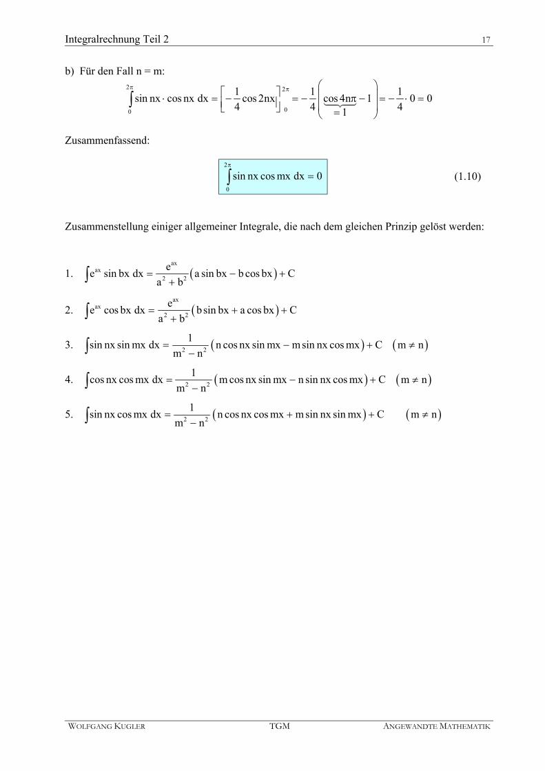
Integralrechnung Teil 2 17
b) Für den Fall n = m: 2 2
00
1 1 1sin nx cos nx dx cos 2nx cos 4n 1 0 04 4 41
π π ⋅ = − = − π − = − ⋅ =
∫ =
Zusammenfassend:
2
0
sin nx cos mx dx 0π
=∫ (1.10)
Zusammenstellung einiger allgemeiner Integrale, die nach dem gleichen Prinzip gelöst werden:
1. ( )ax
ax2 2
ee sin bx dx a sin bx b cos bx Ca b
= −+∫ +
2. ( )ax
ax2 2
ee cos bx dx bsin bx a cos bx Ca b
= ++∫ +
3. ( )2 2
1sin nx sin mx dx n cos nx sin mx m sin nx cos mx C m nm n
= − +−∫ ( )≠
4. ( )2 21cos nx cos mx dx m cos nx sin mx n sin nx cos mx C m n
m n= − +
−∫ ( )≠
5. ( )2 2
1sin nx cos mx dx n cos nx cos mx m sin nx sin mx C m nm n
= + +−∫ ( )≠
WOLFGANG KUGLER TGM ANGEWANDTE MATHEMATIK
Integralrechnung Teil 2 18
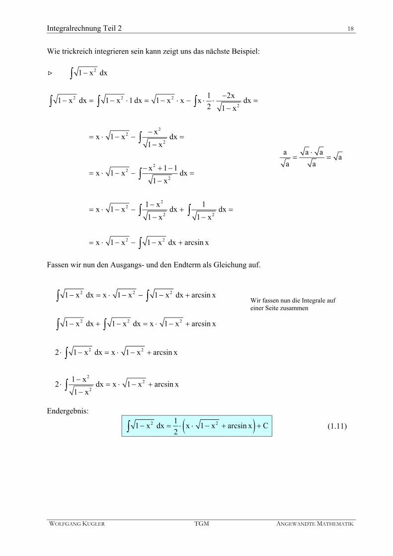
Wie trickreich integrieren sein kann zeigt uns das nächste Beispiel:
21 x dx−∫
2 2 2
2
22
2
22
2
22
2 2
2 2
1 2x1 x dx 1 x 1 dx 1 x x x dx2 1 x
xx 1 x dx1 x
x 1 1x 1 x dx1 x
1 x 1x 1 x dx dx1 x 1 x
x 1 x 1 x dx arcsin x
−− = − ⋅ = − ⋅ − ⋅ ⋅
−
−= ⋅ − − =
−
− + −= ⋅ − − =
−
−= ⋅ − − + =
− −
= ⋅ − − − +
∫ ∫ ∫
∫
∫
∫ ∫
∫
=
a a a aa a
⋅= =
Fassen wir nun den Ausgangs- und den Endterm als Gleichung auf.
2 2 2
2 2 2
2 2
22
2
1 x dx x 1 x 1 x dx arcsin x
1 x dx 1 x dx x 1 x arcsin x
2 1 x dx x 1 x arcsin x
1 x2 dx x 1 x arcsin x1 x
− = ⋅ − − − +
− + − = ⋅ − +
⋅ − = ⋅ − +
−⋅ = ⋅ − +
−
∫ ∫
∫ ∫
∫
∫
Wir fassen nun die Integrale auf einer Seite zusammen
Endergebnis:
( )2 211 x dx x 1 x arcsin x C2
− = ⋅ ⋅ − + +∫ (1.11)
WOLFGANG KUGLER TGM ANGEWANDTE MATHEMATIK
Integralrechnung Teil 2 19
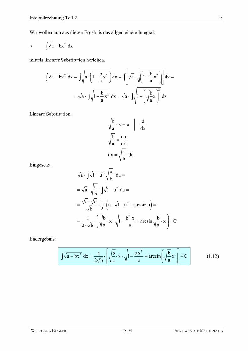
Wir wollen nun aus diesen Ergebnis das allgemeinere Integral:
2a bx dx−∫
mittels linearer Substitution herleiten.
2 2
2
2
b ba bx dx a 1 x dx a 1 x dxa a
b ba 1 x dx a 1 x dxa a
− = ⋅ − = ⋅ −
= ⋅ − = ⋅ −
∫ ∫ ∫
∫ ∫
2 =
Lineare Substitution:
b dx ua d
b dua dx
adx dub
⋅ =
=
= ⋅
x
Eingesetzt:
( )
2
2
2
2
aa 1 u dub
aa 1 u dub
a a 1 u 1 u arcsin u2b
a b b x bx 1 arcsin x Ca a a2 b
⋅ − ⋅ =
= ⋅ ⋅ − =
⋅= ⋅ ⋅ ⋅ − + =
= ⋅ ⋅ ⋅ − + ⋅ + ⋅
∫
∫
Endergebnis:
2
2 a b b x ba bx dx x 1 arcsin x Ca a a2 b
− = ⋅ ⋅ ⋅ − + +
∫ (1.12)
WOLFGANG KUGLER TGM ANGEWANDTE MATHEMATIK
Integralrechnung Teil 2 20
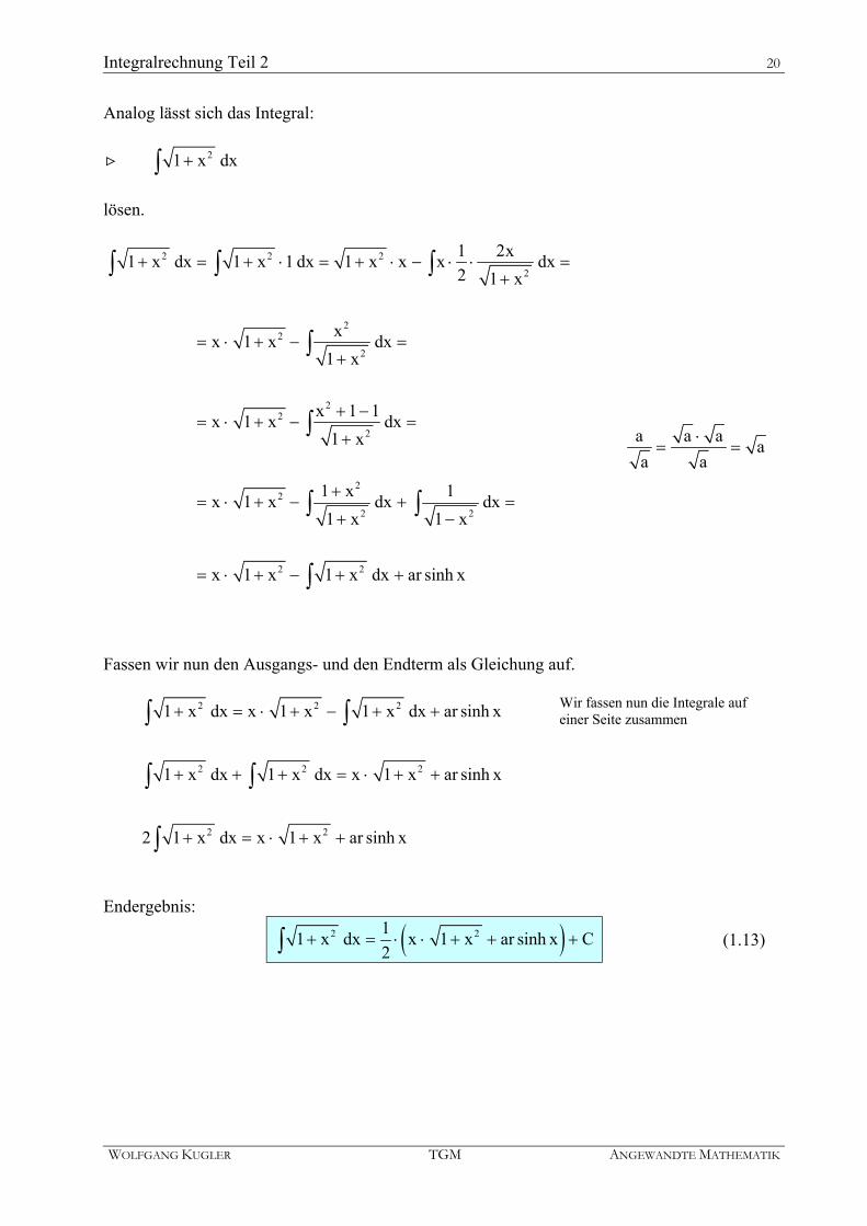
Analog lässt sich das Integral:
21 x dx+∫
lösen.
2 2 2
2
22
2
22
2
22
2 2
2 2
1 2x1 x dx 1 x 1 dx 1 x x x dx2 1 x
xx 1 x dx1 x
x 1 1x 1 x dx1 x
1 x 1x 1 x dx dx1 x 1 x
x 1 x 1 x dx ar sinh x
+ = + ⋅ = + ⋅ − ⋅ ⋅+
= ⋅ + − =+
+ −= ⋅ + − =
+
+= ⋅ + − + =
+ −
= ⋅ + − + +
∫ ∫ ∫
∫
∫
∫ ∫
∫
=
a a a aa a
⋅= =
Fassen wir nun den Ausgangs- und den Endterm als Gleichung auf.
2 2 2
2 2 2
2 2
1 x dx x 1 x 1 x dx ar sinh x
1 x dx 1 x dx x 1 x ar sinh x
2 1 x dx x 1 x ar sinh x
+ = ⋅ + − + +
+ + + = ⋅ + +
+ = ⋅ + +
∫ ∫
∫ ∫
∫
Wir fassen nun die Integrale auf einer Seite zusammen
Endergebnis:
( )2 211 x dx x 1 x ar sinh x C2
+ = ⋅ ⋅ + + +∫ (1.13)
WOLFGANG KUGLER TGM ANGEWANDTE MATHEMATIK
Integralrechnung Teil 2 21
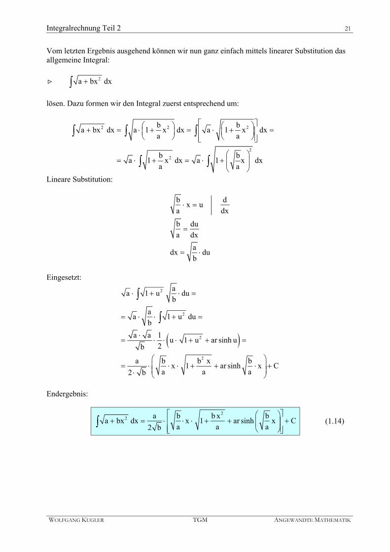
Vom letzten Ergebnis ausgehend können wir nun ganz einfach mittels linearer Substitution das allgemeine Integral:
2a bx dx+∫
lösen. Dazu formen wir den Integral zuerst entsprechend um:
2 2
2
2
b ba bx dx a 1 x dx a 1 x dxa a
b ba 1 x dx a 1 x dxa a
+ = ⋅ + = ⋅ +
= ⋅ + = ⋅ +
∫ ∫ ∫
∫ ∫
2 =
Lineare Substitution:
b dx ua d
b dua dx
adx dub
⋅ =
=
= ⋅
x
Eingesetzt:
( )
2
2
2
2
aa 1 u dub
aa 1 u dub
a a 1 u 1 u ar sinh u2b
a b b x bx 1 ar sinh xa a a2 b
⋅ + ⋅ =
= ⋅ ⋅ + =
⋅= ⋅ ⋅ ⋅ + + =
= ⋅ ⋅ ⋅ + + ⋅ ⋅
∫
∫
C+
Endergebnis:
2
2 a b b x ba bx dx x 1 ar sinh x Ca a a2 b
+ = ⋅ ⋅ ⋅ + + +
∫ (1.14)
WOLFGANG KUGLER TGM ANGEWANDTE MATHEMATIK
Integralrechnung Teil 2 22
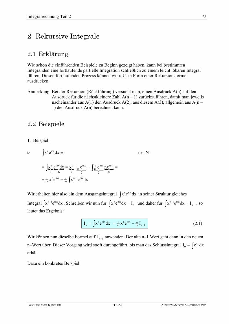
2 Rekursive Integrale
2.1 Erklärung
Wie schon die einführenden Beispiele zu Beginn gezeigt haben, kann bei bestimmten Integranden eine fortlaufende partielle Integration schließlich zu einem leicht löbaren Integral führen. Diesen fortlaufenden Prozess können wir u.U. in Form einer Rekursionsformel ausdrücken. Anmerkung: Bei der Rekursion (Rückführung) versucht man, einen Ausdruck A(n) auf den
Ausdruck für die nächstkleinere Zahl A(n – 1) zurückzuführen, damit man jeweils nacheinander aus A(1) den Ausdruck A(2), aus diesem A(3), allgemein aus A(n – 1) den Ausdruck A(n) berechnen kann.
2.2 Beispiele
1. Beispiel:
n n mxx e dx =∫ N∈
n mx n mx mx n 11 1m m
u u ddv v v
n mx n 1 mx1 nm m
x e dx x e e nx
x e x e dx
−
−
= = ⋅ −
= −
∫ ∫
∫u
=
Wir erhalten hier also ein dem Ausgangsintegral in seiner Struktur gleiches
Integral . Schreiben wir nun für und daher für , so
lautet das Ergebnis:
n mxx e dx∫n mx
ndx I=n 1 mxx e dx−∫ x e∫ n 1 mxn 1x e dx I−−=∫
n mx n mx1 n
n m mI x e dx x e I −= = −∫ n 1 (2.1)
Wir können nun dieselbe Formel auf anwenden. Der alte n–1 Wert geht dann in den neuen
n–Wert über. Dieser Vorgang wird sooft durchgeführt, bis man das Schlussintegral
erhält.
n 1I −
x0I e d= ∫ x
Dazu ein konkretes Beispiel:
WOLFGANG KUGLER TGM ANGEWANDTE MATHEMATIK
Integralrechnung Teil 2 23
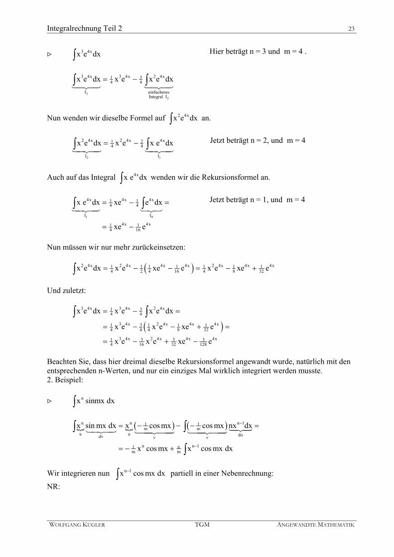
3 4xx e dx∫
32
3 4x 3 4x 2 4x314 4
I einfacheresIntegral I
x e dx x e x e dx= −∫ ∫
Hier beträgt n = 3 und m = 4 .
Nun wenden wir dieselbe Formel auf an. 2 4xx e dx∫
2 1
2 4x 2 4x 4x1 24 4
I I
x e dx x e x e dx= −∫ ∫ Jetzt beträgt n = 2, und m = 4
Auch auf das Integral wenden wir die Rekursionsformel an. 4xx e dx∫
1 0
4x 4x 4x1 14 4
I I
4x 4x1 14 16
x e dx xe e dx
xe e
= −
= −
∫ ∫ =
Jetzt beträgt n = 1, und m = 4
Nun müssen wir nur mehr zurückeinsetzen: ( )2 4x 2 4x 4x 4x 2 4x 4x 4x1 1 1 1 1 1 1
4 2 4 16 4 8 32x e dx x e xe e x e xe e= − − = − +∫
Und zuletzt:
( )
3 4x 3 4x 2 4x314 4
3 4x 2 4x 4x 4x31 1 1 14 4 4 8 32
3 4x 2 4x 4x 4x3 3 314 16 32 128
x e dx x e x e dx
x e x e xe e
x e x e xe e
= − =
= − − +
= − + −
∫ ∫=
Beachten Sie, dass hier dreimal dieselbe Rekursionsformel angewandt wurde, natürlich mit den entsprechenden n-Werten, und nur ein einziges Mal wirklich integriert werden musste. 2. Beispiel:
nx sinmx dx∫
( ) ( )n n n1 1
m mu u dudv v v
n n 11 nm m
x sin mx dx x cos mx cos mx nx dx
x cos mx x cos mx dx
−
−
= − − −
= − +
∫ ∫
∫
1 =
x
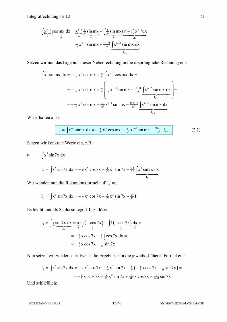
Wir integrieren nun partiell in einer Nebenrechnung: n 1x cos mx d−∫NR:
WOLFGANG KUGLER TGM ANGEWANDTE MATHEMATIK
Integralrechnung Teil 2 24
( )
( )
n 2
n 1 n 1 n 21 1m m
u udv v v du
n 1n 1 n 21m m
I
x cos mx dx x sin mx sin mx n 1 x dx
x sin mx x sin mx dx
−
− −
−− −
= − −
= −
∫ ∫
∫
− =
Setzen wir nun das Ergebnis dieser Nebenrechnung in die ursprüngliche Rechnung ein:
( )
n 2
n n n 11 nm m
n 1n n 1 n 21 n 1m m m m
I
x sinmx dx x cos mx x cos mx dx
x cos mx x sin mx x sin mx dx
−
−
−− −
= − + =
= − + − =
∫ ∫
∫
( )2 2
n 2
n n 1n n 1 n 21 nm m m
I
x cos mx x sin mx x sin mx dx
−
−− −= − + − ∫
Wir erhalten also: ( )
2n n 1n n n 11 n
n n 2m m mI x sinmx dx x cos mx x sin mx I−−
−= = − + −∫ 2 (2.2)
Setzen wir konkrete Werte ein, z.B.:
5x sin7x dx∫
3
5 45 5 4 3515 7 49 25
I
I x sin7x dx x cos 7x x sin 7x x sin7x dx⋅= = − + −∫ ∫
Wir wenden nun die Rekursionsformel auf an: 3I 3 3 23 31
3 17 49I x sin7x dx x cos 7x x sin 7x I⋅= = − +∫ 249−
Es bleibt hier als Schlussintegral zu lösen: 1I
( ) ( )1 11 7 7
duu udv v v
1 17 7
1 17 49
I x sin 7x dx x cos 7x cos 7x dx
x cos 7x cos 7x dx
x cos 7x sin 7x
= = ⋅ − − −
= − + =
= − +
∫ ∫
∫
=
Nun setzen wir wieder schrittweise die Ergebnisse in die jeweils „höhere" Formel ein:
( )3 3 23 61 1
3 7 49 49 7 49
3 23 6 617 49 343 2401
I x sin7x dx x cos 7x x sin 7x x cos 7x sin 7x
x cos 7x x sin 7x x cos 7x sin 7x
= = − + − − +
= − + + −
∫ 1 =
Und schließlich:
WOLFGANG KUGLER TGM ANGEWANDTE MATHEMATIK
Integralrechnung Teil 2 25
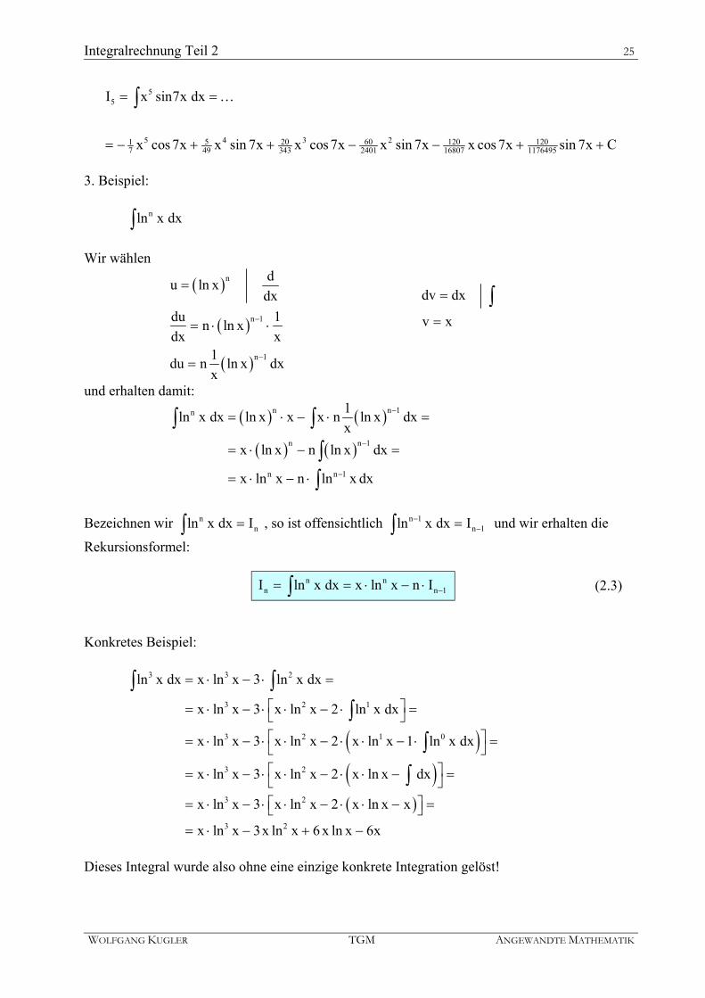
55
5 4 3 25 20 60 120 12017 49 343 2401 16807 1176495
I x sin7x dx
x cos 7x x sin 7x x cos 7x x sin 7x x cos 7x sin 7x C
= =
= − + + − − + +
∫ …
3. Beispiel: nln x dx∫ Wir wählen
( )
( )
( )
n
n 1
n 1
du ln xdx
du 1n ln xdx x
1du n ln x dxx
−
−
=
= ⋅ ⋅
=
dv dx
v x
=
=∫
und erhalten damit:
( ) ( )
( ) ( )
n nn
n n 1
n n 1
1ln x dx ln x x x n ln x dxx
x ln x n ln x dx
x ln x n ln x dx
−
−
−
= ⋅ − ⋅
= ⋅ − =
= ⋅ − ⋅
∫ ∫
∫∫
1 =
Bezeichnen wir , so ist offensichtlich und wir erhalten die
Rekursionsformel:
nnln x dx I=∫ n 1
n 1ln x dx I−−=∫
n nnI ln x dx x ln x n I −= = ⋅ − ⋅∫ n 1 (2.3)
Konkretes Beispiel:
Dieses Integral wurde also ohne eine einzige konkrete Integration gelöst!
( )( )( )
3 3 2
3 2 1
3 2 1 0
3 2
3 2
3 2
ln x dx x ln x 3 ln x dx
x ln x 3 x ln x 2 ln x dx
x ln x 3 x ln x 2 x ln x 1 ln x dx
x ln x 3 x ln x 2 x ln x dx
x ln x 3 x ln x 2 x ln x x
x ln x 3x ln x 6 x ln x 6x
= ⋅ − ⋅ =
= ⋅ − ⋅ ⋅ − ⋅ = = ⋅ − ⋅ ⋅ − ⋅ ⋅ − ⋅ = = ⋅ − ⋅ ⋅ − ⋅ ⋅ − = = ⋅ − ⋅ ⋅ − ⋅ ⋅ − =
= ⋅ − + −
∫ ∫∫
∫
∫
WOLFGANG KUGLER TGM ANGEWANDTE MATHEMATIK
Integralrechnung Teil 2 26
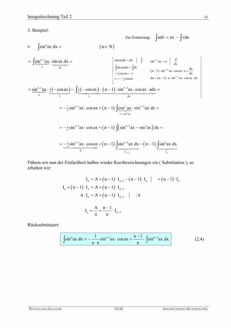
3. Beispiel: Zur Erinnerung: udv uv vdu= −∫ ∫
( )nsin ax dx n N= ∈∫
n 1
u dv
sin ax sin ax dx−= ⋅∫ =
1a
1a
sin axdx dv
sin axdx dv
cos ax vv cos ax
=
=
− =
= −
∫∫ ∫
( )
( )
n 1
n 2
n 2
dsin ax udx
dun 1 sin ax cos ax adx
du n 1 a sin ax cos ax dx
−
−
−
=
− ⋅ ⋅ ⋅ =
= − ⋅ ⋅ ⋅ ⋅
( ) ( ) ( )n 1 n 21 1a a
u v v du
sin ax cos ax cos ax n 1 sin ax cos ax adx− −= ⋅ − − − ⋅ − ⋅ ⋅ ⋅∫ =
( )
( ) ( )
( ) ( )
2
n 2 n
n 1 2 n 21a
1 sin ax
n 1 n 2 n1a
n 1 n 2 n1a
A I I
sin ax cos ax n 1 cos ax sin ax dx
sin ax cos ax n 1 sin ax sin ax dx
sin ax cos ax n 1 sin ax dx n 1 sin ax dx
−
− −
= −
− −
− −
= − ⋅ + − ⋅ =
= − ⋅ + − − =
= − ⋅ + − − −
∫
∫
∫ ∫
Führen wir nun der Einfachheit halber wieder Kurzbezeichnungen ein ( Substitution ), so erhalten wir:
( ) ( ) ( )
( ) ( )( )
n n 2 n
n n n 2
n n 2
I A n 1 I n 1 I n 1 I
I n 1 I A n 1 I
n I A n 1 I : n
−
−
−
= + − ⋅ − − ⋅ + − ⋅
+ − ⋅ = + − ⋅
⋅ = + − ⋅
n
n nA n 1n n −
−= + ⋅ 2I I
Rücksubstituiert:
n n 1 n1 n 1sin ax dx sin ax cos ax sin ax dxa n n
− −= − ⋅ + ⋅
⋅∫ 2−∫ (2.4)
WOLFGANG KUGLER TGM ANGEWANDTE MATHEMATIK
Integralrechnung Teil 2 27
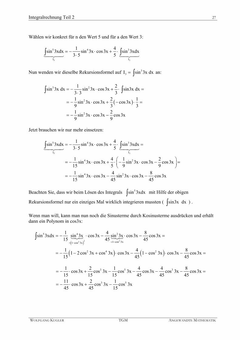
Wählen wir konkret für n den Wert 5 und für a den Wert 3:
5 3
5 4
I I
1 4sin 3xdx sin 3x cos 3x sin 3xdx3 5 5
= − ⋅ + ⋅⋅∫ ∫ 3
x
Nun wenden wir dieselbe Rekursionsformel auf an: 3
3I sin 3x d= ∫
( )
3 2
2
2
1 2sin 3x dx sin 3x cos 3x sin3x dx3 3 31 2sin 3x cos 3x cos 3x9 31 2sin 3x cos 3x cos 3x9 9
= − ⋅ + ⋅ =⋅
= − ⋅ + − ⋅ =
= − ⋅ −
∫ ∫13
Jetzt brauchen wir nur mehr einsetzen:
5 3
5 4 3
I I
4 2
4 2
1 4sin 3xdx sin 3x cos 3x sin 3xdx3 5 5
1 4 1 2sin 3x cos 3x sin 3x cos 3x cos 3x15 5 9 91 4 8sin 3x cos 3x sin 3x cos 3x cos 3x
15 45 45
= − ⋅ + ⋅ =⋅
= − ⋅ + ⋅ − ⋅ − =
= − ⋅ − ⋅ −
∫ ∫
Beachten Sie, dass wir beim Lösen des Integrals mit Hilfe der obigen
Rekursionsformel nur ein einziges Mal wirklich integrieren mussten ( ) .
5sin 3xdx∫sin3x dx∫
Wenn man will, kann man nun noch die Sinusterme durch Kosinusterme ausdrücken und erhält dann ein Polynom in cos3x:
( )
( ) ( )
2 22
5 4 2
1 cos 3x1 cos 3x
2 4 2
1 4 8sin 3xdx sin 3x cos 3x sin 3x cos 3x cos 3x15 45 45
1 41 2 cos 3x cos 3x cos 3x 1 cos 3x cos 3x cos 3x15 45 45
= −= −
= − ⋅ − ⋅ − =
= − − + ⋅ − − ⋅ − =
∫
8
3 5 3
3 5
1 2 1 4 4 8cos 3x cos 3x cos 3x cos 3x cos 3x cos 3x15 15 15 45 45 4511 2 1cos 3x cos 3x cos 3x45 45 15
= − ⋅ + − − − − =
= − ⋅ + −
WOLFGANG KUGLER TGM ANGEWANDTE MATHEMATIK
Integralrechnung Teil 2 28
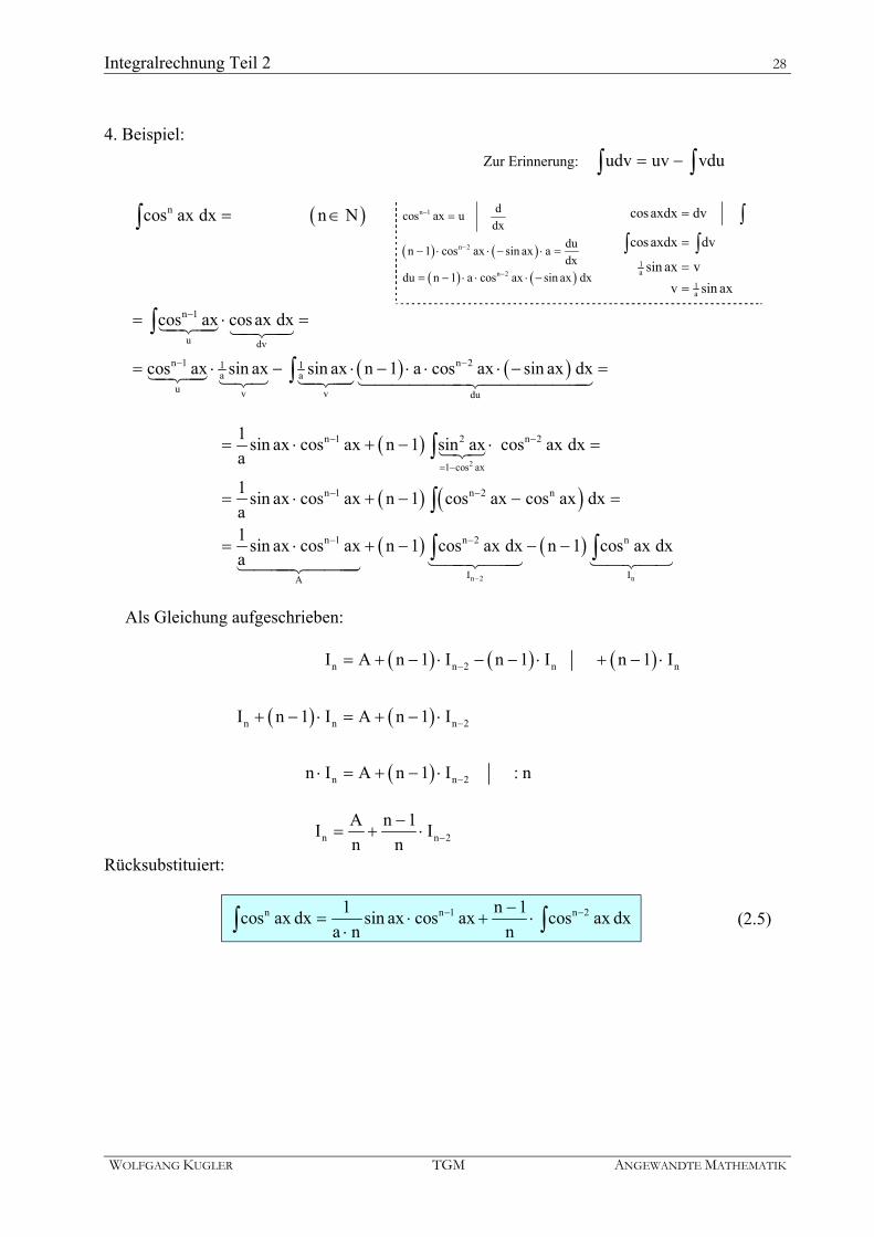
4. Beispiel: Zur Erinnerung: udv uv vdu= −∫ ∫
( )ncos ax dx n N= ∈∫ ( ) ( )
( ) ( )
n 1
n 2
n 2
dcos ax udx
dun 1 cos ax sin ax adx
du n 1 a cos ax sin ax dx
−
−
−
=
− ⋅ ⋅ − ⋅ =
= − ⋅ ⋅ ⋅ −
1a
1a
cos axdx dv
cos axdx dv
sin ax vv sin ax
=
=
=
=
∫∫ ∫
( ) ( )
n 1
u dv
n 1 n 21 1a a
u v v du
cos ax cos ax dx
cos ax sin ax sin ax n 1 a cos ax sin ax dx
−
− −
= ⋅ =
= ⋅ − ⋅ − ⋅ ⋅ ⋅ −
∫
∫ =
( )
( ) ( )
( ) ( )
2
n 2 n
n 1 2 n 2
1 cos ax
n 1 n 2 n
n 1 n 2 n
I IA
1 sin ax cos ax n 1 sin ax cos ax dxa
1 sin ax cos ax n 1 cos ax cos ax dxa1 sin ax cos ax n 1 cos ax dx n 1 cos ax dxa
−
− −
= −
− −
− −
= ⋅ + − ⋅ =
= ⋅ + − − =
= ⋅ + − − −
∫
∫
∫ ∫
Als Gleichung aufgeschrieben:
( ) ( ) ( )
( ) ( )
( )
n n 2 n
n n n 2
n n 2
I A n 1 I n 1 I n 1 I
I n 1 I A n 1 I
n I A n 1 I : n
−
−
−
= + − ⋅ − − ⋅ + − ⋅
+ − ⋅ = + − ⋅
⋅ = + − ⋅
n
n nA n 1I In n −
−= + ⋅ 2
Rücksubstituiert:
n n 11 n 1cos ax dx sin ax cos ax cos ax dxa n n
− −= ⋅ + ⋅
⋅∫ n 2∫ − (2.5)
WOLFGANG KUGLER TGM ANGEWANDTE MATHEMATIK
Integralrechnung Teil 2 29
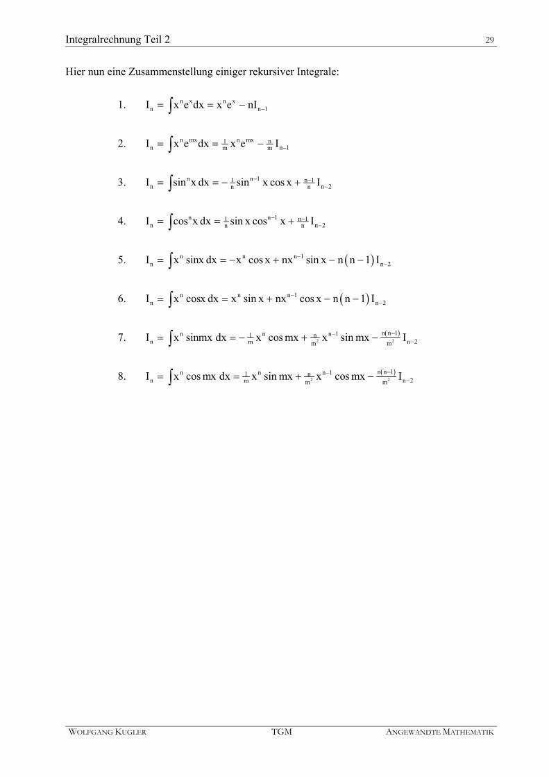
Hier nun eine Zusammenstellung einiger rekursiver Integrale:
1. n x n xn n 1I x e dx x e nI −= = −∫
2. n mx n mx1 nn n 1m mI x e dx x e I −= = −∫
3. n n 11 n− −1n n 2n nI sin x dx sin x cos x I −= = − +∫
4. n n 11 n− −1n n 2n nI cos x dx sin x cos x I −= = +∫
n n 2I x sinx dx x cos x nx sin x n n 1 I −= = − + − −∫
n n 2I x cosx dx x sin x nx cos x n n 1 I −= = + − −∫
5. ( )n n n 1−
6. ( )n n n 1−
7. ( )n n 1n n n 11 n −− 2 2n n 2m m mI x sinmx dx x cos mx x sin mx I −= = − + −∫
8. ( )n n 1n n n 11 n −− 2 2n n 2m m mI x cos mx dx x sin mx x cos mx I −= = + −∫
WOLFGANG KUGLER TGM ANGEWANDTE MATHEMATIK
Integralrechnung Teil 2 30
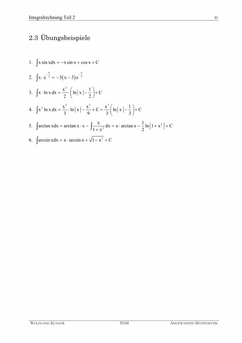
2.3 Übungsbeispiele
1. x sin xdx x sin x cos x C= − + +∫
2. ( )x x3 3x e 3 x 3 e
− −⋅ = − −∫
3. 2x 1x ln x dx ln x C
2 2 ⋅ = ⋅ − ∫ +
4. 3 3 3
2 x x x 1x ln x dx ln x C ln x C3 9 3 3
= ⋅ − + = − + ∫
5. 22
x 1arctan xdx arctan x x dx x arctan x ln 1 x C1 x 2
= ⋅ − = ⋅ − ++∫ ∫ +
6. 2arcsin xdx x arcsin x 1 x C= ⋅ + − +∫
WOLFGANG KUGLER TGM ANGEWANDTE MATHEMATIK
Integralrechnung Teil 2 31
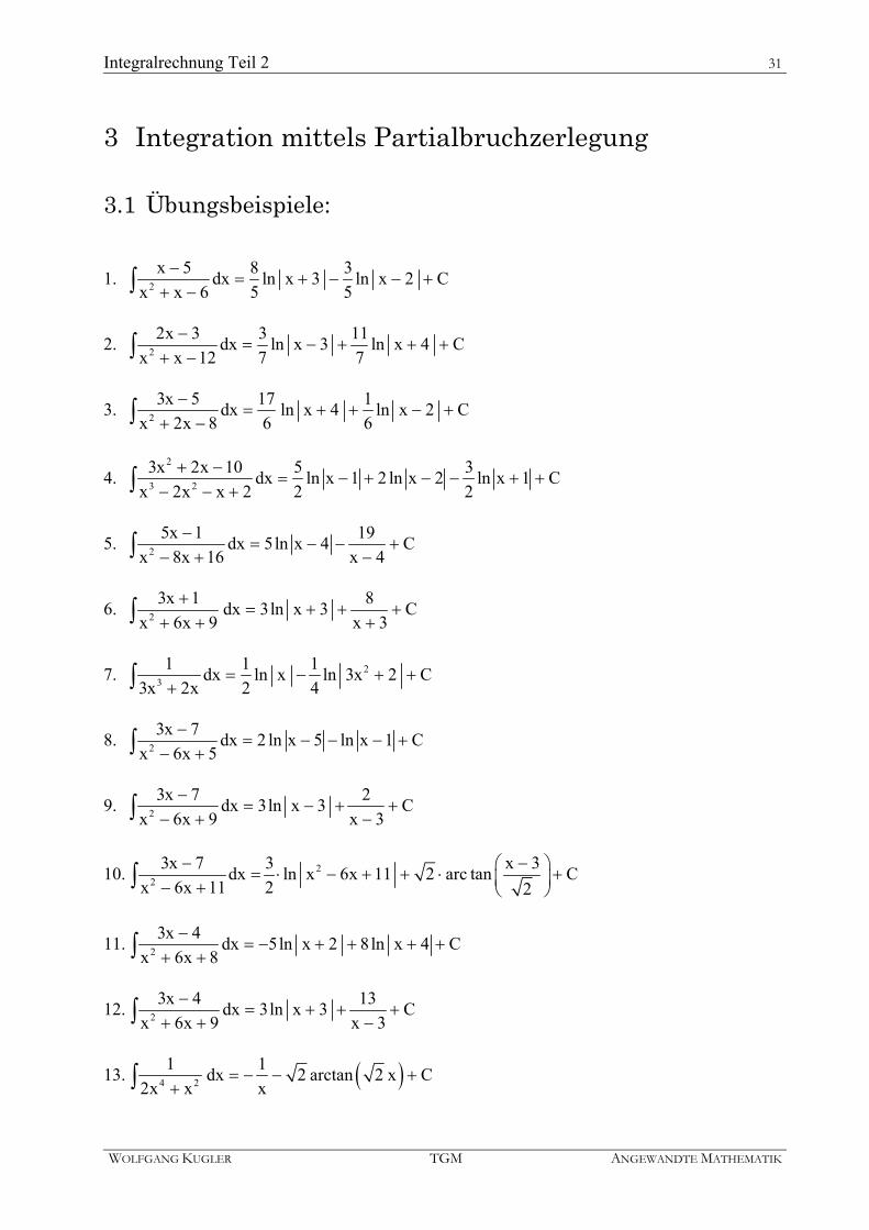
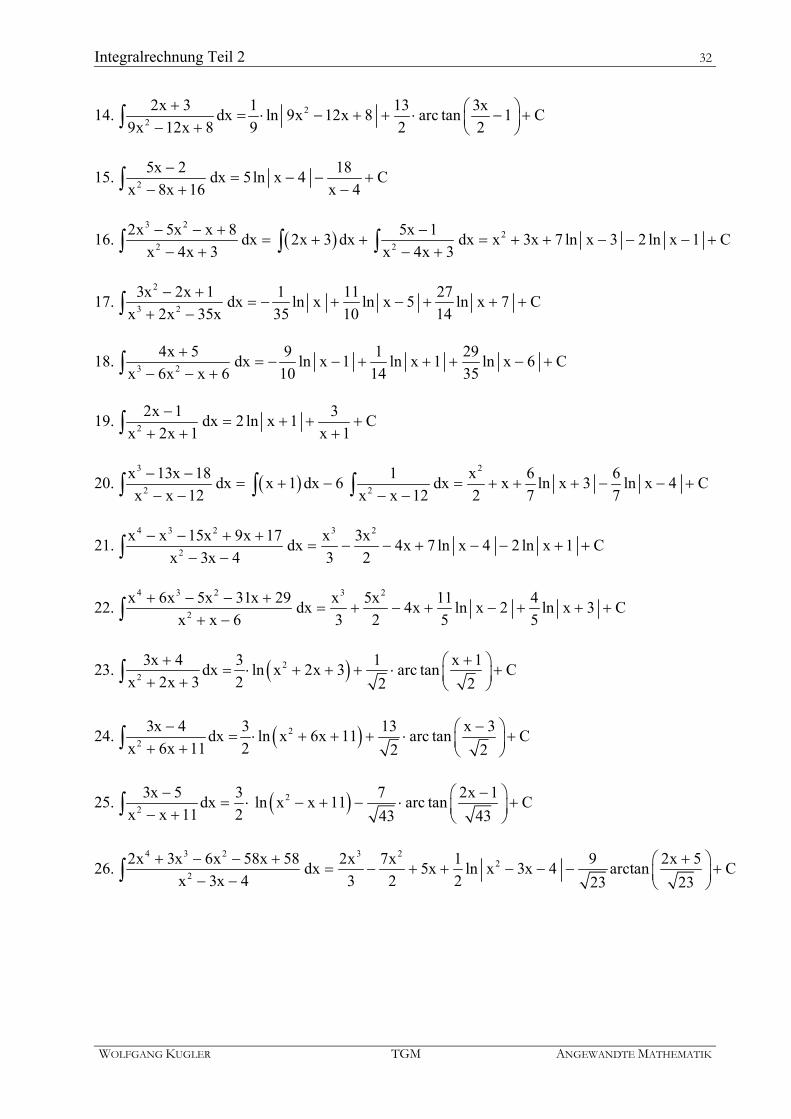
3 Integration mittels Partialbruchzerlegung
3.1 Übungsbeispiele:
1. 2
x 5 8 3dx ln x 3 ln x 2 Cx x 6 5 5
−= + − −
+ −∫ +
2. 22x 3 3 11dx ln x 3 ln x 4 C
x x 12 7 7−
= − + ++ −∫ +
3. 2
3x 5 17 1dx ln x 4 ln x 2 Cx 2x 8 6 6
−= + + −
+ −∫ +
4. 2
3 2
3x 2x 10 5 3dx ln x 1 2 ln x 2 ln x 1 Cx 2x x 2 2 2
+ −= − + − − + +
− − +∫
5. 2
5x 1 19dx 5ln x 4 Cx 8x 16 x 4
−= − − +
− + −∫
6. 2
3x 1 8dx 3ln x 3 Cx 6x 9 x 3
+= + + +
+ + +∫
7. 231 1 1dx ln x ln 3x 2 C
3x 2x 2 4= − +
+∫ +
8. 2
3x 7 dx 2 ln x 5 ln x 1 Cx 6x 5
−= − − − +
− +∫
9. 2
3x 7 2dx 3ln x 3 Cx 6x 9 x 3
−= − + +
− + −∫
10. 22
3x 7 3 x 3dx ln x 6x 11 2 arc tan Cx 6x 11 2 2
− − = ⋅ − + + ⋅ + − + ∫
11. 2
3x 4 dx 5ln x 2 8ln x 4 Cx 6x 8
−= − + + + +
+ +∫
12. 23x 4 13dx 3ln x 3 C
x 6x 9 x 3−
= + ++ + −∫ +
13. ( )4 2
1 1dx 2 arctan 2 x C2x x x
= − − ++∫
WOLFGANG KUGLER TGM ANGEWANDTE MATHEMATIK
Integralrechnung Teil 2 32
14. 222x 3 1 13 3xdx ln 9x 12x 8 arc tan 1 C
9x 12x 8 9 2 2+ = ⋅ − + + ⋅ − + − + ∫
15. 2
5x 2 18dx 5ln x 4 Cx 8x 16 x 4
−= − − +
− + −∫
16. ( )3 2
22 2
2x 5x x 8 5x 1dx 2x 3 dx dx x 3x 7 ln x 3 2 ln x 1 Cx 4x 3 x 4x 3− − + −
= + + = + + − − − +− + − +∫ ∫ ∫
17.2
3 2
3x 2x 1 1 11 27dx ln x ln x 5 ln x 7 Cx 2x 35x 35 10 14
− += − + − + + +
+ −∫
18. 3 24x 5 9 1 29dx ln x 1 ln x 1 ln x 6 C
x 6x x 6 10 14 35+
= − − + + + − +− − +∫
19. 2
2x 1 3dx 2 ln x 1 Cx 2x 1 x 1
−= + +
+ + +∫ +
20. ( )3 2
2 2
x 13x 18 1 x 6 6dx x 1 dx 6 dx x ln x 3 ln x 4 Cx x 12 x x 12 2 7 7− −
= + − = + + + − − +− − − −∫ ∫ ∫
21.4 3 2 3 2
2
x x 15x 9x 17 x 3xdx 4x 7 ln x 4 2 ln x 1 Cx 3x 4 3 2
− − + += − − + − − + +
− −∫
22.4 3 2 3 2
2
x 6x 5x 31x 29 x 5x 11 4dx 4x ln x 2 ln x 3 Cx x 6 3 2 5 5
+ − − += + − + − + + +
+ −∫
23. ( )22
3x 4 3 1 x 1dx ln x 2x 3 arc tan Cx 2x 3 2 2 2
+ + = ⋅ + + + ⋅ + + + ∫
24. ( )22
3x 4 3 13 x 3dx ln x 6x 11 arc tan Cx 6x 11 2 2 2
− − = ⋅ + + + ⋅ + + + ∫
25. ( )22
3x 5 3 7 2x 1dx ln x x 11 arc tan Cx x 11 2 43 43
− − = ⋅ − + − ⋅ + − + ∫
26.4 3 2 3 2
22
2x 3x 6x 58x 58 2x 7x 1 9 2x 5dx 5x ln x 3x 4 arctan Cx 3x 4 3 2 2 23 23
+ − − + + = − + + − − − + − − ∫
WOLFGANG KUGLER TGM ANGEWANDTE MATHEMATIK
Integralrechnung Teil 2 33
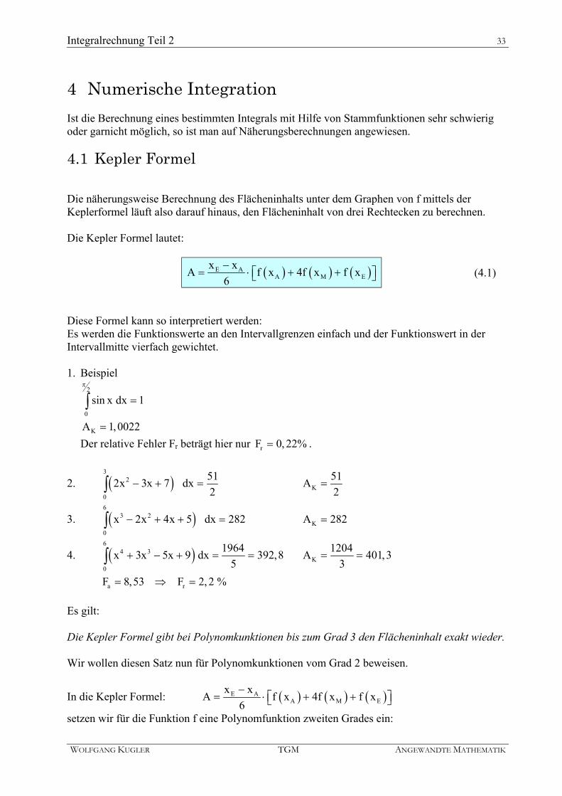
4 Numerische Integration
Ist die Berechnung eines bestimmten Integrals mit Hilfe von Stammfunktionen sehr schwierig oder garnicht möglich, so ist man auf Näherungsberechnungen angewiesen.
4.1 Kepler Formel
Die näherungsweise Berechnung des Flächeninhalts unter dem Graphen von f mittels der Keplerformel läuft also darauf hinaus, den Flächeninhalt von drei Rechtecken zu berechnen. Die Kepler Formel lautet:
( ) ( ) ( )E AA M
x xA f x 4f x f6−
= ⋅ + + Ex (4.1)
Diese Formel kann so interpretiert werden: Es werden die Funktionswerte an den Intervallgrenzen einfach und der Funktionswert in der Intervallmitte vierfach gewichtet. 1. Beispiel
2
0
sin x dx 1π
=∫KA 1,0022=
Der relative Fehler Fr beträgt hier nur .
rF 0, 22%=
2. ( )3
2
0
512x 3x 7 dx2
− + =∫ K51A2
=
3. ( )6
3 2
0
x 2x 4x 5 dx 282− + + =∫ KA 282=
4. ( )6
4 3
0
1964x 3x 5x 9 dx 392,85
+ − + = =∫ K1204A 401,3
3= =
a rF 8,53 F 2, 2 %= ⇒ = Es gilt: Die Kepler Formel gibt bei Polynomkunktionen bis zum Grad 3 den Flächeninhalt exakt wieder. Wir wollen diesen Satz nun für Polynomkunktionen vom Grad 2 beweisen.
In die Kepler Formel: ( ) ( ) ( )E AA M
x xA f x 4f x f x6−
= ⋅ + + E
setzen wir für die Funktion f eine Polynomfunktion zweiten Grades ein:
WOLFGANG KUGLER TGM ANGEWANDTE MATHEMATIK
Integralrechnung Teil 2 34
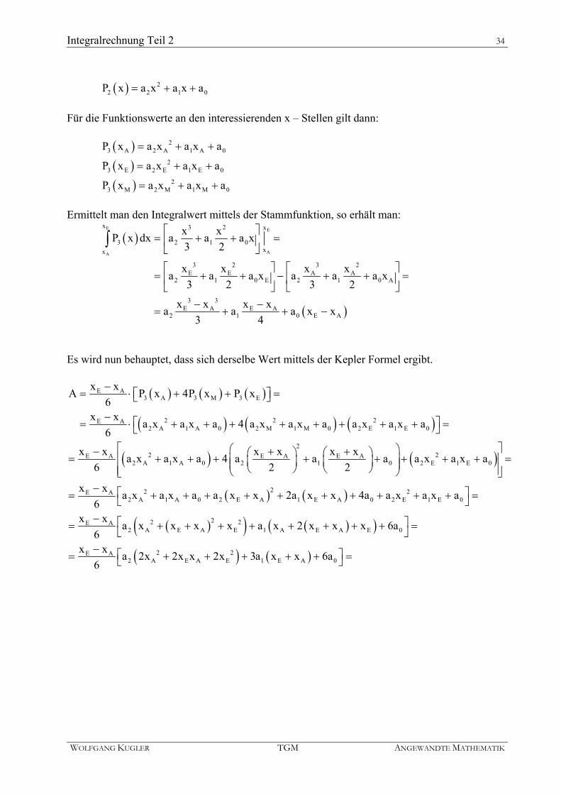
( ) 2
2 2 1P x a x a x a= + + 0
0
Für die Funktionswerte an den interessierenden x – Stellen gilt dann:
( )( )( )
23 A 2 A 1 A 0
23 E 2 E 1 E 0
23 M 2 M 1 M
P x a x a x a
P x a x a x a
P x a x a x a
= + +
= + +
= + + Ermittelt man den Integralwert mittels der Stammfunktion, so erhält man:
( )
( )
E E
AA
x 3 2 x
3 2 1 0xx
3 2 3 2E E A A
2 1 0 E 2 1 0 A
3 3E A E A
2 1 0 E A
x xP x dx a a a x3 2
x x x xa a a x a a a x3 2 3 2
x x x xa a a x x3 4
= + + =
= + + − + +
− −= + + −
∫
=
Es wird nun behauptet, dass sich derselbe Wert mittels der Kepler Formel ergibt.
( ) ( ) ( )
( ) ( ) (
E A3 A 3 M 3 E
2 2 2E A2 A 1 A 0 2 M 1 M 0 2 E 1 E 0
x xA P x 4P x P x6
x x a x a x a 4 a x a x a a x a x a6
−= ⋅ + + =
− = ⋅ + + + + + + + + ) =
( ) ( )
( ) ( )
( )( ) ( )( )
22 2E A E A E A
2 A 1 A 0 2 1 0 2 E
22 2E A2 A 1 A 0 2 E A 1 E A 0 2 E 1 E
22 2E A2 A E A E 1 A E A E 0
E A
x x x x x xa x a x a 4 a a a a x6 2 2
x x a x a x a a x x 2a x x 4a a x a x6
x x a x x x x a x 2 x x x 6a6
x x
− + + = + + + + + + −
= + + + + + + + +
− = + + + + + + + + −
=
1 E 0
0
a x a
a
+
+ + =
=
+ =
( ) ( )2 22 A E A E 1 E A 0a 2x 2x x 2x 3a x x 6a
6 + + + + + =
WOLFGANG KUGLER TGM ANGEWANDTE MATHEMATIK
Integralrechnung Teil 2 35
( ) ( )
( ) ( )
( ) ( ) ( ) ( ) ( )
2 2E A2 A E A E 1 E A 0
2 2E A2 A E A E 1 E A 0
2 22 E A A E A E 1 E A E A 0 E A
x x 2a x x x x 3a x x 6a6
x x 2a x x x x 3a x x 6a6
1 1a x x x x x x a x x x x a x x3 2
− = + + + + + =
− = + + + + + =
= − + + + − + + − =
( ) ( ) ( )
( )
3 3 2 22 E A 1 E A 0 E A
3 3 2 2E A E A
2 1 0 E A
1 1a x x a x x a x x3 2
x x x xa a a x x3 4
= − + + − + − =
− −= + + −
( ) ( ) ( )E AA M E
x xA f x 4f x f x6−
= ⋅ + +
( ) 3 23 3 2 1 0P x a x a x a x a= + + +
( )( )( )
3 23 A 3 A 2 A 1 A 0
3 23 E 3 E 2 E 1 E 0
3 23 M 3 M 2 M 1 M 0
P x a x a x a x a
P x a x a x a x a
P x a x a x a x a
= + + +
= + + +
= + + +
( )E E
AA
x 4 3 2 x
3 3 2 1 0xx
4 3 2E E E
3 2 1 0 E
4 4 3 3
x x xP x dx a a a a x4 3 2
x x xa a a a x a4 3 2
x x x x x x
= + + + =
= + + + −
− −
∫
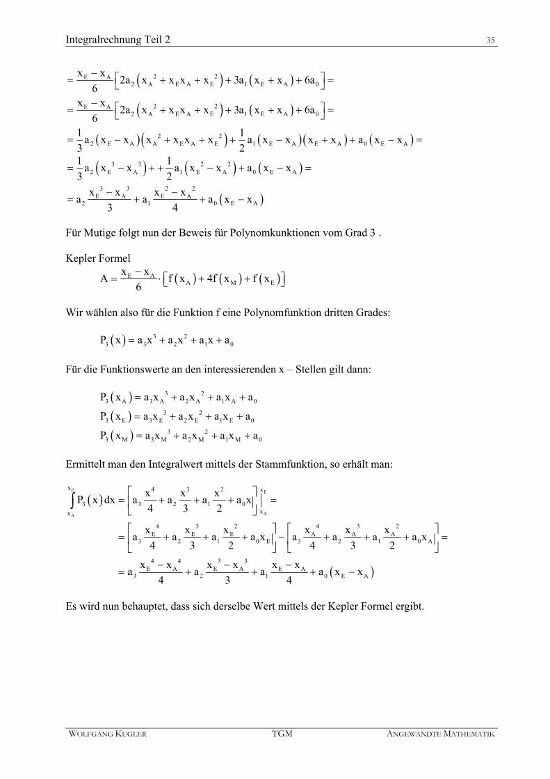
Für Mutige folgt nun der Beweis für Polynomkunktionen vom Grad 3 . Kepler Formel
Wir wählen also für die Funktion f eine Polynomfunktion dritten Grades: Für die Funktionswerte an den interessierenden x – Stellen gilt dann:
Ermittelt man den Integralwert mittels der Stammfunktion, so erhält man:
( )
4 3 2A A A
3 2 1 0 A
E A E A E A3 2 1 0 E A
x x xa a a x4 3 2
a a a a x x4 3 4
+ + +
−
= + + + −
=
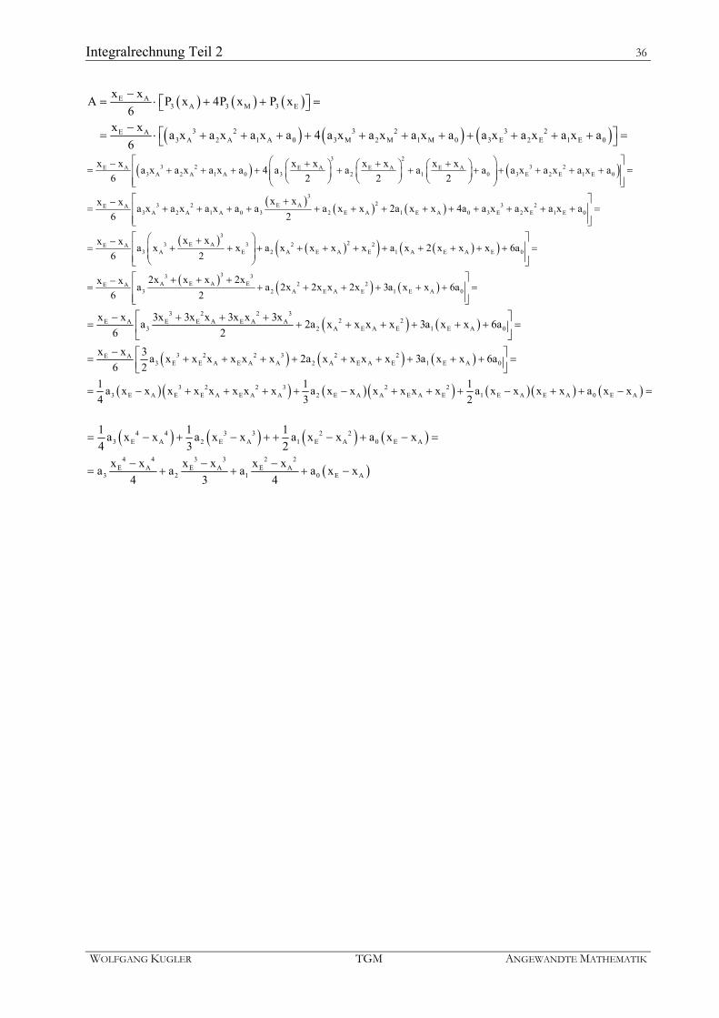
Es wird nun behauptet, dass sich derselbe Wert mittels der Kepler Formel ergibt.
WOLFGANG KUGLER TGM ANGEWANDTE MATHEMATIK
Integralrechnung Teil 2 36
( ) ( ) ( )
( ) ( ) (
E A3 A 3 M 3 E
3 2 3 2 3 2E A3 A 2 A 1 A 0 3 M 2 M 1 M 0 3 E 2 E 1 E 0
x xA P x 4P x P x6
x x a x a x a x a 4 a x a x a x a a x a x a x a6
−= ⋅ + + =
− = ⋅ + + + + + + + + + + + ) =
( ) ( )
( ) ( ) ( )
3 23 2 3 2E A E A E A E A
3 A 2 A 1 A 0 3 2 1 0 3 E 2 E 1 E 0
32E A3 2 3 2E A
3 A 2 A 1 A 0 3 2 E A 1 E A 0 3 E 2 E 1 E 0
x x x x x x x xa x a x a x a 4 a a a a a x a x a x a6 2 2 2
x xx x a x a x a x a a a x x 2a x x 4a a x a x a x a6 2
− + + + = + + + + + + + + + + +−
= + + + + + + + + + + + + +
+ =
( ) ( )( ) ( )( )
( ) ( ) ( )
32E A3 3 2 2E A
3 A E 2 A E A E 1 A E A E 0
33 3A E A E 2 2E A
3 2 A E A E 1 E A 0
x xx x a x x a x x x x a x 2 x x x 6a6 2
2x x x 2xx x a a 2x 2x x 2x 3a x x 6a6 2
=
+− = + + + + + + + + + + + = + + +−
= + + + + + + =
( ) ( )
( ) ( ) ( )
( ) ( ) ( ) ( ) ( )
3 2 2 32 2E A E E A E A A
3 2 A E A E 1 E A 0
3 2 2 3 2 2E A3 E E A E A A 2 A E A E 1 E A 0
3 2 2 3 2 23 E A E E A E A A 2 E A A E A E 1 E A E
x x 3x 3x x 3x x 3xa 2a x x x x 3a x x 6a6 2
x x 3 a x x x x x x 2a x x x x 3a x x 6a6 2
1 1 1a x x x x x x x x a x x x x x x a x x x x4 3 2
− + + += + + + + + + =
− = + + + + + + + + + =
= − + + + + − + + + − +( ) (A 0 Ea x+ − ) =Ax
( ) ( ) ( ) ( )
( )
4 4 3 3 2 23 E A 2 E A 1 E A 0 E A
4 4 3 3 2 2E A E A E A
3 2 1 0 E A
1 1 1a x x a x x a x x a x x4 3 2
x x x x x xa a a a x x4 3 4
= − + − + + − + − =
− − −= + + + −
WOLFGANG KUGLER TGM ANGEWANDTE MATHEMATIK
Integralrechnung Teil 2 37
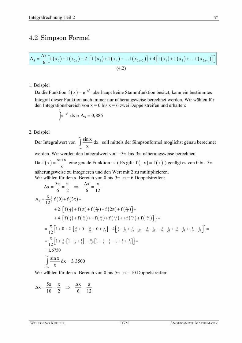
4.2 Simpson Formel
( ) ( ) ( ) ( ) ( ) ( ) ( ) ( )S 0 2n 2 4 2n 2 1 3 2n 1xA f x f x 2 f x f x f x 4 f x f x f x
6 − −
∆ = + + ⋅ + + + + + … …
(4.2) 1. Beispiel
Da die Funktion f x überhaupt keine Stammfunktion besitzt, kann ein bestimmtes Integral dieser Funktion auch immer nur näherungsweise berechnet werden. Wir wählen für den Integrationsbereich von x = 0 bis x = 6 zwei Doppelstreifen und erhalten:
( ) 2xe−=
2
Sdx A≈ =6
x
0
e 0,886−∫
2. Beispiel
Der Integralwert von sin x dxx
∞
− ∞∫ soll mittels der Simpsonformel möglichst genau berechnet
werden. Wir werden den Integralwert von bis 3 näherungsweise berechnen.
Da
3− π π
( ) sin xx
=f x eine gerade Funktion ist ( Es gilt: f x ) genügt es von 0 bis
näherungsweise zu integrieren und den Wert mit 2 zu multiplizieren. Wir wählen für den x–Bereich von 0 bis n = 6 Doppelstreifen:
( ) (f x− = ) 3π
3π3 xx6 2 6 1π π ∆ π
∆ = = ⇒ =2
( ) ( ){( ) ( ) ( ) ( ) ( )( ) ( ) ( ) ( ) ( ) ( ) }
2
94
132 2
1
π
π
π
+
+
⋅
=
2=
1 17
4
π +
−
3
3
sin x dx 3,3500x
π
− π
=∫
Wir wählen für den x–Bereich von 0 bis n = 10 Doppelstreifen:
5π
5 xx10 2 6 12π π ∆ π
∆ = = ⇒ =
[ ]
[ ] [ ]
S
3 52 2
3 5 7 114 4 4 4 4
2 2 2 4 1 4 4 1 4 1 4 1 4 13 5 5 7 9 112 2 2
164 1 1 1 13 5 3 5 9 112
A f 0 f 312
2 f f f f 2 f
4 f f f f f f
1 0 2 0 012
1 1 112
π π
π π π π π
π π π π π π π π
π π
π= + π +
+ ⋅ + π + +
+ ⋅ + + + + + + = π = + + ⋅ + − + + + ⋅ + − ⋅ − ⋅ + ⋅ + ⋅ π = + ⋅ − + + + − + +
= 1, 6750
WOLFGANG KUGLER TGM ANGEWANDTE MATHEMATIK
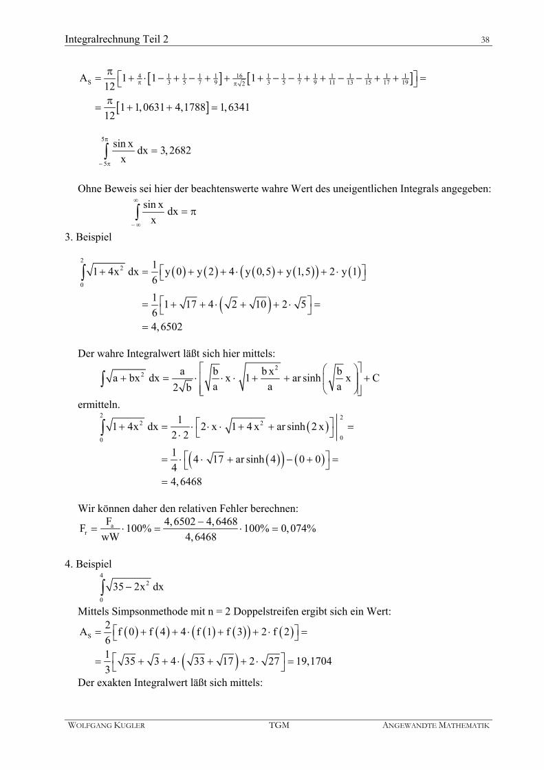
Integralrechnung Teil 2 38
[ ] [ ]
[ ]
164 1 1 1 1 1 1 1 1 1 1 1 1 1S 3 5 7 9 3 5 7 9 11 13 15 17 192
A 1 1 112
1 1,0631 4,1788 1,634112
π π
π = + ⋅ − + − + + + − − + + − − + + =
π= + + =
5
5
sin x dx 3, 2682x
π
− π
=∫
Ohne Beweis sei hier der beachtenswerte wahre Wert des uneigentlichen Integrals angegeben:
sin x dxx
∞
− ∞
= π∫
( ) ( ) ( ) ( )( ) ( )
( )
22
0
11 4x dx y 0 y 2 4 y 0,5 y 1,5 2 y 161 1 17 4 2 10 2 564,6502
+ = + + ⋅ + + ⋅
= + + ⋅ + + ⋅ = =
∫
22 a b b x ba bx dx x 1 ar sinh x C
a a a2 b
+ = ⋅ ⋅ ⋅ + + +
∫
( )
( )( ) ( )
2 22 2
00
11 4x dx 2 x 1 4 x ar sinh 2 x2 21 4 17 ar sinh 4 0 044,6468
+ = ⋅ ⋅ ⋅ + + = ⋅
= ⋅ ⋅ + − + = =
∫
ar
F 4,6502 4,6468F 100% 100% 0,074%wW 4,6468
−= ⋅ = ⋅ =
42
0
35 2x dx−∫
( ) ( ) ( ) ( )( ) ( )2A f 0 f 461 35 3 4
= + +
= + +
4
33⋅
3. Beispiel
Der wahre Integralwert läßt sich hier mittels:
ermitteln.
Wir können daher den relativen Fehler berechnen:
4. Beispiel
Mittels Simpsonmethode mit n = 2 Doppelstreifen ergibt sich ein Wert:
( )S f 1 f 3 2 f 2
17 2 27 19,17043
⋅ + + ⋅ =
+ + ⋅ =
Der exakten Integralwert läßt sich mittels:
WOLFGANG KUGLER TGM ANGEWANDTE MATHEMATIK
Integralrechnung Teil 2 39
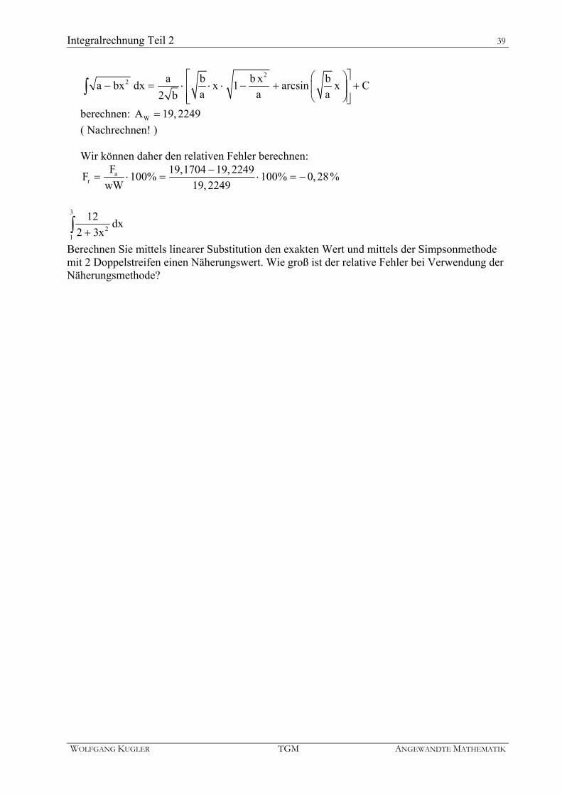
22 a b b x ba bx dx x 1 arcsin x C
a a a2 b
− = ⋅ ⋅ ⋅ − +
∫
WA 19, 2249=
+
berechnen: ( Nachrechnen! ) Wir können daher den relativen Fehler berechnen:
ar
F 19,1704 19, 2249F 100% 100% 0, 28%wW 19, 2249
−= ⋅ = ⋅ = −
2
12 dx2 3x+
3
1∫
Berechnen Sie mittels linearer Substitution den exakten Wert und mittels der Simpsonmethode mit 2 Doppelstreifen einen Näherungswert. Wie groß ist der relative Fehler bei Verwendung der Näherungsmethode?
WOLFGANG KUGLER TGM ANGEWANDTE MATHEMATIK