DLR AT-TRAIB 92517-15 B7

JExTRA – Jet NoiseExperiments at AT-TRA

SUMMER 2015 PROJECT REPORT

Max Nussbaumer and Henri Siller

Deutsches Zentrum für Luft- und Raumfahrte.V.Institut für AntriebstechnikAbteilung TriebwerksakustikBerlin

DLR für Luft- und RaumfahrtDeutsches Zentrum

Deutsches Zentrum für Luft- und Raumfahrt e.V.Institut für AntriebstechnikAbteilung TriebwerksakustikProf. Dr. Lars EnghardtMüller-Breslau-Straße 810623 BerlinTel: +49 30 310006-18

Max Nussbaumer and Henri SillerTel: +49 30 310006-(030) 310 006 -57Fax: +49 30 310006–39E-Mail: Henri.Siller@dlr.de

Dokument-IdentifikationTitel . . . . . . . . . . . . . JExTRA – Jet Noise Experiments at AT-TRAThema . . . . . . . . . . . DLR AT-TRAAutor(en) . . . . . . . . . Max Nussbaumer and Henri SillerDateiname . . . . . . . . . IB92517_15BX_JEXTRA.texZuletzt gespeichert am . . 12. Januar 2016

Dokument-Entwicklung:

Version 1.0 . . . . . . . . . inital version January 12, 2016

DLRDLR – IB 92517-15 B7 iii

Inhaltsverzeichnis

1. Abstract 1

2. Introduction 3

3. Design and Set-up of Rig 53.1. Linear Array Design . . . . . . . . . . . . . . . . . . . . . . . . . . . . . . . . . 5

3.1.1. Microphone spacing . . . . . . . . . . . . . . . . . . . . . . . . . . . . 53.1.2. Length of Array . . . . . . . . . . . . . . . . . . . . . . . . . . . . . . 73.1.3. Design and Construction . . . . . . . . . . . . . . . . . . . . . . . . . 103.1.4. Conclusions for Linear Array Design . . . . . . . . . . . . . . . . . . . 11

3.2. Low-Reflectio Rear and Front Wall for Anechoic channel . . . . . . . . . . 133.3. Positioning of the Anechoic Channel and Microphones . . . . . . . . . . . . 14

3.3.1. Markings on Channel Segments and Room . . . . . . . . . . . . . . 153.3.2. Positioning in X-Y plane . . . . . . . . . . . . . . . . . . . . . . . . . . 153.3.3. Positioning in Z-direction . . . . . . . . . . . . . . . . . . . . . . . . . 163.3.4. Positioning of Microphones . . . . . . . . . . . . . . . . . . . . . . . . 17

3.4. Practical Protocol . . . . . . . . . . . . . . . . . . . . . . . . . . . . . . . . . . 173.4.1. Theme: Anechoic Channel . . . . . . . . . . . . . . . . . . . . . . . . 183.4.2. Theme: Low-Reflectio Rear and Front Walls . . . . . . . . . . . . . . 203.4.3. Theme: Snow-Flake Data Acquisition System . . . . . . . . . . . . . 213.4.4. Theme: Linear Array . . . . . . . . . . . . . . . . . . . . . . . . . . . . 223.4.5. Theme: Microphone Ring . . . . . . . . . . . . . . . . . . . . . . . . . 26

4. Calibration of Microphones 274.1. Calibration Theory . . . . . . . . . . . . . . . . . . . . . . . . . . . . . . . . . 27

4.1.1. Mathematical Basis . . . . . . . . . . . . . . . . . . . . . . . . . . . . 274.1.2. Calibration Methods . . . . . . . . . . . . . . . . . . . . . . . . . . . . 284.1.3. Comparison of methods for test case . . . . . . . . . . . . . . . . . . 30

4.2. Calibration Script jextra_cal.py . . . . . . . . . . . . . . . . . . . . . . . . . . 304.2.1. Overview of Methodology . . . . . . . . . . . . . . . . . . . . . . . . 304.2.2. Input . . . . . . . . . . . . . . . . . . . . . . . . . . . . . . . . . . . . . 314.2.3. Output . . . . . . . . . . . . . . . . . . . . . . . . . . . . . . . . . . . 324.2.4. Results . . . . . . . . . . . . . . . . . . . . . . . . . . . . . . . . . . . . 32

DLRDLR – IB 92517-15 B7 I

5. Single Source Reflectio Experiments 375.1. Experimental Set-up . . . . . . . . . . . . . . . . . . . . . . . . . . . . . . . . 37

5.1.1. Pop . . . . . . . . . . . . . . . . . . . . . . . . . . . . . . . . . . . . . . 385.1.2. Blank Gun . . . . . . . . . . . . . . . . . . . . . . . . . . . . . . . . . . 39

5.2. Results . . . . . . . . . . . . . . . . . . . . . . . . . . . . . . . . . . . . . . . . 395.2.1. Time Signals . . . . . . . . . . . . . . . . . . . . . . . . . . . . . . . . 395.2.2. Reflectio Contour Maps . . . . . . . . . . . . . . . . . . . . . . . . . 41

5.3. Conclusions of Validity of Anechoic Channel . . . . . . . . . . . . . . . . . . 43

6. Jet Noise Measurements 496.1. Basic theory . . . . . . . . . . . . . . . . . . . . . . . . . . . . . . . . . . . . . 496.2. Experimental Setup . . . . . . . . . . . . . . . . . . . . . . . . . . . . . . . . . 506.3. Comparison Data . . . . . . . . . . . . . . . . . . . . . . . . . . . . . . . . . . 516.4. Mathematical Considerations . . . . . . . . . . . . . . . . . . . . . . . . . . . 51

6.4.1. Atmospheric absorption correction . . . . . . . . . . . . . . . . . . . 516.4.2. Distance correction . . . . . . . . . . . . . . . . . . . . . . . . . . . . 53

6.5. Results . . . . . . . . . . . . . . . . . . . . . . . . . . . . . . . . . . . . . . . . 556.5.1. Data Correction (M = 0.5 case) . . . . . . . . . . . . . . . . . . . . . 556.5.2. SPL Contour Maps (M = 0.5 case) . . . . . . . . . . . . . . . . . . . . 566.5.3. SPL-St Graphs for Different Angles (M = 0.5 case) . . . . . . . . . . 586.5.4. Variation with M . . . . . . . . . . . . . . . . . . . . . . . . . . . . . . 596.5.5. Experiments with Flow Conditioning in Pipe . . . . . . . . . . . . . . 606.5.6. Mach Exponent Scaling . . . . . . . . . . . . . . . . . . . . . . . . . . 626.5.7. Near Field Correction . . . . . . . . . . . . . . . . . . . . . . . . . . . 666.5.8. Inspection of Data from Ring Array . . . . . . . . . . . . . . . . . . . 67

6.6. Discussion of Validity of Rig for Jet Noise Measurements . . . . . . . . . . . 67

7. Future Work 81

Appendices 85

A. Linear Array Strouhal Calculations 87

B. Jet Noise Tables 89

C. Experimental log sheets 91

D. Determination of Microphone Positions 93

IIDLRDLR – IB 92517-15 B7

1. Abstract

Dieser Bericht wurde von Max Nussbaumer im Rahmen seines Praktikums in der DLRAbteilung Triebwerksakustik in Berlin vom 1. Juli 2015 bis zum 11. September 2015 ge-schrieben. Betreut von Henri Siller hat er akustische Messungen an dem JExTRA Strahl-prüfstand mit einem Mikrofonarray durchgeführt. Der Strahlprüfstand wurde von RobertMeyer bereitgestellt, der reflexionsarm Aufbau von Alessandro Bassetti konzipiert undaufgebaut. Unterstützt wurde er von von Wolfram Hage und Larisa Hritsevskyy, die zu-sammen mit Stefan Funke an den Messungen beteiligt waren. Stefan Funke hat bei derAuswertung der Daten beraten und Karsten Liesner unterstützte den Betrieb des Prüf-stands und Anpassungen der Steuersoftware.

This report by Max Nussbaumer is the result of his summer internship from 1. July 2015to 11. September 2015 at DLR engine acoustics in Berlin. Under the supervision of HenriSiller, he performed acoustic measurements with a microphone array in the JExTRA jetfacility. The jet facility was provided by Robert Meyer, the anechoic set-up of the micro-phone array has been conceived and constructed by Alessandro Bassetti with the supportof Wolfram Hage and Larisa Hritsevskyy, who together with Stefan Funke supported theexperiments. Stefan Funke also consulted Max Nussbaumer during the data reduction.Karsten Liesner supported the operation of the jet facility and adapted the control soft-ware.

DLRDLR – IB 92517-15 B7 1

2. Introduction

The JEXTRA project concerns the establishment of a small scale jet noise testing facility atthe DLR Berlin Charlottenburg Location.

This report covers the work carried out on the project from 1. July 2015 to 11. September2015.

In the firs phase of the project, the partially complete JEXTRA rig was brought to a statein which it can be used for measurements. The practical steps taken are documented inchapter 3.

In the second phase of the project the capabilities and limitations of the JEXTRA rig wereinvestigated in a series of tests. Experiments with single sound sources to identify reflections are covered in chapter 5, Jet noise measurements are covered in chapter 6. As part ofthis phase of the project a new microphone calibration script was developed in python,the mathematical background, methodology and implementation of this script are cover-ed in chapter 4. Recommendations for future work on the JEXTRA project are given inchapter 7.

DLRDLR – IB 92517-15 B7 3

3. Design and Set-up of Rig

3.1. Linear Array Design

In order to carry out source identification the construction of a linear array for use in theanechoic channel around the jet is desired. The SODIX method will be used to interpretthe data from this linear array. The necessary length, microphone spacing and numberof microphones to be used need to be determined. There is no define minimum spati-al microphone spacing for the SODIX method [Stephan], although some evidence of analiasing-like effect at high frequencies has been observed. In general however, for SODIX,the more data points are available the better the results from the optimisation.

In order to allow some of the data to be used for an alternative beam-forming technique,the minimum spacing as required for beam-forming will be calculated for the 60° to100° region and applied to the entire array. Sections of the array outside this range maynot be suitable for beam-forming above a certain frequency, but should still be able to beused with SODIX.

3.1.1. Microphone spacing

The microphones initially intended to be used are assumed to be approximately linear upto 16 kHz, so this is taken as the maximum frequency of interest fmax .

The minimum spatial sampling rate for microphones in a linear array, to avoid aliasingwhen using beam-forming methods, is half the smallest wavelength of interest. The re-levant wavelength for this is the ‘trace wavelength’ (λt ) as seen by the microphones[Stephan]. The smallest trace wavelength will occur at the angle furthest from 90°. In thisset-up this is the 60° angle, as below 60° there is no requirement for beam-forming tobe applicable.

DLRDLR – IB 92517-15 B7 5

The definitio of λt is shown in figur 3.1. As the wavelength at 16 kHz is λ= 21.14mm(see below), the closest microphone is around 27 wavelengths away from the sound sour-ce, which justifie the plane wave assumption.

Abbildung 3.1.: Definitio of λt for a polar angle of θ.

First the minimum wavelength λmi n must be calculated. This is given by λmi n = a/ fmax

where a is the speed of sound. Taking the temperature of air as 25 °C, and using standardvalues for R and γ of air, a can be calculated as:

a =√γ∗R ∗Tst ati c

a =p1.4∗287∗ (273.15+20) = 343m/s

thus:

λmi n = 343/16000 = 0.02144m = 21.14mm

Simple trigonometry can then be applied to work out λt :

λt = λcos(60) = 2λ

6DLRDLR – IB 92517-15 B7

then to fin the minimum spatial sampling rate d :

d < [λt ]mi n/2

thus d < 21.14mm

The temperatures of the jet and the surrounding air are likely to rise during operation.This will increase the speed of sound and thus increase λmi n. This means that the coldestoperating temperature is the critical condition. For example, repeating the above calcula-tion with an air temperature of 25 °C gives d < 21.63mm .

In summary, to avoid beam-forming aliasing at 16 kHz, in the range 100° to 60° the mi-nimum spacing required is 21mm.

3.1.2. Length of Array

The length of the array depends on the range of polar angles that are of interest. In thefiel of pure jet noise, ‘observation angles’ or ‘polar angles’ are define from the positivejet axis (i.e. the direction of the jet) (see figur 3.2).

Abbildung 3.2.: Definitio of observer angle θ in jet noise aeroacoustics.

By translating the linear array (or whole anechoic channel) in the axial direction, it ispossible to alter the polar angles of the microphones as shown in figur 3.3.

The axial translation of the anechoic channel is limited by geometric constraints due to aconstruction above the pipe as shown in figur 3.4. The distance marked s in the sketch isthe distance between the frame constraint and the nozzle, this distance can be extendedto a maximum approximately s ≈ 270mm by moving some elements of the construction.If this is less than the required length then either the pipe needs to be lengthened, or the

DLRDLR – IB 92517-15 B7 7

Abbildung 3.3.:Maximum (firs microphone) and minimum (last microphone) po-lar angles measured for a given axial position of the anechoicchannel and linear array relative to the nozzle exit.

range of observer angles reduced. Taking into account the fact that for effective soundinsulation, microphones should not be installed too close to the entrance of the channel,it has been decided to reduce the largest observer angle of interest from 120° to 100°.

Abbildung 3.4.: Geometric constraint of anechoic channel translation. Critical lo-cation marked in orange.

Downstream of the jet, results from another project have shown that microphones atangles lower than 50° may give interesting results [Jonas]. In order to obtain data for thisregion the fina range of observer angles has been specifie as 30° – 100°.

In order to calculate the length of array needed it is firs necessary to consider the radialdistance between the jet axis and the microphones. The inner layer of sound insulation

8DLRDLR – IB 92517-15 B7

starts at 0.7m from the jet axis. In order to avoid interference by possible reflectionfrom the sound-absorbing material it has been proposed [Henri] that the microphonesare placed as far form the wall as possible. With the proposed linear array design a radialdistance of 580mm between the microphone heads and the jet axis can be achieved.

For the range of polar angles specifie (30°- 100°) the following lengths are needed ups-tream and downstream of the nozzle exit:

lupstr eam = 0.580∗ tan10 = 102.3mm

ldownstr eam = 0.580 /tan30 = 1004.6mm

(For comparison the length of one channel element is ' 490mm, so the array will haveto extend over three elements.)

A microphone spacing of 20.9mm has been chosen as this will allow a symmetrical seg-ment to be used for each panel [Wolfram]. Each of these linear array segments will consistof 22 microphone possible positions.

The number of microphones needed for this length of array is roughly 52, with 46 mi-crophones downstream, and 5 microphones upstream of the microphone directly at thenozzle exit. For practical reasons the number of microphones has been reduced to 50 (44downstream). With eight breakout boxes (see source [22]) giving 64 channels, this allows12 channels to be used for microphones on a ring and 2 channels to be free for purpo-ses such as detection of microphone positions (see appendix D) Using 50 microphonesin the linear array still allows an angle of 30.6° to be obtained, which is considered closeenough to the suggested 30°.

In order to avoid the effects of reflection at the channel entrance, the microphones areto be placed as far downstream as possible, with the nozzle exit extending into the an-echoic channel. This is limited by the geometric constraint, characterised by the lengths = 270mm. Thus the microphone directly under the nozzle exit can only be 270mmfrom the channel entrance. This allows for the required fiv microphones upstream of thezero position, with the firs microphone in the array then being roughly 165mm from thechannel entrance.

DLRDLR – IB 92517-15 B7 9

The design of the channel means that it is not possible to avoid gaps between the seg-ments of the linear array on adjacent panels. The spacing between the microphones oneither side of this gap is 490− (21∗20.9) = 51.1mm.

The distribution of the microphones will be such that 16 microphone positions on thefirs element, 22 on the second and 12 on the third element will be used. A benefi ofthe array design is that it can easily be reused for application where a different numberof microphones is required (such as if a different range of polar angles is specified)

Figure 3.5 shows the polar angles of the different microphone positions against their axialcoordinate downstream from the nozzle exit.

Abbildung 3.5.: Polar angle versus axial position of microphone for a dead-centrejet position, and microphones at 580mm from the centre. Micro-phone positions to be used marked in blue.

3.1.3. Design and Construction

Based on the above recommendations, a linear array consisting of an aluminium holdingelement and brass tubes has been designed [Wolfram] and built in the metal workshop.Upon installation of the linear array it has become apparent that imperfections in thebrass tubes (light bends etc.) mean that the positions of the microphones deviate by a

10DLRDLR – IB 92517-15 B7

few mm from there nominal values. It needs to be investigated whether the deviationsfall within the acceptable range, and whether there are methods of precisely determiningthe position of the microphones (see appendix D).

Abbildung 3.6.: CADmodel of Linear Array in position on Anechoic Channel. Chan-nel elements are labelled A-E. Jet direction is indicated by the ar-row labelled Ujet

Figure 3.6 shows a CAD model of the linear array attached to the anechoic channel.Note that, in the actual construction, the position of the linear array has been rotatedby 15° clockwise with respect to the original CAD model for ease of access. Refer tofurther CAD drawings for more details of the design [Wolfram Hage]. Figure 3.7 shows aphotograph of the installed linear array viewed from the exit of the anechoic channel.

3.1.4. Conclusions for Linear Array Design

-To avoid aliasing for beam-forming up to a frequency of 16 kHz and over a polar anglerange 60° to 100°, a microphone spacing of under 21mm is required (calculated usingλt ).

-The length of an array needed to achieve polar angles in the range 30° to 100° is suchthat linear array segments need to span across three elements of the anechoic channel.

-A linear array consisting of three segments, each with 22 microphone positions at spa-cings of 20.9mm has been designed and constructed.

DLRDLR – IB 92517-15 B7 11

Abbildung 3.7.: Photographs of the installed linear array, taken during SingleSource Tests 20/08/15

-For the current scenario, the array would require 50 microphones, spaced at 20.9mmwith two 51.5mm gaps between elements where no microphones can be positioned.

-The true microphone positions deviate slightly from their nominal values. A method fordetermining their true positions to a sufficien degree of accuracy remains to be develo-ped (appendix D).

12DLRDLR – IB 92517-15 B7

3.2. Low-Reflectio Rear and Front Wall for Anechoicchannel

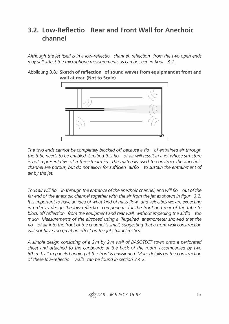
Although the jet itself is in a low-reflectio channel, reflection from the two open endsmay still affect the microphone measurements as can be seen in figur 3.2.

Abbildung 3.8.: Sketch of reflection of sound waves from equipment at front andwall at rear. (Not to Scale)

The two ends cannot be completely blocked off because a flo of entrained air throughthe tube needs to be enabled. Limiting this flo of air will result in a jet whose structureis not representative of a free-stream jet. The materials used to construct the anechoicchannel are porous, but do not allow for sufficien airflo to sustain the entrainment ofair by the jet.

Thus air will flo in through the entrance of the anechoic channel, and will flo out of thefar end of the anechoic channel together with the air from the jet as shown in figur 3.2.It is important to have an idea of what kind of mass flow and velocities we are expectingin order to design the low-reflectio components for the front and rear of the tube toblock off reflection from the equipment and rear wall, without impeding the airflo toomuch. Measurements of the airspeed using a ‘flugelrad anemometer showed that theflo of air into the front of the channel is small, suggesting that a front-wall constructionwill not have too great an effect on the jet characteristics.

A simple design consisting of a 2m by 2m wall of BASOTECT sown onto a perforatedsheet and attached to the cupboards at the back of the room, accompanied by two50 cm by 1m panels hanging at the front is envisioned. More details on the constructionof these low-reflectio ‘walls’ can be found in section 3.4.2.

DLRDLR – IB 92517-15 B7 13

Abbildung 3.9.: Sketch of entrainment of ambient flo by jet. (Not to Scale)

Abbildung 3.10.: Sketch of entrainment of ambient flo by jet, with possible low-reflectio components coloured in blue. (Not to Scale)

3.3. Positioning of the Anechoic Channel andMicrophones

The segments of the anechoic channel are connected into two blocks. Segments A, B andC make up the firs block, which holds the linear array and is to be precisely positioned,while segments D and E make up the second block which can be moved to allow accessto the microphones in block ABC.

The accurate positioning of the channel is a time consuming process, and ideally blockABC should remain in position so that this does not have to be carried out. However, allof the positioning procedures used were chosen for their repeatability. By following thesteps described in this section it should be possible to accurately reassemble and positionblock ABC if for some reason it has had to be disconnected and/or moved. Figure 3.11shows the coordinate system used throughout this document.

14DLRDLR – IB 92517-15 B7

Abbildung 3.11.: Coordinate system used.

3.3.1. Markings on Channel Segments and Room

Figure 3.12 shows markings made on the individual segments of the channel. These canbe used to adjust the segments into the correct shapes by ensuring the dimensions are asnoted in the sketch, and the lines on adjacent sections line up.

Figure 3.13 shows the markings made on the walls. All of these are carefully positionedwith respect to the jet axis. There is a line mirroring the jet axis drawn on the ceiling. Onthe floo , there is a line mirroring the jet axis near the nozzle, while further downstreamthere are two lines parallel to the jet axis, but translated by 26 cm to either side.

3.3.2. Positioning in X-Y plane

In order to position the channel, plumb lines are descended from block ABC: one atthe front and two at the rear. The string is attached using screws in sliding blocks withnotched plates which the string can hook into. Alternatively the string can be wrappedaround the screw and tied in place. The plumb lines are positioned such that the string ishanging down exactly from the relevant markings on the element and the plumb line tip

DLRDLR – IB 92517-15 B7 15

Abbildung 3.12.: Segment markings. Not to scale.

is as close as possible to the ground without actually making contact.

Figure 3.14 shows the plumb line positions on the front and rear of block ABC. The wireconnection to the ceiling is also shown. The ceiling connections are only attached whenthe horizontal position has been set to a firs degree of accuracy. The suspension from theceiling is required to make the channel more regular in shape and help with the verticalpositioning.

The three plumb lines should be accurately positioned on the lines marked on the flooin order to set the position in the y-direction. For the x-direction (i.e. axial) the currentposition is marked with an arrow pointing to the position along the front line on thefloo onto which the front plumb line should descend. The word ‘hier’ is written next tothis arrow for clarification Note that this position could be changed to control the polarangles of the microphones if required.

3.3.3. Positioning in Z-direction

Once the position in the x-y plane has been set, the vertical position of the channel needsto be altered in order to ensure that the jet axis is central. In order to do this, a temporaryconstruction representing the jet axis is used (see figur 3.18 in section 3.4.1).

16DLRDLR – IB 92517-15 B7

Abbildung 3.13.: Side view of markings on walls (in red). Arrows indicate whereplumb lines are used for positioning of elements. Temporary con-struction to represent jet axis and help with vertical alignment isshown in light grey. Not to scale.

The temporary construction is adjusted and positioned using plumb lines and a spiritlevel (Wasserwaage). Block ABC is adjusted so that its centre coincides with the jet axis,by adjusting the length of the feet (bottom) and using the rigging (Wantenspanner) topull up the top. Figure 3.15 gives a side view of the attachment to the ceiling, and thetemporary construction representing the jet axis.

3.3.4. Positioning of Microphones

Figures 3.16 and 3.17, show the distance from the jet-axis of the microphones in thelinear array and ring respectively. The temporary jet-axis pipe construction can be used tocheck these dimensions. Unfortunately this is not as accurate as desirable. Ultimately itwill not be possible to position microphones to a high accuracy. It is therefore importantthat the exact positions of the microphones are known (see appendix D).

3.4. Practical Protocol

This section gives a brief overview of the practical steps taken to set up the jet-noise rig.

DLRDLR – IB 92517-15 B7 17

Abbildung 3.14.: Front (left) and Rear (right) view of element ABC, with plumbline positions indicated by arrows. Not to scale.

3.4.1. Theme: Anechoic Channel

Task: Adjustment of Height and Shape of Channel

Details: Five rings, constructed out of aluminium elements, with two 10 cm layers ofsound insulation (BASOTECT and acoustic wedge foam)

Subtask: Adjust height of rings to ensure jet is positioned centrally. Adjust shape of ringsto ensure that these are of a regular shape. Adjustments need to be done with segmentslying on floo . (see section 3.3 for numerical adjustments made)

Subtask: Suspension from ceiling using steel rope, hook screws and rigging (Wanten-spanner) -this ensures that despite the low rigidity of the segments these are still roughlyregular in shape and not oval. Holes drilled into the ceiling are positioned above the jetcentre line (positioned using plumb lines).

18DLRDLR – IB 92517-15 B7

Abbildung 3.15.: Sketch of room showing wall markings, temporary jet axis set-upand wire ceiling connections for element ABC. Channel segmentsare in dotted lines. Not to scale.

Task: Assembly and Positioning

Subtask: Connect segments A,B,C and D,E together at 14 positions using tabs (German:Laschen) to form two blocks.

Subtask: Horizontal Positioning of block ABC using 3 plumb lines (German: Lot) and linemarkings on the floo (N.B. the floo markings were partially constructed with help of theprecisely positioned traverse situated under the jet). At least two, and preferably threepeople are needed for this positioning.

Subtask: Vertical Positioning of block ABC by setting up a tube to represent the jet axis.This tube is attached to the nozzle (using a specially constructed aluminium nozzle plugwith a centrally positioned hole for the tube) and a stand (with a screw-jack for adju-sting height) on the downstream side. The stand ( shown in figur 3.18) is positioned byplumb lines and a spirit level tool (German: Wasserwaage). Measurements to the top andbottom of the rings are used to position the block vertically, ensuring that the jet axis iscentrally positioned. The vertical adjustment is carried out by changing the length of thefeet (bottom) and the suspension wire (top) (using rigging (German: Wantenspanner)).

Subtask: Attach block DE to block ABC using 14 connectors. Ensure block ABC does notmove from its set position. Attach ceiling suspension to segment E and adjust to correct

DLRDLR – IB 92517-15 B7 19

Abbildung 3.16.: Positioning of Linear array microphones with respect to jet axis.Not to scale.

height. Initially it may be more useful to not attach the two blocks properly, so that themicrophones are more accessible for calibration (this approach was taken for all measu-rements described in this report).

3.4.2. Theme: Low-Reflectio Rear and Front Walls

Subtask: Assemble materials (BASOTECT foam, perforated sheet, string) for front and rearpanels

Subtask: Sow BASOTECT onto perforated sheet with enough stitches to hold the BASO-TECT in place when the perforated sheet is suspended.

Subtask: Adjust aluminium structure over nozzle so that channel can move further ups-tream. Screw a horizontal bar in place from which to suspend the front-wall elements ateither side of the nozzle (with screws and sliding blocks).

Subtask: Screw a 180 cm metal angle to the top of the cupboard at the rear of the room.Angle has holes to attached rear wall elements (two screws each) symmetrically aboutthe midpoint (i.e. jet axis).

20DLRDLR – IB 92517-15 B7

Abbildung 3.17.: Positioning of ring microphones with respect to jet axis. Not toscale.

Subtask: Suspend rear and front wall elements with long screws which fi through theperforated sheet. Use blocks of wood under the rear-wall elements for extra support, andto prevent excessive forces on the BASOTECT from the strings – which could lead to tears.Elements can be removed and re-suspended as required for access. Figure 3.19 shows thefront wall on one side of the jet, the rear wall can also be seen in the background.

3.4.3. Theme: Snow-Flake Data Acquisition System

Subtask: Set up system according to user manual ([22]). Record all connections in a table(see appendix C).

Subtask: Test all connections with signal generator in place of microphones.

Subtask: Test with one microphone and piston-phone to ensure signal is as expected.

DLRDLR – IB 92517-15 B7 21

Abbildung 3.18.: Photograph of temporary stand built to represent jet axis. Taken03/08/15.

3.4.4. Theme: Linear Array

Task: Preparation of Brass Pipes

Details: Brass pipes of length 38 cm, with hole ∼6mm diameter 8 cm from one edge.

Subtask: Polish outside with finishin pad (Scotch-Brite Very Fine, Red A-VFN finishinpads were used)

Subtask: Clean interior of pipes with pipe cleaners (German: Pfeifen Reiniger), pulledthrough by wire (3 pipe cleaners hooked to end of wire.

Subtask: Sort pipes by internal diameter (7.4mm marked ‘4’, 7.3mm marked ‘.’)

22DLRDLR – IB 92517-15 B7

Abbildung 3.19.: Photograph of rig showing one low-reflectio front wall ele-ment. Taken 03/09/15.

Task: Aluminium Holder

Details: See figur 3.20 for schematic. [Wolfram Hage]

Abbildung 3.20.: Design for Linear Array Aluminium holder. [Wolfram Hage]

Subtask: Create holder: holes for pipes at 20.9mm spacing with tapered holes for plasticscrews to hold pipes in place. Two additional tapered holes for screws to attach to cornerelement. Corner element to position. Additional tool ordered and used to slightly increasehole diameter so that pipes fi in. All steps carried out at in-house metal workshop.

Subtask: Screw holders in place on anechoic channel segments A-C at easily accessibleheight (cables and access). Ensure they are all at the same height.

DLRDLR – IB 92517-15 B7 23

Subtask: Twist brass pipes into position in the slots needed (see section 3.1). Pipes twistedin as far as practical: 2 cm of pipe sticking out of holder on exterior side. Once all pipesare in correct position, fi position with plastic screws.

Task: Insulation and Connection of Microphones

Details: Using G.R.A.S 40BP microphones with Type 26AC pre-amplifiers The pre-amplifielength is 107mm, and to distinguish this length of pre-amplifie from the other (shorter)length available they will here be referred to as long pre-amplifiers"(http://ww .gras.dk/26ac.html)

Subtask: Assemble G.R.A.S microphones with long pre-amplifier (not enough availableso using short pre-amplifier for the last two positions and for the ring)

Subtask: As some microphones were found to have deposits of oxide on the casing andthe membrane, these were carefully cleaning. A fin brush and micro-fibr cloth we-re used to clean the membranes, which were carefully inspected by magnifying glassthroughout. The protective cage was cleaned using pressurised air.

Subtask: Insert microphones to tubes and secure using shrink tube and tape at preciseposition (sticking out 4 cm from the end of brass tube). The shrink tube should be longenough to cover all of the metal of the pre-amplifie housing that is within the tube, andthus provide electrical insulation [Lech].

Subtask: Connect microphones to break-out-boxes, wrap up wires using Velcro straps.

Subtask: Run snowflake to identify channels with problems. Check connections and swapmicrophones to identify issues such as faulty microphones / connections.

Subtask: Use multimeter to check microphones are electrically insulated.

24DLRDLR – IB 92517-15 B7

Task: Calibration of Microphones

Subtask: Build a stand to lie the piston-phone on so that this does not have to be heldby hand. The stand consists of a plank of wood running through the channel and can beseen in the photographs in figur 3.21.

Abbildung 3.21.: Photographs of calibration with octopus extension. Taken on20/08/15

Subtask: Connect piston-phone to octopus - connect to six microphones at a time. Ensureall six connections are filled leaving some open will result in erroneous measurements onthe others

Subtask: Position sound-insulating front wall to block noise from snowflak computer(see section 3.4.2) (not essential).

Subtask: Take calibration measurements with snowflak following standard calibrationprotocol, using an octopus piston-phone extension and recording in a specialised log-sheet (see appendix C). The calibration sampling frequency is set to approximately 10 kHz,the calibration time to approximately 2 seconds.

Subtask: Analyse measurements with new Python calibration script jextra_cal.py (see Sec-tion 4.2).

DLRDLR – IB 92517-15 B7 25

3.4.5. Theme: Microphone Ring

Details: Microphones are installed into one of the rings on the anechoic channel to seewhat kind of results can be obtained from these. The ring chosen for this is the ring insegment B, which is at a polar angle of roughly 60 degrees.

Subtask: Install G.R.A.S microphones with small pre-amplifier (due to availability) intoring. Hold in position using tube and tape, as for linear array. Use ruler to determine radi-al position (unfortunately this has low accuracy).

Subtask: Take calibration measurements with snowflak following standard calibrationprotocol, (see above).

26DLRDLR – IB 92517-15 B7

4. Calibration of Microphones

4.1. Calibration Theory

4.1.1. Mathematical Basis

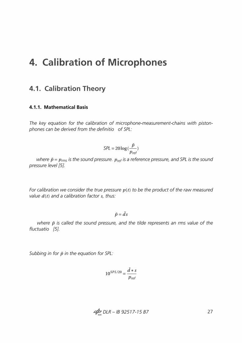
The key equation for the calibration of microphone-measurement-chains with piston-phones can be derived from the definitio of SPL:

SPL= 20log(p̃

pref)

where p̃ = prms is the sound pressure. pref is a reference pressure, and SPL is the soundpressure level [5].

For calibration we consider the true pressure p(t ) to be the product of the raw measuredvalue d(t ) and a calibration factor s, thus:

p̃ = d̃ s

where p̃ is called the sound pressure, and the tilde represents an rms value of thefluctuatio [5].

Subbing in for p̃ in the equation for SPL:

10SPL/20 = d̃ ∗ s

pref

DLRDLR – IB 92517-15 B7 27

Which leads to an equation for s:

s = prefd̃

10SPL/20

This is the standard calibration equation, where s is the calibration factor, pref is a refe-rence pressure, d̃ is the raw measured signal and SPL is the known sound pressure levelof the piston-phone used.

The traditional method of calibration is to use:

d̃ = drms

where drms is the rms value of the time signal measured.

However, when measuring in noisy environments, as is often the case for fiel measure-ments, the rms value of the time signal contains a lot of noise from sources other thanthe piston-phone leading to an inaccurate calibration.

In order to avoid this loss of accuracy a number of alternative methods have been deve-loped which involve a fourier transformation to the frequency domain. In the frequencydomain, pressure fluctuation that correspond to the piston-phone can be singled outfrom background noise at other frequencies. These alternative methods are discussed inthis section.

Note that technically s should be seen as a conversion factor between the raw data andpressure values rather than a true calibration factor.

4.1.2. Calibration Methods

The calibration methods discussed in this section are:

28DLRDLR – IB 92517-15 B7

1. d̃ from rms value of time signal

2. d̃ from TOB corresponding to pistonphone frequency. (Hanning window with eitherPS or PSD)

3. d̃ from peak of power spectrum with flatto window

RMS

The standard normed method of calibration is to use the rms value of the time signal,which is calculated directly from the raw time signal measured as follows:

drms =√

1

n

n∑i=1

d(ti )2

TOB with Hanning PS or PSD

The PSD (power spectral density) or PS (power spectrum) (discretised into frequencynarrow-bands) can be calculated using the scipy.signal.welch function in python. Thefollowing equation gives the relation between these and d̃ :

d̃ 2 = PSD∗∆ f = PSwindow/ENBWwindow

where PSD and PS are the linear power spectral density and linear power spectrumrespectively of the raw time signal d(t ). ∆ f is the narrow-band bandwidth and ENBW isthe Equivalent Noise Band Width, which is a correction factor based on the windowingmethod used. Different types of window will result in different values of PS and ENBW,but the product of these is independent of the method used. The ENBW for a Hanningwindow is 1.5 .

Flat top

The fla top method also uses the scipy.signal.welch function in python. The functionis used to generate a power spectrum with a flat op window. The value for the powerspectrum at the maximum will exactly equal d̃ 2.

DLRDLR – IB 92517-15 B7 29

4.1.3. Comparison of methods for test case

The agreement between RMS, TOB and flatto methods is very good. Refer to the Wikion microphone calibration for a quantitative comparison based on a test case generatedfrom JEXTRA data.

N.B. the units of the original raw time series data are irrelevant to the process.

4.2. Calibration Script jextra_cal.py

jextra_cal.py is a calibration script for the calibration of microphones using pistonphones.The methodology is loosely based on pre-existing scripts in C and python. The calibrati-on is based on an FFT using a flatto window with the scipy.signal.welch python package.

4.2.1. Overview of Methodology

1. Read command line arguments specifying the folder containing calibration data,and properties of the calibration set-up (eg. piston-phone used).

2. Read file-name in folder, then cycle through, loading and checking data.

2.1 Read the .set fil with read_adat_set to obtain information about the dataset.

2.2 adjust_range_variables provides some basic error control to ensure the com-mand line input matches what is specifie in the .set file

3. Find which channels contain calibration signals ( find_channel ).

3.1 Cycle through the channels in each .bin fil

3.2 Select a short snippet of the time signal.

30DLRDLR – IB 92517-15 B7

3.3 Use signal.welch to calculate the power spectrum of the signal, using a Hanningwindow.

3.4 Correct for the FFT window with a factor of 1.5 .

3.4 Convert the power spectrum into TOBs using spec_tob_oct.

3.5 Select the TOB corresponding to the calibration frequency and compare this tothe average to identify which channels have calibration signals.

4. Calibrate the channels with calibration signals (calibrate_channels).

4.1 Cycle through the channels containing calibration signals in each .bin fil

4.2 Use signal.welch with a fla top window to calculate the power spectrum of theentire time signal.

4.3 Select the maximum and then take the square root to fin dtop

4.4 Apply the octopus correction factor (roct) if relevant.

4.5 Calculate the calibration factor s from dtop and the known piston-phone SPL

4.2.2. Input

Path of folder containing .bin and .set calibration filesFrequency of piston-phone used.SPL of piston-phone used.(Optional) octopus correction factor.First sample to consider.Last sample to consider.First channel of interest. (-i.e. connected to a microphone)Last channel of interest. (-i.e. connected to a microphone)Verbose parameter to control command line and graphical output for inspection and de-bugging.

Note that the pythonic channel numeration begins at 0, so is equal to the snowflakchannel numeration - 1.

DLRDLR – IB 92517-15 B7 31

4.2.3. Output

The main output of the script is a fil containing the calibration factors for different chan-nels. If the same channel has been calibrated multiple times, all the resulting calibrationfactors are listed for inspection, along with the names of the file they have been calcula-ted from. This allows for manual inspection and comparison to the calibration log sheet.A calibration table in the correct format for use can then be created manually.

4.2.4. Results

The figure in this section show comparison between the results from calibration on twodifferent days, both using the flatto method described above. Faulty microphones canbe identifie by large differences in calibration values. In general, the match between thetwo calibrations, carried out two weeks apart is very good.

The calibration script jextra_cal.py was used in both cases, in version 3a. The resultingcalibration tables were manually compared to the log sheet, and a condensed calibrationtable with one factor per channel was created in the suitable format. These calibrationtables are saved in the following files

JEXTRA_calibration_table_200815.txtJEXTRA_calibration_table_030915.txt

Figure 4.1 shows that the calibration factor for channel 45 as calculated on 03/09 isseveral orders of magnitude higher than expected. This agrees with the comment ‘chan-nel 46 very low’ recorded on the calibration log sheets, and suggests a faulty microphone.

Figure 4.2 shows the same plot as Figure 4.1, but with a reduced scale. It is clear that thevariation in the calibration factors for channels across the two days is, with the excepti-on of channels 14 and 15, much lower than the variation in calibration factor betweendifferent channels. The uncharacteristically low values of calibration factor calculated on20/08 for channels 14 and 15 could be explained by the fact that for this measurementonly two of six arms of the octopus-piston-phone-extension were connected, rather thanthe full six that were used for every other measurement.

32DLRDLR – IB 92517-15 B7

Abbildung 4.1.: Comparison of calibration factors for calibration on 20/08 (blue)and 03/09 (red).

In Figure 4.3 the percentage discrepancies between calibration factors are shown. The3 cases where errors are suspected (discussed above) are not included in this plot. Thepercentage variation in calibration factor is below 0.04 % for all other channels.

Finally, Figure 4.4 shows the logarithmic difference between the calibration factors, whichis most relevant as it is the SPL of the sound signal that will be inspected. Not taking intoaccount the three erroneous cases, the value is below 0.32 for all channels.

DLRDLR – IB 92517-15 B7 33

Abbildung 4.2.: Comparison of calibration factors for calibration of 28/08 (blue)and 03/09 (red). Channel 45 off scale.

Abbildung 4.3.: Percentage discrepancy in calibration factors between measure-ments from 20/08 and 03/09

34DLRDLR – IB 92517-15 B7

Abbildung 4.4.: Logarithmic difference in calibration factors between measure-ments from 20/08 and 03/09

DLRDLR – IB 92517-15 B7 35

5. Single Source Reflectio Experiments

In order to verify the anechoic properties of the experimental rig, a series of tests usingsingle sound sources were conducted to investigate what reflection can be observed. Anideal ‘single sound source’ is, in this context, define as a sound source which generatesan impulsive pressure signal in the time domain radiating from a single point in the spacedomain. In practical terms, this means a short, loud signal originating from a small area. Inorder to achieve this, two methods were attempted. The popping of a rubber membraneusing air pressure, and firin a blank gun. Photographs of the experimental setup can beseen in section 5.1. The results of these ‘single sound source’ experiments are presentedand analysed in this section.

5.1. Experimental Set-up

Experiments measuring the microphone array’s response to an impulsive sound sourcewere carried out in order to identify reflection and other issues with the array. In orderto achieve an approximately impulsive signal, two methods were used. The firs involvedpopping a thin ‘rubber’ membrane, which was carried out at the nozzle exit and at fivnozzle diameters downstream of the nozzle exit. The measurements at fiv nozzle dia-meters were carried out because it is possible that, for a sound source at the nozzle exit,the nozzle itself will scatter the sound signal and thus lead to unrepresentative results.A distance of fiv nozzle diameters was chosen, as the literature suggests that at thislocation there is a peak in sound generation in the jet [5].

The second method used a blank gun. The blank gun needs to be held by hand, so itspositioning is less accurate. The position aimed for was approximately two nozzle diame-ters downstream of the nozzle exit in order to avoid scattering effects due to the nozzle.

DLRDLR – IB 92517-15 B7 37

5.1.1. Pop

A thin ‘rubber’ membrane (cut from blue rubber gloves) was stretched over a metalbicycle-pump-valve-adapter and firml attached by string. By pumping air into the pi-pe using a bike pump, it is possible to burst the sheet (similar to popping a balloon) andthus achieve a ‘pop’ sound. This ‘pop’ is a reasonably impulsive sound signal. Figure 5.1shows the construction.

Abbildung 5.1.: Photograph of the thin ‘rubber’ sheet (blue) stretched over a me-tal pipe segment which connects to a bicycle pump. The ‘rubber’sheet is firml tied in place with (black) string. Taken 20/08/15.

The bike pump used was clamped to the underside of a wooden board situated justbelow and upstream of the nozzle (figur 5.2). In order to pop the ‘rubber’ fil theoperator pushed the pump handle upwards towards the wooden board. The set up waslater improved by tying a piece of foam to the pump, which softened the sound of thepump handle hitting the pump when it was pushed right to the top. This modificatio isnot shown in the photo.

Pop at Nozzle exit

The position of the popping contraption can be seen in figur 5.3

Pop at 5D

The position of the popping contraption can be seen in figur 5.4. Note that the positionis slightly off-centre.

38DLRDLR – IB 92517-15 B7

Abbildung 5.2.: Photograph of the bicycle pump clamped to underside of woodenboard for ‘pop’ single sound source tests. Taken 20/08/15.

5.1.2. Blank Gun

In order to generate a loader sound, a blank gun was fire within the anechoic channel.The gun was held by hand, with the sound source at roughly 10 cm from the nozzle exit,as can be seen in figur 5.5.

5.2. Results

5.2.1. Time Signals

Figures 5.6 to 5.8 show the response of the linear array microphone at a polar angle of52.3°. The y-axis shows pressure while the x-axis shows time multiplied by the speed ofsound, so give a measure of how far the sound has travelled. The plots only show data fora few meters past the initial impulse, as after this the signal decays away, and no furtherartefacts of interest can be identified The pressure initially decreases, before increasing,which could be due to the phase of the microphones.

The pop at the nozzle seems to give the cleanest impulse, while the signal from the blankgun, which it was assumed would be superior is less clean.

DLRDLR – IB 92517-15 B7 39

Abbildung 5.3.: Photograph of rubber-membrane construction at the nozzle exit.Taken 20/08/15.

Abbildung 5.4.: Photograph of rubber-membrane construction at fiv nozzle dia-meters from the nozzle exit. Taken 20/08/15.

These time signals, and those for all other microphones were analysed to produce reflection contour maps. A Hilbert transformation is carried out to fin the envelop of the signal,the pressure value is then converted to an SPL. Contours of SPL on a grid of distance tra-velled by sound against distance of microphone from nozzle can then be plotted. Thesecontour maps can be seen in section 5.2.2.

Further analysis suggested for future work would be to calculate signal to noise ratios,and look at the data in the frequency domain.

40DLRDLR – IB 92517-15 B7

Abbildung 5.5.: Photograph of Blank Gun held in position. Taken 20/08/15.

5.2.2. Reflectio Contour Maps

In order to observe the pattern of reflection on the entire microphone array contourmaps have been generated. Contours of Sound Pressure Level are shown on an axis oftime versus microphone position. The time axis is converted to show the distance travel-led by sound (with an arbitrary zero) by multiplying the time intervals with the speed ofsound.

As sound pressure is a fluctuatin value, a Hilbert transformation was carried out tofin the envelope. The absolute value of the Hilbert transform is then converted to asound pressure level. The python script jex_quick_look.py contains all these steps, and isavailable on the JEXTRA hard drive.

Results

Figure 5.9 shows the microphone response to a gun shot. Firstly it should be noted thatafter the initial signal, all further pressure fluctuation are more than 20 dB under theinitial impulse in magnitude. The suggests that the anechoic set-up is very effective atreducing reflections A comparison to a test case with no sound insulation would beuseful to provide a quantitative assessment. The sounds close to the initial impulse arelikely to be due to scattering at the nozzle, while the faintly visible sounds at that havetravelled a further distance are most likely to be caused by reflection from the rear wall.It will be shown later that there shape fit very well to the expected shape for reflectionfrom walls perpendicular to an array and that the distance travelled by the sound for thecloser of the two corresponds very well to a reflectio from the back wall of the room.

DLRDLR – IB 92517-15 B7 41

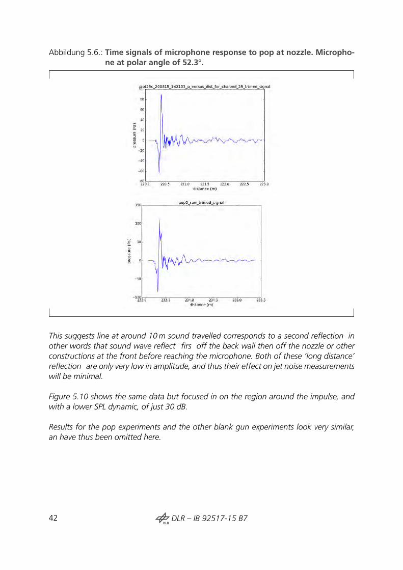
Abbildung 5.6.: Time signals of microphone response to pop at nozzle. Micropho-ne at polar angle of 52.3°.

This suggests line at around 10m sound travelled corresponds to a second reflection inother words that sound wave reflect firs off the back wall then off the nozzle or otherconstructions at the front before reaching the microphone. Both of these ‘long distance’reflection are only very low in amplitude, and thus their effect on jet noise measurementswill be minimal.

Figure 5.10 shows the same data but focused in on the region around the impulse, andwith a lower SPL dynamic, of just 30 dB.

Results for the pop experiments and the other blank gun experiments look very similar,an have thus been omitted here.

42DLRDLR – IB 92517-15 B7

Comparison to Room Geometry

A simple MATLAB simulation of reflection from different artefacts in the room was car-ried out. The simulation takes into account the law of reflection that the angle of reflection is equal to the angle of incidence, and uses this to calculate distances that soundwaves would travel between a source at the nozzle and the microphone.

Figure 5.11 shows the reflectio contour map for the fourth blank gun measurement,with reflectio simulations superimposed. The distance between the nozzle and the mi-crophone (plotted in black) is used to align the reflectio contour map with its arbitraryzero in the y axis, and the simulation results. The magenta line represents a reflectiofrom the opposite wall of the anechoic channel. This falls in the region where the reflection contour map shows some evidence of reflections but at a magnitude much lowerthan the original signal. The red line represents a reflectio from the low-reflectio rearwall. This matches very well in shape and position to a line that can be observed faintlyon the reflectio contour map, suggesting that there is indeed a reflectio from the rearwall. The SPL of this reflectio is around 30 dB lower than the original impulse, so this isnot an issue.

5.3. Conclusions of Validity of Anechoic Channel

There are no major issues with reflection for the experimental set-up. A quantitativeassessment of how effective the ‘anechoic’ channel is would require a similar set of mea-surements to be carried out in the room, without the ‘anechoic’ channel in place. This isrecommended for future work on the project.

N.B. A further single source experiment has been carried out with a reflectiv board pla-ced inside the anechoic channel. The measurements from this experiment are available,but the analysis has not been carried out at time of writing.

DLRDLR – IB 92517-15 B7 43

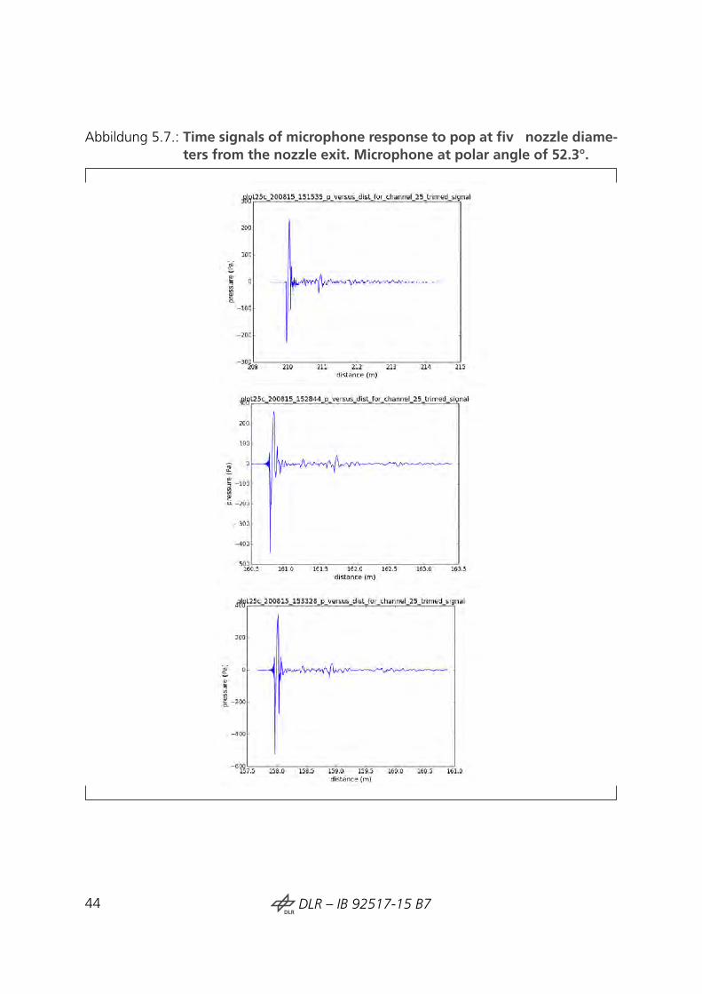
Abbildung 5.7.: Time signals of microphone response to pop at fiv nozzle diame-ters from the nozzle exit. Microphone at polar angle of 52.3°.

44DLRDLR – IB 92517-15 B7

Abbildung 5.8.: Time signals of microphone response to blank gun shot at twonozzle diameters from the nozzle exit. Microphone at polar angleof 52.3°.

DLRDLR – IB 92517-15 B7 45

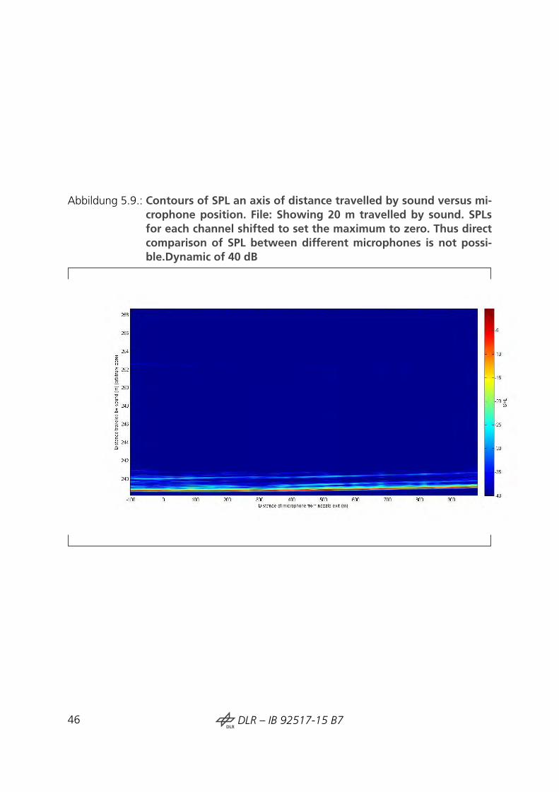
Abbildung 5.9.: Contours of SPL an axis of distance travelled by sound versus mi-crophone position. File: Showing 20 m travelled by sound. SPLsfor each channel shifted to set the maximum to zero. Thus directcomparison of SPL between different microphones is not possi-ble.Dynamic of 40 dB

46DLRDLR – IB 92517-15 B7

Abbildung 5.10.: Contours of SPL an axis of distance travelled by sound versus mi-crophone position. File: Showing 4 m travelled by sound. SPLsfor each channel shifted to set the maximum to zero. Thus directcomparison of SPL between different microphones is not possi-ble.Dynamic of 30 dB

DLRDLR – IB 92517-15 B7 47

Abbildung 5.11.: Simulated reflection

48DLRDLR – IB 92517-15 B7

6. Jet Noise Measurements

6.1. Basic theory

The potential core of the jet extends 4 - 5 nozzle diameters downstream of the nozzleexit. At the boundary between the jet flo with the outer ambient flo a shear layerforms. The instability of this shear layer generates turbulent structures. These turbulentstructures start off small, close to the nozzle exit, and grow into larger turbulent structurestowards the end of the potential core, before these fall apart again into small structures.[5] The key regions are shown in the schematic in figur 6.1.

Abbildung 6.1.: Schematic of jet showing shear region and potential core.

The fine-scal structures (FSS) near the nozzle exit are associated with high frequencycomponents. The large-scale structures (LSS) are associated with lower frequency sound.The high frequency FSS sound is radiated primarily to high observer angles, while thelower frequency LSS sound can be measured at smaller observer angles. [11] See figur6.2.

The different scales of turbulent structures are associated by Karabasov with two distinctphysical mechanisms of jet noise. The physical mechanism for FSS is the pressure exertedby fine-scal turbulence in the shear layer, which is equivalent to classical lighthill acousticanalogy. The physical mechanism suggested for LSS is the growth and decay of linearinstability waves [11].

DLRDLR – IB 92517-15 B7 49

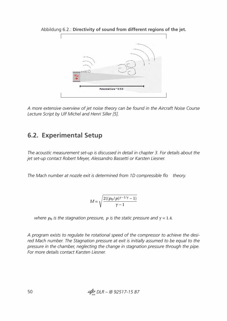
Abbildung 6.2.: Directivity of sound from different regions of the jet.

A more extensive overview of jet noise theory can be found in the Aircraft Noise CourseLecture Script by Ulf Michel and Henri Siller [5].

6.2. Experimental Setup

The acoustic measurement set-up is discussed in detail in chapter 3. For details about thejet set-up contact Robert Meyer, Alessandro Bassetti or Karsten Liesner.

The Mach number at nozzle exit is determined from 1D compressible flo theory.

M=√

2((p0/p)γ−1/γ−1)

γ−1

where p0 is the stagnation pressure, p is the static pressure and γ= 1.4.

A program exists to regulate he rotational speed of the compressor to achieve the desi-red Mach number. The Stagnation pressure at exit is initially assumed to be equal to thepressure in the chamber, neglecting the change in stagnation pressure through the pipe.For more details contact Karsten Liesner.

50DLRDLR – IB 92517-15 B7

6.3. Comparison Data

Comparison of Jet Noise measurements from the JExTRA linear array with results from‘The Generation and Radiation of Supersonic Jet Noise. Volume III, Turbulent Mixing Noi-se Data’ by Lockheed [9]. which contains tables for jet noise experiments with a 2 inchnozzle published in 1976.

For details on the experimental set-up and data handling refer to the book [9]. It shouldbe noted that an atmospheric absorption correction has been applied ot the data. The SPLresults are taken directly from the tables, with no additional data handling or correctionsapplied.

The test cases used for comparison purposes are cases 20, 21, 22, 23. These cover arange of Mach numbers from 0.4 to 0.7 .

Figure 6.3 shows a contour map of Sound Pressure Level (SPL), on a Strouhal Numberversus Microphone polar angle plane. Features typical of jet noise can be observed, suchas an increase in Strouhal Number for the peak SPL as the polar angle of the microphoneincreases. The magnitude of peak SPL at low angles is also greater than that at higherangels, another common feature in jet noise. For the 90° measurement the peak SPLoccurs at a Strouhal number of 1.8, whereas at 30°, the peak is closer to St = 0.5 .

6.4. Mathematical Considerations

6.4.1. Atmospheric absorption correction

Atmospheric absorption of sound prevents accurate comparison at microphones at dif-ferent distances, even when the R2 dependency of sound power on distance has be-en considered. Moreover, the absorption of sound is frequency dependent, with higherfrequencies being absorbed more than lower frequencies. Thus in order to look at thefrequency characteristics of a jet it is important to apply an atmospheric absorption cor-rection otherwise the high frequency content will be under-estimated.

The general equation for atmospheric sound absorption is:

DLRDLR – IB 92517-15 B7 51

Abbildung 6.3.: Contour Map of SPL variation for Strouhal number versus anglesfrom downstream jet axis, for Lockheed data[9], M = 0.5. (TP 21).

SPL2 = SPL1 − r 10log10 (a)

where α( f ) = 10log10 (a) is a frequency dependent damping coefficien usually refer-red to as the ‘absorption coefficient’ and SPL is the sound pressure level.

The equation for α( f ) is quite long, and can be found as equation 1.80 in the AircraftNoise Course lecture script by Ulf Michel and Henri Siller [5].

Note that the atmospheric absorption correction is not a distance correction, and that itshould be implemented before the distance correction. Once the atmospheric absorptioncorrection has been applied, a distance correction can be applied to allow comparisonbetween the JEXTRA and Lockheed data [9] (see section 6.4.2).

Applying an atmospheric correction can lead to an over-correction at high frequencies,leading to a non-physical rise in SPL at the highest frequencies. It is difficul to quantifythis effect.

52DLRDLR – IB 92517-15 B7

6.4.2. Distance correction

In order to compare the two datasets it is necessary to non-dimensionalise the frequency,by calculating the Strouhal number:

St = fsD j

U j

The Lockheed data [9] was measured at a constant distance from the nozzle exit for allangles, whereas the JExTRA data comes from a linear array, and thus the distance increa-ses as the angle to the downstream jet axis moves away from 90°.

In order to enable a direct comparison between the data sets it will be necessary to applya correction to the JExTRA data based on the decay of the sound over space. In order todo this a few simplifying assumptions will be made:

1. The absorption of sound by the air has already been taken into account.

2. For a given angle and frequency sound pressure is only a function of distance (r )from the sound source.

3. The sound source is at the nozzle. (This is not technically exclusively the case, butthis assumption significantl simplifie the comparison to the Lockheed data [9], as anyother sound source location would mean both data sets need adjusting).

With these assumptions we can derive a relationship for the variation of SPL with r , whichcan be used to apply a ‘correction’ to the JExTRA data and allow for a more direct com-parison.

Energy flu through a sphere around the source is constant.

From assumption 2, we can then say that energy flu through an infinitesimall small

DLRDLR – IB 92517-15 B7 53

area of the sphere along a line propagating radially outwards from the sound source isconstant.

i.e.

A∗4πr 2I = K = const

where I is the intensity, r is the radial distance and a is an infinitesimall small constantdefinin the proportion of the surface area through which we are considering an energyflu of magnitude K .

Simplifying and rearranging:

I = B/R2

where B = K /(A∗4π) = const

The intensity I is given by:

I = p̃2/ρc

where ρ is the mean value of density and c is the speed of sound [5].

Combining these two equations we get:

p̃2 = ρcB/r 2 = D/r 2

Converting to logarithmic values:

SPL= 10log(p̃2

pref) = 10log(

E

r 2)

where SPL is the sound pressure level.

54DLRDLR – IB 92517-15 B7

SPL= F −10logr 2

SPL= F −20logr

Then, as we know SPL and r for the measurement at each microphone position, we candetermine a value of F for each polar angle. Once a value of F has been obtained fromF = SPL+ 20logr , an estimation of the SPL that would be measured at any distance rcan be made, so it is possible to calculate an estimation of the SPL at the same distancer = Ryb for each angle, thus allowing better comparison to the Lockheed data [9]. Thefina equation for the correction to apply is:

SPL estimation at distance Ryb= SPL variable distance (r ) +20log(r /Ryb)

6.5. Results

6.5.1. Data Correction (M = 0.5 case)

The effect of applying the data corrections described in section 6.4 are shown in thissection. Figure 6.4 shows the uncorrected data for microphones at three different anglesplotted on a Sound Pressure Level versus frequency axis. Figure 6.5 shows the same dataafter an atmospheric absorption correction has been applied. Figure 6.6 shows the datacorrected for both atmospheric absorption and distance. A constant microphone distanceof 3.9m has been chosen to allow direct comparison to the Lockheed data.

By comparing figure 6.4 and 6.5 it is clear that the absorption correction does not havea major effect on the results. This is as would be expected considering that the distancesbetween the jet and microphones are small, so very little sound absorption will have takenplace. The only noticeable difference is at high frequencies. High frequencies are affectedmost by sound absorption, so the correction increases the SPL at these frequencies most.In the region where this increase in SPL is observable, the data already deviates from theexpected jet-noise pattern, and thus it is questionable whether the results here are valid.The ring measurements show that for the M=0.5 case at above approximately 10 kHz (orSt = 3), the measurements at different positions on the ring start to deviate from eachother. This departure from axisymmetric behaviour casts further doubts on the validity ofthe data at high frequencies.

DLRDLR – IB 92517-15 B7 55

Abbildung 6.4.: Uncorrected data for JEXTRA (02/09). M = 0.5 case.

Comparing figure 6.5 and 6.6 shows that the distance correction does not change theoverall patterns observed. Instead the distance correction brings the results closer to theLockheed data in terms of the magnitude of the SPLs. Further, the difference betweenthe positions is increased. Whereas the SPLs at different microphone positions were quitesimilar for the raw data, the distance corrected data very clearly shows a trend of SPLincreasing as the observer angle drops, which matches the Lockheed data (see section6.3).

Note that for all figure in this report, the frequency and Strouhal Number axes are plot-ted in third octave bands rather than narrow-bands.

6.5.2. SPL Contour Maps (M = 0.5 case)

Figure 6.3 in section 6.3 shows a contour map of the Lockheed data for the M = 0.5test case, showing the variation of SPL on the Strouhal Number-Angle plane. Figure 6.7shows the same graph for the JEXTRA data, with the atmospheric absorption and distancecorrections described in section 3.1 applied. The two figure look significantl different.It must be noted that the Strouhal Number axis for the JEXTRA data covers a larger

56DLRDLR – IB 92517-15 B7

Abbildung 6.5.: Uncorrected data for JEXTRA (02/09). M = 0.5 case.

range, extending to significantl lower Strouhal numbers than the Lockheed data, whilethe Lockheed data extends to slightly higher Strouhal numbers. The Lockheed data alsoextends to lower microphone angles.

To enable a more direct visual comparison, the same data has been plotted on axis thathave been reduced to cover only overlapping test points. These contour maps can beseen in figur 6.8. The general trend matches reasonably well, especially at lower angles.At higher polar angles the JEXTRA data does not reach a peak at the Strouhal numbersexpected, instead the SPL continues to increase at higher frequencies, which questionsthe validity of these results.

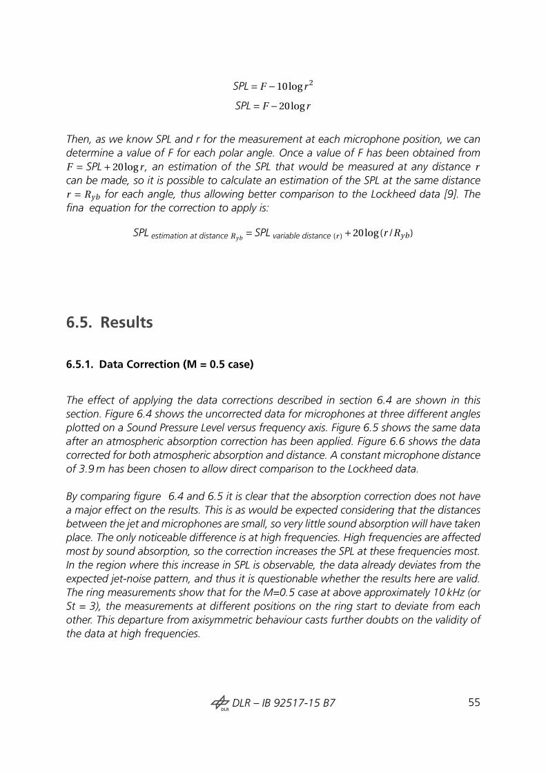
The low frequency behaviour of the JEXTRA data is more clearly visualised in the single-colour plot in figur 6.9, where the SPL dynamic is limited to 30 dB, and the data is shiftedso that the maximum is at 0 dB.

From Figure 6.9 it can be seen that, particularly at low angles, there is an additionallow frequency peak. The magnitude of this peak is lower than the higher frequencypeak, especially at higher angles. The low frequency peak varies in both magnitude andfrequency for different microphone positions. It is a rounded peak which suggests that

DLRDLR – IB 92517-15 B7 57

Abbildung 6.6.: Corrected data for JEXTRA (02/09). M = 0.5 case.

it is related to the jet. Tonal external noise sources would be expected to give a sharperpeak. Mach Number exponent analysis in section 6.5.6 further supports the suggestionthat the low frequency peak is linked to the flo rather than external noise.

6.5.3. SPL-St Graphs for Different Angles (M = 0.5 case)

Graphs of Sound Pressure level against Strouhal Number are shown in this section forangles at 30°, 52° and 90°.

The Aircraft Noise Course Lecture Script by Ulf Michel and Henri Siller [5] suggests thata peak in SPL at a Strouhal Number of 1.0 for unheated or 0.7 for heated jets is to beexpected. The broadband nature of the peak, and the dependency of the jet on a rangeof external factors mean that the peak position will vary between different experimentalset-ups. In general however a peak in the range St = 0.1 - 2.0 is to be expected.

Figure 6.10 gives a comparison between microphones at observer angles of roughly 30° ,52° and 90°.

58DLRDLR – IB 92517-15 B7

Abbildung 6.7.: Contour Map of SPL variation for Strouhal number versus anglesfrom downstream jet axis, for JExTRA data, M = 0.5.

Figures 6.11 to 6.13 show the JEXTRA and Lockheed results plotted on the same graphfor comparison.

The pattern agrees well in the range of Strouhal Numbers from 0.1 to 3.0. The peak inSPL occurs at roughly the same Strouhal number for all three angles presented. For the52° and 90° cases the Sound Pressure Level is also very similar. For the 30° microphonethe difference in SPL at the peak is roughly 3dB. Taking into account the fact that no near-fil correction has been applied (see section 6.5.7) to the JEXTRA data, the agreementwith the comparison data is good.

6.5.4. Variation with M

Figure 6.14 shows the variation of the SPL-freq-angle characteristic with Mach number.The pattern observed is fairly consistent over different Mach numbers.

Figure 6.15 shows the data from the 90° microphone at different Mach numbers. Themagnitude of SPL over the entire frequency range increases with Mach number as wouldbe expected [5]. The Strouhal Number of the peak seems to be fairly independent ofMach number, suggesting Strouhal scaling.

DLRDLR – IB 92517-15 B7 59

Abbildung 6.8.: Contour Map of SPL variation for Strouhal number versus anglesfrom downstream jet axis. M = 0.5 case. Lockheed data [9] (left)and JEXTRA data (02/09) (right)

6.5.5. Experiments with Flow Conditioning in Pipe

Experimental Setup

In order to investigate whether the low frequency peak could be due to resonances inthe pipe, a resistance element was built into the pipe in order to disrupt the flo and seewhether differences can be observed in the sound signals.

Figure 6.16 shows the conical element and cylindrical rectifie inserted into the pipe. Figu-re 6.17 shows the conical resistance element inserted into the pipe. In order to accuratelydetermine the Mach number of the flo at the nozzle, the calculation is altered to inclu-de the pressure difference across the pipe. For simplicity it is assumed that, throughoutthe constant area pipe the change in air density is negligible and thus, by continuity, thevelocity is constant. This means that the drop in stagnation pressure across the pipe isequal to the drop in static pressure across the pipe. This assumption neglects the change

60DLRDLR – IB 92517-15 B7

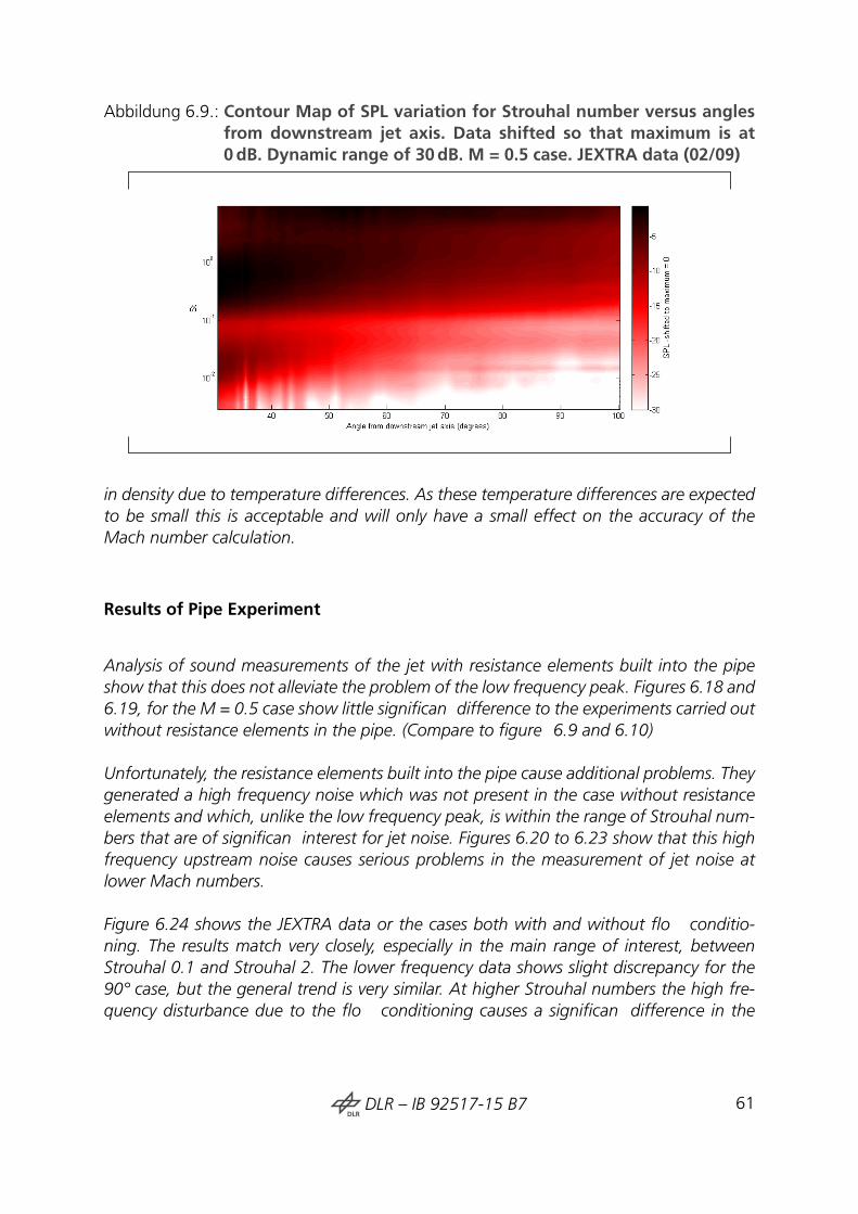
Abbildung 6.9.: Contour Map of SPL variation for Strouhal number versus anglesfrom downstream jet axis. Data shifted so that maximum is at0dB. Dynamic range of 30dB. M = 0.5 case. JEXTRA data (02/09)

in density due to temperature differences. As these temperature differences are expectedto be small this is acceptable and will only have a small effect on the accuracy of theMach number calculation.

Results of Pipe Experiment

Analysis of sound measurements of the jet with resistance elements built into the pipeshow that this does not alleviate the problem of the low frequency peak. Figures 6.18 and6.19, for the M = 0.5 case show little significan difference to the experiments carried outwithout resistance elements in the pipe. (Compare to figure 6.9 and 6.10)

Unfortunately, the resistance elements built into the pipe cause additional problems. Theygenerated a high frequency noise which was not present in the case without resistanceelements and which, unlike the low frequency peak, is within the range of Strouhal num-bers that are of significan interest for jet noise. Figures 6.20 to 6.23 show that this highfrequency upstream noise causes serious problems in the measurement of jet noise atlower Mach numbers.

Figure 6.24 shows the JEXTRA data or the cases both with and without flo conditio-ning. The results match very closely, especially in the main range of interest, betweenStrouhal 0.1 and Strouhal 2. The lower frequency data shows slight discrepancy for the90° case, but the general trend is very similar. At higher Strouhal numbers the high fre-quency disturbance due to the flo conditioning causes a significan difference in the

DLRDLR – IB 92517-15 B7 61

Abbildung 6.10.: SPL versus Strouhal number for microphones at angles∼30° ∼32.5° and 90°. For Lockheed data [9](left) and JEXTRA(02/09) data (right). M = 0.5 case

results between Strouhal 2 and Strouhal 3, which is a region that is still of significaninterest for jet noise.

It can be concluded that the low frequency peak is unlikely to be due to pipe resonancesas these would have been disturbed by the flo conditioning. The high frequency distur-bance, probably caused by the chosen flo conditioning configuration has a negativeimpact on the range of frequencies over which useful results can be measured. The over-all repeatability of the jet noise measurements on the rig have been shown to be good.

6.5.6. Mach Exponent Scaling

Dimensional Analysis

Dimensional analysis can be performed with the following variables:

Variable Dimension DescriptionQq MLT−4 source termWqq M2 L−2 T−7 cross spectral density of quadrupole source of strength Qq

D j L nozzle diameter∆U j =U j −U f LT−1 relative jet speedρ∞ ML−3 ambient density

The standard notation for the mass-distance-time set of dimensions (M for mass, L fordistance, T for time) has been used [24].

62DLRDLR – IB 92517-15 B7

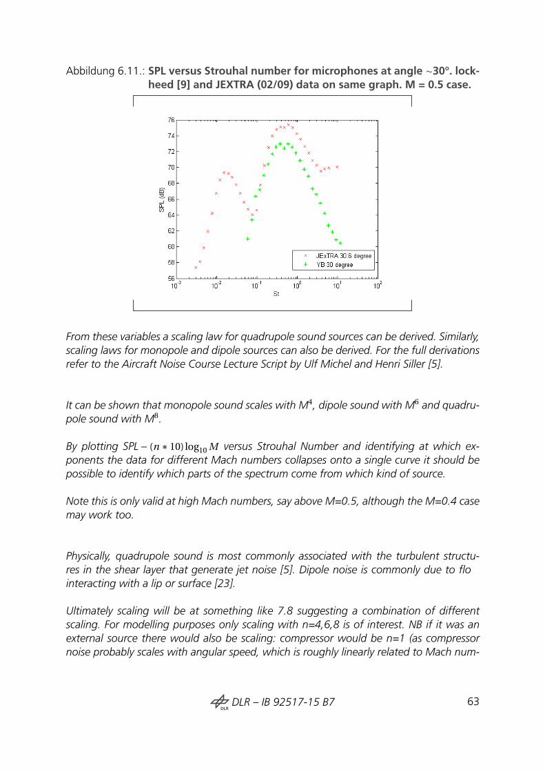
Abbildung 6.11.: SPL versus Strouhal number for microphones at angle ∼30°. lock-heed [9] and JEXTRA (02/09) data on same graph. M = 0.5 case.

From these variables a scaling law for quadrupole sound sources can be derived. Similarly,scaling laws for monopole and dipole sources can also be derived. For the full derivationsrefer to the Aircraft Noise Course Lecture Script by Ulf Michel and Henri Siller [5].

It can be shown that monopole sound scales with M4, dipole sound with M6 and quadru-pole sound with M8.

By plotting SPL− (n ∗ 10)log10 M versus Strouhal Number and identifying at which ex-ponents the data for different Mach numbers collapses onto a single curve it should bepossible to identify which parts of the spectrum come from which kind of source.

Note this is only valid at high Mach numbers, say above M=0.5, although the M=0.4 casemay work too.

Physically, quadrupole sound is most commonly associated with the turbulent structu-res in the shear layer that generate jet noise [5]. Dipole noise is commonly due to flointeracting with a lip or surface [23].

Ultimately scaling will be at something like 7.8 suggesting a combination of differentscaling. For modelling purposes only scaling with n=4,6,8 is of interest. NB if it was anexternal source there would also be scaling: compressor would be n=1 (as compressornoise probably scales with angular speed, which is roughly linearly related to Mach num-

DLRDLR – IB 92517-15 B7 63

Abbildung 6.12.: SPL versus Strouhal number for microphones at angle ∼52.5°.Lockheed [9] and JEXTRA (02/09) data on same graph. M = 0.5case.

ber), if it was the power supply it is possible that scaling would be with n=2 i.e. the powerrequired (kinetic energy scales with v2).

Comparison data

Figure 6.25) shows the Lockheed data scaled with n=4, n=6 and n=8 to identify the MachNumber exponent that best characterises the data. Clearly n=8 gives the best collapse on-to a single curve. The M=0.4 case does not collapse onto the curve with the other cases,which is explained by the fact that the scaling relation is only really valid at higher Machnumbers. M8 collapse indicates quadrupole sound [6].

JEXTRA data

Figures 6.26 shows the data for the microphone at a polar angle of 90° to the jet axis forvarious Mach numbers plotted on the same axis as described above. By visual inspection,the points composing the high frequency peak seem to collapse onto a single curve bestat n=8, while the points composing the low frequency peak collapse onto a single curve

64DLRDLR – IB 92517-15 B7

Abbildung 6.13.: SPL versus Strouhal number for microphones at angle 90°. Lock-heed [9] and JEXTRA (02/09) data on same graph. M = 0.5 case.

best at n=6.

The M8 scaling matches the comparison data well over a similar range of Strouhal num-bers and indicates quadrupole noise [6]. The M6 scaling suggest dipole noise which couldbe accounted for by a lip or surface interaction [23].

Figure 6.27 shows zoomed in views of the regions of interest.

In order to validate or reject the hypothesis made about the low frequency peak foundin the jet noise results, SODIX could be used to identify where the low frequency sourcesare. If the sources come from the jet this would support the evidence from scaling analysispresented in this section. This application of SODIX is highlighted as an area for furtherwork on the project.

An additional area for further work on the scaling analysis results, could be to plot howthe Mach exponent varies with frequency. This analysis could be carried out on the dataalready available.

DLRDLR – IB 92517-15 B7 65

6.5.7. Near Field Correction

As shown in figur 6.28, based on information in [5], different regions of the jet containsound sources with different directivities and different frequencies. Small scale structu-res near the nozzle are responsible for high frequency sound with a high polar emissionangle, while larger structures towards the end of the potential core are responsible forlower frequency sound, with a directivity that extends to much lower polar angles. This isrepresented schematically in figur 6.28.

When measuring in the far field each microphone will receive sound from sources witha similar directivity, and thus the directivity pattern of the entire jet can be analysed.

For microphones in the near field such as the one shown in figur 6.28, the situation isdifferent. Microphones will ‘see’ different sources at very different angles, and the polarangle of a microphone with respect to the nozzle exit, can be very different from thatwith respect to low frequency sources. This effect is generally refered to as biasing.

To illustrate this consider the microphone at an observer angle of 90°. For a micropho-ne in the far fiel this will measure the sound from all sources at a source directivity ofvery close to 90°. For a microphone in the near field sound from the high frequencysources near the nozzle will be at a source directivity of roughly 90°, but the low frequen-cy sound measured (from sources further downstream) will have been emitted at higherpolar angles. The same effect applies for all other microphone positions, which meansthat a direct comparison of near fiel and far fiel data is not possible.

Note that in the measurements conducted the closest microphone to the nozzle is only11.6 nozzle diameters away, so the microphones are located in the geometric near fieldIn comparison the Lockheed data [9] was taken at a distance of Ryb = 78D, which is inthe far field

In order to be able to compare the results a near-fiel correction must be carried out forthe measured data. There are two possible methods for this. The firs is to use a micro-phone to measure the frequency of sources within the jet itself. Knowledge of the sourcedistribution can then be used to correct the data. Alternatively a SODIX source identi-ficatio calculation can be carried out on the near fiel data, and the resulting sourcedistribution used to calculate a far-fiel result. This SODIX simulation is recommended forfuture work on this project.

66DLRDLR – IB 92517-15 B7

6.5.8. Inspection of Data from Ring Array

Figure 6.29 shows that all microphones on the ring give very similar values of SPL for thehigh frequency lobe, but that there is significan discrepancy for the low frequency lobe.In terms of Strouhal number, the Sound Pressure Level at the different microphones onthe ring matches well in the region St = 0.1 – 3.0, which is the main area of interest forjet noise.

A possible cause for the discrepancy at high frequencies is scattering at the microphones.The high frequency waves have a very short wavelengths, so this could be a very localisedeffect.

The low frequency discrepancy could be related to standing waves set up in the room.This possibility could be investigated by traversing a microphone.

6.6. Discussion of Validity of Rig for Jet NoiseMeasurements

In the range of Strouhal numbers from St = 0.1 to St = 3 there is good agreement bet-ween the spectra measured on the Rig, and comparison data from experiments carriedout by Lockheed [9].

The high frequency discrepancy could be due to effects of the set-up, such as scatteringfrom the brass pipes of the microphone array or other effects.

The comparison data does not extend to low frequencies, but the second low frequencypeak would not usually be expected in far-fiel jet noise spectra.

A Mach exponent scaling analysis showed that for Mach numbers above M = 0.5 theresults in the range of Strouhal numbers from St = 0.1 to St = 3 collapse quite well onto

DLRDLR – IB 92517-15 B7 67

a single curve at n=8 for both the comparison data and the data from measurements onthe JEXTRA rig, which is characteristic of sound from quadrupole sources. The low fre-quency results from the JEXTRA measurements collapse at n = 6, which suggests dipolesources. Dipole sources are often associated with flow-surfac interactions [23].

Inspection of results from measurements on a ring of microphones at a moderate polarangle show good consistency in the range of Strouhal numbers from St = 0.1 to St = 2.Below Strouhal 0.1 the pattern is the same for all microphone positions but the SPL varies.

68DLRDLR – IB 92517-15 B7

Abbildung 6.14.: Contour plots to show variation with Mach number. M = 0.3, 0.4,0.5, 0.6 0.7 from top left to bottom.

DLRDLR – IB 92517-15 B7 69

Abbildung 6.15.: Sound Pressure Level versus Strouhal Number for microphone atpolar angle of 90°. M = 0.3 – 0.7. JEXTRA data (02/09).

Abbildung 6.16.: Photograph of perforated cone and honeycomb. [Wolfram Hage]

70DLRDLR – IB 92517-15 B7

Abbildung 6.17.: Photograph of perforated cone inserted into pipe. Taken03/09/15 .

Abbildung 6.18.: Case with resistance element (JEXTRA 03/09). Contour Map ofSPL on an axis of Strouhal number versus Microphone Angle. M= 0.5 case.

DLRDLR – IB 92517-15 B7 71

Abbildung 6.19.: Case with resistance element (JEXTRA 03/09). SPL versus Strouhalnumber for different angles. M = 0.5 case.

Abbildung 6.20.: Case with resistance element (JEXTRA 03/09). Contour Map ofSPL on an axis of Strouhal number versus Microphone Angle(left). Plot of SPL versus Strouhal number for different angles(right). M = 0.3 case.

72DLRDLR – IB 92517-15 B7

Abbildung 6.21.: Case with resistance element (JEXTRA 03/09). Contour Map ofSPL on an axis of Strouhal number versus Microphone Angle(left). Plot of SPL versus Strouhal number for different angles(right). M = 0.4 case.

DLRDLR – IB 92517-15 B7 73

Abbildung 6.22.: Case with resistance element (JEXTRA 03/09). Contour Map ofSPL on an axis of Strouhal number versus Microphone Angle(left). Plot of SPL versus Strouhal number for different angles(right). M = 0.5 case.

74DLRDLR – IB 92517-15 B7

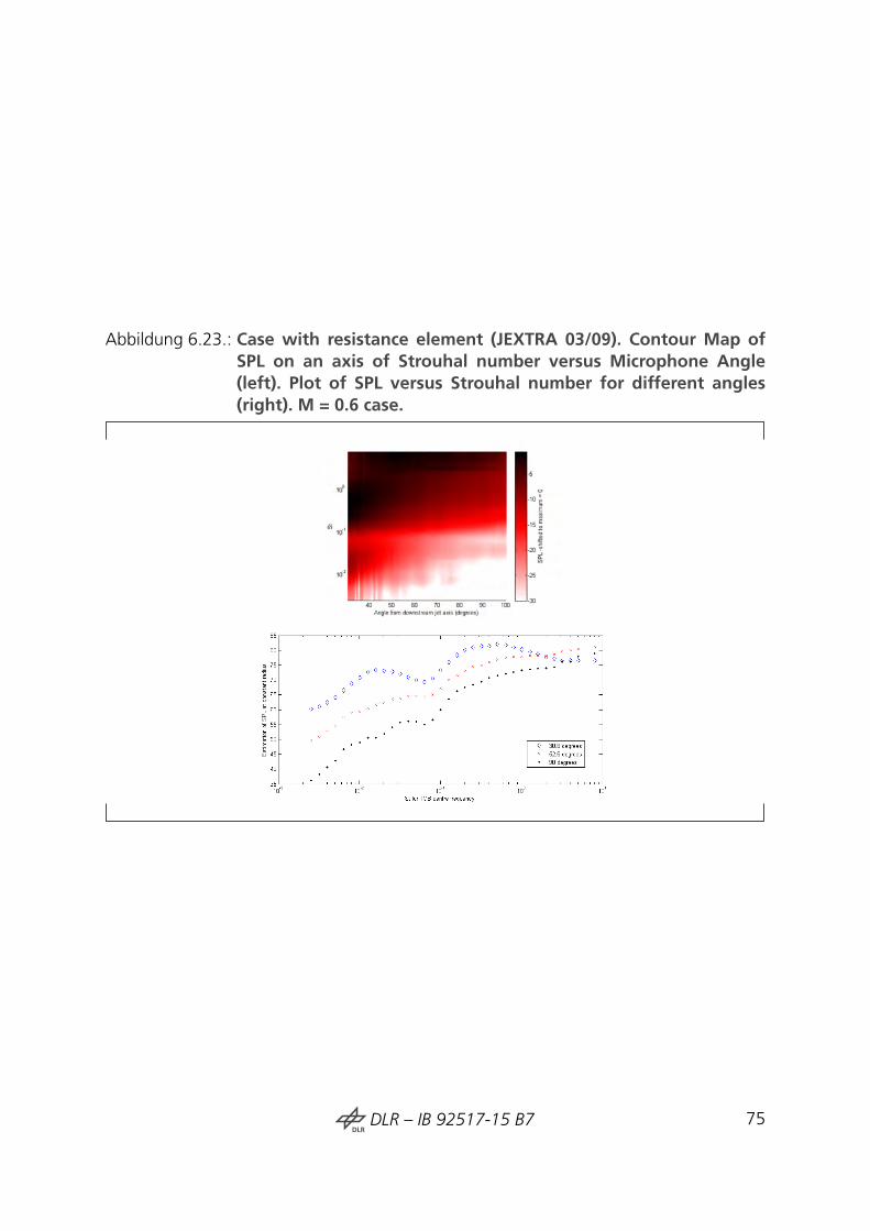
Abbildung 6.23.: Case with resistance element (JEXTRA 03/09). Contour Map ofSPL on an axis of Strouhal number versus Microphone Angle(left). Plot of SPL versus Strouhal number for different angles(right). M = 0.6 case.

DLRDLR – IB 92517-15 B7 75

Abbildung 6.24.: Estimation of SPL 10log10(p̃/pr e f ) at Constant Radius 3.9m versusStrouhal Number for microphones at different angles. Results wi-thout flo conditioning shown in blue, results with f ow condi-tioning shown in red.

76DLRDLR – IB 92517-15 B7

Abbildung 6.25.: (SPL− (n ∗ 10)log10 (M)) versus Strouhal Number for values of nfrom 4 (top left) to 9 (bottom right). Lockheed data [9]. Thirdoctave bands for microphone at 90°, over a range of Mach Num-bers 0.4 - 0.7.

Abbildung 6.26.: (SPL− (n ∗10)log10 (M)) versus Strouhal Number for values of n =4, 6, 8 (left to right). JEXTRA data for case without resistanceelement (day 02/09). Third octave bands for microphone at 90°,over a range of Mach Numbers 0.4 - 0.7.

DLRDLR – IB 92517-15 B7 77

Abbildung 6.27.: (SPL−(n∗10)log10 (M)) versus Strouhal Number for values of n = 6(left) showing only the low frequency lobe, and n = 8 (right) sho-wing only the high frequency lobe. JEXTRA data for case withoutresistance element (day 02/09). Third octave bands for micropho-ne at 90°, for a range of Mach numbers 0.4 - 0.7.

Abbildung 6.28.: Sketch of sound source regions in a typical jet.

78DLRDLR – IB 92517-15 B7

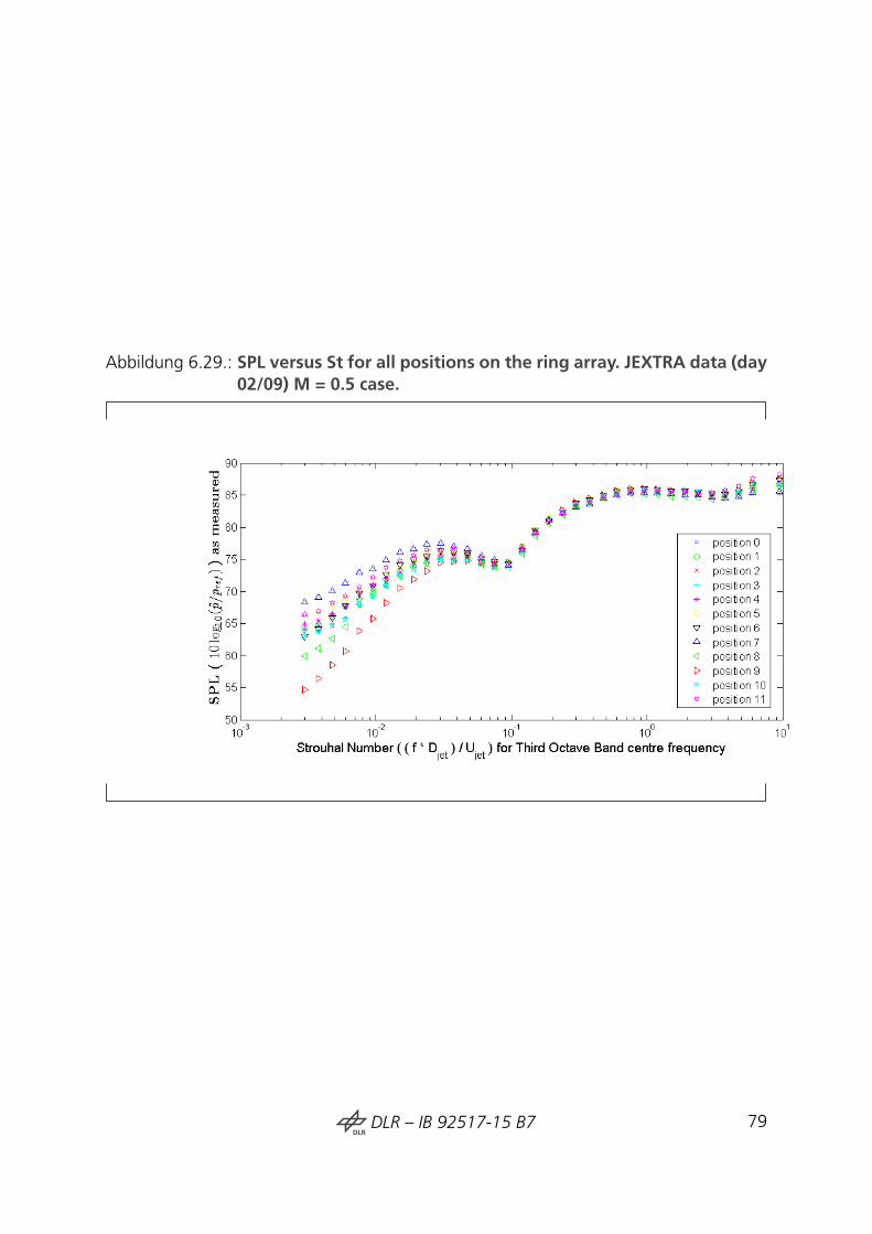
Abbildung 6.29.: SPL versus St for all positions on the ring array. JEXTRA data (day02/09) M = 0.5 case.

DLRDLR – IB 92517-15 B7 79

7. Future Work

Single Sound Source tests in the room without the ‘anechoic’ channel in place, to enablea quantitative comparative assessment of the effectiveness of the low-reflectio construc-tion.

Extension of the linear array to lower polar angles (i.e. more microphones in the down-stream direction). It would be interesting to see at what downstream angle a peak isreached. Eventually there should be a cone of relative silence. The aluminium holder onanechoic channel segment C already has further positions in the downstream direction.These simply have to be fille with brass pipes and microphones, following the protocolin section 3.4.

Analysis of coherence for the measurements on the microphone ring.

Application of SODIX for source identificatio of the sources contributing to the low fre-quency peak, in order to confirm/rejec whether this peak is directly related to the jet.

Application of SODIX to all jet data for source identification

Experiments with a different nozzle. A smaller nozzle will require the bypass to be in ope-ration.

Near fiel correction of data using results from SODIX. Comparison of corrected data withoriginal data.

DLRDLR – IB 92517-15 B7 81

Literaturverzeichnis

[1] McCowan, I. ‘A Microphone Array Tutorial’ 2004.

[2] McCowan, I. ‘Microphone Arrays: A Tutorial’ 2001.

[3] Sinayoko, S. Agarwal, A. ‘Flow decomposition and aerodynamic sound generation’Journal of Fluid Mechanics February 2011.

[4] Dowling, A. Ffowcs Williams, J.E. ‘Sound and Sources of Sound’ Ellis HorwoodLimited 1983.

[5] Ulf, M. Siller, H. ‘Lecture Script: Aircraft Noise Course’

[6] Suzuki, T. ‘A review of diagnostic studies on jet-noise sources and generationmechanisms of subsonically convecting jets’ Fluid Dynamics Research 2010.

[7] Fisher, M. J. et al. ‘A Modelling of the Noise from Simple Coaxial Jets, Part I: WithUnheated Primary Flow’ Journal of Sound and Vibration 1998.

[8] Michalke, A. Fuchs, H. V. ‘On turbulence and noise of an axisymmetric shear flow J.Fluid Mech. 1975.

[9] Tanna, H.K. ‘The Generation and Radiation of Supersonic Jet Noise. Volume III, Tur-bulent Mixing Noise Data’ Lockheed-Georgia Company 1976.

[10] Xiang, N. et al. ‘Experimental validation of a coprime linear microphone array forhigh-resolution direction-of-arrival measurements’ JASA Express Letters 2015.

[11] Karabasov, S. A. ‘Understanding jet noise’ Philosophical Transactions of The RoyalSociety 2010.

DLRDLR – IB 92517-15 B7 83

[12] Ouellette, N. T. ‘On the dynamical role of coherent structures in turbulence’ C. R.Physique 2012.

[13] Gramer, L. ‘Kelvin-Helmholtz Instabilities’ GFD-II 2007.

[14] Funke, S. et al. ‘SODIX in comparison with various deconvolution methods’ BerlinBeamforming Conference 2014.

[15] Michel, U. Funke, S. ‘New Source Analysis of an Aeroengine with a new InverseMethod SODIX’ 14th AIAA/CEAS Aeroacoustics Conference 2008.

[16] Michel, U. Funke, S. ‘Inverse Method for the Acoustic Source Analysis of an Aeroen-gine’ Berlin Beamforming Conference 2008.

[17] Funke, S. et al. ‘An extended formulation of the SODIX method with application toaeroengine broadband noise’ 18th AIAA/CEAS Aeroacoustics Conference 2012.

[18] Viswanathan, K. et al. ‘The sources of jet noise: experimental evidence’ J. Fluid Mech.2008.

[19] Doebler, D. et al. Automatic Detection of Microphone Coordinates Berlin Beamfor-ming Conference 2010.

[20] Bechert, D. W. Pfizenmaie , E. Amplificatio of Jet Noise by Higher-Mode AcousticalExcitation AIAA Journal CHECK from vol 15 no9. -1977?

[21] Doebler, D. et al. Coherent Structures in Jet Turbulence and Noise AIAA Journal 1977

[22] WRITE UP SOURCE PROPERLY.(The power point about the snowflak measurement system.)

[23] N. Curle The Influenc of Solid Boundaries upon Aerodynamic Sound Proceedings ofthe Royal Society of London 1955

[24] Barenblatt, G. I. Scaling Cambridge Texts in Applied Mathematics 2003

84DLRDLR – IB 92517-15 B7

Appendices

DLRDLR – IB 92517-15 B7 85

A. Linear Array Strouhal Calculations

For reference, the frequencies that can be expected at different Strouhal and Mach num-bers for the experimental set-up are shown here. The Strouhal number (St ) is the dimen-sionless frequency of a static jet. It is given by:

St = fs D j

U j

where fs = frequency, D j is the jet diameter, and U j is the jet speed.

For the tests being carried out, the Mach number at nozzle exit is specified This can beused to calculate the jet velocity U j :

U j = M j ∗a j

Where a j is the speed of sound in the jet, this will be slightly higher than the speed ofsound in the free stream, as the jet is slightly hotter than the free stream. Assuming a jettemperature of around 40 °C, a j is given by:

a j =√γ∗R ∗T j et

a j =p

1.4∗287∗ (40+273.15) = 355 m/s

giving:

U j = 355∗M j

DLRDLR – IB 92517-15 B7 87

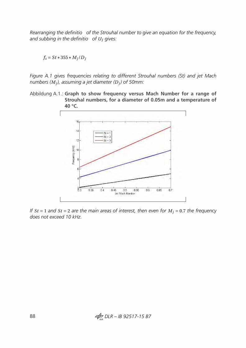
Rearranging the definitio of the Strouhal number to give an equation for the frequency,and subbing in the definitio of UJ gives:

fs = St ∗355∗M j /D j

Figure A.1 gives frequencies relating to different Strouhal numbers (St) and jet Machnumbers (M j ), assuming a jet diameter (D j ) of 50mm:

Abbildung A.1.: Graph to show frequency versus Mach Number for a range ofStrouhal numbers, for a diameter of 0.05m and a temperature of40 °C.

If St = 1 and St = 2 are the main areas of interest, then even for M j = 0.7 the frequencydoes not exceed 10 kHz.

88DLRDLR – IB 92517-15 B7

B. Jet Noise Tables

All the data and scripts (Python 3 and MATLAB) used to generate the graphical contentof this report is stored in electronic form on the JEXTRA hard drive.

Jet Noise Tables in the format of the Lockheed data [9] can be generated from the storeddata for SPLs, polar angles and frequencies if required, or by re-analysing the data fromscratch if preferred.

DLRDLR – IB 92517-15 B7 89

C. Experimental log sheets

For the experiential log sheets please refer to the physical JEXTRA folder.

Some log-sheets have been typed up and can thus also be found in electronic form onthe JEXTRA hard drive.

All log-sheets are clearly labelled with the date on which the experiments that they do-cument were performed on, as is all the measurement data stored on the hard drive.README file are included to aid navigation through the data on the hard drive.

At time of writing a further electronic version exists under:/home/terra/Transfer/Bassetti/JEXTRA/

DLRDLR – IB 92517-15 B7 91

D. Determination of MicrophonePositions

For all data analysis in this report, nominal microphone positions have been used. Asdiscussed in the report, the true microphone positions will deviate from these nominalvalues.

The determination of microphone positions was a topic of discussion throughout the pro-ject, but at the time of writing no suitable method had been agreed upon.

Methods similar to the one described in source [19], were considered, but rough calcu-lations suggest that the accuracy of this method will be insufficie t, especially when themaximum sampling frequency of the snowflak system is taken into account.

The identificatio or development of a technique to accurately determine microphonepositions is an important area for future work on the project. The application of SODIX inparticular would benefi from more accurate knowledge of microphone coordinates.

DLRDLR – IB 92517-15 B7 93