econstor www.econstor.eu

Der Open-Access-Publikationsserver der ZBW – Leibniz-Informationszentrum WirtschaftThe Open Access Publication Server of the ZBW – Leibniz Information Centre for Economics

Standard-Nutzungsbedingungen:

Die Dokumente auf EconStor dürfen zu eigenen wissenschaftlichenZwecken und zum Privatgebrauch gespeichert und kopiert werden.

Sie dürfen die Dokumente nicht für öffentliche oder kommerzielleZwecke vervielfältigen, öffentlich ausstellen, öffentlich zugänglichmachen, vertreiben oder anderweitig nutzen.

Sofern die Verfasser die Dokumente unter Open-Content-Lizenzen(insbesondere CC-Lizenzen) zur Verfügung gestellt haben sollten,gelten abweichend von diesen Nutzungsbedingungen die in der dortgenannten Lizenz gewährten Nutzungsrechte.

Terms of use:

Documents in EconStor may be saved and copied for yourpersonal and scholarly purposes.

You are not to copy documents for public or commercialpurposes, to exhibit the documents publicly, to make thempublicly available on the internet, or to distribute or otherwiseuse the documents in public.

If the documents have been made available under an OpenContent Licence (especially Creative Commons Licences), youmay exercise further usage rights as specified in the indicatedlicence.

zbw Leibniz-Informationszentrum WirtschaftLeibniz Information Centre for Economics

Braga, Michela; Paccagnella, Marco; Pellizzari, Michele

Working Paper

The Academic and Labor Market Returns ofUniversity Professors

IZA Discussion Paper, No. 7902

Provided in Cooperation with:Institute for the Study of Labor (IZA)

Suggested Citation: Braga, Michela; Paccagnella, Marco; Pellizzari, Michele (2014) : TheAcademic and Labor Market Returns of University Professors, IZA Discussion Paper, No. 7902

This Version is available at:http://hdl.handle.net/10419/93362

DI

SC

US

SI

ON

P

AP

ER

S

ER

IE

S

Forschungsinstitut zur Zukunft der ArbeitInstitute for the Study of Labor

The Academic and Labor Market Returns ofUniversity Professors

IZA DP No. 7902

January 2014

Michela BragaMarco PaccagnellaMichele Pellizzari

The Academic and Labor Market Returns of

University Professors

Michela Braga Università Statale di Milano

and fRDB

Marco Paccagnella Bank of Italy

and fRDB

Michele Pellizzari University of Geneva,

IZA, NCCR-LIVES and fRDB

Discussion Paper No. 7902 January 2014

IZA

P.O. Box 7240 53072 Bonn

Germany

Phone: +49-228-3894-0 Fax: +49-228-3894-180

E-mail: iza@iza.org

Any opinions expressed here are those of the author(s) and not those of IZA. Research published in this series may include views on policy, but the institute itself takes no institutional policy positions. The IZA research network is committed to the IZA Guiding Principles of Research Integrity. The Institute for the Study of Labor (IZA) in Bonn is a local and virtual international research center and a place of communication between science, politics and business. IZA is an independent nonprofit organization supported by Deutsche Post Foundation. The center is associated with the University of Bonn and offers a stimulating research environment through its international network, workshops and conferences, data service, project support, research visits and doctoral program. IZA engages in (i) original and internationally competitive research in all fields of labor economics, (ii) development of policy concepts, and (iii) dissemination of research results and concepts to the interested public. IZA Discussion Papers often represent preliminary work and are circulated to encourage discussion. Citation of such a paper should account for its provisional character. A revised version may be available directly from the author.

IZA Discussion Paper No. 7902 January 2014

ABSTRACT

The Academic and Labor Market Returns of University Professors*

This paper estimates the impact of college teaching on students’ academic achievement and labor market outcomes using administrative data from Bocconi University (Italy) matched with Italian tax records. The estimation exploits the random allocation of students to teachers in a fixed sequence of compulsory courses. We find that good teaching matters more for the labor market than for academic performance. Moreover, the professors who are best at improving the academic achievement of their best students are also the ones who boost their earnings the most. On the contrary, for low ability students the academic and labor market returns of teachers are largely uncorrelated. We also find that professors who are good at teaching high ability students are often not the best teachers for the least able ones. These findings can be rationalized in a model where teaching is a multi-dimensional activity with each dimension having differential returns on the students’ academic outcomes and labor market success. JEL Classification: I20, M55 Keywords: teacher quality, higher education Corresponding author: Michele Pellizzari Department of Economics University of Geneva Uni Mail, Bd du Pont d’Arve 40 1211 Geneva 4 Italy E-mail: michele.pellizzari@unige.ch

* We would like to thank Bocconi University for granting us access to its administrative archives for this project. In particular, the following persons provided invaluable and generous help: Giacomo Carrai, Mariele Chirulli, Mariapia Chisari, Alessandro Ciarlo, Alessandra Gadioli, Roberto Grassi, Enrica Greggio, Gabriella Maggioni, Erika Palazzo, Giovanni Pavese, Cherubino Profeta, Alessandra Startari and Mariangela Vago. We are also indebted to Tito Boeri, Giacomo De Giorgi, Marco Leonardi, Tommaso Monacelli, Tommy Murphy and Tommaso Nannicini for their precious comments. Davide Malacrino and Alessandro Ferrari provided excellent research assistance. The views expressed in this paper are solely those of the authors and do not involve the responsibility of the Bank of Italy. The usual disclaimer applies.

1 Introduction

Improving the quantity or the quality of the inputs in the education production function, such asteachers, peers or class size, may have very different effects on the academic and labor marketperformances of the students. The skills required to do well in school are not necessarilythose that are also the most valued by employers and the ability to negotiate a good salary andworking conditions is not necessarily reflected in school grades. Additionally, labor marketsuccess and school performance are realized at different times and many intervening factorsmay play an important role. For example, students who do poorly in school may catch up laterby exerting more effort to learn on the job or by receiving more inputs from other sources, suchas parents.

Despite these considerations, the studies that estimate the returns of inputs in the educationproduction function almost invariably consider academic achievement as an outcome measure.Obviously, linking school and labor market data is the main impediment to extending the anal-ysis to labor market outcomes and, to our knowledge, only a small set of very recent papershave been able to overcome this problem (Raj Chetty, John N. Friedman, Nathaniel Hilger,Emmanuel Saez, Diane Whitmore Schanzenbach & Danny Yagan 2011, Raj Chetty, John N.Friedman & Jonah E. Rockoff 2011, Giacomo De Giorgi, Michele Pellizzari & William G.Woolston 2012, Christian Dustmann, Patrick A. Puhani & Uta Schnberg 2012).

In this paper we estimate and compare measures of the academic and labor market returnsof university professors using administrative data from Bocconi University, which allow fol-lowing students throughout their academic careers and into the labor market. We constructsuch measures by comparing the future performance, either in subsequent coursework or in thelabor market, of students who are randomly allocated to different teachers in their compulsorycourses. For this exercise we use administrative data containing detailed records for one cohortof students at Bocconi University (Italy) - the 1998/1999 freshmen - who were required to takea fixed sequence of compulsory courses and who where randomly allocated to a set of teachersfor each of such courses. The data are exceptionally rich in terms of observable characteristicsof both the students, the professors and the classes. For example, we have a very good measureof ex-ante ability for all the students in our data, namely their scores in an attitudinal test thatthey take as part of their admission process. Hence, we can purge our measures of teacher’squality from most potential confounding factors and we can also document how they vary withthe observables of both the students and the professors.

We find that good teaching matters more in the labor market than for academic performance.Moreover, by splitting the sample of students by levels of ability we can estimate the impact ofteachers on the performance of their best and worse students separately. We find that for high-ability students the academic and labor market returns of professors are positively correlated.In other words, the professors who are best at improving their students’ grades at university arealso the ones who boost their earnings the most. For low-ability students we find the opposite,

2

namely that the academic and labor market returns of teachers are largely uncorrelated. Wealso find that professors who are good at teaching high-ability students are often not the bestteachers for the least able students.

These results are consistent with the view that teaching is a multidimensional activity in-volving multiple tasks each having different returns in the academia and in the labor market.The empirical evidence produced in this paper is informative about the degree of complemen-tarity between teachers’ competence (or effort) in each task and the ability of the students. Inparticular, our findings suggest that the returns to student’s ability are larger in the labor marketthan in the academia, perhaps because school grades can only capture a sub-set of the students’competencies. Moreover, the complementarity of student’s and teacher’s abilities appear to bestronger in the earnings process than in the process generating school grades.

Our focus on higher education is only one of the factors differentiating our work fromthe paper by Chetty, Friedman & Rockoff (2011), which is probably the closest to ours inthe literature. Due to the non-random allocation of teachers to pupils in their setting (3rd-8thgraders in the US), Chetty, Friedman & Rockoff (2011) cannot separately estimate the effectof teachers on school and labor market performance. They can only estimate the former andthey then compute the effect of being assigned to a good teacher, defined as someone whoimproves school performance, on a variety of long-term outcomes, including employment andearnings. By exploiting the specificities of the process of class formation at Bocconi University,where students are randomly allocated to instructors for each compulsory subject, we are ableto produce separate estimates of the academic and labor market effects of teachers. We canthen look at the joint distribution of those estimates, something that has never been done beforein the literature. On the other hand, contrary to Chetty, Friedman & Rockoff (2011), we cannotlook at long-term labor market performance, since we only observe taxable income at one pointin time, for most students around one to two years after graduation.

Our work is also closely linked to Scott E. Carrell & James E. West (2010), with whom weshare the focus on higher education and the methodology to compute measures of teacher ef-fectiveness based on future students’ outcomes. Their analysis, however, is limited to academicoutcomes, whereas we extend it to earnings.

Both we and Carrell & West (2010) depart from the most popular approach to measureteacher quality, the value added model (VA), which rests on the comparison of students’ per-formance in standardized tests between two (or more) grades (Eric Hanushek 1971, Jonah E.Rockoff 2004, Steven G. Rivkin, Eric A. Hanushek & John F. Kain 2005, Thomas J. Kane &Douglas O. Staiger 2008, Daniel Aaronson, Lisa Barrow & William Sander 2007). The VAmodel is commonly used in the context of primary and secondary education but it cannot beeasily extended to college education, where there is no obvious definition of a grade and wherenot all courses can be unambiguously associated to a subject sequence. Nevertheless, the largeincrease in college enrollment experienced in almost all countries around the world in the pastdecades (OECD 2008) calls for analyses focusing specifically on higher education, as in this

3

paper.The need to develop better measures of the performance of university professors is further

emphasized by a series of studies that cast serious doubts about the validity of student-reportedevaluations, which are currently used in most universities around the world (William E. Becker& Michael Watts 1999, Byron W. Brown & Daniel H. Saks 1987). For example, in a previouspaper using the same data (Michela Braga, Marco Paccagnella & Michele Pellizzari 2011) weshow that the teachers whose students perform better in subsequent coursework often receiveworst evaluations, a finding that is confirmed in Carrell & West (2010).

Measuring teacher quality in any school level is both extremely important and extremelydifficult. On the one hand, there is now ample evidence that teachers matter substantially indetermining students’ performance (Rivkin, Hanushek & Kain 2005, Carrell & West 2010)while at the same time the most common observable teachers’ characteristics, such as theirqualifications or experience, appear to be only mildly correlated with students’ scores (Alan B.Krueger 1999, Rivkin, Hanushek & Kain 2005, Eric A. Hanushek & Steven G. Rivkin 2006).Hence, it is difficult to identify good teachers ex-ante and contingent contract based on ex-postoutcomes would be the most obvious alternative to address the agency problem in this settingbut implementing them requires measures of performance.

It is for this reason that value-added indicators of teacher quality have become popular inmany countries and especially in the United States, where several studies advocated their usein the hiring and promotion decisions of teachers (Chetty, Friedman & Rockoff 2011, Eric A.Hanushek 2009, Robert Gordon, Thomas J. Kane & Douglas O. Staiger 2006) and a few schooldistricts recently adopted such a practice.

Despite their popularity, the validity of the VA approach has been questioned on variousgrounds, especially when students and teachers are not randomly assigned to one another(Chetty, Friedman & Rockoff 2011, Jesse Rothstein 2010, Kane & Staiger 2008). This paperimportantly contributes to this debate by showing that the academic and labor market returnsof good teaching may not be perfectly aligned.

For the policy viewpoint, our results suggest that performance measurement is cruciallylinked to the definition of the objective function of the education institution. Some schools oruniversities may see themselves as elite institutions and consequently aim at recruiting the verybest students and the teachers who are best at maximizing the performance of such students.Also, some institutions may be more academic oriented and aim at transmitting the body ofknowledge of one or several disciplines, regardless of the market value of such knowledge,whereas others may take a more pragmatic approach and decide to provide their students withthe competencies with the highest market returns at a specific point in time and space. Thedifferences between community colleges and universities in the US or the dual systems ofacademic and vocational education that are common in countries like Germany and Switzerlandare very good examples of teaching institutions with different objective functions, which shouldcoherently adapt their recruitment, evaluation and incentive policies.

4

The paper is organized as follows. Section 2 describes our data and the institutional detailsof Bocconi University. Section 3 discusses our strategy to estimate the academic and the labormarket returns of professors. In Section 4 we present the main empirical results and we compareestimates produced using different outcomes (grades and earnings). Robustness checks arediscussed in Section 4.1. In Section 5 we discuss the interpretation of our findings in theframework of a very simple theory. Section 6 concludes.

2 Data and institutional details

The empirical analysis in this paper is based on data for one enrollment cohort of undergraduatestudents at Bocconi University, an Italian private institution of tertiary education offering degreeprograms in economics, management, public policy and law.1 We select the cohort of studentswho enrolled as freshmen in the 1998/1999 academic year, as this is the only cohort in ourdata whose students were randomly allocated to teaching classes for each of their compulsorycourses.2 In later cohorts, the random allocation was repeated at the beginning of each academicyear, so that students would take all the compulsory courses of each academic year with thesame group of classmates, which only permits to identify the joint effectiveness of the entireset of teachers in each academic year.3 For earlier cohorts the class identifiers, which are acrucial piece of information for our study, were not recorded in the university archives.

The students entering Bocconi in the 1998/1999 academic year were offered seven differ-ent degree programs, although only three of them attracted a sufficient number of studentsto require the splitting of lectures into more than one class: Management, Economics andLaw&Management.4 Students in these programs were required to take a fixed sequence ofcompulsory courses that span the entire duration of their first two years, a good part of theirthird year and, in a few cases, also their last year. Table 1 lists the exact sequence for each ofthe three programs that we consider, breaking down courses by the term (or semester) in whichthey were taught and by subject areas (classified with different colors: red for management,black for economics, green for quantitative subjects, blue for law).56

1This section borrows heavily from Braga, Paccagnella & Pellizzari (2011)2The terms class and lecture often have different meanings in different countries and sometimes also in dif-

ferent schools within the same country. In most British universities, for example, lecture indicates a teachingsession where an instructor - typically a full faculty member - presents the main material of the course; classes areinstead practical sessions where a teacher assistant solves problem sets and applied exercises with the students.At Bocconi there was no such distinction, meaning that the same randomly allocated groups were kept for bothregular lectures and applied classes. Hence, in the remainder of the paper we use the two terms interchangeably.

3De Giorgi, Pellizzari & Woolston (2012) use data for these later cohorts for a study of class size.4The other degree programs were Economics and Social Disciplines, Economics and Finance, Economics and

Public Administration.5Subject areas are defined according to the department that was responsible for organizing and teaching the

course.6Notice that Economics and Management share exactly the same sequence of compulsory courses in the first

three terms. Indeed, students in these two programs did attend these courses together and made a final decisionabout their major at the end of the third term. Giacomo De Giorgi, Michele Pellizzari & Silvia Redaelli (2010)

5

[INSERT TABLE 1 ABOUT HERE]

Most but not all of the courses listed in Table 1 were taught in multiple classes. The num-ber of such classes varied across both degree programs and specific courses. For example,Management was the program that attracted the most students (over 70% in our cohort), whowere normally divided into 8 to 10 classes. Economics and Law&Management students weremuch fewer and were rarely allocated to more than just two classes, sometimes to a single one.The number of classes also varied within degree program depending on the number of avail-able teachers for each subject. For instance, back in 1998/1999 Bocconi did not have a lawdepartment and all law professors were contracted from nearby universities. Hence, the num-ber of classes in law courses were normally fewer than in other subjects. Similarly, since themanagement department was (and still is) much larger than the economics or the mathematicsdepartments, courses in the management areas were normally split in more classes than coursesin other subjects.

In Section 3 we construct measures of teacher effectiveness for the professors of the com-pulsory courses listed in Table 1 that were taught in multiple classes (see Section 3 for details).We do not consider elective subjects, as the endogenous self-selection of students would com-plicate the analysis.

Regardless of the specific class to which students were allocated, they were all taught thesame material. In other words, all professors of the same course were required to follow exactlythe same syllabus, although some variations across degree programs were allowed (i.e. mathe-matics was taught slightly more formally to students in Economics than in Law&Management).

Additionally, the exam questions were also the same for all students (within degree pro-gram), regardless of their classes. Specifically, one of the teachers in each course (normally asenior person) acted as a coordinator, making sure that all classes progressed similarly duringthe term, deciding changes in the syllabus and addressing specific problems that might arose.The coordinator also prepared the exam paper, which was administered to all classes. Gradingwas usually delegated to the individual teachers, each of them marking the papers of the stu-dents in his/her own class, typically with the help of one or more teaching assistants. Beforecommunicating the marks to the students, the coordinator would check that there were no largediscrepancies in the distributions across teachers. Other than this check, the grades were notcurved, neither across nor within classes.

[INSERT TABLE 2 ABOUT HERE]

Table 2 reports some descriptive statistics that summarize the distributions of (compulsory)courses and their classes across terms and degree programs. For example, in the first termManagement students took 3 courses, divided into a total of 24 different classes: management

study precisely this choice. In the rest of the paper we abstract from this issue and we treat the two degree programsas entirely separate but our results are robust to this assumption.

6

I, which was split into 10 classes; private law, 6 classes; mathematics, 8 classes. The table alsoreports basic statistics (means and standard deviations) for the size of these classes.

Our data cover in details the entire academic histories of the students in these programs,including their basic demographics (gender, place of residence and place of birth), high schoolleaving grades as well as the type of high school (academic or technical/vocational), the gradesin each single exam they sat at Bocconi together with the date when the exams were sat. Gradu-ation marks are observed for all non-dropout students.7 Additionally, all students took a cogni-tive admission test as part of their application to the university and the test scores are availablein our data for all the students. Moreover, since tuition fees varied with family income, thisvariable is also recorded in our dataset. Importantly, we also have access to the random classidentifiers that allow us to know in which class each students attended each of their courses.

[INSERT TABLE 3 ABOUT HERE]

Table 3 reports some descriptive statistics for the students in our data by degree program.A large majority of them were enrolled in the Management program (74%), while Economicsand Law&Management attracted 11% and 14%, respectively. Female students were generallyslightly under-represented in the student body (43% overall), apart from the degree programin Law&Management. About two thirds of the students came from outside the province ofMilan, which is where Bocconi is located, and such a share increased to 75% in the Economicsprogram. Family income was recorded in brackets and one quarter of the students were in thetop bracket, whose lower threshold was in the order of approximately 110,000 Euros (gross)at current prices. Students from such a wealthy background were under-represented in theEconomics program and over-represented in Law&Management. High school grades and entrytest scores (both normalized on the scale 0-100) provide a measure of ability and suggest thatEconomics attracted the best students, a finding that is also confirmed by university grades.

Data on earnings are obtained from tax records. We were able to merge the Bocconi datawith the universe of all tax declarations submitted in Italy in 2005 (incomes earned in 2004).Over 85% of the students in our sample graduate before May 2004, so this can be consideredas a measure of initial earnings.8 Unfortunately, only the 2004 tax declarations are currentlyavailable for research purposes and, thanks to a special agreement with Bocconi university,we have been able to merge them to the administrative records of the students. Of the 1,206students in our sample 1,074 submitted a tax declaration in Italy in 2005, corresponding toapproximately 90%. The others are likely to be either still looking for a job, or working abroad,

7The dropout rate, defined as the number of students who, according to our data, do not appear to have com-pleted their programs at Bocconi over the total size of the entering cohort, is around 4%. Notice that some of thesestudents might have transferred to another university or still be working towards the completion of their program,whose formal duration was 4 years. In Section 4.1 we perform robustness checks showing that excluding thedropouts from our calculations is irrelevant for our results.

8Taxable income includes all earnings from employment, be it dependent or self-employment, as well as otherincomes from properties (rents). Capital incomes are taxed separately and do not count towards personal taxableincome.

7

or being out of the labor force (possibly enrolled in some post-graduate programme).9 In ourmain analysis we will maintain the assumption that the students that are observed in the tax filesare a random sub-group of the entire cohort and in Section 4.1 we present a series of robustnesschecks to support such an assumption.

2.1 The random allocation

In this section we present evidence that the random allocation of students into classes wassuccessful, namely that the observables of students and teachers are balanced. De Giorgi,Pellizzari & Redaelli (2010) use data for the same cohort (although for a smaller set of coursesand programs) and provide similar evidence.

The randomization was (and still is) performed via a simple random algorithm that assigneda class identifier to all the students, who were then instructed to attend the lectures for thespecific course in the class labeled with the same identifier.10 The university administrationadopted the policy of repeating the randomization for each course with the explicit purpose ofencouraging wide interactions among the students.

[INSERT TABLE 4 ABOUT HERE]

Table 4 presents evidence that the students’ observable characteristics are balanced acrossclasses. More specifically, it reports test statistics derived from probit (columns 1,2,5,6,7) orOLS (columns 3 and 4) regressions of the observable students’ characteristics (by column)on class dummies for each course in each degree program that we consider, Hence, for eachcharacteristic there are 20 such tests for the degree program in Management, corresponding tothe 20 compulsory courses that were taught in multiple classes, 11 tests for Economics and 7tests for Law&Management. The null hypothesis under consideration is that the coefficientson the class dummies in each model are jointly equal to zero, which amounts to testing forthe equality of the means of the observable variables across classes within courses and degreeprograms. The table shows descriptive statistics of the distribution of p-values for such tests.

The mean and median p-values are in all cases far from the conventional thresholds forrejection. Furthermore, the table also reports the number of tests that reject the null at the 1%and 5% levels, showing that this happens only in a very limited number of cases. The most

9Bocconi also runs regular surveys of all alumni approximately 1 to 1.5 years since graduation and these sur-veys include questions on entry wages. Braga, Paccagnella & Pellizzari (2011), De Giorgi, Pellizzari & Woolston(2012) and De Giorgi, Pellizzari & Redaelli (2010) use this source to measure wages. About 60% of the studentsin our cohort answer the survey, a relatively good response rate for surveys, but still substantially lower than thematching we obtain with the tax records. In the subset of students that appear in both datasets, the two measuresare highly correlated.

10In fact, the allocation is not exactly random as the algorithm is designed to avoid assigning too many studentsto certain classes and too few to others. The probability of being allocated to a given class varies with the relativenumber of students who were previously assigned to the class. However, the probability of being assigned to anyclass is never zero nor one.

8

notable exception is residence outside Milan, which is abnormally low in two Managementgroups. Overall, Table 4 suggests that the randomization was successful.

[INSERT FIGURE 1 ABOUT HERE]

Testing the equality of means is not a sufficient test of randomization for continuous vari-ables. Hence, in Figure 1 we compare the distributions of our measures of ability (high schoolgrades and entry test scores) for the entire student body and for a randomly selected class ineach program. The figure evidently shows that the distributions are extremely similar and for-mal Kolmogorov-Smirnov tests confirm the visual impression.

Even though students were randomly assigned to classes, one may still be concerned aboutteachers being selectively allocated to classes. Although no explicit random algorithm was usedto assign professors to classes, for obvious organizational reasons that was (and still is) donein the spring of the previous academic year, i.e. well before students were allowed to enroll, sothat even if teachers were allowed to choose their class identifiers they would have no chanceto know in advance the characteristics of the students who would be given that same identifier.

More specifically, the matching of professors to class identifiers was (and still is) highlypersistent and, if nothing special occurs, professors kept the same class identifiers of the previ-ous academic year. It is only when some teachers needed to be replaced or the overall numberof classes changed that modifications took place. Even in these instances, though, the distribu-tion of class identifiers across professors changed only marginally. For example if one teacherdropped out, then a new teacher would take his/her class identifier and none of the others weregiven a different one. Similarly, if the total number of classes needed to be increases, the newclasses would be added at the bottom of the list of identifiers with new teachers and no changewould affect the existing classes and professors.11

At about the same time when teachers were given class identifiers (i.e. in the spring ofthe previous academic year), also classrooms and time schedules were defined. On these twoitems, though, teachers did have some limited choice. Typically, the administration suggested atime schedule and room allocation and professors could request modifications, which were ac-commodated only if compatible with the overall teaching schedule (e.g. a room of the requiredsize was available at the new requested time).

In order to avoid distortions in our estimates of teaching effectiveness due to the more orless convenient teaching times, we collected detailed information about the exact timing ofthe lectures in all the classes that we consider (see Section 3). Additionally, we also know inwhich exact room each class was taught and we further condition on the characteristics of theclassrooms, namely the buildings and the floors where they were located. There is no variationin other features of the rooms, such as the furniture (all rooms were - and still are - fitted withexactly the same equipment: projector, computer, white-board).12

11As far as we know, the total number of classes for a course has never been reduced.12In principle we could also condition on room fixed effects but there are several rooms in which only one class

of the courses that we consider was taught.

9

Table 5 provides evidence of the lack of correlation between teachers’ and classes’ char-acteristics, namely we show the results of regressions of teachers’ observable characteristicson classes’ observable characteristics. For this purpose, we estimate a system of 9 seeminglyunrelated simultaneous equations, where each observation is a class in a compulsory course.The dependent variables are 9 teachers’ characteristics (age, gender, h-index, average citationsper year and 4 dummies for academic positions) and the regressors are the class characteris-tics listed in the rows of the table.13 The reported statistics test the null hypothesis that thecoefficients on each class characteristic are all jointly equal to zero in all the equations of thesystem.14

[INSERT TABLE 5 ABOUT HERE]

Results show that only the time of the lectures is significantly correlated with the teachers’observables at conventional statistical levels. In fact, this is one of the few elements of theteaching planning over which teachers had some limited choice. In our empirical analysis wedo control for all the factors in Table 5, so that our measures of teaching effectiveness arepurged from the potential confounding effect of teaching times on students’ learning.

3 Estimating the academic and labor market returns of uni-versity professors

We use performance data for our students to measure the returns to university teaching and wedo so separately for academic and labor market performance.

Namely, for each of the compulsory courses listed in Table 1 we compare the future out-comes of students that attended those courses in different classes, under the assumption thatstudents who were taught by better professors enjoyed better outcomes later on. When com-puting the academic returns we consider the grades obtained by the students in all future com-pulsory courses in their degree programs and we look at their earnings when computing thelabor market returns to teaching.

This approach is similar to the value-added methodology that is commonly used in pri-mary and secondary schools (Dan Goldhaber & Michael Hansen 2010, Eric A. Hanushek &Steven G. Rivkin 2010, Hanushek & Rivkin 2006, Jesse Rothstein 2009, Rivkin, Hanushek &Kain 2005, Eric A. Hanushek 1979, Chetty, Friedman & Rockoff 2011) but it departs from itsstandard version, that uses contemporaneous outcomes and conditions on past performance,since we use future performance to infer current teaching quality.

13 The h-index is a quality-adjusted measure of individual citations based on search results on Google Scholar.It was proposed by J. E. Hirsch (2005) and it is defined as follows: A scientist has index h if h of his/her papershave at least h citations each, and the other papers have no more than h citations each.

14To construct the tests we use the small sample estimate of the variance-covariance matrix of the system.

10

The use of future performance is meant to overcome potential distortions due to explicitor implicit collusion between the teachers and their current students. In higher education,this is a particularly serious concern given that professors are often evaluated through stu-dents’ questionnaires, which have been shown to be poorly correlated with harder measures ofteaching quality (Bruce A. Weinberg, Belton M. Fleisher & Masanori Hashimoto 2009, Carrell& West 2010, Antony C. Krautmann & William Sander 1999). Bocconi university is not anexception and, in a companion paper, we have shown that such a correlation is indeed nega-tive whereas students’ evaluations of professors are positively correlated with students’ currentgrades (Braga, Paccagnella & Pellizzari 2011).

Another obvious concern with the estimation of teacher quality is the non-random assign-ment of students to professors. For example, if the best students self-select themselves intothe classes of the best teachers, then estimates of teacher quality would be biased upward.Rothstein (2009) shows that such a bias can be substantial even in well-specified models andespecially when selection is mostly driven by unobservables. We avoid these complicationsby exploiting the random allocation of students in our cohort to different classes for each oftheir compulsory courses. For this same reason, we focus exclusively on compulsory courses,as self-selection is an obvious concern for electives. Moreover, elective courses were usuallytaken by fewer students than compulsory ones and they were often taught in one single class.

We compute the returns to teaching in two steps and, for the sake of clarity, we first describethe computation of the academic returns and, then, we discuss how this procedure is adapted tocompute the labor market returns. Our methodology is similar to the one adopted by Weinberg,Fleisher & Hashimoto (2009); in their setting, however, students are not randomly assigned toteachers.

In the first step, we estimate the conditional mean of the future grades of the students ineach class according to the following procedure. Consider a set of students enrolled in degreeprogram d and indexed by i = 1, . . . , Nd, where Nd is the total number of students in theprogram. In our application there are three degree programs (d = {1, 2, 3}): Management,Economics and Law&Management. Each student i attends a fixed sequence of compulsorycourses indexed by c = 1, . . . , Cd, where Cd is the total number of such compulsory courses indegree program d. In each course c the student is randomly allocated to a class s = 1, . . . , Sc,where Sc is the total number of classes in course c. Denote by ζ ∈ Zc a generic (compulsory)course, different from c, which student i attends in semester t ≥ tc, where tc denotes thesemester in which course c is taught. Zc is the set of compulsory courses taught in any termt ≥ tc.

Let yidsζ be the grade obtained by student i in course ζ . To control for differences in thedistribution of grades across courses, yidsζ is standardized at the course level. Then, for eachcourse c in each program d we run the following regression:

yidsζ = αdcs + βXi + εidsζ (1)

11

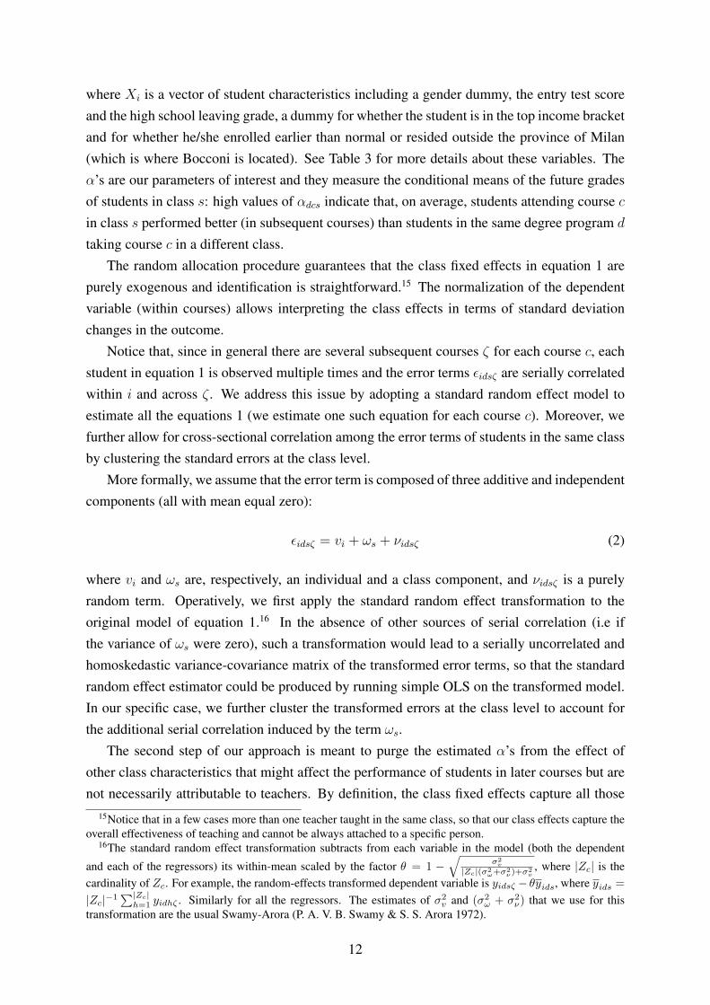
where Xi is a vector of student characteristics including a gender dummy, the entry test scoreand the high school leaving grade, a dummy for whether the student is in the top income bracketand for whether he/she enrolled earlier than normal or resided outside the province of Milan(which is where Bocconi is located). See Table 3 for more details about these variables. Theα’s are our parameters of interest and they measure the conditional means of the future gradesof students in class s: high values of αdcs indicate that, on average, students attending course cin class s performed better (in subsequent courses) than students in the same degree program d

taking course c in a different class.The random allocation procedure guarantees that the class fixed effects in equation 1 are

purely exogenous and identification is straightforward.15 The normalization of the dependentvariable (within courses) allows interpreting the class effects in terms of standard deviationchanges in the outcome.

Notice that, since in general there are several subsequent courses ζ for each course c, eachstudent in equation 1 is observed multiple times and the error terms εidsζ are serially correlatedwithin i and across ζ . We address this issue by adopting a standard random effect model toestimate all the equations 1 (we estimate one such equation for each course c). Moreover, wefurther allow for cross-sectional correlation among the error terms of students in the same classby clustering the standard errors at the class level.

More formally, we assume that the error term is composed of three additive and independentcomponents (all with mean equal zero):

εidsζ = vi + ωs + νidsζ (2)

where vi and ωs are, respectively, an individual and a class component, and νidsζ is a purelyrandom term. Operatively, we first apply the standard random effect transformation to theoriginal model of equation 1.16 In the absence of other sources of serial correlation (i.e ifthe variance of ωs were zero), such a transformation would lead to a serially uncorrelated andhomoskedastic variance-covariance matrix of the transformed error terms, so that the standardrandom effect estimator could be produced by running simple OLS on the transformed model.In our specific case, we further cluster the transformed errors at the class level to account forthe additional serial correlation induced by the term ωs.

The second step of our approach is meant to purge the estimated α’s from the effect ofother class characteristics that might affect the performance of students in later courses but arenot necessarily attributable to teachers. By definition, the class fixed effects capture all those

15Notice that in a few cases more than one teacher taught in the same class, so that our class effects capture theoverall effectiveness of teaching and cannot be always attached to a specific person.

16The standard random effect transformation subtracts from each variable in the model (both the dependent

and each of the regressors) its within-mean scaled by the factor θ = 1 −√

σ2v

|Zc|(σ2ω+σ

2ν)+σ

2v

, where |Zc| is thecardinality of Zc. For example, the random-effects transformed dependent variable is yidsζ − θyids, where yids =|Zc|−1

∑|Zc|h=1 yidhζ . Similarly for all the regressors. The estimates of σ2

v and (σ2ω + σ2

ν) that we use for thistransformation are the usual Swamy-Arora (P. A. V. B. Swamy & S. S. Arora 1972).

12

features, both observable and unobservable, that are fixed for all students in the class. Thesecertainly include teaching quality but also other factors that are documented to be importantingredients of the education production function, such as class size and class composition (DeGiorgi, Pellizzari & Woolston 2012).

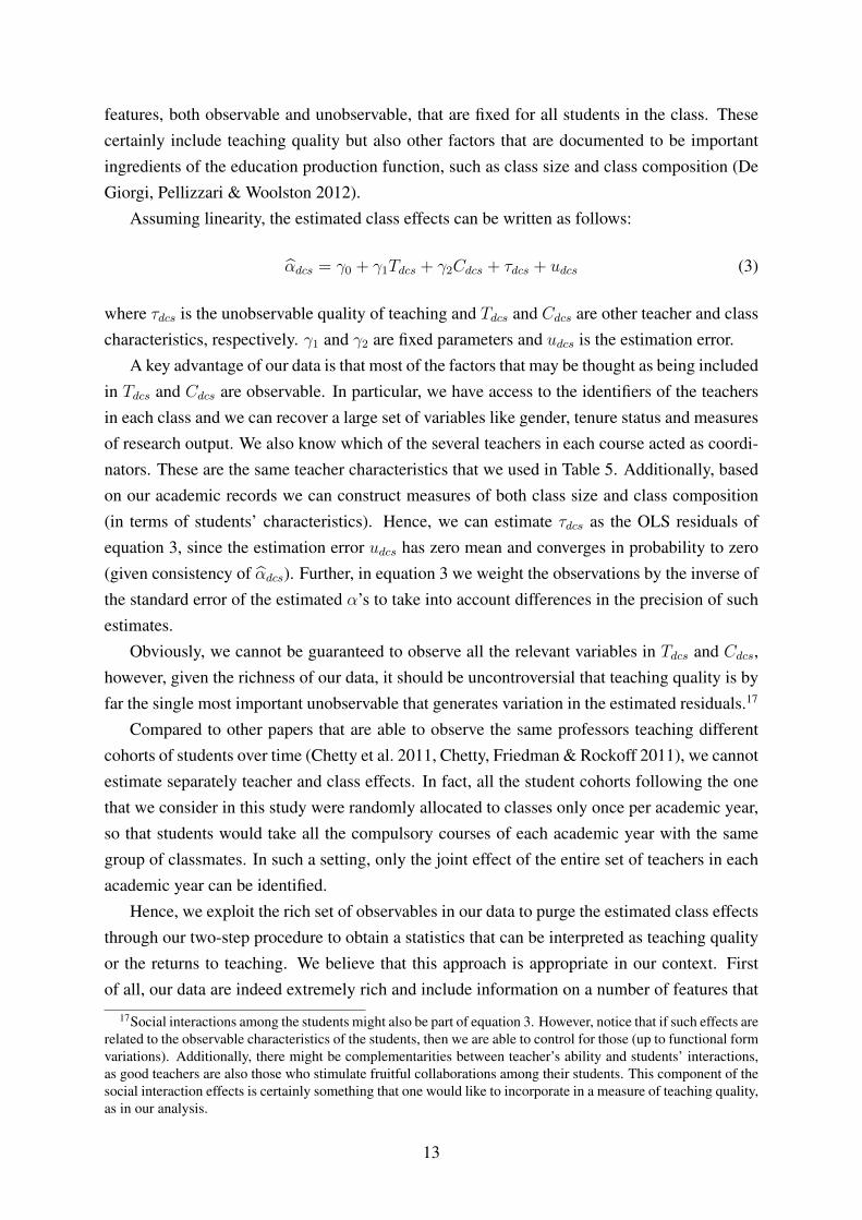
Assuming linearity, the estimated class effects can be written as follows:

α̂dcs = γ0 + γ1Tdcs + γ2Cdcs + τdcs + udcs (3)

where τdcs is the unobservable quality of teaching and Tdcs and Cdcs are other teacher and classcharacteristics, respectively. γ1 and γ2 are fixed parameters and udcs is the estimation error.

A key advantage of our data is that most of the factors that may be thought as being includedin Tdcs and Cdcs are observable. In particular, we have access to the identifiers of the teachersin each class and we can recover a large set of variables like gender, tenure status and measuresof research output. We also know which of the several teachers in each course acted as coordi-nators. These are the same teacher characteristics that we used in Table 5. Additionally, basedon our academic records we can construct measures of both class size and class composition(in terms of students’ characteristics). Hence, we can estimate τdcs as the OLS residuals ofequation 3, since the estimation error udcs has zero mean and converges in probability to zero(given consistency of α̂dcs). Further, in equation 3 we weight the observations by the inverse ofthe standard error of the estimated α’s to take into account differences in the precision of suchestimates.

Obviously, we cannot be guaranteed to observe all the relevant variables in Tdcs and Cdcs,however, given the richness of our data, it should be uncontroversial that teaching quality is byfar the single most important unobservable that generates variation in the estimated residuals.17

Compared to other papers that are able to observe the same professors teaching differentcohorts of students over time (Chetty et al. 2011, Chetty, Friedman & Rockoff 2011), we cannotestimate separately teacher and class effects. In fact, all the student cohorts following the onethat we consider in this study were randomly allocated to classes only once per academic year,so that students would take all the compulsory courses of each academic year with the samegroup of classmates. In such a setting, only the joint effect of the entire set of teachers in eachacademic year can be identified.

Hence, we exploit the rich set of observables in our data to purge the estimated class effectsthrough our two-step procedure to obtain a statistics that can be interpreted as teaching qualityor the returns to teaching. We believe that this approach is appropriate in our context. Firstof all, our data are indeed extremely rich and include information on a number of features that

17Social interactions among the students might also be part of equation 3. However, notice that if such effects arerelated to the observable characteristics of the students, then we are able to control for those (up to functional formvariations). Additionally, there might be complementarities between teacher’s ability and students’ interactions,as good teachers are also those who stimulate fruitful collaborations among their students. This component of thesocial interaction effects is certainly something that one would like to incorporate in a measure of teaching quality,as in our analysis.

13

are normally unobservable in other studies (Chetty, Friedman & Rockoff 2011, Kane & Staiger2008, Daniel F. McCaffrey, Tim R. Sass, J. R. Lockwood & Kata Mihaly 2009). Moreover, weconsider a single institution rather than all schools in an entire region or school district as inChetty, Friedman & Rockoff (2011) or in Kane & Staiger (2008). As a consequence, variationin class and student characteristics is limited and very likely to be captured by our rich set ofcontrols.

In fact, one may actually be worried that we purge for too many factors rather than too few,insofar as teaching quality is itself a function of some of the teachers’ observables. For thisreason, we present results conditioning on all the available class and teachers’ characteristicsas well as conditioning only on the class characteristics.

While the OLS residuals of equation 3 are consistent estimates of the τdcss, estimating theirvariance requires taking into account the variance of the estimation error udcs. For this purposewe follow again Weinberg, Fleisher & Hashimoto (2009), adopting a procedure that is similarto the shrinkage models commonly used in the literature (Kane & Staiger 2008, Gordon, Kane& Staiger 2006, Thomas J. Kane, Jonah E. Rockoff & Douglas O. Staiger 2008, Rockoff 2004)but that is adapted to our peculiar framework where teachers are observed only once.

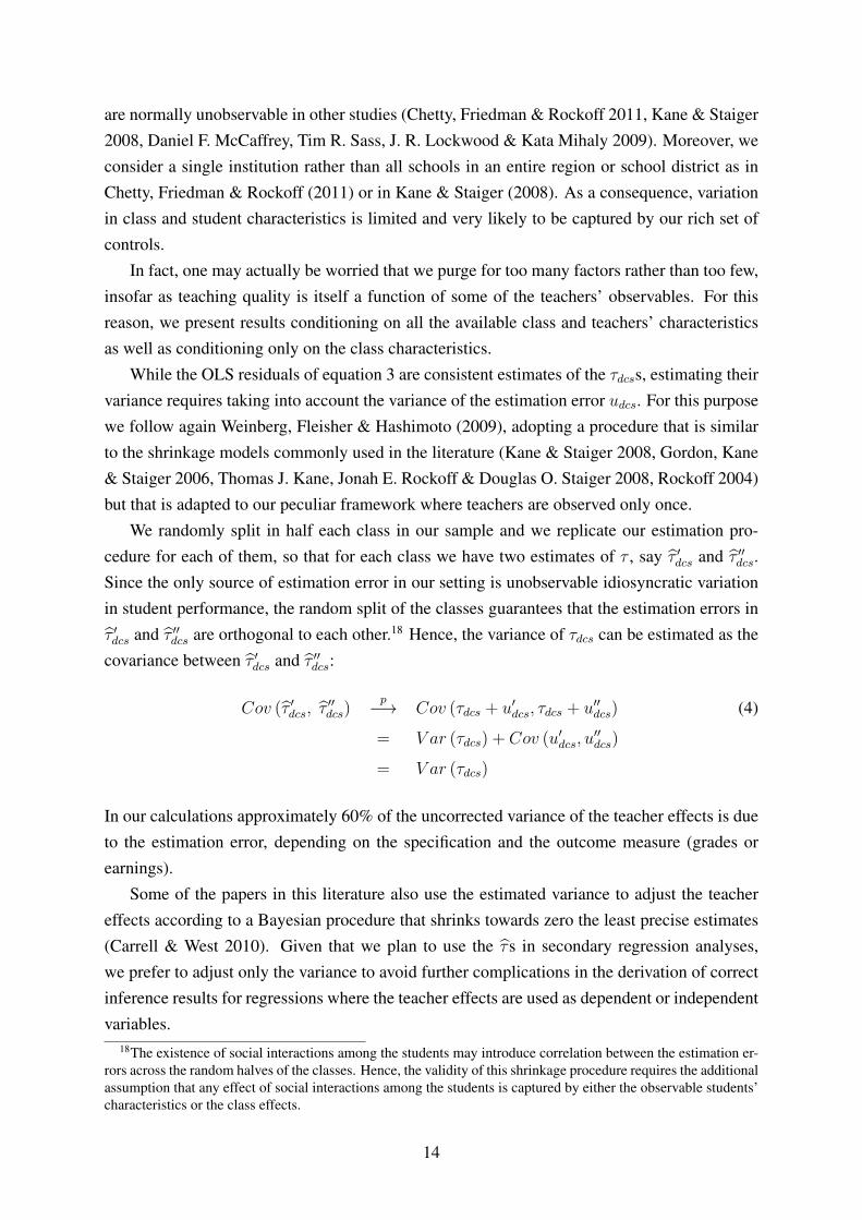
We randomly split in half each class in our sample and we replicate our estimation pro-cedure for each of them, so that for each class we have two estimates of τ , say τ̂ ′dcs and τ̂ ′′dcs.Since the only source of estimation error in our setting is unobservable idiosyncratic variationin student performance, the random split of the classes guarantees that the estimation errors inτ̂ ′dcs and τ̂ ′′dcs are orthogonal to each other.18 Hence, the variance of τdcs can be estimated as thecovariance between τ̂ ′dcs and τ̂ ′′dcs:

Cov (τ̂ ′dcs, τ̂′′dcs)

p−→ Cov (τdcs + u′dcs, τdcs + u′′dcs) (4)

= V ar (τdcs) + Cov (u′dcs, u′′dcs)

= V ar (τdcs)

In our calculations approximately 60% of the uncorrected variance of the teacher effects is dueto the estimation error, depending on the specification and the outcome measure (grades orearnings).

Some of the papers in this literature also use the estimated variance to adjust the teachereffects according to a Bayesian procedure that shrinks towards zero the least precise estimates(Carrell & West 2010). Given that we plan to use the τ̂s in secondary regression analyses,we prefer to adjust only the variance to avoid further complications in the derivation of correctinference results for regressions where the teacher effects are used as dependent or independentvariables.

18The existence of social interactions among the students may introduce correlation between the estimation er-rors across the random halves of the classes. Hence, the validity of this shrinkage procedure requires the additionalassumption that any effect of social interactions among the students is captured by either the observable students’characteristics or the class effects.

14

To estimate the labor market returns of teaching, we follow the same procedure describedabove for the academic returns but we replace future exam grades with earnings as a dependentvariable in equation 1. This simplifies the estimation substantially, since there is only oneoutcome per student and no need to account for serial correlation. However, we still cluster thestandard errors at the level of the class.

4 Empirical results

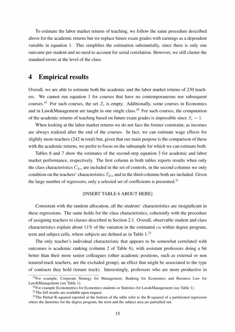
Overall, we are able to estimate both the academic and the labor market returns of 230 teach-ers. We cannot run equation 1 for courses that have no contemporaneous nor subsequentcourses.19 For such courses, the set Zc is empty. Additionally, some courses in Economicsand in Law&Management are taught in one single class.20 For such courses, the computationof the academic returns of teaching based on future exam grades is impossible since Sc = 1.

When looking at the labor market returns we do not face the former constraint, as incomesare always realized after the end of the courses. In fact, we can estimate wage effects forslightly more teachers (242 in total) but, given that our main purpose is the comparison of thesewith the academic returns, we prefer to focus on the subsample for which we can estimate both.

Tables 6 and 7 show the estimates of the second-step equation 3 for academic and labormarket performance, respectively. The first column in both tables reports results when onlythe class characteristics Cdcs are included in the set of controls, in the second columns we onlycondition on the teachers’ characteristics Tdcs and in the third columns both are included. Giventhe large number of regressors, only a selected set of coefficients is presented.21

[INSERT TABLE 6 ABOUT HERE]

Consistent with the random allocation, all the students’ characteristics are insignificant inthese regressions. The same holds for the class characteristics, coherently with the procedureof assigning teachers to classes described in Section 2.1. Overall, observable student and classcharacteristics explain about 11% of the variation in the estimated αs within degree program,term and subject cells, where subjects are defined as in Table 1.22

The only teacher’s individual characteristic that appears to be somewhat correlated withoutcomes is academic ranking (column 2 of Table 6), with assistant professors doing a bitbetter than their more senior colleagues (other academic positions, such as external or nontenured-track teachers, are the excluded group), an effect that might be associated to the typeof contracts they hold (tenure track). Interestingly, professors who are more productive in

19For example, Corporate Strategy for Management, Banking for Economics and Business Law forLaw&Management (see Table 1).

20For example Econometrics for Economics students or Statistics for Law&Management (see Table 1).21The full results are available upon request.22The Partial R-squared reported at the bottom of the table refer to the R-squared of a partitioned regression

where the dummies for the degree program, the term and the subject area are partialled out.

15

research do not seem to be better at teaching.23 In general, as in Hanushek & Rivkin (2006)and Krueger (1999), the individual traits of the teachers explain only approximately 5% of the(residual) variation in students’ achievement. Overall, the complete set of observable class andteachers’ variables explain approximately 16% of the (residual) variation (column 3 of Table6).

[INSERT TABLE 7 ABOUT HERE]

The results in Table 7 show that the overall explanatory power of teacher and class observ-able characteristics is extremely poor also when earnings are taken as the relevant outcome.The R-squared of the richest specification (column 3 of Table 7) is around 11% and each of thetwo sets of variables (class and teacher characteristics) contributes approximately half.

Our final measure of the academic returns to teaching are the residuals of the regressionof the estimated αs on all the observable variables, i.e the regression reported in columns 3of Table 6. The labor market returns are computed analogously on the basis of the residualsof the regression in column 3 of Table 7. In Table 8 we present descriptive statistics of suchmeasures and for completeness the lower panel of the table (panel B) also reports the sameresults computed without conditioning on the teachers’ observable characteristics (i.e. residualsof the regressions in columns 1 of Table 6 and Table 7).24

[INSERT TABLE 8 ABOUT HERE]

The average standard deviation of the academic returns is 0.038.25 As discussed in Section3, this number can be readily interpreted in terms of standard deviations of the distribution ofstudents’ grades. In other words, assigning students to a teacher whose academic effectivenessis one standard deviation higher than their current professor would improve grades by 3.8% ofstandard deviation, corresponding to approximately 0.5% over the average.

This effect is smaller but comparable to the findings in Carrell & West (2010), who estimatean increase in GPA of approximately 0.052 of a standard deviation for a one standard deviationincrease in teaching quality. To further put the magnitude of our estimates into perspective, itis useful to also consider the effect of a reduction in class size, which has been estimated bynumerous papers in the literature (Joshua D. Angrist & Victor Lavy 1999, Krueger 1999, OrianaBandiera, Valentino Larcinese & Imran Rasul 2010) and also on the same data used for thisstudy (De Giorgi, Pellizzari & Woolston 2012). The estimates in most of these papers are in therange of 0.1 to 0.15 of a standard deviation increase in achievement for a one standard deviationreduction in class size, thus about two to three times the effect of teachers that we estimate here.

23See Marta De Philippis (2013) for a formal evaluation of research incentives on teaching performance usingour same data.

24Table A-1 in the Appendix shows the same descriptive statistics for the original class effects (the αs fromequation 1)

25The standard deviation is computed on the basis of the shrinkage method described in Section 3.

16

Notice, however, that one of the obvious mechanisms through which reducing the size of theclass affects performance is the possibility for the professors to tailor their teaching styles totheir students in small classes, that is an improvement in the quality of teaching. In other words,our estimates of teaching quality are computed holding constant the size of the class whereasthe usual class size effect allows the quality of teaching to vary.

In Table 8 we also report the standard deviations of the academic returns to teachers in thecourses with the least and the most variation. Overall, we find that in the course with the highestvariation (macroeconomics in the Economics program) the standard deviation of our measureof academic teaching quality is 0.14 of a standard deviation in grades, approximately 3.5 timesthe average. This compares to a standard deviation of essentially zero in the course with thelowest variation (accounting in the Law&Management program).

The second column in Table 8 reports similar statistics for the labor market returns of pro-fessors, measured by the conditional average earnings of one’s randomly assigned students, asexplained in Section 3. Interestingly, the average labor market returns of professors are approx-imately 20% larger than their academic returns. A one standard deviation better professor leadsto an increase in earnings by almost 0.05 of a standard deviation on average. Given that wagesare much more disperse than grades, this translates in an annual increase of gross income of958 Euros, slightly more than 5% over the average. Beside the mean effect, it is interestingto notice that the entire distribution of the market returns is shifted to the right of that of theacademic returns.

Also the labor market returns are vastly heterogeneous across subjects, with the variationreaching 16% of a standard deviation in earnings for mathematics in the Economics programand being close to zero for management III in the Management program.

In the lower panel (panel B) of Table 8 we report the same descriptive statistics for ourmeasures of professors’ quality that do not purge the effect of the observable characteristics ofthe teachers. Consistent with the finding that such characteristics bear little explanatory powerfor students’ performances (see Tables 6 and 7), the results in panels A and B of Table 8 areextremely similar.

By restricting the set of students to those of high or low ability, measured as those whoseperformance in the attitudinal entry test is above or below the median, it is possible to replicatethe procedure described in Section 3 to produce indicators of the academic and labor marketreturns of professors for each of such categories of students. The descriptive statistics for theseindicators are reported in Table 9 and their analysis allows understanding whether it is the bestor the worst students who benefit the most from good teachers and in what dimension.26

[INSERT TABLE 9 ABOUT HERE]

When considering academic performance the dispersion in teachers’ returns appears to be26Notice that the effects reported in Table 8 cannot be derived as simple averages of the effects for high- and

low-ability students in Table 9, as we also clarify in Section 5.

17

rather homogeneous across student types, with an average standard deviation of about 0.06in both cases. Larger differences emerge when teaching quality is measured with students’earnings. In this case, the low-ability students seem to benefit from effective teaching more thantheir high ability peers, the average standard deviations being 0.124 and 0.079, respectively.

One obvious question that one can ask with these data is whether the professors who arebest at improving the academic performance of their students are also the ones who boosttheir earnings the most. In Table 10 we estimate the correlation between the academic andlabor market returns to teachers, conditional on degree program, term and subject area fixedeffects. In these regressions both the dependent variable and the main regressor of interestare estimates produced in previous steps of the analysis and to take into proper account thisadditional randomness, we weight each observation by the inverse of the standard error of theestimated academic returns (which is the dependent variable) and we bootstrap the covariancematrix.

[INSERT TABLE 10 ABOUT HERE]

Results show a strong positive correlation when the returns are computed using data on allthe students in each class, a finding that is consistent with Chetty, Friedman & Rockoff (2011).The point estimate suggests that a 1-standard deviation improvement in the labor market returnsof the teacher are associated with approximately one fourth of standard deviation increase in theacademic returns of the same teacher. Notice, however, that earnings are much more dispersedthan grades - the coefficients of variation being 0.89 and 0.15 respectively - so that this findingis perfectly consistent with the findings in Table 9 showing that the labor market returns are onaverage larger than the academic returns of professors.

When the analysis is replicated for low- and high-ability students separately, some interest-ing additional results emerge. The positive association of academic and labor market returnsto teaching is confirmed for high ability students but disappears for the low ability ones, forwhom the point estimate is actually negative although statistically insignificant at conventionallevels.

[INSERT TABLE 11 ABOUT HERE]

Finally, in Table 11 we estimate the cross-correlation between the academic and labor mar-ket returns for high- and low-ability students. In other words, we ask the question whether theprofessors who are the most effective for the good students are so also for the least able ones.As for the results of Table 10, in these regressions we condition on degree program, term andsubject areas fixed effect, we weight observations by the inverse of the standard error of theestimated dependent variable and we bootstrap the covariance matrix of the estimates.

Interestingly, we find that none of these correlations is statistically significant at conven-tional levels. When considering academic performance the point estimate is positive (column

18

1), whereas for the labor market returns the estimated correlation is negative (still insignificant),suggesting that good teaching can have very different meanings depending on both the type ofstudents and the outcomes considered.

In Section 5 we discuss in more details the interpretation of these results.

4.1 Robustness checks

In this section we provide a number of robustness checks for the main results of our analysis.A first obvious concern is the fact that we do not observe earnings for all the students in

our sample. However, this problem is limited to approximately 10% of the observations sincewe are able to match in the tax records 1,074 out of the 1,206 students in the enrollment cohortthat we consider. We have access to the entire population of students who enrolled at Bocconiuniversity in the academic year 1998/1999 and to the complete list of tax declarations submittedin Italy in 2005 (on income earned in 2004), therefore our data are more akin to census datathan to representative samples.

Most Bocconi students find employment within a relatively short period of time after grad-uation, especially when compared with other Italian universities: of the 1,206 students thatwe observe entering Bocconi in 1998/99, two thirds graduate before 2004 and 94% graduatebefore 2005 (the minimum legal duration of degree programs being four years). Hence, thefew students who are not matched can only be either unemployed or enrolled in post-graduateeducation or working abroad. Another possibility is total tax evasion, a phenomenon that is,however, quite uncommon even in Italy. The vast majority of people report at least some in-come and tax evasion is particularly common among the self-employed, which represent lessthan 3% of our sample. Dependent employees are taxed at the source directly by their em-ployers (Carlo V Fiorio & Francesco D’Amuri 2005) therefore having very limited chances toevade. Notice additionally that tax evasion can distort our indicators of teaching quality onlyunder the assumption that more or less effective teachers influence their students’ performanceas well as their propensity to evade taxes.

To show that our findings are unaffected by the imperfect matching of the university admin-istrative records and the tax files we employ two different strategies. First, we use data from anindependent source (a survey of graduates regularly run by Bocconi University) to estimate theconditional probability of employment 1 year after graduation. We estimate the model on 6,355individuals interviewed from 2002 to 2006 and we use the estimated parameters to compute thestandard Heckman correction term for our sample. We then add it as an additional regressorin the estimation of equation 1. Second, we impute missing values using the predicted mean

matching method. Such method uses linear predictions from a standard OLS model to measuredistance across selected and non-selected observations. Then, a set of nearest neighbors foreach non-selected unit is identified on the basis of such distance. Finally, imputed outcomes

19

for the missing observations are randomly drawn from their neighbors.27

[INSERT FIGURE 2 ABOUT HERE]

In figure 2 we show that the labor market returns computed in either ways are extremelysimilar to the ones we presented in section 4. The slope coefficients are not significantly differ-ent from one in both cases and the R-squared are always above 90%.

A second concern is the possible lack of compliance with the random assignment to classes.There are a number of reasons why students could choose to attend lectures in a different classfrom the one they were assigned to and, especially if such a choice is related to the quality ofthe teachers, this could be problematic for our analysis. In principle students could request tobe assigned to a different class but such requests would be accepted only in a very limited setof cases. For example, a student with some disability, temporary or permanent, who would findit difficult to climb stairs could request to be assign to a class taught on the ground floor. Thedesire to attend a class with one’s friend or with a different teachers were never accepted (norsubmitted, in fact). Apart from these very few cases, informal class switching is not recordedin our data as we only observe the class identifiers formally assigned to the students by theadministration.

To address this concern we make use of a specific item in the students’ evaluation question-naires asking about congestion in the classroom. Specifically, the question asks whether thenumber of students in the classroom was detrimental to learning.28 If non-compliance with therandom allocation is orthogonal to the teachers’ characteristics, then it should have no obviouseffect on class congestion and it merely results in measurement error in the estimation of ourclass effects, inflating the variance of the estimation error without affecting their interpretation.The most worrisome type of class switching occurs when students cluster in the class of thebest or the most pleasant teachers. For example, anecdotal evidence suggests that in the mostdifficult quantitative courses the students tend to bunch in the class of the professors who havea reputation for being particularly clear in their explanations. The courses most affected byclass switching are those in which students concentrate in one or few classes, that end up beingoverly congested, whereas the other classes of the course remain half empty.

Following this intuition, we compute for each course the difference in the congestion indi-cator between the most and the least congested class (over the standard deviation), thus iden-tifying the courses most likely affected by class switching behavior. In table 12 we reportdescriptive statistics of academic and labor market returns of professors, as in table 8, droppingthe most switched course (in panel B), the two most switched courses (in panel C) and thefive most switched courses (in panel D), showing that our main results are virtually unaffected(panel A reports the main results of Table 8 for comparison).

27We impute 10 values from 3 neighbors.28The questionnaires were administered in each class during one of the last lectures of the course. See Braga,

Paccagnella & Pellizzari (2011).

20

[INSERT TABLE 12 ABOUT HERE]

Finally, we show that our results are not driven by the exclusion from the estimation sampleof students that, after enrolling in their first year in the academic year 1998/99, dropped outbefore graduating. Such students total about 4% of all individuals in our enrollment cohort.In figure 3 we compare our estimates of the academic and labor market returns with similarestimates computed including the dropouts. The two sets of estimates are very similar, for bothacademic and labor market returns and there are no major discrepancies at either ends of thedistributions. As for the results in Figure 2, the slope coefficients are indistinguishable fromone and the R-squared are always above 90%.

[INSERT FIGURE 3 ABOUT HERE]

5 Interpretation and discussion

In order to interpret the findings of Section 4 it is necessary to extend the theoretical frameworkthat is, implicitly or explicitly, adopted by most of the literature (Eric A. Hanushek 2011,Florian Hoffman & Philippe Oreopoulos 2009, Rothstein 2010, Hanushek 1979, Hanushek& Rivkin 2006), including the many studies on teachers’ value added (Chetty, Friedman &Rockoff 2011, Rivkin, Hanushek & Kain 2005, Hanushek & Rivkin 2010). Such a standardframework views teaching quality as a unidimensional input entering the education productionfunction and, while it appears to be consistent with the overall positive correlation betweenthe academic and the labor market returns to teaching (column 1 in Table 10), it can hardlyrationalize the results that we obtain for students of different abilities.

While we do not seek to develop a full theoretical contribution, which is beyond the scopeof this paper, in this section we simply sketch the very general intuition of a model of humancapital formation and academic and labor market performance that is helpful to interpret ourempirical findings.

Consider a setting where students accumulate human capital in school or university and hu-man capital is a multidimensional factor composed of a vector of different skills. For simplicity,consider only two skills, h1 and h2. Skills are the key ingredients of the processes generatingthe observed academic (g for grade) and labor market (w for wage) outcomes.29 For simplicity,assume that only h1 affects school grades whereas earnings only depend on h2:

g = g(h1) (5)

w = w(h2) (6)

Skills are the product of both innate ability a and the learning process. Holding constant allother usual inputs of the education production function (class size, peers, et.), the key element

29Chetty et al. (2011) use a similar argument to rationalize the long-term effect of class quality.

21

of the learning process is the teacher’s input t, which we also assume to be multidimensionaland, consistently with prior assumptions, we characterize professors by their abilities to teachacademic (t1) and labor market (t2) specific skills:

h1 = h1(a, t1) (7)

h2 = h1(a, t2) (8)

Hence, the reduced form versions of equations 5 and 6 can be written as:

g = G(a, t1) (9)

w = W (a, t2) (10)

In this setting our measures of the academic and labor market returns of professors can beinterpreted as the partial derivatives of these reduced form equations with respect to t1 and t2,respectively.

For simplicity we think of t1 and t2 as exogenous characteristics of the teachers but it isrelatively easy to extend this framework with an endogenous choice of effort by professors, as inVictor Lavy (2009), Joshua D. Angrist & Jonathan Guryan (2008), Esther Duflo, Rema Hanna& Stephen P. Ryan (2012) or David N. Figlio & Lawrence Kenny (2007). In our framework,t1 is the teacher’s ability to teach material that is mostly relevant for academic courseworkwhile t2 is the ability to teach more work-related notions. Of course, these are complementaryinputs in the production of human capital but they are also characterized by differential returnsin the academia and in the labor market. For example, for an economics professor t1 wouldbe the ability to teach technical material, such as solving complex theoretical models, whereast2 would refer to developing the students’ capacity to work in groups, give presentations orwriting a computer code.

Our empirical analysis in Section 4 shows that, the labor market returns are generally largerthan the academic returns, namely Wt(a, t2) ≥ Gt(a, t1), where a is the average ability of thestudents (Table 8). This is probably due to the fact that grades are only an imperfect proxy ofstudents’ competencies, as exams and tests can only detect a subset of them, whereas the labormarket rewards a broader set of skills.

Under the reasonable assumption of complementarity between the student’s and the profes-sor’s abilities, both partial derivatives increase with a and the results in Table 9 suggests thatGt(a, t1) increases faster than Wt(a, t2) leading to the finding that the labor market returns arelarger for the low ability students than for their more able peers.

Similarly, the findings in Table 10 can be rationalized under the additional assumption thatthe returns to ability are higher in the labor market than in the academia, i.e Wa(a, t1) ≥Ga(a, t2). Due to the complementarities of students’ and teachers’ abilities, good studentsenjoy high academic returns from good academic teachers, i.e. teachers with high t1. At the

22

same time, thanks to their high ability such students also enjoy high labor market returns evenfrom teachers with relatively low t2, leading to the positive correlation estimated in the thirdcolumn of Table 10. The opposite holds for less able students, thus rationalizing also thefindings in Table 11, as the teachers who are good for some students may not be the best forothers.

6 Conclusions and policy discussion

In this paper we estimate the effect of teaching quality separately for students’ academic andlabor market performances. Although we perform this exercise on one single institution, thisis, to the best of our knowledge, the first study ever to produce such estimates. Two featuresof the empirical setting that we consider - Bocconi university in the late 1990s - are crucial forour analysis. First of all, students are randomly allocated to teachers and the randomizationis repeated independently for each compulsory course, thus allowing us to produce measuresof teaching quality that are not distorted by issues of selection. Second, we were able to linkthe academic records of the students with the complete tax files of one fiscal year (2005),when the vast majority of our students are employed. Hence, we observe both the academicperformance and the earnings of all the students who were allocated to each professor and weuse this information to estimate the ability of the teacher to improve students academic andlabor market outcomes, separately.

Our results show that the returns to university professors are larger in the labor market thanin the academia and that the teachers who are best at enhancing the academic performance oftheir students are, on average, also capable of boosting their earnings. However, when focusingon students of different abilities we find that such a positive correlation is driven exclusively bythe effect of teachers on high ability students whereas for low ability ones the returns of profes-sors in the academia and in the labor market are largely uncorrelated. If anything, the estimatedcorrelation is negative, albeit not statistically significant. Moreover, the cross-correlations be-tween the effects of teachers on high- and low-ability students are also not significant, suggest-ing that teachers who are good for the best students may not be equally beneficial for the leastable.

These results can be rationalized within a model where teaching is a multidimensional ac-tivity, involving tasks having different returns in school and in the market. For example, amath teacher could be particularly good at explaining complex notions such as integrals, limitsor derivatives and less at developing students’ problem solving skills. Despite their comple-mentarity, a good understanding of the fundamental concepts of mathematics is probably moreimportant for the students’ performance in subsequent coursework than in the labor market andthe opposite for problem solving.

From the policy perspective, our results speak to the entire literature on teachers’ perfor-mance and raise a number of important questions both for measurement and for the design of

23

incentive contracts. First and above all, the definition of teaching quality needs to be preciselyclarified before any measurement can be implemented. Being a good instructor may meanvery different things depending on the types of students who are taught and for some studentsteachers who are particularly good at some activities may not be as good at others.

Hence, before thinking about how to measure teachers’ performance and before decidingwhether and how to use such measurements to design incentive contracts, any education institu-tion should define its own objective function. Some schools or universities may see themselvesas elite institutions and consequently aim at recruiting the very best students and the teacherswho are best at maximizing their performance. Other schools may adopt a more egalitarianapproach and decide to improve average performance by lifting the achievement of the leastable students. Similarly, some institutions may be more academic oriented and adopt as theirmain objective the teaching of one or more disciplines, regardless of the market value of suchknowledge, whereas others may take a more pragmatic approach and decide to endow theirstudents with the competencies that have the highest market returns. The differences betweencommunity colleges and universities in the US or the dual systems of academic and vocationaleducation that are common in countries like Germany and Switzerland are very good examplesof teaching institutions with different objective functions.

Our results emphasize the importance of defining the measures of teaching performance andthe types of incentives provided to teachers according to the objective function of the educationinstitution.

ReferencesAaronson, Daniel, Lisa Barrow, and William Sander. 2007. “Teachers and Student Achieve-

ment in the Chicago Public High Schools.” Journal of Labor Economics, 25: 95–135.

Angrist, Joshua D., and Jonathan Guryan. 2008. “Does Teacher Testing Raise Teacher Qual-ity? Evidence from State Certification Requirements.” Economics of Education Review,27(5): 483–503.

Angrist, Joshua D., and Victor Lavy. 1999. “Using Maimonides’ Rule To Estimate The Ef-fect Of Class Size On Scholastic Achievement.” The Quarterly Journal of Economics,114(2): 533–575.

Bandiera, Oriana, Valentino Larcinese, and Imran Rasul. 2010. “Heterogeneous ClassSize Effects: New Evidence from a Panel of University Students.” Economic Journal,120(549): 1365–1398.

Becker, William E., and Michael Watts. 1999. “How departments of economics should eval-uate teaching.” American Economic Review (Papers and Proceedings), 89(2): 344–349.

Braga, Michela, Marco Paccagnella, and Michele Pellizzari. 2011. “Evaluating Students’Evaluations of Professors.” Institute for the Study of Labor (IZA) IZA Discussion Papers5620.

24

Brown, Byron W., and Daniel H. Saks. 1987. “The microeconomics of the allocation ofteachers’ time and student learning.” Economics of Education Review, 6(4): 319–332.

Carrell, Scott E., and James E. West. 2010. “Does Professor Quality Matter? Evidencefrom Random Assignment of Students to Professors.” Journal of Political Economy,118(3): 409–32.

Chetty, Raj, John N. Friedman, and Jonah E. Rockoff. 2011. “The Long-Term Impacts ofTeachers: Teacher Value-Added and Student Outcomes in Adulthood.” National Bureauof Economic Research Working Paper 17699.

Chetty, Raj, John N. Friedman, Nathaniel Hilger, Emmanuel Saez, Diane WhitmoreSchanzenbach, and Danny Yagan. 2011. “How Does Your Kindergarten Classroom Af-fect Your Earnings? Evidence From Project STAR.” Quarterly Journal of Economics,126(4): 1593–1660.

De Giorgi, Giacomo, Michele Pellizzari, and Silvia Redaelli. 2010. “Identification of SocialInteractions through Partially Overlapping Peer Groups.” American Economic Journal:Applied Economics, 2(2): 241–275.

De Giorgi, Giacomo, Michele Pellizzari, and William G. Woolston. 2012. “Class Size andClass Heterogeneity.” Journal of the European Economic Association, 10(4): 795–830.

De Philippis, Marta. 2013. “Research Incentives and Teaching Performance. Evidence from aNatural Experiment.” mimeo.

Duflo, Esther, Rema Hanna, and Stephen P. Ryan. 2012. “Incentives Work: Getting Teachersto Come to School.” American Economic Review, 102(4): 1241–1278.

Dustmann, Christian, Patrick A. Puhani, and Uta Schnberg. 2012. “The Long-term Effectsof School Quality on Labor Market Outcomes and Educational Attainment.” Centre forResearch and Analysis of Migration (CReAM), Department of Economics, UniversityCollege London CReAM Discussion Paper Series 1208.

Figlio, David N., and Lawrence Kenny. 2007. “Individual teacher incentives and studentperformance.” Journal of Public Economics, 91: 901–914.

Fiorio, Carlo V, and Francesco D’Amuri. 2005. “Workers’ Tax Evasion in Italy.” Giornaledegli Economisti, 64(2-3): 247–270.

Goldhaber, Dan, and Michael Hansen. 2010. “Using performance on the job to in-form teacher tenure decisions.” American Economic Review (Papers and Proceedings),100(2): 250–255.

Gordon, Robert, Thomas J. Kane, and Douglas O. Staiger. 2006. “Identifying EffectiveTeachers Using Performance on the Job.” The Hamilton Project White Paper 2006-01.

Hanushek, Eric. 1971. “Teacher Characteristics and Gains in Student Achievement: Estima-tion Using Micro Data.” American Economic Review, 61(2): 280–88.

Hanushek, Eric A. 1979. “Conceptual and empirical issues in the estimation of educationalproduction functions.” Journal of Human Resources, 14: 351–388.

25

Hanushek, Eric A. 2009. “Teacher Deselection.” In Creating a New Teaching Profession. , ed.Dan Goldhaber and Jane Hannaway, 165–180. Urban Institute Press.

Hanushek, Eric A. 2011. “The economic value of higher teacher quality.” Economics of Edu-cation Review, 30(3): 466–479.

Hanushek, Eric A., and Steven G. Rivkin. 2006. “Teacher quality.” In Handbook of the Eco-nomics of Education. Vol. 1, , ed. Eric A. Hanushek and Finis Welch, 1050–1078. Ams-terdam:North Holland.

Hanushek, Eric A., and Steven G. Rivkin. 2010. “Generalizations about using value-addedmeasures of teacher quality.” American Economic Review (Papers and Proceedings),100(2): 267–271.

Hirsch, J. E. 2005. “An index to quantify an individual’s scientific research output.”Proceedings of the National Academy of Sciences of the United States of America,102(46): 16569–16572.

Hoffman, Florian, and Philippe Oreopoulos. 2009. “Professor Qualities and StudentAchievement.” Review of Economics and Statistics, 91(1): 83–92.

Kane, Thomas J., and Douglas O. Staiger. 2008. “Estimating teacher impacts on studentachievement: an experimental evaluation.” NBER Working Paper Series 14607.

Kane, Thomas J., Jonah E. Rockoff, and Douglas O. Staiger. 2008. “What does certifica-tion tell us about teacher effectiveness? Evidence from New York City.” Economics ofEducation Review, 27(6): 615–631.

Krautmann, Antony C., and William Sander. 1999. “Grades and student evaluations ofteachers.” Economics of Education Review, 18: 59–63.

Krueger, Alan B. 1999. “Experimental estimates of education production functions.” Quar-terly Journal of Economics, 114: 497–532.

Lavy, Victor. 2009. “Performance Pay and Teachers’ Effort, Productivity and Grading Ethics.”American Economic Review, 95(5): 1979–2011.

McCaffrey, Daniel F., Tim R. Sass, J. R. Lockwood, and Kata Mihaly. 2009. “The Intertem-poral Variability of Teacher Effect Estimates.” Education Finance and Policy, 4(4): 572–606.

OECD. 2008. Education at a Glance. Paris:Organization of Economic Cooperation and Devel-opment.

Rivkin, Steven G., Eric A. Hanushek, and John F. Kain. 2005. “Teachers, Schools andAcedemic Achievement.” Econometrica, 73(2): 417–458.

Rockoff, Jonah E. 2004. “The impact of individual teachers on student achievement: evidencefrom panel data.” American Economic Review (Papers and Proceedings), 94(2): 247–252.

Rothstein, Jesse. 2009. “Student Sorting and Bias in Value Added Estimation: Selection onObservables and Unobservables.” Education Finance and Policy, 4(4): 537–571.

26

Rothstein, Jesse. 2010. “Teacher Quality in Educational Production: Tracking, Decay, andStudent Achievement.” Quarterly Journal of Economics, 125(1): 175–214.

Swamy, P. A. V. B., and S. S. Arora. 1972. “The Exact Finite Sample Properties of the Es-timators of Coefficients in the Error Components Regression Models.” Econometrica,40(2): pp. 261–275.

Weinberg, Bruce A., Belton M. Fleisher, and Masanori Hashimoto. 2009. “EvaluatingTeaching in Higher Education.” Journal of Economic Education, 40(3): 227–261.

27

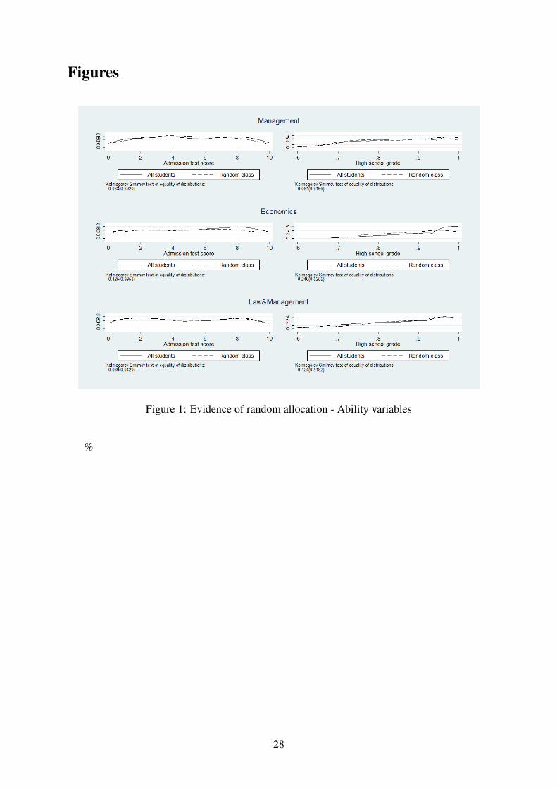
Figures

Figure 1: Evidence of random allocation - Ability variables

%

28

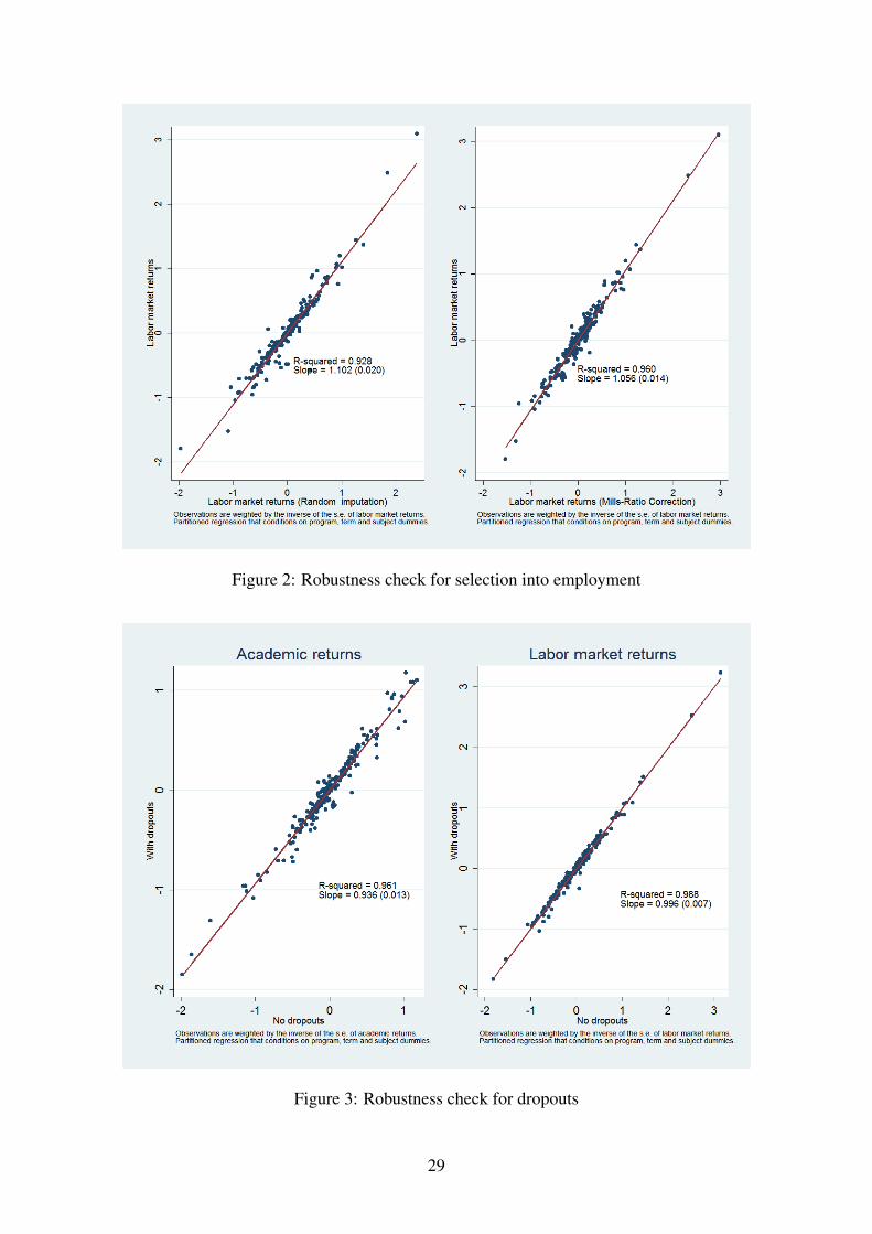
Figure 2: Robustness check for selection into employment

Figure 3: Robustness check for dropouts

29

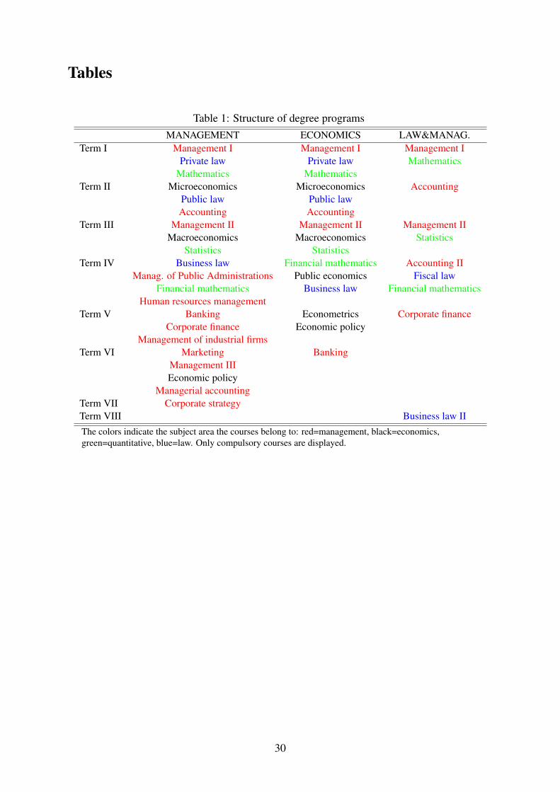
Tables

Table 1: Structure of degree programsMANAGEMENT ECONOMICS LAW&MANAG.

Term I Management I Management I Management IPrivate law Private law Mathematics

Mathematics MathematicsTerm II Microeconomics Microeconomics Accounting

Public law Public lawAccounting Accounting

Term III Management II Management II Management IIMacroeconomics Macroeconomics Statistics

Statistics StatisticsTerm IV Business law Financial mathematics Accounting II

Manag. of Public Administrations Public economics Fiscal lawFinancial mathematics Business law Financial mathematics

Human resources managementTerm V Banking Econometrics Corporate finance

Corporate finance Economic policyManagement of industrial firms

Term VI Marketing BankingManagement IIIEconomic policy

Managerial accountingTerm VII Corporate strategyTerm VIII Business law IIThe colors indicate the subject area the courses belong to: red=management, black=economics,green=quantitative, blue=law. Only compulsory courses are displayed.

30

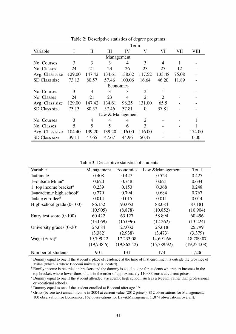
Table 2: Descriptive statistics of degree programsTerm

Variable I II III IV V VI VII VIIIManagement

No. Courses 3 3 3 4 3 4 1 -No. Classes 24 21 23 26 23 27 12 -Avg. Class size 129.00 147.42 134.61 138.62 117.52 133.48 75.08 -SD Class size 73.13 80.57 57.46 100.06 16.64 46.20 11.89 -

EconomicsNo. Courses 3 3 3 3 2 1 - -No. Classes 24 21 23 4 2 2 - -Avg. Class size 129.00 147.42 134.61 98.25 131.00 65.5 - -SD Class size 73.13 80.57 57.46 37.81 0 37.81 - -

Law & ManagementNo. Courses 3 4 4 4 2 - - 1No. Classes 5 5 5 6 3 - - 1Avg. Class size 104.40 139.20 139.20 116.00 116.00 - - 174.00SD Class size 39.11 47.65 47.67 44.96 50.47 - - 0.00

Table 3: Descriptive statistics of students

Variable Management Economics Law &Management Total1=female 0.408 0.427 0.523 0.4271=outside Milana 0.620 0.748 0.621 0.6341=top income bracketb 0.239 0.153 0.368 0.2481=academic high schoolc 0.779 0.794 0.684 0.7671=late enrolleed 0.014 0.015 0.011 0.014High-school grade (0-100) 86.152 93.053 88.084 87.181

(10.905) (8.878) (10.852) (10.904)Entry test score (0-100) 60.422 63.127 58.894 60.496

(13.069) (15.096) (12.262) (13.224)University grades (0-30) 25.684 27.032 25.618 25.799

(3.382) (2.938) (3.473) (3.379)Wage (Euro)e 19,799.22 17,233.08 14,691.66 18,789.87

(19,738.6) (19,862.42) (15,389.92) (19,234.08)

Number of students 901 131 174 1,206a Dummy equal to one if the student’s place of residence at the time of first enrollment is outside the province of

Milan (which is where Bocconi university is located).b Family income is recorded in brackets and the dummy is equal to one for students who report incomes in the

top bracket, whose lower threshold is in the order of approximately 110,000 euros at current prices.c Dummy equal to one if the student attended a academic high school, such as a lyceum, rather than professional

or vocational schools.d Dummy equal to one if the student enrolled at Bocconi after age 19.e Gross (before tax) annual income in 2004 at current value (2012 prices). 812 observations for Management,

100 observation for Economics, 162 observations for Law&Management (1,074 observations overall).

31

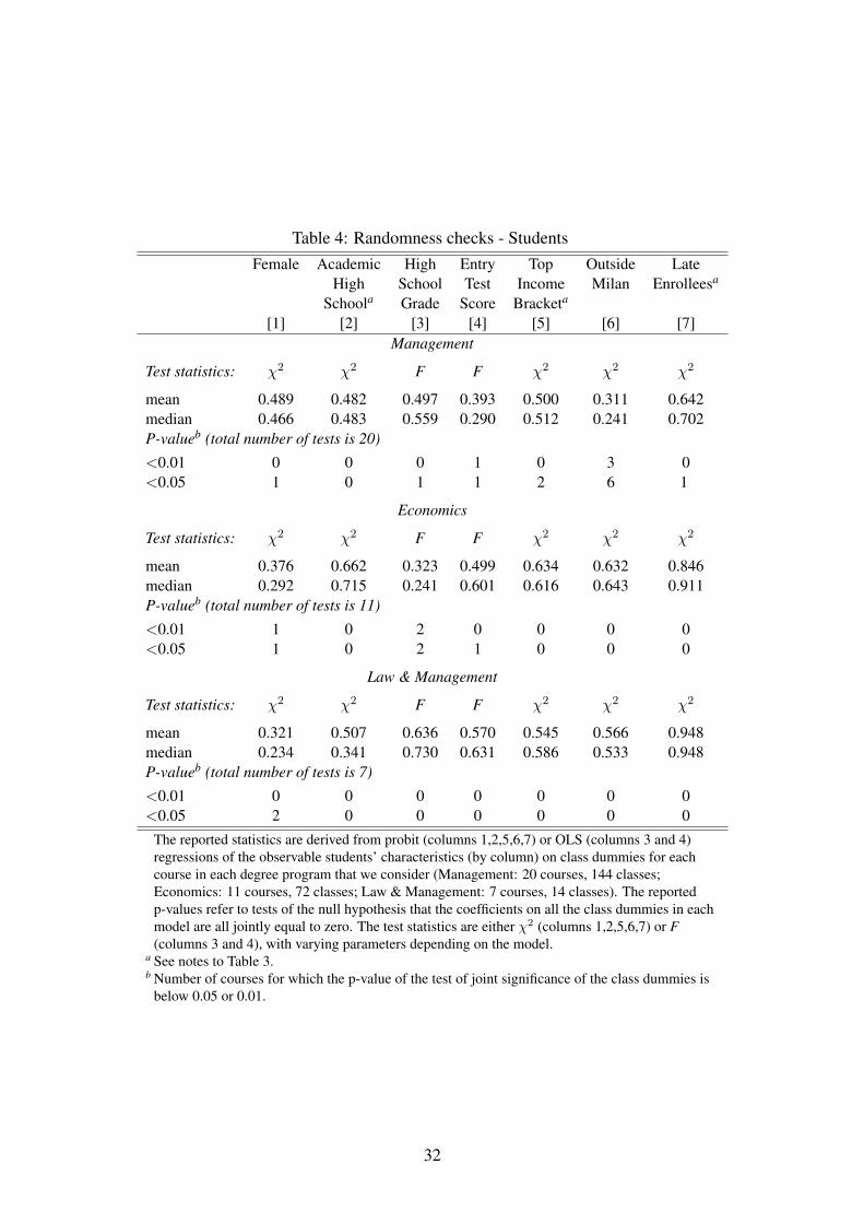
Table 4: Randomness checks - StudentsFemale Academic High Entry Top Outside Late

High School Test Income Milan Enrolleesa

Schoola Grade Score Bracketa

[1] [2] [3] [4] [5] [6] [7]Management

Test statistics: χ2 χ2 F F χ2 χ2 χ2

mean 0.489 0.482 0.497 0.393 0.500 0.311 0.642median 0.466 0.483 0.559 0.290 0.512 0.241 0.702P-valueb (total number of tests is 20)

<0.01 0 0 0 1 0 3 0<0.05 1 0 1 1 2 6 1

Economics

Test statistics: χ2 χ2 F F χ2 χ2 χ2

mean 0.376 0.662 0.323 0.499 0.634 0.632 0.846median 0.292 0.715 0.241 0.601 0.616 0.643 0.911P-valueb (total number of tests is 11)

<0.01 1 0 2 0 0 0 0<0.05 1 0 2 1 0 0 0

Law & Management

Test statistics: χ2 χ2 F F χ2 χ2 χ2

mean 0.321 0.507 0.636 0.570 0.545 0.566 0.948median 0.234 0.341 0.730 0.631 0.586 0.533 0.948P-valueb (total number of tests is 7)

<0.01 0 0 0 0 0 0 0<0.05 2 0 0 0 0 0 0

The reported statistics are derived from probit (columns 1,2,5,6,7) or OLS (columns 3 and 4)regressions of the observable students’ characteristics (by column) on class dummies for eachcourse in each degree program that we consider (Management: 20 courses, 144 classes;Economics: 11 courses, 72 classes; Law & Management: 7 courses, 14 classes). The reportedp-values refer to tests of the null hypothesis that the coefficients on all the class dummies in eachmodel are all jointly equal to zero. The test statistics are either χ2 (columns 1,2,5,6,7) or F(columns 3 and 4), with varying parameters depending on the model.

a See notes to Table 3.b Number of courses for which the p-value of the test of joint significance of the class dummies is

below 0.05 or 0.01.

32

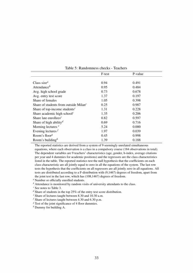
Table 5: Randomness checks - TeachersF-test P-value

Class sizea 0.94 0.491Attendanceb 0.95 0.484Avg. high school grade 0.73 0.678Avg. entry test score 1.37 0.197Share of females 1.05 0.398Share of students from outside Milanc 0.25 0.987Share of top-income studentsc 1.31 0.228Share academic high schoolc 1.35 0.206Share late enrolleesc 0.82 0.597Share of high abilityd 0.69 0.716Morning lectures e 5.24 0.000Evening lectures f 1.97 0.039Room’s floorg 0.45 0.998Room’s buildingh 1.39 0.188

The reported statistics are derived from a system of 9 seemingly unrelated simultaneousequations, where each observation is a class in a compulsory course (184 observations in total).The dependent variables are 9 teachers’ characteristics (age, gender, h-index, average citationsper year and 4 dummies for academic positions) and the regressors are the class characteristicslisted in the table. The reported statistics test the null hypothesis that the coefficients on eachclass characteristic are all jointly equal to zero in all the equations of the system. The last rowtests the hypothesis that the coefficients on all regressors are all jointly zero in all equations. Alltests are distributed according to a F-distribution with (9,1467) degrees of freedom, apart fromthe joint test in the last row, which has (108,1467) degrees of freedom.

a Number or officially enrolled students.b Attendance is monitored by random visits of university attendants to the class.c See notes to Table 3.d Share of students in the top 25% of the entry test score distribution.e Share of lectures taught between 8.30 and 10.30 a.m.f Share of lectures taught between 4.30 and 6.30 p.m.g Test of the joint significance of 4 floor dummies.h Dummy for building A.

33

Table 6: Determinants of class effectsDependent variable = α̂s [1] [2]a [3]Class sizeb -0.000 - -0.000

(0.000) (0.000)Avg. HS grade -0.468 - -0.432

(0.447) (0.468)Avg. entry test score -0.316 - -0.502

(0.599) (0.615)Share of females 0.102 - 0.090

(0.102) (0.107)Share from outside Milan 0.133 - 0.125

(0.087) (0.088)Share of top incomeb -0.024 - -0.009

(0.116) (0.121)Share from academic HS 0.000 - 0.014

(0.129) (0.137)Share of late enrollees -0.671* - -0.657*

(0.356) (0.369)Share of high abilityb 0.148 - 0.174

(0.170) (0.170)Morning lecturesb 0.001 - -0.011

(0.016) (0.017)Evening lecturesb -0.147 - -0.026

(0.194) (0.214)1=coordinator - 0.011 0.015

(0.017) (0.017)Male - -0.003 -0.002

(0.010) (0.011)Age - -0.001 0.001

(0.002) (0.002)Age squared - 0.000 -0.000

(0.000) (0.000)H-index - -0.002 -0.001

(0.003) (0.003)Citations per year - -0.000 0.000

(0.000) (0.000)Full professorc 0.023 0.045

(0.029) (0.031)Associate professorc 0.037 0.067**

(0.027) (0.029)Assistant professorc 0.049* 0.066**

(0.027) (0.028)Classroom characteristicsd yes no yesDegree program dummies yes yes yesSubject area dummies yes yes yesTerm dummies yes yes yes

Partial R squarede 0.117 0.046 0.155Observations 230 230 230

Observations are weighted by the inverse of the standard error of the estimated α’s. * p<0.1, **p<0.05,***p<0.01

a Weighted averages of individual characteristics if there is more than one teacher per class.b See notes to Table 5.c All variables regarding the academic position refer to the main teacher of the class. The excluded dummy is a

residual category (visiting prof., external experts, collaborators.)d Four floor dummies, one building dummy and a dummy for multi-classrooms classes.e R squared computed once program, term and subject fixed effects are partialled out.

34

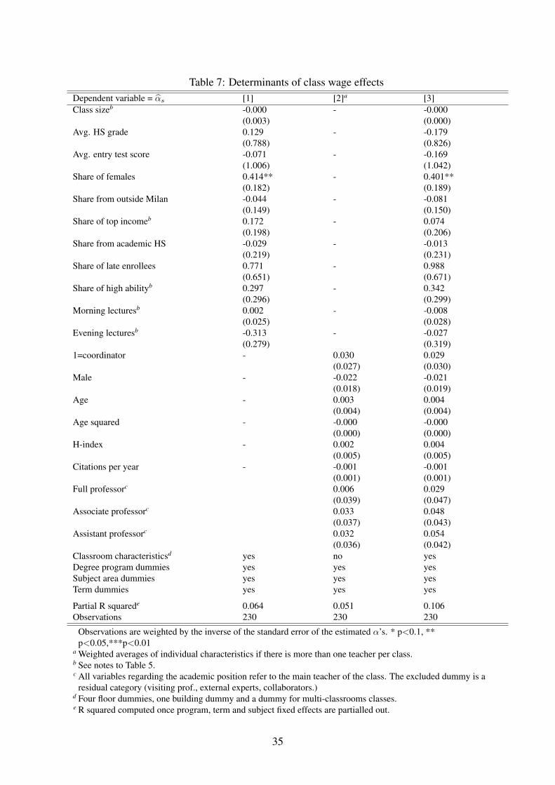
Table 7: Determinants of class wage effectsDependent variable = α̂s [1] [2]a [3]Class sizeb -0.000 - -0.000

(0.003) (0.000)Avg. HS grade 0.129 - -0.179

(0.788) (0.826)Avg. entry test score -0.071 - -0.169

(1.006) (1.042)Share of females 0.414** - 0.401**

(0.182) (0.189)Share from outside Milan -0.044 - -0.081

(0.149) (0.150)Share of top incomeb 0.172 - 0.074

(0.198) (0.206)Share from academic HS -0.029 - -0.013

(0.219) (0.231)Share of late enrollees 0.771 - 0.988

(0.651) (0.671)Share of high abilityb 0.297 - 0.342

(0.296) (0.299)Morning lecturesb 0.002 - -0.008

(0.025) (0.028)Evening lecturesb -0.313 - -0.027

(0.279) (0.319)1=coordinator - 0.030 0.029

(0.027) (0.030)Male - -0.022 -0.021

(0.018) (0.019)Age - 0.003 0.004

(0.004) (0.004)Age squared - -0.000 -0.000

(0.000) (0.000)H-index - 0.002 0.004

(0.005) (0.005)Citations per year - -0.001 -0.001

(0.001) (0.001)Full professorc 0.006 0.029

(0.039) (0.047)Associate professorc 0.033 0.048

(0.037) (0.043)Assistant professorc 0.032 0.054

(0.036) (0.042)Classroom characteristicsd yes no yesDegree program dummies yes yes yesSubject area dummies yes yes yesTerm dummies yes yes yes

Partial R squarede 0.064 0.051 0.106Observations 230 230 230

Observations are weighted by the inverse of the standard error of the estimated α’s. * p<0.1, **p<0.05,***p<0.01

a Weighted averages of individual characteristics if there is more than one teacher per class.b See notes to Table 5.c All variables regarding the academic position refer to the main teacher of the class. The excluded dummy is a

residual category (visiting prof., external experts, collaborators.)d Four floor dummies, one building dummy and a dummy for multi-classrooms classes.e R squared computed once program, term and subject fixed effects are partialled out.

35

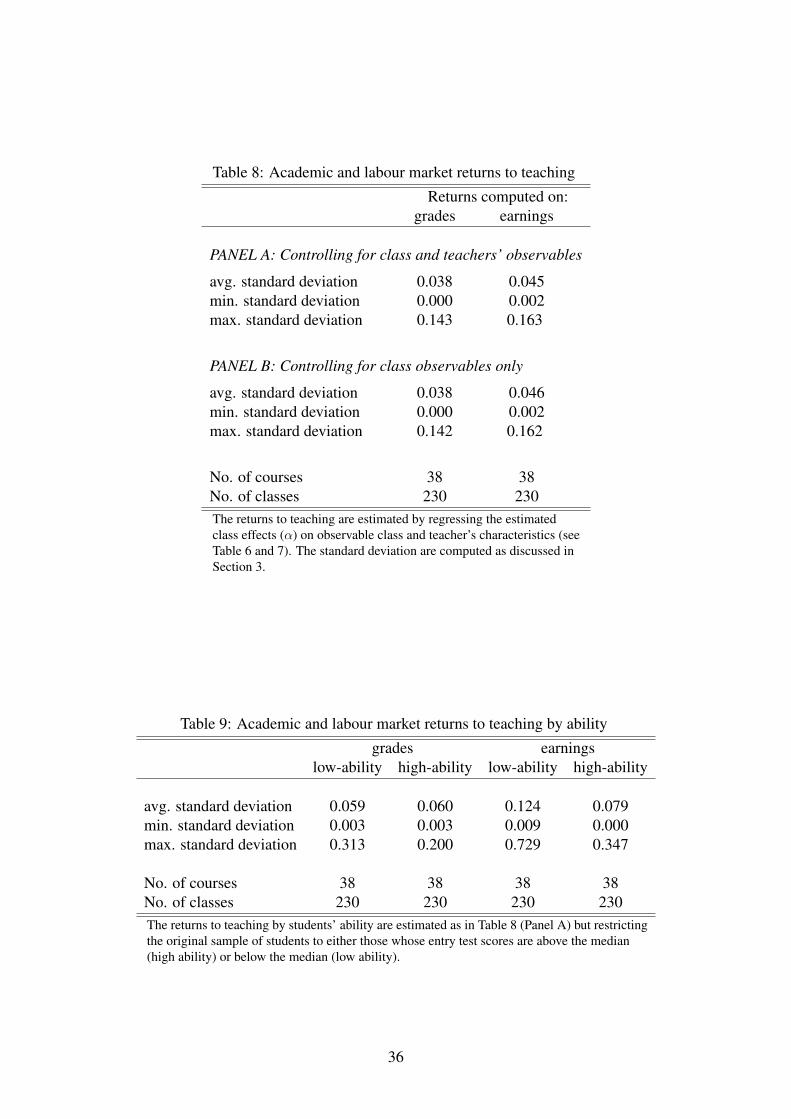
Table 8: Academic and labour market returns to teaching

Returns computed on:grades earnings

PANEL A: Controlling for class and teachers’ observables

avg. standard deviation 0.038 0.045min. standard deviation 0.000 0.002max. standard deviation 0.143 0.163

PANEL B: Controlling for class observables only

avg. standard deviation 0.038 0.046min. standard deviation 0.000 0.002max. standard deviation 0.142 0.162

No. of courses 38 38No. of classes 230 230The returns to teaching are estimated by regressing the estimatedclass effects (α) on observable class and teacher’s characteristics (seeTable 6 and 7). The standard deviation are computed as discussed inSection 3.

Table 9: Academic and labour market returns to teaching by ability

grades earningslow-ability high-ability low-ability high-ability

avg. standard deviation 0.059 0.060 0.124 0.079min. standard deviation 0.003 0.003 0.009 0.000max. standard deviation 0.313 0.200 0.729 0.347

No. of courses 38 38 38 38No. of classes 230 230 230 230The returns to teaching by students’ ability are estimated as in Table 8 (Panel A) but restrictingthe original sample of students to either those whose entry test scores are above the median(high ability) or below the median (low ability).

36

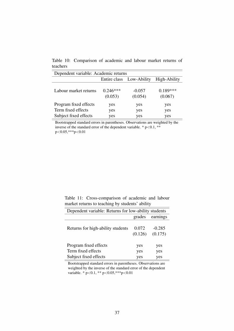
Table 10: Comparison of academic and labour market returns ofteachers

Dependent variable: Academic returnsEntire class Low-Ability High-Ability

Labour market returns 0.246*** -0.057 0.189***(0.053) (0.054) (0.067)

Program fixed effects yes yes yesTerm fixed effects yes yes yesSubject fixed effects yes yes yesBootstrapped standard errors in parentheses. Observations are weighted by theinverse of the standard error of the dependent variable. * p<0.1, **p<0.05,***p<0.01

Table 11: Cross-comparison of academic and labourmarket returns to teaching by students’ ability

Dependent variable: Returns for low-ability studentsgrades earnings

Returns for high-ability students 0.072 -0.285(0.126) (0.175)

Program fixed effects yes yesTerm fixed effects yes yesSubject fixed effects yes yesBootstrapped standard errors in parentheses. Observations areweighted by the inverse of the standard error of the dependentvariable. * p<0.1, ** p<0.05,***p<0.01

37

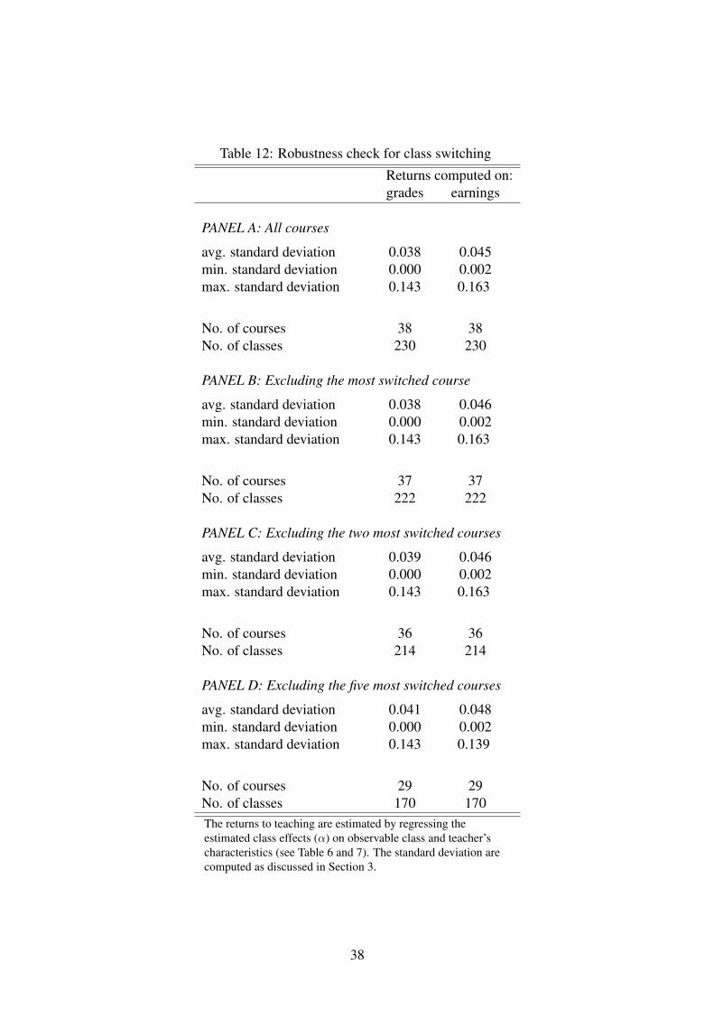
Table 12: Robustness check for class switching

Returns computed on:grades earnings

PANEL A: All courses

avg. standard deviation 0.038 0.045min. standard deviation 0.000 0.002max. standard deviation 0.143 0.163

No. of courses 38 38No. of classes 230 230

PANEL B: Excluding the most switched course

avg. standard deviation 0.038 0.046min. standard deviation 0.000 0.002max. standard deviation 0.143 0.163

No. of courses 37 37No. of classes 222 222

PANEL C: Excluding the two most switched courses

avg. standard deviation 0.039 0.046min. standard deviation 0.000 0.002max. standard deviation 0.143 0.163

No. of courses 36 36No. of classes 214 214

PANEL D: Excluding the five most switched courses

avg. standard deviation 0.041 0.048min. standard deviation 0.000 0.002max. standard deviation 0.143 0.139

No. of courses 29 29No. of classes 170 170The returns to teaching are estimated by regressing theestimated class effects (α) on observable class and teacher’scharacteristics (see Table 6 and 7). The standard deviation arecomputed as discussed in Section 3.

38

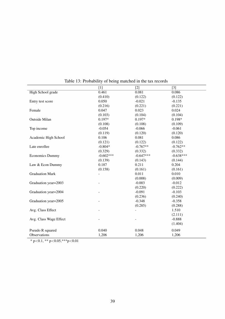
Table 13: Probability of being matched in the tax records[1] [2] [3]

High School grade 0.461 0.081 0.086(0.410) (0.122) (0.122)

Entry test score 0.050 -0.021 -0.135(0.216) (0.221) (0.221)

Female 0.047 0.023 0.024(0.103) (0.104) (0.104)

Outside Milan 0.197* 0.197* 0.198*(0.108) (0.108) (0.109)

Top income -0.054 -0.066 -0.061(0.119) (0.120) (0.120)

Academic High School 0.106 0.081 0.086(0.121) (0.122) (0.122)

Late enrollee -0.804* -0.767** -0.762**(0.329) (0.332) (0.332)

Economics Dummy -0.602*** -0.647*** -0.638***(0.139) (0.143) (0.144)

Law & Econ Dummy 0.187 0.211 0.204(0.158) (0.161) (0.161)

Graduation Mark - 0.011 0.010(0.008) (0.009)

Graduation year=2003 - -0.003 -0.012(0.220) (0.222)

Graduation year=2004 - -0.091 -0.103(0.236) (0.240)

Graduation year=2005 - -0.348 -0.358(0.285) (0.288)

Avg. Class Effect - - 1.510(2.111)

Avg. Class Wage Effect - - -0.888(1.404)

Pseudo R squared 0.040 0.048 0.049Observations 1,206 1,206 1,206

* p<0.1, ** p<0.05,***p<0.01

39

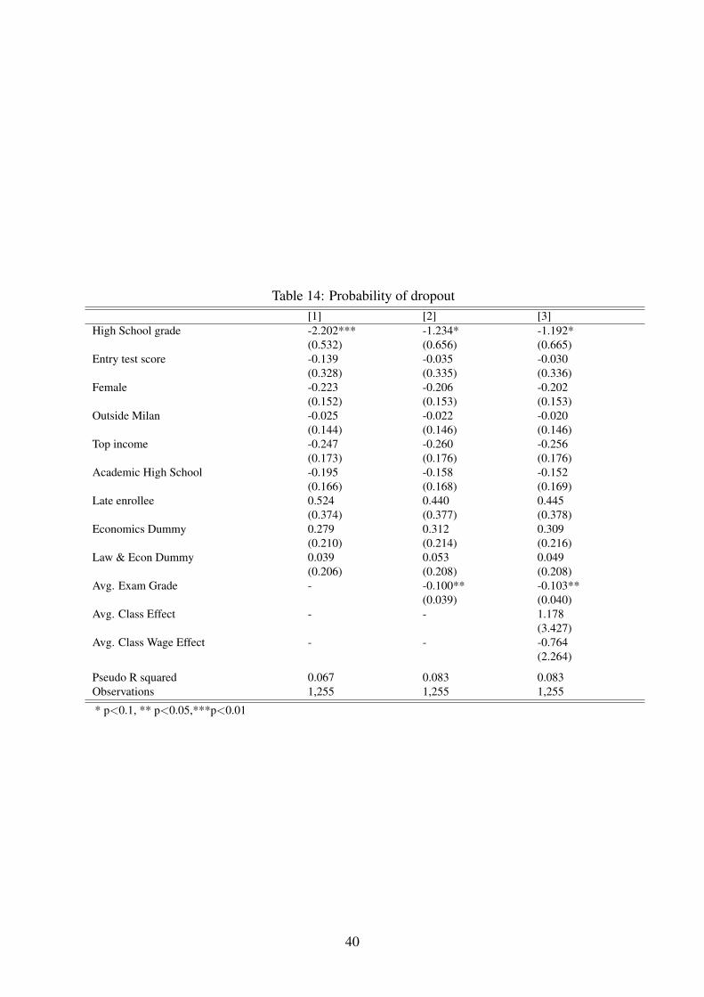
Table 14: Probability of dropout[1] [2] [3]

High School grade -2.202*** -1.234* -1.192*(0.532) (0.656) (0.665)

Entry test score -0.139 -0.035 -0.030(0.328) (0.335) (0.336)

Female -0.223 -0.206 -0.202(0.152) (0.153) (0.153)

Outside Milan -0.025 -0.022 -0.020(0.144) (0.146) (0.146)

Top income -0.247 -0.260 -0.256(0.173) (0.176) (0.176)

Academic High School -0.195 -0.158 -0.152(0.166) (0.168) (0.169)

Late enrollee 0.524 0.440 0.445(0.374) (0.377) (0.378)

Economics Dummy 0.279 0.312 0.309(0.210) (0.214) (0.216)

Law & Econ Dummy 0.039 0.053 0.049(0.206) (0.208) (0.208)

Avg. Exam Grade - -0.100** -0.103**(0.039) (0.040)

Avg. Class Effect - - 1.178(3.427)

Avg. Class Wage Effect - - -0.764(2.264)

Pseudo R squared 0.067 0.083 0.083Observations 1,255 1,255 1,255

* p<0.1, ** p<0.05,***p<0.01

40

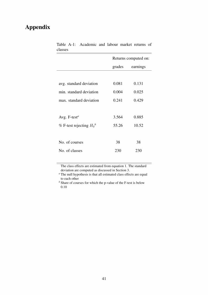
Appendix

Table A-1: Academic and labour market returns ofclasses

Returns computed on:

grades earnings

avg. standard deviation 0.081 0.131

min. standard deviation 0.004 0.025

max. standard deviation 0.241 0.429

Avg. F-testa 3.564 0.885

% F-test rejecting H0b 55.26 10.52

No. of courses 38 38

No. of classes 230 230

The class effects are estimated from equation 1. The standarddeviation are computed as discussed in Section 3.

a The null hypothesis is that all estimated class effects are equalto each other

b Share of courses for which the p-value of the F-test is below0.10

41