Embed Size (px)
Citation preview
Model evaluation and data assimilation impact
studies in the framework of COPS
Kumulative Dissertation zur Erlangung des Doktorgradesder Naturwissenschaften (Dr. rer. nat.)
Fakultat NaturwissenschaftenUniversitat Hohenheim
Institut fur Physik und Meteorologie (IPM)
vorgelegt vonThomas Schwitalla
aus Ostfildern-Ruit2012

Dekan: Prof. Dr. rer. nat. Heinz Breer
1. berichtende Person: Prof. Dr. rer. nat. Volker Wulfmeyer
2. berichtende Person: Prof. Dr. rer. nat. Clemens Simmer
Eingereicht am: 17.11.2011
Mundliche Prufung am: 16.04.2012
Die vorliegende Arbeit wurde am von der Fakultat Naturwissenschaften der UniversitatHohenheim als “Dissertation zur Erlangung des Doktorgrades der Naturwissenschaften”angenommen.
Abstract
The goal of this thesis was the study of new approaches for improving and investigating quantita-tive precipitation forecasting (QPF), e.g., by optimizing model resolution, physics combination,and data assimilation.
A forecasting system based on the Mesoscale Model 5 (MM5) was compared against otheroperational numerical weather prediction models from Meteo France, MeteoSwiss and the Ger-man Weather Service primarily with respect to daytime precipitation. First, a notable daytimedry bias was observed. It appears to be the result of a too small high-resolution domain andthe switched-off convection parameterization from the second to the innermost domain. Eventhe application of a 4-dimensional variational data assimilation (4DVAR) with GPS slant totaldelays (STD) does not solve this problem due to inconsistent model physics between the 4DVARand the forecasting model. Nevertheless, the MM5 is in good agreement with the shape of theobserved diurnal cycle after the spin-up phase.
As the development of the MM5 was suspended, a transition to the new Weather Researchand Forecasting (WRF) model system was made after the D-PHASE period (end of 2007). Thissystem features state-of-the-art physics packages and also a variational data assimilation system.As a new observing system, GPS Zenith Total Delay (ZTD) data from Central Europe wereincorporated into the 3-dimensional variational data assimilation (3DVAR) system to furtherimprove the initial water vapor field. A first study with this system revealed an improvement ofthe integrated water vapor RMSE of about 15% and a small but positive impact on the spatialand quantitative precipitation forecast. Additionally, the importance of assimilating upper airobservations and the necessity to select a large, convection permitting model domain emerged.
Finally a rapid update cycle (RUC) approach, comparable to operational forecast centers,has been developed for a convection-permitting configuration of the WRF model. The system iscapable to assimilate radar observations from Germany and France, GPS-ZTD data and satelliteradiances and can be applied even for near real-time applications. First experiments with thissystem show promising results in comparison to other operational models.
Zusammenfassung
Das Ziel dieser Arbeit war die Untersuchung von neuen Ansatzen zur Verbesserung und Evalu-ierung der quantitativen Niederschlagsvorhersage z.B. durch anpassen der Modellauflosung, derKombination von verschiedenen Parametrisierungen sowie der Datenassimilation.
Ein Vorhersagesystem auf Basis des mesoskaligen Atmospharenmodells MM5 wurde mitanderen operationellen Vorhersagesystemen von Meteo France, MeteoSchweiz und dem Deut-schen Wetterdienst hinsichtlich des Tagesniederschlags verglichen. Zu Beginn wurde eine deut-liche Unterschatzung des Niederschlags festgestellt. Diese ist das Resultat eines zu kleinen hochaufgelosten Modellgebiets sowie des Abschaltens der Konvektionsparametrisierung im innerstenModellgebiet. Der Einsatz einer 4-dimensionalen, variationellen Datenassimilation mit GPS slanttotal delays (STD) brachte auch keine wesentlich Verbesserung der Resultate. Dennoch konn-te eine gute Ubereinstimmung mit der Gestalt des beobachteten Tagesgangs nach Ablauf derspin-up Phase erzielt werden.
Nachdem die Entwicklung des MM5 zwischenzeitlich eingestellt worden war, wurde am Endeder D-PHASE Periode (November 2007) auf das Weather Research and Forecasting (WRF)Modellsystem gewechselt. Dieses beinhaltet dem aktuellen Stand der Forschung entsprechendeModellphysik sowie ein variationelles Datenassimilationssystem. Als neuartige Beobachtungenwurden GPS zenith total delay (ZTD) Messungen in die 3DVAR mit eingebunden, um dasWasserdampfanfangsfeld weiter zu verbessern.
Eine erste Fallstudie ergab eine Verbesserung des RMSE des integrierten Wasserdampfgehaltsum 15%, und einen schwachen, aber positiven Einfluß auf die raumliche und quantitative Nie-derschlagsvorhersage. Außerdem ergaben sich Hinweise, dass es wichtig ist, Hoheninformationenzu assimilieren und ein moglichst großes, konvektionserlaubendes Modellgebiet zu wahlen.
Im letzten Teil wurde ein rapid update cycle (RUC) Ansatz, vergleichbar mit anderen Vorher-sagezentren, entwickelt. Zusatzlich ist das 3DVAR-System nun so vorbereitet, dass es gleichzeitigRadardaten aus Deutschland und Frankreich, GPS-ZTDs sowie Satellitendaten benutzen und innahezu Echtzeit verwendet werden kann. Ein erstes Experiment mit diesen System ergab Erfolgversprechende Resultate im Vergleich zu anderen operationellen Modellen.
4 CONTENTS
Contents
1 Motivation 5
2 Data assimilation 10
2.1 Mathematical background of variational data assimilation . . . . . . . . . . . . . 13
2.2 FGAT/4DVAR . . . . . . . . . . . . . . . . . . . . . . . . . . . . . . . . . . . . . 16
2.3 Properties and derivation of the background error covariance matrix B . . . . . . 16
2.4 Incremental 3/4DVAR . . . . . . . . . . . . . . . . . . . . . . . . . . . . . . . . . 19
2.5 Minimization Algorithm . . . . . . . . . . . . . . . . . . . . . . . . . . . . . . . . 20
2.6 Brief outlook to ensemble data assimilation . . . . . . . . . . . . . . . . . . . . . 21
2.7 Rapid Update Cycle (RUC) system with the WRF model . . . . . . . . . . . . . 23
3 Water vapor information from Global Positioning System 26
3.1 Example for the generation of an adjoint for the GPS-ZTD forward operator inthe WRF model . . . . . . . . . . . . . . . . . . . . . . . . . . . . . . . . . . . . 30
4 Radar data assimilation 32
4.1 Measurement principle . . . . . . . . . . . . . . . . . . . . . . . . . . . . . . . . . 32
4.2 Possible error sources . . . . . . . . . . . . . . . . . . . . . . . . . . . . . . . . . . 34
4.3 Application of radar data in NWP models . . . . . . . . . . . . . . . . . . . . . . 36
5 Summary of publications 46
5.1 Schwitalla et al. (2008) . . . . . . . . . . . . . . . . . . . . . . . . . . . . . . . . . 47
5.2 Bauer et al. (2011a) . . . . . . . . . . . . . . . . . . . . . . . . . . . . . . . . . . 47
5.3 Schwitalla et al. (2011) . . . . . . . . . . . . . . . . . . . . . . . . . . . . . . . . . 48
6 Summary and outlook 50
A Practical implementation of a RUC system for the WRF model 53
5
1 Motivation
Numerical weather prediction (NWP) models are the basis for weather forecasting by simulatingthe temporal and spatial evolution of the atmospheric state. They consist of several differen-tial equations describing the evolution of wind, temperature, humidity and pressure (so-called“prognostic variables“) which are in based on the continuity equation and Euler-Lagrange equa-tion. The first attempt to solve this set of differential equations was performed by Richardsonin 1922. Without the aid of computers, he and his staff needed 6 weeks for a 6 h forecast. Theforecast failed with a pressure change of 145 hPa due to the lack of accurate initial conditionsand deficits in numerics (Lynch, 2006). Because of this experience, NWP was considered im-possible and further research activities concerning this topic were abandoned for decades but ascomputers became available, NWP models have been developed.
In principle, NWP models can be divided into two categories. The first category are globalmodels with current horizontal resolutions between 50 km (e.g. Global Forecast System (GFS)of NOAA1) and 12–15 km (ECMWF2). In global models, the model top often reaches 0.01 hPa(≈ 100 km) as they should also represent variations in the ozone concentration and are oftencoupled to aerosol models. Global models are mostly applied for medium range forecasting upto 10 days and climate projections. The main focus is on the correct representation of synopticscale features of the global circulation. Examples are traveling high and low pressure systems(e.g. Hadley cell or Monsoon in the tropics).
The second category are limited area (mesoscale) models (LAM) for short-range predictions. Inthe past, these models typically featured a horizontal resolution of 10 km with a model top ofabout 50–20 hPa corresponding to about 20–25 km altitude. An example is the COSMO-EU3
model operated at the German Meteorological Service (DWD). Increasing computing perfor-mance allows to further increase the horizontal resolution down to a few kilometers like inCOSMO-DE (Baldauf et al., 2009), AROME (Bouttier, 2007), Mesoscale Model 5 (MM5; Grellet al., 1995) and the Weather Research and Forecasting (WRF) model (Skamarock et al., 2008).In contrast to global models, limited area models require boundary conditions which are ob-tained from coarser resolution LAMs or global models. They are necessary to conserve the massdue to advection in the model.
In todays NWP models the horizontal resolution is still far too coarse to represent physicalprocesses except from gridscale advection and diffusion. It is therefore necessary to parameter-ize these processes. This is achieved through several physics packages for cloud microphysics,the planetary boundary layer (PBL), radiation, land-surface interaction and convection. Therequired complexity of the schemes is different for global and regional applications. E.g on theglobal scale it is not necessary to have a highly complex cloud microphysics scheme containingprognostic variables for graupel and hail because the model is not capable to simulate strongupdrafts required for the formation of graupel due to the comparatively coarse horizontal res-olution, . In current global models like the ECMWF model, the applied microphysics schemeonly distinguishes between water vapor, liquid water and ice.
1National Oceanic and Atmospheric Administration2European Centre for Medium range Weather Forecast3Consortium for Small-scale Modeling, www.cosmo-model.org
6 1 MOTIVATION
To support the model to simulate (summertime) convective precipitation, a convection param-eterization (also known as cumulus scheme) is applied at resolutions down to ≈ 4–8 km (Kainet al., 2008).
Basically two types of cumulus schemes exist. 1) A mass-flux based scheme where the strengthof convection is controlled by entrainment and detrainment in clouds (Tiedtke, 1989) and 2)an approach with a CAPE (Convective Available Potential Energy) closure, where CAPE isremoved within a convective time period (Kain, 2004). The disadvantage of these schemesare that they contain only a simple single column cloud model compared to cloud microphysicsschemes which allow a horizontal mass transport to neighboring grid cells. Due to the former andin combination with the usually medium horizontal resolution, the models show a windward-leeprecipitation pattern and also other systematic errors described e.g in Schwitalla et al., 2008.
If the horizontal resolution increases to a few kilometers, the model is assumed to be able tosimulate convection explicitly and thus the cumulus scheme is often switched off. More sophisti-cated cloud microphysics schemes are necessary to include more microphysical physical processesrelevant at higher resolutions like the formation of graupel and hail. The most commonly ap-plied type of scheme are one-moment schemes containing hydrometeor mass mixing ratios asprognostic variables like the Reisner2 scheme available in the MM5 (Reisner et al., 1998). Incontrast to cumulus schemes, they update the temperature tendency with an additional termcoming from the latent heat release during the phase transition of different hydrometeors.
In recent years, 2-moment schemes have been developed which additionally predict hydrometeornumber concentrations like the schemes of Milbrandt and Yau (2005), Seifert and Beheng (2006)and Morrison et al. (2009). With these schemes, it is possible to more realistically describe thevariability of the size distributions of different hydrometeors due to the fact that the total num-ber concentration and mass mixing ratio are not monotonically related (Milbrandt and Yau,2005). The prognostic calculation of number concentrations is a key for deriving the micro-physical process rates (e.g. autoconversion, accretion) which becomes especially important inmid-latitude mixed-phase clouds. 2-moment schemes are also required for the coupling of aerosolmodels because they require prognostic number concentrations of hydrometeors. Compared tothe one-moment schemes available e.g. in the WRF model, the computing time is not an issuedue to improved parallelization of the code.
When getting to higher horizontal resolutions of a few kilometers, the PBL processes are be-coming more and more important. Thus it is necessary to increase not only the horizontalbut also the vertical resolution to avoid violating the Courant-Friedrichs-Lewy (CFL) condition.The maximum CFL number depends on the applied time integration scheme (e.g. 1.43 for a3rd-order Runge-Kutta scheme with 5th-order advection) and gives an upper limit for the modeltime step in combination with a given horizontal and vertical resolution. Typically, LAMs onthe mesoscale consists of 45 levels up to altitudes of 20 to 25 km from which often 15 or morelayers reside below 3 km above ground level (AGL) and typically require a time step [s] of ∼ 6times the horizontal resolution [km].
To represent boundary layer properties in an NWP model, two different approaches are com-monly applied. 1) The Turbulent Kinetic Energy (TKE) closure approach based on the workof Mellor and Yamada (1974) implying that the exchange coefficients for heat and momentumare derived from TKE and 2) the countergradient approach used by e.g. Hong et al. (2006)where the exchange coefficients are calculated from prescribed profile functions depending on
7
the Prandtl number complemented by a countergradient term to take non-local mixing (mixingwith e.g the second level from the current one) into account.
As the surface is the lower boundary for the PBL schemes, Land-Surface-Models (LSM, e.g. Eket al., 2003) are necessary. They provide information of the soil properties like temperature, snowcover, moisture and surface fluxes which are then fed back to the PBL scheme. Additionally theycalculate the transport of energy and water in the soil. As the resolution of mesoscale models iscontinuously increasing, it is important to properly initialize the soil variables especially whenperforming climate projections. Although soil moisture and temperature are prognostic variablesin most of todays NWP models, each new forecast cycle needs a new soil analysis which is oftennot included in the 3/4-dimensional variational data assimilation (3DVAR/4DVAR) system.Thus, e.g. ECMWF performs an off-line soil analysis based on 2 m temperature, humidityand precipitation or snow coverage (Douville et al., 2001) due to the lack of operational soilmeasurements. As this can lead to erroneous soil water content, further improvements for theinitialization of LSM variables are necessary which are e.g. addressed in the Water and EarthSystem Science (WESS) project4.
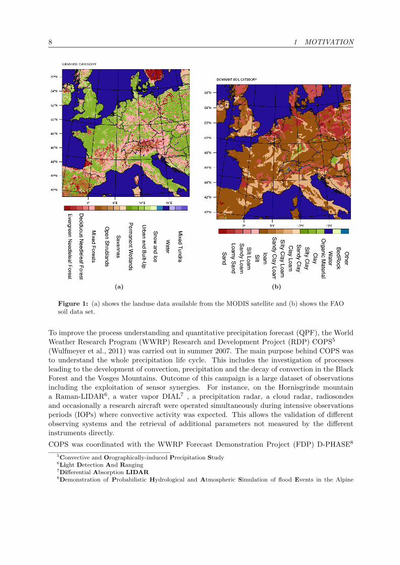
A still remaining problem in this context is to get fine resolution data for surface and soiltextures. As an example, the topography data for the WRF model comes from the United StateGeological Survey (USGS) and for COSMO-DE from the GLOBE data set of NOAA with aresolution of 30” (1 km). Landuse information for WRF is e.g. provided by the InternationalGeosphere-Biosphere Programme (IGBP) MODIS data set. It is based on a satellite retrievalmade in 2001 available at a 1 km resolution containing 20 different land use types.
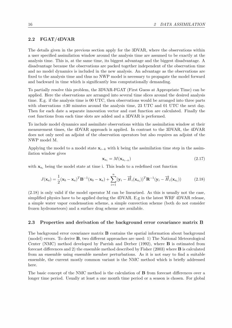
For the representation of the soil, currently data from the United Nations Food and AgriculturalOrganization (FAO) is used which is only available on a 10’ resolution (20 km). This can lead toerroneous results especially in climate simulations because the soil type determines the energyand water budget and thus the surface fluxes. Figure 1 shows the land use and soil data currentlyavailable in the WRF model.
In addition to the model physics and numerics, the forecast quality also depends on the qualityof the initial conditions. NWP with LAMs is an initial and boundary problem and their forecastquality depends, besides the model physics, on the quality of the driving model. Depending onthe desired resolution of the selected model, this driving model can either be a global model oralso a LAM covering the desired area.
One of the largest drawbacks of using global models as initial field is their relatively coarseresolution of about 30–50 km (except ECMWF) which is only able to represent large scalesynoptic patterns. To reduce inaccuracies at initialization, NWP centers like Meteo France,the DWD or the UK MetOffice developed their own model chain containing a global model, amesoscale model and a convection-permitting model with similar physics packages to overcomemajor inconsistencies due to the different physics and numerics schemes applied in the models.
In summer, quantitative precipitation forecasting (QPF) in low mountain regions is still a veryimportant research area as NWP models still have deficiencies in correctly forecasting the spatialand temporal evolution of precipitation.
4www.wess.info
8 1 MOTIVATION
(a) (b)
Figure 1: (a) shows the landuse data available from the MODIS satellite and (b) shows the FAOsoil data set.
To improve the process understanding and quantitative precipitation forecast (QPF), the WorldWeather Research Program (WWRP) Research and Development Project (RDP) COPS5
(Wulfmeyer et al., 2011) was carried out in summer 2007. The main purpose behind COPS wasto understand the whole precipitation life cycle. This includes the investigation of processesleading to the development of convection, precipitation and the decay of convection in the BlackForest and the Vosges Mountains. Outcome of this campaign is a large dataset of observationsincluding the exploitation of sensor synergies. For instance, on the Hornisgrinde mountaina Raman-LIDAR6, a water vapor DIAL7 , a precipitation radar, a cloud radar, radiosondesand occasionally a research aircraft were operated simultaneously during intensive observationsperiods (IOPs) where convective activity was expected. This allows the validation of differentobserving systems and the retrieval of additional parameters not measured by the differentinstruments directly.
COPS was coordinated with the WWRP Forecast Demonstration Project (FDP) D-PHASE8
5Convective and Orographically-induced Precipitation Study6Light Detection And Ranging7Differential Absorption LIDAR8Demonstration of Probabilistic Hydrological and Atmospheric Simulation of flood Events in the Alpine
9
(Rotach et al., 2009) which took place from June to November 2007. During this time, 31operational and research NWP models with different horizontal resolutions ranging from 60 kmto 2 km were operated simultaneously. The aim was to validate these models over the same timeperiod applying the rich data set collected during COPS.
The German part of COPS was partially funded by the the priority program 1167 “QuantitativePrecipitation Forecast” which was established in 2004 by the German Research Foundation(DFG). Within this framework, the objectives of this thesis are:
� Select the most suitable physics combination in the atmospheric model MM5 for centralEurope and especially the COPS region (Black Forest, Vosges Mountains and SwabianJura)
� Evaluate the MM5 performance on 2 km resolution in comparison with other operationalhigh-resolution models
� Perform data assimilation case studies at a convection-permitting resolution with GPS-ZTD data and conventional observations over Europe
� Developing a rapid update cycle (RUC) with GPS and radar data on a convection-permitting resolution
In the following chapter, an introduction into variational data assimilation will be given. Chap-ters 3 and 4 will give information about GPS and radar data and how they can be beneficialfor data assimilation. Chapter 5 contains a summary of three useful publications followed by anoutlook into possible future research activities.
region
10 2 DATA ASSIMILATION
2 Data assimilation
Due to the large number of model grid cells compared to the number of observations, NWP isan under-determined initial value problem. To overcome this handicap, a technique is requiredwhich gives a best estimate of the true atmosphere by taking the actual model field as backgroundand observations into account: the so-called “data assimilation”.
The oldest data assimilation scheme in operation is the Newtonian Relaxation technique (Nudg-ing) or Four-Dimensional Data Assimilation (FDDA) which is operationally applied in theCOSMO models (Schraff, 1997) and is an option for MM5 and WRF (Stauffer and Seaman,1994). Here, an extra relaxation term is added to the prognostic equations containing a valuefor the strength (how reliable is the observation) and a time weighting factor. The advantage ofthis technique is that the additional amount of computing time is negligible. A big drawback isthat only observations of model prognostic variables can be assimilated.
Additional observations which do not measure the model’s prognostic variables can, if at all,only be processed with additional error-prone assumptions. In COSMO-DE, radar latent heatnudging (LHN) is used because the nudging scheme does not have the possibility to assimilateradar reflectivities directly to support the development of convection. Another example is theassimilation of GPS-ZTD data in the COSMO model where an IWV content, calculated fromthe Zenith Wet Delay (ZWD), is utilized to adjust the vertical humidity profile.
As new indirect observation types arose in recent decades, new techniques had to be developedthat also allow to assimilate non-prognostic variables like remote sensing observations. Theseare variational data assimilation techniques where a least square fit is performed by minimizinga cost function which contains the difference between the model state (background) and theobservations. Currently two different deterministic variational approaches are applied both onthe global scale and on the mesoscale: The 3DVAR and 4DVAR approach (Courtier et al., 1998;Barker et al., 2004; Huang et al., 2009) where the least square fit is performed on a deterministicanalysis and the Ensemble Kalman filter (EnKF, Evensen, 1994, 2003) where an ensemble withO∼ 30-100 members is applied to estimate the new analysis.
While both variational techniques require a forward operator to simulate the observation inthe model world, the 4DVAR, in addition, requires the tangent linear and adjoint of the wholeforecast model which, depending on the complexity of the model, can become very difficult oreven impossible to derive. Concerning this matter, the Ensemble filter has the advantage thatthe adjoint is not necessary.
For both variational assimilation schemes, information about the background error and covari-ances between different model variables is needed which has to be derived from a climatologicalestimate or from a forecast ensemble. This estimation is crucial because the real model errorsare unknown and it is assumed the model is free of a bias. As the number of model variables isO∼ 107, the covariance matrix has 1014 elements. As this matrix has to be inverted, techniquesto reduce the matrix dimension have to be applied in addition.
Today’s 3DVAR and 4DVAR systems make use of a so-called ”incremental approach“. Here,the full non-linear model forward operators are applied to calculate the initial value of the costfunction (outer loop). Then, linear versions of forward and adjoint operators are applied tominimize the cost function (inner loop) saving computing time at the cost of accuracy and
11
allowing to apply optimized numerical algorithms to minimize the cost function. The inner loopis executed until the gradient becomes sufficiently small.
When performing a 4DVAR more often the inner loop is performed on a coarser resolution (e.g.at ECMWF) due to the enormous computing time consumption because of the application ofespecially the adjoint of the forecast model. Ongoing research of combining e.g. 3DVAR andEnKF (Hybrid approach) shows promising results but due to the large number of ensemblemembers it is also very time consuming. A future task may be the application of an ensemble of3(4)DVAR schemes on a deterministic forecast. Further details about the mathematical aspectsof variational data assimilation can be found below in section 2.1.
The most commonly assimilated variables are temperature, moisture, wind, and surface pres-sure (conventional observations). In recent years, more often remote sensing observations likesatellite brightness temperatures (Hollinger, 1989; Mo and Liu, 2008) and Atmospheric Mo-tion Vectors (AMV, EUMETSAT, 2009) are used. The assimilation of brightness temperaturesmeasured from satellite sounders like IASI (Infrared Atmospheric Sounding Interferometer) orAMSU (Advanced Microwave Sounding Unit) requires a radiative transfer model and is currentlyperformed only in a cloud free environment. The available radiative transfer models are RTTOV(Radiative Transfer for TOVS; Saunders et al., 1999) and the CRTM (Community RadiativeTransfer Model; Chen et al., 2008) which are applied in todays NWP models. The former isapplied e.g. by ECMWF or DWD either in a 4DVAR or for the generation of synthetic satelliteimages respectively.
The retrieval algorithm for satellite winds for MSG (Meteosat Second Generation; e.g. Singhet al., 2011) is based on a combination of brightness temperatures of the water vapor and infraredchannels combined with the US standard atmosphere or the ECMWF model and has beendeveloped by EUMETSAT. It is currently only reliable above 700 hPa because the assumptionthat clouds move with the main wind breaks down over orography (EUMETSAT, personalcommunication).
A still remaining problem is the distribution of the different types of observations. Synopticstations (SYNOP) together with airport reports (METAR), measuring hourly 2 m temperature,2 m humidity, 10 m wind and surface pressure, are commonly available over land. Dependingon the time of the day, also large amounts of aircraft measurements (AMDAR, AIREP) areavailable but they mostly measure only temperature and wind.
A new TAMDAR (Tropospheric Airborne Meteorological Data Reporting) network, currentlyonly available over the US, additionally measures humidity together with wind and temperature.These three variables are important for representing the convective environment and thus for theprediction of the precipitation development. Radiosonde ascents are, apart from some researchvessels, only available over land and usually only available at 0000 UTC and 1200 UTC. Inspite of their sparsity, they are still the major source for information about the 3-dimensionalhumidity field due to their accuracy.
To give some numbers, within an assimilation time window of two hours, ∼ 3000 aircraft mea-surements, ∼ 1000 surface measurements, 10 wind profiler, ∼ 80 ship measurements and ∼ 50radiosonde ascents are available from the ECMWF data archive (MARS) over central Europe.
To further improve the 3-dimensional humidity field, Global Positioning System (GPS) derivedwater vapor information are assimilated at e.g. Meteo France to complement other observations.
12 2 DATA ASSIMILATION
Here, the GPS signal delay between the line of sight through the neutral atmosphere and thereal ray path through the ionosphere and earth atmosphere is considered. After performing ex-tensive ionospheric corrections through the application of dual-frequency receivers and applyinga complex retrieval algorithm, the atmospheric refractivity N is obtained (Gendt et al., 2004).Integration of N along the ray path through the atmosphere and subsequent multiplication witha constant factor of 10−6 gives the slant total delay (STD) and zenith total delay (ZTD). Inthis study, GPS data is provided by the Helmholtz Centre Potsdam German Research Centrefor Geosciences (GFZ).
Although both STD and ZTD are integrated quantities, they can be used to adjust the vertical(and horizontal in case of STD) distribution of water vapor in a variational assimilation scheme.A critical point is the estimation of the receiver altitude. It has to be very accurate because afew meters difference in the altitude assignment of the receiver can cause a difference of 1 cm inthe value of the wet delay which can become critical during hot and dry weather conditions.
In recent years, the most commonly used parameter derived from GPS data for assimilation pur-poses is the Integrated Water Vapor (IWV) content. In a variational scheme, the IWV contentis converted to water vapor and air density, allowing to adjust the water vapor distribution. Thedisadvantage is that the calculation of GPS-observed IWV requires the assumption of a meantemperature and moisture measurement at the GPS receiver location. Therefore, the NWP com-munity switches more and more to the assimilation of ZTD measurements (Vedel and Huang,2004) which are only dependent on surface temperature and pressure. When assimilating ZTDdata in a variational scheme, it is transferred to pressure, temperature and humidity via theadjoint operator and thus has a higher information content compared to IWV (see section 3.1).
The next step in complexity and realism is the application of GPS STDs (e.g. Zus et al.,2008; Bauer et al., 2011b) for the assimilation where the real ray path between satellite andreceiver is considered. This allows for fully exploiting the water vapor information provided byGPS. This means that due to the large spatial coverage information about the vertical watervapor distribution especially in the boundary layer can be obtained which can have a significantimpact on summertime convection. Further examples for the application of GPS data besidedata assimilation is the 3-dimensional reconstruction of the water vapor field (tomography)applying STD data (Bender et al., 2009) and the validation of other remote sensing instrumentsand models (Bender et al., 2008; Bauer et al., 2011a).
As the assimilation is an under-determined problem, it is desired to have as many as possibleobservations on the one hand side. On the other side, the quality of the observations is a criticalpoint during the assimilation. In general, a variational data assimilation approach minimizesa cost function which roughly contains differences between the model background and the ob-servations (O-B) weighted by the measurement quality. If the distance between the model andthe observations is large, the cost function has a high value and thus the minimization takesmore and more iterations to converge. It is possible, that the model is forced to a new analysisresulting in a large model imbalance as e.g. hydrometeors are not updated during a 3DVARexcept when applying radar reflectivities.
As shown later in section 2.1, the observations are weighted by 1/σ2 (with σ being the obser-vation error) during the assimilation process. This implies that observations with a large errorare degraded and thus the influence in the assimilation process and the new analysis becomessmaller. However, users wish to have low observation errors but this can reduce the number of
2.1 Mathematical background of variational data assimilation 13
observations significantly due to the O-B check. This is usually performed in the outer loop of anincremental variational assimilation (section 2.4) where the full non-linear observation operatoris applied to simulate the observation. This rejection can e.g happen for GPS measurementsdue to an inaccurate water vapor background field or for radar reflectivities in the case that themodel did not trigger convection.
The ECMWF and the WRF assimilation systems e.g. apply statistically derived errors forstandard variables like wind, temperature and humidity. For remote sensing observations likesatellite radiances or radar radial velocities, the user has to apply a bias correction (for satellitedata) and also a thinning by averaging values in a model grid box due to the high resolution(more than one observation can exist in one model grid box) and correlations between neigh-boring pixels in the measurements. E.g in the French AROME Model, data are thinned to a15*15 km grid box (Montmerle and Faccani, 2009) and satellite brightness temperatures areusually thinned to a distance of 50–100 km.
It can also occur that the minimization algorithm, often done with the conjugate gradientmethod, is only able to find a relative minimum of the cost function instead of a global minimumdegrading the quality of the new analysis. Therefore the observations have to be screened ina way that the difference between the model and the observations is not too large (so-calledO-B check). However this can be dangerous if the background field has a bad quality, becauseone may reject observations which have a good quality but are too far away from the analysis.This happened e.g. at DWD for the winter storm Lothar in December 1999 (Wergen andBuchhold, 2002). Here a sounding over Newfoundland was rejected in the data assimilationof the global model GME (Majewski et al., 2009). This happened due to unreasonable (butreally observed) low pressure values as the balloon of the scheduled radiosonde burst early anda second radiosonde had to be launched later which was assigned at the original time in theformer data assimilation scheme.
The following section will give further details about the mathematical background applied invariational data assimilation schemes with a focus on the WRF model.
2.1 Mathematical background of variational data assimilation
Data assimilation is a suitable technique to improve the model initial state. Variational dataassimilation schemes, independent on whether it is an deterministic or ensemble-base method,are based on the maximum likelihood and least-square method and the Bayes-Theorem (Lorenc,1986; Bouttier and Courtier, 1999). The model state xb with the dimension of the model domainin West-East direction i, South-North direction j, z-direction k and the number of prognosticvariables v can be described by a vector
xb =
x1
x2
....
....xn
(2.1)
with the dimension of n= i·j·k·v in the range of 107.
14 2 DATA ASSIMILATION
The Bayes’s Theorem describes the joint probability P for the occurrence of two events xb (modelbackground) and y (observations):
P (y) · P (xb | y) = P (y | xb) · P (xb) (2.2)
The first term on the l.h.s. denotes the a priori pdf of an observation y, the second term denotesthe conditional probability to find xb for given observation y. The first term on the r.h.s. denotesthe probability for the observation with a given background xb and the second term denotes thea priori pdf for a model background xb. As the probability P(y) for a measurement is equal toone, the probability for finding x with the observation y is
P (x | y) = P (y | x) · P (x) (2.3)
which is the basis for all variational data assimilation schemes. Under the assumption of Gaus-sian distribution, the probability for true observations yt when observations y are given is
P (yt | y) =1
(2π)n2
√detO
e−12
(y−yt)TO−1(y−yt) (2.4)
O denotes the observation error covariance matrix describing error correlations between differentobservation types and variables and n is the dimension of the observation vector y. In case ofno bias it is defined as
O =< (y − yt)(y − yt)T >
=< εεT >(2.5)
where <> means the expectation value.
The same mathematical formalism can be applied for the probability of a true model state xtwhen a given model background xb is present:
P (xt | xb) =1
(2π)n2
√detB
e−12
(xb−xt)TB−1(xb−xt) (2.6)
Similar to equation (2.4), B denotes the model background error covariance matrix. In generalit describes correlations of different model variables on the model grid, e.g. the correlationbetween water vapor and horizontal wind. In case only one observation of e.g. water vapor isavailable, B spatially distributes the new information to other variables if correlations exist.
To find the most likely values for the new model analysis state xa for xt and ya for yt, whenboth observation and model background are given, the probability P has to be maximized:
P (xa | xb)P (ya | y) = P (xa,ya)!
= max (2.7)
P (xa | xb)P (ya | y) ∝ e12
(xb−xa)TB−1(xb−xa) · e12
(y−ya)TO−1(y−ya) (2.8)
To obtain the maximum value for P(xa,ya), it is equivalent to minimize -ln (P(xa,ya)) which isreferred to as cost function J:
J(xa,ya) =1
2((xb − xa)
TB−1(xb − xa) + (y − ya)TO−1(y − ya))
!= min (2.9)
2.1 Mathematical background of variational data assimilation 15
As ya is not directly available from the model, a (not necessarily linear) “interpolation” operator
(forward operator)−→H has to be developed for each type of observations which generates the
observation from the model state xa:ya =
−→H (xa) (2.10)
Due to the application of−→H , the observation error covariance matrix O has to be replaced by
the matrix RR =< (y −
−→H (xa))(y −
−→H (xa))
T > (2.11)
which includes the covariances (observation and representativeness errors) between y and−→H (xa).
Therefore equation 2.9 for a single observing system reads now:
J(xa) =1
2(xb − xa)
TB−1(xb − xa) +1
2[(y −
−→H (xa))
TR−1(y −−→H (xa))]
!= min (2.12)
In most of the current variational data assimilation schemes, R is a block-diagonal matrixassuming no correlation of errors between the single observations and thus most off-diagonalelements are zero. This assumption can be violated especially for satellite radiances or radarradial velocities. Due to their high spatial resolution, neighboring pixels are correlated with eachother.
To obtain the minimum of J(xa), the gradient has to be zero with respect to xa. This requiresthe solution of
∇J(xa) = −B−1(xb − xa)−H∗R−1(y −−→H (xa)) = 0. (2.13)
H∗ is the adjoint of the forward operator−→H . Assuming x = xb + δx with an infinitesimal
perturbation δx, the forward operator−→H (x) can be developed into a Taylor expansion
−→H (xb + δx) =
−→H (xb) +
∂−→H
∂xδx+
1
2
∂2−→H∂x2
δx2 + O[(δx)3]. (2.14)
In most of today’s data assimilation schemes,−→H (x) is assumed to be linear. Thus higher order
terms except the linear in the Taylor expansion are neglected. The first derivative ∂−→H∂x δx is called
the Tangent Linear Model (TLM) in data assimilation and is the Jacobi Matrix H of−→H (x):
H =
∂−→H1∂x1
.... ∂−→H1∂xn
.... .... ....∂−→Hm∂x1
.... ∂−→Hm∂xn
(2.15)
m denotes the model space dimension, more precisely the number of model grid points and n thenumber grid boxes times the number of model state variables which are pressure p, temperatureT, specific humidity q, zonal and meridional wind u and v.
The adjoint H∗ of the forward operator−→H is the transpose of H and thus reads
H∗ = HT =
∂−→H1∂x1
.... ∂−→Hm∂x1
.... .... ....∂−→H1∂xn
.... ∂−→Hm∂xn
(2.16)
An example for the derivation of H and HT for GPS-ZTD data is given later in section 3.1.
16 2 DATA ASSIMILATION
2.2 FGAT/4DVAR
The details given in the previous section apply for the 3DVAR, where the observations withina user specified assimilation window around the analysis time are assumed to be exactly at theanalysis time. This is, at the same time, its biggest advantage and the biggest disadvantage. Adisadvantage because the observations are packed together independent of the observation timeand no model dynamics is included in the new analysis. An advantage as the observations arefixed to the analysis time and thus no NWP model is necessary to propagate the model forwardand backward in time which is significantly less computationally demanding.
To partially resolve this problem, the 3DVAR-FGAT (First Guess at Appropriate Time) can beapplied. Here the observations are arranged into several time slices around the desired analysistime. E.g. if the analysis time is 00 UTC, then observations would be arranged into three partswith observations ±30 minutes around the analysis time, 23 UTC and 01 UTC the next day.Then for each date a separate innovation vector and cost function are calculated. Finally thecost functions from each time slots are added and a 3DVAR is performed.
To include model dynamics and assimilate observations within the assimilation window at theirmeasurement times, the 4DVAR approach is applied. In contrast to the 3DVAR, the 4DVARdoes not only need an adjoint of the observation operators but also requires an adjoint of theNWP model M.
Applying the model to a model state xi−k with k being the assimilation time step in the assim-ilation window gives
xai = M(xai−k) (2.17)
with xai being the model state at time i. This leads to a redefined cost function
J(xa) =1
2(xb − xa)
TB−1(xb − xa) +n∑i=1
(yi −−→H i(xai))
TR−1(yi −−→H i(xai)) (2.18)
(2.18) is only valid if the model operator M can be linearized. As this is usually not the case,simplified physics have to be applied during the 4DVAR. E.g in the latest WRF 4DVAR release,a simple water vapor condensation scheme, a simple convection scheme (both do not considerfrozen hydrometeors) and a surface drag scheme are available.
2.3 Properties and derivation of the background error covariance matrix B
The background error covariance matrix B contains the spatial information about background(model) errors. To derive B, two different approaches are used: 1) The National MeteorologicalCenter (NMC) method developed by Parrish and Derber (1992), where B is estimated fromforecast differences and 2) the ensemble method described by Fisher (2003) where B is calculatedfrom an ensemble using ensemble member perturbations. As it is not easy to find a suitableensemble, the current mostly common variant is the NMC method which is briefly addressedhere.
The basic concept of the NMC method is the calculation of B from forecast differences over alonger time period. Usually at least a one month time period or a season is chosen. For global
2.3 Properties and derivation of the background error covariance matrix B 17
models like ECMWF the forecast differences x′ between the 48 h and 24 h forecast of differentinitial dates are calculated for a target date. For regional models like WRF, usually differencesbetween a 24 h and a 12 h forecast are chosen:
B = x′x′T
= (xt+24h − xt+12h) (xt+24h − xt+12h)T(2.19)
which is similar to the definition of the observation error covariance matrix O shown in equation2.5. As the reader may have noticed, this is not a real background error as the name promises. Itis a climatological estimate of the model variances. The reason not to chose differences betweenthe model and observations at certain time is the lack of observations in this case.
Each model grid point requires an observation which is not possible and thus would also introduceinterpolation errors which are not useful for model error characteristics. The reason not to chooseforecast differences between a 6 h forecast and the analysis are twofold. First this would includethe model spin-up when starting from an analysis and secondly, the error of the analysis wouldbe taken into account.
Another problem is the representation of the model error covariances in B. If assuming 550x550x50model grid boxes, they contain about ∼ 107 prognostic variables. The representation of errorsin the B-matrix would lead to Ne= 0.5·(107)2 = 0.5·1014 elements in B. As the data has to bestored with double precision, this would lead to a file size of ∼364 Petabyte, which is impossibleto store even on a high-performance computer as e.g the German Climate Computing Centerwhich has about 20 Petabyte memory. Therefore, a technique is required, which reduces thesize of B without loosing too much information. This can be done with a transformation of Binto an almost diagonal matrix.
Starting point for this transformation are equations 2.14 and 2.22. First, a control variabletransformation δx = Uv is introduced where U has to fulfill the relation B = UUT and v is acontrol variable. This transformation ensures that covariances between the new control variablesv are minimized. For the WRF model, the control variable v consists of five variables to meetthe 5 prognostic variables:
� Stream function Ψ, derived from vorticity by solving the Poisson equation
� Velocity potential derived from divergence by solving the Poisson equation
� Temperature
� Pseudo relative humidity
� Surface pressure
Pseudo relative humidity is defined as ratio between the current water vapor mixing ratio andthe saturation water vapor mixing ratio of the background field.
Furthermore, the transformation matrix U is separated into 3 matrices so that U = UhUvUp.Uh is the horizontal correlation matrix which holds horizontal correlations and Uv denotes thevertical correlation matrix. Up finally contains the the transformation of the control variables
18 2 DATA ASSIMILATION
back to model prognostic variables. This decomposition reduces the elements from Ne to ∼√Ne
with very small off-diagonal terms. Further details about the transformation are given in Lorencet al. (2000), Barker et al. (2003) and Barker et al. (2004).
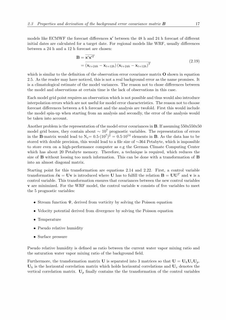
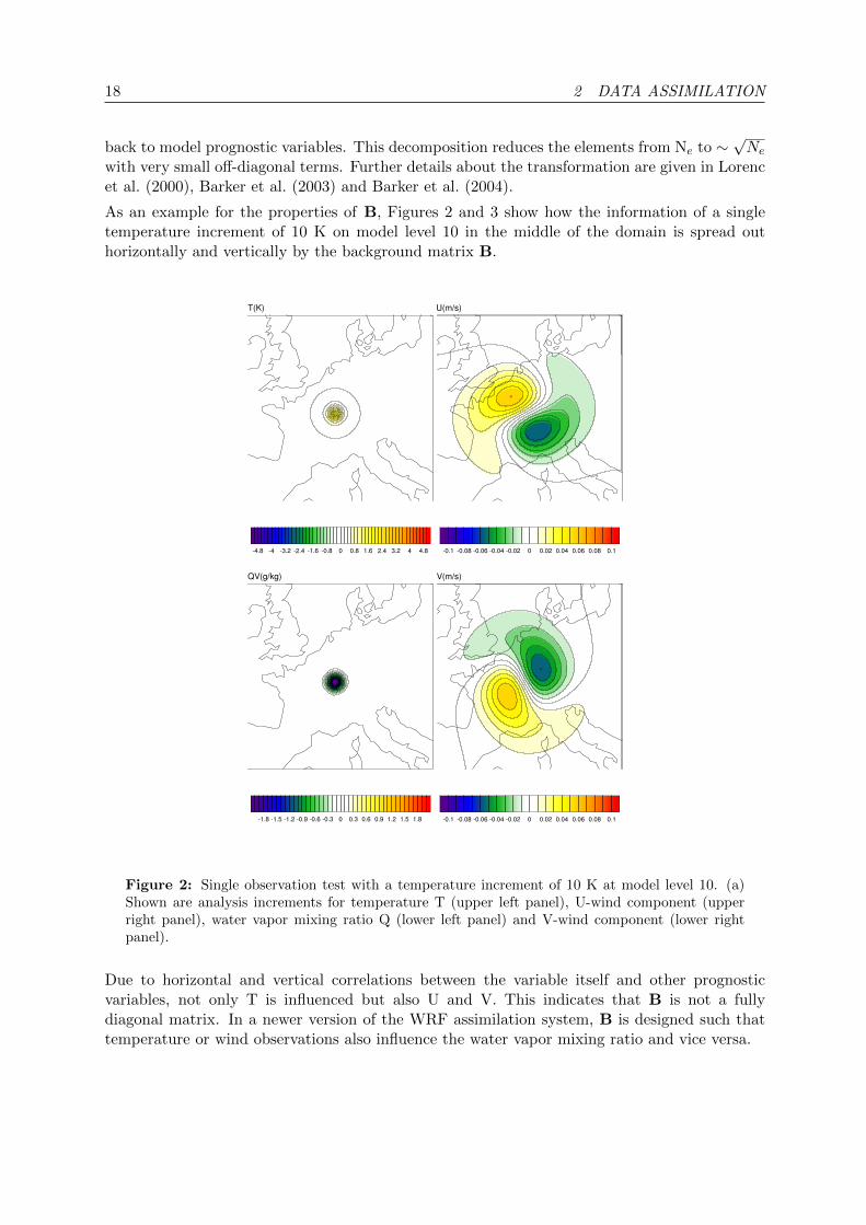
As an example for the properties of B, Figures 2 and 3 show how the information of a singletemperature increment of 10 K on model level 10 in the middle of the domain is spread outhorizontally and vertically by the background matrix B.
Figure 2: Single observation test with a temperature increment of 10 K at model level 10. (a)Shown are analysis increments for temperature T (upper left panel), U-wind component (upperright panel), water vapor mixing ratio Q (lower left panel) and V-wind component (lower rightpanel).
Due to horizontal and vertical correlations between the variable itself and other prognosticvariables, not only T is influenced but also U and V. This indicates that B is not a fullydiagonal matrix. In a newer version of the WRF assimilation system, B is designed such thattemperature or wind observations also influence the water vapor mixing ratio and vice versa.
2.4 Incremental 3/4DVAR 19
Figure 3: Vertical distribution of T, u, v and Q increments at the increment position.
2.4 Incremental 3/4DVAR
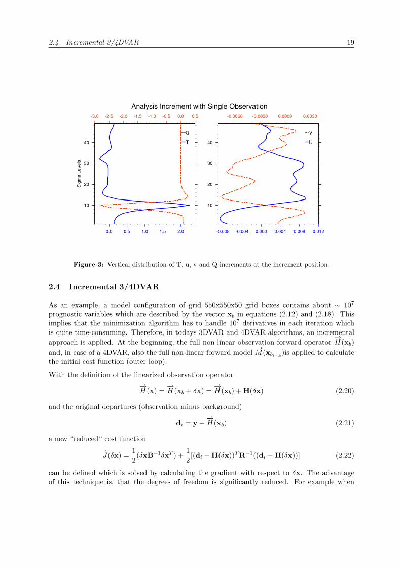
As an example, a model configuration of grid 550x550x50 grid boxes contains about ∼ 107
prognostic variables which are described by the vector xb in equations (2.12) and (2.18). Thisimplies that the minimization algorithm has to handle 107 derivatives in each iteration whichis quite time-consuming. Therefore, in todays 3DVAR and 4DVAR algorithms, an incremental
approach is applied. At the beginning, the full non-linear observation forward operator−→H (xb)
and, in case of a 4DVAR, also the full non-linear forward model−→M(xbi−k
)is applied to calculatethe initial cost function (outer loop).
With the definition of the linearized observation operator
−→H (x) =
−→H (xb + δx) =
−→H (xb) + H(δx) (2.20)
and the original departures (observation minus background)
di = y −−→H (xb) (2.21)
a new “reduced“ cost function
J(δx) =1
2(δxB−1δxT ) +
1
2[(di −H(δx))TR−1((di −H(δx))] (2.22)
can be defined which is solved by calculating the gradient with respect to δx. The advantageof this technique is, that the degrees of freedom is significantly reduced. For example when
20 2 DATA ASSIMILATION
4000 observations are available, the number of elements of δx is ∼104 allowing a much fastercomputation of the gradient compared to the original formulation 2.12. Further details can befound in Courtier (1997), Barker et al. (2003) and Huang et al. (2009).
2.5 Minimization Algorithm
The general purpose of a variational data assimilation scheme is the minimization of the costfunction J (2.22) describing the sum of differences between model background and modeledobservations. To minimize J , it is required to set ∇J = 0. As the dimension can be in the rangeof n2 ∼1014 it is very inefficient or even impossible to solve equation 2.13 directly. Therefore, intodays assimilation schemes two different minimization algorithms are applied: 1) the Lanczosalgorithm described by Golub and Van Loan (1996) and the conjugate gradient (CG) method(Shewchuk, 1994) which is explained in more detail using the example implemented into theWRF model.
The conjugate gradient method is an iterative method which can be applied to systems of linearequations as shown in equation 2.22. A precondition for this method is that the matrix R hasto be a symmetric matrix and positive definite. The latter relation is fulfilled, if
[di −H(δx)]TR−1[di −H(δx)] > 0 (2.23)
with di defined in equation 2.21.
In a first guess, a residual vector
g0 = y −−→H (xb)−
−→H (δx0) (2.24)
describing the negative gradient of a quadratic function f (δx0) and a conjugate vector
p0 = g0 (2.25)
as first guess are calculated. The second term on the right hand side of equation 2.24 is zeroas no minimization took place so far. In an incremental approach, this is done in the outerloop where the full observation operator is applied to calculate the observed quantity. From thisstarting point, the inner iteration process starts.
In the first inner iteration k (starting at k=0), a scalar
αk =| gk |2
pTk (∇2J)pk(2.26)
=| gk |2
pTk (B−1 + HTR−1H)pk
is calculated leading to an updated guess
δxk+1 = δxk + αk · pk (2.27)
and gradient (residual)gk+1 = gk + αk · (∇2J) · pk (2.28)
2.6 Brief outlook to ensemble data assimilation 21
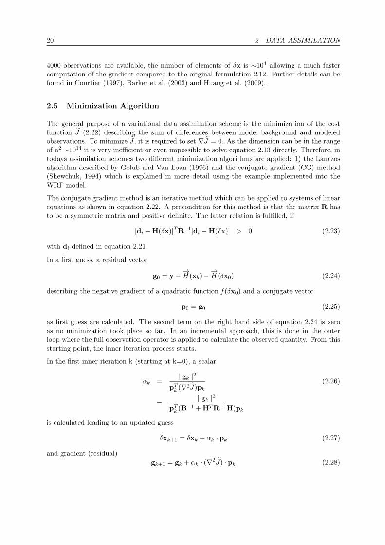
Figure 4: Schematic flow diagram of an incremental variational assimilation scheme.
where H is the linearized observation operator and HT is the adjoint observation operator. Stillin the inner loop k, a scalar
β =| gk+1 |2
| gk |2(2.29)
is introduced which gives a new estimate for the conjugate vector
pk+1 = gk+1 + β · pk. (2.30)
withδxTk+1(∇2J)pk+1 = 0 (2.31)
This procedure is executed in a loop until gk+1 is sufficiently small to end the minimizationprocess here. A peculiarity in the WRF model is the fact, that the minimization procedure isperformed in the control variable space described in section 2.3.
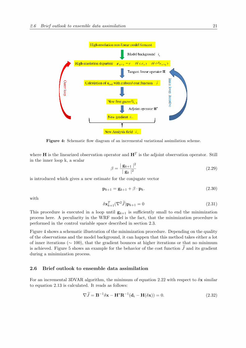
Figure 4 shows a schematic illustration of the minimization procedure. Depending on the qualityof the observations and the model background, it can happen that this method takes either a lotof inner iterations (∼ 100), that the gradient bounces at higher iterations or that no minimumis achieved. Figure 5 shows an example for the behavior of the cost function J and its gradientduring a minimization process.
2.6 Brief outlook to ensemble data assimilation
For an incremental 3DVAR algorithm, the minimum of equation 2.22 with respect to δx similarto equation 2.13 is calculated. It reads as follows:
∇J = B−1δx−H∗R−1(di −H(δx)) = 0. (2.32)
22 2 DATA ASSIMILATION
(a) (b)
Figure 5: Example for the behavior of the cost function J (a) and its gradient (b) during theinner loop.
This equation can be rewritten as
δx = (B−1 + H∗R−1H)−1[H∗R−1di]. (2.33)
Applying the Woodbury matrix identity (Hager, 1989), this leads to
δx = BH∗(R + HBH∗)−1︸ ︷︷ ︸K
di. (2.34)
which is then added to xb to obtain the new analysis. The matrix product BH∗(R+HBH∗)−1
is the “Kalman gain matrix” K for a deterministic forecast.
In the previous section, the creation of the static matrix B describing model errors and covari-ances of the different model prognostic variables was performed by the NMC method of Parrishand Derber (1992) describing errors and covariances by a model climatology.
Recently, operational forecast centers like Meteo France tend to derive B from an ensemble offorecasts from the selected NWP model (Berre, 2000; Fisher, 2003) applying a Kalman Filter(Evensen, 2003). Here the errors and covariances are calculated from ensemble perturbationswith respect to the ensemble mean. Thus, the matrix B, now renamed as Pe, is the ensemblederived error covariance matrix and can be rewritten as
Pe =1
K − 1
K∑i=1
(xif − xe)(xif − xe)
T = xpxTp (2.35)
2.7 Rapid Update Cycle (RUC) system with the WRF model 23
with xe denoting the ensemble mean of the K members and xif being the forecast of the i-thensemble member. In a matrix notation this can be rewritten as
Pe =1
K − 1
K∑i=1
xpxTp =
1
K − 1XpX
Tp (2.36)
with Xp denoting the matrix of the ensemble perturbation vectors xp. With the notation of theensemble Kalman Gain Matrix Ke, the new analysis mean xae is obtained from
xae = xe + PeH∗(R + HPeH
∗)−1[y0 −H(xe)] = xe + Ke[y0 −H(xe)] (2.37)
The analysis error covariance matrix Pae is obtained by (Evensen, 1994)
Pae = (1−KeH)Pe. (2.38)
The analysis error covariances for each member are added to the ensemble mean and the nextensemble forecast is performed. The advantage of applying a Kalman Filter is that a situationdependent error covariance matrix is obtained but the quality critically depends on the ensemblequality.
To realize a good ensemble spread, today often a multi-physics ensemble with perturbed bound-ary conditions of the applied NWP model is selected (e.g. Zhang et al., 2011). To update theindividual ensemble members, a transformation matrix T is needed, which contains an “infla-tion factor“ to give more weight on the ensemble perturbations (e.g. Wang et al., 2008). Asthe number of ensembles is limited by the available computing power, hybrid data assimilationschemes come into focus which combine an ensemble prediction system with a 3DVAR on theensemble mean. During the 3DVAR update, not only B but also the ensemble error covariancePe is considered in the following way (Wang et al., 2007):
Be = (1− α)Pe + αB (2.39)
α is a weighting factor determining the influence of the ensemble on the 3DVAR analysis. Inthe next step, the analysis error covariances Pa
e are added to the updated ensemble mean to getan updated ensemble for the next forecast step. The method described above for calculatingPae is the Ensemble Transform Kalman Filter (ETKF; Bishop et al., 2001). The main difference
to the EnKF is that only the analysis covariances are calculated and the ensemble mean is notupdated. The latter is done by the 3DVAR in this case.
2.7 Rapid Update Cycle (RUC) system with the WRF model
As mentioned in the section 2.2, applying the 4DVAR can be an enormous challenge on the km-scale both with respect to computing resources and model physics. Therefore, the 3DVAR-RUCapproach is in operation at many forecast centers around the world.
In general, due to the coarser resolution and different physics configurations of the driving modelcompared to the LAM, inconsistencies can occur during the first few hours because the modelhas to find its own balance. To overcome this difficulties, the model is initialized once with thecoarser driving model at the beginning of the desired RUC. After the initialization, optional with
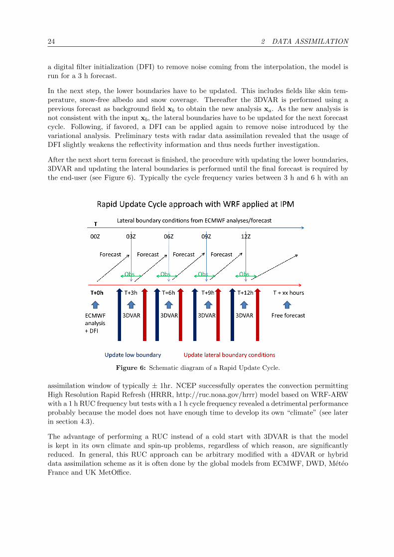
24 2 DATA ASSIMILATION
a digital filter initialization (DFI) to remove noise coming from the interpolation, the model isrun for a 3 h forecast.
In the next step, the lower boundaries have to be updated. This includes fields like skin tem-perature, snow-free albedo and snow coverage. Thereafter the 3DVAR is performed using aprevious forecast as background field xb to obtain the new analysis xa. As the new analysis isnot consistent with the input xb, the lateral boundaries have to be updated for the next forecastcycle. Following, if favored, a DFI can be applied again to remove noise introduced by thevariational analysis. Preliminary tests with radar data assimilation revealed that the usage ofDFI slightly weakens the reflectivity information and thus needs further investigation.
After the next short term forecast is finished, the procedure with updating the lower boundaries,3DVAR and updating the lateral boundaries is performed until the final forecast is required bythe end-user (see Figure 6). Typically the cycle frequency varies between 3 h and 6 h with an
Figure 6: Schematic diagram of a Rapid Update Cycle.
assimilation window of typically ± 1hr. NCEP successfully operates the convection permittingHigh Resolution Rapid Refresh (HRRR, http://ruc.noaa.gov/hrrr) model based on WRF-ARWwith a 1 h RUC frequency but tests with a 1 h cycle frequency revealed a detrimental performanceprobably because the model does not have enough time to develop its own “climate” (see laterin section 4.3).
The advantage of performing a RUC instead of a cold start with 3DVAR is that the modelis kept in its own climate and spin-up problems, regardless of which reason, are significantlyreduced. In general, this RUC approach can be arbitrary modified with a 4DVAR or hybriddata assimilation scheme as it is often done by the global models from ECMWF, DWD, MeteoFrance and UK MetOffice.
2.7 Rapid Update Cycle (RUC) system with the WRF model 25
Another important point is the size of the LAM model domain where the assimilation is per-formed especially in case of a 3DVAR. During COPS and D-PHASE, the 4DVAR for the MM5was performed on 18 km grid with a domain size of 64x70 grid points (∼ 1100x1200 km; Zuset al., 2008) in order to minimize computational costs. Afterwards, a forecast with a 2-waynested configuration was performed with a resolution of 18-6-2 km. In retrospect this resultedin 2 deficiencies (see Publication II in chapter 5): The application of a convection parameteri-zation and the obviously too small model domain for the inner nest.
To avoid nesting and the application of a convection parameterization, it is the best way todesign a single domain for both the assimilation and the subsequent free forecast. E.g. theALADIN model of Meteo France covers an area of ∼ 3000x3000 km, and the high resolutionAROME model covers an area of ∼ 1900x1800 km. A particular point for Central Europe is thatat least the British Channel is covered by the convection-permitting domain. The importanceof the model domain is shown later in publication III in chapter 5.
As the desired model domain is set up, the question arises how to use already available and new(remote sensing) observations. For conventional observations data simply have to be reformattedinto the required data structure. For observations like GPS ZTD or STD, radar data and satelliteradiances, several things have to be taken into account.
E.g. GPS-ZTD data are available every 15 min with about 400 stations. They are only assimi-lated in the nearest time windows around the assimilation date as the Zenith Wet Delay (ZWD)field is highly variable in time. The same applies for STD data, but the data density usually isfar too high so that data thinning is necessary also to avoid that more than one STD ray goesthough one model grid box. As similar procedure has to be performed for assimilating radarradial velocities. This is described in more detail in chapter 4.
For satellite radiances it is a bit more difficult as they are not available on a regular schedule,except geostationary satellite data like MSG. Therefore they will be assimilated within a ± 1 htime window around the analysis time.
To give the reader an impression of the RUC work flow in detail, appendix 6 shows an examplehow a RUC for the COPS period was recently set up including GPS-ZTD, radar and satelliteradiance data for near real time applications.
26 3 WATER VAPOR INFORMATION FROM GLOBAL POSITIONING SYSTEM
3 Water vapor information from Global Positioning System
In this section, a brief introduction into the GPS and the retrieval of water vapor informationwill be given. GPS was originally introduced to provide accurate position information under allweather conditions that is to say like cloudy conditions, rain or snow everywhere on earth. Theonly requirement is that a direct line of sight exists to at least four of the satellites of the GPSnetwork which currently consists of 32 satellites at an altitude of ∼ 20000 km above the earthsurface.
GPS satellites transmit two different radio frequencies of 1.57542 GHz (f1) and 1.2276 GHz (f2)corresponding to wavelengths of 0.19 m (λ1) and 0.244 m (λ2). To determine the position of aantenna (receiver), it is necessary to have at least four satellites i available. The unknown pa-rameters for the determination of position are the coordinates x,y,z and time difference betweenthe satellite and receiver time. To obtain the position, one has to know the vector
xi =
xiyiziti
(3.1)
of each of the four satellites plus a clock bias tb of the receiver. From this point, a pseudo rangeΘ describing a phase difference in length units for each satellite can be defined:
Θ =√
(x− xi)2 + (y − yi)2 + (z − zi)2 − tbc (3.2)
withΘ = (tr − ti)c (3.3)
where tr denotes the receiver time, ti denotes the satellite time and c is the speed of light inthe vacuum. With equations 3.2 and 3.3 the receiver location coordinates x,y and z can bedetermined with an accuracy of a few centimeters.
If the exact location of the GPS receiver is known, additional information can be obtained. Dueto the earth’s troposphere (with water vapor) and the ionosphere, the received signal is delayedcompared to the vacuum which is known as tropospheric or slant path total and ionosphericdelay. Following Hofmann-Wellenhof et al. (1997), the pseudorange can be also estimated by
Θ = d+ c(dts − dtr) + λini + STD + I (3.4)
where d is the distance between the receiver and satellite, dts and dtr denote the offset ofsatellite and receiver time compared to GPS reference time, λi is the carrier wave length, nidenotes an integer of wavelengths λi between satellite and receiver due to an unknown phaseand STD and I represent the slant path and ionospheric delay respectively. If dual frequency(f1 and f2) receivers are available, the ionospheric delay can be removed from equation 3.4 andthus the accuracy of Θ increases.
The slant total delay STD caused by the neutral atmosphere is given by (Bevis et al., 1992)
STD = 10−6
∫SNds (3.5)
27
where N is the atmospheric refractivity which depends on pressure, temperature and water vaporand ds denotes the signal path from the GPS satellite to the receiver.
In case of an elevation of 90° (see Figure 10), the STD is called Zenith Total Delay (ZTD). Bothcan be split into a wet delay depending on the 3-dimensional temperature T, water vapor mixingratio q, pressure p and a dry delay only depending on ps. For a ZTD, the wet delay ZWD canbe determined by integrating refractivity profiles i starting at the surface:
ZWD =n∑i=1
k1pi qi
0.622 Ti+ k2
pi qi0.622 T 2
i
(3.6)
with constants k1 = 2.21· 10−7 K/Pa and k2 = 3.73· 10−3 K2/Pa (Bevis et al., 1994). The dryhydrostatic delay ZHD is that suggested by Saastamoinen (1972):
ZHD =k4 ps
1− 0.00266 cos(2φ)− 0.00000028h(3.7)
with k4 = 0.000022768 m Pa−1, φ being the receiver latitude [deg], h the receiver altitude abovethe surface, ps the surface pressure [Pa]. Thus the ZTD [m] reads now as
ZTD = ZWD + ZHD (3.8)
The magnitude of the total delay depends on the elevation angle to the receiver with respect toa tangent at the earth surface. It can reach up to 2.5 m for ZTD and 10 m for low elevationSTD measurements. Deriving STDs from an NWP model can be challenging as the refractivityprofiles Ni have to be derived according to the line of sight to the satellite and the ray bendingnear the surface have to be taken into account. Further details about this issue can be found inthe PhD thesis of Zus (2010).
Although STD and ZTD are integrated quantities, the application of a variational assimilationscheme gives information about the 3-dimensional structure of the atmosphere. With the appli-cation of an adjoint operator it is possible to adjust the 3-dimensional humidity, temperatureand pressure fields in the model either above the receiver station in case of a ZTD or along theray path through the atmosphere in case of STDs.
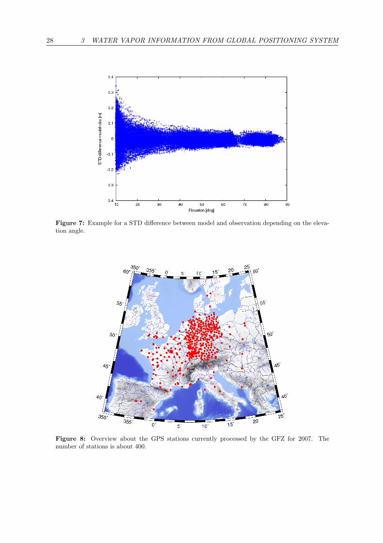
Application of STD instead of ZTD has a beneficial effect in a data assimilation scheme. AsSTDs can be measured with all elevations greater than zero, the tilted STD can give additionalinformation about the horizontal water vapor distribution in the boundary layer which is es-pecially important for summertime convection. The disadvantage or the critical point is thatwhen STDs are obtained at low elevations < 20°(ε in Figure 10), the ray bending due to gravityhas to be taken into account (Ereesma and Jarvinen, 2006; Zus, 2010) in a similar way as it isconsidered for radar measurements (see later in section 4.3). An example for a difference mod-eled minus observed STD from the WRF model is given in Figure 7. A simple STD operatorwas implemented into the 3DVAR system to obtain an O-B statistics but cannot be used forassimilation purposes.
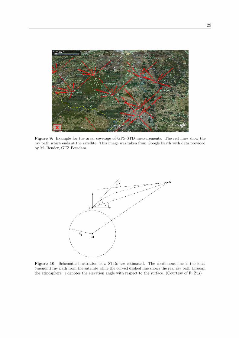
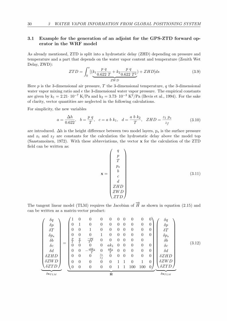
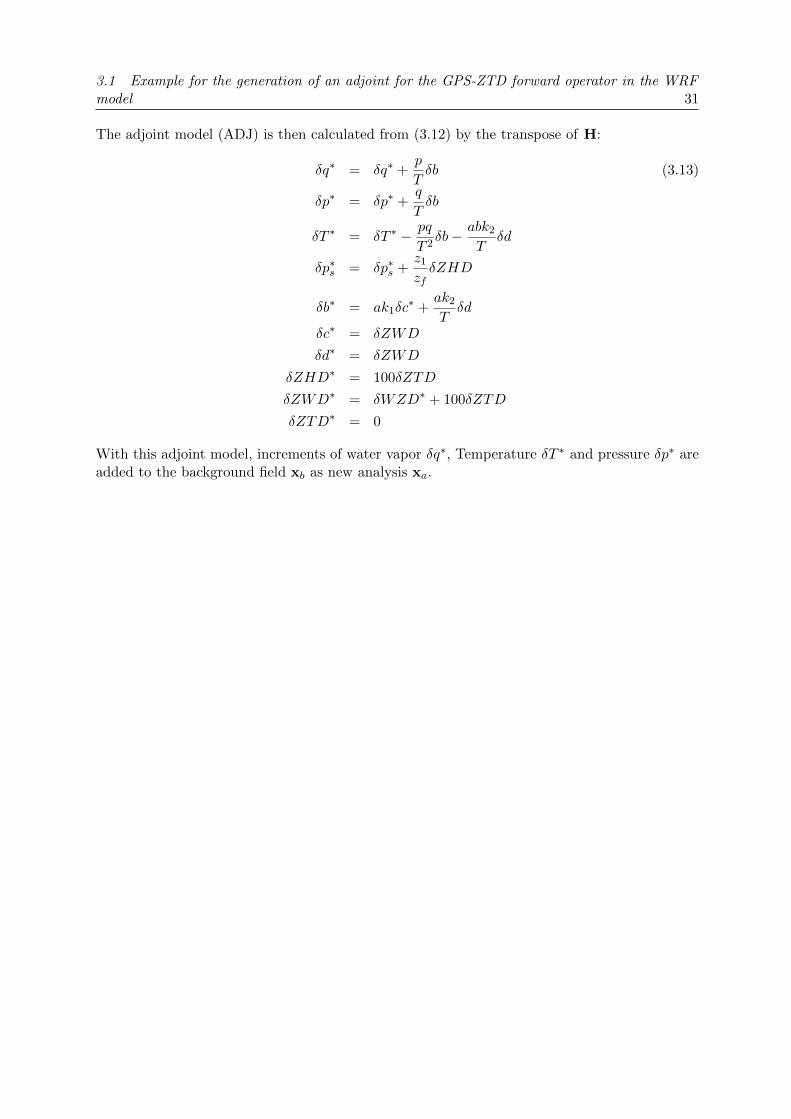
An example for the derivation of an adjoint model for ZTD is given in section 2.1 and Figure 8shows the distribution of the GPS receiver network currently re-processed by the GFZ9 EPOSsoftware (Gendt et al., 2004) for 2007. Figure 9 shows an example for the coverage of GPS-STDdata and Figure 10 illustrates how the STD is estimated.
9Helmholtz Centre Potsdam, GFZ German Research Centre for Geosciences
28 3 WATER VAPOR INFORMATION FROM GLOBAL POSITIONING SYSTEM
Figure 7: Example for a STD difference between model and observation depending on the eleva-tion angle.
Figure 8: Overview about the GPS stations currently processed by the GFZ for 2007. Thenumber of stations is about 400.
29
Figure 9: Example for the areal coverage of GPS-STD measurements. The red lines show theray path which ends at the satellite. This image was taken from Google Earth with data providedby M. Bender, GFZ Potsdam.
Figure 10: Schematic illustration how STDs are estimated. The continuous line is the ideal(vacuum) ray path from the satellite while the curved dashed line shows the real ray path throughthe atmosphere. ε denotes the elevation angle with respect to the surface. (Courtesy of F. Zus)
30 3 WATER VAPOR INFORMATION FROM GLOBAL POSITIONING SYSTEM
3.1 Example for the generation of an adjoint for the GPS-ZTD forward op-erator in the WRF model
As already mentioned, ZTD is split into a hydrostatic delay (ZHD) depending on pressure andtemperature and a part that depends on the water vapor content and temperature (Zenith WetDelay, ZWD):
ZTD =
∫ s
0[(k1
p q
0.622 T+ k2
p q
0.622 T 2︸ ︷︷ ︸ZWD
) + ZHD]ds (3.9)
Here p is the 3-dimensional air pressure, T the 3-dimensional temperature, q the 3-dimensionalwater vapor mixing ratio and e the 3-dimensional water vapor pressure. The empirical constantsare given by k1 = 2.21· 10−7 K/Pa and k2 = 3.73· 10−3 K2/Pa (Bevis et al., 1994). For the sakeof clarity, vector quantities are neglected in the following calculations.
For simplicity, the new variables
a =∆h
0.622, b =
p q
T, c = a b k1, d =
a b k2
T, ZHD =
z1 pszf
(3.10)
are introduced. ∆h is the height difference between two model layers, ps is the surface pressureand z1 and zf are constants for the calculation the hydrostatic delay above the model top(Saastamoinen, 1972). With these abbreviations, the vector x for the calculation of the ZTDfield can be written as:
x =
qpTpsbcd
ZHDZWDZTD
(3.11)
The tangent linear model (TLM) requires the Jacobian of−→H as shown in equation (2.15) and
can be written as a matrix-vector product:
δqδpδTδpsδbδcδd
δZHDδZWDδZTD
︸ ︷︷ ︸
δxTLM
=
1 0 0 0 0 0 0 0 0 00 1 0 0 0 0 0 0 0 00 0 1 0 0 0 0 0 0 00 0 0 1 0 0 0 0 0 0pT
qT
−pqT 2 0 0 0 0 0 0
0 0 0 0 ak1 0 0 0 0 0
0 0 −abk2T 0 ak2
T 0 0 0 0 00 0 0 z1
zf0 0 0 0 0 0
0 0 0 0 0 1 1 0 1 00 0 0 0 0 1 1 100 100 0
︸ ︷︷ ︸
H
δqδpδTδpsδbδcδd
δZHDδZWDδZTD
︸ ︷︷ ︸
δxTLM
(3.12)
3.1 Example for the generation of an adjoint for the GPS-ZTD forward operator in the WRFmodel 31
The adjoint model (ADJ) is then calculated from (3.12) by the transpose of H:
δq∗ = δq∗ +p
Tδb (3.13)
δp∗ = δp∗ +q
Tδb
δT ∗ = δT ∗ − pq
T 2δb− abk2
Tδd
δp∗s = δp∗s +z1
zfδZHD
δb∗ = ak1δc∗ +
ak2
Tδd
δc∗ = δZWD
δd∗ = δZWD
δZHD∗ = 100δZTD
δZWD∗ = δWZD∗ + 100δZTD
δZTD∗ = 0
With this adjoint model, increments of water vapor δq∗, Temperature δT ∗ and pressure δp∗ areadded to the background field xb as new analysis xa.
32 4 RADAR DATA ASSIMILATION
4 Radar data assimilation
In the previous chapter, the focus was set on the application of (active remote sensing) GPS STDand ZTD data to improve the spatially and temporally highly variable water vapor distribution.As for example in an area which is highly favorable for convection or convective initiation, it canbe inadequate to assimilate only tropospheric humidity in this conditions. An option to obtaininformation about dynamics are active remote sensing systems. Recently, Doppler LIDAR andDoppler precipitation RADAR10 are employed to obtain information on the dynamic structure.
A Doppler LIDAR employs a LASER beam (mostly in the ultraviolet) which is send out tothe atmosphere through a telescope. Due to the aerosols in the atmosphere, the scatteredbeam exhibits a frequency change which allows the detection of wind speed along the ray path(Line of sight, LOS). A LIDAR system typically has a LOS resolution of 50–100 m and canmeasure up to altitudes of 15 km. As large as the advantage of the high resolution is, due to thescattering properties of particles a LIDAR measurement is restricted to cloud free areas. Dueto the applied wavelength, the beam does not penetrate clouds and thus a strong backscattersignal is detected of which no doppler shift can be extracted. Further details about the basicsand recent developments of Doppler LIDAR wind measurements can be found e.g. in Reitebuchet al. (2009).
In contrast to a LIDAR System, radar systems have an larger spatial coverage but they needtracers for the detection of Doppler radial velocities. Additionally, reflectivity measurementsdescribing the intensity ratio between the emitted and scattered/reflected microwave beam arein use to allow meteorologists drawing conclusions of the strength of a convective system, e.g ifhail can be expected on the ground. This makes it currently a favorable measurement system inareas where convection already took place. Radar systems use microwaves (so called “C-Band”,“X-Band“ or ”S-Band“ radars, depending on the frequency) and have a range of ≈ 200 km.
As a supplement for getting information about dynamics (wind), passive remote sensing instru-ment retrievals from satellites (e.g. MSG from EUMETSAT; EUMETSAT (2009)) are appliedin current NWP data assimilation schemes. The advantage is that a large area is covered bythe satellite. Depending on the satellite orbit, the temporal resolution can be very coarse, e.gpolar-orbiting satellites overpasses one location twice a day whereas satellite derived winds fromMSG are available every hour. Another disadvantage is the fact, that clouds have to be present,since the wind information is retrieved by tracking cloudy pixels in the satellite image.
As the application of radar data in combination with NWP is a relatively new research area, thenext section will give further details about radar radial velocity and reflectivity measurementsand their application in current NWP assimilation schemes.
4.1 Measurement principle
Doppler precipitation radars emit electromagnetic pulses which are backscattered from hydrometeorslike rain droplets or hail particles as well as from insects (”clear air echoes”). Precipitation radarsin general are usually classified into 3 categories depending on the emitted wavelength:
10Radio Detection And Ranging
4.1 Measurement principle 33
� S-Band Radar with frequencies of ≈ 3 GHz
� C-Band Radar with frequencies of ≈ 6 GHz
� X-Band Radar with frequencies of ≈ 10 GHz
In Europe mostly C-Band and X-Band radar systems are in operation. They have a typicalrange of 200–250 km with a horizontal resolution of 30–250 m which is often averaged to about500–1000 m in the horizontal to reduce the amount of raw data. The radar antenna can berotated so that different antenna azimuths and elevations can be scanned. Typical azimuthincrements are 1°and the elevation angle increments increase with the antenna elevation from1°–10°.
To benefit from the Doppler effect, precipitation radars operate with a pulse repetition rate(PRT) of 200–1500 Hz meaning that e.g. every 5 µs an electromagnetic pulse is emitted. Withinthis time, the hydrometeors can move in the 3 directions u,v, and w. Due to the motion, thescattered electromagnetic wave has a different phase compared to the emitted wave. From thisbehavior, the radial velocity vr of a target can be derived following e.g. Doviak and Zrnic (1993):
vr =λ · PRT
4=λ∆Φ
4π∆t(4.1)
with λ being the wavelength of the pulse, ∆Φ the phase difference of the scattered wave and ∆tthe time between two radar pulses.
Equation 4.1 shows, that Doppler radars do not really measure a Doppler shift rather than aphase shift between two electromagnetic waves from which the radial velocity is derived. Asthe number of particles in the scanned volume, which increases with the distance from theantenna, is assumed to be large, a continuous velocity distribution of the particles is assumed.The velocity spectrum is then weighted by the power to obtain the mean radial velocity (seee.g. Doviak and Zrnic, 1993).
Unfortunately, the so-called ”Doppler dilemma“ complicates the derivation of radial velocities(Doviak and Zrnic, 1993). It allows only one unambiguous radial velocity vumax (Nyquist velocity,see e.g. Holleman and Beekhuis, 2003)
vumax =1
Rumax
λ · c8
(4.2)
dependent on the wavelength λ with the speed of light c and the unambiguous maximum rangeRumax. The latter is defined by
Rumax =c
2 · PRF(4.3)
If a scatterer is at a distance R farther than Rumax, it appears that the scatter has a distance ofR′ = R − (M − 1) · Rumax where M denotes the number of Rumax intervals. PRF describes thepulse repetition frequency.
As an example, for the DWD C-Band radar λ is 5.3 cm and the pulse repetition frequency is600 Hz. This would lead to Rumax of 250 km and to an unambiguous radial velocity of ±3.31 m/s.Here the range is acceptable but the unambiguous velocity is too small as particles can move
34 4 RADAR DATA ASSIMILATION
up to 80 m/s when measuring in the jet stream area. Therefore, the dual PRF described inHolleman and Beekhuis (2003) is often used which decreases Rumax but significantly increasesvumax.
To keep the DWD example, the low PRF is 800 Hz and the high PRF is 1200 Hz leading toa maximum unambiguous range of 125 km and velocity of ±32 m/s. Recently Meteo Franceemploys a triple PRF scheme allowing unambiguous velocities of about 60 m/s and a maximumrange of 250 km (Tahanout et al., 2009). The data availability window for reflectivity andradial velocity in Europe is usually 15 min because of the antenna rotation speed and other scanprocedures (e.g. PPI scan at a constant elevation with a comparatively low PRF).
Another important feature for short range forecasting and nowcasting is the intensity of thescattered radar beam. This is called the reflectivity Z which depends on the particle diameterD and the assumed drop size distribution N(D) and is related to the number of droplets perunit volume and the sixth power of the droplet diameter (mm6/m3). Assuming e.g. a Marshall-Palmer distribution N(D) for hydrometeors (Marshall and Palmer, 1948), the reflectivity Z reads
Z =
∫ D
0N(D)dD =
∫ D
0N0e
−ΓDD6dD (4.4)
N0 describes a droplet concentration at 0 radius. For radar reflectivity the unit dbZ is used whichis 10 times the logarithm of Z. From this kind of reflectivity, one can detect whether a convectivesystem contains only rain or also hail which is more likely when the reflectivity exceeds 55 dbZ.It is also interesting to note that aircrafts are advised to avoid areas with reflectivities greaterthan 37 dbZ as this can lead to substantial damage to the aircraft and loss of control due toassumed strong updrafts.
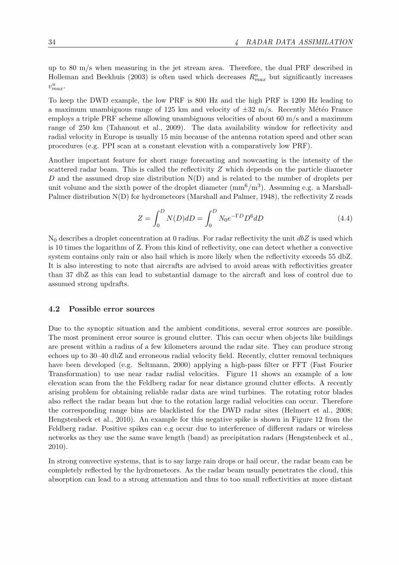
4.2 Possible error sources
Due to the synoptic situation and the ambient conditions, several error sources are possible.The most prominent error source is ground clutter. This can occur when objects like buildingsare present within a radius of a few kilometers around the radar site. They can produce strongechoes up to 30–40 dbZ and erroneous radial velocity field. Recently, clutter removal techniqueshave been developed (e.g. Seltmann, 2000) applying a high-pass filter or FFT (Fast FourierTransformation) to use near radar radial velocities. Figure 11 shows an example of a lowelevation scan from the the Feldberg radar for near distance ground clutter effects. A recentlyarising problem for obtaining reliable radar data are wind turbines. The rotating rotor bladesalso reflect the radar beam but due to the rotation large radial velocities can occur. Thereforethe corresponding range bins are blacklisted for the DWD radar sites (Helmert et al., 2008;Hengstenbeck et al., 2010). An example for this negative spike is shown in Figure 12 from theFeldberg radar. Positive spikes can e.g occur due to interference of different radars or wirelessnetworks as they use the same wave length (band) as precipitation radars (Hengstenbeck et al.,2010).
In strong convective systems, that is to say large rain drops or hail occur, the radar beam can becompletely reflected by the hydrometeors. As the radar beam usually penetrates the cloud, thisabsorption can lead to a strong attenuation and thus to too small reflectivities at more distant
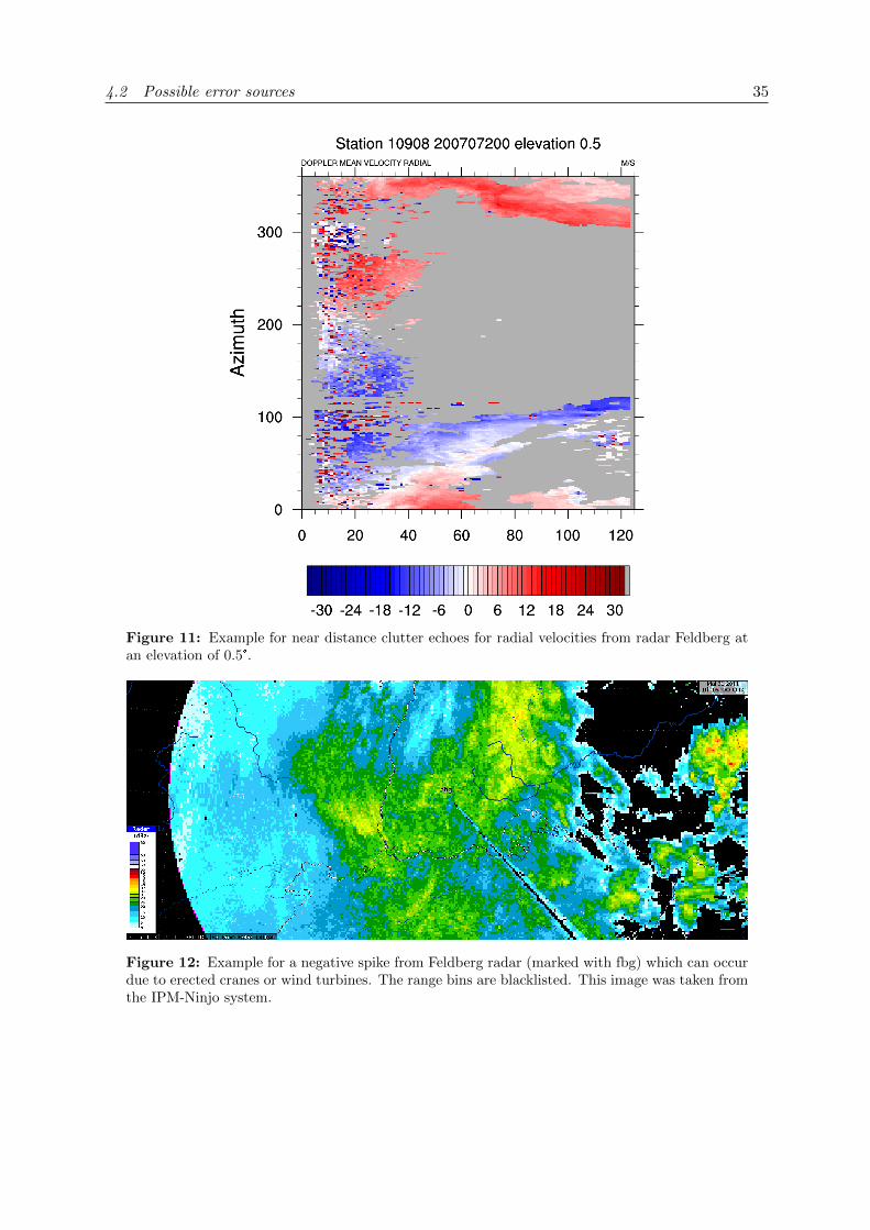
4.2 Possible error sources 35
Figure 11: Example for near distance clutter echoes for radial velocities from radar Feldberg atan elevation of 0.5°.
Figure 12: Example for a negative spike from Feldberg radar (marked with fbg) which can occurdue to erected cranes or wind turbines. The range bins are blacklisted. This image was taken fromthe IPM-Ninjo system.
36 4 RADAR DATA ASSIMILATION
ranges. This can partially be overcome by an overlapping area between two radar sites but istechnically not easy to implement.
When working with radars, it is assumed that the backscattered beam has the same direction asthe emitted beam but this is not fully correct. The wave is scattered in all directions and espe-cially when hail is present, a non-negligible part is scattered towards the surface and scatteredback to the hydrometeor and is recorded as an increased intensity also leading to an positionerror of the signal. This phenomena is referred to as ”Hail spike“ and is described in more detailby Lemon (1998).
Other phenomena are the anomalous beam propagation due to super refractivity and the socalled ”bright band”. The former especially occurs in the morning when a strong temperatureinversion can occur which prevents the radar beam penetrating the warm air above the inversionlayer (Bech et al., 2003). The bright-band effect occurs when frozen particles penetrate themelting layer. They are covered by a thin layer of water which better reflects the radar beamcompared to snow leading to increased reflectivities. Usually this zone has a depth of fewhundred meters. Further details about possible detection algorithms for bright band effects canbe found e.g. in Gourley and Calvert (2003).
4.3 Application of radar data in NWP models
The direct assimilation of radar reflectivities, polarizations and radial velocities are only possi-ble within a variational or ensemble data assimilation framework as observation operators arerequired. For NWP models where the analysis is updated with a simpler nudging scheme, adifferent method has to be applied. E.g. the DWD applies the LHN procedure for COSMO-DEwhich should force convection in the short term time-scale. LHN is based on a radar derivedprecipitation rate Rr which is obtained the following relation:
Rr = aZb (4.5)
where Z is the 3-dimensional radar reflectivity and a,b are empirically derived constants. It isassumed that the falling hydrometeors and their phase transitions release a certain amount oflatent heat leading to a warming ∆T of the ambient air masses. This temperature incrementis then related to the model derived precipitation Rmodel, the latent heat release and observedrain rate in the following way (see e.g. Stephan et al., 2008 for the application in COSMO-DE):
∆T = (α− 1)1
Cp∆LH (4.6)
where α is defined as RrRmodel
, Cp is the specific heat capacity for dry air at constant pressure. ∆LHis the latent heat released by condensation which is usually calculated in the cloud microphysicsscheme. The profile temperature increment is finally added to the model background with anadditional weighting term.
A weak point is the addition of only the temperature increment to the model background state.This can lead to strong precipitation in a short-term forecast as the often positive incrementleads to a potential instability (increase of CAPE).
4.3 Application of radar data in NWP models 37
A similar method compared to LHN is the Physical Initialisation Bonn (PIB, developed byHaase, 2002) for improving the very short term precipitation forecast. The aim of this approachis to change the vertical velocity field in order to initiate and support convection. PIB usesthe same radar derived and model rain rates (Rr and Rmodel) to obtain an updated rain rateRupdate. Then, a new rain rate Rnew is derived from Rupdate based whether a cloud exists in themodel or not. Based on Rupdate, the vertical velocity inside the clouds is calculated. Comparedto the LHN, this method also changes the vertical structure of cloud water and cloud ice. Thedisadvantage of this approach is that a synthetic 3-dimensional radar derived rain rate has tobe assumed because the radar does not scan the whole hemisphere. Further details and resultscan be found in Milan et al. (2008).
Especially in summer, convergence lines play a major role for the initiation of convection. Tobetter represent (near) surface wind, to date mostly synoptic and airport measurements areincorporated into data assimilation schemes. Figure 13 shows an example for surface wind dataobtained from the Global Telecommunication System (GTS) and for the COPS year 2007. Itcan be seen from Figure 13a, that the station density obtained from the GTS is very coarsewith an average distance of 25–30 km compared to the Joint D-PHASE COPS data set data set(Dorninger et al. (2009), Figure 13b). In the summer season, this can be too coarse to representconvergence lines so that this may be not very useful for correctly predicting the triggering ofconvection with the aid of an assimilation system. Therefore, the assimilation of high resolutionradar radial velocities and reflectivities becomes important.
Unfortunately radial velocities are only available in the presence of scattering targets, that isinsects or hydrometeors. One of the first attempts using radar data for assimilation in NWPmodels was performed by Sun and Crook (1997) who developed a 3DVAR containing observationoperators for radar radial velocities and reflectivities for the application of a convective stormin Florida. Further attempts were made e.g. by Xiao et al. (2005) and Xiao and Sun (2007) forthe U.S. applying the WRF model and by Lindskog et al. (2004) and Montmerle and Faccani(2009) applying the HIRLAM and AROME models over Europe.
To assimilate radar radial velocities in a variational assimilation system, a model forward oper-ator is needed. The three model wind components u, v, and w have to be projected to the radarbeam position. In the WRF model, this is done in the following way (Xiao and Sun, 2007):
vr =x− xiri
u+y − yiri
v +z − ziri
(w − vT ) (4.7)
Here x,y, and z denotes the radar location, xi,yi and zi are the location of the radar observationand ri is the distance between the radar location and the observation relative to the center ofthe earth (see Figure 14). vT is the so called “terminal velocity” describing the fallspeed of rainparticles in the model and is defined by
vT = a b q0.125r (4.8)
where qr is the rain water mixing ratio and b is estimated as
b =pspb
(4.9)
ps is the surface pressure and pb denotes the base state model pressure. a has a value of 5.4 m/sand is derived under the assumption that the Reynolds Number is ∼ 300 and with a dragcoefficient of 1. Further details can be found in Pruppacher and Klett (1997).
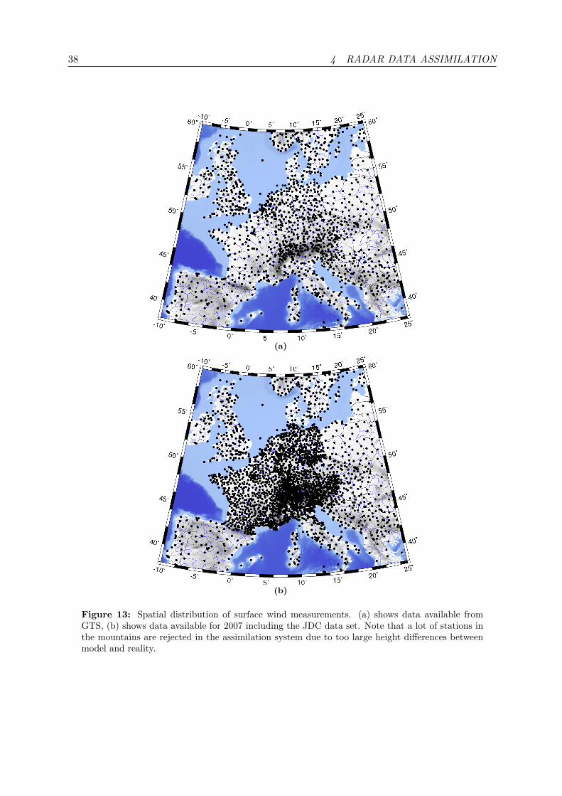
38 4 RADAR DATA ASSIMILATION
(a)
(b)
Figure 13: Spatial distribution of surface wind measurements. (a) shows data available fromGTS, (b) shows data available for 2007 including the JDC data set. Note that a lot of stations inthe mountains are rejected in the assimilation system due to too large height differences betweenmodel and reality.
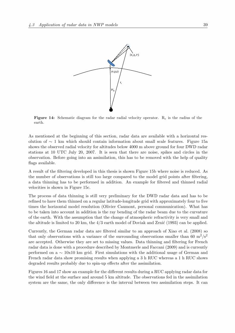
4.3 Application of radar data in NWP models 39
Figure 14: Schematic diagram for the radar radial velocity operator. Re is the radius of theearth.
As mentioned at the beginning of this section, radar data are available with a horizontal res-olution of ∼ 1 km which should contain information about small scale features. Figure 15ashows the observed radial velocity for altitudes below 4000 m above ground for four DWD radarstations at 10 UTC July 20, 2007. It is seen that there are noise, spikes and circles in theobservation. Before going into an assimilation, this has to be removed with the help of qualityflags available.
A result of the filtering developed in this thesis is shown Figure 15b where noise is reduced. Asthe number of observations is still too large compared to the model grid points after filtering,a data thinning has to be performed in addition. An example for filtered and thinned radialvelocities is shown in Figure 15c.
The process of data thinning is still very preliminary for the DWD radar data and has to berefined to have them thinned on a regular latitude-longitude grid with approximately four to fivetimes the horizontal model resolution (Olivier Caumont, personal communication). What hasto be taken into account in addition is the ray bending of the radar beam due to the curvatureof the earth. With the assumption that the change of atmospheric refractivity is very small andthe altitude is limited to 20 km, the 4/3 earth model of Doviak and Zrnic (1993) can be applied.
Currently, the German radar data are filtered similar to an approach of Xiao et al. (2008) sothat only observations with a variance of the surrounding observations smaller than 60 m2/s2
are accepted. Otherwise they are set to missing values. Data thinning and filtering for Frenchradar data is done with a procedure described by Montmerle and Faccani (2009) and is currentlyperformed on a ∼ 10x10 km grid. First simulations with the additional usage of German andFrench radar data show promising results when applying a 3 h RUC whereas a 1 h RUC showsdegraded results probably due to spin-up effects after the assimilation.
Figures 16 and 17 show an example for the different results during a RUC applying radar data forthe wind field at the surface and around 5 km altitude. The observations fed in the assimilationsystem are the same, the only difference is the interval between two assimilation steps. It can
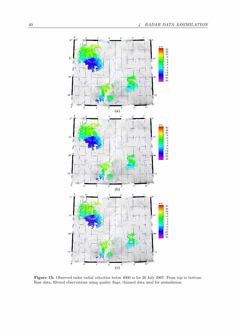
40 4 RADAR DATA ASSIMILATION
(a)
(b)
(c)
Figure 15: Observed radar radial velocities below 4000 m for 20 July 2007. From top to bottom:Raw data, filtered observations using quality flags, thinned data used for assimilation.
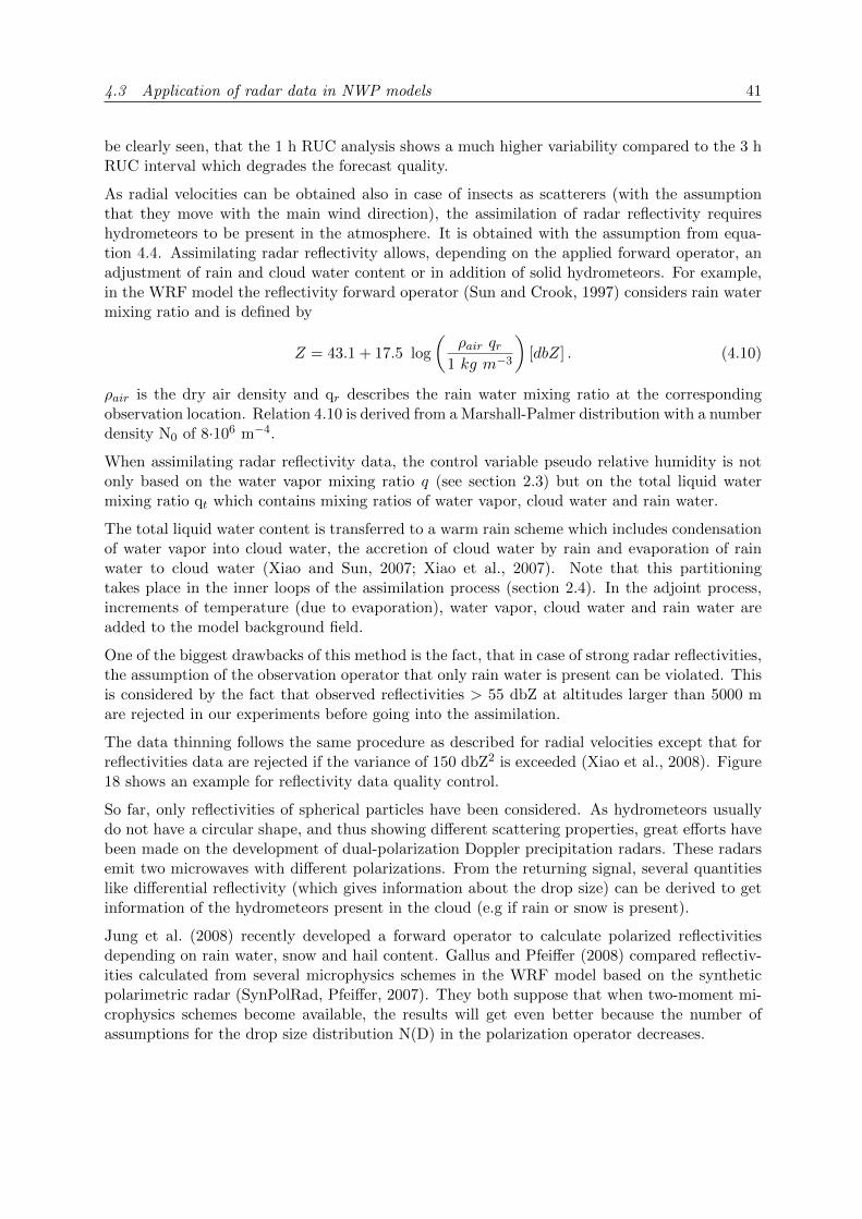
4.3 Application of radar data in NWP models 41
be clearly seen, that the 1 h RUC analysis shows a much higher variability compared to the 3 hRUC interval which degrades the forecast quality.
As radial velocities can be obtained also in case of insects as scatterers (with the assumptionthat they move with the main wind direction), the assimilation of radar reflectivity requireshydrometeors to be present in the atmosphere. It is obtained with the assumption from equa-tion 4.4. Assimilating radar reflectivity allows, depending on the applied forward operator, anadjustment of rain and cloud water content or in addition of solid hydrometeors. For example,in the WRF model the reflectivity forward operator (Sun and Crook, 1997) considers rain watermixing ratio and is defined by
Z = 43.1 + 17.5 log
(ρair qr
1 kg m−3
)[dbZ] . (4.10)
ρair is the dry air density and qr describes the rain water mixing ratio at the correspondingobservation location. Relation 4.10 is derived from a Marshall-Palmer distribution with a numberdensity N0 of 8·106 m−4.
When assimilating radar reflectivity data, the control variable pseudo relative humidity is notonly based on the water vapor mixing ratio q (see section 2.3) but on the total liquid watermixing ratio qt which contains mixing ratios of water vapor, cloud water and rain water.
The total liquid water content is transferred to a warm rain scheme which includes condensationof water vapor into cloud water, the accretion of cloud water by rain and evaporation of rainwater to cloud water (Xiao and Sun, 2007; Xiao et al., 2007). Note that this partitioningtakes place in the inner loops of the assimilation process (section 2.4). In the adjoint process,increments of temperature (due to evaporation), water vapor, cloud water and rain water areadded to the model background field.
One of the biggest drawbacks of this method is the fact, that in case of strong radar reflectivities,the assumption of the observation operator that only rain water is present can be violated. Thisis considered by the fact that observed reflectivities > 55 dbZ at altitudes larger than 5000 mare rejected in our experiments before going into the assimilation.
The data thinning follows the same procedure as described for radial velocities except that forreflectivities data are rejected if the variance of 150 dbZ2 is exceeded (Xiao et al., 2008). Figure18 shows an example for reflectivity data quality control.
So far, only reflectivities of spherical particles have been considered. As hydrometeors usuallydo not have a circular shape, and thus showing different scattering properties, great efforts havebeen made on the development of dual-polarization Doppler precipitation radars. These radarsemit two microwaves with different polarizations. From the returning signal, several quantitieslike differential reflectivity (which gives information about the drop size) can be derived to getinformation of the hydrometeors present in the cloud (e.g if rain or snow is present).
Jung et al. (2008) recently developed a forward operator to calculate polarized reflectivitiesdepending on rain water, snow and hail content. Gallus and Pfeiffer (2008) compared reflectiv-ities calculated from several microphysics schemes in the WRF model based on the syntheticpolarimetric radar (SynPolRad, Pfeiffer, 2007). They both suppose that when two-moment mi-crophysics schemes become available, the results will get even better because the number ofassumptions for the drop size distribution N(D) in the polarization operator decreases.
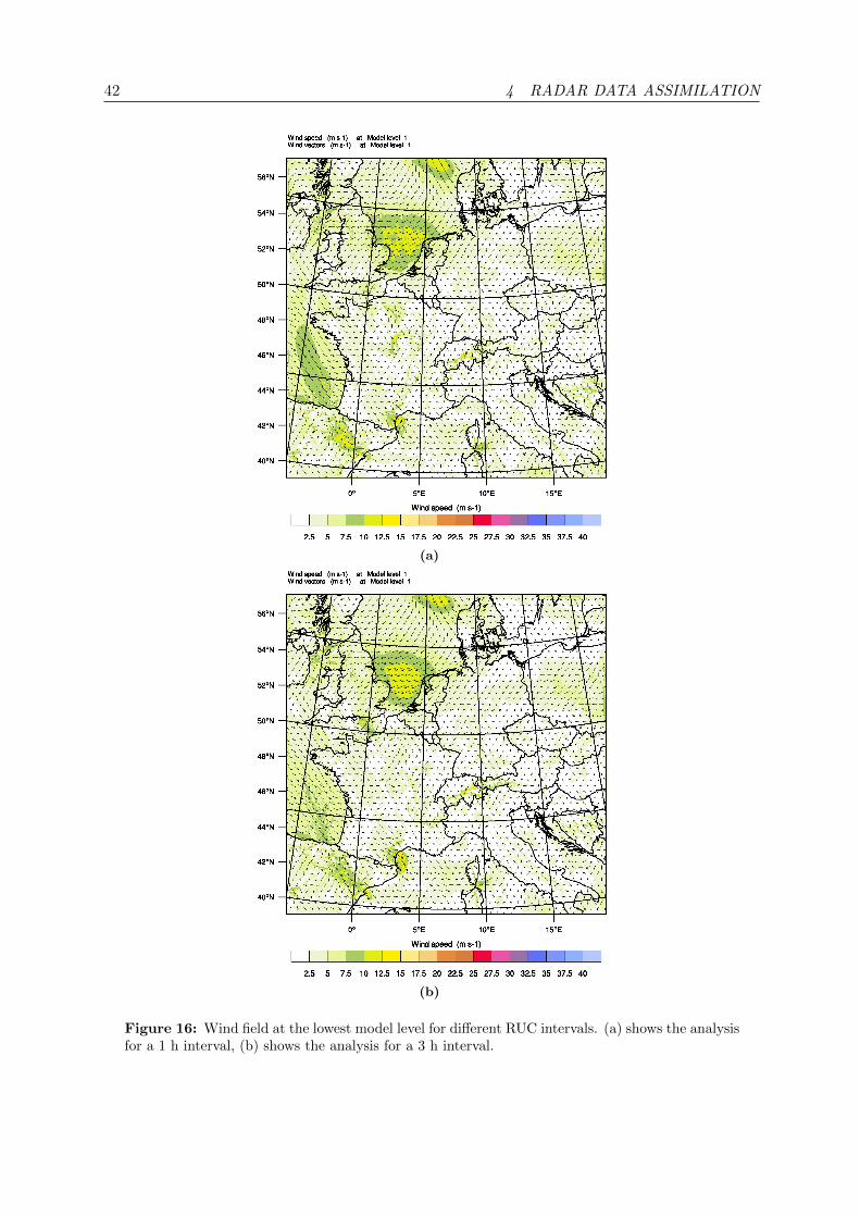
42 4 RADAR DATA ASSIMILATION
(a)
(b)
Figure 16: Wind field at the lowest model level for different RUC intervals. (a) shows the analysisfor a 1 h interval, (b) shows the analysis for a 3 h interval.
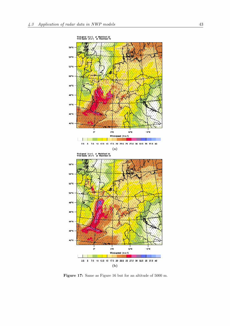
4.3 Application of radar data in NWP models 43
(a)
(b)
Figure 17: Same as Figure 16 but for an altitude of 5000 m.
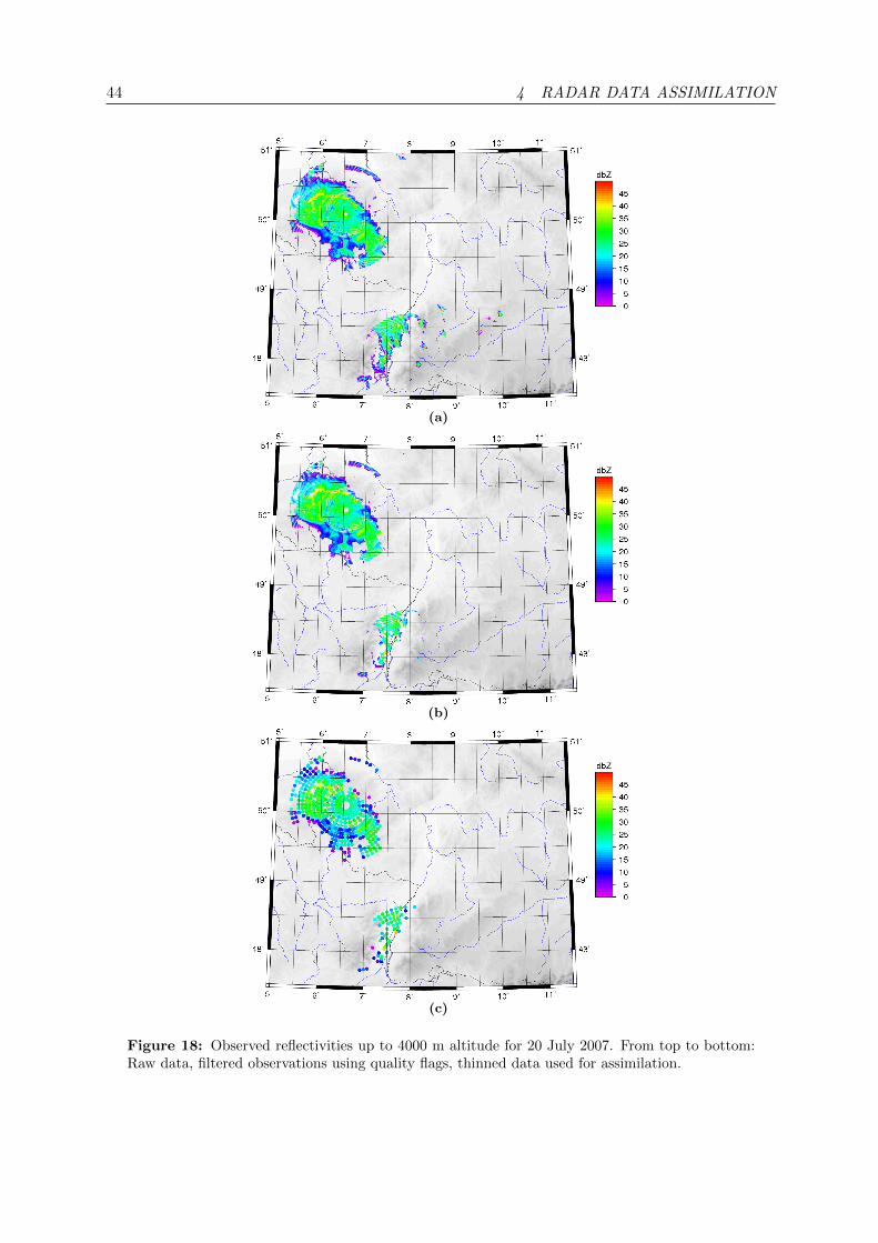
44 4 RADAR DATA ASSIMILATION
(a)
(b)
(c)
Figure 18: Observed reflectivities up to 4000 m altitude for 20 July 2007. From top to bottom:Raw data, filtered observations using quality flags, thinned data used for assimilation.

4.3 Application of radar data in NWP models 45
To partially overcome the problem of designing a reflectivity forward operator, Caumont et al.(2010) recently developed a 1DVAR scheme for radar reflectivity assimilation in the AROMEmodel. The assimilation of reflectivity is split into two parts. First the reflectivity measurementsat different elevations are split into vertical columns at one location (x,y). Afterwards, a 1DVARretrieval is performed where the difference between modeled and observed reflectivity profile isapplied as a weighting factor to the background relative humidity. The relative humidity profileis then assimilated as conventional observations.
This method is similar to latent heat nudging (e.g Schraff et al., 2006) but takes the hydrometeorbackground into account. As this method adjusts the humidity distribution, information canbe lost if the lifting condensation level (LCL) is relatively high or the moisture imbalance afterthe assimilation can be very large. Also if the relative humidity is set to 100% below the LCL,precipitation may be not able to evaporate and thus additional water vapor is missing for possiblefurther convective developments which is similar to the the PIB scheme of Milan (2009).
46 5 SUMMARY OF PUBLICATIONS
5 Summary of publications
In this chapter, brief summaries of three publications covering physics sensitivity tests withMM5 (I), the evaluation of the MM5 system operational during COPS (II), and first assimilationresults with the new WRF model (III) are given in this section.
Publication I:T. Schwitalla, H.-S. Bauer, V. Wulfmeyer und G. Zangl, 2008: Systematic errors of QPF inlow-mountain regions as revealed by MM5 simulations, Meteorol. Z., 17, 903 - 919.IF: 1.4
Publication II:H.-S. Bauer, T. Weusthoff, M. Dorninger, V. Wulfmeyer, T. Schwitalla, T. Gorgas, M. Arpa-gaus, K. Warrach-Sagi, 2010: Predictive Skill of a Subset of models that participated duringD-PHASE in the COPS Region. Q. J. R. Meteorol. Soc., 137, S1, 287-305. IF: 2.98
Publication III:T. Schwitalla, H.-S. Bauer, V. Wulfmeyer und F. Aoshima, 2010: High-resolution simulationover central Europe: Assimilation experiments during COPS IOP9c. Q. J. R. Meteorol. Soc.,137, S1, 156-175. IF: 2.98
5.1 Schwitalla et al. (2008) 47
5.1 Schwitalla et al. (2008)
In publication I, high-resolution numerical simulations were performed using the mesoscale modelMM5. The investigated area was the COPS region (Vosges Mountain, Black Forest and SwabianJura) and the focus was set on convective-induced summertime precipitation.
A representative set of 13 precipitation events for this region was chosen and simulations witha horizontal resolution of 7 km and 1 km were performed. The major finding is that the 7 kmsimulations show a strong windward-lee effect for precipitation, implying an overestimation onthe windward side with hardly any precipitation on the lee side.
Moreover precipitation occurred too early due to an incorrect simulation of the flow which isseen in averaged 850 hPa vertical velocity fields.
The high-resolution simulation with 1 km horizontal resolution, in contrast, shows a temporaldelay of ∼ 2 h in the precipitation development while the shape of the diurnal cycle is fairly wellrepresented.
To select an applicable physics configuration for an operational setup for COPS, a subset of 4 ofthese 13 cases was selected. Three different boundary layer and two different land-surface modelswere applied. In general, all configurations have problems simulating the surface humiditycorrectly showing a strong decrease during sunset probably due to a too strong mixing and havecold 2 m temperature bias during daytime.
A configuration combining a countergradient, non-local PBL scheme (that is mixing can occurnot only between adjacent model layers in one time step) with the 5-layer soil model was foundto be most successful and was finally applied for the operational model setup during COPS. Incontrast, a turbulence closure scheme (ETA-scheme) produced unrealistic results with a moistand cold bias due to an inaccurate simulation of sensible and latent heat fluxes.
Finally a comparison with GPS IWV for the 1 km domain indicated that the model overestimatedthe IWV content by about 15–20% throughout the simulation indicating a too moist boundarylayer. A possible error source seems to be the NOAH-LSM which, in combination with theMRF boundary layer scheme, predicts comparatively high latent heat fluxes and low sensibleheat fluxes.
5.2 Bauer et al. (2011a)
In publication II, a subset of the D-PHASE model ensemble has been evaluated over the COPSperiod with the main focus set on daytime precipitation in the COPS area. This model subsetalso includes the MM5 with the physics package selected in publication I.
The selected models include the operational models of DWD and the pre-operational modelsof Meteo Swiss and Meteo France and two MM5 forecasts. For the verification of the daytimeprecipitation, the gridded VERA data (Steinacker et al., 2006) and for the validation of thediurnal cycle of precipitation, surface wind and 2 m temperature from the JDC-plus data set(Dorninger et al., 2009) were employed which consists of up to 10000 surface observations overcentral Europe.
48 5 SUMMARY OF PUBLICATIONS
These observations had to be translated into a homogeneous format as every meteorologicalservice has its own data format and quality information. The second step was the reformattingto feed this data into the MET package (DTC, 2009) while doublets had to be filtered or removedto avoid falsifying the evaluation.
In general, both COSMO models with convection parameterization overestimate the daytimeprecipitation and show the well known windward-lee effect. Both MM5 models (initialized withand without a 4DVAR) show, in contrast to all other models a dry bias. It is assumed, that theposition of the inner model domain (which seems too small) and the turning-off of the cumulusscheme is the main reason for that. The 4DVAR initialized simulation slightly improves thesituation but not as much as expected.
Regarding the diurnal cycle of precipitation, both MM5 simulations show a good performancecompared to the operational models. Interestingly the 4DVAR driven MM5 shows a significantoverestimation of precipitation in the first simulation hours whereas the CONTROL experimentshows the usual cold start spin-up. The former is probably the effect of different model andassimilation packages (3.7 vs. 3.4.3). Although the assimilation is performed on 18 km resolution,the innermost domain is also affected during the forecast because of the applied 2-way nestingoption. In a further improved, unofficial version of the 4DVAR, a more complex cumulus scheme(Grell, 1993) and its adjoint was available attenuating the spin-up effect (Zus et al., 2008).
Even though applying a 4DVAR, it appears not sufficient to assimilate humidity data but touse as much observations as possible to constrain the model as much as possible. It appearsalso evident to switch to convection-resolving resolutions to avoid the necessity of a cumulusscheme for which it can be difficult to derive an adjoint code. The first attempt has been madein publication III with the WRF model.
The diurnal cycle of temperature is well simulated by all models but the 10 m wind speed isoverestimated with a positive bias of 0.5 m/s which is, in case of the MM5, caused by the MRFPBL scheme and is also (but weakly) observed in the successor scheme YSU.
5.3 Schwitalla et al. (2011)
In publication III, the impact on the forecast quality of the assimilation of conventional andGPS-ZTD observations was investigated with the WRF model for COPS IOP 9c (July 20,2007). For this purpose different experiments were carried out to investigate the influence ofassimilating different types of observations.
A high-resolution, convection resolving model set-up with a horizontal resolution of 3600 mcovering whole central Europe was designed (see the dashed rectangle in Figure 8).
The major reason for this large domain was that during D-PHASE several nested models hadproblems to simulate frontal or pre-frontal precipitation due to the fact that the front is disruptedat the boundary between the coarse outer and finer inner domain.
In such a large domain, the whole synoptic situation can completely develop inwardly of thedomain avoiding inconsistencies between different physics selections responsible for destroyingthe synoptic features. Another reason was the observed dry bias in the precipitation patterns of
5.3 Schwitalla et al. (2011) 49
the high-resolution D-PHASE models due to the switch-off of the cumulus scheme in the nesteddomain (Bauer et al., 2011a).
it is also evident that as many high quality observations as possible should be assimilatedsimultaneously (independent whether 3DVAR or 4DVAR methodology is applied) to provide anoptimal constraint of the model during the assimilation process. Due to a noticeable bias, GPSdata from France were reprocessed at the GFZ Potsdam with their EPOS software so that intotal about 330–360 GPS measurements were available every 15 minutes. A critical point wasthe estimation of the observation error for ZTD measurements. As there is hardly any expertise,we set the error to 2–3 mm which corresponds to about 1.5 mm IWV (Zus, 2010).
The first conclusion which can be drawn is that it is necessary to assimilate upper air (humidity)observations as otherwise the surface is uncoupled from the 3D atmosphere. When assimilatingGPS-ZTD observations in addition to conventional observations, small improvements in theprecipitation scores and its diurnal cycle were observed.
Also with data assimilation the simulated precipitation amounts are too high (bias ∼20%) whichalso does not change when applying the Thompson one-moment microphysics scheme. Bothmicrophysics schemes show a large amount of integrated graupel which immediately melts intorain when the ambient temperature is greater than 0 ◦C.
We also discovered a too strong mixing in the boundary layer resulting in a too large water vaporcontent before/after sunrise/sunset similar to the behavior in publication I apparently causedby too large boundary layer heights and too strong mixing during night, respectively. In themeantime, this problem was confirmed by the developer of the boundary layer scheme (Hong,personal communication) and a bug fix will be tested soon.
Compared to other operational D-PHASE models, WRF was the only one predicting the rede-velopment of the front in the lee of the black forest while e.g. COSMO-EU only produced lightwidespread precipitation. This appears to be the result of inaccurate initial conditions as WRFwas driven by ECMWF data. COSMO-EU was driven by GME and applies a FDDA scheme toimprove the initial conditions which seems to be not as good as the ECMWF analysis.
50 6 SUMMARY AND OUTLOOK
6 Summary and outlook
In this thesis, several different topics have been addressed. In the first part, a high-resolutionsetup of the mesoscale model MM5 was investigated to determine a suitable physics configurationto run an operational forecast system during COPS in 2007 and to compare a 7 km resolutionMM5 model with the operational version of the Lokal Modell (LM, predecessor of the COSMO-EU) of DWD.
Here, 13 representative convective cases of 2005 have been selected and divided into three differ-ent categories depending on the synoptic situation. Independent of the synoptic situation, both7 km resolution models show a systematic positive precipitation bias on the windward side ofthe Vosges Mountains and the Black Forest. The precipitation was initiated too early likely dueto the application of a convection parameterization and comparatively strong upward motionat 850 hpa. For the high resolution setup, it was found that the shape of the diurnal cycle ofprecipitation follows the observation except that the precipitation maximum was simulated toolate.
Additionally, a poor man’s physics ensemble was created for four of the 13 convective cases.Here, the PBL schemes and the land-surface model have been exchanged. It was found thatthe 5-layer soil model produces more realistic latent and sensible heat fluxes compared to theNOAH-LSM leading to a better representation of the diurnal cycle of the temperature wherethe simulations with the NOAH-LSM show a notable cold bias.
Comparison with soundings and GPS integrated water vapor revealed a positive bias of themodel with the different physics configurations indicating a too moist boundary layer. As thiswas state of the art at this time, the combination of the 5-layer soil model in combinationwith the MRF-PBL scheme was chosen for the operational forecasting system for COPS and D-PHASE with a slightly different nesting setup compared to the original study domain describedin Schwitalla et al. (2008).
During D-PHASE, an operational forecasting system, providing two forecasts per day, was setup with one forecast driven by the ECMWF operational model level analysis only. For thesecond forecast, an additional 4DVAR applying GPS STD data (Zus et al., 2008) was performedto especially improve the water vapor distribution in the outermost domain. The investigationfor the COPS period revealed an improvement of the water vapor field during the first six hoursof the forecast. With the assimilation, the precipitation spin-up is reduced compared to thecontrol experiment and the mean diurnal cycle fits better to the observation.
It appears that the inconsistent model physics (especially the poor convection parameterization)led to this “improvement” of the precipitation spin-up. In general, both forecasts tend tounderestimate precipitation during the day probably due to the design of the domains. Theinnermost domain with a horizontal resolution of 2 km appears to be too small to captureprecipitation events which are moving inside the domain. This behavior was also seen in severalother models which were operated during D-PHASE.
As the development of the MM5 model was suspended before the COPS experiment, the WRFmodel system was introduced as a successor of MM5 including the preparation of the correspond-ing infrastructure for case study experiments. It incorporates a new dynamical core based onthe Runge-Kutta scheme and more enhanced physics options. The NOAH-LSM is now a unified
51
version which is also applied at the National Centers for Environmental Prediction (NCEP) in itsoperational forecast system. A major step was the introduction of 2-moment cloud microphysicsschemes allowing a better representation of microphysical processes.
With the WRF model version 3.1 an assimilation experiment for the COPS IOP 9c was car-ried out. The model set up was chosen in a way that only a single domain with a horizontalresolution of 3.6 km covering whole central Europe was applied. When simulating such a largecomputational demanding area, normally a nest is placed inside the coarser domain covering theregion of interest. As this would imply that the convection parameterization is switched off inthe inner nest, undesirable effects like destruction of frontal systems can occur (see e.g. Baueret al., 2011a). Therefore this large domain with 550∗550 horizontal grid points was chosen.
Four different experiments have been conducted with this high resolution to determine theinfluence of assimilating different observations including GPS ZTD data on the analysis andforecast. This is unique in combination with the WRF model over Europe. Even the experimentwith the assimilation of surface only data shows an improvement compared to the simulationwithout data assimilation. Its performance clearly improves with the assimilation of additionalupper air observations, especially soundings. When assimilating additional GPS ZTD data, thevertical distribution of water vapor is clearly improved during the first 12 h of the forecast, butthe impact on QPF is not clearly visible. One reason can be that from ∼ 320 observationsonly ∼ 100 stations are left for the assimilation partly due to the assumption of a too smallobservation error. This error determines the weight of the observations during the assimilationprocess and will be adjusted for future experiments.
What still remains is a significant overestimation of precipitation although the IWV content ison average only slightly higher as compared to GPS observations. The 2 m dew point shows astrong increase/decrease on the morning/evening due to a too strong mixing in the PBL duringthis time. In the meantime, an improvement of the YSU scheme is available which shouldprevent this unrealistic behavior in future case study experiments. In addition, a closer lookinto the energy partitioning in the LSM has to be made. Unfortunately there are currently noarea-wide flux measurements available for the verification of the NOAH-LSM.
For the operational 4DVAR system in publication II, the 4DVAR was performed at the initialtime step with a crude matrix B which was basically the ECMWF analysis on a similar reso-lution. As this can result in an additional model spin-up (publication II), the next step is toperform the assimilation a few hours after the initialization time so that the model is balanced(which is usually determined by the 3 h or 6 h surface pressure tendency). This was done inpublication III in a simple way where the assimilation was performed 6 h after the initializationtime so that the model has enough time to adjust the dynamics and moisture fields as well ashydrometeor fields.
As this may be not enough, a recently developed Rapid Update Cycle (RUC) will be appliedin future experiments with an assimilation cycle of 3 h. It is expected that if the RUC isperformed for 12–24 h, this will lead to a better dynamical balance despite the distortion dueto the assimilation. The possible imbalance in the new initial field can be partially reduced bythe application of a digital filter removing noise with a frequency higher than a certain cutofffrequency. This can become especially important for very short-range forecasts.
It is also evident from publications II and III, that one has to select a model domain whichcovers most of the prevailing synoptic features of the region of interest. Ideally, if nested into a
52 6 SUMMARY AND OUTLOOK
global model, the selected domain has a resolution which does not require the application of aconvection scheme.
As stated earlier, the 3DVAR does not incorporate the model physics and can be regardedas a very sophisticated interpolation method. In contrast to a 4DVAR, a 3DVAR, althoughperformed in a RUC, suffers from a static background matrix B which is only a climatologicalestimate of background errors independent of which method is applied to calculate the variancesand covariances for B.
This can be resolved by the application of a 4DVAR which also starts from a static B but due tothe incorporated model physics, the assimilation and the new analysis become flow dependent.The 4DVAR additionally requires the adjoint of the (full) forecast model which is, dependingon the parameterization, impossible and thus simplified physics have to be used. The additionalamount of computing time is not negligible especially for large grid sizes as for each minimizationof the cost function the full forward and adjoint of the forecast model have to be run during theassimilation window (typically 6 h). Another possibility would be the derivation of B from aWRF ensemble which is based on the ECMWF ensemble members with the method describedby Fisher (2003).
To overcome this 4DVAR specific problem, more and more Ensemble Kalman Filters are applied.They do not require the adjoint of a forecast model but the choice of the ensemble or the ensembleinitialization, respectively, can be critical. Todays global ensemble forecast systems consist of20–50 members (e.g. GFS and ECMWF). This is sufficient on the global scale but can be notenough to represent the synoptic situation on a finer grid. For a finer scale, ∼ 100 memberscould be necessary, but this would be prohibitively expensive in terms of computing power. Itwould however, have the advantage of providing situation dependent error covariances (“errorof the day”) from the ensemble perturbations.
Therefore the hybrid approach with e.g an ETKF is more and more considered as a compromisebetween the application of a 4DVAR and an EnKF. Here ∼ 20 members could be sufficient andthe update of the ensemble perturbations is performed by applying the 3DVAR on the ensemblemean. This combines the advantages of reduced computational costs for a 3DVAR and a flowdependent background error matrix B and is subject for future research of high-resolution NWP.
As ensemble forecasting is subject for future research, the focus was set on the development ofa RUC with a convection-permitting resolution of the WRF model based on the 3DVAR. Theimportant point is, that this system includes GPS-ZTD data as well as radar radial velocities,reflectivities and satellite radiances. This system can be used in near-real time and is, to myknowledge, unique in Europe.
Another future task will be the application of polarization radar data, which allows the useof more hydrometeor distribution information, e.g. whether rain or hail is present, and thusallows a comparison with the applied microphysics scheme. If polarization data is employedin the assimilation process (independent whether 3/4DVAR or Ensemble Kalman Filter), it isbeneficial if a 2-moment cloud microphysics scheme is selected because less assumptions for theforward operator are necessary.

53
A Practical implementation of a RUC system for the WRFmodel
##!/ bin /ksh
################################################################################ This s c r i p t automatizes the whole p roce s s nece s sa ry to perform f o r e c a s t s with# the mesosca le numerica l weather p r e d i c t i o n model WRF from the preparat i on o f# the model domain and i n i t i a l f i e l d s to data a s s i m i l a t i o n , model f o r e c a s t , and# l a s t but not l e a s t to post proce s s ing , v i s u a l i z a t i o n and data t r a n s f e r .###############################################################################
############################################################# no use without permis s ion ! !#############################################################
# Author : Thomas Schw i ta l l a# I n s t i t u t e o f Phys ics and Meteorology# Unive r s i ty o f Hohenheim# Garbenstrasse 30# 70599 Stut tga r t# Germany# Email : thomas . schwita l la@uni−hohenheim . de
######################################################################### 1 . Enable/ d i s a b l e th ing s to be done########################################################################
MARS=’ f a l s e ’ # get f o r c i n g dataGEOGDATA=’ f a l s e ’ # get geog raph i ca l s t a t i c data , nece s sa ry f o r c r e a t i n g domainGEOGRID=’ f a l s e ’ # Run geogr id , c r e a t e s domainUNGRIB=’ f a l s e ’ # run ungribMETGRID=’ f a l s e ’ # run metgridFORECAST=’ true ’ # you want to make a f o r e c a s t
###############f i r s t r e s e t everyth ing##############
WRF REAL=’ f a l s e ’RUN WRF FREE=’ f a l s e ’VAR=’ f a l s e ’CYCLING=’ f a l s e ’RUN WRF=’ f a l s e ’ARWPOST=’ f a l s e ’TRANSPORT=’ f a l s e ’DELETE=’ f a l s e ’READ WRF=’ f a l s e ’NCL VAR=’ f a l s e ’NCL STAT VAR=’ f a l s e ’OBSPROC=’ f a l s e ’JDC=’ f a l s e ’TRANSPORT statistics=’ f a l s e ’
54 A PRACTICAL IMPLEMENTATION OF A RUC SYSTEM FOR THE WRF MODEL
TRANSPORT model=’ f a l s e ’PLOT RADIANCE=’ f a l s e ’USE RADIANCE=’ f a l s e ’UPDATE BDY VAR=’ f a l s e ’
###################now d e f i n e what you want##################
i f [ $FORECAST = ’ true ’ ]then
f i
##################################################################################Def ine EXPERIMENT name which i s attached to the date s t r i n g as d i r e c t o r y name#################################################################################
################################################################################## 2 . Def ine v a r i a b l e s used f o r the c a l l o f the MARS r e t r i e v a l s c r i p t s#################################################################################
# Star t and end o f f o r e c a s t . By s e t t i n g the va lue s s e p a r a t e l y i t i s l a t e r p o s s i b l e# to get them automat i ca l l y s e t with the MSJ system
DATA SOURCE=’ f o r e c a s t ’ ### i f you need boundar ies from a n a l y s i s or f o r e c a s t dataFORECAST LENGTH= # Length o f the f o r e c a s t ( hours )LAST DAY= # Last day o f f o r e c a s t i f not a monthly s t a t i s t i c s
########################### adjus t c y c l e l ength as you need i t ! ! !########################
#######################s p e c i a l f o r JDC data f o r 2007# i f JDC i s used f o r other years , the s c r i p t w i l l s top######################
#####################something may go wrong####################
################################################################################
################################################################################## c r e a t e s t a r t and stop dates f o r the WRF f o r e c a s t and a s s i m i l a t i o n#################################################################################
### Now loop over days to automatise the work######
whi le [ ${START DAY} − l e ${LAST DAY} ] ;do
# I n i t i a l date and i n i t i a l time needed by the MARS r e t r i e v a l s c r i p t s
55
# Calcu la t e STOP DATE. This was necessary , when a n a l y s i s and not f o r e c a s t datashould
# be used to f o r c e WRF
# Stop date needed when a n a l y s i s data s h a l l be used f o r the f o r c i n g
################################################################################# end o f c a l c u l a t i o n o f date s t r i n g s################################################################################# 3 . Def ine v a r i a b l e s used to f i l l the namel i s t f i l e ” name l i s t . wps”# used by the WRF pre−p r o c e s s i n g system .##******************* READ THIS CAREFULLY BEFORE YOU START! ! ! ! !****************################################################################################
MAXDOM=1 # Number o f WRF model domains
##############################################d i f f e r e n t i n t e r v a l s f o r f o r e c a s t and a n a l y s i s data############################################
i f [ ${DATA SOURCE} = ’ f o r e c a s t ’ ]thenINTERVAL SECONDS=10800 # I n t e r v a l between two f o r e c a s t t imes tepse l s eINTERVAL SECONDS=21600 # I n t e r v a l between two f o r e c a s t t imes tepsf i
######################################################domain s e t t i n g s f o r name l i s t . wps#####################################################
PARENT ID=’ 1 , 1 , 2 , 3 ’ # ID o f parent domainPARENT GRID RATIO=’ 1 , 3 , 3 , 3 ’ # gr id r a t i o between domainsI PARENT START=’ 1 , 135 , 41 , 172 ’ # X−coord ina te o f the lower l e f t cornerJ PARENT START=’ 1 , 82 , 141 , 132 ’ # Y−coord ina te o f the lower l e f t cornerS WE=’ 1 , 1 , 1 , 1 ’ # Set to ’1 ’ f o r each domainE WE=’ 550 , 250 , 367 , 160 ’ # Number o f east−west g r id po in t sS SN=’ 1 , 1 , 1 , 1 ’ # Set to ’1 ’ f o r each domainE SN=’ 550 , 271 , 271 , 160 ’ # Number o f south−north g r id po in t s
GEOG DATA RES=’ ” modis 30s+30s ” , ” modis 30s+30s ” , ” modis 30s+30s ” , ” modis 30s+30s ” ’DX=3600 # Grid r e s o l u t i o n (m) o f the outermost domainDY=3600 # Grid r e s o l u t i o n (m) o f the outermost domainMAP PROJ=lambert # Map p r o j e c t i o nREF LON=7. # Center po int l a t i t u d e o f the outermost domainREF LAT=48.9 # Center po int l ong i tude o f the outermost domainTRUELAT1=30.0 # Southern l a t i t u d e f o r Lambert p r o j e c t i o nTRUELAT2=60.0 # Northern l a t i t u d e f o r Lambert p r o j e c t i o nSTAND LON=7. # Longitude p a r a l l e l to Y−a x i s
################################################################################
56 A PRACTICAL IMPLEMENTATION OF A RUC SYSTEM FOR THE WRF MODEL
# 4 . ) Def ine v a r i a b l e s to f i l l the f i l e ” name l i s t . input ” which c o n t r o l s#the execut ion o f the programms ” r e a l . exe ” and ” wrf . exe ” .# IMPORTANT: The v a r i a b l e s a l r eady de f ined f o r WPS are r e c y c l e d################################################################################
i f [ ${DATA SOURCE} = ’ f o r e c a s t ’ ]thenANALYSIS INTERVAL=3e l s eANALYSIS INTERVAL=6f i
################################################################# Time c o n t r o l opt ions f o r the namel i s t ” namel i s t . input ”################################################################
######################################################### Domain opt ions f o r the name l i s t ” name l i s t . input ” ( not de f ined above f o r wps )#######################################################
###################################################### Phys ics opt ions ( s e l e c t i o n paramete r i za t i on s schemes ) f o r the ” namel i s t . input ”#####################################################
############################################# f o r I /O q u i l t i n g , u s e f u l f o r l a r g e domains############################################
################################################################# DEFINE OBSERVATIONS you want to use in 3DVAR################################################################
################################################################# Warning ! ! ! ! !# s e t c o r r e c t l o c a t i o n f o r GPS data f i l e b e f o r e us ing GPS−ZTD data !# max error gpsxx was s e t to 5 . 0 !# s e t max errors f o r other v a r i a b l e s l a t e r !#################################################################
USE GPSPWOBS=’ f a l s e ’ ### cannot used toge the r with ZTD!USE GPSZTDOBS=’ true ’USE BUOYOBS=’ true ’USE SYNOPOBS=’ true ’USE METAROBS=’ true ’USE SOUNDOBS=’ true ’USE AIREPOBS=’ true ’USE SHIPSOBS=’ true ’USE PROFILEROBS=’ true ’USE RADAROBS1=’ true ’ ## s c r o l l down to ad jus t f i r s t time when a s s i m i l a t i n gUSE RADAR RV=’ true ’USE RADAR RF=’ true ’CALC STD=’ f a l s e ’USE QSCATOBS=’ true ’USE GEOAMVOBS=’ true ’
57
USE SSMITBOBS=’ f a l s e ’ ### data are a v a i l a b l e , but not t e s t e d
####################################f o r rad i ance s###################################
USE TWO RADIANCE FILES=’ t rue ’i f [ ${USE RADIANCE} = ’ true ’ ]thenUSE HIRS3OBS=’ true ’USE HIRS4OBS=’ f a l s e ’USE MHSOBS=’ true ’USE AMSUAOBS=’ true ’USE AMSUBOBS=’ true ’USE AIRSOBS=’ true ’USE EOS AMSUAOBS=’ true ’USE HSBOBS=’ f a l s e ’USE SSMISOBS=’ f a l s e ’
f i##################################################################################################### From here no changes are nece s sa ry ! ! ################################################################################################################################################################################# 5 . Create working d i r e c t o r y and copy nece s sa ry f i l e s from the e c f s###############################################################################
################# Create data d i r e c t o r y and working d i r e c t o r y################
# Test whether the d i r e c t o r i e s e x i s t . Create i f not the case . This w i l l be changedin
# a way , that an e x i s t i n g d i r e c t o r y i s automat i ca l l y de l e t ed and r e c r e a t e d when# everyth ing i s working .
cd ${WRKDIR}################################################################################# 6 . Inc lude s t a r t date , end date in to the s c r i p t s that r e t r e i v e ob s e rva t i on s f o r#the data a s s i i m i l a t i o n system and a n a l y s i s f i e l d s from the MARS arch ive .################################################################################
i f [ ${MARS} = ’ true ’ ]then
f i ## f i n i s h e d with MARS
################################################################################ 7 . Pre−p r o c e s s i n g . Here , the three pre−p r o c e s s i n g s t ep s to c r e a t e the i n i t i a l# f i e l d s f o r ” r e a l . exe ” are done .###############################################################################
# Set up namel i s t ” namel i s t . wps” with the in fo rmat ion provided above .
cat > namel i s t . wps <<EOF
EOF
58 A PRACTICAL IMPLEMENTATION OF A RUC SYSTEM FOR THE WRF MODEL
################################################################################# 8 . ) Create the model domains ( us ing in fo rmat ion from ” namel i s t . wps”) .#This s tep i s only nece s sa ry when a new domain s h a l l be c rea ted .################################################################################
i f [ ${GEOGRID} = ’ true ’ ]then
f i ## f i n i s h e d geogr id
### check whether geogr id f i l e i s a l r eady a v a i l a b l e
############################################################################# 9 . ) Decode a n a l y s i s g r i b f i l e s ( us ing in fo rmat ion from ” namel i s t . wps”)############################################################################
i f [ ${UNGRIB} = ’ true ’ ]then
f i ## f i n i s h e d ungrib
############################################################################### 1 0 . ) Create m e t e o r o l o g i c a l i n i t i a l f i e l d s f o r WRF##############################################################################
i f [ ${METGRID} = ’ true ’ ]then
f i ## f i n i s h e d metgrid
############################################################################# 1 2 . ) Create name l i s t ” name l i s t . input ” used by the f i n a l p r e p r o c e s s i n g#step and the WRF f o r e c a s t############################################################################
## Change to working d i r e c t o r ycd ${WRKDIR}
## Create name l i s tcat > namel i s t . input <<EOF
EOF
################################################################################################### WRF run r e a l once at the beg inning ######################################################################################################
cd ${WRKDIR}
i f [ ${WRF REAL} = ’ true ’ ]then
f i ### f i n i s h e d REAL
###############################################################################
59
##################END of p r e p r o c e s s i n g########################################################################################################################
#######################################s t a r t f r e e f o r e c a s t be f o r e a s s i m i l a t i o n######################################
i f [ ${RUN WRF FREE} = ’ true ’ ]then
f i ### WRF RUN FREE
######################################################################### mul t ip l e c y c l i n g loop###########################################################################################################
I=00whi l e [ ${ I } − l t ${MULTIPLE} ]do
######################################### to prevent the model blowing up with radar data#### check when radar data a s s i m i l a t i o n s t a r t s ! !######################################
i f [ $ I − l e 0 ] # 0 to not a s s i m i l a t e radar data at the f i r s t c y c l e s tepthenUSE RADAROBS=’ f a l s e ’echo ”Do not want to use radarobs ”echo ”Radar−Obs= ” ${USE RADAROBS}e l s eUSE RADAROBS=${USE RADAROBS1}echo ”you want radarobs ”echo ”Radar−Obs= ” ${USE RADAROBS}f i
## f i blowing prevent
# some counter sJ=‘ expr $ I + 1 ‘K=‘ expr $J + 1 ‘
#############################c a l c u l a t i o n o f d a t e s t r i n g f o r RUC###########################
echo CYCLE YEAR $CYCLE YEARecho CYCLE MONTH $CYCLE MONTHecho CYCLE DAY $CYCLE DAYecho CYCLE HOUR $CYCLE HOUR
################################################################################# export date f o r a s s i m i l a t i o n s t a t i s t i c s l a t e r on##############################################
NCL VAR DATE=${CYCLE YEAR}${CYCLE MONTH}${CYCLE DAY}${CYCLE HOUR}
60 A PRACTICAL IMPLEMENTATION OF A RUC SYSTEM FOR THE WRF MODEL
################################################################################# OBSPROC FOR 3DVAR data a s s i m i l a t i o n################################################################################
################################################################################# c r e a t e namel i s t . 3 dvar obs with v a r i a b l e s dec l a r ed above################################################################################
i f [ $OBSPROC = ’ true ’ ]then
### s e t t imes teps nece s sa ry f o r backward t imes
##############################################Set c o r r e c t d i r e c t o r y f o r GPS DATA ! ! ! ! !############################################
############################################# f o r convent iona l data#############################################
i f t e s t −e ”${CYCLE YEAR}${CYCLE MONTH}${CYCLE DAY} b u f r . asc ”thenecho ” convent iona l obs data a l r eady there ”e l s eecp −o ec :OBS DATA/${CYCLE YEAR}${CYCLE MONTH}${CYCLE DAY} b u f r . asc . gz .gunzip −f ${CYCLE YEAR}${CYCLE MONTH}${CYCLE DAY} b u f r . asc . gz
f i
OBSFILE=${CYCLE YEAR}${CYCLE MONTH}${CYCLE DAY}${CYCLE HOUR} b u f r . asc
############################# copying obs f i l e s f i n i s h e d########################
### d e l e t e f i l e s that are not nece s sa ry any more
### copy a l l nece s sa ry binary f i l e s f o r OBSPROC from ECFS
### c a l c u l a t e r e s o l u t i o n in km from DX
### Create name l i s t f o r obsproc####
cat > namel i s t . obsproc <<EOF
EOF
# execute obsproc. / obsproc . exe
f i # obsproc
##############################################################################################################################################################
61
# BEGIN OF 3DVAR##############################################################################################################################################################
i f [ ${VAR} = ’ true ’ ] # you want to run a 3DVAR f i r s tthen
## copy or l i n k the nece s sa ry f i l e s to 3DVARDIR
###############################neces sa ry f o r v e r s i on e a r l i e r than 3 .3#############################
cd $VARDIR
### copy or l i n k the nece s sa ry f i l e s to 3DVARDIR once
### l i n k and copy the nece s sa ry f i l e s f o r 3DVAR
cp $WRKDIR/ wr f 3dvar input d01 $ {CYCLE YEAR}−${CYCLE MONTH}−${CYCLE DAY} $ {CYCLE HOUR} : 0 0 : 0 0 fg
ln −s f $VARDIR/ o b s g t s $ {CYCLE YEAR}−${CYCLE MONTH}−${CYCLE DAY} $ {CYCLE HOUR} : 0 0 : 0 0 . 3DVAR ob . a s c i i
# use o f SSMI/T data
## copy background matrix from ECFSecp −o ec : be 3600m 550 550 50 . dat be . dat
################################### c r e a t e namel i s t . input f o r 3DVAR##################################
## c r e a t e namel i s t f o r wrfvarcat > namel i s t . input <<EOF
EOF
#########################################need a new wrfbdy f i l e f o r 3DVAR and f o r e c a s t a f t e rwards#update low boundary be f o r e 3DVAR otherwi se DFI w i l l not work a f t e r a s s i m i l a t i o n#######################################i f [ ${UPDATE BDY VAR} = ’ true ’ ]then
cat > namel i s t . i n p u t i n s i d e r u c f o r b d y <<EOF
EOF
### s t a r t r e a l . exe at f i r s t
#copy new wrfbdy to 3DVAR d i r e c t o r ycp wrfbdy d01 $VARDIR
f i ## update bdy be f o r e 3DVAR
###################################################
62 A PRACTICAL IMPLEMENTATION OF A RUC SYSTEM FOR THE WRF MODEL
# c r e a t e parame . in f o r updating boundary c o n d i t i o n s be f o r e 3DVAR##################################################
cat > parame . in <<EOF
EOF# run da update bc
# end o f update low BC
## f o r s a f e t y remove some rad iance f i l e s , o the rw i s e p l o t s can be s t range . . .rm −r f 01 oma* 01 inv * ${VARDIR}/ diag /${NCL VAR DATE}
# f o r radar datai f [ ${USE RADAROBS} = ’ true ’ ]then
i f [ $? −ne 0 ]thenecho ” copying o f radar data f a i l e d f o r date ” ${NCL VAR DATE}e x i t 1f iln −s f ob . r a d a r a l l $ {NCL VAR DATE} . asc ob . radarf i
###### f i radar data
######################################## some preparat i on s t ep s f o r rad i ance s####################################
i f [ ${USE RADIANCE} = ’ true ’ ]then
i f t e s t −d ” rt tov10 ”then
echo ”RTTOV already there ”e l s eecho ”RTTOV has to be copied at f i r s t ”
f if i
# copy nece s sa ry a t a t i c f i l e s oncei f [ [ ${USE RADIANCE} = ’ true ’ && $ I − l e 0 ] ]then
f i
i f [ ${USE RADIANCE} = ’ true ’ ]then
mkdir −p ${VARDIR}/ diag /${NCL VAR DATE}
# check i f r a d i a t i o n data i s a l r eady a v a i l a b l ei f t e s t −e ”${CYCLE YEAR}${CYCLE MONTH}${CYCLE DAY}1bamua . ta r ”then
echo ”AMSUA already there ”e l s e
63
ecp −o ec :OBS DATA/RADIANCES/1bamua . ${CYCLE YEAR}${CYCLE MONTH}${CYCLE DAY} . t a r .gz .
gunzip −f 1bamua . ${CYCLE YEAR}${CYCLE MONTH}${CYCLE DAY} . t a r . gzta r −xvf 1bamua . ${CYCLE YEAR}${CYCLE MONTH}${CYCLE DAY} . t a r
f i
## remove f i l e l i n k s f i r s t to prevent double ob s e rva t i on s in a s s i m i l a t i o n ! !rm −r f *01 . bufr *02 . bufr
i f [ ${CYCLE HOUR} = 00 ]then
ln −s f ${CYCLE YEAR}${CYCLE MONTH}${CYCLE DAY} . 1 bamua/*00 z* amsua01 . bufrln −s f ${CYCLE YEAR}${CYCLE MONTH}${CYCLE DAY} . 1bamub/*00 z* amsub01 . bufrln −s f ${CYCLE YEAR}${CYCLE MONTH}${CYCLE DAY} . 1 bhrs3 /*00 z* h i r s 301 . bufrln −s f ${CYCLE YEAR}${CYCLE MONTH}${CYCLE DAY} . 1 bmhs/*00 z* mhs01 . bufrln −s f a i r s o b s . ${CYCLE YEAR}${CYCLE MONTH}${CYCLE DAY}/*00 z* a i r s e v * a i r s 0 1 . bufr
# t e s t i f f i l e s are the re f o r the next dayi f t e s t −e ” gda sa i r s ob s . ${CYCLE YEAR2}${CYCLE MONTH2}${CYCLE DAY2} . t a r ”then
echo ”AIRS f o r day 2 a l r eady there ”e l s eecp −o ec :OBS DATA/RADIANCES/ gdasa i r s ob s . ${CYCLE YEAR2}${CYCLE MONTH2}${
CYCLE DAY2} . t a r . gz .gunzip −f gda sa i r s ob s . ${CYCLE YEAR2}${CYCLE MONTH2}${CYCLE DAY2} . t a r . gzta r −xvf gda sa i r s ob s . ${CYCLE YEAR2}${CYCLE MONTH2}${CYCLE DAY2} . t a r
f if i
f i###### f i rad i ance s
############################################# now run WRF 3DVAR i n s i d e the RUC############################################
## remove c e r t a i n f i l e srm −f c o s t f n grad fn f o r t . 21
# search f o r f a i l u r egrep − i completed r s l . out .0000i f [ $? != 0 ]thenecho ”3DVAR f a i l e d ” > mail messagee x i t 1f i
### f i run 3DVAR
##############################v a r i a t i o n a l b i a s c o r r e c t i o n f o r rad iance s############################
i f [ ${USE RADIANCE} = ’ true ’ ]thencp VARBC. in VARBC. i n $ {NCL VAR DATE}cp VARBC. out VARBC. out $ {NCL VAR DATE}mv VARBC. out VARBC. in
64 A PRACTICAL IMPLEMENTATION OF A RUC SYSTEM FOR THE WRF MODEL
f i
#backup f i l e scp radar omb oma 01 radar omb oma 01 ${NCL VAR DATE}cp gts omb oma 01 gts omb oma 01 ${NCL VAR DATE}cp f i l t e r e d o b s 0 1 f i l t e r e d o b s 0 1 $ {NCL VAR DATE}cp wrfvar output wr fvar output $ {NCL VAR DATE} . nc
############################################## update l a t e r a l boundary c o n d i t i o n s a f t e r 3DVAR########################################
### c r e a t e parame . in f o r updating l a t e r a l boundary c o n d i t i o n s
cp −f $WRKDIR/ wrf input d01 .
cat > parame . in <<EOF
EOF
# run update o f BC c o n d i t i o n sgrep s u c c e s s f u l l y update l a t bdy $ {NCL VAR DATE} . tx ti f [ $? −ne 0 ]thenecho ”update bc a f t e r 3DVAR f a i l e d , e x i t i n g ”echo ”update bc f a i l e d ” > mail message/ usr / bin / mail −s ”update bc a f t e r ” thomas . schwita l la@uni−hohenheim . de <
mail messagee x i t 1f i
f i # end o f 3DVAR
############################################################################################################################################################### END OF 3DVAR##############################################################################################################################################################
##################################### make a s s i m i l a t i o n s t a t i s t i c p l o t s us ing d e f a u l t NCL s c r i p t s . . . . .##########################################
i f [ ${NCL VAR} = ’ true ’ ]then
#######################i f [ ${NCL STAT VAR} = ’ true ’ ]then
# make some h o r i z o n t a l p l o t s
i f [ ${PLOT HORIZONTAL} = ’ true ’ ]then
echo ” f i n i s h e d h o r i z o n t a l p l o t s at ”
65
datef i
# f o r p l o t t i n g rad iance s t a t i s t i c si f [ [ ${USE RADIANCE} = ’ true ’ && ${PLOT RADIANCE} = ’ true ’ ] ]then
f i
######################################### make an arch ive#######################################
#transpor t s t a t i s t i c s f i l e to UHOHi f [ $TRANSPORT statistics = ’ t rue ’ ]then
f i #### transpor t
f i # f i n i s h e d s t a t i s t i c s###################################### end o f NCL a s s i m i l a t i o n s t a t i s t i c s##################################
## change back to WRKDIRcd ${WRKDIR}
############################################# a f t e r the 3dvar i s f i n i s h e d s t a r t f o r e c a s t from a wrf input f i l e########################################
############################################### Create name l i s t f o r warm s t a r t a f t e r a a s s i m i l a t a i o n############################################
cat > namel i s t . input warm <<EOF
EOF
############################################################# s t a r t s f o r e c a s t a f t e r a s s i m i l a t i o n in RUC mode#############################################################
i f [ [ ${RUN WRF} = ’ true ’ && ${ I } − l t $ ( expr ${MULTIPLE} − 1) ] ]then
echo CYCLE NUMBER $ I ”+1”
#### f i n i s h e d WRF with in RUC
f i # f i n i s h e d WRF f o r e c a s t i n s i d e RUC
I=‘ expr $ I + 1 ‘
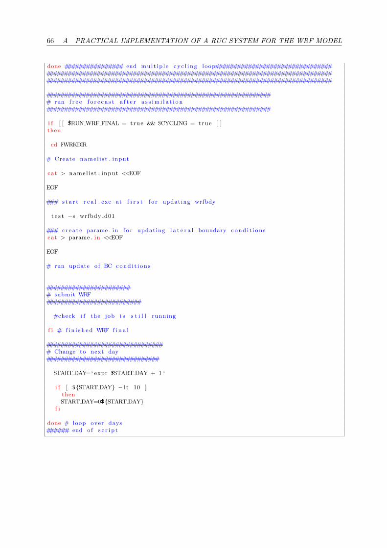
66 A PRACTICAL IMPLEMENTATION OF A RUC SYSTEM FOR THE WRF MODEL
done ################ end mul t ip l e c y c l i n g loop##############################################################################################################################################################################################
############################################################### run f r e e f o r e c a s t a f t e r a s s i m i l a t i o n##############################################################
i f [ [ $RUN WRF FINAL = true && $CYCLING = true ] ]then
cd $WRKDIR
# Create name l i s t . input
cat > namel i s t . input <<EOF
EOF
### s t a r t r e a l . exe at f i r s t f o r updating wrfbdy
t e s t −s wrfbdy d01
### c r e a t e parame . in f o r updating l a t e r a l boundary c o n d i t i o n scat > parame . in <<EOF
EOF
# run update o f BC c o n d i t i o n s
######################## submit WRF##########################
#check i f the job i s s t i l l running
f i # f i n i s h e d WRF f i n a l
################################# Change to next day###############################
START DAY=‘ expr $START DAY + 1 ‘
i f [ ${START DAY} − l t 10 ]thenSTART DAY=0${START DAY}
f i
done # loop over days###### end o f s c r i p t
REFERENCES 67
References
Baldauf, M., J. Forstner, S. Klink, T. Reinhardt, C. Schraff, A. Seifert and K. Stephan, 2009:Kurze Beschreibung des Lokal-Modells Kurzestfrist COSMO-DE (LMK) und seiner Daten-banken auf dem Datenserver des DWD. Technical report, DWD, Offenbach, Germany.
Barker, D. M., Y.-R. Guo, W. Huang and A. Bourgeois, 2003: The three-dimensional variational (3DVAR) data assimilation system for the use withMM5. Technical Report TN-453+STR, NCAR, Boulder/CO. available athttp://www.mmm.ucar.edu/mm53dvar/docs/3DVARTechDoc.pdf.
Barker, D. M., W. Huang, G. Y.-R. and Q. N. Xiao, 2004: A three-dimensional variational(3DVAR) data assimilation system for MM5. Implementation and initial results. Mon. Wea.Rev., 132, 897–914.
Bauer, H.-S., T. Weusthoff, M. Dorninger, V. Wulfmeyer, T. Schwitalla, T. Gorgas, M. Arpagausand K. Warrach-Sagi, 2011a: Predictive skill of a subset of models participating in D-PHASEin the COPS region. Q. J. R. Meteorol. Soc., 137, S1, 287–305.
Bauer, H.-S., F. Zus, V. Wulfmeyer, T. Schwitalla, M. Grzeschik, G. Dick and M. Bender, 2011b:Operational assimilation of GPS slant path delay measurements into the MM5 4DVAR system.Tellus A, 63, 263–282.
Bech, J., B. Codina, J. Lorente and D. Bebbington, 2003: The Sensitivity of Single PolarizationWeather Radar Beam Blockage Correction to Variability in the Vertical Refractivity Gradient.J. Atmos. Oceanic Technol., 20, 845–855.
Bender, M., G. Dick, T. Schmidt, S. Song, G. Gendt, M. Ge and M. Rothacher, 2008: Validationof GPS slant delays using water vapour radiometers and weather models. Meterol. Z., 17,807–812.
Bender, M., G. Dick, J. Wickert, M. Ramatschi, M. Ge, G. Gendt, A. Rothacher, M. Raabeand G. Tetzlaff, 2009: Estimates of the information provided by GPS slant data observed inGermany regarding tomographic applications. J. Geophys. Res., 114, D06303, 11pp.
Berre, L., 2000: Estimation of synoptic and mesoscale forecast error covariances in a limited-areamodel. Mon. Wea. Rev., 128, 644–667.
Bevis, M., S. Businger, T. A. Herring, R. A. Anthes, C. Rocken and R. H. Ware, 1994: GPSMeteorology: Mapping Zenith Wet Delays onto Precipitable Water. J. Appl. Meteor., 33,379–386.
Bevis, M., S. Businger, T. A. Herring, R. A. Anthes and R. H. Ware, 1992: GPS Meteorol-ogy: Remote Sensing of Atmospheric Water Vapor Using the Global Positioning System. J.Geophys. Res., 97, 15787–15801.
Bishop, C., E. B. J. and S. J. Majumdar, 2001: Adaptive sampling with the ensemble transformKalman filter. Part I: Theoretical aspects. Mon. Wea. Rev., 129, 420–436.
Bouttier, F., 2007: AROME, avenir de la prevision regionale. La Meteorologie, 58, 12–20.
68 REFERENCES
Bouttier, F. and P. Courtier, 1999: Data assimilation concepts and methods. Technical re-port, Meteorological Training Course Lecture Series, ECMWF, European Center for MediumRange Weather Forecasting, Reading, UK. available online on: http://www.ecmwf.int/
newsevents/training/rcourse_notes/DATA_ASSIMILATION/index.html.
Caumont, O., V. Ducroq, E. Wattrelot, G. Jaubert and S. Pradier-Vabre, 2010: 1D+3DVarassimilation of radar reflectivity data: a proof of concept. Tellus A, 62, 173–187.
Chen, Y., F. Weng, Y. Han and Q. Liu, 2008: Validation of the community radiative transfermodel (CRTM) by using CloudSat Data. J. Geophys.Res., 113, 15pp.
Courtier, P., 1997: Dual formulation of four-dimensional variational assimilation. Q. J. R.Meteorol. Soc., 123, 2449–2461.
Courtier, P., E. Andersson, W. Heckley, J. Pailleux, D. Vasiljevic, A. Hamruth, A. Hollingsworth,F. Rabier and M. Fisher, 1998: The ECMWF implementation of three dimensional variationalassimilation (3DVAR). I: Formulation. Q. J. R. Meteorol. Soc., 124, 1783–1807.
Dorninger, M., T. Gorgas, T. Schwitalla, M. Arpagaus, M. Rotach and V. Wulfmeyer, 2009:Joint D-PHASE-COPS data set (JDC data set). Technical report, University of Vienna/Uni-versity of Hohenheim/Meteo Swiss.
Douville, H., P. Viterbo, J. F. Mahfouf and A. C. M. Beljars, 2001: Evaluation of the optimuminterpolation and nudging techniques for soil moisture analysis using FIFE data. Mon. Wea.Rev., 128, 1733–1756.
Doviak, R. and D. Zrnic, 1993: Doppler Radar and Weather Observations. Academic Press,,2nd edition.
DTC, 2009: MET: Version 2.0 Model Evaluation Tools User’s Guide. http://www.dtcenter.
org/met/users/docs/overview.php.
Ek, M. B., K. E. Mitchell, Y. Lin, E. Rogers, P. Grummann., V. Koren, G. Gayno and J. D.Tarpley, 2003: Implementation of NOAH land surface model advances in the National Centersfor Environmental Prediction operational Mesoscale Eta Model. J. Geophys. Res., 108, D22.
Ereesma, R. and H. Jarvinen, 2006: An observation operator for ground-based GPS slant delays.Tellus, 58A, 131–140.
EUMETSAT, 2009: MSG Meteorological Products Extraction Facility Algorithm SpecificationDocument. Technical report, EUMETSAT, Darmstadt, Germany.
Evensen, G., 1994: Sequential data assimilation with a nonlinear quasi-geostrophic model usingMonte Carlo methods to forecast error statistics. J. Geophys. Res., 99, 10143–10162.
Evensen, G., 2003: The ensemble Kalman filter: theoretical formulation and practical imple-mentation. Ocean Dynamics, 53, 343–367.
Fisher, M., 2003: Background error covariance modeling. In: Seminar on Recent Developmentin Data Assimilation for Atmosphere and Ocean, pp. 45–63. ECMWF.
REFERENCES 69
Gallus, W. A. J. and M. Pfeiffer, 2008: Intercomparison of simulations using 5 WRF micro-physical schemes with dual-Polarization data for a German squall line. Adv. Geosc., 16,109–116.
Gendt, G., G. Dick, C. Reigber, M. Tomassini, Y. Liu and M. Ramatschi, 2004: Near Real TimeGPS Water Vapor Monitoring for Numerical Weather Prediction in Germany. J. Meteor. Soc.Jpn., 82, 1B, 361–370.
Golub, G. H. and C. F. Van Loan, 1996: Matrix Computations. Johns Hopkins University Press,3rd edition.
Gourley, J. J. and C. Calvert, 2003: Automated Detection of the Bright Band Using WSR-88DData. Wea. Forecasting, 18, 585–599.
Grell, G., 1993: Prognostic evaluation of assumptions used by cumulus parameterizations. Mon.Wea. Rev., 121, 764–787.
Grell, G. A., J. Dudhia and R. R. Stauffer, 1995: A description of the fifth-generation PennState/NCAR mesoscale model (MM5). NCAR technical Note TN-398+STR, NCAR, Boul-der/CO. 122pp.
Haase, G., 2002: A physical initialization algorithm for non-hydrostatic weather predictionmodels using radar derived rain rates. Ph.D. thesis, University of Bonn.
Hager, W. W., 1989: Updating the inverse of a matrix. SIAM Review, 31, 221–239.
Helmert, K., T. Hengstebeck and J. Seltmann, 2008: DWD s operational toolto enhance radar data quality. Extended abstract. ERAD 2008, Helsinki.http://erad2008.fmi.fi/proceedings/extended/erad2008-0083-extended.pdf.
Hengstenbeck, T., K. Helmert and J. Seltmann, 2010: RadarQS - a standard quality con-trol software for radar data at DWD. Extended abstract. ERAD 2010, Sibiu. http:
//www.erad2010.org/pdf/POSTER/03_Quality/05_ERAD2010_0318_modificat.pdf.
Hofmann-Wellenhof, B., H. Lichtenegger and J. Collins, 1997: GPS: Theory and Practice.Springer, 4th edition.
Holleman, I. and H. Beekhuis, 2003: Analysis and Correction of Dual PRF Velocity Data. J.Atmos. Oceanic Technol., 20, 443–453.
Hollinger, J., 1989: DMSP Special Sensor Microwave/Imager Calibration/Validation. Vol. 1.Final rep., Naval Research Laboratory. 153pp.
Hong, S.-Y., Y. Noh and J. Dudhia, 2006: A new vertical diffusion package with an explicittreatment of entrainment processes. Mon. Wea. Rev.,, 134, 2318–2341.
Huang, X. Y., Q. Xiao, D. M. Barker, X. Zhang, J. Michalakes, W. Huang, T. Henderson,J. Brey, Y. Chen, Z. Ma, J. Dudhia, Y. Guo, X. Zhang, D. J. Won, H. C. Lin and Y. H. Kuo,2009: Four-Dimensional Variational Data Assimilation for WRF: Formulation and Prelimi-nary Results. Mon. Wea. Rev., 137, 299–314.
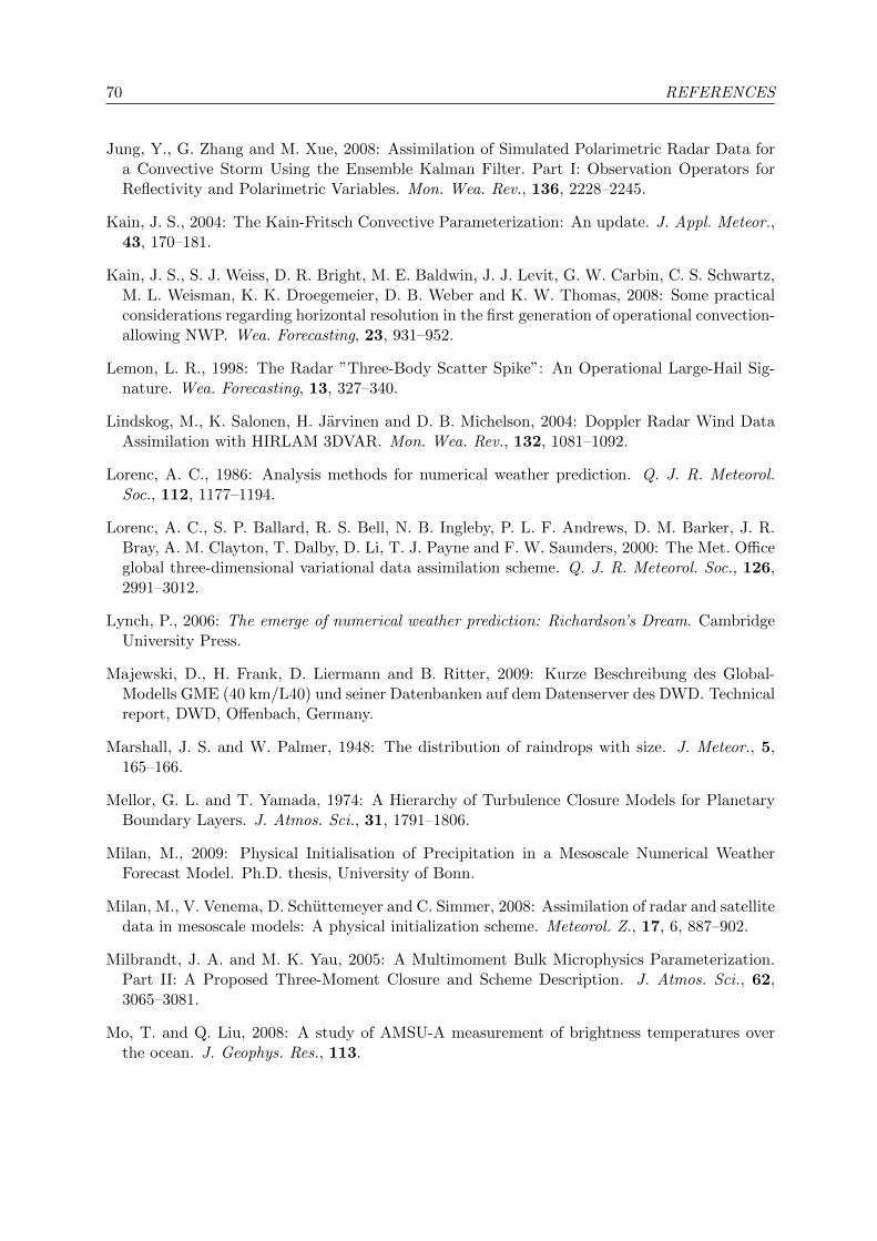
70 REFERENCES
Jung, Y., G. Zhang and M. Xue, 2008: Assimilation of Simulated Polarimetric Radar Data fora Convective Storm Using the Ensemble Kalman Filter. Part I: Observation Operators forReflectivity and Polarimetric Variables. Mon. Wea. Rev., 136, 2228–2245.
Kain, J. S., 2004: The Kain-Fritsch Convective Parameterization: An update. J. Appl. Meteor.,43, 170–181.
Kain, J. S., S. J. Weiss, D. R. Bright, M. E. Baldwin, J. J. Levit, G. W. Carbin, C. S. Schwartz,M. L. Weisman, K. K. Droegemeier, D. B. Weber and K. W. Thomas, 2008: Some practicalconsiderations regarding horizontal resolution in the first generation of operational convection-allowing NWP. Wea. Forecasting, 23, 931–952.
Lemon, L. R., 1998: The Radar ”Three-Body Scatter Spike”: An Operational Large-Hail Sig-nature. Wea. Forecasting, 13, 327–340.
Lindskog, M., K. Salonen, H. Jarvinen and D. B. Michelson, 2004: Doppler Radar Wind DataAssimilation with HIRLAM 3DVAR. Mon. Wea. Rev., 132, 1081–1092.
Lorenc, A. C., 1986: Analysis methods for numerical weather prediction. Q. J. R. Meteorol.Soc., 112, 1177–1194.
Lorenc, A. C., S. P. Ballard, R. S. Bell, N. B. Ingleby, P. L. F. Andrews, D. M. Barker, J. R.Bray, A. M. Clayton, T. Dalby, D. Li, T. J. Payne and F. W. Saunders, 2000: The Met. Officeglobal three-dimensional variational data assimilation scheme. Q. J. R. Meteorol. Soc., 126,2991–3012.
Lynch, P., 2006: The emerge of numerical weather prediction: Richardson’s Dream. CambridgeUniversity Press.
Majewski, D., H. Frank, D. Liermann and B. Ritter, 2009: Kurze Beschreibung des Global-Modells GME (40 km/L40) und seiner Datenbanken auf dem Datenserver des DWD. Technicalreport, DWD, Offenbach, Germany.
Marshall, J. S. and W. Palmer, 1948: The distribution of raindrops with size. J. Meteor., 5,165–166.
Mellor, G. L. and T. Yamada, 1974: A Hierarchy of Turbulence Closure Models for PlanetaryBoundary Layers. J. Atmos. Sci., 31, 1791–1806.
Milan, M., 2009: Physical Initialisation of Precipitation in a Mesoscale Numerical WeatherForecast Model. Ph.D. thesis, University of Bonn.
Milan, M., V. Venema, D. Schuttemeyer and C. Simmer, 2008: Assimilation of radar and satellitedata in mesoscale models: A physical initialization scheme. Meteorol. Z., 17, 6, 887–902.
Milbrandt, J. A. and M. K. Yau, 2005: A Multimoment Bulk Microphysics Parameterization.Part II: A Proposed Three-Moment Closure and Scheme Description. J. Atmos. Sci., 62,3065–3081.
Mo, T. and Q. Liu, 2008: A study of AMSU-A measurement of brightness temperatures overthe ocean. J. Geophys. Res., 113.
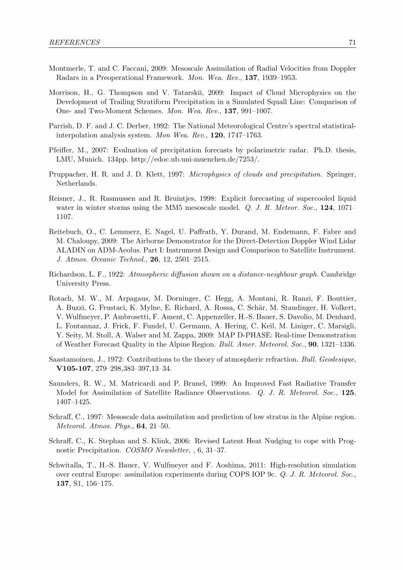
REFERENCES 71
Montmerle, T. and C. Faccani, 2009: Mesoscale Assimilation of Radial Velocities from DopplerRadars in a Preoperational Framework. Mon. Wea. Rev., 137, 1939–1953.
Morrison, H., G. Thompson and V. Tatarskii, 2009: Impact of Cloud Microphysics on theDevelopment of Trailing Stratiform Precipitation in a Simulated Squall Line: Comparison ofOne- and Two-Moment Schemes. Mon. Wea. Rev., 137, 991–1007.
Parrish, D. F. and J. C. Derber, 1992: The National Meteorological Centre’s spectral statistical-interpolation analysis system. Mon Wea. Rev., 120, 1747–1763.
Pfeiffer, M., 2007: Evaluation of precipitation forecasts by polarimetric radar. Ph.D. thesis,LMU, Munich. 134pp. http://edoc.ub.uni-muenchen.de/7253/.
Pruppacher, H. R. and J. D. Klett, 1997: Microphysics of clouds and precipitation. Springer,Netherlands.
Reisner, J., R. Rasmussen and R. Bruintjes, 1998: Explicit forecasting of supercooled liquidwater in winter storms using the MM5 mesoscale model. Q. J. R. Meteor. Soc., 124, 1071–1107.
Reitebuch, O., C. Lemmerz, E. Nagel, U. Paffrath, Y. Durand, M. Endemann, F. Fabre andM. Chaloupy, 2009: The Airborne Demonstrator for the Direct-Detection Doppler Wind LidarALADIN on ADM-Aeolus. Part I: Instrument Design and Comparison to Satellite Instrument.J. Atmos. Oceanic Technol., 26, 12, 2501–2515.
Richardson, L. F., 1922: Atmospheric diffusion shown on a distance-neighbour graph. CambridgeUniversity Press.
Rotach, M. W., M. Arpagaus, M. Dorninger, C. Hegg, A. Montani, R. Ranzi, F. Bouttier,A. Buzzi, G. Frustaci, K. Mylne, E. Richard, A. Rossa, C. Schar, M. Staudinger, H. Volkert,V. Wulfmeyer, P. Ambrosetti, F. Ament, C. Appenzeller, H.-S. Bauer, S. Davolio, M. Denhard,L. Fontannaz, J. Frick, F. Fundel, U. Germann, A. Hering, C. Keil, M. Liniger, C. Marsigli,Y. Seity, M. Stoll, A. Walser and M. Zappa, 2009: MAP D-PHASE: Real-time Demonstrationof Weather Forecast Quality in the Alpine Region. Bull. Amer. Meteorol. Soc., 90, 1321–1336.
Saastamoinen, J., 1972: Contributions to the theory of atmospheric refraction. Bull. Geodesique,V105-107, 279–298,383–397,13–34.
Saunders, R. W., M. Matricardi and P. Brunel, 1999: An Improved Fast Radiative TransferModel for Assimilation of Satellite Radiance Observations. Q. J. R. Meteorol. Soc., 125,1407–1425.
Schraff, C., 1997: Mesoscale data assimilation and prediction of low stratus in the Alpine region.Meteorol. Atmos. Phys., 64, 21–50.
Schraff, C., K. Stephan and S. Klink, 2006: Revised Latent Heat Nudging to cope with Prog-nostic Precipitation. COSMO Newsletter, , 6, 31–37.
Schwitalla, T., H.-S. Bauer, V. Wulfmeyer and F. Aoshima, 2011: High-resolution simulationover central Europe: assimilation experiments during COPS IOP 9c. Q. J. R. Meteorol. Soc.,137, S1, 156–175.
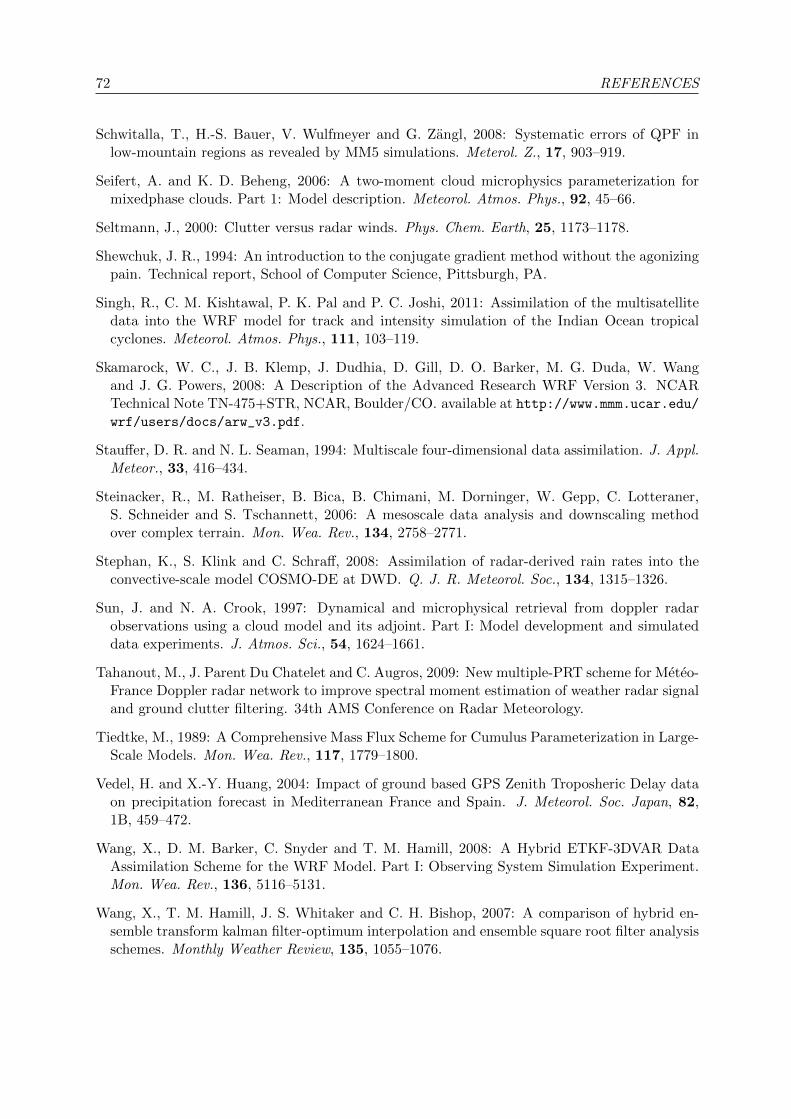
72 REFERENCES
Schwitalla, T., H.-S. Bauer, V. Wulfmeyer and G. Zangl, 2008: Systematic errors of QPF inlow-mountain regions as revealed by MM5 simulations. Meterol. Z., 17, 903–919.
Seifert, A. and K. D. Beheng, 2006: A two-moment cloud microphysics parameterization formixedphase clouds. Part 1: Model description. Meteorol. Atmos. Phys., 92, 45–66.
Seltmann, J., 2000: Clutter versus radar winds. Phys. Chem. Earth, 25, 1173–1178.
Shewchuk, J. R., 1994: An introduction to the conjugate gradient method without the agonizingpain. Technical report, School of Computer Science, Pittsburgh, PA.
Singh, R., C. M. Kishtawal, P. K. Pal and P. C. Joshi, 2011: Assimilation of the multisatellitedata into the WRF model for track and intensity simulation of the Indian Ocean tropicalcyclones. Meteorol. Atmos. Phys., 111, 103–119.
Skamarock, W. C., J. B. Klemp, J. Dudhia, D. Gill, D. O. Barker, M. G. Duda, W. Wangand J. G. Powers, 2008: A Description of the Advanced Research WRF Version 3. NCARTechnical Note TN-475+STR, NCAR, Boulder/CO. available at http://www.mmm.ucar.edu/wrf/users/docs/arw_v3.pdf.
Stauffer, D. R. and N. L. Seaman, 1994: Multiscale four-dimensional data assimilation. J. Appl.Meteor., 33, 416–434.
Steinacker, R., M. Ratheiser, B. Bica, B. Chimani, M. Dorninger, W. Gepp, C. Lotteraner,S. Schneider and S. Tschannett, 2006: A mesoscale data analysis and downscaling methodover complex terrain. Mon. Wea. Rev., 134, 2758–2771.
Stephan, K., S. Klink and C. Schraff, 2008: Assimilation of radar-derived rain rates into theconvective-scale model COSMO-DE at DWD. Q. J. R. Meteorol. Soc., 134, 1315–1326.
Sun, J. and N. A. Crook, 1997: Dynamical and microphysical retrieval from doppler radarobservations using a cloud model and its adjoint. Part I: Model development and simulateddata experiments. J. Atmos. Sci., 54, 1624–1661.
Tahanout, M., J. Parent Du Chatelet and C. Augros, 2009: New multiple-PRT scheme for Meteo-France Doppler radar network to improve spectral moment estimation of weather radar signaland ground clutter filtering. 34th AMS Conference on Radar Meteorology.
Tiedtke, M., 1989: A Comprehensive Mass Flux Scheme for Cumulus Parameterization in Large-Scale Models. Mon. Wea. Rev., 117, 1779–1800.
Vedel, H. and X.-Y. Huang, 2004: Impact of ground based GPS Zenith Troposheric Delay dataon precipitation forecast in Mediterranean France and Spain. J. Meteorol. Soc. Japan, 82,1B, 459–472.
Wang, X., D. M. Barker, C. Snyder and T. M. Hamill, 2008: A Hybrid ETKF-3DVAR DataAssimilation Scheme for the WRF Model. Part I: Observing System Simulation Experiment.Mon. Wea. Rev., 136, 5116–5131.
Wang, X., T. M. Hamill, J. S. Whitaker and C. H. Bishop, 2007: A comparison of hybrid en-semble transform kalman filter-optimum interpolation and ensemble square root filter analysisschemes. Monthly Weather Review, 135, 1055–1076.
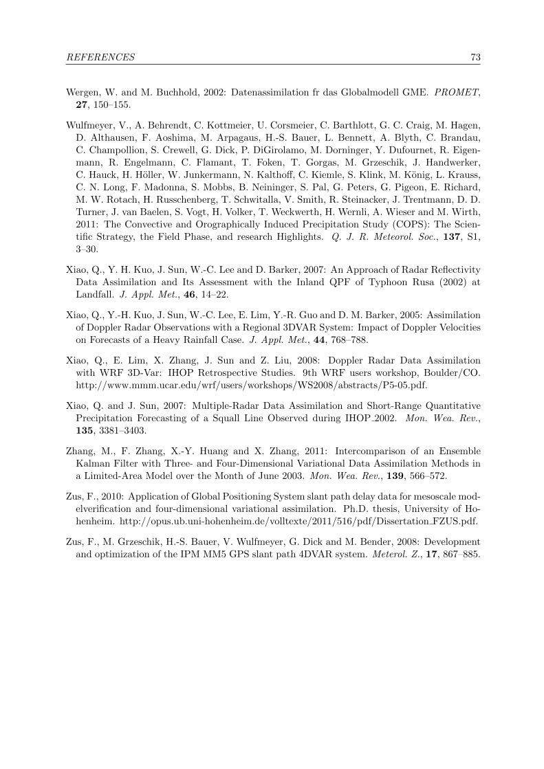
REFERENCES 73
Wergen, W. and M. Buchhold, 2002: Datenassimilation fr das Globalmodell GME. PROMET,27, 150–155.
Wulfmeyer, V., A. Behrendt, C. Kottmeier, U. Corsmeier, C. Barthlott, G. C. Craig, M. Hagen,D. Althausen, F. Aoshima, M. Arpagaus, H.-S. Bauer, L. Bennett, A. Blyth, C. Brandau,C. Champollion, S. Crewell, G. Dick, P. DiGirolamo, M. Dorninger, Y. Dufournet, R. Eigen-mann, R. Engelmann, C. Flamant, T. Foken, T. Gorgas, M. Grzeschik, J. Handwerker,C. Hauck, H. Holler, W. Junkermann, N. Kalthoff, C. Kiemle, S. Klink, M. Konig, L. Krauss,C. N. Long, F. Madonna, S. Mobbs, B. Neininger, S. Pal, G. Peters, G. Pigeon, E. Richard,M. W. Rotach, H. Russchenberg, T. Schwitalla, V. Smith, R. Steinacker, J. Trentmann, D. D.Turner, J. van Baelen, S. Vogt, H. Volker, T. Weckwerth, H. Wernli, A. Wieser and M. Wirth,2011: The Convective and Orographically Induced Precipitation Study (COPS): The Scien-tific Strategy, the Field Phase, and research Highlights. Q. J. R. Meteorol. Soc., 137, S1,3–30.
Xiao, Q., Y. H. Kuo, J. Sun, W.-C. Lee and D. Barker, 2007: An Approach of Radar ReflectivityData Assimilation and Its Assessment with the Inland QPF of Typhoon Rusa (2002) atLandfall. J. Appl. Met., 46, 14–22.
Xiao, Q., Y.-H. Kuo, J. Sun, W.-C. Lee, E. Lim, Y.-R. Guo and D. M. Barker, 2005: Assimilationof Doppler Radar Observations with a Regional 3DVAR System: Impact of Doppler Velocitieson Forecasts of a Heavy Rainfall Case. J. Appl. Met., 44, 768–788.
Xiao, Q., E. Lim, X. Zhang, J. Sun and Z. Liu, 2008: Doppler Radar Data Assimilationwith WRF 3D-Var: IHOP Retrospective Studies. 9th WRF users workshop, Boulder/CO.http://www.mmm.ucar.edu/wrf/users/workshops/WS2008/abstracts/P5-05.pdf.
Xiao, Q. and J. Sun, 2007: Multiple-Radar Data Assimilation and Short-Range QuantitativePrecipitation Forecasting of a Squall Line Observed during IHOP 2002. Mon. Wea. Rev.,135, 3381–3403.
Zhang, M., F. Zhang, X.-Y. Huang and X. Zhang, 2011: Intercomparison of an EnsembleKalman Filter with Three- and Four-Dimensional Variational Data Assimilation Methods ina Limited-Area Model over the Month of June 2003. Mon. Wea. Rev., 139, 566–572.
Zus, F., 2010: Application of Global Positioning System slant path delay data for mesoscale mod-elverification and four-dimensional variational assimilation. Ph.D. thesis, University of Ho-henheim. http://opus.ub.uni-hohenheim.de/volltexte/2011/516/pdf/Dissertation FZUS.pdf.
Zus, F., M. Grzeschik, H.-S. Bauer, V. Wulfmeyer, G. Dick and M. Bender, 2008: Developmentand optimization of the IPM MM5 GPS slant path 4DVAR system. Meterol. Z., 17, 867–885.

Acknowledgements
First I would thank Prof. Dr. Volker Wulfmeyer for the opportunity to prepare my Diplomaand my PhD thesis in his institute and his supervision over the last 3 years. If he did not gavemy the opportunity in his institute, I probably would stay in another research area. I also wantto thank Prof. Dr. Clemens Simmer from the University of Bonn and Prof. Dr. Kurt Jetterfrom the University of Hohenheim for reviewing my dissertation.
Thanks goes to the head of the modeling group, Dr. Hans-Stefan Bauer, for his supervision andnever ending patience with answering all my questions about meteorology.
Thanks goes also to Dr. Kirsten Warrach-Sagi for giving insights to ensemble data assimilationand to Dr. Matthias Grzeschik and Dr. Florian Zus for the fruitful discussions about modelingand the introduction to shell-scripting and help with Fortran.
I highly acknowledge the German Research Foundation for the establishment of the PriorityProgram 1167 in which this thesis was possible and also the Climate Service Center, BW-GRIDfor providing large amounts of computing time.
ECMWF is acknowledged for the provision of meteorological data, the large amount of comput-ing time and their technical support to run WRF on their HPC system.
Thanks goes to Dr. Galina Dick and Dr. Michael Bender from GFZ for the provision andsupport of GPS data, and to Dr. Klaus Stephan, Dr. Kathleen Helmert and Karolin Eichlerfrom DWD for support and provision of German radar data.
Special thanks goes to all members of the IPM for the very friendly atmosphere and discussionsapart from meteorology.
I am most thankful to my parents Veronika and Joachim and my sister Tina who encouragedme to study physics and their never ending patience and support. Although my father will notsee or hear me anymore, he will by proud of me.
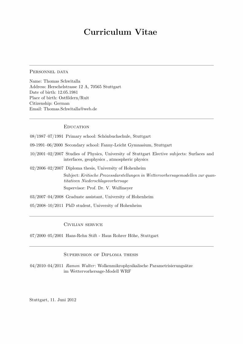
Curriculum Vitae
Personnel data
Name: Thomas SchwitallaAddress: Herschelstrasse 12 A, 70565 StuttgartDate of birth: 12.05.1981Place of birth: Ostfildern/RuitCitizenship: GermanEmail: [email protected]
Education
08/1987–07/1991 Primary school: Schonbuchschule, Stuttgart
09-1991–06/2000 Secondary school: Fanny-Leicht Gymnasium, Stuttgart
10/2001–02/2007 Studies of Physics, University of Stuttgart Elective subjects: Surfaces andinterfaces, geophysics , atmospheric physics
02/2006–02/2007 Diploma thesis, University of Hohenheim
Subject: Kritische Prozessdarstellungen in Wettervorhersagemodellen zur quan-titativen Niederschlagsvorhersage
Supervisor: Prof. Dr. V. Wulfmeyer
03/2007–04/2008 Graduate assistant, University of Hohenheim
05/2008–10/2011 PhD student, University of Hohenheim
Civilian service
07/2000–05/2001 Hans-Rehn Stift - Haus Rohrer Hohe, Stuttgart
Supervision of Diploma thesis
04/2010–04/2011 Ramon Walter : Wolkenmikrophysikalische Parametrisierungsatzeim Wettervorhersage-Modell WRF
Stuttgart, 11. Juni 2012
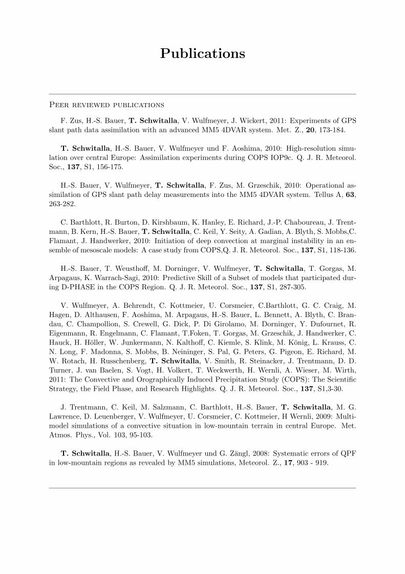
Publications
Peer reviewed publications
F. Zus, H.-S. Bauer, T. Schwitalla, V. Wulfmeyer, J. Wickert, 2011: Experiments of GPSslant path data assimilation with an advanced MM5 4DVAR system. Met. Z., 20, 173-184.
T. Schwitalla, H.-S. Bauer, V. Wulfmeyer und F. Aoshima, 2010: High-resolution simu-lation over central Europe: Assimilation experiments during COPS IOP9c. Q. J. R. Meteorol.Soc., 137, S1, 156-175.
H.-S. Bauer, V. Wulfmeyer, T. Schwitalla, F. Zus, M. Grzeschik, 2010: Operational as-similation of GPS slant path delay measurements into the MM5 4DVAR system. Tellus A, 63,263-282.
C. Barthlott, R. Burton, D. Kirshbaum, K. Hanley, E. Richard, J.-P. Chaboureau, J. Trent-mann, B. Kern, H.-S. Bauer, T. Schwitalla, C. Keil, Y. Seity, A. Gadian, A. Blyth, S. Mobbs,C.Flamant, J. Handwerker, 2010: Initiation of deep convection at marginal instability in an en-semble of mesoscale models: A case study from COPS,Q. J. R. Meteorol. Soc., 137, S1, 118-136.
H.-S. Bauer, T. Weusthoff, M. Dorninger, V. Wulfmeyer, T. Schwitalla, T. Gorgas, M.Arpagaus, K. Warrach-Sagi, 2010: Predictive Skill of a Subset of models that participated dur-ing D-PHASE in the COPS Region. Q. J. R. Meteorol. Soc., 137, S1, 287-305.
V. Wulfmeyer, A. Behrendt, C. Kottmeier, U. Corsmeier, C.Barthlott, G. C. Craig, M.Hagen, D. Althausen, F. Aoshima, M. Arpagaus, H.-S. Bauer, L. Bennett, A. Blyth, C. Bran-dau, C. Champollion, S. Crewell, G. Dick, P. Di Girolamo, M. Dorninger, Y. Dufournet, R.Eigenmann, R. Engelmann, C. Flamant, T.Foken, T. Gorgas, M. Grzeschik, J. Handwerker, C.Hauck, H. Holler, W. Junkermann, N. Kalthoff, C. Kiemle, S. Klink, M. Konig, L. Krauss, C.N. Long, F. Madonna, S. Mobbs, B. Neininger, S. Pal, G. Peters, G. Pigeon, E. Richard, M.W. Rotach, H. Russchenberg, T. Schwitalla, V. Smith, R. Steinacker, J. Trentmann, D. D.Turner, J. van Baelen, S. Vogt, H. Volkert, T. Weckwerth, H. Wernli, A. Wieser, M. Wirth,2011: The Convective and Orographically Induced Precipitation Study (COPS): The ScientificStrategy, the Field Phase, and Research Highlights. Q. J. R. Meteorol. Soc., 137, S1,3-30.
J. Trentmann, C. Keil, M. Salzmann, C. Barthlott, H.-S. Bauer, T. Schwitalla, M. G.Lawrence, D. Leuenberger, V. Wulfmeyer, U. Corsmeier, C. Kottmeier, H Wernli, 2009: Multi-model simulations of a convective situation in low-mountain terrain in central Europe. Met.Atmos. Phys., Vol. 103, 95-103.
T. Schwitalla, H.-S. Bauer, V. Wulfmeyer und G. Zangl, 2008: Systematic errors of QPFin low-mountain regions as revealed by MM5 simulations, Meteorol. Z., 17, 903 - 919.
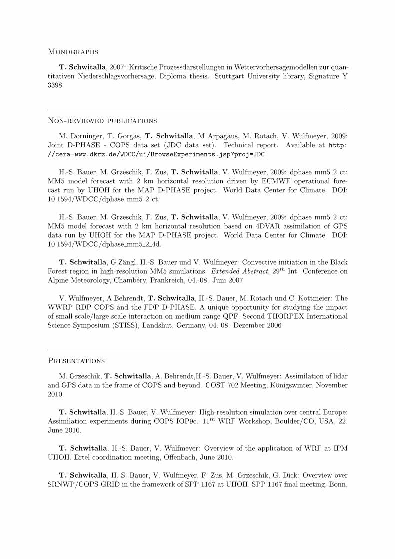
Monographs
T. Schwitalla, 2007: Kritische Prozessdarstellungen in Wettervorhersagemodellen zur quan-titativen Niederschlagsvorhersage, Diploma thesis. Stuttgart University library, Signature Y3398.
Non-reviewed publications
M. Dorninger, T. Gorgas, T. Schwitalla, M Arpagaus, M. Rotach, V. Wulfmeyer, 2009:Joint D-PHASE - COPS data set (JDC data set). Technical report. Available at http:
//cera-www.dkrz.de/WDCC/ui/BrowseExperiments.jsp?proj=JDC
H.-S. Bauer, M. Grzeschik, F. Zus, T. Schwitalla, V. Wulfmeyer, 2009: dphase mm5 2 ct:MM5 model forecast with 2 km horizontal resolution driven by ECMWF operational fore-cast run by UHOH for the MAP D-PHASE project. World Data Center for Climate. DOI:10.1594/WDCC/dphase mm5 2 ct.
H.-S. Bauer, M. Grzeschik, F. Zus, T. Schwitalla, V. Wulfmeyer, 2009: dphase mm5 2 ct:MM5 model forecast with 2 km horizontal resolution based on 4DVAR assimilation of GPSdata run by UHOH for the MAP D-PHASE project. World Data Center for Climate. DOI:10.1594/WDCC/dphase mm5 2 4d.
T. Schwitalla, G.Zangl, H.-S. Bauer und V. Wulfmeyer: Convective initiation in the BlackForest region in high-resolution MM5 simulations. Extended Abstract, 29th Int. Conference onAlpine Meteorology, Chambery, Frankreich, 04.-08. Juni 2007
V. Wulfmeyer, A Behrendt, T. Schwitalla, H.-S. Bauer, M. Rotach und C. Kottmeier: TheWWRP RDP COPS and the FDP D-PHASE. A unique opportunity for studying the impactof small scale/large-scale interaction on medium-range QPF. Second THORPEX InternationalScience Symposium (STISS), Landshut, Germany, 04.-08. Dezember 2006
Presentations
M. Grzeschik, T. Schwitalla, A. Behrendt,H.-S. Bauer, V. Wulfmeyer: Assimilation of lidarand GPS data in the frame of COPS and beyond. COST 702 Meeting, Konigswinter, November2010.
T. Schwitalla, H.-S. Bauer, V. Wulfmeyer: High-resolution simulation over central Europe:Assimilation experiments during COPS IOP9c. 11th WRF Workshop, Boulder/CO, USA, 22.June 2010.
T. Schwitalla, H.-S. Bauer, V. Wulfmeyer: Overview of the application of WRF at IPMUHOH. Ertel coordination meeting, Offenbach, June 2010.
T. Schwitalla, H.-S. Bauer, V. Wulfmeyer, F. Zus, M. Grzeschik, G. Dick: Overview overSRNWP/COPS-GRID in the framework of SPP 1167 at UHOH. SPP 1167 final meeting, Bonn,
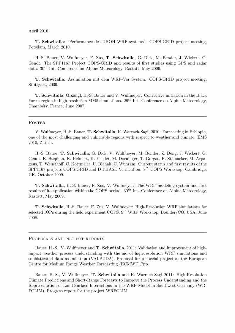
April 2010.
T. Schwitalla: “Performance des UHOH WRF systems”. COPS-GRID project meeting,Potsdam, March 2010.
H.-S. Bauer, V. Wulfmeyer, F. Zus, T. Schwitalla, G. Dick, M. Bender, J. Wickert, G.Gendt: The SPP1167 Project COPS-GRID and results of first studies using GPS and radardata. 30th Int. Conference on Alpine Meteorology, Rastatt, May 2009.
T. Schwitalla: Assimilation mit dem WRF-Var System. COPS-GRID project meeting,Stuttgart, 2009.
T. Schwitalla, G.Zangl, H.-S. Bauer und V. Wulfmeyer: Convective initiation in the BlackForest region in high-resolution MM5 simulations. 29th Int. Conference on Alpine Meteorology,Chambery, France, June 2007.
Poster
V. Wulfmeyer, H.-S. Bauer, T. Schwitalla, K. Warrach-Sagi, 2010: Forecasting in Ethiopia,one of the most challenging and vulnerable regions with respect to weather and climate. EMS2010, Zurich.
H.-S. Bauer, T. Schwitalla, G. Dick, V. Wulfmeyer, M. Bender, Z. Deng, J. Wickert, G.Gendt, K. Stephan, K. Helmert, K. Eichler, M. Dorninger, T. Gorgas, R. Steinacker, M. Arpa-gaus, T. Weusthoff, C. Kottmeier, U. Blahak, C. Wunram: Current status and first results of theSPP1167 projects COPS-GRID and D-PHASE Verification. 8th COPS Workshop, Cambridge,UK, October 2009.
T. Schwitalla, H.-S. Bauer, F. Zus, V. Wulfmeyer: The WRF modeling system and firstresults of its application within the COPS period. 30th Int. Conference on Alpine Meteorology,Rastatt, May 2009.
T. Schwitalla, H.-S. Bauer, F. Zus, V. Wulfmeyer: High-Resolution WRF simulations forselected IOPs during the field experiment COPS. 9th WRF Workshop, Boulder/CO, USA, June2008.
Proposals and project reports
Bauer, H.-S., V. Wulfmeyer and T. Schwitalla, 2011: Validation and improvement of high-impact weather process understanding with the aid of high-resolution WRF simulations andsophisticated data assimilation (VALPUDA), Proposal for a special project at the EuropeanCentre for Medium Range Weather Forecasting (ECMWF),7pp.
Bauer, H.-S., V. Wulfmeyer, T. Schwitalla and K. Warrach-Sagi 2011: High-ResolutionClimate Predictions and Short-Range Forecasts to Improve the Process Understanding and theRepresentation of Land-Surface Interactions in the WRF Model in Southwest Germany (WR-FCLIM), Progress report for the project WRFCLIM.
Bauer, H.-S., V. Wulfmeyer, K. Warrach-Sagi, T. Schwitalla, M. Grzeschik, S. Reich andJ. Wickert, 2010: Research on Consistent Land-Surface-Atmosphere Data Assimilation on theConvection-Permitting Scale with the Hans-Ertel Center Data Assimilation Testbed. Proposalfor the Hans-Ertel Research Center of DWD, 38pp.
Bauer, H.-S., V. Wulfmeyer and T. Schwitalla, 2010: Short-Range QPF by Combining4D Observations of Water Vapor and Wind with Innovative Methods in Data Assimilation.Progress Report for computing time at the German Climate Computing Center (DKRZ), 4pp.
Bauer, H.-S., V. Wulfmeyer, T. Schwitalla, K. Warrach-Sagi and J. Chu, 2010: High-Resolution Climate Predictions and Short-Range Forecasts to Improve the Process Understand-ing and the Representation of Land-Surface Interactions in the WRF Model in Southwest Ger-many (WRFCLIM), Progress report for the project WRFCLIM, 10pp.
Bauer, H.-S., V. Wulfmeyer, T. Schwitalla, K. Warrach-Sagi and J. Chu, 2009: High-Resolution Climate Predictions and Short-Range Forecasts to Improve the Process Understand-ing and the Representation of Land-Surface Interactions in the WRF Model in Southwest Ger-many (WRFCLIM), Proposal for computing time at the High Performance Computing CenterStuttgart, 8pp.
Bauer, H.-S., V. Wulfmeyer and T. Schwitalla, 2009: Short-Range QPF by Combining4D Observations of Water Vapor and Wind with Innovative Methods in Data Assimilation.Proposal for computing time at the German Climate Computing Center (DKRZ), 4pp.
Stuttgart, June 11, 2012

Erklarung:
Hiermit erklare ich, dass ich die vorgelegte Dissertation selbstandig angefertigt und nur dieangegebenen Quellen und Hilfsmittel verwendet habe. Wortlich oder inhaltlich ubernommeneStellen sind als solche gekennzeichnet.
Stuttgart, den 17.07.2012
Thomas Schwitalla