Embed Size (px)
Citation preview
Moderne Methoden Optischer Mikroskopie und Spektroskopie
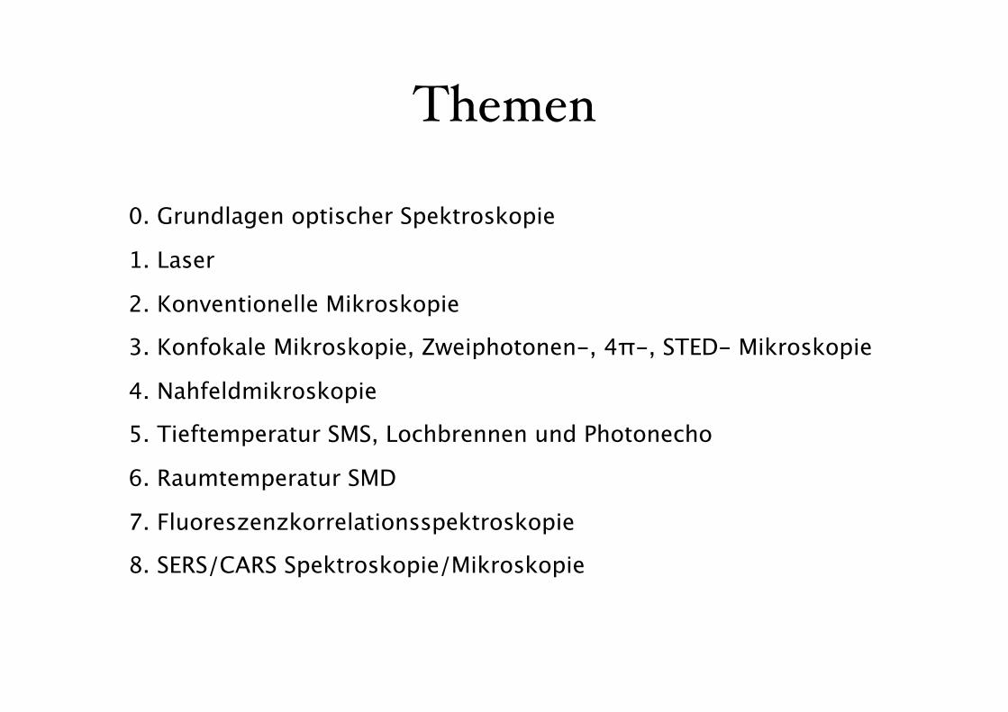
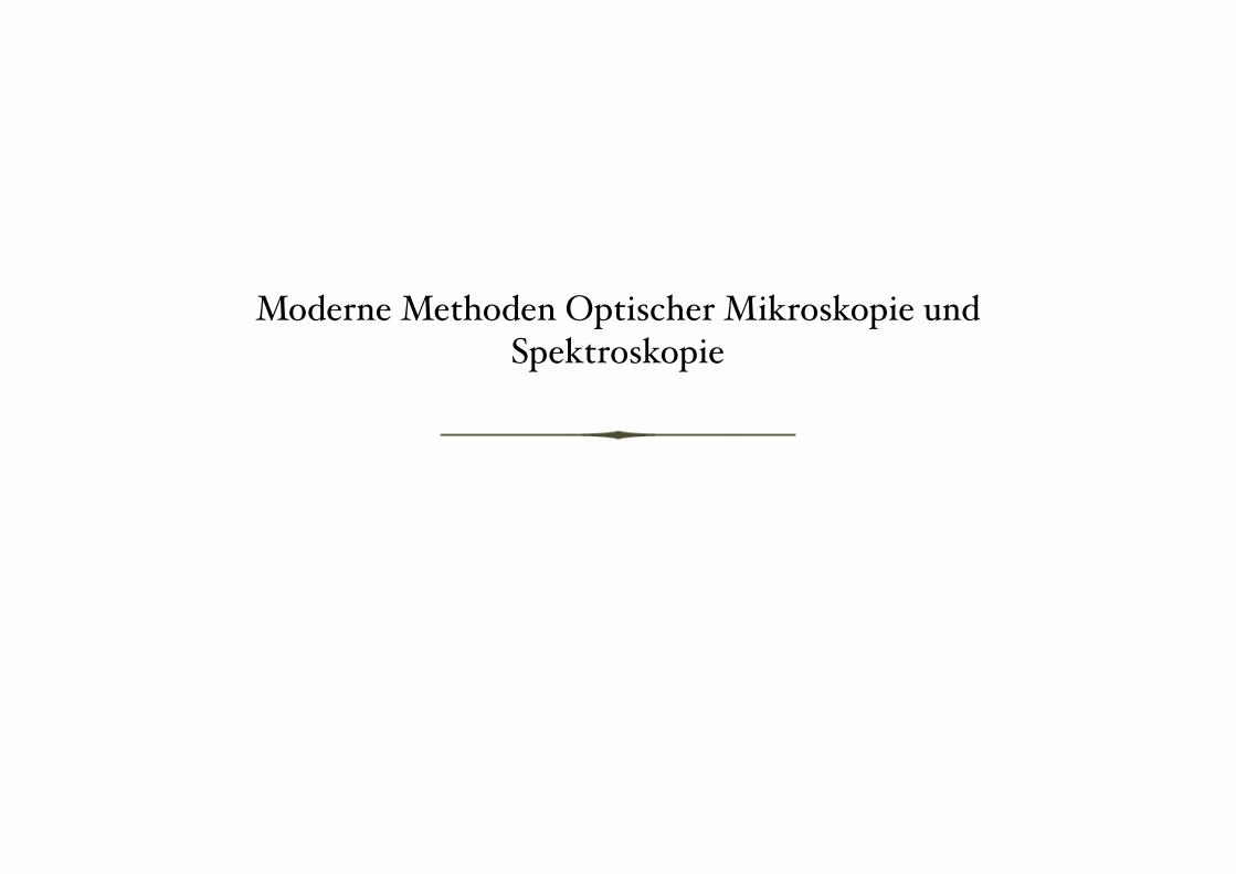
Themen
0. Grundlagen optischer Spektroskopie
1. Laser
2. Konventionelle Mikroskopie
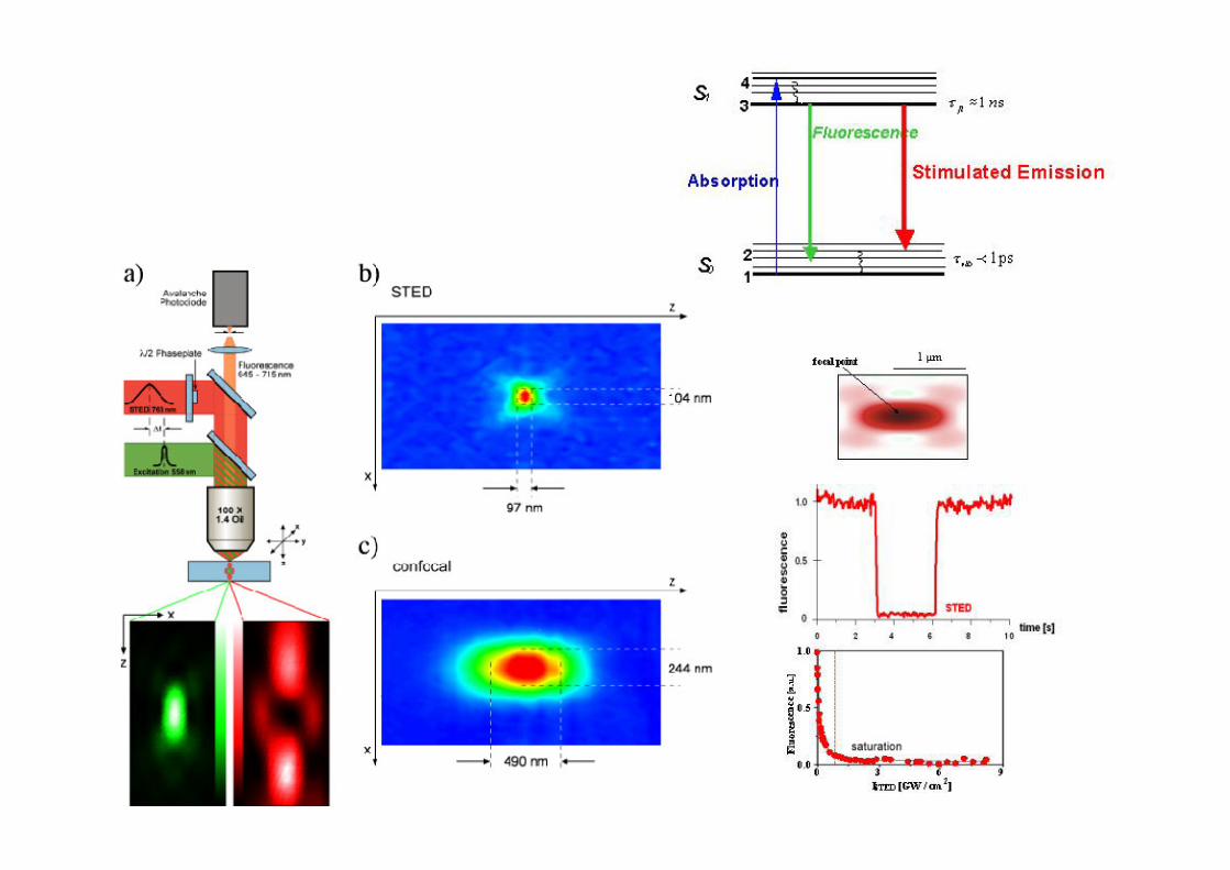
3. Konfokale Mikroskopie, Zweiphotonen-, 4π-, STED- Mikroskopie
4. Nahfeldmikroskopie
5. Tieftemperatur SMS, Lochbrennen und Photonecho
6. Raumtemperatur SMD
7. Fluoreszenzkorrelationsspektroskopie
8. SERS/CARS Spektroskopie/Mikroskopie
Literatur
• Molekülphysik und Quantenchemie, Haken, Wolf, Springer, 1998
• Experimentalphysik III, Demtröder, Springer, 1996• Optik, Hecht, Oldenbourg 2001• Laser, Kneubühl, Sigrist, Teubner 1995• Confocal laser scanning microscopy, C. J. R. Sheppard;
D. M. Shotton, Oxford : Bios Scientific Publ., 1997• Near-field microscopy and near-field optics, Daniel
Courjon, London : Imperial College Press, 2003• Principles of Fluorescence Spectroscopy, Lakowicz,
Kluwer, 1999• Single Molecule Spectroscopy, Rigler, Orrit, Basché (eds), Springer 2001
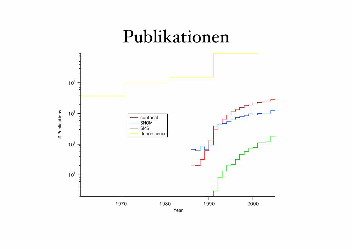
Publikationen
101
102
103
104
# Pu
blic
atio
ns
2000199019801970Year
confocal SNOM SMS fluorescence
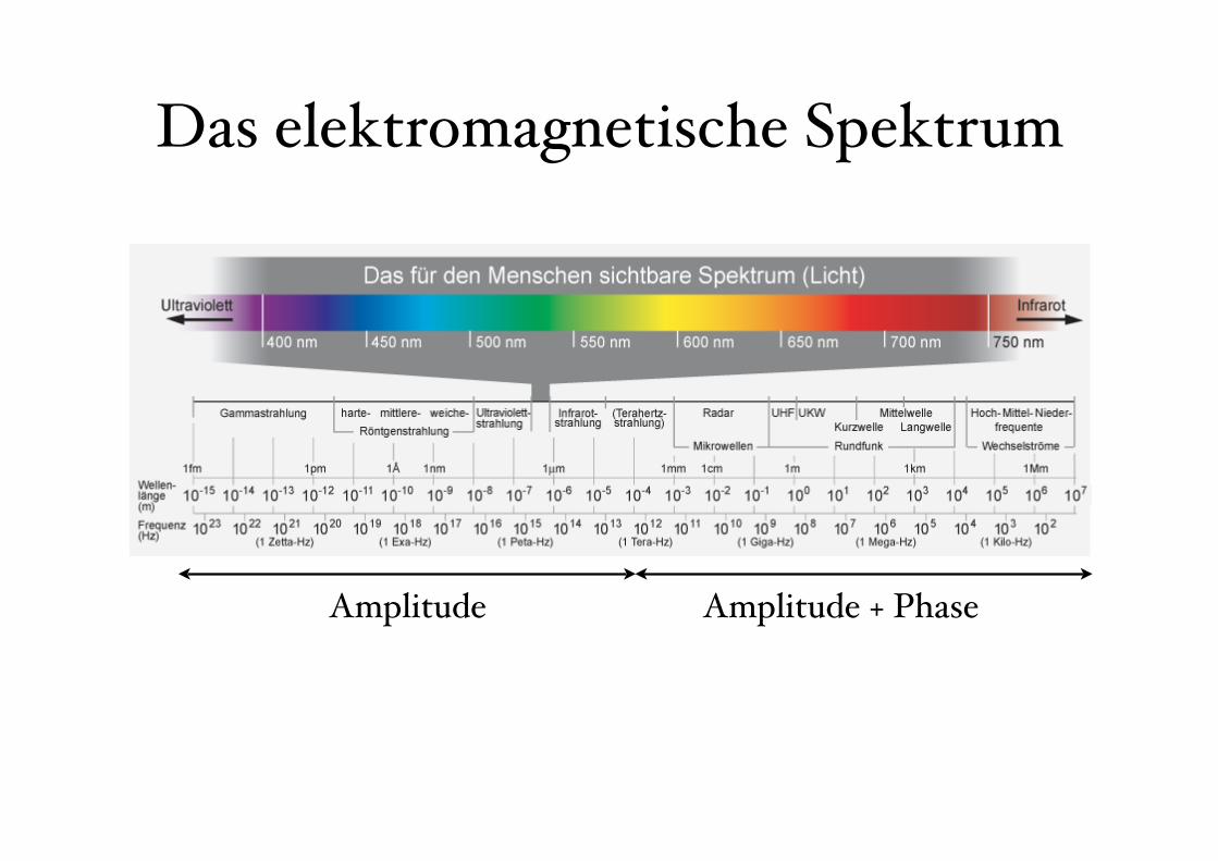
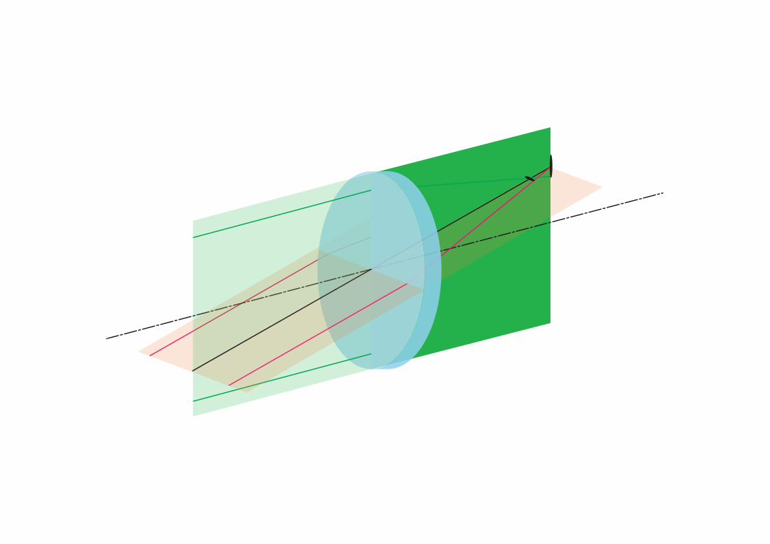
Das elektromagnetische Spektrum
Amplitude + PhaseAmplitude
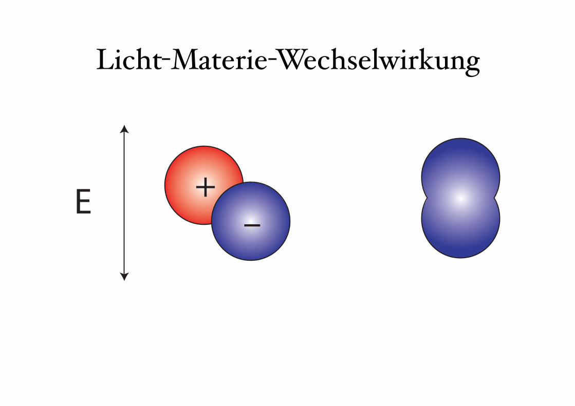
Licht-Materie-Wechselwirkung
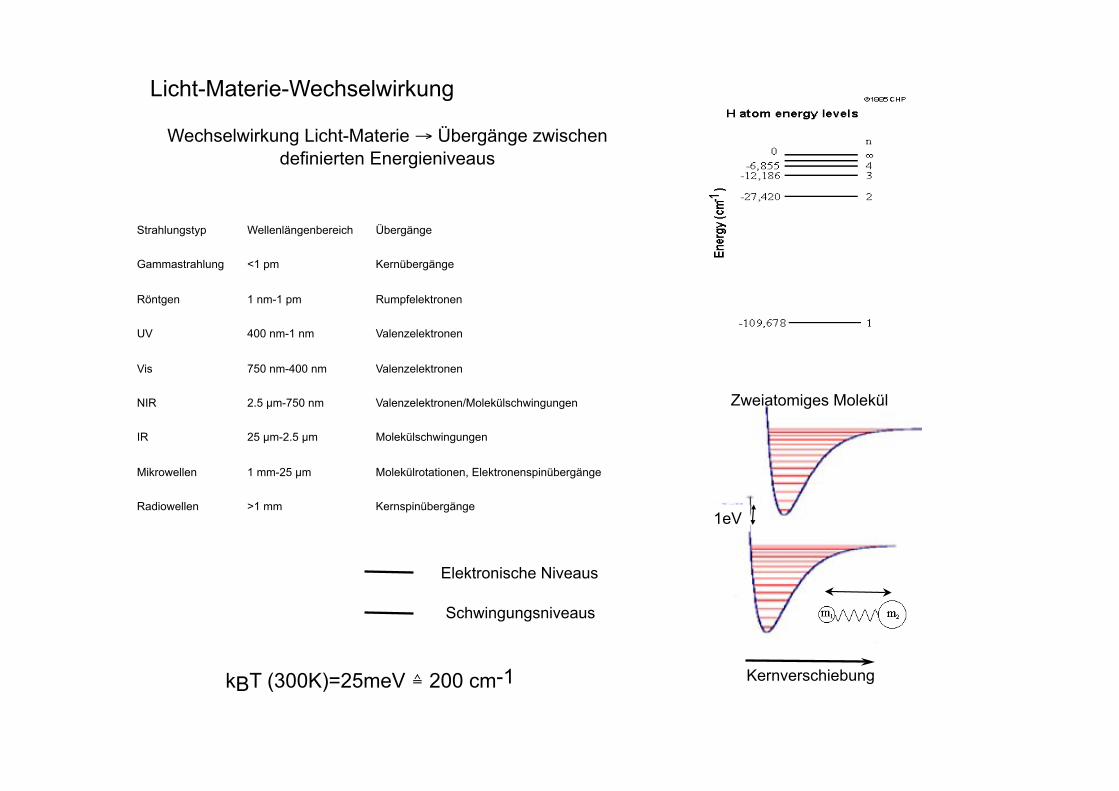
Wechselwirkung Licht-Materie → Übergänge zwischen definierten Energieniveaus
Strahlungstyp Wellenlängenbereich Übergänge
Gammastrahlung <1 pm Kernübergänge
Röntgen 1 nm-1 pm Rumpfelektronen
UV 400 nm-1 nm Valenzelektronen
Vis 750 nm-400 nm Valenzelektronen
NIR 2.5 µm-750 nm Valenzelektronen/Molekülschwingungen
IR 25 µm-2.5 µm Molekülschwingungen
Mikrowellen 1 mm-25 µm Molekülrotationen, Elektronenspinübergänge
Radiowellen >1 mm Kernspinübergänge
kBT (300K)=25meV ≙ 200 cm-1
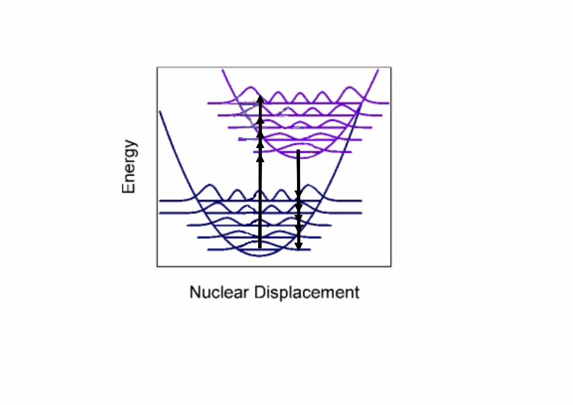
Licht-Materie-Wechselwirkung
Zweiatomiges Molekül
1eV
Elektronische Niveaus
Schwingungsniveaus
Kernverschiebung
0
0.2
0.4
0.6
0.8
1
1.2
1.4
200 250 300 350 400 450 500
700650600550500450400350
Wellenlänge (nm)
20x10-3
15
10
5
0
Em
ission (b.E.)
0.8
0.6
0.4
0.2
0.0
Abs
orpt
ion
N
O
O
N
O
O
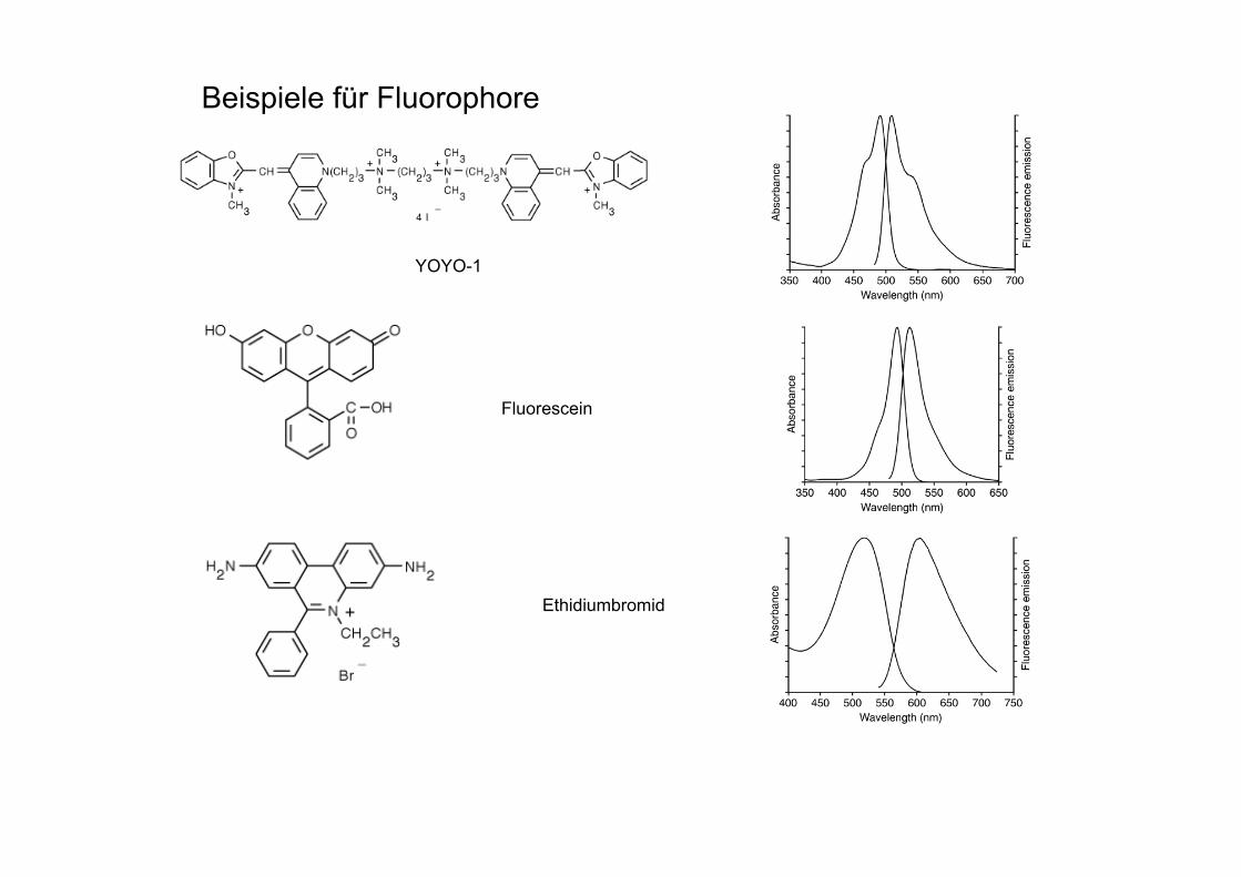
Fluorescein
YOYO-1
Ethidiumbromid
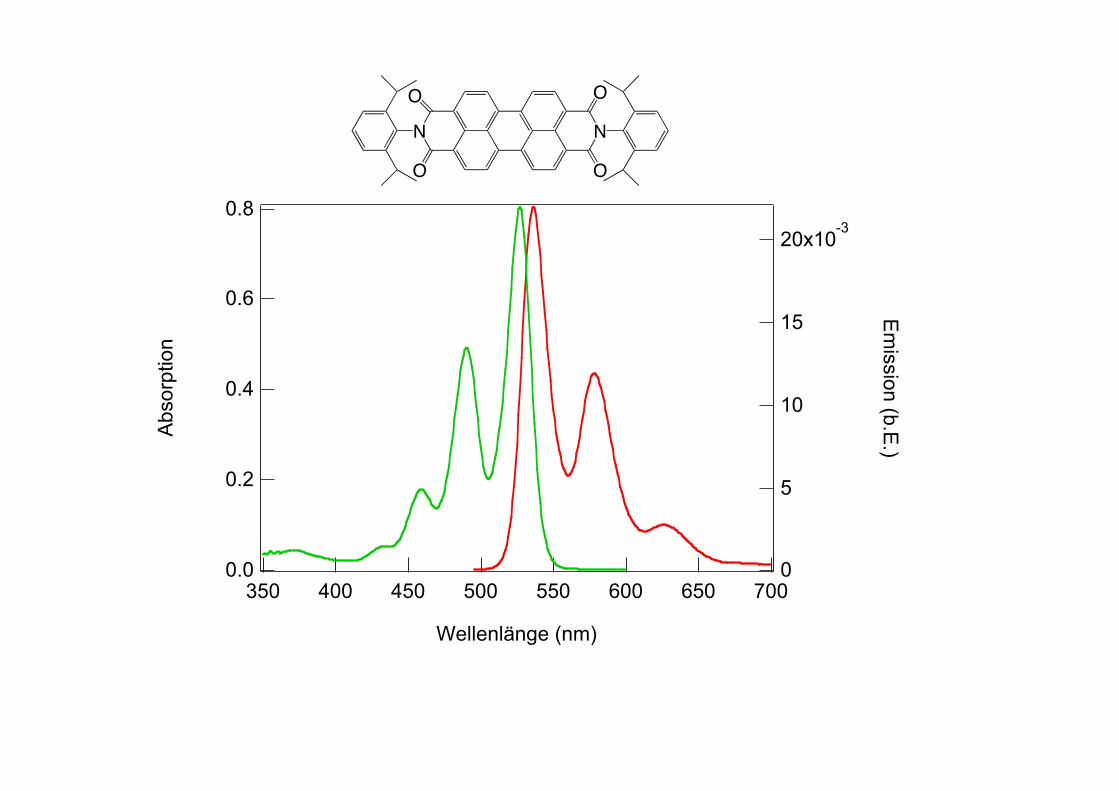
Beispiele für Fluorophore
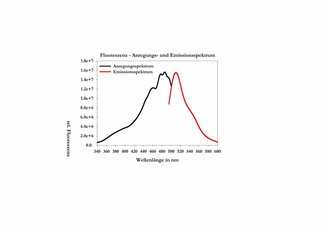
Fluoreszenz - Anregungs- und Emissionsspektrum
Wellenlänge in nm
340 360 380 400 420 440 460 480 500 520 540 560 580 600
rel. Fluoreszenz
0.0
2.0e+6
4.0e+6
6.0e+6
8.0e+6
1.0e+7
1.2e+7
1.4e+7
1.6e+7
1.8e+7AnregungsspektrumEmissionsspektrum
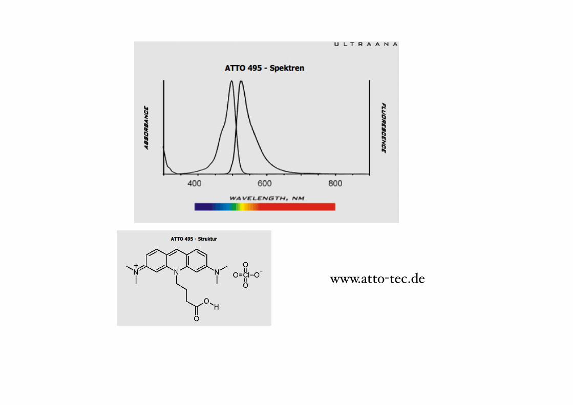
www.atto-tec.de
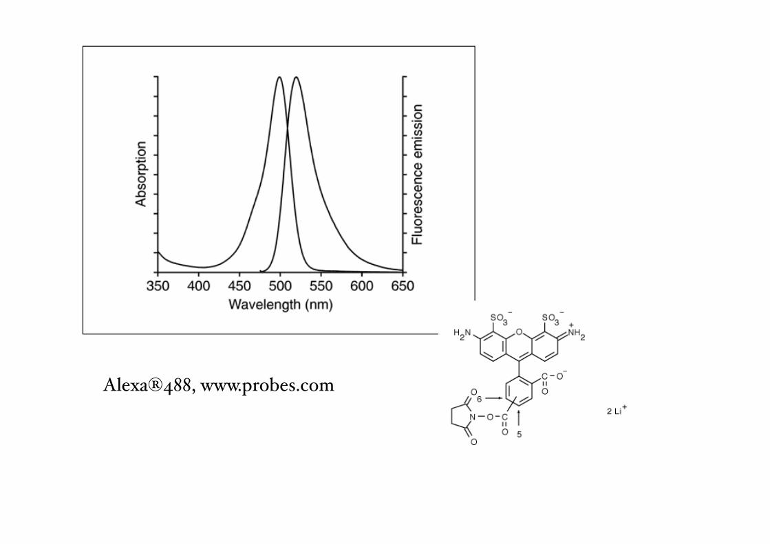
Alexa®488, www.probes.com
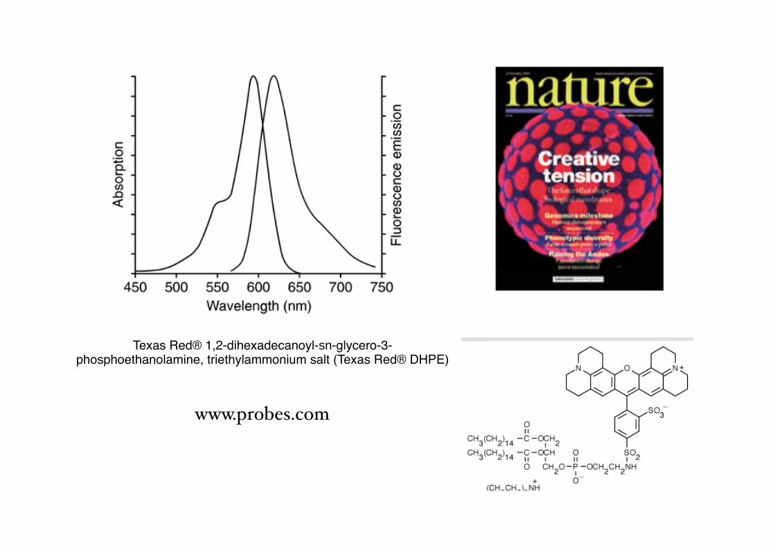
Texas Red® 1,2-dihexadecanoyl-sn-glycero-3- phosphoethanolamine, triethylammonium salt (Texas Red® DHPE)
www.probes.com
10000
8000
6000
4000
2000
0
140120100806040200x103
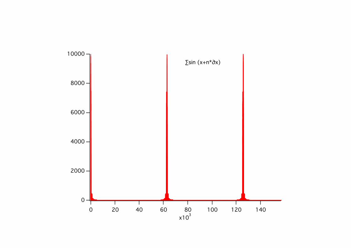
∑sin (x+n*∂x)
Biospektroskopie 5
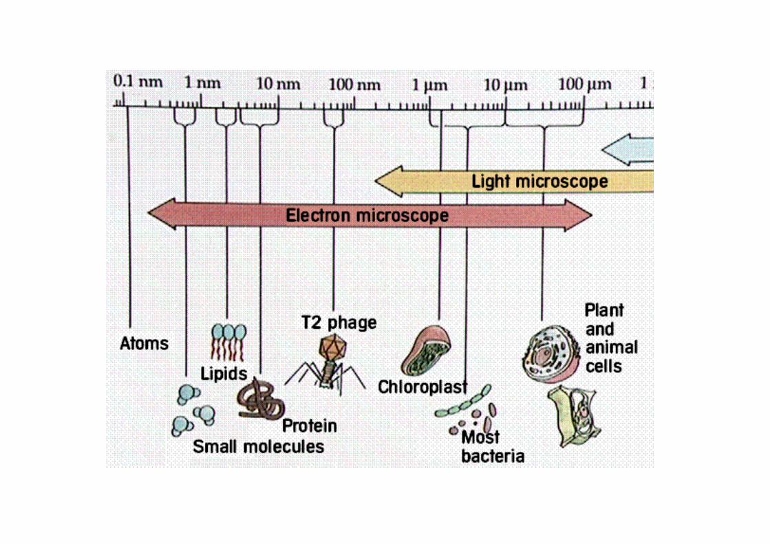
GrößenordnungenGrößenordnungen biologischer Objektebiologischer Objekte
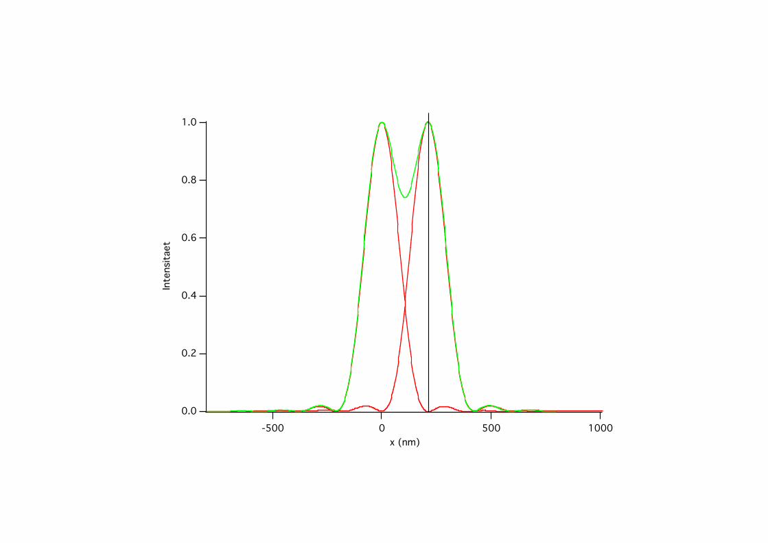
1.0
0.8
0.6
0.4
0.2
0.0
Inte
nsita
et
10005000-500x (nm)
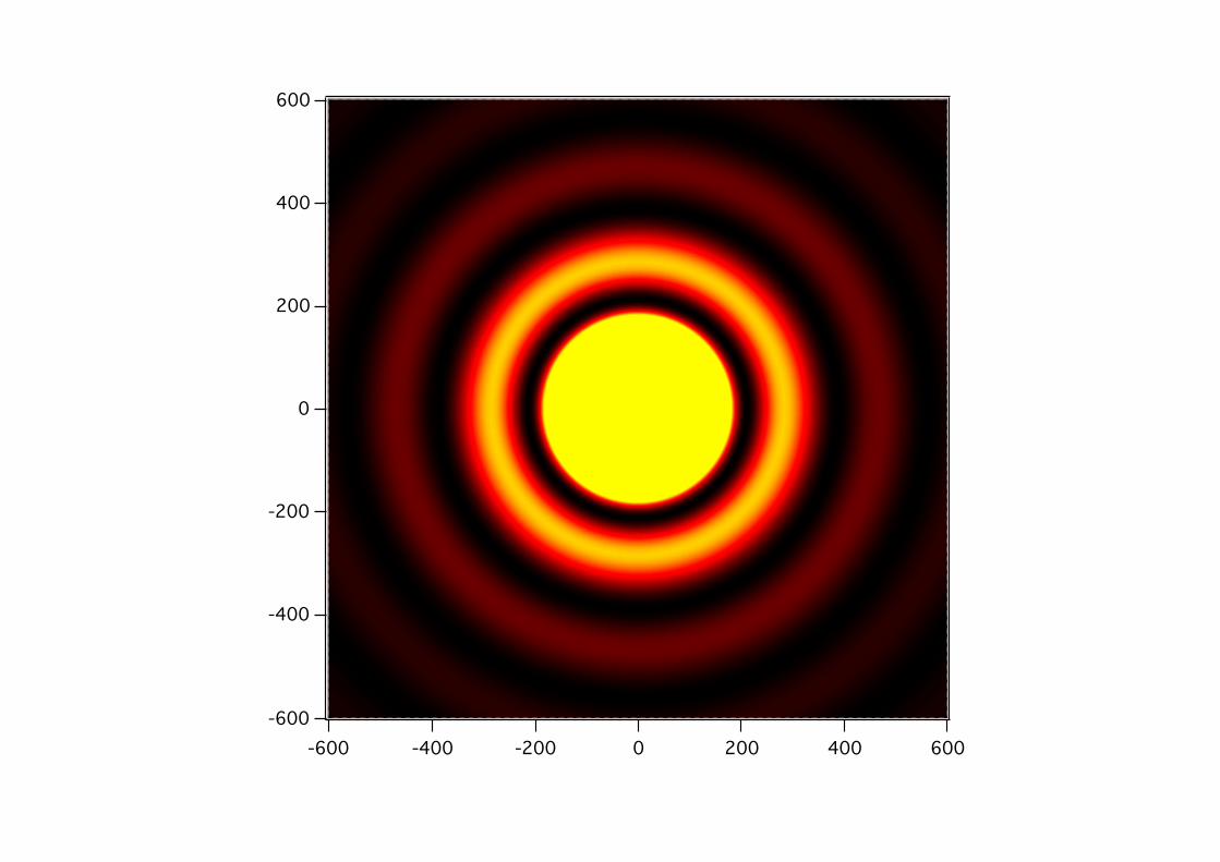
600
400
200
0
-200
-400
-6006004002000-200-400-600
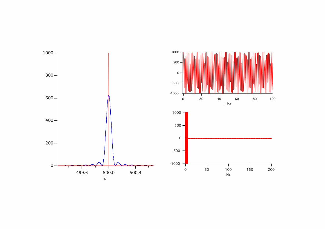
1000
800
600
400
200
0
500.4500.0499.6s
-1000
-500
0
500
1000
100806040200mHz
-1000
-500
0
500
1000
200150100500Hz
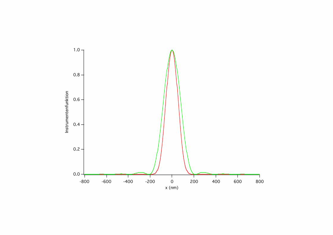
1.0
0.8
0.6
0.4
0.2
0.0
Inst
rum
ente
nfun
ktio
n
-800 -600 -400 -200 0 200 400 600 800x (nm)
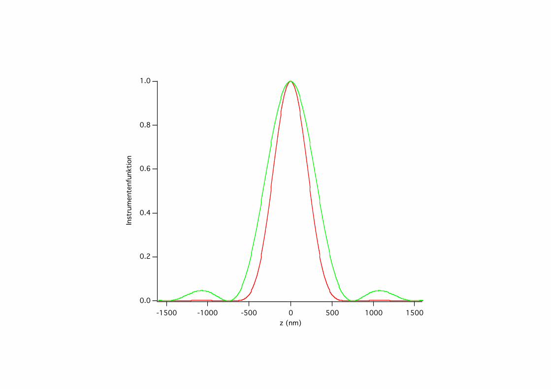
1.0
0.8
0.6
0.4
0.2
0.0
Inst
rum
ente
nfun
ktio
n
-1500 -1000 -500 0 500 1000 1500z (nm)
400
200
0
-200
-400
4002000-200-400
400
200
0
-200
-400
4002000-200-400
600
400
200
0
-200
-400
-6006004002000-200-400-600
600
400
200
0
-200
-400
-6006004002000-200-400-600
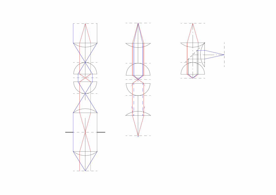
-3000
-2000
-1000
0
1000
2000
3000200010000-1000-2000-3000
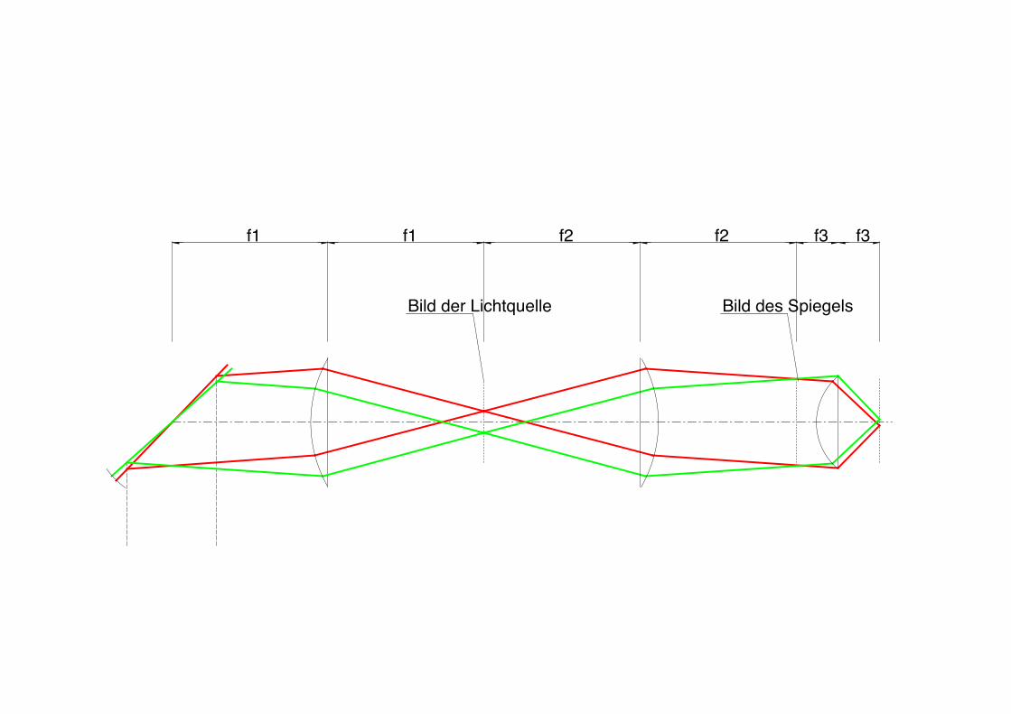
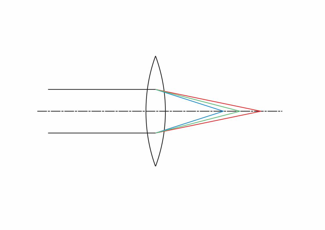
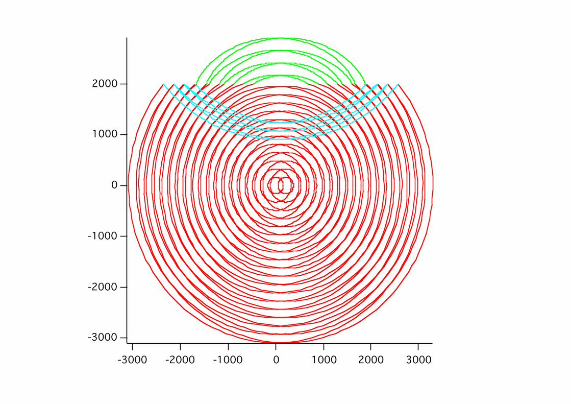
Bild der Lichtquelle Bild des Spiegels
f1 f1 f2 f2 f3 f3

www.olympus.comTransmitted and reflected light
UIS Objectives for Transmitted Light and Reflected Light
Type ArticleCode
Objective Name N.A. W.D.(mm)
F.N. C.C.(mm)
imm. Remarks Trans.DIC
Reflect.DIC
Phasering
Note
PlanApochromat
3758137582375833758437585376513765237656376533765437657376553766537666
PLAPO 1,25xPLAPO 2xPLAPO 40xPLAPO 60x OPLAPO 100x OMPLAPO 1,25xMPLAPO 2,5xMPLAPO 20xMPLAPO 50xMPLAPO 60xMPLAPO 100xMPLAPO 100x OLMPLAPO 150xLMPLAPO 250x
0.040.080.951.401.400.040.080.600.950.900.951.400.900.90
5.16.20.130.100.103.610.70.900.300.400.350.101.00.80
26.526.526.526.526.52226.526.526.526.526.526.526.526.5
--
0.11-0.230.170.17
--0000000
oiloil oil
Sp, CcSpSpDepolaryzerDepolaryzerSpSpSpSpSpSpSp
A, B
A BB
UniversalPlanApochromat
37561375623759637563375643756537566375683759937567
UPLAPO 4xUPLAPO 10xUPLAPO 10x WUPLAPO 20xUPLAPO 20x OUPLAPO 40xUPLAPO 40x OIUPLAPO 60xUPLAPO 60x WUPLAPO 100x OI
0.160.400.400.700.800.85
0.50-1.000.901.20
0.50-1.35
13.03.10.500.650.190.200.120.200.250.10
26.526.526.526.526.526.526.526.526.526.5
-0.170.170.17
-0.11-0.23
-0.11-0.230.15-0.20
0.17
water oil oil wateroil
SpSpSpSp, CcSp, IrisSp, CcSp, CcSp, Iris
A, CA, CA, BA, BA, CA, B
B, C, DA, B, C
UniversalApochromat
3757737597375783759837579
UAPO 20x /340UAPO 20x W/340UAPO 40x /340UAPO 40x W/340UAPO 40x OI/340
0.750.700.901.15
0.65-1.35
0.550.400.200.260.10
2222222222
0.170.17
0.11-0.230.13-0.25
0.17
water
water
oil
Sp, CcSp, CcSp, Iris
A, CA, BA, B
Good transmission at 340nm, (for Fura-2)Good transmission at 340nm, (for Fura-2)Good transmission at 340nm, (for Fura-2)Good transmission at 340nm, (for Fura-2)Good transmission at 340nm, (for Fura-2)
Universal PlanFluorite
375413754237543375443754537547375483744137442374433744437446376213762237623376243762537626375873758837589375913759037592
UPLFL 4xUPLFL 10xUPLFL 20xUPLFL 40xUPLFL 60x OIUPLFL 100x OUPLFL 100x OIUPLFL 4x PUPLFL 10x PUPLFL 20x PUPLFL 40x PUPLFL 100x OPUMPLFL 5xUMPLFL 10xUMPLFL 20xUMPLFL 40xUMPLFL 50xUMPLFL 100xUMPLFL 10x WUMPLFL 20x WLUMPLFL 40x WLUMPLFL 40x W/IRLUMPLFL 60x WLUMPLFL 60x W/IR
0.130.300.500.75
0.65-1.251.30
0.60-1.300.130.300.500.751.300.150.300.460.750.800.950.300.500.800.800.900.90
17.010.01.60.510.100.100.1013.03.11.60.510.1020.010.13.10.630.660.313.33.33.33.32.02.0
26.526.526.526.526.526.526.526.526.526.526.526.526.526.526.526.526.526.526.526.526.526.526.526.5
--
0.170.170.170.170.17
--
0.170.170.17
--0000--0000
oiloiloil
oil
waterwaterwaterwaterwaterwater
SpSpSp, IrisSpSp, Iris SpSpSp SpSpSp
A, CA, BA, B
B, C, DA, B, CA, B, C
A, CA, BA, B
A, B, C
A, B DDDD
B, DB, D
AAAAAA
Strain-freeStrain-freeStrain-freeStrain-freeStrain-free For IR-DIC (775nm) For IR-DIC (775nm)
PlanFluorite
37529374613746237463374653765937660376613766337664
PLFL 100xLCPLFL 20xLCPLFL 40xLCPLFL 60xSLCPLFL 40xLMPLFL 5xLMPLFL 10xLMPLFL 20xLMPLFL 50xLMPLFL 100x
0.950.400.600.700.550.130.250.400.500.80
0.206.9 *2.6 *1.7*7.7*22.521.012.010.63.4
26.522222222
26.526.526.526.526.5
0.14-0.200-2.50-2.50-2.50-2.6
--000
Sp, CcCap-G1,2Cc,Cap-G1,2Cc,Cap-G1,2Cc
C
A, CC
A, C
BBBBB
*:in case CG=1mm*:in case CG=1mm*:in case CG=1mm*:in case CG=1mm
PlanAchromat
3752037521375223752737523375243752537526374313760137602376033760537606
PL 2xPL 4xPL 10xPL 10x CYPL 20xPL 40xPL 50x OIPL 100x OPL 4x PMPL 5xMPL 10xMPL 20xMPL 50xMPL 100x
0.050.100.250.250.400.65
0.50-0.901.250.100.100.250.400.750.90
5.022.010.510.51.20.560.200.1522.019.610.61.30.380.21
2222222222222222222222222222
----
0.170.17
-----000
oiloil
ND filterSpSpSp, IrisSp SpSpSp
Marker pen (U-MARKER) attachable Strain-free
Achromat
37501375023750337504375053750637432374333743437435
ACH 10xACH 20xACH 40xACH 60xACH 100x OACH 100x OIACH 10x PACH 20x PACH 40x PACH 100x OP
0.250.400.650.801.25
0.60-1.250.250.400.651.25
6.13.00.450.150.130.136.13.00.450.13
22222222222222222222
-0.170.170.17
---
0.170.17
-
oiloil
oil
SpSpSpSp, Iris SpSp
Strain-freeStrain-freeStrain-freeStrain-free
TransmittedDIC -
A: U-UCDB/AX-UCDM condenser (NA: 0.9, WD: 1.5 mm)B: U-UCDB/AX-UCDM condenser (NA: 1.4, WD: 0.6 mm)C: IX-LWUCD condenser (NA: 0.55, WD: 23.3 mm)D: U-LWUCD condenser (NA: 0.8, WD: 5.7 mm)
Reflected DIC-
Sp: SpringCc: Correction collarA: U-DICR prism lever -- push posit ionB: U-DICR prism lever -- pull posit ion
LIFE SCIENCE
MATERIAL SCIENCE
IMAGING & PHOTOMETRY
OPTICS & ACCESSORIESOPTICS & ACCESSORIES
Objectives
UIS Objectives
Fluorescence Elements
Reflected light elements
Micromanipulation
OLYMPUS BIOSYSTEMS
OLYMPUS AKADEMIE
VIDEO
NEWSGROUPS
LINKS
CUSTOMER MAGAZINE
MEDICAL NEWSLETTER
Search
Search Results
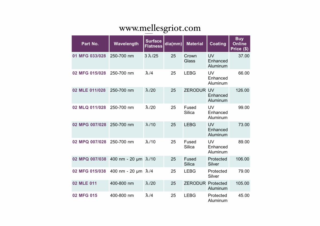
Searched on Round FlatMirrorsSurface Flatness = AllMaterial = AllDimension = 25Coating = MetallicWavelength Range = VisibleWavelength = All
Search all Round Flat Mirrors
Surface Flatness:
All
Coating:
Metallic
Material:
All
Wavelength Range:
Visible
Dimension (mm):
25
Wavelength:
All
Search Clear
22 Item(s) | Page # 1 of 3 Previous Next
Part No. WavelengthSurfaceFlatness
dia(mm) Material CoatingBuy
OnlinePrice ($)
01 MFG 033/028 250-700 nm 3 /25 25 CrownGlass
UVEnhancedAluminum
37.00
02 MFG 015/028 250-700 nm /4 25 LEBG UVEnhancedAluminum
66.00
02 MLE 011/028 250-700 nm /20 25 ZERODUR UVEnhancedAluminum
126.00
02 MLQ 011/028 250-700 nm /20 25 FusedSilica
UVEnhancedAluminum
99.00
02 MPG 007/028 250-700 nm /10 25 LEBG UVEnhancedAluminum
73.00
02 MPQ 007/028 250-700 nm /10 25 FusedSilica
UVEnhancedAluminum
89.00
02 MPQ 007/038 400 nm - 20 !m /10 25 FusedSilica
ProtectedSilver
106.00
02 MFG 015/038 400 nm - 20 !m /4 25 LEBG ProtectedSilver
79.00
02 MLE 011 400-800 nm /20 25 ZERODUR ProtectedAluminum
105.00
02 MFG 015 400-800 nm /4 25 LEBG ProtectedAluminum
45.00
22 Item(s) | Page # 1 of 3 Previous Next
Home | Product Information | Help | Lasers | Optics | Nanopositioning | Machine Vision
Tables & Breadboards | Opto-Mechanical Hardware | Photonics Modules | Instruments | Lab Accessories | Forensics
Copyright 1999-2001 Melles Griot. All rights reserved.
www.mellesgriot.com
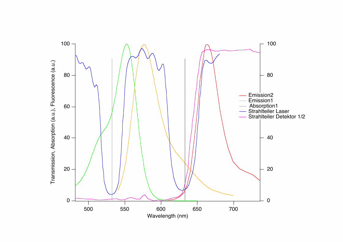
100
80
60
40
20
0
Tran
smiss
ion,
Abs
orpt
ion
(a.u
.), F
luor
esce
nce
(a.u
.)
700650600550500Wavelength (nm)
100
80
60
40
20
0
Emission2 Emission1Absorption1
Strahlteiler Laser Strahlteiler Detektor 1/2
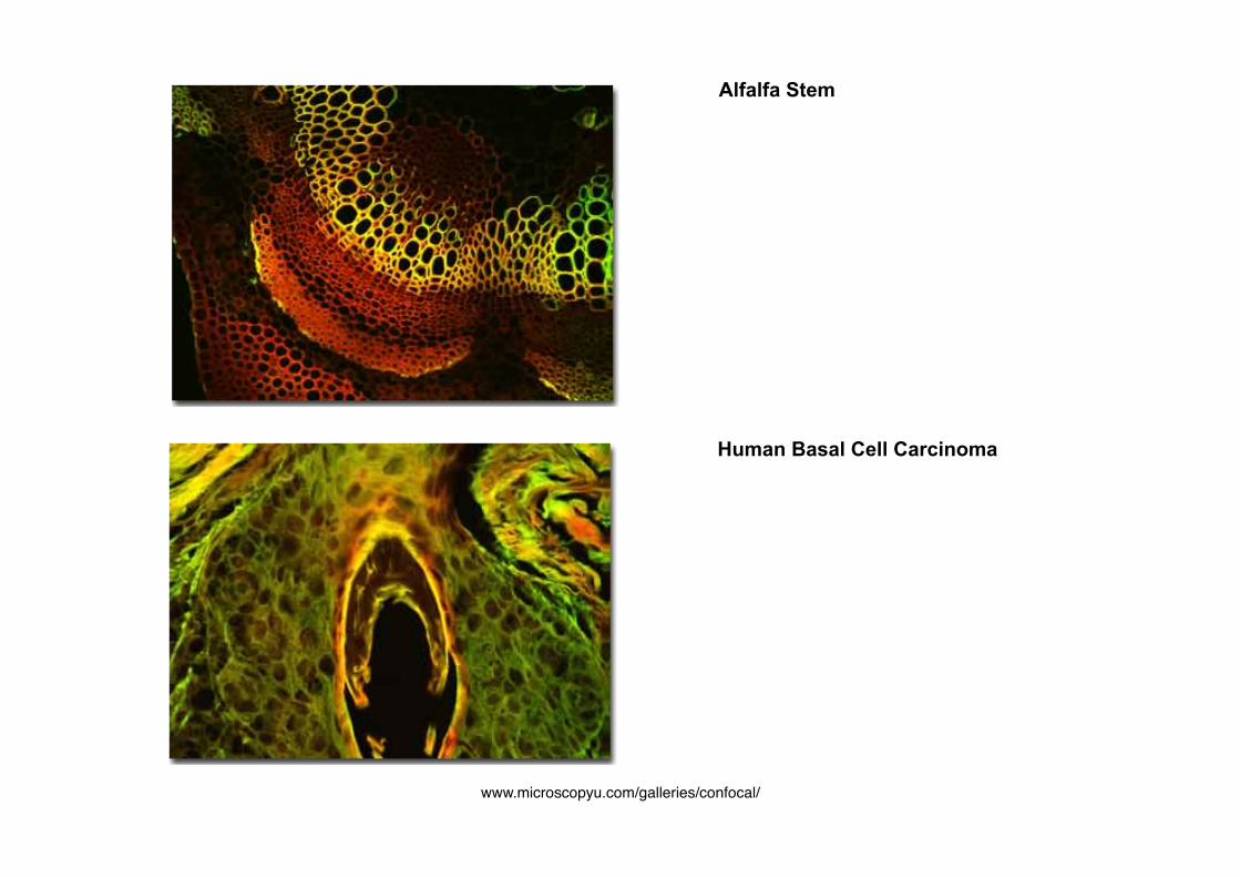
Human Basal Cell Carcinoma
Alfalfa Stem
www.microscopyu.com/galleries/confocal/
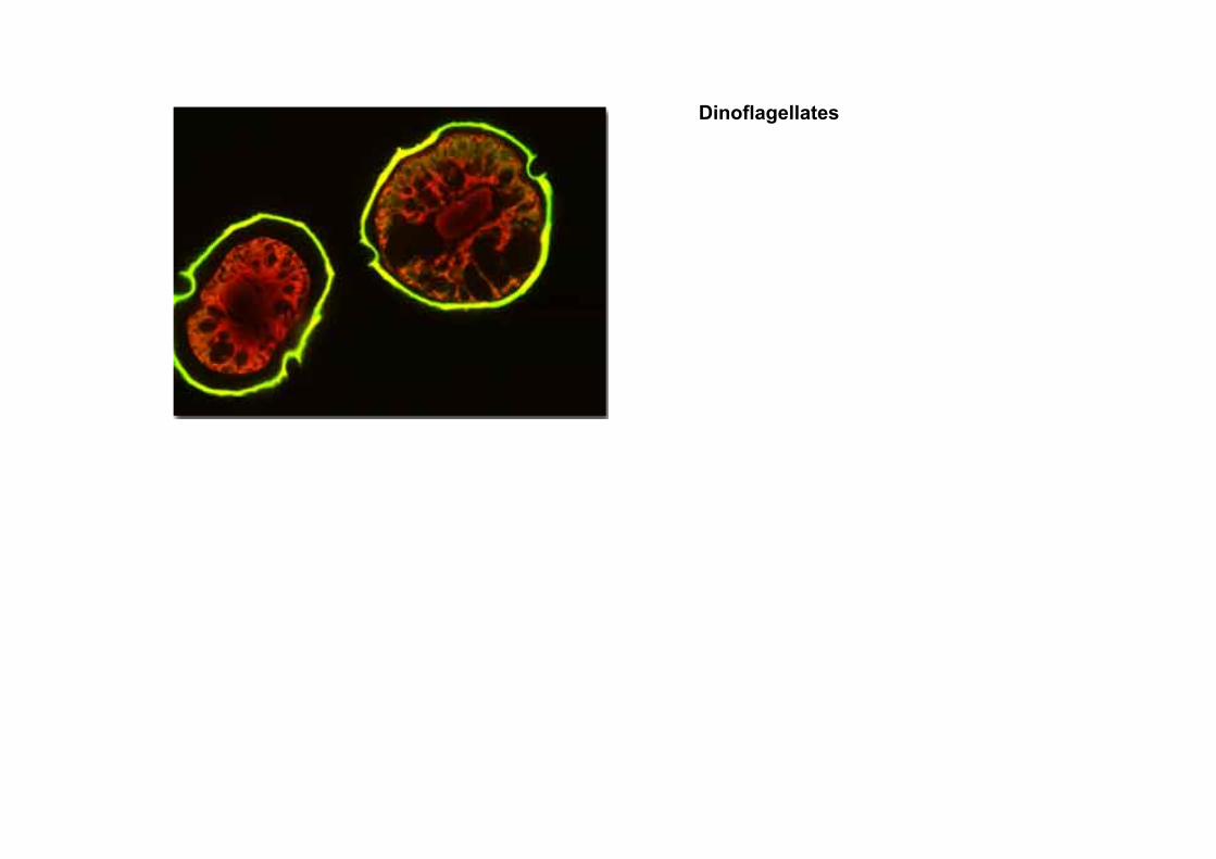
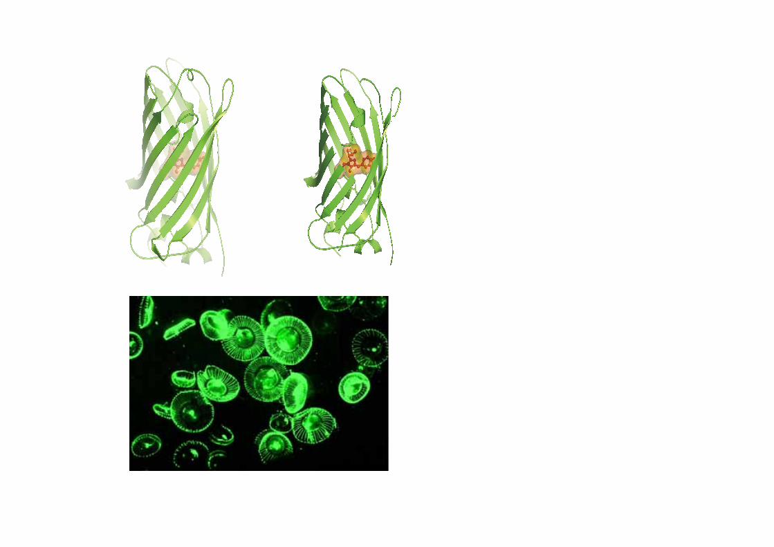
Dinoflagellates
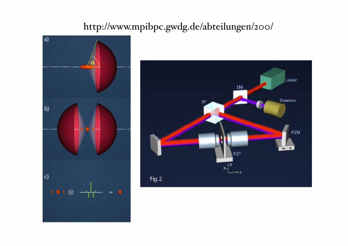
http://www.mpibpc.gwdg.de/abteilungen/200/

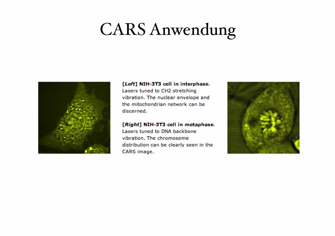
!"#$%&"'($)%*+,-./0$1'2%3#-40)%5,16"#21$7%-8%!+2"9 :
;;;<,+,-.-0$1'2<'(
!<%=,349+#%20"'$#4>%#"0#"2",$+$1-,%
+?+0$"?%8#->
!"$@13 A%B(1'("2$"#)%C'1",'"%!"! DEFFGH%EIJJ
24K;+6"9",3$(%'-,81,"?%81"9?
L1"9?%+K-6"%+,%"M$"#,+997%1994>1,+$"?%2+>09"

4155Cell biology beyond the diffraction limit
exploits the bending of a cantilever attached to the probe as adirect measure of the probe-sample interaction force, in NSOMan indirect method, based on shear-force damping, iscommonly used. For this, the NSOM probe, or a piezoelectrictuning fork attached to it, is oscillated at its resonancefrequency in a lateral vibrational mode (with a <1 nmamplitude); when in proximity to the sample, shear-forcesdampen this motion and induce measurable changes in theoscillation amplitude and phase. An electronic feedbacksystem, controlling the probe-sample distance directly throughthe piezoelectric scan stage, is subsequently used to maintaina constant oscillation amplitude/phase during scanning. In thisway, a constant probe-sample distance of <10 nm is realized(Fig. 2). The feedback signal itself, as in AFM, is used togenerate a topographic map of the sample surface (Fig. 1). Ofcourse, unique to NSOM is the fact that a correspondingfluorescence map is simultaneously generated.
The optical detection sensitivity of NSOM depends largelyon the extremely small excitation/detection volume set by theaperture dimensions as well as the depth of penetration of thenear-field into the specimen. Together, these propertieseffectively reduce background fluorescence and therebyenhance detection sensitivity. Betzig and Chichester exploitedthis eight years ago, providing the first observation of single-molecule fluorescence under ambient conditions (Betzig and
Optical fiber
Sample
Distance
detectionFeedback
x
y
z
Scanners
Polarizers
Laser
Detector 1
Long-pass filter
Objective
De
tecto
r 2
objective
Fig. 1. The principle of scanning probe microscopy. In AFM andNSOM, a sharp probe is used to map the topographic features on thesample surface accurately. This is done by physically scanning theprobe over the surface while maintaining a constant probe-sampledistance by force feedback.
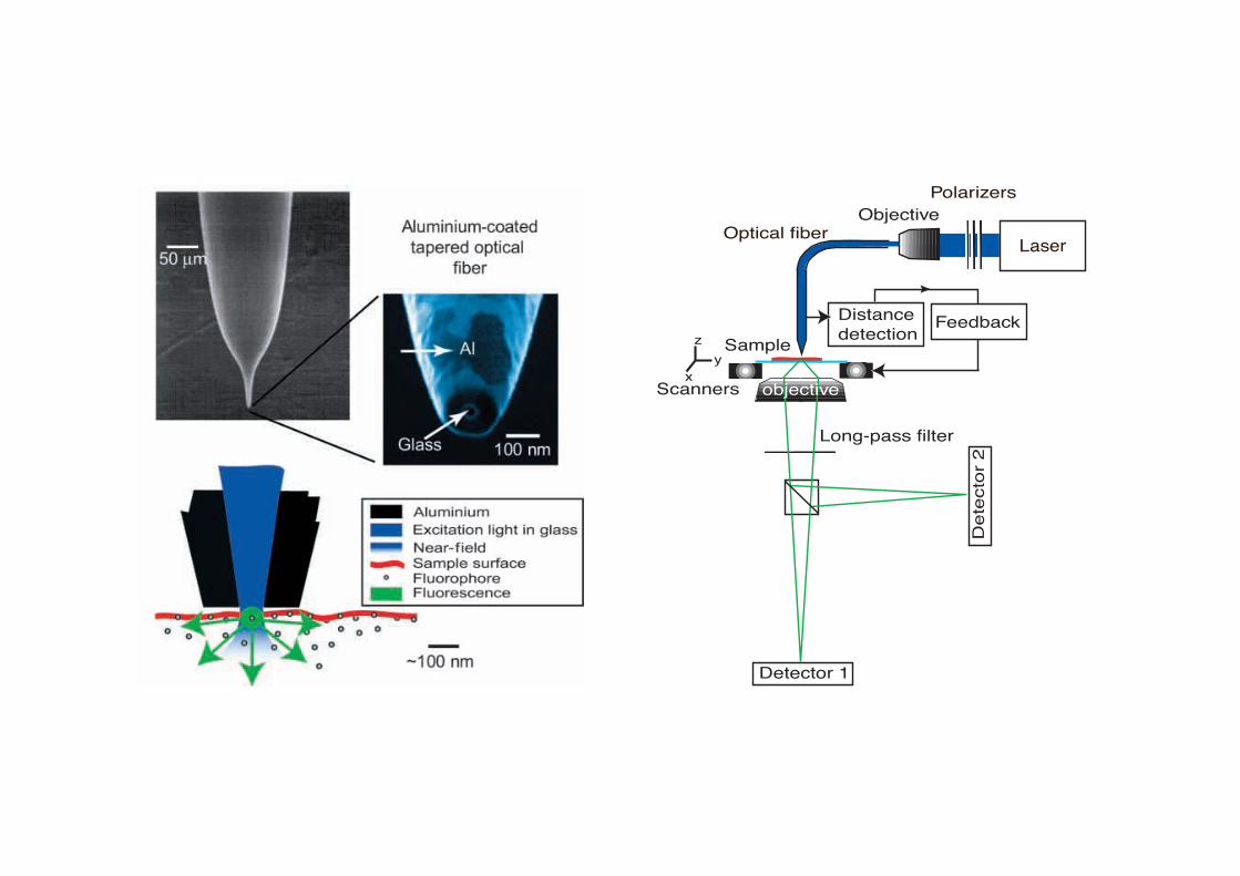
Fig. 2. Schematic lay out of a near-field scanning optical microscope.The NSOM probe is a tapered optical fiber (Fig. 3A). Laser light iscoupled into the fiber and is used to excite fluorophores as the probescans the sample surface. The probe-sample distance is maintainedconstant at <10 nm during scanning by shear-force-based distancedetection in combination with an electronic feedback systemcontrolling the piezoelectric scan stage. Fluorescence is collected bya conventional inverted microscope. Dual-channel optical detectionallows wavelength and/or polarization discrimination.
Fig. 3. The near-field optical probe. (A) An optical fiber is pulled to afinal diameter of 20-120 nm and subsequently coated withaluminum. This coating serves to confine the light to the tip region.A subsequent etching step results in a flat and circular endpoint andaperture. The aperture functions as a miniature light source, and itsdiameter primarily determines the optical resolution of themicroscope. (B) The principle of surface-specific excitation. Theoptical near-field generated at the aperture has significant intensityonly in a layer of <100 nm from the aperture; lower lyingfluorophores are therefore not excited. Hence, backgroundfluorescence is effectively suppressed. This forms the basis for thehigh optical detection sensitivity of this technique.
4155Cell biology beyond the diffraction limit
exploits the bending of a cantilever attached to the probe as adirect measure of the probe-sample interaction force, in NSOMan indirect method, based on shear-force damping, iscommonly used. For this, the NSOM probe, or a piezoelectrictuning fork attached to it, is oscillated at its resonancefrequency in a lateral vibrational mode (with a <1 nmamplitude); when in proximity to the sample, shear-forcesdampen this motion and induce measurable changes in theoscillation amplitude and phase. An electronic feedbacksystem, controlling the probe-sample distance directly throughthe piezoelectric scan stage, is subsequently used to maintaina constant oscillation amplitude/phase during scanning. In thisway, a constant probe-sample distance of <10 nm is realized(Fig. 2). The feedback signal itself, as in AFM, is used togenerate a topographic map of the sample surface (Fig. 1). Ofcourse, unique to NSOM is the fact that a correspondingfluorescence map is simultaneously generated.
The optical detection sensitivity of NSOM depends largelyon the extremely small excitation/detection volume set by theaperture dimensions as well as the depth of penetration of thenear-field into the specimen. Together, these propertieseffectively reduce background fluorescence and therebyenhance detection sensitivity. Betzig and Chichester exploitedthis eight years ago, providing the first observation of single-molecule fluorescence under ambient conditions (Betzig and
Optical fiber
Sample
Distance
detectionFeedback
x
y
z
Scanners
Polarizers
Laser
Detector 1
Long-pass filter
Objective
Dete
cto
r 2
objective
Fig. 1. The principle of scanning probe microscopy. In AFM andNSOM, a sharp probe is used to map the topographic features on thesample surface accurately. This is done by physically scanning theprobe over the surface while maintaining a constant probe-sampledistance by force feedback.
Fig. 2. Schematic lay out of a near-field scanning optical microscope.The NSOM probe is a tapered optical fiber (Fig. 3A). Laser light iscoupled into the fiber and is used to excite fluorophores as the probescans the sample surface. The probe-sample distance is maintainedconstant at <10 nm during scanning by shear-force-based distancedetection in combination with an electronic feedback systemcontrolling the piezoelectric scan stage. Fluorescence is collected bya conventional inverted microscope. Dual-channel optical detectionallows wavelength and/or polarization discrimination.
Fig. 3. The near-field optical probe. (A) An optical fiber is pulled to afinal diameter of 20-120 nm and subsequently coated withaluminum. This coating serves to confine the light to the tip region.A subsequent etching step results in a flat and circular endpoint andaperture. The aperture functions as a miniature light source, and itsdiameter primarily determines the optical resolution of themicroscope. (B) The principle of surface-specific excitation. Theoptical near-field generated at the aperture has significant intensityonly in a layer of <100 nm from the aperture; lower lyingfluorophores are therefore not excited. Hence, backgroundfluorescence is effectively suppressed. This forms the basis for thehigh optical detection sensitivity of this technique.
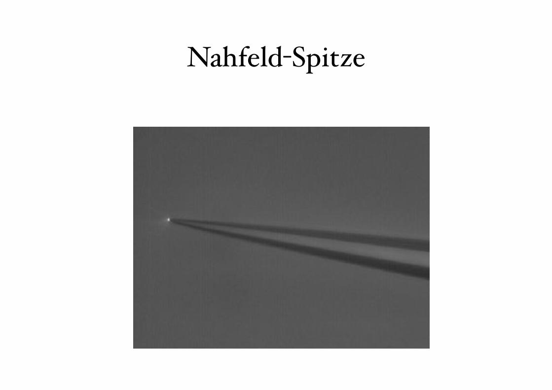
Nahfeld-Spitze
!"#$%&$#'#(()*#+$,-.#'/)01+22.23)4"%.1+')5.1$6(16"7
!"#$%"&'()'*+",-.'/012340'5"04310678#639.':0;0'<323,"38#639.'04;'!0"&'=)'*3#;#""#9>,?
@>#231,"&'<36313%4.'("$%44#':0,3%407'A0B%"0,%"&.'("$%44#.'CA'DEFGH
I#,07739'404%J0",397#1'0"#'%K'34,#"#1,'K%"'60"3%+1'%J,3907'B01#;'1,+;3#1.'3497+;34$'1+"K09#
#4>049#;' L0204' 1J#9,"%19%J&.' 134$7#' 2%7#9+7#' 1J#9,"%19%J&.' 9>#23907' 1#41%"1.' J>%,%439
B04;$0J'1,"+9,+"#1.'#,9)'M>#3"'0B373,&' ,%'1>%N';"020,39' 7%907' K3#7;'#4>049#2#4,'%K' ,>#' 3493;#4,
#7#9,"%20$4#,39' K3#7;' ;+#' ,%' ,>#' 9%>#"#4,' "#1%404,' #7#9,"%4' J70120' #O93,0,3%4.' 01' N#77' 01' ,>#
1#413,363,&' %K' ,>31' B#>063%"' ,%' ,>#' J0",397#' 1>0J#' 04;' 1+""%+4;34$' J>&139%P9>#23907' J"%J#",3#1.
20Q#' ,>#2' J0",39+70"7&' N#77' 1+3,#;' K%"' 204&' %K' ,>#1#' 0JJ7390,3%41)' *>37#' 2%1,' 1,+;3#1' 0"#
J#"K%"2#;'+134$'9%46#4,3%407'K0"PK3#7;'1#,P+J1.',>#'K+4;02#4,07'34,#"09,3%41'%99+"'34',>#'639343,&
%K',>#'J0",397#1'04;'0"#',>#"#K%"#'$%6#"4#;'B&',>#
4#0"PK3#7;' "#1J%41#' %K' ,>#' J0",397#1)' M%' $034' 04
+4;#"1,04;34$' %K' ,>#1#' 34,#"09,3%41.' N#' 0"#
;#6#7%J34$' ,32#P"#1%76#;' 04;' @*' 4#0"PK3#7;
1904434$' %J,3907' 239"%19%J&' ' R:STIU
90J0B373,3#1' 34'%+"' 70B%"0,%"&)'M>31' ,#9>43V+#'>01
B#$+4' ,%' B#' ;#6#7%J#;' 34' ,>#' J01,' ,#4' �"1' ,%
%6#"9%2#' ,>#' 1J0,307' "#1%7+,3%4' 7323,1' %K
9%46#4,3%407' %J,3907' 239"%19%J#1)' M>#&' 071%
"#J"#1#4,' 0' +43V+#' N0&' ,%' 1,+;&' ,>#' 4#0"PK3#7;
"#1J%41#' R;3KK"09,3%4' J0,,#"4U' %K' %B8#9,1' 04;
9%41#V+#4,7&' ,%' +4;#"1,04;' ,>#' 34,#"09,3%41
B#,N##4'%B8#9,1'04;'K3#7;1'0,',>31'1907#)
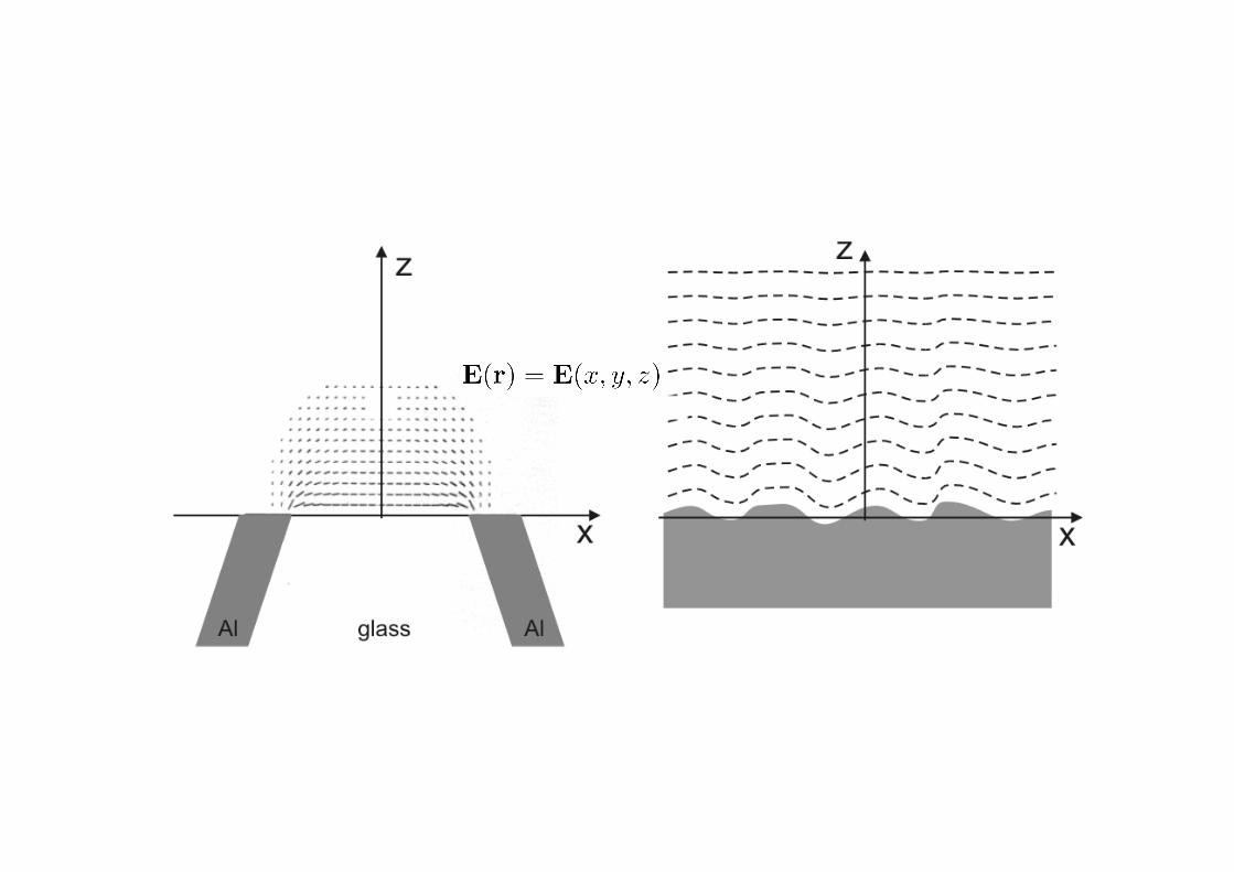
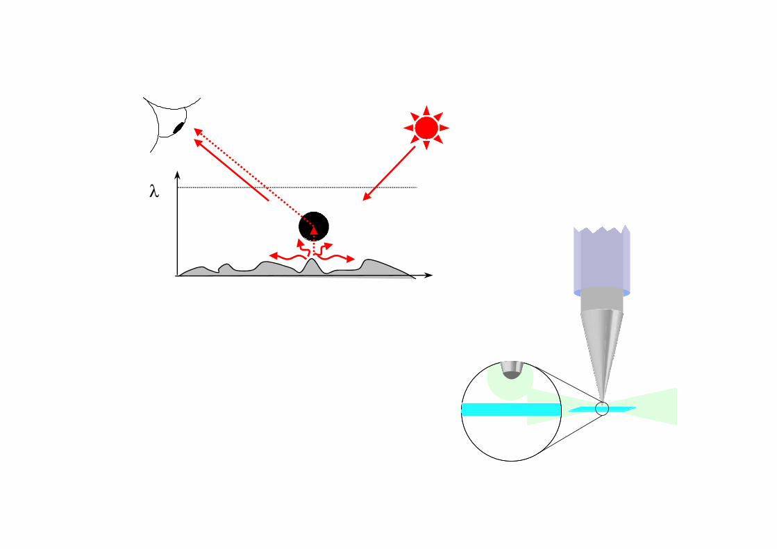
*#'0"#'K%9+134$'%4'W0J#",+"#7#11X':STI.',>#'J"3493J7#'%K'N>39>'31'377+1,"0,#;'34'Y3$+"#
Z)' M>#' 377+2340,#;' 102J7#' 1+"K09#' $#4#"0,#1' ,N%' Q34;1' %K' %J,3907' K3#7;1[' 0' J"%J0$0,34$' K3#7;
"#70,#;',%'%B8#9,';#,0371'$"#0,#"',>04',>#'377+2340,34$'N06#7#4$,>R!U'04;'0'9%4K34#;'R#604#19#4,U
K3#7;'N>39>'9%4,0341'1+BPN06#7#4$,>'34K%"20,3%4)'M%';#,#9,' ,>31'#604#19#4,'K3#7;.'0'404%2#,"39
13-#;'J"%B#'31'322#"1#;'34',>#'%J,3907'4#0"PK3#7;'-%4#'%K',>#'102J7#'1+"K09#)'M>#'J0",397#'190,,#"1
,>#'4#0"PK3#7;'J>%,%41' 34,%'J"%J0$0,34$'N06#1' ,>0,'904' ,>#4'B#';#,#9,#;)'\&'B%,>'1904434$' ,>#
J"%B#' R1+9>' 01' 04' 0K2' ,3JU' 0B%6#' ,>#' 1+"K09#' 04;
;#,#9,34$',>#'J"%B#]102J7#'34,#"09,3%4'0,'#09>'J%34,
%K',>31'J704#'N#'%B,034'0'7%907'20J'%K',>#'4#0"PK3#7;
34,#413,&)' Y3$+"#' ^' 377+1,"0,#1' ,>#' +4+1+07' :STI
13$407'%K',>#';3KK"09,#;'K3#7;'%K'0'1376#"'404%J0",397#
J709#;'%4'04'%J,3907'170B)'M>#'404%J0",397#'>01'0'FE
42' ;302#,#"' 04;' 31' 377+2340,#;' 0,' FEF' 42)' M>#
40,+"#' %K' ,>#' 190,,#"#;' K3#7;' 31' J"#;39,#;
,>#%"#,39077&.' 04;' 31' #OJ#9,#;' ,%' 34K7+#49#' ,>#
2#041' ,>"%+$>' N>39>' 20,#"307' #O93,0,3%41' 904' B#
>0"4#11#;' K%"' ,#7#9%22+4390,3%41' 04;' 9%2J+,34$
0JJ7390,3%41)
''''''''''''''''''''''''''''''''''''''''''''''''?'#P2037'0;;"#11['N3#;#""#9>,_047)$%6
!
S90,,#"#" 13-#'``''!
S90,,#"#" ,%'S+"K09#';31,049#'``''!
-.3&$#)89'="3493J7#'%K'4#0"PK3#7;'%J,391)
Z"2
ZEE'"2'9%"#
;302#,#"'K3B#"
Y3#7;';3KK"09,#;'B&
,>#'J0",397#
# a'HE%
Qb
M3J'R(.'!U
A%B#1'"0;30,#;
B&',>#'J"%B#'
=IM
A%9QPC4
:STI'13$407'_'!.'
"!.)))
!"# $%#&'(Z"2
ZEE'"2'9%"#
;302#,#"'K3B#"
Y3#7;';3KK"09,#;'B&
,>#'J0",397#
# a'HE%
Qb
M3J'R(.'!U
A%B#1'"0;30,#;
B&',>#'J"%B#'
=IM
A%9QPC4
:STI'13$407'_'!.'
"!.)))
!"# $%#&'(Z"2
ZEE'"2'9%"#
;302#,#"'K3B#"
Y3#7;';3KK"09,#;'B&
,>#'J0",397#
# a'HE%
Qb
M3J'R(.'!U
A%B#1'"0;30,#;
B&',>#'J"%B#'
=IM
A%9QPC4
:STI'13$407'_'!.'
"!.)))
!"# $%#&'(Z"2
ZEE'"2'9%"#
;302#,#"'K3B#"
Y3#7;';3KK"09,#;'B&
,>#'J0",397#
# a'HE%
Qb
QQbb
M3J'R(.'!U
A%B#1'"0;30,#;
B&',>#'J"%B#'
=IM
A%9QPC4
:STI'13$407'_'!.'
"!.)))
!"# $%#&'(!"# $%#&'(
-.3&$#):9):STI'13$407'%K'04'31%70,#;
1376#"'404%J0",397#'377+2340,#;'0,',>#
J7012%4'"#1%4049#)
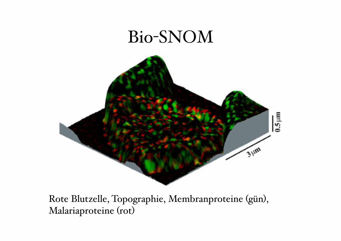
Bio-SNOM
Rote Blutzelle, Topographie, Membranproteine (gün), Malariaproteine (rot)
4158
interactions or intramolecular dynamics at the single-moleculelevel on cells. The first such examples have already beenreported (Kirsch et al., 1999); however, although clearlyshowing resolution below the diffraction limit, single-moleculedetection sensitivity has not yet been reached. Importantly,
NSOM bridges the gap between the diffraction-limitedresponse of normal light microscopy and the 5-10 nm distancesensitivity inherent in FRET and, as such, already providesimportant additional but otherwise unobtainable information.
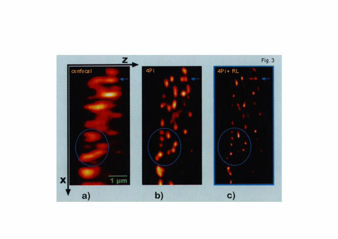
In the past decade, especially the past two years, severalother approaches to break the diffraction limit have beendeveloped. These include interferometric microscopy methodssuch as 4Pi confocal microscopy (Hell and Stelzer, 1992),I5M (Gustafsson et al., 1999), standing-wave-total-internal-reflection fluorescence microscopy (Cragg and So, 2000) andharmonic excitation light microscopy (Frohn et al., 2000).These methods, however, do not have single-moleculedetection sensitivity, and all require extended electronic post-processing of the images. Recently, a novel techniqueinvolving ‘point spread function (PSF) engineering’, whichexploits stimulated emission depletion (STED), has beendescribed (Klar et al., 2000). This method involves theinduced quenching of fluorescence by stimulated emission atthe rim of the diffraction-limited focal spot, thereby squeezingit to an almost spherical shape of ~100 nm in diameter. Thusfar, this is the only technique that seriously rivals the smallexcitation/detection volume and therefore sensitivity ofNSOM. The maximal resolution obtained with aperture-typeNSOM relates to the limited energy throughput of the near-field probe. This limits the minimum size of the aperture to beused and hence the resolution of the microscope to ~20 nm.A possible way around this involves exploiting single-molecule emitters, attached to a scanning probe, which act aslight source to excite molecules in the sample (Michaelis etal., 2000).
The most important technical challenge that remains is theconstruction of an NSOM instrument that operates underphysiologically relevant conditions and allows the study ofsoft, rough and motile surfaces, such as the plasma membraneof living cells. When combined with single-molecule detectionsensitivity and an optical resolution that is comparable totransmission electron microscopy, this will prove to be aninvaluable tool in cell biology. These are truly exciting times.
We thank Jeroen Korterik, Frans Segerink, Marjolein Koopman andBen Joosten for expert technical assistance. Frank de Lange issupported by grant FB-N/T-1a from the Netherlands Foundation forFundamental Research of Matter (FOM). Bärbel de Bakker issupported by grant TTN4812 from the Dutch Technology Foundation(STW). The research by Maria Garcia-Parajo was made possible bya fellowship of the Royal Netherlands Academy of Arts and Sciences(KNAW).
References
Allen, T. D., Cronshaw, J. M., Bagley, S., Kiseleva, E. and Goldberg, M.W. (2000). The nuclear pore complex. J. Cell Sci. 113, 3885-3886.
Ambrose, W. P., Goodwin, P. M., Martin, J. C. and Keller, R. A. (1994).Alterations of single molecule fluorescence lifetimes in near-field opticalmicroscopy. Science 265, 364-367.
Balaban, N. Q., Schwarz, U. S., Riveline, D., Goichberg, P., Tzur, G.,Sabanay, I., Mahalu, D., Safran, S., Bershadsky, A., Addadi, L. andGeiger B. (2001). Force and focal adhesion assembly: a close relationshipstudied using elastic micropatterned substrates. Nat. Cell Biol. 3, 466-472.
Betzig, E. and Chichester, R. J. (1993). Single molecules observed by near-field scanning optical microscopy. Science 262, 1422-1425.
Betzig, E., Chichester, R. J., Lanni, F. and Taylor, D. L. (1993). Near-fieldfluorescence imaging of cytoskeletal actin. Bioimaging 1, 129-133.
JOURNAL OF CELL SCIENCE 114 (23)
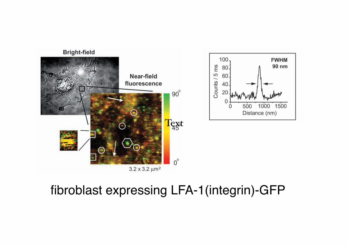
Fig. 4. (A) Single molecule detection on cells by NSOM. This figureshows a 40 nm optical resolution near-field ‘zoom-in’ on the indicatedarea (3.2 ! 3.2 µm2) in the bright-field image of a fibroblastexpressing LFA-1-GFP. GFP excitation is accomplished using 488 nmlight (Ar-Kr laser line) linearly polarized along 90°. Fluorescence iscollected by a 1.3 numerical aperture oil-immersion objective incombination with standard optical filters. A polarizing beam-splittercube (Newport, Fountain Valley, CA) is used to split the fluorescencesignal into two perpendicular polarized components (compare withFig. 2). Both signals are then detected by photon-counting avalanchephotodiode detectors (APD, SPCM-100, EG&G Electro optics,Quebec). The red/green color-coding of the signals reflects theorientation of the GFP molecules in the plane of the sample.Examples of clustered molecules (arrows) as well as examplesshowing clear single-molecule detection sensitivity are indicated(circles and squares). The squares show the fast-blinking behaviortypical of single molecule GFP fluorescence. The circles presentdemonstrations of discrete photodissociation phenomena.(B) Estimation of the resolution in the near-field image. This figureshows a line trace through the feature marked with the hexagon in thenear-field image. The full width at half maximum (FWHM; arrows) ofsuch traces can be used to obtain an estimate for the maximalresolution (half the FWHM) in the near-field image. On this basis, weestimate the resolution in the near-field image to be ~40 nm.
4158
interactions or intramolecular dynamics at the single-moleculelevel on cells. The first such examples have already beenreported (Kirsch et al., 1999); however, although clearlyshowing resolution below the diffraction limit, single-moleculedetection sensitivity has not yet been reached. Importantly,
NSOM bridges the gap between the diffraction-limitedresponse of normal light microscopy and the 5-10 nm distancesensitivity inherent in FRET and, as such, already providesimportant additional but otherwise unobtainable information.
In the past decade, especially the past two years, severalother approaches to break the diffraction limit have beendeveloped. These include interferometric microscopy methodssuch as 4Pi confocal microscopy (Hell and Stelzer, 1992),I5M (Gustafsson et al., 1999), standing-wave-total-internal-reflection fluorescence microscopy (Cragg and So, 2000) andharmonic excitation light microscopy (Frohn et al., 2000).These methods, however, do not have single-moleculedetection sensitivity, and all require extended electronic post-processing of the images. Recently, a novel techniqueinvolving ‘point spread function (PSF) engineering’, whichexploits stimulated emission depletion (STED), has beendescribed (Klar et al., 2000). This method involves theinduced quenching of fluorescence by stimulated emission atthe rim of the diffraction-limited focal spot, thereby squeezingit to an almost spherical shape of ~100 nm in diameter. Thusfar, this is the only technique that seriously rivals the smallexcitation/detection volume and therefore sensitivity ofNSOM. The maximal resolution obtained with aperture-typeNSOM relates to the limited energy throughput of the near-field probe. This limits the minimum size of the aperture to beused and hence the resolution of the microscope to ~20 nm.A possible way around this involves exploiting single-molecule emitters, attached to a scanning probe, which act aslight source to excite molecules in the sample (Michaelis etal., 2000).
The most important technical challenge that remains is theconstruction of an NSOM instrument that operates underphysiologically relevant conditions and allows the study ofsoft, rough and motile surfaces, such as the plasma membraneof living cells. When combined with single-molecule detectionsensitivity and an optical resolution that is comparable totransmission electron microscopy, this will prove to be aninvaluable tool in cell biology. These are truly exciting times.
We thank Jeroen Korterik, Frans Segerink, Marjolein Koopman andBen Joosten for expert technical assistance. Frank de Lange issupported by grant FB-N/T-1a from the Netherlands Foundation forFundamental Research of Matter (FOM). Bärbel de Bakker issupported by grant TTN4812 from the Dutch Technology Foundation(STW). The research by Maria Garcia-Parajo was made possible bya fellowship of the Royal Netherlands Academy of Arts and Sciences(KNAW).
References
Allen, T. D., Cronshaw, J. M., Bagley, S., Kiseleva, E. and Goldberg, M.W. (2000). The nuclear pore complex. J. Cell Sci. 113, 3885-3886.
Ambrose, W. P., Goodwin, P. M., Martin, J. C. and Keller, R. A. (1994).Alterations of single molecule fluorescence lifetimes in near-field opticalmicroscopy. Science 265, 364-367.
Balaban, N. Q., Schwarz, U. S., Riveline, D., Goichberg, P., Tzur, G.,Sabanay, I., Mahalu, D., Safran, S., Bershadsky, A., Addadi, L. andGeiger B. (2001). Force and focal adhesion assembly: a close relationshipstudied using elastic micropatterned substrates. Nat. Cell Biol. 3, 466-472.
Betzig, E. and Chichester, R. J. (1993). Single molecules observed by near-field scanning optical microscopy. Science 262, 1422-1425.
Betzig, E., Chichester, R. J., Lanni, F. and Taylor, D. L. (1993). Near-fieldfluorescence imaging of cytoskeletal actin. Bioimaging 1, 129-133.
JOURNAL OF CELL SCIENCE 114 (23)
Fig. 4. (A) Single molecule detection on cells by NSOM. This figureshows a 40 nm optical resolution near-field ‘zoom-in’ on the indicatedarea (3.2 ! 3.2 µm2) in the bright-field image of a fibroblastexpressing LFA-1-GFP. GFP excitation is accomplished using 488 nmlight (Ar-Kr laser line) linearly polarized along 90°. Fluorescence iscollected by a 1.3 numerical aperture oil-immersion objective incombination with standard optical filters. A polarizing beam-splittercube (Newport, Fountain Valley, CA) is used to split the fluorescencesignal into two perpendicular polarized components (compare withFig. 2). Both signals are then detected by photon-counting avalanchephotodiode detectors (APD, SPCM-100, EG&G Electro optics,Quebec). The red/green color-coding of the signals reflects theorientation of the GFP molecules in the plane of the sample.Examples of clustered molecules (arrows) as well as examplesshowing clear single-molecule detection sensitivity are indicated(circles and squares). The squares show the fast-blinking behaviortypical of single molecule GFP fluorescence. The circles presentdemonstrations of discrete photodissociation phenomena.(B) Estimation of the resolution in the near-field image. This figureshows a line trace through the feature marked with the hexagon in thenear-field image. The full width at half maximum (FWHM; arrows) ofsuch traces can be used to obtain an estimate for the maximalresolution (half the FWHM) in the near-field image. On this basis, weestimate the resolution in the near-field image to be ~40 nm.
Text
fibroblast expressing LFA-1(integrin)-GFP
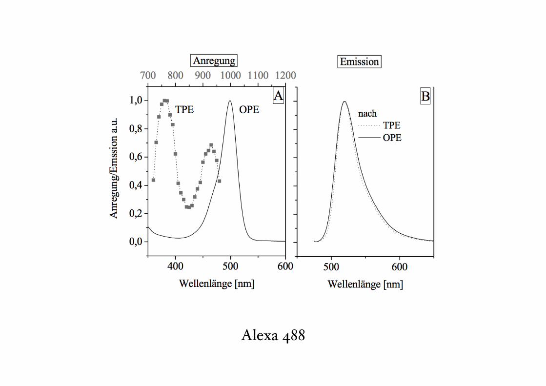
Alexa 488
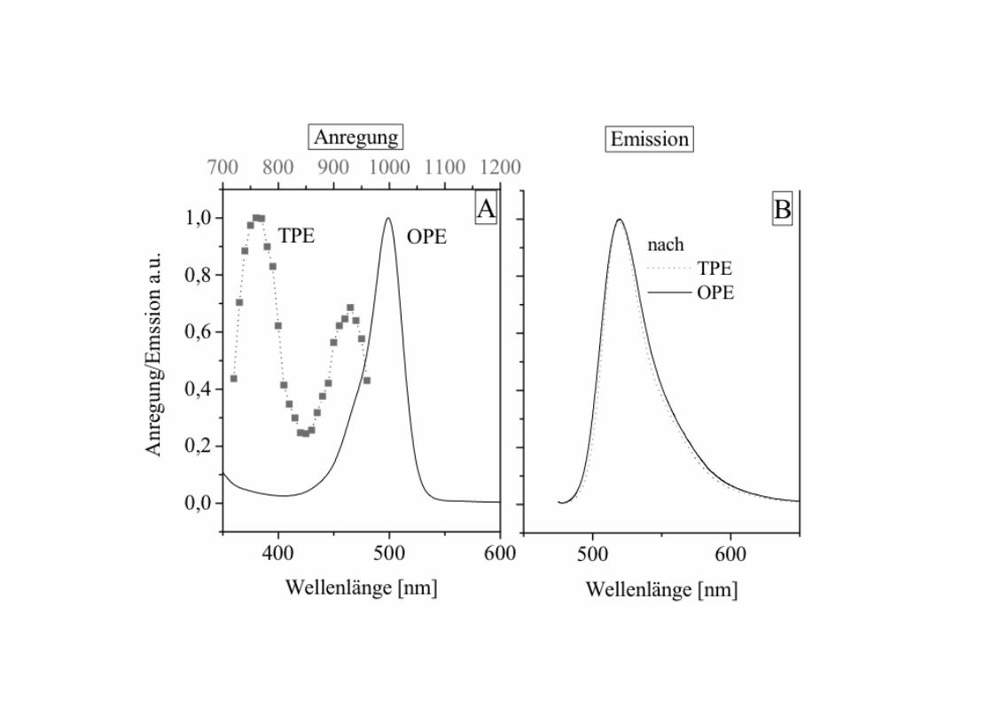
Multiple-photon excitation
fluorescence microscopy
Multiple-photon excitation fluorescence
microscopy is a technique that uses non-linear
optical effects to achieve optical sectioning.
How it works: The sample is illuminated with a wavelength
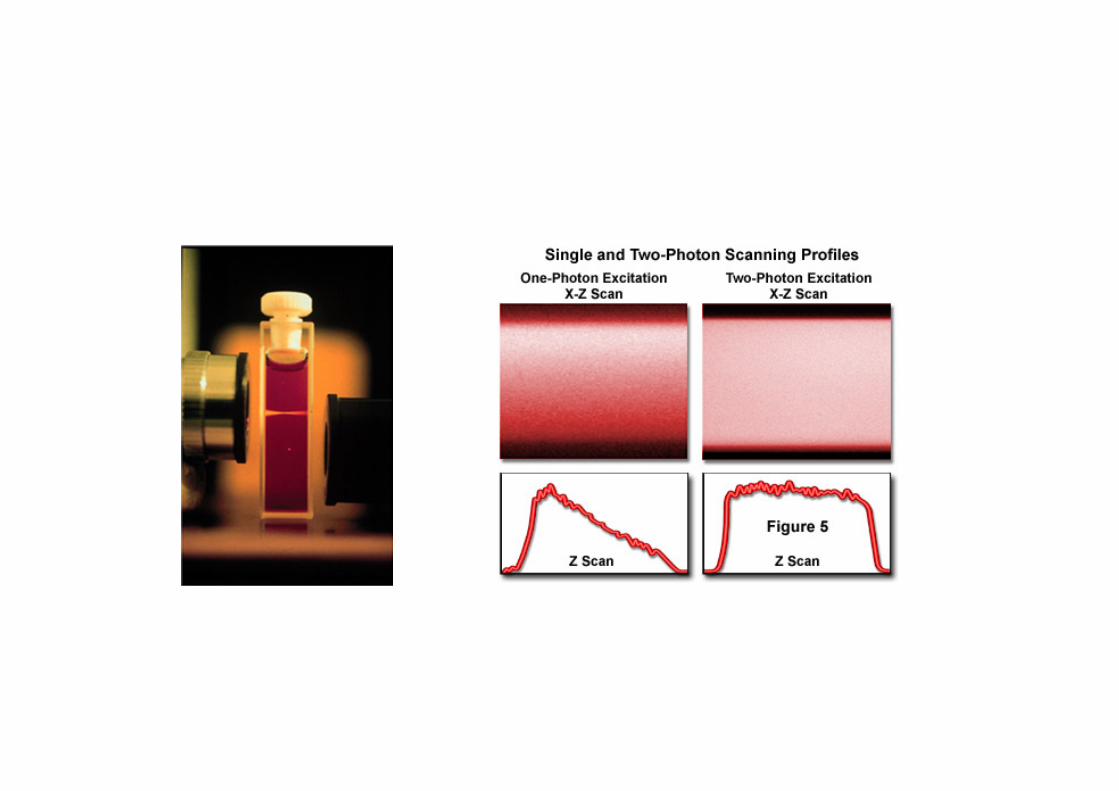
around twice the wavelength of the absorption peak of thefluorophore being used. For example, in the case offluorescein which has an absorption peak around 500nm,1000 nm excitation could be used. Essentially no excitationof the fluorophore will occur at this wavelength. However, ifa high peak-power, pulsed laser is used (so that the meanpower levels are moderate and do not damage the specimen),two-photon events will occur at the point of focus. At thispoint the photon density is sufficiently high that two photonscan be absorbed by the fluorophore essentiallysimultaneously. This is equivalent to a single photon with anenergy equal to the sum of the two that are absorbed. In thisway, fluorophore excitation will only occur at the point offocus (where it is needed) thereby eliminating excitation ofout-of-focus fluorophore and achieving optical sectioning.
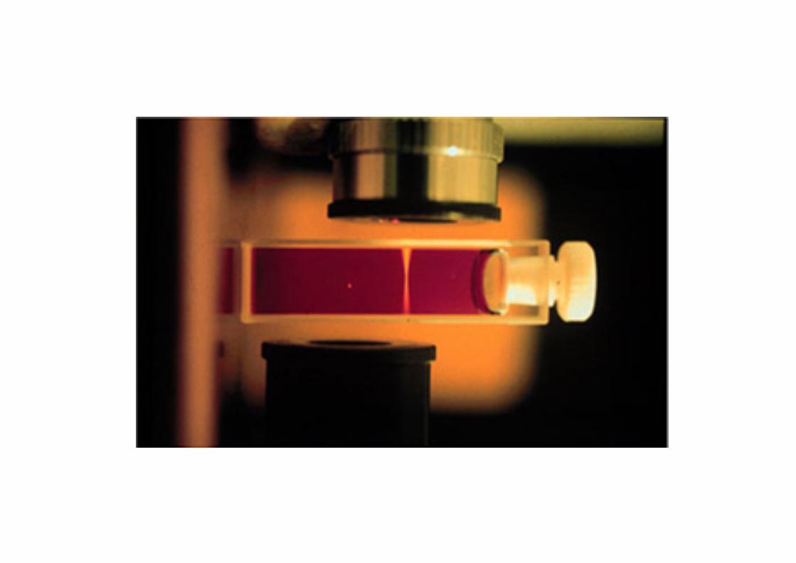
A cuvette of fluorescent dye excited by
single photon excitation (right line) and
multiphoton excitation (localized spot of
fluorescence at left) illustrating that two
photon excitation is confined to the focus of
the excitation beam (courtesy of Brad Amos
CBIT Home
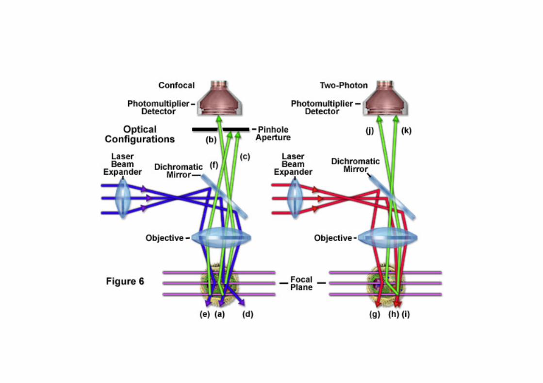
The Center for Biomedical Imaging Technology has engineered atwo-photon laser scanning microscope, which is available for use. Dr.Paul Campagnola has adapted the center's BioRad MRC600 fortwo-photon excitation of fluorescence while still maintaining theMRC600's one-photon CLSM.
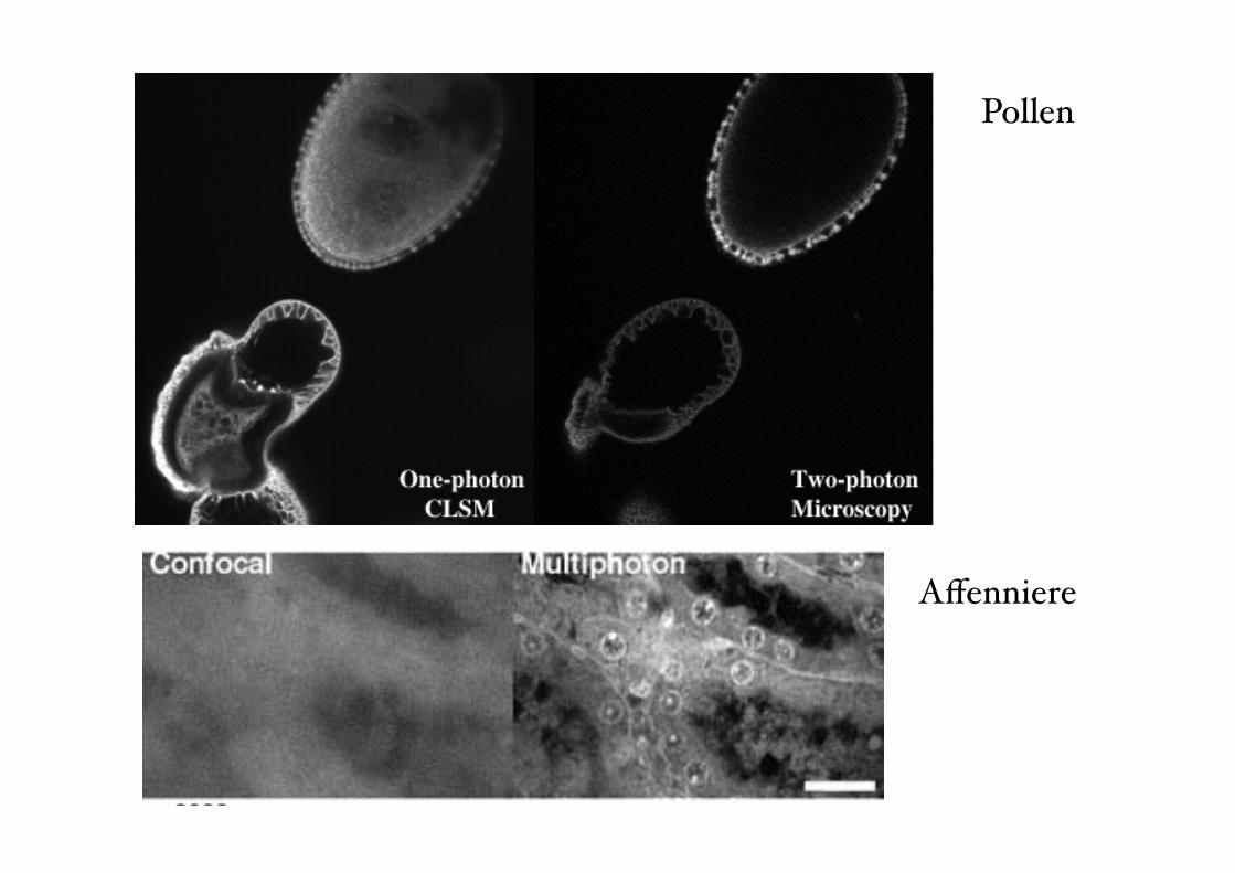
Two-photon excitation of fluorescence is based on the principle thattwo photons of longer wavelength light are simultaneously absorbedby a fluorochrome which would normally be excited by a singlephoton, with a shorter wavelength. The nonlinear optical absorptionproperty, of two-photon excitation, limits the fluorochrome excitationto the point of focus. This is graphically demonstrated in the imageabove. The images below, of pollen granules which were obtained onour system, clearly show the difference between one and two-photonexcitation. The two-photon image was generated using 704nmexcitation light while the one-photon image was generated using488nm.
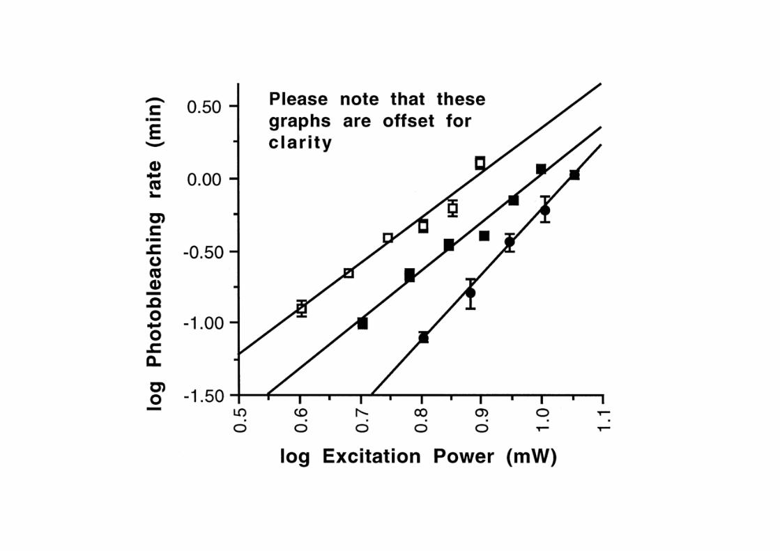
Limiting the excitation light to the point of focus rather than exposing the entire sample greatlyreduces total photobleaching and photodamage. This is one major advantage to using two-photonexcitation.
Two-photon microscopy has several other advantages over confocal microscopy; optical sections canbe obtained deeper within a specimen, a detection pinhole is no longer necessary, thus not limitingthe number of photons being detected. (However, a pinhole may still be used to slightly improve theresolution of two-photon excitation.) In addition, the use of UV fluorophores is no longer limited toUV corrected objectives. Two-photon excitation utilizes visible wavelengths to excite UV fluorescentstains and indicators, therefore the objectives do not have to pass UV light.
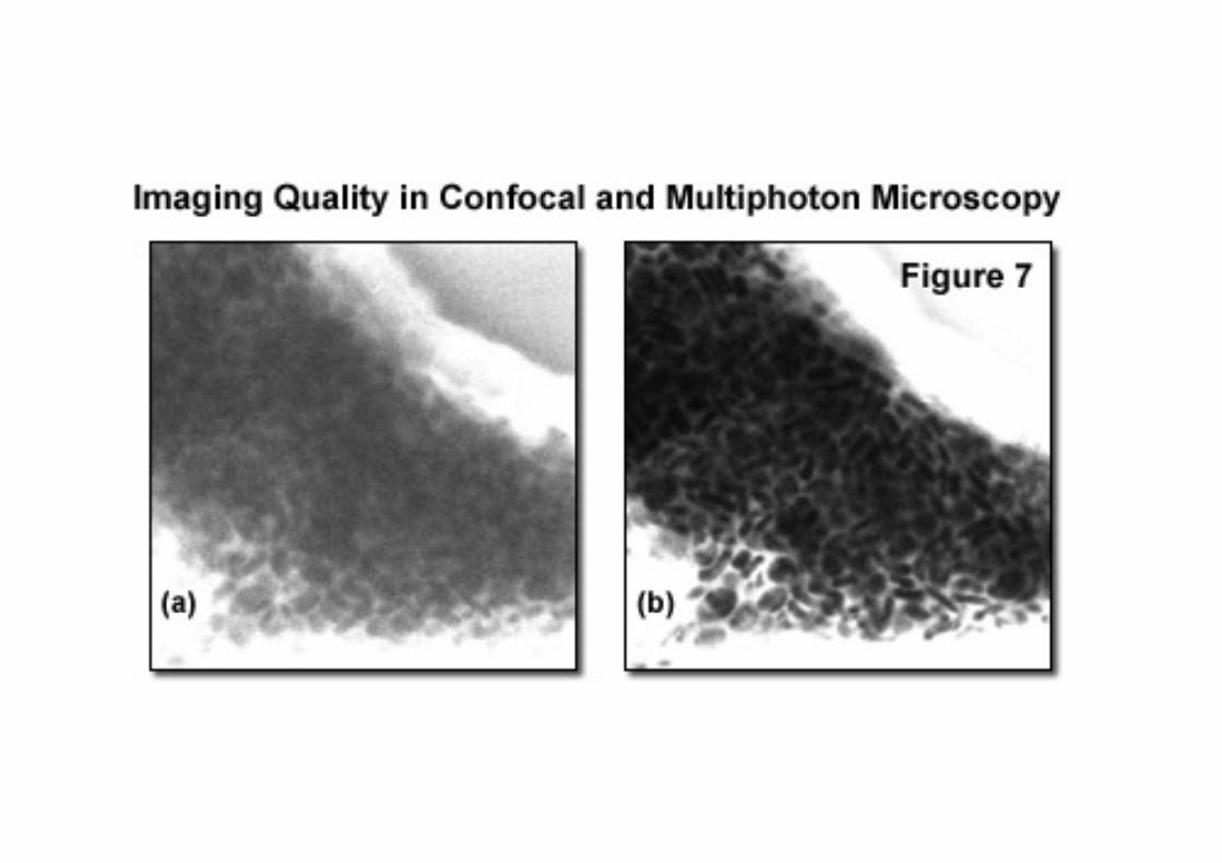
Optical sections may be obtained from deeper within a
tissue that can be achieved by confocal or wide-fieldimaging. There are three main reasons for this:
the excitation source is not attenuated by absorption byfluorophore above the plane of focuslonger excitation wavelengths suffer less scatteringfluorescence signal is not degraded by scattering fromwithin the sample as it is not imaged
When images of optical sections that are deep within alight-scattering sample are obtained using confocalmicroscopy, the fluorescence signal is attenuated by lightscatter. Furthermore, some fluorescence originating fromregions away from the point being instantaneouslyilluminated will be scattered such that this fluorescence willpass through the confocal pinhole thereby increasingbackground. Confocal imaging therefore suffers adeterioration in signal-to-background when obtaining imagesfrom deep within a sample. Multiphoton imaging is largelyimmune from these effects as little fluorescence is generatedaway from the point of illumination and all detectedfluorescence photons may be used for imaging regardless ofwhether they have been scattered or not.
Images of acid fucsin stained monkey kidney taken at a
depth of 60 µm by confocal (left) and multiphoton
microscopy (right). Laser intensities were adjusted to
produce the same mean photons per pixel. The confocal
image shows a significant increase in local background
resulting in a lower contrast image. However, the
multiphoton image maintains contrast even at significant
depths within a light scattering sample.(Reproduced from
Figure 7 of Centonze,V.E and J.G.White. (1998)
Biophysical J. 75:2015-2024)
Affenniere
Pollen
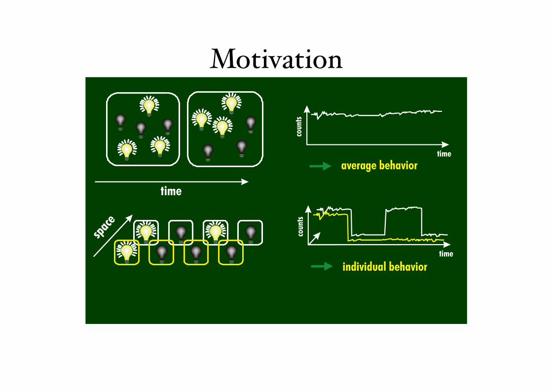
Motivation
average behavior
time
time
individual behaviortime
coun
tsco
unts
spac
e
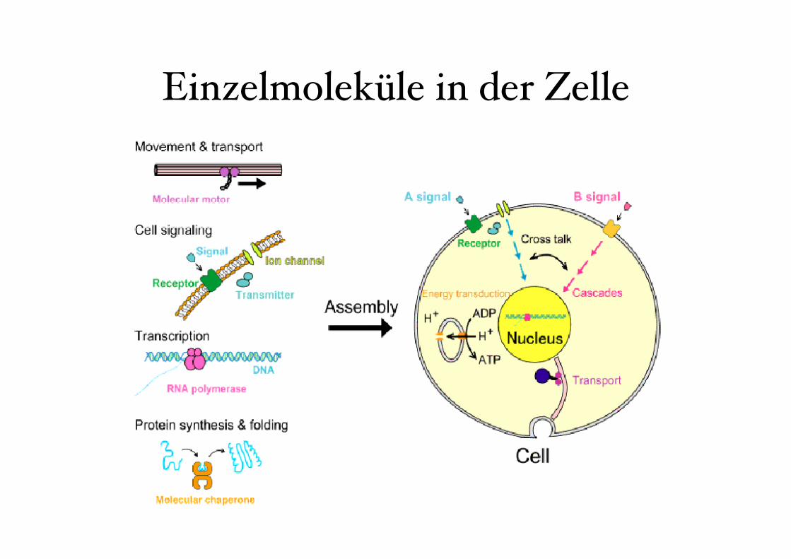
Einzelmoleküle in der Zelle
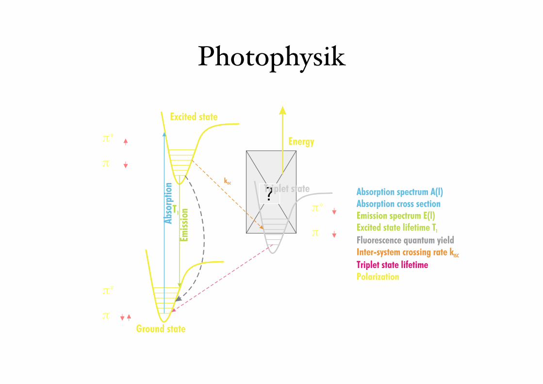
Photophysik
Ground state
Excited state
Triplet state
Abso
rptio
nEm
issio
nT1
kISC
Absorption spectrum A(l)Absorption cross sectionEmission spectrum E(l)Excited state lifetime T1
Fluorescence quantum yieldInter-system crossing rate kISC
Triplet state lifetimePolarizationPhotostability
Energy
Bleaching
π
π∗
π
π∗
π
π∗
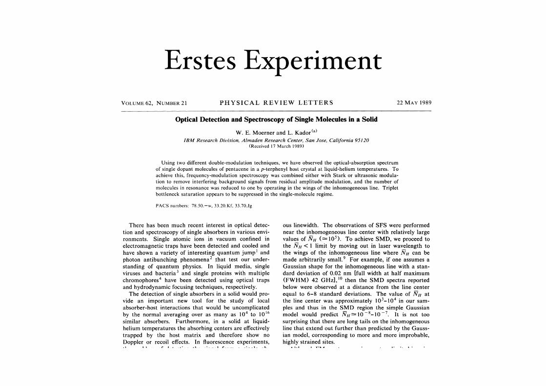
Erstes Experiment
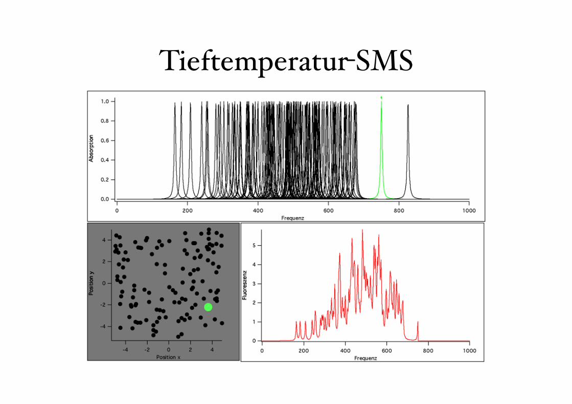
Tieftemperatur-SMS
Biospektroskopie 205
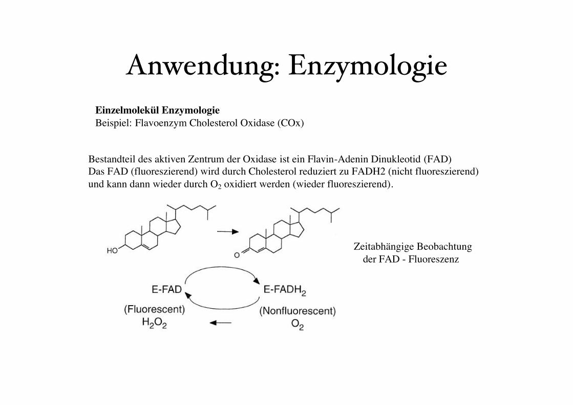
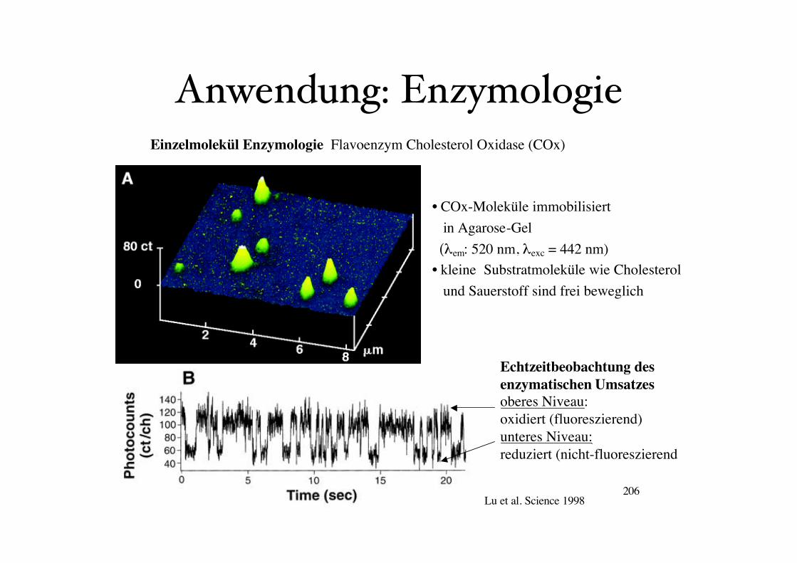
Einzelmolekül Enzymologie
Beispiel: Flavoenzym Cholesterol Oxidase (COx)
Bestandteil des aktiven Zentrum der Oxidase ist ein Flavin-Adenin Dinukleotid (FAD)
Das FAD (fluoreszierend) wird durch Cholesterol reduziert zu FADH2 (nicht fluoreszierend)
und kann dann wieder durch O2 oxidiert werden (wieder fluoreszierend).
Zeitabhängige Beobachtung
der FAD - Fluoreszenz
FluoreszenzspektroskopieAnwendung: Enzymologie
Anwendung: Enzymologie
Biospektroskopie 206
Einzelmolekül Enzymologie Flavoenzym Cholesterol Oxidase (COx)
• COx-Moleküle immobilisiert
in Agarose-Gel
(!em: 520 nm, !exc = 442 nm)
• kleine Substratmoleküle wie Cholesterol
und Sauerstoff sind frei beweglich
Lu et al. Science 1998
Echtzeitbeobachtung des
enzymatischen Umsatzes
oberes Niveau:
oxidiert (fluoreszierend)
unteres Niveau:
reduziert (nicht-fluoreszierend
Fluoreszenzspektroskopie
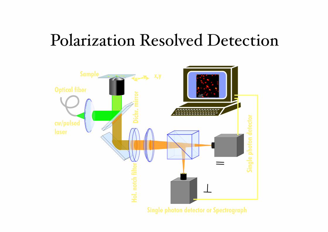
Polarization Resolved Detection
Sample x,y
Dic
hr. m
irro
rH
ol. n
otch
filte
r
Optical fiber
cw/pulsedlaser
1 µm
Single photon detector or Spectrograph
Sing
le p
hoto
n de
tect
or

Polarization Resolved Detection
chromophore orientation
1.2
0.8
0.4
0.0
p co
mpo
nent
12080400time (ms)
120
100
80
60
40
20
0
time
(ms)
1.20.80.40.0s component
-1.0
-0.5
0.0
0.5
1.0
pola
rizat
ion
12080400time (ms)
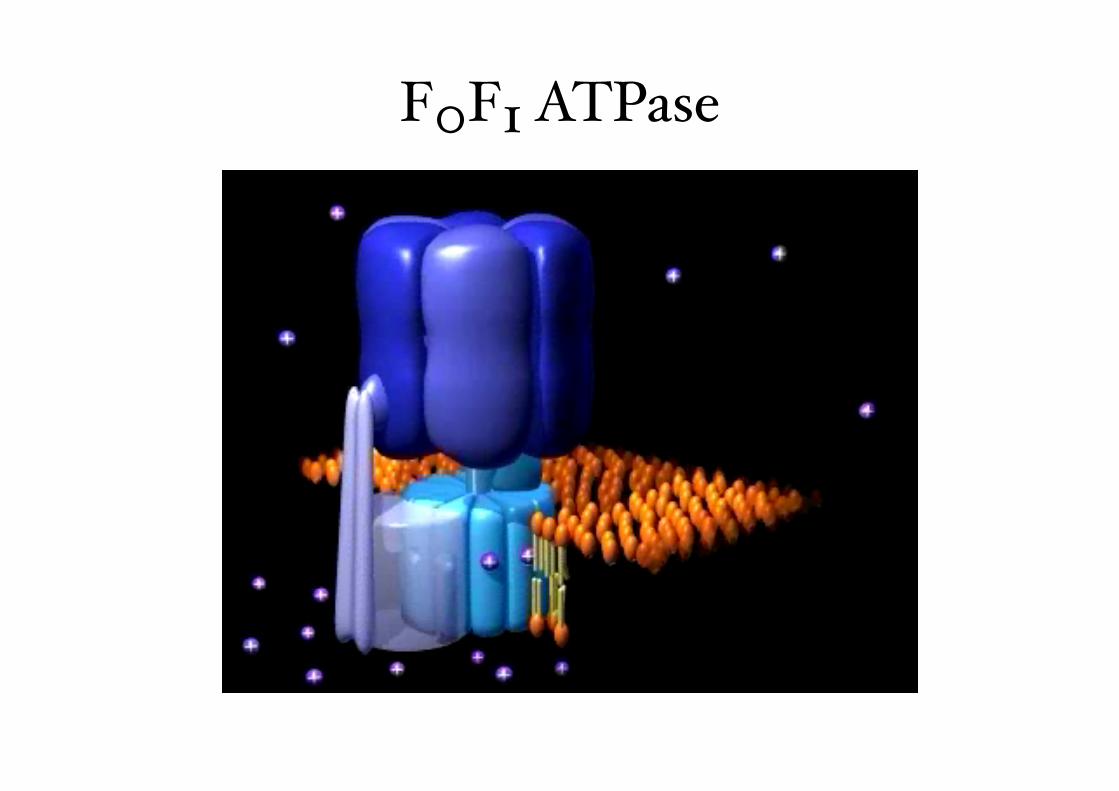
F0F1 ATPase
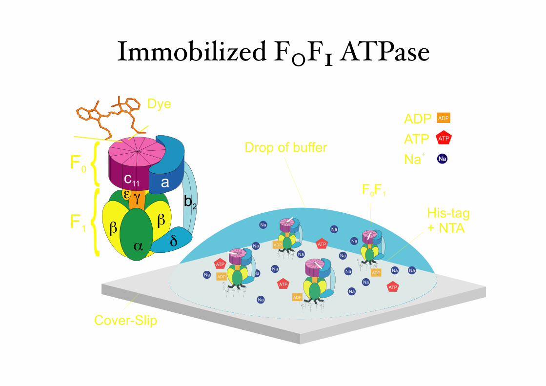
Immobilized F0F1 ATPase
F0
F1
!"
"
#
$
%ac11
b2
Na+
ATP
ADP
Drop of buffer
His-tag+ NTA
F F0 1
Na
Na
Na
Na
Na
Na
Na
Na
Na
Na Na
Na
Na
NaNa
Na
ATP
ATP
ATPATP
H N2
CH2
CH2
CH2
CH2
CH
CH2
N
C
OH
O
C
OH
O
C
OHO
H N2
CH2
CH2
CH2
CH2
CH
CH2
N
C
OH
O
C
OH
O
C
OHO
H N2
CH2
CH2
CH2
CH2
CH
CH2
N
C
OH
O
C
OH
O
C
OHO
H N2
CH2
CH2
CH2
CH2
CH
CH2
N
C
OH
O
C
OH
O
C
OHO
H N2
CH2
CH2
CH2
CH2
CH
CH2
N
C
OH
O
C
OH
O
C
OHO
H N2
CH2
CH2
CH2
CH2
CH
CH2
N
C
OH
O
C
OH
O
C
OHO
H N2
CH2
CH2
CH2
CH2
CH
CH2
N
C
OH
O
C
OH
O
C
OHO
H N2
CH2
CH2
CH2
CH2
CH
CH2
N
C
OH
O
C
OH
O
C
OHO
H N2
CH2
CH2
CH2
CH2
CH
CH2
N
C
OH
O
C
OH
O
C
OHO
HN2
CH2
CH2
CH2
CH2
CH
CH2
N
C
OH
O
C
OH
O
C
OHO
H N2
CH2
CH2
CH2
CH2
CH
CH2
N
C
OH
O
C
OH
O
C
OHO
H N2
CH2
CH2
CH2
CH2
CH
CH2
N
C
OH
O
C
OH
O
C
OHO
H N2
CH2
CH2
CH2
CH2
CH
CH2
N
C
OH
O
C
OH
O
C
OHO
H N2
CH2
CH2
CH2
CH2
CH
CH2
N
C
OH
O
C
OH
O
C
OHO
H N2
CH2
CH2
CH2
CH2
CH
CH2
N
C
OH
O
C
OH
O
C
OHO
H N2
CH2
CH2
CH2
CH2
CH
CH2
N
C
OH
O
C
OH
O
C
OHO
H N2
CH2
CH2
CH2
CH2
CH
CH2
N
C
OH
O
C
OH
O
C
OHO
H N2
CH2
CH2
CH2
CH2
CH
CH2
N
C
OH
O
C
OH
O
C
OHO
H N2
CH2
CH2
CH2
CH2
CH
CH2
N
C
OH
O
C
OH
O
C
OHO
H N2
CH2
CH2
CH2
CH2
CH
CH2
N
C
OH
O
C
OH
O
C
OHO
H N2
CH2
CH2
CH2
CH2
CH
CH2
N
C
OH
O
C
OH
O
C
OHO
H N2
CH2
CH2
CH2
CH2
CH
CH2
N
C
OH
O
C
OH
O
C
OHO
H N2
CH2
CH2
CH2
CH2
CH
CH2
N
C
OH
O
C
OH
O
C
OHO
H N2
CH2
CH2
CH2
CH2
CH
CH2
N
C
OH
O
C
OH
O
C
OHO
H N2
CH2
CH2
CH2
CH2
CH
CH2
N
C
OH
O
C
OH
O
C
OHO
H N2
CH2
CH2
CH2
CH2
CH
CH2
N
C
OH
O
C
OH
O
C
OHO
H N2
CH2
CH2
CH2
CH2
CH
CH2
N
C
OH
O
C
OH
O
C
OHO
H N2
CH2
CH2
CH2
CH2
CH
CH2
N
C
OH
O
C
OH
O
C
OHO
ADP
ADPADP
ADP
F0
F1
!"
"
#
$
%!&11
"2
Na+
ATP
ADP
His-tag+ NTA
F F0 1
Na
Na
Na
Na
Na
Na
Na
Na
Na
Na Na
Na
Na
NaNa
Na
ATP
ATP
ATPATP
H N2
CH2
CH2
CH2
CH2
CH
CH2
N
C
OH
O
C
OH
O
C
OHO
H N2
CH2
CH2
CH2
CH2
CH
CH2
N
C
OH
O
C
OH
O
C
OHO
H N2
CH2
CH2
CH2
CH2
CH
CH2
N
C
OH
O
C
OH
O
C
OHO
H N2
CH2
CH2
CH2
CH2
CH
CH2
N
C
OH
O
C
OH
O
C
OHO
H N2
CH2
CH2
CH2
CH2
CH
CH2
N
C
OH
O
C
OH
O
C
OHO
H N2
CH2
CH2
CH2
CH2
CH
CH2
N
C
OH
O
C
OH
O
C
OHO
H N2
CH2
CH2
CH2
CH2
CH
CH2
N
C
OH
O
C
OH
O
C
OHO
H N2
CH2
CH2
CH2
CH2
CH
CH2
N
C
OH
O
C
OH
O
C
OHO
H N2
CH2
CH2
CH2
CH2
CH
CH2
N
C
OH
O
C
OH
O
C
OHO
HN2
CH2
CH2
CH2
CH2
CH
CH2
N
C
OH
O
C
OH
O
C
OHO
H N2
CH2
CH2
CH2
CH2
CH
CH2
N
C
OH
O
C
OH
O
C
OHO
H N2
CH2
CH2
CH2
CH2
CH
CH2
N
C
OH
O
C
OH
O
C
OHO
H N2
CH2
CH2
CH2
CH2
CH
CH2
N
C
OH
O
C
OH
O
C
OHO
H N2
CH2
CH2
CH2
CH2
CH
CH2
N
C
OH
O
C
OH
O
C
OHO
H N2
CH2
CH2
CH2
CH2
CH
CH2
N
C
OH
O
C
OH
O
C
OHO
H N2
CH2
CH2
CH2
CH2
CH
CH2
N
C
OH
O
C
OH
O
C
OHO
H N2
CH2
CH2
CH2
CH2
CH
CH2
N
C
OH
O
C
OH
O
C
OHO
H N2
CH2
CH2
CH2
CH2
CH
CH2
N
C
OH
O
C
OH
O
C
OHO
H N2
CH2
CH2
CH2
CH2
CH
CH2
N
C
OH
O
C
OH
O
C
OHO
H N2
CH2
CH2
CH2
CH2
CH
CH2
N
C
OH
O
C
OH
O
C
OHO
H N2
CH2
CH2
CH2
CH2
CH
CH2
N
C
OH
O
C
OH
O
C
OHO
H N2
CH2
CH2
CH2
CH2
CH
CH2
N
C
OH
O
C
OH
O
C
OHO
H N2
CH2
CH2
CH2
CH2
CH
CH2
N
C
OH
O
C
OH
O
C
OHO
H N2
CH2
CH2
CH2
CH2
CH
CH2
N
C
OH
O
C
OH
O
C
OHO
H N2
CH2
CH2
CH2
CH2
CH
CH2
N
C
OH
O
C
OH
O
C
OHO
H N2
CH2
CH2
CH2
CH2
CH
CH2
N
C
OH
O
C
OH
O
C
OHO
H N2
CH2
CH2
CH2
CH2
CH
CH2
N
C
OH
O
C
OH
O
C
OHO
H N2
CH2
CH2
CH2
CH2
CH
CH2
N
C
OH
O
C
OH
O
C
OHO
ADP
ADPADP
ADP
NaNa
ATP
ADP
Cover-Slip
Dye
{{
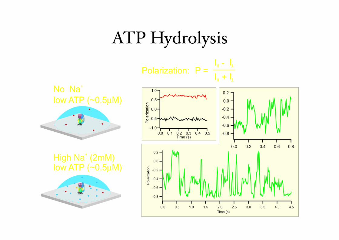
ATP Hydrolysis
No Na
low ATP (~0.5µM)
low ATP (~0.5µM)
+
High Na (2mM) +
P = III II I+
III II I-Polarization:
H N2
CH2
CH2
CH2
CH2
CH
CH2
N
C
OH
O
C
OH
O
C
OHO
H N2
CH2
CH2
CH2
CH2
CH
CH2
N
C
OH
O
C
OH
O
C
OHO
H N2
CH2
CH2
CH2
CH2
CH
CH2
N
C
OH
O
C
OH
O
C
OH O
HN2
CH2
CH2
CH2
CH2
CH
CH2
N
C
OH
O
C
OH
O
C
OH O
H N2
CH2
CH2
CH2
CH2
CH
CH2
N
C
OH
O
C
OH
O
C
OHO
HN2
CH2
CH2
CH2
CH2
CH
CH2
N
C
OH
O
C
OH
O
C
OHO
H N2
CH2
CH2
CH2
CH2
CH
CH2
N
C
OH
O
C
OH
O
C
OHO
+
P = III II I+
III II I-Polarization:
H N2
CH2
CH2
CH2
CH2
CH
CH2
N
C
OH
O
C
OH
O
C
OHO
H N2
CH2
CH2
CH2
CH2
CH
CH2
N
C
OH
O
C
OH
O
C
OHO
H N2
CH2
CH2
CH2
CH2
CH
CH2
N
C
OH
O
C
OH
O
C
OH O
HN2
CH2
CH2
CH2
CH2
CH
CH2
N
C
OH
O
C
OH
O
C
OH O
H N2
CH2
CH2
CH2
CH2
CH
CH2
N
C
OH
O
C
OH
O
C
OHO
HN2
CH2
CH2
CH2
CH2
CH
CH2
N
C
OH
O
C
OH
O
C
OHO
H N2
CH2
CH2
CH2
CH2
CH
CH2
N
C
OH
O
C
OH
O
C
OHO
H N2
CH2
CH2
CH2
CH2
CH
CH2
N
C
OH
O
C
OH
O
C
OHO
H N2
CH2
CH2
CH2
CH2
CH
CH2
N
C
OH
O
C
OH
O
C
OHO
H N2
CH2
CH2
CH2
CH2
CH
CH2
N
C
OH
O
C
OH
O
C
OHO
HN2
CH2
CH2
CH2
CH2
CH
CH2
N
C
OH
O
C
OH
O
C
OHO
H N2
CH2
CH2
CH2
CH2
CH
CH2
N
C
OH
O
C
OH
O
C
OHO
HN2
CH2
CH2
CH2
CH2
CH
CH2
N
C
OH
O
C
OH
O
C
OHO
H N2
CH2
CH2
CH2
CH2
CH
CH2
N
C
OH
O
C
OH
O
C
OHO
-1.0
-0.5
0.0
0.5
1.0
0.50.40.30.20.10.0Time (s)
Po
lariza
tio
n
-0.8
-0.6
-0.4
-0.2
0.0
0.2
0.80.60.40.20.0
-0.8
-0.6
-0.4
-0.2
0.0
0.2P
ola
riza
tio
n
4.54.03.53.02.52.01.51.00.50.0
Time (s)
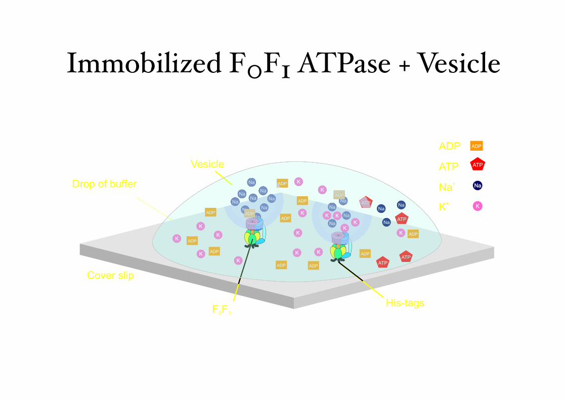
Immobilized F0F1 ATPase + Vesicle
Cover slip
Drop of buffer
F F0 1
Vesicle
Na
Na
Na
Na
Na
Na
NaNa
Na
Na
Na
Na
Na
Na
Na
Na
ATP
ATP
ATP
ATP
OH
OH
ADPADP
ADP
ADPADP
ADP
ADP
ADP
ADP
ADP
ADP
ADP
KK
F F0 1
Na
Na
Na
Na
Na
Na
NaNa
Na
Na
Na
Na
Na
Na
Na
Na
ATP
ATP
ATP
ATP
OH
OH
ADPADP
ADP
ADPADP
ADP
ADP
ADP
ADP
ADP
ADP
ADP
KK
F F0 1
Na
Na
Na
Na
Na
Na
NaNa
Na
Na
Na
Na
Na
Na
Na
Na
ATP
ATP
ATP
ATP
OH
OH
ADPADP
ADP
ADPADP
ADP
ADP
ADP
ADP
ADP
ADP
ADP
KK
F F0 1
Na
Na
Na
Na
Na
Na
NaNa
Na
Na
Na
Na
Na
Na
Na
Na
ATP
ATP
ATP
ATP
OH
OH
ADPADP
ADP
ADPADP
ADP
ADP
ADP
ADP
ADP
ADP
ADP
KK
F F0 1
Na
Na
Na
Na
Na
Na
NaNa
Na
Na
Na
Na
Na
Na
Na
Na
ATP
ATP
ATP
ATP
OH
OH
ADPADP
ADP
ADPADP
ADP
ADP
ADP
ADP
ADP
ADP
ADP
KK
F F0 1
Na
Na
Na
Na
Na
Na
NaNa
Na
Na
Na
Na
Na
Na
Na
Na
ATP
ATP
ATP
ATP
OH
OH
ADPADP
ADP
ADPADP
ADP
ADP
ADP
ADP
ADP
ADP
ADP
KK
F F0 1
Na
Na
Na
Na
Na
Na
NaNa
Na
Na
Na
Na
Na
Na
Na
Na
ATP
ATP
ATP
ATP
OH
OH
ADPADP
ADP
ADPADP
ADP
ADP
ADP
ADP
ADP
ADP
ADP
KKKK
KK
KKKK
KK
KKKK
KKKK
KK
KK
KK
KK
KK
KK
KK
Na+
K+
ATP
ADP
NaNa
ATP
ADP
His-tagsF F0 1
Na
Na
Na
Na
Na
Na
NaNa
Na
Na
Na
Na
Na
Na
Na
Na
ATP
ATP
ATP
ATP
OH
OH
ADPADP
ADP
ADPADP
ADP
ADP
ADP
ADP
ADP
ADP
ADP
KKKK
KK
KKKK
KK
KKKK
KKKK
KK
KK
KK
KK
KK
KK
KK
+
+
NaNa
ATP
ADP
F F0 1
Na
Na
Na
Na
Na
Na
NaNa
Na
Na
Na
Na
Na
Na
Na
Na
ATP
ATP
ATP
ATP
OH
OH
ADPADP
ADP
ADPADP
ADP
ADP
ADP
ADP
ADP
ADP
ADP
KKKK
KK
KKKK
KK
KKKK
KKKK
KK
KK
KK
KK
KK
KK
KK
+
+
NaNa
ATP
ADP
F F0 1
Na
Na
Na
Na
Na
Na
NaNa
Na
Na
Na
Na
Na
Na
Na
Na
ATP
ATP
ATP
ATP
OH
OH
ADPADP
ADP
ADPADP
ADP
ADP
ADP
ADP
ADP
ADP
ADP
KKKK
KK
KKKK
KK
KKKK
KKKK
KK
KK
KK
KK
KK
KK
KK
+
+
NaNa
ATP
ADP
F F0 1
Na
Na
Na
Na
Na
Na
NaNa
Na
Na
Na
Na
Na
Na
Na
Na
ATP
ATP
ATP
ATP
OH
OH
ADPADP
ADP
ADPADP
ADP
ADP
ADP
ADP
ADP
ADP
ADP
KKKK
KK
KKKK
KK
KKKK
KKKK
KK
KK
KK
KK
KK
KK
KK
+
+
NaNa
ATP
ADP
F0 1
Na
Na
Na
Na
Na
Na
NaNa
Na
Na
Na
Na
Na
Na
Na
Na
ATP
ATP
ATP
ATP
OH
OH
ADPADP
ADP
ADPADP
ADP
ADP
ADP
ADP
ADP
ADP
ADP
KKKK
KK
KKKK
KK
KKKK
KKKK
KK
KK
KK
KK
KK
KK
KK
+
+
NaNa
ATP
ADP
F0 1
Na
Na
Na
Na
Na
Na
NaNa
Na
Na
Na
Na
Na
Na
Na
Na
ATP
ATP
ATP
ATP
OH
OH
ADPADP
ADP
ADPADP
ADP
ADP
ADP
ADP
ADP
ADP
ADP
KKKK
KK
KKKK
KK
KKKK
KKKK
KK
KK
KK
KK
KK
KK
KK
+
+
NaNa
ATP
ADP
F0 1
Na
Na
Na
Na
Na
Na
NaNa
Na
Na
Na
Na
Na
Na
Na
Na
ATP
ATP
ATP
ATP
OH
OH
ADPADP
ADP
ADPADP
ADP
ADP
ADP
ADP
ADP
ADP
ADP
KKKK
KK
KKKK
KK
KKKK
KKKK
KK
KK
KK
KK
KK
KK
KK
+
+
NaNa
ATP
ADP
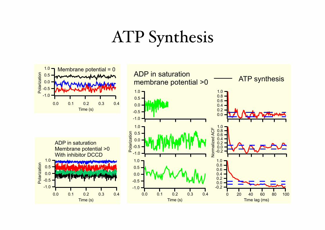
ATP Synthesis
-1.0
-0.5
0.0
0.5
1.0 1.00.80.60.40.20.0
-1.0
-0.5
0.0
0.5
1.0P
ola
riza
tio
n
Po
lariza
tio
nP
ola
riza
tio
n
Norm
aliz
ed A
CF
1.00.80.60.40.20.0
-0.2
-1.0
-0.5
0.0
0.5
1.0 1.00.80.60.40.20.0
-0.2
Time (s)
0.40.30.20.10.0
Time lag (ms)
100806040200
-1.0
-0.5
0.0
0.5
1.0
Time (s)
Time (s)
-1.0
-0.5
0.40.30.20.10.0
0.40.30.20.10.0
0.0
0.5
1.0
Membrane potential = 0ADP in saturationmembrane potential >0 ATP synthesis
ADP in saturationMembrane potential >0With inhibitor DCCD
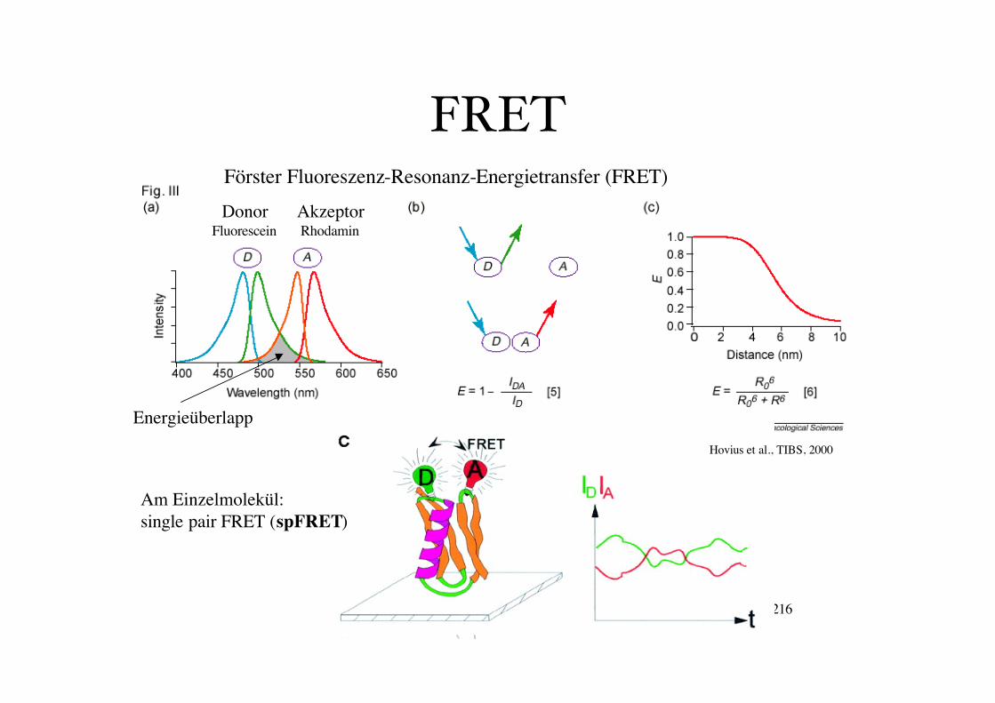
FRET
Biospektroskopie 216
DonorFluorescein
AkzeptorRhodamin
Am Einzelmolekül:
single pair FRET (spFRET)
Förster Fluoreszenz-Resonanz-Energietransfer (FRET)
Energieüberlapp
Hovius et al., TIBS, 2000
Fluoreszenzspektroskopie: Anwendungen auf Einzelmoleküle
FRET
Biospektroskopie 217
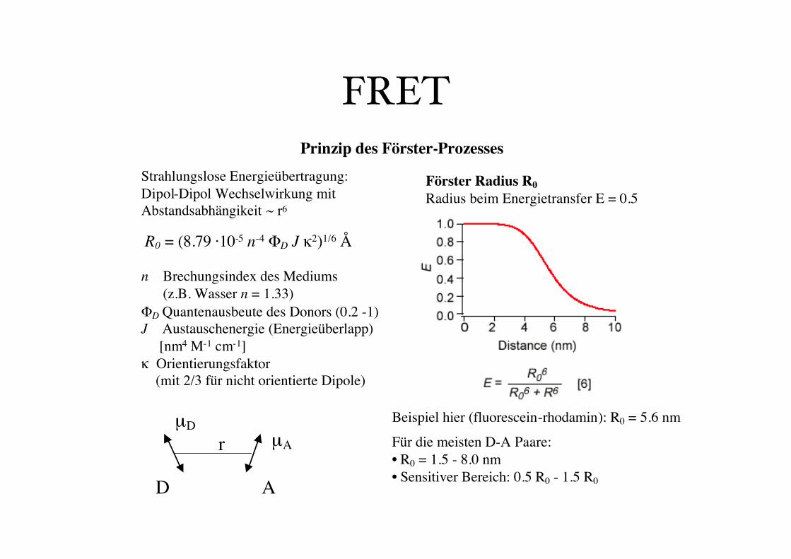
Prinzip des Förster-Prozesses
Förster Radius R0
Radius beim Energietransfer E = 0.5
Beispiel hier (fluorescein-rhodamin): R0 = 5.6 nm
Für die meisten D-A Paare:• R0 = 1.5 - 8.0 nm• Sensitiver Bereich: 0.5 R0 - 1.5 R0
Strahlungslose Energieübertragung: Dipol-Dipol Wechselwirkung mit Abstandsabhängikeit ~ r6
R0 = (8.79 ·10-5 n-4 !D J "2)1/6 Å
n Brechungsindex des Mediums (z.B. Wasser n = 1.33)
!D Quantenausbeute des Donors (0.2 -1)J Austauschenergie (Energieüberlapp)
[nm4 M-1 cm-1]" Orientierungsfaktor
(mit 2/3 für nicht orientierte Dipole)
D A
r µA
µD
Fluoreszenzspektroskopie: Anwendungen auf Einzelmoleküle
FRET - Anwendung
Biospektroskopie 218
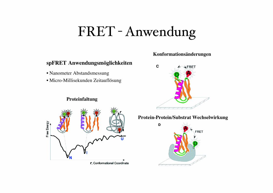
spFRET Anwendungsmöglichkeiten
• Nanometer Abstandsmessung
• Micro-Millisekunden Zeitauflösung
Konformationsänderungen
Protein-Protein/Substrat Wechselwirkung
Proteinfaltung
Fluoreszenzspektroskopie: Anwendungen auf Einzelmoleküle
FRET - Proteinfaltung
Biospektroskopie 222
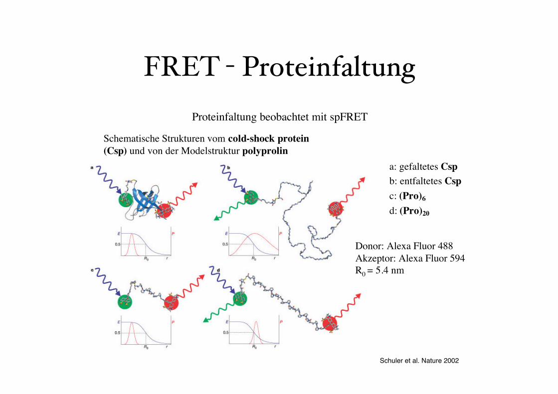
Proteinfaltung beobachtet mit spFRET
Schuler et al. Nature 2002
Schematische Strukturen vom cold-shock protein
(Csp) und von der Modelstruktur polyprolin
a: gefaltetes Csp
b: entfaltetes Csp
c: (Pro)6
d: (Pro)20
Fluoreszenzspektroskopie: Anwendungen auf Einzelmoleküle
Donor: Alexa Fluor 488
Akzeptor: Alexa Fluor 594
R0 = 5.4 nm
Schuler et al. Nature 2002
FRET - Proteinfaltung
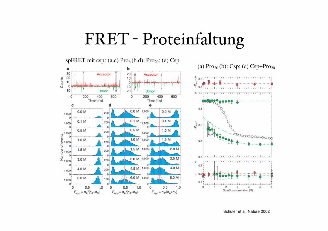
Schuler et al. Nature 2002
Biospektroskopie 223Schuler et al. Nature 2002
spFRET mit csp: (a,c) Pro6 (b,d); Pro20; (e) Csp
Fluoreszenzspektroskopie: Anwendungen auf Einzelmoleküle
(a) Pro20 (b); Csp; (c) Csp+Pro20
Fluoreszenzkorrelationsspektros-kopie
Biospektroskopie 231
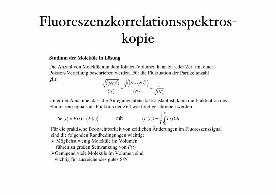
Fluoreszenz-Korrelations-Spektroskopie (FCS):
Studium der Moleküle in Lösung
Die Anzahl von Molekülen in dem fokalen Volumen kann zu jeder Zeit mit einer Poisson-Verteilung beschrieben werden. Für die Fluktuation der Partikelanzahl gilt:
Unter der Annahme, dass die Anregungsintensität konstant ist, kann die Fluktuation desFluoreszenzsignals als Funktion der Zeit wie folgt geschrieben werden:
)()()( tFtFtF !=!
Für die praktische Beobachtbarkeit von zeitlichen Änderungen im Fluoreszenzsignal sind die folgenden Randbedingungen wichtig:! Möglichst wenig Moleküle im Volumen
führen zu großen Schwankung von F(t)!Genügend viele Moleküle im Volumen sind
wichtig für ausreichendes gutes S/N
Fluoreszenzspektroskopie: Anwendungen auf Einzelmoleküle
( ) ( )
NN
NN
N
N 122
=!
=!
"=
T
dttFT
tF0
)(1
)(mit
Fluoreszenzkorrelationsspektros-kopie
Biospektroskopie 232
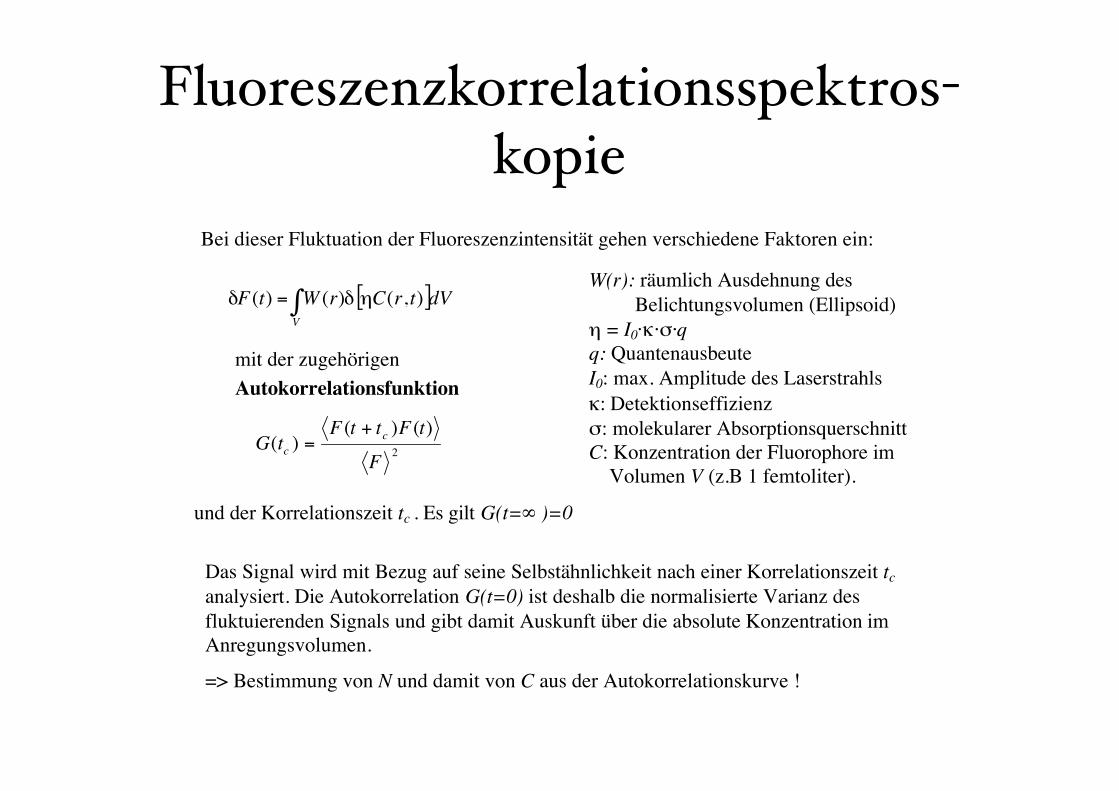
Bei dieser Fluktuation der Fluoreszenzintensität gehen verschiedene Faktoren ein:
und der Korrelationszeit tc . Es gilt G(t=! )=0
2
)()()(
F
tFttFtG
c
c
+=
Fluoreszenz-Korrelations-Spektroskopie (FCS):
[ ]!=V
dVtrCrWtF ),()()( "##W(r): räumlich Ausdehnung des
Belichtungsvolumen (Ellipsoid)
" = I0·#$%$qq: Quantenausbeute
I0: max. Amplitude des Laserstrahls
#: Detektionseffizienz
%: molekularer Absorptionsquerschnitt
C: Konzentration der Fluorophore im
Volumen V (z.B 1 femtoliter).
mit der zugehörigen
Autokorrelationsfunktion
Das Signal wird mit Bezug auf seine Selbstähnlichkeit nach einer Korrelationszeit tc
analysiert. Die Autokorrelation G(t=0) ist deshalb die normalisierte Varianz des
fluktuierenden Signals und gibt damit Auskunft über die absolute Konzentration im
Anregungsvolumen.
=> Bestimmung von N und damit von C aus der Autokorrelationskurve !
FCS - Anwendung
Biospektroskopie 234
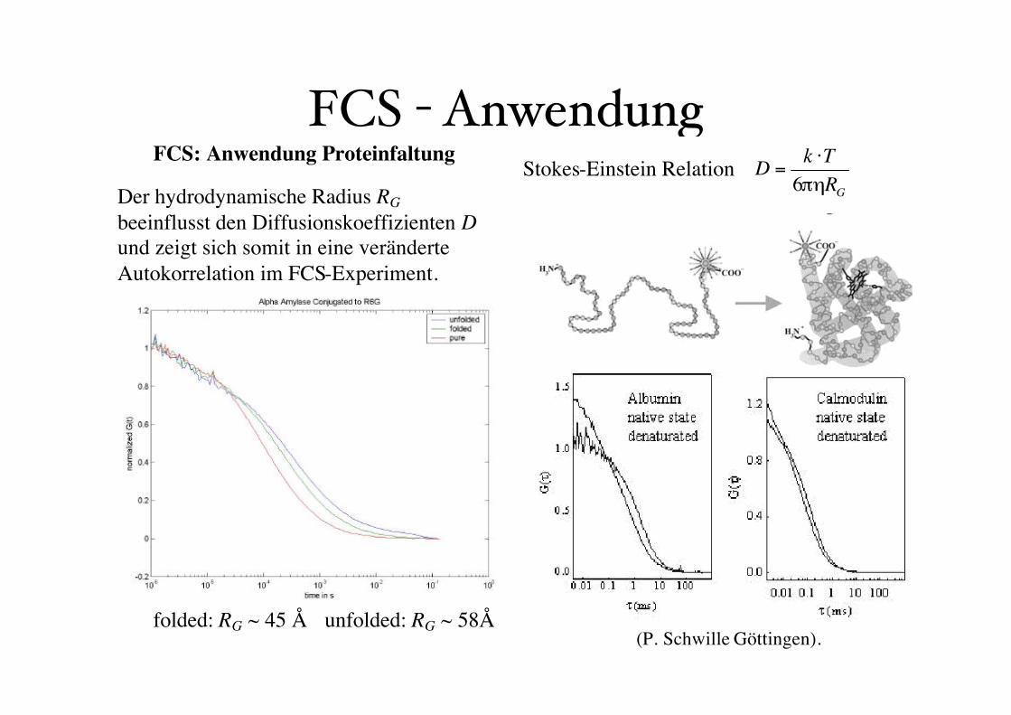
FCS: Anwendung Proteinfaltung
(P. Schwille Göttingen).
Der hydrodynamische Radius RG
beeinflusst den Diffusionskoeffizienten Dund zeigt sich somit in eine veränderte Autokorrelation im FCS-Experiment.
Stokes-Einstein Relation
Fluoreszenz-Korrelations-Spektroskopie (FCS):
GR
TkD
!"6
!=
unfolded: RG ~ 58Åfolded: RG ~ 45 Å
FCS - Anwendung
Biospektroskopie 235
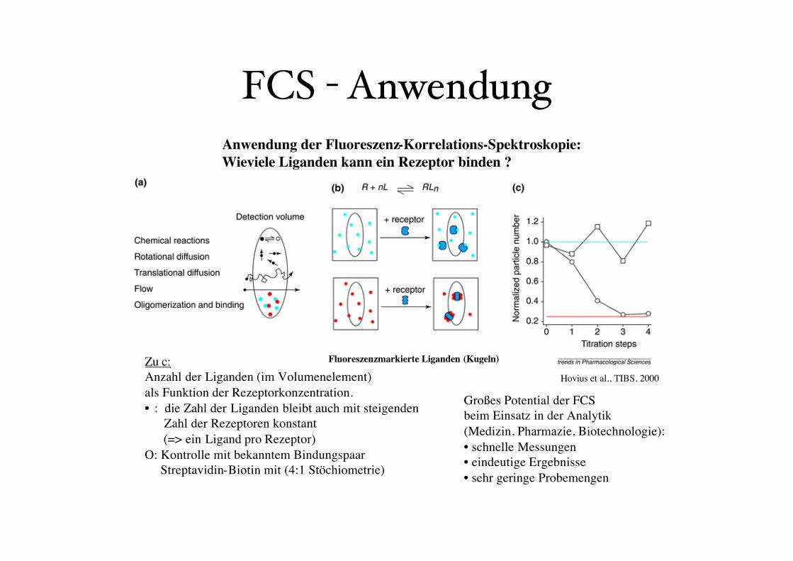
Anwendung der Fluoreszenz-Korrelations-Spektroskopie:
Wieviele Liganden kann ein Rezeptor binden ?
Großes Potential der FCS
beim Einsatz in der Analytik
(Medizin, Pharmazie, Biotechnologie):
• schnelle Messungen
• eindeutige Ergebnisse
• sehr geringe Probemengen
Hovius et al., TIBS, 2000
Fluoreszenzmarkierte Liganden (Kugeln)Zu c:
Anzahl der Liganden (im Volumenelement)
als Funktion der Rezeptorkonzentration.
• : die Zahl der Liganden bleibt auch mit steigenden
Zahl der Rezeptoren konstant
(=> ein Ligand pro Rezeptor)
O: Kontrolle mit bekanntem Bindungspaar
Streptavidin-Biotin mit (4:1 Stöchiometrie)
Fluoreszenz-Korrelations-Spektroskopie (FCS):
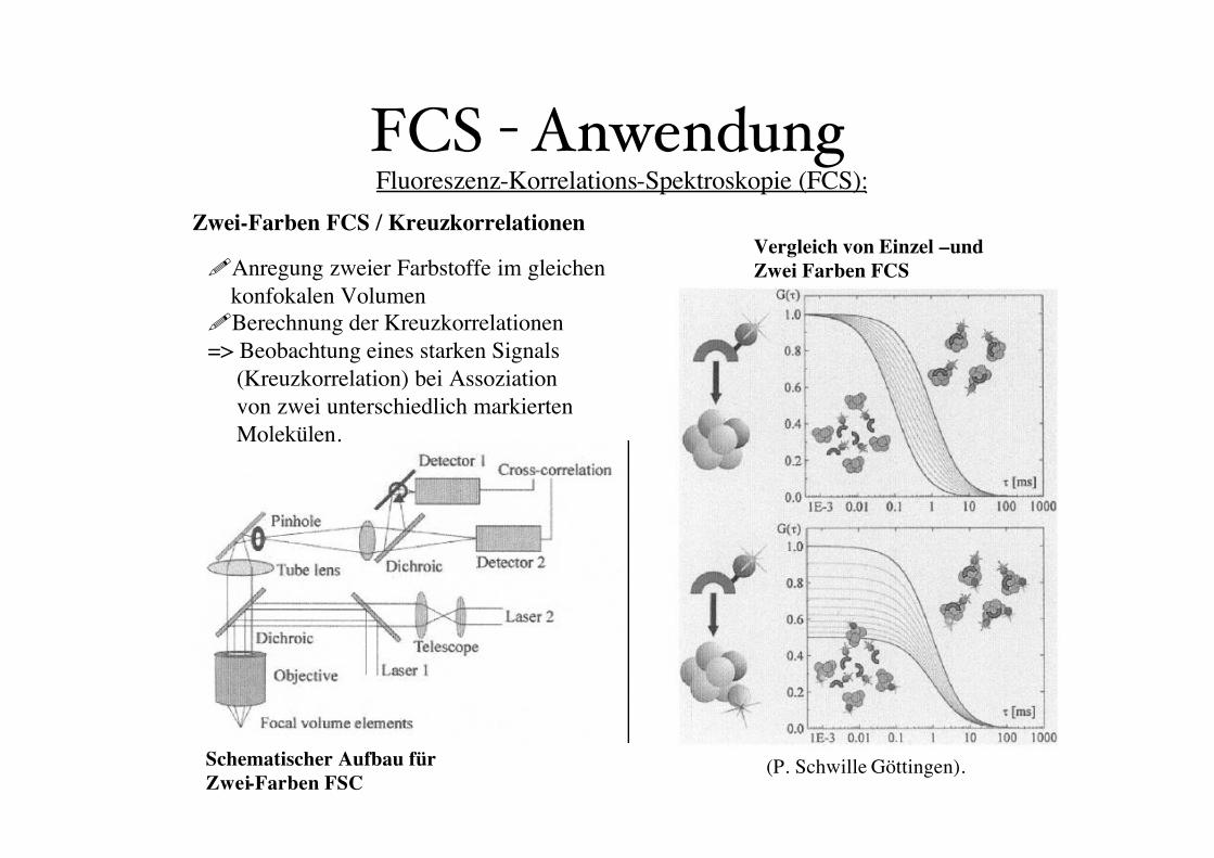
FCS - AnwendungZwei-Farben FCS / Kreuzkorrelationen
Fluoreszenz-Korrelations-Spektroskopie (FCS):
(P. Schwille Göttingen).
Vergleich von Einzel –und
Zwei Farben FCS
Schematischer Aufbau für
Zwei-Farben FSC
!Anregung zweier Farbstoffe im gleichen
konfokalen Volumen
!Berechnung der Kreuzkorrelationen
=> Beobachtung eines starken Signals
(Kreuzkorrelation) bei Assoziation
von zwei unterschiedlich markierten
Molekülen.
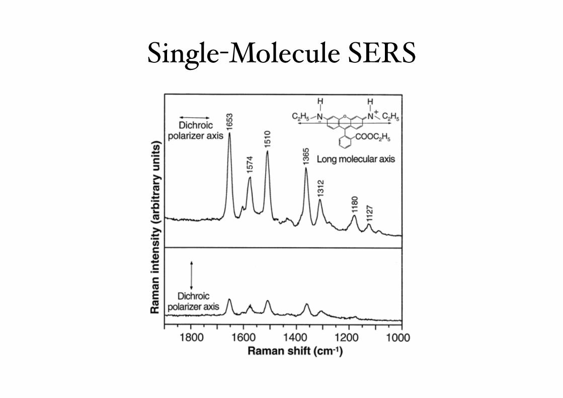
Single-Molecule SERS
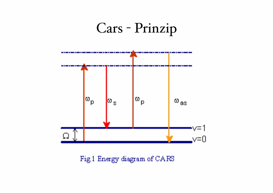
Cars - Prinzip
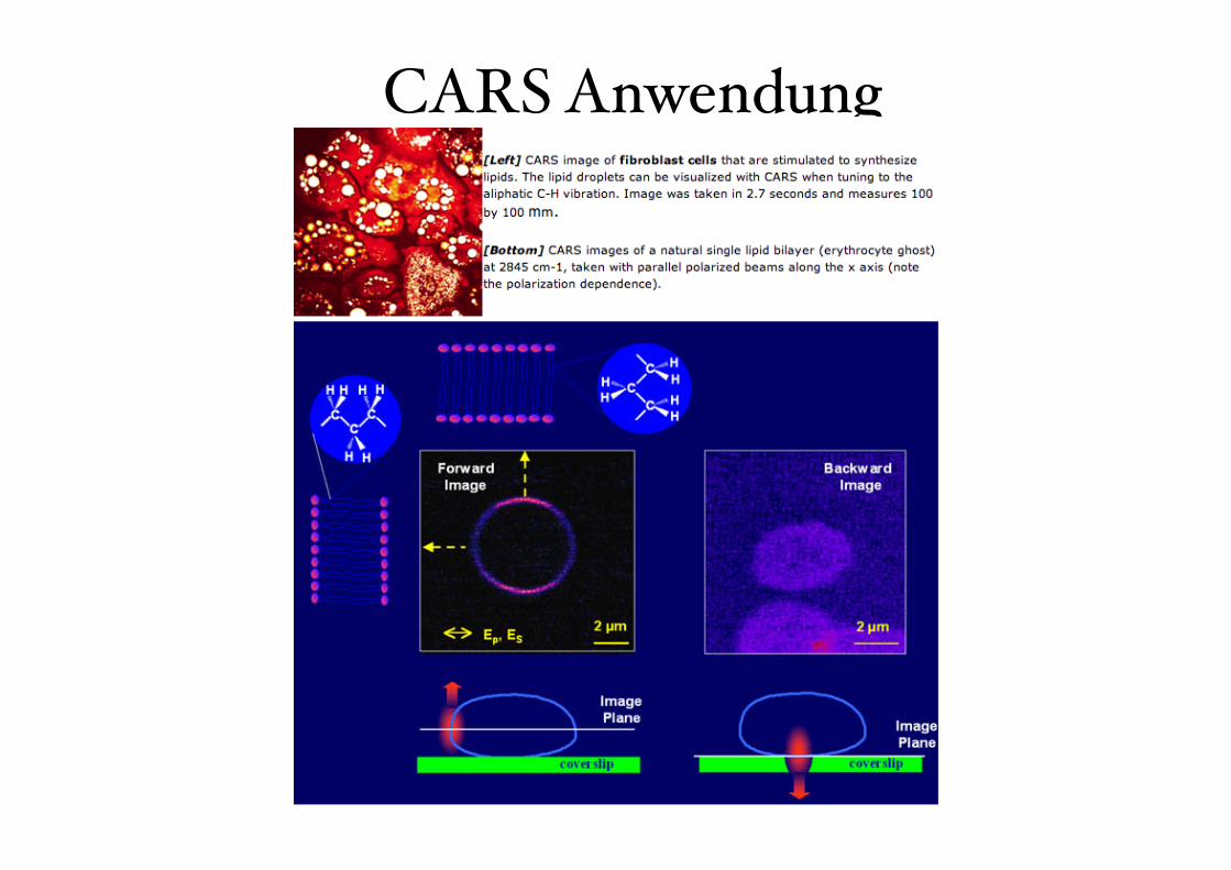
CARS Anwendung
CARS Anwendung