Embed Size (px)
Citation preview
Off-Yrast low-spin structure of deformed nuclei
at mass number A 150≈
Vom Fachbereich Physikder Technischen Universität Darmstadt
zur Erlangung des Gradeseines Doktors der Naturwissenschaften
(Dr. rer. nat.)
genehmigte
D i s s e r t a t i o n
angefertigt von
Andreas Krugmann, M. Sc. aus Heppenheim a.d. Bergstraße
Referent: Professor Dr. Dr. h.c. Norbert PietrallaKorreferent: Professor Dr. Peter von Neumann-Cosel
Tag der Einreichung: 17.06.2014Tag der Prüfung: 14.07.2014
Darmstadt 2014D 17

Supported by the DFG through SFB 634 and NE 679/3-1.
Off-Yrast low-spin structureof deformed nuclei at massnumber A≈150Off-Yrast niedrig-Spin Struktur deformierter Atomkerne mit Massenzahl A≈150Zur Erlangung des Grades eines Doktors der Naturwissenschaften (Dr. rer. nat.)genehmigte Dissertation von Andreas Krugmann, M. Sc. aus Heppenheim a. d. BergstraßeDezember 2014 — Darmstadt — D 17
Fachbereich PhysikInstitut für Kernphysik
Off-Yrast low-spin structure of deformed nuclei at mass number A≈150Off-Yrast niedrig-Spin Struktur deformierter Atomkerne mit Massenzahl A≈150
Genehmigte Dissertation von Andreas Krugmann, M. Sc. aus Heppenheim a. d. Bergstraße
1. Gutachten: Professor Dr. Dr. h.c. Norbert Pietralla2. Gutachten: Professor Dr. Peter von Neumann-Cosel
Tag der Einreichung: 17. Juni 2014Tag der Prüfung: 14. Juli 2014
Darmstadt — D 17
Bitte zitieren Sie dieses Dokument als:URN: urn:nbn:de:tuda-tuprints-42393URL: http://tuprints.ulb.tu-darmstadt.de/4239
Dieses Dokument wird bereitgestellt von tuprints,E-Publishing-Service der TU Darmstadthttp://[email protected]
Die Veröffentlichung steht unter folgender Creative Commons Lizenz:Namensnennung – Keine kommerzielle Nutzung – Keine Bearbeitung 2.0 Deutschlandhttp://creativecommons.org/licenses/by-nc-nd/2.0/de/
It doesn’t matter how beautiful your theory is,
it doesn’t matter how smart you are.
If it doesn’t agree with experiment,it’s wrong.
Richard Feynman
Viel Gerede bringt es nicht,nur das Messen bringt’s ans Licht!
Achim Richter

Zusammenfassung
Die vorliegende Arbeit gliedert sich in zwei Teile. Der erste Teil behandelt die Untersuchung
des 0+1 → 0+2 Übergangs in 150Nd in einem Elektronenstreuexperiment und der zweite Teil
beschäftigt sich mit einem Protonenstreuexperiment am 154Sm, wo Dipolanregungen studiert
wurden.
Im ersten Teil wird ein Pionierexperiment der Elektronenstreuung vorgestellt. Bei einer Ein-
schussenergie von 75 MeV wurden am hochauflösenden 169 Spektrometer des S-DALINAC,
Anregungsspektren bei unterschiedlichen Winkeln aufgenommen. Ziel dieser Untersuchung war
die Bestimmung der ρ2(E0;0+1 → 0+2 ) Übergangsstärke des schweren deformierten Kerns 150Nd.
Der experimentell ermittelte Formfaktor dieses Übergangs wurde mit einem theoretischen Form-
faktor verglichen, der aus einem effektiven Dichteoperator auf mikroskopischem Level mit Hilfe
der Generator-Coordinate-Methode konstruiert wurde. Die kollektiven Wellenfunktionen, die
dazu benötigt wurden, wurden aus dem Confined β-soft Rotor Modell entnommen. In dieser
modellabhängigen Analyse wurde zum ersten mal die E0-Übergangsstärke des 0+1 → 0+2 Über-
gangs in 150Nd bestimmt.
Des weiteren wurde der Verlauf der E0 Übergangsstärke als Funktion der Potentialsteifigkeit
auf dem Weg vom X(5) Phasenübergangspunkt zum Limit des starren Rotors untersucht. Hi-
erbei wurde gezeigt, dass die E0 Stärke am Phasenübergangspunkt sehr hoch ist und mit
steigender Potenzialsteifigkeit immer mehr abnimmt und schließlich im Grenzfall des starren
Rotors verschwindet. In einer abschließenden theoretischen Betrachtung wurden die Wellen-
funktionen des makroskopisch kollektiven Confined β-soft Rotor Modells mit denen aus einem
mikroskopischen relativistischen Meanfield Modell verglichen und eine starke Übereinstimmung
gefunden.
Der zweite Teil der Arbeit behandelt ein Protonenstreuexperiment mit polarisierten Proto-
nen am ebenfalls schweren deformierten Kern 154Sm, welches am RCNP in Osaka (Japan)
durchgeführt wurde. Mittels der Methode der Polarisationstransferobservablen konnte eine
Trennung des Spin-Flip Anteils und des Nicht-Spinflip Anteils vom gesamten Wirkungsquer-
schnitt vorgenommen werden. Im Falle der elektrischen Dipolstärke konnte zum ersten Mal die
Pygmy Dipol Resonanz im schweren deformierten Kern 154Sm identifiziert werden. Eine Dop-
pelstruktur wurde beobachtet. Als mögliche Interpretation wird eine Deformationsaufspaltung
analog zur Dipol Riesenresonanz gegeben. Im Falle der magnetischen Stärke wurde eine brei-
te Verteilung im Anregungsenergiebereich zwischen 6 und 12 MeV gefunden. Die Verteilung
und auch die extrahierte Summenstärke sind in sehr guter Übereinstimmung mit vorherigen
Experimenten.
iii

Abstract
The present work consists of two independent parts. The first part deals with the investigation
of the 0+1 → 0+2 transition in 150Nd with inelastic electron scattering and in the second part a
proton scattering experiment for the investigation of dipole excitations is presented.
In the first part of this thesis a pioneer experiment in inelastic electron scattering is intro-
duced. At an electron energy of 75 MeV, excitation energy spectra have been measured at the
high resolution 169 spectrometer at the S-DALINAC. The aim of this investigation was the de-
termination of the ρ2(E0; 0+1 → 0+2 ) transition strength in the heavy deformed nucleus 150Nd.
The experimental form factor of this particular transition has been compared to a theoretical
form factor that has been constructed by an effective density operator on a microscopic level
with the help of the generator coordinate method. The required collective wave functions have
been calculated in the Confined β soft rotor model. In this model-dependent analysis the E0
transition strength has been determined for the first time. Furthermore the evolution of the E0
transition strength as a function of the potential stiffness has been investigated from the X(5)
phase shape transitional point to the Rigid Rotor limit. It has been shown, that the E0 strength
is relatively high at the shape-phase transitional point and starts to decrease with increasing
stiffness and vanishes completely at the Rigid Rotor limit. Additionally the wave functions of
the macroscopic collective Confined β-soft rotor model have been compared to those from a
microscopic mean field Hamiltonian. Good agreement has been found.
The second part of this thesis covers a polarized-proton scattering experiment on the heavy
deformed nucleus 154Sm, that has been performed at the RCNP in Osaka, Japan. Utilizing the
method of polarization transfer observables, a separation of spinflip and non-spinflip parts of
the cross section has been done. Here, for the first time, the Pygmy Dipole Resonance (PDR)
has been identified in the heavy deformed nucleus 154Sm that appears as a double-hump struc-
ture in the E1 response. A possible interpretation of this double-hump structure in terms of
a deformation splitting analogously to the Giant Dipole Resonance (GDR) has been given. In
case of the spinflip cross section, a broad distribution in the excitation energy range between 6
and 12 MeV has been observed. The distribution and the extracted sum strength are in good
accordance with previous experiments.
v

Contents
Preface - Off Yrast excitations in scattering experiments with charged particles 1
I. Electric monopole strength of the 0+1 → 0+2 transition in 150Nd 3
1. Introduction 5
2. Theoretical background 112.1. Collective coordinates . . . . . . . . . . . . . . . . . . . . . . . . . . . . . . . . . . . . . 11
2.2. The collective Bohr Hamiltonian . . . . . . . . . . . . . . . . . . . . . . . . . . . . . . . 13
2.2.1. E0 transitions in quadrupole collective models . . . . . . . . . . . . . . . . . . 13
2.2.2. Derivation of ρ2(E0) transition strength as a function of potential stiffness 15
2.3. The confined β-soft rotor model . . . . . . . . . . . . . . . . . . . . . . . . . . . . . . . 15
2.3.1. E0 transition strengths in the CBS model . . . . . . . . . . . . . . . . . . . . . 18
2.4. Microscopic relativistic mean-field approach . . . . . . . . . . . . . . . . . . . . . . . 19
3. Inelastic electron scattering at low momentum transfer 233.1. Electron scattering formalism . . . . . . . . . . . . . . . . . . . . . . . . . . . . . . . . . 23
3.2. Model predictions for the 0+1 → 0+2 E0 transition in 150Nd . . . . . . . . . . . . . . . 25
3.2.1. Effective operator for the E0 transition density . . . . . . . . . . . . . . . . . 25
3.2.2. Neutron and proton transition densities . . . . . . . . . . . . . . . . . . . . . . 26
3.2.3. Predicted DWBA form factors for the electron scattering experiment . . . . 27
4. Inelastic electron scattering experiments at the S-DALINAC 294.1. S-DALINAC and experimental facilities . . . . . . . . . . . . . . . . . . . . . . . . . . . 29
4.2. High resolution electron scattering . . . . . . . . . . . . . . . . . . . . . . . . . . . . . 31
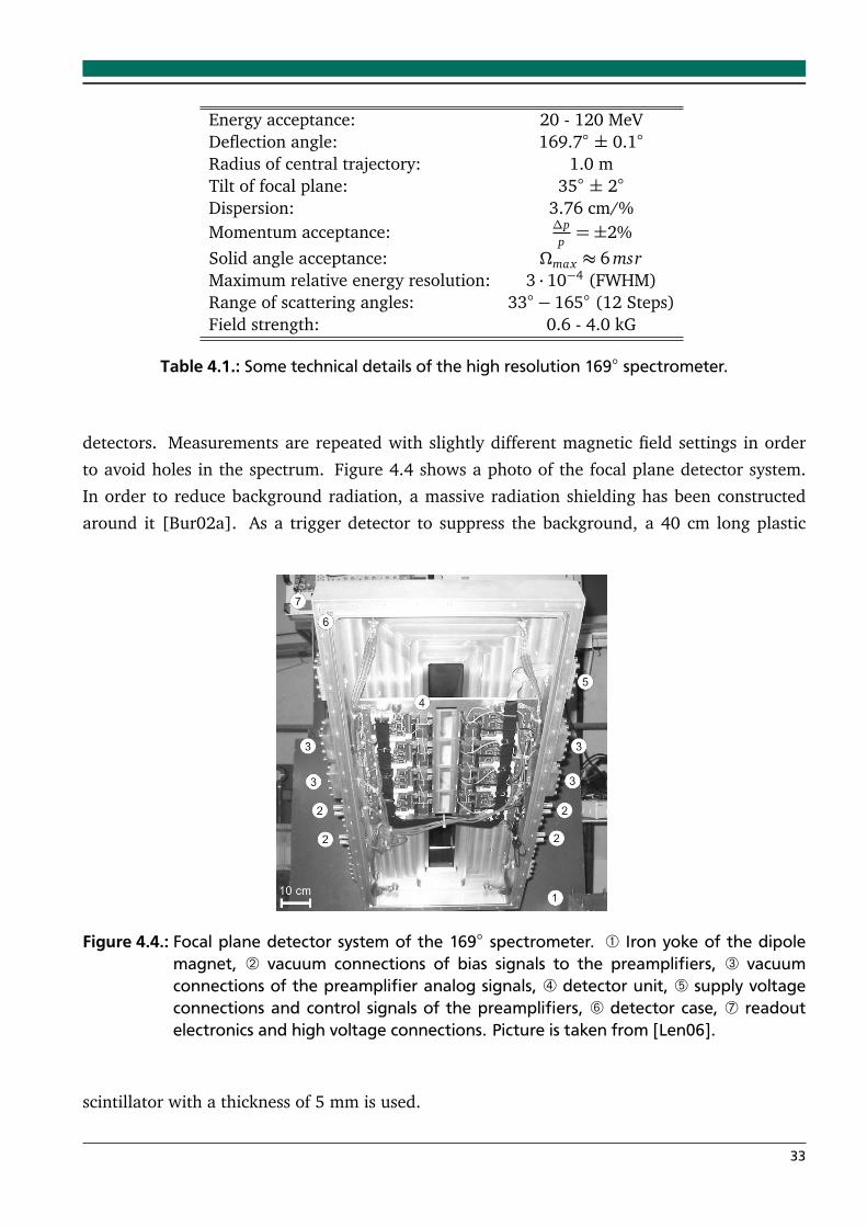
4.3. Focal plane detector system . . . . . . . . . . . . . . . . . . . . . . . . . . . . . . . . . . 32
4.4. Modes of operation . . . . . . . . . . . . . . . . . . . . . . . . . . . . . . . . . . . . . . . 34
4.4.1. Dispersive mode . . . . . . . . . . . . . . . . . . . . . . . . . . . . . . . . . . . . 34
4.4.2. Energy-loss mode . . . . . . . . . . . . . . . . . . . . . . . . . . . . . . . . . . . 34
4.5. 150Nd(e,e’) experiment . . . . . . . . . . . . . . . . . . . . . . . . . . . . . . . . . . . . . 35
5. Data analysis of the electron scattering data 375.1. Line shapes . . . . . . . . . . . . . . . . . . . . . . . . . . . . . . . . . . . . . . . . . . . . 37
5.2. Energy calibration of the excitation spectra . . . . . . . . . . . . . . . . . . . . . . . . 37
vii
5.3. Experimental cross sections . . . . . . . . . . . . . . . . . . . . . . . . . . . . . . . . . . 38
5.3.1. Radiative corrections . . . . . . . . . . . . . . . . . . . . . . . . . . . . . . . . . 39
5.3.2. Dead time correction . . . . . . . . . . . . . . . . . . . . . . . . . . . . . . . . . 40
5.4. Estimation of uncertainties . . . . . . . . . . . . . . . . . . . . . . . . . . . . . . . . . . 41
5.5. Experimental Data . . . . . . . . . . . . . . . . . . . . . . . . . . . . . . . . . . . . . . . 41
6. Discussion of the electron scattering data 436.1. Elastic scattering . . . . . . . . . . . . . . . . . . . . . . . . . . . . . . . . . . . . . . . . 43
6.2. Electric monopole strength of the 0+1 → 0+2 transition in 150Nd . . . . . . . . . . . . 43
6.3. Evolution of absolute E0 strengths . . . . . . . . . . . . . . . . . . . . . . . . . . . . . . 44
6.3.1. Stiffness dependence of the ρ2(E0) transition strengths . . . . . . . . . . . . 46
7. Comparison of the CBS rotor model with a macroscopic collective mean field Hamil-
tonian for 150,152Nd 497.1. Description of K=0 bands and their centrifugal stretching . . . . . . . . . . . . . . . 49
7.2. Comparison of the collective wave functions . . . . . . . . . . . . . . . . . . . . . . . 51
8. Conclusion and Outlook 55
II. Low-energy dipole strength in 154Sm 57
9. Introduction 599.1. Electric Resonances . . . . . . . . . . . . . . . . . . . . . . . . . . . . . . . . . . . . . . . 59
9.2. Magnetic Resonances . . . . . . . . . . . . . . . . . . . . . . . . . . . . . . . . . . . . . . 61
9.3. Separation of E1 and M1: New experimental approaches . . . . . . . . . . . . . . . 63
9.4. Outline . . . . . . . . . . . . . . . . . . . . . . . . . . . . . . . . . . . . . . . . . . . . . . 63
10.Theoretical background for polarized proton scattering at 0 6510.1.Inelastic proton scattering . . . . . . . . . . . . . . . . . . . . . . . . . . . . . . . . . . . 65
10.2.Lippmann-Schwinger equation . . . . . . . . . . . . . . . . . . . . . . . . . . . . . . . . 65
10.3.Distorted waves . . . . . . . . . . . . . . . . . . . . . . . . . . . . . . . . . . . . . . . . . 66
10.4.Optical potential . . . . . . . . . . . . . . . . . . . . . . . . . . . . . . . . . . . . . . . . . 67
10.5.Effective nucleon-nucleus interaction . . . . . . . . . . . . . . . . . . . . . . . . . . . . 67
10.6.Coulomb excitation . . . . . . . . . . . . . . . . . . . . . . . . . . . . . . . . . . . . . . . 69
10.6.1. Classical Coulomb excitations . . . . . . . . . . . . . . . . . . . . . . . . . . . . 69
10.6.2. Semiclassical coulomb excitations . . . . . . . . . . . . . . . . . . . . . . . . . 70
10.6.3. Equivalent virtual photon method . . . . . . . . . . . . . . . . . . . . . . . . . 72
10.6.4. Eikonal description of Coulomb excitation . . . . . . . . . . . . . . . . . . . . 73
viii
10.7.Magnetic dipole transitions and B(M1στ) from (p,p’) cross section data . . . . . . . 75
10.8.Polarization transfer observables (PT observables) . . . . . . . . . . . . . . . . . . . . 77
11.Polarized proton scattering experiment at RCNP 8111.1.Beam line polarimeters (BLPs) . . . . . . . . . . . . . . . . . . . . . . . . . . . . . . . . 82
11.2.The setup for 0 measurements . . . . . . . . . . . . . . . . . . . . . . . . . . . . . . . 82
11.2.1. The Grand Raiden spectrometer . . . . . . . . . . . . . . . . . . . . . . . . . . 82
11.3.The Large Acceptance Spectrometer (LAS) . . . . . . . . . . . . . . . . . . . . . . . . 84
11.4.Detector systems at the 0 scattering facility . . . . . . . . . . . . . . . . . . . . . . . . 85
11.4.1. The Focal Plane Detector System . . . . . . . . . . . . . . . . . . . . . . . . . . 85
11.4.2. The Focal Plane Polarimeter (FPP) . . . . . . . . . . . . . . . . . . . . . . . . . 86
11.5.Experimental conditions . . . . . . . . . . . . . . . . . . . . . . . . . . . . . . . . . . . . 87
11.6.Used targets . . . . . . . . . . . . . . . . . . . . . . . . . . . . . . . . . . . . . . . . . . . 88
11.6.1. The under-focus mode . . . . . . . . . . . . . . . . . . . . . . . . . . . . . . . . 89
11.6.2. The Faraday cups . . . . . . . . . . . . . . . . . . . . . . . . . . . . . . . . . . . . 90
11.6.3. The sieve-slit measurements . . . . . . . . . . . . . . . . . . . . . . . . . . . . . 90
12.Data analysis for proton scattering 9312.1.Data reduction . . . . . . . . . . . . . . . . . . . . . . . . . . . . . . . . . . . . . . . . . . 93
12.1.1. Drift time to distance conversion . . . . . . . . . . . . . . . . . . . . . . . . . . 93
12.1.2. Efficiency determination of the VDCs . . . . . . . . . . . . . . . . . . . . . . . 94
12.1.3. Sieve slit analysis . . . . . . . . . . . . . . . . . . . . . . . . . . . . . . . . . . . . 96
12.1.4. Higher order aberration corrections . . . . . . . . . . . . . . . . . . . . . . . . 97
12.1.5. Excitation energy calibration . . . . . . . . . . . . . . . . . . . . . . . . . . . . 99
12.1.6. Background subtraction . . . . . . . . . . . . . . . . . . . . . . . . . . . . . . . . 101
12.1.7. Double differential cross sections . . . . . . . . . . . . . . . . . . . . . . . . . . 104
12.2.Polarization transfer analysis . . . . . . . . . . . . . . . . . . . . . . . . . . . . . . . . . 106
12.2.1. Method for extracting PT observables: The Estimator Method . . . . . . . . 107
12.3.Results of the polarization transfer analysis . . . . . . . . . . . . . . . . . . . . . . . . 109
12.3.1. Results for 26Mg . . . . . . . . . . . . . . . . . . . . . . . . . . . . . . . . . . . . 109
12.3.2. Results for 154Sm . . . . . . . . . . . . . . . . . . . . . . . . . . . . . . . . . . . . 110
12.4.Electric dipole response in 154Sm . . . . . . . . . . . . . . . . . . . . . . . . . . . . . . 112
12.4.1. Photoabsorption Cross section . . . . . . . . . . . . . . . . . . . . . . . . . . . . 113
12.4.2. B(E1) strength distribution . . . . . . . . . . . . . . . . . . . . . . . . . . . . . . 114
12.4.3. Deformation splitting . . . . . . . . . . . . . . . . . . . . . . . . . . . . . . . . . 114
12.5.Discussion of angular distributions . . . . . . . . . . . . . . . . . . . . . . . . . . . . . 115
12.6.Determination of the spinflip-M1 strength distribution with the unit-cross section
method . . . . . . . . . . . . . . . . . . . . . . . . . . . . . . . . . . . . . . . . . . . . . . 117
ix
13.Conclusion and Outlook 121
A. Derivation of ρ2(E0) transition strength as a function of potential stiffness 123
B. List of ρ2(E0) transition strengths compared in figure 6.5 127
Bibliography 138
Danksagung 140
Lebenslauf 141
Eigene Publikationen 144
Eigenständigkeitserklärung 145
x
List of Figures
0.1. Characteristic response of an atomic nucleus as a function of the excitation
energy Ex and the momentum transfer q. . . . . . . . . . . . . . . . . . . . . . . . 2
1.1. Evolution of the potential as a function of the deformation variable β in the
shape phase transitional area. . . . . . . . . . . . . . . . . . . . . . . . . . . . . . . 5
1.2. CBS square well potentials compared to relativistic mean field potentials for150Nd and 152Nd, respectively. . . . . . . . . . . . . . . . . . . . . . . . . . . . . . . 6
1.3. Empirical ρ2(E0;0+2 → 0+1 ) values for nuclei in the A=100 and 150 transition
regions. . . . . . . . . . . . . . . . . . . . . . . . . . . . . . . . . . . . . . . . . . . . . 7
1.4. Calculated monopole transition strength ρ2(E0; 0+2 → 0+1 ) as a function of
neutron number N in the Nd isotopes within the framework of the relativistic
mean field. . . . . . . . . . . . . . . . . . . . . . . . . . . . . . . . . . . . . . . . . . . 8
2.1. Shape of a spherical nucleus with β=0 and γ=0. . . . . . . . . . . . . . . . . . . 12
2.2. Shape of an axial prolate deformed nucleus with β=0.3 and γ=0. . . . . . . . 12
2.3. Shape of a triaxial deformed nucleus with β=0.3 and γ=π/3. . . . . . . . . . . 12
2.4. X(5) potential as a function of the deformation parameter β . . . . . . . . . . . . 17
2.5. CBS potential as a function of the deformation parameter β . . . . . . . . . . . . 17
3.1. Calculated proton and neutron transition densities for the 0+1 → 0+2 transition
in 150Nd from [Shi09]. . . . . . . . . . . . . . . . . . . . . . . . . . . . . . . . . . . 27
3.2. Correlation between the minimum in the form factor of the 0+2 state and the
node in the wave function of the β band. . . . . . . . . . . . . . . . . . . . . . . . 28
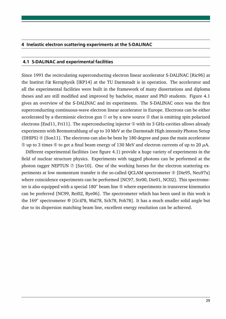
4.1. Overview of the S-DALINAC with its experimental facilities. . . . . . . . . . . . 30
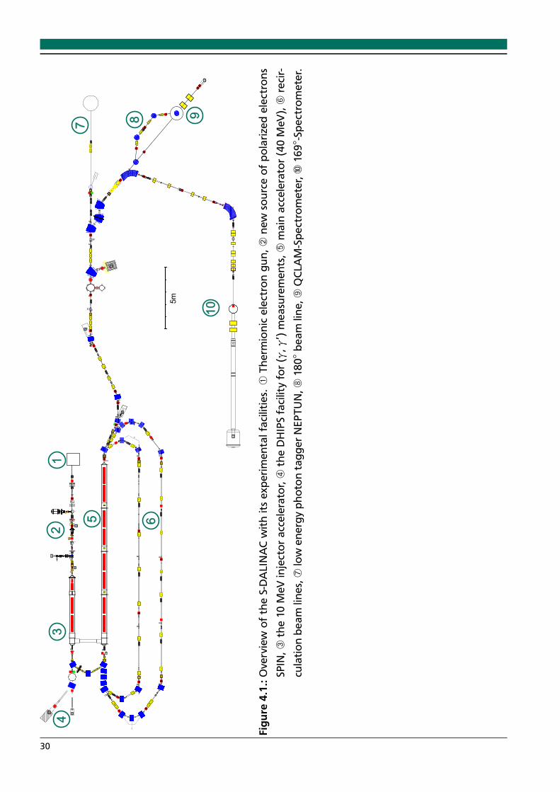
4.2. Photo of the high energy resolution 169 spectrometer. . . . . . . . . . . . . . . 31
4.3. Beam line to the high resolution electron scattering facility with the 169
spectrometer. . . . . . . . . . . . . . . . . . . . . . . . . . . . . . . . . . . . . . . . . 32
4.4. Focal plane detector system of the 169 spectrometer. . . . . . . . . . . . . . . . 33
4.5. Dispersion matching technique. . . . . . . . . . . . . . . . . . . . . . . . . . . . . . 35
4.6. Spectrum of the 150Nd(e,e’) reaction at 73.8 MeV, taken at a scattering angle
of 93. . . . . . . . . . . . . . . . . . . . . . . . . . . . . . . . . . . . . . . . . . . . . 36
5.1. Spectra of the 150Nd(e,e’) reaction with an electron energy of 73.8 MeV at
the scattering angles of 69, 93, 117, 129 and 141. . . . . . . . . . . . . . . 42
xi
6.1. Experimental elastic form factor of the 150Nd(e,e’) reaction at E0=73.8 MeV
as a function of the scattering angle compared to the results of the phase shift
analysis codes DREPHA and PHASHI. . . . . . . . . . . . . . . . . . . . . . . . . . 43
6.2. Excitation energy spectrum at an scattering angle of 69 where the contribu-
tion of the elastic line is subtracted. . . . . . . . . . . . . . . . . . . . . . . . . . . 44
6.3. Form factor of the 0+2 excitation in the 150Nd(e,e’) reaction at 73.8 MeV. . . . . 45
6.4. Absolute E0 transition rates predicted in the CBS model. . . . . . . . . . . . . . 45
6.5. Various ρ2(E0) values in the shape-phase transitional region as a function of
the CBS parameter rβ indicating the potential stiffness. . . . . . . . . . . . . . . 46
6.6. Behaviour of ρ2(E0) transition strengths for the 0+2 → 0+1 transition for dif-
ferent values of rβ . . . . . . . . . . . . . . . . . . . . . . . . . . . . . . . . . . . . . . 47
7.1. Low lying energy levels in 150Nd for the relativistic mean field Hamiltonian,
the CBS rotor model and experimental values. . . . . . . . . . . . . . . . . . . . . 50
7.2. Low lying energy levels in 152Nd for the relativistic mean field Hamiltonian,
the CBS rotor model and experimental values. . . . . . . . . . . . . . . . . . . . . 50
7.3. Experimental Moments of Inertia and their theoretical predictions and a com-
parison of the centrifugal stretching parameter S(J) for the ground state band
in the nuclei 150,152Nd. . . . . . . . . . . . . . . . . . . . . . . . . . . . . . . . . . . 52
7.4. Wave functions of the ground state band in 150,152Nd for the CBS rotor model
and the relativistic mean field model. . . . . . . . . . . . . . . . . . . . . . . . . . 53
7.5. Wave functions of the band heads of the β-band in 150,152Nd. . . . . . . . . . . 54
9.1. Schematic picture of the electric dipole excitations for typical sperical nuclei
and typical deformed nuclei. . . . . . . . . . . . . . . . . . . . . . . . . . . . . . . . 60
9.2. Systematics of the spin-M1 resonance in heavy deformed nuclei measured at
TRIUMF [Hey10] . . . . . . . . . . . . . . . . . . . . . . . . . . . . . . . . . . . . . . 62
9.3. Double-differential cross section of the 154Sm(~p, ~p′) reaction measured at θ =2.8 at TRIUMF [Hey10, Wör94] . A decomposition of the spectrum into
contributions of the IVGDR (horizontally hatched) spin-M1 resonance (black,
low Ex) and the IVGQR (black, high Ex) and a background from quasi-free
scattering (lower smooth line) is shown. From Ref. [Hey10]. . . . . . . . . . . 62
10.1. Energy dependence of the central parts of the nucleon-nucleon scattering in
the q ≈ 0 limit [Lov81]. . . . . . . . . . . . . . . . . . . . . . . . . . . . . . . . . . . 69
10.2. Classical picture of a projectile trajectory in the coulomb scattering process. . 70
10.3. Virtual photon numbers per unit solid angle for E1 transitions in Coulomb
excitation induced by 295 MeV protons on a 154Sm target at Eγ=3 MeV and
16 MeV. . . . . . . . . . . . . . . . . . . . . . . . . . . . . . . . . . . . . . . . . . . . . 74
xii
10.4. Coordinate system in the projectile frame. . . . . . . . . . . . . . . . . . . . . . . 79
11.1. Schematic overview of the RCNP facility in Osaka. . . . . . . . . . . . . . . . . . 81
11.2. Schematic view of one beam line polarimeter (BLP). . . . . . . . . . . . . . . . . 83
11.3. Arrangement of the two beam line polarimeters for the determination of the
beam polarization at the target position. . . . . . . . . . . . . . . . . . . . . . . . 83
11.4. Setup for 0 experiments. . . . . . . . . . . . . . . . . . . . . . . . . . . . . . . . . . 84
11.5. Schematic view of the GR detector system . . . . . . . . . . . . . . . . . . . . . . 87
11.6. Targetladder which was used during the experiment. . . . . . . . . . . . . . . . 89
11.7. Examples of vertical beam envelopes in the y-z plane with three different
focus modes of the Grand Raiden optics. . . . . . . . . . . . . . . . . . . . . . . . 90
11.8. Schematic view of the brass plate that has been used for the sieveslit mea-
surements. . . . . . . . . . . . . . . . . . . . . . . . . . . . . . . . . . . . . . . . . . . 91
12.1. Vertical drift chamber as a schematic view. . . . . . . . . . . . . . . . . . . . . . . 94
12.2. Example of the track reconstruction. . . . . . . . . . . . . . . . . . . . . . . . . . . 95
12.3. Drift time to drift length conversion. . . . . . . . . . . . . . . . . . . . . . . . . . . 95
12.4. Extraction of yLAS, θ f p, y f p and φ f p from the sieve slit analysis . . . . . . . . . 97
12.5. Two-dimensional y − θ histograms before and after correction . . . . . . . . . 99
12.6. Two-dimensional histograms of the x f p − θ f p plane . . . . . . . . . . . . . . . . 100
12.7. Excitation energy calibration with the 26Mg(p, p′) reaction . . . . . . . . . . . . 101
12.8. Correlation between the vertical scattering angleφ f p and the vertical position
in the ’conventional method’ for the background subtraction. On the left
hand side, the untransformed data is shown and on the right hand side the
transformation in equation 12.8 has been utilized. . . . . . . . . . . . . . . . . . 103
12.9. Background subtraction with the ’extended method’. . . . . . . . . . . . . . . . . 104
12.10. Excitation energy spectrum and background spectrum of the 154Sm(p,p’) re-
action at Ep = 295 MeV, and θGR=0, using the full acceptance of the GR. . . 104
12.11. Background-subtracted spectrum 154Sm(p,p’) reaction at Ep = 295 MeV, and
θGR=0, using the full acceptance of the GR. . . . . . . . . . . . . . . . . . . . . 105
12.12. Background subtracted spectra for the 154Sm(p,p’) reaction for the 0 and for
the 3 setting, respectively. . . . . . . . . . . . . . . . . . . . . . . . . . . . . . . . . 106
12.13. Polarization transfer observables for 26Mg . . . . . . . . . . . . . . . . . . . . . . 110
12.14. Polarization transfer observables for 154Sm . . . . . . . . . . . . . . . . . . . . . . 111
12.15. Extraction of total cross section, spinflip cross section and non-spinflip cross
section. . . . . . . . . . . . . . . . . . . . . . . . . . . . . . . . . . . . . . . . . . . . . 112
12.16. Experimentally obtained photoabsorption cross section σabs in comparison
with γ(x) data measured in Saclay [Car74] . . . . . . . . . . . . . . . . . . . . . 113
xiii

12.17. Photoabsorption cross sectionσabs deduced from this experiment in the lower
energy region. . . . . . . . . . . . . . . . . . . . . . . . . . . . . . . . . . . . . . . . . 114
12.18. B(E1) strength distribution, obtained in this experiment. . . . . . . . . . . . . . 115
12.19. Sketch of the B(E1) response in heavy deformed nuclei. . . . . . . . . . . . . . . 116
12.20. Different angle cuts obtained from the finite angle measurements, using the
0 and the 3 setting in combination. . . . . . . . . . . . . . . . . . . . . . . . . . 116
12.21. Experimental angular distributions at different excitations energies. Energy
bins with a width of 200 keV have been used. . . . . . . . . . . . . . . . . . . . . 117
12.22. Spinflip-M1 strength distribution obtained with the unit-cross section method. 119
xiv
List of Tables
4.1. Some technical details of the high resolution 169 spectrometer. . . . . . . . . . . . 33
4.2. Isotopic enrichment of the 150Nd target which has been used in this experiment. . 36
10.1.Variables entering the Franey-Love interaction . . . . . . . . . . . . . . . . . . . . . . 68
11.1.Specifications of GR and LAS spectrometer . . . . . . . . . . . . . . . . . . . . . . . . 85
11.2.Technical details of the VDCs in the Grand Raiden and the Large Acceptance
Spectrometers . . . . . . . . . . . . . . . . . . . . . . . . . . . . . . . . . . . . . . . . . . 86
11.3.Technical details of the MWPCs in the Focal Plane Polarimeter . . . . . . . . . . . . 87
11.4.Summary of the experimental conditions during this experiment . . . . . . . . . . . 88
11.5.Summary of the experimental conditions in each measurement . . . . . . . . . . . . 88
12.1.Table of coefficients for the reconstruction of scattering angles . . . . . . . . . . . . 98
12.2.Table of coefficients for the correction of x f p . . . . . . . . . . . . . . . . . . . . . . . 100
12.3.Transitions used for the energy calibration . . . . . . . . . . . . . . . . . . . . . . . . . 101
12.4.Coefficients for the correction of y f p . . . . . . . . . . . . . . . . . . . . . . . . . . . . 102
12.5.Variables used for the calculation of the differential cross section . . . . . . . . . . . 105
B.1. List of ρ2(E0) values compared in figure 6.5. . . . . . . . . . . . . . . . . . . . . . . . 127
xv

Preface - Off-Yrast excitations in scattering experiments with charged particles
The atomic nucleus is a very tiny object! What people usually do when they want to study very
little objects is putting them in front of a microscope, switching the light on, looking into the
eyepiece and start their investigations. The limiting factor in the resolving power is only the
wavelength of the probe, in that case, the wavelength of visible light. The size of an atomic
nucleus is in the order of 1-10 fm (1 fm = 10−15 m) whereas the wavelength of the visible light
is only in the 380-780 nm range. Here, the discovery of Lois de Broglie (1892-1987) improved
the situation, since he found out that also particles can be associated with a wavelength and one
can decrease the wavelength of particle waves by increasing their momentum. This concept is
now known as ’wave-particle duality’ and de Broglie won the Nobel Price for Physics in 1929 for
this groundbreaking contributions to understanding nature. Now when studying the behavior
of atomic nuclei, the easiest thing is to shoot at it with an appropriate particle beam and detect
reaction products.
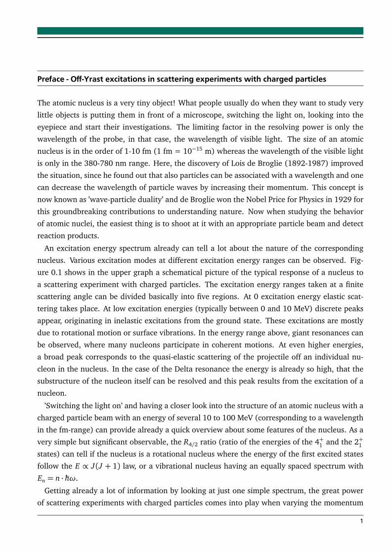
An excitation energy spectrum already can tell a lot about the nature of the corresponding
nucleus. Various excitation modes at different excitation energy ranges can be observed. Fig-
ure 0.1 shows in the upper graph a schematical picture of the typical response of a nucleus to
a scattering experiment with charged particles. The excitation energy ranges taken at a finite
scattering angle can be divided basically into five regions. At 0 excitation energy elastic scat-
tering takes place. At low excitation energies (typically between 0 and 10 MeV) discrete peaks
appear, originating in inelastic excitations from the ground state. These excitations are mostly
due to rotational motion or surface vibrations. In the energy range above, giant resonances can
be observed, where many nucleons participate in coherent motions. At even higher energies,
a broad peak corresponds to the quasi-elastic scattering of the projectile off an individual nu-
cleon in the nucleus. In the case of the Delta resonance the energy is already so high, that the
substructure of the nucleon itself can be resolved and this peak results from the excitation of a
nucleon.
’Switching the light on’ and having a closer look into the structure of an atomic nucleus with a
charged particle beam with an energy of several 10 to 100 MeV (corresponding to a wavelength
in the fm-range) can provide already a quick overview about some features of the nucleus. As a
very simple but significant observable, the R4/2 ratio (ratio of the energies of the 4+1 and the 2+1states) can tell if the nucleus is a rotational nucleus where the energy of the first excited states
follow the E ∝ J(J + 1) law, or a vibrational nucleus having an equally spaced spectrum with
En = n ·ħhω.
Getting already a lot of information by looking at just one simple spectrum, the great power
of scattering experiments with charged particles comes into play when varying the momentum
1
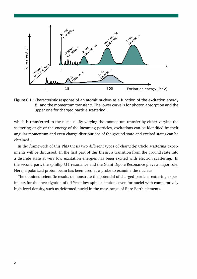
Figure 0.1.: Characteristic response of an atomic nucleus as a function of the excitation energyEx and the momentum transfer q. The lower curve is for photon absorption and theupper one for charged particle scattering.
which is transferred to the nucleus. By varying the momentum transfer by either varying the
scattering angle or the energy of the incoming particles, excitations can be identified by their
angular momentum and even charge distributions of the ground state and excited states can be
obtained.
In the framework of this PhD thesis two different types of charged-particle scattering exper-
iments will be discussed. In the first part of this thesis, a transition from the ground state into
a discrete state at very low excitation energies has been excited with electron scattering. In
the second part, the spinflip M1 resonance and the Giant Dipole Resonance plays a major role.
Here, a polarized proton beam has been used as a probe to examine the nucleus.
The obtained scientific results demonstrate the potential of charged-particle scattering exper-
iments for the investigation of off-Yrast low-spin excitations even for nuclei with comparatively
high level density, such as deformed nuclei in the mass range of Rare Earth elements.
2

Part I.Electric monopole strength ofthe 0+1 → 0+2 transition in150Nd
3

1 Introduction
With increasing particle number, heavy nuclei can undergo rapid quantum phase transitions
with respect to their deformation. These shape phase transitions have been studied experimen-
tally and theoretically already in the 1960s and 1970s. Excellent reviews of the studies can be
found in textbooks, e. g., [Boh75] and [Cas00]. In the early 2000s Iachello proposed analytical
solutions of the geometrical Bohr Hamiltonian near the critical points of various nuclear shape
phase transitions [Iac00, Iac01, Iac03] and the topic gained a new worldwide attention. Due to
their predictive power and simplicity at the same time, the solutions of solving the Schrödinger
equation with different forms of infinite square well potentials have attracted a great deal of
interest and initiated extensive research. The solutions are named E(5) and X (5) refering to
their underlying dynamical symmetries. Figure 1.1 shows the typical evolution of the potential
in the quadrupole deformation coordinate β with increasing number of valence neutrons. The
graph in the middle also includes the typical square well potential that is used in the X(5) model.
Figure 1.1.: Evolution of the potential as a function of the deformation variable β in the shapephase transitional area.
Besides the characteristic excitation energy ratios R4/2 = E(4+1 )/E(2+1 ) = 2.20 [for E(5)] and
R4/2 = 2.90 [for X(5)] or the evolution of the E2 transition strengths as a function of spin along
the ground state band, the properties of the quadrupole-collective, excited 0+ states including
its E2 decays are considered as the identifying signatures of these models. Several experimental
studies [Cla03, Cla04, Cas01, McC05] have dealt with these signatures.
5
Inspired by the success of the X(5) model that was based on the phenomenon of intrinsic ex-
citations and centrifugal stretching in a soft potential, the X(5) model has been generalized in
terms of the confined β-soft rotor model (CBS rotor model) [Pie04, Bon06]. Similar to the X(5)
model, the CBS rotor model considers a square-well potential, however, with the inner potential
boundary shifted away from β = 0. Alike X(5) the CBS rotor model is analytically solvable in
terms of Bessel functions. It has been demonstrated to have a remarkable capability for quan-
titatively describing the evolution of excitation energies of rotational bands in deformed nuclei
[Dus05, Dus06].
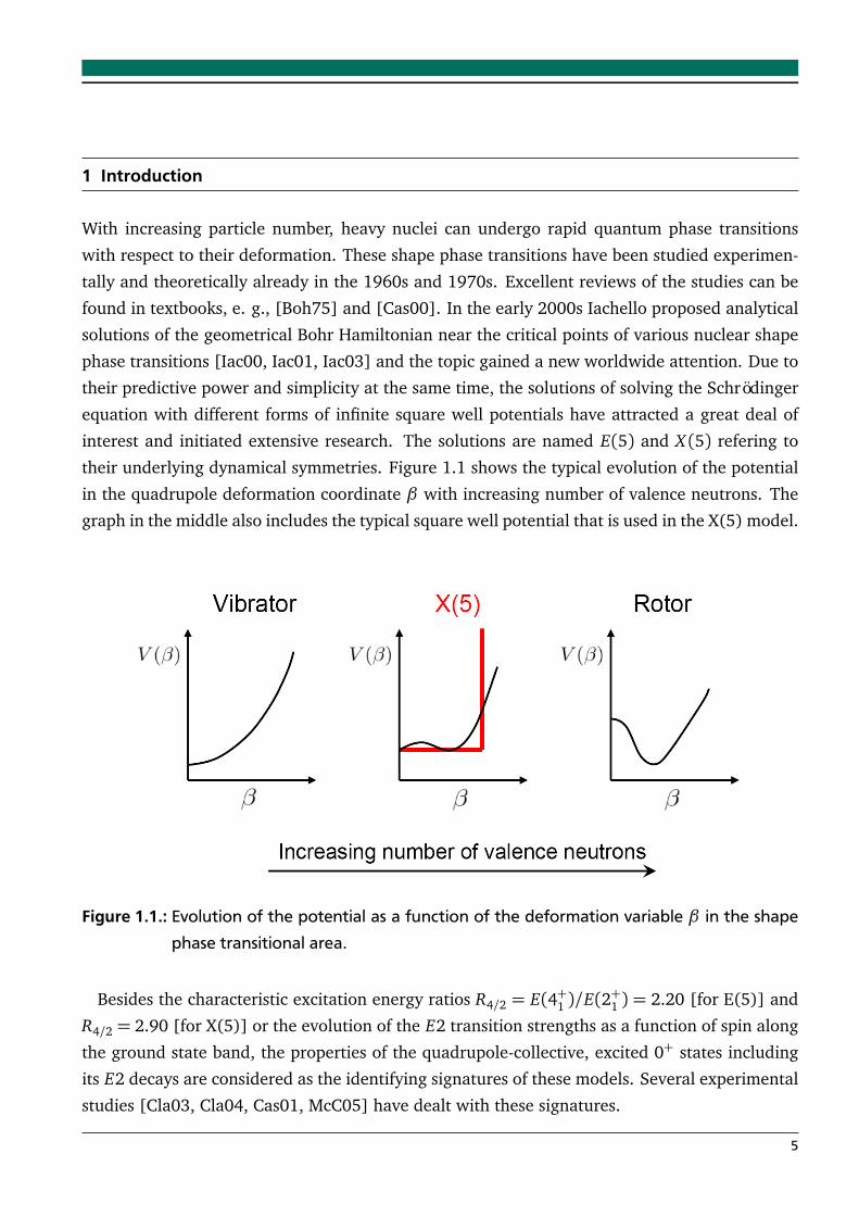
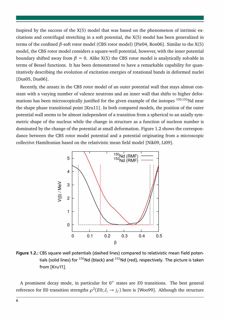
Recently, the ansatz in the CBS rotor model of an outer potential wall that stays almost con-
stant with a varying number of valence neutrons and an inner wall that shifts to higher defor-
mations has been microscopically justified for the given example of the isotopes 150,152Nd near
the shape phase transitional point [Kru11]. In both compared models, the position of the outer
potential wall seems to be almost independent of a transition from a spherical to an axially sym-
metric shape of the nucleus while the change in structure as a function of nucleon number is
dominated by the change of the potential at small deformation. Figure 1.2 shows the correspon-
dance between the CBS rotor model potential and a potential originating from a microscopic
collective Hamiltonian based on the relativistic mean field model [Nik09, Li09].
0
1
2
3
4
5
0 0.1 0.2 0.3 0.4 0.5
V(β
) /
MeV
β
150Nd (RMF)
152Nd (RMF)
Figure 1.2.: CBS square well potentials (dashed lines) compared to relativistic mean field poten-tials (solid lines) for 150Nd (black) and 152Nd (red), respectively. The picture is takenfrom [Kru11].
A prominent decay mode, in particular for 0+ states are E0 transitions. The best general
reference for E0 transition strengths ρ2(E0; Ji → j f ) here is [Woo99]. Although the structure
6
of excited 0+ states in the deformed even-even nuclei has been investigated extensively, their
nature is still discussed controversely. Usually, the first excited 0+ state is interpreted as the β
vibrational excitation of the ground state (0+β
) and the rotational structure that is built on top of
this state is called β band. This is due to the fact that the above mentioned solutions to the Bohr
Hamiltonian show that the collective excitation modes may arise from shape oscillations parallel
to the symmetry axis of the nucleus, so basically an oscillation in the β degree of freedom. The
definition of the β band in terms of the collective wave functions requires the separation of
the wave function Ψ(β ,γ,Ω) = Ψ(β)R(γ,Ω). The excitation occurs in the β dependent part
Ψ(β), resulting in a node in β while the ground state wave function doesn’t have a node. The
typical signatures of β vibrations are strong E0 transitions to the ground state and large reduced
transition probabilities B(E2; 0+β→ 2+1 ).
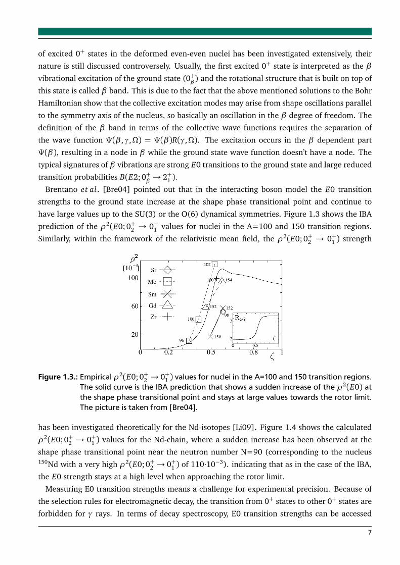
Brentano et al. [Bre04] pointed out that in the interacting boson model the E0 transition
strengths to the ground state increase at the shape phase transitional point and continue to
have large values up to the SU(3) or the O(6) dynamical symmetries. Figure 1.3 shows the IBA
prediction of the ρ2(E0;0+2 → 0+1 values for nuclei in the A=100 and 150 transition regions.
Similarly, within the framework of the relativistic mean field, the ρ2(E0;0+2 → 0+1 ) strength
Figure 1.3.: Empirical ρ2(E0;0+2 → 0+1 ) values for nuclei in the A=100 and 150 transition regions.The solid curve is the IBA prediction that shows a sudden increase of the ρ2(E0) atthe shape phase transitional point and stays at large values towards the rotor limit.The picture is taken from [Bre04].
has been investigated theoretically for the Nd-isotopes [Li09]. Figure 1.4 shows the calculated
ρ2(E0; 0+2 → 0+1 ) values for the Nd-chain, where a sudden increase has been observed at the
shape phase transitional point near the neutron number N=90 (corresponding to the nucleus150Nd with a very high ρ2(E0;0+2 → 0+1 ) of 110·10−3). indicating that as in the case of the IBA,
the E0 strength stays at a high level when approaching the rotor limit.
Measuring E0 transition strengths means a challenge for experimental precision. Because of
the selection rules for electromagnetic decay, the transition from 0+ states to other 0+ states are
forbidden for γ rays. In terms of decay spectroscopy, E0 transition strengths can be accessed
7
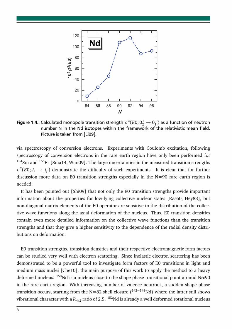
Figure 1.4.: Calculated monopole transition strength ρ2(E0; 0+2 → 0+1 ) as a function of neutronnumber N in the Nd isotopes within the framework of the relativistic mean field.Picture is taken from [Li09].
via spectroscopy of conversion electrons. Experiments with Coulomb excitation, following
spectroscopy of conversion electrons in the rare earth region have only been performed for154Sm and 166Er [Sma14, Wim09]. The large uncertainties in the measured transition strengths
ρ2(E0; Ji → j f ) demonstrate the difficulty of such experiments. It is clear that for further
discussion more data on E0 transition strengths especially in the N=90 rare earth region is
needed.
It has been pointed out [Shi09] that not only the E0 transition strengths provide important
information about the properties for low-lying collective nuclear states [Ras60, Hey83], but
non-diagonal matrix elements of the E0 operator are sensitive to the distribution of the collec-
tive wave functions along the axial deformation of the nucleus. Thus, E0 transition densities
contain even more detailed information on the collective wave functions than the transition
strengths and that they give a higher sensitivity to the dependence of the radial density distri-
butions on deformation.
E0 transition strengths, transition densities and their respective electromagnetic form factors
can be studied very well with electron scattering. Since inelastic electron scattering has been
demonstrated to be a powerful tool to investigate form factors of E0 transitions in light and
medium mass nuclei [Che10], the main purpose of this work to apply the method to a heavy
deformed nucleus. 150Nd is a nucleus close to the shape phase transitional point around N≈90
in the rare earth region. With increasing number of valence neutrons, a sudden shape phase
transition occurs, starting from the N=82 shell closure (142−148Nd) where the latter still shows
vibrational character with a R4/2 ratio of 2.5. 152Nd is already a well deformed rotational nucleus
8
with a R4/2 ratio of 3.27, and with further increase of the neutron number, the rigid rotor limit
(R4/2 ratio of 3.33) is approached towards midshell.
In the end 1980s an electron study has been performed at the old NIKHEF-K facility, deal-
ing with different even-even isotopes in the Nd-chain [San91a, San91b]. Spectra have been
obtained for 142,146,150Nd with the high-resolution electron scattering facility of NIKHEF-K and
covered a momentum transfer range from 0.5 up to 2.8 fm−1. In this study, excitations to the β
band and in particular the 0+2 state has not been analyzed.
In this work, an inelastic electron scattering experiment has been performed at low momen-
tum transfer at the high resolution 169 spectrometer at the S-DALINAC, in order to extract the
E0 transition strength ρ2(E0; 01 → 02) in 150Nd and the radial dependence of the E0 matrix
element by measuring the form factor of this transition. Part I is structured the following way.
In chapter 2 the theoretical background for the geometrical collective model (CBS rotor model)
will be explained. In chapter 3 the electron scattering formalism is summarized and theoretical
model predictions for the transition densities are given. The experiment is described in chapter
4 and after the analysis steps which are explained in chapter 5, chapter 6 deals with the experi-
mental results and their discussion in comparison with theory. In chapter 7 the similarity of the
macroscopic CBS rotor model and a microscopic collective meanfield Hamiltonian will be in-
vestigated in terms of wave functions, energies, transition strengths and centrifugal stretching.
Part I closes with some concluding remarks and an outlook on further studies in chapter 8.
9

2 Theoretical background
In this chapter the theoretical models which are used to describe and interprete the nuclear
structure for the electron scattering experiments are explained. In a more general way the
geometrical model with the so called Bohr Hamiltonian will be introduced and a model to solve
the Bohr Hamiltonian analytically will be presented.
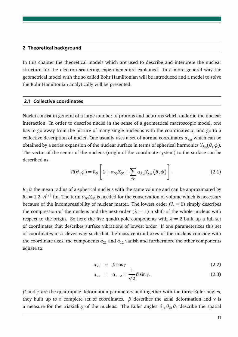
2.1 Collective coordinates
Nuclei consist in general of a large number of protons and neutrons which underlie the nuclear
interaction. In order to describe nuclei in the sense of a geometrical macroscopic model, one
has to go away from the picture of many single nucleons with the coordinates x i and go to a
collective description of nuclei. One usually uses a set of normal coordinates αλµ which can be
obtained by a series expansion of the nuclear surface in terms of spherical harmonics Yλµ(θ ,φ).The vector of the center of the nucleus (origin of the coordinate system) to the surface can be
described as:
R(θ ,φ) = R0
1+α00Y00+∑
λµ
αλµYλµ
θ ,φ
. (2.1)
R0 is the mean radius of a spherical nucleus with the same volume and can be approximated by
R0 = 1.2 ·A1/3 fm. The term α00Y00 is needed for the conservation of volume which is necessary
because of the incompressibility of nuclear matter. The lowest order (λ = 0) simply describes
the compression of the nucleus and the next order (λ = 1) a shift of the whole nucleus with
respect to the origin. So here the five quadrupole components with λ = 2 built up a full set
of coordinates that describes surface vibrations of lowest order. If one parameterizes this set
of coordinates in a clever way such that the mass centroid axes of the nucleus coincide with
the coordinate axes, the components a21 and a12 vanish and furthermore the other components
equate to:
α20 = β cosγ (2.2)
α22 = α2−2 =1p
2β sinγ. (2.3)
β and γ are the quadrupole deformation parameters and together with the three Euler angles,
they built up to a complete set of coordinates. β describes the axial deformation and γ is
a measure for the triaxiality of the nucleus. The Euler angles θ1,θ2,θ3 describe the spatial
11
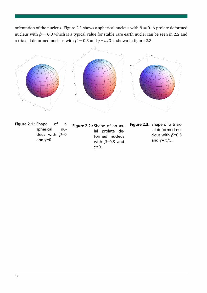
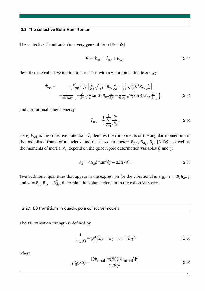
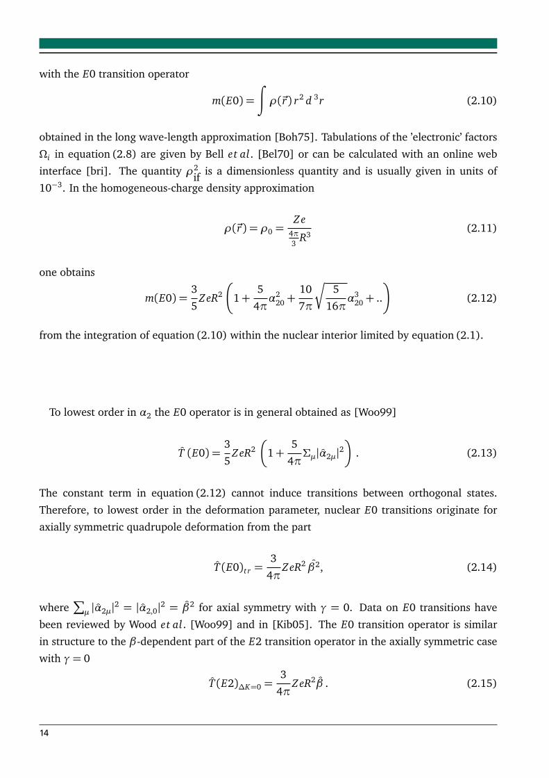
orientation of the nucleus. Figure 2.1 shows a spherical nucleus with β = 0. A prolate deformed
nucleus with β = 0.3 which is a typical value for stable rare earth nuclei can be seen in 2.2 and
a triaxial deformed nucleus with β = 0.3 and γ=π/3 is shown in figure 2.3.
Figure 2.1.: Shape of aspherical nu-cleus with β=0and γ=0.
Figure 2.2.: Shape of an ax-ial prolate de-formed nucleuswith β=0.3 andγ=0.
Figure 2.3.: Shape of a triax-ial deformed nu-cleus with β=0.3and γ=π/3.
12
2.2 The collective Bohr Hamiltonian
The collective Hamiltonian in a very general form [Boh52]
H = Tvib+ Trot+ Vcoll (2.4)
describes the collective motion of a nucleus with a vibrational kinetic energy
Tvib = − ħh2
2p
wr
n
1β4
h
∂
∂ β
p
rwβ4Bγγ
∂
∂ β− ∂
∂ β
p
rwβ3Bβγ
∂
∂ γ
i
+ 1β sin3γ
h
− ∂
∂ γ
p
rw
sin 3γBβγ∂
∂ β+ 1β
∂
∂ γ
p
rw
sin 3γBββ∂
∂ γ
io
(2.5)
and a rotational kinetic energy
Trot =1
2
3∑
k=1
J2k
Ik. (2.6)
Here, Vcoll is the collective potential. Jk denotes the components of the angular momentum in
the body-fixed frame of a nucleus, and the mass parameters Bββ , Bβγ, Bγγ [Jol09], as well as
the moments of inertia Ik, depend on the quadrupole deformation variables β and γ:
Ik = 4Bkβ2 sin2(γ− 2kπ/3) . (2.7)
Two additional quantities that appear in the expression for the vibrational energy: r = B1B2B3,
and w = BββBγγ− B2βγ, determine the volume element in the collective space.
2.2.1 E0 transitions in quadrupole collective models
The E0 transition strength is defined by
1
τ(E0)= ρ2
if(ΩK +ΩLi+ ...+ΩI P) (2.8)
where
ρ2if(E0) =
|⟨Ψfinal|m(E0)|Ψinitial⟩|2
(eR2)2(2.9)
13
with the E0 transition operator
m(E0) =
∫
ρ(~r) r2 d 3r (2.10)
obtained in the long wave-length approximation [Boh75]. Tabulations of the ’electronic’ factors
Ωi in equation (2.8) are given by Bell et al. [Bel70] or can be calculated with an online web
interface [bri]. The quantity ρ2if is a dimensionless quantity and is usually given in units of
10−3. In the homogeneous-charge density approximation
ρ(~r) = ρ0 =Ze
4π3
R3(2.11)
one obtains
m(E0) =3
5ZeR2
1+5
4πα2
20+10
7π
Ç
5
16πα3
20+ ..
(2.12)
from the integration of equation (2.10) within the nuclear interior limited by equation (2.1).
To lowest order in α2 the E0 operator is in general obtained as [Woo99]
T (E0) =3
5ZeR2
1+5
4πΣµ|α2µ|2
. (2.13)
The constant term in equation (2.12) cannot induce transitions between orthogonal states.
Therefore, to lowest order in the deformation parameter, nuclear E0 transitions originate for
axially symmetric quadrupole deformation from the part
T (E0)t r =3
4πZeR2 β2, (2.14)
where∑
µ |α2µ|2 = |α2,0|2 = β2 for axial symmetry with γ = 0. Data on E0 transitions have
been reviewed by Wood et al. [Woo99] and in [Kib05]. The E0 transition operator is similar
in structure to the β-dependent part of the E2 transition operator in the axially symmetric case
with γ= 0
T (E2)∆K=0 =3
4πZeR2β . (2.15)
14
2.2.2 Derivation of ρ2(E0) transition strength as a function of potential stiffness
A derivation of ρ2(E0) transition strength as a function of potential stiffness has been worked
out with the help of Professor Jolos [Jola] from Dubna, Russia, during the research on reference
[Bon09]. In this section the most important formula are presented while the whole derivation
can be found in appendix A. An expression of the ρ2(E0) transition strength only depending on
experimental nuclear structure observables can be found to be:
ρ2
E0; 0+2 → 0+1
= 2
E(2+1 )− E(0+1 )
E(0+2 )− E(0+1 )
B(E2; 0+1 → 2+1 )2
3Z4π
2(e2R4)2
. (2.16)
Using the relation between B(E2;0+1 → 2+1 ) and¬
0+1
β2
0+1¶
:
B(E2; 0+1 → 2+1 ) =
3Z
4πeR22¬
0+1
β2
0+1¶
(2.17)
one obtains from equation 2.16:
ρ2
E0;0+2 → 0+1
= 2
E(2+1 )− E(0+1 )
E(0+2 )− E(0+1 )
3Z
4π
2¬
0+1
β2
0+1¶2
. (2.18)
The most important observation from equation 2.18 is that when the stiffness of the potential
in β increases, the ratio
E(2+1 )−E(0+1 )
E(0+2 )−E(0+1 )
decreases. As a result ρ2
E0;0+2 → 0+1
should also
decrease.
2.3 The confined β -soft rotor model
In this chapter the confined β-soft rotor model (CBS rotor model) [Pie04] will be described
and a solution to the Schrödinger Equation by using a simple square well potential in the
deformation variable β will be presented. The CBS rotor model represents an approximate
analytical solution to the collective Hamiltonian in equation (2.4) proposed by Bohr and Mot-
15
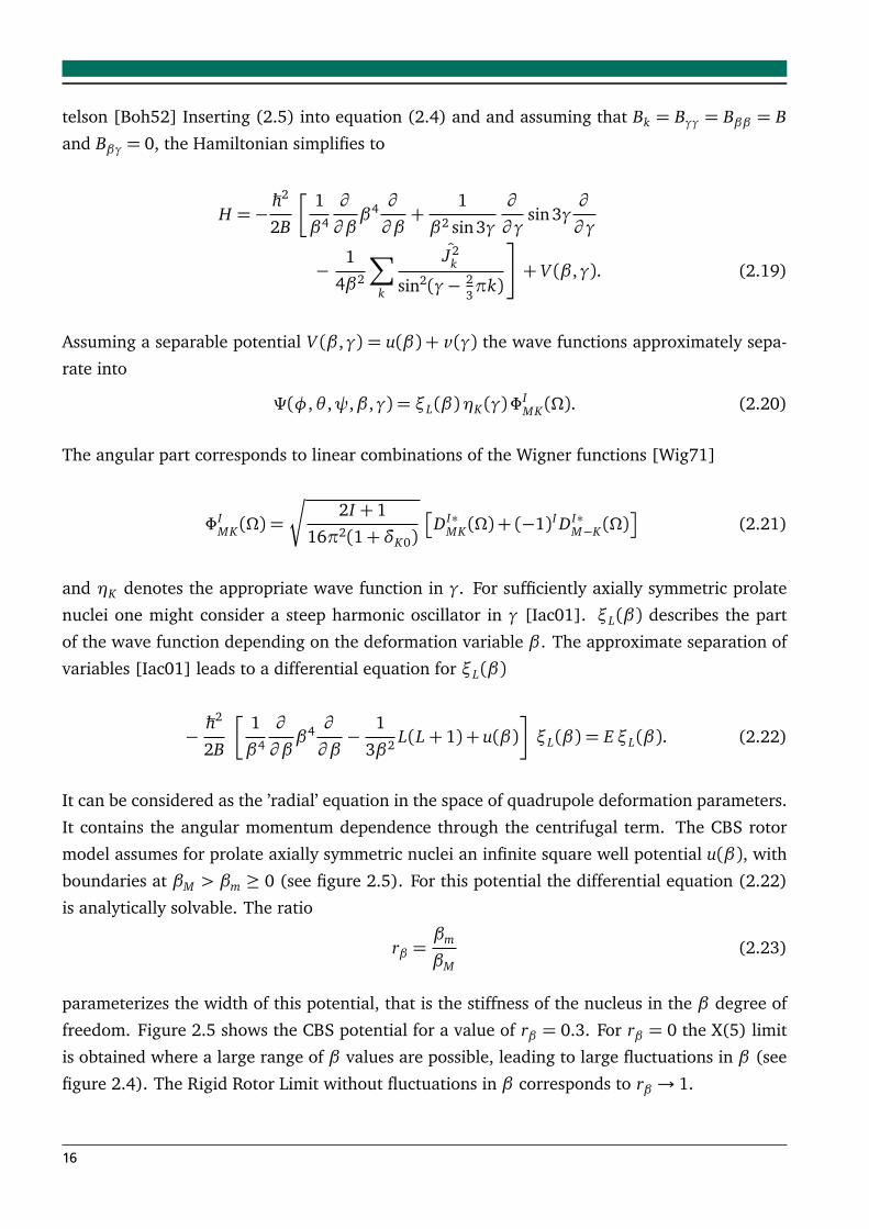
telson [Boh52] Inserting (2.5) into equation (2.4) and and assuming that Bk = Bγγ = Bββ = B
and Bβγ = 0, the Hamiltonian simplifies to
H =−ħh2
2B
1
β4
∂
∂ ββ4 ∂
∂ β+
1
β2 sin3γ
∂
∂ γsin3γ
∂
∂ γ
−1
4β2
∑
k
J2k
sin2(γ− 23πk)
+ V (β ,γ). (2.19)
Assuming a separable potential V (β ,γ) = u(β) + v (γ) the wave functions approximately sepa-
rate into
Ψ(φ,θ ,ψ,β ,γ) = ξL(β)ηK(γ)ΦIMK(Ω). (2.20)
The angular part corresponds to linear combinations of the Wigner functions [Wig71]
ΦIMK(Ω) =
r
2I + 1
16π2(1+δK0)
DI∗MK(Ω)+ (−1)I DI∗
M−K(Ω)
(2.21)
and ηK denotes the appropriate wave function in γ. For sufficiently axially symmetric prolate
nuclei one might consider a steep harmonic oscillator in γ [Iac01]. ξL(β) describes the part
of the wave function depending on the deformation variable β . The approximate separation of
variables [Iac01] leads to a differential equation for ξL(β)
−ħh2
2B
1
β4
∂
∂ ββ4 ∂
∂ β−
1
3β2 L(L+ 1) + u(β)
ξL(β) = E ξL(β). (2.22)
It can be considered as the ’radial’ equation in the space of quadrupole deformation parameters.
It contains the angular momentum dependence through the centrifugal term. The CBS rotor
model assumes for prolate axially symmetric nuclei an infinite square well potential u(β), with
boundaries at βM > βm ≥ 0 (see figure 2.5). For this potential the differential equation (2.22)
is analytically solvable. The ratio
rβ =βm
βM(2.23)
parameterizes the width of this potential, that is the stiffness of the nucleus in the β degree of
freedom. Figure 2.5 shows the CBS potential for a value of rβ = 0.3. For rβ = 0 the X(5) limit
is obtained where a large range of β values are possible, leading to large fluctuations in β (see
figure 2.4). The Rigid Rotor Limit without fluctuations in β corresponds to rβ → 1.
16
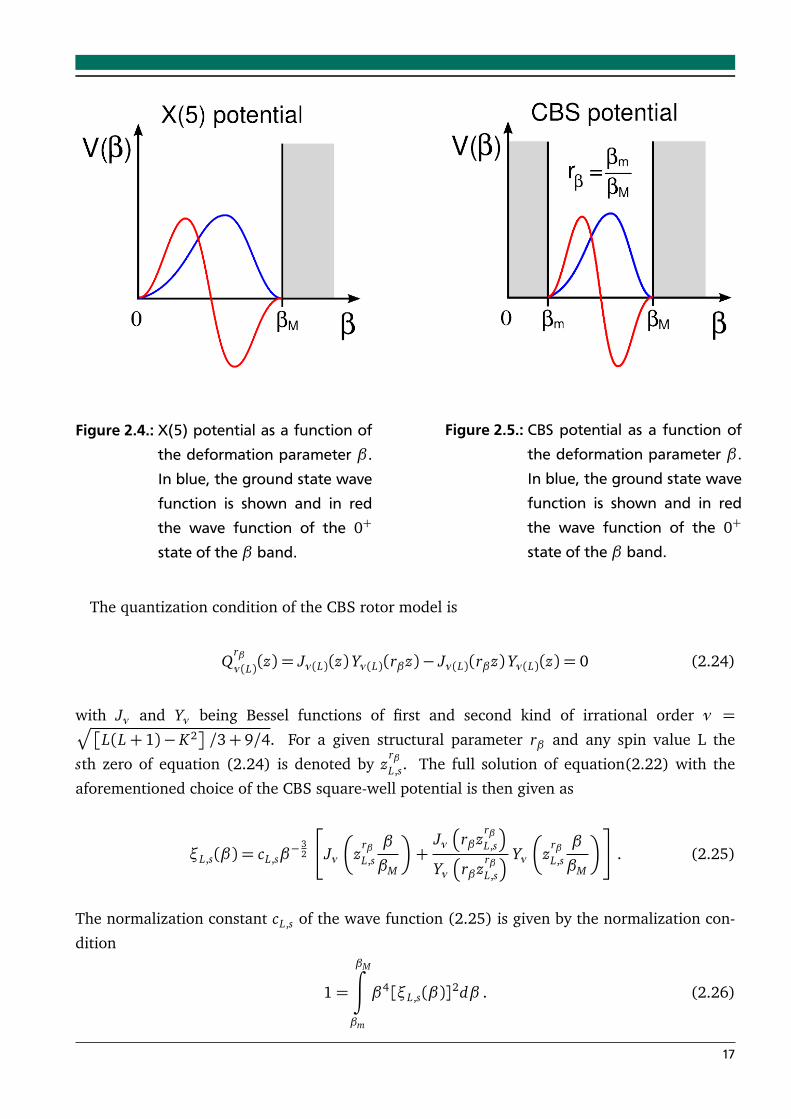
Figure 2.4.: X(5) potential as a function ofthe deformation parameter β .In blue, the ground state wavefunction is shown and in redthe wave function of the 0+
state of the β band.
Figure 2.5.: CBS potential as a function ofthe deformation parameter β .In blue, the ground state wavefunction is shown and in redthe wave function of the 0+
state of the β band.
The quantization condition of the CBS rotor model is
Qrβν(L)(z) = Jν(L)(z)Yν(L)(rβz)− Jν(L)(rβz)Yν(L)(z) = 0 (2.24)
with Jν and Yν being Bessel functions of first and second kind of irrational order ν =p
L(L+ 1)− K2
/3+ 9/4. For a given structural parameter rβ and any spin value L the
sth zero of equation (2.24) is denoted by zrβL,s. The full solution of equation(2.22) with the
aforementioned choice of the CBS square-well potential is then given as
ξL,s(β) = cL,sβ−3
2
Jν
zrβL,s
β
βM
+Jν
rβzrβL,s
Yν
rβzrβL,s
Yν
zrβL,s
β
βM
. (2.25)
The normalization constant cL,s of the wave function (2.25) is given by the normalization con-
dition
1=
βM∫
βm
β4[ξL,s(β)]2dβ . (2.26)
17
The eigenvalues of equation (2.22) are obtained as
EL,s =ħh2
2Bβ2M
zrβL,s
2. (2.27)
For convenience, the reduced deformation parameter b = β
βM∈ [rβ , 1] is used where appropri-
ate.
The CBS rotor model well describes the evolution of low-energy 0+ bands [Pie04], ground
bands of strongly deformed nuclei [Dus05], and the dependence of relative moments of inertia
as a function of spin in deformed transitional nuclei [Dus06]. It has also been successfully used
for studying relative as well as absolute E0 transitions in the region of the X(5) nuclei up to the
rigid rotor limit [Bon09].
2.3.1 E0 transition strengths in the CBS model
Electromagnetic transition strengths can be calculated from the wave functions given above. For
E0 transitions one obtains with Eqs. (2.9,2.14)
ρ2if(E0) =
3Z
4π
2
|⟨ψf|β2|ψi⟩|
2 (2.28)
=
3
4π
2
Z2β4M |⟨ξf|b
2|ξi⟩|2 (2.29)
between states that only differ in the β-dependent part of the wave function, i.e., ⟨Df|Di⟩ =⟨ηf|ηi⟩ = 1. As a function of the choice of the potential, i.e., as a function of the nuclear
deformation (βM) and the nuclear stiffness against centrifugal stretching (rβ), the E0 transition
strengths can be expressed as
ρ2if(E0) =
3
4π
2
Z2β4M
1∫
rβ
ξ∗f (b)b2ξi(b)b
4db
2
(2.30)
= qE0
βM
h
m2,rβ (Ji → J f )i2
, (2.31)
18
with the matrix element
mk,rβ (Ji → J f ) =
1∫
rβ
ξi(b)bkξ f (b)b
4db (2.32)
of kth order in the reduced deformation variable b that only depends on the nuclear stiffness
parameter rβ . The magnitude of the nuclear deformation
βM
appears in the scaling constant
qE0
βM
. The corresponding expression for B(E2) transition strengths of ∆K = 0 transitions
follows as
B(E2; Ji → J f ) = qE2
βM
CJ f 0Ji020
2h
m1,rβ(Ji → J f )
i2, (2.33)
with the scaling constant
qE2
βM
=
3
4π
2
β2M Z2e2R4. (2.34)
CJ f 0Ji020 denotes a Clebsch-Gordan coefficient. Deviations from the homogeneous-charge density
approximation might be taken into account to lowest order by an effective charge Ze→ qEλZe,
with qEλ ≈ 1 for electric transitions with multipolarity λ.
2.4 Microscopic relativistic mean-field approach
In this chapter a microscopic collective Hamiltonian based on the relativistic mean field model
[Nik09, Li09] is introduced. In section 7 comparisons between the CBS rotor model and this
microscopic mean field approach will be discussed. The kinetic energy part of the Hamiltonian
is in the general form as already seen in equations (2.4) - (2.6). The seven functions, i.e.
the three moments of inertia Ik, the three mass parameters Bββ , Bβγ, Bγγ, and the collective
potential Vcoll, are determined by the choice of a particular microscopic nuclear energy-density
functional or effective interaction. In the particle-hole channel the relativistic functional PC-F1
(point-coupling Lagrangian) [Bür02b] has been used, as in the studies of shape transitions in
the Nd-chain [Li09]. Also a density-independent δ force in the particle-particle channel treated
by the BCS approximation was used. The moments of inertia are calculated microscopically
from the Inglis-Belyaev formula:
Ik =∑
i, j
uiv j − v iu j
2
Ei + E j⟨i|Jk| j⟩|2 k = 1, 2,3, (2.35)
19
where the summation runs over the proton and neutron quasi-particle states, and k denotes the
axis of rotation. The quasi-particle energies Ei, occupation probabilities v i, and single-nucleon
wave functions ψi are determined by solutions of the constrained RMF+BCS equations. The
mass parameters associated with the two quadrupole collective coordinates q0 = ⟨Q20⟩ and
q2 = ⟨Q22⟩ are also calculated in the cranking approximation
Bµν(q0, q2) =ħh2
2
h
M−1(1)M(3)M
−1(1)
i
µν, (2.36)
with
M(n),µν(q0, q2) =∑
i, j
⟨i| Q2µ
j
j
Q2ν |i⟩(Ei + E j)n
uiv j + v iu j
2. (2.37)
In contrast to the CBS Model, the potential Vcoll in the collective Hamiltonian Equation (2.4) is
obtained by subtracting the zero-point energy corrections from the total energy that corresponds
to the solution of constrained RMF+BCS equations, at each point on the triaxial deformation
plane.
The Hamiltonian (2.4) describes quadrupole vibrations, rotations, and the coupling of these
collective modes. The corresponding eigenvalue problem is solved using an expansion of eigen-
functions in terms of a complete set of basis functions that depend on the deformation variables
β and γ, and the Euler angles φ, θ and ψ. The diagonalization of the Hamiltonian yields the
excitation energies and collective wave functions
ΨI Mα (β ,γ,Ω) =
∑
K∈∆I
ψIαK(β ,γ)ΦI
MK(Ω), (2.38)
that are used to calculate observables. The angular part corresponds to linear combinations of
the Wigner functions [see equation (2.21)] and the summation in equation (2.38) is over the
allowed set of K values:
∆I =
(
0, 2, . . . , I for I mod 2= 0
2, 4, . . . , I − 1 for I mod 2= 1 .(2.39)
For a given collective state in equation (2.38), the probability density distribution in the β − γ-
plane is defined by
ρIα(β ,γ) =∑
K∈∆I
|ψIαK(β ,γ)|2β3| sin 3γ| . (2.40)
20
The normalization reads∞∫
0
βdβ
2π∫
0
dγ ρIα(β ,γ) = 1 . (2.41)
If we integrate the wave function (2.38) along γ, we obtain the projection
ρ′Iα(β) =∑
K∈∆I
2π∫
0
|ψIαK(β ,γ)|2β4| sin3γ|dγ . (2.42)
of the density distribution as a function of β for the desired comparison with the results from
the CBS model. Its normalization reads:
∞∫
0
ρ′Iα(β)dβ = 1 . (2.43)
21

3 Inelastic electron scattering at low momentum transfer
In this chapter basics of the description of inelastic electron scattering at low momentum transfer
will be given. It is based on [Übe71], although the notation of [Bur08, Neu97b] has been used.
3.1 Electron scattering formalism
Incoming electrons with the energy E0 scatter off atomic nuclei. The ground state and excited
states with discrete excitation energies will be directly visible in an energy-loss spectrum, when
the scattered electrons with the energy E f are bent at an angle of θ in a dipole magnet and
selected by their momenta in the focal plane of the spectrometer. In these scattering processes
energy is conserved
E0 = E f + Ex + ER. (3.1)
Ex is the excitation energy of the excited state and ER the recoil energy of the nucleus. The latter
is negligible and equation 3.1 simplifies to
Ex = E0− E f . (3.2)
Momentum conservation requires
~q = ~pi − ~p f , (3.3)
where pi and p f are the electron momenta before and after the scattering process. The absolute
value of the momentum transfer ~q can be written as
q =1
ħhc
p
2E0(E0− Ex)(1− cosθ) + E2x . (3.4)
Due to the attraction of the Coulomb force during the scattering process, especially for heavier
nuclei, the effective energy of the electron is higher than its energy in the center of mass system.
This leads to an increase in the momentum transfer.
qe f f = q
1+3
2
Ze2
ħhcE0Req
(3.5)
23
Here, ħhc = 197 MeV fm , e2 = 1, 44MeV fm and Req is the radius of a homogeneously charged
sphere.
The electron interacts with the charge and current density of the nucleus by exchange of a
virtual photon. In the first order perturbation theory only the exchange of one photon is used.
Then the differential cross section
dσdΩ
θat the angle θ can be written as
dσ
dΩ
θ
=1
4π2(ħhc)2Ei E f
p f
pi
2J f + 1
2Ji + 1
frec
⟨Ψ f
Hint
Ψi⟩
2. (3.6)
Here, Ji and J f the total angular momenta before and after the scattering process. Hint is the
Hamiltonian of the interaction and frec the recoil factor
frec =
1+2Eisin2(θ/2)
Mc2
−1
(3.7)
The matrix element M(λ(q) = ⟨Ψ f
Hint
Ψi⟩ contains the wave function of the initial and final
state and all informations about the interaction. In order to measure this matrix element, one
defines the squared form factor
F(E0, q)
2=
dσdΩ
ex p
dσdΩ
Mot t
(3.8)
as the ratio of the experimental differential cross section and the Mott cross section defined as
dσ
dΩ
Mot t=
Ze2
2E0
2cos2 θ/2
sin4 θ/2, (3.9)
The squared form factor
F(E0, q)
2is a function of the momentum transfer q. Extracting the
q-dependence of the form factor, one can obtain informations about the charge and current
distributions in the nucleus.
Under electromagnetic interaction, the total angular momentum and the parity of a system
are conserved. For a given angular momentum J and parity π the selection rules for the multi-
polarity λ and the transition from the initial state
ψi
to the final state
ψ f
¶
are for the angular
momentum:
Ji − J f
≤ λ≤ Ji + J f . (3.10)
24
and for the parity:
πiπ f = (−1)λ for electric transitions and (3.11)
πiπ f = (−1)λ+1 for magnetic transitions. (3.12)
In the case of light nuclei, the wave function of the incoming and the scattered electrons can
be approximated with plane waves (Plane Wave Born Approximation, PWBA). In heavy nuclei,
where the Coulomb potential plays a major role as in the case of 150Nd, the influence of the
coulomb field is so big for the incoming electrons that they become accelerated when approach-
ing the nucleus and slowed down after the scattering process. This results in a distortion of the
outgoing electron wave. In this case we explicitly need a nuclear model for calculating Mλ(q).Solving numerically the Dirac equation one can extract the form factors. In order to deduce the
transition strengths on has to scale the experimental data to the theory.
3.2 Model predictions for the 0+1 → 0+2 E0 transition in 150Nd
3.2.1 Effective operator for the E0 transition density
In a recent work [Shi09] a semi-microscopic method has been applied for the calculation of
properties of shape-phase transitional nuclei. Firstly, the effective density operator has been
constructed at a microscopical level. In a second step the collective wave functions obtained in
the CBS rotor model (see section 2.3) have been used to calculate the matrix elements of the
effective operator by integration over the collective variables.
The single particle density operator ρ(~r) can be expressed in terms of the particle creation and
annihilation operators corresponding to the Nilsson single-particle basis with the deformation
parameters β and γ. According to [Shi09] it is written as
ρ(~r) =∑
s,s′ϕ∗s (~r,β)ϕs′(~r,β)a†
s (β)as′(β) (3.13)
with the single-particle wave functions
ϕ(~r,β) =∑
n,l, j
a(s)nl j(β)Rnl j(r)
Yl(θ ,φ)χ1/2
jΩs, (3.14)
25
where a(s)nl j(β) are the Nilsson expansion coefficients, Rnl j(r) is a radial wave function corre-
sponding to the Schrödinger equation with the spherically symmetric Woods-Saxon potential.
Then, the average of ρ(~r) over the quasi-particle vacuum corresponding to the equilibrium
deformation β is given as
¬
β
ρ(~r)
β¶
=∑
s
ϕs(~r,β)
2v 2
s (β), (3.15)
where v 2s (β) denotes the single-particle occupation probability. In order to calculate the E0
transition density for the 0+1 → 0+2 transition it is necessary to integrate equation (3.15) over
the Euler angles, resulting in
¬
β
ρ(r)
β¶
=
∫
d٬
β
ρ(~r)
β¶
(3.16)∑
n,n′,l, j
a(s)nl j(β)a(s)n′ l j(β)Rnl j(r)Rn′ l j(r)v
2s (β). (3.17)
The full expression for the effective E0 transition density operator ρeff(r,β) has been obtained
by using the Generator Coordinate Method (GCM) which is well described in [Rin80]. The
result is
ρeff(r,β) =¬
β
ρ(r)
β¶
+ F(r) +
1
2ZF(r)− G(r)
∂ 2
∂ β2 (3.18)
where the radial functions F(r) and G(r) are lengthy expressions containing the spherically
symmetric part of the nuclear single-particle potential Vsp(r), the single-particle energies εs, the
single quasi-particle energies Es, the energy gap ∆ and the matrix elements¬
s
f Y20
t¶
that are
all functions of the deformation parameter β .
3.2.2 Neutron and proton transition densities
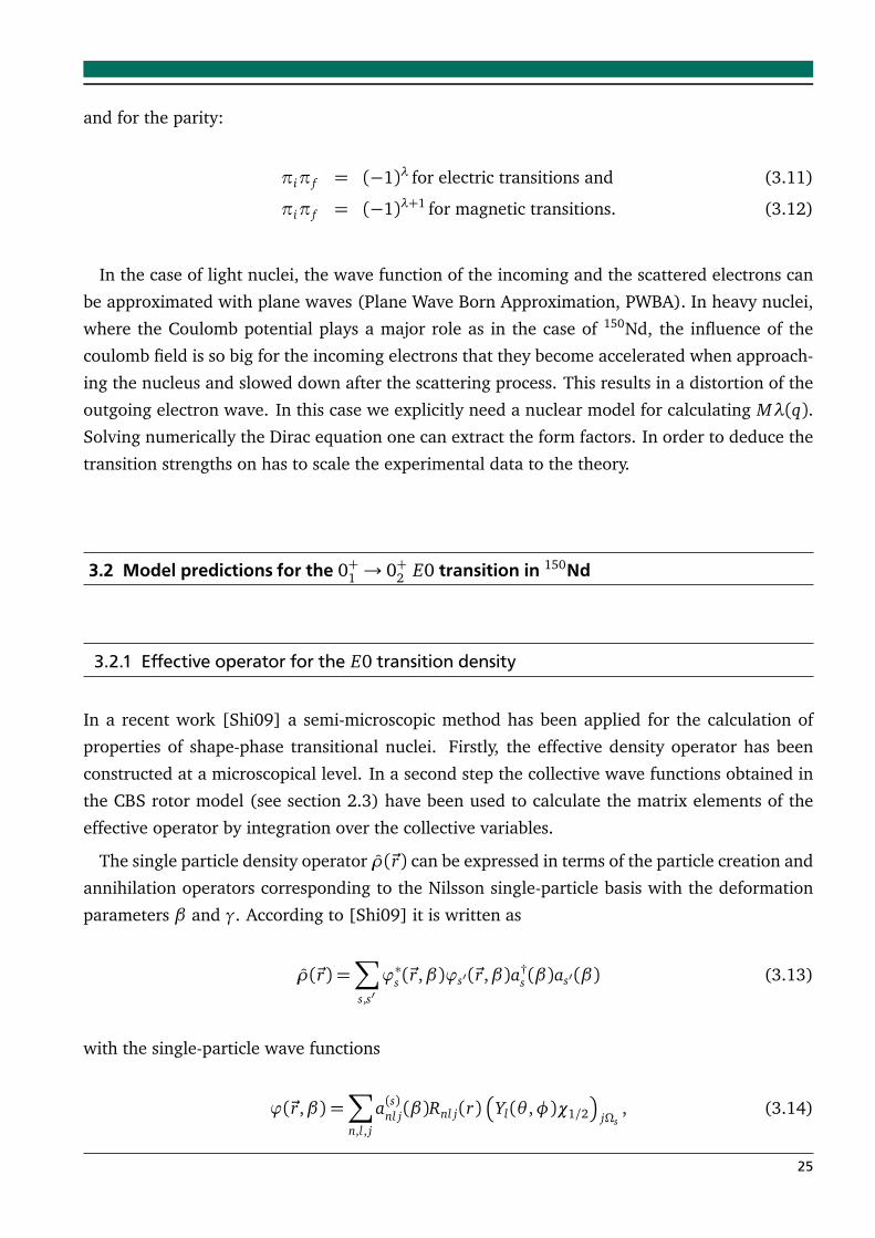
Using the collective wave functions obtained in the CBS rotor model, the neutron and proton
transition densities for the 0+1 → 0+2 transition in 150Nd could have been calculated according
to equation (3.18) and are depicted in figure 3.1. It has been found to be useful to plot a the
ordinate of a transition density multiplied by r2 in order to enhance the effects on the nuclear
surface. Since electron scattering is only sensitive to the charge distribution and not on the
matter distribution, only the proton transition density distribution has been used.
26
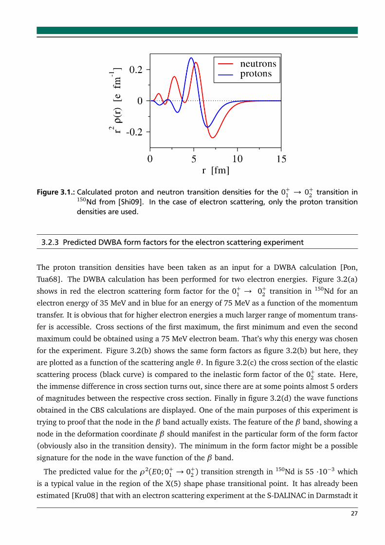
Figure 3.1.: Calculated proton and neutron transition densities for the 0+1 → 0+2 transition in150Nd from [Shi09]. In the case of electron scattering, only the proton transitiondensities are used.
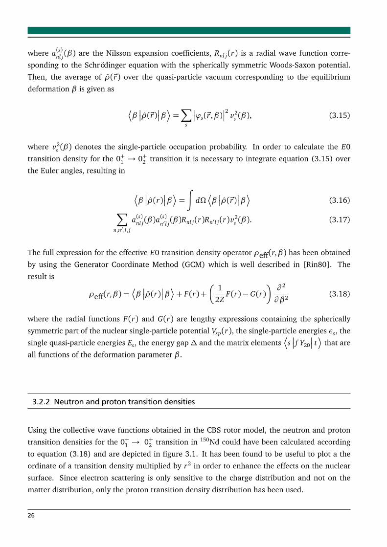
3.2.3 Predicted DWBA form factors for the electron scattering experiment
The proton transition densities have been taken as an input for a DWBA calculation [Pon,
Tua68]. The DWBA calculation has been performed for two electron energies. Figure 3.2(a)
shows in red the electron scattering form factor for the 0+1 → 0+2 transition in 150Nd for an
electron energy of 35 MeV and in blue for an energy of 75 MeV as a function of the momentum
transfer. It is obvious that for higher electron energies a much larger range of momentum trans-
fer is accessible. Cross sections of the first maximum, the first minimum and even the second
maximum could be obtained using a 75 MeV electron beam. That’s why this energy was chosen
for the experiment. Figure 3.2(b) shows the same form factors as figure 3.2(b) but here, they
are plotted as a function of the scattering angle θ . In figure 3.2(c) the cross section of the elastic
scattering process (black curve) is compared to the inelastic form factor of the 0+2 state. Here,
the immense difference in cross section turns out, since there are at some points almost 5 orders
of magnitudes between the respective cross section. Finally in figure 3.2(d) the wave functions
obtained in the CBS calculations are displayed. One of the main purposes of this experiment is
trying to proof that the node in the β band actually exists. The feature of the β band, showing a
node in the deformation coordinate β should manifest in the particular form of the form factor
(obviously also in the transition density). The minimum in the form factor might be a possible
signature for the node in the wave function of the β band.
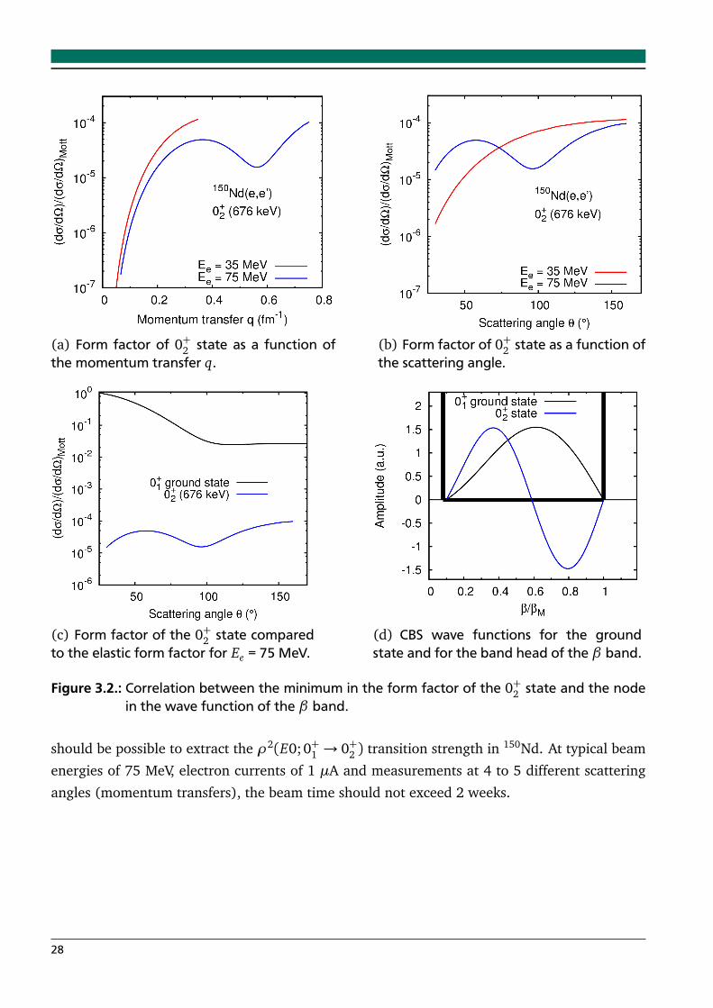
The predicted value for the ρ2(E0; 0+1 → 0+2 ) transition strength in 150Nd is 55 ·10−3 which
is a typical value in the region of the X(5) shape phase transitional point. It has already been
estimated [Kru08] that with an electron scattering experiment at the S-DALINAC in Darmstadt it
27
(a) Form factor of 0+2 state as a function ofthe momentum transfer q.
(b) Form factor of 0+2 state as a function ofthe scattering angle.
(c) Form factor of the 0+2 state comparedto the elastic form factor for Ee = 75 MeV.
(d) CBS wave functions for the groundstate and for the band head of the β band.
Figure 3.2.: Correlation between the minimum in the form factor of the 0+2 state and the nodein the wave function of the β band.
should be possible to extract the ρ2(E0;0+1 → 0+2 ) transition strength in 150Nd. At typical beam
energies of 75 MeV, electron currents of 1 µA and measurements at 4 to 5 different scattering
angles (momentum transfers), the beam time should not exceed 2 weeks.
28
4 Inelastic electron scattering experiments at the S-DALINAC
4.1 S-DALINAC and experimental facilities
Since 1991 the recirculating superconducting electron linear accelerator S-DALINAC [Ric96] at
the Institut für Kernphysik [IKP14] at the TU Darmstadt is in operation. The accelerator and
all the experimental facilities were built in the framework of many dissertations and diploma
theses and are still modified and improved by bachelor, master and PhD students. Figure 4.1
gives an overview of the S-DALINAC and its experiments. The S-DALINAC once was the first
superconducting continuous-wave electron linear accelerator in Europe. Electrons can be either
accelerated by a thermionic electron gun À or by a new source Á that is emitting spin polarized
electrons [End11, Fri11]. The superconducting injector  with its 3 GHz-cavities allows already
experiments with Bremsstrahlung of up to 10 MeV at the Darmstadt High intensity Photon Setup
(DHIPS) Ã [Son11]. The electrons can also be bent by 180 degree and pass the main accelerator
Ä up to 3 times Å to get a final beam energy of 130 MeV and electron currents of up to 20 µA.
Different experimental facilities (see figure 4.1) provide a huge variety of experiments in the
field of nuclear structure physics. Experiments with tagged photons can be performed at the
photon tagger NEPTUN Æ [Sav10]. One of the working horses for the electron scattering ex-
periments at low momentum transfer is the so-called QCLAM spectrometer È [Die95, Neu97a]
where coincidence experiments can be performed [NC97, Str00, Die01, NC02]. This spectrome-
ter is also equipped with a special 180 beam line Ç where experiments in transverse kinematics
can be preferred [NC99, Rei02, Rye06]. The spectrometer which has been used in this work is
the 169 spectrometer É [Grä78, Wal78, Sch78, Foh78]. It has a much smaller solid angle but
due to its dispersion matching beam line, excellent energy resolution can be achieved.
29
Figu
re4.
1.:O
verv
iew
ofth
eS-
DA
LIN
ACw
ithits
expe
rimen
talf
acili
ties.
ÀTh
erm
ioni
cel
ectr
ongu
n,Á
new
sour
ceof
pola
rized
elec
tron
sSP
IN,Â
the
10M
eVin
ject
orac
cele
rato
r,Ã
the
DH
IPS
facil
ityfo
r(γ
,γ’)
mea
sure
men
ts,Ä
mai
nac
cele
rato
r(40
MeV
),Å
recir
-cu
latio
nbe
amlin
es,Æ
low
ener
gyph
oton
tagg
erN
EPTU
N,Ç
180
beam
line,
ÈQ
CLA
M-S
pect
rom
eter
,É16
9-S
pect
rom
eter
.
30
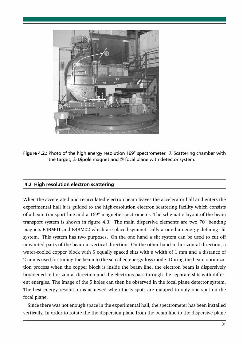
Figure 4.2.: Photo of the high energy resolution 169 spectrometer. À Scattering chamber withthe target, Á Dipole magnet and  focal plane with detector system.
4.2 High resolution electron scattering
When the accelerated and recirculated electron beam leaves the accelerator hall and enters the
experimental hall it is guided to the high-resolution electron scattering facility which consists
of a beam transport line and a 169 magnetic spectrometer. The schematic layout of the beam
transport system is shown in figure 4.3. The main dispersive elements are two 70 bending
magnets E4BM01 and E4BM02 which are placed symmetrically around an energy-defining slit
system. This system has two purposes. On the one hand a slit system can be used to cut off
unwanted parts of the beam in vertical direction. On the other hand in horizontal direction, a
water-cooled copper block with 5 equally spaced slits with a width of 1 mm and a distance of
2 mm is used for tuning the beam to the so-called energy-loss mode. During the beam optimiza-
tion process when the copper block is inside the beam line, the electron beam is dispersively
broadened in horizontal direction and the electrons pass through the separate slits with differ-
ent energies. The image of the 5 holes can then be observed in the focal plane detector system.
The best energy resolution is achieved when the 5 spots are mapped to only one spot on the
focal plane.
Since there was not enough space in the experimental hall, the spectrometer has been installed
vertically. In order to rotate the the dispersion plane from the beam line to the dispersive plane
31
Figure 4.3.: Beam line to the high resolution electron scattering facility with the 169
spectrometer.
of the spectrometer (90) five quadrupoles (labeled as E4QR01-05) are installed. The beam is
then guided into the scattering chamber where measurements at angles between 33 and 165
are possible in discrete steps of 12. A very high percentage of the electrons pass the target
which is situated at the center of the scattering chamber and are dumped in a Faraday cup,
where the collected beam charge is measured. To reduce the beam divergence behind the target
due to multiple scattering, a doublet of two large quadrupoles is installed directly behind the
target chamber. Electrons scattered in the solid angle∆Ω are bent through a dipole magnet and
their momentum is analyzed in the focal plane of the 169 spectrometer. The so-called ’magic
angle’ of πp
8/3 = 169.7 was chosen to improve the improve the electron-optical properties
of the spectrometer [Wal78]. The focal plane is tilted to 35 relative to the electron orbit to
minimize aberration errors. Figure 4.2 shows a photo of the spectrometer. The technical details
of the 169 spectrometer can be found in table 4.1.
4.3 Focal plane detector system
The focal plane detector system [Len05, Len06] consists of 4 silicon strip detector units, each 6.9
cm long and consisting of 96 silicon strips (channels). The whole focal plane covers a range of
24 cm and the distance between two modules corresponds to a gap of 10.5 strips. The obtained
spectra are therefore 415.5 channels wide. Each silicon strip has a thickness of 500 µm and
a pitch of 650 µm. The guard ring around the 96 strips and the printed circuit board carrier
result in an inactive zone of 7 mm, corresponding to the 10.5 strips, between two adjacent
32
Energy acceptance: 20 - 120 MeVDeflection angle: 169.7 ± 0.1
Radius of central trajectory: 1.0 mTilt of focal plane: 35 ± 2
Dispersion: 3.76 cm/%Momentum acceptance: ∆p
p=±2%
Solid angle acceptance: Ωmax ≈ 6 msrMaximum relative energy resolution: 3 · 10−4 (FWHM)Range of scattering angles: 33− 165 (12 Steps)Field strength: 0.6 - 4.0 kG
Table 4.1.: Some technical details of the high resolution 169 spectrometer.
detectors. Measurements are repeated with slightly different magnetic field settings in order
to avoid holes in the spectrum. Figure 4.4 shows a photo of the focal plane detector system.
In order to reduce background radiation, a massive radiation shielding has been constructed
around it [Bur02a]. As a trigger detector to suppress the background, a 40 cm long plastic
Figure 4.4.: Focal plane detector system of the 169 spectrometer. À Iron yoke of the dipolemagnet, Á vacuum connections of bias signals to the preamplifiers, Â vacuumconnections of the preamplifier analog signals, Ã detector unit, Ä supply voltageconnections and control signals of the preamplifiers, Å detector case, Æ readoutelectronics and high voltage connections. Picture is taken from [Len06].
scintillator with a thickness of 5 mm is used.
33
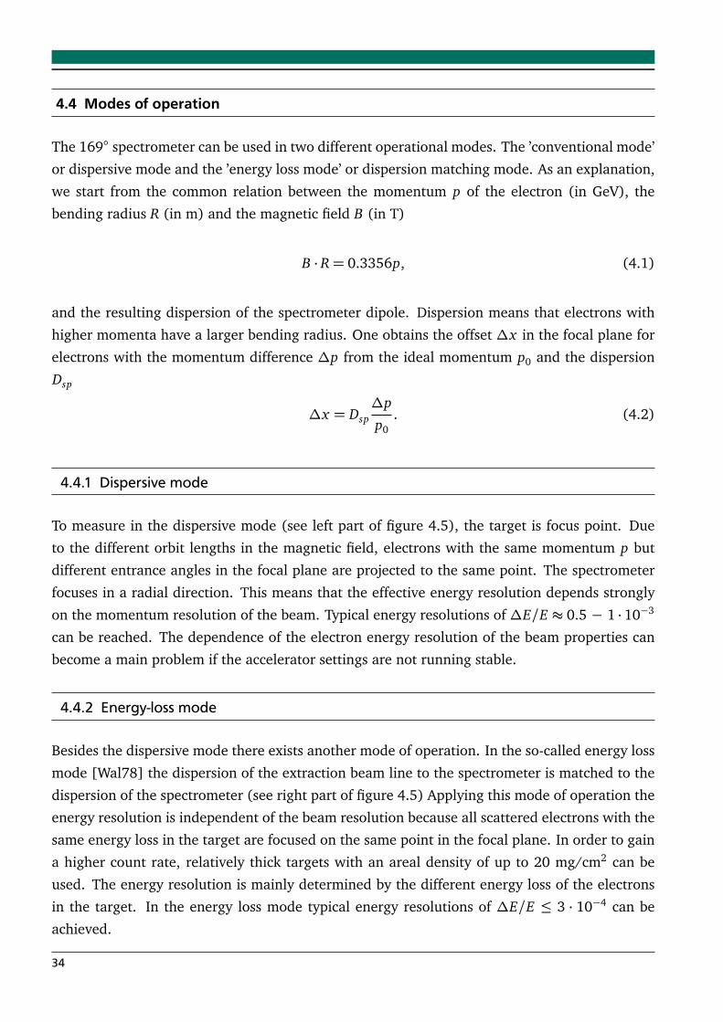
4.4 Modes of operation
The 169 spectrometer can be used in two different operational modes. The ’conventional mode’
or dispersive mode and the ’energy loss mode’ or dispersion matching mode. As an explanation,
we start from the common relation between the momentum p of the electron (in GeV), the
bending radius R (in m) and the magnetic field B (in T)
B · R= 0.3356p, (4.1)
and the resulting dispersion of the spectrometer dipole. Dispersion means that electrons with
higher momenta have a larger bending radius. One obtains the offset ∆x in the focal plane for
electrons with the momentum difference ∆p from the ideal momentum p0 and the dispersion
Dsp
∆x = Dsp∆p
p0. (4.2)
4.4.1 Dispersive mode
To measure in the dispersive mode (see left part of figure 4.5), the target is focus point. Due
to the different orbit lengths in the magnetic field, electrons with the same momentum p but
different entrance angles in the focal plane are projected to the same point. The spectrometer
focuses in a radial direction. This means that the effective energy resolution depends strongly
on the momentum resolution of the beam. Typical energy resolutions of ∆E/E ≈ 0.5 − 1 ·10−3
can be reached. The dependence of the electron energy resolution of the beam properties can
become a main problem if the accelerator settings are not running stable.
4.4.2 Energy-loss mode
Besides the dispersive mode there exists another mode of operation. In the so-called energy loss
mode [Wal78] the dispersion of the extraction beam line to the spectrometer is matched to the
dispersion of the spectrometer (see right part of figure 4.5) Applying this mode of operation the
energy resolution is independent of the beam resolution because all scattered electrons with the
same energy loss in the target are focused on the same point in the focal plane. In order to gain
a higher count rate, relatively thick targets with an areal density of up to 20 mg/cm2 can be
used. The energy resolution is mainly determined by the different energy loss of the electrons
in the target. In the energy loss mode typical energy resolutions of ∆E/E ≤ 3 · 10−4 can be
achieved.
34
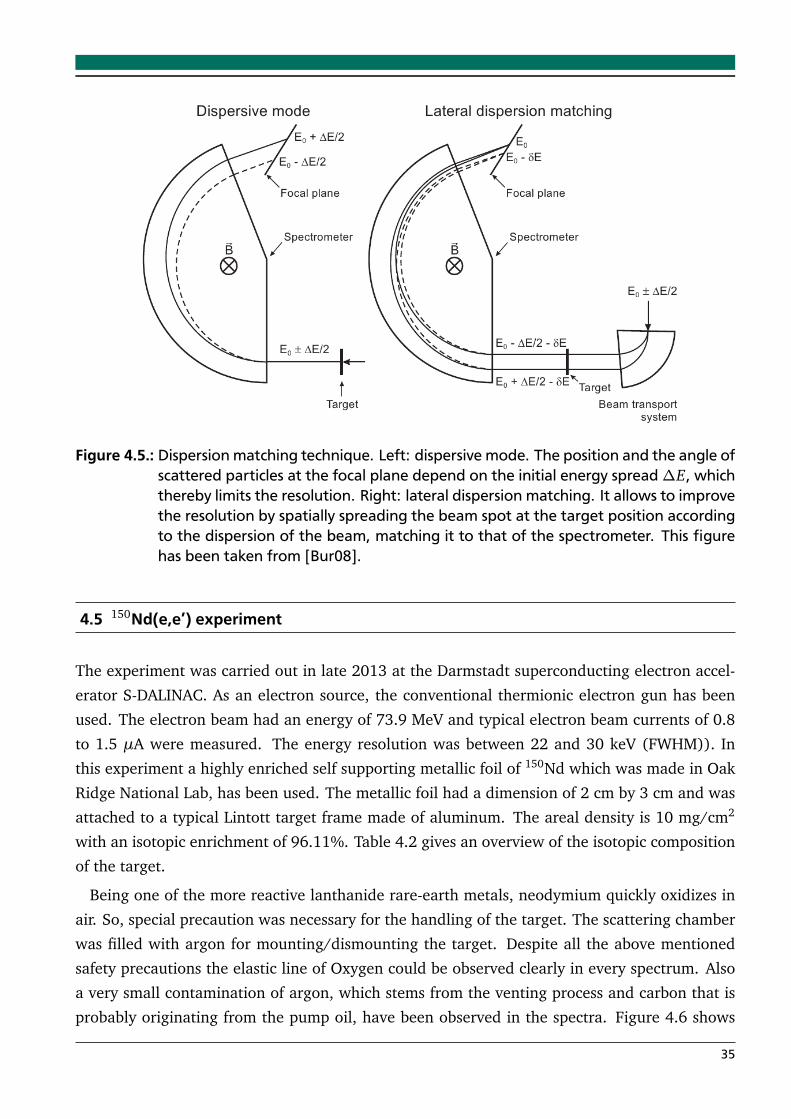
Figure 4.5.: Dispersion matching technique. Left: dispersive mode. The position and the angle ofscattered particles at the focal plane depend on the initial energy spread∆E, whichthereby limits the resolution. Right: lateral dispersion matching. It allows to improvethe resolution by spatially spreading the beam spot at the target position accordingto the dispersion of the beam, matching it to that of the spectrometer. This figurehas been taken from [Bur08].
4.5 150Nd(e,e’) experiment
The experiment was carried out in late 2013 at the Darmstadt superconducting electron accel-
erator S-DALINAC. As an electron source, the conventional thermionic electron gun has been
used. The electron beam had an energy of 73.9 MeV and typical electron beam currents of 0.8
to 1.5 µA were measured. The energy resolution was between 22 and 30 keV (FWHM)). In
this experiment a highly enriched self supporting metallic foil of 150Nd which was made in Oak
Ridge National Lab, has been used. The metallic foil had a dimension of 2 cm by 3 cm and was
attached to a typical Lintott target frame made of aluminum. The areal density is 10 mg/cm2
with an isotopic enrichment of 96.11%. Table 4.2 gives an overview of the isotopic composition
of the target.
Being one of the more reactive lanthanide rare-earth metals, neodymium quickly oxidizes in
air. So, special precaution was necessary for the handling of the target. The scattering chamber
was filled with argon for mounting/dismounting the target. Despite all the above mentioned
safety precautions the elastic line of Oxygen could be observed clearly in every spectrum. Also
a very small contamination of argon, which stems from the venting process and carbon that is
probably originating from the pump oil, have been observed in the spectra. Figure 4.6 shows
35
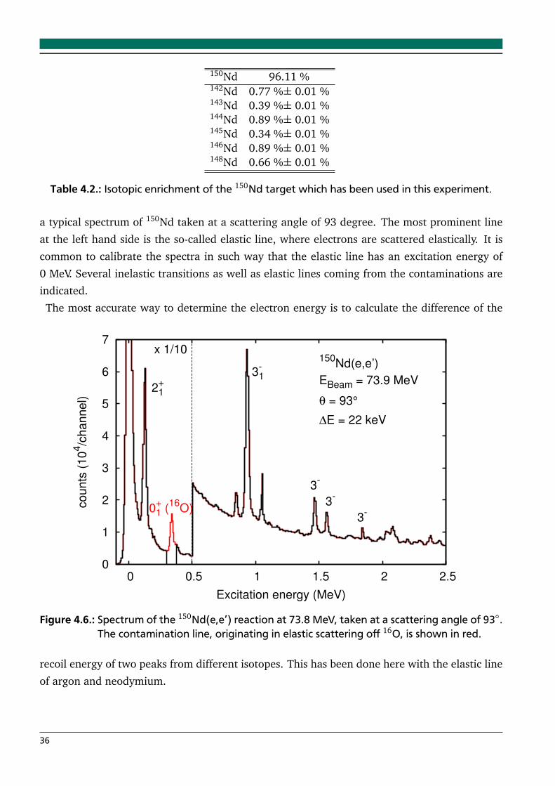
150Nd 96.11 %142Nd 0.77 %± 0.01 %143Nd 0.39 %± 0.01 %144Nd 0.89 %± 0.01 %145Nd 0.34 %± 0.01 %146Nd 0.89 %± 0.01 %148Nd 0.66 %± 0.01 %
Table 4.2.: Isotopic enrichment of the 150Nd target which has been used in this experiment.
a typical spectrum of 150Nd taken at a scattering angle of 93 degree. The most prominent line
at the left hand side is the so-called elastic line, where electrons are scattered elastically. It is
common to calibrate the spectra in such way that the elastic line has an excitation energy of
0 MeV. Several inelastic transitions as well as elastic lines coming from the contaminations are
indicated.
The most accurate way to determine the electron energy is to calculate the difference of the
0
1
2
3
4
5
6
7
0 0.5 1 1.5 2 2.5
counts
(10
4/c
hannel)
Excitation energy (MeV)
150Nd(e,e’)
EBeam = 73.9 MeV
θ = 93°
∆E = 22 keV
x 1/10
21+
31-
3-
3-
3-01
+ (
16O)
Figure 4.6.: Spectrum of the 150Nd(e,e’) reaction at 73.8 MeV, taken at a scattering angle of 93.The contamination line, originating in elastic scattering off 16O, is shown in red.
recoil energy of two peaks from different isotopes. This has been done here with the elastic line
of argon and neodymium.
36
5 Data analysis of the electron scattering data
5.1 Line shapes
For the analysis of the discrete states the line area content Aex pin is determined by adjusting a
model function for the line form to the measured spectrum [Hof02].
y = y0 ·
exp
− ln2 · (x − x0)2/∆x21
x < x0
exp
− ln2 · (x − x0)2/∆x22
x0 < x ≤ x0+η∆x2
A/(B+ x − x0)γ x > x0+η∆x2
(5.1)
withx0 maximum energy,y0 count rate atx0,∆x1,2 half width at half maximum for Ex < x0 and Ex > x0, respectivelyη starting point of the radiative tail in units of ∆x2,γ exponent of the hyperbolic function of the radiative tail.
The parameters A and B result from the condition of the continuous differentiable joining of
the individual functions to the junctures x0 and x0+η∆x2.
The fit of the model functions to the spectral lines has been performed with the program
HDTV [Bra, Bas12]. The parameters σ1,2, η and γ are fixed for a given spectra, and have been
determined by the fit to the dominant elastic line. Then the line positions x0 and line heights y0
of the other peaks are fitted simultaneously. The area content Aex pin is calculated as an integral
of the function used in the parameterization
Aex pin =
x0+k∆x1∫
−∞
y(x)d x , (5.2)
where k is the integral cutoff parameter (by default k = 5).
5.2 Energy calibration of the excitation spectra
For a comprehensive overview over the off-Yrast low-spin excitations it is necessary to measure
the electron scattering spectra up to several MeV. Because of the small momentum acceptance
37
of the spectrometer (only 4%) one needs to perform the measurement at several settings of
the spectrometer magnetic field. Then, it is necessary to make also a calibration measure-
ments for each spectrometer magnetic field setting using other nuclei with known prominent
transitions. The calibration could be performed using a direct correspondence between the
scattered electron energy E′ and a channel number N . One has to take into account also the
electron energy loss in the target. As a result of an ionization of the electrons in the targets
of an effective thickness teff before and after scattering they lose on the average an energy of
∆E [MeV ] = 12× 1.4× teff [g/cm2]. teff is the effective target thickness. For measurements
at the scattering angles θ ≤ 141 the target is set in transmission geometry (perpendicular
to the scattering angle bisector). In this case the electrons have an effective path length
teff = t/cos(θ/2), where t and θ are the target thickness and the scattering angle, respec-
tively. Measurements at angles θ > 141 are only possible in the reflection geometry. Here,
there effective path length of the electrons in the target is teff = t/sin(θ/2).
E′(Ei, Ex ,∆E, M ,θ) =(Ei −∆E)− Ex(1+
Ex2Mc2 )
1+ 2(Ei−∆E)Mc2 sin2 θ
2
−∆E = f (N). (5.3)
If the spectrometer magnetic field is homogeneous, the function f (N) is linear. Thus, one gets
a quadratic equation for Ex . Solving that, one obtains an excitation energy as a function of a
channel number. This calibration is valid only for a given spectrometer magnetic field setting.
The same procedure has to be repeated for other settings.
5.3 Experimental cross sections
The calculation of the experimental cross sections requires the subtraction of the background
and a determination of the area Aex pin of the observed lines. The absolute value of the cross
sections can be calculated from
dσ
dΩ= Aex p
in ·1
∆Ω·
e
I t·
M
ρd xNA, (5.4)
where ∆Ω is the spectrometer solid angle in (sr), I t the accumulated charge in (C), M the mass
number in (g/mol), ρd x the areal density of the target in (g/cm2) and NA the Avogadro number
in (1/mol).
The differential cross section dσ/dΩ for the excitation of a nuclear state can also be extracted
from the measured spectra relative to the elastic cross section
38
(dσ/dΩ)in(dσ/dΩ)el
=Aex p
in
Aex pel
, (5.5)
Since the electron scattering process is purely electromagnetic and the elastic scattering cross
section can be calculated in the framework of Quantum Electrodynamics, one usually deter-
mines the inelastic cross section
dσdΩ
inrelative to the elastic cross section
dσdΩ
el, respectively
in terms of the form factors
|F(θ)|2in|F(θ)|2el
=Ain
Ael, (5.6)
where Ael and Ain are the peak areas corrected for the radiative processes, discussed in the next
chapter. The elastic form factor |F(θ)|2el were calculated with two different phase shift codes
PHASHI [Bäh, Yen54] and DREPHA [Dre, Dre74]. These codes use ground state charge density
distributions for 150Nd which are approximated by three-parameter Fermi distributions. The
parameters were taken from reference [Vri87].
5.3.1 Radiative corrections
Bremsstrahlung leads to a radiative tail in the line shape of electron scattering data. To correct
for that the area under the peak is integrated up to a cutoff limit Ecutoff = x0 +∆E. Electrons
with an energy loss larger than ∆E = 5∆x1 are missed. Therefore, the calculated peak area
Aex pin is corrected by multiplying with correction factors for the radiation effects
Ain = Crad · Aex pin . (5.7)
The total correction Crad includes the Schwinger (δS), bremsstrahlung (δB) and ionization
(δI) correction
Crad = eδB+δS+δI . (5.8)
The Schwinger correction is given by
δS =2α
π
¨
1
2ln
E0
η2∆E
+1
2ln
E′
η∆E
−13
12
×
2 ln
ER
m0c2
− 1
+17
16
«
, (5.9)
39
where ER, E′ and η= 1+ 2 E0Mc2 sin2 θ
2are the recoil energy, the energy of the scattered electrons
and the recoil parameter, respectively.
The bremsstrahlung correction is expressed as
δB =te f f
X0 ln 2
1
2ln
E0
η2∆E
+1
2ln
E′
η∆E
, (5.10)
where X0 is the radiation length
X0 =716.4 M
Z(Z + 1) ln(287 Z−12 )
g
cm2
(5.11)
A detailed description of these factors can be found in [Mo69].
5.3.2 Dead time correction
During times where the data acquisition is busy, no other events can be processed. To calculate
the measurement time and the dead time one uses the expressions
Tmeas[s] =clkdvd
40× 106 · OnTimeArmed= 10−7 · OnTimeArmed (5.12)
Tdead [%] =OnTimeArmed− LifeTimeArmed
OnTimeArmed· 100 (5.13)
clkdvd is a constant, depending on the maximum chosen data rate of the detector system.
The quantities OnTimeArmed and LifeTimeArmed are quantities indicating the time the data
acquisition has been active. Thus, the fitted area under the peak should be corrected on the
following dead time correction factor Cd t
Cd t = (1− Tdead)−1 =
OnTimeArmed
LifeTimeArmed. (5.14)
For calculating the final experimental cross section one has to use this expression for the
corrected peak area
Acorin = Crad · Cd t · A
ex pin . (5.15)
40
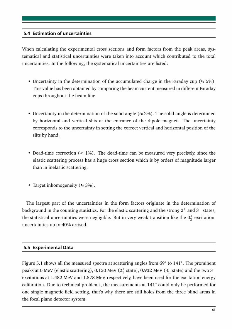
5.4 Estimation of uncertainties
When calculating the experimental cross sections and form factors from the peak areas, sys-
tematical and statistical uncertainties were taken into account which contributed to the total
uncertainties. In the following, the systematical uncertainties are listed:
• Uncertainty in the determination of the accumulated charge in the Faraday cup (≈ 5%).
This value has been obtained by comparing the beam current measured in different Faraday
cups throughout the beam line.
• Uncertainty in the determination of the solid angle (≈ 2%). The solid angle is determined
by horizontal and vertical slits at the entrance of the dipole magnet. The uncertainty
corresponds to the uncertainty in setting the correct vertical and horizontal position of the
slits by hand.
• Dead-time correction (< 1%). The dead-time can be measured very precisely, since the
elastic scattering process has a huge cross section which is by orders of magnitude larger
than in inelastic scattering.
• Target inhomogeneity (≈ 3%).
The largest part of the uncertainties in the form factors originate in the determination of
background in the counting statistics. For the elastic scattering and the strong 2+ and 3− states,
the statistical uncertainties were negligible. But in very weak transition like the 0+2 excitation,
uncertainties up to 40% arrised.
5.5 Experimental Data
Figure 5.1 shows all the measured spectra at scattering angles from 69 to 141. The prominent
peaks at 0 MeV (elastic scattering), 0.130 MeV (2+1 state), 0.932 MeV (3−1 state) and the two 3−
excitations at 1.482 MeV and 1.578 MeV, respectively, have been used for the excitation energy
calibration. Due to technical problems, the measurements at 141 could only be performed for
one single magnetic field setting, that’s why there are still holes from the three blind areas in
the focal plane detector system.
41
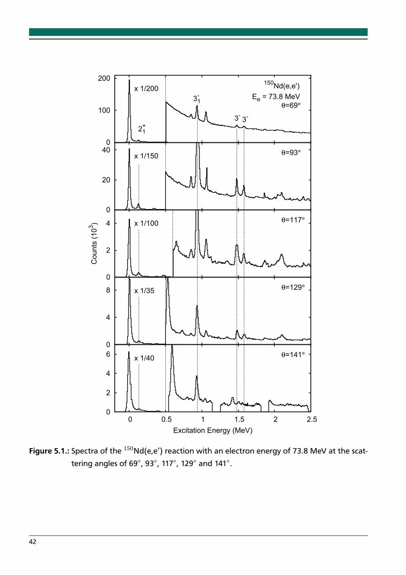
0
2
4
6
0 0.5 1 1.5 2 2.5
Excitation Energy (MeV)
x 1/40 θ=141°
0
4
8 x 1/35 θ=129°
0
2
4
Counts
(10
3) x 1/100 θ=117°
0
20
40x 1/150 θ=93°
0
100
200
21+
31-
3-3
-
150Nd(e,e')
Ee = 73.8 MeV
θ=69°
x 1/200
Figure 5.1.: Spectra of the 150Nd(e,e’) reaction with an electron energy of 73.8 MeV at the scat-tering angles of 69, 93, 117, 129 and 141.
42
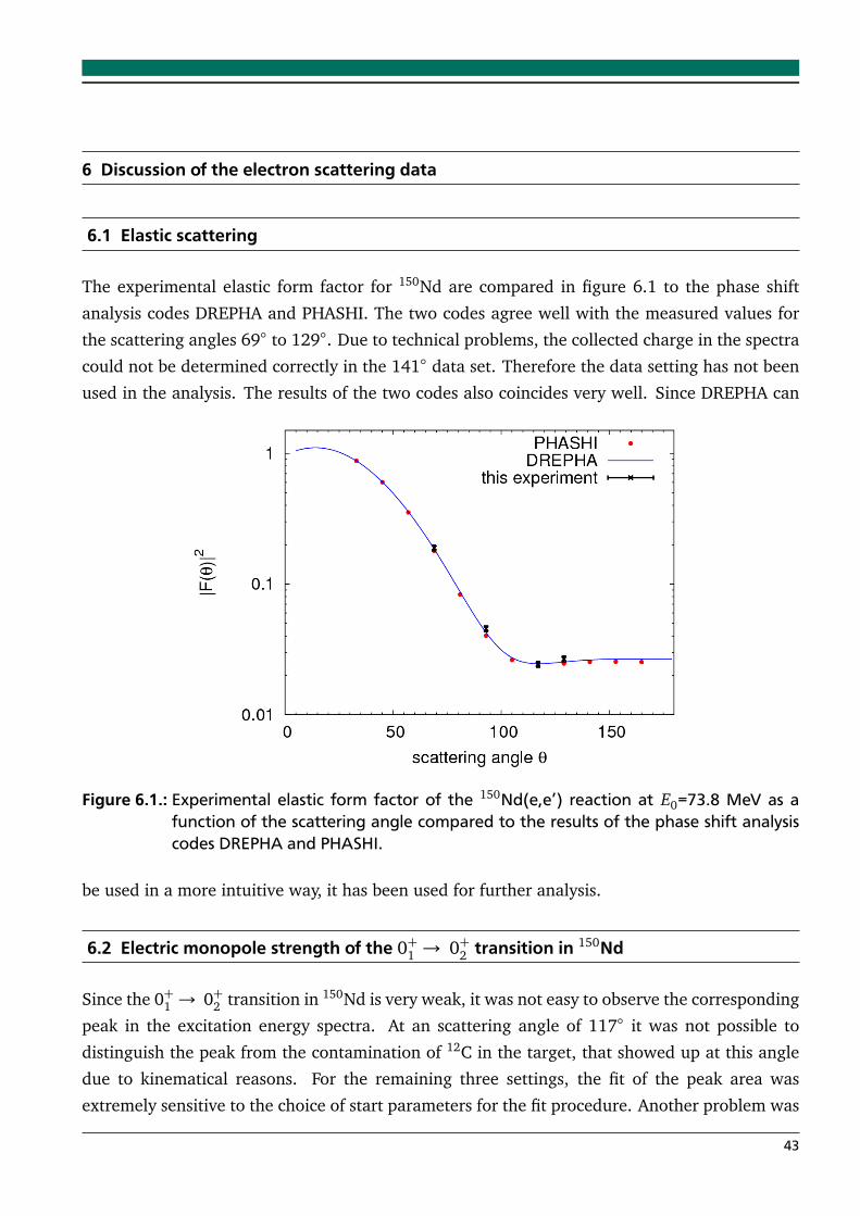
6 Discussion of the electron scattering data
6.1 Elastic scattering
The experimental elastic form factor for 150Nd are compared in figure 6.1 to the phase shift
analysis codes DREPHA and PHASHI. The two codes agree well with the measured values for
the scattering angles 69 to 129. Due to technical problems, the collected charge in the spectra
could not be determined correctly in the 141 data set. Therefore the data setting has not been
used in the analysis. The results of the two codes also coincides very well. Since DREPHA can
Figure 6.1.: Experimental elastic form factor of the 150Nd(e,e’) reaction at E0=73.8 MeV as afunction of the scattering angle compared to the results of the phase shift analysiscodes DREPHA and PHASHI.
be used in a more intuitive way, it has been used for further analysis.
6.2 Electric monopole strength of the 0+1 → 0+2 transition in 150Nd
Since the 0+1 → 0+2 transition in 150Nd is very weak, it was not easy to observe the corresponding
peak in the excitation energy spectra. At an scattering angle of 117 it was not possible to
distinguish the peak from the contamination of 12C in the target, that showed up at this angle
due to kinematical reasons. For the remaining three settings, the fit of the peak area was
extremely sensitive to the choice of start parameters for the fit procedure. Another problem was
43
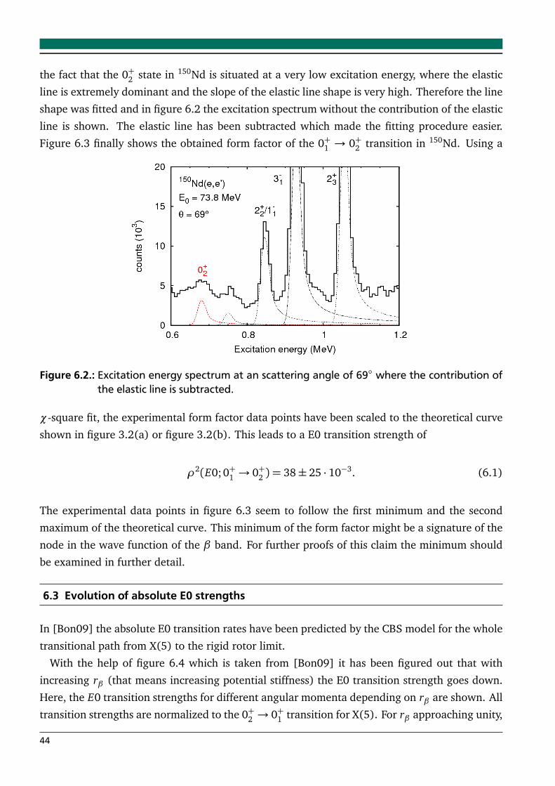
the fact that the 0+2 state in 150Nd is situated at a very low excitation energy, where the elastic
line is extremely dominant and the slope of the elastic line shape is very high. Therefore the line
shape was fitted and in figure 6.2 the excitation spectrum without the contribution of the elastic
line is shown. The elastic line has been subtracted which made the fitting procedure easier.
Figure 6.3 finally shows the obtained form factor of the 0+1 → 0+2 transition in 150Nd. Using a
Figure 6.2.: Excitation energy spectrum at an scattering angle of 69 where the contribution ofthe elastic line is subtracted.
χ-square fit, the experimental form factor data points have been scaled to the theoretical curve
shown in figure 3.2(a) or figure 3.2(b). This leads to a E0 transition strength of
ρ2(E0;0+1 → 0+2 ) = 38± 25 · 10−3. (6.1)
The experimental data points in figure 6.3 seem to follow the first minimum and the second
maximum of the theoretical curve. This minimum of the form factor might be a signature of the
node in the wave function of the β band. For further proofs of this claim the minimum should
be examined in further detail.
6.3 Evolution of absolute E0 strengths
In [Bon09] the absolute E0 transition rates have been predicted by the CBS model for the whole
transitional path from X(5) to the rigid rotor limit.
With the help of figure 6.4 which is taken from [Bon09] it has been figured out that with
increasing rβ (that means increasing potential stiffness) the E0 transition strength goes down.
Here, the E0 transition strengths for different angular momenta depending on rβ are shown. All
transition strengths are normalized to the 0+2 → 0+1 transition for X(5). For rβ approaching unity,
44
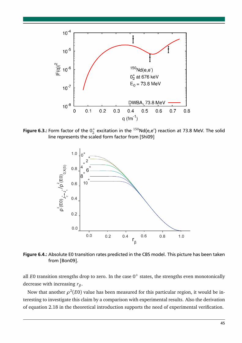
Figure 6.3.: Form factor of the 0+2 excitation in the 150Nd(e,e’) reaction at 73.8 MeV. The solidline represents the scaled form factor from [Shi09]
Figure 6.4.: Absolute E0 transition rates predicted in the CBS model. This picture has been takenfrom [Bon09].
all E0 transition strengths drop to zero. In the case 0+ states, the strengths even monotonically
decrease with increasing rβ .
Now that another ρ2(E0) value has been measured for this particular region, it would be in-
teresting to investigate this claim by a comparison with experimental results. Also the derivation
of equation 2.18 in the theoretical introduction supports the need of experimental verification.
45
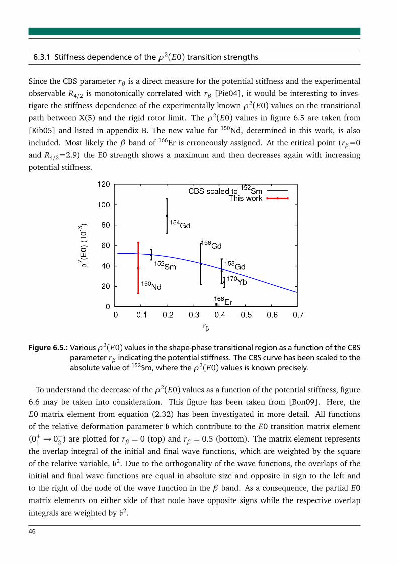
6.3.1 Stiffness dependence of the ρ2(E0) transition strengths
Since the CBS parameter rβ is a direct measure for the potential stiffness and the experimental
observable R4/2 is monotonically correlated with rβ [Pie04], it would be interesting to inves-
tigate the stiffness dependence of the experimentally known ρ2(E0) values on the transitional
path between X(5) and the rigid rotor limit. The ρ2(E0) values in figure 6.5 are taken from
[Kib05] and listed in appendix B. The new value for 150Nd, determined in this work, is also
included. Most likely the β band of 166Er is erroneously assigned. At the critical point (rβ=0
and R4/2=2.9) the E0 strength shows a maximum and then decreases again with increasing
potential stiffness.
Figure 6.5.: Various ρ2(E0) values in the shape-phase transitional region as a function of the CBSparameter rβ indicating the potential stiffness. The CBS curve has been scaled to theabsolute value of 152Sm, where the ρ2(E0) values is known precisely.
To understand the decrease of the ρ2(E0) values as a function of the potential stiffness, figure
6.6 may be taken into consideration. This figure has been taken from [Bon09]. Here, the
E0 matrix element from equation (2.32) has been investigated in more detail. All functions
of the relative deformation parameter b which contribute to the E0 transition matrix element
(0+1 → 0+2 ) are plotted for rβ = 0 (top) and rβ = 0.5 (bottom). The matrix element represents
the overlap integral of the initial and final wave functions, which are weighted by the square
of the relative variable, b2. Due to the orthogonality of the wave functions, the overlaps of the
initial and final wave functions are equal in absolute size and opposite in sign to the left and
to the right of the node of the wave function in the β band. As a consequence, the partial E0
matrix elements on either side of that node have opposite signs while the respective overlap
integrals are weighted by b2.
46
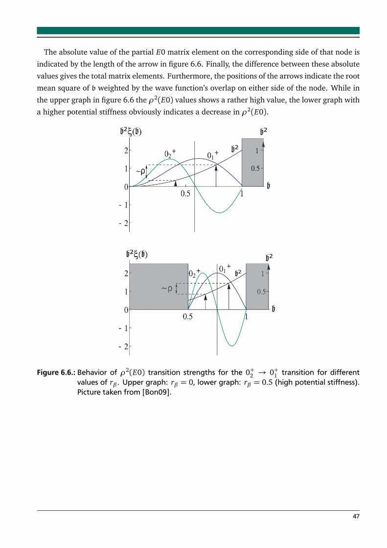
The absolute value of the partial E0 matrix element on the corresponding side of that node is
indicated by the length of the arrow in figure 6.6. Finally, the difference between these absolute
values gives the total matrix elements. Furthermore, the positions of the arrows indicate the root
mean square of b weighted by the wave function’s overlap on either side of the node. While in
the upper graph in figure 6.6 the ρ2(E0) values shows a rather high value, the lower graph with
a higher potential stiffness obviously indicates a decrease in ρ2(E0).
Figure 6.6.: Behavior of ρ2(E0) transition strengths for the 0+2 → 0+1 transition for differentvalues of rβ . Upper graph: rβ = 0, lower graph: rβ = 0.5 (high potential stiffness).Picture taken from [Bon09].
47

7 Comparison of the CBS rotor model with a macroscopic collective mean field
Hamiltonian for 150,152Nd
In this rather theoretical chapter the results of a comparison between the analytical wave func-
tions of the CBS rotor model (see section 2.3) and a collective Hamiltonian based on the rel-
ativistic mean field model (see section 2.4), will be presented. The work has already been
published [Kru11].
7.1 Description of K=0 bands and their centrifugal stretching
Figure 7.1 shows the low lying excitation spectrum of the nucleus 150Nd [Bag76] in compar-
ison to the two models. For the CBS rotor model we have fitted the structural parameter rβto the 4+1 /2
+1 -energy ratio R4/2. For 150Nd we used rβ = 0.078 and for 152Nd rβ = 0.35.
The energy-scale parameter ħh2
2Bβ2M
[see equation (2.27)] has been fitted to the excitation en-
ergies of the 2+1 states and takes the values of 37.9 keV for 150Nd and 30.7 keV for 152Nd.
The effective E2 charges of the first order (∆k = 0)-part of the transition operator T (E2) =3
4πZeR2βM
β/βM
D2µ0 [Pie04] have been scaled to the experimental B(E2;2+1 → 0+1 ) values.
For the calculations we used βM = 0.451 for 150Nd and βM = 0.471 for 152Nd.
For the RMF model we have multiplied the Inglis-Belyaev moments of inertia in equation (2.35)
with a common factor (1 + α) determined in such a way that the calculated energy of the
2+1 state coincides with the experimental value. This is because the well-known fact that the
Inglis-Belyaev formula predicts effective moments of inertia that are considerably smaller than
empirical values. For 150Nd we used α = 0.40 and for 152Nd α = 0.57. The transition strengths
are calculated in the full configuration space using bare charges [Nik09, Li09].
The s=1 ground state band is very well reproduced by the two models. In the microscopic RMF
approach the energies differ only by a few percent compared to the experimental energies. In
the CBS rotor model the deviation is even less than 0.3 % [Dus05]. In the s=2 band, which is
the collective β-band for this nucleus, the rotational structure is very well reproduced in the two
models and the deviations in energy primarily result from a mismatch of the rotational moment
of inertia by up to 25 %. The B(E2) intra- and inter-band transition strengths show a satisfactory
agreement in both models. Note, that both, energies and B(E2) values for the excited k=0 band
in the CBS rotor model, represent model predictions without any further parameter adjustment.
Figure 7.2 shows the same spectra for the nucleus 152Nd [Hel92]. In this case, only few data
is available. Here, the two models show again a nice agreement in the excitation energies and
B(E2) values for the ground state band, as well as for the β-band. One underlying mechanism at
work in the CBS rotor model is the centrifugal stretching of the nucleus which can be classically
49
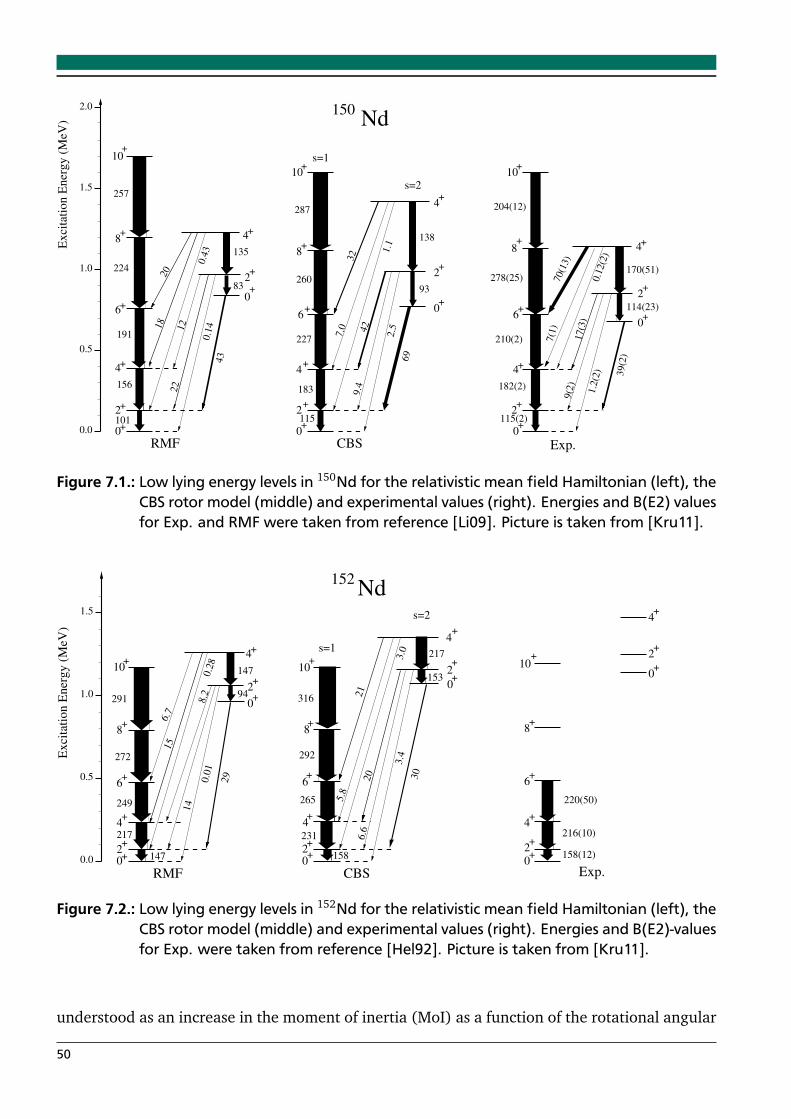
0
2
4+
+
+0
2
4+
+
+
1.0
1.5
2.0
0.5
RMF0.0
Exci
tati
on E
ner
gy (
MeV
)
+
+
+
+
+
+
8
10
6
4
2
0101
156
191
257
224
CBS0
2
4
6
8
10
+
+
+
+
+
+
227
93
138
83
135
69
2.5
9.4
43
2018
0.4
3
22
0.1
4
32 1
.1
7.01
2
42
s=1
s=2
Exp.0
2
4
6
8
10
+
+
+
+
+
+
182(2)
210(2)
204(12)
278(25)
114(23)
170(51)
2+
4+
0+
115(2)
39(2
)
70(1
3)
7(1
)
0.1
2(2
)
17(3
)
9(2
)
1.2
(2)
260
183
287
115
150Nd
Figure 7.1.: Low lying energy levels in 150Nd for the relativistic mean field Hamiltonian (left), theCBS rotor model (middle) and experimental values (right). Energies and B(E2) valuesfor Exp. and RMF were taken from reference [Li09]. Picture is taken from [Kru11].
2
1.0
1.5
0.5
RMF0.0 +0
CBS0+
3.4
+
4+
6+
8+
10+
4+
2+
0+
147
217
249
272
29194
147
29
0.0
1
14
8.2
0.2
8
15
6.7
2+
4+
6+
8+
10+
4
2+
+
0+
216(10)
220(50)
0+ 158(12)
Exp.
Ex
cita
tio
n E
ner
gy
(M
eV)
1582+
6.6
20
231
4+
6+
5.8
8+
s=1
10+
s=2
3.0
21
+
+2
0
+4
30
153
217
316
292
265
Nd152
Figure 7.2.: Low lying energy levels in 152Nd for the relativistic mean field Hamiltonian (left), theCBS rotor model (middle) and experimental values (right). Energies and B(E2)-valuesfor Exp. were taken from reference [Hel92]. Picture is taken from [Kru11].
understood as an increase in the moment of inertia (MoI) as a function of the rotational angular
50
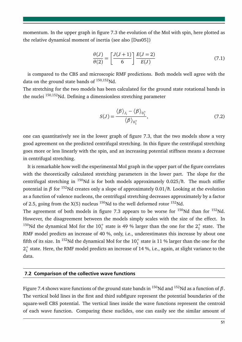
momentum. In the upper graph in figure 7.3 the evolution of the MoI with spin, here plotted as
the relative dynamical moment of inertia (see also [Dus05])
θ(J)θ(2)
=
J(J + 1)6
E(J = 2)E(J)
(7.1)
is compared to the CBS and microscopic RMF predictions. Both models well agree with the
data on the ground state bands of 150,152Nd.
The stretching for the two models has been calculated for the ground state rotational bands in
the nuclei 150,152Nd. Defining a dimensionless stretching parameter
S(J) =
β
Ji−
β
0+1
β
0+1
, (7.2)
one can quantitatively see in the lower graph of figure 7.3, that the two models show a very
good agreement on the predicted centrifugal stretching. In this figure the centrifugal stretching
goes more or less linearly with the spin, and an increasing potential stiffness means a decrease
in centrifugal stretching.
It is remarkable how well the experimental MoI graph in the upper part of the figure correlates
with the theoretically calculated stretching parameters in the lower part. The slope for the
centrifugal stretching in 150Nd is for both models approximately 0.025/ħh. The much stiffer
potential in β for 152Nd creates only a slope of approximately 0.01/ħh. Looking at the evolution
as a function of valence nucleons, the centrifugal stretching decreases approximately by a factor
of 2.5, going from the X(5) nucleus 150Nd to the well deformed rotor 152Nd.
The agreement of both models in figure 7.3 appears to be worse for 150Nd than for 152Nd.
However, the disagreement between the models simply scales with the size of the effect. In150Nd the dynamical MoI for the 10+1 state is 49 % larger than the one for the 2+1 state. The
RMF model predicts an increase of 40 %, only, i.e., underestimates this increase by about one
fifth of its size. In 152Nd the dynamical MoI for the 10+1 state is 11 % larger than the one for the
2+1 state. Here, the RMF model predicts an increase of 14 %, i.e., again, at slight variance to the
data.
7.2 Comparison of the collective wave functions
Figure 7.4 shows wave functions of the ground state bands in 150Nd and 152Nd as a function of β .
The vertical bold lines in the first and third subfigure represent the potential boundaries of the
square-well CBS potential. The vertical lines inside the wave functions represent the centroid
of each wave function. Comparing these nuclides, one can easily see the similar amount of
51
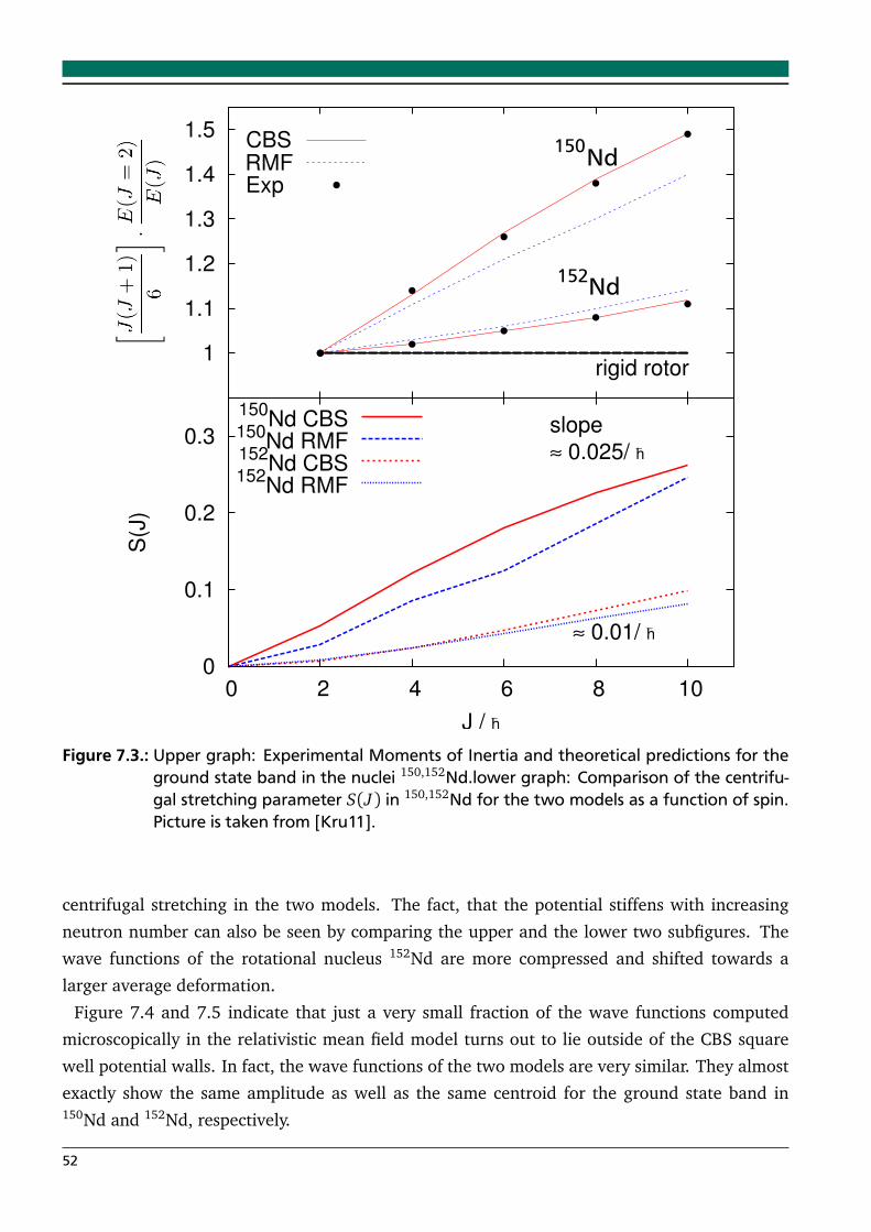
Figure 7.3.: Upper graph: Experimental Moments of Inertia and theoretical predictions for theground state band in the nuclei 150,152Nd.lower graph: Comparison of the centrifu-gal stretching parameter S(J) in 150,152Nd for the two models as a function of spin.Picture is taken from [Kru11].
centrifugal stretching in the two models. The fact, that the potential stiffens with increasing
neutron number can also be seen by comparing the upper and the lower two subfigures. The
wave functions of the rotational nucleus 152Nd are more compressed and shifted towards a
larger average deformation.
Figure 7.4 and 7.5 indicate that just a very small fraction of the wave functions computed
microscopically in the relativistic mean field model turns out to lie outside of the CBS square
well potential walls. In fact, the wave functions of the two models are very similar. They almost
exactly show the same amplitude as well as the same centroid for the ground state band in150Nd and 152Nd, respectively.
52
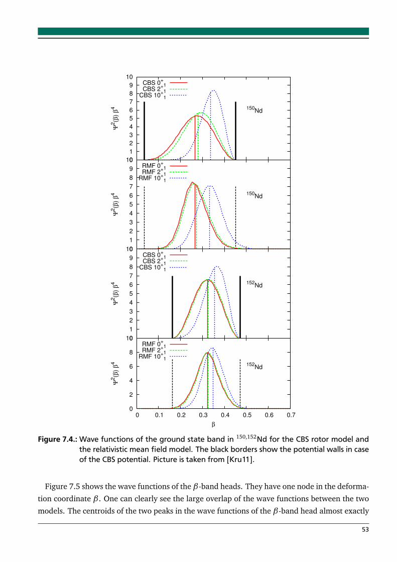
0
2
4
6
8
10
0 0.1 0.2 0.3 0.4 0.5 0.6 0.7
Ψ2(β
) β
4
β
152Nd
RMF 0+
1RMF 2
+1
RMF 10+
1
0
1
2
3
4
5
6
7
8
9
10
Ψ2(β
) β
4 152Nd
CBS 0+
1CBS 2
+1
CBS 10+
1
0
1
2
3
4
5
6
7
8
9
10
Ψ2(β
) β
4 150Nd
RMF 0+
1RMF 2
+1
RMF 10+
1
0
1
2
3
4
5
6
7
8
9
10
Ψ2(β
) β
4 150Nd
CBS 0+
1CBS 2
+1
CBS 10+
1
Figure 7.4.: Wave functions of the ground state band in 150,152Nd for the CBS rotor model andthe relativistic mean field model. The black borders show the potential walls in caseof the CBS potential. Picture is taken from [Kru11].
Figure 7.5 shows the wave functions of the β-band heads. They have one node in the deforma-
tion coordinate β . One can clearly see the large overlap of the wave functions between the two
models. The centroids of the two peaks in the wave functions of the β-band head almost exactly
53
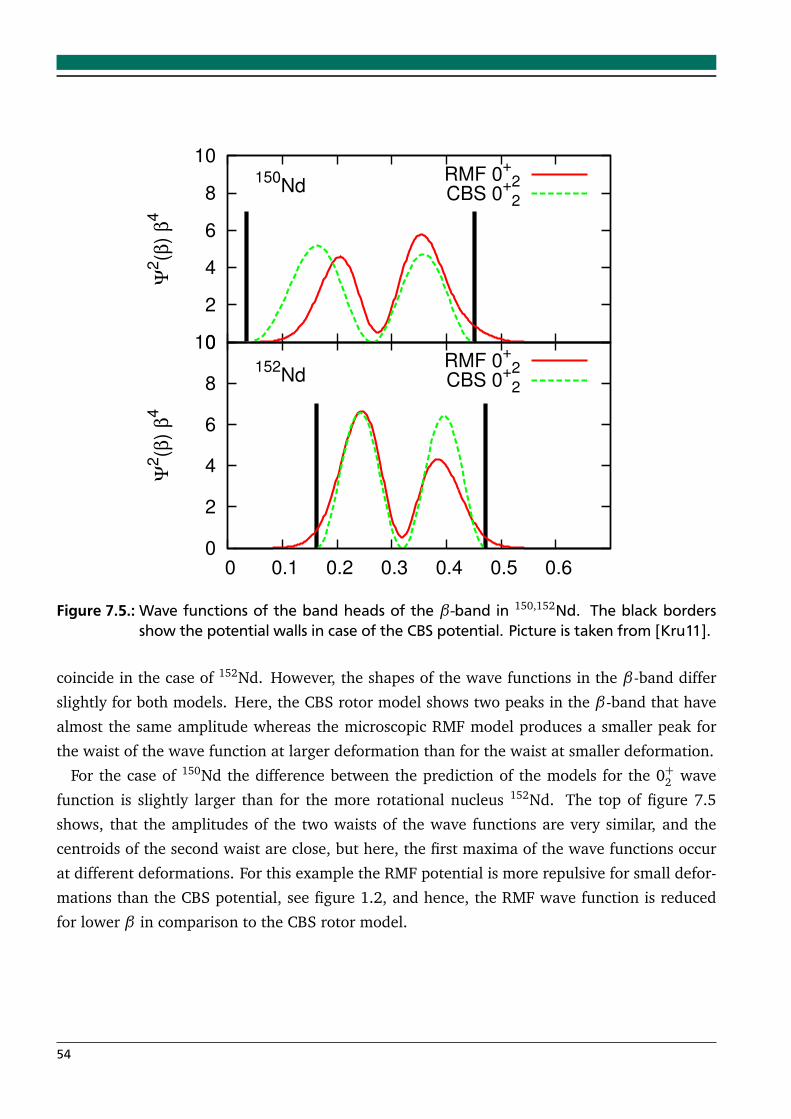
0
2
4
6
8
10
0 0.1 0.2 0.3 0.4 0.5 0.6
Ψ2(β
) β
4
β
152Nd
RMF 0+
2CBS 0
+2
0
2
4
6
8
10Ψ
2(β
) β
4
150Nd
RMF 0+
2CBS 0
+2
Figure 7.5.: Wave functions of the band heads of the β -band in 150,152Nd. The black bordersshow the potential walls in case of the CBS potential. Picture is taken from [Kru11].
coincide in the case of 152Nd. However, the shapes of the wave functions in the β-band differ
slightly for both models. Here, the CBS rotor model shows two peaks in the β-band that have
almost the same amplitude whereas the microscopic RMF model produces a smaller peak for
the waist of the wave function at larger deformation than for the waist at smaller deformation.
For the case of 150Nd the difference between the prediction of the models for the 0+2 wave
function is slightly larger than for the more rotational nucleus 152Nd. The top of figure 7.5
shows, that the amplitudes of the two waists of the wave functions are very similar, and the
centroids of the second waist are close, but here, the first maxima of the wave functions occur
at different deformations. For this example the RMF potential is more repulsive for small defor-
mations than the CBS potential, see figure 1.2, and hence, the RMF wave function is reduced
for lower β in comparison to the CBS rotor model.
54
8 Conclusion and Outlook
Electron scattering experiments at the S-DALINAC in Darmstadt have been performed in order
to extract the electric monopole transition strength ρ2(E0; 0+1 → 0+2 ) for the transitional nucleus150Nd. The experimental form factor of this transition has been scaled to a macroscopic model
prediction so that in a model-dependent analysis the value of ρ2(E0;0+1 → 0+2 ) = 38±25 ·10−3
was obtained. The experimentally obtained form factor follows the theoretical predictions, e.g.
the first minimum of the form factor which might be a signature for the node in the wave
function of the β band, has been seen. This needs further evaluation in terms of a very precise
determination of the form factor. Therefore a much better energy resolution and more data
points in the particular momentum transfer range is required.
Since the experimental uncertainties are still rather high, due to the very low cross section of
this particular state, it is planned to continue this experiment at lower momentum transfer by
using electron energies of 35 MeV to 40 MeV. Reducing the electron energy by a factor of two,
enhances the absolute energy resolution of the spectrometer by the same amount.
Once, this experimental method is established, it will be used to measure the ρ2(E0; 0+1 →0+2 ) for other nuclei in the vicinity of the shape phase transitional point. A good candidate
to start with, would be 152Sm because of the already known ρ2(E0;0+1 → 0+2 ). Also 154Sm is
an interesting option, where the ρ2(E0;0+1 → 0+2 ) could not yet be determined and 154,156Gd,
where the value is known with very large uncertainties.
Since the relativistic mean field model gives predictions about the evolution of the
ρ2(E0; 0+1 → 0+2 ) values, it would be very interesting to have also predictions for transition
densities from this model. First considerations in terms of utilizing the generator coordinate
method have been done already [Vre] and results will be available in the near future.
Furthermore, a comparison between the analytical wave functions of the CBS rotor model and
a microscopic Hamiltonian based on the relativistic mean field model has been performed for
the low lying states in the ground-state band and β-band of the nuclei. A remarkable similarity
of the two models in energies, intra- and inter-band B(E2)-values and centrifugal stretching
has been observed. In particular, the ansatz in the CBS model of an outer potential wall that
stays almost constant with a varying number of valence neutrons and an inner wall that shifts
to higher deformations has been microscopically justified for the given example of the isotopes150,152Nd near the shape phase transitional point. In both compared models, the position of
the outer potential wall seems to be almost independent of a transition from a spherical to an
axially symmetric shape of the nucleus while the change in structure as a function of nucleon
number is dominated by the change of the potential at small deformation.
55

Very recently a derivation for the transition density for the 2+1 state (Ex = 130.21 keV) which
is a member of the ground state rotational band, became available [Jolb]. It would be very
interesting to compare the theoretical form factor with the experimentally obtained form factor
from this experiment.
56

Part II.Low-energy dipole strengthin 154Sm
57

9 Introduction
Many-body fermionic quantum systems like the atomic nucleus provide a huge variety of col-
lective and non-collective phenomena. A good way to test the electric and magnetic response
of such quantum systems is to excite them with electromagnetic or hadronic probes and inves-
tigate their behavior. In nuclei, these collective excitations can be classified by the transfer of
angular momentum (∆L), spin (∆S) and isospin (∆T) [Har01]. While monopole (∆L = 0),
dipole (∆L = 1) and quadrupole (∆L = 2) modes show a compact structure as a function of
excitation energy, resonances with higher ∆L are distributed over much larger excitation en-
ergy regions [Har01, Spe81]. Concerning the isospin degree of freedom, the resonances can be
classified in either isoscalar (∆T = 0) modes, where neutrons and protons move in phase, or
isovector (∆T = 1) modes, where neutrons and protons oscillate out of phase. Similar to the
oscillation in the isospin space, oscillation in spin space may occur when nucleons with spin up
and spin down are excited either in phase (∆S = 0) or out of phase (∆S = 1). The latter class
of excitations is referred to as spinflip excitation.
9.1 Electric Resonances
The investigation of the electric dipole response in nuclei has been started many years ago with
the discovery of the so-called giant dipole resonance (GDR) in 1947 by Baldwin and Klaiber
[Bal47]. Since then extensive studies in different areas of the nuclear chart have been per-
formed with many probes. Today an almost clear picture of the electric dipole response has
been established. Electric dipole excitations can be divided into three groups which can be seen
in figure 9.1. The upper panel shows the case of spherical nuclei, whereas in the lower panel the
case of deformed nuclei is shown: The low-lying two-phonon state, the pygmy dipole-resonance
(PDR) and the giant dipole resonance (GDR).
At low excitations (below 5 MeV) in spherical nuclei, a strong isolated electric dipole excitation
occurs, which is interpreted as a member of a quintuplett of states (Jπ = 1−, ..., 5−). It originates
in the coupling of
2+⊗ 3−
1− [And01]. The term phonon describes in this context low-energy
collective surface vibrations of the nucleus. For deformed nuclei, this isolated excitation even-
tually shows fragmentation [Zil91]. Above the neutron separation threshold Sn, the isovector
giant dipole resonance (IVGDR or GDR) is situated, exhausting the major part of the electric
dipole strength [Har01]. It appears as a broad structure typically in the excitation energy range
between 10 and 20 MeV. In the hydrodynamical model, the GDR is explained as a collective
59
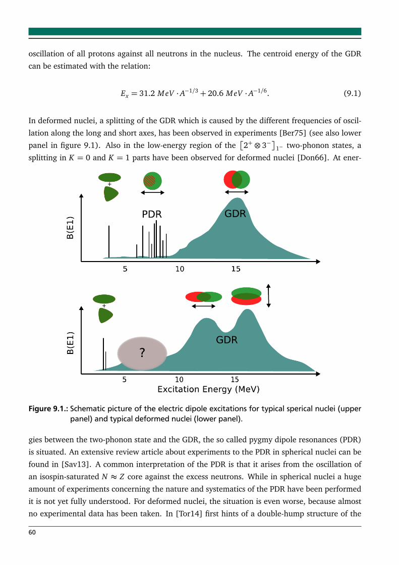
oscillation of all protons against all neutrons in the nucleus. The centroid energy of the GDR
can be estimated with the relation:
Ex = 31.2 MeV · A−1/3+ 20.6 MeV · A−1/6. (9.1)
In deformed nuclei, a splitting of the GDR which is caused by the different frequencies of oscil-
lation along the long and short axes, has been observed in experiments [Ber75] (see also lower
panel in figure 9.1). Also in the low-energy region of the
2+⊗ 3−
1− two-phonon states, a
splitting in K = 0 and K = 1 parts have been observed for deformed nuclei [Don66]. At ener-
Figure 9.1.: Schematic picture of the electric dipole excitations for typical sperical nuclei (upperpanel) and typical deformed nuclei (lower panel).
gies between the two-phonon state and the GDR, the so called pygmy dipole resonances (PDR)
is situated. An extensive review article about experiments to the PDR in spherical nuclei can be
found in [Sav13]. A common interpretation of the PDR is that it arises from the oscillation of
an isospin-saturated N ≈ Z core against the excess neutrons. While in spherical nuclei a huge
amount of experiments concerning the nature and systematics of the PDR have been performed
it is not yet fully understood. For deformed nuclei, the situation is even worse, because almost
no experimental data has been taken. In [Tor14] first hints of a double-hump structure of the
60
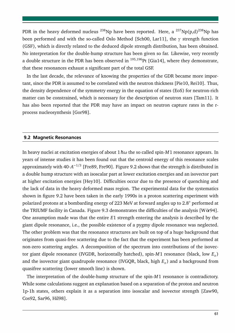
PDR in the heavy deformed nucleus 238Np have been reported. Here, a 237Np(p,d)238Np has
been performed and with the so-called Oslo Method [Sch00, Lar11], the γ strength function
(GSF), which is directly related to the deduced dipole strength distribution, has been obtained.
No interpretation for the double-hump structure has been given so far. Likewise, very recently
a double structure in the PDR has been observed in 195,196Pt [Gia14], where they demonstrate,
that these resonances exhaust a significant part of the total GSF.
In the last decade, the relevance of knowing the properties of the GDR became more impor-
tant, since the PDR is assumed to be correlated with the neutron thickness [Pie10, Rei10]. Thus,
the density dependence of the symmetry energy in the equation of states (EoS) for neutron-rich
matter can be constrained, which is necessary for the description of neutron stars [Tam11]. It
has also been reported that the PDR may have an impact on neutron capture rates in the r-
process nucleosynthesis [Gor98].
9.2 Magnetic Resonances
In heavy nuclei at excitation energies of about 1ħhω the so called spin-M1 resonance appears. In
years of intense studies it has been found out that the centroid energy of this resonance scales
approximately with 40·A−1/3 [Fre89, Fre90]. Figure 9.2 shows that the strength is distributed in
a double hump structure with an isoscalar part at lower excitation energies and an isovector part
at higher excitation energies [Hey10]. Difficulties occur due to the presence of quenching and
the lack of data in the heavy deformed mass region. The experimental data for the systematics
shown in figure 9.2 have been taken in the early 1990s in a proton scattering experiment with
polarized protons at a bombarding energy of 223 MeV at forward angles up to 2.8 performed at
the TRIUMF facility in Canada. Figure 9.3 demonstrates the difficulties of the analysis [Wör94].
One assumption made was that the entire E1 strength entering the analysis is described by the
giant dipole resonance, i.e., the possible existence of a pygmy dipole resonance was neglected.
The other problem was that the resonance structures are built on top of a huge background that
originates from quasi-free scattering due to the fact that the experiment has been performed at
non-zero scattering angles. A decomposition of the spectrum into contributions of the isovec-
tor giant dipole resonance (IVGDR, horizontally hatched), spin-M1 resonance (black, low Ex)
and the isovector giant quadrupole resonance (IVGQR, black, high Ex) and a background from
quasifree scattering (lower smooth line) is shown.
The interpretation of the double-hump structure of the spin-M1 resonance is contradictory.
While some calculations suggest an explanation based on a separation of the proton and neutron
1p-1h states, others explain it as a separation into isoscalar and isovector strength [Zaw90,
Cos92, Sar96, Hil98].
61
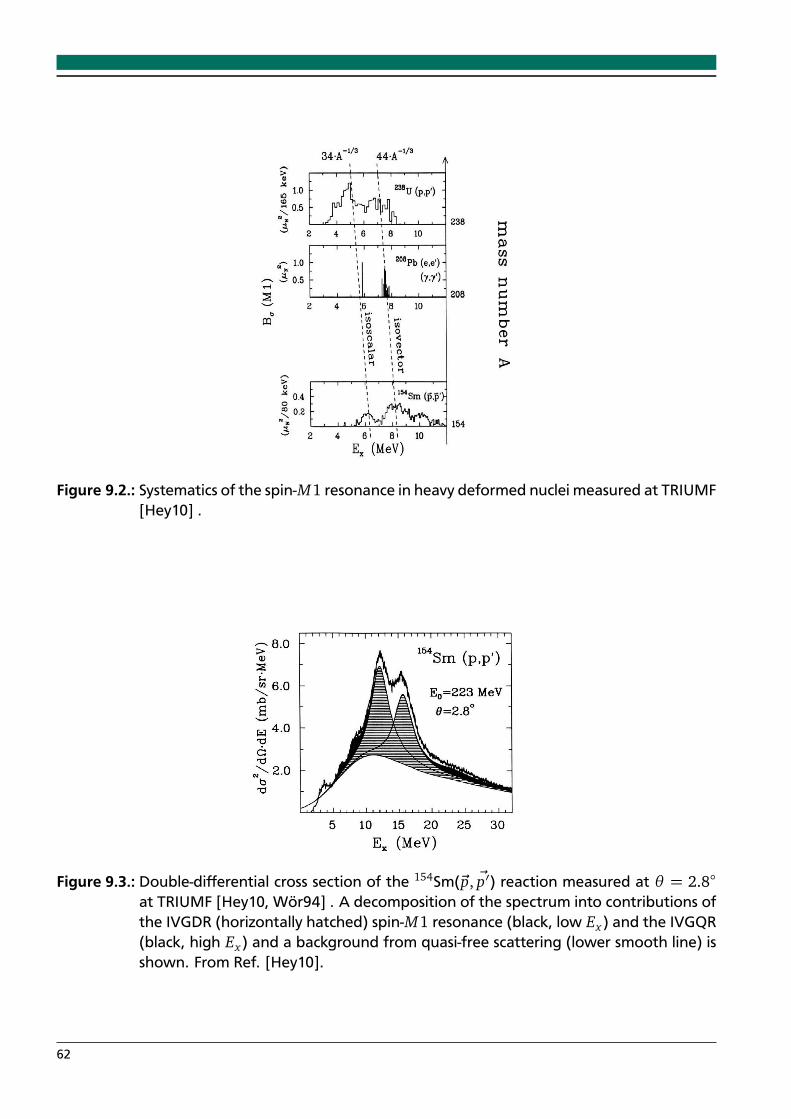
Figure 9.2.: Systematics of the spin-M1 resonance in heavy deformed nuclei measured at TRIUMF[Hey10] .
Figure 9.3.: Double-differential cross section of the 154Sm(~p, ~p′) reaction measured at θ = 2.8
at TRIUMF [Hey10, Wör94] . A decomposition of the spectrum into contributions ofthe IVGDR (horizontally hatched) spin-M1 resonance (black, low Ex ) and the IVGQR(black, high Ex ) and a background from quasi-free scattering (lower smooth line) isshown. From Ref. [Hey10].
62
9.3 Separation of E1 and M1: New experimental approaches
Recently the method of polarized proton scattering at exactly 0 has become available and this
provides a new tool to investigate this intriguing physics with a clearer view. At the Research
Center for Nuclear Research (RCNP) in Osaka one is able to perform polarized proton scattering
at 0 at an intermediate proton energy of 300 MeV. This is optimal for spin-isospin excitations
as the central term of the nucleon-nucleon cross section shows a minimum. Combined with a
very good energy resolution of 25 keV it is possible to do two independent experiments. At first
a separation of E1 and M1 contributions to the cross section can be done by comparing the
experimentally extracted angular distributions. In addition a spinflip/non-spinflip separation of
the cross section can be performed with the method of polarization transfer observables. As a
reference case of a heavy nucleus these types of analyses have been performed for the nucleus208Pb and they show good agreement [Pol11, Tam11, Pol12]. Also in a more recent study in the
nucleus 96Mo [Mar13] the two methods have shown excellent agreement.
9.4 Outline
Within this work a high resolution polarized proton scattering experiment on the heavy de-
formed nucleus 154Sm has been performed at the RCNP in Osaka, Japan. The purpose was the
investigation of the pygmy dipole resonance and the spin-M1 resonance at very forward angles
including 0. Part II of this thesis is structured in the following way. In section 10 the theoreti-
cal background for the polarized proton scattering experiment is introduced. The experimental
proton scattering facility of the RCNP and the experimental setup is shown in section 11. The
many steps of the data analysis procedure are explained in section 12, while the results are
discussed in section 12.3. Part II closes also with a summary and an outlook for the future.
63

10 Theoretical background for polarized proton scattering at 0
In this chapter the theoretical aspects concerning the scattering of (polarized) protons off a
nucleus will be discussed. First of all the projectile-target interaction will be explained in details.
Furthermore the distortion that the projectile wave functions experience by passing the charged
distribution of the nucleus will be explained and since for the strong interaction up to now no
complete picture has been established, information on effective nucleon-nucleon interactions
will be given.
10.1 Inelastic proton scattering
During the scattering process, where the singly charged protons interact with the nucleus, the
electromagnetic Coulomb force causes various kinds of electromagnetic transitions. At extreme
forward angles the dominant transitions are electric and magnetic dipole excitations. Besides
that the target and the projectiles also interact via the nuclear force that may trigger spinflip
transitions.
If energy of the projectile is well below the Coulomb barrier
UCoulomb =1
4πε0
Z1Z2e2
r(10.1)
only Coulomb interaction occurs. Here, ε0 is the dielectric constant, Z1 and Z2 are the atomic
numbers of the target and the projectile, respectively, and r denotes the interaction radius. If
the projectile energy is higher than the Coulomb barrier, both types of interaction take place in
a coherent way.
10.2 Lippmann-Schwinger equation
When solving the quantum mechanical problem of inelastic proton scattering at a nucleus, the
first thing to start with is the time-independent Schrödinger equation (the formalism is mainly
taken from the references [Pol11, Amo00, Sat83, Lip50]):
(H0+ V )ψ= Eψ (10.2)
65
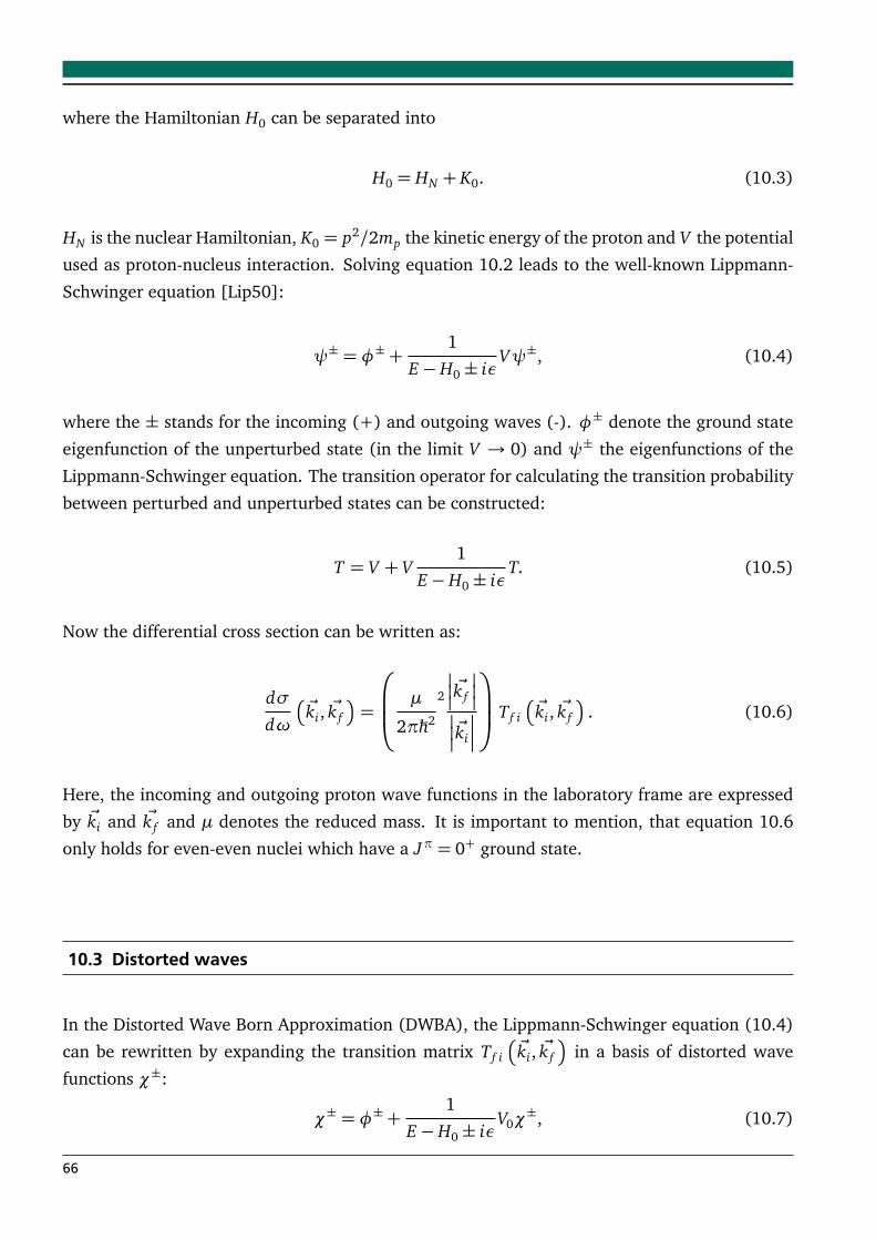
where the Hamiltonian H0 can be separated into
H0 = HN + K0. (10.3)
HN is the nuclear Hamiltonian, K0 = p2/2mp the kinetic energy of the proton and V the potential
used as proton-nucleus interaction. Solving equation 10.2 leads to the well-known Lippmann-
Schwinger equation [Lip50]:
ψ± = φ±+1
E −H0± iεVψ±, (10.4)
where the ± stands for the incoming (+) and outgoing waves (-). φ± denote the ground state
eigenfunction of the unperturbed state (in the limit V → 0) and ψ± the eigenfunctions of the
Lippmann-Schwinger equation. The transition operator for calculating the transition probability
between perturbed and unperturbed states can be constructed:
T = V + V1
E −H0± iεT. (10.5)
Now the differential cross section can be written as:
dσ
dω
~ki, ~k f
=
µ
2πħh2
2
~k f
~ki
T f i
~ki, ~k f
. (10.6)
Here, the incoming and outgoing proton wave functions in the laboratory frame are expressed
by ~ki and ~k f and µ denotes the reduced mass. It is important to mention, that equation 10.6
only holds for even-even nuclei which have a Jπ = 0+ ground state.
10.3 Distorted waves
In the Distorted Wave Born Approximation (DWBA), the Lippmann-Schwinger equation (10.4)
can be rewritten by expanding the transition matrix T f i
~ki, ~k f
in a basis of distorted wave
functions χ±:
χ± = φ±+1
E −H0± iεV0χ
±, (10.7)
66
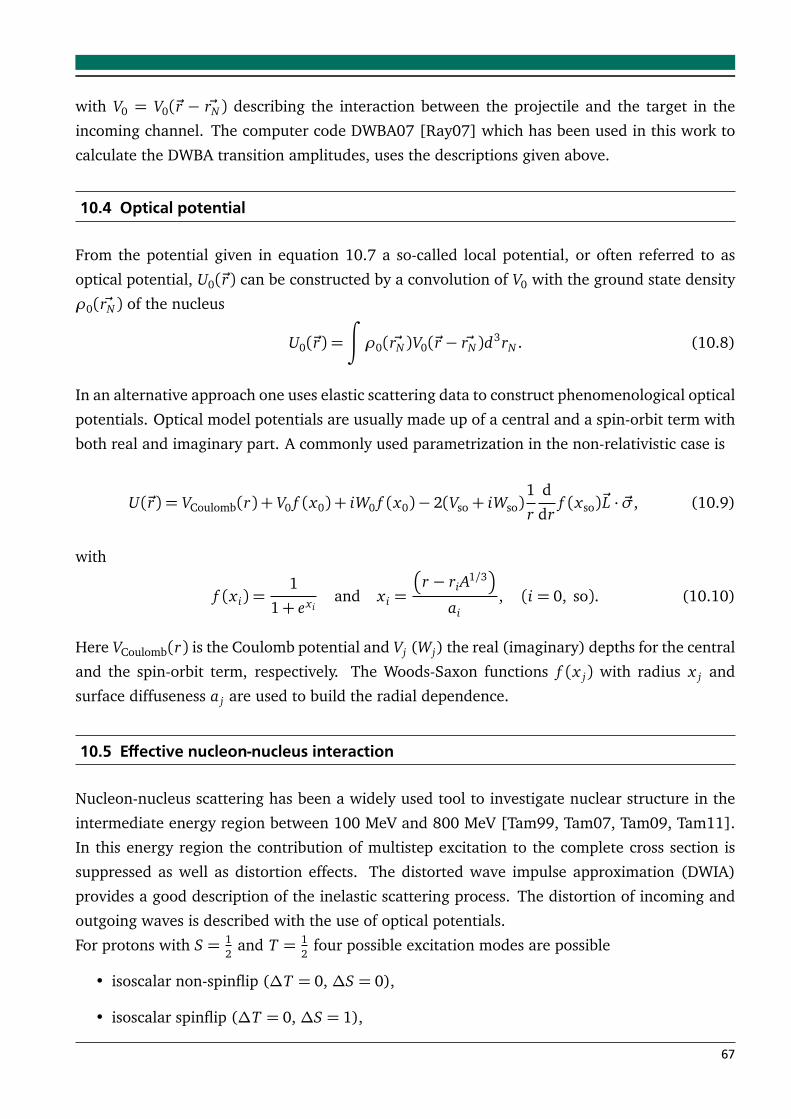
with V0 = V0(~r − ~rN ) describing the interaction between the projectile and the target in the
incoming channel. The computer code DWBA07 [Ray07] which has been used in this work to
calculate the DWBA transition amplitudes, uses the descriptions given above.
10.4 Optical potential
From the potential given in equation 10.7 a so-called local potential, or often referred to as
optical potential, U0(~r) can be constructed by a convolution of V0 with the ground state density
ρ0( ~rN ) of the nucleus
U0(~r) =
∫
ρ0( ~rN )V0(~r − ~rN )d3rN . (10.8)
In an alternative approach one uses elastic scattering data to construct phenomenological optical
potentials. Optical model potentials are usually made up of a central and a spin-orbit term with
both real and imaginary part. A commonly used parametrization in the non-relativistic case is
U(~r) = VCoulomb(r) + V0 f (x0) + iW0 f (x0)− 2(Vso+ iWso)1
r
d
drf (xso)~L · ~σ, (10.9)
with
f (x i) =1
1+ exiand x i =
r − riA1/3
ai, (i = 0, so). (10.10)
Here VCoulomb(r) is the Coulomb potential and Vj (Wj) the real (imaginary) depths for the central
and the spin-orbit term, respectively. The Woods-Saxon functions f (x j) with radius x j and
surface diffuseness a j are used to build the radial dependence.
10.5 Effective nucleon-nucleus interaction
Nucleon-nucleus scattering has been a widely used tool to investigate nuclear structure in the
intermediate energy region between 100 MeV and 800 MeV [Tam99, Tam07, Tam09, Tam11].
In this energy region the contribution of multistep excitation to the complete cross section is
suppressed as well as distortion effects. The distorted wave impulse approximation (DWIA)
provides a good description of the inelastic scattering process. The distortion of incoming and
outgoing waves is described with the use of optical potentials.
For protons with S = 12
and T = 12
four possible excitation modes are possible
• isoscalar non-spinflip (∆T = 0, ∆S = 0),
• isoscalar spinflip (∆T = 0, ∆S = 1),
67
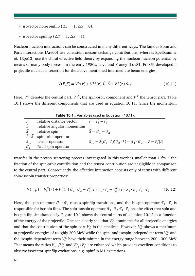
• isovector non-spinflip (∆T = 1, ∆S = 0),
• isovector spinflip (∆T = 1, ∆S = 1).
Nucleon-nucleon interactions can be constructed in many different ways. The famous Bonn and
Paris interactions [Are00] use consistent meson-exchange contributions, whereas Epelbaum et
al. [Epe13] use the chiral effective field theory by expanding the nucleon-nucleon potential by
means of many-body forces. In the early 1980s, Love and Franey [Lov81, Fra85] developed a
projectile-nucleus interaction for the above mentioned intermediate beam energies:
V (~r,~p) = V C(r) + V LS(r) ~L · ~S+ V T (r) S12. (10.11)
Here, V C denotes the central part, V LS, the spin-orbit component and V T the tensor part. Table
10.1 shows the different components that are used in equation 10.11. Since the momentum
Table 10.1.: Variables used in Equation (10.11).~r relative distance vector ~r = ~r1− ~r2~L relative angular momentum~S relative spin ~S = ~σ1+ ~σ2~L · ~S spin-orbit operatorS12 tensor operator S12 = 3(~σ1 · r)(~σ2 · r)− ~σ1 · ~σ2, r = ~r/|~r|~σi Pauli spin operator
transfer in the proton scattering process investigated in this work is smaller than 1 fm−1 the
fraction of the spin-orbit contribution and the tensor contribution are negligible in comparison
to the central part. Consequently, the effective interaction consists only of terms with different
spin-isospin transfer properties:
V (~r,~p) = V C0 (r) + V C
σ (r) ~σ1 · ~σ2+ V Cτ (r) ~τ1 · ~τ2+ V C
στ(r) ~σ1 · ~σ2 ~τ1 · ~τ2. (10.12)
Here, the spin operator ~σ1 · ~σ2 causes spinflip transitions, and the isospin operator ~τ1 · ~τ2 is
responsible for isospin flips. The spin-isospin operator ~σ1 · ~σ2 ~τ1 · ~τ2 has the effect that spin and
isospin flip simultaneously. Figure 10.1 shows the central parts of equation 10.12 as a function
of the energy of the projectile. One can clearly see, that V C0 dominates for all projectile energies
and that the contribution of the spin part V Cσ is the smallest. However, V C
σ shows a maximum
at projectile energies of roughly 200 MeV, while the spin- and isospin-independent term V C0 and
the isospin-dependent term V Cτ have their minima in the energy range between 200 - 300 MeV.
That means the ratios Vστ/VC
0 and V Cστ/V
Cτ are enhanced which provides excellent conditions to
observe isovector spinflip excitations, e.g. spinflip-M1 excitations.
68
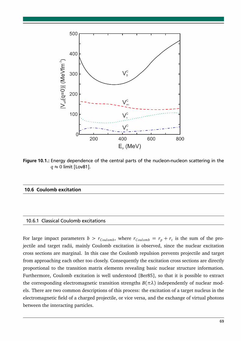
Figure 10.1.: Energy dependence of the central parts of the nucleon-nucleon scattering in theq ≈ 0 limit [Lov81].
10.6 Coulomb excitation
10.6.1 Classical Coulomb excitations
For large impact parameters b > rCoulomb, where rCoulomb = rp + rt is the sum of the pro-
jectile and target radii, mainly Coulomb excitation is observed, since the nuclear excitation
cross sections are marginal. In this case the Coulomb repulsion prevents projectile and target
from approaching each other too closely. Consequently the excitation cross sections are directly
proportional to the transition matrix elements revealing basic nuclear structure information.
Furthermore, Coulomb excitation is well understood [Ber85], so that it is possible to extract
the corresponding electromagnetic transition strengths B(πλ) independently of nuclear mod-
els. There are two common descriptions of this process: the excitation of a target nucleus in the
electromagnetic field of a charged projectile, or vice versa, and the exchange of virtual photons
between the interacting particles.
69
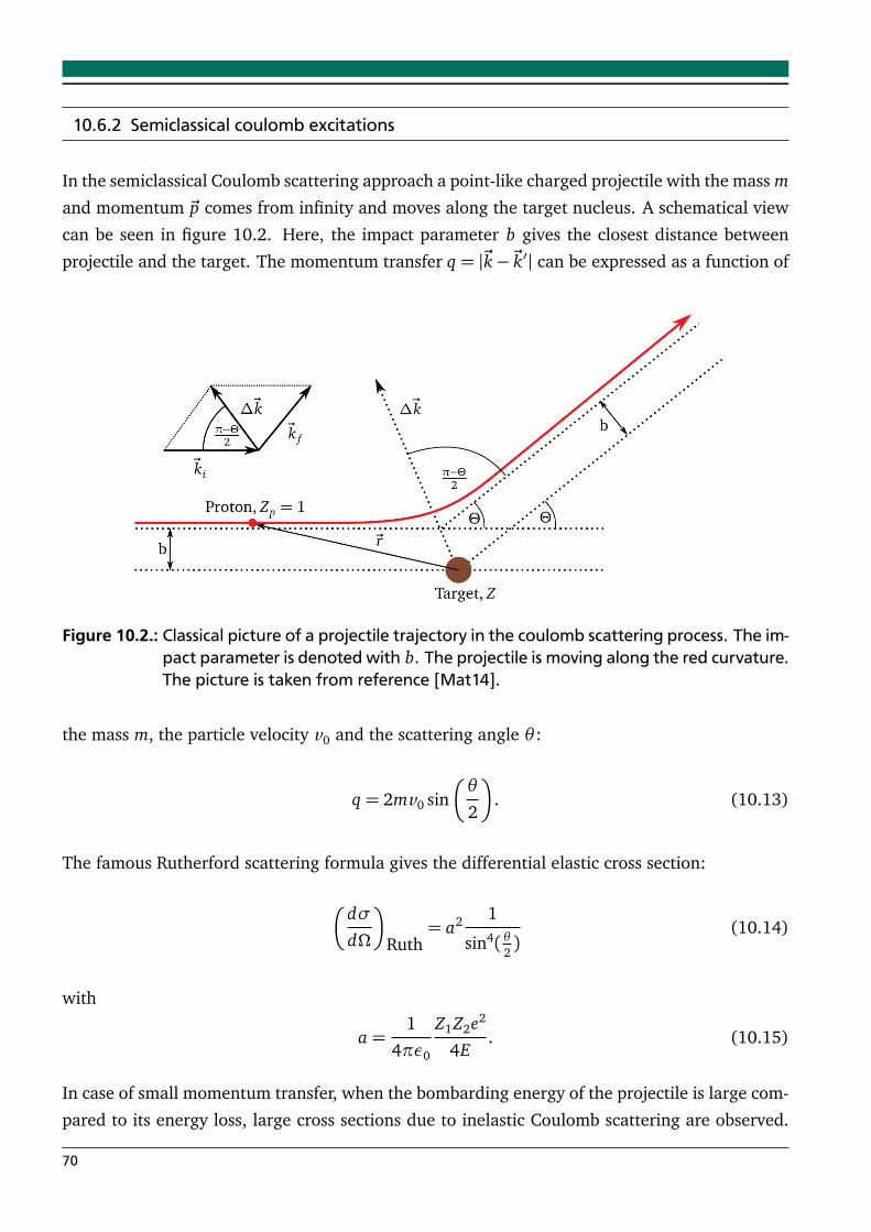
10.6.2 Semiclassical coulomb excitations
In the semiclassical Coulomb scattering approach a point-like charged projectile with the mass m
and momentum ~p comes from infinity and moves along the target nucleus. A schematical view
can be seen in figure 10.2. Here, the impact parameter b gives the closest distance between
projectile and the target. The momentum transfer q = |~k−~k′| can be expressed as a function of
Figure 10.2.: Classical picture of a projectile trajectory in the coulomb scattering process. The im-pact parameter is denoted with b. The projectile is moving along the red curvature.The picture is taken from reference [Mat14].
the mass m, the particle velocity v0 and the scattering angle θ :
q = 2mv0 sin
θ
2
. (10.13)
The famous Rutherford scattering formula gives the differential elastic cross section:
dσ
dΩ
Ruth= a2 1
sin4(θ2)
(10.14)
with
a =1
4πε0
Z1Z2e2
4E. (10.15)
In case of small momentum transfer, when the bombarding energy of the projectile is large com-
pared to its energy loss, large cross sections due to inelastic Coulomb scattering are observed.
70
Introducing relativistic projectile energies (β = v/c), the Rutherford scattering formula (10.14)
transforms to the Mott formula
dσ
dΩ
Mott=
dσ
dΩ
Ruth
1− β2 sin2
θ
2
. (10.16)
In a good approximation, the relative motion follows a classical Rutherford trajectory [Win79].
The differential cross section is then be given by
dσ
dΩ
=
dσ
dΩ
RuthPi→ f . (10.17)
The probability for the excitation of an initial state |i⟩ into a final state
f
is given by Pi→ f . For
a time-dependent electromagnetic field V (~r(t)), that weakly excites the target, Pi→ f = |ai→ f |2
can be calculated in first order perturbation theory by means of the excitation amplitude
ai→ f =1
iħh
∞∫
∞
eiωt f |V (~r(t))|i
d t, (10.18)
with ω = (Ei − E f )/ħh. With a multipole expansion of V (~r(t)), the excitation amplitude can be
given as
ai→ f = i∑
λ
χπλi→ f fλ(ξ), (10.19)
with the strength parameter χπλi→ f , which describes the action of the field in terms of matrix
elements of electric and magnetic multipole moments with parity π and multipolarity λ. The
factors fλ(ξ) define the dependence of the cross section on the degree of adiabaticity, which is
given by the adiabaticity parameter ξ=ωb/(vγ). The total cross section for Coulomb excitation
of a final state | f ⟩ for a component with given πλ yields
σπλ = 2π
∞∫
R
bPi→ f (b) db ≈ 2π
ρa∫
R
b
χπλi→ f (b)
2db. (10.20)
In equation (10.20), R is taken as the sum of the nuclear radii of projectile and target, below
which nuclear interaction will also occur, while ρa = vγ/ω is the impact parameter evaluated
71
at ξ = 1, where the adiabatic cutoff sets in. Inserting χπλi→ f and considering a 0+ ground state
|i⟩ (as in the case of 154Sm), this leads to
σπλ ≈
Z1e2
ħhc
2B(πλ; 0→ λ)
e2R2λπR2
(λ− 1)−1 for λ≥ 2,
2 ln (ρa/R) for λ= 1.(10.21)
Therefore, the reduced transition strength B(πλ, 0 → λ) can be obtained by measuring the
scattering cross sections. In case of E1 transitions that are investigated in this work, equa-
tion (10.21) simplifies to
σE1 ≈
Z1e2
ħhc
22π ln (ρa/R)
e2 B(E1;0→ 1). (10.22)
10.6.3 Equivalent virtual photon method
Coulomb excitation can be considered as the absorption of virtual photons by the target nucleus.
Produced by the moving projectile, the number of virtual photons is related to the amount of real
photons, which would have an equivalent net effect for one specific transition. It is linked to the
Fourier transformation of the time-dependent electromagnetic field induced by the projectile. A
theoretical description of this process is given in [Ber88]. Here, the Coulomb excitation cross
section is expressed as
σi→ f =∑
πλ
∫
Nπλ(Eγ)σπλγ (Eγ)
1
EγdEγ, (10.23)
where σπλγ (Eγ) is the photoabsorption cross section depending on the photon energy Eγ and
Nπλ(Eγ) is the equivalent photon numbers for electric (π =E) or magnetic (π =M) transitions
of multipole order λ. In a semiclassical approximation [Ber88, Win79] the virtual photon num-
bers can be calculated analytically for negligible energy loss of the projectile. As long as the
object is large enough compared to the wavelength of light, this assumption works quite well.
However, microscopic phenomena have to be explained by Maxwell’s equations with the dis-
persion relation ω = kc. In quantum mechanics, microscopic phenomena are described by
Schrödinger’s equation with a dispersion relation ω= ħhk2/2m for small scales, too. Just as well
72
an eikonal approximation can be adopted here for processes concerning small scattering angles
and large impact parameters. This leads to
Nπλ(Eγ) = Z21αλ[(2λ+ 1)!!]2
(2π)3(λ+ 1)
∑
m
Gπλm
c
v0
2
gm(ξ), (10.24)
with the fine structure constant α = e2/ħhc and the functions gm and Gπλm, which are tabulated
in [Win79]. In a similar way, the double differential cross section is derived from virtual photon
numbers asd2σ
dΩdEγ=
1
Eγ
∑
πλ
dNπλdΩ
σπλγ (Eγ). (10.25)
dNE1
dΩ
rel=
Z21α
4π2 ζ2ε2
1
γβ
2
K21 (x) +
1
γ2 K20 (x)
. (10.26)
Here, ζ = ωa/v0 is the adiabaticity parameter with a = Z1Z2e2/µv 20 referring to half of the
closest distance, µ is the reduced mass, and ε = sin−1(θ/2) the eccentricity parameter. The
variable in K(x) of the modified Bessel function of the second kind is an abbreviation for x =(εζ/γ) cos(θ/2). For γ ≈ 1 (ε 1) the equivalent photon number for E1 transitions can be
calculated as
dNE1
dΩ
nonrel=
Z21α
4π2 ε2
1
β
2
x2
K21 (x) + K2
0 (x)
. (10.27)
10.6.4 Eikonal description of Coulomb excitation
Since the semiclassical treatment of the virtual photon number does not work properly at very
low scattering angles and produces a pole at 0, Bertulani and Nathan [Ber93] found a way to
include diffraction and get rid of the semiclassical approximations for the impact parameter. For
the virtual photon numbers they obtain
dNπλdΩ
= Z21α
ωk
γv
2 λ[(2λ+ 1)!!]2
(2π)3(λ+ 1)
∑
m
Gπλm
c
v0
2
Ωm(q)
2(10.28)
73
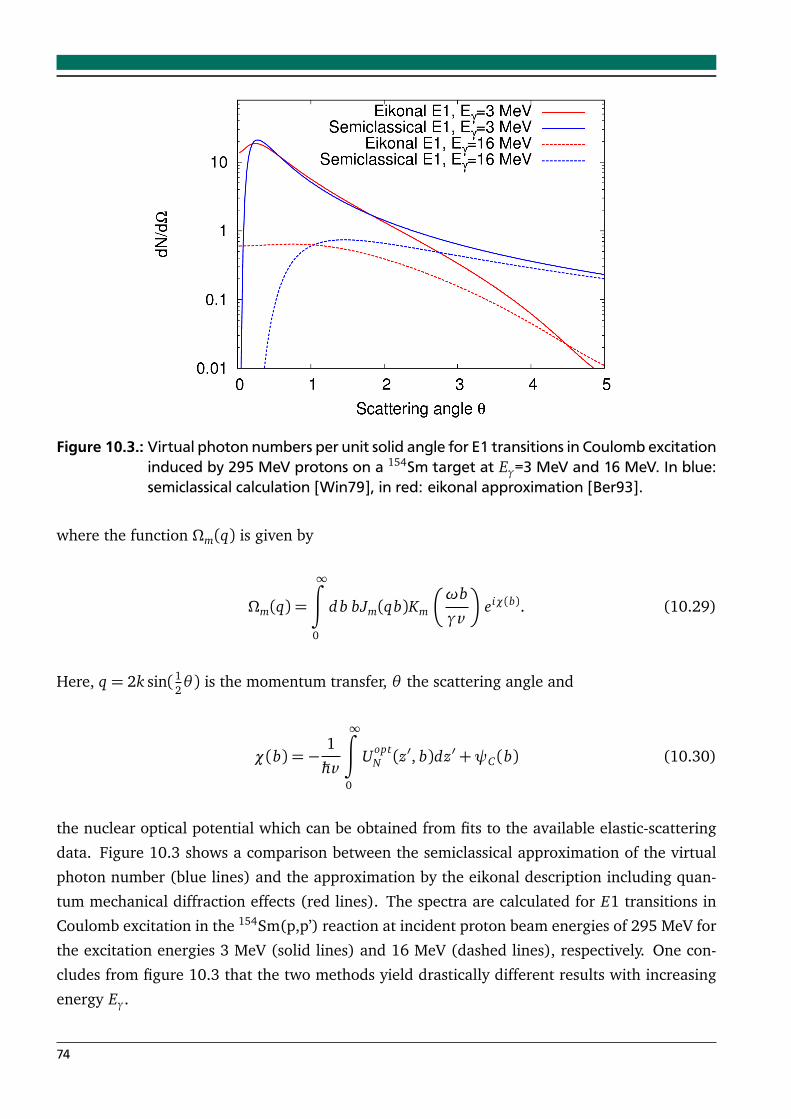
Figure 10.3.: Virtual photon numbers per unit solid angle for E1 transitions in Coulomb excitationinduced by 295 MeV protons on a 154Sm target at Eγ=3 MeV and 16 MeV. In blue:semiclassical calculation [Win79], in red: eikonal approximation [Ber93].
where the function Ωm(q) is given by
Ωm(q) =
∞∫
0
d b bJm(qb)Km
ωb
γv
eiχ(b). (10.29)
Here, q = 2k sin(12θ) is the momentum transfer, θ the scattering angle and
χ(b) =−1
ħhv
∞∫
0
U optN (z
′, b)dz′+ψC(b) (10.30)
the nuclear optical potential which can be obtained from fits to the available elastic-scattering
data. Figure 10.3 shows a comparison between the semiclassical approximation of the virtual
photon number (blue lines) and the approximation by the eikonal description including quan-
tum mechanical diffraction effects (red lines). The spectra are calculated for E1 transitions in
Coulomb excitation in the 154Sm(p,p’) reaction at incident proton beam energies of 295 MeV for
the excitation energies 3 MeV (solid lines) and 16 MeV (dashed lines), respectively. One con-
cludes from figure 10.3 that the two methods yield drastically different results with increasing
energy Eγ.
74
10.7 Magnetic dipole transitions and B(M1στ) from (p,p’) cross section data
For magnetic dipole transitions that are induced by the electromagnetic interaction the total
spin of the nucleus changes by one (∆J = 1) while the parity π of the total nuclear wave
function does not change (πiπ f = 1). This is possible for ∆L = 1 transitions or for ∆S = 1
transitions. Since we are considering spinflip transitions in 154Sm, the B(M1) transition strength
(see [Fuj11] is defined as
B(M1) =3
4π
1
2J + 1
¬
ψ′N ||O(M1)||ψN
¶
2. (10.31)
Here,
ψN
and
ψ′N
¶
are the nuclear wave functions before and after the transition and J is
the total angular momentum of the initial state. O(M1) is the operator of the magnetic dipole
moment, which can be separated into an isoscalar part (IS, ∆T = 0) and an isovector part
(IV, ∆T = 1):
O(M1) =
Z∑
i=1
g pl~li +
1
2g p
s ~σi
+A∑
i=Z+1
gNl~li +
1
2gN
s ~σi
µN (10.32)
=
A∑
i=1
g ISl~li +
1
2g IS
s ~σi +τzi
g IVl~li +
1
2g IV
s ~σi
µN (10.33)
with ~σi being the Pauli spin operator and τzi = 1 (0) for protons and neutrons, respectively.
Utilizing the Wigner-Eckhardt theorem, the B(M1) transition strength can now be rewritten:
B(M1) =3
4π
1
2J + 1
CM1,00p2T ′+ 1
g ISl M(~l) +
1
2g IS
s M(~σ)
+
CM1,10p2T ′+ 1
g IVl M(τ~l) +
1
2g IV
s M(τ~l)
2
µ2N (10.34)
Here, CM1,00 and CM1,10 denote the Clebsch-Gordan coefficients (T Tz00|T ′T ′z) and (T Tz10|T ′T ′z),respectively, and τ represents the isospin operator. T and T ′ stand for the total nuclear isospin
75
in the initial and final state. With the help of equation 10.34 the B(M1) transition strength can
now be separated in an isovector and an isoscalar part:
B(M1)IS =3
4π
1
2J + 1
C2M1,00
2T ′+ 1
g ISl M(~l) +
1
2g IS
s M(~σ)
2
µ2N (10.35)
B(M1)IV =3
4π
1
2J + 1
C2M1,10
2T ′+ 1
g IVl M(τ~l) +
1
2g IV
s M(τ~σ)
2
µ2N . (10.36)
In the case of pure spinflip transitions, these transition strengths reduce to:
B(M1)IS ≈3
16π
1
2J + 1
C2M1,00
2T ′+ 1
g ISs M(~σ)
2µ2
N (10.37)
B(M1)IV ≈3
16π
1
2J + 1
C2M1,10
2T ′+ 1
g IVs M(τ~σ)
2µ2
N . (10.38)
If the nucleus is excited via inelastic proton scattering, the interaction is mainly mediated via
the nuclear force and not via the electromagnetic interaction. Additionally, it has been shown
that at very low momentum transfers (e.g. q→ 0) and proton energies around 300 MeV, mostly
isovector spinflip transitions occur. Thus, an excitation of 154Sm from the ground state to a 1+
state corresponds to a spinflip-M1 excitation with a reduced transition strength of
B(M1στ) =1
2(2J + 1)
C2M1,10
2T ′+ 1|M(τ~σ)|2 . (10.39)
Also refering to [Fuj11] the following relation can be defined
B(M1στ) =
dσdΩ
M1
pp′(0)
FM1σM1(A). (10.40)
Here,
dσdΩ
M1
pp′(0) denotes the spinflip-M1 cross section, measured in inelastic proton scattering
at 0. The kinematical correction factor FM1 can be calculated from the ratio of the theoretical
cross section at excitation energy of Ex = 0 MeV to the theoretical cross section at an excitation
energy of Ex . σM1(A) is the so-called ’unit cross section’ that represents the mass dependence
of B(M1στ). Analogue to equation 10.40 the reduced transition strength for Gamow-Teller
transitions can be defined as
B(GT ) =1
2
1
(2J + 1)
C2GT,±
2T ′+ 1|M(τ~σ)|2 , (10.41)
76
and the corresponding definition, involving the unit cross section for Gamow-Teller transitions
σGT±(A):
B(GT±) =
dσdΩ
GT±
pp′(0)
FGT±σGT±(A). (10.42)
10.8 Polarization transfer observables (PT observables)
Polarized proton scattering is a well established tool for the distinction from spinflip and non-
spinflip transitions in nuclei [Ohl02, Wol56]. In a simple notation, these reactions are of the
type:~1
2+ A→
~1
2+ A′ (10.43)
with~12
denoting a polarized spin-12
proton, A the target nucleus and A′ the excited target nucleus.
Using the plane wave impulse approximation (PWIA), the T -matrix for nucleon-nucleus scat-
tering between an initial state |i⟩ and a final state | f ⟩ can be written as
T =¬
f
M(q)e−i~q·~r
i¶
. (10.44)
The analyzing power for the j-th component of the beam polarization vector, the differential
cross section dσ/dΩ and the polarization transfer observables Di j can then be expressed in
terms of the T -matrix [Kaw02]
A j =Tr (T T †σn)
Tr (T T †),
dσ
dΩ=
1
2Tr (T T †), Di j =
Tr (Tσ j T†σi)
Tr (T T †), (10.45)
where i and j denote the direction of the projectile spin in the initial and final state, respec-
tively. According to [Ker59] one can write the nucleon-nucleon scattering amplitude MNN as a
phenomenological sum of operators in spin space
MNN = A+ Bσ1nσ2n+ C
σ1n+σ2n
+ Eσ1qσ2q + Fσ1pσ2p. (10.46)
77
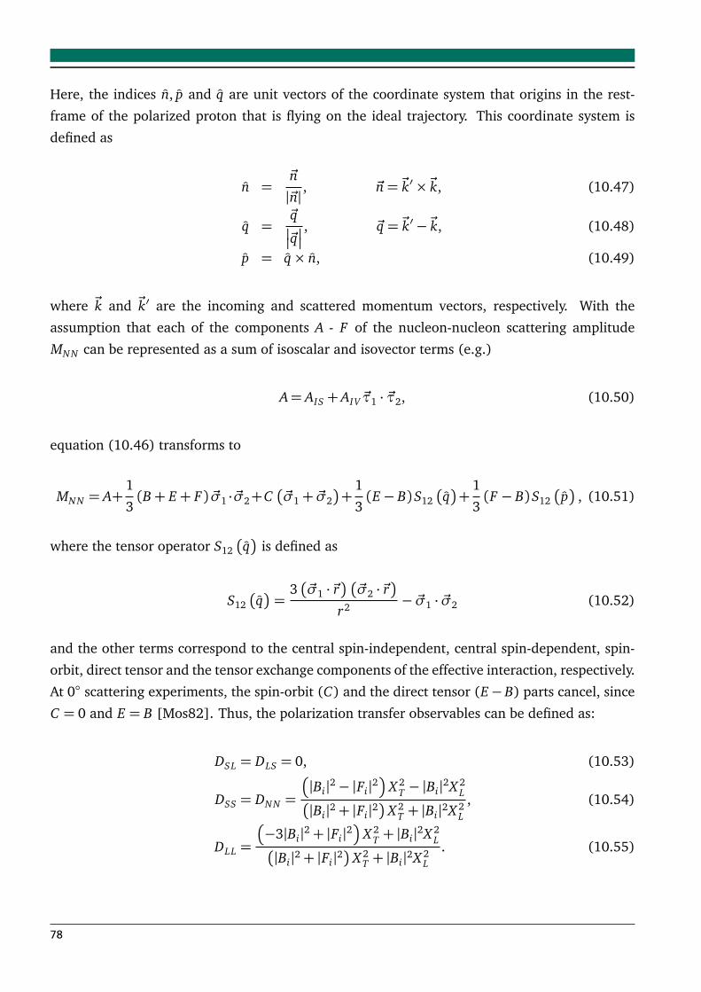
Here, the indices n, p and q are unit vectors of the coordinate system that origins in the rest-
frame of the polarized proton that is flying on the ideal trajectory. This coordinate system is
defined as
n =~n
|~n|, ~n=~k′×~k, (10.47)
q =~q
~q
, ~q =~k′−~k, (10.48)
p = q× n, (10.49)
where ~k and ~k′ are the incoming and scattered momentum vectors, respectively. With the
assumption that each of the components A - F of the nucleon-nucleon scattering amplitude
MNN can be represented as a sum of isoscalar and isovector terms (e.g.)
A= AIS + AIV ~τ1 · ~τ2, (10.50)
equation (10.46) transforms to
MNN = A+1
3(B+ E + F) ~σ1 ·~σ2+C
~σ1+ ~σ2
+1
3(E − B)S12
q
+1
3(F − B)S12
p
, (10.51)
where the tensor operator S12
q
is defined as
S12
q
=3
~σ1 ·~r
~σ2 ·~r
r2 − ~σ1 · ~σ2 (10.52)
and the other terms correspond to the central spin-independent, central spin-dependent, spin-
orbit, direct tensor and the tensor exchange components of the effective interaction, respectively.
At 0 scattering experiments, the spin-orbit (C) and the direct tensor (E− B) parts cancel, since
C = 0 and E = B [Mos82]. Thus, the polarization transfer observables can be defined as:
DSL = DLS = 0, (10.53)
DSS = DNN =
|Bi|2− |Fi|2
X 2T − |Bi|2X 2
L
|Bi|2+ |Fi|2
X 2T + |Bi|2X 2
L
, (10.54)
DLL =
−3|Bi|2+ |Fi|2
X 2T + |Bi|2X 2
L
|Bi|2+ |Fi|2
X 2T + |Bi|2X 2
L
. (10.55)
78
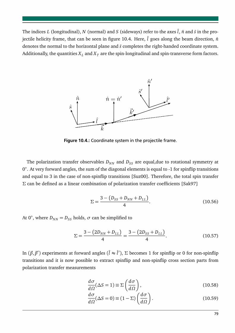
The indices L (longitudinal), N (normal) and S (sideways) refer to the axes l, n and s in the pro-
jectile helicity frame, that can be seen in figure 10.4. Here, l goes along the beam direction, n
denotes the normal to the horizontal plane and s completes the right-handed coordinate system.
Additionally, the quantities X L and XT are the spin-longitudinal and spin-transverse form factors.
Figure 10.4.: Coordinate system in the projectile frame.
The polarization transfer observables DNN and DSS are equal,due to rotational symmetry at
0. At very forward angles, the sum of the diagonal elements is equal to -1 for spinflip transitions
and equal to 3 in the case of non-spinflip transitions [Suz00]. Therefore, the total spin transfer
Σ can be defined as a linear combination of polarization transfer coefficients [Sak97]
Σ =3−
DSS + DNN + DLL
4. (10.56)
At 0, where DNN = DSS holds, σ can be simplified to
Σ =3−
2DNN + DLL
4=
3−
2DSS + DLL
4. (10.57)
In (~p,~p′) experiments at forward angles (l ≈ l ′), Σ becomes 1 for spinflip or 0 for non-spinflip
transitions and it is now possible to extract spinflip and non-spinflip cross section parts from
polarization transfer measurements
dσ
dΩ(∆S = 1)≡ Σ
dσ
dΩ
, (10.58)
dσ
dΩ(∆S = 0)≡ (1−Σ)
dσ
dΩ
. (10.59)
79

Since in proton scattering experiments at very forward angles, dipole excitations are favored,
non-spinflip cross sections can be associated with E1 excitations wheras spinflip cross sections
are assigned to spinflip-M1 excitations. This method has already been successfully applied in
the analysis of nuclei in various mass regions: 12C [Tam99], 16O [Kaw02], 96Mo [Mar13], 120Sn
[Kru] and 208Pb [Pol11].
80
11 Polarized proton scattering experiment at RCNP
At the Research Center for Nuclear Physics (RCNP) [RCN14] in Osaka, Japan, a high resolution
study with polarized protons on the heavy deformed nucleus 154Sm at very forward angles
including 0 was performed. A schematic overview of the experimental facilities at the RCNP is
depicted in figure 11.1.
Figure 11.1.: Schematic overview of the RCNP facility in Osaka.
Polarized protons with a typical polarization of 70% are produced in the High Intensity Po-
larized Ion Source (HIPIS) [Hat97]. Here, hydrogen molecules were dissociated and a beam
of cooled hydrogen atoms was produced. By using the Stern-Gerlach Effect, one polarization
(either up or down) is selected and this part of the beam gets ionized in an electron cyclotron
81
ionizer (ECR). In order to compensate geometrical asymmetries of the experimental setup, the
beam polarization is flipped with a frequency of 1 Hz. For the measurements at finite spectrom-
eter angles, the NEOMAFIOS ECR [Tan91] source has been used due to its ability to provide
much higher proton intensities.
The (polarized) proton beam was then injected in the Azimuthally Varying Field (AVF) Cy-
clotron and accelerated to a kinetic energy of 54 MeV. After the AVF Cyclotron, the beam was
transported to the RING Cyclotron and accelerated to the final energy of 295 MeV. On the way
from the source to the target, two superconducting solenoids and two Beam Line Polarimeters
are installed to control and monitor the magnitude and direction of the beam polarization. The
scattering chamber is connected to two spectrometer. The Large Acceptance spectrometer (LAS)
is used to monitor the vertical beam position. With the Grand Raiden Spectrometer, which con-
sists of two dipole magnets (D1 and D2), a multipole magnet (MX) and a dipole magnet for
spin rotation (DSR) the scattered protons were analyzed in the focal plane. With the help of the
Focal Plane Polarimeter (FPP) polarization transfer observables of protons which were scattered
at a carbon block between the focal plane and the FPP can be extracted.
11.1 Beam line polarimeters (BLPs)
With the two beam line polarimeters BLP1 and BLP2 the polarization of the proton beam was
monitored periodically. Each BLP consists of four pairs of plastic scintillators in order to measure
the p-p scattering asymmetries of a polyethylene foil. As an example, figure 11.2 shows the top
view of one of the BLPs measuring the left-right asymmetry. A similar setup can be found for the
up-down asymmetry. To experimentally determine the scattering asymmetry, elastic scattering
off hydrogen and quasi-elastic scattering off carbon (which both have the same kinematics) are
measured in coincidence with recoiling protons from the target. The analyzing power of the
BPLs for proton scattering at 295 MeV has been measured to be Ay = 0.40± 0.01 [Tak02].
In order to detect all three-dimensional polarization components of the beam, a configuration of
two BLPs and a 50 dipole magnet as shown in figure 11.3 has been used. Each 99 seconds, the
polyethylene target was inserted for 10 seconds into the beam. During that time, the readout
electronic was inactive.
11.2 The setup for 0 measurements
11.2.1 The Grand Raiden spectrometer
The Grand Raiden spectrometer [Fuj99] consists of a Q1-SX-Q2-D1-MP-D2+DSR magnet con-
figuration, where D, Q and SX stand for dipole, quadrupole and sextupole, respectively, and MP
denoting a multipole magnet. Additionally, the DSR (Dipole for spin rotation) magnet has been
82
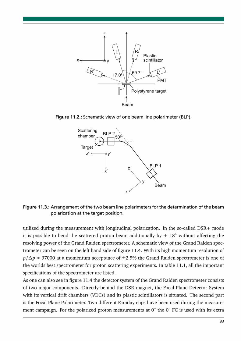
Figure 11.2.: Schematic view of one beam line polarimeter (BLP).
Figure 11.3.: Arrangement of the two beam line polarimeters for the determination of the beampolarization at the target position.
utilized during the measurement with longitudinal polarization. In the so-called DSR+ mode
it is possible to bend the scattered proton beam additionally by + 18 without affecting the
resolving power of the Grand Raiden spectrometer. A schematic view of the Grand Raiden spec-
trometer can be seen on the left hand side of figure 11.4. With its high momentum resolution of
p/∆p ≈ 37000 at a momentum acceptance of ±2.5% the Grand Raiden spectrometer is one of
the worlds best spectrometer for proton scattering experiments. In table 11.1, all the important
specifications of the spectrometer are listed.
As one can also see in figure 11.4 the detector system of the Grand Raiden spectrometer consists
of two major components. Directly behind the DSR magnet, the Focal Plane Detector System
with its vertical drift chambers (VDCs) and its plastic scintillators is situated. The second part
is the Focal Plane Polarimeter. Two different Faraday cups have been used during the measure-
ment campaign. For the polarized proton measurements at 0 the 0 FC is used with its extra
83
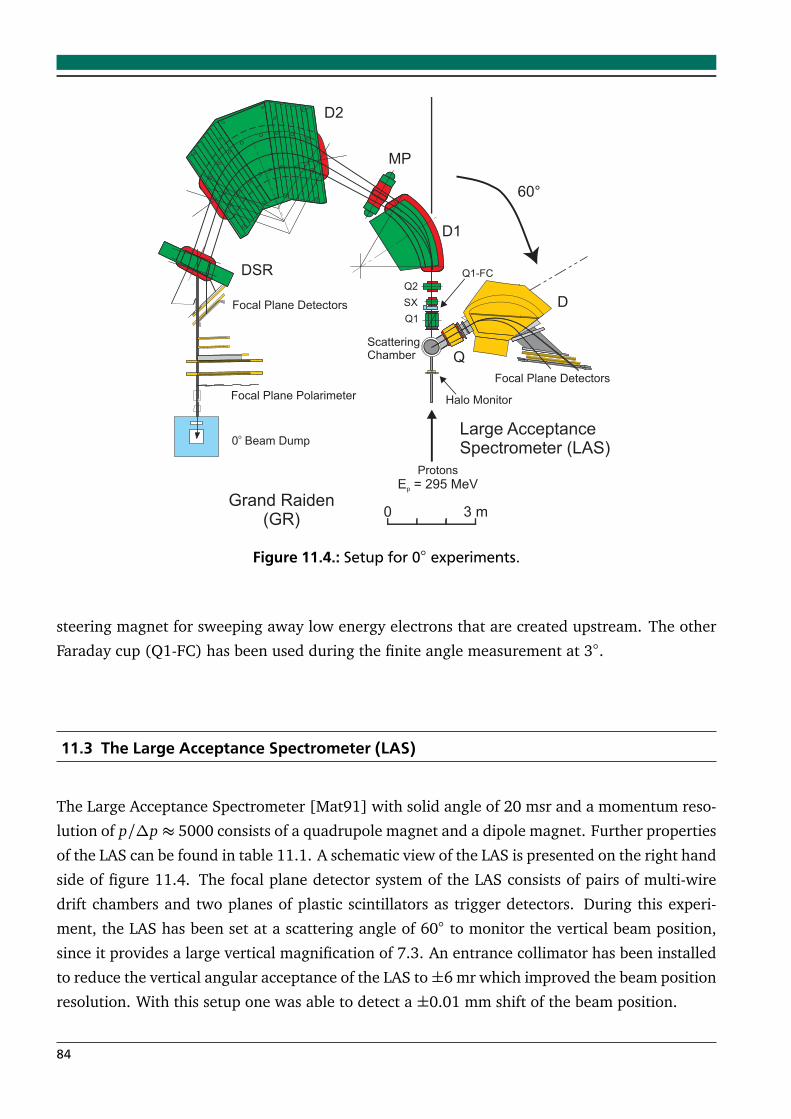
Figure 11.4.: Setup for 0 experiments.
steering magnet for sweeping away low energy electrons that are created upstream. The other
Faraday cup (Q1-FC) has been used during the finite angle measurement at 3.
11.3 The Large Acceptance Spectrometer (LAS)
The Large Acceptance Spectrometer [Mat91] with solid angle of 20 msr and a momentum reso-
lution of p/∆p ≈ 5000 consists of a quadrupole magnet and a dipole magnet. Further properties
of the LAS can be found in table 11.1. A schematic view of the LAS is presented on the right hand
side of figure 11.4. The focal plane detector system of the LAS consists of pairs of multi-wire
drift chambers and two planes of plastic scintillators as trigger detectors. During this experi-
ment, the LAS has been set at a scattering angle of 60 to monitor the vertical beam position,
since it provides a large vertical magnification of 7.3. An entrance collimator has been installed
to reduce the vertical angular acceptance of the LAS to±6 mr which improved the beam position
resolution. With this setup one was able to detect a ±0.01 mm shift of the beam position.
84
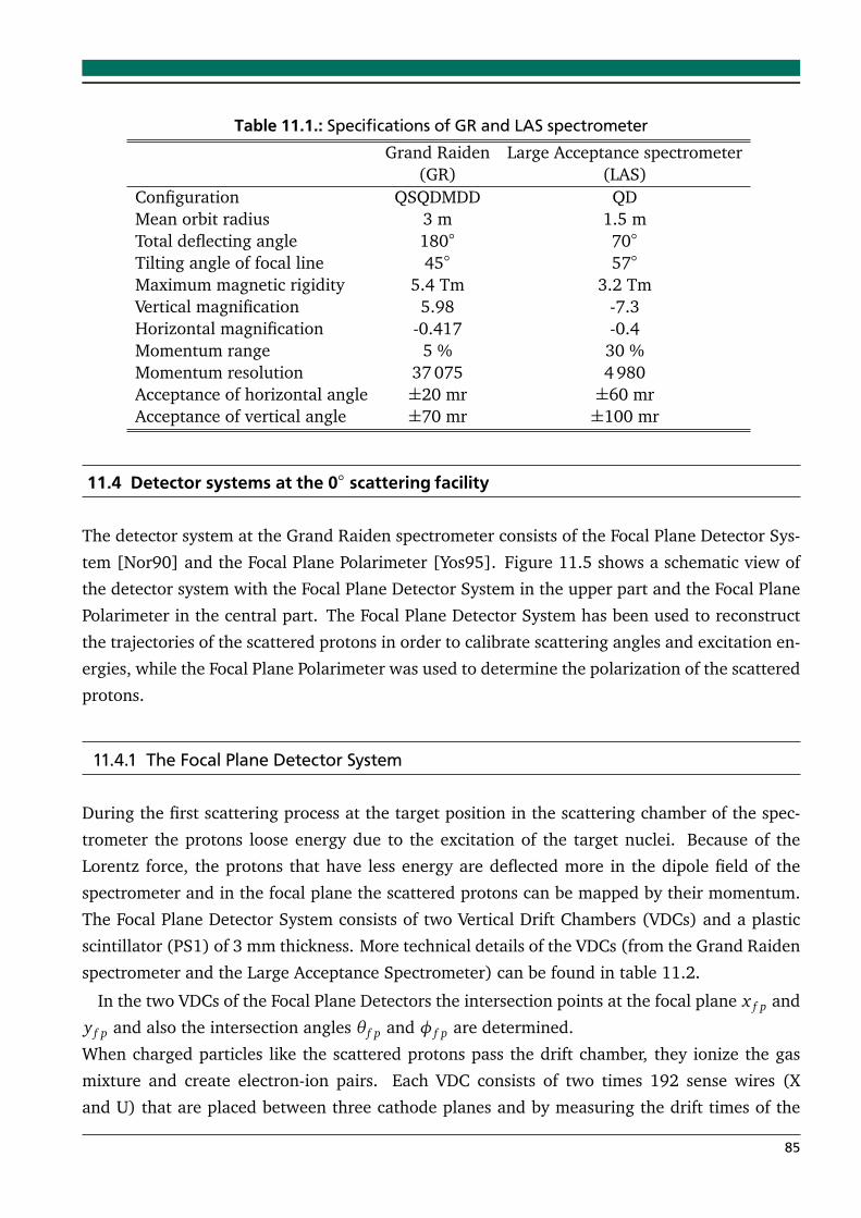
Table 11.1.: Specifications of GR and LAS spectrometerGrand Raiden Large Acceptance spectrometer
(GR) (LAS)Configuration QSQDMDD QDMean orbit radius 3 m 1.5 mTotal deflecting angle 180 70
Tilting angle of focal line 45 57
Maximum magnetic rigidity 5.4 Tm 3.2 TmVertical magnification 5.98 -7.3Horizontal magnification -0.417 -0.4Momentum range 5 % 30 %Momentum resolution 37 075 4 980Acceptance of horizontal angle ±20 mr ±60 mrAcceptance of vertical angle ±70 mr ±100 mr
11.4 Detector systems at the 0 scattering facility
The detector system at the Grand Raiden spectrometer consists of the Focal Plane Detector Sys-
tem [Nor90] and the Focal Plane Polarimeter [Yos95]. Figure 11.5 shows a schematic view of
the detector system with the Focal Plane Detector System in the upper part and the Focal Plane
Polarimeter in the central part. The Focal Plane Detector System has been used to reconstruct
the trajectories of the scattered protons in order to calibrate scattering angles and excitation en-
ergies, while the Focal Plane Polarimeter was used to determine the polarization of the scattered
protons.
11.4.1 The Focal Plane Detector System
During the first scattering process at the target position in the scattering chamber of the spec-
trometer the protons loose energy due to the excitation of the target nuclei. Because of the
Lorentz force, the protons that have less energy are deflected more in the dipole field of the
spectrometer and in the focal plane the scattered protons can be mapped by their momentum.
The Focal Plane Detector System consists of two Vertical Drift Chambers (VDCs) and a plastic
scintillator (PS1) of 3 mm thickness. More technical details of the VDCs (from the Grand Raiden
spectrometer and the Large Acceptance Spectrometer) can be found in table 11.2.
In the two VDCs of the Focal Plane Detectors the intersection points at the focal plane x f p and
y f p and also the intersection angles θ f p and φ f p are determined.
When charged particles like the scattered protons pass the drift chamber, they ionize the gas
mixture and create electron-ion pairs. Each VDC consists of two times 192 sense wires (X
and U) that are placed between three cathode planes and by measuring the drift times of the
85
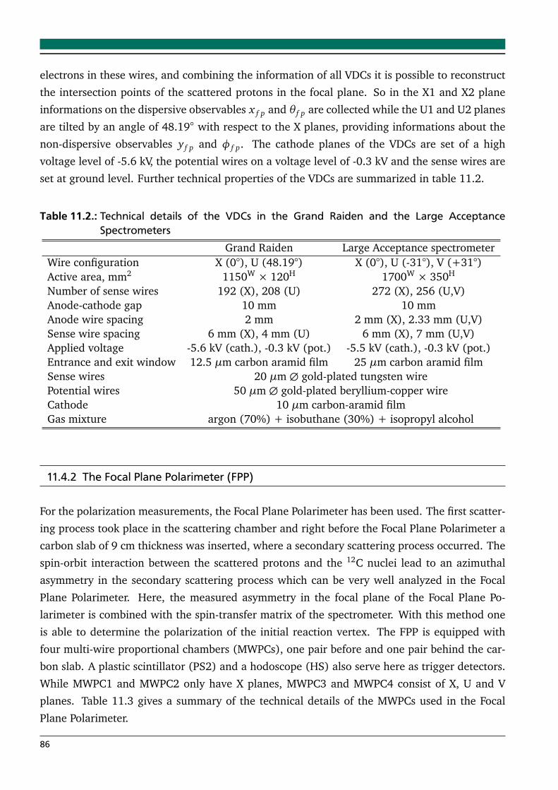
electrons in these wires, and combining the information of all VDCs it is possible to reconstruct
the intersection points of the scattered protons in the focal plane. So in the X1 and X2 plane
informations on the dispersive observables x f p and θ f p are collected while the U1 and U2 planes
are tilted by an angle of 48.19 with respect to the X planes, providing informations about the
non-dispersive observables y f p and φ f p. The cathode planes of the VDCs are set of a high
voltage level of -5.6 kV, the potential wires on a voltage level of -0.3 kV and the sense wires are
set at ground level. Further technical properties of the VDCs are summarized in table 11.2.
Table 11.2.: Technical details of the VDCs in the Grand Raiden and the Large AcceptanceSpectrometers
Grand Raiden Large Acceptance spectrometerWire configuration X (0°), U (48.19°) X (0°), U (-31°), V (+31°)Active area, mm2 1150W × 120H 1700W × 350H
Number of sense wires 192 (X), 208 (U) 272 (X), 256 (U,V)Anode-cathode gap 10 mm 10 mmAnode wire spacing 2 mm 2 mm (X), 2.33 mm (U,V)Sense wire spacing 6 mm (X), 4 mm (U) 6 mm (X), 7 mm (U,V)Applied voltage -5.6 kV (cath.), -0.3 kV (pot.) -5.5 kV (cath.), -0.3 kV (pot.)Entrance and exit window 12.5 µm carbon aramid film 25 µm carbon aramid filmSense wires 20 µm ∅ gold-plated tungsten wirePotential wires 50 µm ∅ gold-plated beryllium-copper wireCathode 10 µm carbon-aramid filmGas mixture argon (70%) + isobuthane (30%) + isopropyl alcohol
11.4.2 The Focal Plane Polarimeter (FPP)
For the polarization measurements, the Focal Plane Polarimeter has been used. The first scatter-
ing process took place in the scattering chamber and right before the Focal Plane Polarimeter a
carbon slab of 9 cm thickness was inserted, where a secondary scattering process occurred. The
spin-orbit interaction between the scattered protons and the 12C nuclei lead to an azimuthal
asymmetry in the secondary scattering process which can be very well analyzed in the Focal
Plane Polarimeter. Here, the measured asymmetry in the focal plane of the Focal Plane Po-
larimeter is combined with the spin-transfer matrix of the spectrometer. With this method one
is able to determine the polarization of the initial reaction vertex. The FPP is equipped with
four multi-wire proportional chambers (MWPCs), one pair before and one pair behind the car-
bon slab. A plastic scintillator (PS2) and a hodoscope (HS) also serve here as trigger detectors.
While MWPC1 and MWPC2 only have X planes, MWPC3 and MWPC4 consist of X, U and V
planes. Table 11.3 gives a summary of the technical details of the MWPCs used in the Focal
Plane Polarimeter.
86
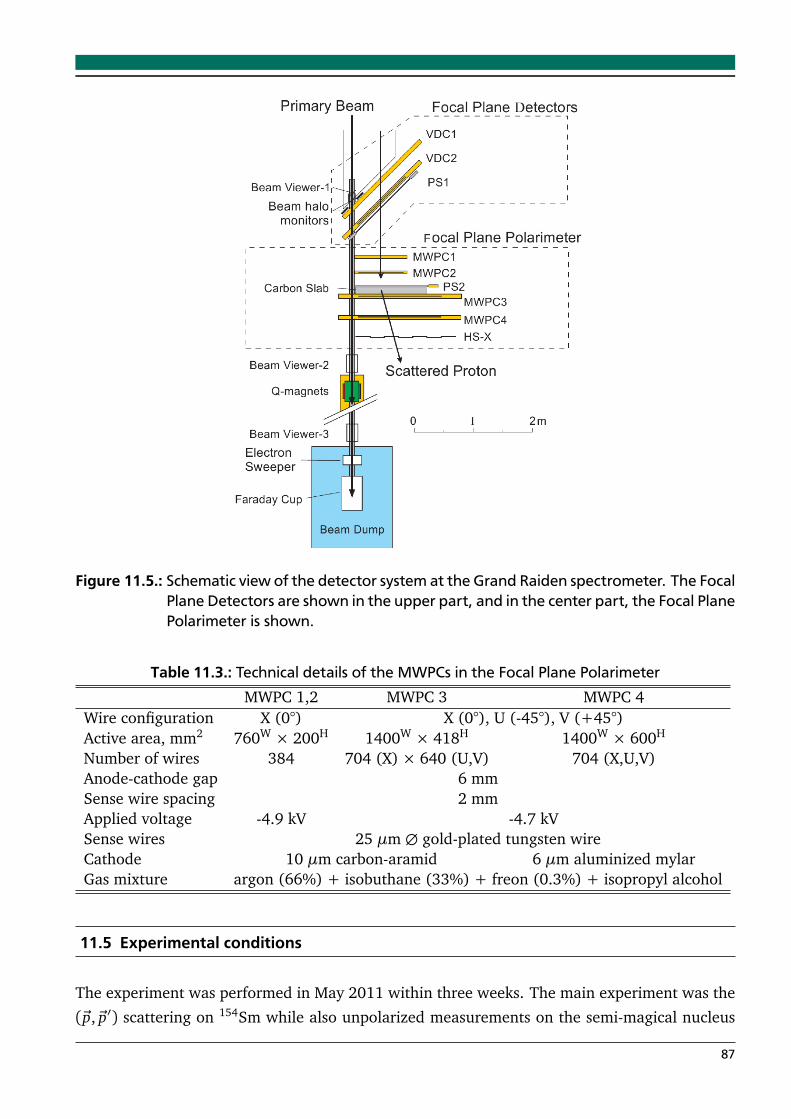
Figure 11.5.: Schematic view of the detector system at the Grand Raiden spectrometer. The FocalPlane Detectors are shown in the upper part, and in the center part, the Focal PlanePolarimeter is shown.
Table 11.3.: Technical details of the MWPCs in the Focal Plane PolarimeterMWPC 1,2 MWPC 3 MWPC 4
Wire configuration X (0°) X (0°), U (-45°), V (+45°)Active area, mm2 760W × 200H 1400W × 418H 1400W × 600H
Number of wires 384 704 (X) × 640 (U,V) 704 (X,U,V)Anode-cathode gap 6 mmSense wire spacing 2 mmApplied voltage -4.9 kV -4.7 kVSense wires 25 µm ∅ gold-plated tungsten wireCathode 10 µm carbon-aramid 6 µm aluminized mylarGas mixture argon (66%) + isobuthane (33%) + freon (0.3%) + isopropyl alcohol
11.5 Experimental conditions
The experiment was performed in May 2011 within three weeks. The main experiment was the
(~p,~p′) scattering on 154Sm while also unpolarized measurements on the semi-magical nucleus
87
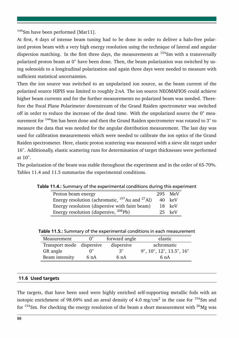
144Sm have been performed [Mar11].
At first, 4 days of intense beam tuning had to be done in order to deliver a halo-free polar-
ized proton beam with a very high energy resolution using the technique of lateral and angular
dispersion matching. In the first three days, the measurements at 154Sm with a transversally
polarized proton beam at 0 have been done. Then, the beam polarization was switched by us-
ing solenoids to a longitudinal polarization and again three days were needed to measure with
sufficient statistical uncertainties.
Then the ion source was switched to an unpolarized ion source, as the beam current of the
polarized source HIPIS was limited to roughly 2 nA. The ion source NEOMAFIOS could achieve
higher beam currents and for the further measurements no polarized beam was needed. There-
fore the Focal Plane Polarimeter downstream of the Grand Raiden spectrometer was switched
off in order to reduce the increase of the dead time. With the unpolarized source the 0 mea-
surement for 144Sm has been done and then the Grand Raiden spectrometer was rotated to 3 to
measure the data that was needed for the angular distribution measurement. The last day was
used for calibration measurements which were needed to calibrate the ion optics of the Grand
Raiden spectrometer. Here, elastic proton scattering was measured with a sieve slit target under
16. Additionally, elastic scattering runs for determination of target thicknesses were performed
at 10.
The polarization of the beam was stable throughout the experiment and in the order of 65-70%.
Tables 11.4 and 11.5 summarize the experimental conditions.
Table 11.4.: Summary of the experimental conditions during this experimentProton beam energy 295 MeVEnergy resolution (achromatic, 197Au and 27Al) 40 keVEnergy resolution (dispersive with faint beam) 18 keVEnergy resolution (dispersive, 208Pb) 25 keV
Table 11.5.: Summary of the experimental conditions in each measurementMeasurement 0 forward angle elasticTransport mode dispersive dispersive achromaticGR angle 0 3 9, 10, 12, 13.5, 16
Beam intensity 6 nA 6 nA 6 nA
11.6 Used targets
The targets, that have been used were highly enriched self-supporting metallic foils with an
isotopic enrichment of 98.69% and an areal density of 4.0 mg/cm2 in the case for 154Sm and
for 154Sm. For checking the energy resolution of the beam a short measurement with 26Mg was
88
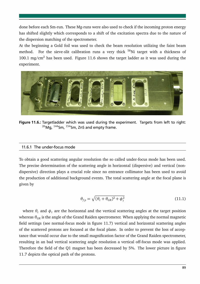
done before each Sm-run. These Mg-runs were also used to check if the incoming proton energy
has shifted slightly which corresponds to a shift of the excitation spectra due to the nature of
the dispersion matching of the spectrometer.
At the beginning a Gold foil was used to check the beam resolution utilizing the faint beam
method. For the sieve-slit calibration runs a very thick 58Ni target with a thickness of
100.1 mg/cm2 has been used. Figure 11.6 shows the target ladder as it was used during the
experiment.
Figure 11.6.: Targetladder which was used during the experiment. Targets from left to right:26Mg, 144Sm, 154Sm, ZnS and empty frame.
11.6.1 The under-focus mode
To obtain a good scattering angular resolution the so called under-focus mode has been used.
The precise determination of the scattering angle in horizontal (dispersive) and vertical (non-
dispersive) direction plays a crucial role since no entrance collimator has been used to avoid
the production of additional background events. The total scattering angle at the focal plane is
given by
θ f p =p
(θt + θGR)2+φ2t (11.1)
where θt and φt are the horizontal and the vertical scattering angles at the target position
whereas θGR is the angle of the Grand Raiden spectrometer. When applying the normal magnetic
field settings (see normal-focus mode in figure 11.7) vertical and horizontal scattering angles
of the scattered protons are focused at the focal plane. In order to prevent the loss of accep-
tance that would occur due to the small magnification factor of the Grand Raiden spectrometer,
resulting in an bad vertical scattering angle resolution a vertical off-focus mode was applied.
Therefore the field of the Q1 magnet has been decreased by 5%. The lower picture in figure
11.7 depicts the optical path of the protons.
89
Figure 11.7.: Examples of vertical beam envelopes in the y-z plane with three different focusmodes of the Grand Raiden optics.
11.6.2 The Faraday cups
Three different kinds of Faraday cups have been used during the experiment to monitor the
proton beam current and to measure the collected charge in the spectra. The 0 Faraday cup
behind the focal plane detectors for measurements at extreme forward angles, the Q1-FC for the
measurement at 3 and the scattering chamber Faraday cup (SC-FC) for the elastic scattering
experiments at higher angles in the dispersive mode. To correct for little losses in the beam
charge collection, the beam transmission from the target to the 0 FC was checked. The absolute
efficiency for the charge measurement at the SC-FC has been already calibrated [Fuj08] with
respect to the rates measured in the BLPs and so it can be used as a reference because the
other Faraday cups can be corrected relative to it. The ratio of the total events in BLP to the
collected charges was measured for each Faraday cup. If transmission losses occurred during
the experiment, then the ratio of the 0 FC and the Q1-FC would become larger than that of
the SCFC. This calibration procedure has been validated in [Mat10] and the resulting correction
factors enter in the determination of the double differential cross sections.
11.6.3 The sieve-slit measurements
To reconstruct the scattering angles at the target position from the data obtained by the Focal
Plane Detector system it is necessary to perform a calibration run for the complicated ion op-
tics of the Grand Raiden spectrometer. This can be done by the so-called sieve slit method. A
5 mm thick brass plate (the ’sieve slit’) with 25 holes was inserted at the beam line 638 mm
downstream of the target position. Figure 11.8 shows a schematic overview of the brass plate.
All holes are aligned in a 5x5 matrix with a horizontal distance of 4.5 mm (corresponding to
7 mrad) and a vertical distance of 12 mm (corresponding to 19 mrad). For a better adjustment,
the center hole had a diameter of 3 mm (4.7 mrad), while all the other holes were only 2 mm
90
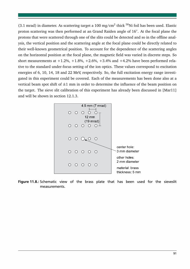
(3.1 mrad) in diameter. As scattering target a 100 mg/cm2 thick 58Ni foil has been used. Elastic
proton scattering was then performed at an Grand Raiden angle of 16. At the focal plane the
protons that were scattered through one of the slits could be detected and so in the offline anal-
ysis, the vertical position and the scattering angle at the focal plane could be directly related to
their well-known geometrical position. To account for the dependence of the scattering angles
on the horizontal position at the focal plane, the magnetic field was varied in discrete steps. So
short measurements at +1.2%, +1.8%, +2.6%, +3.4% and +4.2% have been performed rela-
tive to the standard under-focus setting of the ion optics. These values correspond to excitation
energies of 6, 10, 14, 18 and 22 MeV, respectively. So, the full excitation energy range investi-
gated in this experiment could be covered. Each of the measurements has been done also at a
vertical beam spot shift of ±1 mm in order to determine the influence of the beam position on
the target. The sieve slit calibration of this experiment has already been discussed in [Mar11]
and will be shown in section 12.1.3.
Figure 11.8.: Schematic view of the brass plate that has been used for the sieveslitmeasurements.
91

12 Data analysis for proton scattering
For the data analysis of the 154Sm data, the program code ANALYZER [Tam99] which was de-
veloped at the RCNP has been used. This software package is adapted for the online and offline
analysis of data, taken at the GR spectrometer and LAS. It is written mainly in the program
language C and makes use of the HBOOK and PAW(++) packages of the CERN libraries [CER].
12.1 Data reduction
The data reduction procedure has been performed step by step according to the table below and
will be explained more detailed on the following pages:
• Drift time to distance conversion
• Efficiency determination of the VDCs
• Calibration of scattering angles
• Kinematical corrections and excitation energy calibration
• Higher order aberration corrections
• Subtraction of background
• Cross section determination
• Analysis of polarization transfer observables
Some parts of the data reduction procedure have already been discussed in [Mar11].
12.1.1 Drift time to distance conversion
Vertical drift chambers (VDC) are used for measuring the scattered proton positions. This is
necessary to obtain the trajectory of the particles for determining the angles and excitation
energies with which particles go through the focal plane. In figure 12.1 a schematic view of
a vertical drift chamber is presented. The typical VDC consists of two cathode foils and in
between a layer of wires. Besides the sense wires or signal wires, most of the VDCs also have
potential wires which are used to shape the electric field and to prevent possible cross talk
between different channels. In general, when charged particles go through the detector they
interact with gas molecules and ionize them. The electrons drift towards the anode plane with
an almost constant drift velocity of ≈ 5 cm/µm. Consequently, the drift times are proportional
93
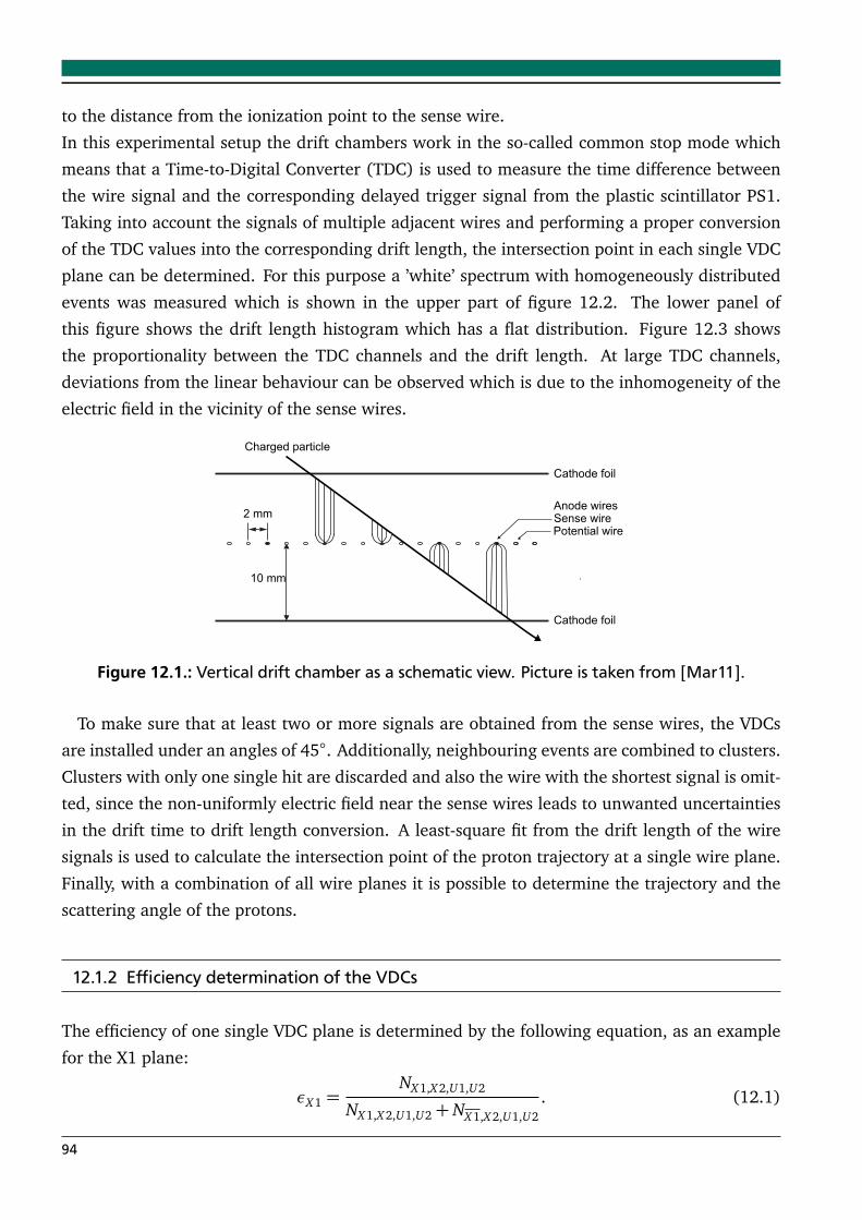
to the distance from the ionization point to the sense wire.
In this experimental setup the drift chambers work in the so-called common stop mode which
means that a Time-to-Digital Converter (TDC) is used to measure the time difference between
the wire signal and the corresponding delayed trigger signal from the plastic scintillator PS1.
Taking into account the signals of multiple adjacent wires and performing a proper conversion
of the TDC values into the corresponding drift length, the intersection point in each single VDC
plane can be determined. For this purpose a ’white’ spectrum with homogeneously distributed
events was measured which is shown in the upper part of figure 12.2. The lower panel of
this figure shows the drift length histogram which has a flat distribution. Figure 12.3 shows
the proportionality between the TDC channels and the drift length. At large TDC channels,
deviations from the linear behaviour can be observed which is due to the inhomogeneity of the
electric field in the vicinity of the sense wires.
Figure 12.1.: Vertical drift chamber as a schematic view. Picture is taken from [Mar11].
To make sure that at least two or more signals are obtained from the sense wires, the VDCs
are installed under an angles of 45. Additionally, neighbouring events are combined to clusters.
Clusters with only one single hit are discarded and also the wire with the shortest signal is omit-
ted, since the non-uniformly electric field near the sense wires leads to unwanted uncertainties
in the drift time to drift length conversion. A least-square fit from the drift length of the wire
signals is used to calculate the intersection point of the proton trajectory at a single wire plane.
Finally, with a combination of all wire planes it is possible to determine the trajectory and the
scattering angle of the protons.
12.1.2 Efficiency determination of the VDCs
The efficiency of one single VDC plane is determined by the following equation, as an example
for the X1 plane:
εX1 =NX1,X2,U1,U2
NX1,X2,U1,U2+ NX1,X2,U1,U2. (12.1)
94
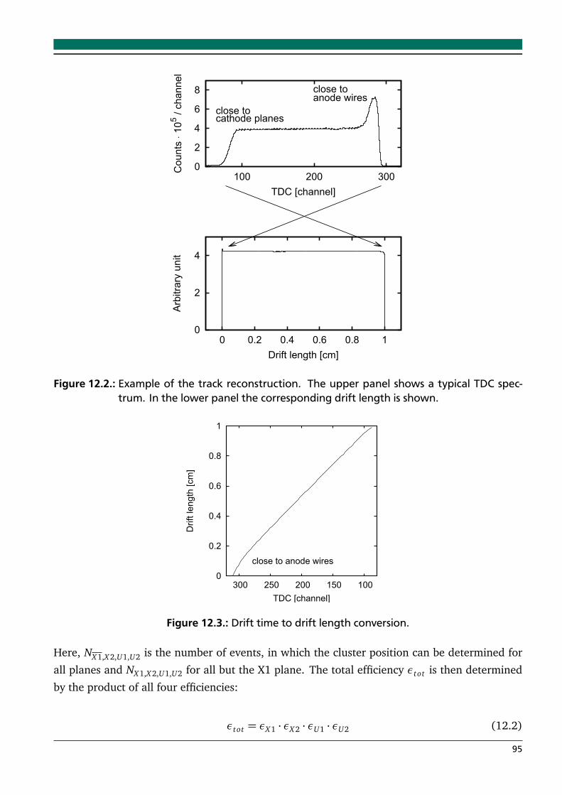
0
2
4
6
8
100 200 300C
ounts
⋅ 1
05 / c
hannel
TDC [channel]
close tocathode planes
close toanode wires
0
2
4
0 0.2 0.4 0.6 0.8 1
Arb
itra
ry u
nit
Drift length [cm]
Figure 12.2.: Example of the track reconstruction. The upper panel shows a typical TDC spec-trum. In the lower panel the corresponding drift length is shown.
0
0.2
0.4
0.6
0.8
1
100 150 200 250 300
Drift length
[cm
]
TDC [channel]
close to anode wires
Figure 12.3.: Drift time to drift length conversion.
Here, NX1,X2,U1,U2 is the number of events, in which the cluster position can be determined for
all planes and NX1,X2,U1,U2 for all but the X1 plane. The total efficiency εtot is then determined
by the product of all four efficiencies:
εtot = εX1 · εX2 · εU1 · εU2 (12.2)
95
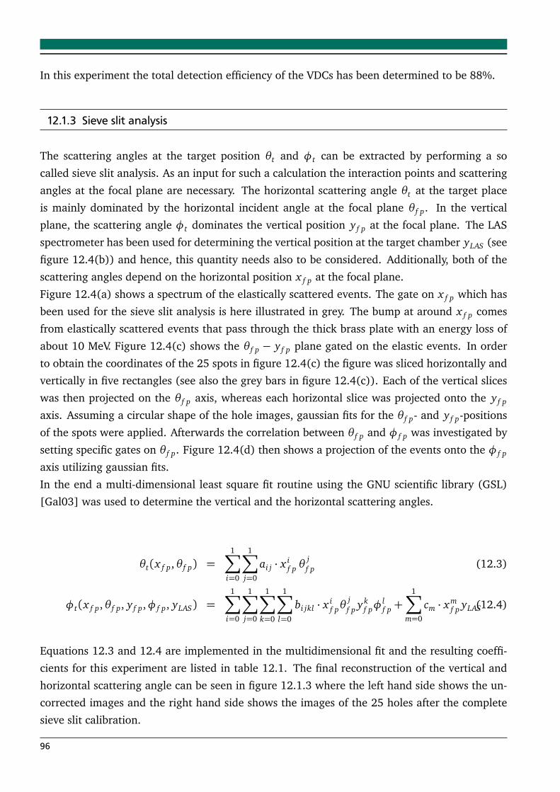
In this experiment the total detection efficiency of the VDCs has been determined to be 88%.
12.1.3 Sieve slit analysis
The scattering angles at the target position θt and φt can be extracted by performing a so
called sieve slit analysis. As an input for such a calculation the interaction points and scattering
angles at the focal plane are necessary. The horizontal scattering angle θt at the target place
is mainly dominated by the horizontal incident angle at the focal plane θ f p. In the vertical
plane, the scattering angle φt dominates the vertical position y f p at the focal plane. The LAS
spectrometer has been used for determining the vertical position at the target chamber yLAS (see
figure 12.4(b)) and hence, this quantity needs also to be considered. Additionally, both of the
scattering angles depend on the horizontal position x f p at the focal plane.
Figure 12.4(a) shows a spectrum of the elastically scattered events. The gate on x f p which has
been used for the sieve slit analysis is here illustrated in grey. The bump at around x f p comes
from elastically scattered events that pass through the thick brass plate with an energy loss of
about 10 MeV. Figure 12.4(c) shows the θ f p − y f p plane gated on the elastic events. In order
to obtain the coordinates of the 25 spots in figure 12.4(c) the figure was sliced horizontally and
vertically in five rectangles (see also the grey bars in figure 12.4(c)). Each of the vertical slices
was then projected on the θ f p axis, whereas each horizontal slice was projected onto the y f p
axis. Assuming a circular shape of the hole images, gaussian fits for the θ f p- and y f p-positions
of the spots were applied. Afterwards the correlation between θ f p and φ f p was investigated by
setting specific gates on θ f p. Figure 12.4(d) then shows a projection of the events onto the φ f p
axis utilizing gaussian fits.
In the end a multi-dimensional least square fit routine using the GNU scientific library (GSL)
[Gal03] was used to determine the vertical and the horizontal scattering angles.
θt(x f p,θ f p) =1∑
i=0
1∑
j=0
ai j · x if p θ
jf p (12.3)
φt(x f p,θ f p, y f p,φ f p, yLAS) =1∑
i=0
1∑
j=0
1∑
k=0
1∑
l=0
bi jkl · x if pθ
jf p yk
f pφlf p +
1∑
m=0
cm · xmf p yLAS(12.4)
Equations 12.3 and 12.4 are implemented in the multidimensional fit and the resulting coeffi-
cients for this experiment are listed in table 12.1. The final reconstruction of the vertical and
horizontal scattering angle can be seen in figure 12.1.3 where the left hand side shows the un-
corrected images and the right hand side shows the images of the 25 holes after the complete
sieve slit calibration.
96
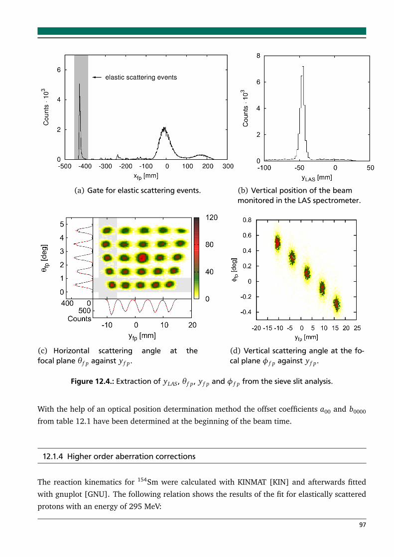
(a) Gate for elastic scattering events. (b) Vertical position of the beammonitored in the LAS spectrometer.
(c) Horizontal scattering angle at thefocal plane θ f p against y f p.
(d) Vertical scattering angle at the fo-cal plane φ f p against y f p.
Figure 12.4.: Extraction of yLAS, θ f p, y f p and φ f p from the sieve slit analysis.
With the help of an optical position determination method the offset coefficients a00 and b0000
from table 12.1 have been determined at the beginning of the beam time.
12.1.4 Higher order aberration corrections
The reaction kinematics for 154Sm were calculated with KINMAT [KIN] and afterwards fitted
with gnuplot [GNU]. The following relation shows the results of the fit for elastically scattered
protons with an energy of 295 MeV:
97
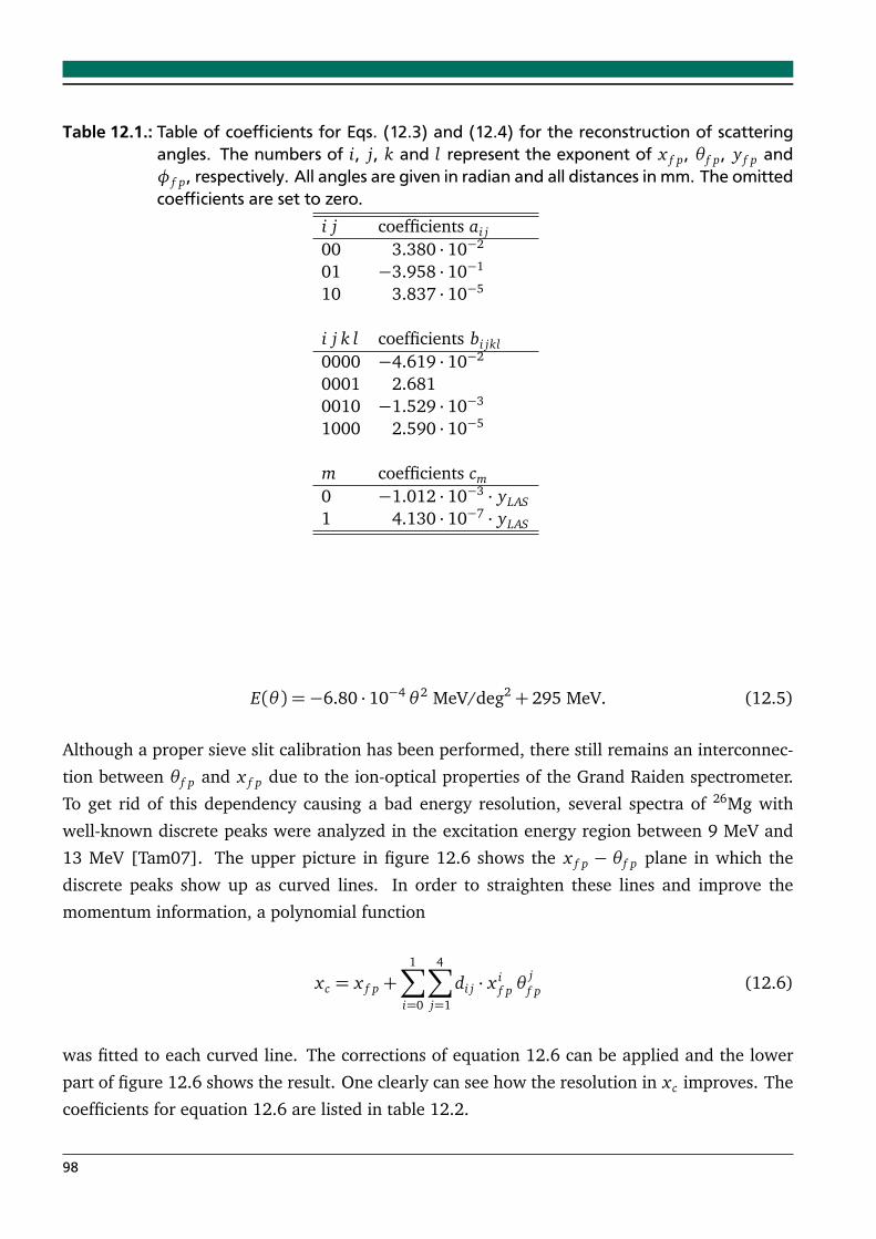
Table 12.1.: Table of coefficients for Eqs. (12.3) and (12.4) for the reconstruction of scatteringangles. The numbers of i, j, k and l represent the exponent of x f p, θ f p, y f p andφ f p, respectively. All angles are given in radian and all distances in mm. The omittedcoefficients are set to zero.
i j coefficients ai j
00 3.380 · 10−2
01 −3.958 · 10−1
10 3.837 · 10−5
i j k l coefficients bi jkl
0000 −4.619 · 10−2
0001 2.6810010 −1.529 · 10−3
1000 2.590 · 10−5
m coefficients cm
0 −1.012 · 10−3 · yLAS1 4.130 · 10−7 · yLAS
E(θ) =−6.80 · 10−4 θ 2 MeV/deg2+ 295 MeV. (12.5)
Although a proper sieve slit calibration has been performed, there still remains an interconnec-
tion between θ f p and x f p due to the ion-optical properties of the Grand Raiden spectrometer.
To get rid of this dependency causing a bad energy resolution, several spectra of 26Mg with
well-known discrete peaks were analyzed in the excitation energy region between 9 MeV and
13 MeV [Tam07]. The upper picture in figure 12.6 shows the x f p − θ f p plane in which the
discrete peaks show up as curved lines. In order to straighten these lines and improve the
momentum information, a polynomial function
xc = x f p +1∑
i=0
4∑
j=1
di j · x if p θ
jf p (12.6)
was fitted to each curved line. The corrections of equation 12.6 can be applied and the lower
part of figure 12.6 shows the result. One clearly can see how the resolution in xc improves. The
coefficients for equation 12.6 are listed in table 12.2.
98
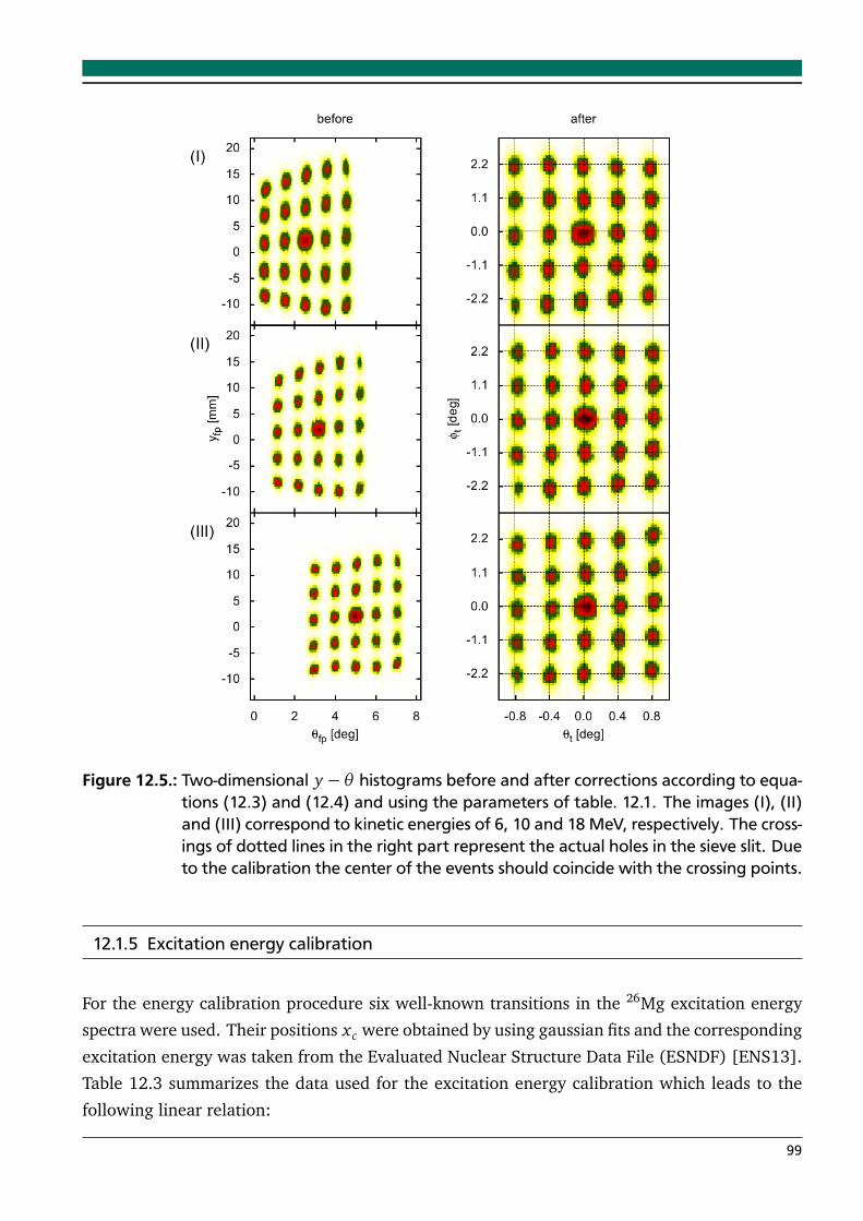
Figure 12.5.: Two-dimensional y−θ histograms before and after corrections according to equa-tions (12.3) and (12.4) and using the parameters of table. 12.1. The images (I), (II)and (III) correspond to kinetic energies of 6, 10 and 18 MeV, respectively. The cross-ings of dotted lines in the right part represent the actual holes in the sieve slit. Dueto the calibration the center of the events should coincide with the crossing points.
12.1.5 Excitation energy calibration
For the energy calibration procedure six well-known transitions in the 26Mg excitation energy
spectra were used. Their positions xc were obtained by using gaussian fits and the corresponding
excitation energy was taken from the Evaluated Nuclear Structure Data File (ESNDF) [ENS13].
Table 12.3 summarizes the data used for the excitation energy calibration which leads to the
following linear relation:
99
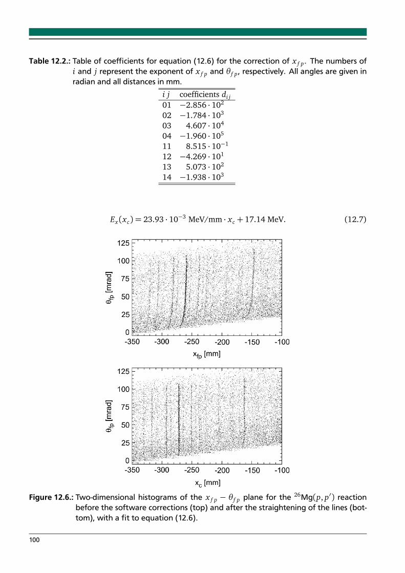
Table 12.2.: Table of coefficients for equation (12.6) for the correction of x f p. The numbers ofi and j represent the exponent of x f p and θ f p, respectively. All angles are given inradian and all distances in mm.
i j coefficients di j
01 −2.856 · 102
02 −1.784 · 103
03 4.607 · 104
04 −1.960 · 105
11 8.515 · 10−1
12 −4.269 · 101
13 5.073 · 102
14 −1.938 · 103
Ex(xc) = 23.93 · 10−3 MeV/mm · xc + 17.14 MeV. (12.7)
Figure 12.6.: Two-dimensional histograms of the x f p − θ f p plane for the 26Mg(p, p′) reactionbefore the software corrections (top) and after the straightening of the lines (bot-tom), with a fit to equation (12.6).
100
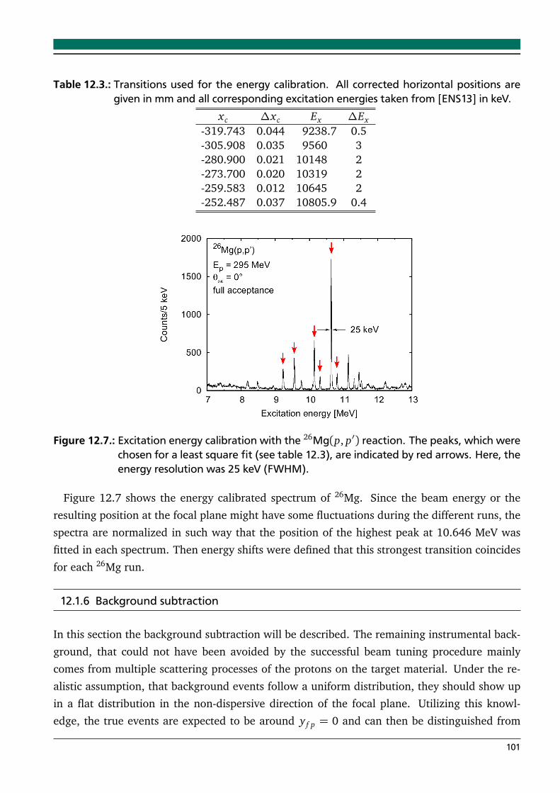
Table 12.3.: Transitions used for the energy calibration. All corrected horizontal positions aregiven in mm and all corresponding excitation energies taken from [ENS13] in keV.
xc ∆xc Ex ∆Ex
-319.743 0.044 9238.7 0.5-305.908 0.035 9560 3-280.900 0.021 10148 2-273.700 0.020 10319 2-259.583 0.012 10645 2-252.487 0.037 10805.9 0.4
Figure 12.7.: Excitation energy calibration with the 26Mg(p, p′) reaction. The peaks, which werechosen for a least square fit (see table 12.3), are indicated by red arrows. Here, theenergy resolution was 25 keV (FWHM).
Figure 12.7 shows the energy calibrated spectrum of 26Mg. Since the beam energy or the
resulting position at the focal plane might have some fluctuations during the different runs, the
spectra are normalized in such way that the position of the highest peak at 10.646 MeV was
fitted in each spectrum. Then energy shifts were defined that this strongest transition coincides
for each 26Mg run.
12.1.6 Background subtraction
In this section the background subtraction will be described. The remaining instrumental back-
ground, that could not have been avoided by the successful beam tuning procedure mainly
comes from multiple scattering processes of the protons on the target material. Under the re-
alistic assumption, that background events follow a uniform distribution, they should show up
in a flat distribution in the non-dispersive direction of the focal plane. Utilizing this knowl-
edge, the true events are expected to be around y f p = 0 and can then be distinguished from
101
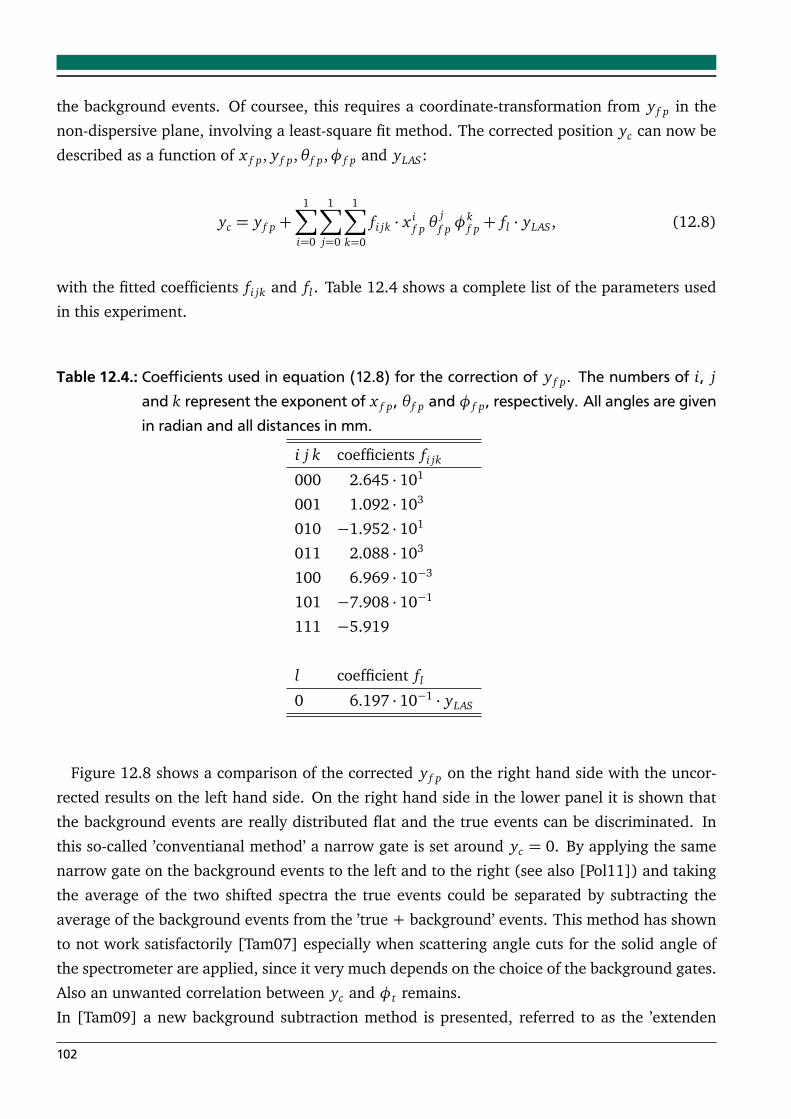
the background events. Of coursee, this requires a coordinate-transformation from y f p in the
non-dispersive plane, involving a least-square fit method. The corrected position yc can now be
described as a function of x f p, y f p,θ f p,φ f p and yLAS:
yc = y f p +1∑
i=0
1∑
j=0
1∑
k=0
fi jk · x if p θ
jf pφ
kf p + fl · yLAS, (12.8)
with the fitted coefficients fi jk and fl . Table 12.4 shows a complete list of the parameters used
in this experiment.
Table 12.4.: Coefficients used in equation (12.8) for the correction of y f p. The numbers of i, j
and k represent the exponent of x f p, θ f p and φ f p, respectively. All angles are givenin radian and all distances in mm.
i j k coefficients fi jk
000 2.645 · 101
001 1.092 · 103
010 −1.952 · 101
011 2.088 · 103
100 6.969 · 10−3
101 −7.908 · 10−1
111 −5.919
l coefficient fl
0 6.197 · 10−1 · yLAS
Figure 12.8 shows a comparison of the corrected y f p on the right hand side with the uncor-
rected results on the left hand side. On the right hand side in the lower panel it is shown that
the background events are really distributed flat and the true events can be discriminated. In
this so-called ’conventianal method’ a narrow gate is set around yc = 0. By applying the same
narrow gate on the background events to the left and to the right (see also [Pol11]) and taking
the average of the two shifted spectra the true events could be separated by subtracting the
average of the background events from the ’true + background’ events. This method has shown
to not work satisfactorily [Tam07] especially when scattering angle cuts for the solid angle of
the spectrometer are applied, since it very much depends on the choice of the background gates.
Also an unwanted correlation between yc and φt remains.
In [Tam09] a new background subtraction method is presented, referred to as the ’extenden
102
Figure 12.8.: Correlation between the vertical scattering angle φ f p and the vertical position inthe ’conventional method’ for the background subtraction. On the left hand side,the untransformed data is shown and on the right hand side the transformation inequation 12.8 has been utilized.
method’. With this method the dependece of yc on the scattering angle φt could be omitted but
needs the implementation of a corrected scattering angle φc which is now independent of yc.
The method is based on the assumption that the background events are homogeneously dis-
tributed in the yc−φc plane (the vertical acceptance of the spectrometer). This requires another
correction, which is performed with respect to φc in a similar way as it has been done to y f p:
φc = φ f p +1∑
i=0
ei · y if p, (12.9)
The coefficients ei are fitted parameters. The corrected vertical acceptance is now shown
on the left hand side of figure 12.9. Here, the true events are distributed inside the black
rectangle around yc = 0 and φc = 0. Analogue to the background subtraction procedure in the
’conventional method’ the data is shifted by a constant factor to the left and to the right (see the
pictures in the middle and on the right hand side of figure 12.9). Then again, the ’true’ dataset
is obtained by subtracting the average of the shifted data from the ’true + background’ events.
In figure 12.10 the resulting excitation energy and background spectrum is presented for 154Sm
at 0 using the full acceptance of the Grand Raiden spectrometer.
Finally the background subtracted spectrum for the full acceptance of the Grand Raiden spec-
trometer is shown in figure 12.11 for the 0 data set. One clearly observes the two bumps of the
103
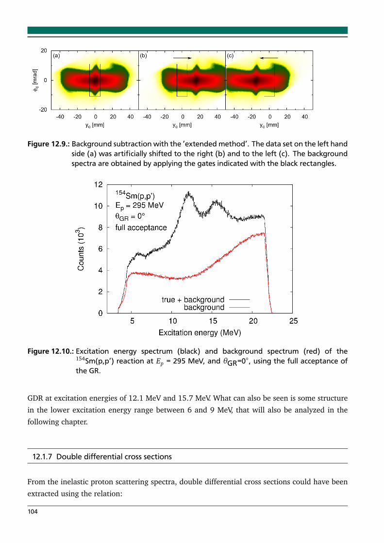
Figure 12.9.: Background subtraction with the ’extended method’. The data set on the left handside (a) was artificially shifted to the right (b) and to the left (c). The backgroundspectra are obtained by applying the gates indicated with the black rectangles.
Figure 12.10.: Excitation energy spectrum (black) and background spectrum (red) of the154Sm(p,p’) reaction at Ep = 295 MeV, and θGR=0, using the full acceptance ofthe GR.
GDR at excitation energies of 12.1 MeV and 15.7 MeV. What can also be seen is some structure
in the lower excitation energy range between 6 and 9 MeV, that will also be analyzed in the
following chapter.
12.1.7 Double differential cross sections
From the inelastic proton scattering spectra, double differential cross sections could have been
extracted using the relation:
104
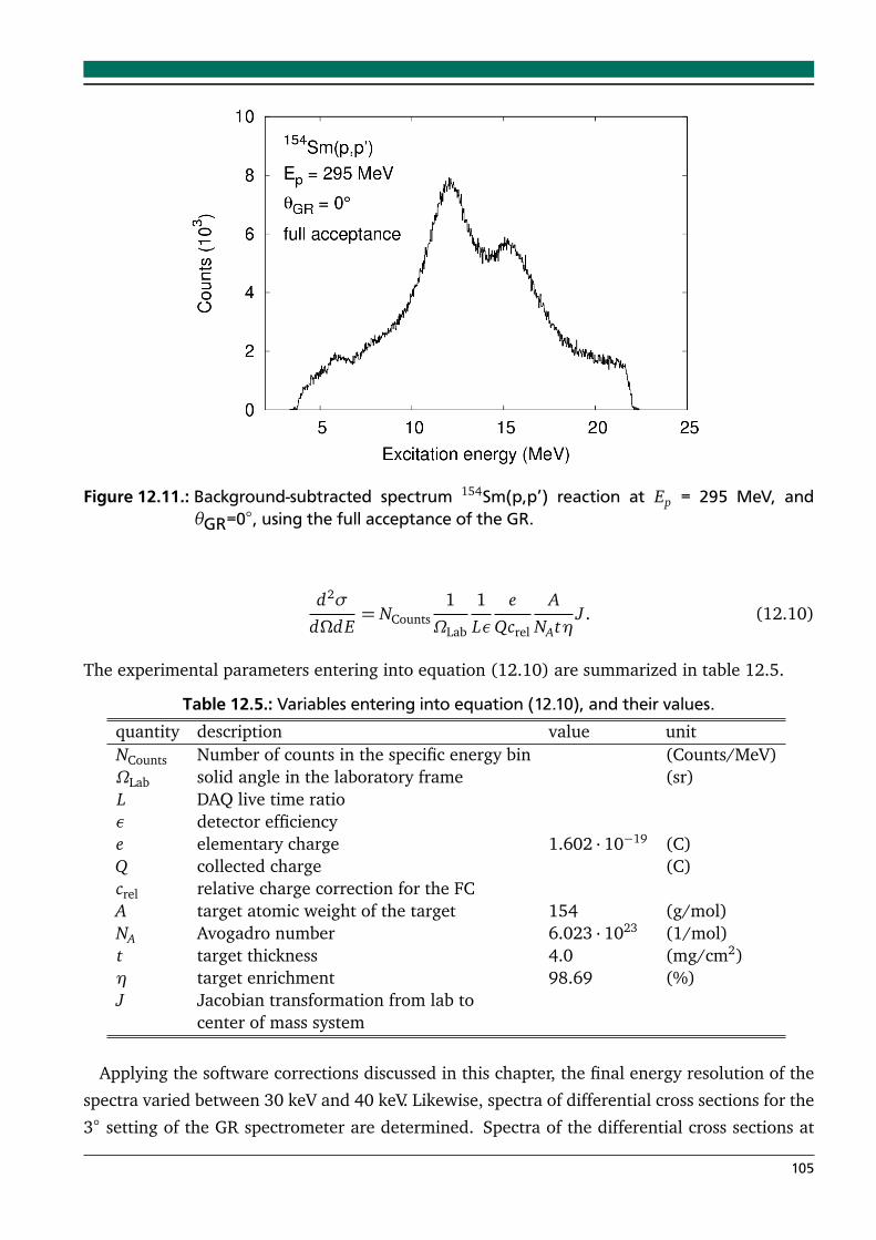
Figure 12.11.: Background-subtracted spectrum 154Sm(p,p’) reaction at Ep = 295 MeV, andθGR=0, using the full acceptance of the GR.
d2σ
dΩdE= NCounts
1
ΩLab
1
Lε
e
Qcrel
A
NAtηJ . (12.10)
The experimental parameters entering into equation (12.10) are summarized in table 12.5.
Table 12.5.: Variables entering into equation (12.10), and their values.quantity description value unitNCounts Number of counts in the specific energy bin (Counts/MeV)ΩLab solid angle in the laboratory frame (sr)L DAQ live time ratioε detector efficiencye elementary charge 1.602 · 10−19 (C)Q collected charge (C)crel relative charge correction for the FCA target atomic weight of the target 154 (g/mol)NA Avogadro number 6.023 · 1023 (1/mol)t target thickness 4.0 (mg/cm2)η target enrichment 98.69 (%)J Jacobian transformation from lab to
center of mass system
Applying the software corrections discussed in this chapter, the final energy resolution of the
spectra varied between 30 keV and 40 keV. Likewise, spectra of differential cross sections for the
3 setting of the GR spectrometer are determined. Spectra of the differential cross sections at
105
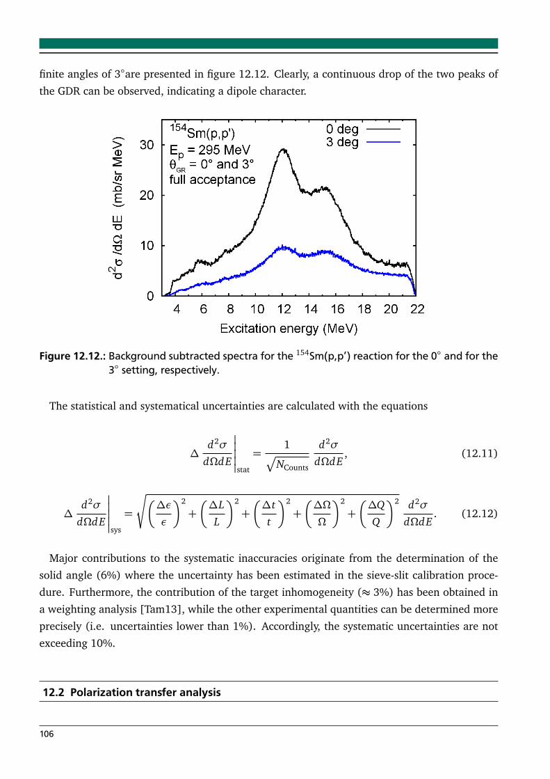
finite angles of 3are presented in figure 12.12. Clearly, a continuous drop of the two peaks of
the GDR can be observed, indicating a dipole character.
Figure 12.12.: Background subtracted spectra for the 154Sm(p,p’) reaction for the 0 and for the3 setting, respectively.
The statistical and systematical uncertainties are calculated with the equations
∆d2σ
dΩdE
stat
=1
p
NCounts
d2σ
dΩdE, (12.11)
∆d2σ
dΩdE
sys
=
È
∆εε
2
+
∆L
L
2
+
∆t
t
2
+
∆ΩΩ
2
+
∆Q
Q
2 d2σ
dΩdE. (12.12)
Major contributions to the systematic inaccuracies originate from the determination of the
solid angle (6%) where the uncertainty has been estimated in the sieve-slit calibration proce-
dure. Furthermore, the contribution of the target inhomogeneity (≈ 3%) has been obtained in
a weighting analysis [Tam13], while the other experimental quantities can be determined more
precisely (i.e. uncertainties lower than 1%). Accordingly, the systematic uncertainties are not
exceeding 10%.
12.2 Polarization transfer analysis
106
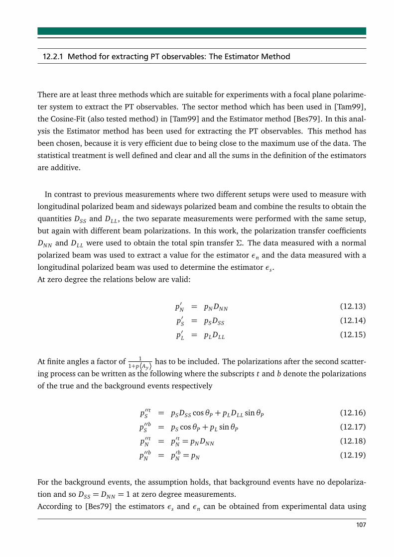
12.2.1 Method for extracting PT observables: The Estimator Method
There are at least three methods which are suitable for experiments with a focal plane polarime-
ter system to extract the PT observables. The sector method which has been used in [Tam99],
the Cosine-Fit (also tested method) in [Tam99] and the Estimator method [Bes79]. In this anal-
ysis the Estimator method has been used for extracting the PT observables. This method has
been chosen, because it is very efficient due to being close to the maximum use of the data. The
statistical treatment is well defined and clear and all the sums in the definition of the estimators
are additive.
In contrast to previous measurements where two different setups were used to measure with
longitudinal polarized beam and sideways polarized beam and combine the results to obtain the
quantities DSS and DLL, the two separate measurements were performed with the same setup,
but again with different beam polarizations. In this work, the polarization transfer coefficients
DNN and DLL were used to obtain the total spin transfer Σ. The data measured with a normal
polarized beam was used to extract a value for the estimator εn and the data measured with a
longitudinal polarized beam was used to determine the estimator εs.
At zero degree the relations below are valid:
p′N = pN DNN (12.13)
p′S = pS DSS (12.14)
p′L = pL DLL (12.15)
At finite angles a factor of 11+p⟨Ay⟩ has to be included. The polarizations after the second scatter-
ing process can be written as the following where the subscripts t and b denote the polarizations
of the true and the background events respectively
p′′tS = pS DSS cosθP + pL DLL sinθP (12.16)
p′′bS = pS cosθP + pL sinθP (12.17)
p′′tN = p′tN = pN DNN (12.18)
p′′bN = p′bN = pN (12.19)
For the background events, the assumption holds, that background events have no depolariza-
tion and so DSS = DNN = 1 at zero degree measurements.
According to [Bes79] the estimators εs and εn can be obtained from experimental data using
107
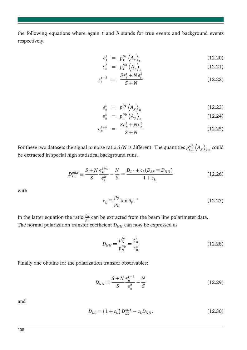
the following equations where again t and b stands for true events and background events
respectively.
εts = p′′ts
¬
Ay
¶
s(12.20)
εbs = p′′bs
¬
Ay
¶
s(12.21)
εt+bs =
Sεts + Nεb
s
S+ N(12.22)
εtn = p′′tn
¬
Ay
¶
n(12.23)
εbn = p′′bn
¬
Ay
¶
n(12.24)
εt+bn =
Sεtn+ Nεb
n
S+ N(12.25)
For these two datasets the signal to noise ratio S/N is different. The quantities p′′bs,n
¬
Ay
¶
s,ncould
be extracted in special high statistical background runs.
DmixLL ≡
S+ N
S
εt+bs
εbs
−N
S=
DLL + cL(DSS = DNN )1+ cL
(12.26)
with
cL ≡pS
pLtanθP
−1 (12.27)
In the latter equation the ratio pSpL
can be extracted from the beam line polarimeter data.
The normal polarization transfer coefficient DNN can now be expressed as
DNN =p′′tN
p′′bN
=εt
n
εbn
(12.28)
Finally one obtains for the polarization transfer observables:
DNN =S+ N
S
εt+bn
εbn
−N
S(12.29)
and
DLL =
1+ cL
DmixLL − cL DNN . (12.30)
108
12.3 Results of the polarization transfer analysis
The polarization transfer analysis as it has been explained in section 12.2 has been performed
and the polarization transfer coefficients DNN and DLL could be determined. With the relation
10.57 the total spin transfer Σ can be calculated that allows to decompose the spectrum into a
spinflip part and a non-spinflip part.
12.3.1 Results for 26Mg
Since 26Mg has some well known 1+ states which have pure spinflip character and 26Mg data
runs have been performed after each 154Sm data run, it is well suited for checking the polar-
ization transfer analysis method. The uppermost panel in figure 12.13 shows the spectrum of26Mg in the excitation energy range between 6 and 14 MeV with some clear peaks coming from
dipole excitations. The corresponding DNN and DLL polarisation transfer observables are shown
in the panels below. The bottom panel of figure 12.13 displays the total spin transfer Σ. In the
observed energy range, 1− states and 1+ states can be correctly assigned and the results are
consistent with older measurements [Tam07].
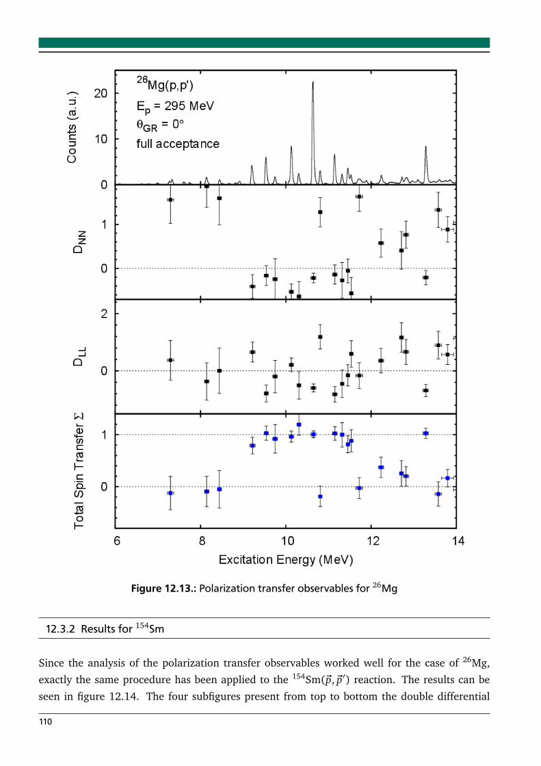
Figure 12.13.: Polarization transfer observables for 26Mg
12.3.2 Results for 154Sm
Since the analysis of the polarization transfer observables worked well for the case of 26Mg,
exactly the same procedure has been applied to the 154Sm(~p,~p′) reaction. The results can be
seen in figure 12.14. The four subfigures present from top to bottom the double differential
110
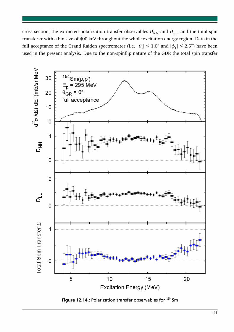
cross section, the extracted polarization transfer observables DNN and DLL, and the total spin
transfer σ with a bin size of 400 keV throughout the whole excitation energy region. Data in the
full acceptance of the Grand Raiden spectrometer (i.e. |θt | ≤ 1.0 and |φt | ≤ 2.5) have been
used in the present analysis. Due to the non-spinflip nature of the GDR the total spin transfer
Figure 12.14.: Polarization transfer observables for 154Sm
111
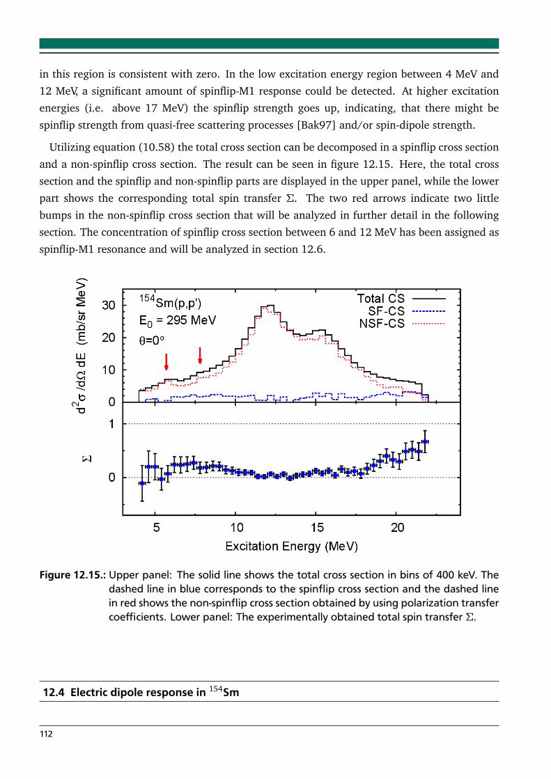
in this region is consistent with zero. In the low excitation energy region between 4 MeV and
12 MeV, a significant amount of spinflip-M1 response could be detected. At higher excitation
energies (i.e. above 17 MeV) the spinflip strength goes up, indicating, that there might be
spinflip strength from quasi-free scattering processes [Bak97] and/or spin-dipole strength.
Utilizing equation (10.58) the total cross section can be decomposed in a spinflip cross section
and a non-spinflip cross section. The result can be seen in figure 12.15. Here, the total cross
section and the spinflip and non-spinflip parts are displayed in the upper panel, while the lower
part shows the corresponding total spin transfer Σ. The two red arrows indicate two little
bumps in the non-spinflip cross section that will be analyzed in further detail in the following
section. The concentration of spinflip cross section between 6 and 12 MeV has been assigned as
spinflip-M1 resonance and will be analyzed in section 12.6.
Figure 12.15.: Upper panel: The solid line shows the total cross section in bins of 400 keV. Thedashed line in blue corresponds to the spinflip cross section and the dashed linein red shows the non-spinflip cross section obtained by using polarization transfercoefficients. Lower panel: The experimentally obtained total spin transfer Σ.
12.4 Electric dipole response in 154Sm
112
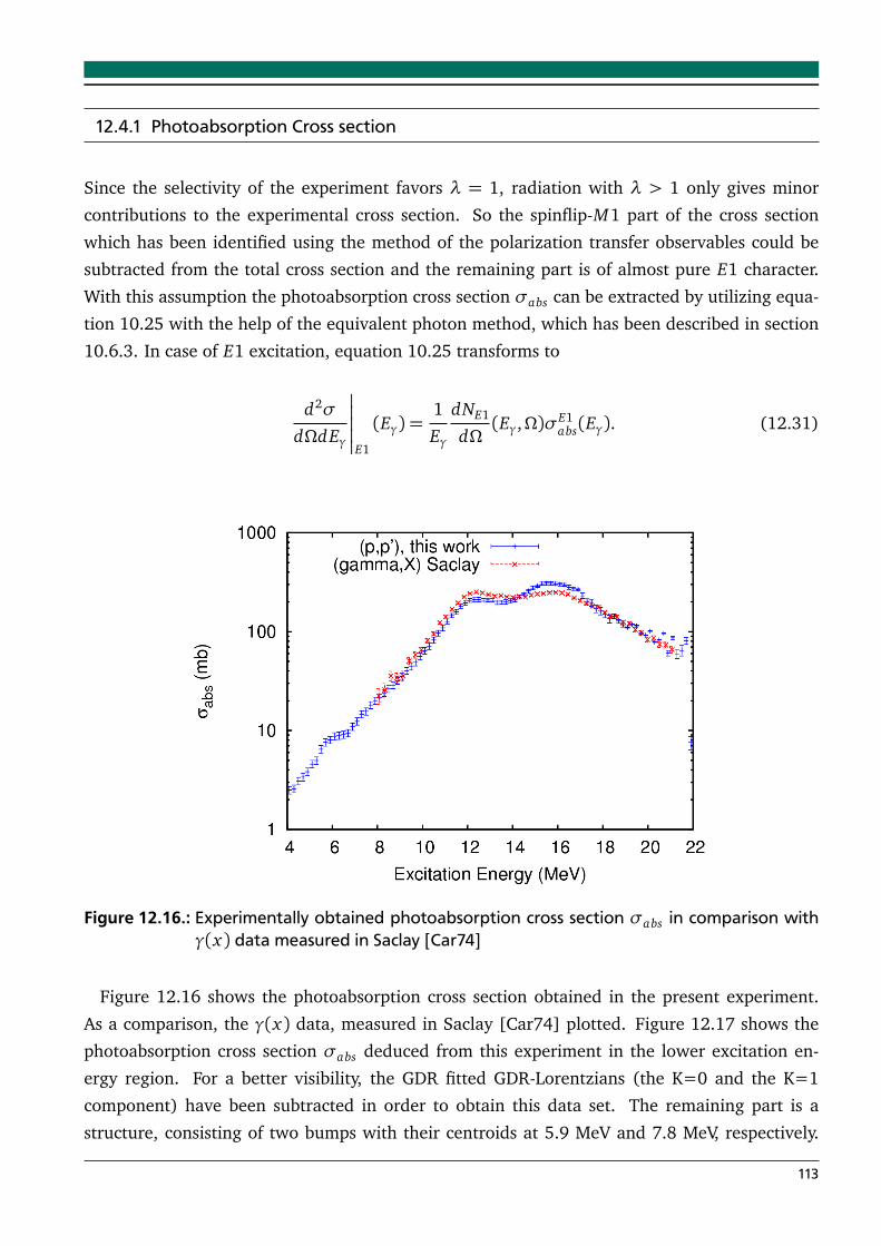
12.4.1 Photoabsorption Cross section
Since the selectivity of the experiment favors λ = 1, radiation with λ > 1 only gives minor
contributions to the experimental cross section. So the spinflip-M1 part of the cross section
which has been identified using the method of the polarization transfer observables could be
subtracted from the total cross section and the remaining part is of almost pure E1 character.
With this assumption the photoabsorption cross section σabs can be extracted by utilizing equa-
tion 10.25 with the help of the equivalent photon method, which has been described in section
10.6.3. In case of E1 excitation, equation 10.25 transforms to
d2σ
dΩdEγ
E1
(Eγ) =1
Eγ
dNE1
dΩ(Eγ,Ω)σ
E1abs(Eγ). (12.31)
Figure 12.16.: Experimentally obtained photoabsorption cross section σabs in comparison withγ(x) data measured in Saclay [Car74]
Figure 12.16 shows the photoabsorption cross section obtained in the present experiment.
As a comparison, the γ(x) data, measured in Saclay [Car74] plotted. Figure 12.17 shows the
photoabsorption cross section σabs deduced from this experiment in the lower excitation en-
ergy region. For a better visibility, the GDR fitted GDR-Lorentzians (the K=0 and the K=1
component) have been subtracted in order to obtain this data set. The remaining part is a
structure, consisting of two bumps with their centroids at 5.9 MeV and 7.8 MeV, respectively.
113
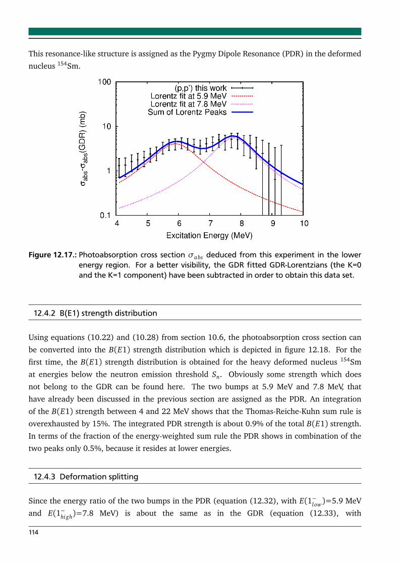
This resonance-like structure is assigned as the Pygmy Dipole Resonance (PDR) in the deformed
nucleus 154Sm.
Figure 12.17.: Photoabsorption cross section σabs deduced from this experiment in the lowerenergy region. For a better visibility, the GDR fitted GDR-Lorentzians (the K=0and the K=1 component) have been subtracted in order to obtain this data set.
12.4.2 B(E1) strength distribution
Using equations (10.22) and (10.28) from section 10.6, the photoabsorption cross section can
be converted into the B(E1) strength distribution which is depicted in figure 12.18. For the
first time, the B(E1) strength distribution is obtained for the heavy deformed nucleus 154Sm
at energies below the neutron emission threshold Sn. Obviously some strength which does
not belong to the GDR can be found here. The two bumps at 5.9 MeV and 7.8 MeV, that
have already been discussed in the previous section are assigned as the PDR. An integration
of the B(E1) strength between 4 and 22 MeV shows that the Thomas-Reiche-Kuhn sum rule is
overexhausted by 15%. The integrated PDR strength is about 0.9% of the total B(E1) strength.
In terms of the fraction of the energy-weighted sum rule the PDR shows in combination of the
two peaks only 0.5%, because it resides at lower energies.
12.4.3 Deformation splitting
Since the energy ratio of the two bumps in the PDR (equation (12.32), with E(1−low)=5.9 MeV
and E(1−high)=7.8 MeV) is about the same as in the GDR (equation (12.33), with
114
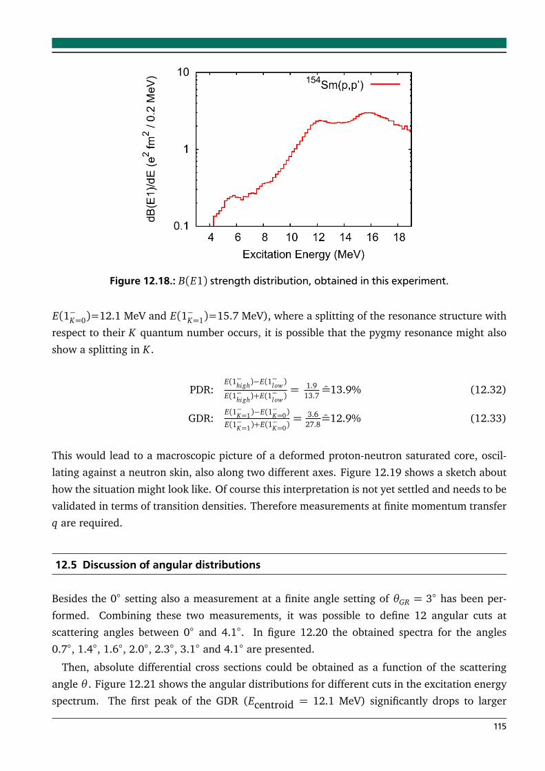
Figure 12.18.: B(E1) strength distribution, obtained in this experiment.
E(1−K=0)=12.1 MeV and E(1−K=1)=15.7 MeV), where a splitting of the resonance structure with
respect to their K quantum number occurs, it is possible that the pygmy resonance might also
show a splitting in K .
PDR:E(1−high)−E(1−low)
E(1−high)+E(1−low)= 1.9
13.7=13.9% (12.32)
GDR:E(1−K=1)−E(1−K=0)
E(1−K=1)+E(1−K=0)= 3.6
27.8=12.9% (12.33)
This would lead to a macroscopic picture of a deformed proton-neutron saturated core, oscil-
lating against a neutron skin, also along two different axes. Figure 12.19 shows a sketch about
how the situation might look like. Of course this interpretation is not yet settled and needs to be
validated in terms of transition densities. Therefore measurements at finite momentum transfer
q are required.
12.5 Discussion of angular distributions
Besides the 0 setting also a measurement at a finite angle setting of θGR = 3 has been per-
formed. Combining these two measurements, it was possible to define 12 angular cuts at
scattering angles between 0 and 4.1. In figure 12.20 the obtained spectra for the angles
0.7, 1.4, 1.6, 2.0, 2.3, 3.1 and 4.1 are presented.
Then, absolute differential cross sections could be obtained as a function of the scattering
angle θ . Figure 12.21 shows the angular distributions for different cuts in the excitation energy
spectrum. The first peak of the GDR (Ecentroid = 12.1 MeV) significantly drops to larger
115
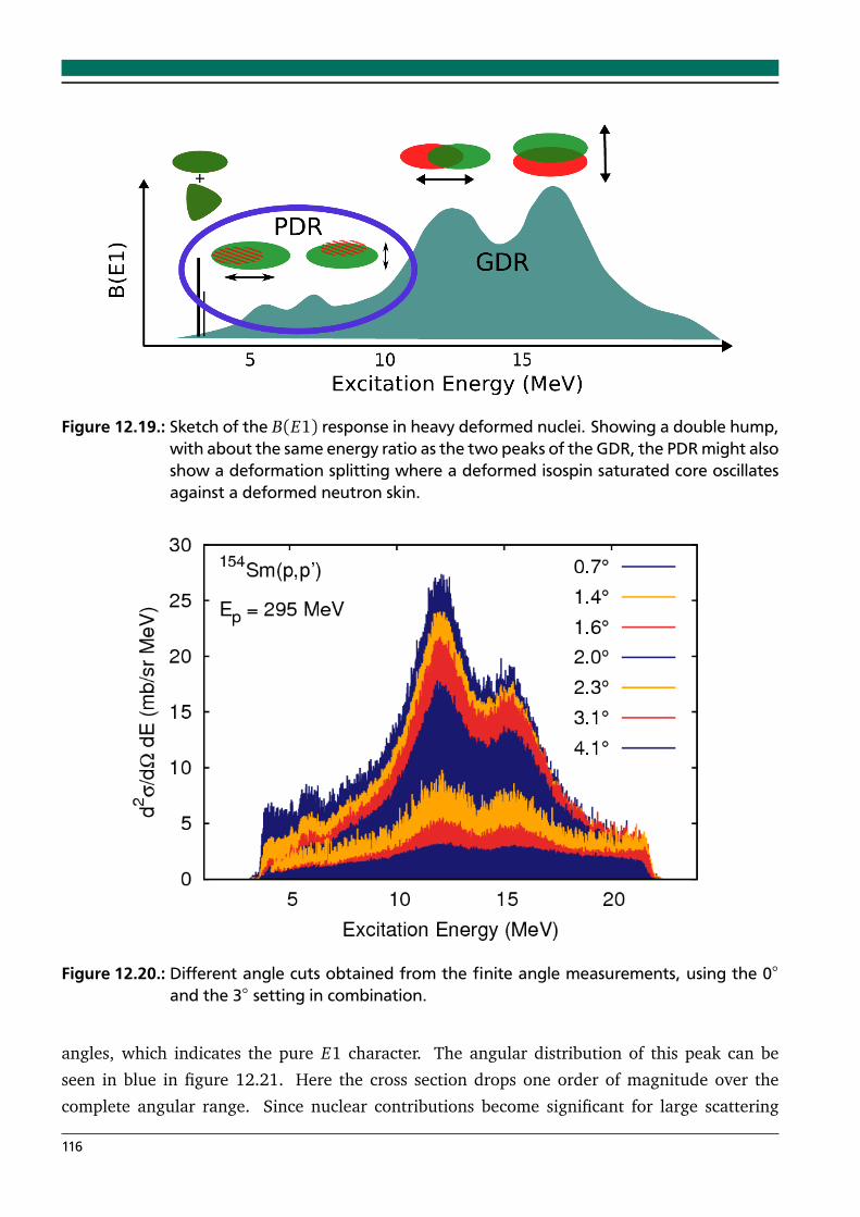
Figure 12.19.: Sketch of the B(E1) response in heavy deformed nuclei. Showing a double hump,with about the same energy ratio as the two peaks of the GDR, the PDR might alsoshow a deformation splitting where a deformed isospin saturated core oscillatesagainst a deformed neutron skin.
Figure 12.20.: Different angle cuts obtained from the finite angle measurements, using the 0
and the 3 setting in combination.
angles, which indicates the pure E1 character. The angular distribution of this peak can be
seen in blue in figure 12.21. Here the cross section drops one order of magnitude over the
complete angular range. Since nuclear contributions become significant for large scattering
116
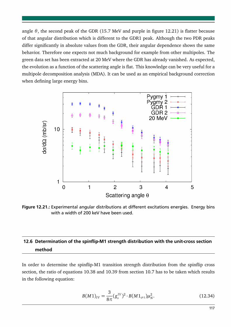
angle θ , the second peak of the GDR (15.7 MeV and purple in figure 12.21) is flatter because
of that angular distribution which is different to the GDR1 peak. Although the two PDR peaks
differ significantly in absolute values from the GDR, their angular dependence shows the same
behavior. Therefore one expects not much background for example from other multipoles. The
green data set has been extracted at 20 MeV where the GDR has already vanished. As expected,
the evolution as a function of the scattering angle is flat. This knowledge can be very useful for a
multipole decomposition analysis (MDA). It can be used as an empirical background correction
when defining large energy bins.
Figure 12.21.: Experimental angular distributions at different excitations energies. Energy binswith a width of 200 keV have been used.
12.6 Determination of the spinflip-M1 strength distribution with the unit-cross section
method
In order to determine the spinflip-M1 transition strength distribution from the spinflip cross
section, the ratio of equations 10.38 and 10.39 from section 10.7 has to be taken which results
in the following equation:
B(M1)IV =3
8π(g IV
s )2 · B(M1στ)µ
2N . (12.34)
117
Utilizing equation 10.40 one obtains
B(M1)IV =3
8π(g IV
s )2 ·
dσdΩ
M1
pp′(0)
FM1σM1(A)µ2
N . (12.35)
The kinematical factor FM1 usually is determined with theoretical angular distributions from
a DWBA calculation. Since no big deviations from 1 are expected throughout the observed
excitation energy range, it has been approximated with unity. The unit-cross section σM1(A) can
be calculated via the unit-cross section of the Gamow-Teller transition σGT−(A). This requires
the ratio from equations 10.40 and 10.42 and also equations 10.39 and 10.41 have to be taken
into account. The Clebsch-Gordan coefficients C2M1,10 =
T0T0+1
and C2GT−= 2T0−1
2T0+1are taken from
reference [Fuj11]. With T0 = 15 for 154Sm and the ratio
dσdΩ
GTFM1
dσdΩ
M1
pp′FM1
= 2 (12.36)
the unit-cross section σM1(A) can be calculated:
σM1(A) =1
2
T0+ 1
T0σGT−(A). (12.37)
In reference [Sas09] it is discussed that σGT−(A) for 300 MeV proton scattering can be obtained
from the phenomenological description
σGT−(A) = N90e−x(A−1/3−90−1/3) (12.38)
with N90 = (3.4± 0.2) mb/sr and x = 0.40± 0.05. Finally the spinflip-M1 strength distribution
can be determined and it is shown in the upper part of figure 12.22. As a reference, the spinflip-
M1 distribution from [Wör94] is shown which indicates a double hump structure. The lower
bump at roughly 6 MeV is seen in hte present (p,p’) experiment but less strength is observed,
concluding that parts of the cross section from [Wör94] was originally of E1 nature. A fairly
good agreement can be seen between between 7 and 9 MeV and even more strength has been
seen in the present experiment at higher energy but with large uncertainties.
The lower part of figure 12.22 shows the running sum of spinflip-M1 strength between 4 MeV
and 12 MeV. The total strength is 13.2± 2.7 µ2N which is in a good agreement to the work of
Wörtche [Wör94] (10.5± 2.0 µ2N ).
118
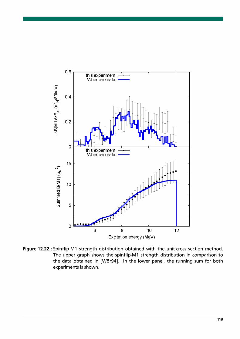
Figure 12.22.: Spinflip-M1 strength distribution obtained with the unit-cross section method.The upper graph shows the spinflip-M1 strength distribution in comparison tothe data obtained in [Wör94]. In the lower panel, the running sum for bothexperiments is shown.
119

13 Conclusion and Outlook
To summarize, in part II of this PhD thesis, the data analysis of a high resolution polarized
proton scattering experiment on the heavy deformed nucleus 154Sm has been presented. The
experiment has been performed at the RCNP in Osaka, Japan, using a 295 MeV beam of polar-
ized protons, scattering off a self-supporting metallic 154Sm foil. With the advanced dispersion
matching techniques, excellent beam conditions were achieved, resulting in a very high energy
resolution of ∆E = 30− 40 keV. Utilizing the polarization transfer analysis, the experimental
cross section could be separated into spinflip and non-spinflip parts. Also measurements at fi-
nite scattering angles have been performed at θGR = 0 and θGR = 3 which made it possible
to extract angular distributions for different modes of excitation. In the case of electric dipole
response, the photoabsorption cross section was calculated and compared to former (γ, n) mea-
surements, showing a good agreement. Also the B(E1) strength distribution has been investi-
gated, where for the first time in 154Sm the pygmy dipole resonance was observed. It appeared
in a double hump structure with peaks in the excitation energy of 5.9 MeV and 7.8 MeV have
been observed. A possible explanation in terms of a deformation splitting of the PDR was given.
Also the spinflip-M1 strength distribution has been determined with the help of the unit-cross
section method. A broad distribution between 5 and 12 MeV has been seen, resulting in a total
spinflip-M1 sum strength of 13.1±2.7 µ2N .
As an outlook in the future the following aspects should be worth investigating:
• The PDR has now been seen in the spherical nucleus 144Sm and the prolate deformed154Sm. It would be interesting to examine the role of the deformation for the PDR in the
whole isotopic chain.
• A multipole decomposition analysis (MDA) as it has been already performed in [Pol11,
Mar13] as an independent tool for the E1 and M1 separation of the cross section would
be ideal to compare to the results from the polarization transfer analysis. Therefore theo-
retical angular distributions are calculated in the framework of the quasi-particle phonon
Model (QPM) [Sol92]. It is a phenomenological microscopic nuclear model where cou-
plings to complex degrees of freedom are considered. With the help of this theoretical
model, various collective excitations in heavy nuclei have been successfully described.
Nice examples for the low-lying quadrupole strength in vibrational nuclei can be seen
in [Wal11] and for the case of the pygmy resonance in 208Pb the article [Pol12] can be
recommended. Since 154Sm is a heavy deformed nucleus, some difficulties in the theoret-
ical description occur. The problems start already on the mean field level. In a spherical
symmetric Woods Saxon potential all single-particle energies of a given orbit are degener-
ate, which results in analytical solutions of the wave functions. In the case of deformation,
121

this degeneracy is usually broken. The number of energy levels increases dramatically and
a lot of particle-hole transitions are possible. Also the configuration space is much bigger
than in the spherical case. The QPM framework needs further development to account
for the complexity of the deformation. An extension of the QPM to real deformed cal-
culations would be preferable and comparison to this experiment in terms of a multipole
decomposition analysis is forseen for the near future.
• Up to now, only dipole contribution to the total cross section have been taken into con-
sideration (e.g. Pygmy-E1, GDR-E1, spinflip-M1). Recent (α,α′) studies [Tam14] show a
non vanishing percentage of E0 and E2 parts coming from the giant monopole resonance
(GMR) and the giant quadrupole resonance (GQR), respectively. It would be useful to esti-
mate the percentage of the E0 and E2 strength that is still hiding in the double differential
cross section.
• As a future perspective for investigating the nature of the double hump structure of the
PDR in heavy deformed nuclei the CAGRA [CAG14] collaboration is planning (p,p’γ) mea-
surements at finite q. A new beam line has been constructed at the RCNP facility where
Grand Raiden angles from 4 to 20 can be addressed with much higher beam intensities
than before.
122
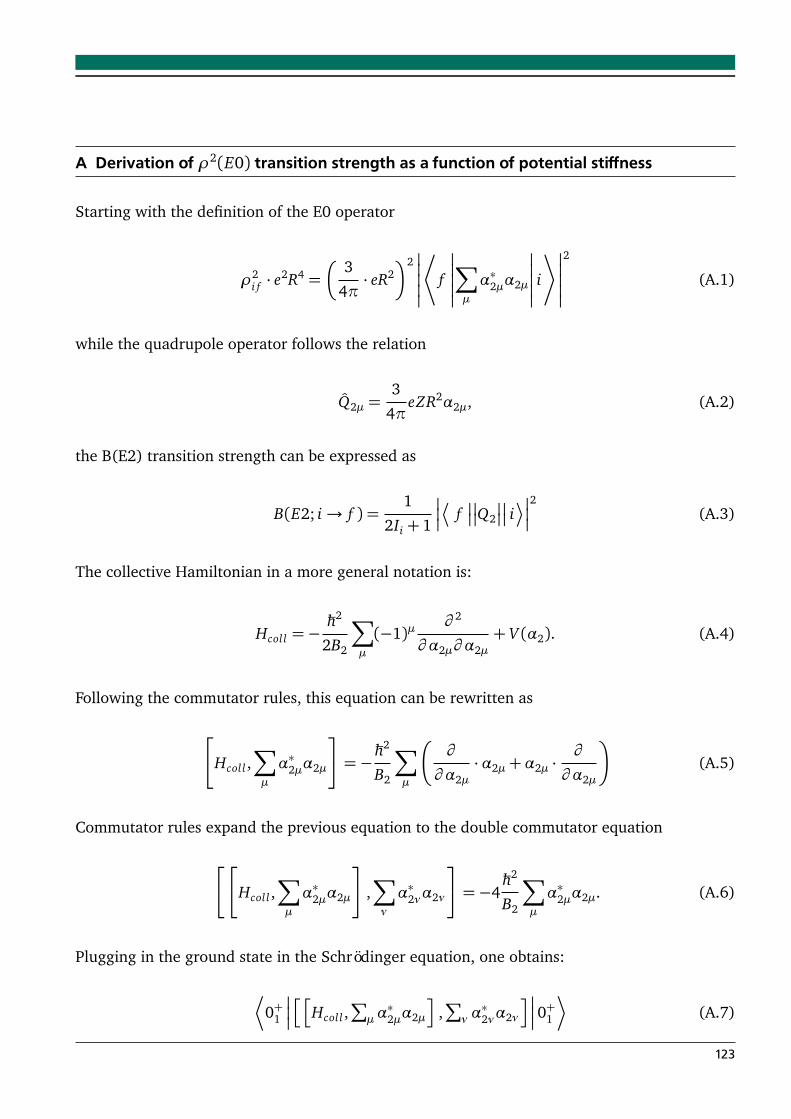
A Derivation of ρ2(E0) transition strength as a function of potential stiffness
Starting with the definition of the E0 operator
ρ2i f · e
2R4 =
3
4π· eR2
2
*
f
∑
µ
α∗2µα2µ
i
+
2
(A.1)
while the quadrupole operator follows the relation
Q2µ =3
4πeZR2α2µ, (A.2)
the B(E2) transition strength can be expressed as
B(E2; i→ f ) =1
2Ii + 1
¬
f
Q2
i¶
2(A.3)
The collective Hamiltonian in a more general notation is:
Hcol l =−ħh2
2B2
∑
µ
(−1)µ∂ 2
∂ α2µ∂ α2µ+ V (α2). (A.4)
Following the commutator rules, this equation can be rewritten as
Hcol l ,∑
µ
α∗2µα2µ
=−ħh2
B2
∑
µ
∂
∂ α2µ·α2µ+α2µ ·
∂
∂ α2µ
(A.5)
Commutator rules expand the previous equation to the double commutator equation
Hcol l ,∑
µ
α∗2µα2µ
,∑
ν
α∗2να2ν
=−4ħh2
B2
∑
µ
α∗2µα2µ. (A.6)
Plugging in the ground state in the Schrödinger equation, one obtains:
0+1
hh
Hcol l ,∑
µα∗2µα2µ
i
,∑
ν α∗2να2ν
i
0+1
·
(A.7)
123
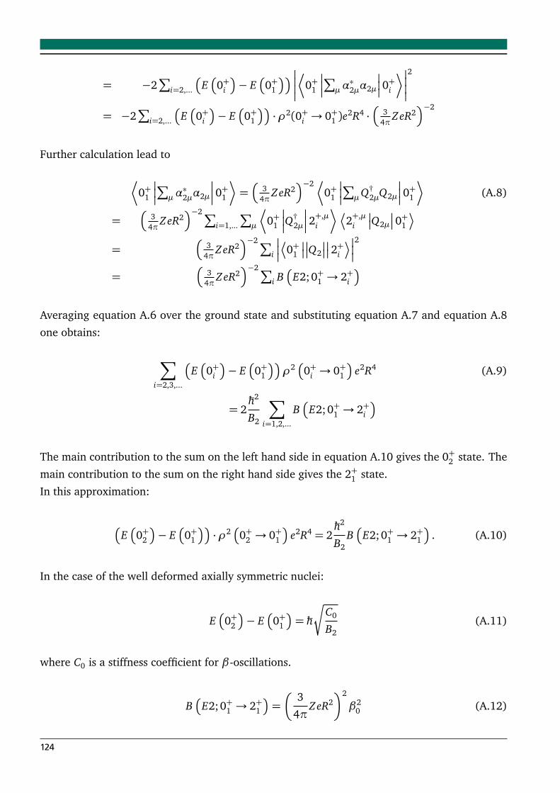
= −2∑
i=2,...
E
0+i
− E
0+1
0+1
∑
µα∗2µα2µ
0+i
·
2
= −2∑
i=2,...
E
0+i
− E
0+1
·ρ2(0+i → 0+1 )e2R4 ·
34π
ZeR2−2
Further calculation lead to
0+1
∑
µα∗2µα2µ
0+1
·
=
34π
ZeR2−2
0+1
∑
µQ†2µQ2µ
0+1
·
(A.8)
=
34π
ZeR2−2∑
i=1,...
∑
µ
0+1
Q†2µ
2+,µi
·
¬
2+,µi
Q2µ
0+1¶
=
34π
ZeR2−2∑
i
¬
0+1
Q2
2+i¶
2
=
34π
ZeR2−2∑
i B
E2;0+1 → 2+i
Averaging equation A.6 over the ground state and substituting equation A.7 and equation A.8
one obtains:
∑
i=2,3,...
E
0+i
− E
0+1
ρ2
0+i → 0+1
e2R4 (A.9)
= 2ħh2
B2
∑
i=1,2,...
B
E2;0+1 → 2+i
The main contribution to the sum on the left hand side in equation A.10 gives the 0+2 state. The
main contribution to the sum on the right hand side gives the 2+1 state.
In this approximation:
E
0+2
− E
0+1
·ρ2
0+2 → 0+1
e2R4 = 2ħh2
B2B
E2; 0+1 → 2+1
. (A.10)
In the case of the well deformed axially symmetric nuclei:
E
0+2
− E
0+1
= ħh
r
C0
B2(A.11)
where C0 is a stiffness coefficient for β-oscillations.
B
E2; 0+1 → 2+1
=
3
4πZeR2
2
β20 (A.12)
124
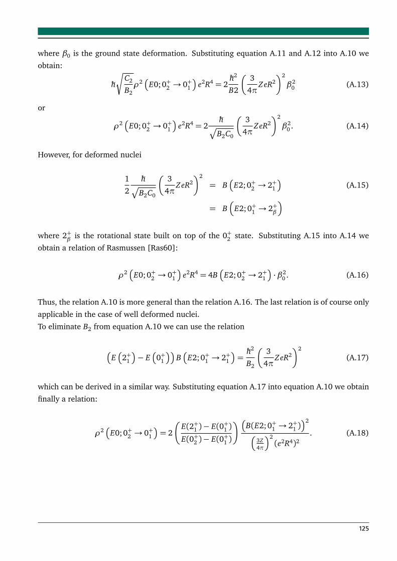
where β0 is the ground state deformation. Substituting equation A.11 and A.12 into A.10 we
obtain:
ħh
r
C2
B2ρ2
E0;0+2 → 0+1
e2R4 = 2ħh2
B2
3
4πZeR2
2
β20 (A.13)
or
ρ2
E0;0+2 → 0+1
e2R4 = 2ħh
p
B2C0
3
4πZeR2
2
β20 . (A.14)
However, for deformed nuclei
1
2
ħhp
B2C0
3
4πZeR2
2
= B
E2; 0+2 → 2+1
(A.15)
= B
E2;0+1 → 2+β
where 2+β
is the rotational state built on top of the 0+2 state. Substituting A.15 into A.14 we
obtain a relation of Rasmussen [Ras60]:
ρ2
E0;0+2 → 0+1
e2R4 = 4B
E2; 0+2 → 2+1
· β20 . (A.16)
Thus, the relation A.10 is more general than the relation A.16. The last relation is of course only
applicable in the case of well deformed nuclei.
To eliminate B2 from equation A.10 we can use the relation
E
2+1
− E
0+1
B
E2; 0+1 → 2+1
=ħh2
B2
3
4πZeR2
2
(A.17)
which can be derived in a similar way. Substituting equation A.17 into equation A.10 we obtain
finally a relation:
ρ2
E0; 0+2 → 0+1
= 2
E(2+1 )− E(0+1 )
E(0+2 )− E(0+1 )
B(E2; 0+1 → 2+1 )2
3Z4π
2(e2R4)2
. (A.18)
125
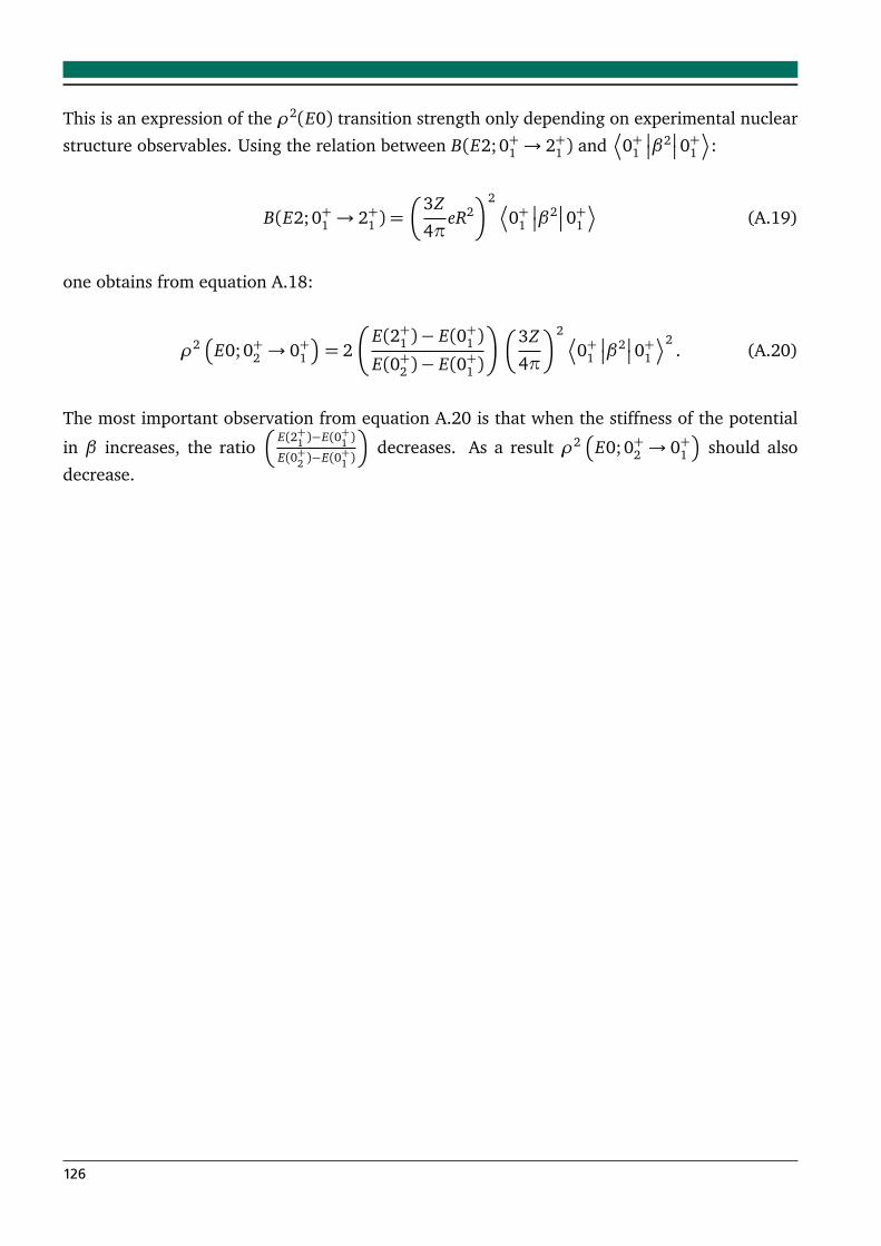
This is an expression of the ρ2(E0) transition strength only depending on experimental nuclear
structure observables. Using the relation between B(E2;0+1 → 2+1 ) and¬
0+1
β2
0+1¶
:
B(E2;0+1 → 2+1 ) =
3Z
4πeR22¬
0+1
β2
0+1¶
(A.19)
one obtains from equation A.18:
ρ2
E0; 0+2 → 0+1
= 2
E(2+1 )− E(0+1 )
E(0+2 )− E(0+1 )
3Z
4π
2¬
0+1
β2
0+1¶2
. (A.20)
The most important observation from equation A.20 is that when the stiffness of the potential
in β increases, the ratio
E(2+1 )−E(0+1 )
E(0+2 )−E(0+1 )
decreases. As a result ρ2
E0;0+2 → 0+1
should also
decrease.
126
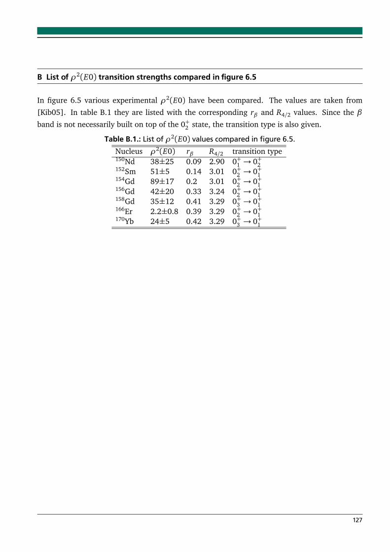
B List of ρ2(E0) transition strengths compared in figure 6.5
In figure 6.5 various experimental ρ2(E0) have been compared. The values are taken from
[Kib05]. In table B.1 they are listed with the corresponding rβ and R4/2 values. Since the β
band is not necessarily built on top of the 0+2 state, the transition type is also given.
Table B.1.: List of ρ2(E0) values compared in figure 6.5.Nucleus ρ2(E0) rβ R4/2 transition type150Nd 38±25 0.09 2.90 0+1 → 0+2152Sm 51±5 0.14 3.01 0+2 → 0+1154Gd 89±17 0.2 3.01 0+2 → 0+1156Gd 42±20 0.33 3.24 0+2 → 0+1158Gd 35±12 0.41 3.29 0+3 → 0+1166Er 2.2±0.8 0.39 3.29 0+2 → 0+1170Yb 24±5 0.42 3.29 0+3 → 0+1
127

Bibliography
[Amo00] Adv. Nucl. Phys. 25 (2000) 275.
[And01] W. Andrejtscheff, C. Kohstall, P. von Brentano, C. Fransen, U. Kneissl, N. Pietralla, and
H. Pitz, Phys. Lett. B 506 (2001) 239.
[Are00] H. Arenhövel, F. Ritz, and T. Wilbois, Phys. Rev. C 61 (2000) 034002.
[Bag76] C. Baglin, Nuclear Data Sheets 18 (1976) 223 .
[Bäh] C. Bähr, Computercode phashi, unpublished.
[Bak97] F. T. Baker, L. Bimbot, C. Djalali, C. Glashausser, H. Lenske, W. G. Love, M. Morlet,
E. Tomasi-Gustafsson, J. V. de Wiele, J. Wambach, and A. Willis, Phys. Rep. 289 (1997)
235.
[Bal47] G. C. Baldwin and G. S. Klaiber, Phys. Rev. 71 (1947) 3.
[Bas12] S. Bassauer, Weiterentwicklung der Online-Datenanalyse sowie der Ladungs- und Stro-
mauslese am LINTOTT-Spektrometer, Bachelor thesis, TU Darmstadt (2012).
[Bel70] D. A. Bell, C. E. Aveledo, M. G. Davidson, and J. P. Davidson, Can. J. Phys 48 (1970)
2542.
[Ber75] B. L. Berman and S. C. Fultz, Rev. Mod. Phys. 47 (1975) 713.
[Ber85] C. A. Bertulani and G. Baur, Nucl. Phys. A 442 (1985) 739.
[Ber88] C. A. Bertulani and G. Baur, Phys. Rep. 163 (1988) 299.
[Ber93] C. Bertulani and A. Nathan, Nuclear Physics A 554 (1993) 158 .
[Bes79] D. Besset, B. Favier, L. Greeniaus, R. Hess, C. Lechanoine, D. Rapin, and D. Werren,
Nuclear Instruments and Methods 166 (1979) 515 .
[Boh52] A. Bohr, Mat. Fys. Medd. K. Dan. Vidensk. Selsk. 26 (1952).
[Boh75] A. Bohr and B. Mottelson, Nuclear Structure, Benjamin, Reading (1975).
[Bon06] D. Bonatsos, D. Lenis, N. Pietralla, and P. A. Terziev, Phys. Rev. C 74 (2006) 044306.
[Bon09] J. Bonnet, A. Krugmann, J. Beller, N. Pietralla, and R. V. Jolos, Phys. Rev. C 79 (2009)
034307.
[Bra] N. Braun, Line shape fitting program, unpublished.
129
[Bre04] P. von Brentano, V. Werner, R. F. Casten, C. Scholl, E. A. McCutchan, R. Krücken, and
J. Jolie, Phys. Rev. Lett. 93 (2004) 152502.
[bri] Online conversion coefficient calculator, http://bricc.anu.edu.au/, accessed:
27.05.2014.
[Bur02a] O. Burda, Design of a shielding for the new focal plane detector system of the energy-loss
spectrometer at the S-DALINAC, Diploma thesis, Karazin Kharkiv National University,
Ukraine (2002).
[Bür02b] T. Bürvenich, D. G. Madland, J. A. Maruhn, and P.-G. Reinhard, Phys. Rev. C 65 (2002)
044308.
[Bur08] O. Burda, Nature of Mixed-Symmetry 2+ States in 94Mo from High-Resolution Electron
and Proton Scattering and Line Shape of the First Excited 1/2+ State in 9Be, Ph.D. thesis,
TU Darmstadt, Darmstadt (2008).
[CAG14] Website of the cagra collaboration, http://www.phy.anl.gov/gammasphere/CAGRA/
(2014), accessed: 13.06.2014.
[Car74] P. Carlos, H. Beil, R. Bergère, A. Leprêtre, A. D. Miniac, and A. Veyssière, Nuclear
Physics A 225 (1974) 171 .
[Cas00] R. Casten, Nuclear structure from a simple perspective, volume 23, Oxford University
Press (2000).
[Cas01] R. F. Casten and N. V. Zamfir, Phys. Rev. Lett. 87 (2001) 052503.
[CER] PAW++ program package (CERN libraries),
http://cern.ch/paw/,
http://cern.ch/cernlib/.
[Che10] M. Chernykh, H. Feldmeier, T. Neff, P. von Neumann-Cosel, and A. Richter, Phys. Rev.
Lett. 105 (2010) 022501.
[Cla03] R. M. Clark, M. Cromaz, M. A. Deleplanque, M. Descovich, R. M. Diamond, P. Fallon,
R. B. Firestone, I. Y. Lee, A. O. Macchiavelli, H. Mahmud, E. Rodriguez-Vieitez, F. S.
Stephens, and D. Ward, Phys. Rev. C 68 (2003) 037301.
[Cla04] R. M. Clark, M. Cromaz, M. A. Deleplanque, M. Descovich, R. M. Diamond, P. Fallon,
I. Y. Lee, A. O. Macchiavelli, H. Mahmud, E. Rodriguez-Vieitez, F. S. Stephens, and
D. Ward, Phys. Rev. C 69 (2004) 064322.
[Cos92] C. D. Coster, K. Heyde, and A. Richter, Nuclear Physics A 542 (1992) 375 .
130
[Die95] H. Diesener, Doctoral thesis D17, TU Darmstadt (1995).
[Die01] H. Diesener, U. Helm, P. von Neumann-Cosel, A. Richter, G. Schrieder, A. Stascheck,
A. Stiller, and J. Carter, Nuclear Physics A 696 (2001) 272 .
[Don66] W. Donner and W. Greiner, Zeitschrift für Physik 197 (1966) 440, ISSN 0044-3328.
[Dre] C. Dreher, Computercode drepha, unpublished.
[Dre74] B. Dreher, J. Friedrich, K. Merle, H. Rothhaas, and G. Lührs, Nuclear Physics A 235
(1974) 219 .
[Dus05] K. Dusling and N. Pietralla, Phys. Rev. C 72 (2005) 011303.
[Dus06] K. Dusling, N. Pietralla, G. Rainovski, T. Ahn, B. Bochev, A. Costin, T. Koike, T. C. Li,
A. Linnemann, S. Pontillo, and C. Vaman, Phys. Rev. C 73 (2006) 014317.
[End11] J. Enders, T. Bahlo, P. Bangert, R. Barday, M. Brunken, C. Eckardt, R. Eichhorn, M. Es-
pig, M. Freudenberger, A. Göök, C. Ingenhaag, J. Lindemann, P. von Neumann-Cosel,
A. Oberstedt, S. Oberstedt, Y. Poltoratska, A. Richter, M. Roth, F. Schneider, M. Wagner,
A. Weber, and B. Zwicker, Journal of Physics: Conference Series 295 (2011) 012152.
[ENS13] Evaluated nuclear structure data file, http://www.nndc.bnl.gov/ensdf (2013), ac-
cessed: 01.02.2013.
[Epe13] E. Epelbaum, arXiv:1302.3241 [nucl-th] (2013).
[Foh78] J. Foh, R. Frey, R. Scheneider, D. Schüll, A. Schwierczinski, H. Theissen, and O. Titze,
Nuclear Instruments and Methods 153 (1978) 43 .
[Fra85] M. A. Franey and W. G. Love, Phys. Rev. C 31 (1985) 488.
[Fre89] D. Frekers, D. Bohle, A. Richter, R. Abegg, R. Azuma, A. Celler, C. Chan, T. Drake,
K. Jackson, J. King, C. Miller, R. Schubank, J. Watson, and S. Yen, Physics Letters B
218 (1989) 439 .
[Fre90] D. Frekers, H. Wörtche, A. Richter, R. Abegg, R. Azuma, A. Celler, C. Chan, T. Drake,
R. Helmer, K. Jackson, J. King, C. Miller, R. Schubank, M. Vetterli, and S. Yen, Physics
Letters B 244 (1990) 178 .
[Fri11] Y. Fritzsche, Aufbau und Inbetriebnahme einer Quelle polarisierter Elektronen am
supraleitenden Darmstädter Elektronenlinearbeschleuniger S-DALINAC, Ph.D. thesis, TU
Darmstadt, Ilmenau (2011).
[Fuj99] M. Fujiwara, H. Akimune, I. Daito, H. Fujimura, Y. Fujita, K. Hatanaka, H. Ikegami,
I. Katayama, K. Nagayama, N. Matsuoka, S. Morinobu, T. Noro, M. Yoshimura, H. Sak-
aguchi, Y. Sakemi, A. Tamii, and M. Yosoi, Nucl. Inst. Meth. A 422 (1999) 484.
131
[Fuj08] N. Fujita, H. Sakaguchi, Y. Maeda, A. Nonaka, H. Okamura, A. Tamii, J. Zenihiro,
H. Matsubara, D. Ishikawa, T. Terashima, and Y. Yasuda, RCNP annual report (2008).
[Fuj11] Y. Fujita, B. Rubio, and W. Gelletly, Progress in Particle and Nuclear Physics 66 (2011)
549 .
[Gal03] M. Galassi, J. Davies, J. Theiler, B. Gough, B. Jungman, M. Booth, and F. Rossi, GNU
Scientific Library Reference Manual, 2nd ed., Network Theory Ltd., Bristol (2003).
[Gia14] F. Giacoppo, F. Bello Garrote, T. Eriksen, A. Gorgen, M. Guttormsen et al. (2014).
[GNU] Gnuplot, version 4.4 patchlevel 0 (2010),
http://www.gnuplot.info/.
[Gor98] S. Goriely, Phys. Lett. B 436 (1998) 10.
[Grä78] H.-D. Gräf, H. Miska, E. Spamer, O. Titze, and T. Walcher, Nuclear Instruments and
Methods 153 (1978) 9 .
[Har01] M. N. Harakeh and A. van der Woude, Giant Resonances, Oxford studies in nuclear
physics (2001).
[Hat97] K. Hatanaka, K. Takahisa, H. Tamura, M. Sato, and I. Miura, Nuclear Instruments and
Methods in Physics Research Section A: Accelerators, Spectrometers, Detectors and
Associated Equipment 384 (1997) 575 .
[Hel92] M. Hellström, B. Fogelberg, H. Mach, D. Jerrestam, and L. Spanier, Phys. Rev. C 46
(1992) 860.
[Hey83] K. Heyde, P. V. Isacker, M. Waroquier, J. Wood, and R. Meyer, Physics Reports 102
(1983) 291 .
[Hey10] K. Heyde, P. von Neumann-Cosel, and A. Richter, Rev. Mod. Phys. 82 (2010) 2365.
[Hil98] R. Hilton, W. Höhenberger, and P. Ring, The European Physical Journal A - Hadrons
and Nuclei 1 (1998) 257.
[Hof02] F. Hofmann, P. von Neumann-Cosel, F. Neumeyer, C. Rangacharyulu, B. Reitz,
A. Richter, G. Schrieder, D. I. Sober, L. W. Fagg, and B. A. Brown, Phys. Rev. C 65
(2002) 024311.
[Iac00] F. Iachello, Phys. Rev. Lett. 85 (2000) 3580.
[Iac01] F. Iachello, Phys. Rev. Lett. 87 (2001) 052502.
[Iac03] F. Iachello, Phys. Rev. Lett. 91 (2003) 132502.
132
[IKP14] Ikp main website, http://www.ikp.tu-darmstadt.de/dasinstitut/index.de.jsp
(2014), accessed: 18.05.2014.
[Jola] R. Jolos, private communication.
[Jolb] R. Jolos, private communication.
[Jol09] R. V. Jolos and P. von Brentano, Phys. Rev. C 79 (2009) 044310.
[Kaw02] T. Kawabata, Polarization transfer in the 16O(p,p’) reaction at forward angles and struc-
ture of the spin-dipole resonance, Ph.D. thesis, Kyoto University, Japan (2002).
[Ker59] A. K. Kerman, H. McManus, and R. M. Thaler, Annu. Phys. 8 (1959) 551.
[Kib05] T. Kibédi and R. Spear, Atomic Data and Nuclear Data Tables 89 (2005) 77 .
[KIN] Computer program KINMAT, iThemba Laboratory for Accelerator Based Sciences,
Faure, South Africa, unpublished.
[Kru] A. M. Krumbholz, Doctoral thesis D17, TU Darmstadt, in preparation.
[Kru08] A. Krugmann, Untersuchung von E0-Übergängen in Kernen am Phasenübergang zwischen
sphärischer und deformierter Kerngestalt, Master thesis, TU Darmstadt (2008).
[Kru11] A. Krugmann, Z. P. Li, J. Meng, N. Pietralla, and D. Vretenar, Journal of Physics G:
Nuclear and Particle Physics 38 (2011) 065102.
[Lar11] A. C. Larsen, M. Guttormsen, M. Krticka, E. Beták, A. Bürger, A. Görgen, H. T. Nyhus,
J. Rekstad, A. Schiller, S. Siem, H. K. Toft, G. M. Tveten, A. V. Voinov, and K. Wikan,
Phys. Rev. C 83 (2011) 034315.
[Len05] A. W. Lenhardt, Entwicklung eines Si-Mikrostreifendetektors für das 169-Spektrometer
am S-DALINAC, Ph.D. thesis, TU Darmstadt, Aachen (2005).
[Len06] A. Lenhardt, U. Bonnes, O. Burda, P. von Neumann-Cosel, M. Platz, A. Richter, and
S. Watzlawik, Nuclear Instruments and Methods in Physics Research Section A: Accel-
erators, Spectrometers, Detectors and Associated Equipment 562 (2006) 320 .
[Li09] Z. P. Li, T. Nikšic, D. Vretenar, J. Meng, G. A. Lalazissis, and P. Ring, Phys. Rev. C 79
(2009) 054301.
[Lip50] B. A. Lippmann and J. Schwinger, Phys. Rev. 79 (1950) 469.
[Lov81] W. G. Love and M. A. Franey, Phys. Rev. C 24 (1981) 1073.
[Mar11] D. Martin, Investigation of the reaction 144Sm(p, p′) under extreme forward angles, Bach-
elor thesis, TU Darmstadt (2011).
133
[Mar13] D. Martin, Gamma Strength Function of 96Mo: A Test of the Axel-Brink Hypothesis, Mas-
ter thesis, TU Darmstadt (2013).
[Mat91] N. Matsuoka, K. Hatanaka, S. Morinobu, T. Noro, A. Okihana, and K. Sagara, RCNP
annual report (1991).
[Mat10] H. Matsubara, Isoscalar and isovector spin-M1 transitions from the even-even, N = Z
nuclei across the sd-shell region, Ph.D. thesis, Osaka University (2010).
[Mat14] M. Mathy, M1 Stärke in 48Ca aus inelastischer Protonenstreuung, Bachelor thesis, TU
Darmstadt (2014).
[McC05] E. A. McCutchan, N. V. Zamfir, and R. F. Casten, Phys. Rev. C 71 (2005) 034309.
[Mo69] L. W. Mo and Y. S. Tsai, Rev. Mod. Phys. 41 (1969) 205.
[Mos82] J. M. Moss, Phys. Rev. C 26 (1982) 727.
[NC97] P. von Neumann-Cosel, C. Rangacharyulu, A. Richter, G. Schrieder, A. Stascheck, and
S. Strauch, Phys. Rev. Lett. 78 (1997) 2924.
[NC99] P. von Neumann-Cosel, F. Neumeyer, S. Nishizaki, V. Y. Ponomarev, C. Rangacharyulu,
B. Reitz, A. Richter, G. Schrieder, D. I. Sober, T. Waindzoch, and J. Wambach, Phys. Rev.
Lett. 82 (1999) 1105.
[NC02] P. von Neumann-Cosel, A. Richter, G. Schrieder, A. Shevchenko, A. Stiller, and H. Aren-
hövel, Phys. Rev. Lett. 88 (2002) 202304.
[Neu97a] F. Neumeyer, Doctoral thesis D17, TU Darmstadt (1997).
[Neu97b] F. Neumeyer, Untersuchungen magnetischer Kernanregungen in 48Ca und 90Zr mit
hochauflösender Elektronenstreuung unter 180 am S-DALINAC, Ph.D. thesis, TU Darm-
stadt, Darmstadt (1997).
[Nik09] T. Nikšic, Z. P. Li, D. Vretenar, L. Próchniak, J. Meng, and P. Ring, Phys. Rev. C 79 (2009)
034303.
[Nor90] T. Noro, Y. Mizuno, H. Togawa, S. Hirata, N. Matsuoka, O. Kamigaito, F. Hiei, Y. Sakemi,
H. Akimune, and T. Takahashi, RCNP annual report (1990).
[Ohl02] G. G. Ohlsen, Rep. Prog. Phys. 35 (2002) 717.
[Pie04] N. Pietralla and O. M. Gorbachenko, Phys. Rev. C 70 (2004) 011304.
[Pie10] J. Piekarewicz, J. Phys. G: Nucl. Part. Phys. 37 (2010) 064038.
134
[Pol11] I. Poltoratska, Complete electric dipole response in 208Pb from high-resolution polarized
proton scattering at 0°, Doctoral thesis D17, TU Darmstadt (2011).
[Pol12] I. Poltoratska, P. von Neumann-Cosel, A. Tamii, T. Adachi, C. A. Bertulani, J. Carter,
M. Dozono, H. Fujita, K. Fujita, Y. Fujita, K. Hatanaka, M. Itoh, T. Kawabata,
Y. Kalmykov, A. M. Krumbholz, E. Litvinova, H. Matsubara, K. Nakanishi, R. Nevel-
ing, H. Okamura, H. J. Ong, B. Özel-Tashenov, V. Yu. Ponomarev, A. Richter, B. Ru-
bio, H. Sakaguchi, Y. Sakemi, Y. Sasamoto, Y. Shimbara, Y. Shimizu, F. D. Smit,
T. Suzuki, Y. Tameshige, J. Wambach, M. Yosoi, and J. Zenihiro, Phys. Rev. C 85 (2012)
041304(R).
[Pon] V. Yu. Ponomarev, Computer code for the extraction of electron scattering form factors
from transition densities, unpublished.
[Ras60] J. O. Rasmussen, Nuclear Physics 19 (1960) 85 .
[Ray07] J. Raynal, Computing code DWBA07, NEA Data Service NEA1209/08 (2007).
[RCN14] Rcnp main website, https://www.rcnp.osaka-u.ac.jp (2014), accessed:
18.05.2014.
[Rei02] B. Reitz, A. M. V. Berg, D. Frekers, F. Hofmann, M. de Huu, Y. Kalmykov, H. Lenske,
P. von Neumann-Cosel, V. Y. Ponomarev, S. Rakers, A. Richter, G. Schrieder, K. Schweda,
J. Wambach, and H. J. Wörtche, Physics Letters B 532 (2002) 179.
[Rei10] P.-G. Reinhard and W. Nazarewicz, Phys. Rev. C 81 (2010) 051303(R).
[Ric96] A. Richter, EPAC 96: European Particle Accelerator Conference <5, 1996, Sitges,
Barcelona>: [Proceedings]. Vol. 1. Hrsg.: S. Myers (u.a.) - Bristol, Philadelphia: Inst.
of Physics Publ.,1996. S. 110-114, Inst. of Physics Publ, Bristol, Philadelphia, ersch.
ebenf. als: Technische Universität Darmstadt, Institut für Kernphysik: IKDA; 96/17.
[Rin80] P. Ring and P. Schuck, The Nuclear many-body problem, Springer, New york (1980).
[Rye06] N. Ryezayeva, Search for the p1/2- Resonance in 7He with the 7Li(d,2He) Reaction and
Measurement of the Deuteron Electrodisintegration under 180-deg at the S-DALINAC,
Ph.D. thesis, TU Darmstadt (2006).
[Sak97] H. Sakai, T. Wakasa, H. Okamura, T. Nonaka, T. Ohnishi, K. Yako, K. Sekiguchi, S. Fu-
jita, Y. Satou, H. Otsu, T. Uesaka, S. Ishida, N. Sakamoto, M. B. Greenfield, and
K. Hatanaka, Proceedings of the International Symposium on New Facet of Spin Gi-
ant Resonances in Nuclei, Tokyo, Japan, 1997, edited by H. Sakai, H. Okamura, T.
Wakasa (World Scientific, Singapore 1998) (1997) 29.
135
[San91a] R. Sandor, Shape transition in the Nd-isotopes: an electron scattering study., Doctoral
thesis, Vrije Universiteit te Amsterdam (1991).
[San91b] R. K. J. Sandor, H. P. Blok, U. Garg, M. Girod, M. N. Harakeh, C. W. de Jager, and
H. de Vries, Phys. Rev. C 43 (1991) R2040.
[Sar96] P. Sarriguren, E. Moya de Guerra, and R. Nojarov, Phys. Rev. C 54 (1996) 690.
[Sas09] M. Sasano, H. Sakai, K. Yako, T. Wakasa, S. Asaji, K. Fujita, Y. Fujita, M. B. Greenfield,
Y. Hagihara, K. Hatanaka, T. Kawabata, H. Kuboki, Y. Maeda, H. Okamura, T. Saito,
Y. Sakemi, K. Sekiguchi, Y. Shimizu, Y. Takahashi, Y. Tameshige, and A. Tamii, Phys.
Rev. C 79 (2009) 024602.
[Sat83] G. Satchler, Direct nuclear reactions, Oxford University Press, New York (1983).
[Sav10] D. Savran, K. Lindenberg, J. Glorius et al., Nuclear Instruments and Methods in Physics
Research Section A: Accelerators, Spectrometers, Detectors and Associated Equipment
613 (2010) 232 .
[Sav13] D. Savran, T. Aumann, and A. Zilges, Prog. Part. Nucl. Phys. 70 (2013) 210.
[Sch78] D. Schüll, J. Foh, H.-D. Gräf, H. Miska, R. Schneider, E. Spamer, H. Theissen, O. Titze,
and T. Walcher, Nuclear Instruments and Methods 153 (1978) 29 .
[Sch00] A. Schiller, L. Bergholt, M. Guttormsen, E. Melby, J. Rekstad, and S. Siem, Nuclear
Instruments and Methods in Physics Research Section A: Accelerators, Spectrometers,
Detectors and Associated Equipment 447 (2000) 498 , ISSN 0168-9002.
[Shi09] N. Shirikova, R. Jolos, N. Pietralla, A. Sushkov, and V. Voronov, The European Physical
Journal A 41 (2009) 393.
[Sma14] J. Smallcombe, P. Davies, C. Barton, D. Jenkins, L. Andersson, P. Butler, D. Cox, R.-D.
Herzberg, A. Mistry, E. Parr, T. Grahn, P. Greenlees, K. Hauschild, A. Herzan, U. Jakob-
sson, P. Jones, R. Julin, S. Juutinen, S. Ketelhut, M. Leino, A. Lopez-Martens, P. Niem-
inen, J. Pakarinen, P. Papadakis, P. Peura, P. Rahkila, S. Rinta-Antila, P. Ruotsalainen,
M. Sandzelius, J. Saren, C. Scholey, J. Sorri, and J. Uusitalo, Physics Letters B 732
(2014) 161 .
[Sol92] V. G. Soloviev, Theory of Atomic Nuclei: Quasiparticles and Phonons, Inst. of Phys. Publ.,
Bristol (1992).
[Son11] K. Sonnabend, D. Savran, J. Beller, M. Büssing, A. Constantinescu, M. Elvers, J. Endres,
M. Fritzsche, J. Glorius, J. Hasper, J. Isaak, B. Löher, S. Müller, N. Pietralla, C. Romig,
A. Sauerwein, L. Schnorrenberger, C. Wälzlein, A. Zilges, and M. Zweidinger, Nuclear
136
Instruments and Methods in Physics Research Section A: Accelerators, Spectrometers,
Detectors and Associated Equipment 640 (2011) 6 .
[Spe81] J. Speth and A. van der Woude, Reports on Progress in Physics 44 (1981) 719.
[Str00] S. Strauch, P. von Neumann-Cosel, C. Rangacharyulu, A. Richter, G. Schrieder,
K. Schweda, and J. Wambach, Phys. Rev. Lett. 85 (2000) 2913.
[Suz00] T. Suzuki, Prog. Theor. Phys. 321 (2000) 859.
[Tak02] H. Takeda, Modification of nucleon-nucleon interactions in nuclear medium and neutron
densities extracted via proton elastic scattering at intermediate energies, Ph.D. thesis,
Kyoto University (2002).
[Tam99] A. Tamii, Polarization transfer observables from proton inelastic scattering from 12C at
zero degrees, Ph.D. thesis, Kyoto University (1999).
[Tam07] A. Tamii, T. Adachi, J. Carter, M. Dozono, H. Fujita, Y. Fujita, K. Hatanaka,
H. Hashimoto, T. Kaneda, M. Itoh, T. Kawabata, H. Matsubara, K. Nakanishi, P. von
Neumann-Cosel, H. Okamura, A. Perez, I. Poltoratska, V. Yu. Ponomarev, L. Popescu,
A. Richter, B. Rubio, H. Sakaguchi, Y. Sakemi, Y. Sasamoto, Y. Shimbara, Y. Shimizu,
F. D. Smit, Y. Tameshige, M. Yosoi, J. Zenihiro, and K. Zimmer, Nucl. Inst. Meth. A 788
(2007) 53.
[Tam09] A. Tamii, Y. Fujita, H. Matsubara, T. Adachi, J. Carter, M. Dozono, H. Fujita, K. Fujita,
H. Hashimoto, K. Hatanaka, T. Itahashi, M. Itoh, T. Kawabata, K. Nakanishi, S. Ni-
nomiya, A. Perez-Cerdan, L. Popescu, B. Rubio, T. Saito, H. Sakaguchi, Y. Sakemi,
Y. Sasamoto, Y. Shimbara, Y. Shimizu, F. Smit, Y. Tameshige, M. Yosoi, and J. Zenhiro,
Nucl. Inst. Meth. A 605 (2009) 326.
[Tam11] A. Tamii, I. Poltoratska, P. von Neumann-Cosel, Y. Fujita, T. Adachi, C. A. Bertu-
lani, J. Carter, M. Dozono, H. Fujita, K. Fujita, K. Hatanaka, D. Ishikawa, M. Itoh,
T. Kawabata, Y. Kalmykov, A. M. Krumbholz, E. Litvinova, H. Matsubara, K. Nakanishi,
R. Neveling, H. Okamura, H. J. Ong, B. Özel-Tashenov, V. Yu. Ponomarev, A. Richter,
B. Rubio, H. Sakaguchi, Y. Sakemi, Y. Sasamoto, Y. Shimbara, Y. Shimizu, F. D. Smit,
T. Suzuki, Y. Tameshige, J. Wambach, R. Yamada, M. Yosoi, and J. Zenihiro, Phys. Rev.
Lett. 107 (2011) 062502.
[Tam13] A. Tamii, priv. communication (2013).
[Tam14] A. Tamii, priv. communication (2014).
[Tan91] M. Tanaka et al., RCNP annual report (1991).
137
[Tor14] T. G. Tornyi, M. Guttormsen, T. K. Eriksen, A. Görgen, F. Giacoppo, T. W. Hagen,
A. Krasznahorkay, A. C. Larsen, T. Renstrøm, S. J. Rose, S. Siem, and G. M. Tveten,
Phys. Rev. C 89 (2014) 044323.
[Tua68] S. Tuan, L. Wright, and D. Onley, Nuclear Instruments and Methods 60 (1968) 70 .
[Übe71] H. Überall, Electron Scattering from Complex Nuclei, Part A+B (1971).
[Vre] D. Vretenar, private communication.
[Vri87] H. D. Vries, C. D. Jager, and C. D. Vries, Atomic Data and Nuclear Data Tables 36
(1987) 495 .
[Wal78] T. Walcher, R. Frey, H.-D. Gräf, E. Spamer, and H. Theissen, Nuclear Instruments and
Methods 153 (1978) 17 .
[Wal11] C. Walz, H. Fujita, A. Krugmann, P. von Neumann-Cosel, N. Pietralla, V. Y. Ponomarev,
A. Scheikh-Obeid, and J. Wambach, Phys. Rev. Lett. 106 (2011).
[Wig71] E. P. Wigner, Group theory and its application to the quantum mechanics of atomic spectra
/ [by] Eugene P. Wigner ; translated from the German by J. J. Griffin, Academic Press
New York, expanded and improved ed. edition (1971).
[Wim09] K. Wimmer, R. Krücken, V. Bildstein, K. Eppinger, R. Gernhäuser, D. Habs, C. Hinke,
T. Kröll, R. Lutter, H. Maier, P. Maierbeck, T. Morgan, O. Schaile, W. Schwerdtfeger,
S. Schwertel, and P. G. Thirolf, AIP Conference Proceedings 1090 (2009) 539.
[Win79] A. Winther and K. Alder, Nucl. Phys. A 319 (1979) 518.
[Wol56] L. Wolfenstein, Annu. Rev. Nucl. Sci. 6 (1956) 43.
[Woo99] J. Wood, E. Zganjar, C. De Coster, and K. Heyde, Nuclear Physics A 651 (1999) 323.
[Wör94] H. Wörtche, Untersuchung der M1-Stärkeverteilung in den schweren deformierten Kernen150Nd, 154Sm, 156Gd, 232Th und 238U mit unpolarisierter und polarisierter Protonenstreu-
ung, Doctoral thesis D17, TH Darmstadt (1994).
[Yen54] D. R. Yennie, D. G. Ravenhall, and R. N. Wilson, Phys. Rev. 95 (1954) 500.
[Yos95] M. Yosoi, H. Akimune, I. Daito, H. Fujiwara, S. Hirata, T. Inomata, O. Kamigaito,
M. Kawabata, T. Noro, H. Sakaguchi, Y. Sakemi, T. Takahashi, A. Tamii, S. Toyama,
A. Yamagoshi, and M. Yoshimura, AIP Conf. Proc. 343 (1995) 157.
[Zaw90] D. Zawischa, M. Macfarlane, and J. Speth, Phys. Rev. C 42 (1990) 1461.
[Zil91] A. Zilges, P. von Brentano, H. Friedrichs, R. Heil, U. Kneissl, S. Lindenstruth, H. Pitz,
and C. Wesselborg, Zeitschrift für Physik A Hadrons and Nuclei 340 (1991) 155.
138
Danksagung
An dieser Stelle möchte ich ein herzliches Dankeschön an all diejenigen aussprechen, die mich
bei der Anfertigung dieser Arbeit unterstützt haben und mir mit Rat und Tat beiseite standen.
Zuallererst danke ich Herrn Professor Dr. Dr. h.c. Norbert Pietralla für die Aufnahme in
seiner Arbeitsgruppe und die Bereitstellung eines solch interessanten Forschungsthemas. Er
hat den Fortschritt meiner Arbeit stets mit sehr großem Interesse verfolgt und seine Tür stand
jederzeit offen für Ratschläge, Diskussionen und Fragen. Außerdem bin ich ihm dankbar für die
Möglichkeit, Forschungsergebnisse auf interessanten Tagungen, Konferenzen und Workshops
im In- und Ausland zu präsentieren. Die Gelegenheit und das Vertrauen, den 6th International
Workshop on Shape-Phase Transitions and Critical-Point Phenomena in Nuclei im Frühjahr 2012,
an dem rund 100 Wissenschaftler teilnahmen, zu einem großen Teil selbst zu organisieren,
hat mir sehr viel bedeutet. Hierbei habe ich sowohl fachlich sehr viel gelernt, als auch viele
wertvolle Kontakte mit anderen Wissenschaftlern geknüpft von denen ich heute noch zehren
kann und die mir in Zukunft sicher noch einiges ermöglichen.
Ein sehr großer Dank gebührt auch Herrn Professor Dr. Peter von Neumann-Cosel. Er er-
möglichte mir die Arbeit an hochinteressanten Experimenten zur Protonenstreuung in Japan
und Südafrika und unterstützte mich mit unglaublichem Zeitaufwand bei den Experimenten
zur Elektronenstreuung am S-DALINAC und nicht zuletzt bei der Anfertigung dieser Arbeit.
Auch über die unzähligen Diskussionen über alle Arten von physikalischen Fragestellungen bin
ich ihm sehr dankbar.
I am deeply grateful to Professor Atsushi Tamii for the amazing help he offered during the
experiments and also afterwards during the analysis procedure. He was always available for
fruitful discussions.
Dankbar bin ich auch an die Kollegen vom Institut für die großartige Hilfe bei den Exper-
imenten und insbesondere Herrn Florian Hug und seinem Team für die Bereitstellung eines
exzellenten Elektronenstrahls für die Experimente.
A big ’thank you’ goes to the accelerator group at RCNP in Osaka, who created excellent
experimental conditions and also to all helpers who participated in the E350 experiment.
I am indebted to Vladimir Ponomarev for providing theoretical support for all kinds of exper-
iments that I have done.
Da ich während meiner gesamten Zeit als Doktorand in verschiedenen Büros gesessen habe,
gilt mein Dank all den netten, hilfsbereiten Kollegen für eine tolle Zeit, unzählige Diskussio-
nen über physikalische und nichtphysikalische Themen. Besonders hervorheben möchte ich in
diesem Zusammenhang Simela Aslanidou, Sergej Bassauer, Jonny Birkhan, Anna Maria Krumb-
holz, Dirk Martin, Maxim Singer und Iryna Zweidinger.
139
Neben den Arbeitskollegen im Büro möchte ich mich aber auch für die besondere Hilfe bei
allen anderen administrativen, finanziellen und technischen Angelegenheiten bedanken. Hier
sind besonders zu erwähnen: Marco Brunken, Ursula von Dungen, Maria Helm, Uli Krebs, Catja
Noll de Lopez, Oliver Möller, Carina Seeger, Giovanna Umberti.
Ein großer Dank geht auch an die Mitarbeiter der elektrischen und mechanischen Werkstatt
unter der Leitung von Herrn Bonnes bzw. Herrn Häckl und Herrn Oppermann, deren kompe-
tente und schnelle Hilfe mich oftmals gerettet haben.
Außerdem danke ich allen Mitgliedern der Arbeitsgruppe Pietralla, sowie der Spektrometer-
gruppe für die allseits nette Arbeitsatmosphäre.
Für den sportlichen Ausgleich am Kickertisch, vor allem in den letzten Wochen der heißen
Phase, danke ich Tobias Klaus und Ilja Homm.
Neben der Arbeit war es immer wieder wertvoll und wichtig gute Freunde zu haben. Darüber
bin ich sehr glücklich und daher möchte ich all meinen Freunden hiermit meinen Dank
aussprechen, die immer für mich da waren, wenn es mal nicht so wollte wie es sollte, aber
natürlich auch wenn alles gut war.
Meiner Familie, insbesondere meinen Eltern, meiner Schwester und vor allem meiner Frau
Kathi und meinen beiden Katern Teddy und Pauli bin ich zu allergrößtem Dank verpflichtet.
Ihr habt mich moralisch unterstützt, mich immer wieder aufgefangen wenn ich am Boden war,
habt Geduld und Verständnis gezeigt und habt euch mit mir gefreut wenn alles gut lief und seid
einfach die allerbesten! Vielen Dank!!!
Diese Arbeit wurde gefördert durch die DFG im Rahmen des Sonderforschungsbereichs 634
und durch das Vorhaben NE 679/3-1.
140
Lebenslauf von Andreas Krugmann
Persönliches
Geburtsdatum 15.08.1983
Geburtsort Heppenheim an der Bergstraße
Eltern Rainer Krugmann und Christine Krugmann (geb. Plickat)
Familienstand verheiratet mit Katharina Krugmann
Bildungsweg
1990 - 1994 Konrad-Adenauer-Grundschule in Heppenheim
1994 - 2003 Starkenburg Gymnasium Heppenheim
2003 - 2004 Zivildienst am ZSP Bergstraße
2004 - 2007 TU Darmstadt, Bachelorstudium
2007 - 2008 TU Darmstadt, Masterstudium
seit Oktober 2008 Wissenschaftlicher Mitarbeiter am Institut für Kernphysik
der TU Darmstadt
141

Eigene Publikationen
Im folgenden werden alle Publikationen aufgelistet, die im Rahmen dieser Dissertation ent-
standen sind und/oder an denen ich mitgewirkt habe. Sie sind in chronologisch sortiert, begin-
nend mit der neuesten Publikation.
[1] A. Scheikh Obeid, S. Aslanidou, J. Birkhan, A. Krugmann, P. von Neumann-Cosel,
N. Pietralla, I. Poltoratska, and V. Yu. Ponomarev, Phys. Rev. C 89 (2014), 037301.
[2] N. Pietralla and A. Krugmann, Meeting reports. Nucl. Phys. News 23 (2013), 33–34.
[3] A. Scheikh Obeid, O. Burda, M. Chernykh, Krugmann, A., P. von Neumann-Cosel,
N. Pietralla, I. Poltoratska, V. Yu. Ponomarev, and C. Walz, Phys. Rev. C 87 (2013), 014337.
[4] A. Krugmann, D. Martin, P. von Neumann-Cosel, N. Pietralla, I. Poltoratska, A. Tamii, EPJ
Web of Conferences 38 (2012), 11001.
[5] N. Pietralla, C. Walz, V. Yu. Ponomarev, H. Fujita, A. Krugmann, P. von Neumann-Cosel,
A. Scheikh-Obeid, and J. Wambach, Journal of Physics: Conference Series 366 (2012),
012037.
[6] A. Krugmann, Z. P. Li, J. Meng, N. Pietralla, and D. Vretenar, Journal of Physics G: Nuclear
and Particle Physics 38 (2011), 065102.
[7] C. Walz, H. Fujita, Krugmann, A., P. von Neumann-Cosel, N. Pietralla, V. Yu. Ponomarev,
A. Scheikh-Obeid, and J. Wambach, Phys. Rev. Lett. 106 (2011), 062501.
[8] A. M. Heilmann, P. von Neumann-Cosel, A. Tamil, T. Adachi, C. Bertulani, J. Carter, H. Fu-
juita, Y. Fujita, K. Hatanaka, K. Hirota, O. H. Jin, T. Kawabata, A. Krugmann, H. Matsubara,
E. Litvinova, R. Neveling, H. Okamura, B. Ozel-Tashenov, I. Poltoratska, V. Yu. Ponomarev,
A. Richter, H. Sakaguchi, Y. Sakemi, Y. Sasamoto, Y. Shimizu, Y. Shimbara, F. D. Smit, T.
Suzuki, Y. Tameshige, Y. Yasuda, M. Yosoi, and J. Zenihiro, Journal of Physics: Conference
Series 312 (2011), 092029.
[9] A. Krugmann, J. Bonnet, N. Pietralla, and R. V. Jolos, Journal of Physics: Conference Series
205 (2010), 012037.
[10] A. Scheikh Obeid, O. Burda, M. Chernykh, A. Krugmann, P. von Neumann-Cosel,
N. Pietralla, I. Poltoratska, V. Ponomarev, and C. Walz, Journal of Physics: Conference Series
205 (2010), 012040.
143

[11] J. Bonnet, A. Krugmann, J. Beller, N. Pietralla, and R. Jolos, Phy. Rev. C 79 (2009),
034307.
[12] A. Scheikh-Obeid, O. Burda, M. Chernykh, A. Krugmann, O. Möller, P. von Neumann-Cosel,
and N. Pietralla, AIP Conference Proceedings 1090 (2009), 607.
[13] N. Pietralla, A. Costin, J. Bonnet, J. Beller, A. Krugmann, O. Möller, H. Ai, R. F. Casten,
A. Heinz, E. A. McCutchan, J. Qian, V. Werner, G. Rainovski, and K. Dusling, AIP Conference
Proceedings 1090 (2009), 524.
144
Eigenständigkeitserklärung
Hiermit versichere ich, die vorliegende Dissertation ohne Hilfe Dritter nur mit den angegebenen
Quellen und Hilfsmitteln angefertigt zu haben. Alle Stellen, die aus Quellen entnommen wur-
den, sind als solche kenntlich gemacht. Diese Arbeit hat in gleicher oder ähnlicher Form noch
keiner Prüfungsbehörde vorgelegen.
Darmstadt, den 17. Juni 2014
145