Optimized Implementation of a Feature Detector for

Bachelor-Thesis

StudiengangTechnische Informatik

Optimized Implementation of a FeatureDetector for Embedded Systems Based onthe ‘Accelerated Segment Test’

Prüfer: Prof. Dr. Gundolf Kiefer

Verfasser:Peter FinkAm Kappengrund 2486946 Issing+49 8194 [email protected].: 924547

Hochschule für angewandteWissenschaften AugsburgAn der Hochschule 186161 AugsburgTelefon: +49 (0)821-5586-0Fax: +49 (0)[email protected]

Bachelor-Thesis

StudiengangTechnische Informatik

Optimized Implementation of a FeatureDetector for Embedded Systems Based onthe ‘Accelerated Segment Test’

Prüfer: Prof. Dr. Gundolf KieferBetreuer 1: Philipp Lutz, M.Eng.Betreuer 2: Dr. Elmar MairDatum: 17.04.2014

Verfasser:Peter FinkAm Kappengrund 2486946 Issing+49 8194 [email protected].: 924547

Hochschule für angewandteWissenschaften AugsburgAn der Hochschule 186161 AugsburgTelefon: +49 (0)821-5586-0Fax: +49 (0)[email protected]

© 2014 Peter Fink

This thesis with the title

»Optimized Implementation of a Feature Detector for Embedded Systems Based on the‘Accelerated Segment Test’«

by Peter Fink is licensed under

Creative Commons Attribution-NonCommercial-ShareAlike 4.0 International(CC BY-NC-SA 4.0).

http://creativecommons.org/licenses/by-nc-sa/4.0/

Use and distribution of source code, software and other results of this work are regulated bythe terms of the GNU General Public License Version 3.

http://www.gnu.de/documents/gpl.de.html

http://creativecommons.org/licenses/by-nc-sa/4.0/

http://www.gnu.de/documents/gpl.de.html

Abstract

Recent developments made portable embedded systems cheaper, even smaller, and also enor-mously increased their computing power. But performance in a system itself cannot onlybe gained by using faster and better hardware or simply utilizing multiple general purposeprocessor cores, it can also be enhanced by adaption for special auxiliary hardware and op-timization of time-critical software parts. Especially when large amounts of data have to beprocessed, as in image processing algorithms, the benefits of parallel data processing canexceed the additional optimization effort. This thesis will show how to take advantage of theadditional processing power of the TI DM3730 processor in the use case of a feature detectorbased on the Accelerated Segment Test. Two ways of unburdening the CPU by using eitherSIMD extensions on the CPU itself or by transferring the task to the on-chip DSP were im-plemented and validated. The evaluation of several ideas and possibilities for optimizationsled to the final implementations that reduced processing times by more than 25% on bothunits.

Contents

Contents

Cover I

Licence III

Abstract IV

Contents V

List of Figures VII

List of Tables VIII

List of Listings IX

1 Introduction 11.1 Motivation . . . . . . . . . . . . . . . . . . . . . . . . . . . . . . . . . . . . . 11.2 Goals . . . . . . . . . . . . . . . . . . . . . . . . . . . . . . . . . . . . . . . . 2

2 Project Environment 32.1 Beagleboard-xM . . . . . . . . . . . . . . . . . . . . . . . . . . . . . . . . . . 3

2.1.1 NEON Co-Processor . . . . . . . . . . . . . . . . . . . . . . . . . . . . 42.1.2 TMS320C64x+ DSP . . . . . . . . . . . . . . . . . . . . . . . . . . . . 5

2.2 FAST Feature Detector . . . . . . . . . . . . . . . . . . . . . . . . . . . . . . 62.3 Sample Application . . . . . . . . . . . . . . . . . . . . . . . . . . . . . . . . . 7

3 Existing and Non-Optimized Implementations 93.1 Code Analyses of Existing Implementations . . . . . . . . . . . . . . . . . . . 9

3.1.1 libCVD Implementation . . . . . . . . . . . . . . . . . . . . . . . . . . 93.1.2 OpenCV Implementation . . . . . . . . . . . . . . . . . . . . . . . . . 10

3.2 Porting of the OpenCV SIMD Implementation . . . . . . . . . . . . . . . . . 153.3 Profiling of the Available Implementations . . . . . . . . . . . . . . . . . . . . 18

4 Optimization 204.1 NEON Optimizations . . . . . . . . . . . . . . . . . . . . . . . . . . . . . . . 20

4.1.1 Code Optimizations . . . . . . . . . . . . . . . . . . . . . . . . . . . . 20

V

Contents

4.1.2 Algorithm Optimizations . . . . . . . . . . . . . . . . . . . . . . . . . 234.1.3 Cache Optimizations . . . . . . . . . . . . . . . . . . . . . . . . . . . . 23

4.2 DSP Implementation and Optimization . . . . . . . . . . . . . . . . . . . . . 23

5 Experimental Results 275.1 Test Settings . . . . . . . . . . . . . . . . . . . . . . . . . . . . . . . . . . . . 275.2 Optimization Results . . . . . . . . . . . . . . . . . . . . . . . . . . . . . . . . 295.3 Comparison between CPU and DSP . . . . . . . . . . . . . . . . . . . . . . . 31

6 Conclusion and Outlook 356.1 Conclusion . . . . . . . . . . . . . . . . . . . . . . . . . . . . . . . . . . . . . 356.2 Outlook . . . . . . . . . . . . . . . . . . . . . . . . . . . . . . . . . . . . . . . 36

Bibliography 37

Affidavit 40

A Appendix aA.1 Census Descriptor . . . . . . . . . . . . . . . . . . . . . . . . . . . . . . . . . a

A.1.1 Binary Census Descriptor . . . . . . . . . . . . . . . . . . . . . . . . . aA.1.2 Ternary Census Descriptor . . . . . . . . . . . . . . . . . . . . . . . . b

A.2 Content of the CD . . . . . . . . . . . . . . . . . . . . . . . . . . . . . . . . . c

VI

List of Figures

List of Figures

2.1 TMS320C64x DSP block diagram . . . . . . . . . . . . . . . . . . . . . . . . . 62.2 Abstract FAST algorithm flow . . . . . . . . . . . . . . . . . . . . . . . . . . 62.3 FAST detection pattern . . . . . . . . . . . . . . . . . . . . . . . . . . . . . . 72.4 Image Omni . . . . . . . . . . . . . . . . . . . . . . . . . . . . . . . . . . . . . 8

3.1 FAST test pattern . . . . . . . . . . . . . . . . . . . . . . . . . . . . . . . . . 103.2 Program flow of single pixel detection (OpenCV) . . . . . . . . . . . . . . . . 113.3 Score Single . . . . . . . . . . . . . . . . . . . . . . . . . . . . . . . . . . . . . 123.4 Vectorized FAST algorithm flow . . . . . . . . . . . . . . . . . . . . . . . . . 133.5 Vectorized FAST test pattern . . . . . . . . . . . . . . . . . . . . . . . . . . . 133.6 Vectorized counter example . . . . . . . . . . . . . . . . . . . . . . . . . . . . 143.7 Counting pixels on the contiguous arc on test pattern . . . . . . . . . . . . . 143.8 Vectorized Corner Score calculation . . . . . . . . . . . . . . . . . . . . . . . . 153.9 Profiling results from test image Lena . . . . . . . . . . . . . . . . . . . . . . 183.10 Profiling results from test image Omni . . . . . . . . . . . . . . . . . . . . . . 19

5.1 Dependence between the number of detected corners and the threshold . . . . 285.2 Test image Lena with detected corners . . . . . . . . . . . . . . . . . . . . . . 285.3 Comparison of execution times before and after the optimization (Lena) . . . 295.4 Comparison of execution times before and after the optimization (Omni) . . . 305.5 Comparison of execution times on CPU and DSP (Omni) . . . . . . . . . . . 325.6 Absolute time consumption of test image Lena . . . . . . . . . . . . . . . . . 335.7 Absolute time consumption of test image Omni . . . . . . . . . . . . . . . . . 335.8 Power consumption measurement (CPU) . . . . . . . . . . . . . . . . . . . . . 345.9 Power consumption measurement (DSP) . . . . . . . . . . . . . . . . . . . . . 34

A.1 Census descriptor (binary) . . . . . . . . . . . . . . . . . . . . . . . . . . . . . aA.2 Census descriptor (ternary) . . . . . . . . . . . . . . . . . . . . . . . . . . . . b

VII

List of Tables

List of Tables

3.1 SIMD implementation intrinsics overview . . . . . . . . . . . . . . . . . . . . 17

4.1 SIMD DSP implementation intrinsics overview . . . . . . . . . . . . . . . . . 26

5.1 Minimum calculation time overview . . . . . . . . . . . . . . . . . . . . . . . 31

VIII

List of Listings

List of Listings

3.1 Movemask equivalent . . . . . . . . . . . . . . . . . . . . . . . . . . . . . . . . 163.2 Corner Score serialization: SSE implementation . . . . . . . . . . . . . . . . . 163.3 Corner Score serialization: NEON implementation . . . . . . . . . . . . . . . 16

4.1 Movemask (Abort Criterion) before optimization . . . . . . . . . . . . . . . . 214.2 Abort Criterion (and movemask replacement) after optimization . . . . . . . 214.3 Movemask (Vector-Detection) before optimization . . . . . . . . . . . . . . . 224.4 Movemask (Vector-Detection) after optimization . . . . . . . . . . . . . . . . 224.5 Abort Criterion (DSP) . . . . . . . . . . . . . . . . . . . . . . . . . . . . . . . 244.6 Detection (DSP) . . . . . . . . . . . . . . . . . . . . . . . . . . . . . . . . . . 254.7 Corner Score serialization: DSP implementation . . . . . . . . . . . . . . . . . 26

IX

1 Introduction

1 Introduction

1.1 Motivation

Computer vision is already used throughout many different applications in industry, medicine,automotive, retail, surveillance and authentication [25]. For example in object detection [12,15], tracking [33], or localization and mapping [13] it is often important to "[d]etect [ . . . ]and match [ . . . ] specific features across different images" [16]. From these three steps, whichare detection, description and matching [16], detection, as the first step, is very important,because the following steps are based on the information gathered in this step. One kind ofthese feature detectors are so called corner detectors, which respond to corners in images.

Recent research has helped to increase efficiency, robustness and repeatability of corner de-tectors in general, e.g. in [22]. But not every system can provide that much computing power,especially when it comes to lightweight embedded systems like small drones, multicoptersor small planes where weight and available energy is limited. They are often designed to beautonomous and so necessary tasks, e.g. to prevent damage to the system itself or persons inreach, have to be done on-the-fly and sometimes even with real-time requirements. Therefore,it is crucial to design these systems as a whole in a way, that every smallest part is efficientand uses available resources with care.

Furthermore, hardware performance improvements on low energy platforms (mostly ARMbased) (Advanced RISC Machines) (Reduced Instruction Set Computing) help to take a steptowards these aims and offer the possibility to let more complex tasks be handled on suchdevices. Typically, highly integrated SoCs (systems on chips) with numerous and specializedon-chip hardware exceeding a single core are predestined for weight-critical applications. Butsoftware needs to be adapted to special hardware at the expense of development time andcosts when it is necessary to increase overall performance at the same energy consumptionlevel, or simply to increase efficiency.

At the German Aerospace Center (DLR) the target platform on a multicopter for a featuredetector is a SoC including a processor with vector extensions and also an on-chip DSP(digital signal processor), which was not used at the time of writing.

1

1 Introduction

1.2 Goals

As there are more tasks on a flying drone than to detect corners in images captured fromon-board cameras, the detection should require as little time as possible, no matter where orhow the calculations are done. A popular, fast and reliable corner detector is Edward Rosten’sFAST (Features from Accelerated Segment Test) [21, 20], which is capable of corner detectionat video rate on desktop computers [14]. For this detector a reference implementation anda vectorized version using Intel’s Streaming SIMD (single instruction multiple data) Exten-sions 2 (SSE2 ) are available. The first goal is the transferring and further optimizing of thevectorized version for the internal multimedia vector extension, which uses the comparableARM NEON instruction set in order to profit from the parallel execution of some parts ofthe algorithm.

The second aim is to outsource the corner detection. Therefore the optimized code will beported to the on-chip DSP that implements a different instruction set, and the base framewill be adapted to work with an available API (application programming interface) for theDSP.

Finally, a comparison of the achieved results, a detailed analysis of calculation times on thedifferent processing units, as well as a comparison of power consumptions and a conclusionwith an outlook on future work will be presented.

2

2 Project Environment


This chapter will present a description of the target platform with all important components,as well as a summary of the FAST algorithm and a description of a sample application atthe DLR.

On small multicopters every gram of weight is crucial, but on highly automated systemscomputational power is important to fulfill necessary tasks on the fly. Some multicoptersat the DLR are equipped with Gumstix Overo® FireSTORM modules weighing only 5.6 g,which contain a DaVinci DM3730 SoC from Texas Instruments (TI ) as the centerpiece toaccomplish the arising tasks [9]. These boards are tiny and have to be mounted on exten-sion platforms to allow easy development and so an even cheaper solution was found in theBeagleboard-xM, which implements the same main chip.

2.1 Beagleboard-xM

The Beagleboard-xM features the TI DaVinci DM3730, containing a superscalar ARM Cortex-A8 core, which is capable of running up to 1 GHz. The ARM core is connected to the on-board 512 MB low power mobile-DDR RAM (double data rate random access memory) viatwo cache levels of 4-way 32 KB Level-1 (L1) for data and instructions each and 256 KB 8ways associative L2 cache [30].

Besides some specialized hardware as a display interface and a camera image signal processorthe SoC features an on-chip TMS320C64x+ DSP and a PowerVR SGX530 GPU (graphicsprocessiung unit) [30]. The graphics unit will not be included in further discussions of thiswork because it is not that powerful when executing algorithms that are highly memorydependent. In [18] is was shown that data transfers, especially from the GPU back to mainmemory, are very slow.

The DSP is embedded in the IVA2.2 (TI video and audio accelerator) mega-module includinglocal caches, a dedicated memory management unit (MMU ), a video hardware accelerationmodule and some more [30]. It uses 32 KB direct mapped L1 cache for instructions and 80 KB2-way associative L1 data cache expanded by 64 KB unified 4-way L2 cache [28]. The C64x+is a fixed-point DSP based on the TMS320C6000 CPU (central processing unit) using theVelociTI™ architecture [29].

3


The Beagleboard additionally features four USB (universal serial bus) ports, Ethernet, RS232,audio in/out, S-Video and DVI (digital visual interface) interfaces. It comes with headers foreasy connection of LCDs (liquid crystal displays) and camera modules.

On the Beagleboard, Ubuntu precise 12.04.1 LTS is running as an operating system (OS)with a 3.0.0 kernel including the realtime preemption patch.

2.1.1 NEON Co-Processor

ARMv7 architecture introduced an optional advanced SIMD extension to the ARMv7-A andARMv7-R profiles called NEON. This add-on extends the already existing small set of SIMDinstructions of the ARMv6 architecture by defining groups of instructions operating on vectorsof 64 and 128-bit vector registers. The NEON instructions support 8-bit, 16-bit, 32-bit, 64-bit signed and unsigned integers, as well as 32-bit single-precision floating point elementsand 8-bit and 16-bit polynomials. The register bank, added for the extension, consists of 3264-bit doubleword registers, which can also be used as 16 128-bit quadword registers. TheNEON instructions can be utilized directly by writing assembly code or by using intrinsics inC/C++ with compilers that support them. Intrinsics look like function calls, but are replacedby (a sequence of) low-level instructions at compilation, providing efficient usage of NEONinstructions in high-level languages. (Cf. [3].)

"The NEON unit is decoupled from the main ARM integer pipeline by the NEON instructionqueue (NIQ). The ARM Instruction Execute Unit can issue up to two valid instructions to theNEON unit each clock cycle. NEON has 128-bit wide load and store paths to the Level-1 andLevel-2 cache, and supports streaming from both. The NEON media engine has its own 10stage pipeline that begins at the end ARM integer pipeline. [ . . . ][It] has three SIMD integerpipelines, a load-store/permute pipeline, two SIMD single-precision floating-point pipelines,and a non-pipelined Vector Floating-Point unit (VFPLite)" [1].

The implemented instructions can be grouped in logical and compare operations, general dataprocessing and arithmetic instructions, as well as shift, multiply and load/store instructions.Generally speaking, the NEON instruction set is very similar to other multimedia extensionslike Intel’s Streaming SIMD Extension (SSE) in version two and three, which could be seenas a minimal common ground for scientific and media applications today within the largevariety of available vector extensions in the desktop (x86) environment [10]. For a completereference see [2].

4


2.1.2 TMS320C64x+ DSP

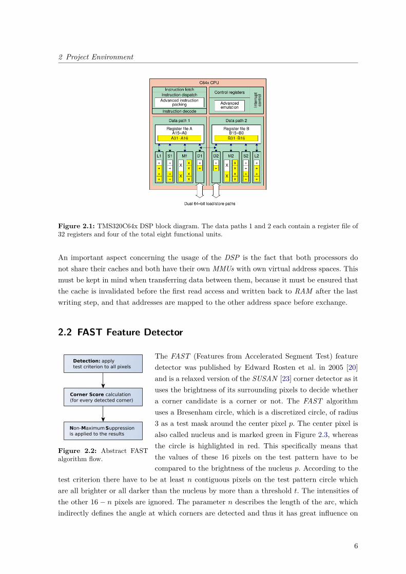
The C64x+ DSP has its own clock and runs at a maximum frequency of 800 MHz, implementsan eleven stage pipeline and is separated into two data paths. Each path contains a general-purpose register file with 32 32-bit registers and four functional units. The "register filessupport data ranging in size from packed [ . . . ][8-bit] data [(vectors)] through 40-bit fixed-point and 64-bit [fixed-/]floating-point data. Values larger than 32 bits, such as 40-bit longand 64-bit [ . . . ][non-integers] are stored in register pairs" [26].

The total of eight functional units (.L1, .S1, .M1, .D1, .L2, .S2, .M2, .D2) are shared equallyamong the data paths, from which two are multipliers and six are arithmetic units with slightlydifferent feature characteristics and supported instructions. So in a best-case scenario eightinstructions can execute in parallel. If an instruction can only be performed on one specificunit at a certain cycle, it is also possible to use data from the other path’s register file viatwo data cross paths. Additionally, each path has its own load and store path to memory, asseen in Figure 2.1.

Compared to the NEON extension, the DSP approach to parallel (multimedia) data pro-cessing is a bit different. The DSP features more functional units, but it keeps the 32-bitregister width. With multiple units executing the same instruction in parallel it may resultin the same processing speed, but dependent on the implementation it may also result inslower or faster execution. For example, logical operations on 32-bit data can be executedon two functional units on each path, which can result in four instructions being executedat the same time, which is exactly the same as one operation on a 128-bit vector (cf. [27]).Many algorithms can profit from instruction parallelism as it can be used here, especiallywhen they cannot be easily parallelized or not at all. For implementations that are capableof vectorized data processing it is also often possible to reach the same performance as withlarger data vectors, as in the NEON architecture.

Although the DSP has its own peripherals, it has no direct means of communication to thehost CPU except the main memory. Therefore, control mechanisms are needed in order tobe able to move certain tasks to the DSP and unburden the host processor. A popular DSP-OS, which manages tasks on the DSP, is the DSP/BIOS operating system from TI, whichis loaded by the host CPU onto the DSP. Once this is accomplished, so called nodes, whichimplement the user applications, can be loaded dynamically into the DSP/BIOS. Althoughthere are other possibilities to control the DSP/BIOS from the host side, here DSP-Bridge,also from TI, is used together with a lightweight DSP API from [18]. This interface includeshost-side bridge logic and easy access to common tasks that are necessary when working withan co-processor. The DSP API and its sublayers implement a mailboxing-system between thetwo processors through the main memory. Through these messages nodes can be launched,parameters can be passed or status messages can be exchanged. (Cf. [31].)

5


Figure 2.1: TMS320C64x DSP block diagram. The data paths 1 and 2 each contain a register file of32 registers and four of the total eight functional units.

An important aspect concerning the usage of the DSP is the fact that both processors donot share their caches and both have their own MMUs with own virtual address spaces. Thismust be kept in mind when transferring data between them, because it must be ensured thatthe cache is invalidated before the first read access and written back to RAM after the lastwriting step, and that addresses are mapped to the other address space before exchange.

2.2 FAST Feature Detector

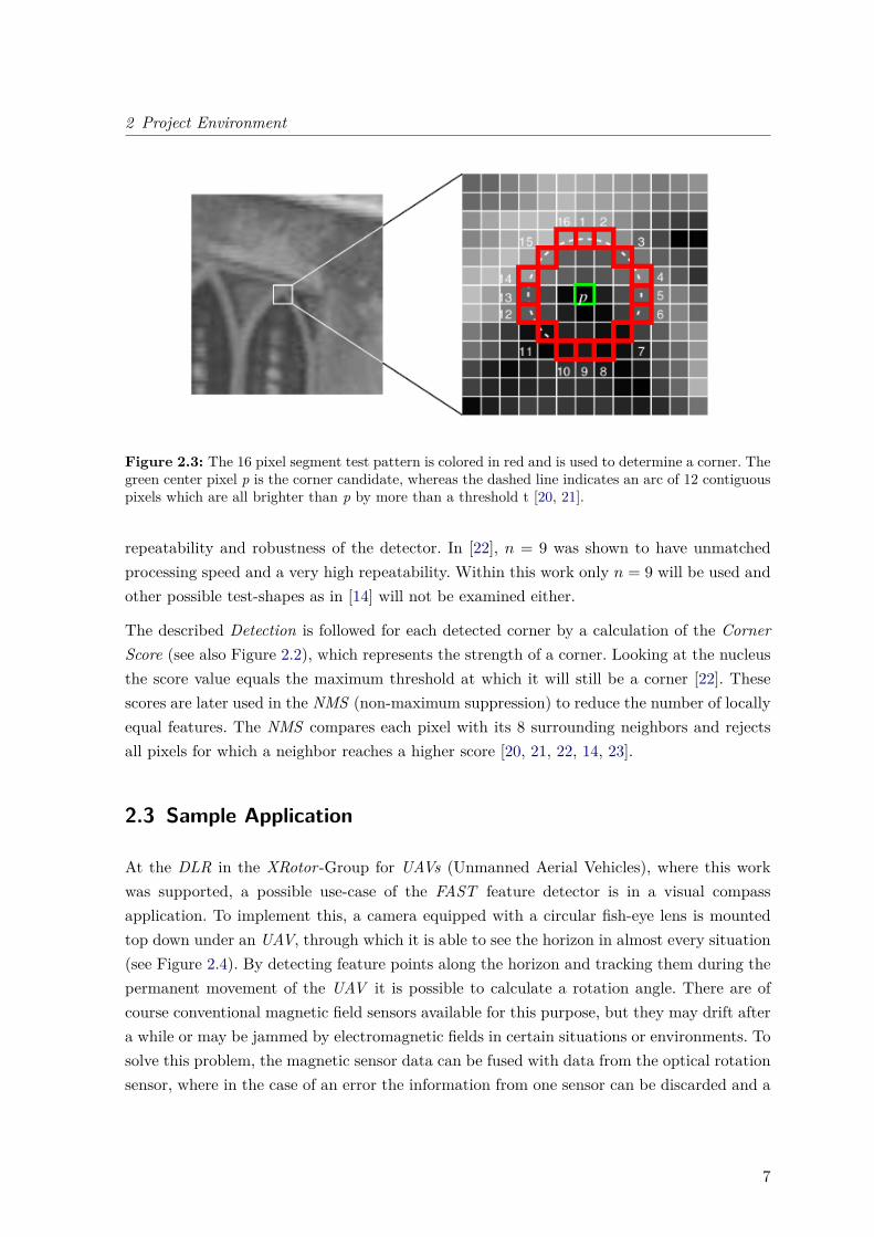
Figure 2.2: Abstract FASTalgorithm flow.

The FAST (Features from Accelerated Segment Test) featuredetector was published by Edward Rosten et al. in 2005 [20]and is a relaxed version of the SUSAN [23] corner detector as ituses the brightness of its surrounding pixels to decide whethera corner candidate is a corner or not. The FAST algorithmuses a Bresenham circle, which is a discretized circle, of radius3 as a test mask around the center pixel p. The center pixel isalso called nucleus and is marked green in Figure 2.3, whereasthe circle is highlighted in red. This specifically means thatthe values of these 16 pixels on the test pattern have to becompared to the brightness of the nucleus p. According to the

test criterion there have to be at least n contiguous pixels on the test pattern circle whichare all brighter or all darker than the nucleus by more than a threshold t. The intensities ofthe other 16 − n pixels are ignored. The parameter n describes the length of the arc, whichindirectly defines the angle at which corners are detected and thus it has great influence on

6


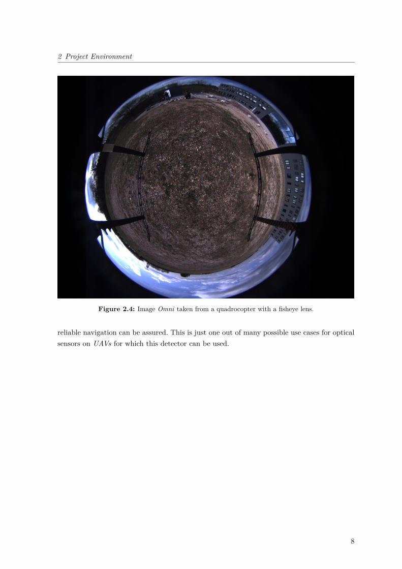
Figure 2.3: The 16 pixel segment test pattern is colored in red and is used to determine a corner. Thegreen center pixel p is the corner candidate, whereas the dashed line indicates an arc of 12 contiguouspixels which are all brighter than p by more than a threshold t [20, 21].

repeatability and robustness of the detector. In [22], n = 9 was shown to have unmatchedprocessing speed and a very high repeatability. Within this work only n = 9 will be used andother possible test-shapes as in [14] will not be examined either.

The described Detection is followed for each detected corner by a calculation of the CornerScore (see also Figure 2.2), which represents the strength of a corner. Looking at the nucleusthe score value equals the maximum threshold at which it will still be a corner [22]. Thesescores are later used in the NMS (non-maximum suppression) to reduce the number of locallyequal features. The NMS compares each pixel with its 8 surrounding neighbors and rejectsall pixels for which a neighbor reaches a higher score [20, 21, 22, 14, 23].

2.3 Sample Application

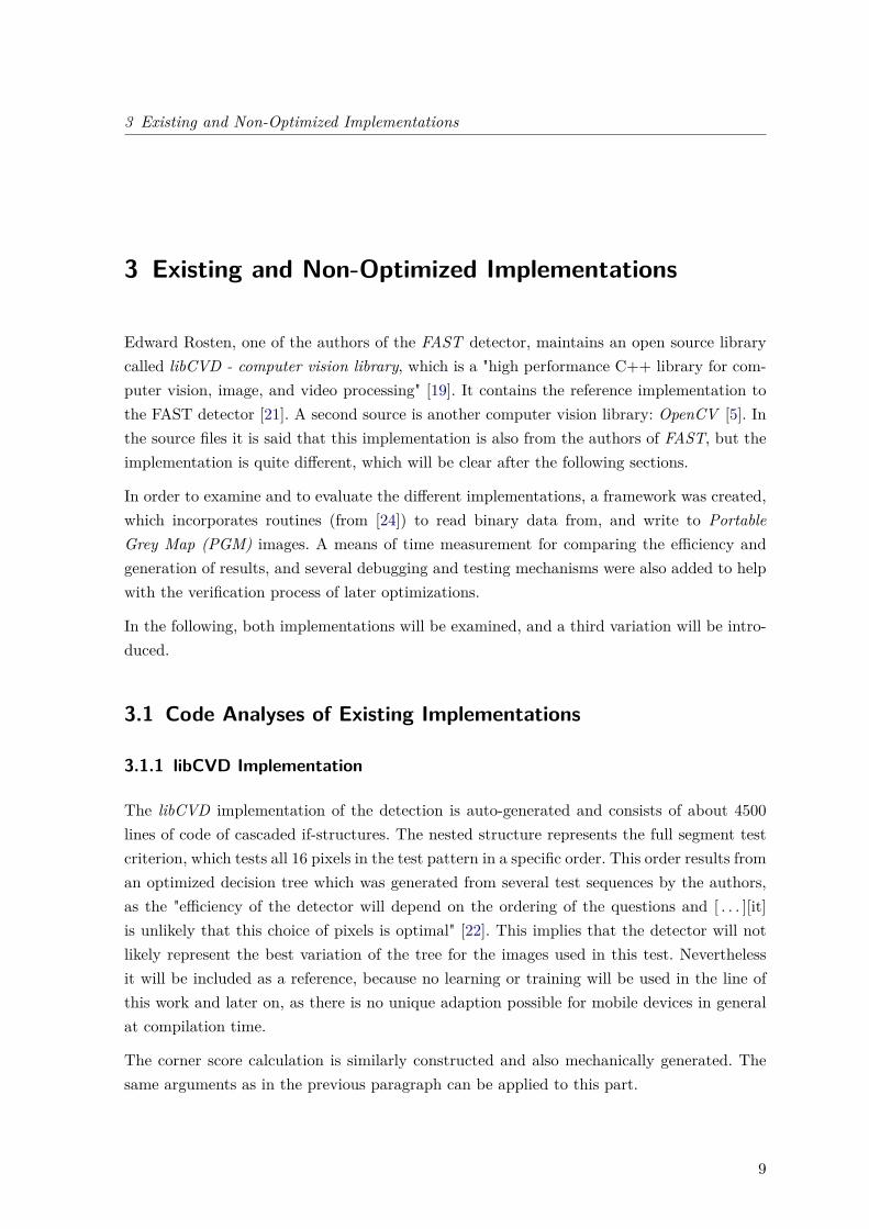
At the DLR in the XRotor-Group for UAVs (Unmanned Aerial Vehicles), where this workwas supported, a possible use-case of the FAST feature detector is in a visual compassapplication. To implement this, a camera equipped with a circular fish-eye lens is mountedtop down under an UAV, through which it is able to see the horizon in almost every situation(see Figure 2.4). By detecting feature points along the horizon and tracking them during thepermanent movement of the UAV it is possible to calculate a rotation angle. There are ofcourse conventional magnetic field sensors available for this purpose, but they may drift aftera while or may be jammed by electromagnetic fields in certain situations or environments. Tosolve this problem, the magnetic sensor data can be fused with data from the optical rotationsensor, where in the case of an error the information from one sensor can be discarded and a

7


Figure 2.4: Image Omni taken from a quadrocopter with a fisheye lens.

reliable navigation can be assured. This is just one out of many possible use cases for opticalsensors on UAVs for which this detector can be used.

8

3 Existing and Non-Optimized Implementations


Edward Rosten, one of the authors of the FAST detector, maintains an open source librarycalled libCVD - computer vision library, which is a "high performance C++ library for com-puter vision, image, and video processing" [19]. It contains the reference implementation tothe FAST detector [21]. A second source is another computer vision library: OpenCV [5]. Inthe source files it is said that this implementation is also from the authors of FAST, but theimplementation is quite different, which will be clear after the following sections.

In order to examine and to evaluate the different implementations, a framework was created,which incorporates routines (from [24]) to read binary data from, and write to PortableGrey Map (PGM) images. A means of time measurement for comparing the efficiency andgeneration of results, and several debugging and testing mechanisms were also added to helpwith the verification process of later optimizations.

In the following, both implementations will be examined, and a third variation will be intro-duced.

3.1 Code Analyses of Existing Implementations

3.1.1 libCVD Implementation

The libCVD implementation of the detection is auto-generated and consists of about 4500lines of code of cascaded if-structures. The nested structure represents the full segment testcriterion, which tests all 16 pixels in the test pattern in a specific order. This order results froman optimized decision tree which was generated from several test sequences by the authors,as the "efficiency of the detector will depend on the ordering of the questions and [ . . . ][it]is unlikely that this choice of pixels is optimal" [22]. This implies that the detector will notlikely represent the best variation of the tree for the images used in this test. Neverthelessit will be included as a reference, because no learning or training will be used in the line ofthis work and later on, as there is no unique adaption possible for mobile devices in generalat compilation time.

The corner score calculation is similarly constructed and also mechanically generated. Thesame arguments as in the previous paragraph can be applied to this part.

9


3.1.2 OpenCV Implementation

The OpenCV implementation includes a generalized approach, which is not based on opti-mized trees and is processor independent. But it also includes a partial vectorized (SIMD)version for the multimedia extension SSE2 on x86 CPUs.

OpenCV Single Pixel Processing

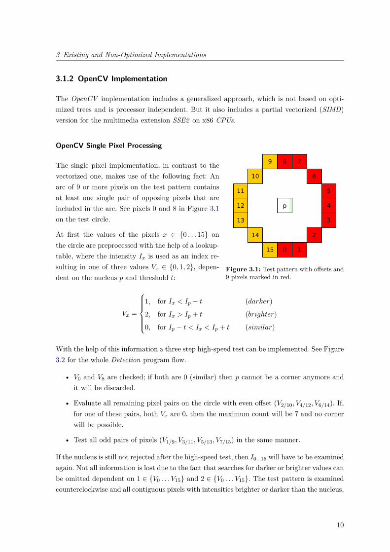
Figure 3.1: Test pattern with offsets and9 pixels marked in red.

The single pixel implementation, in contrast to thevectorized one, makes use of the following fact: Anarc of 9 or more pixels on the test pattern containsat least one single pair of opposing pixels that areincluded in the arc. See pixels 0 and 8 in Figure 3.1on the test circle.

At first the values of the pixels x ∈ 0 . . . 15 onthe circle are preprocessed with the help of a lookup-table, where the intensity Ix is used as an index re-sulting in one of three values Vx ∈ 0, 1, 2, depen-dent on the nucleus p and threshold t:

Vx =

1, for Ix < Ip − t (darker)

2, for Ix > Ip + t (brighter)

0, for Ip − t < Ix < Ip + t (similar)

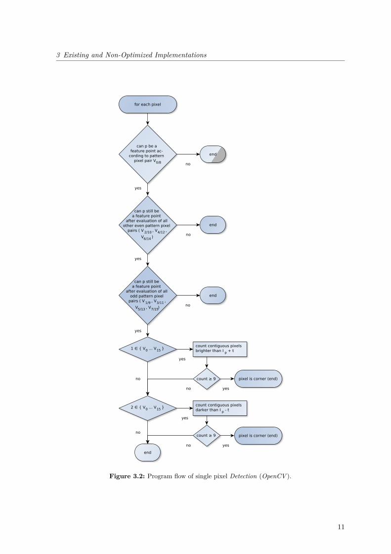
With the help of this information a three step high-speed test can be implemented. See Figure3.2 for the whole Detection program flow.

• V0 and V8 are checked; if both are 0 (similar) then p cannot be a corner anymore andit will be discarded.

• Evaluate all remaining pixel pairs on the circle with even offset (V2/10, V4/12, V6/14). If,for one of these pairs, both Vx are 0, then the maximum count will be 7 and no cornerwill be possible.

• Test all odd pairs of pixels (V1/9, V3/11, V5/13, V7/15) in the same manner.

If the nucleus is still not rejected after the high-speed test, then I0...15 will have to be examinedagain. Not all information is lost due to the fact that searches for darker or brighter values canbe omitted dependent on 1 ∈ V0 . . . V15 and 2 ∈ V0 . . . V15. The test pattern is examinedcounterclockwise and all contiguous pixels with intensities brighter or darker than the nucleus,

10


Figure 3.2: Program flow of single pixel Detection (OpenCV ).

11


by more than the threshold, are counted. When the arc is interrupted by pixels, which donot belong to the same class of brighter or darker, the counter is reset to 0. If the counterexceeds 8, then a valid corner is found.

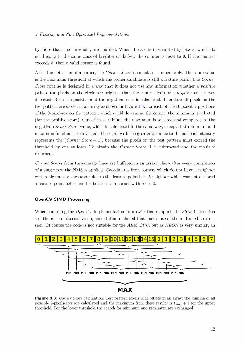
After the detection of a corner, the Corner Score is calculated immediately. The score valueis the maximum threshold at which the corner candidate is still a feature point. The CornerScore routine is designed in a way that it does not use any information whether a positive(where the pixels on the circle are brighter than the center pixel) or a negative corner wasdetected. Both the positive and the negative score is calculated. Therefore all pixels on thetest pattern are stored in an array as shown in Figure 3.3. For each of the 16 possible positionsof the 9-pixel-arc on the pattern, which could determine the corner, the minimum is selected(for the positive score). Out of these minima the maximum is selected and compared to thenegative Corner Score value, which is calculated in the same way, except that minimum andmaximum functions are inverted. The score with the greater distance to the nucleus’ intensityrepresents the (Corner Score + 1), because the pixels on the test pattern must exceed thethreshold by one at least. To obtain the Corner Score, 1 is subtracted and the result isreturned.

Corner Scores from three image lines are buffered in an array, where after every completionof a single row the NMS is applied. Coordinates from corners which do not have a neighborwith a higher score are appended to the feature-point list. A neighbor which was not declareda feature point beforehand is treated as a corner with score 0.

OpenCV SIMD Processing

When compiling the OpenCV implementation for a CPU that supports the SSE2 instructionset, there is an alternative implementation included that makes use of the multimedia exten-sion. Of course the code is not suitable for the ARM CPU, but as NEON is very similar, an

0 4 752 81 3 6 9 013 414 511 210 115 612 3

MIN MINMINMINMIN MIN MINMINMIN MINMINMIN MINMIN MINMIN

MAX

7

Figure 3.3: Corner Score calculation: Test pattern pixels with offsets in an array; the minima of allpossible 9-pixels-arcs are calculated and the maximum from these results is tmax + 1 for the upperthreshold. For the lower threshold the search for minimum and maximum are exchanged.

12


adapted NEON version will be created in the next section. In the following paragraphs theSIMD version will be analyzed and explained.

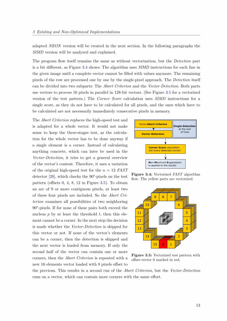
The program flow itself remains the same as without vectorization, but the Detection partis a bit different, as Figure 3.4 shows: The algorithm uses SIMD instructions for each line inthe given image until a complete vector cannot be filled with values anymore. The remainingpixels of the row are processed one by one by the single-pixel approach. The Detection itselfcan be divided into two subparts: The Abort Criterion and the Vector-Detection. Both partsuse vectors to process 16 pixels in parallel in 128-bit vectors. (See Figure 3.5 for a vectorizedversion of the test pattern.) The Corner Score calculation uses SIMD instructions for asingle score, as they do not have to be calculated for all pixels, and the ones which have tobe calculated are not necessarily immediately consecutive pixels in memory.

Figure 3.4: Vectorized FAST algorithmflow. The yellow parts are vectorized.

Figure 3.5: Vectorized test pattern withoffset-vector 0 marked in red.

The Abort Criterion replaces the high-speed test andis adapted for a whole vector. It would not makesense to keep the three-stages test, as the calcula-tion for the whole vector has to be done anyway ifa single element is a corner. Instead of calculatinganything concrete, which can later be used in theVector-Detection, it tries to get a general overviewof the vector’s content. Therefore, it uses a variationof the original high-speed test for the n = 12 FASTdetector [20], which checks the 90°-pixels on the testpattern (offsets 0, 4, 8, 12 in Figure 3.5). To obtainan arc of 9 or more contiguous pixels, at least twoof these four pixels are included. So the Abort Cri-terion examines all possibilities of two neighboring90°-pixels. If for none of these pairs both exceed thenucleus p by at least the threshold t, then this ele-ment cannot be a corner. In the next step the decisionis made whether the Vector-Detection is skipped forthis vector or not. If none of the vector’s elementscan be a corner, then the detection is skipped andthe next vector is loaded from memory. If only thesecond half of the vector can contain one or morecorners, then the Abort Criterion is repeated with anew 16 elements vector loaded with 8 pixels offset tothe previous. This results in a second run of the Abort Criterion, but the Vector-Detectionruns on a vector, which can contain more corners with the same effort.

13


...

...

00000001 000000010000000000000011 ...

SUB SUB SUB SUBc0

m0 11111111 000000000000000011111111

00000000 000000010000000000000010

...

00000001 000000000000000000000011 ...

AND AND AND AND

m0

c0

11111111 000000000000000011111111

Figure 3.6: Vectorized counter example. c0is the counter and m0 contains the compari-son results. The first and the fourth elementare incremented, whereas the second is resetand the third stays at 0.

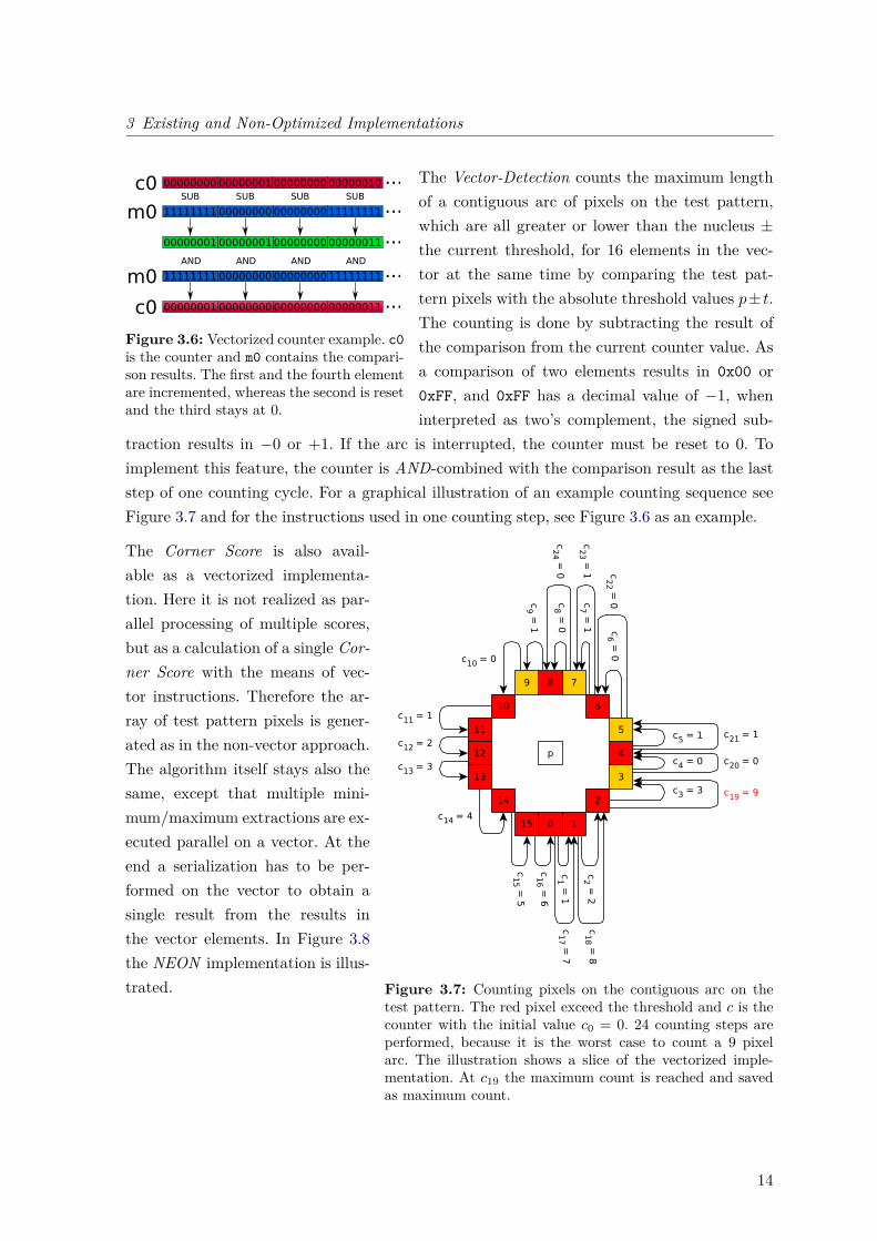
The Vector-Detection counts the maximum lengthof a contiguous arc of pixels on the test pattern,which are all greater or lower than the nucleus ±the current threshold, for 16 elements in the vec-tor at the same time by comparing the test pat-tern pixels with the absolute threshold values p± t.The counting is done by subtracting the result ofthe comparison from the current counter value. Asa comparison of two elements results in 0x00 or0xFF, and 0xFF has a decimal value of −1, wheninterpreted as two’s complement, the signed sub-

traction results in −0 or +1. If the arc is interrupted, the counter must be reset to 0. Toimplement this feature, the counter is AND-combined with the comparison result as the laststep of one counting cycle. For a graphical illustration of an example counting sequence seeFigure 3.7 and for the instructions used in one counting step, see Figure 3.6 as an example.

Figure 3.7: Counting pixels on the contiguous arc on thetest pattern. The red pixel exceed the threshold and c is thecounter with the initial value c0 = 0. 24 counting steps areperformed, because it is the worst case to count a 9 pixelarc. The illustration shows a slice of the vectorized imple-mentation. At c19 the maximum count is reached and savedas maximum count.

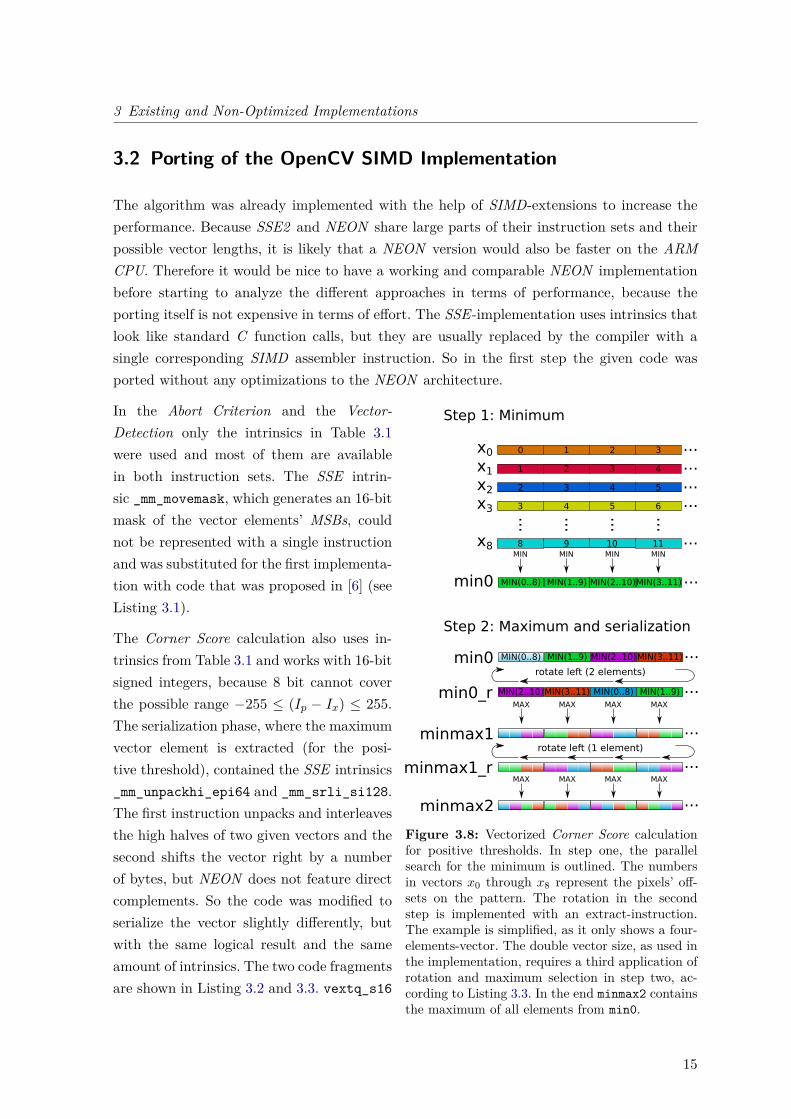
The Corner Score is also avail-able as a vectorized implementa-tion. Here it is not realized as par-allel processing of multiple scores,but as a calculation of a single Cor-ner Score with the means of vec-tor instructions. Therefore the ar-ray of test pattern pixels is gener-ated as in the non-vector approach.The algorithm itself stays also thesame, except that multiple mini-mum/maximum extractions are ex-ecuted parallel on a vector. At theend a serialization has to be per-formed on the vector to obtain asingle result from the results inthe vector elements. In Figure 3.8the NEON implementation is illus-trated.

14


3.2 Porting of the OpenCV SIMD Implementation

The algorithm was already implemented with the help of SIMD-extensions to increase theperformance. Because SSE2 and NEON share large parts of their instruction sets and theirpossible vector lengths, it is likely that a NEON version would also be faster on the ARMCPU. Therefore it would be nice to have a working and comparable NEON implementationbefore starting to analyze the different approaches in terms of performance, because theporting itself is not expensive in terms of effort. The SSE-implementation uses intrinsics thatlook like standard C function calls, but they are usually replaced by the compiler with asingle corresponding SIMD assembler instruction. So in the first step the given code wasported without any optimizations to the NEON architecture.

1 2 3 4 ...x1

2 3 4 5 ...x2

MIN(0..8) MIN(1..9) MIN(2..10)MIN(3..11) ...min0

3 4 5 6 ...x3

0 1 2 3 ...x0

x8

...

...

...

...

8 9 10 11 ...MIN MIN MIN MIN

minmax1_r ...

min0

min0_r

minmax1

minmax2

MIN(0..8) MIN(1..9) MIN(2..10)MIN(3..11) ...

MIN(2..10)MIN(3..11) MIN(0..8) MIN(1..9) ...MAX MAX MAX MAX

...

MAX MAX MAX MAX

...

Step 1: Minimum

Step 2: Maximum and serialization

rotate left (1 element)

rotate left (2 elements)

Figure 3.8: Vectorized Corner Score calculationfor positive thresholds. In step one, the parallelsearch for the minimum is outlined. The numbersin vectors x0 through x8 represent the pixels’ off-sets on the pattern. The rotation in the secondstep is implemented with an extract-instruction.The example is simplified, as it only shows a four-elements-vector. The double vector size, as used inthe implementation, requires a third application ofrotation and maximum selection in step two, ac-cording to Listing 3.3. In the end minmax2 containsthe maximum of all elements from min0.

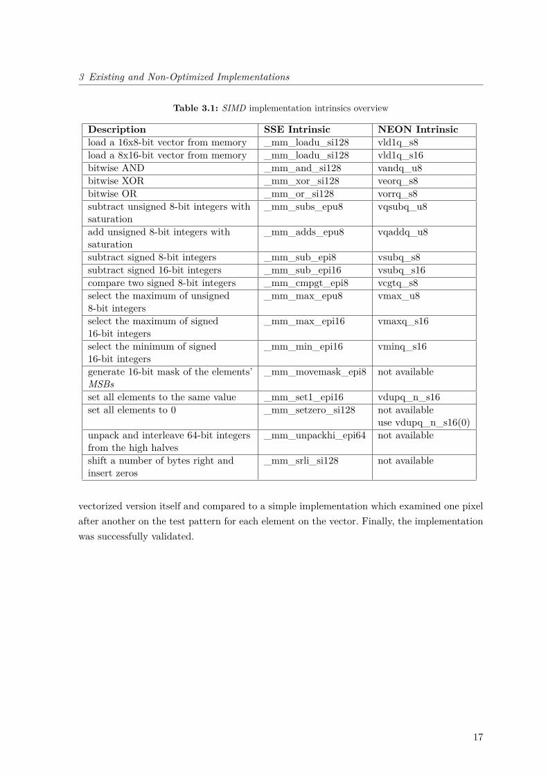
In the Abort Criterion and the Vector-Detection only the intrinsics in Table 3.1were used and most of them are availablein both instruction sets. The SSE intrin-sic _mm_movemask, which generates an 16-bitmask of the vector elements’ MSBs, couldnot be represented with a single instructionand was substituted for the first implementa-tion with code that was proposed in [6] (seeListing 3.1).

The Corner Score calculation also uses in-trinsics from Table 3.1 and works with 16-bitsigned integers, because 8 bit cannot coverthe possible range −255 ≤ (Ip − Ix) ≤ 255.The serialization phase, where the maximumvector element is extracted (for the posi-tive threshold), contained the SSE intrinsics_mm_unpackhi_epi64 and _mm_srli_si128.The first instruction unpacks and interleavesthe high halves of two given vectors and thesecond shifts the vector right by a numberof bytes, but NEON does not feature directcomplements. So the code was modified toserialize the vector slightly differently, butwith the same logical result and the sameamount of intrinsics. The two code fragmentsare shown in Listing 3.2 and 3.3. vextq_s16

15


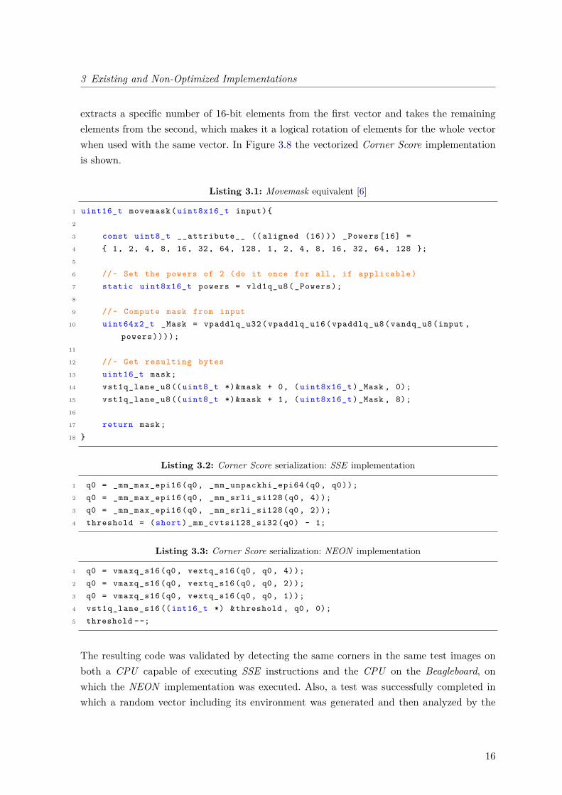
extracts a specific number of 16-bit elements from the first vector and takes the remainingelements from the second, which makes it a logical rotation of elements for the whole vectorwhen used with the same vector. In Figure 3.8 the vectorized Corner Score implementationis shown.

Listing 3.1: Movemask equivalent [6]

1 uint16_t movemask ( uint8x16_t input)2

3 const uint8_t __attribute__ (( aligned (16))) _Powers [16] =4 1, 2, 4, 8, 16, 32, 64, 128, 1, 2, 4, 8, 16, 32, 64, 128 ;5

6 //~ Set the powers of 2 (do it once for all , if applicable )7 static uint8x16_t powers = vld1q_u8 ( _Powers );8

9 //~ Compute mask from input10 uint64x2_t _Mask = vpaddlq_u32 ( vpaddlq_u16 ( vpaddlq_u8 ( vandq_u8 (input ,

powers ))));11

12 //~ Get resulting bytes13 uint16_t mask;14 vst1q_lane_u8 (( uint8_t *)&mask + 0, ( uint8x16_t )_Mask , 0);15 vst1q_lane_u8 (( uint8_t *)&mask + 1, ( uint8x16_t )_Mask , 8);16

17 return mask;18

Listing 3.2: Corner Score serialization: SSE implementation

1 q0 = _mm_max_epi16 (q0 , _mm_unpackhi_epi64 (q0 , q0));2 q0 = _mm_max_epi16 (q0 , _mm_srli_si128 (q0 , 4));3 q0 = _mm_max_epi16 (q0 , _mm_srli_si128 (q0 , 2));4 threshold = (short) _mm_cvtsi128_si32 (q0) - 1;

Listing 3.3: Corner Score serialization: NEON implementation

1 q0 = vmaxq_s16 (q0 , vextq_s16 (q0 , q0 , 4));2 q0 = vmaxq_s16 (q0 , vextq_s16 (q0 , q0 , 2));3 q0 = vmaxq_s16 (q0 , vextq_s16 (q0 , q0 , 1));4 vst1q_lane_s16 (( int16_t *) &threshold , q0 , 0);5 threshold --;

The resulting code was validated by detecting the same corners in the same test images onboth a CPU capable of executing SSE instructions and the CPU on the Beagleboard, onwhich the NEON implementation was executed. Also, a test was successfully completed inwhich a random vector including its environment was generated and then analyzed by the

16


Table 3.1: SIMD implementation intrinsics overview

Description SSE Intrinsic NEON Intrinsicload a 16x8-bit vector from memory _mm_loadu_si128 vld1q_s8load a 8x16-bit vector from memory _mm_loadu_si128 vld1q_s16bitwise AND _mm_and_si128 vandq_u8bitwise XOR _mm_xor_si128 veorq_s8bitwise OR _mm_or_si128 vorrq_s8subtract unsigned 8-bit integers withsaturation

_mm_subs_epu8 vqsubq_u8

add unsigned 8-bit integers withsaturation

_mm_adds_epu8 vqaddq_u8

subtract signed 8-bit integers _mm_sub_epi8 vsubq_s8subtract signed 16-bit integers _mm_sub_epi16 vsubq_s16compare two signed 8-bit integers _mm_cmpgt_epi8 vcgtq_s8select the maximum of unsigned8-bit integers

_mm_max_epu8 vmax_u8

select the maximum of signed16-bit integers

_mm_max_epi16 vmaxq_s16

select the minimum of signed16-bit integers

_mm_min_epi16 vminq_s16

generate 16-bit mask of the elements’MSBs

_mm_movemask_epi8 not available

set all elements to the same value _mm_set1_epi16 vdupq_n_s16set all elements to 0 _mm_setzero_si128 not available

use vdupq_n_s16(0)unpack and interleave 64-bit integersfrom the high halves

_mm_unpackhi_epi64 not available

shift a number of bytes right andinsert zeros

_mm_srli_si128 not available

vectorized version itself and compared to a simple implementation which examined one pixelafter another on the test pattern for each element on the vector. Finally, the implementationwas successfully validated.

17


3.3 Profiling of the Available Implementations

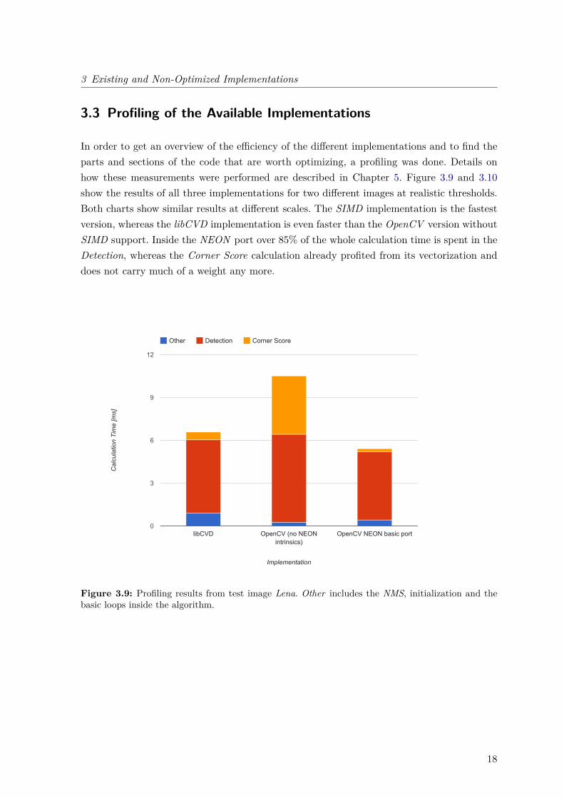
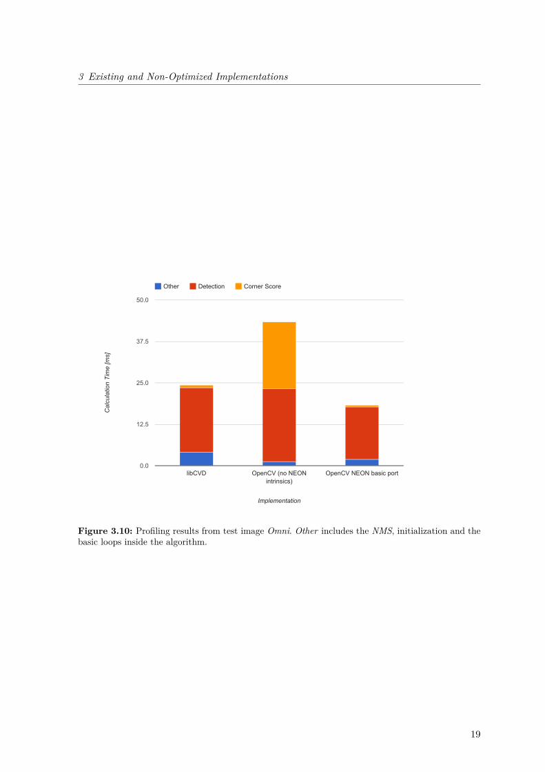
In order to get an overview of the efficiency of the different implementations and to find theparts and sections of the code that are worth optimizing, a profiling was done. Details onhow these measurements were performed are described in Chapter 5. Figure 3.9 and 3.10show the results of all three implementations for two different images at realistic thresholds.Both charts show similar results at different scales. The SIMD implementation is the fastestversion, whereas the libCVD implementation is even faster than the OpenCV version withoutSIMD support. Inside the NEON port over 85% of the whole calculation time is spent in theDetection, whereas the Corner Score calculation already profited from its vectorization anddoes not carry much of a weight any more.

Other Detection Corner Score

libCVD OpenCV (no NEONintrinsics)

OpenCV NEON basic port0

3

6

9

12

Implementation

Cal

cula

tion

Tim

e [m

s]

Figure 3.9: Profiling results from test image Lena. Other includes the NMS, initialization and thebasic loops inside the algorithm.

18


Other Detection Corner Score

libCVD OpenCV (no NEONintrinsics)

OpenCV NEON basic port0.0

12.5

25.0

37.5

50.0

Implementation

Cal

cula

tion

Tim

e [m

s]

Figure 3.10: Profiling results from test image Omni. Other includes the NMS, initialization and thebasic loops inside the algorithm.

19

4 Optimization

4 Optimization

4.1 NEON Optimizations

In Section 3.3 it was shown that the OpenCV basic NEON port was the fastest of thereviewed implementations and it will be further optimized in this section. There is no wayof vectorization or pipeline optimizations in the libCVD implementation because of the highamount of conditional branches, which interrupt the program flow enormously. Also, theOpenCV implementation without NEON intrinsics will not be optimized because the NEONport is already a kind of optimization from this version. So in this section, it will be tried tooptimize the NEON port in respect of code, algorithm and cache with focus on the Detection,as it consumes the most time and therefore offers the highest potential of optimization.

4.1.1 Code Optimizations

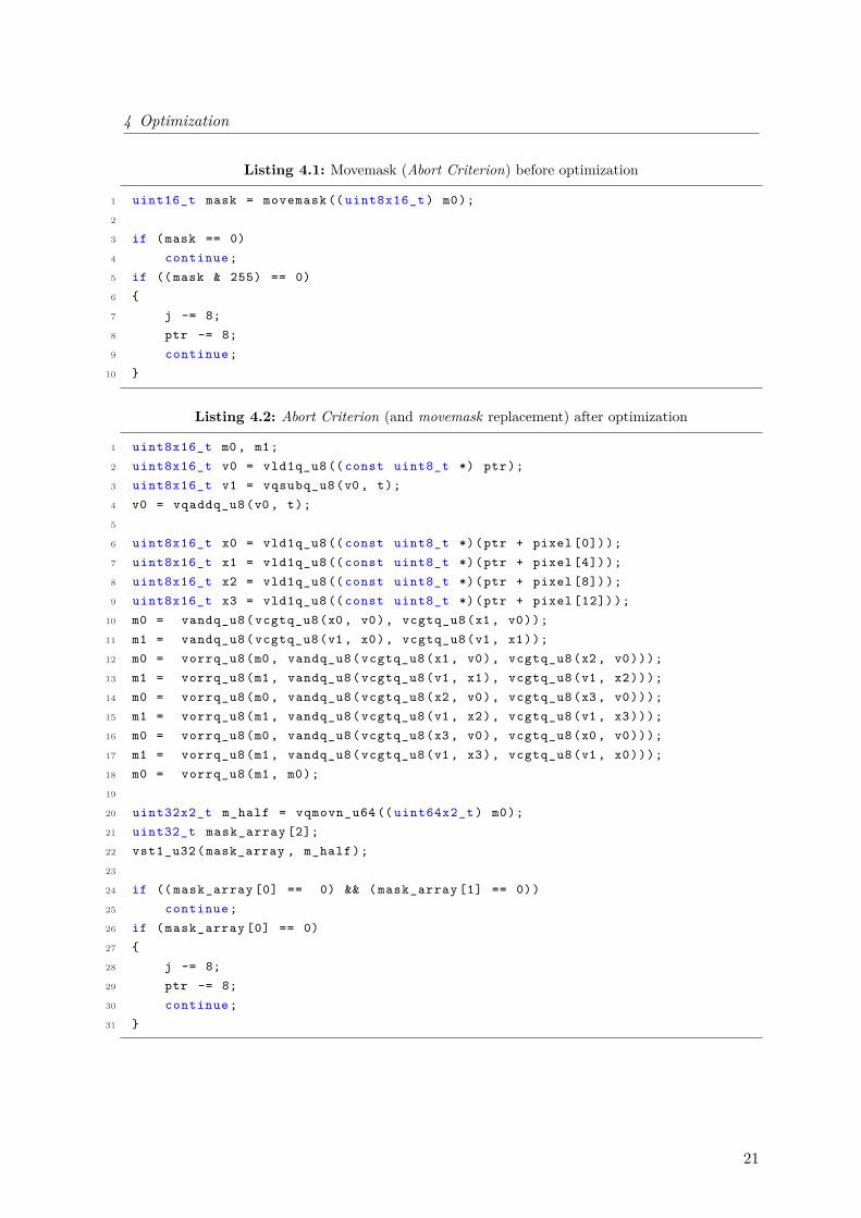
Although gprof [8], a profiling tool, was not able to generate exact timing information due toits sampling resolution, it was able to show in the first tests that the movemask equivalentfrom Listing 3.1 was called quite often. It occurs once in the Abort Criterion and once at theend of the Vector-Detection for every vector. It was clear from the beginning that it was notnecessarily the fastest replacement and would consume quite a bit of the whole calculationtime, but it was a simple and fast solution for a quick porting of the code. Finally, both caseswere exchanged with some modified code in order to avoid the mask exactly as generated bymovemask.

For the Abort Criterion it is only important to know whether there are possible corners inthe first and in the second half of the vector. Thus, a saturated narrowing of each half isperformed, which results in a 64-bit vector. This vector is stored in an array of two 32-bit integers, because there are no instructions for a narrowing down to 32-bit or less. Thedetection whether the whole vector or the half is empty can now be checked by only comparingthe two integers with zero. Listing 4.1 shows the code before, and the bottom section of 4.2shows it after the optimization. The code does not seem to be more efficient on the first sight,because three lines replace a single line in the listing, but the old implementation containsa function call to the even longer movemask routine. All in all the execution time could bereduced by this modification.

20

4 Optimization

Listing 4.1: Movemask (Abort Criterion) before optimization

1 uint16_t mask = movemask (( uint8x16_t ) m0);2

3 if (mask == 0)4 continue ;5 if (( mask & 255) == 0)6 7 j -= 8;8 ptr -= 8;9 continue ;

10

Listing 4.2: Abort Criterion (and movemask replacement) after optimization

1 uint8x16_t m0 , m1;2 uint8x16_t v0 = vld1q_u8 (( const uint8_t *) ptr);3 uint8x16_t v1 = vqsubq_u8 (v0 , t);4 v0 = vqaddq_u8 (v0 , t);5

6 uint8x16_t x0 = vld1q_u8 (( const uint8_t *)(ptr + pixel [0]));7 uint8x16_t x1 = vld1q_u8 (( const uint8_t *)(ptr + pixel [4]));8 uint8x16_t x2 = vld1q_u8 (( const uint8_t *)(ptr + pixel [8]));9 uint8x16_t x3 = vld1q_u8 (( const uint8_t *)(ptr + pixel [12]));

10 m0 = vandq_u8 ( vcgtq_u8 (x0 , v0), vcgtq_u8 (x1 , v0));11 m1 = vandq_u8 ( vcgtq_u8 (v1 , x0), vcgtq_u8 (v1 , x1));12 m0 = vorrq_u8 (m0 , vandq_u8 ( vcgtq_u8 (x1 , v0), vcgtq_u8 (x2 , v0)));13 m1 = vorrq_u8 (m1 , vandq_u8 ( vcgtq_u8 (v1 , x1), vcgtq_u8 (v1 , x2)));14 m0 = vorrq_u8 (m0 , vandq_u8 ( vcgtq_u8 (x2 , v0), vcgtq_u8 (x3 , v0)));15 m1 = vorrq_u8 (m1 , vandq_u8 ( vcgtq_u8 (v1 , x2), vcgtq_u8 (v1 , x3)));16 m0 = vorrq_u8 (m0 , vandq_u8 ( vcgtq_u8 (x3 , v0), vcgtq_u8 (x0 , v0)));17 m1 = vorrq_u8 (m1 , vandq_u8 ( vcgtq_u8 (v1 , x3), vcgtq_u8 (v1 , x0)));18 m0 = vorrq_u8 (m1 , m0);19

20 uint32x2_t m_half = vqmovn_u64 (( uint64x2_t ) m0);21 uint32_t mask_array [2];22 vst1_u32 (mask_array , m_half );23

24 if (( mask_array [0] == 0) && ( mask_array [1] == 0))25 continue ;26 if ( mask_array [0] == 0)27 28 j -= 8;29 ptr -= 8;30 continue ;31

21

4 Optimization

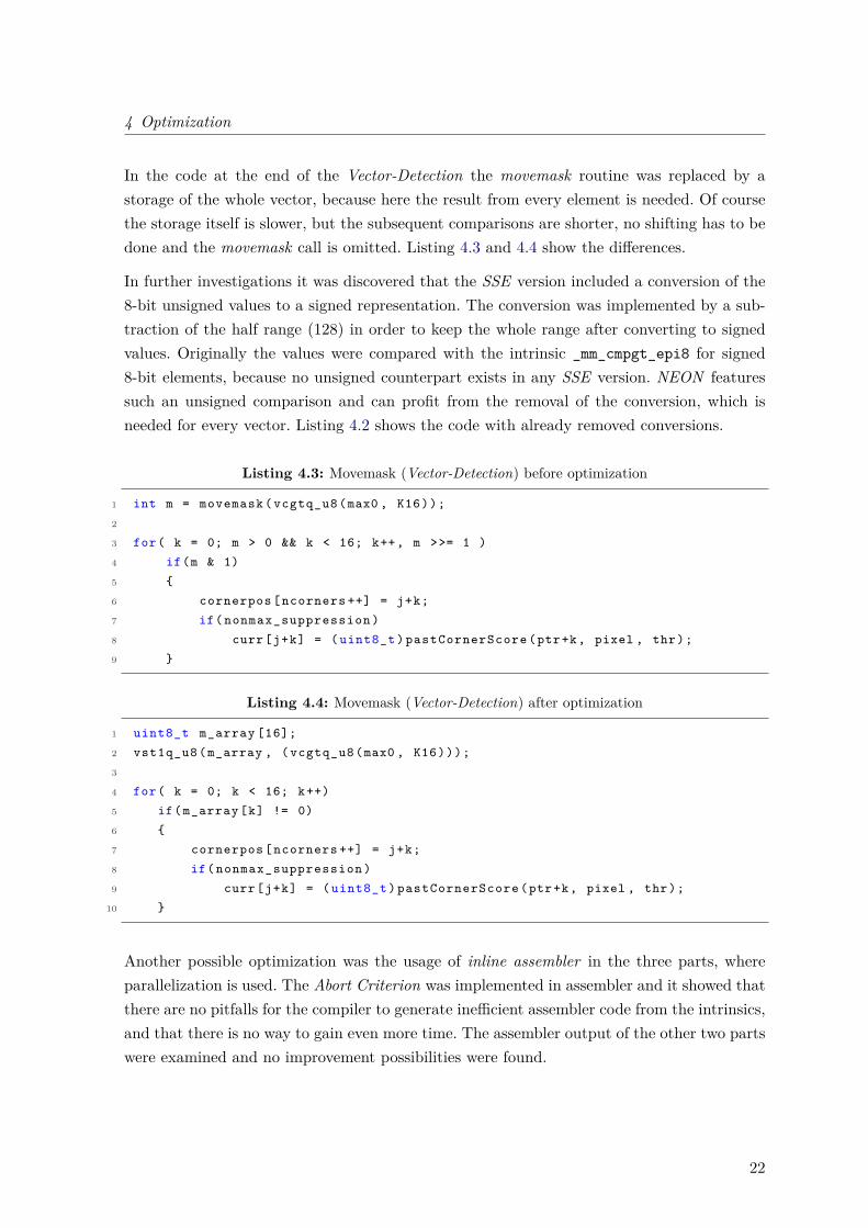
In the code at the end of the Vector-Detection the movemask routine was replaced by astorage of the whole vector, because here the result from every element is needed. Of coursethe storage itself is slower, but the subsequent comparisons are shorter, no shifting has to bedone and the movemask call is omitted. Listing 4.3 and 4.4 show the differences.

In further investigations it was discovered that the SSE version included a conversion of the8-bit unsigned values to a signed representation. The conversion was implemented by a sub-traction of the half range (128) in order to keep the whole range after converting to signedvalues. Originally the values were compared with the intrinsic _mm_cmpgt_epi8 for signed8-bit elements, because no unsigned counterpart exists in any SSE version. NEON featuressuch an unsigned comparison and can profit from the removal of the conversion, which isneeded for every vector. Listing 4.2 shows the code with already removed conversions.

Listing 4.3: Movemask (Vector-Detection) before optimization

1 int m = movemask ( vcgtq_u8 (max0 , K16));2

3 for( k = 0; m > 0 && k < 16; k++, m >>= 1 )4 if(m & 1)5 6 cornerpos [ ncorners ++] = j+k;7 if( nonmax_suppression )8 curr[j+k] = ( uint8_t ) pastCornerScore (ptr+k, pixel , thr);9

Listing 4.4: Movemask (Vector-Detection) after optimization

1 uint8_t m_array [16];2 vst1q_u8 (m_array , ( vcgtq_u8 (max0 , K16)));3

4 for( k = 0; k < 16; k++)5 if( m_array [k] != 0)6 7 cornerpos [ ncorners ++] = j+k;8 if( nonmax_suppression )9 curr[j+k] = ( uint8_t ) pastCornerScore (ptr+k, pixel , thr);

10

Another possible optimization was the usage of inline assembler in the three parts, whereparallelization is used. The Abort Criterion was implemented in assembler and it showed thatthere are no pitfalls for the compiler to generate inefficient assembler code from the intrinsics,and that there is no way to gain even more time. The assembler output of the other two partswere examined and no improvement possibilities were found.

22

4 Optimization

4.1.2 Algorithm Optimizations

It was also tested whether the processing of single pixels at the end of each line could bereplaced by an additional vector processing loop with only a part of its content being validdata. In some cases a rather small reduction of execution time could be reached, but nouniversal improvement could be measured, as it depends on the actual line length and thenumber of features found in each row. A benefit in some cases is definitely possible, but thisshould be evaluated separately for each case.

The algorithm was also modified in a test to integrate the Corner Score calculation intothe Vector-Detection loop and to keep it really parallel. If the vector contained only featurepoints, for which the score had to be calculated anyway, then the algorithm could profitfrom calculating the score in parallel. In standard use cases, in which vectors do not containthat many corners to justify the massive prolonging of the Vector-Detection, it is fasterto only compute the score for the really detected feature points. Another reason why thisimplementation is slower than the original is the fact that the CPU features only 16 NEONregisters, but far more values have to be kept accessible to calculate the Corner Score withinthe detection loop. Even an more optimized version with the whole Vector-Detection unrolledmanually was slower than the basic NEON port.

4.1.3 Cache Optimizations

A reason for different algorithms revealing a poor performance is an inefficient cache usage,which causes pipeline stalls and waiting cycles. As the FAST algorithm only needs sevenimage lines to be quickly accessible, images of moderate resolutions should fit into the CPU ’sL1-cache, which features 32 KB. To prove this statement, a cache simulation was performedwith Dinero IV [7]. Therefore all read accesses to image data were logged including theaddresses, which were then used for the simulation. The simulation results for the testedimages showed only cold misses, which are obligatory and cannot be avoided.

4.2 DSP Implementation and Optimization

The CPU implementation was optimized up to a stage at which the optimization effortslowly exceeds the resulting gain in performance, because the large improvements with bigimpacts were already covered and only small non-optimal parts may be hidden somewhere.To reduce the resource footprint a bit more on the CPU itself, an implementation for theon-chip DSP will be created and adapted for the special needs of the co-processor. As many ofthe optimizations done in the previous sections do not only apply for the NEON instructionset, but are also applicable for the DSP, it was tried to keep as many as possible.

23

4 Optimization

On the host side implementation, a possibility to choose between execution on CPU and DSPwas added. Furthermore, the image data must be copied to an aligned buffer suitable for theDSP. An output buffer must be allocated, and the buffers have to be mapped, too.

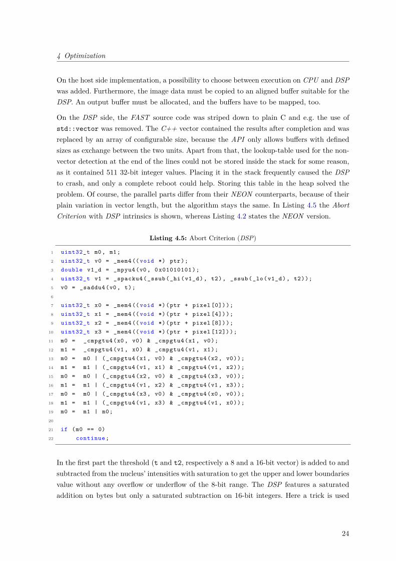
On the DSP side, the FAST source code was striped down to plain C and e.g. the use ofstd::vector was removed. The C++ vector contained the results after completion and wasreplaced by an array of configurable size, because the API only allows buffers with definedsizes as exchange between the two units. Apart from that, the lookup-table used for the non-vector detection at the end of the lines could not be stored inside the stack for some reason,as it contained 511 32-bit integer values. Placing it in the stack frequently caused the DSPto crash, and only a complete reboot could help. Storing this table in the heap solved theproblem. Of course, the parallel parts differ from their NEON counterparts, because of theirplain variation in vector length, but the algorithm stays the same. In Listing 4.5 the AbortCriterion with DSP intrinsics is shown, whereas Listing 4.2 states the NEON version.

Listing 4.5: Abort Criterion (DSP)

1 uint32_t m0 , m1;2 uint32_t v0 = _mem4 (( void *) ptr);3 double v1_d = _mpyu4 (v0 , 0 x01010101 );4 uint32_t v1 = _spacku4 (_ssub(_hi(v1_d), t2), _ssub(_lo(v1_d), t2));5 v0 = _saddu4 (v0 , t);6

7 uint32_t x0 = _mem4 (( void *)(ptr + pixel [0]));8 uint32_t x1 = _mem4 (( void *)(ptr + pixel [4]));9 uint32_t x2 = _mem4 (( void *)(ptr + pixel [8]));

10 uint32_t x3 = _mem4 (( void *)(ptr + pixel [12]));11 m0 = _cmpgtu4 (x0 , v0) & _cmpgtu4 (x1 , v0);12 m1 = _cmpgtu4 (v1 , x0) & _cmpgtu4 (v1 , x1);13 m0 = m0 | ( _cmpgtu4 (x1 , v0) & _cmpgtu4 (x2 , v0));14 m1 = m1 | ( _cmpgtu4 (v1 , x1) & _cmpgtu4 (v1 , x2));15 m0 = m0 | ( _cmpgtu4 (x2 , v0) & _cmpgtu4 (x3 , v0));16 m1 = m1 | ( _cmpgtu4 (v1 , x2) & _cmpgtu4 (v1 , x3));17 m0 = m0 | ( _cmpgtu4 (x3 , v0) & _cmpgtu4 (x0 , v0));18 m1 = m1 | ( _cmpgtu4 (v1 , x3) & _cmpgtu4 (v1 , x0));19 m0 = m1 | m0;20

21 if (m0 == 0)22 continue ;

In the first part the threshold (t and t2, respectively a 8 and a 16-bit vector) is added to andsubtracted from the nucleus’ intensities with saturation to get the upper and lower boundariesvalue without any overflow or underflow of the 8-bit range. The DSP features a saturatedaddition on bytes but only a saturated subtraction on 16-bit integers. Here a trick is used

24

4 Optimization

to widen the data type via a multiplication with 1, which results in a double register. Theupper and the lower half of the double is taken for the subtraction, followed by a narrowingwith saturation of the results down to 8 bit per element.

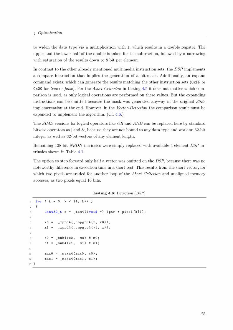
In contrast to the other already mentioned multimedia instruction sets, the DSP implementsa compare instruction that implies the generation of a bit-mask. Additionally, an expandcommand exists, which can generate the results matching the other instruction sets (0xFF or0x00 for true or false). For the Abort Criterion in Listing 4.5 it does not matter which com-parison is used, as only logical operations are performed on these values. But the expandinginstructions can be omitted because the mask was generated anyway in the original SSE-implementation at the end. However, in the Vector-Detection the comparison result must beexpanded to implement the algorithm. (Cf. 4.6.)

The SIMD versions for logical operators like OR and AND can be replaced here by standardbitwise operators as | and &, because they are not bound to any data type and work on 32-bitinteger as well as 32-bit vectors of any element length.

Remaining 128-bit NEON intrinsics were simply replaced with available 4-element DSP in-trinsics shown in Table 4.1.

The option to step forward only half a vector was omitted on the DSP, because there was nonoteworthy difference in execution time in a short test. This results from the short vector, forwhich two pixels are traded for another loop of the Abort Criterion and unaligned memoryaccesses, as two pixels equal 16 bits.

Listing 4.6: Detection (DSP)

1 for ( k = 0; k < 24; k++ )2 3 uint32_t x = _mem4 (( void *) (ptr + pixel[k]));4

5 m0 = _xpnd4 ( _cmpgtu4 (x, v0));6 m1 = _xpnd4 ( _cmpgtu4 (v1 , x));7

8 c0 = _sub4(c0 , m0) & m0;9 c1 = _sub4(c1 , m1) & m1;

10

11 max0 = _maxu4 (max0 , c0);12 max1 = _maxu4 (max1 , c1);13

25

4 Optimization

Table 4.1: SIMD DSP implementation intrinsics overview

Description NEON Intrinsic DSP Intrinsicload vector with signed 8-bit elementsfrom memory

vld1q_s8 _mem4

load vector with signed 16-bit elementsfrom memory

vld1q_s16 _mem4

bitwise AND vandq_u8 &bitwise OR vorrq_u8 |subtract unsigned 8-bit integers withsaturation

vqsubq_u8 not available

subtract signed 8-bit integers vsubq_s8 _sub4subtract signed 16-bit integers vsubq_s16 _sub2add unsigned 8-bit integers vqaddq_u8 _saddu4compare two unsigned 8-bit integers vcgtq_u8 _xpnd4(_cmpgtu4())select the maximum of unsigned8-bit integers

vmaxq_u8 _maxu4

select the maximum of signed16-bit integers

vmaxq_s16 _max2

select the minimum of signed16-bit integers

vminq_s16 _min2

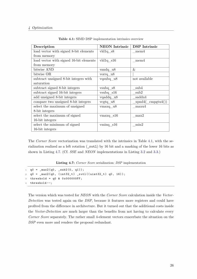
The Corner Score vectorization was translated with the intrinsics in Table 4.1, with the se-rialization realized as a left rotation (_rotl) by 16 bit and a masking of the lower 16 bits asshown in Listing 4.7. (Cf. SSE and NEON implementations in Listing 3.2 and 3.3.)

Listing 4.7: Corner Score serialization: DSP implementation

1 q0 = _max2(q0 , _sub2 (0, q1));2 q0 = _max2(q0 , ( int32_t ) _rotl (( uint32_t ) q0 , 16));3 threshold = q0 & 0 x000000FF ;4 threshold --;

The version which was tested for NEON with the Corner Score calculation inside the Vector-Detection was tested again on the DSP, because it features more registers and could haveprofited from the difference in architecture. But it turned out that the additional costs insidethe Vector-Detection are much larger than the benefits from not having to calculate everyCorner Score separately. The rather small 4-element vectors exacerbate the situation on theDSP even more and renders the proposal redundant.

26

5 Experimental Results


In this chapter the execution times of the different implementations as well as several sub-parts will be examined and compared. The results will show the reduction of calculation timeor the performance boost through various optimizations. Additionally, a comparison of thepower consumptions on both units will be presented.

5.1 Test Settings

The time measurements in this chapter were performed by an internal means of time mea-surement, as external tools as gprof [8] or callgrind [32] do not offer the necessary resolution.gprof, for example, provides a resolution of 0.01 s, which is too inaccurate for these fast im-plementations to generate plausible results. In order to get preciser results, the relevant codeparts were measured with the internal system clock and the system call clock_gettime().

For all measurements only stream relevant code parts were measured, which must be executedfor every single picture. Initialization, reading the picture from a file and printing results wereomitted, as well as allocation of page-size aligned buffers in case of the DSP. These tasks willhave to be performed only once in an use case, where thousands of pictures are processed in astream. To get runtime information from subroutines or parts of the algorithm, sections wereremoved from the implementations and the specific times were calculated by subtraction ofconsecutive measurements. The measurements concerning the consumed time on the CPU incase of the algorithm running on the DSP were generated with the same technique. Here, theblocking time after the node was launched from the host side until the results are available tothe CPU, was measured to get the pure DSP-time. These values might not be 100% accurate,as there are system calls deep inside the kernel involved, but they mark a dimension whichcan be calculated with. To generate representative results, all values given in this chapter arethe average of 100 iterations.

All experiments were made with two different test images: Omni (Figure 2.4 converted to8-bit gray-scale) as a real-world scenario measuring 1280 x 960 pixels and the smaller pictureLena (see Figure 5.2), featuring a resolution of 512 by 512.

27


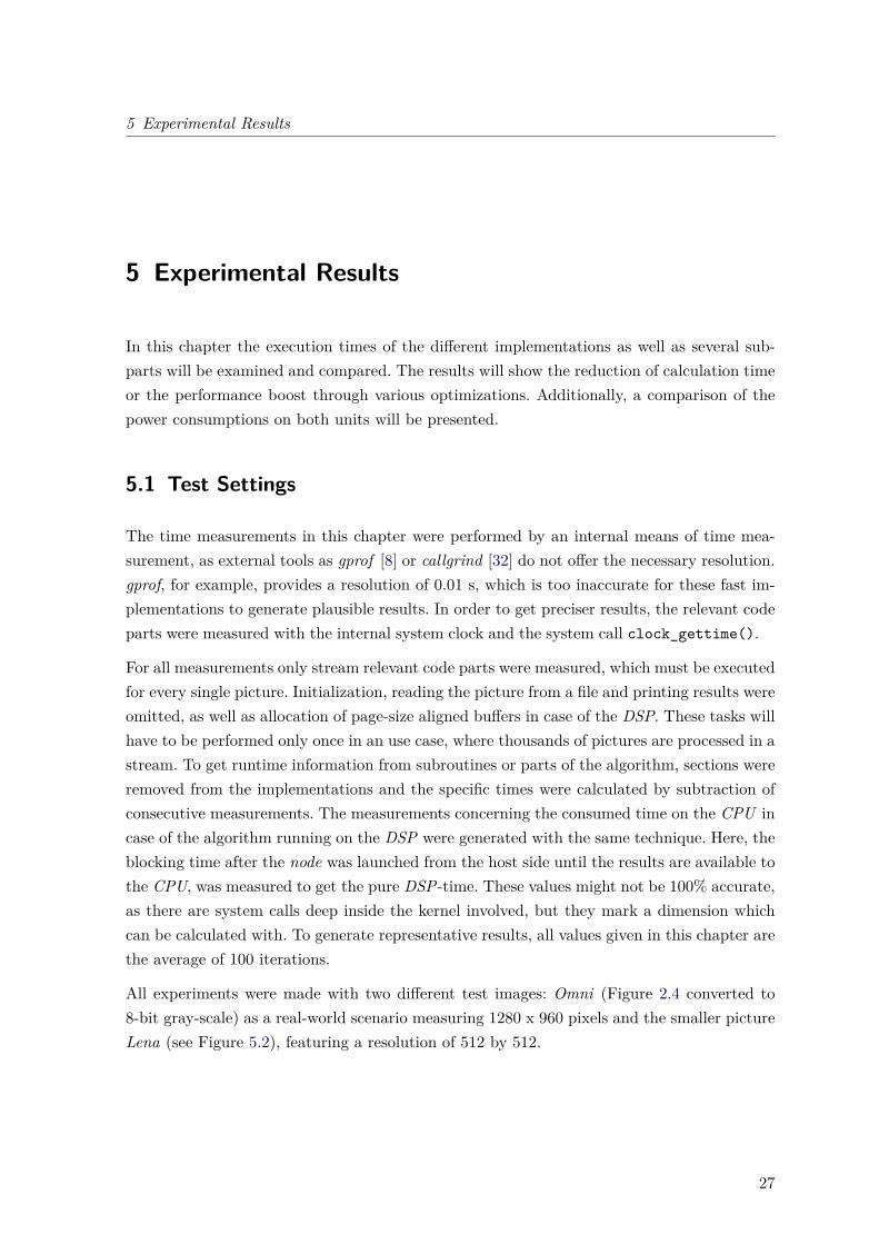
Figure 5.1: Dependence between the number of detected corners and the threshold.

As it is shown in Figure 5.1, the number of detected corners can vary a lot when the thresholdis changed. The Figure only shows the corners up to a number of 2500. In fact, the featurepoint count rises for Lena up to 18574 and 46887 for Omni at a threshold of 1.

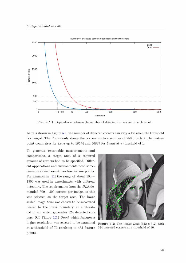
Figure 5.2: Test image Lena (512 x 512) with324 detected corners at a threshold of 40.

To generate reasonable measurements andcomparisons, a target area of a requiredamount of corners had to be specified. Differ-ent applications and environments need some-times more and sometimes less feature points.For example in [11] the range of about 100 −1500 was used in experiments with differentdetectors. The requirements from the DLR de-manded 300 − 500 corners per image, so thiswas selected as the target area. The lowerscaled image Lena was chosen to be measurednearer to the lower boundary at a thresh-old of 40, which generates 324 detected cor-ners. (Cf. Figure 5.2.) Omni, which features ahigher resolution, was selected to be examinedat a threshold of 70 resulting in 433 featurepoints.

28


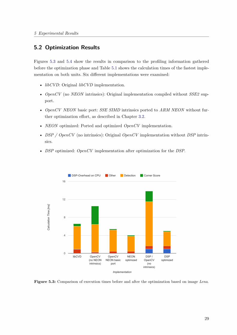
5.2 Optimization Results

Figures 5.3 and 5.4 show the results in comparison to the profiling information gatheredbefore the optimization phase and Table 5.1 shows the calculation times of the fastest imple-mentation on both units. Six different implementations were examined:

• libCVD: Original libCVD implementation.

• OpenCV (no NEON intrinsics): Original implementation compiled without SSE2 sup-port.

• OpenCV NEON basic port: SSE SIMD intrinsics ported to ARM NEON without fur-ther optimization effort, as described in Chapter 3.2.

• NEON optimized: Ported and optimized OpenCV implementation.

• DSP / OpenCV (no intrinsics): Original OpenCV implementation without DSP intrin-sics.

• DSP optimized: OpenCV implementation after optimization for the DSP.

DSP-Overhead on CPU Other Detection Corner Score

libCVD OpenCV(no NEONintrinsics)

OpenCVNEON basic

port

NEONoptimized

DSP /OpenCV

(nointrinsics)

DSPoptimized

0

4

8

12

16

Implementation

Cal

cula

tion

Tim

e [m

s]

Figure 5.3: Comparison of execution times before and after the optimization based on image Lena.

29


DSP-Overhead on CPU Other Detection Corner Score

libCVD OpenCV(no NEONintrinsics)

OpenCVNEON basic

port

NEONoptimized

DSP /OpenCV

(nointrinsics)

DSPoptimized

0

15

30

45

60

Implementation

Cal

cula

tion

Tim

e [m

s]

Figure 5.4: Comparison of execution times before and after the optimization based on image Omni.

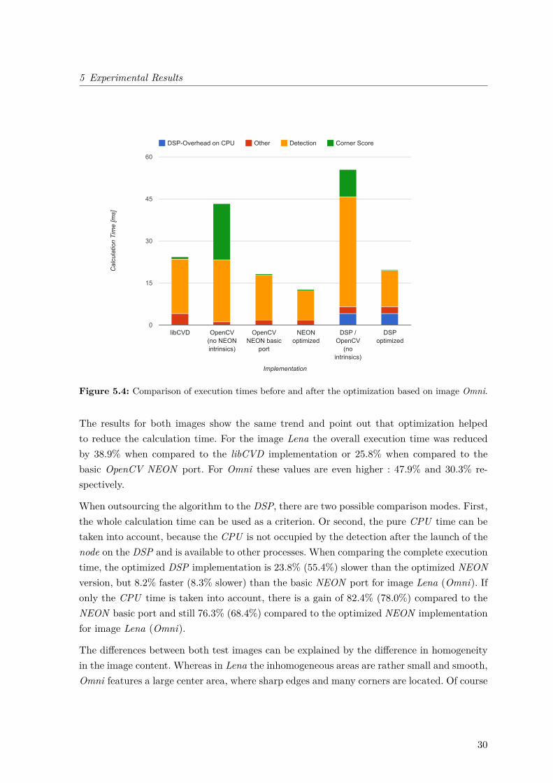
The results for both images show the same trend and point out that optimization helpedto reduce the calculation time. For the image Lena the overall execution time was reducedby 38.9% when compared to the libCVD implementation or 25.8% when compared to thebasic OpenCV NEON port. For Omni these values are even higher : 47.9% and 30.3% re-spectively.

When outsourcing the algorithm to the DSP, there are two possible comparison modes. First,the whole calculation time can be used as a criterion. Or second, the pure CPU time can betaken into account, because the CPU is not occupied by the detection after the launch of thenode on the DSP and is available to other processes. When comparing the complete executiontime, the optimized DSP implementation is 23.8% (55.4%) slower than the optimized NEONversion, but 8.2% faster (8.3% slower) than the basic NEON port for image Lena (Omni). Ifonly the CPU time is taken into account, there is a gain of 82.4% (78.0%) compared to theNEON basic port and still 76.3% (68.4%) compared to the optimized NEON implementationfor image Lena (Omni).

The differences between both test images can be explained by the difference in homogeneityin the image content. Whereas in Lena the inhomogeneous areas are rather small and smooth,Omni features a large center area, where sharp edges and many corners are located. Of course

30


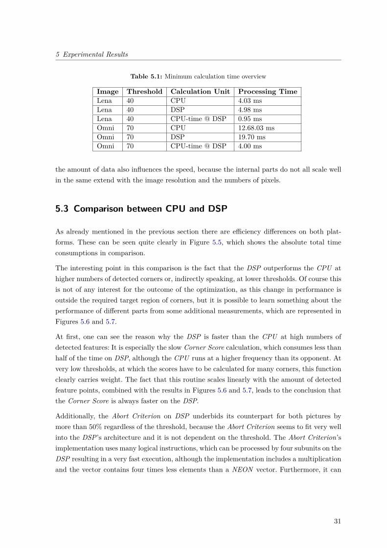
Table 5.1: Minimum calculation time overview

Image Threshold Calculation Unit Processing TimeLena 40 CPU 4.03 msLena 40 DSP 4.98 msLena 40 CPU-time @ DSP 0.95 msOmni 70 CPU 12.68.03 msOmni 70 DSP 19.70 msOmni 70 CPU-time @ DSP 4.00 ms

the amount of data also influences the speed, because the internal parts do not all scale wellin the same extend with the image resolution and the numbers of pixels.

5.3 Comparison between CPU and DSP

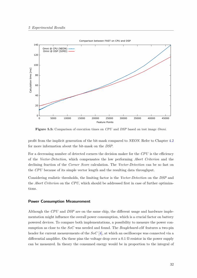
As already mentioned in the previous section there are efficiency differences on both plat-forms. These can be seen quite clearly in Figure 5.5, which shows the absolute total timeconsumptions in comparison.

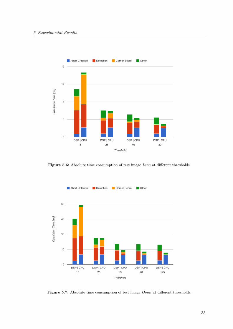
The interesting point in this comparison is the fact that the DSP outperforms the CPU athigher numbers of detected corners or, indirectly speaking, at lower thresholds. Of course thisis not of any interest for the outcome of the optimization, as this change in performance isoutside the required target region of corners, but it is possible to learn something about theperformance of different parts from some additional measurements, which are represented inFigures 5.6 and 5.7.

At first, one can see the reason why the DSP is faster than the CPU at high numbers ofdetected features: It is especially the slow Corner Score calculation, which consumes less thanhalf of the time on DSP, although the CPU runs at a higher frequency than its opponent. Atvery low thresholds, at which the scores have to be calculated for many corners, this functionclearly carries weight. The fact that this routine scales linearly with the amount of detectedfeature points, combined with the results in Figures 5.6 and 5.7, leads to the conclusion thatthe Corner Score is always faster on the DSP.

Additionally, the Abort Criterion on DSP underbids its counterpart for both pictures bymore than 50% regardless of the threshold, because the Abort Criterion seems to fit very wellinto the DSP’s architecture and it is not dependent on the threshold. The Abort Criterion’simplementation uses many logical instructions, which can be processed by four subunits on theDSP resulting in a very fast execution, although the implementation includes a multiplicationand the vector contains four times less elements than a NEON vector. Furthermore, it can

31


Figure 5.5: Comparison of execution times on CPU and DSP based on test image Omni.

profit from the implicit generation of the bit-mask compared to NEON. Refer to Chapter 4.2for more information about the bit-mask on the DSP.

For a decreasing number of detected corners the decision maker for the CPU is the efficiencyof the Vector-Detection, which compensates the low performing Abort Criterion and thedeclining fraction of the Corner Score calculation. The Vector-Detection can be so fast onthe CPU because of its simple vector length and the resulting data throughput.

Considering realistic thresholds, the limiting factor is the Vector-Detection on the DSP andthe Abort Criterion on the CPU, which should be addressed first in case of further optimiza-tions.

Power Consumption Measurement

Although the CPU and DSP are on the same chip, the different usage and hardware imple-mentation might influence the overall power consumption, which is a crucial factor on batterypowered devices. To compare both implementations, a possibility to measure the power con-sumption as close to the SoC was needed and found. The Beagleboard-xM features a two-pinheader for current measurements of the SoC [4], at which an oscilloscope was connected via adifferential amplifier. On these pins the voltage drop over a 0.1 Ω resistor in the power supplycan be measured. In theory the consumed energy would be in proportion to the integral of

32


Abort Criterion Detection Corner Score Other

DSP | CPU DSP | CPU

25

DSP | CPU

40

DSP | CPU

80

0

4

8

12

16

Threshold

Cal

cula

tion

Tim

e [m

s]

8

Figure 5.6: Absolute time consumption of test image Lena at different thresholds.

Abort Criterion Detection Corner Score Other

DSP | CPU

10

DSP | CPU

25

DSP | CPU

55

DSP | CPU

70

DSP | CPU

125

0

15

30

45

60

Threshold

Cal

cula

tion

Tim

e [m

s]

Figure 5.7: Absolute time consumption of test image Omni at different thresholds.

33


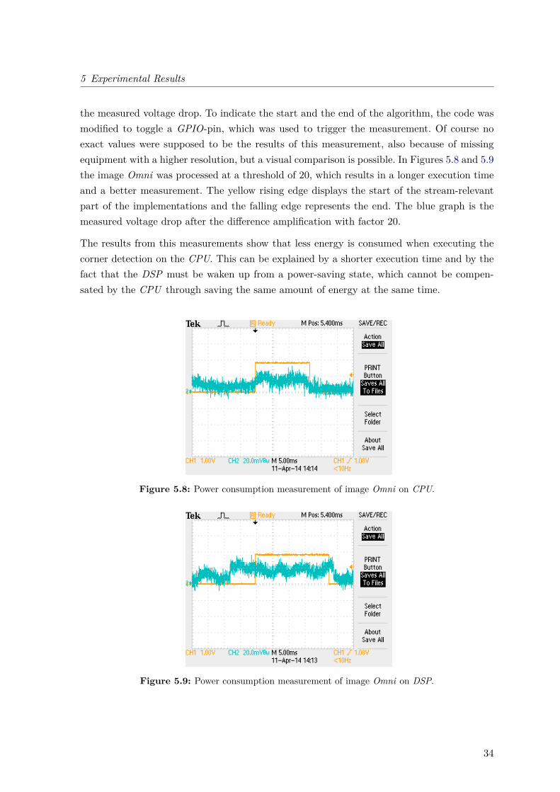
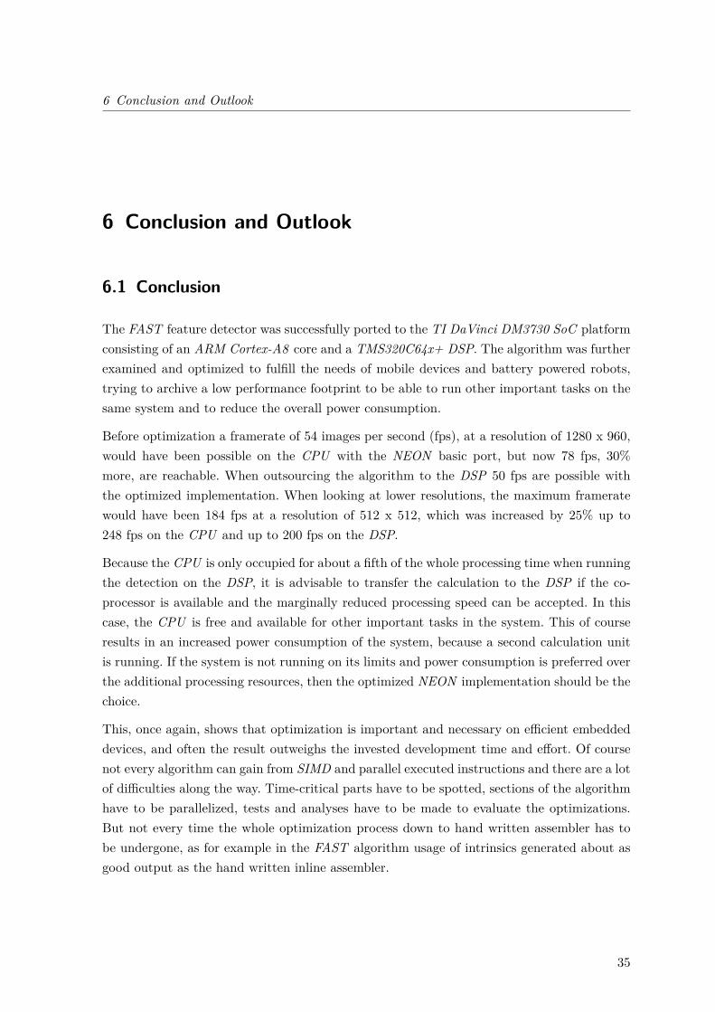
the measured voltage drop. To indicate the start and the end of the algorithm, the code wasmodified to toggle a GPIO-pin, which was used to trigger the measurement. Of course noexact values were supposed to be the results of this measurement, also because of missingequipment with a higher resolution, but a visual comparison is possible. In Figures 5.8 and 5.9the image Omni was processed at a threshold of 20, which results in a longer execution timeand a better measurement. The yellow rising edge displays the start of the stream-relevantpart of the implementations and the falling edge represents the end. The blue graph is themeasured voltage drop after the difference amplification with factor 20.

The results from this measurements show that less energy is consumed when executing thecorner detection on the CPU. This can be explained by a shorter execution time and by thefact that the DSP must be waken up from a power-saving state, which cannot be compen-sated by the CPU through saving the same amount of energy at the same time.

Figure 5.8: Power consumption measurement of image Omni on CPU.

Figure 5.9: Power consumption measurement of image Omni on DSP.

34

6 Conclusion and Outlook


6.1 Conclusion

The FAST feature detector was successfully ported to the TI DaVinci DM3730 SoC platformconsisting of an ARM Cortex-A8 core and a TMS320C64x+ DSP. The algorithm was furtherexamined and optimized to fulfill the needs of mobile devices and battery powered robots,trying to archive a low performance footprint to be able to run other important tasks on thesame system and to reduce the overall power consumption.

Before optimization a framerate of 54 images per second (fps), at a resolution of 1280 x 960,would have been possible on the CPU with the NEON basic port, but now 78 fps, 30%more, are reachable. When outsourcing the algorithm to the DSP 50 fps are possible withthe optimized implementation. When looking at lower resolutions, the maximum frameratewould have been 184 fps at a resolution of 512 x 512, which was increased by 25% up to248 fps on the CPU and up to 200 fps on the DSP.

Because the CPU is only occupied for about a fifth of the whole processing time when runningthe detection on the DSP, it is advisable to transfer the calculation to the DSP if the co-processor is available and the marginally reduced processing speed can be accepted. In thiscase, the CPU is free and available for other important tasks in the system. This of courseresults in an increased power consumption of the system, because a second calculation unitis running. If the system is not running on its limits and power consumption is preferred overthe additional processing resources, then the optimized NEON implementation should be thechoice.

This, once again, shows that optimization is important and necessary on efficient embeddeddevices, and often the result outweighs the invested development time and effort. Of coursenot every algorithm can gain from SIMD and parallel executed instructions and there are a lotof difficulties along the way. Time-critical parts have to be spotted, sections of the algorithmhave to be parallelized, tests and analyses have to be made to evaluate the optimizations.But not every time the whole optimization process down to hand written assembler has tobe undergone, as for example in the FAST algorithm usage of intrinsics generated about asgood output as the hand written inline assembler.

35


In the context of this work, additionally a census descriptor was implemented and optimizedfor the NEON architecture by the author for the DLR to make up a fully applicable module,which is able to cover the first two steps of the three steps of detection - description - matching.A short summary and description is included in Appendix A.1.

6.2 Outlook

At the time of writing a new generation of multicopters is designed at the DLR, for whichvision based sensors will be even more important than in preceding models. Time will tellwhether and where exactly they will use the FAST detector in one of the sensors, or forone of their tasks in the subject of navigation, tracking, object recognition or other purposesrelying on optical information.

The fully tested and optimized implementation can now be used on UAVs or other (mobile)devices featuring an ARM processor providing the NEON instruction set or a SoC withthe on-chip DSP. Even applications in the field of augmented reality are possible on embed-ded devices as phones or tablets. To make it publicly available and to give something backto the open source community, an attempt will be made to supply the optimized NEONimplementation back to the OpenCV library.

For future works, of course the third step of matching could be a point of interest, or theintegration of the implementations into the robot operating system (ROS) [17], which iswidely used among the multicopters.

In case of additional investigations on optimizations for the FAST feature detector the follow-ing points should be addressed first: The part with the highest time consumption for the caseof 300 − 500 detected corners per image is the Vector-Detection on the DSP and the AbortCriterion on the CPU. An idea would be to skip the second run of the Abort Criterion incase of a half-vector step, because the vector was not completely rejected in the first pass andtherefore there must already be a possible corner in the first half of the vector. This would,of course, require some additional code, but the whole second run could be omitted.

36

Bibliography

Bibliography

[1] ARM Ltd.: Architecture and Implementation of the ARM Cortex-A8 Mi-croprocessor. https://pixhawk.ethz.ch/_media/software/optimization/neon_

whitepaper.pdf 2.1.1

[2] ARM Ltd.: ARM NEON Instruction Summary. http://infocenter.arm.com/help/

topic/com.arm.doc.dui0489c/CJAJIIGG.html 2.1.1

[3] ARM Ltd.: Introducing NEON™ Development Article. http://infocenter.arm.com/

help/topic/com.arm.doc.dht0002a/DHT0002A_introducing_neon.pdf 2.1.1

[4] BeagleBorad.org, Coley G.: BeagleBoard-xM System Reference Manual Rev C.1.0.http://www.beagleboard.org/static/BBxMSRM_latest.pdf 5.3

[5] Bradski, G.: OpenCV. In: Dr. Dobb’s Journal of Software Tools (2000) 3

[6] Daoust, Yves: SSE _mm_movemask_epi8 equivalent method for ARM NEON. http:

//stackoverflow.com/a/12383618 3.2, 3.1

[7] Edler, Jan ; Hill, Mark D.: Dinero IV Trace-Driven Uniprocessor Cache Simulator.http://www.cs.wisc.edu/~markhill/DineroIV/ 4.1.3

[8] Graham, Susan L. ; Kessler, Peter B. ; McKusick, Marshall K.: gprof: a Call GraphExecution Profiler. 1982 4.1.1, 5.1

[9] Gumstix Inc.: Overo® FireSTORM COM Overview. https://store.gumstix.com/

index.php/products/267/ 2

[10] Hassaballah, M. ; Omran, Saleh ; Mahdy, Youssef B.: A Review of SIMDMultimediaExtensions and Their Usage in Scientific and Engineering Applications. In: Comput. J.51 (2008), November, Nr. 6, 630–649. http://dx.doi.org/10.1093/comjnl/bxm099.– DOI 10.1093/comjnl/bxm099. – ISSN 0010–4620 2.1.1

[11] Heinrichs, Matthias ; Hellwich, Olaf ; Rodehorst, Volker: Robust Spatio-TemporalFeature Tracking 5.1, A.1.1, A.1.2

[12] Jeong, Kanghun ; Moon, Hyeonjoon: Object Detection Using FAST Corner DetectorBased on Smartphone Platforms. In: Proceedings of the 2011 First ACIS/JNU In-ternational Conference on Computers, Networks, Systems and Industrial Engineering.

37

https://pixhawk.ethz.ch/_media/software/optimization/neon_whitepaper.pdf

https://pixhawk.ethz.ch/_media/software/optimization/neon_whitepaper.pdf

http://infocenter.arm.com/help/topic/com.arm.doc.dui0489c/CJAJIIGG.html

http://infocenter.arm.com/help/topic/com.arm.doc.dui0489c/CJAJIIGG.html

http://infocenter.arm.com/help/topic/com.arm.doc.dht0002a/DHT0002A_introducing_neon.pdf

http://infocenter.arm.com/help/topic/com.arm.doc.dht0002a/DHT0002A_introducing_neon.pdf

http://www.beagleboard.org/static/BBxMSRM_latest.pdf

http://stackoverflow.com/a/12383618

http://stackoverflow.com/a/12383618

http://www.cs.wisc.edu/~markhill/DineroIV/

https://store.gumstix.com/index.php/products/267/

https://store.gumstix.com/index.php/products/267/

http://dx.doi.org/10.1093/comjnl/bxm099

Bibliography

Washington, DC, USA : IEEE Computer Society, 2011 (CNSI ’11). – ISBN 978–0–7695–4417–5, 111–115 1.1

[13] Klippenstein, J. ; Zhang, Hong: Performance evaluation of visual SLAM using severalfeature extractors. In: Intelligent Robots and Systems, 2009. IROS 2009. IEEE/RSJInternational Conference on, 2009, S. 1574–1581 1.1

[14] Mair, Elmar ; Hager, Gregory D. ; Burschka, Darius ; Suppa, Michael ; Hirzinger,Gerhard: Adaptive and Generic Corner Detection Based on the Accelerated SegmentTest. In: Proceedings of the European Conference on Computer Vision (ECCV’10), 20101.2, 2.2

[15] Majumder, Goutam ; Bhowmik, Mrinal K. ; Bhatacharjee, Debotosh: Au-tomatic Eye Detection Using Fast Corner Detector of North East Indian(NEI) Face Images. In: Procedia Technology 10 (2013), Nr. 0, 646 - 653.http://dx.doi.org/http://dx.doi.org/10.1016/j.protcy.2013.12.406. – DOIhttp://dx.doi.org/10.1016/j.protcy.2013.12.406. – ISSN 2212–0173. – First Interna-tional Conference on Computational Intelligence: Modeling Techniques and Applications(CIMTA) 2013 1.1

[16] Moreels, Pierre ; Perona, Pietro: Evaluation of Features Detectors and Descriptorsbased on 3D Objects. In: International Journal of Computer Vision 73 (2007), Nr. 3,263-284. http://dx.doi.org/10.1007/s11263-006-9967-1. – DOI 10.1007/s11263–006–9967–1. – ISSN 0920–5691 1.1

[17] Quigley, Morgan ; Conley, Ken ; Gerkey, Brian ; Faust, Josh ; Foote, Tully B. ;Leibs, Jeremy ; Wheeler, Rob ; Ng, Andrew Y.: ROS: an open-source Robot Oper-ating System. In: ICRA Workshop on Open Source Software, 2009 6.2

[18] Reithmeier, Michael D.: Evaluation of the Ti DaVinci DM3730 Coprocessors focusingon Image Processing Algorithms in order to disburden the CPU. September 2012 2.1,2.1.2

[19] Rosten, E.: libCVD - computer vision library. (2010), May 3

[20] Rosten, Edward ; Drummond, Tom: Fusing points and lines for high performancetracking. In: IEEE International Conference on Computer Vision Bd. 2, 2005, 1508–1511 1.2, 2.2, 2.3, 3.1.2

[21] Rosten, Edward ; Drummond, Tom: Machine learning for high-speed corner detection.In: European Conference on Computer Vision Bd. 1, 2006, 430–443 1.2, 2.3, 2.2, 3

[22] Rosten, Edward ; Porter, Reid ; Drummond, Tom: FASTER and better: A machinelearning approach to corner detection. In: IEEE Trans. Pattern Analysis and Machine

38

http://dx.doi.org/http://dx.doi.org/10.1016/j.protcy.2013.12.406

http://dx.doi.org/10.1007/s11263-006-9967-1

Bibliography

Intelligence 32 (2010), 105–119. http://dx.doi.org/10.1109/TPAMI.2008.275. – DOI10.1109/TPAMI.2008.275 1.1, 2.2, 3.1.1

[23] Smith, S. M. ; Brady, J. M.: SUSAN - A New Approach to Low Level Image Processing.In: International Journal of Computer Vision 23 (1995), S. 45–78 2.2

[24] Stewart, Matt: Stewart Vision; CMU. http://www.contrib.andrew.cmu.edu/

~mstewar1/Source%20Code/stewart_vision.c 3

[25] Szeliski, Richard: Computer Vision: Algorithms and Applications. 1st. New York, NY,USA : Springer-Verlag New York, Inc., 2010. – ISBN 1848829345, 9781848829343 1.1

[26] TI, Texas Instruments Inc.: TMS320C64x Technical Overview. http://www.ti.com/

lit/ug/spru395b/spru395b.pdf. Version: January 2001 2.1.2

[27] TI, Texas Instruments Inc.: TMS320C64x/C64x+ DSP CPU and Instruction Set Refer-ence Guide. http://www.ti.com/lit/ug/spru732j/spru732j.pdf. Version: July 20102.1.2

[28] TI, Texas Instruments Inc.: DM3730, DM3725 - Digital Media Processors. http:

//www.ti.com/lit/ds/sprs685d/sprs685d.pdf. Version: July 2011 2.1

[29] TI, Texas Instruments Inc.: TMS320C6000 Programmer’s Guide. http://www.ti.com/

lit/ug/spru198k/spru198k.pdf. Version: July 2011 2.1

[30] TI et al.: TI Wiki: AM/DM37x Overview. http://processors.wiki.ti.com/index.

php/AM/DM37x_Overview 2.1

[31] Uhrig, Jonas B.: Integration and Development of DSP Algorithms for the ROS Envi-ronment. October 2013 2.1.2

[32] Weidendorfer, Josef ; Kowarschik, Markus ; Trinitis, Carsten: A Tool Suite forSimulation Based Analysis of Memory Access Behavior. In: In Proceedings of Interna-tional Conference on Computational Science, Springer, 2004, S. 440–447 5.1

[33] Xiao, Ming ; Li, Wanli ; Hu, Tianjiang ; Pan, Liang ; Shen, Lincheng ; Bu, Yanlong:SAR aided navigation based on FAST feature. In: Software Engineering and ServiceScience (ICSESS), 2013 4th IEEE International Conference on, 2013. – ISSN 2327–0586, S. 861–864 1.1

[34] Zabih, Ramin ; Woodfill, John: Non-parametric local transforms for computing vi-sual correspondence. Version: 1994. http://dx.doi.org/10.1007/BFb0028345. In:Eklundh, Jan-Olof (Hrsg.): Computer Vision — ECCV ’94 Bd. 801. Springer BerlinHeidelberg, 1994. – DOI 10.1007/BFb0028345. – ISBN 978–3–540–57957–1, 151-158A.1.1

39

http://dx.doi.org/10.1109/TPAMI.2008.275

http://www.contrib.andrew.cmu.edu/~mstewar1/Source%20Code/stewart_vision.c

http://www.contrib.andrew.cmu.edu/~mstewar1/Source%20Code/stewart_vision.c

http://www.ti.com/lit/ug/spru395b/spru395b.pdf

http://www.ti.com/lit/ug/spru395b/spru395b.pdf

http://www.ti.com/lit/ug/spru732j/spru732j.pdf

http://www.ti.com/lit/ds/sprs685d/sprs685d.pdf

http://www.ti.com/lit/ds/sprs685d/sprs685d.pdf

http://www.ti.com/lit/ug/spru198k/spru198k.pdf

http://www.ti.com/lit/ug/spru198k/spru198k.pdf

http://processors.wiki.ti.com/index.php/AM/DM37x_Overview

http://processors.wiki.ti.com/index.php/AM/DM37x_Overview

http://dx.doi.org/10.1007/BFb0028345

Affidavit

Ich, Peter Fink, Matrikel-Nr. 924547, versichere hiermit, dass ich die vorliegende Arbeit mitdem Thema

»Optimized Implementation of a Feature Detector for Embedded Systems Basedon the ‘Accelerated Segment Test’«

selbständig verfasst und keine anderen als die angegebenen Quellen und Hilfsmittel benutzthabe, wobei ich alle wörtlichen und sinngemäßen Zitate als solche gekennzeichnet habe.Die Arbeit wurde bisher keiner anderen Prüfungsbehörde vorgelegt und auch nicht veröf-fentlicht.

Issing, den 17. April, 2014

Peter Fink

40

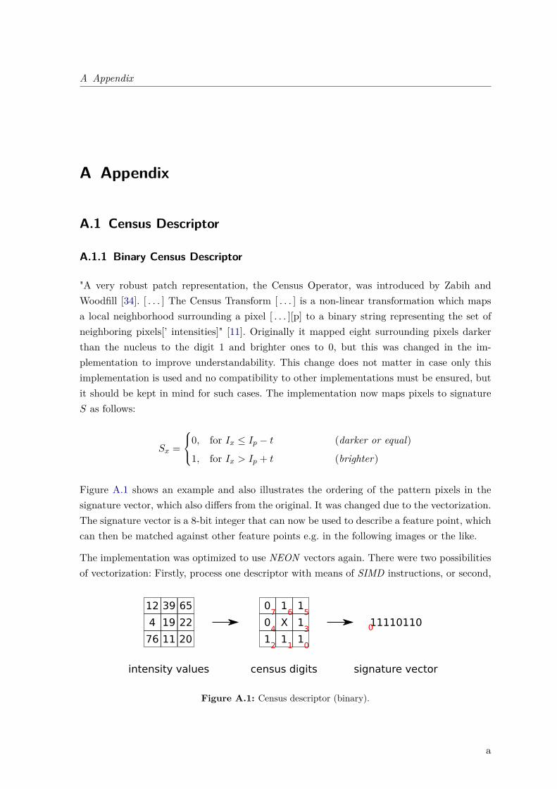
A Appendix

A Appendix

A.1 Census Descriptor

A.1.1 Binary Census Descriptor

"A very robust patch representation, the Census Operator, was introduced by Zabih andWoodfill [34]. [ . . . ] The Census Transform [ . . . ] is a non-linear transformation which mapsa local neighborhood surrounding a pixel [ . . . ][p] to a binary string representing the set ofneighboring pixels[’ intensities]" [11]. Originally it mapped eight surrounding pixels darkerthan the nucleus to the digit 1 and brighter ones to 0, but this was changed in the im-plementation to improve understandability. This change does not matter in case only thisimplementation is used and no compatibility to other implementations must be ensured, butit should be kept in mind for such cases. The implementation now maps pixels to signatureS as follows:

Sx =

0, for Ix ≤ Ip − t (darker or equal)


Figure A.1 shows an example and also illustrates the ordering of the pattern pixels in thesignature vector, which also differs from the original. It was changed due to the vectorization.The signature vector is a 8-bit integer that can now be used to describe a feature point, whichcan then be matched against other feature points e.g. in the following images or the like.

The implementation was optimized to use NEON vectors again. There were two possibilitiesof vectorization: Firstly, process one descriptor with means of SIMD instructions, or second,

12 39 65

4 19 22

76 11 20

0 1 1

0 X 1

1 1 1

intensity values census digits signature vector

11110110

012

34

567

0

Figure A.1: Census descriptor (binary).

a

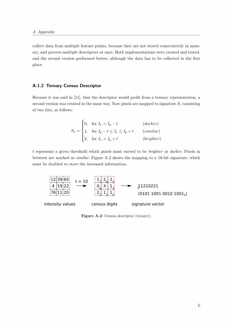
A Appendix

collect data from multiple feature points, because they are not stored consecutively in mem-ory, and process multiple descriptors at once. Both implementations were created and tested,and the second version performed better, although the data has to be collected in the firstplace.

A.1.2 Ternary Census Descriptor

Because it was said in [11], that the descriptor would profit from a ternary representation, asecond version was created in the same way. Now pixels are mapped to signature S, consistingof two bits, as follows:

Sx =

0, for Ix < Ip − t (darker)

1, for Ip − t ≤ Ix ≤ Ip + t (similar)


t represents a given threshold which pixels must exceed to be brighter or darker. Pixels inbetween are marked as similar. Figure A.2 shows the mapping to a 16-bit signature, whichmust be doubled to store the increased information.

12 39 65

4 19 22

76 11 20

1 2 2

0 X 1

2 1 1

intensity values census digits signature vector

11210221

012

34

567

0

t = 10

(0101 1001 0010 10012)

Figure A.2: Census descriptor (ternary).

b

A Appendix

A.2 Content of the CD

The attached CD contains additional content.Besides the work in PDF format, all source files and compiled executables created in thecontext of this work are stored on the medium.

./sources/

Source code directory

./README

Information about the content on the CD

./Thesis_Peter_Fink_924547.pdf

Thesis in PDF format

c

Documents

Optimized Implementation of a Feature Detector for