Diese Arbeit wurde vorgelegt amLehrstuhl II fur Mathematik

Robuste Optimierung von Zielpunktstrategien vonHeliostaten in Solarturmkraftwerken

Robust Optimization of Aiming Strategies of Heliostatsin Solar Tower Power Plants

BachelorarbeitComputational Engineering Science

August 2018

Vorgelegt von Fynn KeppPresented by Mauerstraße 71

52064 AachenMatrikelnummer: 344700fynn.kepp@rwth-aachen.de

Erstprufer Jun.-Prof. Dr. Christina BusingFirst examiner Lehrstuhl II fur Mathematik

RWTH Aachen University

Externer Betreuer Dr. Pascal RichterExternal supervisor Steinbuch Centre for Computing

Karlsruhe Institute of Technology

Koreferent M. Sc. Sascha KuhnkeCo-Supervisor Lehrstuhl II fur Mathematik

RWTH Aachen University

Eigenstandigkeitserklarung

Hiermit versichere ich, dass ich diese Bachelorarbeit selbstandig verfasst und keineanderen als die angegebenen Quellen und Hilfsmittel benutzt habe. Die Stellen meinerArbeit, die dem Wortlaut oder dem Sinn nach anderen Werken entnommen sind, habeich in jedem Fall unter Angabe der Quelle als Entlehnung kenntlich gemacht. Dasselbegilt sinngemaß fur Tabellen und Abbildungen. Diese Arbeit hat in dieser oder einerahnlichen Form noch nicht im Rahmen einer anderen Prufung vorgelegen.

Aachen, im August 2018

Fynn Vincent Kepp

II

Contents

1 Introduction 11.1 Outline of the work . . . . . . . . . . . . . . . . . . . . . . . . . . . . . 11.2 Functioning principle . . . . . . . . . . . . . . . . . . . . . . . . . . . . 21.3 State of the art . . . . . . . . . . . . . . . . . . . . . . . . . . . . . . . 2

2 Optical model 42.1 Methods for obtaining heliostat images . . . . . . . . . . . . . . . . . . 4

2.1.1 Monte Carlo ray tracing . . . . . . . . . . . . . . . . . . . . . . 42.1.2 Convolution method . . . . . . . . . . . . . . . . . . . . . . . . 5

2.2 Sun . . . . . . . . . . . . . . . . . . . . . . . . . . . . . . . . . . . . . . 52.2.1 Irradiation . . . . . . . . . . . . . . . . . . . . . . . . . . . . . . 52.2.2 Sun position . . . . . . . . . . . . . . . . . . . . . . . . . . . . . 52.2.3 Sun shape error . . . . . . . . . . . . . . . . . . . . . . . . . . . 6

2.3 Heliostats . . . . . . . . . . . . . . . . . . . . . . . . . . . . . . . . . . 72.3.1 Component description . . . . . . . . . . . . . . . . . . . . . . . 72.3.2 Set of heliostats . . . . . . . . . . . . . . . . . . . . . . . . . . . 72.3.3 Heliostat errors . . . . . . . . . . . . . . . . . . . . . . . . . . . 72.3.4 Shading and blocking . . . . . . . . . . . . . . . . . . . . . . . . 82.3.5 Incidence angle . . . . . . . . . . . . . . . . . . . . . . . . . . . 82.3.6 Atmospheric attenuation . . . . . . . . . . . . . . . . . . . . . . 92.3.7 Beam power . . . . . . . . . . . . . . . . . . . . . . . . . . . . . 102.3.8 Original HFLCAL method . . . . . . . . . . . . . . . . . . . . . 10

2.4 Receiver . . . . . . . . . . . . . . . . . . . . . . . . . . . . . . . . . . . 112.4.1 Component description . . . . . . . . . . . . . . . . . . . . . . . 112.4.2 Receiver model . . . . . . . . . . . . . . . . . . . . . . . . . . . 122.4.3 Measurement points . . . . . . . . . . . . . . . . . . . . . . . . 132.4.4 Aim points . . . . . . . . . . . . . . . . . . . . . . . . . . . . . 142.4.5 Optimal discretization . . . . . . . . . . . . . . . . . . . . . . . 142.4.6 Discretization of receiver types . . . . . . . . . . . . . . . . . . 15

2.5 Computing heliostat images . . . . . . . . . . . . . . . . . . . . . . . . 182.5.1 Integrating the heat flux . . . . . . . . . . . . . . . . . . . . . . 182.5.2 Adapted HFLCAL method . . . . . . . . . . . . . . . . . . . . . 182.5.3 Distorted heliostat image matrix . . . . . . . . . . . . . . . . . 202.5.4 Rectangular external receiver . . . . . . . . . . . . . . . . . . . 232.5.5 Cylindrical cavity receiver . . . . . . . . . . . . . . . . . . . . . 242.5.6 Cylindrical external receiver . . . . . . . . . . . . . . . . . . . . 262.5.7 Refinement . . . . . . . . . . . . . . . . . . . . . . . . . . . . . 28

2.6 Results . . . . . . . . . . . . . . . . . . . . . . . . . . . . . . . . . . . . 29

3 Deterministic aiming strategy 303.1 Definitions . . . . . . . . . . . . . . . . . . . . . . . . . . . . . . . . . . 30

3.1.1 Heliostats . . . . . . . . . . . . . . . . . . . . . . . . . . . . . . 30

III

3.1.2 Measurement points . . . . . . . . . . . . . . . . . . . . . . . . 303.1.3 Aim points . . . . . . . . . . . . . . . . . . . . . . . . . . . . . 313.1.4 Decision variables . . . . . . . . . . . . . . . . . . . . . . . . . . 313.1.5 Local receiver heat flux . . . . . . . . . . . . . . . . . . . . . . . 31

3.2 Objective function . . . . . . . . . . . . . . . . . . . . . . . . . . . . . 313.3 Constraints . . . . . . . . . . . . . . . . . . . . . . . . . . . . . . . . . 31

3.3.1 Maximum one aim point per heliostat . . . . . . . . . . . . . . . 313.3.2 Upper heat flux limit . . . . . . . . . . . . . . . . . . . . . . . . 323.3.3 Heat flux gradient limit . . . . . . . . . . . . . . . . . . . . . . 32

3.4 Summarized optimization model . . . . . . . . . . . . . . . . . . . . . . 343.5 Heat shield . . . . . . . . . . . . . . . . . . . . . . . . . . . . . . . . . 353.6 Clouds . . . . . . . . . . . . . . . . . . . . . . . . . . . . . . . . . . . . 353.7 Obtaining a specified receiver heat flux distribution . . . . . . . . . . . 36

4 Robust aiming strategy 384.1 Definitions . . . . . . . . . . . . . . . . . . . . . . . . . . . . . . . . . . 38

4.1.1 Additional decision variables . . . . . . . . . . . . . . . . . . . . 384.1.2 Adjusted local receiver heat flux . . . . . . . . . . . . . . . . . . 394.1.3 Worst case aim point . . . . . . . . . . . . . . . . . . . . . . . . 394.1.4 Worst case local heat flux . . . . . . . . . . . . . . . . . . . . . 414.1.5 Interpolation versus precomputation . . . . . . . . . . . . . . . 42

4.2 Objective function . . . . . . . . . . . . . . . . . . . . . . . . . . . . . 424.3 Constraints . . . . . . . . . . . . . . . . . . . . . . . . . . . . . . . . . 43

4.3.1 Maximum number of deviating heliostats . . . . . . . . . . . . . 434.3.2 Heat flux limit . . . . . . . . . . . . . . . . . . . . . . . . . . . 434.3.3 Summarized optimization model . . . . . . . . . . . . . . . . . . 45

5 Application 465.1 Parameters . . . . . . . . . . . . . . . . . . . . . . . . . . . . . . . . . 46

5.1.1 Optical model . . . . . . . . . . . . . . . . . . . . . . . . . . . . 465.1.2 Optimization problem . . . . . . . . . . . . . . . . . . . . . . . 475.1.3 Solver . . . . . . . . . . . . . . . . . . . . . . . . . . . . . . . . 48

5.2 Parameters settings for the applications . . . . . . . . . . . . . . . . . . 485.3 Application cases . . . . . . . . . . . . . . . . . . . . . . . . . . . . . . 485.4 Results . . . . . . . . . . . . . . . . . . . . . . . . . . . . . . . . . . . . 50

5.4.1 Deterministic aiming strategy . . . . . . . . . . . . . . . . . . . 515.4.2 Robust aiming strategy . . . . . . . . . . . . . . . . . . . . . . . 57

6 Conclusion and Outlook 636.1 Comparison of the aiming strategies . . . . . . . . . . . . . . . . . . . . 636.2 Outlook . . . . . . . . . . . . . . . . . . . . . . . . . . . . . . . . . . . 64

References 65

IV

1 Introduction

With renewable energy becoming more and more important globally [3], it is an im-portant objective to increase the efficiency of renewable energy power plants.

A promising option for using renewable energy is concentrated solar power (CSP),whose thermal global capacity increased more than ten times since 2006 [3]. It usesthe direct radiation of the sun to provide electric energy; this technology is not onlyenvironmentally friendly and sustained, it also provides electric energy in a highlyscalable way and is able to compensate fluctuations in the available solar radiation byusing heat storages.

Solar tower power plants are one way to use CSP. Mirrors in a frame equipped with amotor to track the sun, called heliostats, are grouped around a tower and concentratethe solar radiation onto its top end where the receiver is located. The concentratedsolar power at the receiver is used to generate steam, which powers a turbine generat-ing electricity.

The aiming strategies used to align the heliostats are of great importance. They haveto ensure that the maximum of the possible heat flux is transferred to the receiverwhile no safety constrains are violated. To make the aiming strategies applicable toreal power plants the latter has to especially hold true for uncertainties as trackingerrors of the heliostats.

This bachelor thesis presents robust aiming strategies for the heliostats in solar towerpower plants to increase their efficiency and the lifespan of the receiver. Solutions toalign the heliostats in a way to obtain the maximum of the possible heat flux at thereceiver while not violating any safety constraints that could damage it are demon-strated. Additionally an approach for obtaining desired heat flux distributions at thereceiver is presented.

1.1 Outline of the work

At first an overview over the functioning principle of a solar tower power plant and thestate of the art of aiming strategies for heliostats in such power plants is given.

In Section 2 we develop the optical model, which is used to determine the total heatflux distribution at the receiver consisting of the individual heat flux distributions ofthe heliostats. For that purpose we analyze the components of a real solar tower powerplant and derive the mathematical model that we use for computing the distributionsfor a given plant setup afterwards.

In Section 3 we derive the deterministic aiming strategy as integer linear program(ILP). We take the receiver properties given as the maximum allowed heat flux per

1

area, maximum heat flux gradients and the existence of a heat shield as well as cloudsinto account. As we do not consider uncertainties in the model description, we obtainan optimization model with a deterministic outcome.

In Section 4 we consider uncertainties in the aiming mechanism of the heliostats forthe optimization model. Thus the deterministic model is extended to a robust modelsuch that a robust aiming strategy is obtained. We analyze how these uncertaintieshave an effect on the receiver heat flux distribution, embed them into the deterministicmodel and derive the complete mixed integer linear programming (MILP) formulationof the robust aiming strategy.

In Section 5 we apply the aiming strategies we developed to the solar tower powerplant PS10 in Spain. We use different sun positions, receiver properties and solversettings to obtain a variety of realistic application cases.

In Section 6 we draw the conclusion of the aiming strategies and give an outlookwith possibilities to extend this work.

1.2 Functioning principle

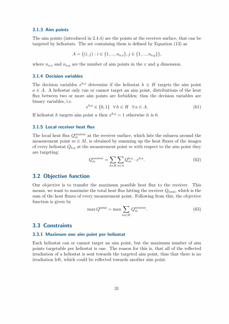
The functioning principle of a typical solar tower power plant is visualised in Figure 1.

To provide electric energy, the heliostats concentrate the solar radiation onto a re-ceiver, which transfers the heat to a medium (water, salt, air, sodium). If the mediumis water, it evaporates through the heat and becomes steam. If the medium is anotherheat carrying fluid, it absorbs the heat from the receiver and exchanges it with a sec-ondary cycle containing water, which then becomes steam. In both cases the steamdrives a turbine. Its mechanical work is converted into electric energy by a generator.The steam water mixture leaving the turbine then is condensed by cooling it usingwater or air.

In order to provide electric energy even after the sundown or to provide a constantoutput of electric energy, the steam can be stored instead of being directly used to gen-erate electric energy. Other heat carrying mediums can be stored in thermal storagesbefore the heat is used to generate steam. Alternatively a gas turbine can compen-sate temporary fluctuations in the thermal energy projected towards the receiver (e.g.caused by clouds shading heliostats).

1.3 State of the art

There already exist different approaches for aiming strategies, which are outlined below:

• Ashley et al.[5] uses linear programming to obtain an optimal aiming strategy.Depending on the resolution of the receiver it provides optimal solutions close toreal time. Heat flux gradients and uncertainties are not considered.

2

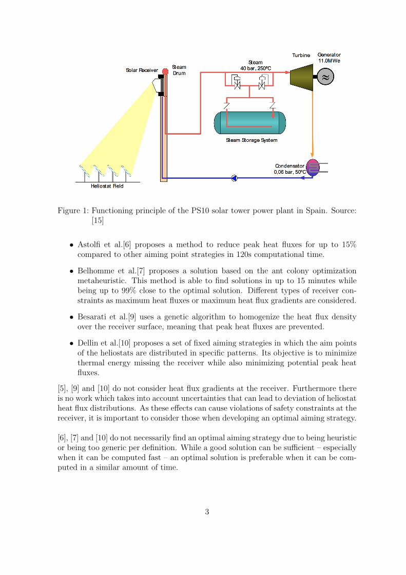
Figure 1: Functioning principle of the PS10 solar tower power plant in Spain. Source:[15]

• Astolfi et al.[6] proposes a method to reduce peak heat fluxes for up to 15%compared to other aiming point strategies in 120s computational time.

• Belhomme et al.[7] proposes a solution based on the ant colony optimizationmetaheuristic. This method is able to find solutions in up to 15 minutes whilebeing up to 99% close to the optimal solution. Different types of receiver con-straints as maximum heat fluxes or maximum heat flux gradients are considered.

• Besarati et al.[9] uses a genetic algorithm to homogenize the heat flux densityover the receiver surface, meaning that peak heat fluxes are prevented.

• Dellin et al.[10] proposes a set of fixed aiming strategies in which the aim pointsof the heliostats are distributed in specific patterns. Its objective is to minimizethermal energy missing the receiver while also minimizing potential peak heatfluxes.

[5], [9] and [10] do not consider heat flux gradients at the receiver. Furthermore thereis no work which takes into account uncertainties that can lead to deviation of heliostatheat flux distributions. As these effects can cause violations of safety constraints at thereceiver, it is important to consider those when developing an optimal aiming strategy.

[6], [7] and [10] do not necessarily find an optimal aiming strategy due to being heuristicor being too generic per definition. While a good solution can be sufficient – especiallywhen it can be computed fast – an optimal solution is preferable when it can be com-puted in a similar amount of time.

3

In this work we extend the approach from [5] and develop two aiming strategies for-mulated as an ILP or respectively as an MILP. The aiming strategies are applicable toarbitrary receiver geometries and determine the optimal aim point at the receiver foreach heliostat in a solar tower power plant.

2 Optical model

The optical model is used to determine the heat flux distribution at the receiver. Inthis work we model that distribution by using the individual heat flux densities of theheliostats, the images, and aggregating them on top of each other. We look to com-pute these images for a given setup of heliostats, tower, outer shape of the receiver,sun position, points at which the heat flux is measured and points that can be targetedby the heliostats and to apply the images to the receiver.

To do that, we discuss different possibilities for generating heliostat images at firstand then choose the method we use in this work. After that, we conceptually followthe path of the sun rays: We start by describing the properties of the sun, whichare relevant for computing heliostat images. Continuing, we model the heliostats andlastly the receiver.

2.1 Methods for obtaining heliostat images

In the following two different ray tracing methods are presented.

2.1.1 Monte Carlo ray tracing

The Monte Carlo ray tracing method uses numerous rays that represent the rays com-ing from the sun. The path these rays take is traced: It ends if the ray does not getreflected at an obstacle and increases a ray counter of a subarea at the receiver if it isabsorbed by it.

A ray hitting a mirror is reflected in the direction set by the orientation of the surfaceof the mirror. With a probability it might scatter or not get reflected at all. If a rayhits the receiver and does not get reflected at its surface (which is very likely due tothe design of the receiver), it increases the counter of the region hit to indicate theheating of the surface. The higher that counter is, the larger is the heat flux hittingthat subarea.

With ray tracing it is possible to create nearly physically correct simulations, as differ-ent errors as well as effects affecting the path of a ray like shading or blocking, whichare outlined in Section 2.3, can be considered. The larger the number of generatedrays is, the higher is the accuracy of the simulation due to the law or large numbers.The drawback is, that this method is computationally very expensive, as a very largenumber of rays has to be evaluated.

4

2.1.2 Convolution method

A faster but less accurate method is the use of error cones, where the probability ofa ray hitting a specific area is represented by a circular Gaussian distribution. Itsmidpoint is the location, which originally was intended to be hit; its distribution size isdefined by the errors taken into account and the distance the ray i.e. the cone travelled.

The heat flux density at every point of the cone can be evaluated analytically. Withthis approach it is possible to compute the heliostat images parallely at a relativelylow computational cost; furthermore its implemenation is relatively simple. For thesereasons this approach is used in this work.

2.2 Sun

2.2.1 Irradiation

The sun sends out solar radiation, which is a sum of direct and diffuse radiation. Thefirst consists of the rays, which directly hit an obstacle as the ground or mirrors, thelatter consists of the rays, which have been scattered. CSP plants can only use directradiation as diffuse radiation cannot be concentrated.

The intensity of direct radiation is specified as the DNI (Direct Normal Irradiance)in W/m2, which can be measured on a surface normal to the direction of the rays sentout by the sun. We assume the DNI to be measured at ground level, so that attenua-tion of the irradiation from the sun at the ground by several effects of the atmosphereis already considered.

If a surface is not normal to the rays direction, the irradiance hitting that surfaceis reduced, because the same heat flux is spread over a larger area. This effect isknown as cosine loss. The intensity I of the solar radiation considering cosine losses iscomputed as

I = DNI · cos(φi), (1)

where φi is the incidence angle between the normal of the plane hit and the directionof the sun rays.

2.2.2 Sun position

For computing the direction of the sun rays we need to determine the position of thesun. This can be done with models as [12] that take the geographic location, date andtime into account and express the position of the sun in polar coordinates using twoangles:

• θsolar is the zenith angle. The zenith is the elongation of the y-axis in Figure 2i.e. an axis normal to the ground into the sky. The zenith angle is the anglebetween it and the sun. It is defined between 0◦ and 90◦.

5

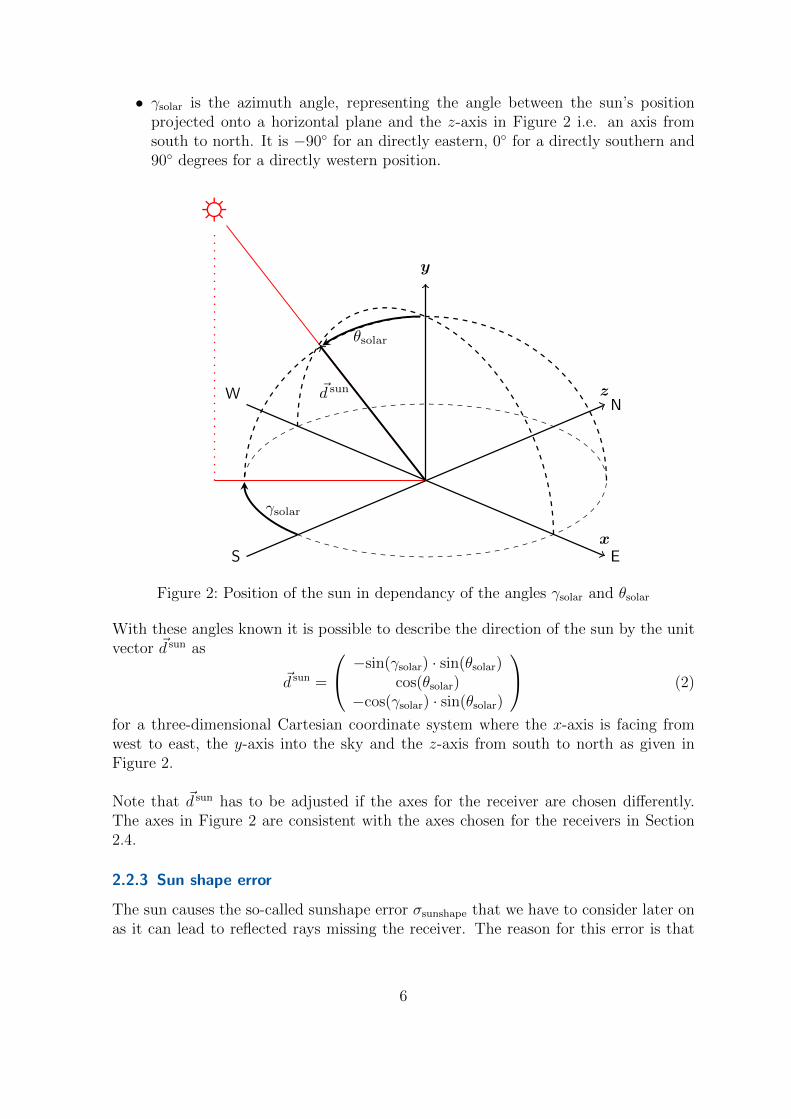
• γsolar is the azimuth angle, representing the angle between the sun’s positionprojected onto a horizontal plane and the z-axis in Figure 2 i.e. an axis fromsouth to north. It is −90◦ for an directly eastern, 0◦ for a directly southern and90◦ degrees for a directly western position.

W

Ex

S

Nz

y

☼

~d sun

γsolar

θsolar

Figure 2: Position of the sun in dependancy of the angles γsolar and θsolar

With these angles known it is possible to describe the direction of the sun by the unitvector ~d sun as

~d sun =

−sin(γsolar) · sin(θsolar)cos(θsolar)

−cos(γsolar) · sin(θsolar)

(2)

for a three-dimensional Cartesian coordinate system where the x-axis is facing fromwest to east, the y-axis into the sky and the z-axis from south to north as given inFigure 2.

Note that ~d sun has to be adjusted if the axes for the receiver are chosen differently.The axes in Figure 2 are consistent with the axes chosen for the receivers in Section2.4.

2.2.3 Sun shape error

The sun causes the so-called sunshape error σsunshape that we have to consider later onas it can lead to reflected rays missing the receiver. The reason for this error is that

6

the rays of the sun are not perfectly parallel but slightly fanned out due to the shapeof the sun being a sphere and thus do not get reflected as intended. σsunshape is givenby 2.51mrad [14] and stochastically independent.

2.3 Heliostats

2.3.1 Component description

The heliostats consist of a motor and a frame, which is holding one or several mirrors.Depending on the size of the power plant, the total mirror area of a heliostat can bebetween 1 and 140 m2 [4]. The coating is made of a highly reflective material such assilver. Above that layer there are protective layers against weather conditions and dirt[1].

The mirrors are curved in a way, that the reflected solar radiation is concentratedat the desired point, which is at the receiver surface. This results in heliostats closerto the tower having a stronger curvature than those further away. As the sun movesduring the day, the mirrors have to be moved as well. To track the sun as well aspossible in order to minimize cosine losses, the tracking is usually done along a verticaland a horizontal axis, which is called biaxial tracking.

2.3.2 Set of heliostats

We combine the heliostats in a solar tower power plant in the set H. It is a listinggiven by

H = {1, ..., nh}, (3)

where nh is the number of heliostats.

2.3.3 Heliostat errors

We model the following errors for a heliostat h ∈ H, which can lead to rays eventuallymissing the receiver.

• The optical error σhoptical caused by the surface(s) of the mirror(s) not being per-

fectly curved and having small roughnesses. We assume σhoptical to be known and

stochastically independent for all h ∈ H.

We consider σoptical in the optical model for computing the heliostat images,because it is a result of the manufacturing process and does not change at all;neither over time nor due to change of another quantity.

• The horizontal and vertical tracking errors σhtracking,hor and σh

tracking,ver caused byseveral effects such as limited accuracy of the motor or imperfections in the deter-mination of the reference position for the tracking mechanic or in the constructionof the frame and the tracking system that can lead to the tracking mechanism

7

as a whole being inaccurate. As most heliostats in solar tower power plants aretracked biaxially to account for changing values of γsolar and θsolar, we considerhorizontal and vertical tracking errors σh

tracking,hor and σhtracking,ver.

Contrary to the optical error, the horizontal and vertical tracking errors are goingto be handled as uncertainties in Section 4. Not only may they change over timeor depending on the aim point the heliostat is targeting but additionally theybehave in a non-Gaussian way [11].

2.3.4 Shading and blocking

The following effects can lead to changes of the heliostat images.

• Shading: If the radiation of the sun does not or only partly hit heliostats due toobstacles being in the way, we speak of shading. The images of the correspondingheliostats are zero or respectively partly zero, as no radiation is reflected fromtheir shaded areas.

Shading can be induced by the solar tower itself or by clouds by casting theirshadows onto the heliostat field. Additionally heliostats can shade each other,when they are aligned in such a way, that those closer to the sun cast a shadowon those further back.

• Blocking: If radiation is reflected by a heliostat, but hits another one on itspath to the receiver, the image is also zero at the corresponding area. This effectis known as blocking.

For the sake of simplicity we neglect shading and blocking in this work.

2.3.5 Incidence angle

The incidence angle φh,ai for the heliostat h ∈ H and the targeted point a at the re-

ceiver surface is located between the normal ~nh,a of the heliostat hit and the vector~d sun representing the position of the sun as seen from every heliostat or respectivelythe direction vector ~dh,a pointing from the heliostat onto a. A visualisation of this isshown in Figure 3.

~d sun is obtained by using Equation (2), ~dh,a is computed by

~dh,a = ~p a − ~ph, (4)

with ~p a and ~ph being the known position vectors of the a and h.

Note that the normal ~nh,a of the heliostat h is exactly between ~d sun and ~dh,a, as

8

the heliostat is aligned in a way that the irradiation is projected towards a. For thisreason we can compute φh,a

i as half the angle between ~d sun and ~dh,a as

φh,ai =

1

2· cos−1(

~d sun · ~dh,a

||~dh,a||2). (5)

☼a

h

~nh,a~d sun

~dh,a

||~dh,a||2 y

z

φh,ai

Figure 3: Computation of φh,ai by using ~d sun and ~dh,a.

2.3.6 Atmospheric attenuation

The heat flux reflected by a heliostat is reduced by the atmospheric attenuation. Thelarger the distance between the heliostat h ∈ H and the targeted point a at the re-ceiver surface, the larger is the effect of the atmospheric attenuation as the ray travelsa larger distance through the atmosphere.

The atmospheric attenuation ηh,aaa is computed by using different approaches dependingon the distance dh,a between h and a. The distance in meter is computed by using theEuclidean norm of the vector ~dh,a from Equation (4) i.e.

dh,a = ||~dh,a||2. (6)

For distances smaller than 1000m we use a polynomial approach as proposed in [13];for distances larger than a 1000m up to about 40000m we use an exponential approachas proposed in [16]. The constants for both approaches are taken from [18].

9

With the distance being known, we then can compute ηh,aaa as

ηh,aaa =

{0.99321− 1.176 · 10−4 · dh,a + 1.97 · 10−8 · dh,a2

for dh,a ≤ 1000

exp(−1.106 · 10−4 · dh,a) for dh,a > 1000.(7)

2.3.7 Beam power

The total amount of heat being reflected by a heliostat h ∈ H that targets point a atthe receiver surface, is the beam power P h,a. It depends on the irradiance Ih,a hittingthe heliostat, the atmospheric attenuation ηh,aaa , the area of the mirror surface Ah andits reflectivity rh.

If a heliostat consists of several mirrors, we assume that Ah is obtained by summing upthe area of its mirrors. The reflectivity rh ∈ [0, 1] represents the amount of incomingradiation that is being reflected by heliostat h. rh = 0 corresponds to no reflection,while rh = 1 means, that everything of the incoming radiation is reflected.

By using Equation (1) we can compute the beam power P h,a of h targeting a as

P h,a = Ih,a · ηh,aaa · Ah · rh = DNI · cos(φh,ai ) · ηh,aaa · Ah · rh. (8)

2.3.8 Original HFLCAL method

The HFLCAL (Heliostat Field Layout CALculation) method [19] is an analytic methodfor obtaining heliostat images. It approximates the heat flux density Q

′′h,ax,y in W

m2 atthe receiver for a heliostat h ∈ H targeting the so called aim point a on the receiversurface as follows:

Q′′h,ax,y =

P h,a

2πσh,aeffective

· exp(− x2 + y2

2σh,aeffective

) (9)

• x and y are the distances of the currently considered infinitesimal element froma, which is located at (0, 0), in the plane of the receiver in x- and y- i.e. inhorizontal and in vertical direction.

• P h,a is the beam power from Equation (8), i.e. the amount of heat being reflectedfrom the heliostat, depending on the heliostat, the targeted aim point and theposition of the sun.

• σh,aeffective is the effective error defining the distribution size.

The effective error is defined as

σh,aeffective =

dh,a · σhtotal√

cos(φh,a)(10)

with dh,a being the distance between the heliostat and the targeted aim point at thereceiver as defined in Equation (6). The effective error and thus the size of the heliostat

10

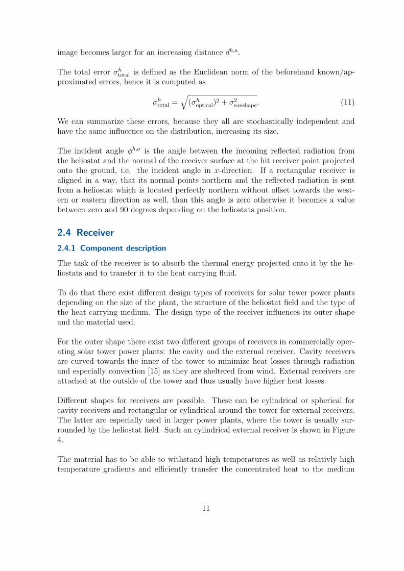
image becomes larger for an increasing distance dh,a.

The total error σhtotal is defined as the Euclidean norm of the beforehand known/ap-

proximated errors, hence it is computed as

σhtotal =

√(σh

optical)2 + σ2

sunshape. (11)

We can summarize these errors, because they all are stochastically independent andhave the same influcence on the distribution, increasing its size.

The incident angle φh,a is the angle between the incoming reflected radiation fromthe heliostat and the normal of the receiver surface at the hit receiver point projectedonto the ground, i.e. the incident angle in x-direction. If a rectangular receiver isaligned in a way, that its normal points northern and the reflected radiation is sentfrom a heliostat which is located perfectly northern without offset towards the west-ern or eastern direction as well, than this angle is zero otherwise it becomes a valuebetween zero and 90 degrees depending on the heliostats position.

2.4 Receiver

2.4.1 Component description

The task of the receiver is to absorb the thermal energy projected onto it by the he-liostats and to transfer it to the heat carrying fluid.

To do that there exist different design types of receivers for solar tower power plantsdepending on the size of the plant, the structure of the heliostat field and the type ofthe heat carrying medium. The design type of the receiver influences its outer shapeand the material used.

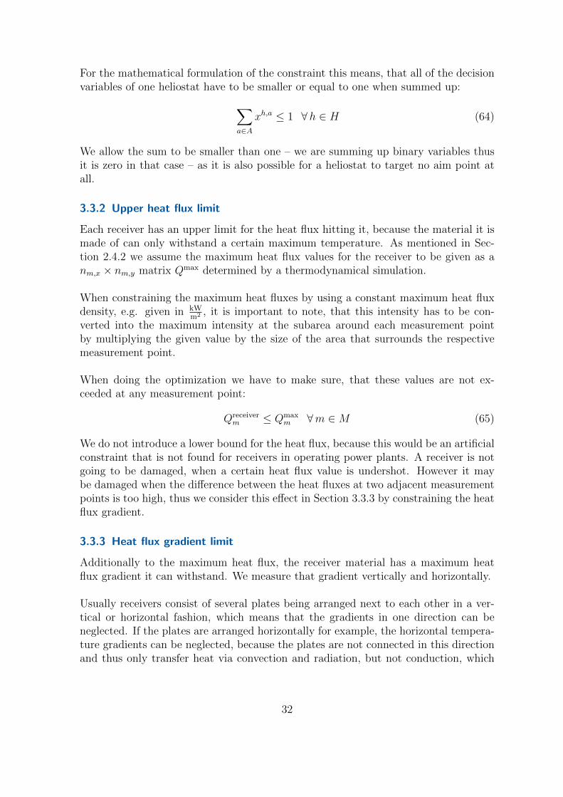
For the outer shape there exist two different groups of receivers in commercially oper-ating solar tower power plants: the cavity and the external receiver. Cavity receiversare curved towards the inner of the tower to minimize heat losses through radiationand especially convection [15] as they are sheltered from wind. External receivers areattached at the outside of the tower and thus usually have higher heat losses.

Different shapes for receivers are possible. These can be cylindrical or spherical forcavity receivers and rectangular or cylindrical around the tower for external receivers.The latter are especially used in larger power plants, where the tower is usually sur-rounded by the heliostat field. Such an cylindrical external receiver is shown in Figure4.

The material has to be able to withstand high temperatures as well as relativly hightemperature gradients and efficiently transfer the concentrated heat to the medium

11

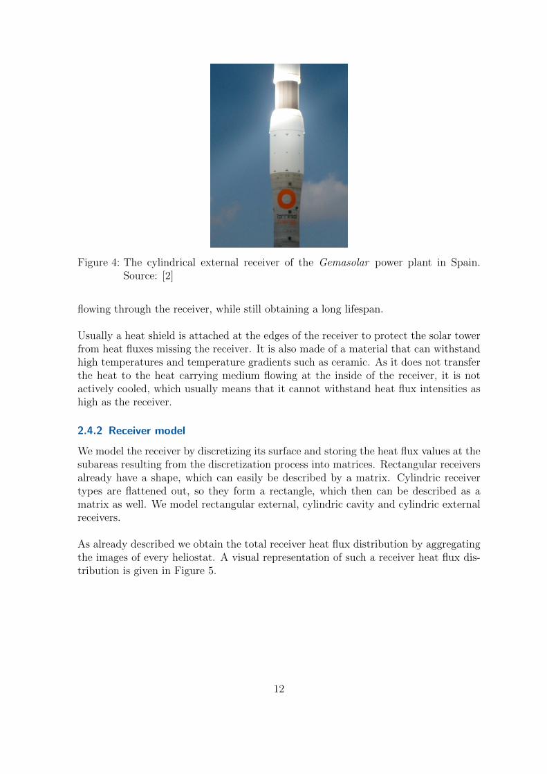
Figure 4: The cylindrical external receiver of the Gemasolar power plant in Spain.Source: [2]

flowing through the receiver, while still obtaining a long lifespan.

Usually a heat shield is attached at the edges of the receiver to protect the solar towerfrom heat fluxes missing the receiver. It is also made of a material that can withstandhigh temperatures and temperature gradients such as ceramic. As it does not transferthe heat to the heat carrying medium flowing at the inside of the receiver, it is notactively cooled, which usually means that it cannot withstand heat flux intensities ashigh as the receiver.

2.4.2 Receiver model

We model the receiver by discretizing its surface and storing the heat flux values at thesubareas resulting from the discretization process into matrices. Rectangular receiversalready have a shape, which can easily be described by a matrix. Cylindric receivertypes are flattened out, so they form a rectangle, which then can be described as amatrix as well. We model rectangular external, cylindric cavity and cylindric externalreceivers.

As already described we obtain the total receiver heat flux distribution by aggregatingthe images of every heliostat. A visual representation of such a receiver heat flux dis-tribution is given in Figure 5.

12

Figure 5: Heat flux distribution in kW at each point for 6× 4 receiver points and oneheat shield point to each side for a 14m × 12m cavity receiver.

2.4.3 Measurement points

We are interested in the heat flux value at each point of the receiver heat flux dis-tribution. As we ’measure’ our simulated heat fluxes at these points, they are calledmeasurement (index m) points.

In this work we will use the tuple (i, j) to refer to them. The set M containingthe measurement points is given by

M = {(i, j) : i ∈ {1, ..., nm,x}, j ∈ {1, ..., nm,y}}, (12)

where nm,x and nm,y are the number of horizontal and vertical measurement points.The numeration starts at the bottom left corner of the receiver. For the external re-ceiver any horizontal coordinate for the start of the numeration can be chosen. i is thehorizontal, j the vertical index.

When deriving aiming strategies based on optimization later on, we are going to usematrices containing the constraints for the optimization as for instance the maximumallowed heat flux values at each receiver point. These matrices have to be determinedby thermodynamic simulations done for the specific receiver and are assumed to begiven. The resolution of those simulations directly defines the number of entries in the

13

constraint matrices and thus also the number of measurement points.

If a specific thermodynamical simulation is not needed – for instance due to the heatflux limit being constant for the whole receiver – or if one has the possibility to dosuch simulations with an arbitrary number of distribution points it is also possible tochoose the number of measurement points.

2.4.4 Aim points

Additionally to the measurement points we need the mentioned aim points (index a).These are the points, which can be targeted by the heliostats. When tracking errorsare neglected, the focus point of the heat flux distribution is at the targeted aim point.The number of aim points can be chosen arbitrarily, but to obtain an optimal dis-cretization one has to use a certain ratio of measurement to aim points as described inthe next paragraph.

The set A containing the aim points is analogously given by

A = {(i, j) : i ∈ {1, ..., na,x}, j ∈ {1, ..., na,y}}, (13)

where na,x and na,y are the number of horizontal and vertical aim points. The indicesi and j are analogous to the indices for the measurement points.

2.4.5 Optimal discretization

For the sake of simplicity we use an equidistant discretization. It is recommended– even though it is not mandatory – to choose the number of aim points in sucha way, that nm,x and nm,y are multiples of the number of aim points na,x and na,y inthe respective directions if a thermodynamic simulation with a fixed resolution is given.

Alternatively – if possible – one can define the resolution of the thermodynamic sim-ulation, which determines the number of measurement points in the horizontal andvertical direction, in such a way, that nm,x and nm,y are multiples of the chosen num-ber of aim points na,x and na,y in the respective directions.

If it holds that

nm,x

na,x

∈ N

nm,y

na,y

∈ N,

we obtain the most accurate results as the local heat flux distribution of a heliostattargeting a specific aim point is represented by the heat flux values of the measurementpoints positioned around the targeted aim point.

14

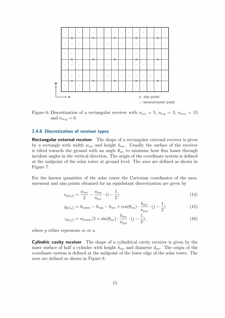
x: aim point

·: measurement point

x

yx x x x x

x x x x x

x x x x x

· · · · · · · · · · · · · · ·

· · · · · · · · · · · · · · ·

· · · · · · · · · · · · · · ·

· · · · · · · · · · · · · · ·

· · · · · · · · · · · · · · ·

· · · · · · · · · · · · · · ·

Figure 6: Discretization of a rectangular receiver with na,x = 5, na,y = 3, nm,x = 15and nm,y = 6

2.4.6 Discretization of receiver types

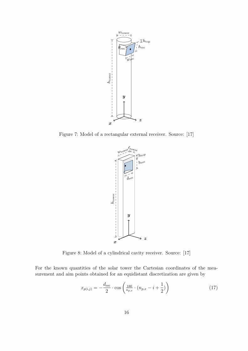
Rectangular external receiver The shape of a rectangular external receiver is givenby a rectangle with width wrec and height hrec. Usually the surface of the receiveris tilted towards the ground with an angle θrec to minimize heat flux losses throughincident angles in the vertical direction. The origin of the coordinate system is definedat the midpoint of the solar tower at ground level. The axes are defined as shown inFigure 7.

For the known quantities of the solar tower the Cartesian coordinates of the mea-surement and aim points obtained for an equidistant discretization are given by

xp(i,j) =wrec

2− wrec

np,x

· (i− 1

2) (14)

yp(i,j) = htower − htop − hrec + cos(θrec) ·hrec

np,y

· (j − 1

2) (15)

zp(i,j) = wtower/2 + sin(θrec) ·hrec

np,y

· (j − 1

2), (16)

where p either represents m or a.

Cylindric cavity receiver The shape of a cylindrical cavity receiver is given by theinner surface of half a cylinder with height hrec and diameter drec. The origin of thecoordinate system is defined at the midpoint of the lower edge of the solar tower. Theaxes are defined as shown in Figure 8.

15

x

y

z

hto

wer

wtower

||wrec

htop

hrecθrec

Figure 7: Model of a rectangular external receiver. Source: [17]

x

y

z

|

|wtow

er | |`tower

hto

wer

||drec

htop

hrec

Figure 8: Model of a cylindrical cavity receiver. Source: [17]

For the known quantities of the solar tower the Cartesian coordinates of the mea-surement and aim points obtained for an equidistant discretization are given by

xp(i,j) = −drec

2· cos

(180np,x· (np,x − i+

1

2)

)(17)

16

yp(i,j) = htower − htop − hrec +hrec

np,y

· (j − 1

2) (18)

zp(i,j) = −drec

2· sin

(180np,x· (np,x − i+

1

2)

), (19)

where p either represents m or a.

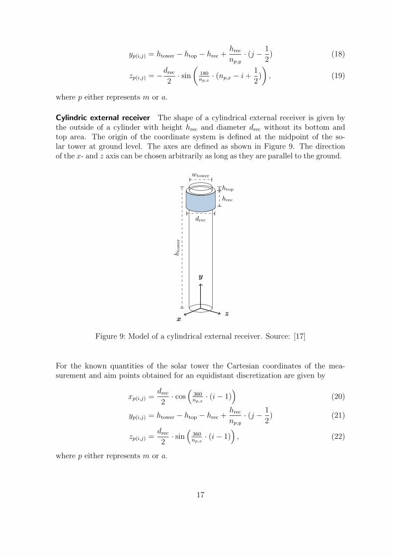
Cylindric external receiver The shape of a cylindrical external receiver is given bythe outside of a cylinder with height hrec and diameter drec without its bottom andtop area. The origin of the coordinate system is defined at the midpoint of the so-lar tower at ground level. The axes are defined as shown in Figure 9. The directionof the x- and z axis can be chosen arbitrarily as long as they are parallel to the ground.

x

y

z

hto

wer

wtower

drec

htop

hrec

Figure 9: Model of a cylindrical external receiver. Source: [17]

For the known quantities of the solar tower the Cartesian coordinates of the mea-surement and aim points obtained for an equidistant discretization are given by

xp(i,j) =drec

2· cos

(360np,x· (i− 1)

)(20)

yp(i,j) = htower − htop − hrec +hrec

np,y

· (j − 1

2) (21)

zp(i,j) =drec

2· sin

(360np,x· (i− 1)

), (22)

where p either represents m or a.

17

2.5 Computing heliostat images

2.5.1 Integrating the heat flux

To obtain the total heat flux of one heliostat, we have to integrate a heat flux densityfunction as given by Equation (9), which results in∫ ∞

−∞

∫ ∞−∞

Q′′h,ax,y dxdy =

∫R2

Q′′h,ax,y dA = P h,a. (23)

As the receiver surface is discrete rather than continuous we are looking to computethe heat flux at the area around the measurement points. To do that we evaluateEquation (9) at the coordinates of the measurement points (x, y) and scale it by thesize of the area around that measurement point

Qh,ax,y = Q

′′h,ax,y · Am, (24)

which is a two-dimensional midpoint quadrature rule.

2.5.2 Adapted HFLCAL method

We need to ensure that no safety constrains are violated when using an aiming strategylater on. For this reason we also have to make sure, that the heliostat images are asaccurate as possible.

When using the incident angle in x-direction like an error amplification in Equation(10), we increase the width of the image in the x and y dimension, meaning we increasethe diameter of the circular Gaussian distribution. When e.g. looking at heliostat im-ages projected onto a rectangular receiver, we notice however, that the projected imageis an ellipse and not a circle and that it not only depends on the incident angle in x-but also the y-direction.

For this reason we use an adapted version of this method to compute the images of theheliostats, in which we take the projections onto the receiver surface into account andconsider the incidence angles in the x- and the y-direction. The incident angle in they-direction is the angle between the incoming reflected radiation from the heliostat andthe normal of the receiver surface at the hit receiver point projected onto the y-z-plane.

For the adapted version of the HFLCAL method we define σh,aeffective as

σh,aeffective = dh,a · σh

total (25)

and do the projection onto the surface of the receiver separately.

The projection process consists of two steps: Firstly we will use the distances (xo, yo),which we from now will call offsets, by projecting the actual distances (x, y) between

18

am

Am

h

x

mo

xo

Am,o

x

y

z

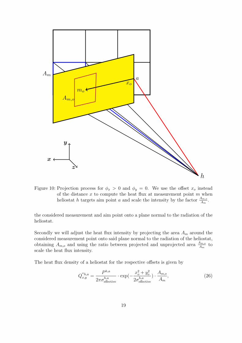
Figure 10: Projection process for φx > 0 and φy = 0. We use the offset xo insteadof the distance x to compute the heat flux at measurement point m whenheliostat h targets aim point a and scale the intensity by the factor Am,o

Am.

the considered measurement and aim point onto a plane normal to the radiation of theheliostat.

Secondly we will adjust the heat flux intensity by projecting the area Am around theconsidered measurement point onto said plane normal to the radiation of the heliostat,obtaining Am,o and using the ratio between projected and unprojected area Am,o

Amto

scale the heat flux intensity.

The heat flux density of a heliostat for the respective offsets is given by

Q′′h,ax,y =

P h,a

2πσh,aeffective

· exp(− x2o + y2

o

2σh,aeffective

) · Am,o

Am

, (26)

19

where we have to determine the offsets (xo, yo) and the projected area Am,o in respectof the distances (x, y) and the incidence angles. The equations needed for the projec-tion process are derived in Section 2.5.3, the computation of the heliostat images as awhole for the known three receiver types is explained in the Sections 2.5.4, 2.5.5 and2.5.6.

The total heat flux hitting a measurement point positioned at (x, y) then can be com-puted by numerically integrating Equation (26) as done in Equation (24) for the originalHFLCAL approach. We obtain

Qh,ax,y = Q

′′h,ax,y · Am, (27)

which simplifies to

Qh,ax,y =

P h,a

2πσh,aeffective

· exp(− x2o + y2

o

2σh,aeffective

) · Am,o. (28)

2.5.3 Distorted heliostat image matrix

In this section we derive the projection process for a point at the receiver plane ontoa plane parallel to the heliostat.

As defined in Section 2.4.2 the x-axis is parallel to the receiver plane, while the z-axispoints towards the heliostat field being normal to the x-axis. For a cylindric externalreceiver the x- and z-axis can be chosen arbitrarily. We assume that the Carthesiancoordinates of the aim points and the heliostat thus that the distances dh,ax , dh,ay anddh,az in the x, y and z dimension from every heliostat to the targeted aim point areknown. With that knowledge we can compute φh,a

x and φh,ay by

φh,ax = tan−1(

dh,ax

dh,az

) and (29)

φh,ay = tan−1(

dh,ay

dh,az

), (30)

which has to be done for every heliostat once per aim point.

Our aim is to compute the offsets (xh,a,mo , yh,a,mo ) to use them in Equation (26) orrespectively Equation (28) to compute the intensity of the heat flux at measurementpoint m ∈M when heliostat h ∈ H targets aim point a ∈ A. These offsets depend onthe incidence angles φh,a

x and φh,ay and the distances between the measurement points

and the aim points, which are given by xa,mr and xa,ml (right and left) in the x- andby ya,mu and ya,ml (upper and lower) in the y-direction. In the following we derive theequations for the x-direction; the equations in y-direction are obtained analogouslywhen exchanging the index x by y.

20

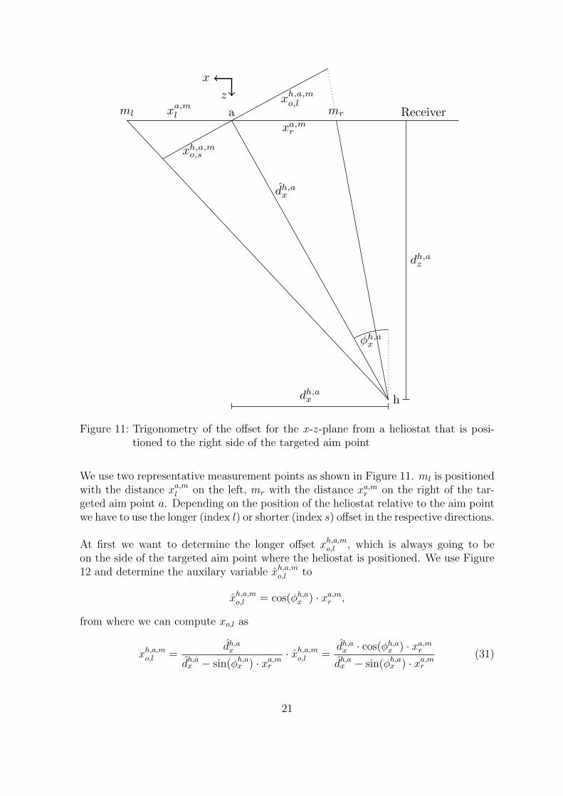
h

dh,ax

a mrml

xh,a,mo,s

xh,a,mo,lReceiverxa,ml

xa,mr

dh,az

dh,ax

φh,ax

x

z

Figure 11: Trigonometry of the offset for the x-z-plane from a heliostat that is posi-tioned to the right side of the targeted aim point

We use two representative measurement points as shown in Figure 11. ml is positionedwith the distance xa,ml on the left, mr with the distance xa,mr on the right of the tar-geted aim point a. Depending on the position of the heliostat relative to the aim pointwe have to use the longer (index l) or shorter (index s) offset in the respective directions.

At first we want to determine the longer offset xh,a,mo,l , which is always going to beon the side of the targeted aim point where the heliostat is positioned. We use Figure12 and determine the auxilary variable xh,a,mo,l to

xh,a,mo,l = cos(φh,ax ) · xa,mr ,

from where we can compute xo,l as

xh,a,mo,l =dh,ax

dh,ax − sin(φh,ax ) · xa,mr

· xh,a,mo,l =dh,ax · cos(φh,a

x ) · xa,mr

dh,ax − sin(φh,ax ) · xa,mr

(31)

21

h

dh,ax

a mr

xh,a,mo,lReceiver

xh,a,mo,l

xa,mr

dh,az

dh,ax

φh,ax

φh,ax

x

z

Figure 12: Right part of the trigonometry of the longer offset in the x-z-plane for aheliostat that is positioned to the right hand side of the targeted aim point

with dh,ax =

√dh,ax

2+ dh,az

2.

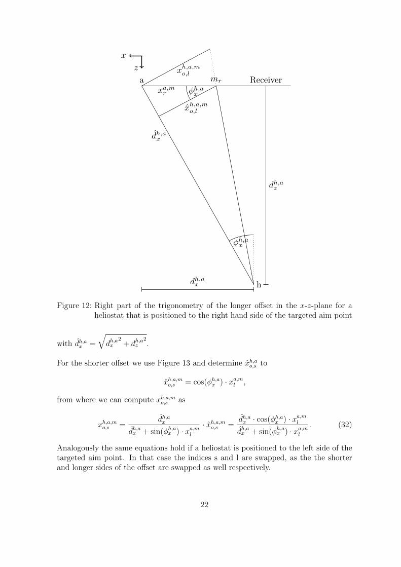
For the shorter offset we use Figure 13 and determine xh,ao,s to

xh,a,mo,s = cos(φh,ax ) · xa,ml ,

from where we can compute xh,a,mo,s as

xh,a,mo,s =dh,ax

dh,ax + sin(φh,ax ) · xa,ml

· xh,a,mo,s =dh,ax · cos(φh,a

x ) · xa,ml

dh,ax + sin(φh,ax ) · xa,ml

. (32)

Analogously the same equations hold if a heliostat is positioned to the left side of thetargeted aim point. In that case the indices s and l are swapped, as the the shorterand longer sides of the offset are swapped as well respectively.

22

h

dh,ax

aml

xh,a,mo,s

Receiverxa,ml

xh,a,mo,s

dh,az

dh,ax

φh,ax

φh,ax

x

z

Figure 13: Left part of the trigonometry of the shorter offset in the x-z-plane for aheliostat that is positioned to the right hand side of the targeted aim point

2.5.4 Rectangular external receiver

For projecting a heliostat image onto a rectangular receiver we need to determine thecartesian coordinates of the measurement and aim points. With those being known,we can compute the areas around the measurement points and the distances betweenmeasurement and aim points, project them into the heliostat plane and finally computethe heat fluxes.

1 The Cartesian coordinates of the measurement points are computed by using theEquations (14) to (16) with nm,x and nm,y.

2 The Cartesian coordinates of the aim points are computed using the Equations(14) to (16) with na,x and na,y.

23

3 The distances ∆x and ∆y between the measurement points and the aim points arecomputed trivially by

∆x = xm(i,j) − xa(i,j) and (33)

∆y =√

(ym(i,j) − ya(i,j))2 + (zm(i,j) − za(i,j))2. (34)

4 The offsets xh,a,mo and yh,a,mo (respectively long or short, depending on the positionof the heliostat relative to the aim point) are computed by using the Equations (31)and (32) with the distances ∆x and ∆y from 3. If αr > 0, we have to use the effective

incident angle in y-direction φh,ay,effective instead of φh,a

y . The effective incident angle iny-direction is given by

φh,ay,effective = φh,a

y − θrec. (35)

5 The edge points of the measurement points are computed by using the Equations(14) to (16) with nm,x and nm,y and adjusted indices. For a point on the left edge weuse the adjusted horizontal index il = i− 1

2, for the right edge respectively ir = i+ 1

2.

Analogously we obtain the adjusted vertical index by jl = j − 12

for the lower andju = j + 1

2for a point on the upper edge.

6 The offsets of the edge points xh,a,mo,left , xh,a,mo,right, yh,a,mo,lower and yh,a,mo,upper (to prevent confusion

with the long and short index the indices are written out) for each measurement pointare computed by using the Equations (31) and (32).

7 The projected areas Am,o for each measurement point are computed by multiplyingthe horizontal and the vertical edge lengths and thus given by

Am,o = (xh,a,mo,right − xh,a,mo,left ) · (yh,a,mo,upper − yh,a,mo,lower). (36)

8 The heat fluxes at the measurement points for every aim point are computed byusing Equation (28) with the offsets (xo, yo) from 4 and the projected areas Am,o from7.

2.5.5 Cylindrical cavity receiver

Projecting the heliostat image onto a cylindrical cavity receiver is analogous to theprocedure done for the rectangular receiver in Section 2.5.4 except that we need toproject the measurement and aim points onto a plane in front of the receiver first.

1 The Cartesian coordinates of the aim point are computed using the Equations (17)to (19) with na,x and na,y.

24

2 With the coordinates xa(i,j), ya(i,j) and za(i,j) of the aim point and xh, yh and zh ofthe heliostat it is possible to compute the intersection point (index isp) from the rayat the middle of the heliostat image and the imaginary plane in front of the receiverat z = 0:

xisp,a = xh + s · (xa(i,j) − xh) (37)

yisp,a = yh + s · (ya(i,j) − yh) (38)

zisp,a = zh + s · (za(i,j) − zh) (39)

with s = − zhza(i,j)−zh

3 The Cartesian coordinates of the measurement are computed using the Equations(17) to (19) with nm,x and nm,y.

4 The intersection points (with the coordinates xisp,m, yisp,m and zisp,m) for each mea-surement point can be computed analogously to 2 by using the coordinates xm(i,j),ym(i,j) and zm(i,j) from 3 instead of xa(i,j), ya(i,j) and za(i,j).

If it holds that

• xisp,m < −r

• xisp,m > r

• yisp,m < 0

• yisp,m > h

the receiver is not going to be hit, thus the intensity hitting that measurement pointis zero. The following steps are not necessary for such a measurement point.

5 The distances ∆x and ∆y between the intersection points of the measurementpoints and the intersection point of the aim point are trivially computed by

∆x = xisp,m − xisp,a and (40)

∆y = yisp,m − yisp,a. (41)

6 The offsets xh,a,mo and yh,a,mo (respectively long or short, depending on the positionof the heliostat relative to the aim point) are obtained by using Equation (31) or (32)respectively by using the distance from 5 as xr or xl.

7 The edge points of the measurement points are computed by using the Equations(17) to (19) with nm,x and nm,y and adjusted indices. For a point on the left edge weuse the adjusted horizontal index il = i+ 1

2, for the right edge respectively ir = i− 1

2.

Analogously we obtain the adjusted vertical index by jl = j − 12

for the lower andju = j + 1

2for a point on the upper edge.

25

8 The intersection points for each edge point for every measurement point are com-puted analogously to 2 using the coordinates of the edge points from 7.

9 The offsets of the edge points xh,a,mo,left , xh,a,mo,right, yh,a,mo,lower and yh,a,mo,upper (to prevent confusion

with the long and short index the indices are written out) are computed by using theEquations (31) and (32).

10 The projected areas Am,o for each measurement point are computed by multiplyingthe horizontal and the vertical edge lengths and thus given by

Am,o = (xh,a,mo,right − xh,a,mo,left ) · (yh,a,mo,upper − yh,a,mo,lower). (42)

11 The heat fluxes at the measurement points are computed by using Equation (28)with the offsets (xo, yo) from 6 and Am,o from 10.

2.5.6 Cylindrical external receiver

Projecting the heliostat image onto a cylindrical external receiver is analogous to theprocedure done for the cylindrical cavity receiver in Section 2.5.5 except that theprojection plane in front of the receiver has to be moved in dependence of the targetedaim point.

1 The coordinates of the aim points are computed using Equations (20) to (22) withna,x and na,y. They can be described by the angle φa = 360

na,x· (i − 1) with i being the

horizontal aim point index. The direction of the heliostat h ∈ H can also be describedby an angle φh, which is given by

φh =

{90− atan(xh

zh) for zh ≤ 0

90− atan(xh

zh) + 180 for zh > 0.

(43)

Due to the shape of the solar tower being a circle in the x-z-plane it becomes apparentthat an aim point at the receiver surface for that heliostat is only targetable for

φa ∈ (φh − 90, φh + 90). (44)

If this is not given, the following steps do not need to be done for that aim point.

2 The planes in front of the receiver at which the offsets are computed are given bythe tangent planes of the receiver, touching it at the intended aim points. Thus theintersection points (xisp,a,yisp,a,zisp,a) of the rays hitting the intended aim points withthat planes are trivially given, as they are the intended aim points themself.

26

3 The Cartesian coordinates of the measurement points are computed using Equa-tions (20) to (22) with nm,x and nm,y. If for φm = 360

nm,x· (i− 1) it holds that

φm ∈ (φh − 90, φh + 90) (45)

the measurement point can be hit, otherwise the intensity at that measurement pointis zero, as the tower is blocking the radiation and the following steps do not need tobe done for that measurement point.

4 With the intersection point as the aim points and the offset being known it againis possible to compute the points at which the receiver surface is hit.

The rays are described by the following equations:

x = xh + s · (xm(i,j) − xh) (46)

y = yh + s · (ym(i,j) − yh) (47)

z = zh + s · (zm(i,j) − zh), (48)

where s needs to be determined in a way, that the receiver surface is hit. Note that wenow also have to take the offset in z-direction into account.

The receiver surface analogously to the cavity receiver is described by

x ∈ [−r, r] (49)

y ∈ [0, h] (50)

z = ±√r2 − x2. (51)

with z now being able to be negative and positive as it describes a whole cylinder.

The tangent planes that connect with the receiver surface at the aim points are givenby

x = xa(i,j) + t · 0 + u · sin(

360

na,x

· (i− 1)

)(52)

y = ya(i,j) + t · 1 + u · 0 (53)

z = za(i,j) + t · 0− u · cos

(360

na,x

· (i− 1)

). (54)

The coordinates xisp,m, yisp,m and zisp,m of the intersection points from the rays hittingthe measurement points with the plane then are obtained by equating the Equations(46), (47) and (48) with (52), (53) and (54), determining s and plugging it into theEquation (46) seq or determining t and u and plugging it into Equation (52) seq. Herewe solve for s and obtain

s =za(i,j) − zh − xh−xa(i,j)

tan( 360na,x·(i−1))

zm(i,j) − zh +xm(i,j)−xh

tan( 360na,x·(i−1))

. (55)

27

For 360na,x· (i− 1) = 0 or 360

na,x· (i− 1) = 180, we use

s =xa(i,j) − xhxm(i,j) − xh

, (56)

which is the result of equating the Equations (46) and (52) while eliminating the sinusterm as it is zero.

5 The distances ∆x and ∆y between the intersection points of the measurementpoints and the aim point are computed analogously to the approaches for the otherreceiver types with the difference, that we have to consider the x and z components.To get the distance in the x-z-plane we use the Euclidean norm.

∆x =√

(xisp,m − xisp,a)2 + (zisp,m − zisp,a)2 (57)

∆y = yisp,m − yisp,a (58)

6,7 These steps are analogous to the cavity receiver in Section 2.5.5.

8 This step also in analogous to the cavity receiver in Section 2.5.5, except that wehave to use the Equations (46) to (48) with (55) or respectively (56).

9-11 These steps are also analogous to the cavity receiver in Section 2.5.5.

2.5.7 Refinement

After computing the intensity for each measurement point at the receiver for everyheliostat and every aim point, the heliostat images are obtained successfully. Whenstoring the results, these computations only need to be done once and can be donebefore running the optimization. For this reason the amount of time needed for thecomputation is negligible, which makes it possible to make the computation even moreaccurate by using refinement.

For the refinement process we choose the refinement factors refx and refy in the x-and y- direction. We then define a new set of measurement points Mref containing theincreased number of measurement point, thus a finer measurement point grid

Mref = {(i, j) : i ∈ {1, ..., nm,x · refx}, j ∈ {1, ..., nm,y · refy}}. (59)

We then compute the heat flux intensity at every measurement point m ∈ Mref forevery a ∈ A and every h ∈ H. Using a finer measurement point grid corresponds tousing a higher number of points for the two-dimensional mid point rule from Equation(24) or respectively (28).

After we computed the heliostat images with the heat fluxes Qh,a,refx,y using Mref we

28

sum them up to obtain the heliostat images as defined for the set of measurementpoints M

Qh,ax,y =

refx−1∑i=0

refy−1∑j=0

Qh,a,refx+i,y+j. (60)

2.6 Results

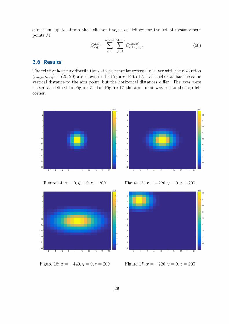
The relative heat flux distributions at a rectangular external receiver with the resolution(nm,x, nm,y) = (20, 20) are shown in the Figures 14 to 17. Each heliostat has the samevertical distance to the aim point, but the horizontal distances differ. The axes werechosen as defined in Figure 7. For Figure 17 the aim point was set to the top leftcorner.

Figure 14: x = 0, y = 0, z = 200 Figure 15: x = −220, y = 0, z = 200

Figure 16: x = −440, y = 0, z = 200 Figure 17: x = −220, y = 0, z = 200

29

The following receiver parameters were used:

htower 120mhtop 0mwrec 20mhrec 20mθrec 0◦

3 Deterministic aiming strategy

In Section 2 we computed the heliostat images Qh,a as matrices for every heliostat andevery aim point. Our objective is to find the optimal choice of aim points at a fixedtime in a way that the maximum available heat flux is transferred to the receiver whilenot violating any safety constraints.

This optimization model describes the deterministic aiming strategy as an ILP. Weassume a scenario in which uncertainties as inaccurate tracking are neglected. Theoptimization model is highly based on [5] as we use this model and extend it to alsotake gradient limits into account.

At first we look at the definitions needed, before we go into detail with the optimizationmodel by deriving the objective function and constraints.

3.1 Definitions

3.1.1 Heliostats

The heliostats (introduced in Section 2.3) are focussing the irradiation of the sun ontoone of the aim points at the receiver surface. The set containing them is defined byEquation (3) as

H = {1, ..., nh},where nh is the number of heliostats.

3.1.2 Measurement points

The measurement points (introduced in 2.4.3) are the points at the receiver surface atwhich the simulated heat fluxes hitting the subarea around the respective measurementpoint are summed up. The set containing them is defined by Equation (12) as

M = {(i, j) : i ∈ {1, ..., nm,x}, j ∈ {1, ..., nm,y}},

where nm,x and nm,y are the number of measurement points in the x and y dimension.

30

3.1.3 Aim points

The aim points (introduced in 2.4.4) are the points at the receiver surface, that can betargeted by heliostats. The set containing them is defined by Equation (13) as

A = {(i, j) : i ∈ {1, ..., na,x}, j ∈ {1, ..., na,y}},

where na,x and na,y are the number of aim points in the x and y dimension.

3.1.4 Decision variables

The decision variables xh,a determine if the heliostat h ∈ H targets the aim pointa ∈ A. A heliostat only can or cannot target an aim point, distributions of the heatflux between two or more aim points are forbidden; thus the decision variables arebinary variables, i.e.

xh,a ∈ {0, 1} ∀h ∈ H ∀ a ∈ A. (61)

If heliostat h targets aim point a then xh,a = 1 otherwise it is 0.

3.1.5 Local receiver heat flux

The local heat flux Qreceiverm at the receiver surface, which hits the subarea around the

measurement point m ∈ M , is obtained by summing up the heat fluxes of the imagesof every heliostat Qh,a at the measurement point m with respect to the aim point theyare targeting:

Qreceiverm =

∑h∈H

∑a∈A

Qh,am · xh,a. (62)

3.2 Objective function

Our objective is to transfer the maximum possible heat flux to the receiver. Thismeans, we want to maximize the total heat flux hitting the receiver Qtotal, which is thesum of the heat fluxes of every measurement point. Following from this, the objectivefunction is given by

maxQtotal = max∑m∈M

Qreceiverm . (63)

3.3 Constraints

3.3.1 Maximum one aim point per heliostat

Each heliostat can or cannot target an aim point, but the maximum number of aimpoints targetable per heliostat is one. The reason for this is, that all of the reflectedirradiation of a heliostat is sent towards the targeted aim point, thus that there is noirradiation left, which could be reflected towards another aim point.

31

For the mathematical formulation of the constraint this means, that all of the decisionvariables of one heliostat have to be smaller or equal to one when summed up:∑

a∈A

xh,a ≤ 1 ∀h ∈ H (64)

We allow the sum to be smaller than one – we are summing up binary variables thusit is zero in that case – as it is also possible for a heliostat to target no aim point atall.

3.3.2 Upper heat flux limit

Each receiver has an upper limit for the heat flux hitting it, because the material it ismade of can only withstand a certain maximum temperature. As mentioned in Sec-tion 2.4.2 we assume the maximum heat flux values for the receiver to be given as anm,x × nm,y matrix Qmax determined by a thermodynamical simulation.

When constraining the maximum heat fluxes by using a constant maximum heat fluxdensity, e.g. given in kW

m2 , it is important to note, that this intensity has to be con-verted into the maximum intensity at the subarea around each measurement pointby multiplying the given value by the size of the area that surrounds the respectivemeasurement point.

When doing the optimization we have to make sure, that these values are not ex-ceeded at any measurement point:

Qreceiverm ≤ Qmax

m ∀m ∈M (65)

We do not introduce a lower bound for the heat flux, because this would be an artificialconstraint that is not found for receivers in operating power plants. A receiver is notgoing to be damaged, when a certain heat flux value is undershot. However it maybe damaged when the difference between the heat fluxes at two adjacent measurementpoints is too high, thus we consider this effect in Section 3.3.3 by constraining the heatflux gradient.

3.3.3 Heat flux gradient limit

Additionally to the maximum heat flux, the receiver material has a maximum heatflux gradient it can withstand. We measure that gradient vertically and horizontally.

Usually receivers consist of several plates being arranged next to each other in a ver-tical or horizontal fashion, which means that the gradients in one direction can beneglected. If the plates are arranged horizontally for example, the horizontal tempera-ture gradients can be neglected, because the plates are not connected in this directionand thus only transfer heat via convection and radiation, but not conduction, which

32

makes the heat transfer much weaker and hence neglectable.

As for the heat flux limit we assume that the heat flux gradient limit is given. For thehorizontal gradients we need a (nm,x − 1)× nm,y matrix Gmax,horizontal, for the verticalgradients a nm,x × (nm,y − 1) matrix Gmax,vertical containing the maximum values forthe gradients in the corresponding directions.

An easy way to define the gradient between two measurement points is

|Qreceiverm −Qreceiver

m−1 |d

, (66)

where d is the distance between the measurement points. In the following we neglectd and assume it to be included in the given heat flux gradient limits Gmax,horizontal andGmax,vertical.

When constraining the maximum heat flux gradients by using a constant gradientlimit e.g. given in kW

m, we need to scale the gradient limits analogously to the maxi-

mum heat flux limits as done in Section 3.3.2 to obtain the maximum allowed heat fluxdifference between two measurement points. This is done my multiplying the givengradient limit with the distance between the considered measurement points in therespective direction.

For the horizontal gradients we obtain the constraints

|Qreceiveri,j −Qreceiver

i−1,j | ≤ Gmax,horizontali−1,j (67)

∀ i ∈ {2, ..., nm,x} ∀ j ∈ {1, ..., nm,y}.

For the vertical gradients we obtain the constraints

|Qreceiveri,j −Qreceiver

i,j−1 | ≤ Gmax,verticali,j−1 (68)

∀i ∈ {1, ..., nm,x} ∀ j ∈ {2, ..., nm,y}.

As we are formulating the optimization problem as an integer linear program we haveto linearize the absolute value. This can be done by constraining the differences of theheat flux values at the measurement points in each direction. A negative difference istrivially smaller than a positive upper bound and a positive difference is constrainedas before for the absolute value.

For the horizontal gradients we obtain the linearized constraints

Qreceiveri,j −Qreceiver

i−1,j ≤ Gmax,horizontali−1,j (69)

Qreceiveri−1,j −Qreceiver

i,j ≤ Gmax,horizontali−1,j (70)

33

∀ i ∈ {2, ..., nm,x} ∀ j ∈ {1, ..., nm,y}.

For the vertical gradients we obtain the linearized constraints

Qreceiveri,j −Qreceiver

i,j−1 ≤ Gmax,verticali,j−1 (71)

Qreceiveri,j−1 −Qreceiver

i,j ≤ Gmax,verticali,j−1 (72)

∀i ∈ {1, ..., nm,x} ∀ j ∈ {2, ..., nm,y}.

3.4 Summarized optimization model

• Definition:

Qreceiverm =

∑h∈H

∑a∈A

Qh,am · xh,a.

• Objective function:

maxQtotal = max∑m∈M

Qreceiverm

• Decision variables:

xh,a ∈ {0, 1} ∀h ∈ H ∀ a ∈ A

• First constraint: ∑a∈A

xh,a ≤ 1 ∀h ∈ H

• Second constraint:Qreceiver

m ≤ Qmaxm ∀m ∈M

• Third constraint:

Qreceiveri,j −Qreceiver

i−1,j ≤ Gmax,horizontali−1,j

Qreceiveri−1,j −Qreceiver

i,j ≤ Gmax,horizontali−1,j

∀ i ∈ {2, ..., nm,x} ∀ j ∈ {1, ..., nm,y}

Qreceiveri,j −Qreceiver

i,j−1 ≤ Gmax,verticali,j−1

Qreceiveri,j−1 −Qreceiver

i,j ≤ Gmax,verticali,j−1

∀ i ∈ {1, ..., nm,x} ∀ j ∈ {2, ..., nm,y}

34

3.5 Heat shield

As mentioned in Section 2.4, a solar tower usually is equipped with a heat shield,that protects it from radiation missing the receiver surface. Radiation hitting the heatshield is not transferred to a heat carrying medium thus that radiation is not used togenerate electrical energy, which results in being undesirable.

Even though we try to avoid radiation missing the receiver, we have to make surethat maximum temperatures and maximum temperature gradients at the heat shieldare not exceeded.

For taking the heat shield into account we can define the additional set Mheatshield

containing the measurement points discretizing the heat shield. We do not have todefine an additional set for the aim points, as targeting the heat shield is undesirable.

We still use the smaller set M containing the measurement points at the receiversurface for the objective function, hence we only summarize the parts of the heliostatimages hitting the receiver surface and neglect the parts hitting the heat shield as thosedo not lead to the transfer of thermal energy to the heat carrying medium.

For the maximum heat flux constraints we have to make sure, that they hold for themeasurement points at the heat shield additionally to the measurement points at thereceiver surface thus we introduce additional constraints ∀m ∈Mheatshield additionallyto the known constraints ∀m ∈M .

For the heat flux gradients we have to introduce additional constraints between thereceiver and the heat shield if these components are directly physically connected andheat transfer between both components shall be considered. Additionally we have tointroduce constraints if we want to consider gradients between heat shield points inthe respective directions.

If both of the above cases hold true we introduce additional constraints ∀m ∈Mheatshield.If only one of the above cases holds true we introduce additional constraints for therespective subset of Mheatshield. If we neither consider gradients between the receiverand the heat shield nor between the heat shield points we do not have to introducenew constraints.

3.6 Clouds

As described in Section 2.2, CSP plants can only use direct radiation. This type ofradiation can be absorbed or reflected by clouds, which means that a heliostat imageis (partly) zero, if a cloud is (partly) positioned between the sun and the heliostat.

When dropping the assumption of a cloudless sky and assuming that the positions

35

of the clouds thus that the shaded heliostats are known, we can adjust our optimiza-tion model and take clouds into account. In the following we assume that a heliostateither is shaded completely or not shaded at all.

With the set of shaded heliostats

Hshaded = {h ∈ H|h is shaded}, (73)

we can define a new set of heliostats

Hhit = H\Hshaded, (74)

which describes the set of heliostats, whose images are not zero due to cloud shading.We then can use the set Hhit instead of our default set H for the optimization model,effectively reducing the size of the problem as we do not have to consider |Hshaded| · |A|decision variables.

3.7 Obtaining a specified receiver heat flux distribution

In reality it usually is not only mandatory to satisfy the constraints that prevent dam-aging of the receiver but also to obtain a certain heat flux distribution.

On the one hand the task of the receiver is, to absorb the thermal energy, that isprojected onto it by the heliostats. On the other hand this energy has to be trans-ferred to the heat carrying medium. If for instance all of the radiation is concentratedonto a small area at the receiver – for now we assume without violating a constraint– it still might not be an optimal solution, because the heat carrying medium will notbe heated anywhere except at that small area.

For this reason there exist desired receiver heat flux distributions that can be com-puted by doing thermodynamical simulations. Sometimes these heat flux distributionsmay not only be desired but form actual constraints, because of the material at certainreceiver areas not being able to withstand certain temperatures. In these cases wespeak of allowed flux density (AFD). Such an allowed flux density given in Figure 18.

If this kind of distribution is given, we can just use it as a regular constraint as describedin Section 3.3.2. If, however, the heat flux distribution is desired but not mandatory,we cannot just use it as a constraint, because we might miss out on optimization po-tential by not using the total of the available thermal energy.

In these cases we can convert a given desired absolute heat flux distribution into a rela-tive one. If the resolution of the grid used in the thermodynamical simulation does notfit our measurement points grid by either being to fine or too rough, we can additionallyresolve the given distribution to fit our measurement point grid. The results for mea-surement point resolutions given by (nm,x, nm,y)a = (6, 4) and (nm,x, nm,y)b = (12, 8)

36

Figure 18: The desired heat flux profile for a receiver as allowed flux density (AFD)given as absolute heat flux density. It is visible, that the tubes containingthe heat carrying medium enter the inner of the receiver area from the uppercorners and are arranged in serpentines leaving the inner of the receiver areaaround the center.

are shown in the Figures 19a and 19b.

(a) Receiver resolution: 6× 4 (b) Receiver resolution: 12× 8.

Figure 19: The desired heat flux profiles for a receiver given as relative heat flux density.

With the relative distribution available we can scale it with a chosen maximum heatflux intensity. The scaling intensity has to be smaller or equal to the the actual con-straint determined by the receiver material, but technically has no lower bound. Byexperimenting one can determine the optimal heat flux intensity. If the receiver dis-tribution deviates too much from the desired distribution, the maximum heat fluxintensity is too large. Ff some heliostats do not target an aim point at all, it is toosmall.

After the scaling heat flux intensity is determined, we can use the relative distributionmultiplied with the scaling factor for constraining the maximum heat flux.

37

4 Robust aiming strategy

In Section 3 we derived an optimization model for an optimal aiming strategy underdeterministic circumstances as an ILP In this section we extend that optimizationmodel and take the tracking errors of the heliostats into account, obtaining an MILP.

As described in Section 2.3 tracking errors can be caused by various effects and causethe heliostat to target another point than intended. As the whole heliostat image ismoved to a different location, violations of the heat flux or heat flux gradient limits atthe receiver can occur. The effects of tracking errors on different heliostats in respectto the total heat flux distribution do not cancel each other out; for this reason we haveto consider the tracking errors as an uncertainty and must not consider it by simplyenlarging the Gaussian distribution representing a heliostat image. More details totracking errors and their non-Gaussian behaviour can be found in [11].

To model tracking errors we use a robust optimization approach called Gamma ro-bustness [8], i.e. we allow a previously determined number of heliostats Γ to deviate.With the Gamma robustness approach it is possible to specify different Γ values foreach considered constraint to specify different requirements of robustness. For the sakeof simplicity however, we assume Γ to be constant.

If a heliostat h ∈ H deviates from its intended aim point, its image can be moved. Weassume the usual case, that the heliostat is tracked biaxially, thus the horizontal andthe vertical tracking error σtracking,hor and σtracking,ver determine the maximum devia-

tion distances dmax,hdev,hor and dmax,h

dev,ver the heliostat image can be moved in the respectivedirections. Depending on the location the heliostat actually targets we then adjust theheat flux value at every measurement point.

In the following we extend the optimization model from Section 3, meaning we usethe definitions, objective function and constraints from Section 3 and extend them totake the tracking errors into account. For the sake of simplicity, however, we neglectthe heat flux gradients at the receiver.

4.1 Definitions

4.1.1 Additional decision variables

Additionally to the decision variables xh,a indicating if heliostat h ∈ H targets aimpoint a ∈ A, we introduce the decision variables xhm indicating if heliostat h deviatesfrom any aim point it targets towards the measurement point m ∈ M . A heliostatonly can or cannot deviate from an originally intented aim point, thus these decisionvariables are binary as well, i.e.

xhm ∈ {0, 1} ∀h ∈ H ∀m ∈M. (75)

If heliostat h deviates towards measurement point m then xhm = 1 otherwise it is 0.

38

4.1.2 Adjusted local receiver heat flux

We adjust the local receiver heat flux Qreceiverm by introducing the additional local heat

flux Qh,am . It represents the worst case difference in the heat flux at the measurement

point m ∈M , when heliostat h ∈ H does not directly hit the intended aim point a ∈ Adue to tracking errors.

Qh,am is defined in a way that the worst case that can possibly occur is still consid-

ered in its formulation: When trying to prevent that a heat flux limit is exceeded,the worst case possible is, that a heliostat deviates the largest possible distance fromthe original aim point a towards the measurement point m, because this results in thelargest possible difference between the initial heat flux value without deviation and theactual heat flux value obtained by considering deviation hitting the subarea aroundthe measurement point m.

For this reason we define the worst case of the additional local heat flux Qh,am by

using the worst thus highest heat flux intensity Qh,aworst,m at m when h initially aimed

at a, asQh,a

m = Qh,aworst,m −Qh,a

m . (76)

Qh,aworst,m in turn is obtained by either bilinearily interpolating the heat flux intensity

hitting the subarea around m by using the heat flux values at m of the heliostat imageswhich aim points surround the worst case aim point or by precomputing the heat fluxvalue when h aims at the worst case aim point directly.

The adjusted local receiver heat flux Qreceiverm then can be written for a possible but

fixed choice of xhm as a sum of the known local receiver heat flux from Section 3 andan additional term to take the possible deviation of the heliostats into account:

Qreceiverm =

∑h∈H

∑a∈A

Qh,am · xh,a +

∑h∈H

∑a∈A

Qh,am · xh,a · xhm. (77)

4.1.3 Worst case aim point

The worst case aim point is the point that is closest to the measurement point m ∈Mwhile deviating the maximum possible distances dmax,h

dev,hor and dmax,hdev,ver from the original

aim point a ∈ A for the heliostat h ∈ H. We only derive the equations for the horizon-tal deviation distance. They also hold for the vertical deviation distance analogously.

If dmax,hdev,hor exceeds the horizontal distance da,mhor between a and m, the worst case hori-

zontal coordinate is the horizontal coordinate mhor of measurement point m ifself, asa focus point of a heliostat image through deviation beyond m would reduce the heatflux hitting m and thus not be the worst possible point with respect to m.

The horizontal coordinate represents the x-coordinate for a rectangular receiver and

39

the x- and z- coordinate for cylindrical receiver types, because for these the x- andz-coordinates depend on each other. Analogously the vertical coordinate representsthe y- and z-coordinate for tilted rectangular and only the y coordinate for cylindricalreceiver types.

With the coordinates mhor and ahor of m and a as well as the distances da,mhor and

dmax,hdev,hor being known, we can compute the horizontal coordinate wh,a

hor,m of the worst

case aim point wh,am as

wh,ahor,m =

mhor, dmax,hdev,hor ≥ da,mhor

ahor +dmax,hdev,hor

da,mhor· (mhor − ahor), otherwise.

(78)

For cylindrical receiver types we do not use the coordinates of the measurement andaim point on the receiver surface mhor and ahor, but the coordinates of the projectionof these points onto a plane in front of the receiver as done in the Sections 2.5.5 and2.5.6. The worst case point wh,a

m then is obtained on that plane as well. We do nothave to project it back onto the receiver surface, as the computation of the heat fluxeswith the respective worst case aim point is done on that plane anyway.

The horizontal maximum possible deviation distance dmax,hdev,hor is analogously obtained

by projecting the horizontal unprojected maximum deviation distance dmaxdev,hor onto a

plane in front of the receiver. The worst case aim point then can be determined bycomputing the worst case aim point on the plane with the equations above and pro-jecting it onto the receiver surface.

The undistorted maximum deviation distance depends on the distance between he-liostat h and aim point a in the x-z-plane dh,ax as introduced in Section 2.5.3 and thehorizontal tracking error:

dmax,hdev,hor = tan(σtracking,hor) · dh,ax . (79)

With that knowledge, we can compute the maximum possible horizontal deviationdistance dmax,h

dev,hor by using the inverse functions of the Equations (31) and (32). With

φh,ax being the incident angle in x-direction as defined in Section 2.5.3, we can determine

the maximum possible horizontal deviation distance for deviation towards a pointpositioned on the heliostat’s side of the aim point a to

dmax,hdev,hor =

dh,ax · dmaxdev,hor

dh,ax · cos(φh,ax ) + dmax

dev,hor · sin(φh,ax )

(80)

and for deviation towards a point positioned on the opposite site of the aim point a to

dmax,hdev,hor =

dh,ax · dmaxdev,hor

dh,ax · cos(φh,ax )− dmax

dev,hor · sin(φh,ax )

. (81)

As the heliostat images, the worst case aim points for each heliostat and measurementpoint can be precomputed.

40

4.1.4 Worst case local heat flux

As mentioned in Section 4.1.2 the heat flux Qh,aworst,m at the measurement point m ∈M

for the worst case when the heliostat h ∈ H targets the aim point a ∈ A can becomputed by using either bilinear interpolation or precomputation of the heat flux atm. We are going to look at these approaches now.

Bilinear interpolation When the coordinates (wh,ahor,m, w

h,aver,m) of the worst case aim

point wh,am are known, we can determine the coordinates of the aim points surrounding

it. For the sake of legibility we neglect the indices that show, that these aim pointsdepend on h and m, as they surround a worst case aim point chosen in respect to m forthe heliostat h. We choose their left and right horizontal coordinates ahor,l and ahor,r

and their lower and upper vertical coordinates aver,l and aver,u in a way that

wh,ahor,m = [ahor,l,ahor,r) (82)

wh,aver,m = [aver,l,aver,u). (83)

For cylindrical receiver types we project the aim points onto a plane in front of thereceiver as done in the Sections 2.5.5 and 2.5.6 and then choose the coordinates of theprojected points accordingly. The surrounding aim points or respectively their projec-tions then are given by a1 = (ahor,l, aver,l), a2 = (ahor,l, aver,u), a3 = (ahor,r, aver,l) anda4 = (ahor,r, aver,u).

As the heat fluxes Qh,am with a = a1 to a = a4 at these aim points are known, we

can approximate Qh,aworst,m by using bilinear interpolation, which results in

Qh,aworst,m ≈ Qh,a1

m · (1−wh,a

hor,m

ahor,r − ahor,l

(1− wh,aver,m

aver,u − aver,l

)− wh,aver,m

aver,u − aver,l

)

+Qh,a2m · (

wh,ahor,m

ahor,r − ahor,l

(1− wh,aver,m

aver,u − aver,l

))

+Qh,a3m · ( wh,a

ver,m

aver,u − aver,l

(1−wh,a

hor,m

ahor,r − ahor,l

))

+Qh,a4m · (

wh,ahor,m

ahor,r − ahor,l

wh,aver,m

aver,u − aver,l

).

Precomputation For precomputing Qh,aworst,m we just have to determine the heat flux

at m when h targets the worst case aim point wh,am . The coordinates of wh,a

m arecomputed by using Equation (78) and now represent the coordinates of the adjustedaim point. As the coordinates of m are known, the local heat flux then can be computedby using Equation (28) as

Qh,aworst,m = Qh,w

x,y . (84)

41

4.1.5 Interpolation versus precomputation

As precomputing and storing the worst case heat fluxes is an exact computationmethod, it is preferable over interpolating heat fluxes. Additionally it can be doneduring the offline runtime of the optical model, which means that it does not increasethe runtime of the optimization model, making it beneficial if computations in realtime are desired.

However, especially for large solar tower power plants memory storage might not beavailable, hence it might not be possible to store both the worst case heat fluxes orrespectively the additional heat fluxes and the heliostat images.

This problem can be further increased if a fine discretization in time is required. Inthis case numerous versions of heliostat images have to be computed for different timesteps and sun positions. In these cases interpolation is preferable.

In the Figures 20a and 20b the relative errors between the exact computation andthe interpolation of the worst case heat fluxes for a rectangular external receiver areshown. The heat flux values at the corners are used to interpolate the intensities at theconsidered measurement point for worst case aim points positioned between them. Forthis reason the relative errors are zero at the corners as the interpolation is exact there.

The order of magnitude of the relative error between the interpolation and the exactcomputation of the worst case heat fluxes is between 0 and 10−4 for both a heliostatwithout and a heliostat with a horizontal offset to the receiver. This confirms, thatit is possible to use interpolation for computing the worst case heat fluxes withoutintroducing large errors.

4.2 Objective function

As in Section 3 the objective function is given by

maxQtotal = max∑m∈M

Qreceiverm . (85)

Note that we do not use Qreceiverm in the objective function, but only as a constraint for

the upper heat flux.

Qreceiverm can only be computed for a possible but fixed choice of xhm, which have to be

chosen in the way that the maximum of the additional local heat flux for a measure-ment point is found. Hence summing up Qreceiver

m would not only not be the objectivewe are optimizing for, but also be incorrect, because we would be summing up theworst cases for each measurement point, which cannot occur simultaneously.

42

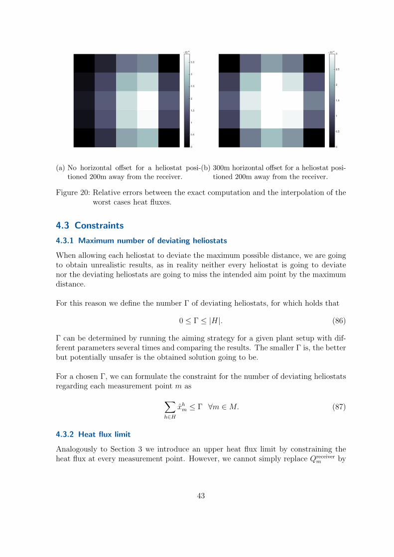
(a) No horizontal offset for a heliostat posi-tioned 200m away from the receiver.

(b) 300m horizontal offset for a heliostat posi-tioned 200m away from the receiver.

Figure 20: Relative errors between the exact computation and the interpolation of theworst cases heat fluxes.

4.3 Constraints

4.3.1 Maximum number of deviating heliostats

When allowing each heliostat to deviate the maximum possible distance, we are goingto obtain unrealistic results, as in reality neither every heliostat is going to deviatenor the deviating heliostats are going to miss the intended aim point by the maximumdistance.

For this reason we define the number Γ of deviating heliostats, for which holds that

0 ≤ Γ ≤ |H|. (86)

Γ can be determined by running the aiming strategy for a given plant setup with dif-ferent parameters several times and comparing the results. The smaller Γ is, the betterbut potentially unsafer is the obtained solution going to be.

For a chosen Γ, we can formulate the constraint for the number of deviating heliostatsregarding each measurement point m as∑

h∈H

xhm ≤ Γ ∀m ∈M. (87)

4.3.2 Heat flux limit

Analogously to Section 3 we introduce an upper heat flux limit by constraining theheat flux at every measurement point. However, we cannot simply replace Qreceiver

m by

43

Qreceiverm in Equation (65), as the latter describes the adjusted local receiver heat flux

for a possible but fixed choice of xhm and we are looking to find the worst case.

This does not only mean, that we have to consider the maximum deviation distancedmax

deviation, when computing Qh,am and hence Qreceiver

m , but also that we have to make surethat all possible combinations of the adjusted local heat flux Qreceiver

m are feasible. Thuswe need to determine the maximum of Qreceiver

m , i.e. the maximum of Qh,am · xh,a · xhm

from Equation (77), which leads to a nested optimization model for the respectivemeasurement point m given by:

• Objective function: maximize the possible additional local heat flux

αm(xh,a) = max∑h∈H

∑a∈A

Qh,am · xh,a · xhm

• Decision variables: every heliostat only can or cannot deviate

xhm ∈ {0, 1} ∀h ∈ H

• Constraint: maximum Γ deviating heliostats∑h∈H

xhm ≤ Γ

The total heat flux limit constraint then is given by∑h∈H

∑a∈A

Qh,am · xh,a + αm(xh,a) ≤ Qmax

m ∀m ∈M, (88)

which means, that the inner optimization model also has to be solved for all m ∈M .

As solving two interleaved optimization models is not suitable for an ILP solver, wedualise the above optimization model, to be able to directly solve the heat flux limitconstraint above. We introduce the variables um and vhm and obtain the dual optimiza-tion model for the respective measurement point m given by:

• Objective function:

αm(xh,a) = min Γ · um +∑h∈H

vhm

• Decision variables:

um ∈ R+0

vhm ∈ R+0 ∀h ∈ H

44

• Constraint:um + vhm ≥

∑a∈A

Qh,am · xh,a ∀h ∈ H.

The constraint matrix of the inner optimization model is total unimodular thus thesolution of the MILP αm(xh,a) is equivalent to the solution of the initial ILP αm(xh,a).That said we can replace αm(xh,a) by αm(xh,a) and obtain∑

h∈H

∑a∈A

Qh,am · xh,a + αm(xh,a) ≤ Qmax

m ∀m ∈M. (89)

Now we can simplify the inner optimization model and obtain∑h∈H

∑a∈A

Qh,am · xh,a + Γ · um +

∑h∈H

vhm ≤ Qmaxm ∀m ∈M (90)

with the decision variables

um ∈ R+0 ∀m ∈M (91)

vhm ∈ R+0 ∀h ∈ H ∀m ∈M (92)

and the constraint

um + vhm ≥∑a∈A

Qh,am · xh,a ∀h ∈ H ∀m ∈M. (93)

This constraint now is directly solvable as an MILP.

4.3.3 Summarized optimization model

• Definitions:

Qreceiverm =

∑h∈H

∑a∈A

Qh,am · xh,a

Qh,am = Qh,a

worst,m −Qh,am

• Objective function:

maxQtotal =∑m∈M

Qreceiverm

• Decision variables:

xh,a ∈ {0, 1} ∀h ∈ H ∀a ∈ Aum ∈ R+

0 ∀m ∈Mvhm ∈ R+

0 ∀h ∈ H ∀m ∈M

45

• First constraint: ∑a∈A

xh,a ≤ 1 ∀h ∈ H

• Second constraint:∑h∈H

∑a∈A

Qh,am · xh,a + Γ · um +

∑h∈H

vhm ≤ Qmaxm ∀m ∈M

• Third constraint:

um + vhm ≥∑a∈A

Qh,am · xh,a ∀h ∈ H ∀m ∈M

5 Application

In this section we apply the deterministic and the robust aiming strategy to the solartower power plant PS10 in Spain. In order to analyse the obtained solutions properly welook at the parameters affecting the outcome of the optimization problem first, beforedescribing the parameter sets chosen for the application of the aiming strategies in thiswork. Lastly we discuss the results obtained for the previously described parameterssets.

5.1 Parameters

Parameters are the quantities that affect the outcome of the aiming point strategy, i.e.the choice of aiming points for each heliostat given by the decision variables xh,a asintroduced in Section 3.1.4. Besides the constraints limiting the heat flux or the heatflux gradient, the obtained result is also influenced by the heliostat images providedby the optical model and by solver parameters.

5.1.1 Optical model

The following parameters can be adjusted to change the obtained heliostat images:

• Sun

– (γsolar, θsolar): the position of the sun as seen from the ground in polar coor-dinates

– DNI: the irradiation strength specified as direct normal irradiation

• Heliostats

– (x, y, z)h the position of a heliostat in our coordinate system as specified inSection 2

– Ah: the total mirror area of a heliostat

46

– σhoptical: the optical error of a heliostat

– rh: the reflectivity of a heliostat

– σhtracking,horizontal,σ

htracking,vertical: the horizontal and vertical tracking error of

a heliostat

• Receiver

– the receiver type (rectangular, cylindric cavity, cylindric external)

– wrec or drec: the width or respectively the diameter of the receiver

– hrec: the height of the receiver

– θrec: the tilt angle of a rectangular receiver

– the existence and discretization of a heat shield at the receiver

– htower: the height of the tower

– htop: the vertical distance from the top edge of the receiver to the top edgeof the tower

– (na,x, na,y): the number of aim points in horizontal and vertical direction

– (nm,x, nm,y): the number of measurement points in horizontal and verticaldirection

Note that the beam power P h,a reflected by one heliostat linearly depends on the DNI,Ah and rh as specified by Equation (8). As these parameters are only used in thisequation it is enough to adjust one of them.

Analogously it is enough to change htop or htower as both heights only influence thecoordinates of the receiver points.

5.1.2 Optimization problem

The following parameters can be adjusted to change the outcome of the optimizationdirectly by adjusting the constraints:

• Deterministic aiming strategy

– Qmaxm ∀m ∈M : the heat flux limit

– Gmax,horizontali−1,j ∀i ∈ {2, ..., nm,x} ∀j ∈ {1, ..., nm,y}: the horizontal heat flux

gradient limit

– Gmax,verticali,j−1 ∀i ∈ {1, ..., nm,x} ∀j ∈ {2, ..., nm,y}: the vertical heat flux gra-

dient limit

• Robust aiming strategy

– Qmaxm ∀m ∈M : the heat flux limit

– Γ: the number of deviating heliostats

47

5.1.3 Solver

The following parameters can be adjusted to influence the behaviour of the solver:

• tmax: the upper bound for the computation time

• ε: the relative gap between the current solution and the current upper bound

5.2 Parameters settings for the applications

In this work we apply the aiming strategies to the solar tower power plant PS10, thusevery optical model parameter except the sun parameters and the receiver resolutionare set. Technical data is taken from [14] and [15]. We use different constraint param-eters and solver settings.

The parameter settings for the optical model are given in Table 1, for the optimizationmodels in Table 2 and for the solver in Table 4.

The scaled heat flux profiles are given by the Figures 19a and 19b scaled by Qmax · f .The factor f is chosen by the method described in Section 3.7. It is given in Table 3.

We terminate the solution process by using upper bounds for the run time and donot use lower bounds for the optimality gap. tmax

1 is an usual upper bound for takingcloud movements into account, tmax

2 is an upper bound acceptable for running the opti-mization periodically for a clear sky szenario without clouds for different sun positionsover the day.

5.3 Application cases

From the settings given in Section 5.2 we define the following application cases for thedeterministic and the robust aiming strategy. The application cases for the determin-istic aiming strategy are given in Table 5, the application cases for the robust aimingstrategy in Table 6.

For every obtained solution we look at the gap ε and the value of the objective functioni.e. the amount of thermal energy that is transferred to the receiver for both run timestmax1 and tmax

2 . The visualisations of the results show the obtained results for the longerrun time except the solver found an optimal solution in a run time less or equal totmax1 .

Because the size of the robust optimization model is very large, it is not possible tobuild the constraint matrix for the fine resolution in Matlab on the used computer, asit would exceed the RAM. For this reason we only use the rough discretization for therobust aiming strategy.

48

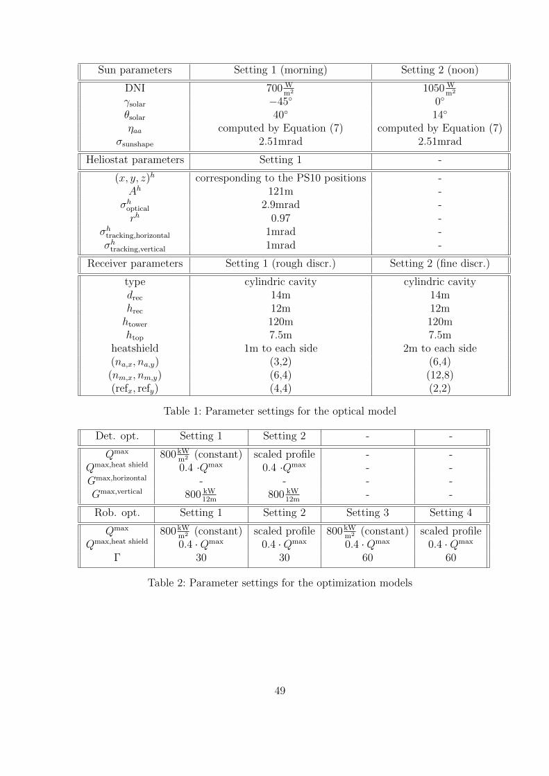
Sun parameters Setting 1 (morning) Setting 2 (noon)

DNI 700 Wm2 1050 W

m2

γsolar −45◦ 0◦

θsolar 40◦ 14◦

ηaa computed by Equation (7) computed by Equation (7)σsunshape 2.51mrad 2.51mrad

Heliostat parameters Setting 1 -

(x, y, z)h corresponding to the PS10 positions -Ah 121m -

σhoptical 2.9mrad -rh 0.97 -

σhtracking,horizontal 1mrad -σh

tracking,vertical 1mrad -

Receiver parameters Setting 1 (rough discr.) Setting 2 (fine discr.)

type cylindric cavity cylindric cavitydrec 14m 14mhrec 12m 12mhtower 120m 120mhtop 7.5m 7.5m

heatshield 1m to each side 2m to each side(na,x, na,y) (3,2) (6,4)(nm,x, nm,y) (6,4) (12,8)(refx, refy) (4,4) (2,2)

Table 1: Parameter settings for the optical model

Det. opt. Setting 1 Setting 2 - -

Qmax 800kWm2 (constant) scaled profile - -

Qmax,heat shield 0.4 ·Qmax 0.4 ·Qmax - -Gmax,horizontal - - - -Gmax,vertical 800 kW

12m800 kW

12m- -

Rob. opt. Setting 1 Setting 2 Setting 3 Setting 4

Qmax 800kWm2 (constant) scaled profile 800kW

m2 (constant) scaled profileQmax,heat shield 0.4 ·Qmax 0.4 ·Qmax 0.4 ·Qmax 0.4 ·Qmax

Γ 30 30 60 60

Table 2: Parameter settings for the optimization models

49

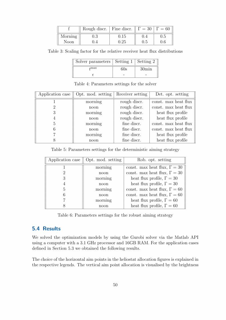
f Rough discr. Fine discr. Γ = 30 Γ = 60

Morning 0.3 0.15 0.4 0.5Noon 0.4 0.25 0.5 0.6

Table 3: Scaling factor for the relative receiver heat flux distributions

Solver parameters Setting 1 Setting 2

tmax 60s 30minε - -

Table 4: Parameters settings for the solver

Application case Opt. mod. setting Receiver setting Det. opt. setting

1 morning rough discr. const. max heat flux2 noon rough discr. const. max heat flux3 morning rough discr. heat flux profile4 noon rough discr. heat flux profile5 morning fine discr. const. max heat flux6 noon fine discr. const. max heat flux7 morning fine discr. heat flux profile8 noon fine discr. heat flux profile

Table 5: Parameters settings for the deterministic aiming strategy

Application case Opt. mod. setting Rob. opt. setting

1 morning const. max heat flux, Γ = 302 noon const. max heat flux, Γ = 303 morning heat flux profile, Γ = 304 noon heat flux profile, Γ = 305 morning const. max heat flux, Γ = 606 noon const. max heat flux, Γ = 607 morning heat flux profile, Γ = 608 noon heat flux profile, Γ = 60

Table 6: Parameters settings for the robust aiming strategy

5.4 Results

We solved the optimization models by using the Gurobi solver via the Matlab APIusing a computer with a 3.1 GHz processor and 16GB RAM. For the application casesdefined in Section 5.3 we obtained the following results.

The choice of the horizontal aim points in the heliostat allocation figures is explained inthe respective legends. The vertical aim point allocation is visualised by the brightness

50

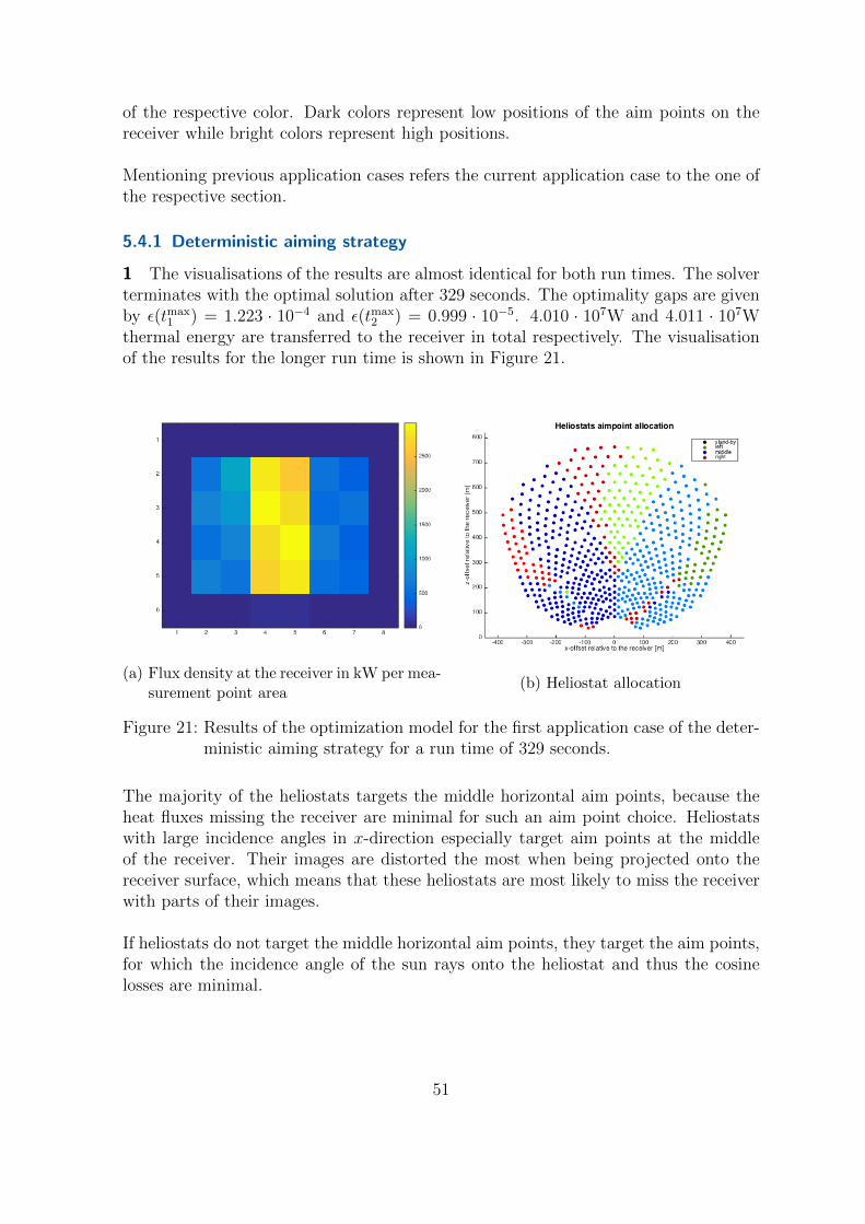
of the respective color. Dark colors represent low positions of the aim points on thereceiver while bright colors represent high positions.

Mentioning previous application cases refers the current application case to the one ofthe respective section.

5.4.1 Deterministic aiming strategy

1 The visualisations of the results are almost identical for both run times. The solverterminates with the optimal solution after 329 seconds. The optimality gaps are givenby ε(tmax

1 ) = 1.223 · 10−4 and ε(tmax2 ) = 0.999 · 10−5. 4.010 · 107W and 4.011 · 107W

thermal energy are transferred to the receiver in total respectively. The visualisationof the results for the longer run time is shown in Figure 21.

(a) Flux density at the receiver in kW per mea-surement point area

(b) Heliostat allocation

Figure 21: Results of the optimization model for the first application case of the deter-ministic aiming strategy for a run time of 329 seconds.

The majority of the heliostats targets the middle horizontal aim points, because theheat fluxes missing the receiver are minimal for such an aim point choice. Heliostatswith large incidence angles in x-direction especially target aim points at the middleof the receiver. Their images are distorted the most when being projected onto thereceiver surface, which means that these heliostats are most likely to miss the receiverwith parts of their images.

If heliostats do not target the middle horizontal aim points, they target the aim points,for which the incidence angle of the sun rays onto the heliostat and thus the cosinelosses are minimal.

51

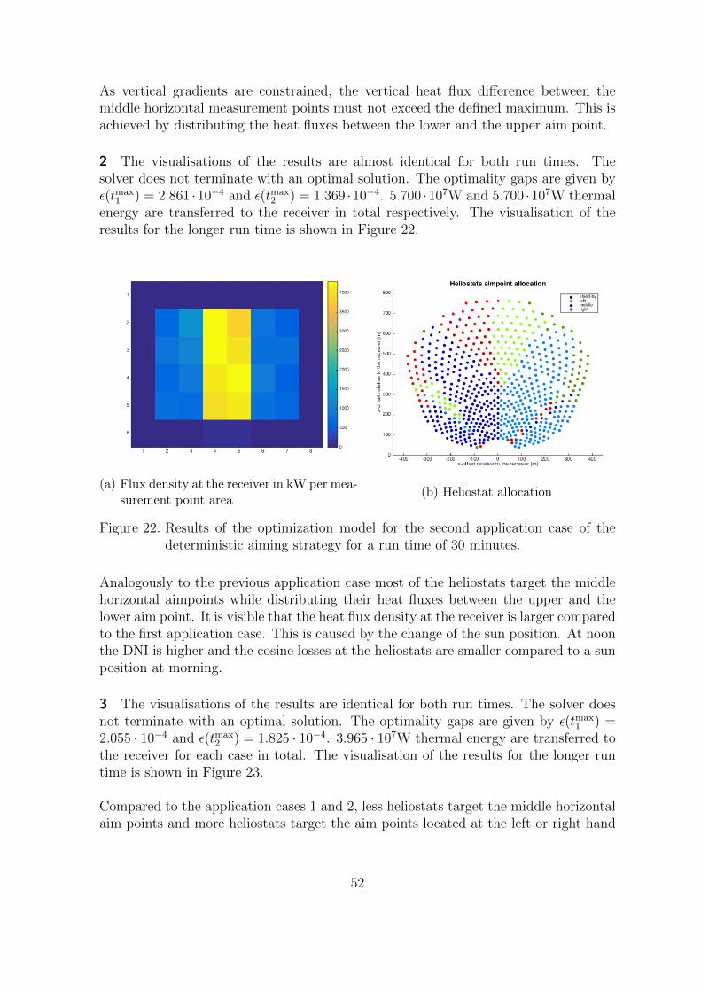
As vertical gradients are constrained, the vertical heat flux difference between themiddle horizontal measurement points must not exceed the defined maximum. This isachieved by distributing the heat fluxes between the lower and the upper aim point.

2 The visualisations of the results are almost identical for both run times. Thesolver does not terminate with an optimal solution. The optimality gaps are given byε(tmax

1 ) = 2.861 ·10−4 and ε(tmax2 ) = 1.369 ·10−4. 5.700 ·107W and 5.700 ·107W thermal

energy are transferred to the receiver in total respectively. The visualisation of theresults for the longer run time is shown in Figure 22.

(a) Flux density at the receiver in kW per mea-surement point area

(b) Heliostat allocation

Figure 22: Results of the optimization model for the second application case of thedeterministic aiming strategy for a run time of 30 minutes.

Analogously to the previous application case most of the heliostats target the middlehorizontal aimpoints while distributing their heat fluxes between the upper and thelower aim point. It is visible that the heat flux density at the receiver is larger comparedto the first application case. This is caused by the change of the sun position. At noonthe DNI is higher and the cosine losses at the heliostats are smaller compared to a sunposition at morning.

3 The visualisations of the results are identical for both run times. The solver doesnot terminate with an optimal solution. The optimality gaps are given by ε(tmax

1 ) =2.055 · 10−4 and ε(tmax

2 ) = 1.825 · 10−4. 3.965 · 107W thermal energy are transferred tothe receiver for each case in total. The visualisation of the results for the longer runtime is shown in Figure 23.

Compared to the application cases 1 and 2, less heliostats target the middle horizontalaim points and more heliostats target the aim points located at the left or right hand

52

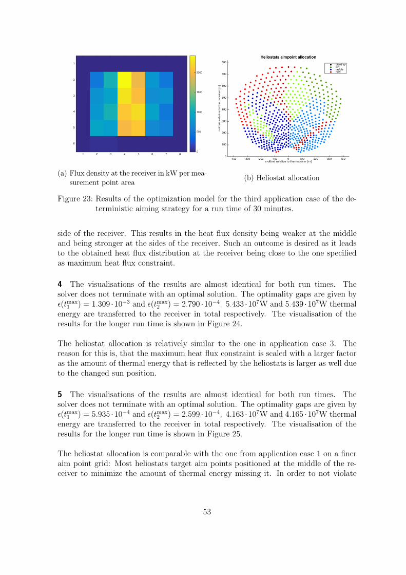
(a) Flux density at the receiver in kW per mea-surement point area

(b) Heliostat allocation

Figure 23: Results of the optimization model for the third application case of the de-terministic aiming strategy for a run time of 30 minutes.

side of the receiver. This results in the heat flux density being weaker at the middleand being stronger at the sides of the receiver. Such an outcome is desired as it leadsto the obtained heat flux distribution at the receiver being close to the one specifiedas maximum heat flux constraint.

4 The visualisations of the results are almost identical for both run times. Thesolver does not terminate with an optimal solution. The optimality gaps are given byε(tmax

1 ) = 1.309 ·10−3 and ε(tmax2 ) = 2.790 ·10−4. 5.433 ·107W and 5.439 ·107W thermal

energy are transferred to the receiver in total respectively. The visualisation of theresults for the longer run time is shown in Figure 24.

The heliostat allocation is relatively similar to the one in application case 3. Thereason for this is, that the maximum heat flux constraint is scaled with a larger factoras the amount of thermal energy that is reflected by the heliostats is larger as well dueto the changed sun position.

5 The visualisations of the results are almost identical for both run times. Thesolver does not terminate with an optimal solution. The optimality gaps are given byε(tmax

1 ) = 5.935 ·10−4 and ε(tmax2 ) = 2.599 ·10−4. 4.163 ·107W and 4.165 ·107W thermal

energy are transferred to the receiver in total respectively. The visualisation of theresults for the longer run time is shown in Figure 25.

The heliostat allocation is comparable with the one from application case 1 on a fineraim point grid: Most heliostats target aim points positioned at the middle of the re-ceiver to minimize the amount of thermal energy missing it. In order to not violate

53

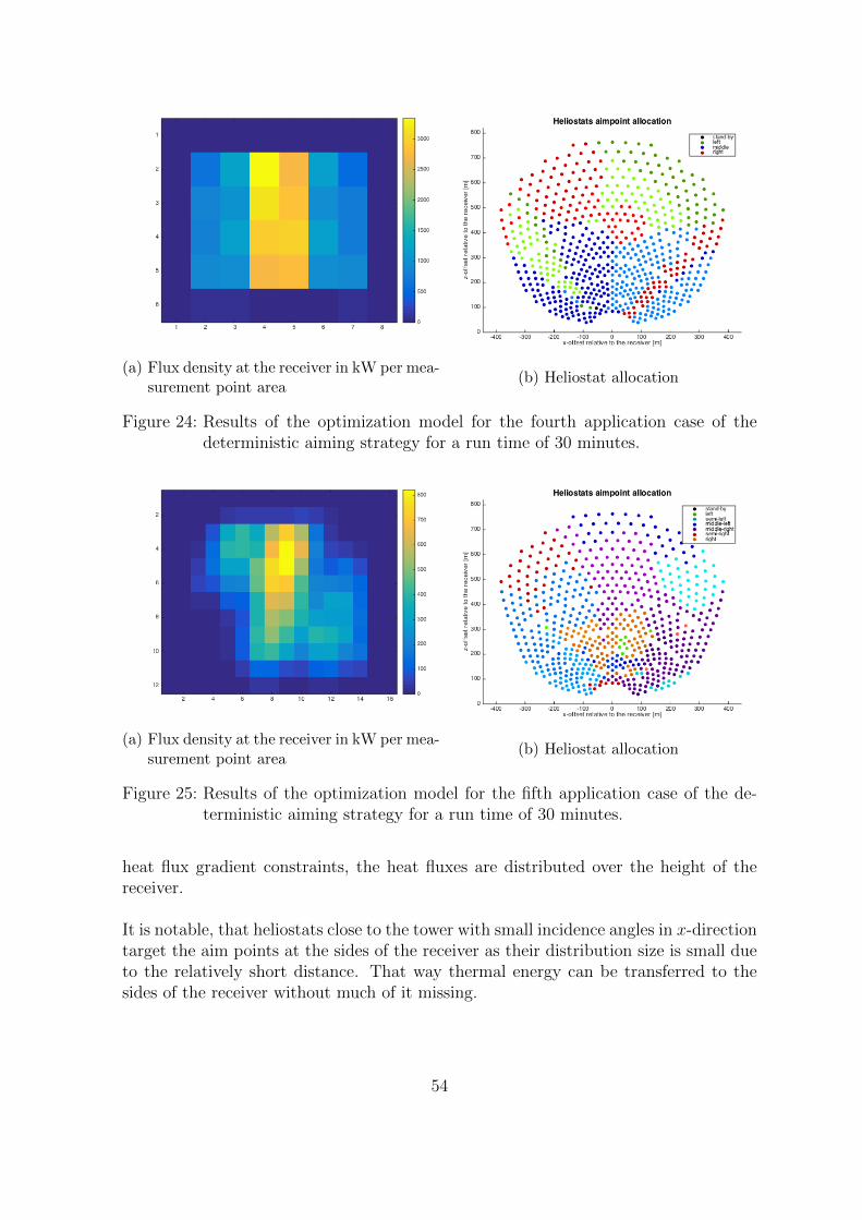
(a) Flux density at the receiver in kW per mea-surement point area

(b) Heliostat allocation

Figure 24: Results of the optimization model for the fourth application case of thedeterministic aiming strategy for a run time of 30 minutes.

(a) Flux density at the receiver in kW per mea-surement point area

(b) Heliostat allocation

Figure 25: Results of the optimization model for the fifth application case of the de-terministic aiming strategy for a run time of 30 minutes.

heat flux gradient constraints, the heat fluxes are distributed over the height of thereceiver.

It is notable, that heliostats close to the tower with small incidence angles in x-directiontarget the aim points at the sides of the receiver as their distribution size is small dueto the relatively short distance. That way thermal energy can be transferred to thesides of the receiver without much of it missing.

54

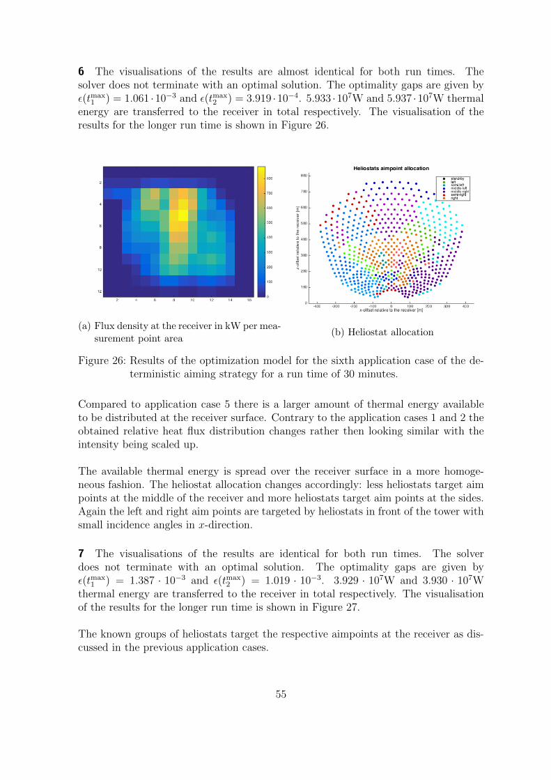
6 The visualisations of the results are almost identical for both run times. Thesolver does not terminate with an optimal solution. The optimality gaps are given byε(tmax

1 ) = 1.061 ·10−3 and ε(tmax2 ) = 3.919 ·10−4. 5.933 ·107W and 5.937 ·107W thermal

energy are transferred to the receiver in total respectively. The visualisation of theresults for the longer run time is shown in Figure 26.

(a) Flux density at the receiver in kW per mea-surement point area

(b) Heliostat allocation

Figure 26: Results of the optimization model for the sixth application case of the de-terministic aiming strategy for a run time of 30 minutes.

Compared to application case 5 there is a larger amount of thermal energy availableto be distributed at the receiver surface. Contrary to the application cases 1 and 2 theobtained relative heat flux distribution changes rather then looking similar with theintensity being scaled up.

The available thermal energy is spread over the receiver surface in a more homoge-neous fashion. The heliostat allocation changes accordingly: less heliostats target aimpoints at the middle of the receiver and more heliostats target aim points at the sides.Again the left and right aim points are targeted by heliostats in front of the tower withsmall incidence angles in x-direction.

7 The visualisations of the results are identical for both run times. The solverdoes not terminate with an optimal solution. The optimality gaps are given byε(tmax

1 ) = 1.387 · 10−3 and ε(tmax2 ) = 1.019 · 10−3. 3.929 · 107W and 3.930 · 107W

thermal energy are transferred to the receiver in total respectively. The visualisationof the results for the longer run time is shown in Figure 27.

The known groups of heliostats target the respective aimpoints at the receiver as dis-cussed in the previous application cases.

55

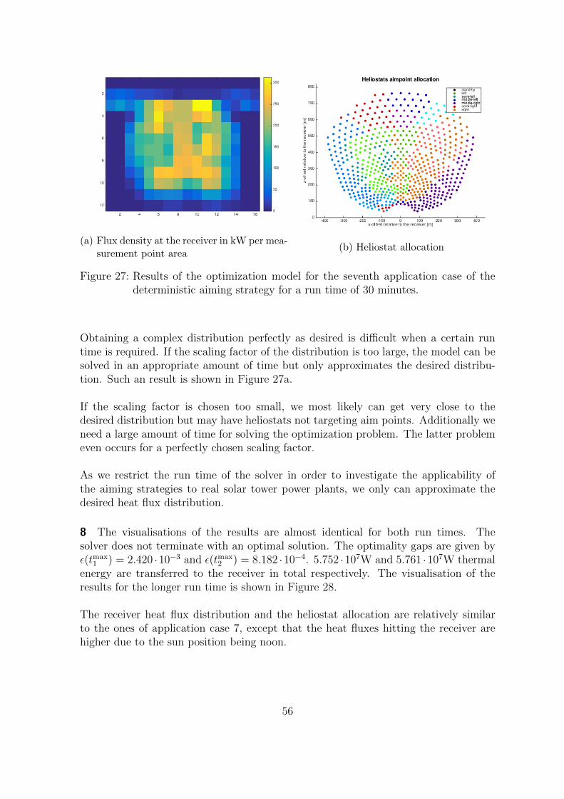
(a) Flux density at the receiver in kW per mea-surement point area

(b) Heliostat allocation

Figure 27: Results of the optimization model for the seventh application case of thedeterministic aiming strategy for a run time of 30 minutes.

Obtaining a complex distribution perfectly as desired is difficult when a certain runtime is required. If the scaling factor of the distribution is too large, the model can besolved in an appropriate amount of time but only approximates the desired distribu-tion. Such an result is shown in Figure 27a.

If the scaling factor is chosen too small, we most likely can get very close to thedesired distribution but may have heliostats not targeting aim points. Additionally weneed a large amount of time for solving the optimization problem. The latter problemeven occurs for a perfectly chosen scaling factor.

As we restrict the run time of the solver in order to investigate the applicability ofthe aiming strategies to real solar tower power plants, we only can approximate thedesired heat flux distribution.

8 The visualisations of the results are almost identical for both run times. Thesolver does not terminate with an optimal solution. The optimality gaps are given byε(tmax

1 ) = 2.420 ·10−3 and ε(tmax2 ) = 8.182 ·10−4. 5.752 ·107W and 5.761 ·107W thermal

energy are transferred to the receiver in total respectively. The visualisation of theresults for the longer run time is shown in Figure 28.

The receiver heat flux distribution and the heliostat allocation are relatively similarto the ones of application case 7, except that the heat fluxes hitting the receiver arehigher due to the sun position being noon.

56

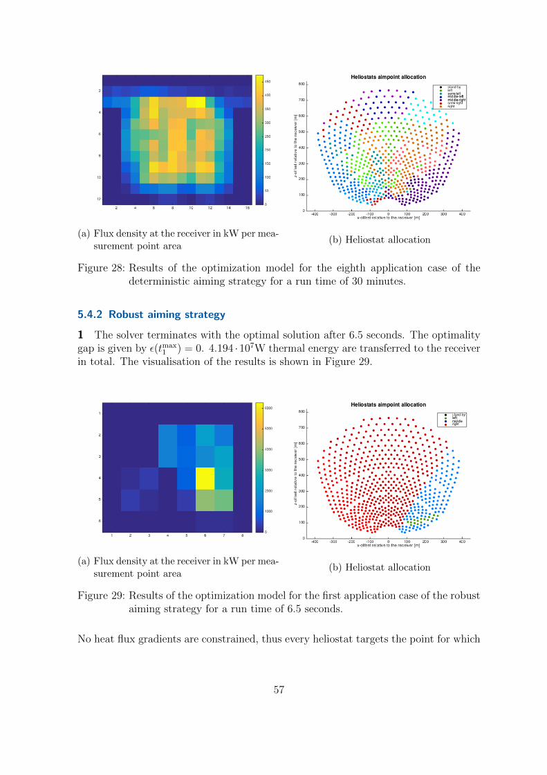
(a) Flux density at the receiver in kW per mea-surement point area

(b) Heliostat allocation

Figure 28: Results of the optimization model for the eighth application case of thedeterministic aiming strategy for a run time of 30 minutes.

5.4.2 Robust aiming strategy

1 The solver terminates with the optimal solution after 6.5 seconds. The optimalitygap is given by ε(tmax

1 ) = 0. 4.194 ·107W thermal energy are transferred to the receiverin total. The visualisation of the results is shown in Figure 29.

(a) Flux density at the receiver in kW per mea-surement point area

(b) Heliostat allocation

Figure 29: Results of the optimization model for the first application case of the robustaiming strategy for a run time of 6.5 seconds.

No heat flux gradients are constrained, thus every heliostat targets the point for which

57

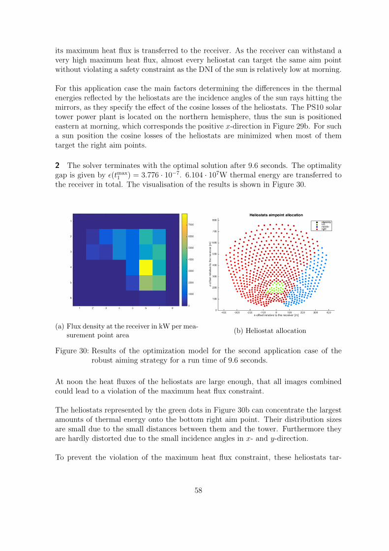
its maximum heat flux is transferred to the receiver. As the receiver can withstand avery high maximum heat flux, almost every heliostat can target the same aim pointwithout violating a safety constraint as the DNI of the sun is relatively low at morning.

For this application case the main factors determining the differences in the thermalenergies reflected by the heliostats are the incidence angles of the sun rays hitting themirrors, as they specify the effect of the cosine losses of the heliostats. The PS10 solartower power plant is located on the northern hemisphere, thus the sun is positionedeastern at morning, which corresponds the positive x-direction in Figure 29b. For sucha sun position the cosine losses of the heliostats are minimized when most of themtarget the right aim points.

2 The solver terminates with the optimal solution after 9.6 seconds. The optimalitygap is given by ε(tmax

1 ) = 3.776 · 10−7. 6.104 · 107W thermal energy are transferred tothe receiver in total. The visualisation of the results is shown in Figure 30.

(a) Flux density at the receiver in kW per mea-surement point area

(b) Heliostat allocation

Figure 30: Results of the optimization model for the second application case of therobust aiming strategy for a run time of 9.6 seconds.

At noon the heat fluxes of the heliostats are large enough, that all images combinedcould lead to a violation of the maximum heat flux constraint.

The heliostats represented by the green dots in Figure 30b can concentrate the largestamounts of thermal energy onto the bottom right aim point. Their distribution sizesare small due to the small distances between them and the tower. Furthermore theyare hardly distorted due to the small incidence angles in x- and y-direction.

To prevent the violation of the maximum heat flux constraint, these heliostats tar-

58

get the aim point, which is furthest away from the critical point. As the critical pointis the measurement point at the position of the lower right aim point, the point furthestaway is the aim point in the top left corner of the receiver.

3 The solver terminates with the optimal solution after 17.0 seconds. The optimalitygap is given by ε(tmax

1 ) = 9.900 · 10−5. 4.180 · 107W thermal energy are transferred tothe receiver in total. The visualisation of the results is shown in Figure 31.

(a) Flux density at the receiver in kW per mea-surement point area

(b) Heliostat allocation

Figure 31: Results of the optimization model for the third application case of the robustaiming strategy for a run time of 17.0 seconds.

As observed for the deterministic application cases with a given heat flux distribution,the heat fluxes are distributed more evenly over the receiver area. Accordingly theheliostats target different aimpoints with the concepts discussed for all of the previousapplication cases.

The center of the receiver is a critical area at which maximum heat flux constraintscould be violated, because heliostats from the left and the right hand side of the receivercould deviate towards the middle. As the robust aiming strategy is more conservativethan the deterministic one, the number of heliostats targeting middle horizontal aimpoints is smaller then for the deterministic aiming strategy as shown in Figure 23b.

4 The solver terminates with the optimal solution after 60.2 seconds. The optimalitygap is given by ε(tmax

1 ) = 2.650 · 10−4. 6.063 · 107W thermal energy are transferred tothe receiver in total. The visualisation of the results is shown in Figure 32.

The heat flux distribution at the receiver and the heliostat allocation at noon areanalogous to application case 3. As described there, violations of the maximum heat

59

(a) Flux density at the receiver in kW per mea-surement point area

(b) Heliostat allocation

Figure 32: Results of the optimization model for the fourth application case of therobust aiming strategy for a run time of 60.2 seconds.

flux constraints are most likely to occur at the middle area of the receiver. To preventthat from happening, some heliostats, that usually would target middle horizontal aimpoints, target the left or right aim points now. They are represented as single red orgreen dots in Figure 32b.

5 The solver terminates with the optimal solution after 61.2 seconds. The optimalitygap is given by ε(tmax

1 ) = 0. 4.194 ·107W thermal energy are transferred to the receiverin total. The visualisation of the results is shown in Figure 33.

The heat flux distribution at the receiver and the heliostat allocation are analogous toapplication case 1.

6 The solver terminates with the optimal solution after 11.1 seconds. The optimalitygap is given by ε(tmax

1 ) = 3.737 · 10−6. 6.103 · 107W thermal energy are transferred tothe receiver in total. The visualisation of the results is shown in Figure 34.

The heat flux distribution at the receiver and the heliostat allocation are analogous toapplication case 2. However, it is noticeable, that the number of heliostats targetingthe aim point that is furthest away from the bottom right aim point is larger dueto the number of deviating heliostats Γ being larger. To prevent the violation of themaximum heat flux constraint, some heliostats even must not target an aim point atall.

7 The solver terminates with the optimal solution after 58.8 seconds. The optimalitygap is given by ε(tmax

1 ) = 9.022 · 10−5. 4.179 · 107W thermal energy are transferred to

60

(a) Flux density at the receiver in kW per mea-surement point area

(b) Heliostat allocation

Figure 33: Results of the optimization model for the fifth application case of the robustaiming strategy for a run time of 61.2 seconds.

(a) Flux density at the receiver in kW per mea-surement point area

(b) Heliostat allocation

Figure 34: Results of the optimization model for the sixth application case of the robustaiming strategy for a run time of 11.1 seconds.

the receiver in total. The visualisation of the results is shown in Figure 35.

The heat flux distribution at the receiver and the heliostat allocation are analogous toapplication case 3. As the number of deviating heliostats is larger for this applicationcase, some heliostats additionally target the aim points at the sides of the receiverinstead of the aim points at the middle to prevent that the maximum heat flux con-straint is violated. These heliostats are represented by the red dots at the left hand

61

(a) Flux density at the receiver in kW per mea-surement point area

(b) Heliostat allocation

Figure 35: Results of the optimization model for the seventh application case of therobust aiming strategy for a run time of 58.8 seconds.

side of the heliostat field in Figure 35b.

8 The solver terminates with the optimal solution after 60.7 seconds. The optimalitygap is given by ε(tmax

1 ) = 1.348 · 10−3. 6.047 · 107W thermal energy are transferred tothe receiver in total. The visualisation of the results is shown in Figure 36.

(a) Flux density at the receiver in kW per mea-surement point area

(b) Heliostat allocation

Figure 36: Results of the optimization model for the eighth application case of therobust aiming strategy for a run time of 60.7 seconds.

The heat flux distribution at the receiver and the heliostat allocation are analogous to

62

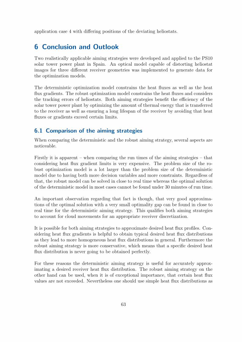
application case 4 with differing positions of the deviating heliostats.

6 Conclusion and Outlook

Two realistically applicable aiming strategies were developed and applied to the PS10solar tower power plant in Spain. An optical model capable of distorting heliostatimages for three different receiver geometries was implemented to generate data forthe optimization models.

The deterministic optimization model constrains the heat fluxes as well as the heatflux gradients. The robust optimization model constrains the heat fluxes and considersthe tracking errors of heliostats. Both aiming strategies benefit the efficiency of thesolar tower power plant by optimizing the amount of thermal energy that is transferredto the receiver as well as ensuring a long lifespan of the receiver by avoiding that heatfluxes or gradients exceed certain limits.

6.1 Comparison of the aiming strategies

When comparing the deterministic and the robust aiming strategy, several aspects arenoticeable.

Firstly it is apparent – when comparing the run times of the aiming strategies – thatconsidering heat flux gradient limits is very expensive. The problem size of the ro-bust optimization model is a lot larger than the problem size of the deterministicmodel due to having both more decision variables and more constraints. Regardless ofthat, the robust model can be solved in close to real time whereas the optimal solutionof the deterministic model in most cases cannot be found under 30 minutes of run time.

An important observation regarding that fact is though, that very good approxima-tions of the optimal solution with a very small optimality gap can be found in close toreal time for the deterministic aiming strategy. This qualifies both aiming strategiesto account for cloud movements for an appropriate receiver discretization.

It is possible for both aiming strategies to approximate desired heat flux profiles. Con-sidering heat flux gradients is helpful to obtain typical desired heat flux distributionsas they lead to more homogeneous heat flux distributions in general. Furthermore therobust aiming strategy is more conservative, which means that a specific desired heatflux distribution is never going to be obtained perfectly.

For these reasons the deterministic aiming strategy is useful for accurately approx-imating a desired receiver heat flux distribution. The robust aiming strategy on theother hand can be used, when it is of exceptional importance, that certain heat fluxvalues are not exceeded. Nevertheless one should use simple heat flux distributions as

63

constraints to avoid obtaining very inhomogeneous distributions.

6.2 Outlook

The following can be done to continue this work:

• A more comprehensive analysis of the effects of the parameters in Section 5.1 onthe solution of the optimization problems can be done to obtain deeper knowlegdeof well suitable parameter choices so that solutions can be computed as fastas possible while maintaining an appropriate accuracy by using the respectivereceiver discretization.

• Robust gradient constraints can be included into the robust optimization model,to obtain an even more realistic and robust aiming strategy.

• The aiming strategies can be extended to not only maximize the amount ofthermal energy hitting the receiver but also actively minimize the difference to agiven receiver heat flux distribution.

• Different Γ values for each measurement point can be used to obtain even higherlevels of robustness at critical areas at the receiver.

64

References

[1] Coating of heliostats. http://www.dlr.de/sf/desktopdefault.aspx/

tabid-10436/20174_read-46859, 2018. Accessed: 19.07.18.

[2] Gemasolar tower power plant. https://csirosolarthermal.wordpress.com/

tag/heliostat/, 2018. Accessed: 14.07.18.

[3] Renewables 2017 global status report. http://www.ren21.net/wp-content/

uploads/2017/06/17-8399_GSR_2017_Full_Report_0621_Opt.pdf, 2018. Ac-cessed: 19.07.18.

[4] Key numbers for solar tower plants. http://www.bine.info/

publikationen/themeninfos/publikation/solarthermische-kraftwerke-2/

turmkraftwerk-buendelt-sonne-punktgenau/?cHash=

8aa0001eb1dade325e6cb1b120f8a7f6&type=333, 2018. Accessed: 19.07.18.

[5] Thomas Ashley, Emilio Carrizosa, and Enrique Fernandez-Cara. Optimisation ofaiming strategies in solar power tower plants. Energy, 137:285–291, 2017.

[6] Marco Astolfi, Marco Binotti, Simone Mazzola, Luca Zanellato, and GiampaoloManzolini. Heliostat aiming point optimization for external tower receiver. SolarEnergy, 157:1114–1129, 2017.

[7] Boris Belhomme, Robert Pitz-Paal, and Peter Schwarzbozl. Optimization of he-liostat aim point selection for central receiver systems based on the ant colonyoptimization metaheuristic. Journal of solar energy engineering, 136(1):011005,2014.

[8] Dimitris Bertsimas and Melvyn Sim. The price of robustness. Operations research,52(1):35–53, 2004.

[9] Saeb M Besarati, D Yogi Goswami, and Elias K Stefanakos. Optimal heliostataiming strategy for uniform distribution of heat flux on the receiver of a solarpower tower plant. Energy Conversion and Management, 84:234–243, 2014.

[10] TA Dellin, MJ Fish, and CL Yang. User’s manual for delsol2: a computer code forcalculating the optical performance and optimal system design for solar-thermalcentral-receiver plants. Technical report, Sandia National Labs., Albuquerque,NM (USA); Sandia National Labs., Livermore, CA (USA), 1981.

[11] LA Dıaz-Felix, M Escobar-Toledo, J Waissman, N Pitalua-Dıaz, andCA Arancibia-Bulnes. Evaluation of heliostat field global tracking error distri-butions by monte carlo simulations. Energy procedia, 49:1308–1317, 2014.

[12] John A Duffie and William A Beckman. Solar engineering of thermal processes.John Wiley & Sons, 2013.

65

[13] PL Leary and JD Hankins. User’s guide for mirval: a computer code for comparingdesigns of heliostat-receiver optics for central receiver solar power plants. Technicalreport, Sandia National Laboratories (SNL-CA), Livermore, CA (United States),1979.

[14] Corey J Noone, Manuel Torrilhon, and Alexander Mitsos. Heliostat field opti-mization: A new computationally efficient model and biomimetic layout. SolarEnergy, 86(2):792–803, 2012.

[15] Rafael Osuna, Rafael Olavarrıa, Rafael Morillo, Marcelino Sanchez, Felipe Can-tero, Valerio Fernandez-Quero, Pedro Robles, T Lopez, Antonio Esteban, Fran-cisco Ceron, et al. Ps10, construction of a 11mw solar thermal tower plant inseville, spain. In Solar-PACES Conference, Seville, Spain, June, pages 20–23,2006.

[16] CL Pitman and LL Vant-Hull. Atmospheric transmission model for a solar beampropagating between a heliostat and a receiver. Proc. Annu. Meet.-Am. Sect. Int.Sol. Energy Soc.;(United States), 5(CONF-820629-Vol. 5-Pt. 2), 1982.

[17] Pascal Richter, Manuel J Castro Diaz, Martin Frank, and Siegfried Muller. Simu-lation and optimization of solar thermal power plants. Technical report, Lehr-undForschungsgebiet Simulation in der Kerntechnik, 2017.

[18] Mark Schmitz, Peter Schwarzbozl, Reiner Buck, and Robert Pitz-Paal. Assessmentof the potential improvement due to multiple apertures in central receiver systemswith secondary concentrators. Solar Energy, 80(1):111–120, 2006.

[19] Peter Schwarzbozl, Robert Pitz-Paal, and Mark Schmitz. Visual hflcal-a softwaretool for layout and optimisation of heliostat fields. In Proceedings, 2009.

66